SEVA: A non-linear mathematical framework for climate change vulnerability assessment

F.N. Tonmoy a and A. El-Zein b

a PhD candidate, b Associate professor of Environmental Engineering Civil Engineering School, University of Sydney, NSW 2006, Australia

Email: fahim.tonmoy@sydney.edu.au

Abstract: Assessing vulnerability to climate change allows policymakers to prioritize policy interventions and better allocate resources. Climate Change Vulnerability Assessment (CCVA) can play an important role in developing long-term environmental and infrastructure plans. Typically, a CCVA exercise combines knowledge from multiple disciplines (e.g., climate science, public health, social science, infrastructure systems, economics) in order to build models of the vulnerability to a climate-related stress of a valued attribute (e.g., health, prosperity, security) of a socio ecological system (SES) (e.g., local government area, councils, counties). In indicator-based vulnerability assessments (IBVA), indicators are adopted as proxy measures of processes generating vulnerability. However, some of the widely recognized challenges of IBVA have been the absence of a mathematically robust framework that can combine information from different knowledge domains, while taking into account the partial compensation of loss/gain between indicators, non-linearities, and tipping points. In one of our previous papers we showed that even though their goals are fundamentally different, Multi-Criteria Decision Analysis (MCDA) and IBVA have the same structural features. Hence, we proposed an aggregation framework for IBVA using insights from the older and more mature field of MCDA (El-Zein and Tonmoy, 2013a) . The goal of this paper is to extend this framework in order to define and deal with non-linear relationships and threshold effects commonly occurring in IBVA. We first identify different sources of non-linearity present in the context of IBVA. We distinguish between a fundamental nonlinearity (dependence of vulnerability on magnitude of stress), a deductive nonlinearity (where a deductive or mechanistic model is required to identify the relationship between a set of indicators and vulnerability) and an intuitive nonlinearity (where the same relationship is characterized as non-linear through inductive arguments by stakeholders and/or experts). Second, we build a new framework called the Sydney Environmental Vulnerability Assessment (SEVA) by introducing harm as a concept that replaces or mediates the relationship between the indicator and the vulnerability it represents. Harm can be conceived of as a more concrete, less abstract form of vulnerability that is more amenable to quantification. A harm criterion then, like an indicator, acts as a proxy for a process generating vulnerability. However, a harm criterion allows us to achieve two key objectives: a) to relax the conditions concerning linearity, and b)

to separate deductive and intuitive nonlinearities in order to better deal with both of them. SEVA conducts aggregation of harm criteria using an outranking framework. In a previous paper, we showed that outranking methods, developed in decision

science, are better suited to IBVA because their theoretical requirements are less stringent than multi-attribute utility theory (MAUT) approaches, and do not require perfect knowledge of preference structures (El-Zein and Tonmoy, 2013a). Outranking procedures are especially powerful in dealing with partial compensation and fuzzy relationships and, through SEVA (Figure 1), we extend the capability of an outranking procedure (ELECTRE III) to deal with the nonlinearities defined above. We simulate various combinations of nonlinearities and partial compensation through specific definitions of thresholds of differences (which are basic parameters of fuzziness in outranking algorithms). We demonstrate the use of SEVA by applying it to a hypothetical model of vulnerability of beach residents to sea level rise and its associated processes.

Keywords: vulnerability assessment, climate change, aggregation, nonlinear, outranking, mathematical framework

Figure 1: Overall architecture of SEVA

20th International Congress on Modelling and Simulation, Adelaide, Australia, 1–6 December 2013 www.mssanz.org.au/modsim2013

2276

Tonmoy and El-Zein, A non-linear mathematical framework for climate change vulnerability assessment

1. INTRODUCTION

The Earth’s climate system includes the natural spheres (e.g., atmosphere, biosphere, hydrosphere and geosphere), the anthropo-sphere (e.g., economy, society, culture), and their interactions (Schellnhuber, 1999). These interactions are one of the main sources of non-linear behaviour and our present inability to characterize them is a major source of uncertainty in our attempts to predict the effects of global environmental change (Rial et al., 2004). Climate change vulnerability assessment (CCVA) is an attempt to understand these interactions in a way that helps a systematic incorporation of climate futures in planning (Füssel, 2007). CCVA involves assessing the risk to populations, economies, and engineering infrastructures from exposure to increased climate hazards by combining the physical dimensions of risk exposure with the socio-economic and institutional processes that moderate the impacts of the hazards in question. A risk-hazard approach combines the Global Circulation Models (GCM) projections with non-linear mechanistic bio-physical or bio-chemical models (e.g., hydrological, epidemiological, atmospheric) to identify regional and local impacts. However, extending this approach to include the socioeconomic dimensions of risk and identify all important forms of nonlinearity (including those characterising the interaction between these two systems) remains a challenge for CCVA.

Indicator-based vulnerability assessments (IBVA) have been widely used because they offer a relatively simple way of quantifying different components of the risk, bio-physical, institutional and socio-economic (Füssel, 2007, Hinkel, 2011). However, IBVA, as typically conducted, suffer from multiple theoretical and methodological shortcomings. First, our imperfect knowledge of the interaction of bio-physical and socio-economic systems makes it difficult to identify and use measurable proxy indicators that can represent all the significant processes generating vulnerability. Second, developing aggregation principles for indicators is challenging because of the multiplicity of knowledge domains (e.g., climatic, social, economic, engineering, institutional), data types (continuous, discrete and ordinal variables), forms of relationships between indicators and vulnerability (linear and non-linear), as well as different possible relationships of compensation and non-compensation between the indicators, present in these analyses (El-Zein and Tonmoy, 2013a). A majority of the IBVA literature uses simple aggregation approaches that are based on Multiple Attribute Utility Theory (MAUT) (e.g., simple additive or multiplicative aggregation). Although MAUT-based additive aggregation is a powerful tool, its strict theoretical requirements (e.g., indicator additive independence, complete knowledge on the system etc) are hardly ever met in the context of IBVA (El-Zein and Tonmoy, 2013a). Moreover, a number of assumptions are typically made in IBVA studies that use MAUT—a linear, monotonic relationship between indicator and vulnerability; complete compensation between indicators—none of which usually hold in reality.

In a previous paper, we showed that even though their goals are fundamentally different, Multi Criteria Decision Analysis (MCDA) and IBVA have the same structural features and therefore we developed an aggregation framework for IBVA borrowing insights from MCDA (El-Zein and Tonmoy, 2013a). We showed that outranking methods built in decision science, are better suited for IBVA because they provide a more structured approach to the challenges mentioned above, and proposed an outranking based framework for IBVA (El-Zein and Tonmoy, 2013a, Tonmoy and El-Zein, 2012). Outranking procedures are especially powerful in dealing with compensation challenges and fuzzy relationships, but in their present form cannot accommodate different forms of non-linearity that might occur in the context of IBVA. In this paper, we define different types of non-linearities relevant to IBVA and propose a new outranking-based framework for IBVA that incorporates and represents these non-linearities.

2.0 DIFFERENT FORMS OF NON-LINEARITIES IN IBVA

We begin with a general mathematical framework for IBVA we developed earlier. This framework operates with a multi-dimensional definition of vulnerability and takes into account the impact of adaptive events. Vulnerability assessment aims to develop some measure, quantitative or qualitative, of the susceptibility to damage of, or damage likely to be inflicted on the valued attribute of an SES, as a result of its exposure to one or more climate stresses. For the purpose of the discussion below, damage is denoted by D, vulnerability by V, and the magnitude of the climate stress in question by M. It is reasonable to assume that as the magnitude M of the climate stress increases so does the damage D. This framework defines vulnerability as the ratio of damage to magnitude, i.e. as the marginal rate of damage relative to the magnitude of the stress (El-Zein and Tonmoy, 2013b), hence: = (1)

2277

Tonmoy and El-Zein, A non-linear mathematical framework for climate change vulnerability assessment

where V is a positive number (for clarity, D and M are represented in italics and the slope connecting them, i.e. vulnerability, in bold-faced font, throughout). In some cases V is largely independent of M and (1) simply reflects a linear relationship between D and M. For example, within a given range, the extent of physical damage inflicted on houses in a “do nothing” scenario may be roughly proportional to the level of sea rise that caused it, i.e. V does not depend on M. In reality such relationships are seldom linear because more often than not, D is a non-linear function of M. Rivers bursting their banks and sea waves breaching beach fortifications are examples in which a threshold effect generates a non-linear relationship between D and M (Table 1). It is possible to represent such non-linearity by introducing a dependence of V on M:

D=V(M)M (2)

Hence, it is now possible to speak about assessing vulnerability to a given magnitude of stress, i.e. developing some measure of V(M) at a given M. We call this non-linearity (i.e. dependence of V on M), the fundamental non-linearity, to distinguish it from other forms of non-linearities that will be introduced below. Provided D is differentiable over M, it is possible to generalise from equation (2) and define vulnerability as: ( ) = (3)

For more details on this mathematical framework please refer to El-Zein and Tonmoy (2013b).

Let sk={s1, …., sn} be a set of n comparable SESs which need to be ranked according to the vulnerability of a valued attribute (e.g., health, economic well-being, productivity etc.) to one or more climate hazards (e.g., increase in average temperatures, rise in sea level, increased frequency of flooding etc.). IBVA expresses the vulnerability as functions of measurable indicators. Hence, above equations applied to a specific socio-economic system (SES) k becomes: ( ) = f (I , I , I , … ) (4)

In IBVA, each indicator is ideally chosen so as to represent a process generating vulnerability, based on intuitive or deductive reasoning. Typically, our degree of knowledge of the relationship between an indicator and the vulnerability it represents is highly variable and as a minimum, can be summed up by: f I , I , I , … (5)

However, this simply reiterates the reason for which these indicators were selected in the first place. A simple, if dangerous, way out of this impasse is to make the following assumption:

f = w I̅ (6)

the bar on variable Ijk denotes normalised indicators; and wj is a weight for the jth indicator. Normalisation can be conducted in a number of different ways; commonly IBVA studies use a normalization method that leads to a new variable which ranges between 0 and 1. Equation (6) essentially generates a function based on multi-attribute utility theory (MAUT) as a form of aggregation of the indicators. This immediately presents us with a problem related to three assumptions underlying equation (6): a) indicators are linearly independent; b) all indicators are commensurable with each other, i.e. a deficiency in one indicator can be made up for with an excess in any other indicator, with the exact rate of exchange between two indicators determined by the choice of respective weights (the indicators incommensurability problem); and c) vulnerability is a linear monotonic function of indicators (the deductive non-linearity problem). Unfortunately, these assumptions do not usually hold in IBVA. Furthermore, in the absence of deductive arguments for characterising the exact relationship between a set of indicators and vulnerability, stakeholders and experts are sometimes able to build an intuitive form of nonlinearity based on their knowledge of the system in question. An example of this form of nonlinearities is given in the last row of table 1. While this approach is obviously less valid than a deductive one, it still carries information that the analysis ought to take into consideration.

An alternative to equation (6) is a Condorcet approach which proceeds by pairwise comparisons of SESs, rather than building a global utility function. In an earlier publication, we showed that outranking methods, based such an approach, are better suited for dealing with the challenges of partial compensation and data uncertainty present in IBVA (El-Zein and Tonmoy, 2013a). Outranking methods have been used widely in the context of environmental decision making (Roy, 1968, Hokkanen and Salminen, 1997, El Hanandeh and El-Zein, 2010, El-Zein and Tonmoy, 2013a, Linkov et al., 2006). Hence, we proposed an IBVA framework

2278

Tonmoy and El-Zein, A non-linear mathematical framework for climate change vulnerability assessment

which aggregates indicators by measuring the truth of the statements “a is more vulnerable than b”, “b is more vulnerable than a” or “a and b are equally vulnerable”, where a and b are two SESs.

In what follows, we extend this framework to deal with the different forms of nonlinearity identified above. We do so by introducing the concept of harm, as a mediator between indicators and the vulnerability they represent.

Table 1: Types, sources and examples of non-linearity in IBVA Types of

non-linearity Source Example

Fundamental non-linearity

Dependence of V on M (Equation 1)

Rivers bursting their banks and sea waves breaching beach fortifications are examples in which a threshold effect generates a non-linear relationship between extent of damage and magnitude of hazard.

Deductive non-linearity

Mechanistically characterised relationship between a set of indicators and vulnerability

Infrastructures are often interdependent and disruption to one usually cascades through the network. As an example, water supply infrastructures are dependent on the power supply, and therefore disruption to the power supply infrastructure during a storm event may lead to disruption of water supply to houses. Therefore, vulnerability of households to a storm event depends on a complex interaction between a set of infrastructure parameters; this interaction can be mechanistically established using simulation models (Tonmoy and El-Zein, 2013).

Intuitive non-linearity

Weakly characterized relationship between an indicator and vulnerability

Based on empirical evidence from social sciences, it is assumed that the adaptive capacity of a community is partly reflected by its collective income and assets—the wealthier it is, the higher its adaptive capacity and the less vulnerable it is to the hazard in question. However, it is very difficult to characterise the exact relationship between wealth W and adaptive capacity Ac. On the other hand, it is reasonable to assume that small differences in wealth do not translate into differences in adaptive capacities or vulnerabilities (Reid et al., 2009)

3.0 THE SYDNEY ENVIRONMENTAL VULNERABILITY APPROACH (SEVA)

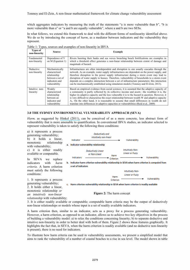
Harm, as suggested by Hinkel (2011), can be conceived of as a more concrete, less abstract form of vulnerability that is more amenable to quantification. In conventional IBVA studies, an indicator selected to represent vulnerability is taken to satisfy the following three conditions:

a) it represents a process generating vulnerability; b) it holds a linear, monotonic relationship with vulnerability; c) it is either readily available or computable.

In SEVA we replace indicators with harm criteria. A harm criterion must satisfy the following conditions:

1. It represents a process generating vulnerability; 2. It holds either a linear, monotonic relationship or an intuitively non-linear relationship with vulnerability; 3. It is either readily available or computable; computable harm criteria may be the output of deductively non-linear relationships or models whose input is a set of readily available indicators.

A harm criterion then, similar to an indicator, acts as a proxy for a process generating vulnerability. However, a harm criterion, as opposed to an indicator, allows us to achieve two key objectives in the process of building a vulnerability model: a) to relax the conditions concerning linearity; b) to separate deductive and intuitive non-linearity in order to better deal with both of them. Figure 2 shows these features graphically. It highlights the fact that, in SEVA, when the harm criterion is readily available (and no deductive non-linearity is present), there is no need for indicators.

To illustrate how harm criteria can be used in vulnerability assessments, we present a simplified model that aims to rank the vulnerability of a number of coastal beaches to a rise in sea level. The model shown in table

Figure 2: The harm concept

2279

Tonmoy and El-Zein, A non-linear mathematical framework for climate change vulnerability assessment

2 is not a complete and accurate representation of vulnerability; it is only illustrative, used to demonstrate key relationships between harm criteria and vulnerability. H1 is the damage cost (damaged private properties) due to a disaster event associated with sea level rise (SLR) (e.g. storm event), in a do nothing scenario. H1 can be estimated through a hazard line study that identifies at-risk properties and infrastructure near the coast, based on mechanistic models (e.g., coastal hydrodynamic models, soil foundation mechanics, structural integrity). Similarly, H2 is an estimate of the likely number of disrupted households as a result of an interruption to services of the public infrastructure that falls inside the hazard line. This can be measured using a system dynamics model that simulates infrastructure interdependency (Tonmoy and El-Zein, 2013). Both H1 and H2 are hence derived on the basis of deductive arguments and are the outcome of deductively non-linear relationships. On the other hand, H3, an income-based proxy measure of adaptive capacity, is usually readily available as primary data from demographic and population census databases.

Finally, the model assumes that H2 is intuitively-linear as it holds a linear relationship to vulnerability—while H1 and H3 are intuitively non-linear. This is to say that, for example, small differences in H3 (income) do NOT translate into differences in vulnerability and, beyond a given threshold, bigger differences in income no longer translate into bigger differences in vulnerability.

Table 2: Hypothetical 3-harm criteria model of vulnerability to sea level rise (D-NL: Deductive Non-Linearity; I-NL: Intuitive Non-Linearity; COMP: compensation)

H Description Dira Process D-NL I-NL COMP

H1 Damage cost of private properties ↑ Densely developed and exposed beaches are more at risk

Yes Yes Total

H2 Total number of affected households due to disruption of public infrastructures during a disaster (e.g., storm event)

↑ Disruption to public infrastructures affects its users (households) adversely

Yes No Partial

H3 Weekly median income of the households ↓ Lack of access to adaptive resources leads to more risk

No Yes Partial

a :Dir= Direction: ↑ (↓) indicates that vulnerability increases (decreases) with increasing harm.

It is now possible to express equation (2) in terms of harm criteria rather than indicators: ( ) = f (H ,H , H ,… ) (7)

where Hik is either given or can be computed as a non-linear function of a set of indicators I1k, I2k, I3k..... or the outcome of a complex mechanistic model, which may contain thresholds and tipping points, with a set of indicators as input. By starting from equation (7), which we now take as fully representing the vulnerability of the system, for each pair of SESs a and b, we can define three different categories of relative vulnerability:

1. b is indifferent to a according to harm criterion Hi if and only if |H − H | ≤ q , where qi≥0 is the relative vulnerability indifference threshold for harm criterion Hi;

2. b is strictly more vulnerable than a according to harm criterion Hi if and only if H − H ≥ p , where pi≥0 is the relative vulnerability threshold for harm criterion Hi (pi≥qi);

3. b is weakly or proportionately more vulnerable than a according to harm criterion Hi if and only if q < − H < p . 4. b is at least as vulnerable as a, if one criterion exists for which H − H > v , regardless of the

performances of a and b on all other harm criteria, where vi≥pi is called dominance threshold for harm criterion Ii.

Hence, vi sets a limit beyond which a disparity in the values of a harm criterion for 2 SESs is so great that the resulting difference in vulnerability cannot be compensated for by reverse disparity in another harm criterion. In other words, compensation is either partial or completely absent. The values of each harm criterion for each SES are assembled in what we call a vulnerability matrix (each row representing a harm criterion and each column representing an SES). Converting the vulnerability matrix into a ranking of SESs according to their vulnerability to a climate change hazard can be made using any available outranking procedures. We use the ELECTRE-III outranking method (Roy, 1968, Tonmoy and El-Zein, 2012). Figure 1 shows the overall architecture of SEVA framework.

4.0 LIMIT CONDITIONS FOR THRESHOLDS OF DIFFERENCE

In outranking methods, thresholds of differences (qi, pi and vi) dictate the extent of intuitive non-linearity and compensation through concordance and discordance matrices. In SEVA, we distinguish between eight possible types of harm criteria depending on the presence (or not) of deductive nonlinearity, intuitive

2280

Tonmoy and El-Zein, A non-linear mathematical framework for climate change vulnerability assessment

nonlinearity and partial compensation. Table 3 shows the limit conditions for thresholds of difference needed to generate the different types of harm criteria. For more details on the thresholds of differences and how they can be estimated, the reader is referred to El-Zein and Tonmoy (2013a), Tonmoy and El-Zein (2012).

Table 3: Limit cases of thresholds of difference for combinations of nonlinearity and partial compensation (qi≤pi≤vi) Intuitively Linear

and Fully-Compensating

Intuitively Non-Linear

Full Compensation

Full or Partial Compensation

Full, Partial or No Compensation

Deductively Linear

Type 1 Hik

qi=0 max(Hik-Hij) (k=1,n;

j=1,n)≤pi≤vi

Type 2 Hik

qi≥min|Hik-Hij| (k=1,n; j=1,n) max(Hik-Hij) (k=1,n;

j=1,n)≤pi≤vi

Type 3 Hik

qi≥0 pi<max(Hik-Hij)(k=1,n;

j=1,n)≤vi

Type 4 Hik

qi≥0; pi≥0 vi≤max(Hik-Hij)(k=1,n; j=1,n)

Deductively Non-Linear

Type 5 Hi=f(I1,I2,...)

qi =0 max(Hik-Hij) (k=1,n;

j=1,n)≤pi≤vi

Type 6 Hi=f(I1,I2,...)

qi≥min|Hik-Hij| (k=1,n; j=1,n) max(Hik-Hij) (k=1,n;

j=1,n)≤pi≤vi

Type 7 Hi=f(I1,I2,...)

qi≥0 pi<max(Hik-Hij)(k=1,n;

j=1,n)≤vi

Type 8 Hi=f(I1,I2,...) qi≥0; pi≥0

pi<vi<max(Hik-Hij)(k=1,n; j=1,n)

5. AN ILLUSTRATIVE EXAMPLE: VULNERABILITY TO SEA LEVEL RISE USING SEVA

Table 4 shows the results of SEVA analyses conducted on the model shown in Table 2. The SESs in this case are four hypothetical city districts of similar scales. We compare the vulnerabilities of the well being of residents of these districts to the effects of a rise in sea level and its associated processes (e.g., long term erosion, increased flooding etc.), assuming they are adequately reflected by the three harm criteria shown in Table 2. Starting from a scenario where all the relationships are linear and full compensation between harm criteria is available (case 1), we generate new scenarios (cases 2 to 4) by gradually introducing different forms of intuitive and deductive non-linearity and partial compensation. It can be seen in Table 4 that, in case 1, SES4 is least vulnerable primarily because of its low damage cost and smaller number of affected households. SES1, SES2 and SES3 are equally vulnerable as the differences between all three criteria for these SESs are in balance in the absence of any indifference thresholds (e.g., SES1 is most vulnerable based on H1, SES3 based on H2, and SES2 based on H3). In case 2, the introduction of an indifference threshold of q3=$90 for H3 disturbs this balance because now any difference below q3 can be regarded as insignificant. This yields SES 1 as the most vulnerable. Case 3 shows the effect of introducing partial compensation for H3, with p3=$100 and v3=$110. Hence, the advantage that SES3 carries over SES2 in terms of median income has become decisive: SES3 can no longer be more vulnerable than SES2, regardless of its performance on other harm criteria. The interaction between infrastructure components is introduced into the model in case 4: it is assumed that power failure leads to water supply disruption which increases the total number of affected households. It is clear that omitting interaction underestimates the impact of power failure. Introducing the non-linear relationship made SES3 most vulnerable because it harbours the highest number of disrupted households. Table 4: Four sample scenarios and effects of nonlinearity and degrees of compensation on rankings using SEVA (rankings: 1: most vulnerable; 4:least vulnerable; cases 2 and 3 are modifications of case 1 with the change highlighted in bold characters; in all intuitively linear relationship qi=0 and pi=max(Hik-Hij), k=1,n; j=1,n); H= Harm criteria;

Case Description H Units Dir1 Type2 qi pi vi wi SES1 SES2 SES3 SES4

Case 1

Intuitively, deductively linear and fully- compensating

H1 $ ↑ 1 0 8000 N/A 1 35,000 29,000 38,000 25,000 H2 count ↑ 1 0 140 N/A 1 100 107 125 113 H3 $ ↓ 1 0 200 N/A 1 $875 $800 $1000 $955

Vulnerability Ranking 1 1 1 4

Case 2

Intuitive non-linearity present only for H3

H1 $ ↑ 1 0 8000 N/A 1 35,000 29,000 38,000 25,000 H2 count ↑ 1 0 140 N/A 1 100 107 125 113 H3 $ ↓ 2 90 200 N/A 1 $875 $800 $1000 $955

Vulnerability Ranking 1 3 2 4

Case 3

Same as case 2 with partial compensation only for H3

H1 $ ↑ 1 0 8000 N/A 1 35,000 29,000 38,000 25,000 H2 count ↑ 1 0 140 N/A 1 100 107 125 113 H3 $ ↓ 4 90 100 110 1 $875 $800 $1000 $955

Vulnerability Ranking 1 2 2 4

Case 4

Deductive non-linearity introduced for H2

H1 $ ↑ 1 0 8000 N/A 1 35,000 29,000 38,000 25,000 H2 count ↑ 1 0 140 N/A 1 430 480 520 380 H3 $ ↓ 5 0 200 N/A 1 $875 $800 $1000 $955

Vulnerability Ranking 3 2 1 4 1Dir= Direction: ↑ (↓) indicates that vulnerability increases (decreases) with increasing harm. 2Type refers to the different relationships shown in Table 3

2281

Tonmoy and El-Zein, A non-linear mathematical framework for climate change vulnerability assessment

6. CONCLUSION

We identified different sources of non-linearity prevalent in the context of IBVA. In the process, we differentiated between fundamental non-linearity, deductive non-linearity and intuitive non-linearity. We developed a multi-dimensional framework (SEVA) which allows a combination of non-linear and partial compensation effects to be incorporated in vulnerability assessments. An illustrative example of ranking vulnerability of four fictional beaches to sea level rise was presented to show how consideration of interdependency of infrastructure (which is a form of deductive non-linearity) can affect the final vulnerability ranking. We are currently applying this framework to a real-life vulnerability assessment exercise, namely the vulnerability of a set of coastal communities in Sydney to a rise in sea level (Tonmoy et al., 2012).

ACKNOWLEDGMENTS

Fahim Tonmoy is a recipient of an Australian Postgraduate Award (APA) from the Australian federal government and a top-up scholarship from the CSIRO Climate Adaptation Flagship (CAF)

REFERENCES

El-Zein, A. & Tonmoy, F. N. 2013a. Assessment of Vulnerability to Climate Change using a Multi-Criteria Outranking Approach with Application to Heat Stress in Sydney. Ecological Economics (Under review).

El-Zein, A. & Tonmoy, F. N. 2013b. Nonlinearity, fuzziness and incommensurability in assessments of vulnerability to climate change: a new framework Environmental Modeling & Software (Under Review).

El Hanandeh, A. & El-Zein, A. 2010. The development and application of multi-criteria decision-making tool with consideration of uncertainty: The selection of a management strategy for the bio-degradable fraction in the municipal solid waste. Bioresource Technology, 101, 555-561.

Füssel, H.-M. 2007. Vulnerability: A generally applicable conceptual framework for climate change research. Global Environmental Change, 17, 155-167.

Hinkel, J. 2011. " Indicators of vulnerability and adaptive capacity": Towards a clarification of the science-policy interface. Global Environmental Change, 21, 198-208.

Hokkanen, J. & Salminen, P. 1997. ELECTRE III and IV Decision Aids in an Environmental Problem. Journal of Multi-Criteria Decision Analysis, 6, 215-226.

Linkov, I., Satterstrom, F. K., Kiker, G., Seager, T. P., Bridges, T., Gardner, K. H., Rogers, S., Belluck, D. & Meyer, A. 2006. Multicriteria decision analysis: a comprehensive decision approach for management of contaminated sediments. Risk analysis, 26, 61-78.

Reid, C. E., O’neill, M. S., Gronlund, C. J., Brines, S. J., Brown, D. G., Diez-Roux, A. V. & Schwartz, J. 2009. Mapping community determinants of heat vulnerability. Environmental Health Perspectives, 117, 1730.

Rial, J. A., Pielke Sr, R. A., Beniston, M., Claussen, M., Canadell, J., Cox, P., Held, H., De Noblet-Ducoudré, N., Prinn, R. & Reynolds, J. F. 2004. Nonlinearities, feedbacks and critical thresholds within the Earth's climate system. Climatic Change, 65, 11-38.

Roy, B. 1968. Classement et choix en présence de points de vue multiples (la méthode ELECTRE)'. RIRO, 8, 57-75.

Schellnhuber, H. J. 1999. ‘Earth system’analysis and the second Copernican revolution. Nature, 402, C19-C23.

Tonmoy, F. N. & El-Zein, A. Climate Change Vulnerability Assessment by outranking methods: Heat stress in Sydney In: SORIAL, G. & HONG, J., eds. Environmental Science and Technology, 2012 2012 Houston, USA American Science Press, 272-279.

Tonmoy, F. N. & El-Zein, A. Vulnerability of infrastructure to sea level rise: a combined outranking and system-dynamics approach. 22nd conference on European Safety and reliability (ESREL-2013), September 2013 (accepted), 2013 Amsterdam

2282