Serie: “SimSEE User Manuals” Volume 1 Editor and Simulator.
71
SimSEE User Manuals, Volume 1 – Editor and Simulator, pág. 1 / 71 SimSEE Serie: “SimSEE User Manuals” Volume 1 Editor and Simulator. Ings. Felipe Palacio, Pablo Soubes y Ruben Chaer. Montevideo – Uruguay. Septiembre 2019.
-
Upload
khangminh22 -
Category
Documents
-
view
2 -
download
0
Transcript of Serie: “SimSEE User Manuals” Volume 1 Editor and Simulator.

SimSEE User Manuals, Volume 1 – Editor and Simulator, pág. 1 / 71
SimSEE
Serie: “SimSEE User Manuals”
Volume 1
Editor and Simulator.
Ings. Felipe Palacio, Pablo Soubes y Ruben Chaer.Montevideo – Uruguay.
Septiembre 2019.

SimSEE User Manuals, Volume 1 – Editor and Simulator, pág. 2 / 71
P R E F A C E .The SimSEE platform is open source. Since its inception in 2007, different
people have been incorporating improvements and new features. This makes it achallenge to keep a set of updated manuals. This manual attempts to reflect thestatus of the platform at November 2019. On the website https://simsee.org you canaccess the online version of the manual and the online help that may reflect thelatest improvements and additions; version that is directly accessible when the helpbuttons of SimSEE applications are pressed.
Historical review.The heart of the SimSEE platform was developed at the Institute of Electrical
Engineering (IIE) of the Faculty of Engineering of the University of the OrientalRepublic of Uruguay within the framework of the PDT-47/12 project of the IDB-CONICYT technological development program. The project involved the work of 2engineers for 18 months and was completed in November 2007. Since that date, theplatform has been continuously improved thanks to the financing of projects in theframework of the Research and Innovation National Agency (ANII)'s Energy SectorFund (PR_FSE_2009-18: “Improvements to the SimSEE platform”, ANII-FSE-1-2011-1-6552: “Modeling of native energies in SimSEE”, ANII-FSE_1_2013_1_10957:“Purchasing Agendas Optimizer LNG shipments for Uruguay ”), PRONOS and VATESprojects (2016-2018) for the assimilation of generation forecasts and continuoussimulation of the next seven-day dispatch.SimSEE was conceived with the philosophy of FREE SOFTWARE and with the purposeof having a platform that could serve the academic purposes of teaching, researchand extension. The software is distributed free of charge under the GNU-GPL v3license type.SimSEE is programmed in Object-Oriented Pascal language, using the Lazarus Pascaldevelopment environment (Freepascal compiler). This development environment, inaddition to being excellent, has the virtue of being free, which allows advancedusers, with programming knowledge, to make improvements and develop newmodels on the SimSEE platform using 100% free software. The Object Orientedprogramming style simplifies the extension of the platform and the development ofnew models.The first version of the manuals was published in September 2013, in collaborationbetween the Institute of Electrical Engineering of the Faculty of Engineering of theUniversity of the Republic (IIE-FING-UDELAR), the Electricity Market Administration(ADME) and the Fundación Julio Américo Ricaldoni (FJR). The Engineers ClaudiaCabrera and Lorena Di Chiara were the main authors of that first version.This second version of the manuals is carried out in September 2019 by the Engs.Felipe Palacio, Pablo Soubes and Ruben Chaer, thanks to the financing of the Inter-American Development Bank (IDB) to update the manuals and translate the manualsand applications into English.
Acknowledgement. I especially thank my wife Alicia Butler who spent many hours reviewing and
improving the Spanish text and its translation into English and the publication of the content of the manuals on the web.Eng. Ruben Chaer / Instituto de Ingeniería Eléctrica - FING - UDELAR.September 2019 - Montevideo - Uruguay.
SimSEE User Manuals, Volume 1 – Editor and Simulator, pág. 3 / 71
Content.1. Introduction. General Description of the Platform.........................................5
1.1. The uses of SimSEE...............................................................................5 1.2. Overview and terminology.....................................................................6
1.2.a) Sources and terminals...................................................................10 1.2.b) Layers and Scenarios.....................................................................11 1.2.c) Dynamic parameters.....................................................................11 1.2.d) Units...............................................................................................11
1.3. Systems without dynamics..................................................................12 1.4. Dynamic systems................................................................................12 1.5. Modeling an electric power system.....................................................14
1.5.a) Representation of the transport network......................................14 1.5.b) Node Restrictions...........................................................................14
1.6. Chaining Playrooms.............................................................................15 2. Installation Procedure.................................................................................17
2.1. Download website...............................................................................17 2.2. SimSEE folder structure. Description of the content...........................17 2.3. SimSEE Binaries...................................................................................19
3. The Rooms Editor.......................................................................................21 3.1. User interface unified methods...........................................................21
3.1.a) Form editing...................................................................................21 3.1.b) Management of listings..................................................................22 3.1.c) Editing a Dynamic Parameters Record...........................................23
3.1.c.i Example 1.................................................................................243.1.c.ii Example 2.................................................................................243.1.c.iii Example 3................................................................................28
3.2. Main Menu of the SimSEE Editor..........................................................30 3.2.a) Opción “Archivo”............................................................................31 3.2.b) “Tools” Option................................................................................31
3.2.b.i Import an Actor.........................................................................313.2.b.ii Export Actors............................................................................323.2.b.iii Generate Thermal Summary....................................................323.2.b.iv “Packing”.................................................................................32
3.2.c) Option “?” (Help)............................................................................32 3.2.d) Option “Language”.........................................................................33
3.3. Main tabs.............................................................................................34 3.3.a) Notes Tab........................................................................................34 3.3.b) Global Variables Tab.......................................................................34 3.3.c) “Sources” Tab.................................................................................36
3.3.c.i Sources and terminals...............................................................38 3.3.d) Actors Tab.......................................................................................40
3.3.d.i Edit Available Units..................................................................443.3.d.ii Failure – Repair Model..............................................................453.3.d.iii Uncertain commitment............................................................453.3.d.iv Uncertain Beginning of Chronicle............................................47

SimSEE User Manuals, Volume 1 – Editor and Simulator, pág. 4 / 71
3.3.e) Files Tab..........................................................................................49 3.3.f) States Tab........................................................................................49 3.3.g) Maintenance Tab............................................................................54 3.3.h) SimRes3 Tab...................................................................................55 3.3.i) Simulator Tab...................................................................................56
3.3.i.i Optimization parameters............................................................573.3.i.ii Simulation parameters..............................................................593.3.i.iii Scenarios..................................................................................603.3.i.iv Call Optimizer / Simulator with the main scenario...................62
3.3.j) ? Tab...............................................................................................63 3.3.k) Fuels...............................................................................................63 3.3.l) CO2 Tab...........................................................................................65
4. The Optimizer/Simulator.............................................................................66 4.1. Optimize Tab........................................................................................66 4.2. Simulation Tab.....................................................................................68 4.3. SimRes3 Tab........................................................................................69 4.4. Auxiliaries Tab......................................................................................70
SimSEE User Manuals, Volume 1 – Editor and Simulator, pág. 5 / 71
1.Introduction. General Description of the Platform.
SimSEE is the acronym for "Simulator of a System of Electric Enegy".
It is a platform for Simulation of Electric Energy Systems, by platformmeaning a set of tools and models, which allows to build a custom simulatorfor each case study.
This introduction shows in general the type of problem that implies theoptimal operation of an electric power system and the architecture of theSimSEE platform as a tool for that objective.
These are the SimSEE User Manuals, so the detailed description of theresolution algorithms and the operation of the energy systems in detail isbeyond the scope of this document. That knowledge is acquired inengineering graduate and postgraduate courses and with professionalpractice.
This is Volume 1 of the “SimSEE User Manuals” series. Chapter 1 contains a general description of the platform to make the
user familiar with the terminology used.Chapter 2 describes the procedure necessary for the installation of
SimSEE.Chapter 3 is the User Manual of the SimSEEEditor application, which is
the most used by users and from which they access to almost all thefunctionalities of the platform.
Chapter 4 is the User Manual of the SimSEESimulador application, whichis the one that carries out the optimization and simulation calculation work.
The other volumes of the “SimSEE User Manuals” are designed tofacilitate the user access to the reference information when working with theplatform.
In Volume 2 the Sources are detailed, in Volume 3 the Actors and inVolume 4 the tool for post-processing of results “SimRes3”.
Volume 5 is the User Manual of AnalisisSerial, an application that isused for the creation of stochastic models to be used in SimSEE.
Volume 6 is the User Manual of the OddFace application, applied to theoptimization of investments in generation.
1.1. The uses of SimSEEThe uses of SimSEE can be very varied, for example:
• Programming the dispatch of resources in the medium and short term.• Calculation of the economic result of different possible scenarios for
long-term system expansions, expected physical and economic results
SimSEE User Manuals, Volume 1 – Editor and Simulator, pág. 6 / 71
for the behavior of different interconnections, spot markets andinternational contracts.
• Analysis of the convenience of different ways of marketing the energyof a generating plant: for example, through contracts or in the spot-mode of the electricity market.
• Modeling of short-term dispatch, with the possibility of includingexchange limits between areas as a way to incorporate transmissionrestrictions in the energy dispatch.
• Estimation of the probability distributions of energy surpluses and theircosts based on the available forecasts of resources, which allows futureoffers to be made.
• Estimate of the annual budget for supplying electricity demand.
1.2. Overview and terminology.The SimSEE platform is designed and implemented 100% Object
Oriented. In this sense, it should be thought of as a “toolbox” that allows youto easily assemble an environment (Playroom) where objects (Actors) thatknow how to behave in that environment are placed. As it is a platform forsimulation of Electric Energy Systems, Actors have to know how to respectelectrical restrictions (for example, the sum of the powers in a bar must bezero) and know how to collaborate in the mission of the system, which is tocomply with supplying the demand at the lowest possible cost in acceptablequality conditions. While this feature of the implementation is transparent tothe user, it is good to keep in mind that it is this implementation philosophythat guides the nomenclature used in the description of the platform.
Simply said, SimSEE is useful for assembling simulators of the optimaloperation of a System of Electric Energy (SEE). The simulators allow us toobserve what the optimal operation of the SEE would be in a time horizon orsimulation window. As it is a simulation based on computational calculations,it is carried out at time intervals or simulation steps. Depending on theAnalysis Horizon, the simulation time-step should be set at appropriatevalues. For example, for long-term simulations (horizons of tens of years) it isprobably convenient to use daily or weekly steps, while for short-termsimulations (horizon of less than one month) surely an hourly simulation stepis appropriate.
Basically there are two types of entities, based on which the model ofany electro-energy system in SimSEE is assembled. These are the Actors andthe Sources. The Actors are entities that know how to handle energy in someway (for example, Generators and Demands of electric energy). The Sourcesare entities capable of generating numerical values (eg. price of a barrel ofoil, wind speed, etc.) that can be used by the Actors and other Sources.
As it is about performing simulations over time, the parameters of theseentities may change over time. Entities may even appear or disappear during
SimSEE User Manuals, Volume 1 – Editor and Simulator, pág. 7 / 71
the analyzed time horizon. To support this possibility of temporary variation ofthe entities and their parameters, the concept of Dynamic ParameterRecords is implemented in SimSEE. As you can see, different sets of DynamicParameters can be defined for each type of entity.
To carry out a simulation, we must create the different Actors that willparticipate in it and place them in a Playroom (or simply Room) which is theenvironment where the simulation will take place. Each Room is stored in afile with the extension “.ese” by default.
The three most important applications of the platform are the RoomEditor “SimSEEEdit”, the Optimizer/Simulator “SimSEESimulador” and thepost-processor of results “SimRes3”. These three applications are referred toin abbreviated form as the Editor, the Simulator and the SimRes3respectively.
The Editor allows to add, remove and modify the Actors of a Room in afriendly way and launch the Simulator application from the same environmentto perform the simulation of the Room and the “SimRes3” application to post-process the results.
Since the systems considered have stochastic processes (for examplethe hydraulic contributions to the dams or the state of breakage/repair of themachines) that make the result of the simulation itself a stochastic process, inthe simulator it is possible to simulate many realizations of stochasticprocesses (i.e. "possible stories"). Each realization of simulated stochasticprocesses is called Simulated Chronicle. For example, if 10 years of thesystem are simulated with a daily time step, the power dispatched by a givenpower station in one of the simulated chronicles can be observed as a 10x365value serie. If 100 chronicles are simulated, 100 series of 10x365 values willbe needed to represent the same observed variable. This set of values thatrepresent a magnitude, can be thought of as a matrix, with time in the rowsand the chronicles in the columns. This representation of a magnitude iscalled in SimSEE "Chronicle Variable" or CronVar in abbreviated form.
To be able to visualize and perform calculations directly with theCronVars, SimSEE has a post processor of chronic results that is the SimRes3application. This application is able to take the simulation results and managethem to perform additional calculations and present them in graphs and plaintext sheets. The SimRes3 application Manual is the subject of Volume 4 of thisseries of manuals.
The Actors are classified into: Network, Demands, Generators, andOthers.
The Network Actors are Nodes and Arcs.The Nodes are places of connection of Actors. At all times the sum of
the energies injected into a Node must be zero.The Arcs are directional connections between the Nodes that allow to
easily represent limits of interconnection between areas of the system.The Demands represent the demands of electric energy. They are able
to extract energy from the Node to which they connect. There are different

SimSEE User Manuals, Volume 1 – Editor and Simulator, pág. 8 / 71
types of Demand models that allow different ways of representing issues suchas projection in the years, daily and hourly variability and the costs associatedwith different rationing levels.
The Generators represent the generating plants. They are able to injectenergy into the Node to which they connect. The main models of actor-generators included in the platform are: hydroelectric power plants withreservoirs and without reservoirs, fossil fuel-based power plants, pumpingstations, wind farms, thermo-solar collectors, interconnections betweencountries and photo voltaic generation power plants.
In Other Actors, the models that are not included in the previous ones,such as models of International Markets, Battery Banks, Models ofManageable Energy Uses, etc. are grouped.
In the context of SimSEE, Optimum Operation is one that guides thesystem in order to supply the Demand at the lowest Future Cost. Theoperation of the system is a continuous process and we can express theabove by saying that the System Operator must, at every moment, performthe operation (dispatch of the different resources) in order to ensure thelowest expected value of the future operation. Since there are energyreservoirs in the system (hydro-power reservoirs, for example), the SystemOperator has the option of using the energy stored in the present, avoidingother use, but eliminating the possibility of using such energy in the future (itmakes the present cheaper at the expense of the future) or conversely,decide to store a resource for future use incurring the cost of using analternative resource in the present. It is this competition, between the cost ofthe present versus the expected value of the future operation, that makes theproblem of resolving the optimal operation policy not as trivial as simplydispatching at all times the resources of lower variable cost to cover thedemand.
The costs incurred by a power generation system in order to supply itsdemand are essentially composed of:
• Variable operating costs of thermal power plants (fuel and the variablepart of O&M).
• Energy import costs minus income from energy exports.• Rationing Costs, defined as the costs for the economy of the country
due to the failure to supply the demand (cost of failure).The Future Cost of the system, over time, is the sum of the costs minus
the aforementioned income from the beginning of the given time step until“The End of Times”.
The set of rules that allow the operation of the system is calledOperation Policy (OP). In practice, this set of rules implies giving a value tothe storable resources that allow comparing the convenience of using them orstoring them at each time-step. That valuation of the storable resources isvariant in time and in the state of the system. The stochastic characteristic ofthe system (machine failures, rain, wind, temperature, etc.) makes the OP astatistically valid indication, but there is no certainty that it is the best when it

SimSEE User Manuals, Volume 1 – Editor and Simulator, pág. 9 / 71
is observed after the events occur. In other words, if you look to the past andjudge a OP based on reality (that is, which were the machines that were reallyavailable, what were the real rains and the available wind energy, etc.) , youwill surely find an operation that could have been done better if all theinformation had been known in advance.
Summing up the above, the optimal operation of the system can beconsidered as an optimization problem whose objective function is tominimize at all times the expected value of the cost of the future operation,that is, simply to minimize the Future Cost. Once the optimization problem isresolved, “The Optimal Operation Policy (OOP)” is available.
In the simulation of the optimal operation of a system with SimSEE, twostages can be distinguished: Optimization and Simulation. During theOptimization, the problem of finding “The Optimal Operation Policy (OOP)” issolved. During the Simulation, the OOP is used to carry out simulations ofpossible realizations of the set of stochastic processes that affect the system.
A Simulation of a Room can be of one or more Chronicles, and to beexecuted it needs that the Optimization stage of the same Room has beenpreviously executed. The sequence of stages Optimization-Simulation is calleda Run.
In practice, neither optimization nor simulation is possible for an infinitetime horizon (or until the End of Times). An approximation is to consider atime horizon long enough to be able to assume that the sum of costsconsidered is representative of the Future Operating Cost. Normally adiscount rate of money (10% per year for example) is used, which means thatthe weight of the costs, in the integral to calculate the Future Cost, decaysexponentially with time and therefore removes relevance to extend the “finaltime” considered in values where the weight of the discount rate makes costsirrelevant.
The user must set a time horizon or time interval specifying the InitialDate and Final Date, both for Optimization and Simulation.
For the purpose of calculating based on the models of the evolution ofthe system, both for Optimization and Simulation, the time horizon isdiscretized in Stages or Time Steps. At each time step, SimSEE will calculatethe evolution of the system based on the State of the system at the beginningof the step, and the realization of the stochastic processes (machines-failures,flow rates of contributions to hydroelectric plants, etc.) dispatching thedifferent resources to comply with the energy balance of each System Node(ec.1) and minimizing the Future Cost.
Demand=Generation+ Import−Export+Rationing ec.(1) Energy balance.
SimSEE has the possibility of working with a sub-partition of the TimeLapse in Time-Bands. This sub-partition implies a classification of the hoursof the passage of time based on the level of demand of the system, groupingthe hours of greatest demand in the first Band (Peak Band), the hours of
SimSEE User Manuals, Volume 1 – Editor and Simulator, pág. 10 / 71
lowest demand in the last band (Valley Band) and distributing the rest of thehours according to their level in the respective bands.
The energy balance (ec.1) is verified in each of the bands of thepassage of time. In the electrical system, rather than the energy balance, thepower balance must be fulfilled, that is, instant by instant. The solution ofsetting a time step and bringing the balance of power to energy is asimplification. The division in bands allows to fix, within the passage, bandssufficiently narrow (of short duration) so that the power balance restriction iswell represented by the energy balance. For example, for simulations with aweekly step, the peak time-band is usually chosen for a duration of 4 hours torepresent the peak power of working days. If the power restrictions must befaithfully represented, the user must use a time step and a single band.
The user must then specify the number of bands in which he wishes tosub-divide the time step and duration of each of the bands. The sum of thehours of the bands will be the length of time. Within each band, constantvalues of generation power and demand are assumed.
1.2.a) Sources and terminals.
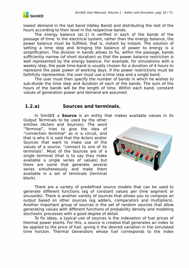
In SimSEE a Source is an entity that makes available values in itsOutput Terminals to be used by the otherentities (Actors and Sources). The word“Terminal”, tries to give the idea of“connection terminal” as in a circuit, andthat is why it is said that the Actors and/orSources that want to make use of thevalues of a source, “connect to one of itsterminals”. Most of the Sources are of asingle terminal (that is to say they makeavailable a single series of values) butthere are some that generate severalseries simultaneously and make themavailable in a set of terminals (terminalblock).
There are a variety of predefined source models that can be used togenerate different functions (eg of constant values per time segment orsinusoids). There is another variety of sources that allows you to compose anoutput based on other sources (eg adders, comparators and multipliers).Another important group of sources is the set of random sources that allowgenerating values with different functions of probability density and modelingstochastic processes with a good degree of detail.
To fix ideas, a typical use of sources is the indexation of fuel prices ofthermal power plants. For this, a source is created that generates an index tobe applied to the price of fuel, giving it the desired variation in the simulatedtime horizon. Thermal Generators whose fuel corresponds to the index

SimSEE User Manuals, Volume 1 – Editor and Simulator, pág. 11 / 71
created by the source, can "connect" to the source so that their productioncost is affected by the variation in the price of their fuel.
1.2.b) Layers and Scenarios.
The SimSEE Room has the possibility of having several Layers. Thedefault Layer is 0 (Zero). When editing a Dynamic Parameter Record you canindicate the layer to which it belongs.
This Layers mechanism allows to set up different scenarios or cases. AScenario is defined by indicating which are the Layers of the Room that areactive in that Scenario. In this way, when executing the Simulation /Optimization stages of the Room, indicating a Scenario, only the Layers thatbelong to the indicated scenario can participate in the execution. ThisScenario mechanism can be seen as a way to analyze many Cases with thesame Room (the same Room file) without having to create several files andthus facilitating the maintenance of the information.
1.2.c) Dynamic parameters.
To create Actors or Sources in SimSEE, the first step is to select the typeor model that best represents it. The second step is to configure the entitythrough specific forms of the selected type that allow setting its parameters.Once the model to be used is selected, there is usually a set of staticparameters that are changed in a main form of the entity and another set ofdynamic parameters that can vary during the time horizon. The dynamicparameter set is edited by means of a form in which, in addition to theparameter values, the date from which these data are valid is indicated. Aninstance of dynamic parameter values with its date is called the DynamicParameter Record. During the editing of the Room, the user can add as manyDynamic Parameters Records as he wishes to represent the evolution of theentity over time. As an example, the availability factor of a generator canvary depending on its useful life and the maintenance routines to which it issubjected.For details on editing dynamic parameter records see the section Error: no seencontró el origen de la referencia.
1.2.d) Units.
Given an Actor, it can be indicated that it has more than one Unit. Forexample, if we configure a 2 MW wind turbine, indicating that the Actor has25 units, we will be representing a 50 MW park. The Units are also dynamicparameters, which allows to remove units to represent the dismantling of aplant or to add Units to represent the incorporation of new units. In addition tothe number of units, you can represent how many are in scheduledmaintenance.
SimSEE User Manuals, Volume 1 – Editor and Simulator, pág. 12 / 71
The possibility of representing the units within the Actor instead ofvarying their power, allows a fine handling of both programmed andaccidental availability. Returning to the example of the park of 25 windturbines of 2 MW, if an availability factor of 0.95 is assumed, it is not thesame to model the park as a single unit of 50 MW than as 25 of 2 MW,because in the first case when the unit undergoes a fortuitous breakage, 50MW of the system will be lost, while in the second case, the accidental breaksof the units are independent and therefore the effect of the unavailability onthe real power available for the system is filtered (damped) by the number ofunits
1.3. Systems without dynamics.It is said that a system has no dynamics when the history of the system
is not relevant for the determination of its future evolution. Equivalently, wecan say that the system "has no memory" or "has no inertia."
In a system without dynamics, the operator's actions haveconsequences only in the passage of time in which they are executed and donot affect possible future operations. If the variable cost of each resource wasknown, the most economical dispatch would be the one obtained simply byordering the resources, at each time step, from the most economical to themost expensive (for its variable generation cost expressed in USD / MWh) andin each band, according to the level of demand of the band, starting with themost economical and continuing with the following until reaching the power ofthe demand.
This could be the case of a purely thermal system, in which it is easy todetermine the cost of production of each unit (for example aeroderivativeturbines and engines). For this to be possible, no component of the systemmust impose restrictions that imply a temporary linkage of decisions. Mostreal systems have dynamic restrictions (which link several time steps) andtherefore the Optimal Operation Policy is more complex than simplydispatching in order of increasing production variable costs. Just as anexample, in a system where the lower variable cost central was a combinedcycle that requires 4 hours of purging and heating the boiler and steam cycleto achieve the combination, even if it is the lower variable cost central, itwould not be the candidate for the coverage of a power peak hour of thesystem.
1.4. Dynamic systems.Dynamic system is understood as one in which the history of the system
is relevant to its future. Equivalently it is said that systems with dynamicshave "memory" or that they have "inertia".
The operation of a system is continuous decision making. From thedefinition itself, it appears that in a dynamic system, the decisions of thepresent affect the future and therefore when trying to make an “optimal
SimSEE User Manuals, Volume 1 – Editor and Simulator, pág. 13 / 71
operation” the past must be considered for its consequences on the presentand, from the set of possible decisions, considering that past , take those thatlead to a lower cost of both the present and the future.
Real systems have inertia that make it necessary to consider them asdynamic systems. For example, they include energy stores such as reservoirsof hydroelectric power plants that create a temporary dependence. A volumeof water that is used now to replace a thermal generation (and thus save thecost of fuel associated with the replaced energy), cannot be used in the futureunless it rains and is replenished. Another example of a temporary (ordynamic) link is the slow-start thermal power plants that impose restrictionson imposing an inflexible dispatch. An example of a dynamic link is a baseplant like a nuclear power plant. A power plant of this type does not acceptpower variations quickly (they are intended to be dispatched “at the base” ofthe demand curve).
The resolution of dynamic systems requires the valuation of storableresources, such as water in hydraulic reservoirs, which does not have anexplicit cost. The valuation consists in calculating the value of the resource byits ability to avoid future costs. This valuation is used later in the solution ofthe economic dispatch in each Time Step.
The State of a system is defined at a given time, as the relevantinformation of the system's past. Knowing the State implies knowingeverything necessary from the past that determines the possible actionspresent and the possible evolution of the system. Once the State is known, itis possible to calculate the evolution of the system with the knowledge offuture events.
The Optimization takes into account the set of state variables thatmodel the fundamental aspects that we are interested in observing of theelectrical system. The status variables can be continuous (eg volumes ofhydroelectric dam reservoirs, volume of fuel stored in a tank) or discrete (egon / off of a thermal machine that has a specified start and stop cost).
Optimization is carried out by Stochastic Dynamic Programming (PDE).The result of it is a function CF (X , k) with the expected value of the FutureCost of operation of the system for each value of the status vector X andevery time step k . This function is also known as Bellman's value function.
The relevant information for decision-making (The Optimal OperationPolicy) is found in the directional derivatives of Bellman's function.
For the ith component of the state vector, said directional derivative
would be:∂CF∂ x i
(X ,k ) .
Note that this derivative allows to assess the use of the resourceassociated with the state variable xi quantifying the effect on the future ofmaking a decision that implies in the present (instant k ) a variation δ xi inthe state variable xi .
SimSEE provides support for the management of the Bellman function,for its calculation and for the calculation of its derivatives in a transparentway for the common user, and very useful for users who intend to developnew models to add to the platform.

SimSEE User Manuals, Volume 1 – Editor and Simulator, pág. 14 / 71
1.5. Modeling an electric power system.
1.5.a) Representation of the transport network.
For the modeling of the network in SimSEE, Actors of the Node type areavailable to which the other Actors are connected, and of the Arc type orenergy transport corridors that connect nodes. The Nodes are simpleconnection bars, the Arcs allow you to specify performance, toll, transportcapacity and availability factor, thus allowing to represent transportrestrictions between the different areas of the system considered.
Just as an example and to set ideas, Fig. 1 shows a scheme of a systemwith two nodes joined by two transport corridors. The G1 generator anddemand D1 are connected to Node_1 and G2 generator and D2 demand toNode_2.
1.5.b) Node Restrictions.
The Power Balance (“Node Restriction”) must be instantly fulfilled ineach NODE, that is, the algebraic sum of the powers injected into the nodemust be ZERO.
Fig. 1: Representation of the transport network.

SimSEE User Manuals, Volume 1 – Editor and Simulator, pág. 15 / 71
1.6. Chaining Playrooms.The search algorithm of an Optimal Operation Policy implies the
exploration of the future to determine the consequences (the value) of theuse (movement of the State) of a resource in the present. As it is not possibleto explore to infinity, in practice a horizon is assumed from which theaffectation of the future is NULL. This assumption is possible in practice fortwo reasons: 1) by using a discount rate to update costs, the future in thevery long term has negligible present value and 2) the very nature of thesystem, with energy stores that saturate (eg reservoirs can store up to amaximum volume and then end up pouring water) and the randomness ofresources that causes the consequences to be diluted over time. Assuming aNULL affectation from the end of the Optimization Horizon implies that thesimulated operation, when it approaches the end of the Horizon, will makeuse of the stored resources assuming that they have no value from the end ofthe Horizon (for example this implies an emptying of the lakes in the system)and for this reason, the Optimization Horizon must include the SimulationHorizon leaving a margin between the end of the Simulation and the end ofthe Optimization. This margin between the end of the Simulation Horizon andthe Optimization Horizon is known as the Optimization Guard Horizon and thenecessary duration of it depends on the structure of the system underanalysis.
It is common to use more than one Room to describe the same systemaccording to the Horizon of analysis. For example, a Long Term Room with ahorizon of tens of years and a weekly simulation step, a Medium Term Roomwith a horizon of months and a daily simulation step and a Short Term Roomwith a horizon of weeks and a time simulation step. If the Optimization GuardHorizon required by the structure of the system is 3 years, it would be veryexpensive to impose that guard in the Short Term Room (time step) and thensimulate only a few weeks. For this reason, it is convenient to have amechanism to transfer information about the consequences of the futurealready explored by the Rooms with the greatest optimization horizonbetween the Rooms.
Fig. 2: Node restriction.
SimSEE User Manuals, Volume 1 – Editor and Simulator, pág. 16 / 71
The Rooms can be chained so that the Optimization stage of one,instead of initiating the Stochastic Dynamic Programming algorithm withoutinformation at the end of the optimization horizon, does so by “looking at” theFuture Cost function of the Room to which it is attached.
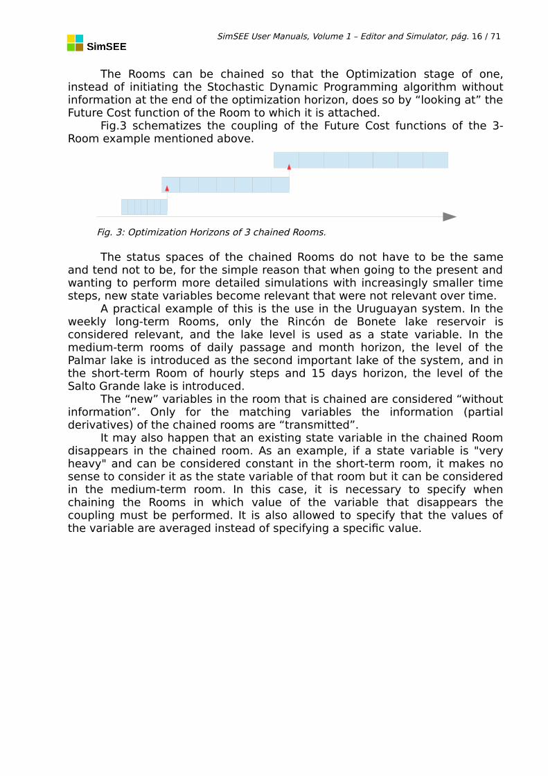
Fig.3 schematizes the coupling of the Future Cost functions of the 3-Room example mentioned above.
The status spaces of the chained Rooms do not have to be the sameand tend not to be, for the simple reason that when going to the present andwanting to perform more detailed simulations with increasingly smaller timesteps, new state variables become relevant that were not relevant over time.
A practical example of this is the use in the Uruguayan system. In theweekly long-term Rooms, only the Rincón de Bonete lake reservoir isconsidered relevant, and the lake level is used as a state variable. In themedium-term rooms of daily passage and month horizon, the level of thePalmar lake is introduced as the second important lake of the system, and inthe short-term Room of hourly steps and 15 days horizon, the level of theSalto Grande lake is introduced.
The “new” variables in the room that is chained are considered “withoutinformation”. Only for the matching variables the information (partialderivatives) of the chained rooms are “transmitted”.
It may also happen that an existing state variable in the chained Roomdisappears in the chained room. As an example, if a state variable is "veryheavy" and can be considered constant in the short-term room, it makes nosense to consider it as the state variable of that room but it can be consideredin the medium-term room. In this case, it is necessary to specify whenchaining the Rooms in which value of the variable that disappears thecoupling must be performed. It is also allowed to specify that the values ofthe variable are averaged instead of specifying a specific value.
Fig. 3: Optimization Horizons of 3 chained Rooms.
SimSEE User Manuals, Volume 1 – Editor and Simulator, pág. 17 / 71
2. Installation Procedure.
This section describes in detail the process for installing the SimSEEprogram on your computer.
2.1. Download website.You can find the latest version of the installation program at the
following web address:
https://simsee.org/downloads.html
Simply download the corresponding compressed file from Windows orLinux depending on your operating system and unzip its contents in the folder{$HOME}/SimSEE/bin, where {$HOME} is “C:\” if your operating system isWindows and your User folder if it is on Linux.
The user can select another location to install SimSEE, but it isrecommended to respect the location suggested in the previous paragraph tofacilitate compatibility with the reference to external files that the createdRooms may have and shared by users.
By default, the application language is Spanish. If you want to changethe language, run the SimSEEEdit application and in the main menu select“Language”. A message will appear indicating that the change was made andthat for it to take effect you must close and reopen the application.
2.2. SimSEE folder structure. Description of the content.
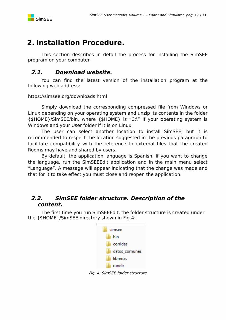
The first time you run SimSEEEdit, the folder structure is created under the {$HOME}/SimSEE directory shown in Fig.4:
Fig. 4: SimSEE folder structure
SimSEE User Manuals, Volume 1 – Editor and Simulator, pág. 18 / 71
The content and purpose of them is described below:
“bin”: SimSEE executable programs, configuration files and languagefiles are stored in this folder. The main applications are the SimSEEEditRoom Editor, the SimSEESimulator optimizer/simulator, the SimRes3results post-processor. For more information see section 2.3 “SimSEEBinaries”.
“corridas”: Generally, in this folder are the sub-folders of the differentRooms executed. One way to organize the work is to create a new sub-folder of the folder “corridas” for each study that is carried out and inthat folder all the rooms related to the study are stored. This is thesuggested organization, but it is not mandatory and the user can savethe Rooms in any folder.
“datos_comunes”: In this folder some common data is stored so thatthey can be used in different rooms. For example, the models ofgeneration of water-flows to the dams of the country based on historicalseries, models of wind-power generation based on historical windseries, detailed demands of historical years, etc.
“librerias”: Actors and Sources are saved in this folder when they areexported from a Room. Each Actor and / or Source is saved in aseparate text file and can be subsequently imported from anotherRoom.
“rundir”: When performing an Optimization or Simulation with theSimulator, a folder is created within the “rundir” folder in which the fileswith results of the Run are stored. If there is no sub-folder under“rundir” with the same name as the room under execution, it is createdat the start of execution. If the folder already exists, the resultscontained therein will be overwritten. The files generated whenexecuting a run are usually of a considerable size, so it is recommendedto check the folder every now and then to delete the subfolders that areno longer being used, to avoid taking up excessive disk space (toregenerate them, if necessary, you must execute again the run). InFig.5, the folder “rundir” is marked on the left side and on the right side,a Room that has been executed whose name is “sala_de_prueba” isshown .

SimSEE User Manuals, Volume 1 – Editor and Simulator, pág. 19 / 71
Fig. 5: Results folder "rundir".
It can be seen that, once a run is executed, the system adds someauxiliary folders to the basic folder structure: debug, docs-word and tmp,which are folders used in an accessory way by the software to saveintermediate results, among other uses .
2.3. SimSEE Binaries.
The following executable programs are found in the “bin” folder ofSimSEE installation:
“SimSEEEdit”: SimSEE editor through which the user can create andedit Rooms and post-processing sequences of the results as well aslaunch optimizations/simulations. Its main menu is described in theChapter 4. Editing a simulation consists in selecting the Actors that willparticipate in the Game and adding them to the Playing Room.
“SimSEESimulador”: the optimizer / simulator that will be invoked bythe Editor when the user has finished editing the Room and decides tooptimize and simulate it (do the Run). It is described in the chapterChapter 4 of the present Manual.
“SimRes3”: the program that allows the user to perform different post-processing calculations of the results obtained in the simulation. It maybe invoked by the Simulator once the corresponding simulation isfinished and from the Editor itself if the simulation has already beenperformed. Its detailed description is found in Volume IV of the SimSEEUser Manual series.
“analisisserial”: It is an auxiliary utility to the platform that allowsanalyzing time series of data and creating a correlation model inGaussian Space with CEGH Histogram. The program “analisisserial” isexplained in detail in Volume V of the SimSEE User Manual series.
“cmdopt”, “cmdsim”: command files that allow the execution of theOptimization and Simulation stages respectively. These programs do nothave a graphical interface and must be called by passing as parameters

SimSEE User Manuals, Volume 1 – Editor and Simulator, pág. 20 / 71
the Room to be executed and other necessary data. These executablesare useful for scheduling the execution of run sets in BATCH mode oneither Windows or Linux. They are also the same executables that areused for the execution of SimSEE in high computational performanceequipment in which the execution is carried out remotely withoutaccess to graphical interfaces.
“datosbin2xlt”: It is an auxiliary utility that allows you to convert adetailed time file in binary format (extension .bin) to a plain text fileusing the tab character as a separator (extension .xlt) in order to beable to visualize its contents (eg to visualize the SimSEE demand files).
“oddface_prepare” and “oddface_pig”: These are applications thatallow you to prepare optimizations for optimal generation plans andexecute them. They are described in detail in Volume VI of the SimSEEManual series.
SimSEE User Manuals, Volume 1 – Editor and Simulator, pág. 21 / 71
3. The Rooms Editor.
The information of a SimSEE Room can be classified as:• Description of the Temporary Horizons.• List of Actors and Sources.• Specification of values to register and their postprocessing.• Scenarios Description.• Additional parameters for execution.
This chapter describes the previous contents and the way in which theycan be edited.
3.1. User interface unified methods.This section presents general characteristics of the editor that are
applied in various types of editing. Generally, all the information of the Roomis organized in lists of entities (Actors, Sources, etc.). The editing work mainlyinvolves: Add / Remove entities from the lists and Edit the parameters of theentities.
3.1.a) Form editing.
Whenever the editing of an entity begins, in SimSEE the entity is“cloned” and a form is opened that displays the current values and allowsthem to be modified. These forms have a “Save” (or Save Changes) buttonand another “Cancel” button. If you press the “Save” button (see example inFig. 1) the new set of values will be copied over the originals, if you press“Cancel” the new set of values will be discarded without modifying theoriginals.

SimSEE User Manuals, Volume 1 – Editor and Simulator, pág. 22 / 71
3.1.b) Management of listings.
In the Editor, whenever it is possible to edit listings (eg Actors, Sources,dynamic parameter tabs of an entity) they are presented by means of tablesembedded in the forms, as the example shown in Fig.7. At the top of the tablethere is a button that allows you to add a tab (record) to the list. In theexample in Fig.7 this button is “Add Source”.
Fig. 7: Example table for editing a list.
The first columns contain a summary of the values of each record. Thecolumns on the right with the buttons are the ones that allow modifying thelist. The meaning of the buttons is as follows:
"Pencil": Opens a form that allows you to edit and modify the values ofthe record.
Fig. 6: Example of editing form.
SimSEE User Manuals, Volume 1 – Editor and Simulator, pág. 23 / 71
“Cross”: It allows to eliminate the record. A window opens asking forconfirmation to proceed with this removal. On the other hand, if the file isbeing referenced by another entity, a window is opened that warns of this,and informs that therefore its elimination is not possible.
"Clone": Clones the record. Pressing this button creates a copy of the selected recordand opens the editing form on the new created record. It is useful to create a new file from anexisting one, avoiding having to enter all the data again.
3.1.c) Editing a Dynamic Parameters Record.
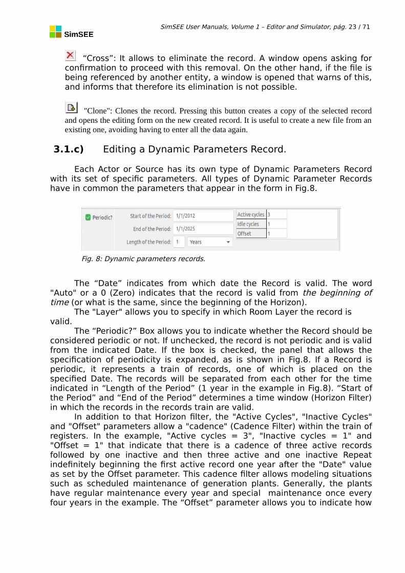
Each Actor or Source has its own type of Dynamic Parameters Recordwith its set of specific parameters. All types of Dynamic Parameter Recordshave in common the parameters that appear in the form in Fig.8.
The “Date” indicates from which date the Record is valid. The word"Auto" or a 0 (Zero) indicates that the record is valid from the beginning oftime (or what is the same, since the beginning of the Horizon).
The "Layer" allows you to specify in which Room Layer the record is valid.
The “Periodic?” Box allows you to indicate whether the Record should beconsidered periodic or not. If unchecked, the record is not periodic and is validfrom the indicated Date. If the box is checked, the panel that allows thespecification of periodicity is expanded, as is shown in Fig.8. If a Record isperiodic, it represents a train of records, one of which is placed on thespecified Date. The records will be separated from each other for the timeindicated in “Length of the Period” (1 year in the example in Fig.8). “Start ofthe Period” and “End of the Period” determines a time window (Horizon Filter)in which the records in the records train are valid.
In addition to that Horizon filter, the "Active Cycles", "Inactive Cycles"and "Offset" parameters allow a "cadence" (Cadence Filter) within the train ofregisters. In the example, "Active cycles = 3", "Inactive cycles = 1" and"Offset = 1" that indicate that there is a cadence of three active recordsfollowed by one inactive and then three active and one inactive Repeatindefinitely beginning the first active record one year after the "Date" valueas set by the Offset parameter. This cadence filter allows modeling situationssuch as scheduled maintenance of generation plants. Generally, the plantshave regular maintenance every year and special maintenance once everyfour years in the example. The “Offset” parameter allows you to indicate how
Fig. 8: Dynamic parameters records.

SimSEE User Manuals, Volume 1 – Editor and Simulator, pág. 24 / 71
many steps (records) the first active record is in relation to the starting“Date”.
In the “Date” and “Start Of Period” a value of “0” (cero) means that thevalue considered will be the start of the Optimization Horizon.
The configuration and use of the periodic records has proved difficult tounderstand and use by users. To try to reaffirm the topic, three examples ofusing periodic files are presented below.
3.1.c.i Example 1As an example, to schedule a plant to be serviced every year for 1
month in September, two periodic records are needed. One, to remove theunit and another to re-establish it a month later. In this case, the startingDates would be 1/9/2013 and 1/10/2013 respectively, both records wouldhave the “Periodic?” box marked and Long Period 1 year box marked. In thehorizon filter the two values would be set to Auto or 0 (Zero), to indicate thatit is from the beginning of the times to the end of the times (that is,throughout the entire analysis horizon). The cadence parameters would be setto "Active Cycles = 1", "Inactive Cycles = 0" and "Offset = 0".
To give an example in which the cadence filter makes sense, imagine acase in which the two records of the previous paragraph define the regularmaintenance of the plant, but that once every four years it is necessary to doa major maintenance that lasts 4 months and you want to start in August. Toachieve this, two more records that model the major maintenance must beadded and the two records in the previous paragraph must be given cadence.The two records that model the major maintenance would have dates1/8/2013 and 1/12/2013, “Period Length = 1 year”. The horizon filter with thetwo values in Auto. The cadence parameters would be: "Active Cycles = 1","Inactive Cycles = 3" and "Offset = (N-1)" with the value of N explainedbelow. To the two records of the previous paragraph we must change thecadence parameters that would be: “Active Cycles = 3”, “Inactive Cycles = 1”and “Displacement = (N-1) +1” to ensure that the beginning of one of thegroups of three active records one year after each major maintenance. Thevalue of (N-1) sets when the major maintenance is compared to the date1/8/2013. If (N-1) = 0 then there is a major maintenance in 2013, if it is 1 in2014 and so on respectively.
3.1.c.ii Example 2.
Fig.9 shows one of the dynamic parameter records of an actor thatrepresents the possibility of importing energy in a Room.

SimSEE User Manuals, Volume 1 – Editor and Simulator, pág. 25 / 71
Fig. 9: Example of use of dynamic parameters.
In the example, it is an import modeled as an Actor of the “Market Spot”type. To represent that the energy availability of the selling country can varysubstantially depending on the season of the year due to parameters such asthe rainfall regime and temperature, variable interconnection availabilityfactors with the seasons of the year are considered. And this is repeated inthe same way every year. Thus, two periodic records can be defined for theActor, one, whose validity begins in May and the other, whose validity beginsin November, as shown in Fig.10 (Note that for these last two records thecolumn “Periodic?” is marked with “YES”, unlike the previous cards thatindicate “NO.” The first two cards are overwritten by the periodic ones).

SimSEE User Manuals, Volume 1 – Editor and Simulator, pág. 26 / 71
Fig. 10: Two periodic cards to give seasonality.
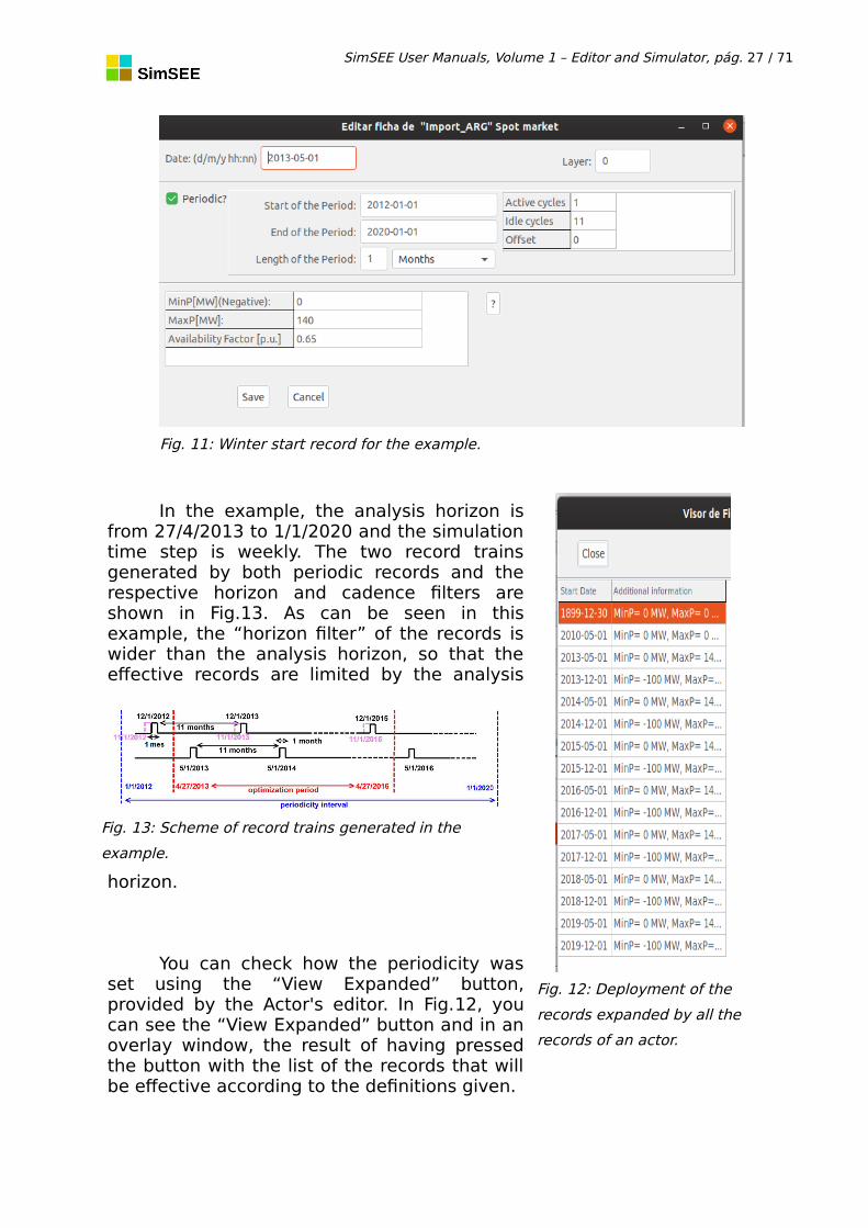
The file corresponding to the summer (in the southern hemisphere)period is shown in Fig.9, and there it can be seen that, although theperiodicity is annual, it was declared in months, in order to allow thebeginning of summer to be displaced by one month. The record is activatedfor one cycle (one month) and is not activated again during the following 11cycles (but remains active until another record overwrites it). This will be thecase for all the months included in the 2012-2020 interval during which it isdeclared that the periodicity is in force, beginning on 1/11/2012 (start date ofthe “summer” record). If the displacement were null, the record would beginto be valid from November, every year. But a displacement of 1 month wasindicated, this means that it will begin to be valid from December every year.When May arrives, the other complementary “winter” card will begin to bevalid, which, as seen in Fig.11, modifies the Power and availability of saidimport.
SimSEE User Manuals, Volume 1 – Editor and Simulator, pág. 27 / 71
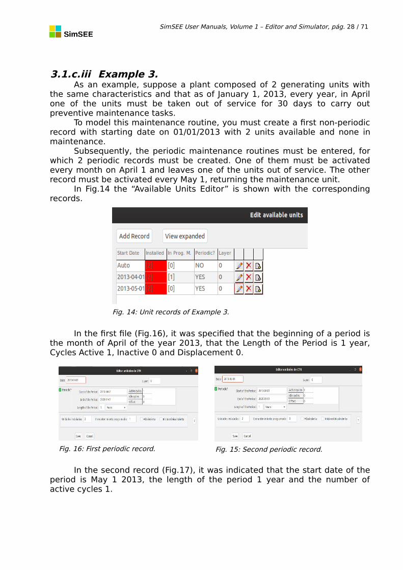
In the example, the analysis horizon isfrom 27/4/2013 to 1/1/2020 and the simulationtime step is weekly. The two record trainsgenerated by both periodic records and therespective horizon and cadence filters areshown in Fig.13. As can be seen in thisexample, the “horizon filter” of the records iswider than the analysis horizon, so that theeffective records are limited by the analysis
horizon.
You can check how the periodicity wasset using the “View Expanded” button,provided by the Actor's editor. In Fig.12, youcan see the “View Expanded” button and in anoverlay window, the result of having pressedthe button with the list of the records that willbe effective according to the definitions given.
Fig. 11: Winter start record for the example.
Fig. 13: Scheme of record trains generated in the
example.
Fig. 12: Deployment of the
records expanded by all the
records of an actor.
SimSEE User Manuals, Volume 1 – Editor and Simulator, pág. 28 / 71
3.1.c.iii Example 3.As an example, suppose a plant composed of 2 generating units with
the same characteristics and that as of January 1, 2013, every year, in Aprilone of the units must be taken out of service for 30 days to carry outpreventive maintenance tasks.
To model this maintenance routine, you must create a first non-periodicrecord with starting date on 01/01/2013 with 2 units available and none inmaintenance.
Subsequently, the periodic maintenance routines must be entered, forwhich 2 periodic records must be created. One of them must be activatedevery month on April 1 and leaves one of the units out of service. The otherrecord must be activated every May 1, returning the maintenance unit.
In Fig.14 the “Available Units Editor” is shown with the correspondingrecords.
Fig. 14: Unit records of Example 3.
In the first file (Fig.16), it was specified that the beginning of a period isthe month of April of the year 2013, that the Length of the Period is 1 year,Cycles Active 1, Inactive 0 and Displacement 0.
In the second record (Fig.17), it was indicated that the start date of theperiod is May 1 2013, the length of the period 1 year and the number ofactive cycles 1.
Fig. 16: First periodic record. Fig. 15: Second periodic record.

SimSEE User Manuals, Volume 1 – Editor and Simulator, pág. 29 / 71
In this way the maintenance routine was createdthroughout the period of interest.
With the Expanded View button, you can view all therecords (Fig.17). It is clearly observed that every year in Aprilone of the machines goes out of service (indicated with M: 1which means a unit in maintenance) and in the month of Maythe 2 machines are available (indicated with M: 0 whichmeans that no machine is in maintenance). In the table inFig.17 the nomenclature (I: 2 M: 1) means that there are twomachines installed (I: 2) and one in maintenance (M: 1).
Fig. 17:
Expanded
records

SimSEE User Manuals, Volume 1 – Editor and Simulator, pág. 30 / 71
3.2. Main Menu of the SimSEE Editor.The “SimSEEEdit” program is the Room Editor for SimSEE. The initial
screen of the Editor is shown in Fig. .18.
Fig. 18: Pantalla inicial del Editor.
ations that the user considers useful, in order to document your simulation.In the lower part, a “Warnings” window is displayed where warnings
about possible errors are displayed, if they occur. For example, when youchange the version of SimSEE, when you open a Room made with someprevious version, warning messages may appear indicating the changesmade by the version change.
The different options presented in the SimSEE Main Menu aredescribed below.
SimSEE User Manuals, Volume 1 – Editor and Simulator, pág. 31 / 71
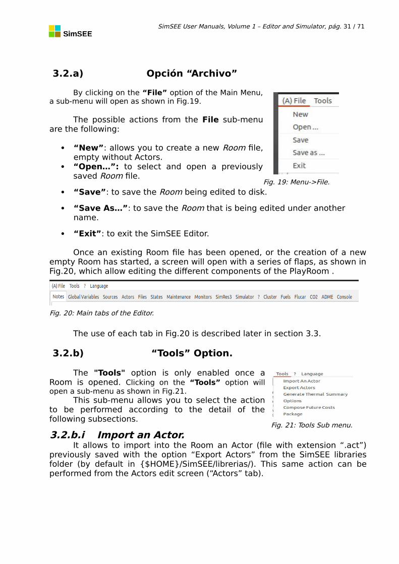
3.2.a) Opción “Archivo”
By clicking on the “File” option of the Main Menu,a sub-menu will open as shown in Fig.19.
The possible actions from the File sub-menuare the following:
“New”: allows you to create a new Room file,empty without Actors.
“Open…”: to select and open a previouslysaved Room file.
“Save”: to save the Room being edited to disk.
“Save As…”: to save the Room that is being edited under another name.
“Exit”: to exit the SimSEE Editor.
Once an existing Room file has been opened, or the creation of a newempty Room has started, a screen will open with a series of flaps, as shown inFig.20, which allow editing the different components of the PlayRoom .
Fig. 20: Main tabs of the Editor.
The use of each tab in Fig.20 is described later in section 3.3.
3.2.b) “Tools” Option.
The "Tools" option is only enabled once aRoom is opened. Clicking on the “Tools” option willopen a sub-menu as shown in Fig.21.
This sub-menu allows you to select the actionto be performed according to the detail of thefollowing subsections.
3.2.b.i Import an Actor.It allows to import into the Room an Actor (file with extension “.act”)
previously saved with the option “Export Actors” from the SimSEE librariesfolder (by default in {$HOME}/SimSEE/librerias/). This same action can beperformed from the Actors edit screen (“Actors” tab).
Fig. 19: Menu->File.
Fig. 21: Tools Sub menu.

SimSEE User Manuals, Volume 1 – Editor and Simulator, pág. 32 / 71
3.2.b.ii Export Actors.Allows you to select one or more Actors to be exported to the SimSEE li-
braries folder. This same action can be performed from the Actors edit screen(“Actors” tab).
3.2.b.iii Generate Thermal Summary.It generates an Excel spreadsheet with a list of the relevant information
for the Actors corresponding to the Thermal Generating Plants present in thesimulation: Minimum power (if specified) and maximum (MW) of each unit,variable cost at minimum power (if specified) and average cost (according toits dispatch in the simulation) in USD / MWh, incremental variable cost of gen-erating the next MWh, availability factor specified for each unit (pu), start andstop cost (USD) (if specified), etc., as shown in Fig.22. This is a summary of itsinitial parameters, not taking into account the evolution of the Generatorsgiven by the dynamic parameter tabs.The summary is automatically saved in the folder {$HOME}/SimSEE/rundir/room_name.
Fig. 22: Summary of thermal generators.
3.2.b.iv “Packing”.Create a compressed file (.zip) in the sub-folder in which the Room file is
located and with the same name of the room, containing the room (.ese file)and all the files referred to by the Room. This allows the room to be trans-ported to another computer.
3.2.c) Option “?” (Help).
The "?" option attempts to open the default web browser of yourcomputer with the online help for the use of SimSEE. For help to be deployed,you must have a browser configured and access to the Internet. In differentparts of the Editor, where the “?” Question symbol appears when pressed, thehelp page is displayed according to the context in which the button appears.The online help is permanently improved thanks to user feedback, so if youhave suggestions on how to improve an explanation, do not hesitate to usethe contact form at: https://simsee.org/contacto_en.php to make yourcontribution.

SimSEE User Manuals, Volume 1 – Editor and Simulator, pág. 33 / 71
3.2.d) Option “Language”.
This option allows you to change the Language used in the SimSEEplatform. For now, the available languages are Spanish (default language) andEnglish. When using this option, a window will open with a message indicatingthat the language change will be effective as of the next time you open theapplication.
SimSEE User Manuals, Volume 1 – Editor and Simulator, pág. 34 / 71
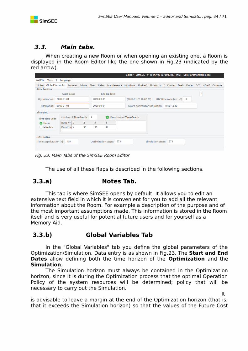
3.3. Main tabs.When creating a new Room or when opening an existing one, a Room is
displayed in the Room Editor like the one shown in Fig.23 (indicated by thered arrow).
The use of all these flaps is described in the following sections.
3.3.a) Notes Tab.
This tab is where SimSEE opens by default. It allows you to edit an extensive text field in which it is convenient for you to add all the relevant information about the Room. For example a description of the purpose and of the most important assumptions made. This information is stored in the Roomitself and is very useful for potential future users and for yourself as a Memory Aid.
3.3.b) Global Variables Tab
In the "Global Variables" tab you define the global parameters of theOptimization/Simulation. Data entry is as shown in Fig.23. The Start and EndDates allow defining both the time horizon of the Optimization and theSimulation.
The Simulation horizon must always be contained in the Optimizationhorizon, since it is during the Optimization process that the optimal OperationPolicy of the system resources will be determined; policy that will benecessary to carry out the Simulation.
Itis advisable to leave a margin at the end of the Optimization horizon (that is,that it exceeds the Simulation horizon) so that the values of the Future Cost
Fig. 23: Main Tabs of the SimSEE Room Editor
SimSEE User Manuals, Volume 1 – Editor and Simulator, pág. 35 / 71
function (which are built from the future to the present, in the recursion of theStochastic Dynamic Programming algorithm) have been stabilized inrepresentative values independent of the initial condition of the algorithm.This margin is called “optimization guard horizon”.
How extensive the “guard horizon” should be depends on the systemunder simulation, and in particular, on the time constants involved. Anotherfactor that affects the stabilization of the Future Cost function is the discountrate used (parameter specified in the Simulator tab sec.3.3.i). We recommendusing rates higher than 8% per year.
The "Start Date" is the start date of the first time step.The “End Date” is the start date of the step following the last time step
considered by the simulation.Strictly, if the start date is called t ini , the end date t fin and Δ t the
duration of the time step, lthe time steps will be identified by the ordinalk=1, 2. ..N with the greater N such that (t ini+(N−1)∗Δ t)<t fin .
The “Sim Guard Date” allows you to specify a date from which thesimulation results are written. This allows you to easily ignore the start of asimulation as a way to become independent of the initial condition of thesystem during the simulation. The value “1899-12-30” shown in the examplein Fig.23, being before the start date of the simulation (“2009-01-01” in theexample), implies that all will be saved the results from the beginning of thesimulation.
In the "Time step" panel, the option to select the "Time step units" ispresented.
In Fig.23 the “Time Step” panel is shown when “Hours” units have beenselected. In that condition, you must specify the number of Bands (or timebands) into which the time step will be divided (4 in the example in Fig. .23)and in the Band duration table specify the duration in hours of each of thebands.
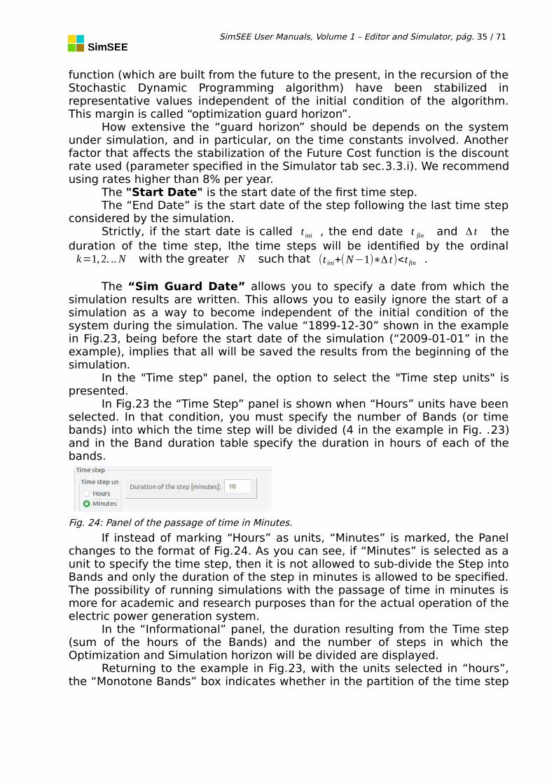
If instead of marking “Hours” as units, “Minutes” is marked, the Panelchanges to the format of Fig.24. As you can see, if “Minutes” is selected as aunit to specify the time step, then it is not allowed to sub-divide the Step intoBands and only the duration of the step in minutes is allowed to be specified.The possibility of running simulations with the passage of time in minutes ismore for academic and research purposes than for the actual operation of theelectric power generation system.
In the “Informational” panel, the duration resulting from the Time step(sum of the hours of the Bands) and the number of steps in which theOptimization and Simulation horizon will be divided are displayed.
Returning to the example in Fig.23, with the units selected in “hours”,the “Monotone Bands” box indicates whether in the partition of the time step
Fig. 24: Panel of the passage of time in Minutes.

SimSEE User Manuals, Volume 1 – Editor and Simulator, pág. 36 / 71
in posts, the hours of the passage are messed up or not. The most commonuse is with the box marked and implies that the hours of the passage of timewill be ordered according to the Monotone Load curve. The Monotone of Loadis constructed by ordering the hourly power of the Demand (from the first ofthe Demand Actors if there is more than one) in decreasing form, thuscreating a new order of the hours in the passage of time. In this way, a neworder is created in the hours of the passage of time. In the new order, the firsthours are those of Band 1 (hours of higher demand), the second hours ofBand 2 and so on until reaching the last Band (hours of lower demand). If thebox is unchecked, the hours of the passage are not messed up and then,Band 1 will contain the first hours of the passage (in the natural chronologicalorder), the second the following ones and so on until completing the time stepwith the last Band. Unmarked use is for academic purposes, so always checkthat the "Monotone Posts" box is checked (unless you are doing some analysisin which it makes sense not to mark it).
If you do not want to use the subdivision mechanism of the Time Lapsein Bands, just indicate that the number of bands is 1 (one) and make thatsingle band have the duration in hours that the Time Pass should have.
3.3.c) “Sources” Tab.
In the Sources tab, it is possible to add and edit the Sources in thePlayRoom. A Source is a generator of values that can be used by the Actorsand other Sources. An example (for a given Room) of the contents of the tabis shown in Fig.25
Fig. 25: Example of the contents of the Sources tab.

SimSEE User Manuals, Volume 1 – Editor and Simulator, pág. 37 / 71
Pressing the “Add Source” button displays the form in Fig.26 that allowsyou to select the type of source to add. The different source models aredetailed in VOLUME 2 of this same series of manuals.
Once selected and configured, the source is added to the list of sourcesshown below the "Add Source" button.
Pressing the "Delete unused" button removes all sources that are notbeing referenced by any other entity from the Room.
To "edit" the parameters of a source, press the pencil in the list, to
remove the cross and to "clone" (make a twin copy) the button .If you try to delete a Source that is referenced by an Actor or another
Source, you will receive an error message. You must go to the entity thatrefers to the source and delete the reference in order to remove the Source.
A common use of sources is to model price growth rates to affect, forexample, the generation costs of Actors who consume the same type of fuel.Another common use is the modeling of resources that are inherentlystochastic such as the flow of contributions to hydroelectric power plants orwind speed in wind generation parks.
As an example of use in an Actor, a dynamic parameter recordcorresponding to a thermal power plant can be seen in Fig.27, in which avariable cost of 224 USD/MWh is considered, and that in the same form, thesource "iGO" and its "fuel" terminal to has been selected as "Fuel Price Index".
Fig. 26: Add Source selector form

SimSEE User Manuals, Volume 1 – Editor and Simulator, pág. 38 / 71
Fig. 27: Actor example using a Source.Fig. 28: Example of Constant
Source.
In Fig. 23 the parameters of the “iGO” Source are shown and as can beseen, it has two dynamic parameter tabs. The first one sets the value 1.1upon its departure as of 01/01/2014 and the second one sets the value 1.2 asof 01/01/2015. In short, this index will be defined as of January 1, 2014 at 1.1,which will imply that the variable cost for the dispatch of the plant will be 224* 1.1 = 246.4 USD/MWh and will have another increase as of January 1, 2015in which it will have a variable generation cost of 224 * 1.21 = 271.04 USD /MWh.
3.3.c.i Sources and terminals.The Sources make available, in their Terminals (or outputs), different
values in order to be used by the Actors or other Sources within the sameRoom. To make use of a source, in a Entity (Actor or Source), the Source andthe Source Terminal to which the Entity will be connected must be selected.
Most sources make a single terminal available, but there are some thatoffer several terminals. The typical example of a multi-terminal source isthose created of the “CEGH Synthesizer” type, representing a multi-variablestochastic process. In these cases, given the correlation between the series, itis not possible to model them as independent sources, and a single source,with multiple terminals, has to model the set of variables whose joint processis to be modeled.
A Source consists of Static Parameters (those that do not vary overtime) and Dynamic Parameters (those that can be specified with timevariation). Fig.29 shows the typical form of static parameters of a Sourceincluding the list of records with definition of dynamic parameters.

SimSEE User Manuals, Volume 1 – Editor and Simulator, pág. 39 / 71
The static parameters common to all sources are the "Name", the"Duration of the Draw Step [h]", the "Summarize averaging (if enslaved in asub-sampling)" box and the list of "Terminals".
The Name is the identifier of the source (as an entity in the Room). Thisidentifier will be the one that appears in the selection listings in the fields ofthe forms in which it is possible to select a source.
The "Duration of the Draw Step [h]" allows you to specify theduration of the draw step (in hours) for the source. This duration of the drawstep is the “natural” of the source, understood as such, that rate ofgeneration of values for which the source was designed. As an example, if asource is constructed to generate values that represent the average weeklyvalues of flows of water inflows to a hydroelectric plant, the natural rate ofthat source will be weekly. If that source is used in a Room with monthly timestep, it would be imposing a fixed value throughout the month with thevariance of weekly values, which does not represent reality. Likewise, if thesource were used in a Room with 1 hour time step, it would be generating anhourly value with the weekly variance that is not correct either. To allow theuse of sources with a natural cadence different from the time step of theRoom, the parameter "Duration of the Draw Step" is used. If a value of 0(Zero) is entered, it is indicated that the source does not have a preferrednatural cadence and that it is used as if its natural cadence coincides with thetime step of the Room. If a value other than Zero is specified, then thebehavior is as follows:a) If the Duration of the Draw Step is greater than the duration of the RoomTime Step (for example a weekly source in an hourly Room), the source will be“enslaved” in an “over-sampling” mechanism. This mechanism is transparent
Fig. 29: Form with the common static parameters of the sources.
SimSEE User Manuals, Volume 1 – Editor and Simulator, pág. 40 / 71
to the user. At runtime, another source is created that supplants the originaland “enslaves” it. The new source generates values in accordance with theRoom Time Step, for which it asks for values from the enslaved source withthe cadence corresponding to the “Duration of the Draw Step” andinterpolates between the values obtained to generate the values available inits terminals .b) If the Duration of the Draw Step is shorter than the duration of the RoomTime Step (for example an hourly source in a weekly step Room), the sourcewill be enslaved in a “sub-sampling” mechanism. This mechanism istransparent to the user. At runtime, another source is created that supplantsthe original and “enslaves” it. The new source generates values according tothe time step of the Room for which it asks for values from the enslavedsource with the cadence corresponding to the “Duration of the Draw Step”and summarizes the set of values received in a value for each time step ofthe Room. This summary can be done in two ways and for this the“Summarize averaging (applicable if enslaved in a subsampling)”checkbox is used. If the box is checked, the sample sets received from theslave source are summarized by a simple average. If the box is not checked,the set of values is summarized by choosing any of them randomly with equalprobability. Note that both ways of summarizing end up giving the sameexpected value as a result, the big difference is in the variance of the valuesproduced. The average method considerably reduces the variance. Therandom method gives maximum variance.
This alternative was developed to estimate the error made in weeklytime step Rooms (Typically long-term rooms for investment analysis) whenconsidering hourly sources of wind power generation.In the case of windpower, in a system with hydroelectric plants, the reservoirs act as a filter ofvariations, reducing the effects of the variance of the resource. As the amountof wind MW in the system increases, that filter will not be able to absorb allthe variations. Executing the same Room with “summarize averaging” markedand unmarked, an estimate of the error made when assuming the average isobtained.
In addition to the static parameters, the Sources have DynamicParameters. Each type of source has a specific set of parameters accordingto its model.
The set of sources available in version viie21.198 of SimSEE is asfollows is the shown in Fig.26.
In the "Source Reference Manual - SimSEE", Volume 2 of this series ofmanuals, the model and configuration parameters for each type of source aredetailed.
3.3.d) Actors Tab
Electric power systems are composed of different Actors (entities),which can deliver energy to de system or consume energy from the system.For example, generation plants deliver energy to the system, international
SimSEE User Manuals, Volume 1 – Editor and Simulator, pág. 41 / 71
interconnections can deliver or consume energy and demands are energyconsumption.
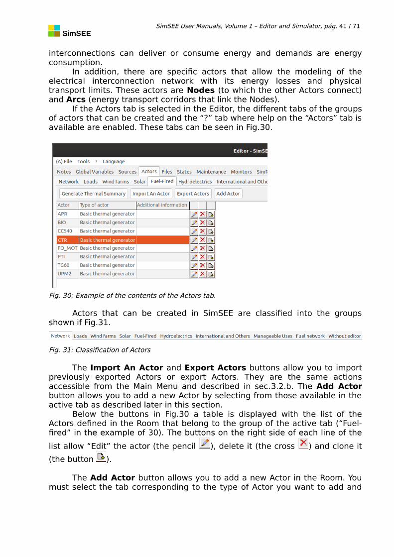
In addition, there are specific actors that allow the modeling of theelectrical interconnection network with its energy losses and physicaltransport limits. These actors are Nodes (to which the other Actors connect)and Arcs (energy transport corridors that link the Nodes).
If the Actors tab is selected in the Editor, the different tabs of the groupsof actors that can be created and the “?” tab where help on the “Actors” tab isavailable are enabled. These tabs can be seen in Fig.30.
Fig. 30: Example of the contents of the Actors tab.
Actors that can be created in SimSEE are classified into the groupsshown if Fig.31.
Fig. 31: Classification of Actors
The Import An Actor and Export Actors buttons allow you to importpreviously exported Actors or export Actors. They are the same actionsaccessible from the Main Menu and described in sec.3.2.b. The Add Actorbutton allows you to add a new Actor by selecting from those available in theactive tab as described later in this section.
Below the buttons in Fig.30 a table is displayed with the list of theActors defined in the Room that belong to the group of the active tab (“Fuel-fired” in the example of 30). The buttons on the right side of each line of the
list allow “Edit” the actor (the pencil ), delete it (the cross ) and clone it
(the button ).
The Add Actor button allows you to add a new Actor in the Room. Youmust select the tab corresponding to the type of Actor you want to add and
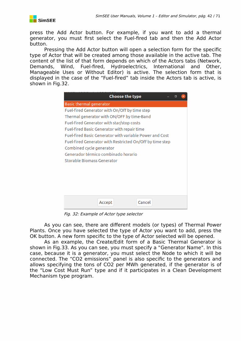
SimSEE User Manuals, Volume 1 – Editor and Simulator, pág. 42 / 71
press the Add Actor button. For example, if you want to add a thermalgenerator, you must first select the Fuel-fired tab and then the Add Actorbutton.
Pressing the Add Actor button will open a selection form for the specifictype of Actor that will be created among those available in the active tab. Thecontent of the list of that form depends on which of the Actors tabs (Network,Demands, Wind, Fuel-fired, Hydroelectrics, International and Other,Manageable Uses or Without Editor) is active. The selection form that isdisplayed in the case of the “Fuel-fired” tab inside the Actors tab is active, isshown in Fig.32.
As you can see, there are different models (or types) of Thermal PowerPlants. Once you have selected the type of Actor you want to add, press theOK button. A new form specific to the type of Actor selected will be opened.
As an example, the Create/Edit form of a Basic Thermal Generator isshown in Fig.33. As you can see, you must specify a "Generator Name". In thiscase, because it is a generator, you must select the Node to which it will beconnected. The “CO2 emissions” panel is also specific to the generators andallows specifying the tons of CO2 per MWh generated, if the generator is ofthe “Low Cost Must Run” type and if it participates in a Clean DevelopmentMechanism type program.
Fig. 32: Example of Actor type selector

SimSEE User Manuals, Volume 1 – Editor and Simulator, pág. 43 / 71
Next, you can see the pale with the list of Dynamic Parameters Records.The “See Expanded Periodicity” button shows in a separate window the set ofrecords including the non-explicit records that are generated by the effect ofthe periodicities that have the explicitly defined in the records. The "Add NewRecord" button creates a new record and opens the form for editing it. Thefields of the dynamic parameters record are specific to each type of Actor andare described in detail in Volume 3 "SimSEE Volume 3 - Actors" from this sameseries of user manuals.
Fig.34 shows an example of the form for editing the dynamicparameters record. In this case, it is a Basic Thermal Generating Actor. Ingeneral, as in any dynamic parameter record, the date from which it is valid,the Layer and the periodicity information must be specified (see sec.3.1.c“).The rest of the parameters are specific to the type of Actor used as anexample and are described for each Actor in Volume 3 as already mentioned.
Fig. 33: Example of creating / editing a simple Actor form.
Fig. 34: Example of the dynamic parameters record of an actor.
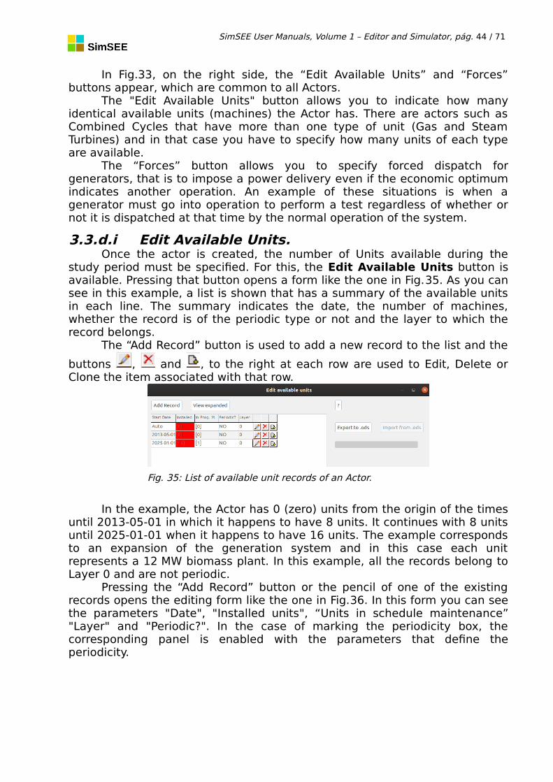
SimSEE User Manuals, Volume 1 – Editor and Simulator, pág. 44 / 71
In Fig.33, on the right side, the “Edit Available Units” and “Forces”buttons appear, which are common to all Actors.
The "Edit Available Units" button allows you to indicate how manyidentical available units (machines) the Actor has. There are actors such asCombined Cycles that have more than one type of unit (Gas and SteamTurbines) and in that case you have to specify how many units of each typeare available.
The “Forces” button allows you to specify forced dispatch forgenerators, that is to impose a power delivery even if the economic optimumindicates another operation. An example of these situations is when agenerator must go into operation to perform a test regardless of whether ornot it is dispatched at that time by the normal operation of the system.
3.3.d.i Edit Available Units.Once the actor is created, the number of Units available during the
study period must be specified. For this, the Edit Available Units button isavailable. Pressing that button opens a form like the one in Fig.35. As you cansee in this example, a list is shown that has a summary of the available unitsin each line. The summary indicates the date, the number of machines,whether the record is of the periodic type or not and the layer to which therecord belongs.
The “Add Record” button is used to add a new record to the list and the
buttons , and , to the right at each row are used to Edit, Delete orClone the item associated with that row.
In the example, the Actor has 0 (zero) units from the origin of the timesuntil 2013-05-01 in which it happens to have 8 units. It continues with 8 unitsuntil 2025-01-01 when it happens to have 16 units. The example correspondsto an expansion of the generation system and in this case each unitrepresents a 12 MW biomass plant. In this example, all the records belong toLayer 0 and are not periodic.
Pressing the “Add Record” button or the pencil of one of the existingrecords opens the editing form like the one in Fig.36. In this form you can seethe parameters "Date", "Installed units", “Units in schedule maintenance”"Layer" and "Periodic?". In the case of marking the periodicity box, thecorresponding panel is enabled with the parameters that define theperiodicity.
Fig. 35: List of available unit records of an Actor.

SimSEE User Manuals, Volume 1 – Editor and Simulator, pág. 45 / 71
Returning to Fig.35, the “Export .ods” and “Import .ods” buttons allowyou to export to a LibreCalc spreadsheet the set of available unit records tofacilitate your joint modification and then import again. The export is done bywriting to the hard disk of your PC a temporary file with extension .ods andopen it to allow editing. The import works by reading the same file, so it isnecessary that you SAVE themodifications you make to the filebefore pressing the “Import .ods”button.
As can be seen in Fig.36 inaddition to the aforementionedparameters, there are the “Uncertaincommitment” and “UncertainBeginning of Chronicle”, options thatare explained in the followingsections.
3.3.d.ii Failure – RepairModel.
Internally, SimSEE creates a Fail-Repair model to manage theavailability of the units of any entity. Between the parameters of the entity(generally between the dynamic parameters) the parameters AvailabilityFactor (AF) and Average Repair Time (ART) can be specified.
The model implies the recognition of two possible states of the units:Available (1) and Unavailable (0) as shown in Fig.37 and the definition oftransition probabilities between these states. The AF represents theprobability that the unit is available if we observe it without knowledge of itsprevious state. For example, an AF = 0.9 will indicate that if we observe theunit, without knowledge of the previous state, with a 90% probability it will bein the Available state and with a 10% probability in Unavailable state. TheAverage Repair Time (in hours) represents the expected value of the time thatonce the unit enters the Unavailable state, it remains in that state. Based onthe AF and ART parameters and the Room’s time-step , SimSEE calculates thetransition probabilities between the applicable states during the simulation.
3.3.d.iii Uncertain commitment.If the “Uncertain commitment” option is selected, when units (that can
be new units or units that were in scheduled maintenance period) areentered, they are added to the Unavailable unit set. This means that they will
Fig. 36: Single generator units record
Fig. 37: Failure-Repair Model of the Units.

SimSEE User Manuals, Volume 1 – Editor and Simulator, pág. 46 / 71
be really operational according to the probability of repair of the units definedin the dynamic parameters record of the Actor. Depending on the parametersFactor of Availability and Average Repair Time, the units may randomly enterin service immediately or not with a delay in the effective entry according tothe specified Average Repair Time.
In the event that this option is not selected, the units will be availableeffectively on the established date.
As an example Fig.38 shows the results of a daily and 1000 chroniclesimulation of a 100 MW average power generator with AF=0.7 y ART=360h.
At the beginning of the simulation the generator has an available unit(record with date "auto" indicating 1 (one) unit available) that goes out ofservice to perform a scheduled maintenance routine (2015-02-01 has a tabindicating 0 (zero ) unit available). The unit is one month in scheduledmaintenance and "returns" (a tab on 2015-03-01 indicating 1 unit available).The two curves in the figure correspond to the same room simulated with“Uncertain Incorporation” marked (Red curve) and unmarked (Blue curve) inthe 2015-03-01 record. The curves correspond to the expected power in theset of the 1000 simulated chronicles. As can be seen, on the right side, bothcurves verify the value of the specified Availability Factor (0.7). Thedifferences are at the time of commitment the unit. In the case of the bluecurve (Uncertain commitment = FALSE) the machine enters for sure, andtherefore has an expected power of 100% value that is decreasing towardsthe steady state probability. In the case of the red curve (Uncertaincommitment = TRUE) the machine will be effectively operational randomlywith the Failure/Repair model in an average time equal to the specifiedAverage Repair Time. For that reason, the expected power starts from 0 (zero)and goes to the stable state value corresponding to the availability factor.
Fig. 38: Efectos del Alta Incierta sobre la Potencia Esperada.

SimSEE User Manuals, Volume 1 – Editor and Simulator, pág. 47 / 71
3.3.d.iv Uncertain Beginning of Chronicle.This option of the unit records (see Fig.36) allows you to specify the
treatment of the availability of the generating units at the beginning of eachsimulated chronicle. Normally, this option is set to FALSE in the case ofsimulations of short-term rooms where the state of the machines can be wellknown and is set to TRUE for long-term studies in future horizons, where theinitial state of the machines is unknown.
If the “Uncertain Beginning of Chronicle” box is checked, at thebeginning of each simulation chronicle, instead of assuming that the units areactually available, raffles are held and will be available according to theStationary Status Availability Factor (AF) that you have specified for thatgenerator in the dynamic parameters record valid at the beginning of thesimulation horizon.
The simulation result of 1000 chronicles of a room in which there aretwo identical simple thermal generators of 100 MW and a demand of 200 MWis shown in Fig.39. The generators have an availability factor AF = 0.7 and anAverage Repair Time of ART = 360 hours. In the example, generators aredispatched whenever they are available, as they are the most economicalresources in the simulation. The only difference is that in generator 1 (G1 inthe figure) it "Uncertain Beginning of Chronicle" is unmarked (False), while ingenerator 2 (G2 in the figure) "Uncertain Beginning of Chronicle" is marked(True).
As you can see, at the beginning of the simulation (left side of thefigure) the blue curve begins with an almost 100% dispatch and decaysexponentially towards 70% corresponding to the steady state probability. Theorange curve starts directly with an expected power of 70% corresponding tothe steady state power given the availability factor of 0.7.
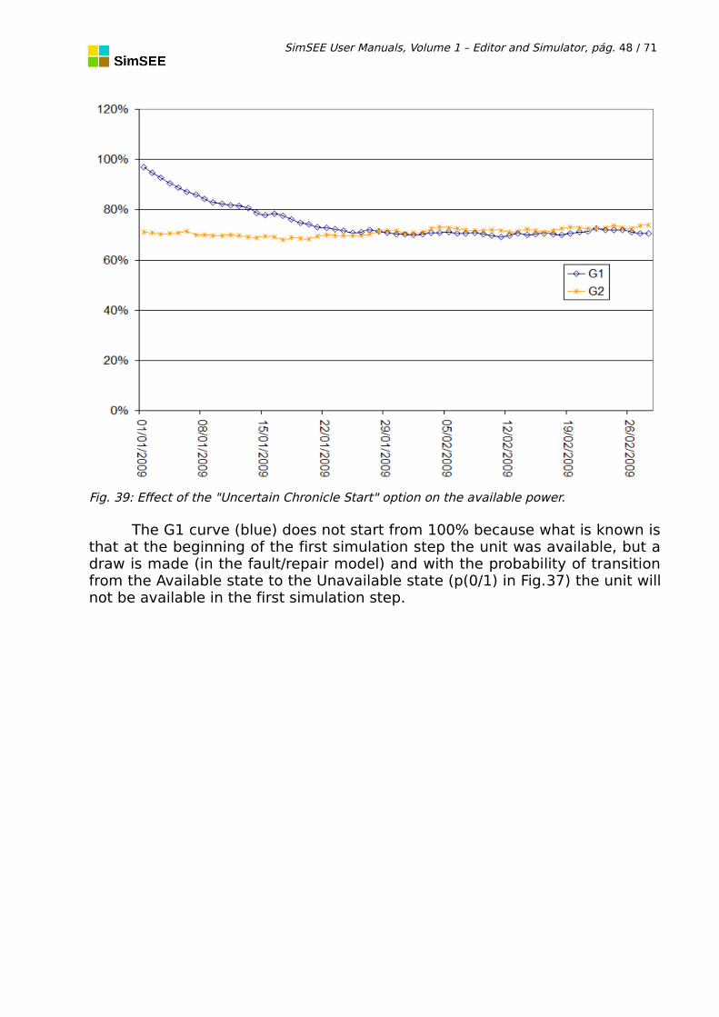
SimSEE User Manuals, Volume 1 – Editor and Simulator, pág. 48 / 71
The G1 curve (blue) does not start from 100% because what is known isthat at the beginning of the first simulation step the unit was available, but adraw is made (in the fault/repair model) and with the probability of transitionfrom the Available state to the Unavailable state (p(0/1) in Fig.37) the unit willnot be available in the first simulation step.
Fig. 39: Effect of the "Uncertain Chronicle Start" option on the available power.
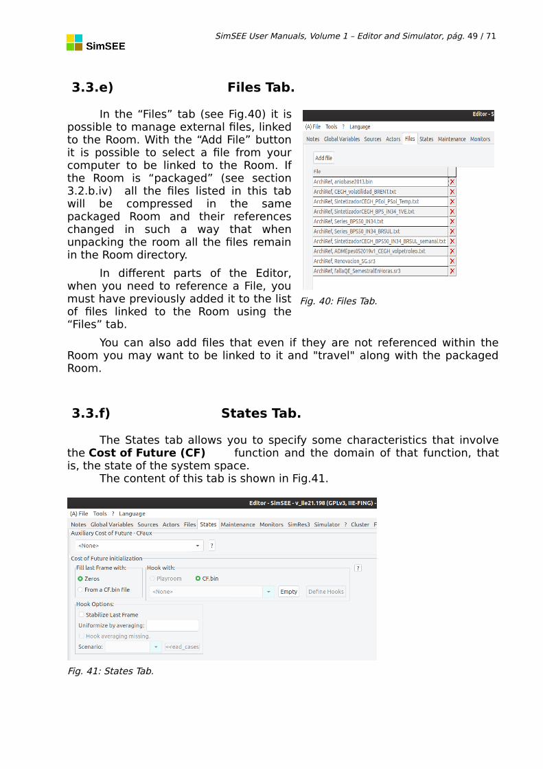
SimSEE User Manuals, Volume 1 – Editor and Simulator, pág. 49 / 71
3.3.e) Files Tab.
In the “Files” tab (see Fig.40) it ispossible to manage external files, linkedto the Room. With the “Add File” buttonit is possible to select a file from yourcomputer to be linked to the Room. Ifthe Room is “packaged” (see section3.2.b.iv) all the files listed in this tabwill be compressed in the samepackaged Room and their referenceschanged in such a way that whenunpacking the room all the files remainin the Room directory.
In different parts of the Editor,when you need to reference a File, youmust have previously added it to the listof files linked to the Room using the“Files” tab.
You can also add files that even if they are not referenced within theRoom you may want to be linked to it and "travel" along with the packagedRoom.
3.3.f) States Tab.
The States tab allows you to specify some characteristics that involvethe Cost of Future (CF) function and the domain of that function, thatis, the state of the system space.
The content of this tab is shown in Fig.41.
Fig. 41: States Tab.
Fig. 40: Files Tab.
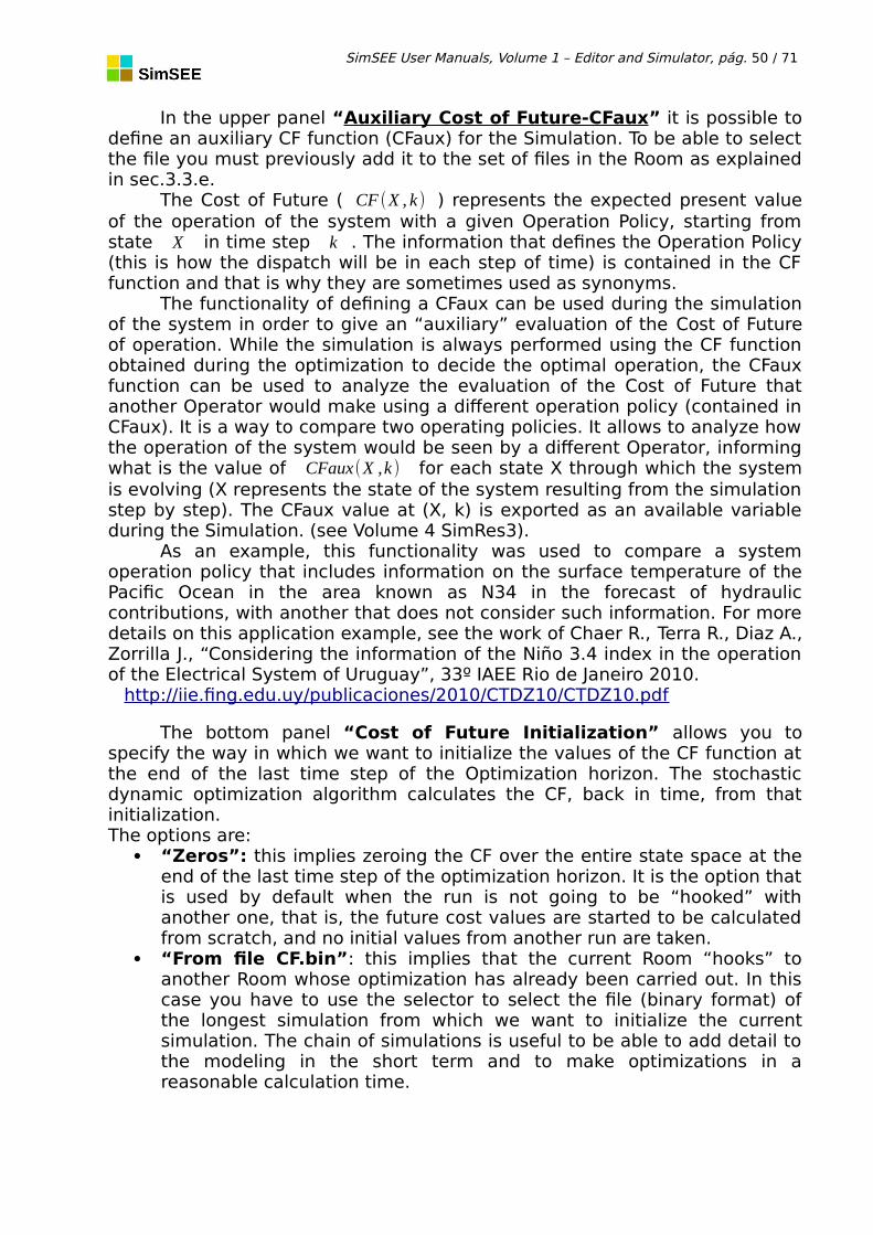
SimSEE User Manuals, Volume 1 – Editor and Simulator, pág. 50 / 71
In the upper panel “Auxiliary Cost of Future-CFaux” it is possible todefine an auxiliary CF function (CFaux) for the Simulation. To be able to selectthe file you must previously add it to the set of files in the Room as explainedin sec.3.3.e.
The Cost of Future ( CF (X , k ) ) represents the expected present valueof the operation of the system with a given Operation Policy, starting fromstate X in time step k . The information that defines the Operation Policy(this is how the dispatch will be in each step of time) is contained in the CFfunction and that is why they are sometimes used as synonyms.
The functionality of defining a CFaux can be used during the simulationof the system in order to give an “auxiliary” evaluation of the Cost of Futureof operation. While the simulation is always performed using the CF functionobtained during the optimization to decide the optimal operation, the CFauxfunction can be used to analyze the evaluation of the Cost of Future thatanother Operator would make using a different operation policy (contained inCFaux). It is a way to compare two operating policies. It allows to analyze howthe operation of the system would be seen by a different Operator, informingwhat is the value of CFaux(X ,k ) for each state X through which the systemis evolving (X represents the state of the system resulting from the simulationstep by step). The CFaux value at (X, k) is exported as an available variableduring the Simulation. (see Volume 4 SimRes3).
As an example, this functionality was used to compare a systemoperation policy that includes information on the surface temperature of thePacific Ocean in the area known as N34 in the forecast of hydrauliccontributions, with another that does not consider such information. For moredetails on this application example, see the work of Chaer R., Terra R., Diaz A.,Zorrilla J., “Considering the information of the Niño 3.4 index in the operationof the Electrical System of Uruguay”, 33º IAEE Rio de Janeiro 2010. http://iie.fing.edu.uy/publicaciones/2010/CTDZ10/CTDZ10.pdf
The bottom panel “Cost of Future Initialization” allows you tospecify the way in which we want to initialize the values of the CF function atthe end of the last time step of the Optimization horizon. The stochasticdynamic optimization algorithm calculates the CF, back in time, from thatinitialization.The options are:
“Zeros”: this implies zeroing the CF over the entire state space at theend of the last time step of the optimization horizon. It is the option thatis used by default when the run is not going to be “hooked” withanother one, that is, the future cost values are started to be calculatedfrom scratch, and no initial values from another run are taken.
“From file CF.bin”: this implies that the current Room “hooks” toanother Room whose optimization has already been carried out. In thiscase you have to use the selector to select the file (binary format) ofthe longest simulation from which we want to initialize the currentsimulation. The chain of simulations is useful to be able to add detail tothe modeling in the short term and to make optimizations in areasonable calculation time.

SimSEE User Manuals, Volume 1 – Editor and Simulator, pág. 51 / 71
The most common use of this option is to recover the informationalready calculated, by the longer-term Room, regarding the value ofwater from hydroelectric power plant reservoirs. For example, in theUruguayan system, simulations involving horizons greater than oneyear are made using weekly time step and only the reservoir of theRincón del Bonete dam is considered, as it is the only one with areservoir capacity of some months. In this way, the water-value fromthe largest reservoir in the country is obtained. This type of Room isuseful for planning purposes. For more short-term dispatchprogramming purposes, more detailed modeling is necessary, so Roomsare built that consider reservoirs whose reservoir capacity is about 2weeks. These weekly deposits are not relevant when consideringmultiannual periods, but they are when analyzing the medium or shortterm.The possibility of hooking Rooms allows to reduce calculation timewithout losing precision, allowing “successive refinements” according tothe time horizon that you want to observe.To make the hitch, SimSEE identifies the date of the end of the last stepof the Room and the values are interpolated in the CF function to whichthe Room is attached. This resolves the temporary hitch, regardless ofwhether the time steps are different, it is enough only that the enddate of the last time step of the optimization horizon of thecurrent Room is comprised in the optimization time horizon of thesimulation to the which we are hooking it.It is also interpolated in the state variables, so it is not necessary thatthe discretizations of the different variables coincide in bothsimulations.When two functions CF (X , k ) are engaged, it may be the case thatthe state spaces are different (in fact that is the case of the examplementioned above). It may happen that in the current simulation thereare new state variables (volume of the reservoir added, in thementioned example). In that case there is no information on thebehavior of CF on that dimension of the state in the simulation to whichwe are hooking the current one, because in that simulation there was nosuch dimension of the state of the system. To initialize the CF in the firstcalculation table on the new dimensions that are added to the statespace, what is done is to assume that the derivative of the CF withrespect to that address is zero (this means assigning a null cost to theuse of the variable of state).Another case that can occur is that in the new simulation a statevariable disappears from those that were defined in the simulation towhich we get hooked. In that case you have to decide what value is setin the CF of the simulation to which we get hooked to that statevariable. For this there is the "Define Hooks" button. By default, thehooks are defined with the midpoint of the intervals of the statusvariables, but using this button it is possible to change the value. Anexample of using this may be the consideration of the randomness ofthe price of oil. In long-term simulations it is not possible to consider the
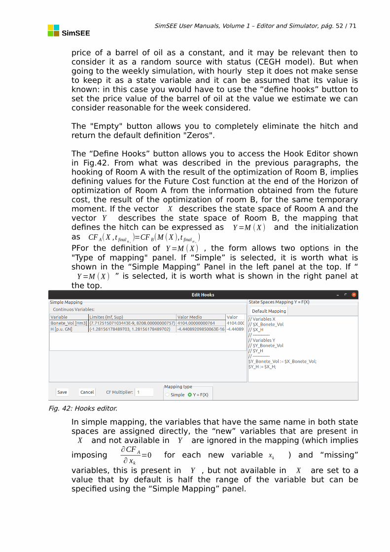
SimSEE User Manuals, Volume 1 – Editor and Simulator, pág. 52 / 71
price of a barrel of oil as a constant, and it may be relevant then toconsider it as a random source with status (CEGH model). But whengoing to the weekly simulation, with hourly step it does not make senseto keep it as a state variable and it can be assumed that its value isknown: in this case you would have to use the “define hooks” button toset the price value of the barrel of oil at the value we estimate we canconsider reasonable for the week considered.
The "Empty" button allows you to completely eliminate the hitch andreturn the default definition "Zeros".
The “Define Hooks” button allows you to access the Hook Editor shownin Fig.42. From what was described in the previous paragraphs, thehooking of Room A with the result of the optimization of Room B, impliesdefining values for the Future Cost function at the end of the Horizon ofoptimization of Room A from the information obtained from the futurecost, the result of the optimization of room B, for the same temporarymoment. If the vector X describes the state space of Room A and thevector Y describes the state space of Room B, the mapping thatdefines the hitch can be expressed as Y=M (X ) and the initializationas CF A(X , t final H A
)=CF B(M (X ), t final H A
)
PFor the definition of Y=M (X ) , the form allows two options in the"Type of mapping" panel. If “Simple” is selected, it is worth what isshown in the “Simple Mapping” Panel in the left panel at the top. If “Y=M (X ) ” is selected, it is worth what is shown in the right panel at
the top.
In simple mapping, the variables that have the same name in both statespaces are assigned directly, the “new” variables that are present inX and not available in Y are ignored in the mapping (which implies
imposing ∂CF A∂ xk
=0 for each new variable xk ) and “missing”
variables, this is present in Y , but not available in X are set to avalue that by default is half the range of the variable but can bespecified using the “Simple Mapping” panel.
Fig. 42: Hooks editor.

SimSEE User Manuals, Volume 1 – Editor and Simulator, pág. 53 / 71
If “Mapping Y=F(X)” is selected, it is possible to write the expressionexplicitly in the corresponding panel. The syntax is as follows:Two “//” bars indicate that what follows until the end of the line is acomment and will not be interpreted.Each state space variable X corresponding to the Room we are editingis identified as "$X_Name", "Name" being the name with which thevariable is published in SimSEE. Cada variable del espacio de estadoY , corresponding to the Future Cost function to which we are hooking
the room in edition, is identified as “$Y_Name”. The assignmentY=M (X ) is then defined by several assignment statements of the type
“$Y_Name := expression;”, using as assignment operator “:=” and theexpression being able to have definitions based on the standardoperators: “+”, “-”, “*”, “/” and standard functions such as log(), exp(),cos(), etc. Each expression must be endend width a semicolon “;”.
In the form in Fig.41, the “Hook Averaging Missing” box is applied onlyin the case of “Simple Mapping” and if that box is marked, the average of theCost of Future in the discretization range of the variable is set average of themissing variable.
In the form in Fig.41, in the “Uniformize by averaging” field it is possibleto enter a list of state variables (separated by “;” semicolon) for which youwant to impose a constant CF value equal to the average of the values in thedirection of each variable inclueded in the list. This uniformization is carriedout at the end of the hooking in any of the types of mapping. This option israrely used and was incorporated for research purposes.
Finally, at the bottom left in Fig.41, there is a “Stabilize Last Frame”box. If this box is checked, the stochastic dynamic programming algorithm isrun several times over the last time step, trying to stabilize the CF function.The procedure consists in calculating the CF value at the beginning of the lasttime step of the optimization horizon from the CF value at the end of saidtime step, then copying the value obtained on the calculation start values andso on until the CF derivatives are stabilized with respect to the differentdirections of the state. This procedure is an alternative to defining a broaderoptimization horizon than the simulation horizon to leave a “guard time” forthe algorithm to stabilize. As the result is approximately the same, it ispreferable to choose to leave the “guard time” and leave this box unchecked,since in that way all the CF values will be recorded in the optimization outputfile, starting with the table of the beginning of the calculation and includingthe guard section. This allows a better visualization of the stabilizationtransient. If you choose to check the box and thus use the stabilization of thefirst calculation box, the possibility of inspecting the transient in theoptimization output file is lost. On the other hand, if years of guarding areused, it is necessary to make the future projections relevant to the system (egdemand, available generation, etc.) that cover that “extended” horizon.
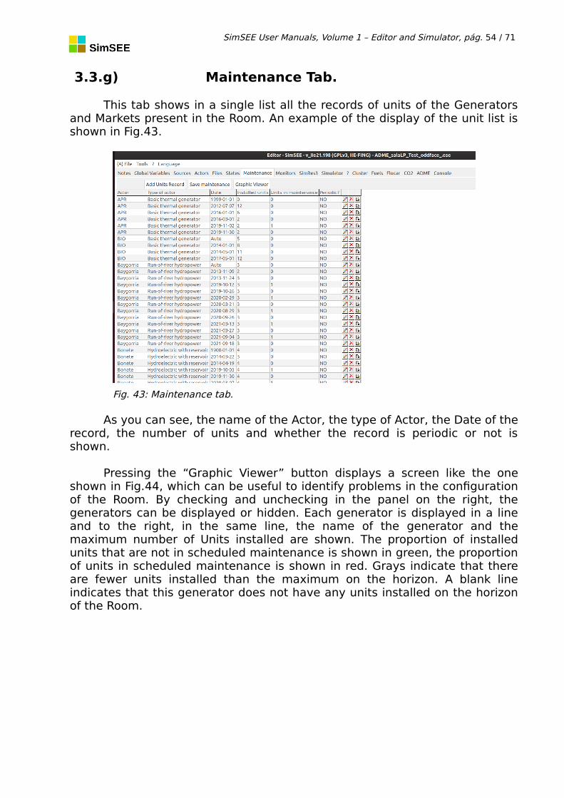
SimSEE User Manuals, Volume 1 – Editor and Simulator, pág. 54 / 71
3.3.g) Maintenance Tab.
This tab shows in a single list all the records of units of the Generatorsand Markets present in the Room. An example of the display of the unit list isshown in Fig.43.
As you can see, the name of the Actor, the type of Actor, the Date of therecord, the number of units and whether the record is periodic or not isshown.
Pressing the “Graphic Viewer” button displays a screen like the oneshown in Fig.44, which can be useful to identify problems in the configurationof the Room. By checking and unchecking in the panel on the right, thegenerators can be displayed or hidden. Each generator is displayed in a lineand to the right, in the same line, the name of the generator and themaximum number of Units installed are shown. The proportion of installedunits that are not in scheduled maintenance is shown in green, the proportionof units in scheduled maintenance is shown in red. Grays indicate that thereare fewer units installed than the maximum on the horizon. A blank lineindicates that this generator does not have any units installed on the horizonof the Room.
Fig. 43: Maintenance tab.
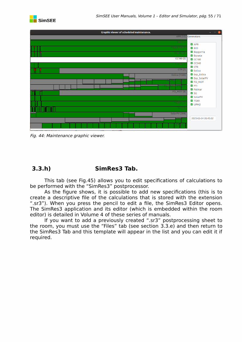
SimSEE User Manuals, Volume 1 – Editor and Simulator, pág. 55 / 71
3.3.h) SimRes3 Tab.
This tab (see Fig.45) allows you to edit specifications of calculations tobe performed with the “SimRes3” postprocessor.
As the figure shows, it is possible to add new specifications (this is tocreate a descriptive file of the calculations that is stored with the extension“.sr3”). When you press the pencil to edit a file, the SimRes3 Editor opens.The SimRes3 application and its editor (which is embedded within the roomeditor) is detailed in Volume 4 of these series of manuals.
If you want to add a previously created “.sr3” postprocessing sheet tothe room, you must use the “Files” tab (see section 3.3.e) and then return tothe SimRes3 Tab and this template will appear in the list and you can edit it ifrequired.
Fig. 44: Maintenance graphic viewer.

SimSEE User Manuals, Volume 1 – Editor and Simulator, pág. 56 / 71
3.3.i) Simulator Tab.
Once the Room has been edited (that is: specified the Global Variables,detailed the different Actors that you want to incorporate into the modeling,specifying their Maintenance and the Random Sources that will give themsome service), the desired characteristics for the Simulation and Optimizationstages must be specified in the "Simulator" tab.
As can be seen in Fig.46 there are three large panels “OptimizationVariables”, “Simulation Variables” and “Scenarios”. The first two allow you toconfigure the parameters for the Optimization and Simulation stagesrespectively. The "Scenarios" panel allows you to configure the scenariosavailable in the Room and execute them.
Fig. 46: Simulator Tab.
Fig. 45: SimRes3 Tab
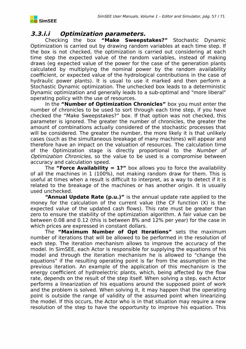
SimSEE User Manuals, Volume 1 – Editor and Simulator, pág. 57 / 71
3.3.i.i Optimization parameters. Checking the box “Make Sweepstakes?” Stochastic Dynamic
Optimization is carried out by drawing random variables at each time step. Ifthe box is not checked, the optimization is carried out considering at eachtime step the expected value of the random variables, instead of makingdraws (eg expected value of the power for the case of the generation plantscalculated by multiplying the nominal power by the random availabilitycoefficient, or expected value of the hydrological contributions in the case ofhydraulic power plants). It is usual to use it marked and then perform aStochastic Dynamic optimization. The unchecked box leads to a deterministicDynamic optimization and generally leads to a sub-optimal and "more liberal"operating policy with the use of resources.
In the “Number of Optimization Chronicles” box you must enter thenumber of chronicles to be used to sort through each time step, if you havechecked the “Make Sweepstakes?” box. If that option was not checked, thisparameter is ignored. The greater the number of chronicles, the greater theamount of combinations actually considered of the stochastic processes thatwill be considered. The greater the number, the more likely it is that unlikelycases (such as the simultaneous breakage of many machines) will appear andtherefore have an impact on the valuation of resources. The calculation timeof the Optimization stage is directly proportional to the Number ofOptimization Chronicles, so the value to be used is a compromise betweenaccuracy and calculation speed.
The “Force Availability = 1?” box allows you to force the availabilityof all the machines in 1 (100%), not making random draw for them. This isuseful at times when a result is difficult to interpret, as a way to detect if it isrelated to the breakage of the machines or has another origin. It is usuallyused unchecked.
“Annual Update Rate (p.u.)” is the annual update rate applied to themoney for the calculation of the current value (the CF function (X) is theexpected value of the updated cash flows). This rate must be greater thanzero to ensure the stability of the optimization algorithm. A fair value can bebetween 0.08 and 0.12 (this is between 8% and 12% per year) for the case inwhich prices are expressed in constant dollars.
The “Maximum Number of Opt Iterations” sets the maximumnumber of iterations that will be allowed to be performed in the resolution ofeach step. The iteration mechanism allows to improve the accuracy of themodel. In SimSEE, each Actor is responsible for supplying the equations of hismodel and through the iteration mechanism he is allowed to "change theequations" if the resulting operating point is far from the assumption in theprevious iteration. An example of the application of this mechanism is theenergy coefficient of hydroelectric plants, which, being affected by the flowrate, depends on the result of the step itself. When solving a step, each Actorperforms a linearization of his equations around the supposed point of workand the problem is solved. When solving it, it may happen that the operatingpoint is outside the range of validity of the assumed point when linearizingthe model. If this occurs, the Actor who is in that situation may require a newresolution of the step to have the opportunity to improve his equation. This

SimSEE User Manuals, Volume 1 – Editor and Simulator, pág. 58 / 71
"consultation of the Actors" is done until everyone confirms to agree with theresult or until the maximum number of iterations established is reached. If setto 0, iterations are not allowed. A fair value can be eg 3 or 4.
The “Rotating Reserve” box allows the Rotating Reserve mechanismto be enabled, which means imposing, in addition to the balance of powersdemanded and delivered in each node, imposing the balance betweendemand and supply of rotating reserve in each node.
The "Risk Aversion" panel below can be activated / deactivated usingthe "Activate" box (by default it is unchecked). It implements riskmanagement in optimization, allowing to choose between using the “VaR”(Value at Risk) or “CVaR” (Conditional Value at Risk) as cost dispersionmeasures.
The “CAR” (Risk Aversion Coefficient) box must specify a numberbetween 0.0 and 1.0 that will indicate the degree of risk aversion to be used.
If it is CAR = 0.0 it is not risk averse and optimization will minimize theexpected value of the future cost function (which is the same as notactivating risk aversion).
If instead the user has maximum risk aversion, enter CAR = 1.0. Thisimplies that the optimization will try to minimize "high costs" (instead of theexpected value of the costs). The measure of “high costs” will be the valuethat is exceeded with a probability P (specified in the “Probability” box) or theexpected value of costs that exceed that probability P as selected as a “VaR”or “ CVaR ” risk measure respectively.
For intermediate values of the Risk Aversion Coefficient, the objectivefunction to be minimized will be a linear combination between the expectedvalue of the costs and the measure of dispersion that has been selected.
The "Probability (p.u.)" box determines the exceedance probabilitylimit set by the user to measure the cost dispersion of a given histogram (thisis a way of measuring risk exposure). VaR (P) is the value that is exceededwith probability P. CVaR (P) is the expected value of costs that exceed VaR (P).
The value “Number of points of the histogram” determines the“fineness” with which the histograms of the Future Cost CF (X, k) function areelaborated, that is, at each stage k of the optimization, not only the expectedvalue of future cost for each discretization of the state variable Xwill berepresented, but there will be a distribution or histogram (with as many pointsas specified) that will be those that allow to calculate the future cost valueswith the probability of exceedance that the user set. A typical value to use is200 when the probability is 0.05.
The “Subtract CF utilities” box if checked, instead of minimizing theexpected value of future cost, will minimize costs by subtracting the utilitiesobtained by the user. This is planned so that the Actors can determine inaddition to the cost incurred over time, the profit generated. For an exampleof a model that specifies utilities, see the “Manageable Uses” Actor in Volume3 of this series of manuals. The normal use of this box is marked and has noconsequences on the calculation time.
The “Consider Payments in CF” box allows you to specify whetheradditional payments (for power made available and for energy) that are notconsidered in the dispatch resolution are or are not added to the Future Cost

SimSEE User Manuals, Volume 1 – Editor and Simulator, pág. 59 / 71
(CF) function. When added, the optimizer takes them into account and theoperation policy can be influenced if the operator had some (operational)mechanism that allows him to reduce payments. By way of example only, if a“payment for energy” is specified in one hydroelectric plant and in another itis not specified, when there are excesses of energy that give rise to dumping,the optimized one will give preference to open the dumps of the plant thatwould be paid to deliver the energy.
The "Random seed" field allows you to specify a seed to initialize therandom number generators used in the Optimization stage. Changing thisnumber is useful to estimate the accuracy of the results with the number ofdraws specified. If the results are sensitive to the initial seed it means that theamount of raffles should be increased.
The "CF_compress" field by default is -1 and implies that acompressed representation of the Future Cost will be used when stored in thebinary file. If 0 (Zero) is specified, no compression is performed.
3.3.i.ii Simulation parameters. The "Number of Simulation Chronicles" determines the number of
chronicles that will be simulated. Each chronicle is simulated separately.Simulating a chronicle means that in each time step (from the first to the lastof the simulation time horizon) the corresponding draws will be made toobtain the values to be considered for all random variables.
The “Force Availability = 1?” Box allows you to force the availabilityof all the machines in 1 (100%), not making random draw for them. It isadvisable not to check this box and use the potential of the platform. The boxis for purposes of analyzing the effects of whether or not to consideraccidental breakage in simulations.
The box "Maximum Number of Sim. Iterations" allows you to setthe maximum number of iterations that are allowed in a time step to improvethe modeling of the different actors. (see the same optimization parameterabove).
The “Obligatory start of uncertain chronicle” box allows you to specifythat all unit records (see sec.3.3.d.i) behave as if they had marked thebeginning of uncertain chronicle.
The "Random seed" field determines the seed with which all randomnumber generators used during the simulation are initialized. By varying thisnumber, different sets of simulation chronicles can be generated and thusdetermine the accuracy of the results based on the number of chroniclesused.
The “Publish Only Variables Used in SimRes3” field should be usedmarked and it means that in the files that are generated with the results ofthe simulations only those variables that are then used in any of the SimRes3files associated with the Room are saved. All the entities of the Room publish(declare) variables that can then be used in the calculations with SimRes3. Ifthe box is not checked, all the variables are registered in the output files evenif they are not referenced in SimRes3 files, which leads to quickly have files ofunmanageable size. The option to uncheck the box is made available only foracademic purposes.
SimSEE User Manuals, Volume 1 – Editor and Simulator, pág. 60 / 71
The “Print End of State Files” box also has academic objectives andhas the effect that if checked, text files are generated with the System Staterecord at the end of each simulated chronicle.
The “Calculate investment gradients in p.u.” box specifies whetherthe Investment Gradients of those Actors for which their calculation isspecified is done per unit or in USD (dollars).
With the box unchecked at each time step for each Actor in whichcalculation is marked, the investment gradient (GradInv) is calculated as:GradInv :=E∗CMG−Costos . The energy delivered by the generator valued at
the marginal cost of the node minus the cost of generation and less paymentsnot considered in the dispatch (availability and energy). If the box is marked,it is done as: GradInv :=(E∗CMG−Costos)/ Pago_ por _ disponibilidad
The “Calculate Payment for Service” of System Conf. ” boxenables the calculation of the participation of generators and demands in theSystem Reliability Service. It is calculated for each Actor and two variables arepublished: SCS Participation and SCS Forcing. The “Spot Roof” box specifiesthe limit value used for the sanction of the Spot price based on the marginalcost. If the Marginal Cost exceeds the Roof value, the spot price is set to theroof value and in that case, the Participation and Forcing variables in the SCSthat correspond to the energy exchanged (to the node to which it isconnected) valued at the Marginal Cost Marginal minus the value specified as“Spot Roof” or the variable cost of generation if it is higher are calculated. Inthe event that the variable generation cost is higher than the Roof,ForcingSCS is assigned the amount corresponding to the Energy for thedifference between the roof and the variable cost.
The pseudo calculation code is the one shown below: ParticipacionSCS:= 0; ForzamientoSCS:=0; CmgMenosTecho:= CMG - TechoDelSpot; if CmgMenosTecho > 0 then begin TechoMenosCV:= TechoDelSpot - CV_spot; if TechoMenosCV > 0 then ParticipacionSCS:= E * CmgMenosTecho else begin ParticipacionSCS:= E * ( CMG - CV_Spot ); ForzamientoSCS:= E * (-TechoMenosCV) ; end end
3.3.i.iii Scenarios.In the “Scenarios” panel, using the “Create new scenario” button,
several simulation scenarios (or cases) can be created in the same Room,thus avoiding duplicating the information and facilitating the maintenance ofthe case set.
A scenario is defined by indicating which are the active layers in thatscenario. Dynamic parameter records have a parameter that is the layer, andthis allows to have sets of records that are activated or not according to the
SimSEE User Manuals, Volume 1 – Editor and Simulator, pág. 61 / 71
scenario. By default, all the records are in layer 0 (zero), which corresponds tothe “Base” scenario, but it is possible to specify dynamic parameter recordswith a different layer number (1, 2, 3, etc.). Two records can have the samestart date, but if they are specified with different layer number, each one willbe activated in the scenario that activates the layer to which it belongs.
This facilitates the creation of small variants of the same Room inthe form of "Scenarios". A scenario has a "name" that identifiesit and a set of active layers that will be considered in Optimization
and Simulation. Layers that are not active DO NOT participate in Optimizationor Simulation of the scenario. (They are removed from the room beforeperforming the Optimization and / or Simulation).
Once a scenario is created, it can be activated / deactivated, edited,deleted and marked / unmarked as the main stage of the simulation, usingdifferent available buttons. The meaning of the buttons is as follows:
"Traffic light" that allows you to activate / deactivate the stage. If it isdeactivated it will have a red background. If the “Execute Automatically”button is pressed, the active scenarios are executed automatically withoutthe user having to intervene.
"Pencil" that allows you to edit and modify the scenario.
"Duplicate" allows you to clone a scenario.
"Cross" that eliminates the scenario.
“Up arrow” allows you to move the stage up in the list of availablescenarios.
“Down arrow” allows you to move the stage down in the list ofavailable scenarios.
"Principal", a red mark that indicates the main scenario (only one canbe at a time). This will be the optimized / simulated scenario when theSimulator is invoked by pressing the "Run manually" button.
When editing a scenario, a form like the one in Fig.47 opens.
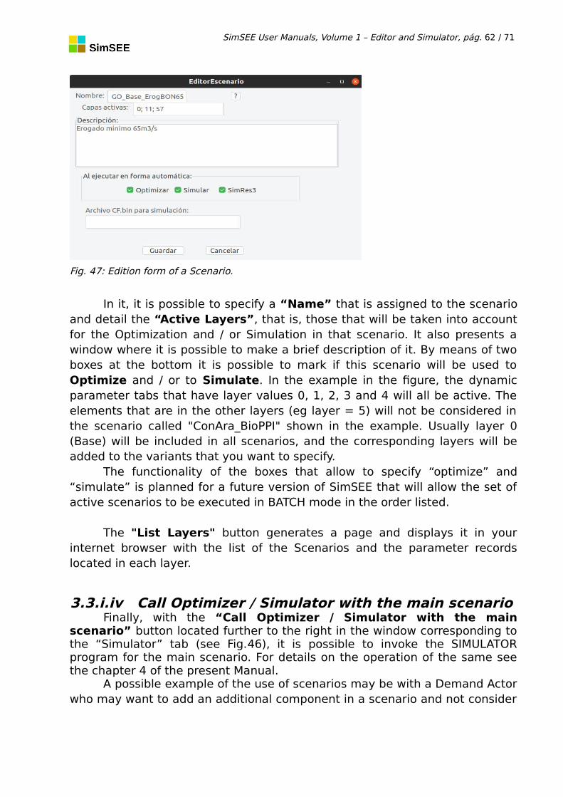
SimSEE User Manuals, Volume 1 – Editor and Simulator, pág. 62 / 71
Fig. 47: Edition form of a Scenario.
In it, it is possible to specify a “Name” that is assigned to the scenarioand detail the “Active Layers”, that is, those that will be taken into accountfor the Optimization and / or Simulation in that scenario. It also presents awindow where it is possible to make a brief description of it. By means of twoboxes at the bottom it is possible to mark if this scenario will be used toOptimize and / or to Simulate. In the example in the figure, the dynamicparameter tabs that have layer values 0, 1, 2, 3 and 4 will all be active. Theelements that are in the other layers (eg layer = 5) will not be considered inthe scenario called "ConAra_BioPPI" shown in the example. Usually layer 0(Base) will be included in all scenarios, and the corresponding layers will beadded to the variants that you want to specify.
The functionality of the boxes that allow to specify “optimize” and“simulate” is planned for a future version of SimSEE that will allow the set ofactive scenarios to be executed in BATCH mode in the order listed.
The "List Layers" button generates a page and displays it in yourinternet browser with the list of the Scenarios and the parameter recordslocated in each layer.
3.3.i.iv Call Optimizer / Simulator with the main scenarioFinally, with the “Call Optimizer / Simulator with the main
scenario” button located further to the right in the window corresponding tothe “Simulator” tab (see Fig.46), it is possible to invoke the SIMULATORprogram for the main scenario. For details on the operation of the same seethe chapter 4 of the present Manual.
A possible example of the use of scenarios may be with a Demand Actorwho may want to add an additional component in a scenario and not consider

SimSEE User Manuals, Volume 1 – Editor and Simulator, pág. 63 / 71
that component in the baseline study scenario, the modeling of the rest of thesystem being the same in both cases. One possibility is to make 2 separaterooms, identical except in that modification, optimize and simulate bothseparately. By managing scenarios it is possible to do it in a single room. Acomponent that will be a random source will then be associated with theDemand Actor, which will have a record with a null value in layer = 1 and thevalue of the additional demand in another record in layer 2. Two scenarios willbe registered: in one of them the active layers will be 0 and 1, while in theother the active layers will be 0 and 2. When optimizing / simulating the firstone, SimSEE will not take into account the values specified in layer 2 (that is,you will not see the additional demand component that was specified withlayer = 2, because that layer is inactive in that scenario), while optimizing /simulating the second scenario, it will take it into account (since this layer isactive).
It is thus possible to introduce small variants to the Room (that is,different scenarios), without needing to duplicate all the information everytime.
3.3.j) ? Tab.
When trying to activate this tab, the browser configured by default isopened and a web page is accessed with the help information on the Main TabBar of the SimSEE Editor.
3.3.k) Fuels
In the "Fuels" tab it is possible to define types of fuels that can be usedby the Actors that are accessed in the "Actors-> Fuel Network" sub-tab. If youdo not use these types of actors, it is not necessary to define types of fuels inthe Room. Fig.48 shows an example of the content of the tab with three typesof fuels defined.
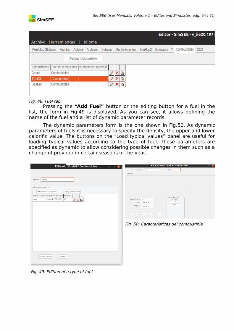
SimSEE User Manuals, Volume 1 – Editor and Simulator, pág. 64 / 71
Pressing the “Add Fuel” button or the editing button for a fuel in thelist, the form in Fig.49 is displayed. As you can see, it allows defining thename of the fuel and a list of dynamic parameter records.
The dynamic parameters form is the one shown in Fig.50. As dynamicparameters of fuels it is necessary to specify the density, the upper and lowercalorific value. The buttons on the “Load typical values” panel are useful forloading typical values according to the type of fuel. These parameters arespecified as dynamic to allow considering possible changes in them such as achange of provider in certain seasons of the year.
Fig. 48: Fuel tab.
Fig. 49: Edition of a type of fuel.
Fig. 50: Características del combustible.
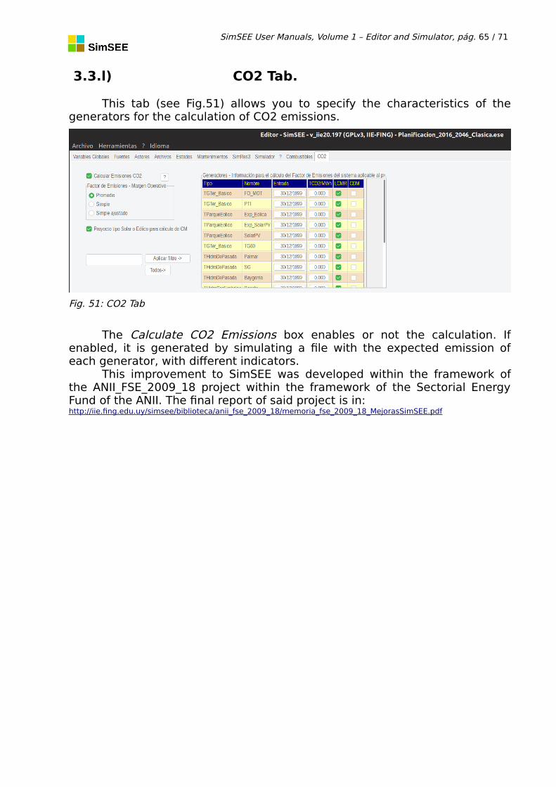
SimSEE User Manuals, Volume 1 – Editor and Simulator, pág. 65 / 71
3.3.l) CO2 Tab.
This tab (see Fig.51) allows you to specify the characteristics of thegenerators for the calculation of CO2 emissions.
The Calculate CO2 Emissions box enables or not the calculation. Ifenabled, it is generated by simulating a file with the expected emission ofeach generator, with different indicators.
This improvement to SimSEE was developed within the framework ofthe ANII_FSE_2009_18 project within the framework of the Sectorial EnergyFund of the ANII. The final report of said project is in:http://iie.fing.edu.uy/simsee/biblioteca/anii_fse_2009_18/memoria_fse_2009_18_MejorasSimSEE.pdf
Fig. 51: CO2 Tab

SimSEE User Manuals, Volume 1 – Editor and Simulator, pág. 66 / 71
4. The Optimizer/Simulator.
This chapter is the "SimSEESimulator.exe" Application User Manual. InSimSEE terms, this application is called “The Simulator” and is in charge ofthe different the steps of Optimization and Simulation over a Room.
In the most common use of the SimSEE platform, the simulator isdirectly called from the Editor (the Editor application is described in sec.3.3),but it can also be manually called or by using a script or batch command toexecute a sequence of simulations.
To run the Simulator from the Editor, you must press the "Manually Run"button that is in the "Simulator" tab (see sec.3.3).
Fig.52 shows the Simulator's screen. As may be appreciated, there is atop panel called "Entry Data", which specifies the Room file to be processed. Ifthe Simulator has been summoned from the Editor, this field appears alreadyfilled in with the Editor’s Room file. In case that the Simulator is openeddirectly with the “Select Room” button, a browser will open which will allowyou to select the Room file to be executed.
At the bottom is the “Alerts” panel, where there will be any alertmessages about dubious definitions or errors detected during the loading ofthe Room.
The main part of the screen (Fig.52) is fomed by the “Optimize”,“Simulate”, “SimRes3” and “Auxiliary” tabs.
4.1. Optimize Tab.The “Optimize” tab is the one that unfolds in Fig.52. In the "Parameters"
panel the values specified in the Room are loaded. If you change these valuesand press the “Optimize” button, the changes will only be effective forongoing optimization and will not be stored in the Room. The possibility ofmaking changes in this panel is only to the effect of being able to make testson the effect of the parameters. If you want to change them permanently youshould do it in the Editor. The meaning of each parameter is explained in thesection “3.2.h.i ) Optimization Patameters”.
When the Optimization is performed, the folder for the simulationoutputs is created {$HOME}/SimSEE/rundir/{$sala} a file with the name“CF_{$escenario}.bin”, where:
{$HOME} is generally “C:\” in case you use Windows or your personalfolder in case you use Linux.
{$sala} is the name of the file of the Room without extension. Werecommend that you do not use spaces or symbols in room file names toavoid inconvenients with changes of operating systems or character encodingaccording to the language.
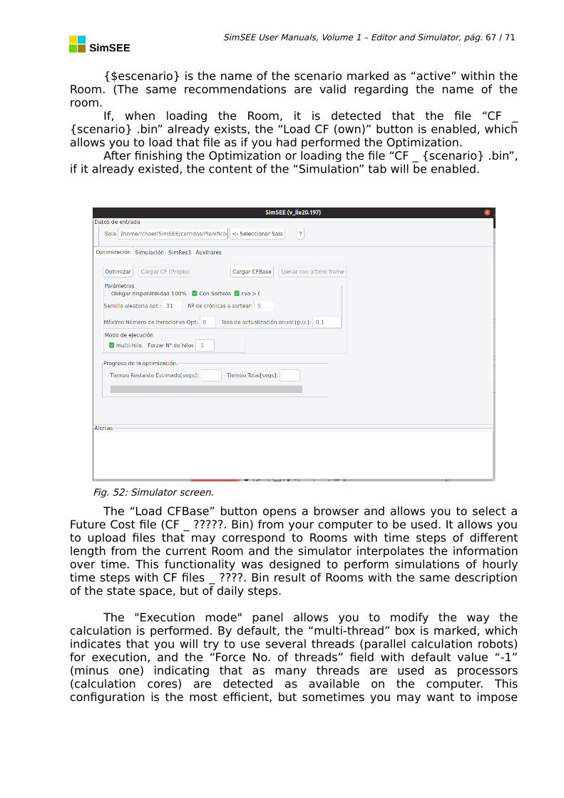
SimSEE User Manuals, Volume 1 – Editor and Simulator, pág. 67 / 71
{$escenario} is the name of the scenario marked as “active” within theRoom. (The same recommendations are valid regarding the name of theroom.
If, when loading the Room, it is detected that the file “CF _{scenario} .bin” already exists, the “Load CF (own)” button is enabled, whichallows you to load that file as if you had performed the Optimization.
After finishing the Optimization or loading the file “CF _ {scenario} .bin”,if it already existed, the content of the “Simulation” tab will be enabled.
The “Load CFBase” button opens a browser and allows you to select aFuture Cost file (CF _ ?????. Bin) from your computer to be used. It allows youto upload files that may correspond to Rooms with time steps of differentlength from the current Room and the simulator interpolates the informationover time. This functionality was designed to perform simulations of hourlytime steps with CF files _ ????. Bin result of Rooms with the same descriptionof the state space, but of daily steps.
The "Execution mode" panel allows you to modify the way thecalculation is performed. By default, the “multi-thread” box is marked, whichindicates that you will try to use several threads (parallel calculation robots)for execution, and the “Force No. of threads” field with default value “-1”(minus one) indicating that as many threads are used as processors(calculation cores) are detected as available on the computer. Thisconfiguration is the most efficient, but sometimes you may want to impose
Fig. 52: Simulator screen.
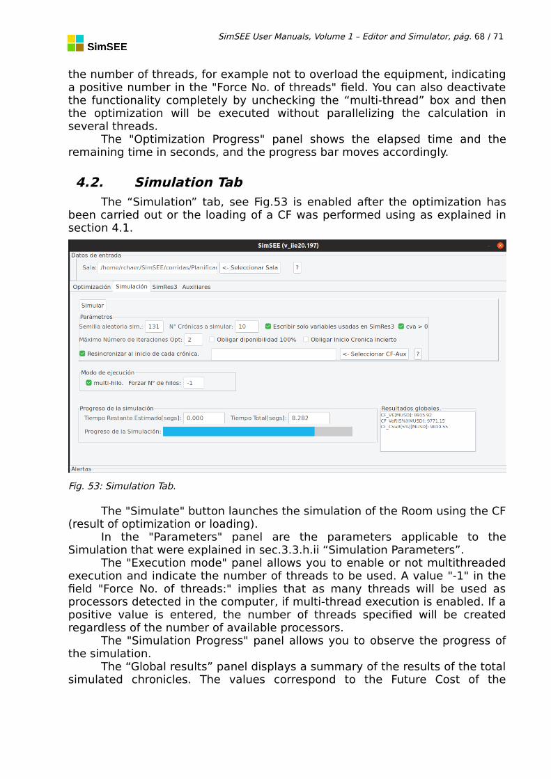
SimSEE User Manuals, Volume 1 – Editor and Simulator, pág. 68 / 71
the number of threads, for example not to overload the equipment, indicatinga positive number in the "Force No. of threads" field. You can also deactivatethe functionality completely by unchecking the “multi-thread” box and thenthe optimization will be executed without parallelizing the calculation inseveral threads.
The "Optimization Progress" panel shows the elapsed time and theremaining time in seconds, and the progress bar moves accordingly.
4.2. Simulation TabThe “Simulation” tab, see Fig.53 is enabled after the optimization has
been carried out or the loading of a CF was performed using as explained insection 4.1.
The "Simulate" button launches the simulation of the Room using the CF(result of optimization or loading).
In the "Parameters" panel are the parameters applicable to theSimulation that were explained in sec.3.3.h.ii “Simulation Parameters”.
The "Execution mode" panel allows you to enable or not multithreadedexecution and indicate the number of threads to be used. A value "-1" in thefield "Force No. of threads:" implies that as many threads will be used asprocessors detected in the computer, if multi-thread execution is enabled. If apositive value is entered, the number of threads specified will be createdregardless of the number of available processors.
The "Simulation Progress" panel allows you to observe the progress ofthe simulation.
The “Global results” panel displays a summary of the results of the totalsimulated chronicles. The values correspond to the Future Cost of the
Fig. 53: Simulation Tab.

SimSEE User Manuals, Volume 1 – Editor and Simulator, pág. 69 / 71
operation, in expected value, which is exceeded only by 5% of the chroniclesand the average of 5% of higher value. Once the simulation is finished, the “SimRes3” tab is automaticallyactivated, so if you want to observe the summary, you must manually returnto the “Simulate” tab.
The summary values are also in the text file that is stored in the resultsdirectory {$ HOME} / SimSEE / rundir / {$ room} with the name “simcosto _{$ seed} x {$ nchronics} _ {$ scenario } .xlt. "Where: {$seed} is the random seed used for simulation, {$ nchronics} is the amount of simulation chronicles and {$ scenario} is the name of the simulated scenario.
4.3. SimRes3 Tab.At the end of the Simulation, the “SimRes3” tab is used to execute the
SimRes3 results postprocessor (see Volume 4 of this series of manuals).
The results processing is described in scripts or SimRes3 Templatesstored in files linked to the Room as explained in sec.3.3.g) “SimRes3 Tab” (ofthe Editor).
Fig.54 shows the content of the SimRes3 tab of the simulator. Thecombo - selector will allow you to select the SimRes3 template to beexecuted, and pressing the “Execute SimRes3” button will execute theSimRes3 program using the template selected on the results of the simulationjust performed. The radio selector “html - Excel” allows you to select whetherthe output of SimRes3 is done in html format or as an Excel workbook.
If html is selected, it is created in a sub-folder of the folder in which theRoom is located with the result sheets (in plain text format with tabulator asdata separator and “.” (period) as decimal separator. In the same folder, thegraphics that have been specified and an “index.html” page are generated.That page is opened in the default browser as shown in Fig. 55. As you can
Fig. 54: SimRes3 Tab of the Simulator.

SimSEE User Manuals, Volume 1 – Editor and Simulator, pág. 70 / 71
see, there is a “Data” panel with links to the data files and then “Graphics”with the generated images.
The option to generate in Excel generates the same information bydirectly writing an Excel workbook. To use this option you must use WindowsOperating System and have Excel installed. This option has been difficult tomaintain due to changes in the Excel application and because it is notportable to Linux and is very likely to be discontinued in the future; thereforeit is advisable to use the "html" option.
4.4. Auxiliaries Tab.The Auxiliaries Flap is available when the Room is loaded and can be
used to generate a summary of the units installed of the Actors in theSimulation Horizon by pressing the “Units.Disp.” Button and two files with thefirm power available from the thermal generators by pressing the"Imp.Pot.Firmes" button.
Fig. 55: Example of a SimRes3 html output.

SimSEE User Manuals, Volume 1 – Editor and Simulator, pág. 71 / 71
Files are created in the results directory {$HOME}/SimSEE/rundir/{$ room} with the following names:
Archive of installed units:{$ room} _U _ scenario} .xlt
Available thermal power file:potencias_Termicas_Firmes_porpaso_{$escenario}.xlt
Monthly available thermal power file:potencias_Termicas_Firmes_mensuales_{$escenario}.xlt
Fig. 56: Auxiliaries Tab of the Simulator.