Sequential application of viscous opening and lower leveling for ...

Sequential application of viscousopening and lower leveling for three-dimensional brain extraction onmagnetic resonance imaging T1

Jorge Domingo Mendiola-SantibañezMartín Gallegos-DuarteMiguel Octavio Arias-EstradaIsrael Marcos Santillán-MéndezJuvenal Rodríguez-ReséndizIván Ramón Terol-Villalobos

Downloaded From: https://www.spiedigitallibrary.org/journals/Journal-of-Electronic-Imaging on 11 Jan 2022Terms of Use: https://www.spiedigitallibrary.org/terms-of-use

Sequential application of viscous opening andlower leveling for three-dimensional brain extraction onmagnetic resonance imaging T1

Jorge Domingo Mendiola-Santibañez,a,d,* Martín Gallegos-Duarte,b Miguel Octavio Arias-Estrada,c

Israel Marcos Santillán-Méndez,d Juvenal Rodríguez-Reséndiz,d and Iván Ramón Terol-Villalobosa

aCentro de Investigación y Desarrollo Tecnológico en Electroquímica, Parque Tecnológico S/N, San Fandila-Pedro Escobedo,CP 76703, Querétaro, MéxicobUniversidad Autónoma de Querétaro, Doctorado de la Facultad de Medicina, Clavel 200, Col Prados de la Capilla, CP 76170, Querétaro, MéxicocInstituto Nacional de Astrofísica, Optica y Electrónica, Coordinación de Ciencias Computacionales, Apdo. Postal 51 y 216, Puebla,Pue. 72000, MéxicodUniversidad Autónoma de Querétaro, Centro Universitario S/N, División de Investigación y Posgrado de la Facultad de Ingeniería,CP 76010, Querétaro, México

Abstract. A composition of the viscous opening and the lower leveling is introduced to extract brain in magneticresonance imaging T1. The innovative transformation disconnects chained components and has better controlon the reconstruction process of the marker inside of the original image. However, the sequential operatorrequires setting several parameters, making its application difficult. Due to this situation, a simplification iscarried out on it to obtain a more practical method. The proposed morphological transformations were testedwith the Internet Brain Segmentation Repository (IBSR) database, which is used as a benchmark among thecommunity. The results are compared using the Jaccard and Dice indices with respect to (i) manual segmen-tations obtained from the IBSR, (ii) mean indices reported in the current literature, and (iii) segmentationsobtained from the Brain Extraction Tool, since this is one of the most popular algorithms used for brain seg-mentation. The average indices of Jaccard and Dice indicate that the reduced transformation produces similarresults to the other methods reported in the literature while the sequential operator presents a better perfor-mance. © The Authors. Published by SPIE under a Creative Commons Attribution 3.0 Unported License. Distribution or repro-duction of this work in whole or in part requires full attribution of the original publication, including its DOI. [DOI: 10.1117/1.JEI.23.3.033010]

Keywords: viscous opening; lower leveling; brain extraction; chained components; three-dimensional morphological segmentation.

Paper 13663 received Nov. 27, 2013; revised manuscript received Apr. 6, 2014; accepted for publication May 9, 2014; publishedonline Jun. 3, 2014.

1 IntroductionThe segmentation of the brain is a task commonly developedin neuroimaging laboratories. The difficulty and importanceof the skull stripping problem has led to a wide range of pro-posals being developed to tackle it. Some techniquesreported in the literature to solve this issue are, for example,surfacing models,1 deformable models,1–3 watershed,4,5

morphology,6 atlas-based methods,7 hybrid techniques,8,9

fuzzy regions of interest,10 histogram analysis,11 active con-tours,12,13 multiresolution approach,14 multiatlas propagationand segmentation (MAPS),15,16 topological constraints,17 andothers. Some revision papers concerning brain segmentationcan be found in Refs. 18–21.

The problem that arises when having many viable tech-niques is to choose the ones that have the best performancefor a particular visualization task. In Refs. 22–24, the authorsselected the popular skull-stripping algorithms reported inthe literature and carried out a comparison among them.These algorithms include Brain Extraction Tool (BET),3

3dIntracranial,25 Hybrid Watershed Algorithm,8 BrainSurface Extractor (BSE),26 and Statistical ParametricMapping v.2 (SPM2).27 The two common and popular

methods mentioned in Refs. 22–24 are BET and BSE.According to the results presented in Ref. 23, the authorsfound that BET and BSE produce similar brain extractionsif adequate parameters are used in those algorithms.Interesting information about BET is reported in Ref. 28,where the authors found that the BET algorithm’s perfor-mance is improved after the removal of the neck slices.Due to the popularity of BET, we will compare our resultsto that algorithm. Two important characteristics of BET are:it is fast and it generates approximated segmentations.

In this paper, a morphological transformation that discon-nects chained components is proposed and applied to seg-ment brain from magnetic resonance imaging (MRI) T1.The operator is built as a composition between the viscousopening29 and the lower leveling30 and it is implemented inMATLAB R2010a on a 2.5 GHz Intel Core i5 processor with2 GB RAM memory. To illustrate the performance of ourproposals, two brain MRI datasets of 20 and 18 normalsubjects,31 obtained from the Internet Brain SegmentationRepository (IBSR) and developed by the Centre forMorphometric Analysis (CMA) at the MassachusettsGeneral Hospital (http://www.nitrc.org), were processed.

In order to introduce our proposals, Sec. 2 providesa background on some morphological transformationssuch as opening and closing by reconstruction,32 viscousopening, and lower leveling. Other approaches on viscous

*Address all correspondence to: Jorge Domingo Mendiola-Santibañez, E-mail:[email protected]

Journal of Electronic Imaging 033010-1 May∕Jun 2014 • Vol. 23(3)

Journal of Electronic Imaging 23(3), 033010 (May∕Jun 2014)


http://dx.doi.org/10.1117/1.JEI.23.3.033010






http://www.nitrc.org



transformations can be found in Refs. 33–36; however,these transformations work differently because they considerstructuring elements that change dynamically, while ourproposals work with a geodesic approach.29

In Sec. 3, a new transformation is built through the com-position of the viscous opening and the leveling. Becausethe composed transformation uses several parameters, a sim-plification of it is introduced for facilitating its application.Such a reduction results in approximated segmentations andless time is utilized during its execution. It is noteworthy tomention that the two operators employ determinate sizeparameters deduced from a granulometric analysis.37

The experimental results are presented in Sec. 4. InSec. 4.1, an explanation is given about the parametersinvolved in the proposed transformations and the perfor-mance of each one is illustrated with several pictures.

In Sec. 4.2, the results obtained with the morphologicaltransformations are compared using the mean values ofthe Jaccard38 and Dice39 indices with respect to thoseobtained from: (i) the BET algorithm and (ii) the resultsreported in Refs. 11, 12, and 40, which utilize the same data-bases. In Sec. 4.3, the advantages and disadvantages ofour method for brain MR image extraction are presented.Section 5 contains our conclusions.

2 Background on Some MorphologicalTransformations

2.1 Opening and Closing by ReconstructionIn mathematical morphology (MM), the basic transforma-tions are the erosion εμBðfÞðxÞ and dilation δμBðfÞðxÞ,where B represents the three-dimensional (3-D) structuringelement which has its origin in the center. Figure 1 illustratesthe shape of the structuring element used in this paper. B̆denotes the transposed set of B with respect its origin,B̆ ¼ f−x: x ∈ Bg, μ is a size parameter, f: Z3 → Z is theinput image, and x is a point on the definition domain.

The next equations represent the morphological erosionεμBðfÞðxÞ and dilation δμBðfÞðxÞ:41

εμBðfÞðxÞ ¼∧ ffðyÞ∶y ∈ μB̆xg

and

δμBðfÞðxÞ ¼∧ ffðyÞ∶y ∈ μB̆xg;

where ∨ and ∧ represent the inf and sup operators. The mor-phological erosion and dilation permit us to build other typesof transformations; these include the morphological openingγμBðfÞðxÞ and closing φμBðfÞðxÞ defined as

γμBðfÞðxÞ ¼ δμB̆½εμBðfÞ�ðxÞ

andFig. 1 Three-dimensional (3-D) structuring element used in thispaper.

Fig. 2 Viscous opening illustration: (a) original volume f , (b) ελ¼6ðf Þ, (c) ~γμ¼16−λ¼10ελ¼6ðf Þ, and(d) δλ¼6 ~γμ¼10ελ¼6ðf Þ.


Mendiola-Santibañez et al.: Sequential application of viscous opening and lower leveling. . .


φμBðfÞðxÞ ¼ εμB̆½δμBðfÞ�ðxÞ:

In addition, the opening (closing) by reconstructionhas the characteristic of modifying the regional maxima(minima) without affecting the remaining components toa large extent. These operators use the geodesic trans-formations.32,42 The geodesic dilation δ1fðgÞ and erosionε1fðgÞ are expressed as δ1fðgÞ ¼ f ∧ δBðgÞ with g ≤ f, andε1fðgÞ ¼ f ∨ εBðgÞ considering g ≥ f, respectively. Whenthe function g is equal to the morphological erosion ordilation, the opening γ̃μBðfÞðxÞ or closing φ̃μBðfÞðxÞ byreconstruction is obtained. Formally, the next expressionsrepresent them

γ̃μBðfÞðxÞ ¼ δ1fδ1f · · · δ1f½εμBðfÞ�

|fflfflfflfflfflfflfflfflfflfflfflfflfflfflffl{zfflfflfflfflfflfflfflfflfflfflfflfflfflfflffl}

until stability

ðxÞ (1)

and

φ̃μBðfÞðxÞ ¼ ε1fε1f · · · ε1f½δμBðfÞ�

|fflfflfflfflfflfflfflfflfflfflfflfflfflfflffl{zfflfflfflfflfflfflfflfflfflfflfflfflfflfflffl}

until stability

ðxÞ:

2.2 Viscous Opening ~γλ;μ and Viscous DifferenceThe viscous opening ~γλ;μ and closing φ̃λ;μ defined in Ref. 29allow one to deal with overlapped or chained components.

Fig. 3 3-D brain segmentation using Eqs. (5) and (6). (a) Original volume f ; (b) marker by openingdefined in Eq. (6); (c) result of Eq. (5) using the marker obtained in (b) with α ¼ 4; (d) result ofEq. (5) using the marker obtained in (b) with α ¼ 3; (e) result of Eq. (5) using the marker obtained in(b) with α ¼ 2, and (f) result of Eq. (5) using the marker obtained in (b) with α ¼ 1.

Fig. 4 Segmentation of a volume [taken from the database Internet Brain Segmentation Repository(IBSR) with 20 subjects] using Eq. (7). (a) Slices of the original volume and (b) slices correspondingto ημ¼1;α2¼20;λ2¼8;μ2¼10;α1¼10;λ1¼10;μ1¼12ðf Þ.




Fig. 5 Execution time of Eq. (5) and some output slices corresponding to several processed volumes.(a) Time spent to compute Eq. (5) considering 60 slices, the marker corresponds to the viscous openingwith λ ¼ 10, μ ¼ 12. The leveling is applied considering α ¼ 1, 3, 6, 9, 12; (b) graph corresponding to thedata presented in (a); (c) slice of the original volume; (d) brain section taking from the viscous openingand used as marker; (e)–(i) set of slices taken from the volumes processed with α ¼ 1, 3, 6, 9, 12, as isillustrated in Fig. 4.

0

0.02

0.04

0.06

0.08

0.1

0.12

0 1 2 3 4 5 6 7 8 9 10 11 12 13 14 15 16 17 18 19 20 21 22 23 24 25 26 27 28 29 30 31 32 33

0

0.005

0.01

0.015

0.02

0.025

0.03

0.035

0.04

0.045

0.05

0 1 2 3 4 5 6 7 8 9 1011 121314151617181920212223242526272829303132333435

υ

λ

µ

χ(a)

(b)

Fig. 6 Granulometric curves computed on certain volume taken from the database IBSR with 20 sub-jects. (a) Granulometry computed from Eq. (10) and (b) viscous granulometry obtained from Eq. (11).




These transformations are denoted by

γ̃λ;μðfÞ ¼ δλγ̃μ−λελðfÞ with λ ≤ μ (2)

and

φ̃λ;μðfÞ ¼ ελφ̃μ−λδλðfÞ with λ ≤ μ:

Equation (2) uses three operators, the morphological ero-sion ελ, the opening by reconstruction ~γμ−λ, and the morpho-logical dilation δλ. The morphological erosion ελðfÞ allowsone to discover and disconnect the λ-components (all com-ponents where the structuring element can go from oneplace to another by a continuous path made of squares andwhose centers move along this path). Then, the openingby reconstruction γ̃μ−λελðfÞ removes all regions less thanμ − λ around the λ-components. Finally, because the viscousopening is defined on the lattice of dilatation, the δλ mustbe obtained on ~γμ−λελðfÞ. An example of Eq. (2) is givenin Fig. 2. The original image is exhibited in Fig. 2(a).

Figure 2(b) shows the morphological erosion ελ¼6ðfÞ.Notice that there are several components around the brain.The image in Fig. 2(c) corresponds to the transformationγ̃μ¼16−λ¼10ελ¼6ðfÞ. In this image, several components havebeen eliminated by the process of opening by reconstruction.Figure 2(d) displays the result of the transformationδλ¼6 ~γμ¼10ελ¼6ðfÞ.

Viscous openings permit the sieving of the image throughthe viscous difference.29 This is defined in

γ̃λ;μ1ðfÞ ÷ γ̃λ;μ2ðfÞ ¼ δλ½γ̃μ1−λðελÞ − γ̃μ2−λðελÞ�with λ ≤ μ1 ≤ μ2:

(3)

According to the explanation given above, the erosion ελdiscovers the λ-components and the difference γ̃μ1−λðελÞ−γ̃μ2−λðελÞ with λ ≤ μ1 ≤ μ2 sieving the image, whereas δλis necessary to obtain the viscous component. The viscousdifference gives the information of all discovered discon-nected components of a certain size λ when μ is increased.

Table 1 Parameters corresponding to Eq. (9). The processed dataset was IBSR1.

Volume λ1 μ1 ρ1 a1 μ α1 ρ2 a2 λ2 μ2 ρ3 a3 μ α2 ρ4 a4

IBSR1_001 8 10 3 90 1 8 5 60 5 8 5 100 1 30 8 100

IBSR1_002 8 10 3 90 1 8 5 60 5 8 5 100 1 20 8 80

IBSR1_004 8 10 8 30 1 7 8 10 5 10 10 60 1 120 8 30

IBSR1_005 12 13 3 10 1 18 3 50 10 12 3 50 1 45 5 30

IBSR1_006 10 12 4 50 1 25 4 50 12 13 5 60 1 20 5 60

IBSR1_007 10 12 8 10 1 10 8 50 8 10 8 50 1 60 5 100

IBSR1_008 10 12 8 10 1 11 8 90 8 10 8 50 1 40 5 100

IBSR1_011 12 14 5 20 1 15 5 20 10 12 5 100 1 25 8 40

IBSR1_012 11 12 4 50 1 30 4 70 11 12 5 100 1 22 5 120

IBSR1_013 12 14 5 20 1 15 5 90 8 9 12 100 1 35 12 120

IBSR1_015 10 14 8 1 1 12 8 1 8 9 12 40 1 20 12 80

IBSR1_016 8 10 3 20 1 12 5 60 5 8 5 60 1 40 8 110

IBSR1_017 8 10 3 20 1 12 5 60 6 8 5 60 1 40 8 110

IBSR1_100 12 14 3 90 1 8 5 60 5 8 5 100 1 30 8 100

IBSR1_110 10 12 3 90 1 20 5 60 5 8 5 100 1 100 8 100

IBSR1_111 12 14 3 90 1 8 5 60 5 8 5 100 1 30 8 100

IBSR1_112 10 12 3 90 1 20 5 60 5 8 5 100 1 12 8 100

IBSR1_191 10 12 3 90 1 20 5 60 5 8 5 100 1 20 8 100

IBSR1_202 12 14 3 90 1 8 5 60 5 8 5 100 1 30 8 100

IBSR1_205 10 12 3 90 1 20 5 60 5 8 5 100 1 20 8 100




2.3 Lower LevelingThe lower leveling transformation is presented as follows:30

ψ1μ;αðf; gÞ ¼ f ∧ fg ∨ ½δμðgÞ − α�g; (4)

where f is the reference image, g is a marker, α ∈ ½0;255� isa positive scalar called slope, and μ is the size of the struc-turing element. Equation (4) is iterated until stability isreached with the purpose of reconstructing the marker g atthe interior of the original mask f, i.e.,

Ψ∞μ;αðf; gÞ ¼ lim

n→∞ψnμ;αðf; gÞ ¼ ψ1

μ;α · · · ψ1μ;α½ψ1

μ;αðgÞ�|fflfflfflfflfflfflfflfflfflfflfflfflfflfflfflfflffl{zfflfflfflfflfflfflfflfflfflfflfflfflfflfflfflfflffl}

until stability

: (5)

On the other hand, the selection of the marker g is veryimportant. In Ref. 30, for example, the following marker wasused to segment the brain:

g ¼ γμBðfÞ: (6)

The parameter α helps to control the reconstruction of themarker g into f. An example to illustrate the performance ofEq. (5) is given in the next section.

3 Segmentation of Brain in MRI T1Equations (2), (5), and (6) were applied in Refs. 29 and 30 toseparate the skull and the brain on slices of an MRI T1 forthe two-dimensional (2-D) case. These transformations allowdisconnecting overlapped components, because they cancontrol the reconstruction process. In 2-D, the structuringelement moves and uniquely touches one image. However,for the 3-D case, neighbors within the structuring elementare taken from three adjacent brain slices. Due to this, severalregions are connected through the shape of the 3-D structur-ing element among the different brain sections, resulting in,as a consequence, a major connectivity. The increase in con-nectivity originates that Eqs. (2) and (5) for the 3-D case donot show the same performance as in the 2-D case, andthe component of the brain cannot be separated by applyingsuch operators once.

This situation is illustrated in Fig. 3 where Eq. (5) hasbeen applied considering the marker obtained by Eq. (6).The original volume appears in Fig. 3(a). Figure 3(b) dis-plays a portion of the brain obtained from Eq. (6) withμ ¼ 25. The set of images in Figs. 3(c)–3(f) illustrates thecontrol in the reconstruction process using different slopesα. However, the extracted brain contains additional compo-nents since this condition is inadequate. The next sectionprovides a solution to this problem.

3.1 Composition of Morphological ConnectedTransformations

As previously stated, viscous opening and lower levelingallow separating the chained components, and it is naturalto think of combining both operators to get one transforma-tion capable of having better control on the reconstructionprocess. Following this idea, an option is to use the viscousopening as a marker of the lower leveling to eliminate a greatportion of the skull; posteriorly, the resulting image is againprocessed with a similar filter to eliminate the remainingregions around the brain. Such a procedure representsa sequential application of the combined transformations

considering different parameters in order to have increasingcontrol in the reconstruction process. The purpose is to elimi-nate the skull softly in two steps. The following equationpermits the disconnection of the chained components andcomes from the combination of Eqs. (2) and (5):

ημ;α2;λ2;μ2;α1;λ1;μ1ðfÞðxÞ¼ Ψ∞

μ;α2ðf; γ̃λ2;μ2fΨ∞μ;α1 ½f; γ̃λ1;μ1ðfÞ�gÞðxÞ: (7)

Nevertheless, Eq. (7) produces an unsatisfactory perfor-mance. Figure 4 shows an example of the transformationημ¼1;α2¼20;λ2¼8;μ2¼10;α1¼10;λ1¼10;μ1¼12ðfÞ. Some slices of theoriginal volume can be seen in Fig. 4(a) where the segmen-tation results in the creation of holes on the brain, as is illus-trated in Fig. 4(b). The viscous opening causes this behavior,since all components not supporting the morphologicalerosion of size λ will merge with the background becausethe 3-D structuring element produces stronger changes as

Table 2 Parameters corresponding to Eq. (12). The processed data-set was IBSR1.

Volume λ1 μ1 ρ1 a1 μ α1 ρ2 a2

IBSR1_001 10 12 4 52 1 14 5 54

IBSR1_002 11 13 5 53 1 15 6 55

IBSR1_004 11 13 5 50 1 8 6 20

IBSR1_005 8 10 5 10 1 7 6 15

IBSR1_006 10 12 4 10 1 10 5 10

IBSR1_007 10 12 4 52 1 14 5 54

IBSR1_008 10 12 4 52 1 14 5 54

IBSR1_011 10 12 4 52 1 14 5 54

IBSR1_012 10 12 4 52 1 14 5 54

IBSR1_013 10 12 4 52 1 14 5 70

IBSR1_015 10 12 4 1 1 3 5 1

IBSR1_016 10 12 4 52 1 14 5 54

IBSR1_017 10 12 4 52 1 14 5 54

IBSR1_100 10 12 4 52 1 14 5 54

IBSR1_110 10 12 4 52 1 14 5 90

IBSR1_111 10 12 4 52 1 14 5 54

IBSR1_112 10 12 4 52 1 14 5 54

IBSR1_191 10 12 4 52 1 14 5 54

IBSR1_202 10 12 4 52 1 14 5 54

IBSR1_205 10 12 4 52 1 14 5 54




the size of the structuring element is increased. One way toget better segmentations consists of computing the operatorin Eq. (8), where f is the input image, h̄ρ represents the meanfilter of size ρ, and Ta expresses a threshold between ½a; 255�sections. The mean filter h̄ρ partially closes the holes, Ta andpermits the selection of certain regions of interest, and ξρ;ahelps to obtain a portion of the original image

ξρ;aðfÞ ¼ f ∧ Tah̄ρðfÞ: (8)

The combination of Eqs. (7) and (8) gives the next oper-ator as a result

η�ρ4;a4;α2;ρ3;a3;λ2;μ2;ρ2;a2;μ;α1;ρ1;a1;λ1;μ1ðfÞðxÞ¼ξρ4;a4Ψ

∞μ;α2ðf;ξρ3;a3 γ̃λ2;μ2fξρ2;a2Ψ∞

μ;α1 ½f;ξρ1;a1 γ̃λ1;μ1ðfÞ�gÞðxÞ:(9)

To apply Eq. (9), the reasoning below needs to beconsidered.

3.2 Parameters α, λ, and μ

3.2.1 Parameter α

The following analysis corresponds to Eq. (5) since Eq. (9)uses it. Large α values produce (i) a time reduction in reach-ing the final result and (ii) a larger control in the reconstruc-tion process.

The quantification of the time when Eq. (5) is applied ona volume of 60 slides—using as a marker γ̃λ¼10;μ¼12 andthe lower leveling Ψ∞

μ¼1;α with α ¼ 1, 3, 6, 9, 12—is pre-sented in Fig. 5. This figure displays several slices belongingto the output volumes obtained for different α values.

3.2.2 Parameter λ

The adequate election of the parameter λ will bring, as a con-sequence, the disconnection between the skull and the brain.Such a parameter is computed from a granulometric analysisapplying Eq. (10)37

υ ¼ vol½γλðfÞ� − vol½γλþ1ðfÞ�vol½f� ; (10)

Table 3 Parameters corresponding to Eq. (9). The processed dataset was IBSR2.

Volume λ1 μ1 ρ1 a1 μ α1 ρ2 a2 λ2 μ2 ρ3 a3 μ α2 ρ4 a4

IBSR2_001 10 12 4 52 1 14 5 54 6 9 6 81 1 37 7 89

IBSR2_002 10 12 4 52 1 14 5 54 6 9 6 81 1 37 7 89

IBSR2_003 14 15 4 20 1 20 5 20 5 6 6 40 1 40 6 40

IBSR2_004 10 12 4 52 1 10 5 50 5 6 6 20 1 30 6 40

IBSR2_005 10 12 4 52 1 10 5 50 10 12 6 40 1 80 6 40

IBSR2_006 10 12 4 52 1 10 5 50 5 6 6 20 1 20 6 50

IBSR2_007 8 10 5 20 1 10 5 10 8 10 8 30 1 20 4 20

IBSR2_008 11 12 4 50 1 2 5 60 6 10 4 50 1 12 6 10

IBSR2_009 11 12 4 50 1 3 5 80 6 8 6 80 1 10 6 80

IBSR2_010 17 18 4 20 1 3 5 50 10 12 6 50 1 1 6 50

IBSR2_011 12 13 4 50 1 8 5 80 8 10 6 80 1 5 6 80

IBSR2_012 11 12 4 50 1 3 5 80 6 8 6 80 1 6 6 60

IBSR2_013 11 12 4 50 1 3 5 80 6 8 6 80 1 10 6 80

IBSR2_014 11 12 4 50 1 3 5 80 6 8 6 80 1 10 6 80

IBSR2_015 11 12 4 50 1 3 5 80 8 10 6 80 1 40 6 80

IBSR2_016 11 12 4 50 1 3 5 80 10 12 6 80 1 25 6 80

IBSR2_017 11 12 4 50 1 3 5 80 10 12 6 80 1 30 6 80

IBSR2_018 11 12 4 50 1 3 5 80 10 12 6 40 1 15 6 20




where vol stands for the volume, i.e., the sum of all graylevels in the image, and γλðfÞ represents the morphologicalopening size λ. The graph in Fig. 6(a) corresponds to theapplication of Eq. (10) taking λ ∈ ½1; 30�. This graph hasthree important intervals. The interval where λ ∈ ½1; 6�shows the elimination of an important part of the skull.Hence, in order to detect the brain, λ will take values greaterthan 6, i.e., λ ≥ 6.

3.2.3 Parameter μ

The parameter μ will be computed using the viscous gran-ulometry χ which is the term of the viscous differencedefined in Eq. (3)29

χ ¼ vol½γ̃λ;μ1ðfÞ ÷ γ̃λ;μ2ðfÞ�volðfÞ : (11)

To apply Eq. (11), the next parameters will be considered:μ1, μ2 ∈ ½1; 30�, and λ ¼ 7 (from the previous analysis for λ),in order to detect the brain component.

Figure 6(b) displays the graph of Eq. (11). For μ ∈ ½7; 13�,the brain component is detected.

3.3 Simplification of Eq. (9)The fact of sequentially applying two transformations alongwith a mask to obtain Eq. (9) brings as a consequence the useof a large number of parameters. This problem is consideredand a simplification is proposed as follows:

τμ;ρ1;a1;λ1;μ1ðfÞðxÞ ¼ Ψ∞μ;α1 ½f; ξρ1;a1 γ̃λ1;μ1ðfÞ�ðxÞ: (12)

According to Eq. (12), the marker ξρ1;a1 ~γλ1;μ1 is obtainedfrom the viscous opening, and it is propagated by the lowerleveling transformation Ψ∞

μ;α1 . Equation (12) presents thefollowing benefits when compared with respect to Eq. (9):(1) the use of fewer parameters and (2) a reduction of the

Table 4 Parameters corresponding to Eq. (12). The processed data-set was IBSR2.

Volume λ1 μ1 ρ1 a1 μ α1 ρ2 a2

IBSR2_001 10 12 4 52 1 14 5 54

IBSR2_002 10 12 4 52 1 14 5 54

IBSR2_003 10 12 4 52 1 8 5 30

IBSR2_004 10 12 4 52 1 14 5 54

IBSR2_005 14 16 4 52 1 16 5 80

IBSR2_006 10 12 4 52 1 14 5 54

IBSR2_007 10 12 4 52 1 4 5 20

IBSR2_008 8 12 4 50 1 4 5 10

IBSR2_009 10 12 4 20 1 5 5 40

IBSR2_010 6 8 4 10 1 2 5 40

IBSR2_011 8 12 4 90 1 4 5 80

IBSR2_012 12 13 4 50 1 4 5 60

IBSR2_013 10 12 4 52 1 14 5 54

IBSR2_014 10 12 4 52 1 14 5 54

IBSR2_015 10 12 4 52 1 17 5 54

IBSR2_016 10 12 4 52 1 18 5 54

IBSR2_017 10 12 4 52 1 14 5 54

IBSR2_018 10 12 4 52 1 5 5 30

Fig. 7 Some brain slices corresponding to the segmentation of the volume IBSR1_100 using Eq. (9) withthe parameters defined in Table 1.




Fig. 8 Some brain slices corresponding to the segmentation of the volume IBSR1_100 using Eq. (12)with the parameters defined in Table 2.

Fig. 9 Images illustrating the segmentation of volume IBSR1_016 through several methods. (a) Brainsections corresponding to the original volume IBSR1_016; (b) manual segmentations provided by theIBSR website; (c) application of Eq. (9) with the parameters defined in Table 1; (d) application of Eq. (12)with the parameters defined in Table 2; and (e) slices obtained from BET using a fractional intensity ¼ 0.5and vertical gradient ¼ 0.0.




execution time. The performances of Eqs. (9) and (12) areillustrated in Sec. 4.

4 Experimental ResultsFor the purpose of measuring the performance of our pro-posed method, the following MRI databases taken fromthe IBSR and developed by the CMA at the MassachusettsGeneral Hospital (http://www.nitrc.org)31 are utilized: (i) 20simulated T1W MRI images (denoted as IBSR1) and (ii) 18real T1W MRI images (denoted as IBSR2), with a slicethickness of 1.5 mm.

4.1 Parameters Involved in Eqs. (9) and (12)Tables 1–4 contain the parameters used in Eqs. (9) and (12)to segment the volumes belonging to the IBSR1 and IBSR2datasets. In the volumes of IBSR1, the neck was cropped toobtain similar images to those of IBSR2. Differences amongthe volumes with respect to the intensity, size, and connec-tivity, originate the parameters’ variation. The guidelines forthe parameter selection are given below:

Analysis for Eq. (9):

i. Parameters λ1, μ1, λ2, and μ2 take their values intothe interval [8, 14]. Furthermore, those volumescomplying with λ1 ≥ λ2 and μ1 ≥ μ2 ≥ λ1 ≥ λ2 ful-fill the order relation ~γλ1;μ1 ≤ ~γλ2;μ2 .

ii. The parameter ρ takes its values within the interval[3, 12]. The mean filter will partially close severalholes produced by the viscous opening as thosepresented in Fig. 4(b). Into MM, the closing trans-formation fills holes; however, from Fig. 4(b),the background and the holes represent the sameregion. This means that larger sizes of the structur-ing element will close the holes; nevertheless, thispractice will increase the execution time of Eq. (9).

iii. The parameter a represents a threshold. This variesin the interval [1, 120]. The application of a thresh-old obeys two things: (a) it eliminates some of theundesirable dark components such as dura matter,skin, and fat and (b) it obtains an appropriatedmarker.

iv. The lower leveling defined in Eq. (4) and utilized inEq. (5) uses the parameters μ and α. The size μ ¼ 1of the morphological dilation keeps its value duringthe processing with the purpose of detecting thedifferent structures of the brain closer to theinput image, whereas the slope α varies in the inter-val [7, 120]. When parameter α increases, a finercontrol is obtained, i.e., a smooth transition is gen-erated in each iteration. Figure 7 shows an exampleof Eq. (9), considering the information of Table 1.

Analysis for Eq. (12):

v. The intervals defined previously are valid forEq. (12). However, notice that the viscous openingand the lower leveling are applied once. For thissituation, the viscous opening must get an appro-priated marker containing the brain, and thelower leveling will reconstruct this marker insidethe original volume. The transition (dura mater)

between the skull and the brain avoids the lower lev-eling reconstructing the skull completely. Figure 8displays an example of Eq. (12) by consideringthe information of Table 2. The input volumeused to exemplify Eq. (12) was the same as thatused in Fig. 7.

4.2 Comparison ResultsFigure 9 illustrates the resulting segmentation correspondingto the volume IBSR1_16 under the application of Eqs. (9),(12), and by BET (default parameters) implemented in theMRIcro software.43 Figure 9(a) shows the original slices.Figure 9(b) displays the respective manual segmentations.

Table 5 Jaccard and Dice indexes corresponding to IBSR1 datasetand segmented with BET, Eqs. (9) and (12) considering the param-eters presented in Tables 1 and 2.

Volume

BET Eq. (12) Eq. (9)

Jaccard Dice Jaccard Dice Jaccard Dice

IBSR1_001 0.7949 0.8857 0.9031 0.9491 0.9538 0.9763

IBSR1_002 0.9091 0.9524 0.9267 0.9620 0.9431 0.9707

IBSR1_004 0.8539 0.9212 0.8318 0.9082 0.9482 0.9734

IBSR1_005 0.4721 0.6414 0.7281 0.8427 0.8817 0.9372

IBSR1_006 0.5335 0.6958 0.7981 0.8877 0.8948 0.9445

IBSR1_007 0.8790 0.9356 0.9441 0.9713 0.9586 0.9789

IBSR1_008 0.7587 0.8628 0.9359 0.9669 0.9458 0.9722

IBSR1_011 0.8444 0.9157 0.8972 0.9458 0.9233 0.9601

IBSR1_012 0.8130 0.8968 0.8800 0.9362 0.9018 0.9484

IBSR1_013 0.8873 0.9403 0.8822 0.9374 0.8855 0.9392

IBSR1_015 0.3976 0.5690 0.7070 0.8284 0.9252 0.9612

IBSR1_016 0.6575 0.7933 0.9115 0.9537 0.9526 0.9757

IBSR1_017 0.6730 0.8045 0.9182 0.9573 0.9556 0.9773

IBSR1_100 0.9085 0.9520 0.9337 0.9657 0.9617 0.9805

IBSR1_110 0.9085 0.9520 0.9160 0.9562 0.9395 0.9688

IBSR_111 0.8233 0.9031 0.8954 0.9448 0.9354 0.9666

IBSR_112 0.8347 0.9099 0.9151 0.9557 0.9346 0.9662

IBSR_191 0.9243 0.9607 0.9406 0.9694 0.9601 0.9797

IBSR_202 0.9082 0.9519 0.9324 0.9650 0.9593 0.9792

IBSR_205 0.9085 0.9520 0.9347 0.9663 0.9547 0.9768







Figure 9(c) presents the application of Eq. (9) with theparameters given in Table 1. Figure 9(d) presents the appli-cation of Eq. (12) with the parameters given in Table 2.Figure 9(e) shows the brain extraction using the BET algo-rithm. The parameters selected for the set of 20 brainsare intensity threshold ¼ 0.50 and vertical gradient ¼ 0.0.In order to compare the segmentations, the Jaccard andthe Dice coefficients are computed. Table 5 contains theindices corresponding to BET and Eqs. (12) and (9) forthe IBSR1.

A similar procedure is applied to the IBSR2 database.Figure 10 presents the segmentations corresponding to theIBSR2_04 volume. Figure 10(a) shows the original slices.Figure 10(b) displays the respective manual segmentations.Figure 10(c) presents the application of Eq. (9) with theparameters given in Table 3. Figure 9(d) presents the appli-cation of Eq. (12) with the parameters given in Table 4.Figure 9(e) shows the brain extraction using the BETalgorithm with the default parameters. Table 6 containsthe Jaccard and Dice indices corresponding to BET andEqs. (12) and (9) for the IBSR2.

Table 7 contains the mean values of the indices presentedin Tables 5 and 6 together with the mean values of the indicesreported in Refs. 11, 12, and 40.

4.3 DiscussionSome commentaries on the segmented volumes are pre-sented as follows:

i. The time performance of our operators is slow comparedto the BET algorithm. The table in Fig. 11(a) presentsseveral times measured during the execution ofEq. (9) and considering an increasing numbers of slices.Its corresponding graph is shown in Fig. 9(b). A similarbehavior is presented using Eq. (12), but within halfthe time.

For the processing of 60 brain slices utilizingEq. (9), our method spent 354.8 s [177.4 s usingEq. (12)], while the BET algorithm required 8 s.

In Ref. 24, the measured time to separate braincomponents varies between 40 s (BET algorithm)to 35 min (SPM2) when considering a complete

Fig. 10 Images illustrating the segmentation of volume IBSR2_04 through several methods. (a) Brainsections corresponding to the original volume IBSR2_04; (b) manual segmentations provided by theIBSR website; (c) application of Eq. (9) with the parameters defined in Table 3; (d) application ofEq. (12) with the parameters defined in Table 4; and (e) slices obtained from BET using afractional intensity ¼ 0.5 and vertical gradient ¼ 0.0.




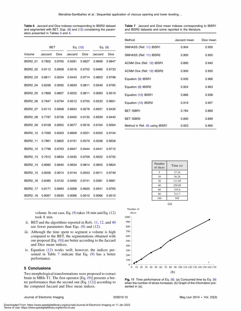
volume. In our case, Eq. (9) takes 16 min and Eq. (12)took 8 min.

ii. BET and the algorithms reported in Refs. 11, 12, and 40use fewer parameters than Eqs. (9) and (12).

iii. Although the time spent to segment a volume is highcompared to the BET, the segmentations obtained withour proposal [Eq. (9)] are better according to the Jaccardand Dice mean indices.

iv. Equation (12) works well; however, the indices pre-sented in Table 7 indicate that Eq. (9) has a betterperformance.

5 ConclusionsTwo morphological transformations were proposed to extractbrain in MRIs T1. The first operator [Eq. (9)] presents a bet-ter performance than the second one [Eq. (12)] according tothe computed Jaccard and Dice mean indices.

Table 6 Jaccard and Dice indexes corresponding to IBSR2 datasetand segmented with BET, Eqs. (9) and (12) considering the param-eters presented in Tables 3 and 4.

Volume

BET Eq. (12) Eq. (9)

Jaccard Dice Jaccard Dice Jaccard Dice

IBSR2_01 0.7802 0.8765 0.9281 0.9627 0.9699 0.9847

IBSR2_02 0.8112 0.8958 0.9516 0.9752 0.9480 0.9733

IBSR2_03 0.8611 0.9254 0.9443 0.9714 0.9603 0.9798

IBSR2_04 0.8336 0.9092 0.9629 0.9811 0.9540 0.9765

IBSR2_05 0.7868 0.8807 0.9252 0.9611 0.9083 0.9519

IBSR2_06 0.7847 0.8794 0.9512 0.9750 0.9233 0.9601

IBSR2_07 0.8113 0.8958 0.8654 0.9278 0.8931 0.9435

IBSR2_08 0.7787 0.8756 0.8402 0.9132 0.8939 0.9440

IBSR2_09 0.8108 0.8955 0.9077 0.9516 0.9164 0.9564

IBSR2_10 0.7099 0.8303 0.8606 0.9251 0.8355 0.9104

IBSR2_11 0.7861 0.8802 0.9191 0.9579 0.9338 0.9658

IBSR2_12 0.7798 0.8763 0.8947 0.9444 0.9441 0.9712

IBSR2_13 0.7912 0.8834 0.9435 0.9709 0.9522 0.9755

IBSR2_14 0.8082 0.8940 0.9634 0.9814 0.9655 0.9824

IBSR2_15 0.8206 0.9014 0.9144 0.9553 0.9511 0.9749

IBSR2_16 0.8385 0.9122 0.9495 0.9741 0.9381 0.9681

IBSR2_17 0.8171 0.8993 0.9268 0.9620 0.9541 0.9765

IBSR2_18 0.8067 0.8930 0.9066 0.9510 0.9066 0.9510

Table 7 Jaccard and Dice mean indexes corresponding to IBSR1and IBSR2 datasets and some reported in the literature.

Method Jaccard mean Dice mean

SMHASS (Ref. 11) IBSR1 0.904 0.950

SMHASS (Ref. 11) IBSR2 0.905 0.950

ACNM One (Ref. 12) IBSR1 0.890 0.940

ACNM One (Ref. 12) IBSR2 0.900 0.950

Equation (9) IBSR1 0.935 0.966

Equation (9) IBSR2 0.924 0.963

Equation (12) IBSR1 0.866 0.938

Equation (12) IBSR2 0.919 0.957

BET ISBR1 0.784 0.869

BET ISBR2 0.800 0.899

Method in Ref. 40 using IBSR1 0.923 0.960

0

100

200

300

400

500

600

700

800

900

1000

0 10 20 30 40 50 60 70 80 90 100 110 120 130 140 150 160 170

Number of slices

Time (s)

5 27.24

10 56.26

20 111.85

40 250.89

60 354.8

80 513.7

160 945

(a)

(b)

Number of slices

s

Fig. 11 Time performance of Eq. (9). (a) Consumed time by Eq. (9)when the number of slices increases. (b) Graph of the information pre-sented in (a).




The idea to segment the brain consisted of smoothlypropagating a marker given by the viscous opening intothe original volume. For this, adequate parameters mustbe obtained from a granulometric analysis. The sequentialapplication of such transformations results in a new morpho-logical operator [Eq. (9)] capable of better controlling thereconstruction process. Nevertheless, the new transformationemploys several parameters; due to this, a second morpho-logical transformation was obtained from a simplification ofthe first one [Eq. (12)].

Our proposals were tested using the two brain databasesobtained from the IBSR home page. In total, 38 volumes ofMR images of the brain were processed. The segmentationswere compared through two popular indices with respect tothe segmentations obtained from the BET algorithm, withmanual segmentations obtained from the IBSR website andwith respect to the values of the indices reported in thecurrent literature. When the mean values of the Jaccard andDice indices are compared, our proposal outperforms theother methodologies. This means that our segmentationsare closer to the manual segmentations obtained from theIBSR website. However, the time spent to segment a volumewith 160 slices, along with the number of parameters utilizedin Eq. (9), is higher compared to the time and the parametersutilized by the BET algorithm.

Although Eq. (12) significantly reduces the number ofparameters, Eq. (9) produces better segmentations. In thisway, Eq. (12) can be used to get approximated segmentationsof the brain.

The main problem of the BET algorithm is that severalregions are not detected; the beginning of Fig. 10(e) clearlyillustrates this situation. Due to this, the Jaccard and Diceindices fall considerably.

Finally, as future work, the proposal presented in thispaper will be improved by the implementation of fastalgorithms and/or parallel implementation on graphicsprocessing units using compute unified device architecturestechnology, so the performance can improve for real-timeapplications.

AcknowledgmentsThe author Iván R. Terol-Villalobos would like to thankDiego Rodrigo and Darío T.G. for their great encouragement.This work was funded by the government agency CONACyTMéxico under the Grant 133697.

References

1. A. M. Dale, B. Fischl, and M. I. Sereno, “Cortical surface-basedanalysis. I. Segmentation and surface reconstruction,” Neuroimage9(2), 179–194 (1999).

2. J. X. Liu, Y. S. Chen, and L. F. Chen, “Accurate and robust extraction ofbrain regions using a deformable model based on radial basis func-tions,” J. Neurosci. Methods 183(2), 255–266 (2009).

3. S. M. Smith, “Fast robust automated brain extraction,” Hum. BrainMapp. 17(3), 143–155 (2002).

4. H. Hahn and H.-O. Peitgen, “The skull stripping problem in MRI solvedby a single 3D watershed transform,” Lect. Notes Comput. Sci. 1935,134–143 (2000).

5. R. Beare et al., “Brain extraction using the watershed transform frommarkers,” Front. Neuroinf. 7(32), 1–15 (2013).

6. B. Dogdas, D. W. Shattuck, and R. M. Leahy, “Segmentation of skulland scalp in 3-D human MRI using mathematical morphology,” Hum.Brain Mapp. 26(4), 273–285 (2005).

7. S. Sandor and R. Leahy, “Surface-based labeling of cortical anatomyusing a deformable database,” IEEE Trans. Med. Imaging 16(1),41–54 (1997).

8. F. Ségonne et al., “A hybrid approach to the skull stripping problem inMRI,” Neuroimage 22(3), 1060–1075 (2004).

9. J. E. Iglesias et al., “Robust brain extraction across datasets and com-parison with publicly available methods,” IEEE Trans. Med. Imaging30(9), 1617–1634 (2011).

10. F. Lotte, A. Lecuyer, and B. Arnaldi, “FuRIA: a novel feature extractionalgorithm for brain-computer interfaces using inverse models andfuzzy regions of interest,” in 3rd Int. IEEE/EMBS Conf. on NeuralEngineering, 2007 (CNE ’07), Kohala Coast, HI, pp. 175–178, IEEE(2007).

11. F. J. Galdames, F. Jaillet, and C. A. Perez, “An accurate skullstripping method based on simplex meshes and histogram analysis formagnetic resonance images,” J. Neurosci. Methods 206(2), 103–119(2012).

12. S. Jiang et al., “Brain extraction from cerebral MRI volume using ahybrid level set based active contour neighborhood model,” Biomed.Eng. Online 12(1), 31 (2013).

13. A. Huang et al., “Brain extraction using geodesic active contours,”Proc. SPIE 6144, 61444J (2006).

14. S. F. Eskildsen et al., “The Alzheimer’s disease neuroimaging initiative,BEaST: brain extraction based on nonlocal segmentation technique,”Neuroimage 59(3), 2362–2373 (2012).

15. K. K. Leung et al., “Automated cross-sectional and longitudinalhippocampal volume measurement in mild cognitive impairment andAlzheimer’s disease,” Neuroimage 51(4), 1345–1359 (2010).

16. K. K. Leung et al., “Alzheimer’s disease neuroimaging initiative, brainMAPS: an automated, accurate and robust brain extraction techniqueusing a template library,” Neuroimage 55(3), 1091–1108 (2011).

17. P. Dokládal et al., “Topologically controlled segmentation of 3D mag-netic resonance images of the head by using morphological operators,”Pattern Recognit. 36(10), 2463–2478 (2003).

18. M. A. Balafar et al., “Review of brain MRI image segmentation meth-ods,” Artif. Intell. Rev. 33(3), 261–274 (2010).

19. J. C. Bezdek, L. O. Hall, and L. P. Clarke, “Review of MR imagesegmentation techniques using pattern recognition,” Med. Phys. 20(4),1033–1048 (1993).

20. A. P. Zijdenbos and B. M. Dawant, “Brain segmentation and whitematter lesion detection in MR images,” Crit. Rev. Biomed. Eng.22(5–6), 401–465 (1994).

21. L. P. Clarke et al., “MRI segmentation: methods and applications,”J. Magn. Reson. Imaging 13(3), 343–368 (1995).

22. C. Fennema-Notestine et al., “Quantitative evaluation of automatedskull-stripping methods applied to contemporary and legacy images:effects of diagnosis, bias correction, and slice location,” Hum. BrainMapp. 27(2), 99–113 (2006).

23. D. W. Shattuck et al., “Online resource for validation of brain segmen-tation methods,” Neuroimage 45(2), 431–439 (2009).

24. K. Boesen et al., “Quantitative comparison of four brain extractionalgorithms,” Neuroimage 22(3), 1255–1261 (2004).

25. B. D. Ward, Intracranial Segmentation, Biophysics Research Institute,Medical College of Wisconsin, Milwaukee (1999), AFNI is NIH sup-ported software at http://afni.nimh.nih.gov/pub/dist/doc/program_help/(23 May 2014).

26. D. W. Shattuck et al., “Magnetic resonance image tissue classificationusing a partial volume model,” Neuroimage 13(5), 856–876 (2001).

27. J. Ashburner and K. J. Friston, “Voxel-based morphometry: the meth-ods,” Neuroimage 11(6 Pt 1), 805–821 (2000).

28. V. Popescu et al., “Optimizing parameter choice for FSL-BrainExtraction Tool (BET) on 3D T1 images in multiple sclerosis,”Neuroimage 61(4), 1484–1494 (2012).

29. I. Santillán et al., “Morphological connected filtering on viscous latti-ces,” J. Math. Imaging Vision 36(3), 254–269 (2010).

30. J. D. Mendiola-Santibañez et al., “Application of morphological con-nected openings and levelings on magnetic resonance images of thebrain,” Int. J. Imaging Syst. Technol. 21(4), 336–348 (2011).

31. Center for Morphometric Analysis, Massachusetts General Hospital,The Internet Brain Segmentation Repository (IBSR) (1995), http://www.cma.mgh.harvard.edu/ibsr/ (23 May 2014).

32. L. Vincent, “Morphological grayscale reconstruction in image analysis:applications and efficient algorithms,” IEEE Trans. Image Process.2(2), 176–201 (1993).

33. F. Meyer and C. Vachier, “Image segmentation based on viscousflooding simulation,” in Mathematical Morphology, H. Talbot andR. Beare, Eds., pp. 69–77, CSIRO Publishing, Melbourne (2002).

34. C. Vachier and F. Meyer, “The viscous watershed transform,” J. Math.Imaging Vis. 22(2–3), 251–267 (2005).

35. P. Maragos and C. Vachier, “A PDE formulation for viscous morpho-logical operators with extensions to intensity-adaptative operators,” inProc. 15th IEEE Int. Conf. in Image Processing, San Diego, CA,pp. 2200–2203, IEEE (2008).

36. C. Vachier and F. Meyer, “News from viscous land,” in Proc. of the 8thInt. Symposium on Mathematical Morphology, , Rio de Janeiro, Brazil,G. J. F. Banon et al., Eds., pp. 189–200, MCT/INPE (2007).

37. L. Vincent, “Fast granulometric methods for the extraction of globalimage information,” in Proc. 11th Annual Symposium of the SouthAfrican Pattern Recognition Association, Johannesburg, South Africa,pp. 119–133, University of Witwatersrand publisher (2000).




http://dx.doi.org/10.1006/nimg.1998.0395

http://dx.doi.org/10.1016/j.jneumeth.2009.05.011

http://dx.doi.org/10.1002/(ISSN)1097-0193


http://dx.doi.org/10.1007/b12345

http://dx.doi.org/10.3389/fninf.2013.00032



http://dx.doi.org/10.1109/42.552054

http://dx.doi.org/10.1016/j.neuroimage.2004.03.032

http://dx.doi.org/10.1109/TMI.2011.2138152

http://dx.doi.org/10.1016/j.jneumeth.2012.02.017

http://dx.doi.org/10.1186/1475-925X-12-31

http://dx.doi.org/10.1186/1475-925X-12-31

http://dx.doi.org/10.1117/12.654160




http://dx.doi.org/10.1016/S0031-3203(03)00118-3

http://dx.doi.org/10.1007/s10462-010-9155-0

http://dx.doi.org/10.1118/1.597000

http://dx.doi.org/10.1016/0730-725X(94)00124-L





http://afni.nimh.nih.gov/pub/dist/doc/program_help/







http://dx.doi.org/10.1007/s10851-009-0184-8

http://dx.doi.org/10.1002/ima.v21.4

http://www.cma.mgh.harvard.edu/ibsr/






http://dx.doi.org/10.1109/83.217222

http://dx.doi.org/10.1007/s10851-005-4893-3

http://dx.doi.org/10.1007/s10851-005-4893-3

38. P. Jaccard, “The distribution of the flora in the alpine zone,” NewPhytol. 11(2), 37–50 (1912).

39. L. R. Dice, “Measures of the amount of ecologic association betweenspecies,” J. Ecol. 26(4), 297–302 (1945).

40. H. Zhang et al., “An automated and simple method for brain MR imageextraction,” Biomed. Eng. Online 10(1), 81 (2011).

41. H. Heijmans, Morphological Image Operators, Academic Press,Boston, Massachusetts (1994).

42. J. Serra and P. Salembier, “Connected operator and pyramids,” Proc.SPIE 2030, 65–76 (1993).

43. C. Rorden and M. Brett, “Stereotaxic display of brain lesions,” Behav.Neurol. 12(4), 191–200 (2000).

Jorge Domingo Mendiola-Santibañez received his PhD degreefrom the Universidad Autónoma de Querétaro (UAQ), México.Currently, he is a professor/researcher at the Universidad Autónomade Querétaro. His research interests include morphological imageprocessing and computer vision.

Martín Gallegos-Duarte is an MD and a PhD student at theUniversidad Autonoma de Querétaro. He is head of the StrabismusService at the Institute for the Attention of Congenital Diseasesand Ophthalmology-Pediatric Service in the Mexican Institute ofOphthalmology in the state of Queretaro, Mexico.

Miguel Octavio Arias-Estrada is a researcher in computer scienceat National Institute of Astrophysics, Optics and Electronics, Puebla,Mexico, with a PhD degree in electrical engineering (computer vision)from Laval University (Canada) and BEng and MEng degrees in

electronic engineering from University of Guanajuato (Mexico).Currently, he is a researcher at INAOE (Puebla, México). His interestsare computer vision, FPGA and GPU algorithm acceleration for three-dimensional machine vision.

Israel Marcos Santillán-Méndez received the BS degree in engi-neering from the Instituto Tecnológico de Estudios Superiores deMonterrey and his MS degree and PhD degree in engineering fromFacultad de Ingeniería de la Universidad Autónoma de Querétaro(México). His research interests include models of biological sensoryand perceptual systems and mathematical morphology.

Juvenal Rodríguez-Reséndiz received his MS degree in automationcontrol from University of Querétaro and PhD degree at the sameinstitution. Since 2004, he has been part of the MechatronicsDepartment at the UAQ. He is the head of the AutomationDepartment. His research interest includes signal processing andmotion control. He serves as vice president of IEEE in QueretaroState.

Iván Ramón Terol-Villalobos received his BSc degree from InstitutoPolitécnico Nacional (I.P.N. México), his MSc degree from Centro deInvestigación y Estudios Avanzados del I.P.N. (México). He receivedhis PhD degree from the Centre de Morphologie Mathématique,Ecole des Mines de Paris (France). Currently, he is a researcher atCIDETEQ (Querétaro, México). His main current research interestsinclude morphological image processing, morphological probabilisticmodels, and computer vision.




http://dx.doi.org/10.1111/nph.1912.11.issue-2

http://dx.doi.org/10.1111/nph.1912.11.issue-2

http://dx.doi.org/10.2307/1932409

http://dx.doi.org/10.1186/1475-925X-10-81

http://dx.doi.org/10.1117/12.146672

http://dx.doi.org/10.1117/12.146672

http://dx.doi.org/10.1155/2000/421719

http://dx.doi.org/10.1155/2000/421719

Sequential application of viscous opening and lower leveling for ...

Documents

Transcript of Sequential application of viscous opening and lower leveling for ...