Sequence-to-Customer Goal with Stochastic Demands for a

Mixed Model Assembly Line

Zhao Xiaobo 1, Xiande Zhao 2, Jeff H.Y. Yeung 2 and Jinxing Xie 3

1 Department of Industrial Engineering, Tsinghua University, Beijing 100084, China. 2 Department of Decision Sciences and Managerial Economics, The Chinese University of Hong

Kong, Hong Kong, China. 3 Department of Mathematical Sciences, Tsinghua University, Beijing 100084, China.

Submitted July 2004.

Correspondence: Prof. Zhao Xiaobo, Department of Industrial Engineering, Tsinghua University,

Beijing 100084, China.

Tel: +86-10-6278-4898; Fax: +86-10-6279-4399; Email: xbzhao@mail.tsinghua.edu.cn

1

Abstract:

A mixed model assembly line (MMAL) comprises a set of workstations in serial and a

conveyor moving at a constant speed, which can assemble variety products in different models

during a working shift or a working day. Initial-units that belong to different models are

successively fed onto the conveyor at a given cycle time length to get into the assembling

operations as semi-products. The conveyor moves semi-products to pass through the workstations

to gradually complete the assembling operations for generating finished-products. A set of

warehouses stores finished-products, and each model has a specified warehouse. Customers arrive

at the warehouses to demand finished-products at stochastic demand forms. A daily scheduling task

is the determination of the sequence that specifies the feeding order of the models, which must be

set out at the beginning of each day. This paper deals with a new goal, “sequence-to-customer”,

with stochastic customer demands. An optimization problem is formulated with the objective of

minimizing the system cost that includes the holding cost for finished-products and the penalty cost

for backordered customers during a decision horizon. A lower bound of the system cost is found,

which is useful in verifying the optimality of any solution. A heuristic algorithm is proposed to

solve the optimization problem, which can obtain optimal solutions or near-optimal solutions with

almost ignorable relative errors to optimal solutions. By using the algorithm, the behavior of the

system cost with respect to the variation in customer demands is also investigated to provide

insights into management of an MMAL.

Keywords: Mixed-model assembly line, sequence, stochastic demand, inventory, algorithm.

1. Introduction A major advantage of “mixed model assembly lines” (MMALs) is that they can assemble a

variety of models within a single working shift without having to “set up” for model changeovers.

Nowadays, MMALs are often adopted in the automobile industry and similar industries in order to

avoid excessive inventories.

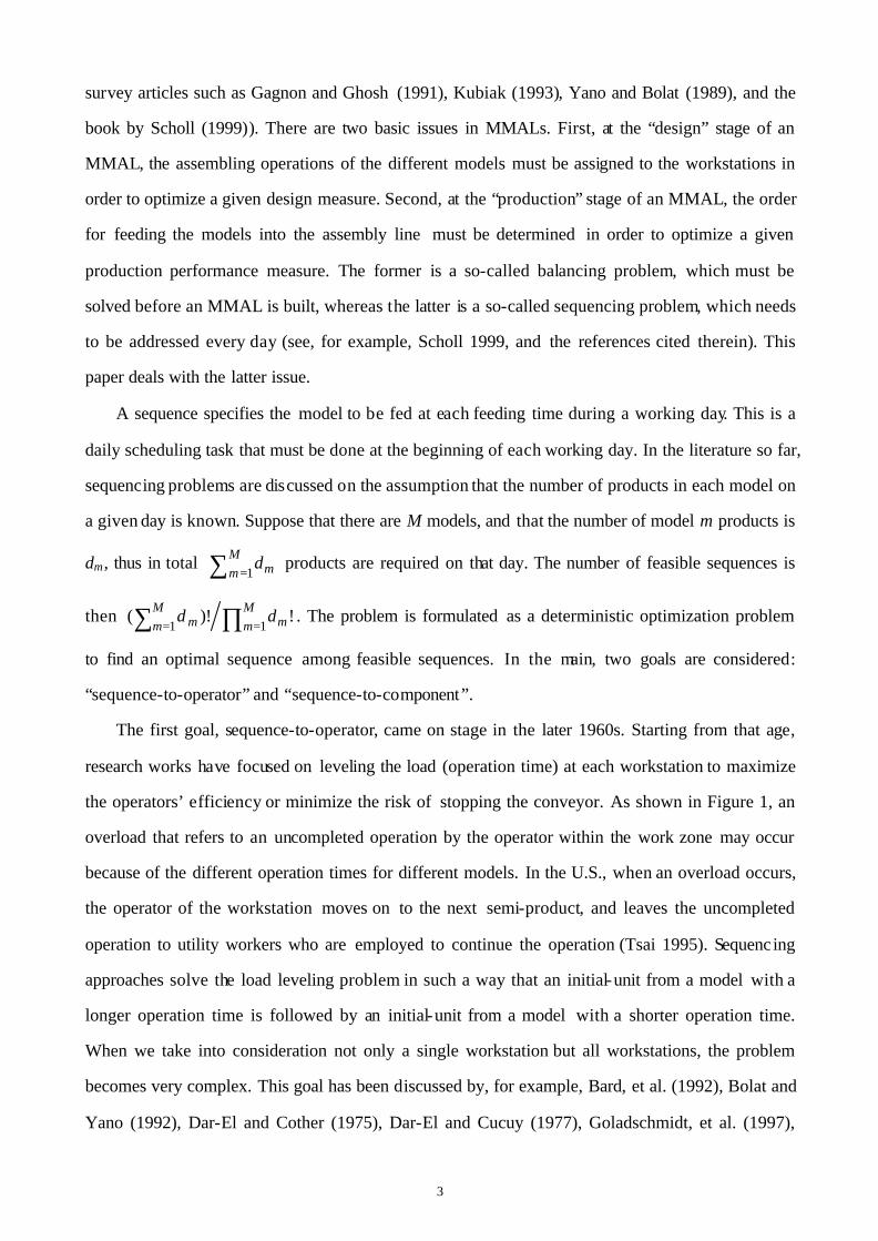
Figure 1 shows an example of an MMAL. Initial-units are successively fed onto the conveyor

at a given cycle time length to get into the assembling operations as semi-products. The conveyor

moves semi-products at a constant speed to pass through a set of workstations in serial. When a

semi-product enters a workstation, the operator in the workstation assembles specified components

onto it. Some components are inner-machined at the same factory (see, for example, components in

2

families 2 and 5 in Figure 1), whereas other components are out-supplied by component suppliers

(see, for example, components in families 1, 3 and 4 in Figure 1). A component family covers a set

of similar, but different, components. For instance, in a car assembly, there are many kinds of

engines that belong to the same family but have different horse-power capacities used in different

models of car. In addition, different product models may require different numbers of components

from a particular family. On the other hand, different models may need different operation times.

An operation diagram of workstation 1 is shown at the bottom left of Figure 1. Finished-products

are stored in different warehouses in according the model types. Customers arrive at the warehouses

to demand finished-products.

Out

-sup

plie

r

Out

-sup

plie

r

Out

-sup

plie

r

Model 2 Model 1 Model 3 Model 1

Model 1

Model 2

Model 3

Model 3

Model 1

Model 2

M

Workstation 1 Workstation 2 Workstation 3

Com

pone

nt f

amily

1

Com

pone

nt fa

mily

2

Com

pone

nt f

amily

3

Com

pone

nt fa

mily

4

Com

pone

nt fa

mily

5

Conveyor of the mixed model assembly line: constant movement speed

Com

pone

nt s

helf

Model 2

Warehouse 1

Warehouse 2

Warehouse 3

Com

pone

nt s

helf

Com

pone

nt s

helf

Com

pone

nt s

helf

Com

pone

nt s

helf

Operation

Walk

Idle

Overload

First unit

Second unit

Third unit

Fourth unit

Inne

r-m

achi

ning

Inne

r-m

achi

ning

Lead time Lead time Lead time

Operation

Walk

Operation

Walk

Operation

Type 1 customer

Type 2 customer

Type 3 customer

Initial-units

Finished-products

(Semi-product) (Semi-product) (Semi-product) (Semi-product) (Semi-product)

Figure 1. Mixed model assembly line

The design and operation of MMALs present challenging theoretical problems. Thus, in recent

decades, MMALs have received considerable attention in the academic literature (see, for example,

3

survey articles such as Gagnon and Ghosh (1991), Kubiak (1993), Yano and Bolat (1989), and the

book by Scholl (1999)). There are two basic issues in MMALs. First, at the “design” stage of an

MMAL, the assembling operations of the different models must be assigned to the workstations in

order to optimize a given design measure. Second, at the “production” stage of an MMAL, the order

for feeding the models into the assembly line must be determined in order to optimize a given

production performance measure. The former is a so-called balancing problem, which must be

solved before an MMAL is built, whereas the latter is a so-called sequencing problem, which needs

to be addressed every day (see, for example, Scholl 1999, and the references cited therein). This

paper deals with the latter issue.

A sequence specifies the model to be fed at each feeding time during a working day. This is a

daily scheduling task that must be done at the beginning of each working day. In the literature so far,

sequencing problems are discussed on the assumption that the number of products in each model on

a given day is known. Suppose that there are M models, and that the number of model m products is

dm, thus in total ∑ =Mm md

1 products are required on that day. The number of feasible sequences is

then ∏∑ ==Mm m

Mm m dd

11!)!( . The problem is formulated as a deterministic optimization problem

to find an optimal sequence among feasible sequences. In the main, two goals are considered:

“sequence-to-operator” and “sequence-to-component”.

The first goal, sequence-to-operator, came on stage in the later 1960s. Starting from that age,

research works have focused on leveling the load (operation time) at each workstation to maximize

the operators’ efficiency or minimize the risk of stopping the conveyor. As shown in Figure 1, an

overload that refers to an uncompleted operation by the operator within the work zone may occur

because of the different operation times for different models. In the U.S., when an overload occurs,

the operator of the workstation moves on to the next semi-product, and leaves the uncompleted

operation to utility workers who are employed to continue the operation (Tsai 1995). Sequenc ing

approaches solve the load leveling problem in such a way that an initial-unit from a model with a

longer operation time is followed by an initial-unit from a model with a shorter operation time.

When we take into consideration not only a single workstation but all workstations, the problem

becomes very complex. This goal has been discussed by, for example, Bard, et al. (1992), Bolat and

Yano (1992), Dar-El and Cother (1975), Dar-El and Cucuy (1977), Goladschmidt, et al. (1997),

4

Johnson (2002), Kim, et al. (1996), Macaskill (1973), Matanachai and Yano (2001), Merengo, et al.

(1999), Mithsumori (1969), Okamura and Yamashina (1979), Rachamadugu and Yano (1994),

Sarker and Pan (2001), Sumichrast, et al. (2000), Thomopoulos (1967), Tsai (1995), Yano and

Rachamadugu (1991). In the mid-1980s, Toyota production system introduced another approach to

treat overloads, in which the operator stops the conveyor until the remaining operation is completed

(Moden 1983 and 1998). With this system, an overload influences operation diagrams in all of the

other workstations due to the stoppage of the conveyor. An optimization problem of minimizing the

total stoppage times is discussed by Celano, et al. (2004), and Zhao and Ohno (2000). It is noticed

that all research works on the sequence-to-operator goal assume deterministic operation times.

However, in most actual assembly lines, all assembling operations are manually performed, which

leads to stochastic operation times. To our knowledge, no published works have yet dealt with the

modeling and analysis of MMALs with stochastic operation times.

The second goal, sequence-to-component, appeared in the mid-1980s. Since that time, Toyota

production system has received much attention from both academic researchers and practitioners.

Two pillars support Toyota production system: just- in-time (JIT) and autonomation (Monden 1983

and 1998). The JIT philosophy reduces the cost by keeping inventories to a minimum, including

raw material inventories, component inventories, semi-product inventories, and finished-product

inventories. The kanban mechanism was introduced to realize the JIT philosophy. Then a

hypothetical condition of stationary market demand is required to efficiently implement such Toyota

production system. Therefore, at every stage in the production system, “smoothing” (HEIJUNKA in

Japanese) is crucial. Toyota Motor Corporation developed a “goal chasing method” to determine a

sequence for realizing the smoothing aim for component consumption. The objective is to keep a

constant usage rate for every component family used in the assembly line. This goal has been

discussed by, for example, Aigbedo (2004), Bautista et al. (1996), Bukchin (1998), Caridi and

Sianesi (2000), Cheng and Ding (1996), Duplaga and Bragg (1998), Inman and Schmeling (2003),

Jin and Wu (2002), Korkmazel and Meral (2001), Kurashige, et al. (2002), Leu, et al. (1997),

Lovgren and Racer (2000), McMullen and Frazier (2000), Merengo, et al. (1999), Miltenburg and

Sinnamon (1989), Ponnambalama, et al. (2003), Steiner and Yeomans (1993), Sumichrast and

Clayton (1996), Sumichrast, et al. (2000), Ventura and Radhakrishnan (2002), Zeramdini, et al.

(2000), Zhang, et al. (2000), and Zhao and Zhou (1999). Several studies address a surrogated

5

objective of keeping the constant feeding rate of every model fed into the assembly line to indirectly

reach the goal of constant usage rate of every component family (see, for example, Ding and Cheng

(1993), Drexl and Kimms (2001), Kubiak (1993), and Miltenburg (1989)). It is noticed that all of

the researches on the sequence-to-component goal ignore the supply lead times of the components.

As shown in Figure 1, components can be inner-machined or out-supplied. The lead times of the

inner-machined components can be ignored, but the lead times for the out-supplied components can

be lengthy, and even uncertain or stochastic. To our knowledge, no published works have yet dealt

with the sequence-to-component goal with stochastic lead times.

This paper deals with a new goal: “sequence-to-customer”. As previously discussed, the

determination of a sequence is a daily scheduling task that must be set out at the beginning of each

day. A determined sequence is then implemented from the beginning of the day to the end of the day,

and cannot be changed once its implementation has been started. On the other hand, in many actual

systems, customers frequently arrive at warehouses and require finished-products, possibly at

random times during a day (see, for example, Aigbedo 2004. In addition, one of the authors of this

paper visited a logistics center at Toyota City in Japan, in which the physical goods distribution by

the center was controlled in accordance with supply kanbans that frequently circled among the

manufacturers-center-customers during a day.). At a time, at most one finished-product is output,

and is then sent to a particular warehouse. This eventually forms a limited capacity multi- item

production-replenishment- inventory system that is very different from other types of

production- inventory systems. In the literature, usually, after a decision making, all goods are

assumed to be instantaneous ly replenished, and the system cost such as holding cost and penalty

cost is charged only once during the time interval of two consecutive decisions. In our system, a

decision is made at the beginning of a day, finished-products gradually replenish the warehouses in

accordance with a pre-determined sequence, and customers arrive at the warehouses at random

times during the day. The system cost has to be charged at smaller time intervals to cope with

frequent ly arrival customers during the day. For any given day, the sequence plays a central role

because it has a strong impact on system performances, such as system costs, service levels for

customers, and so forth. Our motivation is to find optimal sequences to minimize the system costs.

There are basically two popular types of production strategy: “produce-to-stock” and

“produce-to-order” (see Buzacott and Shanthikumar 1993). Production planning with the

6

produce-to-stock strategy is based on market forecasting information, and is widely used in the

appliance industry, the IT industry, and the common-type automobile industry. The production

strategy of produce-to-order is adopted in industries such as aircraft manufacturing, shipbuilding,

and special-type automobile manufacturing. The production planning in such industries is made

only after the demands from customers are received. It is clear that if the exact information of

customer demands is known, then the goals of sequence-to-operator and sequence-to-component are

suitable for a produce-to-order strategy. (In such cases, the number of feasible sequences is

∏∑ ==Mm m

Mm m dd

11!)!( .) In contrast, if the system uses the produce-to-stock strategy, then the

sequence-to-customer goal is more appropriate. In such a case, the customer demands during the

current day and near future days are forecasted for both the gross requirement and the patterns of

the customer demands. Particularly, the patterns of the customer demands are presented at

stochastic forms rather than at a deterministic form. (Note that a deterministic form is only a special

case of stochastic forms.) Based on the forecasted gross requirement, the gross production or the

total number of initial-units to be fed on the current day is determined. Given the total number of

initial-units to be fed on the current day being N, the sequence is then determined based on the

forecasted patterns of the customer demands. However, the number of products in each model on

the current day is not given but is relaxed, which means that the number of feasible sequences is MN.

Thus, the scenario of a sequence-to-customer goal with a produce-to-stock strategy is more complex

than the scenario of a sequence-to-operator or sequence-to-component goal with a produce-to-order

strategy. (It is obvious that determining N is another important issue in the system. Nevertheless, in

this paper, we do not discuss how to determine N but treat it as known.)

The organization of the paper is as follows. In the next section, the system is described in detail.

In section 3, the optimization problem is formulated. Section 4 finds a lower bound of the system

cost. An algorithm is proposed in section 5. The behavior of the system cost with respect to the

variation in customer demands is investigated in section 6. The paper is concluded in section 7.

2. System Description

The system considered in this paper comprises an MMAL that produces different products in M

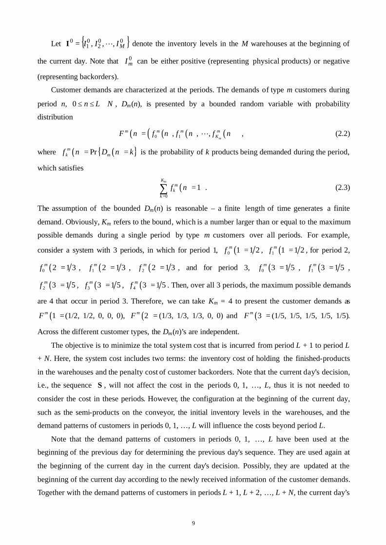
models and M warehouses that hold the finished-products. (See also figures 1 and 2.)

The MMAL consists of a set of workstations in serial. It is determined that N initial-units will

7

be fed into the assembly line during the current day. Then the cycle time length for successively

feeding initial-units onto the conveyor is the length of the regular daily working time length divided

by N. An initial-unit becomes a semi-product as soon as it is fed into the assembly line. A

semi-product, transferred by the constantly moving conveyor, sequentially passes through the

workstations to generate the finished-product. The moving time length from the first workstation to

the final workstation is assumed to be T. That is, if an initial-unit is fed onto the conveyor at time t,

then it will leave the conveyor at time t + T as a finished-product.

Model 2 Model 1 Model 3

Unit

Unit

Unit

MWorkstation 1 Workstation 2 Workstation 3

σ(1)T

σ(2)

σ(3)

σ(4)

σ(5)

σ(6)

σ(7)

σ(8)

σ(9)

σ(10)

σ(2)

σ(3)

σ(4)

σ(5)

σ(6)

σ(7)

σ(8)

σ(9)

σ(10)

Feeding time Leaving time

1 0t =

2t

3t

4t

5t

6t

7t

8t

9t

10t

σ(1)

( ) 3 Model20 =σ

( ) 1 Model30 =σ

( ) 2 Model40 =σ

2t T+

3t T+

4t T+

5t T+

6t T+

7t T+

8t T+

9t T+

10t T+

03t

02t

01t

Initial-units

Finished-products(Semi-product) (Semi-product) (Semi-product)(Semi-product)

Figure 2. Description of the system

The M warehouses are positioned at the end of the conveyor, with warehouse m holding model

m finished-products. Customers arrive at the warehouses to demand finished-products, who are

8

classified into M types. The demand processes of the customers are stochastic. Arrival customers

are backordered when they find no products in the corresponding warehouses.

Denote the set of the models by

M , 2, 1, L=Θ . (2.1)

At the beginning of the current day, some semi-products are on the conveyor, which were fed

into the assembly line before the current day. Because the situations of the customer demands may

be different day by day, the N and thus the cycle time length may be different day by day. At the

beginning of the current day, suppose that there are L semi-products on the conveyor denoted by

=0Σ ( ) ( ) ( )0 0 01 , 2 , , Lσ σ σL , where ( )n0σ ( Θ∈ ) is the model index of the nth semi-product.

They will leave the conveyor during the current day (possibly the current day plus near future days)

at times 01t , 0

2t , … , 0Lt , at which times they enter the corresponding warehouses as

finished-products. That is, the first one ( )0 1σ will leave the conveyor at time 01t and then enter

warehouse ( )0 1σ , the second one will be at time 02t and enter warehouse ( )0 2σ , and so forth.

The time intervals )010, t , )0 0

1 2, t t , … , )0 01 , L Lt t− , )0 , Lt T correspond to the cycle time length

of the previous day, or possibly, the cycle time lengths of the previous days. We call these intervals

“periods” 0, 1, … , L. The above information has been formed at the beginning of the current day

and cannot be changed during the current day and thereafter.

Following the ( )0 Lσ that is the last semi-product in 0Σ is the first one of the current day’s

N initial-units. This initial-unit is fed onto the conveyor at time 0 and will become a

finished-product at time T. During the current day, N initial-units that belong to different models

will be fed into the assembly line at times t1 (= 0), t2, … , tN, and they will leave the conveyor as

finished-products at times T, t2 + T, … , tN + T. The time intervals [0, t2), [t2, t3), … , [tN – 1, tN) in the

feeding process and therefore [T, t2 + T), [t2 + T, t3 + T), … , [tN – 1 + T, tN + T) in the leaving process

correspond to the cycle time length of the current day. We call time intervals [T, t2 + T), [t2 + T, t3 +

T), … , [tN – 1 + T, tN + T) “periods” L + 1, L + 2, … , L + N. The sequence that specifies the model to

be fed at each feeding time must be determined at the beginning of the current day. Let

( ) ( ) ( )Nσσσ , ,2 ,1 L=Σ denote the sequence for the current day, where ( )nσ ( Θ∈ ) is the model

index of the nth initial-unit in the sequence.

Therefore, the leaving process of the finished-products after the beginning of the current day is

formed by the above L + 1 + N periods, i.e., periods 0, 1, … , L, L + 1, L + 2, … , L + N. They may

have different time lengths – periods 0, … L correspond to the cycle time length(s) of the previous

day(s), and the later N periods correspond to the cycle time length of the current day.

9

Let 002

01

0 , , , MIII L=I denote the inventory levels in the M warehouses at the beginning of

the current day. Note that 0mI can be either positive (representing physical products) or negative

(representing backorders).

Customer demands are characterized at the periods. The demands of type m customers during

period n, 0 n L N≤ ≤ + , Dm(n), is presented by a bounded random variable with probability

distribution

( ) ( ) ( ) ( )( )0 1, , , m

m m m mKF n f n f n f n= L , (2.2)

where ( ) ( ) Prmk mf n D n k= = is the probability of k products being demanded during the period,

which satisfies

( )0

1mK

mk

k

f n=

=∑ . (2.3)

The assumption of the bounded Dm(n) is reasonable – a finite length of time generates a finite

demand. Obviously, Km refers to the bound, which is a number larger than or equal to the maximum

possible demands during a single period by type m customers over all periods. For example,

consider a system with 3 periods, in which for period 1, ( )0 1 1 2mf = , ( )1 1 1 2mf = , for period 2,

( )0 2 1 3mf = , ( )1 2 1 3mf = , ( )2 2 1 3mf = , and for period 3, ( )0 3 1 5mf = , ( )1 3 1 5mf = ,

( )2 3 1 5mf = , ( )3 3 1 5mf = , ( )4 3 1 5mf = . Then, over all 3 periods, the maximum possible demands

are 4 that occur in period 3. Therefore, we can take Km = 4 to present the customer demands as

( )1mF = (1/2, 1/2, 0, 0, 0), ( )2mF = (1/3, 1/3, 1/3, 0, 0) and ( )3mF = (1/5, 1/5, 1/5, 1/5, 1/5).

Across the different customer types, the Dm(n)’s are independent.

The objective is to minimize the total system cost that is incurred from period L + 1 to period L

+ N. Here, the system cost includes two terms: the inventory cost of holding the finished-products

in the warehouses and the penalty cost of customer backorders. Note that the current day’s decision,

i.e., the sequence Σ , will not affect the cost in the periods 0, 1, … , L, thus it is not needed to

consider the cost in these periods. However, the configuration at the beginning of the current day,

such as the semi-products on the conveyor, the initial inventory levels in the warehouses, and the

demand patterns of customers in periods 0, 1, … , L will influence the costs beyond period L.

Note that the demand patterns of customers in periods 0, 1, … , L have been used at the

beginning of the previous day for determining the previous day’s sequence. They are used again at

the beginning of the current day in the current day’s decision. Possibly, they are updated at the

beginning of the current day according to the newly received information of the customer demands.

Together with the demand patterns of customers in periods L + 1, L + 2, … , L + N, the current day’s

10

sequence Σ is determined. For the customer demands beyond period N, because of the lack of the

information, it is difficult to attain exact demand patterns of customers. Therefore, in the current

day’s decision, we adopt the information till to period N to determine an optimal sequence. This is

the usual case in actual systems – a daily decision is dynamically made based on the information

during the near-future.

The above procedure repeats day by day to form the dynamic daily decision for the daily

scheduling task.

3. Problem formulation

In accordance with the correspondence between the time intervals and the periods in the

previous section, the finished-product at a time 0lt (0 l L≤ ≤ ) belongs to period l, or at a time tn +

T ( 1L n L N+ ≤ ≤ + ) belongs to period n. We consider the system cost as comprising two terms:

inventory cost and penalty cost. These costs are caused by the decision made at the beginning of the

current day but are charged from period 1 to period N at expectation form. To be able to make the

decision at the beginning of the current day, we must analyze the probability distributions of the

inventory levels in the warehouses at each period.

For the facilitation of expressions later, we make the following definitions.

Definition 3.1 For two row vectors A = (a1, … , ai) and B = (b1, … , bj), a “connecting” operation is

defined as

( ) ( )ji bbaa , , , , , , 11 LL=BA . (3.1)

Definition 3.2 For a set C = c1, … , ci and a number d, a “plus” operation is defined as

dcdcd i ++=+ , ,1 LC . (3.2)

Definition 3.3 A set E = e1, … , ei that satisfies e1 < e2 < … < ei is an “ordered” set.

Let nM

nnn III , , , 21 L=I , 1 n L N≤ ≤ + , represent the inventory levels in the warehouses at

the beginning of period n, which are uncertain at time 0. Note that nmI can be either positive

(representing physical products) or negative (representing backorders).

At the beginning of period 0, as described previously, the initial inventory levels in the

warehouses are 001

0 , , MII L=I , which are certain as given initial information.

At the beginning of period 1, because the ( )10σ in 0Σ becomes the finished-product at the

11

beginning of the period, we must consider two different situations.

Situation 1: For any model ( )10σ≠m , the inventory level in the corresponding warehouse is

analyzed as follows. Because of the stochastic customer demand (2.2), at the beginning of period 1,

the inventory level can feasibly be mm KI −0 , 10 +− mm KI , … , 0mI . These Km + 1 values form the

state space of 1mI that is denoted by

( ) ( ) ( ) ( ) 1 , ,1 ,11 121 += mKmmmm ωωω LΩ , (3.3)

where ( ) mmm KI −= 01 1ω , ( ) 11 02 +−= mmm KIω , … , ( ) 01 1 mKm Im =+ω . Note that the set ( )1mΩ is an

“ordered” set in accordance with Definition 3.3. The probability distribution of the inventory level

1mI on the above state space at the beginning of period 1 is then given by

( ) ( ) ( ) ( )( ) ( ) ( ) ( )( )11 21 01 1 , 1 , , 1 1 , 1 , , 1m

m m

K m m mm m m m K Kg g g f f f+

−= =G L L , (3.4)

i.e., the probability of the inventory level 1mI being ( ) mmm KI −= 01 1ω is given by

( ) ( )1 1 01 Pr 1m

mm m m m Kg I I K f= = − = ,

of it being ( ) 11 02 +−= mmm KIω is given by

( ) ( )2 1 011 Pr 1 1

m

mm m m m Kg I I K f −= = − + = ,

… , and of it being ( ) 01 1 mKm Im =+ω is given by

( ) ( )1 1 001 Pr 1mK m

m m mg I I f+ = = = .

The above result can be expressed in matrix form. First, set Gm(0) = (1), a row vector where the

only single element is 1. Second, determine a one-step transition probability matrix on the state

space, which is a (Km + 1) × (Km + 1) matrix given by

( )

( )( ) ( )

( ) ( ) ( )

0

1 0

1 0

1 0 0

1 1 01

1 1 1m m

m

m m

m

m m mK K

f

f f

f f f−

=

P

LL

ML

. (3.5)

Then, we have

( ) ( )( ) ( )10 , 1 mmKm mPG0G ⋅= , (3.6)

with the operations first “connecting” and then “multiply”, where mK0 is a row vector in which all

of the Km elements are zero. Hence, ( )( )0 , mKmG0 is a row vector in which the first Km elements

are 0 and the Km + 1st element is 1, i.e., ( )( )0 , mKmG0 = (0, 0, … , 0, 1).

12

Situation 2: For the model ( )10σ=m , the inventory level in the warehouse for that model is

analyzed in accordance with the follows. The state space at the beginning of period 1 becomes

( ) ( ) ( ) ( ) 1 , ,1 ,11 121 += mKmmmm ωωω LΩ

1 , ,2 1, 000 ++−+−= mmmmm IKIKI L . (3.7)

Every element is one larger than it is in (3.3). The one-step transition probability matrix is the same

as (3.5). The probability distribution on the state space at the beginning of the period is the same as

(3.6).

At the beginning of period 2, it is clear that the number of feasible values of 2mI is 2Km + 1.

For any model ( )20σ≠m , the state space ( )2mΩ of 2mI is given according to the following two

cases:

1) If the ( )1mΩ corresponds to (3.3), then

( ) ( ) ( ) ( ) 2 , ,2 ,22 1221 += mKmmmm ωωω LΩ

000000 , ,1 , ,1 , ,12 ,2 mmmmmmmmmmm IKIKIKIKIKI LL +−−−−+−−= . (3.8)

2) If the ( )1mΩ corresponds to (3.7), then

( ) ( ) ( ) ( ) 2 , ,2 ,22 1221 += mKmmmm ωωω LΩ

1 , ,2 ,1 , , ,22 1,2 000000 ++−+−−+−+−= mmmmmmmmmmm IKIKIKIKIKI LL . (3.9)

The one-step transition probability matrix on the state space ( )2mΩ is then a (2Km + 1) × (2Km + 1)

matrix, given by

( )

( )( ) ( )

( ) ( ) ( )( ) ( ) ( )

( ) ( ) ( )

( ) ( ) ( )

0

1 0

1 0

1 0

1 0

1 0

2

2 2

2 2 22

2 2 2

2 2 2

2 2 2

m m

m m

m m

m m

m

m m

m m mK K

m m m mK K

m m mK K

m m mK K

f

f f

f f f

f f f

f f f

f f f

−

−

−

−

=

P

ML

LL

O O O OL

.

(3.10)

The probability distribution of 2mI on its state space at the beginning of period 2 is

( ) ( ) ( ) ( )( ) ( )( ) ( )21 , 2 , ,2 ,22 1221mmK

Kmmmm m

mggg PG0G ⋅== +L , (3.11)

13

In contrast, the state space ( )2mΩ of 2mI for the model ( )20σ=m at the beginning of

period 2 becomes the following.

1) If the ( )1mΩ corresponds to (3.3), then

( ) ( ) ( ) ( ) 2 , ,2 ,22 1221 += mKmmmm ωωω LΩ

1 , 1,2 00 ++−= mmm IKI L . (3.12)

2) If the ( )1mΩ corresponds to (3.7), then

( ) ( ) ( ) ( ) 2 , ,2 ,22 1221 += mKmmmm ωωω LΩ

2 , ,22 00 ++−= mmm IKI L . (3.13)

The one-step transition probability matrix is the same as (3.10). The probability distribution on the

state space at the beginning of period 2 is the same as (3.11).

To get a general expression of the state space at the beginning of period n for 1 n L N≤ ≤ + ,

define a δ function as follows

( )( ) ( )01 if for 1 , or, if for 1

0 otherwisem

m n n L m n L L n L Nn

σ σδ

= ≤ ≤ = − + ≤ ≤ +=

(3.14)

It is clear that values of the δ function depend on 0Σ , the semi-products on the conveyor at the

beginning of the current day, and Σ , the current day’s sequence.

At the beginning of any period n (1 n L N≤ ≤ + ), the state space is then

( ) ( ) ( ) ( ) nnnn mnKmmmm

121 , , , += ωωω LΩ

( )∑=

+−=n

tmmmm tInKI

1

00 , , δL , (3.15)

with the “plus” operation as defined in Definition 3.2. (Note that the set ( )nmΩ is an ordered set.)

The one-step transition probability matrix at the beginning of period n is a (nKm + 1) × (nKm + 1)

matrix, given by

14

( )

( )( ) ( )

( ) ( ) ( )( ) ( ) ( )

( ) ( ) ( )

( ) ( ) ( )

0

1 0

1 0

1 0

1 0

1 0

m m

m m

m m

m m

m

m m

m m mK K

m m m mK K

m m mK K

m m mK K

f n

f n f n

f n f n f nn

f n f n f n

f n f n f n

f n f n f n

−

−

−

−

=

P

ML

LL

O O O OL

.

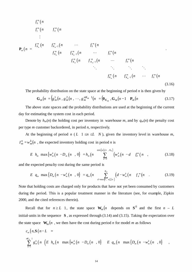
(3.16)

The probability distribution on the state space at the beginning of period n is then given by

( ) ( ) ( ) ( )( ) ( )( ) ( )nnn, g, n, gngn mmKnKmmmm m

m PG0G ⋅−== + 1 , 121 L (3.17)

The above state spaces and the probability distributions are used at the beginning of the current

day for estimating the system cost in each period.

Denote by hm(n) the holding cost per inventory in warehouse m, and by qm(n) the penalty cost

per type m customer backordered, in period n, respectively.

At the beginning of period n ( 1L n L N+ ≤ ≤ + ), given the inventory level in warehouse m,

( )nI km

nm ω= , the expected inventory holding cost in period n is

( ) ( ) ( ) ( )( ) ( )( ) min ,

0

max , 0km mn K

k k mm m m m m d

d

E h n D n h n n d f nω

ω ω=

⋅ − = ⋅ − ⋅ ∑ , (3.18)

and the expected pena lty cost during the same period is

( ) ( ) ( ) ( )( ) ( )( ) max 0 ,

max , 0m

km

Kk k m

m m m m m dd n

E q D n n q n d n f nω

ω ω=

⋅ − = ⋅ − ⋅ ∑ . (3.19)

Note that holding costs are charged only for products that have not yet been consumed by customers

during the period. This is a popular treatment manner in the literature (see, for example, Zipkin

2000, and the cited references therein).

Recall that for 1n L≥ + , the state space ( )nmΩ depends on 0Σ and the first n – L

initial-units in the sequence Σ , as expressed through (3.14) and (3.15). Taking the expectation over

the state space ( )nmΩ , we then have the cost during period n for model m as follows

( )( ),mc n n LΣ − =

( ) ( ) ( ) ( ) ( ) ( ) ( ) ( )1

1

max , 0 max , 0mnK

k k km m m m m m m

k

g n E h n n D n E q n D n nω ω+

=

⋅ ⋅ − + ⋅ − ∑ ,

15

(3.20)

where ( )n LΣ − is a sub-sequence of the sequence ( ) ( )Nσσ , ,1 L=Σ formed by the first n – L

initial-units in Σ , i.e., ( ) ( ) ( )1 , , n L n Lσ σΣ − = −L , and of course ( )NΣ is simply the

sequence Σ .

The system cost over all models during period n is then

( )( ) ( )( )1

, ,M

mm

C n n L c n n LΣ Σ=

− = −∑ . (3.21)

Summing up the system cost from period L + 1 to period L + N, we have the expected system

cost caused by the decision Σ as follows

( ) ( )( ) ( )( )1 1 1

, ,L N L N M

mn L n L m

C n n L c n n LΣ Σ Σ+ +

= + = + =

= − = −∑ ∑ ∑C . (3.22)

Optimization Problem 3.1 Determine an optimal sequence ( ) ( ) ( )Nσσσ , ,2 ,1 L=Σ , where

( ) Θ∈tσ for Nt ≤≤1 , to minimize the expected system cost (3.22).

Remark 3.1 As described at the beginning of this paper, one significant advantage of MMALs is

that they can assemble a variety of models within a single work shift without having to set-up in

model changeovers. Therefore, it is no longer necessary to consider “setup” costs in the

determination of an optimal sequence.

4. Properties

In a sequence ( ) ( ) ( )Nσσσ , ,2 ,1 L=Σ , any element in Θ , i.e., any one of M models, can

serve as a candidate for a ( )tσ , Nt ≤≤1 . Therefore, for a given N, the solution space of

Optimization Problem 3.1 consists of NM feasible solutions. This quickly becomes a calculation

explosion as N increases. Essentially, good heuristics need to be developed for large-scale problems.

Before proposing our algorithm, we first reveal some important properties of the optimization

problem. Eventually, we will provide a lower bound of the objective function over the solution

space of the optimization problem.

Let, for 1L n L N+ ≤ ≤ + and 1 m M≤ ≤ , nmi be the largest value in a state space ( )m nΦ ,

which is an ordered set, and nmj be the number of states therein. Suppose that n

mj is given by

1+= mnm nKj . (4.1)

16

For example, if ( )m nΦ = 2, 3, 4, 5, 6, 7, 8, then nmi = 8 and n

mj = 7.

Referring to (3.20), we define a cost function for period n ( 1L n L N+ ≤ ≤ + ) as follows

( ) ( ) nmm

nm

nm

nm njiR rG ⋅=,

( ) ( )( )( )

( )11

1

, , m

n n nm m m

nKm m

n nm m

r i j

g n g n

r i

+

− + = ⋅

L M

( ) ( ) ( )1

n

n nmm m

n nm m

i l i j nm m

l i j

g n r l− −

= − +

= ⋅∑ , (4.2)

where ( ) ( ) ( )( )ngngn mnKmmm

11 ,, += LG is the probability distribution given by (3.17), and

( ) ( ) ( ) ( ) ( ) max , 0 max , 0nm m m m mr l E h n l D n E q n D n l = ⋅ − + ⋅ − . (4.3)

Note that ( )m nG is determined by the patterns of demands of type m customers Fm(0), … ,

Fm(n), and is independent of the other parameters in the system.

Referring to a standard inventory system such as the newsvendor model (see, for example,

Zipkin 2000), the following result is straightforward.

Lemma 4.1 ( )nmr l is convex with respect to l.

We can then induce the following result.

Proposition 4.1 For a given nmj , ( )n

mnm

nm jiR , is convex with respect to n

mi .

Proof. From the definition of convexity, it is sufficient to verify that

( ) ( )( ) ( ) ( )( ) 0,1,,,1 ≥−−−−+ nm

nm

nm

nm

nm

nm

nm

nm

nm

nm

nm

nm jiRjiRjiRjiR .

It holds from (4.2) that

( ) ( ) ( ) ( ) ( )( )

( ) ( ) ( )1 1

11 1

1, ,n n

n n n nm mm m m m

n nn nm mm m

i il i j l i jn n n n n n n nm m m m m m m m m m

l i jl i j

R i j R i j g n r l g n r l+ − + − − −

= − += + − +

+ − = ⋅ − ⋅∑ ∑

( ) ( ) ( ) ( ) ( ) ( )1 1

1n n

n n n nm mm m m m

n n n nm m m m

i il i j l i jn nm m m m

l i j l i j

g n r l g n r l− − − −

= − + = − +

= ⋅ + − ⋅∑ ∑

( ) ( ) ( ) ( )1

1n

n nmm m

n nm m

i l i j n nm m m

l i j

g n r l r l− −

= − +

= ⋅ + − ∑ .

17

Similarly, we have

( ) ( ) ( ) ( ) ( ) ( )1

, 1, 1n

n nmm m

n nm m

i l i jn n n n n n n nm m m m m m m m m

l i j

R i j R i j g n r l r l− −

= − +

− − = ⋅ − − ∑ .

Therefore,

( ) ( )( ) ( ) ( )( )=−−−−+ nm

nm

nm

nm

nm

nm

nm

nm

nm

nm

nm

nm jiRjiRjiRjiR ,1,,,1

( ) ( ) ( ) ( ) ( ) ( ) 1

1 1n

n nmm m

n nm m

i l i j n n n nm m m m m

l i j

g n r l r l r l r l− −

= − +

⋅ + − − − − ∑ .

Lemma 4.1 then completes the proof.

Taking into consideration all M models, we define a cost function for period n

( 1L n L N+ ≤ ≤ + ) as follows

( ) ( )∑=

=M

m

nm

nm

nm jiRnu

1, . (4.4)

For 1L n L N+ ≤ ≤ + , let ( )nM

nn ii , ,1 L=i and ( )nM

nn jj , ,1 L=j . Suppose that nj is given

by (4.1). For period L, denote ( )1 , , L L LMi i=i L , where L

mi takes the same value as ( )1mLKm Lω +

in (3.15). Note that Li is determined by the initial information I0 and 0Σ , and is independent of

the other parameters in the system.

Definition 4.1 For two vectors ( )iyy , ,1 L=Y and ( )izz , ,1 L=Z , an order ≤ is defined as

ZY ≤ , (4.5)

if jj zy ≤ for all j = 1, … , i.

Definition 4.2 For a vector ( )ixx , ,1 L=X , an operation ⋅ is defined as

ixx ++= L1X . (4.6)

For n = L + 1, suppose that ni (= 1L+i ) satisfies 1L L+≤i i and 1 1L L+ − =i i . That is, the

elements in 1L+i are the same as those in Li , except that one element in 1L+i is one larger than

the corresponding element in Li . Then, consider the following problem:

Problem 4.1 Determine 1L+i to minimize u(L + 1), subject to 1L L+≤i i and 1 1L L+ − =i i .

18

The above problem is similar to a “resource allocation problem” with a separable objective

function for a single resource to be allocated. (Resource allocation problems are introduced in, for

example, Ibaraki and Katoh 1988.) Because ( )1 1 1,L L Lm m mR i j+ + + is convex with respect to 1L

mi+ by

Proposition 4.1, we can easily obtain an optimal solution. Find the index m with the largest

difference, ( ) ( )1 1 1 1, 1,L L L L L Lm m m m m mR i j R i j+ + + +− + , among m = 1, … , M. Allocating the single resource to

this m to form 1Lmi

+ (= 1Lmi + ) can therefore lead to the greatest cost reduction. (Note that a

reduction here can be either a positive reduction or a negative reduction, but a negative reduction

means an increase in cost.) Denote the optimal solution of the problem by * 1L+i and the

corresponding value of the objective function by u*(L + 1). The optimal solution is generated by

setting * 1 1L Lm mi i+ = + for the above-mentioned m, and * 1L L

m mi i+ = for the other m’s.

In general, for 1L n L N+ ≤ ≤ + , suppose that ni satisfies L n≤i i and n L n L− = −i i . Then,

consider the following problem for a given n.

Problem 4.2 Determine ni to minimize u(n), subject to L n≤i i and n L n L− = −i i .

Eventually, the above problem is a “resource allocation problem” with a separable objective

function for n – L resources to be allocated. Because ( )nm

nm

nm jiR , is convex with respect to n

mi by

Proposition 4.1, we can easily obtain an optimal solution by the following marginal procedure. (A

marginal procedure is introduced in, for example, Ibaraki and Katoh 1988).

Marginal procedure for Problem 4.2 for a given n:

Step 1. Calculate nj according to (4.1), calculate ( )nmG according to (3.17), and set *n L=i i

by referring to ( )m LΩ in (3.15);

Step 2. For k = 1 to n – L, carry out the following

1) Calculate ( ) ( )nm

nm

nm

nm

nm

nm jiRjiR ,1, ** +− for all m = 1, … , M;

2) For the index m with the largest ( ) ( )nm

nm

nm

nm

nm

nm jiRjiR ,1, ** +− among m = 1, … , M, set

1** += nm

nm ii .

The final resultant n*i is the optimal solution of Problem 4.2 with the value of the objective

function u*(n) calculated according to (4.4).

19

From the above, u*(n) is eventually the minimum system cost during period n among all

feasible configurations of ni . On the other hand, from (3.21), ( )( ),C n n LΣ − is the system cost

during period n caused by the sub-sequence ( )n LΣ − . Since the sub-sequence ( )n LΣ − leads to

the ( )m nΩ that may result in an ni different from n*i , the following result is obvious.

Lemma 4.2 For any given period n ( 1L n L N+ ≤ ≤ + ), it holds that ( ) ( )( )* ,u n C n n L≤ Σ − .

Summing up u*(n) over n = L + 1 to L + N, we have

( )* *

1

L N

n L

U u n+

= +

= ∑ . (4.7)

The following result is then straightforward.

Proposition 4.2 *U is a lower bound of ( )ΣC , the objective function (3.22) of Optimization

Problem 3.1, i.e., ( ) *U≥ΣC for any sequence Σ .

To obtain the value of the lower bound, we have to solve N optimization problems defined as

Problem 4.2, by using the marginal procedure for each n = L + 1 to L + N. It is clear that the

calculations for obtaining the value of the lower bound cause a polynomial complexity with respect

to N.

For large-scale systems, efficient algorithms are essential for obtaining optimal or near-optimal

solutions of Optimization Problem 3.1. The lower bound will be useful in evaluating the quality of

the solutions for large-scale systems.

5. An algorithm

It is known that the probability distribution ( )nmG on the state space ( )nmΩ , i.e., (3.17), is

independent of the sequence Σ ; it only depends on the probability distributions of demands by type

m customers Fm(0), … , Fm(n). Moreover, the number of states in ( )nmΩ is also independent of the

sequence; the sequence only influences the values of the states. Recall that ( )nmΩ is an ordered

set in which the largest value is ( )nmnKm

1+ω .

By comparing expressions (3.20) and (4.2), Proposition 4.1 directly indicates the following

result.

20

Proposition 5.1 For a given n, ( )( ),mc n n LΣ − is convex with respect to ( )nmnKm

1+ω .

This proposition shows that for any given period the cost function (3.20) of any model is

convex with respect to the largest value in its corresponding state space. Based on this property, we

propose an algorithm in accordance with the following principle. It is executed from n = 1 to n = L

+ N, and from n = 1 to n = L it makes preliminary calculations. A sequence Σ is then generated by

executing the algorithm through n = L + 1 to n = L + N. Each time, for a given n ( 1L n L N+ ≤ ≤ + ),

it finds a model that leads to the greatest reduction in system cost when one more finished-product

of the model is added to the corresponding warehouse. It therefore reflects that an initial-unit of the

model is fed into the assembly line at time tn – L, and the model is set to ( )n Lσ − in the sequence

Σ . Note that a reduction here can either be a positive reduction or a negative reduction, but that a

negative reduction means an increase in cost. Therefore, when one more finished-product in any

model is added then the cost increases, the manner selects a model that leads to the smallest cost

increase.

Algorithm:

Step 1. Initialization of parameters. Set the number of models M, the number of semi-products on

the conveyor at the beginning of the current day L and 0Σ , the initial inventory levels in

the warehouses I0, the probability distributions of demands of customers Fm(n)’s for all n =

0, … , L + N, and the total number of initial-units to be fed on the current day N, etc.

Step 2. From n = 1 to n = L, determine the state space ( )nmΩ ’s according to (3.15), and the

one-step transition probability matrix ( )nmP ’s according to (3.16). Then, calculate the

probability distributions on the state spaces ( )nmG ’s according to (3.17).

Step 3. From n = L + 1 to n = L + N, determine the state space ( )nmΩ ’s according to (3.15), the

one-step transition probability matrix ( )nmP ’s according to (3.16), and calculate the

probability distributions on the state spaces ( )nmG ’s according to (3.17). Sweep over all

models for the system cost by referring to (3.20) and select the model that leads to the

greatest reduction in the current system cost ( )( ),C n n LΣ − of (3.21) by adding one more

finished-product of the model to the corresponding warehouse. Set this model to ( )n Lσ −

to form the (n – L)th element in the sequence Σ . In summary, the (n – L)th element

( )n Lσ − in the sequence Σ is determined in accordance with the greatest reduction in

system cost from ( )( ),C n n LΣ − to ( )( )1, 1C n n L+ Σ − + of (3.21).

21

It can be easily verified that the calculation for obtaining a solution causes a polynomial

complexity with respect to N.

We can use the lower bound *U to evaluate the quality of the solutions generated by the

algorithm. Formally, for a given sequence Σ , let

( ) ( )*

*

U

U−=

ΣΣ∆

C . (5.1)

Denote by *Σ the optimal sequence. Then, we can define a relative error for a given sequence Σ

as follows

( ) ( ) ( )( )*

*

Σ

ΣΣΣ

C

CC −=δ . (5.2)

The following result is obvious.

Proposition 5.2 For a given Σ , ( )Σ∆ is an upper bound of ( )Σδ , i.e., ( ) ( )Σ∆Σ ≤δ .

It is clear that if ( ) 0=Σ∆ , then Σ is optimal.

Example 5.1. Consider a large-scale system with randomly produced parameters. The number of

models M = 10; the number of initial-units N = 100; the number of semi-products on the conveyor

at the beginning of the current day L = 19 and =0Σ 1, 2, 3, 4, 5, 6, 7, 8, 9, 10, 10, 9, 8, 7, 6, 5, 4,

3, 2 ; for all periods n = 0, … , 119, the demand distributions F1(n) = (0.948, 0.030, 0.010, 0.010,

0.002), F2(n) = (0.965, 0.025, 0.010), F3(n) = (0.945, 0.035, 0.010, 0.010), F4(n) = (0.955, 0.025,

0.020), F5(n) = (0.895, 0.105), F6(n) = (0.949, 0.045, 0.005, 0.001), F7(n) = (0.915, 0.065, 0.020),

F8(n) = (0.935, 0.045, 0.010, 0.010), F9(n) = (0.898, 0.075, 0.020, 0.005, 0.002), F10(n) = (0.920,

0.060, 0.020); the initial inventories I0 =(5, –1, 1, –2, 2, –4, 1, 0, 5, 1); for all periods, the holding

cost per inventory H(n) = (h1(n), … , h10(n)) = (2.1, 2.3, 2.5, 1.9, 2.2, 3.2, 4.1, 3.4, 2.8, 3.3); and for

all periods, the penalty cost per backorder Q(n) = (q1(n), … , q10(n)) = (5.5, 6.1, 5.3, 5.6, 6.2, 4.8, 3.9,

4.6, 5.4, 4.4).

Solution. The algorithm generates the solution =Σ 6, 6, 4, 6, 4, 2, 6, 8, 4, 3, 5, 10, 8, 4, 7, 2, 6, 3,

5, 10, 8, 7, 4, 9, 5, 3, 1, 10, 9, 2, 6, 8, 7, 5, 4, 9, 3, 10, 1, 8, 7, 5, 9, 4, 6, 3, 10, 1, 2, 9, 7, 8, 5, 9, 1, 10,

3, 4, 5, 7, 8, 6, 9, 2, 1, 10, 3, 5, 7, 9, 8, 4, 1, 10, 9, 5, 3, 6, 7, 8, 9, 2, 4, 5, 10, 1, 3, 7, 9, 8, 6, 5, 10, 1,

9, 4, 7, 3, 8, 2 . The system cost of the solution ( )=ΣC 8886.672. For the example, we also

calculate the lower bound *U , and further find that the upper bound of the relative error ( ) 0=Σ∆ .

22

Therefore, the algorithm generates an optimal sequence.

Example 5.2. Consider another large-scale system with randomly produced parameters. The

number of models M = 10; the number of initial-units N = 100; the number of semi-products on the

conveyor at the beginning of the current day L = 29 and =0Σ 1, 9, 10, 4, 7, 6, 2, 3, 5, 10, 3, 9, 2,

7, 5, 5, 6, 8, 3, 2, 1, 5, 7, 2, 8, 9, 10, 4, 6 ; for all periods n = 0, … , 129, the demand distributions

F1(n) = (0.955, 0.025, 0.020), F2(n) = (0.952, 0.025, 0.013, 0.010), F3(n) = (0.940, 0.035, 0.015,

0.010), F4(n) = (0.965, 0.025, 0.010), F5(n) = (0.880, 0.107, 0.013), F6(n) = (0.93, 0.07), F7(n) =

(0.923, 0.065, 0.012), F8(n) = (0.912, 0.045, 0.043), F9(n) = (0.88, 0.10, 0.01, 0.01), F10(n) = (0.942,

0.050, 0.008); the initial inventories I0 =(0, –2, 1, –3, 2, –1, 0, 2, 1, –2); the semi-products on the

conveyor; for all periods, the holding cost per inventory H(n) = (h1(n), … , h10(n)) = (13.3, 14.1, 5.2,

13.9, 4.2, 6.1, 14.4, 23.1, 22.7, 16.3); and for all periods, the penalty cost per backorder Q(n) =

(q1(n), … , q10(n)) = (34.1, 27.8, 22.2, 29.4, 20.5, 34.3, 43.7, 18.6, 15.2, 44.8).

Solution. The algorithm generates the solution =Σ 4, 10, 4, 6, 10, 7, 2, 1, 4, 6, 3, 7, 9, 5, 10, 2, 8,

1, 6, 3, 9, 5, 7, 4, 8, 2, 5, 10, 9, 3, 1, 7, 6, 8, 5, 9, 2, 3, 5, 8, 10, 7, 9, 6, 4, 1, 3, 5, 2, 8, 9, 7, 5, 10, 6, 3,

8, 9, 1, 2, 5, 7, 9, 4, 8, 3, 5, 10, 6, 2, 9, 7, 1, 8, 5, 3, 9, 6, 8, 5, 10, 7, 2, 4, 3, 9, 1, 8, 5, 9, 3, 7, 6, 2, 10,

5, 8, 9, 1, 3 . The system cost of the solution ( )=ΣC 46803.19. For the example, we also calculate

the lower bound *U , and further find that the upper bound of the relative error ( )Σ∆ = 0.00001.

This means that the relative error between the solution generated by the algorithm and the optimal

solution is less than or equal to 0.001%, i.e., ( )≤Σδ 0.001%.

Observation 5.1. As we can easily verify the optimality of any solution by propositions 4.2 and 5.2,

many test examples are executed to evaluate the quality of solutions generated by the algorithm.

The summary of parameters of the tested examples is as follows:

Table 1. Summary of the examples

M 3 ~ 10

N 5 ~ 100

L 2 ~ 20

Fm(n) ( )0mf n : 0.5 ~ 0.99, other ( )m

if n ’s: 0 ~ 0.5

I0 All mI0 ’s: – 5 ~ 5

H(n) All hm(n)’s: 1 ~ 15

23

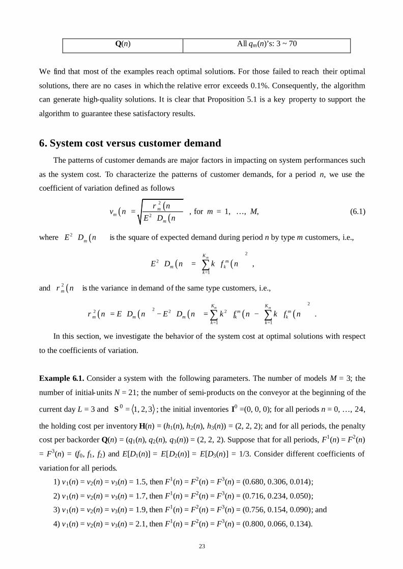
Q(n) All qm(n)’s: 3 ~ 70

We find that most of the examples reach optimal solutions. For those failed to reach their optimal

solutions, there are no cases in which the relative error exceeds 0.1%. Consequently, the algorithm

can generate high-quality solutions. It is clear that Proposition 5.1 is a key property to support the

algorithm to guarantee these satisfactory results.

6. System cost versus customer demand

The patterns of customer demands are major factors in impacting on system performances such

as the system cost. To characterize the patterns of customer demands, for a period n, we use the

coefficient of variation defined as follows

( ) ( )( )

2

2m

mm

nv n

E D nρ

=

, for m = 1, … , M, (6.1)

where ( )2mE D n is the square of expected demand during period n by type m customers, i.e.,

( ) ( )2

2

1

mKm

m kk

E D n k f n=

= ⋅

∑ ,

and ( )2m nρ is the variance in demand of the same type customers, i.e.,

( ) ( ) ( ) ( ) ( )2

22 2 2

1 1

m mK Km m

m m m k kk k

n E D n E D n k f n k f nρ= =

= − = ⋅ − ⋅

∑ ∑ .

In this section, we investigate the behavior of the system cost at optimal solutions with respect

to the coefficients of variation.

Example 6.1. Consider a system with the following parameters. The number of models M = 3; the

number of initial-units N = 21; the number of semi-products on the conveyor at the beginning of the

current day L = 3 and 3 2, 1,0 =Σ ; the initial inventories I0 =(0, 0, 0); for all periods n = 0, … , 24,

the holding cost per inventory H(n) = (h1(n), h2(n), h3(n)) = (2, 2, 2); and for all periods, the penalty

cost per backorder Q(n) = (q1(n), q2(n), q3(n)) = (2, 2, 2). Suppose that for all periods, F1(n) = F2(n)

= F3(n) = (f0, f1, f2) and E[D1(n)] = E[D2(n)] = E[D3(n)] = 1/3. Consider different coefficients of

variation for all periods.

1) v1(n) = v2(n) = v3(n) = 1.5, then F1(n) = F2(n) = F3(n) = (0.680, 0.306, 0.014);

2) v1(n) = v2(n) = v3(n) = 1.7, then F1(n) = F2(n) = F3(n) = (0.716, 0.234, 0.050);

3) v1(n) = v2(n) = v3(n) = 1.9, then F1(n) = F2(n) = F3(n) = (0.756, 0.154, 0.090); and

4) v1(n) = v2(n) = v3(n) = 2.1, then F1(n) = F2(n) = F3(n) = (0.800, 0.066, 0.134).

24

1.5 1.7 1.9 2.1

Coefficients of variations

Syst

em c

osts

100

150

200

250

300

Figure 3. Relationship between the system cost and the coefficients of variation

Using the algorithm to solve each combination of the above, we obtain the optimal solutions

and the corresponding system costs. Figure 3 shows the computational results. The increase in

system cost has a linear relationship with respect to the coefficients of variation. Intuitively, as the

coefficients of variation increase, such possibilities also increase that the inventories become higher

and the backorders become more.

Example 6.2. Consider a system with the following parameters. The number of models M = 3; the

number of initial-units N = 21; the number of semi-products on the conveyor at the beginning of the

current day L = 3 and 3 2, 1,0 =Σ ; for all periods n = 0, … , 24, the distributions of customer

demands F1(n) = F2(n) = F3(n) = (f0, f1, f2) with E[D1(n)] = E[D2(n)] = E[D3(n)] = 1/3; and for all

periods, the coefficients of variation v1(n) = v2(n) = v3(n) = 1.5 ~ 2.1; the initial inventories I0 =(0, 0,

0). Set the cost terms in accordance with the following.

1) For all periods, the penalty cost per backorder Q(n) = (q1(n), q2(n), q3(n)) = (3, 3, 3); the

holding cost per inventory H(n) = (h1(n), h2(n), h3(n)) = (1, 1, 1) ~ (5, 5, 5);

2) For all periods, the holding cost per inventory H(n) = (h1(n), h2(n), h3(n)) = (3, 3, 3); the

penalty cost per backorder Q(n) = (q1(n), q2(n), q3(n)) = (1, 1, 1) ~ (5, 5, 5).

Using the algorithm to solve each combination of the above, we obtain the optimal solutions

and the corresponding system costs. Figure 4 depicts the computational results of part 1) of the

above, plotted for different coefficients of variation. Given the penalty cost per backorder, the

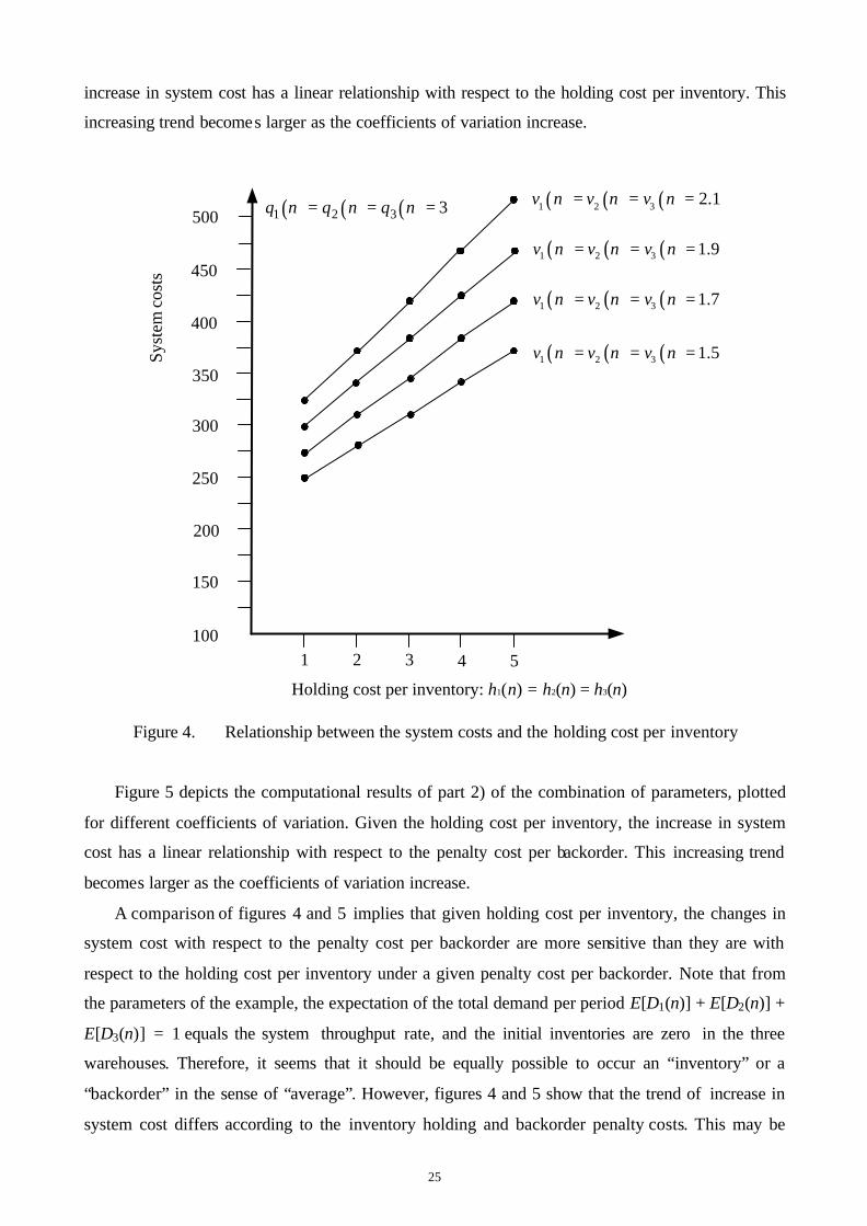
25

increase in system cost has a linear relationship with respect to the holding cost per inventory. This

increasing trend becomes larger as the coefficients of variation increase.

1002 3 4

Holding cost per inventory: h1(n) = h2(n) = h3(n)

Syst

em c

osts

5

( ) ( ) ( )1 2 3 1.5v n v n v n= = =

( ) ( ) ( )1 2 3 1.7v n v n v n= = =

( ) ( ) ( )1 2 3 1.9v n v n v n= = =

( ) ( ) ( )1 2 3 2.1v n v n v n= = =( ) ( ) ( )1 2 3 3q n q n q n= = =

150

250

200

300

400

350

450

500

1

Figure 4. Relationship between the system costs and the holding cost per inventory

Figure 5 depicts the computational results of part 2) of the combination of parameters, plotted

for different coefficients of variation. Given the holding cost per inventory, the increase in system

cost has a linear relationship with respect to the penalty cost per backorder. This increasing trend

becomes larger as the coefficients of variation increase.

A comparison of figures 4 and 5 implies that given holding cost per inventory, the changes in

system cost with respect to the penalty cost per backorder are more sensitive than they are with

respect to the holding cost per inventory under a given penalty cost per backorder. Note that from

the parameters of the example, the expectation of the total demand per period E[D1(n)] + E[D2(n)] +

E[D3(n)] = 1 equals the system throughput rate, and the initial inventories are zero in the three

warehouses. Therefore, it seems that it should be equally possible to occur an “inventory” or a

“backorder” in the sense of “average”. However, figures 4 and 5 show that the trend of increase in

system cost differs according to the inventory holding and backorder penalty costs. This may be

26

caused by the stochastic demand pattern.

1 2 3 4

Penalty cost per backorder: q1(n) = q2(n) = q3(n)

Syst

em c

osts

5

( ) ( ) ( )1 2 3 1.5v n v n v n= = =

( ) ( ) ( )1 2 3 1.7v n v n v n= = =

( ) ( ) ( )1 2 3 1.9v n v n v n= = =

( ) ( ) ( )1 2 3 2.1v n v n v n= = =( ) ( ) ( )1 2 3 3h n h n h n= = =

100

150

300

250

200

350

400

450

500

550

600

Figure 3. Relationship between the system costs and the penalty cost per backorder

In summary, managers should aim to reduce the coefficients of variation, and should pay more

attention to backorders than to inventories. Note that the results in figures 4 and 5 come from cases

in which the holding cost per inventory and the penalty cost per backorder are about equal level. In

a practical situation, it is usually the case that the penalty cost per backorder is much larger than the

holding cost per inventory. Therefore, as long as the penalty cost per backorder is not significantly

less than the holding cost per inventory, one must always manage to efficiently control backorders.

Approaches such as raising the accuracy of the demand forecasts and sharing the information on

customer demands can help to efficiently reduce the coefficients of variation. On the other hand, for

given patterns of customer demands, appropriately setting the cycle time length for feeding

initial-units into the assembly line (or, equivalently, the system throughput rate) is important to

27

balance the trade-off between inventories and backorders.

7. Conclusion

The sequence-to-customer goal is an important issue in mixed model assembly lines with a

produce-to-stock strategy. The optimization problem formulated in this paper possesses particular

properties that dedicate to develop the efficient algorithm and the tool for easily verifying the

optimality of the obtained solutions. The results show that at a polynomial computational

complexity, the algorithm can obtain optimal solutions or near-optimal solutions with almost

ignorable relative errors to optimal solutions. Furthermore, for systems with stochastic customer

demands, the efficient control of the variation in customer demands and the management of

backorders are found to be important factors.

Acknowledgement: The research is supported by NSF of China under grant 70325004, and by

Commission of European Communities under grant External Aid ASI/B7-301/97/0126-49.

References Aigbedo, H., “Analysis of parts requirements variance for a JIT supply chain,” International

Journal of Production Research, 42, 417-430 (2004).

Bard, J.F., Dar-El, E., and Shtub, A., “An analytic framework for sequencing mixed model

assembly lines,” International Journal of Production Research, 30, 35-48 (1992).

Bautista, J., Companys, R., and Corominas, A., “Heuristics and exact algorithms for solving the

Monden problem,” European Journal of Operational Research, 88, 101-113 (1996).

Bolat, A., and Yano, C.A., “A surrogate objective for utility work in paced assembly lines,”

Production Planning & Control, 3, 406-412 (1992).

Bukchin, J., “A comparative study of performance measures for throughput of a mixed model

assembly line in a JIT environment,” International Journal of Production Research, 36,

2669-2685 (1998).

Buzacott, J.A., and Shanthikumar, J.G., Stochastic Models of Manufacturing Systems, Prentice

Hall, New Jersey, 1993.

Caridi, M, and Sianesi, A., “Multi-agent systems in production planning and control: An application

to the scheduling of mixed-model assembly lines,” International Journal of Production

Economics, 68, 29-42 (2000).

28

Celano, G., Costa, A., Fichera, S., and Perrone, G., “Human factor policy testing in the sequence of

manual mixed model assembly lines,” Computers & Operations Research, 31, 39-59 (2004).

Cheng, L., and Ding, F-Y., “Modifying mixed-model assembly line sequencing methods to consider

weighted variations for just-in-time production systems,” IIE Transactions, 28, 919-927 (1996).

Dar-El, E.M., and Cother, R.F., “Assembly line sequencing for model mix,” International Journal

of Production Research, 13, 463-477 (1975).

Dar-El, E., and Cucuy, S., “Optimal mixed-model sequencing for balanced assembly lines,” Omega,

5, 333-342 (1977).

Ding, F-Y., and Cheng, L., “A simple sequencing algorithm for mixed-model assembly lines in

just- in-time production systems,” Operations Research Letters, 13, 27-36 (1993).

Drexl, A., and Kimms, A., “Sequencing JIT mixed-model assembly lines under station-load and

part-usage constraints,” Management Science, 47, 480-491 (2001).

Duplaga, E.A., and Bragg, D.J., “Mixed-model assembly line sequencing heuristics for smoothing

component parts usage: a comparative analysis,” International Journal of Production Research,

36, 2209-2224 (1998).

Gagnon, R., and Ghosh, S., “Assembly line research: historical roots, research life cycles and future

directions,” Omega, 19(5), 381-399 (1991).

Goladschmidt, O., Bard, J.F., and Takvorian, A., “Complexity results for mixed-model assembly

lines with approximation algorithms for the single station case,” The International Journal of

Flexible Manufacturing Systems, 9, 251-272 (1997).

Ibaraki, T., and Kotah, N., Resource Allocation Problems, The MIT Press, Massachusetts, 1988.

Inman, R.R., and Schmeling, D.M., “Algorithm for agile assembling-to-order in the automotive

industry,” International Journal of Production Research, 41, 3831-3848 (2003).

Jin, M, and Wu, S.D., “A new heuristic method for mixed model assembly line balancing problem,”

Computers & Industrial Engineering, 44, 159-169 (2002).

Johnson, D.J., “A spreadsheet method for calculating work completion time probability

distributions of paced or linked assembly lines,” International Journal of Production Research,

40, 1131-1153 (2002).

Kim, Y.K., Hyun, C.J., and Kim, Y., “Sequencing in mixed model assembly lines: a genetic

algorithm approach,” Computers & Operations Research, 23, 1131-1145 (1996).

Korkmazel, T., and Meral, S., “Bicritia sequencing methods for the mixed-model assembly line in

just- in-time production systems,” European Journal of Operational Research, 131, 188-207

(2001).

Kubiak, W., “Minimizing variation of production rates in just- in-time systems: A survey, ” European

Journal of Operational Research, 66, 259-271 (1993).

29

Kurashige, K., Yanagawa, Y, Miyazaki, S., and Kameyama, Y., “Time-based goal chasing method

for mixed-model assembly line problem with multiple work stations,” Production Planning &

Control, 13, 735-745 (2002).

Leu, Y.Y., Huang, P.Y., and Russell, R.S., “Using beam search techniques for sequencing

mixed-model assembly lines,” Annals of Operations Research, 70, 379-397 (1997).

Lovgren, R.H., and Racer, M.J., “Algorithms for mixed-model sequencing with due date

restrictions,” European Journal of Operational Research, 120, 408-422 (2000).

Macaskill, J.L.C., “Computer simulation for mixed-model production lines,” Management Science,

20, 341-348 (1973).

Matanachai, S., and Yano, C.A., “Balancing mixed-model assembly lines to reduce work overload,”

IIE Transactions, 33, 29-42 (2001).

McMullen, P. R., and Frazier, G.V., “A simulated annealing approach to mixed-model sequencing

with multiple objectives on a just- in-time line,” IIE Transactions, 32, 679-686 (2000).

Merengo, C., Nava, F., and Pozzetti, A., “Balancing and sequencing manual mixed-model assembly

lines,” International Journal of Production Research, 37, 2835-2860 (1999).

Miltenburg, J., “Level schedules for mixed-model assembly lines in just- in-time production

systems,” Management Science, 35, 192-207 (1989).

Miltenburg, J., and Sinnamon, G., “Scheduling mixed-model multi- level just- in-time production

systems,” International Journal of Production Research, 27, 1487-1509 (1989).

Mitsumori, S., “Optimum schedule control of conveyer line,” IEEE Transactions on Automatic

Control, 14, 633-639 (1969).

Monden Y. , Toyota Production System, Institute of Industrial Engineers, Norcross, GA, 1983 first

edition, 1993 second edition.

Okamura, K., and Yamashina, H., “A heuristic algorithm for the assembly line model-mix

sequencing problem to minimize the risk of stopping the conveyor,” International Journal of

Production Research, 17, 233-247 (1979).

Ponnambalama, S.G., Aravindanb, P., and Raoc, M.S., “Genetic algorithms for sequencing problems

in mixed model assembly lines,” Computers &Industrial Engineering, 45, 669–690 (2003).

Rachamadugu, R.M.V., and Yano, C.A., “Analytical tools for assembly line design and

sequencing,” IIE Transactions, 26, 2-11 (1994).

Sarker, B.R., and Pan, H., “Design configuration for a closed-station, mixed-model assembly line: a

filing cabinet manufacturing system,” International Journal of Production Research, 39,

2251-2270 (2001).

Scholl, A., Balancing and Sequencing of Assembly Lines, Physica-Verlag, New York, 1999.

30

Steiner, G., and Yeomans, S., “Level schedules for mixed-model, just-in-time processes,”

Management Science, 39, 728-735 (1993).

Sumichrast, R.T., and Clayton, E.R., “Evaluating sequences for paced, mixed-model assembly lines

with JIT component fabrication,” International Journal of Production Research, 34, 3125-3143

(1996).

Sumichrast, R.T., Oxenrider, K.A., and Clayton, E.R., “An evolutionary algorithm for sequencing

production on a paced assembly line,” Decision Sciences, 31, 149-172 (2000).

Thomopoulos, N.T., “Line balancing-sequencing for mixed-model assembly,” Management Science,

14, 59-75 (1967).

Tsai, L., “Mixed-model sequencing to minimize utility work and the risk of conveyor stoppage,”

Management Science, 41, 485-495 (1995).

Ventura, J.A., and Radhakrishnan, S., “Sequencing mixed model assembly lines for a just- in-time

production system,” Production Planning & Control, 13, 199-210 (2002).

Yano, C.A., and Bolat, A., “Survey, development and application of algorithms for sequencing

paced assembly lines,” Journal of Manufacturing and Operations Management, 2(3), 172-198

(1989).

Yano, C.A., and Rachamadugu, R., “Sequencing to minimize work overload in assembly lines with

product options,” Management Science, 37, 572-586 (1991).

Zeramdini, W., Aigbedo, H., and Monden, Y., “Bicriteria sequencing for just- in-time mixed-model

assembly lines,” International Journal of Production Research, 38, 3451-3470 (2000).

Zhang, Y., Luh, P., Yoneda, K., Kano, T., and Yoya, Y., “Mixed-model assembly line scheduling

using the Lagrangian relaxation technique,” IIE Transactions, 32, 125-134, (2000).

Zhao, X., and Ohno, K., “Properties of sequencing mixed models on an assembly line with

conveyor stoppages,” European Journal of Operational Research, 124, 560-570 (2000).

Zhao, X., and Zhou, Z., “Algorithms for Toyota’s goal of sequencing mixed models on an assembly

line with multiple workstations,” Journal of the Operational Research Society, 50, 704-710

(1999).

Zhu, J., and Ding, F-Y., “Atransformed two-stage method for reducing the part-usage variation and

a comparison of the product-level and part-level solutions in sequencing mixed-model

assembly lines,” European Journal of Operational Research, 127, 203-216 (2000).

Zipkin, P.H., Foundations of Inventory Management, McGraw-Hill, New York, 2000.