Sensitivity analysis in the process of COTS mismatch-handling

ORIGINAL ARTICLE

Sensitivity analysis in the process of COTS mismatch-handling

Abdallah Mohamed Æ Guenther Ruhe ÆArmin Eberlein

Received: 4 September 2007 / Accepted: 28 December 2007 / Published online: 29 January 2008

� Springer-Verlag London Limited 2008

Abstract During the selection of commercial off-the-

shelf (COTS) products, mismatches encountered between

stakeholders’ requirements and features offered by COTS

products are inevitable. These mismatches occur as a result

of an excess or shortage of functionality offered by the

COTS. A decision support approach, called mismatch

handling for COTS selection (MiHOS), was proposed

earlier to help address mismatches while considering lim-

ited resources. In MiHOS, several input parameters need to

be estimated such as the level of mismatches and the

resource consumptions and constraints. These estimates are

subject to uncertainty and therefore limit the applicability

of the results. In this paper, we propose sensitivity analysis

for MiHOS (MiHOS-SA), an approach that aims at helping

decision makers gain insights into the impact of input

uncertainties on the validity of MiHOS’ results. MiHOS-

SA draws on existing sensitivity analysis techniques to

address the problem. A case study from the e-services

domain was conducted to illustrate MiHOS-SA and discuss

its added value.

Keywords COTS vs. requirements mismatch �COTS selection � MiHOS � Sensitivity analysis �Case study

1 Introduction

Developing software systems based on commercial off the

shelf (COTS) products requires the evaluation of several

COTS candidates in order to select the one that best fits our

requirements [1–3]. During this process, it is inevitable to

encounter mismatches between these requirements and

COTS features [4, 5]. This is because COTS products are

developed for broad use while stakeholders’ requirements are

specific to their project [6, 7]. Consequently, developers first

select the COTS that fits best, and then try to resolve as many

mismatches as possible by tailoring the selected COTS [3].

In order to help decision makers analyze these mis-

matches, an approach called mismatch handling for COTS

selection (MiHOS) was previously proposed [8] MiHOS

provides the following decision support related to the

COTS-selection process:

1. Support during COTS selection: Since the selected

COTS is eventually tailored after the selection to

resolve its mismatches, COTS candidates should be

compared during the selection process based on the

anticipated fitness if their mismatches are resolved.

However, due to limited resources, only a subset of

mismatches is eventually resolved. Here, MiHOS can

be used to do proactive analysis and identify the right

subset of mismatches, and therefore help estimate the

anticipated fitness of COTS candidates. The antici-

pated fitness is the first output of MiHOS, which is

used during COTS selection.

A. Mohamed

Shoubra Faculty of Engineering, Banha University,

108 Shoubra St, Cairo, Egypt

e-mail: [email protected]

G. Ruhe (&)

University of Calgary, 2500 University Drive, NW,

Calgary, AB T2N1N4, Canada


A. Eberlein

American University of Sharjah, Sharjah, P.O. Box 26666, UAE


123

Requirements Eng (2008) 13:147–165

DOI 10.1007/s00766-008-0062-8

2. Support after COTS selection: It is also important to

apply the right resolution actions in order to resolve

the right subset of mismatches. Alternative resolution

actions can be used to resolve each mismatch. These

actions require different amounts of resources, and

impose different risks on the system. MiHOS can be

used after the selection process to generate mismatch-

resolution plans. These plans suggest the use of

appropriate resolution actions to resolve the right

mismatches with the least risk, and within the given

resource constraints. These plans are the second output

of MiHOS, which is used after selection.

In order to obtain the results discussed above, decision

makers have to identify a variety of inputs for MiHOS, e.g.,

‘‘the amount of mismatches’’, ‘‘the resources required to

apply each resolution action’’, and ‘‘the resource con-

straints’’. The problem is that the process of estimating

these inputs is subject to uncertainty. The uncertainty

might emerge from a variety of sources such as inaccurate

information and linguistic imprecision. This problem is

inherent to all software engineering processes and products

[9]. Failing to deal properly with uncertainty might reduce

the applicability of the results.

Therefore, decision makers need a technique to

examine the impact of the uncertainty on the outputs

obtained from MiHOS. A valuable technique to achieve

this objective is sensitivity analysis (SA). SA involves

determining the extent to which the outputs change as the

inputs vary. Using SA helps make more informed deci-

sions as it allows considering uncertainty when making

decisions.

A question arises, which SA techniques should be used

with MiHOS? Several techniques can be used to employ

SA, e.g., variance-based methods and Monte Carlo analysis

[10]. Which technique is appropriate depends on the

structure and purpose of the model under analysis. In this

paper, we propose sensitivity analysis for MiHOS (Mi-

HOS-SA), a method designed on top of MiHOS. Its

purpose is to help humans make more effective decisions

by allowing them to analyze the impact of input uncer-

tainties on the two main outputs of MiHOS. Further, in this

paper we apply MiHOS-SA to a case study from the

e-services domain in order to illustrate MiHOS-SA and

discuss its added value.

This paper is structured as follows: Sect. 2 discusses the

background necessary to understand the proposed work.

Section 3 describes the proposed MiHOS-SA method.

Section 4 presents the results obtained from the case study.

The limitations of MiHOS-SA are discussed in Sect. 5.

Finally, conclusions are given in Sect. 6.

2 Background

This section is divided into two subsections, which discuss

the background necessary to better understand MiHOS-SA:

(1) an overview of sensitivity analysis techniques, and (2) a

short description of MiHOS approach.

2.1 Sensitivity analysis

Sensitivity analysis (SA) is a common technique used in

different contexts of decision-making. The basic idea of SA

is to vary the inputs to simulate the uncertainty, run the

model, and analyze the impact on the outputs. If small

changes in the inputs cause significant changes in the

outputs, this means low robustness of the outputs [10]. Two

approaches may be considered when performing SA [10]:

• One-at-a-time approach, in which a single input-

parameter is selected for the analysis. This parameter’s

value is changed either systematically or randomly in

successive model runs—all other parameters are fixed

during the analysis. ‘‘Systematically’’ means the value

is gradually incremented (or decremented) by a prede-

fined amount before each model run. ‘‘Randomly’’, on

the other hand, indicates that a random amount is added

or subtracted to the original value before each model

run.

• All-together approach, in which several input param-

eters are changed during the analysis. These parameters

are simultaneously changed either systematically or

randomly before each model run.

Sensitivity analysis is a fundamental technique to evaluate

the robustness of solutions in the context of models and

problems stated in various contexts and disciplines [11].

Software engineering literature includes many applications

of SA in different contexts such as software architecture

[12] and software quality and cost control [13]. More

examples from software engineering area as well as other

disciplines can be found in [14].

2.2 MiHOS in a nutshell

MiHOS [8] is a COTS selection method that focuses on

handling COTS mismatches. A typical COTS selection

process usually defines a set of evaluation criteria based on

stakeholders’ requirements, and then uses the criteria to

evaluate existing COTS and to select the one that fits best.

The COTS fitness is calculated based on a weighing and

aggregation method. The key idea is to give a weight to

148 Requirements Eng (2008) 13:147–165

123

https://www.researchgate.net/publication/228547505_Global_sensitivity_analysis_An_introduction?el=1_x_8&enrichId=rgreq-23a8d55e5c76bb65757bcef97e19a5cf-XXX&enrichSource=Y292ZXJQYWdlOzIyNTIxNTE2NjtBUzoxNzkyMDI2OTk1NzEyMDBAMTQxOTczNjY2MTA1NQ==

https://www.researchgate.net/publication/235324242_Sensitivity_Analysis?el=1_x_8&enrichId=rgreq-23a8d55e5c76bb65757bcef97e19a5cf-XXX&enrichSource=Y292ZXJQYWdlOzIyNTIxNTE2NjtBUzoxNzkyMDI2OTk1NzEyMDBAMTQxOTczNjY2MTA1NQ==



https://www.researchgate.net/publication/2514102_The_Uncertainty_Principle_in_Software_Engineering?el=1_x_8&enrichId=rgreq-23a8d55e5c76bb65757bcef97e19a5cf-XXX&enrichSource=Y292ZXJQYWdlOzIyNTIxNTE2NjtBUzoxNzkyMDI2OTk1NzEyMDBAMTQxOTczNjY2MTA1NQ==

each criterion that represents its importance, and then

evaluate (score) COTS candidates against the criteria.

Scores are then multiplied by the weights, and the

weighted scores are summed [2].

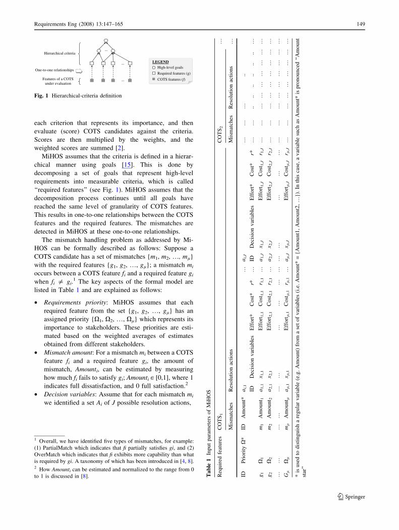
MiHOS assumes that the criteria is defined in a hierar-

chical manner using goals [15]. This is done by

decomposing a set of goals that represent high-level

requirements into measurable criteria, which is called

‘‘required features’’ (see Fig. 1). MiHOS assumes that the

decomposition process continues until all goals have

reached the same level of granularity of COTS features.

This results in one-to-one relationships between the COTS

features and the required features. The mismatches are

detected in MiHOS at these one-to-one relationships.

The mismatch handling problem as addressed by Mi-

HOS can be formally described as follows: Suppose a

COTS candidate has a set of mismatches {m1, m2, …, ml}

with the required features {g1, g2, …, gl}; a mismatch mi

occurs between a COTS feature fi and a required feature gi

when fi = gi.1 The key aspects of the formal model are

listed in Table 1 and are explained as follows:

• Requirements priority: MiHOS assumes that each

required feature from the set {g1, g2, …, gl} has an

assigned priority {X1, X2, …, Xl} which represents its

importance to stakeholders. These priorities are esti-

mated based on the weighted averages of estimates

obtained from different stakeholders.

• Mismatch amount: For a mismatch mi between a COTS

feature fi and a required feature gi, the amount of

mismatch, Amounti, can be estimated by measuring

how much fi fails to satisfy gi; Amounti [ [0,1], where 1

indicates full dissatisfaction, and 0 full satisfaction.2

• Decision variables: Assume that for each mismatch mi

we identified a set Ai of J possible resolution actions,

Hierarchical criteria

Features of a COTS under evaluation

…

One-to-one relationshipsHigh-level goals

Required features (g)

COTS features (f)

LEGEND

…

…

Fig. 1 Hierarchical-criteria definition

Ta

ble

1In

pu

tp

aram

eter

so

fM

iHO

S

Req

uir

edfe

atu

res

CO

TS

1C

OT

S2

…

Mis

mat

ches

Res

olu

tio

nac

tio

ns

Mis

mat

ches

Res

olu

tio

nac

tio

ns

…

IDP

rio

rity

X*

IDA

mo

un

t*a

i,1

…a

i,J

……

…..

IDD

ecis

ion

var

iab

les

Eff

ort

*C

ost

*r*

…ID

Dec

isio

nv

aria

ble

sE

ffo

rt*

Co

st*

r*…

…..

....

....

..…

g1

X1

m1

Am

ou

nt 1

a1,1

x 1,1

Eff

ort

1,1

Co

st1,1

r 1,1

…a

1,J

x 1,J

Eff

ort

1,J

Co

st1,J

r 1,J

……

……

……

……

…g

2X

2m

2A

mo

un

t 2a

2,1

x 2,1

Eff

ort

2,1

Co

st2,1

r 2,1

…a

2,J

x 2,J

Eff

ort

2,J

Co

st2,J

r 2,J

……

……

……

……

……

……

……

……

……

……

……

……

……

……

……

……

…G

lX

lm

lA

mo

un

t la

l,1

x l,1

Eff

ort

l,1

Co

stl

,1r l

,1…

al

,Jx l

,JE

ffo

rtl

,JC

ost

l,J

r l,J

……

……

……

……

…

*is

use

dto

dis

tin

gu

ish

are

gu

lar

var

iab

le(e

.g.

Am

ou

nt)

fro

ma

set

of

var

iab

les

(i.e

.A

mo

un

t*=

{A

mo

un

t1,

Am

ou

nt2

,…

}).

Inth

isca

se,

av

aria

ble

such

asA

mo

un

t*is

pro

no

un

ced

‘‘A

mo

un

t

star

’’

1 Overall, we have identified five types of mismatches, for example:

(1) PartialMatch which indicates that fi partially satisfies gi, and (2)

OverMatch which indicates that fi exhibits more capability than what

is required by gi. A taxonomy of which has been introduced in [4, 8].2 How Amounti can be estimated and normalized to the range from 0

to 1 is discussed in [8].

Requirements Eng (2008) 13:147–165 149

123

https://www.researchgate.net/publication/3625946_A_case_study_in_applying_a_systematic_method_for_COTS_selection?el=1_x_8&enrichId=rgreq-23a8d55e5c76bb65757bcef97e19a5cf-XXX&enrichSource=Y292ZXJQYWdlOzIyNTIxNTE2NjtBUzoxNzkyMDI2OTk1NzEyMDBAMTQxOTczNjY2MTA1NQ==

ð8miÞ : Ai ¼ fai;1; ai;2; . . .; ai;Jg

For instance, if the mismatch mi indicates a required

functionality that a COTS does not support, then Ai will

include possible actions to ensure that the COTS will

support this functionality and thus resolve mi; A

classification of possible resolution actions can be found

in [3]. In MiHOS, the goal is to select (at most) one

resolution action ai,j for each mismatch mi. This is

described by the set of decision variables

Xi ¼ fxi;1; xi;2; . . .; xi;Jg

where xi,j = 1 if the resolution action ai,j is chosen to

resolve the mismatch mi, and xi,j = 0 otherwise. This means

if a mismatch mi is to be resolved using the action ai,1, then

Xi = {1,0,0, …, 0}. If ai,J is to be used, then Xi =

{0,0,0,..,1}. All the other mismatch resolution actions are

defined correspondingly.

• Resources constraints: Applying resolution actions

requires different amount of resources. Each resource

has a maximum capacity that should not be exceeded.

For this paper, we assume two types of resources

related to cost and to effort: available_budget and

available_effort. The method remains applicable also

for the more general case of more constraints.

• Resource consumptions: MiHOS assumes each resolu-

tion action ai,j requires an effort equal to efforti,j and

costs an amount of costi,j (see Table 1). The total effort

and budget consumed by the set of selected resolution

actions (represented by decision variables xi,j) must be

less than the total amounts of resources available:X

i;j

xi;j � efforti;j� available effort

X

i;j

xi;j � costi;j� available budgetð1Þ

• Technical risk: MiHOS assumes that applying each

resolution action ai,j imposes a technical risk ri,j on the

target system. The technical risk is estimated based on:

(1) Development risk: the risk that the developers might

fail to apply the action ai,j, and (2) Instability risk: the

risk that an action ai,j would cause instability of the

target system. The developers may estimate the

technical risk ri,j on a 9-point ordinal scale, ri,j [{1,3,5,7,9}; this indicates very low, low, average, high,

and very high risk. Even numbers can be interpreted as

intermediate values.

Based on the above formal description, a mismatch-

handling process should aim at:

(a) Maximizing COTS fitness.

(b) Minimizing risk for resolution of mismatches.

(c) Fulfillment of resource constraints.

Point (a) is influenced by the requirements priorities Xi and

the mismatch amounts Amounti, point (b) is influenced by

the technical risk ri,j, and point (c) is relevant to the

resource consumptions and constraints. MiHOS defines an

objective function that brings these aspects together in a

balanced way. The objective is to maximize function F(x)

subject to the satisfaction of the resource constraints:

FðxÞ ¼Xl

i¼1

Amounti � Xi �XJ

j¼1

ðxi;j � Dri;jÞ !

ð2Þ

where Dri,j = 10 - ri,j indicates how safe an action ai,j is.

MiHOS uses Dri,j instead of ri,j because maximizing F(x)

should yield the minimum risk (i.e., the maximum safety)

of selected actions.

Based on the above formal model, MiHOS’ two types of

results are generated as follows (see Fig. 2):

(1) The analyst first defines the input parameters

according to the above formal model, e.g., determines the

amount of mismatches for each COTS candidate, and the

resource constraints and consumptions.

(2) This formal model constitutes a integer linear pro-

gramming problem [16] as all the constraints are linear

functions and the decision variables are integers. Integer

linear programming is known to belonmg into the class of

NP-complete problems. Applying an optimization package

called LINDO [17], MiHOS generates a set of five opti-

mum or near optimum solutions for each COTS under

evaluation. The advantage of having five instead of just one

solution is that it allows accommodate additional concerns

(as discussed later). In dependence of the size of the

problem and the response time request, the solution process

might be terminated also when the solution is sufficiently

good, but not necessarily optimal. Each solution constitutes

a mismatch-resolution plan that uses appropriate actions to

resolve a subset of mismatches of one COTS.

To explain the plans’ structure, consider a COTS having

a set of mismatches {m1, m2, …, ml}. A mismatch-reso-

lution plan is represented by the set {y1, y2, …, yl}, where

for each mismatch mi, a suggestion yi may take one of the

following values:

• yi = ‘‘Do not resolve mi’’. Here, all decision variables

xi,j are set to zero; i.e., no resolution action is used.

• yi = ‘‘Resolve mi using resolution action ai,1’’.

Here, only xi,1 = 1 and xi,j = 0 otherwise; i.e., Xi =

{1, 0, 0, …, 0}.

Initial output: Mismatch-resolution plans

Inputs according to MiHOS’

formal model

FormalModel

____________________________

______

LINDOoptimization engine

Output1:

Anticipated fitness

Output2:Mismatch resolution plans

Fig. 2 MiHOS process (overview)


123

• yi = ‘‘Resolve mi using resolution action ai,2’’. Here,

only xi,2 = 1 and xi,j = 0 otherwise; i.e., Xi = {0, 1, 0,

…, 0}.

• …• yi = ‘‘Resolve mi using resolution action ai,J’’. Here,

only xi,J = 1 and xi,j = 0 otherwise; i.e., Xi = {0, 0, 0,

…, 1}.

(3) Based on the five mismatch-resolution plans Yn =

{y1, y2, …, yl}, n = 1, …, 5, two main outputs of MiHOS

are generated for each COTS candidate x as follows:

Output1: The anticipated fitness AAF(x) of a COTS

candidate x is estimated in three steps:

1. Assume that the first mismatch-resolution plan is

applied, and the mismatches are resolved as it

suggests.

2. Having the assumption in (1), recalculate the fitness of

COTS candidates using the weighing and aggregation

method of which the key idea was described at the

beginning of this section.

3. Repeat (1) and (2) for the remaining four mismatch-

resolution plans

The overall anticipated fitness (i.e., Output1) is the average

of the five fitness values obtained in the above three steps:

Anticipated fitness

¼P

n¼1;...;5 Anticipated fitness assuming plan Yn is applied

5

ð3Þ

where Yn is a mismatch-resolution plan generated by

MiHOS, Yn = {y1, y2, …, yl}.

Output2: The second output of MiHOS are the same

mismatch-resolution plans originally generated with the

aid of LINDO. These plans are given to the decision

maker so that s/he selects the one that best suit his/her

interests. The motivation of offering five plans to the

decision maker instead of only one is that it allows

address implicit and additional concerns not formally

described in the original problem statement. In fact, the

quality of the five solutions is rather the same, but they

may differ in terms of their ability to accommodate

additional concerns. This principle of diversification as a

means to handle uncertainty was applied in [18] for the

case of software release planning.

3 Sensitivity analysis for MiHOS

In this section, we describe the structure of the proposed

MiHOS-SA approach, and show how it can be used to

analyze robustness of main results of MiHOS.

3.1 Overview of MiHOS-SA

MiHOS-SA consists of several activities that are organized

in three main phases: initialization, computation, and

analysis. The main flow of the process is described in

Fig. 3.

1. Initialization: This phase includes two activities per-

formed by analysts:

(a) Selecting the input parameters to be analyzed:

The selected input parameters should be the ones

most critical in terms of their degree of uncer-

tainty. This is determined based on the analysts’

judgement. However, the user still has the choice

of applying global SA, and thus analysing all of

the parameters at once.

(b) Determining the sampling range <: MiHOS-SA

uses a sampling approach, where uncertainty is

represented by a range <. This range is defined

by lower and upper bounds that reflect the

uncertainty interval for the input-parameter’s

value.

2. Computation: This phase includes two activities per-

formed by a computer:

(a) Sampling the input parameter: This activity aims

at generating a sample from < for every input

parameter selected in phase 1. The samples are

generated randomly or systematically to simulate

an input uncertainty.

Legend 3. Analysis Visualize the outputs and analyze them.

2. Computationa- Generate a sample from .b- Run MiHOS for the generated sample,

and record the outputs.

Repetitive application while generating new samples

1- Initializationa- Select input parameters (P) for the analysis. b- Define sampling range ( ) for the selected inputs.

Selected inputs (P)& sampling range ( )

Recorded outputs

Input / Output

Set of activities

Data

Outputs obtained from MiHOS

Better understanding of MiHOS’ outputs

Fig. 3 The MiHOS-SA approach


123

(b) Running MiHOS: This activity calculates and

records the outputs corresponding to the gener-

ated sample.

The above two activities are repeatedly applied for a

series of generated problem instances. The number of runs

is context-specific and determined by the analyst in

accordance to the time available and the requests for reli-

ability of results.

3. Analysis: This phase aims at analyzing and interpreting

the results obtained in Phase 2. MiHOS-SA suggests

analyzing by visualizing them, and then allowing

decision makers to analyze them in order to help make

decisions.

3.2 MiHOS-SA in detail

In the following, we describe the different elements of

MiHOS-SA in detail.

3.2.1 Input parameters (P)

The input parameters P include all parameters defined as

input for MiHOS. These parameters can be grouped into

two main categories: ResourceCapacities and Mismatch-

Parameters with

ResourceCapacities

¼ favailable effort; available budgetg:MismatchParameters ¼ Amount� [ r� [ X� [ effort� [ cos t�:

We use the star (*) to indicate a set of input parameters. For

example, consider COTS1 in Table 1. The set Amount*

includes {Amounti : i = 1 to l} and indicates the amounts

of the mismatches {mi : i = 1 to l}. Also, the set effort*

includes all effort values estimated to apply the individual

resolution actions ai,j; i.e., effort* = {effort i,j : i = 1 to l,

j = 1 to J}.

3.2.2 Sampling range (<)

The sampling range < is defined for each input parameter

being analyzed. < is defined differently for ResourceCa-

pacities and MismatchParameters.

(1) Sampling range for ResourceCapacities:

We use systematic sampling to generate samples for input

parameters q [ ResourceCapacities as follows: the

sampling range < is first determined by defining the lower

and upper bounds of q. Then, during the sensitivity

analysis the value of q is gradually incremented from the

lower bound to the upper one. For each single increment,

MiHOS is run once and the output is recorded. The

increment amount is defined based on the required

granularity of the results. For example, assuming the

sampling range < for the available_effort is [900, 1,100]

and the step size is defined to be 40, then the output is

computed at available_effort = 900, 940, … ,1,060, 1,100.

(2) Sampling range for MismatchParameters:

We use random sampling with uniform distribution [10] to

generate samples for the MismatchParameters. This is

performed as follows: Consider a parameter set q* = {q1,

q2, …, ql}, where q*, MismatchParameters, i.e., q* could

refer to Amount*, effort*, etc. For each input parameter qi [q*, a sampling range <i is first defined in terms of a factor

n, where:3

<i ¼ ½ð1� nÞ � qi; ð1þ nÞ � qi�; 0\n\1

The result is a set of sampling ranges <* = {<1, …, <l}

defined for the parameter set q*. For instance, for the

parameter set Amount* with n = 0.1, the elements of <*

are:

<1 ¼ ½0:9 � Amount1; 1:1 � Amount1� defined for Amount1

<2 ¼ ½0:9 � Amount2; 1:1 � Amount2� defined for Amount2

. . . . . .<l ¼ ½0:9 � Amountl; 1:1 � Amountl� defined for Amountl

After defining <*, samples are randomly generated for

each input parameter ql [ q*. For example, for the

Amount* in the above example, a sample is randomly

generated for each Amounti from within the its corre-

sponding sampling range <i. For each random sample,

MiHOS is run and the output is recorded. This process is

executed as many times as possible to address the different

scenarios of random values. The number of executions

depends on the time limits for the analysis. In our case

study, we ran the model 80 times, and found that they are

sufficient to obtain relatively good results.

Why do we use random sampling for MismatchPa-

rameters instead of systematic sampling? For a set of

mismatch-parameters q* = {q1, …, ql}, incrementing the

values of all input parameters q1, …, ql gradually from a

lower to an upper bound will have no effect on the output

of MiHOS. This is because the optimization engine,

LINDO [17], relies on the relative differences between q1,

…, ql in order to find optimum and near optimum

3 In this paper, we assume the sampling range is symmetric around qi

for simplicity. The method is still applicable for non-symmetric

sampling range.


123


solutions. Changing the values of all q1, …, ql propor-

tionally (i.e., by the same amount) will not affect the

relative differences between them, and thus will not affect

the optimization result. On the other hand, it would be

difficult to analyze all permutations of incrementing q1,

…, ql independently in order to address all scenarios of

various relative differences. For example, assume we

want to analyze only one parameter set q* using sys-

tematic sampling. And assume that the values of the

parameters in q* will be gradually incremented from a

lower to an upper bound over 10 steps. Given this

assumption, it would require to run MiHOS 1050 times to

cover all possible permutations when having only 50

mismatches, which is practically impossible to be done.

3.2.3 Outputs of the ‘‘Computation’’ phase

MiHOS-SA defines two metrics to analyze the robustness

of MiHOS’ outputs against input uncertainties: AAF

(Average Anticipated Fitness) and DIFF (the DIFFerence

in structure of the resolution plans’). AAF is used for

analyzing the ‘‘anticipated fitness’’ (Output1 of MiHOS),

and DIFF for analyzing the mismatch-resolution plans

(Output2 of MiHOS). Both AAF and DIFF can be used for

the two categories of input parameters P. In the following,

we define the metrics in more detail.

(1) The AAF Metric

AAF measures the average anticipated fitness a COTS

candidate if its mismatches are resolved. AAF is calculated

as follows: the anticipated fitness of the COTS candidate is

calculated five times. In each time, one of the five

mismatch-resolution plans is assumed to be applied, and

Eq. (3) is used to calculate the anticipated fitness. The

mismatch-resolution plans considered during this process

are the ones generated during the application of MiHOS-

SA; i.e., after varying the input parameters to simulate the

uncertainty.

(2) The DIFF Metric

DIFF measures the percentage of structural change in the

mismatch-resolution plans generated by MiHOS after

varying the inputs. The key idea is as follows: Consider a

set of mismatches {m1, m2, …, ml}. Assume that MiHOS

generates two mismatch-resolution plans: plan Y0 which is

generated before varying the inputs (without applying

MiHOS-SA), and plan Z0 after varying the inputs (after

applying MiHOS-SA); Y0 = {y1, y2, …, yl}, Z0 = {z1, z2,

…, zl}, and yi and zi refer to one of the possible options to

address a mismatch mi.

We use the hamming distance between vectors Y0 and Z0

to describe the degree of the structural change DIFF

between Y0 and Z0. Let D be the total number of structural

differences between Y0 and Z0, then:

DðY0;Z0Þ ¼Xl

i¼1

gðyi; ziÞ; wheregðyi; ziÞ ¼ 0 iff yi ¼ zi

gðyi; ziÞ ¼ 1 iff yi 6¼ zi

� �

ð4Þ

Based on D, we can calculate DIFF(Y0, Z0) between the

two plans Y0 and Z0 as follows:

DIFFðY0; Z0Þ ¼DðY0; Z0Þ

lð5Þ

where l is the total number of mismatches that a mismatch-

resolution plan is addressing.

However, the typical situation in MiHOS is more

complex. MiHOS generates a set of five mismatch-reso-

lution plans Y0, Y1, … Y4. And to calculate DIFF in

MiHOS-SA, we need to compare all of these plans with

another five plans Z0, Z1, …, Z4 that are generated after

changing input parameters. The algorithm of doing this is

detailed in Appendix 1 at the end of the paper.

3.2.4 Visualization and analysis of the outputs

The outputs of MiHOS-SA are visualized differently for

the two categories ResourceCapacities and MismatchPa-

rameters. This is because different sampling techniques are

used for each category.

(1) Visualizing ResourceCapacities: The value of an

input parameter q [ ResourceCapacities is incre-

mented systematically from the lower to the upper

bound defined for each parameter. Each time, the

corresponding output value is recorded. Such a

relationship can be visualized in 2-dimentional

Cartesian co-ordinates. Therefore, MiHOS-SA uses

X–Y graphs to visualize the relationship between qand AAF as well as between q and DIFF.

(b) Visualizing MismatchParameters: For MismatchPa-

rameters, a dataset is collected by running MiHOS

many times based on randomly generated samples.

Box plots [19] are used to illustrate the output. In the

case study presented in Sect. 4, we need to illustrate

20 datasets in one diagram; and each dataset contains

80 data points. These datasets should be clearly

distinguishable from each other. The box plots fulfill

these requirements.

As stated before in the description of the third phase of

MiHOS-SA (Sect. 3.1), after visualizing the results, they

are analyzed by decision makers in order to determine the

extent to which the outputs may be influenced by input

uncertainties. Decision makers may, for example, analyze


123

https://www.researchgate.net/publication/285058550_Exploratory_Data_Analysis?el=1_x_8&enrichId=rgreq-23a8d55e5c76bb65757bcef97e19a5cf-XXX&enrichSource=Y292ZXJQYWdlOzIyNTIxNTE2NjtBUzoxNzkyMDI2OTk1NzEyMDBAMTQxOTczNjY2MTA1NQ==

the robustness of the anticipated fitness or the ranking of

COTS products against uncertainties in the ResourceCa-

pacities or MismatchParameters. More possible analyses

scenarios are given later in the case study (Sect. 4.2).

4 Case study

4.1 Background

This section illustrates the application of MiHOS-SA with

a case study from the e-services domain. Previously [8],

MiHOS was used to select a content management system

(CMS) in order to build a news portal. The users pro-

gressively defined a total of 275 goals: 122 high-level goals

and 153 required features. In order to identify possible

COTS candidates based on these goals, the evaluators used

several information sources, such as online search engines,

e.g., Google and Yahoo, as well as special websites that list

and categorize CMS products, e.g., http://www.cmsreview.

com. To limit the search scope, the evaluators used the

keystone identification strategy4 with the following key-

stone: ‘‘To use open source software (OSS) that is

compatible with Windows XP Pro.’’ This resulted in

identifying an initial set of 32 COTS candidates.

Next, the evaluators collected detailed information

about these 32 COTS from their vendors’ websites and

other online sources, which offer independent evaluation

for CMS products, e.g., http://www.cmsmatrix.org. A

progressive filtering strategy4 was then used to filter out

less-fit products. Eventually, the five most-promising

COTS candidates were identified, COTS1, COTS2, …,

COTS5 (see Table 2).

MiHOS was then iteratively applied to find the antici-

pated fitness of the COTS candidates with resource

constraints set as: available_effort = 60 person-hours,

available_budget = $2,000. Table 3 summarizes some of

the results:

• The original fitness of the five COTS without the

application of MiHOS,

• The anticipated-fitness after applying MiHOS, and

• The number of mismatches for each COTS.

Based [t1]on these results, COTS4 was selected as it had

the highest anticipated fitness. Again, MiHOS was used to

generate five mismatch-resolution plans to help resolve the

64 mismatches of COTS4. These plans were analyzed and

eventually one plan was selected as it used the least

resources and, in the same time, addressed the most desired

set of mismatches.

In this paper, we follow up on this case study and use

MiHOS-SA in order to analyze the robustness of the results

obtained from MiHOS under the assumption of changing

problem parameters.

4.2 Settings

The case study focuses on addressing two groups of

questions with some related sub-questions:

Q1. How robust are the results against ResourceCapac-

ities’ uncertainties?

Q1.1 How robust is the anticipated fitness of COTS

candidates?

Q1.2 How robust is the ranking of COTS

candidates?

Q1.3 When changing the resource capacities, does

the bottleneck constraint5 change?

Q1.4 How robust is the structure of the suggested

mismatch-resolution plans?

Q2. How robust are the results against MismatchParam-

eters’ uncertainties?

Q2.1 How robust is the anticipated fitness of COTS

candidates?

Table 2 Short list of most

promising COTS products for

the CMS case study

ID Product Name Version Website Manufacturer

COTS1 Drupal 4.6.5 http://drupal.org Drupal Team

COTS2 eZ publish 3.0 http://ez.no eZ systems

COTS3 MDPro 1.0.76 http://www.maxdev.com MAXdev

COTS4 TYPO3 3.8.1 http://www.typo3.org Typo3

COTS5 Xaraya 1.0 http://www.xaraya.com Xaraya

4 Keystone Identification is a COTS evaluation strategy that starts by

identifying a key requirement, and then search for products that

satisfy this requirement. Progressive Filtering is an evaluation

strategy that starts with a large number of COTS products, and then

progressively eliminating less-fit COTS through successive iterations

of products evaluation cycles.

5 A bottleneck constraint is the one that controls the optimization

process and suppresses the effect of other constraints [20].


123

http://www.cmsreview.com

http://www.cmsreview.com

http://www.cmsmatrix.org

http://drupal.org

http://ez.no

http://www.maxdev.com

http://www.typo3.org

http://www.xaraya.com

Q2.2 How robust is the ranking of COTS

candidates?

Q2.3 How robust is the structure of the suggested

mismatch-resolution plans?

Research questions Q1 and Q2 are addressed in the fol-

lowing two subsections. In each subsection, we first show

how MiHOS-SA was applied in the case study, and then

illustrate and discuss the impact of changed problem

parameters expressed in terms of anticipated fitness and the

degree of structural change in the mismatch-resolution plans.

4.3 Analysis of the impact of changing

ResourceCapacities

In this section, we discuss the application of MiHOS-SA in

the case study for addressing research question Q1: How

robust are the results against uncertainties of

ResourceCapacities?

4.3.1 MiHOS-SA Application

The three phases of MiHOS-SA were applied in order to

address the question Q1 as follows:

1. Initialization: The project manager wanted to analyze

ResourceCapacities, i.e., available_effort and avail-

able_budget, using the one-at-a-time approach. The

sampling ranges < were chosen as shown in Table 4.

Note that we initially define < with a much narrower range

for Case 1 and 2. Such narrow range is the typical case

when applying SA techniques. However, we decided to

expand the range so as to analyze the behavior of MiHOS

over a wide range of the ResourceCapacities. This allowed

us to obtain some useful observations, such as ‘‘Observa-

tion 1’’ discussed later.

2. Computation: MiHOS-SA was applied twice: once to

analyze the impact of changing available_effort, and

once to analyze the impact of changing available_bud-

get. The LINDO [17] optimization package was used

and two outputs were calculated: AAF using Eq. (3)

and DIFF using Eq. (5).

3. Analysis: The recorded outputs, AAF or DIFF, were

represented to the project manger using X–Y graphs.

The outputs are illustrated in Figs. 4 and 5, where the

x-axis represents the variation in the value of the

selected parameter and the y-axis represents AAF or

DIFF.

4.3.2 Results and discussion

In this section, we present and discuss the impact of

varying the ResourceCapacities on both the AAF and the

DIFF metrics. The discussion is divided into two parts: Part

1 for the AAF metric; and Part 2 for the DIFF metric.

4.3.2.1 Part 1: Measuring anticipated fitness in depen-

dence of changing resource capacities Figure 4 shows

two charts illustrating the value of AAF for Cases 1 and 2

from Table 4: Case1 to study the impact of varying the

available_effort from 10 to 100 person-hours, and Case2 to

study the impact of varying the available_budget from

$120 to $2,000. Each chart shows five curves representing

AAF for the selected five COTS candidates. The dotted line

labeled ‘‘original value’’ refers to the original value of the

resource constraint before applying MiHOS-SA.

Discussion: In the process of addressing the research

questions Q1.1, Q1.2, and Q1.3, two observations were

made:

Q1.1: How robust is the AAF of COTS candidates if

there are uncertainties in the ResourceCapacities?

As can be seen in Fig. 4, the AAF value does not sig-

nificantly change in the neighborhood of the original value

of the resource constraints. Yet, at very low values of the

ResourceCapacities, AAF changes significantly with any

change in the ResourceCapacities. In regards to this point,

Observation1 was made:

Table 3 Results from the previous case study

COTS1 COTS2 COTS3 COTS4 COTS5

Original fitness (without applying MiHOS) 63% 75% 61% 68% 53%

Anticipated fitness (after applying MiHOS) 78% 82% 73% 92% 89%

Number of mismatches 80 60 74 64 86

Table 4 Varying the ResourceCapacities

Case Parameter to be

analyzed (q)

Sampling range (< )

Lower bound Upper bound

Case 1 available_effort 10 person-hours 100 person-hours

Case 2 available_budget $ 120 $ 2400


123

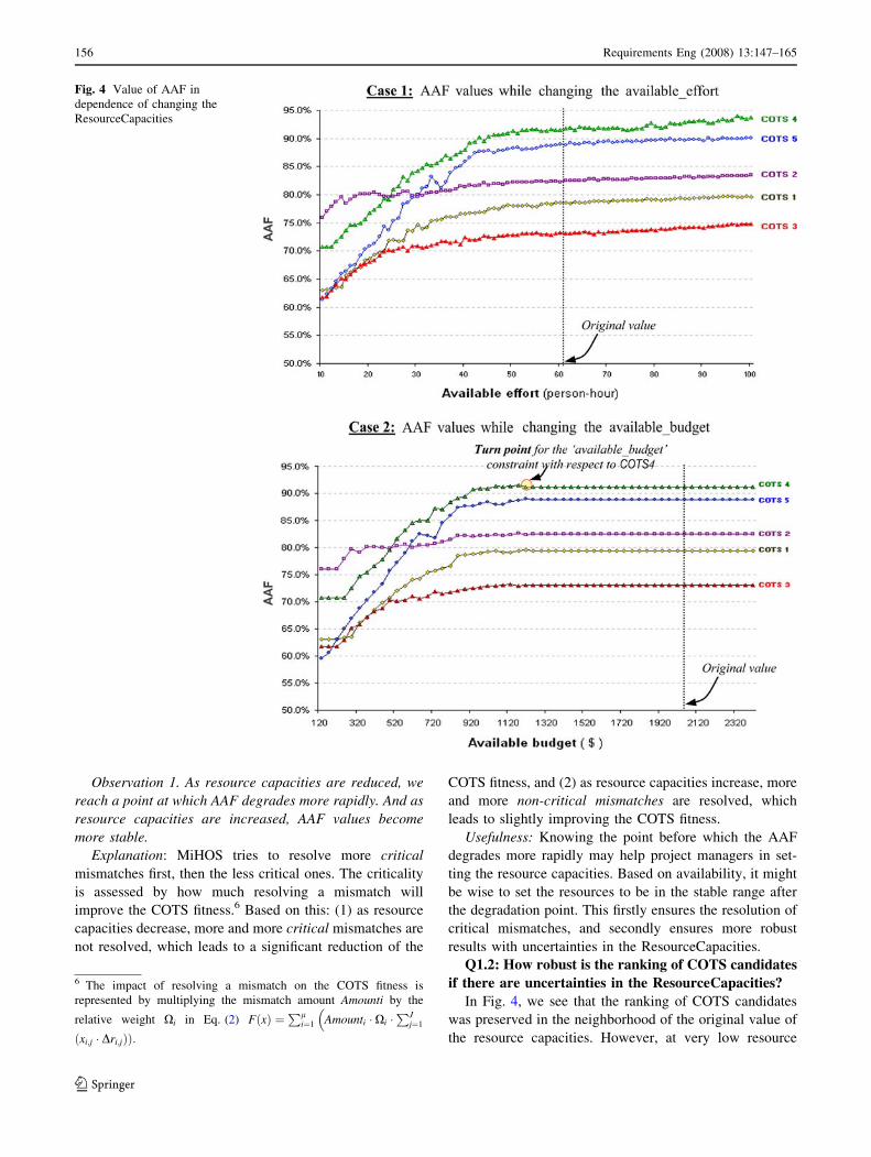
Observation 1. As resource capacities are reduced, we

reach a point at which AAF degrades more rapidly. And as

resource capacities are increased, AAF values become

more stable.

Explanation: MiHOS tries to resolve more critical

mismatches first, then the less critical ones. The criticality

is assessed by how much resolving a mismatch will

improve the COTS fitness.6 Based on this: (1) as resource

capacities decrease, more and more critical mismatches are

not resolved, which leads to a significant reduction of the

COTS fitness, and (2) as resource capacities increase, more

and more non-critical mismatches are resolved, which

leads to slightly improving the COTS fitness.

Usefulness: Knowing the point before which the AAF

degrades more rapidly may help project managers in set-

ting the resource capacities. Based on availability, it might

be wise to set the resources to be in the stable range after

the degradation point. This firstly ensures the resolution of

critical mismatches, and secondly ensures more robust

results with uncertainties in the ResourceCapacities.

Q1.2: How robust is the ranking of COTS candidates

if there are uncertainties in the ResourceCapacities?

In Fig. 4, we see that the ranking of COTS candidates

was preserved in the neighborhood of the original value of

the resource capacities. However, at very low resource

Fig. 4 Value of AAF in

dependence of changing the

ResourceCapacities

6 The impact of resolving a mismatch on the COTS fitness is

represented by multiplying the mismatch amount Amounti by the

relative weight Xi in Eq. (2) FðxÞ ¼Pl

i¼1 Amounti � Xi �PJ

j¼1

�

ðxi;j � Dri;jÞÞ:


123

values, the ranking changed. In regards to this point, the

following observation was made:

Observation 2. The impact of uncertain resource

capacities on COTS ranking depends on the resolvability of

the mismatches of the COTS candidates.

Explanation: The ranking changed at low resource

capacities because the AAF of COTS2 did not degrade by

the same rate as other COTS, and thus COTS2 had the

highest fitness at low resource capacities. Looking into

Table 3, the fitness of COTS2 improves only by 7% after

resolving its mismatches, while all other COTS improve by

amounts ranging from 12% (for COTS3) to 36% (for

COTS5).

By analyzing COTS2, we found that only few mis-

matches with little impact on COTS2’s fitness were

resolvable, while all other mismatches were not resolvable.

This means no matter how much resources are available,

COTS2 fitness would not significantly improve. Thus, the

amount of improvement in the fitness (and thus the ranking

of COTS candidates) relies on the resolvability of mis-

matches of each COTS.

Q1.3: When changing the resource capacities, does

the bottleneck constraint change?

Yes, the bottleneck constraint changes. In Fig. 4

(Case2), if available_budget exceeds the point labeled

‘‘turn point’’, the AAF is not anymore affected by any

change in available_budget. This means available_budget

is the bottleneck constraint before the turn point, while

another constraint (available_effort in our case study)

becomes the bottleneck constraint after the turn point.

Based on this, we define the turn point for a bottleneck

constraint as: ‘‘the point after which another constraint

becomes the bottleneck constraint.’’

Note that the turn point is not visible in Fig. 4 (Case1)

for the available_effort because the graph is plotted while

keeping the available_budget at $2,000, which makes the

available_effort a bottleneck constraint for the range of

values shown in that graph.

Knowing the bottleneck constraint helps to concentrate

our efforts on estimating the bottleneck constraint more

accurately. Knowing the turn point is also important

because if a bottleneck constraint C1 is set to a value near

its turn point, then because of uncertainty it might not be

sure that C1 is really the bottleneck constraint.

4.3.2.2 Part 2: Measuring structural difference in depen-

dence of changing resource capacities Figure 5 shows

two charts illustrating the value of DIFF for Cases 1 and 2

from Table 4: Case1 to study the impact of varying the

available_effort from 10 to 100 person-hours, and Case2 to

study the impact of varying the available_budget from

Fig. 5 Value of DIFF as

ResourceCapacities change (for

COTS4 only)


123

$120 to $2,000. Each chart shows a curve that represents

the value of DIFF for COTS4. We study only COTS4

because, by definition, DIFF measures the structural

changes in mismatch-resolution plans generated for the

selected COTS only, which is COTS4 in our case study.

Discussion: In the process of addressing the research

question Q1.4, one observation was made from the two

charts in Fig. 5.

Q1.4: How robust is the structure of the suggested

plans against uncertainties in ResourceCapacities?

The robustness of the results was acceptable in this case

study. As can be seen in Fig. 5, DIFF is less than 10% in the

neighborhood of the original value of the resource capacities.

For the selected COTS product, i.e., COTS4, this 10%

change represents about 6 changes in the structure of the

suggested mismatch-resolution plans.7 These 6 differences

are acceptable because: MiHOS adopts the concept of pre-

senting a set of plans that must have some differences among

them. In our case study in [8], there were an average of 10

differences between each two suggested plans. Comparing

the number of differences generated by MiHOS with the one

caused by uncertainty, we find that the later can be accept-

able. A key concept in MiHOS is that it relies on human

experience to analyze the differences among the suggested

plans before making any decision. In regards this research

question, the following observation was made:

Observation 3. As resource capacities decrease, the

plan’s structure becomes more sensitive to uncertainties in

ResourceCapacities. This can be seen in Fig. 5 where at

very low resources, DIFF has high values.

Explanation: At very low resources, the number of mis-

matches that can be resolved is very small. This means there

will likely be several small sets of different mismatches that,

if selected by MiHOS, would result in almost the same

objective function F(x) value. But MiHOS selects the set of

mismatches to be resolved based on the F(x) value. This

means MiHOS may select any of these sets and yet yield

almost the same F(x) value. Based on this, we can see that

small changes in the inputs, although might only result in

small changes in F(x) value, will also cause the selection of a

new set of different mismatches, and thus will greatly change

the structure of the suggested mismatch-resolution plan.

4.4 Applying MiHOS-SA to analyze

the MismatchParameters

In this section, we discuss the second part of our case

study, i.e., the application of MiHOS-SA in the case study

for addressing question Q2: How robust are the results

against the uncertainties of MismatchParameters?

4.4.1 MiHOS-SA Application

The three phases of MiHOS-SA were applied in order to

address question Q2 as follows:

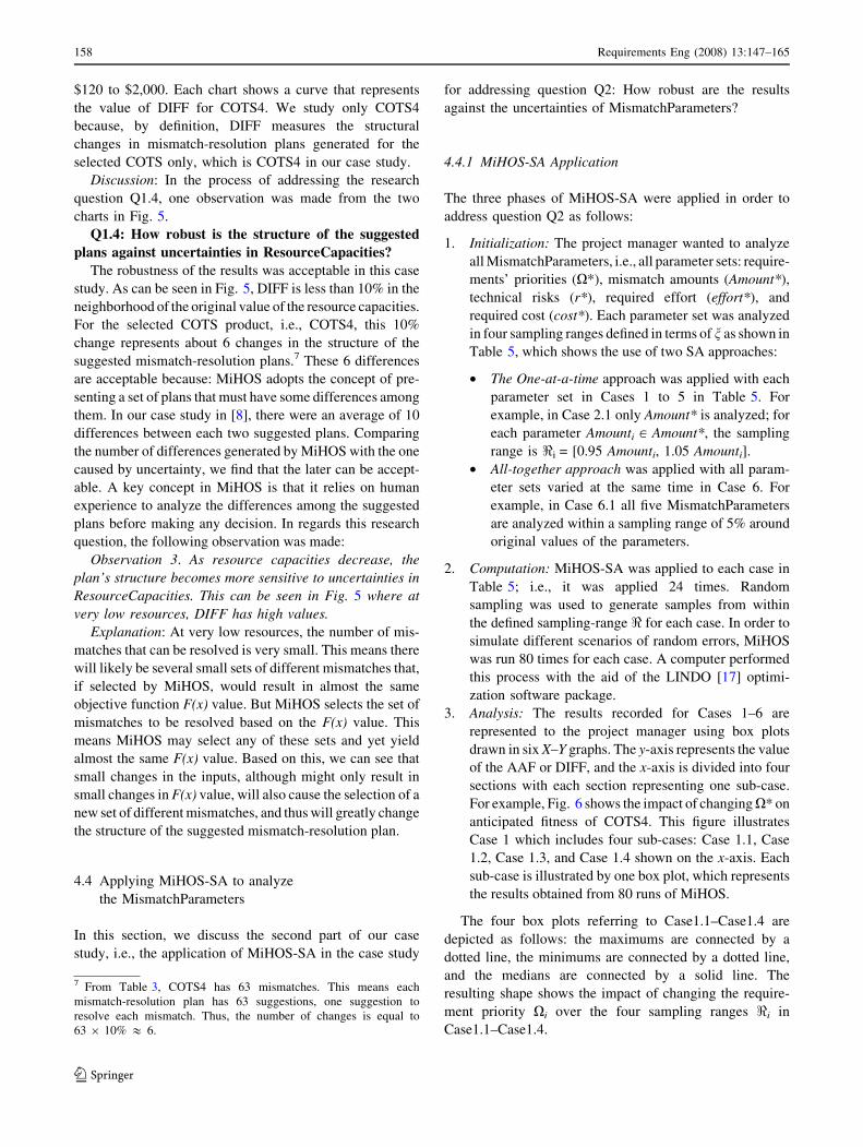
1. Initialization: The project manager wanted to analyze

all MismatchParameters, i.e., all parameter sets: require-

ments’ priorities (X*), mismatch amounts (Amount*),

technical risks (r*), required effort (effort*), and

required cost (cost*). Each parameter set was analyzed

in four sampling ranges defined in terms of n as shown in

Table 5, which shows the use of two SA approaches:

• The One-at-a-time approach was applied with each

parameter set in Cases 1 to 5 in Table 5. For

example, in Case 2.1 only Amount* is analyzed; for

each parameter Amounti [ Amount*, the sampling

range is <i = [0.95 Amounti, 1.05 Amounti].

• All-together approach was applied with all param-

eter sets varied at the same time in Case 6. For

example, in Case 6.1 all five MismatchParameters

are analyzed within a sampling range of 5% around

original values of the parameters.

2. Computation: MiHOS-SA was applied to each case in

Table 5; i.e., it was applied 24 times. Random

sampling was used to generate samples from within

the defined sampling-range < for each case. In order to

simulate different scenarios of random errors, MiHOS

was run 80 times for each case. A computer performed

this process with the aid of the LINDO [17] optimi-

zation software package.

3. Analysis: The results recorded for Cases 1–6 are

represented to the project manager using box plots

drawn in six X–Y graphs. The y-axis represents the value

of the AAF or DIFF, and the x-axis is divided into four

sections with each section representing one sub-case.

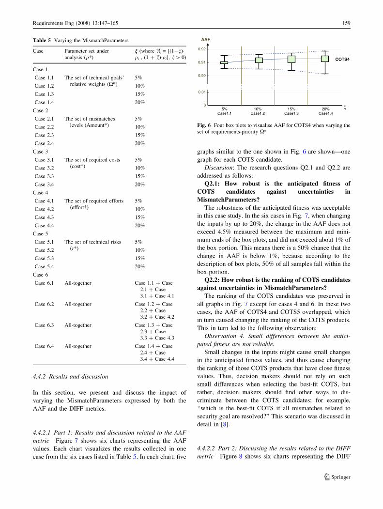
For example, Fig. 6 shows the impact of changing X* on

anticipated fitness of COTS4. This figure illustrates

Case 1 which includes four sub-cases: Case 1.1, Case

1.2, Case 1.3, and Case 1.4 shown on the x-axis. Each

sub-case is illustrated by one box plot, which represents

the results obtained from 80 runs of MiHOS.

The four box plots referring to Case1.1–Case1.4 are

depicted as follows: the maximums are connected by a

dotted line, the minimums are connected by a dotted line,

and the medians are connected by a solid line. The

resulting shape shows the impact of changing the require-

ment priority Xi over the four sampling ranges <i in

Case1.1–Case1.4.

7 From Table 3, COTS4 has 63 mismatches. This means each

mismatch-resolution plan has 63 suggestions, one suggestion to

resolve each mismatch. Thus, the number of changes is equal to

63 9 10% & 6.


123

4.4.2 Results and discussion

In this section, we present and discuss the impact of

varying the MismatchParameters expressed by both the

AAF and the DIFF metrics.

4.4.2.1 Part 1: Results and discussion related to the AAF

metric Figure 7 shows six charts representing the AAF

values. Each chart visualizes the results collected in one

case from the six cases listed in Table 5. In each chart, five

graphs similar to the one shown in Fig. 6 are shown—one

graph for each COTS candidate.

Discussion: The research questions Q2.1 and Q2.2 are

addressed as follows:

Q2.1: How robust is the anticipated fitness of

COTS candidates against uncertainties in

MismatchParameters?

The robustness of the anticipated fitness was acceptable

in this case study. In the six cases in Fig. 7, when changing

the inputs by up to 20%, the change in the AAF does not

exceed 4.5% measured between the maximum and mini-

mum ends of the box plots, and did not exceed about 1% of

the box portion. This means there is a 50% chance that the

change in AAF is below 1%, because according to the

description of box plots, 50% of all samples fall within the

box portion.

Q2.2: How robust is the ranking of COTS candidates

against uncertainties in MismatchParameters?

The ranking of the COTS candidates was preserved in

all graphs in Fig. 7 except for cases 4 and 6. In these two

cases, the AAF of COTS4 and COTS5 overlapped, which

in turn caused changing the ranking of the COTS products.

This in turn led to the following observation:

Observation 4. Small differences between the antici-

pated fitness are not reliable.

Small changes in the inputs might cause small changes

in the anticipated fitness values, and thus cause changing

the ranking of those COTS products that have close fitness

values. Thus, decision makers should not rely on such

small differences when selecting the best-fit COTS, but

rather, decision makers should find other ways to dis-

criminate between the COTS candidates; for example,

‘‘which is the best-fit COTS if all mismatches related to

security goal are resolved?’’ This scenario was discussed in

detail in [8].

4.4.2.2 Part 2: Discussing the results related to the DIFF

metric Figure 8 shows six charts representing the DIFF

Table 5 Varying the MismatchParameters

Case Parameter set under

analysis (q*)

n (where <i = [(1-n)�qi , (1 + n)�qi], n[ 0)

Case 1

Case 1.1 The set of technical goals’

relative weights (X*)

5%

Case 1.2 10%

Case 1.3 15%

Case 1.4 20%

Case 2

Case 2.1 The set of mismatches

levels (Amount*)

5%

Case 2.2 10%

Case 2.3 15%

Case 2.4 20%

Case 3

Case 3.1 The set of required costs

(cost*)

5%

Case 3.2 10%

Case 3.3 15%

Case 3.4 20%

Case 4

Case 4.1 The set of required efforts

(effort*)

5%

Case 4.2 10%

Case 4.3 15%

Case 4.4 20%

Case 5

Case 5.1 The set of technical risks

(r*)

5%

Case 5.2 10%

Case 5.3 15%

Case 5.4 20%

Case 6

Case 6.1 All-together Case 1.1 + Case

2.1 + Case

3.1 + Case 4.1


2.2 + Case

3.2 + Case 4.2


2.3 + Case

3.3 + Case 4.3


2.4 + Case

3.4 + Case 4.4

0.92 –

0.91 –

0.90 –

0.01 –

0

......

......

5%Case1.1

10%Case1.2

20%Case1.4

15%Case1.3

AAF

COTS4

Fig. 6 Four box plots to visualise AAF for COTS4 when varying the

set of requirements-priority X*


123

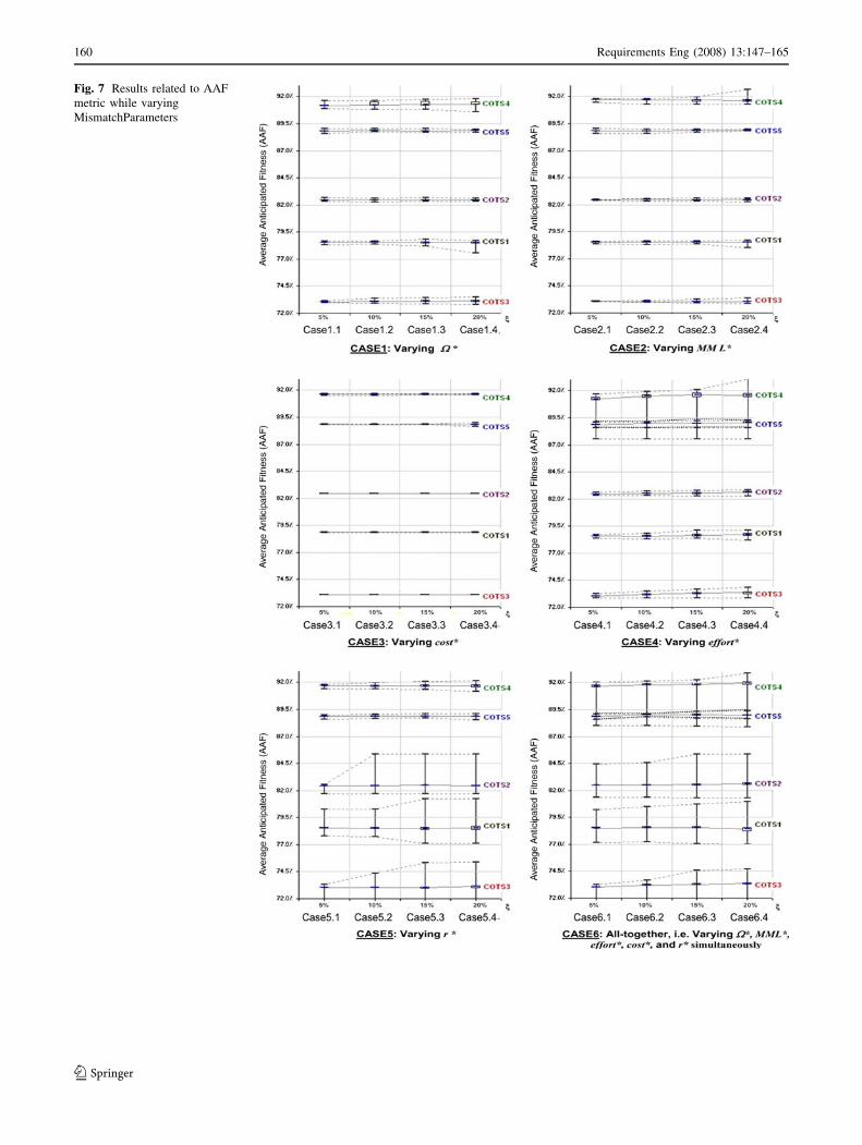
Fig. 7 Results related to AAF

metric while varying

MismatchParameters


123

values. Each chart visualizes the results collected in one

case from the six cases listed in Table 5. In each chart,

DIFF for COTS4 is illustrated using box plots. We only

illustrate COTS4’s results because it was the selected

product in the case study.

Discussion: The answer to the research question Q2.3 is

as follows:

Q2.3: How robust is the structure of the suggested

mismatch-resolution plans against uncertainties in

MismatchParameters?

The robustness of the plans’ structure was acceptable in

this case study. In the six cases in Fig. 7, when changing

the inputs by up to 20%, the maximum value of DIFF is

almost 10% (in Case 4.4). The 10% value indicates that

about 6 differences per plan might occur when resolving

the 63 mismatches of COTS4. Following the same logic in

the answer to Q1.4, this is acceptable in this case study.

5 Limitations

This section describes the limitations related to MiHOS-SA

in general, as well as the limitations to the conclusions

drawn from the case study. The use of MiHOS-SA is

subject to the following limitations:

(1) Estimation of parameters: We have assumed that

analysts can identify the parameters with most

uncertainties and their values. Although this might

be easier for analysts in mature organizations assessed

at CMM4 or CMM5 [21], it might not be as easy or as

accurate in organizations with lower maturity levels.

CMM4&5 organizations use precise measurement

process and can control the software development

effort. Therefore, it would be easier for these

organizations to identify those parameters with high

uncertainty and criticality.

(2) Effort: The overall effort to apply MiHOS-SA is high.

This includes both human effort to define and analyze

the results, as well as computational effort to

repeatedly run the model after each change of the

inputs. The human-effort required for MiHOS appli-

cation was 232 person-hours, and for MiHOS-SA was

24 person-hours.8 Improvements to MiHOS-SA are

required to reduce the run time. Initial efforts that can

be considered can be found in [22] where heuristics

are used to reduce the computation time in a similar

problem, namely software release planning, which

also uses optimization techniques to solve a formal

problem and find the maximum objective-function

value under limited resources.

(3) Simultaneous change of parameters within and

between the two categories: MiHOS-SA only allows

selecting parameters from the same category, Re-

sourceCapacities or MismatchParameters, when

performing all-together sensitivity analysis. To allow

a combined selection from both categories, extra

effort would be required. For example, consider an

analyst selects two parameters from both categories,

the available_effort over 10 steps from 10 to 100

person-hours, and Amount* from the MismatchPa-

rameters. The required effort in this case is equal to

the effort of analyzing Amount* multiplied by ten,

analyzing Amount* ten times for ten increments of

available_effort. Further, representing the output

would require a three-dimensional representation

method, which is currently not implemented in

MiHOS-SA.

(4) Visualization: Box plots are only one of many ways to

represent the results. Although the use of box plots

was justified in this paper, an analyst might want to

use other visualization methods, for example, histo-

gram plots.

(5) Dependability: The dependability of parameters is not

currently addressed by MiHOS-SA. In this regard, we

rely on experts’ judgment to consider such depend-

ability when making his/her estimations.

Further, the level of granularity of the technical goals has

an influence on the whole process of parameters’ estima-

tion and analysis in MiHOS-SA. It is hard to define an

objective criterion that defines the ‘‘best’’ granularity level.

As discussed in [8] and also earlier in this paper, the

stakeholders would have to define the level of granularity

that ensures a 1-to-1 relationship between their needs and

the COTS features. For doing so, the stakeholders should

decompose their goals while considering the descriptions

of the COTS features. Also, in some cases the stakeholders

might need to decompose the COTS features themselves

into sub-features so as to achieve the 1-to-1 relationship.

Currently, this process is subjective and largely depends on

experts’ judgment.

In addition, there are several threats to the validity of the

results obtained in this case study. Firstly, the fact that this

is only one case study applied in one domain raises a

research challenge to conduct further case studies in dif-

ferent domains to confirm or refute the observations.

Secondly, MiHOS was run 80 times for each case of n in

order to analyze MismatchParameters. This resulted in

generating 9600 random samples (5 COTS 9 6 Mis-

matchParameters for each COTS 9 4 Cases of n for each

parameter 9 80 runs for each case). We assumed that 80

8 These numbers do not include administrative activities such as the

effort spent for meetings and reporting, and assuming the analysts are

familiar with both approaches.


123

https://www.researchgate.net/publication/221421264_DynaReP_A_Discrete_Event_Simulation_Model_for_Re-planning_of_Software_Releases?el=1_x_8&enrichId=rgreq-23a8d55e5c76bb65757bcef97e19a5cf-XXX&enrichSource=Y292ZXJQYWdlOzIyNTIxNTE2NjtBUzoxNzkyMDI2OTk1NzEyMDBAMTQxOTczNjY2MTA1NQ==

https://www.researchgate.net/publication/220691208_Managing_Software_Process?el=1_x_8&enrichId=rgreq-23a8d55e5c76bb65757bcef97e19a5cf-XXX&enrichSource=Y292ZXJQYWdlOzIyNTIxNTE2NjtBUzoxNzkyMDI2OTk1NzEyMDBAMTQxOTczNjY2MTA1NQ==

Fig. 8 Results related to DIFF

metric while varying

MismatchParameters (COTS4

only)


123

runs are sufficient to cover enough scenarios of random

samples. However, some extreme scenarios might have

been missed. This means the results obtained from Mi-

HOS-SA should be dealt with caution, and small

differences in the outputs should be considered meaning-

less. Thirdly, we used uniform distribution to generate

samples for MismatchParameters. This was because uni-

form distribution requires less human effort to define, and

is computationally less expensive. However, other distri-

butions might also have been considered; for example,

triangular distribution which might provide more accurate

analysis, but would require more effort, both human and

computational.

6 Summary and conclusions

Sensitivity analysis is a proven technique to investigate

robustness of proposed solutions against parameter changes

of the underlying model. In this paper, the technique was

applied as an add-on to the existing MiHOS method which

aims at supporting selection of COTS by in-depth consid-

eration of the effort, cost, and risk of mismatch resolution

strategies. MiHOS-SA approach is used to perform sensi-

tivity analysis against changes in the resource capacities

and against changes in the different types of mismatch

parameters. Robustness of a selection of COTS products

can be studied this way.

As a proof-of-concept, we applied MiHOS-SA for a case

study from the e-services domain. We addressed several

research questions for analyzing the impact of uncertainties

on both ResourceCapacities and MismatchParameters. The

overall observation is that MiHOS results are robust in the

context of this CMS case study. This means even after

varying the inputs within limited range, COTS4 remained

the best-fit COTS product, and the structure of the sug-

gested resolution plans changed only by small amounts.

We do not claim or suggest applying the method uni-

versally. While the overall results are useful to achieve

higher confidence in selecting a specific COTS, the effort is

substantial to run the different types of scenarios and to

analyze and interpret the results. This means that the

method is primarily intended for applications where finding

the best COTS has a substantial impact on the success of

the overall software project.

It is worth mentioning that although we built our own

method for SA, MiHOS-SA still relies on the basic SA’s

concepts, e.g., the ‘‘one-at-a-time’’ and ‘‘all-together’’

approaches. However, our main intention was to develop a

method that tightly integrates with MiHOS. This was

because of the special nature of MiHOS: (1) The inputs

include two groups of parameters, MismatchParamters and

ResourceCapacities, each of which should be dealt

differently during the sampling and application of MiHOS-

SA. (2) The outputs are also special (e.g., how to measure

the sensitivity of the resolution-plans’ structure?). There-

fore, we had to define special metrics for measuring the

change in the output. (3) The amount of output data is very

large (in the case study, they were sometimes generated

based on 9,600 samples). Thus, we felt we should aid

analysts with an appropriate way to illustrate this enormous

data in a simple and yet intuitive way.

Future research is devoted to provide better computa-

tional and computer support to accompany the whole

process and to facilitate the re-run of problem instances by

exploiting re-optimization features of the optimization

software. Other points that deserve further research

include: (1) Estimation of parameters: as mentioned earlier,

for organizations of maturity levels lower than CMM4, it

would be difficult to identify the parameters with most

uncertainties and their values. We intend to identify

guideline for those organizations to facilitate the use of

MiHOS-SA. For example, global SA may be used to ini-

tially identify the parameters with most influence on the

output, effort estimation techniques such as in [23] may be

used to qualify our estimations.

Acknowledgments We appreciate the support of the Natural Sci-

ences and Engineering Council of Canada (NSERC) and of the

Alberta Informatics Circle of Research Excellence (iCORE) to con-

duct this research.

Appendix: ‘‘DIFF’’ metric

This appendix elaborates the discussion presented in Sect.

3.2.3 for estimating the value of the DIFF metric when

applying MiHOS-SA. Consider a set of mismatches

M = {m1, …, ml}. Typically, MiHOS suggests a set of 5

plans to handle these mismatches. Assume this set is given

as:

SOL ¼ fY0; . . .; Y4g

For the mismatches {m1, m2, …,ml}, a plan Yn would

suggests a set of actions {y1, y2, …, yl}, where yi refers to

one of the options: ‘‘Do not resolve mi’’, ‘‘Resolve mi using

resolution action ai,1’’, ‘‘Resolve mi using resolution action

ai,2’’, etc.

When MiHOS-SA is applied, the input parameters of

MiHOS are varied to simulate input uncertainties. Thus,

the output is changed. Assume the new set of suggested

plans is:

SOLuncertain ¼ fZ0; . . .; Z4g:

where Zn is a solution plan after changing the input

parameters. Similarly to Yn, a plan Zn can be represented as

follows, Zn = {z1, …, zl} where zi refers to one of the


123

https://www.researchgate.net/publication/225135759_A_flexible_method_for_effort_estimation_by_analogy?el=1_x_8&enrichId=rgreq-23a8d55e5c76bb65757bcef97e19a5cf-XXX&enrichSource=Y292ZXJQYWdlOzIyNTIxNTE2NjtBUzoxNzkyMDI2OTk1NzEyMDBAMTQxOTczNjY2MTA1NQ==

options: ‘‘Do not resolve mi’’, ‘‘Resolve mi using resolution

action ai,1’’, etc.

As discussed in Sect. 3.2.3, if we want to estimate DIFF

only between two plans, e.g., Y1 and Z1, then we have to

compare each yi with zi, and then count the number of

occurrences where yi(=zi. However, in MiHOS we have to

compare all of the five plans Y0, …, Y4 with Z0, …, Z4. This

means, DIFF per plan can be estimated by estimated the

total number of differences between all plans in SOL and

those in SOLuncertain divided by the number of plans. This

is calculated as follows:

where: ‘‘K’’ is the total number of plans in SOL (K = 5 for

five solution plans).

‘‘l’’ is the total number of mismatches.

We divide by ‘‘K’’ to get the average number of struc-

tural differences per plan; and by ‘‘l’’ because DIFF, by

definition, indicates the percentage (not the number) of

structural difference, and thus we have to calculate it with

respect to the total number of mismatches.

The challenge here is to estimate the numerator in Eq.

(6). The order of the plans in SOL and SOLuncertain is

meaningless. This means we cannot calculate the total

number of differences by comparing Y0 with Z0, Y1 with Z1,

etc. But rather, we should ‘‘link’’ each plan from

SOLuncertain to exactly one plan in SOL based on the fol-

lowing hypothesis:

‘‘the correct linking scheme between the plans in

SOLuncertain’s and the plans in SOL’s would result in a total

number of differences between SOLuncertain and SOL that is

lower than any other linking scheme’’.

The above hypothesis stems from the fact that each plan

in SOLuncertain should be linked to the most similar plan in

SOL because it should represent that plan after it has been

changed. To find the ‘‘correct linking’’, the following

procedure is used:

1. Create an empty 5 9 5 table where the rows are

labelled Y0, …, Y4 and the columns Z0, …, Z4 (Fig. 9).

The first cell in the table is denoted Cell(0,0).

2. For all values of two variables m and n, where

0 \ m \ 4 and 0 \ n \ 4: count the number of

differences between Ym and Zn and record the result

in Cell(m, n).

3. For all linking permutations between {Z0, …, Z4} and

{Y0, …, Y4}, calculate the total number of differences

using the data stored in the 5 9 5 table. for example,

for a permutation Z0 ? Y0, Z1 ? Y1, Z2 ? Y2,

Z3 ? Y3, and Z4 ? Y4, the total number of differences

is equal to Cell(0,0) + Cell(1,1) + Cell(2,2) +

Cell(3,3) + Cell(4,4).

4. The correct linking indicates the permutation that

results in the minimum number of differences.

References

1. Carney D (1998) COTS evaluation in the real world, Carnegie

Mellon University

2. Kontio J (1995) OTSO: a systematic process for reusable soft-

ware component selection. University of Maryland, Maryland

CS-TR-3478, December 1995

3. Vigder MR, Gentleman WM, Dean J (1996) COTS software

integration: state of the art. National Research Council Canada

(NRC) 39198

4. Mohamed A (2007) Decision support for selecting COTS soft-

ware products based on comprehensive mismatch handling. PhD

Thesis, Electrical and Computer Engineering Department, Uni-

versity of Calgary, Canada

5. Mohamed A, Ruhe G, Eberlein A (2007) Decision support for

handling mismatches between COTS products and system

requirements. In: The 6th IEEE international conference on

COTS-based software systems (ICCBSS’07), Banff, pp 63–72

6. Alves C (2003) COTS-based requirements engineering. In:

Component-based software quality—methods and techniques, vol

2693. Springer, Heidelberg, pp 21–39

7. Carney D, Hissam SA, Plakosh D (2000) Complex COTS-based

software systems: practical steps for their maintenance. J Softw

Maintenance 12:357–376

8. Mohamed A, Ruhe G, Eberlein A (2007) MiHOS: an approach to

support handling the mismatches between system requirements

and COTS products. Requirements Eng J (Accepted on Jan 2,

2007, http://www.dx.doi.org/10.1007/s00766-007-0041-5)

Z0 Z1 Z2 Z3 Z4

Y0

Y1

Y2

Y3

Y4

Cell(1,3) contains the number of differences

between Y1 and Z3

Cell(0,0)

Fig. 9 A 5 9 5 table used when estimating DIFF

DIFF ¼ Total number of differences between ðall plans in SOLÞ and ðall plans in SOLuncertainÞK � l


123

http://www.dx.doi.org/10.1007/s00766-007-0041-5

9. Ziv H, Richardson D, Klosch R (1996) The uncertainty principle

in software engineering. University of California, Irvine UCI-TR-

96-33, Aug 1996

10. Saltelli A, Chan K, Scott EM (2000) Sensitivity analysis. Wiley,

New York

11. Saltelli A (2004) Global sensitivity analysis: an introduction. In:

4th international conference on sensitivity analysis of model

output (SAMO ‘04), Los Alamos National Laboratory, pp 27–43

12. Lung C-H, Van KK (2000) An approach to quantitative software

architecture sensitivity analysis. Int J Softw Eng Knowl Eng

10:97–114

13. Wagner S (2007) Global sensitivity analysis of predictor models

in software engineering. In: Ihe 3rd international PROMISE

workshop (co-located with ICSE’07), Minneapolis

14. Saltelli A, Tarantola S, Campolongo F, Ratto M (2004) Sensi-

tivity analysis in practice: a guide to assessing scientific models.

Wiley, New York

15. Kontio J (1996) A case study in applying a systematic method for

COTS selection. In: 18th International Conference on Software

Engineering (ICSE’96), Berlin, pp 201–209

16. Wolsey LA, Nemhauser GL (1998) Integer and combinatorial

optimization. Wiley, New York

17. LINDO_Systems: http://www.lindo.com

18. Ngo-The A, Ruhe G (2008) A systematic approach for solving

the wicked problem of software release planning. Soft Comput,

12 (in press)

19. Tukey JW (1977) Exploratory data analysis. Addison-Wesley,

Reading

20. Goldratt EM (1998) Essays on the theory of constraints. North

River Press, Great Barrington

21. Humphrey W (1989) Managing the software process. Addison-

Wesley Professional, Reading

22. Al-Emran A, Pfahl D, Ruhe G (2007) DynaReP: a discrete event

simulation model for planning and re-planning of software

releases, Minneapolis, May 2007

23. Li J, Ruhe G, Al-Emran A, Richter M (2006) A flexible method

for effort estimation by analogy. Emp Softw Eng 12:65–106


123

http://www.lindo.com





















Sensitivity analysis in the process of COTS mismatch-handling

Documents

Transcript of Sensitivity analysis in the process of COTS mismatch-handling