Sensing Human Sentiment via Social Media Images - CORE

Sensing Human Sentiment via Social Media Images: Methodologies and Applications

by

Yilin Wang

A Dissertation Presented in Partial Fulfillmentof the Requirements for the Degree

Doctor of Philosophy

Approved July 2018 by theGraduate Supervisory Committee:

Baoxin Li, ChairHuan Liu

Hanghang TongYi Chang

ARIZONA STATE UNIVERSITY

August 2018

ABSTRACT

Social media refers computer-based technology that allows the sharing of information and

building the virtual networks and communities. With the development of internet based

services and applications, user can engage with social media via computer and smart mobile

devices. In recent years, social media has taken the form of different activities such as social

network, business network, text sharing, photo sharing, blogging, etc. With the increasing

popularity of social media, it has accumulated a large amount of data which enables under-

standing the human behavior possible. Compared with traditional survey based methods, the

analysis of social media provides us a golden opportunity to understand individuals at scale

and in turn allows us to design better services that can tailor to individuals needs. From

this perspective, we can view social media as sensors, which provides online signals from a

virtual world that has no geographical boundaries for the real world individual’s activity.

One of the key features for social media is social, where social media users actively

interact to each via generating content and expressing the opinions, such as post and

comment in Facebook. As a result, sentiment analysis, which refers a computational model

to identify, extract or characterize subjective information expressed in a given piece of text,

has successfully employs user signals and brings many real world applications in different

domains such as e-commerce, politics, marketing, etc. The goal of sentiment analysis is to

classify a users attitude towards various topics into positive, negative or neutral categories

based on textual data in social media. However, recently, there is an increasing number of

people start to use photos to express their daily life on social media platforms like Flickr

and Instagram. Therefore, analyzing the sentiment from visual data is poise to have great

improvement for user understanding.

In this dissertation, I study the problem of understanding human sentiments from large

scale collection of social images based on both image features and contextual social network

features. We show that neither visual features nor the textual features are by themselves

i

sufficient for accurate sentiment prediction. Therefore, we provide a way of using both

of them, and formulate sentiment prediction problem in two scenarios: supervised and

unsupervised. We first show that the proposed framework has flexibility to incorporate

multiple modalities of information and has the capability to learn from heterogeneous

features jointly with sufficient training data. Secondly, we observe that negative sentiment

may related to human mental health issues. Based on this observation, we aim to understand

the negative social media posts, especially the post related to depression e.g., self-harm

content. Our analysis, the first of its kind, reveals a number of important findings. Thirdly,

we extend the proposed sentiment prediction task to a general multi-label visual recognition

task to demonstrate the methodology flexibility behind our sentiment analysis model.

ii

DEDICATION

I dedicate my dissertation work to my loving parents, Haibo Wang and Yipan Zhang, for

making me be who I am!

I also dedicate this dissertation to my girlfriend, Yi Qin, for supportng me all the way!

Without her help and encouragement, this journey would have not been possible.

iii

ACKNOWLEDGMENT

This dissertation is impossible without the help from my advisor Dr. Baoxin Li. I would

like to thank him, for his guidance, encouragement, and support during my Phd career. I

would also like to thank him to give me large freedom through my Ph.D. to explore various

research problems and his excellent advising skills combining patience and guidance make

my Ph.D. experience colorful, exciting and productive. Six year experience with him are my

lifelong tresure. I learnt many abilities from him that I can benefit all my life: how to write

papers and give presentations, how to find and address challenging problems, and how to

establish your career and see the big vision. Dr. Li, I cannot thank you enough.

I would like to thank my committee members, Dr. Huan Liu, Dr. Hanghang Tong, and

Dr. Yi Chang, for helpful suggestions and insightful comments. I take the social media

course from Dr. Huan Liu, who opens a new door for my reseach world. Without taking

his course, I would not even know my dissertation topic: sentiment anlaysis. His insightful

discussions and commits provide me new angles to rethink about my research. I always

consider Dr. Liu as my secondary advisor because many research ideas were initialized

with his discussions. Dr. Yi Chang is my intern manager, he gave me lots of constructive

comments and would like to share his industy experience to me, which I couldn’t learn it

from school. I also want to thank Dr. Hanghang Tong, who gives valuable comments and

suggestion on dissertation.

I was lucky to work as interns in Yahoo!Labs and Adobe Research with amazing

colleagues and mentors: Neil O’Hare, Jiliang Tang, Zhaowen Wang, Zhe Lin, Xin Lu and

Xiaohui Shen. I enjoyed two wonderful and productive summers; and because of you, I was

able to contribute my knowledge to exciting projects. Thank you for everything.

During my Ph.D. study, my friends and colleagues provided me consistent support and

encouragement and they deserve a special thank. I am thankful to my colleagues at ASU:

Qiang Zhang, Qiongjie Tian, Lin Chen, Suhang Wang, Kai Shu, Jundong Li, Liang Wu,

iv

Xinsheng Li, Xilun Chen, Shengyu Huang, Xiang Zhang, Yao Zhou, Dawei Zhou, Chen

Chen, Liangyue Li, Ziming Zhao, Mengxue Liu, Yuzhen Ding, Kevien Ding, Yikang Li,

Tianshu Yu, Parag, Ragav, Xu Zhou, Jiayu Zhou, Xia Hu, Huiji Gao and Yuheng Hu. I would

also like to thanks Dr. Subbarao Kambhampati to advise me on my first research work. I

will remember a lot of memories when I spent on Brickyard fifth floor. They are my friends

who have provide me very helpful suggestions insight comments, and encouagement.

Finally, I am deeply indebted to my dear mother and father for their love and strong

support during my graduate study. I would like to thank my dear girlfriend Yi Qin for her

strong support through all these years to my study. How fortunate I am having her in my

life! This dissertation is dedicated to them.

v

TABLE OF CONTENTS

Page

LIST OF TABLES . . . . . . . . . . . . . . . . . . . . . . . . . . . . . . . . . . . . . . . . . . . . . . . . . . . . . . . . . . . . ix

LIST OF FIGURES . . . . . . . . . . . . . . . . . . . . . . . . . . . . . . . . . . . . . . . . . . . . . . . . . . . . . . . . . . . x

CHAPTER

1 INTRODUCTION . . . . . . . . . . . . . . . . . . . . . . . . . . . . . . . . . . . . . . . . . . . . . . . . . . . . . . 1

1.1 Research Challenges . . . . . . . . . . . . . . . . . . . . . . . . . . . . . . . . . . . . . . . . . . . . . . . 2

1.2 Contributions . . . . . . . . . . . . . . . . . . . . . . . . . . . . . . . . . . . . . . . . . . . . . . . . . . . . . 3

1.3 Organization . . . . . . . . . . . . . . . . . . . . . . . . . . . . . . . . . . . . . . . . . . . . . . . . . . . . . . 4

2 RELATED WORK . . . . . . . . . . . . . . . . . . . . . . . . . . . . . . . . . . . . . . . . . . . . . . . . . . . . . 6

3 SUPERVISED SENTIMENT ANALYSIS FOR SOCIAL MEDIA IMAGES . 10

3.1 Supervised sentiment analysis for Social Media Images . . . . . . . . . . . . . . . 10

3.2 The Proposed RSAI Framework . . . . . . . . . . . . . . . . . . . . . . . . . . . . . . . . . . . . 13

3.2.1 Basic Model . . . . . . . . . . . . . . . . . . . . . . . . . . . . . . . . . . . . . . . . . . . . . . . 13

3.2.2 Extracting and Modeling Visual Features . . . . . . . . . . . . . . . . . . . . . 15

3.2.3 Constructing Prior Knowledge . . . . . . . . . . . . . . . . . . . . . . . . . . . . . . . 16

3.2.4 Incorporating Prior Knowledge . . . . . . . . . . . . . . . . . . . . . . . . . . . . . . 18

3.2.5 Algorithm Correctness and Convergence . . . . . . . . . . . . . . . . . . . . . 20

3.3 Empirical Evaluation . . . . . . . . . . . . . . . . . . . . . . . . . . . . . . . . . . . . . . . . . . . . . . 22

3.3.1 Experiment Settings . . . . . . . . . . . . . . . . . . . . . . . . . . . . . . . . . . . . . . . . 23

3.3.2 Performance Evaluation. . . . . . . . . . . . . . . . . . . . . . . . . . . . . . . . . . . . . 25

3.3.3 Analysis and Discussion . . . . . . . . . . . . . . . . . . . . . . . . . . . . . . . . . . . . 27

3.4 Summary . . . . . . . . . . . . . . . . . . . . . . . . . . . . . . . . . . . . . . . . . . . . . . . . . . . . . . . . . 30

4 UNSUPERVISED SENTIMENT ANALYSIS . . . . . . . . . . . . . . . . . . . . . . . . . . . . . 32

4.1 Motivation . . . . . . . . . . . . . . . . . . . . . . . . . . . . . . . . . . . . . . . . . . . . . . . . . . . . . . . . 32

4.2 Problem Statement . . . . . . . . . . . . . . . . . . . . . . . . . . . . . . . . . . . . . . . . . . . . . . . . 34

vi

CHAPTER Page

4.3 Unsupervised Sentiment Analysis for Social Media Images . . . . . . . . . . . . 35

4.3.1 Exploiting Textual Information . . . . . . . . . . . . . . . . . . . . . . . . . . . . . . 35

4.3.2 The Framework: USEA . . . . . . . . . . . . . . . . . . . . . . . . . . . . . . . . . . . . . 37

4.3.3 An Optimization Method . . . . . . . . . . . . . . . . . . . . . . . . . . . . . . . . . . . 38

4.4 Experiments . . . . . . . . . . . . . . . . . . . . . . . . . . . . . . . . . . . . . . . . . . . . . . . . . . . . . . 43


4.4.2 Performance Evaluation. . . . . . . . . . . . . . . . . . . . . . . . . . . . . . . . . . . . . 45

4.4.3 Impact of Textual Information . . . . . . . . . . . . . . . . . . . . . . . . . . . . . . . 47

4.5 Summary . . . . . . . . . . . . . . . . . . . . . . . . . . . . . . . . . . . . . . . . . . . . . . . . . . . . . . . . . 48

5 SELF-HARM SOCIAL MEDIA IMAGE UNDERSTANDING . . . . . . . . . . . . . 50

5.1 Introduction . . . . . . . . . . . . . . . . . . . . . . . . . . . . . . . . . . . . . . . . . . . . . . . . . . . . . . 50

5.2 Data Analysis . . . . . . . . . . . . . . . . . . . . . . . . . . . . . . . . . . . . . . . . . . . . . . . . . . . . . 53

5.2.1 Data . . . . . . . . . . . . . . . . . . . . . . . . . . . . . . . . . . . . . . . . . . . . . . . . . . . . . . 53

5.2.2 Understanding Self-harm Content . . . . . . . . . . . . . . . . . . . . . . . . . . . . 55

5.3 Self-harm Content Prediction . . . . . . . . . . . . . . . . . . . . . . . . . . . . . . . . . . . . . . . 62

5.3.1 A Supervised Self-harm Content Prediction Framework . . . . . . . . 63

5.3.2 An Unsupervised Self-harm Content Prediction Framework . . . . 64

5.4 Experiments . . . . . . . . . . . . . . . . . . . . . . . . . . . . . . . . . . . . . . . . . . . . . . . . . . . . . . 66


5.4.2 Performance Comparisons for Supervised Self-harm Content

Prediction . . . . . . . . . . . . . . . . . . . . . . . . . . . . . . . . . . . . . . . . . . . . . . . . . 68

5.4.3 Performance Comparisons for Unsupervised Self-harm Content

Prediction . . . . . . . . . . . . . . . . . . . . . . . . . . . . . . . . . . . . . . . . . . . . . . . . . 70

5.5 Summary . . . . . . . . . . . . . . . . . . . . . . . . . . . . . . . . . . . . . . . . . . . . . . . . . . . . . . . . . 72

vii

CHAPTER Page

6 BEYOND SENTIMENT ANALYSIS: A GENERAL APPROACH FOR MULTI-

LABEL IMAGE LEARNING . . . . . . . . . . . . . . . . . . . . . . . . . . . . . . . . . . . . . . . . . . . 74

6.1 Introduction . . . . . . . . . . . . . . . . . . . . . . . . . . . . . . . . . . . . . . . . . . . . . . . . . . . . . . 74

6.2 The Proposed Method . . . . . . . . . . . . . . . . . . . . . . . . . . . . . . . . . . . . . . . . . . . . . 78

6.2.1 Baseline Models . . . . . . . . . . . . . . . . . . . . . . . . . . . . . . . . . . . . . . . . . . . 79

6.2.2 Capturing Relations between Poinwise and Pairwise Labels . . . . 80

6.2.3 The Proposed Framework . . . . . . . . . . . . . . . . . . . . . . . . . . . . . . . . . . . 82

6.3 An Optimization Method for PPP . . . . . . . . . . . . . . . . . . . . . . . . . . . . . . . . . . . 82

6.3.1 Updating W . . . . . . . . . . . . . . . . . . . . . . . . . . . . . . . . . . . . . . . . . . . . . . . 84

6.3.2 Updating P . . . . . . . . . . . . . . . . . . . . . . . . . . . . . . . . . . . . . . . . . . . . . . . . 86

6.3.3 Updating Q . . . . . . . . . . . . . . . . . . . . . . . . . . . . . . . . . . . . . . . . . . . . . . . . 86

6.3.4 Updating Λ1,Λ2 and µ . . . . . . . . . . . . . . . . . . . . . . . . . . . . . . . . . . . . . . 87

6.3.5 Convergence Analysis . . . . . . . . . . . . . . . . . . . . . . . . . . . . . . . . . . . . . . 87

6.3.6 Time Complexity Analysis . . . . . . . . . . . . . . . . . . . . . . . . . . . . . . . . . . 87

6.4 Experiment . . . . . . . . . . . . . . . . . . . . . . . . . . . . . . . . . . . . . . . . . . . . . . . . . . . . . . . 88

6.4.1 Experiments Settings . . . . . . . . . . . . . . . . . . . . . . . . . . . . . . . . . . . . . . . 89

6.4.2 Performance Comparison . . . . . . . . . . . . . . . . . . . . . . . . . . . . . . . . . . . 89

6.4.3 Pointwise label Prediction . . . . . . . . . . . . . . . . . . . . . . . . . . . . . . . . . . . 91

6.4.4 Pairwise label Prediction . . . . . . . . . . . . . . . . . . . . . . . . . . . . . . . . . . . . 94

6.5 Summary . . . . . . . . . . . . . . . . . . . . . . . . . . . . . . . . . . . . . . . . . . . . . . . . . . . . . . . . . 95

7 FUTURE WORK AND CONCLUSION . . . . . . . . . . . . . . . . . . . . . . . . . . . . . . . . . . 96

7.1 Conclusion . . . . . . . . . . . . . . . . . . . . . . . . . . . . . . . . . . . . . . . . . . . . . . . . . . . . . . . 96

7.2 Future Work . . . . . . . . . . . . . . . . . . . . . . . . . . . . . . . . . . . . . . . . . . . . . . . . . . . . . . 99

REFERENCES . . . . . . . . . . . . . . . . . . . . . . . . . . . . . . . . . . . . . . . . . . . . . . . . . . . . . . . . . . . . . . . 100

viii

LIST OF TABLES

Table Page

3.1 Notations . . . . . . . . . . . . . . . . . . . . . . . . . . . . . . . . . . . . . . . . . . . . . . . . . . . . . . . . . . . . 14

3.2 Sentiment Strength Score Examples . . . . . . . . . . . . . . . . . . . . . . . . . . . . . . . . . . . . 18

3.3 Sentiment Prediction Results. . . . . . . . . . . . . . . . . . . . . . . . . . . . . . . . . . . . . . . . . . . 26

4.1 The comparison results of different methods for sentiment analysis. . . . . . . . . 45

5.1 A Set of Extended Tags that Help Identify Selfharm Posts. . . . . . . . . . . . . . . . 55

5.2 Textual Analysis (the number stands for the ratio). . . . . . . . . . . . . . . . . . . . . . . . 56

5.3 Unigrams from Self-harm lexicon that Appear with High Frequencies in the

Self-harm Content. . . . . . . . . . . . . . . . . . . . . . . . . . . . . . . . . . . . . . . . . . . . . . . . . . . . . 58

5.4 Owner Analysis. . . . . . . . . . . . . . . . . . . . . . . . . . . . . . . . . . . . . . . . . . . . . . . . . . . . . . . 59

5.5 Performance Comparisons for Supervised Self-harm Content Prediction. . . . 70

5.6 Performance Comparisons for Unsupervised Self-harm Content Prediction. 71

6.1 Performance Comparison for Classification (The number after each dataset

means the class label number). . . . . . . . . . . . . . . . . . . . . . . . . . . . . . . . . . . . . . . . . . 91

6.2 Performance Comparison in terms of Tag Recommendation. . . . . . . . . . . . . . . 92

6.3 The Average Ranking Accuracy on Three Dataset . . . . . . . . . . . . . . . . . . . . . . . . 94

ix

LIST OF FIGURES

Figure Page

1.1 An Example of Social Media Images. . . . . . . . . . . . . . . . . . . . . . . . . . . . . . . . . . . 2

3.1 The Framework of RSAI. . . . . . . . . . . . . . . . . . . . . . . . . . . . . . . . . . . . . . . . . . . . . . . 13

3.2 Sample Tag Labeled Images from Flickr and Instagram. . . . . . . . . . . . . . . . . . . 24

3.3 Sample Visual Results from RSAI. . . . . . . . . . . . . . . . . . . . . . . . . . . . . . . . . . . . . . 24

3.4 Fine Grained Sentiment Prediction Results (Y-axis represents the accuracy

for each method). . . . . . . . . . . . . . . . . . . . . . . . . . . . . . . . . . . . . . . . . . . . . . . . . . . . . . 27

3.5 Sentiment Distribution based on Visual Features (From left to rigth is number

of positive, neutral, negative images in Instagram and Flickr, receptively. Y

axis represents the number of images). . . . . . . . . . . . . . . . . . . . . . . . . . . . . . . . . . . 28

3.6 Performance Gain by Incorporating Training Data. . . . . . . . . . . . . . . . . . . . . . . . 29

3.7 The Value of β versus Model Performance (X axis is β value, y axis is value

of model performance). . . . . . . . . . . . . . . . . . . . . . . . . . . . . . . . . . . . . . . . . . . . . . . . 30

4.1 Sentiment Analysis for Social Media Images. . . . . . . . . . . . . . . . . . . . . . . . . . . . . 34

4.2 Performance Variance w.r.t. α (Y axis is the accuracy performance and X

axis is the value of α). . . . . . . . . . . . . . . . . . . . . . . . . . . . . . . . . . . . . . . . . . . . . . . . . . 47

4.3 Performance Variance w.r.t. γ (Y axis is the accuracy performance and X

axis is the value of γ). . . . . . . . . . . . . . . . . . . . . . . . . . . . . . . . . . . . . . . . . . . . . . . . . . 48

5.1 An example of Self-harm Posts from Flickr (Due to the privacy issue, we

blurred the visual content in this post). . . . . . . . . . . . . . . . . . . . . . . . . . . . . . . . . . . 51

5.2 Tag Cloud for Self-harm Content . . . . . . . . . . . . . . . . . . . . . . . . . . . . . . . . . . . . . . . 59

5.3 Temporal Analysis (Y axis represents the normalized portions of data volume

of each hour. X axis is the time segment, which ranges from [0 23]). . . . . . . . 60

5.4 Visual Analysis. . . . . . . . . . . . . . . . . . . . . . . . . . . . . . . . . . . . . . . . . . . . . . . . . . . . . . . 61

5.5 Parameter Analysis for Unsupervised Framework USCP. . . . . . . . . . . . . . . . . . 72

x

Figure Page

6.1 An Example of Image Classification and Image Representation . . . . . . . . . . . 75

6.2 An Illustrative Example of Poinwise Labels and Pairwise Labels. (Pointwise

label “4 door” is better than the pairwise label to describe presence of 4 door

in a car, while “sporty” is better to use pairwise label to describe the car

style, as the right is more sporty than the left. For example it is hard to label

the middle (we ask 10 human viewer – 40% agree with the non sporty and

60% agree with sporty, but 100% agree with middle one is more sporty than

the left one and less sporty than right one)). . . . . . . . . . . . . . . . . . . . . . . . . . . . . . 76

6.3 The Demonstration of Capturing the Relations between Pointwise Label and

Pairwise Label via Bipartite Graph (For example, the attribute “formal” with

tags “leather, lace up, congnac” will form a group via the upper bipartite

graph, while label “sandal” with attribute “less formal” and tags “high heel,

party” will form a group via the lower bipartite graph). . . . . . . . . . . . . . . . . . . . 78

6.4 Learning Curve of Average Ranking Accuracy with Regarding to Different

numbers of Training Pairs. . . . . . . . . . . . . . . . . . . . . . . . . . . . . . . . . . . . . . . . . . . . . . 93

xi

Chapter 1

INTRODUCTION

Social media which allows people to participate in online activities and shatters the barrier

for online users to create and share information in any place at any time generates massive

data in an unprecedented rate. With such a large amount of social media user activity

records, it makes the analysis of online social media user possible. Mining the user online

activities patterns will greatly improve the Internet based services and enable many real

world applications such as content/item recommendation, personalized information retrieval,

event prediction and etc. From application perspective, social media provides online signals

that can sense people physical world activities.

Recently, an increasing number of people start to use photos to express their daily life on

social media platforms like Facebook, Snapchat and Instagram. For example, in every minute

of 2016 1 , 38,194 photo uploaded to Instagram, 527,760 shared on Snapchat and 37,722

tweets posted on Twitter. Meanwhile, people likely to post image in social media. Since

by sharing photos, users could also express opinions or sentiments, social media images

provide a potentially rich source for understanding public opinions/sentiments. Similar to

textual sentiment analysis, sentiment analysis for social media images could benefit many

applications such as advertisement, recommendation, marketing, health-care and etc. To this

end, I am motivated to take advantage of both data mining and computer vision techniques

to better understand the content of social media images. However, different with recent

intensively studied textual based sentiment analysis Pang et al. (2008); Pak and Paroubek

(2010); Wilson et al. (2005); Pang and Lee (2004); Taboada et al. (2011) and visual based1http://www.visualcapitalist.com/what-happens-internet-minute-2016/

1

sentiment analysis Borth et al. (2013b,a); Hussain et al. (2017), characteristic of sentiment

analysis for social media images presents new challenges.

1.1 Research Challenges

Sentiment analysis for social media images aims to infer human sentiment: positive,

negative and neutral, from the photos shared on social media websites such Flickr and

Instagram. Two examples with text descriptions are shown in Figure 1.1.

(a) A Women Cries. (b) My Cute Baby is Crying.

Figure 1.1: An Example of Social Media Images.

Compared to the intensive studied on sentiment analysis of textual data such as Tweets

Pang and Lee (2004); Pang et al. (2008), sentiment analysis of images is still in its infancy.

A popular approach is to identify visual features from a photo that are related to human

sentiments Borth et al. (2013b,a). For example, detecting and recognizing objects (e.g., toys,

birthday cakes, gun), human actions (e.g., crying or laughing), and other low level visual

features such as color temperature, brightness and etc. However, such an approach is often

insufficient because the same objects/actions may convey different sentiments in different

photo contexts. For example, consider Figure 1: one can easily detect the crying lady and

girl (using computer vision algorithms such as face detection and expression recognition).

2

However, the same crying action conveys two clearly different sentiments: the crying in

Figure 1a is obviously positive as the result of a successful marriage proposal. In contrast,

the tearful girl in Figure 1b looks quite unhappy thus expresses negative sentiment. In other

words, the so-called visual affective gap Machajdik and Hanbury (2010) exists between

rudimentary visual features and human sentiment embedded in a photo. On the other hand,

one may also consider inferring the sentiment of a photo via its textual descriptions (e.g.,

titles) using existing off-the shelf text-based sentiment analysis tools [3]. Although these

descriptions can provide very helpful context information of the photos, solely relying

on them while ignoring the visual features of the photos can lead to poor performance as

well. Consider Figure 1 again: by analyzing only the text description from caption, we

can conclude that both Figure 1a and 1b convey negative sentiment as the keyword crying

is often classified as negative sentiment in standard sentiment lexicon. Last, both visual

feature-based and text-based sentiment analysis approaches require massive amounts of

training data in order to learn high quality models. However, manually annotating the

sentiment of a vast amount of photos and/or their textual descriptions is time consuming

and error-prone, presenting a bottleneck in learning good models. Last but not least, image

sentiment analysis should be a special case of image classification, the methodology used

for sentiment analysis should has flexibility to extend to general image classification task.

1.2 Contributions

The aforementioned challenges present a series of unsolved research questions: (1) How

can we model the textual information and visual information jointly for sentiment analysis

of social media images? (2) how can we adapt weakly supervised or unsupervised learning

to avoid labor effort for the sentiment annotation of social media images? (3) By applying

sentiment analysis on social media images, could we discover interest pattern for social

media users? (4) is there a unified framework to extend sentiment analysis for general

3

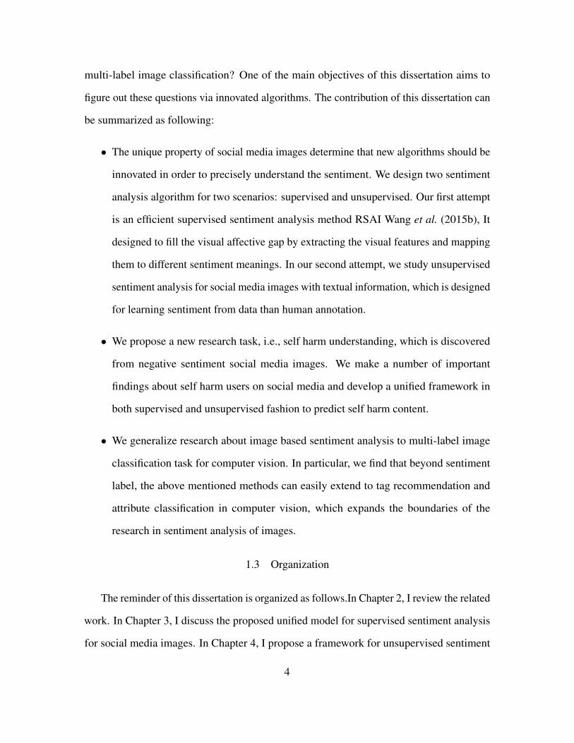
multi-label image classification? One of the main objectives of this dissertation aims to

figure out these questions via innovated algorithms. The contribution of this dissertation can

be summarized as following:

• The unique property of social media images determine that new algorithms should be

innovated in order to precisely understand the sentiment. We design two sentiment

analysis algorithm for two scenarios: supervised and unsupervised. Our first attempt

is an efficient supervised sentiment analysis method RSAI Wang et al. (2015b), It

designed to fill the visual affective gap by extracting the visual features and mapping

them to different sentiment meanings. In our second attempt, we study unsupervised

sentiment analysis for social media images with textual information, which is designed

for learning sentiment from data than human annotation.

• We propose a new research task, i.e., self harm understanding, which is discovered

from negative sentiment social media images. We make a number of important

findings about self harm users on social media and develop a unified framework in

both supervised and unsupervised fashion to predict self harm content.

• We generalize research about image based sentiment analysis to multi-label image

classification task for computer vision. In particular, we find that beyond sentiment

label, the above mentioned methods can easily extend to tag recommendation and

attribute classification in computer vision, which expands the boundaries of the

research in sentiment analysis of images.

1.3 Organization

The reminder of this dissertation is organized as follows.In Chapter 2, I review the related

work. In Chapter 3, I discuss the proposed unified model for supervised sentiment analysis

for social media images. In Chapter 4, I propose a framework for unsupervised sentiment

4

analysis. In Chapter 5, I present a new research problem for negative sentiment discovery

with a study case on self harm content analysis. In Chapter 6, I propose to extend sentiment

analysis prediction task to general image classification task. In Chapter 7, I conclude and

present the future work.

5

Chapter 2

RELATED WORK

Sentiment analysis for social media images is a novel and practical problem. Recently,with

increasing popularity of social networks, it attracts a lot of attention from academia and

industry. In this dissertation, I firstly provide a systematic and in depth literature review in

the literature.

Sentiment analysis on text and images: Recently, sentiment analysis has shown its

success in opinion mining on textual data, including product reviewLiu (2012); Hu and

Liu (2004), newspaper articles Pang et al. (2002), and movie rating Pang and Lee (2004).

Besides, there have been increasing interests in social media data Borth et al. (2013b); Yang

et al. (2014); Jia et al. (2012); Yuan et al. (2013), such as Twitter and Weibo data. Unlike text-

based sentiment prediction approaches, Borth et al. (2013b); Yuan et al. (2013) employed

mid-level attributes of visual feature to model visual content for sentiment analysis. Yang

et al. (2014) provides a method based on low-level visual features and social information

via a topic model. While Jia et al. (2012) tries to solve the problem by a graphical model

which is based on friend interactions. In contrast to our approach, all such methods restrict

sentiment prediction to the specific data domain. For example, in Figure 1, we can see that

approaches using pure visual information Borth et al. (2013b); Yuan et al. (2013) may be

confused by the subtle sentiment embedded in the image. e.g., two crying people convey

totally different sentiment. Jia et al. (2012); Yang et al. (2014) assume that the images

belong to the same sentiment share the same low-level visual features is often not true,

because positive and negative images may have similar low-level visual features, e.g., two

black-white images contain smiling and sad faces respectively. Recent, deep learning has

shown its success in feature learning for many computer vision problem, You et al. (2015)

6

provides a transfer deep neutral network structure for sentiment analysis. However, for deep

learning framework, millions of images with associated sentiment labels are needed for

network training. In real world, such label information is not available and how to deal with

overfitting for small training data remains a challenging problem.

Multimodal classification for social media: Multimodal classification techniques can

be classified into two main classes: early fusion and late fusion, which are depending on

how the information from multiple modalities are combined. In early fusion, features are

extracted from different modalities are combined together. Then the combined features are

feed into a classification framework. Various early fusion methods have been proposed to

classify social media content. In You et al. (2016a), the proposed algorithm first learns the

joint embedding for both text and image, then applied LSTM (long short term memory)

for sentiment classification. In Zeppelzauer and Schopfhauser (2016), the hierarchical

structure is proposed to learn the concatenated features. Compared to early fusion, late

fusion methods are more widely used. In late fusion, separated classification result or

representation is obtained on each modality independently. Then all the result or feature

is combined at decision level. There are only a few works on analyzing sentiment using

multi-modal features, such as text and images. Wang et al. (2014) employed both text and

images for sentiment analysis, where late fusion is employed to combine the prediction

results of using n-gram textual features and mid-level visual features. You et al. (2016b)

proposed a cross-modality scheme for joint sentiment analysis. Their approach employed

deep visual and textual features to learn a regression model.

Our work is built on non-negative matrix factorization, where we joint learn the textual

-visual feature together. Our method belongs to late fusion for multimodal classification

problem.

Non-negative matrix factorization(NMF): Our proposed framework is also inspired

by recent progress in matrix factorization algorithms. NMF has been shown to be useful in

7

computer vision and data mining applications including face recognitionWang et al. (2005),

object detection Lee and Seung (1999) and feature selection Das Gupta and Xiao (2011),

etc. Specifically, the work in Lee and Seung (2001) brings more attention to NMF in the

research community, where the author proposed a simple multiplicative rule to solve the

problem and showed the factor coherence of original image data. Ding et al. (2005) shows

that if adding orthogonal constrains, the NMF is equivalent to K-means clustering. Further,

Ding et al. (2006) presents a work that shows, when incorporating freedom control factors,

the non-negative factors will achieve a better performance on classification. In this paper,

motivated by previous NMF framework for learning the latent factors, we extend these

efforts significantly and propose a comprehensive formulation which incorporates more

physically-meaningful constraints for regularizing the learning process in order to find a

proper solution. In this respect, our work is similar in spirit to Hu et al. (2013) which

develops a factorization approach for sentiment analysis of social media responses to public

events.

In the dissertation, we discovery self harm user patterns from negative sentiment. There-

fore, in the following, we review related work on self ham and public health.

Selfharm research from psychology and medicine: Some work from psychology and

medicine have been done on understanding and characterizing the deliberate self-harm

patients. In Hawton et al. (1997), it investigates 8, 950 deliberate self-harm (DSH) patients

from 1990 to 2000 in Oxford, UK to capture their behavior trends. It shows that from 1997

to 2000, gender and age became a large portion of DSH – DSH rates in female and aged

in 15 to 24 and 34 to 54 have been significantly increased. The major reasons of DSH

are alcohol abuse, violence and misusing drugs. In Chapman et al. (2006), the authors

reported that DSH helps the patients escape or regulate the emotions and most self-injurious

behaviors are along with cognitive disabilities. In recent years Daine et al. (2013); Dyson

et al. (2016); Robinson et al. (2015), more and more attention has been paid on social media

8

platforms and studies Robinson et al. (2015) have shown that self-harm and suicide can

be prevented from social supports from other social media users. However, the limitation

of these studies is that they are typically based on surveys and self-reports about emotion.

Most assessments are designed to collect the data about DSH experiences over long periods

of time (1 to 5 years). Few studies are on the short term since the resources and invasiveness

are required to observe individuals’ behaviors over days and months.

Social Media and Public Health: In the last few years, the interests of studying public

health in social media are keep growing in the research community. Sadilek et al. (2012)

explored how to find diseases based on the posts in Twitter. Chancellor et al. (2016)

studied the eating-disorder community on Tumblr and finds that the tags for eating-disorder

community are keep evolving. In De Choudhury et al. (2013, 2016), authors investigated

the patterns of activities for depression groups on web by analyzing the posts from Twitter

and Reddit, respectively. However, research on self-harm understanding in social media is

still in its infancy.

9

Chapter 3

SUPERVISED SENTIMENT ANALYSIS FOR SOCIAL MEDIA IMAGES

In this chapter, I focus on the problem of exploiting textual and visual information for

sentiment prediction from social media images. Due to the distinct characteristics of social

media data, I focus on supervised learning method in this chapter. I will firstly review the

background of this problem, and then formally define the problem and present the proposed

method. The real-world dataset from Flickr and Instagram will be used to evaluate the

effectiveness of the proposed method by comparing with the state-of-the-art baselines.

3.1 Supervised sentiment analysis for Social Media Images

A picture is worth a thousand words. It is surely worth even more when it comes to

convey human emotions and sentiments. Examples that support this are abundant: great

captivating photos often contain rich emotional cues that help viewers easily connect with

those photos. With the advent of social media, an increasing number of people start to use

photos to express their joy, grudge, and boredom on social media platforms like Flickr and

Instagram. Automatic inference of the emotion and sentiment information from such ever-

growing, massive amounts of user-generated photos is of increasing importance to many

applications in health-care, anthropology, communication studies, marketing, and many

sub-areas within computer science such as computer vision. Think about this: Emotional

wellness impacts several aspects of people’s lives. For example, it introduces self-empathy,

giving an individual greater awareness of their feelings. It also improves one’s self-esteem

and resilience, allowing them to bounce back with ease, from poor emotional health, and

physical stress and difficulty. As people are increasingly using photos to record their daily

10

lives 1 , we can assess a person’s emotional wellness based on the emotion and sentiment

inferred from her photos on social media platforms (in addition to existing emotion/sentiment

analysis effort, e.g., see De Choudhury et al. (2012) on text-based social media).

As mentioned in Chapter 1. Both text based methods and visual content based methods

are not suit for social media images. For example, re-consider Figure 1.1: visual feature

usually has no contextual information on the visual content such as the action of ”proposal” in

figure 1.1a. On the other hand, textual feature in the social media images usually not contain

enough content information as the text messages are very short. For example, Twitter allows

users to post message up to 140 characters. Moreover, such textual messages are also very

unstructured and noisy. For example, users often prefer to use popular abbreviation words.

Since the slang words don’t usually appear on conventional text documents. Therefore the

textual sentiment lexicon seldom contains them.

The weaknesses discussed in the foregoing motivate the need for a more accurate

automated framework to infer the sentiment of photos, with 1) considering the photo context

to bridge the “visual affective gap”, 2) considering a photo’s visual features to augment

text-based sentiment, and 3) considering the availability of textual information, thus a photo

may have little or no social context (e.g., friend comments, user description). While such

a framework does not exist, we can leverage some partial solutions. For example, we can

learn the photo context by analyzing the photo’s social context (text features). Similarly,

we can extract visual features from a photo and map them to different sentiment meanings.

Last, while manual annotation of all photos and their descriptions is infeasible, it is often

possible to get sentiment labeling for small sets of photos and descriptions. In essence, I

investigate the following three questions:cm

• How do we model heterogeneous information sources, i.e., the visual information and

textual information, properly in a unified framework.1http://www.pewinternet.org/2015/01/09/social-media-update-2014/

11

• How do we seamlessly exploit both sources of information for the problem?

• How do we alleviate limited label information for efficient training?

Technical Contribution: We propose an efficient and effective framework, named RSAI

(Robust Sentiment Analysis for Images), for inferring human sentiment from photos that

leverages these partial solutions. Figure 3.1 depicts the procedure of RSAI. Specifically,

to fill the visual affective gap, we first extract visual features from a photo using low-level

visual features (e.g., color histograms) and a large number of mid-level (e.g., objects) visual

attribute/object detectors Yuan et al. (2013); Tighe and Lazebnik (2013). Next, to add

sentiment meaning to these extracted non-sentimental features, we construct Adjective Noun

Pairs (ANPs)Borth et al. (2013b). Note that ANP is a visual representation that describes

visual features by text pairs, such as “cloudy sky”, “colorful flowers”. It is formed by

merging the low-level visual features to the detected mid-level objects and mapping them to

a dictionary (more details on ANP are presented in Section 3). On the other hand, to learn

the image’s context, we analyze the image’s textual description and capture its sentiment

based on sentiment lexicons. Finally, with the help from ANPs and image context, RSAI

infers the image’s sentiment by factorizing an input image-features matrix into three factors

corresponding to image-term, term-sentiment and sentiment-features. The ANPs here can be

seen as providing the initial information (“prior knowledge”) on sentiment-feature factors.

Similarly, the learnt image context can be used to constrain image-term and term-sentiment

factors. Last, the availability of labeled sentiment of the images can be used to regulate the

product of image-term, term-sentiment factors. We pose this factorization as an optimization

problem where, in addition to minimizing the reconstruction error, we also require that the

factors respect the prior knowledge to the extent possible. We derive a set of multiplicative

update rules that efficiently produce this factorization, and provide empirical comparisons

with several competing methodologies on two real datasets of photos from Flickr and

12

Instagram. We examine the results both quantitatively and qualitatively to demonstrate that

our method improves significantly over baseline approaches.

Figure 3.1: The Framework of RSAI.

3.2 The Proposed RSAI Framework

In this section, we first propose the basic model of our framework. Then we show the

details of how to generate the ANPs. After that, we describe how to obtain and leverage the

prior knowledge to extend the basic model. We also analyze the algorithm in terms of its

correctness and convergence. Table 1 lists the mathematical notation used in this paper.

3.2.1 Basic Model

Assuming that all the images can be partitioned intoK sentiment (K = 3 in this paper as

we focus on positive, neutral and negative. However, our framework can be easily extended

to handle more fine-grained sentiment.) Our goal is to model the sentiment for each image

based on visual features and available text features. Let n be the number of images and the

size of contextual vocabulary is t. We can then easily cluster the images with similar word

frequencies and predict the cluster’s sentiment based on its word sentiment. Meanwhile, for

each image, which has m-dimensional visual features (ANPs, see below), we can cluster the

images and predict the sentiment based on the feature probability. Accordingly, our basic

framework takes these n data points and decomposes them simultaneously into three factors:

13

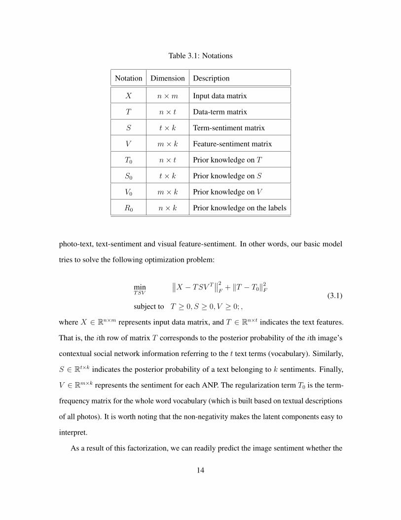
Table 3.1: Notations

Notation Dimension Description

X n×m Input data matrix

T n× t Data-term matrix

S t× k Term-sentiment matrix

V m× k Feature-sentiment matrix

T0 n× t Prior knowledge on T

S0 t× k Prior knowledge on S

V0 m× k Prior knowledge on V

R0 n× k Prior knowledge on the labels

photo-text, text-sentiment and visual feature-sentiment. In other words, our basic model

tries to solve the following optimization problem:

minTSV

∥∥X − TSV T∥∥2

F+ ‖T − T0‖2

F

subject to T ≥ 0, S ≥ 0, V ≥ 0; ,

(3.1)

where X ∈ Rn×m represents input data matrix, and T ∈ Rn×t indicates the text features.

That is, the ith row of matrix T corresponds to the posterior probability of the ith image’s

contextual social network information referring to the t text terms (vocabulary). Similarly,

S ∈ Rt×k indicates the posterior probability of a text belonging to k sentiments. Finally,

V ∈ Rm×k represents the sentiment for each ANP. The regularization term T0 is the term-

frequency matrix for the whole word vocabulary (which is built based on textual descriptions

of all photos). It is worth noting that the non-negativity makes the latent components easy to

interpret.

As a result of this factorization, we can readily predict the image sentiment whether the

14

contextual information (comments, user descriptions,etc.) is available or not. For example,

if there is no social information associated with the image, then we can directly derive the

image sentiment by applying non-negative matrix factorization for the input data X , when

we characterize the sentiment of each image through a new matrix R = T × S. Specifically,

our basic model is similar to the probabilistic latent semantic indexing (PLSI) Hofmann

(1999) and the orthogonal nonnegative tri-matrix factorization Ding et al. (2006). In their

work, the factorization means the joint distribution of documents and words.

3.2.2 Extracting and Modeling Visual Features

In Tighe and Lazebnik (2013); Tu et al. (2005); Yuan et al. (2013), visual content

can be described by a set of mid-level visual attributes, however, most of the attributes

such as “car”, “sky”,“grass”, etc., are nouns which make it difficult to represent high level

sentiments. Thus, we followed a more tractable approach Borth et al. (2013b), which

models the correlation between visual attributes and visual sentiment with adjectives, such

as “beautiful” , “awesome”, etc. The reason for employing such ANPs is intuitive: the

detectable nouns (visual attributes) make the visual sentiment detection tractable, while the

adjectives add the sentiment strength to these nouns. In Borth et al. (2013b), a large scale

ANPs detectors are trained based on the features extracted from the images and the labeled

tags with SVM. However, we find that such pre-defined ANPs are very hard to interpret. For

example the pairs like “warm pool” , “abandoned hospital”, and it is very difficult to find

appropriate features to measure them. Moreover, in their work, during the training stage, the

SVM is trained on the features extracted from the image directly, the inability of localizing

the objects and scales bounds the detection accuracy. To address these problems, we have

a two stage approach to detect ANPs based on the Visual Sentiment Ontology Borth et al.

(2013b) and train a one vs all classifier for each ANP.

15

Noun Detection: The nouns in ANPs refer to the objects presented in the image. As

one of fundamental tasks in computer vision, object detection has been studied for many

years. One of most successful works is Deformable Part Model (DPM) Felzenszwalb et al.

(2010) with Histogram of Oriented Gradient (HOG) Dalal and Triggs (2005) features. In

Felzenszwalb et al. (2010), the deformable part model has shown its capability to detect

most common objects with rigid structure such as: car, bike and non-rigid objects such as

pedestrian, dogs. Pandey and Lazebnik (2011) further demonstrates that DPM can be used

to detect and recognize scenes. Hence we adopt DPM to for nouns detection. The common

objects(noun) are trained by the public dataset ImageNetDeng et al. (2009). The scene

detectors are trained on SUN dataset Xiao et al. (2010). It is worth noting that selfie is one

of most popular images on the web Hu et al. (2014) and face expression usually conveys

strong sentiment, consequently, we also adopt one of state-of-the-art face detection methods

proposed in Zhu and Ramanan (2012).

Adjective Detection: Modeling the adjectives is more difficult than nouns due to the fact

that there are no well defined features to describe them. Following Borth et al. (2013b),

we collect 20,000 images associate with specific adjective tags from Web. The a set of

discriminative global features, including Gist, color histogram and SIFT, are applied for

feature extraction. Finally the adjective detection is formulated as a traditional image

classification problem based on Bag of words(BOW)model. The dictionary size of BOW is

1,000 with the feature dimension size 1,500 after dimension reduction based on PCA.

3.2.3 Constructing Prior Knowledge

So far, our basic matrix factorization framework provides potential solution to infer

the sentiment regarding the combination of social network information and visual features.

However, it largely ignores the sentiment prior knowledge on the process of learning

16

each component. In this part, we introduce three types of prior knowledge for model

regularization: (1) sentiment-lexicon of textual words, (2) the normalized sentiment strength

for each ANP, and (3) sentiment labels for each image.

Sentiment Lexicon The first prior knowledge is from a public sentiment lexicon named

MPQA corpus 2 . In this sentiment lexicon, there are 7,504 human labeled words which are

commonly used in the daily life. The number of positive words (e.g.“happy”, “terrific”) is

2,721 and the number of negative words (e.g. “gloomy”, “disappointed”) is 4,783. Since

this corpus is constructed without respect to any specific domain, it provides a domain

independent prior on word-sentiment association. It should be noted that the English

usage in social network is very casual and irregular, we employ a stemmer technique

proposed in Han and Baldwin (2011). As a result, the ill-formed words can be detected and

corrected based on morphophonemic similarity, for example “good” is a correct version

of “goooooooooooood”. Besides some abbreviation of popular words such as “lol”(means

laughing out loud) is also added as prior knowledge. We encode the prior knowledge in a

word sentiment matrix S0 where if the ith word belongs to jth sentiment, then S0(i, j) = 1,

otherwise it equals to zero.

Visual Sentiment In addition to the prior knowledge on lexicon, our second prior knowl-

edge comes from the Visual Sentiment Ontology (VSO) Borth et al. (2013b), which is based

on the well known previous researches on human emotions and sentiments Darwin (1998);

Plutchik (1980). It generates 3000 ANPs using Plutchnik emotion model and associates the

sentiment strength (range in[-2:2] from negative to positive) by a wheel emotion interface 3

. The sample ANP sentiment scores are shown in Table 2. Similar to the word sentiment2http://mpqa.cs.pitt.edu/3http://visual-sentiment-ontology.appspot.com

17

Table 3.2: Sentiment Strength Score Examples

ANP Sentiment Strength

innocent smile 1.92

happy Halloween 1.81

delicious food 1.52

cloudy mountain -0.4

misty forest -1.00

... ...

matrix S0, the prior knowledge on ANPs V0 is the sentiment indicator matrix.

Sentiment labels of Photos Our last prior knowledge focuses on the prior knowledge on

the sentiment label associated with the image itself. As our framework essentially is a semi-

supervised learning approach, this leads to a domain adapted model that has the capability

to handle some domain specific data. The partial label is given by the image sentiment

matrix R0 where R0 ∈ Rn×k. For example if the ith image belongs to jth sentiment, the

R0(i, j) = 1 otherwise R0(i, j) = 0. The improvement by incorporating these label data is

empirically verified in the experiment section.

3.2.4 Incorporating Prior Knowledge

After defining the three types of prior knowledge, we incorporate them into the basic

model as regularization terms in following optimization problem:

18

minTSV

∥∥X − TSV T∥∥2

F+ α ‖V − V0‖2

F

+ β ‖T − T0‖2F + γ ‖S − S0‖2

F

+ δ ‖TS −R0‖2F

subject to T ≥ 0, S ≥ 0, V ≥ 0

(3.2)

where α ≥ 0, β ≥ 0, γ ≥ 0 and δ ≥ 0 are parameters controlling the extent to which we

enforced the prior knowledge on the respective components. The model above is generic

and allows flexibility . For example, if there is no social information available for one image,

we can simply set the corresponding row of T0 to zeros. Moreover, the square loss function

leads to an unsupervised problem for finding the solutions. Here, we re-write Eq (2) as :

L =Tr(XTX − 2XTTSV T + V STT TTSV T )

+ αTr(V TV − 2V TV0 + V T0 V )

+ βTr(T TT − 2T TT0 + T T0 T0)

+ γTr(STS − 2STS0 + ST0 S0)

+ δTr(STT TTS − 2STT TR0 +RT0R0)

(3.3)

From Eq 3.3 we can find that it is very difficult to solve T , S and V simultaneously.

Thus we employ the alternating multiplicative updating scheme shown in Ding et al. (2006)

to find the optimal solutions. First, we use fixed V and S to update T as follows:

Tij ← Tij

√[XV ST + βT0 + δR0ST ]ij

[TSV TV ST + βT + δTSST ]ij(3.4)

Next, we use the similar update rule to update S and V :

Sij ← Sij

√[T TXV + γS0 + δT TR0]ij

[T TTSV TV + γS + δT TTS]ij(3.5)

19

Vij ← Vij

√[XTTS + αV0]ij

[V STT TTS + αV ]ij(3.6)

The learning process consists of an iterative procedure using Eq 3.4, Eq 3.5 and Eq 3.6

until convergence. The description of the process is shown in Algorithm 1.

Algorithm 1 Multiplicative Updating AlgorithmInput: X,T0, S0, V0, R0, α, β, γ, δ

Output: T, S, V

Initialization: T, S, V

while Not Converge do

Update T using Eq(4) with fixed S, V

Update S using Eq(5) with fixed T, V

Update V using Eq(6) with fixed T, S

end whileEnd

3.2.5 Algorithm Correctness and Convergence

In this part, we prove the guaranteed convergence and correctness for Algorithm 1 by

the following two theorems.

Theorem 1. When Algorithm 1 converges, the stationary point satisfies the Karush-

Kuhn-Tuck(KKT) condition, i.e., Algorithm 1 converges correctly to a local optima.

Proof of Theorem 1. We prove the theorem when updating V using Eq 3.6, similarly,

all others can be proved in the same way. First we form the gradient of L regards V as

Lagrangian form:

∂L

∂V= 2(V STT TTS + αV )− 2(XTTS + αV0)− µ (3.7)

20

Where µ is Lagrangian multiplier µij enforces the non-negativity constraint on Vij . From

the complementary slackness condition, we can obtain

(2(V STT TTS + αV )− 2(XTTS + αV0))ijVij = 0 (3.8)

This is the fixed point relation that local minima for V must hold. Given the Algorithm

1., we have the convergence point to the local minima when

Vij = Vij

√[XTTS + αV0]ij

[V STT TTS + αV ]ij(3.9)

Then the Eq 3.9 is equivalent to

(2(V STT TTS + αV )− 2(XTTS + αV0))ijV2ij = 0 (3.10)

This is same as the fixed point of Eq 3.9,i.e., either Vij = 0 or the left factor is 0. Thus if

Eq 3.10 holds the Eq 3.9 must hold and vice versa.

Theorem 2. The objective function is nondecreasing under the multiplicative rules of

Eq (4), Eq (5) and Eq (6), and it will converge to a stationary point.

Proof of Theorem 2. First, let H(V ) be:

H(V ) = Tr((V STT TTS + αV )V T − (XTTS + αV0 + µ)V T ) (3.11)

and it is very easy to verify that H(V ) is the Lagrangian function of Eq 3.3 with KKT

condition. Moreover, if we can verify that the update rule of Eq 3.4 will monotonically

decrease the value of H(V ), then it means that the update rule of Eq 3.4 will monotonically

21

decrease the value of L(V )(recall Eq 3.3). Here we complete the proof by constructing the

following an auxiliary function h(V, V ).

h(V, V ) =∑ik

(V (V STT TTS + αV ))ikV2ik

Vik

−∑ik

(XTTS + αV0 + µ)ikVik(1 + logVik

Vik)

(3.12)

Since z ≥ (1 + log z),∀z > 0 and similar in Ding et al. (2006), the first term in h(V, V )

is always larger than that in H(V ), then the inequality holds h(V, V ) ≥ H(V ). And it is

easy to see h(V, V ) = H(V ), thus h(V, V ) is an auxiliary function of H(V ). Then we have

the following inequality chain:

H(V 0) = h(V 0, V 0) ≥ h(V 0, V 1) = H(V 1).... (3.13)

Thus, with the alternate updating rule of V, S and T , we have the following inequality

chain:

L(V 0, T 0, S0) ≥ L(V 1, T 0, S0) ≥ L(V 1, T 1, S0).... (3.14)

Since L(V, S, T ) ≥ 0. Thus L(V, S, T ) is bounded and the Algorithm 1 converges ,

which completes the proof.

3.3 Empirical Evaluation

We now quantitatively and qualitatively compare the proposed model on image sen-

timent prediction with other candidate methods. We also evaluate the robustness of the

proposed model with respect to various training samples and different combinations of prior

knowledge. Finally, we perform a deeper analysis of our results.

22

3.3.1 Experiment Settings

We perform the evaluation on two large scale image datasets collected from Flickr and

Instagram respectively. The collection of Flickr dataset is based on the image IDs provided

by Yang et al. (2014), which contains 3,504,192 images from 4,807 users. Because some

images are unavailable now, and without loss of generality, we limit the number of images

from each user. Thus, we get 120,221 images from 3921 users. For the collection of the

Instagram dataset, we randomly pick 10 users as seed nodes and collect images by traversing

the social network based on breadth first search. The total number of images from Instagram

is 130,230 from 3,451 users.

Establishing Ground Truth: For training and evaluating the proposed method, we

need to know the sentiment labels. Thus, 20,000 Flickr images are labeled by three human

subjects, the majority voting is employed. However, manually acquiring the labels for these

two large scale datasets is expensive and time consuming. Consequently, the rest of more

than 230,000 images are labeled by the tags, which was suggested by the previous works

Yang et al. (2014); Go et al. (????) 4 . Since labeling the images based on the tags may

cause noise issue, and for better reliability we only label the images with primary sentiment

labels, which include: positive, neutral and negative. It is worth noting that the human

labeled images have both primary sentiment labels and fine grained sentiment labels. The

fine grained labels, including: happiness, amusement, anger, fear, sad and disgust, are used

to for fine grained sentiment prediction.

The comparison methods include: Senti API 5 , SentiBank Borth et al. (2013b), ELYang

et al. (2014) and the baseline method.

• Senti API is a text based sentiment prediction API, it measures the text sentiment by4More details can be found inYang et al. (2014) and Go et al. (????)5http://sentistrength.wlv.ac.uk/,a text based sentiment prediction API

23

(a) Negative (b) Neutral (c) Positive

Figure 3.2: Sample Tag Labeled Images from Flickr and Instagram.

(a) Negative (b) Neutral (c) Positive

Figure 3.3: Sample Visual Results from RSAI.

counting the sentiment strength for each text term.

• SentiBank is a state-of-the-art visual based sentiment prediction method. The method

extracts a large number of visual attributes and associates them with a sentiment score.

Similar to Senti API, the sentiment prediction is based on the sentiment of each visual

attributes.

• EL is a graphical model based approach, it infers the sentiment based on the friend

interactions and several low level visual features.

• Baseline: The baseline method comes from our basic model. To compare it fairly, we

24

also introduce R0 with the basic model which makes the baseline method have the

ability to learn from training data.

3.3.2 Performance Evaluation

Large scale image sentiment prediction: As mentioned in Sec 3, the proposed

model has the flexibility to incorporate the information and capability to jointly learn from

the visual features and text features. For each image, the visual features are formed by the

confidence score of each ANP detector, the feature dimension is 1200, which is as large as

VSO (prior knowledge V0). For the text feature, it is formed based on the term frequency

and the dimension relies on the input data. To predict the label, the model input is unknown

data X ∈ Rn×m and its corresponding text feature matrix T0 ∈ Rn×t, where n is the number

of images, m = 1200 and t is the vocabulary size, we decompose it via Aglorithm 1 and get

the label based on max pooling each row of X ∗ V . It is worth noting that in the proposed

model, tags are not included as input feature.

The results of comparison are shown in Table 3. We employ 30% data for training and

remaining for testing. To verify the reliability of tags labeled images, we also included

20000 labeled Flickr images with primary sentiment label. Especially, the classifier setting

for SentiBank and EL followed the original papers. The classifier of Sentibank is logistic

regression and for EL it is SVM. From the results we can see that, the proposed method

performs best in both datasets. Noting that proposed method improved 10% and 6% over

state-of-the-art methods Borth et al. (2013b). Results from proposed method are shown in

Figure 4. Noting that the number we reported in Table 3 is the prediction accuracy for each

method.

From the table, we can see that, even though noise exists in the Flickr and Instagram

dataset, the results are similar to the performance on human labeled dataset. Another

interesting observation is that the performance of EL on Instagram is worse than on Flickr,

25

Table 3.3: Sentiment Prediction Results.

Senti API SentiBank EL Baseline Proposed method

20000 Flickr 0.32 0.42 0.47 0.48 0.52

Flickr 0.34 0.47 0.45 0.48 0.57

Instagram 0.27 0.56 0.37 0.54 0.62

one reason could be that the wide usage of ”picture filters” lowers discriminative ability of

the low level visual features, while the models based on the mid level attributes can easily

avoid this filter ambiguity. Another interesting observation is that our basic model performs

fairly well even if it does not incorporate the knowledge from sentiment strength of ANPs,

which indicates that the object based ANPs by our method are more robust than the features

used in Borth et al. (2013b).

Fine Grained Sentiment Prediction: Although our motivation is to predict the

sentiment (positive, negative) on the visual data, to show the robustness and extension

capability of the proposed model, we further evaluate the proposed model on a more

challenging task in social media; predicting human emotions. Based on the definition of

human emotion Ekman (1992), our fine grained sentiment study labels the user posts with

following human emotion categories including: happiness, amusement, disgust, anger, fear

and sadness. The results on 20000 manually labeled flickr post are shown in Figure 5.

Compared to sentiment prediction, fine grained sentiment prediction would give us more

precise user behavior analysis and new insights on the proposed model.

As Figure 5 shows, compared to SentiBank and EL, the proposed method has the highest

average classification accuracy and the variance of proposed method on these 6 categories is

smaller than that of the baseline methods, which demonstrates the potential social media

applications of the proposed method such as predicting social response. We noticed that the

26

Figure 3.4: Fine Grained Sentiment Prediction Results (Y-axis represents the accuracy for

each method).

sad images have the highest prediction accuracy, and both disgust and anger are difficult to

predict. Another observation is the average performance of positive categories, happiness

and amusement, is similar to the negative categories. Explaining reason for this drives us to

dig deeper into sentiment understanding in the following section.

3.3.3 Analysis and Discussion

In this section, we present an analysis of parameters for the proposed method and the

results of the proposed method. Specifically, in last section we have studied the performance

of different methods. In this part, our objective is to have deeper understanding on the

datasets and the correlation between different features and the sentiments embedded in the

images. Without loss of generality, we collected additional 20k images from Flickr and

Instagram respectively (totally 40K) and we address the following research questions:

• RQ1:What is the relationship between visual features and visual sentiments?

• RQ2:Since the proposed method is better than pure visual feature based method, How

does the model gain?

First, we start with RQ1 by extracting the visual features used in Borth et al. (2013b) and

Yang et al. (2014) for each image in the Flickr and Instagram datasets. Then we use k-means

27

Figure 3.5: Sentiment Distribution based on Visual Features (From left to rigth is number of

positive, neutral, negative images in Instagram and Flickr, receptively. Y axis represents the

number of images).

clustering to obtain 3 clusters of images for each dataset, where the image similarity is

measured as Euclidean distance in the feature spaces. Based on each cluster center, we used

the classfier trained in the previous experiment for cluster labeling. The results are shown

in Figure 6. The x-axis is the different class label for each dataset and the y-axis is the

number of images that belong to each cluster. From the results, we notice that the “visual

affective gap” does exist between human sentiment and visual features. For the state-of-the

art method Borth et al. (2013b), the neural images are largely misclassified based on the

visual features. While for Yang et al. (2014), we observe t the low level features, e.g., color

histogram, contrast and brightness, are not closely related to human sentiment as visual

attributes.

We further analyze the performance of the proposed method based on these 40,000

images.

Parameter study: In the proposed model, we incorporate three types of prior knowledge:

sentiment lexicon, sentiment labels of photos and visual sentiment for ANPs. It is important

and interesting to explore the impact of each of them on the performance of the proposed

model. Figure 7 presents the average results (y-axis) of two datasets on sentiment prediction

28

Figure 3.6: Performance Gain by Incorporating Training Data.

with different amount of training data (x-axis) 6 , where the judgment is on the same three

sentiment labels with different combinations respectively. It should be noted that each

combination is optimized by Algorithm 1, which has similar formulations. Moreover, we

set the same parameter for α,β, γ and δ (0.9, 0.7, 0.8 and 0.7). Results give us two insights.

First, employing more prior knowledge will make the model more effective than using

only one type of prior knowledge. For our matrix factorization framework, T and V have

independent clustering freedom by introducing S, thus it is natural to add more constraints

for desired decomposed component. Second, when no training data, the basic model with

S0 performs much better than SentiAPI (refer Table 3), which means incorporating ANPs

significantly improves image sentiment prediction. It is worth noting that there is no training

stage for the proposed method. Thus when compared to fully supervised approaches, our

method is more applicable in practice when the label information is unavailable.

Bridging the Visual Affective Gap (RQ2): Figure 1 and Figure 7 demonstrate that a

visual affective gap exists between visual features and human sentiments (i.e., the same6The experiments setting is as same as discussed above.

29

visual feature may correspond to different sentiments in different context). To bridge this gap,

we show that one possible solution is to utilize heterogeneous data and features available in

social media to augment the visual feature-based sentiment. In the previous parameter study,

we have studied the importance of the prior knowledge. Furthermore, we study importance

of β which contains the degree of contextual social information used in the proposed model.

From Figure 8, we can observe that the performance of the proposed model increases along

the value of β. However, when β is greater than 0.8, the performance drops. This is because

textual information in social media data is usually incomplete. Larger β will cause negative

effects on the prediction accuracy where there is none or little information available.

Figure 3.7: The Value of β versus Model Performance (X axis is β value, y axis is value of

model performance).

3.4 Summary

In this chapter, we proposed a novel approach for visual sentiment analysis by leveraging

several types of prior knowledge including: sentiment lexicon, sentiment labels and visual

sentiment strength. To bridge the “affective gap” between low-level image features and

high-level image sentiment, we proposed a two-stage approach to general ANPs by detecting

mid-level attributes. For model inference, we developed a multiplicative update algorithm

to find the optimal solutions and proved the convergence property. Experiments on two

large-scale datasets show that the proposed model is superior to other state-of-the-art models

30

in both inferring sentiment and fine grained sentiment prediction.

31

Chapter 4

UNSUPERVISED SENTIMENT ANALYSIS

In this chapter, I focus on the problem of exploiting textual features to enable unsupervised

sentiment analysis for social media images. I will firstly review the background of this

problem that address why textual feature could be potentially useful for visual sentiment

analysis. And then I formally define the problem and introduce the proposed method.

Real world datasets from Flickr and Instagram are used to evaluate the effectiveness of the

proposed methods.

4.1 Motivation

Current methods of sentiment analysis for social media images include low-level visual

feature based approaches Jia et al. (2012); Yang et al. (2014), mid-level visual feature based

approaches Borth et al. (2013b); Yuan et al. (2013) and deep learning based approaches You

et al. (2015). The vast majority of existing methods are supervised, relying on labeled images

to train sentiment classifiers. Unfortunately, sentiment labels are in general unavailable

for social media images, and it is too labor- and time-intensive to obtain labeled sets large

enough for robust training. In order to utilize the vast amount of unlabeled social media

images, an unsupervised approach would be much more desirable. This paper studies

unsupervised sentiment analysis.

Typically, visual features such as color histogram, brightness, the presence of objects and

visual attributes lack the level of semantic meanings required by sentiment prediction. In

supervised case, label information could be directly utilized to build the connection between

the visual features and the sentiment labels. Thus, unsupervised sentiment analysis for

social media images is inherently more challenging than its supervised counterpart. As

32

images from social media sources are often accompanied by textual information, intuitively

such information may be employed. However, textual information accompanying images

is often incomplete (e.g., scarce tags) and noisy (e.g., irrelevant comments), and thus

often inadequate to support independent sentiment analysis Hu and Liu (2004); Hu et al.

(2013). On the other hand, such information can provide much-needed additional semantic

information about the underlying images, which may be exploited to enable unsupervised

sentiment analysis. How to achieve this is the objective of our approach.

In this chapter, we study unsupervised sentiment analysis for social media images

with textual information by investigating two related challenges: (1) how to model the

interaction between images and textual information systematically so as to support sentiment

prediction using both sources of information, and (2) how to use textual information to

enable unsupervised sentiment analysis for social media images. In addressing these two

challenges, we propose a novel Unsupervised SEntiment Analysis (USEA) framework,

which performs sentiment analysis for social media images in an unsupervised fashion.

Figure 4.1 schematically illustrates the difference between the proposed unsupervised

method and existing supervised methods. Supervised methods use label information to

learn a sentiment classifier; while the proposed method does not assume the availability of

label information but employ auxiliary textual information. Our main contribution can be

summarized as below:

• A principled approach to enable unsupervised sentiment analysis for social media

images.

• A novel unsupervised sentiment analysis framework USEA for social media images,

which captures visual and textual information into a unifying model. To our best

knowledge, USEA is the first unsupervised sentiment analysis framework for social

media images; and

33

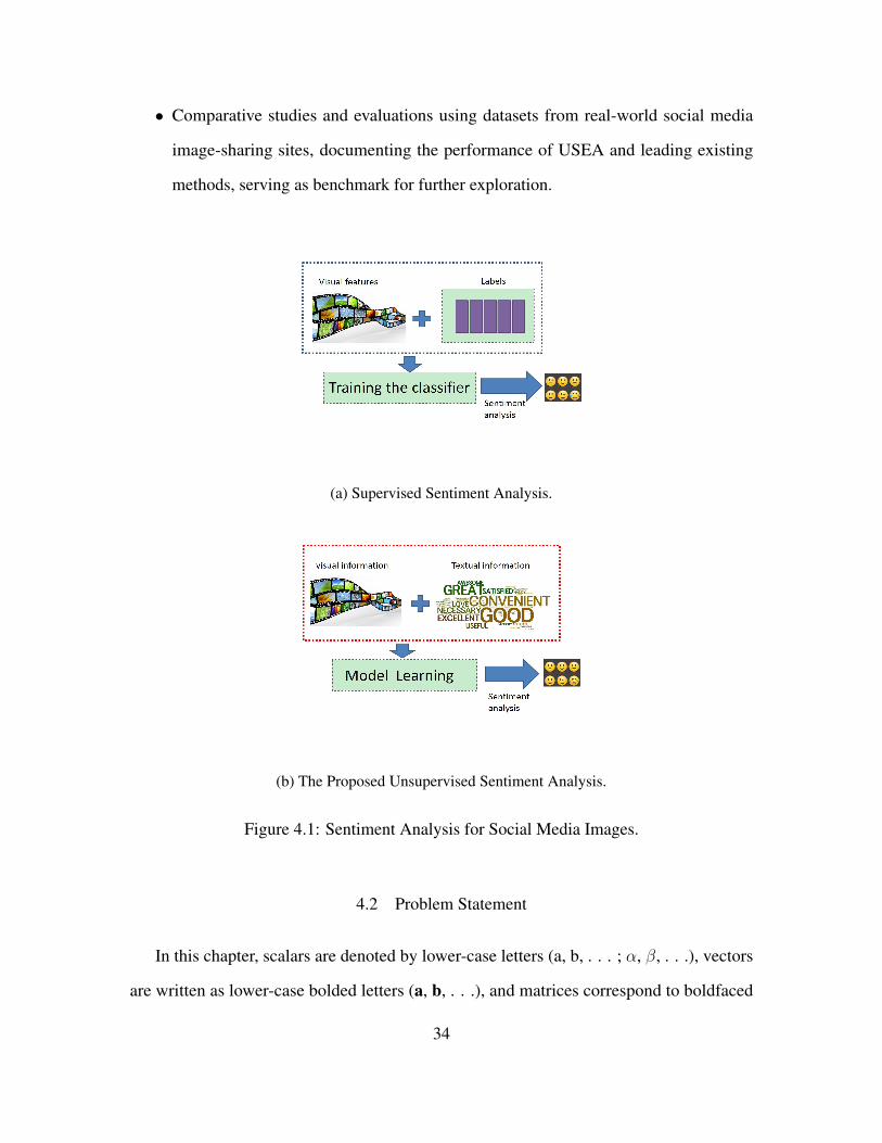
• Comparative studies and evaluations using datasets from real-world social media

image-sharing sites, documenting the performance of USEA and leading existing

methods, serving as benchmark for further exploration.

(a) Supervised Sentiment Analysis.

(b) The Proposed Unsupervised Sentiment Analysis.

Figure 4.1: Sentiment Analysis for Social Media Images.

4.2 Problem Statement

In this chapter, scalars are denoted by lower-case letters (a, b, . . . ; α, β, . . .), vectors

are written as lower-case bolded letters (a, b, . . .), and matrices correspond to boldfaced

34

uppercase letters (A, B, . . .). Let I = I1, I2, . . . , In be the set of images where n is the

number of images. We use P = p1, p2, . . . , pn to denote associated textual information

about images where pi is the textual information about Ii. Let Fv be set ofmv visual features

and Ft be set of mt textual features. We use Xv ∈ Rn×mv and Xt ∈ Rn×mt to denote visual

and textual information about images, respectively. Let C = c1, c2, . . . , ck be the set of

sentiment labels. Note that in this work we only consider positive, neutral and negative

sentiments with k = 3 but the generalization of the proposed framework to multi-class

sentiment analysis is straightforward.

With the aforementioned notations/definitions, the problem of unsupervised sentiment

analysis for social media images with textual information is formally defined as:

Given n images with visual information Xv and textual information Xt, to predict sen-

timent labels in C for the given n images.

4.3 Unsupervised Sentiment Analysis for Social Media Images

In this section, we first present our method for exploiting text information and then

introduce the unsupervised sentiment analysis framework with an optimization method.

4.3.1 Exploiting Textual Information

Without label information, it is challenging for unsupervised sentiment analysis to

connect visual features with sentiment labels. Textual information associated with social

media images may be exploited to help, as it provides semantics about the underly images

and in particular rich sentiment signals such as sentiment words and emotion symbols may

be found in the textual fields. Hence, to exploit textual information, we investigate (1) how

to incorporate textual information into visual information; and (2) how to model sentiment

signals in textual information.

35

Since visual and textual information are two views about the same set of images, it is

reasonable to assume that they share the same sentiment label space. More specifically, the

sentiment of Ii should be consistent with that of its associated textual information pi. Let

U0 ∈ Rn×k be the sentiment label space where U0(i, j) = 1 if the i-th data instance belongs

to cj , and U0(i, j) = 0 otherwise. We propose the following formulation to incorporate

visual information with textual information based on nonnegative matrix factorization:

minUV

∥∥Xv −UvVTv

∥∥2

F+ α

∥∥Xt −UtVTt

∥∥2

F

+ β(‖Uv −U0‖2F + ‖Ut −U0‖2

F )

subject to Uv ≥ 0; Ut ≥ 0; ||U0(i, :)||0 = 1, i ∈ 1, 2, ..n

U0(i, j) ∈ 0, 1 j ∈ 1, 2, ..k

(4.1)

where α controls how textual information contributes to the model and || · ||0 is `0, which

counts the number of nonzero entries in the vector. Uv ∈ Rn×k and Ut ∈ Rn×k are the

sentiment label spaces learned from visual information and textual information, respectively.

The term of β(‖Uv −U0‖2F + ‖Ut −U0‖2

F ) ensures that these two types of information

should share the sentiment label space U0. Vv ∈ Rmv×k and Vt ∈ Rmt×k indicate the

sentiment polarities of visual and textual features, respectively.

Textual information contains rich sentiment signals. First, some words may contain

sentiment polarities. For example, some words are positive such as “happy” and “terrific”;

while others are negative such as “gloomy” and “disappointed”. The sentiment polarities

of words can be obtained via some public sentiment lexicons. For example, the sentiment

lexicon MPQA contains 7,504 human labeled words which are commonly used in the daily

life with 2,721 positive words and 4,783 negative words. Second, some abbreviations and

emoticons are strong sentiment indicators. For example, ”lol”(means laughing out loud)

is a positive indicator while “:(” is a negative indicator. Let Vt0 ∈ Rmv×k be the matrix

coding sentiment signals in textual information where Vt0(i, j) = 1 if i-th word belongs to

36

cj and Vt0(i, j) = 0 otherwise. To model sentiment signals, we force the learned sentiment

polarities of textual features to be consistent with those indicated by sentiment signals.

Furthermore, not all textual features in Ft contain sentiment polarities and Vt should be

sparse. We propose the following formulation to achieve these two goals as:

min ‖Vt −Vt0‖2,1 (4.2)

‖X‖2,1 is the `2,1 of the matrix X, which ensures the row sparsity of X Nie et al. (2010).

The significance of textual information in unsupervised sentiment analysis for social

media images is two-fold. First, textual information bridges the semantic gap between visual

features and sentiment labels. Second, we are allowed to do sentiment analysis for social

media images in an unsupervised scenarios by modeling textual information via Eqs. (4.1)

and (4.2).

4.3.2 The Framework: USEA

By combining the above discussion, we can have the following initial framework, which

provides a potential solution to inferring sentiments by jointly considering visual information

and corresponding contextual information:

minUV

∥∥Xv −UvVTv

∥∥2

F+ α

∥∥Xt −UtVTt

∥∥2

F

+ β(‖Uv −U0‖2F + ‖Ut −U0‖2

F )

+ γ‖Vt −Vt0‖2,1

s.t. Uv ≥ 0; Ut ≥ 0; ||U0(i, :)||0 = 1, i ∈ 1, 2, ..n

U0(i, j) ∈ 0, 1 j ∈ 1, 2, ..k

(4.3)

The parameter γ controls the sparsity of regularization term. However, the constrains

of U0 in Eq. (3), mixed vector zero norm with integer programming, make the problem

difficult to solve. To tackle this problem, we consider the relaxation of U0 by adding the

37

extra orthogonal constraint on the value of U0. With the relaxation, the proposed framework

(USEA) is to solve the following optimization problem:

minUV

∥∥Xv −UvVTv

∥∥2

F+ α

∥∥Xt −UtVTt

∥∥2

F

+ β(‖Uv −U0‖2F + ‖Ut −U0‖2

F )

+ γ‖Vt −Vt0‖2,1

s.t. Uv ≥ 0; Ut ≥ 0;

UT0 U0 = I; U0 ≥ 0

(4.4)

4.3.3 An Optimization Method

There are 5 components, i.e. Uv,Vv, Ut,Vt and U0, in Eq. (4). Thus it is difficult

to optimize all the components simultaneously. In the following parts, we demonstrate

an alternating algorithm to optimize the objective function by updating each component

iteratively.

Update Vt: If U0, Uv, Vv and Ut are fixed, then the objective function is decoupled

and the constrains are independent of Vt. Thus we can optimize Vt separately and ignore

the term without Vt, leading to the following:

minVvJ (Vt) =

∥∥Xt −UtVTt

∥∥2

F+ δ ‖Vt −Vt0‖2

F (4.5)

where δ = γα

. Taking the derivation of J (Vt) and setting it to zero, we can obtain the

following form:

(−XTt Ut + VtU

Tt Ut) + δDt(Vt −Vt0) = 0 (4.6)

where Dt is a diagonal matrix with jth element on the diagonal D(j, j) = 12‖Vt(j,:)−Vt0(j,:)‖2

.

In Eq. (6), solving Vt directly is intractable. Since Dt and UTt Ut are symmetric and positive

38

definite, we employ eigen decomposition for them as:

UTt Ut = U1Λ1U

T1

Dt = U2Λ2UT2

(4.7)

where U1,U2 are eigen vectors and Λ1,Λ2 are diagonal matrices with eigen values on the

diagonal. Substituting UTt Ut and Dt in Eq. (6), we have:

VtU1Λ1UT1 + δU2Λ2U

T2 Vt = XT

t Ut + δDtVt0 (4.8)

Multiplying UT2 and U1 from left to right on both sides:

UT2 VtU1Λ1 + δΛ2U

T2 VtU1 = UT

2 (XtUt + δDtVt0)U1 (4.9)

Let Vt = UT2 VtU1 and Q = UT

2 (XtUt+δDtVt0)U1 , Eq. (9) becomes VtΛ1 +δΛ2Vt =

Q, then we can obtain the Vt and Vt as:

Vt(s, l) =Q(s, l)

δλs2 + λl1

Vt = U2VtUT1

(4.10)

where λs2 is the s-th eigen value of Dt and λl1 is l-th eigen value of UTt Ut. The following

theorem shows that the updating rule in Eq(10) can monotonically decrease the objective

function J (Vt).

Theorem 1. The update rule in Eq. (10) can monotonically decrease the value of J (Vt)

Proof. The proof is similar to that in Nie et al. (2010), due to space limit, we omit the

details of the proof.

Update Vv. If U0, Ut, Vt and Uv are fixed, by setting the derivation of the objective

function to zero, Vv can be easily obtained as Vv = XTv Uv(U

Tv Uv)

−1. Moreover, we can

easily verify updating Vv will monotonically decrease the objective function.

Update Uv: If Vv, Ut, Vt and U0 are fixed, Uv can be obtained by the following

39

optimization problem:

minUv

J (Uv) =∥∥Xv −UvV

Tv

∥∥2

F+ β ‖Uv −U0‖2

F

s.t. Uv ≥ 0

(4.11)

The Lagrangian function of Eq. (11) is :

minUv

L(Uv) =∥∥Xv −UvV

Tv

∥∥2

F+ β ‖Uv −U0‖2

F

− Tr(ΓUv)

(4.12)

where Γ is Lagrangian multiplier. Taking the deviation of J (Uv) and using the KKT

condition (Γ(s, l)Uv(s, l) = 0), we can obtain:

(−XvVv + UvVTv Vv + βUv − βU0)sl(Uv)sl = 0 (4.13)

which leads to the following update rule for Uv:

(Uv)sl ← (Uv)sl

√((XvVv)+ + Uv(VT

v Vv)− + βU0)sl((XvVv)− + Uv(VT

v Vv)+ + βUv)sl(4.14)

where X(s, l)+ = (|X(s, l)| + X(s, l))/2, X(s, l)− = (|X(s, l)| − X(s, l))/2 and X =

X+ −X−.

Theorem 2. Let

40

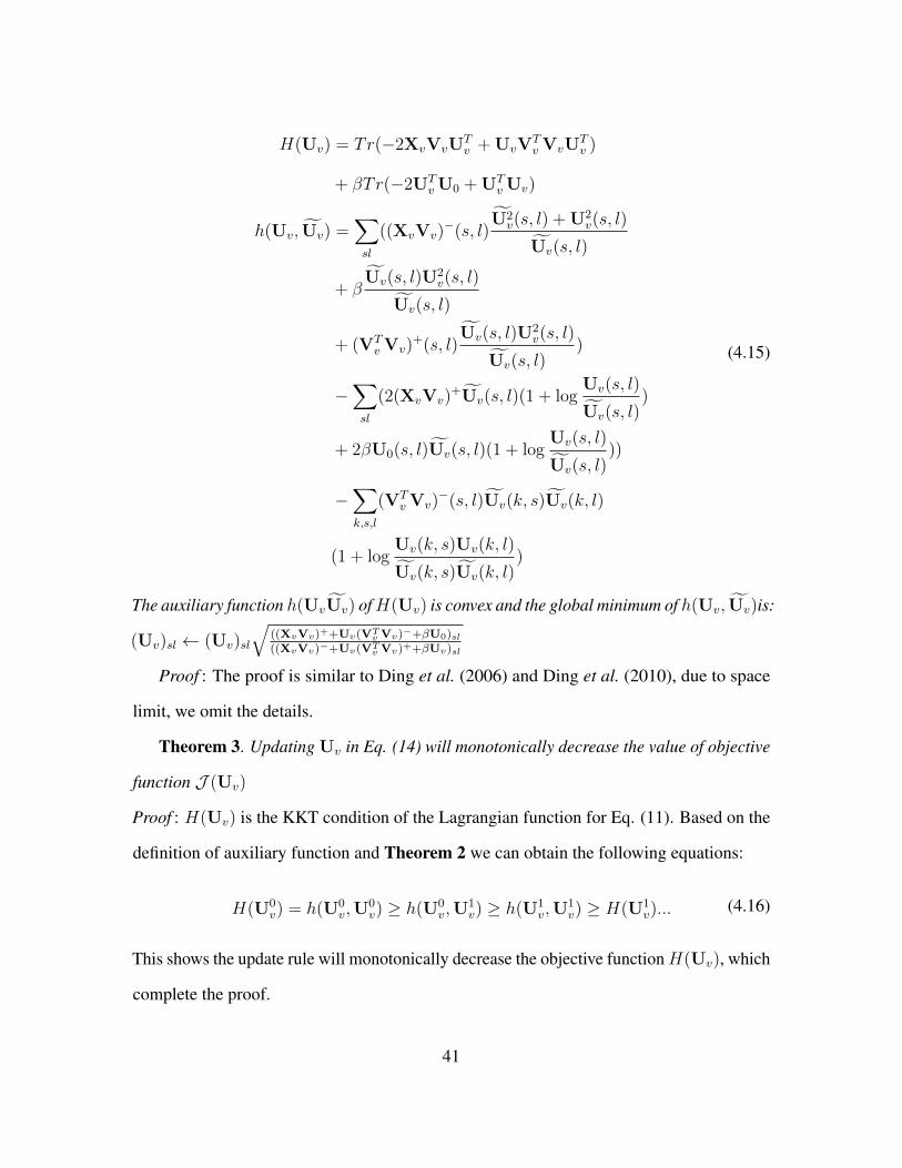
H(Uv) = Tr(−2XvVvUTv + UvV

Tv VvU

Tv )

+ βTr(−2UTv U0 + UT

v Uv)

h(Uv, Uv) =∑sl

((XvVv)−(s, l)

U2v(s, l) + U2

v(s, l)

Uv(s, l)

+ βUv(s, l)U

2v(s, l)

Uv(s, l)

+ (VTv Vv)

+(s, l)Uv(s, l)U

2v(s, l)

Uv(s, l))

−∑sl

(2(XvVv)+Uv(s, l)(1 + log

Uv(s, l)

Uv(s, l))

+ 2βU0(s, l)Uv(s, l)(1 + logUv(s, l)

Uv(s, l)))

−∑k,s,l

(VTv Vv)

−(s, l)Uv(k, s)Uv(k, l)

(1 + logUv(k, s)Uv(k, l)

Uv(k, s)Uv(k, l))

(4.15)

The auxiliary function h(UvUv) ofH(Uv) is convex and the global minimum of h(Uv, Uv)is:

(Uv)sl ← (Uv)sl

√((XvVv)++Uv(VT

v Vv)−+βU0)sl((XvVv)−+Uv(VT

v Vv)++βUv)sl

Proof : The proof is similar to Ding et al. (2006) and Ding et al. (2010), due to space

limit, we omit the details.

Theorem 3. Updating Uv in Eq. (14) will monotonically decrease the value of objective

function J (Uv)

Proof : H(Uv) is the KKT condition of the Lagrangian function for Eq. (11). Based on the

definition of auxiliary function and Theorem 2 we can obtain the following equations:

H(U0v) = h(U0

v,U0v) ≥ h(U0

v,U1v) ≥ h(U1

v,U1v) ≥ H(U1

v)... (4.16)

This shows the update rule will monotonically decrease the objective functionH(Uv), which

complete the proof.

41

Update Ut: It is worth noting that the procedure of solving Ut is exactly the same as

that of Uv. Thus, we omit the solution of Ut here.

Update U0: With Uv, Ut, Vt and Vv fixed, the sentiment label U0 can be obtained by

solving the following optimization problem:

minUJ (U0) = ‖Uv −U0‖2

F + ‖Ut −U0‖2F

s.t. UT0 U0 = I; U0 ≥ 0

(4.17)

The Lagrangian function of Eq. (17) is:

minUJ (U0) = ‖Uv −U0‖2

F + ‖Ut −U0‖2F

+ Tr(Λ(UT0 U0 − I))− Tr(ΓU0)

(4.18)

where Λ and Γ are Lagrangian multipliers. Taking the derivation of J (U0) and using KKT

conditions we can obtain

(U0 −Uv + U0 −Ut + U0Λ)sl(U0)sl = 0 (4.19)

which leads the following update rule for U0:

(U0)sl ← (U0)sl

√(Uv + Ut + (U0Λ)−)sl

((U0Λ)+ + 2U0)sl(4.20)

Note that updating U0 needs updating the Lagrangian multiplier Λ as well. To obtain Λ,

we sum over s and get Λ(s, s) = (UT0 Uv − I + UT

0 Ut − I)s,s. The offdiagonal elements

of Λ are approximately obtained from non-negative value of U0, leading to Λ(s, t) =

(UT0 Uv − I + UT

0 Ut − I)st. Overall, we can obtain Λ by combining the diagonal values

and off-diagonal values.

With the update rules for all the components in the proposed model, we summarize the

solution in Algorithm 1. The convergence of Algorithm 1 is demonstrated as below:

42

Theorem 4.With Algorithm 1, the objective function Eq. (4) will converge.

Proof From Theorem 1 and Theorem 2, the object function monotonically decreases:

J (V0v,U

0v) ≥ J (V1

v,U0v) ≥ J (V1

v,U1v)J (V2

v,U1v)... ≥ 0 (4.21)

Similarly, we can have the inequality chain for J (Vt, Ut). Thus we complete the proof.

Algorithm 2 The proposed USEA

Input: Xv,Xt,Vt0 α, β, γ

Output: k sentiment label for each data.

Initialization: Ut,Uv,Vv,Vt

while Not Converge do

Update Vt using Eq.(10) and compute Vv = XTv Uv(U

Tv Uv)

−1.

Computing (XvVv)+,−, (XtVt)

+,−, (VTv Vv)

+,− and (VTt Vt)

+,−

Update Uv using Eq. (14), similarly update Ut

Computing Λ

Update U0

end whileEnd

Using max-pooling for U0 to predict sentiment label.

4.4 Experiments

In this section, we conduct experiments to answer the following questions - (1) can the

proposed framework do sentiment analysis in an unsupervised scenario? and (2) how does

the textual information affect the performance of the proposed framework? We begin by

giving details about the experimental settings.

43


We collect datasets from Flickr and Instagram for this study and we give more details

below,

Flickr: On Flickr, an image-hosting Website, users can provide tags and descriptions

for each uploaded image. Thus the textual information could be comments, image caption,

user profile and tags. The collection of Flickr dataset is based on the image id provided by

Yang et al. (2014), which contains 350,4192 images from 4807 users. Some images are

unavailable when we crawled the data; hence we limit the number of images from one user

as 50, which leads to a dataset with 140,221 images from 4341 users.

Instagram: Instagram is a service supporting photo-sharing via mobile app, where users

take pictures and share them on social networking platforms like Facebook and Twitter.

Similar to Flickr, we crawl at most 50 images for each user and get totally 131,224 images

from 4853 users. Although the textual information as same as that on Flickr, for some

images the number of comments is much bigger than that in Flickr, e.g., the images from

celebrities usually contain thousands of comments, and we only consider the latest 50

comments for each image in Instagram.

Establishing Ground Truth: For evaluation purpose, we need to create sentiment labels

of images. We follow the scheme in Yang et al. (2014); Liu (2012) and create labels for

images via images’ tags. Since we use tags to create labels of images, we do not consider

tag information as textual information in the proposed framework. Labeling each post solely

relying on tags may cause noise in the ground truth. Therefore we additionally select 20000

images from Flickr and ask three human subjects to manually create labels for them.

Feature extraction: the proposed method has the ability to incorporate visual and

textual information. For visual information, we follow the recent approaches Yuan et al.

44

Table 4.1: The comparison results of different methods for sentiment analysis.

Method Flickr (#20,000) Flickr (#140,221) Instagram (#131,224)

Senti API 32.30% 34.15% 37.80%

SentiBank-K 41.32% 41.12% 46.31%

EL-K 36.39% 42.90% 43.21%

USEA-T 37.90% 40.22% 36.41%

USEA 55.22% 56.18% 59.94%

Random 32.81% 33.12% 33.05%

(2013); Borth et al. (2013b) by using mid-level visual features. The visual features are

extracted by a large-scale visual attribute detectors Borth et al. (2013b) and the feature

dimension is 1200. Text-based features are formed by the term frequency in user profiles,

image captions and comments. It is worth noting that textual features, which contain

user descriptions, friends’ comments and image captions, are preprocessed by stop word

removing and stemming. MPQA 1 lexicon is employed as sentiment signals.

4.4.2 Performance Evaluation

The proposed framework USEA is compared with the following sentiment analysis

algorithms:

• Senti API: 2 . This API is natural language processing API that performs unsupervised

sentiment prediction using word-based sentiment. The method only uses textual

information.

• Sentibank: As a mid-level visual feature based sentiment analysis approach, it uses1http://mpqa.cs.pitt.edu/2http://sentistrength.wlv.ac.uk/

45

http://mpqa.cs.pitt.edu/

large-scale visual attribute detectors and low-level visual features to form the Adjective

and Nouns visual sentiment description pairs Borth et al. (2013b).

• EL: A topical graphical model based sentiment analysis approach, which models the

sentiment by low-level visual features and friends information Yang et al. (2014).

• USEA-T: A variant of the proposed method that only considers the textual information

including user profiles, image captions and friends’ comments.

• Random: It predicts sentiment labels of images by randomly guessing.

Noting that SentiBank Borth et al. (2013b) and ELYang et al. (2014) are originally

proposed for supervised sentiment analysis. We extend them to unsupervised scenarios by

replacing original classifiers such as SVM or logistic regression with K-means. However, the

clusters identified by K-means have no sentiment labels and we determine their sentiment

labels with the Euclidean distance to the ground truth. We use SentiBank-K, and EL-K to

represent these modifications.

Table 4.1 lists the comparison results and we make several key observations:

• Most of the time, textual based approaches obtain slight better performance than

Random. These results support - (1) textual information is often incomplete and noisy

and thus often inadequate to support independent sentiment analysis; and (2) textual

information contains important cues for sentiment analysis.

• The proposed framework often obtains better performance than baseline methods.

There are two major reasons. First textual information provides semantic meanings

and sentiment signals for images. Second we combine visual and textual information

for sentiment analysis. The impact of textual information on the proposed framework

will be discussed in the following subsection.

46

In summary, compared to the performance Random, the proposed framework can

significantly improve the sentiment analysis performance in a unsupervised scenario.

4.4.3 Impact of Textual Information

We introduce two parameters α and γ to control contributions from textual informa-

tion. In this subsection, we investigate the impact of textual information on the proposed

framework by examining how the performance of USEA varies with the changes of these

parameters.

To study the impact of α, we fix γ = 0.7 and vary the value of α as 0.001, 0.1, 0.2, 0.3, 0.5, 0.7, 1.5, 2, 10.

The performance variance of USEA w.r.t. α is demonstrated in Figure 4.2. Note that we

only show results in Flickr with manual labels since we have similar observations for other

datasets. In general, with the increase of α, the performance first increases greatly, reach

its peak value and then decrease dramatically. When we increase α from 0.001 to 0.1, the

performance increases from 43.21% to 48.07%, which suggests the importance of textual

information. With larger values of α (> 1.5), textual information dominates the learning

process and the learnt parameters may overfit.

Figure 4.2: Performance Variance w.r.t. α (Y axis is the accuracy performance and X axis is

the value of α).

47

Similarly, to study the impact of γ, we fix α = 0.7 and vary the value of γ as

0.1, 0.2, 0.3, ..., 0.9, 1. The performance variance of USEA w.r.t. γ is demonstrated

in Figure 4.3. We also only show results in Flickr with manual labels since similar obser-

vations are made for other datasets. When γ increases from 0.1 to 0.6, the performance

increases a lot, which further supports the importance of sentiment signals from textual

information. After 0.8, the increase of γ will reduce the performance dramatically because

the proposed framework may overfit to sentiment signals from textual information.

0.1 0.2 0.3 0.4 0.5 0.6 0.7 0.8 0.9 153

53.5

54

54.5

55

55.5

56

56.5

Figure 4.3: Performance Variance w.r.t. γ (Y axis is the accuracy performance and X axis is

the value of γ).

4.5 Summary

In this chapter, we proposed a novel unsupervised sentiment analysis framework USEA

by leveraging textual information and visual information in a unified model. Moreover,

USEA provides a new viewpoint for us to better understand how textual information helps

bridge the “semantic gap” between visual feature and image sentiment. Experiments on three

large-scale datasets demonstrated 1) the advantages of the proposed methods in unsupervised

sentiment analysis; 2) the importance of textual information. In the future, we will exploit

more social media sources, such as link information, user history, geo-location, etc., for

48

sentiment analysis.

49

Chapter 5

SELF-HARM SOCIAL MEDIA IMAGE UNDERSTANDING

In this chapter, I will reveal my discovery on the social media images from negative sentiment

label. Especially, I focus on the understanding of self harm visual content in social media. I

will firstly review the background of this problem and explain my findings that why online

communities have such negative content. Then, I formally detailed my data collection and

introduce the user pattern from my data. Last, I propose a framework to automatically

discover self harm content. Data collected from Flickr is used to evaluate the proposed

method.

5.1 Introduction

A central challenge in public health revolves around how to identify individuals who

are at risk for taking their own lives. Deliberate self-injury is a behavior that some people

use to cope with difficulties or painful feelings, and it has become the second leading cause

of death for young people aged 15 to 19 years, and the tenth leading cause of death among

those aged 10 to 14 Muehlenkamp et al. (2012). It has been reported by the National

Alliance on Mental Illness 1 that there are around 2 million young adults and teenagers

who have injured themselves. Another research from Britain Hawton et al. (2002) reported

that among 400 pupils aged 14∼16, more than 6.5% confirmed they harmed themselves

in the last year. Self-harm prevention is challenging since it is a multi-faceted problem,

with different categories of self-harm behaviors due to different social/personal reasons,

pathogenesis, and/or underlying illnesses Hawton et al. (1997).1www.nami.org

50

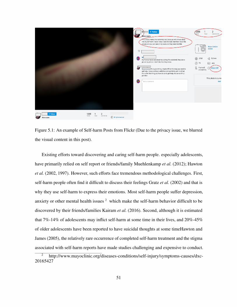
Figure 5.1: An example of Self-harm Posts from Flickr (Due to the privacy issue, we blurred

the visual content in this post).

Existing efforts toward discovering and caring self-harm people. especially adolescents,

have primarily relied on self report or friends/family Muehlenkamp et al. (2012); Hawton

et al. (2002, 1997). However, such efforts face tremendous methodological challenges. First,

self-harm people often find it difficult to discuss their feelings Gratz et al. (2002) and that is

why they use self-harm to express their emotions. Most self-harm people suffer depression,

anxiety or other mental health issues 2 which make the self-harm behavior difficult to be

discovered by their friends/families Kairam et al. (2016). Second, although it is estimated

that 7%-14% of adolescents may inflict self-harm at some time in their lives, and 20%-45%

of older adolescents have been reported to have suicidal thoughts at some timeHawton and

James (2005), the relatively rare occurrence of completed self-harm treatment and the stigma

associated with self-harm reports have made studies challenging and expensive to conduct.2 http://www.mayoclinic.org/diseases-conditions/self-injury/symptoms-causes/dxc-

20165427

51

In addition, extremely long follow-up intervals are typically required for effective study. As

consequence, there are limited research efforts on examining factors associated with the

development of future self-harm thoughts among self-harm-prone people Hawton and James

(2005).

Nowadays people are increasingly using social media platforms, such as Twitter and

Flickr, to share their thoughts and daily activities. The ubiquity of smart phones/tablets has

also made such sharing easy and often instantaneous. As a result, social media provides a

means to capture behavioral attributes that are relevant to an individual’s thinking, mood,

personal and social activities, and so on. In the physical world, people in need of help

on mental issues usually do not know who to ask for help, and they often afraid that their

trust could be betrayed, or they fear that asking for help may lead to more problems for

themselves Houghton and Joinson (2012); Hawton and James (2005). On the other hand,

they could be very active and open on social media when it comes to communication of the

self-harm problem Dyson et al. (2016). Given the enormous volume of social media data

that is created daily, a crucial step to enable the voices of self-harm users to be heard is to

identify self-harm content that could be buried by the vast amount of normal content. A

self-harm post from Flickr is demonstrated in Figure 5.1, which consists of multiple sources

including text, photo, temporal information and meta information of its owner (highlighted

by red circles in Figure 5.1). It appears that, while this problem has not been well-studied

before, the rich information in social media posts may provide unprecedented opportunities

for us to understand self-harm content.

In this chapter, we aim to understand and discover self-harm content in social media.

To achieve this goal, we need to (1) reveal the distinct characteristics of self-harm content

from normal content; and (2) leverage these characteristics to build models to automatically

discover self-harm content. We conduct a comprehensive analysis on self-harm social

media content using textual, owner-related, temporal and visual information, and our major

52

understandings are summarized as: (1) The language of self-harm content has different

structures compared with normal content, and the self-harm content expresses much more

negative sentiments; (2) On average, owners of self-harm content are likely to have more

activities, more social responses and less online friends compared to owners of normal

content; (3) Posting time of self-harm content presents hourly patterns different from those

of normal content, and self-harm content is likely to be posted during the night especially

late night; and (4) Photos in self-harm content are more gloomy and tend to focus on the

salient body image patterns. In summary, the key contributions of this work are:

• Findings: A first and comprehensive study on deliberate self-harm posts on social

media by analyzing more than 1 billion posts on Flickr. We find that the self-harm

users have different patterns on social media platform on: language structure and

usage, online activity, temporal variation and visual content preference.

• Applications: We develop a scalable framework that can discover self-harm content

automatically for both supervised and unsupervised scenarios. The features from our

findings are used to boost the prediction performance. The solution we developed

may be used for public health monitoring and/or directly helping the self-harm users

by providing advices when they post self-harm related content.

5.2 Data Analysis

In this section, we first introduce the dataset for our study and then perform analysis to

understand self-harm-related social media content.

5.2.1 Data

In this investigation, we use data from Flickr which is one of the largest image hosting

websites owned by Yahoo! Inc. In Flickr, users can upload images along with short textual

53

descriptions and tags as a post to share with others. In addition to posting some content,

users can also engage in different interest groups.

Since the user’s contact information is private, in order to avoid user bias, we collect data

from Flickr by checking the visual content of the posts. For our initial data collection, we

adopted an approach used in prior work on examination of eating disorders and anorexia in

social media sites Chancellor et al. (2016). We first examine more than 1 billion public Flickr

posts and select those public posts that annotated with “selfharm” and “selfinjury” tags. It

results 15, 729 posts from 3, 328 distinct users. Then five experienced researchers manually

check 2000 random selected Flickr posts that annotated with self-harm or self-injury tags.

Based on the snowball sampling approach Goodman (1961) during the inspection phase, we

obtain an initial 30 tags of the highest frequencies along with selfharm content 3 . Some

examples include “selfhate”, “suicide”, “depressed”, etc. By removing common tags such

as wounds, scares, cut, we use 15 seed tags as shown in Table 5.1 to further retrieve posts

from Flickr. In this stage, we want collect self-harm data as a complementary of first stage

and it may help to make the bias as small as possible. For example “secretsociety123” and

its variations are widely used by self-harm users Moreno et al. (2016) .

During the process, we collect 383, 614 Flickr posts from 63, 949 users. According to the

findings from prior work on expression of self-harm tendencies in social media, frequently

used tags can be a strong indication that a user has mental issues Chancellor et al. (2016);

Moreno et al. (2016); Yom-Tov et al. (2012). Therefore, to obtain a set of relatively reliable

self-harm users, we remove users who use selfharm related tags in less than five posts 4 ,

resulting in 93, 286 self-harm posts from 20, 495 potential self-harm users. Also, we collect

a set of 19, 720 users from YFCC dataset Thomee et al. (2015), which is a 100 million open

access dataset published by Flickr. We check all the historical posts of these 19, 720 users to3The post contains intentional, direct injuring of body tissue content4If only few self-harm related posts, the user could post them by chance

54

ensure that their posts do not contain any self-harm related content. We refer these users

as normal users. We randomly sample 93, 286 normal posts from these normal users for

the following analysis. For each user, we crawled some statistical information such as the

number of total posts and their user profiles; while for each post, we collected its associated

information including the photos, the textual descriptions, user id of the owner, tags, and

timestamps when the photo was taken and when the post was uploaded. Finally, we evaluate

whether posts in the dataset contain signs of self-harm. Five experienced researchers familiar

with social media and selfharm content evaluate the the correctness of the aforementioned

method. In particular, each researcher randomly checked the posts and found that 95% of

the posts with ’selfharm’ and ’selfinjury’ are correctly identified; while 83% of other tags

are correctly identified. The Cohen kappa coefficient Cohen (1968) is 0.85 which suggests

the high rate of agreement on our data collection method.

eatingdisorder suicide anxious anorexia

mental-

illness

depressed killme depression

selfhate anamia anxious secretesociety123

bruised bulimia bleeding

Table 5.1: A Set of Extended Tags that Help Identify Selfharm Posts.

5.2.2 Understanding Self-harm Content

A typical flickr post contains information from four dimensions including textual, owner,

visual and temporal information. Therefore we analyze self-harm content from these four

perspectives.

55

Self-harm Normal

Linguistic

Nouns 0.158 0.268

Verbs 0.127 0.021

Adjective 0.035 0.084

Adverbs 0.032 0.023

readability 0.41 0.69

Sentiment

Positive 0.06 0.29

Neutral 0.15 0.53

Negative 0.79 0.18

Table 5.2: Textual Analysis (the number stands for the ratio).

Textual Analysis. Linguistic style in texts is related to an individual’s underlying psycho-

logical and cognitive states. It can reveal cues about their social coordination Rude et al.

(2003); De Choudhury et al. (2013); Stirman and Pennebaker (2001); ?); Wang et al. (2015b).

Therefore we compute the distributions of nouns, verbs and adverbs in texts of social media

posts, including the descriptions, titles and comments via the CMUTweetTagger Gimpel

et al. (2011). Also, we calculate readability scores to estimate the complexity and readability

5 of texts. Individuals in self-harm or depression conditions trend to use negative words or

express negative sentiments. Therefore, we compute the sentiment polarities of texts based

on an off-the-shelf manually labeled sentiment lexicon, i.e., MPQA subjective lexicon, for

self-harm and normal content, respectively. The comparison between self-harm and normal

content is shown in Table 5.2.5https://pypi.python.org/pypi/textstat/0.2

56

From Table 5.2, we can observe that self-harm content tends to include more verbs and

adjectives/adverbs than nouns which is very consistent with suicidal word usage Stirman and

Pennebaker (2001). The average readability score of self-harm content is lower than normal

content. The poor linguistic structure usage and language suggest the decreased cognitive

functioning and coherence Petrie and Brook (1992). Further, in addition to less usage of

nouns, we note that a large portion of negative sentiment words are used in self-harm content.

Such observation shows lower interests in objects and things from owners of self-harm

content. It is also well known to appear for suicide users Pestian et al. (2012).

There is no lexicon to understand the usage of self-harm related terms in social media.

Therefore, we build a lexicon of terms that are likely to appear in the texts of self-harm

content. We first extract each term in texts and after post-processing each term, we calculate

its vector via word2vec Mikolov et al. (2013) and cluster all the terms. Thereafter, we

deploy the lexicon to calculate the frequencies of terms in self-harm content. In Table 5.3,

we report sample unigrams from the self-harm lexicon. From Table 5.3, we observe that

most captured expression/symptom terms indicate actions on eating habits, relations with

others and sleeping. These are known to be correlated with sensitive disclosures Houghton

and Joinson (2012). Owners of self-harm content more frequently use action words such as

“help”, “treatments”, and “plans”, and entity words such as “people”, “girls”, and “woman”.

These observations suggest that the self-harm users turn to social media to communicate and

share the experiences with others in order to seek for help or attract attention from others.

Tags are a special type of textual information. We visualize most frequently used tags

in self-harm content as shown in Figure 5.2. Despite the fact that most of the tags are

self-harm related, some tags such as “secret society 123”, “triggerwarning”, and “svv”, are

not explicitly related to self-harm but indicate self-harm content. Similar to eating disorder

Chancellor et al. (2016), self-harm users are likely to use some group tags that are merely

used and can only be understood by themselves. To further verify these tags, we search

57

Theme Token

Expression/ Symptom anamia, anorexia, suicide,

alone, stress, pretty, harms,

stress, pain, angry, addiction,

failure, beautiful, peace, ill-

ness, bulimic, individual, de-

pressive, disorder

Disclosure cuts, help, kill, live, die, plans,

inflicted, treatments, eating,

celebrates, suffer, saveme,

triggers

Relationship/Noun 365days, razor, scar , blood,

arms, wrist, band, knife,

bathroom, bath, tattoo, girls,

woman, boyfriend, people,

body, night

Table 5.3: Unigrams from Self-harm lexicon that Appear with High Frequencies in the

Self-harm Content.

these tags on Instagram and we find each of these tags returns lots of self-harm content 6 .

Owner Analysis. The owners of self-harm content provide crucial context to under-

stand self-harm content. We analyze behaviors of owners from the following perspec-

tives De Choudhury et al. (2013) – volume, proportion of reply, number of favorites, and

number of friends. The volume is defined as the normalized number of posts per day by the6 The retrieving results with the tag “svv”,for example, can be found via https:

//www.instagram.com/explore/tags/svv/

58

https://www.instagram.com/explore/tags/svv/

https://www.instagram.com/explore/tags/svv/

Figure 5.2: Tag Cloud for Self-harm Content

owner. Proportion of reply, number of favorites and number of friends from a user suggest

the level of social interactions with other users. The results are shown in Table 5.4.

Volume % of reply # favorite # friends

Self-harm 7.76 0.15 0.56 296.89

Normal 3.79 0.11 0.23 477.57

Table 5.4: Owner Analysis.

From the table, we first note that the average volume, proportion of reply and number

of favorite of owners with self-harm content are much higher than those of normal content.

High volume indicates that potential self-harm users are likely to be more active than normal

users in social media – they desire the public to hear their voices for help and are likely to

use social media to express the emotion and satisfy self-esteem. High proportion of reply

and number of favorites suggest that content from potential self-harm users are likely to

attract more social responses. In addition, the owners of self-harm content are likely to have

fewer number of friends than normal users.

Temporal Analysis. People with mental issues could suffer from insomnia; and they may

59

(a) Self-harm related Content (b) Normal Content.

Figure 5.3: Temporal Analysis (Y axis represents the normalized portions of data volume of

each hour. X axis is the time segment, which ranges from [0 23]).

present different temporal patterns from normal users in terms of their on-line activities. For

each self-ham post, we first obtain the local time information on when the post is published,

and then count the number of self-harm posts in each hour of a day. The number distributions

of self-harm content over hours of a day is demonstrated in Figure 5.3a. Following a similar

process, the distributions of normal content is shown in Figure 5.3b. Note that the numbers

in the Figures are normalized to (0,1] for better visualization. Note that, in this study, we

cluster the posts by examining the EXIF data from the user upload images, which accurately

records the time when the image is taken.

For normal content, in general, they are more likely to be published during the daytime

instead of night. In particular, (1) fewer number is published later in the night (i.e., post-

midnight) and early in the morning; (2) the number generally increases through the day; and

(3) afternoon and early night show peaks. For self-harm content, a large number is posted

during nights especially late in the night (22pm to 1am), while fewer number in the morning

(7am to 8 am). As mentioned earlier, people with mental issues could suffer from insomnia

and their mood tends to worsen during the night Lustberg and Reynolds (2000).

Visual analysis. Color patterns are important cues to understand the emotion and affective

value of a picture Kairam et al. (2016). Therefore, we first compute a global contrast metric

60

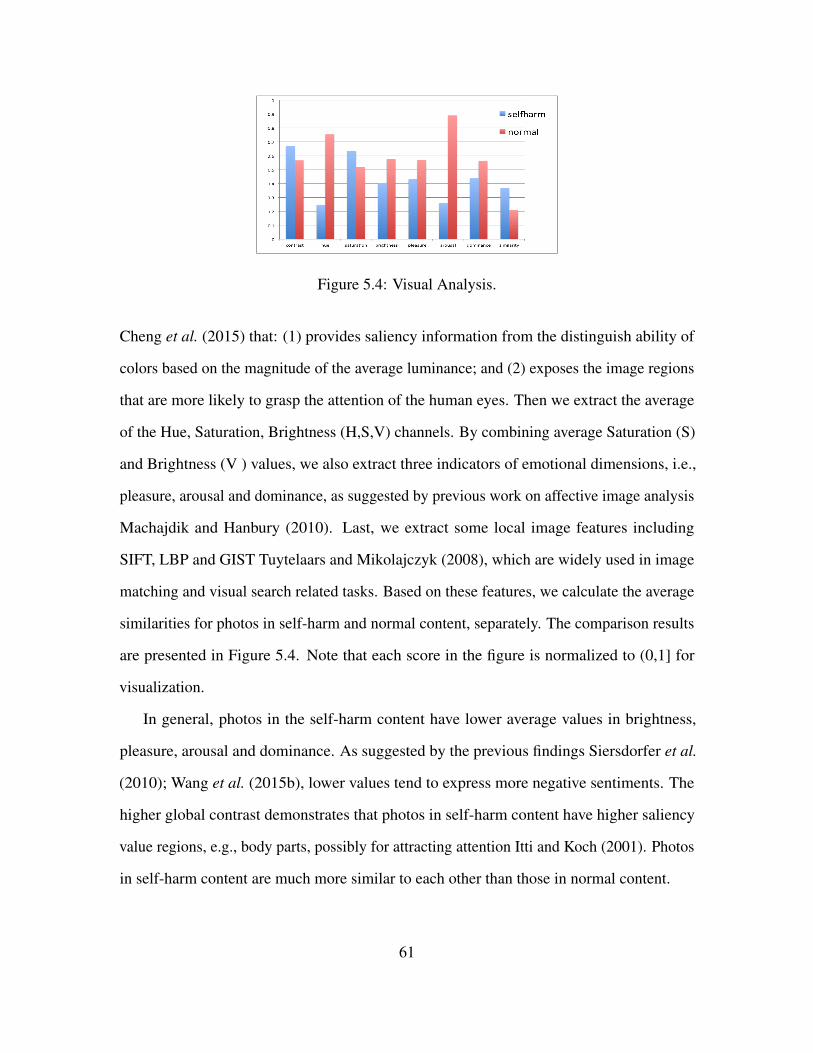
Figure 5.4: Visual Analysis.

Cheng et al. (2015) that: (1) provides saliency information from the distinguish ability of

colors based on the magnitude of the average luminance; and (2) exposes the image regions

that are more likely to grasp the attention of the human eyes. Then we extract the average

of the Hue, Saturation, Brightness (H,S,V) channels. By combining average Saturation (S)

and Brightness (V ) values, we also extract three indicators of emotional dimensions, i.e.,

pleasure, arousal and dominance, as suggested by previous work on affective image analysis

Machajdik and Hanbury (2010). Last, we extract some local image features including

SIFT, LBP and GIST Tuytelaars and Mikolajczyk (2008), which are widely used in image

matching and visual search related tasks. Based on these features, we calculate the average

similarities for photos in self-harm and normal content, separately. The comparison results

are presented in Figure 5.4. Note that each score in the figure is normalized to (0,1] for

visualization.

In general, photos in the self-harm content have lower average values in brightness,

pleasure, arousal and dominance. As suggested by the previous findings Siersdorfer et al.

(2010); Wang et al. (2015b), lower values tend to express more negative sentiments. The

higher global contrast demonstrates that photos in self-harm content have higher saliency

value regions, e.g., body parts, possibly for attracting attention Itti and Koch (2001). Photos

in self-harm content are much more similar to each other than those in normal content.

61

5.3 Self-harm Content Prediction

Our findings in the previous section indicate that potential self-harm users inclined to

express their feelings and emotions in social media, with the purpose of seeking for help and

attention. Social media content is generated at an unprecedented rate, and self-harm content

is likely to be buried by the majority of normal content. Hence a crucial step to help their

voices be heard by the public is to identify self-harm content. A social media post consists

of multiple types of information. As suggested by our previous analysis, each type provides

useful and complementary patterns to characterize self-harm content. Therefore combining

multiple sources could provide a more comprehensive view about social media posts and

has the potential to improve performance.

Typically supervised methodsWang et al. (2016, 2015b) can achieve better performance

because the label information can guide the learning performance. However, most social

media posts are unlabeled and annotating their labels is expensive and time consuming.

Therefore an unsupervised method is also desired. In the following subsections, we will

introduce frameworks to discover self-harm content automatically with and without labeled

data. Before presenting the details, we first introduce the notations and definitions we will

use in the proposed frameworks.

Let P = p1, p2, p3, ..., pn be a set of posts where n is the number of social media

posts. Assume that the set of posts i.e., P , can be represented by m heterogeneous feature

spaces corresponding to m available sources. For Flickr posts in the studied dataset, m

is 4 including textual, owner, temporal and visual sources. Let F = f1, f2, f3, ..., fm

be a set of m feature spaces where fi ∈ Rli denotes the feature space for the i-th source

and li is the number of features in fi. We use X = Xi ∈ Rn×limi=1 as the set of data

matrices and Xi is the matrix representation of the i-th source. Note that for each source,

we extract a set of features based on the previous analysis to augment the set of traditional

62

features because these features cannot be captured by traditional ones but have abilities to

discriminate self-harm content from normal content. For instance, we augment traditional

word embedding features for the textual source by extracting features such as linguistic style

and sentiments according to the textual analysis. More details about the traditional features

can be found in the experiments section.

5.3.1 A Supervised Self-harm Content Prediction Framework

Under the supervised setting, we assume the availability of the label information of

posts in P . Let Y ∈ Rn×2 denote the label information of the n posts in P where Yi1 =

1,Yi2 = 0 and Yi1 = 0,Yi2 = 1 if the post pi is labeled as self-harm and normal

content, respectively. We concatenate Xi ∈ Rn×limi=1 into one matrix X ∈ Rn×∑mi=1 li .

The goal is to learn a function W ∈ R∑mi=1 li×2 that can map X to Y. In this work, the basic

method learns W via solving the following least square problem as:

minW‖XW−Y‖2

F (5.1)

However, after concatenating m feature spaces, the feature dimension of X is∑m

i=1 li

and X could be very high-dimensional. Therefore the basic method in Eq. (5.1) could suffer

from the curse of dimensionality. Meanwhile not all features especially these traditional

features are useful to distinguish self-harm content and normal content. Therefore it is

desired to incorporate feature selection into the framework that is achieved via adding `2,1-

norm regularization on W. With the feature selection component, the supervised self-harm

content prediction framework SCP is to solve the following optimization problem:

minW‖XW−Y‖2

F + α‖W‖2,1 (5.2)

where ‖W‖2,1 ensures that W is sparse in rows, making it particularly suitable for feature

selection. The parameter α controls the sparsity of W.

63

Taking the derivative of the objective function in Eq. (5.2) and setting it to be zero, we

can obtain the closed-form solution for W as:

W = (X>X + αD)−1X>Y (5.3)

where D is a diagonal matrix with its j-th diagonal element as D(j, j) = 12‖W(j,:)‖2 .

5.3.2 An Unsupervised Self-harm Content Prediction Framework

Under the unsupervised scenario?, we do not have label information to guide the learning

process. However, in our studied problem, we have multiple sources that could make it

possible to develop advanced framework for self-harm content prediction. The immediate

challenge is how to capture relations among sources. Since we have the same set of posts

for different sources, hence no matter which source we rely on to cluster posts, we should

obtain similar cluster affiliations. This intuition paves us a way to capture relations among

sources by assuming that all sources share the same cluster affiliations. We assume that

Z ∈ Rn×2 is the shared cluster indicator matrix. Each post belongs to only one cluster where

Z(i, 1) = 1 if pi belongs to the first cluster, otherwise Z(i, 1) = 0. Thus Z should satisfy

the following constraints:

Z(i, :) ∈ 0, 1k , ‖Z(i, :)‖0 = 1, 1 ≤ i ≤ n. (5.4)

where ‖∗‖0 is the vector zero norm, which counts the number of non-zero elements in the

vector.

With the shared cluster indicator matrix Z, we are further allowed to take advantages of

information from multiple sources. First, we assume that similar data instances should have

similar cluster indicators and then Z can be learned by spectral clustering:

minZ

Tr(ZTLiZ) (5.5)

64

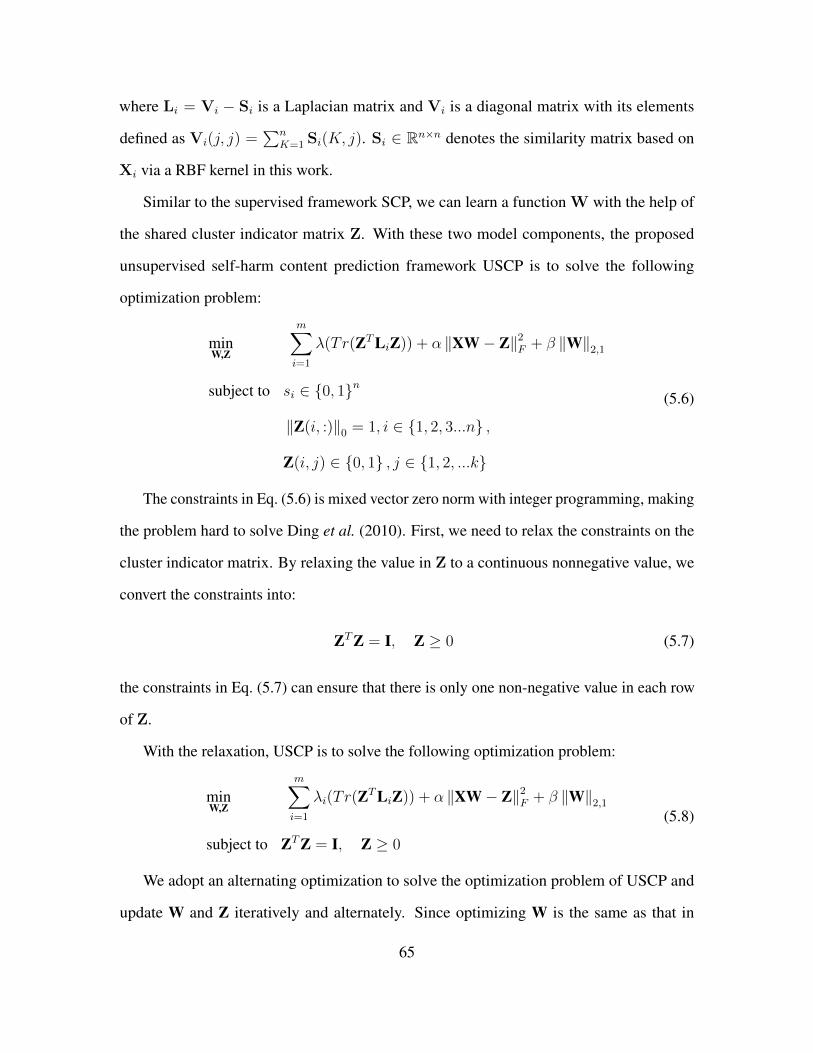
where Li = Vi − Si is a Laplacian matrix and Vi is a diagonal matrix with its elements

defined as Vi(j, j) =∑n

K=1 Si(K, j). Si ∈ Rn×n denotes the similarity matrix based on

Xi via a RBF kernel in this work.

Similar to the supervised framework SCP, we can learn a function W with the help of

the shared cluster indicator matrix Z. With these two model components, the proposed

unsupervised self-harm content prediction framework USCP is to solve the following


minW,Z

m∑i=1

λ(Tr(ZTLiZ)) + α ‖XW− Z‖2F + β ‖W‖2,1

subject to si ∈ 0, 1n

‖Z(i, :)‖0 = 1, i ∈ 1, 2, 3...n ,

Z(i, j) ∈ 0, 1 , j ∈ 1, 2, ...k

(5.6)

The constraints in Eq. (5.6) is mixed vector zero norm with integer programming, making

the problem hard to solve Ding et al. (2010). First, we need to relax the constraints on the

cluster indicator matrix. By relaxing the value in Z to a continuous nonnegative value, we

convert the constraints into:

ZTZ = I, Z ≥ 0 (5.7)

the constraints in Eq. (5.7) can ensure that there is only one non-negative value in each row

of Z.

With the relaxation, USCP is to solve the following optimization problem:

minW,Z

m∑i=1

λi(Tr(ZTLiZ)) + α ‖XW− Z‖2F + β ‖W‖2,1

subject to ZTZ = I, Z ≥ 0

(5.8)

We adopt an alternating optimization to solve the optimization problem of USCP and

update W and Z iteratively and alternately. Since optimizing W is the same as that in

65

Eq. (5.2), we focus on how to update Z in the following part. Fixing W, Z can be obtained

via the following optimization problem:

minZ

m∑i=1

J (Z) = λi(Tr(ZTLiZ)) + α ‖XW− Z‖2F

subject to ZTZ = I, Z ≥ 0

(5.9)

The Lagrangian function of Eq. (5.9) is:

Z = Tr(ZTMZ) + Tr(Γ(ZZ − I)

− Tr(ΛZ) + αTr(−2A>Z + ZTZ)

(5.10)

where we use M =∑m

i=1 λiLi, and A = XW. Γ and Λ are Lagrangian multipliers. Due

to the space limit, we omit the derivations to optimize Eq. (5.10), and more details can be

found in Ding et al. (2010). The provided updating rule for Z is as following:

Z(p, q)← Z(p, q)

√(M−Z + αA+ + ZΓ−)(p, q)

(M+Z + αA− + Z + ZΓ+)(p, q)(5.11)

where X+(p, q) = (|X(p, q)| + X(p, q))/2, X−(p, q) = (−|X(p, q)| + X(p, q))/2, X =

X+ + X−, and Γ = α(ZTA− I)− ZTMZ

With the updating rules of Z and W, we present the detailed algorithm to optimize

Eq. (5.8) in Algorithm 3.

5.4 Experiments

In this section, we conduct experiments which (a) quantify the effectiveness of the

proposed frameworks, and (b) validate the importance of findings from data analysis in

discovering self-harm content. We begin by introducing experimental settings.


Datasets. We perform the evaluation on the dataset used in the data analysis section.

That dataset is balanced with equal size of self-harm and normal content. In reality, there

66

Algorithm 3 Pseudo Code of the USCP1: Input: Xi, λi , α, β

2: Output: the cluster label for each instance

3: for i = 1 to m: do

4: Constructing Laplacian Matrix Li

5: end for

6: while Not converge do

7: Update W by Eq. 5.3

8: Compute A = XW

9: Compute Γ = α(ZTA− I)− ZTMZ

10: Update Z using Eq. (5.11)

11: end while

12: for i = 1 to n: do

13: Max pooling in Z to find the cluster label for each instance

14: end for

could be more normal content than self-harm content. To consider this situation, we sample

850, 000 more normal content from these normal users to construct an imbalanced dataset.

We will assess the performance of self-harm content prediction on both balanced and

imbalanced datasets under supervised and unsupervised settings.

The Finding Features. Our findings in the previous section contain multiple cues. For

each finding, we regard as one feature source. (1) lingual feature (a vector of language

structure ratios and normalized term frequencies in the lexicon) (2) owner feature (a vector

of user information) (3) temporal feature(1-hot vector of time) (4) visual feature (a vector of

averaged saliency value, averaged HSV value, averaged pleasure, arousal and dominance

value, and normalized SIFT,LBP GIST feature 7 )7We use PCA to reduce the feature dimension of concatenated of SIFT,LBP and GIST

67

Traditional Features. In addition to features extracted according to our findings in

the data analysis section, we also follow the state-of-the-art methods to extract traditional

features for textual and visual sources as follows:

• The textual features are extracted from texts in social media posts including descrip-

tions, titles and comments. For each word, we first transform it to a 100-dimension

vector representation using a pre-trained word2vec Mikolov et al. (2013) model. The

final feature representation is the sum of vector representation for all the words.

• The CNN features are the last layer of fully connected layer of the convolutional

neutral network. In our experiment, we use AlexNetKrizhevsky et al. (2012) pre-

trained on ImageNet. The feature size is 4096.

Note that we use both the finding features and traditional features. Thus, the m is set to

be 6 in both SCP and USCP.

5.4.2 Performance Comparisons for Supervised Self-harm Content Prediction

Evaluation metrics: In imbalanced datasets, the accuracy metric under supervised

settings is well known to be misleading De Choudhury et al. (2013). For example, given

the massive data on social media, a trivial classifier that labels all the samples as non

self-harm post can achieve very high accuracy. In self-harm content prediction, we aim to

achieve high precision and recall over self-harm posts defined in terms of the confusion

matrix of a classifier– prescision = tptp+fp

, recall = tptp+fn

and F1 = 2 precision·recallprecision+recall

.

Usually precision and recall are combined into their harmonic mean, the Fmeasure; hence

we will adopt F1-measure as one metric for the performance evaluation. As suggested in

De Choudhury et al. (2013), in some scenarios, we put more emphasis on precision because

features. The final dimension of these three features is 128

68

the most challenging task is to seek for some self-harm posts with high probability, even at

the price of increasing false negatives. Hence, we also report the precision performance.

We compare the proposed supervised framework SCP with the following baselines:

• Word-embedding(WE): We represent each text as the sum of the embedding of the

words it contains; and the prediction is based on a 2 layer convolutional neural

network Kim (2014). This method is one of the state-of-the-arts in textual classification

tasks such as sentiment classification Kim (2014);

• CNN-image: It is one of the state-of-the-art model for image classification Krizhevsky

et al. (2012). We use the same architecture except the softmax layer with self-harm

and normal labels;

• CNN+WE : We combine CNN and word embedding features and the prediction is

based on a linear regression model; and

• SCP-lite: A lite version of SCP which only considers traditional features; while

ignoring features extracted by our findings.

We use 60% of the data as training and the remaining as testing, and parameters are

determined via cross-validation. The comparison results are demonstrated in Table 5.5. We

make the following observations:

• CNN+WE obtains much better performance than Word-embedding and CNN-image.

This result suggests that textual and visual sources contain complementary informa-

tion;

• By incorporating feature selection, SCP-lite performs slightly better than CNN+WE;

and

69

AlgorithmBalanced Imbalanced

F1 precision F1 precision

Word-embedding 57.9% 63.7% 37.9% 30.1 %

CNN-image 61.8% 64.5% 48.6% 44.7%

CNN+WE 68.3% 72.3% 53.1% 46.7%

SCP-lite 68.4% 73.1% 54.5% 47.9%

SCP 72.1% 75.2% 56.7% 49.8%

Table 5.5: Performance Comparisons for Supervised Self-harm Content Prediction.

• SCP outperforms SCP-lite in both balanced and imbalanced datasets. We conduct t-test

on the results and the evidence from t-test indicates the improvement is significant. The

remarkable improvement of SCP over SCP-lite is from the augmented features. These

results demonstrate that (1) traditional features cannot fully cover our findings; and

(2) features extracted based on our findings can boost the performance significantly.

5.4.3 Performance Comparisons for Unsupervised Self-harm Content Prediction

In this subsection, we evaluate the proposed unsupervised framework USCP. Following

the common practiceVinh et al. (2010), we choose NMI and accuracy (ACC) to assess the

clustering performance. The baseline methods are defined as follows:

• CNN+kmeans: We use pre-trained CNN features Krizhevsky et al. (2012) and then

perform kmeans for clustering;

• Word-embedding+kmeans: We use word embedding features and then perform kmeans

for clustering;

• CNN+WE+kmeans: We combine CNN and word embedding features and then per-

70

AlgorithmBalanced Imbalanced

NMI ACC NMI ACC

CNN+kmean 0.36 47.3% 0.15 15.3%

WE+kmeans 0.08 33.8% 0.04 10.3 %

CNN+WE+kmeans 0.46 56.2% 0.23 23.1%

USCP-lite 0.48 58.3% 0.26 24.3%

USCP 0.51 61.2% 0.31 27.4%

Table 5.6: Performance Comparisons for Unsupervised Self-harm Content Prediction.

form kmeans for clustering; and

• USCP-lite: It is a variant of the proposed framework USCP that ignores features

extracted according to our findings.

Since kmeans can only obtain local optimal solutions, we repeat experiments for these

baselines based on kmeans 10 times and report the average performance. The performance

comparisons are shown in Table 5.6. From the table, we make similar observations as

the supervised self-harm content prediction experiments: (1) textual and visual sources

are complementary to each other; and (2) the features extracted based on our findings can

significantly improve the prediction performance under the unsupervised setting.

Parameter Analysis. There is one important parameter α for the proposed unsupervised

framework USCP. The parameter controls the contribution of the model component capturing

relations among sources. Next we study the impact of the component on the proposed

framework by investigating how the performance changes with different values of α. We

vary α as 0.001, 0.1, 0.2, 0.3, 0.4, 0.5, 0.6, 0.7, 0.8, 0.9,

10. The performance variance w.r.t. α in terms of ACC is shown in Figure 5.5. Note

that we do not show performance in terms of NMI since we make similar observations. In

71

general, with the increase of α, the performance tends to first increase and then decrease.

In particular, (1) the performance increases a lot when α is increased from 0.001 to 0.1

that indicates the importance of capturing relations among sources; (2) when α in certain

regions, the performance is relatively stable that can ease the process of parameter selection

in practice; and (3) when α increases to 10, the performance degrades significantly since the

term capturing relations among sources will dominate the learning process that will lead to

overfitting.

(a) Balanced Data

(b) Imbalanced Data

Figure 5.5: Parameter Analysis for Unsupervised Framework USCP.

5.5 Summary

In this paper, we aim to understand and discover self-harm content in social media since

social media has become increasingly popular for self-harm users to discuss their problems.

We conducted the first comprehensive analysis on self-harm content with data from the

social media site Flickr. Our analysis suggests that characteristics of self-harm content are

72

different from those of normal content, from textual, owner, temporal and visual perspectives.

These findings have potentials to help us distinguish self-harm content from others, and

we have thus developed frameworks by incorporating these findings to discover self-harm

content automatically. Empirical results demonstrate that (1) the proposed frameworks can

accurately identify self-harm content under both supervised and unsupervised settings; and

(2) our findings play an important role in boosting the prediction performance.

There are several interesting directions for further investigations. First, we would like

to extend our proposed models to the semi-supervised setting because in reality we can

obtain a small amount of labeled data but need to deal with a large amount of unlabeled data

Wang et al. (2016). Second, while the findings on self-harm content motivated us to develop

approaches for identifying posts related to self-harm, it is interesting to further understand

how such post-level analysis can be extended to automatically identify the self-harm users.

Third, social networks are pervasively available in social media and it could be promising to

study the impact of peer influence on self-harm user behaviors and leverage social networks

to improve predictive tasks in self-harm research.

73

Chapter 6

BEYOND SENTIMENT ANALYSIS: A GENERAL APPROACH FOR MULTI-LABEL

IMAGE LEARNING

Image classification, which tries to assign an image label to to a given image and one

example is shown in Figure 6.1 1 , is a core computer vision problem and has been well

studied in past decades. In this chapter, I introduce a general multi-label image classification

approach that derives from the sentiment analysis framework in previous chapters. The

motivation behind our method is that sentiment analysis is a special application of a general

image classification problem. It is possible to extend the method for sentiment analysis for a

general image content analysis, i.e., image classification. In this chapter, I will firstly review

the background of this problem that why label relationship is essential. Then I proposed a

unified label relationship modelling method for multi-label image classification . Real-world

Flickr and shopping datasets are used to evaluate the performance of the proposed method

by comparing with the state-of-the-art baseline methods.

6.1 Introduction

The increasing popularity of social media generates massive data at an unprecedented

rate. The ever-growing number of images has brought new challenges for efficient and

effective image analysis tasks, such as image classification, annotation and image ranking.

Based on the types of labels, we can roughly divide the supervised vision tasks into two

categories – pointwise label based approaches and pairwise label based approaches. Point-

wise approaches adopt pointwise labels such as image categories or tags as training targets

Jiang et al. (2011); Toderici et al. (2010); Chen et al. (2013); Sigurbjornsson and Van Zwol1http://cs231n.github.io/classification/

74

http://cs231n.github.io/classification/

Figure 6.1: An Example of Image Classification and Image Representation

(2008); Jannach et al. (2010); Wang et al. (2015c,d). Class labels in classification often

capture high-level image content, while tags in tag annotation are likely to describe a piece

of information in the image, such as “high heel, buckle, leather” in a shoe image. In Wang

et al. (2009), these two tasks are considered together because the labels and tags may have

some relations in an image. Recently, due to the semantic gap between low-level image

features and high-level image concepts, human nameable visual attributes are proposed

to solve the vision tasksFarhadi et al. (2009); Lampert et al. (2009); Berg et al. (2010);

Kumar et al. (2009). However, for a large variety of attributes, the pointwise binary setting

is restrictive and unnatural. For example, it is very difficult to assign or not assign “sporty”

to the middle car in Figure 6.2 because different people have different opinions. Thus,

pairwise approaches Parikh and Grauman (2011); Kovashka and Grauman (2013a,b) have

been proposed, which aim to learn a ranking function to predict the attribute strength for

images. For example, in Figure 6.2. most of the people would agree that the middle car is

more “sporty” than the left one and less “sporty” than the right one

Pointwise and pairwise labels have their own advantages as well as limitations in terms

of labeling complexity and representational capability. Labeling complexity: given 10

75

Figure 6.2: An Illustrative Example of Poinwise Labels and Pairwise Labels. (Pointwise

label “4 door” is better than the pairwise label to describe presence of 4 door in a car, while

“sporty” is better to use pairwise label to describe the car style, as the right is more sporty

than the left. For example it is hard to label the middle (we ask 10 human viewer – 40%

agree with the non sporty and 60% agree with sporty, but 100% agree with middle one is

more sporty than the left one and less sporty than right one)).

images, we only need 10 sets of class categories/tags. However, we need to label at least 45

image pairs to capture the overall ordering information. (Although the ranking relation is

considered as transferable, e.g. A B&B C ⇒ A C). Representational capability:

pointwise labels such as tags/class labels imply the presence of content properties such

as whether a shoe is made of leather, contains a heel, buckle, etc. While pairwise labels

capture the relations in a same property, e.g., A has a higher heel than B. Solely relying

on pointwise labels may cause ambiguity or produce noisy data for the models as in the

example of assigning “sporty” to the middle car in Figure 6.2, while only using pairwise

labels may also cause problems when the images have very similar properties.

As pointwise and pairwise labels encapsulate information of different types and may

have different benefits for vision problems and recommendation systemsWang et al. (2015a)

, we develop a new framework for fusing different types of training data by capturing their

underlying relations. For example, in Figure 6.3, the tags, “leather, cognac, lace up” may

suggest the left shoe with a higher score on the “formal” attribute, while the “high heel”

may indicate the right shoe with a lower score on the “comfort” attribute. On the other

hand, the higher score on “formal” and “comfort” with tag “Oxford” could help label the

76

left image as “shoe” and enable the rare tag annotation such as “wingtip”. To the best of

our knowledge, there are only a few recent works that fused pointwise and piarwise labels

Sculley (2010); Chen et al. (2015). However, they simply combined regression and ranking

in the loss functions for ranking tasks and totally ignored the relations between pointwise

labels and pairwise labels.

In this paper, we investigate the problem of fusing pointwise and pairwise labels by

exploiting their underlying relations for joint pointwise label prediction such as, image

classification and annotation, and pairwise label prediction, e.g., relative ranking. We derive

a unified bipartite graph model to capture the underlying relations among two types of

labels. Since traditional approaches cannot take advantages of relations among pointwise

and pairwise labels, we proceed to study two fundamental problems: (1) how to capture

relations between pointwise and pairwise labels mathematically; and (2) how to make use

of the relations for jointly addressing vision tasks. These two problems are tackled by the

propose framework PPP and our contributions are summarized as follows:

• We provide a principled approach to modeling relations between pointwise and

pairwise labels;

• we propose a novel joint framework PPP, which can predict both pointwise and

pairwise labels for images simultaneously; and

• We conduct experiments on various benchmark datasets to understand the working of

the proposed framework PPP.

In the remaining of the paper, we first give a formal problem definition and basic model

in Section 2. Then the proposed framework and an optimization method for model learning

is presented in Section 3. Experiments and results are demonstrated in Section 4, with

further discussion in section 5.

77

Figure 6.3: The Demonstration of Capturing the Relations between Pointwise Label and

Pairwise Label via Bipartite Graph (For example, the attribute “formal” with tags “leather,

lace up, congnac” will form a group via the upper bipartite graph, while label “sandal” with

attribute “less formal” and tags “high heel, party” will form a group via the lower bipartite

graph).

6.2 The Proposed Method

Before detailing the proposed framework, we first introduce notations used in this paper.

We use X ∈ Rn×d to denote a set of images in the database where n is the number of images

and d is the number of features. Note that there are various ways to extract features such

as SIFT, Gist or the features learned via deep learning frameworks. Let Yt ∈ Rn×c1 and

Yc ∈ Rn×c3 be the data-tag and data-label matrices which represent the pointwise labels.

Y(i, j) = 1 if the i-th image is annotated/classified with j-th tag/class label, Y(i, j) = 0

otherwise. Given a fixed training set D, a candidate pair set P can be drawn. The pair

set implied by the fixed training set D uses pairwise labels. In the proposed framework,

78

given a pair of images < a, b > on the attribute q, if ya yb, then a has a positive attribute

score y(a, q, 1) = |ya − yb|, and a negative score y(a, q, 2) = 0; while b has a positive

attribute y(b, q, 1) = 0, and a negative score y(b, q, 2) = |ya − yb|. Thus, the pairwise label

is defined as Yr ∈ Rm×c2 , where m is the number of pairs drawn from training samples and

c2 = 2q where q is the number of attributes. For example, let < a, b > be the first pair, the

pairwise label Yr(1, 2(q−1) + 1) represents how likely the ya yb and Yr(1, 2(q−1) + 2)

represents how likely ya ≺ yb on attribute q.

6.2.1 Baseline Models

In our framework, pointwise labels are considered for classification and annotation

tasks. For classification, we assume that there is a linear classifier Wc ∈ Rd×c3 to map X

to the pointwise label Yc as Yc = XWc. Wc can be obtained by solving the following


minWc

Ω(Wc) + L(Wc,Yc, D) (6.1)

where L() is a loss function and Ω is a regularization penalty to avoid overfitting, D is the

training sample set. Here we employ least square for loss function L.

For tag annotation, we also assume that there is a linear function Wt ∈ Rd×c1 which

captures the relation between data X and pointwise label Yt as Yt = XWt. Similarly, the

optimization problem to learn Wt is:

minWt

Ω(Wt) + L(Wt,Yt, D) (6.2)

For pairwise label based approaches, a simple and successful approach to utilizing the

pairwise label is Rank SVM, whose goal is to learn a model W that achieves little loss

over a set of previously unseen data, using a prediction function. Similar to RankSVM, in

our framework, the original distribution of training examples are expanded into a set of

candidate pairs and the learning process is over a set of pairwise feature vectors as:

79

minWL(W,Yr, P ) + Ω(Wr) (6.3)

where P is a set of training pairs. The loss function L is defined over the pairwise difference

vector x:

L(W,Yr, P ) =∑

((a,ya,qa),(b,yb,qb))∈P

l(t(ya − yb), f(w, a− b)) (6.4)

where the transformation function t(y) transforms the difference of the labels Sculley (2010).

In our framework, the transformation function is defined as t(y) = sign(y).

Note that one may form a unified model by simply adding all the above objective

functions together. Such an approach would still essentially treat the component models as

independent tasks (albeit trade-off among them might be considered via weighting), since

no explicit relations among them are considered.

6.2.2 Capturing Relations between Poinwise and Pairwise Labels

In the previous subsection, we defined three tasks that use pointwise and pairwise labels

separately. Capturing the relations between pointwise and pairwise labels can further pave

a way for us to develop a joint framework that enables interaction between classification,

annotation and ranking simultaneously.

First, the relations between attributes and tags can be denoted as a bipartite graph as

shown in Figure 6.3. We assume that B ∈ Rc2×c1 is the adjacency matrix of the graph

where B(i, j) = 1 if both the i-th tag and the j-th attribute co-occur in the same image

and B(i, j) = 0 otherwise. Note that in this paper, we do not consider the concurrence

frequencies of tags and attributes and we would like to leave it as one future work. From

the bipartite graph, we can identify groups of attributes and tags where attributes and tags

in the same group could share similar properties such as semantical meanings. A feature

80

X(:, i) should be either relevant or irrelevant to the attributes and tags in the same group.

For example, Wr(i, j) indicates the effect of the i-th feature on predicting the j-th attribute;

while Wt(i, k) denotes the impact of the i-th feature on the k-th tag. Therefore we can

impose constraints on Wt and Wr together, which are derived from group information on

the bipartite graph, to capture relations between attributes and tags.

We can adopt any community detection algorithms to identify groups from the bipartite

graph. In this paper, we use a very simple way to extract groups from the bipartite graph –

for the j-th attribute, we consider the tags that connect to that attribute in the bipartite graph

as a group, i.e., B(i, j) = 1. Note that a tag may connect to several attributes thus extracted

groups via the aforementioned process have overlaps. Assume that G is the set of groups

we detect from the attribute-tag bipartite graph and we propose to minimize the following

term to capture relations between attributes and tags as:

ΩG(Wt,r) =d∑i=1

∑g∈G

αg∥∥wi

g

∥∥2

(6.5)

where Wt,r = [Wt,Wr] and αg is the confidence of the group g and wig is a vector concate-

nating Wt,r(i, j)j∈g. For example, if g = 1, 5, 9, wig = [Wt,r(i, 1),Wt,r(i, 5),Wt,r(i, 9)]

. Next we discuss the inner workings of Eq. (6.5). Let us check terms in Eq. (6.5) related

to a specific group g,∑d

i=1

∥∥wig

∥∥2, which is equal to adding a `1 norm on the vector

g = [w1g,w

2g, . . . ,w

dg ], i.e., ‖g‖1. That ensures a sparse solution of g; in other words, some

elements of g could be zero. If gi = 0 or ‖w2g‖2 = 0, the effects of the i-th feature on both

the attribute and tags in the group g are eliminated simultaneously.

Similarly, we build the bipartite graph to capture the underlying relations for the attributes

and class labels. In Wang et al. (2009), it was suggested that the co-occurrence of tags

and labels should also be considered. Thus, we build a mixture bipartite graph to extract

the group information between class labels, tags, and attributes. The group regularization

81

ΩG2(Wt,r,c) is similar to Eq. 6.5 and illustration is shown in Figure 6.3, where a tag or an

attribute will connect to the class label if they are associated with each other. Note that a

group extracted from Figure 6.3 could include a class label, a set of attributes and a set of

tags.

6.2.3 The Proposed Framework

With the model component to exploit the bipartite graph structures, the proposed frame-

work is to solve the following optimization problem:

minWL(Wc,Yc, D) + L(Wt,Yt, D) + L(Wr,Yr, P )

+ λ(‖Wc‖2F + ‖Wt‖2

F + ‖Wr‖2F )

+ αΩG1(Wt,r) + βΩG2(Wt,r,c)

(6.6)

In Eq. 6.6, the first six term is from the basic models to predict the class label, tags and

ranking order. The seventh and eighth term are to capture the overlapped structure of the

output, which is controlled by α and β respectively. The group regularization is defined as

blow:

ΩG(Z) =∑i∈G

‖Zg‖2 =d∑i=1

∑i∈G

‖zig‖2 (6.7)

6.3 An Optimization Method for PPP

Since the group structures are overlapped, directly optimizing the objective function is

difficult. We propose to use Alternating Direction Method of Multiplier (ADMM)(Yogatama

and Smith (2014); Boyd et al. (2011)) to optimize the objective function. We first in-

troduce two auxiliary variables P = [Wt,Wr]M1 and Q = [Wt,Wr,Wc]M2. M1 ∈

0, 1(c1+c2)×c2(c1+c2) is defined as: if i− th tag connects to the jth attribute then M1(i, (c1 +

c2)(j−1)+ i) = 1, otherwise it is zero. The definition of M2 ∈ 0, 1(c1+c2+c3)×c3(c1+c2+c3)

is similar to M1. With these two variable, solving the overlapped group lasso on W is

82

transfered to the non-overlapped group lasso on P and Q, respectively. Therefore, the

objective function becomes:

minW,P,Q

L(Wc, D) + L(Wt, D) + L(Wr, P )

+ αΩG(P) + βΩG2(Q)

+ λ(‖Wc‖2F + ‖Wt‖2

F + ‖Wr‖2F )

s.t.P = [Wt,Wr]M1; Q = [Wt,Wr,Wc]M2;

(6.8)

which can be solved by the following ADMM problem:

minW,P,Q

L(Wc,Yc, D) + L(Wt,Yt, D) + L(Wr,Yr, P )

+ λ(‖Wc‖2F + ‖Wt‖2

F + ‖Wr‖2F ) + αΩG(P)

+ βΩG2(Q) + 〈Λ1,P− [Wt,Wr]M1〉

+ 〈Λ2,Q− [Wt,Wr,Wc]M2〉

+µ

2‖P− [Wt,Wr]M1‖2

F

+µ

2‖Q− [Wt,Wr,Wc]M2‖2

F

(6.9)

where Λ is the Lagrangian multiplier and µ is a scaler to control the penalty for the violation

of equality constrains P = [Wt,Wr]M1 and Q = [Wt,Wr,Wc]M2. Noting that the loss

function L has lots of choices, we use the least square loss function in this paper.

83

6.3.1 Updating W

To update W, we fix the other variable except W and remove terms that are irrelevant

to W. Then the Eq. 6.9 becomes:

minW

∑x∈D

‖xWt − yt‖22 +

∑x∈D

‖xWc − yc‖22

+∑

xi,xj∈P

‖(xi − xj)Wr − yr‖22

+ λ(‖Wc‖2F + ‖Wt‖2

F + ‖Wr‖2F )

+µ

2‖(P +

1

µΛ1)− [Wt,Wr]M1‖2

F

+µ

2‖(Q +

1

µΛ2)− [Wt,Wr,Wc]M2‖2

F

(6.10)

Setting the derivative of Eq. 6.10 w.r.t Wt to 0, we get:

XTDXDWt + λWt + Wt(M

t1M

tT1 + Mt

2MtT2 )

= XTY +µ

2[(P +

1

µΛ1)Mt

1 + (Q +1

µΛ2)Mt

2](6.11)

where Mt1 is the part of M1 corresponding to Wt. Directly getting the close form solution

from Eq. 6.11 is intractable. On the other hand XTDXD + 1

2λI and Mt

1MtT1 +Mt

2MtT2 + 1

2λI

are symmetric and positive definite. Thus, we employ eigen decomposition for each of them:

XTDXD +

1

2λI = U1Σ1U

T1

Mt1M

tT1 + Mt

2MtT2 +

1

2λI = U2Σ2U

T2

(6.12)

whereU1,U2 are eigen vectors and Σ1,Σ2 are diagonal matrices with eigen value on the

diagonal. Substituting Eq. 6.12 into Eq. 6.11:

U1Σ1UT1 Wt+WtU2Σ2U

T2 = XT

DYt +µ

2(P +

1

µΛ1)Mt

1

+µ

2(Q +

1

µΛ2)Mt

2

(6.13)

84

Multiplying UT1 and U2 from left to right on both sides, and letting Wt = UT

1 WtU2

and Zt = UT1 [XT

DYt + µ2[(P + 1

µΛ1)Mt

1 + (Q + 1µΛ2)Mt

2]]U2 , we can obtain:

Σ1Wt + WtΣ2 = Zt (6.14)

Then, we can get Wt and Wt as:

Wt(s, t) =Zt(s, t)

σs1 + σt2(6.15)

Wt = U1WtUT2 (6.16)

Similarly, setting the derivative of Eq. 6.10 w.r.t Wc to zero and apply the eigen decom-

position, we have the closed form solution of Wc:

Wc(s, t) =Zc

σs1 + σt3(6.17)

Wc = U1WcUT3 (6.18)

where Zc = UT3 [XT

DYc + µ2(Q + 1

µΛ2)]Mc

2 and U3, σ3 are the eigen vector and eigen value

for the symmetric and positive definite matrix Mc2M

cT2 + 1

2λI.

Noting that for Wr, which input is data pairs, we can use the same learning process

by using the transform label function mentioned above. For example, we regard the pair

difference as one data sample for XP and use the positive and negative label for label

transformation. Setting the Eq. 6.10 w.r.t Wr to zero, we can obtain:

XTPXPWr + λWr + Wr(M

r1M

rT1 + Mr

2MrT2 )

= XTPYr +

µ

2[(P +

1

µΛ1)Mr

1 + (Q +1

µΛ2)Mr

2](6.19)

Similar to Wc, with eigen decomposition, we can get the closed form solution for Wr

as:

Wr(s, t) =Zr

σs4 + σt5(6.20)

Wr = U4WrUT5 (6.21)

85

where Zr = U4[XTPYr+ µ

2[(P+ 1

µΛ1)Mr

1 +(Q+ 1µΛ2)Mr

2]UT5 , U4, σ4 are eigen vector and

eigen values for XTPXP + 1

2λI, and U5, σ5 are eigen vector and eigen value for Mr

1MrT1 +

Mr2M

rT2 + 1

2λI.

6.3.2 Updating P

After removing terms that are irrelevant to P, Eq. 6.9 becomes:

minP

µ

2‖P− [Wt,Wr]M1‖2

F + αΩG(P) + Tr(Λ1P) (6.22)

When applied to the collection of group for the parameters, P, ΩG(P)) no longer have

overlapping groups. We denote j− th group in i-th row as Pi,j = P(i, (c1 + c2)(j− 1) + 1 :

(c1 + c2)j). Hence, we can solve the problem separately for each row of P within one group

by the following optimization:

minPi,j

α‖Pi,j‖22 +

µ

2‖Pi,j − (([Wc,Wr]M1)i,j −

Λ1ij

µ)‖2F (6.23)

Note that Eq. 6.23 is the proximal operator Yuan et al. (2011) of 1µ(P )i,j applied to

(([Wc,Wr]M1)i,j − Λ1ij

µ). Let ZP

i,j = ([Wc,Wr]M1)i,j − Λ1ij

µ. The solution by applying

the proximal operator used in non-overlapping group lasso to each sub-vector is:

Pi,j = prox(ZPi,j) =

0 if‖ZP

i,j‖2 ≤ αµ

‖ZPi,j‖2−αµ

‖ZPi,j‖2

ZPi,j otherwise

(6.24)

6.3.3 Updating Q

Similar to P, we can update Q by proximal operator used in non-overlapping group

lasso to each sub-vector of Q:

Qi,j = prox(ZQi,j) =

0 if‖ZQ

i,j‖2 ≤ βµ

‖ZQi,j‖2−βµ

‖ZQi,j‖2

ZQi,j otherwise

(6.25)

where Qij = Q(i, (c1+c2+c3)(j−1)+1 : (c1+c2+c3)j) and ZQi,j = ([Wt,Wr,Wc]M2)i,j−

Λi,jµ

86

6.3.4 Updating Λ1,Λ2 and µ

After updating the variables, we now need to update the ADMM parameters. According

to Boyd et al. (2011), they are updated as follows:

Λ1 = Λ1 + µ(P− [Wt,Wr]M1) (6.26)

Λ2 = Λ2 + µ(Q− [Wt,Wr,Wc]M2) (6.27)

µ = min(ρµ, µmax) (6.28)

Here, ρ > 0 is a parameter to control the convergence speed and µmax is a large number to

prevent µ from becoming too large.

With these updating rules, the optimization method for our proposed method is summa-

rized in Algorithm 4

6.3.5 Convergence Analysis

Since the sub-problems are convex for P and Q, respectively, Algorithm 1 is guaranteed

to converge because they satisfy the two assumptions required by ADMM. The proof of the

convergence can be found in Boyd et al. (2011). Specially, Algorithm 1 has dual variable

convergence. Our empirical results show that our algorithm often converges within 100

iterations for all the datasets we used for evaluation.

6.3.6 Time Complexity Analysis

The main computation cost for W involves the eigen decomposition on XTX + 12βI,

while other terms that involve eigen decomposition is very fast because the feature dimension

of MMT is small. The time complexity for eigen decomposition is O(d3). However, in

Algorithm 1 the eigen decomposition is only computed once before the loop and dimension

reduction algorithm can be employed to reduce image feature dimensions d. The computa-

tion cost for Z is O(nd2) due to the sparsity of M. The computation of P depends on the

87

Algorithm 4 The Algorithm for the FramworkInput: XD ∈ RN×d and XP ∈ Rm×d and corresponding label Yt,Yc and Yr

Output: c1 tags label c2 relative score and c3

class label for each data instance

1: Initialize random Sample training set D and drawn random pair set P from D.

2: Setting µ = 10−3, ρ = 1.1, µmax = 108 and building M1 and M2

3: Precompute the eigen decomposition

4: repeat

5: Calculate Wt, Wt and Wr

6: Update Wt,Wr and Wc by Eq. 6.16, Eq. 6.21, and Eq. 6.18, respectively.

7: Calculate ZP and ZQ

8: Update P and Q

9: Update Λ1, Λ2 and µ

10: until convergence

11: Using max pooling for testing use XW to predict tags, relative relation and labels.

proximal method within each group. Since there are c2 groups which have the group size

c1 + c2 for each feature dimension, the total computation cost for P is O(dc2(c1 + c2)) and

it is similar for Q. It is worth noting that P and Q can be computed in parallel for each

feature dimension.

6.4 Experiment

In this section, we conduct experiments to evaluate the effectiveness of PPP. After

introducing datasets and experimental settings, we compare PPP with the state-of-the-art

methods of tag prediction, classification and ranking.

88

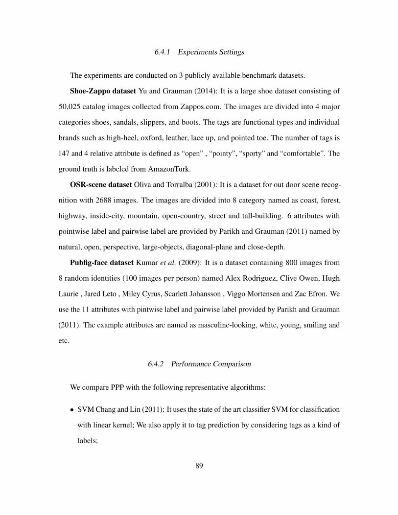
6.4.1 Experiments Settings

The experiments are conducted on 3 publicly available benchmark datasets.

Shoe-Zappo dataset Yu and Grauman (2014): It is a large shoe dataset consisting of

50,025 catalog images collected from Zappos.com. The images are divided into 4 major

categories shoes, sandals, slippers, and boots. The tags are functional types and individual

brands such as high-heel, oxford, leather, lace up, and pointed toe. The number of tags is

147 and 4 relative attribute is defined as “open” , “pointy”, “sporty” and “comfortable”. The

ground truth is labeled from AmazonTurk.

OSR-scene dataset Oliva and Torralba (2001): It is a dataset for out door scene recog-

nition with 2688 images. The images are divided into 8 category named as coast, forest,

highway, inside-city, mountain, open-country, street and tall-building. 6 attributes with

pointwise label and pairwise label are provided by Parikh and Grauman (2011) named by

natural, open, perspective, large-objects, diagonal-plane and close-depth.

Pubfig-face dataset Kumar et al. (2009): It is a dataset containing 800 images from

8 random identities (100 images per person) named Alex Rodriguez, Clive Owen, Hugh

Laurie , Jared Leto , Miley Cyrus, Scarlett Johansson , Viggo Mortensen and Zac Efron. We

use the 11 attributes with pintwise label and pairwise label provided by Parikh and Grauman

(2011). The example attributes are named as masculine-looking, white, young, smiling and

etc.

6.4.2 Performance Comparison

We compare PPP with the following representative algorithms:

• SVM Chang and Lin (2011): It uses the state of the art classifier SVM for classification

with linear kernel; We also apply it to tag prediction by considering tags as a kind of

labels;

89

• GLasso Yuan and Lin (2006): The original framework of group lasso is to handle

high-dimensional and multi-class data. To extend it for joint classification and tag

prediction, we also consider tags as a kind of labels and apply GLasso to learn the

mapping of features to tags and label. Note that it does not make use of the pointwise

and pairwise label bipartite graph. We use the implementation in Liu et al. (????);

• sLDA Wang et al. (2009): It is a joint framework based on topic models, which learns

both class labels and annotations given latent topics;

• LS Ji et al. (2008): A multi-label classification method that exploits the label correla-

tion information. To apply LS for joint classification and tag prediction, we consider

tags as a kind of labels and use tag and label relations to replace the label correlation

in the original model; and

• FT Chen et al. (2013): It is one of the state-of-the art annotation method which

is based on linear mapping and co-regularized joint optimization. To apply it for

classification, we consider labels as tags to annotate; and

• RD: It predicts labels and tags by randomly guessing.

• MultiRank Chen et al. (2014): It is a ranking method based on the assumption that the

correlation exists between attributes, where the ranking function learns all attributes

together via multi task learning framework.

• RA Parikh and Grauman (2011): It is the method for image ranking based on relative

attributes.

Note that for all the baseline methods, none of them can utilize both pointwise and

pairwise labels. Although we get the performance of the proposed framework by jointly

predicting both pointwise and pairwise labels, we present our results for each task separately

90

Table 6.1: Performance Comparison for Classification (The number after each dataset means

the class label number).

Method Zappos(4) OSR(8) Pubfig (8)

SVM 67.41 % 42.21 % 50.77%

GLasso 78.31% 50.11% 59.13%

sLDA 74.32% 46.33% 56.21%

LS 84.46% 61.22% 66.56%

FT 84.69% 59.38% 67.45%

RD 25.01% 12.51% 12.50%

PPP 89.39% 62.33% 74.95%

for a clear comparison. Moreover, we could use more advanced features, e.g., CNN feature,

however, to compare with other methods fairly, we adopt the original feature provided by

each datasets, which can easily show the performance gain from the proposed model.

6.4.3 Pointwise label Prediction

For pointwise label prediction, our method is compared with SVM, Glasso, sLDA,

LS, FT, and RD. For all the baseline methods with parameters, we use cross validation to

determine their values. For the Shoe dataset, we use the same data split and features (990

gist and color features) in Yu and Grauman (2014). It contains 11102 data samples for

training and 2400 data sample for testing. For OSR and Pubfig, we use the same data split

and features in Parikh and Grauman (2011).

Since OSR and Pubfig contain a small number of attributes, we leave one random-picked

attribute for pairwise prediction and use the rest for tag annotation. Especially, to evaluate

the performance of tag annotation, we rank all the tags based on their relevant scores

91

Table 6.2: Performance Comparison in terms of Tag Recommendation.

MethodZappo OSR Pubfig

AP@3 AP@5 AP@1 AP@3 AP@1 AP@5

SVM 50.57% 38.53% 68.51% 60.12% 46.21% 34.12%

GLasso 64.34% 55.37% 87.11% 80.87% 90.12% 86.41%

sLDA 62.57% 51.63% 90.15% 84.78% 91.12% 84.17%

LS 74.76% 61.85% 94.19% 92.75% 93.71% 91.91%

FT 67.37% 51.98% 98.62% 92.22% 92.45% 90.16%

RD 1.44% 1.44% 20.00% 20.01% 10.01% 10.01%

PPP 77.10% 62.95% 96.69% 90.14% 94.48% 92.71%

and return the top K ranked tags. We use the average precision AP@K as the evaluation

metric which has been widely used in the literature Chen et al. (2013); Wang et al. (2009).

Meanwhile since the data samples are balanced, we use accuracy as the metric to evaluate

the classification performance. The comparison results are shown in Table 6.1 and Table 6.2

for classification and tag annotation, respectively. We repeat 10 times for the training-testing

process and report the average performance.

From the tables, we make the following observations:

• The proposed method that utilizes pairwise labels to predict pointwise labels tends

to outperform the methods which solely rely on pointwise labels. These results

support that (1) pairwise attributes can provide evidence for the pointwise label

prediction; especially for the Pubfig dataset that contains 8 label classes, our method

utilizes information from pairwise attributes significantly improve the classification

performance. (2) The performance of tag predictionAP@K indicates that the pairwise

attributes contain important information for tag prediction;

92

• Our method with model components to capture relations between pairwise and point-

wise labels outperforms those without. For example, compared to GLasso, the

proposed framework, modeling the relations via the bipartite graph, gains remarkable

performance improvement for both classification and tag prediction; and

• Most of the time, the proposed framework PPP performs the best among all the

baselines, which demonstrates the effectiveness of the proposed algorithm. There are

two major reasons. First, PPP jointly performs pointwise and pairwise label prediction.

Second, PPP captures relations between labels by extracting group information from

the bipartite graph, which works as the bridge for building interactions between

pointwise and pairwise labels.

Figure 6.4: Learning Curve of Average Ranking Accuracy with Regarding to Different

numbers of Training Pairs.

93

Table 6.3: The Average Ranking Accuracy on Three Dataset

Method Zappos OSR Pubfig

RA 70.37% 76.10% 71.23%

MultiRank 76.12% 84.93% 74.91%

PPP 79.67% 88.40% 76.32%

6.4.4 Pairwise label Prediction

For pairwise label prediction, we generate pairs drawn from the training set used in

the pointwise label prediction. For the Shoe dataset, we use 300 pairs; while for OSR and

Pubfig, we use 100 pairs (the number suggested in Chen et al. (2014)) drawn from training

set. We compute the average ranking accuracy with standard deviation by running 10 rounds

of each implementation. The results are shown in Table 6.3. Moreover, we also plot in

Figure 6.4 to show how average accuracy changes with different sizes of training samples

on the attributes on the Shoe dataset (due to the space limits, we omit the figure on OSR and

Pubfig).

From Table 6.3 and Figure 6.4, we can have the following observations:

• The proposed method that leverages pointwise labels to predict pairwise labels often

outperforms the methods which only use pairwise labels. These results support that

pointwise labels can help the pairwise label prediction;

• The performance of the ranking accuracy varies with the number of the training pairs.

With a small amount of labeled data, e.g., 10 pairs, the proposed method significantly

outperforms relative attribute methods, which demonstrates that the pointwise labels

contain important information for attribute ranking;

• The comparison based on multi-task attribute learning methods and our method

94

demonstrates that simply combining the attributes together fails to differentiate these

attributes which are not related to other attributes, while our methods use group

structures, which makes the correlated attributes have strong overlaps, providing a

discriminative way to capture the correlation between attributes.

6.5 Summary

In this paper, we propose a novel way to capture the relations between pointwise labels

and pairwise labels. Moreover, PPP provides a new viewpoint for us to have a better

understanding how pointwise and pairwise labels interact with each other. Experiments

demonstrated : (1) the advantages of the proposed methods for pointwise label based tasks

including image classification, tag annotation and pairwise label based image ranking; and(2)

the importance of considering the group correlation between pointwise labels and pairwise

labels.

95

Chapter 7

FUTURE WORK AND CONCLUSION

In this chapter, I summarize my research results and their broader impacts, and highlighting

the future directions.

7.1 Conclusion

With the growing availability of social media services, sentiment analysis is becoming

an essential problem and attracts a lot of attention from academia and industry. Sentiment

analysis for social media images aims to understand the sentiment of an image on social

media. Successful detecting the visual sentiment in social media is important to improve

the quality of user experience, and to promote the healthy use and development of a social

networking system. Compared to traditional image classification problem in computer

vision , sentiment analysis for social media data is more challenging. First, solely rely on

the visual information is not enough as the visual content lacks of contextual information.

At the mean time, due to the characteristics of social media, the textual data along the image

is short and noisy. Therefore, text based sentiment analysis is also not satisfying. In this

dissertation, I firstly address the key challenges of this novel problem. Then I proposed

novel and effective computational model to tackle challenges and achieve good performance.

Moreover, from the social media data, I am able to find user patterns or predict the activities

in the physical world . In this dissertation, I propose four innovative research tasks - super-

vised and unsupervised sentiment analysis for social media images, understand self harm

users from their image posts, and extend proposed computational model for general image

classification tasks.

96

For supervised model of sentiment analysis , I first address the properties of social media

images and find traditional approaches are not suit for this novel task. Therefore, I exploit

both visual content and textual information and proposed a novel computational framework

RSAI. It leverages several types of prior knowledge including: sentiment lexicon, sentiment

labels and visual sentiment strength. To bridge the “affective gap” between low-level image

features and high-level image sentiment, I propose a novel way to generate robust image

representations. The results from the proposed computational model indicate that visual

content and textual information are complementary to each other and considering both of

them can improve the prediction performance.

Many supervised learning methods suffer from the lack of label information in real-

world applications. It presents great challenges for sentiment analysis of social media

images when there is no sufficient label data. In the dissertation, I proposed a principled

approach to model the problem by utilzing textual information. Our novel strategy enable

the unsupervised learning for sentiment analysis and achieve comparable performance to

its supervised setting. The successful experience unsupervised sentiment analysis indicates

that the importance of considering textual information.

Given the large scale of negative sentiment social media images and the anonymous

nature of social media. I formally define the problem of self harm content prediction from

social media images and make a number of important findings about the self harm users

in social media. By investigate this novel task, first of this kind in the literature, we obtain

the following observations: (1) The language of self-harm content has different structures

compared with normal content, and the self-harm content expresses much more negative

sentiments; (2)On average, owners of self-harm content are likely to have more activities,

more social responses and less online friends compared to owners of normal content; (3)

Posting time of self-harm content presents hourly patterns different from those of normal

content, and self-harm content is likely to be posted during the night especially late night;

97

and (4) Photos in self-harm content are more gloomy and tend to focus on the salient body

image patterns. These findings serve the groundwork of a supervised and an unsupervised

framework, which can predict selfharm content from large amount of normal contents.

In order to generalize the methodologies used for sentiment analysis, I investigate the

generalization algorithms for multi-label classification task in computer vision. To tack the

problem, I investigate the problem of fusing pointwise and pairwise labels by exploiting

their underlying relations. As a result, I derive a unified bipartite graph model to capture the

underlying relations among two types of labels. Experimens on real Flickr and Shoe dataset

show that the proposed framework can effectively integrate both kinds of information to

outperform the state-of-the-art methods.

This dissertation investigates original problems that entreat unconventional computer

vision and data mining tasks. They are challenging because the exists of “affective gap”.

Methodologies and techniques presented in this dissertation also have broader impacts:

• Social media provides a virtual world for users online activities and makes it possible to

observe human behavior and interaction from tons of data. Our successful experience

of using visual content and textual information pave the way for new research endeavor

to study user behaviors in social media via computational model.

• Data availability is still challenging problem and our unified unsupervised sentiment

analysis framework directly tack this challenges and could have impact for social

scientist and computer scientists.

• A central challenge in public health revolves around how to identify individuals

who are at risk for taking their own lives. Our findings from self harm content in

social media could play important roles in helping public health agencies to help and

assistant people who suffers depression in physical world.

98

7.2 Future Work

Predicting sentiment from social media images is still in its infant. Blow I present some

promising research directions:

• Weakly Supervised Methods: Our previous study suggests that the “Affective and

Noun Pairs” Borth et al. (2013b) achieves good representations for images in sentiment

analysis tasks. While recent advanced deep learningLeCun et al. (2015) based image

representations have shown great power in traditional computer vision tasks such as

image classification and detection. Recently, You et al. (2016a) also demonstrate

that applied deep neural network greatly improve the sentiment analysis performance.

However, the deep learning based methods usually relies on a large amount of labelled

data for training while the nature of social media data is unlabelled. Therefore, Using

partial or limited data for robust network training for sentiment analysis of social

media images is more applicable.

• Interpreting and characterizing the Sentiment in the Visual Content: Another

key challenge in visual sentiment analysis is how to interpret the prediction model. One

research direction is how to understand the dominant factors and visual content that

invoke the sentiment. For example, do those image share the similar sentiment with

similar objects and vice versa? or do they have similar visual features? By interpreting

the image regions related to human sentiment and emotions, the computation model

can pay more attention on those regions which could be potentially improve the

prediction performance. Moreover, charaterizing the visual content can also benefit

social scientist to understand and interpret human behavior and activities in physical

world. We will investigate how to locate the objects, action or other visual features

that related to human sentiment.

99

REFERENCES

Berg, T. L., A. C. Berg and J. Shih, “Automatic attribute discovery and characterizationfrom noisy web data”, in “Computer Vision–ECCV 2010”, pp. 663–676 (Springer, 2010).

Borth, D., T. Chen, R. Ji and S.-F. Chang, “Sentibank: large-scale ontology and classifiersfor detecting sentiment and emotions in visual content”, in “Proceedings of the 21st ACMinternational conference on Multimedia”, pp. 459–460 (ACM, 2013a).

Borth, D., R. Ji, T. Chen, T. Breuel and S.-F. Chang, “Large-scale visual sentiment ontologyand detectors using adjective noun pairs”, in “Proceedings of the 21st ACM internationalconference on Multimedia”, pp. 223–232 (ACM, 2013b).

Boyd, S., N. Parikh, E. Chu, B. Peleato and J. Eckstein, “Distributed optimization andstatistical learning via the alternating direction method of multipliers”, Foundations andTrends R© in Machine Learning 3, 1, 1–122 (2011).

Chancellor, S., Z. J. Lin and M. D. Choudhury, “”this post will just get taken down”:Characterizing removed pro-eating disorder social media content”, in “CHI, San Jose,CA, USA, May 7-12, 2016”, (2016).

Chang, C.-C. and C.-J. Lin, “Libsvm: A library for support vector machines”, ACMTransactions on Intelligent Systems and Technology (TIST) 2, 3, 27 (2011).

Chapman, A. L., K. L. Gratz and M. Z. Brown, “Solving the puzzle of deliberate self-harm:The experiential avoidance model”, Behaviour research and therapy 44, 3, 371–394(2006).

Chen, L., P. Zhang and B. Li, “Fusing pointwise and pairwise labels for supporting user-adaptive image retrieval”, in “Proceedings of the 5th ACM on International Conferenceon Multimedia Retrieval”, pp. 67–74 (ACM, 2015).

Chen, L., Q. Zhang and B. Li, “Predicting multiple attributes via relative multi-task learning”,in “Computer Vision and Pattern Recognition (CVPR), 2014 IEEE Conference on”, pp.1027–1034 (IEEE, 2014).

Chen, M., A. Zheng and K. Weinberger, “Fast image tagging”, in “Proceedings of the 30thinternational conference on Machine Learning”, pp. 1274–1282 (2013).

Cheng, M.-M., N. J. Mitra, X. Huang, P. H. Torr and S.-M. Hu, “Global contrast basedsalient region detection”, IEEE Transactions on Pattern Analysis and Machine Intelligence37, 3, 569–582 (2015).

Cohen, J., “Weighted kappa: Nominal scale agreement provision for scaled disagreement orpartial credit.”, Psychological bulletin 70, 4, 213 (1968).

Daine, K., K. Hawton, V. Singaravelu, A. Stewart, S. Simkin and P. Montgomery, “Thepower of the web: a systematic review of studies of the influence of the internet onself-harm and suicide in young people”, PloS one 8, 10, e77555 (2013).

100

Dalal, N. and B. Triggs, “Histograms of oriented gradients for human detection”, in “Com-puter Vision and Pattern Recognition, 2005. CVPR 2005. IEEE Computer Society Con-ference on”, vol. 1, pp. 886–893 (IEEE, 2005).

Darwin, C., The expression of the emotions in man and animals (Oxford University Press,1998).

Das Gupta, M. and J. Xiao, “Non-negative matrix factorization as a feature selection toolfor maximum margin classifiers”, in “Computer Vision and Pattern Recognition (CVPR),2011 IEEE Conference on”, pp. 2841–2848 (IEEE, 2011).

De Choudhury, M., S. Counts and M. Gamon, “Not all moods are created equal! exploringhuman emotional states in social media”, in “Sixth International AAAI Conference onWeblogs and Social Media”, (2012).

De Choudhury, M., M. Gamon, S. Counts and E. Horvitz, “Predicting depression via socialmedia.”, in “ICWSM”, p. 2 (2013).

De Choudhury, M., E. Kiciman, M. Dredze, G. Coppersmith and M. Kumar, “Discoveringshifts to suicidal ideation from mental health content in social media”, in “Proceedingsof the 2016 CHI Conference on Human Factors in Computing Systems”, pp. 2098–2110(ACM, 2016).

Deng, J., W. Dong, R. Socher, L.-J. Li, K. Li and L. Fei-Fei, “Imagenet: A large-scalehierarchical image database”, in “Computer Vision and Pattern Recognition, 2009. CVPR2009. IEEE Conference on”, pp. 248–255 (IEEE, 2009).

Ding, C., T. Li and M. I. Jordan, “Convex and semi-nonnegative matrix factorizations”,Pattern Analysis and Machine Intelligence, IEEE Transactions on 32, 1, 45–55 (2010).

Ding, C., T. Li, W. Peng and H. Park, “Orthogonal nonnegative matrix t-factorizationsfor clustering”, in “Proceedings of the 12th ACM SIGKDD international conference onKnowledge discovery and data mining”, pp. 126–135 (ACM, 2006).

Ding, C. H., X. He and H. D. Simon, “On the equivalence of nonnegative matrix factorizationand spectral clustering.”, in “SDM”, vol. 5, pp. 606–610 (SIAM, 2005).

Dyson, M. P., L. Hartling, J. Shulhan, A. Chisholm, A. Milne, P. Sundar, S. D. Scott andA. S. Newton, “A systematic review of social media use to discuss and view deliberateself-harm acts”, PLoS one 11, 5, e0155813 (2016).

Ekman, P., “An argument for basic emotions”, Cognition & Emotion 6, 3-4, 169–200 (1992).

Farhadi, A., I. Endres, D. Hoiem and D. Forsyth, “Describing objects by their attributes”, in“Computer Vision and Pattern Recognition, 2009. CVPR 2009. IEEE Conference on”, pp.1778–1785 (IEEE, 2009).

Felzenszwalb, P. F., R. B. Girshick, D. McAllester and D. Ramanan, “Object detection withdiscriminatively trained part-based models”, Pattern Analysis and Machine Intelligence,IEEE Transactions on 32, 9, 1627–1645 (2010).

101

Gimpel, K., N. Schneider, B. O’Connor, D. Das, D. Mills, J. Eisenstein, M. Heilman,D. Yogatama, J. Flanigan and N. A. Smith, “Part-of-speech tagging for twitter: Annotation,features, and experiments”, in “Proceedings of the 49th Annual Meeting of the Associationfor Computational Linguistics: Human Language Technologies: short papers-Volume 2”,pp. 42–47 (Association for Computational Linguistics, 2011).

Go, A., R. Bhayani and L. Huang, “Twitter sentiment classification using distant supervi-sion”, (????).

Goodman, L. A., “Snowball sampling”, The annals of mathematical statistics pp. 148–170(1961).

Gratz, K. L., S. D. Conrad and L. Roemer, “Risk factors for deliberate self-harm amongcollege students.”, American journal of Orthopsychiatry 72, 1, 128 (2002).

Han, B. and T. Baldwin, “Lexical normalisation of short text messages: Makn sens a#twitter”, in “Proceedings of the 49th Annual Meeting of the Association for ComputationalLinguistics: Human Language Technologies-Volume 1”, pp. 368–378 (Association forComputational Linguistics, 2011).

Hawton, K., J. Fagg, S. Simkin, E. Bale and A. Bond, “Trends in deliberate self-harm inoxford, 1985-1995. implications for clinical services and the prevention of suicide.”, TheBritish Journal of Psychiatry 171, 6, 556–560 (1997).

Hawton, K. and A. James, “Suicide and deliberate self harm in young people”, Bmj 330,7496, 891–894 (2005).

Hawton, K., K. Rodham, E. Evans and R. Weatherall, “Deliberate self harm in adolescents:self report survey in schools in england”, Bmj 325, 7374, 1207–1211 (2002).

Hofmann, T., “Probabilistic latent semantic indexing”, in “Proceedings of the 22nd annualinternational ACM SIGIR conference on Research and development in informationretrieval”, pp. 50–57 (ACM, 1999).

Houghton, D. J. and A. N. Joinson, “Linguistic markers of secrets and sensitive self-disclosure in twitter”, in “System Science (HICSS), 2012 45th Hawaii InternationalConference on”, pp. 3480–3489 (IEEE, 2012).

Hu, M. and B. Liu, “Mining and summarizing customer reviews”, in “Proceedings of thetenth ACM SIGKDD international conference on Knowledge discovery and data mining”,pp. 168–177 (ACM, 2004).

Hu, Y., L. Manikonda and S. Kambhampati, “What we instagram: A first analysis ofinstagram photo content and user types”, (2014).

Hu, Y., F. Wang and S. Kambhampati, “Listening to the crowd: automated analysis of eventsvia aggregated twitter sentiment”, in “Proceedings of the Twenty-Third international jointconference on Artificial Intelligence”, pp. 2640–2646 (AAAI Press, 2013).

Hussain, Z., T. Patanam and H. Cate, “Group visual sentiment analysis”, arXiv preprintarXiv:1701.01885 (2017).

102

Itti, L. and C. Koch, “Computational modelling of visual attention”, Nature reviews neuro-science 2, 3, 194–203 (2001).

Jannach, D., M. Zanker, A. Felfernig and G. Friedrich, Recommender systems: an introduc-tion (Cambridge University Press, 2010).

Ji, S., L. Tang, S. Yu and J. Ye, “Extracting shared subspace for multi-label classification”,in “Proceedings of the 14th ACM SIGKDD international conference on Knowledgediscovery and data mining”, pp. 381–389 (ACM, 2008).

Jia, J., S. Wu, X. Wang, P. Hu, L. Cai and J. Tang, “Can we understand van gogh’s mood?:learning to infer affects from images in social networks”, in “Proceedings of the 20thACM international conference on Multimedia”, pp. 857–860 (ACM, 2012).

Jiang, Y.-G., G. Ye, S.-F. Chang, D. Ellis and A. C. Loui, “Consumer video understand-ing: A benchmark database and an evaluation of human and machine performance”, in“Proceedings of the 1st ACM International Conference on Multimedia Retrieval”, p. 29(ACM, 2011).

Kairam, S., J. Kaye, J. A. G. Gomez and D. A. Shamma, “Snap decisions? how users,content, and aesthetics interact to shape photo sharing behaviors”, CHI 2016 (2016).

Kim, Y., “Convolutional neural networks for sentence classification”, arXiv preprintarXiv:1408.5882 (2014).

Kovashka, A. and K. Grauman, “Attribute adaptation for personalized image search”, in“Computer Vision (ICCV), 2013 IEEE International Conference on”, pp. 3432–3439(IEEE, 2013a).

Kovashka, A. and K. Grauman, “Attribute pivots for guiding relevance feedback in imagesearch”, in “Computer Vision (ICCV), 2013 IEEE International Conference on”, pp.297–304 (IEEE, 2013b).

Krizhevsky, A., I. Sutskever and G. E. Hinton, “Imagenet classification with deep convo-lutional neural networks”, in “Advances in neural information processing systems”, pp.1097–1105 (2012).

Kumar, N., A. C. Berg, P. N. Belhumeur and S. K. Nayar, “Attribute and simile classifiersfor face verification”, in “Computer Vision, 2009 IEEE 12th International Conferenceon”, pp. 365–372 (IEEE, 2009).

Lampert, C. H., H. Nickisch and S. Harmeling, “Learning to detect unseen object classesby between-class attribute transfer”, in “Computer Vision and Pattern Recognition, 2009.CVPR 2009. IEEE Conference on”, pp. 951–958 (IEEE, 2009).

LeCun, Y., Y. Bengio and G. Hinton, “Deep learning”, nature 521, 7553, 436 (2015).

Lee, D. D. and H. S. Seung, “Learning the parts of objects by non-negative matrix factoriza-tion”, Nature 401, 6755, 788–791 (1999).

103

Lee, D. D. and H. S. Seung, “Algorithms for non-negative matrix factorization”, in “Ad-vances in neural information processing systems”, pp. 556–562 (2001).

Liu, B., “Sentiment analysis and opinion mining”, Synthesis Lectures on Human LanguageTechnologies 5, 1, 1–167 (2012).

Liu, J., S. Ji, J. Ye et al., “Slep: Sparse learning with efficient projections”, (????).

Lustberg, L. and C. F. Reynolds, “Depression and insomnia: questions of cause and effect”,Sleep medicine reviews 4, 3, 253–262 (2000).

Machajdik, J. and A. Hanbury, “Affective image classification using features inspired bypsychology and art theory”, in “Proceedings of the 18th ACM international conferenceon Multimedia”, pp. 83–92 (ACM, 2010).

Mikolov, T., K. Chen, G. Corrado and J. Dean, “Efficient estimation of word representationsin vector space”, arXiv preprint arXiv:1301.3781 (2013).

Moreno, M. A., A. Ton, E. Selkie and Y. Evans, “Secret society 123: understanding thelanguage of self-harm on instagram”, Journal of Adolescent Health 58, 1, 78–84 (2016).

Muehlenkamp, J. J., L. Claes, L. Havertape and P. L. Plener, “International prevalenceof adolescent non-suicidal self-injury and deliberate self-harm”, Child and AdolescentPsychiatry and Mental Health 6, 1, 1 (2012).

Nie, F., H. Huang, X. Cai and C. H. Ding, “Efficient and robust feature selection via joint 2,1-norms minimization”, in “Advances in Neural Information Processing Systems”, pp.1813–1821 (2010).

Oliva, A. and A. Torralba, “Modeling the shape of the scene: A holistic representation ofthe spatial envelope”, International journal of computer vision 42, 3, 145–175 (2001).

Pak, A. and P. Paroubek, “Twitter as a corpus for sentiment analysis and opinion mining.”,in “LREc”, vol. 10 (2010).

Pandey, M. and S. Lazebnik, “Scene recognition and weakly supervised object localiza-tion with deformable part-based models”, in “Computer Vision (ICCV), 2011 IEEEInternational Conference on”, pp. 1307–1314 (IEEE, 2011).

Pang, B. and L. Lee, “A sentimental education: Sentiment analysis using subjectivitysummarization based on minimum cuts”, in “Proceedings of the 42nd annual meetingon Association for Computational Linguistics”, p. 271 (Association for ComputationalLinguistics, 2004).

Pang, B., L. Lee and S. Vaithyanathan, “Thumbs up?: sentiment classification using machinelearning techniques”, in “Proceedings of the ACL-02 conference on Empirical methodsin natural language processing-Volume 10”, pp. 79–86 (Association for ComputationalLinguistics, 2002).

Pang, B., L. Lee et al., “Opinion mining and sentiment analysis”, Foundations and Trends R©in Information Retrieval 2, 1–2, 1–135 (2008).

104

Parikh, D. and K. Grauman, “Relative attributes”, in “Computer Vision (ICCV), 2011 IEEEInternational Conference on”, pp. 503–510 (IEEE, 2011).

Pestian, J. P., P. Matykiewicz, M. Linn-Gust, B. South, O. Uzuner, J. Wiebe, K. B. Cohen,J. Hurdle and C. Brew, “Sentiment analysis of suicide notes: A shared task”, Biomedicalinformatics insights 5, Suppl. 1, 3 (2012).

Petrie, K. and R. Brook, “Sense of coherence, self-esteem, depression and hopelessness ascorrelates of reattempting suicide”, British Journal of Clinical Psychology 31, 3, 293–300(1992).

Plutchik, R., Emotion: A psychoevolutionary synthesis (Harper & Row New York, 1980).

Robinson, J., G. Cox, E. Bailey, S. Hetrick, M. Rodrigues, S. Fisher and H. Herrman, “Socialmedia and suicide prevention: a systematic review”, Early Interv Psychiatry (2015).

Rude, S. S., C. R. Valdez, S. Odom and A. Ebrahimi, “Negative cognitive biases predictsubsequent depression”, Cognitive Therapy and Research 27, 4, 415–429 (2003).

Sadilek, A., H. A. Kautz and V. Silenzio, “Modeling spread of disease from social interac-tions.”, (2012).

Sculley, D., “Combined regression and ranking”, in “Proceedings of the 16th ACM SIGKDDinternational conference on Knowledge discovery and data mining”, pp. 979–988 (ACM,2010).

Siersdorfer, S., E. Minack, F. Deng and J. Hare, “Analyzing and predicting sentiment ofimages on the social web”, in “Proceedings of the 18th ACM international conference onMultimedia”, pp. 715–718 (ACM, 2010).

Sigurbjornsson, B. and R. Van Zwol, “Flickr tag recommendation based on collectiveknowledge”, in “Proceedings of the 17th international conference on World Wide Web”,pp. 327–336 (ACM, 2008).

Stirman, S. W. and J. W. Pennebaker, “Word use in the poetry of suicidal and nonsuicidalpoets”, Psychosomatic Medicine 63, 4, 517–522 (2001).

Taboada, M., J. Brooke, M. Tofiloski, K. Voll and M. Stede, “Lexicon-based methods forsentiment analysis”, Computational linguistics 37, 2, 267–307 (2011).

Thomee, B., D. A. Shamma, G. Friedland, B. Elizalde, K. Ni, D. Poland, D. Borth andL.-J. Li, “The new data and new challenges in multimedia research”, arXiv preprintarXiv:1503.01817 (2015).

Tighe, J. and S. Lazebnik, “Finding things: Image parsing with regions and per-exemplardetectors”, in “Computer Vision and Pattern Recognition (CVPR), 2013 IEEE Conferenceon”, pp. 3001–3008 (IEEE, 2013).

Toderici, G., H. Aradhye, M. Pasca, L. Sbaiz and J. Yagnik, “Finding meaning on youtube:Tag recommendation and category discovery”, in “Computer Vision and Pattern Recogni-tion (CVPR), 2010 IEEE Conference on”, pp. 3447–3454 (IEEE, 2010).

105

Tu, Z., X. Chen, A. L. Yuille and S.-C. Zhu, “Image parsing: Unifying segmentation,detection, and recognition”, International Journal of Computer Vision 63, 2, 113–140(2005).

Tuytelaars, T. and K. Mikolajczyk, “Local invariant feature detectors: a survey”, Foundationsand trends R© in computer graphics and vision 3, 3, 177–280 (2008).

Vinh, N. X., J. Epps and J. Bailey, “Information theoretic measures for clusterings compari-son: Variants, properties, normalization and correction for chance”, JLMR pp. 2837–2854(2010).

Wang, C., D. Blei and F.-F. Li, “Simultaneous image classification and annotation”, in“Computer Vision and Pattern Recognition, 2009. CVPR 2009. IEEE Conference on”, pp.1903–1910 (IEEE, 2009).

Wang, M., D. Cao, L. Li, S. Li and R. Ji, “Microblog sentiment analysis based on cross-media bag-of-words model”, in “Proceedings of international conference on internetmultimedia computing and service”, p. 76 (ACM, 2014).

Wang, S., J. Tang, Y. Wang and H. Liu, “Exploring implicit hierarchical structuresfor recommender systems”, in “Proceedings of the Twenty-Fourth International JointConference on Artificial Intelligence, IJCAI 2015, Buenos Aires, Argentina, July25-31, 2015”, pp. 1813–1819 (2015a), URL http://ijcai.org/papers15/Abstracts/IJCAI15-258.html.

Wang, Y., Y. Hu, S. Kambhampati and B. Li, “Inferring sentiment from web images withjoint inference on visual and social cues: A regulated matrix factorization approach”, in“Ninth international AAAI conference on web and social media”, (2015b).

Wang, Y., Y. Hu, S. Kambhampati and B. Li, “Inferring sentiment from web imageswith joint inference on visual and social cues: A regulated matrix factorization ap-proach”, in “Proceedings of the Ninth International Conference on Web and Social Media,ICWSM 2015, University of Oxford, Oxford, UK, May 26-29, 2015”, pp. 473–482(2015c), URL http://www.aaai.org/ocs/index.php/ICWSM/ICWSM15/paper/view/10532.

Wang, Y., Y. Jia, C. Hu and M. Turk, “Non-negative matrix factorization framework for facerecognition”, International Journal of Pattern Recognition and Artificial Intelligence 19,04, 495–511 (2005).

Wang, Y., S. Wang, J. Tang, H. Liu and B. Li, “Unsupervised sentiment analysisfor social media images”, in “Proceedings of the Twenty-Fourth International JointConference on Artificial Intelligence, IJCAI 2015, Buenos Aires, Argentina, July25-31, 2015”, pp. 2378–2379 (2015d), URL http://ijcai.org/papers15/Abstracts/IJCAI15-336.html.

Wang, Y., S. Wang, J. Tang, H. Liu and B. Li, “PPP: Joint pointwise and pairwise imagelabel prediction”, in “Proceedings of the IEEE Conference on Computer Vision andPattern Recognition”, (2016).

106

http://ijcai.org/papers15/Abstracts/IJCAI15-258.html


http://www.aaai.org/ocs/index.php/ICWSM/ICWSM15/paper/view/10532

http://www.aaai.org/ocs/index.php/ICWSM/ICWSM15/paper/view/10532



Wilson, T., J. Wiebe and P. Hoffmann, “Recognizing contextual polarity in phrase-levelsentiment analysis”, in “Proceedings of the conference on human language technologyand empirical methods in natural language processing”, pp. 347–354 (Association forComputational Linguistics, 2005).

Xiao, J., J. Hays, K. A. Ehinger, A. Oliva and A. Torralba, “Sun database: Large-scale scenerecognition from abbey to zoo”, in “Computer vision and pattern recognition (CVPR),2010 IEEE conference on”, pp. 3485–3492 (IEEE, 2010).

Yang, Y., J. Jia, S. Zhang, B. Wu, J. Li and J. Tang, “How do your friends on social mediadisclose your emotions?”, (2014).

Yogatama, D. and N. Smith, “Making the most of bag of words: Sentence regularizationwith alternating direction method of multipliers”, in “Proceedings of the 31st InternationalConference on Machine Learning (ICML-14)”, pp. 656–664 (2014).

Yom-Tov, E., L. Fernandez-Luque, I. Weber and S. P. Crain, “Pro-anorexia and pro-recoveryphoto sharing: a tale of two warring tribes”, Journal of medical Internet research 14, 6,e151 (2012).

You, Q., L. Cao, H. Jin and J. Luo, “Robust visual-textual sentiment analysis: When attentionmeets tree-structured recursive neural networks”, in “Proceedings of the 2016 ACM onMultimedia Conference”, pp. 1008–1017 (ACM, 2016a).

You, Q., J. Luo, H. Jin and J. Yang, “Robust image sentiment analysis using progressivelytrained and domain transferred deep networks”, (2015).

You, Q., J. Luo, H. Jin and J. Yang, “Cross-modality consistent regression for joint visual-textual sentiment analysis of social multimedia”, in “Proceedings of the Ninth ACMInternational Conference on Web Search and Data Mining”, pp. 13–22 (ACM, 2016b).

Yu, A. and K. Grauman, “Fine-grained visual comparisons with local learning”, in “Com-puter Vision and Pattern Recognition (CVPR), 2014 IEEE Conference on”, pp. 192–199(IEEE, 2014).

Yuan, J., S. Mcdonough, Q. You and J. Luo, “Sentribute: image sentiment analysis from amid-level perspective”, in “Proceedings of the Second International Workshop on Issuesof Sentiment Discovery and Opinion Mining”, p. 10 (ACM, 2013).

Yuan, L., J. Liu and J. Ye, “Efficient methods for overlapping group lasso”, in “Advances inNeural Information Processing Systems”, pp. 352–360 (2011).

Yuan, M. and Y. Lin, “Model selection and estimation in regression with grouped variables”,Journal of the Royal Statistical Society: Series B (Statistical Methodology) 68, 1, 49–67(2006).

Zeppelzauer, M. and D. Schopfhauser, “Multimodal classification of events in social media”,Image and Vision Computing 53, 45–56 (2016).

Zhu, X. and D. Ramanan, “Face detection, pose estimation, and landmark localization inthe wild”, in “Computer Vision and Pattern Recognition (CVPR), 2012 IEEE Conferenceon”, pp. 2879–2886 (IEEE, 2012).

107

Sensing Human Sentiment via Social Media Images - CORE

Documents

Transcript of Sensing Human Sentiment via Social Media Images - CORE