
Semiring-Based CSPs and Valued CSPs: Frameworks, Properties, and Comparison
42
Constraints, 4, 199–240 (1999) c 1999 Kluwer Academic Publishers, Boston. Manufactured in The Netherlands. Semiring-Based CSPs and Valued CSPs: Frameworks, Properties, and Comparison S. BISTARELLI [email protected] University of Pisa, Dipartimento di Informatica, Corso Italia 40, 56125 Pisa, Italy U. MONTANARI [email protected] University of Pisa, Dipartimento di Informatica, Corso Italia 40, 56125 Pisa, Italy F. ROSSI [email protected] University of Pisa, Dipartimento di Informatica, Corso Italia 40, 56125 Pisa, Italy T. SCHIEX [email protected] INRA, Chemin de Borde Rouge, BP 27, 31326 Castanet-Tolosan Cedex, France G. VERFAILLIE [email protected] CERT/ONERA, 2 Av. E. Belin, BP 4025, 31055 Toulouse Cedex, France H. FARGIER [email protected] IRIT, 118 route de Narbonne, 31062, Toulouse Cedex, France Abstract. In this paper we describe and compare two frameworks for constraint solving where classical CSPs, fuzzy CSPs, weighted CSPs, partial constraint satisfaction, and others can be easily cast. One is based on a semiring, and the other one on a totally ordered commutative monoid. While comparing the two approaches, we show how to pass from one to the other one, and we discuss when this is possible. The two frameworks have been independently introduced in [2], [3] and [35]. Keywords: overconstrained problems, constraint satisfaction, optimization, soft constraint, dynamic program- ming, branch and bound, complexity 1. Introduction Classical constraint satisfaction problems (CSPs) [25], [27] are a very expressive and natural formalism to specify many kinds of real-life problems. In fact, problems ranging from map coloring, vision, robotics, job-shop scheduling, VLSI design, etc., can easily be cast as CSPs and solved using one of the many techniques that have been developed for such problems or subclasses of them [11], [12], [24], [26], [27]. However, they also have evident limitations, mainly due to the fact that they are not very flexible when trying to represent real-life scenarios where the knowledge is not completely available nor crisp. In fact, in such situations, the ability of stating whether an instantiation of values to variables is allowed or not is not enough or sometimes not even possible. For these reasons, it is natural to try to extend the CSP formalism in this direction. For example, in [8], [32], [33], [34] CSPs have been extended with the ability to associate with each tuple, or with each constraint, a level of preference, and with the possibility of combining constraints using min-max operations. This extended formalism has been called
Transcript of Semiring-Based CSPs and Valued CSPs: Frameworks, Properties, and Comparison
Constraints, 4, 199–240 (1999)c© 1999 Kluwer Academic Publishers, Boston. Manufactured in The Netherlands.
Semiring-Based CSPs and Valued CSPs:Frameworks, Properties, and Comparison
S. BISTARELLI [email protected] of Pisa, Dipartimento di Informatica, Corso Italia 40, 56125 Pisa, Italy
U. MONTANARI [email protected] of Pisa, Dipartimento di Informatica, Corso Italia 40, 56125 Pisa, Italy
F. ROSSI [email protected] of Pisa, Dipartimento di Informatica, Corso Italia 40, 56125 Pisa, Italy
T. SCHIEX [email protected], Chemin de Borde Rouge, BP 27, 31326 Castanet-Tolosan Cedex, France
G. VERFAILLIE [email protected]/ONERA, 2 Av. E. Belin, BP 4025, 31055 Toulouse Cedex, France
H. FARGIER [email protected], 118 route de Narbonne, 31062, Toulouse Cedex, France
Abstract. In this paper we describe and compare two frameworks for constraint solving where classical CSPs,fuzzy CSPs, weighted CSPs, partial constraint satisfaction, and others can be easily cast. One is based on asemiring, and the other one on a totally ordered commutative monoid. While comparing the two approaches, weshow how to pass from one to the other one, and we discuss when this is possible. The two frameworks have beenindependently introduced in [2], [3] and [35].
Keywords: overconstrained problems, constraint satisfaction, optimization, soft constraint, dynamic program-ming, branch and bound, complexity
1. Introduction
Classical constraint satisfaction problems (CSPs) [25], [27] are a very expressive and naturalformalism to specify many kinds of real-life problems. In fact, problems ranging from mapcoloring, vision, robotics, job-shop scheduling, VLSI design, etc., can easily be cast as CSPsand solved using one of the many techniques that have been developed for such problemsor subclasses of them [11], [12], [24], [26], [27].
However, they also have evident limitations, mainly due to the fact that they are not veryflexible when trying to represent real-life scenarios where the knowledge is not completelyavailable nor crisp. In fact, in such situations, the ability of stating whether an instantiationof values to variables is allowed or not is not enough or sometimes not even possible. Forthese reasons, it is natural to try to extend the CSP formalism in this direction.
For example, in [8], [32], [33], [34] CSPs have been extended with the ability to associatewith each tuple, or with each constraint, a level of preference, and with the possibility ofcombining constraints using min-max operations. This extended formalism has been called
200 BISTARELLI ET AL.
Fuzzy CSPs (FCSPs). Other extensions concern the ability to model incomplete knowledgeof the real problem [9], to solve over-constrained problems [13], and to represent costoptimization problems.
In this paper we present and compare two frameworks where all such extensions, as wellas classical CSPs, can be cast. However, we do not relax the assumption of a finite domainfor the variables of the constraint problems.
The first framework, that we call SCSP (for Semiring-based CSP), is based on the obser-vation that a semiring (that is, a domain plus two operations satisfying certain properties)is all that is needed to describe many constraint satisfaction schemes. In fact, the domainof the semiring provides the levels of consistency (which can be interpreted as cost, ordegrees of preference, or probabilities, or others), and the two operations define a way tocombine constraints together. Specific choices of the semiring will then give rise to differentinstances of the framework.
In classical CSPs, so-called local consistency techniques [11], [12], [24], [25], [27], [28]have been proved to be very effective when approximating the solution of a problem. Inthis paper we study how to generalize this notion to this framework, and we provide somesufficient conditions over the semiring operations which guarantee that such algorithms canalso be fruitfully applied to our scheme. Here for being “fruitfully applicable” we meanthat 1) the algorithm terminates and 2) the resulting problem is equivalent to the given oneand it does not depend on the nondeterministic choices made during the algorithm.
The second framework, that we call VCSP (for Valued CSP), relies on a simpler struc-ture, an ordered monoid (that is, an ordered domain plus one operation satisfying someproperties). The values of the domain are interpreted as levels of violation (which can beinterpreted as cost, or degrees of preference, or probabilities, or others) and can be combinedusing the monoid operator. Specific choices of the monoid will then give rise to differentinstances of the framework.
In this framework, we study how to generalize the arc-consistencypropertyusing thenotion of “relaxation” and we generalize some of the usual branch and bound algorithms forfinding optimal solutions. We provide sufficient conditions over the monoid operation whichguarantee that the problem of checking arc-consistency on a valued CSP is either polynomialor NP-complete. Interestingly, the results are consistent with the results obtained in theSCSP framework in the sense that the conditions which guarantee the polynomiality in theVCSP framework are exactly the conditions which guarantee thatk-consistency algorithmsactually “work” in the SCSP framework.
The advantage of these two frameworks is that one can just see any constraint solvingparadigm as an instance of either of these frameworks. Then, one can immediately inherit theresults obtained for the general frameworks. This also allows one to justify many informallytaken choices in existing constraint solving schemes. In this paper we study several knownand new constraint solving frameworks, casting them as instances of SCSP and VCSP.
The two frameworks are not however completely equivalent. In fact, only if one assumesa total order on the semiring set, it is possible to define appropriate mappings to pass fromone of them to the other.
The paper is organized as follows. Section 2 describes the framework based on semiringsand its properties related to local consistency. Then, Sect. 3 describes the other framework
SEMIRING-BASED CSPS AND VALUED CSPS 201
and its applications to search algorithms, including those relying on arc-consistency. Then,Sect. 4 compares the two approaches, and finally Sect. 5 summarizes the main results ofthe paper and hints at possible future developments.
2. Constraint Solving over Semirings
The framework we will describe in this section is based on a semiring structure, where theset of the semiring specifies the values to be associated with each tuple of values of thevariable domain, and the two semiring operations (+and×) model constraint projection andcombination respectively. Local consistency algorithms, as usually used for classical CSPs,can be exploited in this general framework as well, provided that some conditions on thesemiring operations are satisfied. We then show how this framework can be used to modelboth old and new constraint solving schemes, thus allowing one both to formally justify manyinformally taken choices in existing schemes, and to prove that local consistency techniquescan be used also in newly defined schemes. The content of this section is based on [2], [3].
2.1. C-Semirings and Their Properties
We associate a semiring with the standard definition of constraint problem, so that differentchoices of the semiring represent different concrete constraint satisfaction schemes. Suchsemiring will give us both the domain for the non-crisp statements and also the allowedoperations on them. More precisely, in the following we will considerc-semirings, that is,semirings with additional properties of the two operations.
Definition 1.A semiringis a tuple(A,+,×,0,1) such that
• A is a set and0,1 ∈ A;
• +, called the additive operation, is a closed (i.e.,a,b ∈ A implies a + b ∈ A),commutative (i.e.,a + b = b+ a) and associative (i.e.,a + (b+ c) = (a + b) + c)operation such thata+ 0= a = 0+ a (i.e.,0 is its unit element);
• ×, called the multiplicative operation, is a closed and associative operation such that1is its unit element anda× 0= 0= 0× a (i.e.,0 is its absorbing element);
• × distributes over+ (i.e.,a× (b+ c) = (a× b)+ (a× c)).
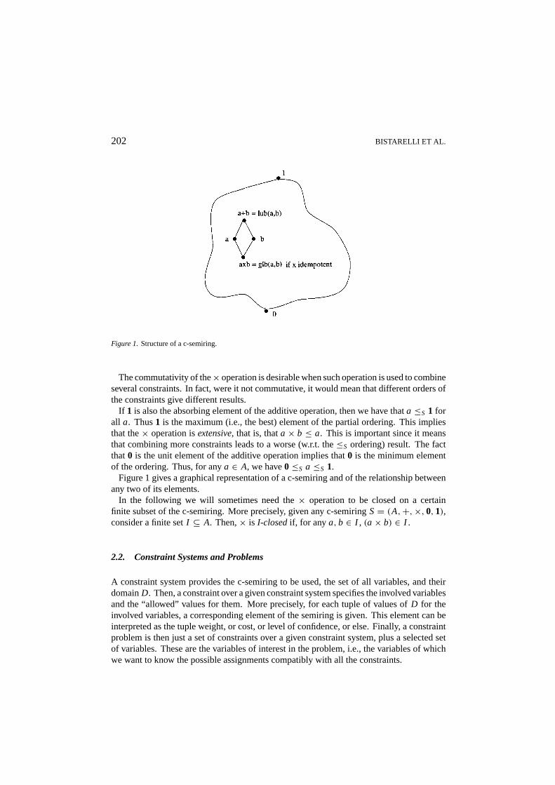
A c-semiringis a semiring such that+ is idempotent (i.e.,a ∈ A impliesa+ a = a),× iscommutative, and1 is the absorbing element of +.
The idempotency of the+ operation is needed in order to define a partial ordering≤S
over the setA, which will enable us to compare different elements of the semiring. Suchpartial order is defined as follows:a ≤S b iff a + b = b. Intuitively, a ≤S b means thatb is “better” thana. This will be used later to choose the “best” solution in our constraintproblems. It is important to notice that both+ and× are monotone on such ordering.
202 BISTARELLI ET AL.
Figure 1. Structure of a c-semiring.
The commutativity of the× operation is desirable when such operation is used to combineseveral constraints. In fact, were it not commutative, it would mean that different orders ofthe constraints give different results.
If 1 is also the absorbing element of the additive operation, then we have thata ≤S 1 forall a. Thus1 is the maximum (i.e., the best) element of the partial ordering. This impliesthat the× operation isextensive, that is, thata× b ≤ a. This is important since it meansthat combining more constraints leads to a worse (w.r.t. the≤S ordering) result. The factthat0 is the unit element of the additive operation implies that0 is the minimum elementof the ordering. Thus, for anya ∈ A, we have0≤S a ≤S 1.
Figure 1 gives a graphical representation of a c-semiring and of the relationship betweenany two of its elements.
In the following we will sometimes need the× operation to be closed on a certainfinite subset of the c-semiring. More precisely, given any c-semiringS= (A,+,×,0,1),consider a finite setI ⊆ A. Then,× is I-closedif, for any a,b ∈ I , (a× b) ∈ I .
2.2. Constraint Systems and Problems
A constraint system provides the c-semiring to be used, the set of all variables, and theirdomainD. Then, a constraint over a given constraint system specifies the involved variablesand the “allowed” values for them. More precisely, for each tuple of values ofD for theinvolved variables, a corresponding element of the semiring is given. This element can beinterpreted as the tuple weight, or cost, or level of confidence, or else. Finally, a constraintproblem is then just a set of constraints over a given constraint system, plus a selected setof variables. These are the variables of interest in the problem, i.e., the variables of whichwe want to know the possible assignments compatibly with all the constraints.
SEMIRING-BASED CSPS AND VALUED CSPS 203
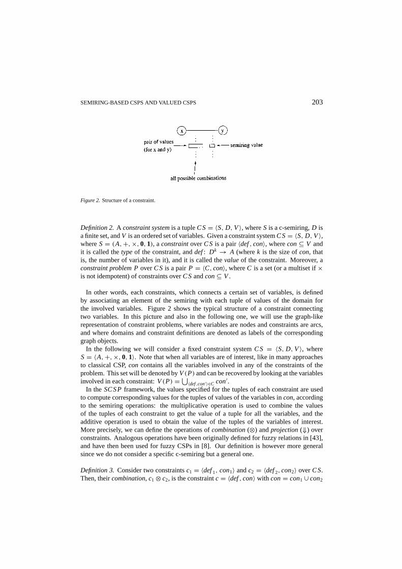
Figure 2. Structure of a constraint.
Definition 2.A constraint systemis a tupleCS= 〈S, D,V〉, whereS is a c-semiring,D isa finite set, andV is an ordered set of variables. Given a constraint systemCS= 〈S, D,V〉,whereS= (A,+,×,0,1), aconstraintoverCS is a pair〈def, con〉, wherecon⊆ V andit is called thetypeof the constraint, anddef: Dk → A (wherek is the size ofcon, thatis, the number of variables in it), and it is called thevalueof the constraint. Moreover, aconstraint problem PoverCS is a pairP = 〈C, con〉, whereC is a set (or a multiset if×is not idempotent) of constraints overCSandcon⊆ V .
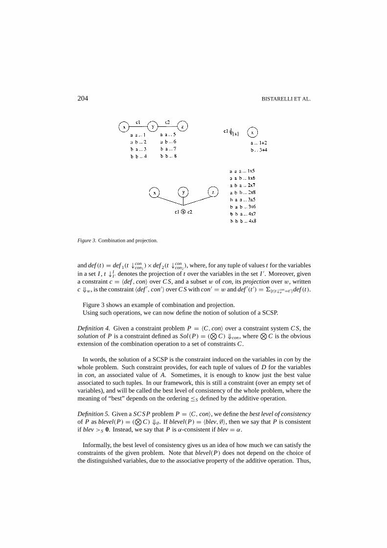
In other words, each constraints, which connects a certain set of variables, is definedby associating an element of the semiring with each tuple of values of the domain forthe involved variables. Figure 2 shows the typical structure of a constraint connectingtwo variables. In this picture and also in the following one, we will use the graph-likerepresentation of constraint problems, where variables are nodes and constraints are arcs,and where domains and constraint definitions are denoted as labels of the correspondinggraph objects.
In the following we will consider a fixed constraint systemCS = 〈S, D,V〉, whereS= 〈A,+,×,0,1〉. Note that when all variables are of interest, like in many approachesto classical CSP,con contains all the variables involved in any of the constraints of theproblem. This set will be denoted byV(P) and can be recovered by looking at the variablesinvolved in each constraint:V(P) =⋃〈def,con′〉∈C con′.
In the SCSPframework, the values specified for the tuples of each constraint are usedto compute corresponding values for the tuples of values of the variables incon, accordingto the semiring operations: the multiplicative operation is used to combine the valuesof the tuples of each constraint to get the value of a tuple for all the variables, and theadditive operation is used to obtain the value of the tuples of the variables of interest.More precisely, we can define the operations ofcombination(⊗) andprojection(⇓) overconstraints. Analogous operations have been originally defined for fuzzy relations in [43],and have then been used for fuzzy CSPs in [8]. Our definition is however more generalsince we do not consider a specific c-semiring but a general one.
Definition 3. Consider two constraintsc1 = 〈def1, con1〉 andc2 = 〈def2, con2〉 overCS.Then, theircombination, c1⊗ c2, is the constraintc = 〈def, con〉 with con= con1 ∪ con2
204 BISTARELLI ET AL.
Figure 3. Combination and projection.
anddef(t) = def1(t ↓concon1
)×def2(t ↓concon2
), where, for any tuple of valuest for the variablesin a setI , t ↓I
I ′ denotes the projection oft over the variables in the setI ′. Moreover, givena constraintc = 〈def, con〉 overCS, and a subsetw of con, its projectionoverw, writtenc ⇓w, is the constraint〈def′, con′〉 overCSwith con′ = w anddef′(t ′) = 6{t |t↓con
w =t ′}def(t).
Figure 3 shows an example of combination and projection.Using such operations, we can now define the notion of solution of a SCSP.
Definition 4. Given a constraint problemP = 〈C, con〉 over a constraint systemCS, thesolutionof P is a constraint defined asSol(P) = (⊗C) ⇓con, where
⊗C is the obvious
extension of the combination operation to a set of constraintsC.
In words, the solution of a SCSP is the constraint induced on the variables inconby thewhole problem. Such constraint provides, for each tuple of values ofD for the variablesin con, an associated value ofA. Sometimes, it is enough to know just the best valueassociated to such tuples. In our framework, this is still a constraint (over an empty set ofvariables), and will be called the best level of consistency of the whole problem, where themeaning of “best” depends on the ordering≤S defined by the additive operation.
Definition 5.Given aSCSPproblemP = 〈C, con〉, we define thebest level of consistencyof P asblevel(P) = (⊗C) ⇓∅. If blevel(P) = 〈blev,∅〉, then we say thatP is consistentif blev>S 0. Instead, we say thatP is α-consistent ifblev= α.
Informally, the best level of consistency gives us an idea of how much we can satisfy theconstraints of the given problem. Note thatblevel(P) does not depend on the choice ofthe distinguished variables, due to the associative property of the additive operation. Thus,
SEMIRING-BASED CSPS AND VALUED CSPS 205
since a constraint problem is just a set of constraints plus a set of distinguished variables, wecan also apply functionblevelto a set of constraints only. Also, since the type of constraintblevel(P) is always an empty set of variables, in the following we will just write the valueof blevel.
Another interesting notion of solution, more abstract than the one defined above, butsufficient for many purposes, is the one that provides only the tuples that have an associatedvalue which coincides with (thedef of) blevel(P). However, this notion makes sense onlywhen≤S is a total order. In fact, were it not so, we could have an incomparable set oftuples, whose sum (via+) does not coincide with any of the summed tuples. Thus it couldbe that none of the tuples has an associated value equal toblevel(P).
By using the ordering≤S over the semiring, we can also define a corresponding partialordering on constraints with the same type, as well as a preorder and a notion of equivalenceon problems.
Definition 6. Consider two constraintsc1, c2 over CS, and assume thatcon1 = con2.Then we define theconstraint orderingvS as the following partial ordering:c1 vS c2
if and only if, for all tuplest of values fromD, def1(t) ≤S def2(t). Notice that, ifc1 vS c2 andc2 vS c1, thenc1 = c2. Consider now twoSCSPproblemsP1 and P2 suchthat P1 = 〈C1, con〉 and P2 = 〈C2, con〉. Then we define theproblem preordervP as:P1 vP P2 if Sol(P1) vS Sol(P2). If P1 vP P2 and P2 vP P1, then they have the samesolution. Thus we say thatP1 andP2 areequivalentand we writeP1 ≡ P2.
The notion of problem preorder can also be useful to show that, as in the classical CSPcase, also the SCSP framework is monotone:(C, con) vP (C ∪C′, con). That is, if someconstraints are added, the solution (as well as theblevel) of the new problem is worse orequal than that of the old one.
2.3. Local Consistency
Computing any one of the previously defined notions (like the best level of consistency andthe solution) is an NP-hard problem. Thus it can be convenient in many cases to approximatesuch notions. In classical CSP, this is done using the so-called local consistency techniques.Such techniques can be extended also to constraint solving over any semiring, provided thatsome properties are satisfied. Here we define whatk-consistency [11], [12], [18] means forSCSP problems. Informally, an SCSP problem isk-consistent when, taken any setW ofk− 1 variables and anyk-th variable, the constraint obtained by combining all constraintsamong thek variables and projecting it ontoW is better or equal (in the orderingvS) thanthat obtained by combining the constraints among the variables in W only.
Definition 7. Given aSCSPproblemP = 〈C, con〉 we say thatP is k-consistent if, forall W ⊆ V(P) such that size(W) = k − 1, and for allx ∈ (V(P) −W), ((⊗{ci | ci ∈ C∧ coni ⊆ (W ∪ {x})}) ⇓W) wS (⊗{ci | ci ∈ C ∧coni ⊆ W)}, whereci = 〈defi , coni 〉 forall ci ∈ C.
206 BISTARELLI ET AL.
Note that, since× is extensive, in the above formula fork-consistency we could alsoreplacewS by≡S. In fact, the extensivity of× assures that the formula always holds whenvS is used instead ofwS.
Making a problemk-consistent means explicitating some implicit constraints, thus pos-sibly discovering inconsistency at a local level. In classical CSP, this is crucial, since localinconsistency implies global inconsistency. This is true also in SCSPs. But here we can beeven more precise, and relate the best level of consistency of the whole problem to that ofits subproblems.
THEOREM1 (LOCAL AND GLOBAL α-CONSISTENCY) Consider a set of constraints C overCS, and any subset C′ of C. If C′ is α-consistent, then C isβ-consistent, withβ ≤S α.
Proof: If C′ is α-consistent, it means that⊗C′ ⇓∅= 〈α,∅〉. Now, C can be seen asC′ ⊗ C′′ for someC′′. By extensivity of×, and the monotonicity of+, we have thatβ = ⊗(C′ ⊗ C′′) ⇓ ∅ vS ⊗(C) ⇓ ∅ = α.
If a subset of constraints ofP is inconsistent (that is, itsblevel is 0), then the abovetheorem implies that the whole problem is inconsistent as well.
We now define a generick-consistency algorithm, by extending the usual one for classicalCSPs [11], [18]. We assume to start from aSCSPproblem where all constraints of arityk−1 are present. If some are not present, we just add them with a non-restricting definition.That is, for any added constraintc = 〈def, con〉, we setdef(t) = 1 for all con-tuplest . Thisdoes not change the solution of the problem, since1 is the unit element for the× operation.
The idea of the (naive) algorithm is to combine any constraintc of arity k − 1 with theprojection over suchk−1 variables of the combination of all the constraints connecting thesamek− 1 variables plus another one, and to repeat such operation until no more changescan be made to any (k− 1)-arity constraint.
In doing that, we will use the additional notion oftyped locations. Informally, a typedlocation is just a location (as in ordinary imperative programming) which can be assigned toa constraint of the same type. This is needed since the constraints defined in Definition 2.2are just pairs〈def, con〉, wheredef is afixedfunction and thus not modifiable. In this way,we can also assign the value of a constraint to a typed location (only if the type of thelocation and that of the constraint coincide), and thus achieve the effect of modifying thevalue of a constraint.
Definition 8. A typed locationis an objectl : con whose type iscon. The assignmentoperationl := c, wherec is a constraint〈def, con〉, has the meaning of associating, in thepresent store, the valuedef to l . Whenever a typed location appears in a formula, it willdenote its value.
Definition 9. Consider anSCSPproblemP = 〈C, con〉 and take any subsetW ⊆ V(P)such that size(W) = k − 1 and any variablex ∈ (V(P) − W). Let us now consider atyped locationl i for each constraintci = 〈defi , coni 〉 ∈ C such thatl i : coni . Then ak-consistency algorithmworks as follows.
1. Initialize all locations by performingl i := ci for eachci ∈ C.
SEMIRING-BASED CSPS AND VALUED CSPS 207
2. Consider
• l j : W,
• A(W, x) = ⊗{l i | coni ⊆ (W ∪ {x})} ⇓ W, and
• B(W) = ⊗{l i | coni ⊆ W}.Then, if A(W, x) 6wS B(W), performl j := l j ⊗ A(W, x).
3. Repeat step 2 on allW andx until A(W, x) w B(W) for all W and allx.
Upon stability, assume that each typed locationl i : coni haseval(l i ) = def′i . Thenthe result of the algorithm is a new SCSP problemP′ = k-cons(P) = 〈C′, con〉 such thatC′ =⋃i 〈def′i , coni 〉.
Assuming the termination of such algorithm (we will discuss such issue later), it is obviousto show that the problem obtained at the end isk-consistent. This is a very naive algorithm,whose efficiency can be improved easily by using the methods which have been adoptedfor classicalk-consistency.
In classical CSP, anyk-consistency algorithm enjoys some important properties. We nowwill study these same properties in our SCSP framework, and point out the correspondingproperties of the semiring operations which are necessary for them to hold. The desiredproperties are as follows: that anyk-consistency algorithm returns a problem which isequivalent to the given one; that it terminates in a finite number of steps; and that the orderin which the (k−1)-arity subproblems are selected does not influence the resulting problem.
THEOREM2 (EQUIVALENCE) Consider a SCSP problem P and a SCSP problem P′ = k-cons(P). Then, P≡ P′ (that is, P and P′ are equivalent) if× is idempotent.
Proof: AssumeP = 〈C, con〉 andP′ = 〈C′, con〉. Now,C′ is obtained byC by changingthe definition of some of the constraints (via the typed location mechanism). For each ofsuch constraints, the change consists of combining the old constraint with the combinationof other constraints. Since the multiplicative operation is commutative and associative(and thus also⊗), ⊗C′ can also be written as(⊗C) ⊗ C′′, where⊗C′′ wS ⊗C. If × isidempotent, then((⊗C)⊗ C′′) = (⊗C). Thus(⊗C) = (⊗C′). ThereforeP ≡ P′.
THEOREM3 (TERMINATION) Consider any SCSP problem P where CS= 〈S, D,V〉 andthe set AD= ⋃
〈def,con〉∈C R(def), where R(def) = {a | ∃t with def(t) = a}. Then theapplication of the k-consistency algorithm to P terminates in a finite number of steps if ADis contained in a set I which is finite and such that+ and× are I-closed.
Proof: Each step of thek-consistency algorithm may change the definition of one con-straint by assigning a different value to some of its tuples. Such value is strictly worse (interms of≤S) since× is extensive. Moreover, it can be a value which is not inAD but inI − AD. If the state of the computation consists of the definitions of all constraints, then ateach step we get a strictly worse state (in terms ofvS). The sequence of such computationstates, until stability, has finite length, since by assumptionI is finite and thus the valueassociated with each tuple of each constraint may be changed at most size(I ) times.
208 BISTARELLI ET AL.
An interesting special case of the above theorem occurs when the chosen semiring hasa finite domainA. In fact, in that case the hypotheses of the theorem hold withI = A.Another useful result occurs when+ and× are AD-closed. In fact, in this case onecan also compute the time complexity of thek-consistency algorithm by just looking atthe given problem. More precisely, if this same algorithm isO(nk) in the classical CSPcase [11], [12], [24], [26], then here it isO(size(AD) × nk) (in [8] they reach the sameconclusion for the fuzzy CSP case).
No matter in which order the subsetsW of k − 1 variables, as well as the additionalvariablesx, are chosen during thek-consistency algorithm, the result is always the sameproblem. However, this holds in general only if× is idempotent.
THEOREM4 (ORDER-INDEPENDENCE) Consider a SCSP problem P and two different ap-plications of the k-consistency algorithm to P, producing respectively P′ and P′′. ThenP′ = P′′ if × is idempotent.
In some cases, where the given problem has a tree-like structure (where each node of thetree may be any subproblem), a variant of the above definedk-consistency algorithm canbe applied: just apply the main algorithm step to each node of the tree, in any bottom-uporder [28]. For such algorithm, which is linear in the size of the problem and exponentialin the size of the larger node in the tree structure, the idempotency of× is not needed tosatisfy the above properties (except the order independence, which does not make sensehere).
Notice that the definitions and results of this section would hold also in the more generalcase of a local consistency algorithm which is not required to achieve consistency on everysubset ofk variables, but may in general make only some subsets of variables consistent(not necessarily a partition of the problem). These more general kinds of algorithms havebeen considered in [28], and similar properties have been shown there for the special caseof classical CSPs.
2.4. Instances of the Framework
We will now show how several known, and also new, frameworks for constraint solvingmay be seen as instances of the SCSP framework. More precisely, each of such frameworkscorresponds to the choice of a specific constraint system (and thus of a semiring). Thismeans that we can immediately know whether one can inherit the properties of the generalframework by just looking at the properties of the operations of the chosen semiring, andby referring to the theorems in the previous subsection. This is interesting for knownconstraint solving schemes, because it puts them into a single unifying framework and itjustifies in a formal way many informally taken choices, but it is especially significant fornew schemes, for which one does not need to prove all the properties that it enjoys (or not)from scratch. Since we consider only finite domain constraint solving, in the following wewill only specify the semiring that has to be chosen to obtain a particular instance of theSCSP framework.
SEMIRING-BASED CSPS AND VALUED CSPS 209
2.4.1. Classical CSPs
A classical CSP problem [25], [27] is just a set of variables and constraints, where eachconstraint specifies the tuples that are allowed for the involved variables. Assuming thepresence of a subset of distinguished variables, the solution of a CSP consists of a set oftuples which represent the assignments of the distinguished variables which can be extendedto total assignments which satisfy all the constraints.
Since constraints in CSPs are crisp, we can model them via a semiring with only twovalues, say 1 and 0: allowed tuples will have the value 1, and not allowed ones the value 0.Moreover, in CSPs, constraint combination is achieved via a join operation among allowedtuple sets. This can be modeled here by taking as the multiplicative operation the logicaland (and interpreting 1 as true and 0 as false). Finally, to model the projection over thedistinguished variables, as thek-tuples for which there exists a consistent extension to ann-tuple, it is enough to assume the additive operation to be the logicalor. Therefore a CSP isjust an SCSP where the c-semiring in the constraint system CS isSCSP= 〈{0,1},∨,∧,0,1〉.The ordering≤S here reduces to 0≤S 1. As predictable, all the properties related tok-consistency hold. In fact,∧ is idempotent. Thus the results of Theorems 2 and 4 apply.Also, since the domain of the semiring is finite, the result of Theorem 3 applies as well.
2.4.2. Fuzzy CSPs
Fuzzy CSPs (FCSPs) [8], [32], [33], [34] extend the notion of classical CSPs by allowingnon-crisp constraints, that is, constraints which associate a preference level with each tupleof values. Such level is always between 0 and 1, where 1 represents the best value (that is,the tuple is allowed) and 0 the worst one (that is, the tuple is not allowed). The solution ofa fuzzy CSP is then defined as the set of tuples of values which have the maximal value.The value associated withn-tuple is obtained by minimizing the values of all its subtuples.Fuzzy CSPs are already a very significant extension of CSPs. In fact, they are able tomodel partial constraint satisfaction [13], so to get a solution even when the problem isover-constrained, and also prioritized constraints, that is, constraints with different levelsof importance [5].
Fuzzy CSPs can be modeled in our framework by choosing the c-semiringSFCSP =〈{x | x ∈ [0,1]},max,min,0,1〉. The ordering≤S here reduces to the≤ ordering onreals. The multiplicative operation ofSFCSP (that is,min) is idempotent. Thus Theorem 2and 4 can be applied. Moreover,min is AD-closed for any finite subset of [0,1]. Thus,by Theorem 3, anyk-consistency algorithm terminates. Thus FCSPs, although providinga significant extension to classical CSPs, can exploit the same kind of local consistencyalgorithms. An implementation of arc-consistency, suitably adapted to be used over fuzzyCSPs, is given in [34] (although no formal properties of its behavior are proved).
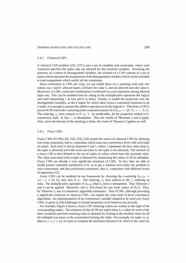
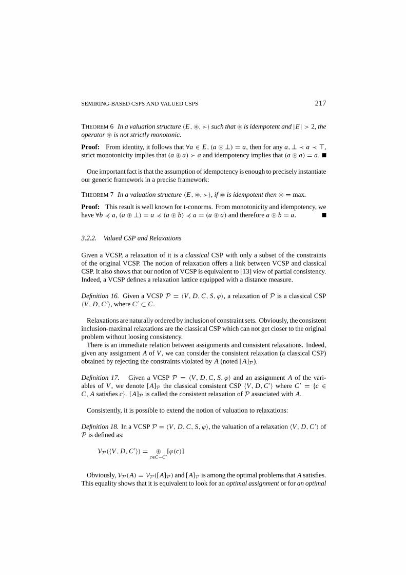
For example, Figure 4 shows a fuzzy CSP. Semiring values are written to the right of thecorresponding tuples. The solutions of this SCSP are triples (that is, a value for each of thethree variables) and their semiring value is obtained by looking at the smallest value for allthe subtuples (as many as the constraints) forming the triple. For example, for tuple〈a,a〉(that is,x = y = a), we have to compute the minimum between 0.9, which is the value for
210 BISTARELLI ET AL.
Figure 4. A fuzzy CSP.
x = a, 0.8, which is the value for〈x = a, y = a〉, and 0.9, which is the value fory = a.So the resulting value for this tuple is 0.8.
2.4.3. Probabilistic CSPs
Probabilistic CSPs [9] have been introduced to model those situations where each constraintchas a certain independent probabilityp(c) to be part of the given real problem. This allowsone to reason also about problems which are only partially known. The probability of eachconstraint gives then, to each instantiation of all the variables, a probability that it is asolution of the real problem. This is done by associating with ann-tuple t the probabilitythat all constraints thatt violates are in the real problem. This is just the product of all1− p(c) for all c violated byt . Finally, the aim is to get those instantiations with themaximum probability.
The relationship between Probabilistic CSPs and SCSPs is complicated by the fact that theformer contain crisp constraints with probability levels, while the latter contain non-crispconstraints. That is, we associate values with tuples, and not to constraints. However, itis still possible to model Probabilistic CSPs, by using a transformation which is similarto that proposed in [8] to model prioritized constraints via soft constraints in the FCSPframework. More precisely, we assign probabilities to tuples instead of constraints: considerany constraintc with probability p(c), and lett be any tuple of values for the variablesinvolved in c; then we setp(t) = 1 if t is allowed byc, otherwisep(t) = 1 − p(c).The reasons for such a choice are as follows: if a tuple is allowed byc andc is in thereal problem, thent is allowed in the real problem; this happens with probabilityp(c);if insteadc is not in the real problem, thent is still allowed in the real problem, and thishappens with probability 1− p(c). Thust is allowed in the real problem with probabilityp(c) + 1 − p(c) = 1. Consider instead a tuplet which is not allowed byc. Then itwill be allowed in the real problem only ifc is not present; this happens with probability1− p(c).
To give the appropriate value to ann-tuplet , given the values of all the smallerk-tuples,with k ≤ n and which are subtuples oft (one for each constraint), we just perform theproduct of the value of such subtuples. By the way values have been assigned to tuples inconstraints, this coincides with the product of all 1− p(c) for all c violated byt . In fact, if asubtuple violatesc, then by construction its value is 1− p(c); if instead a subtuple satisfies
SEMIRING-BASED CSPS AND VALUED CSPS 211
c, then its value is 1. Since 1 is the unit element of×, we have that 1× a = a for eacha.Thus we get5(1− p(c)) for all c thatt violates.
As a result, the c-semiring corresponding to the Probabilistic CSP framework isSprob =〈{x | x ∈ [0,1]},max,×,0,1〉, and the associated ordering≤S here reduces to≤ overreals. Note that the fact thatP′ is α-consistent means that inP there exists ann-tuplewhich has probabilityα to be a solution of the real problem.
The multiplicative operation ofSprob (that is,×) is not idempotent. Thus neither Theo-rem 2 nor Theorem 4 can be applied. Also,× is not closed on any superset of any non-trivialfinite subset of [0,1]. Thus Theorem 3 cannot be applied as well. Therefore,k-consistencyalgorithms do not make much sense in the Probabilistic CSP framework, since none ofthe usual desired properties hold. However, the fact that we are dealing with a c-semiringimplies that, at least, we can apply Theorem 1: if a Probabilistic CSP problem has a tuplewith probabilityα to be a solution of the real problem, then any subproblem has a tuplewith probability at leastα to be a solution of a subproblem of the real problem. This can befruitfully used when searching for the best solution in a branch-and-bound search algorithm.
2.4.4. Weighted CSPs
While fuzzy CSPs associate a level of preference with each tuple in each constraint, inweighted CSPs (WCSPs) tuples come with an associated cost. This allows one to modeloptimization problems where the goal is to minimize the total cost (time, space, number ofresources. . . ) of the proposed solution. Therefore, in WCSPs the cost function is definedby summing up the costs of all constraints (intended as the cost of the chosen tuple for eachconstraint). Thus the goal is to find then-tuples (wheren is the number of all the variables)which minimize the total sum of the costs of their subtuples (one for each constraint).
According to this informal description of WCSPs, the associated c-semiring isSWCSP=〈R−,max,+,−∞,0〉, with ordering≤S which reduces here to≤ over the reals. Thismeans that a value is preferred to another one if it is greater. Notice that we represent costsas negative numbers. Thus we need to maximize these numbers in order to minimize thecosts.
The multiplicative operation ofSWCSP (that is,+) is not idempotent. Thus thek-consistency algorithms cannot be used (in general) in the WCSP framework, since noneof the usual desired properties hold. However, again, the fact that we are dealing with ac-semiring implies that, at least, we can apply Theorem 1: if a WCSP problem has a bestsolution with costα, then the best solution of any subproblem has a cost greater thanα. Thiscan be convenient to know in a branch-and-bound search algorithm. Note that the sameproperties hold also for the semirings〈Q−,max,+,−∞,0〉 and 〈Z−,max,+,−∞,0〉,which can be proved to be c-semirings.
2.4.5. Egalitarianism and Utilitarianism: FCSP + WCSP
The FCSP and the WCSP systems can be seen as two different approaches to give a meaningto the notion of optimization. The two models correspond in fact, respectively, to two defini-
212 BISTARELLI ET AL.
tions of social welfare in utility theory [29]:egalitarianism, which maximizes the minimalindividual utility, andutilitarianism, which maximizes the sum of the individual utilities:FCSPs are based on the egalitarian approach, while WCSPs are based on utilitarianism.
In this section we show how our framework allows also for the combination of thesetwo approaches. In fact, we construct an instance of the SCSP framework where thetwo approaches coexist, and allow us to discriminate among solutions which otherwisewould result indistinguishable. More precisely, we first compute the solutions according toegalitarianism (that is, using amax−mincomputation as in FCSPs), and then discriminatemore among them via utilitarianism (that is, using amax− sumcomputation as in WCSPs).The resulting c-semiring isSue = 〈{〈l , k〉 | l , k ∈ [0,1]}, max,min, 〈0,0〉, 〈1,0〉〉, wheremaxandminare defined as follows:
〈l1, k1〉max〈l2, k2〉 ={〈l1,max(k1, k2)〉 if l1 = l2〈l1, k1〉 if l1 > l2
〈l1, k1〉min〈l2, k2〉 ={〈l1, k1+ k2〉 if l1 = l2〈l2, k2〉 if l1 > l2
That is, the domain of the semiring contains pairs of values: the first element is usedto reason via themax-min approach, while the second one is used to further discriminatevia themax-sumapproach. More precisely, given two pairs, if the first elements of thepairs differ, then themax−minoperations behave like a normalmax−min, otherwise theybehave likemax-sum. This can be interpreted as the fact that, if the first element coincide,it means that themax-min criteria cannot discriminate enough, and thus themax− sumcriteria is used.
Sincemin is not idempotent,k-consistency algorithms cannot in general be used mean-ingfully in this instance of the framework.
A kind of constraint solving similar to that considered in this section is the one presentedin [10], where Fuzzy CSPs are augmented with a finer way of selecting the preferred solution.More precisely, they employ a lexicographic ordering to improve the discriminating powerof FCSPs and avoid the so-calleddrowning effect. We plan to rephrase this approach in ourframework (as it is done in the VCSP framework).
2.4.6. N-dimensional SCSPs
Choosing an instance of the SCSP framework means specifying a particular c-semiring.This, as discussed above, induces a partial order which can be interpreted as a (partial)guideline for choosing the “best” among different solutions. In many real-life situations,however, one guideline is not enough, since, for example, it could be necessary to reasonwith more than one objective in mind, and thus choose solutions which achieve a goodcompromise w.r.t. all such goals.
Consider for example a network of computers, where one would like to both minimizethe total computing time (thus the cost) and also to maximize the work of the least usedcomputers. Then, in the SCSP framework, we would need to consider two c-semirings,one for cost minimization (weighted CSP), and another one for work maximization (fuzzy
SEMIRING-BASED CSPS AND VALUED CSPS 213
CSP). Then, one could work first with one of these c-semirings and then with the other one,trying to combine the solutions which are the best for each of them.
However, a much simpler approach consists of combining the two c-semirings and thenwork with the resulting structure. The nice property is that such a structure is a c-semiringitself, thus all the techniques and properties of the SCSP framework can be used for such astructure as well. More precisely, the way to combine several c-semirings and get anotherc-semiring just consists of vectorizing the domains and operations of the combined c-semirings.
Definition 10.Given then c-semiringsSi = 〈Ai ,+i ,×i ,0i ,1i〉, for i = 1, . . . ,n, we de-fine the structureComp(S1, . . . , Sn) = 〈〈A1, . . . , An〉,+,×, 〈01, . . . ,0n〉, 〈11 . . .1n〉〉.Given〈a1, . . . ,an〉 and〈b1, . . . ,bn〉 such thatai ,bi ∈ Ai for i = 1, . . . ,n, 〈a1, . . . ,an〉 +〈b1, . . . ,bn〉 = 〈a1 +1 b1, . . . ,an +n bn〉, and 〈a1, . . . ,an〉 × 〈b1, . . . ,bn〉 = 〈a1 ×1
b1, . . . ,an ×n bn〉.
According to the definition of the ordering≤S (in Sect. 2.1), such an ordering forS =Comp(S1, . . . , Sn) is as follows. Given〈a1, . . . ,an〉 and〈b1, . . . ,bn〉 such thatai ,bi ∈ Ai
for i = 1, . . . ,n, we have〈a1, . . . ,an〉 ≤S 〈b1, . . . ,bn〉 if and only if 〈a1+1 b1, . . . ,an +n
bn〉 = 〈b1, . . . ,bn〉. Since the tuple elements are completely independent,≤S is in generala partial order, even though each of the≤Si is a total order. Thus it is in this instance that thepower of a partially ordered domain (as opposed to a totally ordered one, as in the VCSPframework discussed later in the paper) can be exploited.
The presence of a partial order means that the abstract solution of a problem over such asemiring may in general contain an incomparable set of tuples, none of which hasblevel(P)as its associated value. In this case, if one wants to reduce the number of “best” tuples (orto get just one), one has to specify some priorities among the orderings of the componentc-semirings.
3. Valued Constraint Problems
The framework described in this section is based on an ordered monoid structure (a monoidis essentially a semi-group with an identity). Elements of the set of the monoid, calledvaluations, are associated with each constraint and the monoid operation (denoted~) isused to assign a valuation to each assignment, by combining the valuations of all theconstraints violated by the assignment. The order on the monoid is assumed to be totaland the problem considered is always to minimize the combined valuation of all violatedconstraints (the reader should note that the choice of associating one valuation to eachconstraint rather than to each tuple (as in the SCSP framework) is done only for the sake ofsimplicity and is not fundamentally different, as Sect. 4 will show).
We show how the VCSP framework can be used to model several existing constraintsolving schemes and also to relate all these schemes from an expressiveness and computa-tional complexity point of view. We define an extended version of the arc-consistencyproperty and study the influence of the monoid operation properties on the computa-tional complexity of the problem of checking arc-consistency. We then try to extend
214 BISTARELLI ET AL.
some usual look-ahead backtrack search algorithms to the VCSP framework. The re-sults obtained formally justify the current algorithmic “state of art” for several existingschemes.
In this section, a classical CSP is defined by a setV = {v1, . . . , vn} of variables, eachvariablevi having an associated finite domaindi . A constraintc = (Vc, Rc) is defined bya set of variablesVc ⊆ V and a relationRc between the variables ofVc i.e., a subset ofthe Cartesian product
∏vi∈Vc
di . A CSP is denoted by〈V, D,C〉, whereD is the set ofthe domains andC the set of the constraints. A solution of the CSP is an assignment ofvalues to the variables inV such that all the constraints are satisfied: for each constraintc = (Vc, Rc), the tuple of the values taken by the variables ofVc belongs toRc. The contentof this section is based on [35].
3.1. Valuation Structure
In order to deal with over-constrained problems, it is necessary to be able to express the factthat a constraint may eventually be violated. To achieve this, we annotate each constraintwith a mathematical item which we call avaluation. Such valuations will be taken from asetE equipped with the following structure:
Definition 11.A valuation structureis defined as a tuple〈E,~,Â〉 such that:
• E is a set, whose elements are called valuations, which is totally ordered byÂ, with amaximum element noted> and a minimum element noted⊥;
• ~ is a commutative, associative closed binary operation onE that satisfies:
– Identity: ∀a ∈ E,a~⊥ = a;
– Monotonicity: ∀a,b, c ∈ E, (a < b)⇒ ((a~ c) < (b~ c)
);
– Absorbing element: ∀a ∈ E, (a~>) = >.
This structure of a totally ordered commutative monoid with a monotonic operator is alsoknown in uncertain reasoning,E being restricted to [0,1], as a “triangular co-norm” [7].One may notice that this set of axioms is not minimal.
THEOREM5 The “absorbing element” property can be inferred from the other axiomsdefining a valuation structure.
Proof: Since⊥ is the identity,(⊥~>) = >; since⊥ is minimum,∀a ∈ E, (a~>) <(⊥~>) = >; since,> is maximum,∀a ∈ E, (a~>) = >
Notice also that a c-semiring, as defined in Section 2.1, can be seen as a commutativemonoid, the role of the~ operator being played by×. The+ operation defines an orderon the monoid. In the rest of the paper, we implicitly suppose that the computation ofÂand~ are always polynomial in the size of their arguments.
SEMIRING-BASED CSPS AND VALUED CSPS 215
3.2. Valued CSP
A valued CSP is then simply obtained by annotating each constraint of a classical CSP witha valuation denoting the impact of its violation or, equivalently, of its rejection from the setof constraints.
Definition 12.A valued CSPis defined by a classical CSP〈V, D,C〉, a valuation structureS= (E,~,Â), and an applicationϕ from C to E. It is denoted by〈V, D,C, S, ϕ〉. ϕ(c)is called the valuation ofc.
An assignmentA of values to some variablesW ⊂ V can now be simply evaluated bycombining the valuations of all the violated constraints using~:
Definition 13. In a VCSPP = 〈V, D,C, S, ϕ〉 the valuation of an assignment Aof thevariables ofW ⊂ V is defined by:
VP(A) = ~c∈C,Vc⊂WA violatesc
[ϕ(c)]
The semantics of a VCSP is a distribution of valuations on the assignments ofV (potentialsolutions). The problem considered is to find an assignmentA with a minimumvaluation.The valuation of such an optimal solution will be called the CSP valuation. It providesa gradual notion of inconsistency, from⊥, which corresponds to consistency, to>, forcomplete inconsistency.
Abstracting a little, one may also consider that a VCSP actually defines an orderingon complete assignments: an assignment is better than another one iff its valuation issmaller. This induced ordering makes it possible to compare two VCSP, independently ofthe valuation structure used in each VCSP:
Definition 14.A VCSPP = 〈V, D,C, S, ϕ〉 is arefinementof the VCSPP ′ = 〈V, D,C′,S′, ϕ′〉 if for any pair of assignmentsA, A′ of V such thatVP ′(A) Â VP ′(A′) in S′ thenVP(A) Â VP(A′) in S. P is astrong refinementof P ′ if the property holds whenA, A′ areassignments of subsets ofV .
The main point is that ifP is a refinementof P ′, then the set of optimal assignments ofP is included in the set of optimal assignments ofP ′; the problem of finding an optimalassignment ofP ′ can be reduced to the same problem inP. A related notion, “aggregation-compatible simplification function”, has been introduced in [16] along with stronger results.
Definition 15. Two VCSPP = 〈V, D,C, S, ϕ〉 andP ′ = 〈V, D,C′, S′, ϕ′〉 will be saidequivalentiff each one is a refinement of the other. They will be saidstrongly equivalentifeach one is a strong refinement of the other.
Equivalent VCSP define the same ordering on assignments ofV and have the same set ofoptimal assignments: the problem of finding an optimal assignment is equivalent in both
216 BISTARELLI ET AL.
VCSP. Note that this definition of equivalence is weaker than the definition used in SCSPsince it does not require that two equivalent VCSP always give the same valuation to thesame assignments but only that they order assignments similarly.
3.2.1. Justification and Properties
It is now possible to informally justify the choice of the axioms that define a valuationstructure:
• The ordered setE allows different levels of violations to be expressed and compared.The order is assumed to be total because in practice this assumption is extremely usefulto define algorithms that will be able to solve VCSP.
• Commutativity and associativity are needed to guarantee that the valuation of an as-signment depends only on the set of the valuations of the violated constraints, and noton the way they are aggregated.
• The element> corresponds to unacceptable violation and is used to expresshardconstraints. The element⊥ corresponds to complete satisfaction. These maximumand minimum elements can be added to any totally ordered set, and their existence issupposed without any loss of generality.
• Monotonicity guarantees that an assignment that satisfies a setB of constraints willnever be considered as worse than an assignment which satisfies only a subset ofB.
This set of axioms is a compromise between generality (to be able to capture as many existingCSP extensions as possible) and specificity (to be able to prove interesting theorems anddefine generic algorithms). Two additional properties will be considered later because oftheir influence on algorithms and computation:
• Strict monotonicity(∀a,b, c ∈ E, if (a  c), (b 6= >) then (a ~ b)  (c ~ b))is interesting from the expressiveness point of view. Essentially, strict monotonicitystrengthen the monotonicity property: it guarantees that an assignment that satisfiesa setB of constraints will not only be never considered as worse than an assignmentwhich satisfies only a strict subset ofB but will always be considered as better, whichseems quite natural. This type of property is usual in multi-criteria theory, namely insocial welfare theory [29].
• Idempotency(∀a ∈ E, (a~ a) = a) is interesting from the algorithmic point of view.Basically, allk-consistency enforcing algorithms work by explicitly adding constraintsthat are only implicit in a CSP. Idempotency is needed for the resulting CSP to have thesame meaning as the original CSP.
These two interesting properties are actually incompatible as soon as the valuation struc-ture used is not trivial.
SEMIRING-BASED CSPS AND VALUED CSPS 217
THEOREM6 In a valuation structure〈E,~,Â〉 such that~ is idempotent and|E| > 2, theoperator~ is not strictly monotonic.
Proof: From identity, it follows that∀a ∈ E, (a~⊥) = a, then for anya,⊥ ≺ a ≺ >,strict monotonicity implies that(a~ a) Â a and idempotency implies that(a~ a) = a.
One important fact is that the assumption of idempotency is enough to precisely instantiateour generic framework in a precise framework:
THEOREM7 In a valuation structure〈E,~,Â〉, if ~ is idempotent then~ = max.
Proof: This result is well known for t-conorms. From monotonicity and idempotency, wehave∀b 4 a, (a~⊥) = a 4 (a~ b) 4 a = (a~ a) and thereforea~ b = a.
3.2.2. Valued CSP and Relaxations
Given a VCSP, a relaxation of it is aclassicalCSP with only a subset of the constraintsof the original VCSP. The notion of relaxation offers a link between VCSP and classicalCSP. It also shows that our notion of VCSP is equivalent to [13] view of partial consistency.Indeed, a VCSP defines a relaxation lattice equipped with a distance measure.
Definition 16. Given a VCSPP = 〈V, D,C, S, ϕ〉, a relaxation ofP is a classical CSP〈V, D,C′〉, whereC′ ⊂ C.
Relaxations are naturally ordered by inclusion of constraint sets. Obviously, the consistentinclusion-maximal relaxations are the classical CSP which can not get closer to the originalproblem without loosing consistency.
There is an immediate relation between assignments and consistent relaxations. Indeed,given any assignmentA of V , we can consider the consistent relaxation (a classical CSP)obtained by rejecting the constraints violated byA (noted [A]P ).
Definition 17. Given a VCSPP = 〈V, D,C, S, ϕ〉 and an assignmentA of the vari-ables ofV , we denote [A]P the classical consistent CSP〈V, D,C′〉 whereC′ = {c ∈C, A satisfiesc}. [A]P is called the consistent relaxation ofP associated withA.
Consistently, it is possible to extend the notion of valuation to relaxations:
Definition 18.In a VCSPP = 〈V, D,C, S, ϕ〉, the valuation of a relaxation〈V, D,C′〉 ofP is defined as:
VP(〈V, D,C′〉) = ~c∈C−C′
[ϕ(c)]
Obviously,VP(A) = VP([ A]P) and [A]P is among the optimal problems thatA satisfies.This equality shows that it is equivalent to look for anoptimal assignmentor for an optimal
218 BISTARELLI ET AL.
consistent relaxation. Both will have the same valuation and any solution of the latter (aclassical CSP) will be an optimal solution of the original VCSP.
The valuation of the top of the relaxation lattice, the CSP〈V, D,C〉, is obviously⊥. Thevaluations of the other relaxations can be understood as a distance to this ideal problem. Thebest assignments ofV are the solutions of the closest consistent problems of the lattice. Themonotonicity of~ ensures that the order on problems defined by this valuation distributionis consistent with the inclusion order on relaxations.
THEOREM8 Given a VCSPP = 〈V, D,C, S, ϕ〉, and〈V, D,C′〉, 〈V, D,C′′〉, two relax-ations ofP:
C′ ( C′′ ⇒ VP(〈V, D,C′〉) < VP(〈V, D,C′′〉)
When~ is strictly monotonic, the right inequality becomes strict (as far as the valuationofP is not>).
Proof: The theorem follows directly from the monotonicity, associativity and (strict)commutativity of the operator~.
This last result shows that strict monotonicity is indeed a desirable property since itguarantees that the order induced by the valuation distribution will respect thestrict inclusionorder on relaxations (if the VCSP valuation is not equal to>). In this case, optimal consistentrelaxations are always selected among inclusion-maximal consistent relaxations, whichseems quiterational.
Since idempotency and strict monotonicity are incompatible as soon asE has morethan two elements, idempotency can be seen as an undesirable property, at least from therationality point of view. Using an idempotent operator, it is possible for a consistentnon inclusion-maximal relaxation to get an optimal valuation. This has been called the“drowning-effect” in possibilistic logic/CSP [10].
3.3. Instances of the Framework
We now show how several extensions of the CSP framework can be cast as VCSP. Most ofthese instances have already been described as SCSP in the sect. 2.4 and we just give herethe valuation structure needed to cast each instance.
3.3.1. Classical CSP
In a classical CSP, an assignment is considered unacceptable as soon as one constraint isviolated. Therefore, classical CSP correspond to the trivial boolean latticeE = {t, f },t = ⊥ ≺ f = >, ~ = ∧ (or max), all constraints being annotated with>. The operation∧ is both idempotent and strictly monotonic (this is the only case where both propertiesmay exist simultaneously in a valuation structure).
SEMIRING-BASED CSPS AND VALUED CSPS 219
3.3.2. Possibilistic and Fuzzy CSP
Possibilistic CSPs [34] are closely related to Fuzzy CSPs [8], [32], [33]. Each constraintis annotated with a priority (usually a real number between 0 and 1). The valuation of anassignment is defined as the maximum valuation among violated constraints. The problemdefined is therefore a min-max problem [40], dual to the max-min problem of Fuzzy CSP.
Possibilistic CSPs are defined by the operation~ = max. Traditionally,E = [0,1],0 = ⊥, 1 = > but any totally ordered set (either symbolic or numeric) may be used.The annotation of a constraint is interpreted as a priority degree. A preferred assignmentminimizes the priority of the most important violated constraint. The idempotency of maxleads to the so-called “drowning-effect”: if a constraint with priorityα has to be necessarilyviolated then any constraint with a priority lower thenα is simply ignored by the combinationoperator~ and therefore such a constraint can be rejected from any consistent relaxationwithout changing its valuation. The notion of lexicographic CSP has been proposed in [10]to overcome this apparent weakness.
Obviously, a classical CSP is simply a specific possibilistic CSP where the valuation>alone is used to annotate the constraints. Note that finite fuzzy CSP [8] can easily be castas possibilistic CSP and vice-versa (see Sect. 4).
3.3.3. Weighted CSP
Weighted CSP try to minimize the weighted sum of the elementary weights associated withviolated constraints. Weighted CSP correspond to the operation~ = + in N ∪ {+∞},using the usual ordering<. The operation is strictly monotonic.
First considered in [39], weighted CSP have been considered asPartial CSPin [13], allconstraint valuations being equal to 1. The problem of finding a solution to such a CSP isoften called theMAX -CSPproblem.
3.3.4. Probabilistic CSP
Probabilistic CSP have been defined in [9] to enable the user to represent ill-known problems,where the existence of constraints in the real problem is uncertain. Each constraintc isannotated with its probability of existence, all supposed to be independent. The probabilitythat an assignment that violates 2 constraintsc1 andc2 will not be a solution of the realproblem is therefore 1− (1− ϕ(c1))(1− ϕ(c2)). Therefore, probabilistic CSP correspondto the operationx ~ y = 1− (1− x)(1− y) in E = [0,1]. The operation is strictlymonotonic.
3.3.5. Lexicographic CSP
Lexicographic CSP offer a combination of weighted and possibilistic CSP and suppress the“drowning effect” of the latter [10]. As in possibilistic CSP, each constraint is annotated
220 BISTARELLI ET AL.
with a priority. The idea is that the valuation of an assignment will not simply be definedby the maximum valuation among the valuations of violated constraints but will depend onthe number of violated constraints at each level of priority, starting from the most prioritaryto the least prioritary.
To reduce lexicographic CSP to VCSP, a valuation will be either a designated maximumelement> (needed to represent hard constraints) or a multiset (elements may be repeated) ofelements of [0,1[ (any other totally ordered set may be used instead of [0,1[). Constraintswill usually be annotated with a multi-set that contains a single element: the priority of theconstraint.
The operation~ is simply defined by multi-set union, extended to treat> as an absorbingelement (the empty multi-set being the identity⊥). The order is the lexicographic (oralphabetic) total order induced by the order> on multisets and extended to give> its roleof maximum element: letv andv′ be two multisets andα andα′ be the largest elements inv andv′, v  v′ iff either α > α′ or (α = α′ andv − {α}  v′ − {α′}). The recursion endson∅, the minimum multi-set.
This instance is closely related to the HCLP framework [5]. It can also be related tothe “FCSP+ WCSP” instance considered in sect. 2.4: since the number of constraintsviolated at each level of priority are used to discriminate assignments in the lexicographicCSP approach, it is finer than the “FCSP+WCSP” which simply relies on the number ofconstraints at one level.
3.4. Relationships Between Instances
Our first motivation for defining the VCSP framework was to understand why some frame-works (eg. weighted CSP, lexicographic CSP, probabilistic CSP) define harder problemsthan possibilistic or classical CSP. By harder, we mean both the hardness of the problemof finding a provenly optimal solution and the difficulty of extension of algorithms such asarc-consistency enforcing.
Elementary theoretical complexity is essentially useless to analyze this situation becauseall the decision problems “Is there is a complete assignment whose valuation is less thanα?” are simplyNP-complete and there is not much more to say. In order to be ableto compare VCSP classes that relies on different valuation structures, we introduced thefollowing notion:
Definition 19.GivenSandS′, two valuation structures, a polynomial time refinement fromS to S′ is a function8 that:
• transforms any VCSPP = 〈V, D,C, S, ϕ〉 in a VCSPP ′ = 〈V, D,C, S′, ϕ′〉 whereϕ′ = 8 ◦ ϕ and such thatP ′ is a refinement ofP;
• is deterministic polynomial time computable.
This notion of polynomial-time refinement is inspired by the notion of polynomial transfor-mation (or many-one reduction) usual in computational complexity [31]. As for polynomial
SEMIRING-BASED CSPS AND VALUED CSPS 221
transformation, if there exists a polynomial time refinement fromS to S′ then any VCSPP defined overScan be solved by first applying this polynomial time refinement toP andthen solving the resulting problem overS′. This shows that problems defined overS arenot harder than problems defined overS′.
As we will see, the notion allows one to bring to light subtle differences between differentvaluation structures. We have recently discovered that a similar idea has been developedin [20] for optimization problems overN in general. This work introduces a notion ofpolynomial “metric reduction” closely related to the notion of polynomial-time refinementintroduced here as well as specific classes with an associated notion of completeness.
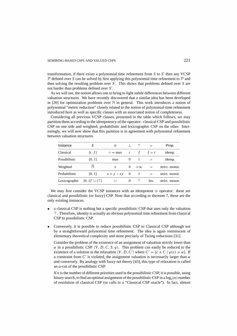
Considering all previous VCSP classes, presented in the table which follows, we maypartition them according to the idempotency of the operator: classical CSP and possibilisticCSP on one side and weighted, probabilistic and lexicographic CSP on the other. Inter-estingly, we will now show that this partition is in agreement with polynomial refinementbetween valuation structures.
Instance E ~ ⊥ > Â Prop.
Classical {t, f } ∧ = max t f f  t idemp.
Possibilistic [0,1] max 0 1 > idemp.
Weighted N + 0 +∞ > strict. monot.
Probabilistic [0,1] x + y− xy 0 1 > strict. monot.
Lexicographic [0,1]∗ ∪ {>} ∪ ∅ > lex. strict. monot.
We may first consider the VCSP instances with an idempotent~ operator: these areclassical and possibilistic (or fuzzy) CSP. Note that according to theorem 7, these are theonly existing instances.
• a classical CSP is nothing but a specific possibilistic CSP that uses only the valuation>. Therefore, identity is actually an obvious polynomial time refinement from classicalCSP to possibilistic CSP.
• Conversely, it is possible to reduce possibilistic CSP to Classical CSP although notby a straightforward polynomial time refinement. The idea is again reminiscent ofelementary theoretical complexity and more precisely of Turing reductions [31].
Consider the problem of the existence of an assignment of valuation strictly lower thanα in a possibilistic CSP〈V, D,C, S, ϕ〉. This problem can easily be reduced to theexistence of a solution in the relaxation〈V, D,C′〉 whereC′ = {c ∈ C | ϕ(c) < α}. Ifa constraint fromC′ is violated, the assignment valuation is necessarily larger thanα
and conversely. By analogy with fuzzy-set theory [43], this type of relaxation is calledanα-cut of the possibilistic CSP.
If n is the number of different priorities used in the possibilistic CSP, it is possible, usingbinary search, to find an optimal assignment of the possibilistic CSP in a log2(n)numberof resolution of classical CSP (or calls to a “Classical CSP oracle”). In fact, almost
222 BISTARELLI ET AL.
all traditional polynomial classes, properties, theorems and algorithms (k-consistencyenforcing. . . ) of classical CSP can be extended to possibilistic CSP using the sameidea.
We now consider some VCSP instances with a strictly monotonic operator: these areprobabilistic CSP, weighted CSP and lexicographic CSP.
• a simple polynomial refinement exists from weighted CSP to lexicographic CSP: thevaluationk ∈ N is transformed in a multiset containing a given elementα 6= 0 repeatedk times (noted{(α, k)}), whereα is a fixed priority and the valuation+∞ is transformedto >. The lexicographic VCSP obtained is in factstrongly equivalentto the originalweighted VCSP.
• interestingly, a lexicographic CSP may also be transformed into astrongly equivalentweighted CSP. Letα1, . . . , αk be the elements of ]0,1[ that appear in all the Lexico-graphic CSP annotations, sorted in increasing order. Letni be the number of occurrencesofαi in all the annotations of the VCSP. The lowest priorityα1 corresponds to the weightf (α1) = 1, and inductivelyαi corresponds tof (αi ) = f (αi−1)× (ni−1+1) (this way,the weight f (αi ) corresponding to priorityi is strictly larger than the largest possiblesum of f (αj ), j < i . This is immediately satisfied forα1 and inductively verified forαi ). An initial lexicographic valuation is converted in the sum of the penaltiesf (αi )
for eachαi in the valuation. The valuation> is converted to+∞. All the operationsinvolved, sum and multiplication, are polynomial and the sizes of the operands remainpolynomial: if k is the number of priorities used in the VCSP and` the maximumnumber of occurrences of a priority, then the largest weightf (αk) is in O(`k), with alength inO(k. log(`))while the original annotations used at least spaceO(k+ log(`)).Therefore, the refinement is polynomial.
• Finally, if we allow the valuations in weighted CSP to take values inR instead ofN,then probabilistic CSP and weighted CSP can be related by a simple isomorphism:a constraint with a probabilityϕ(c) of existence can be transformed into a constraintwith a weight of− log(1− ϕ(c)) (and conversely using the transformation 1− e−ϕ(c)).The two VCSP obtained in this way are obviouslystrongly equivalent. However, andbecause real numbers are not countable this isomorphism is not a true polynomialtime refinement. It is nevertheless usable to efficiently (but approximately) transforma probabilistic CSP in a weighted CSP, real numbers being approximated by floatingpoint numbers.
Finally, a bridge between idempotent and strictly monotonic VCSP is provided by apolynomial refinement from possibilistic CSP to Lexicographic CSP: the LexicographicCSP is simply obtained by annotating each constraint with a multi-set containing oneoccurrence of the original (possibilistic) annotation if it is not equal to 1, or by> otherwise.In this case, an optimal assignment of the Lexicographic CSP not only minimizes thepriority of the most important constraint violated, but also, the number of constraint violatedsuccessively at each level of priority, from the highest first to the lowest. The refinement isobviously polynomial.
SEMIRING-BASED CSPS AND VALUED CSPS 223
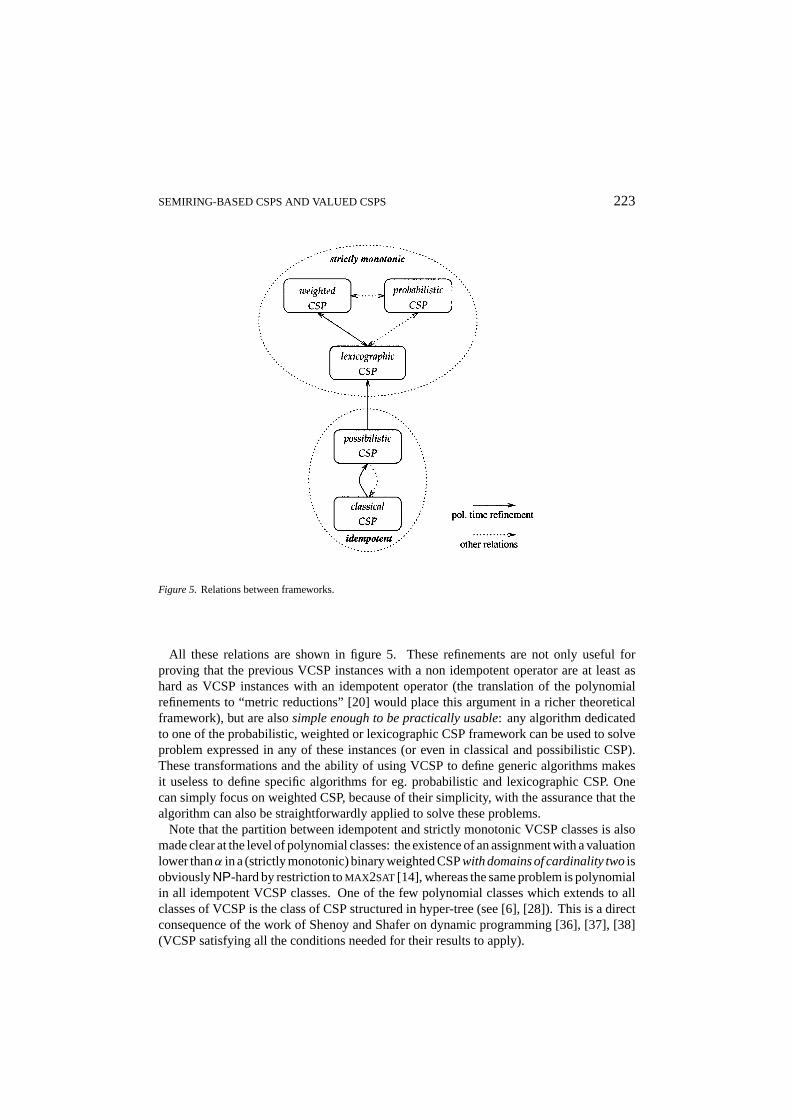
Figure 5. Relations between frameworks.
All these relations are shown in figure 5. These refinements are not only useful forproving that the previous VCSP instances with a non idempotent operator are at least ashard as VCSP instances with an idempotent operator (the translation of the polynomialrefinements to “metric reductions” [20] would place this argument in a richer theoreticalframework), but are alsosimple enough to be practically usable: any algorithm dedicatedto one of the probabilistic, weighted or lexicographic CSP framework can be used to solveproblem expressed in any of these instances (or even in classical and possibilistic CSP).These transformations and the ability of using VCSP to define generic algorithms makesit useless to define specific algorithms for eg. probabilistic and lexicographic CSP. Onecan simply focus on weighted CSP, because of their simplicity, with the assurance that thealgorithm can also be straightforwardly applied to solve these problems.
Note that the partition between idempotent and strictly monotonic VCSP classes is alsomade clear at the level of polynomial classes: the existence of an assignment with a valuationlower thanα in a (strictly monotonic) binary weighted CSPwith domains of cardinality twoisobviouslyNP-hard by restriction toMAX 2SAT[14], whereas the same problem is polynomialin all idempotent VCSP classes. One of the few polynomial classes which extends to allclasses of VCSP is the class of CSP structured in hyper-tree (see [6], [28]). This is a directconsequence of the work of Shenoy and Shafer on dynamic programming [36], [37], [38](VCSP satisfying all the conditions needed for their results to apply).
224 BISTARELLI ET AL.
3.5. Extending Local Consistency Property
In classical binary CSP (all constraints are supposed to involve two variables only), sat-isfiability defines anNP-complete problem.k-consistency properties and algorithms [26]offer a range of polynomial time weaker properties: enforcing strongk-consistency in aconsistent CSP will never lead to an empty CSP.
Arc-consistency (strong 2-consistency) is certainly the most prominent level of localconsistency and has been extended to possibilistic/Fuzzy CSP years ago [32], [40], [34].Considering that the extension of the arc-consistency enforcing algorithms to strictly mono-tonic frameworks was resisting all efforts, we tried to tackle the problem by extending theproperty itself rather than the algorithms. The idea is to rely on the notion of relaxation,which provides a link between VCSP and classical CSP.
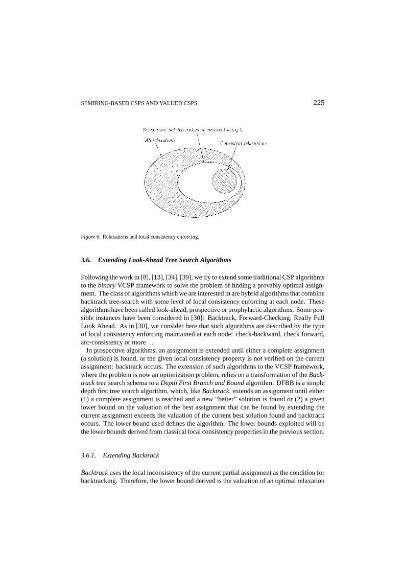
The crucial property of all local consistency properties is that they approximate trueconsistencyi.e., they may detect inconsistency only if CSP is inconsistent. A classical localconsistency property, when extended to the VCSP framework, will approximateoptimalityby providing a lower bound on the cost of an optimal solution of the VCSP. This extensioncan be done for any existing local consistency property using the notion of relaxation, whichprovides a link between VCSP and classical CSP.
THEOREM9 (GENERIC LOWER BOUND FORVCSP) Given any classical local consistencyproperty L, a lower bound on the valuation of an optimal solution of a given VCSPP isdefined by the valuationα of an optimal relaxation ofP among those that are not detectedas inconsistent by the local consistency property L.
In this case, we will say that the VCSP isα-L-consistent.
Proof: This is better explained using figure 6. Because the set of the relaxations whichare detected as inconsistent using a given local consistency propertyL necessarily containsthe set of the consistent relaxations, the minimum of the valuation on the larger set willnecessarily be smaller and therefore provides a lower bound on the valuation of an optimalconsistent relaxation. The results follows from the fact that the valuation of an optimalassignment is also the valuation of an optimalconsistentrelaxation.
The previous definition can be instantiated for arc-consistency:
Definition 20.A VCSP will be saidα-arc-consistent iff the optimal relaxations among allthe relaxations which have a non empty arc-consistent closure have a valuation lower thanα.
The generic bounds defined satisfy two interesting properties:
• they guarantee that the extended algorithm will behave as the original “classical” al-gorithm when applied to a classical CSP seen as a VCSP (such a VCSP has only onerelaxation with a valuation lower than>: itself);
• a stronger local consistency property will define a better lower bound. In the frameworkof a branch and bound algorithm, this allows to exploit possible compromises betweenthe size of the tree search and the work done at each node.
SEMIRING-BASED CSPS AND VALUED CSPS 225
Figure 6. Relaxations and local consistency enforcing.
3.6. Extending Look-Ahead Tree Search Algorithms
Following the work in [8], [13], [34], [39], we try to extend some traditional CSP algorithmsto thebinary VCSP framework to solve the problem of finding a provably optimal assign-ment. The class of algorithms which we are interested in are hybrid algorithms that combinebacktrack tree-search with some level of local consistency enforcing at each node. Thesealgorithms have been called look-ahead, prospective or prophylactic algorithms. Some pos-sible instances have been considered in [30]: Backtrack, Forward-Checking, Really FullLook Ahead. As in [30], we consider here that such algorithms are described by the typeof local consistency enforcing maintained at each node: check-backward, check forward,arc-consistency or more. . .
In prospective algorithms, an assignment is extended until either a complete assignment(a solution) is found, or the given local consistency property is not verified on the currentassignment: backtrack occurs. The extension of such algorithms to the VCSP framework,where the problem is now an optimization problem, relies on a transformation of theBack-track tree search schema to aDepth First Branch and Boundalgorithm. DFBB is a simpledepth first tree search algorithm, which, likeBacktrack, extends an assignment until either(1) a complete assignment is reached and a new “better” solution is found or (2) a givenlower bound on the valuation of the best assignment that can be found by extending thecurrent assignment exceeds the valuation of the current best solution found and backtrackoccurs. The lower bound used defines the algorithm. The lower bounds exploited will bethe lower bounds derived from classical local consistency properties in the previous section.
3.6.1. Extending Backtrack
Backtrackuses the local inconsistency of the current partial assignment as the condition forbacktracking. Therefore, the lower bound derived is the valuation of an optimal relaxation
226 BISTARELLI ET AL.
in which the current assignment is consistent. This is simply the relaxation which preciselyrejects the constraints violated by the current assignment (these constraints have to berejected or else local inconsistency will occur; rejecting these constraint suffices to restorethe consistency of the current assignment in the relaxation). The lower bound is thereforesimply defined by:
~c∈C
A violatesc
ϕ(c)
and is obviously computable in polynomial time.The lower bound can easily be computed incrementally when a new variablexi is assigned:
the lower bound associated with the father of the current node is aggregated with thevaluations of all the constraints violated byxi using~.
In the possibilistic and weighted instances, this generic VCSP algorithm defined co-incides with the “Branch and Bound” algorithms defined for possibilistic or weightedCSP in [13], [33], [34]. Note that for possibilistic CSP, thanks to idempotency, it isuseless to test whether constraints whose valuation is lower than the lower bound asso-ciated with the father node have to be rejected since their rejection cannot influence thebound.
3.6.2. Extending Forward Checking
Forward-checkinguses an extremely limited form of arc-consistency: backtracking occursas soon as all the possible extensions of the current assignmentA on any uninstantiatedvariable are locally inconsistent: the assignment is said non forward-checkable. Therefore,the lower bound used is the minimum valuation among the valuations of all the relaxationsthat makes the current assignment forward-checkable.
A relaxation in whichA is forward-checkable (1) should necessarily reject all the con-straints violated byA itself and (2) for each uninstantiated variablevi it should reject oneof the setsC(vi , ν) of constraints that are violated ifvi is instantiated with valueν of itsdomain. Since~ is monotonic, the minimum valuation is reached by taking into account,for each variable, the valuation of the setC(vi , ν) of minimum valuation. The bound isagain computable in polynomial time since it is the aggregation of (1) the valuations allthe constraints violated byA itself (i.e., the bound used in the extension of the backtrackalgorithm, see 3.6.1) and (2) the valuations of the constraint in all theC(vi , ν). This com-putation needs less than(e.n.d) constraint checks and~ operations (e is the number ofconstraints); all the minimum valuation can be computed with less than(d.n) comparisonsand aggregated with less thann ~ operations. Note that the lower bound derived includesthe bound used in the backtrack extension plus an extra component and will always be betterthan the “Backtrack” bound.
The lower bound may be incrementally computed by maintaining during tree search, andfor each valueν of every unassigned variablevi the aggregated valuationB(ν, vi ) of all theconstraints that will be violated ifν is assigned tovi given the current assignment. Initially,
SEMIRING-BASED CSPS AND VALUED CSPS 227
all B(ν, vi ) are equal to⊥. When the assignmentA is extended toA′ = A∪ {vj = µ}, theB may be updated as follows:
B(ν, vi )← B(ν, vi )~
~c∈C,Vc={vi ,vj }
A′∪{vi =ν} violatesc
[ϕ(c)]
that takes into account all the constraints betweenvi andvj that are necessarily violatedif µ is assigned tovj . Upon backtrack, theB have to be restored to their previous values,as domains in classicalForward-checking. Note that theB offer a default value heuristic:choose the value with a minimumB.
The lower bound is simply obtained by aggregating, using~, the valuations of all theconstraints violated by the assignment and all the minimumB(ν, vi ) for each unassignedvariable. The aggregated valuationv(A′), A′ = A ∪ {vj = µ}), of all the constraintsviolated by the assignmentA′ is easily computed by taking the valuationv(A) computedon the father node~’ed with B(µ, vj ).
Additional sophistications include deleting valuesν of the domains of non instanti-ated variables if the aggregated valuation ofv(A′) and B(ν, vi ) exceeds the upper bound(see [13]). On the possibilistic and weighted VCSP instances, this generic VCSP algo-rithm coincides roughly with the forward-checking based algorithm for possibilistic CSPdescribed in [34] or thePartial Forward-checkingalgorithm defined for weighted CSP in[13]. It has been improved using a directed arc consistency pre-processing step in [42], [21].Further crucial improvements have been introduced in [41], [22], [23]. Note that for pos-sibilistic CSP, and thanks to idempotency, the updating ofB can ignore constraints whosevaluation is less than theB updated or than the current lower-bound.
3.6.3. Trying to Extend Really Full Look Ahead
Really Full Look Aheadmaintains arc consistency during tree search and backtracks as soonas the current assignment induces a domain wipe-out: the CSP has no arc-consistent closure.For a VCSP, the bound which can be derived from arc-consistency will be the minimumvaluation among the valuations of all the relaxations such that the current assignment doesnot induces a domain wipe-out.
Let us consider any class~-VCSP of the VCSP framework such that~ is strictly mono-tonic and for anya,b ∈ E,a,b ≺ >, (a~ b) ≺ >. Let ` be any valuation different from> and⊥. The decision problem corresponding to the computation of the lower bound inthis class can be formulated as:
Definition 21.Given such a~-VCSP and a valuationα, is there a setC′ ⊂ C such that therelaxation〈V, D,C′〉 has a non empty arc-consistent closure and a valuation lower thanα?
Note that this problem corresponds also to the verification that the VCSP is at leastα-arc-consistent.
THEOREM10 MAX -AC-CSPis stronglyNP-complete.
228 BISTARELLI ET AL.
Proof: The problem belongs toNP since computing the arc-consistent closure of a CSPcan be done in polynomial time and we supposed that~ and are polynomial in the sizeof their arguments.
To prove completeness, we use a polynomial transformation from theNP-complete prob-lemMAX 2SAT [14]. An instance ofMAX 2SAT is defined by a set ofn propositional variablesL = {`1, . . . , `n}, a set8 of m 2-clauses onL and a positive integerk ≤ m. The problemis to prove the existence of a truth assignment ofL that satisfies at leastk clauses of8. Theproblem is known to be stronglyNP-complete [14].
Given an instance ofMAX 2SAT, we built an instance ofMAX -AC-CSPdefined by a binaryCSP(V, D,C). The setV of the CSP variables containsn+ 2n.(m+ 1) variables:
1. the firstn variablesv1, . . . , vn correspond to then propositional variables ofL and havea domain of cardinality two corresponding to the boolean valuest and f ;
2. the next 2n.(e+ 1) variables will have a domain of cardinality one, containing onlythe valueF. This set of variables is composed ofn setsVi , 1 ≤ i ≤ n, of 2e+ 2variables: Vi = {vt
i,1, . . . vti,e+1, v
fi,1, . . . , v
fi,e+1}. Each setVi is associated with the
original variablevi previously defined.
The constraints that appear inC are composed of three sets:
1. the setCu is the direct translation of them 2-clauses of theMAX 2SAT instance as CSPconstraints. A 2-clauseφ ∈ 8 that involves i and`j will be translated to a constraintthat involvesvi andvj and whose relation contains all the truth assignments of{`i , `j }that satisfyφ;
2. the setCt contains, for each variablevi , 1 ≤ i ≤ n, and for each variablevti, j ,
1≤ j ≤ m+ 1, a constraint involvingvi andvti, j authorizing only the pair(t,~);
3. the setC f contains, for each variablevi , 1 ≤ i ≤ n, and for each variablev fi, j ,
1≤ j ≤ m+ 1, a constraint involvingvi andv fi, j authorizing only the pair( f,~);
There is a total of 2n.(m+ 1) +m constraints. All the constraints are annotated with thevaluationα, different from> and⊥. For example, Fig. 7 illustrates the micro-structure ofthe CSP built from theMAX 2SAT instance defined by8 = {v1 ∨ v2, v2 ∨ v3, v1 ∨ v3}.
The CSP containsO(m2) constraints,O(m2) variables and domains of cardinalityO(1)and therefore the transformation is clearly polynomial. We shall now prove that the existenceof a truth assignment that satisfies at leastk clauses of8 is equivalent to the existence ofa relaxation of the VCSP which is non arc-inconsistent and whose valuation is lower than(α ~ · · ·~ α) with n.(m+ 1)+ (m− k) occurrences ofα.
We first remark that the CSP(V, D,C) is not arc-consistent: the valuest of the variablesvi , 1 ≤ i ≤ n, have no support on each of them+ 1 constraints ofC f that connectvi
to v fi, j , 1 ≤ j ≤ m+ 1. Similarly, the valuesf of the variablesvi , 1 ≤ i ≤ n, have no
support on each of them+ 1 constraints ofCt that connectvi to vti, j , 1 ≤ j ≤ m+ 1.
Therefore, a relaxation(V, D,C′),C′ ⊂ C, with a non-empty arc-consistent closure willnever simultaneously contain constraints fromCt andC f involving the same variablevi ,1 ≤ i ≤ n. Let us consider a truth assignmentω of the variables ofL that satisfies more
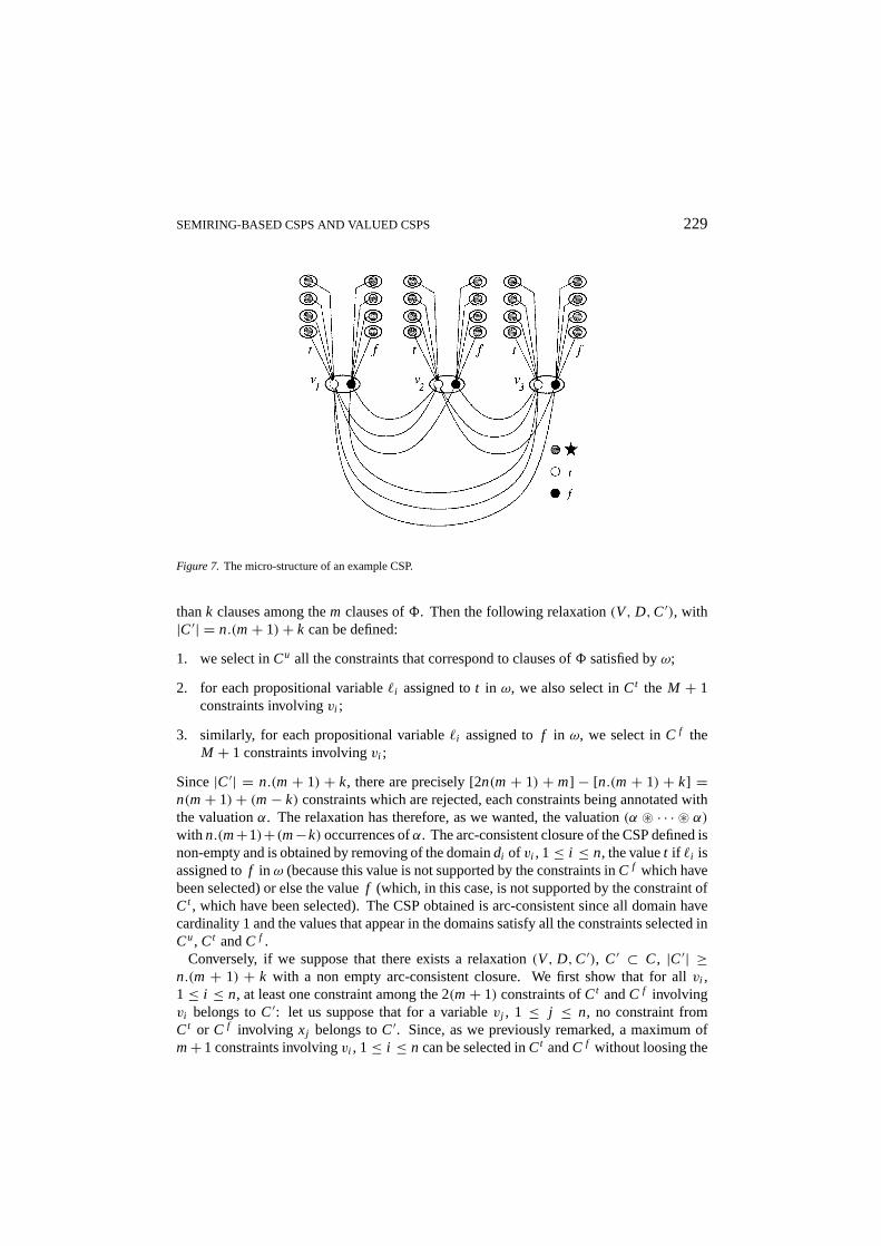
SEMIRING-BASED CSPS AND VALUED CSPS 229
Figure 7. The micro-structure of an example CSP.
thank clauses among them clauses of8. Then the following relaxation(V, D,C′), with|C′| = n.(m+ 1)+ k can be defined:
1. we select inCu all the constraints that correspond to clauses of8 satisfied byω;
2. for each propositional variablei assigned tot in ω, we also select inCt the M + 1constraints involvingvi ;
3. similarly, for each propositional variablei assigned tof in ω, we select inC f theM + 1 constraints involvingvi ;
Since|C′| = n.(m+ 1) + k, there are precisely [2n(m+ 1) + m] − [n.(m+ 1) + k] =n(m+ 1)+ (m− k) constraints which are rejected, each constraints being annotated withthe valuationα. The relaxation has therefore, as we wanted, the valuation(α ~ · · · ~ α)with n.(m+1)+(m−k) occurrences ofα. The arc-consistent closure of the CSP defined isnon-empty and is obtained by removing of the domaindi of vi , 1≤ i ≤ n, the valuet if `i isassigned tof in ω (because this value is not supported by the constraints inC f which havebeen selected) or else the valuef (which, in this case, is not supported by the constraint ofCt , which have been selected). The CSP obtained is arc-consistent since all domain havecardinality 1 and the values that appear in the domains satisfy all the constraints selected inCu, Ct andC f .
Conversely, if we suppose that there exists a relaxation(V, D,C′), C′ ⊂ C, |C′| ≥n.(m + 1) + k with a non empty arc-consistent closure. We first show that for allvi ,1 ≤ i ≤ n, at least one constraint among the 2(m+ 1) constraints ofCt andC f involvingvi belongs toC′: let us suppose that for a variablevj , 1 ≤ j ≤ n, no constraint fromCt or C f involving xj belongs toC′. Since, as we previously remarked, a maximum ofm+1 constraints involvingvi , 1≤ i ≤ n can be selected inCt andC f without loosing the
230 BISTARELLI ET AL.
existence of a non-empty arc-consistent closure, a maximum of(n−1).(m+1) constraintsof C′ may be selected fromCt andC f . SinceC′ can not select more thanm constraintsin Cu and(n − 1).(M + 1) + m < n.(m+ 1) + k sincek > 0, we get a contradiction.Since no more thann.(m+ 1) constraints ofCt andC f appear inC′, there is at leastkconstraints fromCu which appear inC′ in order to reach then.(m+ 1) + k constraints.Each variable being involved in at least one of the constraints fromCt andC f , the variablesfrom the arc-consistent closure of the CSP have exactly one value in their domain et thesevalue necessarily satisfy the constraints ofCu since we are considering the arc-consistentclosure. Therefore, the truth assignmentω of the variables i defined by the assignment ofthe corresponding variablesvi in this arc-consistent closure satisfy more thank clauses of8. This finally shows thatMAX 2SAT∝ MAX -AC-CSP.
Therefore, extendingReally Full Look Aheadseems difficult since computing the lowerbound itself isNP-complete. Furthermore, this also proves that the extension of the arc-consistency property to strictly monotonic VCSP such that for any∀a,b ∈ E,a,b ≺>, (a ~ b) ≺ > looses the quality of being a polynomial time checkable property (ifP 6=NP). However, it is still possible to enforce a form ofDirected Arc Consistencyin apreprocessing step, see [42], [21].
For idempotent VCSP, this bound may be computed using polynomial time algorithmsfor enforcing arc-consistency in Fuzzy or possibilistic CSPs [32], [34], [40] or equivalentlythe arc-consistency algorithm defined for SCSP, which works fine for idempotent operators.We first apply the extended arc-consistent enforcing algorithm which yields an equivalentproblem and then compute a lower bound as follows: we take the maximum on all variablesvi of the minimum on all valuesν ∈ di of the valuation of the assignment{vi = ν} in thisproblem.
4. Comparison
In this section we will compare the two approaches described above in this paper. Inparticular, we will show that, if one assumes a total order, there is a way to pass from anySCSP problem to an equivalent VCSP problem, and vice-versa. We also define normalforms both for VSCPs and SCSPs and we discuss their relationship with the transformationfunctions (from VCSPs to SCSPs and vice-versa).
4.1. From SCSPs to VCSPs
We will consider SCSPs〈C, con〉 wherecon involves all variables. Thus we will omit it inthe following. A SCSP is thus just a set of constraintsC over a constraint system〈S, D,V〉,whereS is a c-semiringS = 〈A,+,×,0,1〉, andD is the domain of the variables inV .Moreover, we will assume that the+ operation induces an order≤S which is total. Thismeans that+ corresponds tomax, or, in other words, that it always chooses the value whichis closer to1.

SEMIRING-BASED CSPS AND VALUED CSPS 231
Figure 8. From SCSPs to VCSPs.
Given a SCSP, we will now show how to obtain a corresponding VCSP, where by corre-spondence we mean that they associate the same value with each variable assignment, andthat they have the same solution.
Definition 22. Given a SCSPP with constraintsC over a constraint system〈S, D,V〉,whereS is a c-semiringS= 〈A,+,×,0,1〉, we obtain the VCSPP′ = 〈V, D,C′, S′, ϕ〉,whereS′ = 〈E,~,Â〉, whereE = A,~ = ×, and≺=>S. (Note that> = 0 and⊥ = 1.)
For each constraintc = 〈def, con〉 ∈ C, we obtain a set of constraintsc′1, . . . , c′k, where
k is the cardinality of the range ofdef. That is,k = |{a s.t. ∃t with def(t) = a}|. Let uscall a1, . . . ,ak such values, and let us callTi the set of all tuplest such thatdef(t) = ai .All the constraintsci involve the same variables, which are those involved inc. Then, foreachi = 1, . . . , k, we setϕ(c′i ) = ak, and we definec′i in such a way that the tuples allowedare those not inTi . We will write P′ = sv(P). Note that, by construction, each tuplet isallowed by all constraintsc1, . . . , ck except the constraintci such thatϕ(ci ) = def(t).
Example 1. Consider a SCSP which contains the constraintc = 〈con,def〉, wherecon= {x, y}, anddef(〈a,a〉) = l1, def(〈a,b〉) = l2, def(〈b,a〉) = l3, def(〈b,b〉) = l1.Then, the corresponding VCSP will contain the following three constraints, all involvingxandy:
• c1, with ϕ(c1) = l1 and allowed tuples〈a,b〉 and〈b,a〉;
• c2, with ϕ(c2) = l2 and allowed tuples〈a,a〉, 〈b,a〉 and〈b,b〉;
• c3, with ϕ(c3) = l3 and allowed tuples〈a,a〉, 〈a,b〉 and〈b,b〉.Figure 8 shows bothc and the three constraintsc1, c2, andc3.
232 BISTARELLI ET AL.
First we need to make sure that the structure we obtain via the definition above is indeeda valued CSP. Then we will prove that it is equivalent to the given SCSP.
THEOREM11 (FROM C-SEMIRING TO VALUATION STRUCTURE) If we consider a c-semiringS= 〈A,+,×,0,1〉 and the structure S′ = 〈E,~,Â〉, where E= A,~ = ×, and≺=>S
(obtained using the transformation in Definition 4.1), then S′ is a valuation structure.
Proof: First, is a total order, since we assumed that≤S is total and that≺=>S. Moreover,> = 0 and⊥ = 1, from the definition of≤S. Then, since~ coincides with×, it is easy tosee that it is commutative, associative, monotone, and closed. Moreover,1 (that is,⊥) isits unit element and0 (that is,>) is its absorbing element.
THEOREM12 (EQUIVALENCE BETWEENSCSPAND VCSP) Consider a SCSP problem Pand the corresponding VCSP problem P′. Consider also an assignment t to all the variablesof P, with associated value a∈ A. ThenVP′(t) = a.
Proof: Note first thatP and P′ have the same set of variables. InP, the value oftis obtained by multiplying the values associated with each subtuple oft , one for eachconstraint ofP. Thus,a = ∏{defc(tc), for all constraintsc = 〈defc, conc〉 in C and suchthattc is the projection oft over the variables ofc}. Now,VP′(t) =
∏{ϕ(c′) for all c′ ∈ C′
such that the projection oft over the variables ofc′ violatesc′}. It is easy to see that thenumber of values multiplied is this formula coincides with the number of constraints inC, since, as noted above, each tuple violates only one of the constraints inC′ which havebeen generated because of the presence of the constraintc ∈ C. Thus we just have to showthat, for eachc ∈ C, defc(tc) = ϕ(ci ), whereci is the constraint violated bytc. But thisis easy to show by what we have noted above. In fact, we have defined the translationfrom SCSP to VCSP in such a way that the only constraint of the VCSP violated by a tupleis exactly the one whose valuation coincides with the value associated with the tuple inthe SCSP.
Note that SCSPs which do not satisfy the restrictions imposed at the beginning of thesection, that is, thatcon involves all the variables and that≤S is total, do not have acorresponding VCSP.
COROLLARY 1 (SAME SOLUTION) Consider a SCSP problem P and the corresponding VCSPproblem P′. Then P and P′ have the same solution.
Proof: It follows from Theorem 12, from the fact thatP uses+ = max which goestowards1, that P′ usesmin which goes towards⊥, that1 = ⊥, and and that a solution isjust one of the total assignments.
4.2. From VCSPs to SCSPs
Here we will define the opposite translation, which allows one to get a SCSP from a givenVCSP.
SEMIRING-BASED CSPS AND VALUED CSPS 233
Figure 9. From VCSP to SCSP.
Definition 23.Given the VCSPP = 〈V, D,C, S, ϕ〉, whereS= 〈E,~,Â〉, we will obtainthe SCSPP′ with constraintsC′ over the constraint system〈S′, D,V〉, whereS′ is thec-semiring〈E,+,~,>,⊥〉, and+ is such thata+ b = a iff a 4 b. It is easy to see that≥S=4. For each constraintc ∈ C with allowed set of tuplesT , we define the correspondingconstraintc′ = 〈con′,def′〉 ∈ C′ such thatcon′ contains all the variables involved inc and,for each tuplet ∈ T , def′(t) = ⊥, otherwisedef′(t) = ϕ(c). We will write P′ = vs(P).
Example 2. Consider a VCSP which contains a binary constraintc connecting variablesx and y, for which it allows the pairs〈a,b〉 and 〈b,a〉, and such thatϕ(c) = l . Then,the corresponding SCSP will contain the constraintc′ = 〈con,def〉, wherecon= {x, y},def(〈a,b〉) = def(〈b,a〉) = ⊥, anddef(〈a,a〉) = def(〈b,b〉) = l . Figure 9 shows bothcand the correspondingc′.
Again, we need to make sure that the structure we obtain via the definition above is indeeda semiring-based CSP. Then we will prove that it is equivalent to the given VCSP.
THEOREM13 (FROM VALUATION STRUCTURE TO C-SEMIRING) If we consider a valuationstructure〈E,~,Â〉 and the structure S= 〈E,+,~,>,⊥〉, where+ is such that a+b = aiff a 4 b (obtained using the transformation in Definition 4.2), then S is a c-semiring.
Proof: Since is total,+ is closed. Moreover,+ is commutative by definition, andassociative because of the transitivity of the total orderÂ. Furthermore,0 is the unit elementof +, since it is the top element ofÂ. Finally,+ is idempotent because of the reflexivityof Â, and1 is the absorbing element of+ since1 = ⊥. Operation× of S coincides with~. Thus it is closed, associative, and commutative, since~ is so. Also,> is its absorbingelement and⊥ is its identity (from corresponding properties of~). The distributivity of~over+ can easily be proved. For example, considera,b, c ∈ E, and assumeb 4 c. Thena~ (b+ c) = a~ b (by definition of+) = (a~ b)+ (a~ c) (by the definition of+ andthe monotonicity of~). The same reasoning applies to the case wherec 4 b.
THEOREM14 (EQUIVALENCE BETWEENVCSPAND SCSP) Consider a VCSP problem Pand the corresponding SCSP problem P′. Consider also an assignment t to all the variablesof P. The value associated with such an assignment is A= VP(t) = ~{ϕ(c) for all c ∈ Csuch that the projection of t over the variables of c violates c}. Instead, the value associated
234 BISTARELLI ET AL.
with the same assignment in P′ is B = ~{defc′(tc′), for all constraints c′ = 〈defc′ , conc′ 〉in C′ and such that tc′ is the projection of t over the variables of c′}. Then, A= B.
Proof: The values multiplied to produceA are as many as the constraints violated byt ;instead, the values multiplied to produceB are as many as the constraints inC′. However, byconstruction, each tupletc involving the variables of a constraintc ∈ C has been associated,in P′, with a value which is eitherϕ(c) (if tc violatesc), or⊥ (if tc satisfiesc). Thus thecontribution oftc to the value ofB is important only iftc violatedc in P, because⊥ is theunit element for~. ThusA andB are obtained by the same number of significant values.Now we have to show that such values are the same. But this is easy, since we have definedthe translation in such a way that each tuple for the variables ofc is associated with thevalueϕ(c) exactly when it violatesc.
4.3. Normal Forms and Equivalences
Note that, while passing from an SCSP to a VCSP the number of constraints in generalincreases, in the opposite direction the number of constraints remains the same. This canalso be seen in Example 1 and 2. This means that, in general, going from a SCSPP to aVCSP P′ and then from the VCSPP′ to the SCSPP′′, we do not getP = P′′. In fact,for each constraintc in P, P′′ will have in general several constraintsc1, . . . , ck over thesame variables asc. However, it is easy to see thatc1 ⊗ · · · ⊗ ck = c, and thusP andP′′
associate the same value with each variable assignment.
Example 3. Figure 10 shows how to pass from a SCSP to the corresponding VCSP (thispart is the same as in Example 1), and then again to the corresponding SCSP. Note that thestarting SCSP and the final one are not the same. In fact, the latter has three constraintsbetween variablesx andy, while the former has only one constraint. However, one can seethat the combination of the three constraints yields the starting constraint.
Consider now the opposite cycle, that is, going from a VCSPP to a SCSPP′ and thenfrom P′ to a VCSPP′′. In this case, for each constraintc in P, P′′ has two constraints:one isc itself, and the other one is a constraint with associated value⊥. This means thatviolating such a constraint has cost⊥, which, in other words, means that this constraint canbe eliminated without changing the behavior ofP′′ at all.
Example 4. Figure 11 shows how to pass from a VCSP to the corresponding SCSP (this partis the same as in Example 2), and then again to the corresponding VCSP. Note that the startingVCSP and the final one are not the same. In fact, the latter one has two constraints betweenvariablesx andy. One is the same as the one in the starting VCSP, while the other one hasassociated the value⊥. This means that violating such constraint yields a cost of value⊥.
Let us define now normal forms for both SCSPs and VCSPs, as follows. For each VCSPP, its normal form is the VCSPP′ = nfv(P) which is obtained by deleting all constraintsc such thatϕ(c) = ⊥. It is easy to see thatP andP′ are equivalent.
SEMIRING-BASED CSPS AND VALUED CSPS 235
Figure 10.From SCSP to VCSP and back to SCSP again.
Definition 24. ConsiderP = 〈V, D,C, S, ϕ〉, a VCSP whereS= 〈E,~,Â〉. ThenP issaid to be in normal form if there is noc ∈ C such thatϕ(c) = ⊥. If P in not in normal form,then it is possible to obtain a unique VCSPP′ = 〈V, D,C − {c ∈ C | ϕ(c) = ⊥}, S, ϕ〉,denoted byP′ = nfv(P), which is in normal form.
THEOREM15 (NORMAL FORM) For any VCSP P, P and nfv(P) are equivalent.
Proof: The theorem follows from the fact that∀a, (⊥~ a) = a and from the definitionsof VP(A) andVP′(A).
Also, for each SCSPP, its normal form is the SCSPP′ = nfs(P) which is obtained bycombining all constraints involving the same set of variables. Again, this is an equivalentSCSP.
Definition 25.Consider any SCSPP with constraintsC over a constraint system〈S, D,V〉,whereS is a c-semiringS= 〈A,+,×,0,1〉. Then,P is in normal form if, for each subsetW of V , there is at most one constraintc = 〈def, con〉 ∈ C such thatcon= W. If P isnot in normal form, then it is possible to obtain a unique SCSPP′, as follows. For eachW ⊆ V , consider the setCW ⊆ C which contains all the constraints involvingW. AssumeCW = {c1, . . . , cn}. Then, replaceCW with the single constraintc =⊗CW. P′, denotedby nfs(P), is in normal form.
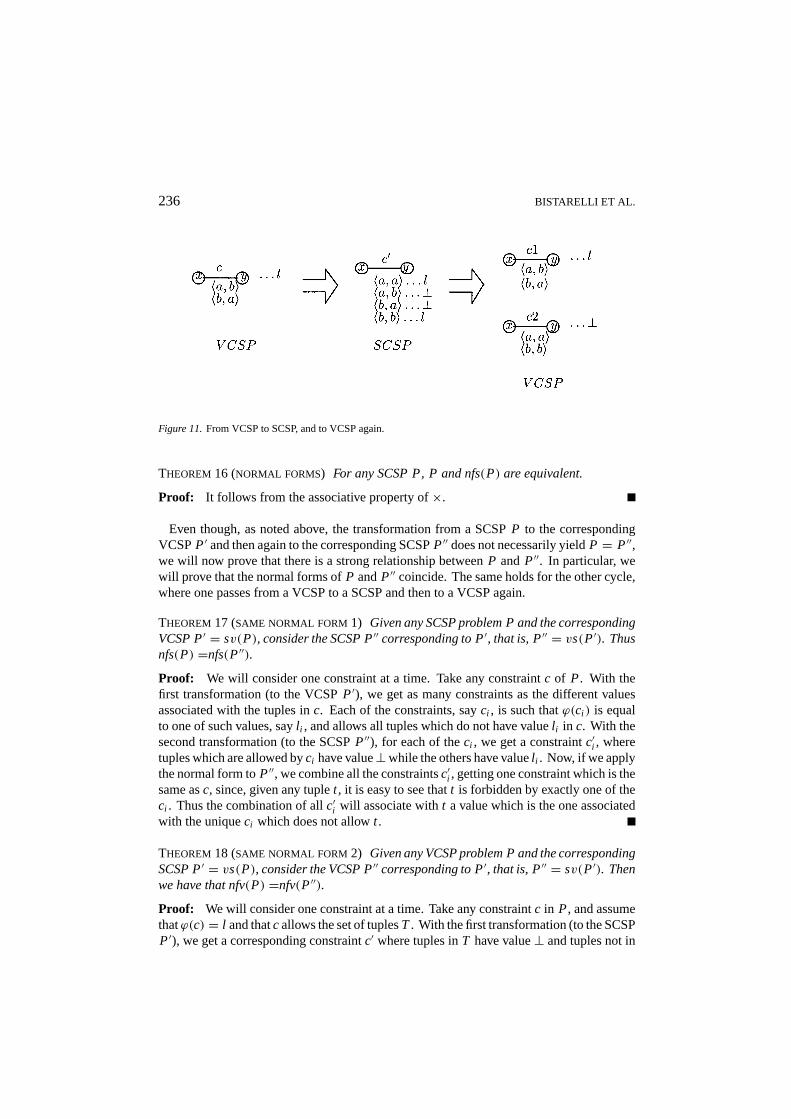
236 BISTARELLI ET AL.
Figure 11.From VCSP to SCSP, and to VCSP again.
THEOREM16 (NORMAL FORMS) For any SCSP P, P and nfs(P) are equivalent.
Proof: It follows from the associative property of×.
Even though, as noted above, the transformation from a SCSPP to the correspondingVCSPP′ and then again to the corresponding SCSPP′′ does not necessarily yieldP = P′′,we will now prove that there is a strong relationship betweenP andP′′. In particular, wewill prove that the normal forms ofP andP′′ coincide. The same holds for the other cycle,where one passes from a VCSP to a SCSP and then to a VCSP again.
THEOREM17 (SAME NORMAL FORM 1) Given any SCSP problem P and the correspondingVCSP P′ = sv(P), consider the SCSP P′′ corresponding to P′, that is, P′′ = vs(P′). Thusnfs(P) =nfs(P′′).
Proof: We will consider one constraint at a time. Take any constraintc of P. With thefirst transformation (to the VCSPP′), we get as many constraints as the different valuesassociated with the tuples inc. Each of the constraints, sayci , is such thatϕ(ci ) is equalto one of such values, sayl i , and allows all tuples which do not have valuel i in c. With thesecond transformation (to the SCSPP′′), for each of theci , we get a constraintc′i , wheretuples which are allowed byci have value⊥while the others have valuel i . Now, if we applythe normal form toP′′, we combine all the constraintsc′i , getting one constraint which is thesame asc, since, given any tuplet , it is easy to see thatt is forbidden by exactly one of theci . Thus the combination of allc′i will associate witht a value which is the one associatedwith the uniqueci which does not allowt .
THEOREM18 (SAME NORMAL FORM 2) Given any VCSP problem P and the correspondingSCSP P′ = vs(P), consider the VCSP P′′ corresponding to P′, that is, P′′ = sv(P′). Thenwe have that nfv(P) =nfv(P′′).
Proof: We will consider one constraint at a time. Take any constraintc in P, and assumethatϕ(c) = l and thatc allows the set of tuplesT . With the first transformation (to the SCSPP′), we get a corresponding constraintc′ where tuples inT have value⊥ and tuples not in
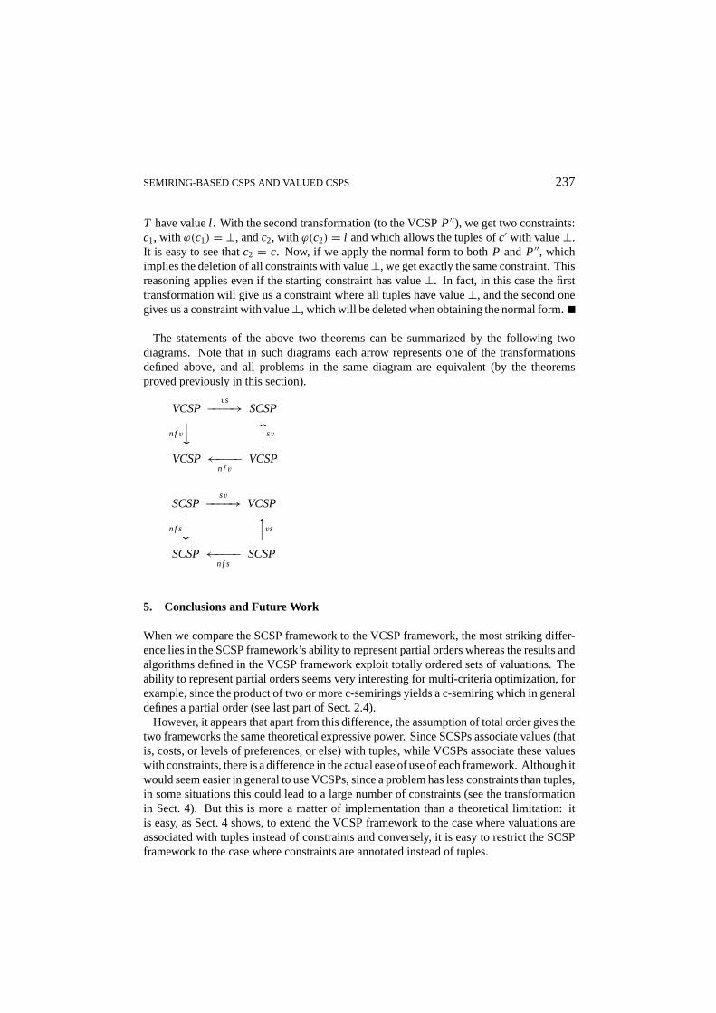
SEMIRING-BASED CSPS AND VALUED CSPS 237
T have valuel . With the second transformation (to the VCSPP′′), we get two constraints:c1, with ϕ(c1) = ⊥, andc2, with ϕ(c2) = l and which allows the tuples ofc′ with value⊥.It is easy to see thatc2 = c. Now, if we apply the normal form to bothP and P′′, whichimplies the deletion of all constraints with value⊥, we get exactly the same constraint. Thisreasoning applies even if the starting constraint has value⊥. In fact, in this case the firsttransformation will give us a constraint where all tuples have value⊥, and the second onegives us a constraint with value⊥, which will be deleted when obtaining the normal form.
The statements of the above two theorems can be summarized by the following twodiagrams. Note that in such diagrams each arrow represents one of the transformationsdefined above, and all problems in the same diagram are equivalent (by the theoremsproved previously in this section).
VCSPvs−−−−→ SCSP
n f v
y xsv
VCSP←−−−−n f v
VCSP
SCSPsv−−−−→ VCSP
n f s
y xvs
SCSP←−−−−n f s
SCSP
5. Conclusions and Future Work
When we compare the SCSP framework to the VCSP framework, the most striking differ-ence lies in the SCSP framework’s ability to represent partial orders whereas the results andalgorithms defined in the VCSP framework exploit totally ordered sets of valuations. Theability to represent partial orders seems very interesting for multi-criteria optimization, forexample, since the product of two or more c-semirings yields a c-semiring which in generaldefines a partial order (see last part of Sect. 2.4).
However, it appears that apart from this difference, the assumption of total order gives thetwo frameworks the same theoretical expressive power. Since SCSPs associate values (thatis, costs, or levels of preferences, or else) with tuples, while VCSPs associate these valueswith constraints, there is a difference in the actual ease of use of each framework. Although itwould seem easier in general to use VCSPs, since a problem has less constraints than tuples,in some situations this could lead to a large number of constraints (see the transformationin Sect. 4). But this is more a matter of implementation than a theoretical limitation: itis easy, as Sect. 4 shows, to extend the VCSP framework to the case where valuations areassociated with tuples instead of constraints and conversely, it is easy to restrict the SCSPframework to the case where constraints are annotated instead of tuples.
238 BISTARELLI ET AL.
What we get are complementary results. In the SCSP framework, we observe that idem-potency of the combination operator guarantees thatk-consistency algorithms work (intotally ordered SCSP or equivalently VCSP, the only structure with an idempotent combi-nation operator is the Fuzzy CSP instance). We get the same result in the VCSP frameworkfor arc-consistency, but we also show that strict monotonicity is a dreadful property thatturns arc-consistency checking in anNP-complete problem and which also defines harderoptimization problems, both from the theoretical and practical point of view.
To solve these difficult problems, we are looking for better lower bounds that could beused in Branch and Bound algorithms to solve{S,V}CSP more efficiently. The boundspresented in this paper have been recently improved along two lines. A first idea is to usedirected arc consistency as a preprocessing step in order to strengthen theForward checkinglower bound [42], [21]. Larger improvements of the lower bound can be obtained usingeither theRussian Doll Searchalgorithm [41] or the notion ofReversible Directed ArcConsistencyintroduced in [22] and later improved in [23].
Another algorithmic approach of{S,V}CSP which is worth considering, and which isalso able to cope with non idempotent combination operators, is the dynamic programmingapproach, which is especially suited to tree-structured problems.
Finally, we are studying the possibility of embedding one of the two frameworks (ora merge of them) in the constraint logic programming (CLP) paradigm (see [19]). Thepresence of such a general framework for constraint solving within CLP would facilitatethe use of new or additional constraint systems in the language, and also would allow for anew concept of logic programming, where the relationship between goals is not regulatedby the usualand andor logical connectives, but instead by general+ and× operators.An important issue will be the semantics of the languages defined. This issue has beenalready addressed for WCSPs [1] and for general semirings in [4]. An implementation ofsemiring-based CLP has been developed on top of the clp(fd) system and has been describedin [15].
References
1. S. Bistarelli (1994). Programmazione con vincoli pesati e ottimizzazione (in italian). Dipartimento di Infor-matica, Universit`a di Pisa, Italy.
2. S. Bistarelli, U. Montanari, and F. Rossi (1995). Constraint solving over semirings. InProc. IJCAI95. MorganKaufman.
3. S. Bistarelli, U. Montanari and F. Rossi (1997). Semiring-based constraint solving and optimization.Journalof the ACM44(2): 201–236.
4. S. Bistarelli, U. Montanari, and F. Rossi (1997). Semiring-based constraint logic programming. InProc.IJCAI97. Morgan Kaufman.
5. A. Borning, M. Maher, A. Martindale, and M. Wilson (1989). Constraint hierarchies and logic programming.In M. Martell, Levi G., editors,Proc. 6th ICLP. MIT Press.
6. R. Dechter, A. Dechter, and J. Pearl (1990). Optimization in constraint networks. In R. M. Oliver andJ. Q. Smith, editors,Influence Diagrams, Belief Nets and Decision Analysis, chapter 18, pages 411–425.John Wiley & Sons Ltd.
7. D. Dubois and H. Prade (1982). A class of fuzzy measures based on triangular norms. a general frameworkfor the combination of uncertain information.Int. Journal of Intelligent Systems8(1): 43–61.
SEMIRING-BASED CSPS AND VALUED CSPS 239
8. D. Dubois, H. Fargier, and H. Prade (1993). The calculus of fuzzy restrictions as a basis for flexible constraintsatisfaction. InProc. IEEE Int. Conf. on Fuzzy Systems. IEEE.
9. H. Fargier and J. Lang (1993). Uncertainty in constraint satisfaction problems: a probabilistic approach.Proc. ECSQARU. Springer-Verlag, LNCS 747.
10. H. Fargier and J. Lang and T. Schiex (1993). Selecting preferred solutions in fuzzy constraint satisfactionproblems.Proc. 1st European Congress on Fuzzy and Intelligent Technologies(EUFIT).
11. E. Freuder (1978). Synthesizing constraint expressions.CACM21(11).
12. E. Freuder (1988). Backtrack-free and backtrack-bounded search. In Kanal and Kumar, editors,Search inArtificial Intelligence, Springer-Verlag.
13. E. Freuder and R. Wallace (1992). Partial constraint satisfaction.Artificial Intelligence Journal58.
14. M. Garey, D. Johnson, and L. Stockmeyer (1976). Some simplified NP-complete graph problems.TheoreticalComputer Science1: 237–267.
15. Y. Georget, and P. Codognet (1998). Compiling semiring-based constraints with clp(FD,S).Proc. CP98,Springer Verlag, LNCS 1520.
16. S. de Givry, G. Verfaillie and T. Schiex (1997). Bounding the optimum of constraint optimization problems.Proc. of the Third International Conference on Principles and Practice of Constraint Programming, pages405–419, Schloss Hagenberg, Austria.
17. P. Hubbe and E. Freuder (1992). An efficient cross-product representation of the constraint satisfactionproblem search space. InProc. of AAAI-92, pages 421–427, San Jose, CA.
18. V. Kumar (1992). Algorithms for constraint satisfaction problems: a survey.AI Magazine13(1).
19. J. Jaffar and J.L. Lassez (1987). Constraint logic programming.Proc. POPL, ACM.
20. M. Krentel (1988). The complexity of optimization problems.Journal of Computer and System Sciences36: 490–509.
21. J. Larrosa and P. Meseguer (1996). Exploiting the use of DAC in MAX-CSP.Proc. of the Second InternationalConference on Principles and Practice of Constraint Programming, pages 308–322, Cambridge (MA).
22. J. Larrosa, P. Meseguer, T. Schiex, and G. Verfaillie (1998). Reversible DAC and other improvements forsolving Max-CSP.Proc. of the National Conf. on Artificial Intelligence (AAAI’98), pages 347–352, Madison(WI).
23. J. Larrosa, P. Meseguer, and T. Schiex (1999). Maintaining reversible DAC for Max-CSP.Artificial Intelli-gence Journal, 107(1).
24. A. Mackworth (1977). Consistency in networks of relations.Artificial Intelligence Journal, 8(1).
25. A. Mackworth (1988).Encyclopedia of AI, chapter Constraint Satisfaction, pages 205–211. Springer Verlag.
26. A. Mackworth and E. Freuder (1985). The complexity of some polynomial network consistency algorithmsfor constraint satisfaction problems.Artificial Intelligence Journal25.
27. U. Montanari (1974). Networks of constraints: Fundamental properties and application to picture processing.Information Science7.
28. U. Montanari and F. Rossi (1991). Constraint relaxation may be perfect.Artificial Intelligence Journal48:143–170.
29. H. Moulin (1988).Axioms for Cooperative Decision Making. Cambridge University Press.
30. B. A. Nadel (1989). Constraint satisfaction algorithms.Comput. Intell. 5(4): 188–224.
31. C. M. Papadimitriou (1994).Computational Complexity. Addison-Wesley Publishing Company.
32. A. Rosenfeld, R. Hummel, and S. Zucker (1976). Scene labelling by relaxation operations.IEEE Trans. onSys., Man, and Cyb. 6(6).
33. Z. Ruttkay (1994). Fuzzy constraint satisfaction.Proc. 3rd Int. Conf. on Fuzzy Systems.
34. T. Schiex (1992). Possibilistic constraint satisfaction problems, or “How to handle soft constraints?”.Proc.8th Conf. of Uncertainty in AI.
240 BISTARELLI ET AL.
35. T. Schiex, H. Fargier, and G. Verfaillie (1995). Valued constraint satisfaction problems: Hard and easyproblems. InProc. IJCAI95. Morgan Kaufmann.
36. G. Shafer (1991). An axiomatic study of computation in hypertrees. Working paper 232, University ofKansas, School of Business, Lawrence.
37. P. Shenoy (1991). Valuation-based systems for discrete optimization. In Bonissone, Henrion, Kanal andLemmer, editors,Uncertainty in AI. North-Holland Publishers.
38. P. Shenoy (1994). Valuation-based systems: A framework for managing uncertainty in expert systems. InL. Zadeh and J. Kacprzyk, editors,Fuzzy Logic for the Management of Uncertainty. Wiley.
39. L. Shapiro and R. Haralick (1981). Structural descriptions and inexact matching.IEEE Transactions onPattern Analysis and Machine Intelligence3: 504–519.
40. P. Snow and E. Freuder (1990). Improved relaxation and search methods for approximate constraint satis-faction with a maximin criterion. InProc. of the 8th Biennal Conf. of the Canadian Society for Comput.Studies of Intelligence, pages 227–230.
41. G. Verfaillie, M. Lematre, and T. Schiex (1996). Russian doll search. InProc. of AAAI-96, pages 181–187,Portland (OR).
42. R. J. Wallace (1994). Directed arc consistency preprocessing as a strategy for maximal constraint satisfaction.In theProc. of ECAI’94 Workshop on Constraint Processing. pages 69–77. Also available in LNCS 923,pp. 121–138 (1995).
43. L. Zadeh (1975). Calculus of fuzzy restrictions. In K. Tanaka, L.A. Zadeh, K.S. Fu and M. Shimura, editors,Fuzzy sets and their applications to cognitive and decision processes. Academic Press.


![MinMaxgd, A Toolbox to Handle Periodic Series in Semiring Max in [[γ, δ]]](https://static.fdokumen.com/doc/165x107/633795877dc7407a2703d6fc/minmaxgd-a-toolbox-to-handle-periodic-series-in-semiring-max-in-g-d.jpg)