Selfishness and altruism in the distribution of travel timeand income

Nebiyou Tilahun • David Levinson

Received: 30 October 2011 / Accepted: 12 January 2013 / Published online: 6 March 2013� Springer Science+Business Media New York 2013

Abstract Most economic models assume that individuals act out their preferences based

on self-interest alone. However, there have also been other paradigms in economics that

aim to capture aspects of behavior that include fairness, reciprocity, and altruism. In this

study we empirically examine preferences of travel time and income distributions with and

without the respondent knowing their own position in each distribution. The data comes

from a Stated Preference experiment where subjects were presented paired alternative

distributions of travel time and income. The alternatives require a tradeoff between dis-

tributional concerns and the respondent’s own position. Choices also do not penalize or

reward any particular choice. Overall, choices show individuals are willing forgo alter-

natives where they would be individually well off in the interest of distributional concerns

in both the travel time and income cases. Exclusively self-interested choices are seen more

in the income questions, where nearly 25 % of respondents express such preferences, than

in the travel time case, where only 5 % of respondents make such choices. The results also

suggest that respondents prioritize their own position differently relative to regional dis-

tributions of travel time and income. Estimated choice models show that when it comes to

travel time, individuals are more concerned with societal average travel time followed by

the standard deviation in the region and finally their own travel time, while in the case of

income they are more concerned with their own income, followed by a desire for more

variability, and finally increasing the minimum income in their region. When individuals

do not know their fate after a policy change that affects regional travel time, their choices

appear to be mainly motivated by risk averse behavior and aim to reduce variability in

outcomes. On the other hand, in the income context, the expected value appears to drive

choices. In all cases, population-wide tastes are also estimated and reported.

N. Tilahun (&)Department of Urban Planning and Policy, University of Illinois at Chicago,412 S. Peoria St. Suite 254, Chicago, IL 60607, USAe-mail: ntilahun@uic.edu

D. LevinsonDepartment of Civil Engineering, University of Minnesota, 500 Pillsbury Drive SE, Minneapolis,MN 55455, USAe-mail: dlevinson@umn.eduURL: http://nexus.umn.edu

123

Transportation (2013) 40:1043–1061DOI 10.1007/s11116-013-9456-7

Keywords Selfishness � Altruism � Travel time distribution � Income distribution �Preferences � Inequality � Choice experiment

Introduction

Both time and money are scarce resources. We schedule our daily activities and prioritize

among them in the 24 h available. We are willing to use some of that time to travel to

activities often balancing between the time travelled, time spent at the destination, and time

left for other activities. We treat money in the same fashion. Most of us have to live within

a budget and prioritize how it is spent or saved for other purposes. There are of course

differences between the two. The value of time is contingent on the activities it is tied to.

Time during a leisurely drive has a different value from that spent over the morning

commute which is again different from what it would be during an emergency. Money on

the other hand doesn’t usually suffer from such fluctuations in the short run, while over the

long run its value can change dramatically.

Distributional concerns over income have long been a part of political and economic dis-

course. The impact of how income is distributed in a society shows up in disparities in living

conditions, education, skills, and health outcomes. Many governments put in place redistrib-

utive policies through taxation and spending to address these disparities. Comparatively, the

distribution of travel time attracts much less attention even though many transportation policies

also alter travel time distributions either implicitly or explicitly. But debates are seldom framed

in terms of travel time distribution. These views prevail because travel time outcomes are

mostly seen as arising from household choices of residence and destinations.

Transportation system changes, including traffic signals and ramp meters, advanced travel

guidance systems, and route expansions, alter travel time distributions and create winners and

losers. Individual reactions to these outcomes may depend on how much the losers from these

policies lose as well as whether they understand the overall societal gains to be had from the

change. Properly understanding the thresholds that people accept can help engineers, plan-

ners, and policy makers adjust their prescriptions by balancing efficiency with what is

behaviorally acceptable. Preferences about policies where people are fully informed about

what they may give up personally and what is broadly gained by the region or community may

be different from situations where such information is missing or incorrect.

This paper reports on an experiment where individuals are asked to trade off their own

travel time and income for overall changes in travel time distributions and income dis-

tributions, respectively. The travel time questions in the experiments are framed in the

context of a transportation improvement. The end distribution of the improvements and

where it leaves the traveller are explicitly shown. In the income context, preferences reflect

a choice between alternate locations where the person wishes to live. In this case no policy

is presented which alters the individuals own income to avoid the intricacies of political

debates around taxation and the role of government in redistributing income. Respondents

choose a region to live in given two similar jobs in places where the income distributions

and offered salaries are different. Both sets of questions are also asked in a context where

respondents do not know their own position. This allows us to discuss how preferences

change when uncertainty about one’s own fate is introduced.

The next section provides a brief background on economic models that consider fairness

and distribution as part of decision making. That is followed by a discussion of the survey

and a section on the data. The choice patterns under conditions where respondents know

1044 Transportation (2013) 40:1043–1061

123

their position in the travel time and income distributions are then discussed. That is

followed by a section where a choice model is estimated using the data. Finally, ‘‘Model

estimates’’ section provides summary and conclusions.

Background

The traditional economic paradigm is that people are self-interested actors whose choices

derive from a goal of maximizing their individual utility. The rational utility maximizing

actor is concerned about getting the highest utility given his budget by allocating it to

consumption at prevailing prices. Increases in income lead to higher utilities and maxi-

mization of individual utility drives consumption decisions. Allocation of time for the

utility maximizing individual also proceeds similarly though there exists a hard constraint

where increases in time are not possible. Given this constraint the individual chooses an

allocation of time between different activities that leads to the highest utility. Some

activities such as work are linked to generating the income that goes to consumption; other

time is allocated to leisure and still other is allocated to activities such as travel where there

are minimum time requirements (DeSerpa 1971; Evans 1972). This formulation leads to

the derivation of different values of time and also provides the basis for a value of travel

time savings for activities such as travel where a person spends the minimum required time

(DeSerpa 1971; Mackie et al. 2001).

We do not dispute that choices are in large part self-interested. People choose where to

live so that the location best suits their needs subject to a budget. They choose particular

routes to go to work because they expect it will bring them to their destination faster. We

have no evidence that any traveler makes systematic route or destination choices so that

others are able to have shorter travel times (though individuals often yield to others at

intersections, merges, or lane changes, which is a small version of this phenomenon,

accruing delay to avoid delay for another). This is however not to argue that individuals

would not want reduced travel time for others even while being self-interested. Such

behavior may be observed because individuals see benefits from redistribution even if it

leaves them personally worse off in one dimension. For instance higher travel time may be

acceptable if individuals see that the change that increases their travel time also reduces

overall pollution, the benefits of which they will share directly. Alternatively, altruistic

preferences, where people accept higher travel times for some other global gain may also

be present. Personal position may be sacrificed if people believe some level of overall

efficiency is realized, or if they perceive that being fair to others, a group that includes

friends and relatives, is a good thing or is consistent with their moral values. These kinds of

choices are presented to people often through policy initiatives that have the effect of

altering their own experiences as well as that of those around them. In the transportation

context, the willingness for such tradeoffs can inform implementation of ramp metering,

signals, advanced traveler information systems, and other Intelligent Transportation Sys-

tems technologies, which by their very nature adjust time distributions while fulfilling

different societal/global objectives [e.g. see (Zhang and Levinson 2005)]. The implication

here would be that individuals may have a willingness to pay (or at least have a willingness

to give up) some of their own travel time, if they knew that policy measures could leave a

majority of others well off.

A willingness to forego one’s own income for a distribution that avoids extreme poverty

is also possible. One can be motivated by a variety of concerns none of which are nec-

essarily looking at fairness itself as an end (Scanlon 1997). If one perceives that more

Transportation (2013) 40:1043–1061 1045

123

equality will lead to a better quality of life, better healthcare, less crime, or better schools,

these may in fact be within the individuals self-interest since these benefits apply to the

individual as well as their kin. The self-interested paradigm need not change to accom-

modate these concerns. But preferences can also be driven by the desire to see others well

off, though the motivations behind such willingness could be difficult to discern (Elster

2006).

Several experiments from ultimatum games summarized in Thaler (1988) provide

evidence for the existence of fairness consideration in decision making. In such games one

person would offer another a share s of a total amount x. In the event of acceptance, the

proposer gets x - s and the acceptor s. If the acceptor rejects the offer, then both get

nothing. While the game theoretic solution (for a non-repeated game) to this problem is

that the person proposing should offer a very small amount and the person getting the offer

should accept any positive gain, experimental findings do not reflect this outcome. For

instance, in the experiments of Guth et al. (1982), most of the offers made were generous

and were accepted, while in the experiments of Kahneman et al. (1986), respondents were

willing to reject what were unfair offers even when it meant the payoffs to themselves

would have been positive. More recently, Marchetti et al. (2011) have shown acceptance

rates also depend on the characteristics of those making the offer. The rejections show the

existence of a willingness to pay to attain fairness from others (Kahneman et al. 1986).

While those who offered generous amounts may have been motivated by a need for

fairness, fear of rejection might also induce a similar behavior.

Attempts to incorporate fairness into traditional economic models have been made. For

instance Rabin (1993) proposes a model where people are nice to those who are nice to them,

and mean to those who are mean to them. Fehr and Schmidt (1999) offers a theory of fairness

based on the hypothesis that individuals want equitable outcomes. A utility form is proposed

that penalizes an unfair allocation. In this framework, both an advantageous (where the

individual is earning more than others) as well as a disadvantageous inequality (where they

are earning less) are penalized. Bolton and Ockenfels (2000) also find support for inequality

aversion using their theory of Equity, Reciprocity and Competition. They propose to account

for the anomalies in the experiments with a model where players try to maximize a ‘‘moti-

vation function’’ which depends on their payoff (in absolute terms) and their relative share of

the payoff. Engelmann and Strobel (2004), on the other hand, argue that efficiency and

maximin strategies explain the observed behavior rather than the inequality aversion models

offered in Fehr and Schmidt (1999) and Bolton and Ockenfels (2000).

Adopting a different strategy from the game theoretic approach, Carlsson et al. (2005) try

to understand whether individuals are inequality averse or just risk averse. In their study they

ask respondents to choose a society for their grandchild to live in using uniform income

distributions. In one set of cases, the position of the grandchild is given and in another the

position is not known. They propose utility forms from which both risk aversion and

inequality aversion coefficients can be extracted. When the position for the grandchild is

known, there is no risk to the grandchild and choices reflect preferences on inequality. When

the grandchild’s position is unknown, both risk and inequality aversion can play a role in the

decision. They find that many people are inequality averse as well as risk averse. In addition

they report a sizable correlation between individual risk and inequality aversion.

The survey for our study is similar to the one used by Carlsson et al. (2005) but with a

few notable differences including the types of distributions used and the method of

analysis. Our aim is to test whether distributional considerations affect choices about own

travel time and income distributions, how these preferences change once uncertainty about

own position is introduced, and whether these preferences are informed by different

1046 Transportation (2013) 40:1043–1061

123

aspects of the distributions for travel time and income. The following sections discuss the

survey used to gather data for this study and the participants followed by the analysis and

interpretations of what respondents choices imply.

Survey

The data for this analysis comes from a computer-based Stated Preference survey

administered at the University of Minnesota in March of 2006. The stated preference (SP)

approach was chosen because it allows the exploration of tradeoffs that are hard to observe

in real life. In this setting we are able to test preferences over a range of individual and

societal travel time and income distributions that in reality would not be observed for the

same individual. A revealed preference approach would be difficult to undertake because

there are many factors outside of the researcher’s and the respondent’s control that dictate

where one lives. The SP approach gives us more control over the variables of interest. Even

with some of its limitations, a stated preference approach seems to be the most straight

forward way to empirically evaluate the tradeoffs we are interested in this paper.

The survey consists of two parts. One part deals with the distribution of travel time in

the community where people live and their own position in that distribution. These

questions are posed in the context of a project which is about to alter travel time distri-

butions in the respondents area. A second part deals with the distribution of income and the

persons position in that distribution. Since policy scenarios that redistribute income may be

politicized, these questions are posed within the context of a relocation decision to one of

two locations because of a job change where different income distributions are observed.

Survey design

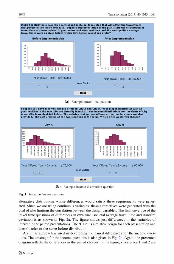
The travel time questions are posed as before and after scenarios resulting from a change in

policy. Respondents are told that a study is underway to put in place a new ramp metering

strategy. They are informed that when put in place, this strategy will lead to a redistribution

of travel time for people in the Twin Cities area. Histograms are used to depict the travel

time distributions in the before and after scenarios. The respondent’s personal position in

either case is also identified. An example of the question is given in Fig. 1a. The

respondent is then asked to choose between the before and after conditions.

In the second case, we consider income. In this case, respondents are told that a job offer is

on the table for them which requires them to relocate to a new area. There are two job offers

located in two different cities. The respondent is told that the positions are virtually identical

and that the cost of living is equal in either city. The income distribution in the two locations is

however different. In either case the distribution of income for residents of each city is given

using a histogram and the offered salary for the respondent is also given. Figure 1b shows one

of the questions. The respondent is then asked to choose between the two offers.

The design of both the travel time and income questionnaires were based on the dif-

ferences in personal position, differences in social average, and differences in the standard

deviation of the distributions in question. For travel time, the before after differences

between own time was set up so that the difference could be a at least as good as before the

change or loss, the societal average difference was setup to be either negative (societal

average increasing) or positive (decreasing in after period). These were in addition paired

with large and small differences in the standard deviation of the population distribution.

This roughly 2 9 2 9 2 design has 8 potential combinations for the three factors. Next

Transportation (2013) 40:1043–1061 1047

123

alternative distributions whose differences would satisfy these requirements were gener-

ated. Since we are using continuous variables, these alternatives were generated with the

goal of also limiting the correlation between the design variables. The final coverage of the

travel time questions of differences in own time, societal average travel time and standard

deviation is as shown in Fig. 2a. The figure shows just differences in the variables of

interest in the paired presentations. The ‘Base’ is a relative origin for each presentation and

doesn’t refer to the same before distribution.

A similar approach is used in developing the paired differences for the income ques-

tions. The coverage for the income questions is also given in Fig. 2b. Again, the presented

diagram reflects the differences in the paired choices. In the figure, since place 1 and 2 are

(a) Example travel time question

(b) Example income distribution question

Fig. 1 Stated preference questions

1048 Transportation (2013) 40:1043–1061

123

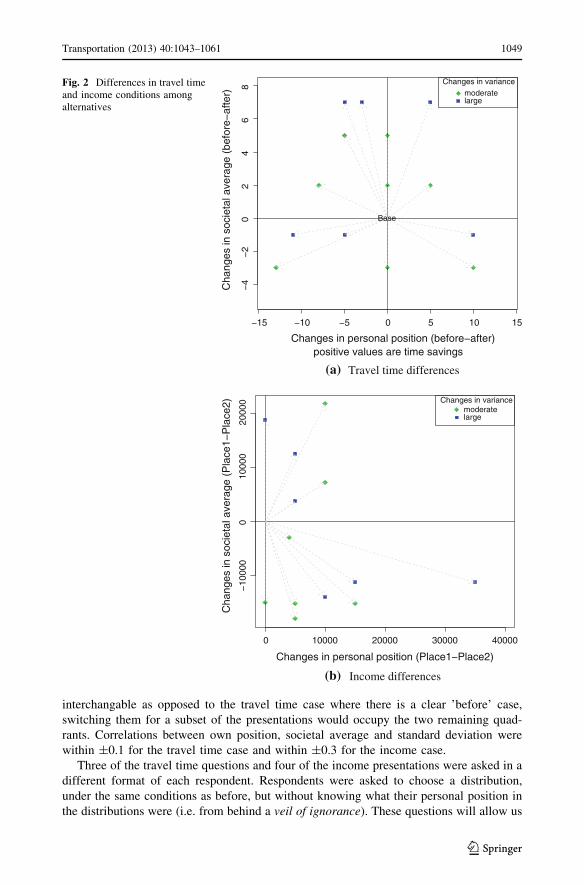
interchangable as opposed to the travel time case where there is a clear ’before’ case,

switching them for a subset of the presentations would occupy the two remaining quad-

rants. Correlations between own position, societal average and standard deviation were

within ±0.1 for the travel time case and within ±0.3 for the income case.

Three of the travel time questions and four of the income presentations were asked in a

different format of each respondent. Respondents were asked to choose a distribution,

under the same conditions as before, but without knowing what their personal position in

the distributions were (i.e. from behind a veil of ignorance). These questions will allow us

−15 −10 −5 0 5 10 15

−4

−2

02

46

8

Changes in personal position (before−after) positive values are time savings

Cha

nges

in s

ocie

tal a

vera

ge (

befo

re−

afte

r)Base

Changes in variancemoderatelarge

Travel time differences

0 10000 20000 30000 40000

−10

000

010

000

2000

0

Changes in personal position (Place1−Place2)

Cha

nges

in s

ocie

tal a

vera

ge (

Pla

ce1−

Pla

ce2) Changes in variance

moderatelarge

Income differences

(a)

(b)

Fig. 2 Differences in travel timeand income conditions amongalternatives

Transportation (2013) 40:1043–1061 1049

123

to test whether distributional concerns are different when people do not know their own

position. In the other scenarios, the respondent must decide if they are willing to trade

some of their own income or travel time to live in a region that has a more equal distri-

bution. In total, respondents were given a eighteen questions relating to time preferences

and seventeen questions relating to income preferences.

Survey administration

Prior to starting the survey individuals are given a quick tutorial on interpreting distri-

butions that are presented by using histograms. The tutorial takes them through mean and

variance identification, comparing mean and variance of different distributions, reading

frequency of an event occurrence based on given distributions and identifying their own

positions within a distribution when explicitly indicated. The survey then presents the

respondents with a series of binary alternatives where they make choices based on their

own personal position as well as the position of those around them in the travel time and

income contexts discussed above. There were a total of three randomizations that were

used to preorder the survey questions. In addition the information was presented in two

ways. In one case the distributions for the alternatives were placed one over the other and

in the other they were placed side by side. One of these was installed per computer. As

respondents came in, they were each randomly assigned to a computer.

Participants

Subjects for the survey were recruited via email from the University of Minnesota’s

employee database. Invitations were sent out to 2,500 randomly selected non-faculty, non-

student employees who had not participated in previous transportation studies conducted

by the authors. The recruitment email indicated that individuals were invited to participate

in a computer based commute study and offered $15 for participation. Participants were

asked to come to a central testing station, where the survey was administered. Based on

previous experience of similar recruitments, a target of 200 participants was set (split

evenly between male and female). A total of 187 respondents agreed and participated in the

study. Descriptive statistics for the subjects are given in Table 1.

In addition to the income and travel time questions, a separate set of questions about

route preferences was also administered along with the survey (Tilahun and Levinson

2010). Two questions in that set were control questions that were used to gauge whether

respondents understood the distributions that they were making choices over. Briefly, the

questions asked if the respondent would pay a higher toll to use a route that had on average

a longer travel time and large variance of travel time between the same origin-destination

pair. Only eight of the 187 respondents made what appeared to be an irrational choice,

illustrating respondents largely understood the questions.

Analysis and results

Self-interested choices

In a majority of the travel time and income choices that a respondent faces, one alternative

leaves him personally better off than the other (either with a lower travel time or a higher

personal income, respectively). This was true in 12 of the 15 travel time questions and 11

1050 Transportation (2013) 40:1043–1061

123

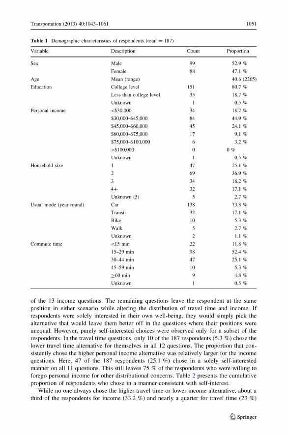
of the 13 income questions. The remaining questions leave the respondent at the same

position in either scenario while altering the distribution of travel time and income. If

respondents were solely interested in their own well-being, they would simply pick the

alternative that would leave them better off in the questions where their positions were

unequal. However, purely self-interested choices were observed only for a subset of the

respondents. In the travel time questions, only 10 of the 187 respondents (5.3 %) chose the

lower travel time alternative for themselves in all 12 questions. The proportion that con-

sistently chose the higher personal income alternative was relatively larger for the income

questions. Here, 47 of the 187 respondents (25.1 %) chose in a solely self-interested

manner on all 11 questions. This still leaves 75 % of the respondents who were willing to

forego personal income for other distributional concerns. Table 2 presents the cumulative

proportion of respondents who chose in a manner consistent with self-interest.

While no one always chose the higher travel time or lower income alternative, about a

third of the respondents for income (33.2 %) and nearly a quarter for travel time (23 %)

Table 1 Demographic characteristics of respondents (total = 187)

Variable Description Count Proportion

Sex Male 99 52.9 %

Female 88 47.1 %

Age Mean (range) 40.6 (2265)

Education College level 151 80.7 %

Less than college level 35 18.7 %

Unknown 1 0.5 %

Personal income \$30,000 34 18.2 %

$30,000–$45,000 84 44.9 %

$45,000–$60,000 45 24.1 %

$60,000–$75,000 17 9.1 %

$75,000–$100,000 6 3.2 %

[$100,000 0 0 %

Unknown 1 0.5 %

Household size 1 47 25.1 %

2 69 36.9 %

3 34 18.2 %

4? 32 17.1 %

Unknown (5) 5 2.7 %

Usual mode (year round) Car 138 73.8 %

Transit 32 17.1 %

Bike 10 5.3 %

Walk 5 2.7 %

Unknown 2 1.1 %

Commute time \15 min 22 11.8 %

15–29 min 98 52.4 %

30–44 min 47 25.1 %

45–59 min 10 5.3 %

C60 min 9 4.8 %

Unknown 1 0.5 %

Transportation (2013) 40:1043–1061 1051

123

chose alternatives that were not to their personal advantage in over half the questions.

Looking at per-subject choices, the median proportion of questions a subject answered in a

self-interested manner is 72 % for income (out of 11 questions) while it was 58 % for

travel time (out of 13 questions). Unlike results in ultimatum games which involve pen-

alties, subjects in this survey had no direct incentive that could influence their decision to

be fair to others (aside from some psychic reward of being perceived as a fair person either

to themselves or to the research team). Yet, the choices show altruistic motivations for a

large portion of the subjects.

Choices where own position is uncertain

As discussed earlier, a limited number of questions posed travel time and income questions

where the respondent did not know their own position. Because there is an element of

uncertainty, choices in this instance may be quite different from choices where respondents

know their position (where there is no uncertainty). Seven questions from the previous set

(3 for travel time, 4 for income) were takes and the respondent’s income removed from

these questions. These would be the original position in Rawls (1999) formulation, where

the respondent would choose a fair distribution lest they find themselves in either the

highest travel time or lowest income group, respectively.

Here again, there is a great deal of variation in how respondents evaluate these alter-

natives. Relatively simple choices mechanisms are possible in each case that can neatly

explain one motivation or another. For example in the income case, respondents may be

motivated by the risk of falling into the lowest income category and may seek to avoid

those situations. Or, they may seek the distribution with the highest expected income

(average) for the distribution - regarding this as their most likely outcome. In the travel

time case, the risk of ending up with the highest travel time may lead them to select the

distribution with a less extreme outcome, or the lower average may be the most attractive.

Alternatively, highly risk-seeking behavior may dominate where respondents align choices

with the most optimistic outcomes.

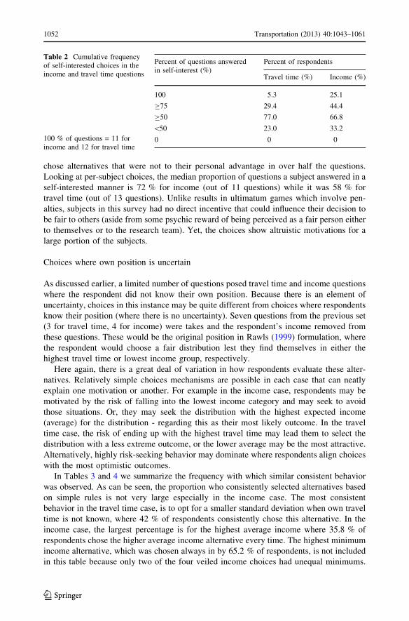
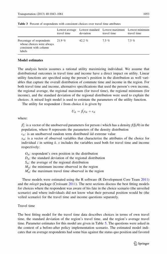
In Tables 3 and 4 we summarize the frequency with which similar consistent behavior

was observed. As can be seen, the proportion who consistently selected alternatives based

on simple rules is not very large especially in the income case. The most consistent

behavior in the travel time case, is to opt for a smaller standard deviation when own travel

time is not known, where 42 % of respondents consistently chose this alternative. In the

income case, the largest percentage is for the highest average income where 35.8 % of

respondents chose the higher average income alternative every time. The highest minimum

income alternative, which was chosen always in by 65.2 % of respondents, is not included

in this table because only two of the four veiled income choices had unequal minimums.

Table 2 Cumulative frequencyof self-interested choices in theincome and travel time questions

100 % of questions = 11 forincome and 12 for travel time

Percent of questions answeredin self-interest (%)

Percent of respondents

Travel time (%) Income (%)

100 5.3 25.1

C75 29.4 44.4

C50 77.0 66.8

\50 23.0 33.2

0 0 0

1052 Transportation (2013) 40:1043–1061

123

Model estimates

The analysis herein assumes a rational utility maximizing individual. We assume that

distributional outcomes in travel time and income have a direct impact on utility. Linear

utility functions are specified using the person’s position in the distribution as well vari-

ables that capture the overall distribution of commute time and income in the region. For

both travel time and income, alternative specifications that used the person’s own income,

the regional average, the regional maximum (for travel time), the regional minimum (for

income), and the standard deviation of the regional distribution were used to explain the

choices. A mixed logit model is used to estimate the parameters of the utility function.

The utility for respondent i from choice k is given by

Uik ¼ b0

ixik þ �ik

where:

b0i: is a vector of the unobserved parameters for person i which has a density f(bi/h) in the

population, where h represents the parameters of the density distribution

�ik: is an unobserved random term distributed iid extreme value

xik: is a vector of observed variables that characterize the attributes of the choice for

individual i in setting k. x includes the variables used both for travel time and income

respectively:

Oik: respondent’s own position in the distribution

Dik: the standard deviation of the regional distribution

Sik: the average of the regional distribution

Mik: the minimum income observed in the region

Mik* : the maximum travel time observed in the region

These models were estimated using the R software (R Development Core Team 2011)

and the mlogit package (Croissant 2011). The next sections discuss the best fitting models

for choices where the respondent was aware of his fate in the choice scenario (the unveiled

scenario) and where individuals did not know what their personal position would be (the

veiled scenario) for the travel time and income questions separately.

Travel time

The best fitting model for the travel time data describes choices in terms of own travel

time, the standard deviation of the region’s travel time, and the region’s average travel

time. Parameter estimates for this model are given in Table 5. The questions were asked in

the context of a before-after policy implementation scenario. The estimated model indi-

cates that on average respondents had some bias against the status quo position and favored

Table 3 Percent of respondents with consistent choices over travel time attributes

Lowest averagetravel time

Lowest standarddeviation

Lowest maximumtravel time

Lowest minimumtravel time

Percentage of respondentswhose choices were alwaysconsistent with columnlabels

21.9 % 42.2 % 7.5 % 7.5 %

Transportation (2013) 40:1043–1061 1053

123

change. This was more true for men, who were significantly more likely to vote against the

status quo than women. Age played a role favoring the status quo with each additional year

increasing the odds of choosing the status quo by 2.2 %, all other things equal.

The model also captures significant variation in the preferences over own travel time,

societal average and the standard deviation of the distribution of travel time. In the popula-

tion, each additional minute of personal travel time, population wide average travel time, and

increases in variances all lead to a reduction in the utility of the decision maker. The distri-

bution of these parameters in the population is modeled using a triangular distribution whose

characteristics are also shown in Table 5. The coefficients for own time (bO), societal time

(bS) are negative consistent with the assumption that increases in time lead to a disutility. For

about 98 % the parameter for the standard deviation (bD) is also negative, suggesting nar-

rower distributions are largely preferred. Though correlation among the random effects was

tested, it was dropped from the model since the model without correlations performed just as

well based on a likelihood ratio test. Respondents wanted to reduce own time, societal/

regional average, as well as the dispersion in travel time in their region.

The estimates also show that the average impact of an increase in societal average travel

time is larger than than the average for a one minute increase in personal travel time in the

population. To estimate the marginal rate of substitution (MRS), we use simulated coef-

ficients based on the estimated coefficients for bO, bS and bD and their respective

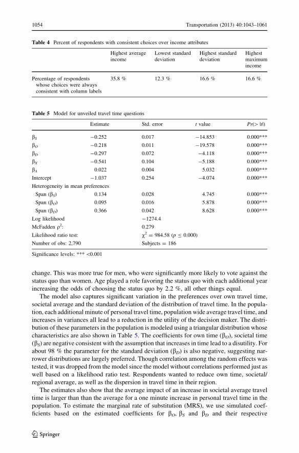
Table 4 Percent of respondents with consistent choices over income attributes

Highest averageincome

Lowest standarddeviation

Highest standarddeviation

Highestmaximumincome

Percentage of respondentswhose choices were alwaysconsistent with column labels

35.8 % 12.3 % 16.6 % 16.6 %

Table 5 Model for unveiled travel time questions

Estimate Std. error t value Pr([ |t|)

bS -0.252 0.017 -14.853 0.000***

bO -0.218 0.011 -19.578 0.000***

bD -0.297 0.072 -4.118 0.000***

bX -0.541 0.104 -5.188 0.000***

bA 0.022 0.004 5.032 0.000***

Intercept -1.037 0.254 -4.074 0.000***

Heterogeneity in mean preferences

Span (bS) 0.134 0.028 4.745 0.000***

Span (bO) 0.095 0.016 5.878 0.000***

Span (bD) 0.366 0.042 8.628 0.000***

Log likelihood -1274.4

McFadden q2: 0.279

Likelihood ratio test: v2 = 984.58 (p B 0.000)

Number of obs: 2,790 Subjects = 186

Significance levels: *** \0.001

1054 Transportation (2013) 40:1043–1061

123

distributions. The mean MRS between the societal average (S) and own time (O) is 1.20—a

willingness to increase own travel time by 1.20 min for a minute reduction in the societal

mean. For the standard deviation, the mean MRS is 1.41 of own minutes for a decrease in 1

minute of the standard deviation. These values along with the standard error of the mean

and the distribution of the MRS values is given in Table 6. These values are based on

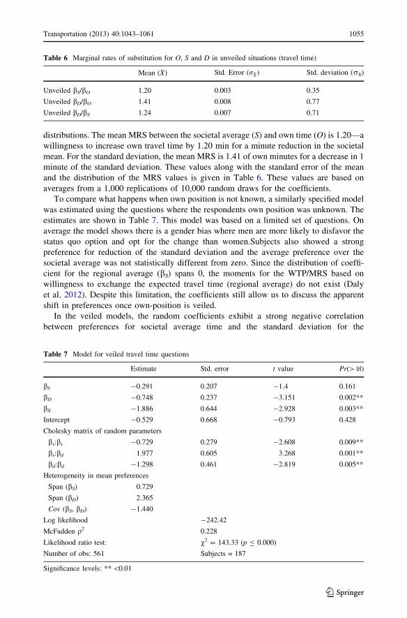
averages from a 1,000 replications of 10,000 random draws for the coefficients.

To compare what happens when own position is not known, a similarly specified model

was estimated using the questions where the respondents own position was unknown. The

estimates are shown in Table 7. This model was based on a limited set of questions. On

average the model shows there is a gender bias where men are more likely to disfavor the

status quo option and opt for the change than women.Subjects also showed a strong

preference for reduction of the standard deviation and the average preference over the

societal average was not statistically different from zero. Since the distribution of coeffi-

cient for the regional average (bS) spans 0, the moments for the WTP/MRS based on

willingness to exchange the expected travel time (regional average) do not exist (Daly

et al. 2012). Despite this limitation, the coefficients still allow us to discuss the apparent

shift in preferences once own-position is veiled.

In the veiled models, the random coefficients exhibit a strong negative correlation

between preferences for societal average time and the standard deviation for the

Table 6 Marginal rates of substitution for O, S and D in unveiled situations (travel time)

Mean (�X) Std. Error (r�X) Std. deviation (rX)

Unveiled bS/bO 1.20 0.003 0.35

Unveiled bD/bO 1.41 0.008 0.77

Unveiled bD/bS 1.24 0.007 0.71

Table 7 Model for veiled travel time questions

Estimate Std. error t value Pr([ |t|)

bS -0.291 0.207 -1.4 0.161

bD -0.748 0.237 -3.151 0.002**

bX -1.886 0.644 -2.928 0.003**

Intercept -0.529 0.668 -0.793 0.428

Cholesky matrix of random parameters

bs:bs -0.729 0.279 -2.608 0.009**

bs:bd 1.977 0.605 3.268 0.001**

bd:bd -1.298 0.461 -2.819 0.005**

Heterogeneity in mean preferences

Span (bS) 0.729

Span (bD) 2.365

Cov (bS, bD) -1.440

Log likelihood -242.42

McFadden q2 0.228

Likelihood ratio test: v2 = 143.33 (p B 0.000)

Number of obs: 561 Subjects = 187

Significance levels: ** \0.01

Transportation (2013) 40:1043–1061 1055

123

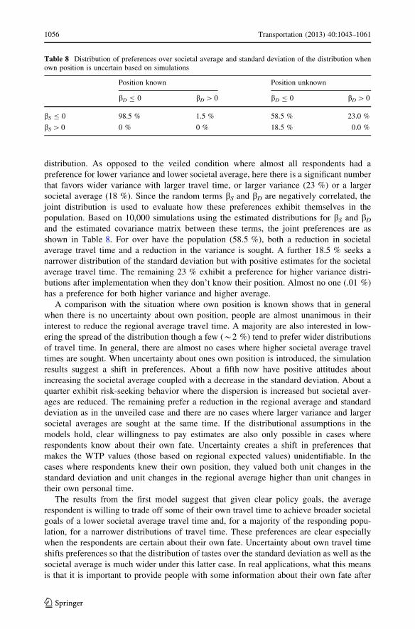
distribution. As opposed to the veiled condition where almost all respondents had a

preference for lower variance and lower societal average, here there is a significant number

that favors wider variance with larger travel time, or larger variance (23 %) or a larger

societal average (18 %). Since the random terms bS and bD are negatively correlated, the

joint distribution is used to evaluate how these preferences exhibit themselves in the

population. Based on 10,000 simulations using the estimated distributions for bS and bD

and the estimated covariance matrix between these terms, the joint preferences are as

shown in Table 8. For over have the population (58.5 %), both a reduction in societal

average travel time and a reduction in the variance is sought. A further 18.5 % seeks a

narrower distribution of the standard deviation but with positive estimates for the societal

average travel time. The remaining 23 % exhibit a preference for higher variance distri-

butions after implementation when they don’t know their position. Almost no one (.01 %)

has a preference for both higher variance and higher average.

A comparison with the situation where own position is known shows that in general

when there is no uncertainty about own position, people are almost unanimous in their

interest to reduce the regional average travel time. A majority are also interested in low-

ering the spread of the distribution though a few (*2 %) tend to prefer wider distributions

of travel time. In general, there are almost no cases where higher societal average travel

times are sought. When uncertainty about ones own position is introduced, the simulation

results suggest a shift in preferences. About a fifth now have positive attitudes about

increasing the societal average coupled with a decrease in the standard deviation. About a

quarter exhibit risk-seeking behavior where the dispersion is increased but societal aver-

ages are reduced. The remaining prefer a reduction in the regional average and standard

deviation as in the unveiled case and there are no cases where larger variance and larger

societal averages are sought at the same time. If the distributional assumptions in the

models hold, clear willingness to pay estimates are also only possible in cases where

respondents know about their own fate. Uncertainty creates a shift in preferences that

makes the WTP values (those based on regional expected values) unidentifiable. In the

cases where respondents knew their own position, they valued both unit changes in the

standard deviation and unit changes in the regional average higher than unit changes in

their own personal time.

The results from the first model suggest that given clear policy goals, the average

respondent is willing to trade off some of their own travel time to achieve broader societal

goals of a lower societal average travel time and, for a majority of the responding popu-

lation, for a narrower distributions of travel time. These preferences are clear especially

when the respondents are certain about their own fate. Uncertainty about own travel time

shifts preferences so that the distribution of tastes over the standard deviation as well as the

societal average is much wider under this latter case. In real applications, what this means

is that it is important to provide people with some information about their own fate after

Table 8 Distribution of preferences over societal average and standard deviation of the distribution whenown position is uncertain based on simulations

Position known Position unknown

bD B 0 bD [ 0 bD B 0 bD [ 0

bS B 0 98.5 % 1.5 % 58.5 % 23.0 %

bS [ 0 0 % 0 % 18.5 % 0.0 %

1056 Transportation (2013) 40:1043–1061

123

policy or project implementation. Absent that information, about 42 % start to favor

outcomes that are at least in one dimension (mean travel time or variance) not very

desirable. The informed respondent is willing to consider the fate of those around him even

while they are interested in reducing their own travel time.

Income

Separate models for the income preferences were also estimated based on the preference

data under conditions where the person was aware of their own income and where their

position is not known. As discussed earlier, this question is presented in the context where

a person is choosing to relocate between two different locations. The two models are

presented in Tables 9 and 10. In both cases, the intercept term is not statistically significant

suggesting there is no preference towards any given alternative that may have arisen from

the questionnaire’s format. Choices were also not explained by personal factors such as

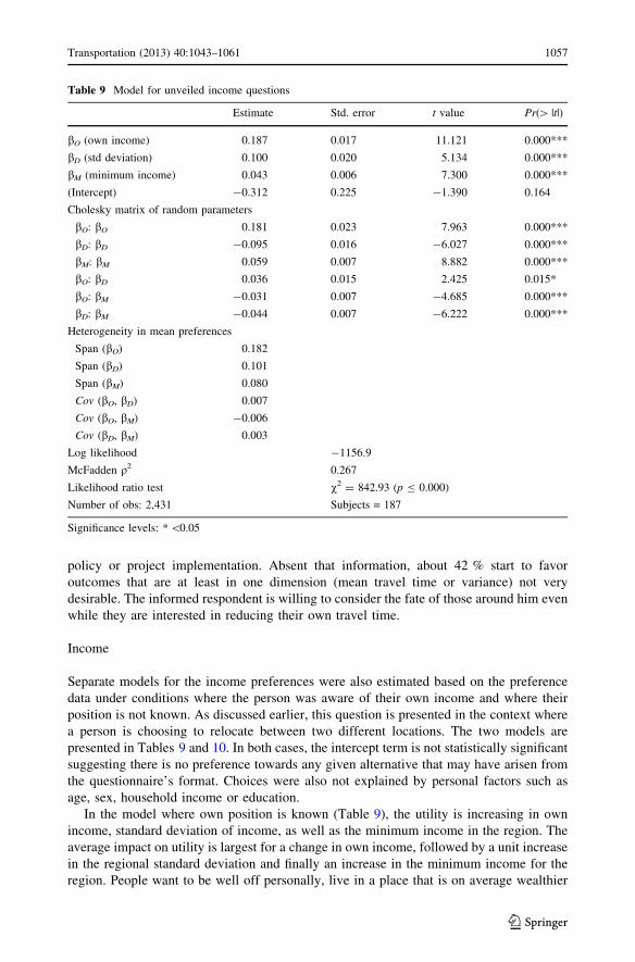
age, sex, household income or education.

In the model where own position is known (Table 9), the utility is increasing in own

income, standard deviation of income, as well as the minimum income in the region. The

average impact on utility is largest for a change in own income, followed by a unit increase

in the regional standard deviation and finally an increase in the minimum income for the

region. People want to be well off personally, live in a place that is on average wealthier

Table 9 Model for unveiled income questions

Estimate Std. error t value Pr([ |t|)

bO (own income) 0.187 0.017 11.121 0.000***

bD (std deviation) 0.100 0.020 5.134 0.000***

bM (minimum income) 0.043 0.006 7.300 0.000***

(Intercept) -0.312 0.225 -1.390 0.164

Cholesky matrix of random parameters

bO: bO 0.181 0.023 7.963 0.000***

bD: bD -0.095 0.016 -6.027 0.000***

bM: bM 0.059 0.007 8.882 0.000***

bO: bD 0.036 0.015 2.425 0.015*

bO: bM -0.031 0.007 -4.685 0.000***

bD: bM -0.044 0.007 -6.222 0.000***

Heterogeneity in mean preferences

Span (bO) 0.182

Span (bD) 0.101

Span (bM) 0.080

Cov (bO, bD) 0.007

Cov (bO, bM) -0.006

Cov (bD, bM) 0.003

Log likelihood -1156.9

McFadden q2 0.267

Likelihood ratio test v2 = 842.93 (p B 0.000)

Number of obs: 2,431 Subjects = 187

Significance levels: * \0.05

Transportation (2013) 40:1043–1061 1057

123

and where there are few very low earners. The model assumes that the random parameter

for all three preferences has a triangular distribution. The coefficient for own income is

always positive spanning the range from (0.006 to 0.37). Mean coefficients for the standard

deviation and minimum income are both positive and statistically significant. Coefficient

for the standard deviation range from 0 to 0.20. However, the range of estimates for the

regional minimum income suggests that about 11 % have a preference for lower minimum

incomes. The coefficient ranges from -0.04 to 0.12. The model also shows a statistically

significant moderate correlation between preferences for income, standard deviation, and

minimum income. Positive correlations are observed between preferences for personal

income and variance as well as for variance minimum income. There is negative corre-

lation between preferences for personal income and the minimum regional income. The

higher the preference for personal income, the higher the preference for income variance,

and the less the person cared for regional minimum incomes. Conversely, those who cared

about the regional minimums had lower preferences for own income and larger income

variance.

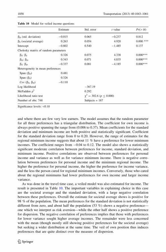
As was done in the travel time case, a veiled model was also estimated for income. The

result is presented in Table 10. The important variables in explaining choice in this case

are the societal average and the standard deviation, with a large negative correlation

between these preferences. Overall the estimate for societal average shows is positive for

98 % of the population. The mean preferences for the standard deviation is not statistically

different from zero, and about half the population (53 %) shows a negative preference—

one which we interpret as risk aversion—while the other half shows a positive preference

for dispersion. The negative correlation of preferences implies that those with preferences

for lower variance sought higher average incomes. The remainder were less concerned

with the mean (though mostly still showing positive preferences for the societal average)

but seeking a wider distribution at the same time. The veil of own position thus induces

preferences that are quite distinct over the measure of dispersion.

Table 10 Model for veiled income questions

Estimate Std. error t value Pr([ |t|)

bD (std. deviation) -0.015 0.065 -0.237 0.812

bS (societal average) 0.263 0.054 4.920 0.000 ***

Intercept -0.802 0.540 -1.485 0.137

Cholesky matrix of random parameters

bS: bS 0.326 0.075 4.338 0.000***

bD: bD 0.343 0.071 4.835 0.000***

bS: bD -0.337 0.081 -4.185 0.000***

Heterogeneity in mean preferences

Span (bD) 0.481

Span (bS) 0.326

Cov (bS, bD) -0.110

Log likelihood -367.19

McFadden q2 0.292

Likelihood ratio test v2 = 302.6 (p B 0.000)

Number of obs: 748 Subjects = 187

Significance levels: \0.10

1058 Transportation (2013) 40:1043–1061

123

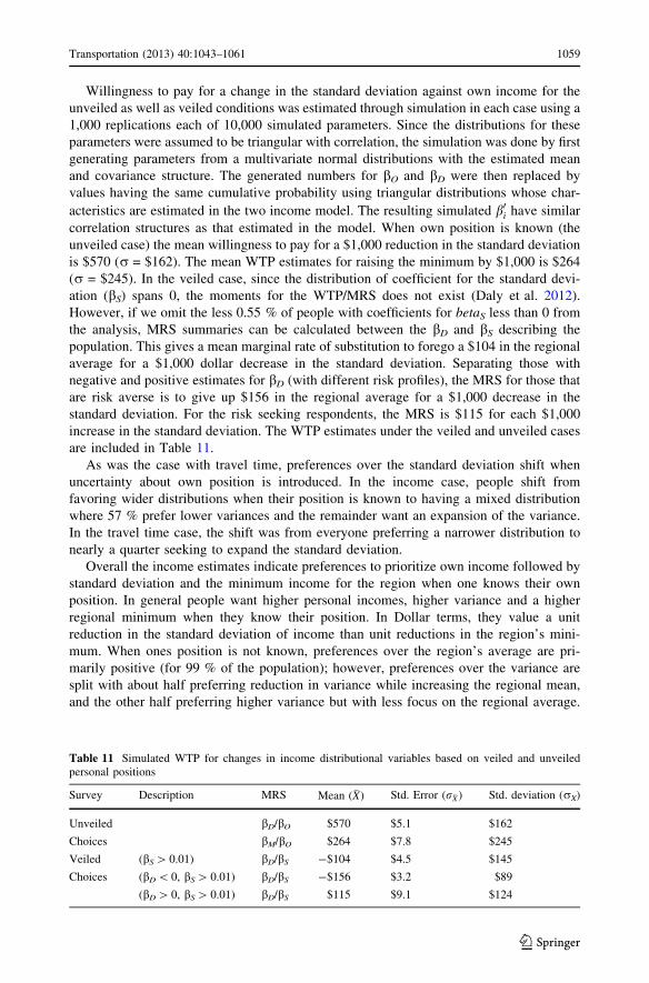
Willingness to pay for a change in the standard deviation against own income for the

unveiled as well as veiled conditions was estimated through simulation in each case using a

1,000 replications each of 10,000 simulated parameters. Since the distributions for these

parameters were assumed to be triangular with correlation, the simulation was done by first

generating parameters from a multivariate normal distributions with the estimated mean

and covariance structure. The generated numbers for bO and bD were then replaced by

values having the same cumulative probability using triangular distributions whose char-

acteristics are estimated in the two income model. The resulting simulated b0i have similar

correlation structures as that estimated in the model. When own position is known (the

unveiled case) the mean willingness to pay for a $1,000 reduction in the standard deviation

is $570 (r = $162). The mean WTP estimates for raising the minimum by $1,000 is $264

(r = $245). In the veiled case, since the distribution of coefficient for the standard devi-

ation (bS) spans 0, the moments for the WTP/MRS does not exist (Daly et al. 2012).

However, if we omit the less 0.55 % of people with coefficients for betaS less than 0 from

the analysis, MRS summaries can be calculated between the bD and bS describing the

population. This gives a mean marginal rate of substitution to forego a $104 in the regional

average for a $1,000 dollar decrease in the standard deviation. Separating those with

negative and positive estimates for bD (with different risk profiles), the MRS for those that

are risk averse is to give up $156 in the regional average for a $1,000 decrease in the

standard deviation. For the risk seeking respondents, the MRS is $115 for each $1,000

increase in the standard deviation. The WTP estimates under the veiled and unveiled cases

are included in Table 11.

As was the case with travel time, preferences over the standard deviation shift when

uncertainty about own position is introduced. In the income case, people shift from

favoring wider distributions when their position is known to having a mixed distribution

where 57 % prefer lower variances and the remainder want an expansion of the variance.

In the travel time case, the shift was from everyone preferring a narrower distribution to

nearly a quarter seeking to expand the standard deviation.

Overall the income estimates indicate preferences to prioritize own income followed by

standard deviation and the minimum income for the region when one knows their own

position. In general people want higher personal incomes, higher variance and a higher

regional minimum when they know their position. In Dollar terms, they value a unit

reduction in the standard deviation of income than unit reductions in the region’s mini-

mum. When ones position is not known, preferences over the region’s average are pri-

marily positive (for 99 % of the population); however, preferences over the variance are

split with about half preferring reduction in variance while increasing the regional mean,

and the other half preferring higher variance but with less focus on the regional average.

Table 11 Simulated WTP for changes in income distributional variables based on veiled and unveiledpersonal positions

Survey Description MRS Mean (�X) Std. Error (r�X) Std. deviation (rX)

Unveiled bD/bO $570 $5.1 $162

Choices bM/bO $264 $7.8 $245

Veiled (bS [ 0.01) bD/bS -$104 $4.5 $145

Choices (bD \ 0, bS [ 0.01) bD/bS -$156 $3.2 $89

(bD [ 0, bS [ 0.01) bD/bS $115 $9.1 $124

Transportation (2013) 40:1043–1061 1059

123

Discussion

This paper examines individual preferences over travel time and income distributions.

Traditional economic models posit that choices are mainly self-interested though several

exceptions to this have been documented in the experimental economics literature. The

empirical evidence from our survey also illustrates that choices are complex and do not

easily fall into one category. We observe choices both in income and travel time distri-

butions where individuals are willing to forego some of their own wellbeing (either in

terms of higher income, or lower travel times) to allow for distributions that increase

minimum income or reduce average travel time in the region. Willingness to pay measures

for outcomes that were altruistic (reduced variance or increased minimum income for

others) even at personal loss were recorded.

In contrast with ultimatum game experiments, our presentations do not have explicit

penalties for purely self-interested decisions. However in a majority of cases, purely self-

interested choices were not observed. In fact, only 5.3 % of respondents always chose the

lower travel time alternative for themselves in the choices presented. Most showed a will-

ingness to improve travel time outcomes for others to varying degrees. The proportion for

income that always chose the better outcome for themselves was higher with about a quarter

of the respondents consistently choosing in that manner. But that still leaves three quarters of

the respondents who traded their own incomes to achieve the well being of others.

In the estimated unveiled income model (Table 9), the average parameter for own-

position in the income case pointed to the importance of own-position as compared to other

variables. In the travel time case, respondents cared less about unit changes in own position

as compared to societal measures. Perhaps this may may be because they believe they are

more likely to face different travel time conditions (e.g. either due to a job change, due to

non-work travel, etc.) than they are to face different income conditions. These order of

preferences also suggest that preferences about income and time may be informed dif-

ferently based on the best fitting models and parameter estimates discussed in the previous

section. Travel time preferences seem predominantly to be informed by societal average,

followed by the own travel time, and finally by the standard deviation of the distribution

considered. For income, unit shifts in own income take priority, followed by a higher

standard deviation, and finally the minimum of the distributions. These preferences are also

correlated with one another.

Though the data which looks at preferences when own position is uncertain is limited, it

suggests that preferences about travel time mainly focus on a reduction of the standard

deviation of the distribution when a person does not know their own fate with mixed

preferences over the societal average. For income, a strategy to increase the regional

average income explains the choices most with variable preferences over the standard

deviation.

We had started out with a hypothesis that choices are likely not entirely self regarding.

The summary of choices and the estimated models support this hypothesis. The question of

how to capture the other regarding preferences is tested with different specifications of the

utility function and the best models are reported here. Overall, the study illustrates that

choices are seldom explained in terms of very simple motivations. Fewer than a majority in

both the veiled and unveiled choice alternatives chose in a manner that was purely in line

with one strategy exclusively. Most respondents showed a combination of altruism and

selfishness depending on the questions asked, suggesting that clearly articulated policy

goals would have backers even among those that stand to lose some of their own imme-

diate welfare.

1060 Transportation (2013) 40:1043–1061

123

References

Bolton, G.E., Ockenfels, A.: A theory of equity, reciprocity and competition. Am. Econ. Rev. 90(1),166–193 (2000)

Carlsson, F., Daruvala, D., Johansson-Stenman, O.: Are people inequality-averse, or just risk-averse?.Economica 72(287), 375–396 (2005)

Daly, A., Hess, S., Train, K.: Assuring finite moments for willingness to pay in random coefficient models.Transportation 39(1), 19–31 (2012)

DeSerpa, A.C.: A theory of the economics of time. Econ. J. 81(324), 828–846 (1971)Elster, J.: Altruistic behavior and altruistic motivations. Handbook Econ. Giv. Recip. Altruism 1, 183–206

(2006)Engelmann, D., Strobel, M.: Inequality aversion, efficiency, and maximin preferences in simple distribution

experiments. Am. Econ. Rev. 94(4), 857–869 (2004)Evans, A.W.: On the theory of the valuation and allocation of time*. Scott. J. Polit. Econ. 19(1), 1–17 (1972)Fehr, E., Schmidt, K.M.: A theory of fairness, competition, and cooperation*. Q. J. Econ. 114(3), 817–868

(1999)Guth, W., Schmittberger, R., Schwarze, B.: An experimental analysis of ultimatum bargaining. J. Econ.

Behav. Organ. 3(4), 367–388 (1982)Kahneman D., Knetsch J.L., Thaler R.H.: Fairness and the assumptions of economics. J. Business 285–300

(1986)Mackie, P.J., Jara-Dıaz, S., Fowkes, A.S.: The value of travel time savings in evaluation. Transp. Res. Part

E. 37(2), 91–106 (2001)Marchetti A., Castelli I., Harle K.M., Sanfey A.G.: Expectations and outcome: The role of proposer features

in the ultimatum game. J. Econ. Psychol. (2011)R Development Core Team. R: A language and environment for statistical computing. R Foundation for

Statistical Computing, Vienna, (2011). URL http://www.R-project.org/. ISBN 3-900051-07-0.Rabin M.: Incorporating fairness into game theory and economics. Am. Econ. Rev. 1281–1302 (1993)Rawls J.: A Theory of Justice. Belknap Press, Cambridge (1999)Scanlon T.: The Diversity of Objections to Inequality. Department of Philosophy, University of Kansas,

Lawrence (1997)Thaler, R.H.: Anomalies: The ultimatum game. J. Econ. Perspect. 2(4), 195–206 (1988)Tilahun, N.Y., Levinson, D.M.: A moment of time: reliability in route choice using stated preference.

J. Intell. Transp. Syst. 14(3), 179–187 (2010)Yves Croissant. mlogit: multinomial logit model, 2011. URL http://CRAN.R-project.org/package=mlogit. R

package version 0.2-2Zhang, L., Levinson, D.: Balancing efficiency and equity of ramp meters. J. Transp. Eng. 131, 477 (2005)

Author Biographies

Dr. Nebiyou Tilahun an Assistant Professor in the Department of Urban Planning and Policy at theUniversity of Illinois at Chicago. He earned his PhD in Civil Engineering from the University of Minnesotain 2010. His research focuses on travel behavior, travel for social activities, and the use of agent basedmodels for transportation planning applications.

Prof. David Levinson serves on the faculty of the Department of Civil Engineering at the University ofMinnesota and is Director of the Networks, Economics, and Urban Systems (NEXUS) research group. Heholds the Richard P. Braun/CTS Chair in Transportation. He also serves on the graduate faculty of theApplied Economics and Urban and Regional Planning programs at the University of Minnesota. ProfLevinson is the author of The Transportation Experience and 6 other books. He is the editor of the Journal ofTransport and Land Use.

Transportation (2013) 40:1043–1061 1061

123