sedimentology and geochemistry of core sediments ... - Dyuthi

SEDIMENTOLOGY AND GEOCHEMISTRY OF CORE

SEDIMENTS FROM THE ASHTAMUDI ESTUARY AND THE

ADJOINING COASTAL PLAIN, CENTRAL KERALA, INDIA

Thesis submitted to

THE COCHIN UNIVERSITY OF SCIENCE AND TECHNOLOGY

In partial fulfillment of the requirements for the award of the Degree of DOCTOR OF PHILOSOPHY

in MARINE GEOLOGY

Under the Faculty of Marine Sciences

By

TIJU I. VARGHESE

NATIONAL CENTRE FOR EARTH SCIENCE STUDIES THIRUVANANTHAPURAM, KERALA, INDIA–695011

DECEMBER 2014

Bible says in Philippians 4:13

"I can do all things through Christ which strengtheneth me"

To

My beloved family

ACKNOWLEDGEMENTS

I wish to place on record my deep sense of gratitude to my research guide

Dr. T.N. Prakash, Group Head (Coastal Processes), National Centre for Earth

Science Studies (NCESS), who has been a source of inspiration and support to me

throughout the course of my research work. I owe him a lot for the constant

encouragement and guidance and also for sparing his invaluable time, without which

this work wouldn't have taken this shape.

I am grateful to Dr. N.P. Kurian, Director, NCESS for the support and

encouragement rendered throughout this work. I consider myself extremely fortunate

to have worked with him, since I found every discussion with him inspiring and

enlightening. Thanks are also due to him for providing all the necessary facilities of

the institute for the successful completion of my research work.

I express my immense gratitude to Dr. L. Sheela Nair, Scientist-E, Coastal

Processes Group, NCESS for the constant guidance and encouragement received for

the research work and for the support in the preparation of this thesis.

Prof. R. Nagendra, Dept. of Geology, Anna University, Chennai and Dr. N.

Nagarajan, Asst. Professor, Dept. of Applied Geology, Curtin University, Malaysia

are greatly acknowleged for fruitful discussion on geochemical aspects.

It is with great pleasure and gratitude that I acknowledge the valuable

guidance received from Dr. K.V. Thomas, former Group Head and Dr. T.S. Shahul

Hameed, Scientist-G, Coastal Processes Group during the course of my work.

I am grateful to Dr. G.R. RavindraKumar, Scientist G and Senior Consultant

of Crustal Processes Group, for the guidance in final preparation of the thesis. I am

thankful to Dr. M. Baba, former Director, NCESS, for the constant encouragement.

I acknowledge with gratitude the help received from M/s. D. Raju,

Vijayakumaran Nair, Ajith Kumar, Ramesh Kumar and S. Mohanan, Scientific

Officers at various stages of this study.

Prof. P. Seralathan, former Head, Dept. of Marine Geology and Geophysics,

School of Marine Sciences, CUSAT has provided me valuable support and guidance

in his capacity as Doctoral Committee member.

I am thankful to the Department of Science and Technology for financial

support in the form of Senior Research Fellow under the Project No. SR/S4/ES-

310/2007.

I acknowledge with thanks the administrative support provided by M/s. P.

Sudeep, Chief Manager, M.A.K.H. Rasheed, Manager (F & A) and other officers and

staff of the Administrative and Accounts sections of NCESS. Special thanks are due to

Librarian and other staff of the library for extending the Library facilities.

It is my pleasure to put on record the support and friendliness I have enjoyed

from the company of Dr. V.R. Shamji, Mr. C. Sreejith, Dr. C.S. Prasanth, Mr. N.

Nishanth during my tenure at NCESS.

I have pleasure in acknowledging Mr. R. Prasad and Mr. Anish S. Anand for

their unstinting support and timely help from the starting stages of my research work

till the submission of this thesis.

Thanks are due to Dr. K.O. Badarees, Dr. K. Rajith, and Dr. Reji Srinivas for

their support and encouragement at various stages of my research work.

Thanks are due to Dr. S.S. Praveen, Mr. S. Arjun, Mr. Arun J. John,Mr.

Sreeraj M.K., Mr. Eldhose Kuriakose, Mrs. Krishna R. Prasad, Mrs. Raji S. Nair, Ms.

Kalarani, Mrs. Gopika R. Nair and Mrs. Sindhu, NCESS for the help and support

extended to me in various stages of the work. I also thank Ms. Gayathri and Mr.

Sathyamurty Research Scholars, Anna University for their help in laboratory

computation.

Last but not the least I am to express my deep gratitude to my father (K.I.

Varghese), my mother (Aleyamma), my loving brothers (Biju and Liju) and my sister-

in-law (Raji Liju) for their prayers and unflinching support for completion of this

work.

Tiju I. Varghese

CONTENTS

Acknowledgements

List of Tables

List of Figures

Abstract

Chapter 1 INTRODUCTION

1.1 Introduction 1

1.2 Scientific Rationale 2

1.3 Objectives of the Present study 3

1.4 Study Area 3

1.4.1 Ashtamudi Estuary 5

1.4.2 Kayamkulam Lagoon 5

1.5 Physiography 6

1.6 Geology 7

1.6.1 Geological Setting of the Ashtamudi Estuary 7

1.6.2 Geological Setting of the Kayamkulam Lagoon 9

1.7 Geomorphology 9

1.7.1 Coastal Cliff 9

1.7.2 Coastal Plain with Ridge-Runnel Systems 9

1.7.3 Flood Plains 11

1.8 Climate and Rainfall 12

1.9 Physio-chemical Properties 12

Chapter 2 LITERATURE REVIEW

2.1 Introduction 14

2.2 Quaternary Studies 14

2.2.1 International Status 14

2.2.2 National Status 15

2.2.2.1 Studies on the East Coast of India 16

2.2.2.2 Studies on the West Coast of India 17

2.3 Kerala Scenario 19

Chapter 3 FIELD DATA COLLECTION AND ANALYSES

3.1 Introduction 26

3.2 Field Mapping and Collection of Sediment Cores 26

3.2.1 Field Mapping 26

3.2.2 Collection of Sediment Cores 26

3.3 Analyses of Sediment Core Samples 31

3.3.1 Textural Analysis 31

3.3.2 Surface Texture Analysis 33

3.3.3 Clay Mineral Analysis 33

3.3.4 Organic Matter Estimation 34

3.3.5 Determination of Calcium Carbonate 35

3.3.6 Geochemical Analysis 35

3.3.6.1 Sample Preparation and Instruments Used 36

3.3.6.2 Major Elements 37

3.3.6.3 Trace Elements 37

3.3.7 Radiocarbon Dating 37

Chapter 4 SEDIMENTOLOGY OF CORE SEDIMENTS

4.1 Introduction 39

4.2 Lithological Variation 40

4.2.1 Sediment core along the southern transect (Kollam) 40

4.2.1.1 Coastal Plain (Core 1) 40

4.2.1.2 Ashtamudi Estuary (Core 2) 42



4.2.1.5 Offshore (Core 5) 45

4.2.2 Sediment core along the northern Transect 46

4.2.2.1 Coastal Plain (Core 6) 40

4.2.2.2 Kayamkulam Lagoon (Core 7) 49

4.2.2.3 Offshore (Core 8) 50

4.3 Textural Parameters 51

4.3.1 Southern Transect 52

4.3.1.1 Coastal Plain 52

4.3.1.2 Ashtamudi Estuary 53

4.3.1.3 Offshore 54

4.3.2 Northern Transect 55

4.3.2.1 Coastal plain 55

4.3.2.2 Lagoon 56

4.3.2.3 Offshore 56

4.4 Sediment classification 57

4.5 Depositional Environment 57

4.5.1 Hydrodynamic condition 58

4.5.2 Suite Statistics 60

4.6 Clay Minerals 62

4.7 Radiocarbon Dating 64

4.8 Discussion 66

4.9 Summary 69

Chapter 5 MICROMORPHOLOGICAL CHARACTERISTICS OF

QUARTZ GRAINS – IMPLICATIONS ON DEPOSITIONAL

ENVIRONMENT

5.1 Introduction 71

5.2 Microtextural Characteristics 72

5.2.1 Southern Transect 72


5.2.1.2 Estuary 78

5.2.1.3 Offshore 81

5.2.2 Northern transect 82


5.2.2.2 Offshore 90

5.3 Transport Mechanism and Depositional History 92

5.4 Summary 95

Chapter 6 MAJOR AND TRACE ELEMENT GEOCHEMISTRY OF

SEDIMENT CORES

6.1 Introduction 97

6.2 Distribution of Major elements 98

6.2.1 Normalisation of major and trace elements with

UCC

98

6.3 Geochemical Classification 112

6.4 Paleoweathering and Sediment Maturity 113

6.4.1 Chemical Index of Alteration 113

6.4.2 ICV Relation to Recycling and Weathering Intensity 117

6.4.3 Textural maturity 118

6.5 Provenance 120

6.6 Environment of Deposition 126

6.7 Geoaccumulation index (Igeo) 126

6.8 Summary 129

Chapter 7 DEPOSITIONAL ENVIRONMENTS AND COASTAL

EVOLUTION

7.1 Introduction 130

7.2 Depositional Environment 130

7.3 Relationship between Organic matter and Calcium

Carbonate

131

7.4 Geochemical Proxies 131

7.5 Bathymetry 132

7.6 Holocene sea level changes 134

7.7 Evolution of the coast 135

7.8 Evolution of Ashtamudi Estuary 138

Chapter 8 SUMMARY AND CONCLUSIONS

8.1 Summary 140

8.2 Evolution of the coast 143

8.3 Evolution of Asthamudi Estuary 144

8.4 Recommendations for Future Work 145

REFERENCES 146

PUBLICATIONS 179

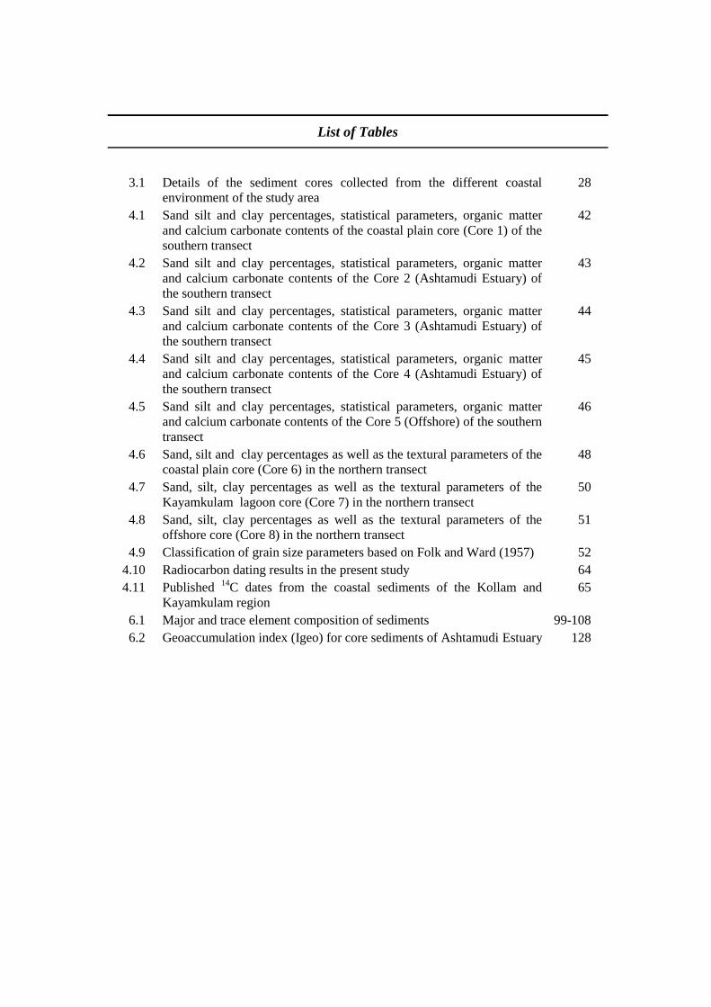
List of Tables

3.1 Details of the sediment cores collected from the different coastal

environment of the study area

28

4.1 Sand silt and clay percentages, statistical parameters, organic matter

and calcium carbonate contents of the coastal plain core (Core 1) of the

southern transect

42


and calcium carbonate contents of the Core 2 (Ashtamudi Estuary) of

the southern transect

43




44




45


and calcium carbonate contents of the Core 5 (Offshore) of the southern

transect

46

4.6 Sand, silt and clay percentages as well as the textural parameters of the

coastal plain core (Core 6) in the northern transect

48

4.7 Sand, silt, clay percentages as well as the textural parameters of the

Kayamkulam lagoon core (Core 7) in the northern transect

50

4.8 Sand, silt, clay percentages as well as the textural parameters of the

offshore core (Core 8) in the northern transect

51

4.9 Classification of grain size parameters based on Folk and Ward (1957) 52

4.10 Radiocarbon dating results in the present study 64

4.11 Published 14

C dates from the coastal sediments of the Kollam and

Kayamkulam region

65

6.1 Major and trace element composition of sediments 99-108

6.2 Geoaccumulation index (Igeo) for core sediments of Ashtamudi Estuary 128

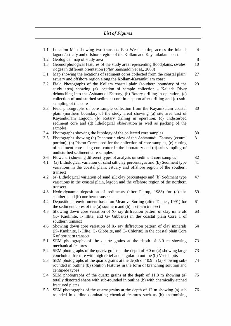
List of Figures

1.1 Location Map showing two transects East-West, cutting across the inland,

lagoon/estuary and offshore region of the Kollam and Kayamkulam coast

4

1.2 Geological map of study area 8

1.3 Geomorphological features of the study area representing floodplains, swales,

ridges in different orientation (after Samsuddin et al., 2008)

10

3.1 Map showing the locations of sediment cores collected from the coastal plain,

estuary and offshore region along the Kollam-Kayamkulam coast

27

3.2 Field Photographs of the Kollam coastal plain (southern boundary of the

study area) showing (a) location of sample collection - Kallada River

debouching into the Ashtamudi Estuary, (b) Rotary drilling in operation, (c)

collection of undisturbed sediment core in a spoon after drilling and (d) sub-

sampling of the core

29

3.3 Field photographs of core sample collection from the Kayamkulam coastal

plain (northern boundary of the study area) showing (a) site area east of

Kayamkulam Lagoon, (b) Rotary drilling in operation, (c) undisturbed

sediment core and (d) lithological observation as well as packing of the

samples

30

3.4 Photographs showing the lithology of the collected core samples 30

3.5 Photographs showing (a) Panamoric view of the Ashtamudi Estuary (central

portion), (b) Piston Corer used for the collection of core samples, (c) cutting

of sediment core using core cutter in the laboratory and (d) sub-sampling of

undisturbed sediment core samples

31

3.6 Flowchart showing different types of analysis on sediment core samples 32

4.1 (a) Lithological variation of sand silt clay percentages and (b) Sediment type

variations in the coastal plain, estuary and offshore region of the southern

transect

41

4.2 (a) Lithological variation of sand silt clay percentages and (b) Sediment type

variations in the coastal plain, lagoon and the offshore region of the northern

transect

47

4.3 Hydrodynamic deposition of sediments (after Pejrup, 1988) for (a) the

southern and (b) northern transects

59

4.4 Depositional enviornment based on Mean vs Sorting (after Tanner, 1991) for

the sediment cores of the (a) southern and (b) northern transect

61

4.5 Showing down core variation of X- ray diffraction pattern of clay minerals

(K- Kaolinite, I- Illite, and G- Gibbsite) in the coastal plain Core 1 of

southern transect

63

4.6 Showing down core variation of X- ray diffraction pattern of clay minerals

(K- Kaolinite, I- Illite, G- Gibbsite, and C- Chlorite) in the coastal plain Core

6 of northern transect

64

5.1 SEM photographs of the quartz grains at the depth of 3.0 m showing

mechanical features

73

5.2 SEM photographs of the quartz grains at the depth of 9.0 m (a) showing large

conchoidal fracture with high relief and angular in outline (b) V-etch pits

73

5.3 SEM photographs of the quartz grains at the depth of 10.9 m (a) showing sub-

rounded in outline (b) solution features in the form of branching solution and

centipede types

74

5.4 SEM photographs of the quartz grains at the depth of 11.8 m showing (a)

totally distorted shape with sub-rounded in outline (b) with chemically etched

fractured plates

75

5.5 SEM photographs of the quartz grains at the depth of 12 m showing (a) sub

rounded in outline dominating chemical features such as (b) anatomising

76

pattern, silica pellicle, silica precipitation in conchoidal pattern leading to

silica plastering (c) and pressure solution feature (d) indicating diagenesis

5.6 SEM photographs of the quartz grains at the depth of 15.5 m showing

chemical features in the form of (a) dissolution etching and (b) honey comb

structure indicating prolong diagenesis

77

5.7 SEM photographs of the quartz grains of Core 2 showing (a) large conchoidal

fracture (b) silica solution

79

5.8 photographs of the quartz grains of Ashtamudi estuary Core 3 at the depth of

0.80 m showing (a) sub-rounded with prismatic shape (b) series of fracture

plates (c) retainment of mechanical plates (d) erosion of silica overgrowth

80

5.9 SEM photographs of the quartz grains of the southern offshore core (a) Grain

breakage associated with fracture (b) chemical upturned plates (c) silica

solution (d) silica dissolution

81


mechanical features such as impact pits, chattermarks (b) crescentric groups

with friction marks (c) deep grooves with elongate scratches and troughs (d)

grooves oriented in a preferred direction

83

5.11 SEM photographs of the quartz grains at the depth of 8.9 m showing (a) sub-

rounded with bulbous projection, linear grooves (b) fracture plates with slight

chemical modification

84

5.12 SEM photographs of the quartz grains at the depth of 10.9 m showing (a) low

relief distorted in nature with solution pits and crevasses (b) different oriented

etch pits

85


cross hatching network, deep haloes (b) smoothness of breakage blocks

indicating silica precipitation

87

5.14 SEM photographs of the quartz grains at the depth of 16.0 m (a) showing

mechanical features such as sub rounded in outline; (b) chemical features

such as pressure solution, and (c) deep triangle within triangle indicating

intense chemical weathering

88

5.15 SEM photographs of the quartz grains at the depth of 19.7 m showing (a) total

etching of the grains (b) silica plastering, silica pellicle, and (c) leaf like

structure

89

5.16 SEM photographs of the quartz grains (0.60 m) of northern offshore at the

depth of 10 m showing (a) large breakage conchoidal fracture (b) solution

crevasses (c) chatter mark trails on upturned plates (d) crystalline overgrowth

with irregular solution pits

91

6.1 Normalisation of Major elements (a) and Trace elements(b) diagram against

Upper Continental Crust (UCC: Taylor and McLennan, 1985; McLennan,

2001)

109

6.2 Fig. 6.2 SiO2/Al2O3 vs K2O/Na2O plot for the core sediments representing the

coastal plain, estuary and offshore compared with different possible source

rocks

112

6.3 Geochemical classification diagram of sediment cores representing coastal

plain, estuary/lagoon and offshore core sediments (after Herron, 1988)

113

6.4 A-CN-K (Al2O3-CaO+Na2O+K2O) ternary diagram showing the general

weathering trend and intensity of weathering in the source region for the

coastal plain, estuary and offshore (after Nesbitt and Young, 1984)

116

6.5 ICV vs CIA plot shows the maturity and intensity of chemical weathering for

the sediment cores representing coastal plain, estuary and offshore (after

Long et al., 2012b)

119

6.6 TiO2 vs Al2O3 (after Flyod et al., 1989) bivariate plot showing the possible

provenance for the core sediments representing coastal plain, estuary and

offshore

121

6.7 K2O vs Rb plot shows the provenance field for core sediments representing

coastal plain, estuary and offshore

122

6.8 Discriminant function diagram for the provenance signatures of the core

sediments using major elements (after Roser and Korsch, 1988)

123

6.9 TiO2 vs Ni diagram (after Flyod et al., 1989) for the core sediments

representing coastal plain, Ashtamudi estuary and offshore

125

6.10 MgO/Al2O3 and K2O/Al2O3 diagram (after Roaldset, 1978) to differentiate

between marine and non-marine clays representing coastal plain, estuary and

offshore region

126

7.1 Kayals of the Ashtamudi estuary 133

7.2 Paleo-shoreline derived from geomorphological signatures and radiocarbon

dating during Late Holocene (5,000 to 6,000 Yrs BP) and Late Pleistocene

(42,000 Yrs BP). Borehole lithology of 1 & 6 showing peat and

corresponding 14

C dates. Sea level fall cause marine regression exposing shelf

region even up to 80 m during LGM.

136

7.3 Conceptual model showing the evolution of the coast during the Quaternary 137

ABSTRACT

The evolution of coast through geological time scale is dependent on the

transgression-regression event subsequent to the rise or fall of sea level. This

event is accounted by investigation of the vertical sediment deposition patterns

and their interrelationship for paleo-enviornmental reconstruction. Different

methods like sedimentological (grain size and micro-morphological) and

geochemical (elemental relationship) analyses as well as radiocarbon dating are

generally used to decipher the sea level changes and paleoclimatic conditions of

the Quaternary sediment sequence. For the Indian coast with a coastline length of

about 7500 km, studies on geological and geomorphological signatures of sea

level changes during the Quaternary were reported in general by researchers

during the last two decades. However, for the southwest coast of India

particularily Kerala which is famous for its coastal landforms comprising of

estuaries, lagoons, backwaters, coastal plains, cliffs and barrier beaches, studies

pertaining to the marine transgression-regression events in the southern region

are limited. The Neendakara-Kayamkulam coastal stretch in central Kerala where

the coast is manifested with shore parallel Kayamkulam Lagoon on one side and

shore perpendicular Ashtamudi Estuary on the other side indicating existence of

an uplifted prograded coastal margin followed by barrier beaches, backwater

channels, ridge and runnel topography is an ideal site for studying such events.

Hence the present study has been taken up in this context to address the gap area.

The location for collection of core samples representing coastal plain, estuary-

lagoon and offshore regions have been identified based on published literature

and available sedimentary records. The objectives of the research work are:

To study the lithological variations and depositional environments of

sediment cores along the coastal plain, estuary-lagoon and offshore

regions between Kollam and Kayamkulam in the central Kerala coast

To study the transportation and diagenetic history of sediments in the area

To investigate the geochemical characterization of sediments and to

elucidate the source-sink relationship

To understand the marine transgression-regression events and to propose

a conceptual model for the region

The thesis comprises of 8 chapters. The first chapter embodies the

preamble for the selection and significance of this research work. The study area

is introduced with details on its physiographical, geological, geomorphological,

rainfall and climate information.

A review of literature, compiling the research on different aspects such as

physico-chemical, geomorphological, tectonics, transgression-regression events

are presented in the second chapter and they are broadly classified into three viz:-

International, National and Kerala.

The field data collection and laboratory analyses adopted in the research

work are discussed in the third chapter. For collection of sediment core samples

from the coastal plains, rotary drilling method was employed whereas for the

estuary-lagoon and offshore locations the gravity/piston corer method was

adopted. The collected subsurficial samples were analysed for texture, surface

micro-texture, elemental analysis, XRD and radiocarbon dating techniques for

age determination.

The fourth chapter deals with the textural analysis of the core samples

collected from various predefined locations of the study area. The result reveals

that the Ashtamudi Estuary is composed of silty clay to clayey type of sediments

whereas offshore cores are carpeted with silty clay to relict sand. Investigation of

the source of sediments deposited in the coastal plain located on either side of the

estuary indicates the dominance of terrigenous to marine origin in the southern

region whereas it is predominantly of marine origin towards the north. Further

the hydrodynamic conditions as well as the depositional enviornment of the

sediment cores are elucidated based on statistical parameters that decipher the

deposition pattern at various locations viz., coastal plain (open to closed basin),

Ashtamudi Estuary (partially open to restricted estuary to closed basin) and

offshore (open channel). The intensity of clay minerals is also discussed. From

the results of radiocarbon dating the sediment depositional environments were

deciphered.

The results of the microtextural study of sediment samples (quartz grains)

using Scanning Electron Microscope (SEM) are presented in the fifth chapter.

These results throw light on the processes of transport and diagenetic history of

the detrital sediments. Based on the lithological variations, selected quartz grains

of different environments were also analysed. The study indicates that the

southern coastal plain sediments were transported and deposited mechanically

under fluvial environment followed by diagenesis under prolonged marine

incursion. But in the case of the northern coastal plain, the sediments were

transported and deposited under littoral environment indicating the dominance of

marine incursion through mechanical as well as chemical processes. The quartz

grains of the Ashtamudi Estuary indicate fluvial origin. The surface texture

features of the offshore sediments suggest that the quartz grains are of littoral

origin and represent the relict beach deposits.

The geochemical characterisation of sediment cores based on geochemical

classification, sediment maturity, palaeo-weathering and provenance in different

environments are discussed in the sixth chapter.

In the seventh chapter the integration of multiproxies data along with

radiocarbon dates are presented and finally evolution and depositional history

based on transgression–regression events is deciphered.

The eighth chapter summarizes the major findings and conclusions of the

study with recommendation for future work.

CHAPTER 1

INTRODUCTION

1.1. Introduction

Coastal areas are one of the most populated, diverse and dynamic landscapes

on earth. The coastal environment is characterized by a range of erosional and

depositional landforms that undergoes constant changes. Natural processes such as the

eustatic and isostatic sea level changes, neotectonic activity and other environmental

and weather related phenomenona play a significant role in reshaping the coastline.

Hence, for understanding the formation and evolution of coasts, the use of a reliable

and useful chronological tool is needed (Jacob, 2008). A better understanding of the

sediment proxy data in sedimentary archives is vital as it is a valuable source of

information on the changes in environmental conditions and sediment supply. For an

efficient interpretation of the coastal evolution, a synthesis of all inferences derived

from various lithological units that encompasses the sedimentary architecture is a pre-

requisite. The changes in sea level and sediment supply within a geological cycle and

their interrelationship can be deciphered from a detailed analysis of the lithological

constitutents. One of the direct methods used for investigation is by conducting

detailed analyses of sediment samples collected from the outcrops and drilled cores.

Knowledge of the vertical sequences of sedimentary depositional pattern on the areal

distribution particularly their interrelationship as well as temporal varaition can lead

to a total understanding of the geological evolution of an area (Bateman, 1985).

The evolution of various coastal landforms like estuaries, deltas, lagoons,

mangroves, marshes, barrier, dunes, etc, can be linked to the interaction of coastal

geomorphology with waves, tides, fluvial supplies as well as relative sea level

changes, and anthropogenic activities (Davies, 1964; Chiverrell, 2001). This can lead

to changes in the local sedimentation rates, creation of geomorphological formations

(spits, cheniers, levees), alteration of the natural hydrodynamics (Leduc et al., 2002;

Gerdes et al., 2003; Ybert et al., 2003). For a detailed understanding of these changes

in the coastal landforms a thorough analysis combining geomorphological,

sedimentological, faunal and mineralogical features is inevitable (Chamley, 1989;

Dalrymple et al., 1992; De la Vega et al., 2000; Edwards, 2001; Umitsu et al., 2001).

2

Sea level and climatic changes during the Quaternary period have strongly influenced

the geomorphic and sedimentation processes in the coastal regions. Major portion of

the coastal land formed during the late Quaternary period and geomorphic evolution

has greatly influence the history of mankind (Narayana and Priju, 2004). The study of

Quaternary deposits on continental margins provides the opportunity for explaining

the relations between surfaces and deposits that originate during one cycle of relative

sea-level fluctuation (Posamentier et al., 1988).

India has a vast coastline of about 7,500 km length, covering both west and

east coasts. The west coast particularily the Kerala coast located in the southwest part

of Indian penisula is highly dynamic compared to the east coast. Out of the 560 km

coastline of Kerala, a cumulative length of 360 km show dynamic changes in terms of

erosion and deposition patterns (Narayana and Priju, 2004). Tectonic processes,

resulting in uplift/subsidence alter the fluvial regime (Valdiya and Narayana, 2007)

with subsequent changes in the rates of erosion and deposition of sediments (Soman,

1997). Occurrence of prograding coastlines are also observed along the Kerala coast

as evident from the chain of coast-parallel estuaries/lagoons with rivers debouching

into them and separated from the sea by spits/bars (Narayana and Priju, 2004).

1.2. Scientific Rationale

The evolution of coast through geological time scale is dependent on the

transgression-regression event subsequent to the rise or fall of sea level. This event is

accounted by investigation of the vertical sediment deposition patterns and their

interrelationship for paleo-enviornmental reconstruction. Different methods like

sedimentological (grain size and micro-morphological) and geochemical (elemental

relationship) analyses as well as radiocarbon dating are generally used to decipher the

sea level changes and paleoclimatic conditions of the Quaternary sediment sequence.

For the Indian coast, studies on geological and geomorphological signatures of sea

level changes during the Quaternary were reported in general by researchers during

the last two decades. However, for the southwest coast of India particularily Kerala

which is famous for its coastal landforms comprising of estuaries, lagoons,

backwaters, coastal plains, cliffs and barrier beaches, studies pertaining to the marine

transgression-regression events in the southern region are limited.

3

The Neendakara-Kayamkulam coastal stretch in central Kerala where the

coast is manifested with shore parallel Kayamkulam Lagoon on one side and shore

perpendicular Ashtamudi Estuary on the other side indicating existence of an uplifted

prograded coastal margin followed by barrier beaches, backwater channels, ridge and

runnel topography is an ideal site for studying such events. Hence the present study

has been taken up in this context to address the gap area. The location for collection

of core samples representing coastal plain, estuary-lagoon and offshore regions have

been identified based on published literature and available sedimentary records. The

present research work aims to study the evolution history of the Neendakara-

Kayamkulam coastal region utilizing the sub-surface sediment cores for

sedimentological and geochemical characteristics supported with proxy

environmental indicators. The field and laboratory test results of the sediment cores,

being a source of primary information on marine geological processes is expected to

unravel the evolutionary history of the Ashtamudi Estuary and its surrounding region.

1.3. Objectives of the Present study

The present study envisages:

1. To study the lithological variations and depositional environments of sediment

cores along the coastal plain, estuary-lagoon and offshore regions between

Kollam and Kayamkulam in the central Kerala coast

2. To study the transportation and diagenetic history of sediments in the area

3. To investigate the geochemical characterization of sediments and to elucidate

the source-sink relationship

4. To understand the marine transgression-regression events and to propose a

conceptual model for the region

1.4. Study Area

To understand the coastal evolution during the Pleistocene-Holocene period, a

systematic study along two East-West transects originating from the coastal plain and

cutting across the estuary/lagoon to the near inner shelf domain has been considered.

The study is carried out for the coastal strecth along Kollam and Kayamkulam regions

of the central Kerala, India (Fig. 1.1).

4

Fig. 1.1 Location Map showing two transects East-West, cutting across the inland,

lagoon/estuary and offshore region of the Kollam and Kayamkulam coast

5

1.4.1. Ashtamudi Estuary

The Ashtamudi Estuary is the second largest in Kerala located between the

latitudes of 8º 31'–9º 02' N and 76º 31'–76 º 41' E respectively. It has an unique

configuration characterised by a palm-shaped extensive water body with eight

prominent arms/heads, justifying its name ‘Ashta’ (eight), ‘mudi’ (head) adjoining the

Kollam town. The estuary drains into the Arabian Sea through a 200 m wide mouth

that serves as a permanent connection. It has an average depth of 2.14 m in the

Neendakara area where fishing harbour has been developed. This is one of the

biggest fish-landing centres of the southwest coast in the country (Nair et al., 1983).

The Ashtamudi estuary has a length of 16 km with an area of 54 km2. Steep slopes of

lateritic capping and escarpments are exposed around the estuary like Padappakara

area. The estuary is charaterised with a long-axis perpendicular to the shoreline and

the sides are fringed with escarpments of laterite developed over Tertiary formations

(Prakash et al., 2001; Sabu and Thrivikramaji, 2002).

The tides in the estuary are semidiurnal with a range of about 1 m. Thus, the

sources of sedimentation in the estuary are from the enormous quantities of silt-ladden

fresh water inflow from the rivers and the stirred up sediments brought into the

estuary during the flood tides (Nair and Azis, 1987). The major fresh water input to

the estuary is from the 121 km long Kallada River formed by the confluence of the

Kulathupuzha, Chendurni and Kalthuruthy tributaries that originate in the highlands

of the Western Ghats. The area of the drainage basin is 1,919 km2. The annual run off

to the basin is 2,270 million m3 (PWD, 1976). A few individual islets (thuruths) with

very steep side slopes are also observed within the estuary. The deltaic island of

Monrothuruth is located at the mouth of the Kallada River where it discharges into the

estuary. The presence of a number of water bodies on both sides of the Kallada River

and paleo-river channels that connect them with the river indicates that the estuary

was more extensive in the past. Soman (1997) reported that the area of the estuary has

reduced from 53.80 km2 in1968 to 44.77 km

2 in 1983 due to reclamation.

1.4.2. Kayamkulam Lagoon

The Kayamkulam Lagoon is located in the coastal lands of Kollam and

Alappuzha districts (9º 2'–9º 16' N; 76º 25'–76º 32' E) in the form of a linear water

6

body extending from Sankaramangalam (Kollam district) in the south to Karthikapalli

(Alappuzha district) in the north. It covers a length of about 25 km and the width

varies between 0.1 and 1 km. The depth ranges from 0.5 m to 2.5 m. The lagoon,

which is connected to the Arabian Sea, is separated from the sea by a barrier beach.

The barrier beach has a total length of 22 km with a varying width of 2 to 5 km and is

enriched with the beach placer deposits. The foreshore slopes vary between 4–10°,

and the direction of longshore currents remain predominently northerly in this

segment (Prakash et al., 1987). Three major drainage channels that drain the lagoon

basin are the Pallikkal thodu in the south; the Krishnapuram Ar and the Kayamkulam

Canal in the central region and Thrikkunnappuzha in the north (Fig. 1.1). In addition

to these, a few low order streams and minor canals as well as distributaries of Pamba

and Achankovil Rivers also debouch into the Kayamkulam basin at different

locations. The general drainage pattern is dendritic reflecting the homogenous terrain.

The lake is connected through inland waterways canal to the Vembanad in the north

and Ashtamudi in the south.

1.5. Physiography

Kerala is a narrow strip of land on the south western part of the Peninsular

India, with width varying from 30 km at the two ends (north and south) and to about

130 km in the central region. The total geographic area of the state is only 38,854.97

km (approximately 1% of India's total area). Physiographically, Kerala can be divided

into three well-defined natural divisions viz. low lands, midlands and high lands.

These physiographic zones determine the drainage systems, vegetational pattern and

resources in the area.

The physical features exhibit wide-ranging variation occasionally broken by a

few passes. The Western Ghats, which form an almost continuous mountain chain,

borders the eastern part of the state. Kerala has a total of 7 lagoons and 27 estuaries

(Nair et al., 1988) of which the Vembanad Lake is the largest estuary with an area of

205 km2. The state of Kerala is enriched with 44 rivers of which 41 are west flowing

eventually draining into the Arabian Sea (Soman, 1997). The total run-off from all the

rivers is about 2,50,000 million cubic feet i.e. about 5% of India’s total water potential

(Shajan, 1998).

7

The Kollam district consists of three distinct physiographic zones, the lowland

(< 8 m above MSL) the midland (8-75 m above MSL) and the high land (< 75 m

above MSL) (KSUB, 1995).

It has been reported that about 63% of the total area of the district comprises

of lowland, 23% midland and the remaining 14% highland (Shaji, 2003). The

physiographic zone surrounding the Kayamkulam region can be divided into two

broad zones – the lowland (< 8 m above MSL) and the midland (8-75 above MSL)

(KSUB, 1995). The region is devoid of mountains and hills except for some residual

hillocks lying between the Bharnikavau and Chengannur blocks in the eastern part of

the district (EDGI, 1998).

1.6. Geology

Geologically, Kerala region is characterised by Precambrian crystallines,

coastal Tertiary and Quaternary formations. With reference to the study area, the

region can be divided into two sections based on the geological settings, which are

discussed below:

1.6.1. Geological Setting of the Ashtamudi Estuary

The area surrounding the Ashtamudi Estuary forms an important geological

segment of the southern Indian peninsular shield. The area is surrounded by three

major rock formations viz., the Archaean crystalline basement, the Tertiary and the

Quaternary sedimentary sequences (Fig. 1.2). The Archaean crystalline basement,

represented by the garnet–biotite gneisses, khondalites and charnockites, are dominant

in the eastern and southeastern parts of the Kallada basin. The Tertiary sediments are

represented by the Quilon and Warkalli Formations of Lower Miocene age. The

Warkalli formation composed of sandstones and clays is exposed on the laterite

hillocks surrounding the Sasthamkotta and Chelupola Lakes. The Quilon formation,

occurring below the Warkalli formation is represented by fossiliferous limestones and

sandy carbonaceous clays. The Archaean crystalline basement and the Tertiary

sedimentary sequences are lateralized at the top. The cliff section on the banks of

estuary is the Quilon bed type. The Quaternary formations are represented by alluvial

clays, sandy clays and peat on the southeastern side of the lake.

8

Fig. 1.2 Geological map of study area

9

1.6.2. Geological Setting of the Kayamkulam Lagoon

The area sourrounding the lagoon can be classified into three distinct units,

viz., the Precambrian cystallines, the Tertiary sedimentaries and the Quaternary

deposits (Fig. 1.2). As mentioned earlier, laterite is exposed as cap rocks at some

places.

The Precambrian crystallines are composed predominantly of garnet-biotite

gneisses with associated migmatites, garnet-sillimanite gneisses with graphites

(Khondalite) and patches of quartz-feldspar-hypersthene granulite (Charnockite).

These rocks are found to be intruded at many places by acidic (pegmatites and quartz

veins) and basic (pyroxene granulite) dykes. The Precambrians are confined mainly to

the eastern part of the watershed area of the estuary. Towards west the Tertiary

sediments represented by sandstones and claystones with seams of lignite (Warkali

Formation) are observed. Coastal sands and alluvium of Quaternary age dominates the

western part close to the estuarine basin. This zone is marked by a series of ridges and

runnels that can be attributed to the Quaternary sea level oscillations.

1.7. Geomorphology

The evolution and subsequent changes of the coastal landforms are influenced

by factors like the coastal processes, sea level changes, climate, tectonic settings, etc.

Several landform units can be seen in the coastal lowlands of the study area. The

major landfoms of the study area are described below:

1.7.1. Coastal Cliff

These are erosional features of marine origin. Laterite cliff is present in the

Thangasseri area (southern bounadry of the study area). The cliff occupies an area of

0.14 km2 with a slope of nearly 20 % (CESS, 1998).

1.7.2. Coastal Plain with Ridge-Runnel Systems

The coastal plain has an area of about 169.0 km2 extending more towards the

northern portion of the district, i.e. beyond the Ashtamudi Estuary (Fig. 1.3). The

coastal plain is more or less flat with an average slope of 10% and extends upto

Chuarnad and Todiyur in the north and towards the south, it decreases considerably.

10

The coastal plain covers all the backwaters, lakes, small wetlands like Valumel, Punja

and Vatta Kayal in the north. Ridge and runnel topography within the coastal plain is

dominant from Karunagapally in the north. N-S trending sand ridges and intermittent

longitudinal valleys of small tributary streams of Pallikkal Thodu are also present.

Fig. 1.3 Geomorphological features of the study area representing floodplains,

swales, ridges in different orientation (after Samsuddin et al., 2008)

11

Plains with paleostrandlines with beach ridge is categorised as complex

system (CESS, 1998). The width of the ridge, which comprises sand of various grade

ranges from 50 to 180 m and height, varies between 0.5 and 1.0 m. The width of the

runnels ranges from 50 to 200 m. These features represent successive stillstand

position of an advancing shoreline in relation to the sea (Narayana and Priju, 2006).

The coastal plain is carpeted by rich placer deposits particularily along the Chavara

coast. Chavara is world famous for its ilmenite rich sand and has an estimated reserve

of 36 million tonnes (Soman, 1997).

1.7.3. Flood Plains

Terraces adjoining the main rivers, levees, back swamps and alluvial fans

constitute the flood plains. About 211 km2 of area come under this category. It is flat

bottomed and ocassionally stepped and sloping in the upper part within the midland

and highland region. Wide flood plains are noticed in the Kallada, Ittikara and Pallikal

Rivers. Side slopes bounding these valleys belong to moderate to steep category. The

elongated NW-SE trending valleys indicate structural control in formation over the

Precambrian crystalline rocks traversed by lineaments and joints that have facilitated

the formation of straight course of these valleys. In the case of the Kallada River, with

the exception of wide floodplains in the downstream reaches near Naduvelikara,

Mullikala broad N-S trending floodplains are observed around Anthamam thodu near

Kulakkada and Pazhi todu near Manjakkala (Fig. 1.3). Low rolling terrain with gentle

side slopes < 15% occupies 340 km2 of the Kollam district.

Gentle undulations with small ridges are characetristics features of the coastal

plain upto Kootangara Chattanpu and Talakulam region. Low rolling terrain gradually

merges with moderate undulating terrain with moderate side slope of 15-25%. This

unit spread over 317 km2

of area in the district is dissected and ridges lines are

prominent. Highly undulated terrain with moderately steep side slopes of 25 to 38%

characterise 350 km2 of the area of the district. The stream traversing through this

undulated terrain form calaracts and small water falls relative relief is as high as 250

m. High undualting terrain with steep slopes ranging from 38.55% bordering the

foothills zone of Western Ghats occupies nearly 319 Km2 (CESS, 1988).

12

1.8 Climate and Rainfall

The Kerala coast in general experiences tropical monsoon climate. Based on

hydro-meteorological conditions, three seasons are identified namely, premonsoon or

hot weather period (March-May), southwest monsoon (June-September) and post-

monsoon (October-December).

The southwest monsoon constitutes the principal and primary rainy season,

which gives about 75 % of the annual rainfall while the post-monsoon is the

secondary rainy season with less rainfall. The total annual rainfall of the state varies

from about 4,500 mm in the north to about 2,000 mm in the south (average 3,010

mm). The study area has the typical tropical humid climate. A dry summer season

from February to May (Pre-monsoon) is followed by the southwest monsoon (June to

September) of heavy rain and then the post-monsoon season (October to December)

with relatively low rainfall and occasional scanty thunderstorms. The climate has been

identified as an important parameter that affects the various stages of morphogenic

processes, and the quality and quantity of particulate materials within the estuarine

system.

Mean maximum temperatures vary between 30 °C and 32 °C in the coastal

belts but rises up to 38 °C in the interior part of the watershed areas of the estuary

(Pisharody, 1992). The seasonal and diurnal variations of temperature are not

uniform. The stations located near the coasts are influenced by the land and sea

breezes and have seasonal and diurnal variations of temperature, which are more or

less of the same range.

1.9 Physio-chemical Properties

The salinity of the Kayamkulam lagoon ranges from 0.5 to 33 parts per

thousand (ppt) and temperature varies between 26.9 and 32 °C (Kuttiyamma, 1980).

The dissolved oxygen recorded in the estuarine water ranges from 3.2 ml/L to 6.5

ml/L. The maximum tidal range is about 1.25 m near the bar mouth at Vallivathukkal

Tura. The tidal range exhibits a progressive decrease far inland (Nair, 1971).

The minimum temperature recorded in the Ashtamudi estuary is 26 °C in

June/July and maximum is 35 °C in April/May. The sediment pH in the estuary is

13

noticeably acidic (Soumya et al., 2011). The dissolved oxygen ranges from 7.23 to

9.83 ml/L (Qazim, 2002). Salinity gradient exists from upstream to downstream, with

average salinity values of 28.4 ppt and 4.13 ppt during the pre-monsoon and the

monsoon periods respectively (Black and Baba, 2001).

CHAPTER 2

LITERATURE REVIEW

2.1. Introduction

The regional and global variations in sea level during the Quaternary have

brought out many episodes of marine transgression and regression around the world.

Often these have influenced the coastal geomorphologic settings of the region

resulting in the formation of beach ridges, strandlines, drowning of river valleys

including estuarine systems. The studies carried out nationally and internationally on

these aspects are reviewed here.

2.2. Quaternary Studies

2.2.1. International Status

The beginning of the Holocene studies based on the fluctuations or rising

gradually of the curve representing global sea level changes Fairbridge (1961) and

Shepard (1964). The global sea level data confirmed the existence of Holocene sea

level histories varying considerably around the world (Pirazolli, 1976; Bloom, 1977).

The Holocene sea level curve proposed by Jelgersma (1966) indicated, that the

eustatic sea level changes during the last 10,000 years ie. Holocene were divergent.

Pirazolli (1991) proposed three possibities: (i) an oscillating eustatic sea level, (ii) a

steady sea level after 5,000 Yrs BP and (iii) a continuously rising sea level.

Subsequently investigators around the world have worked on one or other of these

possibilities. Morner (1976) recognised the regional sea-level curves after

compilations of age/altitude graphs of sea level curves from different areas. This

paper contribution marks the milestones in the sea level record and work models.

Goring-Morris and Belfer-Cohen (1998) had reported that the Earth experienced

relatively warm, wet, stable, CO2 rich environments since 11,600 Yrs BP. According

to Lamb et al. (1995), Cronin (1999), Partridge et al. (1999), and Satkunas and

Stancikaite (2009) the Quaternary history reveals that the environment varied

drastically from place to place inferred by climatic and other aspects. Williams and

Clarke (1995) and Sinha et al. (2005) reported that the unconsolidated sediment

accumulation is the characteristic lithology of Quaternary.

15

Fairbridge (1983) has shown that the interplay between the marine sediments

and submerged deposits can be used to reconstruct various episodes of high and low

sea levels, enable to establish a sea level curve along the coast. As the result of

eustatic rise, large quantity of sand got accumulated in many of the coastal parts of the

world. They are considered as prominent geoscientific tool in deciphering former sea

level strands. In general, the longer the sea level rise is, the higher the possibility of its

burial or drowning by marine sediments. Longer the fall in sea level, the more

probable is their preservation as depositional bodies such as beach ridges and coastal

dunes.

According to Intergovernmental Panel on Climate Change (IPCC), the global

sea level rise for this century is in the order of 18 to 59 cm (IPCC, 2007), while Kerr

(2008) contends that it would be between 80 and 200 cm, taking into account of the

retreating rate of glaciers and runoff rate of surface water into the sea. Fairbridge

(1983) observed that the world has undergone geological disturbances at the advent of

Holocene, manifested by transgressions and regressions. Curray and Moore (1971)

illustrated the formation of beach ridges and their importance in elucidating sea level

changes.

The studies of Schumm (1969), William and Faure (1980), Butzer (1980), and

Goudie (1981) have brought out paleogeomorphic environments from the

geomorphology, palynology, micropaleontology and geoarchaeology of the

Quaternary deposits in Europe, North America, Africa and Australia. Semeniuk and

Searle (1985) studied the Holocene coastal sand in south western Australia based on

Calcrete. Mid-Late Holocene sea level curves in the southern hemisphere are

invariably characterized by either a falling or a fluctuating trend as per the studies of

Pirazzoli (1991). Prentice et al. (2000) reported that the Mid-Holocene proxy play an

important role in delineating changes in vegetation and lake levels in the monsoon

regions of Asia and northern Africa.

2.2.2. National Status

The sea level changes along the Indian coast are sporadic, qualitative, and

pertaining to the strandline generated through erosional and depositional processes

(Merh, 1982). Ahmad (1972) decribed the morphology of the Indian coastline through

16

sea level changes and correlated the land features to the global interglacial

transgression/regression. During the last two decades, attempts are being made to

integrate the knowledge globally along the coast by correlating strandline features to

the glacio-eustatic sea level changes of the Quaternary.

2.2.2.1. Studies on the East Coast of India

On the east coast of India, Quaternary studies are sporadic and restricted to the

major river mouths and with the depositional and erosional landforms like inland

beach ridges rock terrace caves etc. Along the West Bengal coast, Sen (1985)

investigated the subsurface Holocene sediments around Calcutta. The presence of

rich floral and faunal assemblages indicating flourished tidal mangroove forest further

north of the present Sunderbans about 6,000 to 7,000 Yrs BP. Niyogi (1968, 1971)

reported 3 terraces in the Subarnekha river delta at altitude of 6.1, 4.7 and 3.8 m

above the MSL during the post Pleistocene.

During the Holocene, the eastern coast of India experienced a number of

marine transgressions, which reached its maximum during the postglacial Flandrian

transgression (Selby, 1985) i.e., between 7,000 and 6,000 Yrs BP when the shoreline

shifted far inland with respect to the present coast (Banerjee and Sen, 1987;

Chakraborti, 1991). Banerjee and Sen (1987) systematically dated several sets

of ancient mud from the Bengal basin, which ranged from 7,000 to 3,000 Yrs BP

using radiocarbon dating. The study documented that sea level rise was rapid and

accompanied by quick siltation.

Several records relating to maximum humidity and strong monsoon during the

early–Mid Holocene over India at 10°N and 15°N were reported by Williams and

Clarke (1984), Swain et al. (1983) and Cullen (1981). Farooqui and Vaz (2000)

studied Holocene sea level and climatic fluctuations of Pulicat Lagoon found that the

maximum fluctuation of sea level was observed around 6,650 Yrs BP based on

radiocarbon dates. The occurrences of the organic rich peat layer below the shell bed

at 9 m and 15 m can be linked to the deposition during the transgressive phase. The

plant organic matter in the peat layer was deposited in 6,650±10 and 4,800±780 Yrs

BP, during the transgressive and regressive phases of sea level changes respectively in

the dried part of the present Pulicat Lagoon in Palar Basin (southeast coast of India).

17

Stanley and Hait (2000) differentiated distribution and geometery of

subsurface Holocene sedimentation of the Ganges-Brahmaputra related to the

neotectonic activity. The study distinguishes the Holocene deltaic and underlying

transgressive units and late Pleistocene alluvial deposits. Late Plesitocene muds are

slightly stiff with low amount of dispersed plant matter and without interbedded peat

layers whereas the Holocene muds are comparatively very soft to moderately compact

grey to dark olive grey and black in colour with high organic matter content with the

presence of large amount of plant material and interbedded peat.

Rao et al. (1992) studied the sediment cores from eastern continental margin

of India in a water depth of 1,200 m and inferred that the sedimentary enviornment

were attributed to climate and sea level changes during Pleistocene and Holocene

based on sedimentological and geochemical records. Mohana Rao et al. (1989, 1990)

and Srinivasa Rao et al. (1990) reported the occurrences of coarse sand deposits in the

deeper parts of the innershelf viz., Gopalpur, Visakhapatnam and Nizampatnam.

According to these authors, the sediments were formed during the Holocene

stagnation of the sea level at that depth. Mohana Rao and Rao (1994) identified the

strandline deposits consisting of coarse sand having mean size of around 1.0 ɸ

between 20 and 30 m depth off Visakhapatnam, formed due to low sea level during

Holocene has been identified. Hence, the accurate study of grain size parameter is

essential and important to establish the palaeoclimatic conditions and depositional

environments. A confirmed linear patch of coarse sand with higher concentration of

CaCO3 (>15%) low organic matter (<0.4%) and SEM photomicrographs features at

a depth around 50-53 m in the innershelf sediments, off Kalpakkam, southeast coast

of India showing the existence of the paleoshoreline, formed probably during the

Holocene low sea level (Selvaraj and Mohan, 2003).

2.2.2.2. Studies on the West Coast of India

The transgression and regression along the Maharashtra coast based on

radiocarbon dates were first reported by Agrawal and Kusumgar (1974) and Kale et

al. (1984). Accordingly, before 35,000 to 30,000 Yrs BP, the sea level was considered

to be lower than the present, but started rising from 30,000 Yrs BP. This was followed

by a regression, coupled with a rise in sea level around 15,000 Yrs BP. The sea level

attained its maximum level during the mid-Holocene. It was also observed that at

18

about 6,000 Yrs BP the sea level was almost the same as that at present, but in

subsequent periods, i.e., between 6,000 and 2,000 Yrs BP, a further rise of 1 m to 6 m

was reported. Similarly, Sukhthankar and Pandian (1990) identified various

geomorphic features related to marine regression during Holocene in the Maharashtra

coast and highlighted the significance of neotectonism in shaping the shoreline.

Nair (1975) first reported Holocene event in the western contiental shelf olitic

limestone based on radiocarbon dates. The outer shelf samples had recorded

radiocarbon dates of 11,000-9,000 Yrs BP. Formation of submeregd terrace at -92, -

85, -75 and -55 m indicated steady sea level dated between 11,000 and 9,000 Yrs BP

during Holocene. Hashimi et al. (1995) generated a new Holocene curve for the

western contiental margin based on dated material. The curve shows a fall at 100 m

depth around 14,500 Yrs BP and a rise of 80 m around 12,000 Yrs BP showing a rate

of approx. 10m/1,000 years which was followed by constant condition for about 2,000

years. From 10,000 to 7,000 years it rose at a very high rate (20m/1,000 years).

Beyond 7,000 years it showed minor fluctuations.

Kale and Rajaguru (1985) reconstructed the late Quaternary transgressional

and regressional history of the west coast. They postulated a rise from 12,000 Yrs BP

the rate being very rapid (18mm/year) during early Holocene. The sea level along the

west coast reached very close to the current level.

Manjunath and Shankar (1992) studied sub-surface samples off Mangalore,

which indicates the occurence of outer shelf sand ranging in age from 11,000 to 9,000

Yrs BP at various depths below mean sea level in the northern and southern parts of

the western continental shelf. Radiocarbon dating of carbonised wood samples from

the inner continental shelf of Taingapatnam in the southwestern coast of India depicts

9,400-8,400 Yrs BP and correlated with the ages of carbonised wood from inner

continental shelf of Ponnani and Karwar. The occurrence of carbonised wood in

widely spread offshore areas represents a regional transgressive event in the west

coast, which resulted in submergence and destruction of coastal mangroves as

reported by Nambiar and Rajagopalan (1995). It has long been recognised that the

west coast of India represents a drowned coast (Nair, 1974) and the rise in sea level

due to late Pleistocene glaciation affected continental shelf sedimentation. The

Holocene transgression permitted a variety of terrestrial and marine processes to

19

operate over the shelf with the result the nature of the shelf sediments varied

significantly with rise in sea level and changing climatic conditions (Reddy and Rao,

1992).

2.3. Kerala Scenario

In the Kerala coast the studies have been carried out on sea level changes from

the point of view of stratigraphic, lithological, geochronological and paleontological

framework (Jacob and Sastri, 1952; Paulose and Narayanaswamy, 1968; Aditya and

Sinha, 1976; Raha et al., 1983, 1987; Ramanujam, 1987). From the study of beach

rocks along the southwest coast of India, Thrivikramji and Ramasarma (1981)

inferred a 4 to 5 m fall in sea level during the Holocene period. Sawarkar (1969) has

located auriferous alluvial gravels farther inland in the Nilambur valley at an elevation

of 150 m above mean sea level. Guzder (1980) attributed the alluvial gravels in

Nilambur valley to sea level changes during the early late Pleistocene period.

The peat beds that form prominent Quaternary units in Kerala were considered

to be developed from the submergence of coastal forests, thereby representing series

of transgression and regression events (Powar et al., 1983; Rajendran et al., 1989).

Nair and Hashimi (1980) ascribed the formation of oolitic limestone in the Kerala

shelf to warmer conditions and low terrestrial run off during the Holocene period

(11,000-9,000 Yrs BP). Agarwal (1990) considered the west coast of India to be an

emergent type and identified a rise in sea level of the order of 0.3 m during the past 57

years. Nair et al. (1978) and Hashimi et al. (1978) identified three distinct

sedimentary facies, the first two consisting of sand and mud, which are of recent

origin, while the third outer shelf comprising of relict carbonates, sand facies of late

Pleistocene formed at the time of lowest sea level. From the study of carbonate

sediments and size of the quartz grains, Nair and Hashimi (1980) inferred a wamer

climate and low terrestrial run off during the Holocene (about 10,000 Yrs BP).

Further, feldspar content in the sediments has also been used by Hashimi and Nair

(1986) to infer the climatic aridity over India around 11,000 Yrs BP. These evidences

indicate contrasting climatic changes in the deposition of the carbonate and clastic

sediments on the shelf, thus suggesting rapid changes in climate from arid to humid.

A review article by Rao and Wagle (1997) gives an elaborate account of the

geomorphology and the surficial sediments of the continental margins of India.

20

Krishnan Nair (1987) studied the morphostartigraphic Quaternary surface of

the Kasargod-Cannanore districts and identified the Payyannur strandline as retrearted

deposit representing palaeo-coastal plain of late Pleistocene to early Holocene period.

Rajendran et al. (1989) dated the peat sample of Tannisseri to be 7,230±120 Yrs BP

indicating transgression of the sea and lime shell of Payyannur in Cannanore district.

These authors have estimated an age of 4,370 ± 100 Yrs BP for the regression.

Samsuddin et al. (1992) considered the strand plain deposits along the

northern Kerala coast to be the morphological manifestations of marine

transgression/regressions event. Haneesh (2001) studied sea level variations during

the late Quaternary and coastal evolution along the northern Kerala coast.

Radiocarbon dating of shell samples collected from a depth of 6.3 m from the

Thekkekad Island gave an age of 2,830 ± 30 Yrs BP. This shows that the deposition

of shells was associated with a regressive phase, which took place at around 3,000 Yrs

BP. The radiocarbon dates obtained from the shell and peat samples in dark gray

coloured fine and very fine sands from the Onakkunnu transect at a depth of 3.2 m

and 10.4 m infered an age of 5,650±110 Yrs BP and >30,000 Yrs BP respectively.

The chronostratigraphy illustrates eight episodes of regressive events corresponding

to eight sets of ridges and swales. The innermost ridge event took place around 6,000

Yrs BP and the fore dune adjacent to the beach is a morphologic continuum since

1,000 Yrs BP. From the morphostratigraphic study of strandlines, the innermost

ridges are the morphological manifestation of sea level maxima during mid-Holocene

(Suchindan et al., 1996). An earlier report by Rajendran et al. (1989) on the origin of

sand bar along this coast also attributed to the regression of the sea during 5,000-

3,000 Yrs BP.

Sedimentological studies indicate that a palaeo-beach that existed off Kerala

coast during late Quaternary low stand of sea level, which, at present, remain

detached from the mainland due to the subsequent transgression. The expanse of

sandy sediments at a water depth of 40 m in the mid-shelf has an age of 8,000-7,000

Yrs BP. Haneesh (2001) reported that the radiocarbon dating on shells from the

innershelf and outershelf cores collected at 40 m and 150 m water depths indicates a

sedimentation rate of 0.12 mm/yr for the innershelf and 0.05 mm/yr for the outershelf.

21

Relict terrigeneous sediments in the outer shelf between Mangalore and

Cochin indicate that the Holocene sedimentation to the outer shelf is minimal and

were not sufficient to cover the Late Pleistocene sediments (Rao and Thamban, 1997).

They also confirmed the results by observing the exposure of terrestrial carbonates

such as calcretes and paleosols of Pleistocene age at 50 to 60 m water depth.

Rajan et al. (1992) analysed the radiocarbon dating of decayed wood from

carbonaceous clay from Ponnani infered an age of 10,240-8,230 Yrs BP indicating

transgression of the sea during early Holocene period which ultimately resulted in

destruction of the coastal mangroves. According to Mathai and Nair (1988), the

strandlines and linear sand dunes of the Kodungallur area are evidences for a periodic

cyclicity in the regression of the sea, indicating dominance of marine forces in the

evolution of various landforms. Rajendran et al. (1989) after analysing the peat

sample in the Irinjalakuda region estimated an age of 6,420±120 Yrs BP indicating

early to middle Holocene. Prithviraj and Prakash (1991) based on the sediment

granulometery and quartz grain microtextural features in the outer and near innershelf

infered that the sands are of beach deposits indicating Holocene. Further, distribution

and geochemical association of clay minerals on the innershelf of central Kerala was

studied by Prithviraj and Prakash (1991). Kaolinite and montmorillonite exhibited an

inverse relationship in spatial distribution which has been attributed to the differential

settling veolcities of the minerals. The geochemical association indicated a terrestrial

origin for all the clay minerals.

Agrawal et al. (1970) initiated the Holocene studies along the Ernakulam area

and they estimated the age of Wellington Island near Cochin as 8,080±120 Yrs BP

indicating the Holocene period based on peat. The studies were further strengthened

the ages reported by Agrawal and Kusumgar (1974, 1975), Agrawal et al. (1979)

based on carbon dating of samples. Based on the study of satellite images, Mallik and

Suchindan (1984) observed striking parallelism of Vembanad Lake with that of the

series of strandlines in the central Kerala coast, which is an example of the

transgressive-regressive episodes. Their orientation is controlled by changes in

direction of approach of wave front. Narayana et al. (2001) have reported the

abundance of peat deposits at many onshore locations adjacent to the present

shoreline of the west coast showing varying ages between 45,000 and 7,200 Yrs BP.

22

Narayana and Priju (2004) reported the progradation of the coastline during late

Quaternary by observing a number of parallel strandlines that standout a signature of

marine transgression and regression phenomena in the Vemabanad Lake.

Narayana (2007) studied the enviornmental and climate change during the late

Quaternary from the coastal land of Cochin based on peat deposit. The study

emphasised that the peat deposits which occurring in association with the Quaternary

sediments indicated their origin from the submergence of the coastal tract and

consequent transgression of the sea. It was proposed that the flooding could be related

to transgression occured likely during 8,000-6,000 Yrs BP destroyed the mangroove

vegetation and gave rise to the formation of peat layers. Usually the peat layers occur

at 2 m, 6 m, 20 m and 40 m below the surface of the coastal alluvium (Narayana and

Priju, 2002). The presence of peat suggests intense plant productivity and luxuriant

growth of forests in the immediate vicinity. Priju and Narayana (2007) studied the

particle size characterization and late Holocene depositional processes in Vembanad

Lake based on Tanner’s bivariate plot of grain size parameters.

Reddy et al. (1992) studied the clay mineralogy of innershelf sediments of

Cochin west coast of India. The clay minerals Kaolinite and illite were found to occur

in decrease order of abundance in the Holocene sediments of the innershelf and

adjacent coastal enviornment of Cochin region. Higher proportions of Kaolinite in

sediments of outer parts of innershelf are considered to have been deposited during a

fall in sea level in the Holocene. The innershelf sediments of Cochin coast exhibit

lens of coarse sands at 30 m water depth, which indicates that they have been

deposited during a still stand of Holocene transgression at that level and is therefore

relict in nature (Reddy and Rao, 1992).

Rajendran et al. (1989) estimated an age of 3,130±100 Yrs BP in the Muhama

region of Alleppey district based on carbon dating of lime shell samples indicating the

regression of sea. Nair et al. (2006) estimated an age of 6,740±120 Yrs BP based on

dating of sediment collected from a depth of 8.45 m in the Kalarkod region

confirming the Holocene period. Based on the sedimentological radiocarbon dating

and palynological studies, the presence of a marine and marginal marine

enviornmental complex during Holocene was confirmed. The oldest Holocene

sediments dated 8,000-7,000 Yrs BP, and those upto approx. 4,000 Yrs BP had an

23

abundance of terrestrial organic matter, which probably could be from a period of

higher precipitation. A detailed playnological study in the region indicating

occurrence and relative abundance of Cullenia exarillata pollen along with other wet

evergreen forest members at certain intervals indicate the prevalence of heavy rainfall

during the early Holocene. This aspect is further complemented by the presence of a

large number of fungal remains. In contrast, their scarcity and even absence at higher

levels in boreholes point towards relatively dry climate during late Holocene

(Kumaran, 2008).

Nair (1990) and Soman (1997) based on their studies reported that the NE-SW

to ENE-WSW trending lineaments marked in the coastal belt is considered to be

youngest. Chattopadhyay (2001) interpreted two sets of regresson-transgression sand

ridges along the Kayamkulam sector during Holocene. The N-S trending sand ridges

are associated with Holocene sea level rise along with tectonic disturbances that had

caused further sea level change. The NNW-SSE sand ridges formed as a result of mid

Holocene (6,000-4,000 Yrs BP) sea level changes. Apart from transgression and

regression events, which cause alternate waterlogging and fast drainage of the valleys,

there are evidences of high rainfall in different spells during early to mid-Holocene

(Nair and Hashimi, 1980). Nair and Padmalal (2004) presented that thickest

Quaternary sediments is best exposed in the south Kerala sedimentary basin which

extends from Kollam to Kodungallur in a form of curvilinear area with a maximum

width of approx. 25 km and a thickness of approx. 80 m. The basin is divided into

Central Depression (CD) flanked by Southern Block (SB) and Northern Block (NB).

The first marine transgression in the basin took place around 42,000 Yrs BP. The

Holocene marine transgression was experienced by about 7,000 Yrs BP. This was

followed by a regression, which left the present landscape of lagoons, wetlands and

the ridge-runnel topography.

Jayalakshmi et al. (2004) analysed two boreholes one at Eruva and another at

Muthukulam near Kayamkulam for delineating the late Plesitocene-Holocene history

of the southern western Kerala basin. Carbon dating age determination of the wood

fragments from the Muthukulam core sample (depth: 1.27-3.0 m) showed the range of

3,700 to 7,200 Yrs BP, indicating a Holocene history. The upper part of the section

shows a progressively reduced rainfall pattern culminating in a period of very low

24

precipitation with the development of a paleosol, which is traceable all over the south

Kerala sedimentary basin where late Holocene sediments are available. This period

witnessed aeolian activity modifying the sand ridges in the ridge-runnel systems

formed by the Holocene regression. The study linked the Quaternary transgression to

abnormally high intensity of Asian summer monsoons. Limaye et al. (2010) studied

late Quaternary sediments from the boreholes of PanavalIy and Ayiramthengu of

Kollam districts based on cynobacteria. The beds at Warkalli (Kerala) which probably

accumulated in coastal lagoons of Pleistocene, suggest high sea level (Kale and

Rajaguru, 1985). Pascoe (1964) has also reported the existence of an old sea beach at

the base of Warkalli cliff.

The studies on Ashtamudi Estuary are also reviewed. The study was first taken

by Prabhakara Rao (1962) in which he discussed the sediments of nearshore region of

Neendakara-Kayamkulam coast adjoining the Ashtamudi and Vatta Estuaries. The

recent studies conducted on Ashtamudi Estuary during the last two decades are

mainly focused on the physico-chemical features of water and sediment nutrients

primary productivity, organic carbon (Nair et al., 1983), and calcium carbonate

(Damodran and Sajan, 1983). Sajan (1988) studied the surficial sediments of

Ashtamuid Estuary for mineralogy and geochemistry. The variations in the

mineralogy of heavy, light and clay minerals directly reflect the variation in their

respective sources. The progressive depletion of feldspars and corresponding

enrichment of quartz from the eastern to the western part can be attributed to the

selective abrasion and chemical weathering. The dual source of supply of sediments

to the lake was brought out from the mineralogical studies. The results of the

geochemical analysis for the bulk sediments and clay fractions showed that most of

the elements were concentrated in the finer fractions and the variation in their content

was due to the different geochemical environment in the estuary.

In 2011, the Ashtamudi Management Plan was prepared by the Centre for

Earth Science Studies (CESS) based on detailed study of socio-economics, gender,

fisheries and tourisim in the context of the physical, chemical and biological aspect of

the Ashtamudi Estuary (Black and Baba, 2001). The geology and surficial sediment

characteristics of the estuary were well documented by Prakash et al. (2001) and it

was found that silt and clayey silt were the dominant sediment type in the estuary.

25

Kurian et al. (2001) after examining the bathymeteric data of the Ashtamudi Estuary

inferred that the major part of the estuary is shallow (<3 m) with a maximum depth of

14 m near the Kallada River confluence.

Nair et al. (2010) discussed the sedimentological and palynological analysis

of two boreholes collected near the confluence of Kallada River with Ashtamudi

Estuary to decipher the late Quaternary evolution of this region. The palynoflora

analysis revealed that the depositional site was within the tidal limit and deposition

occurred under high precipitation and atmospheric humidity. The similarity in 14

C

dates of wood sample at 5 m bgl (7,490±90 Yrs BP) and the embedding sediments

(7,480±80 Yrs BP) indicate quick burial of the riparian vegetation. The West Kallada

borehole reveals middle to late Holocene sequence of clayey silt (6,250±110 Yrs BP;

3,880±80 Yrs BP) and sand resting unconformably over greyish white, clayey sand

with pebbles and granules derived from laterite provenance. Palynological analysis

shows that the Holocene sedimentation took place under marine/nearly marine

environment and later changed to brackish water and finally to freshwater

environment. Marine transgression approximately 6,000 Yrs BP coupled with heavy

rainfall in the hinterlands was responsible for faster sedimentation in the region. The

heavy mineral contents, especially opaques, garnet and sillimanite in the sediment

samples of the study area as well as the bathymetric configuration of the Ashtamudi,

Sasthamkotta and Chelupola Lakes reiterate the fact that these lakes have been

evolved from an embayment consequent to incomplete/partial silting up during early

to middle Holocene higher sea levels and high rainfall of the Holocene climatic

optimum of around 10,000–7,000 yrs.

CHAPTER 3

FIELD DATA COLLECTION AND ANALYSES

3.1. Introduction

Detailed field mapping and collection of sediment cores from the coastal plain,

estuary/lagoon and offshore regions of the Kollam-Kayamkulam coast were carried

out to achieve the objectives as outlined in the Chapter 1. The field mapping work

involved identification of various geomorphologic units and signatures of past sea

level changes in the form of beach ridges and swales present in the study area. For

studying the downcore lithological variations, organic matter and calcium carbonate

contents, clay mineralogy, major and trace element geochemistry sediment core

collcetions were needed. The peat/organic rich sediments from the core sections were

dated with radiocarbon technique for age determination.

3.2. Field Mapping and Collection of Sediment Cores

The work related to the field mapping and core sample collections are

discussed in this section.

3.2.1. Field Mapping

The first and foremost step in field mapping is to identify the study area,

which consist of three segment viz., the coastal region, the estuarine/lagoon system

and the offshore region. The study area encompasses the coastal region showing coast

perpendicular Ashtamudi Estuary (locally known as the Ashtamudi Kayal) and coast

parallel Kayamkulam Lagoon situated in the southern and northern part respectively.

In addition to this, the Sasthamkotta, the largest freshwater lake, and other wetland

bodies like Chelupola, Cherayattu Lake, and Chittumala Chira are also situated along

this coastal belt. Following the base map of Samsuddin et al. (2008) various landuse

and landforms features such as beach ridges and swales were mapped for this study.

3.2.2. Collection of Sediment Cores

The collection of sediment cores is necessary for obtaining accurate and

reliable data thereby deducing environmental reconstructions from lacustrine and

marine realms (Tomkins et al., 2007). The sediment cores are collected along the two

27

transects representing the Kollam and Kayamkulam coast as part of this study (Fig.

3.1) and details of core collection with recovery are presented in Table 3.1.

Fig. 3.1 Map showing the locations of sediment cores collected from the coastal

plain, estuary and offshore region along the Kollam-Kayamkulam coast

28

Table 3.1 Details of the sediment cores collected from the different coastal

environment of the study area

Location Core

No. Environment

Sample

collection

Water

depth

(m)

Core

retrieved

(m)

South

Transect-I

(Kollam)

1 Coastal Plain

Borehole

(Rotary

Drilling)

-- 15.5

2 Ashtamudi Estuary Piston Corer 2.5 1.08

3 Ashtamudi Estuary Piston Corer 4.5 1.48

4 Ashtamudi Estuary Gravity Corer 2.5 0.75

5 Kollam Offshore Gravity Corer 12.5 0.88

North

Transect-II

(Kayamkulam)

6 Coastal Plain

Borehole

(Rotary

Drilling)

-- 20

7 Kayamkulam

Lagoon Gravity Corer 3 0.65

8 Kayamkulam

Offshore Gravity Corer 10 0.73

The sediment cores are collected by employing rotary drilling and

gravity/piston core methods. In the coastal plain, the sediment cores are collected

using rotary drilling. Based on this technique, first every 1 m drilling is done. Then a

split spoon sampler (108 cm length and 1.6 cm diameter) is attached to the bottom of

a core barrel with a mark of 50 and 75 cm and is forced into the sediment by a drive

weight, which is dropped repeatedly onto the drive head located at the top of the drill

rod. As a result undisturbed sediment core is collected in the split spoon. When the

split spoon is brought to the surface, it is splitted apart and the core section is then

sub-sampled at every 10 cm interval (Figs. 3.2, 3.3 and 3.4). The sub-samples are

transferred into a plastic bag and are preserved in the deep freezer at 4 °C.

Estuarine cores are collected using the Piston corer (Fig. 3.5). The Corer is

assembled onboard a fishing vessel and operated with the help of a davit and pulley

system. A piston inside the core pipe is attached to the wire that lowers the corer to

the bottom. The corer itself is held in place temporarily by release mechanism

activated by a trigger weight hanging about some weight below the bottom of the core

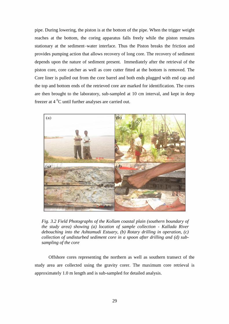
29

pipe. During lowering, the piston is at the bottom of the pipe. When the trigger weight

reaches at the bottom, the coring apparatus falls freely while the piston remains

stationary at the sediment–water interface. Thus the Piston breaks the friction and

provides pumping action that allows recovery of long core. The recovery of sediment

depends upon the nature of sediment present. Immediately after the retrieval of the

piston core, core catcher as well as core cutter fitted at the bottom is removed. The

Core liner is pulled out from the core barrel and both ends plugged with end cap and

the top and bottom ends of the retrieved core are marked for identification. The cores

are then brought to the laboratory, sub-sampled at 10 cm interval, and kept in deep

freezer at 4 0C until further analyses are carried out.

Fig. 3.2 Field Photographs of the Kollam coastal plain (southern boundary of

the study area) showing (a) location of sample collection - Kallada River

debouching into the Ashtamudi Estuary, (b) Rotary drilling in operation, (c)

collection of undisturbed sediment core in a spoon after drilling and (d) sub-

sampling of the core

Offshore cores representing the northern as well as southern transect of the

study area are collected using the gravity corer. The maximum core retrieval is

approximately 1.0 m length and is sub-sampled for detailed analysis.

30

Fig. 3.4 Photographs showing the lithology of the collected core samples

Fig. 3.3 Field photographs of core sample collection from the

Kayamkulam coastal plain (northern boundary of the study area) showing

(a) site area east of Kayamkulam Lagoon, (b) Rotary drilling in

operation, (c) undisturbed sediment core and (d) lithological observation

as well as packing of the samples

31

3.3. Analyses of Sediment Core Samples

The sediment cores collected are subjected to detailed textural analysis of, clay

mineralogy, organic and calcium carbonate content, geochemical parameters,

radiocarbon dating etc. as highlighted in the flow chart (Fig. 3.6). The details on

various analysis carried out are briefly given below.

3.3.1. Textural Analysis

In general, the term texture represents size, shape, roundness, grain surface

features and fabric of grains (Pettijohn, 1963). The deposition sequence and

environmental reconstruction can be studied by determining the particle size

distributions of sediments (Lario et al., 2002). The percentage of sand, silt and clay

contents and statistical parameters of the sediment core samples are estimated using

standard method (Carver, 1971). The textural analysis for this work is discussed in

detail below.

Fig. 3.5 Photographs showing (a) Panoramic view of the Ashtamudi

Estuary (central portion), (b) Piston Corer used for the collection of

core samples, (c) cutting of sediment core using core cutter in the

laboratory and (d) sub-sampling of undisturbed sediment core samples

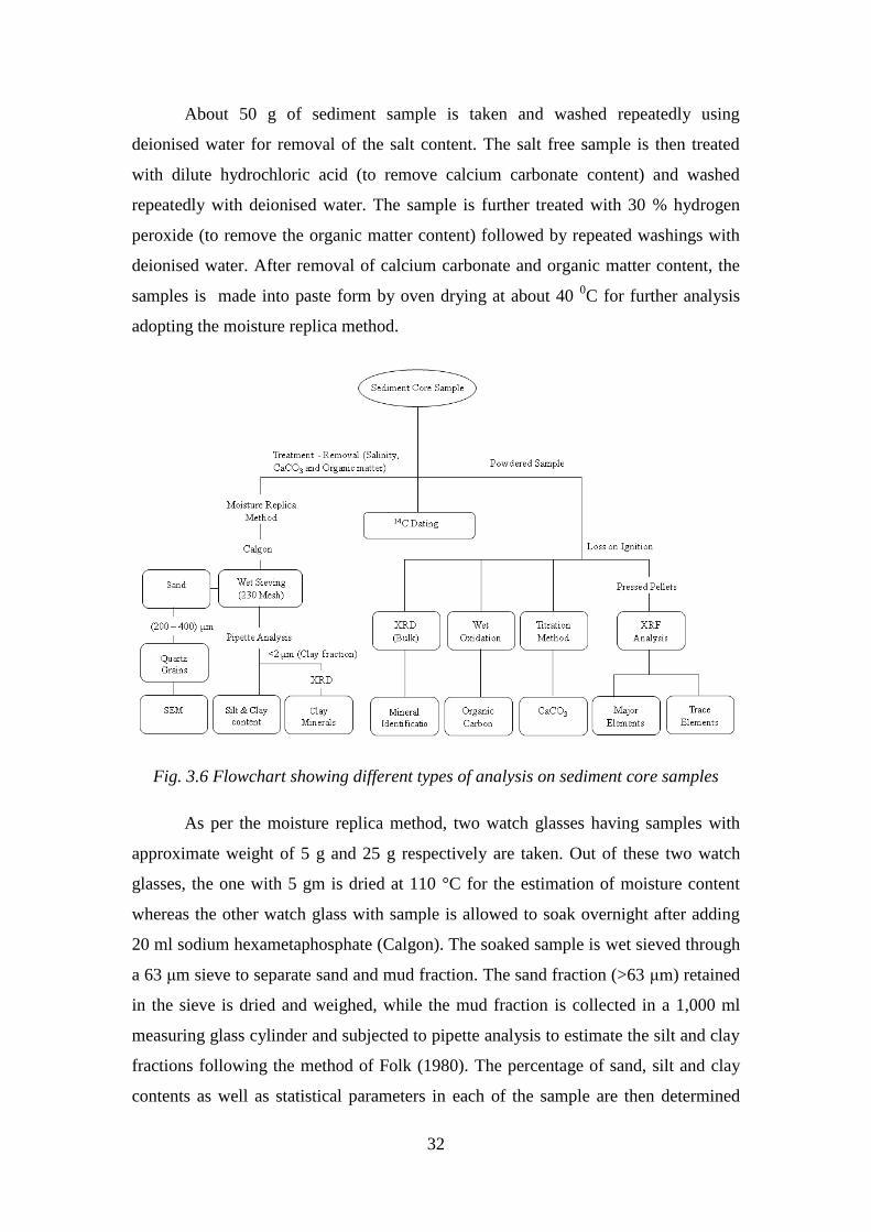
32

About 50 g of sediment sample is taken and washed repeatedly using

deionised water for removal of the salt content. The salt free sample is then treated

with dilute hydrochloric acid (to remove calcium carbonate content) and washed

repeatedly with deionised water. The sample is further treated with 30 % hydrogen

peroxide (to remove the organic matter content) followed by repeated washings with

deionised water. After removal of calcium carbonate and organic matter content, the

samples is made into paste form by oven drying at about 40 0C for further analysis

adopting the moisture replica method.

Fig. 3.6 Flowchart showing different types of analysis on sediment core samples

As per the moisture replica method, two watch glasses having samples with

approximate weight of 5 g and 25 g respectively are taken. Out of these two watch

glasses, the one with 5 gm is dried at 110 °C for the estimation of moisture content

whereas the other watch glass with sample is allowed to soak overnight after adding

20 ml sodium hexametaphosphate (Calgon). The soaked sample is wet sieved through

a 63 μm sieve to separate sand and mud fraction. The sand fraction (>63 μm) retained

in the sieve is dried and weighed, while the mud fraction is collected in a 1,000 ml

measuring glass cylinder and subjected to pipette analysis to estimate the silt and clay

fractions following the method of Folk (1980). The percentage of sand, silt and clay

contents as well as statistical parameters in each of the sample are then determined

33

using the Gradistat software (Simon, 2007). The sand-silt-clay ratios are plotted on

trilinear diagram for textural nomenclature based on Shepard (1954) classification.

3.3.2. Surface Texture Analysis

The study of surface features of quartz grains using Scanning Electron

Microscopy (SEM) techniques has been developed into a method for relating

microtexture of the samples to specific sedimentary enviornments (Krinsley et al.,

1964; Le Ribault, 1975).

For surface textural analysis of quartz grains, sand fraction of the treated

samples are separated from the mud content by sieving using 63 μm sieve based on

Carver (1971) method discussed in the previous section. Sand grain fractions between

200 and 400 μm sizes are further separated from the total grains by sieving for SEM

analysis (Krinsley and Doornkamp, 1973). The Monocrystalline quartz grains are then

hand-picked after examination using stereozoom binocular microscope and then

treated with stannous chloride solution to remove the iron stains (Krinsley and

Doornkamp, 1973; Helland and Holmes, 1997). On an average, about twenty-five

quartz grains are selected from the sand size fraction of each sample to understand the

microtextural variations present and also to interpret the depositional history (Krinsley

and Doornkamp, 1973; Baker, 1976). The selected quartz grains mounted on stubs,

sputter-coated with silver tape are examined using a Hitachi S-3400N Variable

Pressure Scanning Electron Microscope (SEM) with Deben Peltier Coolstage. The

SEM available with the Department of Civil Engineering, Anna University, Chennai,

India has been used for the present study. The various types of quartz grain

microtextures seen in the sample have been analyzed and studied in detail by

comparing with the published literatures (Krinsley and Donahue, 1968; Krinsley and

Margolis, 1971; Margolis and Kennet, 1971; Krinsley and Doornkamp, 1973; Le

Ribault, 1975; Higgs, 1979).

3.3.3. Clay Mineral Analysis

Clay mineral analysis of samples is essential, as they are indicators of

enviornmental changes (Chamley, 1989; Weaver, 1989). The species and proportions

of individual clay minerals in sediments depend mainly on the climatic conditions and

34

on the nature of the source rocks (Biscaye, 1965; Griffin et al., 1968). The steps

involved in clay mineral analysis adopted for the present study are summarised below.

Based on the settling velocity (Stokes’ law) of the sediment particles

(following the procedure of Carver, 1971) discussed in section 3.3.1, the sample is

allowed to stand for 6 hours 54 minute and the clay suspension (< 2 μm) from the top

10 cm of the column (approx. 300 ml) is siphoned out. The siphoned liquid is

centrifuged for 15 minutes to form thick suspension of clay slurry. Clay slurry is then

mounted on a grounded slide following the smearing technique proposed by Gibbs

(1965). The glass slides are allowed to dry at room temperature without any

contamination (Biscaye, 1964; Gibbs, 1965). The clay slides are then subjected to X-

ray diffraction analysis using the Philips X’PERT PRO X-ray diffractometer installed

in the XRD laboratory of the National Centre for Earth Science Studies,

Thiruvananthapuram.

The clay slide is scanned from 5° to 40° at 2° 2θ /minute with a copper target

and nickel filter at a setting of 40 KV and 30 mA. The resultant scanned peak is

generated and the presence of clay minerals like kaolinite (7 Ǻ), gibbsite (4.85 Ǻ),

chlorite (14 Ǻ), illite (10 Ǻ) and montmorillonite (15-17 Ǻ) (Rao and Rao, 1996) are

confirmed by running the High Score Plus software consisting of ICDD and JCPDS

data. Further to differentiate the kaolinite and chlorite peaks, the samples are also

rescanned from 24 to 26° 2 at 0.5° 2/minute (Biscaye, 1964).

3.3.4. Organic Matter Estimation

Organic matter in soils and sediments is widely distributed over the earth’s

surface occurring in almost all terrestrial and aquatic environments (Schnitzer, 1978).

Organic matter is a good index of the environment in which the sediments are

deposited. For the present study, the procedure proposed by Gaudette et al. (1974)

modified version of El Wakeel and Riley (1957) method has been adopted. The

various steps in laboratory analysis are enumerated below.

The selected core samples is dried in an oven at 50 °C and finely powdered in

agate mortar. Precisiely 0.5 gm of sample is weighed and treated with 10 ml of

potassiun dichromate solution and 20 ml of Conc. H2SO4 (1.25 g Ag2SO4 dissolved in

500 ml conc. H2SO4) which is mixed gently by rotating the flask for a minute. The

35

mixture is kept for an hour and then diluted by adding 200 ml of distilled water. After

acquiring normal conditions, 7 to 8 drops of ferroin indicator is added. The solution is

titrated against the 0.5 N Ferrous Ammonium Sulphates in a burette to a single drop

end point (brilliant red wine). A standard blank without sediment is run with each of

the new batch of samples. Organic carbon is calculated and then mutiplied with a

scale factor of 1.74 (Nelson and Sommers, 1996) to obtain the organic matter content.

3.3.5. Determination of Calcium Carbonate

Calcium carbonate content of the sediment (being a function of production,

dissolution and dilution) has been widely used for stratigraphic correlation, and

interpretation of palaeo-oceanographic changes (Dunn et al., 1981; Gardner, 1982;

Pisias et al., 1985). For accurate interpretation of the marine sediment record in-depth

knowledge of the processes controlling the preservation of CaCO3 is needed

(Milliman et al., 1999). The variations in the carbonate contents reflect the differences

in the environmental conditions of deposition (Setty and Madhusudhana Rao, 1972).

In this study, the percentage of CaCO3 in sediment samples is determined

adopting the Hutchinson and Mcheman (1947) method. The principle involves,

treating the sample with a known quantity of HCl and estimating the excess of HCl by

back titration with standard NaOH using pehnolphthalein indicator. The different

steps used in this method are described in the following paragraph.

A known weight (approx. 1 gm) is taken in an Ermelyer flask and 50 ml of 0.2

N dil. HCl is added. It is mixed gently and kept for half an hour. About 25 ml from

the dissolved carbonate solution is then transferred into another Ermelyer flask and 3

to 4 drops of phenolphtahlein indicator is added for titration against 0.2 N NaOH

solutions. The end point is indicated by light pink colour.

3.3.6. Geochemical Analysis

Geochemistry is the functional characterization, evaluation of elemental

distribution and concentration of chemical elements in the rock, soil and water. The

study further includes understanding of chemical processes and reactions that govern

the composition and chemical flux between various states (Kabata-Pendias and

Pendias, 2001; Neuendorf et al., 2005). The geochemical signature of sediment is a

36

reflection of its source material and also the processes within the sedimentary cycle

that can result in chemical fractionation (Taylor and McLennan, 1985).

X-ray Fluorescence (XRF) is a well-established technique adopted for the

analysis of geological materials due to its precision, accuracy, versatility, automation,

sensitivity and selectivity. It is one of the most rapid and relevant method of

geochemical analysis for obtaining qualitative and quantitative elemental analysis.

The steps involved are described below.

3.3.6.1. Sample Preparation and Instruments Used

The sediment cores samples collected from the different coastal environment

is washed thoroughly to remove salt and then dried at 50 °C. The sediment is

powdered with help of pestle and motar and then sieved through 230 mesh. The

powder sample passing through 230 mesh (< 63 μm) is collected and then dried at 110

°C overnight in order to remove the moisture content. Afte removing mositure content

the sample is then subjected to Loss on Ignition (LOI).

LOI is a widely used technique in geological marine and soil science

investigation (Bisutti et al., 2004). The dried powder samples are heated in a muffle

furnace at 950 °C for one hour in order to eliminate the volatile constituents like

organic matter, calcium carbonate contents and interstitial waters etc. Pressed pellets

are prepared by using collapsible aluminium cups (Govil, 1985). These cups are filled

with boric acid as binder and about 1 g of the finely powdered sample (after LOI) is

put on the top of the boric acid and pressed under a hydraulic press at 20 tons pressure

to obtain a 40 mm diameter pellet.

Bruker model S4 Pioneer sequential wavelength-dispersive X-ray

spectrometer equipped with a goniometer (which holds seven analyzing crystals) with

4 kW Rh X-ray tube and 60 samples automatic loading system avaliable at XRF

Laboratory, National Centre for Earth Science Studies is used to measure different

peaks and background counts for the major and trace elements. The supporting

software used for computer analyses is able to take care of dead time correction,

background, line overlap corrections and matrix effects giving the output directly as

the concentration in weight percentage or in ppm after converting the counts into

concentration with the help of calibration curves.

37

3.3.6.2. Major Elements

Major element concentrations are determined adopting the X-ray fluorescence

spectrometry method following the procedures given by Calvert (1990). The XRF

intensities measured from elements in dry samples show variations depending on the

XRF absorption rates (Tertian and Claisse, 1982). The major elements determined

are: Si, Al, Fe, Ti, Ca, Na, K, Mg, Mn and P.

3.3.6.3. Trace Elements

Determination of the Trace element abundances in sediments allow us to

reconstruct the paleodepositional conditions (Weme et al., 2003; Riboulleau et al.,

2003; Algeo, 2004; Nameroff et al., 2004; Rimmer, 2004). While using trace element

concentrations to reconstruct paleoenvironmental conditions, one must assess whether

they are relatively enriched or depleted. In general, the degree of enrichment or

depletion of a trace element in a sample is evaluated relative to its concentration in a

reference that is usually average shale value (Wedepohl, 1971, 1991; Mclennan,

2001). The trace elements consisting mainly of Cr, Co, Ni, Cu, Zn, Ga, Rb, Y, Zr, Nb,

Ba, La, Ce, Sm are analysed using XRF.

3.3.7. Radiocarbon Dating

Recent scientific work has demonstrated the capability of peat and organic

rich muddy sediment to store information of the past environments with a high

temporal resolution (Goodsite et al., 2001). Peat sections have served as archives of

heavy metal pollutants of the atmosphere (Benoit et al., 1998; Shotyk et al., 1998) and

yielded records of both climate and atmospheric CO2 content (White et al., 1994;

Martinez-Cortizas et al., 1999). For the present study, the Radiocarbon dating (14

C)

analysis is carried out in the Radiocarbon Laboratory at Birbal Sahni Institute of

Paleobotany (BSIP), Lucknow. The process involved following steps.

Combustion of the cleaned and pre-treated (using 10% HCl)

sediment sample is carried out in a quartz electrical furnace in presence of clean and

dry oxygen-flow at 750 to 900 °C. This is followed by allowing the reaction with

copper oxide to convert carbon monoxide, if any left over, to the carbon dioxide.

Since the sample carbon dioxide may contain several impurities like

sulfur and halides in addition to moisture, multi-stage cleaning using acidified

38

potassium permanganate, potassium dichromate, silver chloride in definite

concentrations and moisture absorbers like cooled silica gel and molecular sieve are

carried out. The cleaned and dried carbon dioxide is collected using liquid nitrogen.

It is freed from oxygen followed by formation of lithium carbide in the presence of

catalyst (molten lithium) and slow hydrolysis to obtain acetylene. In the presence of a

catalyst, the acetylene is trimerised to obtain benzene. After careful weighing of

sample benzene, a calculated amount of scintillator (PBD Butyle purum) is added to

benzene vial and the vial is placed in the counter Quantulus 1220 for 25 cycles of

counting. Appropriate SQP correction is applied to estimate the radiocarbon amount

and ages calculated using the standard formula based on radioactive decay of

radiocarbon. While determing the age, the half-life used is 5,530 years as per the

traditional method even though the accepted present value is 5,730 years. The

obtained radiocarbon dates is calibrated using IntCal09 software of the Washington

University.

39

CHAPTER 4

SEDIMENTOLOGY OF CORE SEDIMENTS

4.1. Introduction

Sedimentary deposits are often considered as the pages of the earth’s history.

A better understanding of the proxy evidences in sedimentary archieves would

provide a wealth of information including changes in enviornmental conditions and

sediment supply. Interpretation of the depositional and paleoclimate enviornment

requires synthesis of all the inferences that can be retrieved from the various

lithological units that encompasses sedimentary architecture. The constitutent part of

the sedimentary packages/units indicates the position of sea level and also changes in

sediment supply within a cycle and enables interpretation of their interrelationship

through the time. Studies of sedimentary packages collected from exposed outcrops

and or drilled borehole cores are one of the direct methods in sedimentological

investigations. A cursory glance of literature reveals that several studies have been

undertaken in different parts of the world for archieving the past enviornmental

climatic and sea level changes (Fairbanks, 1989; Prell et al., 1992; Rao et al., 2003;

Pandarinath et al., 2004; Verma and Sudhakar, 2006; Nair et al., 2010).

Knowledge of sediment texture is vital to differentiate various depositional

enviornment of ancient as well as recent sediments (Manson and Folk, 1958;

Freidman, 1961). Many of the earlier researchers have successfully adopted the

granulometric analysis of unconsolidated sediments as an efficient tool for a thorough

understanding of the depositional pattern of the sediments. Size parameters can also

give insight into the spatial and temporal variations of transportation and depositional

processes even within the same enviornment (Samsuddin, 1986; Samsuddin et al.,

1991).

In this chapter, the sedimentological characteristics, like the downcore

variations in the sediment facies, organic matter, calcium carbonate, clay mineralogy

and radiocarbon dating of the samples collected from predefined locations in the study

area are discussed. The collection of sediment cores representing the coastal plain,

estuary/lagoon and offshore along the two transects are discussed in Chapter 2.

40

4.2. Lithological Variation

The lithological variations of the cores representing the coastal plain,

estuary/lagoon and offshore of the southern and northern transect are enumerated in

the following section.

4.2.1. Sediment core along the southern transect (Kollam)

The sediment cores along the southern transect comprises of 5 cores

representing the coastal plain (Core 1), the Ashtamudi Estuary (Core 2, 3, 4) and the

Offshore (Core 5) respectively (Fig. 3.1 in Chapter 3).

4.2.1.1. Coastal Plain (Core 1)

The Core 1 (08° 59' 11" N, 76° 36' 49" E) is located in the coastal plain where

the Kallada River joins the Ashtamudi Estuary. The core is sub-divided into 5 litho-

units (Figs. 4.1a & b) and the percentage of sand, silt, clay, organic matter and

calcium carbonate in each of the units are presented in Table 4.1. The first litho-unit

starts with a top soil of 0 to 2 m. This is followed by the second unit of 2 to 7 m where

the sand particles are angular to sub-angular in nature ranging from 70.09 to 89.11%.

The silt and clay content are much less in this unit and varies from 3.9 to 11% and

6.98 to 18.91% respectively. The organic matter and calcium carbonate contents are

least with an average value of 1.53% and 0.66%. The third unit of 7 to 9 m is

dominated by sand to silty sand sediments where the sand, silt and clay contents

ranges from 66.94 to 78.87%, 5.90 to 20.42% and 5.88 to 12.64% respectively.

Broken shells and traces of heavy minerals were also observed. In this unit a marginal

increase of calcium carbonate (av. 1%) and a decrease of organic matter (av. 0.56%)

are noted.

Muddy sediments dominate the fourth unit representing the 9 to 11 m with

clay percentage ranging from 36.97 to 84.06%. The upper part of this unit is soft with

brownish to reddish colour with traces of brachiopod shells. However, the lower part

is characterised by very hard clay of white to greyish colour. Less percentage of sand

and silt was observed. Towards the end of this unit, a thin layer of black peat with an

approximate thickness of 0.20 m was observed which has an organic matter of 47%.

The last unit (11-15.5 m) comprises of silty clay type sediments. The percentages of

sand, silt and clay ranges from 0.41 to 12.65%; 25.11 to 33.26%; and 56.35 to 72.12%

41

respectively. The unit also shows enrichment of organic sediments ranging from 10 to

14 % with well-preserved vegetative plant material.

Fig. 4.1 (a) Lithological variation of sand silt clay percentages and (b) Sediment type

variations in the coastal plain, estuary and offshore region of the southern transect

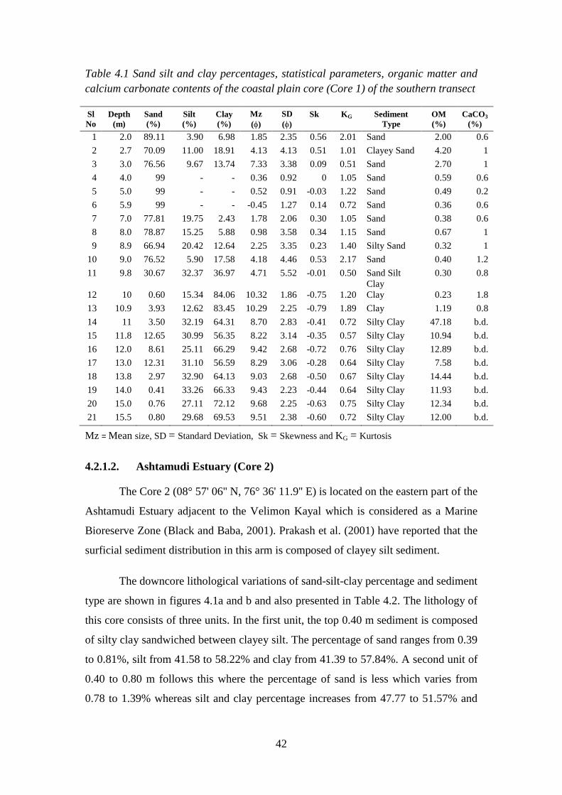
42

Table 4.1 Sand silt and clay percentages, statistical parameters, organic matter and

calcium carbonate contents of the coastal plain core (Core 1) of the southern transect

Sl

No

Depth

(m)

Sand

(%)

Silt

(%)

Clay

(%)

Mz

()

SD

()

Sk

KG

Sediment

Type

OM

(%)

CaCO3

(%)

1 2.0 89.11 3.90 6.98 1.85 2.35 0.56 2.01 Sand 2.00 0.6

2 2.7 70.09 11.00 18.91 4.13 4.13 0.51 1.01 Clayey Sand 4.20 1

3 3.0 76.56 9.67 13.74 7.33 3.38 0.09 0.51 Sand 2.70 1

4 4.0 99 - - 0.36 0.92 0 1.05 Sand 0.59 0.6

5 5.0 99 - - 0.52 0.91 -0.03 1.22 Sand 0.49 0.2

6 5.9 99 - - -0.45 1.27 0.14 0.72 Sand 0.36 0.6

7 7.0 77.81 19.75 2.43 1.78 2.06 0.30 1.05 Sand 0.38 0.6

8 8.0 78.87 15.25 5.88 0.98 3.58 0.34 1.15 Sand 0.67 1

9 8.9 66.94 20.42 12.64 2.25 3.35 0.23 1.40 Silty Sand 0.32 1

10 9.0 76.52 5.90 17.58 4.18 4.46 0.53 2.17 Sand 0.40 1.2

11 9.8 30.67 32.37 36.97 4.71 5.52 -0.01 0.50 Sand Silt

Clay

0.30 0.8

12 10 0.60 15.34 84.06 10.32 1.86 -0.75 1.20 Clay 0.23 1.8

13 10.9 3.93 12.62 83.45 10.29 2.25 -0.79 1.89 Clay 1.19 0.8

14 11 3.50 32.19 64.31 8.70 2.83 -0.41 0.72 Silty Clay 47.18 b.d.

15 11.8 12.65 30.99 56.35 8.22 3.14 -0.35 0.57 Silty Clay 10.94 b.d.

16 12.0 8.61 25.11 66.29 9.42 2.68 -0.72 0.76 Silty Clay 12.89 b.d.

17 13.0 12.31 31.10 56.59 8.29 3.06 -0.28 0.64 Silty Clay 7.58 b.d.

18 13.8 2.97 32.90 64.13 9.03 2.68 -0.50 0.67 Silty Clay 14.44 b.d.

19 14.0 0.41 33.26 66.33 9.43 2.23 -0.44 0.64 Silty Clay 11.93 b.d.

20 15.0 0.76 27.11 72.12 9.68 2.25 -0.63 0.75 Silty Clay 12.34 b.d.

21 15.5 0.80 29.68 69.53 9.51 2.38 -0.60 0.72 Silty Clay 12.00 b.d.

Mz = Mean size, SD = Standard Deviation, Sk = Skewness and KG = Kurtosis

4.2.1.2. Ashtamudi Estuary (Core 2)

The Core 2 (08° 57' 06'' N, 76° 36' 11.9'' E) is located on the eastern part of the

Ashtamudi Estuary adjacent to the Velimon Kayal which is considered as a Marine

Bioreserve Zone (Black and Baba, 2001). Prakash et al. (2001) have reported that the

surficial sediment distribution in this arm is composed of clayey silt sediment.

The downcore lithological variations of sand-silt-clay percentage and sediment

type are shown in figures 4.1a and b and also presented in Table 4.2. The lithology of

this core consists of three units. In the first unit, the top 0.40 m sediment is composed

of silty clay sandwiched between clayey silt. The percentage of sand ranges from 0.39

to 0.81%, silt from 41.58 to 58.22% and clay from 41.39 to 57.84%. A second unit of

0.40 to 0.80 m follows this where the percentage of sand is less which varies from

0.78 to 1.39% whereas silt and clay percentage increases from 47.77 to 51.57% and

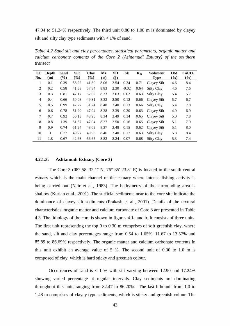
43

47.04 to 51.24% respectively. The third unit 0.80 to 1.08 m is dominated by clayey

silt and silty clay type sediments with < 1% of sand.


calcium carbonate contents of the Core 2 (Ashtamudi Estuary) of the southern

transect

SL

No.

Depth

(m)

Sand

(%)

Silt

(%)

Clay

(%)

Mz

( )

SD

()

Sk

KG

Sediment

Type

OM

(%)

CaCO3

(%)

1 0.1 0.39 58.22 41.39 8.06 2.54 0.24 0.71 Clayey Silt 4.6 8.4

2 0.2 0.58 41.58 57.84 8.83 2.30 -0.02 0.64 Silty Clay 4.6 7.6

3 0.3 0.81 47.17 52.02 8.33 2.63 0.02 0.63 Silty Clay 5.4 5.7

4 0.4 0.66 50.03 49.31 8.32 2.50 0.12 0.66 Clayey Silt 5.7 6.7

5 0.5 0.99 47.77 51.24 8.48 2.40 0.13 0.66 Silty Clay 5.4 7.8

6 0.6 0.78 51.29 47.94 8.38 2.39 0.20 0.63 Clayey Silt 4.9 6.9

7 0.7 0.92 50.13 48.95 8.34 2.49 0.14 0.65 Clayey Silt 5.0 7.8

8 0.8 1.39 51.57 47.04 8.27 2.50 0.16 0.65 Clayey Silt 5.1 7.9

9 0.9 0.74 51.24 48.02 8.27 2.48 0.15 0.62 Clayey Silt 5.1 8.0

10 1 0.77 49.27 49.96 8.46 2.40 0.17 0.63 Silty Clay 5.3 8.4

11 1.8 0.67 42.68 56.65 8.82 2.24 0.07 0.68 Silty Clay 5.3 7.4


The Core 3 (08° 58' 32.1'' N, 76° 35' 23.3'' E) is located in the south central

estuary which is the main channel of the estuary where intense fishing activity is

being carried out (Nair et al., 1983). The bathymetry of the surrounding area is

shallow (Kurian et al., 2001). The surficial sediments near to the core site indicate the

dominance of clayey silt sediments (Prakash et al., 2001). Details of the textural

characteristics, organic matter and calcium carbonate of Core 3 are presented in Table

4.3. The lithology of the core is shown in figures 4.1a and b. It consists of three units.

The first unit representing the top 0 to 0.30 m comprises of soft greenish clay, where

the sand, silt and clay percentages range from 0.54 to 1.65%, 11.67 to 13.57% and

85.89 to 86.69% respectively. The organic matter and calcium carbonate contents in

this unit exhibit an average value of 5 %. The second unit of 0.30 to 1.0 m is

composed of clay, which is hard sticky and greenish colour.

Occurrences of sand is < 1 % with silt varying between 12.90 and 17.24%

showing varied percentage at regular intervals. Clay sediments are dominating

throughout this unit, ranging from 82.47 to 86.20%. The last lithounit from 1.0 to

1.48 m comprises of clayey type sediments, which is sticky and greenish colour. The

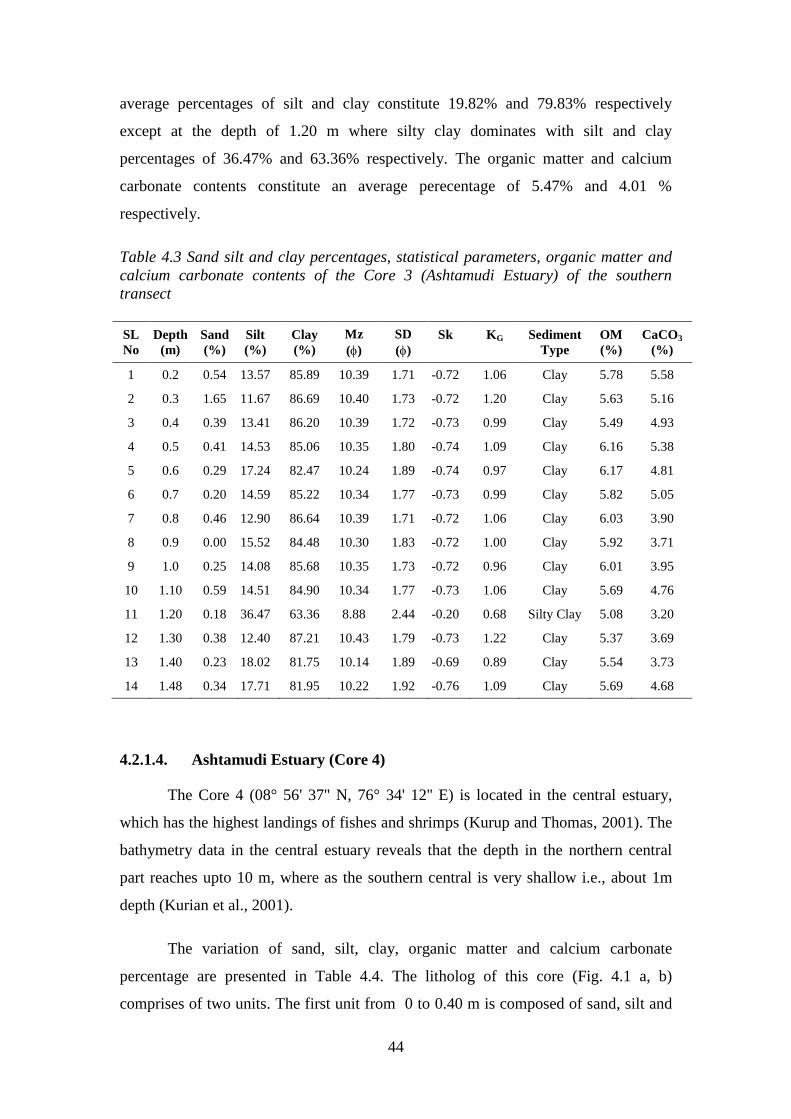
44

average percentages of silt and clay constitute 19.82% and 79.83% respectively

except at the depth of 1.20 m where silty clay dominates with silt and clay

percentages of 36.47% and 63.36% respectively. The organic matter and calcium

carbonate contents constitute an average perecentage of 5.47% and 4.01 %

respectively.



transect

SL

No

Depth

(m)

Sand

(%)

Silt

(%)

Clay

(%)

Mz

()

SD

()

Sk

KG

Sediment

Type

OM

(%)

CaCO3

(%)

1 0.2 0.54 13.57 85.89 10.39 1.71 -0.72 1.06 Clay 5.78 5.58

2 0.3 1.65 11.67 86.69 10.40 1.73 -0.72 1.20 Clay 5.63 5.16

3 0.4 0.39 13.41 86.20 10.39 1.72 -0.73 0.99 Clay 5.49 4.93

4 0.5 0.41 14.53 85.06 10.35 1.80 -0.74 1.09 Clay 6.16 5.38

5 0.6 0.29 17.24 82.47 10.24 1.89 -0.74 0.97 Clay 6.17 4.81

6 0.7 0.20 14.59 85.22 10.34 1.77 -0.73 0.99 Clay 5.82 5.05

7 0.8 0.46 12.90 86.64 10.39 1.71 -0.72 1.06 Clay 6.03 3.90

8 0.9 0.00 15.52 84.48 10.30 1.83 -0.72 1.00 Clay 5.92 3.71

9 1.0 0.25 14.08 85.68 10.35 1.73 -0.72 0.96 Clay 6.01 3.95

10 1.10 0.59 14.51 84.90 10.34 1.77 -0.73 1.06 Clay 5.69 4.76

11 1.20 0.18 36.47 63.36 8.88 2.44 -0.20 0.68 Silty Clay 5.08 3.20

12 1.30 0.38 12.40 87.21 10.43 1.79 -0.73 1.22 Clay 5.37 3.69

13 1.40 0.23 18.02 81.75 10.14 1.89 -0.69 0.89 Clay 5.54 3.73

14 1.48 0.34 17.71 81.95 10.22 1.92 -0.76 1.09 Clay 5.69 4.68


The Core 4 (08° 56' 37'' N, 76° 34' 12'' E) is located in the central estuary,

which has the highest landings of fishes and shrimps (Kurup and Thomas, 2001). The

bathymetry data in the central estuary reveals that the depth in the northern central

part reaches upto 10 m, where as the southern central is very shallow i.e., about 1m

depth (Kurian et al., 2001).

The variation of sand, silt, clay, organic matter and calcium carbonate

percentage are presented in Table 4.4. The litholog of this core (Fig. 4.1 a, b)

comprises of two units. The first unit from 0 to 0.40 m is composed of sand, silt and

45

clay sediments where the sand, silt and clay contents ranges from 23.57 to 53.80%,

23.15 to 33.08% and 23.05 to 33.08% respectively. The percentage of calcium

carbonate and organic matter shows an average value of 6.5% and 3.4% respectively.

This is followed by the second unit of 0.40 to 0.70 m where the sediments are clayey

silt with a dominance of silt which is evident from an average value of 54.93%. Here

the sand content is less compared to the first unit with the percentage varying between

6.26 and 18.02%. The clay content ranges from 29.63 to 35.14%. An enrichment of

calcium carbonate with an average value of 11 % is observed whereas the organic

matter remains more or less same (4%) as that of the unit above it.



transect

Sl.

No.

Depth

(m)

Sand

(%)

Silt

(%)

Clay

(%)

Mz

()

SD

()

Sk

KG

Sediment

Type

OM

(%)

CaCO3

(%)

1 0.10 53.80 23.15 23.05 5.82 2.85 0.86 0.86 Sand Silt Clay 0.71 8.7

2 0.20 24.01 45.73 30.26 6.98 3.02 0.32 0.69 Sand Silt Clay 4.17 6.7

3 0.30 20.95 45.97 33.08 7.07 3.03 0.32 0.68 Sand Silt Clay 4.31 4.4

4 0.40 23.57 46.69 29.74 6.91 3.00 0.36 0.74 Sand Silt Clay 4.16 6.2

5 0.50 18.02 52.35 29.63 7.01 2.99 0.35 0.77 Clayey Silt 3.71 9.4

6 0.60 11.54 53.84 34.62 7.44 2.90 0.19 0.74 Clayey Silt 4.31 10.8

7 0.70 6.26 58.60 35.14 7.59 2.79 0.25 0.77 Clayey Silt 4.35 12.5

4.2.1.5. Offshore (Core 5)

The Core 5 (08° 57' 28'' N, 76°

29' 12'' E) is collected off Kollam coast at a

depth of 12.5 m with a recovery of 0.88m. In general, the offshore areas are carpeted

by clayey silt distribution (Prakash, 2000). Table 4.5 gives the percentages of sand,

silt, clay, calcium carbonate and organic matter in Core 5. The lithological variation

reveals that the core is divided into three units (Figs. 4.1a & b). The first unit from 0

to 0.40 m is dominated by silt varying between 60.22 and 80.47% followed by clay

ranging from 20.28 to 37.70%. The sand percentage is less ranging from 1.63 to

3.79%. The calcium carbonate content ranges up to 11% whereas the organic matter

constitutes only 3% in this unit. This is followed by the second unit, 0.40 to 0.60 m

where the sediments are clayey silt with less percentage of sand. There is a gradual

increase of silt (54.46 to 58.59%) down the core whereas the clay percentage

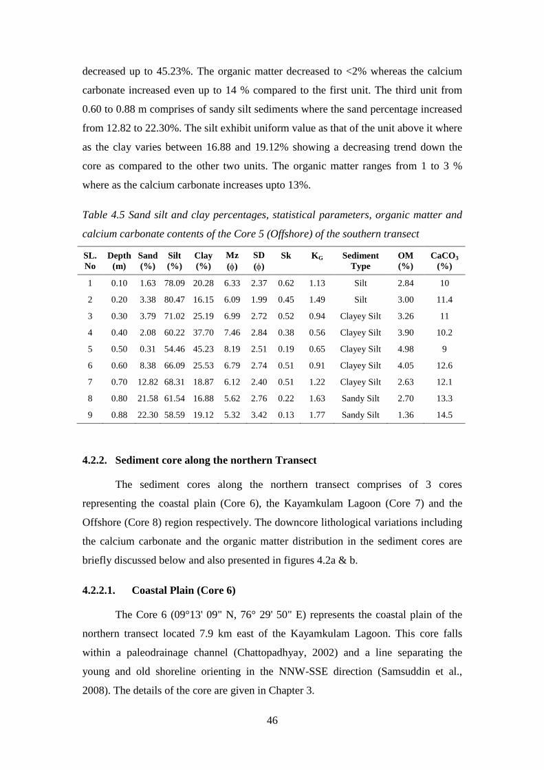
46

decreased up to 45.23%. The organic matter decreased to <2% whereas the calcium

carbonate increased even up to 14 % compared to the first unit. The third unit from

0.60 to 0.88 m comprises of sandy silt sediments where the sand percentage increased

from 12.82 to 22.30%. The silt exhibit uniform value as that of the unit above it where

as the clay varies between 16.88 and 19.12% showing a decreasing trend down the

core as compared to the other two units. The organic matter ranges from 1 to 3 %

where as the calcium carbonate increases upto 13%.


calcium carbonate contents of the Core 5 (Offshore) of the southern transect

SL.

No

Depth

(m)

Sand

(%)

Silt

(%)

Clay

(%)

Mz

()

SD

()

Sk

KG

Sediment

Type

OM

(%)

CaCO3

(%)

1 0.10 1.63 78.09 20.28 6.33 2.37 0.62 1.13 Silt 2.84 10

2 0.20 3.38 80.47 16.15 6.09 1.99 0.45 1.49 Silt 3.00 11.4

3 0.30 3.79 71.02 25.19 6.99 2.72 0.52 0.94 Clayey Silt 3.26 11

4 0.40 2.08 60.22 37.70 7.46 2.84 0.38 0.56 Clayey Silt 3.90 10.2

5 0.50 0.31 54.46 45.23 8.19 2.51 0.19 0.65 Clayey Silt 4.98 9

6 0.60 8.38 66.09 25.53 6.79 2.74 0.51 0.91 Clayey Silt 4.05 12.6

7 0.70 12.82 68.31 18.87 6.12 2.40 0.51 1.22 Clayey Silt 2.63 12.1

8 0.80 21.58 61.54 16.88 5.62 2.76 0.22 1.63 Sandy Silt 2.70 13.3

9 0.88 22.30 58.59 19.12 5.32 3.42 0.13 1.77 Sandy Silt 1.36 14.5

4.2.2. Sediment core along the northern Transect

The sediment cores along the northern transect comprises of 3 cores

representing the coastal plain (Core 6), the Kayamkulam Lagoon (Core 7) and the

Offshore (Core 8) region respectively. The downcore lithological variations including

the calcium carbonate and the organic matter distribution in the sediment cores are

briefly discussed below and also presented in figures 4.2a & b.

4.2.2.1. Coastal Plain (Core 6)

The Core 6 (09°13' 09" N, 76° 29' 50" E) represents the coastal plain of the

northern transect located 7.9 km east of the Kayamkulam Lagoon. This core falls

within a paleodrainage channel (Chattopadhyay, 2002) and a line separating the

young and old shoreline orienting in the NNW-SSE direction (Samsuddin et al.,

2008). The details of the core are given in Chapter 3.

47

Fig. 4.2 (a) Lithological variation of sand silt clay percentages and (b) Sediment type

variations in the coastal plain, lagoon and the offshore region of the northern

transect

48

The percentage of sand, silt, clay, organic matter and calcium carbonate are

presented in Table 4.6. The sediment litholog starts with a top soil of 2.5 m and

consist of 4 units (Fig. 4.2a & b). The first unit from 2.5 to 4 m comprises of medium

to fine sand showing light to brownish colour. Here in this unit the sand dominates

ranging from 89.81 to 91.81% (av. 90.81%) where as silt and clay contents are

minimum with an average percentage of 3.61% and 5.58% respectively. The

percenatge of organic matter and calcium carbonate are least in this unit. This is

followed by a second unit, from 4 to 10 m where sand of light greenish colour

dominates with an intercalation of silty sand at the top and bottom. The sand content

varies between 66.94 and 99% with considerable increase of silt (av. 7.31%) whereas

the clay percentage ranges from 2.70 to 7.26% except at the depths of 4.3 and 8 m

where an increase of 12% is observed. At the end of this unit (10 m), minute broken

shells with considerable amount of heavy minerals are noted. The organic matter and

calcium carbonate percentages are insignificant throughout the unit except at 8 and 10

m depths where it increases to 7 and 14% respectively.

Table 4.6 Sand, silt and clay percentages as well as the textural parameters of the

coastal plain core (Core 6) in the northern transect

Sl.

No.

Depth

(m)

Sand

(%)

Silt

(%)

Clay

(%)

Mz

()

SD

()

Sk

KG

Sediment

Type

OM

(%)

CaCO3

(%)

1 2.7 89.81 2.72 7.47 2.26 2.20 0.37 2.75 Sand 0.20 1.2

2 3.0 91.81 4.50 3.69 1.98 1.50 0.33 1.50 Sand 0.14 0.4

3 4.3 67.38 20.34 12.28 4.10 2.36 0.68 2.15 Silty Sand 0.64 1.2

4 4.6 88.13 7.73 4.14 2.39 1.58 0.31 1.96 Sand 0.15 0.8

5 5.3 95.41 1.89 2.70 1.57 1.03 0.36 1.04 Sand 0.07 0.2

6 6.0 96.36 0.87 2.76 1.61 1.07 0.12 0.99 Sand 0.07 0.6

7 7.0 88.23 4.51 7.26 2.69 1.72 0.70 5.21 Sand 0.31 1.6

8 8.0 66.94 20.42 12.64 3.37 1.58 0.52 6.10 Silty Sand 0.43 7.2

9 8.9 93.49 2.73 3.78 2.92 0.88 0.59 4.12 Sand 0.15 0.8

10 10.0 99 - - 3.23 0.45 -0.07 1.11 Sand 0.35 14.4

11 10.9 79.78 8.22 12.00 3.76 1.89 0.40 5.30 Sand 0.33 38

12 11.6 13.06 38.27 48.67 8.03 2.92 -0.01 0.67 Silty Clay 1.84 23.6

13 11.8 6.80 53.17 40.03 7.77 2.70 0.25 0.76 Clayey Silt 1.89 19.8

14 12.0 16.56 46.35 37.09 7.28 3.09 0.20 0.69 Clayey Silt 1.79 23

15 13.0 23.33 34.71 41.96 7.31 3.14 0.15 0.54 Sand Silt Clay 1.85 17.8

16 13.9 2.15 49.14 48.70 8.19 2.66 0.10 0.60 Clayey Silt 1.84 25.6

17 15.0 7.68 43.49 48.82 7.91 2.92 0.00 0.56 Silty Clay 1.54 21.8

18 16.0 10.55 44.62 44.82 7.55 3.04 0.19 0.52 Silty Clay 1.51 20

19 17.0 3.31 39.51 57.17 8.47 2.77 -0.19 0.61 Silty Clay 1.70 22.6

20 18.0 9.76 39.65 50.59 7.98 3.00 -0.07 0.55 Silty Clay 1.60 18.8

21 19.7 11.14 31.07 57.80 8.57 3.17 -0.49 0.60 Silty Clay 1.36 23.2

22 20.0 2.63 39.97 57.40 8.52 2.71 -0.16 0.61 Silty Clay 1.96 21

49

This is followed by a third unit of 10 to 14 m, where the sandy sediments

sequence is changed to silty clay/clayey silt type of sediments. Large amount of

minute broken shells of brachiopods and pelecypods were observed for a thickness of

1 m showing 38% of calcium carbonate with sand content as high as 80%. At 11 to 12

m the brachiopods and pelecypods shells are completely embedded with the clayey

silt type sediments. Towards the lower part of this unit the sandy sediments decreases

with an increase in silt and clay content. As a whole, the percentage of sand, silt and

clay contents in this unit ranges from 2.15 to 13.06%, 34.71 to 53.17% and 37.09 to

48.70% respectively indicating an abrupt change in the sand-silt-clay content. In

general, there is an increase of calcium carbonate along this unit with percentage

varying between 14 and 38% where as the organic matter showed a maximum value

of 1.89% as compare to the top litho-units.

The fourth unit comprises of 14 to 20 m where silty clay sediments dominate

throughout with silt and clay ranging from 31.07 to 44.62% and 44.82 to 57.80%

respectively. The sand content which ranges from 2.63 to 11.14% exhibits less

variation. A sizeable quantity of broken shells is encountered with the fine sediments

down the core with the calcium carbonate ranging from 18 to 25% and organic matter

of 1.96%.

4.2.2.2. Kayamkulam Lagoon (Core 7)

The Core 7 (09° 12' 03'' N, 76°

26' 29'' E) collected from the Kayamkulam

Lagoon consists of three units. The percentages of sand, silt, clay, organic matter and

calcium carbonate are given in Table 4.7. The first unit 0 to 0.10 m is dominated by

sand ranging from 44.75 to 79.87% followed by clay and silt showing 8.38 to 31.09%

and 11.75 to 24.16% respectively. The calcium carbonate shows an average value of

6.25% whereas the organic matter is less (av. 2.58%). In the second unit from 0.10 to

0.30 m the sand percentage decreased from 10.08 to 3.15% with an increase in silt and

clay percentage in the range of 25.81 to 72.50% and 19.24 to 71.04% respectively.

The organic matter and calcium carbonate content shows an average value of >6%.

This is followed by the third unit of 0.30 to 0.65 m where the sediments are of silty

clay showing negligible sand (av. 1%) content with the dominance of clay (av.

68.10%) through out this unit. The organic matter (av. 7%) and the calcium carbonate

(av. 6%) percentages are high as compared to the first two units.

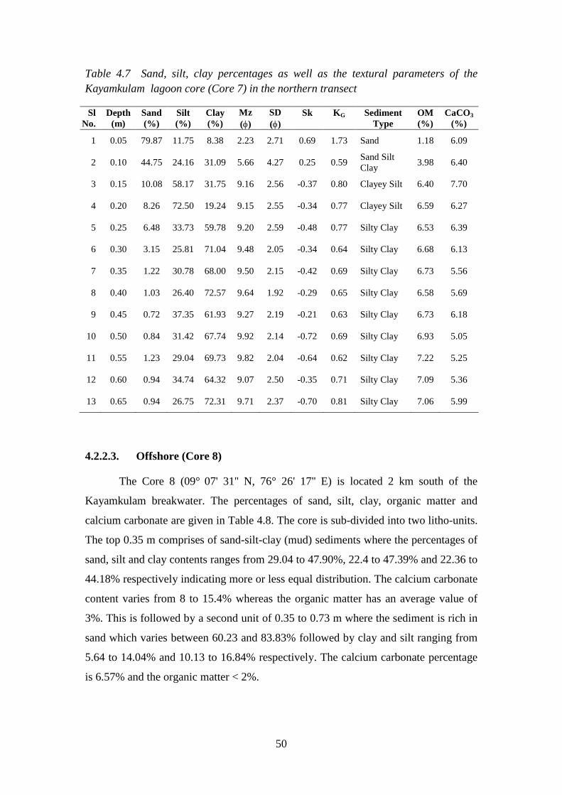
50

Table 4.7 Sand, silt, clay percentages as well as the textural parameters of the

Kayamkulam lagoon core (Core 7) in the northern transect

Sl

No.

Depth

(m)

Sand

(%)

Silt

(%)

Clay

(%)

Mz

()

SD

()

Sk

KG

Sediment

Type

OM

(%)

CaCO3

(%)

1 0.05 79.87 11.75 8.38 2.23 2.71 0.69 1.73 Sand 1.18 6.09

2 0.10 44.75 24.16 31.09 5.66 4.27 0.25 0.59 Sand Silt

Clay 3.98 6.40

3 0.15 10.08 58.17 31.75 9.16 2.56 -0.37 0.80 Clayey Silt 6.40 7.70

4 0.20 8.26 72.50 19.24 9.15 2.55 -0.34 0.77 Clayey Silt 6.59 6.27

5 0.25 6.48 33.73 59.78 9.20 2.59 -0.48 0.77 Silty Clay 6.53 6.39

6 0.30 3.15 25.81 71.04 9.48 2.05 -0.34 0.64 Silty Clay 6.68 6.13

7 0.35 1.22 30.78 68.00 9.50 2.15 -0.42 0.69 Silty Clay 6.73 5.56

8 0.40 1.03 26.40 72.57 9.64 1.92 -0.29 0.65 Silty Clay 6.58 5.69

9 0.45 0.72 37.35 61.93 9.27 2.19 -0.21 0.63 Silty Clay 6.73 6.18

10 0.50 0.84 31.42 67.74 9.92 2.14 -0.72 0.69 Silty Clay 6.93 5.05

11 0.55 1.23 29.04 69.73 9.82 2.04 -0.64 0.62 Silty Clay 7.22 5.25

12 0.60 0.94 34.74 64.32 9.07 2.50 -0.35 0.71 Silty Clay 7.09 5.36

13 0.65 0.94 26.75 72.31 9.71 2.37 -0.70 0.81 Silty Clay 7.06 5.99

4.2.2.3. Offshore (Core 8)

The Core 8 (09° 07' 31'' N, 76° 26' 17'' E) is located 2 km south of the

Kayamkulam breakwater. The percentages of sand, silt, clay, organic matter and

calcium carbonate are given in Table 4.8. The core is sub-divided into two litho-units.

The top 0.35 m comprises of sand-silt-clay (mud) sediments where the percentages of

sand, silt and clay contents ranges from 29.04 to 47.90%, 22.4 to 47.39% and 22.36 to

44.18% respectively indicating more or less equal distribution. The calcium carbonate

content varies from 8 to 15.4% whereas the organic matter has an average value of

3%. This is followed by a second unit of 0.35 to 0.73 m where the sediment is rich in

sand which varies between 60.23 and 83.83% followed by clay and silt ranging from

5.64 to 14.04% and 10.13 to 16.84% respectively. The calcium carbonate percentage

is 6.57% and the organic matter < 2%.

51

Table 4.8 Sand, silt, clay percentages as well as the textural parameters of the

offshore core (Core 8) in the northern transect

Sl.

No.

Depth

(cm)

Sand

(%)

Silt

(%)

Clay

(%)

Mz

()

SD

()

Sk

KG

Sediment

Type

OM

(%)

CaCO3

(%)

1 0.05 41.41 36.23 22.36 6.39 3.27 0.64 1.01 Sand Silt Clay 2.09 15.4

2 0.10 38.64 36.73 24.64 6.46 3.27 0.65 0.88 Sand Silt Clay 2.14 11.4

3 0.15 29.04 41.01 29.95 6.86 3.21 0.48 0.50 Sand Silt Clay 2.44 13.6

4 0.20 30.52 33.58 35.9 7.00 3.35 0.33 0.52 Sand Silt Clay 2.85 12

5 0.25 31.62 45.43 22.95 6.33 3.39 0.55 1.06 Sand Silt Clay 2.60 12

6 0.30 8.43 47.39 44.18 7.99 2.85 0.12 0.66 Clayey Silt 5.44 10.8

7 0.35 47.9 22.4 30.06 5.99 3.79 0.52 0.57 Sand Silt Clay 3.00 8

8 0.40 71.99 12.19 15.82 4.07 3.24 0.56 1.59 Clayey Sand 1.93 6.6

9 0.45 60.23 19.22 20.55 5.29 4.08 0.52 0.89 Clayey Sand 2.29 8

10 0.50 75.33 10.05 14.62 3.65 3.24 0.65 1.65 Sand 1.73 6.8

11 0.55 83.83 5.64 10.53 2.16 2.45 0.69 2.37 Sand 1.27 6

12 0.60 79.41 10.46 10.13 2.38 2.60 0.67 1.69 Sand 1.27 6

13 0.65 76.02 13.56 10.42 2.46 2.76 0.67 1.59 Sand 1.12 5.6

14 0.70 69.12 14.04 16.84 4.15 3.56 0.58 1.19 Clayey Sand 1.73 7.4

15 0.73 82.36 6.57 11.08 2.43 2.56 0.66 1.80 Sand 1.22 5.4

4.3. Textural Parameters

Grain size parameters form the basis of many schemes for classifying the

sedimentary environments. Several researchers during the past 50 years have

employed different methods and criteria to distinguish enviornment of deposition

from the grain size distributions (Folk and Ward, 1957; Friedman, 1961, 1979; Sahu,

1964; Moiola and Weiser, 1968; Vincent, 1986). Every enviornment of deposition

may be assumed to have characteristics, typical of the energy conditions as functions

of location and time (Sahu, 1964). In the present study from the cumulative weight

percentages of the grain size distribution the parameters such as the mean size,

standard deviation, skewness and kurtosis are calculated following the Folk and Ward

(1957). The classification of grain size parameters is presented in Table. 4.9. The

textural characteristics of different locations of the study area representing the coastal

plain, estuary/lagoon and offshore for the southern and northern transect are presented

in the following sections.

52

Table 4.9. Classification of grain size parameters based on Folk and Ward (1957)

Mean Size Value Nature of sediment

-∞ to -1 Gravel

-1 to 0 Very coarse sand

0 to +1 Coarse sand

+1 to +2 Medium sand

+2 to +3 Fine sand

+3 to +4 Very fine

+4 to +8 Silt

+8 to -∞ Clay

Standard Deviation values Nature of sediment

<0.35 Very well sorted

0.35 to 0.50 Well sorted

0.50 to 0.70 Moderately well sorted

0.70 to 1.0 Moderately sorted

1.0 to 2.0 poorly sorted

2.0 to 4.0 Very poorly sorted

>4.0 Extremely poorly sorted

Skewness values Nature of Sediment

+1.00 to +0.30 Very finely skewed

+0.30 to +0.10 Fine skewed

+0.10 to -0.10 Nearly symmetrical

-0.10 to -0.30 Coarse skewed

-0.30 to -1.00 Very coarse skewed

Kurtosis values Nature of Sediment

0.07 to 0.67 Very Platykurtic

0.67 to 0.90 Platykurtic

0.90 to 1.11 Mesokurtic

1.10 to 1.50 Leptokurtic

1.50 to 3.00 Very leptokurtic

3.00 to ∞ Extremely leptokurtic

4.3.1. Southern Transect

The statistical parameters like the mean size, standard deviation, skewness and

kurtosis for the coastal plain, estuary and offshore for the southern transect are briefly

discussed below.

4.3.1.1. Coastal Plain

The mean grain size of the sediment core of the southern coastal plain

represented by Core 1 ranges from 0.36 to 10.32 with an average of 6.05 (Table

53

4.1). The mean grain size from the depth 2.0 to 4.0 m ranges from 0.36 to 7.33

indicating the presence of coarse-medium sand to coarse silt grade. The sediments

were very poorly sorted at the beginning and becomes better down the unit with a

range of 0.92 to 2.35. Skewness reveals very fine to symmetrical in nature with a

value of 0.55 to 0.09. The peakedness of the sediments in this unit is of very-lepto to

very-platykurtic in nature. The mean size decreases further down the core from 4.0 to

7.0 m ranging from 0.52 to 1.78 indicating coarse to very coarse sand. The

sediments are poorly sorted with symmetrical to fine skewed nature and mesokurtic in

nature. Below this unit (7.0 to 9.0 m) the mean grain size changes from coarse to fine

sand grade with a value of 0.98 to 4.18. The sediments are poorly to very poorly

sorted type with a value of 3.58 to 4.46. Moreover the sediments are fine skew to very

fine skewed (0.33 to 0.52) with its peakedness dominating in lepto to very leptokurtic

region.

Below 9.0 m, the mean size increases sharply from 4.71 to 8.70 showing that

the sediments are modified from fine sand to coarse silt except at the depth from 9.9

to 10.9 m, where the mean size exhibits clay type with a value of 10.32 . In this unit

the sediments are very poorly to extremely poorly sorted with a value ranging from

1.86 to 5.52. Symmetry of the sediments is of very coarse skewed with a value

ranging from 0.79 to 0.01 with lepto-platykurtic in nature. Further, from 11 m to

down the core (15.5 m) the mean size varies from 8.22 to 9.68 with an average of

9.08 indicating fine grade sequence of clayey type sediments. Here the sediments

are very poorly sorted in nature with a value ranging from 2.23 to 3.14 and coarse to

very coarse skewed with a negative value ranging from 0.28 to 0.72. The peakedness

of the sediments reveals the sediments are platykurtic to very platykurtic in nature

with a value ranging from 0.57 to 0.75 respectively.

4.3.1.2. Ashtamudi Estuary

The statistical parameters for the 3 cores from the Ashtamudi estuary namely

Core 2, 3and 4 are discussed below.

In Core 2 (Table 4.2), the mean grain size along the entire core varies from

8.06 to 8.88 with an average of 8.41 indicating the dominance of very fine silt

down the core. Sediments are very poorly sorted with a value ranging from 2.24 to

54

2.63 with finely skewed in nature. Kurtosis show the sediments are of platykurtic in

nature with a value ranging from 0.63 to 0.71.

The mean size of Core 3 (Table 4.3) varies from 10.14 to 10.40 with an

average of 10.32 indicating clayey type sediments from the top to down the core

except at a depth of 1.2 m where the mean size indicates very fine silt type with a

value of 8.88. The sediments are poorly sorted with a value ranging from 1.71 to

2.44 along the entire core. The sediments are of coarse skewed in nature with a value

ranging from 0.20 to 0.76. The sediments exhibit mesokurtic in nature upto a depth of

1.10 m but changes to platykurtic down the core.

The statistical parameters of Core 4 (Table 4.4) reveal that the mean size

varies from 5.82 to 7.59 with an average of 6.97 indicating fine sediments. The

mean size of the estaurine core (Core 4) starts with coarse silt with a value of 5.82

followed by the fining of the grain size revealing fine to medium silt with a value

ranging from of 6.91 to 7.07 upto a depth of 0.40 m. Below this up to the end of the

core the mean size varies from 7.01 to 7.59 indicating fine silt down the core. The

entire core exhibits sediments of very poorly sorted nature with a value ranging from

2.79 to 3.03. The skewness value varies between 0.19 and 0.86 indicating that the

sediments are of fine to very fine skewed in nature. The peakedness of the sediments

along the entire core is of platykurtic in nature with a value ranging from 0.68 to 0.86.

4.3.1.3. Offshore

The statistical parameters of the core from the southern offshore location are

presented in the Table 4.5. The mean grain size of the top 0.40 m core indicates that it

is dominated by medium to fine-silt with size ranging from 6.33 to 7.46. Here the

sediments are of very poorly sorted type with a value ranging from 1.99 to 2.84. The

symmetry reveals that the sediments are of very fine skewed in nature with a value

ranging from 0.32 to 0.62. The peakedness of the sediments varies from 0.56-1.14

indicating the variation in the kurtosis value from lepto-meso-platykurtic in nature.

From 0.40 to 0.60 m, the mean size varies from 6.79-8.19 showing the dominance

of very fine to medium silt which is poorly sorted in nature. The sediments are fine to

very fine skewed with a value ranging from 0.19 to 0.51. The peakedness of the

sediments reveals very platykurtic in nature. From 0.60 m to down the core, the mean

55

size exhibits medium to coarse silt with a value ranging from 5.32 to 6.12. The

sediments are very poorly sorted with fine to very fine skewed. The Kurtosis value

ranges from 1.22 to 1.77 indicating lepto-very leptokurtic in nature.

4.3.2. Northern Transect

The statistical parameters of the cores representing the coastal plain, lagoon

and offshore locations of the northern transect are discussed below.

4.3.2.1. Coastal plain

In the northern coastal plain, the average statistical parameters of the entire

core sediments (Table 4.6) reveal a mean size of 5.33 and a sorting co-efficient of

2.19. The top 4 m of the core section exhibits a mean size of 1.98 to 2.26

indicating medium to fine sand with a sorting co-efficient of 1.50 to 2.20 indicating

poorly sorted sediments. The grains are of very fine skewed with a value of 0.33 and

lepotkurtic in nature. From 4 to 10.0 m the mean grain size varies considerably from

top to bottom with a mean size ranging from 1.57 to 4.10 indicating medium to very

fine sand and coarse silt down the unit. The sorting co-efficient shows a decreasing

trend down the unit from 2.36 to 0.45 indicating that the poorly sorted nature is

changed to moderately to well sorted type.

Skewness reveals the sediments are very fine skewed with a value ranging

from 0.12 to 0.70 except at the bottom of the unit where the sediments show a

symmetrical nature with a value of 0.07. The peakedness of the sediments reveals

very lepto-meso to extremely leptokurtic in nature with a value ranging from 0.99 to

6.10. This unit is followed by the change in the statistical parameters where the mean

size changes from fine sand to very fine to fine silt up to a depth of 14 m with a value

ranging from 3.76 to 8.19. The sediments are very poorly sorted with a value ranging

from 1.89-3.14. Skewness reveals mixed variety with fine skewed to symmetry in

nature with a value ranging from 0.10-0.40. The peakedness of the sediments changes

from lepto- platykurtic in nature with a value ranging from 5.30 to 0.54. From 14 m to

down the core, the mean size varies between 7.91 and 8.57 indicating alternate

layers of fine to very fine silt components of poorly sorted nature with a sorting co-

efficient ranging from 2.71 to 3.04. The skewness exhibits mixed variety in nature

56

with a value ranging from -0.16 to -0.19. The Kurtosis reveals that the sediments are

very platykurtic in nature with a value ranging from 0.52 to 0.61.

4.3.2.2. Lagoon

The statistical parameters of Core 7 located in the lagoon are presented in

Table 4.7. The mean grain size of the top 0.10 m indicates fine sand to coarse silt with

a value ranging from 2.23 to 5.65. From 0.10 to down the core (0.65 m), the

sediments are of clay type with a value of 9.46. The sediments are poorly sorted,

coarse skewed and platykurtic as indicated by the average values of 2.3, -0.44 and

0.71respectively.

4.3.2.3. Offshore

The textural parameters of the northern offshore core (Table 4.8) indicates that

the mean size are of fine to very fine silt grade with a value ranging from 6.33 to 7.0

(avg. 6.6 ) up to a depth of 0.25 m where the sediments are poorly sorted with a

value ranging from 3.21 to 3.29. The symmetry reveals that the sediments fall in the

category of very fine skewed in nature with a value ranging from 0.33 to 0.64. The

peakedness of the sediments starts with mesokurtic in nature with a value of 1.01,

which is followed by platy to very-platykurtic in nature with a value ranging from

0.88 to 0.52. From 0.30-0.45 m, the mean size increases from fine to very coarse silt

with a value ranging from7.99 to 5.29. The sediments are poorly to extremely poorly

sorted with very fine skewed in nature.

Kurtosis reveals that the sediments are accumulated in the tail position with

better sorting value ranging from 0.66 to 0.89. But from 0.50 m onwards to the end of

the core, the mean size changes from coarse silt to very fine sand grade with a value

ranging from 2.16 to 3.65 indicating a change in the enviornment except at 0.70 m

where the mean size corresponds to very coarse silt grade. However the sorting is

very poor with a value ranging from 2.45 to 3.56. The degree of asymmetry in the

frequency distribution curve reveals that the sediments falls in the category of very

fine skewed nature with a value ranging from 0.58 to 0.69. Kurtosis reveals that the

central positions are better sorted with a value ranging from 1.19 to 2.37 indicating

very leptokurtic in nature.

57

4.4. Sediment classification

Nomenclature describing the sediment distributions is important to geologists

and sedimentologists because the grain size is the most basic attribute of sediments

(USGS, 2006). Traditionally, geologists have divided sediments into four size

fractions namely - gravel, sand, silt and clay based on their grain sizes and classified

these sediments based on ratios of the various proportions of the fractions. Several

classification schemes exist (Robinson, 1949; Trefethen, 1950; Folk, 1954; Shepard,

1954). Shepard's classification scheme emphasizes the ratios of sand, silt and clay

because they reflect sorting and reworking (Poppe et al., 2005). The original

classification scheme developed by Shepard (1954) used a single ternary diagram with

sand, silt and clay in the corners and 10 categories to graphically represent the relative

proportions among these three grades within a sample.

The dominant sediment types in the coastal plain of the southern transect falls

under the category of sand, silty sand, clayey sand, silty clay and clay. The estuarine

cores fall under the category of silty clay, clayey silt and muddy type of sediments.

Silty type sediments are found to dominate in the offshore areas.

In the northern transect the coastal plain core falls under the category of sand,

silty clayey, clayey silt and sand silt clay. The lagoon core falls under the silty clay

and sand silt clay. Finally the offshore core falls under the category of sand-silt-clay

(mud), clayey silt, clayey sand and sand.

4.5. Depositional Environment

To interpret the depositional environment of sediments many research workers

have utilized the textural parameters such as the mean grain size, sorting, skewness

and kurtosis (Folk, 1974; Folk and Ward, 1957). In addition to the textural parameters

the ratios of sand, silt, clay on the Ternary diagram (Pejrup, 1998) and scatter plots of

mean size and sorting (Tanner, 1991 a,b) are used to characterize the energy condition

of the environment. For the present study, the above ratios were used to understand

the depositional environment and are briefly described below.

http://pubs.usgs.gov/of/2006/1195/htmldocs/images/shephard.gif

http://pubs.usgs.gov/of/2006/1195/htmldocs/references.htm#Poppe2005

58

4.5.1. Hydrodynamic condition

The ternary diagram proposed by Pejrup (1988) is used to understand the

hydrodynamic condition of deposition. This is basically a distinction between an

aggregated fine fraction and non-aggregated coarse fraction which forms the basis for

one of the interpretive tools employed to discuss the particle size distributions.

The ternary diagram is divided into four sections and each section is further

divided into four classes. The triangle consists of 16 groups, each one of which is

named by a letter indicating the type of sediment and a number indicating the

hydrodynamic conditions during the deposition. For example, group DII represents

sediments containing sand from 0 to 10% deposited under rather quiet hydrodynamic

condition. According to Pejrup (1988) section I indicate very calm hydrodynamic

conditions rarely found in the estuaries and sections II to IV indicate increasingly

violent hydrodynamic conditions.

The sand, silt and clay content of each of the core samples representing the

coastal plain, estuary and the offshore of the southern transect (Fig. 4.3a) are plotted

in Pejrup’s (1988) diagram. Based on the lithological variation the samples of the

coastal plain (Core 1) are divided into three units. The core samples of 2.7 to 9.8 m

falls in the category of III and IV indicating that the sediments were deposited under

violent to the most violent environment. The sediments from 9.9 to 10.9 m fall under

the category I indicating quitest enviornment. Further down the core from 11 to 15.5

m the sediments falls under the category (II) indicating a calm environment.

Out of the three estuarine cores (Core 2, 3, 4), Core 2 sediment falls under the

category I representing quietest enviornment except one sample falling under the

category II indicating a calm environment. In Core 3, most of the samples fall near the

boundary line of category II and III indicating violent to calm environment. In Core 4,

most of the samples fall in the category III indicating violence except one sample

which falls in the boundary line of category II and III showing violent to calm

environment. The sediment of the offshore Core 5 comes under the category III which

falls in the violent environment.

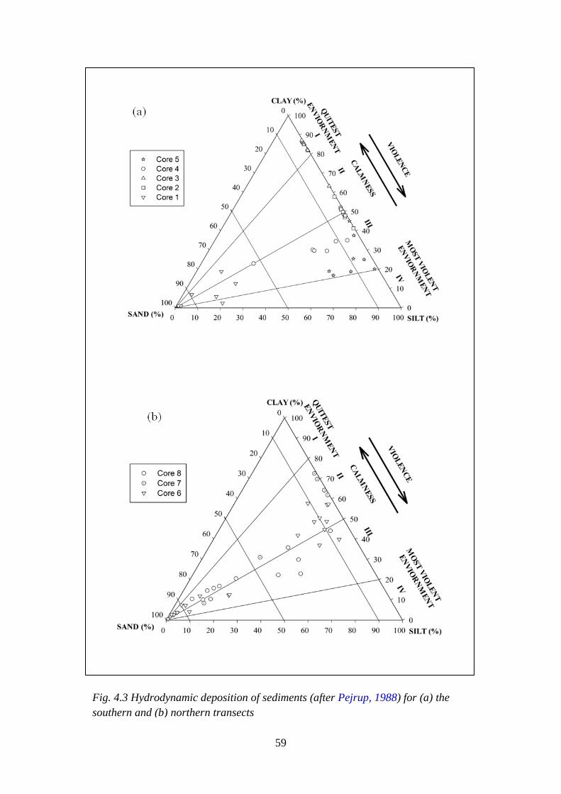
59

Fig. 4.3 Hydrodynamic deposition of sediments (after Pejrup, 1988) for (a) the

southern and (b) northern transects

60

The sand, silt and clay percentages for the coastal plain, lagoon and the

offshore cores of the northern transect are also plotted in Pejrup’s diagram and are

shown in figure 4.3b. The samples representing the top 10.8 m of the coastal plain

falls under the category III indicating violent environment whereas from 11 m to

down the core the sediments falls under the category II indicating calmness. The

sediments of the Core 7 also falls under the category II indicating calmness. In the

offshore (Core 8), the top 0.45 m falls under the category II indicating calmness

whereas down the core, the sediments falls under the category III indicating violent

environment.

4.5.2. Suite Statistics

The Tanner plot uses the mean size and sorting value to understand the

depositional energy condition. The suite statistics model proposed by Tanner

(1991a,b) uses the bivaraite plots of the mean size and sorting in a logarithimic scale.

This plot is sub-divided into three different fields representing the different energy

conditions of deposition as (i) fluvial and storm episodes, (ii) partially open to

restricted estuary and (iii) closed basin, giving the effective discrimination of

depositional enviornments. Spencer et al. (1998) have modified the plots of Tanner

(1991a,b) by including the open channel field in the plot. The biplot adopted from

Spencer et al. (1998) focuses on the part of the diagram related to new supply

enviornments and attempts to distinguish between the river and the closed basin or the

settling environment. The distinction relates primarily to current energies of the

depositional setting. For example, it distinguishes between calm settling conditions

and fluvial flood or storm episodes (Lario et al., 2000) or between closed and open

conditions related to barrier development (Spencer et al., 1998).

For the present study the mean grain size and sorting of the coastal plain,

estuary and the offshore sediments of the southern transect were superimposed on the

suite statistics proposed by Tanner (1991a,b) and modified by Spencer et al. (1998).

The bivariate plots of the mean size versus standard deviation shows that the

sediments of the coastal plain core (Core 1) of southern transect (Fig. 4.4a) falls under

two categories. From 2 to 9 m the sediments falls under the open channel conditions

indicating high energy whereas from 10.9 to 15.5 m, the sediments falls in the closed

61

basin indicating low energy. The sediments of the estuarine cores show variation in

the depositional enviornment.

(a)

(b)

Fig. 4.4 Depositional environment based on Mean vs Sorting (after Tanner, 1991a,b)

for the sediment cores of the (a) southern and (b) northern transect

62

In core 4, all the sediments fall under the partially open to restricted estuary

environment whereas the Core 2 sediments fall in the closed basin with some falling

in the margin of closed basin and partially open to restricted estuary conditions. The

offshore sediments (Core 5) fall in the partially open to restricted estuary.

In the northern transect (Fig. 4.4b), the coastal plain Core 6 is divided into two

groups. From 2.6 to 10.9 m the sediments fall under the open channel conditions

indicating high energy whereas from 11 to 20 m, the sediments fall under the category

of closed basin indicating low energy. The sediments of the lagoon core (Core 7)

exhibit a dominance of closed basin condition indicating low energy. In the offshore

core (Core 8), the top 0.45 m falls close to the partially open restricted estuary

indicating moderate energy whereas from 0.50 to 0.73 m the sediments fall in the

fluvial and storm episode conditions.

4.6. Clay Minerals

The clay mineral composition of the coastal and estuarine sediments is of

broad interest because its sensitivity is an indicator of environmental change (Velde,

1995; Stanley et al., 1998). Clay mineral characteristics of the aquatic sediment reflect

the prevailing climatic conditions, hydrography, geology and topography of the

continental source area (Chamley, 1989). The variation in the clay mineral

distribution is therefore a tool for deciphering the sediment sources and transport to

the area. The clay mineral composition indicates the intensity of weathering,

especially the degree of hydrolysis, at source rock regions which can be used as

paleoclimatic indicators (Chamley, 1989).

The dominance of the kaolinite group of minerals followed by gibbsite, illite,

chlorite and montmorillonite along the Kerala coast have been reported by many

researchers (Rao et al., 1983; Prithviraj and Prakash, 1991).

In the present study, the clay minerals were analysed for the selected cores

representing the coastal plains of the southern (Core 1) and the northern (Core 5)

transects. In this study the down core clay mineral variation of both cores were

studied for intensities and crystallinity characteristics.

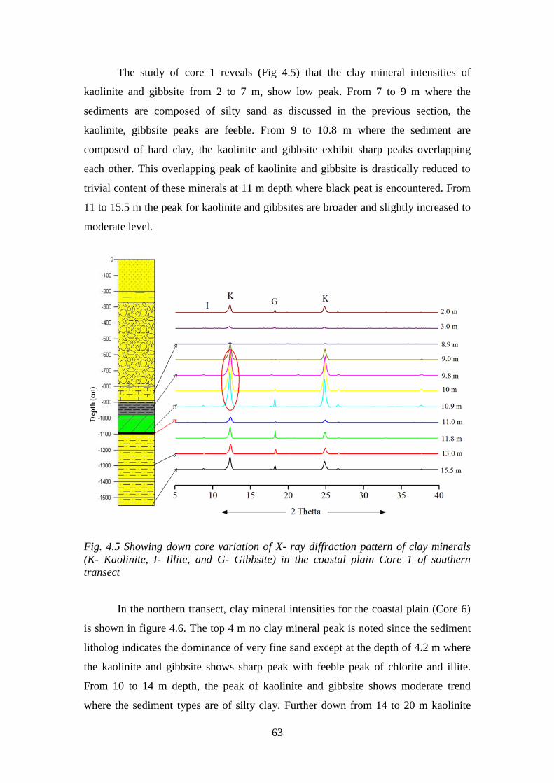
63

The study of core 1 reveals (Fig 4.5) that the clay mineral intensities of

kaolinite and gibbsite from 2 to 7 m, show low peak. From 7 to 9 m where the

sediments are composed of silty sand as discussed in the previous section, the

kaolinite, gibbsite peaks are feeble. From 9 to 10.8 m where the sediment are

composed of hard clay, the kaolinite and gibbsite exhibit sharp peaks overlapping

each other. This overlapping peak of kaolinite and gibbsite is drastically reduced to

trivial content of these minerals at 11 m depth where black peat is encountered. From

11 to 15.5 m the peak for kaolinite and gibbsites are broader and slightly increased to

moderate level.

Fig. 4.5 Showing down core variation of X- ray diffraction pattern of clay minerals

(K- Kaolinite, I- Illite, and G- Gibbsite) in the coastal plain Core 1 of southern

transect

In the northern transect, clay mineral intensities for the coastal plain (Core 6)

is shown in figure 4.6. The top 4 m no clay mineral peak is noted since the sediment

litholog indicates the dominance of very fine sand except at the depth of 4.2 m where

the kaolinite and gibbsite shows sharp peak with feeble peak of chlorite and illite.

From 10 to 14 m depth, the peak of kaolinite and gibbsite shows moderate trend

where the sediment types are of silty clay. Further down from 14 to 20 m kaolinite

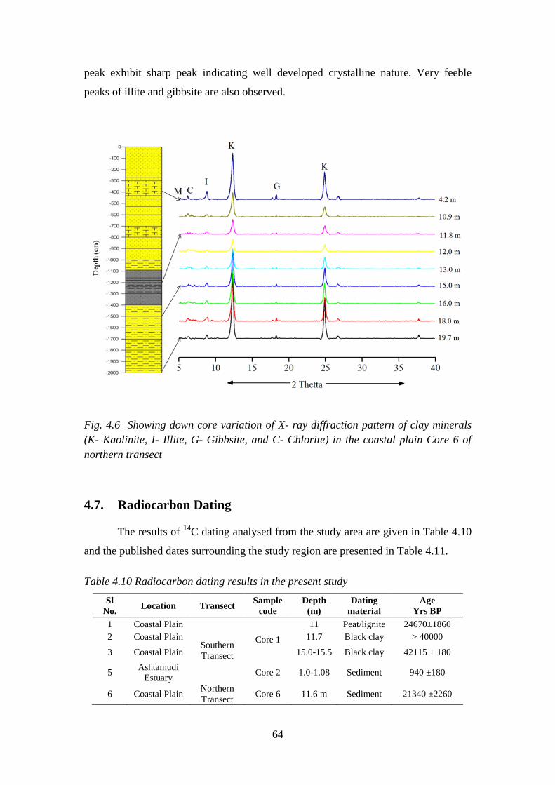
64

peak exhibit sharp peak indicating well developed crystalline nature. Very feeble

peaks of illite and gibbsite are also observed.

Fig. 4.6 Showing down core variation of X- ray diffraction pattern of clay minerals

(K- Kaolinite, I- Illite, G- Gibbsite, and C- Chlorite) in the coastal plain Core 6 of

northern transect

4.7. Radiocarbon Dating

The results of 14

C dating analysed from the study area are given in Table 4.10

and the published dates surrounding the study region are presented in Table 4.11.

Table 4.10 Radiocarbon dating results in the present study

Sl

No. Location Transect

Sample

code

Depth

(m)

Dating

material

Age

Yrs BP

1 Coastal Plain

Southern

Transect

Core 1

11 Peat/lignite 24670±1860

2 Coastal Plain 11.7 Black clay > 40000

3 Coastal Plain 15.0-15.5 Black clay 42115 ± 180

5 Ashtamudi

Estuary Core 2 1.0-1.08 Sediment 940 ±180

6 Coastal Plain Northern

Transect Core 6 11.6 m Sediment 21340 ±2260

65

Table 4.11 Published 14C dates from the coastal sediments of the Kollam and

Kayamkulam region

From the Table 4.10, out of the 5 dates, 4 dates are from the southern transect

representing the coastal plain and the Ashtamudi Estuary, whereas 1 date represents

the coastal plain of the northern transect. Based on the present study the age ranges

from 42,115 Yrs BP to 940 Yrs BP indicating the evolution from late Pleistocene to

Recent. For the southern transect, selected samples consisting of organic rich

sediments and peat for the coastal plain (Core 1) were dated and the results are

presented in Table 4.10. The results reveal that the black clay sediments rich in

organic matter (14%) at the depth ranging from 15.0 to 11.7 m have an age of 42,115

Yrs BP to 40,000 Yrs BP. The peat sample with an organic matter content of 47% at

the depth of 11 m, which is above the black clay rich sediments shows an age of

24,670 Yrs BP. The inferred dates from study indicate the late Pleistocene. The core

representing the Ashtamudi Estuary (Core 2) yielded an age of 940 Yrs BP from the

core retrieved of 1.0 to 1.08 m indicating recent sediments. In the northern transect

SL

No. Location

Sample

Type

Depth

(m)

Radiocarbon

Dating (Age) References

1 Munrothuruth Sediment 11 4350± 90 Padmalal et al. 2011

2 Puthenthuruthu

Sediment 12.5 6117± 101 Padmalal et al. 2011

3 Sediment 21 9376± 140 Padmalal et al. 2011

4 Sediment 31 12504± 148 Padmalal et al. 2011

5

Pangod

Wood 3 5260 ± 120 Nair et al. 2009

6 Wood 5 7490 ± 90 Nair et al. 2009

7 Sediment 5 7480 ± 80 Nair et al. 2009

8 Sediment 6 7550 ± 160 Nair et al. 2009

9

West Kallada

Sediment 10.5 3880 ± 80 Nair et al. 2009

10 Sediment 15.9 4050 ± 80 Nair et al. 2009

11 Sediment 23.5 6250 ± 110 Nair et al. 2009

12 Ashtamudi

surface Lime shell - 1330 ± 100 Rajenderan et al. 1989

13 Kadapuzha

Sediment 11 6518±119 Padmalal et al. 2013

14 Sediment 16 8269±44 Padmalal et al. 2013

15 Thevalkara Sediment 10-12 41788 ±574 Padmalal et al. 2013

16 Parayakadavu Shell 6.5 4610±100 Padmalal et al. 2013

17 Ayiramthengu

Shell 5 2580± 110 Padmalal et al. 2013

18 Sediment 20 40000 Padmalal et al. 2013

19 Ramapuram Sediment 3 2460±120 Nair et al. 2006

20 Ramapuram Shell 7.6 39370±1000 Nair et al. 2006

21 Ramapuram Wood - 2460 ± 120 Jayalakshmi et al. 2004

22 Muthukulam

(Kayamkulam west ) Wood 1.27-1.35

3362 ± 114

Jayalakshmi et al. 2004

23 Muthukulam Wood 2.07-2.12 6276 ± 112 Jayalakshmi et al .2004

24 Muthukulam Shell 3.0-3.10 7176 ± 82 Jayalakshmi et al. 2004

66

the coastal plain (core 6) of the present study (Table 4.10) at the depth of 11.6 m

yields an age of 21,340 Yrs BP indicating the late Pleistocene.

4.8. Discussion

The study of Quaternary sediments is important in any coastal region since

they contain the record of sea level changes, palaeoclimate and tectonics, which have

given rise to the present landscape (Nair and Padmalal, 2004). The occurrence of

Quaternary formations at various elevations along the Kerala coast speaks of recent

uplift. Incidence of a chain of coast-parallel estuaries/lagoons with rivers debouching

into them and separated from the sea by spits/bars along the central Kerala coast

provides evidence of a prograding coastline (Narayana and Priju, 2004). Many coastal

lowland environments can therefore be expected to contain a relatively abundant,

well-preserved sedimentary archive that makes high-resolution reconstructions of a

regional depositional history in response to the Pleistocene sea level changes (Bowen,

1978; Lowe and Walker, 1997).

In the study area the results of the sediment litholog of the southern transect

indicates several depositional as well as erosion episodes. The top 7 m of the sediment

column encompasses sand of medium to fine size grade of angular nature. Nair and

Padmalal (2004) have reported a Holocene sediment thickness of 8 m in this region.

The Holocene sediment is characterised by soft compact clay rich in organic material.

But the present study reveals that these Holocene sediments have been replaced by

almost equal thickness of modern sediments containing least organic matter content

brought by the Kallada River. The fluvial signature has been deciphered through SEM

studies and their details are given in Chapter 5. Overpeck et al. (1996) concluded that

the monsoon strength increased suddenly in two steps, 13,000–12,5000 14

C Yrs BP

and 10,000–9,500 14

C Yrs BP.

Most climatic proxies suggest that the stronger monsoon in the early Holocene

was associated with high lake levels; increased flow discharges floods and scouring

(Kale et al., 2004). Moreover the Kallada River which is existing as major depocentre

of the Ashtamudi Estuary brought heavy discharge consequent to the stronger

monsoon during the mid-Holocene resulting in the incised valley formation leading to

the progradation towards the coast. Below 7 to 9 m, the sediments are of medium to

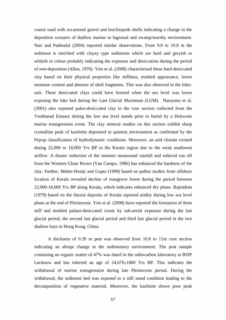
67

coarse sand with occasional gravel and brachiopods shells indicating a change in the

deposition scenario of shallow marine to lagoonal and swamp/marshy environment.

Nair and Padmalal (2004) reported similar observations. From 9.0 to 10.8 m the

sediment is enriched with clayey type sediments which are hard and greyish to

whitish in colour probably indicating the exposure and desiccation during the period

of non-deposition (Allen, 1970). Yim et al. (2008) characterised these hard desiccated

clay based on their physical properties like stiffness, mottled appearance, lower

moisture content and absence of shell fragments. This was also observed in the litho-

unit. These desiccated clays could have formed when the sea level was lower

exposing the lake bed during the Last Glacial Maximum (LGM). Narayana et al.

(2001) also reported paleo-desiccated clay in the core section collected from the

Vembanad Estuary during the low sea level stands prior to burial by a Holocene

marine transgression event. The clay mineral studies on this section exhibit sharp

crystalline peak of kaolinite deposited in quietest environment as confirmed by the

Pejrup classification of hydrodynamic conditions. Moreover, an arid climate existed

during 22,000 to 18,000 Yrs BP in the Kerala region due to the weak southwest

airflow. A drastic reduction of the summer monsoonal rainfall and reduced run off

from the Western Ghats Rivers (Van Campo, 1986) has enhanced the hardness of the

clay. Further, Meher-Homji and Gupta (1999) based on pollen studies from offshore

location of Kerala revealed decline of mangrove forest during the period between

22,000-18,000 Yrs BP along Kerala, which indicates enhanced dry phase. Rajendran

(1979) based on the littoral deposits of Kerala reported aridity during low sea level

phase at the end of Pleistocene. Yim et al. (2008) have reported the formation of three

stiff and mottled palaeo-desiccated crusts by sub-aerial exposure during the last

glacial period, the second last glacial period and third last glacial period in the two

shallow bays in Hong Kong, China.

A thickness of 0.20 m peat was observed from 10.8 to 11m core section

indicating an abrupt change in the sedimentary environment. The peat sample

containing an organic matter of 47% was dated in the radiocarbon laboratory at BSIP

Lucknow and has inferred an age of 24,670±1860 Yrs BP. This indicates the

withdrawal of marine transgression during late Pleistocene period. During the

withdrawal, the sediment bed was exposed to a still stand condition leading to the

decomposition of vegetative material. Moreover, the kaolinite shows poor peak

68

intensity further suggesting the absence of clay, related to intense plant productivity

and luxuriant growth of forests in the immediate vicinity (Mascarenhas et al., 1993).

The peat beds, which form Quaternary units in Kerala, indicate their formation from

submerged coastal forests i.e. initial subsidence of the coast and consequent

transgression of the sea (Powar et al., 1983; Rajendran et al., 1989). According to

Woodroffe (1983), peat formation is normally restricted to sheltered areas where low

energy conditions prevail, gently sloping intertidal areas, substrates favourable for

plant growth and a relatively stable sea level. Shajan (1998) reported an age of 25,000

to 30,000 Yrs BP from the peat samples at depths of 18 m and 24 m just below the

secondary lateritic horizon in the central Kerala coast.

From 11 to 15.5 m the sediments are composed of black clay with high

organic content and interblended with vegetative matter. Moreover, the radiocarbon

dating estimated an age ranging from 42,000 to 40,000 Yrs BP, which indicates the

first marine transgression event surrounding the Ashtamudi Estuary during the late

Pleistocene period This marine transgression event lead to the submergence of

mangroves and other vegetation forest which might have existed along this region

during 40,000 Yrs BP. Narayana et al. (2002) reported that the central Kerala coast

i.e. Vembanad region was covered with intensive mangroves and other forest

vegetation even at 40,000 Yrs BP and was inundated during higher sea level stands.

Since the estuary are the transition zones between rivers and the sea, the nature

of bottom sediment depend upon the hinterland geology and river runoff. The fresh

water inflow from the rivers and the tidal inflow near the estuarine mouth largely

determine the quantity of sediment deposition in the estuary. The textural

characteristics based on surficial sediments of the Ashtamudi Estuary indicate the

distribution of silt, clayey silt and sand (Black and Baba, 2001). The present study is

related to the sub-surficial sediments of the three cores. Out of the three cores, Core 3

is entirely composed of clay where as Core 2 sediments are dominated by clayey silt

to silty clay and Core 4 composed of sand-silt-clay to clayey silt. The ternary plots

proposed by Pejrup and suite statistics proposed by Tanner for all the three cores

confirms that the sediments were deposited under closed basin indicating low energy

environment

69

In the northern coastal plain core (Core 6), which comprises of 20 m length,

the top 10 m sediments comprise of very fine sand associated with minute broken

shells deposited under open channel with violent environment indicating beach-

littoral environment. Normally the sediments of the beach environment shows well

rounded nature. This was studied through SEM analysis and discussed in Chapter 5.

Nair et al. (2006) reported that the Ramapuram borehole which is adjacent to the Core

6 consist of medium to fine sand of Holocene age at a depth of 7 m. Similar

observations were also noted in the study core which elucidates that sediments above

10 m depth underwent marine transgression event during Holocene period. From 10

to 14 m depth, the sediment rich in sand are completely changed to mud interblended

with pelecypods and gastropods shells showing stiffness and maximum occurrence of

calcium carbonate content (38%) indicating a lagoonal littoral enviornment. High

calcium carbonate content also indicates the cooling period related to glacial event.

Moreover the sand silt clay ratios of Pejrup diagram and Tanner plot for energy

condition confirm that the sediments of this litho-unit were deposited under the

calmness of low energy environment. The radiocarbon dating analysed at the depth of

11.8 m reveals an age of 21,340 Yrs BP. The dates reveal that the age is close to arid

phase and the beginning of Last Glacial Maximum leading to the stiffness of sediment

indicating its deposition during the late Pleistocene. From 14 to 20 m the sequence of

the sediments that are composed of silty clay with 3% organic content show similiar

trend as that of the Core 1 except in the lagoonal deposit below 15 m. The sediment

associated with presence of broken shells confirms its deposition under the beach

lagoonal environment.

In the offshore region, the sediments of the southern core (Core 5) were

deposited under moderate energy environment where as the northern core (Core 8)

sediments were deposited under violent environment. Moreover down the core the

sediment are composed of sand with less percentage of organic content indicating

relict beach deposits.

4.9. Summary

The study deals with the textural analysis of the core samples collected from

various predefined locations of the study area. The result reveals that the Ashtamudi

Estuary is composed of silty clay to clayey type of sediments whereas offshore cores

70

are carpeted with silty clay to relict sand. Investigation of the source of sediments

deposited in the coastal plain located on either side of the estuary indicates the

dominance of terrigenous to marine origin in the southern region whereas it is

predominantly of marine origin towards the north. Further the hydrodynamic

conditions as well as the depositional environment of the sediment cores are

elucidated based on statistical parameters that decipher the deposition pattern at

various locations viz., coastal plain (open to closed basin), Ashtamudi Estuary

(partially open to restricted estuary to closed basin) and offshore (open channel).

From the results of radiocarbon dating, the coastal region surrounding the Ashtamudi

Estuary underwent the first marine transgression event during 40,000 yrs BP which

resulted in the submergence of mangroves as well as vegetative material as present in

the sediments and this lasted up to 24,000 yrs BP as indicated by the peat deposit.

CHAPTER 5

MICROMORPHOLOGICAL CHARACTERISTICS OF

QUARTZ GRAINS – IMPLICATIONS ON

DEPOSITIONAL ENVIRONMENT

5.1. Introduction

Quartz grains are the most commonly occurring particles in the clastic

sediments due to high stability and absence of cleavage planes. Because of the overall

abundance of quartz grains in siliciclastic successions, petrographers,

sedimentologists and soil scientists have long tried to find properties on the surface of

quartz that may be related or linked to transport characteristics. With the use of

Scanning Electron Microscopy (SEM) to earth sciences applications during the

1960’s, the properties of the surface of quartz grains became a focus for researchers,

especially for determining the transportation and deposition of sediments. The first

atlas on the morphological features of quartz grain (Krinsley and Doornkamp, 1973)

included a wide range of surface features related to transport and depositional history.

Later, the analysis of detrital grain surfaces became a widely used tool in

sedimentology, physical geography, and soil science. Many surface features on

detrital sediment grains are considered to be characteristic of the fluid dynamics in

distinct sedimentary environments (see for e.g., Krinsley and Doornkamp, 1973;

Mahaney, 2002), though different environments can include almost identical

mechanical (i.e., grinding, sliding, or cracking) and chemical (i.e., dissolution or

precipitation) processes.

The study of quartz grain microtextures (>200 μm) with SEM technique has

been shown to be a valid method in sedimentary petrology for interpreting

sedimentary environments and transport mechanisms (Krinsley and McCoy, 1977;

Krinsley and Marshall, 1987). The microtextures provide vital information regarding

the various processes acting on the grains during transportation and/or after deposition

(Doornkamp and Krinsley, 1971; Mahaney, 1998). The criteria for distinguishing

mechanical and chemical features and their implications have been well-established

(see, Rahman and Ahmed, 1996). Thus, the microtextural study on quartz grains is

72

considered as a powerful tool in the identification of provenance, processes of

transport and diagenetic history of the detrital sediments (Krinsley et al., 1976;

Madhavaraju et al., 2006). Surface textures of clastic particles are also repositories of

information about the physical and chemical processes to which the particles have

been subjected (Krinsley and Doornkamp, 1973). A grain of quartz sand taken from

the beach bears characteristic texturalsignatures on its surface, which strongly reflects

the wave action. This signature is quite distinct from those produced by the action of

rivers, wind or glaciers.

Surface textures can be grouped into two categories. One class deals with the

dullness or polish of the grain and the other concerns the marking on the grain

surface. Many investigators opined that a systematic study of the above two classes

can provide an insight into the history of transportation and deposition of clastic

particles (Krinsley and Doornkamp, 1973; Baker, 1976; Marshall, 1987).

5.2. Microtextural Characteristics

In order to understand the transport mechanism and post depositional history

of sediments of the study area, SEM analyses were carried on the quartz grains

selected from sediment cores representing the coastal plain, estuary/lagoon and

offshore region of the southern and northern transect (see also Fig. 3.1 in Chapter 3).

The detailed microtextural characteristics of the sand grains for the transect is

enumerated below following well established guidelines used in literatures applied for

SEM features as cited in Chapter 3.

5.2.1. Southern Transect

The microtextural analysis representing the coastal plain (Core 1), Ashtamudi

Estuary (Core 2 and Core 3) and offshore core (Core 5) were used for the southern

transect. The SEM features are envisgaed below.

5.2.1.1. Coastal Plain

The detailed description of litho-units and textural variation of samples

representing the coastal plains are presented in Chapter 4. The SEM analysis have

been carried out on the core samples representing southern transect based on

lithological variations by selecting the quartz grains from selected depth (3 m, 9 m,

73

10.9 m, 11.8 m, 12 m, 15.5 m). The surface texture of quartz grains at the depth of 3

m predominantly shows fresh angular features (Fig. 5.1) with series of conchoidal

fractures.

At the depth of 9 m, the

grains are angular with irregular

margins; the edges are sharp and

show conchoidal fractures (Figs.

5.2 a & b). The grain exhibits

high relief with numerous pits

with V-shaped scratches. These

are attributed to the fluvial

process related to high degree of

turbulence in the flow, causing

collision and compression of

grains against each other (see,

Krinsley and Doornkamp, 1973; Joshi, 2009).

A large number of quartz grains bear the distinct abrasion marks (Fig. 5.2a),

which are frequently noticed at the edge of the grains rather than the smooth surface

relating to fluvial transport (Krinsley and Takahashi, 1962) and suggestive of

moderately long distance of transport in an aqueous medium having a high energy

condition (Krinsley and Doornkamp, 1973). However, this type of features may also

be formed during transport of the host grains in a turbulent river (Ly, 1978) or at the

Fig. 5.1 SEM photographs of the quartz

grains at the depth of 3.0 m showing

mechanical features

Fig. 5.2 SEM photographs of the quartz grains at the depth of 9.0 m (a) showing

large conchoidal fracture with high relief and angular in outline (b) V-etch pits

(a) (b)

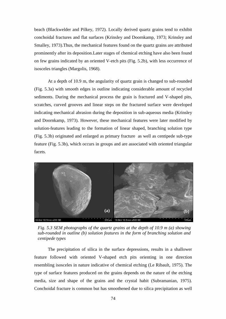
74

beach (Blackwelder and Pilkey, 1972). Locally derived quartz grains tend to exhibit

conchoidal fractures and flat surfaces (Krinsley and Doornkamp, 1973; Krinsley and

Smalley, 1973).Thus, the mechanical features found on the quartz grains are attributed

prominently after its deposition.Later stages of chemical etching have also been found

on few grains indicated by an oriented V-etch pits (Fig. 5.2b), with less occurrence of

isosceles triangles (Margolis, 1968).

At a depth of 10.9 m, the angularity of quartz grain is changed to sub-rounded

(Fig. 5.3a) with smooth edges in outline indicating considerable amount of recycled

sediments. During the mechanical process the grain is fractured and V-shaped pits,

scratches, curved grooves and linear steps on the fractured surface were developed

indicating mechanical abrasion during the deposition in sub-aqueous media (Krinsley

and Doornkamp, 1973). However, these mechanical features were later modified by

solution-features leading to the formation of linear shaped, branching solution type

(Fig. 5.3b) originated and enlarged as primary fracture as well as centipede sub-type

feature (Fig. 5.3b), which occurs in groups and are associated with oriented triangular

facets.

The precipitation of silica in the surface depressions, results in a shallower

feature followed with oriented V-shaped etch pits orienting in one direction

resembling isosceles in nature indicative of chemical etching (Le Ribault, 1975). The

type of surface features produced on the grains depends on the nature of the etching

media, size and shape of the grains and the crystal habit (Subramanian, 1975).

Conchoidal fracture is common but has smoothened due to silica precipitation as well

(b) (a)

Fig. 5.3 SEM photographs of the quartz grains at the depth of 10.9 m (a) showing

sub-rounded in outline (b) solution features in the form of branching solution and

centipede types

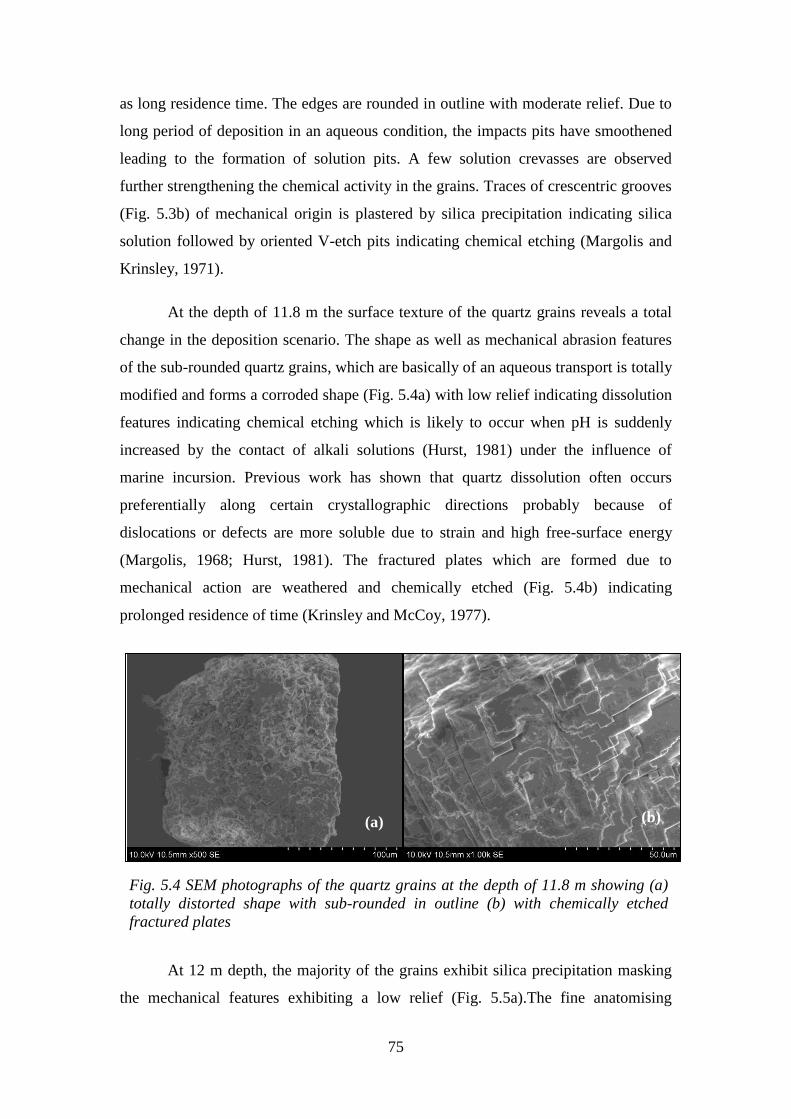
75

as long residence time. The edges are rounded in outline with moderate relief. Due to

long period of deposition in an aqueous condition, the impacts pits have smoothened

leading to the formation of solution pits. A few solution crevasses are observed

further strengthening the chemical activity in the grains. Traces of crescentric grooves

(Fig. 5.3b) of mechanical origin is plastered by silica precipitation indicating silica

solution followed by oriented V-etch pits indicating chemical etching (Margolis and

Krinsley, 1971).

At the depth of 11.8 m the surface texture of the quartz grains reveals a total

change in the deposition scenario. The shape as well as mechanical abrasion features

of the sub-rounded quartz grains, which are basically of an aqueous transport is totally

modified and forms a corroded shape (Fig. 5.4a) with low relief indicating dissolution

features indicating chemical etching which is likely to occur when pH is suddenly

increased by the contact of alkali solutions (Hurst, 1981) under the influence of

marine incursion. Previous work has shown that quartz dissolution often occurs

preferentially along certain crystallographic directions probably because of

dislocations or defects are more soluble due to strain and high free-surface energy

(Margolis, 1968; Hurst, 1981). The fractured plates which are formed due to

mechanical action are weathered and chemically etched (Fig. 5.4b) indicating

prolonged residence of time (Krinsley and McCoy, 1977).

At 12 m depth, the majority of the grains exhibit silica precipitation masking

the mechanical features exhibiting a low relief (Fig. 5.5a).The fine anatomising

Fig. 5.4 SEM photographs of the quartz grains at the depth of 11.8 m showing (a)

totally distorted shape with sub-rounded in outline (b) with chemically etched

fractured plates

(a) (b)

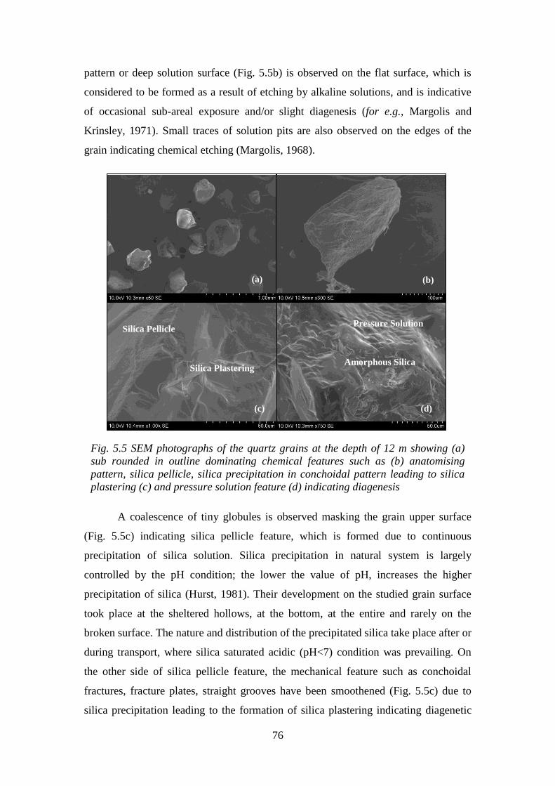
76

pattern or deep solution surface (Fig. 5.5b) is observed on the flat surface, which is

considered to be formed as a result of etching by alkaline solutions, and is indicative

of occasional sub-areal exposure and/or slight diagenesis (for e.g., Margolis and

Krinsley, 1971). Small traces of solution pits are also observed on the edges of the

grain indicating chemical etching (Margolis, 1968).

Fig. 5.5 SEM photographs of the quartz grains at the depth of 12 m showing (a)

sub rounded in outline dominating chemical features such as (b) anatomising

pattern, silica pellicle, silica precipitation in conchoidal pattern leading to silica

plastering (c) and pressure solution feature (d) indicating diagenesis

A coalescence of tiny globules is observed masking the grain upper surface

(Fig. 5.5c) indicating silica pellicle feature, which is formed due to continuous

precipitation of silica solution. Silica precipitation in natural system is largely

controlled by the pH condition; the lower the value of pH, increases the higher

precipitation of silica (Hurst, 1981). Their development on the studied grain surface

took place at the sheltered hollows, at the bottom, at the entire and rarely on the

broken surface. The nature and distribution of the precipitated silica take place after or

during transport, where silica saturated acidic (pH<7) condition was prevailing. On

the other side of silica pellicle feature, the mechanical feature such as conchoidal

fractures, fracture plates, straight grooves have been smoothened (Fig. 5.5c) due to

silica precipitation leading to the formation of silica plastering indicating diagenetic

Pressure Solution Silica Pellicle

(a) (b)

(c) (d)

Amorphous Silica Silica Plastering

77

process (Krinsley and Donahue, 1968). The deep sub-circular resembling rounded

hillocks like features (Fig. 5.5c) observed on the grains have been identified as

pressure solutions (see, Srivastava, 1989), which is an indication of diagenetic process

(Krinsley and Doornkamp, 1973) as well as linked to overburden (Srivastava, 1989).

Pressure solution is another mechanism that causes dissolution of silicate grains and is

based on the principle that silica solubility increases as pressure is applied to silicate

grains (Dewers and Ortoleva, 1990). Isolated patches of amorphous silica (Fig. 5.5c),

precipitated from seawater, formed on flat conchoidal surfaces (Krinsley and

Margolis, 1969) associated with pressure solution. Closely spaced chemical etch pits

form on sand grains by abrasion solution or during diagenesis, when grains are

exposed to high pH solution (Margolis and Krinsley, 1971). The grains generally are

covered with, what is either amorphous silica or quartz precipitated from sea water;

these precipitates forms knobby or bumpy projections on flat, conchoidal surfaces, but

follows the upturned plate lithology on irregular surfaces. Commonly, solution and

precipitation are found together, perhaps indicating more than one period of chemical

action.

At the depth of 15.5 m, the grain is sub-rounded, low relief with solution pits.

The grains exhibits dissolution etching (Fig. 5.6a), which is considered as extreme

form of weathering and is located on the old fractured surfaces of quartz, which

suggests that its formation is assisted by the fractured, which has weakened and later

weathered (Mahaney and Kalm, 1995). Long residence time might have lead to the

etching on the incipient quartz growth.The overall appearance looks like honey comb

structure (Fig. 5.6b).

Fig. 5.6 SEM photographs of the quartz grains at the depth of 15.5 m showing

chemical features in the form of (a) dissolution etching and (b) honey comb

structure indicating prolong diagenesis

Dissolution etching

Honey Comb

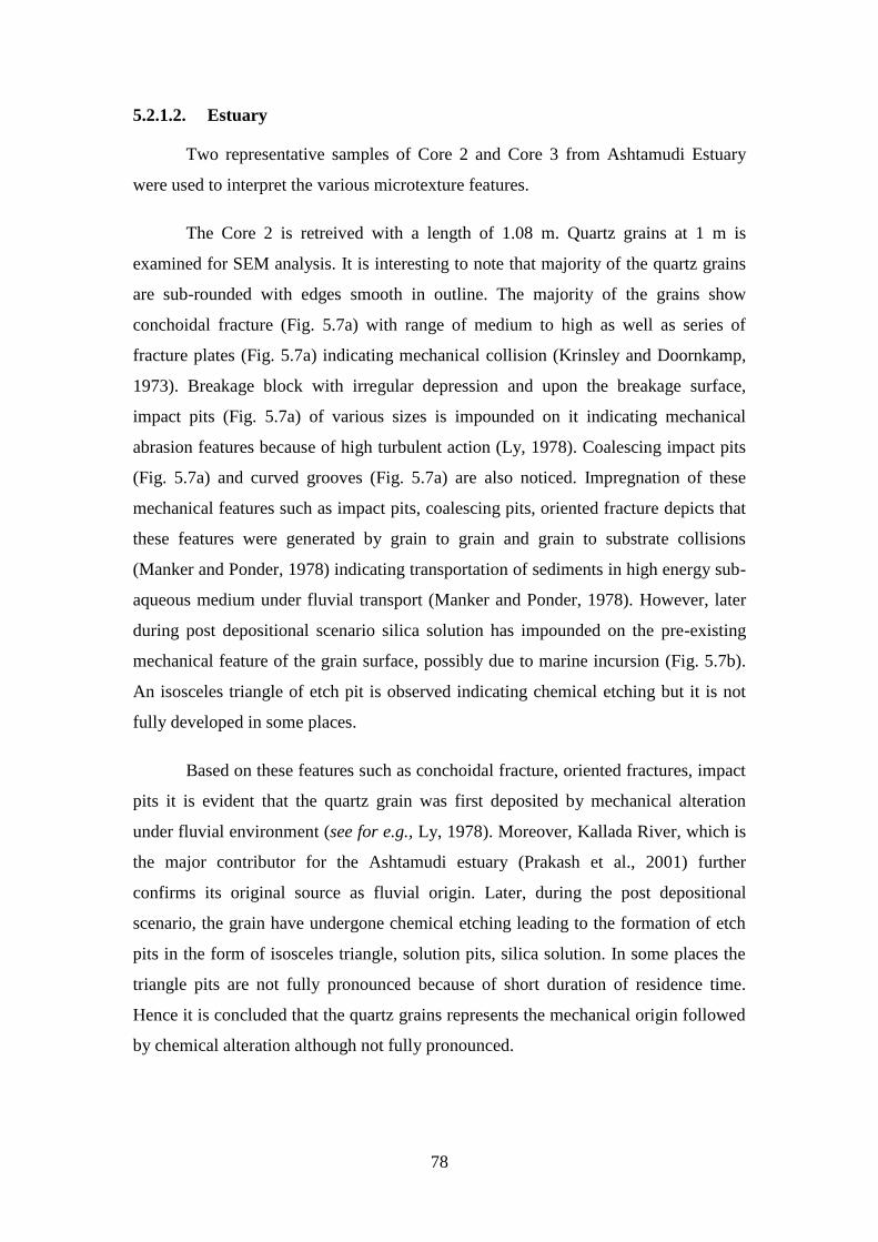
78

5.2.1.2. Estuary

Two representative samples of Core 2 and Core 3 from Ashtamudi Estuary

were used to interpret the various microtexture features.

The Core 2 is retreived with a length of 1.08 m. Quartz grains at 1 m is

examined for SEM analysis. It is interesting to note that majority of the quartz grains

are sub-rounded with edges smooth in outline. The majority of the grains show

conchoidal fracture (Fig. 5.7a) with range of medium to high as well as series of

fracture plates (Fig. 5.7a) indicating mechanical collision (Krinsley and Doornkamp,

1973). Breakage block with irregular depression and upon the breakage surface,

impact pits (Fig. 5.7a) of various sizes is impounded on it indicating mechanical

abrasion features because of high turbulent action (Ly, 1978). Coalescing impact pits

(Fig. 5.7a) and curved grooves (Fig. 5.7a) are also noticed. Impregnation of these

mechanical features such as impact pits, coalescing pits, oriented fracture depicts that

these features were generated by grain to grain and grain to substrate collisions

(Manker and Ponder, 1978) indicating transportation of sediments in high energy sub-

aqueous medium under fluvial transport (Manker and Ponder, 1978). However, later

during post depositional scenario silica solution has impounded on the pre-existing

mechanical feature of the grain surface, possibly due to marine incursion (Fig. 5.7b).

An isosceles triangle of etch pit is observed indicating chemical etching but it is not

fully developed in some places.

Based on these features such as conchoidal fracture, oriented fractures, impact

pits it is evident that the quartz grain was first deposited by mechanical alteration

under fluvial environment (see for e.g., Ly, 1978). Moreover, Kallada River, which is

the major contributor for the Ashtamudi estuary (Prakash et al., 2001) further

confirms its original source as fluvial origin. Later, during the post depositional

scenario, the grain have undergone chemical etching leading to the formation of etch

pits in the form of isosceles triangle, solution pits, silica solution. In some places the

triangle pits are not fully pronounced because of short duration of residence time.

Hence it is concluded that the quartz grains represents the mechanical origin followed

by chemical alteration although not fully pronounced.

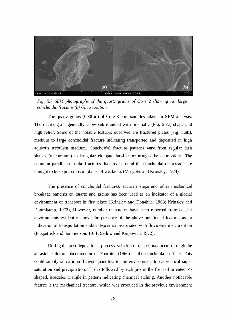
79

The quartz grains (0.80 m) of Core 3 core samples taken for SEM analysis.

The quartz grain generally show sub-rounded with prismatic (Fig. 5.8a) shape and

high relief. Some of the notable features observed are fractured plates (Fig. 5.8b),

medium to large conchoidal fracture indicating transported and deposited in high

aqueous turbulent medium. Conchoidal fracture patterns vary from regular dish

shapes (uncommon) to irregular elongate fan-like or trough-like depressions. The

common parallel step-like fractures thatcurve around the conchoidal depression are

thought to be expressions of planes of weakness (Margolis and Krinsley, 1974).

The presence of conchoidal fractures, accurate steps and other mechanical

breakage patterns on quartz and grains has been used as an indicator of a glacial

environment of transport in first place (Krinsley and Donahue, 1968; Krinsley and

Doornkamp, 1973), However, number of studies have been reported from coastal

environments evidently shown the presence of the above mentioned features as an

indication of transportation and/or deposition associated with fluvio-marine condition

(Fitzpatrick and Summerson, 1971; Setlow and Karpovich, 1972).

During the post depositional process, solution of quartz may occur through the

abrasion solution phenomenon of Fournier (1960) in the conchoidal surface. This

could supply silica in sufficient quantities to the environment to cause local super

saturation and precipitation. This is followed by etch pits in the form of oriented V-

shaped, isosceles triangle in pattern indicating chemical etching. Another noticeable

feature is the mechanical fracture, which was produced in the previous environment

Fig. 5.7 SEM photographs of the quartz grains of Core 2 showing (a) large

conchoidal fracture (b) silica solution

(a) (b)

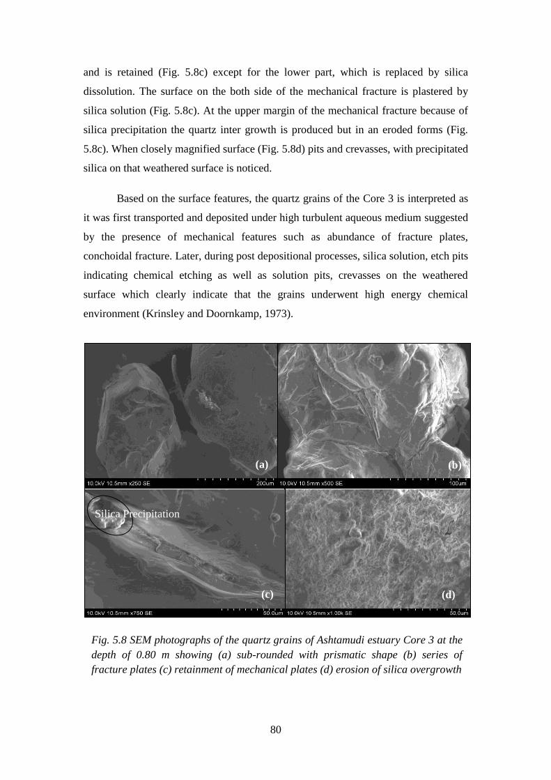
80

and is retained (Fig. 5.8c) except for the lower part, which is replaced by silica

dissolution. The surface on the both side of the mechanical fracture is plastered by

silica solution (Fig. 5.8c). At the upper margin of the mechanical fracture because of

silica precipitation the quartz inter growth is produced but in an eroded forms (Fig.

5.8c). When closely magnified surface (Fig. 5.8d) pits and crevasses, with precipitated

silica on that weathered surface is noticed.

Based on the surface features, the quartz grains of the Core 3 is interpreted as

it was first transported and deposited under high turbulent aqueous medium suggested

by the presence of mechanical features such as abundance of fracture plates,

conchoidal fracture. Later, during post depositional processes, silica solution, etch pits

indicating chemical etching as well as solution pits, crevasses on the weathered

surface which clearly indicate that the grains underwent high energy chemical

environment (Krinsley and Doornkamp, 1973).

Fig. 5.8 SEM photographs of the quartz grains of Ashtamudi estuary Core 3 at the

depth of 0.80 m showing (a) sub-rounded with prismatic shape (b) series of

fracture plates (c) retainment of mechanical plates (d) erosion of silica overgrowth

(a) (b)

(d)

Silica Precipitation

(c)

81

5.2.1.3. Offshore

The southern shelf representing the Kollam offshore has a core length of 0.88

m retrieved from a depth of 12 m. Quartz grains of 0.80 m taken for SEM analysis. It

is observed that the grains are sub-rounded in shape. Grain breakage associated with

fracture at regular interval is observed (Fig. 5.9a). Medium to large conchoidal

fracture impact pits, mechanical upturned plates, and deep mechanical V-shaped pits

are observed, clearly indicating the transportation and deposition of the quartz grain

under turbulence subaqueous medium. Sparse polygonal cracks (Fig. 5.9a) are

identified on the quartz grains, which may be the result of physical or chemical

weathering of salts crystallised on grains when they were at rest (Krinsley et al.,

1976). During the post depositional scenario, chemically upturned plates are observed

in the form of precipitated silica in the deep crack along the grain centre (Fig. 5.9b),

when highly magnified (Fig. 5.9c) as well as along the conchoidal fracture surface in

the form of step like appearance (Fig. 5.9c). The edges are smoothened by

reprecipitation of silca in the form of boulbous projection (Fig. 5.9d) as well as pre-

existing mechanical features such as impact pits as well as V-shaped pits, scratches

are well preserved.

Fig. 5.9 SEM photographs of the quartz grains of the southern offshore core (a)

Grain breakage associated with fracture (b) chemical upturned plates (c) silica

solution (d) silica dissolution

(a) (b)

(c) (d)

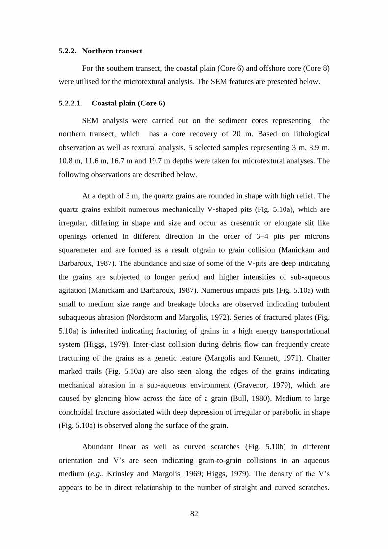
82

5.2.2. Northern transect

For the southern transect, the coastal plain (Core 6) and offshore core (Core 8)

were utilised for the microtextural analysis. The SEM features are presented below.

5.2.2.1. Coastal plain (Core 6)

SEM analysis were carried out on the sediment cores representing the

northern transect, which has a core recovery of 20 m. Based on lithological

observation as well as textural analysis, 5 selected samples representing 3 m, 8.9 m,

10.8 m, 11.6 m, 16.7 m and 19.7 m depths were taken for microtextural analyses. The

following observations are described below.

At a depth of 3 m, the quartz grains are rounded in shape with high relief. The

quartz grains exhibit numerous mechanically V-shaped pits (Fig. 5.10a), which are

irregular, differing in shape and size and occur as cresentric or elongate slit like

openings oriented in different direction in the order of 3–4 pits per microns

squaremeter and are formed as a result ofgrain to grain collision (Manickam and

Barbaroux, 1987). The abundance and size of some of the V-pits are deep indicating

the grains are subjected to longer period and higher intensities of sub-aqueous

agitation (Manickam and Barbaroux, 1987). Numerous impacts pits (Fig. 5.10a) with

small to medium size range and breakage blocks are observed indicating turbulent

subaqueous abrasion (Nordstorm and Margolis, 1972). Series of fractured plates (Fig.

5.10a) is inherited indicating fracturing of grains in a high energy transportational

system (Higgs, 1979). Inter-clast collision during debris flow can frequently create

fracturing of the grains as a genetic feature (Margolis and Kennett, 1971). Chatter

marked trails (Fig. 5.10a) are also seen along the edges of the grains indicating

mechanical abrasion in a sub-aqueous environment (Gravenor, 1979), which are

caused by glancing blow across the face of a grain (Bull, 1980). Medium to large

conchoidal fracture associated with deep depression of irregular or parabolic in shape

(Fig. 5.10a) is observed along the surface of the grain.

Abundant linear as well as curved scratches (Fig. 5.10b) in different

orientation and V’s are seen indicating grain-to-grain collisions in an aqueous

medium (e.g., Krinsley and Margolis, 1969; Higgs, 1979). The density of the V’s

appears to be in direct relationship to the number of straight and curved scratches.

83

Deep grooves with elongate scratches and troughs (Fig. 5.10c) as well as curved such

as crescentric in nature (Fig. 5.10c) is also observed reflecting sustained high shear

stress (Mahaney and Kalm, 2000; Mahaney, 2002). These grooves are oriented in a

preferred direction (Fig. 5.10d), occur with a conchoidal fracture and appear in sets.

Linear groove plates occur as a series of linear grooves of different dimensions

aligned at an angle to the grain surface.

The surface texture found include all those modern characteristics of modern

beach sand, i.e., V-shaped indentations, straight or slightly curved grooves and blocky

conchoidal breakage pattern (Krinsley and Donahue, 1968). The irregular orientations

of V-shaped indentations, their average depth, their density per square micron and the

groove markings (a creiterion of wave action) further indicate that the specimen is

derived from the high energy or surf zone of the littoral environment (Krinsley and

Donahue, 1968). Margolis and Kennett (1971) reported V’s generally occur on less

than 50 % of the grains from the fluvial origin and on more than 50 % of those from


(a) mechanical features such as impact pits, chattermarks (b) crescentric

groups with friction marks (c) deep grooves with elongate scratches and

troughs (d) grooves oriented in a preferred direction

(a) (b)

(c) (d)

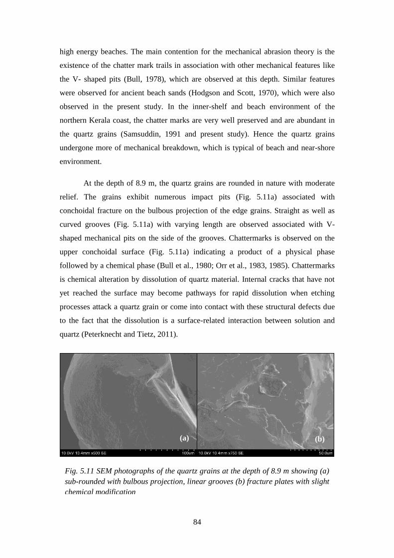
84

high energy beaches. The main contention for the mechanical abrasion theory is the

existence of the chatter mark trails in association with other mechanical features like

the V- shaped pits (Bull, 1978), which are observed at this depth. Similar features

were observed for ancient beach sands (Hodgson and Scott, 1970), which were also

observed in the present study. In the inner-shelf and beach environment of the

northern Kerala coast, the chatter marks are very well preserved and are abundant in

the quartz grains (Samsuddin, 1991 and present study). Hence the quartz grains

undergone more of mechanical breakdown, which is typical of beach and near-shore

environment.

At the depth of 8.9 m, the quartz grains are rounded in nature with moderate

relief. The grains exhibit numerous impact pits (Fig. 5.11a) associated with

conchoidal fracture on the bulbous projection of the edge grains. Straight as well as

curved grooves (Fig. 5.11a) with varying length are observed associated with V-

shaped mechanical pits on the side of the grooves. Chattermarks is observed on the

upper conchoidal surface (Fig. 5.11a) indicating a product of a physical phase

followed by a chemical phase (Bull et al., 1980; Orr et al., 1983, 1985). Chattermarks

is chemical alteration by dissolution of quartz material. Internal cracks that have not

yet reached the surface may become pathways for rapid dissolution when etching

processes attack a quartz grain or come into contact with these structural defects due

to the fact that the dissolution is a surface-related interaction between solution and

quartz (Peterknecht and Tietz, 2011).


sub-rounded with bulbous projection, linear grooves (b) fracture plates with slight

chemical modification

(a) (b)

85

Curved as well as straight scratches also observed. Compared to the above,

mechanical features prevail in these samples but with little chemical action. Series of

fractured plate (Fig. 5.11b) are also observed, on which chemical precipitation has

undertaken associated with adhering particles (Fig. 5.11b). The above features

indicate that at the depth of 8.9 m, beach environment prevailed with slight

modification on the features by chemical action.

At the depth of 10.9 m, the shape of the grain exhibits sub-rounded, low relief

and corroded (Fig. 5.12a) as well as distorted in nature. The mechanical features

produced in the grain have been totally obliterated. Series of solution pits (Fig. 5.12a)

highly variable in size, with circular and sub-circular or elongate in shapes (Krinsley

and Doornkamp, 1973) is impounded on the grain. Conchoidal fractures have been

recycled with silica solution (Fig. 5.12a). The effects of solution all over the grain are

clearly seen and are rounded in shape. Solution crevasses (Fig. 5.12a) seen on the

grains have undergone intense surface disintegration by chemical dissolution.

Limited quartz dissolution is indicated by solution rounding of primary

angularity and by the formation of etch pits. Etch pits ranges from V-shaped deep

oriented triangular pits, isosceles triangles, rectangular/rhombohedral pits,

anatomising features of ridges and valley and oriented striations pits are observed

(Fig. 5.12b). On the other hand, silica pellicle (Fig. 5.12b) masking the mechanical

features is also observed. Such differences in etch pit density can be attributed to

differences in crystallographic orientation (Hicks, 1985; Gratz et al., 1991) and/or to


(a) low relief distorted in nature with solution pits and crevasses (b) different

oriented etch pits

(b) (a)

86

variations in micro-weathering environments (Schultz and White, 1999). Conversely,

the density and size of etch pits associated with selective weathering of dislocations

on the quartz surface increase with decreasing depth (Schultz and White, 1999). The

degree of etching also varies according to the residence time (Udayaganesan et al.,

2011). These etch features exist more frequently in the marine environments, where

the rate of chemical solution exceeds the rate of mechanical abrasion (Margolis,

1968).

A period of solution by sea water in a quietescent environment is indicated by

the presence of oriented etch pits superimposed on the earlier mechanical features.

The larger triangle is a composite form consisting of a whole series of successively

smaller triangles towards the base of the pit. This pit has the form attributed by

Krinsley and Donahue (1968) and Margolis (1968) to chemical etching. Margolis

(1968) concluded that this etch form is the result of relatively slow chemical

solution.Thus, the type of surface produced– V, U, triangular shape, anatomising

ridges or oriented patterns depends on the nature of the etching media, size and shape

of the grains and the crystal habit (Subramanian, 1975) as well as different

crystallography orientations (Hicks, 1985; Brantley et al., 1986; Gratz et al., 1991)

and/or to variations in micro-weathering environments (Schultz and White, 1999).

Geological time replaces the intensity of etching as an important factor by prolonging

the contact between the grains and a solvent, such as sea water. Previous work has

shown that quartz dissolution often occurs preferentially along certain

crystallographic directions probably because dislocations or defects are more soluble

due to strain and high free-surface energy (Margolis, 1968; Hurst, 1981). The most

diagenetic features of this environment are the triangular etch depressions where

chemical etching along planes of weakness occur extensively. This texture usually

indicates a high energy chemical environment. The increasing rate of evaporation and

the abundance of salts in the pore water generally increase the pH which affects the

quartz grains and influences the development of chemical features (Washmi and

Gheith, 2003). Solution crevasses mainly occur in association with solution pits

(Krinsley and Doornkamp, 1973).

At the depth of 11.6 m, quartz grains are sub-rounded with intense weathering

in the form of cross-hatching network of etch pits (Fig. 5.13a) in the depressed

87

conchoidal surface indicating prolonged chemical etching (Margolis, 1968).

Formation of deep haloes (Fig. 5.13a) at the centre of the grain is observed indicating

further prolonged chemical etching during diagenesis. Mechanical abrasion features is

totally obliterated. The conchoidal fractures which were produced on the edges of the

grain are smoothened by silica precipitation. The breakage block (Fig. 5.13b) has

been smoothened with silica precipitation and then dissolution has taken place leading

to solution crevasses. Based on these microfeatures, it is evident that due to prolonged

residence time, the complete shape of the grain has been modified, which result in

chemical alteration of the quartz in prolonged immersion in marine environment.

At the depth of 16.0 m, the surface texture exhibit sub-rounded in shape with

moderate relief. In the lower part of the grains, slightly curved grooves with an

approximate length of 8 microns, impact pits, straight scratches (Fig. 5.14a), which

are the typical features of mechanical abrasion of beach environment (see for e.g.,

Krinsley and Donahue, 1968) is visible indicating the grain were transported as well

as deposited through mechanical process but later during post-depositional process,

plastering of silica solution took place leading to the smoothness of the edges

indicating reworked sediments. On the upper part, the smooth edges of the grains are

etched in the form of irregular in outline. The upper surface is plastered by silica

solution over which coalescence of tiny silica globules leading to the formation of

soluble silica pellicles (Fig. 5.14a) are observed. Depending upon the available silica

solution silica pellicle may grow partly or wholly, which mask the earlier

microtextures and are generally formed on the quartz grains during post


cross hatching network, deep haloes (b) smoothness of breakage blocks indicating

silica precipitation

(b) (a)

88

deposition/diagenesis on the broken

surfaces or conchoidal surface

(Madhavaraju et al., 2004).

When magnified closely (Fig.

5.14b), the conchoidal surface, which

was formed during mechanical process

has been found smoothened chemically

through silica solution, giving rise to

heap mound of circular to sub-circular

hillock like feature such as pressure

solution (Fig. 5.14b) associated with

solution pits and oriented V-shaped

etch pits (Fig. 5.14b) upon the precipitated upturned plates (Fig. 5.14c). Etch pits of

oriented crystallographic direction is observed (Fig. 5.14c) on the other side. Inside

the breakage surfaces, the fractured surface has been widened by silica plastering

because of silica precipitation. Moreover, precipitated upturned plates in the form of

step like appearance is noticed with a deep triangle within triangle at the centre (Fig.

5.14c) is noticed indicating a long period of chemical etching probably in basic

environment (Krinsley and Doornkamp, 1973).

Fig. 5.14 SEM photographs of the quartz grains at the depth of 16.0 m showing (b)

chemical features such as pressure solution and (c) deep triangle within triangle

indicating intense chemical weathering

At the depth of 19.7 m, the quartz grains are totally etched forming irregular in

outlines (Fig. 5.15a) indicating prolonged deposition of the grain in the marine

Fig. 5.14(a) SEM photographs of the

quartz grains at the depth of 16.0 m

showing mechanical features such as sub

rounded in outline

(b) (c)

(a)

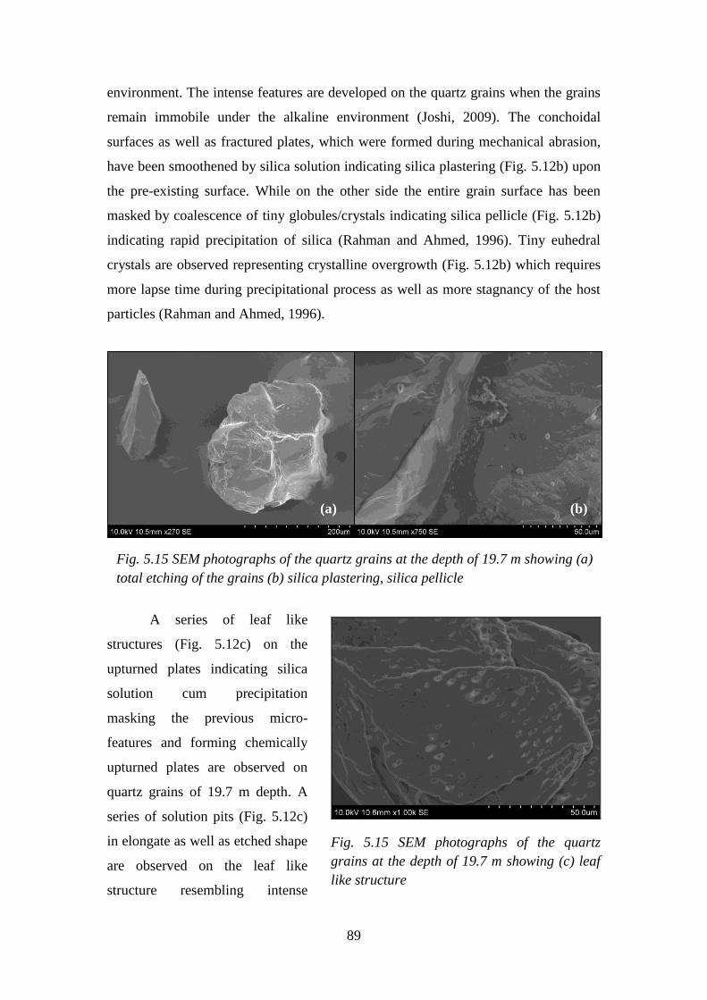
89

environment. The intense features are developed on the quartz grains when the grains

remain immobile under the alkaline environment (Joshi, 2009). The conchoidal

surfaces as well as fractured plates, which were formed during mechanical abrasion,

have been smoothened by silica solution indicating silica plastering (Fig. 5.12b) upon

the pre-existing surface. While on the other side the entire grain surface has been

masked by coalescence of tiny globules/crystals indicating silica pellicle (Fig. 5.12b)

indicating rapid precipitation of silica (Rahman and Ahmed, 1996). Tiny euhedral

crystals are observed representing crystalline overgrowth (Fig. 5.12b) which requires

more lapse time during precipitational process as well as more stagnancy of the host

particles (Rahman and Ahmed, 1996).

A series of leaf like

structures (Fig. 5.12c) on the

upturned plates indicating silica

solution cum precipitation

masking the previous micro-

features and forming chemically

upturned plates are observed on

quartz grains of 19.7 m depth. A

series of solution pits (Fig. 5.12c)

in elongate as well as etched shape

are observed on the leaf like

structure resembling intense

Fig. 5.15 SEM photographs of the quartz

grains at the depth of 19.7 m showing (c) leaf

like structure


total etching of the grains (b) silica plastering, silica pellicle

(a) (b)

90

chemical etching indicating silica dissolution over a period of long residence time.

Hence, it is confirmed that at this depth, quartz grains undergone chemical alteration

rigorously in the form of silica precipitation such as silica plastering silica pellicle and

crystalline over growth then followed by silica dissolution in the form of solution pits

which indicate that diagenesis is the major contributor in the formation of

microsurfcae texture features at this depth.

5.2.2.2. Offshore

In the northern transect offshore core (Core 8), is collected from Kayamkulam

offshore at a depth of 10 m with a core length of 0.73 m. Based on lithological

observations, quartz grains at 0.60 m depth is taken for SEM analysis.

It is observed that the grain is subrounded in shape with large amount of

breakage fracture. Mechanical V-shaped impact pits (Fig. 5.16a), large breakage

conchoidal fracture (Fig. 5.16a), fracture plates (Fig. 5.16a) is observed indicating

transportation of grains under high turbulent aqueous medium (e.g., Krinsley and

Doornkamp, 1973). Linear shaped, branching solution feature originated and

enlarged as primary fracture is also observed (Fig. 5.16b) in the quartz grain.

Abundance of solution crevasses mainly occur in association with solution pits (Fig.

5.16b) (Krinsley and Doornkamp, 1973) is observed. The solution crevasses (Fig.

5.16b) takes the form of a very thin surface layer peeling backwards away from

thelinear hollow (Doornkamp and Krinsley, 1971). Processes of solution tend to open

up cracks and crevasses along the structural weakness in these quartz grains (Joshi,

2009). Whenever a weak spot is found by the same process, a solution pit is created

(Krinsley and Doornkamp, 1973; Joshi, 2009) indicating silica dissolution took place

during the post depositional process. Some of the solution is seen in the formation of

cracks with much curved edges between the conchoidal fracture (Fig. 5.16b)

indicating early stages of development of crevasses (Krinsley and Doornkamp, 1971)

leading to the formation of secondary conchoidal fracture. Krinsley and Doornkamp

(1971) reported that these conchoidal features will become lines of weakness on the

grain surface and will automatically opened-up by chemical action. Therefore,

solution and chemical weathering have led to mechanical action, which in turn, has

resulted in a new phase of chemical activity.

91

On the upturned plates (Fig. 5.16c) series of straight to crescent-shaped

grooves of chemical alteration by dissolution of quartz material (Bull, 1977) known as

chattermarks trails randomly oriented is observed (Fig. 5.16c). These microstructures

as observed became wider and deeper with increasing duration of etching

(Peterknetch and Tietz, 2011). Internal cracks that have not yet reached the surface

may become pathways for rapid dissolution when etching processes attack a quartz

grain or come into contact with these structural defects due to the fact that the

dissolution is a surface-realted interactions bewteen solution and quartz (Peterknecht

and Tietz, 2011). In this process, the etching procedure affects the entire surface of

the grain and totally destroys the polish by dissolution and subsequent removal of

quartz. This removal opens the previously internal cracks for invading solution and

further material removal, thus sculpting the grooves of the chattermark trail.

Fig. 5.16 SEM photographs of the quartz grains (0.60 m) of northern offshore at the

depth of 10 m showing (a) large breakage conchoidal fracture (b) solution crevasses

(c) chatter mark trails on upturned plates (d) crystalline overgrowth with irregular

solution pits

(a) (b)

(c) (d)

92

Another important feature is numerous majority of the precipitated silica

represents tiny euhedral crystals crystal faces termed crystalline overgrowth (Fig.

5.16d) have formed on the upturned plates by precipitation. A number of

rhombohedral faces are well developed with occasional pyramid faces also present.

This chemically precipitated texture represents an acidic enviornment having lower

pH value and capable of silica precipitation (Krauskopf, 1956). Development of

euhedral crystalline overgrowth require to lapse more time during precipitational

process as well as more stagnancy of the host particles (Rahman and Ahmed, 1996).

Upon the crystalline overgrowth in the form columnar shape, irregular solution pits

(Fig. 5.16d) with solution crevasses is observed. Moreover, a long period of chemical

etching probably in basic enviornment (Krinsley and Doornkamp, 1973) has produced

a deep triangle within triangle form at the centre (Fig. 5.16d). Upon these isosceles

triangle as well as along the sides excess of silica solution after prologned residence

time forms etched silica flakes (Fig. 5.16d) indicating dissolution of silica dominated

when the pH condition is suddenly increased by the contact of alkali solutions (Hurst,

1981) under the influence of marine ingression.

5.3. Transport Mechanism and Depositional History

The environment in which the mineral grains were deposited is significant in

the study of influence of time on the grain surface textures (Ly, 1978). The

microtextural analyses of quartz grains representing the sediment core which is 9.5

km east of the present day coastline shows the dominance of angular grains with high

relief, impact pits, imbrigated breakage block, medium to large conchoidal fractures,

oriented fracture plates, flat cleavage surfaces, which are indicative of the sediments

up to a depth of 9 m were transported and deposited under fluvial enviornment

through mechanical processes. This is corroborated with the sediment texture

revealing medium to fine sand with angular in nature. Overpeck et al. (1996) based on

radiocarbon dating inferred that the southwest Indian monsoon strength increased

suddenly during 13,000–12,500 Yrs BP and 10,000–9,500 Yrs BP respectively. The

climatic proxies suggest that the stronger monsoon in the early Holocene was

associated with high lake levels; increased flow discharges floods and scouring (Kale

et al., 2004). Since the Kallada River is a major depocentre for the Ashtamudi

Estuary, it may be during the time of stronger monsoon, incised valley has taken place

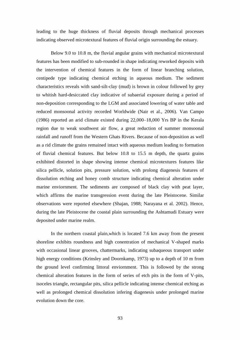
93

leading to the huge thickness of fluvial deposits through mechanical processes

indicating observed microtextural features of fluvial origin surrounding the estuary.

Below 9.0 to 10.8 m, the fluvial angular grains with mechanical microtextural

features has been modified to sub-rounded in shape indicating reworked deposits with

the intervention of chemical features in the form of linear branching solution,

centipede type indicating chemical etching in aqueous medium. The sediment

characteristics reveals with sand-silt-clay (mud) is brown in colour followed by grey

to whitish hard-desiccated clay indicative of subaerial exposure during a period of

non-deposition corresponding to the LGM and associated lowering of water table and

reduced monsoonal activity recorded Worldwide (Nair et al., 2006). Van Campo

(1986) reported an arid climate existed during 22,000–18,000 Yrs BP in the Kerala

region due to weak southwest air flow, a great reduction of summer monsoonal

rainfall and runoff from the Western Ghats Rivers. Because of non-deposition as well

as a rid climate the grains remained intact with aqueous medium leading to formation

of fluvial chemical features. But below 10.8 to 15.5 m depth, the quartz grains

exhibited distorted in shape showing intense chemical microtextures features like

silica pellicle, solution pits, pressure solution, with prolong diagenesis features of

dissolution etching and honey comb structure indicating chemical alteration under

marine enviornment. The sediments are composed of black clay with peat layer,

which affirms the marine transgression event during the late Pleistocene. Similar

observations were reported elsewhere (Shajan, 1988; Narayana et al. 2002). Hence,

during the late Pleistocene the coastal plain surrounding the Ashtamudi Estuary were

deposited under marine realm.

In the northern coastal plain,which is located 7.6 km away from the present

shoreline exhibits roundness and high conentration of mechanical V-shaped marks

with occasional linear grooves, chattermarks, indicating subaqueous transport under

high energy conditions (Krinsley and Doornkamp, 1973) up to a depth of 10 m from

the ground level confirming littoral enviornment. This is followed by the strong

chemical alteration features in the form of series of etch pits in the form of V-pits,

isoceles triangle, rectangular pits, silica pellicle indicating intense chemical etching as

well as prolonged chemical dissolution infering diagenesis under prolonged marine

evolution down the core.

94

Based on the quartz surface texture for the coastal plains of the northern as

well as southern transect, it can be concluded that the northern coastal plain

underwent more pronounced trangression regression events during late Quaternary.

This is also confirmed by radiocarbon dates as well as formation of ridges and swales

of different sets of orientation based on series of episodes of transgression as well as

regression events, which were reported elsewhere (Chattopadhyay, 2002; Jayalekshmi

et al., 2004; Samsuddin et al., 2008). The borehole of the coastal plain in the southern

transect is dominated quartz grains of terrigenous characteristics even up to a depth of

10 m indicating absence of marine incursion during Holocene, whereas the chemical

alteration is enhanced further down core confirming longer resident time under the

low energy marine enviornment during Late Pleistocene which is also confirmed by

the dating results of the peat below 10 m depth.

In the Ashtamudi Estuary, surface textures features such as conchoidal

fracture, oriented fractures plates, impact pits are infered which confirms that the

quartz grain was first deposited by mechanical altertaion through subaqueous impact

under fluvial enviornment (Krinsley and Doornkamp, 1973; Ly, 1978; Monker and

Ponder, 1978). Moreover, the Kallada River, which is the major sediment source of

Ashtamudi estuary (Prakash et al., 2001) further confirms its original source from

fluvial origin. Later, during the post depositional scenario, the grains have undergone

chemical etching leading to the formation of etch pits in the form of isoceles triangle,

solution pits, silica solution. At places, the triangle pits are not fully pronounced

because of rapid silica reprecipitation as well as short duration of residence time.

Hence, it is concluded that the quartz grains were deposited through mechanical

process under fluvial origin followed by post depositional process of chemical

alteration but not fully pronounced.

In the offshore region, based on microtexture features it is inferred that the

quartz grains were first transported and deposited under littoral enviornment based on

the presence of series of fractures plates, conchoidal fracture and V-shaped pits

indicating formation of these features in the turbulent aqueous high energy

enviornment (Ly, 1978; Krinsley and Doornkamp, 1973). During the post

depositional process, quartz grains underwent chemical alteration process of silica

precipitation as well as silica dissolution in the form of quartz intergrowth, solution

95

pits, crevasses, etch pits, chemical etching in the form of triangle within triangle

indicating high chemical energy enviornment. Moreover, the presence of chattermark

observed in the quartz grain reveals a two-phase formation process: the first phase is

the mechanical collision of components (Paterson, 1978; Swain, 1979) during

sediment transport followed by a second (depositional) phase characterized by the

establishment of a chemical reaction upon any quartz surface available for dissolution

(Peterknetch and Tietz, 2011).

It has been reported by earlier workers that the coarser sandy sized sediments

are not of recent origin supplied from the hinterland by the present day rivers, but, are

the beach and nearshore sediments of Holocene period during the lower stand of sea

level, which was later submerged by rise in sea level (Nair et al., 1978) and emplaced

in the present day outer-innershelf enviornment. Similar observations with SEM

features were reported elsewhere (Prithiviraj and Prakash, 1991) along the Kerala

Coast.

Coch and Krinsley (1971) reported that the intensity of chemical action

depend on the age of deposits, with stronger etching effects observed in the older

sediments. The longer the residence time in the marine environment, more the

chemical action for the quartz grain (Prithiviraj and Prakash, 1991). It has also been

shown that quartz grains from modern beach enviornment do not exhibit significant

chemical action (Ly, 1978). Therefore, it is confirmed the quartz grains are of littoral

origin and also represent some of relict beach deposits. These relict sands were

probably deposited on the shelf during the last low stand of sea level and were then

submerged as the sea transgressed over the shelf during the Holocene post glacial

period. Moreover, the coastal currents in shelf might have reworked these relict sands

which werein marine environment for a long period time on the innershelf.

5.4. Summary

The results of the microtextural study of sediment samples (quartz grains)

using Scanning Electron Microscope (SEM) are presented. These results throw light

on the processes of transport and diagenetic history of the detrital sediments. Based on

the lithological variations, selected quartz grains of different environments were also

analysed. The study indicates that the southern coastal plain sediments were

96

transported and deposited mechanically under fluvial environment followed by

diagenesis under prolonged marine incursion. But in the case of the northern coastal

plain, the sediments were transported and deposited under littoral environment

indicating the dominance of marine incursion through mechanical as well as chemical

processes. The quartz grains of the Ashtamudi Estuary indicate fluvial origin. The

surface texture features of the offshore sediments suggest that the quartz grains are of

littoral origin and represent the relict beach deposits.

CHAPTER 6

MAJOR AND TRACE ELEMENT GEOCHEMISTRY OF

SEDIMENT CORES

6.1. Introduction

The chemical composition of sedimentary rocks is dependent on the

depositional processes, including source rocks, weathering, sorting, tectonic setting

and paleoclimate (McLennan, 1989; McLennan and Taylor, 1991; McLennan et al.,

1993). Therefore, provenance analysis will help in reconstructing the predepositional

history of a sediment or sedimentary rock. This includes the distance and direction,

size and setting of the source region, climate and relief in the source area, and the

specific type of sedimentary rocks (Pettijohn et al., 1987; Von Eynatten and Gaupp,

1999).

Elemental variations observed in sediments can also provide vital information

on the environmental conditions like diagenetic processes and pollutant inputs, and

can assist in sediment correlation and process studies (e.g., Rothwell and Rack 2006).

Certain elements or element ratios can be used as proxies for environmental

conditions that are either generally valid or constrained to specific conditions (Koinig

et al., 2003). Similarly, trace elements such as Th, Zr, Nb, Sc, Y, Cr and REE such as

La, Ce, Nd, Gd, Yb are most suited for discriminates of provenance and tectonic

setting since these elements have relatively low mobility during sedimentary

processes and have short residence time in seawater (Taylor and McLennan, 1985).

This study presents geochemical analysis of the sediment cores representing

coastal plain, estuary and offshore of Kollam region. The close examination of the

various major and trace elemental compositions of core sediment and their inter-

relationship are studied to understand the paleoenvironmental conditions prevailing in

the coastal area. The geochemical proxies are used to identify the origins of the

estuarine sediments, especially to infer the provenance and source sink relationship.

Furthermore, weathering in the source area and maturity of the sediments is also

discussed.

98

6.2. Distribution of Major elements

The distribution of the major elements for the sediment cores representing the

coastal plain, estuary and offshore are presented in Table 6.1. SiO2 (wt%) is recorded

higher in coastal plain sediments ranging between 32.2 and 87.5 wt% with an average

of 58.5 wt%, which is higher than the offshore (Core 5) (av. 46.8 wt%) and estuarine

sediments of Core 4 – 48.6; Core 3 – 37.9 and Core 2 – 40.3 wt%. Al2O3 content

shows variation among the estuarine sediments (Core 4 – 15.3; Core 3– 21.5 and Core

2 – 18.5 wt%), which are comparable with offshore (15.15 wt %) and coastal plain

sediments (18.1 wt%). Al2O3 in Core 3 sediments varies between 20.1 and 23.8 wt%,

which is recorded higher than Core 4 (12.6-16.4 wt%) and Core 2 (18.0-19.3 wt%).

Offshore sediments shows comparatively higher TiO2, Fe2O3, CaO, MgO,

Na2O, K2O and P2O5 contents than the coastal plain sediments, meanwhile these

elements concentration in offshore sediments can be comparable with estuarine

sediments particularly for the sediments obtained in Core 4. Among the estuarine

sediments, SiO2, CaO and P2O5 content is recorded higher in Core 4 sediments (av.

48.6 wt%; 7.4 wt%; and 0.4 wt%), whereas Al2O3, Fe2O3 and Na2O content is

recorded higher in Core 3 (av. 21.5 wt%; 9.8 wt% and 4.6 wt% respectively). Core 2

sediment show an intermediate composition between Core 4 and Core 3 except MgO

content (av. 4.1 wt%) recorded higher than the other cores.

6.2.1. Normalisation of major and trace elements with UCC

The overall major oxides comprising coastal plain, estuary and offshore were

normalised against the UCC values based on Taylor and Mclennan (1985) and is

presented in figure 6.1a. The analysed samples are depleted in SiO2, K2O and

enriched in TiO2, Fe2O3, MgO (except Core 1 samples), and P2O5. In general, the

sediments of Core 3 are enriched in Al2O3, Fe2O3, MnO, Na2O and depleted in CaO

compared to the sediments of other two cores (Core 4 and Core 2). Sediments of Core

Core 4 and Core 2 show relatively similar trend in concentration of major oxides

compared to sediments of Core 3. The high concentration of Fe2O3 in these sediments

is an indication of oxidation, hydration and leaching processes involved during

weathering (Mikkel and Henderson, 1983).

99

Table 6.1. Major Element concentration in weight percentages for Coastal Plain (Core 1) sediment core

Element 2 2.7 3 4 5 6 7 8 8.9 9 9.8 9.9 10.9 11.8 12 13 13.8 14 15 15.5

(wt %) (m) (m) (m) (m) (m) (m) (m) (m) (m) (m) (m) (m) (m) (m) (m) (m) (m) (m) (m) (m)

SiO2 75.26 65.06 70.54 84.36 82.87 84.40 87.46 67.73 71.55 70.38 43.96 43.95 44.16 35.74 44.39 41.56 32.18 35.44 34.74 36.64

TiO2 0.81 0.74 0.74 0.44 0.38 0.32 0.42 0.55 0.75 0.94 0.98 1.08 0.99 0.80 0.85 0.85 0.79 0.79 0.80 0.85

Al2O3 12.11 15.57 13.73 8.61 8.82 8.35 6.99 9.93 12.92 16.21 26.56 32.68 31.37 23.40 22.57 23.70 21.57 23.72 23.07 24.31

MnO 0.01 0.008 0.008 ND ND ND ND ND 0.002 ND 0.001 ND ND 0.016 ND ND 0.001 0.058 0.050 0.057

Fe2O3 3.29 4.47 4.06 2.02 1.93 2.28 1.21 6.47 6.19 4.07 10.19 1.85 1.22 7.19 4.90 3.34 4.52 8.73 9.75 9.01

CaO 0.49 0.53 0.47 0.31 0.33 0.31 0.28 4.91 0.31 0.26 0.33 0.28 0.30 0.35 0.38 0.44 0.45 0.35 0.36 0.37

MgO 1.06 1.10 1.07 0.94 0.98 0.94 0.95 0.91 0.94 0.94 0.91 0.91 0.98 1.26 1.33 1.36 1.39 1.21 1.17 1.15

Na2O 0.61 0.69 0.59 0.29 0.38 0.24 0.26 0.30 0.44 0.71 0.97 1.39 1.64 1.85 1.71 1.86 2.02 1.42 1.27 1.27

K2O 1.31 1.43 1.30 0.70 0.82 0.55 0.34 0.02 0.03 0.02 0.34 0.46 0.49 1.48 2.04 1.93 1.44 1.56 1.35 1.30

P2O5 0.07 0.08 0.08 0.06 0.06 0.06 0.04 0.14 0.11 0.11 0.16 0.08 0.10 0.08 0.08 0.11 0.09 0.10 0.10 0.10

LOI 4.95 10.28 7.36 2.27 3.36 2.59 2.01 8.95 6.69 6.37 15.54 17.28 18.64 27.78 21.69 24.76 35.48 26.55 27.25 24.89

CIA 78.06 80.31 80.4 83.42 80.55 85.75 84.97 90.83 89.66 87.27 88.17 86.57 84.14 75.31 74.23 74.29 72.47 78.88 80.35 81.29

ICV 0.62 0.58 0.60 0.55 0.55 0.56 0.50 1.33 0.67 0.43 0.52 0.18 0.18 0.55 0.50 0.41 0.49 0.59 0.64 0.574

Al/Ti 15.00 21.18 18.66 19.48 22.96 26.49 16.84 17.98 17.29 17.34 27.10 30.20 31.82 29.21 26.49 28.01 27.24 29.91 28.73 28.57

K/Na 2.16 2.08 2.20 2.43 2.19 2.26 1.30 0.08 0.06 0.02 0.35 0.33 0.30 0.80 1.19 1.04 0.72 1.10 1.07 1.02

Si/Al 6.21 4.18 5.14 9.80 9.40 10.11 12.51 6.82 5.54 4.34 1.66 1.34 1.41 1.53 1.97 1.75 1.49 1.49 1.51 1.51

K/Al 0.108 0.092 0.095 0.082 0.093 0.065 0.049 0.002 0.002 0.001 0.013 0.014 0.015 0.063 0.090 0.082 0.067 0.066 0.059 0.054

Mg/Al 0.087 0.071 0.078 0.109 0.111 0.113 0.136 0.092 0.073 0.058 0.034 0.028 0.031 0.054 0.059 0.057 0.065 0.051 0.051 0.047

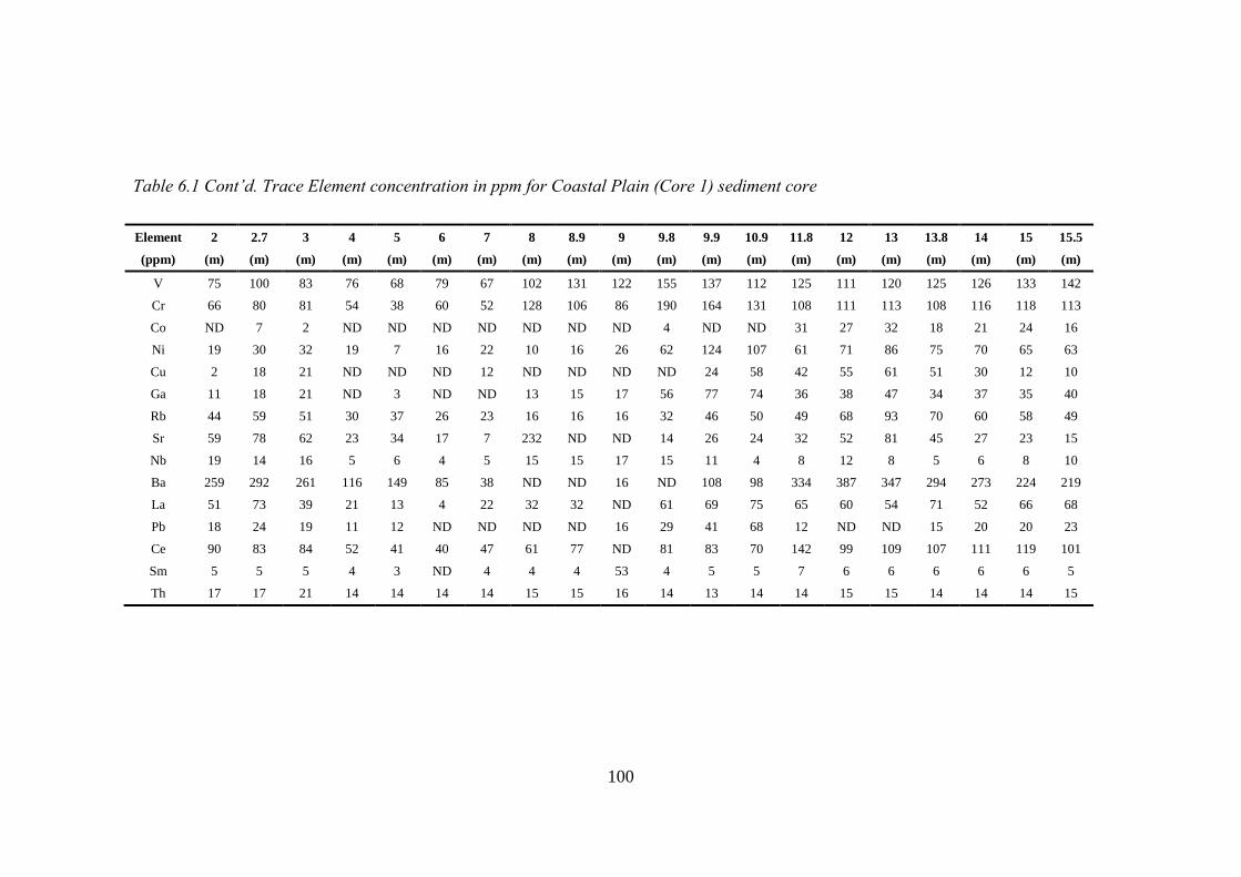
100

Table 6.1 Cont’d. Trace Element concentration in ppm for Coastal Plain (Core 1) sediment core

Element 2 2.7 3 4 5 6 7 8 8.9 9 9.8 9.9 10.9 11.8 12 13 13.8 14 15 15.5

(ppm) (m) (m) (m) (m) (m) (m) (m) (m) (m) (m) (m) (m) (m) (m) (m) (m) (m) (m) (m) (m)

V 75 100 83 76 68 79 67 102 131 122 155 137 112 125 111 120 125 126 133 142

Cr 66 80 81 54 38 60 52 128 106 86 190 164 131 108 111 113 108 116 118 113

Co ND 7 2 ND ND ND ND ND ND ND 4 ND ND 31 27 32 18 21 24 16

Ni 19 30 32 19 7 16 22 10 16 26 62 124 107 61 71 86 75 70 65 63

Cu 2 18 21 ND ND ND 12 ND ND ND ND 24 58 42 55 61 51 30 12 10

Ga 11 18 21 ND 3 ND ND 13 15 17 56 77 74 36 38 47 34 37 35 40

Rb 44 59 51 30 37 26 23 16 16 16 32 46 50 49 68 93 70 60 58 49

Sr 59 78 62 23 34 17 7 232 ND ND 14 26 24 32 52 81 45 27 23 15

Nb 19 14 16 5 6 4 5 15 15 17 15 11 4 8 12 8 5 6 8 10

Ba 259 292 261 116 149 85 38 ND ND 16 ND 108 98 334 387 347 294 273 224 219

La 51 73 39 21 13 4 22 32 32 ND 61 69 75 65 60 54 71 52 66 68

Pb 18 24 19 11 12 ND ND ND ND 16 29 41 68 12 ND ND 15 20 20 23

Ce 90 83 84 52 41 40 47 61 77 ND 81 83 70 142 99 109 107 111 119 101

Sm 5 5 5 4 3 ND 4 4 4 53 4 5 5 7 6 6 6 6 6 5

Th 17 17 21 14 14 14 14 15 15 16 14 13 14 14 15 15 14 14 14 15

101

Table 6.1 Cont’d. Major Element concentration in weight percentages for Ashtamudi Estaury (Core 2) sediment core

Element 10 0.20 0.30 0.40 0.50 0.60 0.70 0.80 0.90 1.0 1.08

(wt %) (m) (m) (m) (m) (m) (m) (m) (m) (m) (m) (m)

SiO2 40.59 39.62 39.84 40.23 40.73 40.25 39.72 39.91 40.44 40.05 41.19

TiO2 0.96 0.89 0.88 0.84 0.88 0.88 0.86 0.84 0.85 0.83 0.84

Al2O3 17.96 19.04 19.02 18.67 19.25 18.19 17.99 18.37 18.47 18.18 18.62

MnO 0.03 0.04 0.05 0.04 0.05 0.04 0.05 0.04 0.04 0.04 0.05

Fe2O3 8.52 9.28 9.20 8.71 9.55 10.08 9.70 9.32 9.23 9.11 8.96

CaO 3.90 3.03 3.35 4.30 3.14 3.74 3.97 4.24 3.77 4.59 4.08

MgO 3.89 3.96 4.11 3.97 4.21 4.24 4.22 4.19 4.33 3.96 4.35

Na2O 4.83 4.15 3.79 3.81 3.74 3.40 3.38 3.57 3.52 3.67 3.71

K2O 1.51 1.49 1.47 1.41 1.50 1.53 1.51 1.44 1.51 1.40 1.53

P2O5 0.49 0.44 0.42 0.44 0.42 0.44 0.44 0.44 0.44 0.44 0.46

LOI 17.21 17.96 17.77 17.47 16.44 17.96 18.07 17.54 17.31 17.64 16.11

CIA 53.65 59.63 59.58 57.02 60.70 58.64 58.50 58.01 58.27 57.21 57.33

ICV 1.32 1.20 1.20 1.23 1.20 1.31 1.32 1.29 1.26 1.30 1.26

Al2O3/TiO2 18.70 21.34 21.57 22.34 21.98 20.72 20.94 21.84 21.78 22.01 22.11

K2O/Na2O 0.31 0.36 0.39 0.37 0.40 0.45 0.45 0.40 0.43 0.38 0.41

SiO2/Al2O3 2.26 2.08 2.09 2.15 2.12 2.21 2.21 2.17 2.19 2.20 2.21

K2O/Al2O3 0.08 0.08 0.08 0.08 0.08 0.08 0.08 0.08 0.08 0.08 0.08

MgO/Al2O3 0.22 0.21 0.22 0.21 0.22 0.23 0.23 0.23 0.23 0.22 0.23

102

Table 6.1 Cont’d. Trace Element concentration in ppm for Ashtamudi Estuary (Core 2) sediment core

Element 0.1 0.2 0.3 0.4 0.5 0.6 0.7 0.8 0.9 1.0 1.08

(ppm) (m) (m) (m) (m) (m) (m) (m) (m) (m) (m) (m)

Cr 191 188 184 183 184 193 188 184 184 182 182

Co 11 12 12 12 13 14 13 13 13 13 13

Ni 79 83 82 77 80 81 80 82 80 80 81

Cu 13 21 17 25 29 25 21 32 27 29 21

Zn ND 7 2 ND 18 18 11 8 2 ND ND

Ga 19 25 27 24 26 25 24 19 22 18 26

Rb 72 83 85 83 79 75 81 60 80 65 100

Y 17 16 12 17 16 22 16 23 14 20 12

Zr 176 72 96 72 111 99 81 109 59 78 34

Nb 10 10 10 10 9 9 9 6 9 7 12

Ba 306 278 274 275 299 275 283 269 282 250 268

La 49 56 49 47 44 52 50 46 53 48 49

Ce 76 88 97 95 84 78 85 86 90 83 75

Sm 6 6 5 5 6 5 5 6 6 6 5

103


Element 0.2 0.3 0.4 0.5 0.6 0.7 0.8 0.9 1.0 1.1 1.2 1.3 1.4 1.48

(%) (m) (m) (m) (m) (m) (m) (m) (m) (m) (m) (m) (m) (m) (m)

SiO2 37.39 37.34 37.85 39.04 NA 37.16 37.17 37.20 37.36 39.18 38.39 38.45 38.57 37.77

TiO2 0.81 0.78 0.83 0.85 NA 0.84 0.87 0.85 0.83 0.86 0.86 0.86 0.85 0.83

Al2O3 20.20 23.77 20.12 20.63 NA 20.98 21.47 21.54 21.86 22.42 21.29 21.71 21.95 22.83

MnO 0.08 0.06 0.08 0.08 NA 0.10 0.09 0.09 0.08 0.09 0.09 0.10 0.12 0.10

Fe2O3 9.06 9.32 9.35 9.26 NA 9.68 10.27 10.08 9.85 10.21 10.11 10.23 10.63 10.01

CaO 1.85 0.92 1.90 1.93 NA 2.03 1.27 1.07 1.40 1.28 1.34 0.96 1.70 1.43

MgO 3.78 2.67 3.89 3.92 NA 3.63 3.42 3.31 3.33 3.22 3.51 3.43 3.62 3.36

Na2O 5.63 4.20 4.89 4.96 NA 4.56 4.26 4.40 4.17 4.39 4.48 4.27 4.01 3.90

K2O 1.40 1.68 1.39 1.44 NA 1.35 1.36 1.33 1.31 1.36 1.35 1.34 1.34 1.29

P2O5 0.37 0.34 0.37 0.38 NA 0.36 0.32 0.31 0.33 0.35 0.34 0.33 0.38 0.33

LOI 19.34 18.82 19.22 17.41 NA 19.19 19.38 19.73 19.39 16.53 18.13 18.20 16.71 17.98

CIA 60.40 71.30 62.40 62.60 NA 64.10 68.10 68.50 68.50 68.80 67.10 69.70 68.20 70.40

ICV 1.12 0.82 1.11 1.08 NA 1.05 1.00 0.98 0.96 0.95 1.02 0.97 1.01 0.91

K2O/Na2O 0.25 0.40 0.29 0.29 NA 0.29 0.32 0.30 0.31 0.31 0.30 0.31 0.33 0.33

SiO2/Al2O3 1.85 1.57 1.88 1.89 NA 1.77 1.73 1.73 1.71 1.75 1.80 1.77 1.76 1.65

Al2O3/TiO2 25.00 30.56 24.23 24.36 NA 24.95 24.77 25.46 26.37 26.22 24.90 25.40 25.70 27.51

K2O/Al2O3 0.07 0.07 0.07 0.07 NA 0.06 0.06 0.06 0.06 0.06 0.06 0.06 0.06 0.06

MgO/Al2O3 0.19 0.11 0.19 0.19 NA 0.17 0.16 0.15 0.15 0.14 0.16 0.16 0.17 0.15

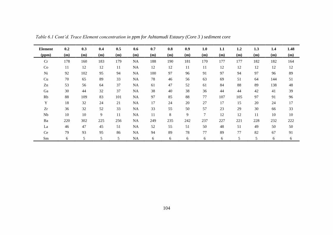
104

Table 6.1 Cont’d. Trace Element concentration in ppm for Ashtamudi Estaury (Core 3 ) sediment core

Element 0.2 0.3 0.4 0.5 0.6 0.7 0.8 0.9 1.0 1.1 1.2 1.3 1.4 1.48

(ppm) (m) (m) (m) (m) (m) (m) (m) (m) (m) (m) (m) (m) (m) (m)

Cr 178 160 183 179 NA 188 190 181 170 177 177 182 182 164

Co 11 12 12 11 NA 12 12 11 11 12 12 12 12 12

Ni 92 102 95 94 NA 100 97 96 91 97 94 97 96 89

Cu 70 65 89 33 NA 78 46 56 63 69 51 64 144 51

Zn 53 56 64 37 NA 61 47 52 61 84 88 89 138 48

Ga 30 44 32 37 NA 38 40 38 36 44 44 42 41 39

Rb 88 109 83 101 NA 97 85 88 77 107 105 97 91 96

Y 18 32 24 21 NA 17 24 20 27 17 15 20 24 17

Zr 36 32 52 33 NA 33 55 50 57 23 29 30 66 33

Nb 10 10 9 11 NA 11 8 9 7 12 12 11 10 10

Ba 220 302 225 256 NA 249 235 242 237 227 221 228 232 222

La 46 47 45 51 NA 52 55 51 50 48 51 49 50 50

Ce 79 93 95 86 NA 94 89 78 77 89 77 82 67 91

Sm 6 5 5 5 NA 6 6 6 6 6 5 5 6 6

105


Element 0.1 0.2 0.3 0.4 0.5 0.6 0.7

(Wt%) (m) (m) (m) (m) (m) (m) (m)

SiO2 57.87 45.29 47.55 47.64 47.89 43.39 41.62

TiO2 0.79 0.81 0.81 0.83 0.80 0.84 0.81

Al2O3 12.60 16.34 16.43 16.27 15.31 16.45 16.25

MnO 0.02 0.03 0.03 0.03 0.02 0.03 0.02

Fe2O3 4.64 7.36 7.55 7.85 6.69 7.96 7.92

CaO 7.33 6.50 5.67 6.66 9.87 7.83 8.22

MgO 3.06 4.01 3.68 3.61 3.85 4.14 4.09

Na2O 2.77 3.75 3.42 3.53 3.08 3.27 3.18

K2O 1.66 1.62 1.60 1.73 1.68 1.59 1.67

P2O5 0.38 0.47 0.42 0.40 0.45 0.47 0.49

LOI 8.60 13.68 12.62 11.22 10.13 13.86 15.54

CIA 53.62 53.70 55.89 54.67 56.18 56.86 57.00

ICV 1.61 1.47 1.38 1.49 1.70 1.56 1.59

K2O/Na2O 0.60 0.43 0.47 0.49 0.55 0.48 0.52

SiO2/Al2O3 4.59 2.77 2.89 2.93 3.13 2.64 2.56

Al2O3/TiO2 15.91 20.10 20.34 19.65 19.23 19.67 20.09

K2O/Al2O3 0.13 0.10 0.10 0.11 0.11 0.10 0.10

MgO/Al2O3 0.24 0.25 0.22 0.22 0.25 0.25 0.25

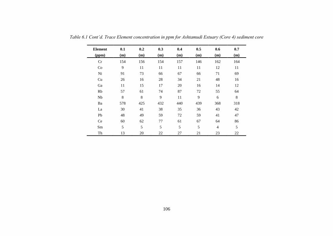
106

Table 6.1 Cont’d. Trace Element concentration in ppm for Ashtamudi Estuary (Core 4) sediment core

Element 0.1 0.2 0.3 0.4 0.5 0.6 0.7

(ppm) (m) (m) (m) (m) (m) (m) (m)

Cr 154 156 154 157 146 162 164

Co 9 11 11 11 11 12 11

Ni 91 73 66 67 66 71 69

Cu 26 16 28 34 21 48 16

Ga 11 15 17 20 16 14 12

Rb 57 61 74 87 72 55 64

Nb 8 8 9 11 9 6 8

Ba 578 425 432 440 439 368 318

La 30 41 38 35 36 43 42

Pb 48 49 59 72 59 41 47

Ce 60 62 77 61 67 64 86

Sm 5 5 5 5 5 4 5

Th 13 20 22 27 21 23 22

107

Table 6.1 Cont’d. Major Element concentration in weight percentages for Offshore (Core 5) sediment core

Element 0.1 0.2 0.3 0.4 0.5 0.6 0.7 0.8 0.88

(wt%) (m) (m) (m) (m) (m) (m) (m) (m) (m)

SiO2 48.13 46.79 45.28 45.48 41.54 45.29 48.20 50.21 49.16

TiO2 0.91 0.87 0.87 0.85 0.85 0.99 0.85 0.73 0.83

Al2O3 15.31 15.57 15.73 15.72 16.25 15.58 14.01 13.63 14.39

MnO 0.03 0.03 0.03 0.03 0.02 0.03 0.03 0.02 0.03

Fe2O3 6.55 6.60 7.18 7.21 7.33 6.74 6.12 5.74 6.39

CaO 8.32 8.38 8.05 7.92 5.04 8.42 9.52 10.17 9.86

MgO 3.56 3.80 4.13 4.38 4.36 4.23 3.89 3.71 3.85

Na2O 3.43 3.26 3.48 3.82 4.33 3.56 3.23 2.85 2.94

K2O 1.96 1.81 1.88 1.83 1.55 1.68 1.73 1.65 1.82

P2O5 0.59 0.62 0.61 0.60 0.58 0.60 0.52 0.51 0.53

LOI 10.91 12.07 12.52 11.93 18.04 12.55 11.65 10.51 9.92

CIA 53.28 55.13 53.82 51.92 50.53 53.49 52.84 54.96 55.27

ICV 1.62 1.59 1.63 1.65 1.44 1.65 1.81 1.82 1.78

K2O/Na2O 0.57 0.55 0.54 0.48 0.36 0.47 0.54 0.58 0.62

SiO2/Al2O3 3.14 3.01 2.88 2.89 2.56 2.91 3.44 3.68 3.42

Al2O3/TiO2 16.84 17.91 18.15 18.45 19.07 15.80 16.57 18.70 17.38

K2O/Al2O3 0.13 0.12 0.12 0.12 0.10 0.11 0.12 0.12 0.13

MgO/Al2O3 0.23 0.24 0.26 0.28 0.27 0.27 0.28 0.27 0.27

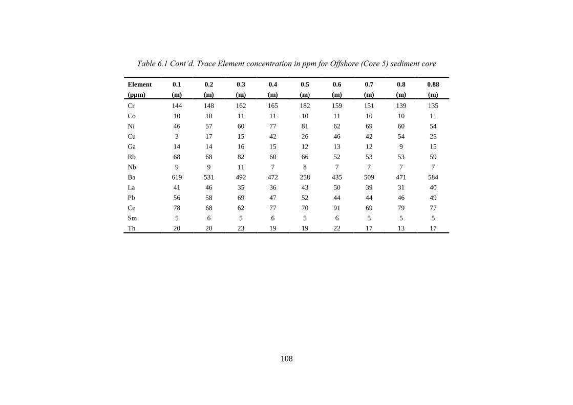
108

Table 6.1 Cont’d. Trace Element concentration in ppm for Offshore (Core 5) sediment core

Element 0.1 0.2 0.3 0.4 0.5 0.6 0.7 0.8 0.88

(ppm) (m) (m) (m) (m) (m) (m) (m) (m) (m)

Cr 144 148 162 165 182 159 151 139 135

Co 10 10 11 11 10 11 10 10 11

Ni 46 57 60 77 81 62 69 60 54

Cu 3 17 15 42 26 46 42 54 25

Ga 14 14 16 15 12 13 12 9 15

Rb 68 68 82 60 66 52 53 53 59

Nb 9 9 11 7 8 7 7 7 7

Ba 619 531 492 472 258 435 509 471 584

La 41 46 35 36 43 50 39 31 40

Pb 56 58 69 47 52 44 44 46 49

Ce 78 68 62 77 70 91 69 79 77

Sm 5 6 5 6 5 6 5 5 5

Th 20 20 23 19 19 22 17 13 17

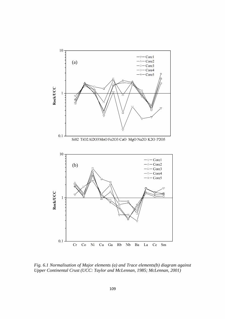
109

(a)

(b)

Fig. 6.1 Normalisation of Major elements (a) and Trace elements(b) diagram against

Upper Continental Crust (UCC: Taylor and McLennan, 1985; McLennan, 2001)

110

The coastal plain core (Core 1) sediments show similar trend as estuarine

sediments however, MnO, CaO, MgO, K2O and P2O5 contents are much depleted than

the other core sediments. The offshore sediments (Core 5) also comparable with

estuarine sediments, which show higher content of CaO and P2O5, compare to other

sediments and UCC.

The UCC normalised trace element distribution based on Taylor and

Mclennan (1985) in the core sediments representing the coastal plain, estuary and

offshore is shown in figure 6.1b. Core 4 and Core 3 have lower concentrations of Rb,

Nb, Ba, Y, Zr and Zn compare to UCC, whereas the Cr and Ni content in these

sediments is 4-5 fold higher than the UCC. Core 3 shown higher content of Cr, Ni,

Cu, Ga, La, Ce and Sm and are depleted in Rb, Nb, Ba and Zr. Co, Cu, Ce, Sm in

Core 4 and Core 2, and Co, Y and Zn in Core 3 are similar to UCC. Pb and Th was

only recorded in Core 4 sediments, have higher concentration than UCC. The

observed depletion of Zr, and Y in Core 2 is relative to the lack of enrichment of

heavy minerals like zircon and monazite by sedimentary sorting. Offshore sediments

(Core 5) shows similar trend as shown by Core 4 whereas coastal plain core sediments

(Core 1) show a different trend compare to estuarine and offshore sediments. Core 1

sediments show enrichment in Cr, Co, Ni, Cu, Ga, La, Ce and Sm and depletion in

Rb, Nb.

SiO2 and Al2O3 are the two most dominant elements which shows a strong negative

correlation (r=-0.94) with respect to each other in the Core 4, Core 1 , and Core 5 (r=-

0.88), while the Core 3 and Core 2 does not have any correlation and/or shows weak

correlation between SiO2 and Al2O3. The negative linear relationships of SiO2 with

other major oxides such as TiO2, Al2O3, Fe2O3, MnO, MgO, Na2O and P2O5 in the

sediments of Core 4 indicate that the most of silica being sequestered in quartz

(Rahman and Suzuki, 2007). Both Na2O and CaO show negative correlation with

Al2O3 suggesting concentration of plagioclase in the Core 3 sediments than the other

core sediments. Titanium is mainly concentrated in phyllosilicates (Condie et al.,

1992) and TiO2 is relatively immobile compared to other elements during various

sedimentary processes and may strongly represent the source rocks (McLennan et al.,

1993). Significantly high content of TiO2 in all the core sediments (average = 0.8

111

wt.% in Core 4 and Core 3; 0.9 wt. % in Core 2; 0.71 wt. % in Core 1; and 0.86 wt.%

in Core 5) indicate the presence of significant amounts of phyllosilicates in these

sediments (Dabard, 1990), which has been released from Ti-bearing rocks by physical

erosion (Cohen, 2003) through weathering and minerals containing Ti, which are not

sensitive to dissolution (Demory et al., 2005). MgO have positive correlation with

SiO2 ( r=0.24) in Core 2 and Core 3 (r=0.17) indicate the presence of biotite while

other core sediments shows negative correlation (Moosaviradi et al., 2012). Fe2O3 and

MgO exhibits strong positive correlation with Al2O3 (r = 0.9) in the sediments of Core

4 suggests the presence of chlorite and ferromagnesian minerals (e.g., biotite,

hornblende) (Moosaviradi et al., 2012). The high correlation coefficients between Fe

and Ti (0.79), Fe and Mg (0.89), Fe and Mn (0.83), and Ti and Mg (0.64) in sediments

of Core 4 indicate that these elements likely reside in similar mineral phases, probably

biotite, muscovite and garnet. Values of Al2O3/TiO2 ratio of the sediments are high in

all the core sediments (average = 18.9 wt.% in Core 4; 21.2 wt.% in Core 3: 25.7

wt.% in Core 2: 17.65 in Core 5 and Core1 24.31 wt.% ), which indicate the

derivation of the detrital materials from a continental source (Fyffe and Pickerill,

1993).

On K2O/Na2O vs SiO2/Al2O3 plot (Fig. 6.3) all the core sediments fall away

from the PAAS, UCC and Khondalites. Core 4 sediments fall nearer to intermediate

charnockites and all the samples fall on the linear range of TTG, Average Garnet

Biotite Gneiss and intermediate Charnockite but overall the sediments are depleted in

K2O/Na2O and SiO2/Al2O3 ratios. Core 4 sediments are slightly lower in K2O/Na2O

and SiO2/Al2O3 ratios than gneisses, intermediate Charnockites, and Khondalites of

the adjacent source area (Kerala Khondalite Belt of southern India; Chacko et al.,

1992). Core 5 sediment are clustered nearer to Charnockite, which clearly supports

that these sediments are mainly derived from Charnockites. Core 1 sediments are

clustered away from the other studied sediments and rock types. However, these

sediments show higher content of SiO2 and K2O than the other sediments and some of

the sediments show high content SiO2 and low content of K2O. Those three samples

recorded very low content of SiO2 and K2O. Considering the somewhat mobile nature

of these major elements, the above observations suggest that this felsic to intermediate

igneous rocks could be a source for these sediments.

112

Fig. 6.2 SiO2/Al2O3 vs K2O/Na2O plot for the core sediments1 representing the coastal

plain, estuary and offshore compared with different possible source rocks: 2Taylor

and McLennan (1985); 3

Chacko et al. (1992); 4Condie (1993);

5Sreejith and Ravindra

Kumar (2013)

6.3. Geochemical Classification

Several authors (Pettijohn et al., 1972; Blatt et al., 1980) have proposed the

geochemical classification diagrams for terrigenous sedimentary rocks using major

elements. However, the modified classification diagram proposed by Herron (1988)

facilitates arkoses to be more successfully classified than Pettijohn et al. (1972)

diagram do and it is a measure of mineral stability, as the ferromagnesian minerals

tend to be amongst the least stable minerals during weathering. The Log ratio of

SiO2/Al2O3 indicates mineralogical maturity of sediment (Pettijohn, et al., 1972).

Fe2O3/K2O ratio is an indication of the mineralogical stability of the sediment

(Herron, 1988).

In the Herron (1988; Fig. 6.3) diagram all the core sediments from estuary

(Core 2,3,4), plot within Fe- shale field except one sample falls on the field of shale,

113

whereas coastal plain core sediments (Core 1) show wide distribution plot in the fields

of Fe-shale, Fe-Sand, shale, wacke and litharenites which indicates that the chemistry

and provenance show wider distribution over the stratigraphic periods. Apart from

that, depositional system might be changed from quite environment to high energy

environment; during this period more detrital sediments are deposited. Wide variation

of Fe2O3/K2O and SiO2/Al2O3 ratios in the inland sediments clearly indicates that

these sediments are weakly to moderately mature. Offshore sediments (Core 5)

typically plot in the Fe-shale field and are comparable with the estuarine core

sediments.

Fig. 6.3 Geochemical classification diagram of sediment cores representing coastal

plain, estuary/lagoon and offshore core sediments (after Herron, 1988)

6.4. Paleoweathering and Sediment Maturity

6.4.1. Chemical Index of Alteration

Alteration of sedimentary rocks can be determined by various parameters like

chemical index of alteration (CIA, Nesbitt and Young, 1982), K2O/Na2O (Nesbitt and

Young, 1984; Lindsey, 1999; Dey et al., 2009), Rb/Sr (McLennan et al., 1993), and

114

Th/U ratios (McLennan et al., 1993). These parameters have been successfully used in

several studies to identify the intensity of weathering (Hurowitz and McLennan, 2005;

Selvaraj and Chen, 2006; Van Staden et al., 2006; Pe-Piper et al., 2008; Zimmermann

and Spalletti, 2009; Wani and Mondal, 2010; Armstrong-Altrin et al., 2013;

Nagarajan et al., 2013). In order to quantify the degree of weathering in the sediments

and infer their possible provenance, the chemical Index of Alteration (CIA) was used

(Nesbitt and Young, 1982) and this index was calculated using the molecular

proportions as shown in the equation below:

CIA = [Al2O3 / (Al2O3 + CaO* + Na2O + K2O)] × 100

Where, CaO* is the amount of CaO incorporated in the silicate fraction of the

rock. Correction for CaO from carbonate contribution was not done in this study due

to the absence of CO2 value. Thus, to compute for CaO* from the silicate fraction, the

assumption proposed by Bock et al. (1998) was adopted. In this regard, CaO values

were accepted only if CaO < Na2O; consequently, when CaO > Na2O, it was assumed

that the concentration of CaO equals to that of Na2O. This procedure provides

measure of the ratio of the secondary aluminous mineral to feldspar, and forms a basis

for the measure of intensity of weathering. This assumption seems to be valid as the

sediments of the studied area are deviod of carbonate matter.

A CIA value of 100 indicates strong chemical weathering because all the

alkali and alkaline earth elements are completely removed from the weathered

sediment. Average upper continental crust (UCC) and unaltered granite rocks have

CIA values of about 50 and 47, respectively. Plagioclase and potassium feldspar have

a CIA value of 50. Since chemical weathering is tightly related to climate condition,

these geochemical proxies have been widely used to reconstruct the

paleoenvironmental changes of various marine and terrestrial sediments (Nesbitt and

Young, 1982; Nesbitt et al., 1996; Vital and Stattegger, 2000; Yang et al., 2004; Singh

et al., 2005). The CIA is a measure of the weathering of feldspar minerals and their

hydration to form clay minerals. As clay content increases Al should also increase,

whereas Ca, K, and Na contents should decrease, leading to higher CIA values.

Kaolinite has a CIA value of 100 and represents the highest degree of weathering.

Illite is between 75 and 90, muscovite at 75, the feldspars at 50. Fresh basalts have

115

values between 30 and 45, fresh granites and granodiorites of 45 to 55 (Nesbitt and

Young, 1982; Fedo et al., 1995).

The CIA actually reflects changes in the proportion of feldspar and various

clay minerals in the weathering product (Nesbitt and Young, 1982). It is well known

that aluminous minerals such as kaolinite, gibbsite and beidellite are secondarily

formed while Na- and Ca

- bearing silicate minerals are significantly removed from the

weathering profile during intense chemical weathering, resulting in high CIA values

in the weathered sediments. As a consequence, CIA values of about 45 to 55 indicate

virtually no weathering, whereas the value of 100 indicates intense weathering with

complete removal of alkali and alkaline earth elements (McLennan, 1993).

Sediments from coastal plain core (Core 1) show the higher CIA values

compared to estuarine and offshore core sediments, which is ranging between 72 and

91 (av. 82). Amongst estuarine core sediments, the average CIA values are recorded

higher in Core 3 (av.67) than Core 4 (av. 58) and Core 2 (av.57). The average CIA

values of 58 to 67 are consistent with average shale value, which indicate weak to

moderate weathering in the source region (Nesbitt and Young, 1982; Nesbitt et al.,

1996; Vital and Stattegger, 2000; Yang et al., 2004; Singh et al., 2005). The offshore

sediments show the lowest CIA values ranges between 53 and 56, which indicates that

these sediments are mostly unweathered to weakly weathered (see, McLennan, 1993).

The intensity of weathering was also analysed using A-CN-K trilinear plot

proposed by Nesbitt and Young (1982), which indicates not only the intensity of

weathering but also depicts the relationship between Al2O3 (aluminous clays),

CaO+Na2O (Plagioclase), and K2O (K-feldspar) (Nesbitt and Young, 1984). This

diagram also evaluates bulk source rock composition, diagenetic effects, and

tectonism in the source area. The samples fall parallel to trend of weathering in the A-

CN-K diagram indicating a little or no loss of K during weathering (Fig 6.4). The core

sediments of Ashtamudi estuary and surrounding environment form a single trend

originating from a bulk source composition near average granodiorite and toward

smectite on the A-CN edge. Thus, the data trends along the ideal weathering trend,

which theoretically should lie parallel to the A-CN edge. Estuarine (Core 2, 3 4)

116

sediments show that these sediment undergone weak to moderate weathering rather

than intensive. Offshore (Core 5) sediments are clustered near plagioclase and potash

feldspar join while coastal plain (Core 1) sediments are clustered near A-apex (CIA

72-91) indicating intensive source area weathering respectively.

Fig. 6.4 A-CN-K (Al2O3-CaO+Na2O+K2O) ternary diagram showing the general

weathering trend and intensity of weathering in the source region for the coastal

plain, estuary and offshore (after Nesbitt and Young, 1984)

The low average CIA values in Core 4 and Core 5 sediments are due to direct

input of immature continent detrital minerals into the depositional system, which

indicates weak weathering of sediments of Core 2 and Core 3. Sediments of Core 1

are clustered away from the Plagioclase-K-feldspar line and plotted neared to A-apex

indicates that Core 1 sediments are intensively weathered than the other core

sediments. Intersection of this weathering trend with K-feldspar-plagioclase joint

represents source rock composition. Backward projection of the linear trend for the

studied sediments in the A-CN-K diagram can be traced to be possible granodioritic –

(UCC-Intermediate) source composition.

117

6.4.2. ICV Relation to Recycling and Weathering Intensity

Cox et al. (1995) proposed the Index of Compositional Variability (ICV),

which is an approach toward assessing original detrital mineralogy for characterizing

the sediments.

ICV is defined as [(Fe2O3+K2O+Na2O+CaO+MgO+TiO2)/Al2O3] and

measures the abundance of alumina relative to the other major cations in a rock or

mineral. ICV values for clay minerals are in the range of 0.03–0.78, and for feldspars

in the range of 0.54–0.87 (Cox et al., 1995). The ICVs of constituent minerals

increase, for instance, in the order of kaolinite (~0.03–0.05), montmorillionite (~0.15–

0.3), muscovite-illite (~0.3), plagioclase (~0.6), alkali feldspar (~0.8–1), biotite (~8),

and amphibole-pyroxene (~10–100) (Cox et al., 1995). Generally non-clay minerals

show higher ICV compared to clay minerals. Typical rock forming minerals

(feldspars, amphibols and pyroxenes) show ICV values >0.84, whereas typical

alteration products such as Kaolinite, illite and muscovite show <0.84 (Cox et al.,

1995).

The ICV values for coastal plain core sediments (Core 1) ranges from 0.18 to

0.62 (av. 0.55), except one sample with an ICV value of 1.33. This indicates matured

sediments followed by tectonically quiescent or cratonic environments (Weaver,

1989) with minimal uplift and are associated with extensive chemical weathering

(Cox et al., 1995), where recycling and concomitant weathering are active. However,

intense chemical weathering of first-cycle material may also produce such

signatures (Barshad, 1966). First cycle terrigenous sediment formed during intense

chemical weathering or with long residence times in soils, however, may also become

intensely weathered (Barshad, 1966; Johnsson et al., 1988) and thus form ICVs less

than one.

ICV values for Ashtamudi Estuary varies significantly with higher ICV

values in Core 4 sediments ranging from 1.38 to 1.70 with mean value of 1.55 than

the sediments of Core 2 (1.20-1.31; av.1.26) and Core 3 sediments (0.82-1.11; av.

1.00) respectively. The ICV values of offshore core (Core 5) sediments vary from

1.44 to 1.82 with an average value of 1.67. These ICV values exhibits higher values

http://www.sciencedirect.com/science/article/pii/S0037073801001749#BIB9





118

than PAAS (ICV=0.85; Taylor and McLennan, 1985) suggesting the predominance of

rock forming minerals such as plagioclase, K-feldspar, amphiboles, pyroxenes and

lithics over clay minerals as well as tend to be found in tectonically active settings

which are characterised by first-cycle deposits (Pettijohn et al., 1987; Van De Kamp

and Leake, 1985) in the sediments of Ashtamudi estuary and offshore.

Similarly, the variations in CIA values also indicate the sediment sorting

effect. Physical sorting of sediments during transportation and deposition leads to

concentration of quartz and feldspar with some heavy minerals in the coarse fraction

and more weatherable minerals in the suspended load sediments (Garcia et al., 2004).

Long et al. (2012) proposed the chemical maturity and intensity of weathering based

on ICV and CIA ratios. ICV value in Core 4 sediments is 1.55 and offshore core

(Core 5) sediments (1.67), which is higher than the sediments of Core 2 and Core 3

(1.26 and 1.00 respectively) and PAAS (ICV=0.85). These features suggest the

predominance of rock forming minerals such as plagioclase, K-feldspar, amphiboles,

pyroxenes and lithics over clay minerals in the sediments of Ashtamudi estuary and

offshore. The Ashtamudi estuary core sediments and offshore core sediments have

ICV values ranging between 0.82 to 1.60; and 1.44 to 1.82 and CIA ratios from 64 to

78 and 51 to 55. The ICV values are thus greater than PAAS (ICV = 0.85; Taylor and

McLennan, 1985), whereas CIA in lower except Core 3. This confirms that the

Ashtamudi estuarine sediments and offshore sediments are geochemically immature

(Fig. 6.5), and were derived from a weakly to moderately weathered source as

discussed above. Sediments from coastal plain (Core 1) shows CIA values ranging

between 72 to 91 higher than PAAS and ICV values between 0.18 to 0.67 (except

one sample ICV=1.33) lower than PAAS values clearly confirms their intense

weathering condition in the source area and high maturity (Fig. 6.5). Overall, several

samples have ICV>1, suggesting first cycle input (e.g., Cullers and Podkovyrov,

2000).

6.4.3. Textural maturity

The ratio between SiO2 and Al2O3 was also used to know the textural maturity

of sediments since the relative enrichment of Al-rich phyllosilicates at the expense of

silica rich phases in fine grained sediments are expected (see for e.g., McLennan et



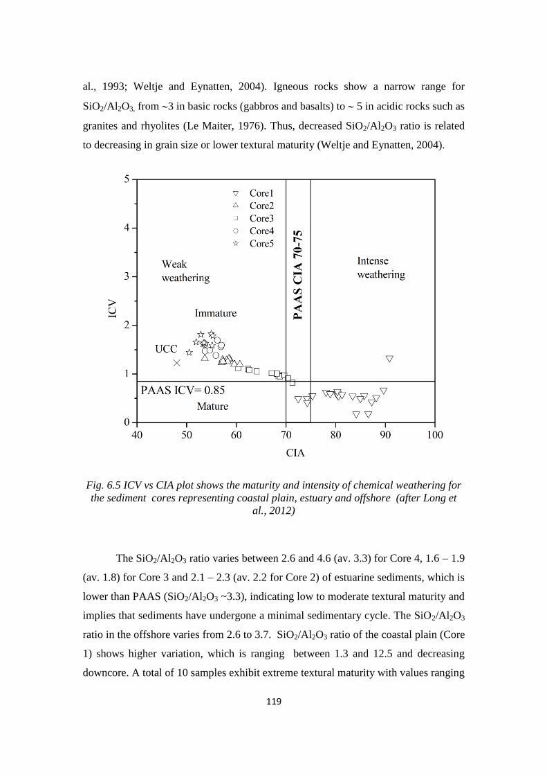
119

al., 1993; Weltje and Eynatten, 2004). Igneous rocks show a narrow range for

SiO2/Al2O3, from 3 in basic rocks (gabbros and basalts) to 5 in acidic rocks such as

granites and rhyolites (Le Maiter, 1976). Thus, decreased SiO2/Al2O3 ratio is related

to decreasing in grain size or lower textural maturity (Weltje and Eynatten, 2004).

Fig. 6.5 ICV vs CIA plot shows the maturity and intensity of chemical weathering for

the sediment cores representing coastal plain, estuary and offshore (after Long et

al., 2012)

The SiO2/Al2O3 ratio varies between 2.6 and 4.6 (av. 3.3) for Core 4, 1.6 – 1.9

(av. 1.8) for Core 3 and 2.1 – 2.3 (av. 2.2 for Core 2) of estuarine sediments, which is

lower than PAAS (SiO2/Al2O3 ~3.3), indicating low to moderate textural maturity and

implies that sediments have undergone a minimal sedimentary cycle. The SiO2/Al2O3

ratio in the offshore varies from 2.6 to 3.7. SiO2/Al2O3 ratio of the coastal plain (Core

1) shows higher variation, which is ranging between 1.3 and 12.5 and decreasing

downcore. A total of 10 samples exhibit extreme textural maturity with values ranging

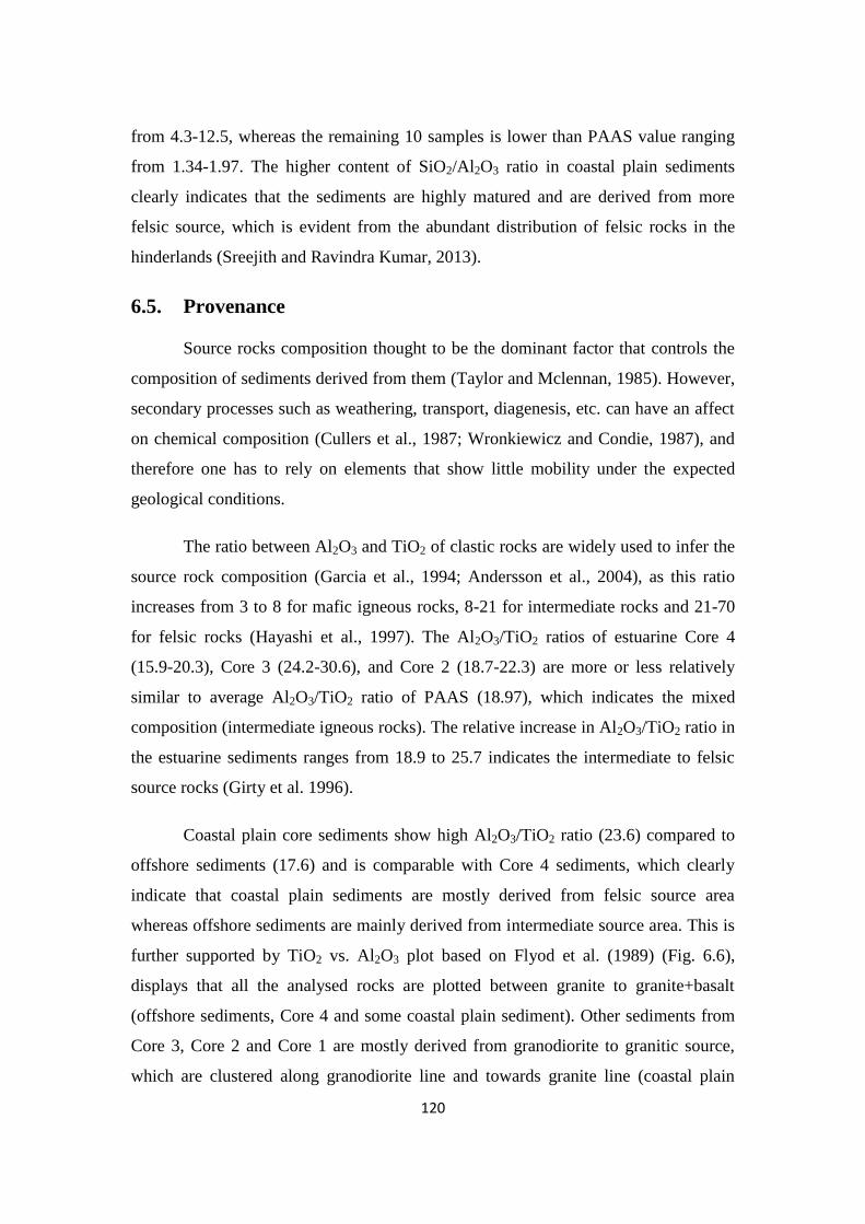
120

from 4.3-12.5, whereas the remaining 10 samples is lower than PAAS value ranging

from 1.34-1.97. The higher content of SiO2/Al2O3 ratio in coastal plain sediments

clearly indicates that the sediments are highly matured and are derived from more

felsic source, which is evident from the abundant distribution of felsic rocks in the

hinderlands (Sreejith and Ravindra Kumar, 2013).

6.5. Provenance

Source rocks composition thought to be the dominant factor that controls the

composition of sediments derived from them (Taylor and Mclennan, 1985). However,

secondary processes such as weathering, transport, diagenesis, etc. can have an affect

on chemical composition (Cullers et al., 1987; Wronkiewicz and Condie, 1987), and

therefore one has to rely on elements that show little mobility under the expected

geological conditions.

The ratio between Al2O3 and TiO2 of clastic rocks are widely used to infer the

source rock composition (Garcia et al., 1994; Andersson et al., 2004), as this ratio

increases from 3 to 8 for mafic igneous rocks, 8-21 for intermediate rocks and 21-70

for felsic rocks (Hayashi et al., 1997). The Al2O3/TiO2 ratios of estuarine Core 4

(15.9-20.3), Core 3 (24.2-30.6), and Core 2 (18.7-22.3) are more or less relatively

similar to average Al2O3/TiO2 ratio of PAAS (18.97), which indicates the mixed

composition (intermediate igneous rocks). The relative increase in Al2O3/TiO2 ratio in

the estuarine sediments ranges from 18.9 to 25.7 indicates the intermediate to felsic

source rocks (Girty et al. 1996).

Coastal plain core sediments show high Al2O3/TiO2 ratio (23.6) compared to

offshore sediments (17.6) and is comparable with Core 4 sediments, which clearly

indicate that coastal plain sediments are mostly derived from felsic source area

whereas offshore sediments are mainly derived from intermediate source area. This is

further supported by TiO2 vs. Al2O3 plot based on Flyod et al. (1989) (Fig. 6.6),

displays that all the analysed rocks are plotted between granite to granite+basalt

(offshore sediments, Core 4 and some coastal plain sediment). Other sediments from

Core 3, Core 2 and Core 1 are mostly derived from granodiorite to granitic source,

which are clustered along granodiorite line and towards granite line (coastal plain

121

sediments). K2O and Rb contents in sediments also can be used as an indicator of

source rocks and both elements were applied successfully by many studies (Floyd and

Leveridge, 1987). The K and Rb are also sensitive to sedimentary recycling processes

and have been widely used as indicators for source composition (Floyd et al., 1989).

In the K2O vs Rb plot all the samples except six samples from inland sediments fall in

the acid+intermediate composition field.

Fig. 6.6 TiO2 vs Al2O3 (after Flyod et al., 1989) bivariate plot showing the possible

provenance for the core sediments representing coastal plain, estuary and offshore

The six samples from Core 1 fall in the basic compositions is due to low

content of K2O and may be due the fractionation and sorting effect which may be

brought more ferromagnesian minerals from the source region to the depositional

system. All the core sediments show uniform K/Rb ratios and they plot close to a

typical differentiated magmatic suite defined by a trend with K/Rb ratio of 230 (Fig

6.7; Shaw, 1968). The high Rb concentrations (>40 ppm) and the phenomenon

shown by the studied samples demonstrates the chemically coherent nature of the

sediments and derivation from rocks of intermediate and acidic compositions.

122

Fig. 6.7 K2O vs Rb plot shows the provenance field for core sediments representing

coastal plain, estuary and offshore

Roser and Korsch (1988) devised a discriminant function diagram, provides a

convenient method of viewing stratigraphic variation among sample suites. All the

estuarine samples fall within the intermediate igneous provenance field (Fig 6.8) but

one sample from core 5 fall on the felsic igneous provenance. This pattern is

consistent with derivation from intermediate igneous source terrane. Core 1 sediments

are mostly clustered in quartzose sedimentary provenance area which indicates that

these sediments may be derived from recycled sources represented by quartzose

sediments of mature continental provenance (granitic-gneissic source area), similar to

PM derived sediments categorized by Roser and Korsch (1988). However, some of

the Core 1 sediments fall in mafic igneous province. Overall, the estuary sediments

clustered near the boundary between intermediate igneous rocks and mafic igneous

rocks. Fractionation of some immature mafic minerals such as orthopyroxenes and

garnets may be derived from the source area, which has elevated the ferromagnesiun

elements in the studied sediments. In general, the estuarine sediments (Core 2, 3, and

4) mostly derived from intermediate igneous rocks, charnockites, and gneisses and

sediments fall in mafic igneous provenance indicates their immaturity.

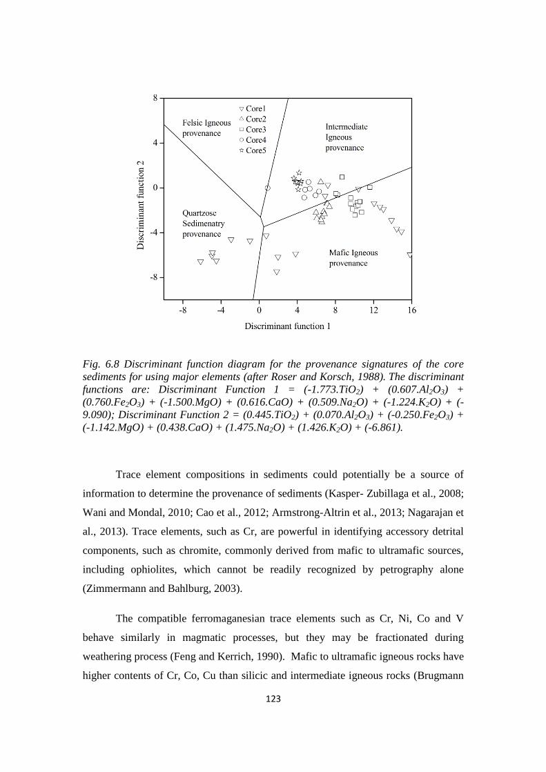
123

Fig. 6.8 Discriminant function diagram for the provenance signatures of the core

sediments for using major elements (after Roser and Korsch, 1988). The discriminant

functions are: Discriminant Function 1 = (-1.773.TiO2) + (0.607.Al2O3) +

(0.760.Fe2O3) + (-1.500.MgO) + (0.616.CaO) + (0.509.Na2O) + (-1.224.K2O) + (-

9.090); Discriminant Function 2 = (0.445.TiO2) + (0.070.Al2O3) + (-0.250.Fe2O3) +

(-1.142.MgO) + (0.438.CaO) + (1.475.Na2O) + (1.426.K2O) + (-6.861).

Trace element compositions in sediments could potentially be a source of

information to determine the provenance of sediments (Kasper- Zubillaga et al., 2008;

Wani and Mondal, 2010; Cao et al., 2012; Armstrong-Altrin et al., 2013; Nagarajan et

al., 2013). Trace elements, such as Cr, are powerful in identifying accessory detrital

components, such as chromite, commonly derived from mafic to ultramafic sources,

including ophiolites, which cannot be readily recognized by petrography alone

(Zimmermann and Bahlburg, 2003).

The compatible ferromaganesian trace elements such as Cr, Ni, Co and V

behave similarly in magmatic processes, but they may be fractionated during

weathering process (Feng and Kerrich, 1990). Mafic to ultramafic igneous rocks have

higher contents of Cr, Co, Cu than silicic and intermediate igneous rocks (Brugmann

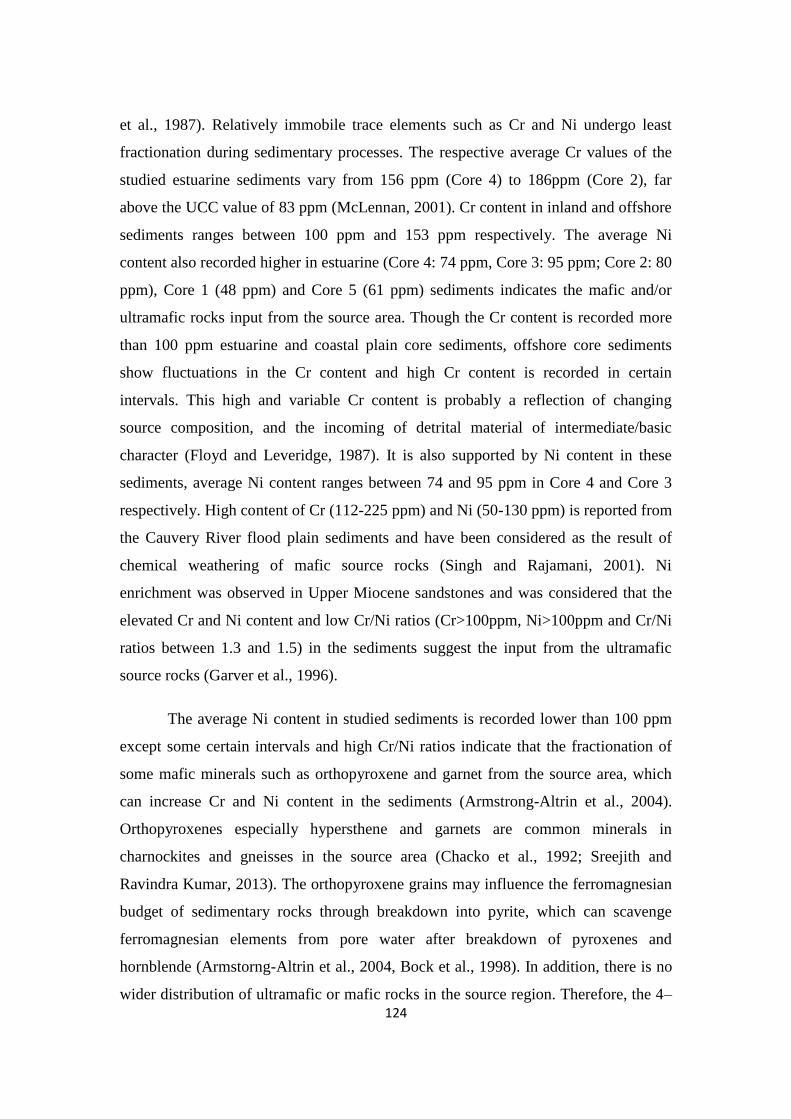
124

et al., 1987). Relatively immobile trace elements such as Cr and Ni undergo least

fractionation during sedimentary processes. The respective average Cr values of the

studied estuarine sediments vary from 156 ppm (Core 4) to 186ppm (Core 2), far

above the UCC value of 83 ppm (McLennan, 2001). Cr content in inland and offshore

sediments ranges between 100 ppm and 153 ppm respectively. The average Ni

content also recorded higher in estuarine (Core 4: 74 ppm, Core 3: 95 ppm; Core 2: 80

ppm), Core 1 (48 ppm) and Core 5 (61 ppm) sediments indicates the mafic and/or

ultramafic rocks input from the source area. Though the Cr content is recorded more

than 100 ppm estuarine and coastal plain core sediments, offshore core sediments

show fluctuations in the Cr content and high Cr content is recorded in certain

intervals. This high and variable Cr content is probably a reflection of changing

source composition, and the incoming of detrital material of intermediate/basic

character (Floyd and Leveridge, 1987). It is also supported by Ni content in these

sediments, average Ni content ranges between 74 and 95 ppm in Core 4 and Core 3

respectively. High content of Cr (112-225 ppm) and Ni (50-130 ppm) is reported from

the Cauvery River flood plain sediments and have been considered as the result of

chemical weathering of mafic source rocks (Singh and Rajamani, 2001). Ni

enrichment was observed in Upper Miocene sandstones and was considered that the

elevated Cr and Ni content and low Cr/Ni ratios (Cr>100ppm, Ni>100ppm and Cr/Ni

ratios between 1.3 and 1.5) in the sediments suggest the input from the ultramafic

source rocks (Garver et al., 1996).

The average Ni content in studied sediments is recorded lower than 100 ppm

except some certain intervals and high Cr/Ni ratios indicate that the fractionation of

some mafic minerals such as orthopyroxene and garnet from the source area, which

can increase Cr and Ni content in the sediments (Armstrong-Altrin et al., 2004).

Orthopyroxenes especially hypersthene and garnets are common minerals in

charnockites and gneisses in the source area (Chacko et al., 1992; Sreejith and

Ravindra Kumar, 2013). The orthopyroxene grains may influence the ferromagnesian

budget of sedimentary rocks through breakdown into pyrite, which can scavenge

ferromagnesian elements from pore water after breakdown of pyroxenes and

hornblende (Armstorng-Altrin et al., 2004, Bock et al., 1998). In addition, there is no

wider distribution of ultramafic or mafic rocks in the source region. Therefore, the 4–

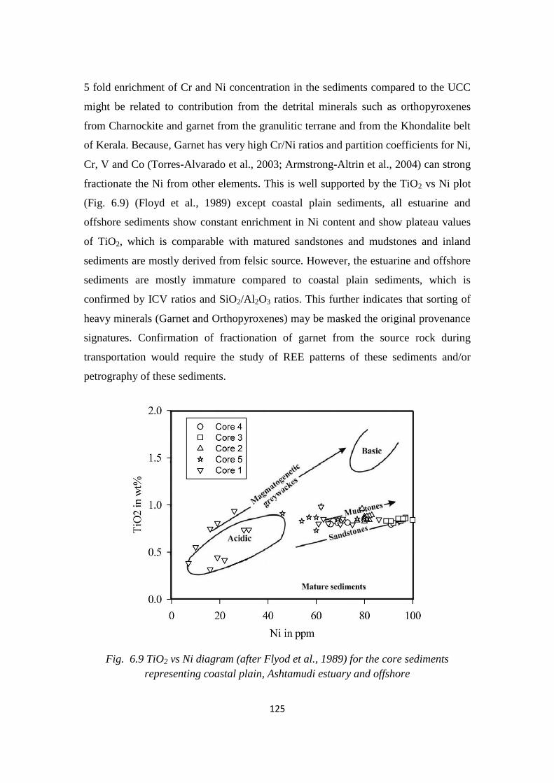
125

5 fold enrichment of Cr and Ni concentration in the sediments compared to the UCC

might be related to contribution from the detrital minerals such as orthopyroxenes

from Charnockite and garnet from the granulitic terrane and from the Khondalite belt

of Kerala. Because, Garnet has very high Cr/Ni ratios and partition coefficients for Ni,

Cr, V and Co (Torres-Alvarado et al., 2003; Armstrong-Altrin et al., 2004) can strong

fractionate the Ni from other elements. This is well supported by the TiO2 vs Ni plot

(Fig. 6.9) (Floyd et al., 1989) except coastal plain sediments, all estuarine and

offshore sediments show constant enrichment in Ni content and show plateau values

of TiO2, which is comparable with matured sandstones and mudstones and inland

sediments are mostly derived from felsic source. However, the estuarine and offshore

sediments are mostly immature compared to coastal plain sediments, which is

confirmed by ICV ratios and SiO2/Al2O3 ratios. This further indicates that sorting of

heavy minerals (Garnet and Orthopyroxenes) may be masked the original provenance

signatures. Confirmation of fractionation of garnet from the source rock during

transportation would require the study of REE patterns of these sediments and/or

petrography of these sediments.

Fig. 6.9 TiO2 vs Ni diagram (after Flyod et al., 1989) for the core sediments

representing coastal plain, Ashtamudi estuary and offshore

126

6.6. Environment of Deposition

The relation between K2O/Al2O3 and MgO/Al2O3 was used by Roaldset (1978) to

differentiate between marine and non-marine clays. Majority of the core samples

representing the estuary (Core 2,3,4) and offshore (Core 5) (Fig. 6.10) falls in the

marine dominance except the coastal plain core sediments (Core 1), where top 7m

sediment samples falls under non-marine or fresh water conditions,7-11m samples

falling along the marginal line of non-marine-marine conditions and from 11m to

down the core falls under marine conditions.

Fig. 6.10 MgO/Al2O3 and K2O/Al2O3 diagram (after Roaldset, 1978) to differentiate

between marine and non-marine clays representing coastal plain, estuary and

offshore region

6.7. Geoaccumulation Index (Igeo)

The geoaccumulation index (Igeo), (Muller, 1981), was used to quantitatively

measure the metal pollution in the core sediments based on a pollution intensity

127

classification (Igeo Class), consists of seven classes (0-6; Table 6.2). The

geoaccumulation index (Igeo) values were calculated for the surface sediments of

study area using the equation after (Muller, 1981).

Igeo = log [Me]studied area/1.5[Me]baseline values

in which, [Me] baseline value represents the metal concentration in the average crust

values taken from Wedepohl (1995) since the standard background values for Indian

soils are not available. The 1.5 factor is included because of possible variations in the

background data due to lithogenic effects (Salomons and Forstner, 1984). The highest

class indicates 100 fold enrichment of metal pollution over the baseline values. As

shown in Table 6.2, the calculated Igeo values from the core sediments Core 4 as

follows -0.27 to -0.53 for Fe, -2.51 to 1.72 for Mn, 1.48 to 1.64 for Cr; -0.42 to 1.16

for Cu, 0.69 to 1.50 for Pb, 1.24 to 1.71 for Ni, and 0.84 to 0.92 for Co respectively.

The calculated Igeo values for cores Core 3 and Core 2 are ranges as follows 0.46 to

0.68 and 0.36 to 0.61 for Fe, -0.67 to 0.18 and -1.67 to 1.88 for Mn, 1.61 to 1.86 and -

0.03 to 1.86 for Cr; 0.62 to 2.75 and -0.72 to 0.22 for Cu, -1.08 to0.82 and -5.29 to -

2.12 for Zn, 1.67 to 1.87 and 1.46 to 1.57 for Ni, and 0.63 to 0.75 and 0.77 to 0.97 for

Co in the sediments of Core 3 and Core 2 respectively.

The average geoaccumulation indexes are less than zero for Mn in AS 05; Mn

and Zn in Core 3; and Cu and Zn in Core 2 suggesting that the sediments have not

been polluted by these metals. Based on the individual trace metals Igeo values, Core

4 and Core 2 core sediments are categorized as unpolluted to moderately polluted

(Igeo class 0-2), whereas Core 3 sediments are categorized as unpolluted to Strongly

polluted (Igeo class 0-3). 26% of the elements belong to Igeo class 0; 39% of the

elements belong to Igeo class 1(unpolluted to moderately polluted) and 36% of the

elements belong to Igeo class 2 (moderately polluted). The remaining 0.86% of the

elements (Cu) in sediments of Core 3 belonged to Igeo class 3 (moderate – extremely

polluted). Overall, results from this study indicated that Core 4 sediments are

moderately polluted with Cr, Pb and Ni; Core 3 sediments are moderate to strongly

polluted with Cr, Cu and Ni and Core 2 sediments are moderate to strongly polluted

with Cr and Ni.

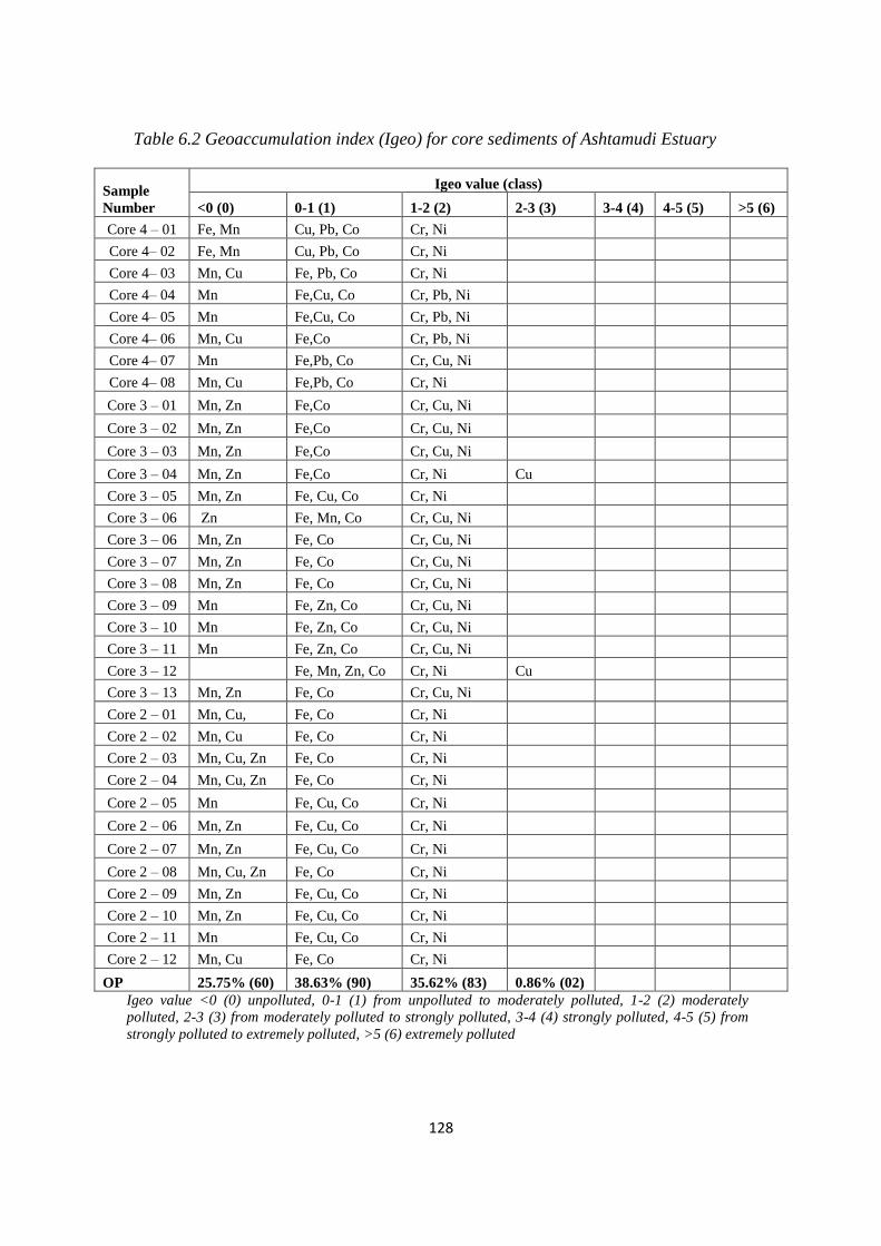
128

Table 6.2 Geoaccumulation index (Igeo) for core sediments of Ashtamudi Estuary

Sample

Number

Igeo value (class)

<0 (0) 0-1 (1) 1-2 (2) 2-3 (3) 3-4 (4) 4-5 (5) >5 (6)

Core 4 – 01 Fe, Mn Cu, Pb, Co Cr, Ni

Core 4– 02 Fe, Mn Cu, Pb, Co Cr, Ni

Core 4– 03 Mn, Cu Fe, Pb, Co Cr, Ni

Core 4– 04 Mn Fe,Cu, Co Cr, Pb, Ni

Core 4– 05 Mn Fe,Cu, Co Cr, Pb, Ni

Core 4– 06 Mn, Cu Fe,Co Cr, Pb, Ni

Core 4– 07 Mn Fe,Pb, Co Cr, Cu, Ni

Core 4– 08 Mn, Cu Fe,Pb, Co Cr, Ni

Core 3 – 01 Mn, Zn Fe,Co Cr, Cu, Ni



Core 3 – 04 Mn, Zn Fe,Co Cr, Ni Cu

Core 3 – 05 Mn, Zn Fe, Cu, Co Cr, Ni

Core 3 – 06 Zn Fe, Mn, Co Cr, Cu, Ni

Core 3 – 06 Mn, Zn Fe, Co Cr, Cu, Ni



Core 3 – 09 Mn Fe, Zn, Co Cr, Cu, Ni



Core 3 – 12 Fe, Mn, Zn, Co Cr, Ni Cu


Core 2 – 01 Mn, Cu, Fe, Co Cr, Ni

Core 2 – 02 Mn, Cu Fe, Co Cr, Ni

Core 2 – 03 Mn, Cu, Zn Fe, Co Cr, Ni


Core 2 – 05 Mn Fe, Cu, Co Cr, Ni






Core 2 – 11 Mn Fe, Cu, Co Cr, Ni

Core 2 – 12 Mn, Cu Fe, Co Cr, Ni

OP 25.75% (60) 38.63% (90) 35.62% (83) 0.86% (02)

Igeo value <0 (0) unpolluted, 0-1 (1) from unpolluted to moderately polluted, 1-2 (2) moderately

polluted, 2-3 (3) from moderately polluted to strongly polluted, 3-4 (4) strongly polluted, 4-5 (5) from

strongly polluted to extremely polluted, >5 (6) extremely polluted

129

6.8. Summary

The geochemical characterisation of sediment cores have been carried out to

address the source rock composition, sediment maturity, palaeo-weathering and

digenetic processes. The ICV values for coastal plain core sediments (Core 1)

suggesting matured characteristics of sediments which were subjected to tectonically

quiescent or cratonic environments with minimal uplift. Extensive chemical

weathering, where recycling and concomitant weathering are active is also indicated

by the data. ICV values for Ashtamudi Estuary varies significantly with higher

values in Core 4 sediments than the sediments of Core 2 and Core 3 sediments.

These ICV values exhibits higher values than PAAS (ICV=0.85); suggesting the


pyroxenes and lithics over clay minerals as well as tend to be found in tectonically

active settings which are characterised by first-cycle deposits in the sediments of

Ashtamudi estuary and offshore. Ashtamudi estuarine sediments and offshore

sediments are geochemically immature, and were derived from a weakly to

moderately weathered source. The SiO2/Al2O3 ratio of estuarine sediments, is lower

than PAAS (SiO2/Al2O3 ~3.3), indicating low to moderate textural maturity, implying

that Ashtamudi estuary sediments have undergone a minimal sedimentary cycle. The

higher content of SiO2/Al2O3 ratio in coastal plain sediments clearly indicates that the

sediments are highly matured and are derived from more felsic source, which is

evident from the abundant distribution of felsic rocks in the hinterlands. All the core

sediments from estuary (Core 2,3,4) indicates that the chemistry and provenance show

wider distribution over the stratigraphic periods. Application of discriminant diagrams

for the estuarine samples suggest intermediate igneous provenance (see Fig 6.9)

suggesting that sediments derived from intermediate igneous provenance. ore 1

sediments are mostly clustered in quartzose sedimentary provenance, few plotting in

igneous field. These sediments are interpreted to have derived from recycled sources.

Majority of the core samples representing the estuary (Core 2,3,4) and offshore (Core

5), are except the coastal plain core sediments (Core 1), show marine dominance. The

geo-accumulation index (Igeo) values for the surface sediments of study area suggest

varying element and concentration levels.

CHAPTER 7

DEPOSITIONAL ENVIRONMENTS AND

COASTAL EVOLUTION

7.1. Introduction

The coastal lands of the study area comprises of different sub-environments,

which includes coastal plain, river, estuaries, lagoon, marshes, dunes and beaches.

Since each of these environments is characterized by unique sediment characteristics

the determination and interpretation of sediment characteristics is particularly

important for a better understanding of the evolution of the coastal plain during the

Quaternary. Further, the study of sediment characteristics in relation to the

depositional features is important in terms of resource exploitation of the various

natural resources in the coastal region.

7.2. Depositional Environment

The surface sediments of the southern and northern sector transects and its

adjoining coastal plain show a wide spectrum of textural classes viz., sand, siltyclay,

clayeysilt, mud, etc. The coastal plain bordering the river-estuary confluence on the

southern sector is covered by coarse sand and gravel dominated sediments whereas

the northern sector is covered by fine sand mixed with siltyclay sediments. The coarse

sand and gravel representing the top 9 m of the sediment core were deposited under

the `violent to most violent environment'. Below these depths the sediments were

deposited during the ‘quite environment’ which is similar to the samples of the

estuarine cores. That means below the 9 m depth the depositional conditions are

similar. The sediment of the offshore Core 5 falls in the category III indicating

‘violent environment’. Though the samples of the northern coastal sector also show a

similar trend in the energy condition the sediments were deposited under a

comparatively low energy depositional regime.

In contrast, the ternary plots of sand, silt and clay after Pejrup (1988) showing

the inferred depositional environments of the southern coastal plain sediments fall

under the open channel conditions indicating high energy, whereas the sediments

below it falls in the closed basin indicating low energy, which is an indication of

131

partially open to restricted estuary. In the northern coastal plain also the sediments

were deposited in almost similar conditions. This indicates that the sedimentation took

place under a moderate environmental setting. The river-estuary region of the

southern coastal plain is characterised by a faster sedimentation process from the

fluvial source because of the early Holocene climatic optimum, whereas the lower

part of core is influenced by still-water condition under the rising Holocene sea level

rise through the incised estuarine basin.

7.3. Relationship between Organic matter and Calcium Carbonate

There is an intimate relationship between the climate and sedimentation

pattern that has a synergistic effect on preservation potential of the organic matter and

CaCO3 in the sediments. Carbonate content of sediments has been found to be a good

indicator of the glacial and inter-glacial stages. Generally high concentration of

CaCO3 indicates cooler periods while a lower content indicates warmer period.

The top 9 m of the sediment Core 1 representing the southern transect has less

percentage of organic matter and negligible amount of calcium carbonates. At a depth

of 11 to 15.5 m the organic matter has increased to as high as 47 % with a range of 7

to 15 %. This anomalous enrichment of organic matter was dated with an age of

42,000 Yrs BP representing the first marine transgression event during the late

Pleistocene period in the study area. In the estuary the organic matter and calcium

carbonate are varying in all the three cores (Core 2, 3 & 4) as it represents the sink for

the fluvial detritus. The offshore region has a calcium carbonate of 9 to 14 % with < 5

% organic matter. The organic matter is less throughout the sediment core of the

northern coastal plain. The calcium carbonate content is < 1.5 % up to a depth of 9 m

but from 10 m downwards the percentage has increased considerably going even up to

38 % and that can be attributed to the inter-glacial period causing marine

transgression. In the lagoon and offshore area the organic matter and calcium

carbonates are in varying proportion limited to a maximum of 8 and 15 %

respectively.

7.4. Geochemical Proxies

The various major and trace elemental composition of the core sediment and

their inter-relationships were studied to understand the depositional environment that

132

prevailed in the coastal area. Some of the geochemical proxies were used to identify

provenance of these sediments. The relation between K2O/Al2O3 and MgO/Al2O3 was

used to differentiate between the marine and non-marine clays. Majority of the core

samples representing the southern transect falls in the marine dominance except the

coastal plain core (Core 1), where the top 7 m sediment falls under the non-marine

conditions or fresh water conditions, 7-11 m samples falling along marginal line of

non-marine -marine (mixed) conditions and from 11 m to down the core falls under

marine conditions which further substantiates the late Pleistocene transgression event.

The Ashtamudi estuary cores as well as the offshore sediments fall totally in the

marine environment.

7.5. Bathymetry

The bathymetry of the Ashtamudi estuary prepared as part of the Asthamudi

Management Plan (Kurian et al., 2001) is used here to understand the bottom

configuration of the estuarine basin (Fig. 7.1). Most of the estuary is shallow (< 3 m)

with maximum depths of up to 14 m measured in the eastern kayal where the Kallada

river debouches into the estuary. Depths in the northern central kayal reach up to 10 m

whereas the southern central kayal is very shallow showing a depth of < 1 m. The

estuary also has a few deep gorges in the eastern part near to the Kallada river

confluence. At present, the estuary is connected with the Sea by a comparatively

narrow entrance channel. The present width of the basin is over-sized compared to the

narrow channel at the estuarine mouth. It may be conjectured that the present width of

the lake is the result of the erosional phase that prevailed during the late Pleistocene

period. The bathymetric contours and the presence of many flood tide islands at the

estuarine entrance are indicative of the high input of sediments from the nearshore

regions. Modelling studies carried out for the Ashtamudi estuary as part of the

estuarine management plan do indicate the arrival of sediments from the offshore

(Black and Mathew, 2001). All these features indicate that the lake basin has started

getting filled up by the transport of sediments from the nearshore region due to tidal

flux. In addition, the eastern end of the estuary also started getting filled by the

sediments brought through the river channels.

The input of sediment was at much higher rate during the middle Holocene

(Padmalal et al., 2013) though the process has slowed down in recent years as

133

compared to the sediment from the nearshore environments. The incised valley

formed on the bed of the estuary started filling at both ends and has intermittently

resulted in funnel shaped depression in the eastern part of the estuary. The overall

contribution of the sediments from the river catchments region and siltation of

estuarine mouth might be responsible for the present configuration of estuarine basin.

Much faster arrival of sediment from the offshore might have initiated during the

early Holocene transgression event.

Central Kayal

Eastern Kayal

Wes

tern

Kay

al

South

ern

Kayal

Kallada River

Entrance

Fig. 7.1 Kayals of the Ashtamudi estuary

134

7.6. Holocene sea level changes

Holocene sea level changes documented by Woodroff and Horton (2005)

reveal broad similarity in all the locations in the Indo-Pacific region. However, these

authors believe that differences do exist, in the timing and magnitude of the Mid-

Holocene High Stand (MHHS) and the nature of late Holocene sea level fall across

the region. This is probably due to lack of consistent methodology throughout the

Indo-Pacific for the analysis of sea level change. When the Indo-Pacific is subdivided

into smaller regions, these discrepancies do not disappear, and in some cases the

discrepancies are large within a single coastline.

Banerjee (2000) reconstructed the mid Holocene sea level changes for the east

coast of India using Radiocarbon and Uranium series methods by dating beach ridges,

Porites coral colony and intertidal shells at 5 locations. He identified the 1st

high stand

of sea level at 7,300–5,660 Yrs BP and 2nd

high stand at 4,330–2,500 Yrs BP.

Katupotha and Fujiwara (1988) used radiocarbon dating of corals and marine shells at

4 locations along the Srilankan coast and recognized the 1st high stand sea level at

6,485–5,370 Yrs BP and 2nd

high stand at 2,902–1,558 Yrs BP in mid Holocene.

Ramsay (1995) produced a 9,000 Yrs BP record showing the early Holocene

rising sea level (RSL) rise to a mid-Holocene high stand of +3.5 m at 4,650 Yrs BP

with RSL subsequently falling below the present levels, but also identified a

secondary high stand at 1,610 Yrs BP (+1.5 m) before the attainment of the mean sea

level at 900 Yrs BP. The sea-level observations are taken from a 180 km long stretch

of coastline in the eastern South Africa, thus reflecting regional RSL influences. It

may be observed here that the Holocene sea level changes of the South African and

Srilankan coasts show close similarity.

Since, the present study area is in close geographic enclosure with the Sri

Lankan coast, it is prudent to extrapolate the Holocene sea level changes to the

present study area on the west coast of India. Pluet and Pirazzoli (1991) reconstructed

sea level changes during Holocene for both stable and Deltaic regions throughout the

world. According to the world Atlas of the Holocene sea level changes (Pluet and

Pirazzoli, 1991) the sea level high stand was around 1,200 Yrs BP and the subsequent

gradual transgression led to the present mean sea levels attained around 900 Yrs BP.

135

By correlating the age dates of 940 years at 1.0–1.08 m in Core 2 of the Ashtamudi

estuary, the bottom depth is likely to fall within the transgressive phase of the late

Holocene sea level.

7.7. Evolution of the coast

The ancient sediments exposed near the shoreline are manifestations of

specific environments of deposition. The instantaneous position of the shoreline

results from the sea level variations and the rate of subsidence. The present day

surface of the continental shelf and the coastal plain has resulted from the eustatic sea

level fluctuations during the Quaternary. The rising of sea level results in

transgression or landward migration of the shoreline. Conversely, the falling sea level

results in seaward migration of the shoreline or regression. However, determination of

different aspects of transgression and regression such as the duration of time involved,

rate of sediment supply, rate of dispersal and deposition of sediments are seldom

achieved with precision. Moreover, it is difficult to assess the relative role of the

Eustatic sea level change and tectonic movement responsible for the shoreline

evolution.

The paleo-coastline of the study area during the late Pleistocene, early

Holocene and LGM during the last 18,000 Yrs BP along with the substrate is shown

in figure 7.2. These paleo-coastlines in any part of the globe are formed due to rise

and fall of the sea level at different stages during the Quaternary period. There are two

stages of which the Stage 1 beginning in the late Pleistocene approximately at

18,000–19,000 Yrs BP, continued progressively through the Holocene to the present.

This rise in the sea level is directly related to the melting of polar glaciers called the

Stage 2 (Wisconsin). The rate of melting and the proportional sea level rise was not

constant through time. Sea level rose quickly during warm periods, but stopped or

even temporarily fell during the cold periods.

The evolution of coastal lands of the region has been influenced by regional

factors including changes in climate, sea level, and local and regional tectonics as

depicted in the conceptual model (Fig. 7.3). There are many pieces of evidences in the

study area indicating that the region has been subjected to a series transgression and

136

regression starting as early as in the late Pleistocene unlike the earlier report as

Holocene (Padmalal et al., 2011).

Fig. 7.2 Paleo-shoreline derived from geomorphological signatures and radiocarbon

dating during Late Holocene (5,000 to 6,000 Yrs BP) and Late Pleistocene (42,000

Yrs BP). Borehole lithology of 1 & 6 showing peat and corresponding 14

C dates. Sea

level fall cause marine regression exposing shelf region even up to 80 m during LGM.

137

Fig. 7.3 Conceptual model showing the evolution of the coast during the Quaternary

The present study, for the first time, reports a peat layer at a depth of 11 m in

sediment Core 1 yielded an age 24,670±1,869 Yrs BP and further down at 15.0 m has

yielded an age of 42,115±180 Yrs BP representing the old coastline (See also Table.

4.10 in Chapter 4). Many evidences exist in the Kerala coast to reveal that the region

was subjected to several spells of sea level rise and falls and the first marine

transgression in the study area took place around 42,000 Yrs BP followed by the

gradual lowering of sea level corresponding to the Last Glacial Maximum (LGM)

which is approximately at 80 to 110 m water depth from the present day shoreline.

The high rainfall during >40,000 to 28,000 Yrs BP has brought many depositional and

landform features. Some of the depositional features seen are ferruginous yellow clay,

white clay or clayey sand, peat etc., on the continental environment.

Following the Flandrian transgression from the LGM the sea level rose rapidly

in the late Pleistocene but the rate of sea level rise has slowed down drastically during

the progress of the Holocene. The Kallada River, which was part of a major river

debouching sediment much inside into the shelf resulted in the development of valleys

over the Neogene sediments. These valleys were subsequently broadened during the

mid-Holocene period due to heavy precipitation. The Neogene sediments (Quilon and

Warkali beds) are exposed on the uplifted southern block of the study area. The

138

presence of uplifted terrain on the southern side resulting in the river/estuarine

entrenchment following the formation of a bay head environment.

There are also reports indicating that the Kallada River was a major deltaic

system of which offshore evidences are reported in the geophysical surveys carried

out by the National Institute of Oceanography, Goa (Personal communication). The

formation of bay head delta on the upper part of estuarine basins began in the Early

Holocene as is evident from the 14

C age 8,296±44 Yrs BP (Padmalal et al., 2011).

Based on the new set of 14

C age ranging between 42,000 and 24,000 Yrs BP, the

formation of the bay head delta was initiated as early as late Pleistocene.

The intense rainfall witnessed during the early Holocene not only broadened

valleys and eroded the sediment when the sea level was much lower during the LGM.

The surface exposure of the Quilon bed seen on the periphery of the estuary further

substantiates erosion of the Neogene sediments. The rise in the sea level during 5,000

to 6,000 Yrs BP had forced deposition of river-borne materials/alluvium leading to

the filling of channels and building of sediments in the river mouth zones. This is

evident from the rich deposit of fluvial sediment of nearly 9 m. The characteristics of

these sediments are studied applying SEM technique and details are given in Chapter

5. The progradation of the alluvial sediments towards the estuarine zones brought out

many separate water bodies in the basin including the formation of many fresh water

lakes from the Asthamudi estuary (Padmalal et al., 2013). The bell shape coastline

formed during 6,000 to 5,000 Yrs BP in the study area shows further evidence of

progradation of the Holocene coastline.

7.8. Evolution of Ashtamudi Estuary

Palaeo records of sediment cores provide evidence of a prograding coastline

indicating the occurrence of Quaternary formations at various elevations along the

Kerala coast. Also the formation of a chain of coast-parallel estuaries/lagoons with

rivers debouching into them and separated from the sea by spits/bars is reported.

Padmalal et al. (2011) and Nair et al. (2010) through sedimentological and

palynological analysis of the boreholes samples around the Ashtamudi estuary

deciphered a thick sequence of Holocene sediments (20–35.0 m) containing good

archives of landform evolution and climate changes. The sediment lithological

139

variations from the above observations and a detailed sedimentological study along

with carbon dating has brought out clear understanding on the evolution of estuary

during the Quaternary. In the southern coastal plain bordering the Asthamudi estuary

the results of sediment lithology indicates several deposition as well as erosion

episodes. The top 7 m is carpeted with fluvial sand of medium to fine grade of angular

to sub-angular in nature is considered to be of recent deposition. This is also well

documented in the SEM studies. Below 7 to 9 m are medium to coarse sand with

occasional gravel and brachiopods shells indicating a change in the deposition

scenario of shallow marine to lagoonal and swamp/marsh environment. Overpeck et

al. (1996) concluded that the monsoon strength increased suddenly in two steps,

13,000–12,500 Yrs BP and 10,000–9,500 Yrs BP. Most climatic proxies suggest that

the stronger monsoon in the early Holocene was associated with the high lake levels;

increased flow discharges floods and scouring (Kale et al., 2004). The stronger

monsoon during the early Holocene results in the formation incised valley at the

entrance of the Kallada River. This was followed by the Holocene transgression

event submerging the adjacent coastal plain resulting in the formation of coast

perpendicular estuary. The Pleistocene-Holocene boundaries were also encountered in

the study area. The Holocene sediment was replaced by 7 to 9 m thick modern

sediments which is directly overlying the late Pleistocene of 40,000 Yrs BP.

CHAPTER 8

SUMMARY AND CONCLUSIONS

8.1. Summary

The geological and geomorphological signatures of sea level changes during

the Quaternary period have been reported in general for the Indian coast by many

researchers during the last two decades. However, studies for the Kerala coast, which

is known for various coastal landforms such as estuaries, lagoons, backwaters, coastal

plains, cliffs and barrier beaches, are limited. The present study deals with

sedimentological and geochemical characteristics of late Quaternary sediments and

attempts to reconstruct of palaeo-environmental conditions of the central Kerala coast.

Different sediment proxies and sediment cores collected from the coastal plain,

estuary/lagoon and offshore regions have been used to decipher the sea level changes

and palaeo-climatic conditions of the Late Pleistocene-Holocene sediment sequence.

The study area is in the Neendakara-Kayamkulam coastal stretch, in central Kerala

where the coast is manifested with shore parallel Kayamkulam Lagoon on one side

and shore perpendicular Ashtamudi Estuary on the other side. This distinctive feature

is suggestive of existence of an uplifted prograded coastal margin followed by barrier

beaches, backwater channels, ridge and runnel topography and hence is an ideal site

for studying the marine transgression-regression events. The thesis embodies the

results obtained on the evolution history of this coastal region. The field and

laboratory test results of the sediment cores have also helped in better understanding

of the evolutionary history of the Ashtamudi Estuary and its surrounding regions.

The sedimentological study of sediment cores of different coastal

environments show a wide spectrum of textural classes comprised of sand, siltyclay,

clayeysilt, mud, etc. The study reveals that the sediment were deposited in different

regime with dominance of terrigenous to marine origin in the southern coastal plain

and dominance of marine origin towards north. The Ashtamudi Estuary is composed

of silty clay to clayey type of sediments whereas offshore cores are made of siltyclay

to relict sand. The study also presents hydrodynamic conditions as well as the

depositional environment of the sediment cores based on statistical parameters that

decipher the deposition pattern at various levels viz., coastal plain (open to closed

141

basin), Ashtamudi Estuary (partially open to restricted estuary to closed basin) and

offshore (open channel).

The statistical parameters like mean size, standard deviation, skewness and

kurtosis for the coastal plain, estuary/lagoon and offshore for both southern and

northern transects sediment cores are discussed and down core variations have been

deciphered.

The dominant clay minerals observed in the core section are essentially made

up of kaolinite and gibbsite with minor occurrence of illite and chlorite. The down

core variation of clay mineral intensities have helped in distinguishing the hard

desiccated clay (late Pleistocene) from that of the Holocene clay. The Kaolinite

mineral peak shows much sharper peak at 10.8 m depth, possibly the Pleistocene-

Holocene boundary, indicating the strong crystalline nature of clay and a uniform

particle size distribution.

The radiocarbon dating reveals the ages ranging from 42,115 Yrs BP to 940

Yrs BP. The dated organic rich sediments and peat (Core 1) reveal that the black clay

sediments rich in organic matter (14%) occurring at the depth of 15.0 to 11.7 m have

ages from 42,115 Yrs BP to 40,000 Yrs BP. The peat sample with an organic matter

content of 47% occurring at a depth of 11 m, above the black clay, gives an age of

24,670 Yrs BP. The northern coastal plain core has also given similar age of 21,340

yrs BP at a depth of 11.6m. The dates obtained from the study region are therefore of

late Pleistocene age. The dates were reconfirmed by conducting blank analysis test at

BSIP, Lucknow. The core representing the Ashtamudi Estuary (Core 2) has yielded an

age of 940 yrs indicating the sediments to be Recent age.

The result of surface micro-morphological study of quartz grains, selected

based on the lithological variation and their environment of deposition, using

Scanning Electron Microscope (SEM) techniques, throws light on the processes of

transportation and diagenetic history of sediments. The study indicates that the

sediments of the southern coastal plain were transported and deposited mechanically

under fluvial environment. This was followed by diagenesis under the prolonged

marine incursion. In the northern coastal plain, the sediments were transported and

deposited under the littoral environment which suggests dominance of marine

142

incursion through mechanical as well as chemical processes. The surface texture

features of the offshore sediments suggest that the quartz grains are of littoral origin

and represent the relict beach deposits.

The geochemical characterisation of sediment cores have been carried out to

address the source rock composition, sediment maturity, palaeo-weathering and

digenetic processes. The ICV values for coastal plain core sediments (Core 1)

suggesting matured characteristics of sediments which were subjected to tectonically

quiescent or cratonic environments with minimal uplift. Extensive chemical

weathering, where recycling and concomitant weathering are active is also indicated

by the data. ICV values for Ashtamudi Estuary varies significantly with higher

values in Core 4 sediments than the sediments of Core 2 and Core 3 sediments. These

ICV values exhibits higher values than PAAS (ICV=0.85); suggesting the


pyroxenes and lithics over clay minerals as well as tend to be found in tectonically

active settings which are characterised by first-cycle deposits in the sediments of

Ashtamudi estuary and offshore. Ashtamudi estuarine sediments and offshore

sediments are geochemically immature, and were derived from a weakly to

moderately weathered source. The SiO2/Al2O3 ratio of estuarine sediments, is lower

than PAAS (SiO2/Al2O3 ~3.3), indicating low to moderate textural maturity, implying

that Ashtamudi estuary sediments have undergone a minimal sedimentary cycle. The

higher content of SiO2/Al2O3 ratio in coastal plain sediments clearly indicates that the

sediments are highly matured and are derived from more felsic source, which is

evident from the abundant distribution of felsic rocks in the hinterlands. All the core

sediments from estuary (Core 2,3,4) indicates that the chemistry and provenance show

wider distribution over the stratigraphic periods. Application of discriminant diagrams

for the estuarine samples suggest intermediate igneous provenance suggesting that

sediments derived from intermediate igneous provenance. Core 1 sediments are

mostly clustered in quartzose sedimentary provenance, few plotting in igneous field.

These sediments are interpreted to have derived from recycled sources. Majority of

the core samples representing the estuary (Core 2,3,4) and offshore (Core 5), are

except the coastal plain core sediments (Core 1), show marine dominance. The geo-

accumulation index (Igeo) values for the surface sediments of the Astamudi Estuary

suggest varying element and concentration levels.

143

8.2. Evolution of the coast

The evolution of coastal lands of the region has been influenced by regional

factors like climate changes, sea level rise, and local and regional tectonics. These are

well depicted in the schematic diagram (see Figure 7.3). Based on these evidences it

is suggested that the region was subjected to series of transgression and regression

events, starting as early as in the late Pleistocene. This observation is not reported

before as earlier reports have suggested the period to be Holocene. The study also

records for the first time an age 24,670±1,869 Yrs BP from a peat layer occurring at a

depth of 11 m (Core 1) and an age of 42,115±180 Yrs BP for the old coastline

recorded from 15.0 m depth. Many evidences are present indicating that the region

was subjected to several spells of sea level rise and falls and that the first marine

transgression, in the study area, took place around 42,000 Yrs BP. The study suggests

that this was followed by the gradual lowering of sea level corresponding to the Last

Glacial Maximum (LGM), which is located approximately at 80 to 110 m water depth

from the present day shoreline. The study also suggest that high rainfall during

>40,000 to 28,000 Yrs BP did bring about many depositional and landform features,

including the initiation of incised valley formation.

Following the Flandrian transgression, from the LGM, the sea level rose

rapidly during early part of late Pleistocene but the rate of sea level rise has reduced

drastically during the progress of the Holocene. The study suggests that Kallada

River, which was part of a major deltaic river debouching sediments much inside into

the shelf, resulted in the initiation of valley development over the Neogene sediments.

These valleys were subsequently widened during the mid-Holocene period due to

heavy precipitation. The formation of bay head delta on the upper part of estuarine

basins appear to have begun in the Early Holocene as reported from the 14

C age of

8,296±44 Yrs BP (Padmalal et al., 2011).

The intense rainfall witnessed during the early Holocene, broadened the

valleys and resulted in erosion of sediments. The sea level was much lower during the

LGM. The surface exposure of the Quilon bed seen on the periphery of the estuary

further substantiates erosion of the Neogene sediments. The rise in the sea level

during 5,000 to 6,000 Yrs BP had forced deposition of river-borne materials/alluvium

leading to the filling of channels and building of sediments in the river mouth zones.

144

This is evident from the rich deposit of fluvial sediment of nearly 9 m. The

progradation of the alluvial sediments towards the estuarine zones have brought out

many separate water bodies in the basin including the formation of many fresh water

lakes from the Asthamudi estuary.The bell shape coastline formed during 6,000 to

5,000 Yrs BP in the study area shows further evidence of progradation of the

Holocene coastline.

8.3. Evolution of Asthamudi Estuary

Palaeo records of sediment cores provide evidence for a prograding coastline

and occurrence of Quaternary formations at various elevations along the Kerala coast.

The study reports the formation of a chain of coast-parallel estuaries/lagoons,

separated from the sea by spits/bars. Sedimentological and palynological analysis of

the bore hole samples around the Ashtamudi Estuary reveal a thick sequence of

Holocene sediments containing good record of landform evolution and climate

changes. Detailed sedimentological studies, variations in sediment types and carbon

dating have provided new knowledge on the evolution of estuary during the Holocene

period. In the southern coastal plain bordering the Asthamudi Estuary the results of

sediment litholog indicates several deposition as well as erosion episodes. Grain size

study of core samples at different depths is suggestive of changes in the depositional

scenario from shallow marine to lagoonal and swamp/marsh environment. Most

climatic proxies suggest that the stronger monsoon in the early Holocene was

associated with the high lake levels; increased flow discharges floods and scouring.

The stronger monsoon during the early Holocene resulted in widening of incised

valley at the entrance of the Kallada River. This was followed by the Holocene

transgression event which submerged the adjacent coastal plain, resulting in the

formation of coast perpendicular estuary. The study has also identified Pleistocene-

Holocene boundaries in the study area and recorded that the Holocene sediment was

replaced by 7 to 9 m thick modern fluvial sediments, directly overlying the late

Pleistocene (40,000Yrs BP) sediments.

145

8.4. Recommendations for Future Work

Studies on inland and offshore Quaternary deposits to develop a high

resolution climate prediction system.

Studies on early and mid Quaternary stratigraphy.

Studies on fluvial, estuarine and coastal stratigraphy and neo-tectonism.

Studies on Anthropocene defining the late part of Holocene?

146

REFERENCES

Aditya, S., Sinha, R.N., 1976. Geology and the hydrocarbon prospects of the west

coast basin. Workshop on coastal sedimentaries of India south of 18° N.

ONGC Madras.

Agarwal, D.P., Gupta, S.K, Kusumgar, S., 1970. Radiocarbon dates of Quaternary

samples. Current Science 39, 1, 219-222.

Agarwal, D.P., Avasia, R.K., Guzdar, S., 1973. A multidisciplinary approach to the

Quaternary problems in Maharashtra. Radiocarbon and Indian Archaeologist,

TIFR, Bombay (3-17 pp.).

Agarwal, D.P., Kusumgar, S., 1974. Prehistoric chronology and radiocarbon dating in

India, MunshiramManoharlal, New Delhi.

Agrawal , D.P. , Kusumgar, S., 1975. Radiocarbon dates of some Late Quaternary

Samples. Current Science, 44 (5), 149-151.

Agrawal, D.P., Krishnamurthy, R.V. , Kusumgar, S., Pant, R.K. , 1979. Physical

Research Laboratory Radiocarbon Dates: II. Current Science, 48 (5), 190-194.

Agarwal, J.M., 1990. Sea level variation-through bathymetric data example-Azhikkal

on west coast of India. In: sea level variation and its impact on coastal

environment. Tamil university Press, Thanjavur (1-6 pp.).

Ahamed, E., 1972. Coastal Geomorphology of India.Orient. Longman, New Delhi.

(222 pp.).

Algeo, T.J., Maynard, J.B., 2004. Trace element behaviour and redox facies in core

shales of upper Pennsylvanian Kansas-type cyclothems.Chemical Geology.

206, 289–318.

Allen, J.R.L., 1970. Physical Processes of Sedimentation, 4th

edn. Allen & Unwin,

London, (248 pp.).

Andersson, P.O.D., Worden, R.H., Hodgson, D.M., Flint, S., 2004. Provenance

evolution and chenostartigraphy of a plaeozoic submarine fan-complex:

Tanqua Karoo Basin, South Africa. Mar. Petrol. Geol. 21, 555-577.

147

Armstrong-Altrin, J.S., Lee, Y.I., Verma, S.P., Ramasamy, S., 2004. Geochemistry of

sandstones from the upper Miocene Kudankulam Formation, southern India:

Implications for provenance, weathering, and tectonic setting. Journal of

Sedimentary Research 74(2), 285-297.

Armstrong-Altrin, J.S., Nagarajan, R., Madhavaraju, J., Rosalez-Hoz, L., Lee, Y.I.,

Balaram, V., Cruz-Martinez, A., Avila-Ramirez, G., 2013. Geochemistry of

Jurassic and upper Cretaceous shales from the Molango Region, Hidalgo,

eastern Mexico: Implications for source-area weathering, provenance and

tectonic setting. Comptes Rendus Geosci. 345, 185-202, DOI:

10.1016/j.crte.2013.03.004.

Baker, H.W., 1976. Environmental sensitivity of submicroscopic surface textures on

quartz sand grains - A statistical evaluation. Journal of Sedimentary Petrology

46, 871-880.

Banerjee, M., Sen, P.K., 1987.Palaeobiologyinunderstanding the change of sea level

and coast-line in Bengal basin during Holocene period. Indian Journal of Earth

Sciences 14, 307–320.

Banerjee, P.K., 2000. Holocene and Late Pleistocene relative sealevel fluctuations

along the east coast of India. Mar. Geol. 167 (3-4), 243–260.

Barshad, I., 1966. Factors Affecting the Frequency Distribution of Clay Minerals in

Soils. J. Clays and Clay Minerals 14, 207-207.

Bateman, C., 1985. Development and evolution of sedimentary environments during

the Holocene in the western coastal plain of Belgium.Eiszeitalter u.

Gegenwar.35, 23–32.

Benoit, J.M., Fitzgerald, W.F., Damman, A.W.H., 1998. The biogeochemistry of an

ombrotrophic bog: evaluation of use as an archive of atmospheric mercury

deposition. Environmental Research 78, 118–133.

Biscaye, P.E., 1964. Distinction between chlorite and kaolinite in recent sediments by

X-ray diffraction. American Mineralogy 49, 1281-1289.

Biscaye, P.E., 1965. Mineralogy and sedimentation in the recent deep-sea clay in the

Atlantic and adjacent seas and oceans. Bulletin Geological Society of America

76, 803-832.

148

Bisutti, I., Hilke, I., Raessler, M., 2004. Determination of total organic carbon - an

overview of current methods. TRAC - Trends in Analytical Chemistry 23, 10-

11, 716-726.

Black, K., Baba, M., 2001. Developing Management Plan for Ashtamudi estuary,

Kollam, India, Technical Memoir (Eds. Black, K., Baba, M.,) ASR, New

Zealand and Center for Earth Science Studies, Trivandrum, pp. 546.

Black, K., Mathew, J., 2001. Numerical modelling of circulation, sea levels and

pollution/larval dispersal. In: Black, K., Baba, M., (Eds.), Developing a

management plan for Ashtamudi estuary, Kollam, India. ASR Ltd., Marine

and Fresh water consultants, Hamilton, NewZealand; Centre for Earth Science

Studies, Trivandrum, India. pp. 471-500.

Blackwelder, P.L., Pilkey, O.H., 1972, Electron microscopy of quartz grain surface

textures: The U.S. Eastern Atlantic continental margin. Jour. Sod. Petrology

42, 520-526.

Blatt, H.G., Middleton, G.V., Murray, R.C., 1980. Origin of Sedimentary Rocks. 2nd

ed., Prentice-Hall, New Jersey, (634 pp.).

Bloom, A.L., 1977. Atlas of sea level curves. (Ed.), Dept. Geol. Sci. Cornell Univ. pp.

114.

Bock, B., McLennan, S.M., Hanson, G.N., 1998. Geochemistry and provenance of the

Middle Ordovician Austin Glen Member (Normanskill Formation) and the

Taconian Orogeny in New England. Sedimentol. 45, 635-655.

Bowen, D.Q., 1978. Quaternary Geology. Pergamon Press, Oxford, (221 pp.).

Brantley, S.L., Crane, S.R., Crerar, D.A., Hellmann, R., Stallard, R., 1986.

Dissolution at dislocation etch pits in quartz. Geochimicaet. Cosmochimica

Acta. 50, 2349-2361.

Brugmann, G.E., Arndt, N.T., Hofmann, A.W., Tobschall, H.J., 1987. Noble metal

abundances in komatiite suites from Alexo, Ontario, and Gorgona Island,

Columbia. Geochim. Cosmochim. Acta. 51, 2159-2169.

Bull, P.A., 1977. Glacial deposits identified by chattermark trails in detritalgarnets:

comment. Geology 5, 248.

149

Bull, P.A., 1978. A quantitative approach to scanning electron microscope analysis of

cave sediments, in Whalley, W.B., (Ed.), Scanning Electron Microscopy in the

Study of Sediments. Norwich, Geo-books, pp. 821-828.

Bull, P.A., Culver, S.J., Gardner, R., 1980. The nature of the late Palaeozoic

glaciation in Gondwana as determined from an analysis of garnets and other

heavy minerals: Discussion: Canadian Journal of Earth Science, 17.

Bull, P.A., Culver, S.J., Gardner, R., 1980., Chattermark trails as paleo-environmental

indicators. Geology 8, 318-322.

Butzer, K.W., 1980. Holocene alluvial sequence: Problems of dating and correlation.

In: Cullinford, R.A., Davidson, D.A., Lewin, J. (Eds). Time scales in

Geomorphology. John Wiley, New York, pp. 131-142.

Calvert, S.E., 1990. Geochemistry and origin of the Holocene sapropel in the Black

Sea. In: Ittekkot, V. (Ed.), Facets of Modem Biogeochemistry. Springer-

Verlag, Berlin, pp. 327-353.

Cao, J., Wu, M., Chen, Y., Hu, K., Bian, L., Wang, L., Zhang, Y., 2012. Trace and

rare earth element geochemistry of Jurassic mudstones in the northern Qaidam

Basin, northwest China. Chem. Erde Geochem.,

http://dx.doi.org/10:1016/j.chemer.2011.12.002.

Carver, R.E., 1971. Procedures in sedimentary petrology (Ed.). Wiley-Interscience,

New York, pp. 653.

CESS., 1988. Environmental Geomorphic Atlas Kerala Coastal Zone, pp. 145.

CESS., 1998. Natural Resource Inventory for Hazard Management for Kollam

District- A system approach. Project report submitted to the State Committee

on Science, Technology and Environment. Govt. of Kerala, Centre for Earth

Science Studies, pp. 70.

Chacko, T., Ravindra Kumar, G.R., Meen, J.K., Rogers, J.J.W., 1992. Geochemistry

of high-grade supracrustal rocks from the Kerala Khondalite Belt and adjacent

massif charnockites, south India. Precambrian Research 55, 469-489.

Chakraborti, P., 1991. Subarnarekha delta - a geomorphic appraisal.Memoir of the

Geological Society of India 22, (25-30 pp.).

http://dx.doi.org/10:1016/j.chemer.2011.12.002

150

Chamley, H., 1989. Clay Sedimentology. Springer Verlag, Berlin (623 pp.).

Chattopadyay, S., 2001.Emergence of central Kerala coastal plain- a geomophic

analysis. In: Tandon, S.K., Thakur, B., (Eds.), Recent advances in

geomorphology, Quaternary geology and environmental geoscience: India

case studies, Manisha publication, pp. 287–298.

Chattopadyay, S., 2002. Emergence of central Kerala coastal plain-a geomophic

analysis. In: Tandon S.K., Thakur, B., (Eds.) Recent advances in

Geomorphology, Quaternary geology and enviornmental geoscience: India

case studies, Mnaisha publication, pp. 287-298.

Chiverrell, R.C., 2001. A proxy record of late Holocene climate change from May

Moss, northeast England. J. Quat. Sci. 16 (1), 9-29.

Coch, N.K., Krinsley, D.H., 1971. Comparison of stratigraphic and electron

microscopic studies in Virginia Pleistocene coastal sediments. J. Geol., 79,

425-437.

Cohen, A.S., 2003. Paleolimnology. The history and evolution of lake systems.

Oxford University Press, New York, 1st Edition (500 pp.), ISBN: 0-19-

513353-6.

Condie, C.K., Noll, P.D.Jr., Conway, C.M., 1992. Geochemical and detrital mode

evidence for two sources of Early Proterozoic sedimentary rocks from the

Tonto Basin Supergroup, central Arizona. Sediment. Geol. 77, 51-76.

Cox, R., Lowe, D.R., Cullers, R.L., 1995. The influence of sediment recycling and

basement composition on evolution of mudrock chemistry in the

southwestern United States. Geochimica et Cosmochimica Acta 59(14),

2919-2940.

Cronin, T.M., 1999. Principles of Paleoclimatology, Columbia University Press, New

York.

Cullen, J.L., 1981. Palaeogeogr.,Palaeoclimat., Palaeoecol. 35, 121-144.

Cullers, R.L., Barrett, T., Carlson, R., Robinson, B., 1987. Rare earth element and

mineralogic changes in Holocene soil and stream sediment: a case study in the

Wet Mountains, Colorado, USA. Chem. Geol. 63, 275-297.

151

Cullers, R.L., Podkovyrov, V.N., 2000. Geochemistry of the Mesoproterozoic

Lakhanda shales in southeastern Yakutia, Russia: implications for

mineralogical and provenance control, and recycling. Precambrian Res. 104(1-

2), 77-93.

Curray, J.R., Moore, D.G., 1971. Growth of the Bengal Deep - Sea Fan and

denudation in the Himalayas. Geol. Soc. Am. Bull. 82, (563-573 pp.).

Dabard, M.P., 1990. Lower Brioverian formations (Upper Proterozoic) of the

Armorican Massif (France): geodynamic evolution of source areas revealed by

sandstone petrography and geochemistry. Sedim. Geol. 69, 45-58.

Dalrymple, R.W., Zaitlin, B.A., Boyd, R., 1992. Estuarine facies models: conceptual

basis and stratigraphic implications. J. Sediment. Petrol. 62 (6) 1030-1046.

Damodaran, K.T., Sajan, K., 1983. Carbonate content of sediments in the Ashtamudy

lake, west coast of India. Indian Journal of Marine Sciences, 12, pp. 228-230.

Davies, J.L., 1964. A morphogenic approach to world shorelines. Z. Geomorphol.

8(1), 27-42.

De la Vega, A.C., Keen, D.H., Jones, R.L., Wells, J.M., Smith, D.E., 2000. Mid-

Holocene environmental changes in the Bay of Skaill, Mainland Orkney,

Scotland: an integrated geomorphogical, sedimentological and tratigraphical

study. J. Quat. Sci. 15, 509-528.

Demory, F., Oberhänsli, H., Nowaczyk, N.R., Gottschalk, M., Wirth, R., Naumann,

R., 2005. Detrital input and early diagenesis in sediments from Lake Baikal

revealed by rock magnetism. Global and Planetary Change 46, 145-66.

Dewers, T., Ortoleva, P., 1990. Force of crystallization during the growth of siliceous

concretions. Geology 18, 204-207.

Dey, S., Rai, A.K., Chaki, A., 2009. Palaeoweathering, composition and tectonics of

provenance of the Proterozoic intracratonic Kaladgi-Badami basin, Karnataka,

southern India: evidence from sandstone petrography and geochemistry. J.

Asian Earth Sci. 34, 703-715.

Doornkamp, J.C., Krinsley, D.H., 1971. Electron microscopy applied to quartz grains

from a tropical environment, Sedimentology 17, 89-101.

152

Dunn, D.A., Moore, T.C., Keigwin, L.D., 1981. Atlantic-type carbonate stratigraphy

in the late Miocene Pacific. Nature 291, 225–227.

EDGI, 1998.The encyclopedia district of gazetters of India, southern zone, (S.C.

Bhatt, Ed.), Gyan Publishing house, New Delhi 2, (701-1293 pp.).

Edwards, R.J., 2001. Mid-to late Holocene relative sea-level change in Poole Harbour,

southern England. J. Quaternary Sci. 16 (3), 221-235.

El Wakeel, S.K., Riley, J.P., 1957. Determination of organic carbon in the marine

muds. J. Cons.perm.int. Explor. Mer. 22, 180-183.

Fairbanks, R.G., 1989. A 17,000-year glacio-eustatic sea level record: influence of

glacial melting rates on the younger Dryas event and deep-ocean circulation.

Nature 342, 637-642.

Fairbridge, R.W., 1961. Eustatic changes in sea level. In: Ahrews, L.H., Press,

F., Rankama, K., Runcom, S.K. (Eds.) Physics and Chemistry of the Earth,

New York, Pergamon, 4, pp. 99-185.

Fairbridge, R.W., 1983. The pleistocene-holocene boundary, Quaternary Science

Reviews (215-244 pp.).

Farooqui, A., Vaz, G.G., 2000. Holocene sea-level changes and climatic fluctuations:

Pulicat Lagoon: A case study. Curr. Sci. 79 (10), 1484–1488.

Fedo, C.M., Nesbitt, H.W., Young, G.M., 1995. Unraveling the effects of potassium

metasomatism in sedimentary rocks and paleosols, with implications for

paleoweathering conditions and provenance. J. Geol. 23 (10), 921-924.

Feng, R., Kerrich, R., 1990. Geochemistry of fine grained clastic sediments in the

Archaean Abitibi greenstone belt, Canada: implication for provenance and tec-

tonic setting. Geochim. Cosmochim. Acta 54, 1061-1081.

Fitpatrick, K.T., Summerson, C.H., 1971. Some observations on electron micrographs

of quartz sand grains, Ohio Journal Science 71, 106-119.

Floyd, P.A., Leveridge, B.E., 1987. Tectonic environments of the Devonian

Gramscatho basin, south Cornwall: framework mode and geochemical

evidence from turbidite sandstones. J. Geol. Soc. London 144 (4), 531-542.

153

Floyd, P.A., Winchester, J.A., Park, R.G., 1989. Geochemistry and tectonic setting of

Lewisian clastic metasediments from the early Proterozoic Loch Maree Group

of Gairloch, N.W. Scotland. Precambrian Research 45, 203-214.

Folk, R.L., 1954. The distinction between grain size and mineral composition in

sedimentary rock nomenclature. J. Geol. 62 (4), 344-359.

Folk, R.L., 1980.Petrology of Sedimentary Rocks. Austin, Texas, U.S.A. Hemphill

Publishing Co., 2nd edition, (184 pp.).

Folk, R.L., Ward, W.C., 1957. Brazos River bar: a study in the significance of grain

size parameters. J. Sediment. Petrol. 27 (1), 3-26.

Fournier, R., 1960. Solubility of quartz in water in the temperature interval from 25

oC to 300 0C, GSA Bull., 71, 1867-1868.

Friedman, G.M., 1961. Distinction between dune, beach and river sands from their

textural characteristics. J. Sediment. Petrol. 3 (4), 514-529.

Friedman, G.M., 1979. Differences in size distributions of populations of particles

among sands of various origins. Sedimentology 26, 3-32.

Fyffe, L.R., Pickerill, R.K., 1993. Geochemistry of Upper Cambrain Lower

Ordovician black shale along a north eastern Appalachian transect. Geological

Society of America Bulletin 105, 897-910.

Garcia, D., Fonteilles, M., Moutte, J., 1994. Sedimentary fractionations between Al,

Ti, and Zr, and the genesis of strongly peraluminous granites. J. Geol. 102 (4),

411-422.

Gardner, J.V., 1982. High-resolution carbonate and organic-carbon stratigraphies for

the late Neogene and Quaternary from the western Carribbean and eastern

equatorial Pacific. In: Prell, W.L., Gardner, J.V., et al., (Eds.) Init. reports

Deep Sea Drilling Projects Reports and Publications (DSDP), Washington

(U.S. Govt. Printing Office) 68, pp. 347–364.

Garver, J.I., Royce, P.R., Smick, T.A., 1996. Chromium and nickel in shale of the

Taconic Foreland: A case study for the provenance of fine-grained sediments

with an ultramafic source. Journal of Sedimentary Research 66, 100-106.

154

Gaudette, H.E., Flight, W.R., Toner, L., Folger, D.W., 1974. An inexpensive titration

method for determination of organic carbon in recent sediments.Journal of

sedimentary petrology 44 (1), 249-253.

Gerdes, G., Petselberger, B.E.M., Scholz-Bottcher, B.M., Streif, H., 2003.The record

of climatic change in the geological archives of shallow marine, coastal, and

adjacent lowland areas of northern Germany.Quat. Sci. Rev. 22 (1), 101–124.

Gibbs, R.J., 1965. Error due to segregation in quantitative clay mineral X-ray

diffraction mounting techniques. American Mineralogy 50 (5-6), 741–751.

Girty, G.H., Ridge, D.L., Knaack, C., Johnson, D., Al-Riyami, R.K., 1996.

Provenance and depositional setting of Paleozoic chert and argillite, Sierra

Nevada, California. J. Sedim. Res. 66, 107-118.

Goodsite, M.E., Rom, W., Heinemeier, J., Lange, T., Ooi, S., Appleby, P.G., Shotyk,

W., Van der Knaap, W.O., Lohse, C. H., Hansen, T.S., 2001. High-resolution

AMS 14C dating of post-bomb peat archives of atmospheric pollutants.

Radiocarbon 43(2B), 495–515.

Goring-Morris, A.N., Belfer-Cohen, A., 1998. The Articulation of Cultural Processes

and Late Quaternary Environmental Changes in Cisjordan, Paléorient23, 71-

93.

Goudie, A.S., 1981. The Human impact Man's role in environmental Change,

Blackwell Publishers, Oxford (326 pp.).

Govil, P.K., 1985. X-ray fluorescence analysis of major, minor and selected trace

elements in new IWG reference rock samples. Journal of the Geological

Society of India, 26, 38-42.

Gratz, A.J., Manne, S., Hansma, P.K., 1991. Atomic force microscopy of atomic-scale

ledges and etch pits formed during dissolution of quartz. Science 251, 1343-

1346.

Gravenor, C.P., 1979. The nature of the Late Paleozoic glaciation in Gondwana as

determined from an analysis of garnets and other heavy minerals. Canadian

Journal of Earth Sciences 16, 1137-1153.

Griffin, J.J., Windom, H., Goldberg, E.D., 1968. The distribution of clay minerals in

the World Ocean.Deep-Sea Research. 15, 433-459.

155

Guzder, S.J., 1980. Quaternary environment and stone age cultures of the Konkan,

Coastal Maharastra, Decan College, Pune.

Haneesh, V., 2001.Sea level variations during the late Quaternary and coastal

evolution along the northern Kerala, south west of India.Ph.D. thesis

submitted to Cochin University of Science and Technology, Cochin,

Unpublished (184 pp.).

Hashimi, N.H., Gupta, M.V.S., Kidwai, R.M., 1978.Sediments and sedimentary

processes on the continental shelf off Bombay.Mahasagar 11, 51-161.

Hashimi, N.H., Nair, R.R., 1986. Climatic aridity over India 1000 years ago:

evidence from feldspar distribution in the shelf sediments.

Paleogeog.Paleoclimatol.Paleoecol. 53, 309-319.

Hashimi, N.H., Nigam, R., Nair, R.R., Rajagopalan, G., 1995. Holocene sea level

fluctuations on western Indian Continental margin: An update, Jour. Geol.

Soc. India 46, 157-162.

Hayashi, K., Fujisawa, H., Holland, H.D., Ohmoto, H., 1997. Geochemistry of ≈1.9

Ga sedimentary rocks from northeastern Labrador, Canada. Geochimica et

Cosmochimica Acta 61(19), 4115-4137.

Helland, P.E., Holmes, M.A., 1997, Surface textural analysis of quartz sand grains

from ODP Site 918 off the southeast coast of Greenland suggests glaciation of

southern Greenland at 11 Ma: Palaeogeography, Palaeoclimatology,

Palaeoecology 135, 109-121.

Herron, M.M., 1988. Geochemical classification of terrigenous sands and shales from

core or log data. Journal of Sediment Petrology 58(5), 820-829, doi:

10.1306/212F8E77-2B24-11D7-8648000102C1865D.

Hicks, B.D., 1985. Quartz dissolution features: An experimental and petrofabric study

(unpublished MS thesis). University of Missouri-Columbia, Columbia, (114

pp.).

Higgs, R., 1979. Quartz grain surface features of Mesozoic- Cenozoic sands from the

Labrador and Western Greenland continental margins. Journal of Sedimentary

Petrology 49, 599-610.

156

Hodgson, A.V., Scott, W.B., 1970. The identification of ancient beach sands by

the combination of size analysis and electron microscopy. Sedimentology

14, 67-75.

Hurowitz, J.A., McLennan, S.M., 2005. Geochemistry of Cambro-Ordovician

Sedimentary Rocks of the Northeastern United States: Changes in Sediment

Sources at the Onset of Taconian Orogenesis. Jour. Geol. 113, 571-587.

Hurst, A.R., 1981. A scale of dissolution for quartz and it’s implication for diagenetic

processes in sandstones. Sedimentology 28, 451-459.

Hutchinson., Mcheman., 1947. Soil and plant analysis by Piper.The University of

Adelaide (368 pp.).

IPCC, 2007. The Intergovernmental Panel of Climate Change, The Fourth

Assessment Report (AR4), Climate Change, Cambridge Univ. Press, Oxford.

Jacob, K., Sastri, V.V., 1952. Miocene foraminifera from Chavara near Kollam,

Travancore, Rec. Geot. Surv.India, 32, (65-67 pp.).

Jacob, Z., 2008. Luminescence chronologies for coastal and marine sediments.

Boreas 37, 508–535.

Jayalakshmi, K., Nair, K.M., Kumai, H., Santhosh, M., 2004. Late Pleistocene–

Holocene palaeoclimatic history of the southern Kerala basin, southwest India.

Gondwana Res. 7 (2), 585-594.

Jelgersma, S., 1966. Sea level changes during the last 10, 000 years. In: proceedings

of the International symposium on World climate 8,000 to O BC, Royal

Meterological Society London 54-70.

Johnsson, M.J., Stallard, R.F., 1988. First-cycle quartz arenities in the Orinoco River

basin, Venezuela and Colombia. Journal of Geology 96, 263-277.

Joshi, V.U., 2009. Grain surface features of alluvial sediments of upper Pravara basin

and their environmental implications. Jour. Geol. Soc. India 74, 711-722.

Kabata-Pendias, A., Pendias, H., 2001. Trace elements in soils and plants (3rd ed.).

Boca Raton, FL, CRC Press (505 pp.).

Kale, V.S., Kshirsagar, A.A., Rajaguru, S.N., 1984. Late Pleistocene Beach rock from

Uran Maharashtra India.Curr. Sci. 53, 317-319.

157

Kale, V.S., Rajaguru, S.N., 1985. Neogene and Quaternary transgressional and

regressional history of the west coast of India, An overview, Bull Deccan

college, Res. Inst. 44 (153-165 pp.).

Kale, V.S., Gupta, A., Singhvi, A.K., 2004. Late Pleistocene-Holocene palaeo-

hydrology of Monsoon Asia, Jour. Geol. Soc. India 64 (10), 403-417.

Kasper-Zubillaga, J.J., Carranza-Edwards, A., Mortonbermea, O., 2008. Heavy

Minerals and Rare Earth Elements in Coastal and Inland Dune Sands of El

Vizcaino Desert, Baja California Peninsula, Mexico. Marine Georesources &

Geotechnology 26(3), 172-188.

Katupotha, J., Fujiwara, K., 1988. Holocene sea level change on the southwest and

south coasts of Sri Lanka. Palaeogeography, Palaeoclimatology,

Palaeoecology 68, 189-203.

Kerr, A.R., 2008. Geology: A time war over the period we live. Science 319, 5862,

402 - 403.

Koinig, K.A., Shotyk, W., Lotter, A.F., Ohlendorf, C., Sturm, M., 2003. 9000 years of

geochemical evolution of lithogenic major and trace elements in the sediment

of an alpine lake - the role of climate, vegetation, and land-use history. J.

Paleolimnol. 30 (3), 307-320.

Krauskopf, K.B., 1956. Dissolution and precipitation of silica at low

temperatures.Geochim.Cosmochim.Acta. 10, 1-26.

Krinsley, D.H., Takahashi, T., 1962. Applications of electron microscopy to

geology.Transactions of the New York Academy of Sciences. Series II, 25, pp.

3-22.

Krinsley, D.H., Takahashi, T., Silberman, M.L., Newman, W.S., 1964.Transportation

of sand grains along the Atlantic shore of Long Island, New York.An

application of electron microscopy. Marine Geology, 2, 100-120.

Krinsley, D.H., Donahue, J., 1968. Environmental interpretations of sand grain

surface textures by electron microscopy. Geological Society of America

Bulletin 79, 743-748.

158

Krinsley, D.H., Margolis, S.V., 1969. A study of quartz sand grains surface textures

with the scanning electron microscopes. Trans. N.Y. Acad. Sci., 31, 457.

Krinsley, D.H., Margolis, S., 1971. Grain surface texture, in Carver, R.E., (ed.),

Procedures in Sedimentary Petrology. New York, Wiley, pp. 151-180.

Krinsley, D.H., Doornkamp, J.C., 1971. Electron microscopy applied to quartz grains

from a tropical environment. Sedimentology17, 89-101.

Krinsley, D.H., Doornkamp, J.C., 1973. Atlas of quartz sand surface textures.

Cambridge, England, Cambridge University Press (91 pp.).

Krinsley, D., Smalley, I., 1973. Shape and nature of small sedimentary quartz

particles. Science 180, 1277-1279.

Krinsley, D.H., Friend, P., Klimentidis, R., 1976. Eeolian transport textures on the

surface of sand grains of Early Triassic age: Geological Society of America

Bulletin, 87, pp. 130-132.

Krinsley, D.H., McCoy, F.W., 1977. Significance and origin of surface textures on

broken sand grains in deep sea sediments. Sedimentology 24, 857-862.

Krinsley, D.H., Marshall, J.R., 1987. Sand grain textural analysis: an assessment. In:

Marshall, J.R., (Ed.), Clastic particles: Scanning Electron Microscopy and

Shape Analysis of Sedimentary and Volcanic Clasts. New York, Van

Nostrand-Reinhold, pp. 2-15.

Krishnan Nair, K., 1987. Geomorphological and Quaternary geological studies along

the coastal plain in parts of Cannanore and Kasargod districts, Kerala. J. Geol.

Soc. India 29, 433-439.

KSUB, 1995. Land resource of Kerala state, Kerala state land use board.

Kumaran, K.P.N., Limaye, R.B., Nair, K.M., Padmalal, D., 2008. Palaeoecological

and palaeoclimate potential of subsurface palynological data from the Late

Quaternary sediments of South Kerala Sedimentary Basin, southwest

India.Curr. Sci. 90 (4), 515-526.

Kurian, N.P., Mathew J., Harish, C.M., Shahul Hameed, T.S., Prakash, T.N., 2001. In:

Kerry, B., Baba, M., (Eds.), Developing a management plan for Ashtamudi

estuary, Kollam, India. Bathymetery of Ashtamudi estuary, ASR Ltd., Marine

159

and Fresh water consultants, Hamilton, NewZealand; Centre for Earth Science

Studies, Trivandrum, India, pp. 329-340.

Kurup, B.M., Thomas, K.V., 2001 In: Black, K., Baba, M., (Eds.), Developing a

management plan for Ashtamudi estuary, Kollam, India. Fisheries resources of

the Ashtamudi estuary. pp. 514-541.

Kuttiyamma, V.J., 1980. Studies on the prawn and prawn larvae of the

Kayamkulamlake and the Cochin backwaters. Bull. Dept. Marine Sci. Univ.,

Cochin (1-38 pp.).

Lamb, H.F., Gasse, F., Benkaddour, A., Hamount, N., van defKaars, S., Perkins,

W.T., Pearce, N.J., Roberts, C.N., 1995. Relation between century scale

Holocene arid intervels in tropical and temperate zones. Nature 373, 134-137.

Lario, J., Zazo, C., Plater, AJ., Goy, J.L., Dabrio, C., Bolja, F., Sierro, F.J., Lllque, L.,

2000. Particle size and magnetic properties of Holocene estuarine deposits

from the Doñana National Park (SW Iberia): evidence of gradual and abrupt

eoastal sedimenlalion. Z. Geomorphol 45 (1), 33-54.

Lario, J., Spencer, C., Plater, A.J., Zazo, C., Goy, J.L., Dabrio, C.J., 2002. Particle

size characterisation of Holocene back-barrier sequences from North Atlantic

coasts (SW Spain and SE England). Geomorphol. 42 (1-2), 25–42.

Leduc, J., Bileodeau, G., Vernal, A., Mucci, A., 2002.Distribution of benthic

foraminiferal populations in surface sediments of the Saguinay Fjord, before

and after the 1996 flood.Palaeogeogr.Palaeoclimatol.Palaeoecol. 180 (1-3),

207–223.

Le-Ribault, L., 1975. L’exoscopie. Methodeet applications. CompagnieFrancaise des

petroles, Notes et Memoires, 12, (231 pp.).

Limaye, R.B., Kumaran, K.P.N., Nair, K.M., Padmalal, D., 2010. Cyanobacteria as

potential biomarkers of hydrological changes in the Late Quaternary sediments

of South Kerala Sedimentary Basin, India, Quaternary International 213(1–2),

79-90.

Lindsey, D.A., 1999. An evaluation of alternative chemical classifications of

sandstones. USGS Open File Report 99-34, pp. 23.

http://www.sciencedirect.com/science/journal/10406182/213/1

160

Long, X., Yuan, C., Sun, M., Xiao, W., Wang, Y., Cai, K., Jiang, Y., 2012.

Geochemistry and Nd isotopic composition of the Early Paleozoic flysch

sequence in the Chinese Altai, Central Asia: Evidence for a northward-derived

mafic source and insight into Nd model ages in accretionary orogen. Gond.

Res. 22, 554-566.

Lowe, J., Walker, M.,1997. Reconstructing Quaternary Environments, Addison,

Wesley, Longman, London, (446 pp.).

Ly, C., 1978. Grain surface texture in environmental determination of late Quaternary

deposits in New South Wales, Jou. Sed. Petrol. 48, 1219-1226.

Madhavaraju, J., Lee, Y.I., Armstrong-Altrin, J.S., Hussain, S.M., 2006.

Microtextures on detrital quartz grains of upper Maastrichtian-Danian rocks of

the Cauvery Basin, Southeastern India: implications for provenance and

depositional environments. Geosciences Journal 10, 23-34.

Madhavaraju, J., Ramasamy, S., Mohan, S.P., Hussain, S.M., Gladwin GnanaAsir, N.,

Stephen Pitchaimani, V., 2004. Petrography and surface textures on quartz

grains of Nimar Sandstone, Bagh Beds, Madhya Pradesh - Implications for

provenance and depositional environment. Journal of the Geological Society

of India 64, 747-762.

Mahaney, W.C., Kalm, V., 1995. Scanning Electron Microscopy of Pleistocene tills in

Estonia, Boreas 24, 13-29.

Mahaney, W.C., 1998. Scanning electron microscopy of Pleistocene sands from

Yamal and Taz peninsulas, Ob River estuary, northwestern Siberia.

Quaternary International, 45-46, pp. 49-58.

Mahaney, W.C., Kalm, V., 2000. Comparative SEM study of oriented till blocks,

glacial grains and Devonian sands in Estonia and Latvia. Boreas 29, 35-51.

Mahaney, W.C., 2002. Atlas of Sand Grain Surface Textures and Applications.

Oxford University Press, (237 pp.)

Mallik, T.K., Suchindan, G.K., 1984. Some sedimentological aspects of Vembanad

Lake, Kerala, west coast of India.Indian Jour.Mar.Sci. 13, 159-163.

Manickam, S., Barbaroux., 1987. Variations in the surface texture of suspended quartz

grains in the Loire River: A SEM Study. Sedimentology 34, 495-510.

161

Manjunatha, B.R., Shankar, R., 1992. A note on the factors controlling the

sedimentation rate along the western continental shelf of India. Mar. Geol.

104, 219-224.

Manker, J.P., Ponder, R.F., 1978. Quartz grain surface features from fluvial

environments of north-eastern Georgia. Journal of Sedimentary Petrology 2,

243-256.

Manson, C.C., Folk, R.L., 1958. Differentiation of beach, dune and aeolian flat

environments by size analyses, Mustang Island, Texas. J. Sed. Petrol. 28 (2),

211-226.

Margolis, S., 1968. Electron microscopy of chemical solution and mechanical

abrasion features on quartz sand grains. Sedimentary Geology 2, 243-256.

Margolis, S.V., Kennett, J.P., 1971. Cenozoic glacial history of Antarctica recorded in

sub-antarctic deep-sea cores. Am. Jour. Sci. 271, 1-36.

Margolis, S.V., Krinsley, D.H., 1971. Sub-microscopic frosting on eolian and

subaqueous quartz sand grains. Geological Society of America. Bulletin 82,

12, pp. 3395-406.

Margolis, S.V., Krinsley, D.H., 1974. Processes of formation and environmental

occurrence of microfeatures on detrital quartz grains. Amer. Jour. Sci., 274,

449-464.

Marshall, J.R., 1987. Clastic particles Scanning Electron Microscopy and shapre

analysis of sedimentary and volcanic clasts.Van Nostrand, Reinhold Company,

New York (346 pp.).

Martinez-Cortizas, A., Pontevedra-Pombal, X., Garcia- Rodeja, E., N6voa-Muiioz, J.

C., Shotyk, W., 1999. Mercury in a Spanish peat bog, archive of climate

change and atmospheric metal deposition, Science 284, 939- 942.

Mascarenhas, A., Paropakari, A.L., Babu, C.P., 1993. On the possibility of

allochonous peat on the inner shelf off Karwar. Curr. Sci. 64 (9), 684-687.

Mathai, J., Nair, S.B., 1988. Stages in the emergence of the Cochin-Kodungallur

coast - evidence for the interaction of marine and fluvial process. Proc. Indian.

Nat. Sci. Acad. 54A (3), (439-447 pp.).

162

McLennan, S.M., 1989. Rare earth elements in sedimentary rocks; influence of

provenance and sedimentary processes, In: Lipin, B.R., McKay G.A., (Eds.),

Geochemistry and Mineralogy of Rare Earth Elements, Rev. Mineral 21, pp.

169-200.

McLennan, S.M., Taylor, S.R., 1991. Sedimentary rocks and crustal evolution:

tectonic setting and secular trends. J. Geol. 99 (1), 1-21.

McLennan, S.M., 1993. Weathering and global denudation. J. Geol. 101 (2), 295-303.

McLennan, S.M., 2001. Relationships between the trace element composition of

sedimentary rocks and upper continental crust. Geochemistry, geophysics,

geosystems 2(4), 1021. http://dx.doi.org/10.1029/2000GC000109.

Meher-Homji, V.M., Gupta, H.P., 1999. A critical appraisal of vegetation and climate

changes during quaternary in the Indian Region. Proc. Indian Natl. Sci. Acad.

B65, pp. 205-244.

Merh, S.S., 1992. Quaternary Sea Level Changes along Indian Coast.Proceedings of

Indian National Sciences Academy 58, 5, (461pp.).

Mikkel, S., Henderson, J.B., 1983. Archean chemical weathering at three localities on

the Canadian shield. Precamb. Res., 20, 189-224.

Milliman, J.D., Troy, P.J., Balch, W.M., Adams, A.K., Li Y.H., Mackenzie, F.T.,

1999. Biologically mediated dissolution of calcium carbonate above the

chemical lysocline? Deep-Sea Res.46, 653–1669.

Mohana Rao, K., Durgaprasada Rao, N.V.N., Rao, T.C.S., 1990. Holocene sea levels

on Visakhapatnam shelf, east coast of India, Paper presented at National

Seminar on Continental Margins of India at Andhra University,

Visakhapatnam, India.

Mohana Rao, K., Rajamanickam, G.V., Rao, T.C.S., 1989. Holocene Marine

transgression as interpreted from bathymetry and sand grain- size parameters

off Gopalpur. Proc. Indian Acad.Sci. (Earth Planet Sci.).98, 2, (173-181 pp.).

Mohana Rao, K., Rao, T.C.S., 1994. Holocene sea-levels of Visakhapatnam shelf, east

coast of India. J. Geol. Soc. India 44, 685-689.

163

Moiola, R.J., Weiser, D., 1968. Textural parameters: an evaluation. Sediment. Petrol.

38 (1), 45-53.

Moosaviradi, et al., 2012. Geochemistry of Lower Jurassic Sandstones of Shemshak

Formation, Kerman Basin, Central Iran : Provenance, Source Weathering and

Tectonic Setting.

Morner, N.A., 1976. Eustatic changes during the last 8000 years in view of

radiocarbon calibration and new information from the Kattegatt region and

other northwestern European areas: Palaeogeog, Palaeoclimatol, Palaeoecol.

19, (63-85 pp.).

Muller, G., 1981. The heavy metal pollution of the sediments of Neckars and its

tributary: A stocktaking, Chem. Zeit. 105, 157-164.

Nagarajan, R., Roy, P.D., Jonathan, M.P., Rufino, Lozano-Santacruz., Franz L.

Kessler., Prasanna, M.V., 2013. Geochemistry of Neogene sedimentray rocks

from Borneo Basin, East Malaysia. Paleo-weathering, provenance, and

tectonic setting. Chemie der Erde - Geochemistry,1-8.

http://dx.doi.org/10.1016/j. chemer. 2013. 04.003.

Nair, S., 1971. Some observation on the hydrology of Kayamkulam estuary, Bull.

Dept. Biol. Oceano; Cochin University, 5, (87-96 pp.).

Nair, R.R., 1974. Holocene sea levels of the western continental shelf of India. Proc.

Indian Acad. Sci. 79, (197-203 pp.).

Nair, R.R., 1975. Nature and origin of small scale topographic prominence on the

western continental shelf of India.Ind. Jour. Marine. Sci. 4, 25-29.

Nair, R.R., Hashmi, N.H., Kidwai, R.M., Gupta, M.V.S. Paropkari, A.L., Ambre,

N.V., Muralinath, A.S., Mascarenhas, A., D Costa, G.P., 1978. Topography

and sediments of the Western Continental Shelf of India-Vengurla to

Mangalore. Indian Jour. Mar. Sci. 7, 224-230.

Nair, R.R., Hashimi, N.H., 1980. Holocene climatic inferences from the sediments of

the western Indian continental shelf. Proc. Ind. Acad.Sci. 89, 3, (299-315

pp.).

Nair, N.B., Azis, P.K.A., Dharmaraj, K., Arunachalam, M., Krishnakumar, K. and

Balasubramanian, N.K. 1983. Ecology of Indian Estuaries: Part I- Physico-

http://dx.doi.org/10.1016/j.%20chemer.%202013.%2004.003

164

chemical features of water and sediment nutrients of Ashtamudi estuary.

Indian J. Mar. Sci. 12, 143-150.

Nair, N.B., Azis, P.K.A., 1987. Hydrobiology of Ashtamudi estuary: a tropical

backwater system in Kerala, Proc. Nat. Sem. Estuarine Mnagement, Nair,

N.B., (Ed.) National committee on science technology and environment,

Government of Kerala, Trivandrum (268-280 pp.).

Nair, N.J.K., Nalinakumar, S., Regunathan, P.K., Suresh Babu, D., 1988.

Environmental geomorphic atlas Kerala, coastal zone. Project report submitted

to Centre for Earth Science Studies report (PRT 88-5) (145 pp.).

Nair, N.M., 1990. Structural trend line patterns and lineaments of the Western Ghats,

South of 13° latitude. Jour. Geol. Soc. of India 35, 99-105.

Nair, K.M., Padmalal, D., 2004. Quaternary geology and geomorphologic evolution

of the south Kerala sedimentary basin, west coast of India. In: Earth System

Science and Natural Resources Management, Silver Jubilee Compendium,

Centre for Earth Science Studies. pp. 69-81.

Nair, K.M., Padmalal, D., Kumaran, K.P.N., 2006. Quaternary Geology of South

Kerala Sedimentary Basin - An outline, Journal of Geological Society of India

67, 165-179.

Nair, K.M., Kumaran, K.P.N., Padmalal, D., 2009. Tectonic and hydrologic control

on Late Pleistocene - Holocene landforms, palaeoforest and non forest

vegetation: Southern Kerala, Project Completion Report, Kerala State Council

for Science, Technology and Environment, Thiruvananthapuram, pp. 83.

Nair, K.M., Padmalal, D., Kumaran, K.P.N., Sreeja, R., Limaye., Ruta B., Srinivas,

R., 2010. Late Quaternary evolution of Ashtamudi-Sasthamkotta Lake systems

of Kerala, south west India. J. Asian Earth Sci. 37 (4), 361-372.

Nambiar, A.R., Rajagopalan, G., 1995. Radiocarbon dates of sediment cores from

inner continental shelf off Taingapatnam, southwest coast of India. Curr.Sci.

68 (11), 1133–11137.

Nameroff, T.J., Calvert, S.E., Murray, J.W., 2004. Glacial-interglacial variability in

the eastern tropical north Pacific oxygen minimum zone recorded by redox-

165

sensitive trace metals. Paleoceanography 19 (1), doi: 10.1029/2003PA0009l2.

ISSN: 0883-8305.

Narayana, A.C., Priju, C.P., Chakrabarti, A., 2001. Identification of a palaeodelta

near the mouth of Periyar river in central Kerala, Journal of the Geological

Society of India 57, 545-547.

Narayana, A.C., Priju, C.P., Rajagopalan, G., 2002. Late Quaternary peat deposits

from Vembanad Lake (lagoon), Kerala, south-west coast of India. Current

Science 83 (3), 318-321.

Narayana, A.C., Priju, C.P., 2004. Evolution of coastal landforms and sedimentary

environments of the late Quaternary period along central Kerala, southwest

coast of India. J. Coast. Res. SI 39, 1898–1902.

Narayana, A.C., Priju, C.P., 2006. Landforms and shoreline changes inferred from

satellite images along the central Kerala coast. J. Geol. Soc. India 68, 35-49.

Narayana, A.C., 2007. Peat deposits of the west coast of India: implications for

environmental and climate changes during Late Quaternary, J. Coast. Res. SI

50, 683–687.

Nelson, D.W., Sommers, L.E., 1996. Methods of Soil Analysis.Part 3.Chemical

Methods.Soil Science Society of America, Book Series no. 5, (961-1010 pp.).

Nesbitt, H.W., Young, G.M., 1982. Early Proterozoic climates and plate motions

inferred from major element chemistry of lutites. Nature 299, 715-717.

Nesbitt, H.W., Young, G.M., 1984. Prediction of some weathering trends of plutonic

and volcanic rocks based on thermodynamic and kinetic considerations.

Geochimica et Cosmochimica Acta 48, 1523-1534.

Nesbitt, H.W., Young, G.M., Mclennan, S.M., Keays, R.R., 1996. Effects of chemical

weathering and sorting on the petrogenesis of siliciclastic sediments, with

implications for provenance studies. J. Geol. 104 (5), 525-542.

Neuendorf, K.K.E., J.P. Mehl, Jr., Jackson, J.A., 2005. Glossary of Geology (5th ed.).

Alexandria, Virginia, American Geological Institute.ISBN 0-922152-76-4,

(779 pp.).

http://en.wikipedia.org/wiki/Special:BookSources/0922152764

166

Niyogi, D., 1968. Morphology and evolution of Subernarekha delta,

India.TridsskriftSaertrkyafGeografisk 67, 230–241.

Niyogi, D., 1971. Morphology and evolution of Balasore shoreline, Orissa.Studies in

Earth Sciences, West Commemoration Volume, Today and Tomorrow

Publishers, New Delhi (289–304 pp.).

Nordstrom, C., Margolis, S., 1972. Sedimentary history of central California shelf

sands as revealed by scanning electron microscopy. Jour. Sed. Petrology, 42,

527-536.

Orr, E.D., Folk, R.L., 1983. New scents on the chattermark trail: Weathering enhances

obscure micro fractures. Journal of Sedimentary Petrology 53, 121–129.

Orr, E.D., Folk, R.L., 1985. Chattermarked garnets found in soil profiles and beach

environments. Sedimentology 32, 307–308.

Overpeck, J., Anderson, D., Trumbore, S., Prell, W.L., 1996. The southwest Indian

monsoon over the last 18000 years. Clim. Dynam. 12 (3), 213–225.

Padmalal, D., Kumaran, K.P.N., Nair, K.M., Baijulal, B., Limaye, R.B., Vishnu

Mohan, S., 2011. Evolution of the coastal wetland systems of SW India during

the Holocene: evidence from marine and terrestrial archives of Kollam coast,

Kerala, Quaternary Inter. 237 (1), 123-139.

Padmalal, D., Maya, K., Vishnu Mohan, S., 2013. Late Quaternary climate, sea level

changes and coastal evolution - A case study from SW India, Monograph,

Published by Centre for Earth Science Studies, Thiruvananthapuram, (164

pp.), ISBN 81-901842-1-0.

Pandarinath, K., Verma, S.P., Yadava, M.G., 2004. Dating of sediment layers and

sediment accumulation studies along the westem continental margin of India:

a review. Inter. Geol. Rev. 46 (10), 939-956.

Partridge, T.C., Scott, L., Hamilton, J.E., 1999. Synthetic reconstructions of southern

African environments during the Last Glacial Maximum (21-28 kyr) and

the Holocene Altithennal, (8-6 kyr), Quaternary International 57/58, 207-214.

Pascoe, E.H., 1964. A manual of the geology of India and Burma.Govt. of India,

Delhi, 3rd Edition.

167

Paterson, M.S., 1978. Experimental rock deformation: The brittle field. NewYork,

Springer-Verlag (254 pp.).

Paulose, K.V., Narayanaswami, S., 1968. The Tertiaries of Kerala

coast.Mem.Geol.Soc. India, No.2, (300-308 pp.).

Pejrup, M., 1988. The triangular diagram used for classification of estuarine

sediments: A new approach. In: de Boer, P.L., (Ed.), Tide Influenced

Sedimentary Environment and Facies. Riedal Publishing, pp. 289-300.

Pe-Piper, G., Triantafyllidis, S., Piper, D.J.W., 2008. Geochemical identification of

clastic sediment provenance from known sources of similar geology: the

Cretaceous Scotian Basin, Canada. Jour. Sediment. Res. 78, 595-607.

Peterknecht, K.M., Tietz, G.F., 2011. Chattermark trails: surface features on detrital

quartz grains indicative of a tropical climate. Journal of Sedimentary Research

81,153-158.

Pettijohn, F.J., 1963. Chemical composition of sandstones – excluding carbonate

andvolcanic sands, in Data of Geochemistry 6th edn. US Geological Survey

Professional Paper 440S.

Pettijohn, F.H., Potter, P.E., Siever, R., 1972. Sand and Sandstone. Springer-Verlag,

New York. (618 pp.).

Pettijohn F.J., Potter, P.E., Siever R., 1987. Sand and Sandstone. Springer, New

York. (553 pp.).

Pirazolli, P.A., 1976. Les Varaitions du Niveau Marin Depuis 2000 Ans. Memoris du

Laboratorie de Geomorphologie de lEcolePratique des Hautes Etude, Dinard,

France, no.30, (1-421 pp.).

Pirazzoli, P.A., 1991.World Atlas of Holocene Sealevel Changes. ElsevierOceanograp

hy Series 58, Elsevier, Amsterdam (300 pp.)

Pisharody, P.R., 1992. KeralathileKalavastha (Climate in Kerala). State institute of

Language Publ. (26 pp.) [in Malayalam].

Pisias, N.G., Prell, W.L., 1985. High resolution carbonate records from the hydraulic

pistoncored section of Site 572. In: Mayer, L., Theyer, F., etal., Init. Repts.,

DSDP, 85, Washington (U.S. Govt. Printing Office) (711-722 pp.).

168

Pluet, J., Pirazzoli, P., 1991. World Atlas of Holocene Sea-Level Changes. Elsevier,

Vol. 58.

Poppe, L.J., Williams, S.J., Paskevich, V.F., 2005. USGS east coast sediment

analysis: procedures, database, and GIS data. US Geol. Surv. Open-File

Report -1001.

Posamentier, H.W., Jervey, M.T., Vail, P.R., 1988. Eustatic controls on clastic

deposition - Conceptual framework. In: Wilgus, C.K., Hastings, B.S., et al.

(eds.). Sea level changes:An Integrated Approach. Society of Economic

Paleontologists and Mineralogists.Special Publication.42, (109-124 pp.).

Powar, S.D., Venkataramana, B., Mathai, T., Mallikarjuna, C., 1983. Progress report,

Unpublish. Geol. Surv. India, Trivandrum.

Prabhakar Rao, G., 1962. Some aspects of the placer deposits of south Kerala in

relation to the geomorphic evolution of the west coast of India. Ph. d. thesis

submitted to the Andhra University (Unpublished) (199 pp.).

Prakash, T.N., Varghese, A.P., 1987. Seasonal beach changes along Quilon District

Coast, Kerala. Jour. of Geol. Soc. India, 29, 390-398.

Prakash, T.N., 2000. Sediment distribution and placer mineral enrichment in the

innershelf of Quilon, SW coast of India, Indian Journal of Marine Sciences 29,

120-127.

Prakash, T.N., Muraleedharan Nair, M.N., Kurian, N.P., Vinod, M., 2001. In: Black,

K., Baba, M., (Eds.) Developing a management plan for Ashtamudi estuary,

Kollam, India. Geology and Sediment characteristics, pp. 341-361.

Prell, W.L., Murray, D.W., Clemens, S.C., Anderson, D.M., 1992. Evolution and

variability of the Indian ocean summer monsoon: evidence from the western

Arabian Sea drilling program; Geophysical. Monograph 70, pp. 447-469.

Prentice, I.C., Jolly, D., (with BIOME 6000 participants), 2000.Mid-Holocene and

glacial-maximum vegetation geography of the northern continents and Africa.

J. Biogeogr., 27, 507-519.

Priju, C.P., Narayana, A.C., 2007. Evolution of Coastal Landforms and Sedimentary

Environments of the Late Quaternary Period along Central Kerala,

Southwest Coast of India, Journal of Coastal Research 39, 1898-1902.

169

Prithviraj, M., Prakash, T.N., 1991. Surface Microtextural study of detrital quartz

grains off inner shelf sediments off Central Kerala coast. Indian Journal

of Marine Science 20, 3-16.

PWD, 1976.Water Resources of Kerala. Public Works Department, Govt. of Kerala

(60 pp.).

Qasim, S.Z., 2002. Indian Estuaries.Allied Publishers, New Delhi (189-200 pp.).

Raha, P.K., Roy, S.K.S., Rajendran, C.P., 1983 A new approach to the

Iithostratigraphy of the cenozoic sequence of Kerala, Jour. Geol. Soc. India,

24, 114-115.

Rahman, M.H., Ahmed, F., 1996. Scanning electron microscopy of quartz grain

surface textures of the Gondwana Sediments, Barapukuria, Dinajpur,

Bangladesh. Journal of the Geological Society of India 47, 207-214.

Rahman, M.J.J., Suzuki, S., 2007. Geochemistry of sandstones from the Miocene

Surma Group, Bengal Basin, Bangladesh: implications for Provenance,

tectonic setting and weathering. Geochemical Journal 41, 415-428.

Rajan, T.N. (with nine others), 1992. Report on the Geotechnical investigations off

Kodungallur and Ponnani, Kerala. Unpublished GSI Report.

Rajendran, P., 1979. Environment and stone age cultures of north Kerala. Ph.D.

Dissertation, University of Poona, Pune. (Unpublished) (145 pp.).

Rajendran, C.P., Rajagopalan, G., Narayanaswamy, N., 1989. Quaternary geology of

Kerala: evidence from radiocarbon dates. J. Geol. Soc. India 33, 218-222.

Ramanujam, C.G.K., 1987. Palinology of the Neogene Warkalli beds of Kerala state

of South India. Jour. Pal. Soc. India 32, 26-42.

Ramsay, P.J., 1995. 9000 years of sea-level change along the southern African

coastline. Quaternary Inter. 31 (5), 71-75.

Rao, V.P., Rao, Ch.M., Mascarenhas, A., Rao, K.M., Reddy, N.P.C. Das, H.C., 1992.

Changing sedimentary environments during Pleistocene-Holocene in a core

from the eastern continental margin of India. J. Geol. Soc. India 40, 59-69.

170

Rao, P.C., Thamban, M., 1997. Dune Associated Calcretes, Rhizoliths and Paleosols

from the Western Continental Shelf of lndia. Jour. Geol. Soc. India 49, 297-

306.

Rao, P.C., Wagle, B.G., 1997. Geomorphology and surficial geology of the western

continental shelf and slope of India: A review. Current Science 73, No. 4,

330-350.

Rao, V.P., Nair, R.R., Hashimi, N.H., 1983. Clay mineral distribution on the Kerala

continental shelf and slope. Jour. Geol. Soc. India. 24, 540-546.

Rao, V.P., Rajagopalan, G., Vora, K.H., Almeida, F., 2003. Late Quaternary sea level

and environmental changes from relic carbonate deposits of the western

margin of India, Proc. Ind. Acad. Sci. (Earth Planet. Sci.) 112(1), pp. 1-25.

Reddy, N.P.C., Rao, N. V.N. D.P., Dora, Y.L., 1992. Clay mineralogy of inner shelf

sediments off Cochin, west coast of India. Ind. Jour. Mar. Sc. 21, 2, 152-154.

Reddy, N.P.C., Rao, N.V.N.D.P., 1992. A mid-Holocene strandline deposit on the

innershelf of Cochin, West coast of India. Jour. Geol. Soc. India. 39, 205-

211.

Riboulleau, A., Baudin, F., Deconinck, J.F., Derenne, S., Largeau, C., Tribovillard,

N., 2003. Depositional conditions and organic matter preservation pathways in

an epicontinental environment: the Upper Jurassic Kashpir Oil Shales (Volga

basin, Russia). Palaeogeography, Palaeoclimatology, Palaeoecology, 197, 171-

197.

Rimmer, S.M., Thompson, J.A., Goodnight, S.A., Robl, T., 2004. Multiple controls

on the preservation of organic matter in Devonian-Mississippian marine black

shales: Geochemical and petrographic evidence. Palaeogeography,

Palaeoclimatology, Palaeoecology, 215, 125-154.

Roaldset, E., 1978. Mineralogical and chemical changes during weathering,

transportation and sedimentation in different environments with particular

references to the distribution of Yttrium and lanthanide elements, Ph.D.

Thesis, Geol. Inst., Univ. of Oslo, Norway (unpublished).

Robinson, G.W., 1949. Soils, Wiley, New York , (22 pp.).

171

Roser, B.P., Korsch, R.J., 1988. Provenance signatures of sandstone–mudstone suites

determined using discrimination function analysis of major-element data.

Chem. Geol. 67, 119-139.

Rothwell, R.G., Rack, F.R., 2006. New techniques in sediment core analysis: an

introduction.In:Rothwell, R.G., (Ed.), New techniques in sediment core an

alysis. Special Publications. Geological Society, London, pp. 1-29.

Sabu, J., Thrivikramji, K.P., 2002. Kayals of Kerala coastal land and implications to

Quaternary sea-level changes. In: Narayana, A.C. (Ed.), Late Quaternary

Geology of India and Sea Level Changes, Memoir No. 49. Geol. Soc. India

51-64.

Sahu, B.K., 1964. Depositional mechanisms from the size analysis of clastic

sediments. J. Sediment. Petrol. 34 (1), 73-83.

Salomons, W., Forstner, U., 1984. Metals in the hydrocycle. Springer-Verlag, Berlin,

Heidelberg, New York, ISBN 3540127550.

Samsuddin, M., 1986. Textural differentiation of foreshore and breaker zone

sediments on the northern Kerala coast, India. Sed. Geol. 46 (1-2), 135-145.

Samsuddin, M., 1991. Sedimentology and mineralogy of the beach strand plain and

innershelf sediments of the northern Kerala coast. Ph.D. thesis submitted to

the Cochin Univeristy of Science and Technology, Cochin, Unpublished (160

pp.).

Samsuddin, M., Ramachandran, K.K., Dora, Y.L., 1992.Quartz grain surface textures

and depositional history of beach and strand plain sediments along the

northern Kerala coast. Jour. Geol. Soc. India 40, 501-508.

Samsuddin, M., Ramachandran, K.K., John Mathai., Jayaprasad, B.K., Neelakandan,

V.N., 2008. Natural Resources and Environmental Atlas of Kerala., Alapuzha

and Kollam District.

Satkunas, J., Stancikaite, M., 2009. Pleistocene and Holocene palaeo-environments

and recent processes across NE Europe, Quaternary International 207, 13.

Sawarkar, A.P., 1969. Gold bearing alluvial gravels of Nilambur valley, Kozhikode

district, Kerala. Indian Minerals 23 (3), 1-19.

172

Schnitzer M., 1978. Humic substances: chemistry and reactions. In:Schnitzer M, Khan

SU (Eds.) Soil organicmatter. Elsevier, Amsterdam, pp. 1-64.

Schulz, M.S., White, A.F., 1999. Chemical weathering in a tropical watershed,

Luquillo Mountains, Puerto Rico III: quartz dissolution rates, Geochimicaet

CosmochimicaActa 63, 337–350.

Schumm, S.A., 1969. Geomorphic implications of climate change. In: Chorley, R.J.,

(Ed.), Introduction to Fluvial Processes, Methuen, London (202–210 pp.).

Selby, M.J., 1985. Earth’s Changing Surface-An Introduction to

Geomorphology.Clarendon, Oxford (607 pp.).

Selvaraj, K.,, Chen, C.T.A., 2006. Moderate chemical weathering of subtropical

Taiwan: constraints from solid-phase geochemistry of sediments and

sedimentary rocks. J. Geol. 114, 101-116.

Selvaraj. K., Ram Mohan, V., 2003. Textural variation and depositional environments

of innershelf sediments, off Kalpakkam, Soth-East coast of India. Journal of

Geological Society of India 61, 449-462.

Semeniuk, V., Searle, D.J., 1985. Distribution of calcrete in Holocene coastal sands in

relationship to climate, southwestern Australia. Journal of Sedimentary

Research 55, 86-95.

Sen, P.K., 1985. The genesis of flood in the lower Damodarcatchment.In: Sen P.K.,

(ed.) The concepts and methods in Geography. The University of Burdwan,

Burdwan (71-85 pp.).

Setlow, L.M., Karpovich, R.P., 1972. Glacial microtextures on quartz and heavy

mineral sand grains from the littoral environment. Journal of Sedimentary

Petrology 42, 864–975.

Setty, A.P.M.G., Madhusudhana Rao, C., 1972. Phosphate, carbonate and organic

matter distribution in sediment cores of Bomaby- Saurashtra coast, India. 24th

IGC., Section 8.

Shajan, K.P., 1998. Studies on Late Quaternary sediments and sea level changes of

the central Kerala coast, India. Ph. D., Thesis, Cochin University of Science

and Technology, Cochin, Kerala, Unpublished (101 pp.).

http://www.sciencedirect.com/science/article/pii/S0016703799000563

http://www.sciencedirect.com/science/article/pii/S0016703799000563

http://www.sciencedirect.com/science/journal/00167037



173

Shaji, E., 2003. Groundwater management studies of Kollam district, Kerala (AAP

2000-2011). Central Ground Water Board, Ministry of Water Resources,

Government of India, (113 pp.).

Shaw, D.M., 1968. A review of K-Rb fractionation trends by covariance analysis.

Geochim. Cosmochim. Acta 32, 573-602.

Shepard, F.P., 1954. Nomenclature based on sand-silt-clay ratios. J. Sediment. Petrol.

24 (3), 151-158.

Shepard, F.P., 1964. Sea level changes in the past 6000 years, possible archaeological

significance, Science 143, 3606, 574-576.

Shotyk, W., Weiss, D., Appleby, P.G., Cheburkin, R., Frei, M., Gloor, J.D., Kramers,

S.R., W.O.van der Knaap, 1998. History of atmospheric lead deposition since

12,370 14Cyr BP recorded in a peat bog profile, Jura Mountains, Switzerland.

Science 281, 1635-1640.

Simon, B., 2007. Grain size distribution and statistic package for the analysis of un

consolidated sediments by sieving or laser granulometer. Gradistat programme

(Ver. 4.0).

Singh, P., Rajamani, V., 2001. Geochemistry of the floodplain sediments of the

Kaveri River, southern India, Journal of Sedimentary Research 71, 50-60.

Singh, S.K., Sarin, M.M., France-Lanord, C., 2005. Chemical erosion in the Eastern

Himalaya: major ion composition of the Brahmaputra and δ13C of dissolved

inorganic carbon. Geochim. Cosmochim. Acta 69, 3573-3588.

Sinha, R., Tandom, S.K., Gibling, M.R., Bhattacharjee, P.S., Dasgupta, A.S., 2005.

Late Quaternary geology and alluvial stratigraphy of the Ganga basin.

Himalayan Geology, 26, 223-240.

Soman, K.I., 1997. Geology of Kerala: Published by Geological Society of India.

Soumya, W., Tresa Radhakrishnan, Radhakrishnan, S., 2011. Sediment

Characteristics along the Ashtamudi Estuarine System, International Journal of

Biological Technology 2(3), 11-16.

174

Spencer, C.D., Plater, A.J., Long, A.J., 1998. Rapid coastal change during the mid-to

late-Holocene: the record of barrier estuary sedimentation in the Romney

marsh region, south-east England. Holocene 8 (2), 143-163.

Sreejith, C., Ravindra Kumar, G.R., 2013. Petrogenesis of high-K metagranites in the

Kerala Khondalite Belt, southern India: a possible magmatic-arc link between

India, Sri Lanka, and Madagascar, Journal of Geodynamics 63, 69-82,

http://dx.doi.org/10.1016/j.jog.2012.10.002.

Srinivasa Rao, P., Krishna Rao, G., Rao, N.V.N.D.P., Swamy, A.S.R., 1990.

Sedimentation and sea level variations in Nizampatnam Bay, east coast of

India. Ind. Jour.Mar. Sci. 19, 261-264.

Srivastava, S.P., Arthur, M., Clement, B., 1989. Morphology and surface texture of

quartz grains from odp site 645, Baffin Bay Michel Cremer and Philippe

Legigan. Proceedings of the Ocean Drilling Program, Scientific Results, Vol.

1, pp. 21-30.

Stanley, D.J., Nir, Y., Galili, E., 1998. Clay mineral distributions to interpret Nile Cell

provenance and dispersal: III. Offshore margin between Nile delta and

northern Israel. Journal of Coastal Research 169-217.

Stanley, D.J., Hait, A.G., 2000. Holocene Depositional Patterns, Neotectonics and

Sundarban Mangroves in the Western Ganges-Brahmaputra Delta. Journal of

Coastal Research 16(1), 26-39.

Subramanian, V., 1975. Origin of surface pits on quartz as revealed by scanning

electron microscopy. J. Sediment. Petrol. 45, 530-534.

Suchindan, G.K., Samsuddin, M., Ramachandran, K.K., Haneeshkumar, V., 1996.

Holocene coastal landforms along the northern Kerala coast and their

implications on sea level changes, Paper presented in International seminar

on Quaternary sea level variations, shore line displacement and coastal

environment, held at Tamil University Thanjavur (72 pp.).

Sukhtankar, R.K., Pandian, R.S., 1990. Evaluation of sea level rise on the shore zone

areas of the Maharashtra coast. In: sea level variation and its impact on coastal

environment. Tamil university Press, Thanjavur (329-338 pp.).

175

Swain, M.V., 1979. Microfracture about scratches in brittle solids.Royal Society of

London, Proceedings, ser. A, 366, pp. 575-597.

Swain, A.M., Kutzbach, J.E., Hastenrath, S., 1983. Quat. Res. 19, 1–17.

Tanner, W.F., 1991a. Suite statistics: the hydrodynamic evolution of the sediment

pool. In: Syvitski, J.P.M., (Ed.), Principles, methods and application of

particle size analysis, Cambridge, Cambridge University Press, pp. 225-236.

Tanner, W.F., 1991b. Application of suite statistics to stratigraphy and sea-level

changes. In: Syvitski J.P.M., (Ed.), Principles, methods and application of

particle size analysis, Cambridge, Cambridge University Press, pp. 283-292.

Taylor, S.R., McLennan, S.M., 1985. The Continental Crust: its composition and

evolution. Blackwell Scientific Publication, Oxford. (301 pp.).

Tertian, R., Claisse, F., 1982.Principles of quantitative X-ray fluorescence

analysis.Heyden, London, U.K. (385 pp.).

Thrivikramji, K.P., Ramasarma, M., 1981.Implication of sedimentary structural facies

of a calcareous sand body at Kovalam, Kanyakumari District, Tamil Nadu.

Jour. Geol. Soc. India 24, 203-207.

Tomkins, J.D., Dermot, A., Scott, F.L., Warwick, F.V., 2007. A simple and effective

method for preserving the sediment–water interface of sediment cores during

transport. J. Paleolimnol, DOI 10.1007/s10933-007-9175-1.

Torres-Alvarado, I.S., Verma, S.P., Palacios-Berruete, H., Guevara, M., gonza´

lezcastillo, O.Y., 2003. DC-BASE: a database system to manage Nernst

distribution coefficients and its application to partial melting modeling.

Computers and Geosciences 29, 9, 1191-1198.

Trefethen, J.M., 1950. Classification of sediments. American Journal of Science, 248,

55-62.

Udayaganesan, P., Angusamy, N., Gujar, A.R., Rajamanickam, G.V., 2011. Surface

microtextures of quartz grains from the central coast of Tamil Nadu.

Journal of Geological Society of India 77, 26-34.

176

Umitsu, M., Buman, M., Kawase, K., Woodrole, C.D., 2001.Holocene paleoecology

and formation of the Shoalhaven River deltaic-estuarine plains, southeast

Australia.Holocene 11 (4), 407-418.

USGS, 2006. Surficial sediment character of the Louisiana offshore continental shelf

region: a GIS Compilation. U.S. Geological Survey, Open-File Report (1195

pp.).

Valdiya, K.S., Narayanan, A.C., 2007. River response to neotectonic activity,

Example from Kerala. India. J. Geol. Soc. India 70, 427-443.

Van Campo, E., 1986. Monsoon fluctuations in two 20,000 yr BP Oxygen-

isotope/pollen records off southwest India. Quaternary Res. 26 (3), 376-388.

Van De Kamp, P.C., Leake, B.E., 1985. Petrography and geochemistry of feldspathic

and mafic sediments of the northeastern Pacific margin. Transactions of

the Royal Society of Edinburgh: Earth Sciences 76, pp. 411-449.

Van Staden, A., Naidoo, T., Zimmermann, U., Germs, G.J.B., 2006. Provenance

analysis of selected clastic rocks in Neoproterozoic to lower Paleozoic

successions of southern Africa from the Gariep Belt and the Kango Inlier.

South African Jour. Geol. 109, 215-232.

Wani, H., Mondal, M.E.A., 2010. Petrological and geochemical evidence of the

Paleoproterozoic and the Meso- Neoproterozoic sedimentary rocks of the

Bastar craton, Indian Peninsula: Implications on paleoweathering and

Proterozoic crustal evolution. Jour. Asian Earth Sci. 38(5), 220-232.

Washmi, H.A., Gheith, A.M., 2003. Recognition of diagenetic Dolomite and chemical

Surface Features of the Quartz Grains in Coastal Sabkha Sediments of the

HypersalineShuaiba Lagoon, Eastern Red Sea Coast, Saudi Arabia. J. KAU:

Mar. Sci. 14, 101-112.

Weaver, C.E., 1989. Clays, muds and shales, Developments in Sedimentology.

Elsevier, Amsterdam, (819 pp.).

Wedepohl, K.H., 1971. Environmental influences on the chemical composition of

shales and clays. In: Ahrens, L.H., Press, F., Runcorn, S.K., Urey, H.C.

(Eds.), Physics and Chemistry of the Earth. Pergamon, Oxford, pp. 305-333.

177

Wedepohl, K.H., 1995. The composition of the continental crust, Geochimica et

Cosmochimica Acta 59, 217-239.

Velde, B., 1995. Origin and mineralogy of clays. Clays and the environment, Berlin,

Springer-Verlag. (356 pp.).

Weltje, G.J., Von Eynatten, H., 2004. Quantitative Provenance Analysis of

Sediments: Review and Outlook. Sedimentary Geology 171, 1-11.

Verma, K., Sudhakar, M., 2006. Evidence of reworking and resuspension of

carbonates during last glacial maximum and early deglacial period along the

southwest coast of India. J. Earth Syst. Sci. 115 (6), 695-702.

Werne, J.P., Lyons, T.W., Hollander, D.J., Formolo, M.J., SinningheDamsté, J.S.,

2003. Reduced sulfur in euxinic sediments of the Cariaco Basin: sulfur

isotope constraints on organic sulfur formation. Chemical Geology 195,

159-179.

White, J.W.C., Ciais, P., Figge, R.A., Kenny, R., Markgraf, V., 1994. A high-

resolution record of atmospheric C02 content from carbon isotopes in peat.

Nature 367, 153-156.

William, M.A.J., Faure, H., 1980. In: Balkema I Rotterdam A.A., (Ed). The Sahara

and the Nile.

Williams, M.A.J., Clarke, M.F., 1984. Late Quaternary environments in North-Central

India, Nature, 308, 633-35.

Williams, M.A.J., Clarke, M.F., 1995. Quaternary geology and prehistoric

environments in the Son and Belan Valleys, north-central India. Geol. Soc.

India Memoir 32, 282-308.

Vincent, P., 1986. Differentiation of modern beach and coastal dune sands-a logic

regression approach using the parameters of the hyperbolic

distribution. Sedimentary Geol. 49 (3-4), 167-176.

Vital, H., Stattegger, K., 2000. Major and trace elements of stream sediments from the

lowermost Amazon River. Chem. Geol. 168 (1-2), 151-168.

178

Von Eynatten, H., Gaupp, R., 1999. Provenance of Cretaceous synorogenic

sandstones in the Eastern Alps: constraints from framework petrography,

heavy mineral analysis and mineral chemistry. Sed. Geol. 124 (1-4), 81-111.

Woodroffe, C.D., 1983. Development of mangrove forests from a geological

perspective. In: Teas H.J., (Ed.), Biology and Ecology of Mangroves, pp. 118.

Woodroffe, S.A., Horton, B.P., 2005. Holocene sea-level changes in the Indo-Pacific.

J. Asian Earth Sci. 25 (1), 29-43.

Wronkiewicz, D.J., Condie, K.C., 1987. Geochemistry of Archaean shales form the

Witwatersrand Supergroup, South Africa. Source-area weathering and

provenance. Geochim. Cosmochim. Acta 51, 2401-2416.

Yang, S.Y., Jung, H.S., Li, C.X., 2004. Major elements geochemistry of sediments

from Chinese and Korean River. Geochimica et Cosmochimica Acta 33 (1),

99-106.

Ybert, J.P., Mareschi Bissa, W., Martins Catharino, E.L., Kutner, M., 2003.

Environmental and sea-level variations on the southeastern Brazilian coast

during the Late Holocene with comments of pre-historic human occupation.

Palaeogeogr. Palaeoclimatol. Palaeoecol. 189 (1-2), 11-24.

Yim, W.W.S., Higlers, A., Huang, G., Radtke, U., 2008. Stratigraphy and optically

stimulated luminescence dating of sub-aerially exposed Quaternary deposits

from two shallow bays in Hong Kong, China. Quaternary Inter. 183 (1), 23-39.

Zimmermann, U., Bahlburg, H., 2003. Provenance analysis and tectonic setting of the

Ordovician deposits in the southern Puna basin, NW Argentina.

Sedimentology 50, 1079-1104.

Zimmermann, U., Spalletti, L.S., 2009. Provenance of the Lower Paleozoic Belcarce

Formation (Tandilia System, Buenos Aires Province, Argentina): Implications

for paleogeographic reconstructions of SW Gondwana. Sediment. Geol. 219,

7-23.

179

PUBLICATIONS

Tiju I. Varghese, Prakash, T.N., Nagendra, R., Samsuddin, M., 2010. Studies of

sub-crop sediments in souhern Kerala; Implications to sea level changes

Coastal processes in a critically eroding sector of south west Coast of

India. Proceedings, Indian National Conference on Coastal Processes,

Resources and Management, Thiruvanathapuram, pp. 362-368.

Tiju I. Varghese, Prakash, T.N., Nagendra, R., 2012. Depositional environment

of inland, lagoon and offshore sediments of Kayamkulam area, Kerala

National Seminar on Coastal Zone- Processes, Resources & Social

Relevance held at School of Marine Sciences, Cochin University of

Science and Technology (CUSAT), Cochin, p9.

Tiju I. Varghese, Prakash, T.N., Shahul Hameed, T.S., 2014. Morphological

changes and sediment characterization in tsunami affected innershelf,

southern Kerala, India. Indian Journal of Geo-Marine Sciences (In Press).

Tiju I. Varghese, Prakash, T.N., Nagendra, R., 2014. Micromorphological

Characteristics and Depositional history of Coastal plain sediments,

southern Kerala, SW India. Journal of Geological Society of India (Under

Review).

sedimentology and geochemistry of core sediments ... - Dyuthi

Documents

Transcript of sedimentology and geochemistry of core sediments ... - Dyuthi