SECOND EDITION - Government Arts College Coimbatore

Editor-in-Chief

Jerry D. GibsonSouthern Methodist UniversityDallas, Texas

COMMUNICATIONSTHE

H A N D B O O K

CRC PRESS

SECOND EDITION

Boca Raton London New York Washington, D.C.

This book contains information obtained from authentic and highly regarded sources. Reprinted material is quoted withpermission, and sources are indicated. A wide variety of references are listed. Reasonable efforts have been made to publishreliable data and information, but the authors and the publisher cannot assume responsibility for the validity of all materialsor for the consequences of their use.

Neither this book nor any part may be reproduced or transmitted in any form or by any means, electronic or mechanical,including photocopying, microfilming, and recording, or by any information storage or retrieval system, without priorpermission in writing from the publisher.

All rights reserved. Authorization to photocopy items for internal or personal use, or the personal or internal use of specificclients, may be granted by CRC Press LLC, provided that $1.50 per page photocopied is paid directly to Copyright ClearanceCenter, 222 Rosewood Drive, Danvers, MA 01923 USA The fee code for users of the Transactional Reporting Service isISBN 0-8493-0967-0/02/$0.00+$1.50. The fee is subject to change without notice. For organizations that have been granteda photocopy license by the CCC, a separate system of payment has been arranged.

The consent of CRC Press LLC does not extend to copying for general distribution, for promotion, for creating new works,or for resale. Specific permission must be obtained in writing from CRC Press LLC for such copying.

Direct all inquiries to CRC Press LLC, 2000 N.W. Corporate Blvd., Boca Raton, Florida 33431.

Trademark Notice: Product or corporate names may be trademarks or registered trademarks, and are used only foridentification and explanation, without intent to infringe.

Visit the CRC Press Web site at www.crcpress.com

© 2002 by CRC Press LLC

No claim to original U.S. Government worksInternational Standard Book Number 0-8493-0967-0

Printed in the United States of America 1 2 3 4 5 6 7 8 9 0Printed on acid-free paper

Library of Congress Cataloging-in-Publication Data

Catalog record is available from the Library of Congress

©2002 CRC Press LLC

Preface

The handbook series published by CRC Press represents a truly unique approach to disseminatingtechnical information. Starting with the first edition of The Electrical Engineering Handbook, edited byRichard Dorf and published in 1993, this series is dedicated to the idea that a reader should be able topull one of these handbooks off the shelf and, at least 80% of the time, find what he or she needs to knowabout a subject area. As handbooks, these books are also different in that they are more than just a drylisting of facts and data, filled mostly with tables. In fact, a hallmark of these handbooks is that the articlesor chapters are designed to be relatively short, written as tutorials or overviews, so that once the readerlocates the broader topic, it is easy to find an answer to a specific question.

Of course, the authors are the key to achieving the overall goal of the handbook, and, having read all of thechapters personally, the results are impressive. The chapters are authoritative, to-the-point, and enjoyable toread. Answers to frequently asked questions, facts, and figures are available almost at a glance. Since theauthors are experts in their field, it is understandable that the content is excellent. Additionally, the authorswere encouraged to put some of their own interpretations and insights into the chapters, which greatly enhancesthe readability. However, I am most impressed by the ability of the authors to condense so much informationinto so few pages. These chapters are unlike any ever written—they are not research journal articles, they arenot textbooks, they are not long tutorial review articles for magazines. They really are a new format.

In reading drafts of the chapters, I applied two tests. If the chapter covered a topic with which I wasfamiliar, I checked to see if it contained what I thought were the essential facts and ideas. If the chapterwas in an area of communications less familiar to me, I looked for definitions of terms I had heard ofor for a discussion that informed me why this area is important and what is happening in the field today.I was amazed at what I learned.

Using The Communications Handbook is simple. Look up your topic of interest either in the Table ofContents or the Index. Go directly to the relevant chapter. As you are reading the chosen chapter, youmay wish to refer to other chapters in the same main heading. If you need some background informationin the general communications field, you need only consult Section I, Basic Principles. There is no needto read The Communications Handbook beginning-to-end, start-to-finish. Look up what you need rightnow, read it, and go back to the task at hand.

The pleasure of such a project as this is in working with the authors, and I am gratified to have hadthis opportunity and to be associated with each of them. The first edition of this handbook was well-received and served an important role in providing information on communications to technical andnon-technical readers alike. I hope that this edition is found to be equally useful.

It is with great pleasure that I acknowledge the encouragement and patience of my editor at CRC Press,Nora Konopka, and the efforts of both Nora and Helena Redshaw in finally getting this edition in print.

Jerry D. GibsonEditor-in-Chief


Editor-in-Chief

Jerry D. Gibson currently serves as chairman of the Department of Electrical Engineering atSouthern Methodist University in Dallas, Texas. From 1987 to 1997, he held the J. W. Runyon, Jr.Professorship in the Department of Electrical Engineering at Texas A&M University. He also has heldpositions at General Dynamics—Fort Worth, the University of Notre Dame, and the University ofNebraska—Lincoln, and during the fall of 1991, Dr. Gibson was on sabbatical with the InformationSystems Laboratory and the Telecommunications Program in the Department of Electrical Engineeringat Stanford University.

He is co-author of the books Digital Compression for Multimedia (Morgan–Kaufmann, 1998) and Intro-duction to Nonparametric Detection with Applications (Academic Press, 1975 and IEEE Press, 1995) andauthor of the textbook Principles of Digital and Analog Communications (Prentice-Hall, 2nd ed., 1993). Heis editor-in-chief of The Mobile Communications Handbook (CRC Press, 2nd ed., 1999) and The Commu-nications Handbook (CRC Press, 1996) and editor of the book Multimedia Communications: Directions andInnovations (Academic Press, 2000).

Dr. Gibson was associate editor for speech processing for the IEEE Transactions on Communicationsfrom 1981 to 1985 and associate editor for communications for the IEEE Transactions on InformationTheory from 1988 to 1991. He has served as a member of the Speech Technical Committee of the IEEESignal Processing Society (1992–1995), the IEEE Information Theory Society Board of Governors(1990–1998), and the Editorial Board for the Proceedings of the IEEE. He was president of the IEEEInformation Theory Society in 1996. Dr. Gibson served as technical program chair of the 1999 IEEEWireless Communications and Networking Conference, technical program chair of the 1997 AsilomarConference on Signals, Systems, and Computers, finance chair of the 1994 IEEE International Confer-ence on Image Processing, and general co-chair of the 1993 IEEE International Symposium on Infor-mation Theory. Currently, he serves on the steering committee for the Wireless Communications andNetworking Conference.

In 1990, Dr. Gibson received The Fredrick Emmons Terman Award from the American Society forEngineering Education, and, in 1992, was elected fellow of the IEEE “for contributions to the theory andpractice of adaptive prediction and speech waveform coding.” He was co-recipient of the 1993 IEEESignal Processing Society Senior Paper Award for the field of speech processing.

His research interests include data, speech, image, and video compression, multimedia over networks,wireless communications, information theory, and digital signal processing.


Contributors

Joseph A. BannisterThe Aerospace CorporationMarina del Rey, California

Melbourne BartonTelcordia TechnologiesRed Bank, New Jersey

Vijay K. BhargavaUniversity of VictoriaVictoria, British Columbia, Canada

Ezio BiglieriPolitecnico di TorinoTorino, Italy

Anders BjarklevTechnical University of DenmarkLyngby, Denmark

Daniel J. BlumenthalUniversity of CaliforniaSanta Barbara, California

Helmut BölcskeiETH ZurichZurich, Switzerland

Madhukar BudagaviTexas InstrumentsDallas, Texas

James J. Caffery, Jr.University of CincinnatiCincinnati, Ohio

Pierre CatalaTexas A&M UniversityCollege Station, Texas

Wai-Yip ChanIllinois Institute of TechnologyChicago, Illinois

Li Fung ChangMobilink TelecomMiddletown, New Jersey

Biao ChenUniversity of TexasRichardson, Texas

Matthew ChengMobilink TelecomMiddletown, New Jersey

Giovanni CherubiniIBM ResearchRuschlikon, Switzerland

Niloy ChoudhuryNetwork Elements, Inc.Beaverton, Oregon

Youn Ho ChoungTRW Electronics & TechnologyRolling Hills Estates, California

Leon W. Couch, IIUniversity of FloridaGainesville, Florida

Donald C. CoxStanford UniversityStanford, California

Rene L. CruzUniversity of CaliforniaLa Jolla, California

Marc DelpratAlcatel Mobile Network DivisionVelizy, France

Paul DiamentColumbia UniversityNew York, New York

Robert L. DouglasHarding UniversitySearcy, Arkansas

Eric DuboisUniversity of OttawaOttawa, Ontario, Canada

Niloy K. DuttaUniversity of ConnecticutStorrs, Connecticut

Bruce R. ElbertApplication Technology Strategy, Inc.Thousand Oaks, California

Ahmed K. ElhakeemConcordia UniversityMontreal, Quebec, Canada

Ivan J. FairUniversity of AlbertaEdmonton, Alberta, Canada

Michael D. FloydMotorola Semiconductor ProductsAustin, Texas

Lew E. FranksUniversity of MassachusettsAmherst, Massachusetts

Susan A. R. GarrodPurdue UniversityWest Lafayette, Indiana

Costas N. GeorghiadesTexas A&M UniversityCollege Station, Texas

Ira GersonAUVO Technologies, Inc.Itasca, Illinois


Jerry D. GibsonSouthern Methodist UniversityDallas, Texas

Paula R.C. GomezFEEC/UNICAMPCampinas, Brazil

Steven D. GrayNokia Research CenterEspoo, Finland

David HaccounÉcole Polytechnique de MontréalMontreal, Quebec, Canada

Frederick HalsallUniversity of Wales, SwanseaEast Sussex, England

Jeff HamiltonGeneral Instrument CorporationDoylestown, Pennsylvania

Lajos HanzoUniversity of SouthamptonSouthampton, England

Roger HaskinIBM Almaden Research CenterSan Jose, California

Tor HellesethUniversity of BergenBergen, Norway

Garth D. HillmanMotorola Semiconductor ProductsAustin, Texas

Michael L. HonigNorthwestern UniversityEvanston, Illinois

Hwei P. HsuFarleigh Dickinson UniversityTeaneck, New Jersey

Erwin C. HudsonWildBlue Communications, Inc.Denver, Colorado

Yeonging HwangPinnacle EM WaveLos Altos Hills, California

Louis J. Ippolito, Jr.ITT IndustriesAshburn, Virginia

Bijan JabbariGeorge Mason UniversityFairfax, Virginia

Ravi K. JainTelcordia TechnologiesMorristown, New Jersey

Varun KapoorEricsson Wireless CommunicationSan Diego, California

Byron L. KasperAgere SystemsIrwindale, California

Mark KolberGeneral Instrument CorporationHorsham, Pennsylvania

Boneung KooKyonggi UniversitySeoul, Korea

P. Vijay KumarUniversity of Southern CaliforniaLos Angeles, California

Vinod KumarAlcatel Research & InnovationMarcoussis, France

B. P. LathiCalifornia State UniversityCarmichael, California

Allen H. LevesqueWorcester Polytechnic InstituteWorcester, Massachusetts

Curt A. LevisThe Ohio State UniversityColumbus, Ohio

Chung-Sheng LiIBM T.J. Watson Research CenterHawthorne, New York

Yi-Bing LinNational Chaio Tung UniversityHsinchu, Taiwan

Joseph L. LoCiceroIllinois Institute of TechnologyChicago, Illinois

John LodgeCommunications Research CentreOttawa, Ontario, Canada

Mari W. MaedaIPA from CNRI/DARPA/ITOArlington, Virginia

Nicholas MalcolmHewlett-Packard (Canada) Ltd.Burnaby, British Columbia Canada

Masud MansuripurUniversity of ArizonaTucson, Arizona

Gerald A. MarinUniversity of Central FloridaOrlando, Florida

Nasir D. MemonPolytechnic UniversityBrooklyn, New York

Paul MermelsteinINRS-TelecommunicationsMontreal, Quebec, Canada

Toshio MikiNTT Mobile Communications

Network, Inc.Tokyo, Japan

Laurence B. MilsteinUniversity of CaliforniaLa Jolla, California

Abdi R. ModarressiBellSouth Science and

TechnologyAtlanta, Georgia


Seshadri MohanComverse Network SystemsWakefield, Massachusetts

Michael MoherCommunications Research CentreOttawa, Ontario, Canada

Jaekyun MoonUniversity of MinnesotaMinneapolis, Minnesota

Madihally J. NarasimhaStanford UniversityStanford, California

A. Michael NollUniversity of Southern CaliforniaLos Angeles, California

Peter NollTechnische UniversitätBerlin, Germany

Peter P. NusplW. L. Pritchard & Co.Bethesda, Maryland

Michael O’FlynnSan Jose State UniversitySan Jose, California

Tero OjanperäNokia GroupEspoo, Finland

Raif O. OnvuralOrologicCamarillo, California

Geoffrey C. OrsakSouthern Methodist UniversityDallas, Texas

Kaveh PahlavanWorcester Polytechnic InstituteWorcester, Massachusetts

Joseph C. PalaisArizona State UniversityTempe, Arizona

Bernd-Peter ParisGeorge Mason UniversityFairfax, Virginia

Bhasker P. PatelIllinois Institute of TechnologyChicago, Illinois

Achille PattavinaPolitecnico di MilanoMilan, Italy

Arogyaswami J. PaulrajStanford UniversityStanford, California

Ken D. PedrottiUniversity of CaliforniaSanta Cruz, California

Roman PichnaNokiaEspoo, Finland

Samuel PierreUniversité du QuébecQuebec, Canada

Alistair J. PriceCorvis CorporationColumbia, Maryland

David R. PritchardNorlight TelecommunicationsSkokie, Illinois

Wilbur PritchardW. L. Pritchard & Co.Bethesda, Maryland

John G. ProakisNortheastern UniversityBoston, Massachusetts

Bala RajagopalanTellium, Inc.Ocean Port, New Jersey

Ramesh R. RaoUniversity of CaliforniaLa Jolla, California

A. L. Narasimha ReddyTexas A&M UniversityCollege Station, Texas

Whitham D. ReeveReeve EngineersAnchorage, Alaska

Daniel ReiningerSemandex Networks, Inc.Princeton, New Jersey

Bixio RimoldiSwiss Federal Institute of TechnologyLausanne, Switzerland

Thomas G. RobertazziSUNY at Stony BrookStony Brook, New York

Martin S. RodenCalifornia State UniversityLos Angeles, California

Izhak RubinUniversity of CaliforniaLos Angeles, California

Khalid SayoodUniversity of Nebraska—LincolnLincoln, Nebraska

Charles E. SchellGeneral Instrument CorporationChurchville, Pennsylvania

Erchin SerpedinTexas A & M UniversityCollege Station, Texas

A. Udaya ShankarUniversity of MarylandCollege Park, Maryland

Marvin K. SimonJet Propulsion LaboratoryPasadena, California

Suresh SinghPortland State UniversityPortland, Oregon


Bernard SklarCommunications Engineering

ServicesTarzana, California

David R. SmithGeorge Washington UniversityAshburn, Virginia

Jonathan M. SmithUniversity of PennsylvaniaPhiladelphia, Pennsylvania

Richard G. SmithCenix, Inc.Center Valley, Pennsylvania

Raymond SteeleMultiple Access CommunicationsSouthampton, England

Gordon L. StüberGeorgia Institute of TechnologyAtlanta, Georgia

Raj TalluriTexas InstrumentsDallas, Texas

Len TaupierGeneral Instrument CorporationHatboro, Pennsylvania

Jahangir A. TehranilIranian Society of Consulting

EngineeringTehran, Iran

Rüdiger UrbankeSwiss Federal Institute of TechnologyLausanne, Switzerland

Harrell J. Van NormanUnisys CorporationMiamisburg, Ohio

Qiang WangUniversity of VictoriaVictoria, Canada

Richard H. WilliamsUniversity of New MexicoCorrales, New Mexico

Maynard A. WrightActernaSan Diego, California

Michel Daoud YacoubFEEC/UNICAMPCampinas, Brazil

Shinji YamashitaThe University of TokyoTokyo, Japan

Lie-Liang YangUniversity of SouthamptonSouthampton, England

William C. YoungBell Communications ResearchMiddletown, New Jersey

Wei ZhaoTexas A&M UniversityCollege Station, Texas

Roger E. ZiemerUniversity of ColoradoColorado Springs, Colorado


Contents

SECTION I Basic Principles

1 Complex Envelope Representationsfor Modulated Signals Leon W. Couch, II

2 Sampling Hwei P. Hsu

3 Pulse Code Modulation Leon W. Couch, II

4 Probabilities and Random Variables Michael O’Flynn

5 Random Processes, Autocorrelation, and SpectralDensities Lew E. Franks

6 Queuing Richard H. Williams

7 Multiplexing Martin S. Roden

8 Pseudonoise Sequences Tor Helleseth and P. Vijay Kumar

9 D/A and A/D Converters Susan A.R. Garrod

10 Signal Space Roger E. Ziemer

11 Channel Models David R. Smith

12 Optimum Receivers Geoffrey C. Orsak


13 Forward Error Correction Coding Vijay K. Bhargavaand Ivan J. Fair

14 Automatic Repeat Request David Haccoun and Samuel Pierre

15 Spread Spectrum Communications Laurence B. Milsteinand Marvin K. Simon

16 Diversity Arogyaswami J. Paulraj

17 Information Theory Bixio Rimoldi and Rüdiger Urbanke

18 Digital Communication System Performance Bernard Sklar

19 Synchronization Costas N. Georghiades

20 Digital Modulation Techniques Ezio Biglieri

SECTION II Telephony

21 Plain Old Telephone Service (POTS) A. Michael Noll

22 FDM Hierarchy Pierre Catala

23 Analog Telephone Channels and the Subscriber LoopWhitham D. Reeve

24 Baseband Signalling and Pulse Shaping Michael L. Honigand Melbourne Barton

25 Channel Equalization John G. Proakis

26 Pulse-Code Modulation Codec-Filters Michael D. Floydand Garth D. Hillman


27 Digital Hierarchy B.P. Lathi and Maynard A. Wright

28 Line Coding Joseph L. LoCicero and Bhasker P. Patel

29 Telecommunications Network SynchronizationMadihally J. Narasimha

30 Echo Cancellation Giovanni Cherubini

SECTION III Networks

31 The Open Systems Interconnections (OSI) Seven-LayerModel Frederick Halsall

32 Ethernet Networks Ramesh R. Rao

33 Fiber Distributed Data Interface and Its Use forTime-Critical ApplicationsBiao Chen, Nicholas Malcolm, and Wei Zhao

34 Broadband Local Area Networks Joseph A. Bannister

35 Multiple Access Methods for CommunicationsNetworks Izhak Rubin

36 Routing and Flow Control Rene L. Cruz

37 Transport Layer A. Udaya Shankar

38 Gigabit Networks Jonathan M. Smith

39 Local Area Networks Thomas G. Robertazzi

40 Asynchronous Time Division Switching Achille Pattavina


41 Internetworking Harrell J. Van Norman

42 Architectural Framework for Asynchronous TransferMode Networks: Broadband Network ServicesGerald A. Marin and Raif O. Onvural

43 Service Control and Management in Next Generation Networks:Challenges and Opportunities Abdi R. Modarressiand Seshadri Mohan

SECTION IV Optical

44 Fiber Optic Communications Systems Joseph C. Palais

45 Optical Fibers and Lightwave Propagation Paul Diament

46 Optical Sources for TelecommunicationNiloy K. Dutta and Niloy Choudhury

47 Optical Transmitters Alistair J. Price and Ken D. Pedrotti

48 Optical Receivers Richard G. Smith and Byron L. Kasper

49 Fiber Optic Connectors and Splices William C. Young

50 Passive Optical Components Joseph C. Palais

51 Semiconductor Optical Amplifiers Daniel J. Blumenthal

52 Optical Amplifiers Anders Bjarklev

53 Coherent Systems Shinji Yamashita

54 Fiber Optic Applications Chung-Sheng Li


55 Wavelength-Division Multiplexed Systemsand Applications Mari W. Maeda

SECTION V Satellite

56 Geostationary Communications Satellitesand Applications Bruce R. Elbert

57 Satellite Systems Robert L. Douglas

58 The Earth Station David R. Pritchard

59 Satellite Transmission Impairments Louis J. Ippolito, Jr.

60 Satellite Link Design Peter P. Nuspl and Jahangir A. Tehranil

61 The Calculation of System Temperaturefor a Microwave Receiver Wilbur Pritchard

62 Onboard Switching and Processing Ahmed K. Elhakeem

63 Path Diversity Curt A. Levis

64 Mobile Satellite Systems John Lodge and Michael Moher

65 Satellite Antennas Yeongming Hwang and Youn Ho Choung

66 Tracking and Data Relay Satellite System Erwin C. Hudson

SECTION VI Wireless

67 Wireless Personal Communications: A PerspectiveDonald C. Cox


68 Modulation Methods Gordon L. Stüber

69 Access Methods Bernd-Peter Paris

70 Rayleigh Fading Channels Bernard Sklar

71 Space-Time Processing Arogyaswami J. Paulraj

72 Location Strategies for Personal Communications ServicesRavi K. Jain, Yi-Bing Lin, and Seshadri Mohan

73 Cell Design Principles Michel Daoud Yacoub

74 Microcellular Radio Communications Raymond Steele

75 Microcellular Reuse PatternsMichel Daoud Yacoub and Paula R. C. Gomez

76 Fixed and Dynamic Channel Assignment Bijan Jabbari

77 Radiolocation Techniques Gordon L. Stüberand James J. Caffery, Jr.

78 Power Control Roman Pichna and Qiang Wang

79 Enhancements in Second Generation SystemsMarc Delprat and Vinod Kumar

80 The Pan-European Cellular System Lajos Hanzo

81 Speech and Channel Coding for North American TDMACellular Systems Paul Mermelstein

82 The British Cordless Telephone Standard: CT-2 Lajos Hanzo

83 Half-Rate Standards Wai-Yip Chan, Ira Gerson, and Toshio Miki


84 Wireless Video CommunicationsMadhukar Budagavi and Raj Talluri

85 Wireless LANs Suresh Singh

86 Wireless Data Allen H. Levesque and Kaveh Pahlavan

87 Wireless ATM: Interworking Aspects Melbourne Barton,Matthew Cheng, and Li Fung Chang

88 Wireless ATM: QoS and Mobility ManagementBala Rajagopalan and Daniel Reininger

89 An Overview of cdma2000, WCDMA, and EDGE Tero Ojanperäand Steven D. Gray

90 Multiple-Input Multiple-Output (MIMO) Wireless SystemsHelmut Bölcskei and Arogyaswami J. Paulraj

91 Near-Instantaneously Adaptive Wireless Transceiversof the Near Future Lie-Liang Yang and Lajos Hanzo

92 Ad-Hoc Routing Techniques for Wireless LANsAhmed K. Elhakeem

SECTION VII Source Compression

93 Lossless Compression Khalid Sayood and Nasir D. Memon

94 Facsimile Nasir D. Memon and Khalid Sayood

95 Speech Boneung Koo

96 Video Eric Dubois


97 High Quality Audio Coding Peter Noll

98 Cable Jeff Hamilton, Mark Kolber, Charles E. Schell,and Len Taupier

99 Video Servers A. L. Narasimha Reddy and Roger Haskin

100 Videoconferencing Madhukar Budagavi

SECTION VIII Data Recording

101 Magnetic Storage Jaekyun Moon

102 Magneto-Optical Disk Data Storage Masud Mansuripur


IBasic Principles

1 Complex Envelope Representations for Modulated Signals Leon W. Couch, IIIntroduction • Complex Envelope Representation • Representation of ModulatedSignals • Generalized Transmitters and Receivers • Spectrum and Power of BandpassSignals • Amplitude Modulation • Phase and Frequency Modulation • QPSK, pi /4 QPSK,QAM, and OOK Signalling

2 Sampling Hwei P. HsuIntroduction • Instantaneous Sampling • Sampling Theorem • Sampling of SinusoidalSignals • Sampling of Bandpass Signals • Practical Sampling • Sampling Theorem in theFrequency Domain • Summary and Discussion

3 Pulse Code Modulation Leon W. Couch, IIIntroduction • Generation of PCM • Percent Quantizing Noise • Practical PCMCircuits • Bandwidth of PCM • Effects of Noise • Nonuniform Quantizing: µ-Lawand A-Law Companding • Example: Design of a PCM System

4 Probabilities and Random Variables Michael O’FlynnIntroduction • Discrete Probability Theory • The Theory of One Random Variable • TheTheory of Two Random Variables • Summary and Future Study

5 Random Processes, Autocorrelation, and Spectral Densities Lew E. Franks Introduction • Basic Definitions • Properties and Interpretation • Baseband DigitalData Signals • Coding for Power Spectrum Control • Bandpass Digital DataSignals • Appendix: The Poisson Sum Formula

6 Queuing Richard H. WilliamsIntroduction • Little’s Formula • The M/M/1 Queuing System: State Probabilities • TheM/M/1 Queuing System: Averages and Variances • Averages for the Queue and the Server

7 Multiplexing Martin S. RodenIntroduction • Frequency Multiplexing • Time Multiplexing • SpaceMultiplexing • Techniques for Multiplexing in Spread Spectrum • Concluding Remarks

8 Pseudonoise Sequences Tor Helleseth and P. Vijay KumarIntroduction • m Sequences • The q-ary Sequences with Low Autocorrelation • Familiesof Sequences with Low Crosscorrelation • Aperiodic Correlation • OtherCorrelation Measures

9 D/A and A/D Converters Susan A.R. Garrod D/A and A/D Circuits

10 Signal Space Roger E. Ziemer Introduction • Fundamentals • Application of Signal Space Representation to SignalDetection • Application of Signal Space Representation to Parameter Estimation


11 Channel Models David R. SmithIntroduction • Fading Dispersive Channel Model • Line-of-Sight ChannelModels • Digital Channel Models

12 Optimum Receivers Geoffrey C. Orsak Int roduct ion • Pre l iminar ies • Karhunen–Loève Expans ion • Detec t ionTheory • Performance • Signal Space • Standard Binary Signalling Schemes • M-aryOptimal Receivers • More Realistic Channels • Dispersive Channels

13 Forward Error Correction Coding Vijay K. Bhargava and Ivan J. FairIntroduction • Fundamentals of Block Coding • Structure and Decoding of BlockCodes • Important Classes of Block Codes • Principles of ConvolutionalCoding • Decoding of Convolutional Codes • Trellis-Coded Modulation • AdditionalMeasures • Turbo Codes • Applications

14 Automatic Repeat Request David Haccoun and Samuel Pierre Introduction • Fundamentals and Basic Automatic Repeat Request Schemes • PerformanceAnalysis and Limitations • Variants of the Basic Automatic Repeat RequestS c h e m e s • Hy b r i d Fo r w a r d E r ro r C o n t ro l / Au t o m a t i c Re p e a t Re q u e s tSchemes • Application Problem • Conclusion

15 Spread Spectrum Communications Laurence B. Milstein and Marvin K. SimonA Brief History • Why Spread Spectrum? • Basic Concepts and Terminology • SpreadSpectrum Techniques • Applications of Spread Spectrum

16 Diversity Arogyaswami J. PaulrajIntroduction • Diversity Schemes • Diversity Combining Techniques • Effect of DiversityCombining on Bit Error Rate • Concluding Remarks

17 Information Theory Bixio Rimoldi and Rüdiger UrbankeIntroduction • The Communication Problem • Source Coding for Discrete-AlphabetSources • Universal Source Coding • Rate Distortion Theory • Channel Coding • SimpleBinary Codes

18 Digital Communication System Performance Bernard SklarIntroduction • Bandwidth and Power Considerations • Example 1: Bandwidth-LimitedUncoded System • Example 2: Power-Limited Uncoded System • Example 3: Bandwidth-Limited and Power-Limited Coded System • Example 4: Direct-Sequence (DS) Spread-Spectrum Coded System • Conclusion • Appendix: Received Eb/N0 Is Independentof the Code Parameters

19 Synchronization Costas N. Georghiades and Erchin SerpedinIntroduction • Carrier Synchronization • Symbol Synchronization • FrameSynchronization

20 Digital Modulation Techniques Ezio BiglieriIntroduction • The Challenge of Digital Modulation • One-Dimensional Modulation:Pu l s e - A m p l i t u d e Mo d u l a t i o n ( PA M ) • Tw o - D i m e n s i o n a lModulations • Multidimensional Modulations: Frequency-Shift Keying(FSK) • Multidimensional Modulations: Lattices • Modulations with Memory


1Complex EnvelopeRepresentations forModulated Signals*

1.1 Introduction 1.2 Complex Envelope Representation 1.3 Representation of Modulated Signals1.4 Generalized Transmitters and Receivers1.5 Spectrum and Power of Bandpass Signals 1.6 Amplitude Modulation1.7 Phase and Frequency Modulation1.8 QPSK, p/4 QPSK, QAM, and OOK Signalling

1.1 Introduction

What is a general representation for bandpass digital and analog signals? How do we represent a mod-ulated signal? How do we evaluate the spectrum and the power of these signals? These are some of thequestions that are answered in this chapter.

A baseband waveform has a spectral magnitude that is nonzero for frequencies in the vicinity of theorigin (i.e., f = 0) and negligible elsewhere. A bandpass waveform has a spectral magnitude that is nonzerofor frequencies in some band concentrated about a frequency f = ±fc (where fc 0), and the spectralmagnitude is negligible elsewhere. fc is called the carrier frequency. The value of fc may be arbitrarilyassigned for mathematical convenience in some problems. In others, namely, modulation problems, fc

is the frequency of an oscillatory signal in the transmitter circuit and is the assigned frequency of thetransmitter, such as 850 kHz for an AM broadcasting station.

In communication problems, the information source signal is usually a baseband signal, for example,a transistor–transistor logic (TTL) waveform from a digital circuit or an audio (analog) signal from amicrophone. The communication engineer has the job of building a system that will transfer the infor-mation from this source signal to the desired destination. As shown in Fig. 1.1, this usually requires theuse of a bandpass signal, s(t), which has a bandpass spectrum that is concentrated at ± fc, where fc isselected so that s(t) will propagate across the communication channel (either a wire or a wireless channel).

Modulation is the process of imparting the source information onto a bandpass signal with a carrierfrequency fc by the introduction of amplitude and/or phase perturbations. This bandpass signal is calledthe modulated signal s(t), and the baseband source signal is called the modulating signal m(t). Examples of

*Source: Couch, L. W., II. 2001. Digital and Analog Communication Systems, 6th ed., Prentice Hall, Upper SaddleRiver, NJ.

>>

Leon W. Couch, IIUniversity of Florida


exactly howmodulation bandpass sig

As the monoise wavefo

of trying to

1.2 Co

All

bandpasbe represent

bandpass w

n

(

t

)

≡

v

(

t

),

bandpass wa

Theorem 1.1

Re

{

⋅

}

denote

frequency (h

and

where

FIGURE 1.1

Systems,

6th e

*The symb

0967_frame_C01.fm Page 2 Tuesday, March 5, 2002 2:30 AM

©2002 CRC P

modulation is accomplished are given later in this chapter. This definition indicates thatmay be visualized as a mapping operation that maps the source information onto thenal s(t) that will be transmitted over the channel.dulated signal passes through the channel, noise corrupts it. The result is a bandpass signal-plus-rm that is available at the receiver input, r(t), as illustrated in Fig. 1.1. The receiver has the jobrecover the information that was sent from the source; denotes the corrupted version of m.

mplex Envelope Representation

s waveforms, whether they arise from a modulated signal, interfering signals, or noise, mayed in a convenient form given by the following theorem. v(t) will be used to denote theaveform canonically. That is, v(t) can represent the signal when s(t) ≡ v(t), the noise whenthe filtered signal plus noise at the channel output when r(t) ≡ v(t), or any other type ofveform.*

Any physical bandpass waveform can be represented by

(1.1a)

s the real part of {⋅}. g(t) is called the complex envelope of v(t), and fc is the associated carrierertz) where ωc = 2π fc . Furthermore, two other equivalent representations are

(1.1b)

(1.1c)

(1.2)

(1.3a)

(1.3b)

(1.4a)

(1.4b)

Bandpass communication system. Source: Couch, L.W., II. 2001. Digital and Analog Communicationd., Prentice Hall, Upper Saddle River, NJ, p. 231. With permission.

ol ≡ denotes an equivalence and the symbol denotes a definition.

m̃

∆=

v t( ) Re g t( )ejωct

{ }=

v t( ) R t( ) ωct θ t( )+[ ]cos=

v t( ) x t( ) ωct y t( ) ωctsin–cos=

g t( ) x t( ) jy t( )+ g t( ) e j g t( )∠ R t( )e jθ t( )≡= =

x t( ) Re g t( ){ } R t( ) θ t( )cos≡=

y x( ) Im g t( ){ } R t( ) θ t( )sin≡=

∆R t( ) g t( ) x2 t( ) y2 t( )+≡=

∆θ t( ) g t( )∠ tan 1– y t( )x t( )---------

= =

ress LLC

The waveforms g(t), x(t), y(t), R(t), and θ(t) are all baseband waveforms, and, except for g(t), theyare all real waveforms. R(t) is a nonnegative real waveform. Equation (1.1) is a low-pass-to-bandpasstransformatg(t) from bathe basebancomplex funbe a complephasor repreamplitude a

Represent

where x(t) =and y(t) is sarepresented coordinates always nonnphase modul

The usefuphasized. Inone for x(t)In digital cominimized bg(t) is the ba

1.3 Re

Modulationsignal s(t) (bandpass re

where ωc = signal m(t).

Thus g[⋅] peTable 1.1

function g[mphase moduSC), single-s(SSB-EV), sig[m], Table correspondisignals are otransistor lo

Obviouslyare they usef

jωct


©2002 CRC P

ion. The factor in Eq. (1.1a) shifts (i.e., translates) the spectrum of the baseband signalseband up to the carrier frequency fc. In communications terminology, the frequencies ind signal g(t) are said to be heterodyned up to fc. The complex envelope, g(t), is usually action of time and it is the generalization of the phasor concept. That is, if g(t) happens tox constant, then v(t) is a pure sine wave of frequency fc and this complex constant is thesenting the sine wave. If g(t) is not a constant, then v(t) is not a pure sine wave because the

nd phase of v(t) varies with time, caused by the variations of g(t).ing the complex envelope in terms of two real functions in Cartesian coordinates, we have

(1.5)

Re{g(t)} and y(t) = Im{g(t)}. x(t) is said to be the in-phase modulation associated with v(t),id to be the quadrature modulation associated with v(t). Alternatively, the polar form of g(t),by R(t) and θ(t), is given by Eq. (1.2), where the identities between Cartesian and polarare given by Eqs. (1.3) and (1.4). R(t) and θ(t) are real waveforms, and, in addition, R(t) isegative. R(t) is said to be the amplitude modulation (AM) on v(t), and θ(t) is said to be theation (PM) on v(t).lness of the complex envelope representation for bandpass waveforms cannot be overem-

modern communication systems, the bandpass signal is often partitioned into two channels, called the I (in-phase) channel and one for y(t) called the Q (quadrature-phase) channel.mputer simulations of bandpass signals, the sampling rate used in the simulation can bey working with the complex envelope, g(t), instead of with the bandpass signal, v(t), becauseseband equivalent of the bandpass signal [1].

presentation of Modulated Signals

is the process of encoding the source information m(t) (modulating signal) into a bandpassmodulated signal). Consequently, the modulated signal is just a special application of thepresentation. The modulated signal is given by

(1.6)

2π fc . fc is the carrier frequency. The complex envelope g(t) is a function of the modulatingThat is,

(1.7)

rforms a mapping operation on m(t). This was shown in Fig. 1.1.gives an overview of the big picture for the modulation problem. Examples of the mapping] are given for amplitude modulation (AM), double-sideband suppressed carrier (DSB-SC),

lation (PM), frequency modulation (FM), single-sideband AM suppressed carrier (SSB-AM-ideband PM (SSB-PM), single-sideband FM (SSB-FM), single-sideband envelope detectablengle-sideband square-law detectable (SSB-SQ), and quadrature modulation (QM). For each1.1 also shows the corresponding x(t) and y(t) quadrature modulation components and theng R(t) and θ(t) amplitude and phase modulation components. Digitally modulated bandpassbtained when m(t) is a digital baseband signal, for example, the output of a transistor

gic (TTL) circuit. , it is possible to use other g[m] functions that are not listed in Table 1.1. The question is:ul? g[m] functions are desired that are easy to implement and that will give desirable spectral

e

g x( ) x t( ) jy t( )+≡

s t( ) Re g t( )ejωct

{ }=

g t( ) g m t( )[ ]=

ress LLC

TABLE 1.1 Complex Envelope Functions for Various Types of Modulationa

Type of Modulation

Corresponding Quadrature Modulation

AM

DSB-SC

PM

FM

SSB-AM-SCb

SSB-PMb

SSB-FMb

SSB-EVb

SSB-SQb

QM

Type of Modulation

AM

DSB-SC

PM

FM

SSB-AM-SCb

SSB-PMb

SSB-FMb

SSB-EVb

SSB-SQb

QM

Source: CNJ, p. 235–23

a Ac > 0 is and [ ] is th

b Use uppec In the str

condition.

⋅̂


©2002 CRC P

Mapping Functiong(m) x(t) y(t)

0

0

Corresponding Amplitude and Phase Modulation

R(t) θ(t) Linearity Remarks

Lc m(t) > − 1 required for envelope detection

L Coherent detection required

NL Dp is the phase deviation constant

(rad/volt)

NL Df is the frequency deviation

constant (rad/volt-sec)

L Coherent detection required

NL

NL

NL m(t) > − 1 is required so that the ln(⋅) will have a real value

NL m(t) > − 1 is required so that the ln(⋅) will have a real value

L Used in NTSC color television; requires coherent detection

ouch, L.W., II. 2001. Digital and Analog Communication Systems, 5th ed., Prentice Hall, Upper Saddle River,6. With permission.

a constant that sets the power level of the signal as evaluated by use of Eq. (1.11); L, linear; NL, nonlinear;e Hilbert transform (a −90° phase-shifted version of [⋅]). For example, (t) = m(t) ∗ .r signs for upper sideband signals and lower signals for lower sideband signals.ict sense, AM signals are not linear because the carrier term does not satisfy the linearity (superposition)

Ac 1 m t( )+[ ] Ac 1 m t( )+[ ]

Acm t( ) Acm t( )

AcejDpm t( ) Ac Dpm t( )[ ]cos Ac Dpm t( )[ ]sin

AcejDf ∫ ∞–

tm σ( ) σd

Ac Df m σ( ) σd∞–

t

∫cos Ac Df m σ( ) σd∞–

t

∫sin

Ac m t( ) jm̂ t( )±[ ] Acm t( ) A± cm̂ t( )

AcejDp m t( ) jm̂ t( )±[ ] Ace

Dpm̂ t( )+−Dpm t( )[ ]cos Ace

Dpm̂ t( )+−Dpm t( )[ ]sin

AcejDf ∫ ∞–

tm σ( ) jm̂ σ( )±[ ] σd

AceDf ∫ ∞–

tm̂ σ( ) σd+−

Df m σ( ) σd∞–

t

∫cos AceDf ∫ ∞–

tm̂ σ( ) σd+−

Df m σ( ) σd∞–

t

∫sin

Ace1+m t( )[ ] j ln̂ 1+m t( )±ln{ }

Ac 1 m t( )+[ ] ln̂ 1 m t( )+[ ]{ }cos Ac 1 m t( )+[ ] ln̂ 1 m t( )+[ ]{ }sin±

Ace1/2( ) 1+m t( )[ ] j ln̂ 1 m t( )+±ln{ } Ac 1 m t( )+

12-- ln̂ 1 m t( )+[ ]

cos Ac 1 m t( )+12-- ln̂ 1 m t( )+[ ]

sin±

Ac m1 t( ) jm2 t( )+[ ] Acm1 t( ) Acm2 t( )

Ac 1 m t( )+0, m t( ) 1–>180° , m t( ) 1–<

Ac m t( )0, m t( ) 0>180° , m t( ) 0<

Ac Dpm t( )

Ac Df m σ( ) σd∞–

t

∫

Ac m t( )[ ]2 m̂ t( )[ ]2+ m̂ t( )/m t( )±[ ]

1–tan

AceDpm̂ t( )±

Dpm t( )

AceDf±

m̂∞–

t

∫ σ( )dσ Df m σ( ) σd∞–

t

∫Ac 1 m t( )+ ln̂ 1 m t( )+[ ]±

Ac 1 m t( )+ 12-- ln̂ 1 m t( )+[ ]±

Ac m12 t( ) m2

2 t( )+ m2 t( )/m1 t( )[ ]1–tan

m̂ 1πt----- 1

π---

m λ( )t λ–------------- λd

∞–

∞

∫=

ress LLC

properties. Furthermore, in the receiver, the inverse function m[g] is required. The inverse should besingle valued over the range used and should be easily implemented. The inverse mapping should suppressas much noi

1.4 Ge

A more detaThere are

Equation (1circuit genergiven in Tabeither by usiunder softwconverter (Aconverters (radio freque

Figure 1.3quadrature-

FIGURE 1.2and Analog C

FIGURE 1.3Digital and A


©2002 CRC P

se as possible so that m(t) can be recovered with little corruption.

neralized Transmitters and Receivers

iled description of transmitters and receivers, as first shown in Fig. 1.1, will now be illustrated. two canonical forms for the generalized transmitter, as indicated by Eqs. (1.1b) and (1.1c)..1b) describes an AM-PM type circuit, as shown in Fig. 1.2. The baseband signal processingates R(t) and θ(t) from m(t). The R and θ are functions of the modulating signal m(t), as

le 1.1, for the particular modulation type desired. The signal processing may be implementedng nonlinear analog circuits or a digital computer that incorporates the R and θ algorithmsare program control. In the implementation using a digital computer, one analog-to-digitalDC) will be needed at the input of the baseband signal processor, and two digital-to-analog

DACs) will be needed at the output. The remainder of the AM-PM canonical form requiresncy (RF) circuits, as indicated in the figure. illustrates the second canonical form for the generalized transmitter. This uses in-phase andphase (IQ) processing. Similarly, the formulas relating x(t) and y(t) to m(t) are shown in

Generalized transmitter using the AM-PM generation technique. Source: Couch, L.W., II. 2001. Digitalommunication Systems, 6th ed., Prentice Hall, Upper Saddle River, NJ, p. 282. With permission.

Generalized transmitter using the quadrature generation technique. Source: Couch, L.W., II. 2001.nalog Communication Systems, 6th ed., Prentice Hall, Upper Saddle River, NJ, p. 283. With permission.

ress LLC

Table 1.1, and the baseband signal processing may be implemented by using either analog hardware ordigital hardware with software. The remainder of the canonical form uses RF circuits as indicated. Moderntransmitters

AnalogouRF carrier cirare of the suposcillator) tocanonical for

(t), respect(t) and (t

the recoveredin the carrierand (t). (

Once agaior detected (baseband prto realize thetype can be r

1.5 Sp

The spectruthe Fourier

where G( f )

and the asteof the bandp

where Pg( f )The avera

the voltage bandpass wavalues of v(t

where de

θ̃R̃ θ̃

ỹ x̃

⋅⟨ ⟩


©2002 CRC P

and receivers, such as those used in cellular telephones, often use IQ processing.s to the transmitter realizations, there are two canonical forms of receiver. Each one consists ofcuits followed by baseband signal processing, as illustrated in Fig. 1.1. Typically, the carrier circuitserheterodyne-receiver type which consist of an RF amplifier, a down converter (mixer plus local

some intermediate frequency (IF), an IF amplifier, and then detector circuits [1]. In the firstm of the receiver, the carrier circuits have amplitude and phase detectors that output (t) and

ively. This pair, (t) and (t), describe the polar form of the received complex envelope, (t).) are then fed into the signal processor, which uses the inverse functions of Table 1.1 to generate modulation, (t). The second canonical form of the receiver uses quadrature product detectors circuits to produce the Cartesian form (IQ processing) of the received complex envelope, (t)t) and (t) are then inputted to the signal processor, which generates (t) at its output.n, it is stressed that any type of signal modulation (see Table 1.1) may be generated (transmitted)received) by using either of these two canonical forms. Both of these forms conveniently separateocessing from RF processing. Digital signal processing (DSP) techniques are especially useful baseband processing portion. Furthermore, if DSP circuits are used, any desired modulationealized by selecting the appropriate software algorithm. This is the basis for software radios [1].

ectrum and Power of Bandpass Signals

m of the bandpass signal is the translation of the spectrum of its complex envelope. Takingtransform of Eq. (1.1a), the spectrum of the bandpass waveform is [1]

(1.8)

is the Fourier transform of g(t),

risk superscript denotes the complex conjugate operation. The power spectra density (PSD)ass waveform is [1]

(1.9)

is the PSD of g(t).ge power dissipated in a resistive load is or , where Vrms is the rms value ofwaveform across the load and Irms is the rms value of the current through the load. Forveforms, Eq. (1.1) may represent either the voltage or the current. Furthermore, the rms) and g(t) are related by [1]

(1.10)

notes the time average and is given by

R̃R̃ θ̃ g̃

m̃x̃

ỹ m̃

V f( ) 12-- G f fc–( ) G∗ f– fc–( )+[ ]=

G f( ) g t( )e j2πft– td∞–

∞

∫=

Pv f( ) 14-- Pg f fc–( ) Pg f– fc–( )+[ ]=

Vrms2 /RL Irms

2 RL

vrms2 v2 t( )⟨ ⟩ 1

2-- g t( ) 2⟨ ⟩=

12--grms

2= =

� � 1T---

t ∞→lim td

T/2–

T/2

∫=

ress LLC

Thus, if v(t) of Eq. (1.1) represents the bandpass voltage waveform across a resistive load, the averagepower dissipated in the load is

where grms is

1.6 Am

Amplitude mof an AM si

so that the s

Using Eq. (1

and, using E

where δ( f ) =the modulatfrom an anausing Eq. (1magnitude s

The 1 in

causes delta from Fig. 1.4of the AM s

The avera


©2002 CRC P

(1.11)

the rms value of the complex envelope, and RL is the resistance of the load.

plitude Modulation

odulation (AM) will now be examined in more detail. From Table 1.1, the complex envelopegnal is

(1.12)

pectrum of the complex envelope is

(1.13)

.6), we obtain the AM signal waveform

(1.14)

q. (1.8), the AM spectrum

(1.15)

δ(−f ) and, because m(t) is real, M∗( f ) = M(−f ). Suppose that the magnitude spectrum ofion happens to be a triangular function, as shown in Fig. 1.4(a). This spectrum might ariselog audio source where the bass frequencies are emphasized. The resulting AM spectrum,.15), is shown in Fig. 1.4(b). Note that because G( f − fc) and G∗(−f − fc) do not overlap, thepectrum is

(1.16)

functions to occur in the spectrum at f = ± fc, where fc is the assigned carrier frequency. Also, and Eq. (1.16), it is realized that the bandwidth of the AM signal is 2B. That is, the bandwidthignal is twice the bandwidth of the baseband modulating signal.ge power dissipated into a resistive load is found by using Eq. (1.11).

PL

vrms2

RL

-------- v2 t( )⟨ ⟩RL

----------------- g t( ) 2⟨ ⟩2RL

--------------------grms

2

2RL

---------= = = =

g t( ) Ac 1 m t( )+[ ]=

G f( ) Acδ f( ) AcM f( )+=

s t( ) Ac 1 m t( )+[ ]= ωctcos

S f( ) 12--Ac δ f fc–( ) M f fc–( ) δ f fc+( ) M f fc+( )+ + +[ ]=

S f( )

12--Acδ f fc–( ) 1

2--Ac M f fc–( ) , f 0>+

12--Acδ f f+( )c

12--Ac M f– f–( )c , f 0<+

=

g t( ) Ac 1 m t( )+[ ]=

PL

Ac2

2RL

--------- 1 m+ t( ) 2⟨ ⟩Ac

2

2RL

--------- 1 2+ m t( )⟨ ⟩ m2 t( )⟨ ⟩+[ ]= =

ress LLC

If we assuinto the load

where mrms iif the rms vpeak value o

Assume thatthe average

The Federal case, Eq. (1.AM station.

Now let tused for a bon–off keyeda binary zerowatts since m

FIGURE 1.46th ed., Prent


©2002 CRC P

me that the dc value of the modulation is zero, ⟨m(t)⟩ = 0, then the average power dissipated is

(1.17)

s the rms value of the modulation, m(t). Thus, the average power of an AM signal changesalue of the modulating signal changes. For example, if m(t) is a sine wave test tone with af 1.0 for 100% modulation,

Ac = 1000 volts and RL = 50 ohms, which are typical values used in AM broadcasting. Then,power dissipated into the 50 Ω load for this AM signal is

watts (1.18)

Communications Commission (FCC) rated carrier power is obtained when m(t) = 0. In this17) becomes PL = (1000)2/100 = 10,000 watts, and the FCC would rate this as a 10,000 watt The sideband power for 100% sine wave modulation is 5000 watts.he modulation on the AM signal be a binary digital signal such that m(t) = ±1 where +1 isinary one and −1 is used for a binary 0. Referring to Eq. (1.14), this AM signal becomes an (OOK) digital signal where the signal is on when a binary one is transmitted and off when is transmitted. For Ac = 1000 and RL = 50 Ω, the average power dissipated would be 20,000

rms = 1 for m(t) = ±1.

Spectrum of an AM signal. Source: Couch, L.W., II. 2001. Digital and Analog Communication Systems,ice Hall, Upper Saddle River, NJ, p. 239. With permission.

PL

Ac2

2RL

--------- 1 mrms2+⟨ ⟩=

mrms 1/ 2=

PL1000( )2

2 50( )------------------ 1

12--+ 15,000= =

ress LLC

1.7 Phase and Frequency Modulation

Phase moduIn angle-mo

Using Eq. (1

For PM, the

where the pradians per integral of m

where the frrized by the

By compais also FM o

where the sumodulated b

By using Eqcascade with

Other profrom Eq. (1(1.22), θ(t) by a PM or

That is, the The insta

derivative of

where Mp = by 2π to con


©2002 CRC P

lation (PM) and frequency modulation (FM) are special cases of angle-modulated signalling.dulated signalling, the complex envelope is

(1.19)

.6), the resulting angle-modulated signal is

(1.20)

phase is directly proportional to the modulating signal:

(1.21)

roportionality constant Dp is the phase sensitivity of the phase modulator, having units ofvolt [assuming that m(t) is a voltage waveform]. For FM, the phase is proportional to the(t):

(1.22)

equency deviation constant Df has units of radians/volt-second. These concepts are summa- PM and FM entries in Table 1.1.ring the last two equations, it is seen that if we have a PM signal modulated by mp(t), theren the signal corresponding to a different modulating waveshape that is given by

(1.23)

bscripts f and p denote frequency and phase, respectively. Similarly, if we have an FM signaly mf(t), the corresponding phase modulation on this signal is

(1.24)

. (1.24), a PM circuit may be used to synthesize an FM circuit by inserting an integrator in the phase modulator input.perties of PM and FM are that the real envelope, R(t) = |g(t) | = Ac, is a constant, as seen

.19). Also, g(t) is a nonlinear function of the modulation. However, from Eqs. (1.21) andis a linear function of the modulation m(t). Using Eq. (1.11), the average power dissipatedFM signal is the constant

(1.25)

average power of a PM or FM signal does not depend on the modulating waveform m(t).ntaneous frequency deviation for an FM signal from its carrier frequency is given by the its phase θ(t). Taking the derivative of Eq. (1.22), the peak frequency deviation is

Hz (1.26)

max[m(t)] is the peak value of the modulation waveform and the derivative has been dividedvert from radians/sec to Hz units.

g t( ) Acejθ t( )=

s t( ) Ac ωc θ t( )+[ ]cos=

θ t( ) Dpm t( )=

θ t( ) Df m σ( ) dσ∞–

t

∫=

mf t( )Dp

Df

------dmp t( )

dt-----------------=

mp t( )Df

Dp

------ mf σ( ) σd∞–

t

∫=

PL

Ac2

2RL

---------=

∆F1

2π------Df Mp H=

ress LLC

For FM and PM signals, Carson’s rule estimates the transmission bandwidth containing approximately98% of the total power. This FM or PM signal bandwidth is

where B is bFM and β =

The AMPdeviation ofbandwidth accommodaareas. This ainterferencephones. Howto 5.5 volts

The GSM(MSK) wherand binary zdata source rate (bits/sec(with rectanshaped frequis then fed inFM signal w

Other dig

1.8 QP

Quadrature where m1(t)

where x(t) =QPSK signafor the compFig. 1.3, whdata at a timthe second bThis is repreFig. 1.5a. LiQPSK signasignal consteno amplitudthe signal co

For QPSKpulses of valzero data, thlations is [1]


©2002 CRC P

(1.27)

andwidth (highest frequency) of the modulation. The modulation index β, is β = ∆F/B for max[Dpm(t)] = DpMp for PM.S (Advanced Mobile Phone System) analog cellular phones use FM signalling. A peak 12 kHz is specified with a modulation bandwidth of 3 kHz. From Eq. (1.27), this gives aof 30 kHz for the AMPS signal and allows a channel spacing of 30 kHz to be used. Tote more users, narrow-band AMPS (NAMPS) with a 5 kHz peak deviation is used in somellows 10 kHz channel spacing if the carrier frequencies are carefully selected to minimize

to used adjacent channels. A maximum FM signal power of 3 watts is allowed for the AMPSever, hand-held AMPS phones usually produce no more than 600 mW, which is equivalent

rms across the 50 Ω antenna terminals. (Group Special Mobile) digital cellular phones use FM with minimum frequency-shift-keyinge the peak frequency deviation is selected to produce orthogonal waveforms for binary oneero data. (Digital phones use a speech codec to convert the analog voice source to a digital

for transmission over the system.) Orthogonality occurs when ∆F = 1/4R where R is the bit)[1]. Actually, GSM uses Gaussian shaped MSK (GMSK). That is, the digital data waveform

gular binary one and binary zero pulses) is first filtered by a low-pass filter having a Gaussianency response (to attenuate the higher frequencies). This Gaussian filtered data waveformto the frequency modulator to generate the GMSK signal. This produces a digitally modulatedith a relatively small bandwidth. ital cellular standards use QPSK signalling, as discussed in the next section.

SK, ππππ/4 QPSK, QAM, and OOK Signalling

phase-shift-keying (QPSK) is a special case of quadrature modulation, as shown in Table 1.1, = ±1 and m2(t) = ±1 are two binary bit streams. The complex envelope for QPSK is

±Ac and y(t) = ±Ac. The permitted values for the complex envelope are illustrated by thel constellation shown in Fig. 1.5a. The signal constellation is a plot of the permitted valueslex envelope g(t). QPSK may be generated by using the quadrature generation technique of

ere the baseband signal processor is a serial-to-parallel converter that reads in two bits ofe from the serial binary input stream, m(t), and outputs the first of the two bits to x(t) andit to y(t). If the two input bits are both binary ones, (11), then m1(t) = +Ac and m2(t) = + Ac.sented by the top right-hand dot for g(t) in the signal constellation for QPSK signalling inkewise, the three other possible two-bit words, (10), (01), and (00), are also shown. Thel is also equivalent to a four-phase phase-shift-keyed signal (4PSK) since all the points in thellation fall on a circle where the permitted phases are θ(t) = 45°, 135°, 225°, and 315°. There ise modulation on the QPSK signal since the distances from the origin to all the signal points onnstellation are equal., the spectrum of g(t) is of the sin x/x type since x(t) and y(t) consist of rectangular data

ue ± Ac. Moreover, it can be shown that for equally likely independent binary one and binarye power spectral density of g(t) for digitally modulated signals with M point signal constel-

(1.28)

BT 2 β 1+( )B=

g t( ) x t( ) jy t( )+ Ac m1 t( ) jm2 t( )+[ ]= =

Pg f( ) Kπf�Tbsin

πf�Tb

----------------------

2

=

ress LLC

FIGURE 1.5


©2002 CRC P

Signal constellations (permitted values of the complex envelope).

y(t)

y(t)

(a) QPSK Signal Constellation

g(t)

Real(In phase)

(t)

Ac

Ac

y(t)

g(t)

Ac Real(In phase)

(t)

(t)

Imaginary (Quadrature)

Imaginary (Quadrature)

(01)

(00) (10)

(11)Ac

Ac

g(t)

−Ac

−Ac

−Ac

−3Ac

−3Ac

3Ac

2Ac

3Ac

−Ac

Real(In phase)

(b) 16 QAM Signal Constellation

Imaginary(Quadrature)

(c) OOK Signal Constellation

x

x

x

ress LLC

where K is ain the signaplotted in Ffrequency as

Referringnull-to-null

For examplebandwidth o

Referringthe sidelobesrounds off tQPSK signasince the tradata pulses Code Divisi

π/4 QPSKa signal consthe peak-to-there are nomodulation

Equation ulation (QA

FIGURE 1.6shown). SourSaddle River,


©2002 CRC P

constant, R = 1/Tb is the data rate (bits/sec) of m(t), and M = 2�. M is the number of pointsl constellation. For QPSK, M = 4 and � = 2. This PSD for the complex envelope, Pg( f ), isig. 1.6. The PSD for the QPSK signal (� = 2) is given by translating Pg( f ) up to the carrier indicated by Eq. (1.9). to Fig. 1.6 or using Eq. (1.28), the first-null bandwidth of g(t) is R/� Hz. Consequently, thebandwidth of the modulated RF signal is

(1.29)

, if the data rate of the baseband information source is 9600 bits/sec, then the null-to-nullf the QPSK signal would be 9.6 kHz since � = 2.

to Fig. 1.6, it is seen that the sidelobes of the spectrum are relatively large, so, in practice, of the spectrum are filtered off to prevent interference to the adjacent channels. This filteringhe edges of the rectangular data pulses and this causes some amplitude modulation on thel. That is, the points in the signal constellation for the filtered QPSK signal would be fuzzynsition from one constellation point to another point is not instantaneous because the filteredare not rectangular. QPSK is the modulation used for digital cellular phones with the IS-95on Multiple Access (CDMA) standard.

is generated by alternating symbols between a signal constellation shown by Fig. 1.5a andtellation (of Fig. 1.5a) rotated by 45°. π/4 QPSK has the same spectrum as QPSK. However,average power ratio of filtered π/4 QPSK is much lower than that for filtered QPSK because 180° phase transitions (from symbol to symbol) in the π/4 QPSK signal. π/4 QPSK is thetechnique used for IS-136 TDMA digital cellular phones.(1.28) and Fig. 1.6 also represent the spectrum for quadrature modulation amplitude mod-M) signalling. QAM signalling allows more than two values for x(t) and y(t). For example,

PSD for the complex envelope of MPSK and QAM where M = 2� and R is bit rate (positive frequenciesce: Couch, L.W., II. 2001. Digital and Analog Communication Systems, 6th ed., Prentice Hall, UpperNJ, p. 358. With permission.

Bnull2R�

------ Hz=

ress LLC

QAM where M = 16 has 16 points in the signal constellation with 4 values for x(t) and 4 values for y(t)such as, for example, x(t) = +Ac, −Ac, +3Ac, −3Ac and y(t) = +Ac, −Ac, +3Ac, −3Ac. This is shown in Fig. 1.5b.Each point compared wunique two-would have

For OOKM = 2 pointbit/sec inforsince � = 1.

Defining

Bandpass wtrated

Baseband wComplex en

descri

Fourier tran

whereModulated

whereModulationReal envelop

is des

Signal const

Reference

1. Couch, LRiver, NJ

Further I

1. Bedrosian2071–207

2. Couch, LNew York


©2002 CRC P

in the M = 16 QAM signal constellation would represent a unique four-bit data word, asith the M = 4 QPSK signal constellation shown in Fig. 1.5a, where each point represents abit data word. For an R = 9600 bits/sec information source data rate, an M = 16 QAM signala null-to-null bandwidth of 4.8 kHz since � = 4. signalling, as described at the end of Section 1.6, the signal constellation would consist ofs along the x axis where x = 0, 2Ac and y = 0. This is illustrated in Fig. 1.5c. For an R = 9600mation source data rate, an OOK signal would have a null-to-null bandwidth of 19.2 kHz

Terms

aveform: The spectrum of the waveform is nonzero for frequencies in some band concen- about a frequency fc 0; fc is called the carrier frequency.aveform: The spectrum of the waveform is nonzero for frequencies near f = 0. velope: The function g(t) of a bandpass waveform v(t) where the bandpass waveform isbed by

sform: If w(t) is a waveform, then the Fourier transform of w(t) is

f has units of hertz.signal: The bandpass signal

fluctuations of g(t) are caused by the information source such as audio, video, or data.: The information source, m(t), that causes fluctuations in a bandpass signal.e: The function R(t) = |g(t)| of a bandpass waveform v(t) where the bandpass waveform

cribed by

ellation: The permitted values of the complex envelope for a digital modulating source.

.W., II, Digital and Analog Communication Systems, 6th ed., Prentice Hall, Upper Saddle, 2001.

nformation

, E., The analytic signal representation of modulated waveforms. Proc. IRE, vol. 50, October,6, 1962..W., II, Modern Communication Systems: Principles and Applications, Macmillan Publishing, (now Prentice Hall, Upper Saddle River, NJ), 1995.

>>


{ }=

W f( ) ℑ w t( )[ ] w t( )e j2πft– td∞–

∞

∫= =

s t( ) Re g t( )ejωct

{ }=


{ }=

ress LLC

3. Dugundji, J., Envelopes and pre-envelopes of real waveforms. IRE Trans. Information Theory, vol. IT-4, March, 53–57, 1958.

4. Voelcker,IRE, vol.

5. Voelcker,54, May,

6. Ziemer, R1995.


©2002 CRC P

H.B., Toward the unified theory of modulation—Part I: Phase-envelope relationships. Proc.54, March, 340–353, 1966. H.B., Toward the unified theory of modulation—Part II: Zero manipulation. Proc. IRE, vol.735–755, 1966..E. and Tranter, W.H., Principles of Communications, 4th ed., John Wiley & Sons, New York,

ress LLC

2.1 Int

To transmit to be convertis the first ptime signal osampling the

In this chand discuss

2.2 Ins

Suppose we

rate, once ev

{

m

(

nT

s

)}, wh

We refer to

T

(samples pe

Ideal Sam

Let

m

s

(

t

) be

that is,

Hwei P. H

Fairleigh Dick


©2002 CRC P

2Sampling

2.1 Introduction2.2 Instantaneous Sampling

Ideal Sampled Signal • Band-Limited Signals

2.3 Sampling Theorem2.4 Sampling of Sinusoidal Signals2.5 Sampling of Bandpass Signals2.6 Practical Sampling

Natural Sampling • Flat-Top Sampling

2.7 Sampling Theorem in the Frequency Domain2.8 Summary and Discussion

roduction

analog message signals, such as speech signals or video signals, by digital means, the signal hased into digital form. This process is known as analog-to-digital conversion. The sampling processrocess performed in this conversion, and it converts a continuous-time signal into a discrete-r a sequence of numbers. Digital transmission of analog signals is possible by virtue of theorem, and the sampling operation is performed in accordance with the sampling theorem.apter, using the Fourier transform technique, we present this remarkable sampling theoremthe operation of sampling and practical aspects of sampling.

tantaneous Sampling

sample an arbitrary analog signal m(t) shown in Fig. 2.1(a) instantaneously at a uniformery Ts seconds. As a result of this sampling process, we obtain an infinite sequence of samplesere n takes on all possible integers. This form of sampling is called instantaneous sampling.

s as the sampling interval and to its reciprocal 1/Ts = fs as the sampling rate. Sampling rater second) is often cited in terms of sampling frequency expressed in hertz.

pled Signal

obtained by multiplication of m(t) by the unit impulse train δT(t) with period Ts [Fig. 2.1(c)],

(2.1)

ms t( ) m t( )δTst( ) m t( ) δ t nTs–( )

n=−∞

∞

∑= =

m t( )δ t nTs–( )n=−∞

∞

∑ m nTs( )δ t nTs–( )n=−∞

∞

∑= =

suinson University

ress LLC

where we us

is referred to

Band-Lim

A real-valued

where

ω

M

=

low-pass sign

FIGURE 2.1

m (t )

−

−

s−T

s−T

M (ω)


©2002 CRC P

ed the property of the δ function, m(t)δ(t − t0) = m(t0)δ(t − t0). The signal ms(t) [Fig. 2.1(e)] as the ideal sampled signal.

ited Signals

signal m(t) is called a band-limited signal if its Fourier transform M(ω) satisfies the condition

(2.2)

2π fM [Fig. 2.1(b)]. A band-limited signal specified by Eq. (2.2) is often referred to as aal.

Illustration of instantaneous sampling and sampling theorem.

t0(a)

m (t )s

sT s T s2T0(e)

t

(c)sT s T s2T0 t

δ (t )Ts

δ (t )Ts

s T s2T0(g)

t

m (t )s

s T s2T0

(i)

t

M (ω)s

(b)

(f)

(d)

(h)

( j )

−ωM ωM

0

0

−ωs ωs

−ωM ωM−ωs ωs

ω

ω

ω0

−ωs ωs ω0−2ωs 2ωs

M (ω)s

−ωs ωs ω0−2ωs 2ωs

−ωM ωM

F [δ (t )]Ts

F [δ (t )]Ts

M ω( ) 0 for ω ωM>=

ress LLC

2.3 Sampling Theorem

The samplin

determined

T

s

=

π

/

ω

M

,

m

which is kno

series

. The sa

is known asIllustratio

Fourier tran

Then, by thsampled sign

where ∗ den= M(ω − ωMs(ω) will rfrom Fig. 2.1an ideal low

where ωM =

Taking the ipass filter as


©2002 CRC P

g theorem states that a band-limited signal m(t) specified by Eq. (2.2) can be uniquelyfrom its values m(nTs) sampled at uniform interval Ts if Ts ≤ π/ωM = 1/(2fM). In fact, when(t) is given by

(2.3)

wn as the Nyquist–Shannon interpolation formula and is also sometimes called the cardinalmpling interval Ts = 1/(2fM) is called the Nyquist interval and the minimum rate fs = 1/Ts = 2fM

the Nyquist rate.n of the instantaneous sampling process and the sampling theorem is shown in Fig. 2.1. Thesform of the unit impulse train is given by [Fig. 2.1(d)]

(2.4)

e convolution property of the Fourier transform, the Fourier transform Ms(ω) of the idealal ms(t) is given by

(2.5)

otes convolution and we used the convolution property of the δ-function M(ω) ∗ δ(ω − ω0)

0). Thus, the sampling has produced images of M(ω) along the frequency axis. Note thatepeat periodically without overlap as long as ωs ≥ 2ωM or fs ≥ 2fM [Fig. 2.1(f)]. It is clear(f) that we can recover M(ω) and, hence, m(t) by passing the sampled signal ms(t) through

-pass filter having frequency response

(2.6)

π/Ts. Then

(2.7)

nverse Fourier transform of Eq. (2.6), we obtain the impulse response h(t) of the ideal low-

(2.8)

m t( ) m nTs( )ωM t nTs–( )sin

ωM t nTs–( )-------------------------------------

n=−∞

∞

∑=

F δTst( ){ } ωs δ ω nωs–( ) ωs

n=−∞

∞

∑ 2π/Ts= =

Ms ω( ) 12π------ M ω( ) ∗ ωs δ ω nωs–( )

n=−∞

∞

∑=

1Ts

----- M ω nωs–( )n=−∞

∞

∑=

H ω( )Ts, ω ωM≤

0, otherwise

=

M ω( ) Ms ω( )H ω( )=

h t( )ωMtsin

ωMt-----------------=

ress LLC

Taking the inverse Fourier transform of Eq. (2.7), we obtain

which is Eq.The situa

overlap betwthis aliasingthe sampledNyquist rateand the lowexample, spesignal throuis normally sampling radesign the lo

2.4 Sam

A special casfs > 2fM rathis taken at tsituation is a

2.5 Sam

A real-value

where ω1 = The samp

adequate foEq. (2.10) asfor the sampallowable sa

Let us cothe sampledShown in Frecovering o


©2002 CRC P

(2.9)

(2.3).tion shown in Fig. 2.1(j) corresponds to the case where fs < 2fM. In this case, there is aneen M(ω) and M(ω − ωM). This overlap of the spectra is known as aliasing or foldover. When

occurs, the signal is distorted and it is impossible to recover the original signal m(t) from signal. To avoid aliasing, in practice, the signal is sampled at a rate slightly higher than the. If fs > 2fM, then, as shown in Fig. 2.1(f), there is a gap between the upper limit ωM of M(ω)er limit ωs − ωM of M(ω − ωs). This range from ωM to ωs − ωM is called a guard band. As anech transmitted via telephone is generally limited to fM = 3.3 kHz (by passing the sampled

gh a low-pass filter). The Nyquist rate is, thus, 6.6 kHz. For digital transmission, the speechsampled at the rate fs = 8 kHz. The guard band is then fs − 2fM = 1.4 kHz. The use of a

te higher than the Nyquist rate also has the desirable effect of making it somewhat easier tow-pass reconstruction filter so as to recover the original signal from the sampled signal.

pling of Sinusoidal Signals

e is the sampling of a sinusoidal signal having the frequency fM. In this case, we require thater than fs ≥ 2fM. To see that this condition is necessary, let fs = 2fM. Now, if an initial samplehe instant the sinusoidal signal is zero, then all successive samples will also be zero. Thisvoided by requiring fs > 2fM.

pling of Bandpass Signals

d signal m(t) is called a bandpass signal if its Fourier transform M(ω) satisfies the condition

(2.10)

2π f1 and ω2 = 2π f2 [Fig. 2.2(a)].ling theorem for a band-limited signal has shown that a sampling rate of 2f2 or greater is

r a low-pass signal having the highest frequency f2. Therefore, treating m(t) specified by a special case of such a low-pass signal, we conclude that a sampling rate of 2f2 is adequateling of the bandpass signal m(t). But it is not necessary to sample this fast. The minimum

mpling rate depends on f1, f2, and the bandwidth fB = f2 − f1.nsider the direct sampling of the bandpass signal specified by Eq. (2.10). The spectrum of signal is periodic with the period ωs = 2π fs, where fs is the sampling frequency, as in Eq. (2.4).ig. 2.2(b) are the two right shifted spectra of the negative side spectrum M−(ω). If thef the bandpass signal is achieved by passing the sampled signal through an ideal bandpass

m t( ) ms t( ) ∗ h t( )=

m nTs( )δ t nTs–( ) ∗ ωMtsin

ωMt-----------------

n=−∞

∞

∑=

m nTs( )ωM t nTs–( )sin

ωM t nTs–( )-------------------------------------

n=−∞

∞

∑=

M ω( ) 0 except forω1 ω ω2< <ω2 ω ω1–< <–

=

ress LLC

filter coverinproblem. Fr

and

where ω1 = expressed as

and

A graphicrepresent wh

FIGURE 2.2

M

−ω

M (ω)


©2002 CRC P

g the frequency bands (−ω2, −ω1) and (ω1, ω2), it is necessary that there be no aliasingom Fig. 2.2(b), it is clear that to avoid overlap it is necessary that

(2.11)

(2.12)

(2.13)

2π f1, ω2 = 2π f2, and k is an integer (k = 1, 2,…). Since f1 = f2 − fB, these constraints can be

(2.14)

(2.15)

al description of Eqs. (2.14) and (2.15) is illustrated in Fig. 2.3. The unshaded regionsere the constraints are satisfied, whereas the shaded regions represent the regions where the

(a) Spectrum of a bandpass signal; (b) Shifted spectra of M−(ω).

(ω)

M [ω − (k − 1) ω ]

02

−

s−

−ω 1 ω 1 ω 2

B

M (ω)+

ω

ω

M (ω − k ω )s−

ω 1 ω 20 ω

(k − 1) ω − ωs 1 k ω − ωs 2

(a)

(b)

ωs 2 ω2 ω1–( )≥

k 1–( )ωs ω1 ω1≤–

kωs ω2 ω2≥–

1 kf2

fB

---- k2--

fs

fB

----≤ ≤ ≤

k 1–2

-----------fs

fB

----f2

fB

----≤ 1–

ress LLC

constraints minimum sa

where m is thsampling ratfB = f2 − f1 =rate is 2f2/2 =

2.6 Pra

In practice, and the sam

Natural S

Natural samexpressed as

FIGURE 2.3

1

2

3

4

5

6

7

f fs B/


©2002 CRC P

are not satisfied and overlap will occur. The solid line in Fig. 2.3 shows the locus of thempling rate. The minimum sampling rate is given by

(2.16)

e largest integer not exceeding f2/fB. Note that if the ratio f2/fB is an integer, then the minimume is 2fB. As an example, consider a bandpass signal with f1 = 1.5 kHz and f2 = 2.5 kHz. Here,

1 kHz and f2/fB = 2.5. Then, from Eq. (2.16) and Fig. 2.3, we see that the minimum sampling f2 = 2.5 kHz, and allowable ranges of sampling rate are 2.5 kHz ≤ fs ≤ 3 kHz and fs ≥ 5 kHz (= 2f2).

ctical Sampling

the sampling of an analog signal is performed by means of high-speed switching circuits,pling process takes the form of natural sampling or flat-top sampling.

ampling

pling of a band-limited signal m(t) is shown in Fig. 2.4. The sampled signal mns(t) can be

(2.17)

Minimum and permissible sampling rates for a bandpass signal.

2 2.5 3 4 5 6 7

k = 1

k = 2

k = 3

f f2 B/

min fs{ }2f2

m------=

mns t( ) m t( )xp t( )=

ress LLC

where xp(t) pulse in xp(tconsists of a[Fig. 2.4(c)]

The Four

where

Then the

from which wby a constanpassing mns(rate 2fM.

FIGURE 2.4

m (t )


©2002 CRC P

is the periodic train of rectangular pulses with fundamental period Ts, and each rectangular) has duration d and unit amplitude [Fig. 2.4(b)]. Observe that the sampled signal mns(t) sequence of pulses of varying amplitude whose tops follow the waveform of the signal m(t).ier transform of xp(t) is

(2.18)

(2.19)

Fourier transform of mns(t) is given by

(2.20)

e see that the effect of the natural sampling is to multiply the nth shifted spectrum M(ω − nωs)t cn. Thus, the original signal m(t) can be reconstructed from mns(t) with no distortion by

t) through an ideal low-pass filter if the sampling rate fs is equal to or greater than the Nyquist

Natural sampling.

x (t )p

m (t )ns

t

s t

t

−T s T s2T

0

0

0

d

s−T s T s2T

(a)

(b)

(c)

1

Xp ω( ) cnδ ω nωs–( ) ωs

n=−∞

∞

∑ 2π/Ts= =

cndTs

-----nωsd/2( )sin

nωsd/2------------------------------e

jnωsd/2–=

Mns ω( ) M ω( ) ∗ Xp ω( ) cnM ω nωs–( )n=−∞

∞

∑= =

ress LLC

Flat-Top

The sampledthe form [Fi

where p(t) iis known as

Using theis given by

FIGURE 2.5

p (t )


©2002 CRC P

Sampling

waveform, produced by practical sampling devices that are the sample and hold types, hasg. 2.5(c)]

(2.21)

s a rectangular pulse of duration d with unit amplitude [Fig. 2.5(a)]. This type of samplingflat-top sampling. Using the ideal sampled signal ms(t) of Eq. (2.1), mfs(t) can be expressed as

(2.22)

convolution property of the Fourier transform and Eq. (2.4), the Fourier transform of mfs(t)

(2.23)

Flat-top sampling.

m (t )

m (t )fs

t

t

t

0

0

0

d

s−T s T s2T

(a)

(b)

(c)

1

mfs t( ) m nTs( )p t nTs–( )n=−∞

∞

∑=

mfs t( ) p t( ) ∗ m nTs( )δ t nTs–( )n=−∞

∞

∑ p t( ) ∗ ms t( )= =

Mfs ω( ) P ω( )Ms ω( ) 1Ts

----- P ω( )M ω nωs–( )n=−∞

∞

∑= =

ress LLC

where

From Eq. (2time delay, aas the aperturesponse He

essentially c

2.7 Sam

The samplinthis time-do

Time-lim

Frequenctransform Mits values M(

2.8 Su

The samplintheorem in

Theorem 2.1its samples ta

Theorem 2.2second or hig

The precesignal is banto be samplethat the freqbandwidth, real signals theorem. What a rate slig

Defining

Band-limitespecifi

Bandpass sifreque


©2002 CRC P

(2.24)

.23) we see that by using flat-top sampling we have introduced amplitude distortion andnd the primary effect is an attenuation of high-frequency components. This effect is knownre effect. The aperture effect can be compensated by an equalizing filter with a frequency

q(ω) = 1/P(ω). If the pulse duration d is chosen such that d Ts, however, then P(ω) isonstant over the baseband and no equalization may be needed.

pling Theorem in the Frequency Domain

g theorem expressed in Eq. (2.4) is the time-domain sampling theorem. There is a dual tomain sampling theorem, i.e., the sampling theorem in the frequency domain.ited signals: A continuous-time signal m(t) is called time limited if

(2.25)

y-domain sampling theorem: The frequency-domain sampling theorem states that the Fourier(ω) of a time-limited signal m(t) specified by Eq. (2.25) can be uniquely determined fromnωs) sampled at a uniform rate ωs if ωs ≤ π/T0. In fact, when ωs = π/T0, then M(ω) is given by

(2.26)

mmary and Discussion

g theorem is the fundamental principle of digital communications. We state the samplingtwo parts.

. If the signal contains no frequency higher than fM Hz, it is completely described by specifyingken at instants of time spaced 1/2fM s.

. The signal can be completely recovered from its samples taken at the rate of 2fM samples perher.

ding sampling theorem assumes that the signal is strictly band limited. It is known that if ad limited, it cannot be time limited, and vice versa. In many practical applications, the signald is time limited and, consequently, it cannot be strictly band limited. Nevertheless, we knowuency components of physically occurring signals attenuate rapidly beyond some definedand for practical purposes we consider these signals band limited. This approximation ofby band limited ones introduces no significant error in the application of the samplingen such a signal is sampled, we band limit the signal by filtering before sampling and sample

htly higher than the nominal Nyquist rate.

Terms

d signal: A signal whose frequency content (Fourier transform) is equal to zero above someed frequency.gnal: A signal whose frequency content (Fourier transform) is nonzero only in a band ofncies not including the origin.

P ω( ) dωd/2( )sin

ωd/2-------------------------e jωd/2–=

<<

m t( ) 0 for t T0>=

M ω( ) M nωs( )T0 ω nωs–( )sin

T0 ω nωs–( )-------------------------------------

n=−∞

∞

∑=

ress LLC

Flat-top sampling: Sampling with finite width pulses that maintain a constant value for a time periodless than or equal to the sampling interval. The constant value is the amplitude of the signal at thedesire

Ideal samplNyquist rate

band Nyquist-Sha

termsSampling inSampling ra

of theTime-limite

Reference

1. Brown, JTheory, I

2. Byrne, C.Informat

3. Hsu, H.P4. Hsu, H.P5. Hulthén,

causal sig6. Jerri, A.J.

Proc. IEE

Further I

For a tutoria


©2002 CRC P

d sampling instant. ed signal: A signal sampled using an ideal impulse train. : The minimum allowable sampling rate of 2fM samples per second, to reconstruct a signal

limited to fM hertz. nnon interpolation formula: The infinite series representing a time domain waveform in

of its ideal samples taken at uniform intervals.terval: The time between samples in uniform sampling.te: The number of samples taken per second (expressed in Hertz and equal to the reciprocal sampling interval).d: A signal that is zero outside of some specified time interval.

s

.L. Jr., First order sampling of bandpass signals—A new approach. IEEE Trans. InformationT-26(5), 613–615, 1980.L. and Fitzgerald, R.M., Time-limited sampling theorem for band-limited signals, IEEE Trans.ion Theory, IT-28(5), 807–809, 1982.., Applied Fourier Analysis, Harcourt Brace Jovanovich, San Diego, CA, 1984.., Analog and Digital Communications, McGraw-Hill, New York, 1993. R., Restoring causal signals by analytical continuation: A generalized sampling theorem fornals. IEEE Trans. Acoustics, Speech, and Signal Processing, ASSP-31(5), 1294–1298, 1983.

, The Shannon sampling theorem—Its various extensions and applications: A tutorial review,E. 65(11), 1565–1596, 1977.

nformation

l review of the sampling theorem, historical notes, and earlier references, see Jerri [6].

ress LLC

3.1 Int

Pulse code m

contained inbit stream.

If we assu

are possible,signal, howethe amplitud

using the exwhere there

PCM is ve

• Relat

• PCMmultispeed

• In lo

regenThe n

• The nthe prcodin

These advthat of the c

*

Source:

C

River, NJ. Wit

Leon W. C

University of

0967_Frame_C03.fm Page 1 Tuesday, March 5, 2002 2:41 AM

©2002 CRC P

3Pulse Code Modulation*

3.1 Introduction 3.2 Generation of PCM 3.3 Percent Quantizing Noise3.4 Practical PCM Circuits 3.5 Bandwidth of PCM3.6 Effects of Noise3.7 Nonuniform Quantizing: µ-Law and

A-Law Companding3.8 Example: Design of a PCM System

roduction

odulation (PCM) is analog-to-digital conversion of a special type where the information the instantaneous samples of an analog signal is represented by digital words in a serial

me that each of the digital words has n binary digits, there are M = 2n unique code words that each code word corresponding to a certain amplitude level. Each sample value from the analogver, can be any one of an infinite number of levels, so that the digital word that representse closest to the actual sampled value is used. This is called quantizing. That is, instead of

act sample value of the analog waveform, the sample is replaced by the closest allowed value,are M allowed values, and each allowed value corresponds to one of the code words. ry popular because of the many advantages it offers. Some of these advantages are as follows.

ively inexpensive digital circuitry may be used extensively in the system.

signals derived from all types of analog sources (audio, video, etc.) may be time-divisionplexed with data signals (e.g., from digital computers) and transmitted over a common high- digital communication system.

ng-distance digital telephone systems requiring repeaters, a clean PCM waveform can beerated at the output of each repeater, where the input consists of a noisy PCM waveform.oise at the input, however, may cause bit errors in the regenerated PCM output signal.

oise performance of a digital system can be superior to that of an analog system. In addition,obability of error for the system output can be reduced even further by the use of appropriateg techniques.

antages usually outweigh the main disadvantage of PCM: a much wider bandwidth thanorresponding analog signal.

ouch, L.W., II. 2001. Digital and Analog Communication Systems, 6th ed., Prentice Hall, Upper Saddleh permission.

ouch, IIFlorida

ress LLC

3.2 Generation of PCM

The PCM si(see Fig. 3.1

modulated

The quan

be

uniform

sby using a fi

output analThe quantizoutput of th

size [2]. If w

analog signa

noise,

on thof as a roun

PAM signal.The PCM

into a digitaparticular quwhere the PThe Gray coConsequentanalog level,

FIGURE 3.1

ed., Prentice H


©2002 CRC P

gnal is generated by carrying out three basic operations: sampling, quantizing, and encoding). The sampling operation generates an instantaneously-sampled flat-top pulse-amplitude(PAM) signal.tizing operation is illustrated in Fig. 3.2 for the M = 8 level case. This quantizer is said toince all of the steps are of equal size. Since we are approximating the analog sample valuesnite number of levels (M = 8 in this illustration), error is introduced into the recovered

og signal because of the quantizing effect. The error waveform is illustrated in Fig. 3.2c.ing error consists of the difference between the analog signal at the sampler input and thee quantizer. Note that the peak value of the error (±1) is one-half of the quantizer stepe sample at the Nyquist rate (2B, where B is the absolute bandwidth, in hertz, of the inputl) or faster and there is negligible channel noise, there will still be noise, called quantizing

e recovered analog waveform due to this error. The quantizing noise can also be thoughtd-off error. The quantizer output is a quantized (i.e., only M possible amplitude values)

signal is obtained from the quantized PAM signal by encoding each quantized sample valuel word. It is up to the system designer to specify the exact code word that will represent aantized level. If a Gray code of Table 3.1 is used, the resulting PCM signal is shown in Fig. 3.2d

CM word for each quantized sample is strobed out of the encoder by the next clock pulse.de was chosen because it has only 1-b change for each step change in the quantized level.

ly, single errors in the received PCM code word will cause minimum errors in the recovered provided that the sign bit is not in error.

TABLE 3.1 Three-Bit Gray Code for M = 8 Levels

Quantized Sample Voltage

Gray Code Word (PCM Output)

+7 110+5 111+3 101+1 100

Mirror image except for sign bit

−1 000−3 001−5 011−7 010

Source: Couch, L.W., II. 2001. Digital and Analog Communication Systems,6th ed., Prentice Hall, Upper Saddle River, NJ, p. 141. With permission.

A PCM transmitter. Source: Couch, L.W., II. 2001. Digital and Analog Communication Systems, 6thall, Upper Saddle River, NJ, p. 139. With permission.

ress LLC

Here we h

code words.other than

the number

circuits are

FIGURE 3.2

munication Sy


©2002 CRC P

ave described PCM systems that represent the quantized analog sample values by binary Of course, it is possible to represent the quantized analog samples by digital words usingbase 2. That is, for base q, the number of quantized levels allowed is M = qn, where n is of q base digits in the code word. We will not pursue this topic since binary (q = 2) digitalmost commonly used.

Illustration of waveforms in a PCM system. Source: Couch, L.W., II. 2001. Digital and Analog Com-stems, 6th ed., Prentice Hall, Upper Saddle River, NJ, p. 140. With permission.

ress LLC

3.3 Percent Quantizing Noise

The quantizin Fig. 3.2c. Tanalog signaamplitude o

or

where

P

is t

n

needed in

sides of Eq.

where

n

is t

the recovere

3.4 Pra

Three techniare the

coun

In the coua binary couvalue; whenread. This coto zero and componentsICL7126 CM

The seriadepend on win large stepgenerated bcontrolled bthe PCM woramp techniThe Nationa

The paralquantized vaor low levellogic. This isCA3318 eigh


©2002 CRC P

er at the PCM encoder produces an error signal at the PCM decoder output, as illustratedhe peak value of this error signal may be expressed as a percentage of the maximum possible

l amplitude. Referring to Fig. 3.2c, a peak error of 1 V occurs for a maximum analog signalf M = 8 V, as shown in Fig. 3.1c. Thus, in general,

(3.1)

he peak percentage error for a PCM system that uses n bit code words. The design value of order to have less than P percent error is obtained by taking the base 2 logarithm of both(3.1), where it is realized that log2(x) = [log10(x)]/log10(2) = 3.32 log10(x). That is,

(3.2)

he number of bits needed in the PCM word in order to obtain less than P percent error ind analog signal (i.e., decoded PCM signal).

ctical PCM Circuits

ques are used to implement the analog-to-digital converter (ADC) encoding operation. Theseting or ramp, serial or successive approximation, and parallel or flash encoders.nting encoder, at the same time that the sample is taken, a ramp generator is energized andnter is started. The output of the ramp generator is continuously compared to the sample

the value of the ramp becomes equal to the sample value, the binary value of the counter isunt is taken to be the PCM word. The binary counter and the ramp generator are then resetare ready to be reenergized at the next sampling time. This technique requires only a few, but the speed of this type of ADC is usually limited by the speed of the counter. The MaximOS ADC integrated circuit uses this technique.

l encoder compares the value of the sample with trial quantized values. Successive trialshether the past comparator outputs are positive or negative. The trial values are chosen firsts and then in small steps so that the process will converge rapidly. The trial voltages are

y a series of voltage dividers that are configured by (on-off) switches. These switches arey digital logic. After the process converges, the value of the switch settings is read out asrd. This technique requires more precision components (for the voltage dividers) than the

que. The speed of the feedback ADC technique is determined by the speed of the switches.l Semiconductor ADC0804 eight-bit ADC uses this technique.lel encoder uses a set of parallel comparators with reference levels that are the permittedlues. The sample value is fed into all of the parallel comparators simultaneously. The high

of the comparator outputs determines the binary PCM word with the aid of some digital a fast ADC technique but requires more hardware than the other two methods. The Harrist-bit ADC integrated circuit is an example of the technique.

2P100-------- 1

M----- 1

2n-----= =

2n 50P-----=

n 3.32 log1050P-----

≥

ress LLC

All of the integrated circuits listed as examples have parallel digital outputs that correspond to thedigital word that represents the analog sample value. For generation of PCM, the parallel output (digitalword) needsby using a p

(SIO) chip. or 16 input single outpuis, they haveregister convtaneously, thare available

receiver/tran

synchronous

serial data, tUART and a

At the recconverter (Dconverted toare then conusually accoa resistive cu

multiplying

multiplied bDAC0808 eiquantized anreconstructi

The Com

771–782] gi

3.5 Ba

A good quespectrum ofbecause the in Figs. 3.1 aof the PCM the spectrumand on the Pthe bit rate

where

n

is th

require

The dimens

where equal

exact spectru

fs ≥


©2002 CRC P

to be converted to serial form for transmission over a two-wire channel. This is accomplishedarallel-to-serial converter integrated circuit, which is also known as a serial-input-output

The SIO chip includes a shift register that is set to contain the parallel data (usually, from 8lines). Then the data are shifted out of the last stage of the shift register bit by bit onto at line to produce the serial format. Furthermore, the SIO chips are usually full duplex; that two sets of shift registers, one that functions for data flowing in each direction. One shifterts parallel input data to serial output data for transmission over the channel, and, simul-e other shift register converts received serial data from another input to parallel data that at another output. Three types of SIO chips are available: the universal asynchronoussmitter (UART), the universal synchronous receiver/transmitter (USRT), and the universal/asynchronous receiver transmitter (USART). The UART transmits and receives asynchronoushe USRT transmits and receives synchronous serial data, and the USART combines both a USRT on one chip.eiving end, the PCM signal is decoded back into an analog signal by using a digital-to-analogAC) chip. If the DAC chip has a parallel data input, the received serial PCM data are first a parallel form using a SIO chip as described in the preceding paragraph. The parallel dataverted to an approximation of the analog sample value by the DAC chip. This conversion ismplished by using the parallel digital word to set the configuration of electronic switches onrrent (or voltage) divider network so that the analog output is produced. This is called a

DAC since the analog output voltage is directly proportional to the divider reference voltagey the value of the digital word. The Motorola MC1408 and the National Semiconductorght-bit DAC chips are examples of this technique. The DAC chip outputs samples of thealog signal that approximate the analog sample values. This may be smoothed by a low-pass

on filter to produce the analog output.munications Handbook [6, pp 107–117] and The Electrical Engineering Handbook [5, ppve more details on ADC, DAC, and PCM circuits.

ndwidth of PCM

stion to ask is: what is the spectrum of a PCM signal? For the case of PAM signalling, the the PAM signal could be obtained as a function of the spectrum of the input analog signalPAM signal is a linear function of the analog signal. This is not the case for PCM. As shownnd 3.2, the PCM signal is a nonlinear function of the input signal. Consequently, the spectrumsignal is not directly related to the spectrum of the input analog signal. It can be shown that of the (serial) binary PCM signal depends on the bit rate, the correlation of the PCM data,CM waveform pulse shape (usually rectangular) used to describe the bits [2, 3]. From Fig. 3.2,

is

(3.3)

e number of bits in the PCM word (M = 2n) and fs is the sampling rate. For no aliasing, we where B is the bandwidth of the analog signal (that is to be converted to the PCM signal).

ionality theorem [2, 3] shows that the bandwidth of the PCM waveform is bounded by

(3.4)

ity is obtained if a (sin x)/x type of pulse shape is used to generate the PCM waveform. Them for the PCM waveform will depend on the pulse shape that is used as well as on the type

R nfs=

2B

BPCM12--R≥ 1

2--nfs=

ress LLC

of line encodline coding,

Table 3.2 prthat Eq. (3.4

where fs > 2Bn, the bandwanalog signawill be at lebandwidth osystem that that pulses too serious,interference

3.6 Eff

The analog produce thistransmitter well as impr

TABLE 3.2 Performance of a PCM System with Uniform Quantizing and No Channel Noise


©2002 CRC P

ing. For example, if one uses a rectangular pulse shape with polar nonreturn to zero (NRZ)the first null bandwidth is simply

(3.5)

esents a tabulation of this result for the case of the minimum sampling rate, fs = 2B. Note) demonstrates that the bandwidth of the PCM signal has a lower bound given by

(3.6)

and B is the bandwidth of the corresponding analog signal. Thus, for reasonable values ofidth of the PCM signal will be significantly larger than the bandwidth of the corresponding

l that it represents. For the example shown in Fig. 3.2 where n = 3, the PCM signal bandwidthast three times wider than that of the corresponding analog signal. Furthermore, if thef the PCM signal is reduced by improper filtering or by passing the PCM signal through a

has a poor frequency response, the filtered pulses will be elongated (stretched in width) socorresponding to any one bit will smear into adjacent bit slots. If this condition becomes it will cause errors in the detected bits. This pulse smearing effect is called intersymbol (ISI).

ects of Noise

signal that is recovered at the PCM system output is corrupted by noise. Two main effects noise or distortion: (1) quantizing noise that is caused by the M-step quantizer at the PCM

and (2) bit errors in the recovered PCM signal. The bit errors are caused by channel noise asoper channel filtering, which causes ISI. In addition, if the input analog signal is not strictly

Number of Quantizer

Levels Used, M

Length of the PCM Word, n

(bits)

Bandwidth of PCM Signal (First Null Bandwidth)a

Recovered Analog Signal Power-to-Quantizing Noise Power Ratios (dB)

(S/N)out

2 1 2B 6.04 2 4B 12.08 3 6B 18.1

16 4 8B 24.132 5 10B 30.164 6 12B 36.1

128 7 14B 42.1256 8 16B 48.2512 9 18B 54.2

1,024 10 20B 60.22,048 11 22B 66.24,096 12 24B 72.28,192 13 26B 78.3

16,384 14 28B 84.332,768 15 30B 90.365,536 16 32B 96.3

a B is the absolute bandwidth of the input analog signal. Source: Couch, L.W., II. 2001. Digital and Analog Communication Systems,

6th ed., Prentice Hall, Upper Saddle River, NJ, p. 144. With permission.

BPCM R nfs Hz= =

BPCM nB≥

ress LLC

band limited, there will be some aliasing noise on the recovered analog signal [12]. Under certain assump-tions, it can be shown that the recovered analog average signal power to the average noise power [2] is

where M is probability back into anwe assume terrors is

Numerical vTo realize

at the input this correspthe quantizewaveshape, tlevel of the

From a printo four typgranular nothe PCM enpeak input dtops near thand the recharmonic co

The seconsystem undeis assumed large, the S/or less rando

If the inpvalues are nbeing pourepower decrebit rate. Altelaw or A-law

The fourtIt can occurzero level). between twoat the outputhe quantizethe no signanoise can beinstead of a


©2002 CRC P

(3.7)

the number of uniformly spaced quantizer levels used in the PCM transmitter and Pe is theof bit error in the recovered binary PCM signal at the receiver DAC before it is converted analog signal. Most practical systems are designed so that Pe is negligible. Consequently, ifhat there are no bit errors due to channel noise (i.e., Pe = 0), the S/N due only to quantizing

(3.8)

alues for these S/N ratios are given in Table 3.2. these S/N ratios, one critical assumption is that the peak-to-peak level of the analog waveformto the PCM encoder is set to the design level of the quantizer. For example, referring to Fig. 3.2,onds to the input traversing the range −V to +V volts where V = 8 V is the design level ofr. Equation (3.7) was derived for waveforms with equally likely values, such as a trianglehat have a peak-to-peak value of 2V and an rms value of , where V is the design peak

quantizer.actical viewpoint, the quantizing noise at the output of the PCM decoder can be categorizedes depending on the operating conditions. The four types are overload noise, random noise,

ise, and hunting noise. As discussed earlier, the level of the analog waveform at the input ofcoder needs to be set so that its peak level does not exceed the design peak of V volts. If theoes exceed V, the recovered analog waveform at the output of the PCM system will have flate peak values. This produces overload noise. The flat tops are easily seen on an oscilloscope,overed analog waveform sounds are distorted since the flat topping produces unwantedmponents. d type of noise, random noise, is produced by the random quantization errors in the PCMr normal operating conditions when the input level is properly set. This type of condition

in Eq. (3.8). Random noise has a white hissing sound. If the input level is not sufficientlyN will deteriorate from that given by Eq. (3.8); the quantizing noise will still remain morem.

ut level is reduced further to a relatively small value with respect to the design level, the errorot equally likely from sample to sample, and the noise has a harsh sound resembling graveld into a barrel. This is called granular noise. This type of noise can be randomized (noiseased) by increasing the number of quantization levels and, consequently, increasing the PCMrnatively, granular noise can be reduced by using a nonuniform quantizer, such as the µ- quantizers that are described in Section 3.7.h type of quantizing noise that may occur at the output of a PCM system is hunting noise. when the input analog waveform is nearly constant, including when there is no signal (i.e.,For these conditions, the sample values at the quantizer output (see Fig. 3.2) can oscillate adjacent quantization levels, causing an undesired sinusoidal type tone of frequency 1/2fs

t of the PCM system. Hunting noise can be reduced by filtering out the tone or by designingr so that there is no vertical step at the constant value of the inputs, such as at 0-V input forl case. For the no signal case, the hunting noise is also called idle channel noise. Idle channel reduced by using a horizontal step at the origin of the quantizer output–input characteristicvertical step as shown in Fig. 3.2.

SN----

out

M2

1 4 M2 1–( )Pe+--------------------------------------=

SN----

out

M2=

V/ 3

ress LLC

Recalling that M = 2n, we may express Eq. (3.8) in decibels by taking 10 log10(⋅) of both sides of theequation,

where n is thout the signobtained fora wide varieistics), althoare no bit equantizing l

One may high fidelityinstead of thit is seen thbandwidth o15 = 600 kHdigital audiothat expensi70 dB. Thusmarketplacea sampling rused to corr

3.7 No

Voice analogallowed. Forhave voltageamplitude dreduced for quantizing sshown in Fi

The effeccompressionU.S., a µ-law

where the aparameter. Tthat µ → 0Canada, andsystems [4].

In practicchords as shquantizer w


©2002 CRC P

(3.9)

e number of bits in the PCM word and α = 0. This equation—called the 6-dB rule—pointsificant performance characteristic for PCM: an additional 6-dB improvement in S/N is each bit added to the PCM word. This is illustrated in Table 3.2. Equation (3.9) is valid forty of assumptions (such as various types of input waveshapes and quantification character-ugh the value of α will depend on these assumptions [7]. Of course, it is assumed that thererrors and that the input signal level is large enough to range over a significant number ofevels.use Table 3.2 to examine the design requirements in a proposed PCM system. For example, enthusiasts are turning to digital audio recording techniques. Here, PCM signals are recordede analog audio signal to produce superb sound reproduction. For a dynamic range of 90 dB,at at least 15-b PCM words would be required. Furthermore, if the analog signal had af 20 kHz, the first null bandwidth for rectangular bit-shape PCM would be 2 × 20 kHz ×z. Consequently, video-type tape recorders are needed to record and reproduce high-quality signals. Although this type of recording technique might seem ridiculous at first, it is realizedve high-quality analog recording devices are hard pressed to reproduce a dynamic range of, digital audio is one way to achieve improved performance. This is being proven in the with the popularity of the digital compact disk (CD). The CD uses a 16-b PCM word andate of 44.1 kHz on each stereo channel [9, 10]. Reed–Solomon coding with interleaving isect burst errors that occur as a result of scratches and fingerprints on the compact disk.

nuniform Quantizing: µ-Law and A-Law Companding

signals are more likely to have amplitude values near zero than at the extreme peak values example, when digitizing voice signals, if the peak value allowed is 1 V, weak passages may levels on the order of 0.1 V (20 dB down). For signals such as these with nonuniformistribution, the granular quantizing noise will be a serious problem if the step size is not

amplitude values near zero and increased for extremely large values. This is called nonuniformince a variable step size is used. An example of a nonuniform quantizing characteristic isg. 3.3.t of nonuniform quantizing can be obtained by first passing the analog signal through a (nonlinear) amplifier and then into the PCM circuit that uses a uniform quantizer. In the type of compression characteristic is used. It is defined [11] by

(3.10)

llowed peak values of w1(t) are ±1 (i.e., |w1(t)| ≤ 1) and µ is a positive constant that is ahis compression characteristic is shown in Fig. 3.3(b) for several values of µ, and it is noted

corresponds to linear amplification (uniform quantization overall). In the United States, Japan, the telephone companies use a µ = 255 compression characteristic in their PCM

e, the smooth nonlinear characteristics of Fig. 3.3b are approximated by piecewise linearown in Fig. 3.3d for the µ = 255 characteristic [4]. Each chord is approximated by a uniformith 16 steps and an input step size that is set by the particular segment number. That is, 16

SN----

dB

6.02n α+=

w2 t( )ln 1 µ w1 t( )+( )

ln 1 µ+( )----------------------------------------=

ress LLC

steps (includwidth 2∆ arthat the fullsegmenting the eight-bithree chordwithin the scodecs, availsite, http://w

Another c

where |w1(t)The typical

FIGURE 3.3Communicati


©2002 CRC P

ing a half-width step on each side of zero) of width ∆ are used for Segment 1, 16 steps ofe used for Segment 2, 16 steps of width 4∆ for Segment 3, etc. The value of ∆ is chosen so-scale value (last step of Segment 8) matches the peak value of the input analog signal. Thistechnique is now accepted worldwide for the µ = 255 characteristic. As shown in Fig. 3.3d,t PCM code word consists of a sign bit that denotes a positive or negative input voltage, bits that denote the segment number, and four step bits that denote the particular stepegment. For more details, see the data sheet for the Motorola MC145500 series of PCMable on the World Wide Web from Motorola Semiconductor Products at the company’s Webww.motorola.com.ompression law, used mainly in Europe, is the A-law characteristic. It is defined [1] by

(3.11)

| < 1 and A is a positive constant. The A-law compression characteristic is shown in Fig. 3.3(c).value for A is 87.6.

Compression characteristics (first quadrant shown). Source: Couch, L.W., II. 2001. Digital and Analogon Systems, 6th ed., Prentice Hall, Upper Saddle River, NJ, pp. 148–149. With permission.

w2 t( )

A w1 t( )1 Aln+-------------------- , 0 w1 t( ) 1

A---≤ ≤

1 A w1 t( )( )ln+1 Aln+

--------------------------------------- ,1A--- w1 t( ) 1≤ ≤

=

ress LLC

When coreceiver outinverse of tha compando

Once aga

where, for u

and for suffi

FIGURE 3.3

*See Lathi,

PCM code word structure

Step bitsChord bitsSign

Nega(just lpositi


©2002 CRC P

mpression is used at the transmitter, expansion (i.e., decompression) must be used at theput to restore signal levels to their correct relative values. The expandor characteristic is thee compression characteristic, and the combination of a compressor and an expandor is calledr.in, it can be shown that the output S/N follows the 6-dB law [2]

(3.12)

niform quantizing,

(3.13)

ciently large input levels* for µ-law companding

(3.14)

(Continued)

1998 for a more complicated expression that is valid for any input level.

Codewords

bit

Segment 311010000

Codewords A total of

8 chords alongpositive axis

Chord 4

Chord 3

Chord 2

Chord 1

11011111

Codeword

Signbit

Chordbits

Stepbits

+ Full scale 1 000 0000+ Zero 1 111 1111− Zero 0 111 1111− Full scale 0 000 0010

PositiveInputVoltageSegment 8

(last segment)16 stepsstep size

128∆

Segment 316 stepsstep size

4∆

Segment 216 stepsstep size

2∆

Segment 116 steps

step size ∆

tiveikeve)

(d) m = 255 Quantizer

0

4∆

0 1 2 3 4 5 6 7

SN----

dB

6.02 α+=

α 4.77 20 V/xrms( )log–=

α 4.77 20 1 µ+( )ln[ ]log–≈

ress LLC

and for A-la

n is the numrms value ouniform quacompandingset for a loapractice, thisfor the ideal

3.8 Ex

Assume thatransmitted In practice, used for voiis represente

FIGURE 3.4and Analog C


©2002 CRC P

w companding [7]

(3.15)

ber of bits used in the PCM word, V is the peak design level of the quantizer, and xrms is thef the input analog signal. Notice that the output S/N is a function of the input level for thentizing (no companding) case but is relatively insensitive to input level for µ-law and A-law, as shown in Fig. 3.4. The ratio V/xrms is called the loading factor. The input level is oftending factor of 4 (12 dB) to ensure that the overload quantizing noise will be negligible. In gives α = −7.3 for the case of uniform encoding as compared to α = 0, which was obtained conditions associated with Eq. (3.8).

ample: Design of a PCM System

t an analog voice-frequency signal, which occupies a band from 300 to 3400 Hz, is to beover a binary PCM system. The minimum sampling frequency would be 2 × 3.4 = 6.8 kHz.the signal is oversampled, and in the U.S., a sampling frequency of 8 kHz is the standardce-frequency signals in telephone communication systems. Assume that each sample valued by 8 b; then the bit rate of the PCM signal is

(3.16)

Output S/N of 8-b PCM systems with and without companding. Source: Couch, L.W., II. 2001. Digitalommunication Systems, 6th ed., Prentice Hall, Upper Saddle River, NJ, p. 151. With permission.

α 4.77 20 1 Aln+[ ]log–≈

R fs samples/s( ) n b/s( )=

8k samples/s( ) 8 b/s( ) 64 kb/s= =

ress LLC

Referring to the dimensionality theorem [Eq. (3.4)], we realize that the theoretically minimum absolutebandwidth of the PCM signal is

and this is ris used, the

That is, we rof the originanalog signafactor, V/xrm

Using Eqs. (

These result

Defining

Intersymbosmear

Pulse ampliampli

Pulse code msampl

Quantizing:

Reference

1. Catterm2. Couch,

River, N3. Couch,

New Yo4. Damma

B. S. T. 5. Dorf, R6. Gibson,7. Jayant, 8. Lathi, B

New Yo9. Miyaok


©2002 CRC P

(3.17)

ealized if the PCM waveform consists of (sin x)/x pulse shapes. If rectangular pulse shapingabsolute bandwidth is infinity, and the first null bandwidth [Eq. (3.5)] is

(3.18)

equire a bandwidth of 64 kHz to transmit this digital voice PCM signal where the bandwidthal analog voice signal was, at most, 4 kHz. Using n = 8 in Eq. (3.1), the error on the recoveredl is ±0.2%. Using Eqs. (3.12) and (3.13) for the case of uniform quantizing with a loading

s, of 10 (20 dB), we get, for uniform quantizing,

(3.19)

3.12) and (3.14) for the case of µ = 255 companding, we get

(3.20)

s are illustrated in Fig. 3.4.

Terms

l interference: Filtering of a digital waveform so that a pulse corresponding to 1 b will (stretch in width) into adjacent bit slots.tude modulation: An analog signal is represented by a train of pulses where the pulsetudes are proportional to the analog signal amplitude.

odulation: A serial bit stream that consists of binary words which represent quantizede values of an analog signal.

Replacing a sample value with the closest allowed value.

s

ole, K.W., Principles of Pulse-code Modulation, American Elsevier, New York, 1969.L.W., II, Digital and Analog Communication Systems, 6th ed., Prentice Hall, Upper SaddleJ, 2001.L.W., II, Modern Communication Systems: Principles and Applications, Macmillan Publishing,rk, 1995.nn, C.L., McDaniel, L.D., and Maddox, C.L., D2 Channel Bank—Multiplexing and Coding.J., 12(10), 1675–1700, 1972..C., The Electrical Engineering Handbook, CRC Press, Boca Raton, FL, 1993. J.D., The Communications Handbook, CRC Press, Boca Raton, FL, 1997.N.S. and Noll, P., Digital Coding of Waveforms, Prentice Hall, Englewood Cliffs, NJ, 1984..P., Modern Digital and Analog Communication Systems, 3rd ed., Oxford University Press,rk, NY, 1998.a, S., Digital Audio is Compact and Rugged. IEEE Spectrum, 21(3), 35–39, 1984.

Bmin12--R 32 kHz= =

Bnull R1Tb

----- 64 kHz= = =

SN----

dB

32.9 dB=

SN----

38.05 dB=

ress LLC

10. Peek, J.B.H., Communication Aspects of the Compact Disk Digital Audio System. IEEE Comm. Mag.,23(2), 7–15, 1985.

11. Smith, B12. Spilker,

Further I

Many practilines, fiber o


©2002 CRC P

., Instantaneous Companding of Quantized Signals. B. S. T. J., 36(5), 653–709, 1957. J.J., Digital Communications by Satellite, Prentice Hall, Englewood Cliffs, NJ, 1977.

nformation

cal design situations and applications of PCM transmission via twisted-pair T-1 telephoneptic cable, microwave relay, and satellite systems are given in [2] and [3].

ress LLC

4.1 Int

Probability

of random w

is uniformly

second-orde

follows:

1.

Discr

evalu

mula

into w2.

The t

probato apof a system

3.

The t

plete

Michael O

San Jose State

0967_frame_C04 Page 1 Tuesday, March 5, 2002 7:52 AM

©2002 CRC P

4Probabilities and

Random Variables

4.1 Introduction 4.2 Discrete Probability Theory

Counting Formulas • Axiomatic Formulas of Probability Theory • The Theorem of Total Probability and Bayes’ Theorem

4.3 The Theory of One Random VariableFinding Probabilities from Density and Mass Functions • The Density or Mass Function of a Function of a Known Random Variable • Statistics of a Random Variable • Time Averages as Statistical Averages for Finite Power Waveforms

4.4 The Theory of Two Random Variables Definitions of Joint Distribution, Density, and Mass Functions • Finding Density and Mass Functions from Joint Functions • The Density (or Mass) Function of a Function of Two Random Variables • Statistics of Two Random Variables • Second-Order Time Averages for Finite Power Waveforms (FPW)

4.5 Summary and Future Study Special Terminology for Random Finite Power Waveforms

roduction

theory is presented here for those who use it in communication theory and signal processingaveforms. The concept of sampling a finite power waveform, where a value of time t or n

chosen over a long time and x(t) or x(n) is observed, is introduced early. All first- andr time averages are visualized statistically. The topics covered with some highlights are as

ete probability theory. The definitions of probability and conditional probability and theiration for outcomes of a random phenomenon using relative frequency and axiomatic for-s are given. The theorem of total probability, which elegantly subdivides compound problems

eighted subproblems, is highlighted along with Bayes’ theorem.heory of one random variable. The use of random variables allows for the solution ofbilistic problems using integration and summations for sequences. The bridge from theory

plications is very short as in the relationship between finding the density or mass functionfunction of a random variable and the communication problem of finding statistics of a

’s random output given statistics of its random input.heory of two random variables. Joint distribution, density, and mass functions give com-probabilistic information about two random variables and are the key to solving most

’Flynn University

ress LLC

applications involving continuous and discrete random waveforms and later random processes.Again, the bridge from theory to application is short as in the relationship between finding thedensiof finopera

4.2 Di

Probability comes which

any outcom

where

N

,

N

A

both

A

and

required to

Counting

A permutati

size

k

wheredeveloped, pThese count

which is the

which is the

and so on u

which is the

For exam

the first threthree 0s, and

roll.The only

for the num


©2002 CRC P

ty or mass function of a function of two random variables and the communication problemding statistics of a system’s random output when two random inputs are combined bytions such as summing or multiplying (modulation).

screte Probability Theory

theory concerns itself with assumed random phenomena, which are characterized by out- occur with statistical regularity. These statistical regularities define the probability p(A) of

e A and the conditional probability of A given B, p(A/B) by

(4.1)

, NAB, and NB denote the total number of trials, those for which A occurs, those for whichB occur, and those for which B occurs, respectively. In order to use these definitions, it isknow counting theory or permutations and combinations.

Formulas

on of size k is an ordered array of k objects and a combination of size k is a group or set of order of inclusion is immaterial. From four basic counting formulas, which are inductivelylus an understanding of counting factors, probabilities of complex outcomes may be found.ing formulas are:

(4.2)

number of permutations of size k from n different objects,

(4.3)

number of permutations of size n from a total of n objects of which n1 are identical of type 1ntil nk are identical of type k, and

(4.4)

number of permutations of size k from an infinite supply of a different types.ple, there are (10)3 = 720 different possible results from a race with 10 competitors where onlye positions are listed, there are 56 different 8-bit words that can be formed from five 1s and there are 65 = 7776 different results from rolling a die five times and stating the result of each

formula used for combinations, which is the most versatile formula in counting, is

(4.5)

ber of combinations of size k from n different objects.

p A( ) NA

N------

N→∞lim= and p A/B( )

NAB

NB

---------N→∞lim=

Pn ,k n( )k n n 1–( ) … n k– 1+( )××= =

Pn ,n n1,n2,… ,nk( )n!

n1!n2! … nk!××----------------------------------------=

P∞ ,k a types( ) a( )k=

Cn ,k

n

k n( )k

k!---------= =

ress LLC

For example, given 52 balls which come in four colors with each color numbered from 1 to 13, we canform

combination

combinationpermutation

A sample prformulas.

Problem 1

Consider anfrom the urn

1. Exact2. Exact

Consider

Solution

1. Case

P ex([


©2002 CRC P

s of size 5 where each contains three of one number and two of another number and

s of size 6 where each contains two each of three different numbers. Also, the number ofs of size 5 where each contains three of one number and two of another number is

oblem will be solved using the relative frequency definitions of probabilities and counting

urn with 50 balls of which 20 are red and 30 have other colors. If a sample of size 6 is drawn, find the following probabilities:

ly four red balls are drawn.ly four red balls given at least three are red.

the case drawing the sample with and without replacement.

without replacement between draws:

13

1 12

1 4

3 4

2

13

3 4

2 4

2 4

2

13

1 12

1 4

3 4

2 5!

P exactly 4 red[ ]

20

4 30

2

50

6

----------------------=

or

20( )4 30( )26!

4!2!----------

50( )6

------------------------------------ 0.13= =

actly 4 red)/ at least 3 red( )]

20

4 30

2

50

6 30

6 30

5 20

1 30

4 20

2 ++–

--------------------------------------------------------------------------------------------=

or

20( )4 30( )26!

4!2!----------

50( )6 30( )6 30( )5 20( ) 6!5!1!---------- 30( )4 20( )2

6!4!2!----------++–

-----------------------------------------------------------------------------------------------------------------------=

0.291=

ress LLC

2. Case with replacement between draws:

On reflectioformulas, wthe case wita time and n

Axiomati

The axiomsof the unionare:

and

Equation (4

Also, two ou

and this may

Solution1. With

The osame


©2002 CRC P

n, much philosophy is involved in this problem. In order to use the relative frequencye imagine all of the balls are different and, from symmetry, know the answer is correct. Inhout replacement, we can consider drawing a sample of six balls at once or drawing one atoting the result.

c Formulas of Probability Theory

of probability state that a probability is between zero and one and that the probability of mutually exclusive outcomes is the sum of their probabilities. The axiomatic formulas

(4.6)

(4.7)

.7) may be extended for the intersection of n outcomes to give

(4.8)

tcomes are independent if

(4.9)

be extended to n outcomes. Let us now resolve part of Problem 1 using the axiomatic formulas.

out replacement:

utcome of exactly 4 red is the union of 6!/4! 2! mutually exclusive outcomes, each with the probability.

P exactly 4 red[ ]204302 6!

4!2!----------

50( )6-------------------------- 0.4( )4 0.6( )2 6!

4!2!---------- 0.138= = =

P exactly 4 red( )/ at least 3 red( )[ ]

20( )4 30( )2 6!4!2!----------

50( )6 30( )6 30( )5 20( ) 6!5!2!---------- 30( )4 20( )2 6!

4!2!----------++–

-----------------------------------------------------------------------------------------------------------------------=

0.303=

P A/B( ) P AB( )P B( )

----------------= if P B( ) 0≠

p AB( ) P A( )P B/A( )=

P Aii=1

n

∩ p A1( )p A2/A1( ) … p An Aii=1

n−1

∩ ××=

P AB( ) P A( )P B( ) or P A/B( ) P A( )= =

P exactly 4 red( )[ ] 2050----- 19

49----- 18

48----- 17

47----- 30

46----- 29

45-----×××××

6!4!2!----------=

ress LLC

2. With replacement:

as be

The Theo

An historicastate it in a

Bayes’ The

Consider a phenomenais the proba

This is the t

This is Baye

Problem 2

Consider th

which is shoone period)

then find

SolutionLet us definthe 2t − 8 pothe event (−


©2002 CRC P

fore.

rem of Total Probability and Bayes’ Theorem

lly elegant theorem which simplifies compound problems is Bayes’ Theorem, and we willcasual manner and note some applications.

orem(s)

random phenomenon where one trial consists in performing a trial of one of m random B1, B2,…,Bm where the probability of performing a trial of B1 is P(B1) and so on until P(Bm)bility of performing a trial of Bm. Then, for any outcome A,

(4.10)

heorem of total probability. Using the axiomatic formula, we obtain

(4.11)

s’ theorem.

e random phenomenon of sampling the periodic waveform

wn plotted in Fig. 4.1. A value of time is uniformly chosen over a long time (or over exactly and x(t) is observed. First find

e the Bayesian space (B1, B2, B3) to denote sampling the portion, the x(t) = −1 portion, orrtion, respectively, with probabilities p(B1) = 0.4, p(B2) = 0.2, and p(B3) = 0.4. If we let A be

0.2 < x(t) ≤ 2.3), then, using the theorem of total probability,

P exactly 4 red( )[ ] 0.4( )4 0.6( )2[ ] 6!4!2!----------=

P A( ) P B1( )P A/B1( ) P B2( )P A/B2( ) … P Bm( )P A/Bm( )+ + +=

P Bk/A( )P Bk( )P A/Bk( )

∑i=1m P Bi( )P A/Bi( )

-------------------------------------------=

x t( ) g t 5n–( )n

∑=

P 0.2 x t( ) 2.3≤<–[ ]

P x t( ) from 1t-- part

0.2 x t( ) 2.3≤<–( )

1t--

P A( ) P B1( )P A/B1( ) P B2( )P A/B2( ) P B3( )P A/B3( )+ +=

0.42 0.43–( )

2----------------------- 0.2 0( ) 0.4

5 3.9–5 3–

----------------+ + 0.534= =

ress LLC

and

using Bayes’

Structured

Whenever mgiven for the

In step 1, sample descwhereas an probability formulas. In

For exama team winsis in how lo

where, for e

Similarly, weeasily solved

and

FIGURE 4.1

x(t) = åg(t - 5n)


©2002 CRC P

theorem.

Problem Solving

any probabilistic questions are asked about a random phenomenon, a structured outline is solution in three steps.an appropriate event space or the sample description space of the phenomenon is listed. Theription space is the set of finest grain, mutually exclusive, collectively exhaustive outcomes,event space is a listing of mutually exclusive, collectively exhaustive outcomes. In step 2, ais assigned to each outcome of the chosen space using the relative frequency or axiomatic step 3, any desired probabilities are found by using the axiomatic formulas.ple, consider a seven-game playoff series between two teams A and B, which terminates when four games. Assume that for any game, P(A wins) = 0.6 and P(B wins) = 0.4. If our interestng the series lasts and who wins in how many games, then an appropriate event space is

xample, eB6 is the outcome B wins in exactly six games and

can find the probabilities for the other seven outcomes. Some problems which now can be are

The periodic function for Problem 2.

-3 2 3 5 7 8 t

0.5

-2

-1

1

2

s

n

1t

g(t)= , 0£ t£2

= -1, 2< t£3= 2t-8, 3< t£5

1t

-1 2t -8

p B1/A( ) 0.2 2 0.43–( )0.534

------------------------------- 0.59= =

E eA4, eA5, eA6, eA7, eB4, eB5, eB6, eB7{ }=

p eB6( ) 0.4( )4 0.6( )2 5!3!2!---------- 0.092= =

P series lasts at least 6 games( )[ ] p eA6( ) p eA7( ) p eB6( ) p eB7( )+ + +=

P A wins in at most 6 games( )/ series lasts at least 5 games( )[ ]

p eA5[ ] p eA6[ ]+( ) p eAi( )i=5

7

∑ p eBi( )i=5

7

∑+

÷=

ress LLC

4.3 The Theory of One Random Variable

A random va real numb

1. The c

2. The d

3. If app

Given a rand

Problem 3

Given the pe

of Fig. 4.1, lFX(α) and fX

SolutionObserving xsampling x(theorem of found. In thjumps. The

Figure 4.3the continufunctions. A

FIGURE 4.2

0.5α2

2

0.5 1

0.5

FX1(α)

fX1(α)

2 − α−1

2


©2002 CRC P

ariable X assigns to every outcome of the sample description space of a random phenomenoner X(si). Associated with X are three very important functions:

umulative distribution function FX(α) defined by

(4.12)

ensity function fX(α) defined by

ropriate, the probability mass function pX(α i) defined by pX(α i) = P[X = α i].

om phenomenon, finding FX(α), fX(α)∆α, or pX(α i) are problems in discrete probability.

riodic waveform

et the random variable X describe sampling x(t) with a one-to-one mapping. Find and plot(α).

(t) in Fig. 4.1, we will define X1 as sampling x(t) = 1/t, X2 as sampling x(t) = −1, and X3 ast) = 2t − 8. Figure 4.2(a) shows the solution for (α) and (α) and Fig. 4.2(b) uses thetotal probability to find FX(α) as 0.4 (α) + 0.2 (α) + 0.4 (α) and, similarly, fX(α) isis case, X is said to be a mixed random variable as FX(α) changes both continuously and indelta function allows for the inclusion of a point taking on a specific probability in fX(α). shows density or mass functions for four of the most commonly occurring random variables:

ous uniform and Gaussian density functions and the discrete binomial and Poisson masslso included are some statistics to be encountered later.

(a) FX(α) for x(t) in Fig. 4.1 for Problem 3 and (b) fX(α) for x(t) in Fig. 4.1.

FX α( ) P X α≤[ ], ∞– α ∞< <=

fX α( ) ddα-------FX α( )=

x t( ) g t 5n–( )n

∑=

FXifXi

FX1FX2

FX3

(a)

(b)

α

α

α

αα α

α

1

−1

1

11

−2

1

−2 2

2− 2

0.25

2− 1− 0.5

2−

0.2α2

0.2α2

0.1 +

1− 0.5 2

FX2(α) FX3

(α) FX(α)

fX2(α) fX3

(α) fX(α)

0.1(α + 2) + 0.2 + 0.2(2 − α−1)

0.1(α + 2)0.1(α + 2) + 0.2

α + 22

0.10.2

ress LLC

Finding P

Density andquestions ab

Problem 4

Consider thotherwise. F

SolutionA sketch of

Problem 5

Given the pr5, α i integer

Solution1. A ske

FIGURE 4.3

FIGURE 4.4


©2002 CRC P

robabilities from Density and Mass Functions

mass functions allow for the use of integration and summations to answer probabilisticout a random variable. This is illustrated with two problems.

e density function fX(α) = e2α, − ∞ < α ≤ 0; fX(α) = 0.11(α − 2), 2 ≤ α ≤ 5; and fX(α) = 0ind P[(−1.0 < X < 4.0)/(−X2 < −5)].

fX(α) is shown in Fig. 4.4. Using the axiomatic formula,

obability mass function pX(αi) = 0.01, −40 ≤ α1 ≤ −10, α i integer; pX(αi) = 0.10(0.9) , α i ≥; and pX(αi) = 0 otherwise. Find (1) P[(|X| ≤ 20)/(X2 > 200)] and (2) pX[α i / (X2 > 200)].

tch of pX(αi) is shown in Fig. 4.5(a). Using the axiomatic formula,

Important density and mass functions.

Density function fX(α) for Problem 4.

2 5 a

fX(a) = e2a, a < 0 = 0.11(a-2), 2 < a < 5 = 0, other

fX(a)

P 1.0– X 4.0< <( )/ X2– 5–<( )[ ]0 ∫2.24

4 0.11 α 2–( )dα+

∫ ∞–

2.24–0.5eαdα ∫2.24

50.11 α 2–( ) dα+

----------------------------------------------------------------------------------=

0.398=

αi

P X 20≤( )/ X2 200>( )[ ]∑ 20–

15–0.01 ∑15

200.10 0.9( )α i+

∑ 40–15–

0.01 ∑15∞

0.10 0.9( )α i+------------------------------------------------------------- 0.156

0.467------------ 0.34= = =

ress LLC

The f

and f

were 2. The s

and i

The DenRandom

Continuou

Consider th

In order to fi

For example

FIGURE 4.5


©2002 CRC P

ormulas for a finite geometric progression

or a geometric progression

used in the calculation.econd solution is

s shown plotted in Fig. 4.5(b).

sity or Mass Function of a Function of a Known Variable

s Case

e problem: Given Y = g(X) where fX(α) is known, find fY(β).

nd fY(β) directly, Leibnitz’s rule is used. Leibnitz’s rule states

(4.13)

, if

Probability mass function pX(α i) and pX(α i /X2 > 200) for Problem 5.

α p

p=0

n

∑ 1 α n+1–( ) 1 α–( )÷=

α p

p=0

∞

∑ 1 α–( ) 1– , α 1<=

pX αi/ X2 200>( )( )pX αi( )

P X2 200>[ ]----------------------------- , αi

2 200>=

0, otherwise=

FY β( ) P g X( ) β≤[ ] fX α( )dα where g α( ) β≤α∫= =

ddβ------ fX

k1 β( )

k2 β( )

∫ α( )dα fX k2 β( )( )k2′ β( ) fX k1 β( )( )k1′ β( )–=

fX α( ) 1

2πσ--------------e

α−µ( )2

2σ2------------------–

=

ress LLC

and Y = aX + b, where a > 0,

Using Leibn

which mean

Discrete C

The discreteexample, if Y

Problem 6

Given the potherwise, a

Solution

Range 1:

Range 2:

Statistics

The three m

β−b


©2002 CRC P

itz’s rule,

s Y is also Gaussian with µY = aµ + b and = (aσ)2.

ase

case is much more direct. If Y = g(x) where pX(α i) is known, then pY(βj) = pX(g−1(β)). For = X2, then pY(βj) = pX( ) + pX(− ).

robability mass function , −5 ≤ α i ≤ 30, α i integer, pX(α i) = 0nd Y = |2X|, find pY(β j).

βj = 2, 4, 6, 8, 10 or βj = |2α i|, α i = ±1,…,±5,

βj = 12, 14,…,60, βj = 2α i, α i = 6, 30

of a Random Variable

ost widely used statistics of a random variable are

FY β( ) P aX b β≤+[ ] fX α( ) dα∞–

a-----------

∫= =

fY β( ) 1

2πσ--------------e

β−b−aµ( )2

2a2σ2

----------------------------–1a-- N aµ b, aσ( )2+( )= =

σY2

βj βj

pX(αi) 0.096(0.9)αi+5

=

Y 2X 2X, X 0≥= =2X– , X 0<=

pY 0( ) 0.096 0.9( )5=

pY βj( ) 0.096 0.9( )βj+10

2--------------

0.9( )βj+10–

2-----------------

+=

pY βj( ) 0.096 0.9( )βj+10

2--------------

=

X αfX α( )dα∞–

∞

∫=

or

αipX αi( )α i

∑=

X2 α2fX α( )dα∞–

∞

∫=

or

αi2pα αi( )

α i

∑=

ress LLC

and

These are thfollow fromHigher orde

and

These are calmay be foun

where

uniform, Ga

Time Ave

Continuou

A finite pow

exists. The time

called the av

∞

Xn =


©2002 CRC P

e mean or average value, the mean squared value, and the variance, respectively. The formulas a relative frequency interpretation based on a large number of trials of a phenomenon.r statistics are defined by

led moments and central moments, respectively. General expressions for higher order statisticsd using the moment generation function M(t) defined by

(4.14)

for n ≥ 1. In Fig. 4.3, moment generating functions plus and are given for theussian, binomial, and Poisson random variables.

rages as Statistical Averages for Finite Power Waveforms

s Waveforms

er waveform is defined as one for which

average definition for some first-order time averages are

(4.15)

erage and mean squared value, respectively.

σX2 X X–( )2 α X–( )2

fX α( )dα∞–∫ X2 X( )2

–= = =

mn Xn αnfX α( )dα∞

∞

∫= =

or

αinpX αi( )

αi

∑=

X X–( )n α X–( )nfX α( )dα

∞–

∞

∫=

or

α X–( )npX αi( )

αi

∑=

M t( ) etX etαipX αi( )

αi

∑= =

or

etαfX α( )dα∞–

∞

∫=

Mn 0( ) X σX2

Pav1

2T------ x2 t( ) dt

T–

T

∫T→∞lim=

x̃ t( ) 12T------

T→∞lim x t( ) dt and

˜x2tT–

T

∫ 12T------

T→∞lim x2 t( ) dt

T–

T

∫= =

ress LLC

Applying

shown in Fi

We will now

long time an

to show

and

FIGURE 4.6

and

p

X

(

α

i

) fo

~ ~

x(t) = ∑ g(t − 3n)n

fX(α)g(t) = −1 + 2t, 0 ≤ t ≤ 2 = 1, 2 < t < 3 = 0, other


©2002 CRC P

these definitions to the periodic waveform

g. 4.6(a), it is easy to find the average and mean squared values,

interpret these averages statistically. Let the random variable X describe sampling t over ad observing x(t). The density function fX(α) is shown plotted in Fig. 4.6(a), and it is easy

(a) Waveform x(t) = ∑n g(t − 3n) and fX(α) for sampling x(t), and (b) waveform x(n) = ∑k g(n − 3k)r sampling x(n).

3

1

−1 2 3

1

−1 + 2t −1 + 2(t + 3)

−1 1 3

16

x(n) = ∑ g(n − 3k)k

pX(αi)

13

(a)

g(n) = 3δ(n) − δ(n − 1) + 2δ(n − 2)

−2 −1−1

1 2 3 4 5 6

2

3

−1 2 3 αi

(b)

~ ~

13

x t( ) g t 3n–( )n

∑=

x̃ t( ) 13-- x t( ) dt

0

3

∫ 13-- 1– 2t+( ) dt

0

2

∫ 1 dt2

3

∫+ 1.0= = =

x̃2 t( ) 13-- 1– 2t+( )2 dt

0

2

∫ 1 dt2

3

∫+ 1.89 and σx t( )2 0.89= = =

x̃ t( ) X α 16-- dα

1–

3

∫ α 13--δ α 1–( )dα

∞–

∞

∫+ 1.0= = =

x̃2 t( ) X2 α2 16-- dα

1–

3

∫ α2 13--δ α 1–( )dα

∞–

∞

∫+ 1.89= = =

ress LLC

The general formula for any first-order statistic is

Discrete W

A finite pow

exists.The time

called the avform

shown in Fi

If the randomthe statistica

which is ideand =

Random W

A finite-powof a large sectime and ran

x̃2 n( )


©2002 CRC P

(4.16)

aveforms

er discrete waveform is one for which

average definitions for some first-order time averages are

(4.17)

erage and mean square value, respectively. Applying these definitions to the periodic wave-

g. 4.6(b), it is easy to find the average, mean square, and variance of x(n),

variable X describes uniformly choosing an integer n, − N ≤ n ≤ N and observing x(n), thenl definition for any first-order time average is

ntical to Eq. (4.16). PX (α i) is shown in Fig. 4.6(b), = = 3( ) + (−1)( ) + 2( ) = 1.33, = 9( ) + 1( ) + 4( ) = 4.67 as before.

aveforms

er random or noise waveform is defined as being nondeterministic and such that statisticstion or of the whole waveform exist. Often, x(t) or x(n) is represented by a formula involvingdom variables,

g̃ x t( )( ) g α( )fX α( )dα∞–

∞

∫=

Pav1

2N 1+---------------- x2 n( )

n=−N

N

∑N→∞lim=

˜x n( ) 12N 1+---------------- x n( )

−N

N

∑N→∞lim and x̃2 n( ) 1

2N 1+---------------- x2 n( )

−N

N

∑N→∞lim= =

x n( ) g n 3k–( )k=−∞

∞

∑=

˜x n( ) 13-- 3 1–( ) 2+ +[ ] 1.33= =

x̃2 n( ) 13-- 9 1 4+ +[ ] 4.67 and σx n( )

2 4.67 1.78– 2.89= = = =

g̃(x(n))

g̃ x n( )[ ] g X( ) g α( )fX α( ) dα∫= =

or

g αi( )pX αi( )∑=

x̃(n) X 13-- 1

3--

13--

X2 13-- 1

3-- 1

3--

x t( ) f t, r. vs( ) or x n( ) f n, r. vs( )= =

ress LLC

where “r. vs”

is a periodicjoint densityeach with

A section

where g(n) =α ≤ 2; (α

If X descrdiscretely unpX(α i) may

Any time

Two simple

FIGURE 4.7

g(t)

2

4

−2 −1−1

g(

pAi(α)

0.6 A−2 = 1A−1 = 1

A = 1 A3= 1x(t) = ∑ An g(t − n)

p

fAi


©2002 CRC P

denotes “random variables.” For example,

function with each period weighted by a value statistically determined by the density or functions for the As. Consider when g(t) = 2, 0 ≤ t ≤ 1, and T0 = 1 and the As are independent,(1) = 0.6 and (0) = 0.4.

of x(t) may be as shown in Fig. 4.7(a). Consider

4δ(n) − δ(n − 1) and the As are independent random variables each with (α) = 0.5, 0 ≤) = 0 otherwise. A typical section of x(n) may appear as in Fig. 4.7(b).ibes sampling x(t) or x(n) where t is uniformly chosen −T < t < T and x(t) observed or n isiformly chosen −N ≤ n ≤ N and x(n) observed, then, as T or N approach infinity, fX(α) or

be found. average may be found by the statistical formula (4.16)

examples will be used for demonstration.

The random waveforms: (a) x(t) = ∑n An g(t − n) and (b) x(n) = ∑k Ak g(n − 2k).

1

1 2 3

n) fAi(α)

1

0.5

2

0.4

10

α

1

A0= 0 A2= 01 2 3 4 5−2 −1

~ ~ ~ ~

2

x(n) = ∑ Ak g(n − 2k)

2A−12A0

2A12A2

2A4

−0.5A−1 −0.5A1−0.5A2

2 4 6 8

4

8

−2

~ ~n

(a)

(b)

x t( ) Ang t nT0–( )n=−∞

∞

∑=

AipAi

x n( ) Akg n 2k–( )k

∑=

fAi

g̃ x t( )( ) or g̃ x n( )[ ] g α( )fX α( ) dα∞–

∞

∫=

or

g αi( )pX αi( )αi

∑=

ress LLC

Problem 7

Given the ra

where g(t) =variables wit

SolutionFigure 4.8(avalues unifoof total prob

FIGURE 4.8

g(t)

3

-4

fAi(a)x(t) = åAn g(t - 3n)

n6

19

fX

d(n

1

-3

1


©2002 CRC P

ndom waveform

3, 0 ≤ t ≤ 2; g(t) = −4, 2 < t ≤ 3; g(t) = 0 otherwise and the As are independent randomh (α) = , −1 ≤ α ≤ 2; (α) = 0 otherwise, find fX(α), , and .

) shows a plot of a typical section of x(t). We notice the front two units of a pulse take onrmly from −3 to 6 and the last unit takes on that value multiplied by −1.33. Using the theoremability, fX(α) = (α) + (α) where X1 and X2 describe sampling the first two and last

The random waveform of (a) Problem 7 and fX(α) and (b) Problem 8 and pX(α i).

2 3 t -1 2 2 3 6 t

3A0

3A1

3A2

-4A0

-4A1

-4A2

4

-3

-8

1(a) fX2

(a)

112 1

36

fX(a) = fX1(a) + fX2

(a)23

13

)

pAi(a)

0.3

0.7

x(n) = åAk d(n - k)k

A-1 =1

A3 =00 1 1 2 3 4 5 6 7 8 n

~ ~~ ~

pX(ai)

0.3

0.7

1

(a)

(b)

3

227

+

136 2

27

6 -8 4 -8 -3 4 6 a

a

1

Ai = 0.5

Ai = 12

x t( ) Ang t 3n–( )n

∑=

fAi

13-- fAi

x̃(t) x̃2(t)

23-- fX1

13-- fX2

ress LLC

unit of a pulse, respectively. The density function fX(α) is shown in Fig. 4.8(a) and it is easy to find; = = (3 ) + (−4 ) = 0.33 and = = (9 + (16 ) = 11.33.

Problem 8

Given the ra

where the A and

SolutionFigure 4.8(b

Finally, le

The Squar

Consider a nthe density f

find fY(β) fo

Solution

and by Leib

which is the

4.4 Th

Definitio

Given a randspace onto aand Y :

This is the j

is the joint d

is the joint m

x̃(t) X 23-- Ai

13-- Ai x̃2(t) X

2 23-- Ai

2 13-- Ai

2

x̃(t) x̃2


©2002 CRC P

ndom waveform

s are independent random variables with (1) = 0.7 and (0) = 0.3, find pX(α i),.

) shows a plot for a typical section of x(n) and pX(α i). = = (1)0.7 and = = 0.7.t us consider an application for the density function of a known random variable.

e Wave Detector

oise waveform input to a system where the output and input are related by y(t) = x2(t). Ifunction for sampling the input x(t) is

r sampling the output y(t).

nitz’s rule

famous chi-squared density function.

e Theory of Two Random Variables

ns of Joint Distribution, Density, and Mass Functions

om phenomenon, two random variables X and Y map every point of the sample descriptionn α–β plane via X(si) and Y(si). The following important functions are associated with X

(4.18)

oint cumulative distribution function.

(4.19)

ensity function and

(4.20)

ass function when appropriate.

x n( ) Akδ n k–( )k

∑=

pAipAi

(t)

x̃(n) X x̃2(t) X2

fX α( ) 1

2π σ----------------e

α µ–( )2

2σ2--------------------–

=

FY β( ) 21

2π σ----------------e

α−µ( )2

2σ2------------------–

dα0

β

∫=

fY β( ) 2

2π σ----------------e

β−µ( )2

2σ----------------------–

0.5 β( ) 0.5–=

FXY α, β( ) P X α≤( ) ∩ Y β≤( )[ ]= , ∞ α ∞, ∞ β ∞< <–≤<–

fXY α, β( ) ∂ 2

∂α∂β-------------- FXY α, β( )=

pXY αi, βj( ) P X αi=( ) Y βj=( )∩[ ]=

ress LLC

Finding FXY(α, β), fXY (α, β) ∆α ∆β, or pXY(α i, β j) are problems in discrete probability theory. KnowingfXY(α, β) and pXY(αi, β j) or FXY(α, β), it is possible to answer any probabilistic question about X and Y,X given a coto derive sta

where the tw

and

The use of t

Finding D

Problem 9

Given fXY(α,and fX(α /(Y

SolutionThe region f

FIGURE 4.9

α


©2002 CRC P

ndition on Y, or Y given a condition on X. The following are some formulas which are easyrting from a statement with probabilistic meaning:

(4.21)

(4.22)

o missing limits of integration are: all α such that g(α) < C1,

(4.23)

(4.24)

hese formulas involves detailed attention and care with different ranges.

ensity and Mass Functions from Joint Functions

β) = −0.0010β, 0.2β ≤ α ≤ −0.2β, −20 ≤ β ≤ −8; fXY(α, β) = 0 otherwise. Find and plot fY(β) = β)).

or which fXY(α, β) is defined is shown in Fig. 4.9(a). Using

(a) Region for fXY(α, β) for Problem 9 and (b) fY(β) and fX(α /(Y = β)).

fX α( ) fXY α, β( )dβ , pY βj( )∞–

∞

∫ pXY αi, βj( )βj

∑= =

fY β/g X( ) C1<( )∫fXY α, β( ) dα

∫ ∞–∞ ∫fXY α, β( )dα dβ

-------------------------------------------------=

pX αi/Y2 25≤( )

∑βj= 5–5

pXY αi, βj( )

∑αi∑βj= 5–

5pXY αi, βj( )

------------------------------------------------=

fY β/X α=( )fXY α, β( )

fX α( )----------------------- all β when X α= =

fY β( ) fXY α, β( ) dα∞–

∞

∫=

− 4 − 1.6 41.6

− 8

− 20

α

β

= 0.2β α = − 0.2β

fXY(α, β) = − 0.0010β

− 8− 20 β

0.00040β2

fY(β)

0.2β − 0.2β α

fX(α/Y = β)

(a) (b)

−2.5β

ress LLC

we obtain thRange 1:

The density

Problem 1

Given pXY(αpX(α i) and p

SolutionThe region f

Range 1:

using the fo

Looking at F

FIGURE 4.10


©2002 CRC P

e following. −20 ≤ β ≤ −8

functions are plotted in Fig. 4.9(b).

0

i, β j) = 0.0033|βj|, −α i ≤ β j ≤ αi, 6 ≤ α i ≤ 20, both integer, pXY(α i, β j) = 0 otherwise, find

X(α i/(Y = β j)) for −20 ≤ β j ≤ −6. Are X and Y independent?

or which pXY(α i, β j) is defined is shown in Fig. 4.10(a).6 ≤ α i ≤ 20

rmula for an arithmetic progression. Otherwise, pX(α i) = 0.

ig. 4.10(a), for the region when −20 ≤ βj ≤ −6, the formula

(a) Region for pXY(α i, β j) for Problem 10 and (b) pX(α i/(Y = β j)).

fY β( ) 0.0010β dα–0.2β

0.2β–

∫ 0.0004β 2, 20 β 8–≤ ≤–= =

0 otherwise, and=

fX α/Y β=( )fXY α, β( )

fY β( )----------------------=

0.0010β–0.0004β2---------------------- 2.5–

β---------- , 0.2β α 0.2β–< <= =

for any β, 20 β 8–≤ ≤–

0 otherwise=

pX αi( ) 0.0033 βj

βj=−αi

αi

∑ 2 0.0033βj

1

αi

∑= =

0.0033 2( )αi 1+( )αi

2------------------------ 0.0033 αi 1+( )αi= =

pX αi/Y βj=[ ]pXY αi, βj( )

pY βj( )--------------------------=

pY βj( ) pXY αi, βj( )αi

∑=

ress LLC

becomes

and

This conditiall α i, then X

The Den

Continuou

Given Z = g

where the liBy Leibni

Problem 1

Given fXY(α,

SolutionFigure 4.11 = γ as γ var= γ. FZ(γ) =

FIGURE 4.11

pX αi/(


©2002 CRC P

onal mass function is plotted in Fig. 4.10(b). Since pX(α i /(Y = βj)) does not equal pX(α i) for and Y are not independent.

sity (or Mass) Function of a Function of Two Random Variables

s Case

(X, Y) where fXY(α, β) is known, fZ(γ ) is found as

(4.25a)

mits on the double integral satisfy g(α, β) ≤ γ .tz’s rule, Eq. (4.25a) becomes, for the case Z = aX + bY,

(4.25b)

1

β) = 0.25; 0 ≤ β ≤ 2α, 0 < α < 2; fXY(α, β) = 0 otherwise, find fZ(γ) when Z = Y − 2X.

shows the region for which fXY(α, β) is defined. If we visualize the family of curves β − 2αies, − ∞ < γ < ∞, we note FZ(γ) is the weighed integral of all points to the right of β − 2α0, γ < −4, and FZ(γ) = 1, γ > 0.

(a) Region of fXY(α, β) for Problem 11 and (b) fZ(γ), Z = Y − 2X.

pY βj( ) pXY αi, βj( )αi=−βj

20

∑ 0.0033 21 βj+( ) βj–( )= =

Y βj= )0.0033 βj–( )

0.0033 21 βj+( ) βj–( )-------------------------------------------------- 1

21 βj+---------------- , βj– αi 20, any βj, 20 – ≤ βj ≤ 6–≤ ≤= =

0 otherwise.=

fZ γ( ) ddγ------FZ γ( ) d

dγ------ fXY α, β( )dα dβ∫∫= =

fZ γ( ) C1 fXY α, g1 α, γ( )( )dα∞–

∞

∫=

or

C2 fXY g2 β, γ( ), β( )dβ∞–

∞

∫=

4

2

β

α

β = 2α β − 2α = γ (γ + 4)

fZ(γ)

0.5

−4 γ

(a) (b)

18

ress LLC

In genera

Observing F

which is shoAn impor

fX(α) fY(β) f

which is theβ ≤ 3, fXY(α,

, −1 ≤ β ≤and fY(β) an

Discrete C

Given Z = g

for all α i, β j

FIGURE 4.12

181

fX(α)

fX+Y(γ)

3

−1−3

β

14--


©2002 CRC P

l, FZ(γ) = dα and using Leibnitz’s rule

ig. 4.11(a),

wn in Fig. 4.11(b). tant situation occurs when X and Y are independent random variables or when fXY(α, β) =

or all α, β. In this case, if Z = X + Y, then

(4.26)

convolution of the two density functions. For example, if fXY(α, β) = , −3 ≤ α ≤ 5, −1 ≤β) = 0 otherwise, then it is easy to find fX(α) = , −3 ≤ α ≤ 5, fX(α) = 0 otherwise and fY(β) = 3, fY(β) = 0 otherwise. Also, X and Y are independent. Figure 4.12 shows fXY(α, β), fX(α),d gives the convolution of fX(γ) with fY(γ).

ase

(X, Y) where pXY(α i, β j) is known,

such that g(α i, β j) = γi . For example, if Z = XY,

Function fZ(γ) by convolution when fXY(α, β) = ; −3 ≤ α ≤ 5, −1 ≤ β ≤ 3, and Z = X + Y.

32fXY =

(8 − γ)fY(β)

−3

−1

5

3

5 α

β

α

8−4 4 γ14

(γ + 4)18

18

0.5

132-----

∫ ∞–∞ ∫ ∞–

2α+γ fXY α, β( ) dβ( )

fZ γ( ) fXY α, 2α γ+( )dα∞–

∞

∫=

fZ γ( ) 0.25 dαγ2--–

2

∫=

18-- γ 4+( ), 4– γ 0< <=

fZ γ( ) = fX γ( ) ∗ fY γ( ) fX γ β–( )fY β( )dβ∞–

∞

∫=

or

fX α( )fY γ α–( )dα∞–

∞

∫=

132-----

18--

pZ γ i( ) pXY αi, βj( )αi

∑βj

∑=

pZ γ i( ) pXY αi, γ i

αi

-----

αi

∑ pXY

γ i

βj

---- , βj

βj

∑= =

ress LLC

Problem 1

Given

p

XY

(

α

X

+

Y

, find (

Solution

1. A ske

when

We w

and f

Figur

2. It is e

FIGURE 4.13

1

−1

β

pX(α i)


©2002 CRC P

2

i, β j) = , 1 ≤ α i ≤ ∞, −1 ≤ βj ≤ 1, both integers, pXY(α i, β j) = 0 otherwise, and Z =1) pZ(γi) directly and (2) if X and Y are independent, find pZ(γi) using discrete convolution.

tch of the region for which pXY(α i, β j) exists is shown in Fig. 4.13. Since Z = X + Y, then, Z = γi,

ill use the latter formula as βj has only three values:

or the range γi ≥ 2,

e 4.13(b) shows pZ(γ i) plotted.asy to show that pX(α i) = , α i ≥ 1 and is zero otherwise and

(a) Region of pXY(α i) for Problem 12 and (b) pX(α i), pY(γ i − α i), pX+Y (γ i), Z = X + Y.

1 2 3 4 α

αi + βj = 0αi + βj = γ i

γ i

(0.5)αi

~ ~

13

~ ~

(0.5)αi

0 1 2 3 4 5 6

0.17

pY(γi − αi)

γi − 1 γi + 1

1.17(0.5)γi for γi ≥ 2

1 2 α

α

γ

(a) (b)

pX+Y(γi)

13

13-- (0.5)

αi

pZ γ i( ) pXY αi, γ i αi–( )αi

∑ pXY γ j βj– , βj( )βj

∑= =

pZ 0( ) pXY 1, 1–( ) 16--= =

pZ 1( ) 13-- 1

2--

2 1

2--

+ 14--= =

pZ γ i( ) pXY γ i βj, βj–( ) 13-- 1

2--

γ i−1 1

2--

γ i 1

2--

γ i+1

+ +=βj=−1

1

∑=

76-- 1

2--

γ i

1.17 0.5( )γ i= =

0.5( )αi

pY βj( ) 13-- 0.5( )

αi

1

∞

∑ 13-- , 1– βj 1;≤ ≤= =

0, otherwise=

ress LLC

Since pXY(α i, β j) = pX(α i)pY(β j), then X and Y are independent and

which

For th+ ( )

Statistics

Associated w

The generalwidely used with these s

and

The momenvariables.

Second-O

The time au

or

The ∼ symbused for ran

13-- 1

2--


©2002 CRC P

(4.27)

is the discrete convolution of pX(γ i) with pY(γ i). We will use

e range γ i < 0, pZ(γi) = 0 as pY(γi − αi) has not reached αi = 1. pZ(0) = ( ) = , pZ(1) = ( ) = , and

of Two Random Variables

ith two random variables X and Y, the general second-order moment is

(4.28)

second-order central moment LXY = is similarly defined. The two mostof these are the correlation RXY = and the covariance LXY = . Associatedtatistics, a two-dimensional moment generating function is defined:

t generating function is particularly useful for obtaining results for jointly Gaussian random

rder Time Averages for Finite Power Waveforms (FPW)

tocorrelation function for a deterministic or random finite power waveform (FPW) is

(4.29)

(4.30)

ol is used to distinguish them from the fundamental ensemble definition for Rxx(τ) or Rxx(k)dom processes.

pZ γ i( ) pX γ i βj–( )pY βj( ) or pX αi( )pY γ i αi–( )αi

∑βj

∑=

pZ γ i( ) pX αi( )pY γ i αi–( )αi

∑=

13-- 1

2-- 1

6-- 1

3-- 1

4--

14--

pZ γ i( ) 0.5( )αi

γ i−1

γ i+1

∑ 13-- 7

6-- 0.5( )

γ i 1.17 0.5( )γ i, γ i 2.≥= = =

Mp ,q XpYq α pβ qfXY α, β( ) dα dβ∞–

∞

∫∞–

∞

∫= =

or

αipβj

qpXY αi, βj( )∑∑=

(X X)–p(Y Y)–

q

XY (X X– )(Y Y )–

M s, t( ) esX+tY esα +tβ fXY α, β( ) dα dβ∞–

∞

∫∞–

∞

∫= =

XpY q δ p+q

δs( )p δl( )q------------------------M s, t( )|s=t=0=

R̃xx τ( ) ˜x t( )x t τ+( ) 12T------ x t( )x t τ+( ) dt

T–

T

∫T→∞lim= =

R̃xx k( ) ˜x n( )x n k+( ) 12N 1+---------------- x n( )x n k+( )

n=−N

N

∑N→∞lim= =

ress LLC

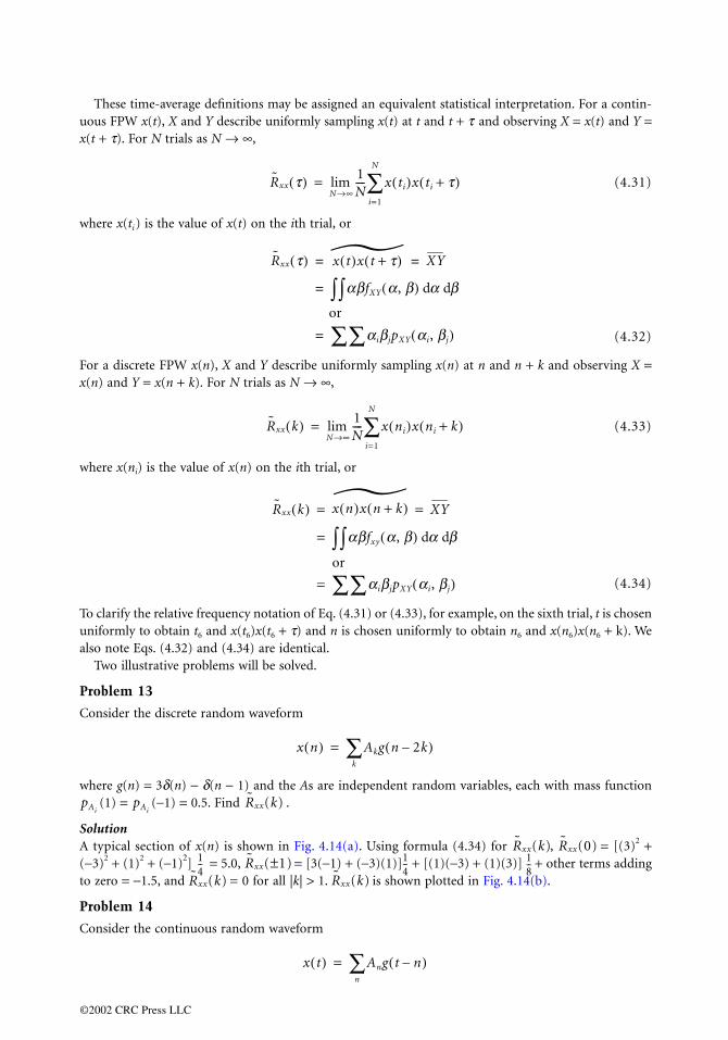
These time-average definitions may be assigned an equivalent statistical interpretation. For a contin-uous FPW x(t), X and Y describe uniformly sampling x(t) at t and t + τ and observing X = x(t) and Y =x(t + τ). For

where x(ti) i

For a discrex(n) and Y =

where x(ni)

To clarify thuniformly toalso note Eq

Two illust

Problem 1

Consider th

where g(n) =(1) =

SolutionA typical se(−3)2 + (1)2 to zero = −1

Problem 1

Consider th

pAipA


©2002 CRC P

N trials as N → ∞,

(4.31)

s the value of x(t) on the ith trial, or

(4.32)

te FPW x(n), X and Y describe uniformly sampling x(n) at n and n + k and observing X = x(n + k). For N trials as N → ∞,

(4.33)

is the value of x(n) on the ith trial, or

(4.34)

e relative frequency notation of Eq. (4.31) or (4.33), for example, on the sixth trial, t is chosen obtain t6 and x(t6)x(t6 + τ) and n is chosen uniformly to obtain n6 and x(n6)x(n6 + k). Wes. (4.32) and (4.34) are identical.rative problems will be solved.

3

e discrete random waveform

3δ(n) − δ(n − 1) and the As are independent random variables, each with mass function(−1) = 0.5. Find .

ction of x(n) is shown in Fig. 4.14(a). Using formula (4.34) for , = [(3)2 ++ (−1)2] = 5.0, = [3(−1) + (−3)(1)] + [(1)(−3) + (1)(3)] + other terms adding.5, and = 0 for all |k| > 1. is shown plotted in Fig. 4.14(b).

4

e continuous random waveform

R̃xx τ( ) 1N---- x ti( )x ti τ+( )

i=1

N

∑N→∞lim=

R̃xx τ( ) ˜x t( )x t τ+( ) XY= =

αβfXY α, β( ) dα dβ∫∫=

or

αiβjpXY αi, βj( )∑∑=

R̃xx k( ) 1N---- x ni( )x ni k+( )

i=1

N

∑N→∞lim=

R̃xx k( ) ˜x n( )x n k+( ) XY= =

αβfxy α, β( ) dα dβ∫∫=

or

αiβjpXY αi, βj( )∑∑=

x n( ) Akg n 2k–( )k

∑=

iR̃xx(k)

R̃xx(k) R̃xx(0)14-- R̃xx( 1)± 1

4-- 1

8--

R̃xx(k) R̃xx(k)

x t( ) Ang t n–( )n

∑=

ress LLC

where g(t) =, 0 ≤ α ≤ 2

SolutionA typical sec

= 1 foFor 0 < τ

FIGURE 4.14

FIGURE 4.15

g(n)

3

−1

pAi(αi)

3

x(n) = ∑ Ak g(n − k)

A2 = 1

1

g(t

12--

AiAj


©2002 CRC P

1, 0 ≤ t ≤ 1; g(t) = 0 otherwise and the As are independent random variables with (α) =, (α) = 0 otherwise. Find .

tion of x(t) is shown in Fig. 4.15(a). Since the As are independent, = 1, = 1.33, andr all . Observing Fig. 4.15(a), we obtain the following. < 1:

(a) A typical section of x(n) for Problem 13 and (b) .

(a) A typical section of x(t) for Problem 14 and (b) .

n

0.5

−1 1 αi−2 −1 2 4 6 n

−3 A3 = −1

−1−2−3 1 2 3

−1.5

5.0

k

R~

XX(k)

(a)

(b)

R̃XX ˜x n( )x n k+( ) XY= =

2

1.33

−1

) fAi(α) Ai = 1

Ai = 1.332

12

α

x(t) = ∑ An g(t − n)

1

−1 1 2 3 4 50

2

−1 1

t

τ

A0

A−1A2

~ ~

RXX(τ)

(a)

(b)

R̃XX τ( )

fAi

fAiR̃xx(τ)

Ai Ai2

i j≠

R̃xx τ( ) Ai2 1 τ–( ) AiAi+1τ+=

1.33 0.33τ–=

ress LLC

For τ > 1:

and result is obtThus, many

4.5 Su

The elementrandom proorder time at or at t andn and n + kencounteredensemble avof a waveforand its Four

Defining

CumulativeP[X =powercorresto FX(

Joint distribFXY(α

Joint randomProbability:

trials P(AB)

Random phoccur

Random varSample desc

outco

Special T

Finite powe

R̃xx τ–(


©2002 CRC P

by symmetry. is shown plotted in Fig. 4.15(b). We also note that the sameained when the As are independent and (α) or (α) are such = 1 and = 1.33. different waveforms have the same autocorrelation function.

mmary and Future Study

s of probability and random variable theory were presented as a prerequisite to the study ofcesses and communication theory. Highlighted were the concepts of finding first- and second-verages statistically, by uniformly sampling a continuous random finite power waveform at t + τ or discretely uniformly sampling a random finite power discrete waveform at n or at. The illustrative problems chosen were simple. When ergodic random processes are later, the time averages for any one member of the ensemble will be equivalent to correspondingerages. A future task is to approximate time averages on a computer. Here, from a sectionm T with its values sampled every τ seconds, an estimate for the autocorrelation functionier transom SXX( f ) called the power spectral density will be found.

Terms

distribution, density and mass function: FX(α) = P[X ≤ α], fX(α) = d/dα FX(α), pX(αi) = α i]. Other noted distribution or density functions are: total signal energy or total signal vs. frequency, corresponding to FX(α); energy or power spectral density vs. frequency,ponding to fX(α); total signal power vs. frequency for a periodic waveform, correspondingα) for a discrete random variable.ution, density and mass function: FXY(α, β) = P[(X ≤ α) (Y ≤ β)], fXY(α, β) = /, β), pXY(α i, β j) = P[(X = α i) (Y = β j)].

variables X and Y: X(si) and Y(si) jointly map each outcome of the SDS onto an α–β plane.P(A) is the statistical regularity of A, P(A/B) is the statistical regularity of A based only on

when B occurs, axiomatically P(A) = p(si) if and sisj = 0, . P(A/B) =/P(B) if enomenon: An experiment which, when performed many times N, yields outcomes that with statistical regularity as .iable X: X(si) maps the outcomes of the SDS onto a real axis.ription space (SDS): A listing of mutually exclusive, collectively exhaustive, finest grain

mes.

erminology for Random Finite Power Waveforms

r waveform:

R̃xx τ( ) AiAj 1= =

) R̃xx τ( )= R̃xx τ( )fAi

pAiAi Ai

2

∩ ∂ 2 ∂α ∂β∩

∑i=1n

A sii=1

n∪= i j≠P(B) 0.≠

N ∞→

Pavlim

T→∞

12T------ x2 t( )dt

T–

T

∫=

or

limN→∞

1

2N 1+---------------- x2 n( ) exists.

n= N–

N

∑=

ress LLC

First-order time averages:

and

The mostJointly samp

uniforSampling a

time T≤ N o

Second-ord

and st

The mfuncti

Reference

Olkin, GleseO’Flynn, M.Papoulis, A.Parzen, E. 19Ross, S. 199

Further I

Some imporjoint densityThe topic ofThe case of random varmost generadefined as aO’Flynn [19


©2002 CRC P

noted first-order statistics are or = , or = and = .ling a waveform: Uniformly choosing t and observing X = x(t) and Y = x(t + τ) or discretelymly choosing n and observing X = x(n) and Y = x(n + k).waveform: For a continuous waveform uniformly choosing a value of time over a long and observing X = x(t); for a discrete waveform discretely uniformly choosing n, −N ≤ n

ver a long time 2N + 1 and observing x(n). The random variable X describes x(t) or x(n).er time averages:

atistically

ost noted second-order statistics are , the time autocorrelationon, and/or or , the covariance function.

s

r, and Derman. 1994. Probability Models and Applications, Macmillan, New York. 1982. Probabilities, Random Variables and Random Processes, Wiley, New York. 1965. Probability, Random Variables and Stochastic Processes, McGraw-Hill, New York.60. Modern Probability Theory and Its Applications, Wiley, New York.

4. A First Course in Probability, Macmillan, New York.

nformation

tant topics were omitted or only briefly mentioned here. The bivariate Gaussian or normal function is given an excellent treatment in Olkin, Gleser, and Derman [1994, Chap. 12]. finding the density function of a function of two known random variables can be extended.finding the joint density function for U and V, each defined as a function of two known

iables X and Y, is well handled in Olkin, Gleser, and Derman [1994, Chap. 13]. Finally, thel transformation problem of finding the joint density function of m random variables, each linear combination of n known jointly Gaussly random variables, is given in Chap. 9 of82].

g̃ x t( )( ) limT→∞

1

2T------ g x t( )( ) dt

T–

T

∫ g α( )fx α( )dα∞–

∞

∫= =

g̃ x n( )( ) limN→∞

1

2N 1+---------------- g x n( )( )

N–

N

∑ g α( )fx α( )dα∞–

∞

∫= =

x̃(t) x̃(n) X x̃2(t) x̃2(n) X2 σX2

(X X)–2

˜g x t( ), x t τ+( )[ ] g X,Y( ) limT→∞

1

2T------ g x t( ), x t τ+( )[ ]dt

T–

T

∫= =

˜g x n( ), x n k+( )[ ] g X,Y( ) 12N 1+----------------

N→∞lim= g x n( ), x n k+( )[ ]

N∑=

g X, Y( ) g α, β( )fXY α, β( )dα dβ∫∫=

or

g αi, βj( )pXY αi, βj( )∑∑=

R̃xx τ( ) or R̃xx k( ) XY=L̃xx τ( ) L̃xx k( ) X X–( ) Y Y–( ) XY XY–= =

ress LLC

5Random Processes,

Autocorrelation, andSpectral Densities

5.1 Introduction 5.2 Basic Definitions5.3 Properties and Interpretation5.4 Baseband Digital Data Signals5.5 Coding for Power Spectrum Control 5.6 Bandpass Digital Data Signals5.7 Appendix: The Poisson Sum Formula

5.1 Introduction

The modeling of signals and noise in communication systems as random processes is a well-establishedand proven tradition. Much of the system performance characterization and evaluation can be done interms of a few low-order statistical moments of these processes. Hence, a system designer often needs tobe able to evaluate mean values and the autocorrelation of a process and the cross correlation of twoprocesses. It is especially true in communication system applications that a frequency-domain-basedevaluation is often easier to perform and interpret. Therefore, a knowledge of spectral properties ofrandom processes is valuable.

More recently, engineers are finding that modeling of typical communication signals as cyclostationary(CS) processes, rather than stationary processes, more accurately captures their true nature and permitsthe design of more effective signal processing operations. In the book edited by Gardner [1994], severalauthors describe applications that have benefited from the exploitation of cyclostationarity. Althoughthese processes are nonstationary, frequency-domain methods prove to be very effective, as in the stationarycase.

Another notion that is becoming well accepted by communication engineers is the utility of complex-valued representations of signals. Accordingly, all of the results and relations presented here will be validfor complex-valued random processes.

5.2 Basic Definitions

We consider the random process, x(t), defined as a set of jointly distributed random variables {x(t)}indexed by a time parameter t. If the set of values of t is the real line, we say the process is a continuous-time process. If the set of values is the integers, we call the process a discrete-time process. The mean andautocorrelation of the process are given by the expected values E[x(t)] and E[x(t1)x ∗ (t2)], respectively.

Lew E. FranksUniversity of Massachusetts


In dealing with cyclostationary processes, it is often more convenient to define an autocorrelation functionin terms of a simple transformation on the t1 and t2 variables; namely, let t = (t1 + t2)/2 and τ = t1 − t2

denote the mean value and difference of t1 and t2. Accordingly, we define the autocorrelation functionfor the process as

(5.1)

A process is cyclostationary, in the wide sense, with period T if both the mean and autocorrelation areperiodic in t with period T. Hence, for a cyclostationary process CS(T), we can write*

(5.2)

(5.3)

Equation (5.3) results from an application of the Poisson sum formula (see Appendix), where is the Fourier transform of cxx(t, τ) with respect to the t variable; that is,

(5.4)

hence,

(5.5)

is the mth Fourier coefficient for the t-variation in Rxx(t, τ). It is called the cyclic autocorrelation functionfor x(t) with cycle frequency m/T [Gardner, 1989]. Note that the cxx(t, τ) function in Eq. (5.3) is notuniquely determined by the autocorrelation; only a discrete set of values of its Fourier transform arespecified, as indicated in Eq. (5.3). Nevertheless, the notation is useful because the cxx(t, τ) function arisesnaturally in modeling typical communication signal time-sequential formats that use sampling, scanning,or multiplexing. The pulse amplitude modulation (PAM) signal discussed in Section 5.4 is a goodexample of this.

A frequency-domain characterization for the CS(T) process is given by the double Fourier transformof Rxx(t, τ).

(5.6)

where Cxx(ν, f ) is the double Fourier transform of cxx(t, τ); hence, it is the Fourier transform, with respectto the τ-variation, of the cyclic autocorrelation. It is called the cyclic spectral density for the cycle frequencym/T. Notice that Eq. (5.6) is a set of impulse fences located at discrete values of n in the dual-frequency(n, f ) plane. The impulse fence at ν = 0 has a special significance as the (one-dimensional) power spectral

*All summation indices will run from −∞ to ∞ unless otherwise indicated. The same is true for integration limits.

Rxx t, t( ) E x t t/2+( )x∗ t t/2–( )[ ]=

mx t( ) E x t( )[ ] Mx m( )e j2pmt/T

m∑= =

Rxx t, t( ) Tcxx t kT, t–( )k∑=

c̃xxmT---- , t

e j2pmt/T

m∑=

c̃xx(n, t)

c̃xx n, t( ) cxx t, t( )e j2p nt– dt∫=

c̃xx m/T, t( ) 1T--- Rxx t, t( )e j2pmt/T– dt

0

T

∫=

Sxx n, f( ) Rxx t, t( )e j2p nt+ft( )– dt dt∫∫=

CxxmT---- , f

d n mT----–

m∑=


density of the process. The other impulse fences characterize the correlation between signal componentsin different spectral regions. The physical significance of these concepts is discussed in the next section.

A process is wide-sense stationary (WSS) if the mean and autocorrelation are independent of the tvariable, that is, if only the m = 0 terms in Eqs. (5.2) and (5.3) are nonzero. For the WSS process, wewrite the autocorrelation function as

(5.7)

since the cyclic autocorrelation is nonzero only for a cycle frequency of n = 0. The power spectral densityof the process is simply the Fourier transform of Rxx(τ):

(5.8)

A CS(T) process can be converted to a WSS process by phase randomization. Let x′(t) = x(t − θ) wherethe time shift θ is a random variable which is independent of the other parameters of the process. Thenthe mean and autocorrelation of the new process are obtained by convolution, with respect to the tvariable, with the probability density function pθ(⋅) for the θ variable. Letting pθ(⋅) denote the Fouriertransform of pθ(⋅), we have

(5.9a)

(5.9b)

which indicates that phase randomization tends to suppress the cyclic components with cycle frequenciesdifferent from zero. In fact, for a uniform distribution of θ over a T-second interval, only the m = 0 termsin Eq. (5.9) remain; hence, x′(t) is WSS. Using the Poisson sum formula, we see that any pθ(σ) satisfying∑k pθ(σ − kT) = 1/T makes Pθ(m/T) = 0 for m ≠ 0, hence making x′(t) WSS.

It is important to note [from Eq. (5.5)] that the autocorrelation of the phase-randomized process isthe same as the time average of the autocorrelation of the original CS(T) process [Franks, 1969].

For a WSS discrete-time process a(k), where k is an integer, we write the mean and autocorrelation as

(5.10a)

(5.10b)

The power spectral density of the discrete-time process is the discrete-time Fourier transform (DTFT) ofthe autocorrelation function; that is,

(5.11)

which is always a periodic function of f with a period of 1/T. A case of frequent interest is when the a(k)are uniformly spaced sample values of a continuous-time WSS random process. Suppose a(k) = y(kT),then using the alternate form of the Poisson sum formula (Appendix), we have Raa(m) = Ryy(mT) and

(5.12)

Rxx t( ) Rxx 0, t( ) c̃xx 0, t( )= =

Sxx f( ) Rxx t( )e j2pft– dt∫=

mx ′ t( ) PqmT----

Mx m( )e j2pmt/T; Pq 0( )m∑ 1= =

Rx ′ x ′ t, t( ) PqmT----

c̃xxmT---- , t

e j2pmt/T

m∑=

a E a k( )[ ]=

Raa m( ) E a k m+( )a∗ k( )[ ]=

Saa f( ) Raa m( )e j2pmTf–

m∑=

Saa f( ) Ryy mT( )e j2pmTf–

m∑ 1

T--- Syy f

nT---–

n∑= =


In communication system applications, the a(k) sequence usually represents digital information to betransmitted, and the WSS assumption is reasonable. In some cases, such as when synchronizing pulsesor other header information are added to the data stream, the a(k) sequence is more appropriatelymodeled as a cyclostationary process also. The examples we consider here, however, will assume that a(k)is a WSS process

5.3 Properties and Interpretation

Many interesting features of a random process are revealed when the effects of a linear transformationon the first- and second-moment statistics are examined. For this purpose, we use linear transformationswhich are a combination of frequency shifting and time-invariant filtering, as shown in Fig. 5.1. Theexponential multipliers (modulators) provide the frequency shifts, and the filters with transfer functionsH1( f ) and H2( f ) provide frequency selective filtering. If H1( f ) and H2( f ) are narrowband low-pass filters,each path of the structure in Fig. 5.1 can be regarded as a sort of heterodyne technique for spectrumanalysis. The cross-correlation between the outputs of the two paths provides further useful character-ization of the input process.

The cross-correlation function for a pair of jointly random complex processes is defined as

(5.13)

Substituting the indicated expressions for y(t) and z(t) in Fig. 5.1 and using Eq. (5.3) for the autocorre-lation of the x(t) process, we can derive the following general expression for the cross-correlation:

(5.14)

First, we consider the case where H1( f ) = H2( f ) = B( f ), which is a very narrowband low-pass analysisfilter. Let B(0) = 1 and let ∆ denote the noise bandwidth of the filter given by

(5.15)

Hence, an ideal low-pass filter with a rectangular gain shape and a cutoff frequency at f = ∆/2 has a noisebandwidth of ∆. On the other hand, a low-pass filter resulting from averaging a signal over the last T0 s,that is, one with an impulse response b(t) = 1/T0 in 0 < t < T0 and zero elsewhere, has a noise bandwidth

FIGURE 5.1 Conceptual apparatus for analysis of random processes.

Ryz t, t( ) E y t t/2+( )z∗ t t/2–( )[ ]=

Ryz t, t( ) ejp f1+f2( )t

ej2p f1−f2( )t

e j2pmt/T H1 f f1m2T------+ +

∫⋅ ⋅ ⋅m∑=

H2∗ f f2

m2T------–+

CxxmT---- , f

e j2pft d f×

∆ B f( )B 0( )------------

2 d f∫=

X

Xx(t )

e j2πf2t

e j2πf1t

H1(f )

H2(f ) z (t ) = ∫h2(t − σ)e j2πf2σx(σ)dσ

y (t) = ∫h1(t − σ)e j2πf1σx(σ)dσ


of ∆ = 1/T0. Whatever kind of analysis filter we want to use, we shall consider the results as ∆ approacheszero so that we can assume that factors of the form B(f + m/2T)B∗ (f − m/2T) which will appear in Eq.(5.14) will vanish except for m = 0.

For example, let f1 = f2 = −f0. Then we see that both paths in the figure are identical, so that z(t) = y(t) and

(5.16)

because only the m = 0 term in Eq. (5.14) is nonzero under these conditions. Note also that y(t) is WSS,and its mean-squared value (also called the power of the process) is given by

(5.17)

This expression, valid for small ∆, gives the power in x(t) due to components in a narrow band centeredat a frequency of f0. This provides the motivation for calling Sxx( f ) = Cxx(0, f ) the power spectral densityof the x(t) process. Note that our spectrum analyzer gives the same results for a CS(T) process and itsphase-randomized WSS version because of the time averaging inherent in the B( f ) analysis filter.

Now, keeping the same low-pass filters, H1( f ) = H2( f ) = B( f ), let f0 = −( f1 + f2)/2 and n/T = (f2 − f1),so that the mean value of the two analysis frequencies is f0 and their difference is an integer multiple of1/T. Then, only the m = n term in Eq. (5.14) is nonzero and we have the following expression for thecross correlation of the y(t) and z(t) processes:

(5.18)

for small ∆. Thus, a physical significance of the cyclic spectral density, defined implicity in Eq. (5.6), isthat it represents the correlation that exists between spectral components separated by the cycle frequency.Note that no such spectral correlation exists for a WSS process. This spectral correlation is used toadvantage in communication systems to extract timing or synchronization information or to eliminatecertain kinds of interference by means of periodically time-varying filtering of signals [Gardner, 1994].

Equation (5.14) is useful to establish many other useful relationships. For example, let x(t) be WSSand let f1 = f2 = 0, then y(t) and z(t) are jointly WSS and the cross-spectral density is

(5.19)

and so, if H1( f ) = H2( f ), then z(t) = y(t) and the power spectral density of a filtered WSS process is given by

(5.20)

whereas letting H2( f ) = 1 makes z(t) = x(t) so that the cross-spectral density of the input and output ofa filtered WSS process is

(5.21)

If for all f, then Syz( f ) = 0, indicating that spectral components in nonoverlappingfrequency bands are always uncorrelated. This is a fundamental property of all WSS processes.

Ryy t, t( ) ej2pf0 t–

B f f0–( ) 2Cxx 0, f( )e j2pft d f∫=

E y t( ) 2[ ] Ryy 0( ) B f f0–( ) 2Cxx 0, f( ) d f∫= =

∆Cxx 0, f0( )≅ ∆ Sxx f0( ) as ∆ 0→=

Ryz t, 0( ) B f f0–( ) 2CxxnT--- , f

d f∫=

∆Cxx n/T, f0( )≅

Syz f( ) H1 f( )H2∗ f( )Sxx f( )=

Syy f( ) H1 f( ) 2Sxx f( )=

Syx f( ) H1 f( )Sxx f( )=

H1 f( )H2∗ f( ) 0=


5.4 Baseband Digital Data Signals

Perhaps the most basic form of mapping from a discrete-time data sequence {a(k)} into a continuous-time signal x(t) for transmission over a communication channel is baseband pulse amplitude modulation.The mapping uses a single carrier pulse shape, g(t), and is a linear function of the data, which we willassume is a WSS discrete-time process [Eq. (5.10)].

(5.22)

The x(t) process is CS(T) with

(5.23a)

(5.23b)

By inspection, the cxx (t, τ) function in Eq. (5.3) is

(5.24)

so that the cyclic autocorrelation is

(5.25)

Note that the strength of the cyclic autocorrelations (equivalently, the amount of spectral correlation)depends strongly on the amount of overlap of G( f ) and its frequency-translated versions. Data carrierpulses are often sharply bandlimited, with excess bandwidth factors not exceeding 100%. A pulse with100% excess bandwidth is bandlimited to the frequency interval | f | < 1/T. In this case, x(t) has cyclefrequencies of 0 and ±1/T only. Note also that an excess bandwidth of less than 100% means that G(n/T) =0 for n ≠ 0 so that the mean of the PAM signal [Eq. (5.23a)] is constant.

Using time averaging to get the power spectrum of the PAM signal, we can write

(5.26)

where

(5.27)

is the time-ambiguity function for the data pulse, g(t) [Franks, 1969]. Its Fourier transform is |G( f )|2,called the energy spectral density of the pulse. Hence, taking the Fourier transform of Eq. (5.26), thepower spectral density of the PAM signal is

(5.28)

which nicely separates the influence of the pulse shape from the correlation structure of the data.

x t( ) a k( )g t kT–( )k∑=

mx t( ) a g t kT–( )k∑ a/T( ) G

mT----

e j2pmt/T

m∑= =

Rxx t, t( ) Raa m( )g tt2-- kT mT––+

g∗ tt2-- kT––

m∑

k∑=

cxx t, t( ) 1T--- Raa m( )g t

t2-- mT–+

g∗ tt2--–

m∑=

c̃xx n/T, t( ) 1T--- Saa f( )G

nT--- f+

G∗ f( )e j2pft d f e jpnt/T⋅∫=

Rxx t( ) 1T--- Raa m( )rg t mT–( )

m∑=

rg t( ) g t t+( )g∗ t( ) dt∫=

Sxx f( ) 1T---Saa f( ) G f( ) 2=


Although it may not be apparent from Eq. (5.28), the power spectrum expression may contain δ-functionterms, which represent nonzero concentrations of power at a discrete set of frequencies. In order to makeevident the discrete part of the power spectrum, we express the continuous part of the spectrum as theFourier transform of the autocovariance function, which is the autocorrelation of the zero-mean process,x′(t) = x(t) − mx(t). Then

(5.29)

where

(5.30)

and

(5.31)

Now, performing the time averaging, the power spectrum is expressed as

(5.32)

The second term in Eq. (5.32) is the discrete part of the spectrum. Notice that there are no discretecomponents for zero-mean data or if the data pulse has less than 100% excess bandwidth (G(n/T)= 0 for n ≠ 0). For zero-mean independent data, pulse amplitudes are uncorrelated and the powerspectrum is simply

(5.33)

where is the data variance.A more general format for baseband data signals is to use a separate waveform for each data symbol

from the symbol alphabet. Familiar examples are frequency-shift keying (FSK), phase-shift keying (PSK),and pulse-position modulation (PPM). For the binary alphabet case, [a(k) � {0, 1}], the format is basicallyPAM. Using waveforms g0(t) and g1(t) to transmit a zero or one, respectively, we have

(5.34)

which can be rewritten, using d(t) = g1(t) − g0(t), as

(5.35)

which is a periodic fixed term plus a binary PAM signal. Let p = Pr[a(k) = 1] = and let P11(m) denotethe conditional probability, Pr[a(k + m) = 1|a(k) = 1], then with a′(k) = a(k) − ,

(5.36)

Rxx t, t( ) R ′xx t, t( ) mx t t/2+( )mx∗ t t/2–( )+=

R ′xx t, t( ) Rx ′ x ′ t, t( ) 1T--- R ′aa m( )rg t mT–( )

m∑= =

R ′aa m( ) Raa m( ) a 2–=

Sxx f( ) 1T--- S ′aa f( ) G f( ) 2 a

T---

2

GnT---

2

d fnT---–

n∑+=

(a 0)=

Sxx f( )sa

2

T------ G f( ) 2=

sa2

x t( ) 1 a k( )–[ ] g0 t kT–( ) a k( )g1 t kT–( )+k∑=

x t( ) g0 t kT–( ) a k( )d t kT–( )k∑+

k∑=

aa

R ′aa m( ) E a ′ k m+( )a ′ k( )[ ]=

Raa m( ) p2– pP11 m( ) p2–= =


and carrying out the calculations, the power spectral density is

(5.37)

where the second term gives the discrete components. Note that the strength of the discrete componentsdepends only on the mean value of the data and not the correlation between data symbols.

To generalize the preceding result to an M-ary symbol alphabet for the data, we write

(5.38)

with am(k) � {0, 1} and, for each k, only one of the am(k) is nonzero for each realization of the process.Then, calculating the autocorrelation function, we find that cxx(t, τ) in Eq. (5.3) can be expressed as

(5.39)

We assume that the data process can be modeled as a Markov chain characterized by a probabilitytransition matrix Pmn(i) giving the probability that am (i + j) = 1 under the condition that an( j) = 1. Wefurther assume the process is in a steady-state condition so that it is WSS. This means that the symbolprobabilities, pn = Pr[an( j) = 1], must satisfy the homogeneous equation

(5.40)

and all of the transition matrices can be generated by recursion:

(5.41)

Now, calculation of the autocorrelation can proceed using E[am (i + j)an( j)] = qmn(i) in Eq. (5.39), where

(5.42)

Taking the DTFT of the qmn(i) sequence

(5.43)

we arrive at a remarkably compact expression for the power spectral density of this general form for thebaseband data signal

(5.44)

Sxx f( ) 1T--- s ′aa f( ) G1 f( ) G0 f( )– 2=

1T---

2

1 p–( )G0nT---

pG1nT---

+2

d fnT---–

n∑+

x t( ) am k( )gm t kT–( )m=0

M−1

∑k∑=

cxx t, t( ) 1T--- E am i j+( )an i( )[ ] gm t

t2-- iT–+

gn∗ t

t2--–

∑m ,n=0

M−1

∑i

∑=

pm Pmn 1( )pn

n=0

M−1

∑=

Pmn i 1+( ) Pmk i( )Pkn 1( ); i 1≥k=0

M−1

∑=

qmn i( ) Pr am i j+( ) 1 and an j( ) 1= =[ ]=Pmn i( )pn for i 0>=dmnpn for i 0= =Pmn i–( )pm for i 0<=

Qmn f( ) qmn i( )e j2piTf–

i∑=

Sxx f( ) 1T--- Qmn f( )Gm f( )Gn

∗ f( )∑m ,n=0

M−1

∑=


The power spectrum may contain discrete components. The continuous part of the spectrum can beextracted by replacing the qmn(i) in Eqs. (5.42–5.44) by qmn(i) − pmpn. Then, the remaining part is thediscrete spectrum given by

(5.45)

For the special case of independent data from symbol to symbol, the probability transition matrix takeson the special form Pmn(i) = pm for each m and each i > 1; that is, all columns are identical and consistof the set of steady-state symbol probabilities. In this case, the continuous part of the power spectrum is

(5.46)

and the discrete part is the same as in Eq. (5.45).As an example of signalling with M different waveforms and with independent, equiprobable data,

consider the case of pulse position modulation where

(5.47)

The resulting power spectrum is

(5.48)

where

The continuous part of the spectrum will be broad because pulse widths will be narrow (on theorder of T/M s duration) for a reliable determination of which symbol was transmitted. Note,however, that the spectrum has nulls at multiples of 1/T due to the shape of the Q( f ) factor in Eq.(5.48).

5.5 Coding for Power Spectrum Control

From Eq. (5.28) or (5.44), we see that that the shape of the continuous part of the power spectral densityof data signals can be controlled either by choice of pulse shapes or by manipulating the correlationstructure of the data sequence. Often the latter method is more convenient to implement. This can beaccomplished by mapping the data sequence into a new sequence by a procedure called line coding [Leeand Messerschmitt, 1988]. The simpler types of line codes are easily handled by Markov chain models.As an example, we consider the differential binary (also called NRZI) coding scheme applied to a binarydata sequence. Let a(k) � {0, 1} represent the data sequence and b(k) the coded binary sequence. Thecoding rule is that b(k) differs from b(k − 1) if a(k) = 1, otherwise b(k) = b(k − 1). This can also be

Sxx f( )discrete1T---

2

pmGmkT---

m=0

M−1

∑2

d fkT---–

k∑=

Sxx f( )continuous1T--- pm Gm f( ) 2 pmGm f( )

m=0

M−1

∑2

–m=0

M−1

∑=

gm t( ) g t mTM-----–

; pm 1/M; m 0, 1, 2, …, M 1–= = =

Sxx f( ) 1T---

Q f( ) G f( ) 2 1T---

2

GkMT

--------

2

d fkM

T---------–

k∑+=

Q f( ) 11M-----

sin2 pTf( )sin2 pTf /M( )-------------------------------–=


expressed as b(k) = [b(k − 1) + a(k)]mod2. Letting q = Pr[a(k) = 1], the probability transition matrixcan be expressed as

(5.49)

from which it follows that the steady-state probabilities for b(k) = 1 or 0 [Eq. (5.40)] are given by p =1 − p = 1/2, regardless of the uncoded symbol probability q. Because the columns of a transition matrixsum to 1, the evolution of the transition probability [Eq. (5.41)] can be written as a single scalar equationwhich, in this case, is a first-order difference equation with an initial condition of P11(0) = 1.

(5.50)

Using P11(i) = P11(− i), the solution is

(5.51)

Supposing that the transmitted signal is binary PAM using the b(k) sequence, that is,

(5.52)

then, taking the DTFT of Eq. (5.51) and using Eq. (5.32), the power spectral density becomes [Franks,1969]

(5.53)

where the spectrum shaping function is

(5.54)

It is sometimes stated that differential binary (NRZI) coding does not alter the shape of the powerspectrum. We see from Eq. (5.54) that this is true only in the case that the original data are equiprobable(q = 1/2). As shown in Fig. 5.2, the shaping factor Q( f ) differs greatly from a constant as q approaches0 or 1. Note, however, that the spectrum of the coded signal depends only on the symbol probability qand not the specific correlation structure of the original data sequence.

A more practical line coding scheme is bipolar coding, also called alternate mark inversion (AMI). It iseasily derived from the differential binary code previously discussed. The bipolar line signal is a ternaryPAM signal

(5.55)

where c(k) = 0 if a(k) = 0 and c(k) = +1 or −1 if a(k) = 1, with the two pulse polarities forming analternating sequence; that is, a positive pulse will always be followed by a negative pulse and vice versa.Hence, the bipolar code can be expressed in terms of the differential binary code as

(5.56)

P 1( ) 1 q– q

q 1 q–=

P11 i 1+( ) 1 2q–( )P11 i( ) q+ ; i 0≥=

P11 i( ) 12-- 1 2q–( ) i 1+[ ]=

x t( ) b k( )g t kT–( )k∑=

Sxx f( ) 14T------

Q f( ) G f( ) 2 12T------

2

GnT---

2

d fnT---–

n∑+=

Q f( ) q 1 q–( ) q2 1 2q–( )sin2 pTf( )+[ ] 1–=

x t( ) c k( )g t kT–( )k∑=

c k( ) b k( ) b k 1–( )–=


which itself is a form of partial response coding [Lee and Messerschmitt, 1988; Proakis and Salehi, 1994].The autocorrelation function for c(k) is easily expressed in terms of the autocorrelation for b(k),

(5.57)

and since

(5.58)

we get

(5.59)

and, taking the DTFT of Rcc(m), the power spectral density for the bipolar signal is

(5.60)

where

Since , the spectrum has no discrete components, which can be a substantialpractical advantage. The spectral shaping factor Q( f ), shown in Fig. 5.3, produces spectral nulls at f = 0and f = 1/T. This was used to advantage in early wire-cable PCM systems to mitigate the effects of nolow-frequency transmission and the effects of increased crosstalk between wire pairs at the higherfrequencies. Note that the spectrum shape is still dependent on data symbol probability but not on thecorrelation structure of the data.

Another simple line code, found useful in optical and magnetic recording systems, is the Miller code,whose power spectrum can be determined with a four-state Markov chain [Proakis and Salehi, 1994].

FIGURE 5.2 Spectral density shaping function for differential binary coding.

0

1

2

3

Q(f )

12T

12T

T qq

1T

f

Q (o) = Q( 1 ) = 1 − 1

Q(o)Q ( ) = = 1

1− q

q = 12

q = 14

q = 34

Rcc m( ) 2Rbb m( ) Rbb m 1–( ) Rbb m 1+( )––=

Rbb m( ) 12--P11 m( ) 1

4-- 1 2q–( ) m 1+[ ]= =

Rcc 0( ) q=

Rcc m( ) q2 1 2q–( ) m 1– ; m 1≥–=

Sxx f( ) 1T---= Q f( ) G f( ) 2

Q f( ) q 1 q–( )sin2 pTf( )[ ] q2 1 2q–( )sin2 pTf( )+[ ] 1–=

E c k( )[ ] c b b– 0= = =


5.6 Bandpass Digital Data Signals

In most communication systems, signals are positioned in a frequency band which excludes low frequen-cies. These are called bandpass signals. For digital data signals, we could simply consider the basebandformats discussed previously, but with data pulse shapes, g(t), which have a bandpass nature. However,it is more common to produce bandpass signals by modulation of a sinusoidal carrier with low-pass(baseband) data signals. Hence, we examine here the correlation and spectral properties of quadratureamplitude modulation (QAM) carrier signals. Let u(t) and v(t) be real baseband signal processes, thenthe QAM signal with a carrier frequency of f0 is

(5.61)

which can be more conveniently handled in terms of complex signals

(5.62)

The signals u(t) and v(t) are often called the in-phase and quadrature components, respectively, of theQAM signal. The autocorrelation function for x(t) becomes

(5.63)

First we consider the situation where u(t) and v(t) are jointly WSS processes, which might be a goodmodel for some types of analog systems. In this case, there are three cycle frequencies (0, + 2f0 , − 2f0).We obtain the cyclic autocorrelation functions from Eq. (5.5) by time averaging over a period of T = 1/f0

with the result that

(5.64a)

(5.64b)

FIGURE 5.3 Spectral density shaping function for bipolar coding.

0

1

2

3

Q(f )

f1

2T1T

q = 12

q =

q = 14

Q(o) = Q(1T ) = O

Q(2T ) = q

1−q

34

1

x t( ) u t( ) cos 2pf0t( ) v t( ) sin 2pf0t( )–=

x t( ) ℜ w t( )ej2pf0t

[ ] ; w t( ) u t( ) jv t( )+= =

Rxx t, t( ) 12-- ℜ Rww t, t( )e

j2pf0 t[ ]=

12-- ℜ R

ww∗ t, t( )ej2p 2f0( )t

[ ]+

c̃xx 0, t( ) 12-- ℜ Rww t( )e

j2pf0 t[ ]=

c̃xx 2f0, t( ) 14--R

ww∗ t( ) c̃xx∗ 2f0, t–( )= =


From the second term in Eq. (5.63), in the WSS case, it is evident that a period of T = 1/2f0 would alsowork; however, we choose to regard the QAM signal as CS(1/f0) since the mean value could have acomponent at f0. The autocorrelation result is the same in either case.

We note that x(t) itself would be WSS under the condition that the cross-correlation, Rww∗ (τ), vanishes,making the second term in Eq. (5.63) disappear. This condition is equivalent to Ruu(τ) = Rvv(τ) and Rvu(τ)= − Ruv(τ) = − Rvu(− τ); in other words, x(t) is WSS if the in-phase and quadrature components have thesame autocorrelation and their cross-correlation function is odd. If u(t) and v(t) are independent zero-mean processes, then we require only that their autocorrelations match. This is called balanced QAMand its power spectral density is

(5.65)

For the case of digital data signals, we examine the QAM/PAM signal where the complex basebandsignal is a pair of PAM signals,

(5.66)

Here we encounter a problem regarding the period of the cyclostationarity, because the PAM signalexhibits a period of T while the carrier modulation introduces a period of 1/f0, and these periods are notnecessarily commensurate. The problem is easily handled by methods used for almost periodic functions,by extending the integration interval indefinitely

(5.67a)

(5.67b)

The values of νi for which Eq. (5.67b) are nonzero are the cycle frequencies. The process is sometimescalled polycyclostationary. Now, using Eq. (5.25) for the cyclic autocorrelations of w(t) and Eq. (5.63) forthe effect of the modulation, then taking Fourier transforms, we get the following results for the cyclicspectral density functions for x(t):

(5.68a)

(5.68b)

(5.68c)

where, for convenience, we have defined the function

(5.69)

Sxx f( ) Cxx 0, f( ) 12--Suu f f0–( ) 1

2--Suu f f0+( )+= =

w t( ) c k( )g t kT–( ); c k( )k∑ a k( ) jb k( )+= =

Rxx t, t( ) c̃xx ni, t( )ej2p nit

i∑=

c̃xx ni, t( ) 12T0

-------- Rxx t, t( )ej2p nit–

dtT0–

T0

∫T0→• lim=

CxxmT---- , f

14T------

Scc f f0m2T------––

K f f0; m–( )=

14T------

Scc f f0m2T------+––

K f f0; m+( )+

CxxmT---- 2f0, f+

14T------

Scc ∗ fm2T------–

K f ; m( )=

CxxmT---- 2f0, f–

14T------

S∗cc ∗ f

m2T------+–

K f ; m( )=

K f ; m( ) G fm2T------+

G∗ fm2T------–

=


The cycle frequencies are {m/T, m/T + 2f0, m/T − 2f0}. For example, if the data pulse g(t) had less than100% excess bandwidth, then K(f ; m) vanishes for |m| > 2 and there are a total of nine cycle frequencies.If the QAM is balanced, for example, by making the a(k) and b(k) identically distributed and independent,then the cross-spectral density Scc∗ ( f ) vanishes and only three cycle frequencies remain.

As an illustration, let us assume that the a(k) and b(k) sequences are independent and each sequencehas zero-mean, independent data, but with variances, and , for in-phase and quadrature data,respectively. Then and , giving the following simple expressionsfor the cyclic spectral densities:

(5.70a)

(5.70b)

and the power spectral density is

(5.71)

which is simply a pair of frequency-translated versions of the corresponding baseband PAM spectrum.The case of double-sideband amplitude modulation (DSB-AM/PAM) is covered in the preceding equa-

tions simply by making all of the b(k) equal to zero. This can be regarded as extremely unbalanced QAM;hence, the nonzero cyclic components will tend to be greater than in the QAM case. Other modulationformats can be handled by essentially the same methods. For example, vestigial-sideband modulation(VSB-AM/PAM) uses a single data stream and a complex data pulse; +

. A more general version of QAM uses a different pulse shape in the in-phase and quadraturechannels. Staggered QAM (SQAM) uses time-shifted versions of the same pulse; for example, w(t) =Σa(k)g(t − kT) + jb(k)g(t − T/2 − kT). Quaternary phase-shift keying (QPSK) is a special case of QAMwith a(k), b(k) � {+1, −1}.

5.7 Appendix: The Poisson Sum Formula

For any time function g(t) having Fourier transform G( f ), the following relation is often useful in systemanalysis:

(A.5.1)

The relation is easily verified by making a Fourier series expansion of the periodic function on the left-hand side of Eq. (A.5.1). The mth Fourier coefficient is

(A.5.2)

and, by a change of integration variable,

(A.5.3)

sa2 sb

2

Scc f( ) sa2 sb

2+= Scc∗ f( ) sa2 sb

2= =

CxxmT---- , f

sa2 sb

2+4T

------------------ K f f0; m–( ) K f f0; m+( )+[ ]=

CxxmT---- 2f0, f+

CxxmT---- 2f0, f–

sa2 sb

2–4T

------------------K f ; m( )= =

Sxx f( ) Cxx 0, f( )sa

2 sb2+

4T------------------ G f f0–( ) 2 G f f0+( ) 2+[ ]= =

w t( ) ∑a k( )= [g t kT–( )jg̃ t kT–( )]

g t kT–( )k∑ 1

T--- G

mT----

e j2pmt/T

m∑=

c m( ) 1T--- g t kT–( )e j2pmt/T– dt

k∑

0

T

∫=

c m( ) 1T--- g s( )e j2pms/T– ds

•–

•

∫ 1T--- G

mT----

= =


Another useful version of the Poisson sum formula is the time/frequency dual of Eq. (A.5.1).

(A.5.4)

Defining Terms

Autocorrelation: The expected value of the product of two elements (time samples) of a single randomprocess. The variables of the autocorrelation function are the two time values indexing the randomvariables in the product.

Cross correlation: The expected value of the product of elements from two distinct random processes.Cycle frequency: The frequency parameter associated with a sinusoidal variation of a component of

the autocorrelation of a cyclostationary process.Cyclic autocorrelation: A parameter characterizing the amount of contribution to the overall autocor-

relation at a particular cycle frequency.Cyclostationary random process (wide-sense): A random process whose mean and autocorrelation

functions vary periodically with time.Excess bandwidth: The amount of bandwidth of a PAM signal that exceeds the minimum bandwidth

for no intersymbol interference. It is usually expressed as a fraction of the Nyquist frequency of1/2T, where 1/T is the PAM symbol rate.

Poisson sum formula: A useful identity relating the Fourier series and sum-of-translates representa-tions of a periodic function.

Power spectral density: A real, nonnegative function of frequency that characterizes the contributionto the overall mean-squared value (power) of a random process due to components in any specifiedfrequency interval.

Pulse amplitude modulation (PAM): A signal format related to a discrete-time sequence by superpos-ing time-translated versions of a single waveform, each scaled by the corresponding element of thesequence.

Quadrature amplitude modulation (QAM): A signal format obtained by separately modulating theamplitude of two components of a sinusoidal carrier differing in phase by 90°. In digital commu-nications, the two components (referred to as in-phase and quadrature components) can each beregarded as a PAM signal.

Time-ambiguity function: A property of a waveform, similar to convolution of the waveform withitself, which characterizes the degree to which the waveform can be localized in time. The Fouriertransform of the time-ambiguity function is the energy spectral density of the waveform.

References

Franks, L.E. 1969. Signal Theory, Prentice–Hall, Englewood Cliffs, NJ; rev. ed. 1981. Dowden and Culver.Gardner, W.A. 1989. Introduction to Random Processes with Applications to Signals and Systems, 2nd ed.,

McGraw–Hill, New York.Gardner, W.A., Ed. 1994. Cyclostationarity in Communications and Signal Processing, IEEE Press.Lee, E.A. and Messerschmitt, D.G. 1988. Digital Communication, Kluwer Academic, Dordrecht, the

Netherlands.Papoulis, A. 1991. Probability, Random Variables, and Stochastic Processes, 3rd ed., McGraw–Hill, New York.Proakis, J.G. 1989. Digital Communications, McGraw–Hill, New York.Proakis, J.G. and Salehi, M. 1994. Communication Systems Engineering, Prentice–Hall, Englewood Cliff, NJ.Stark, H. and Woods, J.W. 1986. Probability Random Processes, and Estimation Theory for Engineers, 2nd

ed., Prentice–Hall, Englewood Cliffs, NJ.

g kT( )e j2pkTf–

k∑ 1

T--- G f

mT----–

m∑=


Further Information

The text by Papoulis [1991] is the third edition of a well known and referenced work on probability andrandom processes that first appeared in 1965. It is a concise and comprehensive treatment of the topicand is widely regarded as an ideal reference source. Gardner [1989] provides the most complete textbooktreatment of cyclostationary processes. He presents a careful development of the theory of such processesas well as several examples of applications relevant to the communications field. Stark and Woods [1986]is a somewhat more advanced textbook. It uses modern notation and viewpoints and gives the reader agood introduction to the related topics of parameter estimation and decision theory.


6Queuing*

6.1 Introduction 6.2 Little’s Formula6.3 The M/M/1 Queuing System: State Probabilities6.4 The M/M/1 Queuing System: Averages and

Variances6.5 Averages for the Queue and the Server

6.1 Introduction

Everyone has experienced being in a queue: waiting in line at a checkout counter, waiting in traffic aswe enter a highway’s tollgate, or waiting for a time-sharing computer to run our program. Examples ofqueues from everyday life and technical experiences are almost endless.

A study of queues is important for the following reasons:

1. From the user’s point of view, a queue, that is, waiting in line, is a nuisance and will be toleratedonly at some minimal level of inconvenience.

2. From the point of view of a provider of some service, queues are necessary. It is extremelyuneconomical to provide a large number of servers to handle the biggest possible rush, only tohave many of them idle most of the time.

One motivation to study queues is to find some balance between these two conflicting viewpoints.Probability theory is the tool we use for a study of queues because arrivals and departures from a queuingsystem occur randomly. In Fig 6.1, a customer arrives at the input to the queuing system, and if noserver is free, the customer must wait in a queue until it is his, her, or its turn to be served. A queuediscipline is the name given to a rule by which a customer is selected from a queue for service.

6.2 Little’s Formula

Let the average rate at which customers arrive at a queuing system be the constant l. Departures fromthe queuing system occur when a server finishes with a customer. In the steady state, the average rate atwhich customers depart the queuing system is also l. Arrivals to a queuing system may be described asa counting process A(t) such as shown in Fig 6.2. We estimate an average rate of arrivals with

(6.1)

*Portions are reprinted by permission. Williams, R.H. 1991. Electrical Engineering Probability, Copyright ” byWest, St. Paul MN. All Rights Reserved.

l A t( )t

---------- (per unit time)=

Richard H. WilliamsUniversity of New Mexico


where A(t) is the number of arrivals in [0, t]. Departures from the system D(t) are also described by acounting process, and an example is also shown in Fig. 6.2. Note that must be true at alltimes. The time that each customer spends in the queuing system is the time difference between thecustomer’s arrival and subsequent departure from a server. The time spent in the queuing system forarrival i is denoted ti, i = 1, 2, 3,….

The average time a customer spends waiting in a queuing system is

(6.2)

The average number of customers in a queuing system is, from Eqs. (6.1) and (6.2),

(6.3)

If we assume that, with enough data, sample averages approximate their expected values, then ,, and where N and T are random variables. Also, Eq. (6.3) becomes

(6.4)

This relation is known as Little’s formula [Williams, 1991]; it has a generality much beyond what onemight suppose, given the heuristic demonstration leading to Eq. (6.4).

FIGURE 6.1 Illustration of queuing system: Customers arrive at a queue and, after some time, depart from a serverthat serves the queue.

FIGURE 6.2 Illustration of the arrival and departure counting processes for a queuing system.

{ {

Queuing System: T = TQ + TS

TQ TS

Queuing System: N = NQ + NS

NQ NS

Arrivals

Queue

Server m

Departures

Server 1

Server 2

A(t)

D(t)

Time

12

10

8

6

4

2

00 5 10 15 20

A t( ) D t( )≥

t1

A t( )---------- ti

i=1

A t( )

Â= (units of time)

n

n1t-- ti

i=1

A t( )

Â lt (dimensionless)= =

l lÆt E T[ ]Æ n E N[ ],Æ

E N[ ] lE T[ ]=


Example 1

The data in Table 6.1 are the data used to plot A(t) and D(t) in Fig. 6.1. In Table 6.1, the times, given inthe units of minutes, are: arrival time tA, time spent in the queue tQ, time spent with the server tS, totaltime in the queuing system for the ith arrival ti, and the departure time tD. For each i we see in Table6.1, that ti = tQ + tS and that tD = tA + ti. These data describe a first-in–first-out (FIFO) queuing discipline:If a customer arrives before the previous customer departs, then the customer must wait his turn in thequeue until the server is available. If the previous customer has departed prior to a customer’s arrival,then the waiting time in the queue is tQ = 0.

According to the data in Table 6.1, when t = 20.7 then A(t) = i = 10. From Eq. (6.1),

The sum of all the ti in Table 6.1 is 31.4 min. Therefore, from Eq. (6.2),

Finally, using Little’s formula in Eq. (6.3), the sample average number of customers in the queuing system is

6.3 The M/M/1 Queuing System: State Probabilities

A generally accepted notation used to name a queuing system is A/S/m: A is a description of the dynamicsby which arrivals come to the queuing system; S is a description of the dynamics by which a serverprocesses a customer taken from the queue; and m is the number of servers. The arrivals and the serverare independent of each other except that a server cannot serve a customer who has not yet arrived intothe queue.

We define the state of a queuing system as the total number of customers within it, that is, eitherwithin the queue or being served. The only queuing system that we discuss in this chapter is M/M/1:The arrival dynamics are Markov (with rate constant l), the server dynamics are Markov (with rateconstant l S), and there is only one server.

There can be, at most, only one arrival and, at most, one departure in a time interval Dt when .As far as arrivals are concerned, when Dt is a small increment of time, the probability of an arrival intothe queuing system in the interval Dt is

(6.5)

TABLE 6.1 Data from a FIFO Queue Used with Example 1

i tA tQ tS ti tD

1 0.0 0.0 2.0 2.0 2.02 1.5 0.5 2.9 3.4 4.93 2.2 2.7 2.1 4.8 7.04 4.1 2.9 0.8 3.7 7.85 5.5 2.3 1.7 4.0 9.56 10.0 0.0 1.5 1.5 11.57 11.3 0.2 1.6 1.8 13.18 13.4 0.0 2.3 2.3 15.79 15.0 0.7 2.0 2.7 17.710 15.5 2.2 3.0 5.2 20.7

l 1020.7---------- 0.48 (min 1– )= =

t31.410

---------- 3.14 (min)= =

n10

20.7---------- 31.4

10----------¥ 1.52= =

Dt 0Æ

P A( ) lDt=


Correspondingly, the probability of no arrival in Dt is

(6.6)

The probability of serving (discharging) a customer P(D) is actually conditioned by the event thatthere is at least one customer in the queuing system. Thus, given that the state is at least one,

(6.7)

The probability of continuing to serve a customer who is already being served is

(6.8)

Suppose that the state of a queuing system is zero at time t + Dt. This can occur in only one of threemutually exclusive ways. If the state at time t is zero, then either there is no arrival in the increment Dt,or, if there is an arrival in Dt, then there is also a departure within the same Dt. If the state at t is one,then there must be one departure and no arrival within Dt. Let Pn(t) denote the probability of a queuingsystem being in the state n at time t. Then, with this notation, a summary of the preceding statement is

Using Eqs. (6.5–6.8), this may be arranged into

Then, taking the limit as we have the derivative

When a queuing system is in the steady state, the rate of change of the probability P0(t) with respect totime is zero, and we have

(6.9)

If at time t + Dt the state of the queuing system is greater than zero, we have

The first term on the right of this equation describes two ways for the state to remain the same whentime increases from t to t + Dt: either no arrival and no departure occur, or exactly one arrival occursand exactly one departure occurs. The second term describes the state n + 1 changing to n by exactlyone departure with no arrival. The third term describes the change from state n - 1 to n by exactly onearrival and no departure. No other combinations of arrivals and departures can happen using our assump-tions when n > 0. Then, as before, finding the derivative of Pn(t) and setting it equal to zero in the steady-state condition, we find

(6.10)

P A( ) 1 lDt–=

P D( ) lSDt=

P D( ) 1 lSDt–=

P0 t Dt+( ) P0 t( ) P A( ) P A( )P D( )+{ }= P1 t( )P A( )P D( )+

P0 t Dt+( ) P0 t( )–Dt

------------------------------------------ lP0 t( ) 1 lSDt–{ } lSP1 t( ) 1 lDt–{ }+–=

Dt 0,Æ

dP0 t( )dt

--------------- lSP1 t( ) lP0 t( )–=

lP0 t( ) lSP1 t( )=

Pn t Dt+( ) Pn t( ) P A( )P D( ) P A( )P D( )+{ }=

Pn+1 t( )P A( )P D( ) Pn-1 t( )P A( )P D( )+ +

l lS+( )Pn t( ) lSPn+1 t( ) lPn-1 t( )+=


We introduce the ratio

(6.11)

Then, when n = 0, we have from Eq. (6.9),

When n = 1, Eq. (6.10) becomes

Combining this with P1(t), we have an expression which, when simplified, becomes

Continuing in this way, it follows that

(6.12)

Since the queuing system can theoretically be in any state n = 0, 1, 2,… (that is, there can be anynonnegative number of customers in the queuing system), we must require that

(6.13)

Combining Eqs. (6.12) and (6.13), we have

By stipulating that r < 1, we can sum the geometric progression [Beyer, 1987, p. 8]:

(6.14)

Thus, when n = 0, we have

(6.15)

Combining Eq. (6.15) with Eq. (6.12) gives the probability of any state n for the M/M/1 queuing system:

(6.16)

As long as the state of a queuing system is greater than zero, then one of the customers must be withthe server. Therefore, the probability that the server is busy is P(N > 0). Since P(N > 0) + P0(t) = 1, itfollows, using Eq. (6.15), that

(6.17)

The result in Eq. (6.17) is why the ratio r is called the utilization of an M/M/1 queuing system.

r llS

-----=

P1 t( ) rP0 t( )=

l lS+( )P1 t( ) lSP2 t( ) lP0 t( )+=

P2 t( ) r2P0 t( )=

Pn t( ) rnP0 t( )=

Pn t( )n=0

•

Â 1=

P0 t( ) rn

n=0

•

Â 1=

rn

n=0

•

Â 11 r–------------=

P0 t( ) 1 r–=

Pn t( ) 1 r–( )rn=

P N 0>( ) r=


Example 2

A manager of a queuing system wants to know the probability that k or more customers are in the queuewaiting to be served by the server; k = 1, 2, 3,…. If even one customer is in the queue, then there mustalso be one customer with the server. Therefore, what the manager wants to know is the probability thatthe state of the queuing system is k + 1 or more. Then, with Eq. (6.16),

If we use the change of variables m = n - (k + 1), and Eq. (6.14), we then answer the manager’s question:

6.4 The M/M/1 Queuing System: Averages and Variances

The purpose of this section is to find the statistical parameters of mean and variance for both randomvariables N and T shown in Fig. 6.1 for an M/M/1 queue. In the following, the lower case n and t standfor realizations of the random variables N and T.

If the geometric progression in Eq. (6.14) is differentiated once with respect to r, we have

Then, differentiating this once again,

The first of these two derivatives can be used along with Eq. (6.16) to show that the mean of N is

(6.18)

The second of these two derivatives is used to express the mean of the square of N,

(6.19)

Equations (6.18) and (6.19) are used to find the variance of N,

(6.20)

One notes that as the utilization approaches unity, and both the mean and the variance of Nfor the M/M/1 queue become unbounded.

P NQ k≥( ) P N k 1+≥( ) 1 r–( )rn

n=k+1

•

Â= =

P NQ k≥( ) 1 r–( )rk+1 rm

m=0

•

Â rk+1= =

nrn

n=0

•

Â r1 r–( )2

-------------------=

n2rn

n=0

•

Â r 1 r+( )1 r–( )3

--------------------=

E N[ ] nPn t( )n=0

•

Â n 1 r–( )rn

n=0

•

Â r1 r–------------= = =

E N2[ ] n2Pn t( )n=0

•

Â n2 1 r–( )rn

n=0

•

Â r 1 r+( )1 r–( )2

---------------------= = =

Var N[ ] E N2[ ] E N[ ]( )2–r

1 r–( )2-------------------= =

lS l,Æ


Assume that a customer arrives at an M/M/1 queuing system at time t = 0. The customer finds thatthe queuing system is in state n where n could be 0, 1, 2,…. We use the notation Tn to denote the randomvariable for the total time in the queuing system given that the state found by a customer is n. Theprobability of that customer leaving the queuing system in the interval between t and t + Dt is

where is the probability cumulative distribution function (cdf) for Tn. Another way of expressingthis probability is

The first of the probabilities is Poisson [Williams, 1991] with rate parameter lS and time interval t. Thesecond probability is obtained from Eq. (6.7). Thus,

Combining these two expressions for we have the following:

We can use this to construct the following derivative:

where is the probability density function (pdf) for Tn,

(6.21)

The random variable T is the time in the queuing system considering all possible states. Then, usingEqs. (6.16), (6.21), and the series expansion for ex [Beyer, 1987, p. 299],

P t Tn t Dt+£<( ) FTnt Dt+( ) FTn

t( )–=

FTnt( )

P t Tn t Dt+£<( ) P exactly n departures from the server between 0 and t( )=P the customer departs from the server in Dt( )¥

P t Tn t Dt+£<( )lSt( )n

n!-------------- e

lSt–

Ó ˛Ì ˝Ï ¸

lSDt=

P t Tn t Dt+£<( ),

FTnt Dt+( ) FTn

t( )–lSt( )n

n!-------------- e

lSt–

Ó ˛Ì ˝Ï ¸

lSDt=

FTnt Dt+( ) FTn

t( )–

Dt-----------------------------------------------

Dt 0Ælim

ddt----- FTn

t( ) fTnt( )= =

fTnt( )

fTnt( )

lSn+1tn

n!-------------- e

lSt–, t 0≥=

fT t( ) fTnt( )Pn 0( )

n=0

•

Â=

lSn+1tn

n!-------------- e

lSt–1 r–( )rn

n=0

•

Â=

1 r–( )lSelSt– lS

ntnrn

n!---------------

n=0

•

Â=

1 r–( )lSelSt–

er lSt

=


Using Eq. (6.11), we finally have the result

(6.22)

This is recognized as the pdf for an exponential random variable. It is therefore known that [Williams,1991]

(6.23)

(6.24)

Example 3

Assume that an M/M/1 queuing system has a utilization of r = 0.6; this means that the server is idle 40%of the time. The average number of customers in the queuing system is, from Eq. (6.18),

The standard deviation for this value is, from Eq. (6.20),

From Eqs. (6.23) and (6.24),

Thus, the mean and the standard deviation of the time a customer spends in the M/M/1 queuing systemare the same.

Realizations of either N and T in an M/M/1 queuing system with r = 0.6 should be expected to fluctuatemarkedly about their means because of their relatively large standard deviations. A similar behavior mayoccur with other values of the utilization.

6.5 Averages for the Queue and the Server

The average number of customers in the server can be calculated using Eq. (6.17):

(6.25)

Combining Eq. (6.18) with Eq. (6.25), we find the average number of customers in the queue:

(6.26)

fT t( ) lS l–( )elS l–( )t

= , t 0≥

E T[ ] 1lS l–--------------

1/lS

1 r–------------= =

Var T[ ] 1

lS l–( )2---------------------

1/lS2

1 r–( )2-------------------= =

E N[ ] r1 r–------------ 1.50= =

Var N[ ] r1 r–------------ 1.94= =

E T[ ] Var T[ ] 11 r–------------Ë ¯

Ê ˆ 1lS

----- 2.5lS

-------= = =

E NS[ ] 1( )P N 0>( ) 0( )P0 t( )+ P N 0>( ) r= = =

E NQ[ ] E N[ ] E NS[ ]–=r

1 r–------------ r–=

r2

1 r–------------=


The average time a customer spends with the server is the reciprocal of the server’s average rate,

(6.27)

Therefore, using Eqs. (6.23) and (6.27), the average time spent waiting in the queue before being served is

(6.28)

Example 4

An M/M/1 queuing system has a utilization of r = 0.6 and a rate at which the server can work of Using Eq. (6.28), customers should expect to spend the following time in the queue before

being served:

At any time, the expected number of customers in the queue waiting to be served is, using Eq. (6.26),

And, the expected number of customers with the server is its utilization, Eq. (6.25),

Defining Terms

Customer: A person or object that is directed to a server. Queue: A line of people or objects waiting to be served by a server.Queue discipline: A rule by which a customer is selected from a queue for service by a server.Queuing system: A combination of a queue, a server, and a queue discipline.Server: A person, process, or subsystem designed to perform some specific operation on or for a

customer.State: The total number of customers within a queuing system.Utilization: The percentage of time that the server is busy.

References

Beyer, W.H. 1987. CRC Standard Mathematical Tables, 28th ed., CRC Press, Boca Raton, FL. Williams, R.H. 1991. Electrical Engineering Probability, West, St. Paul, MN.

Further Information

Asmussen, S. 1987. Applied Probability and Queues, Wiley, Chichester, UK. Kleinrock, L. 1975. Queuing Systems, Vol. 1, Wiley, New York. Leon-Garcia, A. 1994. Probability and Random Processes for Electrical Engineering, 2nd ed., Addison–

Wesley, Reading, MA. Payne, J.A. 1982. Introduction to Simulation, McGraw–Hill, New York.

E TS[ ] 1/lS=

E TQ[ ] E T[ ] E TS[ ]–=1/lS

1 r–------------ 1

lS

-----–=

r/lS

1 r–------------=

lS1

45----- s 1–( ).=

E TQ[ ] 45r1 r–------------ 1.13 (min)= =

E NQ[ ] r2

1 r–------------ 0.90= =

E NS[ ] r 0.6= =


7Multiplexing

7.1 Introduction7.2 Frequency Multiplexing7.3 Time Multiplexing

Need for Frame Synchronization • Dissimilar Channels • Time Multiplexing at Higher Layers

7.4 Space Multiplexing7.5 Techniques for Multiplexing in Spread Spectrum7.6 Concluding Remarks

7.1 Introduction

A channel is the link between a source and a sink (receiver). In the early days of electrical wire commu-nication, each channel was used to transmit only one signal. If you were to view an early photograph ofthe streets of New York, you would note that utility poles dominate the scene. Literally hundreds of wiresformed a web above the city streets. Some people considered this beautiful, particularly on an icy wintermorning. Of course, aside from aesthetic considerations, the proliferation of separate channels could notbe permitted to continue as communications expanded.

In many contemporary applications, a variety of signals must be transmitted on a single channel. Thechannel must, therefore, be shared among the various applications. The process of combining multiplesignals for transmission through a single channel is called multiplexing.

When multiple signals simultaneously occupy the same channel, the various signals must be separablefrom each other. In a mathematical sense, the various signals must be orthogonal.

The form of multiplexing used in everyday conversation requires time separation. In such situations,the participants try not to speak at the same time. But there are more efficient ways that signals can sharea channel without overlapping. This section examines frequency multiplexing, wavelength multiplexing,time multiplexing, space multiplexing, and several multiple access schemes.

7.2 Frequency Multiplexing

Frequency-division multiplexing (FDM) is the technique used in traditional analog broadcast systemsincluding AM radio, FM radio, and television. As a simple example, suppose two people in a room wantedto talk simultaneously. A listener would hear a superposition of both speech waveforms and would havedifficulty separating one from the other. If, however, one of the speakers spoke in a baritone and theother in soprano, the listener could resolve the two voice signals using an acoustic filter. For example, alowpass filter would only admit the baritone’s voice, thereby blocking the other signal.

Of course, we do not want to restrict the various sources in an unrealistic manner. FDM takesadvantage of the observation that all frequencies of a particular message waveform can be easily shiftedby a constant amount. The shifting is performed using a sinusoidal carrier signal. The original message

Martin S. RodenCalifornia State University


signal is multiplied by the carrier. This shifts the frequencies of the message signal by the frequency ofthe carrier. If, for example, the original signal is baseband (composed of relatively low frequenciesaround DC), multiplication of the signal by a sinusoidal carrier shifts all frequencies to a range centeredabout the sinusoidal frequency. We are describing amplitude modulation. By using multiple sinusoids ofdiffering frequencies, signals can be stacked in frequency in a non-overlapping manner. This is illustratedin Fig. 7.1. The right portion of the figure illustrates typical frequency spectra (Fourier transforms). Tobe able to separate the signals, the various carriers must be spaced by at least twice the highest frequencyof the message signal.

The multiplexed signals can be extracted using bandpass filters (i.e., frequency gates). The frequenciescan then be shifted back to baseband using demodulators. This is shown in Fig. 7.2.

The demodulator block in Fig. 7.2 takes on various forms. The coherent form simply shifts the signalback down to baseband frequencies using an exact replica of the original sinusoid. If the original modulatedsignal is modified to explicitly contain the carrier sinusoid, incoherent demodulators (e.g., the envelopedetector) may obviate the need for reproducing the original sinusoid.

In designing FDM systems, attention must be given to the minimum separation between carriers.Although the minimum spacing is twice the highest signal frequency, using this exact value would placeunrealistic constraints on the bandpass filters of Fig. 7.2. For this reason, a guard slot is often includedbetween multiplexed frequency components. The larger the guard band, the easier it is to design theseparation filters. However, the price being paid is a reduction in the number of channels that can bemultiplexed within a given bandwidth. Note that this is not the approach used by broadcast multiplexsystems. Instead, there is no guard slot and the FCC avoids assigning adjacent frequency slots to twostrong signal sources.

FIGURE 7.1 Frequency-division multiplexing.

FIGURE 7.2 Demultiplexing of FDM.


Frequency-division multiplexing is sometimes used to create a composite baseband signal. For exam-ple, in FM stereo, the two audio signals are frequency multiplexed to produce a new baseband signal.One of the audio signals occupies the band of frequencies between DC and 15 kHz, whereas the secondaudio signal is shifted by 38 kHz. It then occupies a band between 23 and 53 kHz. The composite sumsignal can then be considered as a new baseband waveform with frequencies between DC and 53 kHz.The composite baseband waveform frequency modulates a carrier and is frequency multiplexed a secondtime, this time with other modulated composite signals.

When frequency-division multiplexing is used on fiber-optic channels, it is sometimes referred to aswavelength-division multiplexing (WDM). WDM systems encode each signal on a different carrierfrequency. For relatively short distances, WDM is often more complex (i.e., expensive) than runningmultiple fiber cables, but this may change in time.

7.3 Time Multiplexing

There is a complete duality between the time domain and the frequency domain. Therefore, the discussionof FDM of the preceding section can be extended to time-division multiplexing (TDM). This form ofmultiplexing is common to pulse modulation systems.

An analog signal can be transmitted by first sampling the waveform. In accordance with the samplingtheorem, the number of samples required each second is at least twice the highest frequency of thewaveform. For example, a speech waveform with an upper frequency of 4 kHz can be fully representedby samples taken at a rate of 8000 samples/s. If each sample value modulates the height of a pulse, as inPAM, the signal can be sent using 8000 varying-height pulses each second. If each pulse occupies onlya fraction of the time spacing between samples, the time axis can be shared with other sampled signals.Figure 7.3 shows an example for three signals. The notation used designates sij as the ith time sample ofthe jth signal. Thus, for example, s23 is the second sample of the third signal. The three signals are saidto be time-division multiplexed. If the pulses are made narrower, additional signals can be multiplexed.Of course, the narrower the pulses, the wider the bandwidth of the multiplexed signal. Once you aregiven the bandwidth of the channel, the minimum pulse width is set. In using TDM, one must also besensitive to channel distortion, which widens the pulses before they arrive at the receiver. Pulses that donot overlap at the transmitter may, therefore, overlap at the receiver, thus causing intersymbol interference(ISI). Equalizers can be used to reduce the ISI.

If the transmission is (binary) digital rather than analog, each sample is coded into a binary number.Instead of sending a single pulse, multiple binary pulses are sent for each sample. This leads to pulse codemodulation, or PCM. TDM can still be used, but the number of pulses in each sampling interval increasesby a factor equal to the number of bits of A/D conversion.

The T-1 carrier transmission system has historical significance and also forms the basis of many con-temporary multiplexing systems. It was developed by Bell Systems (before divestiture) in the early 1960s.

The T-1 carrier system develops a 1.544-Mb/s pulsed digital signal by multiplexing 24 voice channels.Each channel is sampled at a rate of 8000 samples/s. Each sample is then converted into 8 bits usingcompanded PCM. Although all 8 bits corresponding to a particular sample can be available for sendingthat sample value, one of the bits is sometimes devoted to signaling, which includes bookkeeping needed

FIGURE 7.3 Time-division multiplexing of PAM signals.


to set up the call and keep track of billing. The 24 channels are then time-division multiplexed, as shownin Fig. 7.4.

Each frame, which corresponds to one sampling period, contains 192 bits (8 times 24), plus a 193rdbit for frame synchronization. Since frames occur 8000 times/s, the system transmits 1.544 Mb/s.

Need for Frame Synchronization

When a receiver captures and demodulates a TDM signal, the result is a continuous sequence of numbers(usually binary). These numbers must be sorted to associate the correct numbers with the correct signal.This sorting process is known as demultiplexing. To perform this function, the receiver needs to knowwhen each frame begins. If nothing is known about the value of the signals, frame synchronization mustbe performed using overhead. A known synchronizing signal is transmitted along with the multiplexedsignals. This synchronizing signal can be sent as one of the multiplexed signals, or it can be a framingbit as in the case of T-1 carrier. The receiver searches for the known pattern and locks on to it. Of course,there is some probability that one of the actual signals will resemble the synchronizing signal, and falsesync lock can result. The probability of false lock decreases as the synchronizing signal is made longer.

Dissimilar Channels

The examples given so far in this section assume that the signals to be multiplexed are of the same form.For example, in the T-1 carrier system, each of the 24 signals is sampled at the same rate (8 kHz) andconverted to the same number of bits.

Dissimilar signals must sometimes be multiplexed. In the general case, we refer to this as asynchronousmultiplexing. We present two examples. In the first example, the data rates of the various channels arerationally related. In the second example, they are not rationally related.

Suppose first that we had to multiplex three channels, A, B, and C. Assume further that the data ratesfor both channels B and C are one-half that of A. That is, A is producing symbols at twice the rate of Bor C. A simple multiplexing scheme would include two symbols of signal A for each symbol of B or C.Thus, the transmitted sequence could be

This is known as supercommutation. It can be visualized as a rotating switch with one contact each forsignal B and C and two contacts for signal A. This is shown in Fig. 7.5.

Supercommutation can be combined with subcommutation to yield greater flexibility. Suppose, in thepreceding example, the signal C were replaced by four signals, C1, C2, C3, and C4, each of which producessymbols at 1/4 the rate of C. Thus, every time the commutator of Fig. 7.5 reaches the C contact, we wishto feed a sample of one of the lower rate signals. This is accomplished using subcommutation, as shownin Fig. 7.6.

If the rational relationships needed to do sub- and supercommutation are not present, we need to usea completely asynchronous multiplexing approach. Symbols from the various sources are stored in abuffer and the buffer sorts things out and transmits the interleaved symbols at the appropriate rate.

FIGURE 7.4 Multiplexing structure of T-1 carrier.

A B A C A B A C A B A C A B A C º


This is a variation of the statistical multiplexer (stat-MUX) commonly used in packet switching andother asynchronous applications. If the individual channels are not synchronous, the symbols arrive atvarying rates and times. Consider, for example, the output of a workstation connected to a network. Thehuman operator certainly does not create symbols at a synchronous rate. The buffer in the multiplexer,therefore, must be carefully sized. If it is too small, it could become overloaded and lose information. Atthe other extreme, if symbols exit the MUX too rapidly, then the buffer could become empty and stuffingsymbols must be added.

Time Multiplexing at Higher Layers

We have been talking about interleaving at the sample or symbol (bit) level. There are many contemporarysystems that share a channel at the signal level. Thus, each source has the resources of the channel for asegment of time. This is particularly suited to bursty signals.

In time-division multiple access (TDMA), the channel is shared among multiple users by assigningtime slots to each user. Each source, therefore, must transmit its signal in bursts that occur only duringthe time allocated to that source.

In fixed-assignment TDMA, the time axis is divided into frames. Each frame is composed of time slotsassigned to various users. Figure 7.7(a) shows a typical frame structure for N users. Two consecutiveframes are illustrated. If a particular user generates a signal with a high symbol rate, that user couldbe assigned more than one time slot within the frame. Figure 7.7(b) shows a representative time slot.

FIGURE 7.5 Supercommutation.

FIGURE 7.6 Combination of sub- and supercommutation.

FIGURE 7.7 Typical frame for fixed-assignment TDMA.


Note that the transmission begins with a preamble which contains addressing information. Each slotmust be self-synchronizing (i.e., an individual receiver needs to be able to establish symbol synchroni-zation), and so the preamble might also contain a unique waveform to help establish synchronization.In some systems, the preamble also contains error control data (e.g., parity bits).

Sources sharing the channel need not be in the same geographical location. Therefore, as the signalsline up in the channel as a frame, they experience varying time delays depending on the length of thetransmission path. For this reason, guard time slots are included in the frame structure to assure thatthe delayed signals do not overlap in time.

Interleaving at the signal burst level includes such concepts as packet switching and asynchronoustransfer mode (ATM).

7.4 Space Multiplexing

Time and frequency are the traditional domains used for multiplexing. However, there are other forms ofmultiplexing that force the signals to be orthogonal to each other. Among these are space and polarizationmultiplexing.

When terrestrial multipoint communication became popular, the general approach was to maximizethe distance over which signals could be transmitted. In broadcast commercial systems, advertisingrevenue is related to the number of households the signal reaches. Obviously, higher powers and greaterdistances translate into more revenue. However, with the proliferation of high-power signal sources,frequency and time separation became increasingly difficult. Mobile radio was the driving force for areversal of philosophy. The cellular radio concept is based on intentionally reducing the signal coveragearea. With signal power low enough to limit range, signals that overlap in all other domains (e.g., timeand frequency) can be transmitted simultaneously and separated by concentrating on the limited geo-graphical area of coverage. To achieve communication over a distance, these low-frequency wirelesstechniques must be combined with more traditional long distance communication systems. The practi-cality of this approach had to wait for developments in electronics and computing that permitted reliablehanding off among antennas as the location of the transmitter and/or receiver changes.

Space-division multiplexing can also be accomplished with highly directional antennas. Spot beamantennas can focus a signal along a particular direction, and multiple signals can be transmitted usingslightly different headings. Some satellite systems (e.g., INTELSAT) divide the earth into regions and dosimultaneous transmission of different signals to these regions using directional antennas.

Polarization multiplexing is yet another way to simultaneously send multiple signals on the samechannel. If two signals occupy the same frequency band on the same channel yet are polarized in differentplanes, they can be separated at the receiver. The receiving antenna must be polarized in the same directionas the desired signal.

7.5 Techniques for Multiplexing in Spread Spectrum

We have examined three areas of nonoverlapping signals: time, frequency, and space. There are hybridvariations of these in which the signals appear to overlap in all three domains, yet are still separable. Theproliferation of spread spectrum systems has opened up the domain of code-division multiple access(CDMA). Spread spectrum is a transmission method that intentionally widens the signal bandwidth bymodulating the bandlimited message with a wideband noiselike signal. Since the spreading function ispseudorandom (i.e., completely known although possessing noiselike properties), different wideningfunctions can be made orthogonal to each other.

One way to visualize this is by considering the frequency hopping form of spread spectrum. This isa form of spread spectrum where the bandlimited message modulates a carrier whose frequency jumpsaround over a very wide range. The pattern of this jumping follows a noiselike sequence. However, sincethe jumping is completely specified, a second signal could occupy the same frequency band but jumpacross carrier frequencies that are always different from the first. The signals can be demodulated using


the same jumped carrier that was used in the transmitter. This is illustrated in Fig. 7.8. A pseudonoisesequence generator (labeled PN in the figure) produces a noiselike sequence. This sequence controls thefrequency of an oscillator (known as a frequency hopper). The two pseudonoise sequences, PN1 andPN2, result from different initiating sequences, so their resulting frequency patterns appear unrelated.

7.6 Concluding Remarks

We have seen that signals can be forced to be nonoverlapping in a variety of domains. As it becomespossible to implement increasingly complex hardware and/or software systems, we can expect additionalforms of multiplexing to be developed. The expanding applications of wireless communication aresignificantly increasing the volume of signals being transmitted. As competition for channel use expandsat an accelerating pace, the ingenuity and imagination of engineers will be continually challenged.

Defining Terms

Asynchronous multiplexing: A technique for combining the output of various sources when thosesources are producing information at unrelated rates.

Cellular radio: Each transmitting antenna uses a sufficiently low power so that the transmission rangeis relatively short (within a cell).

Code-division multiple access (CDMA): A technique for simultaneous transmission of widebandsignals (spread spectrum) that occupy the same band of frequencies.

Commutation: Interspersing of signal pulses using the equivalent of a rotating multi-contact switch.Frame synchronization: In time-division multiplexing, frame synchronization allows the receiver to

associate pulses with the correct original sources.Frequency-division multiplexing (FDM): Multiplexing technique that requires that signals be confined

to assigned, nonoverlapping frequency bands.Frequency hopping: Spread spectrum technique that uses carriers whose frequencies hop around in a

prescribed way to create a wideband modulated signal.Interleaving: Putting signals together in a defined sequence. Similar to shuffling a deck of cards.Multiplexing: The process of combining signals for transmission on a single channel.Polarization multiplexing: More than one signal can share a channel if the signals are polarized to

different planes.Space-division multiplexing: Sharing of a channel by concentrating individual signals in non-over-

lapping narrow beams.

FIGURE 7.8 Code-division multiple access.


Statistical multiplexer (Stat-MUX): Multiplexer that can accept asynchronous inputs and produce asynchronous output signal.

T-1 carrier: Time-division multiplexing technique for combining 24 voice channels.Time-division multiple access (TDMA): A channel is shared among various users by assigning time

slots to each user. Transmissions are bursts within the assigned time slots.Time-division multiplexing (TDM): Multiplexing technique which requires that signal symbols be

confined to assigned, non-overlapping portions of the time axis.Wavelength-division multiplexing: Optical multiplexing systems where each signal is modulated on

a different carrier frequency.

References

Couch, L. W., II, 2001, Digital and Analog Communication Systems, 6th ed., Prentice-Hall, Upper SaddleRiver, NJ.

Haykin, S., 2000, Communication Systems, 4th ed., John Wiley & Sons, New York.Proakis, J. G., 2000, Digital Communications, McGraw-Hill, New York.Roden, M.S., 2000, Analog and Digital Communication Systems, 4th ed., Discovery Press, Los Angeles, CA.Sklar, B., 2001, Digital Communications, Fundamentals and Applications, 2nd ed., Prentice-Hall, Upper

Saddle River, NJ.

Further Information

The basics of multiplexing are covered in any general communications textbook. The more recent state-of-the-art information can be found in the technical literature, primarily that of the IEEE. In particular,the IEEE Transactions on Communications and IEEE Selected Papers on Communications contain articleson advances in research areas. Other IEEE Transactions often contain related articles (e.g., the IEEETransactions on Vehicular Technology contain articles related to multiplexing in mobile radio systems).The IEEE Communications Magazine is a highly readable periodical that covers the broad spectrum ofcommunications in the form of tutorial papers. IEEE Spectrum Magazine occasionally contains articlesof interest related to communications, and special issues of IEEE Proceedings cover communicationstopics.


8

Pseudonoise Sequences

8.1 Introduction

8.2

m

Sequences

8.3 The

q

-ary Sequences with Low Autocorrelation

8.4 Families of Sequences with Low Crosscorrelation

Gold and Kasami Sequences • Quaternary Sequences with Low Crosscorrelation • Binary Kerdock Sequences

8.5 Aperiodic Correlation

Barker Sequences • Sequences with High Merit Factor• Sequences with Low Aperiodic Crosscorrelation

8.6 Other Correlation Measures

Partial-Period Correlation • Mean Square Correlation• Optical Orthogonal Codes

8.1 Introduction

Pseudonoise sequences

(PN sequences), also referred to as pseudorandom sequences, are sequencesthat are deterministically generated and yet possess some properties that one would expect to find inrandomly generated sequences. Applications of PN sequences include signal synchronization, navigation,radar ranging, random number generation, spread-spectrum communications, multipath resolution,cryptography, and signal identification in multiple-access communication systems. The

correlation

between two sequences {

x

(

t

)} and {

y

(

t

)} is the complex inner product of the first sequence with a shiftedversion of the second sequence. The correlation is called (1) an autocorrelation if the two sequencesare the same, (2) a crosscorrelation if they are distinct, (3) a periodic correlation if the shift is a cyclicshift, (4) an aperiodic correlation if the shift is not cyclic, and (5) a partial-period correlation if theinner product involves only a partial segment of the two sequences. More precise definitions are givensubsequently.

Binary

m

sequences

, defined in the next section, are perhaps the best-known family of PN sequences.The balance, run-distribution, and autocorrelation properties of these sequences mimic those of randomsequences. It is perhaps the random-like correlation properties of PN sequences that make them mostattractive in a communications system, and it is common to refer to any collection of low-correlationsequences as a family of PN sequences.

Section 8.2 begins by discussing

m

sequences. Thereafter, the discussion continues with a descriptionof sequences satisfying various correlation constraints along the lines of the accompanying self-explanatory figure, Fig. 8.1. Expanded tutorial discussions on pseudorandom sequences may be foundin [14], in [15, Chapter 5], and in [6].

Tor Helleseth

University of Bergen

P. Vijay Kumar

University of Southern California



8.2

m

Sequences

A binary {0, 1}

shift-register sequence

{

s

(

t

)} is a sequence that satisfies a linear recurrence relation ofthe form

(8.1)

where

r

≥

1 is the

degree

of the recursion; the coefficients

f

i

belong to the finite field

GF

(2)

=

{0, 1} wherethe leading coefficient

f

r

=

1. Thus, both sequences {

a(t)

} and {

b(t)

} appearing in Fig. 8.2 are shift-registersequences. A sequence satisfying a recursion of the form in Eq. (8.1) is said to have

characteristic polynomialf

(

x

)

=

f

i

x

i

. Thus, {

a

(

t

)} and {

b

(

t

)} have characteristic polynomials given by

f

(

x

)

=

x

3

+

x

+

1 and

f

(

x

)

=

x

3

+

x

2

+

1, respectively.Since an

r

-bit binary shift register can assume a maximum of 2

r

different states, it follows that everyshift-register sequence {

s

(

t

)} is eventually periodic with period

n

≤

2

r

, i.e.,

for all

t

≥

N

for some integer

N

. In fact, the maximum period of a shift-register sequence is 2

r

−

1, since a shift registerthat enters the all-zero state will remain forever in that state. The upper shift register in Fig. 8.2, wheninitialized with starting state 0 0 1, generates the periodic sequence {

a

(

t

)} given by

0010111 0010111 0010111

⋅⋅⋅

(8.2)

FIGURE 8.1

Overview of pseudonoise sequences.

FIGURE 8.2

An example Gold sequence generator. Here {

a

(

t

)} and {

b

(

t

)} are

m

sequences of length 7.

fis t i+( )i=0

r

∑ 0, for all t 0≥=

∑i=0r

s t( ) s t n+( ),=



of period

n

=

7. It follows then that this shift register generates sequences of maximal period startingfrom any nonzero initial state.

An

m

sequence is simply a binary shift-register sequence having maximal period. For every

r

≥

1,

m

sequences are known to exist. The periodic

autocorrelation

function

θ

s

of a binary {0, 1} sequence {

s

(

t

)}of period

n

is defined by

An

m

sequence of length 2

r

−

1 has the following attributes: (1)

Balance property:

in each period of the

m

sequence there are 2

r

−

1

ones and 2

r

−

1

−

1 zeros, (2)

Run property:

every nonzero binary

s

-tuple,

s

≤

r

occurs 2

r

−

s

times, the all-zero

s-tuple occurs 2r−s − 1 times, and (3) Two-level autocorrelation function:

(8.3)

The first two properties follow immediately from the observation that every nonzero r-tuple occursprecisely once in each period of the m sequence. For the third property, consider the difference sequence{s(t + τ) − s(τ)} for τ ≠ 0. This sequence satisfies the same recursion as the m sequence {s(t)} and isclearly not the all-zero sequence. It follows, therefore, that {s(t + τ) − s(t) � {s(t + τ ′)} for some τ ′,0 ≤ τ ′ ≤ n − 1, i.e., is a different cyclic shift of the m sequence {s(t)}. The balance property of the sequence{s(t + τ ′)} then gives us attribute 3. The m sequence {a(t)} in Eq. (8.2) can be seen to have the threelisted properties.

If {s(t)} is any sequence of period n and d is an integer, 1 ≤ d ≤ n, then the mapping {s(t)} → {s(dt)}is referred to as a decimation of {s(t)} by the integer d. If {s(t)} is an m sequence of period n = 2r − 1 andd is an integer relatively prime to 2r − 1, then the decimated sequence {s(dt)} clearly also has period n.Interestingly, it turns out that the sequence {s(dt)} is always also an m sequence of the same period. Forexample, when {a(t)} is the sequence in Eq. (8.2), then

a(3t) = 0011101 0011101 0011101 ⋅⋅⋅ (8.4)

and

a(2t) = 0111001 0111001 0111001 ⋅⋅⋅ (8.5)

The sequence {a(3t)} is also an m sequence of period 7, since it satisfies the recursion

s(t + 3) + s(t + 2) + s(t) = 0 for all t

of degree r = 3. In fact {a(3t)} is precisely the sequence labeled {b(t)} in Fig. 8.2. The sequence {a(2t)} issimply a cyclically shifted version of {a(t)} itself; this property holds in general. If {s(t)} is any m sequenceof period 2r − 1, then {s(2t)} will always be a shifted version of the same m sequence. Clearly, the sameis true for decimations by any power of 2.

Starting from an m sequence of period 2r − 1, one can generate all m sequences of the same periodthrough decimations by integers d relatively prime to 2r − 1. The set of integers d, 1 ≤ d ≤ 2r − 1, satisfying(d, 2r − 1) = 1 forms a group under multiplication modulo 2r − 1, with the powers {2i | 0 ≤ i ≤ r − 1} of 2forming a subgroup of order r. Since decimation by a power of 2 yields a shifted version of the same msequence, it follows that the number of distinct m sequences of period 2r − 1 is [φ(2r − 1)/r] where φ(n)denotes the number of integers d, 1 ≤ d ≤ n, relatively prime to n. For example, when r = 3, there are justtwo cyclically distinct m sequences of period 7, and these are precisely the sequences {a(t)} and {b(t)}

θs τ( ) 1–( )s t+τ( )−s t( ), 0 τ n≤ 1–≤t=0

n−1

∑=

θs τ( ) n if τ 0=

1 if τ 0≠–

=



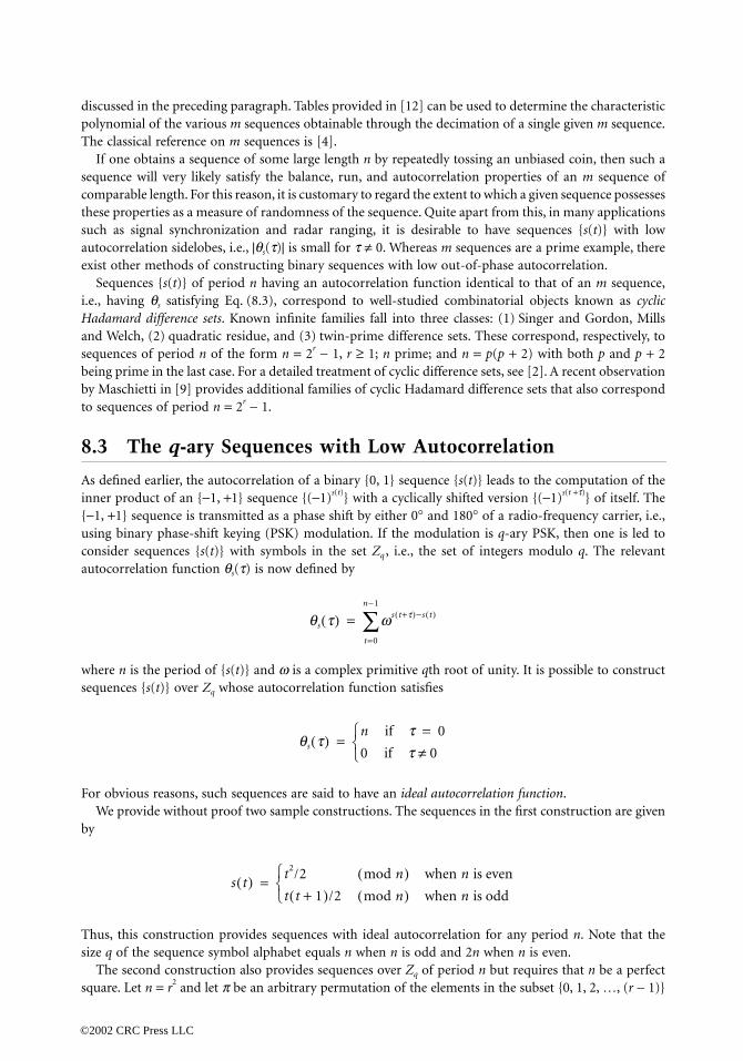
discussed in the preceding paragraph. Tables provided in [12] can be used to determine the characteristicpolynomial of the various m sequences obtainable through the decimation of a single given m sequence.The classical reference on m sequences is [4].

If one obtains a sequence of some large length n by repeatedly tossing an unbiased coin, then such asequence will very likely satisfy the balance, run, and autocorrelation properties of an m sequence ofcomparable length. For this reason, it is customary to regard the extent to which a given sequence possessesthese properties as a measure of randomness of the sequence. Quite apart from this, in many applicationssuch as signal synchronization and radar ranging, it is desirable to have sequences {s(t)} with lowautocorrelation sidelobes, i.e., |θs(τ)| is small for τ ≠ 0. Whereas m sequences are a prime example, thereexist other methods of constructing binary sequences with low out-of-phase autocorrelation.

Sequences {s(t)} of period n having an autocorrelation function identical to that of an m sequence,i.e., having θs satisfying Eq. (8.3), correspond to well-studied combinatorial objects known as cyclicHadamard difference sets. Known infinite families fall into three classes: (1) Singer and Gordon, Millsand Welch, (2) quadratic residue, and (3) twin-prime difference sets. These correspond, respectively, tosequences of period n of the form n = 2r − 1, r ≥ 1; n prime; and n = p(p + 2) with both p and p + 2being prime in the last case. For a detailed treatment of cyclic difference sets, see [2]. A recent observationby Maschietti in [9] provides additional families of cyclic Hadamard difference sets that also correspondto sequences of period n = 2r − 1.

8.3 The q-ary Sequences with Low Autocorrelation

As defined earlier, the autocorrelation of a binary {0, 1} sequence {s(t)} leads to the computation of theinner product of an {−1, +1} sequence {(−1)s(t)} with a cyclically shifted version {(−1)s(t +τ)} of itself. The{−1, +1} sequence is transmitted as a phase shift by either 0° and 180° of a radio-frequency carrier, i.e.,using binary phase-shift keying (PSK) modulation. If the modulation is q-ary PSK, then one is led toconsider sequences {s(t)} with symbols in the set Zq , i.e., the set of integers modulo q. The relevantautocorrelation function θs(τ) is now defined by

where n is the period of {s(t)} and ω is a complex primitive qth root of unity. It is possible to constructsequences {s(t)} over Zq whose autocorrelation function satisfies

For obvious reasons, such sequences are said to have an ideal autocorrelation function.We provide without proof two sample constructions. The sequences in the first construction are given

by

Thus, this construction provides sequences with ideal autocorrelation for any period n. Note that thesize q of the sequence symbol alphabet equals n when n is odd and 2n when n is even.

The second construction also provides sequences over Zq of period n but requires that n be a perfectsquare. Let n = r2 and let π be an arbitrary permutation of the elements in the subset {0, 1, 2, …, (r − 1)}

θs τ( ) ωs t+τ( )−s t( )

t=0

n−1

∑=

θs τ( )n if τ 0=0 if τ 0≠

=

s t( ) t2/2 mod n( ) when n is even

t t 1+( )/2 mod n( ) when n is odd

=



of Zn: Let g be an arbitrary function defined on the subset {0, 1, 2, …, r − 1} of Zn. Then any sequenceof the form

s(t) = rt1π(t2) + g(t2) (mod n)

where t = rt1 + t2 with 0 ≤ t1, t2 ≤ r − 1 is the base-r decomposition of t and has an ideal autocorrelationfunction. When the alphabet size q equals or divides the period n of the sequence, ideal-autocorrelationsequences also go by the name generalized bent functions. For details, see [6].

8.4 Families of Sequences with Low Crosscorrelation

Given two sequences {s1(t)} and {s2(t)} over Zq of period n, their crosscorrelation function θ1,2(τ) isdefined by

where ω is a primitive qth root of unity. The crosscorrelation function is important in code-divisionmultiple-access (CDMA) communication systems. Here, each user is assigned a distinct signature sequence,and to minimize interference due to the other users, it is desirable that the signature sequences havepairwise, low values of crosscorrelation function. To provide the system in addition with a self-synchronizingcapability, it is desirable that the signature sequences have low values of the autocorrelation function aswell.

Let F = {{si(t)} |1 ≤ i ≤ M} be a family of M sequences {si(t)} over Zq, each of period n. Let θi , j(τ)denote the crosscorrelation between the ith and jth sequence at shift τ, i.e.,

The classical goal in sequence design for CDMA systems has been minimization of the parameter

for fixed n and M. It should be noted though that, in practice, because of data modulation, the correlationsthat one runs into are typically of an aperiodic rather than a periodic nature (see Section 8.5). Theproblem of designing for low aperiodic correlation, however, is a more difficult one. A typical approach,therefore, has been to design based on periodic correlation and then analyze the resulting design for itsaperiodic correlation properties. Again, in many practical systems, the mean square correlation propertiesare of greater interest than the worst-case correlation represented by a parameter such as θmax. The meansquare correlation is discussed in Section 8.6.

Bounds on the minimum possible value of θmax for given period n, family size M, and alphabet size qare available that can be used to judge the merits of a particular sequence design. The most efficientbounds are those due to Welch, Sidelnikov, and Levenshtein, see [6]. In CDMA systems, there is greatestinterest in designs in which the parameter θmax is in the range ≤ θmax ≤ 2 . Accordingly, Table 8.1uses the Welch, Sidelnikov, and Levenshtein bounds to provide an order-of-magnitude upper bound onthe family size M for certain θmax in the cited range.

Practical considerations dictate that q be small. The bit-oriented nature of electronic hardware makesit preferable to have q a power of 2. With this in mind, a description of some efficient sequence familieshaving low auto- and crosscorrelation values and alphabet sizes q = 2 and q = 4 are described next.

θ1,2 τ( ) ωs1 t+τ( )−s2 t( )

t=0

n−1

∑=

θi , j τ( ) ωsi t+τ( )−sj t( )

, 0 τ≤ n 1–≤t=0

n−1

∑=

θmax max θi , j τ( ) either i j or τ 0≠≠{ }=

n n



Gold and Kasami Sequences

Given the low autocorrelation sidelobes of an m sequence, it is natural to attempt to construct familiesof low correlation sequences starting from m sequences. Two of the better known constructions of thistype are the families of Gold and Kasami sequences.

Let r be odd and d = 2k + 1, where k, 1 ≤ k ≤ r − 1, is an integer satisfying (k, r) = 1. Let {s(t)} be acyclic shift of an m sequence of period n = 2r − 1 that satisfies S(dt) � 0 and let G be the Gold family of2r + 1 sequences given by

Then, each sequence in G has period 2r − 1 and the maximum-correlation parameter θmax of G satisfies

An application of the Sidelnikov bound coupled with the information that θmax must be an odd integer yieldsthat for the family G, θmax is as small as it can possibly be. In this sense, the family G is an optimal family.We remark that these comments remain true even when d is replaced by the integer d = 22k − 2k + 1 withthe conditions on k remaining unchanged.

The Gold family remains the best-known family of m sequences having low crosscorrelation. Appli-cations include the Navstar Global Positioning System whose signals are based on Gold sequences.

The family of Kasami sequences has a similar description. Let r = 2v and d = 2v + 1. Let {s(t)} be acyclic shift of an m sequence of period n = 2r − 1 that satisfies s(dt) � 0, and consider the family ofKasami sequences given by

Then the Kasami family K contains 2v sequences of period 2r − 1. It can be shown that in this case

This time an application of the Welch bound and the fact that θmax is an integer shows that the Kasamifamily is optimal in terms of having the smallest possible value of θmax for given n and M.

Quaternary Sequences with Low Crosscorrelation

The entries in Table 8.1 suggest that nonbinary (i.e., q > 2) designs may be used for improved performance.A family of quaternary sequences that outperform the Gold and Kasami sequences is discussed next.

Let f(x) be the characteristic polynomial of a binary m sequence of length 2r − 1 for some integer r.The coefficients of f (x) are either 0 or 1. Now, regard f (x) as a polynomial over Z4 and form the product(−1)r f (x) f (−x). This can be seen to be a polynomial in x2. Define the polynomial g(x) of degree r by

TABLE 8.1 Bounds on Family Size M for Given n, θmax

θmax

Upper bound on M q = 2

Upper Bound on Mq > 2

n/2 n n n2/2

3n2/10 n3/2

n2n

2 n

G s t( ){ } s dt( ){ } s t( ) s d t τ+[ ]( )+{ } 0 τ n 1–≤≤{ }∪∪=

θmax 2r+1 1+≤

K s t( ){ } s t( ) s d t τ+[ ]( )+{ } 0 τ 2v 2–≤≤{ }∪=

θmax 1 2v+=



setting g(x2) = (−1)rf (x)f (−x). Let g(x) = gi xi and consider the set of all quaternary sequences {a(t)}satisfying the recursion gia(t + i) = 0 for all t.

It turns out that with the exception of the all-zero sequence, all of the sequences generated in this wayhave period 2r − 1. Thus, the recursion generates a family A of 2r + 1 cyclically distinct quaternary sequences.Closer study reveals that the maximum correlation parameter θmax of this family satisfies θmax ≤ 1 + .Thus, in comparison to the family of Gold sequences, the family A offers a lower value of θmax (by afactor of ) for the same family size. In comparison to the set of Kasami sequences, it offers a muchlarger family size for the same bound on θmax. Family A sequences may be found discussed in [16, 3].

We illustrate with an example. Let f (x) = x3 + x + 1 be the characteristic polynomial of the m sequence{a(t)} in Eq. (8.1). Then over Z4

so that g(x) = x3 + 2x2 + x + 3. Thus, the sequences in family A are generated by the recursion s(t + 3)+ 2s(t + 2) + s(t + 1) + 3s(t) = 0 mod 4. The corresponding shift register is shown in Fig. 8.3. By varyinginitial conditions, this shift register can be made to generate nine cyclically distinct sequences, each oflength 7. In this case θmax ≤ 1 + .

Binary Kerdock Sequences

The Gold and Kasami families of sequences are closely related to binary linear cyclic codes. It is wellknown in coding theory that there exist nonlinear binary codes whose performance exceeds that of thebest possible linear code. Surprisingly, some of these examples come from binary codes, which are imagesof linear quaternary (q = 4) codes under the Gray map: 0 → 00, 1 → 01, 2 → 11, 3 → 10. A prime exampleof this is the Kerdock code, which recently has been shown to be the Gray image of a quaternary linearcode. Thus, it is not surprising that the Kerdock code yields binary sequences that significantly outperformthe family of Kasami sequences.

The Kerdock sequences may be constructed as follows: let f (x) be the characteristic polynomial of anm sequence of period 2r − 1, r odd. As before, regarding f (x) as a polynomial over Z4 (which happensto have {0, 1} coefficients), let the polynomial g(x) over Z4 be defined via g(x2) = −f(x)f (−x). [Thus, g(x)is the characteristic polynomial of a family A sequence set of period 2r − 1.] Set h(x) = −g(−x) = hix

i,and let S be the set of all Z4 sequences satisfying the recursion his(t + i) = 0. Then S contains 4r-distinct sequences corresponding to all possible distinct initializations of the shift register.

Let T denote the subset S of size 2r consisting of those sequences corresponding to initializations ofthe shift register only using the symbols 0 and 2 in Z4. Then the set S − T of size 4r − 2r contains a set Uof 2r−1 cyclically distinct sequences each of period 2(2r − 1). Given x = a + 2b � Z4 with a, b � {0, 1},let µ denote the most significant bit (MSB) map µ(x) = b. Let KE denote the family of 2r −1 binary sequencesobtained by applying the map µ to each sequence in U. It turns out that each sequence in U also hasperiod 2(2r − 1) and that, furthermore, for the family KE , θmax ≤ 2 + . Thus, KE is a much largerfamily than the Kasami family, while having almost exactly the same value of θmax.

For example, taking r = 3 and f (x) = x3 + x + 1, we have from the previous family A example thatg(x) = x3 + 2x2 + x + 3, so that h(x) = −g(−x) = x3 + 2x2 + x + 1. Applying the MSB map to the head of

FIGURE 8.3 Shift register that generates family A quaternary sequences {s(t)} of period 7.

∑i=0r

∑i=0r

2r

2

g x2( ) 1–( )3f x( )f x–( ) x6 2x4 x2 3+ + += =

8

∑i=0r

∑i=0r

2r+1



the shift register and discarding initializations of the shift register involving only 0’s and 2’s yields a familyof four cyclically distinct binary sequences of period 14. Kerdock sequences are discussed in [6,11,1,17].

8.5 Aperiodic Correlation

Let {x(t)} and {y(t)} be complex-valued sequences of length (or period) n, not necessarily distinct. Theiraperiodic correlation values {ρx,y(τ) | − (n − 1) ≤ τ ≤ n − 1} are given by

where y∗(t) denotes the complex conjugate of y(t). When x � y, we will abbreviate and write ρx in placeof ρx,y. The sequences described next are perhaps the most famous example of sequences with low-aperiodic autocorrelation values.

Barker Sequences

A binary {−1, +1} sequence {s(t)} of length n is said to be a Barker sequence if the aperiodic autocorrelationvalues ρs(τ) satisfy |ρs(τ)| ≤ 1 for all τ, −(n − 1) ≤ τ ≤ n − 1. The Barker property is preserved under thefollowing transformations:

s(t) → −s(t), s(t) → (−1)ts(t) and s(t) → s(n − 1 − t)

as well as under compositions of the preceding transformations. Only the following Barker sequencesare known:

n = 2 + +n = 3 + + −

n = 4 + + + −

n = 5 + + + − +

n = 7 + + + − − + −

n = 11 + + + − − − + − − + −

n = 13 + + + + + − − + + − + − +

where + denotes +1 and − denotes −1 and sequences are generated from these via the transformationsalready discussed. It is known that if any other Barker sequence exists, it must have length n > 1,898,884,a multiple of 4.

For an upper bound to the maximum out-of-phase aperiodic autocorrelation of an m sequence,see [13].

Sequences with High Merit Factor

The merit factor F of a {−1, +1} sequence {s(t)} is defined by

ρx , y τ( ) x t τ+( )y∗ t( )t=max 0, τ–{ }

min n−1,n−1−τ{ }

∑=

Fn2

2∑τ=1n−1ρs

2 τ( )---------------------------=



Since ρs(τ) = ρs(−τ) for 1 ≤ |τ | ≤ n − 1 and ρs(0) = n, factor F may be regarded as the ratio of the squareof the in-phase autocorrelation to the sum of the squares of the out-of-phase aperiodic autocorrelation values.Thus, the merit factor is one measure of the aperiodic autocorrelation properties of a binary {−1, +1} sequence.It is also closely connected with the signal to self-generated noise ratio of a communication system inwhich coded pulses are transmitted and received.

Let Fn denote the largest merit factor of any binary {−1, +1} sequence of length n. For example, atlength n = 13, the Barker sequence of length 13 has a merit factor F = F13 = 14.08. Assuming a certainergodicity postulate it was established by Golay that limn→∞ Fn = 12.32. Exhaustive computer searchescarried out for n ≤ 40 have revealed the following.

1. For 1 ≤ n ≤ 40, n ≠ 11, 13,

3.3 ≤ Fn ≤ 9.85,

2. F11 = 12.1, F13 = 14.08.

The value F11 is also achieved by a Barker sequence. From partial searches, for lengths up to 117, thehighest known merit factor is between 8 and 9.56; for lengths from 118 to 200, the best-known factor isclose to 6. For lengths >200, statistical search methods have failed to yield a sequence having merit factorexceeding 5.

An offset sequence is one in which a fraction θ of the elements of a sequence of length n are choppedoff at one end and appended to the other end, i.e., an offset sequence is a cyclic shift of the originalsequence by nθ symbols. It turns out that the asymptotic merit factor of m sequences is equal to 3 andis independent of the particular offset of the m sequence. There exist offsets of sequences associated withquadratic-residue and twin-prime difference sets that achieve a larger merit factor of 6. Details may befound in [7].

Sequences with Low Aperiodic Crosscorrelation

If {u(t)} and {v(t)} are sequences of length 2n − 1 defined by

and

then

(8.6)

Given a collection

of sequences of length n over Zq, let us define

u t( )x t( ) if 0 t n 1–≤≤0 if n t≤ 2n 2–≤

=

v t( )y t( ) if 0 t n 1–≤≤0 if n t≤ 2n 2–≤

=

ρx ,y τ( ) n 1–( ) τ n 1–≤≤–{ } θu ,v τ( ) 0 τ 2n 2–≤≤{ }=

U xi t( ){ } 1 i M≤≤{ }=

ρmax max ρa ,b τ( ) a,b U, either a b or τ 0≠≠∈{ }=



It is clear from Eq. (8.6) how bounds on the periodic correlation parameter θmax can be adapted togive bounds on ρmax. Translation of the Welch bound gives that for every integer k ≥ 1,

Setting k = 1 in the preceding bound gives

Thus, for fixed M and large n, Welch’s bound gives

There exist sequence families which asymptotically achieve ρmax ≈ O(n1/2), [10].

8.6 Other Correlation Measures

Partial-Period Correlation

The partial-period (p-p) correlation between the sequences {u(t)} and {v(t)} is the collection {∆u,v(l, τ, t0)| 1 ≤l ≤ n, 0 ≤ τ ≤ n − 1, 0 ≤ t0 ≤ n − 1} of inner products

where l is the length of the partial period and the sum t + τ is again computed modulo n.In direct-sequence CDMA systems, the pseudorandom signature sequences used by the various users

are often very long for reasons of data security. In such situations, to minimize receiver hardware complexity,correlation over a partial period of the signature sequence is often used to demodulate data, as well as toachieve synchronization. For this reason, the p-p correlation properties of a sequence are of interest.

Researchers have attempted to determine the moments of the p-p correlation. Here the main tool isthe application of the Pless power-moment identities of coding theory [8]. The identities often allow thefirst and second p-p correlation moments to be completely determined. For example, this is true in thecase of m sequences (the remaining moments turn out to depend upon the specific characteristic poly-nomial of the m sequence). Further details may be found in [15].

Mean Square Correlation

Frequently in practice, there is a greater interest in the mean-square correlation distribution of a sequencefamily than in the parameter θmax. Quite often in sequence design, the sequence family is derived froma linear, binary cyclic code of length n by picking a set of cyclically distinct sequences of period n. Thefamilies of Gold and Kasami sequences are so constructed. In this case, as pointed out by Massey, themean square correlation of the family can be shown to be either optimum or close to optimum, undercertain easily satisfied conditions, imposed on the minimum distance of the dual code. A similar situationholds even when the sequence family does not come from a linear cyclic code. In this sense, mean square

ρmax2k n2k

M 2n 1–( ) 1–----------------------------------

M 2n 1–( )2n+k−2

k

------------------------- 1–

≥

ρmax nM 1–

M 2n 1–( ) 1–----------------------------------≥

ρmax O n1/2( )≥

∆u ,v l, τ, t0( ) u t τ+( )v∗ t( )t=t0

t=t0+ l−1

∑=



correlation is not a very discriminating measure of the correlation properties of a family of sequences.An expanded discussion of this issue may be found in [5].

Optical Orthogonal Codes

Given a pair of {0, 1} sequences {s1(t)} and {s2(t)} each having period n, we define the Hamming correlationfunction θ12(τ), 0 ≤ τ ≤ n − 1, by

Such correlations are of interest, for instance, in optical communication systems where the 1s and 0s ina sequence correspond to the presence or absence of pulses of transmitted light.

An (n, w, λ) optical orthogonal code (OOC) is a family F = {{si(t)} | i = 1, 2, …, M}, of M {0, 1} sequencesof period n and constant Hamming weight w, where w is an integer lying between 1 and n − 1 satisfyingθij(τ) ≤ λ whenever either i ≠ j or τ ≠ 0.

Note that the Hamming distance da,b between a period of the corresponding codewords {a(t)}, {b(t)},0 ≤ t ≤ n − 1, in an (n, w, λ) OOC having Hamming correlation ρ, 0 ≤ ρ ≤ λ, is given by da,b = 2(w − ρ),and, thus, OOCs are closely related to constant-weight error correcting codes. Given an (n, w, λ) OOC, byenlarging the OOC to include every cyclic shift of each sequence in the code, one obtains a constant-weight, minimum distance dmin ≥ 2(w − λ) code. Conversely, given a constant-weight cyclic code oflength n, weight w, and minimum distance dmin, one can derive an (n, w, λ) OOC code with λ ≤ w − dmin/2by partitioning the code into cyclic equivalence classes and then picking precisely one representativefrom each equivalence class of size n.

By making use of this connection, one can derive bounds on the size of an OOC from known boundson the size of constant-weight codes. The bound given next follows directly from the Johnson bound forconstant weight codes [8]. The number M(n, w, λ) of codewords in a (n, w, λ) OOC satisfies

An OOC code that achieves the Johnson bound is said to be optimal. A family {Fn} of OOCs indexedby the parameter n and arising from a common construction is said to be asymptotically optimum if

Constructions for optical orthogonal codes are available for the cases when λ = 1 and λ = 2. For largervalues of λ, there exist constructions which are asymptotically optimum. Further details may be found in [6].

Defining Terms

Autocorrelation of a sequence: The complex inner product of the sequence with a shifted version itself.Crosscorrelation of two sequences: The complex inner product of the first sequence with a shifted

version of the second sequence.m Sequence: A periodic binary {0, 1} sequence that is generated by a shift register with linear feedback

and which has maximal possible period given the number of stages in the shift register.Pseudonoise sequences: Also referred to as pseudorandom sequences (PN), these are sequences that

are deterministically generated and yet possess some properties that one would expect to find inrandomly generated sequences.

θ12 τ( ) s1 t τ+( )s2 t( )t=0

n−1

∑=

M n, w, λ( ) 1w--- n 1–

w 1–------------… n λ 1+–

w λ 1+–---------------------- n λ–

w λ–------------- …≤

Fn

M n, w, λ( )--------------------------

n→∞lim 1=



Shift-register sequence: A sequence with symbols drawn from a field, which satisfies a linear-recurrencerelation and which can be implemented using a shift register.

References

1. Barg, A., On small families of sequences with low periodic correlation, Lecture Notes in ComputerScience, 781, 154–158, Springer-Verlag, Berlin, 1994.

2. Baumert, L.D., Cyclic Difference Sets, Lecture Notes in Mathematics 182, Springer–Verlag, New York,1971.

3. Boztaş, S., Hammons, R., and Kumar, P.V. 4-phase sequences with near-optimum correlation prop-erties, IEEE Trans. Inform. Theory, IT-38, 1101–1113, 1992.

4. Golomb, S.W., Shift Register Sequences, Aegean Park Press, San Francisco, CA, 1982.5. Hammons, A.R., Jr. and Kumar, P.V., On a recent 4-phase sequence design for CDMA, IEICE Trans.

Commun., E76-B(8), 1993.6. Helleseth, T. and Kumar, P.V. (planned), Sequences with low correlation, In Handbook of Coding

Theory, V.S. Pless and W.C. Huffman, Eds., Elsevier Science Publishers, Amsterdam, 1998.7. Jensen, J.M., Jensen, H.E., and Høholdt, T., The merit factor of binary sequences related to difference

sets, IEEE Trans. Inform. Theory, IT-37(May), 617–626, 1991.8. MacWilliams, F.J. and Sloane, N.J.A., The Theory of Error-Correcting Codes, North-Holland, Amster-

dam, 1977.9. Maschietti, A., Difference sets and hyperovals, Designs, Codes and Cryptography, 14, 89–98, 1998.

10. Mow, W.H., On McEliece’s open problem on minimax aperiodic correlation, In Proc. IEEE Intern.Symp. Inform. Theory, 75, 1994.

11. Nechaev, A., The Kerdock code in a cyclic form, Discrete Math. Appl., 1, 365–384, 1991.12. Peterson, W.W. and Weldon, E.J., Jr., Error-Correcting Codes, 2nd ed., MIT Press, Cambridge, MA,

1972.13. Sarwate, D.V., An upper bound on the aperiodic autocorrelation function for a maximal-length

sequence, IEEE Trans. Inform. Theory, IT-30(July), 685–687, 1984.14. Sarwate, D.V. and Pursley, M.B., Crosscorrelation properties of pseudorandom and related sequences,

Proc. IEEE, 68(May), 593–619, 1980.15. Simon, M.K.,Omura, J.K., Scholtz, R.A., and Levitt, B.K., Spread Spectrum Communications Hand-

book, revised ed., McGraw-Hill, New York, 1994.16. Solé, P., A quaternary cyclic code and a family of quadriphase sequences with low correlation

properties, Coding Theory and Applications, Lecture Notes in Computer Science, 388, 193–201, Berlin,Springer-Verlag, 1989.

17. Udaya, P. and Siddiqi, M., Optimal biphase sequences with large linear complexity derived fromsequences over Z4, IEEE Trans. Inform. Theory, IT-42 (Jan), 206–216, 1996.

Further Information

A more in-depth treatment of pseudonoise sequences may be found in the following.1. Golomb, S.W., Shift Register Sequences, Aegean Park Press, San Francisco, 1982.2. Helleseth, T. and Kumar, P.V., Sequences with Low Correlation, in Handbook of Coding Theory, edited

by V.S. Pless and W.C. Huffman, Elsevier Science Publishers, Amsterdam, 1998 (planned).3. Sarwate, D.V. and Pursley, M.B., Crosscorrelation Properties of Pseudorandom and Related Sequences,

Proc. IEEE, 68, May, 593–619, 1980.4. Simon, M.K., Omura, J.K., Scholtz, R.A., and Levitt, B.K., Spread Spectrum Communications Handbook,

revised ed., McGraw Hill, New York, 1994.



9D/A and A/D

Converters

9.1 D/A and A/D Circuits D/A and A/D Converter Performance Criteria • D/A Conversion Processes • D/A Converter ICs • A/D Conversion Processes • A/D Converter ICs • Grounding and Bypassing on D/A and A/D ICs • Selection Criteria for D/A and A/D Converter ICs

Digital-to-analog (D/A) conversion is the process of converting digital codes into a continuous range ofanalog signals. Analog-to-digital (A/D) conversion is the complementary process of converting a contin-uous range of analog signals into digital codes. Such conversion processes are necessary to interface real-world systems, which typically monitor continuously varying analog signals, with digital systems thatprocess, store, interpret, and manipulate the analog values.

D/A and A/D applications have evolved from predominately military-driven applications to consumer-oriented applications. Up to the mid-1980s, the military applications determined the design of manyD/A and A/D devices. The military applications required very high performance coupled with hermeticpackaging, radiation hardening, shock and vibration testing, and military specification and record keeping.Cost was of little concern, and “low power” applications required approximately 2.8 W. The major applica-tions up to the mid-1980s included military radar warning and guidance systems, digital oscilloscopes,medical imaging, infrared systems, and professional video.

The applications currently requiring D/A and A/D circuits have different performance criteria fromthose of earlier years. In particular, low power and high speed applications are driving the developmentof D/A and A/D circuits, as the devices are used extensively in battery-operated consumer products. Thepredominant applications include cellular telephones, hand-held camcorders, portable computers, andset-top cable TV boxes. These applications generally have low power and long battery life requirements,or they may have high speed and high resolution requirements, as is the case with the set-top cable TVboxes.

9.1 D/A and A/D Circuits

D/A and A/D conversion circuits are available as integrated circuits (ICs) from many manufacturers. Ahuge array of ICs exists, consisting of not only the D/A or A/D conversion circuits, but also closely relatedcircuits such as sample-and-hold amplifiers, analog multiplexers, voltage-to-frequency and frequency-to-voltage converters, voltage references, calibrators, operation amplifiers, isolation amplifiers, instru-mentation amplifiers, active filters, DC-to-DC converters, analog interfaces to digital signal processingsystems, and data acquisition subsystems. Data books from the IC manufacturers contain an enormousamount of information about these devices and their applications to assist the design engineer.

Susan A.R. GarrodPurdue University


The ICs discussed in this chapter will be strictly the D/A and A/D conversion circuits. Table 9.1 listsa small sample of the variety of the D/A and A/D converters currently available. The ICs usually performeither D/A or A/D conversion. There are serial interface ICs, however, typically for high-performanceaudio and digital signal processing applications, that perform both A/D and D/A processes.

D/A and A/D Converter Performance Criteria

The major factors that determine the quality of performance of D/A and A/D converters are resolution,sampling rate, speed, and linearity.

The resolution of a D/A circuit is the smallest change in the output analog signal. In an A/D system,the resolution is the smallest change in voltage that can be detected by the system and that can producea change in the digital code. The resolution determines the total number of digital codes, or quantizationlevels, that will be recognized or produced by the circuit.

TABLE 9.1 D/A and A/D Integrated Circuits

Multiplying vs Input DataD/A Converter ICs Resolution, b Fixed Reference Settling Time, ms Format

Analog devices AD558

8 Fixed reference 3 Parallel


8 Multiplying 0.400 Parallel


Quad, 12 Fixed reference 8 Parallel


16 Fixed reference 1.5 Serial

Burr–Brown DAC729

18 Fixed reference 8 Parallel

DATEL DACHF8


National DAC0800


A/D Converter ICs Resolution, b Signal Inputs Conversion Speed, ms Output Data Format


12 1 25 Serial and Parallel

Burr–Brown ADC803

12 1 1.5 Parallel

Burr–Brown ADC701

16 1 1.5 Parallel

NationalADC1005B

10 1 50 Parallel

TI, National ADC0808

8 8 100 Parallel

TI, National ADC0834

8 4 32 Serial

TI TLC0820 8 1 1 ParallelTI TLC1540 10 11 21 Serial

Interface ICs A/D and D/A Resolution, b Onboard Filters Sampling Rate, kHz Data Format

TI TLC32040 14 Yes 19.2 (programmable) SerialTI 2914 PCM

codec and filter 8 Yes 8 Serial


The resolution of a D/A or A/D IC is usually specified in terms of the bits in the digital code or in terms ofthe least significant bit (LSB) of the system. An n-bit code allows for 2n quantization levels, or 2n - 1 stepsbetween quantization levels. As the number of bits increases, the step size between quantization levels decreases,therefore increasing the accuracy of the system when a conversion is made between an analog and digitalsignal. The system resolution can be specified also as the voltage step size between quantization levels. For A/Dcircuits, the resolution is the smallest input voltage that is detected by the system.

The speed of a D/A or A/D converter is determined by the time it takes to perform the conversionprocess. For D/A converters, the speed is specified as the settling time. For A/D converters, the speed isspecified as the conversion time. The settling time for D/A converters will vary with supply voltage andtransition in the digital code; thus, it is specified in the data sheet with the appropriate conditions stated.

A/D converters have a maximum sampling rate that limits the speed at which they can performcontinuous conversions. The sampling rate is the number of times per second that the analog signal canbe sampled and converted into a digital code. For proper A/D conversion, the minimum sampling ratemust be at least two times the highest frequency of the analog signal being sampled to satisfy the Nyquistsampling criterion. The conversion speed and other timing factors must be taken into consideration todetermine the maximum sampling rate of an A/D converter. Nyquist A/D converters use a sampling ratethat is slightly more than twice the highest frequency in the analog signal. Oversampling A/D convertersuse sampling rates of N times rate, where N typically ranges from 2 to 64.

Both D/A and A/D converters require a voltage reference in order to achieve absolute conversionaccuracy. Some conversion ICs have internal voltage references, whereas others accept external voltagereferences. For high-performance systems, an external precision reference is needed to ensure long-termstability, load regulation, and control over temperature fluctuations. External precision voltage referenceICs can be found in manufacturers’ data books.

Measurement accuracy is specified by the converter’s linearity. Integral linearity is a measure of linearityover the entire conversion range. It is often defined as the deviation from a straight line drawn betweenthe endpoints and through zero (or the offset value) of the conversion range. Integral linearity is alsoreferred to as relative accuracy. The offset value is the reference level required to establish the zero ormidpoint of the conversion range. Differential linearity is the linearity between code transitions. Differ-ential linearity is a measure of the monotonicity of the converter. A converter is said to be monotonic ifincreasing input values result in increasing output values.

The accuracy and linearity values of a converter are specified in the data sheet in units of the LSB ofthe code. The linearity can vary with temperature, and so the values are often specified at +25°C as wellas over the entire temperature range of the device.

D/A Conversion Processes

Digital codes are typically converted to analog voltages by assigning a voltage weight to each bit in thedigital code and then summing the voltage weights of the entire code. A general D/A converter consistsof a network of precision resistors, input switches, and level shifters to activate the switches to converta digital code to an analog current or voltage. D/A ICs that produce an analog current output usuallyhave a faster settling time and better linearity than those that produce a voltage output. When the outputcurrent is available, the designer can convert this to a voltage through the selection of an appropriateoutput amplifier to achieve the necessary response speed for the given application.

D/A converters commonly have a fixed or variable reference level. The reference level determines theswitching threshold of the precision switches that form a controlled impedance network, which in turncontrols the value of the output signal. Fixed reference D/A converters produce an output signal that isproportional to the digital input. Multiplying D/A converters produce an output signal that is propor-tional to the product of a varying reference level times a digital code.

D/A converters can produce bipolar, positive, or negative polarity signals. A four-quadrant multiplyingD/A converter allows both the reference signal and the value of the binary code to have a positive ornegative polarity. The four-quadrant multiplying D/A converter produces bipolar output signals.


D/A Converter ICs

Most D/A converters are designed for general-purpose control applications. Some D/A converters, how-ever, are designed for special applications, such as video or graphic outputs, high-definition video displays,ultra high-speed signal processing, digital video tape recording, digital attenuators, or high-speed func-tion generators.

D/A converter ICs often include special features that enable them to be interfaced easily to micropro-cessors or other systems. Microprocessor control inputs, input latches, buffers, input registers, andcompatibility to standard logic families are features that are readily available in D/A ICs. In addition, theICs usually have laser-trimmed precision resistors to eliminate the need for user trimming to achievefull-scale performance.

A/D Conversion Processes

Analog signals can be converted to digital codes by many methods, including integration, successiveapproximation, parallel (flash) conversion, delta modulation, pulse code modulation, and sigma–deltaconversion. Two of the most common A/D conversion processes are successive approximation A/Dconversion and parallel or flash A/D conversion. Very high-resolution digital audio or video systemsrequire specialized A/D techniques that often incorporate one of these general techniques as well asspecialized A/D conversion processes. Examples of specialized A/D conversion techniques are pulse codemodulation (PCM) and sigma–delta conversion. PCM is a common voice encoding scheme used notonly by the audio industry in digital audio recordings but also by the telecommunications industry forvoice encoding and multiplexing. Sigma–delta conversion is an oversampling A/D conversion wheresignals are sampled at very high frequencies. It has very high resolution and low distortion and is beingused in the digital audio recording industry.

Successive approximation A/D conversion is a technique that is commonly used in medium- to high-speed data acquisition applications. It is one of the fastest A/D conversion techniques that requires aminimum amount of circuitry. The conversion times for successive approximation A/D conversiontypically range from 10 to 300 ms for 8-b systems.

The successive approximation A/D converter can approximate the analog signal to form an n-bit digitalcode in n steps. The successive approximation register (SAR) individually compares an analog inputvoltage to the midpoint of one of n ranges to determine the value of 1 b. This process is repeated a totalof n times, using n ranges, to determine the n bits in the code. The comparison is accomplished as follows.The SAR determines if the analog input is above or below the midpoint and sets the bit of the digitalcode accordingly. The SAR assigns the bits beginning with the most significant bit. The bit is set to a 1if the analog input is greater than the midpoint voltage, or it is set to a 0 if it is less than the midpointvoltage. The SAR then moves to the next bit and sets it to a 1 or a 0 based on the results of comparingthe analog input with the midpoint of the next allowed range. Because the SAR must perform oneapproximation for each bit in the digital code, an n-bit code requires n approximations.

A successive approximation A/D converter consists of four functional blocks, as shown in Fig. 9.1: theSAR, the analog comparator, a D/A converter, and a clock.

Parallel or flash A/D conversion is used in high-speed applications such as video signal processing,medical imaging, and radar detection systems. A flash A/D converter simultaneously compares the inputanalog voltage to 2n - 1 threshold voltages to produce an n-bit digital code representing the analogvoltage. Typical flash A/D converters with 8-b resolution operate at 20–100 MHz.

The functional blocks of a flash A/D converter are shown in Fig. 9.2. The circuitry consists of a precisionresistor ladder network, 2n-1 analog comparators, and a digital priority encoder. The resistor networkestablishes threshold voltages for each allowed quantization level. The analog comparators indicatewhether the input analog voltage is above or below the threshold at each level. The output of the analogcomparators is input to the digital priority encoder. The priority encoder produces the final digital outputcode that is stored in an output latch.


An 8-b flash A/D converter requires 255 comparators. The cost of high-resolution A/D comparatorsescalates as the circuit complexity increases and as the number of analog converters rises by 2n-1. Asa low-cost alternative, some manufacturers produce modified flash A/D converters that perform theA/D conversion in two steps to reduce the amount of circuitry required. These modified flash A/Dconverters are also referred to as half-flash A/D converters, since they perform only half of the conversionsimultaneously.

A/D Converter ICs

A/D converter ICs can be classified as general-purpose, high-speed, flash, and sampling A/D converters.The general-purpose A/D converters are typically low speed and low cost, with conversion times rangingfrom 2 ms to 33 ms. A/D conversion techniques used by these devices typically include successiveapproximation, tracking, and integrating. The general-purpose A/D converters often have control signalsfor simplified microprocessor interfacing. These ICs are appropriate for many process control, industrial,and instrumentation applications, as well as for environmental monitoring such as seismology, ocean-ography, meteorology, and pollution monitoring.

High-speed A/D converters have conversion times typically ranging from 400 ns to 3 ms. The higherspeed performance of these devices is achieved by using the successive approximation technique, modifiedflash techniques, and statistically derived A/D conversion techniques. Applications appropriate for theseA/D ICs include fast Fourier transform (FFT) analysis, radar digitization, medical instrumentation, andmultiplexed data acquisition. Some ICs have been manufactured with an extremely high degree of linearityto be appropriate for specialized applications in digital spectrum analysis, vibration analysis, geologicalresearch, sonar digitizing, and medical imaging.

FIGURE 9.1 Successive approximation A/D converter block diagram. (Source: Garrod, S. and Borns, R. 1991, DigitalLogic: Analysis, Application, and Design, p. 919 Copyright ” 1991 by Saunders College Publishing, Philadelphia, PA.Reprinted with permission of the publisher.)


Flash A/D converters have conversion times ranging typically from 10 to 50 ns. Flash A/D conversiontechniques enable these ICs to be used in many specialized high-speed data acquisition applications suchas TV-video digitizing (encoding), radar analysis, transient analysis, high-speed digital oscilloscopes,medical ultrasound imaging, high-energy physics, and robotic vision applications.

Sampling A/D converters have a sample-and-hold amplifier circuit built into the IC. This eliminatesthe need for an external sample-and-hold circuit. The throughput of these A/D converter ICs rangestypically from 35 kHz to 100 MHz. The speed of the system is dependent on the A/D technique used bythe sampling A/D converter.

A/D converter ICs produce digital codes in a serial or parallel format, and some ICs offer the designerboth formats. The digital outputs are compatible with standard logic families to facilitate interfacing toother digital systems. In addition, some A/D converter ICs have a built-in analog multiplexer and thereforecan accept more than one analog input signal.

Pulse code modulation (PCM) ICs are high-precision A/D converters. The PCM IC is often referred toas a PCM codec with both encoder and decoder functions. The encoder portion of the codec performsthe A/D conversion, and the decoder portion of the codec performs the D/A conversion. The digital codeis usually formatted as a serial data stream for ease of interfacing to digital transmission and multiplexingsystems.

PCM is a technique whereby an analog signal is sampled, quantized, and then encoded as a digitalword. The PCM IC can include successive approximation techniques or other techniques to accomplishthe PCM encoding. In addition, the PCM codec may employ nonlinear data compression techniques,such as companding, if it is necessary to minimize the number of bits in the output digital code. Com-panding is a logarithmic technique used to compress a code to fewer bits before transmission. The inverse

FIGURE. 9.2 Flash A/D converter block diagram. (Source: Garrod, S. and Borns, R., Digital Logic: Analysis, Appli-cation, and Design, p. 928. Copyright ” 1991 by Saunders College Publishing, Philadelphia, PA. Reprinted withpermission of the publisher.)

logarithmic function is then used to expand the code to its original number of bits before converting itto the analog signal. Companding is typically used in telecommunications transmission systems tominimize data transmission rates without degrading the resolution of low-amplitude signals. Two stan-dardized companding techniques are used extensively: A-law and m-law. The A-law companding is usedin Europe, whereas the m-law is used predominantly in the United States and Japan. Linear PCMconversion is used in high-fidelity audio systems to preserve the integrity of the audio signal throughoutthe entire analog range.

Digital signal processing (DSP) techniques provide another type of A/D conversion ICs. Specialized A/Dconversion such as adaptive differential pulse code modulation (ADPCM), sigma–delta modulation, speechsubband encoding, adaptive predictive speech encoding, and speech recognition can be accomplished throughthe use of DSP systems. Some DSP systems require analog front ends that employ traditional PCM codecICs or DSP interface ICs. These ICs can interface to a digital signal processor for advanced A/D applications.Some manufacturers have incorporated DSP techniques on board the single-chip A/D IC, as in the caseof the DSP56ACD16 sigma–delta modulation IC by Motorola.

Integrating A/D converters are used for conversions that must take place over a long period of time,such as digital voltmeter applications or sensor applications such as thermocouples. The integrating A/Dconverter produces a digital code that represents the average of the signal over time. Noise is reduced bymeans of signal averaging, or integration. Dual-lope integration is accomplished by a counter thatadvances while an input voltage charges a capacitor in a specified time interval, T. This is compared toanother count sequence that advances while a reference voltage is discharging across the same capacitorin a time interval, delta t. The ratio of the charging count value to the discharging count value isproportional to the ratio of the input voltage to the reference voltage. Hence, the integrating converterprovides a digital code that is a measure of the input voltage averaged over time. The conversion accuracyis independent of the capacitor and the clock frequency since they affect both the charging and dischargingoperations. The charging period, T, is selected to be the period of the fundamental frequency to berejected. The maximum conversion rate is slightly less than 1/(2T) conversions per second. While thislimits the conversion rate to be too slow for high-speed data acquisition applications, it is appropriatefor long-duration applications of slowly varying input signals.

Grounding and Bypassing on D/A and A/D ICs

D/A and A/D converter ICs require correct grounding and capacitive bypassing in order to operateaccording to performance specifications. The digital signals can severely impair analog signals. To combatthe electromagnetic interference induced by the digital signals, the analog and digital grounds should bekept separate and should have only one common point on the circuit board. If possible, this commonpoint should be the connection to the power supply.

Bypass capacitors are required at the power connections to the IC, the reference signal inputs,and the analog inputs to minimize noise that is induced by the digital signals. Each manufacturerspecifies the recommended bypass capacitor locations and values in the data sheet. The 1-mF tantalumcapacitors are commonly recommended, with additional high-frequency power supply decouplingsometimes being recommended through the use of ceramic disc shunt capacitors. The manufacturers’recommendations should be followed to ensure proper performance.

Selection Criteria for D/A and A/D Converter ICs

Hundreds of D/A and A/D converter ICs are available, with prices ranging from a few dollars to severalhundred dollars each. The selection of the appropriate type of converter is based on the applicationrequirements of the system, the performance requirements, and cost. The following issues should beconsidered in order to select the appropriate converter.

1. What are the input and output requirements of the system? Specify all signal current and voltageranges, logic levels, input and output impedances, digital codes, data rates, and data formats.


2. What level of accuracy is required? Determine the resolution needed throughout the analog voltagerange, the dynamic response, the degree of linearity, and the number of bits encoding.

3. What speed is required? Determine the maximum analog input frequency for sampling in an A/Dsystem, the number of bits for encoding each analog signal, and the rate of change of input digitalcodes in a D/A system.

4. What is the operating environment of the system? Obtain information on the temperature rangeand power supply to select a converter that is accurate over the operating range.

Final selection of D/A and A/D converter ICs should be made by consulting manufacturers to obtaintheir technical specifications of the devices. Major manufacturers of D/A and A/D converters includeAnalog Devices, Burr–Brown, DATEL, Maxim, National, Phillips Components, Precision Monolithics,Signetics, Sony, Texas Instruments, Ultra Analog, and Yamaha. Information on contacting these manu-facturers and others can be found in an IC Master Catalog.

Defining Terms

Companding: A process designed to minimize the transmission bit rate of a signal by compressing itprior to transmission and expanding it upon reception. It is a rudimentary “data compression”technique that requires minimal processing.

Delta modulation: An A/D conversion process where the digital output code represents the change, orslope, of the analog input signal, rather than the absolute value of the analog input signal. A 1indicates a rising slope of the input signal. A 0 indicates a falling slope of the input signal. Thesampling rate is dependent on the derivative of the signal, since a rapidly changing signal wouldrequire a rapid sampling rate for acceptable performance.

Fixed reference D/A converter: The analog output is proportional to a fixed (nonvarying) referencesignal.

Flash A/D: The fastest A/D conversion process available to date, also referred to as parallel A/D con-version. The analog signal is simultaneously evaluated by 2n - 1 comparators to produce an n-bitdigital code in one step. Because of the large number of comparators required, the circuitry forflash A/D converters can be very expensive. This technique is commonly used in digital videosystems.

Integrating A/D: The analog input signal is integrated over time to produce a digital signal thatrepresents the area under the curve, or the integral.

Multiplying D////A: A D/A conversion process where the output signal is the product of a digital codemultiplied by an analog input reference signal. This allows the analog reference signal to be scaledby a digital code.

Nyquist A/D converters: A/D converters that sample analog signals that have a maximum frequencythat is less than the Nyquist frequency. The Nyquist frequency is defined as one-half of the samplingfrequency. If a signal has frequencies above the Nyquist frequency, a distortion called aliasingoccurs. To prevent aliasing, an antialiasing filter with a flat passband and very sharp rolloff isrequired.

Oversampling converters: A/D converters that sample frequencies at a rate much higher than theNyquist frequency. Typical oversampling rates are 32 and 64 times the sampling rate that wouldbe required with the Nyquist converters.

Pulse code modulation (PCM): An A/D conversion process requiring three steps: the analog signal issampled, quantized, and encoded into a fixed length digital code. This technique is used in manydigital voice and audio systems. The reverse process reconstructs an analog signal from the PCMcode. The operation is very similar to other A/D techniques, but specific PCM circuits are optimizedfor the particular voice or audio application.

Sigma–delta A/D conversion: An oversampling A/D conversion process where the analog signal issampled at rates much higher (typically 64 times) than the sampling rates that would be requiredwith a Nyquist converter. Sigma–delta modulators integrate the analog signal before performing


the delta modulation. The integral of the analog signal is encoded rather than the change in theanalog signal, as is the case for traditional delta modulation. A digital sample rate reduction filter(also called a digital decimation filter) is used to provide an output sampling rate at twice theNyquist frequency of the signal. The overall result of oversampling and digital sample rate reductionis greater resolution and less distortion compared to a Nyquist converter process.

Successive approximation: An A/D conversion process that systematically evaluates the analog signalin n steps to produce an n-bit digital code. The analog signal is successively compared to determinethe digital code, beginning with the determination of the most significant bit of the code.

References

Analog Devices. 1989. Analog Devices Data Conversion Products Data Book. Analog Devices, Inc.,Norwood, MA.

Burr–Brown. 1989. Burr–Brown Integrated Circuits Data Book. Burr–Brown, Tucson, AZ.DATEL. 1988. DATEL Data Conversion Catalog. DATEL, Inc., Mansfield, MA.Drachler, W. and Murphy, B. 1995. New High-Speed, Low-Power Data-Acquisition ICs, Analog Dialogue

29(2):3–6. Analog Devices, Inc., Norwood, MA. Garrod, S. and Borns, R. 1991. Digital Logic: Analysis, Application and Design, Chap. 16. Saunders College

Publishing, Philadelphia PA.Jacob, J.M. 1989. Industrial Control Electronics, Chap. 6. Prentice–Hall, Englewood Cliffs, NJ.Keiser, B. and Strange, E. 1995. Digital Telephony and Network Integration, 2nd ed. Van Nostrand Reinhold,

New York.Motorola. 1989. Motorola Telecommunications Data Book. Motorola, Inc., Phoenix, AZ.National Semiconductor. 1989. National Semiconductor Data Acquisition Linear Devices Data Book.

National Semiconductor Corp., Santa Clara, CA.Park, S. 1990. Principles of Sigma–Delta Modulation for Analog-to-Digital Converters. Motorola, Inc.,

Phoenix, AZ.Texas Instruments. 1986. Texas Instruments Digital Signal Processing Applications with the TMS320 Family.

Texas Instruments, Dallas, TX. Texas Instruments. 1989. Texas Instruments Linear Circuits Data Acquisition and Conversion Data Book.

Texas Instruments, Dallas, TX.

Further Information

Analog Devices, Inc. has edited or published several technical handbooks to assist design engineers withtheir data acquisition system requirements. These references should be consulted for extensive technicalinformation and depth. The publications include Analog-Digital Conversion Handbook, by the engineeringstaff of Analog Devices, published by Prentice–Hall, Englewood Cliffs, NJ, 1986; Nonlinear CircuitsHandbook, Transducer Interfacing Handbook, and Synchro and Resolver Conversion, all published by AnalogDevices Inc., Norwood, MA.

Engineering trade journals and design publications often have articles describing recent A/D and D/Acircuits and their applications. These publications include EDN Magazine, EE Times, and IEEE Spectrum.Research-related topics are covered in IEEE Transactions on Circuits and Systems and IEEE Transactionson Instrumentation and Measurement.


10Signal Space

10.1 Introduction 10.2 Fundamentals10.3 Application of Signal Space Representation

to Signal Detection10.4 Application of Signal Space Representation

to Parameter EstimationWavelet Transforms • Mean Square Estimation—the Orthogonality Principle

10.1 Introduction

Signal space concepts have their roots in the mathematical theory of inner product spaces known asHilbert spaces [Stakgold, 1967]. Many books on linear systems touch on the subject of signal spaces inthe context of Fourier series and transforms [Ziemer, Tranter, and Fannin, 1998]. The applications ofsignal space concepts in communication theory find their power in the representation of signal detectionand estimation problems in geometrical terms, which provides much insight into signalling techniquesand communication system design. The first person to have apparently exploited the power of signalspace concepts in communication theory was the Russian Kotel’nikov [1968], who presented his doctoraldissertation in January, 1947. Wozencraft and Jacobs [1965] expanded on this approach and their workis still today widely referenced. Arthurs and Dym [1962] made use of signal space concepts in theperformance analysis of several digital modulation schemes. A one-chapter summary of the use of signalspace methods in signal detection and estimation is provided in Ziemer and Tranter [2002]. Anotherapplication of signal space concepts is in signal and image compression. Wavelet theory [Rioul andVetterli, 1991] is currently finding use in these application areas. In the next section, the fundamentalsof generalized vector spaces are summarized, followed by an overview of several applications to signalrepresentations.

10.2 Fundamentals

A linear space or vector space (signal space) [Stakgold, 1967] is a collection of elements (called vectors)x, y, z,…, for which the following axioms are satisfied:

1. To every pair of vectors x and y there corresponds a vector x + y, with the properties:a. x + y = y + xb. x + (y + z) = (x + y) + zc. There exists a unique element 0 such that x + 0 = x for every xd. To every x, there exists a unique vector labeled -x such that x + (-x) = 0

2. To all vectors x and y, and all numbers a and b (in general, complex), the following commutativeand associative rules hold:

Roger E. ZiemerUniversity of Coloradoat Colorado Springs


a. a(bx) = (a b)xb. (a + b)x = ax + byc. a(x + y) = ax + ayd. 1x = x, where 1 is the identity element

A vector is said to be a linear combination of the vectors x1, x2,…,xk in a vector space if there existnumbers (in general, complex) a1, a2,…,ak such that

(10.1)

The vectors x1, x2,…,xk are said to be linearly dependent (or form a dependent set) if there exist complexnumbers a1, a2,…,ak, not all zero, such that

(10.2)

If Eq. (10.2) can be satisfied only for a1 = a2 = = ak = 0, the vectors are linearly independent.One is tempted to use the infinite-sum version of Eq. (10.2) in defining the notion of independence

for an infinite set of vectors. This is not true in general; one needs the notion of convergence, which isbased on the concept of distance between vectors.

With the idea of linear independence firmly in mind, the concept of dimension of a vector spacereadily follows. A vector space is n-dimensional if it possesses a set of n independent vectors, but everyset of n + 1 vectors is a dependent set. If for every positive integer k, a set of k independent vectors inthe space can be found, the space is said to be infinite dimensional. A basis for a vector space means afinite set of vectors e1, e2,…,ek with the following attributes:

1. They are linearly independent.2. Every vector x in the space can be written as a linear combination of the basis vectors; that is

(10.3)

It can be proved that the representation (10.3) is unique and that if the space is n-dimensional, any setof n independent vectors e1, e2,…, en forms a basis.

The next concept to be developed is that of a metric space. In addition to the addition of vectors andmultiplication of vectors by scalars, as is true of ordinary three-dimensional vectors, it is important tohave the notions of length and direction of a vector imposed. In other words, a metric structure mustbe added to the algebraic structure already defined. A collection of elements x, y, z,… in a space will becalled a metric space if to each pair of elements x, y there corresponds a real number d(x, y) satisfyingthe properties:

1. d(x, y) = d(y, x)2. d(x, y) ≥ 0 with equality if and only if x = y3. d(x, z) d(x, y) + d(x, z) (called the triangle inequality)

The function d(x, y) is called a metric (or distance function). Note that the definition of d(x, y) does notrequire that the elements be vectors; there may not be any way of adding elements or multiplying themby scalars as required for a vector space.

With the definition of a metric, one can now discuss the idea of convergence of a sequence { xk} ofelements in the space. Note that d(xk, x) is a sequence of real numbers. Therefore, it is sensible to write that

0 (10.4)

x aixi

i=1

k

∑=

a1x1 a2x2… akxk+ + + 0=

…

x xiei

i=1

k

∑=

≤

xkk→∞lim x=


if the sequence of numbers d(xk, x) converges to 0 in the ordinary sense of convergence of sequences ofreal numbers. If

(10.5)

the sequence {xk} is said to be a Cauchy sequence. It can be shown that if a sequence {xk} converges, itis a Cauchy sequence. The converse is not necessarily true, for the limit may have carelessly been excludedfrom the space. If the converse is true, then the metric space is said to be complete.

The next vector space concept to be defined is that of length or norm of a vector. A normed vectorspace (or linear space) is a vector space in which a real-valued function (known as the norm of x) isdefined, with the properties

1. with equality if and only if x = 02.3.

A normed vector space is automatically a metric space if the metric is defined as

(10.6)

(see definition below) which is called the natural metric for the space. A normed vector space may beviewed either as a linear space, a metric space, or both. Its elements may be interpreted as vectors or points.

The structure of a normed vector space will now be refined further with the definition of the notionof angle between two vectors. In particular, it will be possible to tell whether two vectors are perpendicular.The notion of angle between two vectors will be obtained by defining the inner product (also known asa scalar or dot product). In general, an inner product in a vector space is a complex-valued function ofordered pairs x, y with the properties

1. (the asterisk denotes complex conjugate) 2.3.4. with equality if and only if x = 0

From the first two properties, it follows that

(10.7)

Also, Schwarz’s inequality can be proved and is given by

(10.8)

with equality if and only if x = ay. The real, nonnegative quantity satisfies all of the propertiesof a norm. Therefore, it is adopted as the definition of the norm, and Schwartz’s inequality assumes theform

(10.9)

The natural metric in the space is given by Eq. (10.6). An inner product space, which is complete in itsnatural metric, is called a Hilbert space.

Example 10.1

Consider the space of all complex-valued functions x(t) defined on a ≤ t ≤ b for which the integral

(10.10)

d xm, xp( )m ,p→∞lim 0=

x

x 0≥ax a x=x1 x2+ x1 x2+≤

d x, y( ) x y– x y– , x y–⟨ ⟩ 1/2= =

x, y⟨ ⟩ y, x⟨ ⟩ ∗=ax, y⟨ ⟩ a x, y⟨ ⟩=x1 x2+ , y⟨ ⟩ x1, y⟨ ⟩ x2, y⟨ ⟩+=x, x⟨ ⟩ 0≥

x, ay⟨ ⟩ a∗ x, y⟨ ⟩=

x, y⟨ ⟩ x, x⟨ ⟩ 1/2 y, y⟨ ⟩ 1/2≤

x, x⟨ ⟩ 1/2

x, y⟨ ⟩ x y≤

Ex x t( ) 2 dta

b

∫=


exists (i.e., the space of all finite-energy signals in the interval [a, b]). The inner product may be defined as

(10.11)

The natural norm is

(10.12)

and the metric is

(10.13)

respectively. Schwarz’s inequality becomes

(10.14)

It can be shown that this space is complete and, hence, is a Hilbert space.An additional requirement that can be imposed on a Hilbert space is separability, which, roughly

speaking, restricts the number of elements in the space. A Hilbert space H is separable if there exists acountable (i.e., can be put in one-to-one correspondence with the positive integers) set of elements ( f1,f2,…,fn,…) whose finite linear combinations are such that for any element f in H there exist an index Nand constants a1,a2,…,aN such that

(10.15)

The set ( f1, f2,…, fn,…) is called a spanning set. The discussions from here on are limited to separableHilbert spaces.

Any finite-dimensional Hilbert space En is separable. In fact, there exists a set of n vectors (f1, f2,…, fn)such that each vector x in En has the representation

(10.16)

It can be shown that the spaces consisting of square-integrable functions on the intervals [a, b], (−∞, b],[a, ∞), and (−∞, ∞) are all separable, where a and b are finite, and spanning sets exist for each of thesespaces. For example, a spanning set for the space of square-integrable functions on [a, b] is the set (1, t,t2,…), which is clearly countable.

The concepts of convergence and Cauchy sequences carry over to Hilbert spaces, with convergence inthe mean defined as

(10.17)

Similarly, the ideas of independence and basis sets apply to Hilbert spaces in infinite-dimensional form.It is necessary to distinguish between the concepts of a basis and a spanning set consisting of indepen-

dent vectors. As � is reduced in Eq. (10.15), it is expected that N must be increased, and it may also be

x, y⟨ ⟩ x t( )y∗ t( ) dta

b

∫=

x x t( ) 2 dta

b

∫1/2

=

d x, y( ) x y– x t( ) y t( )– 2 dta

b

∫1/2

= =

x t( )y∗ t( ) dta

b

∫ x t( ) 2 dta

b

∫1/2

y t( ) 2 dta

b

∫1/2

≤

f ak fk

k=1

N

∑– �< , � 0>

x ak fk

k=1

n

∑=

xk t( ) x t( )– 2

a

b

∫k→∞lim 0=


necessary to change the previously found coefficients a1,…,a N. Hence, there might not exist a fixedsequence of constants x1, x2,º ,xn,º with the property

(10.18)

as would be required if the set { fk} were a basis. For example, on the space of square-integrable functionson [−1, 1], the independent set f0 = 1, f1 = t, f2 = t2,… , is a spanning set, but not a basis, since there aremany square-integrable functions on [−1, 1] that cannot be expanded in a series like Eq. (10.18) (anexample is ). Odd as it may seem at first, it is possible if the powers of t in this spanning set areregrouped into the set of polynomials known as the Legendre polynomials, Pk(t).

Two vectors x, y are orthogonal or perpendicular if ⟨x, y⟩ = 0. A finite or countably infinite set ofvectors { f1, f2,…,fk,…} is said to be an orthogonal set if ⟨φi, φj⟩ = 0, i ≠ j. A proper orthogonal set is anorthogonal set none of whose elements is the zero vector. A proper orthogonal set is an independent set.A set is orthonormal if

(10.19)

An important concept is that of a linear manifold in a Hilbert space. A set M is said to be a linearmanifold if, for x and y belonging to M, so does ax + by for arbitrary complex numbers a and b ; thus,M is itself a linear space. If a linear manifold is a closed set, it is called a closed linear manifold (i.e.,every Cauchy sequence has a limit in the space) and is itself a Hilbert space. In three-dimensionalEuclidean space, linear manifolds are simply lines and planes containing the origin. In a finite-dimensionalspace, every linear manifold is necessarily closed.

Let M be a linear manifold, closed or not. Consider the set M ⊥ of all vectors which are orthogonal toevery vector in M. It is a linear manifold, which can be shown to be closed. If M is closed, M and M⊥

are known as orthogonal complements. Given a linear manifold M, each vector in the space can bedecomposed in a unique manner, as a sum xp + z, where xp is in M and z is in M ⊥ .

Given an infinite orthonormal set { f1, f2,…,fn,…} in the space of all square-integrable functions onthe interval [a, b], let { an} be a sequence of complex numbers. The Riesz–Fischer theorem tells how torepresent an element in the space and states:

1. If

(10.20)

diverges, then

(10.21)

diverges.2. If Eq. (10.20) converges, then Eq. (10.21) also converges to some element g in the space and

(10.22)

The next question that arises is how to construct an orthonormal set from an independent set { e1, e2,…,ek,…} . A way to do this is known as the Gram–Schmidt procedure. The construction is as follows:

x xk fk

k=1

∞

∑=

t

fi, fj⟨ ⟩ 0, i j≠1, i = j

=

an2

n=1

∞

∑

anfn

n=1

∞

∑

an g, fn⟨ ⟩=


1. Pick a function from the set { ek} , say e1. Let

(10.23)

2. Remove from a second function in the set { ek} , say e2, its projection on f1. This yields

(10.24)

The vector g2 is a linear combination of e1 and e2, and is orthogonal to f1. To normalize it, form

(10.25)

3. Pick another function from the set { ek} , say e3, and form

(10.26)

Normalize g3 in a manner similar to that used for g2.4. Continue until all functions in the set { ek} have been used.

Note that the sets { ek} , { gk} , and { fk} all generate the same linear manifold.A basis consisting of orthonormal vectors is known as an orthonormal basis. If the basis vectors are

not normalized, it is simply an orthogonal basis.

Example 10.2

Consider the interval [−1, 1] and the independent set e0 = 1, e2 = t,…,ek = tk,…. The Gram–Schmidtprocedure applied to this set without normalization, but with the requirement that all orthogonalfunctions take on the value 1 at t = 1, gives the set of Lengendre polynomials, which is

(10.27)

It is next desired to approximate an arbitrary vector x in a Hilbert space in terms of a linear combinationof the independent set { e1,…,ek} , where k ≤ n if the space is an n-dimensional Euclidean space, and k isan arbitrary integer if the space is infinite-dimensional. First, the orthonormal set { f1,…,fk} is con-structed from { e1,…,ek} . The unique, best approximation to x is the Fourier sum

(10.28)

which is geometrically the projection of x onto the linear manifold generated by { f1,…,fk} , or equiva-lently, the sum of the projections along the individual axes defined by f1, f2,…,fk. The square of thedistance between x and its projection is

(10.29)

f1

e1

e1, e1⟨ ⟩ 1/2-----------------------=

g2 e2 e2, f1⟨ ⟩ f1–=

f2

g2

g2, g2⟨ ⟩ 1/2-----------------------=

g3 e3 e3, f2⟨ ⟩ f2 e3, f1⟨ ⟩ f1––=

y0 t( ) 1= , y1 t( ) t= , y2 t( ) 12-- 3t2 1–( ),= y3 t( ) 1

2-- 5t3 3t–( ),…=

x, fi⟨ ⟩ fi

i=1

k

∑

x x, fi⟨ ⟩ fi

i=1

k

∑–2

x 2 x, fi⟨ ⟩ 2

i=1

k

∑–=


Since the left-hand side is nonnegative, Eq. (10.29) gives Bessel’s inequality, which is

(10.30)

A convenient feature of the Fourier sum is the following: If another vector fk+1 is added to theorthonormal approximating set of vectors, the best approximation now becomes

(10.31)

Thus, an additional term is added to the series expansion without changing previously computed coef-ficients, which makes the extension to a countably infinite orthonormal approximating set simple toenvision. In the case of an infinite orthonormal approximating set, Bessel’s inequality (10.30) now hasan infinite limit on the sum. Does the approximating sum (10.31) converge to x? The answer is thatconvergence can be guaranteed only if the set {fk} is extensive enough, that is, if it is a basis or a completeorthonormal set. In such cases, Eq. (10.30) becomes an equality. In fact, a number of equivalent criteriacan be stated to determine whether an orthonormal set { fk} is a basis or not [Stakgold, 1967]. These are:

1. In finite n-dimensional Euclidean space, {fk} has exactly n elements for completeness.2. For every x in the space of square-integrable functions,

(10.32)

3. For every x in the space of square-integrable functions,

(10.33)

(known as Parseval’s equality).4. The only x in the space of square-integrable functions for which all of the Fourier coefficients

vanish is the 0 function.5. There exists no function f(t) in the space of square-integrable functions such that { f1, f2,…,

fk,…} is an orthonormal set.

Examples of complete orthonormal sets of trigonometric functions over the interval [0, T] are asfollows: (1) The complex exponentials with frequencies equal to the harmonics of the fundamentalfrequency w0 = 2p /T, or

(10.34)

The factor (T)1/2 in the denominator is necessary to normalize the functions and is often not includedin the definition of the complex exponential Fourier series. (2) The sines and cosines with frequenciesequal to harmonics of the fundamental frequency w0 = 2p /T, or

(10.35)

Note that if any function is left out of these sets, the basis is incomplete.

x 2 x, fi⟨ ⟩ 2

i =1

k

∑≥

x, fi⟨ ⟩ fi

i =1

k+1

∑

x x, fi⟨ ⟩ fi

i∑=

x 2 x, fi⟨ ⟩ 2

i =1

k

∑=

1

T------- ,

ejw0t

T--------- ,

ejw0t–

T----------- ,

ej2w0t

T----------- ,

ej2w0t–

T------------- ,…

1

T------- ,

w0tcos( )T/2

--------------------- ,w0tsin( )

T/2--------------------- ,

2w0tcos( )T/2

------------------------- ,2w0tsin( )T/2

------------------------ ,…


10.3 Application of Signal Space Representation to Signal Detection

The M-ary signal detection problem is as follows: given M signals, s0(t), s1(t),…,sM(t), defined over. One is chosen at random and sent each T-second interval through a channel that adds white,

Gaussian noise of power spectral density N0/2 to it. The challenge is to design a receiver that will decidewhich signal was sent through the channel during each T-second interval with minimum probability ofmaking an error.

An approach to this problem, as expanded upon in greater detail by Wozencraft and Jacobs [1965,Chap. 4] and Ziemer and Tranter [2002, Chap. 9], is to construct a linear manifold, called the signalspace, using the Gram–Schmidt procedure on the M signals. Suppose that this results in the orthonormalbasis set { f1, f2,…, fK} where K ≤ M. The received signal plus noise is represented in this signal spaceas vectors with coordinates (note that they depend on the signal transmitted)

(10.36)

where

(10.37)

The numbers Zij are components of vectors referred to as the signal vectors, and the space of all signalvectors is called the observation space. An apparent problem with this approach is that not all possiblenoise waveforms added to the signal can be represented as vectors in this K-dimensional observationspace. The part of the noise that is represented is

(10.38)

where

(10.39)

In terms of Hilbert space terminology, Eq. (10.38) is the projection of the noise waveform onto theobservation space (i.e., a linear manifold). The unrepresented part of the noise is

(10.40)

and is the part of the noise that must be represented in the orthogonal complement of the observationspace. The question is, will the decision process be harmed by ignoring this part of the noise? It can beshown that n⊥ (t) is uncorrelated with n|(t). Thus, since n(t) is Gaussian they are statistically independentand n⊥ (t) has no bearing on the decision process; nothing is lost by ignoring n⊥ (t).

The decision process can be shown to reduce to choosing the signal s�(t), which minimizes the distanceto the data vector; that is,

(10.41)

0 t T≤≤

Zij Aij Nj+= , j = 1, 2, …, K,

i = 1, 2, …, M,

Aij si t( )fj t( )dt0

T

∫=

n| t( ) Njfj t( )j =1

K

∑=

Nj n t( )fj t( ) dt0

T

∫=

n⊥ t( ) n t( ) n| t( )–=

d z, s�( ) z s�– Zij A� j–( )2

j =1

K

∑1/2

minimum, � 1, 2, …, M= = = =


where

(10.42)

and

(10.43)

Thus, the signal detection problem is reduced to a geometrical one, where the observation space issubdivided into decision regions in order to make a decision, as shown in Fig. 10.1.

10.4 Application of Signal Space Representationto Parameter Estimation

The procedure used in applying signal space concepts to estimation is similar to that used for signaldetection. Consider the observed waveform consisting of additive signal and noise of the form

(10.44)

where A is a parameter to be estimated and the noise is white as before. Let { fk(t)} , k = 1, 2,…, be acomplete orthonormal basis set. The observed waveform can be represented as

(10.45)

where

(10.46)

FIGURE 10.1 Observation space in two dimensions, showing five signal points with boundaries for decision regionsproviding the minimum distance decision in each case.

φ1(t )

φ2(t )

S1

S5 S2

S4

S3

z t( ) Zijfj t( )j=1

K

∑=

s� t( ) A� jfj t( )j=1

K

∑=

y t( ) s t, A( ) n t( )+ , 0 t T≤ ≤=

y t( ) Sk A( )fk t( )k=1

∞

∑ Nkfk t( )k=1

∞

∑+=

Sk A( ) s, fk⟨ ⟩ s t, A( )fk t( ) dt0

T

∫= =


and Nj is defined by Eq. (10.39). Hence, an estimate can be made on the basis of the set of coefficients

(10.47)

or on the basis of a vector in the signal space with these coordinates. A reasonable criterion for estimatingA is to maximize the likelihood ratio, or a monotonic function thereof. Its logarithm, for n(t) Gaussian,can be shown to reduce to

(10.48)

In the limit as k → ∞, this becomes

(10.49)

A necessary condition for the value of A that maximizes Eq. (10.49) is

(10.50)

The value of A that maximizes Eq. (10.49), denoted , is called the maximum likelihood estimate.

Wavelet Transforms

Wavelet transforms can be continuous time or discrete time. They find applications in speech and imagecompression, signal and image classification, and pattern recognition. Wavelet representations have beenadopted by the U.S. Federal Bureau of Investigation for fingerprint compression.

The continuous-time wavelet transform of a signal x(t) takes the form [Rioul and Vetterli, 1991]

(10.51)

where

(10.52)

are basis functions called wavelets. Thus, the wavelets defined in Eq. (10.52) are scaled and translatedversions of the basic wavelet prototype h(t) (also known as the mother wavelet), and the wavelet transformis seen to be a convolution of the conjugate of a wavelet with the signal x(t). Substitution of Eq. (10.52)into Eq. (10.51) yields

(10.53)

Note that h(t/a) is contracted if a < 1 and expanded if a > 1. Thus, an interpretation of Eq. (10.53) isthat as a increases, the function h(t/a) becomes spread out over time and takes the long-term behavior

Zk Sk A( ) Nk+=

� A( ) LK A( )K→∞lim

2N0

------ ZkSk A( )k =1

K

∑ 1N0

------ Sk2 A( )

k =1

K

∑–K→∞lim= =

� A( ) 2N0

------ z t( )s t, A( ) dt1

N0

------ s2 t, A( ) dt0

T

∫–0

T

∫=

� A( )∂A∂

-------------- 2N0

------ z t( ) s t, A( )–[ ] s t, A( )∂A∂

------------------dtA=Â0

T

∫ 0= =

Â

Wx t, a( ) x t( )ha , t∗ t( ) dt

∞–

∞

∫=

ha , t t( ) 1

a-------h

t t–a

---------- =

Wx t, a( ) 1

a------- x t( )h∗ t t–

a----------

dt∞–

∞

∫=


of x(t) into account; as a decreases the short-time behavior of x(t) is taken into account. A change ofvariables in Eq. (10.53) gives

(10.54)

Now the interpretation of Eq. (10.54) is as the scale increases (a < 1), an increasingly contracted versionof the signal is seen through a constant-length sifting function, h(t). This is only the barest of introductionsto wavelets, and the reader is urged to consult the references to learn more about wavelets and theirapplications, particularly their discrete-time implementation.

Mean Square Estimation—The Orthogonality Principle

Given n random variables, X1, X2,…, Xn, it is desired to find n constants a1, a2,…,an such that whenanother random variable S is estimated by the sum

(10.55)

then the mean square error

(10.56)

is a minimum, where E{} denotes expectation or statistical average. It is shown in [Papoulis, 1984] thatthe mean square estimate (MSE) is minimized when the error is orthogonal to the data, or when

(10.57)

This is known as the orthogonality principle or projection theorem and can be interpreted as statingthat the MSE is minimized when the error vector is orthogonal to the subspace (linear manifold)spanned by the vectors X1, X2,…,Xn, as shown in Fig. 10.2. The projection theorem has many applications including MSE filtering of noisy signals, known as Wiener filtering.

FIGURE 10.2 Schematic representation of mean square estimation in three dimensions with the estimate expressedin terms of a linear combination of two random variables, X1 and X2, which lie in the f 1 − f 2 plane.

Wx t, a( ) a x at( )h∗ tta--–

dt∞–

∞

∫=

Ŝ aiXi

i=1

n

∑=

MSE E S aiXi

i=1

n

∑–2

=

E S aiXi

i=1

n

∑– Xj∗

0,= j 1, 2, …, n=

S Ŝ–

φ1

φ2

φ3

X1

X2

S

S − Ŝ

Ŝ


Defining Terms

Basis (basis functions): An independent set of vectors in a linear space in terms of which any vectorin the space can be represented as a linear combination.

Bessel’s inequality: The statement that the norm squared of any vector in a vector space is greater orequal to the sum of the squares of the projections onto a set of orthonormal basis vectors.

Cauchy sequence: A convergent sequence whose members become progressively closer as the limit isapproached.

Complete: The idea that a basis set is extensive enough to represent any vector in the space as a Fouriersum.

Countable: A set that can be put in one-to-one correspondence with the positive integers.Dimension: A vector space is n-dimensional if it possesses a set of n independent vectors, but every

set of n + 1 vectors is linearly dependent.Fourier sum: An approximation of a vector in a Hilbert space as a linear combination of orthonormal

basis functions where the coefficient of each basis function is the projection of the vector onto therespective basis function.

Gram–Schmidt procedure: An algorithm that produces a set of orthonormal vectors from an arbitraryset of vectors.

Hilbert space: A normed linear space complete in its natural metric.Identity element: An element in a vector space that when multiplied by any vector reproduces that vector. Independent vectors: A set of vectors is independent if any one of them cannot be expressed as a linear

combination of the others.Inner product: A function of ordered pairs of vectors in a vector space, which is analogous to the dot

product in ordinary Euclidean vector space.Linear combination: A linear sum of a set of vectors in a vector space with each member in the sum,

in general, multiplied by a different scalar.Linear manifold: A subspace of a Hilbert space that contains the origin. Linearly dependent (dependent): A set of vectors that is not linearly independent. Linearly independent (independent): A set of vectors, none of which can be expressed as a linear

combination of the others. Maximum likelihood estimate: An estimate for a parameter that maximizes the likelihood function.Mean square estimation: Estimation of a random variable by a linear combination of n other random

variables that minimizes the expectation of the squared difference between the random variableto be estimated and the approximating linear combination.

Metric: A real-valued function of two vectors in a vector space that is analogous to the distance betweenthem in the ordinary Euclidean sense.

Metric space: A vector space in which a metric is defined. Norm: A function of a single vector in a vector space that is analogous to the length of a vector in

ordinary Euclidean vector space.Normed vector space: A vector space in which a norm has been defined. Observation space: The space of all possible received data vectors in a signal detection or estimation

problem.Orthogonal: The property of two vectors expressed by their inner product being zero. Orthogonal complement: The space of vectors that are orthogonal to a linear manifold or subspace.Orthogonality principle: The theorem that states that the minimum mean-square estimate of a random

variable in terms of a linear combination of n other random variables requires the differencebetween the random variable and linear combination, or error, to be statistically orthogonal toeach random variable in the linear combination (i.e., the expectation of the product of the errorand each random variable is zero). Also called the projection theorem.

Orthonormal: Orthogonal vectors that have unit norm.Orthonormal basis: A basis set for which the basis vectors are orthonormal.


Parseval’s equality: The statement that the norm squared of a vector in a complete Hilbert space equalsthe sum of the squares of the vector’s projections onto an orthonormal basis set in the space.

Projection theorem: See orthogonality principle.Riesz–Fischer theorem: A theorem that states the conditions under which an element of a space of

square-integrable functions can be represented in terms of an infinite orthonormal set.Schwarz’s inequality: An inequality expressing the fact that the absolute value of the inner product of

any pair of vectors in a Hilbert space is less than or equal to the product of their respective norms.Separable: A Hilbert space in which a countable set of elements exists that can be used to represent

any element in the space to any degree of accuracy desired as a linear combination of the membersof the set.

Signal vector: A vector representing a received signal in a signal detection or estimation problem.Spanning set: The set of elements of a separable Hilbert space used to represent an arbitrary element

with any degree of accuracy desired.Triangle inequality: An inequality of a normed linear space that is analogous to the fact that the length

of the sum of any two sides of a triangle is less than or equal to the sum of their respective lengths.Vector: An element of a linear, or vector, space.Vector space: A space of elements, called vectors, which obey certain laws of associativity and commu-

tativity and have identity elements for scalar multiplication and element addition defined.Wavelet: See wavelet transform.Wavelet transform: Resolution of a signal into a set of basis functions called wavelets. As a parameter

of the wavelet is changed, the behavior of the signal over progressively shorter time intervals isresolved.

References

Arthurs, E. and Dym, H. 1962. On the optimum detection of digital signals in the presence of whitegaussian noise—A geometric approach and a study of three basic data transmission systems. IRETrans. Commn. Syst., CS-10 (Dec.):336–372.

Kotel’nikov, V.A. 1968. The Theory of Optimum Noise Immunity (trans. R.A. Silverman), Dover, New York. Papoulis, A. 1984. Probability, Random Variables, and Stochastic Processes, 2nd ed., McGraw–Hill, New

York.Rioul, O. and Vetterli, M. 1991. Wavelets in signal processing. IEEE Signal Proc. Mag., 8(Oct.):14–38.Stakgold, I. 1967. Boundary Value Problems of Mathematical Physics, Vol. 1, Macmillan, Collier–Macmillan

Ltd., London.Wozencraft, J.M. and Jacobs, I.M. 1965. Principles of Communication Engineering, Wiley, New York.

(Available from Waveland Press, Prospect Heights, IL.)Ziemer, R.E., Tranter, W.H., and Fannin, D.R. 1998. Signals and Systems: Continuous and Discrete, 4th ed.,

Macmillan, New York.Ziemer, R.E. and Tranter, W.H. 2002. Principles of Communications: Systems, Modulation, and Noise, 5th

ed., Houghton Mifflin, Boston, MA.

Further Information

Very readable expositions of signal space concepts as applied to signal detection and estimation are foundin Chapter 4 of the classic book by Wozencraft and Jacobs. The paper by Arthurs and Dym listed in thereferences is also very readable. A treatment of signal space concepts and applications to signal detectionand parameter estimation is given in Chapter 9 of the book by Ziemer and Tranter. For the mathematicaltheory behind signal space concepts, the book by Stakgold is recommended. For those interested inwavelet transforms and their relationship to signal spaces, the April 1992 issue of the IEEE Signal ProcessingMagazine provides a tutorial article on wavelet transforms.


11Channel Models

11.1 Introduction11.2 Fading Dispersive Channel Model

Frequency-Selective Channel • Time-Selective Channel • Time- and Frequency-Selective Channel • Nonselective Channel

11.3 Line-of-Sight Channel Models11.4 Digital Channel Models

11.1 Introduction

Early channel models used in conjunction with analysis of communication systems assumed a binarysymmetric channel (BSC) [Wozencraft and Jacobs, 1967]. In this case, the probability of bit error isassumed constant. This channel is memoryless, that is, the presence or absence of an error for a particularsymbol has no influence on past or future symbols. Few transmission paths can be characterized as aBSC; most channels of interest are subject to some degree of fading and dispersion which introducememory (correlation) between symbol errors. Therefore, it is necessary that a fading dispersive channelmodel be described to allow complete characterization of communication systems for typical applications.

Modeling of the fading dispersive channel is based on the use of mathematics to describe the physicalor observed properties of the channel. Stein, Schwartz, and Bennett [1966] and Kennedy [1969] firstused a deterministic characterization of the channel and then introduced dynamics into the model toaccount for the time-varying nature of a fading channel. Bello [1963] described a channel model usinga tapped delay line representation, which is based on knowledge of the correlation properties of thechannel.

The fading dispersive channel is described in Section 11.2 as a linear time-varying filter. Mobile andscatter channels produce a received signal consisting of the sum of multiple time-variant paths. Suchchannels are assumed to impart zero mean Gaussian statistics on a transmitted signal. Characterizationof the channel then reduces to the specification of a correlation function or power spectral density. Manyradio channels are adequately modeled by making these assumptions, including tropospheric scatter,high-frequency (HF) skywave, VHF/UHF mobile channels, and lunar reflection channels. Line-of-sight(LOS) channels, however, consist of a direct ray plus multiple indirect rays. The LOS channel, therefore,is assumed to impart nonzero mean Gaussian statistics on the transmitted signal. Modeling of the LOSchannel can be somewhat simplified as compared to the general fading dispersive channel model, asshown in Section 11.3.

Digital communication channels introduce errors in bursts, which invalidates the use of the BSC. Tocharacterize error clustering effects, various error models have been proposed, which can be divided intotwo basic categories, descriptive and generative. Descriptive models attempt to characterize channels byuse of statistics that describe the general behavior of the channel. The Neyman type A distribution[Neyman, 1939] is an example of a descriptive model; here channel errors are modeled as a compoundPoisson distribution in which error clusters have a Poisson distribution and errors within a cluster also

David R. SmithGeorge Washington University


have a Poisson distribution. Such models have been shown to apply to channels that have relatively fewerror-causing mechanisms, such as cable transmission [Becam et al., 1984], but have not been effectivelyused with more complex channels such as digital radio. Generative models, however, are able to matchchannel data by iteratively expanding the size of the model to fit the data. The generative model allowserror statistics to be generated from a model made up of a finite-state Markov chain, using the statesand transitions to represent the error behavior in the communications channel. These error models areusually developed to represent empirical results, but extensions are often made to more general cases.

11.2 Fading Dispersive Channel Model

Fading arises from destructive interference among multiple propagation paths, hence the term multipathfading. These paths arise due to reflection, refraction, or diffraction in the channel. The amplitude andphase of each path vary in time due to changes in the structure of the medium. The resultant signal ata receiver will experience fading, defined as changes in the received signal level in time, where resultingdestructive or constructive interference depends on the relative amplitudes and phases of the multiplepaths. The received signal may also experience dispersion, defined as spreading of the signal in time orfrequency. Channels may be characterized as having multiple, randomly behaving paths or as having adominant path in addition to multiple secondary paths. Forward scatter and mobile channels tend tohave a large number of indirect paths, whereas line-of-sight channels tend to have a direct path thatpredominates over a few indirect paths.

The fading dispersive channel model may be best presented by using complex representation of thetransmitted and received waveforms. Let us define s(t) to be the transmitted signal and y(t) to be thereceived signal. Assuming both s(t) and y(t) are narrowband signals, we can represent them as

(11.1)

(11.2)

where fc is the carrier frequency and z(t) and w(t) are the complex envelopes of s(t) and y(t), respectively.The complex envelope notation carries information about the amplitude and phase of the signal wave-forms. The magnitude of the complex envelope is the conventional envelope of the signal, and the angleof the complex envelope is the phase of the signal with respect to the carrier frequency fc.

The first assumption made in characterizing the fading dispersive channel is that a large number ofpaths exist, and so the central limit theorem can be applied. We then can represent the channel impulseresponse as a complex Gaussian process, g(t, ξ), which displays the time-varying nature of the channel.Assuming a linear channel,

(11.3)

We also need to define the time-varying transfer function of the channel, which is the Fourier transformdual of the channel impulse response

(11.4)

In this section, we will further assume that no direct or dominant path is present in the channel andthat the scatterers behave as a random process, so that the statistics are Gaussian with zero mean. Thereceived envelope then displays Rayleigh law statistics. Mobile and scatter communication systems areexamples of such channels.

s t( ) Re z t( )ej2p fct

[ ]=

y t( ) Re w t( )ej2p fct

[ ]=

w t( ) z t x–( )g t, x( ) dx∞–

∞

∫=

G f, t( ) g t, x( )e j2p fx– dx∞–

∞

∫=


The final assumption required for characterization of the channel model involves the stationarity ofthe channel impulse response. Although the fluctuations in the channel are due to non-stationarystatistical phenomena, on a short enough time scale and for small enough bandwidth, the fluctuationsin time and frequency can be characterized as approximately stationary. This approximate stationarityis often called quasistationarity. Since our interest here is in short-term fading, it is reasonable to assumethat g(t, ξ) is stationary in a time sense. Channels displaying stationarity in time are called wide-sensestationary (WSS). For most scatter and mobile channels, the channel may be modeled as a continuumof uncorrelated scatters. If the channel impulse response g(t, ξ) is independent for different values ofdelay (ξ), the channel is said to exhibit uncorrelated scattering (US). When the time-varying impulseresponse is assumed to have stationary fluctuations in time and frequency, the channel is said to be wide-sense stationary with uncorrelated scattering (WSSUS).

A WSSUS complex Gaussian process is completely determined statistically by specifying its autocor-relation function or its power spectral density. Because of the dual (time and frequency) nature of thechannel, there exist several correlation functions and power spectral densities that are used to characterizethe channel, and the most applicable of these are defined and briefly described as follows:

1. The time-frequency correlation function (sometimes called the two-frequency correlation function)is defined as

(11.5)

Note that the complex character of G( f, t) requires a slightly altered definition of autocorrelation,with the asterisk denoting the complex conjugate operation. R(Ω, τ) represents the cross-correlationfunction between the complex envelopes of received carriers transmitted Ω Hz apart. Since thetransfer function is assumed stationary with uncorrelated scattering, R(Ω, τ) is dependent onlyon the frequency separation Ω and time delay τ.

2. The tap gain correlation function (sometimes called the path gain correlation function) is defined as

(11.6)

where δ(•) is the unit impulse function and Q(τ, ξ) is the Fourier transform of R(Ω, τ) on the Ωvariable. Q(τ, ξ ) represents the autocorrelation function of the gain fluctuations for paths pro-viding delays in the interval (ξ, ξ + ∆ξ). The form of Eq. (11.6) implies that the fluctuations ofthe complex gains at different delays are uncorrelated, which is a result of the uncorrelatedscattering assumption.

3. The scattering function is defined as the power spectrum of the complex gain fluctuations at delayξ and is obtained from Q(τ, ξ ) by applying the Fourier transform on the τ variable,

(11.7)

The scattering function directly exhibits the delay and Doppler spreading characteristics of thedispersive channel. The power spectral density associated with values of time delay ξ and Dopplerfrequency ν in this interval ξ to ξ + ∆ξ and ν to ν + ∆ν, respectively, is then S(ξ, ν) ∆ξ ∆ν. Thescattering function is also seen to be the double Fourier transform of the time-frequency corre-lation function.

Special cases of the described channel model that are of interest include the frequency-selective channel,time-selective channel, time- and frequency-selective channel, and nonselective channel. These cases aredescribed by first showing how the general model is simplified and then showing the physical conditionsfor which these special cases arise.

R Ω, t( ) E G∗ f, t( )G f Ω, t t++( )[ ]=

Q t, x( )d ∆x( ) E g∗ t, x( )g t t+ , x ∆x+( )[ ]=

S x, n( ) Q t, x( )e j2p fn– dt∞–

∞

∫=


Frequency-Selective Channel

The frequency-selective channel is characterized by a transfer function that varies in a more or lessrandom fashion with frequency. An approximately constant amplitude and phase can only be observedover a frequency interval sufficiently small. The fading, which occurs at each frequency, will be verynearly the same, that is, highly correlated, for closely spaced frequencies and essentially independent,that is, no correlation for frequencies sufficiently far apart. The lack of correlation in fading of spacedfrequencies is thus called frequency-selective fading.

A fading channel which is selective only in frequency is then implicitly also a nontime selective ortime-flat channel. This time-flat channel is characterized by a channel impulse response that is timeinvariant. When the fading rate is so slow that little change in the channel impulse response occurs overthe duration of a transmitted pulse, that channel may be approximated as a time-flat channel. Assumingthe channel impulse response to be time invariant, the input–output relationship (11.3) may be simplifiedto the usual convolution integral

(11.8)

in which g(ξ) is now the time-invariant channel impulse response. With the time-invariance assumption,the complex correlation function of g(ξ) becomes

(11.9)

where the function

(11.10)

is called the delay power spectrum. The frequency correlation function, which is the Fourier transform ofthe delay power spectrum, is given by

(11.11)

where G( f ) is the time-invariant channel transfer function. A sufficient characterization of this channelis provided by either the delay power spectrum Q(ξ) or the frequency correlation function q(Ω).

The frequency correlation function q(Ω) would be determined experimentally by transmitting twosine waves of different frequency and measuring the correlation between the complex envelopes as afunction of frequency separation of the sine waves. When the frequency separation Ω is such that thecorrelation function q(Ω) is very near the maximum value q(O) for all Ω < Bc, all transmitted frequenciesless than Bc will be received fading in a highly correlated fashion. For this reason Bc is called the coherencebandwidth, where Bc has been defined as the frequency separation for which q(Ω) equals 1/e, or alter-natively, 1/2.

The delay power spectrum Q(ξ ) is the average power at time delay ξ in the multipath structure of thechannel. One may define a multipath or delay spread parameter L as the width of Q(ξ ). Two measuresof L that occur frequently are total and 2σ. The total delay spread L T is meant to define the spread ofQ(ξ) for values of ξ where Q(ξ ) is significantly different from zero. The 2σ delay spread L2σ is definedas twice the standard deviation of Q(ξ ) when it has been normalized to unit area and regarded as aprobability density function. Note that the coherence bandwidth and delay spread are reciprocals of oneanother, due to the Fourier transform relationship between q(Ω) and Q(ξ ).

If we assume that the received signal consists of scattered components ranging over a delay intervalL, then the received signal corresponding to a transmitted symbol of duration T will be spread over T +L. As long as L > T, the received signal is spread in time, and the corresponding channel is said to betime dispersive. In a digital communications system, the effect of time dispersion is to cause intersymbolinterference and a corresponding degradation in probability of symbol error.

w t( ) z t x–( )g x( ) dx∞–

∞

∫=

E g∗ x( )g x ∆x+( )[ ] Q x( )d ∆x( )=

Q x( ) Q O, x( )=

q Ω( ) R Ω, x( ) E G∗ f( )G f Ω+( )[ ]= =


A channel exhibits frequency selectivity when the transmitted bandwidth of the signal is sufficientlylarger than the coherence bandwidth of the channel. Stated another way, frequency selectivity is observedif the delay spread L of the channel is sufficiently larger than the transmitted signal duration T. Thischannel is simultaneously time flat since the duration of a transmitted pulse is sufficiently small comparedto the fading correlation time. For example, a high-speed troposcatter channel (in the range of megabitsper second) often exhibits frequency selectivity since the transmitted bandwidth is larger than the channelcoherence bandwidth.

Time-Selective Channel

The time-selective channel has the property that the impulse response is time variant. An approximatelyconstant amplitude and phase can only be observed over a time interval sufficiently small. The fadingwhich occurs at some frequency will be very nearly the same, that is, highly correlated, for closely spacedtimes, and essentially independent for times sufficiently far apart. The lack of correlation in fading of agiven frequency over time intervals is thus called time-selective fading.

A fading channel that is selective only in time is then implicitly also a nonfrequency selective or frequency-flat channel. Such a channel has the property that the amplitude and phase fluctuations observed on thechannel response to a given frequency are the same for any frequency. The frequency-flat fading channelis observed when the signal bandwidth is smaller than the correlation bandwidth of the channel. Low-speed data transmission over an HF channel (in the range of kilobits per second) is an example of timeselectivity wherein the transmitted pulse width is greater than the average fade duration.

For the frequency-flat fading channel the channel impulse response is independent of the frequencyvariable, so that the input–output relationship (11.3) becomes

(11.12)

in which g(t) is the time-varying, frequency-invariant, impulse response. The complex correlation func-tion of g(t) then becomes

(11.13)

where the function p(τ) is the time ( fading) correlation function. A sufficient characterization of thischannel is provided by either the time correlation function p(τ), or its Fourier transform P(ν), the Dopplerpower spectrum.

To make an experimental determination of p(τ), one could simply transmit a sine wave and evaluatethe autocorrelation function of the received process. Here one may define a coherence time parameter(also called fading time constant) Tc in terms of p(t) in the same way as Bc was defined in terms of q(Ω).The channel parameter Tc is then a measure of the average fade duration and is particularly useful inpredicting the occurrence of time-selective fading in the channel, just as Bc is useful in predicting theoccurrence of frequency-selective fading.

The Fourier transform of the time-correlation function is the Doppler power spectrum P(ν), whichyields signal power as a function of Doppler shift. The total Doppler spread BT and 2σ Doppler spreadB2σ parameters are defined analogous to delay spread L T and L2σ , respectively, and have analogous utilities.Note that the coherence time and Doppler spread are reciprocals of one another, due to the Fouriertransform relationship between p(τ) and P(ν). If the Doppler spread B is greater than the transmittedsignal bandwidth W, then the received signal will be spread over W + B. For the case B > W, the receivedsignal is spread in frequency and the corresponding channel is said to be frequency dispersive.

Observation of Doppler effects is evidence that the channel is behaving as a time-varying filter. Thesetime variations in the channel can be related directly to motion in the medium or motion by thecommunications device. In the case of a troposcatter channel, fluctuations caused by motion in thescatterers within the medium cause Doppler effects. Motion of the user or vehicle in a mobile commu-nications channel likewise gives rise to Doppler effects.

w t( ) z t( )g t( )=

E g∗ t( )g t t+( )[ ] p t( ) R 0, t( )= =


Time- and Frequency-Selective Channel

Channels that exhibit both time and frequency selectivity are called doubly dispersive. Such channels areneither time flat nor frequency flat. In general, real channels do not exhibit time and frequency selectivitysimultaneously. To simultaneously exhibit time and frequency selectivity, the coherence bandwidth mustsimultaneously be both larger and smaller than the transmitted bandwidth, or alternatively, the multipathspread must simultaneously be both larger and smaller than the signal duration. In view of this contra-diction, we assume that either time or frequency selectivity effects can occur with this channel but notsimultaneously. For this channel we then can make the often used approximation

(11.14)

which thus separates the frequency and time selectivity effects on the channel. Equation (11.14) pointsout the fact that time and frequency selectivity are independent phenomena.

Nonselective Channel

The nonselective fading channel exhibits neither frequency nor time selectivity. This channel is also calledtime flat, frequency flat, or just flat-flat. This channel is then the random-phase Rayleigh fading channel.For a transmitted signal given by Eq. (11.1), the received signal is

(11.15)

where A and θ are statistically independent random variables that are time invariant, the former beingRayleigh distributed and the latter being uniformly distributed in the interval −π to π.

The flat-flat fading model can closely approximate the behavior of a channel if the bandwidth of thetransmitted signal is much less than the correlation bandwidth of the channel and if the transmittedpulse width is very much less than the correlation time of the fading. However, these two requirementsare usually incompatible since the time-bandwidth product of the transmitted signal has a lower bound.

11.3 Line-of-Sight Channel Models

Multipath channel models for line-of-sight (LOS) radio systems assume a direct path in addition to oneor more secondary paths observed at the receiver. The channel impulse response is modeled as a nonzeromean, complex Gaussian process, where the envelope has a Ricean distribution and the channel is knownas a Ricean fading channel. Both multipath and polynomial transfer functions have been used to modelthe LOS channel.

Several multipath transfer function models have been developed, usually based on the presence of two[Jakes, 1978] or three [Rummler, 1979] rays. In general, the multipath channel transfer function can bewritten as

(11.16)

where the direct ray has been normalized to unity and the βi and τi are amplitude and delay of theinterfering rays relative to the direct ray. The two-ray model can thus be characterized by two parameters,β and τ. In this case, the amplitude of the resultant signal is

(11.17)

S x, n( ) P n( )Q x( )=

y t( ) A Re z t( )ej 2p fct−q( )

[ ]=

H w( ) 1 biejw ti

i=1

n

∑+=

R 1 b 2 2b wtcos+ +( )1/2=


and the phase of the resultant is

(11.18)

The group delay is then

(11.19)

The deepest fade occurs with

(11.20)

where both R and T are at a minimum, with

(11.21)

(11.22)

The frequency defined by ωd is known as the notch frequency and is related to the carrier frequency ωc by

(11.23)

where ω0 is referred to as the offset frequency.Although the two-ray model described here is easy to understand and apply, most multipath propa-

gation research points toward the presence of three (or more) rays during fading conditions. Out of thisresearch, Rummler’s three-ray model is the most widely accepted [Rummler, 1979].

Experiments conducted to develop or verify multipath channel models are limited by the narrowbandchannels available in existing radio systems. These limited channel bandwidths are generally insufficientto resolve parameters of a two- or three-ray multipath model. One alternative is to use polynomialfunctions of frequency to analytically fit measured data. Such polynomials have been used to describeamplitude and group delay distortion. Curve fits can be made to individual records of amplitude andgroup delay distortion using an Mth-order polynomial,

(11.24)

To obtain the coefficients {C1, C2, …, CM}, a least squares fit has been used with polynomials typicallyof order M = 2, 4, and 6. For fades that are frequency selective, the most suitable order has been foundto be M = 4. During periods of nonfading or flat fading, polynomials of order M = 0 or 2 have providedacceptable accuracy [Smith and Cormack, 1982]. As shown by Greenstein and Czekaj [1980] thesepolynomial coefficients can be related to a power series model of the channel transfer function

(11.25)

Studies have shown that at least a first-order polynomial, with three coefficients {A0, A1, and B1}, isrequired for LOS channels, and that a second-order polynomial with five coefficients may be requiredfor highly dispersive channels [Greenstein and Czekaj, 1980].

f arctanb wsin t

1 b wcos t+----------------------------

=

T w( ) dfdw------- bt b wcos t+

1 2b wcos t b 2+ +--------------------------------------------

= =

w dt p 2n 1–( ) n 1, 2 3,…,=( )=

Rmin 1 b–=

Tminbt

1 b–------------=

wd wc w0+=

p w( ) C0 C1w C2w2 … CMwM+ + + +=

H w( ) A0 Ak jBk+( ) jw( )k

k=1

n

∑+=


11.4 Digital Channel Models

For digital communications channels, one must be able to relate probability of (symbol, bit) error to thebehavior of real channels, which tend to introduce errors in bursts. Two approaches may be taken. Theclassical method relates signal level variation to error rate statistics. Here, an equation for probability oferror for a particular modulation technique is used to develop error statistics such as outage probability,outage rate, and outage duration for a given probability density function of signal level representing acertain channel. The drawback to this approach is the limitation of the results to only classical channels,such as Gaussian or Rayleigh, for which the signal statistics are known. As shown earlier, real channelstend to exhibit complex and time-varying behavior not easily represented by known statistics. Forexample, radio channels may experience time-selective fading, frequency-selective fading, rain attenua-tion, interference, and other forms of degradation at one time or another.

The second approach uses error models for channels with memory, that is, for channels where errorsoccur in bursts. If based on actual channel data, error models have the advantage of exactly reflectingthe vagaries of the channel and, depending on the model, allowing various error statistics to be representedas a function of the model’s parameters. The chief problem with error modeling is the selection of themodel and its parameters to provide a good fit to the data and to the channel(s) in general. The Gilbertmodel focused on the use of a Markov chain composed of a good state G, which is error free, and abad state B, with a certain probability of error [Gilbert, 1960]. Subsequent applications used a largernumber of states in the Markov chain to better simulate error distributions in real channels. Fritchman[1967] first introduced the simple partitioned Markov chain with k error-free states and N − k errorstates, which has shown good agreement with experimental results [Knowles and Drukarev, 1988;Semmar et al., 1991].

The single-error partitioned Fritchman model, in which the N states are divided into N − 1 error-freestates and one error state, with transition probabilities Pij, i, j = 1 to N, has been popularly used tocharacterize sequences of error-free and errored events (e.g., bits or symbols), known as gaps and clusters,respectively. For a binary error sequence where the presence or absence of a bit error is represented by1 and 0, the error gap distribution P(0m |1) is the probability that at least m error-free bits will followgiven that an errored bit has occurred. Similarly, the error cluster distribution P(1m|0) is the probabilitythat at least m errored bits will follow given that an error-free bit has occurred. For the single-errorFritchman model [1967],

(11.26)

or

(11.27)

where the values α i or βi are the Fritchman model parameters. For i = 1 to k and N − k = 1, the transitionprobabilities are related to Fritchman’s parameters by

(11.28)

(11.29)

(11.30)

(11.31)

P 0m |1( )PN ,i

Pi ,i

-------- Pi ,i( )m

i=1

k

∑=

P 0m |1( ) aibim

i=1

k

∑=

Pi ,i bi=

Pi ,N 1 b– i=

PN ,i aibi=

PN ,N 1 aibi

i=1

k

∑–=


After obtaining P(0m|1) empirically for a given channel, curve fitting techniques can be employed torepresent P(0m|1) as the sum of (N − 1) exponentials, with coefficients αi and βi. Even simpler, for the singleerror state model, the error cluster distribution can be described with a single exponential with suitablecoefficients αN and βN. Fritchman [1967] and others have found that a model with k = 2 or 3 exponentialfunctions is generally sufficient. For high error rate sequences, a model with up to four exponential functionsis required [Semmar et al., 1991].

Defining Terms

Coherence bandwidth: Bandwidth of a received signal for which fading is highly correlated.Coherence time: Time interval of a received signal for which fading is highly correlated.Doppler spread: Range of frequency over which the Doppler power spectrum is significantly different

from zero.Frequency-selective fading: Fading with high correlation for closely spaced frequencies and no corre-

lation for widely spaced frequencies.Multipath spread or delay spread: Range of time over which the delay power spectrum is significantly

different from zero.Time-selective fading: Fading with high correlation for closely spaced times and no correlation for

widely spaced times.

References

Becam, D., Brigant, P., Cohen, R., and Szpirglas, J. 1984. Testing Neyman’s model for error performanceof 2 and 140 Mb/s line sections. In 1984 International Conference on Communications, pp. 1362–1365.

Bello, P.A. 1963. Characterization of randomly time-variant linear channels. IEEE Trans. Commun., CS-11(Dec.):360–393.

Fritchman, B.D. 1967. A binary channel characterization using partitioned Markov chains. IEEE Trans.Commun., IT-13(April):221–227.

Gilbert, E.N. 1960. Capacity of a burst noise channel. Bell Syst. Tech. J., 39(Sept.):1253–1265.Greenstein, L.C. and Czekaj, B.A. 1980. A polynomial model for multipath fading channel responses.

Bell Syst. Tech. J., 59(Sept.):1197–1205.Jakes, W.C. 1978. An approximate method to estimate an upper bound on the effect of multipath

delay distortion on digital transmission. In 1978 International Conference on Communications,pp. 47.1.1–47.1.5.

Kennedy, R.S. 1969. Fading Dispersive Communication Channels, Wiley, New York.Knowles, M.D. and Drukarev, A.I. 1988. Bit error rate estimation for channels with memory. IEEE Trans.

Commun., COM-36(June):767–769.Neyman, J. 1939. On a new class of contagious distribution, applicable in entomology and bacteriology.

Ann. Math. Stat., 10:35–57.Rummler, W.D. 1979. A new selective fading model: Application to propagation data. Bell Syst. Tech. J.,

58(May/June):1037–1071.Semmar, A., Lecours, M., Chouinard, J., and Ahern, J. 1991. Characterization of error sequences in UHF

digital mobile radio channels. IEEE Trans. Veh. Tech., 40(Nov.):769–776.Smith, D.R. and Cormack, J.J. 1982. Measurement and haracterization of a multipath fading channel. In

1982 International Conference on Communications, pp. 7B.4.1–7B.4.6.Stein, S., Schwartz, M., and Bennett, W. 1966. Communication Systems and Techniques, McGraw–Hill, New York.Wozencraft, J.M. and Jacobs, I.M. 1967. Principles of Communication Engineering, Wiley, New York.

Further Information

A comprehensive treatment of channel models is given in Fading Dispersive Communication Channels byR.S. Kennedy. Data Communications via Fading Channels, an IEEE volume edited by K. Brayer, providesan excellent collection of papers on the subject.


12Optimum Receivers

12.1 Introduction12.2 Preliminaries12.3 Karhunen–Loève Expansion12.4 Detection Theory12.5 Performance12.6 Signal Space12.7 Standard Binary Signalling Schemes12.8 M-ary Optimal Receivers12.9 More Realistic Channels

Random Phase Channels • Rayleigh Channel

12.10 Dispersive Channels

12.1 Introduction

Every engineer strives for optimality in design. This is particularly true for communications engineerssince in many cases implementing suboptimal receivers and sources can result in dramatic losses inperformance. As such, this chapter focuses on design principles leading to the implementation of opti-mum receivers for the most common communication environments.

The main objective in digital communications is to transmit a sequence of bits to a remote locationwith the highest degree of accuracy. This is accomplished by first representing bits (or more generally shortbit sequences) by distinct waveforms of finite time duration. These time-limited waveforms are thentransmitted (broadcasted) to the remote sites in accordance with the data sequence.

Unfortunately, because of the nature of the communication channel, the remote location receives acorrupted version of the concatenated signal waveforms. The most widely accepted model for the com-munication channel is the so-called additive white Gaussian noise1 channel (AWGN channel). Mathe-matical arguments based upon the central limit theorem [7], together with supporting empirical evidence,demonstrate that many common communication channels are accurately modeled by this abstraction.Moreover, from the design perspective, this is quite fortuitous since design and analysis with respect tothis channel model is relatively straightforward.

1For those unfamiliar with AWGN, a random process (waveform) is formally said to be white Gaussian noise ifall collections of instantaneous observations of the process are jointly Gaussian and mutually independent. Animportant consequence of this property is that the power spectral density of the process is a constant with respectto frequency variation (spectrally flat). For more on AWGN, see Papoulis [4].

Geoffrey C. OrsakSouthern Methodist University


12.2 Preliminaries

To better describe the digital communications process, we shall first elaborate on so-called binary com-munications. In this case, when the source wishes to transmit a bit value of 0, the transmitter broadcastsa specified waveform s0(t) over the bit interval t ∈ [0, T]. Conversely, if the source seeks to transmit thebit value of 1, the transmitter alternatively broadcasts the signal s1(t) over the same bit interval. Thereceived waveform R(t) corresponding to the first bit is then appropriately described by the followinghypotheses testing problem:

(12.1)

where, as stated previously, η(t) corresponds to AWGN with spectral height nominally given by N0/2. Itis the objective of the receiver to determine the bit value, i.e., the most accurate hypothesis from thereceived waveform R(t).

The optimality criterion of choice in digital communication applications is the total probability oferror normally denoted as Pe. This scalar quantity is expressed as

(12.2)

The problem of determining the optimal binary receiver with respect to the probability of error issolved by applying stochastic representation theory [10] to detection theory [5, 9]. The specific waveformrepresentation of relevance in this application is the Karhunen–Loève (KL) expansion.

12.3 Karhunen–Loève Expansion

The Karhunen–Loève expansion is a generalization of the Fourier series designed to represent a randomprocess in terms of deterministic basis functions and uncorrelated random variables derived from theprocess. Whereas the Fourier series allows one to model or represent deterministic time-limited energysignals in terms of linear combinations of complex exponential waveforms, the Karhunen–Loève expan-sion allows us to represent a second-order random process in terms of a set of orthonormal basisfunctions scaled by a sequence of random variables. The objective in this representation is to choose thebasis of time functions so that the coefficients in the expansion are mutually uncorrelated randomvariables.

To be more precise, if R(t) is a zero mean second-order random process defined over [0, T] withcovariance function KR(t, s), then so long as the basis of deterministic functions satisfy certain integralconstraints [9], one may write R(t) as

(12.3)

where

H0: R t( ) s0 t( ) h t( )+ 0 t T≤ ≤=H1: R t( ) s1 t( ) h t( )+=

Pe Pr declaring 1|0 transmitted( )Pr 0 transmitted( )=Pr declaring 0|1 transmitted( )Pr 1 transmitted( )+

R t( ) Rifi t( )i=1

∞

∑= 0 t T≤ ≤

Ri R t( )fi t( )0

T

∫ dt=


In this case the Ri will be mutually uncorrelated random variables with the φi being deterministic basisfunctions that are complete in the space of square integrable time functions over [0, T]. Importantly, inthis case, equality is to be interpreted as mean-square equivalence, i.e.,

for all 0 ≤ t ≤ T.

FACT 12.1 If R(t) is AWGN, then any basis of the vector space of square integrable signals over [0, T] resultsin uncorrelated and therefore independent Gaussian random variables.

The use of Fact 12.1 allows for a conversion of a continuous time detection problem into a finite-dimensional detection problem. Proceeding, to derive the optimal binary receiver, we first construct ourset of basis functions as the set of functions defined over t ∈ [0, T] beginning with the signals of interests0(t) and s1(t). That is,

In order to ensure that the basis is orthonormal, we must apply the Gramm–Schmidt procedure* [6] tothe full set of functions beginning with s0(t) and s1(t) to arrive at our final choice of basis {φi(t)}.

FACT 12.2 Let {φi(t)} be the resultant set of basis functions.Then for all i > 2, the φi(t) are orthogonal to s0(t) and s1(t). That is,

for all i > 2 and j = 0, 1.

Using this fact in conjunction with Eq. (12.3), one may recognize that only the coefficients R1 and R2

are functions of our signals of interest. Moreover, since the Ri are mutually independent, the optimalreceiver will, therefore, only be a function of these two values.

Thus, through the application of the KL expansion, we arrive at an equivalent hypothesis testingproblem to that given in Eq. (12.1),

(12.4)

where it is easily shown that η1 and η2 are mutually independent, zero-mean, Gaussian random variableswith variance given by N0/2, and where φ1 and φ2 are the first two functions from our orthonormal setof basis functions. Thus, the design of the optimal binary receiver reduces to a simple two-dimensionaldetection problem that is readily solved through the application of detection theory.

*The Gramm-Schmidt procedure is a deterministic algorithm that simply converts an arbitrary set of basisfunctions (vectors) into an equivalent set of orthonormal basis functions (vectors).

E R t( ) Rifi t( )i=1

N

∑–

2

N ∞→lim 0=

s0 t( ), s1 t( ), plus a countable number of functions which complete the basis{ }

fi t( )sj t( ) dt0

T

∫ 0=

H0: Rf1 t( )s0 t( ) dt

0

T

∫f2 t( )s0 t( ) dt

0

T

∫h1

h2

+=

H1: Rf1 t( )s1 t( ) dt

0

T

∫f2 t( )s1 t( ) dt

0

T

∫h1

h2

+=


12.4 Detection Theory

It is well known from detection theory [5] that under the minimum Pe criterion, the optimal detectoris given by the maximum a posteriori rule (MAP),

(12.5)

i.e., determine the hypothesis that is most likely, given that our observation vector is r. By a simpleapplication of Bayes theorem [4], we immediately arrive at the central result in detection theory: theoptimal binary detector is given by the likelihood ratio test (LRT),

(12.6)

where the πi are the a priori probabilities of the hypotheses Hi being true. Since in this case we haveassumed that the noise is white and Gaussian, the LRT can be written as

(12.7)

where

By taking the logarithm and cancelling common terms, it is easily shown that the optimum binary receivercan be written as

(12.8)

This finite-dimensional version of the optimal receiver can be converted back into a continuous timereceiver by the direct application of Parseval’s theorem [4] where it is easily shown that

(12.9)

By applying Eq. (12.9) to Eq. (12.8) the final receiver structure is then given by

(12.10)

choosei largest pHi |RHi | R r=( )

L R( )pR |H1

R( )pR |H0

R( )--------------------

H1

><H0

p0

p1

-----=

L R( )∏1

2 1

pN0

-------------- 12--

Ri s1 i,–( )2

N0/2------------------------–

exp

∏12 1

pN0

-------------- 12--

Ri s0 i,–( )2

N0/2------------------------–

exp

-------------------------------------------------------------

H1

><H0

=p0

p1

-----

sj i, fi t( )sj t( ) dt0

T

∫=

2N0

------ Ri s1 i, s0 i,–( )1

2

∑ 1N0

------ s1 i,2 s0 i,

2–( )

H1

><H0

lnp0

p1

-----1

2

∑–

Risk i,

i=1

2

∑ R t( )sk t( ) dt0

T

∫=

sk i,2

i=1

2

∑ sk2 t( ) dt

0

T

∫=

R t( ) s1 t( ) s0 t( )–[ ] dt12-- E1 E0–( )–

0

T

∫H1

><H0

N0

2------ ln

p0

p1

-----


where E1 and E0 are the energies of signals s1(t) and s0(t), respectively. (See Fig. 12.1 for a block diagram.)Importantly, if the signals are equally likely (π0 = π1), the optimal receiver is independent of the typicallyunknown spectral height of the background noise.

One can readily observe that the optimal binary communication receiver correlates the receivedwaveform with the difference signal s1(t) − s0(t) and then compares the statistic to a threshold. Thisoperation can be interpreted as identifying the signal waveform si(t) that best correlates with the receivedsignal R(t). Based on this interpretation, the receiver is often referred to as the correlation receiver.

As an alternate means of implementing the correlation receiver, we may reformulate the computationof the left-hand side of Eq. (12.10) in terms of standard concepts in filtering. Let h(t) be the impulseresponse of a linear, time-invariant (LTI) system. By letting h(t) = s1(T − t) − s0(T − t), then it is easilyverified that the output of R(t) to a LTI system with impulse response given by h(t) and then sampledat time t = T gives the desired result. (See Fig. 12.2 for a block diagram.) Since the impulse response ismatched to the signal waveforms, this implementation is often referred to as the matched filter receiver.

12.5 Performance

Because of the nature of the statistics of the channel and the relative simplicity of the receiver, performanceanalysis of the optimal binary receiver in AWGN is a straightforward task. Since the conditional statisticsof the log likelihood ratio are Gaussian random variables, the probability of error can be computeddirectly in terms of Marcum Q functions* as

where the si are the two-dimensional signal vectors obtained from Eq. (12.4), and where denotes theEuclidean length of the vector x. Thus, is best interpreted as the distance between the respectivesignal representations. Since the Q function is monotonically decreasing with an increasing argument,

FIGURE 12.1 Optimal correlation receiver structure for binary communications.

FIGURE 12.2 Optimal matched filter receiver structure for binary communications. In this case h(t) = s(T − t) −s0(t − t).

*The Q function is the probability that a standard normal random variable exceeds a specified constant, i.e.,Q x( ) ∫x

∞1/ 2p z2– /2( ) dzexp .=

Pe Qs0 s1–

2N0

------------------ =

xs0 s1–


one may recognize that the probability of error for the optimal receiver decreases with an increasingseparation between the signal representations, i.e., the more dissimilar the signals, the lower the Pe.

12.6 Signal Space

The concept of a signal space allows one to view the signal classification problem (receiver design) withina geometrical framework. This offers two primary benefits: first, it supplies an often more intuitiveperspective on the receiver characteristics (e.g., performance) and second, it allows for a straightforwardgeneralization to standard M-ary signalling schemes.

To demonstrate this, in Fig. 12.3 we have plotted an arbitrary signal space for the binary signalclassification problem. The axes are given in terms of the basis functions φ1(t) and φ2(t). Thus, everypoint in the signal space is a time function constructed as a linear combination of the two basis functions.By Fact 12.2 we recall that both signals s0(t) and s1(t) can be constructed as a linear combination of φ1(t)and φ2(t) and as such we may identify these two signals in this figure as two points.

Since the decision statistic given in Eq. (12.8) is a linear function of the observed vector R which isalso located in the signal space, it is easily shown that the set of vectors under which the receiver declareshypothesis Hi is bounded by a line in the signal space. This so-called decision boundary is obtained bysolving the equation ln[L(R)] = 0. (Here again we have assumed equally likely hypotheses.) In the caseunder current discussion, this decision boundary is simply the hyperplane separating the two signals insignal space. Because of the generality of this formulation, many problems in communication systemdesign are best cast in terms of the signal space, that is, signal locations and decision boundaries.

12.7 Standard Binary Signalling Schemes

The framework just described allows us to readily analyze the most popular signalling schemes in binarycommunications: amplitude-shift keying (ASK), frequency-shift keying (FSK), and phase-shift keying(PSK). Each of these examples simply constitutes a different selection for signals s0(t) and s1(t).

In the case of ASK, s0(t) = 0, while s1(t) = sin(2p fct), where E denotes the energy of the waveformand fc denotes the frequency of the carrier wave with fcT being an integer. Because s0(t) is the null signal,the signal space is a one-dimensional vector space with f1(t) = sin(2p fct). This, in turn, impliesthat = Thus, the corresponding probability of error for ASK is

For FSK, the signals are given by equal amplitude sinusoids with distinct center frequencies, that is,si(t) = sin(2p fit) with fiT being two distinct integers. In this case, it is easily verified that the signal

FIGURE 12.3 Signal space and decision boundary for optimal binary receiver.

2E/T

2/Ts0 s1– E.

Pe ASK( ) QE

2N0

--------- =

2E/T


space is a two-dimensional vector space with fi(t) = sin(2p fit) resulting in = Thecorresponding error rate is given to be

Finally, with regard to PSK signalling, the most frequently utilized binary PSK signal set is an exampleof an antipodal signal set. Specifically, the antipodal signal set results in the greatest separation betweenthe signals in the signal space subject to an energy constraint on both signals. This, in turn, translatesinto the energy constrained signal set with the minimum Pe. In this case, the si(t) are typically given by

where θ(0) = 0 and θ(1) = π. As in the ASK case, this results in a one-dimensional signal space, however, in this case resulting in probability of error given by

In all three of the described cases, one can readily observe that the resulting performance is a functionof only the signal-to-noise ratio E/N0. In the more general case, the performance will be a function ofthe intersignal energy to noise ratio. To gauge the relative difference in performance of the three signallingschemes, in Fig. 12.4, we have plotted the Pe as a function of the SNR. Please note the large variation inperformance between the three schemes for even moderate values of SNR.

12.8 M-ary Optimal Receivers

In binary signalling schemes, one seeks to transmit a single bit over the bit interval [0, T]. This is to becontrasted with M-ary signalling schemes where one transmits multiple bits simultaneously over the so-called symbol interval [0, T]. For example, using a signal set with 16 separate waveforms will allow oneto transmit a length four-bit sequence per symbol (waveform). Examples of M-ary waveforms arequadrature phase-shift keying (QPSK) and quadrature amplitude modulation (QAM).

FIGURE 12.4 Pe vs. the signal to noise ratio in decibels [dB = 10log(E/N0)] for amplitude-shift keying, frequency-shift keying, and phase-shift keying; note that there is a 3-dB difference in performance from ASK to FSK to PSK.

2/T s0 s1– 2E.

Pe FSK( ) QE

N0

------ =

2E/T 2p fct q i( )+[ ] ,sins0 s1– 2 E,=

Pe PSK( ) Q2EN0

------ =


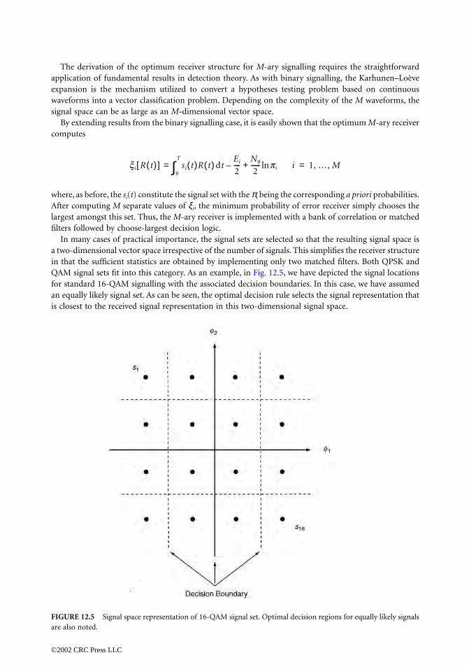
The derivation of the optimum receiver structure for M-ary signalling requires the straightforwardapplication of fundamental results in detection theory. As with binary signalling, the Karhunen–Loèveexpansion is the mechanism utilized to convert a hypotheses testing problem based on continuouswaveforms into a vector classification problem. Depending on the complexity of the M waveforms, thesignal space can be as large as an M-dimensional vector space.

By extending results from the binary signalling case, it is easily shown that the optimum M-ary receivercomputes

where, as before, the si(t) constitute the signal set with the πi being the corresponding a priori probabilities.After computing M separate values of ξi, the minimum probability of error receiver simply chooses thelargest amongst this set. Thus, the M-ary receiver is implemented with a bank of correlation or matchedfilters followed by choose-largest decision logic.

In many cases of practical importance, the signal sets are selected so that the resulting signal space isa two-dimensional vector space irrespective of the number of signals. This simplifies the receiver structurein that the sufficient statistics are obtained by implementing only two matched filters. Both QPSK andQAM signal sets fit into this category. As an example, in Fig. 12.5, we have depicted the signal locationsfor standard 16-QAM signalling with the associated decision boundaries. In this case, we have assumedan equally likely signal set. As can be seen, the optimal decision rule selects the signal representation thatis closest to the received signal representation in this two-dimensional signal space.

FIGURE 12.5 Signal space representation of 16-QAM signal set. Optimal decision regions for equally likely signalsare also noted.

xi R t( )[ ] si t( )R t( ) dt0

T

∫Ei

2----

N0

2------+ piln–= i 1 … M, ,=


12.9 More Realistic Channels

As is unfortunately often the case, many channels of practical interest are not accurately modeled assimply an AWGN channel. It is often that these channels impose nonlinear effects on the transmittedsignals. The best example of this is channels that impose a random phase and random amplitude ontothe signal. This typically occurs in applications such as in mobile communications, where one oftenexperiences rapidly changing path lengths from source to receiver.

Fortunately, by the judicious choice of signal waveforms, it can be shown that the selection of the φi

in the Karhunen–Loève transformation is often independent of these unwanted parameters. In thesesituations, the random amplitude serves only to scale the signals in signal space, whereas the randomphase simply imposes a rotation on the signals in signal space.

Since the Karhunen–Loève basis functions typically do not depend on the unknown parameters, wemay again convert the continuous time classification problem to a vector channel problem where thereceived vector R is computed as in Eq. (12.3). Since this vector is a function of both the unknownparameters (i.e., in this case amplitude A and phase ν), to obtain a likelihood ratio test independent ofA and ν, we simply apply Bayes theorem to obtain the following form for the LRT:

where the expectations are taken with respect to A and ν and where are the conditionalprobability density functions of the signal representations. Assuming that the background noise is AWGN,it can be shown that the LRT simplifies to choosing the largest amongst

(12.11)

It should be noted that in Eq. (12.11) we have explicitly shown the dependence of the transmitted signalssi on the parameters A and ν. The final receiver structures, together with their corresponding performanceare, thus, a function of both the choice of signal sets and the probability density functions of the randomamplitude and random phase.

FIGURE 12.6 Optimum receiver structure for noncoherent (random or unknown phase) ASK demodulation.

L R( )E pR |H1 A ,n, R|H1 A n, ,( )[ ]E pR |H0, A ,n R|H0 A n, ,( )[ ]----------------------------------------------------------

H1

><H0

p0

p1

-----=

pR |Hi , A , n

xi R t( )[ ] pi2

N0

------ R t( )0

T

∫ si t|A n,( ) dtEi A n,( )

N0

-------------------–

pA n, A n,( ) dA dnexpA ,n∫=

i 1 … M, ,=


Random Phase Channels

If we consider first the special case where the channel simply imposes a uniform random phase on thesignal, then it can be easily shown that the so-called in-phase and quadrature statistics obtained fromthe received signal R(t) (denoted by RI and RQ, respectively) are sufficient statistics for the signal classi-fication problem. These quantities are computed as

and

where, in this case, the index i corresponds to the center frequencies of hypotheses Hi, (e.g., FSKsignalling). The optimum binary receiver selects the largest from amongst

where I0 is a zeroth-order, modified Bessel function of the first kind. If the signals have equal energy andare equally likely (e.g., FSK signalling), then the optimum receiver is given by

One may readily observe that the optimum receiver bases its decision on the values of the two envelopesof the received signal and, as a consequence, is often referred to as an envelope or square-law detector. Moreover, it should be observed that the computation of the envelope is independent ofthe underlying phase of the signal and is, as such, known as a noncoherent receiver.

The computation of the error rate for this detector is a relatively straightforward exercise resulting in

As before, note that the error rate for the noncoherent receiver is simply a function of the SNR.

Rayleigh Channel

As an important generalization of the described random phase channel, many communication systemsare designed under the assumption that the channel introduces both a random amplitude and a randomphase on the signal. Specifically, if the original signal sets are of the form si(t) = mi(t)cos(2πfc t) wheremi(t) is the baseband version of the message (i.e., what distinguishes one signal from another), then theso-called Rayleigh channel introduces random distortion in the received signal of the following form:

where the amplitude A is a Rayleigh random variable* and where the random phase ν is a uniformlydistributed between zero and 2π.

*The density of a Rayleigh random variable is given by pA(a) = a/σ 2exp(−a2/2σ 2) for a ≥ 0.

RI i( ) R t( ) 2p fc i( )t[ ]cos0

T

∫ dt=

RQ i( ) R t( ) 2p fc i( )t[ ]sin0

T

∫ dt=

xi R t( )[ ] pi

Ei

N0

------– exp I0

2N0

------ RI2 i( ) RQ

2 i( )+ i 1 … M, ,= =

RI2 1( ) RQ

2 1( )

H1

><H0

+ RI2 0( ) RQ

2 0( )+

RI2 i( ) RQ

2 i( )+

Pe noncoherent( ) 12-- E

2N0

---------– exp=

si t( ) Ami t( ) 2p fct n+( )cos=


To determine the optimal receiver under this distortion, we must first construct an alternate statisticalmodel for si(t). To begin, it can be shown from the theory of random variables [4] that if XI and XQ arestatistically independent, zero mean, Gaussian random variables with variance given by σ2, then

Equality here is to be interpreted as implying that both A and n will be the appropriate random variables.From this, we deduce that the combined uncertainty in the amplitude and phase of the signal is incor-porated into the Gaussian random variables XI and XQ. The in-phase and quadrature components of thesignal si(t) are given by sIi(t) = mi(t)cos(2πfc t) and (t) = mi(t)sin(2πfc t) respectively. By appealing toEq. (12.11), it can be shown that the optimum receiver selects the largest from

where the inner product

Further, if we impose the conditions that the signals be equally likely with equal energy over the symbolinterval, then the optimum receiver selects the largest amongst

Thus, much like for the random phase channel, the optimum receiver for the Rayleigh channelcomputes the projection of the received waveform onto the in-phase and quadrature components of thehypothetical signals. From a signal space perspective, this is akin to computing the length of the receivedvector in the subspace spanned by the hypothetical signal. The optimum receiver then chooses the largestamongst these lengths.

As with the random phase channel, computing the performance is a straightforward task resulting in(for the equally likely equal energy case)

Interestingly, in this case, the performance depends not only on the SNR, but also on the variance (spread)of the Rayleigh amplitude A. Thus, if the amplitude spread is large, we expect to often experience whatis known as deep fades in the amplitude of the received waveform and, as such, expect a commensurateloss in performance.

12.10 Dispersive Channels

The dispersive channel model assumes that the channel not only introduces AWGN but also distorts thesignal through a filtering process. This model incorporates physical realities such as multipath effects andfrequency selective fading. In particular, the standard model adopted is depicted in the block diagramgiven in Fig. 12.7. As can be seen, the receiver observes a filtered version of the signal plus AWGN. If theimpulse response of the channel is known, then we arrive at the optimum receiver design by applying thepreviously presented theory. Unfortunately, the duration of the filtered signal can be a complicating factor.

Ami t( ) 2p fct n+( )cos mi t( )XI 2p fct( )cos mi t( )XQ 2p fct( )sin+=

sQi

xi R t( )[ ]pi

12Ei

N0

-------s 2+---------------------- s 2

12--

Ei

N0

------s 2+---------------------- R t( ), sIi t( )⟨ ⟩ 2 R t( ), sQi

t( )⟨ ⟩ 2+( )exp=

R t( ),Si t( )⟨ ⟩ R t( )si t( ) dt0

T

∫=

xi R t( )[ ] R t( ),sIi t( )⟨ ⟩ 2 R t( ),sQit( )⟨ ⟩ 2+=

Pe(Rayleigh)

12--

1 Es2

N0

---------+ ----------------------=


More often than not, the channel will increase the duration of the transmitted signals, hence, leading tothe description, dispersive channel.

However, if the designers take this into account by shortening the duration of si(t) so that the durationof is less than T, then the optimum receiver chooses the largest amongst

If we limit our consideration to equally likely binary signal sets, then the minimum Pe matches thereceived waveform to the filtered versions of the signal waveforms. The resulting error rate is given by

Thus, in this case, the minimum Pe is a function of the separation of the filtered version of the signalsin the signal space.

The problem becomes substantially more complex if we cannot insure that the filtered signal durationsare less than the symbol lengths. In this case, we experience what is known as intersymbol interference(ISI). That is, observations over one symbol interval contain not only the symbol information of interestbut also information from previous symbols. In this case, we must appeal to optimum sequenceestimation [5] to take full advantage of the information in the waveform. The basis for this procedure isthe maximization of the joint likelihood function conditioned on the sequence of symbols. This procedurenot only defines the structure of the optimum receiver under ISI but also is critical in the decoding ofconvolutional codes and coded modulation. Alternate adaptive techniques to solve this problem involvethe use of channel equalization.

Defining Terms

Additive white Gaussian noise (AWGN) channel: The channel whose model is that of corrupting atransmitted waveform by the addition of white (i.e., spectrally flat) Gaussian noise.

Bit (symbol) interval: The period of time over which a single symbol is transmitted.Communication channel: The medium over which communication signals are transmitted. Examples

are fiber optic cables, free space, or telephone lines.Correlation or matched filter receiver: The optimal receiver structure for digital communications in

AWGN.Decision boundary: The boundary in signal space between the various regions where the receiver

declares Hi. Typically a hyperplane when dealing with AWGN channels.Dispersive channel: A channel that elongates and distorts the transmitted signal. Normally modeled

as a time-varying linear system.

FIGURE 12.7 Standard model for dispersive channel. The time varying impulse response of the channel is denotedby hc(t, τ).

si∗ t( )

xi R t( )( )N0

2------ piln R t( ),si

∗ t( )⟨ ⟩ 12--Ei

∗–+=

Pe(dispersive) Qs0

∗ s0∗–

2N0

-------------------

=


Intersymbol interference: The ill-effect of one symbol smearing into adjacent symbols thus interferingwith the detection process. This is a consequence of the channel filtering the transmitted signalsand therefore elongating their duration. See dispersive channel.

Karhunen–Loève expansion: A representation for second-order random processes. Allows one toexpress a random process in terms of a superposition of deterministic waveforms. The scale valuesare uncorrelated random variables obtained from the waveform.

Mean-square equivalence: Two random vectors or time-limited waveforms are mean-square equivalentif and only if the expected value of their mean-square error is zero.

Orthonormal: The property of two or more vectors or time-limited waveforms being mutually orthog-onal and individually having unit length. Orthogonality and length are typically measured by thestandard Euclidean inner product.

Rayleigh channel: A channel that randomly scales the transmitted waveform by a Rayleigh randomvariable while adding an independent uniform phase to the carrier.

Signal space: An abstraction for representing a time limited waveform in a low-dimensional vectorspace. Usually arrived at through the application of the Karhunen–Loève transformation.

Total probability of error: The probability of classifying the received waveform into any of the symbolsthat were not transmitted over a particular bit interval.

References

1. Gibson, J.D., Principles of Digital and Analog Communications, 2nd ed., MacMillan, New York, 1993.2. Haykin, S., Communication Systems, 3rd ed., John Wiley & Sons, New York, 1994.3. Lee, E.A. and Messerschmitt, D.G., Digital Communication, Kluwer Academic Publishers, Norwell,

MA, 1988.4. Papoulis, A., Probability, Random Variables, and Stochastic Processes, 3rd ed., McGraw-Hill, New York,

1991.5. Poor, H.V., An Introduction to Signal Detection and Estimation, Springer-Verlag, New York, 1988.6. Proakis, J.G., Digital Communications, 2nd ed., McGraw-Hill, New York, 1989.7. Shiryayev, A.N., Probability, Springer-Verlag, New York, 1984.8. Sklar, B., Digital Communications, Fundamentals and Applications, Prentice Hall, Englewood Cliffs,

NJ, 1988.9. Van Trees, H.L., Detection, Estimation, and Modulation Theory, Part I, John Wiley & Sons, New York,

1968.10. Wong, E. and Hajek, B., Stochastic Processes in Engineering Systems, Springer-Verlag, New York, 1985.11. Wozencraft, J.M. and Jacobs, I., Principles of Communication Engineering, reissue, Waveland Press,

Prospect Heights, IL, 1990.12. Ziemer, R.E. and Peterson, R.L., Introduction to Digital Communication, Macmillan, New York, 1992.

Further Information

The fundamentals of receiver design were put in place by Wozencraft and Jacobs in their seminal book.Since that time, there have been many outstanding textbooks in this area. For a sampling see [1, 2, 3, 8,12]. For a complete treatment on the use and application of detection theory in communications see [5, 9].For deeper insights into the Karhunen–Loève expansion and its use in communications and signalprocessing see [10].


13Forward Error

Correction Coding

13.1 Introduction13.2 Fundamentals of Block Coding13.3 Structure and Decoding of Block Codes13.4 Important Classes of Block Codes13.5 Principles of Convolutional Coding13.6 Decoding of Convolutional Codes

Maximum Likelihood Decoding • Maximum A Posteriori (MAP) Decoding • Sub-Optimal Decoding Techniques

13.7 Trellis-Coded Modulation13.8 Additional Measures13.9 Turbo Codes13.10 Applications

13.1 Introduction

In 1948, Claude Shannon issued a challenge to communications engineers by proving that communica-tion systems could be made arbitrarily reliable as long as a fixed percentage of the transmitted signal wasredundant [Shannon, 1948]. He showed that limits exist only on the rate of communication and not itsaccuracy, and he went on to prove that errorless transmission could be achieved in an additive whiteGaussian noise (AWGN) environment with infinite bandwidth if the ratio of energy per data bit to noisepower spectral density exceeds the Shannon limit of -1.6 dB. He did not, however, indicate how thiscould be achieved. Subsequent research has led to a number of techniques that introduce redundancy toallow for correction of errors without retransmission. These techniques, collectively known as forwarderror correction (FEC) coding techniques, are used in systems where a reverse channel is not availablefor requesting retransmission, the delay with retransmission would be excessive, the expected numberof errors would require a large number of retransmissions, or retransmission would be awkward toimplement [Sklar, 1988].

A simplified model of a digital communication system that incorporates FEC coding is shown in Fig. 13.1.The FEC code acts on a discrete data channel comprised of all system elements between the encoderoutput and decoder input. The encoder maps the source data to q-ary code symbols that are modulatedand transmitted. During transmission, this signal can be corrupted, causing errors to arise in the demod-ulated symbol sequence. The FEC decoder attempts to correct these errors and restore the original sourcedata.

A demodulator that outputs only a value for the q-ary symbol received during each symbol intervalis said to make hard decisions. In the binary symmetric channel (BSC), hard decisions are made onbinary symbols and the probability of error is independent of the value of the symbol. One example of

Vijay K. BhargavaUniversity of Victoria

Ivan J. FairUniversity of Alberta


a BSC is the coherently demodulated BPSK signal corrupted by AWGN. The conditional probabilitydensity functions that result with this system are depicted in Fig. 13.2. The probability of error is givenby the area under the density functions that lies across the decision threshold and is a function of thesymbol energy Es and the one-sided noise power spectral density N0.

Alternatively, the demodulator can make soft decisions, or output an estimate of the symbol valuealong with an indication of its confidence in this estimate. For example, if the BPSK demodulator usesthree-bit quantization, the two least significant bits can be taken as a confidence measure. Possible soft-decision thresholds for the BPSK signal are depicted in Fig. 13.2. In practice, there is little to be gainedby using many soft-decision quantization levels.

Block and convolutional codes introduce redundancy by adding parity symbols to the message data.They map k source symbols to n code symbols and are said to have code rate R = k/n. With fixedinformation rates, this redundancy results in increased bandwidth and lower energy per transmittedsymbol. At low signal to noise ratios, these codes cannot compensate for these impairments, and perfor-mance is degraded. However, at higher ratios of information symbol energy Eb to noise spectral densityN0, there is coding gain since the performance improvement offered by coding more than compensatesfor these impairments. Coding gain is usually defined as the reduction in required Eb/N0 to achieve aspecific error rate in an error-control coded system over one without coding. In contrast to block andconvolutional codes, trellis-coded modulation introduces redundancy by expanding the size of the signalset rather than increasing the number of symbols transmitted and so offers the advantages of coding tobandlimited systems.

Each of these coding techniques is considered in turn. Following a discussion of interleaving andconcatenated coding, an overview is given of the most recent significant advance in FEC coding, thedevelopment of turbo codes. A brief overview of FEC applications concludes this chapter.

13.2 Fundamentals of Block Coding

In block codes there is a one-to-one mapping between k-symbol source words and n-symbol codewords.With q-ary signaling, qk out of the qn possible n-tuples are valid code vectors. The set of all n-tuples formsa vector space in which the qk code vectors are distributed. The Hamming distance between any twocode vectors is the number of symbols in which they differ; the minimum distance dmin of the code isthe smallest Hamming distance between any two codewords.

FIGURE 13.1 Block diagram of a digital communication system with forward error correction.

FIGURE 13.2 Hard and soft decision demodulation of a coherently-demodulated BPSK signal corrupted by AWGN.f(z|1) and f(z|0) are the Gaussianly distributed conditional probability density functions at the threshold device.

SourceFEC

EncoderModulator Channel Demodulator

FECDecoder

Sink

Discrete Data Channel

Noise

f(z|0) f(z|1)

Soft decision output:Hard decision output:

000 001

0

010 011

0

100 101 110 111

1

− Eg Eg


Contradictory objectives of block codes are:

• to distribute the code vectors in the vector space such that the distance between them is maximized.Then, if the decoder receives a corrupted vector, by evaluating the nearest valid code vector it willdecode the correct word with high probability.

• to pack the vector space with as many code vectors as possible to reduce the redundancy intransmission.

When code vectors differ in at least dmin positions, a decoder that evaluates the nearest code vector toeach received word is guaranteed to correct up to t random symbol errors per word if

(13.1)

Alternatively, all qn - qk illegal words can be detected, including all error patterns with dmin - 1 or fewererrors. In general, a block code can correct all patterns of t or fewer errors and detect all patterns of uor fewer errors provided that u ≥ t and

(13.2)

If q = 2, knowledge of the positions of the errors is sufficient for their correction; if q > 2, the decodermust determine both the positions and values of the errors. If the demodulator indicates positions inwhich the symbol values are unreliable, the decoder can assume their value unknown and has only tosolve for the value of these symbols. These positions are called erasures. A block code can correct up tot errors and v erasures in each word if

(13.3)

13.3 Structure and Decoding of Block Codes

Shannon showed that the performance limit of codes with fixed code rate improves as the block lengthincreases. However, as n and k increase, practical implementation requires that the mapping from messageto code vector not be arbitrary but that an underlying structure to the code exist. The structures developedto date limit the error correcting capability of these codes to below what Shannon proved possible, onaverage, for a code with random codeword assignments. Although turbo codes have made significantstrides toward approaching the Shannon limit, the search for good constructive codes continues.

A property which simplifies implementation of the coding operations is that of code linearity. A codeis linear if the addition of any two code vectors forms another code vector, which implies that the codevectors form a subspace of the vector space of n-tuples. This subspace, which contains the all-zero vector,is spanned by any set of k linearly independent code vectors. Encoding can be described as the multipli-cation of the information k-tuple by a generator matrix G, of dimension k ¥ n, which contains thesebasis vectors as rows. That is, a message vector mi is mapped to a code vector ci according to

(13.4)

where element-wise arithmetic is defined in the finite field GF(q). In general, this encoding procedureresults in code vectors with non-systematic form in that the values of the message symbols cannot bedetermined by inspection of the code vector. However, if G has the form [Ik, P] where Ik is the k ¥ kidentity matrix and P is a k ¥ (n - k) matrix of parity checks, then the k most significant symbols of eachcode vector are identical to the message vector and the code has systematic form. This notation assumes

dmin 2t 1+≥

dmin t u 1+ +≥

dmin 2t v 1+ +≥

ci miG, i 0, 1, …, qk 1–= =


that vectors are written with their most significant or first symbols in time on the left, a convention usedthroughout this article.

For each generator matrix there is an (n - k) ¥ k parity check matrix H whose rows are orthogonalto the rows in G, i.e., GHT = 0. If the code is systematic, H = [PT, In-k]. Since all codewords are linearsums of the rows in G, it follows that ciH

T = 0 for all i, i = 0, 1, º, qk - 1, and that the validity of thedemodulated vectors can be checked by performing this multiplication. If a codeword c is corruptedduring transmission so that the hard-decision demodulator outputs the vector = c + e, where e is anon-zero error pattern, the result of this multiplication is an (n - k)-tuple that is indicative of the validityof the sequence. This result, called the syndrome s, is dependent only on the error pattern since

(13.5)

If the error pattern is a code vector, the errors go undetected. However, for all other error patterns, thesyndrome is non-zero. Since there are qn-k - 1 non-zero syndromes, qn-k - 1 error patterns can be corrected.When these patterns include all those with t or fewer errors and no others, the code is said to be a perfectcode. Few codes are perfect; most codes are capable of correcting some patterns with more than t errors.Standard array decoders use look-up tables to associate each syndrome with an error pattern but becomeimpractical as the block length and number of parity symbols increases. Algebraic decoding algorithmshave been developed for codes with stronger structure. These algorithms are simplified with imperfectcodes if the patterns corrected are limited to those with t or fewer errors, a simplification called boundeddistance decoding.

Cyclic codes are a subclass of linear block codes with an algebraic structure that enables encoding tobe implemented with a linear feedback shift register and decoding to be implemented without a look-up table. As a result, most block codes in use today are cyclic or are closely related to cyclic codes. Thesecodes are best described if vectors are interpreted as polynomials and arithmetic follows the rules forpolynomials where the element-wise operations are defined in GF(q). In a cyclic code, all codewordpolynomials are multiples of a generator polynomial g(x) of degree n - k. This polynomial is chosen tobe a divisor of xn - 1 so that a cyclic shift of a code vector yields another code vector, giving this class ofcodes its name. A message polynomial mi(x) can be mapped to a codeword polynomial ci(x) in non-systematic form as

(13.6)

In systematic form, codeword polynomials have the form

(13.7)

where ri(x) is the remainder of mi(x)xn-k divided by g(x). Polynomial multiplication and division can beeasily implemented with shift registers [Blahut, 1983].

The first step in decoding the demodulated word is to determine if the word is a multiple of g(x). Thisis done by dividing it by g(x) and examining the remainder. Since polynomial division is a linear operation,the resulting syndrome s(x) depends only on the error pattern. If s(x) is the all-zero polynomial, trans-mission is errorless or an undetectable error pattern has occurred. If s(x) is non-zero, at least one errorhas occurred. This is the principle of the cyclic redundancy check (CRC). It remains to determine themost likely error pattern that could have generated this syndrome.

Single error correcting binary codes can use the syndrome to immediately locate the bit in error. Morepowerful codes use this information to determine the locations and values of multiple errors. The mostprominent approach of doing so is with the iterative technique developed by Berlekamp. This technique,which involves computing an error-locator polynomial and solving for its roots, was subsequently inter-preted by Massey in terms of the design of a minimum-length shift register. Once the location and values

ĉ

s ĉHT c e+( )HT cHT eHT+ eHT= = = =

ci x( ) mi x( )g x( ), i 0, 1, º, qk= = 1–

ci x( ) mi x( )xn-k ri x( )– , i 0, 1, º, qk= = 1–


of the errors are known, Chien’s search algorithm efficiently corrects them. The implementation com-plexity of these decoders increases only as the square of the number of errors to be corrected [Bhargava,1983] but does not generalize easily to accommodate soft-decision information. Other decoding tech-niques, including Chase’s algorithm and threshold decoding, are easier to implement with soft-decisioninput [Clark and Cain, 1981]. Berlekamp’s algorithm can be used in conjunction with transform-domaindecoding which involves transforming the received block with a finite field Fourier-like transform andsolving for errors in the transform domain. Since the implementation complexity of these decodersdepends on the block length rather than the number of symbols corrected, this approach results in simplercircuitry for codes with high redundancy [Wu et al., 1987].

Other block codes have also been constructed, including product codes that extend the above ideas totwo or more dimensions, codes that are based on transform-domain spectral properties, codes designedspecifically for correction of burst errors, and codes that are decodable with straightforward thresholdor majority logic decoders [Blahut, 1983; Clark and Cain, 1981; Lin and Costello, 1983].

13.4 Important Classes of Block Codes

When errors occur independently, Bose–Chaudhuri–Hocquenghem (BCH) codes provide among thebest performance of known codes for a given block length and code rate. They are cyclic codes with n =qm - 1 where m is any integer greater than two. They are designed to correct up to t errors per word andso have designed distance d = 2t + 1; the minimum distance may be greater. Generator polynomials forthese codes are listed in many texts, including [Clark and Cain, 1981]. These polynomials have degreeless than or equal to mt, and so k ≥ n - mt. BCH codes can be shortened to accommodate systemrequirements by deleting positions for information symbols.

Some subclasses of these codes are of special interest. Hamming codes are perfect single error cor-recting binary BCH codes. Full length Hamming codes have n = 2m - 1 and k = n - m for any m greaterthan two. The duals of these codes are maximal-length codes, with n = 2m - 1, k = m, and dmin = 2m-1.All 2m - 1 non-zero code vectors in these codes are cyclic shifts of a single non-zero code vector. Reed–Solomon (RS) codes are non-binary BCH codes defined over GF(q), where q is often taken as a powerof two so that symbols can be represented by a sequence of bits. In these cases, correction of even a singlesymbol allows for correction of a burst of bit errors. The block length is n = q - 1, and the minimumdistance dmin = 2t + 1 is achieved using only 2t parity symbols. Since RS codes meet the Singleton boundof dmin ≤ n - k + 1, they have the largest possible minimum distance for these values of n and k and arecalled maximum distance separable codes.

The Golay codes are the only non-trivial perfect codes that can correct more than one error. The (11, 6)ternary Golay code has minimum distance five. The (23, 12) binary code is a triple error correcting BCHcode with dmin = 7. To simplify implementation, it is often extended to a (24, 12) code through additionof an extra parity bit. The extended code has dmin = 8.

The (23, 12) Golay code is also a binary quadratic residue code. These cyclic codes have prime lengthof the form n = 8m ± 1, with k = (n + 1)/2 and dmin ≥ . Some of these codes are as good as the bestcodes known with these values of n and k, but it is unknown if there are good quadratic residue codeswith large n [Blahut, 1983].

Reed–Muller codes are equivalent to binary cyclic codes with an additional overall parity bit. For any m,the rth-order Reed–Muller code has n = 2m, k = , and dmin = 2m-r. The rth-order and (m - r - 1)th-order codes are duals, and the first order codes are similar to maximal-length codes. These codes, andthe closely related Euclidean geometry and projective geometry codes, can be decoded with thresholddecoding.

The performance of several of these block codes is shown in Fig. 13.3 in terms of decoded bit errorprobability vs. Eb/N0 for systems using coherent, hard-decision demodulated BPSK signaling. Many otherblock codes have also been developed, including Goppa codes, quasi-cyclic codes, burst error correctingFire codes, and other lesser-known codes.

n

∑i=0r m

iË ¯Ê ˆ


13.5 Principles of Convolutional Coding

Convolutional codes map successive information k-tuples to a series of n-tuples such that the sequenceof n-tuples has distance properties that allow for detection and correction of errors. Although these codescan be defined over any alphabet, their implementation has largely been restricted to binary signals, andonly binary convolutional codes are considered here.

In addition to the code rate R = k/n, the constraint length K is an important parameter for thesecodes. Definitions vary; we will use the definition that K equals the number of k-tuples that affectformation of each n-tuple during encoding. That is, the value of an n-tuple depends on the k-tuple whicharrives at the encoder during that encoding interval as well as the K - 1 previous information k-tuples.

Binary convolutional encoders can be implemented with k(K - 1)-stage shift registers and n modulo-2adders, an example of which is given in Fig. 13.4(a) for a rate 1/2, constraint length 3 code. The structuredepicted in this figure is the encoder for a non-recursive, non-systematic convolutional code becausethe encoder does not involve feedback and the data sequence is not directly visible in the encodedsequence; recursive and systematic structures are described below. Regardless of their recursive or sys-tematic nature, each convolutional encoder shifts in a new k-tuple during each encoding interval andsamples the outputs of the adders sequentially to form the coded output.

Although connection diagrams similar to that of Fig. 13.4(a) completely describe the code, a moreconcise description can be given by stating the values of n, k, and K and giving the adder connectionsin the form of vectors or polynomials. For instance, the rate 1/2 code has the generator vectors g1 = 111and g2 = 101, or equivalently, the generator polynomials g1(x) = x2 + x + 1 and g2(x) = x2 + 1. Sincefeedforward shift registers of this form implement polynomial multiplication [Blahut, 1983], the sequenceof bits from each tap can be interpreted as the product of the source sequence and the corresponding

FIGURE 13.3 Block code performance. (From Sklar, B., 1988, Digital Communications: Fundamentals and Appli-cations, Prentice-Hall, Englewood Cliffs, NJ. With permission.)

10−2

10−3

10−4

10−5

10−6

10−7

Pro

babi

lity

of D

ecod

ed B

it E

rror

4 5 6 7 8 9 10 11Eb /N0 [dB]

(127, 64) BC

H

(24, 12) Golay

(31, 26) Ham

ming

(15, 11) Ham

ming

Uncoded

BP

SK

(7, 4) Ham

ming


FIGURE 13.4 A rate 1/2, constraint length 3, non-recursive, non-systematic convolutional code.
DataInput

FirstBit

SecondBit

Encoded Output

(a) Connection diagram

0/00

001/11 0/11

0/10

1/10

1/010/01

1/0010 01

11

(b) State machine model

00

00

00

0000

00

00

00

00

11

11

11

11

11

11

11

1011

11

10

10

10

10

10

10

01

0101

01

01

01

01

100111000110001110011100011000111001110001100011100111000110

(c) Tree diagram

State

0000 00

00 00 00

00 00 00

10

10 10 10

10 10 10 10

01 0101 01 01

010101

11

11 1111 11 11

111111

(d) Trellis diagram


generator polynomial. Alternatively, a convolutional code can be characterized by its impulse response,the coded sequence generated due to input of a single logic-1. It is straightforward to verify that theimpulse response of the circuit in Fig. 13.4(a) is 111011 followed by zeros. Since modulo-2 addition isa linear operation, convolutional codes are linear and the coded output can be viewed as the convolutionof the input sequence with the impulse response, hence the name of this coding technique. Shiftedversions of the impulse response or generator vectors can be combined to form an infinite-order generatormatrix that also describes the code.

Shift register circuits can be modeled as finite state machines. A Mealy machine description of a convo-lutional encoder requires 2k(K-1) states, each describing a different value of the K - 1 k-tuples in the shiftregister. Each state has 2k exit paths that correspond to the value of the incoming k-tuple. A state machinedescription for the rate 1/2 encoder depicted in Fig. 13.4(a) is given in Fig. 13.4(b). States are labeledwith the contents of the shift register; edges are labeled with information bit values followed by theircorresponding coded output.

The dimension of time is added to the description of the encoder with tree and trellis diagrams. Thetree diagram for the rate 1/2 convolutional code is given in Fig. 13.4(c), assuming the shift register is initiallyclear. Each node represents an encoding interval, from which the upper branch is taken if the input bitis a 0 and the lower branch is taken if the input bit is a 1. Each branch is labeled with the correspondingoutput bit sequence. A drawback of the tree representation is that it grows without bound as the lengthof the input sequence increases. This is overcome with the trellis diagram depicted in Fig. 13.4(d). Again,encoding results in left-to-right movement, where the upper of the two branches is taken whenever theinput is a 0, the lower branch is taken when the input is a 1, and the output is the bit sequence thatweights the branch taken. Each level of nodes corresponds to a state of the encoder, as shown on the left-hand side of the diagram.

Figure 13.5(a) depicts a recursive systematic convolutional encoder that generates a code that is equiv-alent to the code depicted in Fig. 13.4. This encoder is systematic because the source bit stream is copieddirectly into the encoded sequence; it is recursive because it involves feedback. Since a feedback shiftregister implements polynomial division, the sequence of non-systematic bits can be interpreted as thesource sequence divided by the feedback polynomial g1(x) = x2 + x + 1 and multiplied by the feedforwardpolynomial g2(x) = x2 + 1. The codes in Figs. 13.4 and 13.5 are equivalent because their state diagrams,code trees, and trellises are identical with the exception of the mapping from source sequence to encodedsequence. For example, the state diagram in Fig. 13.5(b) for the recursive systematic code exhibits thesame structure as the diagram in Fig. 13.4(b); only the input data bits weighting some of the branchesdiffer. Recursive non-systematic codes and non-recursive systematic codes also exist.

If the received sequence contains errors, it may no longer depict a valid path through the tree or trellis.It is the job of the decoder to determine the original path. In doing so, the decoder does not so muchcorrect errors as find the closest valid path to the received sequence. As a result, the error correcting

FIGURE 13.5 A rate 1/2, constraint length 3, recursive systematic convolutional code.

1/11

0/00

1/1100

10 0/001/10

01

0/0111

1/10

0/01

(b) State machine model(a) Connection diagram

SecondBit

Encoded

Output

FirstBit

Data Input


capability of a convolutional code is more difficult to quantify than that of a block code; it depends onhow valid paths differ. One measure of this difference is the column distance dc(i), the minimumHamming distance between all coded sequences generated over i encoding intervals that differ in thefirst interval. The non-decreasing sequence of column distance values is the distance profile of the code.The column distance after K intervals is the minimum distance of the code, and is important for evaluatingthe performance of a code that uses threshold decoding. As i increases, dc(i) approaches the free distanceof the code dfree which is the minimum Hamming distance in the set of arbitrarily long paths that divergeand then remerge in the trellis.

With maximum likelihood decoding, convolutional codes can generally correct up to t errors withinthree to five constraint lengths, depending on how the errors are distributed, where

(13.8)

The free distance can be calculated by exhaustively searching for the minimum weight path that returnsto the all-zero state or by evaluating the term of lowest degree in the generating function of the code.

The objective of a convolutional code is to maximize these distance properties. They generally improveas the constraint length of the code increases, and non-recursive, non-systematic codes generally havebetter properties than non-recursive systematic ones. As indicated above, non-recursive, non-systematiccodes always have an equivalent recursive systematic form that has identical distance properties. Goodcodes have been found by computer search and are tabulated in many texts, including [Clark and Cain,1981].

Convolutional codes with high code rate can be constructed by puncturing or periodically deletingcoded symbols from a low rate code. A list of low rate codes and perforation matrices that result in goodhigh rate codes can be found in many sources, including [Wu et al., 1987]. The performance of goodpunctured codes approaches that of the best convolutional codes known with similar rate, and decoderimplementation is significantly less complex.

Convolutional codes can be catastrophic, having the potential to generate an unlimited number ofdecoded bit errors in response to a finite number of errors in the demodulated bit sequence. Catastrophicerror propagation is avoided if the code has generator polynomials with a greatest common divisor ofthe form xa for any a, or equivalently, if there are no closed loop paths in the state diagram with all-zerooutput other than the one taken with all-zero input. Systematic codes are not catastrophic.

13.6 Decoding of Convolutional Codes

Maximum Likelihood Decoding

Maximum likelihood (ML) decoding selects the source sequence mi that maximizes the probabilityP(x |mi), i ∈ 0, 1, …, 2L - 1, where x is the received sequence and L is the number of symbols in the sourcesequence. Maximizing this probability is equivalent to selecting the path through the tree or trellis thatdiffers from the received sequence by the smallest amount. In 1967, Viterbi developed a maximumlikelihood decoding algorithm that takes advantage of the trellis structure to reduce the complexity of thisevaluation. This algorithm has become known as the Viterbi algorithm. With each received n-tuple, thedecoder computes a metric or measure of likelihood for all paths that could have been taken during thatinterval and discards all but the most likely to terminate on each node. An arbitrary decision is made ifpath metrics are equal. The metrics can be formed using either hard- or soft-decision information withlittle difference in implementation complexity.

If the message has finite length and the encoder is subsequently flushed with zeros, a single decodedpath remains. With a BSC, this path corresponds to the valid code sequence with minimum Hammingdistance from the demodulated sequence. Full-length decoding becomes impractical as the length of themessage sequence increases. However, the most likely paths tend to have a common stem, and selecting

dfree 2t 1+≥


the trace value four or five times the constraint length prior to the present decoding depth results innear-optimum performance. Since the number of paths examined during each interval increases expo-nentially with the constraint length, the Viterbi algorithm becomes impractical for codes with largeconstraint length.

Maximum A Posteriori (MAP) Decoding

In contrast to ML decoding, maximum a posteriori (MAP) decoding selects the source sequence mi thatmaximizes the a posteriori probability P( ) , i Œ 0, 1, …, 2L - 1, where x and L are as defined above.Using Bayes rule, this probability can be written

(13.9)

Since the denominator is constant for all mi it does not affect selection of the source sequence. Thedifference between MAP and ML decoding lies in the fact that through the P(mi) term in the numerator,MAP decoding takes into account the different probabilities of occurrence of different source sequences.When all source sequences are equally likely, ML and MAP decoding techniques are equivalent.

Several MAP decoding algorithms have been developed. One of the most efficient for non-recursiveconvolutional codes is the BCJR algorithm [Bahl et al., 1974]. This algorithm has been modified toaccommodate recursive codes. The BCJR algorithm requires both a forward and reverse recursion throughthe trellis, evaluating and using metrics in a fashion similar to the Viterbi algorithm. This algorithm ispractical only for codes with relatively small constraint lengths, and because of the dual pass nature ofthis algorithm, its complexity exceeds twice that of the Viterbi algorithm. Further, under most practicalconditions, the performance of the Viterbi algorithm is almost identical to the performance of the BCJRalgorithm. However, a strength of the BCJR algorithm is its ability to easily provide soft, rather thanhard, decision information for each source symbol. This characteristic is necessary for decoding of turbocodes.

Sub-Optimal Decoding Techniques

The inherent complexity of the Viterbi and BCJR algorithms make them unsuitable for decoding con-volutional codes with constraint lengths larger than about 12. Other decoding techniques, such assequential and threshold decoding, can be used with larger constraint lengths. Sequential decoding wasproposed by Wozencraft, and the most widely used algorithm was developed by Fano. Rather thantracking multiple paths through the trellis, the sequential decoder operates on a single path whilesearching the code tree for a path with high probability. It makes tentative decisions regarding thetransmitted sequence, computes a metric between its proposed path and the demodulated sequence, andmoves forward through the tree as long as the metric indicates that the path is likely. If the likelihood ofthe path becomes low, the decoder moves backward, searching other paths until it finds one with highprobability. The number of computations involved in this procedure is almost independent of theconstraint length and is typically quite small, but can be highly variable, depending on the channel.Buffers must be provided to store incoming sequences as the decoder searches the tree. Their overflowis a significant limiting factor in the performance of these decoders.

Figure 13.6 compares the performance of the Viterbi and sequential decoding algorithms for severalconvolutional codes operating on coherently-demodulated BPSK signals corrupted by AWGN. Otherdecoding algorithms have also been developed, including syndrome decoding methods such as tablelook-up feedback decoding and threshold decoding [Clark and Cain, 1981]. These algorithms are easilyimplemented but suffer from a reduction in performance.

mi x

P mi x( )P x mi( )P mi( )

P x( )----------------------------------, i 0, 1, …, 2LŒ 1–=


13.7 Trellis-Coded Modulation

Trellis-coded modulation (TCM) has received considerable attention since its development by Ungerboeckin the late 1970s [Ungerboeck, 1987]. Unlike block and convolutional codes, TCM schemes achieve codinggain by increasing the size of the signal alphabet and using multi-level/phase signaling. Like convolutionalcodes, sequences of coded symbols are restricted to certain valid patterns. In TCM, these patterns arechosen to have large Euclidean distance from one another so that a large number of corrupted sequences canbe corrected. The Viterbi algorithm is often used to decode these sequences. Since the symbol transmissionrate does not increase, coded and uncoded signals require the same transmission bandwidth. If trans-mission power is held constant, the signal constellation of the coded signal is denser. However, the lossin symbol separation is more than overcome by the error correction capability of the code.

Ungerboeck investigated the increase in channel capacity which can be obtained by increasing the sizeof the signal set and restricting the pattern of transmitted symbols, and he concluded that almost all ofthe additional capacity can be gained by doubling the number of points in the signal constellation. Thisis accomplished by encoding the binary data with a rate R = k/(k + 1) code and mapping sequences ofk + 1 coded bits to points in a constellation of 2k+1 symbols. For example, the rate 2/3 encoder of Fig. 13.7(a)encodes pairs of source bits to three coded bits. Figure 13.7(b) depicts one stage in the trellis of the codedoutput where, as with the convolutional code, the state of the encoder is defined by the contents of theshift register. Note that unlike the trellis for the convolutional code, this trellis contains parallel pathsbetween nodes.

The key to improving performance with TCM is to map the coded bits to points in the signal spacesuch that the Euclidean distance between transmitted sequences is maximized. A method that ensures

FIGURE 13.6 Convolutional code performance. (From Omura, J.K. and Levitt, B.K., 1982, Coded error probabilityevaluation for antijam communication systems, IEEE Trans. Commun., COM-30(5), 896–903. With permission.)

10−1

10−2

10−3

10−4

10−5

10−6

Pro

babi

lity

of D

ecod

ed B

it E

rror

0 2 4 6 8 10 12Eb/N0 [dB]

Uncoded

BP

SK

R=1/3, K

=7, Hard

decision, Viterbi

R=1/2, K

=7, Hard

decision, Viterbi

R=1/3, K

=41, Sequential

R=1/2, K

=7, Soft decision, V

iterbi

R=1/3, K

=7, Soft decision, V

iterbi

R=

1/2, K=

41, Sequential


improved Euclidean distance is the method of set partitioning. This involves separating all parallel pathson the trellis with maximum distance and assigning the next greatest distance to paths that diverge fromor merge onto the same node. Figure 13.7(c) and (d) gives examples of mappings for the rate 2/3 codewith 8-PSK and 8-PAM signal constellations, respectively.

As with convolution codes, the free distance of a TCM code is defined as the minimum distancebetween paths through the trellis, where the distance of concern is now Euclidean distance rather thanHamming distance. The free distance of an uncoded signal is defined as the distance between the closestsignal points. When coded and uncoded signals have the same average power, the coding gain of theTCM system is defined as

(13.10)

It can be shown that the simple rate 2/3 8-PSK and 8-PAM TCM systems provide gains of 3 dB and 3.3 dB,respectively [Clark and Cain, 1981]. More complex TCM systems yield gains up to 6 dB. Tables of goodcodes are given in [Ungerboeck, 1987].

13.8 Additional Measures

When the demodulated sequence contains bursts of errors, the performance of codes designed to correctindependent errors improves if coded sequences are interleaved prior to transmission and deinterleavedprior to decoding. Deinterleaving separates the burst errors, making them appear more random andincreasing the likelihood of accurate decoding. It is generally sufficient to interleave several block lengthsof a block coded signal or several constraint lengths of a convolutionally encoded signal. Block interleavingis the most straightforward approach, but delay and memory requirements are halved with convolutionaland helical interleaving techniques. Periodicity in the way sequences are combined is avoided with pseudo-random interleaving.

FIGURE 13.7 A rate 2/3 TCM code.

DataInput

+ +

Intermediate Binary Form

FirstBit

SecondBit

SecondBit

ThirdBit

(a) Connection diagram

State

00000

100011111

011

111

001

101

010110

000

100

001101

010

110

10

01

11

(b) One stage in trellis

(c) 8-PSK constellation

011

111

010 101

001 110

100000

(d) 8-PAM constellation

011 111010 101 001110100000

coding gain 20 log10

dfree, coded

dfree, uncoded

----------------------- .=


Serially concatenated codes, first investigated by Forney, use two levels of coding to achieve a level ofperformance with less complexity than a single coding stage would require. The inner code interfaceswith the modulator and demodulator and corrects the majority of the errors; the outer code correctserrors which appear at the output of the inner-code decoder. A convolutional code with Viterbi decodingis usually chosen as the inner code, and an RS code is often chosen as the outer code due to its abilityto correct the bursts of bit errors that can result with incorrect decoding of trellis-coded sequences.Interleaving and deinterleaving outer-code symbols between coding stages offers further protectionagainst the burst error output of the inner code.

Product codes effectively place the data in a two (or more)-dimensional array and use FEC techniquesover the rows and columns of this array. Not only do these codes result in error protection in multipledimensions, but the manner in which the array is constructed can offer advantages similar to thoseachieved through interleaving.

13.9 Turbo Codes

The most recent significant advancement in FEC coding is the development of turbo codes [Berrou, Glavieux,and Thitimajshima, 1993]. The principle of this coding technique is to encode the data with two or moresimple constituent codes concatenated through an interleaver. The received sequence is decoded in aniterative, serial approach using soft-input, soft-output decoders. The iterative decoder involves feedback ofinformation in a manner similar to processes within the turbo engine, giving this coding technique its name.

Turbo codes effectively result in the construction of relatively long codewords with few codewordsbeing close in terms of Hamming distance, while at the same time constraining the implementationcomplexity of the decoder to practical limits. The first turbo codes that were developed used recursivesystematic convolutional codes as the constituent codes and concatenated them in parallel through apseudo-random interleaver, as depicted in Fig. 13.8(a). The use of other types of constituent codes, andthe serial concatenation of constituent codes, has since been considered.

As in other multi-stage coding techniques, the complexity of the turbo decoder is limited through useof separate decoding stages for each constituent code. The input to the first stage is the soft output ofthe demodulator for a finite-length received symbol sequence. As shown in Fig. 13.8(b), subsequent stagesuse both the demodulator output and the extrinsic information from the previous decoding stage.Extrinsic information is the new, soft information evaluated in each stage of decoding that can be usedas a priori information for each source symbol during the next stage of decoding.

FIGURE 13.8 Turbo code with parallel concatenated constituent codes.

Data

Input

Interleaver

Recursive SystematicConvolutional Encoder 1

Recursive SystematicConvolutional Encoder 2

(a) Encoder

Puncturing(if desired)

EncodedOutput

Demodulated

Sequence

Code 1 parity

Code 2 parity

MAPDecoder 1

Systematic symbols

Extrinsic

InformationInterleaver

Interleaver

MAPDecoder 2

Extrinsic

InformationDeinterleaver

Decision

DecodedOutput

(b) Decoder


Decoding proceeds by iterating through constituent decoders, each forwarding updated extrinsicinformation to the next decoder until a predefined number of iterations has been completed or theextrinsic information indicates that high reliability has been achieved. Typical simulation results areshown in Fig. 13.9. As indicated in this figure, performance tends to improve with the number ofiterations, where the largest performance gains are made during the initial iterations. Excellent perfor-mance can be obtained at signal-to-noise ratios appreciably less than 1 dB, however at higher values ofEb/N0, the performance curves tend to exhibit flattening similar to error floors. Flattening of the BERcurves is a result of the relatively small overall Hamming distance typical of most turbo codes.

Since the discovery of turbo codes, a significant amount of effort has been directed towards explainingand analyzing their performance. Recent work demonstrating the relationship between turbo codes andbelief propagation in Bayesian networks shows promise in furthering these goals. There has also beensignificant effort in determining optimal code parameters. With convolutional constituent codes, it hasbeen found that coding gain through turbo decoding is only possible with recursive codes and that thereis little advantage to using codes with constraint lengths larger than about five. These short constraintlengths allow the soft-in, soft-out BCJR algorithm to be used. It has also been recognized that decodingperformance increases with decreased correlation between the extrinsic information and the demodulateddata at the input of the constituent decoders, implying that highly random interleavers should be used.It has also been established that it is important for interleavers to ensure that sequences highly susceptibleto error not occur simultaneously in both constituent codes.

Even though great strides have been made over the last few years in understanding the structure of thesecodes and relating them to serially concatenated and product codes, work regarding their analysis, optimi-zation, and efficient implementation will interest coding theorists and practitioners for many years to come.

13.10 Applications

FEC coding remained of theoretical interest until advances in digital technology and improvements indecoding algorithms made their implementation possible. It has since become an attractive alternativeto improving other system components or boosting transmission power. FEC codes are commonly usedin digital storage systems, deep-space and satellite communication systems, terrestrial wireless and band-limited wireline systems, and have also been proposed for fiber optic transmission. Accordingly, thetheory and practice of error correcting codes now occupies a prominent position in the field of commu-nications engineering.

Deep-space systems began using forward error correction in the early 1970s to reduce transmissionpower requirements, and used multiple error correcting RS codes for the first time in 1977 to protect againstcorruption of compressed image data in the Voyager missions [Wicker and Bhargava, 1994]. The Consultative

FIGURE 13.9 Performance in AWGN of a turbo code with parallel concatenated constituent codes of rate 1/2 andconstraint length 4. Pseudo-random interleaver of size 65536.

Curves labeled with number of iterations

10−5

0 0.5 1 1.5 2

Eb/N0 (dB)

2.5 3 3.5 4 4.5

10−4

10−3

10−2

10−1

1

BE

R

#10 #6 #3 #2 #1


Committee for Space Data Systems (CCSDS) has recommended use of a concatenated coding systemwhich uses a rate 1/2, constraint length 7 convolutional inner code and a (255, 223) RS outer code.

Coding is now commonly used in satellite systems to reduce power requirements and overall hardwarecosts and allow closer orbital spacing of geosynchronous satellites [Berlekamp, 1987]. FEC codes play integralroles in the VSAT, MSAT, INTELSAT, and INMARSAT systems [Wu et al., 1987]. Further, a (31, 15) RS codeis used in the joint tactical information distribution system (JTIDS), a (7, 2) RS code is used in the air forcesatellite communication system (AFSATCOM), and a (204, 192) RS code has been designed specificallyfor satellite TDMA systems. Another code designed for military applications involves concatenation ofa Golay and RS code with interleaving to ensure an imbalance of 1s and 0s in the transmitted symbolsequence and enhance signal recovery under severe noise and interference [Berlekamp, 1987].

TCM has become commonplace in transmission of data over voiceband telephone channels. Modemsdeveloped since 1984 use trellis coded QAM modulation to provide robust communication at rates above9.6 kb/s.

Various coding techniques are used in the new digital cellular and personal communication standards[Rappaport, 1996]. Convolutional codes are employed in the second generation GSM, TDM, and CDMAsystems. More recent standards use turbo coding to provide error protection for data signals.

FEC codes have also been widely used in digital recording systems, most prominently in the compactdisc digital audio system. This system uses two levels of coding and interleaving in the cross-interleaved RScoding (CIRC) system to correct errors which result from disc imperfections and dirt and scratches whichaccumulate during use. Steps are also taken to mute uncorrectable sequences [Wicker and Bhargava, 1994].

Defining Terms

Binary symmetric channel: A memoryless discrete data channel with binary signaling, hard-decisiondemodulation, and channel impairments that do not depend on the value of the symbol transmitted.

Bounded distance decoding: Limiting the error patterns which are corrected in an imperfect code tothose with t or fewer errors.

Catastrophic code: A convolutional code in which a finite number of code symbol errors can cause anunlimited number of decoded bit errors.

Code rate: The ratio of source word length to codeword length, indicative of the amount of informationtransmitted per encoded symbol.

Coding gain: The reduction in signal-to-noise ratio required for specified error performance in a blockor convolutional coded system over an uncoded system with the same information rate, channelimpairments, and modulation and demodulation techniques. In TCM, the ratio of the squaredfree distance in the coded system to that of the uncoded system.

Column distance: The minimum Hamming distance between convolutionally encoded sequences of aspecified length with different leading n-tuples.

Constituent codes: Two or more FEC codes that are combined in concatenated coding techniques.Cyclic code: A block code in which cyclic shifts of code vectors are also code vectors.Cyclic redundancy check: When the syndrome of a cyclic block code is used to detect errors.Designed distance: The guaranteed minimum distance of a BCH code designed to correct up to t errors.Discrete data channel: The concatenation of all system elements between FEC encoder output and

decoder input.Distance profile: The minimum Hamming distance after each encoding interval of convolutionally

encoded sequences which differ in the first interval.Erasure: A position in the demodulated sequence where the symbol value is unknown.Extrinsic information: The output of a constituent soft decision decoder that is forwarded as a priori

information for the source symbols to the next decoding stage in iterative decoding of turbo codes.Finite field: A finite set of elements and operations of addition and multiplication which satisfy specific

properties. Often called Galois fields and denoted GF(q), where q is the number of elements inthe field. Finite fields exist for all q which are prime or the power of a prime.


Free distance: The minimum Hamming weight of convolutionally encoded sequences which divergeand remerge in the trellis. Equals the maximum column distance and the limiting value of thedistance profile.

Generator matrix: A matrix used to describe a linear code. Code vectors equal the information vectorsmultiplied by this matrix.

Generator polynomial: The polynomial which is a divisor of all codeword polynomials in a cyclic blockcode; a polynomial which describes circuit connections in a convolutional encoder.

Hamming distance: The number of symbols in which codewords differ.Hard decision: Demodulation which outputs only a symbol value for each received symbol.Interleaving: Shuffling the coded bit sequence prior to modulation and reversing this operation fol-

lowing demodulation. Used to separate and redistribute burst errors over several codewords (blockcodes) or constraint lengths (trellis codes) for higher probability of correct decoding by codesdesigned to correct random errors.

Linear code: A code whose code vectors form a vector space. Equivalently, a code where the additionof any two code vectors forms another code vector.

Maximum a posteriori decoding: A decoding algorithm that selects the source sequence that maximizesthe probability of the source sequence being transmitted, given reception of the received sequence.

Maximum distance separable: A code with the largest possible minimum distance given the blocklength and code rate. These codes meet the Singleton bound of dmin £ n - k + 1.

Maximum likelihood decoding: A decoding algorithm that selects the source sequence that maximizesthe probability of the received sequence occurring given transmission of this source sequence.

Metric: A measure of goodness against which items are judged. In the Viterbi algorithm, an indicationof the probability of a path being taken given the demodulated symbol sequence.

Minimum distance: In a block code, the smallest Hamming distance between any two codewords. Ina convolutional code, the column distance after K intervals.

Parity check matrix: A matrix whose rows are orthogonal to the rows in the generator matrix of alinear code. Errors can be detected by multiplying the received vector by this matrix.

Perfect code: A t error correcting (n, k) block code in which qn-k - 1 = Puncturing: Periodic deletion of code symbols from the sequence generated by a convolutional encoder

for purposes of constructing a higher rate code. Also, deletion of parity bits in a block code.Set partitioning: Rules for mapping coded sequences to points in the signal constellation which always

result in a larger Euclidean distance for a TCM system than an uncoded system, given appropriateconstruction of the trellis.

Shannon limit: The ratio of energy per data bit Eb to noise power spectral density N0 in an AWGNchannel above which errorless transmission is possible when no bandwidth limitations are placedon the signal and transmission is at channel capacity. This limit has the value ln2 = 0.693 = -1.6 dB.

Soft decision: Demodulation which outputs an estimate of the received symbol value along with anindication of the reliability of this value. Usually implemented by quantizing the received signalto more levels than there are symbol values.

Standard array decoding: Association of an error pattern with each syndrome by way of a look-up table.Syndrome: An indication of whether or not errors are present in the demodulated symbol sequence.Systematic code: A code in which the values of the message symbols can be identified by inspection

of the code vector.Vector space: An algebraic structure comprised of a set of elements in which operations of vector

addition and scalar multiplication are defined. For our purposes, a set of n-tuples consisting ofsymbols from GF(q) with addition and multiplication defined in terms of element-wise operationsfrom this finite field.

Viterbi algorithm: A maximum-likelihood decoding algorithm for trellis codes which discards lowprobability paths at each stage of the trellis, thereby reducing the total number of paths whichmust be considered.

Âi=1t n

iË ¯Ê ˆ

.


References

Bahl, L.R., Cocke, J., Jelinek, F., and Raviv, J., Optimal decoding of linear codes for minimizing symbolerror rate, IEEE Trans. Inf. Theory, 20, 248, 1974.

Berlekamp, E.R., Peile, R.E., and Pope, S.P., The application of error control to communications, IEEECommn. Mag., 25(4), 44, 1987.

Berrou, C., Glavieux, A., and Thitimajshima, P., Near Shannon limit error-correcting coding and decod-ing: turbo codes, Proceedings of ICC’93, Geneva, Switzerland, 1064, 1993.

Bhargava, V.K., Forward error correction schemes for digital communications, IEEE Commn. Mag., 21(1),11, 1983.

Blahut, R.E., Theory and Practice of Error Control Codes, Addison-Wesley, Massachusetts, 1983.Clark, G.C., Jr. and Cain, J.B., Error Correction Coding for Digital Communications, Plenum Press, New

York, 1981.Lin, S. and Costello, D.J., Jr., Error Control Coding: Fundamentals and Applications, Prentice-Hall, Engle-

wood Cliffs, NJ, 1983.Rappaport, T.S., Wireless Communications, Principles and Practice. Prentice-Hall and IEEE Press, Engle-

wood Cliffs, NJ, 1996.Shannon, C.E., A mathematical theory of communication, Bell Syst. Tech. J., 27(3), 379, 1948.Sklar, B., Digital Communications: Fundamentals and Applications, Prentice Hall, Englewood Cliffs, NJ,

1988.Ungerboeck, G., Trellis-coded modulation with redundant signal sets, IEEE Commun. Mag., 25(2), 5,

1987.Wicker, S.B. and Bhargava, V.K., Reed–Solomon Codes and Their Applications, IEEE Press, New Jersey, 1994.Wu, W.W., Haccoun, D., Peile, R., and Hirata, Y., Coding for satellite communication, IEEE J. Selected

Areas Commn., SAC-5(4), 724, 1987.

For Further Information

There is now a large amount of literature on the subject of FEC coding. An introduction to the philosophyand limitations of these codes can be found in the second chapter of Lucky’s book Silicon Dreams:Information, Man, and Machine, St. Martin’s Press, New York, 1989. More practical introductions can befound in overview chapters of many communications texts. The number of texts devoted entirely to thissubject also continues to grow. Although these texts summarize the algebra underlying block codes, morein-depth treatments can be found in mathematical texts. Survey papers appear occasionally in theliterature, but the interested reader is directed to the seminal papers by Shannon, Hamming, Reed andSolomon, Bose and Chaudhuri, Hocquenghem, Wozencraft, Fano, Forney, Berlekamp, Massey, Viterbi,Ungerboeck, and Berrou and Glavieux, among others. The most recent advances in the theory andimplementation of error control codes are published in IEEE Transactions on Information Theory, IEEETransactions on Communications, and special issues of IEEE Journal on Selected Areas in Communications.


14Automatic Repeat

Request

14.1 Introduction14.2 Fundamentals and Basic Automatic Repeat Request Schemes

Basic Principles • Stop-and-Wait Automatic Repeat Request • Sliding Window Protocols

14.3 Performance Analysis and LimitationsStop-and-Wait Automatic Repeat Request • Continuous Automatic Repeat Request: Sliding Window Protocols

14.4 Variants of the Basic Automatic RepeatRequest Schemes

14.5 Hybrid Forward Error Control/Automatic RepeatRequest Schemes

14.6 Application ProblemSolution

14.7 Conclusion

14.1 Introduction

In most digital communication systems, whenever error events occur in the transmitted messages, someaction must be taken to correct these events. This action may take the form of an error correctionprocedure. In some applications where a two-way communication link exists between the sender andthe receiver, the receiver may inform the sender that a message has been received in error and, hence,request a repeat of that message. In principle, the procedure may be repeated as many times as necessaryuntil that message is received error free. An error control system in which the erroneously receivedmessages are simply retransmitted is called automatic-repeat-request (ARQ).

In ARQ systems, the receiver must perform only an error detection procedure on the received messageswithout attempting to correct the errors. Hence, an error detecting code, in the form of specific redundantor parity-check symbols, must be added to the information-bearing sequence. In general, as the errordetecting capability of the code increases, the number of added redundant symbols must also be increased.Clearly, with such a system, an erroneously received message is delivered to the user only if the receiverfails to detect the presence of errors. Since error detection coding is simple, powerful, and quite robust,ARQ systems constitute a simple and efficient method for providing highly reliable transfer of messagesfrom the source to the user over a variety of transmission channels. ARQ systems are therefore widelyused in data communication systems that are highly sensitive to errors, such as in computer-to-computercommunications.

This chapter presents and discusses principles, performances, limitations, and variants of basic ARQstrategies. The fundamentals of the basic ARQ schemes are presented in Section 14.2, whereas the

David HaccounÉcole Polytechnique de Montréal

Samuel PierreUniversité du Québec


performance analysis and the limitations are carried out in Section 14.3. Section 14.4 presents some ofthe most common variants of the basic ARQ schemes, and hybrid forward error control (FEC)/ARQtechniques are outlined in Section 14.5. Finally, an application problem is provided in Section 14.6.

14.2 Fundamentals and Basic Automatic RepeatRequest Schemes

Messages transmitted on a communication channel are subjected to errors, which must be detectedand/or corrected at the receiver. This section presents the basic principles underlying the concept of errorcontrol using retransmission schemes.

Basic Principles

In the seven-layer open system interconnection (OSI) model, error control refers to some basic functionsthat may be performed at several layers, especially at the transport layer (level 4) and at the data link layer(level 2). The transport layer is responsible for the end-to-end transport of information processed asprotocol data unit (PDU) through a network infrastructure. An intermediate layer, called the networklayer (level 3), ensures that messages, which are broken down into smaller blocks called packets, cansuccessfully be switched from one node to another of the network.

The error control on each individual link of the network is performed by the data link layer, whichtransforms packets received from the network layer into frames by adding address, control, and errorcheck fields prior to their transmission into the channel. Figure 14.1 shows an example of the framestructure, whose length, which depends on the particular data link protocol used, usually varies approx-imately between 50 and 200 bytes. The length of each field also depends on the particular data linkcontrol protocol employed. The data link layer must ensure a correct and orderly delivery of packetsbetween switching nodes in the network. The objective of the error control is to maintain the integrityof the data in the frames as they transit through the links, overcoming the loss, duplication, desequencing,and damage of data and control information bits at these various levels. Most ARQ error controltechniques integrate error detection using standard cyclic redundancy check (CRC), as well as requests forretransmission using PDU.

Error control coding consists essentially of adding to the information bits to be transmitted some extraor redundant bits, called parity-check bits, in a regular and controlled manner. These parity-check bits,which are removed at the receiver, do not convey information but allow the receiver to detect and possiblycorrect errors in the received frames.

The single parity-check bit used in ASCII is an example of a redundant bit for error detection purposes.It is an eighth bit added to the seven information bits in the frame representing the alphanumericcharacter to be transmitted. This bit takes the value 1 if the number of 1s in the first seven bits is odd(odd parity), and 0 otherwise. At the receiver, the parity-check bit of the received frame is computedagain in order to verify whether it agrees with the received parity check bit. A mismatch of these parity-check bits indicates that an odd number of errors has occurred during transmission, leading the receiverto request a retransmission of the erroneous frame.

FIGURE 14.1 Structure of a frame.


ARQ refers to retransmission techniques, which basically operate as follows. Erroneously receivedframes are retransmitted until they are received or detected as being error-free; errors are detected usinga simple detection code. Positive (ACK) or negative (NAK) acknowledgments are sent back by the receiverto the sender over a reliable feedback channel in order to report whether a previously transmitted framehas been received error-free or with errors. In principle, a positive acknowledgment signals the transmitterto send the next data frame, whereas a negative acknowledgment is a request for frame retransmission.Stop-and-wait, go-back-N, and selective-repeat are the three basic versions of ARQ, the last two schemesbeing usually referred to as sliding window protocols.

Stop-and-Wait Automatic Repeat Request

Stop-and-wait ARQ is a very simple acknowledgment scheme, which works as follows. Sender and receivercommunicate through a half-duplex point-to-point link. Following transmission of a single frame to thereceiver, the sender waits for an acknowledgment from the receiver before sending the next data frame orrepeating the same frame. Upon receiving a frame, the receiver sends back to the sender a positiveacknowledgment (ACK) if the frame is correct; otherwise it transmits a negative acknowledgment (NAK).

Figure 14.2 illustrates the frame flow for stop-and-wait ARQ. Frames F1, F2, F3,… are in queue fortransmission. At time t0, the sender transmits frame F1 to the receiver and stays idle until either an ACKor NAK is received for that frame. At time t1, F1 is correctly received, hence an ACK is sent back. At timet2, the sender receives this ACK and transmits the next frame F2, which is received at time t3 and detectedin error. Frame F2 is then discarded at the receiver and a NAK is therefore returned to the sender. Attime t4, the sender receiving a NAK for F2 retransmits a copy of that frame and waits again, until itreceives at time t6 either an ACK or NAK for F2. Assuming it is an ACK, as illustrated in Fig. 14.2, thesender then proceeds to transmit the next frame F3, and so on. Clearly, such a technique requires thesender to store in a buffer a copy of a transmitted frame until a positive acknowledgment has beenreceived for that frame.

Obviously, this technique does not take into account all contingencies. Indeed, it is possible that sometransmitted frames damaged by transmission impairments do not even reach the receiver, in which casethe receiver cannot even acknowledge them. To overcome this situation, a timer is integrated in the senderfor implementing a time-out mechanism. A time-out is some pre-established time interval beyond whicha transmitted frame is considered lost if its acknowledgment is not received; a timed-out frame is usuallysimply retransmitted.

Another undesirable situation can be described as follows. The sender transmits a copy of some frameF, which is received correctly by the receiver. A positive acknowledgment (ACK) is then returned to thesender. Unfortunately, this ACK may be corrupted during its transmission in the feedback channel sothat it becomes unrecognizable by the sender which therefore transmits another copy of the same frame.As a result, there is a possibility of frame duplication at the receiver leading to an ambiguity between a

FIGURE 14.2 Stop-and-wait ARQ.


frame and its immediate predecessor or successor. This ambiguity can be easily resolved by attaching asequence number in each transmitted frame. In practice, a single-bit (0 or 1) inserted in the header ofeach frame is sufficient to distinguish a frame from its duplicate at the receiver.

Stop-and-wait ARQ schemes offer the advantage of great simplicity. However, they are not very suitablefor high-speed modern communication systems since data is transmitted in one direction only. Protocolsin which the ACK for a frame must be received by the sender prior to the transmission of the next frameare referred to as positive acknowledgment with retransmission (PAR) protocols. The principal weaknessof PAR schemes is an inefficient link utilization related to the time lost waiting for acknowledgmentsbefore sending another frame, especially if the propagation delay is significantly longer than the packettransmission time, such as in satellite links. To overcome this shortcoming, PAR schemes have beenadapted to more practical situations, which require transmitting frames in both directions, using full-duplex links between sender and receiver. Clearly then, each direction of transmission acts as the forwardchannel for the frames and as the return channel for the acknowledgments. Now in order to improvefurther the efficiency of each channel, ACK/NAK control packets and information frames need not besent separately. Instead, the acknowledgment about each previously received frame is simply appendedto the next transmitted frame. In this technique, called piggybacking, transmission of the acknowledgmentof a received frame is clearly delayed by the transmission of the next data frame. A fixed maximumwaiting time for the arrival of a new frame is thus set. If no new frame has arrived by the end of thatwaiting time, then the acknowledgment frame is sent separately. Even with piggybacking, PAR schemesstill require the sender to wait for an acknowledgment before transmitting another frame. An obviousimprovement of the efficiency may be achieved by relaxing this condition and allowing the sender totransmit up to W, W > 1 frames without waiting for an acknowledgment. A further improvement stillis to allow a continuous transmission of the frames without any waiting for acknowledgments. Theseprotocols are called Continuous ARQ and are associated with the concept of sliding window protocols.

Sliding Window Protocols

To overcome the inefficiency of PAR schemes, an obvious solution is not to stay idle between frametransmissions. One approach is to use a sliding window protocol where a window refers to a subset ofconsecutive frames.

Consider a window that contains N frames numbered ω, ω + 1,…, ω + N -1, as shown in Fig. 14.3Every frame using a number smaller than ω has been sent and acknowledged, as identified in Fig. 14.3as frames before the window, whereas no frame with a number larger than or equal to ω + N, identifiedas frames beyond the window, has yet been sent. Frames in the window that have been sent but that havenot yet been acknowledged are said to be outstanding frames. As outstanding frames are being acknowl-edged, the window shifts to the right to exclude acknowledged frames and, subsequently, to include the

FIGURE 14.3 Frame sequencing in a sliding window protocol (sender side).


new frames that have to be sent. Since the window must always contain frames that are numberedconsecutively, the frames are excluded from the window in the same order in which they were included.

To limit the number of outstanding frames, a limit on the window size may be determined. When thislimit is reached, the sender accepts no more frames. A window size N = 1 corresponds to the stop-and-wait protocol, whereas a window size greater than the total number of frames that can be represented inthe header field of the frame refers to an unrestricted protocol . Clearly, the window size has some influenceon the network traffic and on buffering requirements. Go-back-N and selective-repeat may be consideredas two common implementations of a sliding window protocol, as will be described next.

Go-Back-N Automatic Repeat Request

Go-back-N ARQ schemes use continuous transmission without waiting for ACK between frames. Clearly,a full-duplex link between the sender and the receiver is required, allowing a number of consecutiveframes to be sent without receiving an acknowledgment. In fact, ACKs may not even be transmitted.Upon detecting a frame in error, the receiver sends a NAK for that frame and discards that frame andall succeeding frames until that erroneous frame has been correctly received. Following reception of aNAK, the sender completes the transmission of the current frame and retransmits the erroneous frameand all subsequent ones.

In accordance with the sliding window protocol, each frame is numbered by an integer � = 0, 1, 2, …,2k - 1, where k denotes the number of bits in the number field of the frame. In general, in order tofacilitate their interpretation, frames are all numbered consecutively modulo-2k. For example, for k = 3,frames are numbered 0–7 repeatedly.

It is important to fix the maximum window size, that is, the maximum number of outstanding frameswaiting to be transmitted at any one time. To avoid two different outstanding frames having the samenumber, as well as to prevent pathological protocol failures, the maximum window size is N = 2k - 1. Itfollows that the number of discarded frames is at most equal to N ; however, the actual exact number ofdiscarded frames depends also on the propagation delay. For most usual applications, a window of sizeN = 7 (i.e., k = 3) is adequate, whereas for some satellite links the window size N is usually equal to 127.

Figure 14.4 illustrates the frame flow for a go-back-N ARQ scheme, with k = 3 and, hence, N = 7.Thus, the sender can transmit sequences of frames numbered F0, F1, F 2, …, F7. As shown in Fig. 14.4,since the receiver detects an error on frame F3, it returns NAK3 to the sender and discards both F3 andthe succeeding frames F4, F5, and F6, which because of propagation delays have already been transmittedby the sender before it received the negative acknowledgment NAK3. Then, the sender retransmits F3and the sequence of frames F4, F5, and F6, and proceeds to transmit F7 (using the current sequencing)

FIGURE 14.4 Go-back-N ARQ.


as well as frames F0, F1,…, using the next sequencing. Obviously, should any of the preceding frames bereceived in error, then the same repeat procedure is implemented, starting from that frame in error.

Go-back-N procedures have been implemented in various data link protocols such as high-level datalink control (HDLC), which refers to layer 2 of the seven-layer OSI model, and transmission controlprotocol/internet protocol (TCP/IP), which supports the Internet, the world’s largest interconnection ofcomputer networks. Indeed, to ensure reliable end-to-end connections and improve the performance,TCP uses a sliding window protocol with timers. In accordance with this protocol, the sender can transmitseveral TCP messages or frames before an acknowledgment is received for any of the frames. The numberof frames allowed in transit is negotiated dynamically using the window field in the TCP header.

As an implementation of the sliding window protocol, the go-back-N scheme is more efficient andmore general than the stop-and-wait scheme, which is clearly equivalent to go-back-N, with N = 1.However, go-back-N presents the disadvantage of requiring a prerequisite numbering of frames as well asthe buffering in the window of N frames awaiting positive acknowledgments. Furthermore, in the absenceof a controlled source, all incoming frames not yet accepted by the window must be buffered while theywait to be inserted in the window. Inefficiency is also due to the discarding of all frames that follow theframe received in error, even though these frames may be error free. On the other hand, such a procedurepresents the advantage of maintaining the proper sequencing of the frames accepted at the receiver.

Selective-Repeat Automatic Repeat Request

To overcome the inefficiency resulting from unnecessarily retransmitting the error-free frames, retrans-mission can be restricted to only those frames that have been detected in error. Repeated frames corre-spond to erroneous or damaged frames that are negatively acknowledged as well as frames for which thetime-out has expired. Such a procedure is referred to as selective-repeat ARQ, which obviously shouldimprove the performance over both stop-and-wait and go-back-N schemes. Naturally, a full-duplex linkis again assumed.

Figure 14.5 illustrates the frame flow for selective-repeat ARQ. The frames appear to be disjointed butthere is no idle time between consecutive frames. The sender transmits a sequence of frames F1, F2,F3,…. As illustrated in Fig. 14.5, the receiver detects an error on the third frame F3 and thus returns anegative acknowledgment denoted NAK3 to the sender. However, due to the continuous nature of theprotocol, the succeeding frames F4, F5, and F6 have already been sent and are in the pipeline by the timethe sender receives NAK3. Upon receiving NAK3, the sender completes the transmission of the currentframe (F6) and then retransmits F3 before sending the next frame F7 in the sequence. The correctly

FIGURE 14.5 Selective-repeat ARQ.


received but incomplete sequence F 4, F5, F6 must be buffered at the receiver, until F3 has been correctlyreceived and inserted in its proper place to complete the sequence F3, F4, F5, F6,…, which is then delivered.

If F3 is correctly received at the first retransmission, the buffered sequence is F4, F5, and F6. However, ifF3 is received in error during its retransmission and hence must be retransmitted again, then clearly thebuffered sequence is F4, F 5, F 6, F 7, F 8, F 9. Therefore, multiple retransmissions of a given frame lead to anever larger buffering, which may be theoretically unbounded. To circumvent such a possibility and the ensuingbuffer overflow, a time-out mechanism is usually incorporated in all practical selective-repeat ARQ systems.

In practice, each correctly received frame prior to the appearance of an erroneous frame denoted F isdelivered to the user (i.e., the physical layer). Thereafter, all error-free successive frames are buffered atthe receiver, until frame F is correctly received. It is then inserted at the beginning of the buffered sequence,which can thus be safely delivered to the user up to the next frame received in error. However, thereordering becomes somewhat more complex if other frames are received in error before frame F is finallyreceived error free. As a consequence, proper buffering must be provided by the sender, which must alsointegrate the appropriate logic in order to send frames that are out of sequence. The receiver must alsobe provided with adequate buffering to store the out-of-order frames within the window until the frame inerror is correctly received, in addition to being provided with the appropriate logic for inserting theaccepted frames in their proper place in the sequence. The required buffers may be rather large for satellitetransmission with long propagation delays and long pipelines corresponding to the many frames in transitbetween sender and receiver. As a result, the selective-repeat ARQ procedure tends to be less commonly usedthan the go-back-N ARQ scheme, even though it may be more efficient from a throughput point of view.

14.3 Performance Analysis and Limitations

In ARQ systems, the performance is usually measured using two parameters: throughput efficiency andundetected error probability on the data bits. The throughput efficiency is defined as the ratio of theaverage number of information bits per second delivered to the user to the average number of bits persecond that have been transmitted in the system. This throughput efficiency is obviously smaller than100%. For example, using an error-detecting scheme with a coding rate R = 0.98, an error-free trans-mission would then correspond to a throughput efficiency of 98%, and clearly, any frame retransmissionyields a further decrease of the throughput efficiency.

The reliability of an ARQ system is measured by its frame error probability, which may take one ofthe following forms:

• P = Probability of error detection. It is the probability of an erroneously received frame detectedin error by the error detecting code.

• Pu = Probability of undetected error. It is the probability of an erroneously received frame notdetected in error by the error-detecting code.

Let Pc denote the probability of receiving an error-free frame. We then have Pc = 1 - P - Pu . All ofthese probabilities depend on both the channel error statistics and the error detection code implementedby the CRC. By a proper selection of the CRC, these error probabilities can be made very small. Assumingwhite noise on a channel having a bit error probability p, the probabilities of correctly receiving a frameof length L is Pc = (1 - p)L. As for the undetectable error probability Pu, it is usually vanishingly small,typically Pu < 1 × 10-10.

Stop-and-Wait Automatic Repeat Request

For error-free operation using the stop-and-wait ARQ technique, the utilization rate UR of a link is defined as

(14.1)UR

TS

TT

------=


where Ts denotes the time required to transmit a single frame, and TT is the overall time between trans-mission of two consecutive frames, including processing and ACK/NAK transmissions. As shown inFig. 14.6, the total time TT can be expressed as

(14.2)

In this expression, Tp denotes the propagation delay, that is, the time needed for a transmitted bit toreach the receiver; Tc is the processing delay, that is, the time required for either the sender or the receiverto perform the necessary processing and error checking, whereas Ts and Ta denote the transmissionduration of a data frame and of an ACK/NAK frame, respectively.

Assuming the processing time Tc is negligible with respect to Tp and that the sizes of the ACK/NAKframes are very small, leading to negligible value for Ta, then Eq. (14.2) becomes

(14.3)

Defining the propagation delay ratio α = Tp/Ts, then Eq. (14.1) can be written as

(14.4)

Clearly Eq. (14.4) may be seen as a lower bound on the utilization rate or throughput efficiency that thecommunication link can achieve over all of the frames.

The utilization rate expressed by Eq. (14.4) may be used to evaluate the throughput efficiency on aper frame basis. In the remainder of the chapter, unless specified otherwise, the throughput efficiency isconsidered on a per frame basis. Because of repetitions caused by transmission errors, using Eq. (14.1),the average utilization rate, or throughput efficiency, is defined as

(14.5)

where Nt is the expected number of transmissions per frame. In this definition of the throughput efficiency, the coding rate of the error detecting code, as well as

the other overhead bits, are not taken into account. That is, definition (14.5) represents the throughputefficiency on a per frame performance basis. Some other definitions of the throughput efficiency may berelated to the number of information bits actually delivered to the destination. In such a case, the new

FIGURE 14.6 Timing of successive frames in stop-and-wait ARQ scheme.

TT Tp TS Tc Tp Ta Tc+ + + + +=

TT Ts 2Tp+ª

UR

11 2a+----------------=

hUR

Nt

------Ts

NtTT

------------= =


throughput efficiency is simply equal to

where ρ represents the fraction of all redundant and overhead bits in the frame.Assuming error-free transmissions of ACK and NAK frames, and assuming independence for each

frame transmission, the probability of requiring exactly k attempts to successfully receive a given frameis Pk = Pk−1 (1 − P), k = 1, 2, 3,… , where P is the frame error probability. The average number oftransmissions Nt that are required before a frame is accepted by the receiver is then

(14.6)

Using Eqs. (14.4–14.6) the throughput efficiency can thus be written as

(14.7)

The average overall transmission time Tv , for an accepted frame, is then given by

(14.8)

As expected, Eq. (14.8) indicates that if the channel is error-free and thus P = 0, then Tv = TT , whereasif the channel is very noisy with P → 1, then the average transmission time Tv may become theoreticallyunbounded.

Continuous Automatic Repeat Request: Sliding Window Protocols

For continuous ARQ schemes, the basic expression of the throughput efficiency, Eq. (14.5), must be usedwith the following assumptions: the transmission duration of a data frame is normalized to Ts = 1; thetransmission time of an ACK/NAK frame, Ta, as well as the processing delay of any frame, Tc , arenegligible. Since α = Tp/Ts and Ts = 1, then the propagation delay Tp is equal to α .

Let the sender start transmitting the first frame F1 at time t0 . Since Tp = α , the beginning of thatframe will reach the receiver at time t0 + α. Therefore, given that Ts = 1, frame F1 will be entirely receivedat time (t0 + α + 1). The processing delay being negligible, the receiver can immediately acknowledgeframe F1 by returning ACK1. As a result, since the transmission duration Ta of an ACK/NAK frame isnegligible, ACK1 will be delivered to the sender at time (t0 + 2α + 1). Let N be the window size, thentwo cases may be considered: N ≥ 2α + 1 and N < 2α + 1.

If N ≥ 2α + 1, the acknowledgment ACK1 for frame F1 will reach the sender before it has exhausted(e.g., emptied) its own window, and hence the sender can transmit continuously without stopping. Inthis case, the utilization rate of the transmission link is 100%, that is, UR = 1.

If N < 2α + 1, the sender will have exhausted its window at time t0 + N, and thus cannot transmitadditional frames until time (t0 + 2α + 1). In this case, the utilization rate is obviously smaller than100% and can be expressed as UR = N/(2α + 1). Furthermore, the protocol is no longer a continuousprotocol since there is a break in the sender transmission.

Assuming there are no transmission errors, it follows that the utilization rate of the transmission linkfor a continuous ARQ using a sliding window protocol of size N is given by

(14.9)

h∗

h ∗ h 1 r–( )=

Nt kPk

k=1

∞

∑ kPk−1

1 P–( )k=1

∞

∑ 11 P–------------= = =

h 1 P–1 2a+----------------=

Tv kPkTT

k=1

∞

∑ TT

1 P–------------= =

UR

1, N 2a 1+≥N

1 2a+---------------- , N 2a 1+<

=


Selective-Repeat Automatic Repeat Request

For selective-repeat ARQ scheme, the expression for the throughput efficiency can be obtained by dividingEq. (14.9) by Nt = 1/(1 − P) yielding

(14.10)

Go-Back-N Automatic Repeat Request

For the go-back-N ARQ scheme, each frame in error necessitates the retransmission of M frames (M ≤ N)rather than just one frame, where M depends on the roundtrip propagation delay and the frame size.Let g(k) denote the total number of transmitted frames corresponding to a particular frame beingtransmitted k times. Since each repetition involves M frames, we can write [Stallings, 1994]

Using the same approach as in Eq. (14.6), the average number of transmitted frames Nt to successfullytransmit one frame can be expressed as

(14.11)

If N ≥ 2α + 1, the sender transmits continuously and, consequently, M is approximately equal to 2α + 1.In this case, in accordance with Eq. (14.11), Nt = (1 + 2α P)/(1 − P). Dividing Eq. (14.9) by Nt , thethroughput efficiency becomes η = (1 − P)/(1 + 2α P).

If N < 2α + 1, then M = N, and hence Nt = (1 − P + PN)/(1 − P). Dividing Eq. (14.9) again by Nt , weobtain U = N(1 − P)/(1 + 2α) (1 − P + PN).

Summarizing, the throughput efficiency of go-back-N ARQ is given by

(14.12)

Assuming negligible processing times, the average transmission time of a frame as seen by the sender isgiven by

(14.13)

where Ts is the actual transmission duration of a frame and where again TT = Ts + 2Tp. Since α = Tp/Ts ,then the total time TT can be written as: TT = Ts + 2α Ts = Ts(1 + 2α). As a result, using Eq. (14.13) theaverage transmission time of a frame becomes

(14.14)

hSR

1 P, N 2a 1+≥–

N 1 P–( )1 2a+

--------------------- , N 2a 1+<

=

g k( ) 1 k 1–( )M+ 1 M–( ) kM+= =

Nt g k( )P k−1 1 P–( )k=1

∞

∑ 1 P– PM+1 P–

--------------------------= =

hGB

1 P–1 2ap+------------------- , N 2a 1+≥

N 1 P–( )1 2a+( ) 1 P– PN+( )

----------------------------------------------------, N 2a 1+<

=

Tv Ts NtTT+ Ts kPk 1 P–( )TT

k =1

∞

∑+= =

Tv Ts=PTT

1 P–------------+ Ts

1 2a P+1 P–

-------------------- =


Figures 14.7–14.10 show the throughput efficiency η of the three basic ARQ schemes as a function of thepropagation delay ratio α, for frame error probabilities P = 1 × 10−1, 1 × 10−2, 1 × 10−3, and 1 × 10−4,respectively.
Basic ARQ schemes present some limitations. The stop-and-wait scheme suffers from inefficiency dueto the fact that the channel is idle between the transmission of the frame and the reception of theacknowledgment from the receiver. As shown in Figs. 14.7–14.10, this inefficiency is especially severe for

FIGURE 14.7 Throughput efficiency for various ARQ protocols (P = 0.1).



large values of α, that is, when the roundtrip delay between the sender and the receiver is long comparedto the transmission duration of a frame. In systems where the channel roundtrip delay is large and/orwhen the frame error probability P is relatively high, such as in satellite broadcast channels, the through-put efficiency of a stop-and-wait ARQ scheme becomes too poor to be acceptable. On the other hand,the selective-repeat ARQ scheme offers the best performance in terms of throughput efficiency, and, asshown in Figs. 14.7–14.10, it is insensitive to the propagation delay ratio. To overcome some of theselimitations, hybrid FEC/ARQ schemes have been proposed.




14.4 Variants of the Basic Automatic Repeat Request Schemes

Several variants of the basic ARQ schemes with the objective of increasing the throughput efficiency anddecreasing both buffer size and average transmission time have been proposed in the literature [Sastry,1995; Despins and Haccoun, 1993]. Some variants have been proposed with the objective of alleviatingparticular drawbacks of specific ARQ schemes or satisfying special constraints for specific applications.However, these objectives may not be all satisfied, they may even be conflicting.

The main idea of these variants is to send multiple copies of a retransmitted frame rather than justsending a single copy. Variants of both stop-and-wait and continuous ARQ schemes have been proposedby Sastry [1995] for improving the throughput for channels having high error rates and long transmissiondelays such as satellite links. The modification consists of sending consecutively n copies, n > 1, of anerroneous frame before waiting for an ACK. This procedure substantially improves the probability ofcorrectly receiving at least one error-free copy of that frame, which, hence, decreases multiple requestsfor retransmission of a given frame. For channels with long transmission delays, the increased transmis-sion time for the n copies is more than compensated for by the fewer retransmission requests, leadingto improved throughput effficiency over the usual stop-and-wait scheme. For continuous ARQ, whenevera NAK for a frame is received by the sender, that same frame is repeatedly transmitted until receptionby the sender of its corresponding ACK. Here again the throughput may be substantially improved,especially for high error rate channels having a transmission delay much larger than the transmissionduration of a frame.

A variation of the usual selective-repeat ARQ protocol has been recently proposed and analyzed byDespins and Haccoun [1993] for full-duplex channels suffering from a high error rate in both the forwardand reverse directions. It consists essentially of sending a frame composed entirely of NAKs instead ofpiggybacking a single NAK on a data frame over the feedback channel. The idea is to provide a virtualerror-free feedback channel for the NAKs, thus eliminating the need for implementing a time-out andbuffer control procedure. For very severely degraded channels, the procedure is further refined by sendinga number m(m > 1) of NAK frames for each incorrectly received data frame. The number of NAK framesm is calculated to ensure a practically error-free feedback channel. It is shown that the elimination ofneedless retransmissions outweighs the additional overhead of the NAK frames, leading to higherthroughput efficiency and smaller buffer requirements over conventional selective-repeat ARQ, especiallyover fading channels.

For point-to-multipoint communication, Wang and Silvester [1993] have proposed adaptive multire-ceiver ARQ schemes. These variants can be applied to all three basic ARQ schemes. They differ from theclassic schemes in the way the sender utilizes the outcome of a previous transmission to alter its nexttransmission. Basically, upon receiving a NAK for an erroneous frame from some given receivers, insteadof repeating the transmission of that frame to all of the receivers in the system, the sender transmits anumber of copies of that frame to only those receivers that previously received that frame in error. It hasbeen shown that the optimal number of copies that the sender should transmit depends on the trans-mission error probability, the roundtrip propagation delay, and the number of receivers that have incor-rectly received the data frame.

14.5 Hybrid Forward Error Control/Automatic RepeatRequest Schemes

In systems where the channel roundtrip delay is large and/or where there is a large number of receivers,such as in satellite broadcast channels, the throughput efficiencies of the basic ARQ schemes, especiallystop-and-wait, become unacceptable. Thus, hybrid ARQ schemes, consisting of an FEC subsystem inte-grated into an ARQ system, can overcome the drawbacks of ARQ and FEC schemes considered separately.Such combined schemes are commonly named hybrid FEC/ARQ schemes.


The principle of hybrid FEC/ARQ schemes is to reduce the number of retransmissions by improvingthe channel using an FEC procedure. As shown in Fig. 14.11, a hybrid FEC/ARQ system is a concatenatedsystem consisting of an inner FEC system and an outer ARQ system. The function of the inner FECsystem is to improve the quality of the channel as seen by the ARQ system by correcting as many framesin error as possible, within its error correcting capability. Since only those erroneous frames that havenot been corrected by the FEC will be retransmitted, clearly, under a poor channel condition where frameerror rates are high and retransmission requests numerous, hybrid FEC/ARQ schemes can be especiallyuseful for improving the efficiency of conventional ARQ schemes.

Hybrid FEC/ARQ schemes in data point-to-point communications over noisy channels are retrans-mission techniques that employ both error correction and error detection coding in order to achievehigh throughput and low undetected error probabilities. There are two basic types of hybrid FEC/ARQschemes: type I hybrid ARQ scheme, which includes parity bits for both error detection and errorcorrection in each transmitted frame, and type II hybrid ARQ scheme, where parity bits for errorcorrection only are sent on the first transmission.

In a type I hybrid FEC/ARQ scheme, when a frame is detected in error, the receiver first attempts tocorrect these errors. If the error-correcting capability allows the receiver to correct all of the errors detectedin the frame, those errors are then corrected and the decoded frame is considered ready to be deliveredto the user. In the case where a frame detected in error is revealed uncorrectable, the receiver rejects thatframe and requests its retransmission, until that frame is successfully received or decoded. Clearly, a codedesigned to perform simultaneous error detection and correction is required. As a result, type I hybridFEC/ARQ schemes require more parity-check bits than a code used only for error detection in a basicARQ scheme. These extra redundant bits obviously increase the overhead of each transmission.

For low channel error probabilities, type I hybrid FEC/ARQ schemes provide lower throughput effi-ciencies than any basic ARQ scheme. However, for high channel error probabilities, since the number ofretransmissions is reduced by the error-correcting capability of the system, type I hybrid FEC/ARQschemes provide higher throughput efficiencies than any basic ARQ scheme. These schemes require thata fixed number of parity-check bits are sent with every frame for error correction purposes. Consequently,they are not adaptive to changing channel conditions and are best suited for channels with fairly constantnoise or interference levels. For varying channel conditions, other adaptive error control techniques calledtype II hybrid FEC/ARQ schemes have been proposed [Rice and Wicker, 1994].

Type II hybrid FEC/ARQ schemes basically operate as follows. A frame F to be sent is coded, for itsfirst transmission, with parity-check bits which only allow error detection. If that frame is detected inerror in the form , the receiver stores in its buffer and then requests a retransmission. Instead of

FIGURE 14.11 Principle of hybrid FEC/ARQ schemes.

F∗ F∗


retransmitting F in its original form, the sender retransmits a parity-check frame F1 consisting of theoriginal frame F and an error-correcting code. The receiver, which receives this parity-check frame F1,uses it to correct the erroneous frame currently stored in its buffer. In the case of error correctionfailure, a second retransmission of the original frame F is requested by the receiver. Depending on theretransmission strategy and the type of error-correcting codes that are used, the second retransmissionmay be either a repetition of the original frame F or the transmission of another parity-check framedenoted F2 [Lin, Costello, and Miller, 1984].

Both type I and type II hybrid FEC/ARQ schemes may use block or convolutional error-correctingcodes. It is shown, by means of analysis as well as computer simulations, that both hybrid schemes arecapable of providing high throughput efficiencies over a wide range of signal-to-noise ratios. Moreprecisely, performance analysis of type II hybrid FEC/ARQ scheme shows that it is fairly robust againstnonstationary channel noise due to the use of parity retransmission. In summary, hybrid FEC/ARQschemes are suitable for large file transfers in applications where high throughput and high reliabilityare required over noisy channels, such as in satellite communications.

14.6 Application Problem

In this section, some numerical calculations on performance are presented for illustration purposes.A satellite channel with a data rate of 2 Mb/s transmits 1000-bit frames. The roundtrip propagation

time is 250 ms and the frame error probability is P = 1 × 10−3. Assuming that ACK and NAK frames areerror-free, and assuming negligible processing and acknowledgment times:

1. Calculate the throughput efficiency for stop-and-wait ARQ.2. Determine the average time for correct reception of a frame.3. Find the average transmission time and the throughput efficiency for error-free operation using

go-back-N ARQ, with a window size N = 127.4. Compare the throughput efficiency for go-back-N ARQ and for selective-repeat ARQ, with the

same window size N = 127.5. Repeat step 4 using a window size N = 2047. Discuss.

Solution

The propagation delay Tp = 1/2 × 250 = 125 ms. For a channel transmitting 1000-bit frames, at 2 Mb/s,the transmission duration of a single frame is

The propagation delay ratio is then

and, hence,

1. Given that ACK and NAK frames are error-free, and assuming the processing and acknow-ledgment times are negligible, the throughput efficiency for stop-and-wait ARQ can be calculatedusing Eq. (14.7)

F∗

Ts 1000/ 2 106×( ) 500 10 6–× s 0.5 ms= = =

a Tp/Ts 125/ 0.5( ) 250= = =

2a 1+( ) 501=

hSW 1 P–( )/ 1 2a+( ) 0.999/ 501( ) 2 10 3–×= = =


The throughput efficiency of stop-and-wait ARQ schemes over such a channel is vanishingly lowas also observed in Fig. 14.9. Clearly, stop-and-wait ARQ on satellite channels is not suitable.

2. Using Eq. (14.8), the average time for correct reception of a frame is Tv = TT/(1 − P), where TT

can be computed using Eq. (14.3)

It follows that

Hence, due to the low value of P, the average time for the correct retransmission of a frame isnearly equal to the roundtrip propagation time.

3. The average transmission time for go-back-N ARQ is given by Eq. (14.14)

The throughput efficiency for go-back-N ARQ can be computed using Eq. (14.12). Since thewindow size is N = 127 and (2α + 1) = 501, it follows that

This value for the throughput efficiency may also be read directly from Fig. 14.9. The improvementin throughput efficiency of the go-back-N ARQ over the stop-and-wait scheme is then substantial.

4. The throughput efficiency for selective-repeat ARQ is given by Eq. (14.10). With a window sizeN = 127 and (2α + 1) = 501, then

Again, this value can be read directly from Fig. 14.9, which shows that for these values of N andα , the throughput efficiencies of go-back-N and selective-repeat ARQ are approximately equal.

5. Since N = 2047 and (2α + 1) = 501, using Eqs. (14.12) and (14.10), respectively, it follows that forgo-back-N the throughput efficiency is

For selective-repeat ARQ we obtain

Therefore, the selective-repeat ARQ scheme provides nearly the maximum possible throughputefficiency and is substantially more efficient than go-back-N.

14.7 Conclusion

Fundamentals, performances, limitations, and variants of the basic ARQ schemes have been presented.These schemes offer reliability and robustness at buffering cost and reduced throughput. In systemssuch as packet radio and satellite networks, which are characterized by relatively large frame lengthsand high noise or interference levels, the use of error correction coding may not provide the desiredreliability. A combination of error correction and error detection coding may be therefore especially

TT Ts 2Tp+ 0.5 2 125×+ 250.5 ms= = =

Tv 250.5/0.999 250.75 ms= =

Tv 0.5 1 500 10 3–×+( )/0.999[ ] 751 ms= =

hGB 127 0.999( )/ 501( ) 0.999 0.127+( )[ ] 0.225= =

hSR 127 0.999( )/501 0.253= =

hGB 0.999( )/ 1 2 250 0.001××( )+[ ] 0.667= =

hSR 1 0.001–( ) 0.999= =


attractive to overcome this shortcoming. Furthermore, over real channel systems characterized by greatvariations in the quality of the channel, ARQ systems tend to provide the robustness of the requirederror performance. New trends in digital communications systems using ARQ tend toward increasingthe throughput efficiency without increasing buffering. These tendencies are being integrated into manyapplications involving point-to-multipoint communications over broadcast links used for file distri-bution, videotex systems, and teleconferencing. Such applications are becoming more and more pop-ular, especially with the deployment of Integrated Services Digital Networks (ISDN) linked worldwideby satellite communication systems. Similarly, for wireless communication channels, which are cor-rupted by noise, fading, interference and shadowing, ARQ schemes can be used in order to provideadequate robustness and performance.

Defining Terms

Error correction: Procedure by which additional redundant symbols are added to the messages in orderto allow the correction of errors in those messages.

Error detection: Procedure by which additional redundant symbols are added to the messages in orderto allow the detection of errors in those messages.

Feedback channel: Return channel used by the receiver in order to inform the sender that erroneousframes have been received.

Forward channel: One-way channel used by the sender to transmit data frames to the receiver.Full-duplex (or duplex) link: Link used for exchanging data or ACK/NAK frames between two con-

nected devices in both directions simultaneously.Half-duplex link: Link used for exchanging data or ACK/NAK frames between two connected devices

in both directions but alternatively. Thus, the two devices must be able to switch between sendand receive modes after each transmission.

References

Deng, R.H. 1994. Hybrid ARQ schemes employing coded modulation and sequence combining. IEEETrans. Commun., 42(June):2239–2245.

Despins, C. and Haccoun, D. 1993. A new selective-repeat ARQ protocol and its application to high rateindoor wireless cellular data links. Proceedings of the 4th International Symposium on Personal,Indoor and Mobile Radio Communications, Yokohama, Japan, Sept.

Lin, S., Costello, D.J., and Miller, M.J. 1984. Automatic repeat request error-control schemes. IEEECommun. Mag., 22(12):5–16.

Rice, M. and Wicker, S.B. 1994. Adaptive error control for slowly varying channels. IEEE Trans. Commun.,42(Feb./March/April):917–926.

Sastry, A.R.K. 1975. Improving ARQ performance on satellite channels under high error rate conditions.IEEE Trans. Commun., COM-23(April):436–439.

Stallings, W. 1994. Data and Computer Communications, 4th ed., Macmillan, New York.Wang, J.L. and Silvester, J.A. 1993. Optimal adaptive multireceiver ARQ protocols. IEEE Trans. Commun.,

COM-41(Dec.):1816–1829.

Further Information

Halsall, F. 1995. Data Communications, Computer Networks, and Open Systems. 4th ed., Chap. 4,pp.168–214. Addison–Wesley, Reading, MA.

Bertsekas, D. and Gallager, R.G. 1992. Data Networks, 2nd ed. Chap. 2, pp. 37–127. Prentice–Hall,Englewood Cliffs, NJ.

Tanenbaum, A.S. Computer Networks, 2nd ed., Chap. 4, pp. 196–264. Prentice–Hall, Englewood liffs, NJ.Stallings, W. 1994. Data and Computer Communications, 4th ed., Chaps. 4 and 5, pp. 133–197. Macmillan,

New York.


15Spread Spectrum

Communications

15.1 A Brief History15.2 Why Spread Spectrum?15.3 Basic Concepts and Terminology15.4 Spread Spectrum Techniques

Direct Sequence Modulation • Frequency Hopping Modulation • Time Hopping Modulation • Hybrid Modulations

15.5 Applications of Spread SpectrumMilitary • Commercial

15.1 A Brief History

Spread spectrum (SS) has its origin in the military arena where the friendly communicator is (1) susceptibleto detection/interception by the enemy and (2) vulnerable to intentionally introduced unfriendly inter-ference (jamming). Communication systems that employ spread spectrum to reduce the communicator’sdetectability and combat the enemy-introduced interference are respectively referred to as low probabilityof intercept (LPI) and antijam (AJ) communication systems. With the change in the current worldpolitical situation wherein the U.S. Department of Defense (DOD) has reduced its emphasis on thedevelopment and acquisition of new communication systems for the original purposes, a host of newcommercial applications for SS has evolved, particularly in the area of cellular mobile communications.This shift from military to commercial applications of SS has demonstrated that the basic concepts thatmake SS techniques so useful in the military can also be put to practical peacetime use. In the next section,we give a simple description of these basic concepts using the original military application as the basisof explanation. The extension of these concepts to the mentioned commercial applications will be treatedlater on in the chapter.

15.2 Why Spread Spectrum?

Spread spectrum is a communication technique wherein the transmitted modulation is spread (increased)in bandwidth prior to transmission over the channel and then despread (decreased) in bandwidth bythe same amount at the receiver. If it were not for the fact that the communication channel introducessome form of narrowband (relative to the spread bandwidth) interference, the receiver performancewould be transparent to the spreading and despreading operations (assuming that they are identicalinverses of each other). That is, after despreading the received signal would be identical to the transmittedsignal prior to spreading. In the presence of narrowband interference, however, there is a significantadvantage to employing the spreading/despreading procedure described. The reason for this is as follows.

Laurence B. MilsteinUniversity of California

Marvin K. SimonJet Propulsion Laboratory


Since the interference is introduced after the transmitted signal is spread, then, whereas the despreadingoperation at the receiver shrinks the desired signal back to its original bandwidth, at the same time itspreads the undesired signal (interference) in bandwidth by the same amount, thus reducing its powerspectral density. This, in turn, serves to diminish the effect of the interference on the receiver performance,which depends on the amount of interference power in the despread bandwidth. It is indeed this verysimple explanation which is at the heart of all spread spectrum techniques.

15.3 Basic Concepts and Terminology

To describe this process analytically and at the same time introduce some terminology that is commonin spread spectrum parlance, we proceed as follows. Consider a communicator that desires to send amessage using a transmitted power S Watts (W) at an information rate Rb bits/s (bps). By introducingan SS modulation, the bandwidth of the transmitted signal is increased from Rb Hz to WSS Hz, whereWSS Rb denotes the spread spectrum bandwidth. Assume that the channel introduces, in addition tothe usual thermal noise (assumed to have a single-sided power spectral density (PSD) equal to N0 W/Hz),an additive interference (jamming) having power J distributed over some bandwidth WJ. After despreading,the desired signal bandwidth is once again now equal to Rb Hz and the interference PSD is now NJ = J/WSS.Note that since the thermal noise is assumed to be white, i.e., it is uniformly distributed over allfrequencies, its PSD is unchanged by the despreading operation and, thus, remains equal to N0. Regardlessof the signal and interferer waveforms, the equivalent bit energy-to-total noise spectral density ratio is,in terms of the given parameters,

(15.1)

For most practical scenarios, the jammer limits performance, and, thus, the effects of receiver noise inthe channel can be ignored. Thus, assuming NJ N0, we can rewrite Eq. (15.1) as

(15.2)

where the ratio J/S is the jammer-to-signal power ratio and the ratio WSS /Rb is the spreading ratio andis defined as the processing gain of the system. Since the ultimate error probability performance of thecommunication receiver depends on the ratio Eb/NJ, we see that from the communicator’s viewpoint hisgoal should be to minimize J/S (by choice of S) and maximize the processing gain (by choice of WSS fora given desired information rate). The possible strategies for the jammer will be discussed in the sectionon military applications dealing with AJ communications.

15.4 Spread Spectrum Techniques

By far the two most popular spreading techniques are direct sequence (DS) modulation and frequencyhopping (FH) modulation. In the following subsections, we present a brief description of each.

Direct Sequence Modulation

A direct sequence modulation c(t) is formed by linearly modulating the output sequence {cn} of apseudorandom number generator onto a train of pulses, each having a duration Tc called the chip time.In mathematical form,

(15.3)

>>

Eb

Nt

----- Eb

N0 NJ+------------------

S/Rb

N0 J/WSS+--------------------------= =

>>

Eb

Nt

----Eb

NJ

-----≅S/Rb

J/WSS

------------- SJ--

WSS

Rb

---------= =

c t( ) cnp t nTc–( )n= •–

∑=


where p(t) is the basic pulse shape and is assumed to be of rectangular form. This type of modulationis usually used with binary phase-shift-keyed (BPSK) information signals, which have the complex formd(t)exp{ j(2π fc t + θc)}, where d(t) is a binary-valued data waveform of rate 1/Tb bits/s and fc and θc arethe frequency and phase of the data-modulated carrier, respectively. As such, a DS/BPSK signal is formedby multiplying the BPSK signal by c(t) (see Fig. 15.1), resulting in the real transmitted signal

(15.4)

Since Tc is chosen so that Tb Tc, then relative to the bandwidth of the BPSK information signal, thebandwidth of the DS/BPSK signal1 is effectively increased by the ratio Tb/Tc = WSS /2Rb, which is one-halfthe spreading factor or processing gain of the system. At the receiver, the sum of the transmitted DS/BPSKsignal and the channel interference I(t) (as discussed before, we ignore the presence of the additive thermalnoise) are ideally multiplied by the identical DS modulation (this operation is known as despreading),which returns the DS/BPSK signal to its original BPSK form whereas the real interference signal is nowthe real wideband signal Re{I(t)c(t)}. In the previous sentence, we used the word ideally, which impliesthat the PN waveform used for despreading at the receiver is identical to that used for spreading at thetransmitter. This simple implication covers up a multitude of tasks that a practical DS receiver mustperform. In particular, the receiver must first acquire the PN waveform. That is, the local PN randomgenerator that generates the PN waveform at the receiver used for despreading must be aligned (syn-chronized) to within one chip of the PN waveform of the received DS/BPSK signal. This is accomplishedby employing some sort of search algorithm which typically steps the local PN waveform sequentiallyin time by a fraction of a chip (e.g., half a chip) and at each position searches for a high degree ofcorrelation between the received and local PN reference waveforms. The search terminates when thecorrelation exceeds a given threshold, which is an indication that the alignment has been achieved. Afterbringing the two PN waveforms into coarse alignment, a tracking algorithm is employed to maintainfine alignment. The most popular forms of tracking loops are the continuous time delay-locked loopand its time-multiplexed version the tau–dither loop. It is the difficulty in synchronizing the receiverPN generator to subnanosecond accuracy that limits PN chip rates to values on the order of hundredsof Mchips/s, which implies the same limitation on the DS spread spectrum bandwidth WSS.

Frequency Hopping Modulation

A frequency hopping (FH) modulation c(t) is formed by nonlinearly modulating a train of pulses witha sequence of pseudorandomly generated frequency shifts {fn}. In mathematical terms, c(t) has the complexform

(15.5)

FIGURE 15.1 A DS-BPSK system (complex form).

1For the usual case of a rectangular spreading pulse p(t), the PSD of the DS/BPSK modulation will have (sin x/x)2

form with first zero crossing at 1/Tc, which is nominally taken as one-half the spread spectrum bandwidth WSS.

x t( ) Re c t( )d t( ) j 2p f ct qc+( )[ ]exp{ }=

>>

c t( ) j 2pfn fn+( ){ }p t nTh–( )expn= •–

•

∑=


where p(t) is again the basic pulse shape having a duration Th, called the hop time, and {φn} is a sequenceof random phases associated with the generation of the hops. FH modulation is traditionally used withmultiple-frequency-shift-keyed (MFSK) information signals, which have the complex form exp{j[2π(fc +d(t))t]}, where d(t) is an M-level digital waveform (M denotes the symbol alphabet size) representingthe information frequency modulation at a rate 1/Ts symbols/s (sps). As such, an FH/MFSK signal isformed by complex multiplying the MFSK signal by c(t) resulting in the real transmitted signal

(15.6)

In reality, c(t) is never generated in the transmitter. Rather, x(t) is obtained by applying the sequence ofpseudorandom frequency shifts {fn} directly to the frequency synthesizer that generates the carrier fre-quency fc (see Fig. 15.2). In terms of the actual implementation, successive (not necessarily disjoint) k-chip segments of a PN sequence drive a frequency synthesizer, which hops the carrier over 2k frequencies.In view of the large bandwidths over which the frequency synthesizer must operate, it is difficult tomaintain phase coherence from hop to hop, which explains the inclusion of the sequence {φn} in the Eq.(15.5) model for c(t). On a short term basis, e.g., within a given hop, the signal bandwidth is identicalto that of the MFSK information modulation, which is typically much smaller than WSS. On the otherhand, when averaged over many hops, the signal bandwidth is equal to WSS, which can be on the orderof several GHz, i.e., an order of magnitude larger than that of implementable DS bandwidths. The exactrelation between WSS, Th, Ts and the number of frequency shifts in the set {fn} will be discussed shortly.

At the receiver, the sum of the transmitted FH/MFSK signal and the channel interference I(t) is ideallycomplex multiplied by the identical FH modulation (this operation is known as dehopping), which returnsthe FH/MFSK signal to its original MFSK form, whereas the real interference signal is now the wideband(in the average sense) signal Re{I(t)c(t)}. Analogous to the DS case, the receiver must acquire and trackthe FH signal so that the dehopping waveform is as close to the hopping waveform c(t) as possible.

FH systems are traditionally classified in accordance with the relationship between Th and Ts. Fastfrequency-hopped (FFH) systems are ones in which there exist one or more hops per data symbol, thatis, Ts = NTh (N an integer), whereas slow frequency-hopped (SFH) systems are ones in which there existmore than one symbol per hop, that is, Th = NTs. It is customary in SS parlance to refer to the FH/MFSKtone of shortest duration as a “chip,” despite the same usage for the PN chips associated with the codegenerator that drives the frequency synthesizer. Keeping this distinction in mind, in an FFH system where,as already stated, there are multiple hops per data symbol, a chip is equal to a hop. For SFH, where thereare multiple data symbols per hop, a chip is equal to an MFSK symbol. Combining these two statements,

FIGURE 15.2 An FH-MFSK system.

x t( ) Re c t( ) j 2p f c d t( )+( )t[ ]{ }exp{ }=


the chip rate Rc in an FH system is given by the larger of Rh = 1/Th and Rs = 1/Ts and, as such, is the highestsystem clock rate.

The frequency spacing between the FH/MFSK tones is governed by the chip rate Rc and is, thus,dependent on whether the FH modulation is FFH or SFH. In particular, for SFH where Rc = Rs, thespacing between FH/MFSK tones is equal to the spacing between the MFSK tones themselves. Fornoncoherent detection (the most commonly encountered in FH/MFSK systems), the separation of theMFSK symbols necessary to provide orthogonality2 is an integer multiple of Rs. Assuming the minimumspacing, i.e., Rs, the entire spread spectrum band is then partitioned into a total of Nt = WSS /Rs = WSS /Rc

equally spaced FH tones. One arrangement, which is by far the most common, is to group these Nt

tones into Nb = Nt/M contiguous, nonoverlapping bands, each with bandwidth MRs = MRc; see Fig. 15.3a.Assuming symmetric MFSK modulation around the carrier frequency, then the center frequencies ofthe Nb = 2k bands represent the set of hop carriers, each of which is assigned to a given k-tuple of thePN code generator. In this fixed arrangement, each of the Nt FH/MFSK tones corresponds to the combi-nation of a unique hop carrier (PN code k-tuple) and a unique MFSK symbol. Another arrangement,which provides more protection against the sophisticated interferer (jammer), is to overlap adjacentM-ary bands by an amount equal to Rc; see Fig. 15.3b. Assuming again that the center frequency ofeach band corresponds to a possible hop carrier, then since all but M - 1 of the Nt tones are availableas center frequencies, the number of hop carriers has been increased from Nt /M to Nt -(M - 1), whichfor Nt M is approximately an increase in randomness by a factor of M.

For FFH, where Rc = Rh, the spacing between FH/MFSK tones is equal to the hop rate. Thus, the entirespread spectrum band is partitioned into a total of Nt = WSS/Rh = WSS /Rc equally spaced FH tones, eachof which is assigned to a unique k-tuple of the PN code generator that drives the frequency synthesizer.Since for FFH there are Rh/Rs hops per symbol, then the metric used to make a noncoherent decision ona particular symbol is obtained by summing up Rh/Rs detected chip (hop) energies, resulting in a so-callednoncoherent combining loss.

Time Hopping Modulation

Time hopping (TH) is to spread spectrum modulation what pulse position modulation (PPM) is toinformation modulation. In particular, consider segmenting time into intervals of Tf seconds and furthersegment each Tf interval into MT increments of width Tf /MT . Assuming a pulse of maximum durationequal to Tf /MT, then a time hopping spread spectrum modulation would take the form

(15.7)

where an denotes the pseudorandom position (one of MT uniformly spaced locations) of the pulse withinthe Tf -second interval.

For DS and FH, we saw that multiplicative modulation, that is, the transmitted signal is the productof the SS and information signals, was the natural choice. For TH, delay modulation is the natural choice.In particular, a TH-SS modulation takes the form

(15.8)

2An optimum noncoherent MFSK detector consists of a bank of energy detectors each matched to one of the Mfrequencies in the MFSK set. In terms of this structure, the notion of orthogonality implies that for a given transmittedfrequency there will be no crosstalk (energy spillover) in any of the other M - 1 energy detectors.

>>

c (t) p t nan

MT

-------+ Tf–

n =-•

•

∑=

x t( ) Re c t d t( )–( ) j 2pf c fT+( )[ ]exp{ }=


where d(t) is a digital information modulation at a rate 1/Ts sps. Finally, the dehopping procedure at thereceiver consists of removing the sequence of delays introduced by c(t), which restores the informationsignal back to its original form and spreads the interferer.

Hybrid Modulations

By blending together several of the previous types of SS modulation, one can form hybrid modulationsthat, depending on the system design objectives, can achieve a better performance against the interfererthan can any of the SS modulations acting alone. One possibility is to multiply several of the c(t) wideband

FIGURE 15.3(a) Frequency distribution for FH-4FSK—nonoverlapping bands. Dashed lines indicate location ofhop frequencies.


waveforms [now denoted by c(i)(t) to distinguish them from one another] resulting in a SS modulationof the form

(15.9)

Such a modulation may embrace the advantages of the various c(i)(t), while at the same time mitigatingtheir individual disadvantages.

FIGURE 15.3(b) Frequency distribution for FH-4FSK—overlapping bands.

c t( ) c i( ) t( )i

∏=


15.5 Applications of Spread Spectrum

Military

Antijam (A

As already noenvironmenjammer was

Assume t

where x(t) i

and nw(t) is aα is the amp

If we emptest statistic

where N(Tb)we can expr

where

is one-half oto-noise-plu

In Eq.(15.15

FIGURE 15.4


©2002 CRC P

J) Communications

ted, one of the key applications of spread spectrum is for antijam communications in a hostilet. The basic mechanism by which a direct sequence spread spectrum receiver attenuates a noise illustrated in Section 15.3. Therefore, in this section, we will concentrate on tone jamming.he received signal, denoted r(t), is given by

(15.10)

s given in Eq. (15.4), A is a constant amplitude,

(15.11)

dditive white Gaussian noise (AWGN) having two-sided spectral density N0/2. In Eq. (15.11),litude of the tone jammer and θ is a random phase uniformly distributed in [0, 2π].loy the standard correlation receiver of Fig. 15.4, it is straightforward to show that the finalout of the receiver is given by

(15.12)

is the contribution to the test statistic due to the AWGN. Noting that, for rectangular chips,ess

(15.13)

(15.14)

f the processing gain, it is straightforward to show that, for a given value of θ, the signal-s-interference ratio, denoted by S/Ntotal, is given by

(15.15)

), the jammer power is

(15.16)

Standard correlation receiver.

r t( ) Ax t( ) I t( ) nw t( )+ +=

I t( ) α 2πfct θ+( )cos=

g Tb( ) ATb α θ c t( )dt N Tb( )+0

Tb

∫cos+=

c t( )dt0

Tb

∫ Tc ci

i=1

M

∑=

∆M

Tb

Tc

-----=

SNtotal

----------- 1N0

2Εb

--------- JMS--------

cos2θ+---------------------------------------=

∆J

α2

2-----=

ress LLC

and the signal power is

If we lookby M. RealizJ/MS is the rthe benefit oto reduce th

Finally, ogiven by

where

If Eq. (15.18this figure tvalue of the

Low-Proba

The oppositby an intellinor exploiteincluding traan interval ithat spread

The basicsay a BPSK spectrum is by an amousufficiently lthe ambienta transmissi

That is noadversary to specifically dto implemensignal. In thetransmitted spread its poperiod of timkey point, ofhe has no kn


©2002 CRC P

(15.17)

at the second term in the denominator of Eq. (15.15), we see that the ratio J/S is divideding that J/S is the ratio of the jammer power to the signal power before despreading, andatio of the same quantity after despreading, we see that, as was the case for noise jamming,f employing direct sequence spread spectrum signalling in the presence of tone jamming ise effect of the jammer by an amount on the order of the processing gain.ne can show that an estimate of the average probability of error of a system of this type is

(15.18)

(15.19)

) is evaluated numerically and plotted, the results are as shown in Fig. 15.5. It is clear fromhat a large initial power advantage of the jammer can be overcome by a sufficiently large processing gain.

bility of Intercept (LPI)

e side of the AJ problem is that of LPI, that is, the desire to hide your signal from detectiongent adversary so that your transmissions will remain unnoticed and, thus, neither jammedd in any manner. This idea of designing an LPI system is achieved in a variety of ways,nsmitting at the smallest possible power level, and limiting the transmission time to as shortn time as is possible. The choice of signal design is also important, however, and it is herespectrum techniques become relevant. mechanism is reasonably straightforward; if we start with a conventional narrowband signal,waveform having a spectrum as shown in Fig. 15.6a, and then spread it so that its new

as shown in Fig. 15.6b, the peak amplitude of the spectrum after spreading has been reducednt on the order of the processing gain relative to what it was before spreading. Indeed, aarge processing gain will result in the spectrum of the signal after spreading falling below thermal noise level. Thus, there is no easy way for an unintended listener to determine thaton is taking place.t to say the spread signal cannot be detected, however, merely that it is more difficult for anlearn of the transmission. Indeed, there are many forms of so-called intercept receivers that areesigned to accomplish this very task. By way of example, probably the best known and simplestt is a radiometer, which is just a device that measures the total power present in the received case of our intercept problem, even though we have lowered the power spectral density of thesignal so that it falls below the noise floor, we have not lowered its power (i.e., we have merelywer over a wider frequency range). Thus, if the radiometer integrates over a sufficiently longe, it will eventually determine the presence of the transmitted signal buried in the noise. The

course, is that the use of the spreading makes the interceptor’s task much more difficult, sinceowledge of the spreading code and, thus, cannot despread the signal.

∆S

A2

2-----=

Pe1

2π------ φ S

Ntotal

-----------– dθ

0

2π

∫=

φ x( ) ∆= 1

2π---------- e y

2/2– dy∞–

x

∫

ress LLC

FIGURE 15.5

FIGURE 15.6

FIGURE 15.6


©2002 CRC P

Plotted results of Eq. (11.18).

a

b

ress LLC

Commercial

Multiple Access Communications

From the pecommunicatto either freqreferred to aWhen usingFDMA, wheTDMA, wheall signals ocin CDMA ar

Since moto have a setsequences inasynchronoufor orthogonone user to anously; in tsystem desig

CDMA happlicationslocal area nspectrum w

To illustrasequence is with one of tshould attemthat arrive awhich the regain of the s

Alternaterepresent indperformancethe data thaa receiver, treturns as poto the use o

The condenvisions whof the chip dbandwidth oThis latter qfrequencies channel is lerespect to thfading chann

In additiothere are twdo with a coin order to a


©2002 CRC P

rspective of commercial applications, probably the most important use of spread spectrumions is as a multiple accessing technique. When used in this manner, it becomes an alternativeuency division multiple access (FDMA) or time division multiple access (TDMA) and is typicallys either code division multiple access (CDMA) or spread spectrum multiple access (SSMA). CDMA, each signal in the set is given its own spreading sequence. As opposed to eitherrein all users occupy disjoint frequency bands but are transmitted simultaneously in time, orreby all users occupy the same bandwidth but transmit in disjoint intervals of time, in CDMA,cupy the same bandwidth and are transmitted simultaneously in time; the different waveformse distinguished from one another at the receiver by the specific spreading codes they employ.st CDMA detectors are correlation receivers, it is important when deploying such a system of spreading sequences that have relatively low-pairwise cross-correlation between any two the set. Further, there are two fundamental types of operation in CDMA, synchronous ands. In the former case, the symbol transition times of all of the users are aligned; this allowsal sequences to be used as the spreading sequences and, thus, eliminates interference fromnother. Alternately, if no effort is made to align the sequences, the system operates asychro-

his latter mode, multiple access interference limits the ultimate channel capacity, but then exhibits much more flexibility.as been of particular interest recently for applications in wireless communications. These include cellular communications, personal communications services (PCS), and wirelessetworks. The reason for this popularity is primarily due to the performance that spreadaveforms display when transmitted over a multipath fading channel.te this idea, consider DS signalling. As long as the duration of a single chip of the spreading

less than the multipath delay spread, the use of DS waveforms provides the system designerwo options. First, the multipath can be treated as a form of interference, which means the receiverpt to attenuate it as much as possible. Indeed, under this condition, all of the multipath returnst the receiver with a time delay greater than a chip duration from the multipath return toceiver is synchronized (usually the first return) will be attenuated because of the processingystem.

ly, the multipath returns that are separated by more than a chip duration from the main pathependent “looks” at the received signal and can be used constructively to enhance the overall of the receiver. That is, because all of the multipath returns contain information regarding

t is being sent, that information can be extracted by an appropriately designed receiver. Suchypically referred to as a RAKE receiver, attempts to resolve as many individual multipathssible and then to sum them coherently. This results in an implicit diversity gain, comparable

f explicit diversity, such as receiving the signal with multiple antennas.ition under which the two options are available can be stated in an alternate manner. If oneat is taking place in the frequency domain, it is straightforward to show that the condition

uration being smaller than the multipath delay spread is equivalent to requiring that the spreadf the transmitted waveform exceed what is called the coherence bandwidth of the channel.

uantity is simply the inverse of the multipath delay spread and is a measure of the range ofthat fade in a highly correlated manner. Indeed, anytime the coherence bandwidth of thess than the spread bandwidth of the signal, the channel is said to be frequency selective withe signal. Thus, we see that to take advantage of DS signalling when used over a multipathel, that signal should be designed such that it makes the channel appear frequency selective.n to the desirable properties that spread spectrum signals display over multipath channels,

o other reasons why such signals are of interest in cellular-type applications. The first has toncept known as the reuse factor. In conventional cellular systems, either analog or digital,void excessive interference from one cell to its neighbor cells, the frequencies used by a given

ress LLC

cell are not used by its immediate neighbors (i.e., the system is designed so that there is a certain spatialseparation between cells that use the same carrier frequencies). For CDMA, however, such spatial isolationis typically n

Further, btransmissiondetection. Th50% of the interferenceonly about o

Interferenc

In addition commercial AJ and LPI military is inintelligent acations is unas the resultalmost alwayof narrow-ba spread speLPI propertcommercial

To illustrsparsely occefficiency ofthus forcingmutual interinterferencespectrum resignals. Simoverall noise

Defining

Antijam comthe enem

Chip time (smaller t

Coarse alignwithin a

Dehopping:Delay-locke

ment.Despreadin

informatDirect sequ

dorandoDirect sequ

signal by


©2002 CRC P

ot needed, so that so-called universal reuse is possible.ecause CDMA systems tend to be interference limited, for those applications involving voice, an additional gain in the capacity of the system can be achieved by the use of voice activityat is, in any given two-way telephone conversation, each user is typically talking only abouttime. During the time when a user is quiet, he is not contributing to the instantaneous

. Thus, if a sufficiently large number of users can be supported by the system, statisticallyne-half of them will be active simultaneously, and the effective capacity can be doubled.

e Rejection

to providing multiple accessing capability, spread spectrum techniques are of interest in thesector for basically the same reasons they are used in the military community, namely theircharacteristics. However, the motivations for such interest differ. For example, whereas theterested in ensuring that the systems they deploy are robust to interference generated by an

dversary (i.e., exhibit jamming resistance), the interference of concern in commercial appli-intentional. It is sometimes referred to as cochannel interference (CCI) and arises naturally

of many services using the same frequency band at the same time. And while such scenarioss allow for some type of spatial isolation between the interfering waveforms, such as the use

eam antenna patterns, at times the use of the inherent interference suppression property ofctrum signal is also desired. Similarly, whereas the military is very much interested in the

y of a spread spectrum waveform, as indicated in Section 15.3, there are applications in thesegment where the same characteristic can be used to advantage.

ate these two ideas, consider a scenario whereby a given band of frequencies is somewhatupied by a set of conventional (i.e., nonspread) signals. To increase the overall spectral the band, a set of spread spectrum waveforms can be overlaid on the same frequency band, the two sets of users to share a common spectrum. Clearly, this scheme is feasible only if theference that one set of users imposes on the other is within tolerable limits. Because of the

suppression properties of spread spectrum waveforms, the despreading process at each spreadceiver will attenuate the components of the final test statistic due to the overlaid narrowbandilarly, because of the LPI characteristics of spread spectrum waveforms, the increase in the level as seen by any of the conventional signals, due to the overlay, can be kept relatively small.

Terms

munication system: A communication system designed to resist intentional jamming byy.

interval): The duration of a single pulse in a direct sequence modulation; typically muchhan the information symbol interval.ment: The process whereby the received signal and the despreading signal are aligned to

single chip interval.Despreading using a frequency-hopping modulation.

d loop: A particular implementation of a closed-loop technique for maintaining fine align-

g: The notion of decreasing the bandwidth of the received (spread) signal back to itsion bandwidth.ence modulation: A signal formed by linearly modulating the output sequence of a pseu-m number generator onto a train of pulses.ence spread spectrum: A spreading technique achieved by multiplying the information a direct sequence modulation.

ress LLC

Fast frequency-hopping: A spread spectrum technique wherein the hop time is less than or equal tothe information symbol interval, i.e., there exist one or more hops per data symbol.

Fine alignmaligned t

Frequency-hsequence

Hop time (iHybrid spre

techniquLow-probab

in a hostof the fri

Processing data rate

RadiometerSearch algor

spread spSlow freque

informatSpread specSpreading:

of its infTau–dither lTime-hoppiTracking alg

Reference

1. Cook, C.Press, 19

2. Dixon, R3. Holmes, 4. Simon, M

book, McPress, 19

5. Ziemer, RNew Yor


©2002 CRC P

ent: The state of the system wherein the received signal and the despreading signal areo within a small fraction of a single chip interval.

opping modulation: A signal formed by nonlinearly modulating a train of pulses with a of pseudorandomly generated frequency shifts.nterval): The duration of a single pulse in a frequency-hopping modulation.ad spectrum: A spreading technique formed by blending together several spread spectrumes, e.g., direct sequence, frequency-hopping, etc.ility-of-intercept communication system: A communication system designed to operateile environment wherein the enemy tries to detect the presence and perhaps characteristicsendly communicator’s transmission.gain (spreading ratio): The ratio of the spread spectrum bandwidth to the information.: A device used to measure the total energy in the received signal.ithm: A means for coarse aligning (synchronizing) the despreading signal with the receivedectrum signal. ncy-hopping: A spread spectrum technique wherein the hop time is greater than theion symbol interval, i.e., there exists more than one data symbol per hop.trum bandwidth: The bandwidth of the transmitted signal after spreading.

The notion of increasing the bandwidth of the transmitted signal by a factor far in excessormation bandwidth.oop: A particular implementation of a closed-loop technique for maintaining fine alignment.ng spread spectrum: A spreading technique that is analogous to pulse position modulation.orithm: An algorithm (typically closed loop) for maintaining fine alignment.

s

F., Ellersick, F.W., Milstein, L.B., and Schilling, D.L., Spread Spectrum Communications, IEEE83..C., Spread Spectrum Systems, 3rd ed., John Wiley & Sons, New York, 1994.J.K., Coherent Spread Spectrum Systems, John Wiley & Sons, New York, 1982..K., Omura, J.K., Scholtz, R.A., and Levitt, B.K., Spread Spectrum Communications Hand-

Graw-Hill, 1994 (previously published as Spread Spectrum Communications, Computer Science85)..E. and Peterson, R.L., Digital Communications and Spread Spectrum Techniques, Macmillan,

k, 1985.

ress LLC

16Diversity

16.1 Introduction16.2 Diversity Schemes

Space Diversity • Polarization Diversity • Angle Diversity • Frequency Diversity • Path Diversity• Time Diversity • Transformed Diversity

16.3 Diversity Combining TechniquesSelection Combining • Maximal Ratio Combining• Equal Gain Combining • Loss of Diversity Gain Dueto Branch Correlation and Unequal Branch Powers

16.4 Effect of Diversity Combining on Bit Error Rate16.5 Concluding Remarks

16.1 Introduction

Diversity is a commonly used technique in mobile radio systems to combat signal fading. The basicprinciple of diversity is as follows. If several replicas of the same information-carrying signal are receivedover multiple channels with comparable strengths, which exhibit independent fading, then there is agood likelihood that at least one or more of these received signals will not be in a fade at any given instantin time, thus making it possible to deliver an adequate signal level to the receiver. Without diversitytechniques, in noise limited conditions, the transmitter would have to deliver a much higher power levelto protect the link during the short intervals when the channel is severely faded. In mobile radio, thepower available on the reverse link is severely limited by the battery capacity of hand-held subscriberunits. Diversity methods play a crucial role in reducing transmit power needs. Also, cellular communi-cation networks are mostly interference limited and, once again, mitigation of channel fading throughuse of diversity can translate into reduced variability of carrier-to-interference ratio (C/I), which in turnmeans lower C/I margin and hence better reuse factors and higher system capacity.

The basic principles of diversity have been known since 1927, when the first experiments in spacediversity were reported. There are many techniques for obtaining independently fading branches, andthese can be subdivided into two main classes. The first are explicit techniques where explicit redundantsignal transmission is used to exploit diversity channels. Use of dual polarized signal transmission andreception in many point-to-point radios is an example of explicit diversity. Clearly, such redundant signaltransmission involves a penalty in frequency spectrum or additional power. In the second class are implicitdiversity techniques: the signal is transmitted only once, but the decorrelating effects in the propagationmedium such as multipaths are exploited to receive signals over multiple diversity channels. A goodexample of implicit diversity is the RAKE receiver in code division multiple access (CDMA) systems,which uses independent fading of resolvable multipaths to achieve diversity gain. Figure 16.1 illustratesthe principle of diversity where two independently fading signals are shown along with the selectiondiversity output signal which selects the stronger signal. The fades in the resulting signal have beensubstantially smoothed out while also yielding higher average power.

Arogyaswami J. PaulrajStanford University


If antennas are used in transmit, they can be exploited for diversity. If the transmit channel is known,the antennas can be driven with complex conjugate channel weighting to co-phase the signals at thereceive antenna. If the forward channel is not known, we have several methods to convert space selectivefading at the transmit antennas to other forms of diversity exploitable in the receiver.

Exploiting diversity needs careful design of the communication link. In explicit diversity, multiplecopies of the same signal are transmitted in channels using either a frequency, time, or polarizationdimension. At the receiver end we need arrangements to receive the different diversity branches (this istrue for both explicit and implicit diversity). The different diversity branches are then combined to reducesignal outage probability or bit error rate.

In practice, the signals in the diversity branches may not show completely independent fading. Theenvelope cross correlation ρ between these signals is a measure of their independence.

where r1 and r2 represent the instantaneous envelope levels of the normalized signals at the two receiversand and are their respective means. It has been shown that a cross correlation of 0.7 [3] betweensignal envelopes is sufficient to provide a reasonable degree of diversity gain. Depending on the type ofdiversity employed, these diversity channels must be sufficiently separated along the appropriate diversitydimension. For spatial diversity, the antennas should be separated by more than the coherence distanceto ensure a cross correlation of less than 0.7. Likewise in frequency diversity, the frequency separationmust be larger than the coherence bandwidth, and in time diversity the separation between channel reusein time should be longer than the coherence time. These coherence factors in turn depend on the channelcharacteristics. The coherence distance, coherence bandwidth, and coherence time vary inversely as theangle spread, delay spread, and Doppler spread, respectively.

FIGURE 16.1 Example of diversity combining. Two independently fading signals 1 and 2. The signal 3 is the resultof selecting the strongest signal.

rE r1 r 1–[ ] r2 r 2–[ ][ ]

E r1 r 1–2E r2 r 2–

2----------------------------------------------------=

r 1 r 2


If the receiver has a number of diversity branches, it has to combine these branches to maximize thesignal level. Several techniques have been studied for diversity combining. We will describe three maintechniques: selection combining, equal gain combining, and maximal ratio combining.

Finally, we should note that diversity is primarily used to combat fading, and if the signal does notshow significant fading in the first place, for example, when there is a direct path component, diversitycombining may not provide significant diversity gain. In the case of antenna diversity, array gain pro-portional to the number of antennas will still be available.

16.2 Diversity Schemes

There are several techniques for obtaining diversity branches, sometimes also known as diversity dimen-sions. The most important of these are discussed in the following sections.

Space Diversity

This has historically been the most common form of diversity in mobile radio base stations. It is easy toimplement and does not require additional frequency spectrum resources. Space diversity is exploited onthe reverse link at the base station receiver by spacing antennas apart so as to obtain sufficient decorrelation.The key for obtaining minimum uncorrelated fading of antenna outputs is adequate spacing of the antennas.The required spacing depends on the degree of multipath angle spread. For example, if the multipath signalsarrive from all directions in the azimuth, as is usually the case at the mobile, antenna spacing (coherencedistance) of the order of 0.5λ to 0.8λ is quite adequate [5]. On the other hand, if the multipath angle spreadis small, as in the case of base stations, the coherence distance is much larger. Also, empirical measurementsshow a strong coupling between antenna height and spatial correlation. Larger antenna heights imply largercoherence distances. Typically, 10λ to 20λ separation is adequate to achieve ρ = 0.7 at base stations insuburban settings when the signals arrive from the broadside direction. The coherence distance can be 3to 4 times larger for endfire arrivals. The endfire problem is averted in base stations with trisectored antennasas each sector needs to handle only signals arriving ±60∞ off the broadside. The coherence distance dependsstrongly on the terrain. Large multipath angle spread means smaller coherence distance. Base stationsnormally use space diversity in the horizontal plane only. Separation in the vertical plane can also be used,and the necessary spacing depends upon vertical multipath angle spread. This can be small for distantmobiles making vertical plane diversity less attractive in most applications.

Space diversity is also exploitable at the transmitter. If the forward channel is known, it works muchlike receive space diversity. If it is not known, then space diversity can be transformed to another formof diversity exploitable at the receiver. (See the section on Transformed Diversity).

If antennas are used at transmit and receive, the M transmit and N receive antennas both contributeto diversity. It can be shown that if simple weighting is used without additional bandwidth or time/memoryprocessing, then maximum diversity gain is obtained if the transmitter and receiver use the left and rightsingular vectors of the M × N channel matrix, respectively. However, to approach the maximum M × Norder diversity will require the use of additional bandwidth or time/memory-based methods.

Polarization Diversity

In mobile radio environments, signals transmitted on orthogonal polarizations exhibit low fade corre-lation and, therefore, offer potential for diversity combining. Polarization diversity can be obtained eitherby explicit or implicit techniques. Note that with polarization, only two diversity branches are availableas compared to space diversity, where several branches can be obtained using multiple antennas. Inexplicit polarization diversity, the signal is transmitted and received in two orthogonal polarizations.For a fixed total transmit power, the power in each branch will be 3 dB lower than if single polarizationis used. In the implicit polarization technique, the signal is launched in a single polarization but is receivedwith cross-polarized antennas. The propagation medium couples some energy into the cross-polarizationplane. The observed cross-polarization coupling factor lies between 8 to 12 dB in mobile radio[8,1].


The cross-polarization envelope decorrelation has been found to be adequate. However, the large branchimbalance reduces the available diversity gain.

With hand-held phones, the handset can be held at random orientations during a call. This results inenergy being launched with varying polarization angles ranging from vertical to horizontal. This furtherincreases the advantage of cross-polarized antennas at the base station since the two antennas can becombined to match the received signal polarization. This makes polarization diversity even more attractive.Recent work [4] has shown that with variable launch polarization, a cross-polarized antenna can givecomparable overall (matching plus diversity) performance to a vertically polarized space diversity antenna.

Finally, we should note that cross-polarized antennas can be deployed in a compact antenna assemblyand do not need large physical separation as needed in space diversity antennas. This is an importantadvantage in the PCS base stations where low profile antennas are needed.

Angle Diversity

In situations where the angle spread is very high, such as indoors or at the mobile unit in urban locations,signals collected from multiple nonoverlapping beams offer low fade correlation with balanced power inthe diversity branches. Clearly, since directional beams imply use of antenna aperture, angle diversity isclosely related to space diversity. Angle diversity has been utilized in indoor wireless LANs, where its useallows substantial increase in LAN throughputs [2].

Frequency Diversity

Another technique to obtain decorrelated diversity branches is to transmit the same signal over differentfrequencies. The frequency separation between carriers should be larger than the coherence bandwidth.The coherence bandwidth, of course, depends on the multipath delay spread of the channel. The largerthe delay spread, the smaller the coherence bandwidth and the more closely we can space the frequencydiversity channels. Clearly, frequency diversity is an explicit diversity technique and needs additionalfrequency spectrum.

A common form of frequency diversity is multicarrier (also known as multitone) modulation. Thistechnique involves sending redundant data over a number of closely spaced carriers to benefit fromfrequency diversity, which is then exploited by applying interleaving and channel coding/forward errorcorrection across the carriers. Another technique is to use frequency hopping wherein the interleavedand channel coded data stream is transmitted with widely separated frequencies from burst to burst. Thewide frequency separation is chosen to guarantee independent fading from burst to burst.

Path Diversity

This implicit diversity is available if the signal bandwidth is much larger than the channel coherencebandwidth. The basis for this method is that when the multipath arrivals can be resolved in the receiverand since the paths fade independently, diversity gain can be obtained. In CDMA systems, the multipatharrivals must be separated by more than one chip period and the RAKE receiver provides the diversity [9].In TDMA systems, the multipath arrivals must be separated by more than one symbol period and theMLSE receiver provides the diversity.

Time Diversity

In mobile communications channels, the mobile motion together with scattering in the vicinity of themobile causes time selective fading of the signal with Rayleigh fading statistics for the signal envelope.Signal fade levels separated by the coherence time show low correlation and can be used as diversitybranches if the same signal can be transmitted at multiple instants separated by the coherence time. Thecoherence time depends on the Doppler spread of the signal, which in turn is a function of the mobilespeed and the carrier frequency.

Time diversity is usually exploited via interleaving, forward-error correction (FEC) coding, and auto-matic request for repeat (ARQ). These are sophisticated techniques to exploit channel coding and time


diversity. One fundamental drawback with time diversity approaches is the delay needed to collect therepeated or interleaved transmissions. If the coherence time is large, as, for example, when the vehicle isslow moving, the required delay becomes too large to be acceptable for interactive voice conversation.

The statistical properties of fading signals depend on the field component used by the antenna, thevehicular speed, and the carrier frequency. For an idealized case of a mobile surrounded by scatterers inall directions, the autocorrelation function of the received signal x(t) (note this is not the envelope r(t))can be shown to be

where J0 is a Bessel function of the 0th order and v is the mobile velocity.

Transformed Diversity

In transformed diversity, the space diversity branches at the transmitter are transformed into other formsof diversity branches exploitable at the receiver. This is used when the forward channel is not known andshifts the responsibility of diversity combining to the receiver which has the necessary channel knowledge.

Space to Frequency

• Antenna-delay. Here the signal is transmitted from two or more antennas with delays of the orderof a chip or symbol period in CDMA or TDMA, respectively. The different transmissions simulateresolved path arrivals that can be used as diversity branches by the RAKE or MLSE equalizer.

• Multicarrier modulation. The data stream after interleaving and coding is modulated as a multi-carrier output using an inverse DFT. The carriers are then mapped to the different antennas. Thespace selective fading at the antennas is now transformed to frequency selective fading and diversityis obtained during decoding.

Space to Time

• Antenna hopping/phase rolling. In this method the data stream after coding and interleaving isswitched randomly from antenna to antenna. The space selective fading at the transmitter isconverted into a time selective fading at the receiver. This is a form of “active” fading.

• Space-time coding. The approach in space-time coding is to split the encoded data into multipledata streams, each of which is modulated and simultaneously transmitted from different antennas.The received signal is a superposition of the multiple transmitted signals. Channel decoding canbe used to recover the data sequence. Since the encoded data arrive over uncorrelated fadebranches, diversity gain can be realized.

16.3 Diversity Combining Techniques

Several diversity combining methods are known. We describe three main techniques: selection, maximalratio, and equal gain. They can be used with each of the diversity schemes discussed above.

Selection Combining

This is the simplest and perhaps the most frequently used form of diversity combining. In this technique,one of the two diversity branches with the highest carrier-to-noise ratio (C/N) is connected to the output.See Fig. 16.2(a).

The performance improvement due to selection diversity can be seen as follows. Let the signal in eachbranch exhibit Rayleigh fading with mean power σ2. The density function of the envelope is given by

(16.1)

E x t( )x t t+( )[ ] J0 2ptv/l( )=

p ri( )ri

s2---- e

ri2

–

2s2--------

=


where ri is the signal envelope in each branch. If we define two new variables

then the probability that the C/N is less than or equal to some specified value γs is

(16.2)

The probability that γi in all branches with independent fading will be simultaneously less than orequal to γs is then

(16.3)

This is the distribution of the best signal envelope from the two diversity branches. Figure 16.3 showsthe distribution of the combiner output C/N for M = 1,2,3, and 4 branches. The improvement in signalquality is significant. For example, at 99% reliability level, the improvement in C/N is 10 dB for twobranches and 16 dB for four branches.

Selection combining also increases the mean C/N of the combiner output and can be shown to be [3]

(16.4)

FIGURE 16.2 Diversity combining methods for two diversity branches.

gi

Instantaneous signal power in each branchMean noise power

------------------------------------------------------------------------------------------------------=

GMean signal power in each branch

Mean noise power-----------------------------------------------------------------------------------=

Prob g i gs≤[ ] 1 eg s/G–

–=

Prob g 1,g2,…gM gs≤[ ] 1 eg s/G–

–( )M

=

Mean g s( ) Γ 1k--

k=1

M

∑=


This indicates that with 4 branches, for example, the mean C/N of the selected branch is 2.08 betterthan the mean C/N in any one branch.

Maximal Ratio Combining

In this technique the M diversity branches are first co-phased and then weighted proportionally to theirsignal level before summing. See Fig. 16.2(b). The distribution of the maximal ratio combiner has beenshown to be [5]

(16.5)

The distribution of output of a maximal ratio combiner is shown in Fig. 16.4. Maximal ratio combiningis known to be optimal in the sense that it yields the best statistical reduction of fading of any lineardiversity combiner. In comparison to the selection combiner, at 99% reliability level, the maximal ratiocombiner provides a 11.5 dB gain for two branches and a 19 dB gain for four branches, an improvementof 1.5 and 3 dB, respectively, over the selection diversity combiner.

The mean C/N of the combined signal may be easily shown to be

(16.6)

Therefore, combiner output mean varies linearly with M. This confirms the intuitive result that theoutput C/N averaged over fades should provide gain proportional to the number of diversity branches.This is a situation similar to conventional beamforming.

Equal Gain Combining

In some applications, it may be difficult to estimate the amplitude accurately, the combining gains mayall be set to unity, and the diversity branches merely summed after co-phasing. [See Fig. 16.2(c)].

FIGURE 16.3 Probability distribution of signal envelope for selection combining.

Prob g g m≤[ ] 1 eg m/Γ–( ) g m/Γ( )k-1

k 1–( )!------------------------

k=1

M

∑–=

Mean g m( ) MΓ=


The distribution of equal gain combiner does not have a neat expression and has been computed bynumerical evaluation. Its performance has been shown to be very close to within a decibel to maximalratio combining. The mean C/N can be shown to be [3]

(16.7)

Like maximal ratio combining, the mean C/N for equal gain combining grows almost linearly withM and is approximately only one decibel poorer than maximal ratio combining even with an infinitenumber of branches.

Loss of Diversity Gain Due to Branch Correlation and Unequal Branch Powers

The above analysis assumed that the fading signals in the diversity branches were all uncorrelated andof equal power. In practice, this may be difficult to achieve and, as we saw earlier, the branch cross-correlation coefficient ρ = 0.7 is considered to be acceptable. Also, equal mean powers in diversity branchesare rarely available. In such cases we can expect a certain loss of diversity gain. However, since most ofthe damage in fading is due to deep fades, and also since the chance of coincidental deep fades is smalleven for moderate branch correlation, one can expect a reasonable tolerance to branch correlation.

The distribution of the output signal envelope of maximal ratio combiner has been shown to be [6]:

(16.8)

FIGURE 16.4 Probability distribution for signal envelope for maximal ratio combining.

Mean g e( ) Γ 1p4--- M 1–( )+=

Prob g m[ ]An

2ln

------eg m/2ln–

n=1

M

∑=


where λn are the eigenvalues of the M ¥ M branch envelope covariance matrix whose elements are defined by

(16.9)

and An is defined by

(16.10)

16.4 Effect of Diversity Combining on Bit Error Rate

So far we have studied the distribution of the instantaneous envelope or C/N after diversity combining.We will now briefly survey how diversity combining affects BER performance in digital radio links; weassume maximal ratio combining.

To begin let us first examine the effect of Rayleigh fading on the BER performance of digital trans-mission links. This has been studied by several authors and is summarized in [7]. Table 16.1 gives theBER expressions in the large Eb/N0 case for coherent binary PSK and coherent binary orthogonal FSKfor unfaded and Rayleigh faded AWGN (additive white Gaussian noise channels) channels. repre-sents the average Eb/N0 for the fading channel.

Observe that error rates decrease only inversely with SNR as compared to exponential decreases forthe unfaded channel. Also note that for fading channels, coherent binary PSK is 3 dB better thancoherent binary FSK, exactly the same advantage as in the unfaded case. Even for the modest targetBER of 10-2 that is usually needed in mobile communications, the loss due to fading can be very high—17.2 dB.

To obtain the BER with maximal ratio diversity combining, we have to average the BER expressionfor the unfaded BER with the distribution obtained for the maximal ratio combiner given in Eq. (16.5).Analytical expressions have been derived for these in [7]. For a branch SNR greater than 10 dB, the BERafter maximal ratio diversity combining is given in Table 16.2.

We observe that the probability of error varies as 1/ raised to the Lth power. Thus, diversityreduces the error rate exponentially as the number of independent branches increases.

TABLE 16.1 Comparison of BER Performance for Unfaded and Rayleigh Faded Signals

Modulaton Unfaded BER Faded BER

Coh BPSK

Coh FSK

TABLE 16.2 BER Performance for Coherent BPSK and FSK with Diversity

Modulaton Post Diversity BER

Coherent BPSK

Coherent FSK

Rij E rirj*[ ]=

An1

1 lk/ln–------------------

k =1

M

∏=

k nπ

Eb/N0

Eb/N0

12--erfc Eb/N0( )

1

4 Eb/N0( )----------------------

12-erfc

12--Eb /N0

1

2 Eb/N0( )----------------------

1

4Eb/N0

-----------------

L 2L 1–

L

1

2Eb/N0

-----------------

L 2L 1–

L



Diversity provides a powerful technique for combating fading in mobile communication systems. Diver-sity techniques seek to generate and exploit multiple branches over which the signal shows low fadecorrelation. To obtain the best diversity performance, the multiple access, modulation, coding, andantenna design of the wireless link must all be carefully chosen so as to provide a rich and reliable levelof well-balanced, low-correlation diversity branches in the target propagation environment. Successfuldiversity exploitation can impact a mobile network in several ways. Reduced power requirements canresult in increased coverage or improved battery life. Low signal outage improves voice quality andhandoff performance. Finally, reduced fade margins directly translate to better reuse factors and, hence,increased system capacity.

Defining Terms

Automatic request for repeat: An error control mechanism in which received packets that cannot becorrected are retransmitted.

Channel coding/forward error correction: A technique that inserts redundant bits during transmissionto help detect and correct bit errors during reception.

Fading: Fluctuation in the signal level due to shadowing and multipath effects.Frequency hopping: A technique where the signal bursts are transmitted at different frequencies sep-

arated by random spacing that are multiples of signal bandwidth.Interleaving: A form of data scrambling that spreads burst of bit errors evenly over the received data

allowing efficient forward error correction.Outage probability: The probability that the signal level falls below a specified minimum level.PCS: Personal communications services.RAKE receiver: A receiver used in direct sequence spread spectrum signals. The receiver extracts energy

in each path and then adds them together with appropriate weighting and delay.

References

1. Adachi, F., Feeney, M.T., Williason, A.G., and Parsons, J.D., Crosscorrelation between the envelopesof 900 MHz signals received at a mobile radio base station site. Proc. IEE, 133(6), 506–512, 1986.

2. Freeburg, T.A., Enabling technologies for in-building network communications—four technical chal-lenges and four solutions. IEEE Trans. Veh. Tech., 29(4), 58–64, 1991.

3. Jakes, W.C., Microwave Mobile Communications, John Wiley & Sons, New York, 1974.4. Jefford, P.A., Turkmani, A.M.D., Arowojulu, A.A., and Kellet, C.J., An experimental evaluation of the

performance of the two branch space and polarization schemes at 1800 MHz. IEEE Trans. Veh. Tech.,VT-44(2), 318–326, 1995.

5. Lee, W.C.Y., Mobile Communications Engineering, McGraw-Hill, New York, 1982.6. Pahlavan, K. and Levesque, A.H., Wireless Information Networks, John Wiley & Sons, New York, 1995.7. Proakis, J.G., Digital Communications, McGraw-Hill, New York, 1989. 8. Vaughan, R.G., Polarization diversity system in mobile communications. IEEE Trans. Veh. Tech.,

VT-39(3), 177–186, 1990.9. Viterbi, A.J., CDMA: Principle of Spread Spectrum Communications, Addison-Wesley, Reading, MA,

1995.


17Information Theory

17.1 Introduction17.2 The Communication Problem17.3 Source Coding for Discrete-Alphabet Sources17.4 Universal Source Coding17.5 Rate Distortion Theory17.6 Channel Coding17.7 Simple Binary Codes

Hamming Codes • Low-Density Parity-Check Codes

17.1 Introduction

The field of information theory has its origin in Claude Shannon’s 1948 paper, “A mathematical theoryof communication.” Shannon’s motivation was to study “[The problem] of reproducing at one pointeither exactly or approximately a message selected at another point.” Whereas in this section we will beconcerned only with Shannon’s original problem, one should keep in mind that information theory is agrowing field of research whose profound impact has reached various areas such as statistical physics,computer science, statistical inference, and probability theory. For an excellent treatment of informationtheory that extends beyond the area of communication we recommend Cover and Thomas [1991]. Forthe reader who is strictly interested in communication problems we also recommend Gallager [1968],Blahut [1987], and McEliece [1977].

17.2 The Communication Problem

A rather general diagram for a (point-to-point) communication system is shown in Fig. 17.1.The source might be digital (e.g., a data file) or analog (e.g., a video signal). Since an analog source

can be sampled without loss of information (see chapter on sampling, this volume), without loss ofgenerality we consider only discrete-time sources and model them as discrete-time stochastic processes.

The channel could be a pair of wires, an optical fiber, a radio link, etc. The channel model specifiesthe set of possible channel inputs and, for each input, specifies the output process. Most real-worldchannels are waveform channels, meaning that the input and output sets are sets of waveforms. It is oftenthe case that the communication engineer is given a waveform channel with a modulator and a demod-ulator. In a satellite communication system, the modulator might be a phase-shift keying modulatorwhose input alphabet V is the set {0, 1}; the channel might be modeled by the additive white Gaussiannoise channel, and the demodulator attempts to output a guess (perhaps incorrect) of the modulatorinput. In this case, the modulator output alphabet W equals V. In more sophisticated cases, where |W | >|V | and | . | denotes the number of elements in the enclosed set, the digital data demodulator can alsofurnish information about the reliability of the decision. Either way, one would consider the modulatorand the demodulator as part of the channel. If the statistics of the channel output at a given time depend

Bixio RimoldiSwiss Federal Institute of Technology, Lausanne, Switzerland

Rüdiger UrbankeSwiss Federal Institute of Technology, Lausanne, Switzerland


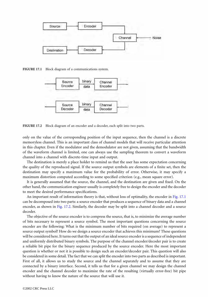
only on the value of the corresponding position of the input sequence, then the channel is a discretememoryless channel. This is an important class of channel models that will receive particular attentionin this chapter. Even if the modulator and the demodulator are not given, assuming that the bandwidthof the waveform channel is limited, one can always use the sampling theorem to convert a waveformchannel into a channel with discrete-time input and output.

The destination is merely a place holder to remind us that the user has some expectation concerningthe quality of the reproduced signal. If the source output symbols are elements of a finite set, then thedestination may specify a maximum value for the probability of error. Otherwise, it may specify amaximum distortion computed according to some specified criterion (e.g., mean square error).

It is generally assumed that the source, the channel, and the destination are given and fixed. On theother hand, the communication engineer usually is completely free to design the encoder and the decoderto meet the desired performance specifications.

An important result of information theory is that, without loss of optimality, the encoder in Fig. 17.1can be decomposed into two parts: a source encoder that produces a sequence of binary data and a channelencoder, as shown in Fig. 17.2. Similarly, the decoder may be split into a channel decoder and a sourcedecoder.

The objective of the source encoder is to compress the source, that is, to minimize the average numberof bits necessary to represent a source symbol. The most important questions concerning the sourceencoder are the following: What is the minimum number of bits required (on average) to represent asource output symbol? How do we design a source encoder that achieves this minimum? These questionswill be considered here. It turns out that the output of an ideal source encoder is a sequence of independentand uniformly distributed binary symbols. The purpose of the channel encoder/decoder pair is to createa reliable bit pipe for the binary sequence produced by the source encoder. Here the most importantquestion is whether or not it is possible to design such an encoder/decoder pair. This question will alsobe considered in some detail. The fact that we can split the encoder into two parts as described is important.First of all, it allows us to study the source and the channel separately and to assume that they areconnected by a binary interface. Second, it tells us that for a given channel we may design the channelencoder and the channel decoder to maximize the rate of the resulting (virtually error-free) bit pipewithout having to know the nature of the source that will use it.

FIGURE 17.1 Block diagram of a communications system.

FIGURE 17.2 Block diagram of an encoder and a decoder, each split into two parts.


17.3 Source Coding for Discrete-Alphabet Sources

We start by considering the simplest possible source, namely, a discrete-time discrete-alphabet memo-ryless information source modeled by a random variable X taking values on a finite alphabet X . A (binarysource) code C for X is a mapping from X into the set of finite length binary sequences called codewords.Such a code can be represented by a binary tree, as shown in the following example.

Example 1

Let X take on values in {1, 2, 3, 4, 5, 6, 7}. A possible binary code for X is given by the (ordered) set ofbinary sequences {1, 010, 011, 0000, 0001, 0010, 0011}. The corresponding tree is shown in Fig. 17.3.Notice that the codeword corresponding to a given source output symbol is the label sequence from theroot to the node corresponding to that symbol.

In Example 1, source output symbols correspond to leaves in the tree. Such a code is called prefix freesince no codeword is the prefix of another codeword. Given a concatenation of codewords of a prefix-free code, we can parse it in an unique way into codewords. Codes with this property are called uniquelydecodable. Although there are uniquely decodable codes which are not prefix free, we will restrict ourattention to prefix-free codes, as it can be shown that the performance of general uniquely decodablecodes is no better than that of prefix-free codes (see Cover and Thomas [1991]).

For each i in X, let C(i) be the codeword associated to the symbol i, let li be its length, L ∫ maxi li, andlet pi be the probability that X = i. A complete binary tree of depth L has 2L leaves. To each leaf at depthl, l £ L, of the binary code tree (which is not necessarily complete) there correspond 2L-l leaves at depthL of the corresponding complete tree (obtained by extending the binary code tree). Further, any twodistinct leaves in the code tree have distinct associated leaves at depth L in the complete binary tree.Hence, summing up over all leaves of the code tree (all codewords) we get

The right-hand side is called the Kraft inequality and is a necessary condition on the codeword lengthsof any prefix-free code. Conversely, for any set of codeword lengths satisfying the displayed inequality,we can construct a prefix-free code having codeword lengths li (start with a complete binary tree ofsufficient length; to each l i associate a node in this tree at level li and make this node a leaf by deletingall of its descendants). The problem of finding the best source code then reduces to that of finding a setof lengths that satisfies the Kraft inequality and minimizes the average codeword lengths L* = Âilipi.Such a code is called optimal.

To any source X with probabilities pi , we associate the quantity H(X), which we call entropy and whichis defined as

FIGURE 17.3 Example of a code tree.

2L 2L li–

2li–

1≤i

∑i

∑≥

H X( ) pi pilogi

∑–=


Usually we take the base of the logarithm to be 2, in which case the units of entropy are called bits.It is straightforward to show by means of Lagrange multipliers that if we neglect the integer constraint

on li , then the minimization of L* subject to the Kraft inequality yields This nonintegerchoice of codeword lengths yields

On the other hand, the (not necessarily optimal) integer choice satisfies the Kraftinequality and yields an expected codeword length

Hence, we have the following theorem.

Theorem 1. The average length L* of the optimal prefix-free code for the random variable X satisfiesH(X) ≤ L* ≤ H(X) + 1.

Example 2

Let X be a random variable that takes on the values 1 and 0 with probabilities θ(0 ≤ θ ≤ 1) and 1 - θ,respectively. Then H(X) = h(θ), where h(θ) = - θ logθ - (1 - θ)log(1 - θ). The function h(θ) is calledthe binary entropy function. In particular, it can be shown that h(θ) ≤ 1 with equality if and only if

. More generally, if X takes on |X | values, then H(X) ≤ log |X | with equality if and only if X isuniformly distributed.

A simple algorithm that generates optimal prefix-free codes is the Huffman algorithm, which can bedescribed as follows:Step 1. Re-index to arrange the probabilities in decreasing order, p1 ≥ p2 ≥ … ≥pm.Step 2. Form a subtree by combining the last two probabilities pm-1 and pm into a single node of weight

= pm-1 + pm.

Step 3. Recursively execute steps 1 and 2, decreasing the number of nodes each time, until a singlenode is obtained.Stpe 4. Use the tree constructed above to assign codewords.

Example 3

As in Example 1, let X take on the values {1, 2, 3, 4, 5, 6, 7}. Assume their corresponding probabilitiesare {0.4, 0.1, 0.1, 0.1, 0.1, 0.1, 0.1}. Figure 17.4 shows the steps in the construction of the Huffman code.For simplicity, probabilities are not shown. The final tree is given in Example 1.

Given a block of n random variables X1,…, Xn, with joint distribution p(X1,…, Xn), define their entropyas

li* pi.log–=

L*

pili*

i

∑ pi pilogi

∑– H X( )= = =

li pilog–=

L C( ) pi pilog–i

∑ pi pilogi

∑ pii

∑+–≤ H X( ) 1+= =

q12--=

p′m

p¢m − 1 = pm − 1 + pm

pm − 1 pm

H X1,…, Xn( ) … p x1, … , xn( ) p x1, …, xn( )logxn

∑x2

∑x1

∑–=


Note that for the special case of n independent random variables, we have H(X1,…,Xn) = nH(X). Thisagrees with the intuitive notion that if it takes H(X) bits to encode one source output symbol, then itshould take nH(X) bits to encode n independent output symbols. For a sequence of random variablesX1, X2,…, Xn, we define If X1, X2,…,Xn is a stationary random process, as n goesto infinity Hn converges to a limit H• called the entropy rate of the process.

Applying Theorem 1 to blocks of random variables, we obtain

In the special case that the process X1, X2,…, Xn is stationary, the left and the right side will both tendto H• as n → ∞. This shows that by encoding a sufficiently large number of source output symbols at atime, one can get arbitrarily close to the fundamental limit of H∞ bits per symbol.

17.4 Universal Source Coding

The Huffman algorithm produces optimal codes, but it requires knowing the statistics of the source. Itis a surprising fact that there are source coding algorithms that are asymptotically optimal withoutrequiring prior knowledge of the source statistics. Such algorithms are called universal source codingalgorithms. The best known universal source coding algorithm is the Lempel–Ziv algorithm, which hasbeen implemented in various forms on computers (as PKZIP command for Windows and Linux-basedsystems). There are two versions of the Lempel–Ziv algorithm: the LZ77, see Ziv and Lempel [1977], andthe LZ78, see Lempel and Ziv [1978]. We will describe the basic idea of the LZ77.

Consider the sequence X1, X2,…, Xk taking values in {a, b, c}, shown in Fig. 17.5, and assume that thefirst w letters (w = 6 in our example) are passed to the decoder with no attempt at compression. At thispoint the encoder identifies the longest string Xw+1, Xw+2,…,Xw+L such that a copy, ,begins (but not necessarily ends) in the portion of data already available to the decoder. In our examplethis string is aabaa, L = 5, and p = 3; see Fig. 17.5. Next, the encoder transmits a binary representationof the pair (L, p) as this is sufficient for the decoder to reconstruct . At this point, theprocedure can be repeated with w replaced by w + L. There are two exceptions: the first occurs whenXw+ � is a new letter that does not appear in Xl,…, Xw ; the second exception occurs when it is moreefficient to encode directly than to encode (L, p). In order to handle such special cases,the algorithm has the option of encoding a substring directly, without attempt at compression. It issurprising that the Lempel–Ziv algorithm is asymptotically optimal for all finite alphabet stationaryergodic sources. This has been shown in Wyner and Ziv [1994].

FIGURE 17.4 Construction of a Huffman code of X as given in Example 1.

Hn

1n---H(X1, …, Xn).=

Hn

L*

n----- Hn

1n---+<≤

Xw-p+1,…, Xw-p+L

Xw +1, …, Xw +L

Xw+1, …, Xw+L


17.5 Rate Distortion Theory

Thus far we have assumed that X is a discrete alphabet and that the decoder must be able to perfectlyreconstruct the source output. Now we drop both assumptions.

Let X1, X2,… be a sequence of independent identically distributed random variables. Let X denote thesource alphabet and Y be a suitably chosen representation alphabet (where Y is not necessarily equal toX ). A distortion measure is a function d: X ¥ Y Æ R+. The most common distortion measures are theHamming distortion dH and the squared error distortion dE defined as follows:

Such a single-letter distortion measure can be extended to a distortion measure on n-tuples by defining

The encoder maps an n-length source output Xn to an index U Œ{1, 2,…, }, where R denotesthe number of bits per source symbol that we are allowed or willing to use. The decoder maps U into ann-tuple Y n, called the representation of Xn. We will call U together with the associated encoding anddecoding function a rate distortion code. Let f be the function that maps Xn to its representation Yn, thatis, f is the mapping describing the concatenation of the encoding and the decoding function. The expecteddisortion D is then given by

The objective is to minimize the average number of bits per symbol, denoted by R, for a given averagedistortion D. What is the minimum R?

Definition. The rate distortion pair (R, D) is said to be achievable if there exists a rate distortion codeof rate R with expected distortion D. The rate distortion function R(D) is the infimum of rates R suchthat (R, D) is achievable for a given D.

Entropy played a key role in describing the limits of lossless coding. When distortion is allowed, asimilar role is played by a quantity called mutual information.

Definition. Given the random variables X and Y with their respective distributions p(x), p(y), and p(x, y),the mutual information I(X; Y) between X and Y is defined as

FIGURE 17.5 Encoding procedure of the Lempel–Ziv algorithm.

dH x, y( ) 0 if x = y

1 if x yπÓÌÏ

=

dE x, y( ) x y–( )2=

d xn, yn( ) 1n--- d xi, yi( )

i=1

n

Â=

2 nR

D p xn( )d xn, f xn( )( )x

nÂ=

I X; Y( ) p x, y( ) p x, y( )p x( )p y( )---------------------log

y YŒÂ

x XŒÂ=


This definition can be extended to blocks of random variables Xn and Y n by replacing p(x), p(y), andp(x, y) with their higher-dimensional counterparts. We can now state the fundamental theorem of ratedistortion theory. For its proof see Cover and Thomas [1991].

Theorem 2. The rate distortion function for an independent identically distributed source X withdistribution p(x) and distortion function d(x, y) is

The rate distortion functions for a binary source that outputs 1 with probability q and Hammingdistortion and for a Gaussian source of variance s 2 and squared error distortion are as follows:

These two functions are plotted in Fig. 17.6.Some insight can be gained by considering the extreme values of both RB(D) and RG(D). Assume that

X1, X2,… is a sequence of independent and identically distributed binary random variables and let q bethe probability that Xi = 1. Without loss of generality, we may assume that q ≥ 1 - q. If we let Y n =(0, …, 0) regardless of Xn, then the expected Hamming distortion equals q. Hence, it must be true thatRB(D) = 0 for D ≥ q. On the other hand, D = 0 means that the reproduction Yn must be a perfect copyof Xn. From Theorem 1 and Example 2 we know that this means RB(0) = H(X) = h(q). Similar consid-erations hold for RG(D). It is interesting to observe that RG(D) tells us that if we are allowed to use R bitsper symbol to describe a sequence of independent Guassian random variables with variance s 2, then weneed to accept a mean squared error of s 22-2R.

17.6 Channel Coding

Now we consider the fundamental limit for the amount of information that can be transmitted througha noisy channel and discuss practical methods to approach it. For simplicity, we assume that the channelcan be modeled as a discrete memoryless channel, defined as follows:

FIGURE 17.6 Examples of rate distortion functions.

R D( ) minp y |x( ) :Âx ,yp x( )p y |x( )d x ,y( ) D£

= I X; Y( )

RB D( ) h q( ) h D( ),– 0 D min q, 1 q–{ }£ £0, D min q, 1 q–{ }>Ó

ÌÏ

=

RG D( )12-- s 2

D------ ,log 0 D s 2£ £

0, D s 2>ÓÔÌÔÏ

=


A discrete memoryless channel (DMC) is a system consisting of an input alphabet X , an outputalphabet Y , and a collection of probability mass functions p(y |x), one for each x Œ X . A specific DMCwill be denoted by (X, p(y |x), Y ).

An (M, n) channel code for the DMC (X, p(y |x), Y) consists of the following:

1. an index set {1, 2, …, M}2. an encoding function Xn: {1, 2, º, M} Æ Xn, yielding codewords X n(1), X n(2), º, Xn(M) (the

set of codewords is called the code book)3. a decoding function g: Yn Æ {1, 2, º, M}, which is a deterministic rule that assigns a guess to

each possible received vector

The most important figures of merit for a channel code for a DMC are the maximal probability of error,defined by

and the transmission rate,

It makes sense to define the rate in this way since the M codewords can be labeled with log M bits.Hence, every time we transmit a codeword, we actually transmit log M bits of information. Since it takesn uses of the channel to transmit one codeword, the resulting information rate is (log M)/n bits perchannel use.

For a given DMC, a rate R is said to be achievable if, for any desired probability of error Pe andsufficiently large block length n, there exists a code for that DMC with maximal probabilityof error l(n) £ Pe.

The operational capacity of a discrete memoryless channel is the supremum of all achievable rates.One would expect that determining the operational capacity would be a formidable task. One of themost remarkable results of information theory is a relatively easy-to-compute way to determine theoperational capacity.

We define the information channel capacity of a discrete memoryless channel (X , p(y|x), Y ) as

where the maximum is taken over all possible input distributions p(x). As we will show in the nextexample, it is straightforward to compute the information channel capacity for many discrete memorylesschannels of interest. Shannon’s channel coding theorem establishes that the information channel capacityequals the operational channel capacity.

Theorem (Shannon’s channel coding theorem). For a DMC, the information channel capacity equalsthe operational channel capacity, that is, for every rate R < C, there exists a sequence of codesfor the DMC with maximum probability of error l(n) Æ 0. Conversely, for any sequence of for codes this DMC with the property that l(n) Æ 0, the rate R must satisfy R £ C.

This is perhaps the most important result of information theory. In order to shed some light on theinterpretation of mutual information and to provide an efficient way to determine C, it is convenient torewrite I(X; Y) in terms of conditional entropy. Given two random variables X and Y with joint probabilitymass function p(x, y), marginal probability mass function p(x) = Â y p(x, y), and conditional probabilitymass function p(x |y) = p(x, y)/p(y), we define the conditional entropy of X given that Y = y as

l n( ) maxi Œ 1, 2,º , M{ }

Pr g Y n( ) i|X n = Xn i( )π{ }∫

RMlog

n-------------- bits/channel use=

( 2nR , n)

C max I X; Y( )∫p x( )

( 2nR , n)( 2nR , n)

H X | Y y=( ) p x|y( ) p x|y( )logx

Â–=


Its average is the conditional entropy of X given Y, denoted by H(X |Y) and defined as

Recall that for the discrete variable X with probability mass function p(x), H(X) is the average numberof binary symbols necessary to describe X. Now let X be the random variable at the input of a DMC andlet Y be the output. The knowledge that Y = y changes the probability mass function of the channelinput from p(x) to p(x | y) and its entropy from H(X ) to H(X |Y = y). According to our previous result,H(X | Y = y) is the average number of bits necessary to describe X after the observation that Y = y. SinceH(X) is the average number of bits needed to describe X (without knowledge of Y ), H(X) - H(X |Y = y)is the average amount of information about X acquired by the observation that Y = y, and

is the average amount of information about X acquired by the observation of Y. One can easily verifythat the latter expression is another way to write I(X; Y). Moreover,

Hence, the amount of information that Y gives about X is the same as the amount of information thatX gives about Y. For this reason, I(X; Y) is called the mutual information between X and Y.

Example (Binary Symmetric Channel). Let X = {0, 1}, Y = {0, 1}, and p(y |x) = p when x π y and 1 - potherwise. This DMC can be conveniently depicted as in Fig. 17.7. For obvious reasons it is called thebinary symmetric channel (BSC).

For the BSC, we bound the mutual information by

FIGURE 17.7 Discrete memoryless channel with crossover probability p.

H X | Y( ) p y( )H X|Y y=( )y

Â=

p x, y( ) p x|y( )logx , yÂ–=

E p X|Y( )log–[ ]=

H X( ) H X | Y( )–

I X; Y( ) H X( ) H X|Y( )–=H Y( ) H Y|X( )–=I Y; X( )=

I X; Y( ) H Y( ) H Y | X( )–=

H Y( ) p x( )H Y | X x=( )x

Â–=

H Y( ) h p( )–=1 h p( )–£


where the last inequality follows because Y is a binary random variable (see Example 2). Equality isachieved when the input distribution is uniform since in this case the output distribution is also uniform.Hence, the information capacity of a binary symmetric channel with parameter p is

This function is plotted in Fig. 17.8.

17.7 Simple Binary Codes

Shannon’s channel coding theorem promises the existence of block codes that allow us to transmit reliablythrough an unreliable channel at any rate below the channel capacity. Unfortunately, the codes con-structed in all known proofs of this fundamental result are impractical in that they do not exhibit anystructure which can be employed for an efficient implementation of the encoder and the decoder. Thisis an important issue, as good codes must have long block lengths and, hence, a large number ofcodewords. For these codes, simple table lookup encoding and decoding procedures are not feasible. Thesearch for good and practical codes has led to the development of coding theory. Although powerfulblock codes are, in general, described by sophisticated techniques, the main idea is simple. We collect anumber k of information symbols which we wish to transmit, we append r check symbols, and transmitthe entire block of n = k + r channel symbols. Assuming that the channel changes a sufficiently small numberof symbols within an n-length block, the r check symbols may provide the receiver with sufficient infor-mation to detect and/or correct the errors.

Traditionally, good codes have been constructed by sophisticated algebraic schemes. More recent codeconstruction techniques are inspired by Shannon’s original work. The idea is to construct the code bymaking random choices on a suitably defined structure. A key property of the structure is that it leadsto codes that may be decoded using powerful iterative techniques. We will demonstrate these two quitedistinct concepts by simple examples.

Hamming Codes

For any positive integer m, there is a Hamming code with parameters k = 2m - m - 1 and n = 2m - 1. Toillustrate, we consider the k = 4, n = 7 Hamming code. All operations will be done modulo 2. Considerthe set of all nonzero binary vectors of length m = 3. Arrange them in columns to form the matrix

FIGURE 17.8 Capacity of the BSC as a function of p.

C 1 h p( ) [bits/channel use]–=

H1 0 1 0 1 0 1

0 1 1 0 0 1 1

0 0 0 1 1 1 1Ë ¯Á ˜Á ˜Á ˜Ê ˆ

=


The row space of H is a vector space of binary 7-tuples of dimension m = 3. The k = 4, n = 7 Hammingcode is the null space of H, that is, the vector space of dimension n - m = 4 consisting of all binary 7-tuples c such that cHT = 0. Hence, it contains the M = 2k = 16 codewords shown in Table 17.1 and its rateis R = (log M)/n = 4/7. If c is transmitted and u is received, then the error is the unique binary n-tuplee such that u = c + e, where addition is component-wise modulo 2. The decoder performs the operation

If there is a single error at position i, that is, if e is zero except for the ith component (which is one),then uHT is the ith row of HT. This tells us the error location. If e contains 2 ones (channel errors), thenuHT is the sum of two rows of HT. Since this cannot be zero, two channel errors are detectable. They arenot correctable, however, since, as one can easily verify when two channel errors occur, there is always acodeword that agrees with the received word in n - 1 positions. This is the codeword that would beselected by the decoder if it were forced to make a decision since the transmitted codeword agrees withthe received word in only n - 2 positions. A simple encoding procedure can be specified as follows: letG be a k ¥ n matrix whose rows span the null space of H. Such a matrix is

Then an information k-tuple a can be mapped into a codeword c = aG by a simple matrix multiplication.

Low-Density Parity-Check Codes

Low-density parity-check (LDPC) codes constitute a family of a new breed of coding techniques variablydescribed as “codes on graphs” or “iterative coding techniques.” They were originally introduced byGallager in his thesis in 1962 (see Gallager [1963]), then long forgotten, and later revived in the wake ofthe discovery of turbo codes by Berrou et. al. (see Berrou et al. [1993] and MacKay [1999]).

LDPC codes are codes which possess a sparse parity check matrix. Because of this sparseness, theycan be decoded very efficiently in an iterative fashion. Although this iterative decoding procedure is,in general, suboptimal, it is sufficiently strong to allow transmission seemingly arbitrarily close tochannel capacity.

Consider the code represented by the following parity check matrix.

TABLE 17.1 Codewords of the (7, 4) Hamming Code

0 0 0 0 0 0 0 1 0 0 0 1 0 10 0 0 1 0 1 1 1 0 0 1 1 1 00 0 1 0 1 1 0 1 0 1 0 0 1 10 0 1 1 1 0 1 1 0 1 1 0 0 00 1 0 0 1 1 1 1 1 0 0 0 1 00 1 0 1 1 0 0 1 1 0 1 0 0 10 1 1 0 0 0 1 1 1 1 0 1 0 00 1 1 1 0 1 0 1 1 1 1 1 1 1

uHT c e+( )HT cHT eHT+ eHT= = =

G

1 0 0 0 1 1 0

0 1 0 0 1 0 1

0 0 1 0 0 1 1

0 0 0 1 1 1 1Ë ¯Á ˜Á ˜Á ˜Á ˜Ê ˆ

=

H

1110111000

0011111100

0110100111

1001010111

1101001011Ë ¯Á ˜Á ˜Á ˜Á ˜Á ˜Á ˜Ê ˆ

=


Note that each row contains exactly 6 ones and that each column contains exactly 3 ones. Such a codeis referred to as a (3, 6)-regular LDPC code. A convenient graphical representation of this code is givenby means of the bipartite graph shown in Fig. 17.9(a). This graph is usually referred to as Tanner graph.In this graph, each left node (variable node) corresponds to one column of the parity check matrix andeach right node (check node) corresponds to one row of H. A left node is connected to a right node ifand only if the corresponding position in the parity check matrix contains a 1.

Let (x = x0,…, x9) be the codeword (0101001010). Assume that we transmit x over a binary erasurechannel (BEC) and that the received word is y = (??01001?10) where ? indicates an erasure. Rather thanemploying a maximum likelihood decoder, we will use the iterative decoding algorithm described in Figs.17.9(a)-(e). The received word y is written on the left (y0 on the bottom and ya on the top). We start bypassing all known values from the left to the right along the corresponding edges. We next accumulateat each check the partial sum (mod 2) of all known values and delete all edges along which messageshave already been passed. The result is shown in Fig. 17.9(b), where a black box indicates a partial sumequal to 1. Now note that check node one (the second from the bottom) has received already all valuesexcept the one from the erased bit seven. Since, by the code constraints, the sum of all values must beequal to zero, we see that we can deduce the value of variable node seven to be equal to zero. This valuecan now again be propagated to the right and all involved edges be deleted. The result is shown in Fig.17.9 (d). After one more iteration all erased values are known. (Fig. 17.9(e)).

As we can see, in the above example the given iterative decoding strategy successfully recovered the erasedbits. This might seem like a lucky coincidence. Nevertheless, it has been shown that long and suitably definedLDPC codes can achieve capacity on the BEC under iterative decoding (see Luby et. al. [1997]).

Even more, the above iterative decoding strategy, suitably extended, can be used to transmit reliablyclose to capacity over a wide array of channels (see Richardson et. al. [2001]).

Defining Terms

Binary source code: A mapping from a set of messages into binary strings.Channel capacity: The highest rate at which information can be transmitted reliably across a channel.Discrete memoryless channel: A channel model characterized by discrete input and output alphabets

and a probability mass function on the output conditioned on the input.

FIGURE 17.9 Iterative decoding.

0

0

0

0

1

1

1

0

?

?

0

0

0

0

1

1

1

0

1

0

0

0

0

0

1

1

1

?

?

?

0

0

0

0

1

1

1

?

?

?

0

0

0

0

1

1

1

0

?

?

(a) (b) (c)

(d) (e)


Entropy: A measure of the average uncertainty of a random variable. For a random variable withdistribution p(x), the entropy H(X) is defined as -Âxp(x)logp(x).

Huffman coding: A procedure that constructs a code of minimum average length for a random variable.Lempel-Ziv coding: A procedure for coding that does not use the probability distribution of the source

but nevertheless is asymptotically optimal.Mutual information: A measure for the amount of information that a random variable gives about another.Rate distortion function: The minimum rate at which a source can be described to the given average

distortion.

References

Berrou, C., Glavieux, A., and Thitimajshima, P. 1993. Near Shannon limit error-correcting coding anddecoding, in Proceedings of ICC’93, Geneva, Switzerland, 1064–1070.

Blahut, R. 1987, Principles and Practice of information Theory, Addison–Wesley, Reading, MA.Csiszár, I. and Körner, J. 1981. Information Theory: Coding Theorems for Discrete Memoryless Systems,

Academic Press, New York.Cover, T.M. and Thomas, J.A. 1991. Elements of Information Theory, Wiley, New York.Gallager, R.G. 1963. Low-Density Parity-Check Codes, Monograph, M.I.T. Press, Cambridge, MA.Gallager, R.G. 1968. Information Theory and Reliable Communication, Wiley, New York.Luby, M., Mitzenmacher, M., Shokrollahi, A., Spielman, D., and Stemann, V. 1997. Practical loss-resilient

codes, in Proceedings of the 29th Annual ACM Symposium on the Theory of Computing, 150–159.McEliece, R.J. 1977. The Theory of Information and Coding, Addison–Wesley, Reading, MA.MacKay, D. 1999. Good error correcting codes based on very sparse matrices, IEEE Trans. Inf. Theory,

45:399–431.Richardson, T., Shokrollahi, A., and Urbanke, R. 2001. Design of probably good low-density parity check

codes, IEEE Trans. Inf. Theory, 47:619–637.Wyner, A.D. and Ziv, J. 1994. The sliding-window Lempel–Ziv algorithm is asymptotically optimal.

Communications and Cryptography, Blahut, R.E., Costello, D.J., Jr., Maurer, V., and Mittclholzer,T., Eds., Kluwer Academic Publishers, Boston, MA.

Ziv, J. and Lempel, A. 1977. A universal algorithm for sequential data compression. IEEE Trans. Inf.Theory, IT-23 (May):337–343.

Ziv, J. and Lempel, A. 1978. Compression of individual sequences by variable rate coding. IEEE Trans.Inf. Theory, IT-24 (Sept.):530–536.

Further Information

For a lucid and up-to-date treatment of information theory extending beyond the area of communication,a most recommended reading is Cover and Thomas [1991]. For readers interested in continuous-timechannels and sources we recommend Gallager [1968]. For mathematically inclined readers who do notrequire much physical motivation, strong results for discrete memoryless channels and sources may befound in Csiszár and Körner [1981]. Other excellent readings are Blahut [1987] and McEliece [1977].Most results in information theory are published in IEEE Transactions on Information Theory.


18Digital Communication

System Performance*1

18.1 IntroductionThe Channel • The Link

18.2 Bandwidth and Power ConsiderationsThe Bandwidth Efficiency Plane • M-ary Signalling • Bandwidth-Limited Systems • Power-Limited Systems • Minimum Bandwidth Requirements for MPSK and MFSK Signalling

18.3 Example 1: Bandwidth-Limited Uncoded SystemSolution to Example 1

18.4 Example 2: Power-Limited Uncoded SystemSolution to Example 2

18.5 Example 3: Bandwidth-Limited and Power-Limited Coded SystemSolution to Example 3 • Calculating Coding Gain

18.6 Example 4: Direct-Sequence (DS) Spread-Spectrum Coded SystemProcessing Gain • Channel Parameters for Example 4• Solution to Example 4

18.7 ConclusionAppendix: Received Eb/N0 Is Independent of the Code Parameters

18.1 Introduction

In this section we examine some fundamental tradeoffs among bandwidth, power, and error performanceof digital communication systems. The criteria for choosing modulation and coding schemes, based onwhether a system is bandwidth limited or power limited, are reviewed for several system examples. Emphasisis placed on the subtle but straightforward relationships we encounter when transforming from data-bits to channel-bits to symbols to chips.

The design or definition of any digital communication system begins with a description of the commu-nication link. The link is the name given to the communication transmission path from the modulator andtransmitter, through the channel, and up to and including the receiver and demodulator. The channel isthe name given to the propagating medium between the transmitter and receiver. A link descriptionquantifies the average signal power that is received, the available bandwidth, the noise statistics, and other

1*A version of this chapter has appeared as a paper in the IEEE Communications Magazine, November 1993, underthe title “Defining, Designing, and Evaluating Digital Communication Systems.”

Bernard SklarCommunications Engineering Services


impairments, such as fading. Also needed to define the system are basic requirements, such as the data rateto be supported and the error performance.

The Channel

For radio communications, the concept of free space assumes a channel region free of all objects thatmight affect radio frequency (RF) propagation by absorption, reflection, or refraction. It further assumesthat the atmosphere in the channel is perfectly uniform and nonabsorbing and that the earth is infinitelyfar away or its reflection coefficient is negligible. The RF energy arriving at the receiver is assumed to bea function of distance from the transmitter (simply following the inverse-square law as used in optics).In practice, of course, propagation in the atmosphere and near the ground results in refraction, reflection,and absorption, which modify the free space transmission.

The Link

A radio transmitter is characterized by its average output signal power Pt and the gain of its transmittingantenna Gt. The name given to the product PtGt, with reference to an isotropic antenna, is effective radiatedpower (EIRP) in watts (or dBW). The average signal power S arriving at the output of the receiver antennacan be described as a function of the EIRP, the gain of the receiving antenna Gr , the path loss (or spaceloss) Ls , and other losses, Lo , as follows [1,2]:

(18.1)

The path loss Ls can be written as follows [2]:

(18.2)

where d is the distance between the transmitter and receiver and l is the wavelength.We restrict our discussion to those links distorted by the mechanism of additive white Gaussian noise

(AWGN) only. Such a noise assumption is a very useful model for a large class of communicationsystems. A valid approximation for average received noise power N that this model introduces is writtenas follows [3,4]:

(18.3)

where k is Boltzmann’s constant (1.38 ¥ 10-23 joule/K), is system effective temperature in kelvin, andW is bandwidth in hertz. Dividing Eq. (18.3) by bandwidth enables us to write the received noise-powerspectral density N0 as follows:

(18.4)

Dividing Eq. (18.1) by N0 yields the received average signal-power to noise-power spectral density S/N0 as

(18.5)

where Gr/T∞ is often referred to as the receiver figure of merit. A link budget analysis is a compilationof the power gains and losses throughout the link; it is generally computed in decibels and thus takes onthe bookkeeping appearance of a business enterprise, highlighting the assets and liabilities of the link.Once the value of S/N0 is specified or calculated from the link parameters, we then shift our attention tooptimizing the choice of signalling types for meeting system bandwidth and error performance requirements.

SEIRP Gr

LsLo

-------------------=

Ls4pd

l---------Ë ¯

Ê ˆ2

=

N kT∞W@

T∞

N0NW----- kT∞= =

SN0

------EIRP Gr/T∞

kLsLo

----------------------------=


In Eq. (18.4), N0 characterizes all the noise in the receiving system since To is the system effectivetemperature; thus, S/N0 is referenced to the predetection point in the receiver [2]. Then we can write theratio of bit energy-to-N0(Eb/N0) at this point, for any data rate R, as

(18.6)

Equation(18.6) follows from the basic definitions that received bit energy is equal to received averagesignal power times the bit duration and that bit rate is the reciprocal of bit duration. Received Eb/N0 isa key parameter in defining a digital communication system. Its value indicates the apportionment ofthe received waveform energy among the bits that the waveform represents. At first glance, one mightthink that a system specification should entail the symbol-energy to noise-power spectral density Es/N0

associated with the arriving waveforms. We will show, however, that for a given S/N0, the value of Es/N0

is a function of the modulation and coding. The reason for defining systems in terms of Eb/N0 stemsfrom the fact that Eb/N0 depends only on S/N0 and R and is unaffected by any system design choices,such as modulation and coding.

18.2 Bandwidth and Power Considerations

Two primary communications resources are the received power and the available transmission band-width. In many communication systems, one of these resources may be more precious than the otherand, hence, most systems can be classified as either bandwidth limited or power limited. In bandwidth-limited systems, spectrally efficient modulation techniques can be used to save bandwidth at the expenseof power; in power-limited systems, power efficient modulation techniques can be used to save powerat the expense of bandwidth. In both bandwidth- and power-limited systems, error-correction coding(often called channel coding) can be used to save power or to improve error performance at the expenseof bandwidth. Recently, trellis-coded modulation (TCM) schemes have been used to improve the errorperformance of bandwidth-limited channels without any increase in bandwidth [5], but these methodsare beyond the scope of this chapter.

The Bandwidth Efficiency Plane

Figure 18.1 shows the abscissa as the ratio of bit-energy to noise-power spectral density Eb/N0 (in decibels)and the ordinate as the ratio of throughput, R (in bits per second), that can be transmitted per hertz ina given bandwidth W. The ratio R/W is called bandwidth efficiency since it reflects how efficiently thebandwidth resource is utilized. The plot stems from the Shannon–Hartley capacity theorem [2,6,7],which can be stated as

(18.7)

where S/N is the ratio of received average signal power to noise power. When the logarithm is taken to thebase 2, the capacity C is given in bits per second. The capacity of a channel defines the maximum numberof bits that can be reliably sent per second over the channel. For the case where the data (information) rateR is equal to C, the curve separates a region of practical communication systems from a region where suchcommunication systems cannot operate reliably [2,6].

M-ary Signalling

Each symbol in an M-ary alphabet can be related to a unique sequence of m bits, expressed as

(18.8)

Eb

N0

------STb

N0

-------- SN0

------ 1R---Ë ¯

Ê ˆ= =

C W log2 1SN----+Ë ¯

Ê ˆ=

M 2m= or m log2 M=


where M is the size of the alphabet. In the case of digital transmission, the term symbol refers to the memberof the M-ary alphabet that is transmitted during each symbol duration Ts. To transmit the symbol, it mustbe mapped onto an electrical voltage or current waveform. Because the waveform represents the symbol, theterms symbol and waveform are sometimes used interchangeably. Since one of M symbols or waveforms istransmitted during each symbol duration Ts, the data rate R in bits per second can be expressed as

(18.9)

Data-bit-time duration is the reciprocal of data rate. Similarly, symbol-time duration is the reciprocal ofsymbol rate. Therefore, from Eq. (18.9), we write that the effective time duration Tb of each bit in termsof the symbol duration Ts or the symbol rate Rs is

(18.10)

Then, using Eqs. (18.8) and (18.10) we can express the symbol rate Rs in terms of the bit rate R as follows:

(18.11)

From Eqs. (18.9) and (18.10), any digital scheme that transmits m = log2 M bits in Ts seconds, using abandwidth of W hertz, operates at a bandwidth efficiency of

(18.12)

where Tb is the effective time duration of each data bit.

FIGURE 18.1 Bandwidth-efficiency plane.

RmTs

-----log2M

Ts

---------------= =

Tb1R---

Ts

m----- 1

m Rs

----------= = =

RsR

log2 M---------------=

RW-----

log2 MWTs

---------------- 1WTb

----------- b/s( )/Hz= =


Bandwidth-Limited Systems

From Eq. (18.12), the smaller the WTb product, the more bandwidth efficient will be any digital commu-nication system. Thus, signals with small WTb products are often used with bandwidth-limited systems.For example, the European digital mobile telephone system known as Global System for Mobile Com-munications (GSM) uses Gaussian minimum shift keying (GMSK) modulation having a WTb productequal to 0.3 Hz/(b/s), where W is the 3-dB bandwidth of a Gaussian filter [8].

For uncoded bandwidth-limited systems, the objective is to maximize the transmitted informationrate within the allowable bandwidth, at the expense of Eb/N0 (while maintaining a specified value of bit-error probability PB). The operating points for coherent M-ary phase-shift keying (MPSK) at PB = 10-5

are plotted on the bandwidth-efficiency plane of Fig. 18.1. We assume Nyquist (ideal rectangular) filteringat baseband [9]. Thus, for MPSK, the required double-sideband (DSB) bandwidth at an intermediatefrequency (IF) is related to the symbol rate as follows:

(18.13)

where Ts is the symbol duration and Rs is the symbol rate. The use of Nyquist filtering results in theminimum required transmission bandwidth that yields zero intersymbol interference; such ideal filteringgives rise to the name Nyquist minimum bandwidth.

From Eqs. (18.12) and (18.13), the bandwidth efficiency of MPSK modulated signals using Nyquistfiltering can be expressed as

(18.14)

The MPSK points in Fig. 18.1 confirm the relationship shown in Eq. (18.14). Note that MPSK modulationis a bandwidth-efficient scheme. As M increases in value, R/W also increases. MPSK modulation can beused for realizing an improvement in bandwidth efficiency at the cost of increased Eb/N0. Althoughbeyond the scope of this chapter, many highly bandwidth-efficient modulation schemes have beeninvestigated [10].

Power-Limited Systems

Operating points for noncoherent orthogonal M-ary FSK (MFSK) modulation at PB = 10-5 are also plottedin Fig. 18.1. For MFSK, the IF minimum bandwidth is as follows [2]:

(18.15)

where Ts is the symbol duration and Rs is the symbol rate. With MFSK, the required transmissionbandwidth is expanded M-fold over binary FSK since there are M different orthogonal waveforms, eachrequiring a bandwidth of 1/Ts. Thus, from Eqs. (18.12) and (18.15), the bandwidth efficiency of non-coherent orthogonal MFSK signals can be expressed as

(18.16)

The MFSK points plotted in Fig. 18.1 confirm the relationship shown in Eq. (18.16). Note that MFSKmodulation is a bandwidth-expansive scheme. As M increases, R/W decreases. MFSK modulation canbe used for realizing a reduction in required Eb/N0 at the cost of increased bandwidth.

In Eqs. (18.13) and (18.14) for MPSK and Eqs. (18.15) and (18.16) for MFSK, and for all the pointsplotted in Fig. 18.1, ideal filtering has been assumed. Such filters are not realizable! For realistic channels

W1Ts

----- Rs= =

R/W log2 M b/s( )/Hz=

WMTs

----- MRs= =

RW-----

log2MM

--------------- b/s( )/Hz=


and waveforms, the required transmission bandwidth must be increased in order to account for realizablefilters.

In the examples that follow, we will consider radio channels that are disturbed only by additive whiteGaussian noise (AWGN) and have no other impairments, and for simplicity, we will limit the modulationchoice to constant-envelope types, i.e., either MPSK or noncoherent orthogonal MFSK. For an uncodedsystem, MPSK is selected if the channel is bandwidth limited, and MFSK is selected if the channel ispower limited. When error-correction coding is considered, modulation selection is not as simple, becausecoding techniques can provide power-bandwidth tradeoffs more effectively than would be possiblethrough the use of any M-ary modulation scheme considered in this chapter [11].

In the most general sense, M-ary signalling can be regarded as a waveform-coding procedure, i.e.,when we select an M-ary modulation technique instead of a binary one, we in effect have replaced thebinary waveforms with better waveforms—either better for bandwidth performance (MPSK) or betterfor power performance (MFSK). Even though orthogonal MFSK signalling can be thought of as beinga coded system, i.e., a first-order Reed-Muller code [12], we restrict our use of the term coded systemto those traditional error-correction codes using redundancies, e.g., block codes or convolutional codes.

Minimum Bandwidth Requirements for MPSK and MFSK Signalling

The basic relationship between the symbol (or waveform) transmission rate Rs and the data rate R wasshown in Eq. (18.11). Using this relationship together with Eqs. (18.13–18.16) and R = 9600 b/s, asummary of symbol rate, minimum bandwidth, and bandwidth efficiency for MPSK and noncoherentorthogonal MFSK was compiled for M = 2, 4, 8, 16, and 32 (Table 18.1). Values of Eb/N0 required toachieve a bit-error probability of 10-5 for MPSK and MFSK are also given for each value of M. Theseentries (which were computed using relationships that are presented later in this chapter) corroboratethe tradeoffs shown in Fig. 18.1. As M increases, MPSK signalling provides more bandwidth efficiencyat the cost of increased Eb/N0, whereas MFSK signalling allows for a reduction in Eb/N0 at the cost ofincreased bandwidth.

18.3 Example 1: Bandwidth-Limited Uncoded System

Suppose we are given a bandwidth-limited AWGN radio channel with an available bandwidth of W =4000 Hz. Also, suppose that the link constraints (transmitter power, antenna gains, path loss, etc.) resultin the ratio of received average signal-power to noise-power spectral density S/N0 being equal to 53 dB-Hz. Let the required data rate R be equal to 9600 b/s, and let the required bit-error performance PB be atmost 10-5. The goal is to choose a modulation scheme that meets the required performance. In general,an error-correction coding scheme may be needed if none of the allowable modulation schemes can meetthe requirements. In this example, however, we shall find that the use of error-correction coding is notnecessary.

TABLE 18.1 Symbol Rate, Minimum Bandwidth, Bandwidth Efficiency, and Required Eb/N0 for MPSK and Noncoherent Orthogonal MFSK Signalling at 9600 bit/s

M mR

(b/s)Rs

(symb/s)

MPSKMinimum

Bandwidth (Hz)MPSKR/W

MPSKEb/N0 (dB)PB = 10-5

NoncoherentOrthog MFSK

Min Bandwidth (Hz)MFSKR/W

MFSKEb/N0 (dB)

PB = 10-5

2 1 9600 9600 9600 1 9.6 19,200 1/2 13.44 2 9600 4800 4800 2 9.6 19,200 1/2 10.68 3 9600 3200 3200 3 13.0 25,600 3/8 9.1

16 4 9600 2400 2400 4 17.5 38,400 1/4 8.132 5 9600 1920 1920 5 22.4 61,440 5/32 7.4


Solution to Example 1

For any digital communication system, the relationship between received S/N0 and received bit-energyto noise-power spectral density, Eb/N0 was given in Eq. (18.6) and is briefly rewritten as

(18.17)

Solving for Eb/N0 in decibels, we obtain

(18.18)

Since the required data rate of 9600 b/s is much larger than the available bandwidth of 4000Hz, thechannel is bandwidth limited. We therefore select MPSK as our modulation scheme. We have confinedthe possible modulation choices to be constant-envelope types; without such a restriction, we would beable to select a modulation type with greater bandwidth efficiency. To conserve power, we compute thesmallest possible value of M such that the MPSK minimum bandwidth does not exceed the availablebandwidth of 4000 Hz. Table 18.1 shows that the smallest value of M meeting this requirement is M = 8.Next we determine whether the required bit-error performance of PB £ 10-5 can be met by using 8-PSKmodulation alone or whether it is necessary to use an error-correction coding scheme. Table 18.1 showsthat 8-PSK alone will meet the requirements, since the required Eb/N0 listed for 8-PSK is less than thereceived Eb/N0 derived in Eq. (18.18). Let us imagine that we do not have Table 18.1, however, and evaluatewhether or not error-correction coding is necessary.

Figure 18.2 shows the basic modulator/demodulator (MODEM) block diagram summarizing thefunctional details of this design. At the modulator, the transformation from data bits to symbols yieldsan output symbol rate Rs, that is, a factor log2 M smaller than the input data-bit rate R, as is seen inEq. (18.11). Similarly, at the input to the demodulator, the symbol-energy to noise-power spectraldensity ES/N0 is a factor log2 M larger than Eb/N0, since each symbol is made up of log2 M bits. BecauseES /N0 is larger than Eb/N0 by the same factor that Rs is smaller than R, we can expand Eq. (18.17), as

FIGURE 18.2 Basic modulator/demodulator (MODEM) without channel coding.

SN0

------Eb

N0

------R=

Eb

N0

------ dB( ) SN0

------ dB-Hz( ) R dB-b/s( )–=

53 dB-Hz 10 log109600¥( ) dB-b/s–=

13.2 dB or 20.89( )=


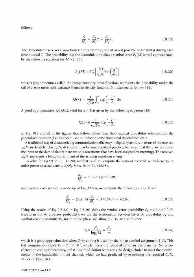
follows:

(18.19)

The demodulator receives a waveform (in this example, one of M = 8 possible phase shifts) during eachtime interval Ts. The probability that the demodulator makes a symbol error PE(M) is well approximatedby the following equation for M > 2 [13]:

(18.20)

where Q(x), sometimes called the complementary error function, represents the probability under thetail of a zero-mean unit-variance Gaussian density function. It is defined as follows [14]:

(18.21)

A good approximation for Q(x), valid for x > 3, is given by the following equation [15]:

(18.22)

In Fig. 18.2 and all of the figures that follow, rather than show explicit probability relationships, thegeneralized notation f(x) has been used to indicate some functional dependence on x.

A traditional way of characterizing communication efficiency in digital systems is in terms of the receivedEb/N0 in decibels. This Eb/N0 description has become standard practice, but recall that there are no bits atthe input to the demodulator; there are only waveforms that have been assigned bit meanings. The receivedEb/N0 represents a bit-apportionment of the arriving waveform energy.

To solve for PE(M) in Eq. (18.20), we first need to compute the ratio of received symbol-energy tonoise-power spectral density Es/N0. Since, from Eq. (18.18),

and because each symbol is made up of log2 M bits, we compute the following using M = 8:

(18.23)

Using the results of Eq. (18.23) in Eq. (18.20) yields the symbol-error probability PE = 2.2 ¥ 10-5. Totransform this to bit-error probability, we use the relationship between bit-error probability PB andsymbol-error probability PE , for multiple-phase signalling [12] PE 1 as follows:

(18.24)

which is a good approximation when Gray coding is used for the bit-to-symbol assignment [13]. Thislast computation yields PB = 7.3 ¥ 10-6, which meets the required bit-error performance. No error-correction coding is necessary, and 8-PSK modulation represents the design choice to meet the require-ments of the bandwidth-limited channel, which we had predicted by examining the required Eb/N0

values in Table 18.1.

SN0

------Eb

N0

------REs

N0

------Rs= =

PE M( ) 2Q2Es

N0

-------sinpM-----Ë ¯

Ê ˆ@

Q x( ) 1

2p---------- exp

u2

2-----–Ë ¯

Ê ˆ dux

•

Ú=

Q x( ) 1

x 2p------------- exp

x2

2----–Ë ¯

Ê ˆ@

Eb

N0

------ 13.2 dB or 20.89( )=

Es

N0

------ log2 M( )Eb

N0

------ 3 20.89¥ 62.67= = =

<<

PB

PE

log2 M---------------@

PE

m-----=


18.4 Example 2: Power-Limited Uncoded System

Now, suppose that we have exactly the same data rate and bit-error probability requirements as inExample 1, but let the available bandwidth W be equal to 45 kHz and the available S/N0 be equal to48 dB-Hz. The goal is to choose a modulation or modulation/coding scheme that yields the requiredperformance. We shall again find that error-correction coding is not required.


The channel is clearly not bandwidth limited since the available bandwidth of 45kHz is more thanadequate for supporting the required data rate of 9600 bit/s. We find the received Eb/N0 from Eq. (18.18),as follows:

(18.25)

Since there is abundant bandwidth but a relatively small Eb/N0 for the required bit-error probability, weconsider that this channel is power limited and choose MFSK as the modulation scheme. To conserve power,we search for the largest possible M such that the MFSK minimum bandwidth is not expanded beyond ouravailable bandwidth of 45 kHz. A search results in the choice of M = 16 (Table 18.1). Next, we determinewhether the required error performance of PB £ 10-5 can be met by using 16-FSK alone, i.e., without error-correction coding. Table 18.1 shows that 16-FSK alone meets the requirements, since the required Eb/N0

listed for 16-FSK is less than the received Eb/N0 derived in Eq. (18.25). Let us imagine again that we do nothave Table 18.1 and evaluate whether or not error-correction coding is necessary.

The block diagram in Fig. 18.2 summarizes the relationships between symbol rate Rs and bit rate R,and between Es/N0 and Eb/N0, which is identical to each of the respective relationships in Example 1. The16-FSK demodulator receives a waveform (one of 16 possible frequencies) during each symbol timeinterval Ts. For noncoherent orthogonal MFSK, the probability that the demodulator makes a symbolerror PE(M) is approximated by the following upper bound [16]:

(18.26)

To solve for PE(M) in Eq. (18.26), we compute ES/N0, as in Example 1. Using the results of Eq. (18.25)in Eq. (18.23), with M = 16, we get

(18.27)

Next, using the results of Eq. (18.27) in Eq. (18.26) yields the symbol-error probability PE = 1.4 ¥ 10-5.To transform this to bit-error probability, PB , we use the relationship between PB and PE for orthogonalsignalling [16], given by

(18.28)

This last computation yields PB = 7.3 ¥ 10-6, which meets the required bit-error performance. Thus, wecan meet the given specifications for this power-limited channel by using 16-FSK modulation, withoutany need for error-correction coding, as we had predicted by examining the required Eb/N0 values inTable 18.1.

Eb

N0

------ dB( ) 48 dB-Hz 10 log10 9600¥( ) dB-b/s 8.2 dB or 6.61( )=–=

PE M( ) M 1–2

--------------expEs

2N0

---------–Ë ¯Ê ˆ£

Es

N0

------ log2 M( )Eb

N0

------ 4 6.61¥ 26.44= = =

PB2m-1

2m 1–( )-------------------PE=


18.5 Example 3: Bandwidth-Limited and Power-LimitedCoded System

We start with the same channel parameters as in Example 1 (W = 4000 Hz, S/N0 = 53 dB-Hz, and R =9600 b/s), with one exception.

In this example, we specify that PB must be at most 10-9. Table 18.1 shows that the system is bothbandwidth limited and power limited, based on the available bandwidth of 4000 Hz and the availableEb/N0 of 20.2 dB, from Eq. (18.18); 8-PSK is the only possible choice to meet the bandwidth constraint;however, the available Eb/N0 of 20.2 dB is certainly insufficient to meet the required PB of 10-9. For thissmall value of PB, we need to consider the performance improvement that error-correction coding canprovide within the available bandwidth. In general, one can use convolutional codes or block codes.

The Bose–Chaudhuri–Hocquenghem (BCH) codes form a large class of powerful error-correctingcyclic (block) codes [17]. To simplify the explanation, we shall choose a block code from the BCH family.Table 18.2 presents a partial catalog of the available BCH codes in terms of n, k, and t, where k representsthe number of information (or data) bits that the code transforms into a longer block of n coded bits(or channel bits), and t represents the largest number of incorrect channel bits that the code can correctwithin each n-sized block. The rate of a code is defined as the ratio k/n; its inverse represents a measureof the code’s redundancy [17].


Since this example has the same bandwidth-limited parameters given in Example 1, we start with thesame 8-PSK modulation used to meet the stated bandwidth constraint. We now employ error-correctioncoding, however, so that the bit-error probability can be lowered to PB £ 10-9.

To make the optimum code selection from Table 18.2, we are guided by the following goals.

1. The output bit-error probability of the combined modulation/coding system must meet the systemerror requirement.

TABLE 18.2 BCH Codes (Partial Catalog)

n k t

7 4 1

15 1175

123

31 26211611

1235

63 575145393630

123456

127 120113106

999285787164

12345679

10


2. The rate of the code must not expand the required transmission bandwidth beyond the availablechannel bandwidth.

3. The code should be as simple as possible. Generally, the shorter the code, the simpler will be itsimplementation.

The uncoded 8-PSK minimum bandwidth requirement is 3200 Hz (Table 18.1) and the allowablechannel bandwidth is 4000 Hz, and so the uncoded signal bandwidth can be increased by no more thana factor of 1.25 (i.e., an expansion of 25%). The very first step in this (simplified) code selection exampleis to eliminate the candidates in Table 18.2 that would expand the bandwidth by more than 25%. Theremaining entries form a much reduced set of bandwidth-compatible codes (Table 18.3).

In Table 18.3, a column designated Coding Gain G (for MPSK at PB = 10-9) has been added. Codinggain in decibels is defined as follows:

(18.29)

G can be described as the reduction in the required Eb/N0 (in decibels) that is needed due to the error-performance properties of the channel coding. G is a function of the modulation type and bit-errorprobability, and it has been computed for MPSK at PB = 10-9 (Table 18.3). For MPSK modulation, Gis relatively independent of the value of M. Thus, for a particular bit-error probability, a given codewill provide about the same coding gain when used with any of the MPSK modulation schemes. Codinggains were calculated using a procedure outlined in the subsequent Calculating Coding Gain section.

A block diagram summarizes this system, which contains both modulation and coding (Fig. 18.3). Theintroduction of encoder/decoder blocks brings about additional transformations. The relationships thatexist when transforming from R b/s to Rc channel-b/s to Rs symbol/s are shown at the encoder/modulator.Regarding the channel-bit rate Rc, some authors prefer to use the units of channel-symbol/s (or code-symbol/s). The benefit is that error-correction coding is often described more efficiently with nonbinarydigits. We reserve the term symbol for that group of bits mapped onto an electrical waveform for trans-mission, and we designate the units of Rc to be channel-b/s (or coded-b/s).

We assume that our communication system cannot tolerate any message delay, so that the channel-bit rate Rc must exceed the data-bit rate R by the factor n/k. Further, each symbol is made up of log2 Mchannel bits, and so the symbol rate Rs is less than Rc by the factor log2 M. For a system containing bothmodulation and coding, we summarize the rate transformations as follows:

(18.30)

(18.31)

At the demodulator/decoder in Fig. 18.3, the transformations among data-bit energy, channel-bit energy,and symbol energy are related (in a reciprocal fashion) by the same factors as shown among the rate

TABLE 18.3 Bandwidth-Compatible BCH Codes

n k tCoding Gain, G (dB)

MPSK, PB = 10-9

31 26 1 2.0

63 5751

12

2.23.1

127 120113106

123

2.23.33.9

GEb

N0

------Ë ¯Ê ˆ

uncoded

Eb

N0

------Ë ¯Ê ˆ

coded

–=

Rcnk---Ë ¯

Ê ˆ R=

Rs

Rc

log2M---------------=


transformations in Eqs. (18.30) and (18.31). Since the encoding transformation has replaced k data bitswith n channel bits, then the ratio of channel-bit energy to noise-power spectral density Ec/N0 is computedby decrementing the value of Eb/N0 by the factor k/n. Also, since each transmission symbol is made upof log2 M channel bits, then ES/N0, which is needed in Eq. (18.20) to solve for PE , is computed byincrementing Ec/N0 by the factor log2 M. For a system containing both modulation and coding, wesummarize the energy to noise-power spectral density transformations as follows:

(18.32)

(18.33)

Using Eqs. (18.30) and (18.31), we can now expand the expression for S/N0 in Eq. (18.19) as follows(see Appendix):

(18.34)

As before, a standard way of describing the link is in terms of the received Eb/N0 in decibels. However,there are no data bits at the input to the demodulator, and there are no channel bits; there are onlywaveforms that have bit meanings and, thus, the waveforms can be described in terms of bit-energyapportionments.

Since S/N0 and R were given as 53 dB-Hz and 9600 b/s, respectively, we find as before, from Eq. (18.18),that the received Eb/N0 = 13.2 dB. The received Eb/N0 is fixed and independent of n, k, and t (see Appendix).As we search in Table 18.3 for the ideal code to meet the specifications, we can iteratively repeat the compu-tations suggested in Fig. 18.3. It might be useful to program on a personal computer (or calculator) the

FIGURE 18.3 MODEM with channel coding.

Ec

N0

------ kn---Ë ¯

Ê ˆ Eb

N0

------=

Es

N0

------ log2 M( )=Ec

N0

------

SN0

------Eb

N0

------REc

N0

------Rc

Es

N0

------Rs= = =


following four steps as a function of n, k, and t. Step 1 starts by combining Eqs. (18.32) and (18.33), as follows.

Step 1:

(18.35)

Step 2:

(18.36)

which is the approximation for symbol-error probability PE rewritten from Eq. (18.20). At each symbol-time interval, the demodulator makes a symbol decision, but it delivers a channel-bit sequence repre-senting that symbol to the decoder. When the channel-bit output of the demodulator is quantized totwo levels, 1 and 0, the demodulator is said to make hard decisions. When the output is quantized tomore than two levels, the demodulator is said to make soft decisions [2]. Throughout this paper, we shallassume hard-decision demodulation.

Now that we have a decoder block in the system, we designate the channel-bit-error probability outof the demodulator and into the decoder as pc , and we reserve the notation PB for the bit-error probabilityout of the decoder. We rewrite Eq. (18.24) in terms of pc for PE 1 as follows.

Step 3:

(18.37)

relating the channel-bit-error probability to the symbol-error probability out of the demodulator, assum-ing Gray coding, as referenced in Eq. (18.24).

For traditional channel-coding schemes and a given value of received S/N0, the value of Es /N0 with codingwill always be less than the value of Es/N0 without coding. Since the demodulator with coding receives lessEs/N0, it makes more errors! When coding is used, however, the system error-performance does not onlydepend on the performance of the demodulator, it also depends on the performance of the decoder. Forerror-performance improvement due to coding, the decoder must provide enough error correction to morethan compensate for the poor performance of the demodulator.

The final output decoded bit-error probability PB depends on the particular code, the decoder, andthe channel-bit-error probability pc . It can be expressed by the following approximation [18].

Step 4:

(18.38)

where t is the largest number of channel bits that the code can correct within each block of n bits. UsingEqs. (18.35–18.38) in the four steps, we can compute the decoded bit-error probability PB as a functionof n, k, and t for each of the codes listed in Table 18.3. The entry that meets the stated error requirementwith the largest possible code rate and the smallest value of n is the double-error correcting (63, 51)code. The computations are as follows.

Step 1:

where M = 8, and the received Eb/N0 = 13.2 dB (or 20.89).

Es

N0

------ log2 M( )=Ec

N0

------ log2 M( ) kn---Ë ¯

Ê ˆ Eb

N0

------ =

PE M( ) 2Q2Es

N0

-------pM-----Ë ¯

Ê ˆsin@

<<

pc

PE

log2 M----------------@

PE

m-----=

PB1n--- j

n

jË ¯Ê ˆ pc

j 1 pc–( )n- j

j=t+1

n

Â@

Es

N0

------ 35163-----Ë ¯

Ê ˆ 20.89 50.73= =


Step 2:

Step 3:

Step 4:

where the bit-error-correcting capability of the code is t = 2. For the computation of PB in step 4, weneed only consider the first two terms in the summation of Eq. (18.38) since the other terms have avanishingly small effect on the result. Now that we have selected the (63, 51) code, we can compute thevalues of channel-bit rate Rc and symbol rate Rs using Eqs. (18.30) and (18.31), with M = 8,

Calculating Coding Gain

Perhaps a more direct way of finding the simplest code that meets the specified error performance is tofirst compute how much coding gain G is required in order to yield PB = 10-9 when using 8-PSKmodulation alone; then, from Table 18.3, we can simply choose the code that provides this performanceimprovement. First, we find the uncoded Es/N0 that yields an error probability of PB = 10-9, by writingfrom Eqs. (18.24) and (18.36), the following:

(18.39)

At this low value of bit-error probability, it is valid to use Eq. (18.22) to approximate Q(x) in Eq. (18.39)By trial and error (on a programmable calculator), we find that the uncoded Es/N0 = 120.67 = 20.8 dB,and since each symbol is made up of log2 8 = 3 bits, the required (Eb/N0)uncoded = 120.67/3 = 40.22 = 16dB. From the given parameters and Eq. (18.18), we know that the received (Eb/N0)coded = 13.2 dB. UsingEq. (18.29), the required coding gain to meet the bit-error performance of PB = 10-9 in decibels is

PE 2Q 101.5p8---Ë ¯

Ê ˆsin¥@ 2Q 3.86( ) 1.2 10 4–¥= =

pc1.2 10 4–¥

3-----------------------@ 4 10 5–¥=

PB3

63-----

63

3Ë ¯Ê ˆ 4 10 5–¥( )3

1 4 10 5–¥–( )60@

463-----

63

4Ë ¯Ê ˆ 4 10 5–¥( )4

1 4 10 5–¥–( )59 º+ +

1.2 10 10–¥=

Rcnk---Ë ¯

Ê ˆ R6351-----Ë ¯

Ê ˆ 9600 11,859 channel-b/sª= =

Rs

Rc

log2 M---------------- 11859

3-------------- 3953 symbol/s= = =

PB

PE

log2 M----------------

2Q2Es

N0

-------pM-----Ë ¯

Ê ˆsin

log2 M---------------------------------------------@ @ 10 9–=

GEb

N0

------Ë ¯Ê ˆ

uncoded

Eb

N0

------Ë ¯Ê ˆ

coded

– 16 13.2– 2.8= = =


To be precise, each of the Eb/N0 values in the preceding computation must correspond to exactly the samevalue of bit-error probability (which they do not). They correspond to PB = 10-9 and PB = 1.2 ¥ 10-10,respectively. At these low probability values, however, even with such a discrepancy, this computationstill provides a good approximation of the required coding gain. In searching Table 18.3 for the simplestcode that will yield a coding gain of at least 2.8 dB, we see that the choice is the (63, 51) code, whichcorresponds to the same code choice that we made earlier.

18.6 Example 4: Direct-Sequence (DS) Spread-Spectrum Coded System

Spread-spectrum systems are not usually classified as being bandwidth or power limited. They aregenerally perceived to be power-limited systems, however, because the bandwidth occupancy of theinformation is much larger than the bandwidth that is intrinsically needed for the information trans-mission. In a direct-sequence spread-spectrum (DS/SS) system, spreading the signal bandwidth by somefactor permits lowering the signal-power spectral density by the same factor (the total average signalpower is the same as before spreading). The bandwidth spreading is typically accomplished by multiplyinga relatively narrowband data signal by a wideband spreading signal. The spreading signal or spreadingcode is often referred to as a pseudorandom code or PN code.

Processing Gain

A typical DS/SS radio system is often described as a two-step BPSK modulation process. In the first step,the carrier wave is modulated by a bipolar data waveform having a value +1 or -1 during each data-bitduration; in the second step, the output of the first step is multiplied (modulated) by a bipolar PN-codewaveform having a value +1 or -1 during each PN-code-bit duration. In reality, DS/SS systems are usuallyimplemented by first multiplying the data waveform by the PN-code waveform and then making a singlepass through a BPSK modulator. For this example, however, it is useful to characterize the modulationprocess in two separate steps—the outer modulator/demodulator for the data, and the inner modulator/demodulator for the PN code (Fig. 18.4).

FIGURE 18.4 Direct-sequence spread-spectrum MODEM with channel coding.


A spread-spectrum system is characterized by a processing gain Gp that is defined in terms of thespread-spectrum bandwidth Wss and the data rate R as follows [19]:

(18.40)

For a DS/SS system, the PN-code bit has been given the name chip, and the spread-spectrum signalbandwidth can be shown to be about equal to the chip rate Rch as follows:

(18.41)

Some authors define processing gain to be the ratio of the spread-spectrum bandwidth to the symbolrate. This definition separates the system performance that is due to bandwidth spreading from theperformance that is due to error-correction coding. Since we ultimately want to relate all of the codingmechanisms relative to the information source, we shall conform to the most usually accepted definitionfor processing gain, as expressed in Eqs. (18.40) and (18.41).

A spread-spectrum system can be used for interference rejection and for multiple access (allowing multipleusers to access a communications resource simultaneously). The benefits of DS/SS signals are best achievedwhen the processing gain is very large; in other words, the chip rate of the spreading (or PN) code is muchlarger than the data rate. In such systems, the large value of Gp allows the signalling chips to be transmittedat a power level well below that of the thermal noise. We will use a value of Gp = 1000. At the receiver, thedespreading operation correlates the incoming signal with a synchronized copy of the PN code and, thus,accumulates the energy from multiple (Gp) chips to yield the energy per data bit. The value of Gp has a majorinfluence on the performance of the spread-spectrum system application. We shall see, however, that thevalue of Gp has no effect on the received Eb/N0. In other words, spread spectrum techniques offer no error-performance advantage over thermal noise. For DS/SS systems, there is no disadvantage either! Sometimessuch spread-spectrum radio systems are employed only to enable the transmission of very small power-spectral densities and thus avoid the need for FCC licensing [20].

Channel Parameters for Example 4

Consider a DS/SS radio system that uses the same (63, 51) code as in the previous example. Instead of usingMPSK for the data modulation, we shall use BPSK. Also, we shall use BPSK for modulating the PN-codechips. Let the received S/N0 = 48 dB-Hz, the data rate R = 9600 b/s, and the required PB £ 10-6. For simplicity,assume that there are no bandwidth constraints. Our task is simply to determine whether or not the requirederror performance can be achieved using the given system architecture and design parameters. In evaluatingthe system, we will use the same type of transformations used in the previous examples.


A typical DS/SS system can be implemented more simply than the one shown in Fig. 18.4. The data andthe PN code would be combined at baseband, followed by a single pass through a BPSK modulator. Wewill, however, assume the existence of the individual blocks in Fig. 18.4 because they enhance ourunderstanding of the transformation process. The relationships in transforming from data bits, to channelbits, to symbols, and to chips, shown in Fig. 18.4, have the same pattern of subtle but straightforwardtransformations in rates and energies as previous relationships (Figs. 18.2 and 18.3). The values of Rc,Rs, and Rch can now be calculated immediately since the (63, 51) BCH code has already been selected.From Eq. (18.30) we write

Gp

Wss

R--------=

Gp

Rch

R-------=

Rcnk---Ë ¯

Ê ˆ R6351-----Ë ¯

Ê ˆ 9600 11,859 channel-b/sª= =


Since the data modulation considered here is BPSK, then from Eq. (18.31) we write

and from Eq. (18.41), with an assumed value of Gp = 1000

Since we have been given the same S/N0 and the same data rate as in Example 2, we find the value ofreceived Eb/N0 from Eq. (18.25) to be 8.2 dB (or 6.61). At the demodulator, we can now expand theexpression for S/N0 in Eq. (18.34) and the Appendix as follows:

(18.42)

Corresponding to each transformed entity (data bit, channel bit, symbol, or chip) there is a change in rateand, similarly, a reciprocal change in energy-to-noise spectral density for that received entity. Equation(18.42) is valid for any such transformation when the rate and energy are modified in a reciprocal way.There is a kind of conservation of power (or energy) phenomenon that exists in the transformations. Thetotal received average power (or total received energy per symbol duration) is fixed regardless of how it iscomputed, on the basis of data bits, channel bits, symbols, or chips.

The ratio Ech/N0 is much lower in value than Eb/N0. This can be seen from Eqs. (18.42) and (18.41),as follows:

(18.43)

But, even so, the despreading function (when properly synchronized) accumulates the energy containedin a quantity Gp of the chips, yielding the same value Eb/N0 = 8.2 dB, as was computed earlier from Eq.(18.25). Thus, the DS spreading transformation has no effect on the error performance of an AWGNchannel [2], and the value of Gp has no bearing on the value of PB in this example.

From Eq. (18.43), we can compute, in decibels,

(18.44)

The chosen value of processing gain (Gp = 1000) enables the DS/SS system to operate at a value of chipenergy well below the thermal noise, with the same error performance as without spreading.

Since BPSK is the data modulation selected in this example, each message symbol therefore correspondsto a single channel bit, and we can write

(18.45)

where the received Eb/N0 = 8.2 dB (or 6.61). Out of the BPSK data demodulator, the symbol-errorprobability PE (and the channel-bit error probability pc) is computed as follows [2]:

(18.46)

Rs Rc 11,859 symbol/sª=

Rch GpR 1000 9600¥ 9.6 106chip/s¥= = =

SN0

------Eb

N0

------REc

N0

------Rc

Es

N0

------Rs

Ech

N0

-------Rch= = = =

Ech

N0

------- SN0

------ 1Rch

--------Ë ¯Ê ˆ S

N0

------ 1GpR----------Ë ¯

Ê ˆ 1Gp

------Ë ¯Ê ˆ Eb

N0

------= = =

Ech

N0

------- Eb/N0 Gp–=

8.2 10 log101000¥( )–=21.8–=

Es

N0

------Ec

N0

------ kn---Ë ¯

Ê ˆ Eb

N0

------ 5163-----Ë ¯

Ê ˆ 6.61¥ 5.35= = = =

pc PE Q2Ec

N0

--------Ë ¯Ê ˆ= =


Using the results of Eq. (18.45) in Eq. (18.46) yields

pc = Q(3.27) = 5.8 ¥ 10-4

Finally, using this value of pc in Eq. (18.38) for the (63, 51) double-error correcting code yields the outputbit-error probability of PB = 3.6 ¥ 10-7. We can, therefore, verify that for the given architecture and designparameters of this example, the system does, in fact, achieve the required error performance.

18.7 Conclusion

The goal of this chapter has been to review fundamental relationships used in evaluating the performanceof digital communication systems. First, we described the concept of a link and a channel and examineda radio system from its transmitting segment up through the output of the receiving antenna. We thenexamined the concept of bandwidth-limited and power-limited systems and how such conditions influ-ence the system design when the choices are confined to MPSK and MFSK modulation. Most important,we focused on the definitions and computations involved in transforming from data bits to channel bitsto symbols to chips. In general, most digital communication systems share these concepts; thus, under-standing them should enable one to evaluate other such systems in a similar way.

Appendix: Received Eb/N0 Is Independent of the Code Parameters

Starting with the basic concept that the received average signal power S is equal to the received symbolor waveform energy, Es, divided by the symbol-time duration, Ts (or multiplied by the symbol rate, Rs),we write

(A18.1)

where N0 is noise-power spectral density characterizing all the noise in the receiving system.Using Eqs. (18.27) and (18.25), rewritten as

let us make substitutions into Eq. (A18.1), which yields

(A18.2)

Next, using Eqs. (18.26) and (18.24), rewritten as

let us now make substitutions into Eq. (A18.2), which yields the relationship expressed in Eq. (18.11)

(A18.3)

Hence, the received Eb/N0 is only a function of the received S/N0 and the data rate R. It is independentof the code parameters n, k, and t. These results are summarized in Fig. 18.3.

SN0

------Es/Ts

N0

------------Es

N0

------Rs= =

Es

N0

------ log2 M( )Ec

N0

------ and Rs

Rc

log2 M----------------= =

SN0

------Ec

N0

------Rc=

Ec

N0

------ kn---Ë ¯

Ê ˆ Eb

N0

------ and Rcnk---Ë ¯

Ê ˆ R= =

SN0

------Eb

N0

------R=


References

1. Sklar, B., What the system link budget tells the system engineer or how I learned to count in decibels,Proc. of the Intl. Telemetering Conf., San Diego, CA, Nov. 1979.

2. Sklar, B., Digital Communications: Fundamentals and Applications, 2nd ed., Prentice-Hall, EnglewoodCliffs, NJ, 2001.

3. Johnson, J.B., Thermal agitation of electricity in conductors, Phys. Rev., 32, 97–109, Jul. 1928.4. Nyquist, H., Thermal agitation of electric charge in conductors, Phys. Rev., 32, 110–113, Jul. 1928.5. Ungerboeck, G., Trellis-coded modulation with redundant signal sets, Pt. I and II, IEEE Comm. Mag.,

25, 5–21. Feb. 1987.6. Shannon, C.E., A mathematical theory of communication, BSTJ. 27, 379–423, 623–657, 1948.7. Shannon, C.E., Communication in the presence of noise, Proc. IRE. 37(1), 10–21, 1949.8. Hodges, M.R.L., The GSM radio interface, British Telecom Technol. J., 8(1), 31–43, 1990.9. Nyquist, H., Certain topics on telegraph transmission theory, Trans. AIEE, 47, 617–644, Apr. 1928.

10. Anderson, J.B. and Sundberg, C. E., Advances in constant envelope coded modulation, IEEE Com-mun. Mag., 29(12), 36–45, 1991.

11. Clark Jr., G.C. and Cain, J.B., Error-Correction Coding for Digital Communications, Plenum Press,New York, 1981.

12. Lindsey, W.C. and Simon, M.K., Telecommunication Systems Engineering, Prentice-Hall, EnglewoodCliffs, NJ, 1973.

13. Korn, I., Digital Communications, Van Nostrand Reinhold Co., New York, 1985.14. Van Trees, H.L., Detection, Estimation, and Modulation Theory, Pt. I, John Wiley & Sons, New York,

1968.15. Borjesson, P.O. and Sundberg, C.E., Simple approximations of the error function Q(x) for commu-

nications applications, IEEE Trans. Comm., COM-27, 639–642, Mar. 1979.16. Viterbi, A.J., Principles of Coherent Communication, McGraw-Hill, New York, 1966.17. Lin, S. and Costello Jr., D.J., Error Control Coding: Fundamentals and Applications, Prentice-Hall,

Englewood Cliffs, NJ, 1983.18. Odenwalder, J.P., Error Control Coding Handbook, Linkabit Corp., San Diego, CA, Jul. 15, 1976.19. Viterbi, A.J., Spread spectrum communications—myths and realities, IEEE Comm. Mag., 11–18,

May, 1979.20. Title 47, Code of Federal Regulations, Part 15 Radio Frequency Devices.

Further Information

A useful compilation of selected papers can be found in Cellular Radio & Personal Communications–A Bookof Selected Readings, edited by Theodore S. Rappaport, Institute of Electrical and Electronics Engineers,Inc., Piscataway, New Jersey, 1995. Fundamental design issues, such as propagation, modulation, channelcoding, speech coding, multiple-accessing, and networking, are well represented in that volume.

Another useful sourcebook that covers the fundamentals of mobile communications in great detail isMobile Radio Communications, edited by Raymond Steele, Pentech Press, London, 1992. That volume isalso available through the Institute of Electrical and Electronics Engineers, Inc., Piscataway, New Jersey.

For spread spectrum systems, an excellent reference is Spread Spectrum Communications Handbook,by Marvin K. Simon, Jim K. Omura, Robert A. Scholtz, and Barry K. Levitt, McGraw-Hill Inc., NewYork, 1994.


19Synchronization

19.1 Introduction19.2 Carrier Synchronization

Carrier Frequency Synchronization • Carrier Phase Synchronization • Synchronization from a Modulated Carrier • To Explore Further: Carrier Acquisition for QAM Constellations

19.3 Symbol SynchronizationTo Browse Further

19.4 Frame SynchronizationPerformance

19.1 Introduction

Etymologically, the word synchronization refers to the process of making two or more events occur atthe same time, or, by duality, at the same frequency. In a digital communication context, various levelsof synchronization must be established before data decoding can take place, including carrier synchroni-zation, symbol synchronization, and frame synchronization.

In radio frequency communications, carrier synchronization refers to the process of generating asinusoidal signal that closely tracks the phase and frequency of a received noisy carrier, transmitted by apossibly distant transmitter. Thus, carrier synchronization in general refers to both frequency and phaseacquisition and tracking. Of the two, in many cases the more difficult problem is extracting carrierphase, which is often a much faster varying process compared to frequency offset. This is especially sosince the advent of highly stable crystal oscillators operating in the UHF or lower frequency bands,although the problem is still prevalent at the higher, microwave frequencies where crystal oscillatorsare not available. Frequency acquisition is a also a problem in mobile radio applications where, due tothe Doppler effect, there is an offset in the frequency of the received carrier.

Communication systems that have available, or somehow extract and make use of, good (theoreticallyperfect) carrier frequency and phase information are known as coherent systems, in contrast to incoherentsystems that neglect the carrier phase. Systems that attempt to acquire phase information but do not doa perfect job are known as partially coherent systems. Coherent systems are known to perform better thanincoherent ones, at the price, however, of more complexity required for carrier synchronization. Thischapter will look at some of the classical techniques for carrier acquisition as well as some of the moderntechniques, which often involve operating on sampled instead of analog data.

Symbol synchronization is the process of deriving at the receiver timing signals that indicate where intime the transmitted symbols are located. The decision part of the receiver subsequently uses thisinformation in order to decide what the symbols are. As with carrier synchronization, the data availableto the receiver for making timing estimates is noisy. Thus, perfect timing information cannot be obtainedin practice, although practical systems come close.

Costas N. GeorghiadesTexas A&M University

Erchin SerpedinTexas A&M University


Once symbol synchronization is achieved, the next highest synchronization level is frame synchroni-zation. Frame synchronization is necessary in systems for which the unit of information is not a symbol,but rather a sequence of symbols. Such systems are, for example, coded systems where the unit ofinformation is a codeword which consists of a number of symbols. In this case, it is clear that knowingwhere the symbols are is not enough, and a further knowledge of where the codewords are is needed. Itis easily seen that the existence of frame synchronization automatically implies symbol synchronization,but the converse is not true. Thus, one might be tempted to attempt frame synchronization before symbolsynchronization is achieved, thereby achieving both at once. Such an approach, although in theory resultingin better performance, has the disadvantage of requiring more complex processing than the approach offirst achieving lower level synchronization before higher levels are attempted. In practice, almost invariablythe latter approach is followed. A rather standard approach to achieving frame synchronization is for thetransmitter to insert at the start of every frame a special synchronization pattern, whose detection at thereceiver locates frame boundaries. We will look at the optimal frame synchronization processing as well assome of the desirable characteristics of synchronization sequences later.

There are two general methodologies for achieving the various synchronization levels needed by thereceiver. One way is to provide at the receiver side an unmodulated carrier, or a carrier modulated by aknown sequence, which can be used solely for the purpose of synchronization. This approach has theadvantage of decoupling the problem of data detection and synchronization and makes the synchroni-zation system design easier. On the other hand, the overall communication efficiency suffers since signalenergy and time is used but no information is sent. A second approach, which is often preferred, is toderive synchronization from the data-modulated carrier, the same signal used for symbol decisions. Inthis way, no efficiency is sacrificed, but the processing becomes somewhat more involved. In the sequel,we will only consider algorithms that utilize a modulated received signal to derive synchronization. Wefirst start with a look at carrier synchronization algorithms. Excellent general treatments of this and theother synchronization problems studied later can be found in the classic texts of Stiffler [1] and Lindseyand Simon [2], and more recently by Meyr [3, 16] and Mengali and D’Andrea [17].

19.2 Carrier Synchronization

Carrier Frequency Synchronization

The objective of a carrier frequency synchronization system consists of estimating and compensating thecarrier frequency offset that may be induced at the receiver by oscillator instabilities and/or Dopplershifts. According to the degree of knowledge of the transmitted symbols, carrier frequency synchronizersare classified into three main categories: data-aided (DA), decision-directed (DD) and non-data aided(NDA) or blind methods. DA methods assume perfect knowledge of the transmitted symbols, whileNDA methods do not require such knowledge. Being more spectrally efficient, the NDA methods arewell suited for burst applications. As an intermediate category between the DA and NDA methods,the DD methods rely on knowledge of the symbols obtained at the output of a symbol-by-symbol decoder.According to the magnitude of the carrier frequency offset that they can cope with, carrier frequencysynchronizers may be classified in two classes:

1. Carrier frequency synchronizers that can compensate frequency offsets much smaller than thesymbol rate (1/T), in general less than 10% of the symbol rate.

2. Carrier frequency synchronizers that can compensate large frequency offsets on the order of thesymbol rate (1/T).

During initial carrier frequency acquisition, the second class of carrier synchronizers is employed in orderto reduce large carrier frequency offsets to a small percentage of the symbol rate and to facilitate othercarrier or symbol synchronization operations. Compensation of large frequency offsets with magnitudes inthe range of 100% of the symbol rate can be performed using either closed-loop (feedback) or open-loop(feedforward) frequency synchronizers. Within the class of closed-loop frequency synchronizers, the most


used carrier recovery systems are the approximate maximum likelihood (ML) frequency error detectors[23, 25], quadricorrelators [24, 26, 33, 34], and dual filter detectors [21, 33], which were shown to beequivalent in [22]. Open-loop frequency recovery schemes [27, 28], referred to also as delay-and-multiplymethods, present shorter acquisition time and are simpler to implement than the closed-loop frequencyrecovery methods. They also exhibit comparable performance to the approximate ML frequency errordetectors [23, 25]. Due to these features, open-loop carrier recovery schemes are used in spontaneous packettransmissions, where the frequency synchronization must be performed within a fixed time interval.

Once that the compensation of the large carrier frequency offsets has been accomplished and thereceiver operates under steady-state conditions, carrier frequency recovery systems that can track andcompensate carrier frequency offsets of magnitude much less than the symbol rate are usually employed.Compensation of frequency offsets with magnitudes in the range of 10% of the symbol rate can beperformed by employing DA methods, such as those proposed by Fitz [30, 31], Luise and Reggiannini[32], and the approximate ML estimator [17, 28]. These methods appear to be the best methods availablein the literature in terms of implementation complexity and performance. All these methods practicallyachieve the Cramer–Rao bound at a signal-to-noise ratio (SNR) of zero dB. For burst mode applications,open-loop NDA frequency recovery schemes have been proposed for arbitrary QAM and M-ary PSKinput symbol constellations [29]. Open-loop NDA frequency recovery schemes estimate the frequencyoffset based on certain higher-order statistics computed from the received samples and present limitedperformance due to the self-noise that is induced by computing the associated higher-order statistics.

Carrier Phase Synchronization

This section will formulate the carrier synchronization problem in mathematical terms as an estimationproblem and will then see how the optimal equations derived can be practically implemented throughappropriate approximations. Our optimality criterion is in the sense of maximum-likelihood, under whichestimates maximize with respect to the parameter to be estimated, the conditional probability density ofthe data given the parameter (see, for example, [4]). As pointed out in the introduction, carrier synchro-nization may be achieved rather easily by tracking the phase of an unmodulated carrier that is frequencymultiplexed with the modulated carrier. In this case, we need not worry about the noise (uncertainty)introduced by the random modulation. On the other hand, the resulting system is inefficient since partof the transmitter power carries no information and is used solely for carrier phase estimation. Althoughwe will look at such synchronizers, our emphasis will be on the more efficient carrier synchronizers thatderive their carrier phase estimates from suppressed carrier signals.

Unmodulated Carrier

The received unmodulated signal r(t) is

(19.1)

where s(t, f) = Acos(2p fct - f) is the transmitted (unmodulated) signal, f is the carrier phase, and n(t)is a zero-mean, white Gaussian noise process with spectral density N0 /2. The maximum-likelihood (ML)estimate of the received noisy carrier is the value of f that maximizes the likelihood function, given by(see, for example, [4])

(19.2)

Since the second integral above is not a function of f, it can be dropped. Taking the logarithm of theresulting expression, we can equivalently maximize the log-likelihood function given by

(19.3)

r t( ) s t ;f( ) n t( ), t T0Œ+=

L f( ) exp2

N0

------ r t( )s t f;( ) t1

N0

------ s2 t; f( ) tdT0

Ú–dT0

Ú=

� f( ) 2N0

------ r t( )s t; f( ) tdT0

Ú=


Differentiating with respect to f and setting to zero, we obtain the following necessary condition for themaximum-likelihood estimate

(19.4)

Solving for we obtain

Figure 19.1 shows how the above estimator can be implemented in block-diagram form in what isreferred to as an open-loop realization.

A closed-loop or tracking synchronizer that uses the optimality condition in Eq. (19.4) in a trackingloop referred to as a phase-locked loop (PLL) is shown in Fig. 19.2. In this figure, VCO stands for VoltageControlled Oscillator and is a device that produces a sinusoid at the carrier frequency fc and has aninstantaneous frequency which is proportional to its input (or, equivalently, a phase that is the integralof its input). The integrator in Fig. 19.2 over the interval T0 is a linear filter that, in general, can bemodeled by an impulse response g(t) or a transfer function G(s) and is referred to as the loop filter.

Let us now investigate the performance of the PLL synchronizer. We have the following equationdescribing the PLL in Fig. 19.2:

(19.5)

where * represents convolution. Substituting for r(t) from Eq. (19.1) the product term becomes

(19.6)

FIGURE 19.1 ML synchronizer: open-loop.

FIGURE 19.2 Phase-locked loop estimator.

LocalOscillator

−π/2

r (t)

∫T0(⋅)dt

∫T0(⋅)dt

X

Y

tan−1

sin(2πfct)

cos(2πfct)

fYX

ˆ

r(t )

VCO

∫T0(⋅)dt φ

sin(2πfct + f)

ˆ

ˆ

f :

r t( )sin 2pfc t fˆ–( ) tdT0

Ú 0=

f

fˆ tan 1–=r t( )sin 2p fc t( ) td

T0Ú

r t( )cos 2p fc t( ) tdT0

Ú-------------------------------------------------

df t( )dt

------------- r t( )sin 2pfct fˆ t( )+[ ]Ó ˛Ì ˝Ï ¸

* g t( )=

r t( )sin 2pfct fˆ t( )+[ ] A2--- sin 4pfct f̂ t( ) f+ +[ ] fˆ t( ) f–[ ]sin+

Ó ˛Ì ˝Ï ¸

n¢ t( )+=


where n¢(t) can be argued to be white and Gaussian with zero mean and spectral density N0/4. Droppingthe double-frequency term in Eq. (19.6), since it will be filtered out by the much lower bandwidth ofthe loop, we obtain the following model for the PLL

(19.7)

Equation (19.7) is a nonlinear stochastic differential equation that describes the evolution of the phaseestimate and is modeled in Fig. 19.3. If we let e(t) = be the phase error, then it is easily seen(since f is not a function of time) that the phase-error is described by

(19.8)

An analytical solution for the density of the error e(t) in steady-state has been derived (see Viterbi [5])for the special case when G(s) = 1 and is given by the Tichonov density function

(19.9)

where a = 4A/N0 and I0(◊) is the zero-order modified Bessel function. For large a, i.e., large signal-to-noise ratios (SNRs), the variance of the phase-error computed from Eq. (19.9) can be approximated by

. Further, for large SNRs, the error will be small on the average, and so, in Eq. (19.8), sin(e) @ e.Under this approximation, Eq. (19.8) (and, consequently, Eq. (19.7)) become linear. Figure 19.4 showsthe linearized model for a PLL.

For the linear model in Fig. 19.4, an expression for the variance of the estimation error in steady-statecan be derived easily by computing the variance of the output when the input is just the noise n¢(t).The following expression for the variance of the estimation error can be derived (which is a goodapproximation to the actual variance at high SNRs when the linearized model is valid)

(19.10)

FIGURE 19.3 Equivalent PLL model for performance analysis.

FIGURE 19.4 Linearized PLL model for performance computation.

−

φ A2

sin(f − f)

n ′(t)

1 sG(s)f(t )

f(t )

+−

φ1 s

A2

n ′(t)

G(s)

f(t )

f(t )

df t( )dt

------------- A2---sin fˆ t( ) f–[ ] n¢ t( )+ * g t( )=

[f̂ (t) f]–

de t( )dt

------------ A2---sin e t( )[ ] n¢ t( )+ * g t( )=

p e( ) exp a e( )cos[ ]2p I0 a( )

----------------------------------, p e p£ £–=

se2 1/a@

f

s e2 2N0BL

A2--------------- ,=


where the parameter BL is known as the (one-sided) loop noise equivalent bandwidth and is given by

(19.11)

In Eq. (19.11), H(s) is the closed-loop transfer function of the (linearized) loop and is given by

(19.12)

A simple computation of the variance given by Eq. (19.9) for the special case when G(s) = 1 yields 1/a,as expected. The advantage of Eq. (19.10) is that it can be used for general G(s), provided the signal-to-noise ratio is large enough for the linear approximation to hold. Note also that the estimation errorbecomes smaller with decreasing bandwidth BL. Thus, one might be tempted to reduce BL to zero. Theproblem in this case is that the transient performance of the loop degrades to the extent that it may takea longer period of time to achieve a small error. Also, in practice, the input phase f is time-varying, inwhich case the loop bandwidth should be large enough so that the loop can track the changes in theinput. We now turn our attention to finding the performance of the ML carrier synchronizer in Fig. 19.1.

We make use of the Cramer–Rao lower bound [4] that states that under some conditions, the varianceof the estimation error for any unbiased estimate of a parameter f is lower-bounded by

(19.13)

where ln p(r|f) is the log-likelihood function given by Eq. (19.3) for the phase estimation problem. UsingEq. (19.13), we obtain

(19.14)

A brief computation shows that 1/T0 corresponds to the equivalent noise bandwidth of the integrator.Thus, if the equivalent noise bandwidths in Eqs. (19.10) and (19.14) are the same, the performances ofthe ML and the PLL synchronizers are the same (assuming that the bound in Eq. (19.14) is achievedclosely). Next, we address carrier extraction from a modulated carrier, which, as pointed out earlier, is,in practice, the preferred approach for efficiency reasons.

Synchronization from a Modulated Carrier

A suboptimal approach, often used in practice, to extract carrier synchronization from a modulatedsignal is to first nonlinearly preprocess the signal to “wipe off” the modulation, and then follow that by,for example, a PLL, as described above. For M-ary phase-shift keying (PSK), the nonlinear preprocessinginvolves taking the Mth power of the signal. This has the effect of multiplying the carrier phase by M,and thus a subsequent division by M is needed to match the original carrier phase. For PSK signaling,a side effect of the power-law nonlinearity is to introduce a phase ambiguity, which must be resolvedeither by using pilot symbols or through the use of differential encoding of the data (information isconveyed by the change in the phase relative to the previous baud interval, rather than absolute phase),which is the case in practice.

Besides the suboptimal power-law technique, ML estimation can be used to suggest the optimalprocessing and possible approximations, which we study next. Let the modulated data be

(19.15)

BL1

max H f( ) 2---------------------------- H f( ) 2 f.d

0

•

Ú=

H s( ) AG s( )2s AG s( )+-------------------------- .=

se2 1–

E ∂ 2ln p r |f( )

∂�2

-----------------------------

-------------------------------- ,=

s e2 2A

N0

------- E r t( )[ ]cos 2p fct f+( ) tdT0

ÚÓ ˛Ì ˝Ï ¸

≥2N0

A2--------- 1

2T0

-------- .=

r t( ) s t;d,f( ) n t( )+=


where d is a sequence of N modulation symbols. For simplicity, we will assume binary antipodal signalsin which case each component, dk, of d is either 1 or -1. If we let the baud rate be 1/T symbols/s, thenthe signal part in Eq. (19.15) can be expressed as

(19.16)

where p(t) is a baseband pulse which determines to a large extent the spectral content of the transmittedsignal, and we are assuming a data window of length N. For simplicity, we will assume a unit heightrectangular pulse next, but the results can be generalized to any arbitrary pulse shape. Assuming for themoment that the modulation sequence d is known, we have the following conditional likelihood function:

(19.17)

All we need to do now is take the expectation of the conditional likelihood function in Eq. (19.17) withrespect to the random modulation sequence. Assuming that each binary symbol occurs with probability1/2 and that symbols are independent, we obtain the following log-likelihood function after droppingterms that are not functions of f and taking the logarithm of the resulting expression:

(19.18)

A maximum likelihood estimator maximizes the above expression with respect to the phase f. Inpractice, to reduce complexity we use the following substitutions, ln cosh(x) µ x2 and ln cosh(x) µ | x|,valid for small and large signal-to-noise ratios, respectively. In the case of small SNRs, the log-likelihoodsimplifies to

(19.19)

Taking the derivative of Eq. (19.19) with respect to f, we obtain the following necessary condition forthe ML estimate of f

(19.20)

A tracking loop that dynamically forces the condition in Eq. (19.20) is shown in Fig. 19.5. Note thatthe product of the two integrals effectively removes the modulation. In practice, the summation operatormay be replaced by a digital filter that applies different weights to the past and present data in order toimprove response.

To Explore Further: Carrier Acquisition for QAM Constellations

The need for high throughputs required by several high-speed applications (such as digital TV) haspushed system designers towards more throughput-efficient modulation schemes. Because of their rel-atively good performance, large QAM constellations are being used in many of these applications. Oneof the problems associated with their use is that of carrier acquisition, which, for efficiency reasons, must

s t; d,f( ) A dk cos 2p fct f+( )p t kT–( ),k=0

N-1

Â=

L f( ) exp2

N0

------ r t( )s t;d,f( ) td0

NT

Ú exp2AN0

------- dk r t( )cos 2p fct f+( ) tdkT

k+1( )T

Úk=0

N-1

Â .= =

L f( ) ln cosh2AN0

------- r t( )cos 2p fct f+( ) tdkT

k+1( )T

Ú .k=0

N-1

Â=

� f( ) r t( )cos 2p fct f+( ) tdkT

k+1( )T

Ú2

.Â=

f

r t( )cos 2p fct fˆ+( ) t r t( )sin 2pfc t fˆ+( ) tdkT

k+1( )T

Ú¥dkT

k+1( )T

Úk=0

N-1

Â 0.=


often be done without the use of a preamble. The problem is further complicated for cross QAM constel-lations, for which the high SNR corner points used by some simple carrier phase estimators are notavailable. Clearly, due to the phase symmetry of QAM constellations, only phase offsets modulo p/2 aredetectable, and differential encoding is used to resolve the ambiguity.

The phase synchronization problem is invariably divided into an acquisition and a tracking part. Inmany practical systems, tracking is done simply and efficiently in a decision-directed (DD) mode afteracquisition has been established, and it is the acquisition problem that is the most troublesome, especiallyin applications where no preamble is allowed. For square QAM constellations, a simple technique forphase acquisition is based on detecting the signals at the four corners and using them to produce anestimate of the phase-offset which can be averaged in time to converge to a reliable estimate. The problemis more complicated for cross constellations which do not have the corner points.

We first look at the ML carrier phase estimator. Let

be the baud-rate samples of the output of a matched filter, where dk is a complex number denoting thetransmitted QAM symbol at time kT (1/T is the signaling rate), and q denotes the unknown phase-offsetto be estimated; the nk are complex, independent identically distributed (i.i.d.), zero-mean, Gaussianrandom variables with independent real and imaginary parts of variance s 2, modeling the effects ofnoise. Without loss of generality, we assume that = 1(i.e., a unit average energy constellation), inwhich case the signal-to-noise ratio per symbol is SNR = 1/2s 2. Then the ML phase estimate of q fromdata over a window of length N is easily obtained as the value of f that maximizes the log-likelihoodfunction

where the inner summation is performed with respect to the data d present in the constellation. Thecomplexity of the ML algorithm is due in part to this inner summation, which, even for small constel-lations, will require more computations than possible, especially for high-speed systems. Another com-plication in implementing the ML estimator is the need to solve a nonlinear maximization problem inorder to find the ML estimate of f. Some simplifications of the ML estimator can be obtained for squareconstellations, but they are not sufficient to bring the ML estimator into a practical form.

For square constellations, a simple algorithm can be used to extract the carrier phase by detecting thepresence of one of the four corner points in the constellation. These points can be detected by settingan amplitude threshold between the peak amplitude of the corner points and the second largest amplitude.The angles of these four points can be expressed as

FIGURE 19.5 Carrier synchronization from modulated data.

−π/2

r(t )

∫T(⋅)dt

∫T (⋅)dt

sin(2πfct + f)

cos(2πfct + f)

VCO Σ(⋅)

�kT

kT

rk dke jq nk+=

E[dk2]

L f( ) exp1

2s 2--------- rk d e jq◊–

2–Ë ¯

Ê ˆd

Â ,lnk=0

N

Â=

fi p4--- i

p2--- , i◊+ 0, 1, 2, 3.= =


Thus,

Since only phase rotations modulo p/2 are required, a simple estimator looks at the angle of the receivedsample rk modulo p/2 and subtracts it from p/4. The result is the required estimate, which can be refinedin time as more data are observed.

Another often used algorithm, which has been shown in [6] to be asymptotically the ML estimator inthe limit of small SNRs, is the Mth power-law estimator, where M = 4 for QAM constellations, and itequals the size of the constellation for PSK signaling. For QAM signaling, the 4th power estimator extractsa phase estimate according to

The approximate mean-square error performance of the above estimator was also obtained in [6].More recently, another algorithm that seems to work well for both square and cross constellations hasbeen reported in [7]. The algorithm referred to as the histogram algorithm (HA) does the following: (1)For each received sample rk it finds the set of signals whose magnitude is closest to |rk|. (2) Compute theangle of the subset of signals from step 1 belonging to the first quadrant. (3) Subtract each of the anglescomputed at step 2 from the angle of rk . (4) Uniformly quantize the angle interval from 0 to 90 degreesinto L bins, and associate a counter with each; increment the counters corresponding to the quantizationintervals where the angles computed at step 3 fall in. (5) Repeat this process for new data rk as they arrive.(6) When enough data is received, find the bin that has the largest counter value. The angle correspondingto this bin is produced as the phase estimate.

Figure 19.6 compares the performance of the ML and HA algorithms obtained through simulation to theCramer–Rao bound for the 128-QAM (cross) constellation. Results for the 4th power estimator are shownseparately in Fig. 19.7 since the performance of this estimator is about two orders of magnitude worse thanthe ML and HA algorithms. The reason behind the bad performance of the 4th power estimator is theexistence of large self-noise, partly due to the absence of the corner points. These results indicate that the 4thpower estimator is not an option for cross constellations, at least not for sizes greater than or equal to 128.

FIGURE 19.6 Mean square error for the various algorithms and 128-QAM.

fi p4--- mod

p2---Ë ¯

Ê ˆ .=

fˆ 14--arg E d*4[ ] rk

4

k=1

N

Â◊ .=

Number of Data Symbols

0 20 40 60 80 100 120 140

Mea

n-S

quar

e E

rror

(D

egre

es2 )

103

102

101

100

10−1

10−2

HA, 45 bins, 25dBHA, 45 bins, 30dBML, 25dBML, 30dBCRB, 25dBCRB, 30dB

128-QAM

CRB =1 rad2

2L.SNR


Figure 19.8 compares the HA and the 4th power estimators for the 256-QAM (square) constellation.As can be seen, the 4th power estimator performs much better with square constellations, and, in fact,it outperforms the HA for a range of data sequence lengths at 25dB SNR. As the SNR increases, however,the self-noise dominates and the performance of the 4th power estimator degrades.

In closing this section, we mention that an algorithm for joint estimation of carrier phase and frequencyfor 16-QAM input constellations has been proposed in [18] and shown to achieve the Cramer–Rao boundfor SNRs greater than 15 dB.

19.3 Symbol Synchronization

We first investigate symbol synchronizers that are optimal in a maximum-likelihood sense. The MLsymbol synchronizer can be used to suggest suboptimal but more easily implementable algorithms andprovides a benchmark against which the performance of other synchronizers can be compared. Let T bethe symbol duration and r(t) be the received data. We assume an additive white Gaussian noise channel,

FIGURE 19.7 The performance of the 4th power estimator for 128-QAM.

FIGURE 19.8 The HA vs. the 4th power algorithms for 256-QAM.

Number of Data Symbols

2000 4000 6000 8000 10000

Mea

n-S

quar

e-E

rror

(D

egre

es2 )

100

101

4-th Power, 20dB4-th Power, 30dBApproximate Analytical

128-QAM

Number of Data Symbols0 50 100 150 200 250

Mea

n-S

quar

e E

rror

(de

gree

s2 )

10−1

100

101

102 4-th Power, 20 dB 4-th Power, 30 dB HA, 45 bins, 25 dBHA, 45 bins, 30 dB

256-QAM


so r(t) is modeled by

(19.21)

where n(t) is zero-mean white Gaussian noise having spectral density N0 /2, d is a sequence of modulationsymbols dk , k = º,-1, 0, 1,º, and t is the timing-error. Assuming pulse-amplitude modulation (PAM),the signal can be described explicitly by

(19.22)

where p(t) is a baseband pulse. Our problem is to process the received signal r(t) in order to obtain anestimate of the timing-error t. To avoid loss in communication efficiency, we will do this in the presenceof modulation symbols. For simplicity, we will assume a binary system with antipodal signals (one signalis just the negative of the other), in which case dk Œ {1, -1}.

As previously for carrier phase estimation, ML synchronization requires the probability density func-tion of the data given the timing-error t. Conditioned on knowing the data sequence d, the likelihood-function is given by Eq. (19.2) (with the signal part now given by Eq. (19.22)). Since the quadratic termdoes not depend on t, the ML function can be reduced to

(19.23)

All we need to do now is take the expectation of the above conditional likelihood function with respectto the data sequence to obtain the likelihood function. Performing the expectation and assuming inde-pendent and equiprobable data, we obtain (after taking the logarithm of the resulting expression) therequired log-likelihood function

(19.24)

where

(19.25)

A maximum-likelihood synchronizer finds the estimate , which maximizes the log-likelihood functionin Eq. (19.24) based on the received data. Several problems arise as we try to implement this optimalsynchronizer: (1) obtaining an ML estimate requires maximizing in real-time Eq. (19.24), an impossibletask in most practical cases; (2) implementation of Eq. (19.24) requires knowledge of the signal-to-noiseratio, which is not readily available and must be estimated; and (3) there is no simple way to exploitEq. (19.24) to extract timing estimates in real-time. The problem associated with (1) above can be partlyalleviated by approximating the lncosh(◊) function for large and small SNRs, as was done before, whichresults in

(19.26)

r t( ) s t; d,t( ) n t( ),+=

s t; d, t( ) dkp t kT– t–( ),k

Â=

L t, d( ) exp2

N0

------ dk r t( )p t kT– t–( ) td•–

•

Úk

Â .=

� t( ) ln cosh2qk t( )

N0

--------------- ,Â=

qk t( ) r t( )p t kT– t–( ) t.d•–

•

Ú=

t̂

� t( ) qk2 t( ), low SNR,

kÂ@

� t( ) qk t( ) , high SNR.k

Â@


In addition to simplifying the log-likelihood function, the approximations above also obviate the needfor knowing the SNR. The need, however, to maximize a nonlinear function in real-time still exists.

As for the carrier synchronization problem, a number of open-loop realizations of the ML timingestimator exist. Perhaps the more interesting algorithms from a practical viewpoint are the closed-loopalgorithms, two of which we motivate next. Taking the derivative of Eq. (19.24) with respect to t andequating to zero results in an equation whose solution is the ML timing estimate:

(19.27)

where we have assumed that p(-•) = p(•) = 0. Note that if the timing t is other than the ML estimate that makes the left-hand side of Eq. (19.27) equal to zero, the above derivative will be either positive ornegative depending on the sign of the error . Thus, the derivative can be used in a tracking loopto provide a correcting signal in a system that dynamically produces the ML timing estimate. Such asystem is shown in Fig. 19.9, where the timing pulse generator adjusts the phase of the timing dependingon the output of the accumulator once every T seconds. In practice, the accumulator may be replacedby a digital filter whose response is such that it puts more emphasis on recent data and less on past data.Clearly, when the timing-jitter is fast changing, better results may be obtained by having a short memoryfilter. On the other hand, if the timing-jitter is slowly varying, a filter with a long memory (low bandwidth)will yield better results.

Further simplifications to the above tracking synchronizer can be made under the assumptions of lowor high signal-to-noise ratios, in which case Eq. (19.26) instead of Eq. (19.24) may be used. If the derivativeof the likelihood function with respect to t is approximated by the difference

(19.28)

then, under the high SNR approximation (for example), Eq. (19.27) can be replaced by

(19.29)

A tracking-loop synchronizer, known as an early-late gate symbol synchronizer, implements Eq. (19.29)and is shown in Fig. 19.10. A similar synchronizer for a low SNR approximation can be implemented.The intuitive explanation of how early-late gate symbol synchronizers work is simple and can be easilyillustrated for the case of non-return to zero (NRZ) pulses whose pulse shape p(t) and autocorrelationfunction a(t) are shown in Fig. 19.11.

FIGURE 19.9 Closed-loop timing synchronizer.

r(t )

∫ (⋅)dt

−d(⋅)/dt

∫ (⋅)dt

tanh(⋅)

Timingpulse

Generator

DigitalFilter

WaveformGenerator

kT

kT

p(t − kT − t̂ )2N0 +

−

∂� t( )∂t

--------------t = tˆ

2N0

------ r t( ) ∂p t kT– t–( )∂t

---------------------------------- td•–

•

Ú tanh2

N0

------ r t( )p t kT– t–( ) td•–

•

Ú¥k

Â 0,= =

t

t t–( )

∂� t( )∂t

-------------- � t d/2+( ) � t d/2–( )–d

--------------------------------------------------------@

∂� t( )∂t

-------------- r t( )p t kT– t– d/2–( ) td•–

•

Ú r t( )p t kT– t– d/2+( ) td•–

•

Ú–k

Â@


In the absence of timing-error, the receiver samples the output of the matched filter at the timescorresponding to the peak of the autocorrelation function of the NRZ pulse (which results in the largestSNR). When a timing error exists, the samples occur at either side of the peak depending on whether theerror is positive or negative. In either case, because of the symmetry of the autocorrelation function, thesamples are of the same value (on the average). In an early-late gate synchronizer, two samples are taken,separated by d seconds and centered around the current timing estimate. Depending on whether theerror is positive or negative, the difference between the absolute values of these samples will be positive ornegative, thus providing a control signal to increase or decrease in the desired direction to reduce theerror. Notice that on the average, due to the even symmetry of the autocorrelation function, the differencebetween the absolute values of the two samples is zero at the actual symbol timing phase, i.e., whenthe timing error is zero. Thus, at least intuitively, the system in Fig. 19.10 is a stable loop for trackingthe symbol timing phase. We end this section by noting that a number of practical implementationsbased on some further simplification of the synchronizers discussed above are used in practice.

To Browse Further

In modern receivers, more and more of the processing is done in the discrete domain, which allows formore complicated algorithms to be accurately implemented compared to analog implementations. Fortiming recovery, the preferred technique is to process samples taken at the output of a matched (or othersuitable) filter at rates as low as the baud rate to a few samples per baud. The advantage of baud-ratesampling is that it uses the same samples that the detector uses to make symbol decisions, and it is thelowest rate possible, making the sampler less costly and the processing of samples faster. The dis-advantage is that baud-rate sampling is below the Nyquist rate and, thus, acquisition performance tendsto suffer somewhat. For bandlimited signaling, two or more samples per baud are at or above the Nyquistrate and, thus, all information contained in the original analog signal is preserved by the sampling process.This means that the sampler can be free-running without the need to adjust its sampling phase sincethat can be done in the discrete domain through interpolation.

Perhaps the most well known paper on timing-recovery from baud-rate samples is that by Muellerand Muller [8]. The timing algorithms studied therein are decision-directed (make use of tentative symboldecisions) and use the baud-rate samples in order to estimate the timing error. The timing error infor-mation is then used to adjust the phase of the sampler towards reducing the timing error. Other worksthat consider two or more samples per baud have been reported in [9–11].

FIGURE 19.10 The early-late gate synchronizer.

FIGURE 19.11 Example for NRZ pulses.

r (t)

∫ (⋅)dt

∫ (⋅)dt

|(⋅)|

|(⋅)|

TimingPulse

Generator

DigitalFilter

Delayδ /2

Advanceδ /2

kT

kT

p(t − kT − t̂ ) +

−

WaveformGenerator

T Tt t

p(t) a(t)

−T

t


19.4 Frame Synchronization

As noted in the introduction, frame synchronization is obtained in practice by locating at the receiverthe position of a frame synchronization pattern (referred to also as a marker), periodically inserted inthe data stream by the transmitter. In most systems, partly for simplicity and partly because the periodicityof the marker insertion makes it easily identifiable when enough frames are processed, the marker is notprevented from appearing in the random data stream. This means that it should be long enough comparedto the frame length to make the probability of it appearing in the data small. If we let the synchronizationpattern be of length L and the frame size (including the marker) be of length N, then the efficiency ofsuch a system, measured by the number of data symbols per channel symbol, is

(19.30)

The efficiency can be made arbitrarily close to one by increasing N for a fixed L or by decreasing Lfor a fixed N. In both cases, however, the probability of correctly detecting the position of the marker isreduced. In practice, good first pass acquisition probabilities can be achieved with efficiencies of about97%. Figure 19.12 shows the contents of a frame.

As for the symbol synchronization case, we will first introduce the optimum (ML) frame synchronizerand then investigate some suboptimum synchronizers. For simplicity, we will only look at binary anti-podal baseband signaling, although, in qualitative terms, similar results hold for non-binary systems. Inthe following, we assume that perfect symbol synchronization is present. As usual, we assume an additivewhite Gaussian noise channel, in which case the sufficient statistic (loosely, the simplest function of thedata required by the optimum synchronizer) is the baud-rate samples of the output of a matched filter.Let r = (r1, r2,º, rN) be the vector of the observed data obtained by sampling the output of a matchedfilter (matched to the baseband pulse) at the correct symbol rate and phase (no symbol timing-error),but not necessarily at the correct frame phase. Under a Gaussian noise assumption, the discrete matchedfilter samples can be modeled by

(19.31)

where E is the signal energy, dk Œ {1, -1} is the kth modulation symbol, and the nks constitute a sequence ofindependent and identically distributed (i.i.d.) Gaussian random variables with zero mean and variance s2.

It is clear that since the frame length is N, there is exactly one frame marker within the observationwindow. Our problem is to locate the position m Œ (0, 1, 2, º ,N - 1) of the marker from the observeddata r. If m is the actual position of the marker, then the data vector corresponding to the observed vectorr is

where the L-symbol sequence starting at position m is the marker. If we denote the marker by S, this means

FIGURE 19.12 The composition of a frame.

e 1LN---- .–=

rk Edk nk,+=

d d1, d2, º, dm-1, dm, º , dm+L-1,º, dN( ),=

S s1, s2, º , sL( ) dm, dm+1,º , dm+L-1( ).= =


For maximum-likelihood estimation of m, we need to maximize the following conditional density:

(19.32)

where d ¢ is the (N - L)-symbol data sequence that surrounds the marker. Assuming equiprobablesymbols, Massey [12] derived the following log-likelihood function:

(19.33)

To account for the periodicity of the marker, indices in Eq. (19.33) are interpreted modulo N. An optimalframe synchronizer computes the above expression for all values of m and chooses as its best estimateof the marker position the value that maximizes L(m).

A few observations are now in order regarding the above likelihood function. First, we note that L(m)is the sum of two terms: a linear term and a nonlinear term. The first term can be recognized as thecorrelation between the received data r and the known marker; the second term can be interpreted asan energy correction term that accounts for the random data surrounding the marker.

For practical implementation, some approximations of the optimal rule can be obtained easily byapproximating ln cosh(◊). For high SNRs, by replacing lncosh(x) by |x|, we obtain

(19.34)

For low SNRs, replacing ln cosh (x) by x2/2, the optimal rule becomes

(19.35)

A further approximation that is quite often used is to drop the second nonlinear term altogether. Theresulting rule then becomes

(19.36)

and is known as the simple correlation rule for obvious reasons. The high SNR approximation and thesimple correlation rule have the added advantage that no knowledge of the SNR is needed for imple-mentation, compared to the optimum and the low SNR approximation rules.

Practical frame synchronizers use the periodicity of the marker in order to improve performance intime and usually include algorithms for detecting loss of synchronization in which re-acquisition isinitiated. The above algorithms can be used as the basis for these practical synchronizers in estimatingthe marker position from a frame’s-worth of data. Their performance in correctly identifying the markerposition significantly affects the overall performance of the frame synchronizer as measured not only bythe probability of correct acquisition, but also by the time it takes for the algorithm to acquire.

Other techniques for marker acquisition (besides those based on the maximum-likelihood principle)can be used as well. For example, in some practical implementations of the simple correlation rule,sequential detection of the marker is often implemented: the correlation of the marker with the data is

p r|m( ) p r|m, d¢[ ]Pr d¢( )d ¢

Â=

L m( ) skrk+m

k=1

L

Â= s2

E------- ln cosh

E

s2-------rk+mË ¯

Ê ˆ .Â–

L m( ) skrk+m

k=1

L

Â@ rk m+ .k=1

L

Â–

L m( ) skrk+m

k=1

L

Â@ E

2s 2--------- rk+m

2

k=1

L

Â– .

L m( ) skrk+m,k=1

L

Â@


computed sequentially for each frame position and the result is compared to some threshold. When forsome value of m the computed correlation exceeds the threshold, the frame synchronizer declares amarker presence. Otherwise the search continues. The value of the threshold is critical for performanceand it is usually chosen to minimize the time to marker acquisition.

Another important aspect of frame synchronization design is the design of good marker sequences.Although the above algorithms work with any chosen sequence, the resulting performance of the syn-chronizer depends critically on the sequence used. In general, sequences that have good autocorrelationproperties perform well as frame markers. These sequences have the property that their autocorrelationfunction is uniformly small for all shifts other than the zero shift. Examples of such sequences include theBarker sequences [13] and the Neuman–Hofman sequences [14]. Barker sequences are binary sequenceswhose largest side-lobe (nonzero shift correlation) is at most 1. Unfortunately, the largest known Barkersequence is of length 13, and there is proof that no Barker sequences of length between 14 and 6084 exist.In many cases, however, there is a need for larger sequences to improve performance. Neuman–Hofmansequences were specifically designed to maximize performance when a simple correlation rule is used.Thus, these sequences perform somewhat better than Barker sequences when a correlation rule is used.What is more important, though, is that Neuman–Hofman sequences of large length exist. Examples ofBarker and Neuman–Hofman sequences of length seven and thirteen are

(1, -1, 1, 1, -1, -1, -1), Barker, L = 7,

(1, 1, 1, 1, 1, -1, -1, 1, 1, -1, 1, -1, 1), Barker, L = 13,

(-1, -1, -1, -1, -1, -1, 1, 1, -1, -1, 1, -1, 1), Neuman–Hofman, L = 13.

Performance

We address briefly the performance of the ML and two suboptimal synchronizers given above, as measuredby the probability of erroneous synchronization. First, we look at the question of how well any framesynchronizer can perform, as a function of the frame length N, marker length L, and SNR. Clearly, inthe limit of infinite SNR we obtain the best performance (smallest probability of erroneous markerdetection). In this case, an error can be made when the marker appears randomly in one or more positionsin the random data part. For bifix-free sequences (i.e., sequences for which no prefix is also a suffix),Nielsen [15] has obtained the following expression for probability of erroneous synchronization in thiscase:

(19.37)

where

(19.38)

and M is the size of the modulation (M = 2 for binary signaling). The bifix-free condition guaranteesthat no partial overlap of the marker with itself results in a perfect match for the overlapped parts.Figure 19.13 shows simulation results for the performance of the ML, high SNR approximation, andsimple-correlation rules of Eqs. (19.33), (19.34) and (19.36), respectively. Also shown is the lower-boundin Eq. (19.37), which is achieved by the ML rule and its high SNR approximation. On the other hand, thesimple-correlation rule performs significantly worse.

PLB1–( )k+1

k 1+-----------------

N L– k L 1–( )–

kË ¯Ê ˆ M kL– ,◊ ◊

k =1

R

Â=

R N L–L

------------- ,=


References

1. J.J. Stiffler, Theory of Synchronous Communications, Prentice-Hall, Englewood Cliffs, NJ, 1971.2. W. Lindsey and M. Simon, Telecommunication Systems Engineering, Prentice-Hall, Englewood

Cliffs, NJ, 1973.3. H. Meyr and G. Ascheid, Synchronization in Digital Communications, John Wiley & Sons, New

York, 1990.4. H.L. Van Trees, Detection, Estimation, and Modulation Theory, John Wiley & Sons, New York, 1968.5. A. Viterbi, Principles of Coherent Communication, McGraw-Hill, New York, 1966.6. M. Moeneclaey and G. de Jonghe, ML-oriented NDA carrier synchronization for general rotation-

ally symmetric signal constellations, IEEE Trans. Commun., 42, 2531–2533, 1994.7. C.N. Georghiades, Blind carrier phase acquisition for QAM constellations, IEEE Trans. Commun.,

45, 1477–1486, 1997. 8. K.H. Mueller and M. Muller, Timing recovery in digital synchronous data receivers, IEEE Trans.

Commun., COM-24, 516–531, 1976.9. O. Agazzi, C.P.J. Tzeng, D.G. Messerschmitt, and D.A. Hodges, Timing recovery in digital subscriber

loops, IEEE Trans. Commun., COM-33, 558–569, 1985.10. F.M. Gardner, A BPSK/QPSK timing-error detector for sampled receivers, IEEE Trans. Commun.,

COM-34, 423–429, 1986.11. C.N. Georghiades and M. Moeneclaey, Sequence estimation and synchronization from nonsyn-

chronized samples, IEEE Trans. Inf. Theory, 37, 1649–1657, 1991.12. J.L. Massey, Optimum frame synchronization, IEEE Trans. Commun., COM-20, 115–119, 1972.13. R.H. Barker, Group synchronization of binary systems, in Communication Theory, W. Jackson, Ed.,

London, 273–287, 1953.14. F. Neuman and L. Hofman, New pulse sequences with desirable correlation properties, Proceedings

of the National Telemetry Conference, Washington, D.C., April 1971, 272–282.15. P.T. Nielsen, On the expected duration of a search for a fixed pattern in random data, IEEE Trans.

Inf. Theory, 702–704, 1973.16. H. Meyr, M. Moeneclaey, and S.A. Fechtel, Digital Communication Receivers, John Wiley & Sons,

New York, 1998.

FIGURE 19.13 The performance of the ML and other rules.

0 2 4 6 8 10

Pro

babi

lity

of W

rong

Syn

chro

niza

tion

100

10−1

10−2

ML RuleHigh SNR Approx.Simple CorrelationLower Bound

SNR, dB

Marker Length: 13 (Barker)Frame Length: 1024


17. U. Mengali and A.N. D’Andrea, Synchronization Techniques for Digital Receivers, Plenum Press,New York, 1997.

18. M. Morelli, A.N. D’Andrea, and U. Mengali, Feedforward estimation techniques for carrier recoveryin 16-QAM modulation, in M. Luise and S. Pupolin, Eds., Broadband Wireless Communications,Springer-Verlag, London, 1998.

19. F.M. Gardner, Multipath Link and Modem Design for Satellite-Mobile Communications, Final Report,ESTEC Contract No. 5146/82/NL/GM(SC), Gardner Research Company, Palo Alto, CA, August 1983.

20. F.M. Gardner, On-board Processing for Mobile-Satellite Communications, Final Technical Report,ESTEC Contract No. 5889/84/NL/GM, Gardner Research Company, Palo Alto, CA, May 1985.

21. T. Alberty and V. Hespelt, A new pattern jitter free frequency error detector, IEEE Trans. Commun.,37, 159–163, 1989.

22. M. Moeneclaey, Overview of Digital Algorithms for Carrier Frequency Synchronization, Interna-tional ESA Workshop on DSP Techniques Applied to Space Communications, September 1992,1.1–1.7.

23. F.M. Gardner, Frequency Detectors for Digital Demodulators via Maximum-Likelihood Derivation,Final Report: Part II, ESTEC Contract No. 8022/88/NL/DG, ESA, June 4, 1990.

24. A.N. D’Andrea and U. Mengali, Design of quadricorrelators for automatic frequency controlsystems, IEEE Trans. Commun., 41, 988–997, 1993.

25. A.N. D’Andrea and U. Mengali, Noise performance of two frequency-error detectors derived frommaximum likelihood estimation methods, IEEE Trans. Commun., 42, 793–802, 1994.

26. A.N. D’Andrea and U. Mengali, Performance of a quadricorrelator driven by modulated signals,IEEE Trans. Commun., 38, 1952–1957, 1990.

27. F. Classen and H. Meyr, Two frequency Estimation Schemes Operating Independently of TimingInformation, Globecom’93 Conference, Houston, TX, November 29-December 2, 1993, p. 1996–2000.

28. F. Classen, H. Meyr, and P. Sehier, Maximum Likelihood Open Loop Carrier Synchronizer forDigital Radio, ICC’93, Geneva, May 1993, 493–497.

29. J.C.I. Chuang and N.R. Sollenberger, Burst coherent demodulation with combined symbol timing,frequency offset estimation, and diversity selection, IEEE Trans. Commun., 39, 1157–1164, 1991.

30. M.P. Fitz, Planar Filtered Techniques for Burst Mode Carrier Synchronization, Globecom’91,Phoenix, AZ, December 1991.

31. M.P. Fitz, Further results in the fast estimation of a single frequency, IEEE Trans. Commun., 42,862–864, 1994.

32. M. Luise and R. Reggiannini, Carrier frequency recovery in all-digital modems for burst-modetransmissions, IEEE Trans. Commun., 43, 1169–1178, 1995.

33. F.M. Gardner, Demodulator Reference Recovery Techniques Suited for Digital Implementation,Final Report, ESTEC Contract No. 6847/86/NL/DG, European Space Agency, August 1988.

34. F.M. Gardner, Properties of frequency difference detectors, IEEE Trans. Commun., 33, 131–138,1985.

Further Information

The proceedings of the International Communications Conference (ICC) and Global Telecommunica-tions Conference (GLOBECOM) are good sources of current information on synchronization work.Other sources of archival value are the IEEE Transactions on Communications and the IEEE Transactionson Information Theory.


20Digital Modulation

Techniques

20.1 Introduction20.2 The Challenge of Digital Modulation

Bandwidth • Signal-to-Noise Ratio • Error Probability

20.3 One-Dimensional Modulation: Pulse-Amplitude Modulation (PAM)

20.4 Two-Dimensional ModulationsPhase-Shift Keying (PSK) • Quadrature Amplitude Modulation (QAM)

20.5 Multidimensional Modulations: Frequency-ShiftKeying (FSK)

20.6 Multidimensional Modulations: LatticesExamples of Lattices • The Coding Gain of a Lattice • Carving a Signal Constellation out of a Lattice

20.7 Modulations with Memory

20.1 Introduction

The goal of a digital communication system is to deliver information represented by a sequence of binarysymbols, through a physical channel, to a user. The mapping of these symbols into signals, selected tomatch the features of the physical channel, is called digital modulation.

The digital modulator is the device used to achieve this mapping. The simplest type of modulatorhas no memory, that is, the mapping of blocks of binary digits into signals is performed independentlyof the blocks transmitted before or after. If the modulator maps the binary digits 0 and 1 into a set oftwo different waveforms, then the modulation is called binary. Alternatively, the modulator may mapsymbols formed by h binary digits at a time onto M = 2h different waveforms. This modulation is calledmultilevel.

The general expression of a signal modulated by a modulator with memory is

where {s(t ; i, j)} is a set of waveforms, xn is the symbol emitted by the source at time nT, and sn is thestate of the modulator at time n. If the modulator has no memory, then there is no dependence on sn.A linear memoryless modulation scheme is one such that s(t - nT; xn ; sn) = xn s(t - nT).

Given a signal set used for modulation, its compact characterization may be given in termsof a geometric representation. From the set of M waveforms we first construct a set of N ≤ M orthonormal

v t( ) s t nT ;xn, sn–( )n= ∞–

∞

∑=

{si(t)}i=1M

Ezio BiglieriPolitecnico di Torino


waveforms (the Gram–Schmidt procedure is the appropriate algorithm to do this). Next weexpress each signal sk(t) as a linear combination of these waveforms,

The coefficients of this expansion may be interpreted as the components of M vectors that geometricallyrepresent the original signal set or, equivalently, as the coordinates in a Euclidean N-dimensional spaceof a set of points called the signal constellation.

20.2 The Challenge of Digital Modulation

The selection of a digital modulation scheme should be done by making the best possible use of theresources available for transmission, namely, bandwidth, power, and complexity, in order to achieve thereliability required.

Bandwidth

There is no unique definition of signal bandwidth. Actually, any signal s(t) strictly limited to a timeinterval T would have an infinite bandwidth if the latter were defined as the support of the Fouriertransform of s(t). For example, consider the bandpass linearly modulated signal

where ¬ denotes real part, f0 is the carrier frequency, s(t) is a rectangular pulse with duration T andamplitude 1, and (xk) is a stationary sequence of complex uncorrelated random variables with E(xn) = 0and E(|xn|2) = 1. Then the power density spectrum of v(t) is given by

where

(20.1)

The function G( f ) is shown in Fig. 20.1.The following are possible definitions of the bandwidth:

• Half-power bandwidth. This is the interval between the two frequencies at which the powerspectrum is 3 dB below its peak value.

• Equivalent noise bandwidth. This is given by

This measures the basis of a rectangle whose height is max f G(f ) and whose area is one-half of thepower of the modulated signal.

• Null-to-null bandwidth. This represents the width of the main spectral lobe.

{yi(t)}i=1N

sk t( ) skiyi t( )i=1

N

Â=

v t( ) ¬ xks t nT–( )ej2p f0 t

n= •–

•

Â=

G f( ) 14-- G f– f0–( ) G f f0–( )+[ ]=

G f( ) Tp f Tsin

p f T-------------------

2

=

Beq12--

Ú •–

• G f( )dfmaxf G f( )------------------------=


• Fractional power containment bandwidth. This bandwidth definition states that the occupied band-width is the band that contains (1 - e) of the total signal power.

• Bounded-power spectral density bandwidth. This states that everywhere outside this bandwidththe power spectral density must fall at least a certain level (e.g., 35 or 50 dB) below its maximumvalue.

Although the actual value of the signal bandwidth depends on the definition that has been acceptedfor the specific application, in general, we can say that

where T is the duration of one of the waveforms used by the modulator, and a reflects the definition ofbandwidth and the selection of waveforms. For example, for Eq. (20.1) the null-to-null bandwidthprovides B = 2/T, that is, a = 2. For 3-dB bandwidth, a = 0.88. For equivalent-noise bandwidth, we havea = 1.

Shannon Bandwidth

To make it possible to compare different modulation schemes in terms of their bandwidth efficiency, itis useful to consider the following definition of bandwidth. Consider a signal set and its geometricrepresentation based on the orthonormal set of signals defined over a time interval withduration T. The value of N is called the dimensionality of the signal set. We say that a real signal x(t) withFourier transform X( f ) is time limited to the interval -T/2 < t < T/2 at level � if

and is bandlimited with bandwidth B at level � if

FIGURE 20.1 Power density spectrum of a linearly modulated signal with rectangular waveforms.

BaT---=

{yi(t)}i=1N

x2 t( )dtt >T/2Ú �<

X f( ) 2 dff >BÚ �<


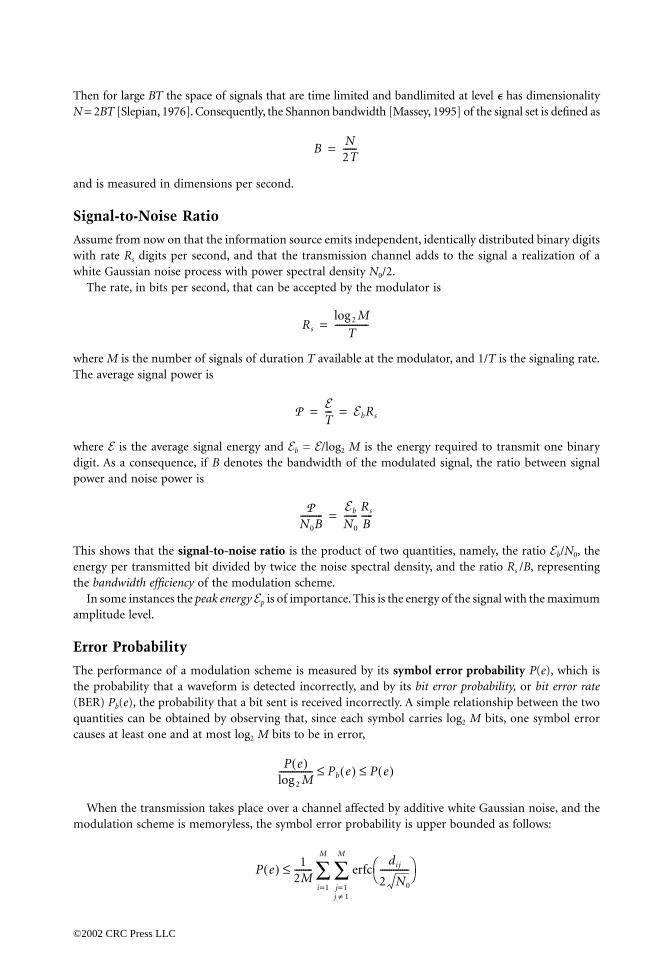
Then for large BT the space of signals that are time limited and bandlimited at level � has dimensionalityN = 2BT [Slepian, 1976]. Consequently, the Shannon bandwidth [Massey, 1995] of the signal set is defined as

and is measured in dimensions per second.

Signal-to-Noise Ratio

Assume from now on that the information source emits independent, identically distributed binary digitswith rate Rs digits per second, and that the transmission channel adds to the signal a realization of awhite Gaussian noise process with power spectral density N0/2.

The rate, in bits per second, that can be accepted by the modulator is

where M is the number of signals of duration T available at the modulator, and 1/T is the signaling rate.The average signal power is

where E is the average signal energy and Eb = E/log2 M is the energy required to transmit one binarydigit. As a consequence, if B denotes the bandwidth of the modulated signal, the ratio between signalpower and noise power is

This shows that the signal-to-noise ratio is the product of two quantities, namely, the ratio Eb/N0, theenergy per transmitted bit divided by twice the noise spectral density, and the ratio Rs /B, representingthe bandwidth efficiency of the modulation scheme.

In some instances the peak energy Ep is of importance. This is the energy of the signal with the maximumamplitude level.

Error Probability

The performance of a modulation scheme is measured by its symbol error probability P(e), which isthe probability that a waveform is detected incorrectly, and by its bit error probability, or bit error rate(BER) Pb(e), the probability that a bit sent is received incorrectly. A simple relationship between the twoquantities can be obtained by observing that, since each symbol carries log2 M bits, one symbol errorcauses at least one and at most log2 M bits to be in error,

When the transmission takes place over a channel affected by additive white Gaussian noise, and themodulation scheme is memoryless, the symbol error probability is upper bounded as follows:

BN2T------=

Rs

M2log

T---------------=

PET--- EbRs= =

PN0B----------

Eb

N0

------Rs

B-----=

P e( )M2log

--------------- Pb e( ) P e( )£ £

P e( ) 12M-------- erfc

dij

2 N0

-------------Ë ¯Ê ˆ

j=1j 1π

M

Âi=1

M

Â£


where dij is the Euclidean distance between signals si(t) and sj(t),

and erfc(◊) denotes the Gaussian integral function

Another function, denoted Q(x), is often used in lieu of erfc(◊). This is defined as

A simpler upper bound on error probability is given by

where dmin = min i π j dij.A simple lower bound on symbol error probability is given by

By comparing the upper and the lower bound we can see that the symbol error probability dependsexponentially on the term dmin, the minimum Euclidean distance among signals of the constellation. Infact, upper and lower bounds coalesce asymptotically as the signal-to-noise ratio increases. For interme-diate signal-to-noise ratios, a fair comparison among constellations should take into account the errorcoefficient as well as the minimum distance. This is the average number n of nearest neighbors [i.e., theaverage number of signals at distance dmin from a signal in the constellation; for example, this is equalto 2 for M-ary phase-shift keying (PSK), M > 2]. A good approximation to P(e) is given by

Roughly, at P(e) = 10-6, doubling n accounts for a loss of 0.2 dB in the signal-to-noise ratio.

20.3 One-Dimensional Modulation: Pulse-Amplitude Modulation (PAM)

Pulse-amplitude modulation (PAM) is a linear modulation scheme in which a signal s(t) is modulatedby random variables taking on values in the set of amplitudes where

The transmitter uses the set of waveforms where s(t) is a unit-energy pulse. The geometricrepresentation of this signal set is shown in Fig. 20.2 for M = 4.

dij2 si t( ) sj t( )–[ ]2dt

0

T

Ú=

erfc x( ) 2

p------- e z

2– dz.x

•

Ú=

Q x( ) 12--erfc

x

2-------Ë ¯

Ê ˆ=

P e( ) M 1–2

--------------erfcdmin

2 N0

-------------Ë ¯Ê ˆ£

P e( ) 1M-----erfc

dmin

2 N0

-------------Ë ¯Ê ˆ≥

P e( ) n2---erfc

dmin

2 N0

-------------Ë ¯Ê ˆª

xn {ai}i=1M ,

ai 2i 1– M–( )dmin

2--------- , i 1,2, º, M==

{ais(t)}i=1M ,


The symbol-error probability is given by

The ratio between peak energy and average energy is

The bandwidth efficiency of this modulation is

20.4 Two-Dimensional Modulations

Phase-Shift Keying (PSK)

This is a linear modulation scheme generating the signal

FIGURE 20.2 Quaternary PAM constellation.

FIGURE 20.3 Symbol error probability of coherently demodulated PAM.

P e( ) 11M-----–Ë ¯

Ê ˆ erfc3 M2log

M2 1–---------------------

Eb

N0

------Ë ¯Á ˜Ê ˆ

=

Ep

E----- 3M 1–M 1+--------------=

Rs

B-----

M2log

T--------------- 2T◊ 2 M2log= =

v t( ) R xns t nT–( )ej2p f0 t

n= •–

•

ÂÓ ˛Ì ˝Ï ¸

=


where takes values in the set

where F is an arbitrary phase. The signal constellation is shown, for M = 8, in Fig. 20.4.The symbol-error probability of M-ary PSK is closely approximated by

for high signal-to-noise ratios (see Fig. 20.5). The bandwidth efficiency of PSK is

o

FIGURE 20.4 An 8-PSK constellation.

FIGURE 20.5 Symbol error probability of coherently demodulated PSK.

xn ejfn=

2pM------ i 1–( ) F+

Ó ˛Ì ˝Ï ¸

i=1

M

P e( ) erfcEb

N0

------ M2logpM-----sinË ¯

Ê ˆª

Rs

B-----

M2log

T--------------- T◊ M2log= =


Quadrature Amplitude Modulation (QAM)

Quadrature amplitude modulation (QAM) is a linear modulation scheme for which the modulatedsignal takes the form

where

and an, bn take on equally spaced values. Figure 20.6 shows a QAM constellation with 16 points.When log2 M is an even integer, we have

with

When log2 M is odd, the following upper bound holds:

(See Fig. 20.7.)

20.5 Multidimensional Modulations: Frequency-ShiftKeying (FSK)

In the modulation technique called frequency-shift keying (FSK) the transmitter uses the waveforms

where fi = f0 + (2i - 1 - M) fd, for i = 1,º, M, and f0 denotes the carrier frequency. The waveforms have

FIGURE 20.6 A 16-QAM constellation.

v t( ) ¬ xns t nT–( )ej2pf0t

n= •–

•

ÂÓ ˛Ì ˝Ï ¸

=

xn an jbn+=

P e( ) 1 1 p–( )2–=

p 11

M---------–Ë ¯

Ê ˆ erfc3 M2log

2 M 1–( )----------------------

Eb

N0

------Ë ¯Ê ˆ=

P e( ) 2erfc3 M2log

2 M 1–( )----------------------

Eb

N0

------Ë ¯Ê ˆ<

si t( ) A 2p fit, 0 t T<£cos=


constant energy E = A2 T/2, and the modulated signal has constant envelope A. The distance propertiesof these waveforms for a given energy depend on the value of their normalized frequency separation 2fd T.

Generation of these waveforms may be accomplished with a set of M separate oscillators, each tunedto the frequency fi. In this case, the phase discontinuities at frequency-transition times cause largesidelobes in the power density spectrum of the modulated signal. A narrower spectrum can be obtainedby using a single oscillator whose frequency is modulated by the source bits. This results in a modulationscheme with memory called continuous-phase FSK (discussed in Section 20.7).

The signals si(t) are orthogonal, that is,

if the frequency separation between adjacent signals is such that 2fdT = m/2, where m is any nonzerointeger. Thus, the minimum frequency separation for orthogonality if 2fd = 1/2T.

The symbol error probability for M orthogonal signals with energy E is upper and lower bounded by

For M = 2 the bounds merge into the exact value. The upper bound to P(e) is plotted in Fig. 20.8.It can be observed from Fig. 20.8 that the error probability for a given value of signal-to-noise ratio

decreases as M increases, contrary to what is observed for PAM, PSK, and QAM. On the other hand, thebandwidth efficiency decreases as M increases, its value being given by

FIGURE 20.7 Symbol error probability of coherently demodulated QAM.

2p f it( ) 2p f jt( )dt 0 i jπ=coscos0

T

Ú

12--erfc

eb M2log

2N0

----------------------Ë ¯Ê ˆ P e( ) M 1–

2--------------erfc

eb M2log

2N0

----------------------Ë ¯Ê ˆ .£ £

Rs

B-----

2 M2log

M--------------------=


20.6 Multidimensional Modulations: Lattices

The QAM constellations may be considered as carved from an infinite constellation of regularly spacedpoints in the plane, called the lattice Z 2. This is represented in Fig. 20.9. This concept can be generalizedto other lattices, both two-dimensional and multidimensional. In this framework, the design of a signalconstellation consists of choosing a lattice, then carving a finite constellation of signal points from the lattice.

In general, a lattice L is defined as a set closed under ordinary addition and multiplication by integers.As such, it forms an additive group as well as a vector space. Specifically, an N-dimensional lattice L isan infinite set of N vectors.

If dmin is the minimum distance between any two points in the lattice, the number n of adjacent latticepoints located at distance dmin, that is, the number of nearest neighbors of any lattice point, is called itskissing number.

FIGURE 20.8 Symbol error probability of coherently demodulated orthogonal FSK.

FIGURE 20.9 The lattice Z 2.


Examples of Lattices

The Lattice ZN

The set ZN of all N-tuples with integer coordinates is called the cubic lattice, or integer lattice. Theminimum distance is dmin = 1, and the kissing number is n = 2N.

The N-Dimensional Lattices AN and

AN is the set of all vectors with (N + 1) integer coordinates whose sum is zero. This lattice may be viewedas the intersection of Z N + 1 and a hyperplane cutting the origin. The minimum distance is dmin = and the kissing number is n = N(N + 1).

The N-Dimensional Lattice DN

DN is the set of all N-dimensional points whose integer coordinates have an even sum. It may be viewedas a punctured version of ZN, in which the points are colored alternately black and white with acheckerboard coloring, and the white points (those with odd sums) are removed. We have dmin = and n = 2N(N - 1). D4 represents the densest lattice packing in R4. This means that if unit-radius, four-dimensional spheres with centers in the lattice points are used to pack R4, then D4 is the lattice with thelargest number of spheres per unit volume.

The Gosset Lattice E8

In the even coordinate system, E8 consists of the points

In words, E8 consists of the eight-vectors whose components are all integers, or all halves of odd integers,and whose sum is even.

The odd coordinate system is obtained by changing the sign of any coordinate: the points are

This lattice has dmin = and n = 240.

Other Lattices

The description and the properties of other important lattices, such as the 16-dimensional Barnes–Walllattice L16 and the 24-dimensional Leech lattice L24, can be found in Chapter 4 of Conway and Sloane[1988].

The Coding Gain of a Lattice

The coding gain gc(L) of the lattice L is defined as

(20.2)

where V(L) is the fundamental lattice volume, that is, the reciprocal of the number of lattice points perunit volume [for example, V(ZN) = 1]. Table 20.1 lists the coding gains of some of the most popular lattices.

AN*

2,

2,

x1,º, x8( ): xi Z or xi Z12-- , xi 0 mod 2∫

i=1

8

Â+Œ"Œ"Ó ˛Ì ˝Ï ¸

x1,º, x8( ): xi Z or xi Z12-- , xi 2x8 mod 2∫

i=1

8

Â+Œ"Œ"Ó ˛Ì ˝Ï ¸

2

gc L( )dmin

2 L( )V L( )2/N-------------------=


Carving a Signal Constellation out of a Lattice

We denote with C(L, R) a constellation obtained from L (or from its translate L + a) by retaining onlythe points that fall in the region R. The resulting constellation has a number of signals approximatelyequal to the ratio between the volume of R and the volume of L,

provided that V(R) >> V(L), that is, that M is large enough.The figure of merit (CFM) of C = C(L, R) is the ratio between and the average energy of the

constellation per dimension pair,

To express the figure of merit of the constellation C(L, R) in terms of parameters related to the latticeL and to the region R, we introduce the definition of the shape gain gs(R) of the region R [Forney andWei, 1990]. This is the reduction in average energy (per dimension pair) required by a constellationbounded by R compared to that which would be required by a constellation bounded by an N-dimensionalcube of the same volume V(R). In formulas, the shape gain is the ratio between the normalized secondmoment of any N-dimensional cube (which is equal to 1/12) and the normalized second moment of R,

(20.3)

where

(20.4)

The following result holds [Forney and Wei, 1990]: The figure of merit of the constellation C(L, R) isgiven by

(20.5)

where g0 is the figure of merit of the one-dimensional PAM constellation with the same bit rate (chosenas the baseline), gc(L) is the coding gain of the lattice L [see Eq. (20.2)], and gs(R) is the shaping gainof the region R. The approximation holds for large constellations.

This result shows that, at least for large constellations, the gain from shaping by the region R is almostcompletely decoupled from the coding gain due to L. Thus, for a good design it makes sense to optimizeseparately gc(L) (i.e., the choice of the lattice) and gs(R) (i.e., the choice of the region).

TABLE 20.1 Coding Gains of Lattices

Name L N gc(L), (dB)

Integer lattice Z 1 0.00Hexagonal lattice A2 2 0.62Schläfli D4 4 1.51Gosset E8 8 3.01Barnes-Wall L16 16 4.52Leech L24 24 6.02

MV R( )V L( )--------------ª

dmin2

CFM C( )dmin

2

E/ N/2( )--------------------=

gs R( ) 1/12G R( )--------------=

G R( )r 2dr

RÚNV R( )1+2/N-----------------------------=

CFM C( ) g0 gc L( ) gs R( )◊◊ª


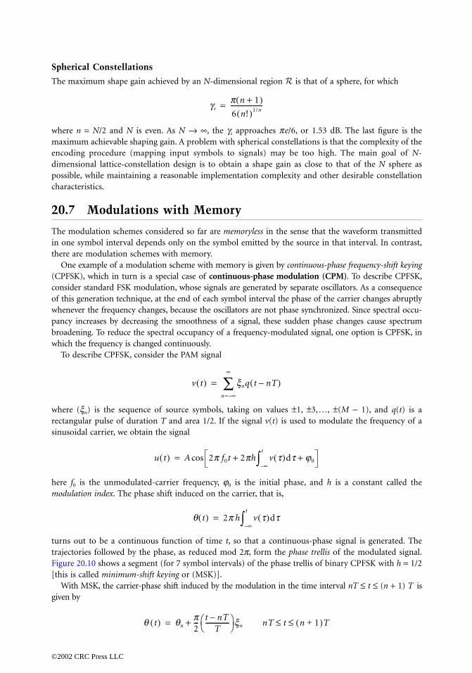
Spherical Constellations

The maximum shape gain achieved by an N-dimensional region R is that of a sphere, for which

where n = N/2 and N is even. As N Æ •, the gs approaches pe/6, or 1.53 dB. The last figure is themaximum achievable shaping gain. A problem with spherical constellations is that the complexity of theencoding procedure (mapping input symbols to signals) may be too high. The main goal of N-dimensional lattice-constellation design is to obtain a shape gain as close to that of the N sphere aspossible, while maintaining a reasonable implementation complexity and other desirable constellationcharacteristics.

20.7 Modulations with Memory

The modulation schemes considered so far are memoryless in the sense that the waveform transmittedin one symbol interval depends only on the symbol emitted by the source in that interval. In contrast,there are modulation schemes with memory.

One example of a modulation scheme with memory is given by continuous-phase frequency-shift keying(CPFSK), which in turn is a special case of continuous-phase modulation (CPM). To describe CPFSK,consider standard FSK modulation, whose signals are generated by separate oscillators. As a consequenceof this generation technique, at the end of each symbol interval the phase of the carrier changes abruptlywhenever the frequency changes, because the oscillators are not phase synchronized. Since spectral occu-pancy increases by decreasing the smoothness of a signal, these sudden phase changes cause spectrumbroadening. To reduce the spectral occupancy of a frequency-modulated signal, one option is CPFSK, inwhich the frequency is changed continuously.

To describe CPFSK, consider the PAM signal

where (xn) is the sequence of source symbols, taking on values ±1, ±3,º, ±(M - 1), and q(t) is arectangular pulse of duration T and area 1/2. If the signal v(t) is used to modulate the frequency of asinusoidal carrier, we obtain the signal

here f0 is the unmodulated-carrier frequency, j0 is the initial phase, and h is a constant called themodulation index. The phase shift induced on the carrier, that is,

turns out to be a continuous function of time t, so that a continuous-phase signal is generated. Thetrajectories followed by the phase, as reduced mod 2p, form the phase trellis of the modulated signal.Figure 20.10 shows a segment (for 7 symbol intervals) of the phase trellis of binary CPFSK with h = 1/2[this is called minimum-shift keying or (MSK)].

With MSK, the carrier-phase shift induced by the modulation in the time interval nT £ t £ (n + 1) T isgiven by

gsp n 1+( )6 n!( )1/n--------------------=

v t( ) xnq t nT–( )n= •–

•

Â=

u t( ) A 2p f0t 2ph v t( )dt j0+•–

t

Ú+cos=

q t( ) 2p h v t( )dt•–

t

Ú=

q t( ) qnp2--- t nT–

T---------------Ë ¯

Ê ˆ xn nT t n 1+( )T£ £+=


where

The corresponding transmitted signal is

which shows that MSK is an FSK using the two frequencies

The frequency separation f2 - f1 = 1/2T is the minimum separation for orthogonality of two sinusoids,which explains the name given to this modulation scheme.

The spectrum of CPFSK depends of the value of h. For h < 1, as the modulation index decreases, sodoes the spectral occupancy of the modulated signal. For MSK the power density spectrum is shown inFig. 20.11.

FIGURE 20.10 Phase trellis of binary CPFSK with h = 1/2 (MSK).

FIGURE 20.11 Power density spectrum of MSK and of quaternary PSK.

qnp2--- xk

k= •–

n-1

Â=

u t( ) A 2p f01

4T------an+Ë ¯

Ê ˆ tnp2

------an qn+–cos=

f1 f01

4T------ f2 f0

14T------+=–=


CPM is a generalization of CPFSK. Here the carrier-phase shift in the interval nT £ t £ (n + 1)T isgiven by

where the waveform q(t) is the integral of a frequency pulse g(t) of arbitrary shape

subject to the constraints g(t) = 0 for t < 0 and

When the modulation index hk varies (usually with a periodic law) from one symbol to another, themodulation is called multi-h. If g(t) π 0 for t > T, then the modulated signal is called partial-responseCPM. Otherwise, it is called full-response CPM.

An example of partial-response CPM is given by Gaussian (GMSK), whose frequency pulse is obtainedby passing a rectangular waveform into a low-pass filter whose impulse response h(t) has a Gaussian shape,

where B denotes the filter bandwidth. By decreasing B, the shape of the frequency pulse becomes smootherand the spectrum occupancy of the modulated signal is reduced. This modulation scheme is employedin the Global System for Mobile Communications (GSM) standard for cellular mobile radio with thechoice BT = 0.3.

Defining Terms

Bandwidth: The frequency interval in which the density spectrum of a signal is significantly differentfrom zero.

Continuous-phase modulation: A digital modulation scheme derived from phase-shift keying in whichthe carrier has no phase jumps, that is, the phase transitions occur continuously.

Digital modulation: The mapping of information-source symbols into signals, performed to carryinformation through the transmission channel.

Error probability: Probability that a symbol emitted by the information source will be received incor-rectly by the end user.

Frequency-shift keying: A digital modulation scheme in which the source information is carried by thefrequency of a sinusoidal waveform.

Geometric signal representation: Representation of a finite set of signals as a set of vector.Lattice: An infinite signal constellation of points regularly located in space.Phase-shift keying: A digital modulation scheme in which the source information is carried by the phase

of a sinusoidal waveform, called the carrier.Pulse-amplitude modulation: A digital modulation scheme in which the source information is carried

by the amplitude of a waveform.Quadrature amplitude modulation: A digital modulation scheme in which the source information is

carried by the amplitude and by the phase of a sinusoidal waveform.

q t( ) 2p akhkq t nT–( )k= •–

n

Â=

q t( ) g t( )dt•–

t

Ú=

g t( )dt0

•

Ú 12--=

h t( ) 2p2ln

--------B2p2B2

2ln--------------t2–

Ó ˛Ì ˝Ï ¸

exp=


Signal constellation: A set of signals geometrically represented in the form of a set of vectors.Signal-to-noise ratio: The ratio of the signal power and noise power. It is an index of channel quality.

References

Anderson, J.B., Aulin, T., and Sundberg, C.E.W. 1986. Digital Phase Modulation, Plenum, New York.Benedetto, S., Biglieri, E., and Castellani, V. 1987. Digital Transmission Theory, Prentice–Hall, Englewood

Cliffs, NJ.Conway, J.H. and Sloane, N.J.A. 1988. Sphere Packings, Lattices and Groups, Springer–Verlag, New York.Forney, G.D. Jr. and Wei, L.F. 1990. Multidimensional constellations—Part I: Introduction, figures of

merit, and generalized cross constellations. IEEE J. Selected Areas Comm., 7(6):877–892.Massey, J.L. 1995. Towards an information theory of spread-spectrum systems. In: Code Division Multiple

Access Communications, Eds. S.G. Glisic and P.A. Leppänen, Kluwer Academic, Boston.Proakis, J.G. 1995. Digital Communications, 3rd ed., McGraw–Hill, New York.Simon, M.K., Hinedi, S.M., and Lindsey, W.C. 1995. Digital Communication Techniques. Signal Design

and Detection, Prentice–Hall, Englewood Cliffs, NJ.Slepian, D. 1976. On bandwidth. IEEE Proc., 64(2):292–300.

Further Information

The monthly journal IEEE Transactions on Communications reports advances in digital modulationtechniques.

The books by Benedetto, Biglieri, and Castellani, 1987, Proakis, 1995, and Simon, Hinedi, and Lindsey,1995 are good introductions to the theory of digital modulation.


IITelephony

21 Plain Old Telephone Service (POTS) A. Michael Noll Introduction • The Network • Station Apparatus • Transmission• Switching • Signalling • Functionality • The Future

22 FDM Hierarchy Pierre CatalaIntroduction • Background Information • Frequency-Division Multiplexing(FDM) • The Hierarchy • Pilots • Direct to Line (DTL) • Summary

23 Analog Telephone Channels and the Subscriber Loop Whitham D. ReeveTelephone Band • Noise • Crosstalk • Circuit Noise • Impulse Noise • AttenuationDistortion • Envelope Delay Distortion • Line Conditioning • Other Impairmentsto Analog Transmission

24 Baseband Signalling and Pulse Shaping Michael L. Honigand Melbourne BartonCommunications System Model • Intersymbol Interference and the NyquistCriterion • Nyquist Criterion with Matched Filtering • Eye Diagrams• Partial-Response Signalling • Additional Considerations • Examples

25 Channel Equalization John G. ProakisCharacterization of Channel Distortion • Characterization of IntersymbolInterference • Linear Equalizers • Decision-Feedback Equalizer • Maximum-LikelihoodSequence Detection • Maximum A Posteriori Probability Detector and TurboEqualization • Conclusions

26 Pulse-Code Modulation Codec-Filters Michael D. Floydand Garth D. Hillman Introduction and General Description of a Pulse-Code Modulation (PCM)Codec-Filter • Where PCM Codec-Filters are Used in the Telephone Network • Design of Voice PCM Codec-Filters: Analog Transmission Performanceand Voice Quality for Intelligibility • Linear PCM Codec-Filter for High-SpeedModem Applications • Concluding Remarks

27 Digital Hierarchy B. P. Lathi and Maynard A. WrightIntroduction • North American Asynchronous Digital Hierarchy

28 Line Coding Joseph L. LoCicero and Bhasker P. PatelIntroduction • Common Line Coding Formats • Alternate Line Codes • MultilevelSignalling, Partial Response Signalling, and Duobinary Coding • BandwidthComparison • Concluding Remarks


29 Telecommunications Network Synchronization Madihally J. NarasimhaIntroduction • Synchronization Distribution Networks • Effect of SynchronizationImpairments • Characterization of Synchronization Impairments • SynchronizationStandards • Summary and Conclusions

30 Echo Cancellation Giovanni CherubiniIntroduction • Echo Cancellation for Pulse-Amplitude Modulation (PAM)Systems • Echo Cancellation for Quadrature-Amplitude Modulation (QAM)Systems • Echo Cancellation for Orthogonal Frequency Division Multiplexing(OFDM) Systems • Summary and Conclusions


21Plain Old Telephone

Service (POTS)

21.1 IntroductionBell’s Vision

21.2 The Network21.3 Station Apparatus21.4 Transmission21.5 Switching21.6 Signalling21.7 Functionality21.8 The Future

21.1 Introduction

The acronym POTS stands for plain old telephone service. Over the years, POTS acquired an undeservedreputation for connoting old-fashioned and even obsolete. The telephone and the switched public networkenable us to reach anyone anywhere on this planet at anytime and to speak to them in our natural voices.The minutes of telephone usage, in the number of access lines, and in the revenue of telephone companies,attest to the central importance of telephone service in today’s information-age, global economy.

The word old in the acronym implies familiarity and ease of use, a major reason for the continued popularityof telephone service. The word telephone and the nuances expressed by natural human speech is what it isall about. Service used to mean responsiveness to the public, and it is sad that this dimension of the acronymhas become so threatened by emphasis on short-term profits, particularly in the new world of competitionthat characterizes telephone service on all levels. The term plain is indeed obsolete, and the provision of today’stelephone service utilizes some of the most sophisticated and advanced transmission and switching technology.In fact, telephone service today with all its intelligent and functional new features, advanced technology,and improved quality is truly fantastic. Allowing for a little misspelling, the acronym POTS can still beused, but with the “P” standing for phantastic! So, POTS it was, and POTS is still where the real action is.

Part of the excitement about the telephone network is that it can be used with a wide variety of devicesto create exciting and useful services, such as facsimile for graphical communication and modems for accessto the Internet. Cellular wireless telephony, pagers, and phones in airplanes extend telephony whereverwe travel. Increased functionality in the network brings us voice mail, call forwarding, call waiting, callerID, and a host of such services. The future of an ever-evolving POTS, indeed, looks bright and exciting.

Bell’s Vision

The telegraph is older than the telephone, but special knowledge of Morse code was necessary to use thetelegraph, thereby relegating it to use by specialists. The telephone uses normal human speech and,therefore, can be used by anyone and can convey all the nuances of the inflections of human speech.

A. Michael NollUniversity of Southern California


Dr. Alexander Graham Bell was very prophetic in his vision of a world wired for two-way telecommu-nication using natural human speech. Bell and his assistant Thomas A. Watson demonstrated the firstworking model of a telephone on March 10, 1876, but Bell had applied for a patent a month earlier onFebruary 14, 1876. Elisha Grey had submitted a disclosure of invention for a telephone on that sameday in February, but ultimately the U.S. Supreme Court upheld Bell’s invention, although in a splitdecision.

21.2 The Network

The telephone has come to signify a public switched network capable of reaching any other telephoneon Earth. This switched network interconnects not only telephones but also facsimile machines, cellulartelephones, and personal computers––anything that is connected to the network. As shown in Fig. 21.1,the telephones and other station apparatus in homes are all connected by pairs of copper wire to a singlepoint, called the protector block, which offers simple protection to the network from overvoltages. Atwisted pair of copper wires then connects the protector block all the way back to the central office. Manytwisted pairs are all carried together in a cable that can be buried underground, placed in conduit, orstrung between telephone poles. The twisted pair of copper wires connecting the station apparatus tothe central office is called the local loop.

The very first stage of switching occurs at the central office. From there, telephone calls may beconnected to other central offices over interoffice trunks. Calls may also be carried over much greaterdistances by connection to the long-distance networks operated by a number of interexchange carriers(IXC) such as AT&T, MCI, and Sprint. The point where the connection is made from the local serviceprovider to the interexchange carrier is known as the point of presence (POP).

The local portion of the telephone network is today known as a local access and transport area (LATA).The local Bell telephone companies (commonly called the Baby Bells) were restricted by the Bell breakupof 1984 solely to the provision of intra-LATA service and were forbidden from providing inter-LATAservice. Although the technology of telephony has progressed impressively over the last 100 years, policyand regulation have also had great impact on the telephone industry.

In the past, telephone service in the U.S. was mostly under the control of AT&T and its Bell systemand a number of smaller independent telephone companies. Today, a number of competing companies

FIGURE 21.1 Network.


own and operate their own long-distance networks, and some futurists believe that local competitionwill occur soon.

The various long-distance and local networks all interconnect and offer what has been called a networkof networks. Data communication for the Internet is carried over data networks. With voice being convertedto digital bits, a technological convergence of voice and data (which is already encoded as bits) is occurring.

21.3 Station Apparatus

Telephones of the past were black with a rotary dial with limited functionality. Today’s telephones comein many colors and sizes and offer push-button dialing along with a variety of intelligent features, such asrepertory dialing and display of the dialed number. However, the basic functions of the telephone instru-ment have not changed and are shown in Fig. 21.2. The telephone needs to signal the central office whenservice is desired. This is accomplished by lifting the handset, which then closes contacts in the tele-phone––the switch hook––so that the telephone draws DC over the local loop from the central office.The switching machine at the central office senses this flow of DC and thus knows that the customerdesires service. The common battery at the central office has an electromotive force (EMF) of 48 V, andthe telephone draws at least about 20 mA of current over the loop. The maximum loop resistance can notexceed about 1300 Ω .

The user needs to specify the telephone number of the called party. This is accomplished by a processcalled dialing. Older telephones accomplished dialing with a rotary dial that interrupted the flow of DCwith short pulses at a rate of about 10 dial pulses per second. Most telephones today use touch-tonedialing and push buttons, as shown in Fig. 21.3. When a specific digit is pushed, a unique combinationof two sinusoidal tones is transmitted over the line to the central office. For example, an 8 is indicatedby the combination of sine waves at 852 Hz and 1336 Hz. Filters are used at the switching machine atthe central office to detect the frequencies of the tones and thus decode the dialed digits. Touch-tonedialing is also known as dual-tone multifrequency (DTMF) dialing.

FIGURE 21.2 Telephone.


Bell’s first telephone microphone, or transmitter, used the principle of variable resistance to create alarge varying current. It consisted of a wire that moved in and out of a small cup of acid in response tothe acoustic speech signal. Clearly, such a transmitter was not very practical, and it was soon replacedby the use of loosely packed carbon, invented in 1878 by Henry Hummings. In 1886, Thomas Alva Edisonimproved on the carbon transmitted by using roasted granules of anthracite coal. Today’s telephonetransmitters use high-quality, small, variable-capacitance, electret microphones. The telephone receiveris a small loudspeaker using a permanent magnet, coil of wire, and metal diaphragm. It was invented in1876 by Thomas Watson, Bell’s assistant, and the basic principles have changed little since then.

The pair of wires going to the telephone transmitter and receiver constitutes a four-wire circuit. Thetransmitter sends a speech signal down the telephone line, and the receiver receives the signal from thecentral office. However, a two-wire local loop connects the telephone instrument to the central office,and, hence, two-wire to four-wire conversion is needed within the telephone instrument. A center-tappedtransformer, called a hybrid, accomplishes this conversion. The leakage current in the secondary receivercircuit depends on how well a balance network exactly matches the impedance of the telephone line.Since this balance network can never match the line perfectly, a small amount of the received transmittedsignal leaks into the receiver circuit, and the user hears one’s own speech, an effect known as sidetone.Actually, a small amount of sidetone is desirable because it makes the telephone seem live and natural,and, thus, the balance network is designed to allow an optimum amount of sidetone. Too much sidetoneresults in the user pulling the handset away from the head, which reduces the transmitted speechsignal––an undesirable effect. The use of an induction coil to balance the electrical sidetone was patentedin 1918 by G.A. Campbell, an AT&T research engineer. The induction coil has been replaced in moderntelephones by a speech network that electronically cancels the sidetone leakage and performs the two-wire to four-wire conversion.

The telephone ringer is connected in parallel across the telephone line before the switch hook’s contacts.Thomas Watson applied for the first ringer patent in 1878, and today’s electromechanical ringers havechanged little since then. A hammer attached to an armature with a magnetic field strengthened by apermanent magnet moves in response to the ringer current loudly striking two bells. The high-impedanceringer was invented in 1890 by John J. Carty, a Bell engineer who had invented the two-wire local loop

FIGURE 21.3 Touch-tone.


in 1881. A capacitor is placed in series with the ringer to prevent DC from flowing through it. The ringersignal consists of a short 2-s burst of a 75-V (rms), 20-Hz sine wave followed by 4 s of silence. Piezoelectrictransducers and small loudspeakers have replaced electromechanical ringers in today’s telephones.

Telephone instruments have progressed greatly in their functionality from the basic-black, rotary-dialphones of the past. Today’s phones frequently include repertory dialers, speakerphones, and liquidcrystal displays (LCDs). Tomorrow’s phones will most likely build up this functionality and extend it tocontrol central office features, to perform e-mail, and to integrate voice and data. Although some peoplestill believe that the telephone of the future will also include a two-way video capability, the videophone,most consumers do not want to be seen while speaking on the phone, and, thus, the videophone will mostprobably remain an element of science fiction.

The public switched network can be used to transmit and switch any signal that remains within itsbaseband, namely, about 4 kHz. Thus, devices other than just a telephone can be used on the telephonenetwork. The recent success of facsimile is one example; modems operating at speeds of 56 kb/s are another.

21.4 Transmission

A wide variety of transmission media have been and are used in providing telephone service. At the locallevel, twisted pairs of copper wire today connect most customers to the central office, although opencopper wire was used in the distant past and in rural areas. Many pairs of wire are placed together in acable, which is then either placed underground or strung between telephone poles. Coaxial cable carriedtelephone calls across the country. Microwave radio carried telephone calls terrestrially from microwavetower to tower across the country, with each tower located about 26 miles from the next. Microwaveradio also carries telephone calls across oceans and continents by communication satellites located ingeosynchronous orbits 22,300 miles above the surface of the earth. Today’s transmission medium ofchoice for carrying telephone calls over long distances and between central offices is optical fiber.

Multiplexing is the means by which a number of communication signals are combined together toshare a single communication medium. With analog multiplexing, signals are combined by frequency-division multiplexing; with digital multiplexing, signals are combined by time-division multiplexing.

Today analog multiplexing is obsolete in telephony. AT&T replaced all its analog multiplexing withdigital multiplexing in the late 1980s; MCI followed suit in the early 1990s. Analog multiplexing wasaccomplished by A-type channel banks. Each baseband telephone channel was shifted in frequency to itsown unique 4-kHz channel. The frequency-division multiplexing was accomplished in hierarchial stages.A hierarchy of multiplexing was created with 12 baseband channels forming a group, 5 groups forminga supergroup, 10 supergroups forming a mastergroup, and 6 mastergroups forming a jumbo group. Ajumbo multiplex group contained 10,800 telephone channels and occupied a frequency range from 654to 17,548 kHz.

With digital multiplexing, each baseband analog voice signal is converted to digital using a samplingrate of 8000 samples/s with 8-b nonlinear quantization for an overall bit rate of 64,000 b/s. A hierarchyof digital multiplexing has evolved with 24 digital telephone signals forming a DS1 signal requiring 1.544Mb/s, 4 DS 1 signals forming a DS2 signal, 7 DS2 signals forming a DS3 signal, 6 DS3 signals forminga DS4 signal. A single digital telephone signal at 64 kb/s is called a DS0 signal. A DS4 signal multiplexes4032 DS0 signals and requires an overall bit rate of about 274 Mb/s.

The transmission media and systems used for long-distance telephone service have progressed overthe decades. The Ll-carrier system, first installed in 1946, utilized three working pairs of coax in a buriedcable to carry 1800 telephone circuits across the country using analog, frequency-division multiplexing.The L5E-carrier system, installed in 1978, carried 132,000 telephone circuits in 10 coax pairs. Terrestrialmicrowave radio has been used to carry telephone signals from towers located about every 26 miles acrossthe country. The first system, TD-2, became available in 1950 and carried 2400 voice circuits. The useof polarized radio waves to reduce channel interference, the horn antenna to allow simultaneous operationin both the 6-GHz and 4-GHz bands, solid-state technology, and single-sideband suppressed-carrieramplitude modulation resulted in a total system capacity in 1981 of 61,800 voice circuits.


Communication satellites located in a geosynchronous orbit 22,300 mi above the Earth’s equator havebeen used to carry telephone signals. Here, too, the technology has progressed, offering ever increasingcapacities. But geosynchronous communication satellites suffer a serious shortcoming. The time requiredfor the radio signals to travel back and forth between satellite and Earth stations creates a round-tripdelay of about 0.5 s, which is quite annoying to most people.

Today’s transmission medium of choice is optical fiber utilizing digital, time-division multiplexingof the voice circuits. The basic idea of guiding light through thin glass fibers is quite old and wasdescribed by the British physicist Charles Vernon Boys in 1887. Today’s optical fiber utilizes ultrapuresilica. Optical fiber itself has progressed from multimode stepped index and graded index fibers totoday’s single-mode fiber. Solid-state lasers have also progressed in their use as light sources, and detectortechnology is also an area of much technological advancement. Today’s fiber strands each carry a fewgigabits per second. Technological advances include color mutliplexing, in which a number of lightsignals at different frequencies are carried on the same fiber strand and erbium doped fiber amplifiersthat increase the strength of the light signal without the need to convert signals back to an electricalform for regeneration. Usually, a number of fiber strands are placed together in a single cable, but thecapacity of each fiber strand is so great that many of the strands are not used and are called dark fiber.The theoretical capacity of a single strand is as much as 100 terabits per second. The synchronousoptical network (SONET) standard facilitates the interconnection of optical networks operating at ratesmeasured in gigabits per second.

Long-distance transmission systems and local carrier systems all utilize separate paths for each directionof transmission, thereby creating four-wire circuits. These four-wire circuits need to be connected to thetwo-wire local loop. The hybrids that accomplish this connection and conversion can not perfectly matchthe transmission characteristics of each and every local loop. The result is that a small portion of thesignal leaks through the hybrid and is heard by the speaking party as a very annoying echo. The echosuppressor senses which party is speaking and then introduces loss in the return path to prevent theecho, but this solution also prevents simultaneous talking. Today, echo elimination is accomplished byan echo canceler, which uses an adaptive filter to create a synthetic echo, which is then subtracted fromthe return signal, thereby eliminating the echo entirely but also allowing simultaneous double talking.An echo canceler is required at each end of the transmission circuit.

21.5 Switching

In the old days, one telephone was connected to another telephone at switchboards operated by humans.The human operators used cords with a plugs at each end to make the connections. Each plug had a tipand a ring about the tip to create the electric circuit to carry the signals. A sleeve was used for signallingpurposes to indicate whether a circuit was in use. Each human operator could reach as many as 10,000jacks. The automation of the switchboard came early in the history of telephony with Almon B. Strowger’sinvention in 1892 of an electromechanical automatic switch and the creation of his Automatic ElectricCompany to manufacture and sell his switching systems, mostly to non-Bell telephone companies. TheStrowger switching was ignored by the Bell System until 1919 when it was finally adopted. Now electro-mechanical switching is totally obsolete in the U.S., and today’s telephone system utilizes electronicswitching systems. However, the Strowger system, known as step-by-step in the Bell System, was a thingof great mechanical ingenuity that gave an intuitive grasp of switching with turning and stepping switchcontacts that is not possible with today’s computerized electronic systems. Electromechanical switchingwas subject to much wear and tear, however, and required considerable space and costly maintenance.Furthermore, electromechanical switching was inflexible and could not be reprogrammed.

In general, a switching system consists of two major functional parts, as shown in Fig. 21.4: (1) theswitching network itself, where one telephone call is connected to another and (2) the means of controlthat determines the specific connections. Calls can be connected by physically connecting wires to createan electrical path, a technique called space switching. With space switching, individual telephone circuits


are connected physically to each other by some form of electromechanical or electronic switch. Callscan also be connected by reordering the time sequence of digitized samples, a technique called timeswitching. Modern digital switching systems frequently utilize both techniques in the switching network.

In the past, the switching network utilized electromechanical technology to accomplish space switching.This technology progressed over time from the automated Strowger switch to the Bell System’s crossbarswitch. The first crossbar switching system was installed in 1938, and crossbar switching systems were stillin use in the U.S. in the early 1990s.

The switching network in today’s switching systems is completely digital. Telephone signals eitherarrive in digital or are converted to digital. The digital signals are then switched, usually using a combi-nation of electronic space switching along with time switching of the sequence of digitized samples. Thespace switches are shared by a number of digital calls connecting each of them for short durations whilea small number of bits in each sample are transferred.

Yesterday’s switching systems were controlled by hard-wired electromechanical relays. Today’s switchingsystems are controlled by programmable digital computers, thereby offering great flexibility. The use of adigital computer to control the operation of a switching network is called electronic switching or stored-program control. The intelligence of stored-program control, coupled with the capabilities of modernsignalling systems, enables a wide variety of functional services tailored to the needs of individual users.

21.6 Signalling

A variety of signals are sent over the telephone network to control its operation, an aspect of POTSknown as signalling. The familiar dial tone, busy signal, and ring-back tone are signals presented to thecalling party. Ringing is accomplished by a 20-Hz signal that is on for 2 s and off for 4 s. In addition tothese more audible signals that tell us when to dial, whether lines are busy, and when to answer thetelephone, other signals are sent over the telephone network itself to control its operation.

In the past, the telephone network needed to know whether a trunk is idle or not, and the presenceor absence of DC indicated whether a local trunk was in use or idle. Long-distance trunks used in-bandand out-of-band tones to indicate whether a circuit was idle or not. A single-frequency tone of 2600 Hz,which is within the voice band, was placed on an idle circuit to indicate its availability. The telephonenumber was sent as a sequence of two tones at a rate of 10 combinations per second, a technique knownas multifrequency key pulsing (MFKP). Signalling today is accomplished by common channel interofficesignalling (CCIS).

With common-channel signalling, a separate dedicated data channel is used solely to carry signallinginformation in the form of short packets of data. Common-channel signalling is known as signallingsystem 7 (SS7) in the U.S. It offers advanced 800-service such as time of day routing, identification ofthe calling party, and various software defined network features. In addition to new features and services,

FIGURE 21.4 Switching system.


common-channel signalling offers more efficient assignment of telephone circuits and operation of thetelephone network. Although first used for long-distance networks, common-channel signalling is alsoused at the local level.

Signalling has been integrated into a modern telecommunications network, depicted in Fig. 21.5, andwhen coupled with centralized data-bases, provides many of the features associated with today’s intelligentnetwork. The database, known as a service control point (SCP), contains the information needed totranslate 800-numbers to the appropriate telephone location, among other items. The signalling infor-mation is sent over its own signalling links from one signalling processor to another, located at nodescalled signal transfer points (STP). The signalling processors determine the actual switching of thecustomer circuits, performed by switching systems at service switching points. The bulk traffic carriedover transmission media can be switched in times of service failures or to balance loads by digital cross-connect systems (DCS). The signalling links connect to the local network at a signalling point of interface(SPI), and the customer circuits connect at a point of presence. Today’s signalling systems add muchfunctionality to the network.

21.7 Functionality

A wide variety of intelligent features was easily available when humans operated the telephone networkand its switchboards. The operator could announce the name of the calling party, hold calls if you werebusy, transfer calls to other phones and locations, and interrupt a call if another more important onearrived. However, human operators were far too costly and were replaced by automated electromechanicalswitching systems. This made telephone service more affordable to more people, but lost the functionalityof the human intelligence of the operators. Today’s telephone switching systems are controlled byprogrammable computers, and, once again, intelligence has returned to the telephone network so thatthe functional services of the past can again be offered using today’s computer-controlled technology.

FIGURE 21.5 Intelligent network.


Call waiting, call forwarding, and caller-ID are examples of some of these functional services. But notall of these services are wanted by all telephone users.

Caller-ID transmits the telephone number of the calling party over the local loop to the called partywhere the number is displayed on a small visual display. The number is encoded as digital data and issent in a short burst, using phase shift keying, during the interval between the first and second ringingsignal. Advanced caller-ID systems also transmit the name associated with the directory listing for thecalling number. With caller-ID, it is possible to know who is calling before answering the telephone.However, some people consider their telephone number to be very private and personal and do not wantit transmitted to others. This privacy issue delayed the availability of caller-ID in some states and is agood example of the importance of understanding the social impacts of the telephone.

21.8 The Future

Based on the false promises of new products and services such as picturephones, videotex, and high-definition television (HDTV), skepticism is warranted toward most new ideas, particularly when so manyof them are really reincarnations of past failures. Accepting these words of warning, some last thoughtsabout the future of POTS will nevertheless be opined.

The telephone system invented by Alexander Graham Bell simply enabled people to convey their speechover distance. Bell’s network has evolved to a system that enables people to stay in contact wherever theymay be through the use of paging and radio-based cellular telephone services, and even telephones incommercial airplanes. The telephone network carries not only voice signals but also facsimile and datasignals.

Bell’s vision of a wired world communicating by human speech has been mostly achieved, althoughthere are still many places on this planet for which a simple telephone call is a luxury. A global system oflow earth orbit satellites could solve this problem, but it would be far too costly to offer telephone serviceto the poorer inhabitants of those places without conventional telephone service. Bell was very wise inemphasizing human speech over the Morse code of telegraphy. However, alphanumeric keyboards negatethe need for knowledge of Morse code or American Standard Code for Information Interchange (ASCII)bits, and now everyone can communicate by text, or e-mail, as such communication is generally called.

Textual communication can have long-holding times but very low average data transmission. Today’spacket-switched networks are most appropriate and efficient for this form of communication. Whetherpacket-switching will become dominant for voice telecommunication, evolving into a form of an inte-grated services digital network (ISDN), is promoted by many and yet unclear given today’s bandwidthglut in backbone networks.

Much is said about the convergence of telephony and television, of telecommunication and entertain-ment, and of telephony and community antenna television (CATV). Yet the purpose of passive enter-tainment seems much different than the interactivity and two-way nature of telephony and most datatelecommunication. The entertainment center is quite different than the communication centers in mosthomes. Yet the myth of convergence continues, although the past would tell us that convergence reallyis a blurring of boundaries between technologies and industry segments.

A trip to a central office will show that although much progress has been made in substituting electronicswitching for electromechanical switching, there are still tens of thousands of physical wires for theprovision of service over the local loops. The solution is the use of time-division multiplexing so thatthousands of circuits are carried over a few physical optical fibers. However, there are still many engi-neering and cost challenges that must be solved before copper local loops are eliminated, but somedaythey clearly will be eliminated, resulting in lower costs and further increases in productivity.

Although the progress of the technology of telephony has been most impressive over the last centuryof the provision of POTS, many other factors are equally important in shaping the future of telecom-munication. Policy, regulatory, and competitive factors caused the breakup of the Bell System in 1984,and this breakup has had tremendous impact on the provision of telecommunication in the U.S. Theentry of long-distance companies into local service and the entry of local telephone companies into long


distance will likewise have considerable impact on the balance of power within the industry. Consumerreactions have halted videophones and delayed caller-ID. The financial risks of the provision of CATVand entertainment have had sobering impact on the plans of telephone companies to expand telephoneservice to these other businesses.

Defining Terms

Common channel signalling: Uses a separate dedicated path to carry signalling information in theform of short packets of data.

Dual tone multifrequency (DTMF) dialing: Touch-tone dialing where pairs of tones denote a dialednumber.

Echo canceler: A device that uses an adaptive filter to create synthetic echo to subtract from the returnsignal to eliminate the echo.

Hybrid: A center tapped transformer that accomplishes two-wire to four-wire conversion.Interexchange carriers (IXC): Companies that operate long-distance networks, such as AT&T, MCI,

and Sprint.Local access and transport area (LATA): The local portion of the telephone network.Multiplexing: Method by which a number of communication channels are combined together to share

a signal to eliminate the echo.Point of presence (POP): The point where the connection is made from the local service provider to

the interexchange carrier.Space switching: Physically connecting wires to create an electrical path.Time switching: Connecting calls by reordering the time sequence of digitized samples.

Further Information

Much of the material in this chapter is based on:Noll, A.M. 1998. Introduction to Telephones and Telephone Systems, 3rd ed., Artech House, Norwood, MA.Pierce, J.R. and Noll, A.M. 1990. Signals: The Science of Telecommunications, Scientific American Library,

New York.Other references are:Elbert, B.R. 1987. Introduction to Satellite Communication, Artech House, Norwood, MA.Hills, M.T. 1979. Telecommunications Switching Principles, MIT Press, Cambridge, MA.Noll, A.M. 1996. Highway of Dreams: A Critical View Along the Information Superhighway, Lawrence

Erlbaurn Associates, Mahwah, NJ.Noll, A.M. 2001. Principles of Modern Communications Technology, Artech House, Norwood, MA.Parker, S.P., Ed. 1987. Communications Source Book, McGraw-Hill, New York.


22FDM Hierarchy

22.1 Introduction22.2 Background Information

Voice-Channel Bandwidth

22.3 Frequency-Division Multiplexing (FDM)Implementation Considerations

22.4 The HierarchyGroup • Supergroup • Mastergroup • Higher Levels • Jumbogroup

22.5 Pilots22.6 Direct to Line (DTL)22.7 Summary

22.1 Introduction

Circuits linking telephone central offices nationwide carry from dozens to thousands of voice channels,all operating simultaneously. It would be very inefficient and prohibitively expensive to let each pair ofcopper wires carry a single voice communication. Therefore, very early in the history of the telephonenetwork, telecommunications engineers searched for ways to combine telephone conversations so thatseveral of them could be simultaneously transmitted over one circuit. At the receiver end, the combinedchannels would be separated back into individual channels.

Such a combining method is called multiplexing. There are two main methods of multiplexing:

• Time-division multiplexing (TDM), which can be used only with digital signals and is a more“recent” (1960s) technology.

• Frequency-division multiplexing (FDM), which was first implemented in 1918 by “Ma Bell”(AT&T) between Baltimore and Pittsburgh and could carry four simultaneous conversations perpair1 of wires.

By the early 1970s, FDM microwave links commonly supported close to 2000 (and sometimes 2700)voice channels on a single radio carrier. In 1981, AT&T introduced its AR6A single sideband (SSB)microwave radio, which carried 6000 channels [Rey, 1987]. Coaxial cable carrier systems, such as theAT&T L5E, could carry in excess of 13,000 channels using frequency-division multiplexing.

This chapter reviews the principle of FDM then describes the details of how FDM channels arecombined in a hierarchy sometimes referred to as the analog hierarchy.

1In reality, you need one pair for each direction since, in telephony, it is necessary to have full-duplex communi-cations, i.e., to be able to talk and listen at the same time. These two pairs are usually labelled “GO” and “RETURN”and they create what is called a four-wire (4W) circuit.

Pierre CatalaTexas A & M University


22.2 Background Information

Voice-Channel Bandwidth

The voice-spectrum bandwidth in telephone circuits is internationally limited to frequencies in the rangefrom 0.3 to 3.4 kHz. Trunk signaling for that voice channel is generally done out of band at 3825 Hz.Furthermore, since bandpass filters are not perfect (the flanks of the filters are not perfectly vertical), itis necessary to provide a guard band between channels. To take all of these factors into account, theoverall voice channel is standardized as a 4-kHz channel.

Although most of the time the voice channels will, indeed, be carrying analog voice signals, they canalso be used to transmit analog data signals, that is, signals generated by data modems. This considerationis important in the calculation of the loading created by FDM baseband signals.

22.3 Frequency-Division Multiplexing (FDM)

Frequency-division multiplexing combines the different voice channels by stacking them one above theother in the frequency domain, as shown in Fig. 22.1, before transmitting them. Therefore, each 4-kHzvoice channel is shifted up to a frequency 4 kHz above the previous channel.

The FDM concept is not specific to telephony transmission. The TV channels in cable TV (or on-the-air broadcasting for that matter) are also stacked in frequency (channels 1–90, etc.) and are, therefore,frequency-division multiplexed. The TV receiver is the demultiplexer in that case. The difference here isthat the TV receiver only needs to receive one channel at a time, whereas the telephone FDM demultiplexermust receive all channels simultaneously.

Implementation Considerations

Practical reasons preclude the assembly (stacking) of the different channels, one above the other, contin-uously from DC on. Problems such as AC power supply hum make the use of low frequencies unwise,

FIGURE 22.1 FDM principle.


thus the first voice channel is usually transposed to a frequency of 60 kHz (although for small capacitysystems, the first channel can be as low as 12 kHz).

The necessity of having compatible equipment so that FDM links could be established betweenequipment of different vendors, and even between different countries, dictated the establishment ofstandards that specified how channels should be grouped for multiplexing. This also allowed the man-ufacturing of modular equipment, which can be combined to increase the capacity of the links.

All of these considerations led to the development of FDM baseband signals that follow a specificorganization and occupy given sets of frequencies, as described in the following sections.

22.4 The Hierarchy

Group

The first step in FDM is to combine 12 voice channels together. This first level of the analog multiplexinghierarchy is called a group (also called basic group by the International Telecommunications Union anda primary group by several countries). The FDM group is, therefore, 48 kHz wide and composed of 12voice channels stacked from 60 to 108 kHz, as shown in Fig. 22.2. For a thin route, that is, a small capacitysystem, the group can instead be translated to a range of 12–60 kHz so as to reduce the overall basebandbandwidth required.

The equipment performing the frequency translation of each channel uses a combination of mixersand single side band (SSB) modulation with appropriate bandpass filters to create this baseband group.That equipment is called channel bank in North America and channel translation equipment (CTE) inother English-speaking countries.

FIGURE 22.2 Basic FDM group.


Supergroup

If more than 12 channels are needed, the next level in the hierarchy is created by combining 5 groupstogether, thus providing a capacity of 60 voice channels. This second level is called a basic supergroup,usually abbreviated as supergroup, and has a bandwidth of 240 kHz going from 312 to 552 kHz, as shownin Fig. 22.3. Some countries call this 60-channel assembly a secondary group.

The related frequency translation equipment is called group bank in the U.S. and Canada but grouptranslation equipment (GTE) in most other countries.

Mastergroup

The international agreements concerning FDM standards unfortunately stop at the supergroup level.Although both the ITU-T and the U.S./Canadian standards include a third level called mastergroup, thenumber of voice channels differ and the two are, therefore, not compatible! The most common master-group in North America was the old Western Electric U600 scheme, which combines 10 supergroups,thus creating a 600-channel system, as shown in Fig. 22.4.

There are several variations of the Western Electric U600 mastergroup such as the AT&T L1 coax-based carrier system, which also carries 600 channels but translated between 60–2788 kHz rather than564–3084 kHz.

The frequency translation equipment creating mastergroups is called supergroup bank or supergrouptranslation equipment (STE). The ITU-T mastergroup on the other hand combines only five supergroupsto create a 300-channel baseband, as shown in Fig. 22.5.

Higher Levels

There are many different multiplexing schemes for the higher density FDM systems. They become quitecomplex and will only be listed here. The reference section of this paper lists several sources where detailsof these higher level multiplexed signals can be found.

• IYU-T supermastergroup. This combines three CCITT mastergroups for a total of 900 channelsoccupying a 3.9 MHz baseband spectrum from 8.516 to 12.388 MHz.

• ITU-T 15-Supergroup Assembly. This also provides 900 channels but bypasses the mastergrouplevel by directly combining 15 supergroups (15 × 60 = 900) occupying a 3.7-MHz spectrum from312 to 4028 kHz. This assembly is sometimes called a hypergroup. There are variations of the 15-supergroup assembly such as a 16-supergroup assembly (960 channels).

FIGURE 22.3 FDM supergroup.


For the very-high capacity FDM systems, grouping of supermastergroups or of 15-supergroup assembliesare used, with a preference for the latter method.

The AT&T high-level FDM hierarchy is, of course, based on the 600-channel mastergroup. The AT&Tmastergroup multiplex (MMX) combines these mastergroups to a variety of levels, shown in Table 22.1,by multiplexing from two to eight mastergroups (except for the four-mastergroup level, which is not used).

Two of the 3000-channel intermediate levels are further combined to form the baseband signal for the6000-channel AR6A microwave radio. At 6000 channels per radio, the AR6A radio system can transmit42,000 voice channels on a single antenna using seven different RF carriers [Rey, 1987].

FIGURE 22.4 U.S. (AT&T) basic mastergroup.

FIGURE 22.5 CCITT basic mastergroup.


Two of the 4200-channel intermediate levels are combined with one 4800-channel intermediate levelto form the line signal for the L5E, 13,200-channel, coaxial cable system, which occupies a frequencyspectrum of 61.592 MHz starting at 3.252 MHz.

Jumbogroup

As was seen in Table 22.1, the basic jumbogroup is composed of six mastergroups (3600 channels). Itwas the basis for the L4 coaxial-cable system and has a spectrum ranging from 0.564 to 17.548 MHz.

When the L5 coaxial system was implemented in 1974, it used a line signal created by multiplexingthree jumbogroups, thus providing a capacity of 10,800 channels occupying frequencies from 3.124 to60.566 MHz.

22.5 Pilots

In addition to the voice channels (and related signalling tone), special tones called pilots are introducedto provide the receiver end (demultiplexer) with frequency and level references.

Each level of the FDM hierarchy (group, supergroup, mastergroup, etc.) will have its own referencepilot tone. Each of the respective demultiplexers monitors the appropriate tone to detect interruptions(faults) in which case it generates an alarm indicating which group, supergroup, etc., is defective. Alarmsare also generated if the level of the tone is 4 dB below (or above) its normal value.

Other pilots, called line regulating, used to be found in gaps between the FDM building groups (e.g.,supergroups). Their name came from the fact that they were used for automatic gain control (AGC) ofthe miscellaneous amplifiers/repeaters. As FDM equipment became better, the regulation function wastransferred to the reference pilots just mentioned and line regulating pilots were no longer implemented.A regulation of 0.5 dB is a typical objective [Freeman, 1989].

Microwave radios use an additional type of pilot tone, the continuity pilot, which is generally insertedat the top of the baseband spectrum and controls the receiver AGC and also serves as an overall continuitypilot.

In older FDM equipment, there were also frequency synchronization pilots used to ensure that thedemultiplexing carriers were within a few hertz of the multiplexing pilots. Otherwise, audio distortionwould occur. Newer FDM equipment has sufficiently precise and stable oscillators so that synchronizationpilots are no longer needed.

22.6 Direct to Line (DTL)

If interfacing with existing FDM equipment is not needed on a particular link, then a cheaper methodof multiplexing can be done with special multiplexing equipment, at least for the low-capacity systems.The direct-to-line (DTL) method of forming the baseband signal moves the voice channels directly totheir respective line frequencies, thus bypassing the group and supergroup building blocks. Such equip-ment is frequently used on thin-route microwave links carrying 60 channels or less but can also be foundin multiplexers providing basebands of up to 600 channels.

TABLE 22.1 AT&T Mastergroup Multiplex Hierarchy

No. of Multiplexed Mastergroups

Resulting No.of Channels AT&T Application

2 1200 TD microwave radio3 1800 TH microwave radio5 3000 Intermediate level6 3600 Jumbogroup7 4200 Intermediate level8 4800 Intermediate level


The DTL method decreases the number of steps in the multiplexing process and, consequently, thenumber of circuit boards and filters. Therefore, it is cheaper, more reliable, and more flexible. DTLequipment, however, is not compatible with the standard FDM equipment.

22.7 Summary

Multiplexing in the frequency domain (FDM) was the mainstay of carrier systems, on twisted pairs,coaxial cable, and microwave links, until digital carrier systems became prevalent in the early 1980s. FDMis done by stacking voice channels, one above the other, in the frequency domain. In other words, eachvoice channel is translated from its original 0–4-kHz spectrum to a frequency above the previous channel.This is generally done in building blocks called groups (12 channels), supergroups (5 groups), master-groups (5 or 10 supergroups), etc., which follow international ITU-T standards or AT&T standards. FDMequipment with fewer than 600 channels can also be implemented using a simpler and cheaper techniquecalled direct to line, where the building blocks are bypassed and the voice channels are transposed directlyto the appropriate line (baseband) frequency. However, DTL is not a standard, and, therefore, directinterconnection with the public telephone network is not possible.

Defining Term

Baseband signal: Modulating signal at the transmitter (i.e., signal found before modulation of the trans-mitter). At the receiver, it would be the demodulated signal, that is, the signal found after thedemodulator. In the case of FDM, the baseband signal (also called line frequency) is, therefore,the combined signal of all the voice channels being transmitted.

References

CCITT (ITU-T). 1989. International Analogue Carrier Systems. Blue Book, Vol. III, Fascicle III. 2, Con-sultative Committee on International Telephony and Telegraphy/International Telecommunica-tions Union, Geneva, Switzerland.

Freeman, R. 1989. Telecommunication System Engineering, Wiley-Interscience, New York.Rey, R.F., Tech. Ed. 1987. Transmission systems, in Engineering and Operations in the Bell System, 2nd

ed., AT&T Bell Labs., Murray Hill, NJ, 345–356.Tomasi, W. 1992. Advanced Electronics Communications Systems, Prentice-Hall, Englewood Cliffs, NJ.

Further Information

General concepts of multiplexing can be found in Chapter 7 of this handbook. Principles of mixers,frequency converters (frequency translation), and single sideband modulation can be found in anyelectronic-communications or communication-system type of book.


23Analog TelephoneChannels and the

Subscriber Loop

23.1 Telephone Band23.2 Noise23.3 Crosstalk23.4 Circuit Noise23.5 Impulse Noise23.6 Attenuation Distortion23.7 Envelope Delay Distortion 23.8 Line Conditioning23.9 Other Impairments to Analog Transmission

23.1 Telephone Band

A voice channel is considered to require a nominal bandwidth of 4000 Hz. For all practical purposes,however, the usable bandwidth of an end-to-end call in the public switched telephone network (PSTN),including the loop, is considered to fall between approximately 300 and 3400 Hz (this is called the voiceband), giving a bandwidth of 3100 Hz. This bandwidth is entirely acceptable from a voice transmissionpoint of view, giving subscriber satisfaction levels above 90% [IEEE, 1984].

Although it is not unduly difficult to provide a 3100-Hz bandwidth in the subscriber loop, the loopand the associated terminal equipment have evolved in such a way that this bandwidth is essentially fixedat this value and will continue to be for analog voice and voiceband data transmission. The bandwidthis somewhat restrictive for data transmission when using voiceband modems, and the speeds attainedare below approximately 64 kb/s. However, the problem of bandwidth restriction has encouraged anumber of innovative solutions in modem design, particularly adaptive equalizers and modulationmethods.

Obviously, on a loop derived entirely from copper cable, the frequency response of the loop itselfwould extend down to DC (zero frequency). The lower response is lost, however, once the loop is switchedor connected to other transmission and signaling equipment, all of which are AC coupled. Where DCcontinuity is not available or not practical, special tone signaling equipment is used to replace the DCsignals. When voice signals or other signals with frequency content approaching zero frequency are placedon the loop, the transmission is considered to be in the baseband.

Similarly, the upper voiceband frequency limit is not exactly 3400 Hz. Depending on how it is specifiedor the type of cable, the limit may be much higher. In practice, the loop does not generally set the upperlimit of a voice channel; the upper limit is mostly due to the design of filters in the equipment thatinterfaces with the loop.

Whitham D. ReeveReeve Engineers


For voice-is defined as1984]. The fipoints. Instetransmissionthe bandwid

Slope test

The loss at frequency sl

23.2 N

Noise is anycoupling mesources are ea manmadecomes fromsources, as w

Noise is cvoiceband susome extentinsulation fa

23.3 C

Crosstalk fal

1. unint2. intell

The latter isdisturbing c

FIGURE 23.1

0967_frame_C23 Page 2 Sunday, July 28, 2002 5:33 PM

©2002 CRC P

band transmission, the bandwidth (or frequency response) of a telecommunication channel the limiting frequencies where loop loss is down by 10 dB from its 1000 Hz value [IEEE,eld measurement of bandwidth usually does not proceed with measurement of the 10-dBad, simple slope tests are made; these provide an indirect but reliable indicator of the channel bandwidth. If the slope, as defined subsequently, is within predetermined limits,th of the channel can be assumed to be acceptable.s are loss measurements at 404, 1004, and 2804 Hz (this is also called the three-tone slope).the reference frequency of 1004 Hz is subtracted from the loss at 404 Hz to give the low-ope, and from 2804 Hz to give the high-frequency slope.

oise

interfering signal on the telecommunication channel. There must be a noise source, achanism, and a receptor. The relationship among the three is illustrated in Fig. 23.1. Noiseither manmade or natural. Practically any piece of electrical or electronic equipment can be

noise source, and power lines are perhaps the most pervasive of all of these. Natural noise lightning and other atmospherics and random thermal motion of electrons and galacticell as electrostatic discharges.

oupled by radiation, induction, and conduction. The predominant coupling mode in analogbscriber loops is by induction from nearby power lines. The other coupling modes exist to

, too, depending on the situation. For example, noise can be conducted into the loop throughults or poor or faulty grounding methods.

rosstalk

ls in two categories:

elligible crosstalk (babble)igible crosstalk

most disturbing because it removes any impression of privacy. It can be caused by a singlehannel with enough coupling to spill into adjacent circuits. Unintelligible crosstalk is usually

Noise diagram.

ress LLC

©20

caused by a large number of disturbing channels, none of which is of sufficient magnitude to beunderstood, or extraneous modulation products in carrier transmission systems.

Crosstalk can be further categorized as near-end and far-end. As these names imply, near-end crosstalkis caused by crosstalk interference at the near end of a circuit with respect to the listener; far-end crosstalkis crosstalk interference at the far end, as shown in Fig. 23.2.

Crosstalk of any kind is caused by insufficient shielding, excessively large disparity between signal levelsin adjacent circuits, unbalanced lines, or overloaded analog carrier transmission systems or interfaces.Crosstalk is a statistical quantity because the number of sources and coupling paths is usually too largeto quantify.

23.4 Circuit Noise

The noise that appears across the two conductors (tip and ring) of a loop, heard by the subscriber, iscalled circuit noise (also called message circuit noise, noise metallic, or differential noise). The noise canbe due to random thermal motion of electrons (known as white noise or Gaussian noise) or static fromlightning storms, but on subscriber loops its most likely source is interference from power line induction.For the purposes of this discussion, then, circuit noise and interference are assumed to be the same.

The total noise power on a loop is related to the noise bandwidth. Since particular frequencies diff-erently affect the various services (for example, voice, data, and radio studio material), filter frequencyresponse curves have been designed to restrict the frequency response of the noise measuring sets withwhich objective tests are made. This frequency response restriction is called weighting.

Noise, in voice applications, is described in terms of decibels above a noise reference when measuredwith a noise meter containing a special weighting filter. There are four common filters that are used toprovide the necessary weighting for analog loop measurements:

• C-message

• 3-kHz flat (3.4 kHz flat and D-filter in newer test equipment)

• 15-kHz flat

The most common filter is called a C-message filter and measurements are based on decibels withrespect to reference noise, C-message weighted (dBrnC). The noise reference is 1 pW (-90 dBm); noisewith reference power of 1 pW will read 0 dBrnC on a properly calibrated meter.

C-message weighting is primarily used to measure noise that affects voice transmission when commontelephone instruments are used, but it also is used to evaluate the effects of noise on analog voicebanddata circuits. It weights the various frequencies according to their perceived annoyance such that fre-quencies below 600 or 700 Hz and above 3000 Hz have less importance (that is, they are attenuated anddo not affect the measurement).

The 3-kHz-flat weighting curve is used on voice circuits, too, but all frequencies within the 3000-Hzbandwidth carry equal importance. This filter rolls off above 3000 Hz and approximates the response ofcommon voiceband modems. It generally is used to investigate problems caused by power induction at

FIGURE 23.2 Crosstalk.

02 CRC Press LLC

the lower power harmonic frequencies or by higher interfering frequencies. Frequencies in these rangescan affect data transmission as well as voice frequency signaling equipment. The 3-kHz-flat filter has beenreplaced in modern test equipment with the 3.4-kHz-flat filter. The 3.4-kHz-flat filter better approximatesthe frequency response of modern high-speed analog voiceband modem loop interface circuits.

The 15-kHz-flat weighting curve is also used to test circuits between radio and television studios andremote transmitter sites. It has a flat response from 20 Hz to 15 kHz.

A comparison of the various weighting curves is shown in Fig. 23.3.

23.5 Impulse Noise

Data circuits are particularly sensitive to impulse noise. Impulse noise, heard as clicks, is usually definedas a voltage increase of 12 dB or more above the background [root mean square (rms)] noise lasting 10 msor less. Its main source is from telephone set rotary dials, switching transients in electromechanical switchingsystems, maintenance activity on adjacent circuits, or electrical system switching transients. It is less of aproblem with modern telecommunication systems because there are fewer rotary dials and very few elec-tromechanical switching systems left in the PSTN.

Impulse noise objectives vary with the type and makeup of the circuit. Usually, a threshold is establishedand counts are made of any impulse noise that exceeds that threshold in a given time period. Whenimpulse noise tests are made on a single circuit, the usual specification is 15 counts in 15 min. When agroup of circuits is being tested, shorter time intervals are used.

On subscriber loops, the background noise threshold historically has been 59 dBrnC when measuredat the central office [Bellcore, 1986]. However, this threshold is obsolete and no industry standards existthat define current requirements. High-speed analog voiceband modems, such as the 56 kb/s V.90modems, are very susceptible to impulse noise and use forward error correction and other means tominimize errors.

23.6 Attenuation Distortion

Attenuation distortion is the change in circuit loss with frequency. It is also known as frequency response.Ideally, attenuation should be constant throughout the frequency band of interest. Unfortunately, this isnot usually the case. Unless it is excessive, however, attenuation distortion is not noticeable to the humanear. Attenuation distortion manifests itself on voice calls by changing the sound of the talker’s voice as

FIGURE 23.3 Weighting curve comparison.


it is heard by the listener. The change may be dramatic enough to render the voice unrecognizable. Onan analog voiceband data circuit, attenuation distortion can manifest itself in the form of errors throughloss of signal energy at critical frequencies.

The inherent attenuation distortion in subscriber loops used in regular switched service is not ob-jectionable except in extreme cases. On voice transmissions, excessive low-frequency slope degrades voicequality, whereas excessive high-frequency slope degrades intelligibility. On data transmissions usingphase-shift keying (PSK) methods and its derivatives, such as quadrature amplitude modulation (QAM),both low- and high-frequency slope affects performance, whereas only high-frequency slope affects low-speed modems that use frequency-shift keying (FSK) [CCITT, 1989]. Some slope is considered necessaryfor stability at band edges.

Attenuation distortion is frequently specified in terms of the three tone slope as discussed previously.The slope objectives for loops used in special switched services [for example, private branch exchange(PBX) trunks and foreign exchange lines] are similar to regular switched loop objectives. It is not anextremely critical parameter on regular switched subscriber loops.

23.7 Envelope Delay Distortion

Envelope delay distortion (EDD), also called group delay distortion, is distortion in the rate of changeof phase shift with frequency of a signal. Ideally, the rate of change should be constant with frequency,and it is approximately so in the voice band with nonloaded cables. With loaded cables this is not thecase, especially near the cutoff frequency.

Envelope delay distortion is defined as the difference, in time units such as microseconds, between themaximum and minimum envelope delay within the frequency band of interest. If the difference is zerothen, by this definition, there is no EDD, but this is hardly ever the case in practical systems.

Voice-band signals (not just voice signals but all signals in the voice band, including analog voicebanddata signals) are made up of many frequencies. Each particular frequency propagates at a differentvelocity (called phase velocity) due to the facility’s inherent transmission characteristics. This causesphase delay. If the relationship between the resulting phase shift and frequency is nonlinear, the facilitywill cause delay distortion. EDD at the upper edge of the voice band can cause near singing (the “rain-barrel effect”) in the conversation. Excessive EDD at the lower edge can cause speech blurring [CCITT,1989].

EDD results from any part of the circuit where a nonlinear relationship exists between phase shift andfrequency. Very little EDD results from the loop itself. Usually this occurs at the terminal and intermediateequipment where filters in analog-to-digital and digital-to-analog converters are located. Some datatransmission modulation techniques are more susceptible to intersymbol interference caused by EDDthan others, which can explain why some modems of a given speed give better performance thanothers.

23.8 Line Conditioning

When the network consisted primarily of analog transmission facilities, attenuation and envelope delaydistortion were major impairments. These were controlled through the use of line conditioning devicessuch as amplifiers and equalizers, which were installed at the ends of the transmission facilities. Whenrequired, equalization was almost always applied to the receiver side of a four-wire circuit. Sometimes,however, predistortion equalization was provided on the transmit side. The loop had little impact onperformance unless it was very long.

In modern telecommunication networks, the transmission facilities are based on digital technologiessuch as optical fibers and digital microwave radios that do not introduce significant distortion. Anyanalog signal to be transported in today’s network requires analog-to-digital (A/D) and digital-to-analog


(D/A) conversion at the ends. The analog signals usually are carried to the A/D conversion points bytwisted pair loops. If the loops are long, the analog signals may first need to be equalized to offset a loop’shigh-frequency rolloff characteristic, which affects both attenuation and envelope delay distortion tosome extent. Line conditioning is not used on switched voice frequency loops.

The inherent loss of a loop used in most special access (private line) applications can be reduced byadding gain with amplifiers. This has to be done carefully to prevent the loop from singing (oscillating)if two-wire conversion is used at any point in the circuit.

With the divestiture of AT&T in 1984, the specification and provisioning of end-to-end transmissionfacilities became much more difficult because the public network moved from being mostly one-dimensionalto having multi-network operator and multi-dimensional characteristics. Any circuit that crossed ex-change boundaries was a concatenation of elements provided by different network operators. A givennetwork operator provided lines with predetermined characteristics according to the facilities owned andoperated by them and them only. As a result, Bellcore (now Telcordia) developed standardized voice grade(VG) circuit types and transmission performance requirements that applied within the Bell OperatingCompany’s service areas. These requirements recognized the widespread use at that time of analogtransmission facilities throughout the Bell System and, thus, were very detailed as to analog transmissionparameters. About 10 years later, the T1 Committee of the Alliance for Telecommunications IndustrySolutions (ATIS), through the American National Standards Institute (ANSI), published a more generalset of specifications that recognized the more widespread use of digital transmission facilities throughoutthe public network. Table 23.1 shows the characteristics specified by the ANSI standard [ANSI, 1994].In this table, the attenuation distortion is shown with respect to the attenuation at 1004 Hz. The envelopedelay distortion is given in terms of the difference between the maximum and minimum envelope delay(in microseconds) within the frequency band shown. All values are for circuits from network operatordemarcation point (network interface) to network operator demarcation point. The ANSI requirementsalso specify limiting values for other transmission impairments, some of which do not apply to facilitiescomposed entirely of digital transmission systems (Group 1 and 2 in the table).

TABLE 23.1 Analog Voiceband Data Transmission Objectives

Group 2

Transmission Parameter Group 1 Tier 1 Tier 2 Group 3

Loss Deviation (dB) ±1 ±1 ±1 ±1Attenuation Distortion (dB)

404–2804 Hz304–3004 Hz304–3204 Hz

-2.0/+5.0-2.0/+6.0-2.0/+8.0

-0.8/+1.5-0.8/+1.5

Not specified

-0.8/+3.5-0.8/+4.5

Not specified

-1.5/+9.5-2.5/+11.5

Not specifiedEnvelope Delay Distortion (µs)

804–2604 Hz604–2804 Hz504–2804 Hz504–3004 Hz

£550 £800

Not specified£1500

£150 £200 £550£2950

£650 Not specifiedNot specifiedNot specified

£1700 Not specifiedNot specifiedNot specified

Intermodulation Distortion (dB)R2R3

≥49≥50

≥32≥42

≥32≥42

≥26≥34

Signal-to-C-Notched Noise Ratio (dB) ≥33 ≥32 ≥32 ≥26Notched Impulse Noise Threshold

(dBrnC)63 65 65 69

Phase Jitter (∞Peak-Peak)20–300 Hz4–300 Hz

Not applicableNot applicable



£8 £13

Frequency Offset (Hz) Not applicable Not applicable Not applicable ±1


23.9 Other Impairments to Analog Transmission

Intermodulation distortion (IMD), also known as nonlinear distortion, is an impairment that arisesdue to the nonlinear characteristics of loop interfaces. IMD is the power generated at extraneous fre-quencies (intermodulation products) when a multi-tone signal is applied to a circuit. Loop facilitiescomposed entirely of twisted pair cables do not contribute to IMD but the cables always are connectedto interfaces. In particular, nonlinearities in the interface electronics lead to generation of undesirablesum and difference signals related to the original desired signals. As with other transmission impairments,IMD manifests itself as analog voiceband modem errors and reduced throughput or connection speed,but IMD does not significantly impair voice quality. Where there is only a single A/D – D/A conversionprocess in an analog circuit, the ratio of desired signal to undesired signal due to IMD is around 40 to50 dB.

Signal-to-Noise Ratio (SNR) is also important to modem transmission. In this case, the signal mustbe high enough above the noise level so the modem receiver can detect and recover the signal with lowprobability of error. SNR can be specified for both background noise and impulse noise. Typical valuesfor SNR are greater than 30 dB. SNR is not as important on voice circuits as the absolute noise level(high noise during speech is not as disturbing as the same noise level during speech pauses).

Jitter and Transients can wreak havoc on high-speed voiceband modem signals and thus must becontrolled. They have little effect on voice communications. Jitter is a small but significant periodicmovement of the signal in either amplitude (amplitude jitter) or phase (phase jitter) from its desiredvalue. Jitter in analog telephone channels is caused by analog interfaces (A/D and D/A converters) andtransmission systems such as analog wireless transmission systems. Digital transmission systems do notintroduce jitter on analog channels. Transients are departures of the signal amplitude or phase that exceeda threshold and are followed by quiet intervals. Transients can be caused by fading in wireless transmissionsystems (both digital and analog) and protection line switching in optical fiber and twisted pair trans-mission systems.

Defining Terms

Analog telephone channel: A telecommunications channel suitable for transmission of a band-limited,time continuous signal.

Voiceband modem: MOdulator-DEModulator, a device used for transmitting digital data over an analogvoiceband channel.

Circuit noise: The noise heard by the subscriber or detected by an analog voiceband modem that appearsacross the pair of conductors in the loop.

Crosstalk: Interference coupled into the present telephone connection from adjacent channels orconnections.

Envelope delay distortion (EDD): Distortion in the rate of change of phase shift as a function offrequency.

Impulse noise: Short voltage increases of 12 dB or more usually caused by electromechanical switchingtransients, maintenance activity, or electrical system switching transients.

Intermodulation distortion (IMD): The power generated at extraneous frequencies (intermodulationproducts) when a multi-tone signal is applied to a channel.

Intersymbol interference (ISI): Interference arising in modem signal detection from the edges ofneighboring pulses.

Jitter: Relatively small but significant periodic movements of a signal’s amplitude or phase from itsdesired value.

kb/s: Kilobits (1000 bits) per second.Line conditioning: The use of amplifiers and equalizers or other devices to control the transmission

characteristics of metallic twisted cable pairs.


Public switched telephone network (PSTN): Traditionally, the network developed to provide dial-upvoice communications but now meant to include all telecommunication facilities available to thepublic.

Signal-to-noise ratio (SNR): The ratio of signal power to noise power in a channel. Analog voicebandmodems require adequate SNR to achieve high throughput and low error rate.

Subscriber loop: The subscriber loop is the transmission and signaling channel between a telephonesubscriber’s terminal equipment and the network.

Transient: Sudden change in the amplitude or phase of a received signal that lasts at least 4 ms.Voice band: The usable bandwidth of a telephone voice channel, often taken to be 300–3400 Hz.

References

AT&T. 1975. Telecommunications Transmission Engineering, Vols. 1–3, Western Electric Company, Inc.Winston-Salem, NC.

TELCORDIA. 2000. Telcordia Notes on the Networks. Telcordia. Morristown, NJ (www.telcordia.com).CCITT. 1989. Telephone Transmission Quality, Series P Recommendations, CCITT Blue Book, Vol. V,

Consultative Committee on International Telephony and Telegraphy. Geneva, Switzerland(www.itu.int).

IEEE. 1984. IEEE Standard Telephone Loop Performance Characteristics. IEEE Standard 820-1984 (R1999),Institute of Electrical and Electronics Engineers, New York (www.ieee.org).

ANSI. 1994. Network Performance—Point-to-Point Voice-Grade Special Access Network Voiceband DataTransmission Objectives, ANSI T1.512-1994, American National Standards Institute, New York(www.ansi.org).

Further Information

See Subscriber Loop Signaling and Transmission Handbook: Analog by Whitham D. Reeve, IEEE Press,1992, Subscriber Loop Signaling and Transmission Handbook: Digital by Whitham D. Reeve, IEEE Press,1995, and the Telcordia Notes on the Networks, 2000.


24Baseband Signalling

and Pulse Shaping

24.1 Communications System Model24.2 Intersymbol Interference and the Nyquist

CriterionRaised Cosine Pulse

24.3 Nyquist Criterion with Matched Filtering24.4 Eye Diagrams

Vertical Eye Opening • Horizontal Eye Opening• Slope of the Inner Eye

24.5 Partial-Response SignallingPrecoding

24.6 Additional ConsiderationsAverage Transmitted Power and Spectral Constraints• Peak-to-Average Power • Channel and Receiver Characteristics • Complexity • Tolerance to Interference • Probability of Intercept and Detection

24.7 ExamplesGlobal System for Mobile Communications (GSM) • U.S. Digital Cellular (IS-136) • Interim Standard-95 • Personal Access Communications System (PACS)

Many physical communications channels, such as radio channels, accept a continuous-time waveformas input. Consequently, a sequence of source bits, representing data or a digitized analog signal, must beconverted to a continuous-time waveform at the transmitter. In general, each successive group of bitstaken from this sequence is mapped to a particular continuous-time pulse. In this chapter we discuss thebasic principles involved in selecting such a pulse for channels that can be characterized as linear andtime invariant with finite bandwidth.

24.1 Communications System Model

Figure 24.1a shows a simple block diagram of a communications system. The sequence of source bits{bi} are grouped into sequential blocks (vectors) of m bits {bi}, and each binary vector bi is mapped toone of 2m pulses, p(bi ; t), which is transmitted over the channel. The transmitted signal as a function oftime can be written as

(24.1)

where 1/T is the rate at which each group of m bits, or pulses, is introduced to the channel. Theinformation (bit) rate is therefore m/T.

s t( ) p bi; t iT–( )i

∑=

Michael L. HonigNorthwestern University

Melbourne BartonTelcordia Technologies


The channel in Fig. 24.1a can be a radio link, which may distort the input signal s(t) in a variety ofways. For example, it may introduce pulse dispersion (due to finite bandwidth) and multipath, as wellas additive background noise. The output of the channel is denoted as x(t), which is processed by thereceiver to determine estimates of the source bits. The receiver can be quite complicated; however, forthe purpose of this discussion, it is sufficient to assume only that it contains a front-end filter and asampler, as shown in Fig. 24.1a. This assumption is valid for a wide variety of detection strategies. Thepurpose of the receiver filter is to remove noise outside of the transmitted frequency band and to compensatefor the channel frequency response.

A commonly used channel model is shown in Fig. 24.1b and consists of a linear, time-invariant filter,denoted as G( f ), followed by additive noise n(t). The channel output is, therefore,

(24.2)

where g(t) is the channel impulse response associated with G( f ), and the asterisk denotes convolution,

This channel model accounts for all linear, time-invariant channel impairments, such as finite bandwidthand time-invariant multipath. It does not account for time-varying impairments, such as rapid fadingdue to time-varying multipath. Nevertheless, this model can be considered valid over short time periodsduring which the multipath parameters remain constant.

In Figs. 24.1a, and 24.1b, it is assumed that all signals are baseband signals, which means that thefrequency content is centered around f = 0 (DC). The channel passband, therefore, partially coincideswith the transmitted spectrum. In general, this condition requires that the transmitted signal be modu-lated by an appropriate carrier frequency and demodulated at the receiver. In that case, the model inFigs. 24.1a, and 24.1b still applies; however, baseband-equivalent signals must be derived from theirmodulated (passband) counterparts. Baseband signalling and pulse shaping refers to the way in which agroup of source bits is mapped to a baseband transmitted pulse.

As a simple example of baseband signalling, we can take m = 1 (map each source bit to a pulse), assigna 0 bit to a pulse p(t), and a 1 bit to the pulse -p(t). Perhaps the simplest example of a baseband pulseis the rectangular pulse given by p(t) = 1, 0 < t ≤ T, and p(t) = 0 elsewhere. In this case, we can write thetransmitted signal as

(24.3)

where each symbol Ai takes on a value of +1 or -1, depending on the value of the ith bit, and 1/T is thesymbol rate, namely, the rate at which the symbols Ai are introduced to the channel.

FIGURE 24.1a Communication system model. The source bits are grouped into binary vectors, which are mappedto a sequence of pulse shapes.

FIGURE 24.1b Channel model consisting of a linear, time-invariant system (transfer function) followed by additivenoise.

x t( ) g t( ) * s t( )[ ] n t( )+=

g t( ) * s t( ) g t t–( )s t( )dt∞–

∞

∫=

s t( ) Aip t iT–( )i

∑=


The preceding example is called binary pulse amplitude modulation (PAM), since the data symbolsAi are binary valued, and they amplitude modulate the transmitted pulse p(t). The information rate (bitsper second) in this case is the same as the symbol rate 1/T. As a simple extension of this signallingtechnique, we can increase m and choose Ai from one of M = 2m values to transmit at bit rate m/T. Thisis known as M-ary PAM. For example, letting m = 2, each pair of bits can be mapped to a pulse in theset {p(t), -p(t), 3p(t), -3p(t)}.

In general, the transmitted symbols {Ai}, the baseband pulse p(t), and channel impulse response g(t)can be complex valued. For example, each successive pair of bits might select a symbol from the set {1, -1,j, -j}, where . This is a consequence of considering the baseband equivalent of passbandmodulation (that is, generating a transmitted spectrum which is centered around a carrier frequency fc).Here we are not concerned with the relation between the passband and baseband equivalent models andsimply point out that the discussion and results in this chapter apply to complex-valued symbols andpulse shapes.

As an example of a signalling technique which is not PAM, let m = 1 and

(24.4)

where f1 and f2 π f1 are fixed frequencies selected so that f1T and f2T (number of cycles for each bit) aremultiples of 1/2. These pulses are orthogonal, namely,

This choice of pulse shapes is called binary frequency-shift keying (FSK).Another example of a set of orthogonal pulse shapes for m = 2 bits/T is shown in Fig. 24.2. Because

these pulses may have as many as three transitions within a symbol period, the transmitted spectrumoccupies roughly four times the transmitted spectrum of binary PAM with a rectangular pulse shape.The spectrum is, therefore, spread across a much larger band than the smallest required for reliabletransmission, assuming a data rate of 2/T. This type of signalling is referred to as spread-spectrum.

FIGURE 24.2 Four orthogonal spread-spectrum pulse shapes.

j 1–=

p 0; t( ) 2sin 2pf1t( ) 0 t T< <0 elsewhereÓ

ÌÏ

=

p 1; t( ) 2sin 2pf2t( ) 0 t T< <0 elsewhereÓ

ÌÏ

=

p 1; t( )0

T

Ú p 0; t( ) dt 0=


Spread-spectrum signals are more robust with respect to interference from other transmitted signals thanare narrowband signals.1

24.2 Intersymbol Interference and the Nyquist Criterion

Consider the transmission of a PAM signal illustrated in Fig. 24.3. The source bits {bi} are mapped to asequence of levels {Ai}, which modulate the transmitter pulse p(t). The channel input is, therefore, given byEq. (24.3) where p(t) is the impulse response of the transmitter pulse-shaping filter P(f ) shown in Fig. 24.3.The input to the transmitter filter P( f ) is the modulated sequence of delta functions Âi Aid(t - iT). Thechannel is represented by the transfer function G( f ) (plus noise), which has impulse response g(t), andthe receiver filter has transfer function R( f ) with associated impulse response r(t).

Let h(t) be the overall impulse response of the combined transmitter, channel, and receiver, which hastransfer function H( f ) = P( f )G( f )R( f ). We can write h(t) = p(t) * g(t) * r(t). The output of the receiverfilter is then

(24.5)

where (t) = r(t) * n(t) is the output of the filter R( f ) with input n(t). Assuming that samples are collectedat the output of the filter R( f ) at the symbol rate 1/T, we can write the kth sample of y(t) as

(24.6)

The first term on the right-hand side of Eq. (24.6) is the kth transmitted symbol scaled by the systemimpulse response at t = 0. If this were the only term on the right side of Eq. (24.6), we could obtain thesource bits without error by scaling the received samples by 1/h(0). The second term on the right-handside of Eq. (24.6) is called intersymbol interference, which reflects the view that neighboring symbolsinterfere with the detection of each desired symbol.

One possible criterion for choosing the transmitter and receiver filters is to minimize intersymbolinterference. Specifically, if we choose p(t) and r(t) so that

(24.7)

FIGURE 24.3 Baseband model of a pulse amplitude modulation system.

1This example can also be viewed as coded binary PAM. Namely, each pair of two source bits are mapped to4 coded bits, which are transmitted via binary PAM with a rectangular pulse. The current IS-95 air interface usesan extension of this signalling method in which groups of 6 b are mapped to 64 orthogonal pulse shapes with asmany as 63 transitions during a symbol.

y t( ) Aih t iT–( ) ñ t( )+i

Â=

ñ

y kT( ) Aih kT iT–( ) ñ kT( )+i

Â=

Akh 0( ) Aih kT iT–( ) ñ kT( )+i kπÂ+=

h kT( )1 k = 0

0 k 0πÓÌÏ

=


then the kth received sample is

(24.8)

In this case, the intersymbol interference has been eliminated. This choice of p(t) and r(t) is called azero-forcing solution, since it forces the intersymbol interference to zero. Depending on the type ofdetection scheme used, a zero-forcing solution may not be desirable. This is because the probability oferror also depends on the noise intensity, which generally increases when intersymbol interference issuppressed. It is instructive, however, to examine the properties of the zero-forcing solution.

We now view Eq. (24.7) in the frequency domain. Since h(t) has Fourier transform

(24.9)

where P( f ) is the Fourier transform of p(t), the bandwidth of H( f ) is limited by the bandwidth of thechannel G( f ). We will assume that G( f ) = 0, | f | > W. The sampled impulse response h(kT) can, therefore,be written as the inverse Fourier transform

Through a series of manipulations, this integral can be rewritten as an inverse discrete Fourier transform,

(24.10a)

where

(24.10b)

This relation states that Heq(z), z = ej2pf T, is the discrete Fourier transform of the sequence {hk}, where hk =h(kT). Sampling the impulse response h(t) therefore changes the transfer function H( f ) to the aliasedfrequency response Heq(e j2p f T). From Eqs. (24.10), and (24.6) we conclude that Heq(z) is the transfer func-tion that relates the sequence of input data symbols {Ai} to the sequence of received samples {yi}, whereyi = y(iT), in the absence of noise. This is illustrated in Fig. 24.4. For this reason, Heq(z) is called theequivalent discrete-time transfer function for the overall system transfer function H( f ).

Since Heq(e j2pfT) is the discrete Fourier transform of the sequence {hk}, the time-domain, or sequencecondition (24.7) is equivalent to the frequency-domain condition

(24.11)

This relation is called the Nyquist criterion. From Eqs. (24.10b) and (24.11) we make the followingobservations.

1. To satisfy the Nyquist criterion, the channel bandwidth W must be at least 1/(2T). Otherwise,G(f + n/T) = 0 for f in some interval of positive length for all n, which implies that Heq(e j2pf T) = 0for f in the same interval.

FIGURE 24.4 Equivalent discrete-time channel for thePAM system shown in Fig. 24.3 [yi = y(iT), (iT)].

y kT( ) Ak ñ kT( )+=

H f( ) P f( )G f( )R f( )=

h kT( ) H f( )e j2pf kTdfW–

W

Ú=

h kT( ) T Heq e j2pf T( )e j2pf kTdf1/ 2T( )–

1/ 2T( )

Ú=

Heq e j2pf T( ) 1T--- H f

kT---+Ë ¯

Ê ˆk

Â=

1T--- P f

kT---+Ë ¯

Ê ˆ G fkT---+Ë ¯

Ê ˆ R fkT---+Ë ¯

Ê ˆk

Â=

Heq e j2pfT( ) 1=

ñi ñ=


2. For the minimum bandwidth W = 1/(2T), Eqs. (24.10b) and (24.11) imply that H( f ) = T for | f |< 1/(2T) and H( f ) = 0 elsewhere. This implies that the system impulse response is given by

(24.12)

(Since , the transmitted signal s(t) = Âi Ai h(t - iT) has power equal to the symbolvariance E[ ].) The impulse response in Eq. (24.12) is called a minimum bandwidth or Nyquistpulse. The frequency band [-1/(2T), 1/(2T)] [i.e., the passband of H( f )] is called the Nyquist band.

3. Suppose that the channel is bandlimited to twice the Nyquist bandwidth. That is, G(f ) = 0 for | f | >1/T. The condition (24.11) then becomes

(24.13)

Assume for the moment that H( f ) and h(t) are both real valued, so that H( f ) is an even functionof f[H( f ) = H(-f )]. This is the case when the receiver filter is the matched filter (see Section 24.3).We can then rewrite Eq. (24.13) as

(24.14)

which states that H( f ) must have odd symmetry about f = 1/(2T). This is illustrated in Fig. 24.5,which shows two different functions H( f ) that satisfy the Nyquist criterion.

4. The pulse shape p(t) enters into Eq. (24.11) only through the product P( f )R( f ). Consequently,either P( f ) or R( f ) can be fixed, and the other filter can be adjusted or adapted to the particularchannel. Typically, the pulse shape p(t) is fixed, and the receiver filter is adapted to the (possiblytime-varying) channel.

Raised Cosine Pulse

Suppose that the channel is ideal with transfer function

(24.15)

To maximize bandwidth efficiency, Nyquist pulses given by Eq. (24.12) should be used where W = 1/(2T).This type of signalling, however, has two major drawbacks. First, Nyquist pulses are noncausal and ofinfinite duration. They can be approximated in practice by introducing an appropriate delay and truncatingthe pulse. The pulse, however, decays very slowly, namely, as 1/t, so that the truncation window must be wide.

FIGURE 24.5 Two examples of frequency responses that satisfy the Nyquist criterion.

h t( ) pt/T( )sinpt/T

------------------------=

Ú- •• h2(t)dt T=

Ai2

H f( ) H f1T---–Ë ¯

Ê ˆ H f1T---+Ë ¯

Ê ˆ++ T=

H f( ) H1T--- f–Ë ¯

Ê ˆ+ T, 0 f1

2T------< <=

G f( )1, f W<0, f W>Ó

ÌÏ

=


This is equivalent to observing that the ideal bandlimited frequency response given by Eq. (24.15) isdifficult to approximate closely. The second drawback, which is more important, is the fact that this typeof signalling is not robust with respect to sampling jitter. Namely, a small sampling offset e produces theoutput sample

(24.16)

Since the Nyquist pulse decays as 1/t, this sum is not guaranteed to converge. A particular choice ofsymbols {Ai} can, therefore, lead to very large intersymbol interference, no matter how small the offset.Minimum bandwidth signalling is therefore impractical.

The preceding problem is generally solved in one of two ways in practice:

1. The pulse bandwidth is increased to provide a faster pulse decay than 1/t.2. A controlled amount of intersymbol interference is introduced at the transmitter, which can be

subtracted out at the receiver.

The former approach sacrifices bandwidth efficiency, whereas the latter approach sacrifices power effi-ciency. We will examine the latter approach in Section 24.5. The most common example of a pulse, whichillustrates the first technique, is the raised cosine pulse, given by

(24.17)

which has Fourier transform

(24.18)

where 0 £ a £ 1.Plots of p(t) and P(f ) are shown in Figs. 24.6a, and 24.6b for different values of a. It is easily verified that

h(t) satisfies the Nyquist criterion (24.7) and, consequently, H( f ) satisfies Eq. (24.11). When a = 0, H( f )is the Nyquist pulse with minimum bandwidth 1/(2T), and when a > 0, H( f ) has bandwidth (1 + a)/(2T)with a raised cosine rolloff. The parameter a, therefore, represents the additional or excess bandwidthas a fraction of the minimum bandwidth 1/(2T). For example, when a = 1, we say that the pulse is araised cosine pulse with 100% excess bandwidth. This is because the pulse bandwidth 1/T is twice theminimum bandwidth. Because the raised cosine pulse decays as 1/t3, performance is robust with respectto sampling offsets.

The raised cosine frequency response (24.18) applies to the combination of transmitter, channel, andreceiver. If the transmitted pulse shape p(t) is a raised cosine pulse, then h(t) is a raised cosine pulse onlyif the combined receiver and channel frequency response is constant. Even with an ideal (transparent)channel, however, the optimum (matched) receiver filter response is generally not constant in the presenceof additive Gaussian noise. An alternative is to transmit the square-root raised cosine pulse shape, whichhas frequency response P(f ) given by the square-root of the raised cosine frequency response in Eq. (24.18).Assuming an ideal channel, setting the receiver frequency response R(f ) = P(f ) then results in an overallraised cosine system response H( f ).

y kT e+( ) Aip k i– e/T+( )[ ]sin

p k i– e/T+( )----------------------------------------------

iÂ=

h t( ) pt/T( )sinpt/T

------------------------ apt/T( )cos

1 2at/T( )2–------------------------------=

H f( )

T 0 f 1 a–2T

------------£ £

T2--- 1 pT

a------- f 1 a–

2T------------–Ë ¯

Ê ˆcos+Ó ˛Ì ˝Ï ¸ 1 a–

2T------------ f 1 a+

2T------------£ £

0 f 1 a+2T

------------>ÓÔÔÔÌÔÔÔÏ

=


24.3 Nyquist Criterion with Matched Filtering

Consider the transmission of an isolated pulse A0d(t). In this case the input to the receiver in Fig. 24.3 is

(24.19)

where is the inverse Fourier transform of the combined transmitter-channel transfer function ( f ) =P( f )G( f ). We will assume that the noise n(t) is white with spectrum N0/2. The output of the receiver

FIGURE 24.6a Raised cosine pulse.

FIGURE 24.6b Raised cosine spectrum.

x t( ) A0 g̃ t( ) n t( )+=

g̃(t) G̃


filter is then

(24.20)

The first term on the right-hand side is the desired signal, and the second term is noise. Assuming thaty(t) is sampled at t = 0, the ratio of signal energy to noise energy, or signal-to-noise ratio (SNR) at thesampling instant, is

(24.21)

The receiver impulse response that maximizes this expression is r(t) = (-t) [complex conjugate of which is known as the matched filter impulse response. The associated transfer function is R(f ) =

Choosing the receiver filter to be the matched filter is optimal in more general situations, such as whendetecting a sequence of channel symbols with intersymbol interference (assuming the additive noise isGaussian). We, therefore, reconsider the Nyquist criterion when the receiver filter is the matched filter.In this case, the baseband model is shown in Fig. 24.7, and the output of the receiver filter is given by

(24.22)

where the baseband pulse h(t) is now the impulse response of the filter with transfer function =|P( f )G( f )|2. This impulse response is the autocorrelation of the impulse response of the combinedtransmitter-channel filter ,

(24.23)

With a matched filter at the receiver, the equivalent discrete-time transfer function is

(24.24)

which relates the sequence of transmitted symbols {Ak} to the sequence of received samples {yk} in theabsence of noise. Note that Heq(e j2pf T) is positive, real valued, and an even function of f. If the channel isbandlimited to twice the Nyquist bandwidth, then H(f ) = 0 for |f | > 1/T, and the Nyquist condition isgiven by Eq. (24.14) where H(f ) = |G(f )P(f )|2. The aliasing sum in Eq. (24.10b) can therefore be describedas a folding operation in which the channel response |H(f )|2 is folded around the Nyquist frequency 1/(2T).For this reason, Heq(ej2pf T) with a matched receiver filter is often referred to as the folded channel spectrum.

FIGURE 24.7 Baseband PAM model with a matched filter at the receiver.

y t( ) r t( ) * x t( ) A0 r t( ) * g̃ t( )[ ] r t( ) * n t( )[ ]+= =

SNRE A0

2[ ] Ú- •• r t–( )g̃ t( ) dt

2

N0

2------Ú- •

• r t( ) 2dt-------------------------------------------------------------=

g̃*

g̃( t)],–

G̃*( f ).–

y t( ) Aih t iT–( ) ñ t( )+i

Â=

G̃ f( ) 2

G̃ f( )

h t( ) g̃*s( )g̃ s t+( ) ds

•–

•

Ú=

Heq e j2p f T( ) 1T--- G̃ f

kT---–Ë ¯

Ê ˆ2

kÂ=

1T--- P f

kT---–Ë ¯

Ê ˆ G fkT---–Ë ¯

Ê ˆ2

kÂ=


24.4 Eye Diagrams

One way to assess the severity of distortion due to intersymbol interference in a digital communicationssystem is to examine the eye diagram. The eye diagram is illustrated in Figs. 24.8a and 24.8b for a raisedcosine pulse shape with 25% excess bandwidth and an ideal bandlimited channel. Figure 24.8a showsthe data signal at the receiver,

(24.25)

FIGURE 24.8a Received signal y(t).

FIGURE 24.8b Eye diagram for received signal shown in Fig. 24.8a.

y t( ) Aih t iT–( ) ñ t( )+i

Â=


where h(t) is given by Eq. (24.17), a = 1/4, each symbol Ai is independently chosen from the set {±1, ±3},where each symbol is equally likely, and is bandlimited white Gaussian noise. (The received SNRis 30 dB.) The eye diagram is constructed from the time-domain data signal y(t) as follows (assumingnominal sampling times at kT, k = 0, 1, 2,º):

1. Partition the waveform y(t) into successive segments of length T starting from t = T/2.2. Translate each of these waveform segments [y(t), (k + 1/2)T £ t £ (k + 3/2)T, k = 0, 1, 2,º] to

the interval [-T/2, T/2], and superimpose.

The resulting picture is shown in Fig. 24.8(b) for the y(t) shown in Fig. 24.8(a). (Partitioning y(t) intosuccessive segments of length iT, i > 1, is also possible. This would result in i successive eye diagrams.)The number of eye openings is one less than the number of transmitted signal levels. In practice, the eyediagram is easily viewed on an oscilloscope by applying the received waveform y(t) to the verticaldeflection plates of the oscilloscope and applying a sawtooth waveform at the symbol rate 1/T to thehorizontal deflection plates. This causes successive symbol intervals to be translated into one interval onthe oscilloscope display.

Each waveform segment y(t), (k + 1/2)T £ t £ (k + 3/2)T, depends on the particular sequence ofchannel symbols surrounding Ak. The number of channel symbols that affects a particular waveformsegment depends on the extent of the intersymbol interference, shown in Eq. (24.6). This, in turn, dependson the duration of the impulse response h(t). For example, if h(t) has most of its energy in the interval0 < t < mT, then each waveform segment depends on approximately m symbols. Assuming binarytransmission, this implies that there are a total of 2m waveform segments that can be superimposed inthe eye diagram. (It is possible that only one sequence of channel symbols causes significant intersymbolinterference, and this sequence occurs with very low probability.) In current digital wireless applicationsthe impulse response typically spans only a few symbols.

The eye diagram has the following important features which measure the performance of a digitalcommunications system.

Vertical Eye Opening

The vertical openings at any time t0, -T/2 £ t0 £ T/2, represent the separation between signal levels withworst-case intersymbol interference, assuming that y(t) is sampled at times t = kT + t0, k = 0, 1, 2, º .It is possible for the intersymbol interference to be large enough so that this vertical opening betweensome, or all, signal levels disappears altogether. In that case, the eye is said to be closed. Otherwise, theeye is said to be open. A closed eye implies that if the estimated bits are obtained by thresholding thesamples y(kT), then the decisions will depend primarily on the intersymbol interference rather than onthe desired symbol. The probability of error will, therefore, be close to 1/2. Conversely, wide verticalspacings between signal levels imply a large degree of immunity to additive noise. In general, y(t) shouldbe sampled at the times kT + t0 , k = 0, 1, 2,º, where t0 is chosen to maximize the vertical eye opening.

Horizontal Eye Opening

The width of each opening indicates the sensitivity to timing offset. Specifically, a very narrow eye openingindicates that a small timing offset will result in sampling where the eye is closed. Conversely, a widehorizontal opening indicates that a large timing offset can be tolerated, although the error probabilitywill depend on the vertical opening.

Slope of the Inner Eye

The slope of the inner eye indicates sensitivity to timing jitter or variance in the timing offset. Specifically,a very steep slope means that the eye closes rapidly as the timing offset increases. In this case, a significantamount of jitter in the sampling times significantly increases the probability of error.

ñ(t)


The shape of the eye diagram is determined by the pulse shape. In general, the faster the baseband pulsedecays, the wider the eye opening. For example, a rectangular pulse produces a box-shaped eye diagram (ass-uming binary signalling). The minimum bandwidth pulse shape Eq. (24.12) produces an eye diagram whichis closed for all t except for t = 0. This is because, as shown earlier, an arbitrarily small timing offset can leadto an intersymbol interference term that is arbitrarily large, depending on the data sequence.

24.5 Partial-Response Signalling

To avoid the problems associated with Nyquist signalling over an ideal bandlimited channel, bandwidthand/or power efficiency must be compromised. Raised cosine pulses compromise bandwidth efficiencyto gain robustness with respect to timing errors. Another possibility is to introduce a controlled amountof intersymbol interference at the transmitter, which can be removed at the receiver. This approach iscalled partial-response (PR) signalling. The terminology reflects the fact that the sampled system impulseresponse does not have the full response given by the Nyquist condition Eq. (24.7).

To illustrate PR signalling, suppose that the Nyquist condition Eq. (24.7) is replaced by the condition

(24.26)

The kth received sample is then

(24.27)

so that there is intersymbol interference from one neighboring transmitted symbol. For now we focuson the spectral characteristics of PR signalling and defer discussion of how to detect the transmittedsequence {Ak} in the presence of intersymbol interference. The equivalent discrete-time transfer functionin this case is the discrete Fourier transform of the sequence in Eq. (24.26),

(24.28)

As in the full-response case, for Eq. (24.28) to be satisfied, the minimum bandwidth of the channel G( f )and transmitter filter P(f ) is W = 1/(2T). Assuming P(f ) has this minimum bandwidth implies

(24.29a)

and

(24.29b)

where sinc x = (sin p x)/(p x). This pulse is called a duobinary pulse and is shown along with the associatedH( f ) in Fig. 24.9. [Notice that h(t) satisfies Eq. (24.26).] Unlike the ideal bandlimited frequency response,the transfer function H(f ) in Eq. (24.29a) is continuous and is, therefore, easily approximated by a physicallyrealizable filter. Duobinary PR was first proposed by Lender [7] and later generalized by Kretzmer [6].

The main advantage of the duobinary pulse Eq. (24.29b), relative to the minimum bandwidth pulseEq. (24.12), is that signalling at the Nyquist symbol rate is feasible with zero excess bandwidth. Becausethe pulse decays much more rapidly than a Nyquist pulse, it is robust with respect to timing errors.

hk

1 k 0, 1=0 all other kÓ

ÌÏ

=

yk Ak Ak 1– ñk+ +=

Heq e j2p f T( ) 1T--- H f

kT---+Ë ¯

Ê ˆk

Â=

1 e j– 2pfT+ 2e j– pfT pf T( )cos= =

H f( ) 2Te j– pfTcos pf T( ) f 1/ 2T( )<0 f 1/ 2T( )>Ó

ÌÏ

=

h t( ) T sinc t/T( ) sinc t T–( )/T[ ]+{ }=


Selecting the transmitter and receiver filters so that the overall system response is duobinary is appropriatein situations where the channel frequency response G(f ) is near zero or has a rapid rolloff at the Nyquistband edge f = 1/(2T).

As another example of PR signalling, consider the modified duobinary partial response

(24.30)

which has equivalent discrete-time transfer function

(24.31)

FIGURE 24.9 Duobinary frequency response and minimum bandwidth pulse.

hk

1 k 1–=1 k– 1=

0 all other kÓÔÌÔÏ

=

Heq e j 2pfT( ) e j2pfT e j– 2pfT–=j2 2pf T( )sin=


With zero excess bandwidth, the overall system response is

(24.32a)

and

(24.32b)

These functions are plotted in Fig. 24.10. This pulse shape is appropriate when the channel response G(f )is near zero at both DC (f = 0) and at the Nyquist band edge. This is often the case for wire (twisted-pair)channels where the transmitted signal is coupled to the channel through a transformer. Like duobinaryPR, modified duobinary allows minimum bandwidth signalling at the Nyquist rate.

FIGURE 24.10 Modified duobinary frequency response and minimum bandwidth pulse.

H f( )j2T 2pf T( ) f 1/ 2T( )<sin

0 f 1/ 2T( )>ÓÌÏ

=

h t( ) T sinc t T+( )/T[ ] sinc t T+( )/T[ ]–{ }=


A particular partial response is often identified by the polynomial

where D (for delay) takes the place of the usual z-1 in the z transform of the sequence {hk}. For example,duobinary is also referred to as 1 + D partial response.

In general, more complicated system responses than those shown in Figs. 24.9 and 24.10 can be generatedby choosing more nonzero coefficients in the sequence {hk}. This complicates detection, however, becauseof the additional intersymbol interference that is generated.

Rather than modulating a PR pulse h(t), a PR signal can also be generated by filtering the sequenceof transmitted levels {Ai}. This is shown in Fig. 24.11. Namely, the transmitted levels are first passedthrough a discrete-time (digital) filter with transfer function Pd(e j2p f T) (where the subscript d indicatesdiscrete). [Note that Pd(e j2p f T) can be selected to be Heq(e j2p f T).] The outputs of this filter form the PAMsignal, where the pulse shaping filter P( f ) = 1, | f | < 1/(2T) and is zero elsewhere. If the transmitted levels{Ak} are selected independently and are identically distributed, then the transmitted spectrum is

for |f | < 1/(2T) and is zero for | f | > 1/(2T), where = E[|Ak|2].

Shaping the transmitted spectrum to have nulls coincident with nulls in the channel response poten-tially offers significant performance advantages. By introducing intersymbol interference, however, PRsignalling increases the number of received signal levels, which increases the complexity of the detectorand may reduce immunity to noise. For example, the set of received signal levels for duobinary signallingis {0, ±2} from which the transmitted levels {±1} must be estimated. The performance of a particularPR scheme depends on the channel characteristics as well as the type of detector used at the receiver. Wenow describe a simple suboptimal detection strategy.

Precoding

Consider the received signal sample Eq. (24.27) with duobinary signalling. If the receiver has correctlyde-coded the symbol Ak-1, then in the absence of noise Ak can be decoded by subtracting Ak-1 from thereceived sample yk. If an error occurs, however, then subtracting the preceding symbol estimate from thereceived sample will cause the error to propagate to successive detected symbols. To avoid this problem,the transmitted levels can be precoded in such a way as to compensate for the intersymbol interferenceintroduced by the overall partial response.

We first illustrate precoding for duobinary PR. The sequence of operations is illustrated in Fig. 24.12.Let {bk} denote the sequence of source bits where bk Œ {0, 1}. This sequence is transformed to the sequence

by the operation

(24.33)

FIGURE 24.11 Generation of PR signal.

FIGURE 24.12 Precoding for a PR channel.

hkDk

k 0=

K

Â

sA2 Pd(e j2p f T)

2 sA2

{bk¢ }

bk¢ bk bk-1¢≈=


where ≈ denotes modulo 2 addition (exclusive OR). The sequence is mapped to the sequence ofbinary transmitted signal levels {Ak} according to

(24.34)

That is, is mapped to the transmitted level Ak = -1 (Ak = 1). In the absence of noise,the received symbol is then

(24.35)

and combining Eqs. (24.33) and (24.35) gives

(24.36)

That is, if yk = ±2, then bk = 0, and if yk = 0, then bk = 1. Precoding, therefore, enables the detector tomake symbol-by-symbol decisions that do not depend on previous decisions. Table 24.1 shows a sequenceof transmitted bits {bi}, precoded bits transmitted signal levels {Ai}, and received samples {yi}.

The preceding precoding technique can be extended to multilevel PAM and to other PR channels.Suppose that the PR is specified by

where the coefficients are integers and that the source symbols {bk} are selected from the set {0, 1,º, M - 1}.These symbols are transformed to the sequence via the precoding operation

(24.37)

Because of the modulo operation, each symbol is also in the set {0, 1,º, M - 1}. The kth transmittedsignal level is given by

(24.38)

so that the set of transmitted levels is {-(M - 1),º,(M - 1)} (i.e., a shifted version of the set of valuesassumed by bk). In the absence of noise, the received sample is

(24.39)

TABLE 24.1 Example of Precoding for Duobinary PR

{bi}: 1 0 0 1 1 1 0 0 1 0: 0 1 1 1 0 1 0 0 0 1 1

{Ai}: -1 1 1 1 -1 1 -1 -1 -1 1 1{yi}: 0 2 2 0 0 0 -2 -2 0 2

{bi¢}

{bk¢ }

Ak 2bk¢ 1–=

bk¢ = 0 (bk¢ 1)=

yk Ak Ak-1+ 2 bk¢ bk-1¢ 1–+( )= =

bk12--yk 1+Ë ¯

Ê ˆ mod 2=

bi¢{ },

Heq D( ) hkDk

k=0

K

Â=

{bk¢ }

bk¢ bk hibk-i¢i=1

K

Â–Ë ¯Á ˜Ê ˆ

mod M=

bk¢

Ak 2bk¢ M 1–( )–=

yk hiAk-i

i=0

K

Â=


and it can be shown that the kth source symbol is given by

(24.40)

Precoding the symbols {bk} in this manner, therefore, enables symbol-by-symbol decisions at the receiver.In the presence of noise, more sophisticated detection schemes (e.g., maximum likelihood) can be usedwith PR signalling to obtain improvements in performance.

24.6 Additional Considerations

In many applications, bandwidth and intersymbol interference are not the only important considerationsfor selecting baseband pulses. Here we give a brief discussion of additional practical constraints that mayinfluence this selection.

Average Transmitted Power and Spectral Constraints

The constraint on average transmitted power varies according to the application. For example, low-average power is highly desirable for mobile wireless applications that use battery-powered transmitters.In many applications (e.g., digital subscriber loops, as well as digital radio), constraints are imposed tolimit the amount of interference, or crosstalk, radiated into neighboring receivers and communicationssystems. Because this type of interference is frequency dependent, the constraint may take the form of aspectral mask that specifies the maximum allowable transmitted power as a function of frequency. Forexample, crosstalk in wireline channels is generally caused by capacitive coupling and increases as afunction of frequency. Consequently, to reduce the amount of crosstalk generated at a particular trans-mitter, the pulse shaping filter generally attenuates high frequencies more than low frequencies.

In radio applications where signals are assigned different frequency bands, constraints on the trans-mitted spectrum are imposed to limit adjacent-channel interference. This interference is generated bytransmitters assigned to adjacent frequency bands. Therefore, a constraint is needed to limit the amountof out-of-band power generated by each transmitter, in addition to an overall average power constraint.To meet this constraint, the transmitter filter in Fig. 24.3 must have a sufficiently steep rolloff at the edgesof the assigned frequency band. (Conversely, if the transmitted signals are time multiplexed, then theduration of the system impulse response must be contained within the assigned time slot.)

Peak-to-Average Power

In addition to a constraint on average transmitted power, a peak-power constraint is often imposed aswell. This constraint is important in practice for the following reasons:

1. The dynamic range of the transmitter is limited. In particular, saturation of the output amplifierwill “clip” the transmitted waveform.

2. Rapid fades can severely distort signals with high peak-to-average power.3. The transmitted signal may be subjected to nonlinearities. Saturation of the output amplifier is

one example. Another example that pertains to wireline applications is the companding processin the voice telephone network [5]. Namely, the compander used to reduce quantization noise forpulse-code modulated voice signals introduces amplitude-dependent distortion in data signals.

The preceding impairments or constraints indicate that the transmitted waveform should have a lowpeak-to-average power ratio (PAR). For a transmitted waveform x(t), the PAR is defined as

bk12-- yk M 1–( ) Heq 1( )◊+( ) mod M=

PARmax x t( ) 2

E x t( ) 2{ }--------------------------=


where E(◊) denotes expectation. Using binary signalling with rectangular pulse shapes minimizes thePAR. However, this compromises bandwidth efficiency. In applications where PAR should be low, binarysignalling with rounded pulses are often used. Operating RF power amplifiers with power back-off canalso reduce PAR, but leads to inefficient amplification.

For an orthogonal frequency division multiplexing (OFDM) system, it is well known that the trans-mitted signal can exhibit a very high PAR compared to an equivalent single-carrier system. Hence moresophisticated approaches to PAR reduction are required for OFDM. Some proposed approaches aredescribed in [8] and references therein. These include altering the set of transmitted symbols and settingaside certain OFDM tones specifically to minimize PAR.

Channel and Receiver Characteristics

The type of channel impairments encountered and the type of detection scheme used at the receiver canalso influence the choice of a transmitted pulse shape. For example, a constant amplitude pulse is appro-priate for a fast fading environment with noncoherent detection. The ability to track channel character-istics, such as phase, may allow more bandwidth efficient pulse shapes in addition to multilevel signalling.

High-speed data communications over time-varying channels requires that the transmitter and/orreceiver adapt to the changing channel characteristics. Adapting the transmitter to compensate for a time-varying channel requires a feedback channel through which the receiver can notify the transmitter ofchanges in channel characteristics. Because of this extra complication, adapting the receiver is often pre-ferred to adapting the transmitter pulse shape. However, the following examples are notable exceptions.

1. The current IS-95 air interface for direct-sequence code-division multiple access adapts the trans-mitter power to control the amount of interference generated and to compensate for channelfades. This can be viewed as a simple form of adaptive transmitter pulse shaping in which a singleparameter associated with the pulse shape is varied.

2. Multitone modulation divides the channel bandwidth into small subbands, and the transmittedpower and source bits are distributed among these subbands to maximize the information rate.The received signal-to-noise ratio for each subband must be transmitted back to the transmitterto guide the allocation of transmitted bits and power [1].

In addition to multitone modulation, adaptive precoding (also known as Tomlinson–Harashima pre-coding [4,11]) is another way in which the transmitter can adapt to the channel frequency response.Adaptive precoding is an extension of the technique described earlier for partial-response channels.Namely, the equivalent discrete-time channel impulse response is measured at the receiver and sent backto the transmitter, where it is used in a precoder. The precoder compensates for the intersymbol inter-ference introduced by the channel, allowing the receiver to detect the data by a simple threshholdoperation. Both multitone modulation and precoding have been used with wireline channels (voicebandmodems and digital subscriber loops).

Complexity

Generation of a bandwidth-efficient signal requires a filter with a sharp cutoff. In addition, bandwidth-efficient pulse shapes can complicate other system functions, such as timing and carrier recovery. Ifsufficient bandwidth is available, the cost can be reduced by using a rectangular pulse shape with a simpledetection strategy (low-pass filter and threshold).

Tolerance to Interference

Interference is one of the primary channel impairments associated with digital radio. In addition toadjacent-channel interference described earlier, cochannel interference may be generated by othertransmitters assigned to the same frequency band as the desired signal. Cochannel interference can becontrolled through frequency (and perhaps time slot) assignments and by pulse shaping. For example,


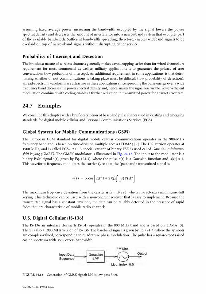
assuming fixed average power, increasing the bandwidth occupied by the signal lowers the powerspectral density and decreases the amount of interference into a narrowband system that occupies partof the available bandwidth. Sufficient bandwidth spreading, therefore, enables wideband signals to beoverlaid on top of narrowband signals without disrupting either service.

Probability of Intercept and Detection

The broadcast nature of wireless channels generally makes eavesdropping easier than for wired channels. Arequirement for most commercial as well as military applications is to guarantee the privacy of userconversations (low probability of intercept). An additional requirement, in some applications, is that deter-mining whether or not communications is taking place must be difficult (low probability of detection).Spread-spectrum waveforms are attractive in these applications since spreading the pulse energy over a widefrequency band decreases the power spectral density and, hence, makes the signal less visible. Power-efficientmodulation combined with coding enables a further reduction in transmitted power for a target error rate.

24.7 Examples

We conclude this chapter with a brief description of baseband pulse shapes used in existing and emergingstandards for digital mobile cellular and Personal Communications Services (PCS).

Global System for Mobile Communications (GSM)

The European GSM standard for digital mobile cellular communications operates in the 900-MHzfrequency band and is based on time-division multiple access (TDMA) [9]. The U.S. version operates at1900 MHz, and is called PCS-1900. A special variant of binary FSK is used called Gaussian minimum-shift keying (GMSK). The GMSK modulator is illustrated in Fig. 24.13. The input to the modulator is abinary PAM signal s(t), given by Eq. (24.3), where the pulse p(t) is a Gaussian function and |s(t)| < 1.This waveform frequency modulates the carrier fc, so that the (passband) transmitted signal is

The maximum frequency deviation from the carrier is fd = 1/(2T), which characterizes minimum-shiftkeying. This technique can be used with a noncoherent receiver that is easy to implement. Because thetransmitted signal has a constant envelope, the data can be reliably detected in the presence of rapidfades that are characteristic of mobile radio channels.

U.S. Digital Cellular (IS-136)

The IS-136 air interface (formerly IS-54) operates in the 800 MHz band and is based on TDMA [3].There is also a 1900 MHz version of IS-136. The baseband signal is given by Eq. (24.3) where the symbolsare complex-valued, corresponding to quadrature phase modulation. The pulse has a square-root raisedcosine spectrum with 35% excess bandwidth.

FIGURE 24.13 Generation of GMSK signal; LPF is low-pass filter.

w t( ) K 2pfct 2pfd s t( ) dt•–

t

Ú+cos=


Interim Standard-95

The IS-95 air interface for digital mobile cellular uses spread-spectrum signalling (CDMA) in the 800-MHz band [10]. There is also a 1900 MHz version of IS-95. The baseband transmitted pulse shapes areanalogous to those shown in Fig. 24.2, where the number of square pulses (chips) per bit is 128. Toimprove spectral efficiency the (wideband) transmitted signal is filtered by an approximation to an ideallow-pass response with a small amount of excess bandwidth. This shapes the chips so that they resembleminimum bandwidth pulses.

Personal Access Communications System (PACS)

Both PACS and the Japanese personal handy phone (PHP) system are TDMA systems which have beenproposed for personal communications systems (PCS), and operate near 2 GHz [2]. The baseband signalis given by Eq. (24.3) with four complex symbols representing four-phase quadrature modulation. Thebaseband pulse has a square-root raised cosine spectrum with 50% excess bandwidth.

Defining Terms

Baseband signal: A signal with frequency content centered around DC.Equivalent discrete-time transfer function: A discrete-time transfer function (z transform) that relates

the transmitted amplitudes to received samples in the absence of noise.Excess bandwidth: That part of the baseband transmitted spectrum which is not contained within the

Nyquist band.Eye diagram: Superposition of segments of a received PAM signal that indicates the amount of inter-

symbol interference present.Frequency-shift keying: A digital modulation technique in which the transmitted pulse is sinusoidal,

where the frequency is determined by the source bits.Intersymbol interference: The additive contribution (interference) to a received sample from trans-

mitted symbols other than the symbol to be detected.Matched filter: The receiver filter with impulse response equal to the time-reversed, complex conjugate

impulse response of the combined transmitter filter-channel impulse response.Nyquist band: The narrowest frequency band that can support a PAM signal without intersymbol

interference (the interval [-1/(2T), 1/(2T)] where 1/T is the symbol rate).Nyquist criterion: A condition on the overall frequency response of a PAM system that ensures the

absence of intersymbol interference.Orthogonal frequency division multiplexing (OFDM): Modulation technique in which the trans-

mitted signal is the sum of low-bit-rate narrowband digital signals modulated on orthogonalcarriers.

Partial-response signalling: A signalling technique in which a controlled amount of intersymbol interfer-ence is introduced at the transmitter in order to shape the transmitted spectrum.

Precoding: A transformation of source symbols at the transmitter that compensates for intersymbolinterference introduced by the channel.

Pulse amplitude modulation (PAM): A digital modulation technique in which the source bits aremapped to a sequence of amplitudes that modulate a transmitted pulse.

Raised cosine pulse: A pulse shape with Fourier transform that decays to zero according to a raisedcosine; see Eq. (24.18). The amount of excess bandwidth is conveniently determined by a singleparameter (a).

Spread spectrum: A signalling technique in which the pulse bandwidth is many times wider than theNyquist bandwidth.

Zero-forcing criterion: A design constraint which specifies that intersymbol interference be eliminated.


References

1. Bingham, J.A.C., Multicarrier modulation for data transmission: an idea whose time has come. IEEECommun. Mag., 28(May), 5–14, 1990.

2. Cox, D.C., Wireless personal communications: what is it? IEEE Personal Comm., 2(2), 20–35, 1995.3. Electronic Industries Association/Telecommunications Industry Association. Recommended mini-

mum performance standards for 800 MHz dual-mode mobile stations. Incorp. EIA/TIA 19B,EIA/TIA Project No. 2216, Mar., 1991.

4. Harashima, H. and Miyakawa, H., Matched-transmission technique for channels with intersymbolinterference. IEEE Trans. on Commun., COM-20(Aug.), 774–780, 1972.

5. Kalet, I. and Saltzberg, B.R., QAM transmission through a companding channel—signal constella-tions and detection. IEEE Trans. on Comm., 42(2–4), 417–429, 1994.

6. Kretzmer, E.R., Generalization of a technique for binary data communication. IEEE Trans. Comm.Tech., COM-14 (Feb.), 67, 68, 1966.

7. Lender, A., The duobinary technique for high-speed data transmission. AIEE Trans. on Comm.Electronics, 82 (March), 214–218, 1963.

8. Muller, S.H. and Huber, J.B., A comparison of peak power reduction schemes for OFDM. Proc.GLOBECOM ’97, (Mon.), 1–5, 1997.

9. Rahnema, M., Overview of the GSM system and protocol architecture. IEEE Commun. Mag., (April),92–100, 1993.

10. Telecommunication Industry Association. Mobile station-base station compatibility standard fordual-mode wideband spread spectrum cellular system. TIA/EIA/IS-95-A. May, 1995.

11. Tomlinson, M., New automatic equalizer employing modulo arithmetic. Electron. Lett., 7 (March),138, 139, 1971.

Further Information

Baseband signalling and pulse shaping is fundamental to the design of any digital communications systemand is, therefore, covered in numerous texts on digital communications. For more advanced treatmentssee E.A. Lee and D.G. Messerschmitt, Digital Communication, Kluwer 1994, and J.G. Proakis, DigitalCommunications, McGraw-Hill 1995.


© 2002 by CRC Pre

25.1 C

Many commcharacterizedresponse

C

(

where

A

(

f

)

that is somet

A channel is

signal,

A

(

f

)

the other ha

signal, the ch

and if

τ

(

f

)

As a resulcharacteristi

bandwidth

W

the receivin

example of pulse having

by the pulsesequence ofthe pulse th

John G. P

Northeastern

0967_frame_C025.fm Page 1 Sunday, July 28, 2002 5:46 PM

ss LLC

25Channel Equalization

25.1 Characterization of Channel Distortion 25.2 Characterization of Intersymbol Interference 25.3 Linear Equalizers

Adaptive Linear Equalizers

25.4 Decision-Feedback Equalizer 25.5 Maximum-Likelihood Sequence Detection 25.6 Maximum A Posteriori Probability Detector

and Turbo Equalization25.7 Conclusions

haracterization of Channel Distortion

unication channels, including telephone channels and some radio channels, may be generally as band-limited linear filters. Consequently, such channels are described by their frequency

f ), which may be expressed as

(25.1)

is called the amplitude response and θ( f ) is called the phase response. Another characteristicimes used in place of the phase response is the envelope delay or group delay, which is defined as

(25.2)

said to be nondistorting or ideal if, within the bandwidth W occupied by the transmitted= const and θ( f ) is a linear function of frequency [or the envelope delay τ( f ) = const]. Onnd, if A( f ) and τ( f ) are not constant within the bandwidth occupied by the transmittedannel distorts the signal. If A( f ) is not constant, the distortion is called amplitude distortion

is not constant, the distortion on the transmitted signal is called delay distortion.t of the amplitude and delay distortion caused by the nonideal channel frequency responsec C( f ), a succession of pulses transmitted through the channel at rates comparable to the

are smeared to the point that they are no longer distinguishable as well-defined pulses atg terminal. Instead, they overlap and, thus, we have intersymbol interference (ISI). As anthe effect of delay distortion on a transmitted pulse, Fig. 25.1(a) illustrates a band-limited zeros periodically spaced in time at points labeled ±T, ±2T, etc. If information is conveyed amplitude, as in pulse amplitude modulation (PAM), for example, then one can transmit a pulses, each of which has a peak at the periodic zeros of the other pulses. Transmission ofrough a channel modeled as having a linear envelope delay characteristic τ( f ) [quadratic

C f( ) A f( )e jθ f( )=

τ f( ) − 12π------ dθ f( )

df--------------=

roakisUniversity

phase θ( f )], however, results in the received pulse shown in Fig. 25.1(b) having zero crossings that areno longer periodically spaced. Consequently, a sequence of successive pulses would be smeared into oneanother, and the peaks of the pulses would no longer be distinguishable. Thus, the channel delay distortionresults in intersymbol interference. As will be discussed in this chapter, it is possible to compensate forthe nonideal frequency response characteristic of the channel by use of a filter or equalizer at the demo-dulator. Figure 25.1(c) illustrates the output of a linear equalizer that compensates for the linear distortionin the channel.

The extent of the intersymbol interference on a telephone channel can be appreciated by observing afrequency response characteristic of the channel. Figure 25.2 illustrates the measured average amplitudeand delay as a function of frequency for a medium-range (180–725 mile) telephone channel of theswitched telecommunications network as given by Duffy and Tratcher [17]. We observe that the usable bandof the channel extends from about 300 Hz to about 3000 Hz. The corresponding impulse response ofthe average channel is shown in Fig. 25.3. Its duration is about 10 ms. In comparison, the transmittedsymbol rates on such a channel may be of the order of 2500 pulses or symbols per second. Hence,intersymbol interference might extend over 20–30 symbols.

FIGURE 25.1 Effect of channel distortion: (a) channel input, (b) channel output, (c) equalizer output.


FIGURE 25.2 Average amplitude and delay characteristics of medium-range telephone channel.

FIGURE 25.3 Impulse response of average channel with amplitude and delay shown in Fig. 25.2.


Besides telephone channels, there are other physical channels that exhibit some form of time dispersionand, thus, introduce intersymbol interference. Radio channels, such as short-wave ionospheric propagation(HF), tropospheric scatter, and mobile cellular radio are three examples of time-dispersive wireless chan-nels. In these channels, time dispersion and, hence, intersymbol interference is the result of multiplepropagation paths with different path delays. The number of paths and the relative time delays among thepaths vary with time and, for this reason, these radio channels are usually called time-variant multipathchannels. The time-variant multipath conditions give rise to a wide variety of frequency response char-acteristics. Consequently, the frequency response characterization that is used for telephone channels isinappropriate for time-variant multipath channels. Instead, these radio channels are characterized statis-tically in terms of the scattering function, which, in brief, is a two-dimensional representation of theaverage received signal power as a function of relative time delay and Doppler frequency (see Proakis, 2001).

For illustrative purposes, a scattering function measured on a medium-range (150 mile) troposphericscatter channel is shown in Fig. 25.4. The total time duration (multipath spread) of the channel responseis approximately 0.7 µs on the average, and the spread between half-power points in Doppler frequency isa little less than 1 Hz on the strongest path and somewhat larger on the other paths. Typically, if oneis transmitting at a rate of 107 symbols/s over such a channel, the multipath spread of 0.7 µs will resultin intersymbol interference that spans about seven symbols.

25.2 Characterization of Intersymbol Interference

In a digital communication system, channel distortion causes intersymbol interference, as illustrated in thepreceding section. In this section, we shall present a model that characterizes the ISI. The digital modulationmethods to which this treatment applies are PAM, phase-shift keying (PSK), and quadrature amplitudemodulation (QAM). The transmitted signal for these three types of modulation may be expressed as

(25.3)

FIGURE 25.4 Scattering function of a medium-range tropospheric scatter channel.

s t( ) uc t( ) 2π f ct us– t( ) 2π f ctsincos=

Re u t( )ej2π fc t[ ]=


where υ(t) = υc(t) + jυx(t) is called the equivalent low-pass signal, fc is the carrier frequency, and Re[]denotes the real part of the quantity in brackets.

In general, the equivalent low-pass signal is expressed as

(25.4)

where gT(t) is the basic pulse shape that is selected to control the spectral characteristics of the transmittedsignal, {In} is the sequence of transmitted information symbols selected from a signal constellationconsisting of M points, and T is the signal interval (1/T is the symbol rate). For PAM, PSK, and QAM,the values of In are points from M-ary signal constellations. Figure 25.5 illustrates the signal constellationsfor the case of M = 8 signal points. Note that for PAM, the signal constellation is one-dimensional. Hence,the equivalent low-pass signal υ(t) is real valued, i.e., υs(t) = 0 and υc(t) = υ(t). For M-ary (M > 2) PSKand QAM, the signal constellations are two-dimensional and, hence, υ(t) is complex valued.

FIGURE 25.5 M = 8 signal constellations for PAM, PSK, and QAM.

u t( ) IngT t nT–( )n=0

∑=

−7 −5 −3 −1 1 3 5 7

000 001 011 010 110 111 101 100

(a) PAM

100

000

001

011

010

110

111 101

2

(b) PSK

(1, 1)

2

2

(1 + 3, 0)

(c) QAM


The signal s(t) is transmitted over a bandpass channel that may be characterized by an equivalent low-pass frequency response C( f ). Consequently, the equivalent low-pass received signal can be represented as

(25.5)

where h(t) = gT(t) ∗ c(t), c(t) is the impulse response of the equivalent low-pass channel, the asteriskdenotes convolution, and w(t) represents the additive noise in the channel.

To characterize the ISI, suppose that the received signal is passed through a receiving filter and thensampled at the rate 1/T samples/s. In general, the optimum filter at the receiver is matched to the receivedsignal pulse h(t). Hence, the frequency response of this filter is H ∗ ( f ). We denote its output as

(25.6)

where x(t) is the signal pulse response of the receiving filter, i.e., X( f ) = H( f )H ∗ ( f ) = |H( f )|2, and n(t)is the response of the receiving filter to the noise w(t). Now, if y(t) is sampled at times t = kT, k = 0, 1,2,…, we have

(25.7)

The sample values {yk} can be expressed as

(25.8)

The term x0 is an arbitrary scale factor, which we arbitrarily set equal to unity for convenience. Then

(25.9)

The term Ik represents the desired information symbol at the kth sampling instant, the term

(25.10)

represents the ISI, and nk is the additive noise variable at the kth sampling instant.The amount of ISI and noise in a digital communications system can be viewed on an oscilloscope.

For PAM signals, we can display the received signal y(t) on the vertical input with the horizontal sweep

r t( ) Inh t nT–( ) w t( )+n=0

∞

∑=

y t( ) In x t nT–( ) n t( )+n=0

∞

∑=

y kT( ) yk≡ In x kT nT–( ) v kT( )+n=0

∞

∑=

In xk−n vk, k+n=0

∞

∑ 0,1,…= =

yk x0 Ik1x0

---- In xk−n

n=0n≠k

∞

∑+

nk, k+ 0,1,…= =

yk Ik In xk−n

n=0n≠k

∞

∑ nk+ +=

In xk−n

n=0n≠k

∞

∑


rate set at 1/T. The resulting oscilloscope display is called an eye pattern because of its resemblance tothe human eye. For example, Fig. 25.6 illustrates the eye patterns for binary and four-level PAM modu-lation. The effect of ISI is to cause the eye to close, thereby reducing the margin for additive noise tocause errors. Figure 25.7 graphically illustrates the effect of ISI in reducing the opening of a binary eye.Note that intersymbol interference distorts the position of the zero crossings and causes a reduction inthe eye opening. Thus, it causes the system to be more sensitive to a synchronization error.

For PSK and QAM it is customary to display the eye pattern as a two-dimensional scatter diagramillustrating the sampled values {yk} that represent the decision variables at the sampling instants. Figure 25.8illustrates such an eye pattern for an 8-PSK signal. In the absence of intersymbol interference and noise,the superimposed signals at the sampling instants would result in eight distinct points corresponding tothe eight transmitted signal phases. Intersymbol interference and noise result in a deviation of the receivedsamples {yk} from the desired 8-PSK signal. The larger the intersymbol interference and noise, the largerthe scattering of the received signal samples relative to the transmitted signal points.

In practice, the transmitter and receiver filters are designed for zero ISI at the desired sampling timest = kT. Thus, if GT( f ) is the frequency response of the transmitter filter and GR( f ) is the frequency

FIGURE 25.6 Examples of eye patterns for binary and quaternary amplitude shift keying (or PAM).

FIGURE 25.7 Effect of intersymbol interference on eye opening.

BINARY QUATERNARY

Sensitivityto timing

error

Optimum samplingtime

Distortion ofzero crossings

Peak distortionNoise margin


response of the receiver filter, then the product GT( f )GR( f ) is designed to yield zero ISI. For example,the product GT( f )GR( f ) may be selected as

(25.11)

where Xrc( f ) is the raised-cosine frequency response characteristic, defined as

(25.12)

where α is called the rolloff factor, which takes values in the range 0 ≤ α ≤ 1, and 1/T is the symbol rate.The frequency response Xrc( f ) is illustrated in Fig. 25.9(a) for α = 0, 1/2, and 1. Note that when α = 0,Xrc( f ) reduces to an ideal brick wall physically nonrealizable frequency response with bandwidth occu-pancy 1/2T. The frequency 1/2T is called the Nyquist frequency. For α > 0, the bandwidth occupied bythe desired signal Xrc( f ) beyond the Nyquist frequency 1/2T is called the excess bandwidth and is usuallyexpressed as a percentage of the Nyquist frequency. For example, when α = 1/2, the excess bandwidth is50%, and when α = 1, the excess bandwidth is 100%. The signal pulse xrc(t) having the raised-cosinespectrum is

(25.13)

Figure 25.9(b) illustrates xrc(t) for α = 0, 1/2, and 1. Note that xrc(t) = 1 at t = 0 and xrc(t) = 0 at t = kT,k = ±1, ±2,… . Consequently, at the sampling instants t = kT, k ≠ 0, there is no ISI from adjacent symbolswhen there is no channel distortion. In the presence of channel distortion, however, the ISI given by Eq.(25.10) is no longer zero, and a channel equalizer is needed to minimize its effect on system performance.

FIGURE 25.8 Two-dimensional digital eye patterns.

GT f( )GR f( ) Xrc f( )=

Xrc f( )

T, 0 f 1 a–( )/2T≤ ≤

T2--- 1 cospT

a------- f 1 a–

2T------------–

, 1 a–2T

------------ f 1 a+2T

------------≤ ≤+

0, f 1 a+2T

------------>

=

xrc t( ) pt/Tsinp t/T

------------------- pat/T( )cos

1 4a2t2/T2–------------------------------=


25.3 Linear Equalizers

The most common type of channel equalizer used in practice to reduce ISI is a linear transversal filterwith adjustable coefficients {ci}, as shown in Fig. 25.10.

On channels whose frequency response characteristics are unknown but are time invariant, we maymeasure the channel characteristics and adjust the parameters of the equalizer; once adjusted, theparameters remain fixed during the transmission of data. Such equalizers are called preset equalizers.On the other hand, adaptive equalizers update their parameters on a periodic basis during the trans-mission of data and, thus, they are capable of tracking a slowly time-varying channel response.

First, let us consider the design characteristics for a linear equalizer from a frequency domain viewpoint.Figure 25.11 shows a block diagram of a system that employs a linear filter as a channel equalizer.

The demodulator consists of a receiver filter with frequency response GR(f ) in cascade with a channelequalizing filter that has a frequency response GE(f ). As indicated in the preceding section, the receiver filterresponse GR(f ) is matched to the transmitter response, i.e., GR(f ) = and the product GR(f )GT(f ) isusually designed so that there is zero ISI at the sampling instants as, for example, when GR(f )GT(f ) = Xrc(f ).

For the system shown in Fig. 25.11, in which the channel frequency response is not ideal, the desiredcondition for zero ISI is

(25.14)

where Xrc( f ) is the desired raised-cosine spectral characteristic. Since GT( f )GR( f ) = Xrc( f ) by design, thefrequency response of the equalizer that compensates for the channel distortion is

(25.15)

FIGURE 25.9 Pulses having a raised-cosine spectrum.

GT∗ ( f ),

GT f( )C f( )GR f( )GE f( ) Xrc f( )=

GE f( ) 1C f( )----------- 1

C f( )--------------e

jqc f( )–= =


Thus, the amplitude response of the equalizer is |GE( f )| = 1/|C( f )| and its phase response is θE ( f ) =−θc( f ). In this case, the equalizer is said to be the inverse channel filter to the channel response.

We note that the inverse channel filter completely eliminates ISI caused by the channel. Since it forcesthe ISI to be zero at the sampling instants t = kT, k = 0, 1,… , the equalizer is called a zero-forcingequalizer. Hence, the input to the detector is simply

(25.16)

where ηk represents the additive noise and Ik is the desired symbol.In practice, the ISI caused by channel distortion is usually limited to a finite number of symbols on

either side of the desired symbol. Hence, the number of terms that constitute the ISI in the summationgiven by Eq. (25.10) is finite. As a consequence, in practice, the channel equalizer is implemented as afinite duration impulse response (FIR) filter, or transversal filter, with adjustable tap coefficients {cn}, asillustrated in Fig. 25.10. The time delay τ between adjacent taps may be selected as large as T, the symbolinterval, in which case the FIR equalizer is called a symbol-spaced equalizer. In this case, the input tothe equalizer is the sampled sequence given by Eq. (25.7). We note that when the symbol rate 1/T < 2W,however, frequencies in the received signal above the folding frequency 1/T are aliased into frequenciesbelow 1/T. In this case, the equalizer compensates for the aliased channel-distorted signal.

On the other hand, when the time delay τ between adjacent taps is selected such that 1/τ ≥ 2W > 1/T,no aliasing occurs, and, hence, the inverse channel equalizer compensates for the true channel distortion.Since τ < T, the channel equalizer is said to have fractionally spaced taps and it is called a fractionallyspaced equalizer. In practice, τ is often selected as τ = T/2. Notice that, in this case, the sampling rateat the output of the filter GR( f ) is 2/T.

FIGURE 25.10 Linear transversal filter.

FIGURE 25.11 Block diagram of a system with an equalizer.

zk Ik hk, k+ 0, 1, …= =


The impulse response of the FIR equalizer is

(25.17)

and the corresponding frequency response is

(25.18)

where {cn} are the (2N + 1) equalizer coefficients and N is chosen sufficiently large so that the equalizerspans the length of the ISI, i.e., 2N + 1 ≥ L, where L is the number of signal samples spanned by the ISI.Since X( f ) = GT( f )C( f )GR( f ) and x(t) is the signal pulse corresponding to X( f ), then the equalizedoutput signal pulse is

(25.19)

The zero-forcing condition can now be applied to the samples of q(t) taken at times t = mT. These samplesare

(25.20)

Since there are 2N + 1 equalizer coefficients, we can control only 2N + 1 sampled values of q(t). Specifically,we may force the conditions

(25.21)

which may be expressed in matrix form as Xc = q, where X is a (2N + 1) × (2N + 1) matrix with elements{x(mT − nτ)}, c is the (2N + 1) coefficient vector, and q is the (2N + 1) column vector with one nonzeroelement. Thus, we obtain a set of 2N + 1 linear equations for the coefficients of the zero-forcing equalizer.

We should emphasize that the FIR zero-forcing equalizer does not completely eliminate ISI because ithas a finite length. As N is increased, however, the residual ISI can be reduced, and in the limit as N → ∞,the ISI is completely eliminated.

Example 25.1

Consider a channel distorted pulse x(t), at the input to the equalizer, given by the expression

where 1/T is the symbol rate. The pulse is sampled at the rate 2/T and equalized by a zero-forcingequalizer. Determine the coefficients of a five-tap zero-forcing equalizer.

gE t( ) cnd t nt–( )n=−N

N

∑=

GE f( ) cne j2p fnt–

n=−N

N

∑=

q t( ) cn x t nt–( )n=−N

∑=

q mT( ) cn x mT nt–( ), mn=−N

N

∑ 0, ±1,…, ±N= =

q mT( ) cn x mT nt–( )n=−N

N

∑ 1, m 0=0, m ±1, ±2,…, ±N=

= =

x t( ) 1

1 2tT-----

2

+-------------------=


Solution 25.1According to Eq. (25.21), the zero-forcing equalizer must satisfy the equations

The matrix X with elements x(mT − nT/2) is given as

(25.22)

The coefficient vector c and the vector q are given as

(25.23)

Then, the linear equations Xc = q can be solved by inverting the matrix X. Thus, we obtain

(25.24)

One drawback to the zero-forcing equalizer is that it ignores the presence of additive noise. As aconsequence, its use may result in significant noise enhancement. This is easily seen by noting that in afrequency range where C( f ) is small, the channel equalizer GE( f ) = 1/C( f ) compensates by placing alarge gain in that frequency range. Consequently, the noise in that frequency range is greatly enhanced.An alternative is to relax the zero ISI condition and select the channel equalizer characteristic such thatthe combined power in the residual ISI and the additive noise at the output of the equalizer is minimized.A channel equalizer that is optimized based on the minimum mean square error (MMSE) criterionaccomplishes the desired goal.

To elaborate, let us consider the noise corrupted output of the FIR equalizer, which is

(25.25)

q mT( ) cnx mT nT /2–( )n=−2

2

∑ 1, m 0=0, m 1, ±2±=

= =

X

15-- 1

10----- 1

17----- 1

26----- 1

37-----

1 12-- 1

5-- 1

10----- 1

17-----

15-- 1

2-- 1 1

2-- 1

5--

117----- 1

10----- 1

5-- 1

2-- 1

137----- 1

26----- 1

17----- 1

10----- 1

5--

=

c

c 2–

c 1–

c0

c1

c2

q

0

0

1

0

0

= =

copt X 1– q

2.2–

4.9

3–

4.9

2.2–

= =

z t( ) cn y t nt–( )n=−N

N

∑=


where y(t) is the input to the equalizer, given by Eq. (25.6). The equalizer output is sampled at times t =mT. Thus, we obtain

(25.26)

The desired response at the output of the equalizer at t = mT is the transmitted symbol Im. The erroris defined as the difference between Im and z(mT). Then, the mean square error (MSE) between the actualoutput sample z(mT) and the desired values Im is

(25.27)

where the correlations are defined as

(25.28)

and the expectation is taken with respect to the random information sequence {Im} and the additive noise.The minimum MSE solution is obtained by differentiating Eq. (25.27) with respect to the equalizer

coefficients {cn}. Thus, we obtain the necessary conditions for the minimum MSE as

(25.29)

These are the (2N + 1) linear equations for the equalizer coefficients. In contrast to the zero-forcingsolution already described, these equations depend on the stastical properties (the autocorrelation) ofthe noise as well as the ISI through the autocorrelation RY(n).

In practice, the autocorrelation matrix RY(n) and the crosscorrelation vector RIY(n) are unknowna priori. These correlation sequences can be estimated, however, by transmitting a test signal over thechannel and using the time-average estimates

(25.30)

in place of the ensemble averages to solve for the equalizer coefficients given by Eq. (25.29).

z mT( ) cn y mT nt–( )n=−1

N

∑=

MSE E|z mT( ) Im|2–=

E cn y mT nt–( ) Im–N=−N

N

∑2

=

cnckRy n k–( )k =−N

N

∑n=−N

N

∑= 2 ckRIY k( ) E Im2( )+

k =−N

N

∑–

RY n k–( ) E y∗ mT nt–( )y mT kt–( )[ ]=

RIY k( ) E y mT kt–( )Im∗[ ]=

cnRY n k–( )n =−N

N

∑ RIY k( ), k 0, ±1, 2,…,±N= =

R̂Y n( ) 1K--- y∗ kT nt–( )y kT( )

k =1

K

∑=

R̂IY n( ) 1K--- y kT nt–( )Ik

∗

k =1

K

∑=


Adaptive Linear Equalizers

We have shown that the tap coefficients of a linear equalizer can be determined by solving a set of linearequations. In the zero-forcing optimization criterion, the linear equations are given by Eq. (25.21). Onthe other hand, if the optimization criterion is based on minimizing the MSE, the optimum equalizercoefficients are determined by solving the set of linear equations given by Eq. (25.29).

In both cases, we may express the set of linear equations in the general matrix form

Bc = d (25.31)

where B is a (2N + 1) × (2Ν + 1) matrix, c is a column vector representing the 2N + 1 equalizer coefficients,and d is a (2N + 1)-dimensional column vector. The solution of Eq. (25.31) yields

copt = B−1d (25.32)

In practical implementations of equalizers, the solution of Eq. (25.31) for the optimum coefficientvector is usually obtained by an iterative procedure that avoids the explicit computation of the inverseof the matrix B. The simplest iterative procedure is the method of steepest descent, in which one beginsby choosing arbitrarily the coefficient vector c, say c0. This initial choice of coefficients corresponds to apoint on the criterion function that is being optimized. For example, in the case of the MSE criterion,the initial guess c0 corresponds to a point on the quadratic MSE surface in the (2N + 1)-dimensionalspace of coefficients. The gradient vector, defined as g0, which is the derivative of the MSE with respectto the 2Ν + 1 filter coefficients, is then computed at this point on the criterion surface, and each tapcoefficient is changed in the direction opposite to its corresponding gradient component. The change inthe jth tap coefficient is proportional to the size of the jth gradient component.

For example, the gradient vector denoted as gk, for the MSE criterion, found by taking the derivativesof the MSE with respect to each of the 2N + 1 coefficients, is

gk = Bck − d, k = 0, 1, 2,… (25.33)

Then the coefficient vector ck is updated according to the relation

ck+1 = ck − ∆gk (25.34)

where ∆ is the step-size parameter for the iterative procedure. To ensure convergence of the iterativeprocedure, ∆ is chosen to be a small positive number. In such a case, the gradient vector gk convergestoward zero, i.e., gk → 0 as k → ∞, and the coefficient vector ck → copt as illustrated in Fig. 25.12 basedon two-dimensional optimization. In general, convergence of the equalizer tap coefficients to copt cannot

FIGURE 25.12 Example of convergence characteristics of a gradient algorithm.


be attained in a finite number of iterations with the steepest-descent method. The optimum solutioncopt, however, can be approached as closely as desired in a few hundred iterations. In digital communi-cation systems that employ channel equalizers, each iteration corresponds to a time interval for sendingone symbol and, hence, a few hundred iterations to achieve convergence to copt corresponds to a fractionof a second.

Adaptive channel equalization is required for channels whose characteristics change with time. In sucha case, the ISI varies with time. The channel equalizer must track such time variations in the channelresponse and adapt its coefficients to reduce the ISI. In the context of the preceding discussion, theoptimum coefficient vector copt varies with time due to time variations in the matrix B and, for the caseof the MSE criterion, time variations in the vector d. Under these conditions, the iterative methoddescribed can be modified to use estimates of the gradient components. Thus, the algorithm for adjustingthe equalizer tap coefficients may be expressed as

(25.35)

where denotes an estimate of the gradient vector gk and denotes the estimate of the tap coefficientvector.

In the case of the MSE criterion, the gradient vector gk given by Eq. (25.33) may also be expressed as

An estimate of the gradient vector at the kth iteration is computed as

(25.36)

where ek denotes the difference between the desired output from the equalizer at the kth time instantand the actual output z(kT), and yk denotes the column vector of 2N + 1 received signal values containedin the equalizer at time instant k. The error signal ek is expressed as

ek = Ik − zk (25.37)

where zk = z(kT) is the equalizer output given by Eq. (25.26) and Ik is the desired symbol. Hence, bysubstituting Eq. (25.36) into Eq. (25.35), we obtain the adaptive algorithm for optimizing the tapcoefficients (based on the MSE criterion) as

(25.38)

Since an estimate of the gradient vector is used in Eq. (25.38), the algorithm is called a stochastic gradientalgorithm; it is also known as the LMS algorithm.

A block diagram of an adaptive equalizer that adapts its tap coefficients according to Eq. (25.38) isillustrated in Fig. 25.13. Note that the difference between the desired output Ik and the actual output zk

from the equalizer is used to form the error signal ek. This error is scaled by the step-size parameter ∆,and the scaled error signal ∆ek multiplies the received signal values {y(kT − nτ)} at the 2N + 1 taps. Theproducts ∆ek y ∗ (kT − nτ) at the (2N + 1) taps are then added to the previous values of the tap coefficientsto obtain the updated tap coefficients, according to Eq. (25.38). This computation is repeated as eachnew symbol is received. Thus, the equalizer coefficients are updated at the symbol rate.

Initially, the adaptive equalizer is trained by the transmission of a known pseudorandom sequence{Im} over the channel. At the demodulator, the equalizer employs the known sequence to adjust its coefficients.Upon initial adjustment, the adaptive equalizer switches from a training mode to a decision-directed mode,

ĉk+1 ĉ k ∆ĝk–=

ĝk ĉk

gk E ek yk∗( )–=

gkˆ

ĝk ek yk∗–=

ĉk+1 ĉ k ∆ek yk∗+=


in which case the decisions at the output of the detector are sufficiently reliable so that the error signalis formed by computing the difference between the detector output and the equalizer output, i.e.,

(25.39)

where is the output of the detector. In general, decision errors at the output of the detector occurinfrequently and, consequently, such errors have little effect on the performance of the tracking algorithmgiven by Eq. (25.38).

A rule of thumb for selecting the step-size parameter so as to ensure convergence and good trackingcapabilities in slowly varying channels is

(25.40)

where PR denotes the received signal-plus-noise power, which can be estimated from the received signal(see Proakis, 2001).

The convergence characteristic of the stochastic gradient algorithm in Eq. (25.38) is illustrated inFig. 25.14. These graphs were obtained from a computer simulation of an 11-tap adaptive equalizeroperating on a channel with a rather modest amount of ISI. The input signal-plus-noise power PR wasnormalized to unity. The rule of thumb given in Eq. (25.40) for selecting the step size gives ∆ = 0.018.The effect of making ∆ too large is illustrated by the large jumps in MSE as shown for ∆ = 0.115. As ∆is decreased, the convergence is slowed somewhat, but a lower MSE is achieved, indicating that theestimated coefficients are closer to copt.

FIGURE 25.13 Linear adaptive equalizer based on the MSE criterion.

τ τ τ τ τ

Σ Σ Σ Σ Σ

+

∆

Input

+

Output

Detector

c−N+1

{ek}

c1c0c−N c N

{zk}

{Ik}

{yk}

ek Ĩk zk–=

Ĩ k

∆ 15 2N 1+( )PR

-------------------------------=


Although we have described in some detail the operation of an adaptive equalizer that is optimizedon the basis of the MSE criterion, the operation of an adaptive equalizer based on the zero-forcing methodis very similar. The major difference lies in the method for estimating the gradient vectors gk at eachiteration. A block diagram of an adaptive zero-forcing equalizer is shown in Fig. 25.15. For more detailson the tap coefficient update method for a zero-forcing equalizer, the reader is referred to the papers byLucky [2,3] and the text by Proakis [2001].

FIGURE 25.14 Initial convergence characteristics of the LMS algorithm with different step sizes.

FIGURE 25.15 An adaptive zero-forcing equalizer.

Σ Σ Σ

τ τ τ

Σ

∆

Input

OutputDetector

yk Ik~

εk

T T T T

~~

−


25.4 Decision-Feedback Equalizer

The linear filter equalizers described in the preceding section are very effective on channels, such as wireline telephone channels, where the ISI is not severe. The severity of the ISI is directly related to thespectral characteristics and not necessarily to the time span of the ISI. For example, consider the ISIresulting from the two channels that are illustrated in Fig. 25.16. The time span for the ISI in channel Ais 5 symbol intervals on each side of the desired signal component, which has a value of 0.72. On theother hand, the time span for the ISI in channel B is one symbol interval on each side of the desiredsignal component, which has a value of 0.815. The energy of the total response is normalized to unityfor both channels.

In spite of the shorter ISI span, channel B results in more severe ISI. This is evidenced in the frequencyresponse characteristics of these channels, which are shown in Fig. 25.17. We observe that channel B hasa spectral null (the frequency response C( f ) = 0 for some frequencies in the band | f | ≤ W) at f = 1/2T,whereas this does not occur in the case of channel A. Consequently, a linear equalizer will introduce alarge gain in its frequency response to compensate for the channel null. Thus, the noise in channel Bwill be enhanced much more than in channel A. This implies that the performance of the linear equalizerfor channel B will be significantly poorer than that for channel A. This fact is borne out by the computersimulation results for the performance of the two linear equalizers shown in Fig. 25.18. Hence, the basiclimitation of a linear equalizer is that it performs poorly on channels having spectral nulls. Such channelsare often encountered in radio communications, such as ionospheric transmission at frequencies below30 MHz, and mobile radio channels, such as those used for cellular radio communications.

A decision-feedback equalizer (DFE) is a nonlinear equalizer that employs previous decisions toeliminate the ISI caused by previously detected symbols on the current symbol to be detected. A simpleblock diagram for a DFE is shown in Fig. 25.19. The DFE consists of two filters. The first filter is calleda feedforward filter and it is generally a fractionally spaced FIR filter with adjustable tap coefficients. Thisfilter is identical in form to the linear equalizer already described. Its input is the received filtered signal

FIGURE 25.16 Two channels with ISI.


y(t) sampled at some rate that is a multiple of the symbol rate, e.g., at rate 2/T. The second filter is afeedback filter. It is implemented as an FIR filter with symbol-spaced taps having adjustable coefficients.Its input is the set of previously detected symbols. The output of the feedback filter is subtracted fromthe output of the feedforward filter to form the input to the detector. Thus, we have

(25.41)

where {cn} and {bn} are the adjustable coefficients of the feedforward and feedback filters, respectively,, n = 1, 2,…, N2 are the previously detected symbols, N1 + 1 is the length of the feedforward filter,

and N2 is the length of the feedback filter. Based on the input zm, the detector determines which of thepossible transmitted symbols is closest in distance to the input signal Im. Thus, it makes its decision andoutputs . What makes the DFE nonlinear is the nonlinear characteristic of the detector that providesthe input to the feedback filter.

FIGURE 25.17 Amplitude spectra for (a) channel A shown in Fig. 25.16(a) and (b) channel B shown in Fig. 25.16(b).

zm cny mT nt–( ) bnI m−n

n=1

N2

∑–n=−N1

0

∑=

Im−n

Ĩm


The tap coefficients of the feedforward and feedback filters are selected to optimize some desiredperformance measure. For mathematical simplicity, the MSE criterion is usually applied, and a stochasticgradient algorithm is commonly used to implement an adaptive DFE. Figure 25.20 illustrates the blockdiagram of an adaptive DFE whose tap coefficients are adjusted by means of the LMS stochastic gradientalgorithm. Figure 25.21 illustrates the probability of error performance of the DFE, obtained by computersimulation, for binary PAM transmission over channel B. The gain in performance relative to that of alinear equalizer is clearly evident.

We note that the decision errors from the detector that are fed back to the feedback filter result in aloss in the performance of the DFE, as illustrated in Fig. 25.21. This loss can be avoided by placing thefeedback filter of the DFE at the transmitter and the feedforward filter at the receiver. Thus, the problemof error propagation due to incorrect decisions in the feedback filter is completely eliminated.

This approach is especially suitable for wireline channels, where the channel characteristics do not varysignificantly with time. The linear fractionally-spaced feedforward filter of the DFE, placed at the receiver,compensates for the ISI that results from any small time variations in the channel response. The synthesis

FIGURE 25.18 Error-rate performance of linear MSE equalizer.

FIGURE 25.19 Block diagram of DFE.

0 5 10 15 20 25 30 35

SNR, dB

10−1

10−2

10−3

10−4

5

2

2

2

5

5No

interference

Channel AChannel B

31 taps in equalizerPro

babi

lity

of e

rror


FIGURE 25.20 Adaptive DFE.

FIGURE 25.21 Performance of DFE with and without error propagation.


of the feedback filter of the DFE at the transmitter side is usually performed after the response of thechannel is measured at the receiver by the transmission of a channel probe signal and the receiver sendsto the transmitter the coefficients of the feedback filter.

One problem with this approach to implementing the DFE is that the signal points at the transmitter,after subtracting the tail (postcursors) of the ISI, generally have a larger dynamic range than the originalsignal constellation and, consequently, require a larger transmitter power. This problem is solved byprecoding the information symbols prior to transmission as described by Tomlinson [5] and Harashimaand Miyakawa [6].

25.5 Maximum-Likelihood Sequence Detection

Although the DFE outperforms a linear equalizer, it is not the optimum equalizer from the viewpointof minimizing the probability of error in the detection of the information sequence {Ik} from the receivedsignal samples {yk} given in Eq. (25.5). In a digital communication system that transmits informationover a channel that causes ISI, the optimum detector is a maximum-likelihood symbol sequence detectorwhich produces at its output the most probable symbol sequence for the given received sampledsequence {yk}. That is, the detector finds the sequence that maximizes the likelihood function.

(25.42)

where p({yk}|{Ik}) is the joint probability of the received sequence {yk} conditioned on {Ik}. The sequenceof symbols that maximizes this joint conditional probability is called the maximum-likelihoodsequence detector.

An algorithm that implements maximum-likelihood sequence detection (MLSD) is the Viterbi algo-rithm, which was originally devised for decoding convolutional codes. For a description of this algorithmin the context of sequence detection in the presence of ISI, the reader is referred to the paper by Forney[1] and the text by Proakis, 2001.

The major drawback of MLSD for channels with ISI is the exponential behavior in computationalcomplexity as a function of the span of the ISI. Consequently, MLSD is practical only for channels wherethe ISI spans only a few symbols and the ISI is severe in the sense that it causes a severe degradation in theperformance of a linear equalizer or a decision-feedback equalizer. For example, Fig. 25.22 illustrates the errorprobability performance of the Viterbi algorithm for a binary PAM signal transmitted through channel B(see Fig. 25.16). For purposes of comparison, we also illustrate the probability of error for a DFE. Bothresults were obtained by computer simulation. We observe that the performance of the maximumlikelihood sequence detector is about 4.5 dB better than that of the DFE at an error probability of 10−4.Hence, this is one example where the ML sequence detector provides a significant performance gain ona channel with a relatively short ISI span.

The MLSD implemented efficiently by use of the Viterbi algorithm is widely used in mobile cellularcommunications systems, such as the GSM system, where the span of the ISI is limited to five or six symbols.

The performance advantage of the MLSD, compared with the linear equalizer and the DFE, in channelswith severe ISI, has motivated a significant amount of research on methods for reducing the complexityof MLSD while retaining its superior performance characteristics. One approach to the design of reducedcomplexity MLSD is focused on methods that reduce the length of the ISI span by pre-processing thereceived signal prior to the maximum-likelihood detector. Falconer and Magee [7] and Beare [8] used alinear equalizer (LE) to reduce the span of the ISI to some small specified length prior to the Viterbidetector. Lee and Hill [9] employed a DFE in place of the LE. Thus, the large ISI span in the channel isreduced to a sufficiently small length, called the desired impulse response, so that the complexity of theViterbi detector following the LE or DFE is manageable. The choice of the desired impulse response istailored to the ISI characteristics of the channel. This approach to reducing the complexity of the Viterbidetector has proved very effective in high-density magnetic recording systems, as illustrated in the papersby Siegel and Wolf [10], Tyner and Proakis [11], Moon and Carley [12] and Proakis [13].

{ Ĩk}{ Ĩk}

Λ Ik{ }( ) ln p yk{ } | Ik{ }( )=

{ Ĩk}


From a performance viewpoint, a more effective approach for reducing the computational complexityof the MLSD is to employ decision feedback within the Viterbi detector to reduce the effective length ofthe ISI. A prefilter, called a whitened matched filter (WMF) precedes the Viterbi detector and reduces thechannel to one that has a minimum phase characteristic, as shown in Fig. 25.23. Preliminary decisionsfrom the Viterbi detector are fed back through a filter, as shown in Fig. 25.23, to synthesize the tail inthe ISI caused by the channel response and, thus, to cancel the ISI at the input to the Viterbi detector.The preliminary decisions from the Viterbi detector can be obtained by using the most probable survivingsequence in the Viterbi detector. This approach to tail cancellation had been called global feedback by

FIGURE 25.22 Comparison of performance between MLSE and decision-feedback equalization for channel B ofFig. 25.16.

FIGURE 25.23 Reduced complexity MLSD using feedback from the Viterbi detector.


Bergmans et al. [14]. Alternatively, Bergmans et al. [14] propose that one can use preliminary decisionscorresponding to each surviving sequence to cancel the ISI in the tail of the corresponding survivingsequence. Thus, the ISI can be perfectly cancelled when the correct sequence is among the survivingsequences in the Viterbi detector, even if it is not the most probable sequence at any instant in time inthe detection process. Bergmans et al. [14] named this approach to tail cancellations as using localfeedback. Simulation results given in the paper by Bergmans et al. [14] indicate that local feedback givessuperior performance compared with global feedback.

25.6 Maximum A Posteriori Probability Detector and Turbo Equalization

For a channel with ISI, the MLSD minimizes the probability of error in the detection of a sequence oftransmitted information symbols. Instead of using the MLSD to recover the information symbols, wemay use a detector that makes optimum decisions on a symbol-by-symbol basis based on the computationof the maximum a posteriori probability (MAP) for each symbol. Consequently, the MAP detector isoptimum in the sense that it minimizes the probability of a symbol error. Basically, the MAP criterionfor the information symbol Ik at the kth time interval involves the computation of the a posterioriprobabilities P(Ik = Si /yk+D , yk+D−1, —, y1) where {yk} is the observed received sequence, D is a delayparameter that is chosen to be equal to or exceed the span of the ISI, and {Si, 1 ≤ i ≤ M} is the set of Mpossible points in the signal constellation. A decision is made of the symbol corresponding to the largesta posteriori probability.

A computationally efficient iterative detection algorithm based on the MAP criterion is described ina paper by Bahl et al. [15] and is usually called the BCJR algorithm. In general, the computationalcomplexity of the BCJR algorithm is greater than that of the Viterbi algorithm, so the latter is preferablein implementing an optimum detector for a channel with ISI.

An equalizer based on the MAP criterion is particularly suitable in a receiver that couples the equalizerto a decoder that performs iterative decoding. To elaborate, suppose that the transmitter of a digitalcommunication system employs a binary systematic convolutional encoder followed by a block interleaverand modulator. The channel is a linear time-dispersive channel that introduces ISI having a finite span.In such a case, we view the channel with ISI as an inner encoder in a serially (cascade) concatenated code,as shown in Fig. 25.24. By treating the system as a serially concatenated coded system, we can applyrecently developed iterative decoding techniques which provide a significant improvement in perfor-mance, compared to a system that performs the equalization and decoding operations separately.

The basic configuration of the iterative equalizer and decoder is shown in Fig. 25.25. The input to theMAP equalizer is the sequence of received signal samples {yk} from the receiver filter, which may be

FIGURE 25.24 Channel with ISI viewed as a serially concatenated coded system.


implemented as a WMF. The MAP equalizer employs the BCJR algorithm to compute the a posterioriprobabilities for each of the possible M signal points and feeds to the outer decoder, after deinterleaving,the so-called extrinsic information, denoted by . The outer decoder uses this information incomputing the corresponding probabilities for each of the coded bits based on the MAP criterion. Thus,the outer decoder for the convolutional code also employs the BCJR algorithm to compute the a posterioriprobabilities for the information bits. Then, the MAP decoder feeds back to the MAP equalizer, afterinterleaving, the so-called extrinsic information, denoted as . This information is used by the MAPequalizer in making another pass through the data and generally achieves better estimates of the codedbits. This iterative process generally continues for several iterations (usually four to eight) until littleadditional improvement is achieved with additional iterations.

By using a MAP equalizer in conjunction with an iterative MAP decoder, it is possible to completelyeliminate the performance loss due to the ISI. The paper by Bauch et al. [16] provides a description ofthe computations performed by the MAP equalizer and MAP decoder and illustrates the performancegain that is achieved by joint MAP equalization and iterative decoding. The implementation of a MAPequalizer used in conjunction with an iterative MAP decoder has been called turbo equalization. Whileit yields superior performance compared to the other equalization techniques described above, turboequalization has the disadvantage of a significantly higher computational complexity. However, weenvision that this equalization technique will eventually be implemented in future communicationsystems that transmit information through time dispersive channels.

25.7 Conclusions

Channel equalizers are widely used in digital communication systems to mitigate the effects of ISI causedby channel distortion. Linear equalizers are widely used for high-speed modems that transmit data overtelephone channels. For wireless (radio) transmission, such as in mobile cellular communications andinteroffice communications, the multipath propagation of the transmitted signal results in severe ISI.Such channels require more powerful equalizers to combat the severe ISI. The decision-feedback equalizerand the MLSD are two nonlinear channel equalizers that are suitable for radio channels with severe ISI.

Turbo equalization is a newly developed method that couples a MAP equalizer to a MAP decoder toachieve superior performance compared with the conventional equalization methods such as the linearequalizer, the DFE, or MLSD, which operate independently of the decoder.

Defining Terms

Adaptive equalizer: A channel equalizer whose parameters are updated automatically and adaptivelyduring transmission of data.

Channel equalizer: A device that is used to reduce the effects of channel distortion in a received signal.

FIGURE 25.25 Iterative MAP equalization and decoding.

LeE(x ′ˆ )

LeD x̂( )


Decision-directed mode: Mode for adjustment of the equalizer coefficient adaptively based on the useof the detected symbols at the output of the detector.

Decision-feedback equalizer (DFE): An adaptive equalizer that consists of a feedforward filter and afeedback filter, where the latter is fed with previously detected symbols that are used to eliminatethe intersymbol interference due to the tail in the channel impulse response.

Fractionally spaced equalizer: A tapped-delay line channel equalizer in which the delay betweenadjacent taps is less than the duration of a transmitted symbol.

Intersymbol interference: Interference in a received symbol from adjacent (nearby) transmitted sym-bols caused by channel distortion in data transmission.

LMS algorithm: See stochastic gradient algorithm.Maximum-likelihood sequence detector: A detector for estimating the most probable sequence of data

symbols by maximizing the likelihood function of the received signal.Preset equalizer: A channel equalizer whose parameters are fixed (time-invariant) during transmission

of data.Stochastic gradient algorithm: An algorithm for adaptively adjusting the coefficients of an equalizer

based on the use of (noise-corrupted) estimates of the gradients.Symbol-spaced equalizer: A tapped-delay line channel equalizer in which the delay between adjacent

taps is equal to the duration of a transmitted symbol.Training mode: Mode for adjustment of the equalizer coefficients based on the transmission of a known

sequence of transmitted symbols.Zero-forcing equalizer: A channel equalizer whose parameters are adjusted to completely eliminate

intersymbol interference in a sequence of transmitted data symbols.

References

1.Forney, G.D., Jr. 1972. Maximum-likelihood sequence estimation of digital sequences in the presence of intersymbol interference. IEEE Trans. Inform. Theory, IT 18(May):363–378.

2.Lucky, R.W. 1965. Automatic equalization for digital communications. Bell Syst. Tech. J., 44(April): 547–588.

3.Lucky, R.W. 1966. Techniques for adaptive equalization of digital communication. Bell Syst. Tech. J., 45(Feb.):255–286.

4.Proakis, J.G. Digital Communications, 4th ed. McGraw-Hill, New York, 2001.5.Tomlinson, M. 1971. A new automatic equalizer employing modulo arithmetic. Electr. Lett., 7:

138–139.6.Harashima, H. and Miyakawa, H. 1972. Matched-transmission technique for channels with intersym-

bol interference. IEEE Trans. Commun., COM-20:774–780.7.Falconer, D.D. and Magee, F.R. 1973. Adaptive channel memory truncation for maximum likelihood

sequence estimation. Bell Syst. Tech. J., 52:1541–1562.8.Beare, C.T. 1978. The choice of the desired impulse response in combined linear-Viterbi algorithm

equalizers. IEEE Trans. Commun., 26:1301–1307.9.Lee, W.U. and Hill, F.S. 1977. A maximum-likelihood sequence estimator with decision-feedback

equalizer. IEEE Trans. Commun., 25:971–979.10. Siegel, P.H. and Wolf, J.K. 1991. Modulation and coding for information storage. IEEE Commun.

Mag., 30:68–86.11. Tyner, D.J. and Proakis, J.G. 1993. Partial response equalizer performance in digital magnetic

recording channels. IEEE Trans. Magnetics, 29:4194–4208.12. Moon, J. and Carley, L.R. 1988. Partial response signaling in a magnetic recording channel. IEEE

Trans. Magnetics, 24:2973–2975.13. Proakis, J.G. 1998. Equalization techniques for high-density magnetic recording. IEEE Signal Pro-

cessing Mag., 15:73–82.


14. Bergmans, J.W.M., Rajput, S.A., and Van DeLaar, F.A.M. 1987. On the use of decision feedbackfor simplifying the Viterbi detector. Philips J. Research, 42(4):399–428.

15. Bahl, L.R., Cocke, J., Jelinek, F., and Raviv, J. 1974. Optimal decoding of linear codes for minimizingsymbol error rate. IEEE Trans. Inform. Theory, IT-20:284–287.

16. Bauch, G., Khorram, H., and Hagenauer, J. 1997. Iterative equalization and decoding in mobilecommunications systems. Proc. European Personal Mobile Commun. Conf. (EPMCC’97), 307–312.

Further Information

For a comprehensive treatment of adaptive equalization techniques and their performance characteristics,the reader may refer to the book by Proakis, 2001. The two papers by Lucky [2,3] provide a treatmenton linear equalizers based on the zero-forcing criterion. Additional information on decision-feedbackequalizers may be found in the journal papers “An Adaptive Decision-Feedback Equalizer” by D.A. George,R.R. Bowen, and J.R. Storey, IEEE Transactions on Communications Technology, Vol. COM-19,pp. 281–293, June 1971, and “Feedback Equalization for Fading Dispersive Channels” by P. Monsen, IEEETransactions on Information Theory, Vol. IT-17, pp. 56–64, January 1971. A thorough treatment of channelequalization based on maximum-likelihood sequence detection is given in the paper by Forney [1].


26Pulse-Code Modulation

Codec-Filters

26.1 Introduction and General Description of a Pulse-Code Modulation (PCM) Codec-Filter

26.2 Where PCM Codec-Filters are Used in the Telephone Network

26.3 Design of Voice PCM Codec-Filters: Analog Transmission Performance and Voice Quality for IntelligibilityFiltering • Quantizing Distortion • Gain Calibration: Transmission Level Point • Idle Channel Noise • Gain Tracking: Gain Variations as a Function of Level

26.4 Linear PCM Codec-Filter for High-Speed Modem Applications


26.1 Introduction and General Description of a Pulse-Code Modulation (PCM) Codec-Filter

This chapter introduces the reader to the pulse-code modulation (PCM) codec-filter function and whereit is used in the telephone network. A PCM codec-filter was originally used in the switching offices andnetwork for digitizing and reconstructing the human voice. Over the last five years, linear PCM codec-filters have been used in high-speed modems at the subscriber’s premise.

The name codec is an acronym from coder for the analog-to-digital converter (ADC) used to digitizevoice, and decoder for the digital-to-analog converter (DAC) used for reconstructing voice. A codec is asingle device that does both the ADC and DAC conversions. A PCM codec-filter includes the bandlimitingfilter for the ADC and the reconstruction smoothing filter for the output of the DAC, in addition to theADC and DAC functions. PCM codec-filter is often referred to as a PCM codec, Combo™ (from NationalSemiconductor), Monocircuit, or Cofidec.

PCM codec-filters were developed to transmit telephone conversations over long distances with improvedperformance and at lower cost. Digitizing the voice channel is relatively economical compared to expensivelow-noise analog transmission equipment.

Multiple digitized voice channels can be multiplexed into one higher data rate digital channel withoutconcern for interference or crosstalk of the analog voice information. Digitized voice data can also be receivedand retransmitted without attenuation and noise degradation. This digitized data could be transmitted viaT1, microwave, satellite, fiber optics, RF carrier, etc. without loss to the digitized voice channel.

Michael D. FloydMotorola Semiconductor Products

Garth D. HillmanMotorola Semiconductor Products


26.2 Where PCM Codec-Filters are Used in the Telephone Network

With the advancements in microeletronics, the PCM codec-filter function has evolved from the early1960s’ technology of passive resistor-capacitor-inductor filters with discrete analog-to-digital converterand discrete digital-to-analog converter implementations to the fully integrated devices that were intro-duced in the late 1970s and early 1980s. As monolithic devices, the PCM codec-filter has experiencedperformance improvements and cost reductions by taking advantage of the improvements in integratedcircuit technology developed within the semiconductor industry. Through this evolutionary progression,the cost reductions of the PCM codec-filter function has increased their applicability to include switchingsystems for telephone central offices (CO), private branch exchanges (PBX), and key systems. The trans-mission applications have increased also to include digital loop carriers, pair gain multiplexers, telephoneloop extenders, integrated services digital network (ISDN) terminals, digital cellular telephones, anddigital cordless telephones. New applications have developed, including voice recognition equipment,voice storage, voice mail, and digital tapeless answering machines.

Figure 26.1 is a simplified diagram showing some of the services that the local telephone serviceprovider has to offer. The telephone network must be able to operate in extreme weather conditions and

FIGURE 26.1 Public switching telephone network (PSTN).


during the loss of AC power by emergency battery backup. This requires low-power dissipation of thePCM codec-filter. Complementary metal-oxide-semiconductor (CMOS) integrated circuit (IC) fabrica-tion technology has proven to be a reliable low-power semiconductor solution for this type of complexanalog and digital very large-scale integration (VLSI) circuit. A PCM codec-filter is used in each locationwith an asterisk (*).

The analog linecard is the interface between the switch and the telephone wires that reach from the centraloffice or service provider to the subscriber’s telephone. The analog linecard also provides the digital interfacefor the switching or transmission equipment. The accepted name for analog telephone service is plain oldtelephone service (POTS). Figure 26.2 is a simplified block diagram for an analog linecard showing thefunctions of the PCM codec-filter.

The PCM codec-filter converts voice into 8-b PCM words at a conversion rate of 8 kilosamples persecond. This PCM data is serially shifted out of the PCM codec-filter in the form of a serial 8-b word.This results in a 64-kb/s digital bit stream. This 64 kb/s PCM data from an analog linecard is typicallymultiplexed onto a PCM data bus or highway for transfer to a digital switch, where it will be routed tothe appropriate output PCM highway, which routes the data to another linecard, completing the signalpath for the conversation (refer to Fig. 26.1).

Transmission equipment will have multiple PCM codec-filters shifting their PCM words onto a singleconductor. This is referred to as a serial bus or PCM highway. Figure 26.3 shows the 8-b PCM words

FIGURE 26.2 Analog telephone linecard.

FIGURE 26.3 Multiplexed PCM highway.


from a PCM codec-filter for one voice channel being multiplexed into a time slot on a PCM highwaythat can accommodate 32 voice channels. For more information on PCM switching, see the chapters inthis handbook on switching systems and common channel signalling. For more information on hybridinterfaces, see the chapters in this handbook on POTS, analog hierarchy, and analog telephone channelsand conditioning.

26.3 Design of Voice PCM Codec-Filters: Analog Transmission Performance and Voice Quality for Intelligibility

Filtering

The pass-band frequency response of the voice channel is roughly 300–3000 Hz. The 300–3000 Hz spec-trum is where most of the energy in the human voice is located. Voice contains spectral energy below300 Hz and above 3 kHz, but its absence is not detrimental to intelligibility. The frequency response withinthe passband of 300 Hz–3 kHz must be tightly controlled, because the public switching telephone network(PSTN) is allowed to have as many as seven ADC/DAC conversions end-to-end. The cumulative effectsof the network plus private equipment such as PBX or key systems could audibly distort the frequencyresponse of the voice channel with less stringent requirements. Figure 26.4 shows the typical half-channelpass-band frequency response requirement of +/-0.25 dB.

The 3-kHz bandwidth for voice signals determines the sample rate for the ADC and DAC. In a samplingenvironment, Nyquist theory states that to properly sample a continuous signal, it must be sampled ata frequency higher than twice the signal’s highest frequency component. Minimizing the sample rate fordigitizing voice is a priority since it determines the system data rates which are directly proportional tocost. The voice bandwidth of 3 kHz plus the filter transition band sampled at 8 kHz represents the bestcompromise that meets the Nyquist criterion.

The amount of attenuation required for frequencies of 4 kHz and higher is dictated by the requiredsignal-to-distortion ratio of about 30 dB for acceptable voice communication as determined by the telephoneindustry. Frequencies in the filter transition band of 3.4–4.6 kHz must be attenuated enough such that theirreconstructed alias frequencies will have a combined attenuation of about 30 dB. This permits typical filtertransition band attenuation of 15 dB at 4 kHz for both the input filter for the ADC and the outputreconstruction filter for the DAC. All frequencies above 4.6 kHz must be satisfactorily attenuated before theADC conversion to prevent aliasing in-band. The requirement for out-of-band attenuation is specified bythe country of interest, but it typically ranges from 25 to 32 dB for frequencies of 4600 Hz and higher.

The requirement for limiting frequencies below 300 Hz is also regionally dependent and applicationdependent, ranging from flat response to 20 dB or more attenuation at 50 and 60 Hz. The telephone lineis susceptible to 50/60-Hz power line coupling, which must be attenuated from the signal by a high-passfilter before the ADC. Attenuation of power line frequencies is desirable to prevent 60 Hz noise duringvoice applications. Figure 26.4 shows a typical frequency response requirement for North Americantelephone equipment.

The digital-to-analog conversion process reconstructs a pulse-amplitude modulated (PAM) staircaseversion of the desired in-band signal, which has spectral images of the in-band signal modulated aboutthe sample frequency and its harmonics. These high-frequency spectral images are called aliasing com-ponents which need to be attenuated to meet performance specifications. The low-pass filter used toattenuate these aliasing components is typically called a reconstruction or smoothing filter. The low-passfilter characteristics of the reconstruction filter are similar to the low-pass filter characteristics of theinput antialiasing filter for the ADC.

The accuracy of these filters requires op amps with both high gain and low noise on the same monolithicsubstrate with precision matched capacitors which are used in the switched-capacitor filter structures.For more information on filter requirements and sampling theory, refer to the chapters in this handbookon analog modulation, sampling, and pulse-code modulation.


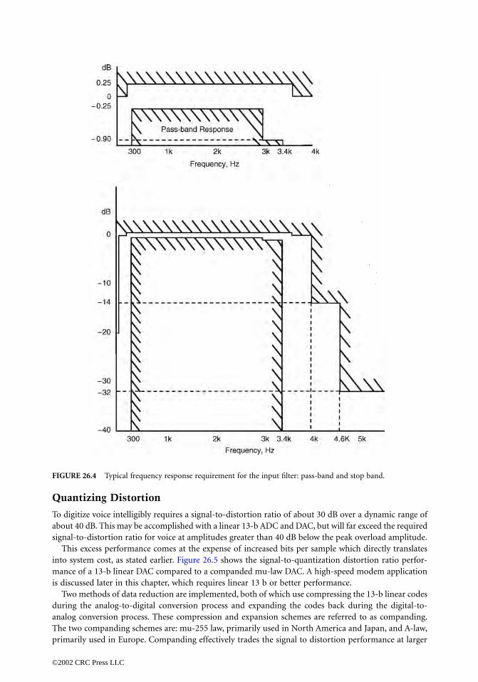
Quantizing Distortion

To digitize voice intelligibly requires a signal-to-distortion ratio of about 30 dB over a dynamic range ofabout 40 dB. This may be accomplished with a linear 13-b ADC and DAC, but will far exceed the requiredsignal-to-distortion ratio for voice at amplitudes greater than 40 dB below the peak overload amplitude.

This excess performance comes at the expense of increased bits per sample which directly translatesinto system cost, as stated earlier. Figure 26.5 shows the signal-to-quantization distortion ratio perfor-mance of a 13-b linear DAC compared to a companded mu-law DAC. A high-speed modem applicationis discussed later in this chapter, which requires linear 13 b or better performance.

Two methods of data reduction are implemented, both of which use compressing the 13-b linear codesduring the analog-to-digital conversion process and expanding the codes back during the digital-to-analog conversion process. These compression and expansion schemes are referred to as companding.The two companding schemes are: mu-255 law, primarily used in North America and Japan, and A-law,primarily used in Europe. Companding effectively trades the signal to distortion performance at larger

FIGURE 26.4 Typical frequency response requirement for the input filter: pass-band and stop band.


amplitudes for fewer bits for each sample. These companding schemes map the 13-b linear codes intopseudologarithmic 8-b codes. These companding schemes follow a segmented or piecewise-linearinput–output transfer curve formatted as sign bit, three chord bits, and four step bits. For a given chord,all 16 of the steps have the same voltage weighting. As the voltage of the analog input increases, the fourstep bits increment and carry over to the three chord bits, which increment. When the chord bits increment,the step bits double their voltage weighting. This results in an effective resolution of six bits (1 sign bit +1 effective chord bit + 4 step bits) with a sinusoidal stimulus across a 42-dB dynamic range (seven chordsabove zero, by 6 dB per chord, i.e., effectively 1 b). This satisfies the original requirement of 30-dB signal-to-distortion over a 40-dB dynamic range. Figure 26.6 is a graphical explanation of mu-law companding.

Note that to minimize die size area, which further cost reduces the PCM codec-filter, compressingADC designs and expanding DAC designs are used instead of linear ADC/DAC designs with read-onlymemory (ROM) conversion lookup tables.

A-law companding is very similar to mu-law with three differences. The first difference is that A-lawhas equal voltage weighting per step for the two positive or negative chords near zero volts. In mu-law,the step weighting voltage for chord zero is one-half the step weighting voltage for A-law chord zero. Thisreduces the A-law resolution for small signals near the voltage origin. The second difference is that thesmallest voltage of the DAC curve does not include zero volts and instead produces a positive half-stepfor positive zero and a negative half-step for negative zero. This is in contrast to mu-law companding,which produces a zero voltage output for both positive and negative zero PCM codes. Both mu-law andA-law have symmetric transfer curves about the zero volts origin, but mu-law has redundancy at zerovolts and, therefore, effectively an unused code. The third difference between the two compandingschemes deals with the data bit format. A-law inverts the least significant bit (LSB) and every other bit,leaving the sign bit unchanged relative to a conventional binary code. For example, applying the A-lawdata format formula to binary zero, s0000000, results in s1010101, the A-law code for +/- zero. Mu-law

FIGURE 26.5 Signal-to-quantization distortion performance for mu-law and 13-b linear DACs compared to thetelephone network requirements.


maintains a positive polarity for the sign bit with all of the magnitude bits inverted. Figure 26.7 showsthe zero codes and full-scale codes for both mu-law and A-law companding schemes.

Mu-law and A-law companding schemes are recognized around the world. Many equipment manu-facturers build products for distribution worldwide. This distribution versatility is facilitated by the PCMcodec-filter being programmable for either mu-law or A-law. With the deployment of ISDN, the PCMcodec-filter is located at the subscriber’s location. The need to place international telephone calls dictatesthe need for a PCM codec-filter that is both mu-law and A-law compatible.

Gain Calibration: Transmission Level Point

The test tone amplitude for analog channels is 3 dB down from the sinusoidal clip level. This test levelfor a POTS line is generally 1 mW, which is 0 dBm. The telephone line historically was referred to ashaving a 0 dB transmission level point (TLP). (With the improvements in transmission quality and fewer

FIGURE 26.6 Mu-law companding showing piecewise-linear approximation of a logarithmic curve.

Mu-Law A-Law

Level Sign Bit Chord Bits Step Bits Sign Bit Chord Bits Step Bits

+Full scale 1 0 0 0 0 0 0 0 1 0 1 0 1 0 1 0+Zero 1 1 1 1 1 1 1 1 1 1 0 1 0 1 0 1-Zero 0 1 1 1 1 1 1 1 0 1 0 1 0 1 0 1-Full scale 0 0 0 0 0 0 0 0 0 0 1 0 1 0 1 0

FIGURE 26.7 Full scale and zero codes for mu-law and A-law.


losses, telephone lines often have attenuation pads to maintain talker/listener appropriate levels.) Amplitudesthat have been TLP calibrated are given unit abbreviations that have a zero added to them, for example,dBm0. The test signal may experience gain or attenuation as it is transmitted through the network. As anexample, the absolute magnitude of one electrical node for the voice channel could result in a measuredvalue of +6 dBm when a 0 dBm0 test signal is applied. This node would be gain calibrated as having a+6 dB TLP. This would result in absolute measurements for noise having this same +6 dB of gain. Toproperly reference the noise, all measurements must be gain calibrated against the 0 dBm0 level, which, inthis example, would result in 6 dB being subtracted from all measurements. All signals in this channel,including distortion and noise, would be attenuated by 6 dB by the time they get to the subscriber’s telephone.

For PCM channels, the 0 dBm0 calibration level is nominally 3 dB down from maximum sinusoidalclip level; specifically, it is 3.17 dB down for mu-law and 3.14 dB down for A-law. These minor deviationsfrom an ideal 3 dB result from using a simple code series, called the digital milliwatt, for generating thedigital calibration signal. The digital milliwatt is a series of eight PCM codes that are repeated to generatethe 1 kHz calibration tone. Figure 26.8 shows the eight PCM codes which are repeated to generate adigital milliwatt for both mu-law and A-law in the DAC.

The digital milliwatt is used to calibrate the gains of telephone networks using voice grade PCM codec-filters.

Idle Channel Noise

Idle channel noise is the noise when there is no signal applied to the voice channel, which is differentfrom the quantization distortion caused by the ADC/DAC process. This noise can be from any circuitelement in the channel, in addition to the PCM codec-filter. Noise may be coupled in from other circuitsincluding, but not limited to, hybrid transformer interfaces, power supply induced noise, digital circuitry,radio frequency radiation, and resistive noise sources.

The PCM codec-filter itself has many opportunities to contribute to the idle channel noise level. Theinput high-pass filter often is third order, whereas both the input and the output low-pass filters aretypically fifth-order elliptic designs. The potential for noise generation is proportional to the order ofthe filter. The ADC and DAC arrays have many components that are controlled by sequencing digitalcircuits. The power supply rejection capability of PCM codec-filters once dominated the noise level ofthe channel. The power supply rejection ratio of these devices has been improved to a level where thedevice is virtually immune to power supply noise within the allowable power supply voltage range. Thisperformance was attained by differential analog circuit designs in combination with tightly controlledmatching between on-chip components.

Noise measurements require a different decibel unit as they usually involve some bandwidth or filterconditioning. One such unit commonly used (especially in North America) is decibels above referencenoise (dBrn). The reference noise level is defined as 1 pW or -90 dBm. Telephone measurements typicallyrefer to dBrnC, which is the noise level measured through a C-message weighting filter (a filter that

Mu-Law A-Law

Phase Sign Bit Chord Bits Step Bits Sign Bit Chord Bits Step Bits

π/ 8 0 0 0 1 1 1 1 0 0 0 1 1 0 1 0 03π/ 8 0 0 0 0 1 0 1 1 0 0 1 0 0 0 0 15π/ 8 0 0 0 0 1 0 1 1 0 0 1 0 0 0 0 17π/ 8 0 0 0 1 1 1 1 0 0 0 1 1 0 1 0 09π/ 8 1 0 0 1 1 1 1 0 1 0 1 1 0 1 0 011π/ 8 1 0 0 0 1 0 1 1 1 0 1 0 0 0 0 113π/ 8 1 0 0 0 1 0 1 1 1 0 1 0 0 0 0 115π/ 8 1 0 0 1 1 1 1 0 1 0 1 1 0 1 0 0

FIGURE 26.8 PCM codes for digital milliwatt.


simulates the frequency response of the human ear’s noise sensitivity). European systems use a relatedterm called dBmp, which is the dBm level noise measured through a psophometric filter. Noise mea-surements made by either dBrnC or dBmp filter weightings have units to show that the noise has beengain referenced to 0 dBm0 by adding a zero, hence dBrnC0 and dBm0p. Two examples are shown toillustrate the use of these units:

1. Mu-law: If 0 dB TLP = +6 dB, then a noise measurement of 20 dBrnC equals 14 dBrnC0.2. A-law: If 0 dB TLP = +4LPdB, then a noise measurement of -70 dBmp equals -74 dBm0p.

The examples are representative of typical idle channel noise measurements for a full-duplex digitalchannel. Idle channel noise measuring 14 dBrnc0 at a 0 dB TLP output is about 123-µV root mean square(rms). This low-noise level is very suceptible to degradation by the noise sources mentioned earlier.

The idle channel noise of the voice channel directly impacts the dynamic range, which is the ratio ofmaximum power the channel can handle to this noise level. Typical dynamic range for a mu-law PCMcodec-filter is about 78 dB. The term dynamic range is similar to signal-to-noise ratio for linear circuits.The signal-to-noise plus distortion ratio for a companded channel is generally limited by the nonlinearcompanding except at very low-signal amplitudes.

Gain Tracking: Gain Variations as a Function of Level

The quantization curves, as discussed earlier, are not linear and may cause additional nonlinear distor-tions. The concern is that the gain through the channel may be different if the amplitude of the signalis changed. Gain variations as a function of level or how well the gain tracks with level is also called gaintracking. This is a type of distortion, but could easily be missed by a tone stimulus signal-to-distortiontest alone. Gain tracking errors can cause ringing in the 2-wire–4-wire hybrid circuits if the gain at anylevel gets too large. Gain tracking performance is dominated by the IC fabrication technology, morespecifically, the matching consistency of capacitors and resistors on a monolithic substrate. Figure 26.9shows the half-channel gain tracking performance recommended for a PCM digital interface.

FIGURE 26.9 Variation of gain with input level using a tone stimulus.


Figure 26.10 is a block diagram for a monolithic MC145480 5 V PCM codec-filter manufactured byMotorola Inc. The MC145480 uses CMOS for reliable low-power operation. The operating temperaturerange is from -40º to +85º C, with a typical power dissipation of 23 mW. All analog signal processingcircuitry is differential utilizing Motorola’s six-sigma quality IC fabrication process. This device includesboth antialiasing and reconstruction switched capacitor filters, compressing ADC, expanding DAC, aprecision voltage reference, shift registers, and additional features to facilitate interfacing to both theanalog and digital circuitry on a linecard.

26.4 Linear PCM Codec-Filter for High-SpeedModem Applications

As discussed in previous sections of this chapter, the original PCM codec-filters were developed tofacilitate the digital switching of voice signals in the central office of the PSTN. The signal processing inthe digital domain consisted of simply moving digitized samples of voice from one time slot to anotherto accomplish the switching function. As such, the A/D and D/A conversion processes could be nonlinear,and companding was employed.

With the advent of the personal computer, the facsimile machine, and most recently the Internet, theneed to transmit data originating at the subscriber over the PSTN at the highest possible rates has grownto the point where the theoretical limits as defined by Shannon’s law [Shannon, 1948] are beingapproached. For data transmission, the signal processing is, in a sense, the inverse of that which spawnedthe original PCM codecs in that the initial signal is data that must be modulated to look like a voicesignal in order to be transmitted over the PSTN. At data rates above 2400 b/s, the modulation is doneusing sophisticated digital signal processing techniques, which have resulted in the development of awhole new class of linear PCM codec-filters.

Codec-filters for V.32 (9.6 kb/s), V.32bis (14.4 kb/s), and V.34 (28.8 kb/s) modems must be highly linearwith a signal to distortion much greater than 30 dB. This linearity and signal to distortion is requiredto implement the echo cancellation function with sufficient precision to resolve the voltages correspond-ing to the data points in the dense constellations of high-speed data modems. Please refer to the chaptersin this handbook on signal space and echo cancellation for more information. The critical signal-to-noise plus distortion plots for two popular commercially available codec-filters used in V.32bis (T7525)and V.34bis (STLC 7545) modems are shown in Fig. 26.11. Both of these codec-filters are implementedusing linear high ratio oversampling sigma–delta (SD) A/D and D/A conversion technology and digital

FIGURE 26.10 MC145480 5 V PCM codec-filter.


filters. This can be contrasted with the nonlinear companding converters and switched capacitor filtersof voice grade PCM codec-filters.

Sigma–delta conversion technology is based on coarsely sampling a signal at a high rate and filteringthe resulting noise [Candy and Temes, 1992; Park, 1990]. A generalized block diagram of sigma–deltaPCM codec-filters for modem applications is shown in Fig. 26.12. The transmit and receive signal pathsare the inverse of each other. The second-order modulators basically consist of two integrators and acomparator with two feedback loops. The action of the modulators is to low-pass filter the signal andhigh-pass filter the noise so that greater than 12 b of resolution (70 dB) can be achieved in-band. If it isassumed that the input signal is sufficiently active to make the quantization noise random, then it canbe shown that [Candy and Oconnell, 1981], for a simple first-order modulator,

where:No = net rms noise in bandfo = oversampling frequency

FIGURE 26.11 Linear codec dynamic range, where fm is the modulator frequency and fs is the sample frequency.

FIGURE 26.12 Generalized SD PCM modem codec-filter: (a) transmit channel and (b) receive channel.

No2 1/fo( )3=


That is, the in-band noise power decreases in proportion to the cube of the oversampling frequencyresulting in improved in-band signal-to-noise performance. The high-frequency quantization noise inthe receive channel is removed by the digital decimation filters, whereas the high-frequency alias noisedue to the interpolation process in the transmit channel is removed by interpolation filters. The transmitand receive channels are synchronous.

The decimation and interpolation operations are done in two stages: a low-ratio (n) stage and a high-ratio (N) stage. The high-ratio stage is implemented with cascaded comb filters, which are simply movingaverage filters having the following frequency response:

where i is the number of cascaded filters. For modem applications, the order i of the cascade is generallythree. Comb filters are essentially linear phase finite impulse response (FIR) filters with unity coefficientsand, therefore, they do not require a multiplier to implement, which makes them silicon area efficient. Thelow-ratio stage is usually implemented with cascaded second-order infinite impulse response (IIR) filters.These filters do require a multiplier to implement. The frequency response of the IIR filters compensate forthe sin x/x droop of the comb filters and shape the pass-band to meet telephone specifications. The totaloversampling product, nN = fo, is typically greater than or equal to 128 with N = 32 or 64. For V.32bismodems, fs is fixed at 9.6 kHz, whereas for V.34bis modems, fs varies from 9.6 to ~14 kHz.


The PCM voice codec-filter has continuously evolved since the late 1950s. With each improvement inperformance and each reduction in cost, the number of applications has increased. The analog ICtechnology incorporated in today’s PCM voice codec-filters represents one of the true bargains in thesemiconductor industry.

Sigma–delta-based PCM codec-filters have become the standard for implementing high-speed modemsbecause they can offer sufficient resolution at the lowest cost. Sigma–delta codecs are cost/performanceeffective because they are 90% digital and digital circuitry scales with integrated circuit (IC) processdensity improvements and associated speed enhancements. It is interesting to note that although the analogportion of the sigma–delta codec-filter is small and does not require precision or matched componentslike other converter technologies, it (the D/A output differential filter) limits the ultimate performance ofthe codec-filter.

References

Bellamy, J., Digital Telephony, John Wiley and Sons, New York, 1991.Bellcore, Functional criteria for digital loop carrier systems, Tech. Ref. Doc., TR-TSY-000057, Issue 1,

April, 1987.Candy, J.C. and Oconnell, J.B., The structure of quantization noise from sigma–delta modulation, IEEE

Trans. Comm., COM-29 (Sept.), 1316, 1981.Candy, J.C. and Temes, G.C., Oversampling Delta–Sigma Data Converters Theory, Design and Simulation,

IEEE Press, New York, 1992.ITU, ITU-T digital networks, transmission systems and multiplexing equipment, CCITT Red Book,

G.711, G.712, G.713, G.714, International Telecommunications Union—Telecommunications,1984.

Park, S., Principles of sigma-delta modulation for analog-to-digital converters, Motorola Digital SignalProcessing Division Application Note, Austin, TX, 1990.

Shannon, C.E., A mathematical theory of communication, Bell Syst. Tech. J., 27 (July), 379, 1948.

H z( ) 1/N 1 z N––( )/ 1 z 1––( )( )i

=


27Digital Hierarchy

27.1 Introduction 27.2 North American Asynchronous Digital Hierarchy

Digital Signal Level 0 (DS0) • Digital Signal Level 1 (DS1) • Digital Signal Level 1C Format • Higher Rate Formats • The Digital Signal Level 2 Rate • The Digital Signal Level 3 Rate

27.1 Introduction

Following the introduction of digital encoding and transmission of voice signals in the early 1960s,multiplexing schemes for increasing the number of channels that could be transported were developedby the Consultative Committee on International Telephony and Telegraphy (CCITT) in Europe and bythe Bell System in North America. The initial development of such systems was aimed at coaxial cableand millimeter waveguide transmission systems. The advent of low-loss optical fiber and efficient mod-ulation schemes for digital radio greatly increased the need to transport digital channels at rates higherthan the primary multiplexing rate.

Separate multiplexing schemes, called digital hierarchies, were developed by CCITT and by the BellSystem. During the period in which the two hierarchies were conceived, there was no reliable way todistribute highly accurate clock signals to each central office that might serve as a multiplexing point.Local clock signals were, therefore, provided by relatively inaccurate crystal oscillators, which were theonly economical signal sources available. Each hierarchy was, therefore, designed with the expectationthat the clocks controlling the various stages of the multiplexing and demultiplexing processes wouldnot be accurate and that means would be required for compensating for the asynchronicities among thevarious signals.

The mechanism chosen to accomplish synchronization of the multiplexing process was positive bitstuffing, as described elsewhere in this handbook. The CCITT development was termed the plesiochro-nous digital hierarchy (PDH) and, in North America, the scheme was designated the asynchronous digitalhierarchy. The two differ significantly. The North American digital hierarchy will be described in thesections that follow.

The advent of accurate and stable clock sources has made possible the deployment of multiplexingschemes that anticipate that most of the signals involved will be synchronous. The North Americansynchronous multiplexing scheme is the Synchronous Optical Network (SONET) and is described else-where in this handbook. The International Telecommunications Union—Telecommunications Standard-ization Sector (ITU-T) version is termed the synchronous digital hierarchy (SDH). In spite of thedevelopment of these synchronous multiplexing hierarchies, the asynchronous hierarchies remain impor-tant because there are substantial numbers of asynchronous legacy systems and routes that must bemaintained and that must support further growth.

B. P. LathiCalifornia State University

Maynard A. WrightActerna


27.2 North American Asynchronous Digital Hierarchy

Following dissolution of the Bell System in 1984, Committee T1—Telecommunications was formed totake responsibility for maintenance and development of North American telecommunications standards.The Alliance for Telecommunications Industry Solutions (ATIS) serves as the secretariat for CommitteeT1. Committee T1 maintains standard T1.107 [T1.107, 1995] that describes the North American asyn-chronous digital hierarchy.

The capacities of the bit streams of the various multiplexing levels in the North American digitalhierarchy are divided into overhead and payload. Overhead functions include framing, error checking,and maintenance functions, which will be described separately for each level. Payload capacity is usedto carry signals delivered from the next lower level or delivered directly to the multiplexer by a customer.

The various rates in the digital hierarchy are termed digital signal n (DSn), where n is the specifiedlevel in the hierarchy. The various rates are summarized in Table 27.1.

In addition, T1.107 provides standards for multiplexing various sub-DS0 digital data signals into a64 kb/s DS0.

The relationships among the various signals are illustrated in Fig. 27.1. Note that DS1C is a dead-endrate. It is useful for channeling paired cable plant but it cannot be multiplexed into higher level signals.DM in Fig. 27.1 represents digital multiplexer.

Digital Signal Level 0 (DS0)

The DS0 signal is a 64-kb/s signal that is usually organized in 8-b bytes and which may be developed byencoding analog signals as described elsewhere in this handbook. Alternatively, the DS0 may be builtfrom digital signals that are synchronous with the DS1 clock. There is no provision for handling asyn-chronous signals at the DS0 rate, although lower rate asynchronous signals are sometimes oversampledat 64 kb/s to accommodate them to the rate of the DS0 channel rate or to the rate of a lower ratesynchronous channel derived from the DS0.

TABLE 27.1 Rates in the North American Digital Hierarchy

DS0 64-kb/s signal that may contain digital data or µ = 255 encoded analog signals

DS1 1.544 Mb/s signal that byte-interleaves 24 DS0sDS1C 3.152 Mb/s signal that bit-interleaves 2 DS1sDS2 6.312 Mb/s signal that bit-interleaves 4 DS1sDS3 44.736 Mb/s signal that bit-interleaves 7 DS2s

FIGURE 27.1 Multiplexing in the North America digital hierarchy.

Digital Signal Level 1 (DS1)

The DS1 signal is built by interleaving 1.536 Mb/s of payload capacity with 8 kb/s of overhead. Followingeach overhead bit, 8-b bytes from each of the 24 DS0 channels to be multiplexed are byte interleaved.The resulting structure appears in Fig. 27.2. The DS0 bytes (channels) are numbered sequentially from1 to 24 in Fig. 27.2, and that scheme is the standard method for interleaving DS0 channels. Other schemes,which employ a nonsequential ordering of DS0 channels, have been used in the past.

This 193-b pattern is called a frame and is repeated 8000 times per second to coincide with the samplingrate for encoding analog signals. Each 8-b encoded sample of a particular channel may be transmittedin the appropriate channel position of a single frame.

Digital Signal Level 1 Overhead: Superframe Format

In the earliest 1.544 Mb/s systems, the framing pattern was simply used to identify the beginning of eachframe so that the channels could be properly demultiplexed by the receiver. With the advent of robbed-bit signaling, it became necessary to identify the particular frames in which robbed-bit signaling occurs.A superframe (SF) of twelve frames was developed in which robbed-bit signaling occurs in the 6th and12th frames. The overhead capacity in the superframe format is organized into two streams. The patterncarried by the overhead bits (Ft bits—terminal framing) in odd-numbered frames identifies the beginningof the frame structure and serves to locate the overhead stream. The pattern in the even-numbered frames(Fs bits—signaling framing) locates the beginning of each superframe so that the robbed-bit signalingcan be properly demultiplexed. The SF framing pattern is shown in Table 27.2.

Note that each frame in which the logical state of the Fs bit changes is a signaling frame that maycarry robbed-bit signaling.

There are two bits per superframe devoted to signaling. They are denoted A and B and may be usedto carry four-state signaling, although two-state signaling (on- and off-hook indications) is more common.

Digital Signal Level 1: Extended Superframe Format

Improvements in electronics and framing algorithms have made it possible for receivers to frame rapidlyand efficiently on patterns with less information than is contained in the 8-kb/s superframe overheadstream. The extended superframe format (ESF) uses a 2-kb/s framing pattern to locate a 24-frameextended superframe. The frame structure remains as for the SF format, and the ESF format thereforeprovides 6 kb/s of overhead capacity which is not devoted to framing.

A communications channel [data link or (DL)] consumes 4 kb/s of overhead. This channel is used toconvey performance monitoring information from one DS1 terminal location to the other (scheduledmessages) and to send alarm messages and loopback requests (unscheduled messages). The use of thischannel is detailed in T1.403 [ANSI, 1999]. When no message is being sent in the DL, it is usually filledwith unconcatenated high-level data link control (HDLC) flags (01111110) although some older

TABLE 27.2 DS1 SF Overhead Bit Assignments

Frame Number: 1 2 3 4 5 6 7 8 9 10 11 12

Ft bits 1 – 0 – 1 – 0 – 1 – 0 –Fs bits – 0 – 0 – 1 – 1 – 1 – 0Composite pattern 1 0 0 0 1 1 0 1 1 1 0 0

FIGURE 27.2 DS1 frame structure.

equipment may fill with an all ones pattern. HDLC frames for carrying performance information fromDS1 path terminations, as well as from intermediate points, are defined in T1.403 as the performancereport message (PRM), the network performance report message (NPRM), and the supplementaryperformance report message (SPRM).

The remaining 2 kb/s of overhead in the ESF format carry a cyclic redundancy code with a 6-bremainder (CRC-6) channel to provide error checking. The divisor polynomial is X6 + X + 1. Divisionis carried out over all 4632 b of an extended superframe with all the overhead bits set to logical ones.The 6-b remainder resulting from the division is written into the CRC-6 bits of the following extendedsuperframe.

Table 27.3 contains a summary of the overhead bit assignments in the ESF format where FAS representsthe frame alignment signal. The bits forming the 4 kb/s DL are represented by D and the six individualbit positions for the CRC-6 remainder from the previous extended superframe are shown as C.

Digital Signal Level 1C Format

Although, as mentioned previously, DS1C cannot be multiplexed to higher levels in the hierarchy, it hasproved useful for channelizing interoffice cable pairs with more channels than can be carried by acomparable DS1 system. A transmission facility for DS1C, the T1C line, was introduced and deployedduring the 1970s. Although lightwave interoffice transmission has significantly diminished the impor-tance of DS1C, a discussion of that rate provides a good starting point for discussing the higher levelsin the hierarchy.

The DS1C format multiplexes two 1.544 Mb/s DS1 signals into a single 3.152 Mb/s stream. Unlike theother levels in the digital hierarchy, DS1C signals cannot be multiplexed to higher levels. Two DS1Cstogether exceed the capacity of a single DS2, making such multiplexing impossible and making DS1Can orphan rate.

As is the case for all the hierarchical rates above DS1, the DS1C format is organized into M-framesand M-subframes. The length of a single M-frame is 1272 b. Overhead bits occur every 53 b, with 52payload bits interspersed between adjacent overhead bits. Each M-frame is divided into 4 M-subframesof 318 b each. Overhead assignments are shown in Table 27.4.

Digital Signal Level 1C Frame Alignment

The information in Table 27.4 is reorganized into columns by M-subframe in Table 27.5.Note that certain of the overhead bits, including the F1 and F2 bits, recur in the same position in every

M-subframe. Typical framing practice, therefore, is to frame on the F bits to locate the boundaries ofthe M-subframes and to then frame on the first bits of the M-subframes to locate the boundaries of theM-frame structure.

Digital Signal Level 1C X Bit

The X bit provides a communications channel between DS1C terminals that runs at just under 2500 b/s.The usual use of the X bit channel is to provide a remote alarm indication (RAI) to the distant terminal.When no alarm condition exists, the X-bit is set to logical one.

TABLE 27.3 DS1 Extended Superframe Overhead Bit Assignments

Frame Number: 1 2 3 4 5 6 7 8 9 10 11 12 13 14 15 16 17 18 19 20 21 22 23 24

FAS 0 0 1 0 1 1DL D D D D D D D D D D D DCRC C C C C C C


Digital Signal Level 1C Bit Stuffing and Stuffing Control Bits

Of the 1272 b in a DS1C M-frame, 24 are overhead bits. The bandwidth available for transporting payloadis therefore:

where:PCmax = maximum payload capacity of the DS1C signalMfbits = number of bits per M-frame, 1272

OHbits = number of overhead bits per M-frame, 24rate = DS1C bit rate, 3.152 Mb/s

TABLE 27.4 DS1C Overhead Bit Assignments

M-frame Bit Number

M-subframe Number

Overhead Bit Assignment Logical Value of Bit

0 1 M1 053 1 C1 first DS1 stuff control

106 1 F1 0159 1 C2 first DS1 stuff control212 1 C3 first DS1 stuff control265 1 F2 1318 2 M2 1371 2 C1 second DS1 stuff control424 2 F1 0477 2 C2 second DS1 stuff control530 2 C3 second DS1 stuff control583 2 F2 1636 3 M3 1689 3 C1 first DS1 stuff control742 3 F1 0795 3 C2 first DS1 stuff control848 3 C3 first DS1 stuff control901 3 F2 1954 4 X X

1007 4 C1 second DS1 stuff control1060 4 F1 01113 4 C2 second DS1 stuff control1166 4 C3 second DS1 stuff control1219 4 F2 1

TABLE 27.5 DS1C M-subframe Structure

M-subframe 1

M-subframe 2

M-subframe 3

M-subframe 4

Overhead Bit Assignment

0 318 636 954 M1/M2/M3/X53 371 689 1007 C1106 424 742 1060 F1159 477 795 1113 C2212 530 848 1166 C3265 583 901 1219 F2

PCmax Mfb ts OHb ts–( )/ Mfb ts * rate( )=

1272 24–( )/ 1272 * 3.152 Mb/s( )=

3.092 Mb/s=


Note that this is more than the payload required to transport two DS1s running at their nominal rates,which is:

Each M-subframe, however, contains a payload bit that is designated as a stuff bit. It can be used to carrya payload bit or it may be passed over and left unused. If it is unused in every M-subframe, the bandwidthmade available for the payload will be:

where: PCmin = minimum payload capacity of the DS1C signal

Sbits = number of stuff bits (opportunities) per M-frame

If all the stuff bits are skipped, the capacity of the DS1C channel is less than the amount required by twoDS1s.

Note that, by either using or skipping stuff bits, the actual payload capacity of the DS1C signal maybe varied between the extremes represented by PCmin and PCmax to handle the rate of the DS1 signalto be transported. The range available between PCmin and PCmax exceeds the range of rates allowed forDS1 signals by T1.102 [ANSI, 1999].

Stuff bits for the first DS1 occur in the first and third M-subframes and for the second DS1 in thesecond and fourth M-subframes. The stuff bit for a particular M-subframe is always the third time slotallocated to the DS1 involved following overhead bit C3. For DS1 number 1, this is the fifth bit after C3,and for DS1 number 2, it is the sixth bit after C3. For a particular M-subframe, stuffing will be performedif the C bits (C1, C2, and C3) for that M-subframe are all set to logical ones. If the C bits are set tological zeroes, no stuffing will occur in that M-subframe. The use of three C bits allows for majorityvoting by the receiver where one of the C bits may have been corrupted by a line error. This makes theprocess much more robust to such errors.

Digital Level 1C Payload

The two DS1s which are to be multiplexed are bit interleaved together to form the DS1C payload. Priorto bit interleaving, DS1 number 2 is logically inverted. Prior to inserting the interleaved payload into theDS1C overhead structure, the payload is scrambled in a single-stage scrambler. The output of thescrambler is the modulo-2 sum of the current input bit and the previous output bit.

Higher Rate Formats

As does DS1C, the DS2 and DS3 formats use positive bit stuffing to reconcile the rates of the signalsbeing multiplexed. Both use the same M-frame and M-subframe structure with overhead bits assignedto the same tasks as for DS1C. Each of the rates uses bit interleaving to insert subsidiary bit streams intotheir payload bits. A synopsis of the characteristics of the various rates appears in Table 27.6. Each ratewill be discussed in the sections that follow.

The Digital Signal Level 2 Rate

The DS2 rate is summarized in Table 27.6. It operates in a manner very similar to DS1C except that therate is higher and four DS1s may be carried by a single DS2. A transmission system for carrying DS2signals over paired copper cable called T2 was once available (1970s) but was never widely deployed.

PCreq 2*1.544 Mb/s=

3.088 Mb/s=

PCm n Mfb ts OHb ts Sb ts––( )/ Mfb ts * rate( )=

1272 24 4––( )/ 1272 * 3.152 Mb/s( )=

3.083 Mb/s=


DS2 serves today primarily as a bridge between DS1 and DS3 and is only rarely found outside the confinesof a single unit of equipment.

The Digital Signal Level 3 Rate

DS3 is heavily used as an interface to lightwave and digital radio systems. DS3 operates in much the sameway as DS1C and DS2. An additional feature of DS3 is the pair of parity bits carried by each M-frame.They are used to transmit a parity error indication for the preceding M-frame. If the modulo-2 sum ofall the information bits in the preceding M-frame is one, then both P bits are set to one. If the modulo-2sum of the information bits is zero, then the P bits are set to zero. The two P bits of an M-frame arealways set to the same value.

The same is true of the two X-bits in an M-frame. They are used as an alarm channel as for DS1Cbut are always set to the same value.

C-Bit Parity Digital Signal Level 3

A DS3 that operates using positive bit stuffing to multiplex its constituent DS2s is known as an M23application. Another DS3 application, C-bit parity, is also defined in T1.107 [ANSI, 1995a].

Since the DS2 rate is almost never used except internal to a multiplexer as a stepping stone from DS1to DS3, it is possible to lock its rate to a particular value which is slaved to the DS3 signal generator inthe multiplexer. If the rate chosen for the DS2s provides for either no bit stuffing or for stuffing at everyopportunity, the receiver can be made to know that and will be able to demultiplex the DS2s withoutreading the stuffing information that is normally carried by the C-bits.

The C-bit parity format operates the DS2 with stuffing at every opportunity and so frees up the controlbits for other uses. There are 21 C bits per M-frame, which provides a channel running at approximately197 kb/s. The 21 C bits per M-frame, are assigned as shown in Table 27.7.

The C-bit parity identifier is always set to logical one and is used as a tag to identify the DS3 signalas C-bit parity formatted. Note that the C-bit parity identifier is necessary but not sufficient for thispurpose because it may be counterfeited by a DS2 in DS3 timeslot number one running at minimumrate, which, therefore, requires stuffing at every opportunity.

The Far End Alarm and Control Channel (FEAC) carries alarm and status information from one DS3terminal to another and may be used as a channel to initiate DS1 and DS3 maintenance loopbacks atthe distant DS3 terminal.

The path parity (CP) bits are set to the same value as are the P-bits at the terminal that generatesthem. The CP-bits are not to be changed by intermediate network elements and, therefore, provide amore reliable end-to-end parity indication than do the DS3 P-bits.

TABLE 27.6 Characteristics of Levels in the Digital Hierarchy

DS1C DS2 DS3

Transmission rate, Mb/s 3.152 6.312 44.736Subsidiary format DS1 DS1 DS2Number of subsidiaries multiplexed 2 4 7Ratio of payload bits to overhead bits 52:1 48:1 84:1M-frame length, b 1272 1176 4760Number of M-subframes per M-Frame 4 4 7M-subframe length, b 318 294 680Number of X bits per M-frame 1 1 2Number of C bits per M-frame 12 12 21Number of M bits per M-frame 3 3 3Number of F bits per M-frame 2 2 4Number of P bits per M-frame 0 0 2Number of stuff opportunities per tributary

channel per M-frame2 1 1


The Far-End Block Error (FEBE) bits are set to all ones (111) only when no framing bit or CP-biterror has been detected in the incoming signal by the terminal generating the outgoing FEBE. Whenerrors are detected, the FEBE-bits are set to any combination of 1s and 0s except 111.

The data link (DL) bits are used as a 28.2 kb/s data channel between the two DS3 terminals. Messagescarried by this channel use the LAPD format. When no messages are carried, LAPD idle code (flags),which consists of repetitions of 01111110, is sent. The DL is used to carry messages identifying the DS3path, the source of a DS3 idle signal, or the source of a DS3 test signal.

A network performance report message (NPRM) for DS3 similar to that defined for DS1 in T1.403[ANSI, 1999] is under development by Working Group T1E1.2 of Committee T1 at the time of thiswriting. The NPRM will be transported by the C-bit parity data link.

Unchannelized Digital Signal Level 3

T1.107 also provides for the use of the DS3 payload for direct transport of data at the payload rate of44.210 Mb/s.

Defining Terms

Alarm Indication Signal (AIS): A signal that is transmitted in the direction of a failure to indicate thata network element has detected the failure. AIS provides a “keep alive” signal to equipmentdownstream from the failure and prevents multiple network elements from issuing redundant andconfusing alarms about the same failure.

Alliance for Telecommunications Industry Solutions (ATIS): The body that serves as the secretariatfor Committee T1—Telecommunications.

Committee T1—Telecommunications: An accredited standards development body that develops andmaintains standards for telecommunications in North America. Note that the “T1” in the com-mittee name above has no connection with the T1 line that operates at the DS1 rate.

Cyclic redundancy code (CRC) with an n-bit remainder (CRC-n): CRC codes provide highly reliableerror checking of blocks of transmitted information.

DL: Data link for transporting messages across a digital path using certain of the overhead bits as adata channel. The DL is sometimes called the FDL, for facility data link.

DSn: DSn stands for digital signal level n and refers to one of the levels (rates) in the North Americandigital hierarchy that are discussed in this chapter.

Extended superframe (ESF): A DS1 superframe that is 24 frames in length and that makes moreefficient use of the overhead bits than the older SF format.

Frame alignment signal (FAS): Serves to allow a receiver to locate significant repetitive points withinthe received bit stream so that the information may be extracted.

FEAC: Far end alarm and control channel used in C-bit parity DS3. The FEAC uses repeated 16-bitcode words to send status messages alarm signals and requests for loopback.

TABLE 27.7 Assignment of C Bits in C-bit Parity Application

C bit Application C bit Application

1 C-bit parity identifier 12 FEBE2 N = 1 (future network use) 13 DL (data link)3 FEAC 14 DL (data link)4 application specific 15 DL (data link)5 application specific 16 application specific6 application specific 17 application specific7 CP (path parity) 18 application specific8 CP (path parity) 19 application specific9 CP (path parity) 20 application specific

10 FEBE 21 application specific11 FEBE


High level data link control (HDLC): A format used to implement layer 2 (the data link layer) of theISO seven-layer model.

Link access procedure—D channel (LAPD): A subset of HDLC used for transporting messages overthe data links (DL) in the North American digital hierarchy.

Network performance report message (NPRM): An HDLC frame that carries DS1 performance infor-mation along the extended superframe data link. The NPRM is intended to allow transmission ofperformance information from points intermediate to the DS1 path terminations in an ESF DLthat is already carrying performance information from the path terminations in PRMs.

Overhead: Bits in a digital signal that do not carry the information signals the signal is intended totransport but that perform housekeeping functions such as framing, error detection, and thetransport of maintenance data from one digital terminal to the other.

Payload: The aggregate of the information bits the digital signal is intended to transport.Performance report message (PRM): An HDLC frame that is intended to carry DS1 performance

information along the extended superframe data link.Remote alarm indication (RAI): A Signal that indicates to the terminal at one end of a digital path

that the terminal at the other end has detected a failure in the incoming signal.SF—DS1 superframe format: A format in which the superframe is twelve frames in length and in

which all the overhead bits are used for framing.SPRM: A PRM that has been modified to use spare bits in the HDLC information field to carry

performance information from a point intermediate to the DS1 path terminations.Superframe: The 12-frame superframe format for DS1 known as SF or an aggregation of frames that

provides a longer repetitive structure than a frame in any format. The latter definition of the termis more often called a multiframe at rates other than DS1.

References

ANSI T1.107-1995, American National Standard for Telecommunications—Digital Hierarchy—FormatsSpecifications.

ANSI T1.403-1999, American National Standard for Telecommunications—Network-to-CustomerInstallation—DS1 Metallic Interface.

ANSI T1.102-1993, American National Standard for Telecommunications—Digital Hierarchy—ElectricalInterfaces.

Further Information

For further information on the North American digital hierarchy, see B. P. Lathi, Modern Digital andAnalog Communication Systems, 3rd ed., Oxford University Press, 1998. Information supplementing thestandards may be found in various technical requirements of Telcordia Technologies, Inc. including GR-499 and TR-TSY-000009.


28Line Coding

28.1 Introduction28.2 Common Line Coding Formats

Unipolar NRZ (Binary On-Off Keying) • Unipolar RZ • Polar NRZ • Polar RZ [Bipolar, Alternate Mark Inversion (AMI), or Pseudoternary] • Manchester Coding (Split Phase or Digital Biphase)

28.3 Alternate Line Codes Delay Modulation (Miller Code) • Split Phase (Mark) • Biphase (Mark) • Code Mark Inversion (CMI) • NRZ (I) • Binary N Zero Substitution (BNZS) • High-Density Bipolar N (HDBN) • Ternary Coding

28.4 Multilevel Signalling, Partial Response Signalling, and Duobinary CodingMultilevel Signalling • Partial Response Signalling and Duobinary Coding

28.5 Bandwidth Comparison 28.6 Concluding Remarks

28.1 Introduction

The terminology line coding originated in telephony with the need to transmit digital information acrossa copper telephone line; more specifically, binary data over a digital repeatered line. The concept of linecoding, however, readily applies to any transmission line or channel. In a digital communication system,there exists a known set of symbols to be transmitted. These can be designated as {mi}, i = 1, 2,…,N, witha probability of occurrence {pi}, i = 1, 2,…,N, where the sequentially transmitted symbols are generallyassumed to be statistically independent. The conversion or coding of these abstract symbols into real,temporal waveforms to be transmitted in baseband is the process of line coding. Since the most commontype of line coding is for binary data, such a waveform can be succinctly termed a direct format for serialbits. The concentration in this section will be line coding for binary data.

Different channel characteristics, as well as different applications and performance requirements, haveprovided the impetus for the development and study of various types of line coding [1,2]. For example,the channel might be AC coupled and, thus, could not support a line code with a DC component orlarge DC content. Synchronization or timing recovery requirements might necessitate a discrete compo-nent at the data rate. The channel bandwidth and crosstalk limitations might dictate the type of linecoding employed. Even such factors as the complexity of the encoder and the economy of the decodercould determine the line code chosen. Each line code has its own distinct properties. Depending on theapplication, one property may be more important than the other. In what follows, we describe, in general,the most desirable features that are considered when choosing a line code.

Joseph L. LoCiceroIllinois Institute of Technology

Bhasker P. PatelIllinois Institute of Technology


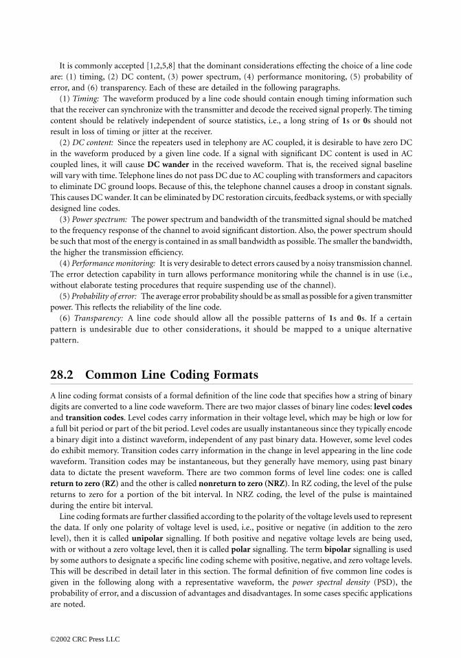
It is commonly accepted [1,2,5,8] that the dominant considerations effecting the choice of a line codeare: (1) timing, (2) DC content, (3) power spectrum, (4) performance monitoring, (5) probability oferror, and (6) transparency. Each of these are detailed in the following paragraphs.

(1) Timing: The waveform produced by a line code should contain enough timing information suchthat the receiver can synchronize with the transmitter and decode the received signal properly. The timingcontent should be relatively independent of source statistics, i.e., a long string of 1s or 0s should notresult in loss of timing or jitter at the receiver.

(2) DC content: Since the repeaters used in telephony are AC coupled, it is desirable to have zero DCin the waveform produced by a given line code. If a signal with significant DC content is used in ACcoupled lines, it will cause DC wander in the received waveform. That is, the received signal baselinewill vary with time. Telephone lines do not pass DC due to AC coupling with transformers and capacitorsto eliminate DC ground loops. Because of this, the telephone channel causes a droop in constant signals.This causes DC wander. It can be eliminated by DC restoration circuits, feedback systems, or with speciallydesigned line codes.

(3) Power spectrum: The power spectrum and bandwidth of the transmitted signal should be matchedto the frequency response of the channel to avoid significant distortion. Also, the power spectrum shouldbe such that most of the energy is contained in as small bandwidth as possible. The smaller the bandwidth,the higher the transmission efficiency.

(4) Performance monitoring: It is very desirable to detect errors caused by a noisy transmission channel.The error detection capability in turn allows performance monitoring while the channel is in use (i.e.,without elaborate testing procedures that require suspending use of the channel).

(5) Probability of error: The average error probability should be as small as possible for a given transmitterpower. This reflects the reliability of the line code.

(6) Transparency: A line code should allow all the possible patterns of 1s and 0s. If a certainpattern is undesirable due to other considerations, it should be mapped to a unique alternativepattern.

28.2 Common Line Coding Formats

A line coding format consists of a formal definition of the line code that specifies how a string of binarydigits are converted to a line code waveform. There are two major classes of binary line codes: level codesand transition codes. Level codes carry information in their voltage level, which may be high or low fora full bit period or part of the bit period. Level codes are usually instantaneous since they typically encodea binary digit into a distinct waveform, independent of any past binary data. However, some level codesdo exhibit memory. Transition codes carry information in the change in level appearing in the line codewaveform. Transition codes may be instantaneous, but they generally have memory, using past binarydata to dictate the present waveform. There are two common forms of level line codes: one is calledreturn to zero (RZ) and the other is called nonreturn to zero (NRZ). In RZ coding, the level of the pulsereturns to zero for a portion of the bit interval. In NRZ coding, the level of the pulse is maintainedduring the entire bit interval.

Line coding formats are further classified according to the polarity of the voltage levels used to representthe data. If only one polarity of voltage level is used, i.e., positive or negative (in addition to the zerolevel), then it is called unipolar signalling. If both positive and negative voltage levels are being used,with or without a zero voltage level, then it is called polar signalling. The term bipolar signalling is usedby some authors to designate a specific line coding scheme with positive, negative, and zero voltage levels.This will be described in detail later in this section. The formal definition of five common line codes isgiven in the following along with a representative waveform, the power spectral density (PSD), theprobability of error, and a discussion of advantages and disadvantages. In some cases specific applicationsare noted.


Unipolar NRZ (Binary On-Off Keying)

In this line code, a binary 1 is represented by a non-zero voltage level and a binary 0 is represented bya zero voltage level as shown in Fig. 28.1(a). This is an instantaneous level code. The PSD of this codewith equally likely 1s and 0s is given by [5,8]

(28.1)

where V is the binary 1 voltage level, T = 1/R is the bit duration, and R is the bit rate in bits per second.The spectrum of unipolar NRZ is plotted in Fig. 28.2a. This PSD is a two-sided even spectrum, althoughonly half of the plot is shown for efficiency of presentation. If the probability of a binary 1 is p, and theprobability of a binary 0 is (1 - p), then the PSD of this code, in the most general case, is 4p(1 - p)S1( f ).Considering the frequency of the first spectral null as the bandwidth of the waveform, the bandwidth ofunipolar NRZ is R in hertz. The error rate performance of this code, for equally likely data, with additivewhite Gaussian noise (AWGN) and optimum, i.e., matched filter, detection is given by [1,5]

(28.2)

where Eb/N0 is a measure of the signal-to-noise ratio (SNR) of the received signal. In general, Eb is theenergy per bit and N0/2 is the two-sided PSD of the AWGN. More specifically, for unipolar NRZ, Eb isthe energy in a binary 1, which is V2T. The performance of the unipolar NRZ code is plotted in Fig. 28.3.

The principle advantages of unipolar NRZ are ease of generation, since it requires only a single powersupply, and a relatively low bandwidth of R Hz. There are quite a few disadvantages of this line code. Aloss of synchronization and timing jitter can result with a long sequence of 1s or 0s because no pulsetransition is present. The code has no error detection capability and, hence, performance cannot bemonitored. There is a significant DC component as well as a DC content. The error rate performance isnot as good as that of polar line codes.

Unipolar RZ

In this line code, a binary 1 is represented by a nonzero voltage level during a portion of the bit duration,usually for half of the bit period, and a zero voltage level for rest of the bit duration. A binary 0 isrepresented by a zero voltage level during the entire bit duration. Thus, this is an instantaneous levelcode. Figure 28.1(b) illustrates a unipolar RZ waveform in which the 1 is represented by a nonzero voltagelevel for half the bit period. The PSD of this line code, with equally likely binary digits, is given by [5,6,8]

(28.3)

where again V is the binary 1 voltage level, and T = 1/R is the bit period. The spectrum of this code is drawnin Fig. 28.2a. In the most general case, when the probability of a 1 is p, the continuous portion of the PSDin Eq. (28.3) is scaled by the factor 4p(1 - p) and the discrete portion is scaled by the factor 4p2. The firstnull bandwidth of unipolar RZ is 2R Hz. The error rate performance of this line code is the same as thatof the unipolar NRZ, provided we increase the voltage level of this code such that the energy in binary 1,Eb, is the same for both codes. The probability of error is given by Eq. (28.2) and identified in Fig. 28.3. Ifthe voltage level and bit period are the same for unipolar NRZ and unipolar RZ, then the energy in a binary1 for unipolar RZ will be V2T/2 and the probability of error is worse by 3 dB.

S1 f( )V 2T

4---------- pf Tsin

pf T-------------------

2 V 2

4------d f( )+=

Pe

12-- erfc

Eb

2N0

--------- =

2 f( )V 2T16

---------- pf T/2sinpf T/2

-----------------------

2 V 2

4p2-------- p2

4----- d f( )

1

2n 1+( )2----------------------d f 2n 1+( )R–( )

n=-∞

•

∑++=


FIGURE 28.1 Waveforms for different line codes.

1 0 1 1 0 0 0 1 1 1 0

T 3T2T 4T 5T 6T 7T 8T 9T 10T 11T

T 3T2T 4T 5T 6T 7T 8T 9T 10T 11T

Unipolar RZ(a)

Unipolar RZ(b)

Polar NRZ(c)

Bipolar (AMI)(d)

Manchester (Bi-phase)(e)

Delay Modulation(f)

Split Phase (Mark)(g)

Split Phase (Space)(h)

Bi-Phase (Mark)(i)

Bi-Phase (Space)(j)

Code Mark Inversion(k)

NRZ (M)(l)

NRZ (s)(m)


The main advantages of unipolar RZ are, again, ease of generation since it requires a single powersupply and the presence of a discrete spectral component at the symbol rate, which allows simple timingrecovery. A number of disadvantages exist for this line code. It has a nonzero DC component and nonzeroDC content, which can lead to DC wander. A long string of 0s will lack pulse transitions and could leadto loss of synchronization. There is no error detection capability and, hence, performance monitoring isnot possible. The bandwidth requirement (2R Hz) is higher than that of NRZ signals. The error rateperformance is worse than that of polar line codes.

Unipolar NRZ as well as unipolar RZ are examples of pulse/no-pulse type of signalling. In this type ofsignalling, the pulse for a binary 0, g2(t), is zero and the pulse for a binary 1 is specified generically as g1(t) =g(t). Using G(f ) as the Fourier transform of g(t), the PSD of pulse/no-pulse signalling is given as [6,7,10]

(28.4)

where p is the probability of a binary 1, and R is the bit rate.

Polar NRZ

In this line code, a binary 1 is represented by a positive voltage +V and a binary 0 is represented by anegative voltage -V over the full bit period. This code is also referred to as NRZ (L), since a bit is repre-sented by maintaining a level (L) during its entire period. A polar NRZ waveform is shown inFig. 28.1(c). This is again an instantaneous level code. Alternatively, a 1 may be represented by a -V

FIGURE 28.2a Power spectral density of different line codes, where R = 1/T is the bit rate.

SPNP f( ) p 1 p–( )R G f( ) 2 p2R2 G nR( ) 2d f nR–( )n=-∞

∞

∑+=


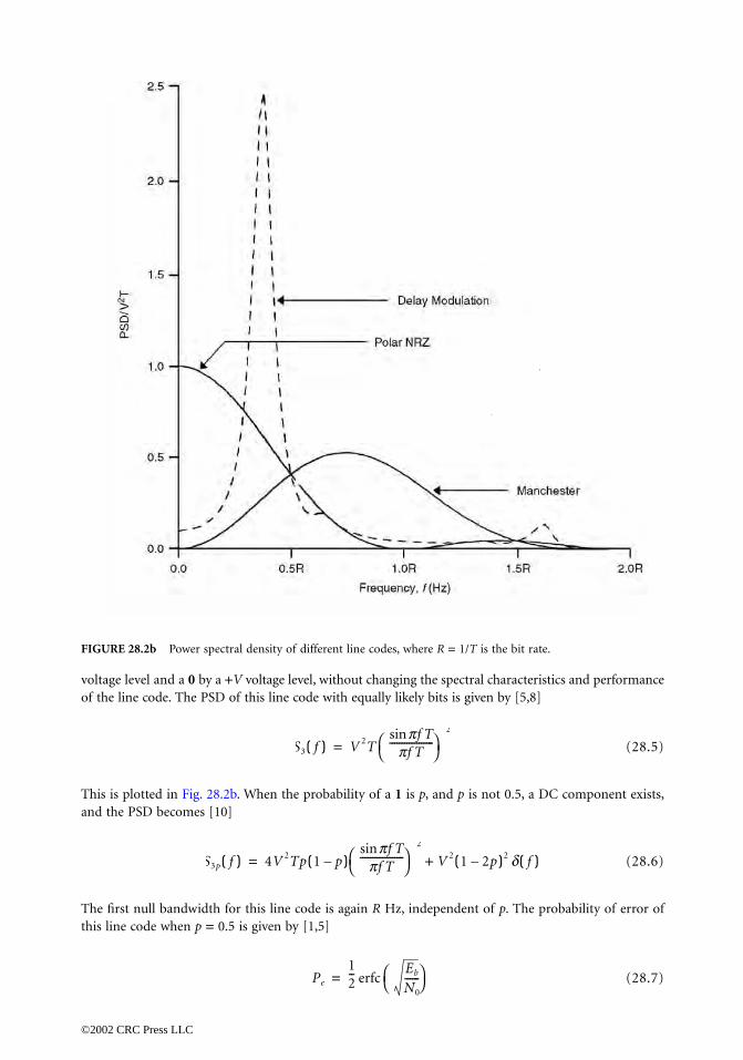
voltage level and a 0 by a +V voltage level, without changing the spectral characteristics and performanceof the line code. The PSD of this line code with equally likely bits is given by [5,8]

(28.5)

This is plotted in Fig. 28.2b. When the probability of a 1 is p, and p is not 0.5, a DC component exists,and the PSD becomes [10]

(28.6)

The first null bandwidth for this line code is again R Hz, independent of p. The probability of error ofthis line code when p = 0.5 is given by [1,5]

(28.7)

FIGURE 28.2b Power spectral density of different line codes, where R = 1/T is the bit rate.

S3 f( ) V 2Tpf Tsin

pf T------------------

2

=

S3p f( ) 4V 2Tp 1 p–( )pf Tsin

pf T------------------

2

V 2 1 2p–( )2 d f( )+=

Pe

12-- erfc

Eb

N0

------ =


The performance of polar NRZ is plotted in Fig. 28.3. This is better than the error performance of theunipolar codes by 3 dB.

The advantages of polar NRZ include a low-bandwidth requirement, R Hz, comparable to unipolar NRZ,very good error probability, and greatly reduced DC because the waveform has a zero DC component whenp = 0.5 even though the DC content is never zero. A few notable disadvantages are that there is no errordetection capability, and that a long string of 1s or 0s could result in loss of synchronization, since thereare no transitions during the string duration. Two power supplies are required to generate this code.

Polar RZ [Bipolar, Alternate Mark Inversion (AMI), or Pseudoternary]

In this scheme, a binary 1 is represented by alternating the positive and negative voltage levels, whichreturn to zero for a portion of the bit duration, generally half the bit period. A binary 0 is representedby a zero voltage level during the entire bit duration. This line coding scheme is often called alternatemark inversion (AMI) since 1s (marks) are represented by alternating positive and negative pulses. It is

FIGURE 28.3 Bit error probability for different line codes.


also called pseudoternary since three different voltage levels are used to represent binary data. Someauthors designate this line code as bipolar RZ (BRZ). An AMI waveform is shown in Fig. 28.1(d). Notethat this is a level code with memory. The AMI code is well known for its use in telephony. The PSD ofthis line code with memory is given by [1,2,7]

(28.8)

where G( f ) is the Fourier transform of the pulse used to represent a binary 1, and p is the probabilityof a binary 1. When p = 0.5 and square pulses with amplitude ±V and duration T/2 are used to representbinary 1s, the PSD becomes

(28.9)

This PSD is plotted in Fig. 28.2a. The first null bandwidth of this waveform is R Hz. This is true for RZrectangular pulses, independent of the value of p in Eq. (28.8). The error rate performance of this linecode for equally likely binary data is given by [5]

(28.10)

This curve is plotted in Fig. 28.3 and is seen to be no more than 0.5 dB worse than the unipolar codes.The advantages of polar RZ (or AMI, as it is most commonly called) outweigh the disadvantages. This

code has no DC component and zero DC content, completely avoiding the DC wander problem. Timingrecovery is rather easy since squaring, or full-wave rectifying, this type of signal yields a unipolar RZwaveform with a discrete component at the bit rate, R Hz. Because of the alternating polarity pulses forbinary 1s, this code has error detection and, hence, performance monitoring capability. It has a low-bandwidth requirement, R Hz, comparable to unipolar NRZ. The obvious disadvantage is that the errorrate performance is worse than that of the unipolar and polar waveforms. A long string of 0s could resultin loss of synchronization, and two power supplies are required for this code.

Manchester Coding (Split Phase or Digital Biphase)

In this coding, a binary 1 is represented by a pulse that has positive voltage during the first-half of thebit duration and negative voltage during second-half of the bit duration. A binary 0 is represented by apulse that is negative during the first-half of the bit duration and positive during the second-half of thebit duration. The negative or positive midbit transition indicates a binary 1 or binary 0, respectively.Thus, a Manchester code is classified as an instantaneous transition code; it has no memory. The codeis also called diphase because a square wave with a 0∞ phase is used to represent a binary 1 and a squarewave with a phase of 180∞ used to represent a binary 0; or vice versa. This line code is used in Ethernetlocal area networks (LANs). The waveform for Manchester coding is shown in Fig. 28.1(e). The PSD ofa Manchester waveform with equally likely bits is given by [5,8]

(28.11)

where ±V are used as the positive/negative voltage levels for this code. Its spectrum is plotted in Fig. 28.2b.When the probability p of a binary 1 is not equal to one-half, the continuous portion of the PSD is reducedin amplitude and discrete components appear at integer multiples of the bit rate, R = 1/T. The resulting

S4p f( ) 2p 1 p–( )R G f( ) 2 1 2pf Tcos–

1 2p 1–( )2 2 2p 1–( ) 2pf Tcos+ +-----------------------------------------------------------------------------------

=

S4 f( )V 2T

4---------- pf T/2sin

pf T/2-----------------------

2

sin2 pf T( )=

Pe

34-- erfc

Eb

2N0

--------- , Eb/N0 2>ª

S5 f( ) V 2Tpf T/2sin

pf T/2-----------------------

2

sin2 pf T/2( )=


PSD is [6,10]

(28.12)

The first null bandwidth of the waveform generated by a Manchester code is 2R Hz. The error rateperformance of this waveform when p = 0.5 is the same as that of polar NRZ, given by Eq. (28.9), andplotted in Fig. 28.3.

The advantages of this code include a zero DC content on an individual pulse basis, so no pattern ofbits can cause DC buildup; midbit transitions are always present making it is easy to extract timinginformation; and it has good error rate performance, identical to polar NRZ. The main disadvantage ofthis code is a larger bandwidth than any of the other common codes. Also, it has no error detectioncapability and, hence, performance monitoring is not possible.

Polar NRZ and Manchester coding are examples of the use of pure polar signalling where the pulsefor a binary 0, g2(t), is the negative of the pulse for a binary 1, i.e., g2(t) = -g1(t). This is also referred toas an antipodal signal set. For this broad type of polar binary line code, the PSD is given by [10]

(28.13)

where |G( f )| is the magnitude of the Fourier transform of either g1(t) or g2(t).A further generalization of the PSD of binary line codes can be given, wherein a continuous spectrum

and a discrete spectrum is evident. Let a binary 1, with probability p, be represented by g1(t) over theT = 1/R second bit interval; and let a binary 0, with probability 1 - p, be represented by g2(t) over thesame T second bit interval. The two-sided PSD for this general binary line code is [10]

(28.14)

where the Fourier transform of g1(t) and g2(t) are given by G1(f ) and G2(f ), respectively.

28.3 Alternate Line Codes

Most of the line codes discussed thus far were instantaneous level codes. Only AMI had memory, andManchester was an instantaneous transition code. The alternate line codes presented in this section allhave memory. The first four are transition codes, where binary data is represented as the presence orabsence of a transition, or by the direction of transition, i.e., positive to negative or vice versa. The lastfour codes described in this section are level line codes with memory.

Delay Modulation (Miller Code)

In this line code, a binary 1 is represented by a transition at the midbit position, and a binary 0 isrepresented by no transition at the midbit position. If a 0 is followed by another 0, however, the signaltransition also occurs at the end of the bit interval, that is, between the two 0s. An example of delaymodulation is shown in Fig. 28.1(f). It is clear that delay modulation is a transition code with memory.

S5p f( ) V 2T4p 1 p–( )pf T/2sin

pf T/2-----------------------

2

sin2pf T

2---------- V 2 1 2p–( )2

2np-------

2

d f nR–(n=-∞ ,nπ0

∞

∑+=

SBP f( ) 4p 1 p–( )R G f( ) 2 2p 1–( )2R2 G nR( ) 2d f nR–( )n=-∞

∞

∑+=

SGB f( ) p 1 p–( )R G1 f( ) G2 f( )– 2 R2 pG1 nR( ) 1 p–( )G2 nR( )+ 2d f nR–( )n=-∞

∞

∑+=


This code achieves the goal of providing good timing content without sacrificing bandwidth. The PSDof the Miller code for equally likely data is given by [10]

(28.15)

This spectrum is plotted in Fig. 28.2b. The advantages of this code are that it requires relatively lowbandwidth and most of the energy is contained in less than 0.5R. However, there is no distinct spectralnull within the 2R-Hz band. It has low DC content and no DC component. It has very good timingcontent, and carrier tracking is easier than Manchester coding. Error rate performance is comparable tothat of the common line codes. One important disadvantage is that it has no error detection capabilityand, hence, performance cannot be monitored.

Split Phase (Mark)

This code is similar to Manchester in the sense that there are always midbit transitions. Hence, this codeis relatively easy to synchronize and has no DC. Unlike Manchester, however, split phase (mark) encodesa binary digit into a midbit transition dependent on the midbit transition in the previous bit period [12].Specifically, a binary 1 produces a reversal of midbit transition relative to the previous midbit transition.A binary 0 produces no reversal of the midbit transition. Certainly this is a transition code with memory.An example of a split phase (mark) coded waveform is shown in Fig. 28.1(g), where the waveform in thefirst bit period is chosen arbitrarily. Since this method encodes bits differentially, there is no 180º -phaseambiguity associated with some line codes. This phase ambiguity may not be an issue in most basebandlinks but is important if the line code is modulated. Split phase (space) is very similar to split phase(mark), where the role of the binary 1 and binary 0 are interchanged. An example of a split phase (space)coded waveform is given in Fig. 28.1(h); again, the first bit waveform is arbitrary.

Biphase (Mark)

This code, designated as Bi φ-M, is similar to a Miller code in that a binary 1 is represented by a midbittransition, and a binary 0 has no midbit transition. However, this code always has a transition at the beginningof a bit period [10]. Thus, the code is easy to synchronize and has no DC. An example of Bi φ-M is givenin Fig. 28.1 (i), where the direction of the transition at t = 0 is arbitrarily chosen. Biphase (space) or Bi φ-Sis similar to Bi φ-M, except the role of the binary data is reversed. Here a binary 0 (space) produces amidbit transition, and a binary 1 does not have a midbit transition. A waveform example of Bi φ-S isshown in Fig. 28.1(j). Both Bi φ-S and Bi φ-M are transition codes with memory.

Code Mark Inversion (CMI)

This line code is used as the interface to a Consultative Committee on International Telegraphy andTelephony (CCITT) multiplexer and is very similar to Bi φ-S. A binary 1 is encoded as an NRZ pulse withalternate polarity, +V or -V. A binary 0 is encoded with a definitive midbit transition (or square wavephase) [1]. An example of this waveform is shown in Fig. 28.1(k) where a negative to positive transition(or 180∞ phase) is used for a binary 0. The voltage level of the first binary 1 in this example is chosenarbitrarily. This example waveform is identical to Bi φ-S shown in Fig. 28.1(j), except for the last bit. CMIhas good synchronization properties and has no DC.

S6 f( )V2T

2 pf T( )2 17 8 2pf Tcos+( )--------------------------------------------------------------- 23 2 pf Tcos– 22 2pf T 12 3pf Tcos–cos–(=

5 4pf Tcos 12 5pf T 2 6 pf Tcos 8 7pf Tcos– 2 8pf Tcos+ )+cos+ +


NRZ (I)

This type of line code uses an inversion (I) to designate binary digits, specifically, a change in level orno change in level. There are two variants of this code, NRZ mark (M) and NRZ space (S) [5,12]. InNRZ (M), a change of level is used to indicate a binary 1, and no change of level is used to indicate abinary 0. In NRZ (S) a change of level is used to indicate a binary 0, and no change of level is used toindicate a binary 1. Waveforms for NRZ (M) and NRZ (S) are depicted in Fig. 28.1(l) and Fig. 28.1(m),respectively, where the voltage level of the first binary 1 in the example is chosen arbitrarily. These codesare level codes with memory. In general, line codes that use differential encoding, like NRZ (I), areinsensitive to 180∞ phase ambiguity. Clock recovery with NRZ (I) is not particularly good, and dc wanderis a problem as well. Its bandwidth is comparable to polar NRZ.

Binary N Zero Substitution (BNZS)

The common bipolar code AMI has many desirable properties of a line code. Its major limitation,however, is that a long string of zeros can lead to loss of synchronization and timing jitter because thereare no pulses in the waveform for relatively long periods of time. Binary N zero substitution (BNZS)attempts to improve AMI by substituting a special code of length N for all strings of N zeros. This specialcode contains pulses that look like binary 1s but purposely produce violations of the AMI pulse conven-tion. Two consecutive pulses of the same polarity violate the AMI pulse convention, independent of thenumber of zeros between the two consecutive pulses. These violations can be detected at the receiverand the special code replaced by N zeros. The special code contains pulses facilitating synchronizationeven when the original data has a long string of zeros. The special code is chosen such that the desirableproperties of AMI coding are retained despite the AMI pulse convention violations, i.e., DC balance anderror detection capability. The only disadvantage of BNZS compared to AMI is a slight increase in crosstalkdue to the increased number of pulses and, hence, an increase in the average energy in the code.

Choosing different values of N yields different BNZS codes. The value of N is chosen to meet thetiming requirements of the application. In telephony, there are three commonly used BNZS codes: B6ZS,B3ZS, and B8ZS. All BNZS codes are level codes with memory.

In a B6ZS code, a string of six consecutive zeros is replaced by one of two the special codes accordingto the rule:

Here a zero indicates a zero voltage level for the bit period; a plus designates a positive pulse, and a minusindicates a negative pulse.

This special code causes two AMI pulse violations: in its second bit position and in its fifth bit position.These violations are easily detected at the receiver and zeros resubstituted. If the number of consecutivezeros is 12, 18, 24,…, the substitution is repeated 2, 3, 4,… times. Since the number of violations is even, theB6ZS waveform is the same as the AMI waveform outside the special code, i.e., between special codesequences.

There are four pulses introduced by the special code that facilitates timing recovery. Also, note thatthe special code is DC balanced. An example of the B6ZS code is given as follows, where the special codeis indicated by the bold characters.

The computation of the PSD of a B6ZS code is tedious. Its shape is given in Fig. 28.4, for comparisonpurposes with AMI, for the case of equally likely data.

Original data: 0 1 0 0 0 0 0 0 1 1 0 1 0 0 0 0 0 0 1 1B6ZS format: 0 + 0 + - 0 - + - + 0 - 0 - + 0 + - + -

If the last pulse was positive +( ), the special code is: 0 + - 0 - +.

If the last pulse was negative -( ), the special code is: 0 - + 0 + -.


In a B3ZS code, a string of three consecutive zeros is replaced by either B0V or 00V, where B denotesa pulse obeying the AMI (bipolar) convention and V denotes a pulse violating the AMI convention. B0Vor 00V is chosen such that the number of bipolar (B) pulses between the violations is odd. The B3ZSrules are summarized in Table 28.1.

Observe that the violation always occurs in the third bit position of the substitution code, and so itcan be easily detected and zero replacement made at the receiver. Also, the substitution code selectionmaintains DC balance. There is either one or two pulses in the substitution code, facilitating synchroni-zation. The error detection capability of AMI is retained in B3ZS because a single channel error wouldmake the number of bipolar pulses between violations even instead of being odd. Unlike B6ZS, the B3ZSwaveform between violations may not be the same as the AMI waveform. B3ZS is used in the digitalsignal-3 (DS-3) signal interface in North America and also in the long distance-4 (LD-4) coaxial trans-mission system in Canada. Next is an example of a B3ZS code, using the same symbol meaning as in theB6ZS code.

The last BNZS code considered here uses N = 8. A B8ZS code is used to provide transparent channelsfor the Integrated Services Digital Network (ISDN) on T1 lines and is similar to the B6ZS code. Here a

TABLE 28.1 B3ZS Substitution Rules

Number of B Pulses Since Last Violation

Polarity of LastB Pulse

SubstitutionCode

Substitution Code Form

Odd Negative (-) 00 −−−− 00VOdd Positive (+) 00++++ 00VEven Negative (-) ++++0 ++++ B0VEven Positive (+) −−−−0 −−−− B0V

FIGURE 28.4 Power spectral density of different line codes, where R = 1/T is the bit rate.

Original data: 1 0 0 1 0 0 0 1 1 0 0 0 0 1 0 0 0 1B3ZS format:Even No. of B pulses: + 0 0 - + 0 + - + - 0 - 0 + 0 0 + -Odd No. of B pulses: + 0 0 - 0 0 - + - + 0 + 0 - 0 0 - +


string of eight consecutive zeros is replaced by one of two special codes according to the following rule:

There are two bipolar violations in the special codes, at the fourth and seventh bit positions. The codeis DC balanced, and the error detection capability of AMI is retained. The waveform between substitutionsis the same as that of AMI. If the number of consecutive zeros is 16, 24,…, then the substitution is repeated2, 3,…, times.

High-Density Bipolar N (HDBN)

This coding algorithm is a CCITT standard recommended by the Conference of European Posts andTelecommunications Administrations (CEPT), a European standards body. It is quite similar to BNZScoding. It is thus a level code with memory. Whenever there is a string of N + 1 consecutive zeros, theyare replaced by a special code of length N + 1 containing AMI violations. Specific codes can be constructedfor different values of N. A specific high-density bipolar N (HDBN) code, HDB3, is implemented as aCEPT primary digital signal. It is very similar to the B3ZS code. In this code, a string of four consecutivezeros is replaced by either B00V or 000V. B00V or 000V is chosen such that the number of bipolar (B)pulses between violations is odd. The HDB3 rules are summarized in Table 28.2.

Here the violation always occurs in the fourth bit position of the substitution code, so that it can beeasily detected and zero replacement made at the receiver. Also, the substitution code selection maintainsDC balance. There are either one or two pulses in the substitution code facilitating synchronization. Theerror detection capability of AMI is retained in HDB3 because a single channel error would make thenumber of bipolar pulses between violations even instead of being odd.

Ternary Coding

Many line coding schemes employ three symbols or levels to represent only one bit of information, likeAMI. Theoretically, it should be possible to transmit information more efficiently with three symbols,specifically the maximum efficiency is log2 3 = 1.58 bits per symbol. Alternatively, the redundancy in thecode signal space can be used to provide better error control. Two examples of ternary coding are describednext [1,2]: pair selected ternary (PST) and 4 binary 3 ternary (4B3T). The PST code has many of thedesirable properties of line codes, but its transmission efficiency is still 1 bit per symbol. The 4B3T codealso has many of the desirable properties of line codes, and it has increased transmission efficiency.

In the PST code, two consecutive bits, termed a binary pair, are grouped together to form a word.These binary pairs are assigned codewords consisting of two ternary symbols, where each ternary symbolcan be +, -, or 0, just as in AMI. There are nine possible ternary codewords. Ternary codewords withidentical elements, however, are avoided, i.e., ++, --, and 00. The remaining six codewords are transmittedusing two modes called + mode and - mode. The modes are switched whenever a codeword with a singlepulse is transmitted. The PST code and mode switching rules are summarized in Table 28.3.

PST is designed to maintain DC balance and include a strong timing component. One drawback ofthis code is that the bits must be framed into pairs. At the receiver, an out-of-frame condition is signalled

TABLE 28.2 HDB3 Substitution Rules

Number of B Pulses Since Last Violation

Polarity of Last B Pulse

Substitution Code

Substitution Code Form

Odd Negative (-) 000−−−− 000VOdd Positive (+) 000++++ 000VEven Negative (-) ++++00++++ B00VEven Positive (+) −−−−00−−−− B00V

If the last pulse was positive +( ), the special code is: 0 0 0 + - 0 - +.

If the last pulse was negative -( ), the special code is: 0 0 0 - + 0 + -.


when unused ternary codewords (++, --, and 00) are detected. The mode switching property of PSTprovides error detection capability. PST can be classified as a level code with memory.

If the original data for PST coding contains only 1s or 0s, an alternating sequence of +- +- … istransmitted. As a result, an out-of-frame condition cannot be detected. This problem can be minimizedby using the modified PST code as shown in Table 28.4.

It is tedious to derive the PSD of a PST coded waveform. Again, Fig. 28.4 shows the PSD of the PSTcode along with the PSD of AMI and B6ZS for comparison purposes, all for equally likely binary data.Observe that PST has more power than AMI and, thus, a larger amount of energy per bit, which translatesinto slightly increased crosstalk.

In 4B3T coding, words consisting of four binary digits are mapped into three ternary symbols. Fourbits imply 24 = 16 possible binary words, whereas three ternary symbols allow 33 = 27 possible ternarycodewords. The binary-to-ternary conversion in 4B3T insures DC balance and a strong timing compo-nent. The specific codeword assignment is as shown in Table 28.5.

TABLE 28.3 PST Codeword Assignment and Mode Switching Rules

Ternary Codewords Mode SwitchingBinary Pair +Mode -Mode

11 + - + - No10 + 0 - 0 Yes01 0 + 0 - Yes00 - + - + No

TABLE 28.4 Modified PST Codeword Assignment and Mode Switching Rules

Binary Pair

Ternary Codewords Mode Switching+ Mode - Mode

11 + 0 0 - Yes10 0 - 0 - No01 - + - + No00 0 + - 0 Yes

TABLE 28.5 4B3T Codeword Assignment

Ternary Codewords

Binary Words Column 1 Column 2 Column 3

0000 - - - + + +0001 - - 0 + + 00010 - 0 - + 0 +0011 0 - - 0 + +0100 - - + + + -0101 - + - + - +0110 + - - - + +0111 - 0 0 + 0 01000 0 - 0 0 + 01001 0 0 - 0 0 +1010 0 + -1011 0 - + 1100 + 0 -1101 - 0 +1110 + - 01111 - + 0


There are three types of codewords in Table 28.5, organized into three columns. The codewords in thefirst column have negative DC, codewords in the second column have zero DC, and those in the thirdcolumn have positive DC. The encoder monitors the integer variable

(28.16)

where Np is the number of positive pulses transmitted and Nn are the number of negative pulses trans-mitted. Codewords are chosen according to following rule:

Note that the ternary codeword 000 is not used, but the remaining 26 codewords are used in a comple-mentary manner. For example, the column 1 codeword for 0001 is - -0, whereas the column 3 codewordis ++0. The maximum transmission efficiency for the 4B3T code is 1.33 bits per symbol compared to 1 bitper symbol for the other line codes. The disadvantages of 4B3T are that framing is required and thatperformance monitoring is complicated. The 4B3T code is used in the T148 span line developed by ITTTelecommunications. This code allows transmission of 48 channels using only 50% more bandwidth thanrequired by T1 lines, instead of 100% more bandwidth.

28.4 Multilevel Signalling, Partial Response Signalling,and Duobinary Coding

Ternary coding, such as 4B3T, is an example of the use of more than two levels to improve the transmissionefficiency. To increase the transmission efficiency further, more levels and/or more signal processing isneeded. Multilevel signalling allows an improvement in the transmission efficiency at the expense of anincrease in the error rate, i.e., more transmitter power will be required to maintain a given probabilityof error. In partial response signalling, intersymbol interference is deliberately introduced by using pulsesthat are wider and, hence, require less bandwidth. The controlled amount of interference from each pulsecan be removed at the receiver. This improves the transmission efficiency, at the expense of increasedcomplexity. Duobinary coding, a special case of partial response signalling, requires only the minimumtheoretical bandwidth of 0.5R Hz. In what follows, these techniques are discussed in slightly more detail.

Multilevel Signalling

The number of levels that can be used for a line code is not restricted to two or three. Since more levelsor symbols allow higher transmission efficiency, multilevel signalling can be considered in bandwidth-limited applications. Specifically, if the signalling rate or baud rate is Rs and the number of levels usedis L, the equivalent transmission bit rate Rb is given by

(28.17)

Alternatively, multilevel signalling can be used to reduce the baud rate, which in turn can reduce crosstalkfor the same equivalent bit rate. The penalty, however, is that the SNR must increase to achieve the sameerror rate. The T1G carrier system of AT&T uses multilevel signalling with L = 4 and a baud rate of 3.152mega-symbols/s to double the capacity of the T1C system from 48 channels to 96 channels. Also, a four

I Np Nn–=

If I 0, choose the ternary codeword from columns 1 and 2.<

If I 0, choose the ternary codeword from columns 2 and 3.>

If I 0, choose the ternary word from column 2, and from column 1=

if the previous I 0 or from column 3 if the previous I> 0.<

Rb Rs log2 L[ ]=


level signalling scheme at 80-kB is used to achieve 160 kb/s as a basic rate in a digital subscriber loop(DSL) for ISDN.

Partial Response Signalling and Duobinary Coding

This class of signalling is also called correlative coding because it purposely introduces a controlled orcorrelated amount of intersymbol interference in each symbol. At the receiver, the known amount ofinterference is effectively removed from each symbol. The advantage of this signalling is that wider pulsescan be used requiring less bandwidth, but the SNR must be increased to realize a given error rate. Also,errors can propagate unless precoding is used.

There are many commonly used partial response signalling schemes, often described in terms of the delayoperator D, which represents one signalling interval delay. For example, in (1 + D) signalling the currentpulse and the previous pulse are added. The T1D system of AT&T uses (1 + D) signalling with precoding,referred to as duobinary signalling, to convert binary (two level) data into ternary (three level) data at thesame rate. This requires the minimum theoretical channel bandwidth without the deleterious effects ofintersymbol interference and avoids error propagation. Complete details regarding duobinary coding arefound in Lender [9] and Schwartz [11]. Some partial response signalling schemes, such as (1 - D), are usedto shape the bandwidth rather than control it. Another interesting example of duobinary coding is a (1 - D2),which can be analyzed as the product (1 - D)(1 + D). It is used by GTE in its modified T carrier system.AT&T also uses (1 - D2) with four input levels to achieve an equivalent data rate of 1.544 Mb/s in only a0.5-MHz bandwidth.

28.5 Bandwidth Comparison

We have provided the PSD expressions for most of the commonly used line codes. The actual bandwidthrequirement, however, depends on the pulse shape used and the definition of bandwidth itself. There aremany ways to define bandwidth, for example, as a percentage of the total power or the sidelobe suppres-sion relative to the main lobe. Using the first null of the PSD of the code as the definition of bandwidth,Table 28.6 provides a useful bandwidth comparison.

The notable omission in Table 28.6 is delay modulation (Miller code). It does not have a first null inthe 2R-Hz band, but most of its power is contained in less than 0.5R Hz.


An in-depth presentation of line coding, particularly applicable to telephony, has been included in thischapter. The most desirable characteristics of line codes were discussed. We introduced five common linecodes and eight alternate line codes. Each line code was illustrated by an example waveform. In mostcases expressions for the PSD and the probability of error were given and plotted. Advantages anddisadvantages of all codes were included in the discussion, and some specific applications were noted.Line codes for optical fiber channels and networks built around them, such as fiber distributed datainterface (FDDI), were not included in this section. A discussion of line codes for optical fiber channelsand other new developments in this topic area can be found in [1,3,4].

TABLE 28.6 First Null Bandwidth Comparison

Bandwidth Codes

Unipolar NRZ BNZSR Polar NRZ HDBN

Polar RZ (AMI) PST

2R Unipolar RZ Split PhaseManchester CMI


Defining Terms

Alternate mark inversion (AMI): A popular name for bipolar line coding using three levels: zero,positive, and negative.

Binary N zero substitution (BNZS): A class of coding schemes that attempts to improve AMI linecoding.

Bipolar: A particular line coding scheme using three levels: zero, positive, and negative.Crosstalk: An unwanted signal from an adjacent channel.DC wander: The DC level variation in the received signal due to a channel that cannot support DC.Duobinary coding: A coding scheme with binary input and ternary output requiring the minimum

theoretical channel bandwidth.4 Binary 3 Ternary (4B3T): A line coding scheme that maps four binary digits into three ternary

symbols.High-density bipolar N (HDBN): A class of coding schemes that attempts to improve AMI.Level codes: Line codes carrying information in their voltage levels.Line coding: The process of converting abstract symbols into real, temporal waveforms to be trans-

mitted through a baseband channel.Nonreturn to zero (NRZ): A signal that stays at a nonzero level for the entire bit duration.Pair selected ternary (PST): A coding scheme based on selecting a pair of three level symbols.Polar: A line coding scheme using both polarity of voltages, with or without a zero level.Return to zero (RZ): A signal that returns to zero for a portion of the bit duration.Transition codes: Line codes carrying information in voltage level transitions.Unipolar: A line coding scheme using only one polarity of voltage, in addition to a zero level.

References

1. Bellamy, J., Digital Telephony, John Wiley & Sons, New York, NY, 1991.2. Bell Telephone Laboratories Technical Staff Members. Transmission Systems for Communications, 4th

ed., Western Electric Company, Technical Publications, Winston-Salem, NC, 1970.3. Bic, J.C., Duponteil, D., and Imbeaux, J.C., Elements of Digital Communication, John Wiley & Sons,

New York, NY, 1991.4. Bylanski, P., Digital Transmission Systems, Peter Peregrinus, Herts, England, 1976.5. Couch, L.W., Modern Communication Systems: Principles and Applications, Prentice-Hall, Englewood

Cliffs, NJ, 1994. 6. Feher, K., Digital Modulation Techniques in an Interference Environment, EMC Encyclopedia Series,

Vol. IX. Don White Consultants, Germantown, MD, 1977.7. Gibson, J.D., Principles of Analog and Digital Communications, MacMillan Publishing, New York,

NY, 1993.8. Lathi, B.P., Modern Digital and Analog Communication Systems, Holt, Rinehart and Winston, Phil-

adelphia, PA, 1989.9. Lender, A., Duobinary Techniques for High Speed Data Transmission, IEEE Trans. Commun. Elec-

tron., CE-82, 214–218, May 1963.10. Lindsey, W.C. and Simon, M.K., Telecommunication Systems Engineering, Prentice-Hall, Englewood

Cliffs, NJ, 1973.11. Schwartz, M., Information Transmission, Modulation, and Noise, McGraw-Hill, New York, NY, 1980.12. Stremler, F.G., Introduction to Communication Systems, Addison-Wesley Publishing, Reading, MA,

1990.


29Telecommunications

NetworkSynchronization

29.1 Introduction29.2 Synchronization Distribution Networks29.3 Effect of Synchronization Impairments29.4 Characterization of Synchronization Impairments29.5 Synchronization Standards29.6 Summary and Conclusions

29.1 Introduction

Today’s telecommunications network comprises customer premises equipment and telephone centraloffices interconnected by suitable transmission facilities. Although analog technology still exists in thecustomer loop, digital time-division multiplex (TDM) technology is more prevalent in the central officeswitching and transmission systems.

A digital switch located within the interoffice network terminates TDM signals originating from manyother offices. It performs a combination of time-slot interchange and space switching to accomplish theinterconnect function amongst the individual channels of the multiplexed signals. In order to accomplishthis function without impairments, the average rates of all of the TDM signals terminating on the switch haveto be synchronized to within some achievable bound. Furthermore, the reference clock of the switchitself must also be synchronized to the common rate of the incoming signals. These synchronizationrequirements are also applicable to a digital cross-connect system since it realizes the channel intercon-nection function in a similar manner.

Synchronous multiplexers, such as synchronous optical network (SONET) and synchronous digitalhierarchy (SDH) terminals, used in fiber optic systems, generate the high-speed output signal by interleavingthe time slots of the lower speed input signals. Again, to accomplish this function properly, the rates of theincoming lines and that of the multiplexer clock have to be synchronized. Primary rate multiplexers (knownas channel banks) also employ synchronous time interleaving of the 64-kb/s, tributary signals, often gen-erated by other network elements (digital switches and signalling transfer points, for example) within thesame office. For unimpaired information transfer in this case, the network elements that terminate these64-kb/s signals have to be synchronized in both frequency and phase (bit and byte synchronization!).

Network synchronization is the background technology that enables the operating clocks of the variousnetwork elements throughout the network to be synchronized. Robust and accurate synchronizationnetworks are essential to the proper functioning of these elements and the reliable transfer of informationbetween them. The growth of data services and the deployment of SONET and SDH transmission equip-ment has further emphasized the need for such networks.

Madihally J. NarasimhaStanford University


29.2 Synchronization Distribution Networks

The goal of the synchronization distribution network is to provide reference clocks, traceable to a highlyaccurate clock called a primary reference source (PRS), to all of the network elements. Since the transportof timing signals over long distances incurs many impairments, the interoffice distribution of synchroni-zation references is generally more difficult compared to the task of distributing these reference clocksto the network elements within an office (intraoffice distribution).

One method of achieving synchronization in the interoffice network is to designate a single PRS as themaster clock for the entire network and transport this clock to every office using a master–slave hierarchicaldiscipline. This method is impractical for large networks because of noise accumulation through manylevels of cascaded slave clocks, delay variations caused by the rerouting of clock distribution paths underfailure conditions, and geopolitical problems. At the other extreme is the plesiochronous mode ofoperation where each office has its own PRS, and no interoffice clock distribution is necessary. This strategyis expensive to implement now, although it can be envisioned in the future because of the projectedavailability of affordable PRSs. Therefore, a combination of the two techniques is typically employed inpractice. As shown in Fig. 29.1, the network is divided into small synchronization regions, each of whichhas a duplicated set of PRSs as the master clock. Within each region, the timing distribution is accom-plished by following a master-slave hierarchy of stratum clocks. A stratum 1 clock, normally implementedwith cesium beam technology, is required to have a long term accuracy of better than 1 × 10-11, completelyautonomous of other references. The PRS is also required to have the same long-term accuracy as astratum 1 clock. However, it can be realized either as an autonomous cesium clock or as a nonautonomousclock disciplined by precision global positioning system (GPS) or LORAN-C radio-navigational signals.Stratum 2, 3, and 4 clocks have progressively lower accuracy and performance requirements. Synchro-nization references are passed from higher performance master clocks to equivalent or lower performanceslave clocks. Path redundancy is achieved by providing primary and secondary reference sources at theslave clocks.

FIGURE 29.1 Network synchronization distribution plan.


Whereas the interoffice plan for distributing synchronization follows the regionalized master–slavehierarchical strategy previously described, the distribution of reference clocks within an office is realizedwith a discipline known as the building integrated timing supply (BITS) plan. As shown in Fig. 29.2, thisplan calls for the deployment of a properly stratified slave clock called the BITS in each office, whichdistributes reference timing to all of the network elements. It is the only clock in the office that is directlysynchronized to an external reference traceable to a PRS. For robustness, it accepts two external referencefeeds and contains duplicated stratum oscillators. If both the external reference feeds are disrupted, theBITS enters the holdover mode of operation where the output reference timing signals are generatedusing the data acquired during the normal (synchronized) mode.

The master–slave synchronization distribution scheme functions well within a (small) region if theunderlying network topology is of the star or tree type. However, self-healing ring topologies are popularwith fiber optic networks using the SONET and SDH technology, especially in the loop environment.Feeding multiple synchronization references to slave clocks, or directly to the network elements at thenodes where the BITS plan is not implemented, in such networks can lead to timing loops under failureconditions [Bellcore, 1992]. Timing loops are undesirable since they lead to isolation of the clocks withinthe loop from the PRS and can also cause frequency instabilities due to reference feedback. Providingonly a single-synchronization reference source at the nodes is one method of avoiding the possibility oftiming loops [Bellcore, 1992]. However, this compromises the path redundancy provided by dual feeds.An alternate procedure is the use of synchronization messages embedded in the overhead channels ofthe reference signals. Here the nodes indicate the synchronization status (e.g., reference traceable tostratum 1, traceability unknown, etc.) of the transmitted signals to neighboring nodes. The slave clocks(or the network elements) at the other nodes can then avoid the inadvertent creation of timing loops bydeciding intelligently, based on the embedded messages, whether or not to switch to the secondarysynchronization reference source upon failure of the primary.

29.3 Effect of Synchronization Impairments

The severity of impact on network traffic due to disruptions in the synchronization distribution systemor accumulation of phase noise depends on many factors. These include buffering techniques employedto manage the incoming phase variations at the network elements, the type of information transportedthrough the traffic network, and the architecture of the synchronization distribution system itself.

Figure 29.3 shows the situation where the reference clocks of the two interconnected digital switches(or two digital cross-connect systems) are operating at different frequencies due to disruptions in thesynchronization distribution network, for example. The receiver at switch 2 has a 125-µs slip buffer to

FIGURE 29.2 Intraoffice synchronization distribution plan.


absorb the phase variations of the incoming line with respect to its clock. Since the rates of the writeand read clocks at the slip buffer are different, however, an eventual overflow or underflow of the bufferis inevitable. This results in a frame of data either being repeated or deleted at the output of the buffer.Such an event is called a controlled slip. The duration between slips is given by (125/ε) µs, where ε isthe fractional frequency deviation |Df |/f. As an example, the duration between slips for plesiochronousoperation (ε = ±10-11) is about 72 days. The impact of slips on various network services is delineated inTable 29.1.

Slips occur infrequently when there are no synchronization disruptions since the 125-µs slip bufferscan readily absorb the phase noise caused by the existing transmission systems. However, excessive phasenoise either in the incoming lines or in the reference clock at a synchronous multiplexer can causeimpairments to the transported data. To understand this, consider the operation of a SONET multi-plexer, shown in Fig. 29.4, that combines three 51.84-Mb/s synchronous transport system level 1 (STS-1)signals to form a 155.52-Mb/s STS-3 signal. Data is written into the small-capacity (8-16 bytes) receivebuffer in the pointer processor at the rate of the incoming line. If the buffer is near its normal half-fullcapacity, it is read out at the rate of the local reference clock. However, if the buffer shows signs offilling up or emptying (determined by the upper and lower threshold settings), its read clock is modifiedby either augmenting or deleting eight pulses from the reference clock. This event, known as a pointeradjustment, results in a phase jump of eight unit intervals for the data read out of the buffer andmultiplexed onto the STS-3 signal. Occasional pointer adjustments occur even in a synchronizednetwork because of short-term phase variations of the incoming signals, and they cause no harm sincedata is not lost. However, existing asynchronous equipment may not function properly when receiving

TABLE 29.1 Impact of Slips on Network Service

Service Observed Effect

PCM voice No noticeable degradation for moderate slip rates

Voice-band data Serious degradation with some modems needing up to 6 s to recover from a slip

Group III fax Each slip can wipe out 0.08 in. of vertical spaceEncrypted voice Serious degradation requiring retransmission

of the encryption keyCompressed video Serious degradation resulting in freeze frames

or missing linesDigital data (e.g., SS7) Loss of messages resulting in requests for

retransmission and degraded throughput

FIGURE 29.3 Slips in the digital network.


severely jittered signals, caused by frequent pointer adjustments, at gateway points between the syn-chronous and the asynchronous networks. Furthermore, the rate of pointer adjustments is not allowedto exceed certain limits in SONET and SDH networks. Severe phase noise may cause these limits to beexceeded resulting in a buffer overflow or underflow situation, which leads to loss or repetition of dataas in the case of a slip.

29.4 Characterization of Synchronization Impairments

The synchronization performance of a telecommunications signal is typically determined from measuredvalues of the deviations in time between when the signal transitions actually occur and when they areideally expected. The master clock that provides the ideal time positions should be significantly moreaccurate than the signal under test. The measurement yields the raw phase error signal, also known asthe time delay or simply phase, in units of time as a function of elapsed time. Postprocessing of this rawdata is, however, necessary to extract useful parameters that help define the underlying synchronizationimpairment model.

The current synchronization impairment model used for the telecommunications signal is basedmainly on the source of the impairments. It refers to the higher frequency components of the phase(error) oscillations as jitter and to the lower frequency components as wander, with 10 Hz being thedemarcation frequency. Jitter is produced mainly by regenerative repeaters and asynchronous multiplex-ers, and normal levels of it can readily be buffered and filtered out. However, excessive jitter is a potentialsource of bit errors in the digital network. Wander, on the other hand, has many causes. These includetemperature cycling effects in cables, waiting time effects in asynchronous multiplexers, and the effectsof frequency and phase quantization in slave clocks which employ narrowband filters in their servocontrolloops. Since it contains very low-frequency components, wander cannot be completely filtered out and,

FIGURE 29.4 SONET multiplexer.


hence, is passed on. Excessive wander adversely affects the slip performance of the network and can alsolead to an unacceptable rate of pointer adjustments in SONET and SDH multiplexers. Furthermore,wander on an input reference signal compromises the holdover performance of a slave clock duringreference interruptions.

Although jitter and wander are adequate descriptors of synchronization impairments in the existingdigital network, a more comprehensive model is necessary to characterize the phase variations causedby the newly introduced SONET and SDH equipment and to appropriately specify the limits on timingnoise at network interfaces. Recently, there has been renewed interest in adapting the traditional noisemodel used with precision oscillators and clocks in time and frequency metrology to the telecommuni-cations applications. This model permits the characterization of the complex timing impairments witha handful of parameters classified into systematic components (phase offset, frequency offset, and fre-quency drift) and stochastic power-law noise components (white PM, flicker PM, white FM, flicker FM,and random walk FM).

Maximum time interval error (MTIE) and time variance (TVAR) are two parameters [ANSI, 1994]for specifying the synchronization performance of telecommunications signals that are defined to capturethe essential features of the traditional model. MTIE is effective in characterizing peak-to-peak phasemovements, which are primarily due to systematic components, whereas TVAR is useful in characterizingthe stochastic power-law noise components of the phase noise.

The algorithm for computing the MTIE from N time delay (phase error) samples xi, i = 1, 2,º,N,measured at time intervals τ0, is illustrated in Fig. 29.5. For a given observation interval S spanning nsamples, the peak-to-peak phase excursion values are noted for all possible positions of the observationwindow that can be accommodated by the collected data. The maximum of all such values yields MTIE(S).This computation can be expressed as

where

FIGURE 29.5 Computation of the MTIE from measured time delay samples.

MTIE S( ) max xppj S( )j=1,… ,N-n+1

=

xppj S( ) max xi min xi, i– j,…, j n 1–+= =


The calculation of TVAR for the same set of time delay samples is expressed by the equation:

where the independent variable τ = nτ0 and spanning n samples is known as the integration time. Thiscalculation may be viewed as a spectral estimation process with a nonuniform bandpass filter bank. Themagnitude response of the bandpass filter corresponding to the integration time τ at frequency f is given by

A standard variance estimate of the filtered samples then yields TVAR(τ). The square root of TVAR isdenoted by time deviation (TDEV).

The graphs of MTIE plotted as a function of the observation interval S and TDEV plotted as a functionof the integration time τ are primarily used to characterize the synchronization performance of atelecommunications signal.

29.5 Synchronization Standards

Standards for synchronization in telecommunications systems are set by the American National StandardsInstitute (ANSI) in the U.S. and by the Consultative Committee on International Telephony and Teleg-raphy (CCITT), now known as the International Telecommunications Union (ITU), for internationalapplications. In addition, Bellcore issues technical references and technical advisories that specify therequirements from the viewpoint of the regional Bell operating companies (RBOCs). These documentsare listed in the References. Some highlights of these standards are reviewed here.

The various standards deal with two categories of specifications: the characteristics of the clocks usedin the synchronization distribution network, and the synchronization performance of the reference signalsat network interfaces.

The free-run accuracy, the holdover stability, and the pull-in range requirements of the stratumclocks employed in the synchronized network are delineated in Table 29.2. (The ITU uses a differentterminology for the stratum levels. Refer to Annex D of the revised ANSI standard T1.101 for thedifferences.) In addition to the pull-in range requirements, the slave clocks should be able to toleratecertain amounts of jitter, wander, and phase transients at their reference inputs. Moreover, there are otherperformance constraints, besides accuracy and stability, on the output signal. These include wander gener-ation, wander transfer, jitter generation, and phase transients. These are detailed in the Bellcore [1993b]Technical Reference TR-NWT-00 1244.

As an illustration, Fig. 29.6 shows the MTIE specification mask for a PRS. Also shown are the measuredperformance curves of typical PRS clocks based on GPS and LORAN-C receiver technology.

TABLE 29.2 Performance Requirements of Stratum Clocks

Stratum Free-Run Accuracy Holdover Stability Pull-In Range

1 ±1 × 10-11 — —2 ±1.6 × 10-8 ±1 × 10-10/day ±1.6 × 10-8

3E ±4.6 × 10-6 ±1 × 10-8/day ±4.6 × 10-6

3 ±4.6 × 10-6 ±3.7 × 10-7/day ±4.6 × 10-6

4/4E ±32 × 10-6 — ±32 × 10-6

TVAR t( )1

6n2 N 3n– 1+( )--------------------------------------- (xj+2n+k 2xj+n+k–

j=0

n-1

∑ xj+k)+

2

j=1

N-3n+1

∑=

83-- sin3 ptf( )

n pt0f( )sin---------------------------


The performance requirements of synchronization references at network interfaces depend on whetheroptical rate signals [i.e., optical carrier level N (OC-N)] or primary rate electrical signals [e.g., digitalsignal level 1 (DS1)] are being considered. The specifications for optical interfaces are tighter becauseSONET and SDH pointer adjustments are sensitive to short-term phase noise. The MTIE and TDEV spec-ification masks for DS1 and OC-N signals are shown in Figs. 29.7 and 29.8.

These reference signals also have to satisfy certain constraints on the magnitude of phase transients.The revised ANSI Standard T1.101-1987 [ANSI, 1994] specifies these details.

FIGURE 29.6 MTIE specification mask and measured performance of GPS and LORAN PRSs.

FIGURE 29.7 MTIE specification for synchronization reference signals at network interfaces.


29.6 Summary and Conclusions

The deployment of digital switching exchanges and cross-connect equipment in telecommunications sys-tems created the necessity for robust synchronization distribution networks. These networks were originallydesigned to guarantee satisfactory slip performance for an end-to-end connection. However, recently intro-duced high-speed synchronous multiplexing and transmission systems based on SONET and SDH tech-nology have emphasized the need for enhancing their accuracy and reliability. A disciplined approach tothe design of such networks is delineated in many of the synchronization standards issued so far.

Our current understanding of the sources of synchronization impairments in telecommunicationsnetworks has not yet reached a mature point. The adaption of traditional clock noise models, such asthose used in time and frequency metrology, to describe these impairments is a step in the right direction.However, much work is necessary to first evaluate reliably the parameters of this model from the phaseerror measurements, and then to identify the actual sources of impairments from them. As newertransport technologies such as asynchronous transfer mode (ATM) are introduced, the distribution ofaccurate synchronization references will be more complicated, and the impact of synchronization dis-ruptions on network services will be harder to predict. These and other issues are currently beinginvestigated by the various standards organizations.

Defining Terms

Free-run accuracy: The maximum long-term (20 years) deviation limit of a clock from the nominalfrequency with no external frequency reference.

Holdover stability: The maximum rate of change of the clock frequency with respect to time uponloss of all input frequency references.

Jitter: The short-term variations of the significant instants (e.g., zero level crossings) of a digital signalfrom their ideal positions in time, where short term implies phase variations of frequency greaterthan or equal to 10 Hz.

Master–slave hierarchy: The hierarchical method where synchronization references are distributedfrom offices with higher performance master stratum clocks to offices with the same or lowerperformance slave stratum clocks.

FIGURE 29.8 TDEV specification for synchronization reference signals at network interfaces.


Phase transient: Perturbations in phase of limited duration (typically several time constants of theslave clock which produces it) seen at synchronization interfaces.

Plesiochronous: Two signals are plesiochronous if their corresponding significant instants (e.g., zerolevel crossings) occur at nominally the same rate, any variation in rate being constrained withinspecified limits.

Pull-in range: Measure of the maximum reference frequency deviation from the nominal rate that canbe overcome by a slave clock to pull itself into synchronization.

Stratum clocks: A classification of clocks in the synchronization network based on performance.Stratum 1 is the highest and stratum 4 is the lowest level of performance.

Timing loop: The situation where a slaved clock receives input reference timing from itself via a chainof other slaved clocks.

Wander: The long-term variations of the significant instants (e.g., zero level crossings) of a digital signalfrom their ideal positions in time, where long term implies phase variations of low frequency (lessthan 10 Hz).

References

ANSI. 1987. Synchronization interface standards for digital networks. ANSI Standard T1.101-1987,American National Standards Institute.

ANSI. 1994. Revision of ANSI Standard T1. 101 - 1987. ANSI T1. 101 - 1994, American National StandardsInstitute.

Bellcore. 1992. SONET synchronization planning guidelines. Special Rep. SR-NWT-002224, Issue 1, Feb.Bellcore. 1993a. Digital network synchronization plan. Tech. Advisory TA-NWT-000436, Issue 2, June.Bellcore. 1993b. Clocks for the synchronized network: Common generic criteria. Tech. Ref. TR-NWT-

001244, Issue 1, June.CCITT. 1988a. Timing requirements at the outputs of primary reference clocks suitable for plesiochro-

nous operation of international digital links. Recommendation G.811, Consultative Committee onInternational Telephony and Telegraphy, Blue Book, Melbourne, Nov.

CCITT. 1988b. Timing requirements at the outputs of slave clocks suitable for plesiochronous operationof international digital links. Recommendation G.812, Consultative Committee on InternationalTelephony and Telegraphy, Blue Book, Melbourne, Nov.

CCITT. 1992. Timing characteristics of slave clocks suitable for operation of SDH equipment. DraftRecommendation G.81s, Consultative Committee on International Telephony and Telegraphy,Geneva, June.

Zampetti, G. 1992. Synopsis of timing measurement techniques used in telecommunications, in Proceed-ings of the 24th Annual Precise Time and Time Interval (PTTI) Applications and Planning Meeting,McLean, VA, 313–324.

Further Information

The ANSI, Bellcore, and ITU (CCITT) documents listed under the references are the most suitable sourcesfor the synchronization standards. Information regarding the revisions to these standards and newerstandards being contemplated is available from the recent contributions to the T1X1.3 working groupof the ANSI and to the SG XIII/WP6 of the ITU. Zampetti’s paper [1992] provides a synopsis of theperformance parameters MTIE and TVAR for characterizing synchronization impairments in the networkand also proposes an additional parameter to gain further insights.


30Echo Cancellation

30.1 Introduction30.2 Echo Cancellation for Pulse-Amplitude

Modulation (PAM) Systems30.3 Echo Cancellation for Quadrature-Amplitude

Modulation (QAM) Systems30.4 Echo Cancellation for Orthogonal

Frequency Division Multiplexing (OFDM) Systems


30.1 Introduction

Full-duplex data transmission over a single twisted-pair cable permits the simultaneous flow of infor-mation in two directions when the same frequency band is used. Examples of applications of thistechnique are found in digital communications systems that operate over the telephone network. In adigital subscriber loop, at each end of the full-duplex link, a circuit known as a hybrid separates the twodirections of transmission. To avoid signal reflections at the near- and far-end hybrid, a precise knowledgeof the line impedance would be required. Since the line impedance depends on line parameters that, ingeneral, are not exactly known, an attenuated and distorted replica of the transmit signal leaks to thereceiver input as an echo signal. Data-driven adaptive echo cancellation mitigates the effects of impedancemismatch.

A similar problem is caused by crosstalk in transmission systems over voice-grade unshielded twisted-pair cables for local-area network applications, where multipair cables are used to physically separate thetwo directions of transmission. Crosstalk is a statistical phenomenon due to randomly varying differentialcapacitive and inductive coupling between adjacent two-wire transmission lines. At the rates of severalmegabits per second that are usually considered for local-area network applications, near-end crosstalk(NEXT) represents the dominant disturbance; hence, adaptive NEXT cancellation must be performed toensure reliable communications.

In voiceband data modems, the model for the echo channel is considerably different from the echomodel adopted in baseband transmission. The transmitted signal is a passband signal obtained byquadrature amplitude modulation (QAM), and the far-end echo may exhibit significant carrier-phasejitter and carrier-frequency shift, which are caused by signal processing at intermediate points in thetelephone network. Therefore, a digital adaptive echo canceller for voiceband modems needs to embodyalgorithms that account for the presence of such additional impairments.

In this chapter, we describe the echo channel models and adaptive echo canceller structures that areobtained for various digital communications systems, which are classified according to the employedmodulation techniques. We also address the tradeoffs between complexity, speed of adaptation, andaccuracy of cancellation in adaptive echo cancellers.

Giovanni CherubiniIBM Research, Zurich ResearchLaboratory


30.2 Echo Cancellation for Pulse-AmplitudeModulation (PAM) Systems

The model of a full-duplex baseband data transmission system employing pulse-amplitude modulation(PAM) and adaptive echo cancellation is shown in Fig. 30.1. To describe system operations, we considerone end of the full-duplex link. The configuration of an echo canceller for a PAM transmission system isshown in Fig. 30.2. The transmitted data consist of a sequence {an} of independent and identically distributed(i.i.d.) real-valued symbols from the M-ary alphabet A = {±1, ±3,…,±(M − 1)}. The sequence {an} isconverted into an analog signal by a digital-to-analog (D/A) converter. The conversion to a staircase signalby a zero-order hold D/A converter is described by the frequency response HD/A(f ) = Tsin(π f T)/(π f T),where T is the modulation interval. The D/A converter output is filtered by the analog transmit filterand is input to the channel through the hybrid.

The signal x(t) at the output of the low-pass analog receive filter has three components, namely, thesignal from the far-end transmitter r(t), the echo u(t), and additive Gaussian noise w(t). The signal x(t)is given by

(30.1)

where is the sequence of symbols from the remote transmitter, and h(t) and hE(t) = {hD/A ⊗ gE}(t)are the impulse responses of the overall channel and the echo channel, respectively. In the expression ofhE(t), the function hD/A(t) is the inverse Fourier transform of HD/A(f ), and the operator ⊗ denotes convo-lution. The signal obtained after echo cancellation is processed by a detector that outputs the sequence ofestimated symbols In the case of full-duplex PAM data transmission over multi-pair cables for

FIGURE 30.1 Model of a full-duplex PAM transmission system.

FIGURE 30.2 Configuration of an echo canceller for a PAM transmission system.

x t( ) r t( ) u t( ) w t( )+ +=

anRh t nT–( )

n=−∞

∞

∑ anhE t nT–( ) w t( )+n=−∞

∞

∑+=

{anR}

{ânR}.


local-area network applications, where NEXT represents the main disturbance, the configuration of adigital NEXT canceller is also obtained as shown in Fig. 30.2, with the echo channel replaced by thecrosstalk channel. For these applications, however, instead of mono-duplex transmission, where one pairis used to transmit only in one direction and the other pair to transmit only in the reverse direction,dual-duplex transmission may be adopted. Bi-directional transmission at rate over two pairs is thenaccomplished by full-duplex transmission of data streams at /2 over each of the two pairs. The lowermodulation rate and/or spectral efficiency required per pair for achieving an aggregate rate equal to represents an advantage of dual-duplex over mono-duplex transmission. Dual-duplex transmissionrequires two transmitters and two receiver at each end of a link, as well as separation of the simultaneouslytransmitted and received signals on each pair, as illustrated in Fig. 30.3. In dual-duplex transceivers, itis therefore necessary to suppress echoes returning from the hybrids and impedance discontinuities inthe cable, as well as self NEXT, by adaptive digital echo and NEXT cancellation [3]. Although a dual-duplex scheme might appear to require higher implementation complexity than a mono-duplex scheme,it turns out that the two schemes are equivalent in terms of the number of multiply-and-add operationsper second that are needed to perform the various filtering operations.

One of the transceivers in a full-duplex link will usually employ an externally provided reference clockfor its transmit and receive operations. The other transceiver will extract timing from the receive signaland use this timing for its transmitter operations. This is known as loop timing, also illustrated in Fig. 30.3.If signals were transmitted in opposite directions with independent clocks, signals received from theremote transmitter would generally shift in phase relative to the also received echo signals. To cope withthis effect, some form of interpolation would be required that can significantly increase the transceivercomplexity [2].

In general, we consider baseband signalling techniques such that the signal at the output of the overallchannel has non-negligible excess bandwidth, i.e., non-negligible spectral components at frequencieslarger than half of the modulation rate, | f | ≥ 1/2T. Therefore, to avoid aliasing, the signal x(t) is sampledat twice the modulation rate or at a higher sampling rate. Assuming a sampling rate equal to m/T, m > 1,the ith sample during the nth modulation interval is given by

(30.2)

where {hnm+i, i = 0,…,m − 1} and {hE,nm+i, i = 0,…,m − 1} are the discrete-time impulse responses of theoverall channel and the echo channel, respectively, and {wnm+i, i = 0,…,m − 1} is a sequence of Gaussiannoise samples with zero mean and variance Equation (30.2) suggests that the sequence of samples{xnm+i, i = 0,…,m − 1} be regarded as a set of m interleaved sequences, each with a sampling rate equalto the modulation rate. Similarly, the sequence of echo samples {unm+i, i = 0,…,m − 1} can be regardedas a set of m interleaved sequences that are output by m independent echo channels with discrete-timeimpulse responses {hE,nm+i}, i = 0,…,m − 1, and an identical sequence {an} of input symbols [8]. Hence,echo cancellation can be performed by m interleaved echo cancellers, as shown in Fig. 30.4. Since the

FIGURE 30.3 Model of a dual-duplex transmission system.

x nm i+( ) Tm---- xnm+i rnm+i unm+i wnm+i, i+ + 0,…,m 1–= = =

hkm+i an−kR

k=−∞

∞

∑ hE ,km+i an−k wnm+i+k=−∞

∞

∑+=

sw2.


performance of each canceller is independent of the other m − 1 units, in the remaining part of thissection we will consider the operations of a single echo canceller.

The echo canceller generates an estimate of the echo signal. If we consider a transversal filterrealization, is obtained as the inner product of the vector of filter coefficients at time t = nT, cn =(cn,0,…,cn,N−1)′ and the vector of signals stored in the echo canceller delay line at the same instant, an =(an,…,an−N+1)′, expressed by

(30.3)

where denotes the transpose of the vector cn. The estimate of the echo is subtracted from the receivedsignal. The result is defined as the cancellation error signal

(30.4)

The echo attenuation that must be provided by the echo canceller to achieve proper system operationdepends on the application. For example, for the Integrated Services Digital Network (ISDN) U-Interfacetransceiver, the echo attenuation must be larger than 55 dB [11]. It is then required that the echo signalsoutside of the time span of the echo canceller delay line be negligible, i.e., hE,n � 0 for n < 0 and n > N − 1.As a measure of system performance, we consider the mean square error at the output of the echocanceller at time t = nT, defined by

(30.5)

where {zn} is the error sequence and E{⋅} denotes the expectation operator. For a particular coefficientvector cn, substitution of Eq. (30.4) into Eq. (30.5) yields

(30.6)

where q = E{xnan} and R = With the assumption of i.i.d. transmitted symbols, the correlationmatrix R is diagonal. The elements on the diagonal are equal to the variance of the transmitted symbols,

= (M2 − 1)/3. The minimum mean square error is given by

(30.7)

FIGURE 30.4 A set of m interleaved echo cancellers.

ûn

ûn

ûn cn′ an cn ,k an−k

k=0

N−1

∑= =

cn′

zn xn ûn– xn cn′ an–= =

en2

en2 E zn

2{ }=

en2 E xn

2{ } 2cn′ q– cn′ Rcn+=

E{anan′ }.

sa2

emin2 E xn

2{ } copt′ Rcopt–=


where the optimum coefficient vector is copt = R−1q. We note that proper system operation is achievedonly if the transmitted symbols are uncorrelated with the symbols from the remote transmitter. If thiscondition is satisfied, the optimum filter coefficients are given by the values of the discrete-time echochannel impulse response, i.e., copt,k = hE,k, k = 0,…,N − 1.

By the decision-directed stochastic gradient algorithm, also known as the least mean square (LMS)algorithm, the coefficients of the echo canceller converge in the mean to copt. The LMS algorithm for anN-tap adaptive linear transversal filter is formulated as follows:

(30.8)

where α is the adaptation gain and

is the gradient of the squared error with respect to the vector of coefficients. The block diagram of anadaptive transversal filter echo canceller is shown in Fig. 30.5.

If we define the vector pn = copt − cn, the mean square error can be expressed as

(30.9)

where the term represents an excess mean square distortion due to the misadjustment of thefilter settings. The analysis of the convergence behavior of the excess mean square distortion was firstproposed for adaptive equalizerss [14] and later extended to adaptive echo cancellers [10]. Under theassumption that the vectors pn and an are statistically independent, the dynamics of the mean squareerror are given by

(30.10)

FIGURE 30.5 Block diagram of an adaptive transversal filter echo canceller.

cn+1 cn12--a ∇ c zn

2{ }– cn azn an+= =

∇ c zn2{ }

∂zn2

∂cn ,0

---------- ,…, ∂zn2

∂cn ,N−1

---------------- ′

2znan–= =

en2 emin

2 pn′ Rpn+=

pn′ Rpn

E en2{ } e0

2 1 asa2 2 aNsa

2–( )–[ ] n 2emin2

2 aNsa2–

-----------------------+=


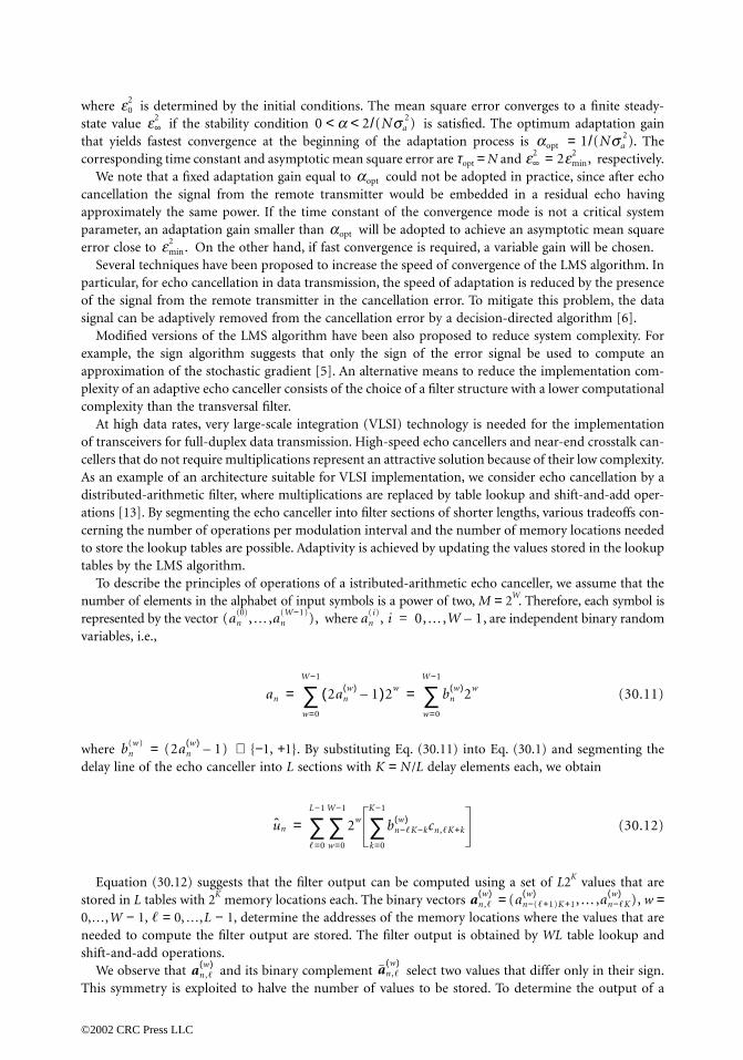
where is determined by the initial conditions. The mean square error converges to a finite steady-state value if the stability condition is satisfied. The optimum adaptation gainthat yields fastest convergence at the beginning of the adaptation process is = Thecorresponding time constant and asymptotic mean square error are τopt = N and = respectively.

We note that a fixed adaptation gain equal to could not be adopted in practice, since after echocancellation the signal from the remote transmitter would be embedded in a residual echo havingapproximately the same power. If the time constant of the convergence mode is not a critical systemparameter, an adaptation gain smaller than will be adopted to achieve an asymptotic mean squareerror close to On the other hand, if fast convergence is required, a variable gain will be chosen.

Several techniques have been proposed to increase the speed of convergence of the LMS algorithm. Inparticular, for echo cancellation in data transmission, the speed of adaptation is reduced by the presenceof the signal from the remote transmitter in the cancellation error. To mitigate this problem, the datasignal can be adaptively removed from the cancellation error by a decision-directed algorithm [6].

Modified versions of the LMS algorithm have been also proposed to reduce system complexity. Forexample, the sign algorithm suggests that only the sign of the error signal be used to compute anapproximation of the stochastic gradient [5]. An alternative means to reduce the implementation com-plexity of an adaptive echo canceller consists of the choice of a filter structure with a lower computationalcomplexity than the transversal filter.

At high data rates, very large-scale integration (VLSI) technology is needed for the implementationof transceivers for full-duplex data transmission. High-speed echo cancellers and near-end crosstalk can-cellers that do not require multiplications represent an attractive solution because of their low complexity.As an example of an architecture suitable for VLSI implementation, we consider echo cancellation by adistributed-arithmetic filter, where multiplications are replaced by table lookup and shift-and-add oper-ations [13]. By segmenting the echo canceller into filter sections of shorter lengths, various tradeoffs con-cerning the number of operations per modulation interval and the number of memory locations neededto store the lookup tables are possible. Adaptivity is achieved by updating the values stored in the lookuptables by the LMS algorithm.

To describe the principles of operations of a istributed-arithmetic echo canceller, we assume that thenumber of elements in the alphabet of input symbols is a power of two, M = 2W. Therefore, each symbol isrepresented by the vector where are independent binary randomvariables, i.e.,

(30.11)

where = ∈ {−1, +1}. By substituting Eq. (30.11) into Eq. (30.1) and segmenting thedelay line of the echo canceller into L sections with K = N/L delay elements each, we obtain

(30.12)

Equation (30.12) suggests that the filter output can be computed using a set of L2K values that arestored in L tables with 2K memory locations each. The binary vectors = w =0,…,W − 1, � = 0,…,L − 1, determine the addresses of the memory locations where the values that areneeded to compute the filter output are stored. The filter output is obtained by WL table lookup andshift-and-add operations.

We observe that and its binary complement select two values that differ only in their sign.This symmetry is exploited to halve the number of values to be stored. To determine the output of a

e02

e∞2 0 a 2/(Nsa

2)< <aopt 1/(Nsa

2).e∞

2 2emin2 ,

aopt

aopt

emin2 .

(an(0),…,an

(W−1)), an(i), i 0,…,W 1,–=

an 2anw( ) 1–( )2w

w=0

W−1

∑ bnw( )2w

w=0

W−1

∑= =

bn(w) (2an

w( ) 1)–

ûn 2w bn−�K−kw( ) cn ,�K+k

k=0

K−1

∑w=0

W−1

∑�=0

L−1

∑=

an ,�w( ) (an−(�+1)K+1

w( ) ,…,an−�Kw( ) ),

an ,�w( ) an ,�

w( )


distributed-arithmetic filter with reduced memory size, we reformulate Eq. (30.12) as

(30.13)

where k0 can be any element of the set {0,…,K − 1}. In the following, we take k0 = 0. Then the binarysymbol determines whether a selected value is to be added or subtracted. Each table has now 2K−1

memory locations, and the filter output is given by

(30.14)

where dn(k, �), k = 0,…,2K−1 − 1, � = 0,…,L − 1, are the lookup values, and w = 0,…,W − 1, � =0,…,L − 1, are the look up indices computed as follows:

(30.15)

We note that, as long as Eqs. (30.12) and (30.13) hold for some coefficient vector (cn,0,…,cn,N−1), adistributed-arithmetic filter emulates the operation of a linear transversal filter. For arbitrary valuesdn(k, �), however, a nonlinear filtering operation results.

The expression of the LMS algorithm to update the values of a distributed-arithmetic echo cancellertakes the form

(30.16)

where = …, with = …, and = …, with

are L2K−1 × 1 vectors and where δi,j is the Kronecker delta. We note that at each iteration, only those valuesthat are selected to generate the filter output are updated. The block diagram of an adaptive distributed-arithmetic echo canceller with input symbols from a quaternary alphabet is shown in Fig. 30.6.

The analysis of the mean square error convergence behavior and steady-state performance has beenextended to adaptive distributed-arithmetic echo cancellers [1]. The dynamics of the mean square errorare, in this case, given by

(30.17)

The stability condition for the echo canceller is 0 < α < For a given adaptation gain, echocanceller stability depends on the number of tables and on the variance of the transmitted symbols.

ûn 2wbn−�K−k0

w( ) cn ,�K+k0bn−�K−k0

w( ) + bn−�K−kw( ) cn ,�K+k

k=0

K−1

∑k≠k0

w=0

W−1

∑�=0

L−1

∑=

bn−�Kw( )

ûn 2wbn−�Kw( ) dn in ,�

w( ),�( )w=0

W−1

∑�=0

L−1

∑=

in ,�(w),

in ,�w( ) ∑k=1

K−1an−�K−kw( ) 2k−1 if an−�K

w( ) 1=

∑k=1K−1an−�K−k

w( )2k−1 if an−�K

w( ) 0=

=

dn+1 dn12--a∇ d zn

2{ }– dn aznyn+= =

dn′ [dn′ (0), dn′ (L 1– )], dn′ (�) [dn(0, �), dn(2K−1 1, �– )], yn′ [yn′ (0),yn′ (L 1– )],

yn′ �( ) 2wbn−�Kw( ) d

0, in ,�w( ),…,d

2K−1−1, in ,�

w( )( )w=0

W−1

∑=

E en2{ } e0

2 1asa

2

2K−1---------- 2 aLsa

2–( )–n 2emin

2

2 aLsa2–

-----------------------+=

2/(Lsa2).


Therefore, the time span of the echo canceller can be increased without affecting system stability, providedthat the number L of tables is kept constant, In that case, however, mean square error convergence willbe slower. From Eq. (30.17), we find that the optimum adaptation gain that permits the fastest meansquare error convergence at the beginning of the adaptation process is αopt = The time constantof the convergence mode is τopt = L2K−1. The smallest achievable time constant is proportional to the totalnumber of values. The realization of a distributed-arithmetic echo canceller can be further simplified byupdating at each iteration only the values that are addressed by the most significant bits of the symbolsstored in the delay line. The complexity required for adaptation can thus be reduced at the price of aslower rate of convergence.

30.3 Echo Cancellation for Quadrature-Amplitude Modulation (QAM) Systems

Although most of the concepts presented in the preceding sections can be readily extended to echocancellation for communications systems employing QAM, the case of full-duplex transmission over avoiceband data channel requires a specific discussion. We consider the system model shown in Fig. 30.7.The transmitter generates a sequence {an} of i.i.d. complex-valued symbols from a two-dimensionalconstellation A, which are modulated by the carrier where T and fc denote the modulation intervaland the carrier frequency, respectively. The discrete-time signal at the output of the transmit Hilbert filtermay be regarded as an analytic signal, which is generated at the rate of m/T samples/s, m > 1. The realpart of the analytic signal is converted into an analog signal by a D/A converter and input to the channel.We note that by transmitting the real part of a complex-valued signal, positive- and negative-frequencycomponents become folded. The image band attenuation of the transmit Hilbert filter thus determinesthe achievable echo suppression. In fact, the receiver cannot extract aliasing image-band components fromdesired passband frequency components, and the echo canceller is able to suppress only echo arising fromtransmitted passband components.

The output of the echo channel is represented as the sum of two contributions. The near-end echouNE(t) arises from the impedance mismatch between the hybrid and the transmission line, as in the caseof baseband transmission. The far-end echo uFE(t) represents the contribution due to echos that aregenerated at intermediate points in the telephone network. These echos are characterized by additional

FIGURE 30.6 Block diagram of an adaptive distributed-arithmetic echo canceller.

1/(Lsa2).

e j2pfcnT,


impairments, such as jitter and frequency shift, which are accounted for by introducing a carrier-phaserotation of an angle φ(t) in the model of the far-end echo.

At the receiver, samples of the signal at the channel output are obtained synchronously with thetransmitter timing, at the sampling rate of m/T sample/s. The discrete-time received signal is convertedto a complex-valued baseband signal {xnm′+i, i = 0, …, m′ − 1}, at the rate of m′/T samples/s, 1 < m′ < m,through filtering by the receive Hilbert filter, decimation, and demodulation. From delayed transmitsymbols, estimates of the near- and far-end echo signals after demodulation, i = 0,… ,m′ − 1}and i = 0,… ,m′ − 1}, respectively, are generated using m′ interleaved near- and far-end echocancellers. The cancellation error is given by

(30.18)

A different model is obtained if echo cancellation is accomplished before demodulation. In this case, twoequivalent configurations for the echo canceller may be considered. In one configuration, the modulatedsymbols are input to the transversal filter, which approximates the passband echo response. Alternatively,the modulator can be placed after the transversal filter, which is then called a baseboard transversal filter[15].

In the considered realization, the estimates of the echo signals after demodulation are given by

(30.19)

and

(30.20)

where and are the coefficients of the m′ interleaved near- andfar-end echo cancellers, respectively, i = 0,… ,m′ − 1} is the sequence of far-end echo phaseestimates, and DFE denotes the bulk delay accounting for the round-trip delay from the transmitter tothe point of echo generation. To prevent overlap of the time span of the near-end echo canceller withthe time span of the far-end echo canceller, the condition DFE > NNE must be satisfied. We also note that,

FIGURE 30.7 Configuration of an echo canceller for a QAM transmission system.

{ûnm ′+ iNE

,{ûnm ′+ i

FE,

z� x� û�NE

– û�FE

–=

ûnm ′+ iNE

cn ,km ′+ iNE an−k, i

k=0

NNE−1

∑ 0,…,m ′ 1–= =

ûnm ′+ iFE

cn ,km ′+ iFE an−k−DFE

k=0

NFE−1

∑ ejfˆnm ′+ i, i 0,…,m ′ 1–= =

(cn ,0NE ,…,cn ,m ′ NNE−1

NE ) (cn ,0FE ,…,cn ,m ′ NFE 1–

FE ){f

nm ′+ i,


because of the different nature of near- and far-end echo generation, the time span of the far-end echocanceller needs to be larger than the time span of the near-end canceller, i.e., NFE > NNE.

Adaptation of the filter coefficients in the near- and far-end echo cancellers by the LMS algorithmleads to

(30.21)

and

(30.22)

respectively, where the asterisk denotes complex conjugation.The far-end echo phase estimate is computed by a second-order phase-lock loop algorithm, where the

following stochastic gradient approach is adopted:

(30.23)

where � = nm′ + i, i = 0,…, m′ − 1, γFE and ζFE are step-size parameters, and

(30.24)

We note that algorithm (30.23) requires m′ iterations per modulation interval, i.e., we cannot resort tointerleaving to reduce the complexity of the computation of the far-end echo phase estimate.

30.4 Echo Cancellation for Orthogonal FrequencyDivision Multiplexing (OFDM) Systems

Orthogonal frequency division multiplexing (OFDM) is a modulation technique whereby blocks of Msymbols are transmitted in parallel over M subchannels by employing M orthogonal subcarriers. Weconsider a real-valued discrete-time channel impulse response {hi, i = 0,… ,L} having length L + 1 M.To illustrate the basic principles of OFDM systems, let us consider a noiseless ideal channel with impulseresponse given by {hi} = {δi}, where {δi} is defined as the discrete-time delta function. Modulation of thecomplex-valued input symbols at the nth modulation interval, denoted by the vector An = {An(i), i =0,…, M − 1}, is performed by an inverse discrete Fourier transform (IDFT), as shown in Fig. 30.8. Weassume that M is even, and that each block of symbols satisfies the Hermitian symmetry conditions, i.e.,An(0) and An(M/2) are real valued, and An(i) = (M − i), i = 1,…, M/2 − 1. Then the signals an = {an(i),

FIGURE 30.8 Block diagram of an OFDM system.

cn+1, km ′+ iNE cn ,km ′+ i

NE aznm ′+ i an−k( )∗+=k 0,…,NNE 1, i– 0,…,m ′ 1–= =

cn+1, km ′+ iFE cn ,km ′+ i

FE aznm ′+ i an−k−DFE( )∗ e

−jfˆnm ′+ i+=

k 0,…,NFE 1, i– 0,…,m ′ 1–= =

fˆ�+1

fˆ�

12--gFE∇

fˆz�

2– ∆f � mod 2p( )+=

∆f �+1 ∆f�12--zFE∇

fˆz�

2–=

∇fˆ

z�2 ∂ z�

2

∂ fˆ�

------------ 2Im z� û�FE( )

∗{ }–= =

<<

An∗


i = 0,…,M − 1} obtained at the output of the IDFT are real valued. After parallel-to-serial conversion,the M signals are sent over the channel at the given transmission rate, M/T, where T denotes themodulation interval. At the output of the channel, the noiseless signals are received without distortion.Serial-to-parallel conversion yields blocks of M elements, with boundaries placed such that each blockobtained at the modulator output is also presented at the demodulator input. Then demodulationperformed by a discrete Fourier transform (DFT) will reproduce the blocks of M input symbols.The overall input–output relationship is therefore equivalent to that of a bank of M parallel,independent subchannels.

In the general case of a noisy channel with impulse response having length greater than one, Mindependent subchannels are obtained by a variant of OFDM also known as discrete multitone modulation(DMT) [12]. In a DMT system, modulation by the IDFT is performed at the rate 1/T ′ = M/(M + L)T <1/T. After modulation, each block of M signals is cyclically extended by copying the last L signals in frontof the block and converted from parallel to serial. The resulting L + M signals are sent over the channel.At the receiver, blocks of samples with length L + M are taken. Block boundaries are placed such thatthe last M samples depend only on the elements of one cyclically extended block of signals. The first Lsamples are discarded, and the vector xn of the last M samples of the block received at the nth modulationinterval can be expressed as

(30.25)

where h is the vector of the impulse response extended with M − L − 1 zeros, wn is a vector of additivewhite Gaussian noise samples, and Γn is a M × M circulant matrix given by

(30.26)

Recalling that FMΓn = diag(An), where FM is the M × M DFT matrix defined as FM = , k,m = 0,… ,M − 1, and diag(An) denotes the diagonal matrix with elements on the diagonal given by An,we find that the output of the demodulator is given by

(30.27)

where H denotes the DFT of the vector h, and Wn is a vector of independent Gaussian random variables.Equation (30.27) indicates that the sequence of transmitted symbol vectors can be detected by assuminga bank of M independent subchannels, at the price of a decrease in the data rate by a factor (M + L)/M.Note that in practice the computationally more efficient inverse fast Fourier transform and fast Fouriertransform are used instead of IDFT and DFT.

We discuss echo cancellation for OFDM with reference to a DMT system [7], as shown in Fig. 30.9.The real-valued discrete-time echo impulse response is {hE,i, i = 0,… ,N − 1}, having length N < M. Weinitially assume N ≤ L + 1. Futhermore, we assume that the boundaries of the received blocks are placedsuch that the last M samples of the nth received block are expressed by the vector

(30.28)

where is the circulant matrix with elements given by the signals from the remote transmitter, andhE is the vector of the echo impulse response extended with M − N zeros. In the frequency domain, the

xn Γnh wn+=

Γn

an 0( ) an M 1–( ) … an 1( )an 1( ) an 0( ) … an 2( )

� � �

an M 1–( ) an M 2–( ) … an 0( )

=

FM1– [(e

j2pM

--------– )km]

Xn diag An( )H Wn+=

xn ΓnRh ΓnhE wn+ +=

ΓnR


echo is expressed as Un = diag(An)HE, where HE denotes the DFT of the vector hE. In this case, the echocanceller provides an echo estimate that is given by n = diag(An)Cn, where Cn denotes the DFT of thevector cn of the N coefficients of the echo canceller filter extended with M − N zeros. In practice, however,we need to consider the case N > L + 1. The expression of the cancellation error is then given by

zn = xn − Ψn,n −1cn (30.29)

where the vector of the last M elements of the nth received block is now xn = h + Ψn,n−1hE + wn, andΨn,n−1 is an M × M Toeplitz matrix given by

(30.30)

In the frequency domain, the cancellation error can be expressed as

(30.31)

where χn,n−1 = Ψn,n−1 − Γn is an M × M upper triangular Toeplitz matrix. Equation (30.31) suggests acomputationally efficient, two-part echo cancellation technique. First, in the time domain, a shortconvolution is performed and the result is subtracted from the received signals to compensate for theinsufficient length of the cyclic extension. Second, in the frequency domain, cancellation of the residualecho is performed over a set of M independent echo subchannels. Observing that Eq. (30.31) is equivalentto Zn = Xn − Cn, where = FM the echo canceller adaptation by the LMS algorithmin the frequency domain takes the form

(30.32)

where α is the adaptation gain, and denotes the transpose conjugate of We note that,alternatively, echo canceller adaptation may also be performed by the algorithm Cn+1 = Cn + α diagZn, which entails a substantially lower computational complexity than the LMS algorithm, at the priceof a slower rate of convergence.

FIGURE 30.9 Configuration of an echo canceller for a DMT transmission system.

Û

ΓnR

Ψn ,n−1 =

an 0( ) an M 1–( ) … an M L–( ) an−1 M 1–( ) … an−1 L 1+( )an 1( ) an 0( ) … an M L– 1+( ) an M L–( ) … an−1 L 2+( )

� O �

an M 1–( ) an M 2–( ) … an M L– 1–( ) an M L– 2–( ) … an 0( )

Zn FM xn cn ,n−1cn–( ) diag An( )Cn–=

Ψ̃n ,n−1 Ψ̃n ,n−1 Ψ̃n ,n−1FM1– ,

Cn+1 Cn a Ψ̃n ,n−1∗

Zn+=

Ψ̃n ,n−1∗ Ψ̃n ,n−1.

(An∗ )


In DMT systems, it is essential that the length of the channel impulse response be much less than thenumber of subchannels, so that the reduction in data rate due to the cyclic extension may be considerednegligible. Therefore, time-domain equalization is adopted in practice to shorten the length of the channelimpulse response. From Eq. (30.31), however, we observe that transceiver complexity depends on therelative lengths of the echo and of the channel impulse responses. To reduce the length of the cyclicextension as well as the computational complexity of the echo canceller, various methods have beenproposed to shorten both the channel and the echo impulse responses jointly [9].

Recently, multitone modulation techniques based on filter banks have been proposed, where the M-branch filters yield very high spectral containment of individual subchannel signals [4]. The filters arefrequency-shifted versions of a prototype filter, designed to reduce the interchannel interference to a levelthat is negligible compared to the level of other noise signals, without having to resort to time-domainequalization. Echo cancellation can be performed in this case entirely in the frequency domain by takinginto account, for each subchannel, only the echo generated by transmission in the opposite direction onthe same subchannel. The implementation of per-subchannel echo cancellation then requires M adaptiveecho cancellers.


Digital signal processing techniques for echo cancellation provide large echo attenuation and eliminatethe need for additional line interfaces and digital-to-analog and analog-to-digital converters that arerequired by echo cancellation in the analog signal domain.

The realization of digital echo cancellers in transceivers for high-speed full-duplex data transmissiontoday is possible at a low cost thanks to the advances in VLSI technology. Digital techniques for echocancellation are also appropriate for near-end crosstalk cancellation in transceivers for transmission overvoice-grade cables at rates of several megabits per second for local-area network applications.

In voiceband modems for data transmission over the telephone network, digital techniques for echocancellation also allow a precise tracking of the carrier phase and frequency shift of far-end echos.

References

1. Cherubini, G., Analysis of the convergence behavior of adaptive distributed-arithmetic echo cancel-lers, IEEE Trans. Commun., 41(11), 1703–1714, 1993.

2. Cherubini, G., Ölçer, S., and Ungerboeck, G., A quaternaty partial-response class-IV transceiver for125 Mbit/s data transmission over unshielded twisted-pair cables: principles of operation and VLSIrealization, IEEE J. Sel. Areas Commun., 13(9), 1656–1669, 1995.

3. Cherubini, G., Creigh, J., Ölçer, S., Rao, S.K., and Ungerboeck, G., 100BASE-T2: a new standard for100 Mb/s Ethernet transmission over voice-grade cables, IEEE Commun. Mag., 35(11), 115–122,1997.

4. Cherubini, G., Cioffi, J.M., Eleftheriou, E., and Ölçer, S., Filter bank modulation techniques for veryhigh-speed digital subscriber lines, IEEE Commun. Mag., 38(5), 98–104, 2000.

5. Duttweiler, D.L., Adaptive filter performance with nonlinearities in the correlation multiplier, IEEETrans. Acoust. Speech Signal Processing, 30(8), 578–586, 1982.

6. Falconer, D.D., Adaptive reference echo-cancellation, IEEE Trans. Commun., 30(9), 2083–2094, 1982.7. Ho, M., Cioffi, J.M., and Bingham, J.A.C., Discrete multitone echo cancellation, IEEE Trans. Com-

mun., 44(7), 817–825, 1996.8. Lee, E.A. and Messerschmitt, D.G., Digital Communication, 2nd ed., Kluwer Academic Publishers,

Boston, MA, 1994.9. Melsa, P.J.W., Younce, R.C., and Rohrs, C.E., Impulse response shortening for discrete multitone

transceivers, IEEE Trans. Commun., 44(12), 1662–1672, 1996.10. Messerschmitt, D.G., Echo cancellation in speech and data transmission, IEEE J. Sel. Areas Commun.,

2(2), 283–297, 1984.


11. Messerschmitt, D.G., Design issues for the ISDN U-Interface transceiver, IEEE J. Sel. Areas Commun.,4(8), 1281–1293, 1986.

12. Ruiz, A., Cioffi, J.M., and Kasturia, S., Discrete multiple tone modulation with coset coding for thespectrally shaped channel, IEEE Trans. Commun., 40(6), 1012–1029, 1992.

13. Smith, M.J., Cowan, C.F.N., and Adams, P.F., Nonlinear echo cancellers based on transpose distrib-uted arithmetic, IEEE Trans. Circuits and Systems, 35(1), 6–18, 1988.

14. Ungerboeck, G., Theory on the speed of convergence in adaptive equalizers for digital communica-tion, IBM J. Res. Develop., 16(6), 546–55, 1972.

15. Weinstein, S.B., A passband data-driven echo-canceller for full-duplex transmission on two-wirecircuits, IEEE Trans. Commun., 25(7), 654–666, 1977.


IIINetworks

31 The Open Systems Interconnections (OSI) Seven-Layer Model Frederick HalsallComputer Communications Requirements • Standards Evolution • InternationalStandards Organization Reference Model • Open SystemStandards • Summary

32 Ethernet Networks Ramesh R. RaoOverview • Historical Development • Standards • Operation

33 Fiber Distributed Data Interface and Its use for Time-Critical ApplicationsBiao Chen, Nicholas Malcolm, and Wei Zhao Introduction • Architecture and Fault Management • The Protocoland Its Timing Properties • Parameter Selection for Real-Time Applications • Final Remarks

34 Broadband Local Area Networks Joseph A. BannisterIntroduction • User Requirements • BLAN Technologies • ATM BLANs• Other BLANs • New Applications • Conclusion

35 Multiple Access Methods for Communications Networks Izhak RubinIntroduction • Features of Medium Access Control Systems • Categorizationof Medium Access Control Procedures • Pol l ing-Based Mult ip le AccessNetworks • Random-Access Protocols • Multiple-Access Schemes for WirelessNetworks • Multiple Access Methods for Spatial-Reuse Ultra-High-Speed OpticalCommunications Networks

36 Routing and Flow Control Rene L. CruzIntroduction • Connection-Oriented and Connectionless Protocols, Services, and Networks • Routing in Datagram Networks • Routing in VirtualCircuit Switched Networks • Hierarchical Routing • Flow Controlin Datagram Networks • Flow Control in Virtual CircuitSwitched Networks

37 Transport Layer A. Udaya ShankarIntroduction • Transport Service • Data-Transfer Protocol • Connection-ManagementProtocol • Transport Protocols • Conclusions

38 Gigabit Networks Jonathan M. SmithIntroduction • Host Interfacing • Multimedia Services • The World-WideWeb • Conclusions

39 Local Area Networks Thomas G. RobertazziIntroduction • Local Area Networks (LANs) • The Future


40 Asynchronous Time Division Switching Achille PattavinaIntroduction • The ATM Standard • Switch Model • ATM Switch with BlockingMultistage IN and Minimum Depth • ATM Switch with Blocking Multistage INand Arbitrary Depth • ATM Switch with Nonblocking IN • Conclusions

41 Internetworking Harrell J. Van NormanIntroduction • Internetworking Protocols • The Total NetworkEngineering Process • Internetwork Simulation • InternetworkOptimization • Summary

42 Architectural Framework for Asynchronous Transfer Mode Networks:Broadband Network Services Gerald A. Marin and Raif O. OnvuralIntroduction • Broadband Integrated Services Digital Network (B-ISDN)Framework • Architectural Drivers • Review of Broadband NetworkServices • How Does It All Fit Together? • Broadband NetworkServices • Conclusions

43 Control and Management in Next Generation Networks: Challengesand Opportunities Abdi R. Modarressi and Seshadri MohanIntroduction • Signaling and Control in PSTN • General Attributes and Requirementsof NGN • A Broad Outline of the NGN Architecture • Evolution Towards NGN: Trialsand Tribulations • Conclusions


31The Open Systems

Interconnections (OSI)Seven-Layer Model

31.1 Computer Communications Requirements31.2 Standards Evolution31.3 International Standards Organization

Reference ModelThe Application-Oriented Layers • The Presentation Layer • The Network-Dependent Layers

31.4 Open System Standards31.5 Summary

31.1 Computer Communications Requirements

Although in many instances computers are used to perform their intended role in a stand-alone mode,in others there is a need to interwork and exchange data with other computers—in financial applications,for example, to carry out fund transfers from one institution computer to another, in travel applicationsto access the reservation systems belonging to various airlines, and so on. The general requirement in allof these applications is for application programs running in different computers to cooperate to achievea specific distributed application function. To achieve this, three basic issues must be considered. Theseare shown in diagrammatic form in Fig. 31.1.

The fundamental requirement in all applications that involve two or more computers is the provisionof a suitable data communications facility. This may comprise a local area network (LAN), if thecomputers are distributed around a single site, a wide area network (WAN), if the computers are situatedat different sites, or an internetwork, if multiple interconnected network types are involved. Associatedwith these different network types is a set of access protocols which enables a communications pathbetween two computers to be established and for data to be transferred across this path. Typically, theseprotocols differ for the different network types. In addition to these access protocols, the communicationsubsystem in each computer must provide additional functionality. For example, if the communicatingcomputers are of different types, possibly with different word sizes and character sets, then a means ofensuring the transferred data is interpreted in the same way in each computer must be incorporated.Also, the computers may use different file systems and, hence, functionality to enable applicationprograms, normally referred to as application processes (APs), to access these in a standardized waymust also be included. All of these issues must be considered when communicating data between twocomputers.

Frederick HalsallUniversity of Wales, Swansea


31.2 Standards Evolution

Until recently, the standards established for use in the computer industry by the various internationalbodies were concerned primarily with either the internal operation of a computer or the connection ofa local peripheral device. The result was that early hardware and software communication subsystemsoffered by manufacturers only enabled their own computers, and so-called plug-compatible systems, toexchange information. Such systems are known as closed systems since computers from other manufac-turers cannot exchange information unless they adhere to the (proprietary) standards of a particularmanufacturer.

In contrast, the various international bodies concerned with public-carrier telecommunication net-works have, for many years, formulated internationally agreed standards for connecting devices to thesenetworks. The V-series recommendations, for example, are concerned with the connection of equipment,normally referred to as a data terminal equipment (DTE), to a modem connected to the public switchedtelephone network (PSTN); the X-series recommendations for connecting a DTE to a public data network;and the I-series recommendations for connecting a DTE to the integrated services digital networks(ISDNs). The recommendations have resulted in compatibility between the equipment from differentvendors, enabling a purchaser to select suitable equipment from a range of manufacturers.

Initially, the services provided by most public carriers were concerned primarily with data trans-mission, and, hence, the associated standards only related to the method of interfacing a device to thesenetworks. More recently, however, the public carriers have started to provide more extensive distributedinformation services, such as the exchange of electronic messages (teletex) and access to public databases(videotex). To cater to such services, the standards bodies associated with the telecommunications industryhave formulated standards not only for interfacing to such networks but also so-called higher levelstandards concerned with the format (syntax) and control of the exchange of information (data) betweensystems. Consequently, the equipment from one manufacturer that adheres to these standards can beinterchangeable with equipment from any other manufacturer that complies with the standards. Theresulting system is then known as an open system or, more completely, as an open systems interconnectionenvironment (OSIE).

In the mid-1970s, as different types of distributed systems (based on both public and private datanetworks) started to proliferate, the potential advantages of open systems were acknowledged by thecomputer industry. As a result, a range of standards started to be introduced. The first was concernedwith the overall structure of the complete communication subsystem within each computer. This wasproduced by the International Standards Organization (ISO) and is known as the ISO reference modelfor open systems interconnection (OSI).

The aim of the ISO reference model is to provide a framework for the coordination of standardsdevelopment and to allow existing and evolving standards activities to be set within a common framework.

FIGURE 31.1 Computer communication schematic.


The aim is to allow an application process in any computer that supports a particular set of standardsto communicate freely with an application process in any other computer that supports the samestandards, irrespective of its origin of manufacture.

Some examples of application processes that may wish to communicate in an open way are thefollowing:

• a process (program) executing in a computer and accessing a remote file system

• a process acting as a central file service (server) to a distributed community of (client) processes

• a process in an office workstation (computer) accessing an electronic mail service

• a process acting as an electronic mail server to a distributed community of (client) processes

• a process in a supervisory computer controlling a distributed community of computer-basedinstruments or robot controllers associated with a process or automated manufacturing plant

• a process in an instrument or robot controller receiving commands and returning results to asupervisory system

• a process in a bank computer that initiates debit and credit operations on a remote system

Open systems interconnection is concerned with the exchange of information between such processes.The aim is to enable application processes to cooperate in carrying out a particular (distributed) infor-mation processing task irrespective of the computers on which they are running.

31.3 International Standards Organization Reference Model

A communication subsystem is a complex piece of hardware and software. Early attempts at implementingthe software for such subsystems were often based on a single, complex, unstructured program (normallywritten in assembly language) with many interacting components. The resulting software was difficultto test and often very difficult to modify.

To overcome this problem, the ISO has adopted a layered approach for the reference model. Thecomplete communication subsystem is broken down into a number of layers, each of which performs awell-defined function. Conceptually, these layers can be considered as performing one of two genericfunctions, network-dependent functions and application-oriented functions. This, in turn, gives rise tothree distinct operational environments:

1. The network environment is concerned with the protocols and standards relating to the differenttypes of underlying data communication networks.

2. The OSI environment embraces the network environment and adds additional application-oriented protocols and standards to allow end systems (computers) to communicate with oneanother in an open way.

3. The real systems environment builds on the OSI environment and is concerned with a manu-facturer’s own proprietary software and services which have been developed to perform a particulardistributed information processing task.

This is shown in diagrammatic form in Fig. 31.2.Both the network-dependent and application-oriented (network-independent) components of the OSI

model are implemented as a number of layers. The boundaries between each layer and the functionsperformed by each layer have been selected on the basis of experience gained during earlier standardiza-tion activity.

Each layer performs a well-defined function in the context of the overall communication subsystem.It operates according to a defined protocol by exchanging messages, both user data and additional controlinformation, with a corresponding peer layer in a remote system. Each layer has a well-defined interfacebetween itself and the layer immediately above and below. Consequently, the implementation of aparticular protocol layer is independent of all other layers.


The logical structure of the ISO reference model is made up of seven protocol layers, as shown inFig. 31.3. The three lowest layers (1–3) are network dependent and are concerned with the protocolsassociated with the data communication network being used to link the two communicating computers.In contrast, the three upper layers (5–7) are application oriented and are concerned with the protocolsthat allow two end user application processes to interact with each other, normally through a range ofservices offered by the local operating system. The intermediate transport layer (4) masks the upperapplication-oriented layers from the detailed operation of the lower network-dependent layers. Essen-tially, it builds on the services provided by the latter to provide the application-oriented layers with anetwork-independent message interchange service.

The function of each layer is specified formally as a protocol that defines the set of rules and conventionsused by the layer to communicate with a similar peer layer in another (remote) system. Each layer providesa defined set of services to the layer immediately above. It also uses the services provided by the layerimmediately below it to transport the message units associated with the protocol to the remote peer layer.For example, the transport layer provides a network-independent message transport service to the sessionlayer above it and uses the service provided by the network layer below it to transfer the set of message

FIGURE 31.2 Operational environments.

FIGURE 31.3 Overall structure of the ISO reference model.


units associated with the transport protocol to a peer transport layer in another system. Conceptually,therefore, each layer communicates with a similar peer layer in a remote system according to a definedprotocol. However, in practice, the resulting protocol message units of the layer are passed by means ofthe services provided by the next lower layer. The basic functions of each layer are summarized in Fig. 31.4.

The Application-Oriented Layers

The Application Layer

The application layer provides the user interface, normally an application program/process, to a rangeof networkwide distributed information services. These include file transfer access and management, aswell as general document and message interchange services such as electronic mail. A number of standardprotocols are either available or are being developed for these and other types of service.

Access to application services is normally achieved through a defined set of primitives, each withassociated parameters, which are supported by the local operating system. The access primitives are thesame as other operating system calls (as used for access to, say, a local file system) and result in anappropriate operating system procedure (process) being activated. These operating system proceduresuse the communication subsystem (software and hardware) as if it is a local device, similar to a diskcontroller, for example. The detailed operation and implementation of the communication subsystem isthus transparent to the (user) application process. When the application process making the call is

FIGURE 31.4 Protocol layer summary.


rescheduled (run), one (or more) status parameters are returned, indicating the success (or otherwise)of the network transaction that has been attempted.

In addition to information transfer, the application layer provides such services as:

• identification of the intended communication partner(s) by name or by address

• determination of the current availability of an intended communication partner

• establishment of authority to communicate

• agreement on privacy (encryption) mechanisms

• authentication of an intended communication partner

• selection of the dialogue discipline, including the initiation and release procedures

• agreement on responsibility for error recovery

• identification of constraints on data syntax (character sets, data structures, etc.)

The Presentation Layer

The presentation layer is concerned with the representation (syntax) of data during transfer between twocommunicating application processes. To achieve true open systems interconnection, a number of commonabstract data syntax forms have been defined for use by application processes together with associatedtransfer (or concrete) syntaxes. The presentation layer negotiates and selects the appropriate transfersyntax(es) to be used during a transaction so that the syntax (structure) of the messages being exchangedbetween two application entities is maintained. Then, if this form of representation is different from theinternal abstract form, the presentation entity performs the necessary conversion.

To illustrate the services provided by the presentation layer, consider a telephone conversation betweena French speaking person and a Spanish speaking person. Assume each uses an interpreter and that theonly language understood by both interpreters is English. Each interpreter must translate from their locallanguage to English, and vice versa. The two correspondents are thus analogous to two application processeswith the two interpreters representing presentation layer entities. French and Spanish are the local syntaxesand English is the transfer or concrete syntax. Note that there must be a universally understood languagewhich must be defined to allow the agreed transfer language (syntax) to be negotiated. Also note that theinterpreters do not necessarily understand the meaning (semantics) of the conversation.

Another function of the presentation layer is concerned with data security. In some applications, datasent by an application is first encrypted (enciphered) using a key, which is (hopefully) known only bythe intended recipient presentation layer. The latter decrypts (deciphers) any received data using thecorresponding key before passing it on to the intended recipient.

The Session Layer

The session layer provides the means that enables two application layer protocol entities to organize andsynchronize their dialogue and manage their data exchange. It is thus responsible for setting up (andclearing) a communication (dialogue) channel between two communicating application layer protocolentities (presentation layer protocol entities in practice) for the duration of the complete networktransaction. A number of optional services are provided, including the following:

• Interaction management: The data exchange associated with a dialogue may be duplex or half-duplex. In the latter case, it provides facilities for controlling the exchange of data (dialogue units)in a synchronized way.

• Synchronization: For lengthy network transactions, the user (through the services provided by thesession layer) may choose periodically to establish synchronization points associated with thetransfer. Then, should a fault develop during a transaction, the dialogue may be restarted at anagreed (earlier) synchronization point.

• Exception reporting: Nonrecoverable exceptions arising during a transaction can be signaled tothe application layer by the session layer.


The Transport Layer

The transport layer acts as the interface between the higher application-oriented layers and the underlyingnetwork-dependent protocol layers. It provides the session layer with a message transfer facility that isindependent of the underlying network type. By providing the session layer with a defined set of messagetransfer facilities, the transport layer hides the detailed operation of the underlying network from thesession layer.

The transport layer offers a number of classes of service which cater to the varying quality of service(QOS) provided by different types of network.

There are five classes of service ranging from class 0, which provides only the basic functions neededfor connection establishment and data transfer, to class 4, which provides full error control and flowcontrol procedures. As an example, class 0 may be selected for use with a packet-switched data network(PSDN), whereas class 4 may be used with a local area network (LAN) providing a best-try service; thatis, if errors are detected in a frame, then the frame is simply discarded.

The Network-Dependent Layers

As the lowest three layers of the ISO reference model are network dependent, their detailed operationvaries from one network type to another. In general, however, the network layer is responsible for estab-lishing and clearing a networkwide connection between two transport layer protocol entities. It includessuch facilities as network routing (addressing) and, in some instances, flow control across the computer-to-network interface. In the case of internetworking, it provides various harmonizing functions betweenthe interconnected networks.

The link layer builds on the physical connection provided by the particular network to provide thenetwork layer with a reliable information transfer facility. It is thus responsible for such functions aserror detection and, in the event of transmission errors, the retransmission of messages. Normally, twotypes of service are provided:

1. Connectionless service treats each information frame as a self-contained entity that is transferredusing a best-try approach.

2. Connection-oriented service endeavors to provide an error-free information transfer facility.

Finally, the physical layer is concerned with the physical and electrical interfaces between the userequipment and the network terminating equipment. It provides the link layer with a means of transmit-ting a serial bit stream between the two equipments.

31.4 Open System Standards

The ISO reference model has been formulated simply as a template for the structure of a communicationsubsystem on which standards activities associated with each layer may be based. It is not intendedthat there should be a single standard protocol associated with each layer. Rather, a set of standards isassociated with each layer, each offering different levels of functionality. Then, for a specific opensystems interconnection environment, such as that linking numerous computer-based systems in a fullyautomated manufacturing plant, a selected set of standards is defined for use by all systems in thatenvironment.

The three major international bodies actively producing standards for computer communications arethe ISO, the American Institute of Electrical and Electronic Engineers (IEEE), and the InternationalTelegraph and Telephone Consultative Committee (CCITT). Essentially, the ISO and IEEE producestandards for use by computer manufacturers, whereas the CCITT defines standards for connectingequipment to the different types of national and international public networks. As the degree of overlapbetween the computer and telecommunications industries increases, however, there is an increasing levelof cooperation and commonality between the standards produced by these organizations.


In addition, prior to and concurrent with ISO standards activity, the U.S. Department of Defense hasfor many years funded research into computer communications and networking through its DefenseAdvanced Research Projects Agency (DARPA). As part of this research, the computer networks associatedwith a large number of universities and other research establishments were linked to those of DARPA.The resulting internetwork, known as ARPANET, has been extended to incorporate internets developedby other government agencies. The combined internet is now known simply as the Internet.

The protocol suite used with the Internet is known as transmission control protocol/internet protocol(TCP/IP). It includes both network-oriented protocols and application support protocols. BecauseTCP/IP is in widespread use with an existing internet, many of the TCP/IP protocols have been used asthe basis for ISO standards. Moreover, since all of the protocol specifications associated with TCP/IP arein the public domain, and hence no licence fees are payable, they have been used extensively by commercialand public authorities for creating open system networking environments. In practice, therefore, thereare two major open system (vendor-independent) standards: the TCP/IP protocol suite and those basedon the evolving ISO standards.

Figure 31.5 shows some of the standards associated with the TCP/IP protocol suite. As can be seen,since TCP/IP has developed concurrently with the ISO initiative, it does not contain specific protocolsrelating to all of the seven layers in the OSI model.

Moreover, the specification methodology used for the TCP/IP protocols differs from that used for theISO standards. Nevertheless, most of the functionality associated with the ISO layers is embedded in theTCP/IP suite. A range of standards has been defined by the ISO/CCITT and a selection of these is shownin Fig. 31.5. Collectively, they enable the administrative authority that is establishing the open system

FIGURE 31.5 TCP/IP protocol suite.


environment to select the most suitable set of standards for the application. The resulting protocol suiteis known as the open system interconnection profile. A number of such profiles have now been defined,including TOP, a protocol set for use in technical and office environments, MAP, for use in manufacturingautomation, U.S. and U.K. GOSIP, for use in U.S. and U.K. government projects, respectively, and asimilar suite used in Europe known as the CEN functional standards. The latter has been defined by theStandards Promotion and Application Group (SPAG), a group of 12 European companies.

As Fig. 31.6 shows, the lower three layers vary for different network types. CCITT has defined V, X,and I series standards for use with public-carrier networks. The V series is for use with the existingswitched telephone network (PSTN), the X series for use with existing switched data networks (PSDN),and the I series for use with the integrated services digital networks (ISDN). Those produced by ISO/IEEEfor use with local area networks are known collectively as the 802 (IEEE) or 8802 (ISO) series.

31.5 Summary

This chapter has reviewed the requirements for the communications subsystem in each of a set ofinterconnected computers that enables them to communicate in an open way to perform various dis-tributed application functions. The philosophy behind the structure of the ISO reference model for opensystems interconnection has been presented and the functionality of the seven layers that make up thereference model has been described. Finally, a selection of the ISO/CCITT standards that were definedhave been identified.

Defining Terms

Internetwork: A collection of different network types that are linked together.Local area network (LAN): Network used to link computers that are distributed around a single site.Open system interconnection (OSI): A standard set of communication protocols that are independent

of a specific manufacturer.

FIGURE 31.6 Standards summary.


Transmission control protocol/Internet protocol (TCP/IP): The standard set of communication pro-tocols that are used by each computer that is connected to the Internet.

Wide area network (WAN): Network used to link computers that are situated at different sites.

Further Information

Further coverage of the material covered in this chapter can be found in:

Halsall, F., Data Communications, Computer Networks and Open Systems, 4th ed., Addison Wesley, Read-ing, MA, 1996.


32Ethernet Networks

32.1 Overview32.2 Historical Development32.3 Standards

10BASE5 • 10BASE2 • 10BROAD36 • 1BASE5• 10BASET • 100BASET

32.4 Operation

32.1 Overview

The term ethernet describes a collection of hardware, software, and control algorithms that togetherprovide a technique for interconnecting dozens of nodes, spread over hundreds of meters, at aggregaterates ranging from 1 to 100 Mb/s. These nodes are typically computer work stations or peripheral devicesthat are part of a community of users that frequently exchange files, messages, and other types of dataamong each other. Shielded coaxial cables and unshielded twisted pairs have been used for the physicalinterconnection.

The primary hardware element used in an ethernet network is the network interface card (NIC). Thesecards are attached to a computer bus at one end and to a media attachment unit (MAU) at the other endvia an attachment unit interface (AUI) cable. An MAU is an active device that includes transceivers andother elements matched to the nature of the physical transmission medium. Some vendors consolidatetwo or more of these elements into a single package, thereby rendering certain elements, such as AUIcables, unnecessary. Repeaters are sometimes used to regenerate signals to ensure reliable communication.The NICs perform a number of control functions in software; chief amongst these is the execution of arandom access protocol for exchanging packets of information.

Nodes attached to an ethernet network exchange packets of information by broadcasting on a commoncommunication channel. Simultaneous transmission by two or more nodes results in a detectable collisionthat triggers a collision resolution protocol. This decentralized protocol induces a stochastic reschedulingof the retransmission instants of the colliding nodes. If the overall traffic on the network is below acertain threshold, eventual delivery of all new and previously collided messages is guaranteed. The valueof the threshold establishes the maximum aggregate information transfer rate that can be sustained. Thisthreshold is influenced by the span of the network, the length of the packets, latency in collision detection,and the dynamics of the external traffic, as well as the rate at which bits can be transported over thephysical medium. The aggregate information transfer rate can never exceed the bit transfer rate on thephysical medium, but understanding the impact of the other variables has been the subject of manystudies.

Standards bodies stipulate the values of some of these variables. For example, both the 10BASE2 and1BASE5 versions of the IEEE 802.3 standards restrict packet lengths to values between 512 and 12,144 b.The 10BASE2 version restricts the network span to 925 m and relies on a bit transfer rate of 10 Mb/sover 50-W coaxial cable with a diameter of 5 mm, whereas 1BASE5 restricts the span to 2.5 kms and

Ramesh R. RaoUniversity of California


relies on a bit transfer rate of 1 Mb/s over unshielded twisted pair. It is not uncommon to observeaggregate information transfer rates of 1.5 Mb/s or less in a 10BASE2 installation.

32.2 Historical Development

Ethernet evolved from a random access protocol that was developed at the University of Hawaii in the1970s for use in the packet-switched Aloha broadcast radio network. The Aloha network was meant toserve many users that generated infrequent and irregularly spaced bursts of data. Techniques such assynchronous time-division multiplexing that require nodes to access a common channel only duringprecoordinated, nonoverlapping intervals of time are ill suited to serving many bursty users. This draw-back motivated the development of the Aloha random access protocol, in which users access a commonchannel freely and invoke a collision resolution process only when collisions occur.

Spurred by the success of Aloha, efforts were undertaken to make the protocol more efficient. Earlyrefinements included the use of a common clock to avoid partial collisions (slotted Aloha) as well as thedevelopment of hybrid protocols that combined elements of random access with reservations (reservationAloha). Another series of refinements became possible in the context of limited span local area networks(LANs) that use low-noise communication links, such as coaxial cables, for the transmission medium.In such environments, a node can accurately and quickly sense ongoing transmissions on the cable. Thisfirst led to the development of carrier sense multiple access (CSMA) in which nodes withhold transmis-sions whenever they sense activity on the channel, thereby reducing the occurrence of collisions andimproving efficiency. The next refinement for the LAN environment was based on a node’s ability todetect a collision in less time than is required for a complete packet transmission. Early collision detectionallows the colliding users to abort the transmission of colliding packets, thereby reducing the durationof collisions and further improving efficiency.

The ethernet protocol uses carrier sense multiple access with collision detection (CSMA/CD). Thetopology of an ethernet network may differ from the Aloha packet radio network. The Aloha packetradio network was configured with a controller node at the center of the network. The member nodestransmitted to the controller on a common inbound frequency band. On a different outbound frequencyband, the controller broadcasts to the member nodes all of the packets it received as well as information,from which the occurrence of a collision could be inferred. In contrast, in some types of ethernet networks,nodes attach to a common communication channel and directly monitor it for carrier sensing andcollision detection, as well as to transmit and receive packets. There is, thus, no central controller in someethernet networks.

Ethernet was conceived at Xerox Palo Alto Research Center (PARC) in 1973 and described in a 1976Association for Computing Machinery (ACM) article by Robert M. Metcalfe and David R. Boggs. Thefirst prototype, also developed at Xerox PARC, operated at a speed of 3 Mb/s. In 1980, the Digital-Intel-Xerox 10 Mb/s ethernet was announced. The non-proprietary nature of the technology contributed toits widespread deployment and use in local area networks. By the mid-1980s, the Institute of Electricaland Electronics Engineers/American National Standards Institute (IEEE/ANSI) standards effort resultedin a set of CSMA/CD standards that were all based on the original ethernet concept.

32.3 Standards

In the terminology of the open systems interconnections (OSI) protocol architecture, the 802.3 series ofstandards are media access control (MAC) protocols. There exists a separate logical link control (LLC)sublayer, called the 802.2, which is above the MAC layer and, together with the MAC layer, forms a datalink layer.

Currently, there are five IEEE/ANSI MAC standards in the 802.3 series. They are designated as 10BASE5,10BASE2, 10BROAD36, 1BASE5, and 10BASET. A new version called 100BASET is currently under study.The numeric prefix in these designations refers to the speed in megabits per second. The term BASE refers


to baseband transmissions and the term BROAD refers to transmission over a broadband medium. Thenumeric suffix, when it appears, is related to limits on network span.

All 802.3 MAC standards share certain common features. Chief among them is a common MAC framingformat for the exchange of information. This format includes a fixed preamble for synchronization,destination and source addresses for managing frame exchanges, a start of frame delimiter and length offrame field to track the boundaries of the frames, a frame check sequence to detect errors, and a data fieldand pad field, which have a role related to collision detection, which is explained further in the sectionon operation. In addition to a common framing format, all of the 802.3 MAC protocols constrain theframe lengths to be between 512 and 12,144 b. A 32-b jam pattern is used to enforce collisions. Aninterframe gap of 9.6 µs is used with the the 10-Mb/s standard and a gap of 96 µs is used with the 1 Mb/sstandard. The parameters that characterize the retransmission backoff algorithm are also the same.

The primary difference between the various 802.3 standards is with regard to the physical com-munication medium used and consequences thereof.

10BASE5

This was the first of the IEEE /ANSI 802.3 standards to be finalized. A 10-mm coaxial cable with acharacteristic impedance of 50 W is the physical medium. The length of any one segment cannot exceed500 m, but a maximum of five segments can be attached together, through the use of four repeaters, tocreate a network span of 2.5 km. There can be no more than 100 attachments to a segment, and thedistance between successive attachments to this cable must be at points that are multiples of 2.5 m toprevent reflections from adjacent taps from adding in phase. In view of the inflexibility of the 10-mmcable, a separate transceiver cable is used to connect the network interface cards to the coaxial cable.Transmitting nodes detect collisions when voltages in excess of the amount that can be attributed to theirtransmission are measured. Nontransmitting nodes can detect collisions when voltages in excess of theamount that can be produced by any one node is detected.

10BASE2

10BASE2 networks are based on a coaxial cable that has a characteristic impedance of 50 W and a diameterof 5 mm. The flexibility of the thinner cable makes it possible to dispense with the transceiver cable anddirectly connect the coaxial cable to the network interface card through the use of a t-connector. Fur-thermore, nodes can be spaced as close as 0.5 m. On the other hand, signals on the thinner cable are lessimmune to noise and suffer greater degradation. Consequently, segment lengths cannot exceed 185 mand no more than 30 nodes can be attached to a segment. As with 10BASE5, up to five segments can beattached together with repeaters to create a maximum network span of 925 m. The 10BASE2 and 10BASE5segments can be attached together as long as the less robust 10BASE2 segments are at the periphery ofthe network.

10BROAD36

The 10BROAD36 networks are based on standard cable TV coaxial cables with a characteristic impedanceof 75 W. The 10BROAD36 networks operate in a manner that is closer to the original Aloha networkthan 10BASE2 or 10BASE5. Nodes on a 10BROAD36 generate differential phaseshift keyed (DPSK) RFsignals. A head-end station receives these signals and repeats them on a different frequency band. Thus,sensing and transmissions are done on two different channels just as in the Aloha network. The distancebetween a node and the head-end station can be as much as 1.8 km for a total network span of 3.6 km.A separate band of frequencies is set aside for the transmission of a collision enforcement signal. Inter-estingly, in this environment, there is a possibility that when two signals collide, one of the two may becorrectly captured by some or even all of the stations. Nonetheless, 10BROAD36 requires that transmitting


stations compare their uplink transmissions with the downlink head-end transmission and broadcast acollision enforcement signal whenever differences are observed.

1BASE5

Also referred to as StarLAN, 1BASE5 networks operate at the lower rate of 1 Mb/s over unshielded twistedpair cables whose diameters range between 0.4 and 0.6 mm. The 1BASE5 networks are physicallyconfigured in the shape of a star. Each node is attached to a hub via two separate pairs of unshieldedtwisted wires: one pair is for transmissions to the hub, and the other pair is for receptions from the hub.Neither of these pairs is shared with any other node. A hub has multiple nodes attached to it and detectscollisions by sensing activity on more than one incoming port. It is responsible for broadcasting allcorrectly received packets on all outgoing links or broadcasting a collision presence signal when one isdetected. The 1BASE5 standard does not constrain the number of nodes that can be attached to a hub.

It is also possible to cascade hubs in a five-layer hierarchy with one header hub and a number ofintermediate hubs. The node-to-hub distance and the inter-hub distances are limited to 250 m and,therefore the largest network span that can be created is limited to 2.5 kms. In view of the lower speedof 1BASE5 networks, they can not be easily integrated with the other IEEE 802.3 networks.

10BASET

The 10BASET network is similar to the older 1BASE5 network in that both use unshielded twisted pairs,but 10BASET networks can sustain data rates of 10 Mb/s. This is accomplished partly by limitingindividual segment lengths to 100 m. Instead of the hierarchical hubs used in 1BASE5, 10BASET usesmultiport repeater sets, which are connected together in exactly the same way as nodes are connected toa repeater set. Two nodes on a 10BASET network can be separated by up to four repeater sets and up tofive segments. Of the five segments, no more than three can be coaxial cable-based 10BASE2 or 10BASE5segments; the remaining segments can be either unshielded twisted pair, point-to-point links of lengthless than 100 m each, or fiber optic point-to-point links of length less than 500 m each. The networkspan that can be supported depends on the mix of repeater sets and segments used.

100BASET

Currently, there is an effort to create a 100-Mb/s standard in the 802.3 series. The 100 BASET networkwill use multiple pairs of unshielded twisted pairs, a more efficient code for encoding the data stream,and a slightly faster clock rate to generate the tenfold increase in bit transfer rates.

32.4 Operation

The core algorithm used in all of the 802.3 series of MAC standards and the original ethernet is essentiallythe same. The MAC layer receives LLC data and encapsulates into MAC frames. Of particular interestin the MAC frame is the pad field, whose role is related to collision detection and will be explained.Prior to transmitting frames, the MAC layer senses the physical channel. If transmission activity isdetected, the node continues to monitor until a break is detected, at which time the node transmits itsframe. In spite of the prior channel sensing performed, it is possible that the frame will collide withone or more other frames. Such collisions may occur either because two or more nodes concurrentlyinitiate transmissions following the end of the previous transmission or because propagation delaysprevent a node from sensing the transmission initiated by another node at an earlier instant.

Colliding users detect collisions through physical mechanisms that depend on the nature of theattachment to the underlying communication medium. As described in the section on standards, in


10BASE2 and 10BASE5 networks, transmitting nodes recognize electrical currents in excess of what theyinjected into the coaxial cable. In 1BASE5 and 10BASET networks, nodes recognize activity on both thetransmitter and receiver ports, and in 10BROAD36 networks, nodes spot differences in the transmittedand received waveforms. All of these collision sensing methods rely on a node’s knowledge of its owntransmission activity. Since this information is not available to all of the other nodes, the disposition ofsome partially received MAC frames may be in doubt. Therefore, to enforce a common view of thechannel outcome, colliding users transmit a jam pattern as soon as they sense a collision.

Thus, the full duration of a collision is the sum of the maximum collision detect time and the jampattern. The first of these two components, the time to detect a collision, is primarily determined by thetime it takes for signals to propagate between any two nodes on the cable. By constraining the span of anetwork, standards such as the IEEE 802.3 limit the maximum collision detect time. The second com-ponent, the jam pattern length, is also constrained by standards. Thus, the longest period of collisionactivity, which can be thought of as an invalid frame, is limited. The pad field of the MAC frame canthen be used to ensure that valid frames are larger than the longest invalid frame that may occur as aresult of collisions. This provides a simple mechanism by which nodes that were not involved in a collisioncan also sense the collision.

In order to resolve collisions, ethernet nodes retransmit after a randomly chosen delay. Further more,the probability distribution of the retransmission delay of a given packet is updated each time the packetexperiences a collision. The choice of the initial probability distribution of the retransmission delay andthe dynamics of its updates determines whether or not the total population of new and retransmittedusers can transmit successfully. Thus, the retransmission algorithm lies at the heart of the ethernetprotocol.

The IEEE 802.3 standard specifies the use of a truncated binary exponential backoff algorithm. In thisalgorithm, a packet that has collided n times is withheld for a duration that is proportional to a quantitythat is uniformly distributed between 0 and 2m - 1, where m = min(10, n). The constant of proportionalityis chosen to be large enough to ensure that nodes that choose to withhold for different durations do notcollide, regardless of their location on the cable. Furthermore, when the number of times a packet hascollided exceeds a user-defined threshold, which is commonly chosen to be 16, it is rejected by the MAClayer and has to be resubmitted at a later time by a higher layer.

As a consequence of the collision resolution process, the order in which ethernet serves packets dependson the traffic intensity. During periods of very light traffic, service is first come first served. During periodsof heavy contention, some colliding users will defer their transmissions into the future even as some laterarrivals transmit sooner. Because of this, packet delivery in ethernet may occur out of sequence and hasto be rectified at the receiver.

The lack of first come first served service and the stochastic nature of the rescheduling algorithm are some-times considered to be weaknesses of the ethernet network. On the other hand, the ability to use un-shielded twisted pair wires for 10-Mb/s communication, the large installed base of users, and the promiseof even faster communication at rates of 100 Mb/s over multiple pairs of unshielded twisted pair wiresmakes ethernet networks very attractive.

References

Abramson, N., The Aloha system—another alternative for computer communications, in Proceedings ofthe Fall Joint Computer Conference, AFIPS Conference, Vol. 37, 281–285, 1970.

Metcalfe, R.M. and Boggs, D.R., Ethernet: distributed packet switching for local computer networks,Commun. ACM (reprinted in The Ethernet Source Book), 3–12, 1976.

Shotwell, R., Ed., The Ethernet Source Book, North Holland, New York, 1985.Stallings, W., Handbook of Computer-Communications Standards, 2nd ed., H.W. Sams, Carmel, IN,

1989–1990.Walrand, J., Communication Networks: A First Course, Aksen Associates, Irwin, Homewood, IL, 1991.


Further Information

The Ethernet Source Book (1985) is a compilation of papers on various aspects of ethernet including thefirst published paper on ethernet entitled “Ethernet: Distributed Packet Switching for Local ComputerNetworks” by R.M. Metcalfe and D.R. Boggs. The Ethernet Source Book includes an introduction by RobertM. Metcalfe who, along with David Boggs, Chuck Thacker, and Tat Lampson, holds the patent on “Multi-point Data Communications System with Collision Detection.” The Handbook of Computer Communi-cation Standards, Vol. 2, by William Stallings, describes most of the details of the IEEE 802.3 standards.N. Abramson described the ALOHA system in an article entitled “The ALOHA System—Another Alter-native for Computer Communications.” Communication Networks—A First Course, by Jean Walrand, isan accessible introductory book on all aspects of networks.


33Fiber Distributed Data

Interface and Its Usefor Time-Critical

Applications*

33.1 Introduction33.2 Architecture and Fault Management33.3 The Protocol and Its Timing Properties

The Network and the Message Models • Constraints • Timing Properties

33.4 Parameter Selection for Real-Time ApplicationsSynchronous Bandwidth Allocation • Selection of Target Token Rotation Time • Buffer Requirements

33.5 Final Remarks

33.1 Introduction

Fiber distributed data interface (FDDI) is an American National Standards Institute (ANSI) standard fora 100-Mb/s fiber optic token ring network. High-transmission speed and a bounded access time [Sevcikand Johnson, 1987] make FDDI very suitable for supporting real-time applications. Furthermore, FDDIemploys a dual-loop architecture, which enhances its reliability; in the event of a fault on one loop, theother loop can be used for transmission. Several new civil and military networks have adopted FDDI asthe backbone network.

In order to achieve efficiency, a high-speed network such as an FDDI network requires simple (i.e.,low overhead) protocols. In a token ring network, the simplest protocol is the token passing protocol. Inthis protocol, a node transmits its message whenever it receives the token. After it completes its trans-mission, the node passes on the token to the next neighboring node. Although it has the least overhead,the token passing protocol cannot bound the time between two consecutive visits of the token to a node(called the token rotation time), which makes it incapable of guaranteeing message delay requirements.The timed token protocol, proposed by Grow [1982], overcomes this problem. This protocol has been

*The work described in this chapter was supported in part by the National Science Foundation under Grant NCR-9210583, by Office of Naval Research under Grant N00014-95-J-0238, and by Texas A&M University under an EngineeringExcellence Grant. The views and conclusions contained in this document are those of the authors and should not beinterpreted as representing official positions or policies of NSF, ONR, University of Texas at Dallas, Hewlett-Packard(Canada) Ltd., or Texas A&M University.

Biao ChenUniversity of Texas

Nicholas MalcolmHewlett-Packard (Canada) Ltd.

Wei ZhaoTexas A&M University


adopted as a standard for the FDDI networks. The idea behind the timed token protocol is to controlthe token rotation time. As a result, FDDI is able to support real-time applications.

In the rest of this chapter, we will first introduce the architecture of FDDI networks and discuss itsfault management capabilities. We then address how to use FDDI to support time-critical applications.

33.2 Architecture and Fault Management

FDDI is a token ring network. The basic architecture of an FDDI network consists of nodes connected bytwo counter-rotating loops, as illustrated in Fig. 33.1(a). A node in an FDDI network can be a single attach-ment station (SAS), a dual attachment station (DAS), a single attachment concentrator (SAC), or a dual attach-ment concentrator (DAC). Whereas stations constitute the sources and destinations for user frames, theconcentrators provide attachments to other stations. The single attachment stations and concentrators are socalled because they connect to only one of the two loops. The two fiber loops of an FDDI network are usuallyenclosed in a single cable. These two loops will be collectively referred to as the FDDI trunk ring.

The FDDI standards have been influenced by the need to provide a certain degree of built-in faulttolerance. The station management (SMT) layer of the FDDI protocol deals with initialization/control,monitoring, and fault isolation/recovery in FDDI networks [Jain, 1994]. In ring networks such as FDDI,faults are broadly classified into two categories: node faults and link faults. The FDDI standard specifiesexplicit mechanisms and procedures for detection of and recovery from both kinds of faults. These faultmanagement capabilities of FDDI provide a foundation for capabilities of FDDI enabled fault-tolerantoperation. We present here a brief sketch of FDDI’s fault management capabilities. For a comprehensivediscussion, see ANSI [1992].

To deal with node faults, each node in FDDI is equipped with an optical bypass mechanism. Usingthis mechanism, a faulty node can be isolated from the ring, thus letting the network recover from anode fault. Link faults are handled by exploiting the dual-loop architecture of FDDI. Many FDDI networksuse one loop as the primary loop and the other as a backup. In the event of a fault on the primary loop,the backup loop is used for transmission [Fig. 33.1(b)].

FIGURE 33.1 Architecture and fault management: (a) FDDI trunk ring consists of primary and secondary loops;(b) a fault on the primary loop, secondary loop used for transmission; (c) single trunk link fault, primary andsecondary loops wrap up to form a new operational loop; and (d) two trunk link faults segment the network, noloop connects all the nodes.


Because of the proximity of the two fiber loops, a link fault on one loop is quite likely to be accompaniedby a fault on the second loop as well, at approximately the same physical location. This is particularlytrue of faults caused by destructive forces. Such link faults, with both loops damaged, may be termed astrunk link faults.

An FDDI network can recover from a single trunk link fault using the so called wrap-up operation.This operation is illustrated in Fig. 33.1(c). The wrap-up operation consists of connecting the primaryloop to the secondary loop. Once a link fault is detected, the two nodes on either side of the fault performthe wrap-up operation. This process isolates the fault and restores a single closed loop.

The fault detection and the wrap-up operation is performed by a sequence of steps defined by FDDI’slink fault management. Once the network is initialized, each node continuously executes the link faultmanagement procedure. The flow chart of the link fault management procedure is shown in Fig. 33.2.Figure 33.2 only presents the gist of the fault management procedure. For details, the reader is referred

FIGURE 33.2 Flow chart of FDDI link fault management procedure.


to ANSI [1992]. The major steps of this procedure are as follows:

• An FDDI node detects a fault by measuring the time elapsed since the previous token visit to thatnode. At network initialization time, a constant value is chosen for a protocol parameter called thetarget token rotation time (TTRT). The FDDI protocol ensures that under fault-free operatingconditions, the duration between two consecutive token visits to any node is not more than 2TTRT.Hence, a node initiates the fault tracing procedure when the elapsed time since the previous tokenarrival at the node exceeds 2TTRT.

• The node first tries to reinitialize the network (using claim frames). If the fault was temporary,the network will recover. Several nodes may initiate the reinitialization procedure asynchronously.However, the procedure converges within TTRT time (which is usually on the order of a fewmilliseconds). The details of this procedure are beyond the scope of this chapter. The reader isreferred to ANSI [1992].

• If the reinitialization procedure times out, then the node suspects a permanent fault in the trunkring. The nodes then execute a series of further steps in order to locate the ring’s fault domain.The nodes within the fault domain perform link tests to check the status of the links on all theirports. If a link is faulty, the ring is wrapped up at the corresponding port. The node then tries toreinitialize the wrapped up ring. Once again, note that these operations are carried out concur-rently and asynchronously by all the nodes in the trunk ring. That is, any of them may initiatethe series of fault recovery steps, but their actions will eventually converge to locate and recoverfrom the fault(s).

• In the event that the last step has also failed, the network is considered unrecoverable. It is possiblethat operator intervention is required to solve the problem.

With the basic fault management mechanism just described, an FDDI network may not be able totolerate two or more faults. This is illustrated in Fig. 33.1(d), where two trunk link faults leave the networkdisconnected. Hence, the basic FDDI architecture needs to be augmented to meet the more stringentfault tolerance requirements of mission-critical applications. In addition, the bandwidth of a single FDDIring may not be sufficient for some high-bandwidth applications. FDDI-based reconfigurable networks(FBRNs) provide increased fault tolerance and transmission bandwidth as compared to standard FDDInetworks. See Agrawal, Kamat, and Zhao [1994]; Chen, Kamart, and Zhao [1995]; and Kamat, Agrawal,and Zhao [1994] for a discussion of this subject.

33.3 The Protocol and Its Timing Properties

FDDI uses the timed token protocol [Grow, 1982]. The timed token protocol is a token passing protocolin which each node gets a guaranteed share of the network bandwidth. Messages in the timed tokenprotocol are segregated into two separate classes: the synchronous class and the asynchronous class [Grow,1982]. Synchronous messages are given a guaranteed share of the network bandwidth and are used forreal-time communication.

The idea behind the timed token protocol is to control the token rotation time. During network initial-ization, a protocol parameter called the target token rotation time (TTRT) is determined, which indicatesthe expected token rotation time. Each node is assigned a portion of the TTRT, known as its synchronousbandwidth (Hi), which is the maximum time a node is permitted to transmit synchronous messages everytime it receives the token. When a node receives the token, it transmits its synchronous messages, if any,for a time no more than its allocated synchronous bandwidth. It can then transmit its asynchronous messagesonly if the time elapsed since the previous token departure from the same node is less than the value ofTTRT, that is, only if the token arrives earlier than expected.

In order to use the timed token protocol for real-time communications, that is, to guarantee that thedeadlines of synchronous messages are met, parameters such as the synchronous bandwidth, the target


token rotation time, and the buffer size must be chosen carefully.

• The synchronous bandwidth is the most critical parameter in determining whether message deadlineswill be met. If the synchronous bandwidth allocated to a node is too small, then the node may nothave enough network access time to transmit messages before their deadlines. Conversely, large syn-chronous bandwidths can result in a long token rotation time, which can also cause message dead-lines to be missed.

• Proper selection of TTRT is also important. Let τ be the token walk time around the network.The proportion of time taken due to token walking is given by τ /TTRT. The maximum networkutilization available to user applications is then 1 - τ /TTRT [Ulm, 1982]. A smaller TTRT resultsin less available utilization and limits the network capacity. On the other hand, if TTRT is toolarge, the token may not arrive at a node soon enough to meet message deadlines.

• Each node has buffers for outgoing and incoming synchronous messages. The sizes of these buffersalso affect the real-time performance of the network. A buffer that is too small can result inmessages being lost due to buffer overflow. A buffer that is too large is wasteful of memory.

In Section 33.4, we will discuss parameter selection for real-time applications. Before that, we need todefine network and message models and investigate protocol properties.

The Network and the Message Models

The network contains n nodes arranged in a ring. Message transmission is controlled by the timed tokenprotocol, and the network is assumed to operate without any faults. Outgoing messages at a node areassumed to be queued in first-in-first-out (FIFO) order.

Recall that the token walk time is denoted by τ , which includes the node-to-node delay and the tokentransmission time. Hereτ is the portion of TTRT that is not available for message transmission. Let αbe the ratio of τ to TTRT, that is, α = τ /TTRT. Then α represents the proportion of time that is notavailable for transmitting messages.

There are n streams of synchronous messages, S1,…,Sn , with stream Si originating at node i . Eachsynchronous message stream Si may be characterized as Si = (Ci , Pi , Di):

• Ci is the maximum amount of time required to transmit a message in the stream. This includesthe time to transmit both the payload data and the message headers.

• Pi is the interarrival period between messages in the synchronous message stream. Let the firstmessage in stream Si arrive at node i at time ti,ji . The jth message in stream Si will arrive at node iat time ti, j = ti, j + ( j - 1) Pi, where j ≥ 1.

• Di is the relative deadline of messages in the stream. The relative deadline is the maximum amountof time that may elapse between a message arrival and completion of its transmission. Thus, thetransmission of the jth message in stream Si, which arrives at ti,j, must be completed by ti, j + Di,which is the absolute deadline of the message. To simplify the discussion, the terms relative andabsolute will be omitted in the remainder of the chapter when the meaning is clear from thecontext.

Throughout this chapter, we make no assumptions regarding the destination of synchronous messagestreams. Several streams may be sent to one node. Alternatively, multicasting may occur in which messagesfrom one stream are sent to several nodes.

If the parameters (Ci, Pi, Di) are not completely deterministic, then their worst-case values must beused. For example, if the period varies between 80 and 100 ms, a period of 80 ms must be assumed.Asynchronous messages that have time constraints can have their deadlines guaranteed by using pseu-dosynchronous streams. For each source of time-constrained asynchronous messages, a correspondingsynchronous message stream is created. The time-constrained asynchronous messages are then promotedto the synchronous class and sent as synchronous messages in the corresponding synchronous messagestream.


Each synchronous message stream places a certain load on the system. We need a measure for theload. We define the effective utilization Ui of stream Si as follows:

(33.1)

Because a message of length Ci arrives every Pi time, Ui = Ci/Pi is usually regarded as the load presentedby stream Si. An exception occurs when Di < Pi. A message with such a small deadline must be sentrelatively urgently, even if the period is very large. Thus, Ui = Ci/Di is used to reflect the load in this case.

The total effective utilization U of a synchronous message set can now be defined as

(33.2)

The total effective utilization is a measure of the demands placed on the system by the entire synchronousmessage set. In order to meet message deadlines, it is necessary that U ≤ 1.

Constraints

The timed token protocol requires several parameters to be set. The synchronous bandwidths, the targettoken rotation time, and the buffer sizes parameters are crucial in guaranteeing the deadlines of synchro-nous messages. Any choice of these parameters must satisfy the following constraints.

The Protocol Constraint

This constraint states that the total bandwidth allocated to synchronous messages must be less than theavailable network bandwidth, that is,

(33.3)

This constraint is necessary to ensure stable operation of the timed token protocol.

The Deadline Constraint

This constraint simply states that every synchronous message must be transmitted before its (absolute)deadline. Formally, let si, j be the time that the transmission of the jth message in stream Si is completed.The deadline constraint requires that for i = 1,… ,n and j = 1, 2,…,

(33.4)

where ti, j is the arrival time and Di is the (relative) deadline. Note that in this inequality, ti,j and Di aregiven by the application, but si, j depends on the synchronous bandwidth allocation and the choice ofTTRT.

The Buffer Constraint

This constraint states that the size of the buffers at each node must be sufficient to hold the maximumnumber of outgoing or incoming synchronous messages that could be queued at the node. This constraintis necessary to ensure that messages are not lost due to buffer overflow.

Timing Properties

According to Eq. (33.4), the deadline constraint of message M is satisfied if and only if the minimumsynchronous bandwidth available to M within its deadline is bigger than or equal to its message size.That is, for a given TTRT, whether or not deadline constraints can be satisfied is solely determined by

Ui

Ci

min Pi, Di( )----------------------------=

U Ui

i=1

n

∑=

Hi TTRT t–≤i=1

n

∑

Si , j ti , j Di+≤


bandwidth allocation. In order to allocate appropriate synchronous bandwidth to a message stream, weneed to know the worst-case available synchronous bandwidth for a stream within any time period.

Johnson and Sevcik [1987] showed that the maximum amount of time that may pass between twoconsecutive token arrivals at a node can approach 2TTRT. This bound holds regardless of the behaviorof asynchronous messages in the network. To satisfy the deadline constraint, it is necessary for a nodeto have at least one opportunity to send each synchronous message before the message deadline expires.Therefore, in order for the deadline constraint to be satisfied, it is necessary that for i = 1,… ,n,

(33.5)

It is important to note that Eq. (33.5) is only a necessary but not a sufficient condition for the deadlineconstraint to be satisfied. For all message deadlines to be met, it is also crucial to choose the synchronousbandwidths Hi appropriately.

Further studies on timing properties have been performed in Chen, Li, and Zhao [1994] and the resultscan be summarized by the following theorem.

Theorem 33.1. Let Xi(t, t + I, H) be the minimum total transmission time available for node i to transmitits synchronous message within the time interval (t, t + I) under bandwidth allocation H = (H1, H2,… ,Hn)T then

(33.6)

where ri = I −

Using Theorem 33.1, deadline constraint (33.4) is satisfied if and only if, for i = 1,…,n,

(33.7)

33.4 Parameter Selection for Real-Time Applications

To support real-time applications on FDDI, we have to properly set the following three types of param-eters: synchronous bandwidth, TTRT, and buffer size. We address this parameter selection problem inthis section.

Synchronous Bandwidth Allocation

In FDDI, synchronous bandwidths are assigned by a synchronous bandwidth allocation scheme. Thissubsection examines synchronous bandwidth allocation schemes and discusses how to evaluate theireffectiveness.

A Classification of Allocation Schemes

Synchronous bandwidth allocation schemes may be divided into two classes: local allocation schemes andglobal allocation schemes. These schemes differ in the type of information they may use. A local synchro-nous bandwidth allocation scheme can only use information available locally to node i in allocating Hi.Locally available information at node i includes the parameters of stream Si (i.e., Ci , Pi , and Di). TTRTand τ are also locally available at node i because these values are known to all nodes. On the other hand,a global synchronous bandwidth allocation scheme can use global information in its allocation of syn-chronous bandwidth to a node. Global information includes both local information and informationregarding the parameters of synchronous message streams originating at other nodes.

Di 2TTRT≥

ITTRT--------------- 1– Hi max 0, min ri t Hj, Hi

j=1,… ,n , j≠i∑––

+⋅

0 if I TTRT≥ otherwise

=

ITTRT--------------- TTRT.⋅

Xi t, t Di, H+( ) Ci≥


A local scheme is preferable from a network management perspective. If the parameters of stream Si

change, then only the synchronous bandwidth Hi of node i needs to be recalculated. The synchronous band-widths at other nodes do not need to be changed because they were calculated independently of Si . Thismakes a local scheme flexible and suited for use in dynamic environments where synchronous messagestreams are dynamically initiated or terminated.

In a global scheme, if the parameters of Si change, it may be necessary to recompute the synchronousbandwidths for all nodes. Therefore, a global scheme is not well suited for a dynamic environment. Inaddition, the extra information employed by a global scheme may cause it to handle more traffic than alocal scheme. However, it is known that local schemes can perform very closely to the optimal synchronousbandwidth allocation scheme when message deadlines are equal to message periods. Consequently, giventhe previously demonstrated good performance of local schemes and their desirable network managementproperties, we concentrate on local synchronous bandwidth allocation schemes in this chapter.

A Local Allocation Scheme

Several local synchronous bandwidth allocation schemes have been proposed for both the case of Di =Pi [Agrawal, Chen, and Zhao, 1993] and the case of Di ≠ Pi [Malcolm and Zhao, 1993; Zheng and Shin,1993]. These schemes all have similar worst-case performance. Here we will consider the scheme proposedin Malcolm and Zhao [1993]. With this scheme, the synchronous bandwidth for node i is allocatedaccording to the following formula:

(33.8)

Intuitively, this scheme follows the flow conservation principle. Between the arrival of a message and itsabsolute deadline, which is Di time later, node i will have at least Hi of transmission timeavailable for synchronous messages by Eq. (33.6). This transmission time is available regardless of thenumber of asynchronous messages in the network. During the Di time, UiDi can loosely be regarded asthe load on node i. Thus, the synchronous bandwidth in Eq. (33.8) is just sufficient to handle the loadon node i between the arrival of a message and its deadline.

The scheme defined in Eq. (33.8) is a simplified version of those in Malcolm and Zhao [1993] andZheng and Shin [1993]. In the rest of this chapter, we assume this scheme is used because it is simple,intuitive, and well understood. Another reason for concentrating on this scheme is that it has beenadopted for use with the SAFENET standard, and thus will be used in distributed real-time systems inthe future.

Schedulability Testing

We now consider schedulability testing. A message set is schedulable if the deadlines of its synchronousmessages can be satisfied. This can be determined by referring to the tests that both the protocol anddeadline constraints [Eqs. (33.3) and (33.4) or Eq. (33.7)] are satisfied.

Testing to see if the protocol constraint is satisfied is very straightforward. But the test of deadlineconstraints is more complicated and requires more information. This test can be greatly simplified if thebandwidths are allocated according to Eq. (33.8). It was shown that if this scheme is used, the protocolconstraint condition defined in Eq. (33.3) implies the deadline constraint condition Eq. (33.4). Testingthe protocol constraint alone is sufficient to ensure that both constraints are satisfied. This is a bigadvantage of using the allocation scheme defined in Eq. (33.8).

A second method of schedulability testing is to use the worst-case achievable utilization criteria. Thiscriteria has been widely used in real-time systems. For a synchronous bandwidth allocation scheme, theworst-case achievable utilization U ∗ defines an upper bound on the effective utilization of a message set:if the effective utilization is no more than the upper bound, both the protocol and the deadline constraints

Hi

UiDi

Di

TTRT--------------- 1–

----------------------------=

Di

TTRT--------------- 1–


are always satisfied. The worst-case achievable utilization U ∗ for the scheme defined in Eq. (33.8) is

(33.9)

where TTRT is the target token rotation time and Dmin is the minimum deadline. For any message set,if its effective utilization Eq. (33.2) is less than U ∗ , both the protocol and deadline constraints areguaranteed to be satisfied.

We would like to emphasize that, in practice, using this criteria can simplify network managementconsiderably. The parameters of a synchronous message set can be freely modified while still maintainingschedulability, provided that the effective utilization remains less than U ∗ .

Let us examine the impact of TTRT and Dmin on the worst-case achievable utilization given in Eq.(33.9). Figure 33.3 shows the worst-case achievable utilization vs. Dmin for several different values of TTRT.This figure was obtained by plotting Eq. (33.9) with τ taken to be 1 ms (a typical value for an FDDInetwork). Several observations can be made from Fig. 33.3 and formula (33.8).

1. For a fixed value of TTRT, the worst-case achievable utilization increases as Dmin increases. FromEq. (33.9) it can be shown that when Dmin approaches infinity, U ∗ approaches (1 − α) = (1 −τ /TTRT). That is, as the deadlines become larger, the worst-case achievable utilization approachesthe available utilization of the network.

2. In Agrawal, Chen, and Zhao [1993], it was shown that for a system in which all relative deadlinesare equal to the corresponding message periods (Di = Pi), a worst-case achievable utilization of

(1 − α) can be achieved. That result can be seen as a special case of Eq. (33.9): if Dmin = 2TTRT,we have and U ∗ = (1 − α).

3. TTRT clearly has an impact on the worst-case achievable utilization. From Fig. 33.3, we see thatwhen Dmin = 50 ms, the case of TTRT = 5 ms gives a higher worst-case achievable utilization thanthe other plotted values of TTRT. When Dmin = 125 ms, the case of TTRT = 10 ms gives a higherU ∗ than the other plotted values of TTRT. This observation provides motivation for maximizingU ∗ by properly selecting TTRT once Dmin is given.

FIGURE 33.3 U ∗ vs. Dmin.

U ∗

Dmin

TTRT--------------- 1–

Dmin

TTRT--------------- 1+

---------------------------- 1 a–( )=

13--

Dmin

TTRT--------------- 2= 1

3--


Selection of Target Token Rotation Time

Recall that TTRT, the target token rotation time, determines the expected value of the token rotationtime. In contrast to the synchronous bandwidths of individual nodes, TTRT is common to all of thenodes and should be kept constant during run time. As we observed in the last section, TTRT has animpact on the worst-case achievable utilization. Thus, we would like to choose TTRT in an optimalfashion so that the worst-case achievable utilization U ∗ is maximized. This will increase the amount ofreal-time traffic that can be supported by the network.

The optimal value of TTRT has been derived in Malcolm and Zhao [1993] and is given by

(33.10)

The impact of an appropriate selection of TTRT is further evident from Fig. 33.4, which uses Eq. (33.10)to show U ∗ vs. TTRT for several different values of Dmin. As with Fig. 33.3, τ is taken to be 1 ms. FromFig. 33.4, the following observations can be made:

1. The curves in Fig. 33.4 verify the prediction of the optimal TTRT value given by Eq. (33.10). Forexample, consider the case of Dmin = 40 ms. By Eq. (33.10), the optimal value of TTRT is 5 ms.The curve clearly indicates that at TTRT = 5 ms, the worst-case achievable utilization is maximized.Similar observations can be made for the other cases.

2. As indicated in Eq. (33.10), the optimal TTRT is a function of Dmin. This coincides with theexpectations from the observations of Fig. 33.3. A general trend is that as Dmin increases, theoptimal TTRT increases. For example, the optimal values of TTRT are approximately 2.5 ms forDmin = 10 ms, 4 ms for Dmin = 20 ms, 5 ms for Dmin = 40 ms, and 6.67 ms for Dmin = 80 ms.

3. The choice of TTRT has a large effect on the worst-case achievable utilization U ∗ . Consider thecase of Dmin = 40 ms shown in Fig. 33.4. If TTRT is too small (say, TTRT = 2 ms), U ∗ can be aslow as 45%. If TTRT is too large (say, TTRT = 15 ms), U ∗ can be as low as 31%.

However, when the optimal value of TTRT is used (i.e., TTRT = 5 ms), U ∗ is 62%. This is an improve-ment of 17% and 31%, respectively, over the previous two cases.

FIGURE 33.4 U ∗ vs. TTRT.

TTRTDmin

3– 98Dmin

t--------------++

2-----------------------------------------

---------------------------------------=


The effect of choosing an optimal value for TTRT is also shown in Fig. 33.5. Figure 33.5 shows theworst-case achievable utilization vs. Dmin when an optimal value of TTRT is used. For ease of comparison,the earlier results of Fig. 33.3 are also shown in Fig. 33.5.

Buffer Requirements

Messages in a network can be lost if there is insufficient buffer space at either the sending or the receivingnode. To avoid such message loss, we need to study the buffer space requirements.

There are two buffers for synchronous messages on each node. One buffer is for messages waiting tobe transmitted to other nodes and is called the send buffer. The other buffer is for messages that havebeen received from other nodes and are waiting to be processed by the host. This buffer is called thereceive buffer.

We consider the send buffer first.

• Case of Di ≤ Pi. In this case, a message must be transmitted within the period in which it arrives.At most, one message will be waiting. Hence, the send buffer need only accommodate one message.

• Case of Di > Pi . In this case, a message may wait as long as Di time without violating its deadlineconstraint. At node i, messages from stream Si arrive every Pi time, requesting transmission. Duringthe Di time following the arrival of a message, there will be further message arrivals. Thus, thesend buffer may potentially have to accommodate + 1 messages. When the deadline is verylarge (tens or hundreds times larger than the period, for example, which can occur in voice transmis-sion), this might become a problem in practice due to excessive buffer requirements.

However, when the synchronous bandwidths are allocated as in Eq. (33.8), the impact of Di on requiredbuffer size is limited: it can be shown that if Eq. (33.8) is used, the waiting time of a message from streamSi is bounded by min(Di , Pi + 2TTRT) [Malcolm, 1994]. Thus, the maximum number of messages fromSi that could be queued at node i is no more than . This allows us to reduce the requiredsize of the send buffer. Let BSi denote the send buffer size at node i. The send buffer will never overflow if

(33.11)

where Bi is the number of bytes in a message of stream Si.

FIGURE 33.5 U ∗ vs. Dmin with optimal TTRT.

Di

Pi

----Di

Pi

----

min(Di , Pi 2TTRT)+Pi

------------------------------------------------------

BSimin Di, Pi 2TTRT+( )

Pi

----------------------------------------------------- Bi≥


An interesting observation is that if Di ≥ Pi + 2TTRT, then

(33.12)

That is, the send buffer requirements for stream Si are independent of the deadline Di. As mentionedearlier, one would expect that increasing the deadline of a stream could result in increased bufferrequirements. When the scheme in Eq. (33.8) is used, however, the buffer requirements are not affectedby increasing the deadline once the deadline reaches certain point.

Now let us consider the receive buffer size. Suppose that node j is the destination node of messagesfrom nodes j1,… , jk. This means that messages from streams Sj1,…,Sjk are being sent to node j. The sizeof the receive buffer at node j depends not only on the message traffic from these streams but also onthe speed at which the host of node j is able to process incoming messages from other nodes. The hostat node j has to be able to keep pace with the incoming messages, otherwise the receive buffer at node jcan overflow. When a message from stream Sji arrives at node j, we assume that the host at node j canprocess the message within Pji time.

Assuming that the host is fast enough, then it can be shown that the number of messages from Si

that could be queued at the destination node is bounded by + 1. With this bound,we can derive the space requirements for the receive buffer at node j. Let BRj denote the receive buffersize at node j. The receive buffer will never overflow if

(33.13)

As in the case of the send buffer, we can observe from Eq. (33.13) that if the deadlines are large, therequired size of the receive buffer will not grow as the deadlines increase.

33.5 Final Remarks

In this chapter, we introduced the architecture of FDDI and discussed its fault-tolerant capability. Wepresented a methodology for the use of FDDI networks for real-time applications. In particular, we con-sidered methods of selecting the network parameters and of schedulability testing. The parameter selectionmethods are compatible with current standards. The synchronous bandwidth allocation method has theadvantage of only using information local to a node. This means that modifications in the characteristicsof synchronous message streams, or the creation of new synchronous message streams, can be handledlocally without reinitializing the network. Schedulability tests that determine whether the time constraintsof messages will be met were presented. They are simple to implement and computationally efficient.

The materials presented in this chapter complement much of the published work on FDDI. Since theearly 1980s, extensive research has been done on the timed token protocol and its use in FDDI networks[Albert and Jayasumana, 1994; Jain, 1994; Mills, 1995; Shah and Ramakrishnan, 1994]. The papers byRoss [1989], Iyer and Joshi [1985], and others [Mccool, 1988; Southard, 1988; Stallings, 1987] providedcomprehensive discussions on the timed token protocol and its use in FDDI. Ulm [1982] discussed theprotocol performance with respect to parameters such as the channel capacity, the network cable length,and the number of stations. Dykeman and Bux [1988] developed a procedure for estimating the maximumtotal throughput of asynchronous messages when using single and multiple asynchronous priority levels.The analysis done by Pang and Tobagi [1989] gives insight into the relationship between the bandwidthallocated to each class of traffic and the timing parameters. Valenzo, Montuschi, and Ciminiera [1990]concentrated on the asynchronous throughput and the average token rotation time when the asynchronous

BSiPi 2TTRT+

Pi

----------------------------- Bi≥

min(Di , Pi 2TTRT)+Pi

------------------------------------------------------

BRj

min Dji, Pji 2TTRT+( )Pji

------------------------------------------------------- 1+ Bjii =1

k

∑≥


traffic is heavy. The performance of the timed token ring depends on both the network load and thesystem parameters. A study of FDDI by Jain [1991] suggests that a value of 8 ms for TTRT is desirableas it can achieve 80% utilization on all configurations and results in around 100 ms maximum accessdelay on typical rings. Further studies have been carried out by Sankar and Yang [1989] to consider theinfluence of the target token rotation time on the performance of varying FDDI ring configurations.

References

ANSI. 1992. FDDI station management protocol (SMT). ANSI Standard X3T9.5/84-89, X3T9/92-067,Aug.

Agrawal, G., Chen, B., and Zhao, W. 1993. Local synchronous capacity allocation schemes for guaran-teeing message deadlines with the timed token protocol. In Proc. IEEE Infocom’93, 186–193.

Agrawal, G., Kamat, S., and Zhao, W. 1994. Architectural support for FDDI-based reconfigurable net-works. In Workshop on Architectures for Real-Time Applications (WARTA).

Albert, B., and Jayasumana, A.P. 1994. FDDI and FDDI-II Architecture, Protocols, and Performance, ArtechHouse, Norwood, MA.

Chen, B., Li, H., and Zhao, W. 1994. Some timing properties of timed token medium access controlprotocol. In Proceedings of International Conference on Communication Technology, 1416–1419,June.

Chen, B., Kamart, S., and Zhao, W. 1995. Fault-tolerant real-time communication in fddi-based networks.Proc. IEEE Real-Time Systems Symposium, 141–151, Dec.

Dykeman, D. and Bux, W. 1988. Analysis and tuning of the FDDI media access control protocol. IEEEJ. Selec. Areas Commun., 6(6).

Grow, R.M. 1982. A timed token protocol for local area networks. In Proc. Electro/ 82, Token AccessProtocols, May.

Iyer, V. and Joshi, S.P. 1985. FDDI’s 100 M-bps protocol improves on 802.5 Spec’s 4-M-bps limit. Elec.Design News, (May 2):151–160.

Jain, R. 1991. Performance analysis of FDDI token ring networks: effect of parameters and guidelines forsetting TTRT. IEEE Lett., (May): 16–22.

Jain, R. 1994. FDDI Handbook—High-Speed Networking Using Fiber and Other Media, Addison Wesley.Kamat, S., Agrawal, G., and Zhao, W. 1994. On available bandwidth in FDDI-based reconfigurable

networks. In Proc. IEEE Infocom’94.Malcolm, N. and Zhao, W. 1993. Guaranteeing synchronous messages with arbitrary deadline constraints

in an FDDI network. In Proc. IEEE Conference on Local Computer Networks, (Sept.): 186–195.Malcolm, N. 1994. Hard real-time communication in high speed networks. Ph.D. Thesis, Dept. of Computer

Science, Texas A&M University, College Station.Mccool, J. 1988. FDDI—getting to the inside of the ring. Data Commun., (March): 185–192.Mills, A. 1995. Understanding FDDI, Prentice–Hall, Englewood Cliffs, NJ.Pang, J. and Tobagi, F.A. 1989. Throughput analysis of a timer controlled token passing protocol under

heavy load. IEEE Trans. Commun., 37(7):694–702.Ross, F.E. 1989. An overview of FDDI: the fiber distributed data interface. IEEE J. Selec. Areas Commun.,

7(Sept.):1043–1051.Sankar, R. and Yang, Y.Y. 1989. Performance analysis of FDDI, In Proceedings of the IEEE Conference on

Local Computer Networks, Minneapolis MN, Oct. 10–12, 328–332.Sevcik, K.C. and Johnson, M.J. 1987. Cycle time properties of the FDDI token ring protocol. IEEE Trans.

Software Eng., SE-13(3):376–385.Shah, A. and Ramakrishnan, G. 1994. FDDI: A High Speed Network, Prentice–Hall, Englewood Cliffs, NJ.Southard, R. 1988. Fibre optics: A winning technology for LANs. Electronics (Feb.): 111–114.Stallings, W. 1987. Computer Communication Standards, Vol 2: Local Area Network Standards, Howard

W. Sams.


Ulm, J.N. 1982. A timed token ring local area network and its performance characteristics. In Proceedingsof the IEEE Conference on Local Computer Networks, Feb., 50–56.

Valenzano, A., Montuschi, P., and Ciminiera, L. 1990. Some properties of timed token medium accessprotocols. IEEE Trans. Software Eng., 16(8).

Zheng, Q. and Shin, K.G. 1993. Synchronous bandwidth allocation in FDDI networks. In Proc. ACMMultimedia’93, Aug., 31–38.


34Broadband LocalArea Networks

34.1 Introduction34.2 User Requirements34.3 BLAN Technologies34.4 ATM BLANs34.5 Other BLANs34.6 New Applications34.7 Conclusion

34.1 Introduction

The local area network (LAN) became a permanent fixture of the computer world during the 1980s,having achieved penetration primarily in the form of the Institute of Electrical and Electronics Engineers(IEEE) 802.3 ethernet* LAN. Thereafter, other types of LANs, such as the IEEE 802.5 token ring and theAmerican National Standards Institute (ANSI) X3T9.5 fiber distributed data interface (FDDI), alsoestablished themselves as lesser—though potent—players. These LANs now form the dominant commu-nications infrastructures that connect computers and related devices within individual enterprises. Theyprovide the transmission substrate for common services such as file transfer, network file services, networkwindow service, electronic mail, hypertext transfer, and others.

The installed base of ethernet, token ring, and FDDI LANs consists fundamentally of shared-mediabroadcast networks in which each node’s transmission may be heard by all other nodes on the LAN. Inany such shared-media LAN, a media-access control protocol must be provided to coordinate thedifferent nodes’ transmissions, lest they interfere adversely with one another. The most serious drawbackof shared-media LANs is that, as more nodes are added, each node receives a proportionally smallershare of the media’s bandwidth. The bandwidth of the media is, therefore, a limiting resource. Thisinability to scale up to meet increased demands for bandwidth makes shared-media LANs inherently unsuit-able for new classes of communications services, such as the transmission of high-resolution image andvideo data. Furthermore, the nature of their media-access control protocols, which can introduce sub-stantial and variable delays into transmissions, often makes shared-media LANs unable to meet the tightlatency and jitter requirements of real-time video and audio transmission.

To address the problems of bandwidth scalability and real-time transmission, a new type of LAN, calledthe broadband local area network (BLAN), has been steadily taking root. BLANs are designed to accom-modate increases in traffic demand by modular expansion. They are also capable of dedicating a set amount

*Originally, ethernet referred to a specific product offering, whereas the IEEE 802.3 LAN was formally known asthe carrier sense multiple access with collision detection LAN. The two LANs differ minutely, and henceforth weconsider them to be the same.

Joseph A. BannisterThe Aerospace Corporation


of bandwidth to a requesting application, guaranteeing that the latency of the application’s transmissionsis bounded and unvarying, if required. The BLAN will thus carry integrated traffic, comprising data, voice,and video. In this respect, the BLAN is a local manifestation of the broadband integrated services digitalnetwork (BISDN), which is intended for deployment in the global telecommunications system. Thecommon ground of the BLAN and the BISDN is their reliance on asynchronous transfer mode (ATM).Special considerations, however, distinguish the BLAN from the BISDN, including different cost structures,the need to support different services, and different approaches to network management and security.

This chapter will describe the common approaches to BLANs, including discussion of the majorrequirements and the hardware and software technologies essential to their operation. The central roleof ATM networks in BLANs as well as other less well-known network technologies, will be covered. Theprotocols used in BLANs themselves will also be discussed. Finally, some of the new applications beingenabled by BLANs will be presented.

34.2 User Requirements

BLAN users expect to run network-based applications that require services not provided by conventionalLANs. These requirements include bandwidth scalability, integrated support for different traffic classes,multicasting, error recovery, manageability, and security.

To meet the increased demand for bandwidth that accompanies the addition of new nodes and thereplacement of old nodes by more-capable equipment, bandwidth scalability in shared-media LANs hasbeen achieved by segmenting users into distinct collision domains, which are interconnected by bridgesand routers so that intrasegment traffic is filtered out before leaving its originating domain, and inter-segment traffic is forwarded to its destination. This approach is, however, not truly scalable, and theresulting web of LANs becomes fundamentally unmanageable. To overcome this difficulty, packet switchesreplace the collision domains, and each node is connected to its switch by a dedicated link. Growth ofthe network is then accomplished by adding switches or selectively replacing the interfaces betweenswitches and nodes with higher speed interfaces.

Network traffic is traditionally divided into three classes: isochronous, synchronous, and asynchro-nous traffic. Isochronous traffic flows at a constant rate and has a strict timing relationship between anyconsecutively transmitted units of data. An example is periodically sampled fixed-size data blocks suchas one would encounter in the transmission of a video frame buffer every 1/30 of a second. Synchronoustraffic flows at a variable rate and has a loose timing relationship between consecutively transmitted unitsof data. An example is the transmission of a compressed video frame buffer every 1/30 of a second.Asynchronous traffic flows at a variable rate but has no definite timing relationship among its data units.An example is file transfer. Although all conventional LANs provide support for asynchronous traffic,few support synchronous traffic. Support for isochronous traffic is not common in conventional LANs.Currently, only BLANs support all three classes of traffic.

Users who desire to run video applications will use a BLAN that supports multicasting, a gener-alization of broadcasting in which a sender may transmit the same message to a number of differentreceivers without sending multiple copies. Easily supported in shared-media LANs, this capability mustbe designed in to switch-based networks. Multicasting is not only used in disseminating video broadcasts,but has become entrenched into the way that shared-media LANs operate, for example, in registeringaddresses. Thus, it must be supported in BLANs to accommodate legacy protocols.

As components of a complex system—such as a BLAN—fail, the system should continue to provideservice with a minimum of interruption. Having assumed the responsibility for transporting nearly allof the traffic in an enterprise, the BLAN of necessity must be robust enough to provide continuous serviceeven in the face of failures. Given that a BLAN can fail in many different ways, it is essential that error-recovery procedures are integrated into its design. The BLAN must detect transmission errors and notifythe system administrator of them. Failures of resource (e.g., a switch or link) must also be recognizedand bypassed. Since failures or oversubscription can cause congestion, there must be the means torecognize and clear congestion from the network.


Owned and operated by a single enterprise, the BLAN usually falls under the responsibility of aspecialized department charged with its management. It is often necessary to track all resources withinthe BLAN so that the network manager knows the precise disposition of all equipment at any given time.Each resource also must be monitored continuously to assess its level of performance. Resources also arecontrolled and configured by the network manager. For the convenience of the network manager, thesefunctions are normally concentrated in a network-management platform. The dynamically changingstate of all resources within the BLAN is referred to as the management information base (MIB), whichmay be viewed as a readable and writeable distributed database through which the network is monitoredand controlled. User information may be extracted from the MIB in order to produce usage and billinginformation.

Although the BLAN resides within the relatively friendly confines of an enterprise, external and internalattacks on the BLAN’s computers are a threat that cannot be ignored. External attacks on a BLANconnected to a larger public network are effectively controlled by use of a network firewall, which barsunauthorized outside access to the enterprise’s computers. Because sensitive information might have tobe denied to internal users, it is also necessary to provide for privacy within some BLANs. Techniquesfor encrypting stored or transmitted data and for providing access controls are then required. To enhancesecurity further, it also could be necessary to provide intrusion-detection software, which passivelymonitors BLAN resources for internal and external attacks.

34.3 BLAN Technologies

The spread of BLANs has been promoted by technological advances on several fronts. Fast packetswitching has been one of the enabling technologies. So, too, has been high-speed transmission technol-ogy. Other important software technologies in BLANs are routing, signalling, and network management.

Packet switching networks are composed of switching nodes connected by links. The switches forwardinput packets to the appropriate output links after reading the packets’ header information and possiblybuffering packets temporarily to resolve contention for common output links. The move to packetswitching LANs was motivated by the realization that shared-media LANs do not scale, because the totalthroughput of all nodes can never exceed the bandwidth of the media. Similarly, latency and jitter growas nodes are added to a shared-media LAN because the media-access control protocol tends to performlike a single-server queueing system, in which the mean and variance of delay increase as the server’sworkload increases. Switching plays a key role in BLANs because a mesh topology, which consists ofswitches connected by links, is necessary to overcome the bandwidth bottleneck of the shared-mediaLAN, as illustrated in Fig. 34.1. In the shared-media LAN only one node at a time can transmit

FIGURE 34.1 The mesh-topology LAN provides higher bandwidth and supports more nodes than the shared-media LAN.

USER NODE

SWITCH

SHARED-MEDIA LAN

MESH-TOPOLOGY LAN


information, but in the mesh-topology LAN several nodes can transmit information simultaneously. Theresult is a dramatic increase in the throughput of the mesh-topology LAN, compared to the shared-mediaLAN. If one can build a packet switch with a sufficient number of input/output ports, then a meshnetwork may be easily expanded by adding new nodes, switches, and links without significantly reducingthe amount of bandwidth that is available to other nodes. It is also true that latency and jitter in a meshtopology may be kept low, since the capacity of the network is an increasing function of the number ofnodes.

Paced by advances in integrated circuits, switch technology has progressed rapidly. Packet switchingfabrics based on high-speed backplane buses, shared memory, or multistage interconnection networks(MINs), such as delta, omega, shuffle-exchange, or Clos networks [Tobagi, 1990], can be constructed toswitch pre-established connections with a throughput of several gigabits per second. Examples of eachof these switch architectures are shown in Fig. 34.2. To increase switch throughput, buses may be replicatedand shared memories interleaved. Although backplane-bus fabrics cannot switch more than a few dozeninput and output ports, because the electrical limits on bus length restrict the number of modules thatmay be attached, two-by-two switching elements can be combined in very deep configurations to imple-ment MINs with arbitrary numbers of input and output ports. Switch latency can be reduced by the useof cut-through routing, which permits the head of a packet to emerge from the switch before its tail haseven entered the switch. This is especially beneficial for long packets, but the switch design is morecomplex and special facilities must often be added to prevent deadlock. Bus-based switching fabricssupport multicasting easily. MIN-based switching fabrics have also been implemented to support mul-ticasting by forking copies of a packet at various stages or using a separate copy network [Turner, 1987].Today’s nonblocking, output-queued MIN-based fabrics can achieve very low latency and high through-put [Hluchyj and Karol, 1988].

High-performance microprocessors—increasingly with reduced instruction set computer architectures—often form an integral part of switch and interface architectures. These provide necessary decision-makingand housekeeping functions such as routing-table maintenance and call processing. They also may beused for such functions as segmenting messages into smaller transmission units at the sender and thenreassembling the message at the receiver. Such segmentation and reassembly functions are sometimesperformed by special-purpose hardware under the control of the microprocessor. High-speed random-access and first-in-first-out memories are also critical for storage and packet buffering.

Examples of chipsets that support high-speed switching are found in Denzel, Engbersen, and Iliadis[1995] and Collivignarelli et al. [1994]. Supporting chipsets are generally implemented as complementarymetal-oxide-semiconductor devices. As higher switching and transmission speeds are needed, however,it is expected that supporting chipsets will be implemented as gallium arsenide or bipolar devices, whichoperate in a much faster regime.

Hand in hand with fast packet switching technology comes high-speed transmission technology. Theenabling technology in this area has been optical fiber technology, which can achieve link speeds of severalgigabits per second. The principal transmission technology for BLANs is multimode optical fibers(MOFs). Using infrared signals with a 1.3-µm wavelength, BLANs can achieve data rates of more than

FIGURE 34.2 Packet switch architectures.


100 Mb/s over distances of up to 2000 m. Transmitters are usually light-emitting diodes, receivers arephotodiodes, and fibers are 125-µm cladding/62.5-µm core multimode silica fibers. To transmit overgreater distances or at higher data rates, 100-µm cladding/9-µm core single-mode silica fibers are usedwith 1.3- or 1.5-µm wavelength laser-diode transmitters. Because LANs are of limited geographical reach,single-mode optical fibers can carry information at rates of several gigabits per second without the needfor optical amplification or regeneration. Optical fiber BLAN links typically operate with direct directionand return-to-zero, 4B/5B, or 8B/10B encoding (nB/mB denotes a scheme in which n data bits are encodedas m transmission bits). Error-detecting or -correcting codes are used sparingly because the transmissionquality is normally very high.

The relatively high cost of optical systems and the installed base of metallic-wire systems make the useof inexpensive metallic-wire media very desirable. Most conventional LANs now use category-3 twisted-pair 24-gauge insulated wires, deployed in a manner similar to telephone wires. By upgrading to category-5 wires or using multiple category-3 wires, it is possible to transmit data at rates up to 155 Mb/s. BLANsare beginning to use category-5 twisted-pair wires for transmission at data rates greater than 100 Mb/s.This is especially attractive for linking office or laboratory equipment to telecommunications closets,which are designed to be situated no more than 100 m away from their users. Switches located insidedistinct telecommunications closets are then usually connected to each other by means of optical fibers,which enjoy a greater geographical span and lower error rates than electronic links. To reduce electro-magnetic interference, it is sometimes necessary to scramble high-speed data traveling over twisted-pairwires. Higher data rates can be achieved more easily by shielding wires to reduce crosstalk and electro-magnetic emission. However, unshielded twisted-pair wires are desirable for BLANs because they arecompatible with the type of wire used to connect desktop telephones to telecommunications closetequipment.

LANs, being complex systems, require substantial software to operate properly. This is even more trueof BLANs, which require more sophisticated control to support all features of conventional LANs, aswell as traffic integration. Common software technologies for BLANs include routing, signalling, andnetwork management. Routing implies the ability to discover paths to a destination, signalling the abilityto reserve resources along the best path, and network management implies the ability to monitor andcontrol the state of those resources.

Wireless and mobile technologies are on the verge of being introduced into BLANs, but prototypeshave yet to appear.

34.4 ATM BLANs

ATM occupies the dominant position among BLANs. Originally conceived as a method for transferringinformation over the public telecommunications network, ATM was quickly accepted as a way to providehigh bandwidth within the premises of a private enterprise. Vendors arose to provide ATM productsspecialized for LAN use. This includes inexpensive switches, computer-interface cards, and software.

A factor that militates against the spread of ATM BLANs is the incomplete state of ATM stan-dardization. ATM standards are officially under the aegis of the International TelecommunicationsUnion—Telecommunications Standardization Sector (ITU-T). The overall framework of BISDN fallswithin the ITU’s purview. The ATM Forum, a large consortium of organizations whose purpose is toaccelerate the acceptance of ATM networking by producing agreements among its members on how toimplement specific standards, augments the contributions of the ITU-T. The ATM Forum has definedmany of the physical- and link-layer standards for ATM, including 100/140-Mb/s transparent asynchro-nous transceiver interface (TAXI) and 25-Mb/s Desktop 25 link protocols, which operate on MOFs andtwisted pairs, respectively. The Internet Engineering Task Force (IETF) also plays a role in ATM BLANsby its consideration of how to integrate ATM into the Internet protocol suite. It produced the standardfor running the classical internet protocol (IP) over ATM.

ATM is a connection-oriented protocol, in which a caller requests to exchange data with a recipient. Thenetwork is responsible for finding the route and reserving any resources needed to complete the exchange.


Once the call has been established, each hop of the call is associated with a virtual path identifier/virtualcircuit identifier (VPI/VCI). The VPI/VCI has only local significance at switches or interfaces and is usedto map an incoming cell (the 53-octet [an octet equals 8 bits] fixed-length ATM packet) to its outputport. The connection guarantees a specific quality of service (QOS), which specifies a contract betweenthe network and the user that the network will satisfy the bandwidth, delay, and jitter requirements ofthe user provided that the user’s traffic meets the constraints of the contract. Several QOS classes maybe specified:

• Constant bit rate (CBR), which supports isochronous traffic

• Variable bit rate/real time (VBR/RT), which supports synchronous traffic

• Variable bit rate/nonreal time (VBR/NRT), which supports asynchronous traffic that requires aminimum bandwidth guarantee

• Available bit rate (ABR), which supports asynchronous traffic with no QOS guarantees (best effort)but increases and reduces bandwidth according to competing demands of other connections

• Unspecified bit rate (UBR), which supports asynchronous traffic but possibly also drops cells

ABR and UBR correspond most closely to the QOS provided by existing LANs. CBR will be needed tocarry uncompressed video, whereas VBRRT will be used to carry compressed video.

An important consideration is to be able to coexist with existing software packages. For IP-basednetworks, this largely means supporting applications that have been written using the UNIX socketsapplication program interface. This type of BLAN uses the classical-IP-over-ATM approach defined bythe IETF. For other networks, such as those based on Novell Netware or AppleTalk protocols, the answeris to use the LAN emulation (LANE) standard developed by the ATM forum. Both of these approachesattempt to hide from the application the fact that its underlying network is a connection-oriented ATMBLAN rather than a connectionless ethernet or token ring shared-media LAN. One of the centraldifficulties in achieving this is that ATM must mimic the broadcasting that is used by the older LANs.

ATM BLANs may use a variety of media. Currently, the most popular media are optical fibers, butunshielded twisted pair (UTP) is fast becoming the media of choice for ATM desktop connection. MOFsfrequently use the synchronous digital hierarchy (SDH) to carry synchronous transport signal (STS) level-3concatenated (STS-3c) frames, which consist of 2430 octets sent every 125 µs for an overall transmissionrate of 155.5 Mb/s. In the U.S., SDH is known as synchronous optical network (SONET) and SDH-3c isknown as optical carrier level 3 concatenated (OC-3c). The maximum reach of a segment must be less than2000 m. STS-3c may also be used with UTP, but the maximum reach of a segment is only 100 m.

Many ATM BLAN devices were based on the TAXI standard, a 100-Mb/s MOF interface with 4B/5Bencoding that was made popular by the FDDI standard. The appeal of TAXI for ATM reflected the factthat several TAXI chipsets were available at the time of initial ATM BLAN introduction. Also used were140-Mb/s TAXI devices. The TAXI devices, however, have rapidly been supplanted by SDH devicesbecause of their more universal appeal.

A host of other physical interfaces have been defined for ATM BLANs. These include the FibreChannel—compatible 155.5-Mb/s MOF and shielded twisted-pair interfaces with 8B/l0B encoding. TheSTS-1/2 interface—also known as Desktop 25—is a 25.9-Mb/s category-3 UTP interface. An STS-1 UTPinterface operates at 51.8 Mb/s. None of these interfaces is widely used in BLANs at this time.

Two principal types of ATM BLAN interfaces are the private user-network interface (PUNI) and theprivate network–node interface (PNNI), where private designates that the interfaces do not impinge onpublic networks. The PUNI is an interface between user equipment and BLAN switches, whereas thePNNI is an interface between BLAN switches. Each type of interface has a protocol associated with it toimplement signalling, routing, connection admission control, traffic shaping, traffic policing, and con-gestion control. These protocols use reserved VCIs to communicate among peers.

Because of their popularity, a great deal of effort has gone into developing special protocols for ATMBLANs. As most networks use IP, the classical-IP-over-ATM protocol was designed to permit connection-less IP to establish a new ATM virtual connection or bind to an existing one by means of an address


resolution protocol similar to that used in shared-media LANs. To support multicasting, the ATM forumhas also defined leaf-initiated join protocols that allow point-to-multipoint multicast trees to be grownfrom the destination leaves to the source root; this is important for LANE operations, which rely heavilyon multicasting. Security is also an important concern for BLAN administrators, and the U.S. government-sponsored Fastlane device allows key-agile end-to-end encryption and decryption of cells on a virtual-connection-by-virtual-connection basis [Stevenson, 1995].

34.5 Other BLANs

Although ATM offers the most capable and widely deployed approach to implementing BLANs, severalother approaches are available. These approaches are IEEE 802.3 ethernet, IEEE 802.9 isochronousethernet, and IEEE 802.12 100VG-AnyLAN.

Given ethernet’s popularity, it is not surprising that there should be ethernet-based BLANs. Ethernetoriginally was designed to use the carrier sense multiple access with collision detection protocol, whichallows a node to share a LAN segment with other nodes by transmitting only when the medium is inactiveand randomly deferring transmission in the event of a collision (simultaneous transmission by two ormore nodes). The inefficiency and nondeterminism that accompany this protocol can be partially over-come by partitioning the LAN so that each node resides on its own dedicated segment. The simplestethernet BLAN consists of 10-Mb/s IEEE 802.3 10BaseT dedicated links connecting nodes to switchinghubs. Using ethernet in this way, one can implement a BLAN that delivers 10 Mb/s of bandwidth directlyto each user if the switch has adequate packet buffers and the user interface can keep up. Although theyprovide no mechanisms for supporting specific levels of QOS, such switched ethernets are able to supporthigh and scalable throughput. Nevertheless, the need of some applications for more than 10 Mb/s ofbandwidth justifies the same switched-ethernet approach but with 100-Mb/s IEEE 802.3 links. The IEEE802.3 100-Mb/s ethernet (sometimes called fast ethernet) is virtually identical to the 10-Mb/s standard,except that the data rate has been increased tenfold and almost all time constants have been decimated.User nodes are attached to switching or nonswitching hubs (the latter of which merely acts as a sharedmedium) either by UTPs or MOFs. The 100BaseTX option uses two category-5 UTPs with 4B/5Bencoding, the 100BaseT4 option uses four category-3 UTPs with 8B/6T encoding (which encodes 8 b assix ternary digits), and the 100BaseFX option uses two MOFs with 4B/5B encoding. Moreover, all ofthese options (including 10BaseT) may be mixed in a single switching hub. Fast ethernet is rapidly gainingwide acceptance, and several vendors supply ethernet and fast ethernet BLAN equipment.

A drawback of using switched ethernet for a BLAN is that there is no explicit support for isochronoustraffic. Isochronous ethernet (isoethernet), as defined by IEEE 802.9, overcomes those drawbacks. Iso-ethernet maintains compatibility with the 10BaseT wiring infrastructure and interoperates with 10BaseTat the hub level. Isoethernet multiplexes onto a category-3 UTP a 10-Mb/s ethernet and a 6.14-Mb/sISDN stream. Using 4B/5B encoding, these streams are mapped into a 125-µs frame, which dedicatesspecific quartet (a quartet equals 4 bit) positions of the frame to ethernet or ISDN traffic. The ethernetsubframe is subject to the usual collision-backoff-retransmit cycle, but the ISDN subframe can beallocated to several CBR connections, which have a fundamental frequency of 8000 Hz. Its signallingprotocol is similar to ATM’s. The isoethernet BLAN has not yet been widely deployed.

The IEEE 802.12 100VG-AnyLAN standard is designed to be run over voice-grade (hence, VG) wiringinfrastructure. It uses four category-3 bidirectional UTPs to connect user nodes to repeaters, which maybe cascaded in a tree configuration. Repeaters poll user nodes for transmission requests, which are grantedin a round-robin discipline. Transmissions are not restricted to any single protocol (hence, AnyLAN)and can, therefore, support traffic integration. Transmission requests have either a low or high priority,with high-priority requests pre-empting those of lower priority. The 100VG-AnyLAN BLAN has not beenwidely deployed.

The complete replacement of a legacy LAN being impractical, it is not uncommon to build a BLANwith a mix of technologies. A backbone ATM network is frequently the point of access for 802.3 LANs,


which can provide from 10 to 100 Mb/s bandwidth to the desktop. User nodes that have higher bandwidthrequirements or need a specific QOS may be attached directly to the ATM backbone. The attachmentequipment in the backbone—called an edge device—provides ATM and other BLAN interfaces. Workingtogether, these edge devices have the capability to form virtual LANs (VLANs) of nodes logically joinedregardless of their physical locations, as shown in Fig. 34.3. Each VLAN forms a unique broadcast domain,in which broadcasts of a node in the VLAN are forwarded to all other members of the VLAN but preventedfrom propagating to nonmembers. In principle, VLANs should simplify BLAN administration andenhance security and performance. The edge devices and the configurations of VLANs that they supportmay be managed through MIB variables specially designed to manipulate VLANs. VLAN creation byaddress, by attachment port, or by several other attributes is currently supported.

34.6 New Applications

Conventional LANs are used principally for a narrow range of client–server applications. BLANs openthe door to new computing applications.

Multimedia computing, which processes data, video, image, and audio, is the driving application areafor BLANs. The local distribution of video to computer users requires the bandwidth and QOS of aBLAN. With the use of corporate video servers growing, it is essential to have a BLAN that can transportseveral simultaneous video streams. Such servers are commonly used in training and film production.Other applications include videoconferencing, with workstation-based frame grabbers, cameras, micro-phones, and electronic whiteboards.

The success of hypermedia browsers, especially those based on the hypertext transport protocol(HTTP), has given rise to the phenomenon of intranetworking, in which enterprises use HTTP to sharedata among members. As HTTP browsers embrace more functions such as audio, animation, video, andimage transfer, the need for higher bandwidth LANs grows. Given the unparalleled traffic growth on theInternet that resulted from HTTP usage, it is reasonable to expect an intranet to experience similargrowth. Deployment of BLANs within these intranets thus becomes imperative.

Today, most enterprise LANs are collections of segmented collision domains interconnected by bridgesand hubs. A cost-effective strategy for expanding a LAN is to use an ATM BLAN as the backbone. In thismanner, existing LANs can be attached to the ATM backbone and power users can also be attached asthe need arises. The use of VLAN technology and edge devices just described makes it relatively simpleto link existing LANs through an ATM BLAN.

Coupled with high-performance workstations, BLANs make it possible to approximate the power ofspecial-purpose supercomputers for a small fraction of the cost. Needing high throughput and low latencybetween communicating processes, parallel–distributed computations of hundreds of processes can tax

FIGURE 34.3 Virtual LANs.

USER NODE

VIRTUAL LAN 1

SWITCH OR HUB

VIRTUAL LAN 2

VIRTUAL LAN 3


conventional LANs. The use of networks of workstations (NOWs) to perform tasks formerly delegatedto expensive supercomputers demands the power of a BLAN. Experimental NOWs based on ATM BLANsare proving the effectiveness of this approach.

34.7 Conclusion

Although still in its infancy, the BLAN is gaining wide acceptance for upgrading legacy LANs and enablingnew applications that require a range of QOS. A wide variety of technologies is used to implement theBLAN, including high-speed integrated circuits, electronic and optical links, and high-level protocolsoftware. By providing guaranteed bandwidth on demand, BLANs enable the integration of differentclasses of traffic in a single network. This, in turn, makes possible a host of new applications, such asvideo servers, image servers, hypermedia browsing, and parallel-distributed computing.

ATM has taken the early lead in the race to become the leading BLAN technology. Strong contenders,however, are fast ethernet, isoethernet, and 100BaseVG-AnyLAN. Moreover, these different technologiesare often mixed together in edge switches to realize hybridized BLANs.

Although much of the hardware technology behind the BLAN is relatively mature, the complexsoftware-based protocols needed to support broadband applications are only partially complete. Advancesin signalling, QOS management, resource reservation, and internetworking must continue before BLANsbecome permanently established.

Defining Terms

Asynchronous traffic: Traffic with no particular timing relationship between successive transmissionunits.

Asynchronous transfer mode: A broadband network technology based on fast cell switching.Broadband integrated services digital network: The cell-relay based technology upon which the next-

generation telecommunications infrastructure is to be based.Broadband local area network: A high-speed LAN that carries integrated traffic.Collision domains: A group of nodes that share a single broadcast medium.Connection-oriented protocol: A protocol that must establish a logical association between two com-

municating peers before exchanging information and then release the association after the exchangeis complete.

Desktop 25: A low-speed (25-Mb/s) link protocol for use in desktop ATM networks.Isochronous traffic: Constant-rate traffic in which successive transmisson units have a strictly fixed

timing relationship.Jitter: The amount of variation in the time between successive arrivals of transmission units of a data

stream.Latency: The delay from transmission of a packet by the source until its reception by the destination.Management information base: The collection of a network’s parameters monitored and controlled

by a network management system.Media-access control protocol: The link-layer protocol in a shared-media LAN that guarantees fair

and orderly access to the media by nodes with packets to transmit.Mesh topology: An arrangement of packet switches connected by dedicated links.Multicasting: Transmitting a packet within a network so that it will be received by a specified group

of nodes.Quality of service: The bandwidth, latency, and error characteristics provided by a network to a group

of users.Shared-media topology: Refers to a network in which any transmission is heard by all nodes.Synchronous traffic: Variable-rate traffic in which successive transmission must be delivered within a

specific deadline.


Transparent asynchronous transceiver interface: A 100-Mb/s link protocol originally developed forFDDI and later adopted for use in ATM networks.

Virtual path/circuit identifier: A pair of designators in an ATM cell which uniquely identifies withina switch the logical connection to which the cell belongs.

References

Collivignarelli, M., Daniele, A., De Nicola, P., Licciardi, L., Turolla, M., and Zappalorto, A. 1994. Acomplete set of VLSI circuits for ATM switching. In Proc. IEEE GLOBECOM’94, 134–138. Nov.,Inst. of Electrical and Electronics Engineers, New York.

Denzel, W.E., Engbersen, A.P.J., and Iliadis, I. 1995. A flexible shared-buffer switch for ATM at Gb/s rates.Comput. Networks ISDN Syst., 27(4):611–634.

Hluchyj, M.G. and Karol, M.J. 1988. Queueing in high-performance packet switching. IEEE J. Select.Areas Commun., 6(9):1587–1597.

Stevenson, D., Hillery, N., and Byrd, G. 1995. Secure communications in ATM networks. Commun. ACM,38(2):45–52.

Tobagi, F.A. 1990. Fast packet switch architectures for broadband integrated services digital networks.Proc. IEEE, 78(1):133–167.

Turner, J.S. 1987. Design of a broadcast packet switching network. IEEE Trans. Commun., 36(6):734–743.

Further Information

Two leading textbooks on ATM networks and fast ethernet are:

• M. Händel, N. Huber, and S. Schröder, ATM Networks: Concepts, Protocols, Applications, 2nd ed.,Addison–Wesley, Reading, MA, 1994.

• W. Johnson, Fast Ethernet: Dawn of a New Network, Prentice–Hall, Englewood Cliffs, NJ, 1995.

Several conferences and workshops cover topics in BLANs, including:

• IEEE INFOCOM (Conference on Computer Communications)

• ACM SIGCOMM (Conference on Applications, Technologies, Architectures, and Protocols forComputer Communications)

• IEEE Conference on Local Computer Networks

• IEEE LAN/MANWorkshop

The important journals that cover BLANs are:

• IEEE/ACM Transactions on Networking

• IEEE Network Magazine

• Computer Communications Review

• Computer Networks and ISDN Systems

• Internetworking Research and Experience

Three prominent organizations that create and maintain BLAN standards are:

• ATM Forum

• IETF

• IEEE Project 802


35Multiple Access

Methods forCommunications

Networks

35.1 Introduction35.2 Features of Medium Access Control Systems

Broadcast (Logical Bus) Topology • Frame Transmission Initiations in Relation to the Number of Simultaneous Transmissions Along the Logical Bus • Frame Removal Method • Mesh (Switching) Topology • Hybrid Logical Bus and Buffered Switching Topologies • Layered Protocols and the Medium Access Control Sublayer

35.3 Categorization of Medium AccessControl ProceduresMedium Access Control Dimensions • Medium Access Control Categories

35.4 Polling-Based Multiple Access Networks Token-Ring Local Area Network • The Fiber Data Distribution Interface Network • Implicit Polling Schemes • Positional-Priority and Collision Avoidance Schemes • Probing Schemes

35.5 Random-Access ProtocolsALOHA Multiple Access • Carrier Sense Multiple-Access • CSMA/CD Local Area Networks

35.6 Multiple-Access Schemes for Wireless Networks35.7 Multiple Access Methods for Spatial-Reuse

Ultra-High-Speed Optical Communications Networks

35.1 Introduction

Modern computer communications networks, particularly local area networks (LANs) and metropolitanarea networks (MANs), employ multiple access communications methods to share their communicationsresources. A multiple-access communications channel is a network system whose communications mediaare shared among distributed stations (terminals, computers, users). The stations are distributed in thesense that there exists no relatively low-cost and low-delay mechanism for a single controlling station togain access to the status of all stations. If such a mechanism exists, the resulting sharing mechanism isidentified as a multiplexing system.

Izhak RubinUniversity of California


The procedure used to share a multiple access communications medium is the multiple access algo-rithm. The latter provides for the control, coordination, and supervision of the sharing of the system’scommunications resources among the distributed stations, which transport information across the under-lying multiple access communications network system.

In the following, we present a categorization of the various medium access control (MAC) methodsemployed for the sharing of multiple access communications channel systems. We demonstrate theseschemes by considering applications to many different classes of computer communication networks,including wired and wireless local and metropolitan area networks, satellite communications networks,and local area optical communications networks.

35.2 Features of Medium Access Control Systems

Typically employed topologies for shared-medium communications networks are shown in Fig. 35.1 andare characterized as follows [Rubin and Baker, 1990].

A star topology, under which each station can directly access a single central node, is shown in Fig. 35.1(a).A switching star network results when the star node provides store and forward buffering and switchingfunctions, whereas a broadcast star network involves the employment of the star node as an unbufferedrepeater, which reflects all of the incoming signals into all outgoing links. A wired star configuration isshown in Fig. 35.1(a1). In Fig. 35.1(a2), we show a wireless cell which employs radio channels for themobile terminals to communicate with a central base station. The terminals use a multiple access algorithm

FIGURE 35.1 Multiple-access network topologies: (a) star, (b) bus, (c) ring, (d) mesh, and (e) broadcast radio net.


to gain access to the shared (mobile to base station, reverse access) radio channel(s), whereas the base-station employs a multiplexing scheme for the transmission of its messages to the mobile terminals acrossthe (base-station to terminals, forward access) communications channels.

A bus topology, under which stations are connected to a bus backbone channel, is shown in Fig. 35.1(b).Under a logical bus topology, each station’s message transmissions are broadcast to all network stations.Under a physical bus implementation, the station is passively connected to the bus, so that a station’sfailure does not interfere with the operation of the bus network. The station is then able to sense andreceive all transmissions that cross its interface with the bus; however, it is not able to strip informationoff the bus or to properly overwrite information passed along the bus; it can transmit its own messagesacross the bus when assigned to do so by the employed MAC protocol.

It is noted that when fiber links are used, due to the unidirectional nature of the channel, to achievefull station-to-station connectivity, a bus network implementation necessitates the use of two buses. Asdepicted in Fig. 35.1(b2), a common approach is to employ two separate counterdirectional buses.Stations can then access each fiber bus through the use of a proper read (sense) tap followed by a write tap.

A ring topology, under which the stations are connected by point-to-point links in, typically, a closed-loop topology, is shown in Fig. 35.1(c). In a physical ring network implementation, each station connectsto the ring through an active interface, so that transmissions across the ring pass through and are delayedin the register of the ring interface units (RIUs) they traverse. To increase network reliability, such imple-mentations include special circuits for ensuring a rapid elimination of a failed RIU, to prevent such afailure from leading to a prolonged overall network failure. Because of the use of an active interface, thestation is now able to strip characters or messages it receives off the medium, as well as to overwrite ontosymbols and messages transmitted across the medium, when the latter pass its interface.

An active interface into the medium further enables the station to amplify the signals it passes along,thus leading to considerable reduction of the insertion loss. This is of particular importance in interfacinga fiber optic medium, whereby a passive interface causes a distinct insertion loss, thus leading to asignificant limitation in the number of stations that can be passively connected to a fiber bus, withoutthe incorporation of optical amplifiers.

For fiber optic links, electrical amplification and MAC processing at the active interface involve doubleconversion: optical-to-electronic of the received signal and electronic-to-optical of the amplified transmit-ted signal. As a result, the station’s access burst rate needs to be selected so that it is compatible with theelectronics processing rate at the station interface, so that no rate mismatch exists at the electronics/opticsinterfaces between the potentially very high transmission burst rate across the optical channel and thelimited processing rate capacity of the electronically based very large-scale integrated (VLSI) access pro-cessor at the station’s medium interface unit.

A mesh topology is one under which the stations are connected by point-to-point links in a more diverseand spatially distributed (mesh) topology [Fig. 35.1(d)]. To traverse a mesh topology, switching nodesare required. Through the use of cross-connect switches, multiple embedded multiple-access subnetworksare constructed. These subnetworks can be dynamically reconfigured (by adjusting the cross-connectmatrices at the switches) to adapt to variations in network loading conditions and in interconnectionpatterns and to allow the support of private virtual networks. Such an architecture, as demonstrated bythe SMARTNet optical network, is presented in Section. 35.7.

A broadcast multiaccess radio net, as shown in Fig. 35.1(e) provides, by the physical features of the radiopropagation across the shared medium, a direct link between any pair of nodes (assuming the terraintopography to induce no blockages in the node-to-node line-of-sight clearances). A packet transmittedby a single station (node) will be received directly by all other stations. Note that this broadcast propertyis physically achieved also by the wireline two-way bus network systems shown in Figs. 35.1(bl) and35.1(b2). In turn, the other network topologies shown in Fig. 35.1 require signal repeating or retransmis-sion protocols to be used to endow them with the broadcast property.

In considering general high-speed local and metropolitan area networks, the following frame distri-bution topologies can be distinguished for basic implementations: broadcast (logical bus) topology andmesh (switching) topology.


Broadcast (Logical Bus) Topology

Under such a distribution method, station messages are routed through the use of a broadcasting method.Since each message frame (the MAC level protocol data unit) contains addressing information, it is copiedautomatically from the medium by the intended destination station or stations, so that MAC routing isautomatically achieved. Typically, bus, ring, or broadcast star topologies are used to simplify the charac-terization of the broadcasting path.

The communications link is set up as a bus (for a physical bus implementation), or as a point-to-point link (for a physical ring implementation). The corresponding station interface unit (SIU) acts asa passive or active MAC repeater. A passive MAC node does not interfere with ongoing transmissionsalong the bus, while being able to copy the messages transmitted across the bus system.

An active MAC station interface unit operates in one out of two possible modes: (1) repeat mode,whereby it performs as a repeater, serving to repeat the frame it receives, and (2) nonrepeat mode, underwhich the SIU is not repeating the information it receives from the medium. In the latter case, under alogical bus configuration, the SIU is also typically set to be in a stripping mode, stripping from the mediumthe information it receives. During this time, the SIU is able to transmit messages across the medium,provided it gains permission to do so from the underlying MAC protocol. Note that if the SIU is providedwith a store-and-forward capability, it can store all of the information it receives while being in a nonrepeatmode and retransmit this information, if so desired, at a subsequent time.

A logical-bus topology can also be associated with an active interface of the station onto the fiberbus/buses. This is, for example, the case for the Institute of Electrical and Electronics Engineers (IEEE)802.6 distributed queue dual bus (DQDB) implementation [Rubin and Baker, 1990]. Under DQDB, thestation can overwrite each passing bus bit through optical to electrical conversion, an electrical OR writeoperation, and an electrical to optical reconversion. The active interface of the station can provide it withthe capacity to also strip bits, and thus message frames, off the bus.

MAC procedures for logical bus configurations can also be characterized by the following featuresrelating to the method used for removing message frames and the constraints imposed upon the numberof simultaneous transmissions carried along the medium. As to the latter feature, we differentiate betweenthe following implementations.

Frame Transmission Initiations in Relation to the Number of Simultaneous Transmissions Along the Logical Bus

Single Message Frame Transmission Across the Medium

A single MAC-frame transmission is permitted across the medium at any time instant; thus, no morethan one station can initiate a transmission onto the medium at any given time instant, and no otherstation can initiate a transmission until this later transmission is removed from the medium.

This is the technique employed by the IEEE 802.5 token ring LAN under a late token release mode,whereby a station holding the token does not release it until it receives its own frame (following the latter’sfull circulation around the ring). This simplifies the operation of the protocol and provides the stationwith the ability to review its acknowledged message frame prior to releasing the token, thus enabling it toimmediately retransmit its MAC message frame if the latter is determined to have not been properlyreceived by the destination.

The latter token ring LAN uses twisted-pair or coaxial media at transmission rates of 4–16 Mb/s. At10 Mb/s, the transmission time of a 1000-b frame is equal to 100 µs, which is longer than the typicalpropagation time across the medium when the overall LAN length is shorter than 20 km, considering apropagation rate of about 5 µs/km.

In turn, when considering a 100-Mb/s LAN or MAN fiber-optic based system, such as the fiberdistribution data interface (FDDI) token ring or the DQDB reservation bus systems, which can spanlonger distances of around 100 km, the corresponding frame transmission time and networkwide prop-agation delay are equal to 10 and 500 µs, respectively. For a corresponding MAN system, which operates


at a channel rate of 1 Gb/s, the propagation delay of 500 µs is much larger than the frame transmissiontime of 1 µs. Thus, under such high-transmission rate conditions, each message transmission occupiesonly a small physical length of the logical bus network medium. Therefore, it is not efficient, from messagedelay and channel bandwidth MAC utilization considerations, to provide for only a single transmissionat a time across the logical bus medium. The following mode of operation is thus preferred. [The followingmode, single transmission initiation, can also be used for the token-ring network under the early tokenrelease option, which can lead to performance improvements at the higher data rate levels.]

Multiple Simultaneous Frame Transmissions Along the Logical Bus Medium

While permitting multiple frame transmissions across the medium, we can consider two different pro-cedures as it relates to whether a single or multiple simultaneous message frame transmission initiationsare allowed.

A single transmission initiation is allowed at any instant of time. When a fiber optic-based token ringMAC scheme, such as FDDI, is used, the station releases the token immediately following the transmis-sion of the station’s message, rather than waiting to fully receive its own message prior to releasing thetoken. In this manner, multiple simultaneous transmissions can take place across the bus, allowing fora better utilization of the bus spatial-bandwidth resources.

A slotted access scheme is often used for logical bus linear topologies. Under such a scheme, a buscontroller is responsible for generating successive time slots within recurring time cycles. A slot propagatesalong the unidirectional fiber bus as an idle slot until captured by a busy station; the slot is then designatedas busy and is used for carrying the inserted message segment. A busy station senses the medium andcaptures an available idle slot, which it then uses to transmit its own message segment. For fairnessreasons, a busy station may be allowed to transmit only a single segment (or a limited maximum numberof segments) during each time cycle. In this manner, such a MAC scheme strives to schedule busy stationaccesses onto the medium such that one will follow the other as soon as possible, so that a message trainis generated efficiently utilizing the medium bandwidth and space (length) dimensions. However, notethat no more than a single station is allowed at any time to initiate transmissions onto the unidirectionalmedium; transmission initiations occur in an order that matches the positional location of the stationsalong the fiber. As a result, the throughput capacity of such networks is limited by the shared medium’sdata rate.

Multiple simultaneous frame transmission initiations are included in the MAC protocol. In using sucha MAC scheduling feature, multiple stations are permitted to initiate frame transmissions at the sametime, accessing the medium at sufficiently distant physical locations, so that multiple transmissions canpropagate simultaneously in time along the space dimension of the shared medium. The underlyingMAC algorithm needs to ensure that these simultaneous transmissions do not cause any frame overlaps(collisions).

In a ring system, such a procedure can involve the proper use of multiple tokens or ring buffer insertionsat each station’s interface. In a logical bus operation, when a slotted channel structure is employed, suchan operation can be implemented through the designation of slots for use by a proper station or groupof stations, in accordance with various system requests and interconnectivity conditions. For example,in the DQDB MAN, stations indicate their requests for channel slots so that propagating idle slots alongeach fiber bus can be identified with a proper station to which they are oriented; in this manner, multiplesimultaneous frame transmission initiations and on-going message propagations can take place. Similarly,when time-division multiple access (TDMA) and demand-assigned circuit or packet-switched TDMAMAC schemes are used.

Further enhancements in bandwidth and space utilization can be achieved by incorporating in theMAC scheme an appropriate message frame removal method, as indicated in the following.

Frame Removal Method

When considering a logical bus network with active SIUs, the removal of frames from the logical bussystem can be carried out in accordance with the following methods.


Source Removal

Considering loop topologies, under a source removal method the source station is responsible for theremoval of its own transmitted frames. This is, as previously noted, the scheme employed by the IEEE802.5 and fiber-based FDDI token ring systems. Such a MAC feature permits the source station (followingthe transmission of a frame) to receive an immediate acknowledgment from its destination station (whichis appended as a frame trailer), or to identify immediate no-response when the destination station is notoperative.

Destination Removal

Under such a scheme, a station, upon identifying a passing frame destined for itself, removes this framefrom the medium. Under such a removal policy, a frame is not broadcast across the overall length ofmedium but just occupies a space segment of the medium that spans the distance between the sourceand destination stations. Such a method can lead to a more complex MAC protocol and managementscheme. Improvement in delay and throughput levels can, however, be realized through spatial reuse,particularly when a noticeable fraction of the system traffic flows among stations that are closely locatedwith respect to each other’s position across the network medium.

To apply such a scheme to a token ring system, multiple tokens are allowed and are properly distributedacross the ring. When two closely located stations are communicating, other tokens can be used by otherstations, located away from the occupied segment(s), to initiate their own nonoverlapping communica-tions paths. Concurrent transmissions are also attained by the use of a slotted access scheme or throughthe use of a buffer insertion ring architecture, as illustrated later.

When such a scheme is applied to a bus system with actively connected SIUs, which is controlled bya slotted access scheme, the destination station is responsible for stripping the information contained inthe slot destined to itself from the bus and for releasing the corresponding slot for potential use by adownstream station.

Removal by Supervisory Nodes

It can be beneficial to employ special supervisory nodes, located across the medium, to remove framesfrom the medium. In this manner, the frame destination removal process can be implemented in onlysupervisory nodes, relieving regular nodes of this task.

Using such frame removal supervisor nodes, the system interconnectivity patterns can be divided(statically or dynamically) into a number of modes. Under an extensively divisive mode, the supervisorystations allow only communications between stations that are located between two neighboring super-visory stations to take place. Under a less divisive connectivity mode, the system is divided into longerdisjoint communications segments. Under a full broadcast mode, each frame is broadcast to all networkstations. Depending on the network traffic pattern, time cycles can be defined such that a specific modeof operation is invoked during each time cycle.

If such supervisory stations (or any station) are operated as store-and-forward buffered switchingunits, then clearly the distribution processes across the medium segments can be isolated, and inter-segment message frames would then be delivered across the logical bus system in a multiple-hop (multi-retransmission) fashion. This is the role played by buffer-insertion ring architectures for the specializedring topology and, in general, by the mesh switching architectures discussed in the following.

Mesh (Switching) Topology

Under a mesh (switching) topology, the network topology can be configured as an arbitrary mesh graph.The network nodes provide buffering and switching services. Communications channels are set up aspoint-to-point links interconnecting the network nodes. Messages are routed through the network throughthe use of specially developed routing algorithms.

Depending on whether the switching node performs store-and-forward or cross-connect switchingfunctions, we distinguish between the following architectures.


Store-and-Forward Mesh Switching Architecture

Under a store-and-forward mesh switching architecture, the nodal switches operate in a store-and-forwardfashion as packet switches. Thus, each packet received at an incoming port of the switch is examined, andbased on its destination address it is queued, switched, and forwarded on the appropriate outgoing port.Each point-to-point channel in such a mesh network needs to be efficiently shared among the multitudeof messages and connections that are scheduled to traverse it. A statistical multiplexing scheme is selected(and implemented at each switch output module) for dynamically sharing the internodal links.

Cross-Connect Mesh Switching Architecture

In this case, each switching node operates as a cross-connect switch. The latter serves as a circuit (orvirtual circuit) switch, which transfers the messages belonging to an established circuit (or virtual circuit)from their incoming line and time slot(s) [or logical connection groups for cross-connect virtual pathswitches used by asynchronous transfer mode (ATM) networks] to their outgoing line and time slot(s)(or logical group connections). The cross-connect matrix used by the node to implement this switchingfunction is either preset and kept constant, or it can be readjusted periodically, as traffic characteristicsvary, or even dynamically in response to the setup and establishment of end-to-end connections. (Seealso Section 35.7 for such an optical network identified as SMARTNet.)

Hybrid Mesh Switching Architecture

The nodal switch can integrate fixed assigned and statistical operations in multiplexing traffic across themesh topology links. For example, in supporting an integrated circuit switched and packet-switchedimplementation, a time cycle (time frame) is typically defined, during which a number of slots are allocatedto the supported circuits that use this channel, while the remainder of the cycle slots are allocated for thetransmission of the packets waiting in the buffers feeding this channel. Frequently, priority-based disci-plines must be employed in statistically multiplexing the buffered packets across the packet-switchedportion of the shared link, so that packets belonging to different service classes can be guaranteed theirdesired quality of service, as it relates to their characteristic delay and throughput requirements. Forexample, voice packets must subscribe to strict end-to-end time delay and delay jitter limits, whereasvideo packets induce high throughput support requirements. Asynchronous transfer mode networkstructures, which employ combined virtual path and virtual circuit switches, serve as another example.

Hybrid Logical Bus and Buffered Switching Topologies

High-speed multigigabit communications networking architectures that cover wider areas often need tocombine broadcast (logical bus) and mesh (switching) architectures to yield an efficient, reliable, andresponsive integrated-services fiber-based network.

In considering logical-bus topologies with active SIUs, we previously noted that certain nodes can bedesignated to act as store-and-forward processors and to also serve as frame removal supervisory nodes.Thus, such nodes actually operate as MAC bridge gateways. These gateways serve to isolate the segmentsinterconnecting them, each segment operating as an independent logical bus network. These gatewaysact to filter MAC bridge interconnections between these segments. The individual segments can operateefficiently when they serve a local community of stations, noting that each segment spans a shorter distance,thus reducing the effect of the end-to-end propagation delay on message performance. To ensure theirtimely distribution, it can be effective to grant access priority, in each segment, to the intersegmentpackets that traverse this segment.

Layered Protocols and the Medium Access Control Sublayer

In relation to the open systems interconnect (OSI) reference model, the data link layer of multiple access(such as typical LAN and MAN) networks is subdivided into the MAC lower sublayer and the logicallink control (LLC) upper sublayer. Services provided by the MAC layer allow the local protocol entity toexchange MAC message frames (which are the MAC sublayer protocol data units) with remote MACentities.


In considering typical LAN and MAN systems, we note that the MAC sublayer provides the followingservices:

1. MAC sublayer services are provided to the higher layer (such as the LLC sublayer for LAN andMAN systems). LLC service data units (SDUs) are submitted to the MAC sublayer for transmissionthrough proper multiple-access medium sharing. In turn, MAC protocol data units (PDUs)received from the medium and destined to the LLC are transferred to the LLC sublayer as properLLC-SDUs. The underlying LLC SDUs include source and destination addresses, the data itself,and service class and quality of service parameters.

2. MAC sublayer services are similarly provided to directly connected isochronous and nonisochro-nous (connection-oriented circuit and packet-switched) channel users (CUs) allowing a local CUentity to exchange CU-data units with peer CU entities. These are connection-oriented services,whereby after an initial connection set-up, the channel user is able to directly access the commu-nications channel through the proper mediation of the MAC sublayer. The CU generates andreceives its data units through the MAC sublayer over an existing connection on an isochronousor nonisochronous basis. Such CU-SDUs contain the data itself and possibly service qualityparameters; no addressing information is needed since an established connection is involved.

Corresponding services are provided for connectionless flows.

3. MAC sublayer services are provided to the local MAC station management entity via the localMAC layer management interface.

Examples of services include: the opening and closing of an isochronous or nonisochronous connec-tion; its profile, features, and the physical medium it should be transmitted on; and the establishmentand disestablishment of the binding between the channel user and the connection endpoint identifier.

The MAC sublayer requires services from the physical layer that provide for the physical transmissionand reception of information bits. Thus, in submitting information (MAC frames) to the physical layer,the MAC sublayer implements the medium access control algorithm, which provides its clients (the LLCor other higher layer messages) access to the shared medium. In receiving information from the physicallayer, the MAC sublayer uses its implemented access control algorithm to select the MAC frames destinedto itself and then to provide them to the higher layer protocol entities. MAC layer addresses are used bythe MAC layer entity to identify the destination(s) of a MAC frame.

Figure 35.2 shows the associated layers as implemented by various local and metropolitan area net-works, as they relate to the OSI data link and physical layers.

35.3 Categorization of Medium Access Control Procedures

A multitude of access control procedures are used by stations to share a multiaccess communicationschannel or network system. We provide in this section a classification of MAC schemes.

Medium Access Control Dimensions

The multiple-access communications medium resource can be shared among the network stationsthrough the allocation of a number of key resource dimensions. The assignment space considered is the(T, F, C, S) = {time, frequency, code, space} space. The allocation of access to the shared medium is providedto stations’ messages and sessions/calls through the assignment of slots, segments, and cells of the time,frequency, code, and space dimensions.

1. Time-division scheduling. Stations share a prescribed channel frequency band by having theirtransmissions scheduled to take place at different segments of time. Typically, only a single messagecan be transmitted successfully across the designated channel at any instant of time.

2. Frequency- and wavelength-division allocation. The bandwidth of the communications channelis divided into multiple disjoint frequency bands (and wavelength channels for an optical channel)


so that a station can be allocated a group, consisting of one or more frequency/wavelengthbands, for use in accessing the medium. Multiple time-simultaneous transmissions can takeplace across the channel, whereby each message transmission occupies a distinct frequency/wavelength channel.

3. Code-division multiple access (CDMA). Each station’s message is properly encoded so that multiplemessages can be transmitted simultaneously in time in a successful manner using a single frequencyband of the shared communications channel, so that each message transmission is correctlyreceived by its destined station. Typically, orthogonal (or nearly orthogonal) pseudonoisesequences are used to randomly spread segments of a message over a wide frequency band (fre-quency hopping method) or to time correlate the message bit stream (direct sequencing method).A message can be encoded by an address-based key sequence that is associated with the identityof the source, the destination, the call/connection, or their proper combination. A wider frequencyband is occupied by such code-divided signals. In return, a common frequency band can be usedby network stations to successfully carry, simultaneously in time, multiple message transmissions.

4. Space-division multiple access. Communications channels are shared along their space dimension.For example, this involves the sharing of groups of physically distinct links or multiple spacesegments located across a single high-speed logical bus network.

Considering the structure of the access control procedure from the dimensional allocation point of view,note the similarity between the space-division and frequency/wavelength-division methods in that theyinduce a channel selection algorithm that provides an allocation of distinct frequency/wavelength or physicalchannels to a user or to a group of users. In turn, once a user has been assigned such a frequency/wavelengthband, the sharing of this band can be controlled in accordance with a time-division and/or a code-divisionMAC method. Thus, under a combined use of these dimensions, the medium access control algorithmserves to schedule the transmission of a message by an active station by specifying the selected channel(in a frequency/wavelength-division or space-division manner) and subsequently specifying the timeslot(s) and/or multiple-access codes to be used, in accordance with the employed time-division and/orcode-division methods.

FIGURE 35.2 The MAC sublayer and its interfacing layers across the OSI data link and physical layers.


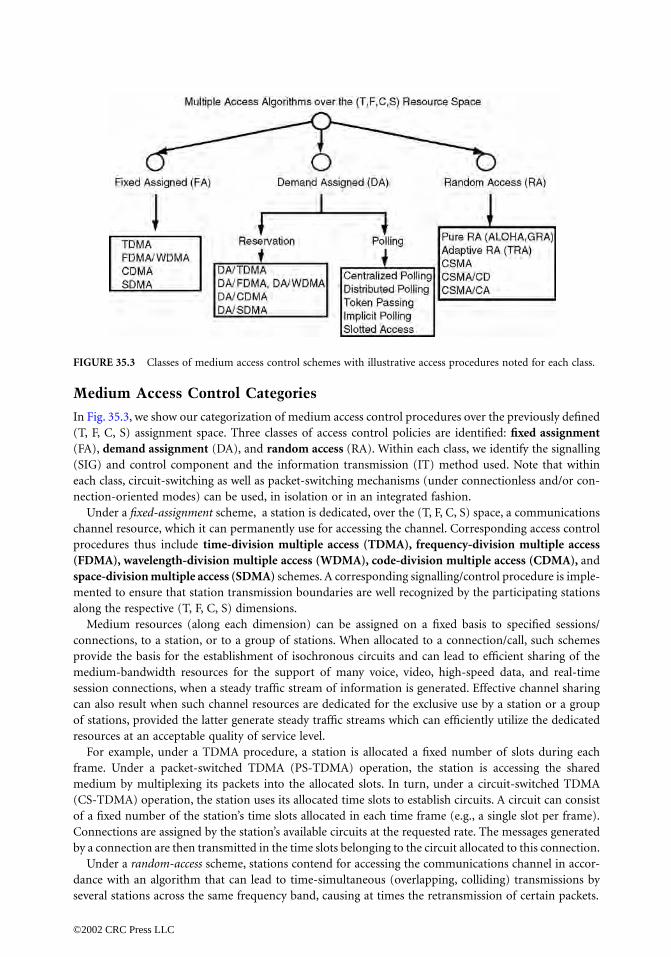
Medium Access Control Categories

In Fig. 35.3, we show our categorization of medium access control procedures over the previously defined(T, F, C, S) assignment space. Three classes of access control policies are identified: fixed assignment(FA), demand assignment (DA), and random access (RA). Within each class, we identify the signalling(SIG) and control component and the information transmission (IT) method used. Note that withineach class, circuit-switching as well as packet-switching mechanisms (under connectionless and/or con-nection-oriented modes) can be used, in isolation or in an integrated fashion.

Under a fixed-assignment scheme, a station is dedicated, over the (T, F, C, S) space, a communicationschannel resource, which it can permanently use for accessing the channel. Corresponding access controlprocedures thus include time-division multiple access (TDMA), frequency-division multiple access(FDMA), wavelength-division multiple access (WDMA), code-division multiple access (CDMA), andspace-division multiple access (SDMA) schemes. A corresponding signalling/control procedure is imple-mented to ensure that station transmission boundaries are well recognized by the participating stationsalong the respective (T, F, C, S) dimensions.

Medium resources (along each dimension) can be assigned on a fixed basis to specified sessions/connections, to a station, or to a group of stations. When allocated to a connection/call, such schemesprovide the basis for the establishment of isochronous circuits and can lead to efficient sharing of themedium-bandwidth resources for the support of many voice, video, high-speed data, and real-timesession connections, when a steady traffic stream of information is generated. Effective channel sharingcan also result when such channel resources are dedicated for the exclusive use by a station or a groupof stations, provided the latter generate steady traffic streams which can efficiently utilize the dedicatedresources at an acceptable quality of service level.

For example, under a TDMA procedure, a station is allocated a fixed number of slots during eachframe. Under a packet-switched TDMA (PS-TDMA) operation, the station is accessing the sharedmedium by multiplexing its packets into the allocated slots. In turn, under a circuit-switched TDMA(CS-TDMA) operation, the station uses its allocated time slots to establish circuits. A circuit can consistof a fixed number of the station’s time slots allocated in each time frame (e.g., a single slot per frame).Connections are assigned by the station’s available circuits at the requested rate. The messages generatedby a connection are then transmitted in the time slots belonging to the circuit allocated to this connection.

Under a random-access scheme, stations contend for accessing the communications channel in accor-dance with an algorithm that can lead to time-simultaneous (overlapping, colliding) transmissions byseveral stations across the same frequency band, causing at times the retransmission of certain packets.

FIGURE 35.3 Classes of medium access control schemes with illustrative access procedures noted for each class.


Under fixed random-access schemes, a station transmits its message frame across the channel at arandom time, in a slotted or unslotted fashion, without coordinating its access with other stations. Astation that detects (through channel sensing, or through nonreceipt of a positive acknowledgment fromits destination) its transmission to collide with another transmission, will retransmit its message after aproperly computed random retransmission delay (whose duration may depend on the estimated channelstate of congestion). Under an adaptive channel-sensing random-access algorithm, a ready station firstsenses the channel to gain certain channel state information and then uses this information to scheduleits message for transmission in accordance with the underlying protocol, again without undertaking fullaccess coordination with all other network stations. Various fixed (such as ALOHA [Abramson, 1973]and group random access [Rubin, 1978]) and adaptive channel-sensing random-access algorithms suchas carrier sense multiple access (CSMA) [Kleinrock and Tobagi, 1975], carrier sense multiple access/collision detection (CSMA/CD), dynamic group random access (DGRA) [Rubin, 1983], tree-random-access collision resolution-based [Capetanakis, 1979] and others [Sachs, 1988; Maxemchuk, 1982; Stall-ings, 1993] can be invoked.

In general, random-access schemes are not well suited as information transmission methods for gov-erning the access of information messages onto a very high-speed fiber communications channel, unlessprovisions are made to considerably limit the extent of message overlaps due to collisions or to limit theuse of this access technique to certain low-throughput messaging classes.

A random-access procedure is typically employed for supporting packet-switching services. At highernormalized throughput levels, high packet delay variances can occur. A proper flow control regulationmechanism must be employed to guarantee maximum delay limits for packets associated with isochro-nous and real-time based services.

Nonchannel-sensing random-access procedures yield low channel utilization levels. In turn, theefficiency of a channel-sensing random-access procedure critically depends upon the timeliness ofthe sensed channel occupancy information and, thus, upon the overhead durations associated withsensing the channel. For high-speed logical-bus systems, when channel-sensing type random-accessschemes are used, performance degradation is caused by the very high ratio of the channel propa-gation delay to the packet transmission time. An active station is required to obtain the channel stateprior to initiating a transmission. However, since a station’s transmission must propagate across thetotal logical-bus medium before its existence can be sensed by all network stations, and since stationsmake uncoordinated access decisions under a random-access scheme, these decisions can be basedon stale channel state information; as a result, this can lead to the occurrence of excessive messagecollisions.

The degrading effects of the propagation delay to message transmission time ratio can be somewhatreduced by the following approaches.

Limit the overall propagation delay by dividing the overall network into multiple tiers or segments,as illustrated by the double-tier LAN and MAN architecture presented in Rubin and Tsai [1987]. Thenetwork stations are divided into groups. A shared backbone medium can be used to provide intercon-nection between groups (on a broadcast global basis using repeaters as gateways, or on a store-and-forward bridged/routing basis) using a noncontention (nonrandom-access)-based MAC algorithm. Arandom-access MAC strategy can be used for controlling the access of messages across the shared group(segment) medium, which now spans a much shorter distance and thus involves considerably reducedpropagation delays. Similarly, such a network configuration is realized by interconnecting LAN (such asethernet) segments by routers, bridges, or switches.

While the propagation delay depends on the conducting medium and is independent of the transmis-sion speed, the packet transmission time is reduced as the transmission speed is increased. The MACmessage frame transmission time can be increased by using FDMA/WDMA or SDMA methods to replacethe single-band high-bandwidth medium with a group of shared multiple channels, each of lowerbandwidth [Chlamtac and Ganz, 1988]. Clearly, this will provide an improvement only if the underlyingservices can be efficiently supported over such a reduced bandwidth channel when a random-access (orother MAC) scheme is used.


Random-access schemes can serve, as part of other MAC architectures, as effective procedures for trans-mitting signalling packets for demand-assigned schemes. Random-access schemes can also be used in con-junction with CDMA and spread spectrum multiple access (SSMA) procedures over high-speed channels.

Random-access protocols are further presented and discussed in Section 35.5.Under a demand-assigned scheme, a signalling procedure is implemented to allow certain network

entities to be informed about the transmission and networking needs and demands of the networkstations. Once these network entities are informed, a centralized or distributed algorithm is used to allo-cate to the demanding stations communications resource segments over the (T, F, C, S) assignment space.

The specific methods used in establishing the signalling channel and in controlling the access ofindividual demanding stations onto this channel characterize the features of the established demand-assignment scheme.

The signalling channel can be established as an out-of-band or in-band fixed channel to whichcommunications resources are dedicated, as is the case for many DA/TDMA, DA/FDMA, or DA/WDMAschemes. In turn, a more dynamic and adaptive procedure can be used to announce the establishmentof a signalling channel at certain appropriate times, as is the case for the many polling, implicit polling,slotted, and packet-train-type access methodologies.

The schemes used to provide for the access of stations onto the signalling channel can be divided intotwo categories: polling and reservation procedures.

Under a reservation scheme, it is up to the individual station to generate a reservation packet andtransmit it across the signalling (reservation) channel to inform the network about its needs for com-munications resources. The station can identify its requirements as they occur or in advance, in accor-dance with the type of service required (isochronous vs. asynchronous, for example) and the precedencelevel of its messages and sessions/connections. Reservation and assignment messages are often trans-mitted over an in-band or out-of-band multiple-access channel so that a MAC procedure must beimplemented to control the access of these MAC-signalling messages.

Under a polling procedure, it is the responsibility of the network system to query the network stationsso that it can find out their transmission needs, currently or in advance. Polling and polling-responsemessages can be transmitted over an in-band or out-of-band multiple-access channel, so that a MACprocedure must be implemented to control the access of these MAC-signalling messages.

Under an implicit polling procedure, stations are granted access into the medium (one at a time orin a concurrent noninterfering fashion) when certain network state conditions occur; such conditionscan be deduced directly by each station without the need to require the station to capture an explicitpolling message prior to access initiation. Such schemes are illustrated by slotted bus systems wherebythe arrival of an idle slot at a station serves as an implicit polling message, and by buffer-insertion schemeswhereby a station is permitted to access the ring if its ring buffer is empty. Additional constraints aretypically imposed on the station regarding utilizing these implicit polling messages for access to thechannel to ensure a fair allocation of communications network bandwidth resources. Such constraintsoften guarantee that a station can transmit a quota of packets within a properly defined cycle.

A multitude of access policies can be adopted in implementing integrated services polling and reser-vation algorithms. Note that polling techniques are used in implementing the IEEE 802.4 token bus andIEEE 802.5 token ring LANs, the FDDI fiber LAN, and many other fiber bus and ring network systems.Reservation techniques are employed by the IEEE 802.6 DQDB metropolitan area network (whereby aslotted positional priority implicit polling access procedure is used to provide access to reservation bits[Newman and Hullett, 1986]), by demand-assigned TDMA, FDMA, CDMA, and WDMA systems, andmany other multiple-access network systems. Integrated reservation and polling schemes are also used.See the following section for further discussion of polling and implicit polling methods.

35.4 Polling-Based Multiple Access Networks

In this section, we describe a number of multiple-access networks whose medium access control archi-tectures are based on polling procedures.


Token-Ring Local Area Network

The token-ring network is a local area network whose physical, MAC, and link layer protocol structuresare based on the IEEE 802.5 Standard. The ring interface units are connected by point-to-point directionallinks, which operate at data rates of`4 Mb/s or 16Mb/s. A distributed polling mechanism, known as atoken passing protocol, is used as the medium access control scheme. A polling packet, known as a token,is used to poll the stations (through their RIUs). When a station receives the token (buffering it for acertain number of bit times to allow the station to identify the packet as a token message and to reactto its reception), it either passes the token along to its downstream neighboring station (when it has nomessage waiting for transmission across the ring network) or it seizes the token. A captured token is thusremoved from the ring so that only a single station can hold a token at a time. The station holding thetoken is then allowed to transmit its ready messages. The dwell time of this station on the ring is limitedthrough the setting of the station’s token holding timer. When the latter expires, or when the stationfinishes transmitting its frames, whichever occurs first, the station is required to generate a new tokenand pass it to its downstream neighboring station. The transmitted frames are broadcasted to all stationson the ring: they fully circulate the ring and are removed from the ring by their source station. Such aprocedure is also known as a source removal mechanism. The token-ring protocol permits a messagepriority-based access control operation. For this purpose, the token contains a priority field. A token ofa certain priority level can be captured by only those stations which wish to transmit across the mediuma message of a priority level equal to or higher than the token’s priority level. Furthermore, stations canmake a reservation for the issue of a token of a higher priority level by setting a priority request tag ina reservation field contained in circulating frames (such tags can also be marked in the reservation fieldof a busy token, which is a token that has been captured but not yet removed from the ring, and taggedas busy by the station which has seized it). Upon its release of a new idle token, the releasing stationmarks the new token at a priority level which is the highest of all of those levels included in the recentlyreceived reservations. At a later time, when no station is interested in using a token of such a high-prioritylevel, this station is responsible for downgrading the priority of the token. In setting priority-basedtimeout levels for the token holding timer, different timeout values can be selected for different prioritylevels.

The throughput capacity attainable by a polling scheme, including a token passing distributed pollingmechanism such as the token ring LAN, is dependent on the walk time parameter. The system walk timeis equal to the total time it takes for the polling message (the token) to circulate around the network (thering) when no station is active. For a token ring network, the walk time is thus calculated as the sum ofthe transmission times, propagation delay, and ring buffer delays incurred by the token in circulatingacross an idle ring. Clearly, the throughput inefficiency of the network operation is proportional to theratio between the walk time and the overall time occupied by message transmissions during a singlerotation of the token around the ring. The network’s maximum achievable throughput level, also knownas the network’s throughput capacity, is denoted as L(C) (b/s); the normalized throughput capacity indexis set to s(C) = L(C)/R, where R (b/s) denotes the data rate of each network link, noting that 0 £ s(C) £1. Thus, if S(C) = 0.8, the network permits a maximum throughput level that is equal to 80% of thelink’s data rate. To assess the network’s throughput capacity level, we assume the network to be highlyloaded so that all stations have frames ready for transmission across the ring. In this case, each cycle(token circulation around the ring) has an average length of E(C) = NK(F/R) + W, where N denotes thenumber of ring stations (RIUs), K denotes the maximum number of frames that a station is allowed totransmit during a single visit of the token, F is the frame’s average length (in bits), so that F/R representsthe average frame transmission time across a ring’s link, whereas W denotes the average duration (inseconds) of the token’s walk time. The network’s normalized throughput capacity index is thus given bys(C) = NK(F/R)/E(C). Clearly, higher throughput levels are attained as the walk time durations (W) arereduced. Note that W = R(p)L + (T/R) + N(M/R), where R(p) denotes the propagation delay per unit-distance across the medium (typically equal to 5 µs/km for wired links); L (km) is the distance spannedby the ring network so that R(p)L represents the overall propagation delay around the ring; T is thetoken’s length, so that T/R represents the token’s transmission time; M denotes the number of bit time


delays incurred at the RIU’s interface buffer, so that N(M/R) expresses the overall delay incurred by aframe in being delayed at each interface around the ring.

The delay-throughput performance behavior exhibited by polling systems, such as the distributedpolling token-passing scheme of the token-ring LAN, follows the behavior of a single server queueingsystem in which the server dynamically moves from one station to the next, staying (for a limited time)only at those stations that have messages requiring service (i.e., transmission across the shared medium).This is a stable operation for which message delays increase with the overall loading on the network, aslong as the latter is lower than the throughput capacity level L(C). As the loading approaches the lattercapacity level, message delays rapidly increase and buffer overflows can be incurred.

The Fiber Data Distribution Interface Network

The fiber data distribution interface network also employs a token passing access control algorithm. Italso uses a ring topology. Two counter-rotating fiber optic rings are used (one of which is in a standbymode) so that, upon the failure of a fiber segment, the other ring is employed to provide for a closed-loop topology. The communications link operates at a data rate of 100 Mb/s. The network can span alooped distance of up to 200 km.

As previously described for the token ring network, on the receipt of a token, an idle station passes itto its downstream station after an interface delay. If the station is busy, it will capture the token andtransmit its frames until its token holding timer times out. As for the token-ring network, a source removalmechanism is used so that the transmitted frames are broadcasted to all stations on the ring; they fullycirculate the ring and are removed from the ring by their source station. The timeout mechanism andthe priority support procedure used by FDDI are different than those employed by the token ring networkand are described subsequently. When a station terminates its dwell time on the medium, it immediatelyreleases the token. This is identified as an early token release operation. For lower speed token-ringimplementations, a late token release operation can be selected. Under the latter, the token is releasedby the station only after it has received all of its transmitted messages and removed them from the ring.Such an operation leads to throughput performance degradations when the network uses higher speedlinks since then the station holds the token for an extra time, which includes as a component the ring’spropagation delay. The latter can be long relative to the frame’s transmission time. As a result, higherspeed token-ring networks are generally set to operate in the early token release mode.

The FDDI MAC scheme distinguishes between two key FDDI service types: synchronous and asyn-chronous. Up to eight priority levels can be selected for asynchronous services. To date, most commonlyemployed FDDI adapter cards implement only the asynchronous priority 1 service; some also provide asynchronous priority service.

The access of frames onto the medium is controlled by a timed token rotation (TTR) protocol. Eachstation continuously records the time elapsed since it has last received the token (denoted as the tokenrotation time). An initialization procedure is used to select a target token rotation time (TTRT) througha bidding process whereby each station bids for a token rotation time (TRT) and the minimum suchtime is selected. As previously noted, two classes of service are defined: synchronous, under which astation can capture the token whenever it has synchronous frames to transmit, and asynchronous, whichpermits a station to capture a token only if the current TRT is lower than the established TTRT. Tosupport multiple priority levels for asynchronous frames, additional time thresholds are defined for eachpriority level. In this manner, a message of a certain priority level is allowed to be transmitted by itsstation, when the latter captures the token, only if the time difference between the time this station hasalready used (at this ring access) for transmitting higher priority messages and the time since the tokenlast visited this station is higher than the corresponding time threshold associated with the underlyingmessage priority level. This priority-based access protocol is similar to the one used for the IEEE 802.4token bus LAN system.

Using this procedure, stations can request and establish guaranteed bandwidth and response time forsynchronous frames. A guaranteed maximum cycle latency-based response time is established for the


ring, since the arrival time between two successive tokens at a station can be shown to not exceed thevalue of 2 × TTRT.

As a polling scheme, the performance of the FDDI network is limited by the ring walk (W) time. Thering throughput is thus proportional to 1 - W/TTRT. While lower TTRT values (such as 4–8 ms) yieldlower guaranteed cycle response times (token intervisit times lower than 8–16 ms), higher TTRT valuesneed to be selected to provide for better bandwidth utilization under higher load conditions. The ringlatency varies from a small value of 0.081 ms for 50 stations, 10-km LAN, to a value of 0.808 ms for 500stations, 100-km LAN. Using a TTRT value of 50 ms for a LAN that supports 75 stations and 30 km offiber, and having a ring latency W = 0.25 ms, a maximum utilization of 99.5% can be achieved [Ross,1986].

To provide messages their desired delay performance behavior across the FDDI ring network, it isimportant to calibrate the FDDI network so that acceptable levels of queueing delays are incurred at thestations’ access queues for each service class [Shah et al., 1992]. This can be achieved by the properselection of the network’s MAC parameters, such as the TTRT level, the timeout threshold levels whenmultipriority asynchronous services are used, and the station synchronous bandwidth allocation levelwhen a station’s FDDI adapter card is set also to provide a synchronous FDDI service. The latter serviceis effective in guaranteeing quality of service support to real-time streams, such as voice, compressedvideo, sensor data, and high-priority critical message processes, which require strictly limited networkdelay jitter levels [Shah et al., 1992]. Note that when a token is received by a station that provides anFDDI synchronous service, the station is permitted to transmit its frames that receive such a service (fora limited time, which is equal to a guaranteed fraction of the TTRT) independently of the currentlymeasured TRT. When no such messages are queued at the station at the arrival of the token, the tokenimmediately starts to serve messages which receive asynchronous service, so that the network’s bandwidthis dynamically shared among all classes of service.

The delay-throughput performance features of the FDDI networks follow the characteristics of adistributed polling scheme already discussed. The FDDI performance results reported in Shah et al.[1992] were obtained by using the PLANYSTTM tool developed by the IRI Corporation. This tool hasbeen also used to calibrate the parameters of FDDI networks through the use of its expert-based analyticalroutines.

Implicit Polling Schemes

Under an implicit polling multiple-access mechanism, the network stations monitor the shared mediumand are then granted access to it by identifying proper status conditions or tags. To illustrate suchstructures, we consider the slotted channel, register-insertion, positional-priority, and collision-avoidanceaccess protocols.

Under a slotted channel access protocol, the shared medium link(s) are time shared through the gener-ation of time slots. Each time slot contains an header which identifies it as busy or idle. In addition, timeslots may also be reserved to connections, so that a circuit-switched mode can be integrated with thepacket-switched multiple-access mode described in the following. To regulate station access rates, toassign time circuits, and to achieve a fair allocation of channel resources, the time slots are normallygrouped into recurring time frames (cycles). A ready station, with packets to transmit across the medium,monitors the medium. When this station identifies an idle slot, which it is allowed to capture, it marksit to be in a busy state and inserts a single segment into this slot. Clearly, in transmitting a packet, astation must break it into multiple segments, whereby the maximum length of a segment is selected suchthat it fits into a single slot. The packet segments must then be assembled into the original packet at thedestination station.

To be able to insert packets into moving slots, the station must actively interface the medium byinserting an active buffer into the channel. A common configuration for such a network is the slottedring topology. A slotted access protocol can also be used in sharing a linear logical bus topology withactive station interfaces. The later configuration is used by the distributed queue dual-bus MAN defined


by the IEEE 802.6 standard. The latter uses a fiber optic-based dual-bus configuration so that each stationis connected to two counterdirectional buses.

To regulate the maximum level of bandwidth allocated to each station, in accordance with the classof service provided to the station, and to control the fair allocation of network resources among stationsthat receive the same class of service, the access algorithm can limit (statically or dynamically) the numberof slots that can be captured by a station during each frame. For the DQDB network, a reservationsubchannel is established for stations to insert reservation tags requesting for slots to be used for thetransmission of their packets. A station is allowed to capture an idle slot which passes its interface onlyif it has satisfied all of the earlier requests it has received signifying slot reservations made by otherstations. The DQDB network also integrates a circuit-switched mode through the establishment ofisochronous circuits as part of the call setup procedure. A frame header is used to identify the slots thatbelong to dedicated time circuits.

Under a register-insertion configuration, each station’s medium interface card includes a register (buffer),which is actively inserted into the medium. Each packet is again broken down into segments. A station ispermitted to insert its segment(s) into the medium when its register contains no in-transit segments (thusdeferring the transmission of its own segments until no in-transit segments are passing by) or when thegap between in-transit segments resident in its register is sufficiently long. In-transit packets arriving atthe station’s interface when the station is in the process of transmitting its own segment are delayed in theregister. To avoid register overflows, its size is set to be equal to at least the maximum segment length. TheIBM Metaring/Orbit [Cidon and Ofek, 1989] network is an example of such a network system whichemploys a ring topology as well as the destination removal spatial reuse features to be presented.

At higher speeds, to further increase the throughput efficiency of the shared medium network, adestination removal mechanism is used. This leads to spatial reuse since different space segments ofthe network’s medium can be used simultaneously in time by different source–destination pairs. Forexample, for a spatial-reuse slotted channel network (such as slotted ring or bus-based topologies),once a segment has reached its destination station, the latter marks the slot as idle, allowing it to bereused by subsequent stations it visits. Similarly, the use of an actively inserted buffer (as performedby the register-insertion ring network) allows for operational isolation of the network links, providingspatial reuse features.

To assess the increase in throughput achieved by spatial reuse ring networks, assume the traffic ma-trix to be uniform (so that the same traffic loading level is assumed between any source–destinationpair of stations). Also assume that the system employs two counter-rotating rings, so that a stationtransmits its segment across the ring that offers the shortest path to the destination. Clearly, themaximum path length is equal to half the ring length, while the average path length is equal to one-quarter of the ring length. Hence, an average of four source–destination station pairs simultaneouslycommunicate across the dual ring network. As a result, the normalized throughput capacity achievedby the spatial reuse dual ring network is equal to 400% (across each one of the rings), as comparedwith a utilization capacity of 100% (per ring) realized when a destination removal mechanism is used.Hence, such spatial reuse methods lead to substantial throughput gains, particularly when the networklinks operate at high speeds. They are thus especially important when used in ultra-high-speed opticalnetworks, as noted in Section 35.7.

Positional-Priority and Collision Avoidance Schemes

Under a hub-polling (centralized polling) positional-priority scheme, a central station (such as a com-puter controller) polls the network stations (such as terminals) in an order which is dictated by theirphysical position in the network (such as their location on a ring network with respect to the centralstation), or by following a service order table [Baker and Rubin, 1987]. Stations located in a higherposition in the ordering list are granted higher opportunities for access to the network’s shared medium.For example, considering a ring network, the polling cycle starts with the controller polling station 1


(the one allocated highest access priority). Subsequently, station 2 is polled. If the latter is found to beidle, station 1 is polled again.

In a similar manner, a terminal priority-based distributed implicit polling system is implemented.Following a frame start tag, station 1 is allowed to transmit its packet across the shared medium. A readystation 2 must wait a single slot of duration T (which is sufficiently long to allow station 1 to starttransmitting and for its transmission to propagate throughout the network so that all stations moni-toring the shared channel can determine that this station is in the process of transmission) before it candetermine whether it is allowed to transmit its packet (or segment). If this slot is monitored by station2 to be idle, it can immediately transmit its packet (segment). Similarly, station i must wait for (i - 1)idle slots (giving a chance to the i - 1 higher priority terminals to initiate their transmissions) followingthe end of a previous transmission (or following a frame start tag when the channel has been idle) beforeit can transmit its packet across the shared communications channel.

Such a multiple-access mechanism is also known as a collision avoidance scheme. It has been im-plemented as part of a MAC protocol for high-speed back-end LANs (which support a relatively smallnumber of nodes) such as HyperChannel. It has also been implemented by wireless packet radio networks, such as the TACFIRE field artillery military nets. In assessing the delay-throughput behaviorof such an implicit polling distributed control mechanism, we note that the throughput efficiencyof the scheme depends critically on the monitoring slot duration T, whereas the message delaybehavior depends on the terminal’s priority level [Rubin and Baker, 1986]. At lower loading levels,when the number of network nodes is not too large, acceptable message delays may be incurred byall terminals. In turn, at higher loading levels, only higher priority terminals will manage to attaintimely access to the network while lower priority ones will be effectively blocked from entering theshared medium.

Probing Schemes

When a network consists of a large number of terminals, each generating traffic in a low duty cyclemanner, the polling process can become highly inefficient in that it will require relatively high bandwidthand will occupy the channel with unproductive polling message transmissions for long periods of time.This is induced by the need to poll a large number of stations when only a few of them will actually havea packet to transmit.

A probing [Hayes, 1984] scheme can then be employed to increase the efficiency of the polling process.For this purpose, rather then polling individual stations, groups of stations are polled. The respondingindividual stations are then identified through the use of a collision resolution algorithm. For example,the following tree-random-access [Capetanakis, 1979; Hayes, 1984] algorithm can be employed. Followingan idle state, the first selected polling group consists of all of the net stations. A group polling messageis then broadcasted to all stations. All stations belonging to this group which have a packet to transmitthen respond. If multiple stations respond, a collision will occur. This will be recognized by the controller,which will subsequently subdivide the latest group into two equal subgroups. The process will proceedwith the transmission of a subgroup polling message. Using such a binary search type algorithm, allcurrently active stations are eventually identified. At this point, the probing phase has been completedand the service phase is initiated. All stations which have been determined to be active are then allocatedmedium resources for the transmission of their messages and streams.

Note that this procedure is similar to a reservation scheme in that the channel use temporally alternatesbetween a signalling period (which is used to identify user requests for network support) and a serviceperiod (during which the requesting stations are provided channel resources for the transmission of theirmessages). Under a reservation scheme, the stations themselves initiate the transmission of their requestsduring the signalling periods. For this purpose, the stations may use a random-access algorithm or otheraccess methods. When the number of network stations is not too large, dedicated minislots for thetransmission of reservation tags can be used.


35.5 Random-Access Protocols

In this section, we describe a number of random-access protocols which are commonly used by manywireline and wireless networks. Random-access protocols are used for networks which require a dis-tributed control multiple-access scheme, avoiding the need for a controller station which distributes(statically or dynamically) medium resources to active network stations. This results in a survivableoperation, which avoids the need for investment of significant resources into the establishment andoperation of a signalling subnetwork. This is of particular interest when the shared communicationsmedium supports a relatively large number of terminals, operating each at a low duty cycle. When astation has just one or a few packets, it needs to transmit in a timely manner (at low delay levels) oninfrequent occasions; it is not effective to allocate to the station a fixed resource of the network (as per-formed by a fixed assignment scheme). It is also not effective to go through a signalling procedure toidentify the station’s communications needs prior to allocating it a resource for the transport of its fewpackets (as performed by demand-assigned polling and reservation schemes). As a consequence, for manynetwork systems, particularly for wireless networks, it is effective to use random-access techniques forthe transport of infrequently generated station packets or, when active connections must be sustained,to use random-access procedures for the multiaccess transport of signalling packets.

The key differences among the random-access methods described subsequently are reflected by themethod used in performing shared medium status monitoring.

When stations use full-duplex radios and the network is characterized by a broadcast communicationsmedium (so that every transmission propagates to all stations), each station receives the transmissionsgenerated by the transmitting station, including the transmitting station itself. Stations can then rapidlyassess whether their own transmission is successful (through data comparison or energy detection). Thisis the situation for many local area network implementations. In turn, when stations are equipped withhalf-duplex transceivers (so that they need to turn around their radios to transition between a receptionmode and a transmission mode) and/or when a fully broadcast channel is not available (as is the casefor mobile radio nets for which topographical conditions lead to the masking of certain stations, lackingline-of-sight connections between certain pairs of stations), the transmitting station cannot automaticallydetermine the status of its transmission. The station must then rely on the receipt of a positive acknowl-edgment packet from the destination station.

ALOHA Multiple Access

Under the ALOHA random-access method, the network stations do not monitor the status of theshared communications channel. When a ready station receives a packet, it transmits it across thechannel at any time (under an unslotted ALOHA scheme) or at the start of time slot (under a slottedALOHA algorithm, where the length of a slot is set equal to the maximum MAC frame length). If twoor more stations transmit packets (frames) at the same time (or at overlapping times), the correspond-ing receivers will not usually be able to correctly receive the involved packets, resulting in a destructivecollision. (Under communications channel capture conditions, the stronger signal may capture thereceiver and may be received correctly, while the weaker signals may be rejected.) When a station hasdetermined that its transmitted packet has collided, it then schedules this packet for retransmissionafter a random retransmission delay. The latter delay can be selected at random from an interval whoselength is dynamically determined based on the estimated level of congestion existing across the sharedcommunications channel. Under a binary exponential backoff algorithm, each station adapts thisretransmission interval on its own by doubling its span each time its packet experiences an additionalcollision.

The throughput capacity of an unslotted ALOHA algorithm is equal to s(C) = 1/(2e) = 18.4%, whereasthat of a slotted ALOHA scheme is equal to s(C) = 1/e = 36.8%. The remainder of the shared channel’sused bandwidth is occupied by original and retransmitted colliding packets. In effect, to reduce the packetdelay level and the delay variance (jitter), the loading on the medium must be reduced significantly below


the throughput capacity level. Hence, the throughput efficiency of ALOHA channels is normally muchlower than that attainable by fixed-assigned and demand-assigned methods. The random-access networksystem is, however, more robust to station failures and is much simpler to implement, not requiring theuse of complex signalling subnetworks.

The ALHOA shared communications channel exhibits a bistable system behavior. Two distinctlydifferent local equilibrium points of operation are noted. Under sufficiently low-loading levels the systemstate resides at the first point, yielding acceptable delay-throughput behavior. In turn, under high-loadinglevels, the system can transition to operate around the second point. Loading fluctuations around thispoint can lead to very high packet delays and diminishing throughput levels. Thus, under high-loadingbursts, the system can experience a high level of collisions, which in turn lead to further retransmissionsand collisions, causing the system to produce very few successful transmissions. To correct this unstablebehavior of the random-access multiaccess channel, flow control mechanisms must be used. The latterregulate admission of new packets into the shared medium at times during which the network is congested.Of course, this in turn induces an increase in the packet blocking probability or in the delay of the packetat its station buffer.

Carrier Sense Multiple-Access

Under the CSMA random-access method, the network stations monitor the status of the shared com-munications channel to determine if the channel is busy (carrying one or more transmissions) or is idle.A station must listen to the channel before it schedules its packet for transmission across the channel.

If a ready station senses the channel to be busy, it will avoid transmitting its packet. It then either(under the nonpersistent CSMA algorithm) takes a random delay, after which it will remonitor thechannel, or (under the 1-persistent CSMA algorithm) it will keep persisting on monitoring the channeluntil it becomes idle.

Once the channel is sensed to be idle, the station proceeds to transmit its packet. If this station is theonly one transmitting its packet at this time, a successful transmission results. Otherwise, the packettransmission normally results in a destructive collision. Once the station has determined that its packethas collided, it schedules its packet for retransmission after a random retransmission delay.

Many local and regional area packet-radio multiaccess networks supporting stationary and mobilestations, including those using half-duplex radio transceivers, have been designed to use a CSMA protocol.The performance efficiency of CSMA networks is determined by the acquisition delay index a = t(a)/T(P),where T(P) denotes the average packet transmission time and t(a) denotes the system’s acquisition timedelay. The latter is defined as the time elapsed from the instant that the ready station initiates itstransmission (following the termination of the last activity on the channel) to the instant that the packet’stransmission has propagated to all network stations so that the latter can sense a transmitting stationand thus avoid initiating their own transmissions. The acquisition delay t(a) includes as components thenetwork’s end-to-end propagation delay, the radio turn-around time, radio detection times of channelbusy-to-idle transitions, radio attack times (times to build up the radio’s output power), various packetpreamble times, and other components. As a result, for half-duplex radios, the network’s acquisitiondelay t(a) may assume a relatively large value. The efficiency of the operation is, however, determinedby the factor a, which is given as the ratio of t(a) and the packet transmission time T(P), since once thestation has acquired the channel and is the only one currently active on the channel [after a period oflength t(a)], it can proceed with the uninterrupted transmission of its full packet [for a period of durationT(P)].

Clearly, this can be a more efficient mechanism for packet radio networks which operate at lowerchannel transmission rates. As the transmission rate increases, T(P) decreases while the index a increasesso that the delay-throughput efficiency of the operation rapidly degrades. A CSMA network will attaingood delay-throughput performance behavior for acquisition delay index levels lower than about 0.05.For index levels around or higher than 0.2, the CSMA network exhibits a throughput level that is lowerthan that obtained by a slotted (or even unslotted) ALOHA multiaccess net. Under such conditions, the


channel sensing mechanism is relatively ineffective since the window of vulnerability for collisions [t(a)]is now relatively too long. It is thus highly inefficient to use a CSMA mechanism for higher data ratechannels as well as for channels which induce relatively long-propagation delays (such as a satellite com-munication network) or for systems which include other mechanisms that contribute to an increase inthe value of the acquisition delay index.

As for the ALOHA scheme, a CSMA network exhibits a bistable behavior. Thus, under loading bursts,the channel can enter a mode under which the number of collisions is excessive so that further loadingof the channel results in diminishing throughput levels and higher packet delays. A flow control-basedmechanism can be used to stabilize the behavior of the CSMA dynamic network system.

CSMA/CD Local Area Networks

A local area network that operates by using a CSMA/CD access control algorithm incorporates into theCSMA multiple-access scheme previously described the capability to perform collision detection (CD).The station’s access module uses a full-duplex radio and appends to its CSMA-based sensing mechanisma CD operation. Once the ready station has determined the channel to be idle, it proceeds to transmitits packet across the shared channel while at the same time it is listening to the channel to determinewhether its transmission has resulted in a collision. In the latter case, once the station has determinedits packet to be involved in a process of collision, the station will immediately abort transmission. In thismanner, colliding stations will occupy the channel with their colliding transmissions only for a limitedperiod of time, the collision detection time T(CD). Clearly, if T(CD) < T(P), where T(P) denotes thetransmission time of a packet (MAC frame) across the medium, the CSMA/CD operation leads toimproved delay-throughput performance over that of a CSMA operation.

The ethernet LAN developed by Xerox Corporation is a bus-based network operating at a channeldata rate of 10 Mb/s and using a 1-persistent CSMA/CD medium access control algorithm. The physical,MAC, and link layers of such a CSMA/CD network are defined by the IEEE 802.3 standard (and acorresponding ISO standard). Ethernet nets can employ different media types: twisted pair, coaxial cable,fiber optic line, as well as radio links (in the case of an ethernet-based wireless LAN system). Theconfiguration of the ethernet LAN is that of a logical bus so that a frame transmission by a stationpropagates across the bus medium to all other stations. In turn, the physical layout of the medium canassume a bus or a star topology. Under the latter configuration, all stations are connected to a centralhub node, at which point the access lines are connected by a reflecting repeater module so that atransmission received from an access line is repeated into all other lines. Typical ethernet layouts arelimited in their geographical span to an overall distance of about 500–2000 m.

The delay-throughput efficiency of the CSMA/CD network operation is determined by the acquisitiontime delay t(a) and index a, as for the CSMA network. In addition, the network efficiency also dependson the CD time T(CD). It is noted that T(CD) can be as long as twice the propagation delay across theoverall span of the bus medium, plus the time required by the station to establish the occurrence of acollision. To ensure that a collision is reliably detected, the power levels of received packets must besufficiently high. This also serves as a factor limiting the length of the bus and of the distance at whichrepeaters must be placed. As a result, the network stations are attached to several ethernet segments, eachassuming a sufficiently short span. The different ethernet segments are interconnected by gateways orrouters. The latter act as store-and-forward switches which serve to isolate the CSMA/CD multiaccessoperation of each segment.

As for the random-access mechanisms previously discussed, burst loads applied to the CSMA/CDnetwork can cause large delay-throughput degradations. In supporting application streams which requirelimited packet delay jitters, it is thus required to prevent the bus from being excessively loaded. Manyimplementations thus plan the net’s offered traffic loading levels to be no higher than 40% (or 4 Mb/s).Also note that, as for other random access schemes, large loading variations can induce an unstablebehavior. A flow control mechanism must then be employed to regulate the maximum loading level ofthe network.


When shorter bus spans are used, or when shorter access link distances are employed in a starconfiguration, it is possible to operate this network at higher channel data rates. Under such conditions,an ethernet operation at a data rate of 100 Mb/s (or higher) has been implemented.

35.6 Multiple-Access Schemes for Wireless Networks

Under a cellular wireless network architecture, the geographical area is divided into cells. Each cellcontains a central base station. The mobile terminals communicate with the base station controlling thecell in which they reside. The terminals use the reverse traffic and signalling channel(s) to transmit theirmessages to the base station. The base station multiplexes the messages it wishes to send to the cell’smobile terminals across the forward traffic and signalling channels.

First-generation cellular wireless networks are designed to carry voice connections employing a circuitswitching method. Analog communications signals are used to transport the voice information. The under-lying signalling subnetwork is used to carry the connection setup, termination, and handover signallingmessages. The voice circuits are allocated through the use of a reservation based demand-assigned/FDMAscheme. A ready mobile uses an allocated signalling channel for its handset to transmit to its cell’s basestation a request message for the establishment of a voice circuit. If a frequency channel is available forthe allocation of such a circuit (traffic channel), the base station will make this allocation by signallingthe requesting handset.

Second-generation cellular wireless networks use digital communications channels. A circuit-switchingmethod is still employed, with the primary service providing for the accommodation of voice connections.Circuits are formed across the shared radio medium in each cell by using either a TDMA-access controlscheme (through the periodic allocation of time slots to form an established circuit, as performed by theEuropean GSM and the U.S. IS-54 standards) or by employing a CDMA procedure (through the allocationof a code sequence to a connection’s circuit, as carried out by the IS-95 standard). A signalling subnetworkis established. Reverse signalling channels (RSCs) are multiple-access channels which are used by themobile terminals to transmit to their cells’ base station their channel-request packets (for a mobileoriginating call), as well as for the transmission of paging response packets (by those mobiles whichterminate calls). Forward signalling channels (FSCs) are multiplexing channels configured for the trans-mission of packets from the base station to the mobiles. Such packets include channel-allocation messages(which are sent in response to received channel request packets) and paging packets (which are broad-casted in the underlying location area in which the destination mobile may reside).

For the reverse signalling channels, a random access algorithm such as the ALOHA scheme is frequentlyemployed. For TDMA systems, time circuit(s) are allocated for the random access transmission of signal-ling packets. For CDMA systems, codes are allocated for signalling channels; each code channel is timeshared through the use of a random access scheme (employing, for example, a slotted or unslottedALOHA multiple-access algorithm).

Paging and channel allocation packets are multiplexed (in a time-shared fashion) across the forwardsignalling channels. To reduce battery consumption at the mobile terminals, a slotted mode operationcan be invoked. In this case, the cell mobiles are divided into groups, and paging messages destined toa mobile belonging to a certain group are transmitted within that group’s allocated channels (time slots)[Rubin and Choi, 1996]. In this manner, an idle mobile handset needs to be activated for the purposeof listening to its FSC only during its group’s allocated slots.

Under the IEEE 802.11 protocol, terminals access the base station by sharing the radio channel throughthe use of a CSMA/CA (collision avoidance) scheme.

Third-generation cellular wireless networks are planned to provide for the support of both voice anddata services. These networks employ packet-switching principles. Many of the multiple-access schemesdescribed in the previous sections can be employed to provide for the sharing of the mobile-to-base-station multiple-access reverse communications channels. In particular, random-access polling (orimplicit polling) and reservation protocols can be effectively implemented. For example, the followingversions of a reservation method have been investigated. Under the packet reservation multiple access


(PRMA) [Goodman et al., 1989] or random-access burst reservation procedure, a random-access mech-anism is used for the mobile to reserve a time circuit for the transmission of a burst (which consists ofa number of consecutively generated packets). For voice bursts, a random-access algorithm is used togovern the transmission of the first packet of the burst across the shared channel (by randomly selectingan unused slot, noting that, in each frame, the base station notifies all terminals as to which slots areunoccupied). If this packet’s transmission is successful, its terminal keeps the captured slot’s position ineach subsequent frame until the termination of the burst’s activity. Otherwise, the voice packet is discardedand the next voice packet is transmitted in the same manner. In selecting the parameters and capacitylevels of such a multiaccess network, it is necessary to ensure that connections receive acceptable through-put levels and that the packet discard probability is not higher than a prescribed level ensuring an acceptablevoice quality performance [Rubin and Shambayati, 1995].

For connection-oriented packet-switching network implementations which also provide data packettransport, including wireless ATM networks, it is necessary to avoid frequent occurrences of packetdiscards to reduce the rate of packet retransmissions and to lower the chances for packet reorderingprocedures needed to guarantee the ordered delivery of packets. Reverse and forward signalling channelsare established to set up the virtual-circuit connection. Channel resources can then be allocated toestablished connections in accordance with the statistical features of such connections. For example, real-time connections can be accommodated through the periodic allocation of time slots (or frequency/coderesources), whereas burst sources can be supported by the allocation of such resources only for the limitedduration of a burst activity. A mechanism must then be employed to identify the start and end times ofburst activities. For example, the signalling channels can be used by the mobiles to signal the start ofburst activity, whereas the in-band channel is used to detect the end of activity (directly and/or throughthe use of tagging marks).

35.7 Multiple Access Methods for Spatial-ReuseUltra-High-Speed Optical Communications Networks

As we have seen above, token-ring and FDDI LANs use token-passing methods to access a shared medium.Furthermore, these networks use a source removal procedure so that each station is responsible forremoving its own transmitted frames from the ring. In this manner, each transmitted frame circulatesthe ring and is then removed by its source station. As a result, the throughput capacity of such networksis limited to a value which is not higher than the ring’s channel data rate.

In turn, as observed in Section 35.4 (in connection with implicit polling-based multiple-access net-works), the bandwidth utilization of shared medium networks, with particular applications to local andmetropolitan area networks operating at high speed using generally fiber optic links, can be significantlyupgraded through the employment of spatial-reuse methods. For example, consider a ring network whichconsists of two counter-rotating unidirectional fiber optic ring topologies. Each terminal (station) isconnected to both rings through ring interface units. The bandwidth resources of the rings are sharedamong the active stations. Assume now that a destination removal method is employed. Thus, when aframe reaches its destination node (RIU), it is removed from the ring by the latter. The network com-munications resources occupied by this frame (such as a time slot) can then be made available to sourcenodes located downstream to the removing station (as well as to the removing station itself).

A source station which has a frame to transmit selects the ring that offers the shortest path to thedestination node. In this manner, the length of a path will be no longer than 1/2 the ring’s length. If weassume a uniform traffic matrix (so that traffic flows between the network terminal nodes are symmet-rically distributed), the average path length will be equal to 1/4 the ring’s length. As a result, using sucha destination removal technique, we conclude that an average of four source-destination flows will becarried simultaneously in time by each one of the two rings. Therefore, the throughput capacity of sucha spatial reuse network can reach a level which is equal to 400% the ring’s channel data rate for each oneof the two rings.


Spatial reuse ring networks can be used to carry traffic on a circuit-switched or packet-switched(connectionless or connection-oriented) basis. For packet-switched network implementations, the fol-lowing two distributed implicit polling multiple-access methods have been used. Under a slotted ringoperation, time slots are generated and circulated across the ring. Each time slot contains a header whichidentifies it as either empty or busy. A station which senses an empty time slot can mark it as busy andinsert a segment (a MAC frame which, for example, can carry an ATM cell) into the slot. The destinationstation will remove the segment from its slot and will designate the slot as idle so that it can be reusedby itself or other stations. Under a buffer-insertion ring multiple-access scheme, each station inserts abuffer into the ring. A busy station will defer the transmission of its packet to packets currently beingreceived from an upstream station. In turn, when its buffer is detected to be empty, the station will insertits segment into the ring. The buffer capacity is set equal to a maximum size packet so that a packetreceived by a station while it is in a process of transmission of its own packet can be stored in the station’sinserted buffer. Each packet is removed from the ring by its destination node.

As previously noted, the DQDB MAN is a slotted dual-bus network which employs active stationinterfaces. To achieve spatial bandwidth reuse gains of the bus’ bandwidth resources, frame removalstations can be positioned across the bus. These stations serve to remove frames which have alreadyreached their destinations so that their slots can be reused by downstream stations. Note that such stationsmust use an inserted buffer of sufficient capacity to permit reading of the frame’s destination node(s) sothat they can determine whether a received frame has already reached its destination(s).

In designing optical communications networks, it is desirable to avoid the need for executing store-and-forward switching and operations at the network nodes. Such operations are undesirable due to thelarge differences existing between the optical communications rates across the fiber optic links and theelectronic processing speeds at the nodes, as well as due to the difficulty involved in performing intelligentbuffering and switching operations in the optical domain. Networks that avoid such operations (at leastto a certain extent) are known as all-optical networks.

Systems commonly used for the implementation of a shared medium local area all-optical networkemploy a star topology. At the center of the star, an optical coupler is used. The coupler serves to repeatthe frame transmissions received across any of its incoming fiber links to all of its outgoing fiber links.The coupler can be operated in a passive transmissive mode or in an active mode (using optical amplifi-cation to compensate for power losses incurred due to the distribution of the received optical signal acrossall output links). Each station is then connected by a fiber link to the star coupler so that the stations sharea multiple-access communications channel. A multiple-access algorithm must then be employed to controlthe sharing of this channel among all active stations. Typical schemes employed for this purpose userandom-access, polling, and reservation methods. Furthermore, multiple wavelengths can be employedso that a WDMA component can be integrated into the multiple-access scheme. The wavelengths can bestatically assigned or dynamically allocated. To illustrate the latter case, consider a reservation-basedDA/WDMA procedure. Under a connection-oriented operation, wavelengths are assigned to source-destination nodes involved in a connection. Both transmitter and receiver based wavelength assignmentconfigurations can be used: the transmitter’s or receiver’s (or both) operating wavelengths can be selecteddynamically to accommodate a configured connection.

Because of its broadcast feature, the star-configured optical network does not offer any spatial orwavelength reuse advantages. In turn, the meshed-ring scalable multimedia adaptable meshed-ring terabit(SMARTNet) optical network introduced by Rubin [1994] capitalizes on the integrated use of spatial-reuse and wavelength-reuse methods. In the following, we illustrate the architecture of the SMARTNetconfiguration. Two counter-rotating fibers make up the ring periphery. The stations access the networkthrough their RIUs, which are actively connected to the peripheral fiber rings. The fiber link resourcesare shared through the use of a wavelength-division scheme. Multiple wavelengths are used, and eachstation has access to all wavelengths (or to a limited number of them). The rings are divided into segments.Each segment provides access to multiple stations through their connected RIUs. Each segment isconnected to its neighboring segments through the use of wavelength cross-connect routers. Such arouter switches messages received at multiple wavelengths from its incoming ports to its outgoing ports.


No store-and-forward switching operations are performed. The switching matrix is preset (on a staticor adjustable basis) so that messages arriving across an incoming link at a certain wavelength are alwaysimmediately switched to a prescribed outgoing link (at the same wavelength, although wavelengthtranslations can also take place). The wavelength routers are also connected (to certain other wavelengthrouters) by chord links (each consisting of a pair of counterdirectional fiber links). The routers and theirchord links form the chord graph topology.

For each configuration of the chord graph, for each assignment of wavelengths, and for each switchingtable configuration of the routers, the SMARTNet topology can be divided into wavelength graphs. Eachwavelength graph represents a subnetwork topology and is associated with a specific wavelength; allstations accessing this subnetwork (which is set here to be a ring or a bus topology) can communicateto each other across this subnetwork by using the associated wavelength. Within each subnetwork,destination-removal spatial-reuse techniques are used. Among the subnetworks, wavelengths can bereused by a number of subnetworks which do not share links.

As previously discussed for the spatial-reuse ring networks, a SMARTNet system can be used to supportconnection-oriented circuit-switching and packet-switching (including ATM) architectures as well asconnectionless packet-switching networking modes. For packet-switching networks, the links (with eachwavelength channel) can be time shared by using slotted or buffer-insertion implicit polling schemes orthrough the use of other multiple-access methods.

As a network which internally employs cross-connect switches, no random delays or packet discardsare incurred within the network. Such a performance behavior is advantageous for the effective supportof multimedia services, including voice and video streams (which require low network delay jitter levels)and data flows (which prefer no network packet discards, avoiding the need for packet and segmentretransmission and reordering operations). An integrated circuit and packet-switched operation is alsoreadily implemented through the allocation of time, wavelength, and subnetwork channels. Such alloca-tions can also be used to support and isolate virtual subnetworks and their associated user communities.

The SMARTNet configuration illustrated in Fig. 35.4 consists of six wavelength routers; each routerhas a nodal degree of 4, connected to four incoming and outgoing pairs of counterdirectional links. Thechord topology is such that every router is connected to its second-neighboring router (rather than toits neighboring router). Analysis shows the network to require the use of a minimum of five wavelengths[Rubin and Hua, 1995]. Five different groups of wavelength graphs are noted. Each group includes threewavelength graph subnetworks (rings) which reuse the same wavelength. Hence, a wavelength reuse factorof 3 is attained. Each ring subnetwork offers a spatial reuse gain of 2.4 (rather than 4, due to the nonuniform

FIGURE 35.4 SMARTNet all-optical network: (a) the network layout; nodes represent wavelength routers;(b) group of wavelength graphs. Five groups are defined, and each group contains three wavelength graphs.


distribution of the traffic across the wavelength graph). Hence, this SMARTNet configuration providesa throughput capacity level of 3 × 2.4 = 720% of the data rate across each wavelength channel, multipliedby the number of wavelengths used (equal to at least five, and can be selected to be any integral multipleof five to yield the same throughput efficiency factor) and by the number of parallel fiber links employed(two for the basic configuration previously discussed).

It can be shown that an upper bound on the throughput gain achieved by a SMARTNet configuration,which employs wavelength routers of degree four, is equal to 800%. Hence, the illustrated configuration,which requires only six wavelength routers and a minimum of only five wavelengths, yields a throughputgain efficiency which reaches 90% of the theoretical upper bound. Clearly, higher throughput gains canbe obtained when the router nodes are permitted to support higher nodal degrees (thus increasing thenumber of ports sustained by each router). Furthermore, it can be shown that such a network structureoffers a throughput performance level which is effectively equal to that obtained when store-and-forwardswitching nodes are employed for such network configurations.

Defining Terms

Carrier sense multiple access (CSMA): A random access scheme that requires each station to listen to(sense) the shared medium prior to the initiation of a packet transmission; if a station determinesthe medium to be busy, it will not transmit its packet.

Carrier sense multiple access with collision avoidance (CSMA/CA): A CSMA procedure under whicheach station uses the sensed channel state and an a priori agreed upon scheduling policy todetermine whether it is permitted, at the underling instant of time, to transmit its packet acrossthe shared medium; the scheduling function can be selected so that collision events are reducedor avoided.

Carrier sense multiple access with collision detection (CSMA/CD): A CSMA procedure under whicheach station is also equipped with a mechanism that enables it to determine if its ongoing packettransmission is in the process of colliding with other packets; when a station detects its transmissionto collide, it immediately acts to stop the remainder of its transmission.

Code-division multiple access (CDMA): A multiple access procedure under which different messagesare encoded by using different (orthogonal) code words while sharing the same time and frequencyresources.

Demand assignment multiple access (DAMA): A class of multiple access schemes that allocate dynam-ically (rather than statically) a resource of the shared medium to an active station; polling andreservation policies are protocols used by DAMA systems; reservation-based TDMA and FDMAsystems are also known as demand assigned (DA)/TDMA and DA/FDMA systems.

Fixed assignment multiple access scheme: A multiple access procedure that allocates to each stationa resource of the communications medium on a permanent dedicated basis.

Frequency-division multiple access (FDMA): A multiple access method under which different stationsare allocated different frequency bands for the transmission of their messages.

Multiple access algorithm: A procedure for sharing a communications resource (such as a communi-cations medium) among distributed end users (stations).

Multiplexing scheme: A system that allows multiple colocated stations (or message streams) to sharea communications medium.

Polling scheme: A multiple access method under which the system controller polls the network stationsto determine their information transmission (or medium resource) requirements; active stationsare then allowed to use the shared medium for a prescribed period of time.

Random access algorithm: A multiple access procedure that allows active stations to transmit theirpackets across the shared medium without first coordinating their selected access time (or otherselected medium’s resource) among themselves; this can result in multiple stations contending foraccess to the medium at overlapping time periods (or other overlapping resource sets), which maylead to destructive collisions.


Reservation scheme: A multiple access method under which a station uses a signalling channel torequest a resource of the shared medium when it becomes active; also known as demand assignedscheme.

Time-division multiple access (TDMA): A multiple access scheme under which a station is assigneddedicated distinct time slots within (specified or recurring) time frames for the purpose of trans-mitting its messages; different stations are allocated different time periods for the transmission oftheir messages.

Token passing scheme: A polling multiple access procedure that employs a distributed control accessmechanism; a token (query) message is passed among the network stations; a station that capturesthe token is permitted to transmit its messages across the medium for a specified period of time.

References

Abramson, N. 1973. The ALOHA system-another alternative for computer communications. In ComputerCommunications Networks, Eds. N. Abramson and F. Kuo, Prentice–Hall, Englewood Cliffs, NJ.

Baker, J.E. and Rubin, I. 1987. Polling with a general service order table. IEEE Trans. Commun.,35(3):283–288.

Capetanakis, J.I. 1979. Tree algorithm for packet broadcast channels. IEEE Trans. Inf. Theory, 25(5):505–515.Chlamtac, I. and Ganz, A. 1988. Frequency-time controlled multichannel networks for high-speed com-

munication. IEEE Trans. Commun., 36(April):430–440.Cidon, I. and Ofek, Y. 1989. METARING—a ring with fairness and spatial reuse. Research Report, IBM

T.J. Watson Research Center.Goodman, D.J., Valenzuela, R.A., Gayliard, K.T., and Ramamurthi, B. 1989. Packet reservation multiple

access for local wireless communications. IEEE Trans. Commun., 37:885–890.Hayes, J.F. 1984. Modeling and Analysis of Computer Communications Networks, Plenum Press, New York.Kleinrock, L. and Tobagi, F.A. 1975. Packet switching in radio channels, Part I—Carrier sense multiple

access models and their throughput-delay characteristics. IEEE Trans. Commun., 23(Dec.):1417–1433.

Maxemchuk, N.F. 1982. A variation on CSMA/CD that yields movable TDM slots in integrated voice/datalocal networks. Bell Syst. Tech. J., 61(7).

Newman, R.M. and Hullett, J.L. 1986. Distributed queueing: a fast and efficient packet access protocolfor QPSX. In Proc. ICCC’86, Munich.

Ross, F.E. 1986. FDDI-A tutorial. IEEE Commun. Mag., 24(5):10–17.Rubin, I. 1978. Group random-access disciplines for multi-access broadcast channels. IEEE Trans. Inf.

Theory, Sept. Rubin, I. 1983. Synchronous and carrier sense asynchronous dynamic group random access schemes for

multiple-access communications. IEEE Trans. Commun., 31(9):1063–1077.Rubin, I. 1994. SMARTNet: a scalable multi-channel adaptable ring terabit network. Gigabit Network

Workshop. IEEE INFOCOM’94, Toronto, Canada, June.Rubin, I. and Baker, J.E. 1986. Performance analysis for a terminal priority contentionless access algorithm

for multiple access communications. IEEE Trans. Commun., 34(6):569–575.Rubin, I. and Baker, J.E. 1990. Medium access control for high speed local and metropolitan area networks.

Proc. IEEE, Special Issue on High Speed Networks, 78(1):168–203. Rubin, I. and Choi, C.W. 1996. Delay analysis for forward signalling channels in wireless cellular networks.

In Proc. IEEE INFOCOM’96 Conf., San Francisco, CA, March.Rubin, I. and Hua, H.K. 1995. SMARTNet: an all-optical wavelength-division meshed-ring packet switch-

ing network. In Proc. IEEE GLOBECOM’95 Conf., Singapore, Nov.Rubin, I. and Shambayati, S. 1995. Performance evaluation of a reservation access scheme for packetized

wireless systems with call control and hand-off loading. Wireless Networks J., 1(II):147–160.Rubin, I. and Tsai, Z. 1987. Performance of double-tier access control schemes using a polling backbone

for metropolitan and interconnected communication networks. IEEE Trans. Spec. Topics Commun.,Dec.


Sachs, S.R. 1988. Alternative local area network access protocols. IEEE Commun. Mag., 26(3):25–45.Shah, A., Staddon, D., Rubin, I., and Ratkovic, A. 1992. Multimedia over FDDI. In Proc. IEEE Local

Comput. Networks Conf., Minneapolis, MN. Stallings, W. 1993. Networking Standards: A Guide to OSI, ISDN, LAN, and MAN Standards, Addison-

Wesley, Reading, MA.

Further Information

For performance analysis of multiple access local area networks, see Performance Analysis of Local Com-puter Networks, by J.J. Hammond and P.J.P. O’Reilly, Addison-Wesley, 1986. For further information onrelated networking standards for local and metropolitan area networks, consult Networking Standards:A Guide to OSI, ISDN, LAN and MAN Standards, by W. Stallings, Addison-Wesley, 1993.


36Routing and

Flow Control

36.1 Introduction36.2 Connection-Oriented and Connectionless

Protocols, Services, and Networks 36.3 Routing in Datagram Networks36.4 Routing in Virtual Circuit Switched Networks36.5 Hierarchical Routing36.6 Flow Control in Datagram Networks36.7 Flow Control in Virtual Circuit

Switched Networks

36.1 Introduction

There are a large number of issues relating to routing and flow control, and we cannot hope to discussthe subject comprehensively in this short chapter. Instead, we outline generic concepts and highlightsome important issues from a high-level perspective. We limit our discussion to the context of packetswitched networks.

Routing and flow control are concerned with how information packets are transported from theirsource to their destination. Specifically, routing is concerned with where packets travel, that is, the pathstraveled by packets through the network. Flow control is concerned with when packets travel, that is, thetiming and rate of packet transmissions.

The behavior of routing and flow control can be characterized by a number of interrelated per-formance measures. These performance measures can be categorized into two groups: user metrics andnetwork metrics. User metrics characterize performance from the perspective of a single user. Commonuser metrics are throughput (rate of information transfer), average delay, maximum delay, delay jitter(variations in delay), and packet loss probability. Network metrics characterize performance from theperspective of the network as a whole and all users of it. Common network metrics are network through-put, number of users that can be supported, average delay (averaged over all users), and buffer require-ments. Fairness issues may also arise from the perspective of the network.

The goals of routing and flow control are to balance these different performance measures. Optimi-zation of user metrics is often at the expense of network metrics, and vice versa. For example, if thenumber of users allowed to access the network is too large, the quality of service seen by some usersmight fall below acceptable levels.

In reality, it is often even difficult to optimize a single performance measure due to the uncertaintyof demand placed on the network. Statistical models can be used, but the appropriate parameters of themodels are often unknown. Even with an accurate model of demand, the problem of predicting perfor-mance for a given routing or flow control strategy is often intractable. For this reason, routing and flowcontrol algorithms are typically based on several simplifying assumptions, approximations, and heuristics.

Rene L. CruzUniversity of California


Before we discuss routing and flow control in more detail, we begin by classifying different modes ofoperation common in packet switched networks.

36.2 Connection-Oriented and Connectionless Protocols, Services, and Networks

In a connection-oriented protocol or service between two network terminals, the two terminals interactwith one another prior to the transport of data, to set up a connection between them. The interactionprior to the exchange of data is required, for example, to identify the terminals to each other and todefine the rules governing the exchange of data. For example, users of the telephone network engage ina connection-oriented protocol in the sense that a phone number must first be dialed, and, typically, theparties involved must identify themselves to each other before the essential conversation can begin. Thetransport control protocol (TCP) used on the Internet is an example of a connection-oriented protocol.Examples of connection-oriented services are rlogin and telnet, which can be built upon TCP. Connection-oriented protocols and services typically involve the exchange of data in both directions. In addition,connection-oriented protocols are frequently used to provide reliable transport of data packets betweennetwork endpoints, whereby the network endpoints continue to interact during the data exchange phasein order to manage retransmission of lost or errored packets.

In connectionless protocols or services between two network terminals, no interaction between theterminals takes place prior to the exchange of data. For example, when a letter is mailed over the postalnetwork, a connectionless protocol is used in the sense that the recipient of the letter need not interactwith the sender ahead of time. An example of a connectionless protocol is the current Internet protocol(IP) used to transport packets on the Internet. Electronic mail provides a connectionless service, in the samesense that the postal network provides a connectionless service. Because of the lack of interaction betweenterminals engaging in a connectionless protocol, retransmission of lost or errored packets is not possible,and, hence, connectionless protocols are not considered intrinsically reliable. On the other hand, connec-tionless protocols are often appropriate in environments where lost or errored packets are sufficiently rare.

A connection-oriented network is a network specifically designed to support connection-orientedprotocols. When a connection request is made to a connection-oriented network, the network establishesa path between the source and destination terminal. The switching nodes are then configured to routepackets from the connection along the established path. Each switching node is aware of the connectionsthat pass through it and may reserve resources (e.g., buffers and bandwidth) on a per-connection basis.A packet switched network that is connection oriented is also referred to as a virtual circuit switchednetwork. Asynchronous transfer mode (ATM) networks are an example of virtual circuit switched networks.

A connectionless network is a network designed to support connectionless protocols. Each node of aconnectionless network typically knows how to route packets to each possible destination since there isno prior coordination between terminals before they communicate. Connectionless networks are some-times referred to as datagram networks.

The terminology as defined is not standard, and indeed there does not appear to be widespreadagreement on terminology. We have made a distinction between a connection-oriented protocol and aconnection-oriented network, and a distinction connectionless protocol and a connectionless network.The reason for these distinctions is because of the many ways in which protocols and networks can belayered. In particular, connection-oriented protocols can be built upon connectionless networks andprotocols, and connectionless protocols can be built upon connection-oriented networks and protocols.For example, TCP is in widespread use on end hosts in the Internet, but the Internet itself is inherentlya connectionless network which utilizes IP. Another example that has received attention recently is inusing an ATM network (connection oriented) as a lower layer transport mechanism to support the IPprotocol between Internet nodes. This may be considered somewhat odd, since IP will, in turn, oftensupport the connection-oriented TCP.

Packet switched networks can be further classified as lossy or lossless according to whether or notnetwork nodes will sometimes be forced to drop (destroy) packets without forwarding them to their


intended destination. Connectionless networks are inherently lossy, since the lack of coordination of datasources creates the possibility that buffers inside the network will overflow. Connection-oriented networkscan be designed to be lossless. On the other hand, connection-oriented networks can also be lossy,depending on if and how flow control is exercised.

36.3 Routing in Datagram Networks

We will first confine our discussion on routing to the context of connectionless networks. A commonapproach to routing in connectionless networks is for each node in the network to have enough intelli-gence to route packets to every possible destination in the network.

A common approach to route computation is shortest path routing. Each link in the network is assigneda weight, and the length of a given path is defined as the sum of the link weights along the path. Theweight of a link can reflect the desirability of using that link and might be based on reliability or queueingdelay estimates on the link, for example. However, another common choice for link weights is unity, andshortest paths in this case correspond to minimum hop paths.

We now briefly review some popular algorithms for computing shortest paths. Suppose there are n nodesin the network, labeled 1, 2,…,n. The label (i, j) is assigned to a link that connects node i to node j. Thelinks are assumed to be oriented, that is, link (i, j) is distinct from (j, i). We assume that if there is a link(i, j) in the network, then there is also a link (j, i) in the network. We say that node i is a neighbor of nodej if the link (i, j) exists. Let N(i) be the set of nodes for which node i is a neighbor. Let wij denote theweight assigned to link (i, j), and define wij = +∞ if node i is not a neighbor of node j. We assume thatwij > 0 for all i and j. Formally, a path from node i1, to node ik is a sequence of nodes (i1, i2,…,ik). Thelength of such a path is the sum of the weights of links between successive nodes, and the path is said tohave k – 1 hops. We assume that the network is strongly connected, that is, there exists a path between allordered pairs of nodes with finite length.

Consider the problem of finding shortest (i.e., minimum length) paths from each node to a givendestination node. Since each node in the network is a potential destination, this problem will be solvedseparately for each destination. Without loss of generality, assume that the destination node is node 1.The distance from a node i to the destination node is defined to be the length of the shortest path fromnode i to the destination node and is denoted as Di. Define D1 = 0.

Consider a shortest path from a node i to the destination: (i, j, k,…,1). Note that the subpath thatbegins at node j, ( j, k,…,1), must be a shortest path from node j to the destination, for otherwise thereexists a path from node i to the destination that is shorter than (i, j, k,…,1). Thus, this subpath haslength Dj, and Di = wij + Dj . Furthermore, since Di is the length of a shortest path, we have Di ≤ wik + Dk

for any k. Thus, we have D1 = 0 and

This is known as Bellman’s equation and forms the basis of an optimization technique known as dynamicprogramming. Let D = (D1, D2,…,Dn) denote the vector of shortest path lengths, and let f denote thevector valued mapping in Bellman’s equation. With these definitions, Bellman’s equation says that D isa fixed point of the mapping f, that is, D = f(D). It can be shown that under our assumption of positivelink weights, there is only one solution x to the equation x = f(x), that is, D is the unique solution toBellman’s equation.

The Bellman–Ford algorithm for shortest paths finds the solution to Bellman’s equation iteratively.Specifically, let D0 = (0, ∞, ∞,…,∞). In the first iteration of the Bellman–Ford algorithm, D1 = f (D0) iscomputed. In the mth iteration, Dm = f(Dm−1) is computed. It can be shown by induction on m that Dm

is the vector of shortest path lengths, where the paths are constrained to have at most m hops. Since linkweights are positive, any shortest path visits a node at most once, and, hence, any shortest path has atmost n − 1 hops. Thus, it follows that the Bellman–Ford algorithm converges within n − 1 iterations. Inother words, we have f(Dn−1) = Dn−1 = D. The shortest paths can be generated from D by examining theargument of the minimum in Bellman’s equation. Specifically, for each i, let Next(i) = j, where j is an

Di min wij Dj : 1 j n≤ ≤+{ } , 1 i n≤<=


argument of the minimum in the equation for Di, that is, Di = wij + Dj . With this definition, Next(i) isclearly the first node along a shortest path from node i to the destination. The worst case time complexityof the Bellman–Ford algorithm is easily seen to be O(n3).

The Bellman–Ford shortest path algorithm is sometimes called a distance vector routing algorithm. Thealgorithm lends itself easily to a distributed, asynchronous implementation that forms the basis for manycommonly used routing algorithms. In such an implementation, each node i is responsible for computingthe distance from itself to the destination Di . Each node initially has an estimate of Di . These initialestimates may be arbitrary, except the destination itself always knows the correct distance from itself toitself, that is, node 1 knows that D1 = 0. Each node i sends, or advertises, to its neighbors the estimate ofDi that it currently has. This advertisement is either done periodically or whenever the estimate changes.Whenever a node receives an estimate from a neighbor, it updates its own estimate in accordance withBellman’s equation. Specifically, if Di(t) is the estimate of Di at time t and if Dj(t − τj) is the estimate ofDj from node j that was most recently advertised to node i, then Di(t) = min{wij + Dj(t − τj): j ∈ N(i)}.Note that this minimum can be taken over only nodes j which are neighbors of node i, since wij = ∞ ifnode i is not a neighbor of node j. It can be shown that each node’s estimate converges to the actualdistance to the destination under essentially arbitrary assumptions regarding propagation delays of adver-tisements and delays associated with computing estimates [Bertsekas and Gallager, 1992].

In the preceding discussion, we assumed that the link weights were constant. In practice, however, thelink weights may change with time. For example, this may be as a result of link failures or changing trafficcharacteristics on the links. If the link weights change slowly enough, the distributed asynchronous Bellman–Ford algorithm will track the shortest paths correctly as the link weights change. However, if the linkweights change fast enough so that the algorithm does not have a chance to converge, problems may arise.For example, if link weights change quickly in response to changing traffic characteristics, it may be possiblefor packets to travel around in loops indefinitely. In such a scenario, the link weights oscillate as the trafficpattern on the links change due to oscillating estimates of shortest paths [Bertsekas and Gallager, 1992].

Another popular approach to finding shortest paths is for each node to independently compute theshortest paths. Each node i broadcasts the link weight wij for all outgoing links (i, j) to all other nodes.Each node then has complete information about the network and can compute shortest paths indepen-dently. Networks that use this approach are sometimes said to use link state routing. Each node coulduse the Bellman–Ford algorithm as described to compute shortest paths. However, with link state routing,it is common to use Dijkstra’s algorithm for shortest paths, described next.

Dijkstra’s algorithm for finding shortest paths first finds the closest node to the destination node (i.e.,the node i other than the destination node with the smallest value of Di), then the second closest node,then the third closest node, and so on. Let us assume again without loss of generality that node 1 is thedestination node. Dijkstra’s algorithm is summarized as follows:

Initialization: m ← 1, Pm ← {1}, D1 ← 0.For all i not in Pm:Xi ← wi1 + D1

Next ← 1Iteration:i ∗ ← argmin {Xi : i not in Pm}

Pm+1 ← Pm

←

For all k not in Pm+1:

If Xk > + then

← +

Next ← i ∗

m ← m + 1If m = n, then terminate, Otherwise, execute iteration again.

i( )

i∗{ }∪Di∗ Xi∗

wki∗ Di∗

Xk wki∗ Di∗

k( )


The set Pm consists of the m closest nodes to the destination, including the destination. In other words,for each m we have |Pm | = m, and Di ≥ Dj if j belongs to Pm and i does not belong to Pm . To see whyDijkstra’s algorithm works, assume after executing the iteration m times that is the set of m + 1closest nodes, that Xk = min{wkj + Dj : j ∈ Pm+1}, and that Dj has been computed correctly for all j ∈ Pm+1.Clearly this is true for m = 0, and we now show by induction that it is true for all m. Consider the (m + 1)stiteration. Suppose that node is a node that could be added to to yield with the desiredproperty and that node k is an arbitrary node that cannot be added to to yield with thedesired property. Note that Dk > . By the induction hypothesis and the fact that all link weights arepositive, it thus follows from Bellman’s equation that = . Furthermore, we have Xk ≥ Dk > Di ∗ =

. Thus, in the (m + 1)st iteration, node is chosen correctly to form and = . Furthermore,we see that Xk is updated correctly to preserve the induction hypothesis.

It is seen that the time complexity of Dijkstra’s algorithm is O(n2), which is less than the worst case-time complexity of O(n3) for the Bellman–Ford algorithm. The description of Dijkstra’s algorithm canalso easily be adapted to address the computation of shortest paths from a given source node to allpossible destinations, which makes it well suited for link state routing.

Deflection routing [Maxemchuk, 1987] has been proposed for high-speed networks. With deflection rout-ing, each node attempts to route packets along a shortest path. If a link becomes congested, however, a nodewill intentionally send a packet to a node which is not along a shortest path. Such a packet is said to bedeflected. If the number of links incoming to a node is equal to the number of outgoing links, and the capacityof all links is the same, packet buffering can be essentially eliminated with deflection routing. It is possiblefor packets to circulate in loops with deflection routing. With a suitable priority structure, however, delay canbe bounded. Deflection routing has also been proposed within high-speed packet switches [Cruz and Tsai, 1996].

In another approach to routing, sometimes called optimal routing, the rate of traffic flow between eachpossible source–destination pair is estimated. Suppose that r(w) is the estimated rate (bits per second)of traffic flow for a given source–destination pair w. A number of possible paths for routing traffic betweeneach source–destination pair are identified, say path 1 through Pw for source–destination pair w. Thetotal flow r(w) is allocated among all of the Pw paths according to a vector ( f1, f2,… , ) such that r(w) =f1 + f2 + … + , and such that fp flows on path p. Typically, bifurcation is allowed, so that fp may bepositive for more than one path p. The path flow allocation for all source–destination pairs is determinedsimultaneously in order to minimize some cost function. Typically, the cost function is of the form Σ Ce(fe),where the sum is taken over all links e in the network and fe denotes the total flow over all paths whichcross link e. A common choice for Ce( fe) is Ce( fe) = fe/(C – fe), where C is the capacity in bits per secondof link e. This would correspond to the average delay on link e if the output queue for link e were anM/M/1 queue. Nonlinear optimization techniques can be used to optimize the path flow allocations withrespect to the cost function. The disadvantage of the optimal routing approach is that it is difficult toestimate the rates r(w) a priori. In addition, the choice of the cost function to minimize is somewhat arbitrary.

Typically, in connectionless networks, the network nodes will determine where to route a packet so thatit gets forwarded to its destination. In such an environment, the source places the address of the destinationin a header field of each packet. Upon receiving a packet, a network node examines the destination addressand uses this to index into a lookup table to determine the outgoing link that the packet should be forwarded on.

In contrast, source routing describes the situation where the route that a packet travels is determinedby the source. In this case, the source explicitly specifies what route the packet should take within aheader field of the packet. Typically, this specification consists of the list of node addresses along the paththat the packet should travel. This eliminates the need for large lookup tables within each network node.For example, link state routing can be used, where the sources compute shortest paths.

36.4 Routing in Virtual Circuit Switched Networks

In connection-oriented networks, sources make connection requests to the network, transmit data to thedestinations through the connection, and then terminate the connection. Since connection requestsare distributed in time, a routing decision is typically made for each connection request as it is made.

Pm+1

i∗ Pm+1 Pm+2

Pm+1 Pm+2

Di∗

Di∗ Xi∗

Xi∗ i∗ Pm+2 Di∗ Xi∗

fpw

fpw


In other words, the sequence of connection requests that will be made is unknown, and a routing decisionfor a connection is not made until the connection request occurs.

Shortest path routing is still a viable approach in connection-oriented networks. The network nodescalculate shortest paths to all possible destinations. When a connection request is made, the connectionrequest is forwarded along a shortest path to the destination, and the switching nodes along the pathcan determine if they have the resources (e.g., bandwidth, buffers) to support the connection request. Ifall network nodes determine that they can support the request, the network accepts the connection, linkweights are updated to reflect the newly formed connection, and data for the connection is forwardedalong the established path. If a network node along the shortest path is not able to support the connectionrequest, the network would then reject the connection request.

It is possible for the network to attempt to route a connection request along another path if the firstattempted path fails. However, this should be done carefully, since routing a connection on a path withmany hops may use up bandwidth that could be better used to support other connection requests. Trunkreservation techniques may be used to advantage in this regard.

Alternatively, the sources might be responsible for specifying a desired path in a connection request,which would be a form of source routing. Obviously in this case, the sources would need knowledge ofthe network topology in order to make intelligent choices for the routes they request.

In connection-oriented networks, the source need not place the destination address into each packet.Rather, it could put a virtual circuit identifier (VCI) in each packet, which labels the connection that thepacket belongs to. This can result in a savings of bandwidth if there are a large number of potentialdestinations and a comparatively smaller number of connections passing through each link. A given con-nection can have a different VCI assigned on every link along the path assigned to it. When a connectionis set up through a node, the node assigns a VCI to the connection to be used on the outgoing link, whichmay be different from the VCI used for the connection on the incoming link. The node then establishes abinding between the VCI used on the incoming link, the VCI assigned on the outgoing link, as well as theappropriate output link itself. Upon receiving a packet, the network node reads the VCI used on the incominglink and uses this as an index into a lookup table. In the lookup table, the node determines the appropriateoutgoing link to forward the packet on, as well as the new VCI to use. This is sometimes referred to as VCItranslation.

36.5 Hierarchical Routing

In a network with a very large number of nodes, lookup tables for routing can get very large. It is possibleto reduce the size of the lookup tables, as well as the complexity of route computation, by using a hierarchicalrouting strategy. One approach to a hierarchical routing strategy is as follows. A subset of the networknodes are identified as backbone nodes. A link connecting two backbones is called a backbone link. The setof backbone nodes and backbone links is called the backbone network. The nonbackbone nodes arepartitioned into clusters of nodes called domains. Each backbone node belongs to a distinct domain andis called the parent of all nodes in the domain. The nodes within a domain are typically geographicallyclose to one another. Routes between pairs of nodes in the same domain are constrained not to go outsidethe domain. Routes between pairs of nodes in different domains are constrained to be a concatenation ofa path completely within the source domain, a path completely within the backbone network, and a pathcompletely within the destination domain. Routes are computed at two levels, the backbone level and thedomain level. Route computations at the backbone level need only information about the backbone networkand can proceed independently of route computations at the domain level. Conversely, route computationsat the domain level need only information about the specific domain for which routes are computed.Because of this decoupling, the problem of route computation and packet forwarding can be considerablysimplified in large networks.

With a hierarchical routing approach it is often convenient to have a hierarchical addressing strategyas well. For example, for the hierarchical routing strategy just described, a node address could be grouped


into two parts, the domain address and the address of the node within the domain. Packet forwardingmechanisms at the backbone level need only look at the domain part of the node address, and packetforwarding mechanisms at the domain level can ignore the domain part of the node address. Of course,it is possible to have hierarchical routing strategies with more than two levels as described.

36.6 Flow Control in Datagram Networks

Since sources in a connectionless network do not interact with the network prior to the transmission ofdata, it is possible that the sources may overload the network, causing buffers to overflow and packetsto be lost. The sources may become aware that their packets have been lost and, as a result, retransmitthe lost packets. In turn, it is possible that the retransmission of packets will cause more buffers tooverflow, causing more retransmissions, and so on; the network may be caught in a traffic jam wherethe network throughput decreases to an unacceptable level. It is also possible that buffers may overflowat the destinations if the sources send data too fast. The objective of flow control in connectionlessnetworks is to throttle the sources, but only as necessary, so that rate of packet loss due to buffer overflowis at an acceptably low level.

A number of schemes have been proposed for flow control in connectionless networks. One techniquethat has been proposed is that network nodes that experience congestion (e.g., buffer overflow) shouldsend the network nodes causing the congestion special control packets, which, in effect, request that theoffending nodes decrease the rate at which packets are injected into the network. This has been imple-mented in the Internet, and the control packets are called source quench packets. A practical problemwith this approach is the lack of accepted standards that specify under what conditions source quenchpackets are sent and exactly how network nodes should react to receiving a source quench packet.

We now focus our discussion on a common flow control technique used on connectionless networks,whereby the network carries traffic predominately from connection-oriented protocols, and window flowcontrol is exercised within the connection-oriented protocols.

Window flow control is a technique where a source may have to wait for acknowledgements of packetspreviously sent before sending new packets. Specifically, a window size W is assigned to a source, and thesource can have at most W unacknowledged packets outstanding. Typically, window flow control is exercisedend-to-end, and the acknowledgements are sent back to the source by the destination as soon as it is readyto receive another packet. By delaying acknowledgements, the destination can slow down the source toprevent buffer overflow within the destination.

Another motivation behind window flow control is that if the network becomes congested, packetdelays will increase. This will slow down the delivery of acknowledgements back to the source, whichwill cause the source to decrease its rate of transmissions. The window size W is typically chosen largeenough so that in the absence of congestion, the source will not be slowed down by waiting for acknowl-edgements to arrive.

Although it is possible to prevent buffer overflow by choosing the window sizes small enough andappropriately managing the creation of connections, this is typically not how datagram networks operate.In many cases, packet loss due to buffer overflow is possible, and window flow control is combined withan automatic repeat request (ARQ) protocol to manage the retransmission of lost packets. In particular,the source will wait only a limited time for an acknowledgement to arrive. After this amount of timepasses without an acknowledgement arriving, the source will timeout and assume that the packet hasbeen lost, causing one or more packets to be retransmitted. The amount of time that the source waits iscalled the timeout value.

As already mentioned, retransmissions should be carefully controlled to prevent the network through-put from becoming unacceptably low. We now provide an explanation of how this is commonly handledwithin the current Internet, specifically within the TCP protocol. The explanation is oversimplified, butit should give a rough idea of how congestion control mechanisms have been built into the TCP protocol.This is the primary method of flow control within the current Internet.


The first idea [Jain, 1986] is that a timeout indicates congestion, and sources should wait for thecongestion to clear and not add to it. In the TCP protocol [Jacobson, 1988], each timeout causes thetimeout value to be doubled. This is called exponential backoff, and is similar to what happens on ethernetnetworks. In practice, so that the timeout values do not get unacceptably large, exponential backoff isstopped when the timeout value reaches a suitable threshold. After acknowledgements begin to arrive atthe source again, the source can reset the timeout value appropriately.

In addition to exponential backoff, the TCP protocol dynamically adjusts the window size in responseto congestion. In particular, a congestion window W ′ is defined. Initially, W ′ is set to the nominal windowsize W , which is appropriate for noncongestion conditions. After each timeout, W ′ is reduced by a factorof two, until W ′ = 1. This is called multiplicative decrease.

The window size used by the TCP protocol is at most W ′, and could be less. The idea is that after aperiod of congestion, a large number of sources could still retransmit a large number of packets andcause another period of congestion. To prevent this, each time a timeout occurs, the window size is resetto one. Hence, a source is then allowed to send one packet. If the source receives an acknowledgementof this packet, it increases the window size by one, and, hence, is then allowed to send two packets. Ingeneral, the source will increase the window size by one for each acknowledgement it receives, until thewindow size reaches the congestion window size W ′. This is called slow start and is also used for newconnections. After the window size reaches W ′, the window size is increased by one for every roundtripdelay, assuming no timeouts occur, until the original window size appropriate for noncongestion con-ditions is reached. This has been called slower start.

36.7 Flow Control in Virtual Circuit Switched Networks

In connection-oriented networks, flow control, in a broad sense, can be exercised at two different levels.At a coarse level, when a connection request is made, the network may assess whether it has the resourcesto support the requested connection. If the network decides that it cannot support the requested con-nection, the request is blocked (rejected). This is commonly called admission control. A connection requestmay carry information such as the bandwidth of the connection that is required, which the network canuse to assess its ability to carry the connection. Some sources do not formally require any specifiedbandwidth from the network, but would like as high a bandwidth as possible. Such sources are not acutelysensitive to delay; as an example, a file transfer might be associated with such a source. These types ofsources have been recently named available bit rate (ABR) sources. If all sources are ABR, it may beunnecessary for the network to employ admission control.

At a finer level, when a connection is made, flow control may be exercised at the packet level. Inparticular, the rate as well as the burstiness of sources may be controlled by the network. We focus ourdiscussion on flow control entirely at the packet level. Proposals have also been made to exercise flowcontrol at an intermediate level, on groups of packets called bursts, but we do not discuss that here.

We first discuss flow control for ABR sources. Given that the bandwidth allocated to an ABR sourceis variable, the issue of fairness arises. There are many possible ways to define fairness. One populardefinition of fairness is max–min fairness, which is defined as follows. Each link in the network has agiven maximum total bandwidth that is allocated to ABR sources using that link. Each ABR source hasan associated path through the network that is used to deliver data from the source to the associateddestination. An allocation of bandwidths to the ABR sources is called max–min fair if the minimumbandwidth that is allocated is as large as possible. Given that constraint, the next lowest bandwidth thatis allocated is as large as possible, and so on.

A simple algorithm to compute the max–min fair allocation of bandwidths to the ABR sources is asfollows. A link is said to be saturated if the sum of the bandwidths of all ABR sources using that linkequals the total bandwidth available to ABR sources on that link. Each ABR source is initially assigneda bandwidth of zero. The bandwidth of all ABR sources is increased equally until a link becomes saturated.The bandwidth allocated to each ABR source that crosses a saturated link is then frozen. The bandwidthof all remaining ABR sources are then increased equally until another link becomes saturated, and the


bandwidth of each ABR source that crosses a newly saturated link is then frozen. The algorithm repeatsthis process until the bandwidth of each ABR source is frozen.

One proposed way to impose flow control on ABR sources is to use window flow control for eachABR connection at the hop level. That is, each ABR connection is subject to a window flow controlalgorithm for each hop along the path of the connection. Thus, each ABR connection is assigned asequence of window sizes which specify the window size to be used at each hop along the path for theconnection. Each node along the path of a connection reserves buffer space to hold a number of packetsequal to the window size for the link incoming to that node. Packet loss is avoided by sending acknowl-edgements only after a packet has been forwarded to the next node along the path. This scheme resultsin backpressure that propagates toward the source in case of congestion. For example, if congestion occurson a link, it inhibits acknowledgements from being sent back on the upstream link, causing the bufferspace allocated to the connection at the node feeding the upstream link to fill. This will cause that nodeto delay sending acknowledgements to the node upstream to that node, and so forth. If congestion persistslong enough, the source will eventually be inhibited from transmitting packets. It has been shown thatif each node transmits buffered packets from ABR connections that pass through it on a round robinbasis, that if window sizes are sufficiently large, and that if each source always has data to send, then theresulting bandwidths that the ABR sources receive are max–min fair [Hahne, 1991]. This scheme is alsoknown as credit-based flow control [Kung and Morris, 1995], and algorithms have been proposed foradaptively changing the window sizes in response to demand.

Another way to achieve max–min fairness (or fairness with respect to any criterion for allocatedbandwidths) is to explicitly compute the bandwidth allocations and enforce the allocations at the entrypoints of the network. Explicit enforcement of bandwidth allocations is known as rate-based flow control.

Bandwidth is defined in a time-average sense, and this needs to be specified precisely in order toenforce a bandwidth allocation. Suppose packet sizes are fixed. One way to precisely define conformanceto a bandwidth allocation of ρ packets per unit time is as follows. In any interval of time of duration x,a source can transmit at most ρx + σ packets. The packet stream departing the source is then said to be(σ, ρ) smooth. The parameter σ is a constant positive integer and is a measure of the potential burstinessof the source. Over short intervals of time, the bandwidth of the source can be larger than ρ, but oversufficiently large (depending on the value σ) intervals of time, the bandwidth is, essentially, at most ρ.The source or network can ensure conformance to this by using leaky bucket flow control [Turner, 1986],defined as follows.

A source is not allowed to transmit a packet unless it has a permit, and each transmitted packet bythe source consumes one permit. As long as the number of permits is less than σ, the source receivesnew permits once every (1/ρ) units of time. Thus, a source can accumulate up to σ permits. A packetthat arrives when there are no permits can either be buffered by the source or discarded. Each ABR sourcecould be assigned the parameters (σ, ρ), where ρ is the allocated bandwidth of the source, and σ representsthe allocated burstiness of the source, in some sense.

Non-ABR sources require a certain minimum bandwidth from the network for satisfactory operationand may also require that latency be bounded. Examples are multimedia sources, interactive databasesources, distributed computing applications, and real-time applications. Leaky bucket flow control canalso be applied to non-ABR sources. The parameter ρ specifies the maximum average bandwidth of thesource, and the parameter σ measures the potential burstiness of the source, in some sense. If leakybucket rate control is applied to all of the sources in the network, delay and buffering requirements canbe controlled, and packet loss can be reduced or eliminated. Some recent analyses of this issue arepresented in Cruz [1995, 1991a, 1991b]. We now briefly describe one important idea in these analyses.

A packet stream may become more bursty as it passes through network nodes. For example, supposea packet stream arriving to a node is (σ, ρ) smooth, and that each packet has a delay in the node of atmost d seconds. Consider the packet stream as it departs the node. Over any interval of length x, say,[t, t + x], the packets that depart must have arrived to the switch in the interval [t – d, t + x] since the delayis bounded by d. The number of these packets is bounded by ρ(x + d ) + σ = ρx + (σ + ρd), since thepacket stream is (σ, ρ) smooth as it enters the node. Hence, the packet stream as it departs the node is


(σ + ρd, ρ) smooth and is potentially more bursty than the packet stream as it entered the node. Thus,as a packet stream passes through network nodes, it can get more bursty at each hop, and the bufferingrequirements will increase at each hop.

We note that buffer requirements at intermediate nodes can be reduced by using rate control (withbuffering) to govern the transmission of packets within the network [Cruz, 1991b; Golestani, 1991]. Thislimits the burstiness of packet flow within the network, at the expense of some increase in average delay.It is also possible to reduce delay jitter by using this approach.

Defining Terms

ARQ protocol: An automatic repeat request (ARQ) protocol ensures reliable transport of packetsbetween two points in a network. It involves labeling packets with sequence numbers and man-agement of retransmission of lost or errored packets. It can be exercised on a link or an end-to-end basis.

Datagram network: A packet switched network that treats each packet as a separate entity. Each packet,or datagram, is forwarded to its destination independently. The data sources do not coordinatewith the network or the destinations prior to sending a datagram. Datagrams may be lost in thenetwork, without notification of the source.

Header field: A packet is generally divided into a header and a payload. The payload carries the databeing transported, whereas the header contains control information for routing, sequence numbersfor ARQ, flow control, error detection, etc. The header is generally divided into fields, and a headerfield contains information specific to a type of control function.

Packet switched network: A network where the fundamental unit of information is a packet. To achieveeconomy, the communication links of a packet switched network are statistically shared. Bufferingis required at network nodes to resolve packet contentions for communication links.

Trunk reservation: A technique used in telephone networks whereby some portion of a communica-tions link is reserved for circuits (trunks) that make most efficient use of the link. A link may rejecta circuit request because of trunk reservation so that other circuits, which make better use of thelink, may later be accepted.

Virtual circuit switched network: A packet switched network that organizes data packets according tothe virtual circuit that they belong to. Packets from a given virtual circuit are routed along a fixedpath, and each node along the path may reserve resources for the virtual circuit. A virtual circuitmust be established before data can be forwarded along it.

References

Bertsekas, D. and Gallager, R. 1992. Data Networks, 2nd ed., Prentice–Hall, Englewood Cliffs, NJ.Comer, D. 1991. Internetworking with TCP/IP, Vol. 1: Principles, Protocols, and Architecture, 2nd ed.,

Prentice–Hall, Englewood Cliffs, NJ.Cruz, R.L. 1995. Quality of service guarantees in virtual circuit switched networks. IEEE J. Selec. Areas

Commum., 13(6):1048–1056.Cruz, R.L. 1991a. A calculus for network delay, Part I: network elements in isolation. IEEE Trans. Inf.

Th., 37(1):114–131.Cruz, R.L. 1991b. A calculus for network delay, Part II: network analysis. IEEE Trans. Inf. Th.,

37(1):132–141.Cruz, R.L. and Tsai, J.T. 1996. COD: alternative architectures for high speed packet switching. IEEE/ACM

Trans. Netwk., 4(1):11–21.Golestani, S.J. 1991. Congestion-free communication in high speed packet networks. IEEE Trans. Com-

mun., 39(12):1802–1812.Hahne, E. 1991. Round-robin scheduling for max-min fairness in data networks. IEEE J. Selec. Areas

Commun., 9(7):1024–1039.


Jacobson, V. 1988. Congestion avoidance and control. In Proc. ACM SIGCOMM’88, Stanford, CA,314–329.

Jain, R. 1986. A timeout-based congestion control scheme for window flow-controlled networks. IEEEJ. Selec. Areas Commun., 4(7):1162–1167.

Kung, H.T. and Morris, R. 1995. Credit-based flow control for ATM networks. IEEE Netwk. Mag.,9(2):40–48.

Maxemchuk, N. 1987. Routing in the Manhattan street network. IEEE Trans. Commun., 35(5):503–512.Steenstrup, M., Ed. 1995. Routing in Communication Networks, Prentice–Hall, Englewood Cliffs, NJ.Turner, J.S. 1986. New directions in communications. IEEE Commun. Mag., 24(10):8–15.

Further Information

Routing in Communication Networks, edited by Martha E. Steenstrup, is a recent survey of the field ofrouting, including contributed chapters on routing in circuit switched networks, packet switched net-works, high-speed networks, and mobile networks.

Internetworking with TCP, Vol. 1, by Douglas E. Comer, provides an introduction to protocols usedon the Internet and provides pointers to information available on-line through the Internet.

Proceedings of the INFOCOM Conference are published annually by the Computer Society of theIEEE. These proceedings document some of the latest developments in communication networks.

The journal IEEE/ACM Transactions on Networking reports advances in the field of networks. Forsubscription information contact: IEEE Service Center, 445 Hoes Lane, P.O. Box 1331, Piscataway NJ,088855-1331. Phone (800) 678-IEEE.


37Transport Layer

37.1 Introduction37.2 Transport Service37.3 Data-Transfer Protocol37.4 Connection-Management Protocol 37.5 Transport Protocols.37.6 Conclusions

37.1 Introduction

The transport layer of a computer network is situated above the network layer and provides reliablecommunication service between any two users on the network. The users of the transport service aree-mail, remote login, file transfer, Web browsers, etc. Within the transport layer are transport entities,one for each user. The entities execute distributed algorithms, referred to as transport protocols, thatmake use of the message-passing service of the network layer to offer the transport service. The mostwell-known transport protocols today are the Internet Transmission Control Protocol (TCP), theoriginal transport protocol, and the ISO TP4.

Historically, transport protocol design has been driven by the need to operate correctly in spite of unreliablenetwork service and failure-prone networks and hosts. The channels provided by the network layerbetween any two entities can lose, duplicate, and reorder messages in transit. Entities and channels can failand recover. An entity failure is fail-stop, that is, a failed entity performs no actions and retains no stateinformation except for stable storage. A channel failure means that the probability of message deliverybecomes negligible; that is, even with retransmissions, a message is not delivered within a specified time.These fault-tolerance considerations are still valid in today’s internetworks.

To a first approximation, we can equate transport service to reliable data transfer between any two users.But reliable data transfer requires resources at the entities, such as buffers and processes for retransmittingdata, reassembling data, etc. These resources typically cannot be maintained across failures. Furthermore,maintaining the resources continuously for every pair of users would be prohibitively inefficient becauseonly a very small fraction of user pairs in a network exchange data with any regularity, especially in a largenetwork such as the Internet.

Therefore, a transport service has two parts: connection management and data transfer. Data transferprovides for the reliable exchange of data between connected users. Connection management provides forthe establishment and termination of connections between users. Users can open and close connections toother users and can accept or reject incoming connection requests. Resources are acquired when a userenters a connection and released when the user leaves the connection. An incoming connection request isrejected if the user has failed or its entity does not have adequate resources for new connections.

A key concern of transport protocols is to ensure that a connection is not infiltrated by old messagesthat may remain in the network from previous terminated connections. The standard techniques are touse the 3-way handshake mechanism for connection management and the sliding window mechanism

A. Udaya ShankarUniversity of Maryland


for data transfer within a connection. These mechanisms use cyclic sequence numbers to identify theconnection attempts of a user and the data blocks within a connection. The protocol must ensure thatreceived cyclic sequence numbers are correctly interpreted, and this invariably requires the network toenforce a maximum message lifetime.

In the following section, we describe the desired transport service. We then describe a simplifiedtransport protocol that illustrates the core of TCP and ISO TP4. We conclude with a brief mention ofperformance issues and minimum-latency transport protocols.

Unless explicitly mentioned, we consider a client–server architecture. That is, the users of the transportlayer are partitioned into clients and servers, and clients initiate connections to servers. Every user has aunique identity (id).

37.2 Transport Service

This section explains the correctness properties desired of the transport layer. We first define the notionof incarnations. An incarnation of a client is started whenever the client requests a connection to anyserver. An incarnation of a server is started whenever the server accepts a (potentially new) connectionrequest from any client. Every incarnation is assigned an incarnation number when it starts; the incar-nation is uniquely distinguished by its incarnation number and entity id.

Once an incarnation x of an entity c is started in an attempt to connect to an entity s, it has one oftwo possible futures. The first possibility is that at some point x becomes open and acquires an incarnationnumber y of some incarnation of s—we refer to this as “x becomes open to incarnation y of s”; at somelater point, x becomes closed. The second possibility is that x becomes closed without ever becomingopen. This can happen to a client incarnation either because its connection request was rejected by theserver or because of failure (in the server, the client, or the channels). It can happen to a server incarnationeither because of failure or because it was started in response to a connection request that later turns outto be a duplicate request from some old, now closed, incarnation.

Because of failures, it is also possible that an incarnation x of c becomes open to incarnation y of sbut y becomes closed without becoming open. This is referred to as a half-open connection.

A connection is an association between two open incarnations. Formally, a connection exists betweenincarnation x of entity c and incarnation y of entity s if y has become open to x and x has become opento y. The following properties are desired of connection management:

• Consistent connections: If an incarnation x of entity c becomes open to an incarnation y of entity s,then incarnation y is either open to x or will become open to x unless there are failures.

• Consistent data transfer: If an incarnation x of entity c becomes open to an incarnation y of entity s,then x accepts received data only if sent by y.

• Progress: If an incarnation x of a client requests a connection to a server, then a connectionis established between x and an incarnation of the server within some specified time, providedthe server does not reject x’s request and neither client, server, nor channels fail within thattime.

• Terminating handshakes: An entity cannot stay indefinitely in a state (or set of states) where it isrepeatedly sending messages expecting a response that never arrives. (Such infinite chatter is worsethan deadlock because in addition to not making progress, the protocol is consuming preciousnetwork resources.)

Given a connection between incarnations x and y, the following properties are desired of the data transferbetween x and y:

• In-sequence delivery: Data blocks are received at entity y(x) in the same order as they were sentby x(y).

• Progress: A data block sent by x(y) is received at y(x) within some specified time, provided theconnection is not terminated (either intentionally or due to failures) within that time.


37.3 Data-Transfer Protocol

This section describes the sliding-window method for achieving reliable flow controlled data transfer,assuming that users are always connected and correctly initialized. Later we add connection managementto this protocol.

Consider two entities c and s connected by unreliable network channels. The user at c produces datablocks to be delivered to the user at s. Because the channels can lose messages, every data block has tobe retransmitted until it is acknowledged. For throughput reasons, entity c should be able to have severaldata blocks outstanding, that is, sent but not acknowledged. Similarly, entity s should be able to bufferdata blocks received out-of-sequence (due to retransmissions or network reordering).

Let us number the data blocks produced by user c with successively increasing sequence numbers,starting from 0. The sliding window mechanism maintains two windows of sequence numbers, one ateach entity.

Entity c maintains the following variables:

• na: {0, 1,… }; initially 0. This is the number of data blocks sent and acknowledged.

• ns: {0, 1,…}; initially 0. This is the number of data blocks produced by the local user.

• sw: {0, 1,…,SW }; initially 0. This is the maximum number of outstanding data blocks that theentity can buffer.

Data blocks na to ns - 1 are outstanding and must be buffered. The entity can accept an additionalsw - ns + na data blocks from its user, that is, data blocks ns to na + sw - 1. The sequence numbersna to na + sw - 1 constitute the send window, and sw is its size.

Entity s maintains the following variables:

• nr: {0, 1,…}; initially 0. This is the number of data blocks delivered to the user.

• rw: {0, 1,…,RW}; initially 0. This is the maximum number of data blocks that the entity can buffer.

Data blocks 0 to nr - 1 have been delivered to the user in sequence. A subset, perhaps empty, of the datablocks nr to nr + rw - 1 has been received and the blocks are buffered. The sequence numbers nr to nr +rw - 1 constitute the receive window, and rw is its size.

The easiest way for an entity to identify a received data block or acknowledgement is for the messageto include the sequence number of the concerned data block. But such a sequence number field wouldgrow without bound. Instead, the protocol uses cyclic sequence numbers; that is, j mod N, for some N,instead of the unbounded sequence number j.

To ensure that a received cyclic sequence number is correctly interpreted, it is necessary for the networkto enforce a maximum message lifetime, that is, no message older than the lifetime remains in thenetwork. It then suffices if N satisfies

where SW and RW are the maximum sizes of the send and receive windows, L is the maximum messagelifetime, and δ is the minimum time between successive data block productions.

Flow control is another issue in data transfer, that is, entity c should not send data faster than the networkor entity s can handle. By dynamically varying the send window size, the sliding window mechanism canalso achieve flow control. In particular, consumer-directed flow control works as follows: entity s dynam-ically varies its receive window size to reflect local resource constraints and regularly requests entity c to setits send window size to the receive window size. Note that in this case, the previous condition on N reducesto N ≥ 2RW + L/δ.

We finish this section with a specification of the sliding window protocol. The data messages of theprotocol have the form (D, sid, rid, data, cj), where sid is the sender’s id, rid is the intended receiver’s id,data is a data block, and cj is its cyclic sequence number.

N SW RWL

d---+ +≥


The acknowledgment (ack) messages of the protocol have the form (ACK, sid, rid, cj, w), where sidand rid are as defined previously, cj is a cyclic sequence number, and w is a window size. When themessage is sent, cj and w are set to the values of nr mod N and rw, respectively. Thus, the message indicatesthe data block next expected in sequence. Because it acknowledges all earlier data blocks, it is referredto as a cumulative ack.

The events of the producer and consumer entities are shown in Fig. 37.1. There are two types of events.A nonreceive event has an enabling condition, denoted ec, and an action, denoted ac; the action can beexecuted whenever the event is enabled. A receive event for a message has only an action; it is executedwhenever the message is received.

37.4 Connection-Management Protocol

This section describes a connection-management protocol. Traditional transport protocols, includingTCP and TP4, identify successive incarnations by increasing, though not necessarily successively, incar-nation numbers from some modulo-N space. Every entity uses a counter or a real-time clock to generateincarnation numbers for local incarnations.

Another feature of traditional transport protocols is that an entity stores a remote incarnation’s numberonly while it is connected to the remote incarnation. This necessitates a 3-way handshake for connectionestablishment. A client that wants to connect to a server sends a connection request with its incarnationnumber, say, x. When the server receives this, it responds by sending a response containing x and a serverincarnation number, say, y. When the client receives the response, it becomes open to y and responds bysending an ack containing x and y. The server becomes open when it receives the ack. The server couldnot become open when it received the connection request containing only x because it may have been aduplicate from a previous, now terminated, connection.

A 2-way handshake suffices for connection closing. An open entity sends a disconnect request that isacknowledged by the other entity. A 2-way handshake also suffices for connection rejection. It is obviousthat a server may have to reject a connection request of a client. What is not so obvious is that a clientmay have to reject a “connection request” of a server. Specifically, if a server receives an old connectionrequest from a terminated incarnation of the client, the server attempts to complete the second stage ofthe 3-way handshake. In this case, the client has to reject the server.

Entity c

Accept datablock from user (data)ec: ns-na < swac: buffer data as datablock ns;

ns:= ns+1

Send datablock (j) //also resendsec: 0 ≤ j ≤ ns-na-1ac: Send (D, c, s, datablock j, j mod N)

Reception of (ACK, s, c, cj, w)ac: tmp := (cj-na) mod N;

if 1 ≤ tmp ≤ ns-na thendelete datablocks na to na+tmp

from send window;na := na+tmp;sw := w

else if tmp = 0 then sw := max(sw, w)// else tmp > ns-na; do nothing

Entity s

Expand receive windowec: rw < RWac: rw := rw+1

Deliver datablock to user (data)ec: datablock nr in receive windowac: data := datablock nr;

nr := nr+1;rw := rw-1

Send acknowledgementec: true // also resendsac: Send (ACK, s, c, nr mod N, rw)

Reception of (D, c, s, data, cj)ac: tmp := (cj-nr) mod N;

if 0 ≤ tmp < rw thenbuffer data as datablock nr+tmp;

// else tmp≥rw; do nothing

FIGURE 37.1 Events of sliding window protocol.


The unreliable channels imply that a k-way handshake has the following structure: In every stage exceptthe last, a message is sent repeatedly until the message of the next stage is received. The message of thelast stage is sent only in response, otherwise the handshake would never terminate.

It is convenient to think of the protocol as a distributed system that is driven by user requests. Eachuser request causes the associated entity to initiate a 2- or 3-way handshake with the other entity. At eachstage of the handshake, one entity learns something about the other entity and may issue an appropriateindication to its local user. At the end of the handshake, the protocol has served the user request. Theprotocol’s behavior can be complex because two handshakes can be executing concurrently, with one ofthem conveying information that is relevant to the other.

There is an intricate relationship between the modulo-N space of the incarnation numbers and thehandshaking algorithms, much more so than in the case of data transfer, since the latter assumes correctlyinitialized users. To achieve correct interpretation of received cyclic incarnation numbers, it is necessaryto have bounds on message lifetime, incarnation lifetime, wait duration, and recovery duration. Underthe reasonable assumption that the incarnation lifetime dominates the wait and recovery durations, it issufficient and necessary to have

where L is the maximum message lifetime, I is the maximum incarnation lifetime, and α is the minimumtime between successive incarnation creations at an entity. Most references in the literature incorrectlyassume that N ≥ 2L/α is sufficient.

This bound may not be satisfiable for exceedingly long-lived incarnations, say, of the order of days.In that case, if we assume that the probability of two successive connections having identical modulo-Nclient and server incarnation numbers is negligible (it is approximately 1/N2 under reasonable assump-tions of incarnation lifetimes), then the following bound, which does not depend on I, suffices:

We now give a specification of the connection-management protocol. A client entity maintains thefollowing variables for each server s:

• status[s]: {CLOSED, OPENING, OPEN, CLOSING}; initially CLOSED. This is the status of theclient’s relationship with server s: CLOSED if client has no incarnation involved with s. OPENINGmeans client has an incarnation requesting a connection with s. OPEN means client has an incar-nation open to s. CLOSING means client has an incarnation closing a connection with s.

• lin[s]: {NIL, 0, 1,…}; initially NIL. This is the local incarnation number: NIL if status[s] equalsCLOSED; otherwise identifies client incarnation involved with server s.

• din[s]: {NIL, 0, 1,…}; initially NIL. This is the distant incarnation number: NIL if status[s] equalsCLOSED or OPENING; otherwise identifies the incarnation of server s with which the clientincarnation is involved.

A server entity maintains the following state variables for each client c:

• status[c]: {CLOSED, OPENING, OPEN}; initially CLOSED. This is status of server’s relationshipwith client c: CLOSED iff server has no incarnation involved with c. OPENING means server hasan incarnation accepting a connection request from c. OPEN means server has an incarnationopen to c.

• lin[c]: {NIL, 0, 1,…}; initially NIL. This is local incarnation number: NIL if status[c] equals CLOSED;otherwise identifies server incarnation involved with client c.

• din[c]: {NIL, 0, 1,…}; initially NIL. This is the distant incarnation number. NIL if status[c] equalsCLOSED; otherwise identifies the incarnation of client c with which the server incarnation isinvolved.

N4L I+

a--------------≥

N4La------≥


The messages of the protocol have the form (M, sid, rid, sin, rin), where M is the type of the message,sid is the sender’s id, rid is the intended receiver’s id, sin is the sender’s incarnation number, and rin isthe intended receiver’s incarnation number. In some messages, sin or rin may be absent.

Each message is either a primary message or a secondary message. A primary message is sent repeatedlyuntil a response is received or the maximum wait duration has elapsed. A secondary message is sent onlyin response to the reception of a primary message. Note that the response to a primary message may beanother primary message, as in a 3-way handshake.

The messages sent by clients are as follows:

• (CR, sid, rid, sin): Connection request; sent when opening; primary message.

• (CRRACK, sid, rid, sin, rin): Acknowledgement to connection request reply (CRR); secondarymessage.

• (DR, sid, rid, sin, rin): Disconnect request; sent when closing; primary message.

• (REJ, sid, rid, rin): Reject response to a connection request reply that is received when closed. Thesin of the received CRR is used as the value of rin; secondary message.

The messages sent by servers are as follows:

• (CRR, sid, rid, sin, rin): Reply to connection request in 3-way handshake; sent when opening;primary message.

• (DRACK, sid, rid, sin, rin): Response to disconnect request; secondary message.

• (REJ, sid, rid, rin): Reject response to a CR received when closed. The sin of the received messageis used as the value of rin, secondary message.

The events of the client and server entities are shown in Figs. 37.2 and 37.3, assuming unbounded in-carnation numbers.

37.5 Transport Protocols

A transport protocol between a client entity c and a server entity s consists of a connection-managementprotocol augmented with two data-transfer protocols, one for data transfer from c to s and another fordata transfer from s to c. At each entity, the data-transfer protocol is initialized each time the entitybecomes open and its events are executed only while open. The data-transfer messages are augmentedby incarnation number fields, which are used by receiving entities to filter out data-transfer messages ofold connections.

We illustrate with the protocols of the previous sections. Start with the connection-managementprotocol of Section 37.4 between c and s. Add two sliding window protocols, one from c to s and onefrom s to c, as follows:

• At each entity, introduce variables ns, na, sw, and the send window buffers for the outgoing datatransfer and nr, rw, and the receive window buffers for the incoming data transfer. These data-transfer variables are initialized whenever the entity becomes open. Whenever the entity becomesclosed, these variables are deallocated.

• Modify the client as follows. Add status[s] = OPEN to the enabling condition of every data-transfer event. Add sin and rin fields to the sliding window protocol messages. When a data-transfer message is sent, sin is set to the local incarnation number lin[s] and rin is set to the remoteincarnation number din[s]. When a data-transfer message is received, first test for status[s] =OPEN, sin = din[s] and rin = lin[s]. If the test fails, ignore the message, otherwise, process themessage as in the sliding window protocol specification.

• Modify the server similarly.

There are various ways to extend and integrate the data-transfer protocols. The messages of the twodata-transfer protocols can be combined. For example, the data messages sent by an entity can have


additional fields to piggy-back acknowledgement information for incoming data, that is, fields for nr andrw. This is done in TCP and ISO TP4.

The preceding protocol uses cumulative acknowledgments. We can also use reject messages to indicate agap in the received data. Rejects allow the data source to retransmit missing data sooner than cumulativeacks. The protocol can also use selective acknowledgements to indicate correctly received out-of-sequencedata. This allows the data source to retransmit only what is needed, rather than everything outstanding.Selective acks and rejects are not used in TCP and ISO TP4, although there are studies indicating that theycan improve performance significantly.

Client entity c: events concerning server s

Connect Request(s)ec: status[s] := CLOSEDac: status[s] := OPENING ; lin[s] := new incarnation number

Disconnect Request(s)ec: status[s] = OPENac: status[s] := CLOSING

Abort(s)ec: status[s] ≠ CLOSED & “response timeout”ac: status[s] := CLOSED ; lin[s] := NIL ; din[s] := NIL

SendCR(s)ec: status[s] = OPENINGac: Send ( CR, c, s, lin[s] )

SendDR(s)ec: status[s] = CLOSINGac: Send ( DR, c, s, lin[s], din[s] )

Receive (CRR, s, c, sin, rin )ac: if status[s] = OPENING & rin = lin[s] then

status[s] := OPEN ; din[s] := sin ;Send (CRRACK, c, s, lin[s], din[s])

else if status[s] = OPEN & rin = lin[s] & sin = din[s] then// duplicate CRRSend (CRRACK, c, s, lin[s], din[s])

else if status[s] = OPEN & rin = lin[s] & sin>din[s] then// server crashed, recovered, responding to old CRSend ( REJ, c, s, sin ) ; status[s] := CLOSED ;din[s] := NIL ; lin[s] := NIL

else if status[s] is CLOSED or CLOSING then Send ( REJ, c, s, sin )

Receive ( REJ, s, c, rin )ac: if status[s] is OPENING or CLOSING & rin = lin[s] then

status[s] := CLOSED ; din[s] :=NIL ; lin[s] :=NIL//else status[s] is OPEN or CLOSED; do nothing

Receive ( DRACK, s, c, sin, rin )ac: if status[s] = CLOSING & rin = lin[s] & sin = din[s] then

status[s] := CLOSED ; din[s] := NIL; lin[s] := NIL// else status[s] is OPENING or OPEN or CLOSED; do nothing

FIGURE 37.2 Client events of connection management protocol.


The preceding protocol uses fixed-size data blocks. An alternative is to send variable-sized data blocks.This can be done by augmenting the data messages with a field indicating the size of the data block. TCPdoes this with an octet, or byte, as the basic unit. A similar modification would be needed for selective acks.

The connection-management protocol can be extended and integrated in several ways.The preceding protocol allows either user to close a connection at any point, without waiting for data

transfer to be completed. An alternative is so-called graceful closing, where a user can close only itsoutgoing data transfer. The user must continue to handle incoming data until the remote user issues aclose also. TCP has graceful closing, whereas ISO TP4 does not. It is a simple matter to add gracefulclosing to a protocol that does not have it.

Server entity s: events concerning client c

Abort(c)ec: status[c] ≠ CLOSED & “response timeout”ac: status[c] := CLOSED ; lin[c] := NIL ; din[c] := NIL

Send CRR(c)ec: status[s] = OPENINGac: Send ( CRR, s, c, lin[c], din[c] )

Receive ( CR, c, s, sin )ac: if status[c] = CLOSED & “rejecting connections” then

Send ( REJ, s, c, sin ) ;else if status[c] = CLOSED & “accepting connections” then

lin[c] := new incarnation number ;status[c] := OPENING ; din[c] := sin

else if status[c] = OPENING & sin>din[c] then// previous din[c] value was from some old CRdin[c] := sin

else if status[c] = OPEN & sin>din[c] then// client crashed, reconnectingif “willing to reopen” then

lin[c] := new incarnation number ;din[c] := sin ; status[c] := OPENING

else status[c] := CLOSED ; lin[c] := NIL ; din[c] := NIL// else status[c] = OPEN & sin ≤ din[c]; do nothing

Receive ( CRRACK, c, s, sin,, rin, )ac: if status[c] = OPENING & sin = din[c] & rin = lin[c] then

status[c] := OPEN// else status[c] is OPEN or CLOSED; do nothing

Receive ( DR, c, s, sin, rin )ac: if status[c] = OPEN & sin = din[c] & rin = lin[c] then

Send ( DRACK, s, c, lin[c], din[c] );status[c] := CLOSED ; lin[c] := NIL ; din[c] := NIL

else if status[c] = CLOSED then Send ( DRACK, s, c, rin, sin ) ;// else status[c] = OPENING; do nothing

Receive ( REJ, c, s, rin )ac: if status[c] = OPENING & rin = lin[c] then

status[c] := CLOSED ; lin[c] := NIL ; din[c] := NIL// else status[c] is OPEN or CLOSED; do nothing

FIGURE 37.3 Server events of connection management protocol.


It is possible to merge connection establishment, data transfer, and connection termination. Theconnection request can contain data, which would be delivered after the server becomes open. Theconnection request can also indicate that after the data is delivered, the connection is to be closed. TCPallows this.

TCP uses a single 32-b cyclic sequence number space to identify both incarnations and data blocks.When an incarnation is created at an entity, an initial sequence number is chosen and assigned to theincarnation. Successive new messages sent by the incarnation, whether of connection management ordata transfer, occupy increasing sequence numbers starting from this initial sequence number.

TCP messages integrate both data transfer and connection management. Every TCP message has fieldsindicating the sequence number of the message, the next sequence number expected, the data segment(if any), the segment length, and receive window size. A connection-management message that requiresan acknowledgement is considered to use up a sequence number, say, n. This means that the next newconnection-management message sent by the entity, whether or not it requires an acknowledgement,would have the sequence number n + 1. The remote entity can acknowledge a connection-managementmessage by sending a message of any type with its next expected sequence number field equal to n + 1.

The TCP messages SYN, SYN-ACK, ACK, FIN, FIN-ACK, and RST correspond, respectively, to themessages CR, CRR, CRRACK, DR, DRACK, and REJ of our protocol.

TCP provides balanced opening, a service that is outside the client–server paradigm. Here, if twoentities request connections to each other at the same time, a single connection is established. In theclient–server architecture, each entity would be considered to have a client-half and a server-half, andtwo connections would be established. In fact, TCP’s algorithm for balanced opening is flawed: it mayresult in valid connection requests being rejected and invalid connection requests leading to connections.Fortunately, no application seems to use TCP’s balanced-opening service. ISO TP4 does not havebalanced opening.

37.6 Conclusions

This chapter has described the service expected of a transport layer and a distributed algorithm, or protocol,that achieves this service. The protocol faithfully illustrates the inner workings of TCP and ISO TP4. Weconclude by outlining two currently active research areas in transport protocols.

One area is that of minimum-latency transport protocols. The delay in connection establishmentincurred by the 3-way handshake is unacceptable for many transaction-oriented applications such asremote procedure calls (RPCs). Note that although transaction data can be sent with a connection request,the server cannot process the transaction until it confirms that this is a new request. This has motivatedthe development of transport protocols where the server can determine the newness of a connectionrequest as soon as it is received, thereby achieving connection establishment with a 2-way handshake.

To achieve this, the server has to retain information about clients even when it is not connected tothem. Consider a 3-way handshake between client incarnation x and server incarnation y. If the serverhad remembered the incarnation number, say, z, that the client had previously used when it connectedto the server, then the server could determine that the connection request with x was new (because xwould be greater than z). In that case, the server could have become open at once, resulting in a 2-wayhandshake connection establishment. A server cannot be expected to indefinitely remember the lastincarnation number of every client to which it was connected, due to the enormous number of clients ina typical internetwork. However, a caching scheme is feasible, and several have been proposed, culminatingrecently in a proposed modification to TCP.

An alternative to caching is to use timer-based mechanisms. Here also, a server is required to maintaininformation on each client it has served for a duration comparable to that in cache-based mechanisms(the major component in both is the message lifetime). In most timer-based protocols, if a client’s entryis removed before the specified duration, for example, due to a crash or memory limitation, then theserver can incorrectly accept old connection requests of that client. Simple connection managementprotocol (SCMP) is an exception: assuming synchronized clocks maintains correctness, but it may reject


new connections for a period of time depending on clock skews and other parameters. In any case, timer-based approaches do not have a backup 3-way handshake.

Another area of current research concerns the performance of transport protocols. As mentionedearlier, transport protocol design has been historically driven by the need to operate correctly in spite ofunreliable network service and failure-prone networks and hosts. This has resulted in the premise thattransport protocols should have minimal knowledge of the network state. For example, message roundtriptimes are the only knowledge that TCP has of the current network state.

In recent years, Internet traffic has grown both in quantity and variety, resulting in increasing utili-zation, delays, and often congestion. This has prompted the development of retransmission and win-dowing policies to reduce network congestion, mechanisms to reduce processing time for transportprotocol messages, etc. However, this performance work is still governed by the premise, motivated byfault tolerance, that a transport protocol should have minimal knowledge of the network state.

It is not clear whether this premise would be valid for the high-speed networks of the near and farfuture. Current implementations of TCP use a very conservative flow control scheme: the source reducesits send window by a multiplicative factor whenever roundtrip times indicate network congestion, andincreases the send window by an additive factor in the absence of such indication. Although this is veryrobust, it tends to underutilize the network resources. It should be noted that most protocol proposalsfor high-speed networks make use of some form of resource reservation to offer varying quality-of-serviceguarantees. It is not clear how this can be incorporated within the current TCP framework, or evenwhether it should be.

Defining Terms

3-way handshake: A handshake between two entities involving three messages, say m1, m2, m3. Theinitiating entity repeatedly sends m1. The other entity responds by repeatedly sending m2. Theinitiating entity responds by sending a single m3 for each m2 received.

Balanced-opening: Where two entities requesting connections to each other at the same time establisha single connection.

Client–server architecture: A paradigm where the users of the transport layer consist of clients andservers, connections are always between clients and servers, and connections are always initiatedby clients.

Connection: An association between two open incarnations.Connection management: That portion of the transport service and protocol responsible for the

establishment and termination of connections between users.Cyclic sequence numbers: The modulo-N sequence numbers used for identifying incarnations and

data blocks.Data transfer: That portion of the transport service and protocol responsible for the reliable exchange

of data between connected users.Incarnation: An instance of an entity created for a connection attempt.Incarnation numbers: Sequence numbers for identifying incarnations.Initial sequence numbers: The incarnation numbers of TCP.Maximum message lifetime: The maximum duration for which a message can reside in the network.Receive window: The data blocks that can be buffered at the consuming entity.Send window: The data blocks that can be outstanding at the producing entity.Sliding-window mechanism: A method for sending data reliably over unreliable channels, using cyclic

sequence numbers to identify data, a send window at the data producer, and a receive window atthe data consumer.

Transport entities: The processes within the transport layer.Transport protocols: The distributed algorithm executed by the transport entities communicating over

the network service.Transport service: The service expected of the transport layer.


Further Information

The specification of TCP can be found in:Postel, J. 1981. Transmission Control Protocol: DARPA Internet Program Protocol Specification. Request for

Comment RFC-793, STD-007, Network Information Center, Sept.The specification of ISO TP4 can be found in:International Standards Organization 1989. Information Processing System–Open Systems Interconnection–

Transport Protocol Specification Addendum 2: Class four operation over connectionless network service.International Standard ISO 8073/DAD 2, ISO, April.

The full specification and analysis of the data-transfer protocol in Section 37.3, including selective acksand rejects, can be found in:Shankar, A.U. 1989. Verified data transfer protocols with variable flow control. ACM Trans. Comput. Syst.,

7(3):281–316.The full specification and analysis of the connection management protocol in Section 37.4, as well ascaching-based protocols and references to timer-based protocols, can be found in:Shankar, A.U. and Lee, D. 1995. Minimum latency transport protocols with modulo-N incarnation

numbers. IEEE/ACM Trans. Networking, 3(3):255–268.Composing data transfer and connection management is explained in:Shankar, A.U. 1991. Modular design principles for protocols with an application to the transport layer.

Proc. IEEE, 79(12):1687–1709.Balanced opening and the flaws of TCP are described in:Murphy, S.L. and Shankar, A.U. 1991. Connection management for the transport layer: service specifi-

cation and protocol verification. IEEE Trans. Commun., 39(12):1762–1775.


38Gigabit Networks*

38.1 Introduction38.2 Host Interfacing 38.3 Multimedia Services38.4 The World-Wide Web38.5 Conclusions

38.1 Introduction

This chapter summarizes what we have learned in the past decade of research into extremely high throughputnetworks. Such networks are colloquially referred to as gigabit networks in reference to the billion bit persecond throughput regime they now operate in. The engineering challenges are in delivering this bandwidthend-to-end from hosts, through access networks and fast transmission systems, to receiving hosts. Hostsrange through PCs, high-performance engineering workstations, to parallel supercomputing systems.

First, some history: high-throughput fiber optic networks, prototype high-speed packet switches, andhigh-performance workstations were all available in the late 1980s. A major engineering challenge wasintegrating these elements into a computer networking system capable of high application-to-applicationthroughput. As a result of a proposal from D. Farber and R. Kahn (the Kahn/Farber Initiative) the U.S.Government [National Science Foundation (NSF) and DARPA] funded sets of collaborators in five gigabittestbeds. [Computer Staff, 1990]. These testbeds were responsible for investigating different issues, suchas applications, metropolitan-area networks (MANs) vs. local-area networks (LANs), and technologiessuch as high performance parallel interface (HIPPI), asynchronous transfer mode (ATM), and synchronousoptical network (SONET) [Partridge, 1993]. The Aurora gigabit testbed linked University of Pennsylvania(Penn), Bellcore, IBM, and MIT, with gigabit transmission facilities provided by collaborators Bell Atlantic,MCI, and Nynex (both Bell Atlantic and Nynex are part of Verizon), and was charged with exploringtechnologies for gigabit networking, whereas the other four testbeds were applications-focused and,hence, used off-the-shelf technologies. The results of Aurora work underpin most of today’s high-speednetwork infrastructures.

Clark et al. [1993] set out the research goals and plans for the testbed and outlined major researchdirections addressed by the testbed. Aurora uniquely addressed the issues of providing switched infra-structure and high end-to-end throughput between workstation class machines. In contrast to supercom-puters, these machines were, and are, the basis for most computing today.

Figures 38.1 and 38.2 provide illustrations of the Aurora geography and logical topologies, respectively.Sections 38.2–38.4 describe network host interface architectures that can operate in gigabit ranges,

*Support for research reported by University of Pennsylvania came from Bellcore (which is now called TelcordiaTechnologies) (through Project Dawn), IBM, Hewlett-Packard, National Science Foundation and Defense AdvancedResearch Projects Agency (DARPA) through Corporation for National Research Initiavtive (CNRI) under cooperativeagreement NCR-89-19038, and the National Science Foundation under CDA-92-14924.

Jonathan M. SmithUniversity of Pennsylvania


multimedia aspects of gigabit networks, and the World Wide Web as an applications programminginterface for gigabit (and beyond) networks. Section 38.5 summarizes our state of knowledge. Table 38.1provides a compact summary of some major Aurora milestones.

38.2 Host Interfacing

Asynchronous transfer mode (ATM) networks were an attempt to use the same data units end-to-end,from host to host through the network. These units were small packets called cells, which were fixed insize (48 byte payloads and 5 byte headers). Aurora work showed that efficient, low-cost host/computerinterfaces to ATM networks could be built and incorporated into a hardware/software architecture forworkstation-class machines. This was believed to be problematic due to the nature of small, fixed-sizeATM cells and their mismatch with workstation memory architectures. Penn designed [Traw and Smith,1991] and implemented an ATM host interface for the IBM RISC System/6000 workstation, which connectsto the machine’s micro channel bus. It translated variable-size application data units into streams of fixed-size ATM cells using dedicated segmentation-and-reassembly logic. The novel application of a content-addressable memory, hardware-implemented linked-list manager, and the reassembly pipeline structureallowed use of a low clock speed and, hence, low-cost technologies. The cellification and decellificationlogic have measured performance which could support data rates of 600–700 Mb/s [Traw, 1995].

What this research illustrated was that hosts could achieve substantial throughputs by appropriate choiceof protocol parameters (for example, by using large TCP/IP window sizes) over high performance wide-area networks. The ATM adapters carried out the job of converting between the variable-sized packet

FIGURE 38.1 Aurora geography.

FIGURE 38.2 Partial Aurora logical topology.


abstraction used by the hosts and applications and the cell abstraction used by the network infrastructure.Today’s deployed infrastructures use 100 megabit or gigabit ethernet [Seifert, 1999] local area networks asinterconnects rather than ATM switches, and, thus, the size conversions that take place are between theapplication’s preferred data unit size and the approximately 1500 byte MTU resulting from limitations onthe size of ethernet frames. Such conversions, as they are on larger data units, are less frequent than withATM networks and so can be performed by host software.

A continuing concern with advanced applications such as medical imaging, e-commerce and commercialteleconferencing is privacy. Privacy transformations have traditionally been rather slow due to the bit-complexity of the substitution—and confusion—introducing operations. Augmentation of network hostinterfaces with cryptographic hardware to achieve high performance [Smith, Traw, and Farber, 1992] hasbeen designed; this work was based on earlier observations by Broscius and Smith [1991] describing the useof parallelism to achieve high performance in an implementation of the National Bureau of Standards (NBS)

TABLE 38.1 Aurora Gigabit Testbed: Selected Milestones

Date Milestone

5/6/93 2.4 Gb/s OC-48 SONET backbone operational Penn <=> Bellcore 5/7/93 End-to-end data between workstations at Penn and Bellcore, interoperating Penn

and Bellcore ATM host interfaces 5/19/93 Sunshine switches ATM cells between IBM RS/6000 at Penn and IBM RS/6000 at

Bellcore 6/7/93 Penn and Bellcore ATM interfaces interoperate through Sunshine 6/8/93 End-to-end video over ATM from Penn workstation w/Penn video card to Bellcore

workstation display10/26/93 2nd Sunshine operational, at Penn11/12/93 Full-motion A/V teleconference over packet transfer mode (PTM)/SONET,

Penn <=> IBM12/31/93 25 Mb/s TCP/IP over Aurora switched loopback 2/25/94 Cheap Video ATM appliance running over Aurora 3/15/94 Telementoring interactive distance learning over Aurora Penn <=> Bellcore using

Cheap Video NTSC/ATM 3/30/94 70 Mb/s TCP/IP over Aurora between RS/6000s 4/17/94 MNFS/AIX solving differential heat equations over Aurora 4/21/94 Avatar, w/audio VC operational Penn <=> Bellcore, and IBM PVS IBM <=> over

PlaNET, and VuNet Penn <=> MIT 5/6/94 Avatar in operation Penn <=> MIT12/31/94 Link to IBM and MIT taken out of operation 7/5/95 HP PA-RISC/Afterburner ATM Link Adapter achieves 144 Mb/s TCP/IP 8/22/95 ATM Link Adapter achieves 215 + Mb/s TCP/IP

FIGURE 38.3 Performance of distributed heat equation solution, DSM/ATM.


data encryption standard. Smith, Traw, and Farber [1992] describe the history and motivation for the archi-tecture and explain how to insert a high-performance cryptographic chip (for example, the VLSI Technol-ogies VM007 data encryption standard (DES) chip, which operates at 192 Mb/s) into the ATM host interfacearchitecture. The resulting system is able to operate at full network speed while providing a per-cell (agile)per virtual channel identifier (VCI) rekeying; both the performance and the operation are transparent to thehost computer while providing much greater key control than possible with link encryption approaches. Acurrent implementation using the new Advanced Encryption Standard (AES) based on the Rijndael ciphermay be able to operate up to 10 Gb/s. The difficulty of getting data to and from the encrypting hardwarethrough a bus remains—one attractive solution (which may or may not be economically feasible) is the useof a cryptographic coprocessor attached directly to the CPU.

A key principle in interface design is to leave all but the most bit-intensive tasks to software. This isone of the virtues of the ethernet design and is among the many reasons for its longevity. A number ofresearchers in the early 1990s (in particular Van Jacobson) characterized this approach as WITLESS, forworkstation interface that’s low-cost efficient and stupid. This approach was adopted by Traw and Smith[1991] and used no microcontrollers in a simple all-hardware adapter, with careful separation of functionsbetween hardware and software implementation. Traw and Smith [1993] report on the implementation ofthe ATM host interface and its support software. The architecture is presented in detail, and design decisionsare evaluated. Later work [Smith and Traw, 1993] focused attention on the adapter to application paththrough software, and some of the key design decisions embedded in the software are examined. Ofparticular interest are the system performance measures where the adaptor operates with a significantapplication workload present.

The initial software subsystem provided an application programmer interface roughly equivalent to araw Internet protocol (IP) socket and was able to achieve more than 90% of the hardware subsystem’sperformance, thus driving an optical carrier level 3 (OC-3) at its full 155 Mb/s rate. Key innovations werethe reduction of data copying (through use of virtual memory (VM) support; this direction was laterfollowed by others, including the University of Arizona team [Druschel, Peterson, and Davie, 1994]designing software for the Osiris [Davie, 1993] interface developed at Bellcore by Bruce Davie) and thepartitioning of functions between hardware and software. As can be seen from Table 38.2 [Druschel et al.,1993] this reduction in data copying was necessitated by the memory bandwidth limitations of early-1990s workstations. The bottleneck on the IBM RS/6000 was initially the workstation’s system bus to I/Obus interconnect [Traw and Smith, 1993], however, improvements to the I/O subsystem architecturemoved the bottleneck to the physical link. For the Hewlett-Packard (HP) PA-RISC implementation [Traw,1995] designed to demonstrate scaling of the host interface architecture to higher speeds, the bottleneckwas the bus attachment (for this environment, the SGC graphics bus served as the attachment point).

The HP PA-RISC/afterburner ATM link adapter held a record for highest reported transport controlprotocol (TCP)/IP/ATM performance of 215 + Mb/s for almost one year. This performance was measuredbetween two HP PA-RISC 755s, connected by a 320 Mb/s SONET-compliant null modem, using thenetperf test program. The best performance was achieved using a 32-kilobyte socket buffer size and 256-kilobyte packets.

The lessons from this research have made their way into common use in all modern systems software.As Table 38.2 illustrates, the memory bandwidths of the second generation of RISC workstations, with

TABLE 38.2 Workstation Memory Bandwidths, Early 1990s

Memory CPU/Memory (Mb/s, sustained)

(Mb/s, peak) Copy Read Write

IBM RS/6000 340 2133 405(0.19) 605(0.30) 590(0.28)Sun SS 10/30 2300 220(0.10) 350(0.15) 330(0.14)HP 9000/720 1600 160(0.10) 450(0.28) 315(0.20)Dec 5000/200 800 100(0.13) 100(0.13) 570(0.71)

Source: Tabulation by Druschel, P., Abbott, M.B., Pagels, M.A., and Peterson, L.L., 1993.Network subsystem design. IEEE Network special issue, 7(4):8–17.


the exception of the RS/6000, were poor. The designers relied on effective caches to maintain highinstruction processing rates. While the architectures were effective on scientific workloads, they were farless effective when the data was moved to and from memory as they are in moving to and from thenetwork. If anything, in the first decade of the 21st century, the ratio between CPU performance andmemory throughput has gotten worse rather than better, and thus the need for reducing memory copieshas increased. Pragmatically, if a modern host is achieving any approximation to a gigabit of throughputthrough a Gb/s ethernet adapter, it is copying the data only once.

38.3 Multimedia Services

Multimedia services for a networking infrastructure capable of gigabit throughputs must be designed withscale, endpoint heterogeneity, and application requirements as the key driving elements. For example, anintegrated multimedia architecture with which applications define which data are to be bundled togetherfor transport and select which data are unbundled from received packages can be far more receiver-drivenin nature. Later work in the Internet community took this approach by “layering” different qualities ofmedia delivery, so that receivers can select the quality of video which they choose to reproduce. This allowssources to choose the degree of resource allocation they wish to provide; receivers choose which elementsof the package they wish to produce. Although potentially wasteful of bandwidth, the massive reductionin the multiplicity of customized channels allows sources to service a far greater number of endpointsand receivers to accommodate endpoint resources by reproducing what they are capable of. The scalingadvantage of this approach is that much of the complexity of customization is moved closest to the pointwhere customization is required, namely, the endpoint.

Multimedia appliances [Udani, 1992] were developed in anticipation of readily available bandwidth,an approach which is now again revived with the model of “always-on” Webcams. For example, this ledto the all-hardware National Television Systems Committee (NTSC)/ATM Avatar ATM [Marcus and Traw,1995] card, which supports NTSC video and CD-quality audio, and is the first example of an ATMappliance, with a parts cost (in 1993) of under $300. Many of these cards were fabricated. They wereused for distance teaching when connecting experimental “Video Windows,” for collaborative workbetween researchers at Penn and Bellcore, and for teleconferencing between Penn and MassachusettsInstitute of Technology (which had its own extensive research effort in ubiquitous ATM hardware, theViewStation, modeled after the Desk Area Network at Cambridge University).

Multimedia provision relies on the development of operating system abstractions which can supporthigh-speed applications. These abstractions use the hardware and low-level operating system support ofthe operating system to provide an application-centered model of quality of service (QoS) requirements.Novel technical means had to be developed for bandwidth allocation implementations, e.g., support fromthe operating system scheduling mechanism for true end-to-end service delivery. Nahrstedt [1995] identifiedthe software support services needed to provide QoS guarantees to advanced applications that control thecharacteristics of their networking system and adapt within parameterized limits. These services form akernel, or a least common subset of services, required to support advanced applications.

A logical relationship between applications-specified QoS [Nahrstedt and Smith, 1996], as well asoperating system policy and mechanism, and network-provided QoS was developed. An examplechallenge is the kinematic data stream directing a robotic arm, which can tolerate neither packet dropsnor packet delays—unlike video or audio, which can tolerate drops but not delays. The approach usedis a bidirectional translator (like a compiler/uncompiler pair for a computer language) which residesbetween the network service interface and the applications’ service primitives. This can dynamicallychange QoS as application requirements or network capabilities change, allowing better use of networkcapacity, which can be mapped more closely to application’s current needs than if a worst-case require-ment is maintained. The implementation [Nahrstedt, 1995] outlined the complete requirements forsuch a strategy, including communication primitives and data necessary for translation between net-work and application. For example, an application request to zoom and refocus a camera on the busiestpart of a scene will certainly require peer-to-peer communication between the application and the


camera management entity. The network may need to understand the implications for interframe com-pression schemes and required bandwidth allocations. The translation method renegotiates QoS asnecessary.

These ideas were described in Nahrstedt and Smith [1995], which describes a mechanism to providebidirectional negotiation of quality-of-service parameters between applications and the other elements ofa workstation participant in advanced network applications. The scheme is modeled on a broker, a traditionalmechanism for carrying on back-and-forth negotiations while filtering implementation details irrelevantto the negotiation. The QoS broker reflects both the dynamics of service demands for complex applicationsand the treatment of both applications and service kernels as first-class participants in the negotiationprocess. The QoS broker was implemented in the context of a system for robotic teleoperation. The brokerwas implemented and evaluated as part of a complete end-to-end architecture Nahrstedt [1995].

Gigabit multimedia is much desired by the applications community. Applications include high-quality(e.g., HDTV) movies, interactive games, and ultra-high-quality conferencing.

38.4 The World-Wide Web

One of the major questions addressed in the gigabit testbeds was what application programming interfacewould be used. The connection-oriented model of telephony and TCP/IP was looking limited, especiallyin the face of long latencies and clashes between the connection-oriented model and the object-accessparadigm (memory and files) used in computer systems. Farber [1995] had proposed distributed sharedmemory (DSM) as a technology solution for integrating computation and communications more closely.At about the same time that the gigabit testbed research was underway, a new paradigm for networkresource access was being developed, the World Wide Web. This model relied on a hypertext model—onewhere documents are named and may link to other named documents. The naming paradigm, such ashttp://my. location.edu/~me/myfile, incorporates both the object name and its location in its name, allowingnon-local objects to be referenced and fetched. In this sense, then, the Web can be seen as a very looselycoupled distributed shared memory. Thus, the Web satisfies some interesting properties when viewed as amemory. First, it can be searched—this is exemplified by various Web-crawling programs, such as http://www.google.com, which make the Web into the equivalent of a large-scale content addressable memory.Second, the objects referenced are often visual. As Shaffer’s thesis [Shaffer 1996] showed, the benefits ofhigh bandwidth accrue directly to applications requiring high throughput by reducing the perceived latencyto the application (such as a web browser) for remotely referencing the object. This advantage will continueto accrue as Web caches are used to reduce the effects of other latencies such as disk accesses and round-tripdelays and will be amplified as protocols such as parallel HTTP and persistent HTTP are used to overcomesome of the delay inherent in TCP/IP’s slow-start behavior.

The Web is a superb application for end-to-end gigabit networks, as the availability of bandwidthmakes more complex content and even the multimedia services of the previous section available to users.Fortunately, the workstations, LANs, and core networks have been evolving rapidly. Less fortunately,deployment of broadband to the home, where most people access the Web, has been far too slow.

38.5 Conclusions

There is an old network saying: Bandwidth problems can be cured with money. Latency problems areharder because the speed of light is fixed—you can’t bribe God.

—D. Clark [Patterson and Hennessy, 1996]

The Aurora gigabit testbed research had a fundamental influence on the design and development of networktechnology. The host interface work answered concerns about the viability of ATM segmentation andreassembly (SAR) and made the performance concerns expressed when the testbeds were begun nonissues.Host interface work from Aurora has influenced all of today’s commercial products, both ATM and ethernet[Chu, 1996].


Operating systems research at Penn and later work at the University of Arizona showed how to reducecopying between host interfaces and applications through careful management of DMA, buffer pools,and process data access [Chu, 1996]. Operating systems can deliver gigabit range throughputs to appli-cations with appropriate restructuring and rethinking of copying and protection boundary crossing.

The still unanswered questions revolve around the discovery and evaluation of mechanisms that delivera practical reduction in latency to applications. These include better cache management algorithms forshared objects as well as techniques for look-ahead referencing, or prefetching. Another important areais the reduction in operating system induced costs in network latency. The multimedia work in the gigabitnetworking research community [Steinmetz and Nahrstedt, 1995] has had impact on the operatingsystems and robotics communities. It also pointed out some issues to be avoided in adapter design, suchas head-of-line blocking observed in serial DMA of large media objects.

The Web remains the most exciting frontier for high-speed networking, as user demand for bandwidthappears insatiable. The increasing availability of home broadband, in the form of digital subscriber lineand ever-faster cable modem bandwidths, and eventually fiber-to-the-home, will make gigabit networkingfor all a reality, a path illuminated by the early work in the Aurora gigabit testbed.

References

Alexander, D.S., Traw, C.B.S., and Smith, J.M. 1994. Embedding high speed ATM in UNIX IP. In USENIXHigh-Speed Networking Symposium, Oakland, CA, Aug., 1–3, 119–121.

Broscius, A.G. and Smith, J.M. 1991. Exploiting parallelism in hardware implementation of the DES. InProceedings, CRYPTO 1991 Conference, Ed. J. Feigenbaum, Santa Barbara, CA, Aug., 367–376.

Chu, J. 1996. Zero-copy TCP in Solaris. In Proceedings USENIX 1996 Annual Technical Conference, SanDiego, CA, Jan. 22–26, 253–264.

Clark, D.D. Davie, B.S., Farber, D.J., Gopal, I.S., Kadaba, B.K., Sincoskie, W.D., Smith, J.M., andTennenhouse, D.L. 1993. The AURORA gigabit testbed. Computer Networks and ISDN Systems,25(6):599–621.

Computer Staff, 1990. Gigabit network testbeds. IEEE Computer, 23(9):77–80.Davie, B.S. 1993. The architecture and implementation of a high speed host interface. IEEE J. Selec. Areas

Common., Special issue on high-speed computer/network interfaces, 11(2):228–239.Druschel, P., Abbott, M.B., Pagels, M.A., and Peterson, L.L. 1993. Network subsystem design. IEEE

Network, Special issue: End-system support for high-speed networks (breaking through the net-work I/O bottleneck), 7(4):8–17.

Druschel, P., Peterson, L.L., and Davie, B.S. 1994. Experiences with a high-speed network adapter: Asoftware perspective. In Proceedings 1994 SIGCOMM Conference, London, UK, Aug. 31–Sept. 2,2–13.

Farber, D.J. 1995. The Convergence of Computers and Communications, Part 2, ACM SIGCOMM AwardLecture, Aug. 30.

Marcus, W.S. 1996. An experimental device for multimedia experimentation. IEEE/ACM Trans. Net-working.

Marcus, W.S. and Traw, C.B.S. 1995. AVATAR: ATM video/audio transmit and receive. Distributed SystemsLaboratory, University of Pennsylvania Tech. Rep., March.

Minnich, R.G. 1993. Mether-NFS: a modified NFS which supports virtual shared memory. In Experienceswith Distributed and Multiprocessor Systems (SEDMS IV), USENIX Assoc., San Diego, CA, 89–107.

Nahrstedt, K. 1995. An Architecture for Provision of End-to-End QoS Guarantees, Ph.D. thesis, Tech.Rep. CIS Dept., University of Pennsylvania.

Nahrstedt, K. and Smith, J.M. 1995. The QoS broker. IEEE Multimedia Mag., 2(l):53–67.Nahrstedt, K. and Smith, J.M. 1996. Design, implementation and experiences of the OMEGA end-point

architecture. IEEE J. Selec. Areas Commun., Special issue on multimedia systems.Partridge, C. 1993. Gigabit Networking, Addison-Wesley, Reading, MA.Patterson, D.A. and Hennessy, J.L. 1996. Computer Architecture: A Quantitative Approach, 2nd ed., Morgan

Kaufmann, San Francisco, CA.


Seifert, R. 1999. Gigabit Ethernet, Addison-Wesley, Reading, MA.Shaffer, J.H. 1996. The Effects of High-Bandwidth Networks on Wide-Area Distributed Systems, Ph.D.

thesis, CIS Dept., University of Pennsylvania.Smith, J.M. and Traw, C.B.S. 1993. Giving applications access of Gb/s networking. IEEE Network, Special

issue: End-system support for high-speed networks (breaking through the network I/O bottleneck),7(4):44–52.

Smith, J.M., Traw, C.B.S., and Farber, D.J. 1992. Cryptographic support for a gigabit network. In Pro-ceedings INET’92, Kobe, Japan, Inaugural Conference of the Internet Society, June 15–18, 229–237.

Steinmetz, R. and Nahrstedt, K. 1995. Multimedia: Computing, Communications, and Applications, Prentice-Hall, Englewood Cliffs, NJ.

Traw, C.B.S. 1995. Applying Architectural Parallelism in High Performance Network Subsystems, Ph.D.thesis, CIS Dept., University of Pennsylvania.

Traw, C.B.S. and Smith, J.M. 1991. A high-performance host interface for ATM networks. In ProceedingsSIGCOMM 1991, Zurich, Switzerland, Sept. 4–6, 317–325.

Traw, C.B.S. and Smith, J.M. 1993. Hardware/software organization of a high-performance ATM hostinterface. IEEE J. Selec. Areas Commun., Special issue on high speed computer/network interfaces11(2):240–253.

Traw, C.B.S. and Smith, J.M. 1995. Striping within the network subsystem. IEEE Network (July/Aug.):22–32.

Udani, S.K. 1992. Architectural Considerations in the Design of Video Capture Hardware, M.S.E thesis(EE), School of Engineering and Applied Sciences, University of Pennsylvania, April.


39Local Area Networks

39.1 Introduction39.2 Local Area Networks (LANs)

Ethernet • Token Ring • Token Bus • WirelessLANs • IEEE 802.12 • ATM LANs and Backbones

39.3 The Future

39.1 Introduction

Local area networks (LANs) are computer networks operating over a small area such as a single departmentin a company. Typically, a single LAN will support a small number of users (say, less than 25). Most LANsprovide communications between terminals, PCs, workstations, and computers. Local area networks werefirst created in the late 1970s and early 1980s. Today, LANs may carry a variety of traffic, such as voice,video, and data.

In general, the elements of a computer or local area network must follow compatible rules of operationtogether to function effectively. These rules of operation are known as protocols. A variety of LANs,operating under different protocols, are available today. These are described below.

39.2 Local Area Networks (LANs)

There are a variety of local network architectures that have been commercially produced to date includingethernets, token rings, wireless LANs, and others. A number of these have been standardized in the IEEE802 series standards.

Ethernet

Ethernet is a very popular LAN technology that has several versions. The original IEEE 802.3 standarddeals with a network architecture and protocol first constructed at Xerox in the 1970s and termed“ethernet.” All stations in the original ethernet protocol are connected, through interfaces, to a coaxialcable that is run through the ceiling or floor near each user’s computer equipment.

The coaxial cable essentially acts as a private radio channel for the users. An interesting protocol calledCarrier Sense Multiple Access with Collision Detection (CSMA/CD) is used in such a network. Each stationconstantly monitors the cable and can detect when it is idle (no user transmitting), when one user is trans-mitting (successfully), or when more than one user is simultaneously transmitting (resulting in an unsuc-cessful collision on the channel). The cable basically acts as a broadcast bus. Any station can transmiton the cable if the station detects it to be idle. Once a station transmits, other stations will not interruptthe transmission. As there is no central control in the network, occasionally two or more stations mayattempt to transmit at about the same time. The transmissions will overlap and be unintelligible (collision).

Thomas G. RobertazziSUNY at Stony Brook


The transmitting stations will detect such a situation and each will retransmit at a randomly chosen latertime. Ethernet operates at 10 Mbps.

Computer capabilities have increased significantly since the introduction of standard 802.3. To keeppace, a 100 Mbps version of Ethernet was standardized in 1995. Furthermore, gigabit ethernet becameavailable in the late 1990s. All versions of ethernet today are generally wired together using a star type-wiring pattern with hubs at the center. Hubs are boxes that provide media sharing or switching capabilitiesfor interconnecting local computers. Moreover, all versions of ethernet today support the use of twistedpair or fiber optics for wiring.

The 100 Mbps version of ethernet is known as fast ethernet (IEEE 802.3u). To maintain channelutilization at a similar rate as 802.3, in spite of the ten-fold speed increase, the maximum segment lengthis ten times smaller for 802.3u compared to 802.3. A combination of ternary signaling (i.e., three logiclevels) and parallel wiring is used to achieve a fast ethernet version 100 Base-T4 signaling speed only25% higher (at 25 MHz) than that for 802.3. The 100-Base-TX version uses twisted pair wires andhandles full duplex 100 Mbps transmission with the use of 4B5B coding. The 4B5B coding providessufficient logic transitions, in spite of long message runs of 1s or 0s, for digital receivers to lock on to forsynchronization.

The gigabit (1000 Mbps) version of ethernet is known as gigabit ethernet. To maintain channel utili-zation at a similar value as 802.3 and 802.3u in spite of the speed increase, the minimum frame lengthhas been increased to 512 bytes from 512 bits. Gigabit standard IEEE 802.3z allows the use of fiber optictransmission while IEEE 802.ab allows the use of twisted pair wiring. Older PCs may not be able to keepup with gigabit ethernet, and performance may actually degrade.

There is work on developing a 10 Gbps version of ethernet. This is a more difficult task than creatingsome of the previous variants as it is not possible to reuse certain technology from other networks, as wasdone in creating fast ethernet and gigabit ethernet. The forthcoming 10 Gbps ethernet standard is IEEE802.3ae and should be finalized in 2002. Pre-standards products appeared in the market in late 2000/early2001 and standards compliant products after the standards ratification. One version of the standard allowssingle mode fiber optic transport for 40+ km. Another means of 10 Gbps ethernet transport is on SONETOC-192 links.

There have been efforts to create a multimedia ethernet known as Iso-ethernet (IEEE 802.9). By using4B5B (80% efficiency) instead of 802.3s Manchester encoding (50% efficiency), one can use 802.3 wiringwith a 60% boost in speed. Specifically, an Iso-ethernet has a speed of 16.384 Mbps. This can be allocatedeither mostly to multimedia traffic (all isochronous mode) or split between 10 Mbps of regular ethernetpacket service and 6.144 Mbps of multimedia traffic (multiservice mode).

Ethernet, in all its variety, is the most popular LAN to date. For instance, a 1999 Sage Research surveyof 700 US organizations indicated that half the organizations planned to buy fast ethernet by the end of1999.

Token Ring

Token rings are covered by the IEEE 802.5 standard. Token ring LANs were developed by IBM in the early1980s. Logically, stations are arranged in a circle with point-to-point links between neighbors. Transmis-sions flow in only one direction (clockwise or counter-clockwise). A message transmitted is relayed overthe point-to-point links to the receiving station and then forwarded around the rest of the ring and backto the sender to serve as an acknowledgement.

Only a station possessing a single digital codeword known as a “token” may transmit. When a stationis finished transmitting, it passes the token to its downstream neighbor. Thus, there are no collisions ina token ring and utilization can approach 100% under heavy loads.

Because of the use of point-to-point links, token rings can use various transmission media such astwisted pair wire or fiber optic cables. The transmission speed of an 802.5 token ring is generally 4 or16 Mbps. A standard for a 100 Mbps variant of token ring is 802.5t and a standard for a gigabit variantis 802.5v. Token rings are often wired in star configurations for ease of installation.


Token Bus

Token bus operation is standardized in the IEEE 802.4 standard. A token bus uses a coaxial cable alongwith the token concept to produce a LAN with improved throughput compared to the 802.3 protocol.That is, stations pass a token from one to another to determine which station currently has permissionto transmit. Also, in a token bus (and in a token ring), response times can be deterministically bounded.This is important in factory automation where commands to machines must be received by set times. Byway of comparison, response times in an ethernet-like network can only be probabilistically defined. Thisis one reason General Motor’s Manufacturing Automation Protocol made use of the token bus. Tokenbuses can operate at 1,5, and 10 Mbps.

Wireless LANs

Wireless LANs use a common radio channel to provide LAN connectivity without any physical wiring.Protocols for wireless LANs include the IEEE 802.11 standard. One might consider the use of a CSMA/CDprotocol in this environment. However, it is not possible to implement the collision detection (CD) partof CSMA/CD in a radio environment. Therefore, a modified protocol known as CSMA/CA is used.CSMA/CA stands for Carrier Sense Multiple Access with Collision Avoidance. In this variant on CSMA,a station requests permission from a station it wishes to transmit to.

An industrial, science, and medical (ISM) band (at 2.4 GHz) is used for 802.11 transmission. The twoarchitectures envisioned are tying stations to a local access point (i.e., base station) connected to abackbone or direct “ad hoc” station to station communication. Spread spectrum technology is used in802.11. Transmission speed is in the low megabit range. The 802.11 standard was finalized in 1997.

A newer standard, IEEE 802.11b, allows data transfer at up to 11Mbps. It uses WEP (wired equivalencyprivacy) encryption for security.

There are also other wireless products such as bluetooth (802.15). Bluetooth establishes a wireless linkbetween devices such as laptops and printers.

An alternative wireless LAN technology uses infrared light as the transmission medium. There are bothdirect infrared systems (range: 1-3 miles) and non-direct systems (bounced off walls or ceilings). For smallareas, data rates are consistent with those of existing ethernet and token ring networks with 100 Mbpssystems possible.

IEEE 802.12

As mentioned, in going from a speed of 10 Mbps to 100 Mbps in creating fast ethernet, it was necessaryto reduce the maximum LAN segment size by a factor of ten in order to maintain channel utilization ata reasonable level. Some people considered this an undesirable compromise. A group of parties split offfrom the 802.3 standardization effort and sought to develop a completely new protocol, known as 802.12.This protocol operates at 100 Mbps. The standard makes use of hubs called repeaters. A station wishingto transmit sends a request to a hub. The repeater arbitrates among requests using a round robinalgorithm. That is, each station requesting access is given some access in turn. Trees of repeaters are possible.Either twisted pair or fiber optics can be used. There is a priority structure in 802.12. This protocol canalso be adapted to higher speeds.

ATM LANs and Backbones

ATM stands for asynchronous transfer mode. This is a packet switching technology utilizing relativelyshort, fixed length packets to provide networking services. ATM was originally seen as a way to developthe next generation wide area telephone network using packet switching, rather than the more conven-tional circuit switching technology. It was envisioned as a way to transport video, voice, and data in anintegrated network. A short packet size was chosen to meet several requirements including minimizingreal time queueing delay.


While progress on the original goal of using ATM technology in wide area telephone networks proceededslowly because of the complexity of the challenge and the large investments involved, a number of smallercompanies introduced ATM local area network and backbone products using much the same technology.Backbones are high speed networks used to interconnect LANs.

An ATM network consists of one or more switches. There are several possibilities for the internalarchitecture of the switch. A low cost switch may essentially be a computer bus in a box. More sophisticatedswitches may use switching fabrics. These are VLSI implementations of patterned networks of simpleswitching elements, sometimes referred to as space division switching. A great deal of effort has gone intoproducing cost-effective ATM switches. It should be pointed out that many of the issues that are difficultfor wide area network ATM (i.e. traffic policing, billing) are more tractable in the private ATM LAN/back-bone environment.

39.3 The Future

The future is likely to see an increase in data rates. This will spur the development of faster switching nodesthrough the use of parallel processing and VLSI implementation. Protocols will have to be simplified toincrease processor throughput. Higher speed computer networks in general, and LANs in particular, willcontinue to proliferate throughout the world, making possible ubiquitous communications between anytwo points on the globe.

Defining Terms

Area networks: LAN, within single building; MAN, metropolitan sized region; WAN, national/inter-national region.

Coaxial cable: A shielded cable that conducts electrical signals and is used in older bus type local areanetworks.

Fiber-optic cable: A glass fiber cable that conducts light signals. Fiber optic cables can carry data atvery high speeds and are immune to electrical interference.

SONET: Synchronous optical network. A widely used fiber optic standard.Twisted pair wire: Two thin wires that are twisted together. Wires with different numbers of twists per

unit length are available that provide different amounts of rejection to electromagnetic interference.

The following are the IEEE 802 series of standards related to local area networks.

IEEE 802.3: Ethernet (CSMA/CD bus) protocol standard.IEEE 802.3u: Fast ethernet (100 Mbps).IEEE 802.3z: Gigabit ethernet (fiber).IEEE 802.3ab: Gigabit ethernet (twisted pair).IEEE 802.3ae: Ten gigabit ethernet.IEEE 802.4: Token bus standard.IEEE 802.5: Token ring standard.IEEE 802.5t: Token ring (100 Mbps).IEEE 802.5v: Token ring (gigabit).IEEE 802.9: Iso-ethernet.IEEE 802.11: CSMA/CA wireless LAN standard.IEEE 802.11b: Wireless LAN (11 Mbps).IEEE 802.12: Demand priority protocol.IEEE 802.15: Bluetooth.

References

Comer, D., Computer Networks and Internets, 2nd ed., Prentice Hall, Upper Saddle River, NJ, 1999.Crow, B.P., Widjaja, I., Kim, J.G. and Sakai, P.T., IEEE 802.11 wireless local area networks, IEEE Commun.

Mag., 116, 1997.


Halsall, F., Data Communications, Computer Networks and Open Systems, 4th ed., Addison-Wesley, Read-ing, MA., 1996.

Molle, M. and Watson, G., 100Base-T/IEEE802.12/packet switching, IEEE Commun. Mag., 64, 1996.Peterson, L. and Davie, B., Computer Networks: A Systems Approach, Morgan Kaufman, San Francisco,

CA, 2000.Ross, F.E. and Vaman, D.R., IsoEthernet: an integrated services LAN, IEEE Commun. Mag., 74, 1996.Tanenbaum, A., Computer Networks, 3rd ed., Prentice Hall, Upper Saddle River, NJ, 1996.Walrand, J. and Varaiya, P., High-Performance Communication Networks, 2nd ed., Morgan Kaufman, San

Francisco, CA, 2000.

Further Information

Tutorial articles on LANs appear in IEEE Communications Magazine and IEEE Network Magazine. Tech-nical articles on LANs appear in IEEE Transactions on Networking, IEEE Transactions on Communications,IEEE Journal on Selected Areas in Communications, and the journal Wireless Networks.


40Asynchronous TimeDivision Switching

40.1 Introduction40.2 The ATM Standard40.3 Switch Model40.4 ATM Switch with Blocking Multistage IN and

Minimum Depth40.5 ATM Switch with Blocking Multistage IN and

Arbitrary Depth 40.6 ATM Switch with Nonblocking IN40.7 Conclusions

40.1 Introduction

In the last decades, separate communication networks have been deployed to support specific sets of services.For example, voice communication services (and, transparently, some low-speed data services) are sup-ported by circuit switched networks, whereas packet switched networks have been specifically designed forlow-to-medium speed data services. During the 1980s, a worldwide research effort was undertaken to showthe feasibility of packet switches capable of supporting narrowband services, such as voice and low-to-medium speed communications, together with broadband services, such as high-speed data communica-tions and those services typically based on video applications.

The challenge of the forthcoming broadband-Integrated Services Digital Network (B-ISDN), as envi-sioned by the International Telecommunication Union—Telecommunication Standardization Sector (ITU-TSS), is to deploy a unique transport network based on asynchronous time-division (ATD) multiplexing andswitching that provides a B-ISDN interface flexible enough to support all of today’s services (voice anddata) as well as future narrowband (for data applications) and broadband (typically for video applications)services to be defined. With ATD, the bandwidth is not preallocated in the transmission and switchingequipment of the broadband network so as to fully exploit by statistical multiplexing the available capacityof communication resources. ITU-TSS has defined a standard for the transfer mode based on ATD switchingcalled the asynchronous transfer mode (ATM) [ITU, 1993].

This chapter is intended to present a brief review of the basic ATM concepts, as well as of the mainarchitectural and performance issues of ATM switching. The basic principles of the asynchronous transfermode are described in Section 40.2, whereas the model of an ATM switch is presented in Section 40.3by discussing its main functions. Three main classes of ATM switching fabrics are identified therein basedon the characteristics of their interconnection network (IN), and the basic characteristics and propertiesfor each class are discussed in the following sections. ATM switches whose IN is blocking with minimum

Achille Pattavina Politecnico di Milano


depth and arbitrary depth are dealt with in Sections 40.4 and 40.5, respectively, whereas architectureswith nonblocking IN are reported on in Section 40.6.

40.2 The ATM Standard

Time-division multiplexing (TDM) today is the most common technique used to transport on the sametransmission medium tens or hundreds of channels, each carrying an independent digital flow of infor-mation, typically digitized voice signals. A preventive per-channel allocation of the transmission capacity,in terms of a set of slots within a periodic frame, is done with TDM that time interleaves the supportedchannels onto the same transmission medium. Therefore, a rigid allocation of the transmission resourceis obtained, in which the available bandwidth is fully used only if all of the channels are active at anytime; that is, all of the channel slots carry user information. Therefore, TDM is well suited to supportcommunication services with a high activity rate, as in the case of voice services, since other serviceswhose information sources are active only for a small percentage of time, typically data services, wouldwaste transmission bandwidth.

The asynchronous time division (ATD) technique is intended to overcome this problem by enablingthe sharing of transmission and switching resources by several channels without any preventive band-width allocation to the single users. Therefore, by means of a suitable storage capability, informationfrom the single channels can be statistically multiplexed onto the same communication resource, thusavoiding resource wastage when the source activity is low. Asynchronous time-division multiplexing(ATDM) requires, however, each piece of information to be accompanied by the owner information,which is no longer given by the position of the information within a frame, as in the case of TDM.Switching ATDM channels requires the availability of ad-hoc packet switching fabrics designed to switchenormous amount of information when compared to the switching fabrics of current narrowband packetswitched networks.

The B-ISDN envisioned by ITU-TSS is expected to support a heterogeneous set of narrowband andbroadband services by sharing as much as possible the functionalities provided by a unique underlyingtransmission medium. ATM is the ATD-based transport mechanism to be adopted in the lower layers ofthe protocol architecture for this purpose [ITU, 1993]. Two distinctive features characterize an ATMnetwork: (1) The user information is transferred through the network in small fixed-size units, calledATM cells, each 53 bytes long, divided into a payload (48 bytes) for the user information and a header(5 bytes) for control data. (2) It is a connection-oriented network, that is, cells are transferred ontopreviously set-up virtual links identified by a label carried in the cell header. Both virtual connections(VC) and virtual paths (VP) are defined in the B-ISDN. A logical connection between two end usersconsists of a series of n + 1 virtual channels if n switching nodes are crossed. A virtual path is a bundleof virtual channels. Since a virtual channel is labeled by means of a hierarchical key virtual path identified/virtual channel identifier (VPI/VCI), a switching fabric can operate either a full VC switching or just aVP switching.

The B-ISDN protocol architecture includes three layers that, from the bottom up, are referred to asthe physical layer, ATM layer, and ATM adaptation layer (AAL) [ITU, 1991]. The task of the physical layeris to provide a transmission capability for the transfer of ATM cells. Its functionalities include some basictasks, such as timing, cell delineation, cell header verification, etc. Since the standard interface has theminimum rate of about 150 Mb/s, even ATM switching nodes of medium size with, say, 128 input andoutput links must be capable of carrying loads of tens of gigabits per second. The ATM layer includesthe VCI/VPI translation, the header generation and extraction, and the multiplexing/demultiplexing ofcells with different VCI/VPI onto the same physical layer connection. The purpose of the ATM adaptationlayer is to add different sets of functionalities to the ATM layer so as to differentiate the kinds of servicesprovided to the higher layers. Four service classes are defined to support connection-oriented and con-nectionless services. These services range from circuit emulation and variable bit rate video to low-speeddata services. Even if the quality-of-service parameters to be guaranteed for each class are still to be


defined, the B-ISDN network should be able to provide different traffic performance to each service classin terms of packet loss and delay figures.

40.3 Switch Model

Research in ATM switching has been developed worldwide for several years showing the feasibility ofATM switching fabrics. However, a unique taxonomy of ATM switching architectures is very hard to findsince different keys used in different orders can be used to classify ATM switches. Very briefly, we cansay that most of the ATM switch proposals rely on the adoption for the interconnection network, whichis the switch core, of multistage arrangements of very simple switching elements (SEs), each using thecell self-routing concept. This technique consists of allowing each SE to switch (route) autonomouslythe received cell(s) only using a self-routing label preceding the cell. Even if other kinds of switchingarchitectures can be used as well (e.g., shared memory or shared medium units), multistage INs providethe processing power required to carry the above-mentioned load foreseen for small-to-large-size ATMswitches. The interconnection network, which is the ATM switch core, operates by transferring in a timewindow, called the slot, the packets, which are received aligned by the IN from the switch inlets to therequested switch outlets.

Rather than using technological features of the switching architecture, the main key to classify theswitch proposals can be found in the functional relationship setup between inlets and outlets by the switch.Multistage INs can be basically classified as blocking or nonblocking. In the former case, differentinput/output (I/O) paths within the IN can share some interstage links; thus, the control of packet lossevents requires the adoption of additional techniques, such as the packet storage capability in theSEs (minimum-depth INs) or deflection routing (arbitrary-depth INs). In the latter case, different I/Opaths are available so that SEs do not need internal buffers and are much simpler to implement (a fewtens of gates per SE). Nevertheless, these INs require more stages than blocking INs. A further distinctivefeature of ATM switches is where the buffers holding cells are placed; three configurations are distinguishedwith reference to each single SE or to the whole IN, that is, input queueing, output queueing, and sharedqueueing.

We will refer here only to the cell switching of an ATM node by discussing the operations related to thetransfer of cells from the inputs to the outputs of the switch. Thus, all of the functionalities relevant to thesetup and teardown of the virtual connections through the switch are intentionally disregarded. The generalmodel of an N × N switch is shown in Fig. 40.1. The reference switch includes N input port controllers (IPC),N output port controllers (OPC), and an interconnection network (IN), where the IN is capable of switchingup to K cells to the same OPC in one slot. The IN is said to have a speedup K if K > 1 and no speedup ifK = 1, since an internal bit rate higher than the external rate (or an equivalent space-division technique)

FIGURE 40.1 Model of ATM switch.


is required to allow the transfer of more than one cell to the same OPC. The IN is usually a multistagearrangement of very simple SEs, typically 2 × 2, which can be either provided with input/output/sharedbuffers (SE queueing), or unbuffered (IN queueing). In this last case, input and output queueing, wheneveradopted, take place at IPC and OPC, respectively, whereas shared queueing is accomplished by means ofadditional hardware associated to the IN. Depending on the type of interconnection network and thequeueing adopted, three classes of ATM switches will be distinguished:

• Blocking multistage IN with minimum depth. SE queueing and no speedup are adopted; the inter-connection network is blocking and makes available only one path per I/O pair.

• Blocking multistage IN with arbitrary depth. IN queueing (typically, output queueing) and a speedupK are adopted; the interconnection network is blocking but makes available more than one pathper I/O pair.

• Nonblocking IN. IN queueing and a speedup K are adopted.

In general, two types of conflicts characterize the switching operation in the interconnection network ineach slot, the internal conflicts and the external conflicts. The former occur when two I/O paths competefor the same internal resource, that is, the same interstage link in a multistage arrangement, whereas thelatter take place when more than K packets are switched in the same slot to the same OPC. An intercon-nection network N × N with speedup K, K ≤ N, is said to be nonblocking if it guarantees absence ofinternal conflicts for any arbitrary switching configuration free from external conflicts for the givennetwork speedup value K. That is, a nonblocking IN is able to transfer to the OPCs up to N packets perslot, in which at most K of them address the same switch output. Note that the adoption of output queueseither in an SE or in the IN is strictly related to a full exploitation of the switch speedup; in fact, a structurewith K = 1 does not require output queues, since the output port is able to transmit downstream onepacket per slot. Whenever queues are placed in different elements of the ATM switch, it is assumed thatthere is no backpressure between queues, so that packets can be lost in any queue due to buffer saturation.

The main functions of the port controllers are:

• Rate matching between the input/output channel rate and the switching fabric rate.

• Aligning cells for switching (IPC) and transmission (OPC) purposes (it requires a temporarybuffer of one cell).

• Processing the cell received (IPC) according to the supported protocol functionalities at the ATMlayer; a mandatory task is the routing (switching) function, that is, the allocation of a switchoutput and a new VPI/VCI to each cell, based on the VCI/VPI carried by the header of the receivedcell.

• Attaching (IPC) and stripping (OPC) self-routing labels to each cell.

• With IN queueing, storing (IPC) the packets to be transmitted and probing the availability of anI/O path through the IN to the addressed output if input queueing is adopted; queueing (OPC)the packets at the switch output if output queueing is adopted.

The traffic performance of the nonblocking ATM switches will be described by referring to an offereduniform random traffic, with p(0 < p ≤ 1) denoting the probability that a packet is received at a switchinput in a slot. All packet arrival events at IPCs are mutually independent, and each switch outlet is selectedwith the same probability by the cells. Typically, three parameters are used to describe the switching fabricperformance, all referred to as steady-state conditions: the switch throughput ρ(0 < ρ ≤ 1) (the traffic carriedby the switch) expressed as a utilization factor of its output links; the average packet delay T(T ≥ 1), that is,average number of slots it takes for a packet received at a switch input to cross the network and thus betransmitted downstream by the addressed switch output, and the packet loss probability π(0 < π ≤ 1),defined as the probability that a packet received at a switch input is lost due to buffer overflow. Themaximum throughput ρmax, also referred to as switch capacity, indicates the load carried by the switch foran offered load p = 1.


Needless to say, our dream is a switching architecture with minimum complexity, capacity very closeto 1, average packet delay less than a few slots, and a packet loss probability as low as desired, for example,less than 10-9. The target loss performance is usually the most difficult task to achieve in an ATM switch.

40.4 ATM Switch with Blocking Multistage IN and Minimum Depth

The class of ATM switch characterized by a blocking multistage IN with minimum depth is based on theadoption of a banyan network as IN. Banyan networks are multistage arrangements of very simple 2 ×2 switching elements without internal speedup with interstage connection patterns such that only onepath exists between any inlet and outlet of the network and different I/O paths can share one or moreinterstage links. SEs in a banyan network are organized in n = log2 N stages, each comprising N/2 SEs.Figure 40.2 represents the reverse baseline network [Wu and Feng, 1980]. An SE with high and low inlets(and outlets) labeled 0 and 1, respectively, can assume only two states, straight giving the I/O paths 0-0and 1-1 in the SE, and cross giving the I/O paths 0-1 and 1-0.

The availability of only one I/O path per inlet/outlet pair with interstage links shared by several I/Opaths causes the banyan network blocking due to the internal conflicts. In spite of its high blockingprobability, the key property of banyan networks that suggests their adoption in ATM switches is their cellself-routing capability: an ATM cell preceded by an address label, the routing tag, is given an I/O paththrough the network in a distributed fashion by the network itself. For a given topology, this path isuniquely determined by the inlet address and by the routing tag, whose bits are used, one per stage, bythe switching elements along the paths to route the cell to the requested outlet. The specific bit to be used,whose value 0(1) means that the cell requires the high (low) SE outlet, depends on the banyan networktopology. An example of self-routing in a reverse baseline network is shown in Fig. 40.2, where a cellreceived on inlet 4 addresses outlet 9.

As is clear from the preceding description, the operations of the SEs in the network are mutuallyindependent, so that the processing capability of each stage in an N × N switch is N/2 times the processing

FIGURE 40.2 Reverse baseline network with self-routing example.


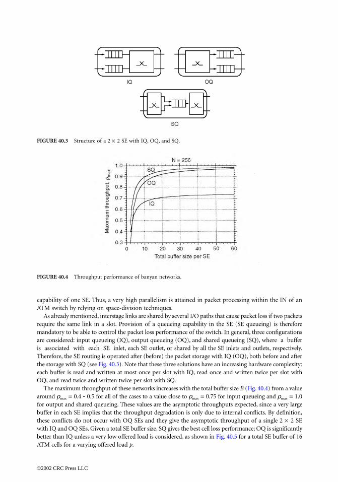
capability of one SE. Thus, a very high parallelism is attained in packet processing within the IN of anATM switch by relying on space-division techniques.

As already mentioned, interstage links are shared by several I/O paths that cause packet loss if two packetsrequire the same link in a slot. Provision of a queueing capability in the SE (SE queueing) is thereforemandatory to be able to control the packet loss performance of the switch. In general, three configurationsare considered: input queueing (IQ), output queueing (OQ), and shared queueing (SQ), where a bufferis associated with each SE inlet, each SE outlet, or shared by all the SE inlets and outlets, respectively.Therefore, the SE routing is operated after (before) the packet storage with IQ (OQ), both before and afterthe storage with SQ (see Fig. 40.3). Note that these three solutions have an increasing hardware complexity:each buffer is read and written at most once per slot with IQ, read once and written twice per slot withOQ, and read twice and written twice per slot with SQ.

The maximum throughput of these networks increases with the total buffer size B (Fig. 40.4) from a valuearound ρmax = 0.4 - 0.5 for all of the cases to a value close to ρmax = 0.75 for input queueing and ρmax = 1.0for output and shared queueing. These values are the asymptotic throughputs expected, since a very largebuffer in each SE implies that the throughput degradation is only due to internal conflicts. By definition,these conflicts do not occur with OQ SEs and they give the asymptotic throughput of a single 2 × 2 SEwith IQ and OQ SEs. Given a total SE buffer size, SQ gives the best cell loss performance; OQ is significantlybetter than IQ unless a very low offered load is considered, as shown in Fig. 40.5 for a total SE buffer of 16ATM cells for a varying offered load p.

FIGURE 40.3 Structure of a 2 × 2 SE with IQ, OQ, and SQ.

FIGURE 40.4 Throughput performance of banyan networks.


40.5 ATM Switch with Blocking MultistageIN and Arbitrary Depth

Another class of ATM switches has been developed using the same concept of cell self-routing character-izing a banyan network but now based on the use of unbuffered SEs. The basic idea behind this type ofswitching fabric is that packet loss events that would occur because of multiple packets requiring the sameinterstage link are avoided by deflecting packets onto unrequested SE output links. Therefore, the packetloss performance is controlled by providing several paths between any inlet and outlet of the switch, whichis generally accomplished by arranging a given number of self-routing stages cascaded one to another.Since each OPC of the switching fabric transmits at most one packet, queueing is still necessary whenthe interconnection network switches more than one packet in a slot to the same outlet interface (theIN has an internal speedup K). In this class of switch architectures, output queueing is obviously acc-omplished by providing each OPC of the switch with a queue.

The interconnection network of an N × N switch is a cascade of switching stages, each including N/2unbuffered SEs, whose interstage link patterns depend on the specific ATM switch architecture. Unlikeall other ATM switch classes, cells cross a variable number of stages before entering the addressed outputqueue, since direct connections to the output queues, through the SE local outlets, are also available fromintermediate stages. Also, the routing strategy operated by the switching block depends on the specificarchitecture. However, the general switching rule of this kind of architecture is to route the packets ontothe local outlet addressed by the cell as early as possible. Apparently, those cells that do not reach thisoutlet at the last switching stage are lost.

The cell output address, as well as any other control information needed during the routing operation,is transmitted through the network in front of the cell itself as the cell routing tag. A feature commonto all ATM switch architectures based on deflection routing is the packet self-routing principle, meaningthat each packet carries all of the information needed in the switching element it is crossing to be properlyrouted toward the network outlet it is addressing. Compared to the simplest case of self-routing operatedin a banyan network, where the routing is based on the analysis of a single bit of the output address,here the routing function can be a little more complicated and varies according to the specific architectureconsidered. Now, however, depending on the specific network architecture, the cell self-routing requiresthe processing of more than one single bit; in some cases, the overall cell address must be processed inorder to determine the path through the network for the cell.

Only two specific ATM switch architectures based on deflection routing will be described here to betterclarify the principles of their internal operations, the shuffleout switch [Decina et al., 1991] and thetandem banyan switch [Tobagi et al., 1991], although other architectures have also been proposed.

FIGURE 40.5 Loss performance of banyan networks.


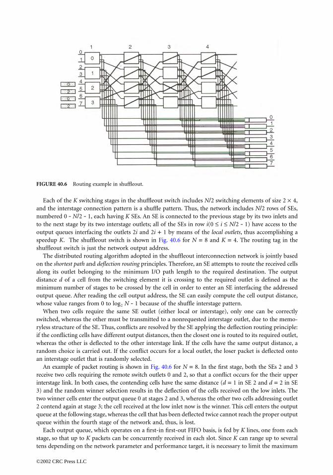
Each of the K switching stages in the shuffleout switch includes N/2 switching elements of size 2 × 4,and the interstage connection pattern is a shuffle pattern. Thus, the network includes N/2 rows of SEs,numbered 0 - N/2 - 1, each having K SEs. An SE is connected to the previous stage by its two inlets andto the next stage by its two interstage outlets; all of the SEs in row i(0 ≤ i ≤ N/2 - 1) have access to theoutput queues interfacing the outlets 2i and 2i + 1 by means of the local outlets, thus accomplishing aspeedup K. The shuffleout switch is shown in Fig. 40.6 for N = 8 and K = 4. The routing tag in theshuffleout switch is just the network output address.

The distributed routing algorithm adopted in the shuffleout interconnection network is jointly basedon the shortest path and deflection routing principles. Therefore, an SE attempts to route the received cellsalong its outlet belonging to the minimum I/O path length to the required destination. The outputdistance d of a cell from the switching element it is crossing to the required outlet is defined as theminimum number of stages to be crossed by the cell in order to enter an SE interfacing the addressedoutput queue. After reading the cell output address, the SE can easily compute the cell output distance,whose value ranges from 0 to log2 N - 1 because of the shuffle interstage pattern.

When two cells require the same SE outlet (either local or interstage), only one can be correctlyswitched, whereas the other must be transmitted to a nonrequested interstage outlet, due to the memo-ryless structure of the SE. Thus, conflicts are resolved by the SE applying the deflection routing principle:if the conflicting cells have different output distances, then the closest one is routed to its required outlet,whereas the other is deflected to the other interstage link. If the cells have the same output distance, arandom choice is carried out. If the conflict occurs for a local outlet, the loser packet is deflected ontoan interstage outlet that is randomly selected.

An example of packet routing is shown in Fig. 40.6 for N = 8. In the first stage, both the SEs 2 and 3receive two cells requiring the remote switch outlets 0 and 2, so that a conflict occurs for the their upperinterstage link. In both cases, the contending cells have the same distance (d = 1 in SE 2 and d = 2 in SE3) and the random winner selection results in the deflection of the cells received on the low inlets. Thetwo winner cells enter the output queue 0 at stages 2 and 3, whereas the other two cells addressing outlet2 contend again at stage 3; the cell received at the low inlet now is the winner. This cell enters the outputqueue at the following stage, whereas the cell that has been deflected twice cannot reach the proper outputqueue within the fourth stage of the network and, thus, is lost.

Each output queue, which operates on a first-in first-out FIFO basis, is fed by K lines, one from eachstage, so that up to K packets can be concurrently received in each slot. Since K can range up to severaltens depending on the network parameter and performance target, it is necessary to limit the maximum

FIGURE 40.6 Routing example in shuffleout.


number of packets entering the queue in the same slot. Therefore, a concentrator with size K × C isgenerally equipped in each output queue interface so that up to C packets can enter the queue concur-rently. The number C of outputs from the concentrator and the output queue size B (cells) will beproperly engineered so as to provide a given cell loss performance target.

In the N × N tandem banyan switch, shown in Fig. 40.7, K banyan networks are serially arranged sothat the total number of stages is now nK(n = log2 N) each including 2 × 2 switching elements. Differenttopologies can be chosen for the basic banyan network of the tandem banyan switch, such as the omega[Lawrie, 1975], the baseline [Wu and Feng, 1980], and others. Each output queue is fed now by only Klinks, one from each banyan network. The first banyan network routes the received packets according tothe very simple bit-by-bit self-routing (the specific bit to be used depends on the specific topology of thebanyan network). In case of a conflict for the same SE outlet, the winner, which is chosen randomly, isrouted correctly; the loser is deflected onto the other SE outlet, also by setting to 1 a proper field D of therouting tag, which is initially set to 0. Since each banyan network is a single I/O-path network, after thefirst deflection the packet cannot reach its addressed outlet in the same network. To prevent a deflectedpacket from causing the deflection of an undeflected packet at a later stage of the same network, the SEalways correctly routes the undeflected packet if two packets with different values of the field D are received.

The output queue i is fed by the outlet i of each of the K banyan networks, through proper packetfilters that select for acceptance only those packets with D = 0, whose routing tag matches the outputqueue address. The kth banyan network (k = 2,…,K) behaves accordingly in handling the packets receivedfrom the upstream network k - 1: it filters out all of the of undeflected packets and accepts only thedeflected packets (D = 1). Analogously to all of the previous architectures, packets that emerge from thenetwork K with D = 1 are lost.

Unlike shuffleout, here a much smaller number of links enter each output queue (one per banyan net-work) so that the output queue, in general, does not need to be equipped with a concentrator. On theother hand, in general, cells cross a larger number of stages here since the routing of a deflected cell isnot restarted just after a deflection, but rather when the cell enters the next banyan network.

Unlike ATM switches with input queueing where the head-of-the-line blocking limits the throughputperformance, the maximum throughput ρmax = 1 can be achieved in an ATM switch with deflectionrouting. Therefore, our attention will be focused on the cell loss probability. Cells can be lost in differentparts of the switch, that is, in the interconnection network (a cell reaches the last stage without enteringthe addressed local outlet), the concentrator, and the output queue. Loss events in the concentrator and

FIGURE 40.7 Architecture of the tandem banyan switch.


in the output queue can be easily constrained to arbitrarily low values by properly designing the numberof concentrator outlets and the output queue size. A much more critical parameter to achieve a low lossis the selection of the number of stages in the interconnection network that gives a particular low cellloss probability. Figure 40.8 shows that less than 20 (50) stages are needed in shuffleout to provide a cellloss probability lower than 10-7 for a switch with size N = 32 (1024) under maximum input load. Lessstages are required for lower input loads. Similar comments apply to the tandem banyan switch referredto the number of networks rather than to the number of stages. Figure 40.9 also shows that the banyannetwork topology significantly affects the overall performance. Adopting an omega topology (O) requiresless networks than with a baseline topology (B).

40.6 ATM Switch with Nonblocking IN

The third class of ATM switching fabrics is characterized by a nonblocking IN with packet queueingcapability placed in the IPCs (input queueing), the OPCs (output queueing), or placed within the INitself (shared queueing). Mixed queueing strategies have been proposed as well. Requiring a nonblockingIN means referring to a network free from internal conflicts, that is, in principle, to a crossbar network(switching in an N × N crossbar network is accomplished by N2 crosspoints, each dedicated to a specificI/O pair). Nevertheless, the centralized control characterizing a crossbar network makes this solution

FIGURE 40.8 Loss performance in shuffleout.

FIGURE 40.9 Loss performance in tandem banyan.


infeasible for a very high-speed ATM environment. As in the previous ATM switch classes, the only viablesolutions are based on the adoption of multistage arrangements of very simple SEs, each capable ofautonomously routing the cell to the required IN outlet.

The simplest ATM switch with nonblocking IN stores the cells in input queues located in the IPCs(IQ nonblocking IN). It is well known that a banyan network is nonblocking if the set of packets to beswitched is sorted (by increasing or decreasing output addresses) and compact (packets received onadjacent network inlets). Therefore, the IN basically includes a sorting network and a routing banyannetwork, which are implemented as a multistage arrangement of very simple sorting and switchingelements, respectively, whose size is typically 2 × 2. The number of stages of these networks is n(n + 1)/2for a Batcher sorting network [Batcher, 1968] and n for a banyan routing network, where n = log 2 N,each stage including N/2 elements. The simplicity of these SEs, each requiring a gate count on the orderof a few tens of gates, is the key feature allowing the implementation of these INs on a small number ofchips by relying on the current very large size integrated (VLSI) complementary metallic oxide (CMOS)technology. An example of sorting-routing IN is given in Fig. 40.10 for an 8 × 8 ATM switch, where thesix cells received by the IN are sorted by the Batcher network and offered as a compact set with increasingaddresses to the n-cube banyan network. Note that the nonblocking feature of the IN means that thenetwork is free from internal conflicts. Therefore, additional means must be available to guarantee theabsence of external conflicts occurring when more than one cell addresses the same switch outlet. Inputqueues hold the packets that cannot be transmitted immediately, and specific hardware devices arbitrateamong the head-of-the-line (HOL) cells in the different input queues to guarantee the absence of externalconflicts.

An OQ N × N nonblocking ATM switch provides cell storage capability only at OPCs. Now the IN isable to transfer up to K packets from K different inlets to each output queue without blocking due tointernal conflicts (it accomplishes an internal speedup K). Nevertheless, now there is no way of guaran-teeing the absence of external conflicts for the speedup K, as N packets per slot can enter the IN withoutany possibility of them being stored to avoid external conflicts. Thus, here the packets in excess of Kaddressing a specific switch outlet in a slot are lost.

According to the first original proposal of an ATM switch with pure output queueing, known as aknockout switch [Yeh et al., 1987], the IN includes a nonblocking N × N structure followed by as manyoutput concentrators as the switch outlets. The N × N nonblocking structure is a set of N buses, eachconnecting one of the switch inlets to all of the N output concentrators. Each of these is an N × Knetwork that is provided with N packet filters (one per attached bus) at its inputs, so as to drop all ofthe packets addressing different switch outlets.

A nonblocking N × N ATM switch with shared queueing behaves as a memory unit available in theIN and shared by all of the switch inlets to contain the packets destined for all of the switch outlets. Thesimplest implementation for this SQ switch model is given by a shared memory unit with N concurrentwrite accesses by the N inlets and up to N concurrent read accesses by the outlets. Clearly, such structure

FIGURE 40.10 Example of cell switching in a Batcher-banyan network.


shows implementation limits due to memory access speed, considering that the bit rate of the externalATM links is about 150 Mb/s. The current VLSI CMOS technology seems to allow the implementationof such N × N switches up to a moderate size, say, N = 16 or 32.

Multistage structures still provide a good answer for the implementation of larger size switches. Themost important proposal is the starlite switch [Huang and Knauer, 1984], whose IN is a Batcher-banyanstructure improved with additional hardware enabling feedback to the IN inlets those packets that cannotbe switched to the addressed outlets because of external conflicts (the architecture does not have aninternal speedup). Therefore, if P recirculation lines are available, then the size of the Batcher sortingnetwork must be increased up to (N + P) × (N + P). These recirculation lines act as a shared buffer of size P.

The maximum throughput of an (unbuffered) crossbar network is ρmax = 0.632 because of the unavoid-able external conflicts, whereas it drops to ρmax = 0.586 in an IQ nonblocking IN for an infinitely largeswitch (N = ∞). Thus, in spite of the queueing capability of this architecture, its capacity is even worsethan in a crossbar switch. This phenomenon is explained by considering that holding in the HOL positionthose cells that cannot be transmitted because of external conflicts is a statistically worse condition thanregenerating all of the cells slot by slot. Note that in a squared N × N switch with all active port controllers(PCs), a number h of blocked HOL cells imply h idle switch outputs, thus resulting in a carried load in theslot of only (N - h)/N. Nevertheless, behind a blocked HOL cell, the queue can hold other cells addressingone of the idle switch outlets in the slot. Such an HOL blocking phenomenon is said to be responsible forthe poor throughput performance of pure IQ switches.

At first glance, a question could arise: what is the advantage of adding input queueing to a nonblockingunbuffered structure (the crossbar switch), since this results in a decrease of the switch capacity? Theanswer is provided in Fig. 40.11 showing the packet loss probability for a crossbar switch and an IQswitch with an input queue size Bi ranging from 1 to 32 cells. If the target loss probability is, say, 10-9,we simply limit the offered load to p = 0.3 with Bi = 8, or to p = 0.5 for Bi = 32 with an IQ switch,whereas the packet loss probability of the crossbar switch is above 10-2 even for p = 0.05. Thus, inputqueueing does control the packet loss performance.

OQ nonblocking ATM switches show a much better traffic performance than IQ nonblocking switchesas they do not have any HOL blocking phenomenon. In fact, the OQ switch capacity is ρmax = 1 for N = Kand infinite output queue capacity. The loss performance is determined by the engineering of two parameters:the number of outlets per concentrator K, and the capacity of each output queue Bo. A speedup K = 8is enough to guarantee a loss in the concentrator on the order of 10-8 with p = 0.5 and 10-6 with p = 1.0 foran arbitrary switch size. Moreover, the offered load p must be kept below a given threshold if we wish tokeep the output queue capacity small by satisfying a given cell loss target (for example, B0 = 64 guaranteesloss figures below 10-7 for loads up to p = 0.9). The delay vs. throughput performance in OQ switches isoptimal since the packet delay is only determined by the congestion for the access to the same output link.

FIGURE 40.11 Loss performance with input queueing.


Nonblocking ATM switches using multiple queueing strategies have also been proposed so as to overcomethe performance limits of structures with input or shared queueing. Architectures with either mixedinput/output queueing (IOQ) [Lee, 1990] or mixed shared/output queueing (SOQ) [Giacopelli et al., 1991]have been proposed. These architectures are basically an expansion of the respective basic Batcher-banyanstructures in which K banyan networks are now available to switch up to K cells to the same OPC (theswitch has an internal speedup K) and OPCs are equipped with output queues, each with a capacity Bo.The main performance results attained by these mixed queueing architectures are that the HOL blockingcharacterizing IQ switches is significantly reduced in an IOQ switch and the number of recirculators P thatgive a certain loss performance decrease considerably in an SOQ switch compared to the basic SQ switch.

Table 40.1 provides the switch capacity of an IOQ switch for different speedups and output queuesizes for Bi = ∞ and N = ∞. Note that the first column only contains the numerical values of the independentvariable for which the switch capacity is evaluated, and its meaning is specified in each of the followingcolumns. The switch capacity grows very fast with the speedup value K for an infinitely large outputqueue, ρmax = 0.996 for K = 4, whereas it grows quite slowly with the output queue size given a switchspeedup K. In general, it is cheaper to provide larger output queues rather than increase the switchspeedup, unless the switching modules are provided in VLSI chips that would prevent memory expan-sions. Thus, these results suggest that a prescribed switch capacity can be obtained acting on the outputbuffer size, given a speedup compatible with the selected architecture and the current technology.

Analogously to OQ switches, pure shared queueing provides maximum switch capacity ρmax = 1 fora shared queue with infinite capacity. The loss performance of SQ and SOQ architectures is given inFig. 40.12 for N = 32 as a function of the normalized shared buffer size P/N for different offered loads.

TABLE 40.1 Switch Capacity with Mixed Input/Output Queueing

xBo = ∞ρm (K)

K = 2ρm(Bo)

K = 4ρm(Bo)

1 0.586 0.623 0.6332 0.885 0.754 0.7854 0.996 0.830 0.8838 1.000 0.869 0.938

16 0.882 0.96732 0.885 0.98264 0.885 0.990

128 0.994256 0.996∞ 1.000 0.885 0.996

FIGURE 40.12 Loss performance with shared queueing.


It is seen that even a small shared queue of 32 cells (P/N = 1) requires the offered load to be limited to p= 0.6 if loss figures below 10-5 are required. It is interesting to note how the SOQ switch capacityapproaches 1 even with a small shared buffer capacity by adopting a very little speedup (ρmax = 1 - 10-6

for K = 3 and P = 7).

40.7 Conclusions

The main architectural and performance features of switching fabrics for broadband networks based onasynchronous time-division switching have been presented. It has been shown that multistage arrange-ments of very simple switching elements is the typical solution adopted in ATM switches, which enablesthe processing required by ATM cells to be compatible with the bit rate on the incoming links. All of thedifferent switch classes presented are able to provide the required performance target in an ATM network,typically the cell loss probability, by means of a suitable limitation of the offered load. Choosing onearchitecture rather than another is just a matter of finding an acceptable tradeoff between implementationcosts and traffic performance.

Defining Terms

Arbitrary depth network: Interconnection network providing more than one internal path per inlet/outlet pair.

Asynchronous transfer mode (ATM): Transport technique defined for the lower layers of the broad-band communication network.

ATM cell: Basic fixed-size unit defined for the transport of user information in a broadband ATM network.Blocking network: Network in which internal conflicts occur for an arbitrary permutation that is free

from external conflicts for a given network speedup.Cell self-routing: Property of a multistage interconnection network that consists of the autonomous

routing of the packets in each switching element only based on a routing tag carried by the cellwithout the use of many central control.

Deflection routing: Routing technique that deviates a packet from its intended route through thenetwork because of an internal conflict.

External conflict: Conflict between packets for the access to the same network outlet.Input queueing: Queueing strategy in which the information units are stored in buffers associated with

the inlets of the interconnection network (or a switching element).Internal conflict: Conflict between packets for the access to the same link internal to the interconnection

network.Minimum depth network: Interconnection network providing only one internal path per inlet/outlet pair.Network speed-up: Number of packets that can be concurrently received at each output interface of

an interconnection network.Nonblocking network: Network free from internal conflicts for an arbitrary permutation that is free

from external conflicts for a given network speedup.Output queueing: Queueing strategy in which the information units are stored in buffers associated

with the outlets of the interconnection network (or a switching element).Shared queueing: Queueing strategy in which the information units are stored in a buffer shared by

all of the inlets and outlets of the interconnection network (or a switching element).

References

Batcher, K.E. 1968. Sorting networks and their applications. In AFIPS Proceedings of Spring Joint ComputerConference, 307–314.

Decina, M., Giacomazzi, P., and Pattavina, A. 1991. Shuffle interconnection networks with deflectionrouting for ATM switching: the open-loop shuffleout. In Proceedings of the 13th InternationalTeletraffic Congress, Copenhagen, Denmark, June, 27–34.


Giacopelli, J.N., Hickey, J.J., Marcus, W.S., Sincoskie, W.D., and Littlewood, M. 1991. Sunshine: a highperformance self-routing broadband packet switch architecture. IEEE J. Select. Areas Commun.,9(Oct.):1289–1298.

Huang, A. and Knauer, S. 1984. Starlite: A wideband digital switch. In Proceedings of GLOBECOM 84,Atlanta, GA, Nov., 121–125.

ITU. 1991. B-ISDN protocol reference model and its application. ITU-TI.321, International Telecommu-nications Union-Telecommunications Standardization Sector, Geneva, Switzerland.

ITU. 1993. B-ISDN asynchronous transfer mode functional characteristics. ITU-TI.150, InternationalTelecommunications Union-Telecommunications Standardization Sector, Geneva, Switzerland.

Lawrie, D.H. 1975. Access and alignment of data in an array processor. IEEE Trans. Comp., C-24(12):1145–1155.Lee, T.T. 1990. A modular architecture for very large packet switches. IEEE Trans. Commun., 38(7):1097–

1106.Tobagi, F.A., Kwok, T., and Chiussi, F.M. 1991. Architecture, performance and implementation of the

tandem banyan fast packet switch. IEEE J. Select. Areas Commun., 9(8):1173–1193.Wu, C.L. and Feng, T.-Y. 1980. On a class of multistage interconnection networks. IEEE Trans. Comp.,

C-29(Aug.) :694–702.Yeh, Y.S., Hluchyj, M.G., and Acampora, A.S. 1987. The knockout switch: a simple, modular architecture

for high-performance packet switching. IEEE J. Select. Areas Commun., SAC-5(Oct.):1274–1283.

Further Information

A greater insight in the area of switching architectures for ATM networks can be obtained consulting themain journals and conference proceedings in the field of telecommunications in the last 15 years. A verycomprehensive survey about architectures and traffic performance of ATM switches can be found inA. Pattavina, Switching Theory, Architectures and Performance in Broadband ATM Networks, John Wiley& Sons, 1998.


41Internetworking

41.1 Introduction 41.2 Internetworking Protocols

TCP/ IP Internetworking • SNA Internetworking• SPX/IPX Internetworking

41.3 The Total Network Engineering ProcessNetwork Awareness • Network Design • Network Management

41.4 Internetwork Simulation41.5 Internetwork Optimization41.6 Summary.

41.1 Introduction

Engineering an internetwork is a lot like a farmer getting his apples delivered from an orchard to thesupermarket. First, the farmer needs something to put the apples in: a bag, a box, a basket, or maybe acrate; second, the farmer needs to drive on some roads over a specific route. Those same two problemsconfront an engineer trying to get data delivered from one local area network (LAN) to another. Devel-oping an internetwork involves finding something to put the apples in and providing a way to transportthem from the orchard to the supermarket. The apples are the data and the container is the communi-cations protocol that encapsulates or contains the data. Communications protocols envelope the appli-cation data and provide a container to ensure the goods are delivered safely and reliably. Internetworksrequire compatible protocols at both the transmitting and receiving sites. Various communicationsprotocols are available such as transmission control protocol/Internet protocol (TCP/IP), system networkarchitecture (SNA), DECnet, IPX, AppleTalk, and XNS, to name a few.

Roads and routes the farmer travels on from the orchard to the supermarkets represent telecom-munications circuits the communications protocols use to route the data from source to destination.Engineering an internetwork involves sizing circuits and designing routes for the efficient and optimaltransfer of information between LANs. Providing cost-effective and properly performing internetworksinvolves designing the best type of circuits, either dedicated or switched, and sizing bandwidth requirements.

Internetworking is defined in the IBM dictionary of computing as “communication between two or morenetworks.” Miller [1991] defined the term as “communication between data processing devices on one networkand other, possibly dissimilar devices on another network.” For the purpose of this chapter, internetworkingwill take on the meaning of connecting two or more LANs to broaden the scope of communications.

41.2 Internetworking Protocols

Understanding, designing, and optimizing an internetwork would be too difficult unless the problemwere broken down into smaller subtasks. Communications architectures partition functionality intoseveral layers, each providing some service to the layer above and using the services of the layer below.

Harrell J. Van NormanUnisys Corporation


Figure 41.1 illustrates the seven-layer International Organization for Standardization (ISO) open systemsinterconnection (OSI) reference model. TCP/IP, SNA, and sequence packet exchange/Internet packetexchange (SPX/IPX) are mapped into the seven-layer model. Each of the communications protocols con-verge at the data link and physical layers; however, the architectures all diverge at the network layer. Eachcommunications protocol is represented uniquely at the upper five layers of the OSI communications model.

The data link layer is relevant to internetworking because this is where bridges operate. The serviceprovided by the data link layer is important to routers—the key internetworking device, operating at thenetwork layer. The transport layer is the user of network services and is influenced by the routing decisionsmade at the network layer. These three layers are the primary focus of internetworking.

Two models represent how an internetwork appears to endnodes. In the connectionless or datagrammodel, an endnode transmits packets containing data and the destination address to which the data isto be delivered. The network does the best to deliver the data, with some probability that the data willget lost, duplicated, or damaged. Packets are individually routed and the network does not guarantee thepackets will be delivered in the same order they were sent.

The connectionless model is similar to the postal system in which each letter enters the postal systemwith the address where it should be delivered. The postal system does its best to deliver the data, withsome probability that the letter will get lost or damaged. Letters are individually routed, and a letterposted on Monday might get delivered after a letter posted on Tuesday, even if both were posted fromthe same location and addressed to the same location.

The other model is the connection-oriented or virtual circuit. Here, an endnode first informs the networkthat it wishes to start a conversation with some other endnode. The network then notifies the destinationthat a conversation is requested, and the destination accepts or refuses. This is similar to the telephonesystem in which the caller informs the telephone system of the wish to start a conversation by dialing thetelephone number of the destination. The telephone system establishes a path, reserves the necessaryresources, contacts the destination by ringing its phone, and after the call is accepted, the conversation cantake place. Often, a connection-oriented service has the following characteristics [Perlman, 1992]:

1. The network guarantees packet delivery.2. A single path is established for the call and all data follows that path.3. The network guarantees a certain minimal amount of bandwidth.4. If the network becomes overly utilized, future call requests are refused.

FIGURE 41.1 Internetworking communications protocol architectures.


TCP/IP Internetworking

TCP/IP has emerged as the primary communications protocol for developing internetworks. Why? Theanswer is simple: interoperability; almost every conceivable combination of computer hardware andoperating system has a driver available for TCP/IP. International travelers know English is the speakingworld’s most common second language. A native language may be preferred when speaking with localfamily and friends, but English is the worldwide second language and is predominately used to commu-nicate internationally. Similarly, TCP/IP has emerged as the primary protocol for communicating betweennetworks.

The suite of TCP/IP protocols, adopted in the 1970s by the U.S. Department of Defense, is the Internetbackbone. Now, over 3.1 million users are connected to the Internet, all speaking IP, up 81% from lastyear. The International Data Corporation (IDC), in Framingham, MA, estimates 4.5 million PCs arerunning TCP/IP and the cumulative installed base for TCP/IP is 8 million computers. TCP/IP is clearlythe internetworking protocol of choice.

Endorsements of TCP/IP just keep coming. First, Microsoft tucked a TCP/IP stack into Windows NTVersion 3.1 and declared TCP/IP its strategic wide-area network protocol family. Most recently, a federallycommissioned panel recommended that the government sanction TCP/IP as a standard and surrenderits open systems interconnection-only stance in the Government OSI Profile (GOSIP). TCP/IP, thepreferred protocol for internetworking, is also becoming the primary backbone protocol for local com-munications.

One of the major forces driving TCP/IP to the PC desktop is UNIX, which usually includes TCP/IP.UNIX has become the de facto standard enterprise server OS. As users downsize from mainframeplatforms and adopt UNIX-based servers, they must outfit their PCs with access to TCP/IP. Downsizingis a major trend as processing power becomes more cost effective in the minicomputer and micro-computer platforms. An Intel 286-based PC introduced in 1983 provided 1 MIPS performance, in1986 the i386 offered 5 MIPS, in 1990 the i486 came with 20 MIPS, and more than 100 MIPS was availablein 1993 with the Pentium. Intel plans to routinely increase desktop processing power with the i686 in1995, offering 175 MIPS, the i786, slated to provide 250 MIPS in 1997, and the i886 in 1999, capable ofapproximately 2000 MIPS.

TCP/IP is a connectionless protocol. TCP operates the transport layer and IP is the network layerprotocol based on 4 octet addresses. A portion of the address indicates a link number and the remain-ing portion a system or host on the network. A 32-b subnet mask has 1s in the bits corresponding tothe link portion of the IP address and 0s in the bits belonging to the host identifier field. If an IP ad-dress is X and its mask is Y, to determine whether a node with IP address Z is on the same link, ANDthe mask Y with X and AND the mask Y with Z. If the result is the same, then Z is on the same link.

Originally, IP addresses were grouped according to three distinct classes: class A contained the networkaddress field in the first octet and host identifier in the remaining 3 octets, class B contained the networkaddress field in the first two octets and the host in the remaining two fields, and class C contained thenetwork address field in the first three octets and the host identifier in the remaining octet. Today, IPallows a variable sized subnet mask and even permits noncontiguous 1s in the mask. This can result inincredibly confusing and computationally inefficient addressing structures. Regardless, each node on alink must know the subnet mask of its own IP address.

IP routers connect networks by routing packets based on destination link numbers, not destinationhost identifiers. If IP routers had to route packets to destination hosts, enormous memory would benecessary to contain information about every machine on the Internet. Consequently, IP routing doesnot route to the destination endnode, it routes only to the destination link.

TCP/IP does have a certain amount of overhead associated with address resolution protocol (ARP)queries and responses that can degrade network performance significantly. The ARP allows a host to findthe physical address of a target host on the same link number, given only the target’s IP address. Forexample, if host A wanted to resolve the IP address of host B, a broadcast query would be transmittedand received by all hosts, but only host B would respond with its physical address. When A receives thereply, it uses the physical address to send packets directly to B. Considerable bandwidth and memory in


routers are consumed by routers keeping track of endnodes rather than just keeping track of links [Comer,1991].

Improvement of the TCP/IP protocol suite will come in new protocols and emerging classes of appli-cations. The dynamic host configuration protocol (DHCP) is being standardized to automatically gatherdetail configuration data for a PC when it joins the network, creating a plug-and-play environment.Historically, network administrators manually set parameters on each workstation, such as IP addressesand domains, but BOOTP and DHCP have advanced TCP/IP to an automated installation process.

Two classes of emerging applications for TCP/IP include interenterprise and personal interenterprise.Interenterprise applications unite different organizations’ networks; for example, a retailer could orderautomatically from his suppliers or check credit-card information, all by TCP/IP. This brings electronicdata interchange transactions, typically separate dial-up links, into the TCP/IP network. Personal inter-enterprise applications customize a PC view of the Internet, so that when connected, specific informationis automatically presented, such as stock portfolio data.

The Internet is the largest network in the world, a network of networks that unarguably demonstratesthe usefulness of TCP/IP. But TCP/IP is suffering from its own success. By the year 2020, the Internet willlikely have exhausted all available addressing space. The Internet’s standards-setting body, the InternetEngineering Task Force, has adopted the next generation IP. Called IPng, this new version of the IP layerwill solve the problem of dwindling address space by supporting 16-byte addresses that will allow billionsmore users to surf the Internet. The new protocol (to be assigned version number IP6) will not requireany immediate changes to users’ existing IP internetworks. However, users will need to upgrade theirrouters and eventually change applications if they want to take advantage of the advanced features ofIPng, such as flow control, autoconfiguration, and encryption-based security.

SNA Internetworking

IBM’s SNA traffic is difficult to integrate into a multiprotocol internetwork because it is a nonroutableprotocol. NetBIOS and Digital’s local area transport (LAT) are also nonroutable protocols. Although itis unfortunate, these nonroutable protocols are without network addresses. Without network layerfunctionality, only bridges can internetwork native SNA. There is no intrinsic reason why these protocolscould not have been designed to run with network layer addresses, they just were not. Perhaps designersnever believed LANs would be internetworked.

Routers, as opposed to bridges, are the primary internetworking devices used to direct traffic from itssource to its destination. Bridging is useful in simple point-to-point networks where alternate paths arenot available and where protocol overhead is not a significant factor. Disadvantages of bridges relativeto routers include:

• Bridges can use only a subnet of the topology (a spanning tree). Routers can use the best paththat physically exists between source and destination.

• Reconfiguration after a topological change is an order of magnitude slower in bridges than routers.

• The total number of stations that can be interconnected through bridges is limited to the tens ofthousands. With routers, the total size of the network is, for all practical purposes, unlimited (atleast with ISO).

• Bridges limit the intermediate hop count to seven, significantly restricting the size of an inter-network.

• Bridges offer no firewall protection against broadcast storms.

• Bridges drop packets too large to forward, since the data link layer cannot fragment and reassemblepackets.

• Bridges cannot give congestion feedback to the endnodes.

For the past several years, most corporations relied on token ring bridges implementing SNA’s data linkprotocol, Logical Link Control 2 (LLC2), to give PCs on remote LANs a way to access IBM mainframe data.


Frames are forwarded throughout the internetwork by token ring bridges using source-route bridgingprotocol to ensure data is delivered to the proper destination. The problem is that even a few seconds ofcongestion on the wide area network (WAN) link can drop the SNA/LLC2 sessions.

IBM’s data link switching (DLSw) standard provides the reliability needed to integrate mission-criticalSNA networks with IP backbones. DLSw products integrate SDLC with IP by stripping off the synchro-nous data link control (SDLC) header and replacing it with a TCP/IP header. Prior to DLSw routers,SNA data was encapsulated in TCP/IP, leaving the SDLC headers intact. Current testing of router vendors’DLSw implementations indicate they keep SNA sessions from being dropped over even the most congestedinternetwork links. Performance at full speed of the WAN link is another big improvement over tokenring bridges. A successor to source-route bridging, DLSw routers deliver high-performance SNA inter-networking even with significantly more complexity than source-route bridging.

The DLSw scheme allows routing IP and internetwork packet exchange (IPX) traffic alongside connection-oriented SNA. DLSw routers have the added complexity of blending connectionless LAN traffic withconnection-oriented SNA traffic by sending messages to the stations on each end of the connections,acknowledging that a path is still open between them. Preventing the SNA connection from timing outand dropping sessions involves considerable overhead traffic, such as frequent receiver ready, keep alivebroadcasts, and timing signals for constant responses.

DLSw routers are criticized by some SNA users because of the inconsistent performance associatedwith contention-based internetworks. IP response time may be nearly instantaneous one time and maytake a second the next, frustrating SNA users accustomed to consistent performance. DLSw can benefitlarge SNA networks suffering from time outs, hop limits, alternate routing disruptions, and the lack ofsecurity mechanisms. DLSw routing gives non-routable SNA traffic the robustness of nondisruptivealternate routing when links or nodes fail, the benefits from open nonproprietary protocols, and the costeffectiveness of standard TCP/IP-based solutions.

For IBM users, there is the option of remaining all “blue” with IBM’s advanced peer-to-peer networking(APPN) family of protocols, the next generation of SNA. IBM continues to develop, position, and promoteits own APPN as the only viable next-generation networking technology for its mainframe customers.The need for guaranteed response time in their mission-critical mainframe applications makes APPN anattractive option. Other advantages to the APPN approach include full class of service applicationpriorities, enhanced fault management through NetView monitoring, the added efficiency from notencapsulating SNA into a routable protocols like TCP/IP and thereby doubling the addressing overhead,and improved accounting from SNA usage statistics.

SPX/IPX Internetworking

The number one LAN protocol is undoubtedly Novell’s sequence packet exchange/Internet packetexchange (SPX/IPX), but most network administrators use TCP/IP for internetworking. As a result,Novell has taken two significant steps to improve the performance of SPX/IPX for internetworking:packet burst and the network link services protocol (NLSP).

Before packet burst, the NetWare core protocol (NCP) was strictly a ping-pong discipline. The work-station and the server were limited to communicating by taking turns sending a single-packet requestand receiving a single-packet response. Packet burst is an NCP call permitting a sliding window techniquefor multiple packet acknowledgment. By transmitting a number of packets in a burst, before waiting foran acknowledgment or request, packet burst eliminates the ping-pong effect and can provide up to a60% reduction in the number of packets to read or write large files. Limited to only file reads and writes,packet burst cannot reduce the ping-pong method of all other NCP communications such as openingdirectory handles, locating and opening files, and querying the bindery.

Rather than reducing the number of packets when the receiving station or internetwork becomescongested, as do most transport layer protocols, packet burst actually varies the interpacket gap (IPG).The IPG is the time between the end of one packet and beginning of the next packet. Varying the IPGfor flow control is called packet metering.


The amount of data sent during a burst is called the message. Message size is based on the numberof packets in the burst, called the window size, and the media access method of the link. The defaultwindow size has been optimized for most communications to 16 packets for a read and 10 for a write.For example, 16 reads on a token ring link with a 4096 packet size gives a 53-KB message. On an ether-net link, a read message is about 22 KB (16 × 1500 bytes). The number of packets in the burst windowcan be increased on high-speed links and where the degree of transmission success is high. If a packetor packets are lost in transmission for any reason, the client will send a request for retransmission of thelost packets. The server will retransmit only those packets that were lost. Once the client has all of thepackets, it requests another message; however, since packets were lost, the IPG is increased for the nexttransmission. The IPG will continue to be increased until packets are no longer being lost.

NLSP is another internetworking improvement to NetWare. Novell developed the link-state routerprotocol NLSP, to replace the older IPX distance-vector based router information protocol (RIP). IPXRIP is similar to Cisco’s IGRP, IP RIP, and RTMP in the AppleTalk suite. Distance-vector routing requireseach node to maintain the distance from itself to each possible destination. Distance vectors are computedusing the information in neighbors’ distance vectors and store this information in routing tables thatshow only the next hop in the routing chain rather than an entire map of the network. As a result, RIPfrequently broadcasts these summaries to adjacent routers.

Distance-vector routing is efficient for routers with limited memory and processing power, but newerrouters typically have reduced instruction set computer (RISC) processors with power to spare. Link-state routers can provide full knowledge of the network including all disabled links with a single query.With distance-vector routers, this would involve querying most, if not all, of the routers. In addition,link state routers, like NSLP, converge more quickly than distance-vector routers, which cannot passrouting information on until distance vector has been recomputed. NSLP supports large, complex IPXinternetworks without the overhead present in NetWare distance-vector routers.

NSLP routers compress service advertizing protocol (SAP) information and only broadcast SAP packetsevery two hours unless a change is made to network services, such as print servers or file servers. SAPbroadcast overhead can be significant, especially with many servers or services. Novell has also reducedSAP traffic on the network by using NetWare Directory Services (NDS) to keep all network servicesinformation on a central server. NDS is available in NetWare 4.x and is similar to TCP/IP’s domain nameserver (DNS). Novell also provides the capability to communicate with different systems through NetWarefor SAA, NetWare NFS, and NetWare TCP/IP Gateway.

41.3 The Total Network Engineering Process

This guide to internetworking provides a step-by-step engineering approach. Migrating from a LAN orseveral LANs to an internetwork is no small undertaking. Key to the process of analyzing and designinginternetworking strategies is employing analytic heuristic algorithms and simulation techniques. Networkdesign tools are essential to effectively evaluate alternative internetworking schemes while attempting tooptimize communications resources. As new networking requirements surface, engineers design capacityand equipment to satisfy the demands. Facing requirements on an as-needed basis results in networkevolution. Networks developed in an evolutionary manner provide incremental solutions to an array ofindividual requirements. With each new requirement, the most cost-effective configuration of equipmentand communications lines is determined, focusing on the specific need. Unfortunately, design decisionsare often made without rigorous analysis of the entire network, addressing only the incremental expan-sion. This approach seldom provides the best design for the total communications environment.

The preferred method of addressing network requirements is through a structured-design approach.Here, alternative design techniques for the entire network are evaluated in terms of response time, cost,availability, and reliability. While avoiding excessive redesign and allowing for orderly capacity expansion,the process of network engineering evaluates current networking requirements and plans for futurenetwork expansion.


Figure 41.2 shows the total network engineering process and its three phases: awareness, design, andmanagement. Network awareness quantifies current traffic, equipment inventories, forecasted growth,and operational objectives. Network design uses design tools, performs a cost/performance breakevenanalysis, and develops line configurations. Network management encompasses management of config-uration, faults, performance, accounting, and security. Equipment and network software is acquired,verified, installed, maintained, and administered.

Network Awareness

The process of network awareness includes the following operations:

• conducting a traffic inventory by collecting measurements of current traffic

• mapping the physical inventory of networking equipment into the logical interconnections

• forecasting requirements for network growth through surveying line management

• qualifying through senior management the criteria used to evaluate operational tradeoffs

Many of these inputs are, of necessity, qualitative or conceptual in nature, whereas others can be quantifiedwith varying degrees of accuracy. Using a network design process often requires a greater level of networkawareness than most engineers generally possess. When an engineer has an accurate understanding ofthe network—including possible bottlenecks, response time spikes, and traffic patterns—the process ofnetwork design can begin. Gaining an accurate awareness of network traffic involves monitoring currentloads via a network analysis tool, like the LANalyzer, Sniffer, or through the use of RMON probes. Trafficstatistics for network planning should be collected, not only for all significant hours of each day, but alsofor a significant number of days in a year. CCITT recommends measuring carried traffic statistics for atleast the 30 days (not necessarily consecutive) of the previous 12 months in which the mean busy hourtraffic is the highest. A second-choice method recommended by CCITT, when the first method is notpossible, consists of a measuring period of 10 consecutive normal working days during the busiest seasonof the year [CCITT, 1979]. Both average and peak loads are characterized hourly over the sampling periodto understand current bandwidth requirements. Monitoring new networked applications predicts theirimpacts to the internetwork. Traffic must also be differentiated between what stays local, remaining onlywithin a LAN, and traffic that is internetworked between remote locations via WAN links.

Interviews with line management help to forecast growth requirements. Many managers have hiddenagendas for using the network for a variety of business purposes. Without surveys or interviews of key

FIGURE 41.2 The total network engineering process.


management personnel, predicting future network requirements is impossible. Questions need to centeraround four key areas:

1. Future business communications requirements based on the use of advancing technologies2. Planned facility changes and population shifts through developing new business partners3. Forecasted needs for external connectivity with customers, vendors, and new markets4. Changes in business practices based on new programs, applications, and remote systems access.

A little-publicized problem, but one that nevertheless causes big headaches, is developing an inventoryof current network equipment. Obtaining an accurate image of the inventory database is helpful in thenetwork engineering process to gain an improved network awareness. Based on network discoverytechniques, like IP discovery and IPX SAP, routing nodes may be identified throughout the internetwork.These techniques only find network layer routing devices; however, internetworks are primarily basedon routers rather than data link layer bridges. Once these devices are identified, MIB browsers are effectiveto understand what mix of protocol traffic is being routed throughout the internetwork. Finally, atopological map can be developed by translating the logical routing to physical locations.

Top level management must also be involved to quantify the operational evaluation criteria. Everybusiness has established measures for effective operations. A network exists to meet the needs of thosewho use the network, not the preferences of those who maintain it. Therefore, objectives for the com-munications resources should be a reflection of those criteria held by the business as a whole. Five keyoperational evaluation criteria or network design goals characterize most networks: performance, avail-ability, reliability, cost, and security. Manufacturing industries and start-up companies often choose costminimization, financial markets mandate high reliability, security is of utmost importance throughoutclassified governmental networks like the Department of Energy (DOE) nuclear weapons complex, andhigh performance is necessary to mass merchandise retail companies. Key operational evaluation criteriaare described below.

Cost minimization is a weighty design factor that includes both monthly recurring and nonrecurringfees. To compare competing alternatives with different cost outlays, the time value of money must beconsidered and the net present value method is usually the best method for financial analysis. In thename of cost minimization, depending on the specific operational objective, one may be led to differentsolutions given the same problem. Variations of cost minimization goals include: build the cheapestnetwork, get the most network for the dollar, maximize profit by allowing the firm to reach new markets,minimize risk of loss, or maximize growth opportunity.

All network designs include an inventory of lines, equipment, and software needed to make them run.Including all of the cost elements (installation costs, shipping costs, purchase price, monthly lease costs,maintenance costs, and service costs) in the optimization process prevents unpleasant surprises. Totalnetwork costs CTOT include the three major cost components in a network design: line costs, equipmentcosts, and software costs:

(41.1)

where:CAL = access line costsCTL = interoffice channel (IXC) line costsCIE = internetworking equipment costs (remote bridge, router, gateway, etc.)CWAE = WAN access equipment costs [modems, computer software unit/data software unit (CSU/DSU),

channel banks, etc.] CS = software costs

Too often, availability and reliability are mistakenly assumed to be synonymous. Reliability and service-ability are both components of availability. Network availability, a value between zero and one, reflectsstability characteristics of communications systems connecting end users. Availability A is composed oftwo factors: reliability, the probability a system will not fail during a given time, is expressed as mean

CTOT CAL CTL CIE CWAE CS+ ++ +=


time between failure (MTBF), and serviceability, including the time required to diagnosis and repair, isexpressed as mean time to repair (MTTR),

(41.2)

Performance is another key operational evaluation criteria. Represented by average transaction responsetimes RT, it can be calculated by the following formula:

(41.3)

whereIT = input message transmission time: number of bits in input message/link speed bits per second +

propagation delayHT = host processing timeOT = output message transmission time: number of bits in output message/link speed bits per second +

propagation delay

At the completion of the network awareness phase, the network planner must objectively evaluate whetheror not this phase has been completed adequately for the purpose of the design process. Questions thatmight be addressed are:

• Do I have a reasonable assessment of current technology in this networking arena?

• Have I quantified the current network traffic?

• Is there a justifiable forecast of network growth?

• Are the operational objectives and goals quantified and agreed upon by upper level management?

Upon completion, quantifiable operational evaluation criteria are available as input into the networkdesign phase.

Network Design

For too long, networks merely evolved to their present condition by adding users and applications withoutanalyzing performance impacts. The better way is for engineers to describe the topology and media viaa network modeling tool. In many network design tools, models are constructed by connecting iconsrepresenting specific network devices or segments. Behind the model, powerful software simulates andanalyzes the behavior of the network. Also, network conditions such as protocols, traffic patterns, andnumber of nodes are specified in the model. Traffic can be characterized from statistical traffic modelsor actual traces of network traffic taken from an analyzer. Simulation and performance evaluation predictnetwork performance and explore future design options. Graphical user interfaces (GUI) simplify chang-ing assumptions on number of users, type of media protocol stacks, application mix, traffic patterns,and so on. When the network model is in place, proposals for adding or deleting resources (such ascontrollers, terminals, multiplexers, protocol converters, remote front-end processors), redesigning appli-cation software, or changing routing strategies may be evaluated.

Network design consists of applying network design tools, evaluating alternative network configura-tions through a cost/performance breakeven analysis, and optimizing communications lines. Becausethere are many ways to configure a network and interconnect transmission components, it is not realisticto evaluate exhaustively every possible option. However, by using certain shortcuts, called heuristics(procedures that approximate an optimal condition using algorithms), the number of feasible designscan be scaled down to a manageable few.

Network design tools are developed using heuristic algorithms that abbreviate the optimization processgreatly by making a few well-chosen approximations. Queuing theory is incorporated in the algorithms

A MTBF/ MTBF MTTR+( )=

RRT IT HT OT+ +=


that calculate response times. A convenient notation used to label queues is:

(41.4)

where:A = arrival process by which messages are generatedB = queue discipline, describing how messages are handledn = number of servers availableK = number of buffering positions availablep = ultimate population size that may possibly request service

Some of the more typical queuing models pertaining to internetworking are as follows:

• Memoryless (exponential) interarrival distribution, memoryless service distribution, one server(M/M/1) is typical of situations involving a communications server or a file server of electronicmail.

• Memoryless (exponential) interarrival distribution, memoryless service distribution, c servers (M/M/c)are typical of situations involving dial-up ports for modem pools or private branch exchange (PBX)trunks.

• Memoryless (exponential) interarrival distribution, fixed (deterministic) service time, one server(M/D/1) is representative of a trunk servicing a packet switched network.

A number of internetworking situations require a more advanced model involving distributions otherthan exponential or deterministic. For the terminal nodes of a communications system, the queue typethat is most appropriate is M/G/l distributions, referring to a generic service time represented by G. Thismeans the process messages that arrive are modeled as Markovian. The M/G/1 solution of queuing delayis given by the Pollaczek–Khinchin (PK) formula:

(41.5)

whered = total delaym = average time to transmit a messagel = number of arriving messages/secondp = utilization of the facility, expressed as a ratio

After a network model is produced, network engineers often use the tool to evaluate different scenariosof transmission components and traffic profiles. Through an iterative process of network refinement,“what if” questions may be addressed concerning various alternative configurations:

• What would be the impact on performance and utilization if more nodes are added to my network?

• How would response times change if my internetwork links were upgraded from voice gradeprivate lines to 56-kb/s digital circuits; from fractional T-1 dedicated circuits to fast packet switchedframe relay?

• How will downsizing to client/server technologies impact the network?

• Should I segment the network with high-speed switches or with traditional routers?

• How much additional capacity is available before having to reconfigure?

• What effect do priorities for applications and protocols have on user response times?

Each of the various alternative configurations will have associated costs and performance impacts. Thisproduces a family of cost/performance curves that forms a solution set of alternative network designs.With the cost/performance curves complete, the final selection of an optimum configuration can be leftup to the manager responsible for balancing budget constraints against user service levels.

A/B/n/K/p

d m l * m2/ 2 1 p–( )[ ]+=


At the completion of network design, the network planner must objectively evaluate whether or notthis phase has been completed adequately for the purpose of the design process. Questions that mightbe asked are:

• Is the model verified by accurately representing the inputs and generating output that satisfy theoperational evaluation criteria?

• Is the cost/performance breakeven analysis selected from the family of feasible solutions the onebest configuration based on the operational evaluation criteria?

• Is the equipment rated to function well within the design objectives?

When this phase is complete, an optimized implementable network design is available as input into thenetwork management phase.

Network Management

Network management includes equipment acquisition, verification, installation, maintenance, and admin-istration. This phase of the network engineering process feeds information into the network awarenesscomponent, which completes the cycle and begins the iterations of design and refinement.

Network design tools use statistical techniques to make certain assumptions about the behavior of anetwork and the profiles of transactions in the network. These assumptions in terms of lengths, distri-butions, and volumes of traffic make the mathematics easier, at the expense of accuracy. Operationalnetworks often violate, to a certain extent, many design assumptions. The optimized network designsconfront the real world of actual network performance during the network management phase. Detectedvariances between optimized network designs and actual network performance provide an improvedawareness concerning host processing requirements, traffic profiles, and protocol characteristics.

In a nutshell, network management improves awareness. Design iterations and refinement based onimproved network awareness progress toward the optimum. Network management refines operationalevaluation criteria. Cost/performance ratios are evaluated against the operational objectives and goalsan organization is employing. Network management avoids crises by reacting proactively to changingtrends in utilization and performance.

At the completion of network management, the network planner must objectively evaluate whetheror not this phase has been completed adequately for the purpose of the design process. Questions thatmight be asked are:

• Is the network operating error free or are there periodic or isolated errors?

• Is the network performing properly by satisfying response time and availability goals?

When this phase is complete, an operational network is available.Finally, the network engineer must verify and validate the model by asking: is the model validated by

the performance of the operational network? If this objective evaluation results in discrepancies betweenthe model and the real world operational network, then there must be a return to the network awarenessphase for model refinement and, possibly, improved optimization. Whenever new needs are placed onthe network, the process must be reinitiated, with a revised needs analysis reflecting these new require-ments. When the model is fully validated and verified, the network planner can exit the total networkengineering decision process with an optimized operational network.

41.4 Internetwork Simulation

Today, with an overwhelming variety of alternative internetwork implementation options, engineers areoften uncertain which technology is best suited for their applications. A few years ago, there were relativelyfew systems from each of several vendors. Times have changed, and now a multitude of interconnectionoptions exist. LAN media choices involve twisted pair, coaxial cable, fiber optics (single mode andmultimode), and even wireless systems. LAN media access protocols include token ring (4 or 16 Mb/s),


token bus, ethernet’s carrier sense multiple access/collision delay (CSMA/CD), 100 Mb/s ethernet, 100base VGAnyLAN, full duplex ethernet, switched ethernet, full duplex switched ethernet, fiber distributeddata interface (FDDI), and distributed queue dual bus (DQDB.) Cabling strategies include star-shapedintelligent hub wiring, distributed cabling interconnected through a high-speed backbone, and central-ized tree-type cabling alternatives.

Discrete event simulation is the preferred design technique for internetworks involving varied LANarchitectures and high-speed routers connected via WAN links. Here, performance prediction is theprimary objective. Engineers specify new or proposed LAN configurations with building blocks ofcommon LAN components. LAN simulation tools predict measures of utilization, queuing buffer capac-ity, delays, and response times. Proposed configurations of departmental LANs or enterprise internet-works can be modeled, evaluating the capabilities of competing designs involving hardware components,protocols, and architectures. This can be achieved without learning complex programming languages orpossessing a depth of queuing theory background. Several excellent design tools have been developedand marketed in recent years for simulation-based modeling and analysis of internetworks.

Can your present configuration handle an increased workload or are hardware upgrades needed? Whatpart of the internetwork hardware should be changed: The backbone? The server? The router or bridge?How reliable is the internetwork, and how can it recover from component failure? Predictive methodspreclude the unnecessary expense of modifying a network only to discover it still does not satisfy userrequirements. What-if analysis applied to network models helps evaluate topologies and plot performanceagainst workloads. Performance and reliability tradeoffs can be effectively identified with simulation.This is essential in service level planning.

Simulation is beneficial throughout the life cycle of a communications system. It can occur beforesignificant development, during the planning stage, as an ongoing part of development, through instal-lation, or as a part of ongoing operations. Alternatives of different configurations are compared andaccurate performance is predicted before implementing new network systems. Presizing networks basedon current workloads and anticipated growth demands and pretesting application performance impactare just a few of the benefits of simulation design.

Simulation tools expedite investigating internetwork capacities and defining growth. Knowing whethercircuits, servers, node processing, or networked applications are the bottlenecks in performance is usefulto any engineer. Managing incremental growth and predicting the impact of additional networkingdemands are other advantages. Justifying configuration designs to upper level management is anotherbig asset of internetwork simulation.

41.5 Internetwork Optimization

Optimization tools balance performance and cost tradeoffs. Acceptable network performance is essential,but due to the nonlinear nature of tariffs, cost calculations are critical. Tariff calculations are not trivial.Designs based on various routing, multiplexing, and bridging approaches can yield widely varying prices.Tariff data changes weekly, further complicating cost calculations. With new tariff filings, there may benew optimal designs. The best topology of circuit routes and circuit speeds can significantly differ frompreviously optimal designs when re-evaluating with new tariff data. All optimization tools evaluate costcalculations against performance requirements.

Figure 41.3 graphically illustrates this cost/performance relationship. The ideal cost/performance pointis where traffic matches capacity, with acceptable zones around this ideal. Acceptable oversizing is dueto economies of scale or forecasted growth, and undersizing is due to excessive rebuilding costs. Outsidethis acceptable zone, networks need redesign. Where capacity significantly exceeds traffic, the networkfeels the effects of overbuilding (performance goals satisfied at unnecessarily high costs). Conversely,where traffic is greater than capacity, the network has been underbuilt (cost goals satisfied yet at theexpense of performance objectives) and rebuilding is necessary.

Network optimization techniques have become even more complex due to recent introductions ofnew service offerings, such as frame relay, integrated services digital network (ISDN), synchronous digital


network (SONET), SMDS and asynchronous transfer mode (ATM), and hubless digital services. Thesenew services are offered by the major interexchange carriers, specialized fiber carriers, and regional Belloperating companies (RBOCs). In addition to reducing costs, new services when designed properly canalso increase network reliability.

The enormous variability in circuit costs is illustrated in pricing a single 56-kb/s circuit. An interex-change circuit between Atlanta and Kansas City varies based on service types (DDS and fractional T-1)and service providers (AT&T, MCI, and WTG) between a high of $2751/month and a low of $795/month.Similarly, an intraLATA circuit between San Jose and Campbell, California varies based on service types(DDS and new hubless digital) and service providers (AT&T, MCI, U.S. Sprint, and LEC-PacBell) betweena high of $1339/month and a low of $136/month.

Furthermore, a variety of customer equipment-based multiplexing alternatives run the gamut fromsimple point-to-point multiplexing, to sophisticated dynamic bandwidth contention multiplexing, tomultiplexer cascading, to colocating the CPE-based multiplexing equipment in the serving central office.Numerous networking options make the network engineer’s job more complex, requiring optimizationtools to evaluate these many new design techniques.

41.6 Summary

Information management today calls for effectively accommodating expansion of interconnected net-works and accurately forecasting networking requirements. Only those who have an accurate awarenessof their current communications requirements who can apply a structured design approach when eval-uating competing networking techniques can confront this formidable challenge. James Jewett, co-founder of Telco Research, states, “Today, U.S. businesses frequently spend up to 40% more than isnecessary on telecommunications services. Managers must be willing to scrutinize current communica-tions networks and alternative networking techniques.”

This is an age when communications budgets are being tightened, head counts are being trimmed,and major capital outlays are being delayed. Vendors selling LANs, internetworking gear, and long distanceservices feel cutbacks in flat revenues and intensely competitive bids. Network engineers feel the pinchas they try to meet increasingly demanding enduser performance objectives with dwindling budgets.Many network managers spend hundreds of thousands of dollars monthly on communications resources.These high costs reflect the importance of networks. Yet, with the high priority placed on LAN/WANinternetworking and the significant expenses devoted to maintain them, insufficient emphasis is placedon rigorous design and analysis. Network engineers tend to focus solely on operational capabilities. Aslong as the network is up and running, analysis or design is rarely conducted.

FIGURE 41.3 The cost/performance and capacity/demand relationship.


An engineering process of analysis and design for internetworks was presented. The process includesthree interrelated phases: network awareness, network design, and network management. Each phase ispart of a feedback control mechanism, progressing toward a network optimum. The industry emphasizesdeveloping internetworking technologies; however, modeling techniques incorporating these technolo-gies into operational networks have received little attention. Engineers applying this design and analysisprocess will be able to optimize their internetworks.

Defining Terms

Connectionless: A best-effort packet delivery model where the network does not guarantee deliveryand data may be lost, duplicated, damaged, or delivered out of order; also called datagram services.

Connection-oriented: A guaranteed packet delivery model where a virtual circuit with minimal band-width is established before any data transfer occurs and packets are delivered sequentially over asingle path.

Data link switching (DLSw): A routing standard for integrating SNA data into IP-based internetworksby stripping off the SDLC header and replacing it with a TCP/IP header.

Distance-vector routing: An early routing information protocol implementation common to IPX RIP,IGRP, IP RIP, and AppleTalk’s RTMP.

Internetwork optimization: This class of network design tools balance performance, cost, and reliabil-ity tradeoffs. Optimization algorithms apply heuristic procedures to greatly abbreviate the opti-mization process by making a few well-chosen approximations. Queuing theory is also incorporatedin the algorithms to calculate response times.

Internetwork simulation: Discrete event simulation tools predict network performance and identifybottlenecks. The nondeterministic nature of internetworking communications is reflected in mod-els by pseudorandom numbers that generate interarrival times of messages, lengths of message,time between failures, and transmission errors.

IPng: The new version of the IP layer that supports 16-byte addresses and offers advanced featuressuch as flow control, autoconfiguration, and encryption-based security.

Link state routing: A new breed of efficient routing information protocols designed for large, complexinternetworking environments and implemented in OSPF, IS-to-IS, and Novell’s NSLP.

Network awareness: The first component in the network design process, in which existing technologyis reviewed, future technology trends are evaluated, current traffic is determined, equipment isinventoried, and future growth is forecasted. An organization’s unique operational evaluationcriteria are also chosen during this phase.

Network design: The second component of the network design process, which includes network designtools, performing a cost-performance breakeven analysis, and developing link configurations.

Network management: The third component of the network design process, which encompasses man-agement of configuration, faults, performance, accounting, and security. Equipment and networksoftware is acquired, verified, installed, maintained, and administered.

Packet burst: A sliding window implementation that allows transmitting multiple packets and receivinga multiple packet acknowledgment, greatly improving the efficiency of SPX/IPX internetworking.

Subnet mask: A four octet field used to identify the link portion of an IP address by setting bits to 1where the network is to treat the corresponding bit in the IP address as part of the network address.

Total network engineering process: A process to engineer and optimize internetworks including thethree phases of awareness, design, and management, with a feedback control mechanism, progress-ing toward a network optimum.

References

CCITT. 1979. Telephone operation: quality of service and tariffs. Orange Book, Vol. II.2, InternationalTelegraph and Telephone Consultative Committee. Geneva, Switzerland.

Comer, D.E. 1991. Internetworking with TCP/IP, Vol. I, Prentice-Hall, Englewood Cliffs, NJ.


Comer, D.E. and Stevens, D.L. 1991. Internetworking with TCP/IP, Vol. II, Prentice-Hall, Englewood Cliffs,NJ.

Ellis, R.L. 1986. Designing Data Networks, Prentice-Hall, Englewood Cliffs, NJ.Marney-Petix, V.C. 1992. Mastering Internetworking, Numedia, Freemont, CA.Marney-Petix, V.C. 1993. Mastering Advanced Internetworking, Numedia, Freemont, CA.Miller, M.A. 1991. Internetworking: A Guide to Network Communications, M&T Books, San Mateo, CA.Perlman, R. 1992. Interconnections. Bridges and Routers, Addison–Wesley, Reading, MA.Shilling, G.D. and Miller, P.C. 1991. Performance modeling. DataPro Netwk. Mgt., NM20(400): 101–112.Van Norman, H.J. 1992. LAN/WAN Optimization Techniques, Artech House, Boston, MA.

Further Information

The most complete reference is the three volume set, Internetworking with TCP/IP, by Douglas E. Comerand David L. Stevens. Volume one covers principles, protocols, architectures design, and implementation;volume two covers design, implementation, and interfaces; volume three covers client/server program-ming and applications.

An excellent self-paced learning series covering the basics in a highly readable style with insightsaddressing an often misunderstood arena of communications technology is Mastering Internetworkingand Mastering Advanced Internetworking, by Victoria C. Marney-Petix.

The best technical treatment of the internal workings of bridges and routers is Interconnections: Bridgesand Routers, by Randia Perlman. It not only presents the algorithms and protocols but points outdeficiencies, compares competing approaches, and weighs engineering tradeoffs.


42Architectural

Framework forAsynchronous Transfer

Mode Networks:Broadband Network

Services

42.1 Introduction 42.2 Broadband Integrated Services Digital Network

(B-ISDN) FrameworkEnabling Asynchronous Transfer Mode Networks

42.3 Architectural DriversSimple Solutions: At a Cost

42.4 Review of Broadband Network Services 42.5 How Does It All Fit Together?42.6 Broadband Network Services

Access Services • Transport Services • Control Point Services

42.7 Conclusions

42.1 Introduction

The main feature of the integrated services digital network (ISDN) concept is the support of a wide rangeof audio, video, and data applications in the same network. Broadband ISDN (B-ISDN) is based on ISDNconcepts and has been evolving during the last decade by progressively incorporating directly into thenetwork additional B-ISDN functions enabling new and advanced services. B-ISDN supports switched,semipermanent and permanent, and point-to-point and point-to-multipoint connections and provideson-demand reserved and permanent services. B-ISDN connections support both circuit-mode andpacket-mode services of a mono- and multimedia type with connectionless or connection-orientednature, in bidirectional and unidirectional configurations.

Since the completion of the initial standardization work on B-ISDN in the late 1980s, there has beena tremendous amount of standards work toward defining B-ISDN interfaces, physical layers, signalling,and transfer mode. Asynchronous transfer mode (ATM) is the transfer mode of choice for B-ISDN. ATMis a connection-oriented, packet switching technique. The ATM architecture and related standards definethe basic framework on which different services with varying source characteristics and quality of service

Gerald A. Marin University of Central Florida

Raif O. Onvural Orologic


(QoS) requirements can be supported in an integrated manner. However, enabling B-ISDNs requires thedesign and development of a complete architectural framework that complements the ATM standardsand includes network services such as congestion-control and path-selection frameworks, directoryservices, and group management protocols.

In this chapter, we first review the B-ISDN architecture, the architectural drivers such as high-bandwidthapplication requirements, and the changes in the networking infrastructure that need to be taken intoaccount to enable ATM networks. We then present a high-level overview of a comprehensive, high-speedmultimedia architecture developed by IBM to address the challenges of enabling ATM networks.

42.2 Broadband Integrated Services DigitalNetwork (B-ISDN) Framework

B-ISDN is envisioned as providing universal communications based on a set of standard interfaces andscaleability in both distance and speed. B-ISDN physical layer interfaces, including the ones currentlybeing defined, scale from 1.5 to 622 Mb/s. We have already started to see ATM being deployed in thelocal area, while a number of network providers have started to experiment with ATM in the wide area,providing seamless integration from local to wide area networks. Furthermore, B-ISDN services concep-tually include every application that we can think of as we go forward into the future:

• Applications with or without timing relationship among the end users

• Variable and continuous bit rate services

• Connectionless and connection-oriented services

Voice and video are two applications that require an end-to-end timing relationship whereas there is nosuch requirement for data services. Most applications generate traffic at varying rates. Voice traffic alternatesbetween talk spurts and silent periods. The amount of data generated per frame in a video service varies,depending on the compression algorithm used and how much information from the previous frame(s) canbe used to reconstruct a new frame at the destination station while providing the required QoS. Variablebit rate (VBR) service refers to a source traffic behavior in which the rate of traffic submitted to the networkvaries over time. Early video and audio services in early ATM networks are expected to be supportedusing continuous bit rate (CBR) traffic in which the traffic is submitted to the network at a constantrate. This is mainly because of the fact that the bandwidth scalability provided by ATM is a relativelynew concept, and our previous experience in supporting such services is based on circuit switching, thatis, PCM voice and H.222 video. As we understand traffic patterns and source characteristics better, VBRservice is expected to replace CBR service for most real-time applications.

ATM is a connection-oriented service, that is, end-to-end connections must be established prior to datatransmission. However, most network applications in current packet switching networks are developedon top of a connectionless service. In order to protect customer investment in current applications, ATMshould support connectionless service. This is provided mainly by providing an overlay on top of ATM.

Enabling Asynchronous Transfer Mode Networks

The main question in enabling ATM networks is how to make it all work as an integrated network. Theanswer to this challenge is the ATM standards and the development of network services such as congestioncontrol, bandwidth management, path selection, and multicast and group-management mechanisms thatcomplement the ATM standards while achieving high-resource utilization in the network.

The ATM standards have been developed by the International Telecommunications Union–Telecommunications Standardization Sector (ITU-TS) and various national standardization organiza-tions such as American National Standards Institute (ANSI) and ETSI. The ATM Forum, on the other hand,is a consortium of more than 500 companies established to speed up the development and deploymentof ATM products through interoperability specifications based on standards whenever available. Here-after, we do not differentiate between the standards and the ATM Forum’s specifications.


Figure 42.1 illustrates the current ATM architecture. A variety of physical layer interfaces are defined,including different transmission mediums such as multimode and single-mode fiber, shielded twistedpair, and coax. Transmission speeds now vary from 45 Mb/s (DS-3) to 622 Mb/s synchronous opticalnetwork (SONET).

The ATM layer is based on the use of 53-byte fixed-size cells composed of a 5-byte header and a 48-byte payload. Of the 5-byte cell header, 28 b are used for routing. There is an 8-b header error checkfield to ensure the integrity of the cell header. This leaves only 4 b, of which 1 b is used for cell losspriority (high or low), and 3 b are used to identify the type of payload information and carry the explicitforward-congestion indicator. As discussed next, there is not really much time to do any processing inthe network nodes as the transmission speeds increase. Some networking experts may have desired anextra byte or two to provide more features at the ATM layer. However, it would have been difficult and/orexpensive to process this additional information as transmission speeds reach several gigabits per second.

Nevertheless, more features than the ATM cell header supports are required to meet applicationrequirements. Considering a wide variety of services with different requirements, the ITU-TS groupedfunctions are common to most applications at the ATM adaptation layer (AAL). AAL type 1 is definedfor CBR services that require an end-to-end timing relationship. The VBR counterpart of these serviceswill be supported via AAL type 2, which is currently being defined. AAL type 3/4 is defined for the initialconnection-oriented and connectionless services. AAL type 5 is a more efficient way of supporting dataservices. All AAL services are defined among end stations only; they are transparent to intermediateswitches in the network.

ATM connections may be pre-established or may be established dynamically on request. Connectionsthat are pre-established are defined by the network’s management layer (not discussed here). Switchedconnections, on the other hand, require the definition of interfaces and signalling at these interfaces.Signalling at an ATM user–network interface (UNI) provides the capabilities needed to signal the networkand to request a connection to a destination. Various capabilities included in UNI version 3.0 [ATM,1994] can be summarized as follows:

• Establishment of point-to-point and point-to-multipoint virtual channel connections

• Three different private ATM address formats

• One public ATM address format

• Symmetric and asymmetric QoS connections with declared QoS class

• Symmetric and asymmetric bandwidth connections with declared bandwidth

• Transport of network transparent parameters among end nodes

• Support of error handling

An ATM user signals to request a connection from the network to a particular destination(s) with aspecified QoS. Information elements such as peak cell rate, sustainable cell rate, cell delay tolerance,maximum burst size, AAL type, and address of destination end node(s) are included in the signallingmessages exchanged across a UNI. Despite the tremendous effort that has gone into the defining thesespecifications, it will take a lot more work to enable high-bandwidth, multimedia applications in ATMnetworks. Various additional services are required:

• Locating destination end node(s): The addresses of end nodes are provided in a related signallingmessage. Determining the exact location of these end nodes, however, is not a part of the currentstandards.

FIGURE 42.1 Current ATM framework.

User-network signalling Q.2931

ATM adaptation layer (AAL)

ATM layer

Physical layer


• Determining how much network resources are needed to provide the required QoS: Guaranteeingthe QoS needs of network applications requires, in general, that resources in the network bereserved. Although the traffic characteristics would be included in the connection request, a wayof determining the commitment of resources needed to support different applications is not apart of today’s ATM.

• Determining a path in the network that can support the connection: Path selection framework inATM networks is quite different from path selection in current packet switching networks. Whilemeeting the QoS requirements of applications, it is highly desirable to minimize resources used bythe network in order to achieve economic resource utilization. This requires the solution of a con-strained optimization problem unlike the shortest path problem posed by traditional packet networks.

• Establishing and managing connections in the network: Routing in ATM networks remains largelyan unresolved issue. Routing metrics and the decision place (i.e., source routing) are the two areasthat are being studied currently at the ATM Forum. However, the efficient distribution of controlinformation in a subnetwork and the quick dissemination of connection establishment and ter-mination flows are two areas that are not addressed in the ATM standards.

42.3 Architectural Drivers

Before discussing how some of these issues may be addressed, let us look at various application require-ments and the changes in the networking infrastructure imposed by advances in the transmissiontechnology.

Perhaps one of the main drivers for emerging ATM networks is the deployment of multimediaapplications. Although initial ATM networks may be deployed as data-overlay networks that keep voiceseparate, it is unavoidable that voice, video, and data will come together as multimedia applications beginto emerge (i.e., videoconferencing, video distribution, distant learning). After all, multimedia networkssupporting multimedia applications have been the main driving force behind the B-ISDN initiative.

Multimedia applications differ from monoapplications in various ways. They often take place amonga group involving more than two users. This necessitates the existence of group-management andmulticast services. Group-management functions would basically allow users to join and leave the groupas they wish and would manage the connection among the group’s members. Multicast trees provide aconnection path among these users efficiently compared with point-to-point connections. Yet, the con-struction of a multicast tree that satisfies end-to-end delay constraints while achieving high-resourceutilization is a hard problem with an exponentially growing time complexity. Addressing this problemin real time requires the development of efficient heuristics.

Multimedia applications also combine the different QoS requirements of individual applications intoa single application. This requires the integration of the service demands of different applications andthe definition of network services that can support such requirements. As an example, voice and lipmotion need to be tightly synchronized in a video service, whereas the synchronization of subtitles (i.e.,data) to video does not need to be as stringent.

ATM networks will support a wide variety of traffic with different traffic characteristics. Using thesource parameters defined in the ATM Forum’s UNI 3.0 specification, a user may pass its peak andsustainable cell rates to the network during the connection-establishment phase. The burstiness (definedin this context as the ratio of peak to average bit rates) of various applications envisioned in ATM networksvaries from 1 (e.g., for CBR service) to 100 s (e.g., for distributed computing). As the burstiness of asource increases, the predictability of its traffic decreases. Accordingly, it becomes harder for the networkto accommodate highly bursty sources while achieving high resource utilization. Another challenge isthe integration of highly bursty sources in the network with less bursty sources, say, CBR services, whilemeeting the mean-delay and jitter requirements. Let us consider two applications at the opposite endsof the spectrum with respect to their burstiness, voice, and distributed computing. When a distributedcomputing source becomes active, it generates traffic at the rate of, say, 100Mb/s. An active period is


followed by a silent period during which the source processes data in its memory and does not generateany network traffic. The high burstiness of the source would mean that the periods of activity persist forconsiderably less time than the periods of inactivity. On the other hand, consider a PCM voice applicationgenerating frames at the constant rate of 64 Kb/s. The challenge is to provide network services such thatwhen the two sources are active simultaneously on one or more physical links, the QoS provided to thevoice source does not degrade due to a sudden spurt of cells belonging to the distributed computingapplication. The problem of dealing with applications with widely varying burstiness in an integratedmanner cannot be avoided as we move toward VBR multimedia services; network services that meet thischallenge are needed to deploy integrated services.

In addition to having to deal with varying source characteristics, ATM networks should support serviceswith quite different QoS requirements. For example, most data applications require fully reliable service(i.e., a banking transaction). However, these services can use the functions provided by a higher layerprotocol (i.e., a transport service) on top of an ATM connection that will recover lost data by retrans-mission. Voice applications can tolerate moderate cell losses without affecting the quality of the service.Interactive VBR video services have very stringent loss requirements since a lost cell could cause the lossof frame synchronization, which in turn would cause the service to degrade for seconds until the streamwas refreshed. All of these applications with different requirements are integrated in the network. Networkservices designed to support these applications should take into consideration their QoS requirementsexplicitly if high resource utilization in the network is desired.

In addressing the challenges of supporting application requirements, it is necessary to consider theconstraints inherent to high-speed networking. As transmission speed increases, two considerations startto play important roles in designing network services: in-flight data becomes huge, and available pro-cessing time at the intermediate nodes decreases.

With high-speed transmission links in the network, the amount of in-flight data increases dramaticallyas the link propagation delay increases. As an example, when the one-way propagation delay on a T1link is 20 ms (i.e., across the U.S.), there can be up to 3750 bytes simultaneously on the link at anyparticular time. This number increases to 2.5 million bytes on a 1 Gb/s link. If hop-by-hop flow controlwere applied between the two ends of such a link, which works well in current packet networks withlow-speed links, millions of bytes of data could be lost by the time a control packet traversed the networkfrom one end to the other. This phenomenon dramatically changes the congestion-control frameworkin high-speed networks. Another aspect of this is the challenge of providing efficient and accuratedistribution of control information in the network, that is, link failures, resource reservation levels, actuallink utilization, etc.

Another key challenge high-speed links introduce is to keep the functions at intermediate networknodes simple while providing enough functionality for high-resource utilization. Consider a 9.6-kb linkand a processor with one million instructions per second capability. Then, up to 44, 166 instructionscan be executed for each cell while keeping the link full. When the transmission rate reaches gigabits persecond, however, this number goes below one. Even with processors that run at 30 MIPS, the functionalityat an intermediate node should be minimized to keep up with high-speed links. Most required functionsneed to be simple enough to be implemented in hardware. This, perhaps, is one of the main reasons forkeeping the ATM cell header so simple.

Simple Solutions: At a Cost

Most of these challenges could be addressed rather easily if the network resource utilization were nottaken into consideration. For example, all applications can be treated in the network with the moststringent loss and delay requirements. Though simple, this approach might prove to be quite costly, inthat an artificially large amount of network resources might be reserved in the network to supportapplications that could tolerate moderate loss and/or delay.

As another example, a very small amount of buffering can be provided at each network node with deter-ministic multiplexing (i.e., peak rate bandwidth allocation). Although this scheme minimizes queueing


delays at each node and guarantees practically no loss, it causes resource utilization in the network to beunacceptably low. As an illustration, consider a source with peak and average bit rate of 10 Mb/s and 1 Mb/s,respectively. On a 100-Mb/s link, only 10 of these connections can be multiplexed, which results in anaverage link utilization of 10%.

Similarly, point-to-point connections can be used to provide communication among a group of users.This might, however, artificially increase the number of links used to provide a multipoint communicationcompared with a multicast tree and thereby reduce the availability of extra links for use in point-to-pointconnections to support traffic from other sources.

In summary, simple things can be done to enable ATM networks; the challenge, however, is to providenetwork services that will meet the application requirements economically.

42.4 Review of Broadband Network Services

This section presents a high-level review of IBM’s broadband network services (BBNS) architecture.BBNS is a comprehensive approach to providing network services for high-speed, multimedia networkingbased on existing ATM standards and ATM Forum specifications. Conceptually, the BBNS architectureis broken down into the following three functional groups:

• Access services provide the framework for supporting standards-based and industry-pervasiveinterfaces and protocols.

• Transport services provide the pipes and the trees needed to switch voice, video, and data acrossthe network in an integrated structure with appropriate QoS guarantees.

• Control point services manage network resources by providing the distributed brain power thatenables all network services.

Access services can be thought of as locators and translators. They interface with the foreign protocolsoutside the BBNS network and translate them into what the network understands inside.

Transport services are the transfer modes defined in the architecture and related services developedto support different types of applications with varying service requirements. In addition to ATM, theBBNS architecture supports variable length packets to provide a migration path from the current stateof the art in networking today to an all-ATM network. Other services developed include the datagramand multicast services and mechanisms to support different delay priorities.

Control point services mainly provide congestion control, path selection, group management formultimedia applications, directory services, and distribution of network control information.

42.5 How Does It All Fit Together?

Before proceeding with the details of the BBNS architecture, we discuss how the various functions requiredto enable high-speed networking relate to each other. This discussion uses can setup as a vehicle.

A new connection request is first received by an access agent at the edge of the network. The agentruns an address resolution mechanism to find the destination end node. Then, using the source trafficcharacteristics and application requirements, the amount of bandwidth required by the application isdetermined. Bandwidth calculation takes into consideration the cell loss requirement of the application,uses the source traffic characteristics, and determines a guaranteed upper bound on the bandwidthrequired to support the application when this connection is multiplexed with the connections alreadyestablished in the network. Then, the path-selection algorithm is run to determine a path from the originnode to the destination node(s). In determining this path, the end-to-end delay requirement of theapplication is taken into consideration explicitly. In particular, the algorithm finds a minimum-hop pathin the network that can support the bandwidth end-to-end requirements of the application.

Once a path is found, an end-to-end connection is established using internal signalling. The trafficcan start flowing after every node along the path accepts the connection establishment request. In this


framework, source routing is used; paths are determined by the nodes the connections originate. Thisapproach requires that each node that supports an access service knows the topology of the network(which is subject to change due to link and node failures) and the utilization and current reservationlevels of network resources. Although the topology of the network does not change that often, utilizationlevels change frequently. This necessitates an efficient means of distributing network control informationthat maximizes the amount of information available to each node while minimizing the amount ofnetwork control traffic overhead. These two objectives are contradictory, and the design and developmentof this feature is a complex task.

At this stage, let us consider the network operating with traffic flowing through a large number ofconnections. At the edge of the network, it is necessary to monitor the traffic generated by each sourceto ensure that each source stays within the parameters negotiated at the call establishment phase. Otherwise,nonconforming sources would cause the QoS provided to conforming sources to degrade. A leaky bucketmechanism is used for this purpose. The main challenge in using a leaky bucket is to determine itsparameters such that its operation would be transparent to conforming sources while ensuring thatnonconforming traffic is detected.

Let us now focus on the nonconforming traffic. There are various reasons that a source might not staywithin the parameters negotiated at the call setup time: the source might not be able to characterize itstraffic behavior accurately, there might be an equipment malfunction, or the source might simply becheating. There are two mechanisms developed in the BBNS architecture to provide some amount offorgiveness to nonconforming sources. The first one is the adaptation function which filters the trafficand estimates the amount of bandwidth required by connections based on the actual traffic generatedby each source. The second mechanism is the use of so called red/green marking. In this mechanism,conforming traffic is marked green before it is transmitted. Red marking allows (some) nonconformingtraffic to enter the network to achieve higher utilization of network resources. Doing so, however, requiresthe development of mechanisms so that the services provided to conforming traffic in the traffic are notaffected by the non-conforming traffic when a node becomes congested.

Another feature required in the network is to minimize the negative effects of resource failures to theservice provided to applications. A closely associated function is that of providing support for differentpriority connections. Nondisruptive path switching is used to reroute connections established on a link(node) around failures in a way that the impact of the failure to the service provided to these affectedconnections is minimal. Similarly, different connections may have different priorities. Depending on theavailability of resources in the network, it may be necessary to take down some low-priority connectionsin order to accommodate a high-priority connection in the network. The main challenge here is tominimize the cascading effect that may occur when a connection that was taken down tries to re-establisha new connection.

A multimedia network should support connections with different delay requirements. The architectureclassifies the multimedia traffic into three categories: real-time, nonreal-time, and nonreserved. Real-time traffic has the stringent delay and loss requirements and requires bandwidth reservation to guaranteeits QoS metrics. Nonreal-time traffic also requires bandwidth reservation but only for the loss guarantee,that is, this type of traffic can tolerate moderate delay. Nonreserved traffic, on the other hand, can tolerateboth loss and delay. Accordingly, there is no bandwidth reserved for this type of traffic.

42.6 Broadband Network Services

Although the availability of high-speed links in the network infrastructure is important, what reallymatters is what customers are able to do with them. Two important steps need to be taken to realize fullythe promise of ATM. They are:

• The development of high-bandwidth applications

• The development of networking services based on the evolving standards


So far, we have discussed various application requirements and types of services that are required toenable high-bandwidth applications in ATM networks. In this section, we will present a more detailedview of IBM’s broadband network services.

Current predominant networking technologies are designed to emphasize service for one or two ofthese QoS classes, for example, telex (delay and loss tolerant); telephony (delay intolerant); TV andcommunity antenna television (CATV) (delay intolerant); and packet-switched networks like X.25, framerelay, APPN, transport control protocol/Internet protocol (TCP/IP), and SNA (delay tolerant). Thepromise of ATM is that networks can be built on a single technology to accommodate all QoS classes.BBNS is a comprehensive approach to providing network services for high-speed, multimedia networksbased on the existing ATM standards and ATM Forum implementation agreements. Various servicesdeveloped in this architecture are presented next.

Access Services

While providing users with a high-speed, multimedia networking infrastructure for emerging high-bandwidth applications, it is necessary to support existing user applications that have been developedbased on multiple protocols. Broadband network services achieve this through access services that supportmultiple protocols including frame relay, ATM, voice, IP, and HDLC data, to name a few. External nodesconnected to BBNS do not require any special knowledge of any BBNS features, that is, these stationscommunicate with BBNS access services using their native protocol.

Functions performed by access services include the following:

• Understanding and interpreting the external service or protocol

• Performing an address resolution function to locate the target resource

• Maintaining and taking down connections across the network in response (for example) toconnection requests received at the ATM UNI

• Selecting the switching mode and network connection parameters that are optimal for the externalprotocol and the service requested

• Mapping the QoS parameters of the external protocol the parameters used by the architecture toensure the availability of sufficient network resources to guarantee that the QoS requirements aremet

• Ensuring fairness among users by calling on BBNS bandwidth management services.

Transport Services

BBNS transport services provide a transport facility across the network for user traffic generated at theedges of the network and accommodated by access services. These include transmission scheduling,hardware-based switching with multicast capability, and provision of a switching mode that meets therequirements of external protocols efficiently. In particular, the architecture supports the followingswitching modes:

• ATM switching

• Automatic network routing, which provides source-routing capability

• Label swap (with tree support)

• Remote access to label-swap tree

The architecture supports ATM natively. Depending on product implementation and customer choice,a network built based on this architecture can support network trunks that carry either ATM cells onlyor a mix of ATM cells and variable length packets, with the former being transported in standard ATMcell format. Just as ATM cells provide native transport for the ATM UNI, BBNS offers support for otherinterfaces such as HDLC, frame relay, and IP. This feature allows customers to introduce early ATMapplications using ATM transport without any changes or performance penalty in supporting their


existing applications. However, any customer committed to ATM-only networking is fully supportedthrough the BBNS architecture.

To provide service appropriate to the QoS classes discussed previously, BBNS supports two types oftraffic priorities: delay and loss. Three different delay priorities are defined: real-time reserved bandwidth,nonreal-time reserved bandwidth, and best-effort service. Logically, each delay class is routed through acorresponding queue in each node. Similarly, four different loss priorities are defined for real-time traffic,and two different loss priorities are defined for nonreal-time traffic. Combined with the power of BBNSbandwidth management, these delay and loss priorities offer the flexibility to support a broad range ofQoS requirements and, thus, to handle efficiently the emerging multimedia applications.

Control Point Services

BBNS control point services control, allocate, and manage network resources. Among other things, theseservices include bandwidth reservation, route computation, topology updates, address resolution, andthe group management support needed for multipoint connections. Some of these services are brieflydescribed next.

Set Management

Set management provides the mechanism to group user resources for the purpose of defining multiple logical(i.e., virtual private) networks. This is a critical requirement for service-provider networks, where resourcesbelonging to one customer may have to be isolated from those of other customers. The same mechanismcan also be used to define multiple virtual local area networks (LANs) on a network.

Set management also gives a network the ability to learn about new resources and users automatically,thereby reducing system definition and increasing productivity. In essence, set management allows anetwork function or a user port to be defined only once to make it available to the entire network.Furthermore, it provides full flexibility and mobility in naming/addressing. A user can be moved fromone point to another without being forced to change his external address (phone number, for example).

Bandwidth Management

BBNS bandwidth management, congestion control, and path selection enable a network to provide qualityof service guarantees on measures such as end-to-end delay, delay jitter, and packet (or cell) loss ratio,while significantly reducing recurring bandwidth cost. This is achieved through efficient bandwidthreservation, load balancing, and dynamic bandwidth allocation.

For each reserved bandwidth connection requiring QoS guarantees, the architecture reserves a suffi-cient amount of bandwidth on the links traversed by the connection. The BBNS approach, which dependson the connection’s traffic characteristics and QoS requirements, computes sufficient bandwidth to satisfythe QoS requirements, taking into account the statistical multiplexing at the links. BBNS path selectionfinds a path from source to destination that satisfies the connection’s QoS requirements using algorithmsthat minimize the number of hops in the path and balance the network traffic load.

The architectural approach supports both reserved and nonreserved bandwidth transport of userframes or cells. Note that no QoS support is provided for nonreserved traffic. When reserved bandwidthconnections are used to support bursty connections (like traditional data traffic), the challenge of settingnetwork connection parameters can be significant. When a user has a good understanding of his trafficcharacteristics, the user may be unable to signal those characteristics to the network until the workstationimplements a new interface, such as the ATM UNI. Even when it is possible to set traffic parameterscorrectly initially, the bandwidth requirements may change dramatically on the order of seconds tominutes. To mitigate these problems, the architecture offers bandwidth adaptation (dynamic bandwidthallocation) as an optional added value. First, BBNS bandwidth management will enforce an existingtraffic contract on a cell time scale of milliseconds or lower. Then, at user option, bandwidth managementwill learn the actual bandwidth requirements of a connection and adapt by rereserving (and possiblyrerouting) the connection using a longer time scale on the order of the roundtrip delay (seconds).


Efficient Distribution of Control Information

BBNS hardware-based multicast switching capability allows fast and efficient distribution of networkcontrol messages. Messages such as topology and link-state updates are multicast on the control-point(CP) spanning tree (a multipoint connection, or tree, that extends to every node in the network) at closeto propagation speed. Furthermore, since these update messages are carried only by links on the CPspanning tree (n - 1 links in an n-node network), the bandwidth needed by the control traffic is greatlyreduced. The BBNS CP spanning tree algorithm maintains the integrity of the spanning tree. Thealgorithm builds the tree and automatically repairs it in case of partitioning caused by link or nodefailures. The topology algorithm provides reliable delivery of multicast messages. Control messages suchas connection setup requests and connection maintenance messages also benefit significantly from thehardware multicast capability. These messages are multicast linearly to every intermediate node along aconnection’s path, thus allowing connection setups and takedowns much faster than through hop-by-hop signalling methods.

Nondisruptive Path Switching (NDPS)

Nondisruptive path switching (NDPS) makes it possible for a network to reroute network connectionsautomatically in the face of node and/or link failures while minimizing user disruption. Although sucha feature is common to other networking architectures, the BBNS version is extremely efficient. First,changes to the network planned or unplanned, are nearly instantly known throughout the networkbecause of the CP spanning tree. Second, all rerouting decisions are made in parallel in a distributedfashion, rather than sequentially at a central control point. This allows for rapid network stabilization.

Call Pre-emption

Call pre-emption enables a network to provide different levels of network availability to users withdifferent relative priorities. When required, call pre-emption will reroute existing connections to accom-modate higher priority connections. BBNS call pre-emption strategy intelligently selects connections tobe pre-empted, minimizing the possible rippling effects. NDPS is used to reroute the pre-empted con-nections; thus, disruption is kept to a minimum. The architecture gives the network operator the flexibilityof assigning a wide range of priorities to network users.

42.7 Conclusions

There are various issues that need to be satisfactorily addressed in order for ATM networks to becomea reality. In this chapter, we reviewed some of these issues based on application requirements and changingnetworking infrastructure. Then, we presented a high-level review of IBM’s architecture for high-speed,multimedia networking that addresses some of these challenges while achieving high resource utilizationin the network. ATM, related standards, and IBM’s broadband network services architecture are evolvingover time. Despite the tremendous amount of work completed on the standards and various networkingissues, and the fact that vendors have been working on the design and development of an architecturalframework to enable ATM networks, there still remain several issues that need to be satisfactorily resolved.This includes the design and development of applications that can take advantage of high bandwidth incustomer premises and public networks as well as network services that can meet the application require-ments while maximizing the usage of network resources. ATM is positioned as the transport methodwith the greatest potential to provide unified voice, video, and data service for high-speed networkssupporting multimedia applications. Much work has been done in defining the B-ISDN standards inwhich ATM transport is featured. Both international standards bodies and the ATM Forum continue theprolific work to enhance the standards and implementers’ agreements that are fundamental to realizingcustomer expectations. Yet, various vendors are expected to provide value-added services that comple-ment the ATM standards, thereby distinguishing their products from others. Broadband network services


are IBM’s architecture for value addition to various ATM networking that includes:

• A set of transport services that allow efficient integration of traffic generated by different sourceswith varying delay and loss requirements

• Bandwidth management framework that provides quality of service guarantees while achievinghigh-resource utilization in the network

• Efficient distribution of control information in the network minimizing the resources used fornetwork control overhead while updating control information at the network nodes (at propaga-tion delay speeds)

• Set management techniques that define and maintain logical groups and allow the network tolearn about new resources and users automatically

• Nondisruptive path switching that minimizes disruption to users in case of network resourcefailures

• Call pre-emption that allows priority handling of connections and minimizes possible cascadingof connection takedowns

• A path selection framework that addresses the requirements of different types of applications withvarying delay and loss demands while achieving high utilization of network resources (this frame-work includes both point-to-point and point-to-multipoint path construction)

• The flexibility to help users evolve their existing applications and networks to ATM transport bymatching the switching mode provided by the network to the native transport mode of existingprotocols and applications.

References

ATM. 1994. User-network specification version 3.0, ATM Forum. ITU-TS Recommendations, International Telecommunications Union-Telecommunications Standards

Sector.Onvural, R.O. 1994. ATM: Performance Issues, Artech House, Norwood, MA. Prycker, Q. Asynchronous Transfer Mode.IBM. Broadband Network Services, IBM Blue Book, Research Triangle Park, NC.


43Control and

Management in NextGeneration Networks:

Challenges andOpportunities

43.1 Introduction 43.2 Signaling and Control in PSTN43.3 General Attributes and Requirements of NGN43.4 A Broad Outline of the NGN Architecture

Connectivity Network Domain • Application Services Domain • Application Services Infrastructure (ASI) Domain

43.5 Evolution Towards NGN: Trials and TribulationsNGN as a Voice-over-Packet Network • Transition to NGN Beyond Voice

43.6 Conclusions

This chapter discusses the challenges and opportunities associated with a fundamental transformationof current networks towards a multiservice ubiquitous infrastructure with a unified control and man-agement architecture. After articulating the major driving forces behind network evolution, we outlinethe fundamental reasons why neither the service control infrastructure of the public switched telephonenetwork (PSTN), nor that of the present-day Internet, are adequate to support the myriad of newapplication services in next generation networks. Although NGN will inherit heavily from both theInternet and the PSTN, its fundamental service control and management architecture is likely to beradically different from both and will be anchored on a clean separation between a QoS-enabled con-nectivity network domain and a component-oriented application service infrastructure domain, with adistributed processing environment that glues things together by providing universal support for distri-bution, redundancy, and communication between distributed components. Finally, we allude to thetransition issues and show how voice-over-packet services are emerging as the bootstrap application formarshaling in the NGN architecture.

43.1 Introduction

The future vision of “information and communication anytime, anywhere, and in any form” is startingto come into focus as major players begin to position themselves for a fundamental transformationof their connectivity network and application service infrastructures (ASI). It has become increasingly

Abdi R. ModarressiBellSouth Science and Technology

Seshadri MohanComverse Network Systems


clear that a prerequisite for realization of such a vision is the convergence of the current multiplenetworks—each employing different transport and control technologies—into a unified, multiservice,data-centric network offering services at different qualities and costs on open service platforms. The evolutiontowards such a vision is undeniably influenced by the growing trends of deregulation in the telecommu-nication industry on the one hand, and the rapidly evolving technological convergence betweendistributed computing and communication (singularly embodied in the Internet and its associatedtechnologies) on the other hand. In a real sense, the necessary technological and environmentalunderpinnings are coming together for next generation service providers to begin the process oftransforming their infrastructures in ways that will enable provision of many new innovative servicesrapidly, economically, on a mass scale, and with the required quality of service. System, hardware, andespecially software vendors will also need to revamp and retune their production processes to meetthe challenges of convergence in next generation networks.

At a high level, the fundamental driving forces for next generation networks can be categorized as follows.Environmental drivers reflect changes that have been happening in the telecommunication business

environment in the course of the past decade and a half. In this period, the global telecommunicationindustry as a whole has been gradually moving away from the model of state-owned and/or regulatedmonopolies into the model of a competitive industry operating in an open market. The process startedwith the breakup of AT&T in 1984, picked up speed with privatization of state-owned enterprises inthe late 1980s and early 1990s, was greatly accelerated by the US Telecom act of 1996, and has pickedup momentum by the progressive opening up of global telecommunication markets in the late 1990s.The rising tide of deregulation and privatization and the emerging competitive landscape, hand-in-hand with market and technology drivers (to be mentioned later), have caused unprecedented regroup-ing and consolidation of service providers and, in parallel, of system and equipment vendors that servethem.

Market/business drivers on the one hand reflect the continuously expanding set of capabilities andfeatures that various markets demand to satisfy an expanding set of personal and professional needs,either as end users of services (consumers), or as intermediaries (wholesalers) who enhance the acquiredservices and offer them to their customers. For example, mobility of various kinds (user, access device,or application) has become a paramount requirement of services in different markets. On the other hand,the never-ending market pressure to minimize costs leads to transformational changes in the core of thenetwork that may not even be visible to customers. Transformation of the TDM core of the circuitswitched network into packet is an example of a business-driven initiative to minimize cost. Other market-driven needs include ready access to information, easy-to-use communication capabilities involving morethan one medium (of both real-time and non-real-time vintage), greater and more granular end-usercontrol over services, and progressively higher-quality content delivered for purposes of entertainmentand/or education. Market drivers, even as other factors modulate them, are unquestionably the decisivefactors for architecture evolution because services are what customers use and pay for and serviceproviders constantly strive to reduce the cost of providing such services.

Technology drivers include all the technological enablers that a service provider, in partnership withits vendors, can take advantage of in the course of architecting and composing its repertoire of services.In today’s information society, technology drivers have a lot to do with shaping customer expectations,thereby modulating market and environmental drivers. It is interesting to recall how common it was nottoo long ago to relegate technology drivers to the backseat and position business considerations andshort-term customer needs as the only driver for network evolution. However, the spectacular rise of theInternet on the heels of the convergence of distributed computing and communication technologies hasunderlined the critical importance of technology drivers in elevating and reshaping customer expectationsand in pushing out the restrictive envelope of regulatory constraints. The Internet, with the technologies ithas spawned, is perhaps the single most prominent technology driver of our time.

These drivers, operating against the backdrop of some mega trends—including the growing diversityand complexity of new application services, the increasing variety and power of end user devices, and


the competitive push to minimize time-to-market—unmistakably underline the urgency of fundamentaltransformation in communication network and application service infrastructures. This chapterattempts to draw the broad outline and requirements of a target next generation architecture, which canserve the role of the distant “lighthouse” that guides the overall process of architecture evolution over thelong haul. Any target NGN architecture would necessarily have to abstract away the current productlimitations to provide a somewhat idealized, top-down perspective of next-generation networks. Through-out the discussion, it will be assumed without further elaboration that the architectural principles ofscalability, reliability, evolvability, controllability, and efficiency will be applied to any concrete interme-diate instantiation of the architecture.

Before outlining the fundamental requirements and salient features of service control and managementin next generation networks, it may be appropriate to sketch an outline of signaling and control in modernPSTN and elaborate on its strengths and weaknesses in the context of evolution towards next generationnetworks.

43.2 Signaling and Control in PSTN

Since the advent of digital networks a quarter of a century ago, control of the TDM-based publicswitched telephone network (PSTN) has by and large been delegated to a physically separate signalingnetwork with its own distinct transport infrastructure and protocol suite. The initial signaling networkwas the Common Channel Interoffice Signaling 6 (CCIS6) network deployed by AT&T in the mid-1970s.This network eventually evolved to the Signaling System No. 7 (SS7) network about a decade later,which is the current most widely deployed signaling network in the world [1]. The SS7 networkprovides a real-time highly reliable means for switches to communicate and exchange call/connection/service control information. PSTN switch software and SS7 call control protocols (e.g., ISUP) alsotypically provide support for a number of supplementary services beyond simple call setup. Callforwarding, call waiting, and calling number identification are some of the better-known switch-basedservices of this type.

To analyze a simplified call setup (involving only two local switches), the central office (CO) switchcan be decomposed into four functional modules (Fig. 43.1). When a telephone connected to theoriginating CO switch goes off-hook, the line module is responsible for detecting the off-hook event,providing a dial tone to the telephone over the analog local loop, and collecting the dialed digits suchas the called party’s telephone number. The line module then hands over the dialed digits for processingto the call processing module. After analyzing the collected digits and determining the appropriateroute to complete the call, the call processing module asks the signaling module to initiate appropriate

FIGURE 43.1 The fundamental structure of signaling and control in modern PSTN.

signaling over the SS7 network. The SS7 network carries the call setup message to the CO switch servingthe called party and initiates establishment of a bearer channel between the originating and terminatingswitches over the TDM-based transport network. The line module of the terminating switch applies aringing tone to the called party’s telephone. When the called party answers, the call is establishedbetween the two parties. The trunk module converts analog speech to digital and appropriately formatsit for transmission over the TDM trunks. At the terminating CO switch, the reverse process takes place.When one of the telephones goes on-hook, the line module serving that telephone detects the on-hookevent and sets off appropriate signaling through the SS7 network to release the resources allocated forthe call.

The complexity of the monolithic switch software, coupled with the inherent lack of flexibility andcontrol over its capabilities by the service providers, led to the inception and deployment of intelligentnetworks (IN) in the early 1980s and advanced intelligent networks (AIN) [2] about a decade later.Here, some of the call processing logic and data were moved to separate centralized network nodes calledservice control points (SCPs). SCPs were also connected to the highly reliable SS7 transport network ofsignal transfer points (STP) just like switches (Fig. 43.1). The signaling network then evolved to supporta client–server protocol for communication between the switches and SCPs in support of IN/AIN services.When the call processing module of the originating switch detects a “trigger” (e.g., a free-phone dialednumber), it passes control of the call to the SCP through a series of signaling messages sent over the SS7network. The SCP continues processing the call and instructs the switch, for example, by providing it aroutable number, on how to proceed completing the service. The connection setup phase of the callwould proceed in the same manner described above for a simple call [2]. Note that Fig. 43.1 does notshow other resources that may be attached to the switch, such as intelligent peripherals to provideadditional services like announcements and tone detection for enhanced services. Nor does it show anytandem switches that may be involved in the call.

IN/AIN effected a partial decoupling between call/connection control and enhanced service controlthrough the use of SCPs, greatly reducing the time-to-market for new SCP-hosted services and features.This enriched the service repertoire of the telephone companies, a process that is still going strong albeitat a slower pace. As some services are switch-based while others are provided by IN/AIN, and becauseeven IN/AIN services are dependent on triggers embedded in switch software, the decoupling of servicecontrol and call/connection control in PSTN/IN is only partial, with substantial dependence still remain-ing on switch vendors for service provisioning.

Some of the attributes and characteristics of the signaling and control infrastructure in modern PSTNthat are particularly relevant to architecture evolution towards NGN are as follows:

• The fundamental assumption about the underlying transport network is that it is a TDM-basednetwork supported by (local and tandem) circuit switches and used almost exclusively for voiceand/or voice-band communication.

• The signaling and control infrastructure of PSTN and its associated protocols are optimized toprovide voice-centric services.

• The control infrastructure of PSTN is proprietary and by and large closed to third-party serviceproviders. This, among other things, implies a fairly high degree of operational complexity whenone network or service provider has to interface to another provider. It also means that the knowledgerequired for service creation in this environment is narrowly specialized and relatively hard tofind or nurture, further contributing to delays in service rollout.

• The customer premise equipment (CPE) used for PSTN access has very limited capabilities andis predominantly analog in nature (the “dumb phone”). Even when this access device is digital,as in the case of an ISDN terminal, its capabilities are still quite restrictive and limited.

• Control and management in PSTN are totally separate domains with different requirements. PSTNsignaling and control requirements are much more real-time sensitive, and call for far greaterreliability and robustness, than PSTN management (operation, administration, and maintenance,or OA&M) requirements.


43.3 General Attributes and Requirements of NGN

Consider some of the attributes and characteristics of NGN and the services that it needs to support.Following the same thread as the one at the end of the previous section, one can note the following:

• The underlying transport network in NGN is unquestionably packet based. This packet infrastruc-ture is expected to support a large variety of new QoS-enabled (broadband and narrowband) appli-cation services involving an arbitrary combination of voice, video, and data. This is in sharp contrastto the predominantly narrowband, single QoS, voice-centric services of PSTN and the best effort,non-QoS-enabled, data services of the Internet.

• The control infrastructure of NGN has to be optimized to support a large variety of broadbandmultimedia applications on a QoS-enabled packet services. Nonetheless, it will still have to exhibita high degree of reliability and robustness, just as signaling does in PSTN.

• The application service infrastructure of NGN has to be open in order to allow third-party applicationservice providers to easily integrate their services into it. This is simply recognition of the fact that,as the Internet has proven, there is no way a single service provider can create all or even the majorityof the application services that its customers need. This openness also makes the whole architecturemore easily evolvable, with a much larger pool of technical staff who can quickly become productivein creating new application services and features.

• Given the nature of services supported by NGN, the CPE involved in service delivery can becomefar more sophisticated than the low functionality phone in PSTN. PCs of various kinds willprobably constitute the dominant kind of powerful CPE in next generation networks. NGN,however, will need to support a wide range of other wired and wireless devices ranging from screenphones to sophisticated multimedia workstations and media centers. Sophisticated CPE gear willnot only facilitate end-to-end multimedia communication and information retrieval, but willprovide a hitherto unprecedented computing platform for local execution of logic and storage ofdata in concert with network-based servers. This, in turn, will have enormous implications forthe service control infrastructure of NGN.

• Finally, the demarcation between control and management is already beginning to fade and willcompletely disappear in NGN. Application service, and to a large extent network, managementfunctions are beginning to require real-time performance, thanks to the rising expectations broughtabout by the Internet. Also, because of an increasing level of reliance by customers on their application(and network) services, the reliability of the associated management functions needs to converge tothe level of reliability of real-time control functions. In short, management and control functions inNGN will not be distinguishable any longer and need to be supported by the same architecture.

As we highlight some of the fundamental differences between PSTN and NGN, it may be instructiveto also highlight the major differences between the Internet and NGN. While the Internet and NGN areboth packet-based and support sophisticated CPE for service delivery, two fundamental differences existbetween them. One is that the current Internet by and large provides services only on a best-effort basis.This means that neither reliability nor quality of the delivered service can be guaranteed. Such will clearlynot be the case for NGN, where QoS and reliability of services (both network services and applicationservices) will have to be engineered and guaranteed (and duly paid for). The other major difference isthat the service architecture in the Internet is ad-hoc: application servers are at the edges of the networkand each application service is architected in its own way without fitting into a unified service infrastruc-ture. NGN, on the other hand, needs to have a fairly sophisticated connectivity network architecturesupporting a unified application service infrastructure that optimizes the distribution of intelligencebetween network servers and end systems and ties into a powerful service creation environment. Inthe absence of such a unified application service architecture, it is highly doubtful that the Internet, evenwith enhanced capabilities to address QoS, can become the single ubiquitous infrastructure for deliveryof sophisticated multimedia multi-party services of the future. Nonetheless, there is no doubt that NGN


will inherit far more from the Internet paradigm than from the PSTN paradigm. Some of the similaritiesand differences between NGN, PSTN/IN, and the current Internet are highlighted in Table 43.1.

43.4 A Broad Outline of the NGN Architecture

As implied by Table 43.1, next generation networks will have both similarities and differences withPSTN/IN, as well as with the Internet. The fact that the connectivity network in NGN is going to bepacket-based opens up vast possibilities in terms of new application services, services that could not evenbe imagined in a TDM environment. Application services, and service interactions, will be much morediverse and complex, requiring a far more sophisticated system of control and management. In the interestof reducing time to market, as well as management of complexity through separation of concerns, NGNwill require a clean separation of functions and domains with maximum degree of reuse built into thearchitecture and its components. Three distinct, separable, and interacting domains will exist in NGNwith clearly defined boundaries. These are the connectivity network domain, the application servicesdomain, and the application services infrastructure (ASI) domain. Although these domains functionallyexist in PSTN/AIN as well, their capabilities are quite limited and boundaries between them are hard todistinguish and maintain.

These three domains are pictorially shown in Fig. 43.2. The two types of customers (residences andbusinesses) are each depicted to have their own internal networks and devices with gateways connectingthem to the service provider’s infrastructure. The mobile users shown in the figure by cars can be eitherbusiness or residential customers. Business networks could also contain servers, which can be thoughtof as third-party servers. Note that all four types of relationships (residence–residence, residence–business,business–residence, and business–business) have to be supported, with the service provider directly ormore likely indirectly through third parties, enabling rollout of all kinds of broadband application servicesto its customers. This enablement on the part of the next generation service provider consists primarilyof providing and operating a highly reliable and large-scale ASI, and to a lesser extent and more selectivelya connectivity network infrastructure. Let us now consider in more detail what constitutes the threedomains.

Connectivity Network Domain

This domain provides connectivity requested by other domains using an underlying packet-based trans-port infrastructure. Such connectivity is characterized by communication associations that meet therequirements of QoS, scalability, traffic engineering, and reliability. These associations can be based oneither connection-oriented or connectionless network services, although connectionless network services

TABLE 43.1 Some of the Attributes of PSTN/IN, Current Internet, and NGN

Parameter PSTN/IN Internet NGN

Multimedia services No Yes YesQoS-enabled Yes (voice) No YesNetwork intelligence Yes No YesIntelligent CPE No Yes YesUnderlying transport network TDM Packet PacketService architecture Semi-distinct Ad-hoc DistinctIntegrated control and management No Yes YesService reliability High Low HighService creation Complex Ad-hoc SystematicEase of use of services Medium High HighEvolvability/modularity Low Medium HighTime to market of services Long Short ShortArchitecture openness Low High High


using IP will become dominant. The connectivity network domain would provide all functions generallyattributed to the lower four layers of the OSI model.

A communications session in the ASI domain maps to a connectivity session in the connectivitynetwork domain. ASI can initiate two types of connectivity sessions. A default connectivity session givesa customer access to the network. Activities such as web browsing, notification, and sending and receivingemail can occur in such a session, and do not require ASI to establish new sessions specific to such activities.Only limited, provisioned QoS is available for such activities (which could in most cases use a best-effortservice). An enhanced connectivity session would go beyond the default connectivity session to supportsome combination of QoS guarantees, policy, and billing. It is within an enhanced connectivity session,mapped to a communication session, that ASI can exert control over establishing and managing con-nections and/or associations.

Application Services Domain

In broad terms and for the purposes of this chapter, an application service is defined as a softwareapplication that provides a useful and well-defined functionality to the user. An application service isrealized by a set of interacting software components distributed across multiple computing elements.

The user of the application service can be any human or machine entity. It may be useful to classifyapplication services into a few major categories to gain insight into architectural issues that impact ASIrequirements in next generation networks.

The first, and perhaps most prominent, class of application services offered by the NGN will beinteractive communication services. These include real-time communication services involving multipleparties interacting in real-time and using multiple media (voice, video, and data). Multiple qualities orgrades of these services will need to be supported. Services of this kind will constitute the evolution oftoday’s voice telephony into next-generation, multimedia, multiparty, communication. Because of theirreal-time performance and dynamic control requirements, these services are likely to become the mostcomplex set of services that NGN will offer to its customers. Communication services also include non-real-time services involving multiple parties and multiple media. These will constitute the evolution oftoday’s messaging (predominantly e-mail and voice mail) into a unified set of store-and-forward multi-media services that have elaborate terminal adaptability, control, and media conversion capabilities.

The second major class of application services can be broadly labeled information/data services. Theseservices may be thought of as the evolution of today’s Internet services: browsing, information retrieval,

FIGURE 43.2 A high-level view of various domains in next-generation networks.


on-line directories, scheduled information delivery, e-commerce, advertising, productivity and othernetwork computing services that the Internet can ubiquitously provide today (excluding e-mail, whichwe classified as a communication service). They also include a rich set of remote access and controlservices such as telemetry, monitoring, security, network management, and other data-oriented services.The evolution of this class of services will not only include their rudimentary versions that exist today,but major improvements to enhance response time and reliability and provide sophisticated billing,quality of service, and policy enforcement options. What will need to be preserved, however, and indeedextended to all other NGN services, is the ease of use inherent in today’s Internet paradigm.

The third class of services that a next generation service provider will inevitably need to offer and/orenable is delivery of content. Typically, such content delivery is for purposes of entertainment, education,training, etc. We label these content delivery services. These services can be offered on demand, nearly ondemand, on a broadcast or multicast basis, or on a deferred-delivery basis for use at a later time. Thevarious flavors of on-demand and/or multicast services (video-on-demand, high quality music-on-demand, etc.) can pose interesting technical challenges from the point of view of scalability. The NGN’sapplication services infrastructure must address these challenges and provide an efficient and economicalway to support them.

Finally, there is another class of services that has to do with management of other services. Theseservices may or may not have revenue-generating potentials by themselves, but they are otherwise everybit as useful and necessary as any other service. These are categorized as ancillary/management services.This class includes services such as subscription, customer provisioning, customer network management,customer service management, etc. The dominant mode of accessing these services is likely to be througha Web-based interface. Many services in this category typically are needed in support of other end-userservices and, hence, are ancillary in nature. Other services in this class include configuration management,performance monitoring and management, billing and accounting management, service security man-agement, policy enforcement, and similar services. The users of some of these services may be internalcustomers (typically IT personnel). Offering efficient and user-friendly versions of these applicationservices, in conjunction with primary services, will become a strong service differentiator in next-generation networks. Although these services have much in common with information and data services,they are separately classified to draw attention to their ancillary and/or management nature. As alludedto earlier, and unlike in PSTN/IN, the same application service infrastructure domain that supportsprimary services can support ancillary/management services, thereby virtually eliminating some of thebiggest historical obstacles in the path of drastic reduction in time-to-market.

The different application service categories and representative examples are shown in Table 43.2.As shown in Fig. 43.2, the application-specific parts of these services will be hosted in application

servers, content servers, and media servers that may belong to and be operated by the next generationservice provider or, what is more likely, by different kinds of third party application service providers.

Application Services Infrastructure (ASI) Domain

As mentioned earlier, the PSTN/IN infrastructure is optimized for narrowband, circuit-switched, voice-centric services. The application services infrastructure of next generation networks seeks to provide auniversal, large-scale, open component-oriented software platform on which a large variety of broadband

TABLE 43.2 NGN Application Service Categories and Examples

Application Service Category Representative Examples

Communication services Multimedia, multiparty conferencing; unified multimedia messagingInformation/data services Internet browsing; e-commerce; directory services; push services;

office productivity services Content delivery services Video-on-demand; music-on-demand; distance learning; multiplayer

network gamesAncillary/management services Subscription services; Web-based provisioning; service management


(as well as narrowband) services can be architected. Software components distributed on various com-puting platforms and communicating with one another constitute the “service plumbing” that theapplication services need for their realization. This service plumbing is the essence of the ASI. Funda-mental to ASI and its support of the application service catagories mentioned above is the notion of asession. A session represents the evolution and outgrowth of the notion of a “call” in telecommunicationnetworks. A session can be defined as the context that brings together related activities, resources, andinteractions in an application service. A service session can be further specialized into three distinguish-able types. An access session is the starting point of interaction between the user of a service and theservice provider. Authentication, authorization, and similar access-control functions would take placewithin the access session. A usage session is the actual context in which application service executiontakes place and constitutes the utilization phase of the service. Clearly, multiple usage sessions can beassociated with the same access session over time. A communication session provides an abstract viewby ASI of connection-related resources necessary for the delivery of a particular service. A communicationsession is typically associated with a unique usage session while a usage session can involve multiplecommunication sessions. The actual connection-related resources are provided by the connectivity net-work through a connectivity session.

In order to support the development and deployment of distributed applications in the next generationnetworks, mechanisms are needed for load-balanced and reliable distribution of software componentsamong computing platforms, and for communication among those components. These mechanisms areembodied in a distributed processing environment (DPE). DPE is the invisible “ether” that enables servicecomponents (and potentially transport components) to interact with one another. It relieves applicationservices of having to deal with and solve the difficult problems of distribution, currency control, andcommunication on a per service basis. Components communicate with other components as though allcomponents were resident on the same local host. Thus, application service developers are by and largerelieved of explicit concerns about details and complexities associated with distributed processing, com-munication protocol design, concurrency control, fail-over strategy, platform redundancy and reliability,etc. These are all addressed by DPE experts, resulting in a separation of concerns that is crucial forevolvability as well as for minimizing time to market and managing complexity. Signaling System No. 7is the closest approximation to a DPE in the voice-centric narrowband network of today. Clearly, DPEin next generation networks will inherit the high-level functions of today’s SS7 and add much morefunctionality to satisfy the requirements of next-generation broadband data-centric application services.Common object request broker architecture (CORBA) may be a good approximation of what NGN’sDPE may look like, provided real-time and reliability issues of CORBA are successfully addressed.Extended markup language (XML), simple object access protocol (SOAP), and related technologies mayprovide another way of realizing DPE functionality in NGN.

43.5 Evolution Towards NGN: Trials and Tribulations

We have briefly sketched a broad outline of the target NGN architecture and discussed how service controlin NGN differs from signaling and control in legacy PSTN networks. The fundamental question thatneeds to be addressed now is how the transition from PSTN/IN (and the current Internet) to NGN islikely to take place, given the fact that such a transition has to preserve the huge investment that theincumbent carriers have in their legacy networks. New entrants clearly have less of a problem in thatrespect but still need to proceed intelligently as all the technologies to support NGN are not yet readyfor prime time. This is a monumental challenge no matter how it is viewed, making the transition toNGN decidedly prolonged and painful.

Curiously, the bootstrap engine for evolution towards NGN seems to have become voice-over-packet(VoP) applications. This may at first seem strange since voice services are currently provided ubiquitouslyand in a more or less optimal fashion by PSTN/IN. Enter the Internet again! The advent and rapidproliferation of a universal packet network infrastructure, in conjunction with the changing environmental


constraints, prompted initially new and subsequently incumbent service providers to turn what, at onepoint, was a decidedly low quality (international) long-distance bypass technology into a system that willparallel the service capabilities of PSTN/IN in an economical manner. But unlike PSTN/IN, this newinfrastructure will have almost unlimited potential in providing innovative new broadband applicationservices, including multimedia, thereby becoming the beginning of, and the nexus to, the next generationnetwork. Loss of focus on this enormous potential, and looking at packet voice application as a be-all-end-all application, can cost prospective service providers their viability in NGN space.

NGN as a Voice-over-Packet Network

Imagine separating all the functional components of a CO switch, as shown in Fig. 43.1, into the followingcomponents of an NGN network:

• A residential gateway (RG) or, equivalently, a customer gateway (CG) that includes the functionsof the line module

• A trunk gateway that replaces the trunk module

• A signaling gateway that replaces the signaling module

• A softswitch or media gateway controller (also known as a call agent) that replaces the call processingmodule

Now, if a packet switching network such as an IP/ATM network underlies platforms that host these fourcomponents, and with an appropriate DPE in place, the result is a network similar to the one shown inFig. 43.3. Interconnection to the PSTN/IN is required in order to allow arbitrary point-to-point commu-nication. When the CO switch functions are distributed as shown, one can view the combined set offunctions as a distributed switch. But now protocols are needed for communication between the distributedentities. And, as can be seen from the figure, there is no shortage of possibilities here! What has beenachieved in this transition architecture, however, is the historically unprecedented complete separation ofbearer/connection control (connectivity network domain) from call/session control (application servicedomain). This is no small step in the overall evolutionary path of network transformation along the linesthat we have sketched towards the NGN target architecture. Note that initially, a ubiquitous DPE capabilitymay not exist due to the immaturity of the middleware products. This, unfortunately, forces adoption ofa growing number of protocols to address specific inter-component communication and application needs.

FIGURE 43.3 Towards NGN with packet voice as the bootstrap engine.

MGCP/H.248

ISUP/TCAP

Signaling

Physical Connections

MGC/CA/SoftSwitch

Signaling Gateway

Trunk Gateway /Media Gateway

SCTP

JAIN, PARLAY, SIP

SIP-T, Q.BICC

ResidentialGateway (RG)

Application Servers3rd Party Services

MGC/CA/SoftSwitch

PSTN/AIN/SS7

Packet Network(e.g., IP/ATM)

ResidentialGateway (RG)


When a DPE eventually gets deployed, only the application-related parts of these protocols will be neededas the DPE will take care of lower levels of communication in a distributed environment.

To provide voice-over-packet services, the protocol between the residential gateway (or trunk gateway)and the softswitch becomes critical. This is identified as the IETF Media Gateway Control Protocol(MGCP) evolving to Megaco/ITU-T’s H.248 protocol [3]. A simple call setup scenario proceeds as follows:

• The telephone goes off-hook.

• The residential gateway (RG) serving the telephone detects the off-hook event, applies a dial tone,collects the dialed digits, and notifies the softswitch using MGCP messages. The RG informs thesoftswitch that it is able to receive real-time transport protocol (RTP) streams at a certain portaddress and the type of audio coding it is able to support.

• The softswitch processes the digits, identifies an egress signaling gateway (if the called party isconnected to the PSTN) or RG (if the called party is connected to the IP network) that can sendsignaling messages to the called party. It also provides the egress gateway with the port and codinginformation provided by the calling RG.

• Assuming the simple case of the called party being served directly by another RG, the egress RGinforms the softswitch that it can receive audio streams from the called party on a certain port.It also applies a ringing tone to the called party’s telephone.

• The softswitch informs the calling RG of the port and audio coding information provided by theegress RG.

• Since the RGs at both ends of the call now know which port to send audio RTP packets to andwhich one to receive on, once the called party answers, the bearer channels are set up and theparties begin to communicate.

Note that the circuit-switched connection in PSTN is now replaced by routing RTP packets over theuser datagram protocol (UDP). RTP refers to the IETF real-time transport protocol standard for thetransport of real-time data such as audio and video. It provides time stamping, sequence numbering,and delivery monitoring. RTP does not guarantee real-time delivery but must be used in conjunctionwith other protocols to guarantee quality of service (QoS). RTP control protocol (RTCP) supportsfeedback from receivers that can be used for monitoring the quality of service. It also supports mediastream synchronization for support of multimedia applications. Another protocol that appears in Fig. 43.3is the streaming control transmission protocol (SCTP), which is designed for the purpose of reliablytransporting SS7 application-part messages (ISUP and TCAP) over an IP network. It may find broaderapplications beyond signaling transport [4].

We have described only a basic two-party call setup over NGN. Intelligent network (IN) services suchas free-phone service or local number portability (LNP) and other supplementary services such as callforwarding and three-way calling may be implemented in a separate server. Alternatively, services in thePSTN/AIN that are implemented in an SCP may be directly accessed by NGN entities, while others thatare currently switch-based may be integrated directly into the softswitch. The figure shows that thesoftswitch can provide an open application programming interface (API) to facilitate provision ofenhanced services by the service provider or by third parties.

Transition to NGN Beyond Voice

Service providers may begin transitioning to NGN by introducing softswitching technologies in an overlayfashion. Initially, the core of the TDM switching network may be progressively transformed into packetwith softswitch control to carry tandem and interoffice voice traffic. Such transformations are generallytriggered by tandem switch exhaust. In the second step, packet voice services, enhanced by innovative datafeatures, are extended to the end users in the form of additional lines consuming part of the broadbandaccess bandwidth. Going beyond this stage into offers of integrated voice, data, and multimedia application


services to intelligent and terminals requires introduction of session control functions and an extensiveinfrastructure of application servers supported by ubiquitous DPE (the true beginnings of ASI). Thecurrent state of technology in this space includes activities to validate key architectural assumptionsthrough modeling, simulation, and prototyping. Session control capabilities in support of true NGNapplication services are only beginning to be understood and prototyped. The pull of the market for newadvanced services, coupled with strategic visions of NGN, will determine how fast providers of largescale application service infrastructures and their technology vendors will move in this direction.

43.6 Conclusions

We have discussed the major driving forces for evolution towards the next-generation networks and thechallenges and opportunities that characterize this evolution. Limitations of the current control andmanagement infrastructures in pre-NGN networks have been discussed, and various classes of applicationservices that NGN will have to support have been elaborated on. True to the principle of separation ofconcerns to maximize evolvability and minimize time to market, the basic building blocks of NGN havebeen identified in three domains: the connectivity network domain, the application services infrastructure(ASI) domain, and the application services domain. We have also shown how the softswitching technologycan be used as a stepping stone towards NGN by providing packet voice services initially in the core andsubsequently to end devices. Evolution beyond voice-centric softswitching to support NGN applicationservices will require development and deployment of session control functions and their integration intothe current softswitching paradigm.

References

1. A.R. Modarressi and R.A. Skoog, Overview of Signaling System No. 7 and its role in the evolvinginformation age network, Proc. IEEE, April 1992, 590.

2. Bellcore AIN Generic Requirements.3. Internet Draft, Megaco Protocol, draft-ietf-megaco-protocol-08, April 2000.4. Internet Draft, Stream Control Transmission Protocol, <draft-ietf-sigtran-sctp-13.txt>, July 11, 2000.5. Multiservices Switching Forum, System Architecture Implementation Agreement, MSF-ARCH-

001.00-FINAL.6. International Softswitch Consortium, http://www.softswitch.org/.


IVOptical

44 Fiber Optic Communications Systems Joseph C. Palais Introduction • Optical Communications Systems Topologies • SignalQuality • System Design

45 Optical Fibers and Lightwave Propagation Paul DiamentTr a n s m i s s i o n A l o n g F i b e r s • To t a l I n t e r n a l Re fl e c t i o n • Mo d e s o fPropagation • Parameters of Fibers • Attenuation • Dispersion • Graded-IndexFibers • Mode Coupling • Summary

46 Optical Sources for Telecommunication Niloy K. Dutta and Niloy ChoudhuryIntroduction • Laser Designs • Quantum Well Lasers • Distributed FeedbackLasers • Surface Emitting Lasers • Laser Reliability • Integrated LaserDevices • Summary and Future Challenges

47 Optical Transmitters Alistair J. Price and Ken D. Pedrotti Introduction • Directly Modulated Laser Transmitters • Externally ModulatedOptical Transmitters

48 Optical Receivers Richard G. Smith and Byron L. KasperIntroduction • The Receiver • Receiver Sensitivity: General

49 Fiber Optic Connectors and Splices William C. YoungIntroduction • Optical Fiber Coupling Theory • Multibeam Interference (MBI)Theory • Connector Design Aspects • Splicing Design Aspects • Conclusions

50 Passive Optical Components Joseph C. Palais I n t ro d u c t i o n • L o s s e s i n a Pa s s i ve O p t i c a l C o m p o n e n t • G r i n Ro dL e n s • I s o l a t o r • D i re c t i o n a l C o u p l e r s • S t a r C o u p l e r • O p t i c a lFilter • Attenuator • Circulator • Mechanical Switch • Polarization Controller

51 Semiconductor Optical Amplifiers Daniel J. BlumenthalIntroduction • Pr inciple of Operation • Types of Semiconductor OpticalA m p l i fi e r s • D e s i g n C o n s i d e r a t i o n s • G a i n C h a r a c t e r i s t i c s • Pu l s eAmplification • Multichannel Amplification • Applications

52 Optical Amplifiers Anders BjarklevIntroduction • General Amplifier Concepts • Alternative Optical Amplifiersfor Lightwave System Applications • Summary

53 Coherent Systems Shinji Yamashita Introduction • Fundamentals of Coherent Systems • Modulation Techniques • Detectionand Demodulation Techniques • Receiver Sensitivity • Practical Constraintsand Countermeasures • Summary and Conclusions


54 Fiber Optic Applications Chung-Sheng LiIntroduction • Optical Interconnects • Local Area Networks and Input/Output (I/O)Interconnections • Access Networks • Wavelength-Division Multiplexing-BasedAll Optical Networks • Fiber Sensors

55 Wavelength-Division Multiplexed Systems and Applications Mari W. MaedaIntroduction • Optical Components for Wavelength-Division MultiplexedSystems • Wavelength-Division Multiplexed System Design • Trunk CapacityEnhancement Applications • Wavelength-Division Multiplexed Networkingand Reconfigurable Optical Transport Layer • Summary


44Fiber Optic

CommunicationsSystems

44.1 Introduction 44.2 Optical Communications Systems Topologies

Fibers • Other Components

44.3 Signal Quality44.4 System Design

44.1 Introduction

Transmission via beams of light traveling over thin glass fibers is a relative newcomer to communicationstechnology, beginning in the 1970s, reaching full acceptance in the early 1980s, and continuing to evolvesince then [Chaffee, 1988]. Fibers now form a major part of the infrastructure for national telecommu-nications information highways in the U.S. and elsewhere and serve as the transmission media of choicefor numerous local area networks. In addition, short lengths of fiber serve as transmission paths for thecontrol of manufacturing processes and for sensor applications.

This section presents the fundamentals of fiber communications and lays foundations for the moredetailed descriptions to follow in this chapter. Many full-length books (e.g., Hoss [1990], Jeunhomme[1990], Palais [1998], and Keiser [1991]) exist for additional reference.

Earlier chapters in this handbook covered data rates and bandwidth requirements for telephone systemsand local area networks. The steadily increasing demand for information capacity has driven the searchfor transmission media capable of delivering the required bandwidths. Optical carrier transmission hasbeen able to meet the demand and should continue to do so for many years. Reasons for this are givenin the following paragraphs.

Optical communications refers to the transmission of information signals over carrier waves thatoscillate at optical frequencies. Optical fields oscillate at frequencies much higher than radio waves ormicrowaves, as indicated on the abbreviated chart of the electromagnetic spectrum in Fig. 44.1. Frequen-cies and wavelengths are indicated on the figure.

For historical reasons, optical oscillations are usually described by their wavelengths rather than theirfrequencies. The two are related by

(44.1)

where f is the frequency in hertz, l is the wavelength, and c is the velocity of light in empty space (3 ×108 m/s). A frequency of 3 × 1014 Hz corresponds to a wavelength of 10-6 m (a millionth of a meter isoften called a micrometer). Wavelengths of interest for optical communications are on the order of a

l c/f=

Joseph C. Palais Arizona State University


micrometer. Glass fibers have low loss in the three regions illustrated in Fig. 44.2, covering a range from0.8 to 1.6 µm (800 to 1600 nm). This corresponds to a total bandwidth of almost 2 × 1014 Hz. The lossis specified in decibels, defined by

dB = 10 log P2/P1 (44.2)

where P1 and P2 are the input and output powers. Typically, fiber transmission components are charac-terized by their loss or gain in decibels. The beauty of the decibel scale is that the total decibel value fora series of components is simply the sum of their individual decibel gains and losses.

Although the dB scale is relative, it can be made absolute by specifying a reference level. Two popularreferences are the milliwatt and microwatt. The respective scales are the dBm (decibels relative to amilliwatt) and the dBm (decibels relative to a microwatt). That is,

P(dBm) = 10 log P(mW) (44.3a)

P(dBm) = 10 log P(mW) (44.3b)

Optical power measuring meters are often calibrated in dBm and dBm. Light emitter power and receiversensitivity (the amount of power required at the receiver) are often given in these units.

FIGURE 44.1 Portion of the electromagnetic spectrum.

FIGURE 44.2 Attenuation of a silica glass fiber showing the three wavelength regions where most fiber systemsoperate. (Source: Palais, J.C. 1998. Fiber Optic Communications, 4th ed., Prentice-Hall, Englewood Cliffs, NJ, p. 112.With permission.)


Losses in the fiber and in other components limit the length over which transmission can occur. Opticalamplification and regeneration are needed to boost the power levels of weak signals for very long paths.

The characteristically high frequencies of optical waves (on the order of 2 × 1014 Hz) allow vast amountsof information to be carried. A single optical channel utilizing a bandwidth of just 1% of this center frequencywould have an enormous bandwidth of 2 × 1012 Hz. As an example of this capacity, consider frequency-division multiplexing of commercial television programs. Since each TV channel occupies 6 MHz, over300,000 television programs could be transmitted over a single optical channel. Although it would bedifficult to actually modulate light beams at rates as high as those suggested in this example, tens of gigahertzrates have been achieved.

In addition to electronic multiplexing schemes, such as frequency-division multiplexing of analogsignals and time-division multiplexing of digital signals, numerous optical multiplexing techniques existfor taking advantage of the large bandwidths available in the optical spectrum. They include wavelength-division multiplexing (WDM) and optical frequency-division multiplexing (OFDM). These technol-ogies allow the use of large portions of the optical spectrum. The total available bandwidth for fibersapproaches 2 × 1014 Hz (corresponding to the 0.8-1.6 mm range). Such a huge resource is hard to ignore.

Although atmospheric propagation is possible, the vast majority of optical communications utilizesthe waveguiding glass fiber.

A key element for optical communications, a coherent source of light, became available in 1960 with thedemonstration of the first laser. This discovery was quickly followed by plans for numerous laser applications,including atmospheric optical communications. Developments on empty space optical systems in the 1960slaid the groundwork for fiber communications in the 1970s. The first low-loss optical waveguide, the glassfiber, was fabricated in 1970. Soon after, fiber transmission systems were being designed, tested, and installed.Fibers have proven to be practical for path lengths of under a meter to distances as long as needed on theEarth’s surface and under its oceans (for example, almost 10,000 km for transpacific links).

44.2 Optical Communications Systems Topologies

Fiber communications are now common for telephone, local area, and cable television networks. Fibersare also found in short data links (such as required in manufacturing plants), closed-circuit video links,and sensor information generation and transmission.

A block diagram of a point-to-point fiber optical communications system appears in Fig. 44.3. Thisis the structure typical of the telephone network. The various components will be described later in thissection and in succeeding sections of this chapter.

FIGURE 44.3 Major components in a point-to-point fiber transmission system.


The fiber telephone network is digital, operating at data rates from a few megabits per second up to2.5 Gb/s and beyond. At the 2.5-Gb/s rate, several thousand digitized voice channels (each operating at64 kb/s) can be transmitted along a single fiber using time-division multiplexing (TDM).

Because cables may contain more than one fiber (in fact, some cables contain hundreds of fibers), asingle cable may be carrying hundreds of thousands of voice channels. Rates in the tens of gigabit persecond are attainable, further increasing the potential capacity of a single fiber.

Telephone applications may be broken down into several distinctly different areas: transmissionbetween telephone exchanges, long-distance links, undersea links, and distribution in the local loop(that is, to subscribers). Although similarities exist among these systems, the requirements are somewhatdifferent. Between telephone exchanges, large numbers of calls must be transferred over moderatedistances. Because of the moderate path lengths, optical amplifiers or regenerators are not required. Onthe other hand, long-distance links (such as between major cities) require signal boosting of some sort(either regenerators or optical amplifiers). Undersea links (such as transatlantic or transpacific) requiremultiple boosts in the signal because of the long path lengths involved [Thiennot, Pirio, and Thomine,1993].

The local loop does not involve long path lengths but does include division of the optical power inorder to share fiber transmission paths over all but the last few tens of meters or so into the subscriber’spremises. One architechure for the subscriber distribution network, called fiber-to-the-curb (FTTC), isdepicted in Fig. 44.4. Signals are transmitted over fibers through distribution hubs into the neighbor-hoods. The fibers terminate at optical network units (ONUs) located close to the subscriber. The ONUconverts the optical signal into an electrical one for transmission over copper cables for the remainingshort distance to the subscriber. Because of the power division at the hubs, optical amplifiers are neededto keep the signal levels high enough for proper signal reception.

Cable television distribution remained totally conducting for many years. This was due to the distortionproduced by optical analog transmitters. Production of highly linear laser diodes [such as the distributedfeedback (DFB) laser diode] in the late 1980s allowed the design of practical analog television fiberdistribution links.

Conversion from analog to digital cable television transmission will be facilitated by the vast band-widths that fibers make available and by signal compression techniques that reduce the required band-widths for digital video signals.

Applications such as local area networks (LANs) require distribution of the signals over shared trans-mission fiber. Possible topologies include the passive star, the active star, and the ring network [Hoss,1990]. These are illustrated in Figs. 44.5 through 44.7.

The major components found in optical communications systems (called out in Figs. 44.3 through 44.7)are modulators, light sources, fibers, photodetectors, connectors, splices, directional couplers, star couplers,regenerators, and optical amplifiers. They are briefly described in the remainder of this section. Morecomplete descriptions appear in the succeeding sections of this chapter.

FIGURE 44.4 Fiber-to-the-curb network.


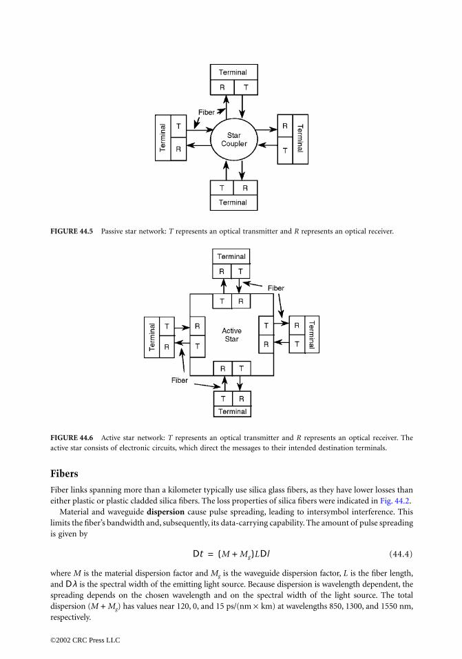
Fibers

Fiber links spanning more than a kilometer typically use silica glass fibers, as they have lower losses thaneither plastic or plastic cladded silica fibers. The loss properties of silica fibers were indicated in Fig. 44.2.

Material and waveguide dispersion cause pulse spreading, leading to intersymbol interference. Thislimits the fiber’s bandwidth and, subsequently, its data-carrying capability. The amount of pulse spreadingis given by

(44.4)

where M is the material dispersion factor and Mg is the waveguide dispersion factor, L is the fiber length,and Dλ is the spectral width of the emitting light source. Because dispersion is wavelength dependent, thespreading depends on the chosen wavelength and on the spectral width of the light source. The totaldispersion (M + Mg) has values near 120, 0, and 15 ps/(nm × km) at wavelengths 850, 1300, and 1550 nm,respectively.

FIGURE 44.5 Passive star network: T represents an optical transmitter and R represents an optical receiver.

FIGURE 44.6 Active star network: T represents an optical transmitter and R represents an optical receiver. Theactive star consists of electronic circuits, which direct the messages to their intended destination terminals.

Dt M Mg+( )LDl=


The fiber’s bandwidth and subsequent data rate is inversely proportional to the pulse spreading. Asnoted, dispersion is a minimum in the second window, actually passing through zero close to 1300 nmfor conventional fibers. Special fibers are designed to compensate for the material dispersion by adjustingthe waveguide dispersion to cancel it at the low-loss 1550-nm third window. Such fibers (called dispersionshifted) are ideal for long fiber links because of their low loss and low dispersion.

Multimode fibers allow more than one mode to simultaneously traverse the fiber. This produces dis-tortion in the form of widened pulses because the energy in different modes travels at different velocities.Again, intersymbol interference occurs. For this reason, multimode fibers are only used for applicationswhere the bandwidth (or data rate) and path length are not large.

Single-mode fibers limit the propagation to a single mode, thus eliminating multimode spreading.Since they suffer only material and waveguide dispersive pulse spreading, these fibers (when operatingclose to the zero dispersion wavelength) have greater bandwidths than multimode fibers and are usedfor the longest and highest data rate systems.

Table 44.1 lists bandwidth limits for several types of fibers and Table 44.2 illustrates typical fiber sizes.Step index fibers (SI) have a core having one value of refractive index and a cladding of another value.Graded-index (GRIN) fibers have a core index whose refractive index decreases with distance from theaxis and is constant in the cladding. As noted, single-mode fibers have the greatest bandwidths. To limitthe number of modes to just one, the cores of single-mode fibers must be much smaller than those ofmultimode fibers.

Because of the relatively high loss and large dispersion in the 800-nm first window, applicationsthere are restricted to moderately short path lengths (typically less than a kilometer). Because of thelimited length, multimode fiber is practical in the first window. Light sources and photodetectorsoperating in this window tend to be cheaper than those operating at the longer wavelength second andthird windows.

The 1300-nm second window, having moderately low losses and nearly zero dispersion, is utilized formoderate to long path lengths. Nonrepeatered paths up to 70 km or so are attainable in this window. Inthis window, both single-mode and multimode applications exist. Multimode is feasible for short lengthsrequired by LANs (up to a few kilometer) and single-mode for longer point-to-point links.

Fiber systems operating in the 1550-nm third window cover the highest rates and longest unamplified,unrepeated distances. Lengths on the order of 200 km are possible. Single-mode fibers are typically usedin this window. Erbium-doped optical amplifiers operate in the third window, boosting the signal levelsfor very long systems (such as those traversing the oceans).

FIGURE 44.7 Ring network: T represents an optical transmitter and R represents an optical receiver. The nodesact as optical regenerators. Fibers connect the nodes together, while the terminals and nodes are connected electron-ically.


Other Components

Semiconductor laser diodes (LD) or light-emitting diodes (LED) serve as the light sources for most fibersystems. These sources are typically modulated by electronic driving circuits. The conversion from signalcurrent i to optical power P is given by

(44.5)

where a0 and a1 are constants. Thus, the optical power waveform is a replica of the modulation current.For very high-rate modulation, external integrated optic devices are available to modulate the light

beam after its generation by the source. Laser diodes are more coherent (they have smaller spectral widths)than LEDs and thus produce less dispersive pulse spreading, according to Eq. (44.4). In addition, laserdiodes can be modulated at higher rates (tens of gigabit per second) than LEDs (which are limited torates of just a few hundred megabit per second). LEDs have the advantage of lower cost and simplerdriving electronics.

Photodetectors convert the optical beam back into an electrical current. Semiconductor PIN photo-diodes and avalanche photodiodes (APD) are normally used. The conversion for the PIN diode is givenby the linear equation

i = ρP (44.6)

where i is the detected current, P is the incident optical power, and ρ is the photodetector’s responsivity.Typical values of the responsivity are on the order of 0.5 mA/mW.

Avalanche photodiodes follow the same equation but include an amplification factor that can be ashigh as several hundred. They improve the sensitivity of the receiver.

According to Eq. (44.6), the receiver current is a replica of the optical power waveform (which is itselfa replica of the modulating current). Thus, the receiver current is a replica of the original modulatingsignal current, as desired.

An optical regenerator (or repeater) consists of an optical receiver, electronic processor, and an opticaltransmitter. Regenerators detect (that is, convert to electrical signals) pulse streams that have weakenedbecause of travel over long fiber paths, electronically determine the value of each binary pulse, and transmita new optical pulse stream replicating the one originally transmitted. Using a series of regenerators spaced

TABLE 44.1 Typical Fiber Bandwidths

Wavelength, Bandwidth,Fiber nm Source MHz ¥ km

Multimode SI 850 LED 30Multimode GRIN 850 LD 500Multimode GRIN 1300 LD or LED 1000Single mode 1300 LD >10,000Single mode 1550 LD >10,000

TABLE 44.2 Glass Fiber Sizes

Core,µm

Cladding,µm

Numerical Aperture Operation

8 125 0.11 Single mode50 125 0.2 Multimode62.5 125 0.27 Multimode85 125 0.26 Multimode100 140 — Multimode200 280 — Multimode

P a0 a1i+=


at distances of tens to hundreds of kilometers, total link lengths of thousands of kilometers are produced.Regenerators can only be used in digital systems.

Optical amplifiers simply boost the optical signal level without conversion to the electrical domain.This simplifies the system compared to the use of regenerators. In addition, optical amplifiers work withboth analog and digital signals.

Splices and connectors are required in all fiber systems. Many types are available. Losses tend to beless than 0.1 dB for good splices and just a few tenths of a decibel for good connectors. Fibers are splicedeither mechanically or by actually fusing the fibers together.

Directional couplers split an optical beam traveling along a single fiber into two parts, each travelingalong a separate fiber. The splitting ratio is determined by the coupler design. In a star coupler (seeFig. 44.5), the beam entering the star is evenly divided among all of the output ports of the star. Typicalstars operate as 8 × 8, 16 × 16, or 32 × 32 couplers. As an example, a 32 × 32 port star can accommodate32 terminals on a LAN.

44.3 Signal Quality

Signal quality is measured by the signal-to-noise ratio (S/N) in analog systems and by the bit error rate(BER) in digital links.

The signal-to-noise ratio in a digital network determines the error rate and is given by

(44.7)

where P is the received optical power, ρ is the detector’s unamplified responsivity, M is the detector gainif an APD is used, n (usually between 2 and 3) accounts for the excess noise of the APD, B is the receiver’sbandwidth, k is the Boltzmann constant (k = 1.38 × 10-23 J/K), e is the magnitude of the charge on anelectron (1.6 × 10-19 C), T is the receiver’s temperature in kelvin, ID is the detector’s dark current, andRL is the resistance of the load resistor that follows the photodetector.

The first term in the denominator of Eq. (44.7) is caused by shot noise, and the second term is attributedto thermal noise in the receiver. If the shot noise term dominates (and the APD excess loss and darkcurrent are negligible), the system is shot-noise limited. If the second term dominates, the system isthermal-noise limited.

In a thermal-noise limited system, the probability of error Pe (which is the same as the bit error rate) is

(44.8)

where erf is the error function, tabulated in many references [Palais, 1998]. An error rate of 10-9 requiresa signal-to-noise ratio of nearly 22 dB (S/N = 158.5).

44.4 System Design

System design involves ensuring that the signal level at the receiver is sufficient to produce the desiredsignal quality. The difference between the power available from the transmitting light source (e.g., Pt indBm) and the receiver’s sensitivity (e.g., Pr in dBm) defines the system power budget L. Thus, the powerbudget is the allowed accumulated loss for all system components and is given (in decibels) by

(44.9)

In addition to ensuring sufficient available power, the system must meet the bandwidth requirementsfor the given information rate. This requires that the bandwidths of the transmitter, the fiber, and thereceiver are sufficient for transmission of the message.

SN----

MrP( )2RL

M n2eRLB ID rP+( ) 4kTB+-------------------------------------------------------------------=

Pe 0.5 0.5 erf 0.354 S/N( )–=

L dB( ) Pt dBm( ) Pr dBm( )–=


Defining Terms

Avalanche photodiode: Semiconductor photodetector that has internal gain caused by avalanche break-down.

Bit error rate: Fractional rate at which errors occur in the detection of a digital pulse stream. It is equalto the probability of error.

Dispersion: Wavelength-dependent phase velocity commonly caused by the glass material and thestructure of the fiber. It leads to pulse spreading because all available sources emit light coveringa (small) range of wavelengths. That is, the emissions have a nonzero spectral width.

Integrated optics: Technology for constructing one or more optical devices on a common waveguidingsubstrate.

Laser: A source of coherent light, that is, a source of light having a small spectral width.Laser diode: A semiconductor laser. Typical spectral widths are on the order of 1–5 nm.Light-emitting diode: A semiconductor emitter whose radiation typically is not as coherent as that of

a laser. Typical spectral widths are on the order of 20–100 nm.Multimode fiber: A fiber that allows the propagation of many modes.Optical frequency-division multiplexing: Multiplexing many closely spaced optical carriers onto a

single fiber. Theoretically, hundreds (and even thousands) of channels can be simultaneouslytransmitted using this technology.

PIN photodiode: Semiconductor photodetector converting the optical radiation into an electrical current.Receiver sensitivity: The optical power required at the receiver to obtain the desired performance

(either the desired signal-to-noise ratio or bit error rate).Responsivity: The current produced per unit of incident optical power by a photodetector.Signal-to-noise ratio: Ratio of signal power to noise power.Single-mode fiber: Fiber that restricts propagation to a single mode. This eliminates modal pulse

spreading, increasing the fiber’s bandwidth.Wavelength-division multiplexing: Multiplexing several optical channels onto a single fiber. The chan-

nels tend to be widely spaced (e.g., a two-channel system operating at 1300 nm and 1550 nm).

References

Chaffee, C.D. 1988. The Rewiring of America, Academic, Orlando, FL.Hoss, R.J. 1990. Fiber Optic Communications, Prentice-Hall, Englewood Cliffs, NJ.Jeunhomme, L.B. 1990. Single-Mode Fiber Optics, 2nd ed., Marcel Dekker, New York.Keiser, G. 1991. Optical Fiber Communications, McGraw-Hill, New York.Palais, J.C. 1998. Fiber Optic Communications, 4th ed., Prentice-Hall, Englewood Cliffs, NJ.Thiennot, J., Pirio, F., and Thomine, J.B. 1993. Optical undersea cable systems trends. Proc. IEEE,

81(11):1610–11.

Further Information

Information on optical communications is included in several professional society journals. These includethe IEEE Journal of Lightwave Technology and the IEEE Photonics Technology Letters. Valuable informationis also contained in several trade magazines such as Lightwave and Laser Focus World.


45Optical Fibers and

Lightwave Propagation

45.1 Transmission Along Fibers45.2 Total Internal Reflection45.3 Modes of Propagation45.4 Parameters of Fibers45.5 Attenuation45.6 Dispersion45.7 Graded-Index Fibers45.8 Mode Coupling45.9 Summary

45.1 Transmission Along Fibers

Light that finds itself at one end of an optical fiber may or may not find its way to the other end. For arandomly chosen combination of the properties and configuration of the light, the optical power hasonly a small chance of propagating significant distances along the fiber. With proper design of the fiberand of the mechanism for launching the light, however, the signal carried by the light can be transmittedover many kilometers without severe leakage or loss [Diament, 1990; Palais, 1988; Jones, 1988; Cheo,1985; Basch, 1987; Green, 1993; Hoss and Lacy, 1993; Buckman, 1992; Sterling, 1987].

In its simplest form, an optical fiber consists of a long cylindrical core of glass, surrounded by acladding of slightly less optically dense glass. See Fig. 45.1. Since both the core and cladding aretransparent, propagation depends on the ability of the combination to confine the light and thwart itsescape across the side of the fiber. It is the interface between the core and cladding that acts as a reflectorto confine any light that would otherwise escape the core and leak away from the cladding into the outsideworld. The mechanism for confinement to the core is that of total internal reflection, a process that iseasy to understand for a planar interface between two dissimilar dielectric media [Diament, 1990; Bornand Wolf, 1965]. See Fig. 45.2. That process applies as well to the cylindrical geometry of the interfacebetween the core and cladding of the optical fiber.

45.2 Total Internal Reflection

When light strikes the planar interface between two dissimilar transparent media, part of the light istransmitted and the rest is reflected. The proportions of each depend on the impedance mismatch betweenthe two media; this, in turn, depends on the dissimilarity of the indices of refraction of the two materials.The index of refraction n measures how much more slowly light travels in the medium than it does ina vacuum.

Paul Diament Columbia University


When light strikes the interface at an angle to the normal, rather than head-on, the light that istransmitted is refracted, or bent away from its original direction, in accordance with Snell’s law,

(45.1)

where n1 and n2 are the refractive indices of the two media and θ1 and θ2 are the angles of the ray to thenormal to the interface in the two regions. See Fig. 45.3. If the light is incident onto the interface fromthe denser medium and if the ray’s direction is close to grazing, so that the angle of incidence θ1 issufficiently large, then it may happen that n1 sin θ1 exceeds n2 and there is then no solution for the angleof refraction θ2 from Snell’s law, since the quantity sin θ2 can never exceed unity. Instead of partial re-flection into the denser medium and partial refraction into the other region, there is then no transmissioninto the less dense medium. Rather, all of the light is reflected back into the denser medium. Total internal

FIGURE 45.1 Structure of an optical fiber: core of radius a, refractive index n1, surrounded by cladding of indexn2. Typical core diameter is 50 µm.

FIGURE 45.2 Ordinary refraction at a planar interface between two media (left), with angle of incidence less thanthe critical angle, compared with total internal reflection (right), with angle of incidence exceeding the critical angle.Light is incident from the denser medium (n1 > n2).

FIGURE 45.3 Snell’s law determines the angle of refraction θ2 at an interface; the angle of reflection θ1 equals the angleof incidence. The case n1 > n2 is illustrated. When the angle of incidence θ1 reaches the critical value θc = sin-1(n2/n1),refraction is at θ2 = 90∞. Beyond the critical angle, there is total internal reflection.

cladding

n2

n1

core 2a

50µm

reflected ray

incident ray

reflected

incident

n1 n2 n1 n2

refractedray decaying

θ1θ1

θ2

n2n1

θ1 θc θ2 90°

n2n1

n1 sin q1 n2 sin q2=


reflection occurs (internal to the denser medium in which the light originated), and the escape of thelight into the less dense medium has been thwarted.

There is more to the process of total internal reflection at a planar boundary than merely reflectionfrom the interface. Although the light does not leak into the less dense medium and thereby get trans-mitted outward, it does seep across the interface and propagate, but only parallel to that interface surface[Diament, 1990]. In the direction normal to the interface, there is no propagation on the less dense sideof the surface but the strength of the light that appears there decays exponentially. The spatial rate ofdecay increases with the angle of incidence, beyond the critical angle at which total internal reflectionbegins. If the decay is sufficiently strong, the light that seeps across is effectively constrained to a thinlayer beyond the interface and propagates along it, while the light left behind is reflected back into thedenser region with its original strength. The reflection coefficient is 100%. There is undiminished opticalpower flow along the reflected ray in the denser medium, but only storage of optical energy in the lightthat seeps across the interface into the less dense region.

Much the same process occurs along the curved, cylindrical interface between the core and claddingof the optical fiber. When the light strikes this interface at a sufficiently high grazing angle, total internalreflection occurs, keeping the optical power propagating at an angle within the core and along the axialdirection in the cladding. The reflected light strikes the core again on the other side of the axis and isagain totally internally reflected there. This confines the light to the core and to a thin layer beyond theinterface in the cladding and keeps it propagating indefinitely along the axial direction. The overall resultis that the light is guided by the fiber and not permitted to leak away across the side of the fiber, providedthe light rays within the core encounter the interface at a sufficiently high grazing angle. See Fig. 45.4.

45.3 Modes of Propagation

For the cylindrical geometry of core and cladding in a fiber, the equivalent of a ray of light in an unboundedmedium is any one of a set of modes of optical propagation. These refer to configurations of electromag-netic fields that satisfy Maxwell’s equations and the boundary conditions imposed by the core–claddinginterface and also conform to the total internal reflection requirement of grazing incidence to allowguided-wave propagation of the mode along the fiber [Diament, 1990; Born and Wolf, 1965].

These modes are nearly all hybrid, meaning that neither the electric nor the magnetic field of themode is fully transverse to the axial direction of propagation, as can be the case for waveguides formedby hollow conducting pipes. Whereas the field configuration in a rectangular metallic waveguide variesas a sine function across the guide, that of an optical fiber follows a Bessel function variation. Besselfunctions oscillate, much like trigonometric ones, but not with a constant amplitude. In the cladding,the fields decay in the radial direction away from the interface, but not exponentially as at a planarinterface under total internal reflection. Rather, the fields in the cladding decay as modified Besselfunctions, but the effect is the same: confinement to a thin layer just beyond the interface.

FIGURE 45.4 Standing wave across the core, formed by a repeatedly reflecting ray, with decaying field strength inthe cladding, formed by the process of total internal reflection at the cylindrical boundary. The entire field patternpropagates along the axis of the fiber.

core cladding


Just as the modes of hollow metal pipes are classified as transverse electric (TE) and transversemagnetic (TM), the hybrid modes of optical fibers also come in two distinguishable varieties [Schlesinger,Diament, and Vigants, 1961], labeled HE and EH, with pairs of subscripts appended to indicate thenumber of oscillations of the fields azimuthally (around the axis) and radially (across the core). Forpractical designs of optical fibers, dictated by the smallness of optical wavelengths, the indices of refractionof the core and cladding are very close to each other, and there exist combinations of the hybrid modesthat are very nearly of the more familiar transverse, linearly polarized types and of greatly simplifieddescription; these are designated LP modes [Gloge, 1971]. The dominant mode, which has no constraintof a minimum frequency, is the HE11 mode, also designated the LP01 mode in the simplified version. Allother modes have a cutoff frequency, a minimum frequency for axial propagation of a confined mode.Even the dominant mode, in practical cases, has fields that are virtually unconfined when the frequencyis too low.

In frequency, then, optical fibers behave as high-pass filters. In angular distribution, fibers allow prop-agation of only those rays that are directed in a sufficiently narrow cone about the axis to satisfy theconditions of total internal reflection.

45.4 Parameters of Fibers

A few parameters are in common use to describe the ability of the fiber to transmit light. One is thenumerical aperture, NA, defined for the fiber as

(45.2)

and measuring the dissimilarity of the core and cladding indices, n1 and n2. This number correspondsmore generally for any optical interface to

NA = n sinθmax (45.3)

a quantity that is conserved across any such interface, by Snell’s law, and that measures how great thedeviation of an incoming ray from the axial direction can get and still allow capture by, and propagationalong, the optical system.

The numerical aperture enters into the formula for the key fiber parameter V, often referred to as thenormalized frequency or sometimes as the mode volume parameter. This is defined for a step-indexfiber of core radius a and for light of vacuum wavelength λ as

(45.4)

The V parameter combines many physical attributes of the fiber and the light source; it is proportionalto the frequency of the light and to the size of the core, as well as to the numerical aperture. It determineswhether a particular mode of the fiber can propagate; in effect, it tells whether the light in that modestrikes the core–cladding interface at a sufficiently high grazing angle to be captured by the fiber. Conse-quently, it also furnishes an estimate of how many modes can propagate along the fiber. For large valuesof V, the approximate number of distinguishable modes that are above cutoff and can therefore propagateis given by V2/2.

For many purposes, including efficiency of launching and detection of the light and maintenance ofthe integrity of the signal carried by the light, it is undesirable to have a multiplicity of modes able topropagate along the fiber. For single-mode operation, the parameter V must be small, less than 2.4048[which is the argument at which the Bessel function J0(x) first goes through zero]. This is not easy toachieve, because wavelengths of light are so tiny: for a core diameter of 2a = 50 µm and an operatingwavelength of λ = 0.8 µm, we have V ª 200(NA) and the core and cladding indices have to be extremely

NA n12 n2

2–( )=

V 2pa/l( ) NA=


close, yet dissimilar, to attain single-mode operation. A much thinner core is needed for a single-modefiber than for multimode operation. For the more readily achieved refractive index differences and corediameters, NA may be about 0.15 and several hundred modes can propagate along the fiber. A conse-quence of this multiplicity of modes is that each travels along the fiber at its own speed and the resultingconfusion of arrival times for the various fractions of the total light energy carried by the many modescontributes to signal distortion ascribed to dispersion.

45.5 Attenuation

Dispersion limits the operation of the fiber at high data rates; losses limit it at low data rates. Lightattenuation due to losses is ascribable to both absorption and scattering. Absorption occurs when impu-rities in the glass are encountered; the hydroxyl ion of water present in the glass as an impurity contributesheavily to absorption, along with certain metal ions and oxides. Careful control of impurity levels duringfabrication of fibers has allowed light attenuation due to absorption to be kept below 1 dB/km.

Scattering is caused by imperfections in the structure of the fiber. A lower limit on losses is due toRayleigh scattering, which arises from thermal density fluctuations in the glass, frozen into it duringmanufacture. The typical attenuation constant a from Rayleigh scattering varies as the inverse fourthpower of the optical wavelength λ,

α = α0(λ0 /λ)4; α0 = 1.7 dB/km, λ0 = 0.85 µm. (45.5)

This makes operation at longer wavelengths less subject to losses, but molecular absorption bands atwavelengths beyond about 1.8 µm must be avoided. Rayleigh scattering is excessive below about 0.8 µmand, between these limits, the hydroxyl ion absorption peak near 1.39 µm must also be avoided. Thishas left three useful transmission windows for fiber optic systems, in the ranges 0.8–0.9 µm, 1.2–1.3 µm,and 1.55–1.6 µm.

45.6 Dispersion

Dispersion is a major concern in a communication system. It refers to processes that cause differentcomponents of the light signal to be affected differently. In particular, the speeds at which the differentcomponents are propagated along the fiber can vary enough to result in significantly different transmis-sion delays or arrival times for the various portions of the signal. The outcome is distortion of the signalwhen it is reconstructed from all its components at the receiver or repeater. The signal componentsreferred to may be the various frequencies in its spectrum, or they can comprise the multiplicity of modesthat each carry their respective fraction of the total optical power to be transmitted.

For optical fibers, there are two aspects to dispersion effects. One is material dispersion, also calledintramodal or chromatic dispersion; the other is termed multimode dispersion, or also intermodaldispersion. Material dispersion arises from the properties of the fiber material that cause the index ofrefraction to depend on frequency. Since the light source is never truly monochromatic but, rather, hasa linewidth, the various frequencies in the light signal are subject to slightly different refractive indexvalues, which entails different speeds of transmission along the fiber even if there is only one mode ofpropagation. It is the spread in transmission delays that distorts the signal, and this spread depends onthe second derivative of the refractive index with respect to wavelength. One way to minimize this sourceof dispersion is to operate at about 1.3 µm because silica glass has a second derivative that goes throughzero at that wavelength.

Multimode dispersion arises from the fact that the optical energy is distributed among the manymodes of propagation of the fiber and each mode has its own group velocity, the rate at which a signalcarried by that mode is transmitted. The relevant measure of dispersion is then the difference between


the propagation delays of the slowest and the fastest of the participating modes. For a step-index fiber,multimode dispersion is much more severe than material dispersion, although it is somewhat mitigatedby the fact that different modes do not propagate independently in a real, imperfect fiber. The phe-nomena of mode mixing and of greater attenuation of high-order modes (those with many field oscil-lations within the core) tend to reduce the differences in arrival times of the various modes that carrythe signal. Nevertheless, intermodal dispersion imposes a severe limitation on data transmission alonga step-index fiber.

45.7 Graded-Index Fibers

The way to reduce the deleterious effects of multimode dispersion on the propagation of a signal alonga fiber becomes clear when the mechanism of this sort of dispersion is understood. That different modesshould exhibit significantly different propagation delays follows from consideration of where the bulk ofthe field energy resides in each mode. As mentioned, high-order modes have field profiles that oscillatemore than those of low-order modes. This includes oscillations in both the radial and the azimuthaldirections. Examination of the behavior of Bessel functions indicates that high-order modes have mostof their energy nearer to the core–cladding boundary than do the low-order ones. The azimuthal variationof the fields corresponds to propagation at an angle to the fiber axis so that there is progression azimuth-ally, around the axis, even as the mode propagates along the axis.

For the high-order modes, the azimuthal component of the propagation is more significant than it isfor low-order modes, with the result that the overall progression of the high-order mode is in a spiralaround the axis, whereas the low-order modes tend to progress more nearly axially than helically. Thespiral trajectories of the energy also tend to concentrate far from the axis, nearer to the cladding, ascompared to the straighter ones of the low-order modes, whose energy is massed near the axis and travelsmore nearly straight along it, as suggested in Fig. 45.5. The difference in propagation delay is then readilyunderstood as arising from the longer, spiral path of the modal energy for high-order modes, as comparedwith the shorter, more direct path taken by the energy in the low-order modes.

This picture of the underlying mechanism for multimode dispersion suggests an equalization schemeaimed at slowing down the low-order modes that are concentrated near the axis, while speeding up thehigh-order ones that spiral around as they progress and are to be found primarily near the core–claddinginterface, farther from the axis. This is achieved by varying the index of refraction of the core gradually,from a high value (for slower speed) near the axis to a lower one (for higher speed) near the cladding.Fibers so fabricated are termed graded-index (or GRIN) fibers. It is found that a refractive index profilethat varies approximately (but not precisely) quadratically with radius can be effective in reducingmultimode dispersion dramatically by equalizing the speeds of propagation of various modes of thatfiber. Figure 45.6 illustrates the radial variation of the refractive index n(r) for both a step-index fiberand a GRIN fiber.

FIGURE 45.5 Spiral path of light energy in higher order modes, compared to more direct trajectory for lower orderones. High-order modes have their energy concentrated near the core–cladding interface; lower order ones areconcentrated closer to the axis. The spiral path takes longer to traverse than the direct one.


45.8 Mode Coupling

One more consideration affecting propagation along an optical fiber is the possibility of mode coupling.Although the theoretical modes of propagation travel independently along fibers of perfect constitutionand perfect geometry, real fibers inevitably have imperfections that can cause different modes to coupleand exchange energy between them as they propagate.

A fiber may be imperfect in geometry in that it may not be perfectly straight axially, or its core may notbe perfectly round, or it may have been bent. The core and cladding may deviate from their nominal refractiveindices. More importantly, there may be fluctuations in their material properties, or the graded-index profilemay not be the ideal one. All such imperfections give rise to coupling between modes of propagation ofthe ideal version of the fiber, such that some of the power in one mode is drained and feeds another mode.When the other mode becomes the stronger one, energy is fed back to the first mode and thereafter sloshesback and forth repeatedly between the modes as the light travels along the fiber. How many modes participatein this periodic exchange of energy depends on the nature of the fluctuations of the imperfections.

A perturbation analysis of the effects of fluctuations in some parameter that would be constant inan ideal fiber reveals that the relevant property is the spatial Fourier spectrum of the fluctuations. Thestrength of the coupling between any two modes is proportional to the statistical average of the powerspectrum of the fluctuations, evaluated at the difference between the propagation constants of the twomodes in the ideal structure.

This implies that deviations on a large scale, such as gradual bending of the fiber, will affect only acertain group of modes. In this case, the spatial power spectrum exhibits a relatively narrow bandwidth,near zero spatial frequency. This allows only modes whose ideal propagation constants are very close toeach other to be coupled by the large-scale fluctuations. Such deviations, therefore, couple only modesthat are nearly degenerate (have nearly equal propagation constants).

On the other hand, periodic fluctuations, such as striations in the material properties, exhibit a spatialspectrum that is peaked in a spectral region corresponding to the period of the striations. In that case,coupling will be significant for modes whose propagation constants differ by the spatial wavenumberassociated with the periodicity of the fluctuations.

One effect of coupling among modes is to increase losses along the fiber, because energy can gettransferred to modes that are not trapped within the core. Some of that energy can then leak out intothe cladding and be lost before it can return to the propagating mode. Another effect, however, is toaverage the dispersion associated with many modes and thereby reduce the overall pulse spreading. Forexample, for closely coupled modes, propagation delays may vary as only the square root of the distancetraveled, rather than with the more severe variation, proportional to distance, for uncoupled modes.

FIGURE 45.6 Radial index profiles of step-index and graded-index fibers. The broken vertical axis is a reminderthat the maximum core index n1 is quite close to the cladding index n2 for practical fibers.

00

n2

n1

n(r)

GRINfiber

Step-indexfiber

claddingcore

ar


45.9 Summary

The step-index optical fiber comprises a dielectric cylindrical core surrounded by a cladding of slightlylower refractive index. This constitutes a dielectric cylinder, which is capable of acting as a waveguide.The mechanism involved in confining and guiding the optical power is that of total internal reflectionat the cylindrical boundary between the core and the cladding. This phenomenon results in a standingwave pattern within the core and a decaying field in the cladding, with the entire field pattern propagatingalong the cylinder. The general modes of propagation are hybrid modes, having axial components ofboth the electric and the magnetic fields, and they advance along the fiber by spiraling around the axis.The exceptional transverse electric or transverse magnetic types are the azimuthally symmetric ones,which do not twist about the axis as they progress along the fiber. The dominant mode is hybrid, however.

Because the optical wavelengths are so short, the core is normally many wavelengths across, with theresult that a large number of modes can propagate along the fiber, even when the refractive indices ofthe core and cladding are kept quite close to each other. Unless single-mode fiber operation is achieved, thisentails multimode dispersion effects. Efforts to overcome the limitations this imposes on data transmis-sion have led to the development of graded-index fibers, with an advantageous refractive index profileof the core that tends to equalize the propagation delays of different modes. With careful fabrication ofthe fibers and with selections of appropriate source wavelengths and bandwidths, attenuation along thefiber can be kept quite low and dispersive effects can be controlled, making optical fibers the mediumof choice for propagation of optical signals.

Defining Terms

Absorption: Process by which light energy is drained from a wave and transferred to the material inwhich it propagates.

Bessel function: A type of mathematical function that oscillates and also decays in amplitude; descrip-tive of the radial dependence of the fields in a uniform-index core.

Chromatic dispersion: The variation of a material’s index of refraction with frequency or wavelength.Cladding: The outer, optically less dense portion of an optical fiber, surrounding the core. Core: The inner, optically dense portion of an optical fiber, surrounded by the cladding.Cutoff: The condition (usually too low an operating frequency) under which a mode is not capable of

propagating; the cutoff frequency is the minimum frequency for propagation of a mode.Degenerate modes: Modes whose propagation constants are equal or nearly equal.Dispersion: The property of a fiber (or any wave-propagating system) that causes different frequencies

(or operating wavelengths) to propagate at different speeds; it is a cause of distortion of signalstransmitted along the structure.

Dominant mode: The mode that can propagate under conditions (usually a specific frequency range)that do not allow any other modes to propagate.

Graded-index fiber: The type of optical fiber whose core has a nonuniform index of refraction.GRIN fiber: Graded-index fiber.Group velocity: The velocity of propagation of a signal whose spectrum occupies a narrow range of

frequencies about some carrier frequency; the rate of change of frequency with respect to propa-gation constant.

High-pass filter: A circuit or structure that passes high-frequency signals but blocks low-frequency ones.Hybrid: Describing a mode for which neither the electric nor the magnetic field vector is fully transverse

to the direction of propagation.Index of refraction: Ratio of the vacuum speed of light to its speed in the medium.Intermodal dispersion: Dispersion effect that arises from a signal’s being carried by many modes that

travel at different speeds.Intramodal dispersion: The variation of a material’s index of refraction with frequency or wavelength,

resulting in dispersive effects for a single mode.


Linearly polarized: Descriptive of a mode of propagation whose field vectors each maintain a fixedorientation in space as they oscillate in time.

Linewidth: The range of frequency or wavelength contained within a nominally monochromatic signal.Material dispersion: The variation of a material’s index of refraction with frequency or wavelength.Maxwell’s equations: The mathematical laws governing the propagation of light and other electromag-

netic waves.Mode: Field configuration of light with well-defined propagation characteristics.Mode coupling: Process by which different modes of propagation can interchange their energy instead

of propagating independently of each other.Mode mixing: Process of transfer or interchange of light energy among different modes of propagation.Mode volume parameter: The V parameter, which determines how many modes can propagate along

an optical fiber; it is proportional to the frequency of the light, to the size of the core, and to thenumerical aperture.

Modified Bessel function: A type of mathematical function that either grows or decays in amplitude;descriptive of the radial dependence of the fields in a uniform-index cladding.

Monochromatic: Of a single frequency or wavelength.Multimode dispersion: Dispersion effect that arises from a signal’s being carried by many modes that

travel at different speeds.Multimode operation: Operation of an optical fiber under conditions that allow many modes to propa-

gate along it.Normalized frequency: The V parameter, which determines whether a mode can propagate along an

optical fiber; it is proportional to the frequency of the light, to the size of the core, and to the numericalaperture.

Numerical aperture (NA): A measure of the ability of an optical structure or instrument to captureincident light; NA = n sin θ, where n is the refractive index and θ is the maximum angle of deviationfrom the optical axis of a ray that can still be captured by the aperture.

Optical fiber: A long, thin glass structure that can guide light.Optically dense: Transmitting light at a relatively slow speed; having a high refractive index.Perturbation analysis: Mathematical process of determining approximately the effects of a relatively

weak disturbance of some system that is otherwise in equilibrium.Power spectrum: Description of some quantity that varies in space or time in terms of the decomposition

of its power into constituent sinusoidal components of different spatial or temporal frequenciesor periodicities.

Propagation constant: The spatial rate of phase progression of a wave.Pulse spreading: Process whereby the width of a pulse increases as it propagates.Rayleigh scattering: A scattering process associated with thermal density fluctuations in the constitu-

tion of the glass.Reflection coefficient: Ratio of strength of reflected light to that of the incident light.Refraction: Process of bending a ray of light away from its original direction.Repeater: Electronic circuitry that takes in a degraded signal and restores or reconstitutes it for further

transmission.Scattering: Process by which portions of light energy are redirected (by encounters with microscopic

obstacles or inhomogeneities) to undesired directions and thereby lost from the propagating wave.Single-mode operation: Operation of an optical fiber under conditions that allow only one mode to

propagate along it.Snell’s law: Law governing reflection (reflection angle equals incidence angle) and refraction (compo-

nent of propagation vector tangential to the interface is preserved) of a ray of light encounteringthe interface between media of different optical density.

Spatial Fourier spectrum: Description of some quantity that varies in space in terms of its decompo-sition into constituent sinusoidal components of different spatial frequencies or periodicities.

Spatial frequency: The number of cycles per unit length of a quantity that varies periodically in space.


Spatial wavenumber: Reciprocal of a quantity’s interval of periodicity in space.Standing wave: Resultant of counterpropagating waves, with a spatial distribution that does not move.Step-index fiber: The type of optical fiber whose core and cladding each have a uniform index of

refraction.Total internal reflection: Process of reflecting light incident from a denser medium toward a less dense

one, at an angle sufficiently grazing to avert transmission into the less dense medium. All of theincident light power is reflected, although optical fields do appear beyond the interface.

Transverse electric: Descriptive of a mode of propagation whose electric field vector is entirely trans-verse to the direction of propagation.

Transverse magnetic: Descriptive of a mode of propagation whose magnetic field vector is entirelytransverse to the direction of propagation.

Waveguide: A structure that can guide the propagation of light or electromagnetic waves along itself.

References

Basch, E.E.B., Ed. 1987. Optical-Fiber Transmission, Howard W. Sams, Indianapolis, IN. Born, M. and Wolf, E. 1965. Principles of Optics, Pergamon Press, Oxford, England. Buckman, A.B. 1992. Guided-Wave Photonics, Saunders College Publishing, Fort Worth, TX. Cheo, P.K. 1985. Fiber Optics Devices and Systems, Prentice-Hall, Englewood Cliffs, NJ. Diament, P. 1990. Wave Transmission and Fiber Optics, Macmillan, New York. Gloge, D. 1971. Weakly guiding fibers. Applied Optics, 10:2252–2258. Green, P.E., Jr. 1993. Fiber Optic Networks, Prentice-Hall, Englewood Cliffs, NJ.Hoss, R.J. and Lacy, E.A. 1993. Fiber Optics, Prentice-Hall, Englewood Cliffs, NJ.Jones, W.B., Jr. 1988. Introduction to Optical Fiber Communication Systems, Holt, Rinehart and Winston,

New York.Palais, J.C. 1988. Fiber Optic Communications, Prentice-Hall, Englewood Cliffs, NJ.Schlesinger, S.P., Diament, P., and Vigants, A. 1961. On higher-order hybrid modes of dielectric cylinders.

IRE Trans. Micro. Theory Tech., MTT-8(March):252–253.Sterling, D.J., Jr. 1987. Technician’s Guide to Fiber Optics, Delmar, Albany, NY.

Further Information

Periodicals that can help one keep up to date with developments in fiber optics and related systemsinclude the following.

Journal of Lightwave Technology, The Institute of Electrical and Electronics Engineers, Inc., New York.IEEE Journal of Quantum Electronics, The Institute of Electrical and Electronics Engineers, Inc., New

York.Journal of the Optical Society of America, Optical Society of America, New York.Optics Letters, Optical Society of America, New York.Applied Optics, Optical Society of America, New York.Bell System Technical Journal, AT&T, New York.Optical Engineering, Society of Photo-Optical Instrumentation Engineers, Bellingham, WA.Optics Communications, North-Holland, Amsterdam.Photonics Spectra, Optical Publishers, Pittsfield, MA.Lightwave, the Journal of Fiber Optics, Howard Rausch Associates, Waltham, MA.


46Optical Sources for

Telecommunication

46.1 Introduction 46.2 Laser Designs46.3 Quantum Well Lasers

Strained Quantum Well Lasers • Other Material Systems

46.4 Distributed Feedback LasersTunable Lasers

46.5 Surface Emitting Lasers46.6 Laser Reliability46.7 Integrated Laser Devices

Laser Array • Integrated Laser Modulator • Multichannel WDM Sources • Spot Size Converters (SSC) Integrated Laser

46.8 Summary and Future Challenges

46.1 Introduction

Phenomenal advances in research results, development, and application of optical sources have occurredover the last decade. The two primary optical sources used in telecommunications are the semiconductorlaser and the light emitting diode (LED). The LEDs are used as sources for low data rate (<200 Mb/s)and short distance applications, and lasers are used for high data rate and long distance applications.The fiber optic revolution in telecommunication which provided several orders of magnitude improve-ment in transmission capacity at low cost would not have been possible without the development ofreliable semiconductor lasers. Today, semiconductor lasers are used not only for fiber optic transmissionbut also in optical reading and recording (e.g., CD players), printers, fax machines, and in numerousapplications as a high power laser source. Semiconductor injection lasers continue to be the laser ofchoice for various system applications primarily because of their small size, simplicity of operation, andreliable performance. For most transmission system applications, the laser output is encoded with databy modulating the current. However, for some high data rate applications which require long distancetransmission, external modulators are used to encode the data. This chapter describes the fabrication,performance characteristics, current state of the art, and research directions for semiconductor lasersand integrated lasers with modulators. The focus of this chapter is laser sources needed for fiber optictransmission systems. These devices are fabricated using the InP material system. For early work andthorough discussion of semiconductor lasers, see Refs. [1–4].

The semiconductor injection laser was invented in 1962 [5–7]. With the development of epitaxialgrowth techniques and the subsequent fabrication of double heterojunction, the laser technology advancedrapidly in the 1970s and 1980s [1–4]. The demonstration of CW operation of the semiconductor laserin the early 1970s [8] was followed by an increase in development activity in several industrial laboratories.

Niloy K. DuttaUniversity of Connecticut

Niloy ChoudhuryNetwork Elements, Inc.


This intense development activity in the 1970s was aimed at improving the performance characteristicsand reliability of lasers fabricated using the AlGaAs material system [1]. These lasers emit near 0.8 µmand were deployed in early optical fiber transmission systems (in the late 1970s and early 1980s).

The optical fiber has zero dispersion near 1.3 µm wavelength and has lowest loss near 1.55 µm wave-length. Thus, semiconductor lasers emitting near 1.3 µm and 1.55 µm are of interest for fiber optictransmission application. Lasers emitting at these wavelengths are fabricated using the InGaAsP/InPmaterials system and were first fabricated in 1976 [9]. Much of the fiber optic transmission systems aroundthe world that are in use or are currently being deployed utilize lasers emitting near 1.3 µm or 1.55 µm.

Initially, these lasers were fabricated using liquid phase epitaxy (LPE) growth technique. With thedevelopment of metal-organic chemical vapor deposition (MOCVD) and gas source molecular beamepitaxy (GSMBE) growth techniques in the 1980s, not only the reproducibility of the fabrication processhas improved but it has also led to advances in laser designs such as quantum well lasers and very highspeed lasers using semi-insulating Fe doped InP current blocking layers [10].

46.2 Laser Designs

A schematic of a typical double heterostructure used for laser fabrication is shown in Fig. 46.1. It consistsof n-InP, undoped In1−xGaxPyAs1−y , p-InP and p-InGaAsP grown over (100) oriented n-InP substrate.The undoped In1−xGaxPyAs1−y layer is the light emitting layer (active layer). It is lattice matched to InPfor x ∼ 0.45 y. The band gap of the In1−xGaxPyAs1−y material (lattice matched to InP) which determinesthe laser wavelength is given by [11]

For lasers emitting near 1.3 µm, y ∼ 0.6. The double heterostructure material can be grown by the LPE,GSMBE, or MOCVD growth technique. The double heterostructure material can be processed to producelasers in several ways. Perhaps the simplest is the broad area laser (Fig. 46.1) which involves puttingcontacts on the p- and n-side and then cleaving. Such lasers do not have transverse mode confinementor current confinement, which leads to high threshold and nonlinearities in light vs. current character-istics. Several laser designs have been developed to address these problems. Among them are the gainguided laser, weakly index guided laser, and buried heterostructure (strongly index guided) laser. A typicalversion of these laser structures is shown in Fig. 46.2. The gain guided structure uses a dielectric layerfor current confinement. The current is injected in the opening in the dielectric (typically 6 to 12 µmwide), which produces gain in that region and, hence, the lasing mode is confined to that region. Theweakly index guided structure has a ridge etched on the wafer, and a dielectric layer surrounds the ridge.The current is injected in the region of the ridge, and the optical mode overlaps the dielectric (whichhas a low index) in the ridge. This results in weak index guiding.

FIGURE 46.1 Schematic of a double heterostructure laser.

Eg eV( ) 1.35 0.72y 0.12y2+–=


The buried heterostructure design shown in Fig. 46.2 has the active region surrounded (buried) bylower index layers. The fabrication process of the DCPBH (double channel planar buried heterostructure)laser, involves growing a double heterostructure, etching a mesa using a dielectric mask, and then re-growing the layer surrounding the active region using a second epitaxial growth step. The second growthcan be a single Fe doped InP (Fe:InP) semi-insulating layer or a combination of p-InP, n-InP, and Fe:InPlayer. Generally, the MOCVD growth process is used for the growth of the regrown layer. Researchershave often given different names to the particular buried heterostructure laser design that they discovered.These are described in detail in Ref. [12]. For the structure of Fig. 46.2, the Fe doped InP layer providesboth optical confinement to the lasing mode and current confinement to the active region. Buried het-erostructure lasers are generally used in communication system applications because a properly designedstrongly index guided buried heterostructure design has superior mode stability, higher bandwidth, andsuperior linearity in light vs. current (L vs. I) characteristics compared to the gain guided and weaklyindex guided designs. Early recognition of these important requirements of communication grade lasersled to intensive research on InGaAsP BH laser designs all over the world in the 1980s. It is worthmentioning that BH lasers are more complex and difficult to fabricate compared to the gain guided andweakly index guided lasers. A scanning electron micrograph of a capped mesa (CMBH) buried hetero-structure laser along with the laser structure is shown in Fig. 46.3. The current blocking layers in thisstructure consist of i-InP (Fe doped InP), n-InP, i-InP, and n-InP layers. These sets of blocking layers havethe lowest capacitance and are therefore needed for high-speed operation. An optimization of the thicknessof these layers is needed for highest speed performance. The laser fabrication involves the following steps.One-micron wide mesas are etched on the wafer and the current blocking layers consisting of i-InP, n-InP,i-InP, and n-InP layers are grown on the wafer with an oxide layer on top of the mesa in place. The oxidelayer is then removed and a third growth of p-InP cladding layer and p-InGaAs contact layer is carried out.The wafer is then processed using standard lithography, metallization, and cleaving techniques to producethe lasers.

The light vs. current characteristics at different temperatures of an InGaAsP BH laser emitting at 1.3 µmis shown in Fig. 46.4. Typical threshold current of a BH laser at room temperature is in the 5 to 10 mArange. For gain guided and weakly index guided lasers, typical room temperature threshold currents arein the 25–50 mA and 50–100 mA range, respectively. The external differential quantum efficiency definedas the derivative of the L vs. I characteristics above threshold is ∼ 0.25 mW/mA/facet for a cleaved uncoatedlaser emitting near 1.3 µm.

An important characteristic of the semiconductor laser is that its output can be modulated simply andeasily by modulating the injection current. The relative magnitude of the modulated light output isplotted as a function of the modulation frequency of the current in Fig. 46.5 at different optical outputpowers. The laser is of the BH type (shown in Fig. 46.3), has a cavity length of 250 µm, and the modulationcurrent amplitude was 5 mA. Note that the 3 dB-frequency to which the laser can be modulated increases

FIGURE 46.2 Schematic of a gain guided, weakly index guided, and strongly index guided buried heterostructurelaser.


with increasing output power and the modulation response is maximum at a certain frequency (ωr). Theresonance frequency ωr is proportional to the square root of the optical power. The modulation responsedetermines the data transmission rate capability of the laser; for example, for 10 Gb/s data transmission,the 3-dB bandwidth of the laser must exceed 10 GHz. However, other system level considerations, suchas allowable error-rate penalty, often introduce much more stringent requirements on the exact modu-lation response of the laser.

A semiconductor laser with cleaved facets generally emits in a few longitudinal modes of the cavity. Atypical spectrum of a laser with cleaved facets is shown in Fig. 46.6. The discrete emission wavelengths areseparated by the longitudinal cavity mode spacing which is ∼ 10 A for a laser (λ ∼ 1.3 µm) with 250 µmcavity length. Lasers can be made to emit in a single frequency using frequency selective feedback, forexample, using a grating internal to the laser cavity as described above.

FIGURE 46.3 Schematic of a BH laser and scanning electron photomicrograph of the same laser.

FIGURE 46.4 Light vs. current characteristics of an InGaAsP buried heterostructure laser emitting at 1.3 µm.

i-InP

n-InP

i-InP

n-InP

n-InP

n-InP (substrate)

p-InGaAsP

p-InP

MQW Active Region

p-InP


46.3 Quantum Well Lasers

So far we have described the fabrication and performance characteristics of regular double heterostructure(DH) laser which has an active region ∼ 0.1 to 0.2 µm thick. Beginning with the 1980s, lasers with verythin active regions, quantum well lasers, were being developed in many research laboratories [13–22].Quantum well (QW) lasers have active regions of ∼ 100 A thick which restricts the motion of the carriers(electrons and holes) in a direction normal to the well. This results in a set of discrete energy levels andthe density of states is modified to a “two dimensional-like” density of states. This modification of thedensity of states results in several improvements in laser characteristics such as lower threshold current,higher efficiency, higher modulation bandwidth, and lower CW and dynamic spectral width. All of theseimprovements were first predicted theoretically and then demonstrated experimentally [23–32].

The development of InGaAsP QW lasers were made possible by the development of MOCVD andGSMBE growth techniques. The transmission electron micrograph (TEM) of a multiple QW laserstructure is shown in Fig. 46.7. Shown are four InGaAs quantum wells grown over n-InP substrate. Thewell thickness is 70 A, and the wells are separated by barrier layers of InGaAsP (λ ∼ 1.1 µm). Multi-quantum well (MQW) lasers with threshold current densities of 600 A/cm2 have been fabricated [33].

FIGURE 46.5 Modulation response of a laser at different optical output powers.

FIGURE 46.6 Emission spectrum of a laser with cleaved facets.


The schematic of a MQW BH laser is shown in Fig. 46.8. The composition of the InGaAsP materialfrom the barrier layers to the cladding layer (InP) is gradually varied in this structure over a thicknessof ∼ 0.1 µm. This produces a graded variation in index (GRIN structure) which results in a higher opticalconfinement of the fundamental mode than that for an abrupt interface design. A larger mode confine-ment factor results in lower threshold current. The laser has an MQW active region and it utilizes Fedoped semi-insulating (SI) InP layers for current confinement and optical confinement. The light vs.current characteristics of an MQW BH laser is shown in Fig. 46.9. The laser emits near 1.5 µm. TheMQW lasers have lower threshold currents than regular DH lasers. Also, the two-dimensional like densityof states of the QW lasers makes the transparency current density of these lasers significantly lower thanthat for regular DH lasers [30]. This allows the fabrication of very low threshold lasers using highreflectivity coatings.

The optical gain (g) of a laser at a current density J is given by

(46.1)

where a is the gain constant and J0 is the transparency current density. Although a logarithmic dependenceof gain on current density [23] is often used in order to account for gain saturation, a linear dependenceis used here for simplicity. The cavity loss α is given by

(46.2)

where αc is the free carrier loss, L is the length of the optical cavity, and R1, R2 are the reflectivity of thetwo facets. At threshold, gain equals loss, hence it follows from Eqs. (46.1) and (46.2) that the threshold

FIGURE 46.7 The transmission electron micrograph of a multiquantum well laser structure.

FIGURE 46.8 Schematic of multiquantum well buried heterostructure laser.

g a J J0–( )=

a ac 1/L( ) 1/R1R2( )ln+=


current density (Jth) is given by

(46.3)

Thus, for a laser with high reflectivity facet coatings (R1, R2 ∼ 1) and with low loss (a c ∼ 0), Jth ∼ J0. Fora QW laser, J0 ∼ 50 A/cm2 and for a DH laser, J0 ∼ 700 A/cm2, hence it is possible to get much lowerthreshold current using QW as the active region.

The light vs. current characteristics of a QW laser with high reflectivity coatings on both facets isshown in Fig. 46.10 [33]. The threshold current at room temperature is ∼ 1.1 mA. The laser is 170 µmlong and has 90% and 70% reflective coating at the facets. This laser has a compressively strained MQWactive region. For a lattice matched MQW active region, a threshold current of 2 mA has been reported[34]. Such low threshold lasers are important for array applications. Recently, QW lasers were fabricatedwhich have higher modulation bandwidth than regular DH lasers. The current confinement and opticalconfinement in this laser is carried out using MOCVD grown Fe-doped InP lasers similar to that shown

FIGURE 46.9 Light vs. current characteristics of a multiquantum well buried heterostructure laser at differenttemperatures.

FIGURE 46.10 Light vs. current of a quantum well laser with high reflectivity coatings on both facets.

Jth ac/a 1/La( ) 1/R1R2( ) J0+ln+=


in Fig. 46.2. The laser structure is then further modified by using a small contact pad and etching channelsaround the active region mesa (Fig. 46.11). These modifications are designed to reduce the capacitanceof the laser structure. The modulation response of the laser is shown in Fig. 46.12. A 3-dB bandwidthof 25 GHz is obtained [35].

Strained Quantum Well Lasers

Quantum well lasers have also been fabricated using an active layer whose lattice constant differs slightlyfrom that of the substrate and cladding layers. Such lasers are known as strained quantum well lasers.Over the last few years, strained quantum well lasers have been extensively investigated all over the world[36–43]. They show many desirable properties such as (1) a very low threshold current density and (2) alower linewidth than regular MQW lasers both under CW operation and under modulation. The originof the improved device performance lies in the band-structure changes brought about by the mismatch-induced strain [44,45]. Figure 46.13 shows the band structure of a semiconductor under tensile and

FIGURE 46.11 Schematic of a laser designed for high speed (Morton et al. [35]).

FIGURE 46.12 Modulation response of multiquantum well high speed lasers (Morton et al. [35]).

FIGURE 46.13 Band structures under stress. The figures on the left and right represent situations under compressiveand tensile strain, respectively.


compressive strains. Strain splits the heavy-hole and the light-hole valence bands at the Γ point of theBrillouin zone where the bandgap is minimum in direct bandgap semiconductors.

Two material systems have been widely used for strained quantum-well lasers: (1) InGaAs grown overInP by the MOCVD or the CBE growth technique [36–40] and (2) InGaAs grown over GaAs by theMOCVD or the MBE growth technique [41–43]. The former material system is of importance for low-chirp semiconductor lasers for lightwave system applications, while the latter material system has beenused to fabricate high-power lasers emitting near 0.98 µm, a wavelength of interest for pumping erbium-doped fiber amplifiers.

The alloy In0.53Ga0.47As has the same lattice constant as InP. Semiconductor lasers with an In0.53Ga0.47Asactive region have been grown on InP by the MOCVD growth technique. Excellent material quality isalso obtained for In1−xGaxAs alloys grown over InP by MOCVD for nonlattice-matched compositions.In this case, the laser structure generally consists of one or many In1−xGaxAs quantum well layers withInGaAsP barrier layers whose composition is lattice matched to that of InP. For x < 0.53, the active layerin these lasers is under tensile stress, while for x > 0.53, the active layer is under compressive stress.

Superlattice structures of InGaAs/InGaAsP with tensile and compressive stress have been grown byboth MOCVD and CBE growth techniques over an n-type InP substrate. Figure 46.14 shows the broad-area threshold current density as a function of cavity length for strained MQW lasers with fourIn0.65Ga0.35As [39] quantum wells with InGaAsP ( µm) barrier layers. The active region in thislaser is under 0.8% compressive strain. Also shown for comparison is the threshold current density as afunction of cavity length of MQW lattice-matched lasers with In0.53Ga0.47As wells. The entire laser struc-ture, apart from the quantum well composition, is identical for the two cases. The threshold currentdensity is lower for the compressively strained MQW structure than that for the lattice-matched MQWstructure.

Buried-heterostructure (BH) lasers have been fabricated using compressive and tensile strained MQWlasers. The threshold current of these lasers as a function of the In concentration is shown in Fig. 46.15[46]. Lasers with compressive strain have a lower threshold current than that for lasers with tensile strain.This can be explained by splitting of the light hole and heavy hole bands under stress [47,48]. However,more recent studies have shown that it is possible to design tensile strained lasers with lower thresholds[37,42].

Strained quantum well lasers fabricated using In1−xGaxAs layers grown over a GaAs substrate have beenextensively studied [41,43,49–54]. The lattice constant of InAs is 6.06 A and that of GaAs is 5.654 A. TheIn1−xGaxAs alloy has a lattice constant between these two values, and to a first approximation it can beassumed to vary linearly with x. Thus, an increase in the In mole fraction x increases the lattice mismatchrelative to the GaAs substrate and therefore produces larger compressive strain on the active region.

A typical laser structure grown over the n-type GaAs substrate is shown in Fig. 46.16 [41] for thismaterial system. It consists of an MQW active region with one to four In1−xGaxAs wells separated by

FIGURE 46.14 Broad-area threshold current density as a function of cavity length for strained and lattice-matchedInGaAs/InP MQW lasers (Tsang et al. [39]).

l 1.25∼


GaAs barrier layers. The entire MQW structure is sandwiched between n- and p-type Al0.3Ga0.7As claddinglayers, and the P-cladding layer is followed by a p-type GaAs contact layer. Variations of the above structurewith different cladding layers or large optical cavity designs have been reported. Emission wavelengthdepends on the In composition, x. As x increases, the emission wavelength increases, and for x largerthan a certain value (typically ∼ 0.25), the strain is too large to yield high-quality material. For x ∼ 0.2,the emission wavelength is near 0.98 µm, a wavelength region of interest for pumping fiber amplifiers[49]. Threshold current density as low as 47 A/cm2 has been reported for In0.2Ga0.8As/GaAs strainedMQW lasers [52]. High-power lasers have been fabricated using an In0.2Ga0.8As/GaAs MQW active region.Single-mode output powers of greater than 200 mW have been demonstrated using a ridge-waveguide-type laser structure.

Frequency chirp of strained and unstrained QW lasers has been investigated. Strained QW lasers (InGaAs/GaAs) exhibit the lowest chirp (or dynamic linewidth) under modulation. The lower chirp of strained QWlasers is consistent with a small linewidth enhancement factor (α-factor) measured in such devices. Theα-factor is the ratio of the real and imaginary part of the refractive index. A correlation between themeasured chirp and linewidth enhancement factor for regular double-heterostructure, strained and un-strained QW lasers is shown in Table 46.1. The high efficiency, high power, and low chirp of strained andunstrained QW lasers make these devices attractive candidates for lightwave transmission applications.

Other Material Systems

A few other material systems have been reported for lasers in the 1.3 µm wavelength range. These arethe AlGaInAs/InP and InAsP/InP materials grown over InP substrates and, more recently, the InGaAsNmaterial grown over GaAs substrates. The AlGaInAsP/InP system has been investigated with the aim ofproducing lasers with better high temperature performance for uncooled transmitters [55]. This material

FIGURE 46.15 Threshold current of buried heterostructure InxGa1−xAs/InP MQW lasers plotted as a function ofIn concentration x (Temkin et al. [46]).

FIGURE 46.16 Typical In1−xGaxAs/GaAs MQW laser structure.


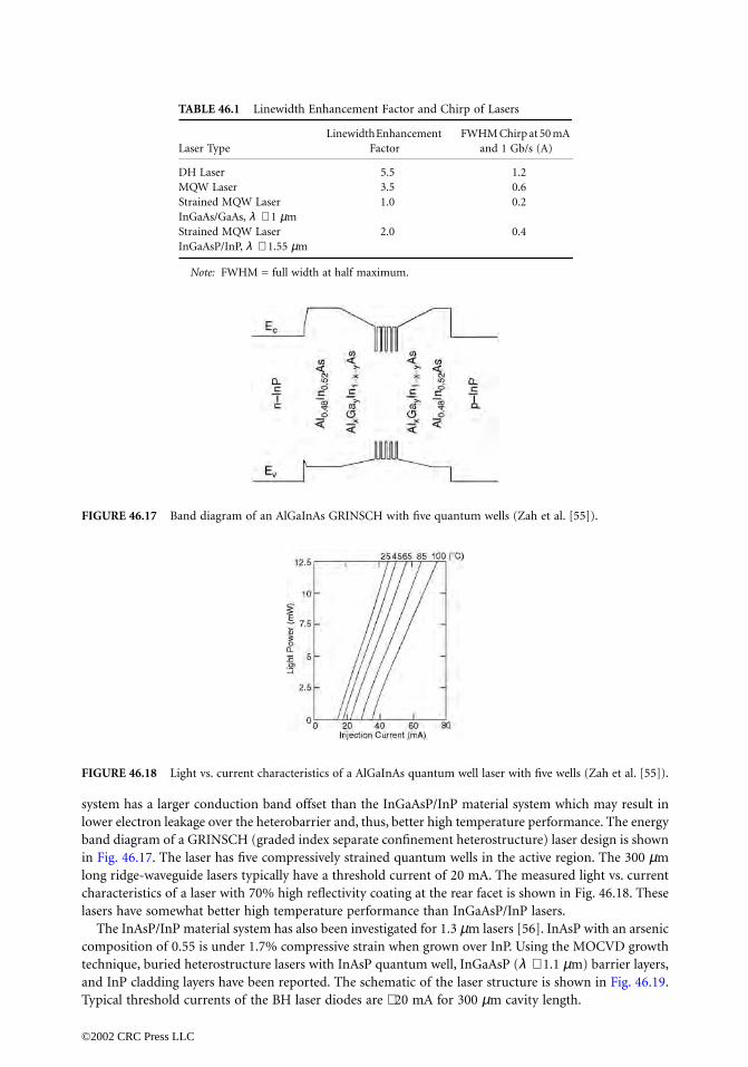
system has a larger conduction band offset than the InGaAsP/InP material system which may result inlower electron leakage over the heterobarrier and, thus, better high temperature performance. The energyband diagram of a GRINSCH (graded index separate confinement heterostructure) laser design is shownin Fig. 46.17. The laser has five compressively strained quantum wells in the active region. The 300 µmlong ridge-waveguide lasers typically have a threshold current of 20 mA. The measured light vs. currentcharacteristics of a laser with 70% high reflectivity coating at the rear facet is shown in Fig. 46.18. Theselasers have somewhat better high temperature performance than InGaAsP/InP lasers.

The InAsP/InP material system has also been investigated for 1.3 µm lasers [56]. InAsP with an arseniccomposition of 0.55 is under 1.7% compressive strain when grown over InP. Using the MOCVD growthtechnique, buried heterostructure lasers with InAsP quantum well, InGaAsP (λ ∼ 1.1 µm) barrier layers,and InP cladding layers have been reported. The schematic of the laser structure is shown in Fig. 46.19.Typical threshold currents of the BH laser diodes are ∼ 20 mA for 300 µm cavity length.

TABLE 46.1 Linewidth Enhancement Factor and Chirp of Lasers

Laser TypeLinewidth Enhancement

FactorFWHM Chirp at 50 mA

and 1 Gb/s (A)

DH Laser 5.5 1.2 MQW Laser 3.5 0.6Strained MQW Laser 1.0 0.2InGaAs/GaAs, λ ∼ 1 µmStrained MQW Laser 2.0 0.4InGaAsP/InP, λ ∼ 1.55 µm

Note: FWHM = full width at half maximum.

FIGURE 46.17 Band diagram of an AlGaInAs GRINSCH with five quantum wells (Zah et al. [55]).

FIGURE 46.18 Light vs. current characteristics of a AlGaInAs quantum well laser with five wells (Zah et al. [55]).


The material InGaNAs, when grown over GaAs, can have very large (∼ 300 meV) conduction band offsetwhich can lead to much better high temperature performance than the InGaAsP/InP material system [57].The temperature dependence of threshold is characterized by Ith(T) = Io exp(T/To) where To is generallycalled the characteristic temperature. Typical To values for an InGaAsP/InP laser is ∼ 60–70 K in thetemperature range of 300–350 K. The predicted To value for the InGaNAs/GaAs system is ∼ 150 K, and,recently, To = 126 K has been reported for an InGaNAs laser emitting near 1.2 µm [57].

46.4 Distributed Feedback Lasers

Semiconductor lasers fabricated using the InGaAsP material system are widely used as sources in manylightwave transmission systems. One measure of the transmission capacity of a system is the data rate.Thus, the drive towards higher capacity pushes the systems to higher data rates where the chromaticdispersion of the fiber plays an important role in limiting the distance between regenerators. Sourcesemitting in a single wavelength help reduce the effects of chromatic dispersion and are, therefore, usedin most systems operating at high data rates (>1.5 Gb/s).

The single wavelength laser source used in most commercial transmission systems is the distributedfeedback (DFB) laser, where a diffraction grating etched on the substrate close to the active region providesfrequency selective feedback which makes the laser emit in a single wavelength. This section reports onthe fabrication, performance characteristics, and reliability of DFB lasers [58].

The schematic of our DFB laser structure is shown in Fig. 46.20. The fabrication of the device involvesthe following steps. First, a grating with a periodicity of 2400 A is fabricated on a (100) oriented n-InPsubstrate using optical holography and wet chemical etching. Four layers are then grown over the substrate.These layers are (1) n-InGaAsP (λ ∼ 1.3 µm) waveguide layer, (2) undoped InGaAsP (λ ∼ 1.55 µm) activelayer, (3) p-InP cladding layer, and (4) p-InGaAsP (λ ∼ 1.3 µm) contact layer. Mesas are then etched onthe wafer using an SiO2 mask and wet chemical etching. Fe doped InP semi-insulating layers are grownaround the mesas using the MOCVD growth technique. The semi-insulating layers help confine thecurrent to the active region and also provide index guiding to the optical mode. The SiO2 stripe is thenremoved and the p-InP cladding layer and a p-InGaAsP contact layer is grown on the wafer using thevapor phase epitaxy growth technique. The wafer is then processed to produce 250 µm long laser chipsusing standard metallization and cleaving procedures. The final laser chips have antireflection coating(<1%) at one facet and high reflection coating (∼ 65%) at the back facet. The asymmetric facet coatingshelp remove the degeneracy between the two modes in the stop band.

The CW light vs. current characteristics of a laser are shown in Fig. 46.21. Also shown is the measuredspectrum at different output powers. The threshold current of these lasers are in the 15 to 20 mA range.For high fiber coupling efficiency, it is important that the laser emit in the fundamental transverse mode.The measured far field pattern parallel and perpendicular to the junction plane at different output powers

FIGURE 46.19 Schematic of a buried heterostructure InAsP/InGaAsP quantum well laser (Kusukawa et al. [56]).


of a device is shown in Fig. 46.22. The figure shows that the laser operates in the fundamental transversemode in the entire operating power range from threshold to 60 mW. The full width at half maximumof the beam divergences parallel and normal to the junction plane are 40° and 30°, respectively.

The dynamic spectrum of the laser under modulation is an important parameter when the laser isused as a source for transmission. The measured 20 dB full width is shown in Fig. 46.23 at two differentdata rates as a function of bias level. Note that for a laser biased above threshold, the chirp width is nearlyindependent of the modulation rate.

Tunable Lasers

Tunable semiconductor lasers are needed for many applications. Examples of application in lightwavetransmission systems are (1) wavelength-division multiplexing where signals at many distinct wavelengthsare simultaneously modulated and transmitted through a fiber and (2) coherent transmission systemswhere the wavelength of the transmitted signal must match that of the local oscillator. Several types oftunable laser structures have been reported in the literature [59–64]. Two principle schemes are (1) multi-section DFB laser and (2) multisection distributed Bragg reflector (DBR) laser. The multisection DBRlasers generally exhibit higher tunability than the multisection DFB lasers. The design of a multisectionDBR laser is shown schematically in Fig. 46.24 [59]. The three sections of this device are (1) the activeregion section that provides the gain, (2) the grating section that provides the tunability, and (3) thephase-tuning section that is needed to access all wavelengths continuously. The current through each ofthese sections can be varied independently. The tuning mechanism can be understood by noting thatthe emission wavelength λ of a DBR laser is given by λ = 2nΛ, where Λ is the grating period and n is

FIGURE 46.20 Schematic of a capped mesa buried heterostructure (CMBH) distributed feedback laser.

FIGURE 46.21 CW light vs. current characteristics and measured spectrum at different output powers. Temperature =30°C.


FIGURE 46.22 Measured far field pattern parallel and perpendicular to the junction plane.

FIGURE 46.23 Measured chirp as a function of bias.

FIGURE 46.24 Schematic of a multisection DBR laser. The laser has an MQW active region. The three sectionsare optically coupled by the thick waveguide layer below the MQW active region (Koch et al. [59]).


the effective refractive index of the optical mode in the grating section. The latter can be changed simplyby varying the current in the grating section.

The extent of wavelength tunability of a three-section DBR laser is shown in Fig. 46.25 [61]. Measuredwavelengths are plotted as a function of phase-section current for different currents in the tuning section.A tuning range in excess of 6 nm can be obtained by controlling currents in the grating and phase-tuningsections.

An important characteristic of lasers for applications requiring a high degree of coherence is the spectralwidth (linewidth) under CW operation. The CW linewidth depends on the rate of spontaneous emissionin the laser cavity. For coherent transmission applications, the CW linewidth must be quite small. Theminimum linewidth allowed depends on the modulation format used. For differential phase-shift keying(DPSK) transmission, the minimum linewidth is approximately given by B/300, where B is the bit-rate.Thus, for 1-Gb/s transmission rate, the minimum linewidth is 3 MHz. The CW linewidth of a laserdecreases with increasing length and varies as α2, where α is the linewidth enhancement factor. Since α issmaller for a multiquantum well (MQW) laser, the linewidth of DFB or DBR lasers utilizing an MQWactive region is smaller than that for lasers with a regular DH active region. The linewidth varies inverselywith the output power at low powers (<10 mW) and shows saturation at high powers. The measuredlinewidth as a function of output power of a 850 µm long DFB laser with an MQW active region isshown in Fig. 46.26. The minimum linewidth of 350 kHz was observed for this device at an operatingpower of 25 mW. For multisection DBR lasers of the type shown in Fig. 46.24, the linewidth varies with

FIGURE 46.25 Frequency tuning characteristics of a three-section MQW DBR laser (Koch et al. [59]).

FIGURE 46.26 Measured CW linewidth plotted as a function of the inverse of the output power for an MQW DFBlaser with a cavity length of 850 µm.


changes in currents in the phase-tuning and grating sections. The measured data for an MQW three-section DBR laser is shown in Fig. 46.27. Measured linewidths are plotted as a function of phase-sectioncurrent for different currents in the tuning section.

46.5 Surface Emitting Lasers

Semiconductor lasers have cleaved facets that form the optical cavity. The facets are perpendicular to thesurface of the wafer and light is emitted parallel to the surface of the wafer. For many applicationsrequiring a two-dimensional laser array or monolithic integration of lasers with electronic components(e.g., optical interconnects), it is desirable to have the laser output normal to the surface of the wafer.Such lasers are known as surface-emitting lasers (SEL). A class of surface emitting lasers also have opticalcavity normal to the surface of the wafer [65–72]. These devices are known as vertical-cavity surface-emitting lasers (VCSEL) in order to distinguish them from other surface emitters.

A generic SEL structure utilizing multiple semiconductor layers to form a Bragg reflector is shown inFig. 46.28. The active region is sandwiched between n- and p-type cladding layers which are themselvessandwiched between the two n- and p-type Bragg mirrors. This structure is shown using the AlGaAs/GaAsmaterial system which has been very successful in the fabrication of SELs. The Bragg mirrors consist ofalternating layers of low index and high index materials. The thicknesses of each layer is one-quarter ofthe wavelength of light in the medium. Such periodic quarter wave thick layers can have very highreflectivity. For normal incidence, the reflectivity is given by [73]

(46.4)

where n2 and n3 are the refractive indices of the alternating layer pairs, n4 and n1 are the refractive indicesof the medium on the transmitted and incident sides of the DBR mirror, and N is the number of pairs.As N increases, R increases. Also, for a given N, R is larger if the ratio of n2/n3 is smaller. For anAlAs/Al0.1Ga0.9As set of quarter wave layers, typically 20 pairs are needed for a reflectivity of ∼ 99.5%.Various types of AlGaAs/GaAs SELs have been reported [74–82].

For an SEL to have a threshold current density comparable to that of an edge-emitting laser, thethreshold gains must be comparable for the two devices. The threshold gain of an edge emitting laser is∼ 100 cm−1. For an SEL with an active-layer thickness of 0.1 µm, this value corresponds to a single-passgain of ∼ 1%. Thus, for the SEL device to lase with a threshold current density comparable to that of anedge emitter, the mirror reflectivities must be >99%.

FIGURE 46.27 Measured CW linewidth as a function of wavelength for a 3-section MQW DBR laser (Koch et al.[61]).

R1 n4/n1 n2/n3( )2N–( )2

1 n4/n1 n2/n3( )2N+( )2---------------------------------------------------=


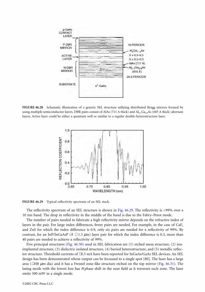
The reflectivity spectrum of an SEL structure is shown in Fig. 46.29. The reflectivity is >99% over a10 nm band. The drop in reflectivity in the middle of the band is due to the Fabry–Perot mode.

The number of pairs needed to fabricate a high reflectivity mirror depends on the refractive index oflayers in the pair. For large index differences, fewer pairs are needed. For example, in the case of CaF2

and ZnS for which the index difference is 0.9, only six pairs are needed for a reflectivity of 99%. Bycontrast, for an InP/InGaAsP (λ ∼ 1.3 µm) layer pair for which the index difference is 0.3, more than40 pairs are needed to achieve a reflectivity of 99%.

Five principal structures (Fig. 46.30) used in SEL fabrication are (1) etched mesa structure, (2) ion-implanted structure, (3) dielectric isolated structure, (4) buried heterostructure, and (5) metallic reflec-tor structure. Threshold currents of ∼ 0.3 mA have been reported for InGaAs/GaAs SEL devices. An SELdesign has been demonstrated whose output can be focussed to a single spot [80]. The laser has a largearea (∼ 100 µm dia) and it has a Fresnel zone-like structure etched on the top mirror (Fig. 46.31). Thelasing mode with the lowest loss has π phase shift in the near field as it traverses each zone. The laseremits 500 mW in a single mode.

FIGURE 46.28 Schematic illustration of a generic SEL structure utilizing distributed Bragg mirrors formed byusing multiple semiconductor layers. DBR pairs consist of AlAs (711 A thick) and Al0.1Ga0.9As (605 A thick) alternatelayers. Active layer could be either a quantum well or similar to a regular double-heterostructure laser.

FIGURE 46.29 Typical reflectivity spectrum of an SEL stack.


An important SEL structure for the AlGaAs/GaAs material system is the oxide aperture device [81](Fig. 46.32). AlAs has the property that it oxidizes rapidly in the presence of oxygen to aluminum oxidewhich forms an insulating layer. Thus, by introducing a thin AlAs layer in the device structure, it is possibleto confine the current to a very small area. This allows the fabrication of very low threshold (<0.2 mA) andhigh bandwidth (∼ 14 GHz) lasers.

Central to the fabrication of low-threshold SELs is the ability to fabricate high-reflectivity mirrors. Inthe late 1970s, Soda et al. [83] reported on an SEL fabricated using the InP material system. The surfacesof the wafer form the Fabry–Perot cavity of the laser. Fabrication of the device involves the growth of adouble heterostructure on an n-InP substrate. A circular contact is made on the p-side using an SiO2 mask.The substrate side is polished, making sure that it is parallel to the epitaxial layer, and ring electrodes (usingan alloy of Au–Sn) are deposited on the n-side. The laser had a threshold current density of ∼ 11 kA/cm2 at77 K and operated at output powers of several milliwatts.

InGaAsP/InP SELs have been investigated by many researchers over the last few years [83–89]. Manyof the schemes utilize alternating layers of InP and InGaAsP to produce Bragg mirrors (Fig. 46.33)[86].The refractive index difference between InGaAsP (λ ∼ 1.3 µm) and InP layers is smaller than that inGaAs SELs, hence InGaAsP/InP SELs utilize more pairs (typically 40 to 50) to produce a high reflectivity(>99%) mirror. Such mirror stacks have been grown by both chemical beam epitaxy (CBE) and MOCVDgrowth techniques and have been used to fabricate InGaAsP SELs. Room temperature pulsed operationof InGaAsP/InP SELs using these mirror stacks and emitting near 1.5 µm have been reported [88].

FIGURE 46.30 Schematic of several SEL designs.

FIGURE 46.31 Schematic of a high power SEL with a Fresnel zone.

Fresnel Zone

Metal Contact

Top Mirror

Active

Bottom Mirror

Metal Contact

H+ Implantation

Focused Laser Beam

LaserFieldDistribution

+

+

+

−

−−

+ + + + +++ – ––– –


An alternative approach is using the technique of wafer fusion [89,90]. In this technique, the Bragg
mirrors are formed using a GaAs/AlGaAs system grown by MBE, and the active region of InGaAsPbounded by thin InP layers is formed by MOCVD. The post type structure of a 1.5 µm wavelength SELformed using this technique is shown in Fig. 46.34 [89]. The optical cavity is formed by wafer fusion of theInGaAsP quantum well between the Bragg mirrors. Room temperature CW threshold currents of 2.3 mAhave been reported for the 8 µm dia post device [89].

FIGURE 46.32 Schematic of a selectivaly oxidized SEL consisting of AlGaAs/GaAs multilayers and buried aluminumoxide layers. AlGaAs layers with higher Al content are oxidized more.

FIGURE 46.33 Schematic of an InGaAsP SEL fabricated using multilayer mirors (Yang et al. [86]).

FIGURE 46.34 Schematic of an InGaAsP SEL fabricated using wafer fusion (Babic et al. [89]).

Ag/Au 0.1 µm p+ + InGaAsPCONTACT LAYER

n+ InP SUBSTRATE

SiO2

60 Å n− InGaAs(ETCH STOP)

0.4 µm n− InP(BUFFER LAYER)

3-PAIR SiO2/Si MIRROR

1 µm n− InP

1 µm n− InGaAsP(ACTIVE LAYER, λ = 1.3 µm)

0.5 µm p+ InP0.5 µm p InP


46.6 Laser Reliability

The performance characteristics of injection lasers used in lightwave systems can degrade during theiroperation. The degradation is generally characterized by a change in the operational characteristics of thelasers and, in some cases, is associated with the formation and/or multiplication of defects in the activeregion. The degraded lasers usually exhibit an increase in the threshold current which is often accompaniedby a decrease in the external differential quantum efficiency. For single wavelength lasers, the degradationmay be a change in the spectral characteristics, e.g., the degraded device may no longer emit in a singlewavelength although the threshold or the light output at a given current has changed very little.

The dominant mechanism responsible for the degradation is determined by any or all of the severalfabrication processes including epitaxial growth, wafer quality, device processing, and bonding [91–101].In addition, the degradation rate of devices processed from a given wafer depends on the operatingconditions, i.e., the operating temperature and the injection current. Although many of the degradationmechanisms are not fully understood, extensive amounts of empirical observations exist in the literaturewhich have allowed the fabrication of InGaAsP laser diodes with extrapolated median lifetimes in excessof 25 years at an operating temperature of 20°C [93].

The detailed studies of degradation mechanisms of optical components used in lightwave systems havebeen motivated by the desire to have a reasonably accurate estimate of the operating lifetime before theyare used in practical systems. Since for many applications, the components are expected to operate reliablyover a period in excess of 10 years, an appropriate reliability assurance procedure becomes necessary,especially for applications such as an undersea lightwave transmission system where the replacement costis very high. The reliability assurance is usually carried out by operating the devices under a high stress(e.g., high temperature), which enhances the degradation rate so that a measurable value can be obtainedin an operating time of a few hundred hours. The degradation rate under normal operating conditionscan then be obtained from the measured high temperature degradation rate using the concept of anactivation energy [93].

The light output vs. current characteristics of a laser change after stress aging. There is generally a small in-crease in threshold current and a decrease in external differential quantum efficiency following the stress aging.Aging data for 1.3 µm InGaAsP lasers used in the first submarine fiber optic cable is shown in Fig. 46.35 [91].

Some lasers exhibit an initial rapid degradation after which the operating characteristics of the lasersare very stable. Given a population of lasers, it is possible to quickly identify the “stable” lasers by a high

FIGURE 46.35 Operating current for 3 mW output at 60°C as a function of operating time. These data weregenerated for 1.3 µm InGaAsP lasers used in the first submarine fiber optic cable (Nash et al. [91]).

TIME (HOURS) AT 60°C-3 mw/FACET

0 1000 2000 3000 4000 5000 6000 7000 8000

1.5

1.0

0.5

I/I0

BURN-IN: 60°C-3 mw FACET

3.1%/kh

14LASERS

EQUIVALENTCABLE LIFETIME(25 YRS. AT 10°C)

ONE TWO THREE FOUR FIVE


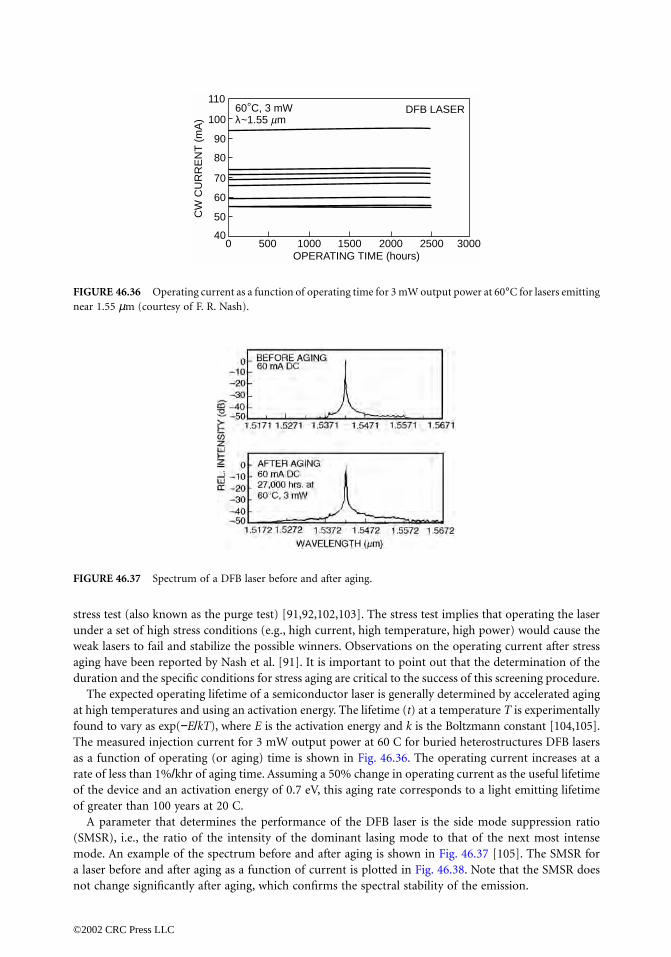
stress test (also known as the purge test) [91,92,102,103]. The stress test implies that operating the laserunder a set of high stress conditions (e.g., high current, high temperature, high power) would cause theweak lasers to fail and stabilize the possible winners. Observations on the operating current after stressaging have been reported by Nash et al. [91]. It is important to point out that the determination of theduration and the specific conditions for stress aging are critical to the success of this screening procedure.

The expected operating lifetime of a semiconductor laser is generally determined by accelerated agingat high temperatures and using an activation energy. The lifetime (t) at a temperature T is experimentallyfound to vary as exp(−E/kT), where E is the activation energy and k is the Boltzmann constant [104,105].The measured injection current for 3 mW output power at 60 C for buried heterostructures DFB lasersas a function of operating (or aging) time is shown in Fig. 46.36. The operating current increases at arate of less than 1%/khr of aging time. Assuming a 50% change in operating current as the useful lifetimeof the device and an activation energy of 0.7 eV, this aging rate corresponds to a light emitting lifetimeof greater than 100 years at 20 C.

A parameter that determines the performance of the DFB laser is the side mode suppression ratio(SMSR), i.e., the ratio of the intensity of the dominant lasing mode to that of the next most intensemode. An example of the spectrum before and after aging is shown in Fig. 46.37 [105]. The SMSR fora laser before and after aging as a function of current is plotted in Fig. 46.38. Note that the SMSR doesnot change significantly after aging, which confirms the spectral stability of the emission.

FIGURE 46.36 Operating current as a function of operating time for 3 mW output power at 60°C for lasers emittingnear 1.55 µm (courtesy of F. R. Nash).

FIGURE 46.37 Spectrum of a DFB laser before and after aging.

OPERATING TIME (hours)0 500 1000 1500 2000 2500 3000

110

100

90

80

70

60

50

40

CW

CU

RR

EN

T (

mA

)

DFB LASER60°C, 3 mWλ~1.55 mm


For some applications such as coherent transmission systems, the absolute wavelength stability of thelaser is important. The measured change in emission wavelength at 100 mA before and after aging ofseveral devices is shown in Fig. 46.39. Note that most of the devices do not exhibit any change inwavelength, and the standard deviation of the change is less than 2 A. This suggests that the absolutewavelength stability of the devices is adequate for coherent transmission applications.

Another parameter of interest in certifying the spectral stability of a DFB laser is the change in dynamiclinewidth or chirp with aging. Since the chirp depends on data rate and the bias level, a certification of thestability of the value of the chirp is, in general, tied to the requirements of a transmission system application.A measure of the effect of chirp on the performance of a transmission system is the dispersion penalty. Wehave measured the dispersion penalty of several lasers at 600 Mb/s for a dispersion of 1700 ps/nm beforeand after aging. The median change in dispersion penalty for 42 devices was less than 0.1 dB and nosingle device showed a change larger than 0.3 dB. This suggests that the dynamic linewidth or the chirpunder modulation is stable.

46.7 Integrated Laser Devices

There have been a significant number of developments in the technology of optical integration of semicon-ductor lasers and other related devices on the same chip. These chips allow higher levels of functionalitythan that achieved using single devices. For example, laser and optical modulators have been integrated,serving as simple monolithic transmitters.

FIGURE 46.38 Side mode suppression ratio (SMSR) as a function of current before and after aging.

FIGURE 46.39 Change in emission wavelength after aging is plotted in the form of a normal probability distribution.

I ERROR BAR

CW CURRENT (mA)

10 50 90 130 170 210

BEFORE AGINGAFTER AGING

50

46

42

38

34

30C

W S

IDE

MO

DE

SU

PP

RE

SS

ION

RA

TIO

(dB

)


Laser Arrays

The simplest of all integrated laser devices are one-dimensional arrays of lasers, LEDs, or photodetectors.These devices are fabricated exactly the same way as individual devices except the wafers are not scribedto make single-device chips but left in the form of a bar. The main required characteristics of a laser arrayare low threshold current and good electrical isolation between the individual elements of the array. Theschematic of two adjacent devices in a 10-channel low threshold laser array is shown in Fig. 46.40 [106].These lasers emit near 1.3 µm and are grown by MOCVD on a p-InP substrate. The lasers have multi-quantum well active region with five 7 nm thick wells, as shown in the insert of Fig. 46.40. The light vs.current characteristics of all the lasers in a 10 element array are shown in Fig. 46.41. The average thresholdcurrent and quantum efficiency are 3.2 mA and 0.27 W/A, respectively. The cavity length was 200 µm andthe facets of the lasers were coated with dielectric to produce 65% and 90% reflectivity, respectively [106].

The vertical cavity surface emitting laser (SEL) design is more suitable for the fabrication of two dimen-sional arrays than the edge emitting laser design. Several researchers have reported two-dimensionalarrays of SELs. Among the individual laser designs used are the proton implanted design and the oxideconfined design. These SELs and SEL arrays have been fabricated so far using the GaAs/AlGaAs materialsystem for emissions near 0.85 µm.

Integrated Laser Modulator

Externally modulated lasers are important for applications where low spectral width under modulationis needed [107–110]. The two types of integrated laser modulator structures that have been investigatedare the integrated electroabsorption modulated laser (EML) and the integrated electrorefraction modulatedlaser. The electrorefraction property is used in a Mach–Zehnder configuration to fabricate a low chirpmodulated light source.

FIGURE 46.40 Schematic of two adjacent devices in a laser array.

FIGURE 46.41 Light vs. current characteristics of all the lasers in a ten element array.

p-InP

p-InP p-InP

n-InPn-InP

n-InP

n-InGaAsP

InGaAsP/InP

10

100

100 nm

oxide

p-Inp sub.

active layer


For some applications it is desirable to have the laser and the modulator integrated on the same chip.Such devices, known as electroabsorption modulated lasers (EMLs), are used for high data rate trans-mission systems with large regenerator spacing. The schematic of an EML is shown in Fig. 46.42 [111].In this device, the light from the DFB laser is coupled directly to the modulator. The modulator regionhas a slightly higher band gap than that of the laser region, which results in very low absorption of thelaser light in the absence of bias. However, with reverse bias, the effective band gap decreases, whichresults in reduced transmission through the modulator. For very high-speed operation, the modulatorregion capacitance must be sufficiently small, which makes the modulator length small resulting in lowon/off ratio. Recently very high-speed EMLs have been reported using a growth technique where thelaser and modulator active regions are fabricated using two separate growths, thus allowing independentoptimization of the modulator band gap and length for high on/off ratio and speed. 40 Gb/s operationhas been demonstrated using this device [111].

EML devices have also been fabricated using the selective area epitaxy growth process [112]. In thisprocess, the laser and the modulator active region are grown simultaneously over a patterned substrate.The patterning allows the materials grown to have slightly different band gaps resulting in separate laserand modulator regions. EMLs have been fabricated with bandwidths of 15 GHz and have operated errorfree over 600 km at 2.5 Gb/s data rate.

An integrated laser Mach–Zehnder device is shown in Fig. 46.43. This device has a ridge-waveguidetype DFB laser integrated with a Mach–Zehnder modulator, which also has a lateral guiding providedby a ridge structure. The Mach–Zehnder traveling wave phase modulator is designed so that the micro-wave and optical velocities in the structure are identical. This allows good coupling of the electrical andoptical signal.

FIGURE 46.42 Schematic of an electroabsorption modulated laser structure (Takeuchi et al. [111]).

FIGURE 46.43 Schematic of an integrated laser and Mach–Zehnder modulator.

Bias electrode forlaser

Passive waveguideY-branch

Coplanar traveling waveelectrodes (Ti/Pl/Au)

2mm Macn Zehncermodulator (BOW’s)

n-InP substrateFo-InP blocking layers

Guide QuantumWells λg-1.3 µm(Selective areagrowth) L-500 µm

Gain QuantumWells λg-1.5 µmBOW’s InGaAs/InP L-300 µm

DFB Grating


Multichannel WDM Sources

An alternative to single channel very high speed (>20 Gb/s) data transmission for increasing transmissioncapacity is multichannel transmission using wavelength division multiplexing (WDM) technology. InWDM systems, many (4, 8, 16, or 32) wavelengths carrying data are optically multiplexed and simul-taneously transmitted through a single fiber. The received signal with many wavelengths is opticallydemultiplexed into separate channels which are then processed electronically in a conventional form.Such a WDM system needs transmitters with many lasers at specific wavelengths. It is desirable to haveall of these laser sources on a single chip for compactness and ease of fabrication like electronic integratedcircuits.

Figure 46.44 shows the schematic of a photonic integrated circuit with multiple lasers for a WDMsource [113]. This chip has four individually addressable DFB lasers, the output of which are combinedusing a waveguide based multiplexer. Since the waveguide multiplexer has an optical loss of ∼ 8 dB, theoutput of the chip is further amplified using a semiconductor amplifier. The laser output in the waveguideis TE polarized and, hence, an amplifier with a multiquantum well absorption region which has a highsaturation power is integrated in this chip.

Spot Size Converter (SSC) Integrated Laser

A typical laser diode has too wide (∼ 30° × 40°) an output beam pattern for good mode matching to asingle mode fiber. This results in a loss of power coupled to the fiber. Thus, a laser whose output spotsize is expanded to match an optical fiber is an attractive device for low loss coupling to the fiber withouta lens and for wide alignment tolerances. Several researchers have reported such devices [114,115].Generally, they involve producing a vertically and laterally tapered waveguide near the output facet ofthe laser. The tapering needs to be done in an adiabatic fashion so as to reduce the scattering losses. Theschematic of an SSC laser is shown in Fig. 46.45 [115]. The laser is fabricated using two MOCVD growthsteps. The SSC section is about 200 µm long. The waveguide thickness is narrowed along the cavity from300 nm in the active region to ∼ 100 nm in the region over the length of the SSC section. The laser emitsnear 1.3 µm, has a multiquantum well active region, and a laser section length of 300 µm. The light vs.current characteristics of a SSC laser [115] at various temperatures are shown in Fig. 46.46. A beamdivergence of 13° was obtained for this device. Beam divergences of 9° and 10° in the lateral and verticaldirection have been reported for similar SSC devices [115].

FIGURE 46.44 Schematic of a photonic integrated circuit with multiple lasers for a WDM source.


46.8 Summary and Future Challenges

Tremendous advances in semiconductor lasers have occurred over the last decade. The advances in researchand many technological innovations have led to the worldwide deployment of fiber optic communicationsystems that operate near 1.3 µm and 1.55 µm wavelengths and compact storage disks which utilize lasersfor read/write purposes. Although most of these systems are based on digital transmission, lasers havealso been deployed for carrying high quality analog cable TV transmission systems. However, manychallenges remain.

The need for higher capacity is pushing the deployment of WDM-based transmission which needstunable or frequency settable lasers. An important research area continues to be the development of laserswith very stable and settable frequency. Integration of many such lasers on a single substrate wouldprovide the ideal source for WDM systems.

The laser-to-fiber coupling is also an important area of research. Recent development in spot sizeconverter integrated lasers is quite impressive, but some more work, perhaps, needs to be done to makethem easy to manufacture. This may require more process developments.

Lasers with better high temperature performance constitute an important area of investigation. TheInGaAsN based system is a promising candidate for making lasers that emit near 1.3 µm with good hightemperature performance. New materials investigation is important.

Although WDM technology is currently being considered for increasing the transmission capacity, theneed for sources with very high modulation capability remains. Hence, research on new mechanisms forvery high-speed modulation is important.

FIGURE 46.45 Schematic of a spot size converter (SSC) laser (Yamazaki et al. [115]).

FIGURE 46.46 Light vs. current characteristics of an SSC laser at different temperatures (Yamazaki et al. [115]).


The surface emitting laser is very attractive for two-dimensional arrays and for single wavelength oper-ation. Several important advances in this technology have occurred over the last few years. An importantchallenge is the fabrication of a device with characteristics superior to that of an edge emitter.

Finally, many of the advances in the laser development would not have been possible without theadvances in materials and processing technology. The challenges of much of the current laser researchare intimately linked with the challenges in materials growth, which include not only the investigationof new material systems but also improvements in existing technologies to make them more reproducibleand predictable.

References

1. H. Kressel and J. K. Butler, Semiconductor Lasers and Heterojunction LEDs, Academic Press, NY, 1977.2. H. C. Casey, Jr. and M. B. Panish, Heterostructure Lasers, Academic Press, NY, 1978.3. G. H. B. Thompson, Physics of Semiconductor Lasers, John Wiley and Sons, NY, 1980.4. G. P. Agrawal and N. K. Dutta, Long Wavelength Semiconductor Lasers, Van Nostrand Reinhold Co.,

New York, 1986.5. N. Holonyuk, Jr. and S. F. Bevacqua, Appl. Phys. Lett., 1, 82, 1962.6. M. I. Nathan, W. P. Dumke, G. Burns, F. H. Dill, Jr., and G. Lasher, Appl. Phys. Lett., 1, 63, 1962.7. T. M. Quist, R. H. Retiker, R. J. Keyes, W. E. Krag, B. Lax, A. L. McWhorter, and H. J. Ziegler, Appl.

Phys. Lett., 1, 91, 1962; R. N. Hall, G. E. Fenner, J. D. Kingsley, T. J. Soltys, and R. O. Carlson, Phys.Rev. Lett., 9, 1962.

8. I. Hayashi, M. B. Panish, P. W. Foy, and S. Sumsky, Appl. Phys. Lett., 47, 109, 1970.9. J. J. Hsieh, Appl. Phys. Lett., 28, 283, 1976.

10. See Chapter 4, Ref. 4.11. R. E. Nahory, M. A. Pollack, W. D. Johnston, Jr., and R. L. Barns, Appl. Phys. Lett., 33, 659, 1978.12. See Chapter 5, Ref. 4.13. N. Holonyak, Jr., R. M. Kolbas, R. D. Dupuis, and P. D. Dapkus, IEEE J. Quantum Electron., QE-16,

170, 1980.14. N. Holonyak, Jr., R. M. Kolbas, W. D. Laidig, B. A. Vojak, K. Hess, R. D. Dupuis, and P. D. Dapkus,

J. Appl. Phys., 51, 1328, 1980.15. W. T. Tsang, Appl. Phys. Lett., 39, 786, 1981.16. W. T. Tsang, IEEE J. Quantum Electron., QE-20, 1119, 1986.17. S. D. Hersee, B. DeCremoux, and J. P. Duchemin, Appl. Phys. Lett., 44, 1984.18. F. Capasso and G. Margaritondo, Eds., Heterojunction Band Discontinuation: Physics and Applica-

tions, North Holland, Amsterdam, 1987.19. N. K. Dutta, S. G. Napholtz, R. Yen, R. L. Brown, T. M. Shen, N. A. Olsson, and D. C. Craft, Appl.

Phys. Lett., 46, 19, 1985.20. N. K. Dutta, S. G. Napholtz, R. Yen, T. Wessel, and N. A. Olsson, Appl. Phys. Lett., 46, 1036, 1985.21. N. K. Dutta, T. Wessel, N. A. Olsson, R. A. Logan, R. Yen, and P. J. Anthony, Electron. Lett., 21, 571,

1985.22. N. K. Dutta, T. Wessel, N. A. Olsson, R. A. Logan, and R. Yen, Appl. Phys. Lett., 46, 525, 1985.23. Y. Arakawa and A. Yariv, IEEE J. Quantum Electron., QE-21, 1666, 1985.24. Y. Arakawa and A. Yariv, IEEE J. Quantum Electron., QE-22, 1887, 1986.25. A. Yariv, C. Lindsey, and V. Sivan, J. Appl. Phys., 58, 3669, 1985.26. A. Sugimura, IEEE J. Quantum Electron., QE-20, 336, 1984.27. A. Sugimura, Appl. Phys. Lett., 43, 728, 1983.28. N. K. Dutta and R. J. Nelson, J. Appl. Phys., 53, 74, 1982.29. L. C. Chiu and A. Yariv, IEEE J. Quantum Electron., QE-18, 1406, 1982.30. N. K. Dutta, J. Appl. Phys., 54, 1236, 1983.31. A. Sugimura, IEEE J. Quantum Electron., QE-19, 923, 1983.32. C. Smith, R. A. Abram, and M. G. Burt, J. Phys., C 16, L171, 1983.


33. H. Temkin, N. K. Dutta, T. Tanbun-Ek, R. A. Logan, and A. M. Sergent, Appl. Phys. Lett., 57, 1610, 1990.34. C. Kazmierski, A. Ougazzaden, M. Blez, D. Robien, J. Landreau, B. Sermage, J. C. Bouley, and A. Mirca,

IEEE JQE, 27, 1794, 1991.35. P. Morton, R. A. Logan, T. Tanbun-Ek, P. F. Sciortino, Jr., A. M. Sergent, R. K. Montgomery, and

B. T. Lee, Electronic Lett.36. P. J. A. Thijs, L. F. Tiemeijer, P. I. Kuindersma, J. J. M. Binsma, and T. van Dongen, IEEE J. Quantum

Electron., 27, 1426, 1991.37. P. J. A. Thijs, L. F. Tiemeijer, J. J. M. Binsma, and T. van Dongen, IEEE J. Quantum Electron., QE-30,

477, 1994.38. H. Temkin, T. Tanbun-Ek, and R. A. Logan, Appl. Phys Lett., 56, 1210, 1990.39. W. T. Tsang, L. Yang, M. C. Wu, Y. K. Chen, and A. M. Sergent, Electron Lett., 2033, 1990.40. W. D. Laidig, Y. F. Lin, and P. J. Caldwell, J. Appl. Phys., 57, 33, 1985.41. S. E. Fischer, D. Fekete, G. B. Feak, and J. M. Ballantyne, Appl. Phys. Lett., 50, 714, 1987.42. N. Yokouchi, N. Yamanaka, N. Iwai, Y. Nakahira, and A. Kasukawa, IEEE J. Quantum Electron., QE-

32, 2148, 1996.43. K. J. Beernik, P. K. York, and J. J. Coleman, Appl. Phys. Lett., 25, 2582, 1989.44. J. P. Loehr and J. Singh, IEEE J. Quantum Electron., 27, 708, 1991.45. S. W. Corzine, R. Yan, and L. A. Coldren, Optical gain in III-V bulk and quantum well semicon-

ductors, in Quantum Well Lasers, P. Zory, Ed., Academic Press, NY, to be published.46. H. Temkin, T. Tanbun-Ek, R. A. Logan, D. A. Coblentz, and A. M. Sergent, IEEE Photonic Technol.

Lett., 3, 100, 1991.47. A. R. Adams, Electron. Lett., 22, 249, 1986.48. E. Yablonovitch and E.O. Kane, J. Lightwave Technol., LT-4, 50, 1986.49. M. C. Wu, Y. K. Chen, M. Hong, J. P. Mannaerts, M. A. Chin, and A. M. Sergent, Appl. Phys. Lett.,

59, 1046, 1991.50. N. K. Dutta, J. Lopata, P. R. Berger, D. L. Sivco, and A. Y. Cho, Electron. Lett., 27, 680, 1991.51. J. M. Kuo, M. C. Wu, Y. K. Chen, and M. A. Chin, Appl. Phys. Lett., 59, 2781, 1991.52. N. Chand, E. E. Becker, J. P. van der Ziel, S. N. G. Chu, and N. K. Dutta, Appl. Phys. Lett., 58, 1704,

1991.53. H. K. Choi and C. A. Wang, Appl. Phys. Lett., 57, 321, 1990.54. N. K. Dutta, J. D. Wynn, J. Lopata, D. L. Sivco, and A. Y. Cho, Electron. Lett., 26, 1816, 1990.55. C. E. Zah, R. Bhat, B. N. Pathak, F. Favire, W. Lin, N. C. Andreadakis, D. M. Hwang, T. P. Lee, Z.

Wang, D. Darby, D. Flanders, and J. J. Hsieh, IEEE J. Quantum Electron., QE-30, 511, 1994.56. A. Kusukawa, T. Namegaya, T. Fukushima, N. Iwai, and T. Kikuta, IEEE J. Quantum Electron., QE-27,

1528, 1993.57. J. M. Kondow, T. Kitatani, S. Nakatsuka, Y. Yazawa, and M. Okai, Proc. OECC’97, July 1997, Seoul,

Korea, 168.58. See Chapter 7, Ref. 4.59. T. L. Koch, U. Koren, R. P. Gnall, C. A. Burrus, and B. I. Miller, Electron. Lett., 24, 1431, 1988.60. Y. Suematsu, S. Arai, and K. Kishino, J. Lightwave Tech., LT-1, 161, 1983.61. T. L. Koch, and U. Koren, IEEE J. Quantum Electron., QE-27, 641, 1991.62. N. K. Dutta, A. B. Piccirilli, T. Cella, and R. L. Brown, Appl. Phys. Lett., 48, 1501, 1986.63. K. Y. Liou, N. K. Dutta, and C. A. Burrus, Appl. Phys. Lett., 50, 489, 1987.64. T. Tanbun-Ek, R. A. Logan, S. N. G. Chu, and A. M. Sergent, Appl. Phys. Lett., 57, 2184, 1990.65. H. Soda, K. Iga, C. Kitahara, and Y. Suematsu, Japan J. Appl. Phys., 18, 2329, 1979.66. K. Iga, F. Koyama, and S. Kinoshita, IEEE J. Quantum Electron., 24, 1845, 1988.67. J. L. Jewell, J. P. Harbison, A. Scherer, Y. H. Lee, and L. T. Florez, IEEE J. Quantum Electron., 27,

1332, 1991.68. C. J. Chang-Hasnain, M. W. Maeda, N. G. Stoffel, J. P. Harbison, and L. T. Florez, Electron. Lett.,

26, 940, 1990.69. R. S. Geels, S. W. Corzine, and L. A. Coldren, IEEE J. Quantum Electron., 27, 1359, 1991.


70. R. S. Geels and L. A. Coldren, Appl. Phys. Lett., 5, 1605, 1990.71. K. Tai, G. Hasnain, J. D. Wynn, R. J. Fischer, Y. H. Wang, B. Weir, J. Gamelin, and A. Y. Cho, Electron.

Lett., 26, 1628, 1990.72. K. Tai, L. Yang, Y. H. Wang, J. D. Wynn, and A. Y. Cho, Appl. Phy. Lett., 56, 2496, 1990.73. M. Born and E. Wolf, Principles of Optics, Pergamon Press, NY, 1977.74. J. L. Jewell, A. Scherer, S. L. McCall, Y. H. Lee, S. J. Walker, J. P. Harbison, and L. T. Florez, Electron

Lett., 25, 1123, 1989.75. Y. H. Lee, B. Tell, K. F. Brown-Goebeler, J. L. Jewell, R. E. Leibenguth, M. T. Asom, G. Livescu, L.

Luther, and V. D. Mattera, Electron. Lett., 26, 1308, 1990.76. K. Tai, R. J. Fischer, C. W. Seabury, N. A. Olsson, D. T. C. Huo, Y. Ota, and A. Y. Cho, Appl. Phys.

Lett., 55, 2473, 1989.77. A. Ibaraki, K. Kawashima, K. Furusawa, T. Ishikawa, T. Yamayachi, and T. Niina, Japan J. Appl.

Phys., 28, L667, 1989.78. E. F. Schubert, L. W. Tu, R. F. Kopf, G. J. Zydzik, and D. G. Deppe, Appl. Phys. Lett., 57, 117, 1990.79. R. S. Geels, S. W. Corzine, J. W. Scott, D. B. Young and L. A. Coldren, IEEE Photonic Tech. Lett., 2,

234, 1990.80. D. Vakhshoori, J. D. Wynn, and R. E. Liebenguth, Appl. Phys. Lett., 65, 144, 1994.81. D. Deppe and K. Choquette, in Vertical Cavity Surface Emitting Lasers, J. Cheng and N. K. Dutta,

Eds., Gordon Breach, NY, 2000.82. N. K. Dutta, L. W. Tu, G. J. Zydzik, G. Hasnain, Y. H. Wang, and A. Y. Cho, Electron. Lett., 27, 208,

1991.83. H. Soda, K. Iga, C. Kitahara, and Y. Suematsu, Japan J. Appl. Phys., 18, 2329, 1979.84. K. Iga, F. Koyama, and S. Kinoshita, IEEE J. Quantum Electron., QE-24, 1845, 1988.85. K. Tai, F. S. Choa, W. T. Tsang, S. N. G. Chu, J. D. Wynn, and A. M. Sergent, Electron. Lett., 27,

1514, 1991.86. L. Yang, M. C. Wu, K. Tai, T. Tanbun-Ek, and R. A. Logan, Appl. Phys. Lett., 56, 889, 1990.87. T. Baba, Y. Yogo, K. Suzuki, F. Koyama, and K. Iga, Electron. Lett., 29, 913, 1993.88. Y. Imajo, A. Kasukawa, S. Kashiwa, and H. Okamoto, Japan J. Appl. Phys. Lett., 29, L1130, 1990.89. D. I. Babic, K. Streubel, R. Mirin, N. M. Margalit, J. E. Bowers, E. L. Hu, D. E. Mars, L. Yang, and

K. Carey, IEEE Photonics Tech. Letts., 7, 1225, 1995.90. Z. L. Liau and D. E. Mull, Appl. Phys. Letts., 56, 737, 1990.91. F. R. Nash, W. J. Sundburg, R. L. Hartman, J. R. Pawlik, D. A. Ackerman, N. K. Dutta, and R. W. Dixon,

AT&T Tech. J., 64, 809, 1985.92. The reliability requirements of a submarine lightwave transmission system are discussion in a special

issue of AT&T Tech. J., 64, 3, 1985.93. B. C. DeLoach, Jr., B. W. Hakki, R. L. Hartman, and L. A. D’Asaro, Proc. IEEE, 61, 1042, 1973.94. P. M. Petroff and R. L. Hartman, Appl. Phys. Lett., 2, 469, 1973.95. W. D. Johnston and B. I. Miller, Appl. Phys. Lett., 23, p. 1972, 1973.96. P. M. Petroff, W. D. Johnston, Jr., and R. L. Hartman, Appl. Phys. Lett., 25, 226, 1974.97. J. Matsui, R. Ishida, and Y. Nannichi, Japan J. Appl. Phys., 14, 1555, 1975.98. P. M. Petroff and D. V. Lang, Appl. Phys. Lett., 31, 60, 1977.99. O. Ueda, I. Umebu, S. Yamakoshi, and T. Kotani, J. Appl. Phys., 53, 2991, 1982.

100. O. Ueda, S. Yamakoshi, S. Komiya, K. Akita, and T. Yamaoka, Appl. Phys. Lett., 36, 300, 1980.101. S. Yamakoshi, M. Abe, O. Wada, S. Komiya, and T. Sakurai, IEEE J. Quantum Electron., QE-17, 167, 1981.102. K. Mizuishi, M. Sawai, S. Todoroki, S. Tsuji, M. Hirao, and M. Nakamura, IEEE J. Quantum Electron.,

QE-19, 1294, 1983.103. E. I. Gordon, F. R. Nash, and R. L. Hartman, IEEE Electron. Device Lett., ELD-4, 465, 1983.104. R. L. Hartman and R. W. Dixon, Appl. Phys. Lett., 26, 239, 1975.105. W. B. Joyce, K. Y. Liou, F. R. Nash, P. R. Bossard, and R. L. Hartman, AT&T Tech. J., 64, 717, 1985.106. S. Yamashita, A. Oka, T. Kawano, T. Tsuchiya, K. Saitoh, K. Uomi, and Y. Ono, IEEE Photonic Tech.

Lett., 4, 954, 1992.


107. I. Kotaka, K. Wakita, K. Kawano, H. Asai, and M. Naganuma, Electron. Lett., 27, 2162, 1991.108. K. Wakita, I. Kotaka, K. Yoshino, S. Kondo, and Y. Noguchi, IEEE Photonic Tech. Letts., 7, 1418, 1995.109. F. Koyama and K. Iga, J. Lightwave Tech., 6, 87, 1988.110. J. C. Cartledge, H. Debregeas, and C. Rolland, IEEE Photonic Tech. Lett., 7, 224, 1995.111. H. Takeuchi, K. Tsuzuki, K. Sato, M. Yamamoto, Y. Itaya, A. Sano, M. Yoneyama, and T. Otsuji,

IEEE Photonic Tech. Lett., 9, 572, 1997.112. M. Aoki, M. Takashi, M. Suzuki, H. Sano, K. Uomi, T. Kawano, and A. Takai, IEEE Photonic Tech.

Letts., 4, 580, 1992.113. T. L. Koch and U. Koren, AT&T Tech. J., 70, 63, 1992.114. R. Y. Fang, D. Bertone, M. Meliga, I. Montrosset, G. Oliveti, and R. Paoletti, IEEE Photonic Tech.

Lett., 9, 1084, 1997.115. H. Yamazaki, K. Kudo, T. Sasaki, and M. Yamaguchi, Proc. OECC’97, Seoul, Korea, paper 10C1-3,

440–441.


47Optical Transmitters

47.1 Introduction47.2 Directly Modulated Laser Transmitters

Laser Diode Characteristics • Electronic Driver Circuit Design • Optoelectronic Package Design • Transmitter Performance Evaluation

47.3 Externally Modulated Optical TransmittersCharacteristics of External Modulators • Modulator Driver Circuit Design

47.1 Introduction

In the last 15 years, optical fiber transmission systems have progressed enormously in terms of informa-tion handling capacity and link distance. Some major advances in transmitter technology, both electronicand optoelectronic, have made this possible. The single longitudinal mode infrared emission fromsemiconductor distributed feedback (DFB) laser diodes can be coupled efficiently into today’s low-losssilica single-mode fibers. In addition, these lasers can be switched on and off with transition times onthe order of 100 ps to provide data rates up to approximately 10 Gb/s. The outstanding performance ofthese laser diodes has, in fact, provoked considerable effort to improve the switching speed of digitalintegrated circuits in order to fully utilize the capability of the optoelectronic components.

The performance of directly modulated laser transmitters greatly surpasses that of light emitting diode(LED) transmitters both in terms of optical power coupled into the fiber and switching speed. Short-distance (<10 km), low-capacity (<1 Gb/s) links use LED transmitters. For these applications, such as forlocal area networks, for example, LED transmitters can provide a cost-effective alternative to the laser.

Where high bit rates and a large regenerator spacing are required, optical pulse distortion occurringin the fiber between the transmitter and receiver is very important. Because of the advent of the opticalamplifier, these requirements are now commonplace in terrestrial as well as submarine communicationsystems because amplifiers can cost-effectively eliminate the loss of very long fiber links. With loss outof the way, distortion becomes a major issue. Phase/frequency shifts accompany the switching of semi-conductor lasers. Commonly referred to as chirp, these shifts cause rapid deterioration of the pulse shapein dispersive optical fibers, thereby limiting the reach of directly modulated transmitters. For example,at a bit rate of 2.5 Gb/s, a distance of 200 km represents the limit of what is currently achievable usingconventional single-mode fiber (assuming an operating wavelength in the 1550 nm low-loss window).Higher performance transmitters use external modulators to exceed these limits. External modulatorsexist which produce little or no switching phase shift.

The following sections include some information about the characteristics of laser diodes used indirectly modulated optical transmitters and the electronic circuits to drive them. A brief description ofpackaging technology is also provided. A section is included on the performance characterization ofhigh-speed digital lightwave transmitters. The use of external modulators introduces a new set of designrequirements. These are also discussed.

Alistair J. PriceCorvis Corporation

Ken D. PedrottiUniversity of California


Whereas digital transmission dominates the field of optical fiber transmission systems, analog systemsare also important for the transmission of cable TV signals and microwave signals for remote antennalocation and phase array radar systems, for example. The requirements for analog transmitters dependon the type of signal to be transmitted and are generally quite different from those of digital systems.Properties which are not very important in digital systems, such as linearity and signal-to-noise ratio,are very important in analog systems because, once degraded, the signal quality cannot be restored. Moreinformation about analog transmission is contained in Kolner and Dalfi [1987], Atlas [1996], and Linderet al. [1995].

47.2 Directly Modulated Laser Transmitters

The design of a state-of-the-art laser transmitter requires the combining of several different technolo-gies. The laser diode is, of course, the critical component whose properties govern the transmitterperformance. Its electrical and optical properties are both very important. The electrical driver circuitand the link between it and the laser are also critical design areas. Finally, the package design is a specializedcombination of a microwave and optical enclosure.

Laser Diode Characteristics

The laser diode must launch optical pulses into the optical fiber at the required wavelength, with highspectral purity, with a high extinction ratio, and with a low-intensity noise. These properties have beendiscussed in a previous chapter. The optical format is typically non-return to zero (NRZ), but return-to-zero (RZ) format is also used. The ideal optical signal will reproduce the data stream faithfully withoutjitter, ringing, or chirp. These cannot be eliminated entirely, and each contributes to the overall systemperformance.

A look at the light, current (L/I) characteristic of a DFB laser reveals a lot about its basic character(see Fig. 47.1). The light output is relatively small until the current reaches a certain value, called thethreshold current. Thereafter, the optical intensity rises approximately linearly with increasing current.For digital modulation, the current to the laser switches between two levels, the 0 level current beingnear the threshold current and the 1 level current being higher. The problems associated with typical

FIGURE 47.1 L/I (light vs. current) characteristic of a DFB laser.


laser diodes are that the curve bends over at high current and tends to shift and bend to the right withincreasing temperature and as the laser ages. In addition, the L/I characteristic often exhibits small kinks,which are usually related to the level of optical power reflected back into the device [Twu et al., 1992].Wavelength fluctuations accompany these kinks. In high bit rate systems, an optical isolator preventsreflections from disturbing the laser. The changes due to temperature and time can, to a large extent, becountered using electronic feedback circuitry, as described in the next section. Often, a temperature-controlled laser mount is also used. Keeping the temperature constant also reduces wavelength drift, anda low temperature extends the laser’s lifetime.

Measurement of laser output while switching the input current between two levels indicates that thedynamic response of these diodes is not straightforward. When switching from low optical power to ahigher power, there is first a turn-on delay, which has a random component. A rapid increase in powerfollows, ringing at the relaxation resonance frequency. An unwanted frequency modulation accompaniesthe ringing. The turn-off is a smooth exponential decay, which is somewhat slower than the turn-ontransition time. Typical waveforms for various current levels are shown in Fig. 47.2. The turn-on delaydecreases as the off-state (bias) current is increased. For many digital applications, the bias is carefullyset close to the laser threshold current to minimize the turn-on delay while at the same time providinga high-extinction ratio.

The dynamic behavior just described can be modeled using the laser rate equations. The single-moderate equations are frequently presented as:

(47.1)

(47.2)

where N = electron density; q = electron charge; τn = electron lifetime; N0g = electron density for zerogain; S = photon density; τp = photon lifetime; IA = current injected into active layer; Vact = volume ofactive layer; g0 = differential gain constant; ε = gain compression factor; G = optical confinement factor;β = spontaneous emission factor.

FIGURE 47.2 Switching waveforms of DFB lasers: (a) logic 0 bias below the threshold current and (b) logic 0 biasabove the threshold current.

ddt-----N

IA

q Vact⋅--------------- N

τn

----– g0 N N0g–( ) 1 ε S⋅–( ) S⋅ ⋅ ⋅–=

ddt-----S Γ g0 N N0g–( ) 1 ε S⋅–( ) 1

τp

----⋅ ⋅ ⋅ S Γ β Nτn

----⋅ ⋅+⋅=


Computer programs intended for nonlinear circuit analysis, such as the Berkeley SPICE simulationprogram, can be used to solve these equations by defining a circuit to represent them [Tucker, 1985;Wedding, 1987]. The electron and photon densities are represented by circuit node voltages. The tech-nique is powerful because it enables additional electronic circuitry to be included in the analysis. Forexample, the driver circuit, bond wires, and the laser electrical parasitics, as well as the rate equations,can all be modeled in the same analysis. This provides a versatile tool for analyzing the dynamic propertiesof laser transmitters.

Electronic Driver Circuit Design

A simple approach to driving a laser diode is to connect the output of a current driver circuit directlyto the laser diode, as shown in Fig. 47.3. This approach is frequently adopted when the operating frequencyis below 1 GHz. However, the inductance of the bond wires combined with the capacitance associatedwith the driver circuit and the laser can significantly degrade the risetime and cause ringing in the currentpulses. This approach is difficult at higher frequencies because it might be impossible to reduce theinductance sufficiently. For narrow-bandwidth designs, sometimes a matching circuit can be used tocancel the effect of the inductance, but for very high-speed digital designs, a different approach is required.Flip-chip laser mounting on top of the driver circuit [Pedrotti et al., 1992] and fully integrated lasersand drivers [Eriksson et al., 1996] are the subjects of ongoing research, but typically some form of trans-mission line is needed between driver and laser. This leads to new requirements for the driver circuit. Itis generally difficult to implement a characteristic transmission line impedance as low as the typicaldynamic resistance of a laser (3–8 Ω ), and so a technique frequently used is to increase its load resistanceto a more manageable value using a closely mounted series resistor. The series resistor increases the powerdissipation of the resultant load for a given modulation current and also the required voltage swing. Theformer has adverse consequences related to laser thermal effects, and the latter affects the driver circuitrequirements. Low impedances are normally used (in the range 12–25 Ω ), although, when the drivercircuit is completely separated from the laser package, the standard 50-Ω transmission line impedanceis frequently used for convenience, allowing the use of standard coaxial connectors (such as sub-miniatureA (SMA) type) and commercial amplifiers to drive the laser. Testing is also simplified because most high-frequency test equipment uses 50-Ω interconnects as standard. An example of a current switch drivercircuit with transmission line link to the laser is shown in Fig. 47.4. The modulation current is equal tothe current in the tail of the differential output pair, which is controlled by the voltage at the Vgmodinput. The laser bias current (the logic 0 current) is determined by the current in the separate bias source.One example of a high-speed GaAs hetero-junction bipolar transistor (HBT) laser driver circuit is thatreported in Runge et al. [1992], which is a monolithic design with several stages of current amplification

FIGURE 47.3 FET laser driver directly connected to laser diode.


for the laser drive. This circuit includes a Cherry–Hooper amplifier stage driving a cascaded differentialpair output driver.

Typically, various feedback loops are used in practical laser transmitter designs to compensate for thebehavior of laser diodes when influenced by variations in data rate, temperature, and aging effects. Thesimplest average power control circuit is shown in Fig. 47.5. The laser is connected in the collector leadof a typical differential pair driver stage. The data signal is applied to one side of the differential pair anda reference voltage is applied to the other. In addition, the drive transistor is connected in parallel withanother transistor, which serves as a bias current source. This current source is controlled by the outputof a monitor photodiode. A portion of the output power from the laser, typically taken from the laser’s

FIGURE 47.4 Current switch laser driver with transmission line coupling to laser diode.

FIGURE 47.5 Average power control circuit.


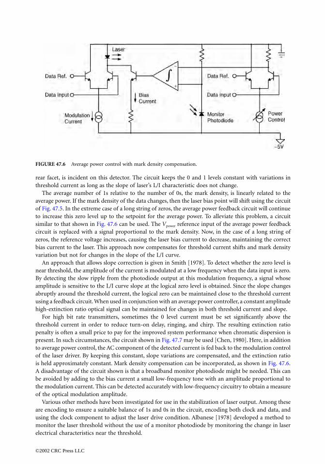
rear facet, is incident on this detector. The circuit keeps the 0 and 1 levels constant with variations inthreshold current as long as the slope of laser’s L/I characteristic does not change.

The average number of 1s relative to the number of 0s, the mark density, is linearly related to theaverage power. If the mark density of the data changes, then the laser bias point will shift using the circuitof Fig. 47.5. In the extreme case of a long string of zeros, the average power feedback circuit will continueto increase this zero level up to the setpoint for the average power. To alleviate this problem, a circuitsimilar to that shown in Fig. 47.6 can be used. The Vpower reference input of the average power feedbackcircuit is replaced with a signal proportional to the mark density. Now, in the case of a long string ofzeros, the reference voltage increases, causing the laser bias current to decrease, maintaining the correctbias current to the laser. This approach now compensates for threshold current shifts and mark densityvariation but not for changes in the slope of the L/I curve.

An approach that allows slope correction is given in Smith [1978]. To detect whether the zero level isnear threshold, the amplitude of the current is modulated at a low frequency when the data input is zero.By detecting the slow ripple from the photodiode output at this modulation frequency, a signal whoseamplitude is sensitive to the L/I curve slope at the logical zero level is obtained. Since the slope changesabruptly around the threshold current, the logical zero can be maintained close to the threshold currentusing a feedback circuit. When used in conjunction with an average power controller, a constant amplitudehigh-extinction ratio optical signal can be maintained for changes in both threshold current and slope.

For high bit rate transmitters, sometimes the 0 level current must be set significantly above thethreshold current in order to reduce turn-on delay, ringing, and chirp. The resulting extinction ratiopenalty is often a small price to pay for the improved system performance when chromatic dispersion ispresent. In such circumstances, the circuit shown in Fig. 47.7 may be used [Chen, 1980]. Here, in additionto average power control, the AC component of the detected current is fed back to the modulation controlof the laser driver. By keeping this constant, slope variations are compensated, and the extinction ratiois held approximately constant. Mark density compensation can be incorporated, as shown in Fig. 47.6.A disadvantage of the circuit shown is that a broadband monitor photodiode might be needed. This canbe avoided by adding to the bias current a small low-frequency tone with an amplitude proportional tothe modulation current. This can be detected accurately with low-frequency circuitry to obtain a measureof the optical modulation amplitude.

Various other methods have been investigated for use in the stabilization of laser output. Among theseare encoding to ensure a suitable balance of 1s and 0s in the circuit, encoding both clock and data, andusing the clock component to adjust the laser drive condition. Albanese [1978] developed a method tomonitor the laser threshold without the use of a monitor photodiode by monitoring the change in laserelectrical characteristics near the threshold.

FIGURE 47.6 Average power control with mark density compensation.


Optoelectronic Package Design

An illustrative example of a laser diode package is shown in Fig. 47.8. In this particular example, the laserdiode is mounted on a diamond heat spreader, which is mounted on a ceramic carrier. Lasers such asthese, which may be purchased from many vendors, allow ease of handling, testing, and replacementwithout handling the device itself. Laser and carrier are mounted on a thermoelectric cooler with athermistor to monitor the temperature and a large-area optical detector, which is used to monitor theoptical power by intercepting the backward wave emission of the laser. It is generally preferred to limitheat generating components mounted on the cooler to a minimum to keep down the cooling requirements.

FIGURE 47.7 Average power and modulation amplitude control circuit.

FIGURE 47.8 Laser package.


Frequently, the temperature controller will be set to keep the temperature near 25∞C or a little higherin order to maximize the range over which stabilization can be maintained (the cooler can be used toheat as well as cool). The electrical link from the driver circuit is provided by a transmission line, asshown in the diagram. This critical link is designed carefully, taking into account dimensional tolerancesin order to repeatedly obtain good performance. To couple power into the optical fiber, a graded index(GRIN) or spherical lens is mounted close to the front facet of the laser to produce a collimated beam.The beam passes through a small optical isolator and is focused into the fiber using a second lens. Anangled optical arrangement is used to reduce reflections. The alignment and stability of this arrangementis critical to achieve a low coupling loss of about 3 dB. For applications that do not require the use ofan isolator to reduce reflections, adequate coupling efficiency may be obtained by directly coupling fromthe laser into the fiber. The end of the fiber is normally tapered, and the tip is formed into a convex lensto match the laser light into the fiber.

Transmitter Performance Evaluation

The methods of evaluating digital optical transmitters and systems have, to a certain extent, been stan-dardized in recent years due to the introduction of synchronous optical network (SONET) and synchronousdigital hierarchy (SDH) optical systems standards [Bell, 1994]. One of the purposes of these standardsis to specify a set of requirements to allow interoperability of equipment from different manufacturers. Anadditional objective is that transmitters from one manufacturer operate with receivers made by anothermanufacturer. Clearly, to achieve this, their characteristics must be sufficiently well specified.

Evaluating the performance of an optical transmitter requires certain measurements of the opticalsignal produced. Using a broadband optical detector, an electrical signal proportional to the opticalintensity is obtained, allowing the intensity modulation to be examined using standard electrical mea-surement techniques. The signal is filtered using a low-pass filter with well-defined characteristics toprovide a standard receiver response. For example, a fourth-order Bessel–Thompson filter with a 3-dBbandwidth equal to 0.75 of the bit rate is specified for testing SONET transmitters. Using an oscilloscope,the signal can then be displayed in the form of an eye pattern. The signal shape must meet certain criteriadefined by an eye pattern mask (see Fig. 47.9). Measurement software overlays these masks on the oscillo-scope screen, measures violations of the limits specified by the masks, and also measures the other char-acteristics such as extinction ratio and jitter.

Eye pattern measurements of the transmitter output signal do not give any indication of phase orfrequency modulation of the optical signal. These, however, are critically important for long-distance

FIGURE 47.9 Eye pattern mask test.


transmission through dispersive fiber. The spectral width is one indicator which is helpful here. A widespectrum is very susceptible to the effects of chromatic dispersion in the transmission medium. For thisreason, a specification is imposed on the spectral width of the transmitted signal. In addition, degradationof the signal must be tested by passing it through a length of optical fiber. Typically, the signal powerrequired at a reference optical receiver input, for example, defined by a 10-10 error rate, when the signalis passed through a given length of optical fiber, is compared with the power required when the trans-mitted signal is passed through a very short length of fiber. The optical power going into the receiver isadjusted using an optical attenuator. The measured power ratio is usually expressed in decibels of dis-persion power penalty for a given chromatic dispersion. A small value is indicative of a high-performance,low-chirp transmitter.

As transmission rates increase, the impairments due to laser chirp combined with chromatic dispersionas well as other signal degradation mechanisms become more severe. One solution to this problem is touse lower chirp modulator sources, as investigated in the following section. Another that can be used inconjunction with either lasers or external modulators is to use forward error correction (FEC) encoding.The fundamentals of FEC are dealt with in detail elsewhere in this volume. Encoding the signal by theaddition of extra bits at the transmitter, their values depending on the bit pattern to be sent, allows thereceiver to not only detect the existence of errors but also to correct them. For example, using the ITU-G.975 optical coding standard which is a Reed–Solomon (255b/239b) code, a received signal with a biterror rate of ~8 × 10-5 with no coding can be received with ~1 × 10-15 BER using the FEC code. Thisimprovement is sometimes expressed in terms of coding gain, which is the difference in received powerwith and without FEC necessary to achieve a certain BER. This gain depends on the BER used for com-parison, but improvements of ~5 dB are common. This transmission improvement can be used to increasethe transmission distance or to allow the use of less expensive components or fiber with wider specificationvariations. This improvement in transmission comes at the cost of the addition of extra bits and requiresthat the transmitter operate at a higher bandwidth, 7% higher in the case of the ITU standard. At 40 Gbit/s,the problems associated with limited electrical bandwidth, device imperfections, and fiber nonlinearitiesrequire the use of FEC in the transmitter to allow reasonable transmission distances with practicalcomponents. The application of other coding schemes with greater coding gain but more complicatedcoding and decoding algorithms are the topics of current investigation.

47.3 Externally Modulated Optical Transmitters

Absorptive modulators and interferometric types are considered here. Because the former type can bemade of the same materials used in the fabrication of lasers, the popularity of these lies in the possibilityof integrating them with the laser diode to save cost [Watanabe, Sato, and Soda, 1992]. The mostcommonly used interferometric type, the Mach–Zehnder, normally uses the electro-optic properties oflithium niobate to provide very precise control over the amplitude and phase of the signal, for high-performance applications.

Characteristics of External Modulators

Electroabsorption (EA) modulators are monolithic semiconductor devices, usually indium phosphide(InP) based. They rely on either the Franz–Keldysh effect (FKE) or the quantum-confined Stark effect(QCSE) and have optical waveguide p-i-n structures grown epitaxially, typically using the InGaAsP-InPor InGaAs-InAlAs material systems [Chin, 1995; Kawano et al., 1992]. Compatibility with laser structuresmakes the integration of laser and modulator possible and very attractive. The advantages of using thesemodulators compared with direct laser modulation are that the chirp associated with the laser relaxationresonance is avoided (although there is some inherent chirp in the modulators (Koyama and Iga, 1988]),the input impedance is high, and these modulators are capable of very high-speed modulation.

A comprehensive comparison of the relative merits of different types of EA modulators is beyond thescope of this text. Some of the factors that affect their suitability in different applications are drive level


requirements, extinction ratio, bandwidth, operating wavelength range, chirp, temperature stability, and,for analog systems, linearity.

Electrically, EA modulators are diodes that operate in reverse bias. The absorption is dependent onthe applied voltage. For high-frequency applications, the capacitance of the device must be considered.A sufficiently low-driving impedance is used so that the low-pass pole caused by the capacitor does notlimit the bandwidth too much. A transmission line link to the drive circuit will frequently be required.In that case, the line could be terminated using a resistor connected in parallel with the modulator atthe end of the transmission line to prevent reflections. For bandpass applications, microwave matchingtechniques are used to improve the modulation efficiency. The bandwidth can also be improved byincorporating the device capacitance into a lumped transmission line structure. The electrical techniquesappropriate to the use of these devices are those that also apply to many other high-impedance devicessuch as FETs and varactor diodes.

Mach–Zehnder modulators operate using interference by splitting the input into two paths, which arelater recombined (see Fig. 47.10). Using lithium niobate or another electro-optic material for the opticalwaveguides, the phase delay is dependent on the electric field applied to the waveguides. Phase modulators

FIGURE 47.10 Mach–Zehnder modulators: (a) package outline, (b) lithium niobate crystal, and (c) detail.


can, therefore, be incorporated in one or both of the split paths allowing electrical control of the phaseof the two signals. Depending on their relative phases when they are recombined, constructive ordestructive interference occurs, resulting in amplitude modulation. The phase modulator electrodes areusually formed into transmission lines following the path of the optical waveguides. In this way, over acertain path length, an applied electrical pulse will continue to modulate an optical signal as both wavesprogress along their respective waveguides. If the velocities are not well matched, which is usually thecase, the optical and electrical waves will not track each other over a long distance and the high-frequencyresponse is affected. For a given required bandwidth, the length of interaction must be limited, whichin turn limits the phase shift induced by a given applied voltage. Typically, therefore, high-bandwidthdesigns require relatively high-drive voltages compared with lower bandwidth designs. The drive voltagerequirements are usually denoted by a value for Vπ, the change in voltage required to produce π-rad phaseshift between the two paths. This corresponds to the voltage needed to go from maximum to minimumamplitude. Typical values are in the order of 10 V for a device with a 10-GHz modulation bandwidth,though this is continually being improved. The extinction ratio for these devices, the ratio of maximumto minimum value expressed in decibels, is dependent on the amplitude balance in the two paths, as wellas the level of other unwanted transmission modes through the device. Typical values are >20 dB.

In modulators for optical transmitters, the path lengths may be several centimeters, equivalent to manywavelengths of the light passing through them. Although great care is taken to maintain device symmetry,the path lengths are not generally identical, and so the required voltage for maximum amplitude trans-mission is usually some random value. In addition, temperature gradients, stresses, and the presence ofimpurities in the optical waveguides all have an effect on the relative phase. For these reasons, care istaken in the packaging and package mounting to avoid mechanical stresses. The terminating resistorsfor the electrical transmission lines are usually isolated from the lithium niobate crystal to prevent heating.Measures are taken to minimize the absorption and subsequent diffusion of impurities in order to reducelong term drifts in the phase difference.

Various transmission line electrode arrangements are possible. Commonly, a single 50-Ω coplanarwaveguide is designed to apply electric fields to both optical waveguides simultaneously such that oneoptical path is retarded while the other is advanced. If the phase shifts are equal but opposite in the twopaths, the resultant amplitude modulation is free of phase modulation (chirp); whereas if only one pathis phase modulated, the resultant modulation contains both amplitude and phase modulation compo-nents. Researchers have discovered [Gnauch et al., 1991] that under certain conditions of chromaticdispersion, transmission distances are actually enhanced if a small amount of phase modulation accom-panies the amplitude modulation by comparison with a completely chirp-free modulation, so now somecommercial modulators provide this optimum amount of chirp. Another type of modulator simplyprovides two separate electrical inputs, each one controlling one arm of the Mach–Zehnder. By controllingthe relative amplitude and sign of the two inputs, the amount and direction of the accompanying chirpcan be precisely controlled. In addition, a differential output driver circuit need supply only half thevoltage swing to each input compared with single-ended drive.

Chirp control is a very important issue when high bit rates are combined with long-distance trans-mission through dispersive fiber. Another approach to phase control is to add a phase modulator incascade with the Mach–Zehnder. It can, of course, be integrated with the Mach–Zehnder by extendingit and incorporating another electrode on the input or output waveguide. The drive waveforms mustthen be coordinated between the Mach–Zehnder and the phase modulator to obtain the required simul-taneous phase and amplitude modulation. Allowance must be made for the optical delay between thetwo modulators, and delay must be provided in the drive signals to compensate.

Whichever electrode configuration is used, the output intensity vs. input voltage is usually the sameshape for all Mach–Zehnder modulators. It is shown in Fig. 47.11, and is sinusoidal in character. Fordigital modulation, the 1 level is aligned with a peak and the 0 level is aligned with an adjacent trough.Restated, the modulator is biased to a half-way point and a modulation swing equal to Vπ (peak-to-peak) is applied. If the modulator has chirp, the sign of the chirp will depend on the sign of the slope,and so the correct side of the peak must be used. Some advantages of the sinusoidal characteristic are


readily apparent. First, because the transfer function is flat at both the peaks and the troughs, noise orspreading of the electrical logic levels will have little effect on the optical intensity levels. Second, thegradient of the transfer function is steepest at the bias point. Provided the bandwidth of the modulatoris sufficiently high, this can result in a reduction in the output optical transition times compared withthe electrical transition times of the drive waveform. The two factors together give rise to an opticaloutput waveform, which is superior in many ways to the electrical waveform used to generate it. This isin marked contrast with the case of direct laser modulation, where the output optical waveforms notonly contain the imperfections of the drive waveform, but also include some added aberrations causedby the laser itself. The waveform improvement is demonstrated in Fig. 47.12.

For most intensity modulation (IM) transmitters, the bias point is at the half-maximum power point,corresponding to phase quadrature between the two paths. The intensity vs. drive voltage characteristicis symmetrical, and the curve is most linear at this point. For most direct detection systems (those inwhich the received optical power is directly converted to a proportional electrical signal), this is thepreferred operating point. However, for some applications, the modulator can be biased at the minimum

FIGURE 47.11 Electrical/optical (E/O) transfer function of Mach–Zehnder modulator.

FIGURE 47.12 Effect of E/O transfer function on optical waveform.


amplitude point. The modulator then behaves very much like the balanced mixers used, for example, asupconverters in microwave radio systems. An electrical signal applied to the modulator will be reproducedat optical frequencies in two sidebands on either side of the (suppressed) optical carrier. This means thatmany of the techniques used to generate radio signals can also be applied to the generation of opticalsignals. The upconversion is quite linear (sinusoidal in fact) so that the electrical signal properties, bothtime domain and frequency domain, are preserved in the conversion. If the electrical signal is filtered toreduce its electrical bandwidth, the optical sidebands will have the same bandwidth. Two referencesprovide examples of such a use, Izutsu et al. [1981] and Price and Le Mercier [1995].

Modulator Driver Circuit Design

A common feature of EA modulators and Mach–Zehnder modulators is that electrically, by contrastwith laser diodes, they present a high impedance to the driving circuit. A low-output impedance circuit,such as an emitter follower, is therefore appropriate for situations where the driver is connected directlyto the modulator. However, as is true for laser driver circuits, the requirements change somewhat whenthe driver must be separated from the modulator, or when the bond wire inductance becomes a sig-nificant factor. Then resonances must be dampened using an appropriate driving resistance or loadresistor. In the case of a transmission line link between driver and modulator, or when the modulatoruses transmission line electrodes, it is essential to either resistively terminate the line, drive the line usinga resistive source, or do both. Again, a 50-Ω transmission line is frequently chosen for convenience andstandardization.

When transmission lines are used, the main driver amplifier requirements for both laser drivers andmodulator drivers become very similar: they must generate electrical pulses of the required power in thetransmission line. The current switch topology of Fig. 47.4 is appropriate for modulators as well as lasers.The main difference is that the required voltage swings are significantly greater for modulators, especiallyexisting Mach–Zehnder designs, compared with laser drivers. For this reason, relatively highpower broad-band 50-Ω amplifiers are frequently used to drive modulators. Power output requirements between 20and 30 dB (1 mW) are typical. Hybrid GaAs metal-semiconductor field-effect transistor (MESFET) designsare used. Integrated circuit solutions include distributed amplifiers.

Automatic control algorithms for Mach–Zehnder modulators contrast those of other optical trans-mitters because the transfer characteristic (see Fig. 47.11) is quite different and there exists the potentialfor multiple operating points and an unlimited lateral drift due to temperature and aging. Typically,some optical power is tapped from the output of the modulator and detected in a low-bandwidth opticaldetector. One method to automatically control the bias point of the modulator is to apply a low-frequencymodulation to the gain of the driver amplifier. A signal will be generated in the detector if the bias pointis not at the quadrature point as intended. By comparing the phase of the detected signal with the originallow-frequency modulation, using a synchronous detector, an error signal can be obtained, which is usedto force the bias point to the quadrature point. Inverting the sense of the feedback loop forces the biaspoint to move to the adjacent quadrature point of opposite slope, causing an inversion of the opticaldata and the chirp. Methods also exist to optimize the modulation amplitude in order to maintain agood optical output waveform. A problem with some Mach–Zehnder modulators is that, over a periodof time, the phase shift might continue to drift over many cycles of phase. An automatic bias circuit isnot able to continue to apply higher and higher voltages to track this drift, so a warning circuit issometimes included to indicate that the voltage might soon reach a limit, after which it would fail totrack. At a convenient time, the circuit is reset by remote control before failure occurs.

Most fielded optical systems today rely on NRZ encoding. However, for long distance transmissionsuch as for undersea links, soliton transmission has for many years been a topic of serious research interest[Agrawal, 1997; Mollenauer et. al., 1997]. A soliton is a particular type of pulse that maintains its shapeduring propagation in a dispersive medium. This is the result of a balancing between the effects ofnonlinear self phase modulation due to the Kerr nonlinearity in the fiber with fiber dispersion. To launcha soliton, a rather high power (sufficient to bring the self phase modulation to an appropriate level) and


narrow pulse of a particular shape is launched into the fiber. Transmitters to create sequences of suitablepulses can be realized using mode-locked fiber ring lasers, gain switched DFB lasers, mode-lockedsemiconductor lasers in hybrid or monolithic extended cavities, and modulators injected with CW beams.Information is typically encoded onto these pulse trains using another Mach–Zehnder interferometer toeither pass or block the individual pulses, resulting in an RZ encoded pulse train. The spacing betweenthese pulses is much greater than their width so that many such pulse trains can be interleaved in timeto create very high bit rate time-division multiplexed signals. New fibers, transmitters, and receivers areresulting in commercialization of the first such soliton systems.

Another related application of RZ modulation is emerging for high bit rate systems operating at ratesof 10 Gb/s and higher. Here, the use of a similar approach to externally modulate a train of short pulsesprovides greater link lengths at high bandwidths although true solitons are not used. The short pulses aregenerated by the use of CW light injected into an external or monolithically integrated modulator. Withappropriate modulator bias and modulation [Veselka, et. al., 1996], a series of short pulses with accuratelycontrolled repetition rate can be generated. These can then be modulated using another amplitude mod-ulator to create the RZ signal. The advantage for high bit rate systems is that the first modulator canoperate narrowband at the pulse repetition frequency using a sinusoidal electrical signal. The resultingnarrow pulses define the edge rates of the transmitted pulses; the second modulator, which must operatewith broadband data, can now have relaxed bandwidth and edge rate response without incurring excessiveinter-symbol interference (ISI), which can also ease the design of the modulator driver electronics.Further, the launch power can be increased, increasing regenerator spacing, and some advantage can beobtained from the interplay of the self phase modulation and fiber dispersion. Additionally, 2-5 dB ofreceiver sensitivity improvement can be realized by the use of this impulsive encoding, depending on thesources of noise in the transmission channel and receiver [Winzer, Kalmar, 1999; Boivin et. al. 1997].

Defining Terms

Chirp: A frequency or phase shift associated with the switching on or off of a laser diode or modulator.Dispersion power penalty: The power penalty in decibels associated with the increase in receiver optical

power level required to achieve a specified error rate, for example, 10–10, when the signal is subjectedto a specified amount of chromatic dispersion.

Electroabsorptive (EA) modulator: Semiconductor modulators using the Franz–Keldysh effect (FKE)or the quantum-confined Stark effect (QCSE).

Extinction ratio: The ratio of maximum to minimum insertion loss for an amplitude modulator. Theterm also applies to the ratio (in decibels) of the average optical energy in a logic 1 level to theaverage optical energy in a logic 0 level of a digitally modulated optical signal.

Eye pattern: Picture built up by overlaying traces corresponding to all possible sequences of a digitalwaveform (see Fig. 47.9).

Jitter: Random and systematic deviations of the arrival times of pulses or transitions in digitallytransmitted data. Observed as a horizontal spreading of an eye pattern displayed on an oscilloscope(see Fig. 47.12).

Laser rate equations: Set of equations representing the dynamic behavior of electron and photonpopulation densities in a laser.

Laser threshold current: Current threshold at which the gain inside the laser cavity exceeds the losses.Below the threshold current, light emission is spontaneous. Above the threshold current, stimulatedemission also occurs.

L/I characteristic: Graph of light output vs. injected current, which exhibits a characteristic knee atthe laser threshold current (see Fig. 47.1).

Mach–Zehnder modulator: A two-path optical interferometer that uses phase shifters in one or bothpaths to provide amplitude modulation.

Non-return to zero (NRZ): Digital format in which the logic 1 pulses occupy the whole bit period (cf.return to zero).


Optical isolator: A device that utilizes the Faraday effect to allow transmission through the device inone direction only. These devices are used to isolate lasers from the effects of reflections.

Relaxation resonance: Internal resonance between electrons and photons in a laser diode.Return to zero (RZ): Digital format in which the logic 1 pulses occupy a fraction (usually 50%) of the

bit period.Thermoelectric (TE) cooler: Device utilizing the Peltier effect to pump heat from one surface to the

other. Reversing the direction of current flow reverses the direction of heat flow, so that the samedevice may be used to heat or cool as necessary.

Vπ: When referred to a phase modulator, it is the voltage change required to give a phase shift of πrad (180∞). For a Mach–Zehnder modulator, this corresponds to the voltage required to changefrom maximum to minimum extinction.

References

Albanese, A. 1978. An automatic bias control (ABC) circuit for injection lasers. Bell Syst. Tech. J., 57:1533-1544.

Agrawal, G. P., Chang, K. (editors). 1997. Soliton communication systems, in Fiber-Optic CommunicationSystems, chap. 10, John Wiley & Sons, NY.

Atlas, D.A. 1996. On the overmodulation limit in externally modulated lightwave AMVSB CATV systems.IEEE phot. Tech. Lett., 8(5):697-699.

Bell. 1994. Physical layer, in Synchronous Optical Network (SONET) Transport Systems: Common GenericCriteria, chap. 4, Issue 1, GR-253-CORE, Bell Communications Research.

Boivin, L., Nuss, M.C., Shah, J. Miller, D.A.B., and Haus H.A. 1997. Receiver sensitivity improvement byimpulsive coding. IEEE Photon. Tech. Lett., 9(5):684-686.

Chen, F.S. 1980. Simultaneous feedback control of bias and modulation currents for injection lasers.Elect. Lett., 16(l):7-8.

Chin, M.K. 1995. Comparative analysis of the performance limits of Franz–Keldysh effect and quantum-confined Stark effect electroabsorption waveguide modulators. IEEE Proc. Optroelectron., 142(2):109-114.

Eriksson, U., Evaldsson, P., Donegan, J.F., Jordan, C., Hegarty, J., Hiei, F., and Ishibashi, A. 1996. Verticalintegration of an InGaAs/InP HBT and a 1.55 um strained MQW p-substrate laser. IEEE Proc.Optoelectron., 143(1):107-109.

Gnauck, A.H., Korotky, S.K., Veselka, J.J., Nagel, J., Kemmerer, C.T., Minford, W.J., and Moser, D.T. 1991.Dispersion penalty reduction using an optical modulator with adjustable chirp. Elec. Lett., 28:954-955.

Izutsu, M. et al. 1981. Integrated optical SSB modulator/frequency shifter. IEEE J. Quant. Electron., QE-17(11):2225.

Kawano, K., Wakita, K., Mitomi, O., Kotaka, I., and Naganuma, M. 1992. Design of InGaAs-InAlAsmultiple-quantum-well (MQW) optical modulators. IEEE J. Quant. Electron., 28(1):224-230.

Koyama, F. and Iga, K. 1988. Frequency chirping in external modulators. J. Lightwave Tech., 6:87-93.Kolner, B.H. and Dolfi, D.W. 1987. Intermodulation distortion and compression in an integrated electro-

optic modulator. Appl. Optics, 26(17):3676-3680.Linder, N., Kiesel, P., Kneissl, M., Knuepfer, B., Quassowski, S., Doehler, G.H., and Traenkle, G. 1995.

Linearity of double heterostructure electroabsorptive waveguide modulators. IEEE J. Quant. Elec-tron., 31(9):1674-1681.

Mollenauer, L.F., Gordon, J. P., Mamyshev, P. V. 1997. Solutions in high bit rate, long distance transmission,In Optical Fiber Telecommunications IIIA, Eds. I.P. Kaminow and T. L. Koch, Academic Press, NY.

Pedrotti, K.D., Seabury, C.W., Sheng, N.H., Lee, C.P., Agarwal, R., Chen, A.D.M., and Renner, D. 1992.6-GHz operation of a flip-chip mounted 1.3-um laser diode on an AlGaAs/GaAs HBT laser drivercircuit. OFC’ 92, ThJ7, 241.


Price, A.J. and Le Mercier, N. 1995. Reduced bandwidth optical digital intensity modulation withimproved chromatic dispersion tolerance. Elec. Lett., 31(1):58-59.

Runge, K., Detlef, D., Standley, R.D., Gimlett, J.L., Nubling, R.B., Peterson, R.L., Beccue, S.M., Wang,K.C., Sheng, N.H., Chang, M.F., Chen, D.M., and Asbeck, P.M. 1992. AlGaAs/GaAs HBT IC’s forhigh-speed lightwave transmission systems. IEEE JSSC, 27(10):1332-1341.

Smith, D.W. 1978. Laser level-control circuit for high-bit-rate systems using a slope detector. Elec. Lett.,14(24):775-776.

Tucker, R.S. 1985. High-speed modulation of semiconductor lasers, J. Lightwave Tech., LT-3(6):1180-1192.Twu, Y., Parayanthal, P., Dean, B.A., and Hartman, R.L. 1992. Studies of reflection effects on device

characteristics and system performances of 1.5 um semiconductor DFB lasers. J. Lightwave Tech.,10(9):1267-1271.

Veselka, J.J., Korotky S.K. 1996. Pulse generation for soliton systems using lithium niobate modulators.IEEE J. Sel. Topics. Quant. Electron., 2(2):300-310.

Watanabe, T., Sato, K., and Soda, H. 1992. Low drive voltage and low chirp modulator integrated DFBlaser light source for multiple-gigabit systems. Fuj. Sci. Tech. J., 28(1):115-121.

Wedding, B. 1987. SPICE simulation of laser diode modules. Elect. Lett., 23(8):383-384.Winzer, P.J. and Kalmar, A. 1999. Sensitivity enhancement of optical receivers by impulsive coding. J. Light-

wave Tech., 17(2):171-177.

Further Information

Alferness, R.C. 1982. Waveguide electrooptic modulators. IEEE Trans. Microwave Th. Tech., MTT-30:1121-1137.

Gu, X. and Blank, L.C. 1993. 10 Gbit/s unrepeatered three-level optical transmission over 100 km ofstandard fiber. Elec. Lett., 29(25):2209-2211.

Henry, P.S. 1985. Lightwave primer. IEEE J. Quant. Electron., QE-21:1862-1879.Ortel. 1992. RF/Microwave Fiber Optic Link Design Guide, Ortel Corp.Patel, B.L. et al. 1992. Transmission at 10 Gb/s over 100 km using a high performance electroabsorption

modulator and the direct prechirping technique. In ECOC’92, postdeadline paper Th PD 1.3,Berlin, Germany.

Pedrotti, K.D., Zucca, F., Zampardi, P.J., Nary, S.M., Beccue, S.M. Runge, K., Meeker, D., Penny, J., andWang, K.C. 1995. HBT transmitter and data regenerator arrays for WDM optical communicationsapplication. IEEE J. Solid-State Circ., 30(10):1141-1144.

Shumate, P.W. 1988. Lightwave transmitters, in Optical Fiber Telecommunications II, Eds. S.E. Miller andI.P. Kaminow, Academic Press, NY, chap. 19.

Wedding, B., Franz, B., and Junginger, B. 1994. 10-Gb/s optical transmission up to 253 km via standardsingle-mode fiber using the method of dispersion-supported transmission. J. Lightwave Tech.,12(10):1720-1727.


48Optical Receivers

48.1 Introduction Goal

48.2 The ReceiverThe Photodetector • Preamplifier • Postamplifier• Filtering • Timing Recovery • Decision Circuit

48.3 Receiver Sensitivity: GeneralSignal Current • Sources of Noise

48.1 Introduction

The optical receiver is an integral part of an optical link. Its function is to detect the received opticalpower, amplify the signal, retime, regenerate, and reshape the signal where it may remain as an electricalsignal (terminal), or be used to drive an optical transmitter which then feeds another fiber section.

Goal

The goal of the optical receiver is to achieve the desired system performance while requiring the minimumamount of received optical power. System performance criteria include bit error ratio (BER) and eyemargin for digital systems, signal-to-noise ratio (SNR) for analog systems, and dynamic range (ratio oflargest to smallest signal levels for which the BER or SNR can be achieved).

Over the past 20 years there has been a large amount of work on optical receivers. This work is well coveredby review papers and book chapters [Kasper, 1988; Muoi, 1984; Smith and Personick, 1982]. Although thefield is fairly mature, there are still advances being made, such as the use of optical preamplifiers to improvereceiver sensitivity [Olsson, 1989].

48.2 The Receiver

A block diagram of the optical receiver is shown in Fig. 48.1. The receiver consists of a photodetector, apreamplifier, postamplifier, filter, timing recovery, and decision circuit.

The Photodetector

The purpose of the photodetector is to convert the received optical signal into a photocurrent. It isessentially a photon-to-electron converter. The most widely used forms of photodetectors used in opticalcommunications are the p-i-n photodiode and the avalanche photodiode (APD). In the case of the p-i-n,a single electron-hole pair is generated for each photon absorbed by the detector. In the case of the APD,electronic gain within the detector itself generates secondary electron-hole pairs, multiplying the photo-current and generally improving the receiver sensitivity. (See chapter on optical detectors for a discussionof photodetectors.)

Richard G. SmithCenix, Inc.

Byron L. KasperAgere Systems


Preamplifier

The preamplifier or front end is the most important element of the receiver in determining the opticalsensitivity. Its principal function is to amplify the generally small photocurrent with the least amount ofadded noise. Under most circumstances (especially with a p-i-n detector), the preamplifier noise is dom-inant in determining the sensitivity. The preamplifier must also have sufficient frequency response so asnot to severely distort the received signal shape (eye margin). In addition to noise level and frequencyresponse, the front end must be able to respond to a wide range of received optical power levels withoutseverely distorting the signal (dynamic range). Often, these objectives are in conflict and compromisesmust be made.

Optimized optical receivers differ in several ways from receivers used at RF or microwave frequencies.This difference arises from the fact that the photodetectors generally used (p-i-n, APD) are currentsources, and therefore have inherently high impedance. Optimal signal generation therefore requires thefront end to have a high impedance, which differs from other types of receivers which are typically drivenby low-impedance detectors.

A second major difference between optical systems derives from the relatively large energy of a photon.For a given received power, there are orders of magnitude fewer photons at optical frequencies than atmicrowave or lower frequencies. In the limit of low received optical power, and, hence, low number ofreceived photons and photogenerated hole–electron pairs, the random arrival rate results in signal relatedshot noise, which is often important in determining receiver sensitivity.

Optical receiver front ends can be broadly classed into one of three types: high-impedance or integratingfront end; transimpedance front end; and low-impedance front end, typically a 50-Ω impedance level.Although the distinction is not hard and fast, these categories characterize the various approaches toreceiver design.

The high-impedance front end achieves the best sensitivity for a given detector. This design approachminimizes the thermal noise generated by resistors, given by 4kT/R, by increasing their values such thatthe noise is reduced to a level where it is small compared to other noise sources. As a result of the increasedimpedance level, the frequency response, determined by the combination of the resistor and the capac-itance at the input node of the receiver, is generally very much limited, typically being a factor of 10 ormore smaller than that required to reproduce the signal shape. Such a receiver integrates the signal, hencethe sometimes used description as an integrating front end. The accepted approach to the limited

FIGURE 48.1 Schematic diagram of an optical receiver.


bandwidth is to equalize the signal after sufficient amplification. A simplified schematic of an equalized,high-impedance front end is shown in Fig. 48.2(a).

The high-impedance front end reduces the thermal noise associated with the input resistor, which hastwo major consequences. The first is related to the dynamic range of the receiver. Although the signalfidelity is restored by the equalizer, the low-frequency components of the received signal generate largevoltages at the input node of the receiver. At received optical signals well in excess of the minimum, thissignal buildup will eventually cause the active device (input transistor) to overload, distorting the signal,or perhaps cutting off the receiver. For many applications, dynamic ranges of 20 to 30 dB of opticalpower (40 to 60 dB electrical) are required. This requirement and the limited dynamic range of the high-impedance type of front end limit the usefulness of this approach.

The second consequence of the equalization is to accentuate the noise generated at the output of theamplifying stage. Because of the effect of the equalization, the noise spectral density associated with the out-put stage is proportional to the square of the input capacitance. Optimization (reduction) of the equivalentnoise of the output stage, and, hence, the receiver front end, requires the minimization of the input capaci-tance, a goal of all optical receiver designs. The details of such optimization and the relevant formulas givingthe analytical expressions for the resulting noise can be found in Kasper [1988], Muoi [1984], and Smithand Personick [1982], and are summarized subsequently.

At the other extreme of receiver design is the low-impedance front end typified by a 50-Ω inputimpedance amplifier. The low-impedance front end is the least sensitive of the receivers as its noise levelis much larger than that of both the high-impedance and transimpedance approaches. Low-impedancereceivers find use in laboratory experiments and are used in practical optical communication systemsonly in conjunction with optical preamplifiers.

The transimpedance receiver is schematically shown in Fig. 48.2(b). It is essentially a current-to-voltageconverter. The bandwidth of the receiver is often dominated by the parasitic capacitance of the feedback resistor,

FIGURE 48.2 Schematic diagrams: (a) an integrating front end with equalization and (b) a transimpedancefront end.


which can be very small. Hence, for a given resistor value, the bandwidth of the transimpedance receiverwill be greater than the high-impedance receiver. Under practical conditions, the transimpedance receiveris usually designed with a bandwidth sufficient to reproduce the signal without recourse to equalization.Typically, this results in a higher noise level and hence a poorer sensitivity compared to a high-impedancereceiver. It does, however, have an improved dynamic range as the input node is effectively a low impedancedue to the electrical feedback. The transimpedance receiver is generally used in optical systems as it offersa good compromise between the various receiver requirements.

Early receivers were realized with discrete transistors. At the present time, many designs are realizedusing integrated circuits, especially Si bipolar and GaAs field-effect transistor (FET) designs. The GaAsreceiver designs generally provide superior receiver sensitivity but are more expensive than their Si bipolarcounterparts. Metal-oxide-semiconductor (MOS) integrated circuit (IC) technology has not found muchapplication in optical receiver front ends, but is used in associated circuitry where the speed is sufficient.Generally speaking, the best sensitivities are still achieved with discrete FET front ends, but for economicconsiderations, integrated circuits are widely used.

Postamplifier

Front ends, as usually employed, typically generate relatively small output signal levels. The output fromthe front end is usually amplified by a postamplifier. Because the range of optical input signals can beas much as 30 dB (60-dB electrical), the postamplifier usually employs some form of output level control.This is typically achieved by an automatic gain control (AGC) function or by using a limiting amplifier.The output signal level is typically of the order of 1 V, which is sufficient to toggle the decision circuit.

Filtering

The main purpose of the filter shown in Fig. 48.1 is to improve the SNR by reducing the noise. Underideal conditions, where the effective bandwidths of the components in the system prior to the filter arelarge, the filter function is such that the signal in a given time slot has zero signal level in all adjacenttime slots. The effective bandwidth of such a filter is approximately 0.6 to 0.7 times the signalling rate,B. In a practical system, the pulse shape incident upon the filter is not ideal as a result of limited bandwidthin the transmitter, front end, postamplifier, and dispersion in the transmission fiber. The actual filterfunction required is one which transforms the waveform prior to the filter into one that produces anacceptable waveform at the decision circuit while minimizing the noise. In many practical lightwavesystems, there is little or no actual filtering done due to the limited bandwidth of components preceedingthe filter. Often, the filtering is accomplished by the preamplifier or front end.

Timing Recovery

In nearly all lightwave systems it is necessary to recover the clock in the process of regenerating the signal.Several commonly used methods of clock recovery make use of phase locked loops or surface acoustic wavefilters, with the latter being the most widely used for high-frequency systems which have strict requirementson the phase transfer function. Because the commonly used nonreturn to zero (NRZ) format does notcontain energy at the clock frequency, it is necessary to use some form of nonlinear device, such as a rectifieror exclusive OR gate, to produce frequency components at or near the clock frequency. This signal is thenpassed through a narrowband filter such as a surface acoustic wave (SAW) filter or dielectric resonator toextract the clock. The extracted clock, suitably phased, is used to clock the decision circuit and may be usedelsewhere in the terminal or regenerator as needed.

Decision Circuit

The decision circuit receives the signal (plus noise) from the postamplifier along with the recovered clock.The decision circuit produces an output which is reshaped and retimed.


48.3 Receiver Sensitivity: General

The sensitivity of a receiver is usually measured in terms of the average optical power required to producethe desired level of system performance. For digital systems, the measure of performance is the BER orbit error ratio (often referred to as the bit error rate, although incorrectly). The performance measurecommonly used is for a BER = 10–9, although many systems require significantly better performance.For analog applications, the measure of performance is usually the carrier-to-noise ratio (CNR). Poweris measured in terms of decibels referred to 1 mW of received power. Further, for digital systems, sensitivityis measured in terms of the average power received, taking into account the population of marks andspaces (i.e., 1s and 0s). The average power is thus approximately one-half of the peak power or 3 dBbelow the peak received power. In order to evaluate the receiver sensitivity, it is necessary to evaluateboth the photogenerated signal current and the sources of noise which corrupt the signal.

Signal Current

The photocurrent generated by a received optical power P is given by

(48.1)

where h is Planck’s constant (6.623E-34 J/s), υ is the optical frequency, q is the electronic charge, and ηis the quantum efficiency of the detector (defined in terms of the number of photoelectrons generatedper photon received). In well-designed detectors, the quantum efficiency is usually between 0.8 and 1.0.When a p-i-n detector is used, Eq. (48.1) becomes the signal current; for an avalanche photodiode, thesignal current is given by

(48.2)

where Μ is the expectation value of the avalanche gain.

Sources of Noise

Amplifier or Circuit Noise

As the received signal level (photocurrent generated in the photodetector) is small it must be amplifiedby an electronic amplifier, which contributes noise to the system. The principal sources of noise in theamplifier are thermal noise from resistors and noise generated in the amplifying transistors. It is commonpractice in the analysis of optical receivers to refer all noise sources to the input node where they can becompared to the signal current, Eq. (48.1) or (48.2).

In evaluating the contributions of the various sources of noise, account is taken of the frequencyresponse of the various components of the receiver. The details of this computation are too numerousto be included in this summary and may be found in Personick [1973, 1979] and in Smith and Personick[1982]. We will summarize here the essential results described in the aforementioned references.

The variance of the circuit noise for an FET front end is given by

(48.3)

where k is Boltzmann’s constant, T is the absolute temperature, RL is the load resistance at the input node,q is the electronic charge, Ig is the gate leakage current, gm is the transconductance of the input transistor,

Is

qhhu------ P p-i-n( )=

I MIs Mqhhu------ P APD( )= =

i2⟨ ⟩ ckt

4kTRL

---------¡2B 2qIg¡2B4kT Γ

gm

--------------- 2p CT( )2¡3B3 (FET)+ +=


CT is the total capacitance at the input node, B is the design bit rate, and Γ is a parameter characterizingthe channel noise, which has a value ª1. The parameters ¡2 and ¡3, referred to as the Personick integrals, aredimensionless numbers, which derive from the details of the transfer function of the system. Typical valuesof ¡2 and ¡3 are 0.6 and 0.1, respectively. (A detailed explanation of the Personick integrals may be foundin Personick [1973] and Smith and Personick [1982].) The B3 dependence of the last term arises from thereferral of the output noise source to the input.

The corresponding equation for the variance of the noise for a bipolar front end, neglecting the effectof noise due to base resistance, is given by

(48.4)

For a bipolar transistor, Ic = βIb and the transconductance gm is proportional to the collector current Ic;hence, the noise can be minimized by operating the input transistor at the optimum collector current.The minimum bipolar circuit noise is given by

(48.5)

Signal Shot Noise

The random arrival rates of photons at the detector result in an additional source of noise, which isproportional to the received photocurrent, referred to as signal-dependent shot noise. The spectral densityof this noise source is given by

(48.6)

where I is the average current. This signal-dependent noise constitutes a major difference in optical systemscompared to radio frequency and microwave systems. The variance of this contribution to the noise isfound by integrating the noise spectral density over the transfer function of the system giving

(48.7)

where ℑ 1 is another Personick integral, which has a value ª0.5, and B is the bit rate.

Shot Noise with an Avalanche Photodiode

In many receivers, an avalanche photodiode is used in place of a p-i-n photodiode. As discussed in thechapter on optical detectors in this volume, the APD multiplies the received primary photocurrent givenby Eq. (48.1) by an average multiplication factor M,

For receivers employing an APD, this becomes the signal current [see Eq. (48.2)].If the avalanche multiplication process were ideal (i.e., deterministic), the shot noise spectral density

associated with the signal would be given by

(48.8)

The avalanche process is, however, a random process and not deterministic. This randomness addsadditional noise, which is accounted for by a multiplicative noise factor, referred to as the excess noise

i2⟨ ⟩χκτ4kTRL

---------¡2B 2qIb¡2B2qIc

gm2

--------- 2p CT( )2¡3B3 bipolar( )+ +=

i2⟨ ⟩βιπχκτ/µιν4kTRL

---------¡2B 8pkTCT

¡2¡3

b--------+=

ddf--- i2⟨ ⟩σιγ 2qI=

i2⟨ ⟩σιγ 2qI¡1B=

IAPD MI Mqhhu------ P= =

ddf--- i2⟨ ⟩ 2qIM2=


factor, and denoted F(M). In this case, the signal-dependent shot noise spectral density becomes

(48.9a)

and the mean square noise after integration with respect to frequency is

(48.9b)

Many approximations for F(M) have been given. Among the most commonly used are

(48.10a)

and

(48.10b)

In Eq. (48.10a), x is an empirical constant, usually between 0 and 1, and in Eq. (48.10b), k is the ratioof the ionization coefficients of holes and electrons (not to be confused with Boltzmann’s constant). Thevalue of k is between 0 and 1 if the avalanche is initiated by the most ionizing carrier, as it should be ina well-designed device. Equation (48.10b) provides a better approximation to the excess noise factor andis generally used.

Sensitivity of a Digital Receiver

In a digital system, the objective is to correctly identify transmitted marks (1s) and spaces (0s). Incorrectlyidentifying the transmitted signal produces an error. The probability of making an error in turn dependson the signal level and the probability distribution of the system noise. Under many circumstances, butnot always, the probability distribution of the noise is Gaussian, with an associated standard deviation σ.

Gaussian Approximation

The assumption of a Gaussian distribution permits simplified analytical approximations to sensitivitycalculations, which are generally close to the more rigorous computational approaches. In optical systems,the noise levels associated with the different signal states are not necessarily identical. The standarddeviation of the noise associated with a transmitted 1 is denoted by σ1 and for a transmitted 0 by σ0.The ratios of the signal levels relative to the decision level D normalized to the associated root meansquare (rms) noise levels are given by

(48.11a)

and

(48.11b)

With these definitions, and using the Gaussian approximation, the probability of misinterpreting a trans-mitted 0 as a 1 is given by

(48.12a)

ddf--- i2⟨ ⟩σιγ 2qIM2F M( )=

i2⟨ ⟩σιγ 2qIM2F M( )¡1B=

F M( ) Mx=

F M( ) M 1 1 k–( ) M 1–M

--------------

2

–=

Q1

S1 D–σ1

---------------=

Q0

D S0–σ0

---------------=

P 0,1( ) 1

2πσ0

---------------- S D–( )2–

2σ02

----------------------- dSexpD

∞

∫ 1

2π---------- Q2

2------–exp dQ

1

2πQ0

-----------------Q0

2

2------–

exp≈Q0

∞

∫= =


and the probability of misinterpreting a transmitted 1 is given by

(48.12b)

To a good approximation, the minimum probability of error occurs when each probability of error isthe same, that is, P(0, 1) = P(1, 0), resulting in Q1 = Q0 = Q with

(48.13)

The probability of error as a function of the Q factor is shown in Fig. 48.3. The desired error performancedetermines the value of Q. The average required signal level is given by

(48.14)

with

(48.15)

When the decision level is not optimally placed (Q1 π Q2), the probability of error becomes

(48.16)

Receiver Sensitivity: p-i-n Detector

We are now in a position to calculate the sensitivity of a receiver using a p-i-n detector. Combining Eqs.(48.1) and (48.15), we find that the required peak signal current is

(48.17)

where we assume the signal in the 0 state is identically zero and S1 = Is. The variance of the noise σ2 isgiven by the sum of the circuit noise and the signal shot noise, Eq. (48.7).

(48.18)

FIGURE 48.3 Probability of error vs. Q value.

QS1 S0–s1 s0+----------------=

SS1 S0+

2----------------=

+

P 1,0( ) 1

2πσ1

---------------- S D–( )2–

2σ12

----------------------- dSexp∞–

D

∫=

1

2π---------- Q2

2------–exp dQ

1

2πQ1

-----------------Q1

2

2------–exp≈

∞–

Q1

∫=

S1 S0– Q σ1 σ0+( )=

P E( ) 0.5 P 1, 0( ) P 0, 1( )+[ ]=

Is Q σ1 σ0+( )=

σ 2 i2⟨ ⟩ ckt i2⟨ ⟩ sig+ i2⟨ ⟩ ckt 2qIsℑ1B+= =


The circuit noise for an FET front end is calculated from Eq. (48.3) and for an optimally biased bipolarfront end by Eq. (48.5). Since the signal current equals Is in the 1 state and 0 in the 0 state, the variancesbecome

(48.19a)

and

(48.19b)

Substituting Eqs. (48.19a) and (48.19b) into Eq. (48.17) gives

(48.20)

The peak optical power is found from Eq. (48.1), and the sensitivity, measured in terms of the averagepower, is given by

(48.21)

Under most circumstances, with a p-i-n detector, the second term in Eq. (48.21) is small compared tothe first, leading to the commonly used expression for the p-i-n sensitivity

(48.22)

where λ is the wavelength expressed in micrometers.

Receiver Sensitivity: Avalanche Photodiode Detector

For an APD receiver, the signal current is given by Eq. (48.2) and the variances of the noise in the twosignal states become

(48.23a)

and

(48.23b)

These relations neglect the effect of photodetector dark current and also assume the received signal isidentically zero when a 0 is received. A more general account maybe found in Smith and Personick [1982].Substituting these equations into Eq. (48.17) gives the result

(48.24)

A plot of this expression vs. the gain of the APD, M, is shown in Fig. 48.4 for a receiver operating at622 Mb/s [Tzeng, 1994]. For low gain, the sensitivity is seen to improve, reaching an optimum, and thendeclines for further increases in the gain. The initial improvement is associated with the amplificationof the signal current by the APD, whereas the decrease at high gain results from the excess signal shotnoise associated with the random nature of the avalanche process.

Receiver Sensitivity: Optical Preamplifier

A recent advance in optical fiber technology is the development of optical amplifiers. The most widelyused is the Er-doped fiber amplifier EDFA (see Chapter 52 in this volume for a detailed discussion of

s02 i2⟨ ⟩ ckt=

s12 i2⟨ ⟩ ckt 2qI s¡1B+=

Is 2s0Q 2qQ2¡1B+=

hPs

huq

------ s0Q qQ2¡1B+[ ] p-i-n( )=

Ps

huq

------ Q i2⟨ ⟩ ckt

1/2 1.24Ql

-------------- i2⟨ ⟩ ckt1/2

= =

s 02 i2⟨ ⟩ ckt=

s 12 i2⟨ ⟩ ckt 2qI sM

2F M( )¡1B+=

hPs

huq

------ s0Q

M--------- qQ2¡1BF M( )+=


optical amplifiers). One application of optical amplifiers is their use as an optical preamplifier precedingthe optical receiver previously described. The optical preamplifier amplifies the received optical signalprior to detection by the photodetector. As with other types of amplifiers, optical amplifiers introducenoise resulting from spontaneous emission in the amplifying region. This type of noise is referred to asamplified spontaneous emission (ASE).

Figure 48.5 is a schematic of an optical preamplifier showing the important parameters defined asfollows:

ηin = coupling efficiency of transmission fiber to the optical amplifierηout = coupling of optical amplifier to photodetector input including transmission loss of the optical

filterη = detector efficiencyG = small signal gain of the optical amplifierFm = noise figure of the optical amplifierBo = bandwidth of the optical filter, HzBe = electrical bandwidth of the receiver, Hz

The noise figure of the amplifier is defined as 2nsp where nsp is the spontaneous emission factor. SeeChapter 52 on optical amplifiers in this volume for more detail.

Photocurrents

In receivers incorporating optical preamplifiers, p-i-n detectors are usually employed. For this case, thesignal photocurrent is given by

(48.25)

FIGURE 48.4 Sensitivity of an APD receiver at 622 Mb/s as a function of the APD gain.

FIGURE 48.5 Schematic diagram of an optical preamplifier.

Is

hqhu------

h inhoutGPs=


and the photocurrent generated by the ASE is given by

(48.26)

Noise Sources

The photodetector behaves as a square law detector. The generated photocurrent, which is proportionalto the square of the incident optical field, contains components proportional to signal*signal, ASE*ASE,and signal*ASE. Following the analysis of Olsson [1989], the components of the noise are given by

(48.27a)

(48.27b)

(48.27c)

The first term, , is the shot noise generated by the amplified signal and ASE and contains a termproportional to the received signal. The second term, , results from the ASE beating with itselfin the detector. Since the bandwidth of the optical gain is large (ª1012 Hz) compared to the signal band-width in common usage, the spectral width of the ASE is normally reduced by the use of an optical filterof bandwidth Bo. Bo can be reduced in principle until it approaches Be. The problems of achieving anarrow optical filter bandwidth and of aligning the optical filter with the signal wavelength set the practicallimit on Bo. The noise term is independent of the signal level and, hence, is present in both the0 and 1 states of the signal.

The term results from the mixing of the signal and ASE fields. This noise term is proportionalto the received optical signal power, and in an ideal system, when the received optical power is zero inthe 0 state, = 0. The total noise associated with the 0 state, assuming zero power received, is givenby

(48.28)

and for the 1 state the noise is given by

(48.29)

The receiver sensitivity can be calculated by combining Eqs. (48.13) and (48.25–48.29), yielding

(48.30)

Typically, G is greater than or equal to 30 dB (1000), in which case the first term in brackets is negligible.Further, since varies as the square of the gain while varies only as the first power of thegain and is independent of the gain,

(48.31)

IASE Fmqhouth G 1–( )Bo=

s shot2 2q Is IASE+( )Be=

sspon-spon2

12--F m

2 q2hout2 h2 G 1–( )2 2Bo Be–( )Be=

ssig-spon2 2qFmhouth G 1–( )[ ]

hqhu------

PshinhoutG Be=

2q2Fmhinh out2 h2G G 1–( )

1hu------

PsBe=

s shot2

s spon-spon2

sspon-spon2

s sig-spon2

s sig-spon2

s 02 s ckt

2 s shot2 ASE( ) s spon-spon

2+ +=

s12 sckt

2 s shot2 ASE signal+( ) s spon-spon

2 s sig-spon2+ + +=

Is 2Q2 qBe qFmhouth G 1–( )Be

s0

Q----+ +=

s spon-spon2 s shot

2

s ckt2

s 02 s spon-spon

2 G >>1( )ª


Substituting this limit gives

and the sensthe limit of

When the opbit rates) an

When the baThe value

ideal conditWith an elec

Sensitivity

Quantum Lare characteper bit recei

Optical Am(Q = 6) is

which is appthree to fourof experimePractical Avis a functionthe excess n10–30 for exachievable sfew hundredworse than tPractical p-cation, the rreceiver fronbased receiv

0967-Frame_C48 Page 12 Sunday, July 28, 2002 6:46 PM

©2002 CRC P

(48.32)

itivity measured in terms of the average received power incident on the optical amplifier inlarge gain is

(48.33)

tical filter bandwidth is comparable to the electrical bandwidth (practical only at very highd for very low BER (Q 1), the limiting sensitivity becomes

(48.34)

ndwidth of the optical filter is large compared to the electrical bandwidth, Eq. (48.33) applies. of the noise figure Fm depends on the detailed characteristics of the optical amplifier. Underions of perfect inversion of the gain medium, Fm = 2. Typical values are somewhat higher.trical bandwidth Be = B/2, the limiting sensitivity for a receiver using an optical preamplifier is

(48.35)

Limits

imit. In the limit that the sensitivity is given by the statistics of the received photons whichrized by a Poisson process, the ultimate sensitivity for a BER = 1 E-9 is 10 detected photonsved [Henry, 1985], which corresponds to

(48.36)

plifier Limit. With an optimized optical amplifier, the limiting sensitivity for BER = 1E-9

(48.37)

roximately four times the quantum limit. Demonstrated sensitivities are within a factor of of this value at bit rates greater than 1 GB/s. See Park and Grandlund [1994] for a discussionntal results.alanche Photodiode Performance. The ultimate receiver sensitivity achievable with an APD of the circuit noise and the excess noise factor associated with the avalanche process. Becauseoise factor increases as the avalanche gain is increased, the optimum gain is in the range ofisting APDs and is significantly below the gains used in optically preamplified receivers. Theensitivity is accordingly poorer than the limit for an optical preamp, being in the range of a to as much as several thousand photons per bit and, hence, between a factor of 10–100he quantum limit.i-n Performance. In the absence of a gain mechanism, either avalanche or optical amplifi-eceiver sensitivity is determined by the circuit noise, hence, depending on the design of thet end. Typically, the sensitivity of a p-i-n-based receiver will be ≈10 dB poorer than an APD-er and, hence, typically a few thousand photons per bit.

Is 2Q2 qFmηoutη G 1–( )Be 11Q----

Bo

Be

----- 12--–

12--

+

=

ηinPs Q2 hυ( )FmBe 11Q----

Bo

Be

----- 12--–

12--

+=

>>

ηinPs Q2 hυ( )FmBe≈

ηinPs Q2 hυ( )B=

ηPlimit 10 hυ( )B=

ηinPs−opt.ampl 36 hυ( )B=

ress LLC

Defining Terms

Amplified spontaneous emission (ASE): The fundamental source of noise in optical amplifiers.Avalanche photodiode (APD): A photodiode with internal current gain resulting from impact ionization.Excess noise factor (ENF): A measure of the amount by which the short noise of an APD exceeds that

of an ideal current amplifier.Front end (FN): The input stage of the electronic amplifier of an optical receiver.Integrating front end (IFE): A type of front end with limited bandwidth which integrates the received

signal; requires subsequent equalization to avoid intersymbol interference.Transimpedance front end (TFE): A type of front end which acts as a current to voltage converter;

usually does not require equalization.

References

Henry, P.S. 1985. Lightwave primer. IEEE J. Quantum Electr., QE-21:1879–1879.Kasper, B.L. 1988. Receiver design. In Optical Fiber Telecommunications II, Eds. S.E. Miller and I.P.

Kaminov, Eds., Academic Press, San Diego, CA, 689–722.Muoi, T.V. 1984. Receiver design for high-speed optical-fiber systems. IEEE J. Lightwave Tech., LT-

2:243–267.Olsson, N.A. 1989, Lightwave systems with optical amplifiers. IEEE J. Lightwave Tech., LT-7:1071–1082.Park, Y.K. and Grandlund 1994. Optical preamplifier receivers: application to long-haul digital transmis-

sion, Optical Fiber Tech., 1:59–71.Personick, S.D. 1973. Receiver design for digital fiber optic communication systems I. Bell Syst. Tech. J.,

52:843–874.Personick, S.D. 1979. Receiver design. In Optical Fiber Telecommunications, Eds. S.E. Miller and A.G.

Chenoweth, Academic Press, New York, 627–651.Smith, R.G. and Personick, S.D. 1982. Receiver design for optical fiber communication systems. In Semi-

conductor Devices for Optical Communication, Topics in Applied Physics, Vol. 39, H. Kressel, Ed.,Springer–Verlag, Berlin, 89–160.

Tzeng, L.D. 1994. Design and analysis of a high-sensitivity optical receiver for SONET OC-12 systems,J. Lightwave Tech., LT-12:1462–1470.

Further Information

This section has focused on direct detection of digital signals, which constitute the most widely usedformat in optical communication systems. Coherent optical systems have been studied for some timebut have not yet found practical application. A discussion of this technology and the associated receiversensitivities may be found in Chapter 53 on coherent systems in this volume. Another application ofoptical fiber technology is in the distribution of analog video, which is being employed by communityantenna television (CATV) distribution companies. A discussion of the sensitivity of analog receiversmay be found in Smith and Personick [1982].


49Fiber Optic Connectors

and Splices

49.1 Introduction49.2 Optical Fiber Coupling Theory

Multimode Fiber Joints • Single-Mode Fiber Joints • Reflectance Factors

49.3 Multibeam Interference (MBI) TheoryMBI Effects on Transmission • MBI Effects on Reflectance

49.4 Connector Design AspectsIntroduction (Types of Connectors) • Factors Contributing to Insertion Loss • Factors Contributing to Reflectance (Physical Core-to-Core Contact)

49.5 Splicing Design AspectsMechanical Splices • Fusion Splices

49.6 Conclusions

49.1 Introduction

In recent years, the state of the art of optical fiber technology has progressed to where the achievableattenuation levels for the fibers are very near the limitations due to Rayleigh scattering. As a result, opticalfibers, and particularly the single-mode fibers that are used in today’s communications systems, can beroutinely fabricated with attenuation levels below 0.5 dB/km at a wavelength of 1300 um and 0.25 dB/kmat 1550 nm. Employing these fibers in optical communications systems requires precise jointing devicessuch as connectors and splices. Considering the small size of the fiber cores, less than 10 µm in diameterfor single mode and 100 µm for multimode fibers, it is not surprising that these interconnecting devicescan easily introduce significant optical losses. Furthermore, since single-mode fibers have practicallyunlimited bandwidth, it is also not surprising that they have become the choice for optical communica-tions applications. To provide low-loss connectors and splices for these single-mode fibers, reliable andcost-effective alignment accuracies in the submicrometer range are required.

This chapter will review the fundamental technology that is presently used for optical connectors andsplices. In particular, since single-mode fibers dominate optical communications systems and also requirethe greatest precision and performance, we will focus mainly on the jointing of these fibers. However,for completeness, we will also briefly review multimode fiber jointing technology as well.

Before reviewing the technology, we should define the implied differences between an optical con-nector and a splice. The term connector is commonly used when referring to the jointing of two opticalfibers in a manner that not only permits but also anticipates the unjointing, or unconnecting, throughthe design intent. Optical connectors are commonly used for terminating components, system config-uration and reconfiguration, testing, and maintenance. In contrast, the term splice is commonly usedwhen referring to the jointing of two optical fibers in a manner that does not lend itself to unjointing.

William C. YoungBell Communications Research


There are two types of splices: mechanical splices that join two butt-ended fibers and use index matchingmaterial between their endfaces, and fusion splices where the two fibers are heated to just below theirmelting point and are pressed together to form a permanent joint. Splices are commonly used when thetotal optical fiber span length can be realized only by the concatenation of shorter sections of fiber, andalso for repairing severed fiber/cables.

49.2 Optical Fiber Coupling Theory

The optical forward coupling efficiency of a connector or splice, that is, the insertion loss, and the opticalbackward coupling efficiency (reflectance) are the main optical performance criteria for optical fiberjoints, and, therefore, these two parameters are used to evaluate the joint’s optical performance overvarious climatic and environmental conditions [Miller, Mettler, and White, 1986].

The factors affecting the optical coupling efficiency of optical fiber joints can be divided into twogroups, extrinsic and intrinsic factors (Table 49.1).

Factors extrinsic to the optical fiber, such as lateral or transverse offset between the fiber cores,longitudinal offset (endface separation), and angular misalignment (tilt), are directly influenced by thetechniques used to join the fibers. In contrast, intrinsic factors are directly related to the particularproperties of the two optical fibers that are joined. In the case of single-mode fibers, the importantintrinsic factor is the fiber’s mode field diameter. With multimode fibers, the intrinsic factors are thecore diameter and numerical aperture (NA). The fiber’s core concentricity and outside diameter are alsocommonly referred to as intrinsic factors, but practical connectors and splices must be designed toaccommodate variations in these two parameters.

The effect that these factors have on coupling efficiency may also depend on the characteristics of theoptical source, and in the case of multimode fiber joints, on the relative location of the joint in the opticalpath. For example, in the case of an incoherent optical source such as a light emitting diode (LED), themode power distribution (MPD) along a continuous fiber’s path largely depends on the length and curvatureof the fiber. With these sources and fibers, the effect a particular offset will have on the coupling efficiencywill decrease until a steady-state mode distribution is realized. Because of these MPD effects, a muchpracticed method of evaluating multimode fiber joints is to use an over-moded launch condition (uniform)followed by a mode filter that selectively filters the higher-ordered modes, thereby establishing a steady-state MPD condition. Characterizing multimode fiber joints in this manner eliminates the uncertainty ofdifferent MPD effects. Of course, in use, the coupling efficiency of the connector or splice is dependent onthe particular MPD (a function of the optical source and location along the optical path). In the case ofsingle-fiber joints, it is only necessary that the fiber is operated in the single-mode wavelength regime.

Multimode Fiber Joints

Various experiments [Chu and McCormick, 1978] and analytical models have been used to quantify theeffects that extrinsic factors have on coupling efficiencies for butt-jointed multimode fibers. Based onthese studies, we have plotted (Fig. 49.1) the coupling loss as a function of normalized lateral, longitudinal,and angular offset for graded-index multimode fibers.

TABLE 49.1 Factors Affecting Coupling Efficiency

Extrinsic factors:

Lateral fiber cone offsetLongitudinal offset Angular misalignment Reflections

Intrinsic factors:

Mismatch in fiber core diameters (mode field diameters) Mismatch in index profiles


In Fig. 49.1, the coupling losses for various offsets are plotted for both a uniform MPD as well as asteady-state MPD. From these curves, it can be seen that as the quality of the alignments improve, theeffect of the presence of higher order modes diminishes. For example, today’s connectors and spliceshave high control on angular (tilt) and longitudinal (gap) offsets, and, as a result, the coupling loss ismainly due to lateral offset. Therefore, as can be seen in Fig. 49.1, a connection of a typical graded-indexmultimode fiber having a 50-mm core diameter and having a lateral offset of about 10 µm has a couplingloss of 0.25 dB with a steady-state MPD, whereas with a uniform MPD the same joint has a loss of 0.5 dB.It is, therefore, very important, in the case of multimode fibers, that the particular MPD be known atthe site of each joint for correct estimation of the loss incurred in the system. It should also be pointedout that due to cross-coupling effects, the offsets at a joint can also change the MPD directly after thejoint. Thus, in summary, because of the many factors that can change the MPD in a multimode fiber,such as optical launch conditions, offsets at joints, fiber length and deployment conditions, mode mixing,and differential mode attenuation of the particular fibers, there is no unique coupling or insertion lossfor multimode fiber joints that is based only on their physical fiber alignment. It therefore is veryimportant for the system designer to analyze the system for these factors and then make the appropriateassignment for expected loss of the connector and splices.

Intrinsic factors can also have a large effect on multimode fiber joints. Therefore, when evaluating thejoint loss of multimode fiber joints one also must consider the characteristics of the fibers on either sideof the joint, as well as the direction of propagation of the optical power through the joint. Again, variousexperiments and analytical models have been used to quantify these effects. Based on these studies, thedependence of the coupling loss on mismatches in numerical apertures and core radii is summarized inFig. 49.2.

As can be seen in Fig. 49.2, we have plotted the coupling loss for the cases when the transmitting fiberhas the larger core radius and larger NA. For the opposite cases, there is no loss incurred at the joints.Referring to Fig. 49.2, for a mismatch in core diameters of 48 and 52 µm, the expected loss is about

FIGURE 49.1 Coupling loss vs. offsets for butt-jointed graded-index multimode fibers (where a is the fiber’s coreradius and d is the offset in micrometers).

FIGURE 49.2 Coupling loss vs. mismatches in numerical aperture NA and fiber core radius a for graded-indexmultimode fiber having a steady-state MPD. The subscripts r and t represent the receiving and transmitting fibers.


0.25 dB, andsignificant wpropagationare very deppath before

Single-M

In the case otoday are nethe couplingGaussian be[Nemota anthat have equoffsets, as w

where

where

n

f

,

n

g

= r

w

t

,

w

r

=

m

λ

=

o

x

,

z

= l

σ

=

a

FIGURE 49.3

misalignment

0967_frame_Ch49 Page 4 Sunday, July 28, 2002 6:56 PM

©2002 CRC P

for a mismatch in numerical aperture of 0.20–0.23 it is about 0.35 dB. These values arehen compared to expected loss due solely to extrinsic alignment inaccuracies and are also

direction dependent. Therefore, the performance of multimode fiber connectors and splicesloyment dependent, requiring a complete understanding of the characteristics of the opticalexpected loss values can be calculated with confidence.

ode Fiber Joints

f single-mode fiber joints, it has been shown that the fields of single-mode fibers being usedarly Gaussian, particularly those designed for use at a wavelength of 1310 nm. Therefore, losses for the joints can be calculated by evaluating the coupling between two misaligned

ams [Marcuse, 1977]. Based on this model, the following general formula has been developedd Makimoto, 1979] for calculating the insertion loss (IL) between two single-mode fibersal or unequal mode field diameters (an intrinsic factor) and lateral, longitudinal, and angular

ell as reflections (extrinsic factors) as defined in Fig. 49.3:

(49.1)

(49.1)

efractive indices of the fiber and the medium between the fibers, respectivelyode field radii of the transmitting and receiving fibers, respectively

perating wavelengthateral and longitudinal offset, respectively ngular misalignment

Schematic representation of a fiber butt joint having lateral and longitudinal offset and angular.

IL 1016nf

2ng2

nf ng+( )4-----------------------

4σ

q------ ρµ

q-------–

exp dBlog–=

ρ 0.5 Kwt( )2; q G2 σ 1+( )2+= =

µ σ 1+( )F2 2σFG q σ G2 σ 1+ +( ) θ2sin+sin+=

F2x

Kwt2

---------- ; G2z

Kwt2

----------= =

σwr

wt

-----

2

; K2png

λ-----------= =

ress LLC

Although the fields of dispersion-shifted fibers (fibers having minimum dispersion near 1550 nm) arenot truly Gaussian, this general formula is still applicable, particularly for the small offsets and misalign-ments that are required by connectors and splices designed for communication applications (<0.5 dB).In the preceding general formula, terms in the first parentheses, inside the square bracket, account forthe loss due to reflection at two fiber/gap interfaces, which can be as high as 0.32 dB for air as a gapmaterial. If fiber core-to-core contact is established in a connector or perfect index matching is used ina mechanical splice, this loss reduces to zero. The formula, however, does not account for the loss variationdue to interference effects caused by multiple beam interference that may exist in joints with fiber endfaceseparation [Wagner and Sandahl, 1982]. Even though high-performance connectors are designed forfiber core-to-core contact and therefore should not be subject to reflections caused by an air gap, thelack of workable standards and manufacturing tolerances may result in endface separation. Even if theend separation is less than a micrometer, it can still have severe results on insertion loss. Although indexmatching material is used in mechanical splices, the refractive index of the material is temperaturedependent and, therefore, the resulting index mismatches can also have an impact on insertion loss. Theeffects from multiple beam interference and its impact on connector and splice performance are discussedin a later section.

The preceding general formula can be reduced to determine the coupling loss due only to a modefield diameter mismatch (intrinsic factor). Assuming no extrinsic factors, and assuming core-to-corecontact, the formula reduces to

(49.2)

Using this expression, the loss due to a 10% mismatch in mode field diameters, typical for today’scommercial fibers and with no other factors present, is calculated to be 0.05 dB. Generally, to controlthe fiber’s cutoff wavelength and zero dispersion wavelength, the mode field diameters of communicationssingle-mode fibers are usually within 10%. A typical requirement range for the mode field diameter ofdispersion-unshifted single-mode fiber is from 8.8 to 9.5 µm. It can also be seen in the precedingexpression that, contrary to multimode fiber joints, the loss of a single-mode fiber joint having modefield diameter mismatches is independent of the direction of propagation through the joint. In Fig. 49.4,the coupling loss between two fibers having different mode field radii is plotted as a function ratio oftransmitting fiber’s radii to the receiving fiber’s radii.

Although for a given fiber type and design the mode field diameters are usually held to within 10%,the loss in Fig. 49.4 is plotted for ratios from 0.6 to 1.54. This large range is needed to describe the intrinsicloss for fiber joints between dispersion-shifted and dispersion-unshifted fibers. This ensemble of fibersmay be experienced when and if dispersion-shifted fibers become prevalent in future fiber deployments.It is common to see references that the mode field diameter of dispersion-shifted fiber is similar to that

FIGURE 49.4 Plot of coupling loss vs. ratio of mode field radii.

coupling loss 10 4wt

wr

-----wr

wt

-----+

2–

dBlog–=


of today’s fiber of choice, 1310-nm optimized dispersion-unshifted fiber. Although this is true, if one usesthe intended wavelength of propagation, 1550-nm for dispersion-shifted and 1310-nm for unshifted fibers,it becomes important to look at the mode field diameters at similar wavelengths. This condition can existwhen these different fiber types meet in a connector joint. Furthermore, both wavelengths, 1310 and1550 nm, can be experienced. Table 49.2 summarizes some typical mode field diameters.

It is noteworthy to look at the intrinsic loss for 1310 nm propagation. The diameter ratios for thiswavelength of propagation are about 0.70 or 1.43, depending on which is the receiving fiber. As Fig. 49.4shows, the intrinsic loss due only to mode field diameter mismatch is 0.55 dB. For the case of 1550-nmpropagation, the ratios are 0.77 and 1.30, and the loss due to mode field diameter mismatch is 0.30 dB.Of course, this loss must be added to any extrinsic loss due to existing misalignments.

Continuing, we can also use this general formula to analyze the types of alignments that are necessaryfor high-performance connectors and splices. As previously stated, angular misalignments and longitu-dinal offsets (endface separation) are more easily minimized, in connectors and splices, than lateraloffsets. Therefore, the main objective in connector and splice design is controlling the lateral offsetbetween the adjacent fibers. For this reason, the preceding general formula can be reduced to the followingexpression that describes the dependence of insertion loss on lateral offset:

(49.3)

This relationship assumes that identical fibers are in the joint, which is a valid assumption consideringthe small variation in mode field diameter in the manufacture of today’s fibers and its effect on couplingloss. It also assumes no reflections, that is, zero end separation or perfect index matching. This expressionhas been used to plot insertion loss vs. lateral offset in Fig. 49.5 for both dispersion-shifted (DS) andunshifted (US) fibers at both 1310 and 1550 nm wavelengths. Also plotted (using the preceding generalformula) are losses for joints between these two different types of fibers. It should be noted that Eq. (49.3)has been verified in numerous experiments [Kummer and Fleming, 1982].

In Fig. 49.5, coupling loss (insertion loss) is plotted as a function of lateral offset between variouscombinations of fiber types. Curve A represents a joint between dispersion-shifted and dispersion-unshifted fibers, and curve B represents a joint between two dispersion-shifted fibers; both curves arefor a propagation wavelength of 1310 nm. Also plotted is curve C, which represents a joint between two

TABLE 49.2 Mode Field Diameters of Different Fiber Types

Fiber TypeMode Field Diameter

(wavelength, 1310 nm)Mode Field Diameter

(wavelength, 1550 nm)

Dispersion-unshifted, mm 9.3 10.5Dispersion-shifted, mm 6.5 8.1

FIGURE 49.5 Plot of coupling loss vs. lateral offset for various fiber type combinations.

insertion loss 4.343xw---

2

dB=


dispersion-unshifted fibers, and curve D, a joint between a dispersion-shifted and dispersion-unshiftedfibers; both of these curves are for a propagation wavelength of 1550 nm. Finally, joints between twodispersion-shifted and two dispersion-unshifted fibers, both for a wavelength of 1550 nm, are shown bycurves E and F, respectively.

A typical specification for today’s connectors is a maximum loss of 0.5 dB and an average loss of 0.25 dB.As can be seen, a lateral alignment of 1.5 µm is required for 0.5 dB and about 1 µm for 0.25 loss, usingtoday’s standard dispersion-unshifted fibers and an operating wavelength of 1310 nm (curve C.) Theinformation in Fig. 49.4 can then be used to predict the performance of today’s connectors (connectorshaving 1.5 and 1 µm lateral offsets) with the various combinations of fiber types and operating wavelengths.Table 49.3 summarizes these losses for a 1.5 µ m lateral offset.

The preceding discussion is based on the fact that today’s insertion loss specifications for high-performanceconnectors, dominated by lateral offsets, are usually a maximum of 0.5 dB and show averages of 0.25 dB thatimply lateral offsets of 1.5 and 1 µ m, respectively. In addition, to minimize reflections and insertion loss, theconnectors must achieve fiber core-to-core contact throughout the operating range. How this submicrometercontrol is achieved in these butt-joint ferrule connectors is discussed in a later section.

Reflectance Factors

Reflectance is the ratio of reflected power to incident power at a fiber joint, expressed in decibels.Reflectance can, therefore, be defined by the following expression:

(49.4)

Historically, insertion loss has been the only performance criterion for connectors and splices. Recently,it has been recognized that a fiber joint’s reflectance performance is also important because opticalreflections from refractive index discontinuities in the fiber path can adversely affect the performance ofdirect-detection, coherent-detection, and analog lightwave communications systems, particularly insingle-mode fiber applications [Mazurczyk, 1981]. In cases having multiple reflectors in the fiber path(such as multiple connectors and splices), high reflectance may also result in the interferometric conver-sion of laser phase noise to intensity noise, resulting in system degradations and/or measurement limi-tations. Optical feedback may also cause detrimental changes in the performance characteristics of activecomponents, resulting in further system degradations and measurement limitations. For example, opticalfeedback into a laser cavity can increase mode-partition noise and add noise caused by reflection-inducedpower fluctuations. In optical amplifiers, reflections can cause lasing or multiple reflection noise, therebyseverely affecting amplifier characteristics, and drastically restricting the amounts of amplifier gain and/orreflectance that can be allowed in high-speed systems.

Thus, besides insertion loss, the reflectance of optical fiber connectors and splices has become animportant optical performance criterion. In this regard, requirements for reflectance are not only rou-tinely specified but are presently becoming more stringent, changing from the minimum of -30 to -40 dB.

Connectors

Since high-performance connectors are usually designed for physical core-to-core contact to reduceinsertion loss, optically transparent fiber joints might be expected (effectively an optically continuouslength of fiber). To understand why physical contact between fiber endfaces does not yet result inreflectances that are equivalent to a continuous fiber, we recall that when bulk silica glass is polished, a

TABLE 49.3 Insertion Loss for 1.5 µm Lateral Offset

US/US Fibers (dB)

DS/DS Fibers (dB)

DS/US Fibers (dB)

1310 nm(λ) 0.5 0.8 1.11310 nm(λ ) 0.3 0.6 0.7

reflectance 10reflected powerincident power-------------------------------------

dBlog=


thin layer with a refractive index higher than the bulk glass is usually formed at the polished surface[Rayleigh, 1937]. This increase in refractive index is the result of compaction of the fiber endface material(increase in density) caused by the mechanics of the polishing process. Almost all connectors use polishedendfaces. This polishing-induced increase in the refractive index of the fiber endface creates an interiorindex discontinuity parallel to the fiber endface. This index discontinuity occurs at a fraction of amicrometer from the fiber endface, and even when fiber endface contact is achieved, these two indexdiscontinuities within the fibers result in increased reflectance. Figure 49.6 shows a model of the endfacefor the cleaved fiber [Fig. 49.6(a)] and for the polished fiber [Fig. 49.6(b)].

The refractive index of the bulk fiber material (here the small difference between the core and claddingindex is neglected), the gap material (generally air), and the index of the thin high-index layer are denotedby n, n1, and n2, respectively. The thickness of the high-index layer is denoted by h.

When physical contact between two polished fiber endfaces occurs, even though the interface betweenthe fiber endface and the gap material disappears, two index discontinuities separated by a distance 2hstill remain near the joint (as shown in Fig. 49.7).

These two interfaces can cause a significant degradation in the connector’s reflectance performancewhile only a negligible increase in insertion loss. This discussion assumes that the fiber endfaces are polishedflat. Many of the commercially available ferrule-type physical-contact (PC) connectors use nonflat end-faces, as shown in Fig. 49.8.

Usually, the fiber endface is polished spherically convex, as shown in Fig. 49.8. The reason for using anonflat fiber endface is to ensure fiber core-to-core contact. Because of point or line contact between the twocontacting spherical surfaces, the axial compressive spring force in the connector body provides the necessaryforce to cause controlled elastic deformation of the fiber/ferrule endface, thereby achieving fiber endfacecontact. Thus, the model presented in Fig. 49.7 still holds for such nonflat fiber endfaces, and the reflectanceperformance is still limited by the two interfaces formed by the high-index layers previously described.

FIGURE 49.6 The model of (a) a cleaved and (b) a polished fiber endface depicting the high-index layer on thepolished endface.

FIGURE 49.7 Schematic representation of two beam interference of a fiber joint having a high index-layer.

FIGURE 49.8 A nonflat, polished fiber endface.


Furthermore, since the refractive index n2 and the thickness h of the high-index layer at the polishedfiber endface are dependent on various polishing conditions, such as the polishing material, polishingpressure, grit size of the polishing material, etc., the reflectance of PC connectors depends critically onthe polishing technique. For example, polishing with diamond with grit size of 1 or 3 µm or with 1 µmgrit size aluminum-oxide coated on a polyester sheet produces a smooth fiber endface having a high-index layer of almost 0.09 µm thick with the refractive index of about 1.54 compared 1.47 for bulk fiberglass. With such a layer present on a fiber endface, a theoretical value of approximately –30 dB is predictedfor the reflectance of such a PC connector. Experimentally, –34 dB has been measured for similarconnectors, indicating good agreement with theoretical predictions.

When it was recently realized that it was possible to obtain better reflectance performance by usingenhanced polishing techniques to significantly minimize the thickness of the compacted endface layer,the performance for some connectors changed from –30 to –40 dB. However, some of these techniquesmay also produce fiber endfaces that are recessed from the ceramic ferrule endface, therefore making itmore difficult to achieve fiber core contact in the connector. The reflectance performance also dependson various environmental conditions. Some conditions may produce an air gap in connectors designedfor physical contact, resulting in multiple beam reflections.

Splices

Recall that there are two types of fiber splices: fusion splices and mechanical splices. Fusion of the twofibers together, with respect to reflectance, results in an optically transparent length of fiber. With thesetypes of splices it is very difficult to measure any level of reflectance. On the other hand, because theindex matching material used for mechanical splices is temperature dependent, mechanical splices canexhibit wide ranges of reflectance. It is not uncommon for a mechanical splice, cleaved perpendicularfiber endfaces, to have reflectances between –25 and –45 dB over a temperature range of –40∞ and 80∞F.In order to avoid this temperature dependence, cleaved angled fiber endfaces have been recently employed.With endface angles between 5∞ and 10∞, and index matching material, mechanical splices with reflec-tance performances equal to fusion splices can be easily achieved. Furthermore, it can be theoreticallyshown that the fibers having angled endfaces can be joined within the splice hardware without regard toensuring that the endfaces are parallel.

49.3 Multibeam Interference (MBI) Theory

MBI Effects on Transmission

The previous sections discussed factors that cause insertion loss and reflectance in the butt coupling oftwo single-mode fibers. It was shown that as long as fiber endface contact is achieved with connectorsor perfect index matching is achieved with splices, the dominating factor that causes insertion loss intypical high-performance connectors and splices is lateral offset. Furthermore, as the connector’s reflec-tance performance became an important performance criterion, it became a requirement that fiber core-to-core contact be achieved in order to minimize both insertion loss and reflectance. Consequently, it isnecessary to ensure fiber endface contact over the expected environmental and climatic conditions. Whencontact is lost, an air gap is created between the fibers and two glass/air interfaces are formed. The Fresnelreflection at the two interfaces (here, for the sake of clarity, cleaved fiber endfaces are assumed) resultsin an additional insertion loss of 0.32 dB, as shown by the following formula:

where

(49.5)

insertion loss 10 1 2R–( )dBlog–=

R Fresnel reflectionnf ng–nf ng+----------------

2

= =


Although an increase in insertion loss of 0.32 dB nearly doubles the typical performance of high-performanceconnectors, it is even more important that the two adjacent fibers and the air gap in the connection form aFabry–Perot etalon. The resulting multiple beam interference, from this gap, can cause additional increasesin insertion loss. In analyzing this effect, consider the two beams, as shown in Fig. 49.9.

Figure 49.9 represents an air gap between two fiber endfaces. The two beams shown in Fig. 49.9 willinterfere with each other both constructively and destructively, depending on the physical path lengthdifference 2x. The effect that this two-beam interference can have on the insertion loss performance ofthe connector can be quite severe. The following expression can be used to evaluate the effect of thismultiple beam interference for the small end separations that unfortunately might develop in some high-performance connectors. In cases having larger end separation (not applicable to connectors or splices),it is necessary to include the effects of the coherence length of the optical source, aperturing of the fibercore, and diffraction of the emitted beam.

where

(49.6)

This expression was used to plot insertion loss vs. end separation shown in Fig. 49.10. As shown, theinsertion loss is highly dependent on the fiber endface separation x, and as a result, the insertion losscan increase by almost 0.7 dB for just a submicrometer air gap. When the realistic case of a polishedconnector is considered, the presence of a polishing-induced high-index layer on the fiber endface canincrease the peak-to-peak variation in insertion loss from 0.7 dB to as much as 1.1 dB [Shah, Young,

FIGURE 49.9 Multiple beam interference model for an air gap between two single-mode fibers.

FIGURE 49.10 Plot of insertion loss vs. endface separation of a butt-joint connector.

L 10 1 2R 14pngs

l--------------

cos–

– dBlog–=

Rng nf–ng nf+---------------

2

=


and Curtis, 1987]. For a performance level of 0.5 dB, such large loss variations are clearly not acceptableand, therefore, must be avoided.

MBI Effects on Reflectance

Next, we consider the effect of multiple beam interference on reflectance performance. In analyzing thiseffect, consider the two reflected beams shown in Fig. 49.11.

We begin by analyzing the reflectance of a fiber butt joint that has fiber endface separation withoutindex matching, an air gap. This type of fiber joint results in two fiber/air interfaces, and the reflectanceis caused by the resulting Fresnel reflections. Again, in cases that have a large air gap, with reference tothe coherence length of the optical source, multiple-beam interference effects can be neglected and thefollowing expression can be used to calculate a reflectance of -11.4 dB:

reflectance = 10 log dB

where

(49.7)

whereng = refractive index of gapnf = refractive index of fiber

Even though a reflectance level of -11.4 dB is much greater than today’s typical performance require-ment of <-40 dB, interference effects can occur with air-gap joints that are even more of a concern.Referring to Fig. 49.11, the two reflected beams shown can interfere with each other both constructivelyand destructively depending on the physical path length difference x, and the effect that this two-beaminterference can have on the reflectance performance of the connector can be quite severe. Figure 49.12illustrates the results of an often verified theoretical analysis.

As Fig. 49.12 shows, a large dependence exists on the fiber endface separation x, and as a result, thereflectance can vary from -8.5 dB to -∞ within a quarter-wavelength change in separation. Since the reflect-ance at its lowest value is an extremely sensitive function of air gap (asymptotic), its average valuetends to be very close to the largest reflectance value, -8.5 dB for the case shown in Fig. 49.11. Aspreviously discussed, a large change in the insertion loss (around 0.7 dB for cleaved endfaces) willsimultaneously occur. Thus, when any air gap exists, the connector reflectance performance usuallywill be severely degraded and approach –8.5 dB, as compared to the extremely low reflectance when fiberendface contact is achieved.

In the case of the polished fiber endfaces, Fig. 49.13 is a schematic of the two-beam reflection modelwhen a high-index layer exists on both fiber endfaces and physical contact between fiber endfaces isachieved. As Fig. 49.13 shows, the two-beam reflection model used in Fig. 49.11 can still be applied todetermine the reflectance performance of the connection between two polished fiber endfaces underphysical contact.

FIGURE 49.11 Schematic representation of two beam interference of a fiber joint having cleaved fiber endfaces.

2R( )

Rng nf–ng nf+---------------

2

=


The amplitudes and relative phase-shifts of the two beams reflected from the polishing induced indexdiscontinuities (shown in Fig. 49.13) are directly determined by the refractive index of the polishing-induced layer n2 and the total thickness of this layer 2h, thereby determining the connector’s reflectanceperformance. Assuming the refractive index of the layer is 1.54, the reflectance performance can becalculated as a function of the total thickness 2h. As Fig. 49.14 shows, the reflectance increases from -∞to -40 dB as the layer thickness increases from 0 to 0.0075 µm (total thickness is 0.015 µm).

The reflectance attains its maximum value of about -21 dB for a layer thickness of 0.1 µm (totalthickness is 0.2 µm), for a wavelength of 1310 nm, and then decreases with further increase in layerthickness. As Fig. 49.14 shows, reflectances of -30, -40, and -60 dB require polishing techniques thatresult in a layer thickness of 0.009, 0.0075, and 0.00075 µm, respectively.

Since physical contact may be lost due to environmental factors such as temperature changes and/ordue to variations in fiber endface profiles resulting in an air gap at the joint, further analysis of the

FIGURE 49.12 Theoretical plot of reflectance vs. endface separation for two cleaved fiber endfaces.

FIGURE 49.13 Schematic representation of two-beam interference of a fiber joint having a high-index layer.

FIGURE 49.14 Reflectance vs. high-index layer thickness for index of 1.54.


interference effects is required. Using the model in Fig. 49.15, three types of plugs, polished with differentpolishing procedures (different high-index layer thickness), are considered.

The hypothetical plugs are such that under physical contact condition, the connector reflectance valuesare -60, -40, and -30 dB, respectively. It is assumed that the index of refraction of the high index layeris 1.54 and that the plugs have different layer thicknesses that yield different reflectance performance.

The reflectances of each of these joints plotted as a function of air gap between the fiber endfaces ata wavelength of 1310 nm are shown in Fig. 49.16.

The plot is an expanded view of the region near zero endface separation showing a rapid asymptoticdecrease in reflectance from its value at physical contact to -∞ dB at a small nonzero separation. Thiseffect is not consistent with the cleaved fiber endfaces, where the first reflectance minimum occurs atphysical contact. The separations for minimum reflectance for the three plugs are 0.00038, 0.0056, and0.0385 µm, respectively. Beyond these separations, the reflectance again increases. Thus, for polishedfiber endfaces, a situation exists wherein the reflectance performance actually improves within a smallrange of nonzero endface separation.

In summary, excellent reflectance performance can be achieved with single-mode fiber, physical-contact connectors when appropriate endface polishing techniques are used. In particular, with theenhanced polishing techniques that have been recently developed, reflectance performance of <-40 dBcan be routinely obtained, provided fiber endface contact is maintained. However, if the fiber/ferruleendface polishing techniques are not fully under control, the performance of physical contact connectorsmay not be maintained over all environmental conditions or with random intermating of connectorsusing different endface polishing treatments.

FIGURE 49.15 Air-gap joint with two polished fibers having high-index layers.

FIGURE 49.16 Reflectance vs. endface separation for three different polishing procedures: –60, –40, and –30 dB;type 1, type 2, and type 3, respectively.


49.4 Connector Design Aspects

Introduction (Types of Connectors)

There are two types of connector designs that have received attention: the expanded-beam type and thebutt-joint connector. The expanded-beam connectors have not yet found acceptance in communicationssystems, and are unlikely to find a niche (based on past results); therefore, this chapter does not discussthem in detail. However, for the sake of completeness, we will briefly describe the philosophy of this typeof connector design.

The goal of the expanded-beam connector is to make the connector more tolerant to lateral alignmentinaccuracies. To accomplish this, the fibers are terminated with a collimating/focusing element (lenses,as shown in Fig. 49.17) that expands and collimates the beam, thereby facilitating connecting anddisconnecting [Nica and Tholen, 1981].

Initially, it appears that the expanded-beam connector has a large advantage over the butt couplingof fibers. However, there are aspects of the design that require the same degree of precision alignment.Although it is a fact that the expanded and collimated beam is more tolerant to lateral offsets, angularmisalignments of the collimated beam, even as small as a few arc-seconds, can result in large insertionlosses. These angular misalignments of the expanded beam result in a lateral displacement of the focuspoint, resulting in high coupling losses between the fiber and lens. Consequently, the fiber and lens mustbe aligned to the same submicrometer tolerances that are required in butt coupling of the fibers. Fur-thermore, to avoid spherical aberrations, and the resulting wavelength dependency of insertion loss,aspheric lenses must be used. Because of these concerns, and the general complexity of the designs,expanded-beam connectors have yet to find general acceptance in communications systems.

Communications systems, both multimode and single-mode fiber systems, have successfully used butt-joint connectors since the very first applications in the mid-1970s. Furthermore, despite the submicro-meter alignment tolerances required, more than 30 million butt-joint connectors have been manufacturedand deployed. This chapter focuses on the cylindrical-ferrule, physical-contact, butt-joint connectors thatare the choice for optical communications systems. Two popular versions of these connectors, bayonet-lock fastened and push/pull snap-lock fastened are shown in Figs. 49.18 and 49.19, respectively.

Factors Contributing to Insertion Loss

Minimizing the lateral offsets between butt-coupled fibers and achieving fiber core-to-core contact arethe two most challenging aspects of designing high-performance single-mode fiber connectors. Themodel in Fig. 49.20 shows the major inaccuracies encountered in minimizing the centering of the fiber’soptical field within a single-mode fiber ferrule.

FIGURE 49.17 Schematic of an expanded-beam type optical fiber connector.


In analyzing the model, the first consideration is the quality of the fiber. As Fig. 49.20 shows, the axialoffsets between the geometric center of the fiber and the fiber core center (optical center of the mode fielddiameter), and the clearance between the ferrule’s hole and the outside diameter of the fiber, are majorcontributors to the final quality of the connector ferrule assembly (the lateral offset between the referencesurface center of the ferrule and the fiber core).

The contributions from the physical dimensions of the ferrule must be also considered. Similarly tothe fiber, fabrication of the connector ferrule results in additional inaccuracies that must be accommo-dated in the connector design. The outside diameter of the ferrule will vary, as will the hole diameterand the offset between the hole center and the reference surface center. As can be seen in Fig. 49.20, theoffset that must be minimized is the offset between the fiber core center and the reference surface center.Recall that when two single-mode fibers are butt coupled, in order to achieve insertion losses <0.25 dB,the total lateral offset should be less than 1 µm.

Statistical analyses of the inaccuracies shown in Fig. 49.20, such as Monte Carlo simulations, havebeen carried out to quantify the tolerances required for a specific optical performance [Young, 1984].

FIGURE 49.18 Bayonet-lock fastened cylindrical ferrule ST type connector.

FIGURE 49.19 Push/pull snap-lock fastened cylindrical ferrule SC type connector.

FIGURE 49.20 Model showing inccuracies encountered in assembling a connector ferrule.


These statistical analyses have also been experimentally verified. First, to achieve total lateral offsetsof <1 µm, the diametral clearance between the hole in the ferrule and the fiber must also be <1 µm.

To more fully understand the difficulty in analyzing the required lateral offsets in the ferrule assembly,two popular ferrule assembly techniques are examined. To begin our analysis, recall that to achieve 1 µmlateral alignment between fiber cores within a connection, which is required for 0.25-dB insertion loss,we need on average 0.5 µm centering of the fiber core within each ferrule. This means that if the ferruleshave the same outside diameters, and the ferrule axes are perfectly aligned by the alignment sleeve, thenwe need to consider only the overlap area that is established by the locus of the core centers in eachferrule assembly. This type of ferrule having the fiber cores centered to within less than 1 µm is shownin Fig. 49.21.

If we consider the popular ceramic cylindrical ferrule connectors, the manufacturing processes do notroutinely yield the necessary hole centering. To overcome this aspect of these ferrules, performancekeying or tuning is frequently used. Figure 49.22 demonstrates how performance keying can be used to

FIGURE 49.21 Ferrule having fiber cores centered to required tolerance.

FIGURE 49.22 Model of a performance keyed ferrule.


achieve a similar size area for the locus of fiber core centers that is achieved in the directly centeredferrules. In performance keying, the location of the key is determined after the fibers are inserted intothe ferrules and the connector endface is finished. Usually, the keying is done by measuring the insertionloss as a function of ferrule rotation against a standard reference ferrule. The use of performance keyingis widespread with single-mode fiber cylindrical ferrule connectors.

The final factor is aligning the two ferrules and realizing a connection requires an alignment sleeve.This alignment sleeve is usually allowed to float in a housing that has the appropriate coupling features(screw threads, etc.). This component is referred to as either a coupling or an adaptor. A schematicrepresentation of a cylindrical ferrule connector is shown in Fig. 49.23. At first observation, it mightappear that the cylindrical alignment sleeve is a trivial component. However, this is not the case. Thematerials of the sleeve have ranged from plastic, austenitic stainless steel, copper alloys, and glass toceramic. It appears there is a tendency today to use single-slit ceramic sleeves. The concern over thealignment sleeve designs for the cylindrical ferrule connector is driven by the fact that the sleeve mustcoaxially align ferrules that have unequal diameters. Even though the diameter of ferrules can be man-ufactured to a tolerance of 1 µm, an insertion loss performance of <0.25 dB requires lateral alignmentof the cores of <1 µm. Additionally, this 1 mm tolerance has to accommodate all inaccuracies, includingthe fiber core offsets within the ferrules. For these reasons, the alignment sleeve is indeed an importantcomponent of an optical fiber connector.

Factors Contributing to Reflectance (Physical Core-to-Core Contact)

As mentioned previously, besides achieving submicrometer lateral alignments, in order to realize lowinsertion loss and low reflectance, high-performance connectors must achieve and maintain fiber core-to-core contact. Again referring to physical contact cylindrical ferrule connectors, at first glance(Fig. 49.23) it appears trivial to achieve physical core contact. However, one has to investigate the geometryin finer detail.

As stressed in this chapter, the lateral offset between adjacent single-mode fibers must be controlledto less than 1 µm in order to achieve 0.25 dB insertion loss performance. The cylindrical geometrytherefore must maintain very small diametral clearances between the ferrules and the alignment sleeveto minimize lateral offsets. These small clearances require precise perpendicularity of the ferrule/fiberendfaces to achieve physical contact of the fiber cores. In practice, this required precision in perpendic-ularity has not been realized. As a result, the usual practice is to use spherically polished endfaces[Shintaku, Nagase, and Sugita, 1991]. In theory, the spherical endface should result in the fiber core beingthe highest point on the ferrule endface, thereby always achieving core contact. However, since thematerial of choice for manufacturing the submicrometer precision ferrule is a ceramic, spherical endface,polishing tends to result in a slight recessing of the fiber endface within the ferrule tip (Fig. 49.24). Thisrecessing is caused by the differential polishing rates of the ceramic ferrules and the glass fibers. Thisrecessing of the fiber endfaces is overcome in the cylindrical ferrule connector by using controlled elasticdeformation of the ferrules.

Therefore, when two ferrules are forced into contact (Fig. 49.25) by the compression springs withinthe fastening hardware, line contact is established and large hertz contact forces are exerted on the ferrules’endfaces. If one correctly selects the ferrule’s material properties, specifies the radius of the sphere, andcontrols the amount of fiber recess, then a controlled elastic deformation of the ferrule can be used that

FIGURE 49.23 Schematic of a cylindrical ferrule alignment machanism.


results in fiber core-to-core contact. If these parameters are not controlled, an unstable physical contactconnection can result.

To summarize this section on fiber core-to-core contact connectors, the controlled elastic deformationtechnique with type PC connectors is presently the overwhelming choice for low reflectance and lowinsertion loss connections. There are many details and features that must be controlled to achieve andmaintain this core-to-core contact to provide the appropriate elastic deformation within the connectors.Some of these are manufacturing know-how and must be fully developed and socialized within theconnector community before appropriate intermateability standards can be realized.

49.5 Splicing Design Aspects

Fiber splices are used in applications where the goal is to achieve a permanent joint between two fibers.Since the splice will be permanent, there are no intermateability concerns as with connectors. Withoutthese concerns, splices are easily designed to have very low insertion losses, <0.1 dB, and very lowreflectance, <-55 dB. With the recent improvement in fiber geometry, multiple fiber splices are nowbecoming feasible as well. As previously mentioned, there are two types of fiber splices: mechanical splicesand fusion splices. The recent use of angled endfaces in mechanical splices have made their opticalperformance equal to that of fusion. A large differentiator between them is the required level of initialcapital investment. Fusion splicing is capital intensive, whereas mechanical splicing is more or less a buy-as-needed process.

FIGURE 49.24 Ferrule endface with recessed fiber.

FIGURE 49.25 Ferrule endface contact of spherical ferrule endfaces with fiber recess.


Mechanical Splices

Mechanical splicing techniques use butt-joint coupling similar to those used in connectors. However, thefact that the splice is permanent implies there do not need to be any intermateable parts. This fact resultsin their higher optical performance and lower cost. Essentially, the mechanical splice is a consumablepart that mechanically aligns the fibers by referencing on their outside diameters [Patterson, 1988]. Thesplicing process is quite simple. The plastic coating on the fiber is removed and the fiber endface iscleaved, either perpendicular or with an angle. The two cleaved fibers are inserted or placed in theconsumable part (the splice) and are usually held in place by a simple clamping method. The low lossis attributable to the use of a continuous alignment surface similar to a v-groove and the use of an indexmatching material in the very small gap that exists between the fibers to eliminate reflections. A typicalmechanical splice is depicted in Fig. 49.26.

The first mechanical splices and most used today employ perpendicular endfaces. Since the cleavedendfaces are not exactly perpendicular, fiber core contact is not achieved within the splice. Consequentlythere exists a gap, which is filled with index matching material. Because the refractive index of the availablematerials varies with temperature, two index mismatches are created, one at each fiber end. These indexmismatches result in multiple beam interference as in the case with connectors. These mismatches arenot sufficient to cause significant increases in insertion loss (about 0.002 dB) but can severely affect thereflectance performance of the splice. As previously mentioned in this chapter, reflectances rangingbetween -25 and -40 dB over the expected temperature range can be realized. With the recent reflectancerequirements of less than -40 dB, angled endfaces are starting to be used in mechanical splices to avoidthis temperature dependence [Young, Shah, and Curtis, 1988]. Simple cleaving tools have been developedthat provide endface angles ranging between 5∞ and 10∞. These angled endfaces can be used in existingmechanical splices and thereby yield reflectance performance equal to that of fusion splices.

Fusion Splices

Much progress has been made in the performance of equipment used to perform arc fusion of opticalfibers. Essentially, the process is quite simple: the fibers’ butt ends are heated to just below their meltingpoint and pressed together to form a continuous fiber [Kato et al. 1984]. After the fusion process iscomplete, a strength reinforcement member is applied to protect the bare fiber. Table 49.4 lists the typicalsteps used in the fusion process. In Fig. 49.27, a simple schematic of a holding and alignment mechanismthat is part of most splicing machines is shown. In reality, these mechanisms are quite sophisticated,involving computer controlled movements to achieve accurate alignment and positioning. The machinesare fully automatic and also provide an estimation of the splice loss.

TABLE 49.4 Typical Steps in Fusion Splicing

• Cable structure removal• Fiber coating removal• Cleaning of bare fiber• Fiber cleaving• Fusion process• Installation of strength reinforcement detail

FIGURE 49.26 Schematic of a typical mechanical splice.


An example of a fusion splicing cycle is depicted in Fig. 49.28. The cycle is usually fully automatic. Theoperator loads the cleaved fibers in the v-grooves and grossly positions the ends. The cycle begins bymoving the fibers into contact and then separating them a fixed amount. Then the arc is energized witha specific current and the fibers are moved toward each other. This step is used to clean and round theedges of the fiber ends. When the fiber ends reach the contact point, the current is increased to softenthe fibers and the fibers are driven past the original contact point (pressed together). Finally, the currentis decreased and brought to zero. Although the process seems quite simple, the tolerances for thesemovements and currents can be quite demanding.

In the fusion splicing of multimode fibers, the surface tension between the fiber endfaces, whilesoftened, can be used to self-align the fibers with reference to their physical geometric axes (outsidediameters). This technique makes the fusion splicing of multimode fibers easy and reliable. With the smallmode field diameters of single-mode fibers and the existence of fiber core eccentricities, this self-alignmenttechnique has usually needed to be avoided. To avoid this self-alignment requires precise control of thetemperature or softness of the end faces during fusion, the distance the fibers move beyond their originalcontact location (overlap distance), and the fiber cleave angles. Cleave angles of less than 1∞, specificarc duration times within 0.1 s, and overlaps to within 1 µm are usually maintained. Also, since theinsertion loss target is typically <0.1 dB, it usually requires that the fibers are aligned with respect totheir mode field diameters not their outside diameters. Various techniques have been used to achieveand monitor these alignments. For these reasons, the fusion splicer has developed into a very sophisti-cated apparatus.

Recently, there has been a marked improvement in the concentricity and diameters of single modefibers. These improvements have had a positive impact on fusion splicing of these fibers. The self-aligning

FIGURE 49.27 Schematic of holding and alignment mechanism.

FIGURE 49.28 Example of a fusion splicing cycle.


of the fibers is becoming acceptable. Also, the relaxed tolerances on fiber cleave angles and overlapdistances have resulted in simpler and less costly splicers, as well as the multiple fiber fusion splices.

Finally, to complete the splicing operation, the splice must be reinforced. Typically, the tensile strengthof an unprotected or reinforced splice is between 10 and 15% of the original coated fiber’s strength. Thestrength of the splice can be improved to between 50 and 70% with the use of a reinforcement detail.An example of a reinforcement detail is shown in Fig. 49.29.

49.6 Conclusions

Major advances have been made in the past 20 years with regard to fiber optic connector and splicingtechnology. The performance of these components has dropped from 1.5 to 0.25 dB for connectors andto <0.1 dB for splices. Along with impressive improvement transmission performance, reflectance per-formances have also improved dramatically. Connectors and mechanical splices have been reported andmarketed with reflectances < -55 dB. These performances have also been achieved with a drastic reductionin cost. However, in spite of a lot of work over the past 15 years, the intermateability standards for theseconnectors have not yet been published. Hopefully, intermateability standards will soon be finalized atthe international level.

With regard to fusion splices there has also been impressive improvement in recent years. Much ofthis improvement can be attributed to the improvement in the geometry of the optical fibers themselves.The increase in the precision of the fibers has resulted in simpler and less costly splicing machines, aswell as the feasibility of multifiber splicing.

Defining Terms

Cleaved fiber: A fiber having an endface prepared by a combination of a prescribed stress distributionand an induced flaw that follows the Griffith fracture theory.

Controlled elastic deformation: A technique used to achieve core-to-core contact when the fiberendfaces have been recessed below the endface of the connector’s ferrule.

Dispersion-unshifted fiber: A single-mode fiber designed to have a minimum dispersion at a wave-length of 1550 nm, the intended operating wavelength window.

Dispersion-unshifted single-mode fiber: A single-mode fiber designed to have minimum dispersionat a wavelength of 1310 nm, the intended operating wavelength window.

Performance keying: A method used to overcome the errors in coaxially aligning the fiber core centerwith the ferrule’s reference surface axis resulting in low insertion loss connections.

Physical core-to-core contact: A connector designed to achieve physical and optical contact between thecore areas of adjacent fibers, thereby minimizing insertion loss and reflectance caused by reflections.

Reflectance: Reflectance is analogous with the term return loss, the only difference being that one termis the negative of the other.

Single-slit alignment ceramic sleeves: A ceramic sleeve having a precise inside diameter and a longi-tudinal slit along its length that increases its compliance to varying ferrule diameters.

FIGURE 49.29 Fusion splice reinforcement detail.


References

Chu, T.C. and McCormick, G.R. 1978. Measurement of loss due to offset, end separation and angularmisalignment in graded-index fibers. Bell Sys. Tech. J., 57(3):595–602.

Kato, Y., Tanifuji, T., Kashima, N., and Arioka, R. 1984. Arc-fusion splicing of single-mode fibers. Appl.Opt., 23:2654–2658.

Kummer, R.B. and Fleming, S.R. 1982. Monomode optical fiber splice loss. In Proceedings of Optical FiberCommunications Conference.

Marcuse, D. 1977. Loss analysis of single-mode fiber splices. Bell Syst. Tech. J., 56:703–117.Mazurczyk, V.J. 1981. Sensitivity of single-mode buried heterostructure lasers to reflected power at 274

Mbit/s. Electron. Lett., 17:143.Miller, C.M., Mettler, S.C., and White, L. 1986. Optical Fiber Splices and Connectors, Marcel Dekker,

New York.Nemota, S. and Makimoto, T. 1979. Analysis of splice loss in single-mode fibers using a Gaussian field

approximation. Opt. Quantum Elec., 11:447.Nica, A. and Tholen, A. 1981. High-efficient ball-lens connector and related functional devices for single-

mode fibers. In Proceedings of 7th European Conference on Optical Communications.Patterson, R.A. 1988. Mechanical optical fiber splice containing and articulated conformable metallic

element. In Proceedings of International Wire and Cable Symposium, Reno, NV.Rayleigh, Lord. 1937. The surface layer of polished silica and glass with further studies on optical contact.

Proc. R. Soc. London, Ser. A, 160:507–526.Shah, V., Young, W.C., and Curtis, L. 1987. Large fluctuations in transmitted power at fiber joints with

polished endfaces. In Proceedings of OFC’87, TUF4, Reno, NV.Shintaku, T., Nagase, R., and Sugita, E. 1991. Connection mechanism of physical-contact optical fiber

connectors with spherical convex polished ends. Appl. Opt., 30(36).Wagner, R.E. and Sandahl, C.R. 1982. Interference effects in optical fiber connections. J. Appl. Opt.,

21(8):1381–1385.Young, W.C. 1984. Single-mode fiber connectors—Design aspects. In Proceedings 17th Annual Connector

and Interconnection Technology Symposium, Electronic Connector Study Group, pp. 295–301.Young, W.C., Shah, V., and Curtis, L. 1988. Optimization of return loss and insertion loss performance

of single-mode fiber mechanical splices. In Proceedings of International Wire and Cable Sympo-sium, Reno, NV.

Further Information

Several technical conferences provide the latest trends and results on fiber optic connectors and splices.Two of the major conferences to follow are the Optical Fiber Communications (OFC) Conference,sponsored by the Optical Society of America (OSA) and IEEE (LEOS), and the International Wire andCable Symposium, sponsored by the U.S. Army Electronics Command, Fort Monmouth, NJ. Both ofthese conferences are held annually.

Three major journals that report latest work are the Journal of Lightwave Technology (OSA), AppliedOptics (OSA), and Electronic Letters (IEE).

Generic requirements and future trends can be followed in the Bellcore Digest of Technical Information,Piscataway, NJ.

To follow the standardization of connectors and splices in the U.S., the Telecommunications IndustriesAssociation (TIA), Washington, D.C., is recommended. To follow international standardization, refer tothe International Electrotechnical Commission in Geneva.


50Passive Optical

Components

50.1 Introduction50.2 Losses in a Passive Optical Component50.3 Grin Rod Lens50.4 Isolator50.5 Directional Couplers50.6 Star Coupler50.7 Optical Filter 50.8 Attenuator50.9 Circulator50.10 Mechanical Switch 50.11 Polarization Controller

50.1 Introduction

Passive optical components play a large role in making simple fiber systems (such as point-to-point links)practical and extending their applications to more complicated systems (such as local-area and subscriber-distribution networks). This chapter limits its coverage to a few of the more important bulk passivecomponents not covered elsewhere in this book.

The components to be described are the following optical devices: GRIN rod lens, isolator, direc-tional coupler, star coupler, optical filter, attenuator, circulator, mechanical switch, and polarizationcontroller.

50.2 Losses in a Passive Optical Component

A generic passive optical component is shown in Fig. 50.1. It has several ports (as few as two and, insome cases, over 100), all of which can be input or output ports. The transmission loss generally refersto the coupling efficiency between any two ports. In terms of decibels, the transmission loss is then

(50.1)

where Pin and Pout are the input and output powers at the two ports being considered. Insertion loss iscommonly used to refer to the loss in a desired direction of signal travel, and isolation or directionalityis used for the transmission loss between two ports where coupling is undesirable. Typical losses fordifferent devices will be presented in the paragraphs where the devices themselves are described.

L 10 Pout/Pin( )log–=

Joseph C. PalaisArizona State University


50.3 Grin Rod Lens

The GRIN rod lens is a short cylindrical length of graded index (GRIN) material that functions as a lens.It is shown schematically in Fig. 50.2 being used to couple between two fibers. An advantage of thisconnector is the improved tolerance to lateral offsets because of the expanded beam. Another advantageis that significant gaps can exist between the lenses without large losses because of the collimation of thebeam. This property also allows the GRIN rod lens to be part of functional devices where gaps are neededto accommodate additional components such as filters, beamsplitters, and gratings. Examples of usefuldevices employing the GRIN lens will be described later.

50.4 Isolator

An isolator, illustrated in Fig. 50.3, is a one-way transmission line. Its defining characteristics are insertionloss (the loss in the direction of allowed propagation) and isolation (the loss in the undesired directionof propagation). Typical insertion losses are less than 1 dB and isolations are 25 dB or more.

Isolators are used to protect laser diodes from back reflections, which can increase the laser noise level.Isolators are also needed in optical amplifiers to prevent feedback, which could initiate unwanted oscil-lations of a beam bouncing back and forth through the amplifier due to reflections.

The principle of the isolator is illustrated in Fig. 50.4. A polarizer aligns the beam along one direction.The polarization is rotated 45∞ by a Faraday rotator to align it with an output polarizer. For a beamtraveling in the opposite direction (to the left in the figure), the beam is rotated such that it aligns at90∞ to the polarizer. It is thus blocked from further travel.

FIGURE 50.1 Passive optical component with N ports.

FIGURE 50.2 GRIN rod lens connector.

FIGURE 50.3 Isolator showing preferred direction of beam travel.


50.5 Directional Couplers

The four-port directional coupler is shown schematically in Fig. 50.5 [Palais, 1998]. Arrows in the diagramindicate the directions of desired power flow. Power entering port 1 is divided between ports 2 and 3according to the desired splitting ratio. Any desired split can be obtained, but the most common one isa 50:50 split. Under ideal (lossless) conditions, the insertion loss to ports 2 and 3 would then be 3 dBand the isolation (coupling loss to port 4) would be (in decibels) infinite. In practice, there are excesslosses associated with the coupler. Excess losses, which can be as low as a few tenths of a decibel for agood coupler, add to the splitting loss. That is, the total insertion loss is the sum of the splitting loss andthe excess loss. Typical insertion losses for the 3-dB coupler are, thus, around 3.3 dB. Typical isolationsare 40 dB or more.

Applications include local monitoring of the power levels of the transmitting light source, tappingpower from a data bus in a local-area network, signal splitting in a subscriber distribution system, powersplitting in an optical sensor, and combining signals in a heterodyne (coherent) receiver.

The fused biconically tapered coupler is one popular construction technique. Two fibers are fusedtogether over a short length by heating. During the fusing process, the fibers are stretched, creating atapered region in the fused section. The fused fiber coupler is shown schematically in Fig. 50.6. Theamount of light coupled between the two fibers depends on the coupling length (L) and can be variedfrom 0 to 100%. A 50% split, creating a 3-dB coupler, is most common.

Directional couplers can also be constructed using GRIN rod lenses. Illustrated in Fig. 50.7 are aprism/beamsplitter and a reflective coating directional coupler.

50.6 Star Coupler

The star coupler is a multiport device (more than four ports) which commonly distributes power enteringone port equally among a number of output ports. Referring to Fig. 50.8, power entering any of the Ninput ports is equally distributed among all of the N output ports. As an example, an ideal 16 × 16 starcoupler would deliver 1/16 of the input power to each output port, resulting in an insertion loss of 12.04 dB.If the coupler were not ideal, for example, having a 2-dB excess loss, the actual insertion loss would be14.04 dB.

FIGURE 50.4 Principle of the optical isolator. P1 and P2 are polarizers that allow propagation of waves polarizedin the directions indicated by the long arrows. The shorter solid arrows refer to waves traveling in the preferreddirection (left to right). The dashed arrows refer to waves traveling in the reverse (undesired) direction. Ideally, nowave will get past polarizer P1 (traveling to the left) because the wave will enter P1 at 90∞ with respect to the alloweddirection of wave polarization.

FIGURE 50.5 A four-port directional coupler.

FIGURE 50.6 Fused biconically tapered directional cou-pler. Two fibers are fused over length L.


The star coupler is heavily used in the passive star local-area network architecture. Using the 16 × 16coupler just described, 16 terminals (each with its own transmitter and receiver) can be interconnected.

The most common implementation is the fused tapered star coupler, as illustrated in Fig. 50.9, where8 fibers are fused to produce an 8 × 8 star. The 16 × 16 star would require that 16 fibers be fused together.

FIGURE 50.7 Directional couplers: (a) prism/beam-splitter coupler and (b) GRIN rod lens reflective coupler.

FIGURE 50.8 A star coupler.

FIGURE 50.9 An 8 × 8 fused star coupler.


50.7 Optical Filter

Optical filters separate (or combine) the power carried by different wavelengths that travel through afiber. Just like electronic filters, they pass or block different wavelengths. Unlike electronic filters, theyoften also spatially separate the various wavelengths present, as indicated in Fig. 50.10.

Optical filters are necessary in wavelength-division multiplexing (WDM) systems where multipleoptical carriers traverse the same fiber to increase system capacity. The fused directional coupler can beused for a two-channel system because the splitting is wavelength dependent. As an example, referringto the directional coupler in Fig. 50.6, if signals at wavelengths 1300 and 1550 nm are received along thesame fiber, they can be separated by a coupler that transmits the 1300-nm beam from port 1 to 2 andthe 1550-nm beam from port 1 to 3. At the transmitter, the same coupler can combine the two signalsonto a fiber connected to port 1 if the 1300-nm signal enters port 2 and the 1550-nm signal enters port3. As is commonly the case, the same device can serve as either a multiplexer or a demultiplexer.

The reflective coupler drawn in Fig. 50.7(b) can also serve as a two-channel multiplexer/demultiplexer.In this case, as illustrated in Fig. 50.11, the coating is reflective at one of the system wavelengths andtransmissive at the other.

WDM systems carrying more than two channels require more complex multiplexers/demultiplexers.Two such devices are sketched in Fig. 50.12. One uses a GRIN rod to collimate the beam diverging fromthe input fiber. The collimated beam strikes the blazed grating, which directs different wavelengths intodifferent directions. The lens then refocuses the collimated (but redirected) beams onto different outputfibers leading to the receivers. In the second device, a curved reflector performs the same function as theGRIN rod lens. Both of these components can multiplex/demultiplex 10 or more channels (wavelengths).Insertion losses and isolations are on the order of 1 dB and 25 dB, respectively.

Another filter is based on Bragg reflection by a waveguide grating imbedded in the fiber, as illustratedin Fig. 50.13. This device has a periodic refractive index variation for a short length along the axis ofthe fiber. The variation is produced by exposing the fiber to a periodic variation in ultraviolet light,which permanently changes the refractive index of the glass fiber, thus producing a grating. Thetransmission characteristics are determined by the grating periodicity and the depth of the refractiveindex changes.

FIGURE 50.10 Optical filter used as a demultiplexer.

FIGURE 50.11 Two-wavelength demultiplexer. By reversing the direction of the arrows, the device acts as amultiplexer.


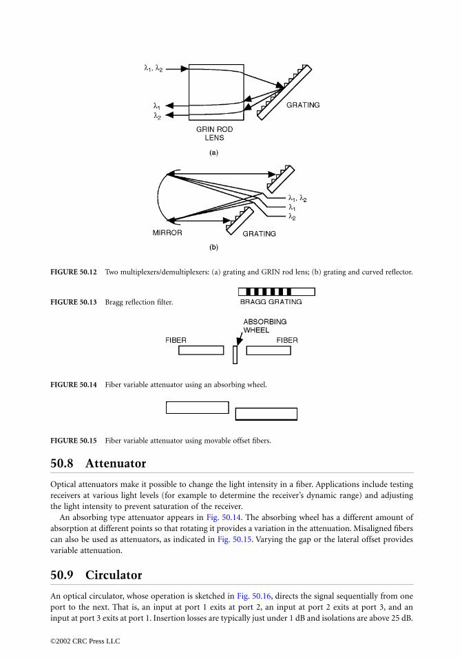
50.8 Attenuator

Optical attenuators make it possible to change the light intensity in a fiber. Applications include testingreceivers at various light levels (for example to determine the receiver’s dynamic range) and adjustingthe light intensity to prevent saturation of the receiver.

An absorbing type attenuator appears in Fig. 50.14. The absorbing wheel has a different amount ofabsorption at different points so that rotating it provides a variation in the attenuation. Misaligned fiberscan also be used as attenuators, as indicated in Fig. 50.15. Varying the gap or the lateral offset providesvariable attenuation.

50.9 Circulator

An optical circulator, whose operation is sketched in Fig. 50.16, directs the signal sequentially from oneport to the next. That is, an input at port 1 exits at port 2, an input at port 2 exits at port 3, and aninput at port 3 exits at port 1. Insertion losses are typically just under 1 dB and isolations are above 25 dB.

FIGURE 50.12 Two multiplexers/demultiplexers: (a) grating and GRIN rod lens; (b) grating and curved reflector.

FIGURE 50.13 Bragg reflection filter.

FIGURE 50.14 Fiber variable attenuator using an absorbing wheel.

FIGURE 50.15 Fiber variable attenuator using movable offset fibers.


The circulator can be used to decouple transmitted and received signals traveling along the same fiber(that is, in a bidirectional communications system such as that sketched in Fig. 50.17).

A circulator uses a Faraday rotator, similar to that found in the optical isolator. A fuller descriptionof the circulator appears in Kashima [1995].

50.10 Mechanical Switch

An optical switch allows an incoming signal to be diverted to any one of two or more different outputfibers, as schematically shown in Fig. 50.18. A mechanical switch does this by physical movement of thefibers or some other element of the switch. The insertion loss (coupling to the desired port) should beno more than a few tenths of a decibel and the isolation (undesired coupling to any other port) shouldbe more than 40 dB. Switching speeds are on the order of a few milliseconds, not fast by electronic andoptical measures, but quick enough for many fiber applications.

On/off switches allow power to be supplied to a system under test only when needed. Multiple outputport switches find applications in measurement systems (for example, to selectively measure the outputpower from a sequence of fibers). Switches can also redirect signals from a disabled fiber link onto analternate fiber route. They are used to produce bypass paths directing signals around disabled equipment,such as a node in a local-area network.

In an on/off switch, a block is inserted into a small gap between fibers in the off position and removedin the on position. In a 1 × N switch, the end of the transmitting fiber physically moves into alignmentwith the desired output fiber.

FIGURE 50.16 Fiber circulator.

FIGURE 50.17 Full duplex fiber transmission system.

FIGURE 50.18 A 1 ¥ N mechanical switch.


50.11 Polarization Controller

The polarization controller is a fiber device for producing a desired state of polarization. Although mostfiber systems operate independently of the state of polarization of the optical beam, coherent systemsand certain sensors are very much dependent on the state of polarization of the optical signal.

A simple polarization controller is constructed by winding the fiber around a disk whose diameter ison the order of a centimeter [Chen, 1996]. Usually, two or three of these fiber disks are connected inseries (Fig. 50.19). Rotating the disks about the axis of the fiber produces a differential change in therefractive index of the two normal orthogonally polarized beams traversing the fiber. Any desired polar-ization state can be obtained with the appropriate rotation of the disks.

Defining Terms

Demultiplexer: Separates different wavelengths entering from a single transmission fiber and directsthem to separate receivers.

Directionality: The fractional change in power level (expressed in decibels) when a signal passesbetween two ports which are ideally meant to be uncoupled.

Excess losses: The fractional amount of input power (expressed in decibels) that reaches all the desiredoutput ports of an optical component.

Faraday rotator: A component which rotates the polarization of the electric field passing through it.Often, the rotation of an incident linearly polarized beam is 45∞. The rotation is nonreciprocal.

Insertion loss: The fractional change in power level (expressed in decibels) when a signal passes betweentwo ports which are designed to be coupled.

Isolation: Same as directionality.Multiplexer: Combines two or more wavelengths from separate light sources onto a single fiber for

transmission.

References

Chen, C.L. 1996. Elements of Optoelectronics and Fiber Optics, Irwin, Chicago, IL.Kashima, N. 1995. Passive Optical Components for Optical Fiber Transmission, Artech, Boston, MA.Palais, J.C. 1998. Fiber Optic Communications, 4th ed., Prentice-Hall, Englewood Cliffs, NJ.

Further Information

Information on components for optical fiber systems appears in several professional society journals.These include the IEEE Journal of Lightwave Technology, the IEEE Photonics Technology Letters, and theOptical Society of America’s Applied Optics. Valuable information is also contained in several trademagazines such as Lightwave and Laser Focus World.

FIGURE 50.19 Fiber polarization controller.


51Semiconductor Optical

Amplifiers

51.1 Introduction 51.2 Principle of Operation51.3 Types of Semiconductor Optical Amplifiers51.4 Design Considerations51.5 Gain Characteristics

Small-Signal Gain and Bandwidth of Traveling Wave Amplifiers • Small-Signal Gain and Bandwidth of FP Amplifiers • Wavelength Dependence of Gain • GainSaturation • Dynamic Range • Polarization Sensitivity • Amplifier Noise

51.6 Pulse Amplification51.7 Multichannel Amplification51.8 Applications

51.1 Introduction

The deployment of optical amplifiers in fiber optic communications systems has received widespreadattention over the past several years. Signal repeaters are needed to overcome inherent transmission lossesincluding fiber absorption and scattering, distribution losses, and connector and component losses.Traditional repeaters are based on optoelectronic conversion where the optical signal is periodicallyconverted to an electronic signal, remodulated onto a new optical signal, and then transmitted onto thenext fiber section. An alternative approach is to use repeaters based on optical amplification. In opticalrepeaters, the signal is amplified directly without conversion to electronics. This approach offers distinctadvantages including longer repeater spacings, simultaneous multichannel amplification, and a band-width commensurate with the transmission window of the optical fiber. The deployment of opticalamplifiers in operational networks has reduced maintenance costs and provided a path for upgradingthe existing fiberplants since the amplifiers and fibers are transparent to signal bandwidth.

Two classes of optical amplifiers are used in fiber-based systems: active fiber amplifiers and semicon-ductor optical amplifiers (SOAs). In this chapter we concentrate on semiconductor amplifiers. Fiber-based amplifiers have advanced more rapidly into the deployment phase due to their high-outputsaturation power, high gain, polarization insensitivity, and long excited state lifetime that reduces crosstalkeffects. Fiber amplifiers have been successfully used in the 1.55-µm fiber transmission window but arenot ideally suited for the 1.31-µm fiber transmission window. Fiber amplifiers are covered in detail inthe companion chapter in this handbook. Recent developments in SOAs have led to dramatic improve-ments in gain, saturation power, polarization sensitivity, and crosstalk rejection. Semiconductor ampli-fiers also have certain characteristics that make their use in optical networks very desirable: (1) they havea flat gain bandwidth over a relatively wide wavelength range that allows them to simultaneously amplify

Daniel J. BlumenthalUniversity of California


signals of different wavelengths, (2) they are simple devices that can be integrated with other semicon-ductor based circuits, (3) their gain can be switched at high speeds to provide a modulation function,and (4) their current can be monitored to provide simultaneous amplification and detection. Additionally,interest in semiconductor amplifiers has been motivated by their ability to operate in the 1.3-µm fibertransmission window. For these reasons, semiconductor optical amplifiers continue to be studied andoffer a complementary optical amplification component to fiber based amplifiers.

In this chapter, we first discuss the principle of operation of SOAs followed by amplifier designconsiderations. The gain characteristics are described next with discussion on small-signal gain, wave-length dependence, gain saturation, dynamic range, polarization sensitivity, and noise. Amplification ofoptical pulses and multichannel amplification are treated followed by a brief discussion of applications.

51.2 Principle of Operation

A semiconductor optical amplifier operates on the principle of stimulated emission due to interactionbetween input photons and excited state electrons and is similar to a laser in its principle of operation.The semiconductor can be treated as a two energy level system with a ground state (valence band) andexcited state (conduction band), as shown in Fig. 51.1. Current is injected into the semiconductor toprovide an excess of electrons in the conduction band. When a photon is externally introduced into theamplifier, it can cause an electron in the conduction band to recombine with a hole in the valence band,resulting in emission of a second photon identical to the incident photon (stimulated emission). Asthese photons propagate in the semiconductor, the stimulated emission process occurs over and overagain, resulting in stimulated amplification of the optical input. Since an SOA can amplify input photons,we can assign it a gain. As will be discussed in further detail, the material gain is only a function of thebasic device composition and operating conditions, whereas the amplifier gain defines the relationshipbetween the input and output optical power.

In addition to amplification of the input photons (signal), it is important to consider how noise isgenerated within the amplifier when an electron in the conduction band spontaneously recombines witha hole without the aid of a photon. This process, known as spontaneous emission, results in an emittedphoton with energy equal to the energy difference between the electron and hole. Photons created fromspontaneous emission will propagate in the amplifier and experience gain through stimulated emission.This process leads to amplification of spontaneous emission and is called amplified spontaneous emis-sion (ASE). ASE is a noise mechanism as it is not related to the input signal and is a random process.Additionally, ASE takes away amplifier gain that would otherwise be available to the signal.

51.3 Types of Semiconductor Optical Amplifiers

SOAs can be classified as either subthreshold or gain clamped. Subthreshold amplifiers are lasersoperated below threshold, and gain-clamped amplifiers are lasers operated above threshold but used asamplifiers. Subthreshold SOAs can be further classified according to whether optical feedback is used. Ifthe SOA amplifies the optical signal in a single pass, it is referred to as a traveling wave amplifier (TWA),as shown in Fig. 51.2. The second type of subthreshold amplifier is a resonant amplifier, which contains

FIGURE 51.1 Spontaneous and stimulated emission occuring between the two energy states of an atom.


a gain medium and some form of optical feedback. In this case, the gain is resonantly enhanced at theexpense of limiting the gain bandwidth to less than that of the TWA case for an equivalent material. Anexample of a resonant amplifier is the Fabry–Perot (FP) amplifier shown in Fig. 51.2. The FP amplifierhas mirrors at the input and output ends, which form a resonant cavity. The resonant cavity creates anoptical comb filter that filters the gain profile into uniformly spaced longitudinal modes (also see Fig. 51.2).The TWA configuration has a bandwidth limited by the material gain itself but is relatively flat, whichis desirable for an optical communications system application. Typical 3-dB bandwidths are on the orderof 60–100 nm. Although the FP amplifier exhibits very large gain at wavelengths corresponding to thelongitudinal modes, the gain rapidly decreases when the input wavelength is offset from the peakwavelengths. This makes the gain strongly dependent on the input wavelength and sensitive to variationsthat may occur in an optical communications system.

Gain-clamped semiconductor optical amplifiers operate on the principle that the gain can be heldconstant by a primary lasing mode and signals can be amplified if their wavelength is located away fromthe main lasing mode. Laser structures suitable for this approach are distributed feedback (DFB) anddistributed Bragg reflector (DBR) lasers, which lase into a single longitudinal mode. Since only a singlemode oscillates, the remainder of the gain profile is available for amplification. Figure 51.3 illustrates theoutput optical spectra of a gain-clamped amplifier with the main lasing mode and the amplified signalidentified. A primary advantage of gain clamped amplifiers is a reduction in crosstalk in multichannelamplification applications discussed in Section 51.7.

FIGURE 51.2 Classification of semiconductor optical amplifiers. (Source: Saitoh, T. and Mukai, T. 1991. In Coher-ence, Amplification, and Quantum Effects in Semiconductor Lasers, Ed. Y. Yamamoto, John Wiley & Sons, New York.)

FIGURE 51.3 Output optical spectrum of a gain clamped amplifier with the main lasing mode and the identifiedamplified signal.


51.4 Design Considerations

For optical communications systems, traveling wave SOAs are desirable due to the wide gain bandwidthand relatively small variation in gain over a wide signal wavelength range. Most practical TWAs exhibitsome small ripples in the gain spectrum that arise from residual facet reflections. A large effort has beendevoted to fabricate amplifiers with low cavity resonances to reduce gain ripple. For an amplifier withfacet reflectivities R1 and R2, the peak-to-valley ratio of the output intensity ripple is given by [Dutta andSimpson, 1993]

(51.1)

where Gs is the single-pass gain of the amplifier. For the ideal case R1, R2 → 0, V = 1, that is, no rippleat cavity mode frequencies in the output spectrum. A practical value of V should be less than 1 dB. Thus,for an amplifier designed to provide gain Gs = 25 dB, the facet reflectivities should be such that must be less than 3.6 × 10-4.

Three principle schemes exist for achieving low facet reflectivities. They are: (1) antireflection dielectriccoated amplifiers [Olsson, 1989], (2) buried facet amplifiers [Dutta et al., 1990], and (3) tilted facetamplifiers [Zah et al., 1987]. In practice, very low facet reflectivities are obtained by monitoring theamplifier performance during the coating process. The effective reflectivity can be estimated from thepeak-to-peak ripple at the FP mode spacings caused by residual reflectivity. Reflectivities less than 10-4

over a small range of wavelengths are possible using antireflection coatings [Olsson, 1989]. In buriedfacet structures, a transparent window region is inserted between the active layer ends and the facets[Dutta et al., 1990]. The optical beam spreads in this window region before arriving at the semiconductor–air interface. The reflected beam spreads even farther and does not couple efficiently into the active layer.Such structures can provide reflectivities as small as 10-4 when used in combination with antireflectiondielectric coatings. Another way to suppress the FP modes of the cavity is to slant the waveguide (gainregion) from the cleaved facet so that the light incident on it does not couple back into the waveguide[Zah et al., 1987]. The process essentially decreases the effective reflectivity. A combination of antire-flection coating and the tilted stripe can produce reflectivities less than 10-4. A disadvantage of thisstructure is that the effective reflectivity of the higher order modes can increase, causing the appearanceof higher order modes at the output which may reduce fiber-coupled power significantly.

Another important consideration in amplifier design is choice of semiconductor material composition.The appropriate semiconductor bandgap must be chosen so that light at the wavelength of interest isamplified. For amplification of light centered around 1.55 µm or 1.31 µm, the InGaAsP semiconductormaterial system must be used with optical gain centered around the wavelength region of interest.

51.5 Gain Characteristics

The fundamental characteristics of the optical amplifiers such as small-signal gain, gain bandwidth, gainsaturation, polarization sensitivity of the gain, and noise are critical to amplifier design and use in systems.The component level behavior of the optical amplifier can be treated in a manner similar to electronicamplifiers.

Small-Signal Gain and Bandwidth of Traveling Wave Amplifiers

The optical power gain of an SOA is measured by injecting light into the amplifier at a particular wavelengthand measuring the optical output power at that wavelength. The gain depends on many parameters,including the input signal wavelength, the input signal power, material gains and losses, amplifier length,current injection level, etc. For a TWA operated with low-input optical power, the small-signal gain is

V1 Gs R1R2+

1 Gs R1R2–-------------------------------=

R1R2


given by the

where

Γ

is t

the

absorpti

profile if thethe materialmaximum)

Figure 51.4 bandwidth.

Small-Sig

The small-sipeaks and is

where

ν

0

is t

mode spacin

R

2

=

0,

FIGURE 51.4

modeled as a

Ed. G.P. Agra

G0FP


©2002 CRC P

unsaturated single-pass gain of the amplifier

(51.2)

he optical mode confinement factor, g0 is the unsaturated material gain coefficient, αm ison coefficient, and L is the amplifier length. The material gain coefficient g0 has a Lorentzian amplifier is modeled as a two-level atomic system. An important distinction is made between gain bandwidth and the amplifier signal bandwidth. The 3-dB bandwidth (full width at half-of g0 is ∆νg = 1/πT2, and the 3-dB bandwidth of the TWA signal gain [Eq. (51.2)], is

(51.3)

illustrates that the material gain bandwidth is greater than the amplifier small-signal gain

nal Gain and Bandwidth of FP Amplifiers

gnal power transmission of an FP amplifier shows enhancement of the gain at transmission given by [Saitoh and Mukai, 1991]

(51.4)

he cavity resonant frequency and ∆ν is the free spectral range (also called the longitudinalg) of the SOA. The single-pass small-signal gain G0 is given by Eq. (51.2). Note that for R1 =reduces to that of a TWA. The 3-dB bandwidth B (full width at half-maximum) of an FP

Lorentzian material gain profile and the corresponding amplifier gain spectrum for an amplifiertwo-level atomic system. (Source: Agrawal, G.P. 1995. In Semiconductor Lasers: Past, Present, and Future,wal, AIP Press.)

G0 ν( )Pout ν( )Pin ν( )----------------- Γg0 ν( ) αm–( )L[ ]exp= =

∆νA ∆νg�n2

Γg0L �n2–---------------------------

=

G0FP ν( )

1 R1–( ) 1 R2–( )G0 ν( )

1 R1R2G0 ν( )–( )24 R1R2G0 ν( )sin2 π ν ν0–( )/∆ν[ ]+

--------------------------------------------------------------------------------------------------------------------------------------=

ress LLC

amplifier is expressed as [Saitoh and Mukai, 1991]

(51.5)

whereas the 3-dB bandwidth of a TWA is three orders of magnitude larger than that of the FP amplifiersince it is determined by the full gain width of the amplifier medium itself. Figure 51.5 shows the small-signal (unsaturated) gain spectra of a TWA within one free spectral range [Saitoh, Mukai, and Noguchi,1986]. Solid curves represent theoretical FP curves fitted to the TWA experimental data. ExperimentalFP amplifier data are also shown (dashed curve). It can be seen that the signal gain fluctuates smoothlyover the entire free spectral range of the TWA in contrast to the FP amplifier, where signal gain is obtainedonly in the vicinity of the resonant frequencies.

Wavelength Dependence of Gain

As seen previously, the amplifier gain varies with the input wavelength for both the TWA and FP cases.The peak and width of the gain can also vary as a function of injection current. The material gain vs.wavelength for a typical amplifier is shown in Fig. 51.6 as a function of injection current. As the injectioncurrent increases, the peak gain increases and the location of the peak gain shifts toward shorter wavelengths.

Gain Saturation

The gain of an optical amplifier, much like its electronic counterpart, can be dependent on the inputsignal level. This condition, known as gain saturation, is caused by a reduction in the number of electronsin the conduction band available for stimulated emission and occurs when the rate of input photons isgreater than the rate at which electrons used for stimulated emission can be replaced by current injection.The time it takes for the gain to recover is limited by the spontaneous lifetime and can cause intersymbolinterference among other effects, as will be described. The saturated material gain coefficient is given by

(51.6)

FIGURE 51.5 Unsaturated gain spectra of a TWA and an FP amplifier within one free spectral range. (Source:Saitoh, T., Mukai, T., and Noguchi, Y. 1986. In First Optoelectronics Conference Post-Deadline Papers Technical Digest,Paper B11-2, The Institute of Electronics and Communications Engineers of Japan, Tokyo.)

B2∆n

p-----------sin-1

1 R1R2G0–

4G0 R1R2( )1/2

-----------------------------------=

g n( )g0 n( )1 P

Ps-----+

-------------=


where g0 is the unsaturated material gain coefficient, P is the total optical power in the active layer of theamplifier, and Ps is the saturation power defined as the light intensity that reduces the material gain g tohalf its value (g0/2). In general, the optical saturation power is related to the carrier lifetime but can bereduced as the optical intensity in the amplifier increases. The single-pass saturated signal gain G(ν) isgiven by [Saitoh and Mukai, 1991]

(51.7)

where Pin and Pout are the input and the output optical powers and G0 is the unsaturated gain given byEq. (51.2). Figure 51.7 shows experimental gain saturation characteristics of both FP and TWAs [Saitohand Mukai, 1987] along with theoretical curves.

Dynamic Range

The dynamic range is defined as the range of input power for which the amplifier gain will remainconstant. The gain saturation curves shown in Fig. 51.8 [Adams et al., 1985] show the relationship betweeninput power and gain for various current injection levels. The flat regions are the unsaturated regions.

FIGURE 51.6 Gain spectrum of a TWA at several current levels. (Source: Saitoh, T. and Mukai, T. 1987. Electron.Lett., 23:218.)

FIGURE 51.7 Theoretical and experimental signal gain of a TWA and FP amplifier as a function of amplifiedoutput power. (Source: Saitoh, T. and Mukai, T. 1987. Electron. Lett., 23:218.)

G n( ) G0 n( )Pout Pin–

Ps

---------------------–exp G0

G 1–G

------------ Pout

Ps

--------–exp= =


As the gain increases, the 3-dB rolloff moves toward lower input power, leading to a decrease in dynamicrange.

Polarization Sensitivity

In general, the optical gain of an SOA is polarization dependent. It differs for the transverse-electric(TE) and transverse-magnetic (TM) polarizations. Figure 51.9 shows the gain spectra of a TWA for bothTE and TM polarization states [Jopson et al., 1986]. The polarization-dependent gain feature of anamplifier is undesirable for lightwave system applications where the polarization state changes withpropagation along the fiber.

Several methods of reducing or compensating for the gain difference between polarizations have beendemonstrated [Saitoh and Mukai, 1991]. A successful technique that leads to polarization dependentgain on the order of 1 dB involves the use of material strain [Dubovetsky et al., 1994]. The measuredgain as a function of injection current for TE and TM polarized light for a tilted-facet amplifier is shownin Fig. 51.10 [Zah et al., 1987]. Figure 51.11 shows the measured optical gain plotted as a function ofoutput power for regular double heterostructure (DH) and multi-quantum well (MQW) amplifiers

FIGURE 51.8 Effect of amplifier injection current on variation in gain as a function of optical input power. Flatregions are unsaturated gain. Range of unsaturated gain vs. input power changes as a function of unsaturated gain.Values indicated on curves are for injected current density. Dashed curves are obtained without taking into accountASE. (Source: Adams, M.J. et al. 1985 IEEE Proceedings Part J, 132:58.)

FIGURE 51.9 Theoretical and experimental gain spectra of TE- and TM-polarized input signals. (Source: Jopson,R.M. et al. 1986. Electron. Lett., 22:1105.)


[Dutta and Simpson, 1993]. The multiquantum well amplifier result is shown for the TE mode, whereasthe gain difference between TE and TM modes for double heterostructure amplifiers was less than 1 dB.

Amplifier Noise

Semiconductor optical amplifiers add noise to the amplified optical signal in the form of amplifiedspontaneous emission. This noise can reduce the signal-to-noise ratio of the detected output and canreduce the overall gain available to the signal through gain saturation. ASE forms a noise floor with awavelength dependence approximately that of the gain. Figure 51.12 shows a typical optical spectrum at

FIGURE 51.10 Measured gain as a function of injection current. (Source: Zah, C.E. et al. 1987. Electron. Lett., 23:990.)

FIGURE 51.11 Measured gain as a function of output power for regular double heterostructure and multiquantumwell amplifiers. (Source: Dutta, N.K. and Simpson, J.R. 1993. Progress in Optics, Ed. E. Wolf, Vol. 31, North-Holland,Amsterdam.)


the output with the amplified signal and the ASE. Semiconductor optical amplifiers can be characterizedby a noise figure. Typical noise figures are in the range of 5–8 dB and can be calculated from the carrierdensity due to current injection N, the carrier density required to reach transparency N0, the saturatedgain g, and the internal amplifier losses aint [Saitoh and Mukai, 1991]:

(51.8)

In calculating signal-to-noise ratio, it is useful to consider the total output of an SOA after it has beenconverted to an electronic signal using a photodetector. Here we consider direct detection where a squarelaw detector is used to convert the optical signal to an electrical signal. In addition to the amplifiedsignal, several noise terms result from interaction between signal and noise in the square law detectionprocess [Mukai, Yamamoto, and Kimura, 1982; Yamamoto, 1980]: amplified signal shot noise, sponta-neous emission shot noise, signal-spontaneous beat noise, spontaneous-spontaneous beat noise, andsignal excess noise. The first and third types of noise are proportional to the signal power, whereas thesecond and fourth types of noise are generated from the ASE that exists independently of the input signal.For a single amplifier, the two beat noise terms dominate as they are G times stronger [Saitoh and Mukai,1991] than the shot noise contributions. The spontaneous-spontaneous beat noise can be reduced byloading a narrowband optical filter matched to the signal frequency, since this noise arises from the beatbetween the ASE components over a wide gain spectrum [Saitoh and Mukai, 1991]. For a direct detectionsystem with a high-gain optical amplifier prior to the photodetector, the electrical SNR is given by [Jopsonand Darcie, 1991]

(51.9)

where the input power to the amplifier is Pin, the optical bandwidth of the output of the amplifier isδνopt, the receiver electrical bandwidth is Be, the amplifier noise figure is F, and the optical frequency is ν.

51.6 Pulse Amplification

The large bandwidth of a TWA suggests that they are capable of amplifying very fast optical pulses withoutsignificant pulse distortion. However, the output pulses can be distorted either when the optical powerexceeds the saturation power or when the pulse width gets short compared to the carrier lifetime [Agrawaland Olsson, 1989].

FIGURE 51.12 A typical optical spectrum at the output with the amplified signal and the amplified spontaneousemission. (Source: BT&D Technologies, Publication No. DS007, 1992.)

F n

SNRin

SNRout

---------------- 2N

N N0–----------------

g

g a int–----------------

= =

SNRdd

Pin/hn( )2

FPin/hn F/2( )2dn opt+[ ]Be

----------------------------------------------------------------=


The Gaussian pulse and its spectrum for various small-signal gains G0 when the pulse width τp is muchsmaller compared to carrier lifetime τc is shown in Fig. 51.13 [Agrawal and Olsson, 1989]. The inputpulse energy Ein is equal to 0.1 times the saturation energy Esat of the SOA. The pulse gets distorted suchthat its leading edge becomes sharper compared with the trailing edge. When the pulse width is on theorder of the carrier lifetime, saturation can lead to a closing of the eye of a pseudo-random bit stream,as shown in Fig. 51.14 [Jopson and Darcie, 1991]. If a sequence of short pulses (bits) are injected, wherethe bit duration is less than the carrier lifetime, bit patterning can occur.

When the pulse width is comparable to τc , the saturated gain has time to recover during the pulse.Figure 51.15(a) shows [Agrawal and Olsson, 1989] the effect of gain recovery on the output pulse shapewhen the input pulse is Gaussian. As the input pulse width is increased, the output pulse becomes lessasymmetric and becomes broader than the input pulse. The gain recovery mainly affects the trailing edgeof the pulse. In the presence of partial gain recovery, the output spectrum also becomes less asymmetricand the spectral shift becomes smaller. When , the gain recovery is complete and the output pulseas well as its spectrum become symmetric. Figure 51.15(b) shows [Agrawal and Olsson, 1989] the output

FIGURE 51.13 Output pulse shapes and spectra for several values of the unsaturated gain when the input pulse isGaussian. The ratio of input pulse energy to the saturation energy is 0.1. (Source: Agrawal, G.P. and Olsson, N.A.1989. IEEE J. Quant. Electron., 25:2297.)

FIGURE 51.14 Effect of gain saturation of binary bit eye diagram. Upper figures show amplifier output as outputpower varies with saturation power. Decrease in bit height as a function of time is due to time constant of gainsaturation. Lower figures show effect of electronic bandpass filtering prior to level discrimination in an optical receiver.Bit period is half the gain saturation time constant. (Source: Jopson, R.M. and Darcie, T.E. 1991. In Coherence,Amplification, and Quantum Effects in Semiconductor Lasers, Ed. Y. Yamamoto, John Wiley & Sons, New York.)

tp >>tc


pulses when . The pulse is also broadened because the peak experiences less amplification thanthe wings because of gain saturation.

51.7 Multichannel Amplification

A TWA can greatly simplify optical repeaters used in wavelength-division multiplexed (WDM) systems,since its wide gain bandwidth allows a single amplifier to simultaneously amplify signals of differentwavelengths. In practice, however, several phenomena in SOAs can induce interchannel crosstalk: cross-gain modulation (XGM) and four-wave mixing (FWM). To understand XGM, the optical power inEq. (51.6) should be replaced by the total power in all channels. Thus, the gain of a specific channel issaturated not only by its own power but also by the power of other channels. If channel powers changedepending on bit patterns, as in amplitude-shift keying (ASK), then the signal gain of one channel changesfrom bit to bit, and the change also depends on the bit pattern of the other channels [Agrawal, 1995].The amplified signal appears to fluctuate randomly, which degrades the signal-to-noise ratio at thereceiver. This crosstalk can be largely avoided by operating SOAs in the unsaturated regime. It is absentfor phase-shift keying (PSK) and frequency-shift keying (FSK) systems, since the power in each channel,and therefore the total power, remains constant with time [Agrawal, 1995].

The four-wave mixing causes the generation of new optical frequencies in closely spaced WDM systems.This phenomenon is similar to interharmonic distortion in electronic systems. The presence of multiplewavelengths in the amplifier results in nonlinear amplification. Two wavelengths can generate additionaloptical frequencies, as shown in Figure 51.16. If these frequencies coincide with existing channels,crosstalk results. This crosstalk can be incoherent [Darcie and Jopson, 1988] or coherent [Blumenthaland Kothari, 1996] in direct detection systems and limitations on the input power can be computed foreach case [Darcie and Jopson, 1988; Blumenthal and Kothari, 1996] for a given number of channels,

FIGURE 51.15 Output pulse shapes for (a) several values of pulse width in the partial gain recovery regime and(b) several values of input power when the pulse width is much larger than the carrier life time. (Source: Agrawal, G.P.and Olsson, N.A. 1989. IEEE J. Quant. Electron., 25:2297.)

FIGURE 51.16 Generation of new frequencies due to FWM interaction between the signals at frequencies f1 and f2.

tp >>tc


channel spacing, and amplifier gain. Unequal channel spacing can be used to minimize crosstalk effectsdue to FWM [Forghieri et al., 1994].

51.8 Applications

Semiconductor optical amplifiers have multiple potential uses in optical communication systems (seeFig. 51.17). Power boosting, optical preamplification prior to photodetection, compensation of distribu-tion losses, and in-line amplification are examples of transmission applications. In-line amplifiers elim-inate the need for electronic regenerators and allow multichannel amplification. As a booster amplifier,the transmission distance can be increased by 10 to 100 km. SQAs can be integrated with a semiconductorlaser to obtain a high-power, narrow-linewidth optical source useful for coherent communication systems[Koch and Koren, 1991; Glance et al., 1992]. Transmission distance can also be increased by putting anamplifier to operate the receiver in the shot noise limit.

Another potential application of SOAs is in the area of dispersion compensation. Midpoint dispersioncompensation in a fiber link is achieved by using the SOA to perform frequency conversion throughfour-wave mixing [Tatham, Sherlock and Westbrook, 1993]. This process inverts the ordering of theoptical spectrum within the pulse, thereby reversing the effect of dispersion in the second section of fiber.An SOA can also be used as a booster amplifier to balance the effect of frequency chirp in direct drivesemiconductor lasers [Yazaki et al., 1992].

A third class of application, photonic switching, may require switching of signals in space and/orwavelength. SOAs can be integrated in space switches as transmission gates [Gustavsson et al., 1992]with very high-extinction ratio in the off state. SOAs can also be used to translate signals betweenwavelengths using wavelength conversion techniques such as cross-gain saturation [Valiente, Simon, andLeLigne, 1993] or four-wave mixing [Zhou et al., 1994].

Acknowledgments

This work was supported in part by the National Science Foundation under a National Young Investigator(NYI) award (contract number ECS-9457148) and the Air Force Office of Scientific Research (AFOSR)(contract number F49620-95-1-0024).

FIGURE 51.17 Configurations for SOA applications. (Source: Yamamoto, Y. and Mukai, T. 1989. Optical Quant.Electron., 21:S1.)


Defining Terms

Absorption coefficient: Amount of optical power absorbed in material per unit length.Amplified spontaneous emission (ASE): Stimulated replication of photons that were originally gen-

erated by spontaneous emission. Amplifier gain: Ratio of optical power at input of amplifier to optical power at output of amplifier.Bit patterning: Influence of a previous bit on subsequent bits in a bit stream due to gain saturation

effects.Comb filter: Transfer function of resonant structure that has repeating periodic passband.Cross-gain modulation (XGM): Modulation of amplifier gain at one wavelength due to variation in

signal at another wavelength.Dispersion compensation: Realignment of phases for different spectral components in a pulse so that

pulse broadening can be reduced.Distributed Bragg reflector laser (DBR): Laser structure with Bragg reflectors at ends of cavity.Distributed feedback laser (DFB): Laser structure with Bragg reflector in middle of cavity and without

mirrors at ends.Fabry–Perot (FP) amplifier: Resonant amplifier using mirrors at input and output for feedback.Four-wave mixing (FWM): Generation of new frequencies, or intermodulation products, through gain

nonlinearity.Free spectral range: Spacing between longitudinal modes in resonant cavity.Frequency chirp: Change in optical frequency as a function of time across a modulated optical signal.Gain clamped: Operation of gain structure above condition where gain equals cavity losses.Gain ripple: Periodic variation in gain over amplifier bandwidth.Gain saturation: Reduction in gain due to increase in optical power.Interchannel crosstalk: Transfer of information between channels due to a physical crosstalk mecha-

nism.Longitudinal modes: Single passband of a resonant cavity with comb-filter type transfer function.Material gain: Number of photons generated per incident photon per unit length of material.Optical mode confinement factor: Amount of optical signal that passes through amplifying medium.Photonic switching: Switching or redirection of optical signals without conversion to electronics.Polarization dependent: Variation in gain for different orientations of optical field.Resonant amplifier: Amplifier with gain and feedback.Saturated material gain: Optical signal-level dependent gain.Space switches: Connection through spatially discrete elements.Spontaneous emission: Emission of a photon by random transition from a high-energy state to a low-

energy state.Stimulated amplification: Stimulated replication of photons through stimulated emission.Stimulated emission: Emission of a photon due to transition from a high-energy state to a low-energy

state that was caused by an initial photon.Subthreshold: Operation of gain structure below condition where gain equals cavity losses.Traveling wave amplifier (TWA): Single-pass amplifier with optical gain.Unsaturated material gain coefficient: Gain provided to optical signal that is not signal-level dependent.Wavelength-division multiplexing (WDM): Transmission of simultaneous channels on parallel optical

wavelengths.

References

Adams, M.J., Collins, J.V., and Henning, I.D. 1985. IEEE Proceedings Part J, 132:58.Agrawal, G.P. 1995. Semiconductor laser amplifiers. In Semiconductor Lasers: Past, Present, and Future,

Ed. G.P. Agrawal, American Institute of Physics Press.Agrawal, G.P. and Olsson, N.A. 1989. IEEE J. Quant. Electron., 25:2297.Blumenthal, D.J. and Kothari, N.C. 1996. IEEE Photon. Tech. Lett., 8:133.


Darcie, T.E. and Jopson, R.M. 1988. Electron. Lett., 24:638.Dubovitsky, S., Mathur, A., Steier, W.H., and Dapkus, P.D. 1994. IEEE Photon. Tech. Lett., 6:176.Dutta, N.K., Lin, M.S., Piccirilli, A.B., Brown, R.L., and Chakrabarti, U.K. 1990. J. Appl. Phys., 67:3943.Dutta, N.K. and Simpson, J.R. 1993. Optical amplifiers. In Progress in Optics, Ed. E. Wolf, Vol. 31, North-

Holland, Amsterdam.Forghieri, F., Tkach, R.W., Chraplyvy, A.R., and Marcuse, D. 1994. IEEE Photon. Tech. Lett., 6:754.Glance, B., Wiesenfeld, J.M., Koren, U., Gnauck, A.H., Presby, H.M., and Jourdan, A. 1992. Electron. Lett.,

28:1714.Gustavsson, M., Lagerstrom, B., Thylen, L., Jansson, M., Lundgren, L., Morner, A.C., Rask, M., and

Stolz, B. 1992. Electron. Lett., 28:2223.Jopson, R.M. and Darcie, T.E. 1991. Semiconductor laser amplifiers in high-bit-rate and wavelength-

division-multiplexed optical communications systems. In Coherence, Amplification, and QuantumEffects in Semiconductor Lasers, Ed. Y. Yamamoto, John Wiley & Sons, New York.

Jopson, R.M., Eisenstein, G., Hall, K.L., Raybon, G., Burrus, C.A., and Koren, U. 1986. Electron. Lett.,22:1105.

Koch, T.L. and Koren, U. 1991. IEEE J. Quant. Electron., 27:641.Mukai, T., Yamamoto, Y., and Kimura, T. 1982. IEEE J. Quant. Electron., QE-18:1560.Olsson, N.A. 1989. IEEE J. Lightwave Tech., 7:1071.Saitoh, T. and Mukai, T. 1987. Electron. Lett., 23:218.Saitoh, T., and Mukai, T. 1991. Traveling-wave semiconductor laser amplifiers. In Coherence, Amplifica-

tion, and Quantum Effects in Semiconductor Lasers, Ed. Y. Yamamoto, John Wiley & Sons, New York.Saitoh, T., Mukai, T., and Noguchi, Y. 1986. Fabrication and gain characteristics of a 1.5 mm GaInAsP

traveling-wave optical amplifier. In First Optoelectronics Conference Post-Deadline Papers TechnicalDigest, The Institute of Electronics and Communications Engineers of Japan, Tokyo, Paper B11-2.

Tatham, M.C., Sherlock, G., and Westbrook, L.D. 1993. Electron. Lett., 29:1851.Valiente, I., Simon, J.C., and LeLigne, M. 1993. Electron. Lett., 29:502.Yamamoto, Y. 1980. IEEE J. Quant. Electron., QE-16:1073.Yazaki, P.A., Komori, K., Arai, S., Endo, A., and Suematsu, Y. 1992. IEEE J. Lightwave Tech., 10:1247.Zah, C.E., Osinski, J.S., Caneau, C., Menocal, S.G., Reith, L.A., Salzman, J., Shokoohi, F.K., and Lee, T.P.

1987. Electron. Lett., 23:990.Zhou, J., Park, N., Dawson, J.W, Vahala, K.J., Newkirk, M.A., and Miller, B.I. 1994. IEEE Photon. Tech.

Lett., 6:50.

Further Information

Yamamoto, Y., Ed. 1991. Coherence, Amplification, and Quantum Effects in Semiconductor Lasers, JohnWiley & Sons, New York.

Agrawal, G.P. and Dutta, N.K. 1993. Semiconductor Lasers, Van Nostrand Reinhold, New York.


52Optical Amplifiers

52.1 Introduction52.2 General Amplifier Concepts52.3 Alternative Optical Amplifiers for Lightwave

System ApplicationsFiber-Raman Amplifiers • Brillouin Amplifiers• Semiconductor Optical Amplifiers • Rare-Earth-Doped Fiber Amplifiers • Rare-Earth-Doped Waveguide Amplifiers • Optical Parametric Amplifiers • Comparison of Amplifier Characteristics

52.4 Summary

52.1 Introduction

From the first demonstration of optical communication, a primary drive in the research activity has beendirected toward constant increase in the system capacity. Until very recently, the ultimate capacity limitshave been determined by the spectral bandwidth of the signal source and of the fundamental fiberparameters: attenuation and dispersion. On the basis of the limiting term of the transmission link, systemshave been denoted as either loss limited or dispersion limited, and it can be seen that there have beenalternations between these two extremes over the past 20 years. In the mid-1980s, the internationaldevelopment had reached a state at which not only dispersion-shifted fibers were available but alsospectrally pure signal sources emerged. The long-haul optical communication systems were, therefore,clearly loss limited and their problems had to be overcome by periodic regeneration of the optical signalsat repeaters applying conversion to an intermediate electrical signal. Because of the complexity and lackof flexibility of such regenerators, the need for optical amplifiers was obvious.

The technological challenge was to develop a practical way of obtaining the needed gain, that is, todevelop amplifiers with a complexity and application flexibility superior to the electrical regenerators.Several means of doing this had been suggested in the 1960s and 1970s, including direct use of thetransmission fiber as gain medium through nonlinear effects [Agrawal, 1989], semiconductor amplifierswith common technical basis in the components used for signal sources [Simon, 1983], or doping opticalwaveguides with an active material (rare-earth ions) that could provide the gain [Koester and Snitzer,1964]. First, however, with the pronounced technological need for optical amplifiers and the spectacularresults on erbium-doped-fiber amplifiers [Mears et al., 1987], an intense worldwide research activity onoptical amplifiers was initiated. This resulted in the appearance of commercially available packagederbium-fiber amplifier modules as early as 1990, and the rapidly expanding technology and transfer ofknowledge from research to practical system implementation make it clear that optical amplifiers and,especially, the erbium-doped-fiber amplifier are bringing about a revolution in communication systems.

The following section provides a short review of the general properties and limitations of opticalamplifiers. Thereafter, the specific technologies available for the realization of optical amplifiers arereviewed, and their key parameters are compared. Finally, the chapter includes a short review of someof most significant results on optical amplifiers in optical communication systems.

Anders BjarklevTechnical University of Denmark


52.2 General Amplifier Concepts

In order to clarify and define the need for optical amplifiers, we discuss here some concepts general to alloptical amplifiers. In an ideal optical amplifier, the signal would be amplified by adding, in phase, a well-defined number of photons to each incident photon. This means that a bit sequence or an analog opticalsignal simply would increase its electromagnetic field strength but not change its shape by passage throughthe optical amplifier, as illustrated in Fig. 52.1(a). In a perfect amplifier, this process would take placeindependent of the wavelength, state of polarization, intensity, (bit) sequence, and optical bandwidth ofthe incident light signal, and no interaction would take place if more than one signal were amplifiedsimultaneously. In practice, however, the optical gain depends not only on the wavelength (or frequency)of the incident signal, but also on the electromagnetic field intensity at any point inside the amplifier.Details of wavelength and intensity dependence of the optical gain depend on the amplifying medium.

Before we turn to describing the different types of amplifiers, however, it is informative to illustratesome general concepts of practical optical amplifiers. To do so, we consider a case in which the gainmedium is modeled as a homogeneously broadened two-level system. In such a medium, the gaincoefficient (i.e., the gain per unit length) can be written as [Agrawal, 1992]:

(52.1)

Here g0 is the peak value of the gain coefficient determined by the pumping level of the amplifier, ω isthe optical angular frequency of the incident signal, and ω0 is the atomic transition angular frequency.Ps is the optical power of the signal and Psat is the saturation power, which depends on the gain mediumparameters such as fluorescence lifetime τ and the transition cross section. The parameter T2 in Eq. (52.1)is normally denoted as the dipole relaxation time [Agrawal, 1992].

Two important amplifier characteristics are described in Eq. (52.1). First, if the signal power ratioobeys Ps /Psat 1 throughout the amplifier, the amplifier is said to be operated in the unsaturated region.The gain coefficient is then maximum when the incident angular frequency ω coincides with the atomictransition angular frequency ω0. The gain reduction for angular frequencies different from ω0 is generallygiven by a more complex function than the Lorentzian profile, but this simple example allows us to definethe general property of the gain bandwidth. This is normally defined as the full-width half-maximum(FWHM) value of the gain coefficient spectrum g(ω). For the Lorentzian spectrum, the gain bandwidthis given by Dωg = 2/T2.

From the communication system point of view, it is more natural to use the related concept of amplifierbandwidth instead of the gain bandwidth, which is related to a point within the gain medium. Thedifference becomes clear when we consider the amplifier gain G defined as

(52.2)

where is the input power and is the output power of a continuous wave (CW) signal beingamplified. The amplifier gain G may be found by using the relation

(52.3)

where P(z) is the optical power at a distance z from the amplifier input end. If the gain coefficient g(ω),for simplicity, is considered constant along the amplifier length, the solution of Eq. (52.3) is an expo-nentially growing signal power P(z) = exp(gz). For an amplifier length L, we then find that

(52.4)

g w( )g0

1 w w 0–( )2T2

2 Ps/Psat+ +-------------------------------------------------------------=

<<

G Psout/Ps

in=

Psin Ps

out

dPdz------ gP=

Psin

G w( ) g w( )L[ ]exp=


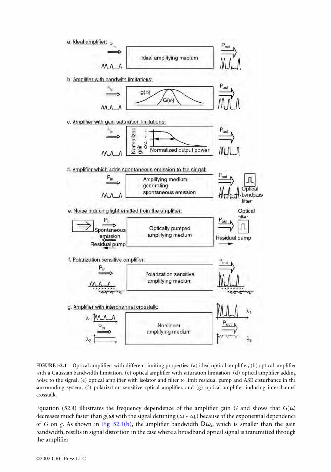
Equation (52.4) illustrates the frequency dependence of the amplifier gain G and shows that G(ω)decreases much faster than g(ω) with the signal detuning (ω - ω0) because of the exponential dependenceof G on g. As shown in Fig. 52.1(b), the amplifier bandwidth DωA, which is smaller than the gainbandwidth, results in signal distortion in the case where a broadband optical signal is transmitted throughthe amplifier.

FIGURE 52.1 Optical amplifiers with different limiting properties: (a) ideal optical amplifier, (b) optical amplifierwith a Gaussian bandwidth limitation, (c) optical amplifier with saturation limitation, (d) optical amplifier addingnoise to the signal, (e) optical amplifier with isolator and filter to limit residual pump and ASE disturbance in thesurrounding system, (f) polarization sensitive optical amplifier, and (g) optical amplifier inducing interchannelcrosstalk.


Another important limitation of the nonideal amplifier is expressed in the power dependence of thegain coefficient. This property, which is known as gain saturation, is included in the example of Eq. (52.1),and it appears in all cases where the term Ps/Psat is nonnegligible. Since the gain coefficient is reducedwhen the signal power Ps becomes comparable to the saturation power Psat, the amplification factor (oramplifier gain) G will also decrease. This is illustrated in Fig. 52.1(c), where it is shown how G decreasesfrom its unsaturated value G0.

Gain saturation might be seen as a serious limitation for multiwavelength optical communicationsystems. However, gain saturated amplifiers have practical use as their self-regulating effect on the signaloutput power is going to be used in planned transoceanic communication links including many concat-enated amplifiers. The principle is as follows: if the signal level in a chain of amplifiers is unexpectedlyincreased along the chain, due to saturation the following amplifiers will be operated at a lower gain andvice versa for a sudden signal power decrease.

Besides the bandwidth and gain saturation limitations of practical optical amplifiers, another propertyis inherent for practical amplifiers today. Optical amplifiers, in general, will add spontaneously emittedor scattered photons to the signal during the amplification process, and this will consequently lead to adegradation of the signal-to-noise ratio (SNR). This property is illustrated in Fig. 52.1(d). The SNRdegradation is quantified through a parameter F, normally denoted as the amplifier noise figure, whichis defined as the SNR ratio between input and output [Yariv, 1990],

(52.5)

It should be noted that it is common practice to refer the SNR to the electrical power generated whenthe optical signal is converted to electrical current by using a photodetector. The noise figure as definedin Eq. (52.5), therefore, in general, would depend on several detector parameters which determine theshot noise and thermal noise associated with the practical detector. However, the influence of detectorparameters will not help us clarify the amplifier noise properties, and it is therefore advantageous toconsider an ideal detector, whose performance is limited by shot noise only [Yariv, 1990].

In practice, the spontaneous emission is reduced by optical filtering of the received signal. Therefore,the SNR generally also will be dependent on the bandwidth of the optical filters and the spectral powerdistribution of the spontaneous emission from the amplifier. However, since this filtering is a processindependent of the amplifier properties, it is also common practice to eliminate this ambiguity byconsidering an ideal filter [Agrawal, 1992]. Such an ideal filter is introduced only to allow the signal andthe spontaneous emission within the signal bandwidth to pass to the detector. Therefore, it will only bethe spontaneous emission spectral power density at the signal wavelength that enters the ideal detector,and the noise figure becomes independent of the spectral shape of the spontaneous emission. Note thatsince the amplifier deteriorates the signal-to-noise ratio, that is, SNRin > SNRout, the noise figure willalways obey the relation F > 1.

For a practical communication system, the amplifier spontaneous emission may have another influencebesides that described through the noise figure (i.e., besides the effect that it adds fluctuations to the amplifiedoptical signal power, which are converted to current fluctuations during the photodetection process). Namely,the spontaneous emission, which is emitted from the amplifier input end, may enter the signal source (asemiconductor laser), where it can result in performance disturbances. Therefore, it is often necessary toinclude isolation between amplifier and light source to avoid additional noise in the system.

Therefore, it must be considered that the optical communication system has to be protected againstundesired emission from the amplifier, and it is necessary to include the special properties of opticallypumped amplifiers. These may also transmit residual pump power onto the transmitter and/or detector.The actual effect of this will be strongly dependent on the spectral properties of the pump light andwhether the signal source or detector is sensitive to such radiation. As shown in Fig. 52.1(e), this oftenimplies the inclusion of separate isolators and filters (if not already included for direct reduction of noise-induced signal power fluctuations).

FSNRin

SNRout

----------------=


Another property that has to be evaluated for the optical amplifier is the polarization sensitivity. A high-polarization sensitivity means that the amplifier gain G differs for different polarization directions of theinput signal. This is shown in Fig. 52.1(f) for two orthogonal linear polarization states. Since opticalcommunication systems normally do not include polarization control, and because the polarization stateis likely to vary due to external factors such as mechanical pressure, acoustic waves, and temperaturevariations, amplifier polarization sensitivity is naturally an undesired property in most cases. Therefore,for amplifiers that are inherently polarization sensitive, it has been a primary goal to reduce or eveneliminate the amplifier output power variation due to changes in the signal input polarization state.

All of the limiting properties, which we have previously discussed, are not surprisingly distinctlydifferent for different types of amplifiers. This is also the case for the crosstalk limitation that relates tomultichannel applications of optical amplifiers. In contrast to the ideal case, where all signal channels(or wavelengths) are amplified by the same amount, undesired nonlinear phenomena may introduceinterchannel crosstalk (i.e., the modulation of one channel is affected or modified by the presence ofanother signal channel). The effect of crosstalk is illustrated in Fig. 52.1(g), where one channel isconsidered to carry a modulated signal, whereas the other carries a continuous wave (CW) signal. Bypassage of the amplifier, the CW has been modulated by the signal carried in the other channel. We willreturn to the more specific nature of these nonlinear phenomena in connection with the discussion ofthe different optical amplifiers.

The final limiting factors that should be mentioned here are closely related to the physical environ-ment in which the amplifier is placed. These may include sensitivity toward vibrations, radioactiveradiation, chemicals, pressure, and temperature. However, since, at least, amplifiers for optical com-munication systems generally are placed in controlled environments, we will not go further into a detaileddiscussion of such properties at this point.

The relative importance of the different limiting factors as just discussed depends on the actualamplifier application. One application is as replacement of electronic regenerators; in such cases, theamplifiers are placed at a considerable distance from the transmitter and receiver and they are denoted asin-line amplifiers. The optical amplifier may also be used to increase the transmitter power by placingan amplifier just after the transmitter. Such amplifiers are called power amplifiers, or boosters, becausetheir main purpose is to boost the transmitted power. Long-distance systems may also be improved bythe inclusion of so-called preamplifiers, which are placed just before the receiver. Finally, optical amplifiersmay find use in local area networks in which they can compensate for distribution losses. Thereby, thenumber of nodes in the networks may be increased.

52.3 Alternative Optical Amplifiers for LightwaveSystem Applications

The most important factors that limit the performance of practical optical amplifiers have now beenidentified. The next task then is to investigate the technologies available for obtaining realistic amplifiers.Basically, six different ways of obtaining optical amplification have to be considered: fiber-Raman andfiber-Brillouin amplifiers, semiconductor optical amplifiers (SOA), rare-earth-doped fiber amplifiers,rare-earth-doped waveguide amplifiers, and parametric amplifiers. The aim of the present descriptionis to present the basic physical properties of these candidates as relates to their applicability as practicaloptical amplifiers.

Fiber-Raman Amplifiers

The fiber-Raman amplifier works through the nonlinear process of stimulated Raman scattering (SRS)occurring in the silica fiber itself. SRS is an interaction between light and the vibrational modes of silicamolecules. The process appears because the SRS converts a small fraction of the incident power fromone optical beam (the pump) to another optical beam (the signal) at a frequency down-shifted by anamount determined by the vibrational modes of the medium.


The light generated by SRS is called the Stokes wave, and Stokes waves are generated both copropagatingand counterpropagating with the incident beam. As early as 1962, it was observed that for very intensepump waves a new phenomenon of SRS can occur in which the Stokes wave grows rapidly inside themedium such that most of the pump energy appears in it. If the signal angular frequency w s and pumpangular frequency wp are chosen with a difference of Ω R = ωp - ωs (the Stokes shift) corresponding tothe value dictated by the vibrational energy of the molecules, the signal may experience Raman gain.

A significant feature of the Raman gain in silica fibers is that it extends over a large frequency range(up to 40 THz with a typical FWHM width of 6 THz) with a broad dominant peak near 13 THz. Thisis due to the amorphous nature of fused silica in which the molecular vibrational frequencies spread outinto bands overlapping each other and creating a continuum (depending on the fiber core composition).The relatively large bandwidth of fiber-Raman amplifiers and a very large saturation power (typicallyaround 1 W) makes them attractive for optical communication systems. Also, their noise properties aregood, since a noise figure close to 3 dB is obtainable. On the other hand, one of the considerable drawbacksof this amplifier type is that to obtain a 20-dB gain in a 100-km-long standard fiber for optical commu-nication, more than 2.5 W of pump power at 1480 nm is needed [Agrawal, 1989]. Another importantlimitation of fiber-Raman amplifiers is their polarization sensitivity. Experiments show the necessity ofmatching the polarization directions of pump and signal, since SRS ceases to occur for the case oforthogonal polarizations. Because polarization control is not normally employed in optical communi-cation systems, this property introduces an additional complexity, which, together with the high pumppower requirements, makes the Raman amplifier only slightly attractive from the point of view of theoptical communication system designer. Table 52.1 lists key parameters for the fiber-Raman amplifier.

Brillouin Amplifiers

Another type of amplifier that makes use of the physical properties of the silica transmission fiber itselfis the stimulated Brillouin scattering (SBS) amplifier [Agrawal, 1989]. The nonlinear SBS processappears through the generation of a backward propagating Stokes wave that carries most of the inputenergy and is, in this sense, similar to the SRS process. There are, however, major differences betweenthe SRS and SBS processes. One aspect is that the Stokes wave in the case of SBS propagates backwardsand, in contrast to SRS, the input power levels needed to obtain SBS are much lower (ª1-mW CW pumppower is sufficient to obtain SBS). Note also that the SBS depends on the spectral width associated withthe pump wave and it nearly ceases to occur for short pump pulses. Finally, the Stokes shift in SBS(ª10 GHz) is smaller by three orders of magnitude compared with that occurring in SRS. The differencesbetween SRS and SBS may be explained from a single fundamental difference; optical phonons participate

TABLE 52.1 Comparison of Optical Amplifiers Around 1550 nm

PropertyRaman

AmplifierBrillouin Amplifier SOA EDFA

RE-Doped Waveguide Amplifiers

Optical Parametric Amplifiers

Small-signal gain >40 dB >40 dB >30 dB >50 dB 20 dB 16 dBEfficiency 0.08 dB/mW 5.5 dB/mW 28 dB/mA 11 dB/mW 0.1 dB/mW 10-4 dB/mWOutput power 1 W 1 mW >0.1 W >0.5 W 2 mWDistortion/

CrosstalkNegligible Negligible Significant

(in saturation)Negligible Negligible

Dynamic performance

>20 Gb/s <100 MHz >25 Gb/s >100 Gb/s >100 Gb/s

Gain bandwidth A few tens of nm <100 MHz 60–70 nm ª30 nm A few tens of nm 5000 GHzNoise figure ª3 dB >15 dB 5–7 dB ª3 dB >3 dBPolarization

sensitivitySignificant None <A few dB Insignificant

(<0.1 dB)<1 dB <A few dB

Coupling loss(to fiber)

<1 dB <1 dB A few dB <1 dB


in the Raman process, whereas acoustical phonons (forming acoustic waves) participate in the Brillouinprocess. In the ideal case Brillouin scattering should not occur in the forward direction in an opticalfiber, but due to spontaneous or thermal Brillouin scattering, small amounts of forward scattered lightmay be measured.

The obtainable SBS gain is nearly three orders of magnitude larger than the Raman gain [Agrawal, 1989].This means that the fiber-Brillouin amplifier can amplify a signal by 30 to 35 dB with a small pump powerin the range of 1 to 10 mW. Also, the saturation power of fiber-Brillouin amplifiers is different from thatof the Raman amplifier; in the case of SBS it is in the milliwatt range. However, from the point of view ofthe optical communication system designer, who in the mid-1980s was seeking an efficient optical amplifier,the central problem of fiber-Brillouin amplifiers was their narrow gain bandwidth (less than 100 MHz).This narrow bandwidth, which, due to fiber inhomogeneities, is broadened even compared to the bulk silicavalue of around 17 MHz [Agrawal, 1992], makes fiber Brillouin amplifiers less suitable as power amplifiers,preamplifiers, or in-line amplifiers in generally used intensity-modulated direct detection systems. Fiber-Brillouin amplifiers need to be pumped by narrow linewidth semiconductor lasers (<10 MHz), whichobviously limit their potential use in optical communication systems since, in practice, a wavelength tuneablenarrow bandwidth pump is required. As a consequence of this, SBS has, since its first observation in opticalfibers in 1972, primarily been studied as a nonlinear phenomenon limiting transmitter power in fiber opticcommunication systems. It is, on the other hand, important to note that the narrow bandwidth nature ofSBS lately has attracted attention, for example, in connection with channel selection in multichannellightwave systems.

Another property that adds to reservations about fiber Brillouin amplifiers is their disadvantageousnoise properties. Noise appears due to a large population of acoustic phonons at room temperature, andnoise figures as large as 15 dB are likely to appear. This makes the Brillouin amplifier highly problematicboth as a preamplifier and for in-line applications.

Semiconductor Optical Amplifiers

The semiconductor optical amplifier, in contrast to both Raman and Brillouin fiber amplifiers, is fabri-cated in a material and structure different than silica transmission fiber. Therefore, light has to be coupledfrom fiber to SOA and vice versa, which inevitably results in coupling losses. Unless special action istaken, the SOA itself also will experience relatively large feedback due to reflections occurring at thecleaved end facets (32% reflectivity due to refractive index differences between semiconductor and air),resulting in sharp and highly disadvantageous gain reduction between the cavity resonances of theFabry–Perot resonator. Therefore, it is necessary to design traveling wave (TW) type SOAs by suppressingthe reflections from the end facets; a common solution is the inclusion of antireflection coating of theend facets. It turns out that to avoid the amplifier bandwidth being determined by the cavity resonancesrather than the gain spectrum itself, it becomes necessary to require that the facet reflectivities satisfythe condition [Agrawal, 1992] Here, G is the single-pass amplification factor, and R1

and R2 are the power reflection coefficients at the input and output facets, respectively. For an SOAdesigned to provide a 30-dB gain, this condition will mean that which is difficultto obtain in a predictable and reproducible manner by antireflection coating alone. Additional methodsto reduce the reflection feedback include designs in which the active-region stripe is tilted from the facetnormal and introduction of a transparent window region (nonguiding) between the active-layer endsand the antireflection coated facets. Reflectivities as small as 10-4 may thereby be provided, and the SOAbandwidth will be determined by the gain medium. Typically, 3-dB amplifier bandwidths of 60–70 nmmay be obtained.

The gain in an SOA depends on the carrier population, which changes with the signal power and theinjection current. Note that, in contrast to the alternative optical amplifiers, the SOA is not opticallypumped, and an important property is the very short effective lifetime of the injected carriers (i.e., ofthe order of 100 ps). This property becomes specifically relevant for multichannel applications of SOAs,where crosstalk limitations are in question. This crosstalk originates from two nonlinear phenomena:

G R1R2 0.17.<

R1R2 0.17 10 4– ,◊<


cross saturation and four-wave mixing. The former appears because the signal in one channel throughstimulated recombinations affects the carrier population and, thereby, the gain of other channels. Thissignificant problem may only be reduced by operating the amplifier well-below saturation, but this isnot an easy task due to the relatively limited saturation output power of 5 to 10 mW. Four-wave mixingalso appears because stimulated recombinations affect the carrier number. More specifically, the carrierpopulation may be found to oscillate at the beat frequencies between the different channels, wherebyboth gain and refractive index are modulated. The multichannel signal therefore creates gain and indexgratings, which will introduce interchannel crosstalk by scattering a part of the signal from one channelto another. Finally, it should be mentioned that, due to their large bandwidth, SOAs have the potentialof amplifying ultra-short pulses (a few picoseconds). However, the gain dynamics will play an importantrole and saturation induced self-phase modulation has to be considered. In other words, the SOA willintroduce a frequency chirp, which may find positive use in terms of dispersion compensation.

The noise properties of the SOA are determined by two factors. One is the emission due to spontaneousdecays and the other is the result of nonresonant internal losses α int (e.g., free carrier absorption orscattering loss), which reduce the available gain from g to (g - α int). Also, residual facet reflectivities (i.e.,loss of signal input power) increase the noise figure. Typical values of the noise figure for SOAs are 5 to7 dB.

An undesirable characteristic of the early SOAs is the polarization sensitivity, which appears because theamplifier gain differs for the transverse-electric (TE) and transverse-magnetic (TM) modes in the semicon-ductor waveguide structure. However, intense research over the last few years has reduced the problem,and an SOA with much reduced polarization sensitivity has been reported by many groups [Stubkjaeret al., 1993]. For such state-of-the-art SOAs, a net gain of 25 dB may be achieved for a bias current of100 mA. At this gain level, the polarization sensitivity is ±1 dB, and it becomes insignificant for gainlevels lower than ª20 dB. Other methods of using serial or parallel coupled amplifiers or two passesthrough the same amplifier are also suggested, but such schemes increase complexity, cost, and stabilityrequirements.

To conclude the discussion of the semiconductor optical amplifier, it is important to note that SOAsthrough the 1980s have shown potential for optical communication applications. However, drawbackssuch as polarization sensitivity, interchannel crosstalk, and large coupling losses have to be overcomebefore their use becomes of practical interest. In favor of the SOA are the large amplifier bandwidth andthe possibility of monolithical optoelectronic integration, especially within the receiver, where the inputsignal powers are weak enough to avoid undesired nonlinearities. Therefore, it is likely that SOAs willfind application in future optical communication systems. It should be mentioned that the SOA itselfcan be used as an amplifier and a detector at the same time, because the voltage across the pn-junctiondepends on the carrier density, which again interacts with the optical input signal. Promising results fortransparent channel drops, channel monitoring, and automatic gain control have been demonstrated[Stubkjaer et al., 1993]. Note that possible future applications of SOAs will not be in their ability asamplifiers alone, but rather as wavelength conversion elements and optical gates [Stubkjaer et al., 1993].

Rare-Earth-Doped Fiber Amplifiers

Parallel to the maturation of semiconductor optical amplifiers, another development has taken place,which in only three years has demonstrated a large impact on optical communication systems. With apoint of reference in work on rare-earth- (RE-) doped glass lasers initiated as early as 1963 [Koester andSnitzer, 1964], the first rare-earth-doped fiber amplifiers (as possible useful devices for telecommunica-tion applications) were demonstrated in 1987 [Mears et al., 1987]. Progress since then has multiplied tothe extent that amplifiers today offer far-reaching new opportunities in telecommunication networks.

The possible operational wavelengths of rare-earth-doped fiber amplifiers are determined by theemission spectra of the rare-earth ions moderately modified by the host material in which they areembedded. Only a few rare-earth materials become relevant for optical communication purposes, pri-marily erbium, which may provide amplification in the 1550 nm wavelength band, and neodymium or


praseodymium, which may be operated around the 1300 nm band. The absorption spectrum holdsaccurate information about the location of possible pump wavelengths and the ability to excite the rare-earth ions to higher energy levels. From this higher energy level the electron can relax, transferring itspacket of energy to the ground state either radiatively or nonradiatively. The nonradiative de-excitationinvolves the creation of phonons (i.e., a quantized vibration of the surrounding medium), whereas theradiative decay to lower energy levels takes one of two forms. These are known as spontaneous andstimulated emission, and in both cases photons are emitted. Spontaneous emission always takes placewhen the electrons of a collection of atoms are in an excited state; therefore, spontaneously emitted lightmay not be avoided in a fiber amplifier. Stimulated emission is the process that allows signal amplificationto take place and, therefore, is the desired property of the fiber amplifier. The process may be explained asfollows. A photon incident on the medium, with an energy equal to the difference in energy of the groundstate and an excited state, promotes de-excitation, with the creation of a photon that is in phase with theincident photon. When the ions are pumped to energy levels above the upper laser level, the populationcascades down through the intervening levels by nonradiative transitions and eventually leads to a popu-lation of the upper laser level. This level is normally described as metastable, since transitions from this tolower manifolds only appear because the crystal field has broken the inversion symmetry of the ion’senvironment, permitting the electric dipole transitions to occur. Note that for this reason, the involvedlifetimes in the upper laser level (typically, 10 to 14 ms for erbium) are many orders of magnitude largerthan the nonradiative lifetimes of the higher energy levels.

Focusing on the erbium-doped-fiber amplifier (EDFA), which may be fabricated using a silica glasshost, semiconductor pump sources have been successfully used to pump amplifiers in the 800-, 980-, and1480-nm absorption bands. In addition, pumping at lower wavelengths is also applicable but less interestingdue to the lack of practical pump sources [Bjarklev, 1993]. Basic differences exist between the applicationof the three mentioned pump choices. First, it should be noted that amplification occurs according to athree-level scheme when 800- or 980-nm pumping is applied, but the erbium ion works as a two-levelsystem when 1480-nm pumping is used. Furthermore, 800-nm pumping is much less efficient than 980-nm pumping due to a pronounced excited-state absorption (ESA) of pump photons [Bjarklev, 1993].Because of these differences, today only 980- and 1480-nm pumping is considered in practical systemapplications. In cases where very low-noise figures are required, 980-nm pumping is the preferred choice,since the three-level nature of the system makes excitation of all erbium ions (full inversion) possible,resulting in a noise figure very close to 3 dB. For 1480-nm pumping, only 70% of the erbium ions maybe excited to the upper laser level, and noise figures down to 5 dB are generally obtainable. However,1480-nm pumping still provides highly efficient amplifiers, and more reliability testing of the semicon-ductor pump sources have been performed at this wavelength, making 1480-nm pumped amplifierspreferred for many present applications.

EDFAs readily provide small-signal gain in the order of 30 to 40 dB, but values as high as 54 dB havebeen demonstrated [Hansen, Dybdal, and Larsen, 1992]. The EDFA also provides high-saturation powers,and signal output powers of more than 500 mW have been demonstrated. In such power amplifierapplications, 80% or more of the pump photons may be converted to signal photons, indicating the highefficiency of the EDFA. A 30-nm bandwidth of the EDFA may easily be obtained, and although this isnot quite as large as that of the SOA, it will be quite sufficient for most multiwavelength applications ofoptical amplifiers.

The long lifetime in the upper laser level makes the EDFA an almost ideal energy reservoir, and it isimportant to note that, with the power levels used in modern optical communication systems, one signalpulse will only interact with very small fraction of the erbium ions within the EDFA. The following pulseis, therefore, very unlikely to interact with the same erbium ions, and it will remain unaffected by otherpulses. For this reason, in practice, no crosstalk will be seen in fiber amplifiers. The EDFA is also veryinsensitive to polarization variations of the signal, and only systems with cascaded amplifiers have latelydemonstrated degradation due to polarization effects. A typical gain variation of 0.1 dB is found [Mazurczykand Zyskind, 1993] when the polarization state of the signal is switched between orthogonal linearlypolarized states. Finally, it should be mentioned that since the EDFA is an optical fiber itself, very low


coupling losses (comparable to ordinary splice losses) are involved in the application of EDFAs. The keynumbers describing the EDFA are shown in Table 52.1.

In contrast to the EDFA, the 1300-nm fiber amplifiers have to deal with a number of difficulties, andtheir applicability still remains an unanswered question. The neodymium-doped fiber amplifier operatesat a wavelength that is too high (around 1340 nm) to provide a realistic gain, and so the best candidate inthe 1300-nm wavelength band is the praseodymium-doped fiber amplifier (PDFA). The primary difficultyis that for 1300-nm applications, the rare-earth dopants have to be placed in a host material other thansilica (otherwise no net gain will appear) [Bjarklev, 1993]. Until now the most promising host materialshave been different compositions of fluoride glasses, which suffer from low strength and hygroscopy.However, a small-signal gain of 34 dB (fiber-to-fiber) and a saturated output power of 200 mW have beendemonstrated for a praseodymium-doped fiber amplifier module. Another problem is that the 1300-nmamplifiers normally have a lower pump efficiency than EDFAs. However, the latest results present values ashigh as 4 dB/mW for praseodymium-doped amplifiers, which also show noise figures in the 5 to 8 dB range.

Rare-Earth-Doped Waveguide Amplifiers

Rare-earth-doped waveguide amplifiers are only different from fiber amplifiers in the respect that therare-earth material is embedded in a planar optical waveguide and not a fiber. This means, at first glance,that only another waveguide geometry has to be considered. However, two important factors have to beconsidered in the design of rare-earth-doped waveguide amplifiers. First, the background loss is severalorders of magnitude larger in a planar waveguide (around 0.1 dB/cm) than in a fiber, and second, a muchhigher rare-earth-dopant concentration is necessary in the relatively short planar waveguides. This raisesthe problem of energy transfer between the rare-earth ions and a resulting lower amplifier efficiency. Notsurprisingly, the focus has been on the erbium-doped planar waveguide amplifiers in silica, and integra-tion with a 980/1530-nm wavelength division multiplexer has been presented [Hattori et al., 1994]. Inthis component, a maximum gain of 13.5 dB for a 600-mW pump power was shown, but gain valuesup to 20 dB have been demonstrated in other amplifiers. Of course, these early amplifiers are far fromoptimized, but the results indicate that the rare-earth-doped planar waveguides have realistic and attrac-tive application possibilities in integrated-optical devices. We may consider other host materials such aslithiumniobat and new applications beside optical communication. On the other hand, it is not realisticto expect that the rare-earth-doped waveguide amplifier will completely replace EDFAs as high-performanceamplifiers in optical communication systems.

Optical Parametric Amplifiers

Finally, it should be mentioned that the possibility of using second-order nonlinearity in electro-opticmaterials for amplification exists. In this case, energy is transferred from a strong optical pump to thesignal with the aid of an optical idler in a degenerate four-wave-mixing process. It is referred to as aparametric process as it originates from light-induced modulation of a medium parameter such as therefractive index, and its origin lies in the nonlinear response of bound electrons of the material to anapplied optical field. The main difficulty is that phase matching of the three interacting waves has to bemaintained. Furthermore, a high-pump-power requirement is a serious limitation, and parametric ampli-fiers are, at present, inferior to erbium-doped and semiconductor optical amplifiers. However, such phasesensitive amplifiers are suitable for squeezed-state amplification, and they have no lower limit for thenoise figure in the limit of high amplification [Kumar, Kath, and Li, 1994].

Comparison of Amplifier Characteristics

Table 52.1 lists the key parameters of all of the different optical amplifiers discussed. In principle, thedifferent types may be operated at any wavelength, except for the erbium-doped amplifiers. However,since the 1550-nm wavelength band is one of the most important for optical communication, Table 52.1refers to this wavelength band, and, as such, it serves as a source of comparison between the differentamplifiers.


52.4 Summary

Through the description of the alternative optical amplifiers for optical communication systems we learnthat fiber-Raman and fiber-Brillouin amplifiers have not been able to completely fulfill the demands ofoptical communication systems, and it was with the demonstration of practical EDFAs that the devel-opment of optical amplifiers for communication systems really first started. The tremendous progressprovided by the EDFA over the past five years has been complemented by the development of high-performance SOAs, and, lately, rare-earth doped planar waveguide amplifiers and parametric amplifiershave been investigated. However, the last two still have to mature before a practical system applicationis demonstrated. For these reasons, we end this description by looking at the system performance of theEDFA and, to a minor extent, the SOA.

The main reason for the strong impact that especially the EDFAs have had and will have on datacommunication systems is to be found in the fact that they are unique in two respects: they are usefulfor amplifying input signals of different bit rates or formats, and they can be used to achieve simultaneousamplification of multiwavelength optical signals over a wide spectral region. These multiwavelengthoptical signals can carry different signal formats, including digital data, digital video, analog video, etc.,allowing flexible upgrading in a broadband distribution network by adding extra wavelength-divisionmultiplexed (WDM) channels as needed. With optical amplifiers, therefore, the bottleneck of the narrowand fixed bandwidth of electrical repeaters is avoided. The outstanding properties offered by the EDFAscan be summarized as follows: high gain, high-power conversion efficiency, low noise, low crosstalk,high-saturation power, polarization insensitivity, broad spectral bandwidth, very low-coupling losses,and low cost. This short list of fiber amplifier properties underlines the huge potential of these compo-nents, which most likely will extend to a large variety of applications in the years to come.

Some of the most significant system capability results achieved over the last few years are plotted inFig. 52.2 as a function of the publication date. For comparison, the highest performance results of directdetection systems without optical amplifiers are also included. Compared to these, it is obvious that onlyby including EDFAs at the ends of the transmission link (as either power boosters or preamplifiers) cana significant bit rate distance improvement be obtained. One of the highest capacities achieved with onlyone EDFA is 2000 Gb/s ◊ km, which was demonstrated by transmitting 20 Gb/s over a distance of 100 km.This is equivalent to the transmission of 300,000 simultaneous telehone channels transmitted over 100 km.

Not surprisingly, most of the later system experiments include one or a multiple of in-line EDFAs, andtransmission over transoceanic distances is obtained in this way. The breakthrough for capacity increase

FIGURE 52.2 Capability of optical direct detection systems measured as reported bit rate distance product againstdata of report.


that happened with the availability of optical amplifiers and especially EDFAs in 1989 is therefore evident.It should also be mentioned that all reported high performance system experiments today use opticalamplifiers. The present record is as much as 45 Tb/s · km, with which, according to Fig. 52.2, we haveobtained a bit rate distance product improvement of a factor of 100 compared to systems without EDFAs.

However, limits also exist for direct detection systems with EDFAs. In contrast to electronic repeaters,the EDFA cannot regenerate the shape of the optical pulses. Thus, in dispersive fiber links, the transmis-sion length will be dispersion limited, especially at high bit rates. However, methods to avoid this arestudied intensively at the present time, and optical amplifiers can also help to overcome the dispersionlimitation by exploiting the nonlinear effects.

From the results in Fig. 52.2, it is evident that optical amplifiers have demonstrated their relevance inhigh-speed, long-distance repeaterless communication systems. The applications here are many, such asundersea and off-shore links, island jumping, and trunk lines between main exchanges. However, it is alsorelevant to consider that many medium-distance applications exist (i.e., interconnection of points spacedby 100–300 km). In such cases (and especially for submarine applications), it may be of interest to avoidthe in-line amplifier, since the system maintenance and reliability problems would then be considerablyreduced. Additionally, the EDFA will find many applications in optical signal distribution systems, andsplits up to 39 million subpaths have been demonstrated for only two stages of amplification. In short,the EDFA has revolutionized thinking on future optical fiber networks.

Finally, note that the application of SOAs in a 10-Gb/s preamplified receiver today realizes systemsensitivities of -28 dB (1 mW) with a fiber-to-fiber gain of the SOA of 18.5 dB. The polarizationdependency of the receiver has been brought below 0.5 dB. For comparison, a fiber preamplifier usedwith the same front-end and the same transmitter resulted in a sensitivity of -34 dB (1 mW) [Stubkjaeret al., 1993].

Defining Terms

Erbium-doped fiber amplifier (EDFA): Fused silica fiber codoped with erbium as the active materialproviding gain in the 1.55-mm wavelength range. The erbium ions are most commonly pumpedat either 0.98 or 1.48 mm using high-power semiconductor pump sources.

Fiber-Brillouin amplifier: Optical fiber (typical of fused silica) providing signal gain through theprocess of SBS.

Fiber-Raman amplifier: Optical fiber (typical of fused silica) providing signal gain through the processof SRS.

Parametric optical amplifier: Amplifier in which optical power is transferred from a strong opticalpump to a signal through a degenerate four-wave mixing process. The term parametric amplifierrefers to the property of using light-induced modulation of a medium parameter such as therefractive index.

Praseodymium-doped fiber amplifier (PDFA): Optical fiber (typically manufactured from a fluorideglass composition) codoped with praseodymium in order to obtain gain in the 1.3-mm wavelengthrange through stimulated emission.

Rare-earth-doped waveguide amplifier: Dielectric waveguide doped with a rare earth material. Thismaterial has the effect of providing gain through stimulated emission, and the necessary powerfor this process appears through absorption of pump photons (propagating within the waveguidestructure at a different frequency than the signal).

Semiconductor optical amplifier (SOA): Electrically pumped active semiconductor component pro-viding optical gain. SOAs have a large potential as amplifiers integrated with receivers, for example,and as wavelength conversion elements.

Stimulated Brillouin scattering (SBS): Interaction between light and acoustic phonons (formingacoustic waves) resulting in conversion of light at one frequency (the pump) to another (the signal).SBS couples energy from one mode to another propagating in the opposite direction and is a quitenarrowband phenomenon (bandwidth less than 100 MHz).


Stimulated Raman scattering (SRS): Interaction between light and vibrational modes (opticalphonons) of the transmission medium that converts a fraction of the incident power from oneoptical beam (the pump) to another optical beam (the signal) at a frequency downshifted by anamount determined by the vibrational modes of the medium.

References

Agrawal, G.P. 1989. Nonlinear Fiber Optics, Academic Press, London.Agrawal, G.Y. 1992. Fiber-Optic Communication Systems, Wiley, New York.Bjarklev, A. 1993. Optical Fiber Amplifiers: Design and System Applications, Artech House, Boston, MA.Hansen, S.L., Dybdal, K., and Larsen, C.C. 1992. Upper gain limit in Er-doped fiber amplifiers due to

internal Rayleigh backscattering. Optical Fiber Communications, OFC’92, San Jose, CA. 1:TuL4.Hattori, K., Kitagawa, T., Oguma, M., Ohmori, Y., and Horiguchi, M. 1994. Erbium-doped silica-based

planar-waveguide amplifier integrated with a 980/1530-nm WDM coupler. Optical Fiber Commu-nications, OFC’94, San Jose, CA. 1:FB2.

Koester, C.J., and Snitzer, E. 1964. Amplification in a fiber laser. Appl. Opt., 3(10):1182.Kumar, P., Kath, W.L., and Li, R.-D. 1994. Phase-sensitive optical amplifiers. Integrated Photonics

Research IPR’94, San Francisco CA. 1:SaB1.Mazurczyk, V.J., and Zyskind, J.L. 1993. Polarization hole burning in erbium doped fiber amplifiers.

Conference on Lasers and Electro-Optics, CLEO’93, Baltimore, MD, May 2–7. CPD26.Mears, R.J., Reekie, L., Jauncey, I.M., and Payne, D.N. 1987. Low-noise erbium-doped fiber amplifier

operating at 1.54 µm. Electron. Lett., 23(19):1026.Simon, J.C. 1983. Semiconductor laser amplifier for single mode optical fiber communications. J. Opt.

Commun., 4(2):51–62.Stubkjaer, K.E., Mikkelsen, B., Durhuus, T., Joergensen, C.G., Joergensen, C., Nielsen, T.N., Fernier, B.,

Doussiere, P., Leclerc, D., and Benoit, J. 1993. Semiconductor optical amplifiers as linear amplifiers,gates and wavelength converters. Proceedings of the 19th European Conference on Optical Com-munication, ECOC’93. 1:TuC5.

Yariv, A. 1990. Signal-to-noise considerations in fiber links with periodic or distributed optical amplifi-cation. Opt. Lett., 15(19):1064–1066.

Further Information

A thorough treatment of fiber optical amplifiers and their applications in optical communication systemscan be found in Optical Fiber Amplifiers: Design and System Applications, by A. Bjarklev, 1993, ArtechHouse, Norwood, MA.

Fiber lasers and amplifiers are treated in detail in Rare Earth Doped Fiber Lasers and Amplifiers, byM.J.F. Digonnet, 1993, Marcel Dekker Inc., and in Optical Fiber Lasers & Amplifiers, by P.W. France, 1991,Blackie and Son Ltd.

The journals IEEE Electronics Letters, IEEE Photonics Technology Letters, and IEEE Journal of LightwaveTechnology reports advances in optical amplifiers and optical communication systems. Also, Proceedingsof the Annual European Conference on Optical Communication (ECOC) and the annual OSA Conferenceon Optical Fiber Communication (OFC) present state-of-the-art results on optical amplifiers. The annualSPIE conference OE/FIBERS also presents valuable information relevant to the subject.


53Coherent Systems

53.1 Introduction53.2 Fundamentals of Coherent Systems 53.3 Modulation Techniques53.4 Detection and Demodulation Techniques53.5 Receiver Sensitivity53.6 Practical Constraints and Countermeasures

Phase and Intensity Noise in the Laser Diode • Frequency Response and Bandwidth of Modulators and Receivers • Polarization Fluctuation in the Fiber • Dispersion and Nonlinearity in the Fiber


53.1 Introduction

Optical fiber communications have been expected to play a leading role in communication networks andhave already been put into commercial operation in domestic and international trunk lines. The presentsystems employ intensity modulation/direct detection (IM/DD), where the transmitter laser diode (LD)is directly on–off modulated and the signal is directly detected by an avalanche photodiode. Althoughadvantageous in simplicity and low cost, these systems are as primitive as the radio communicationsystems prior to 1930, and do not fully utilize the potential ultra-high capacity of an optical fiber. Onthe other hand, in radio communications, the heterodyne scheme has become common, and sophisti-cated coherent modulations such as frequency or phase modulation are also widely used. Immediatelyafter the invention of the laser, some heterodyne-type optical communication systems had been conceived,where they were assumed to use gas lasers and lens waveguides, and were far from practical. After theadvent of LDs and optical fibers in 1970, the IM/DD was the only scheme; the heterodyne scheme hadbeen given up because of the poor spectral purity and frequency stability of the LDs and because of themultimode nature of an optical fiber.

Interest in heterodyne-type optical fiber communications, hereafter called coherent optical fiber com-munications or coherent systems including the homodyne scheme, was revived around 1980 [Okoshiand Kikuchi, 1980] when the truly single-frequency LDs such as distributed-feedback (DFB) LDs andsingle-mode optical fibers began to be available. Since then, research on coherent systems has beenexpanded, along with the drastic improvement of LDs’ spectral purity and the spread of the single-modeoptical fibers, because the coherent systems have two main advantages: (1) dramatic improvement of thereceiver sensitivity and the resulting elongation of the repeaterless transmission distance and (2) drasticimprovement of the frequency selectivity and the resulting possibility of dense frequency-division mul-tiplexing (FDM) [Okoshi and Kikuchi, 1988; Smith, 1987; Linke and Gnauck, 1988; Ryu, 1995]. Manyexperimental demonstrations of long distance and FDM systems have been reported, and, recently, fieldtests of a practical 2.5-Gb/s trunk system over 300 km [Hayashi, Ohkawa, and Yanai, 1993] and a 128-channel FDM distribution system [Oda et al., 1994] have been reported.

Shinji Yamashita The University of Tokyo


This chapter describes the fundamentals, practical implementation, and constraints and countermea-sures of coherent optical fiber communication systems. The emphasis is on digital systems.

53.2 Fundamentals of Coherent Systems

Basic construction of the coherent optical fiber communication system is shown in Fig. 53.1. Amplitude,frequency, or phase of an optical carrier is modulated at a transmitter directly or by using a modulator.The electric field of the optical signal is expressed as

(53.1)

where ES, ωS, and φS are the field amplitude, frequency, and phase of the carrier; d(t) is the basebandinformation impressed on the amplitude and θ(t) is that on the frequency or phase. After passing througha single-mode optical fiber, the optical signal is mixed with a local oscillator (LO) light using a beamsplitter (BS) or a fiber coupler, and detected by the pin photodiode (PD). When we denote the LO lightfield as,

(53.2)

the detected photocurrent becomes, assuming no mismatch of the states of polarization (SOP) betweenthe signal and the LO light fields and ignoring the loss,

(53.3)

where ω IF = ωS - ωLO, φIF = φS - φLO and K is a constant. The third term in Eq. (53.3) is a beat componentbetween the signal and the LO light. It is found to be a down-converted signal from the optical carrierfrequency into the microwave beat frequency. This beat frequency is called an intermediate frequency(IF), and this process is called optical heterodyne detection. The obtained IF signal is fed into a heterodynedemodulator, which is basically identical to that used in radio communications, and then the basebandsignal is regenerated.

In a special case where the IF is equal to zero, that is, where the optical carrier and LO light have thesame frequency, it is called optical homodyne detection. In this case, the baseband signal is obtaineddirectly; however, both the frequencies and phases of the optical carrier and LO light must be matchedexactly.

The high receiver sensitivity near the shot-noise limit of a coherent receiver stems from the fact thatthe shot noise due to the high-power LO light predominates over the thermal noise that a DD receiversuffers from, and the high-frequency selectivity from an electrical filter with sharp cutoff characteristicscan be used at the IF stage instead of a dull optical filter.

FIGURE 53.1 A basic construction of the coherent optical fiber communication system.

ES t( ) ESd t( ) wSt fS q t( )+ +[ ]exp=

ELO t( ) ELO wLOt fLO+( )exp=

iphoto t( ) K ES t( ) ELO t( )+ 2=

KES2d t( )2 KELO

2 2KESELOd t( ) wIFt fIF q t( )+ +[ ]cos+ +=


53.3 Modulation Techniques

In digital coherent systems, information is impressed on an optical carrier in one of three ways: amplitude-shift keying (ASK), frequency-shift keying (FSK), and phase-shift keying (PSK). These are basicallyidentical to those of digital radio communication systems. In a binary ASK, d(t) in Eq. (53.1) is equal to1 for mark data and 0 for space data; similarly, θ(t) = +∆ωt/2 and -Dωt/2 in a binary FSK, and θ(t) = 0and π in a binary PSK, respectively. PSK signals can also be expressed as d(t) = 1 and -1, which meansthat a binary PSK signal is a carrier-suppressed binary ASK signal.

The FSK systems are classified by the magnitude of the frequency deviation Dω. Normalizing it by thebit rate Rb, the modulation index m is defined as m = ∆ω/2πRb.When m ≥ 2, it is referred to as wide-deviation FSK, and when m ≤ 2, it is referred to as narrow-deviation FSK. The minimum value of m is0.5, which is referred to as minimum-shift keying (MSK). If the FSK signal has continuous phases betweenthe mark and the space, which is the case of direct FSK modulation of an LD, it is called continuous-phase FSK (CPFSK).

In many cases, the ASK and PSK signals are produced by using LiNbO3 external waveguide modulators,whereas the FSK signal is obtained by directly modulating the drive current of the transmitter DFB-LD.Direct ASK modulation of the LD, that is, the IM used in the conventional systems, is not availablebecause of the accompanying large frequency shift (chirping). In the LiNbO3 crystal, it is possible tochange the refractive index by applying an electric field (electrooptic effect). Thus, the LiNbO3 waveguidecan be used directly as a phase modulator, as shown in Fig. 53.2(c), or as an amplitude modulator byforming a Mach–Zehnder interferometer, as shown in Fig. 53.2(a). High-speed modulation over 10 Gb/shas been realized by making these modulators traveling-wave types. A drawback of the use of theseLiNbO3 modulators is that high voltage around 10 V needs to be applied to get p phase shift; therefore,a high-power, high-speed, and high-cost driver is required. In contrast, the frequency can be modulatedover 10 Gb/s by using the LD’s chirping characteristics, that is, by modulating its drive current slightlythrough a bias circuit, as shown in Fig. 53.2(b), which is easy and simplifies the transmitter.

The data can be transmitted more efficiently by using multilevel keying formats, which are commonin modern radio systems. In coherent optical fiber communication systems, however, their use has notyet been considered seriously, partly because of the added complication in the system and technicaldifficulties and partly because the available vast bandwidth in an optical fiber has not yet been fullyutilized.

FIGURE 53.2 Modulation schemes: (a) ASK externalmodulator, (b) FSK direct modulation, and (c) PSKexternal modulator.


53.4 Detection and Demodulation Techniques

Detection schemes are basically classified into heterodyne and homodyne types by the IF, as previouslydescribed. A heterodyne-detected IF signal is a down-converted signal from the optical carrier frequencyinto the microwave IF, that is, the heterodyne-scheme has spectral transparency. Demodulation must beperformed to get the baseband signal after detection, whereas only the IF is to be locked, as shown inFig. 53.3(a). Required bandwidth of the PD and IF amplifiers is usually 5–6 times larger than the baseband,which makes it difficult to detect a high bit rate signal.

On the other hand, in a homodyne receiver, detection and demodulation are performed simulta-neously, and the baseband signal is obtained directly. Only the bandwidth identical to the baseband isrequired; therefore, it is suitable for detection of a high bit rate signal. However, an optical phase-lockedloop (PLL) is indispensable, as shown in Fig. 53.3(b). Though there are some realizations such as thepilot carrier PLL and the Costas PLL [Smith, 1987], the optical PLL is extremely difficult due to the largephase noise of the LDs.

Demodulators in heterodyne receivers are also basically identical to those used in digital radio receivers.In most cases, however, asynchronous (square law or differential) demodulators are used because syn-chronous demodulations are difficult because of the large phase noise of the LDs. An ASK signal isdemodulated by a square-law demodulator [Fig. 53.4(a)]. For a wide-deviation FSK signal, a bandpassfilter is used to extract the mark or space spectrum and convert it to an ASK signal, which is fed into asquare-law demodulator [Fig. 53.4(b)]. The signal-to-noise (SN) ratio is enhanced if both the mark andspace spectra are demodulated using dual filters and subtracted. A differential demodulator is used fora narrow-deviation FSK signal as a frequency discriminator [Fig. 53.4(c)]. For a CPFSK signal obtainedby the direct modulation of an LD, the optimum delay τ becomes 1/2mRb [Linke and Gnauck, 1988].Likewise, a PSK signal is demodulated by a differential demodulator having the delay t of 1-bit period1/Rb . In this case, however, the demodulator output is encoded according to d(t)d . (t - τ ) [d(t) = ±1],and a decoder is required to get the original signal d(t). This implementation is called differential PSK(DPSK).

53.5 Receiver Sensitivity

In the detection of the light in the classical coherent state, a quantum mechanical noise exists, which iscalled shot noise. In a DD receiver, the shot-noise power is proportional to the signal power PS . However,the thermal noise predominates over the shot noise when PS is small, and it makes the DD receiver muchless sensitive.

FIGURE 53.3 Detection schemes: (a) heterodyne and (b) homodyne.

FIGURE 53.4 Demodulation schemes: (a) square-law demodulator for ASK, (b) single- or dual-filter demodulatorfor wide-deviation FSK, and (c) differential demodulator for narrow-deviation FSK and PSK.


On the other hand, in a coherent receiver, the shot-noise power is proportional to the LO power PLO

(and predominates over the thermal noise when PLO PS), thus, highly sensitive receivers near the shot-noise limit are possible. Since the beat signal power is proportional to PSPLO, the shot-noise-limited SNratio for the heterodyne scheme is given by

(53.4)

and for the homodyne scheme is

(53.5)

where h is Planck’s constant, η is the quantum efficiency of the PD (ideally, η = 1), and B is the receiverbandwidth. The SN ratio improvement by 3 dB in a homodyne scheme stems from the fact that therequired receiver bandwidth becomes half [Okoshi and Kikuchi, 1988]. The expression of the SN ratiois simplified using the number of received photons per bit N. If we assume that the receiver bandwidthis half of the bit rate (Shannon’s essential limit), N = PS/2hωB. In this case, γhet = ηN, and γhom = 2ηN.

The bit error rate (BER) is approximately given as

(53.6)

where n is an integer inherent in the modulation formats. For ASK and single-filter FSK, n = 4; fordual-filter FSK, n = 2; and for differential FSK and PSK, n = 1. Equation (53.6) holds for both heterodyneand homodyne schemes. Using Eq. (53.6), we can compute the required N for various schemes to achievea prescribed BER. Table 53.1 shows the result of a computation assuming that η = 1 and BER = 10-9.The required beat linewidth is also shown and will be described in the next section. The PSK homodynescheme has the highest sensitivity (Nrequired = 10), the PSK and differential FSK heterodyne schemesare lower by 3 dB and the next best sensitivity (Nrequired = 20), the ASK homodyne and dual-filter FSKheterodyne schemes have a further 3-dB decrease (with Nrequired = 40), and the ASK and single-filter FSKheterodyne is the lowest (Nrequired = 80). Note that the optical power or the number of photons is definedto be the peak values.

For example, we will consider a 10-Gb/s PSK homodyne system having an ideal performance. If weassume that a signal at 1.55 µm of 10 mW is incident to the system fiber, the number of photons in onebit is calculated as PS/hωRb = 7.8 × 106. As Ns required = 10 for an ideal PSK homodyne receiver, it has thepower margin of 7.6 × 105 = 58.9 dB. The loss in a fiber at 1.55 µm is less than 0.2 dB/km; therefore,unrepeated transmission of about 300 km is possible in this case.

The differences in sensitivity among the schemes can be attributed to the degree of coherence the lightutilizes in modulation and demodulation; the PSK scheme is coherent modulation, the ASK, incoherent.

TABLE 53.1 Receiver Sensitivity and Linewidth Requirement

Detection Modulation, Demodulation Nrequired Required Beat Linewidth

Homodyne PSK 10 5 × 10-4 Rb

ASK 40 5 × 10-4 Rb

Heterodyne DPSK 20 3–7 × 10-3 Rb

FSK (narrow-dev.), differential 20 3–20 × 10-3 Rb

FSK (wide-dev.), dual-filter 40 0.1–0.2 Rb

FSK (wide-dev.), single-filter 80 0.1–0.2 Rb

ASK, square-law 80 0.1–0.2 Rb

>>

g het

hPS

2hw B--------------=

g hom

hPS

hw B-----------=

BER12-- g

n---–

exp=


The PSK homodyne is the most coherent system. As the degree of coherence of the system is enhanced,its realization becomes more and more difficult.

53.6 Practical Constraints and Countermeasures

The coherent systems promise excellent performance compared with the conventional IM/DD system,as previously mentioned. However, practical systems have many difficulties, such as the phase andintensity noise of the LD, frequency response and bandwidth of the modulators and receivers, fluctuationof the SOP in a fiber, and the dispersion and nonlinearity in a fiber.

Phase and Intensity Noise in the Laser Diode

The prime concern in realizing coherent systems has been the spectral purity of the signal and local LDs.Because the spectral shape of a single-mode laser under continuous wave (CW) operation becomesLorentzian, the spectral purity is characterized by the linewidth of the full width at half-maximum(FWHM). The origin of the spectral broadening is phase noise generated by spontaneous emission events.Typical linewidth of a commonly used DFB-LD is around 10 MHz, which is in contrast to electrical ormicrowave oscillators having linewidths less than 1 Hz. The required beat linewidth to hold the sensitivitypenalty below 1 dB is shown for various schemes in Table 53.1 [Linke and Gnauck, 1988]. It is propor-tional to the bit rate for all schemes, which can be understood by the fact that the phase correlationbetween adjacent bits becomes higher as the bit duration becomes shorter. As mentioned previously, thehomodyne schemes require extremely narrow linewidth. It is tolerated in heterodyne schemes, but PSKand narrow-deviation FSK schemes require still narrower linewidth. In contrast, ASK and wide-deviationFSK can accept wider linewidth. As the bit rate has grown higher recently (typically, 2.5 Gb/s), therequirement has been relaxed and PSK or the narrow-deviation FSK schemes have become common.Nevertheless, homodyne schemes are still difficult.

To avoid the extremely severe linewidth requirement of the homodyne schemes, the phase-diversityreceiver has been proposed, as shown in Fig. 53.5(a), in which two orthogonal in-phase (I) and quadrature(Q) homodyne-detected signals iI(t) and iQ(t) are produced using a so-called 90° optical hybrid as

(53.7)

(53.8)

By feeding the signals to demodulators (square-law demodulators for ASK and differential demodulatorsfor PSK) and combining, the baseband signal is obtained irrespective of the phase term φIF [Kazovky,1989]. The 90° optical hybrid uses the properties of SOPs of the signal and LO light; I and Q signals areproduced by combining the signal of a 45° linear SOP and the LO of a circular SOP and by splittingthem using a polarization beam splitter (PBS).

If the I and Q signals are up-converted by two electrical LO waves having mutually orthogonal phasescos ωIF2t and sin ωIF2t, as shown in Fig. 53.5(b), instead of demodulating them, the combined up-converted

FIGURE 53.5 Phase-diversity receivers: (a) single-stage and (b) double-stage.

iI t( ) 2KESELOd t( ) fIF q t( )+[ ]cos=

iQ t( ) 2KESELOd t( ) fIF q t( )+[ ]sin–=


signal becomes

(53.9)

which is identical to a heterodyne-detected IF signal having the IF of ωIF2. The baseband signal is obtainedby feeding it to a heterodyne demodulator. It is called the double-stage phase-diversity (DSPD) receiver[Okoshi and Yamashita, 1990]. The receiver sensitivities and the linewidth requirement of the phasediversity and DSPD receivers are both the same with the heterodyne receivers.

An LD not only has phase noise but also intensity noise, which is also generated by spontaneousemission events. Specifically, the intensity noise in a local LD produces additional large noise throughthe second term in Eq. (53.3). It can be suppressed by using a balanced receiver as shown in Fig. 53.6.When we use a 50:50 BS or fiber coupler, the two outputs have the same power but the relative phasesbetween the signal and LO fields have a 180° difference, because the phase does not shift on transmissionbut shifts by 90° on reflection. The two outputs are detected independently and subtracted to be

(53.10)

It is found that terms of the direct-detected signal and LO lights are suppressed. The balanced receiverhas another merit in that it can effectively utilize the optical power that is unused in the single-detectorreceiver. The subtraction is easily performed by combining two PDs in tandem. Therefore, the balancedreceiver is implemented in most systems. It can also be combined with phase-diversity receivers.

Frequency Response and Bandwidth of Modulators and Receivers

In most of the recent experiments, CPFSK modulation is employed because there is no need for anexternal modulator and direct modulation is much easier, as shown in Fig. 53.2(b). However, the normalDFB-LDs have different frequency responses for direct modulation between the low- and high-frequencyregions and cause distortion of the signal waveform. This is a result of the synergism of the heat effectand carrier effect on the modulation of the LDs. To avoid this, we can use an equalization circuit beforethe bias circuit for direct modulation, or we can use the more sophisticated LDs, having flat frequencyresponse such as three-electrode distributed Bragg reflector (DBR) LDs. The LiNbO3 modulators usedfor ASK/PSK modulations do not have this problem, although a high-power, high-speed driver is nec-essary and the transmitter becomes more complicated.

In a heterodyne receiver, the bandwidth of the PD and IF amplifiers must be over 5–6 times thebaseband, as shown in Fig. 53.3(a), which makes high-speed signal (over 5 Gb/s) detection difficult. Inthis point, a homodyne receiver is advantageous because the required bandwidth is only the baseband,as shown in Fig. 53.3(b). The homodyne receiver has another advantage in that it has no image inter-ference from adjacent channels when it is used in an FDM system. These are the reasons why the phase-diversity techniques have been studied.

In principle, it is possible to build an FDM system with an arbitrarily large number of channels havingchannel spacing equal to the bit rate Rb . Actually, this is, of course, not exact since the modulated spectrum

FIGURE 53.6 Balanced heterodyne receiver.

iIF2 t( ) 2KESELOd t( ) wIF2t fIF q t( )+ +[ ]cos=

ibal t( ) K ES t( ) ELO t( )+ 2 K ES t( ) ELO t( )– 2–=4KESELOd t( ) wIFt fIF q t( )+ +[ ]cos=


can be much wider and some guard band is necessary. The narrow-deviation CPFSK signal has a spectrumas narrow as Rb, and the required channel spacing has been found to be about 3Rb in a homodyne receiver[Linke and Gnauck, 1988]. It is increased to be 6Rb in a heterodyne receiver due to image interference.It should be noted that the balanced receiver is indispensable in the FDM system in order to reject thebeat components between channels.

Polarization Fluctuation in the Fiber

In the derivation of Eq. (53.3), we assumed the SOPs of the signal and LO light fields are matched. Inpractice, however, the SOP of the signal fluctuates in a fiber due to the birefringence change caused bythe external stress or the temperature change. There are four countermeasures: (1) use of a polarization-maintaining (PM) fiber such as a PANDA (Polarization-maintaining AND Absorption-reducing) or abow-tie fiber as the system fiber, (2) use of an active polarization controller at the receiver, (3) use of apolarization-scrambling scheme in which the SOP of the signal is scrambled within one bit at the trans-mitter, and (4) use of a polarization-diversity receiver. Among these countermeasures, the fourth isconsidered to be superior and is implemented in many receivers. Figure 53.7 shows the polarization-diversity receiver. It uses an optical circuit similar to the 90° optical hybrid. The LO light is set to be a45° linear SOP and split by the PBS to be x and y linear SOPs having the same amplitude. The PBS splitsthe signal to be k :1 − k according to the power ratio of x to y elements. Then, the IF signals detected bythe x and y branches have the amplitude ratio of Just like the phase-diversity receiver, theyare fed to demodulators having square-law characteristics and combined to be baseband signal indepen-dent of the value of k. The polarization diversity scheme can be combined with phase diversity andbalanced receivers.

Dispersion and Nonlinearity in the Fiber

As bit rate, incident power, transmission distance, and number of channels are increased, optical fiberproperties other than transmission loss become increasingly important. The loss of the single-modeoptical fiber (0.2 dB/km at 1.55 µm and 0.35 dB/km at 1.3 µm) is the basic limitation on transmissiondistance. However, dispersions and various nonlinear effects can dominate under certain conditions [Linkeand Gnauck, 1988]. The single-mode optical fiber has chromatic dispersion around 17 ps/km · nm inthe lowest loss window at 1.55 µm. It is a phenomenon in which the speed of the light is different infrequency and acts on the spectrum spread by the modulation. As the different spectral componentsarrive at different times, it produces distortion in the demodulated waveform, resulting in intersymbolinterference in the received signal and degradation of the receiver sensitivity. Its effect is proportional to

where L is the total system length, and, therefore, becomes more significant as the bit rate becomeshigher. A solution is the use of a dispersion-shifted fiber, which has zero dispersion around 1.55 µm, butit costs much more and is inconsistent with the normal fiber already installed for conventional systems.In a heterodyne receiver, we have another solution: the use of an equalizer at the IF stage [Iwashita andTakachio, 1990]. A microstrip line (typically 20 cm long for the compensation of 100-km fiber) has beenfound to be adequate as the equalizer because it has the reverse characteristics in dispersion. It is possiblebecause the heterodyne scheme is spectrally transparent, that is, the IF spectrum is the down-converted

FIGURE 53.7 Polarization-diversity heterodyne receiver.

k: 1 k– .

Rb2L,


optical spectrum, as shown in Fig. 53.3(a). In a homodyne or a phase-diversity receiver, the detectedspectrum is folded into baseband and, thus, equalization is not possible. The DSPD receiver, in contrast,can equalize at the second IF stage. Thus, the DSPD receiver has both the advantages of the heterodyneand the homodyne schemes.

The birefringence in the fiber causes not only the fluctuation of the SOP but also polarization modedispersion (PMD). It is a phenomenon where two orthogonal polarization modes propagate at differentspeeds in a fiber, and the different spectral components arrive at different SOPs. The propagation delayis known to be proportional to The PMD in a typical fiber is not very large (0.1 − 2.0 ,but it becomes important in a long-distance high-speed system.

Other problems in the optical fiber are the various nonlinear effects [Agrawal, 1989]. For coherentsystems, the stimulated Brillouin scattering (SBS), the stimulated Raman scattering (SRS), and non-linear Kerr effect are the main problems. The SBS and SRS are phenomena where the light incident toa fiber is back-reflected due to the interaction between a photon and a phonon when the power exceedsthe threshold. The threshold of the SBS is typically 3–4 mW, whereas the fiber amplifier can amplify thesignal to 10–100 mW when used as the postamplifier after the transmitter LD. Fortunately, the bandwidthof the SBS is as narrow as 100 MHz. The SBS can be avoided if the high-speed carrier-suppressedmodulations (PSK or CPFSK) or the optical spread-spectrum modulations are employed. The thresholdof the SRS is much higher (∼ 1 W) in a single-channel system, although the SRS brings crosstalk at lowerpower in an FDM system. The Raman induced crosstalk is known to be reduced by closely spacing thechannels, which can be done easily in a coherent system.

The nonlinear Kerr effect is a third-order nonlinear effect. In the presence of the Kerr effect, therefractive index of the fiber becomes n = n0 + n2|E |2, where n0 and n2 are the linear and nonlinear refractiveindices. In the ASK system, the modulation in amplitude causes modulation in phase (AM-PM conver-sion). It is called self-phase modulation (SPM). It causes chirping in the signal spectrum and produceswaveform distortion in conjugation with the chromatic dispersion. In an FDM system, the phase of achannel may be modulated by the amplitude of the other channel. This is called cross-phase modulation(XPM). SPM and XPM can be avoided by using the modulations having constant envelope (PSK or FSK).The most severe restriction in FDM systems is four-wave mixing (FWM), in which the two lightwavesE1exp( jω1t) and E2exp( jω2t) generate another two lightwaves E3exp( jω3t) and E4exp( jω4t) through theKerr effect, where ω3 = 2ω1 − ω2 and ω4 = 2ω2 − ω1. The generated lights may interfere with the otherchannels. It has also been pointed out that, in long-distance single-channel systems using optical ampli-fiers, phase noise is enhanced through the nonlinear interactions between the signal and amplifiedspontaneous emission (ASE) noise, which makes the long-distance coherent system difficult [Ryu, 1992;Ryu, 1995].


Coherent techniques offer the potential of nearly ideal receiver sensitivity together with frequency selec-tivity improvements. Most of the technical obstacles described here have been overcome, and coherentsystems are ready to be practical. Unfortunately, the advent and recent development of the erbium-dopedfiber amplifiers has reduced the first advantage and seems to keep the coherent systems away from practicaluse. Nevertheless, the second advantage still remains very important because it enables us to exploit thevast bandwidth of an optical fiber. Moreover, coherent techniques are found to be effective to enhancethe performance of the amplifier systems [Yamashita and Okoshi, 1994]. Coherent techniques willcertainly play a leading role in future communication networks.

Defining Terms

Balanced receiver: A coherent receiver having two detectors combined in tandem, which can suppressintensity noise.

Chromatic dispersion: A phenomenon in which the speed of the light is different in optical frequency.

L. ps/ km)


Heterodyne scheme: A coherent detection scheme in which the optical signal is down-converted tothe microwave intermediate frequency.

Homodyne scheme: A coherent detection scheme in which the optical signal is down-converted directlyto the baseband.

Intensity noise: Random intensity fluctuation of the light emitted from a laser, which is generated byspontaneous emission events.

Nonlinear Kerr effect: The third-order nonlinear effect in a fiber, which changes the refractive indexin proportion to the intensity of the light.

Phase-diversity receiver: A homodyne receiver composed of a 90° optical hybrid and two sets of detec-tors and demodulators, in which the linewidth requirement is very relaxed.

Phase noise: Random phase fluctuation of the light emitted from a laser, which is generated by spon-taneous emission events.

Polarization-diversity receiver: A heterodyne receiver comprising an optical hybrid and two sets ofdetectors and demodulators, which is insensitive to polarization fluctuation.

Polarization mode dispersion (PMD): A phenomenon in a fiber, in which two orthogonal polarizationmodes propagate at different speeds.

State of polarization (SOP): A spatial trace drawn by the electric field vector of the lightwave, whichis characterized by amplitude and phase differences between the vertical and longitudinal wavecomponents.

Stimulated Brillouin scattering (SBS) and stimulated Raman scattering (SRS): Phenomena in a fiberwhere the incident light is back-reflected due to the interaction between a photon and a phononwhen the power exceeds the threshold.

References

Agrawal, G.P. 1989. Nonlinear Fiber Optics, Academic Press, New York.Hayashi, Y., Ohkawa, N., and Yanai, D. 1993. Estimated performance of 2.488 Gb/s CPFSK optical non-

repeated transmission system employing high-output power EDFA boosters, J. Lightwave Tech.,11(8):1369–1376.

Iwashita, K. and Takachio, N. 1990. Chromatic dispersion compensation in coherent optical communi-cations, J. Lightwave Tech., 8(3):367–375.

Kazovsky, L.G. 1989. Phase- and polarization-diversity coherent optical techniques, J. Lightwave Tech.,7(2):279–292.

Linke, R.A. and Gnauck, A.H. 1988. High-capacity coherent lightwave systems, J. Lightwave Tech.,6(11):1750–1769.

Oda, K., Taba, H., Nosu, K., Kato, K., and Hibirm, Y. 1994. Long-term error-free operation of a fully-engineered 128 channel optical FDM distribution-system. Flee. Lett., 30(l): 62–63.

Okoshi, T. and Kikuchi, K. 1980. Frequency stabilization of semiconductor lasers for heterodyne com-munication systems. Elec. Lett., 16(5):179–181.

Okoshi, T. and Kikuchi, K. 1988. Coherent Optical Fiber Communications, KTK/Kluwer, Tokyo.Okoshi, T. and Yamashita, S. 1990. Double-stage phase-diversity (DSPD) optical receiver: analysis and

experimental confirmation of the principle, J. Lightwave Tech., 8(3):376–386.Ryu, S. 1992. Signal linewidth broadening due to nonlinear Kerr effect in long-haul coherent systems

using cascaded optical amplifiers. J. Lightwave Tech., 10(10):1450–1457.Ryu, S. 1995. Coherent Lightwave Communication Systems, Artech House Publishers, Boston/London.Smith, D.W. 1987. Techniques for multigigabit coherent optical transmission. J. Lightwave Tech.,

5(10):1466–1478.Yamashita, S. and Okoshi, T. 1994. Suppression of beat noise from optical amplifiers using coherent

receivers. J. Lightwave Tech., 12(6):1029–1035.


Further Information

More details on the general aspects of coherent systems are described in Okoshi and Kikuchi [1988] andRyu [1995]. Details on practical constraints can be found in Linke and Gnauck [1988] and Smith [1987].Current research is reported in a number of Technology Letters, and IEEE Electronics Letters. Annualinternational conferences of interest include the Conference on Optical Fiber Communications (OFC),the European Conference on Optical Communication (ECOC), the International Conference on Inte-grated Optics and Optical Fiber Communication (IOOC), the Opto-Electronics Conference (OEC), andmany more.


54Fiber Optic Applications

54.1 Introduction 54.2 Optical Interconnects.

Interconnect Media • Backplane Optical Interconnects • Board and Multichip-Module Optical Interconnects

54.3 Local Area Networks and Input/Output (I/O)Interconnections

54.4 Access Networks54.5 Wavelength-Division Multiplexing-Based

All Optical NetworksBroadcast-and-Select Networks • Wavelength-Routed Networks

54.6 Fiber Sensors

54.1 Introduction

The recent rapid advance of optical technologies includes the following:

• Low-loss single-mode fiber

• Single longitudinal mode distributed feedback (DFB) laser diodes

• Low-threshold-current multiple-quantum-well (MQW) lasers

• Vertical cavity surface emitting lasers (VCSEL)

• High-speed p-i-n and MSM photodetectors and receivers

• Optical amplifiers

• Integrated optics

These enable the deployment of fiber optical components to both computing and communication systems.The rapid commercialization of these components has already had a profound impact in the followingareas:

• Optical interconnect within a system or between systems

• Local area networks

• Access networks

• Backbone networks

• Fiber optic sensors

In this chapter, we will examine each individual application in detail.

Chung-Sheng Li IBM T.J. Watson Research Center


54.2 Optical Interconnects

Current metal technology has difficulty in supporting bus and backplane bandwidth exceeding severalhundred megahertz. Therefore, a serious bandwidth bottleneck exists between processor and memoryor between processors. Thus, new technology is required to overcome these obstacles in order to createlow-latency, high-bandwidth communication paths whose characteristics match the performance of ever-increasing processor speed. Different metal-based technology standards such as Rambus [Farmwald andMooring, 1992], Ramlink [Gjessing et al., 1992], and scalable coherent interface (SCI) [IEEE, 1992] havebeen proposed for parallel metal interconnects to meet the requirements of systems with clock speedsup to 500 MHz and are in the process of being implemented. These systems show that careful engineeringsuch as the use of a controlled-impedance transmission line, fully differential signalling (SCI and Ram-link), and limiting the interconnection structure to point-to-point (SCI and Ramlink) can push the metalinterconnection technology to higher bandwidths than could be supported with existing technology.Nevertheless, the cost of the new technology is initially high, and there is no guarantee that the solutionscan be scaled to clock speeds higher than their present limits. If any of these interconnection technologiesis going to succeed, it must be available at low cost in high volume, and must be able to evolve to supportfuture clock speeds of 1 GHz and beyond.

Optical interconnections provide an alternative technology to solve the interconnection problem. Themultigigabit bandwidth allowed by this technology is more than sufficient for applications, such as com-munications within a multimedia system, for the foreseeable future. Furthermore, it is easier to controlreflections in this technology for both point-to-point and multidrop structures than in metal links [Stoneand Cook, 1991]. Optical links generally exhibit less noise problems due to ground-loop noise becausefibers do not carry currents as do metal links. For these reasons, optical interconnections may be anattractive alternate technology for building high-speed board and backplane interconnections in futuremultimedia systems.

An optical link can be designed to be an almost one-to-one replacement for metal point-to-point ormultidrop connections. The conventional line driver is replaced by a laser driver and an edge-emittingor surface-emitting laser diode/LED, or a laser diode and an external modulator such as a Mach–Zehnderinterferometer, directional coupler, total internal reflection (TIR) modulator spatial light modulator (SLM),self-electro-optic device (SEED), or vertical-to-surface transmission electrophotonic device (VSTEP) at thetransmission end. The conventional line receiver is replaced by a light sensitive device such as a p-i-ndiode or metal-semiconductor-metal (MSM) photodetector and an amplifier at the receiving end. Thelight can be guided from the transmission end to the receiving end through single-mode or multimodefiber ribbon cable, polyimide or silica-on-silicon channel waveguides, or free-space microlenses and/orholograms.

Figure 54.1 shows the structure of a typical optical interconnect, which consists of a driver array, alaser diode or LED (LD/LED) array, a waveguide or fiber ribbon array, a photodetector array (p-i-n orMSM), and a receiver array. Using optical interconnects for high-bandwidth communication channelsbetween boxes has been demonstrated, for example, in Lockwood et al. [1995]. It is conceivable thatoptical interconnect can also be used within a box (both at the board and backplane levels), shown inFig. 54.2.

Interconnect Media

Possible media that can be used for optical interconnects include:

• Free-space interconnect. Light travels fastest in free space. In addition, free-space interconnects alsooffer the highest density and the most sophisticated interconnection patterns. Unfortunately, bulkoptical elements, such as lenses, holograms, beam splitters, etc., are usually unavoidable in free-space optical interconnects and, thus, make the alignment of optical beams very difficult andunstable with respect to environmental disturbances.


• Optical fiber ribbon. Optical fiber has the least loss compared with the other two media, and mostof the technologies used in fabrication are already mature. Fiber ribbon cable also has the potentialof providing reasonable interconnect density with regular interconnection pattern. However, fibersare incompatible with the existing packaging technology at the board or multichip module (MCM)level and they are not suitable for interconnects with very short distance or complicated patternsdue to the possibly excessive volume occupied by the fiber cable. A lot of research effort has thusbeen devoted to develop compatible connector and packaging technologies to interconnect fiberribbon and optical transceiver arrays.

• Planar optic waveguide. Passive planar optic waveguides are emerging as a viable alternative tooptical fiber for very short distance interconnects. They have a higher propagation loss than opticalfiber (0.01 ~ 0.5 dB/cm as compared to 0.2 dB/km) but use technologies that are compatible withexisting PCB or MCM technology. Therefore, they are more suitable for short-distance denseinterconnect applications. However, coupling of light into and from the waveguides is also difficultand careful alignment cannot be avoided.

FIGURE 54.1 Structure of an optical interconnect system.

FIGURE 54.2 A packaging structure uses optical interconnect at board and backplane levels.


Backplane Optical Interconnects

The function of a backplane is to provide a logical bus for all of the boards connected to it. Free space,fibers, and planar waveguides are all suitable for backplane interconnects. An optical backplane can beachieved through the use of star couplers, as shown in Fig. 54.3. Each board in the architecture occupiesone input port and one output port from each of the star couplers so that signals input to any of theinput ports will be broadcast to all of the output ports. The total number of star couplers required canbe greatly reduced by multiplexing several channels into a single waveguide, with each channel using adifferent wavelength.

On the other hand, a topological bus can also be used to interconnect from one board to another, asshown in Fig. 54.4. The bus is either folded back at the end or two independent buses are used becausea unidirectional optical bus structure is usually easier to implement.

Board and Multichip-Module Optical Interconnects

Board-level optical interconnects have to provide interconnects between different single chip modules(SCMs) or MCMs, whereas MCM-level optical interconnects have to provide interconnects betweenunpackaged wire-bonded or solder-ball-bonded flipped chips. At the board level, the electrical to optical(E/O) and optical to electrical (O/E) conversion can be performed within an SCM/MCM, or throughseparate special-purpose E/O and O/E chips. Similarly, the E/O and O/E conversion at the MCM level

FIGURE 54.3 Optical backplane interconnects: star couplers are used to combine and redistribute the data signals.

FIGURE 54.4 Optical backplane interconnects: a topological bus is used to provide a communication path betweenany two boards connected to the backplane.


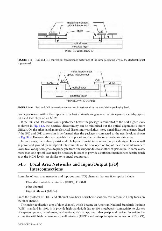
can be performed within the chip where the logical signals are generated or via separate special-purposeE/O and O/E chips on an MCM.

If the E/O and O/E conversion is performed before the package is connected to the next higher level,as shown in Fig. 54.5, the electrical discontinuity can be minimized but the optical alignment is moredifficult. On the other hand, more electrical discontinuity and, thus, more signal distortion are introducedif the E/O and O/E conversion is performed after the package is connected to the next level, as shownin Fig. 54.6. However, this is acceptable for applications that require only moderate data rates.

In both cases, there already exist multiple layers of metal interconnect to provide signal lines as wellas power and ground plane. Optical interconnects can be developed on top of these metal interconnectlayers to allow optical signals to propagate from one chip/module to another chip/module. In some cases,more than one optical layer may be necessary in order to provide a sufficient interconnect density (suchas at the MCM level) just similar to its metal counterpart.

54.3 Local Area Networks and Input/Output (I/O) Interconnections

Examples of local area networks and input/output (I/O) channels that use fiber optics include:

• Fiber distributed data interface (FDDI), FDDI-II

• Fiber channel

• Gigabit ethernet (802.3z)

Since the protocol of FDDI and ethernet have been described elsewhere, this section will only focus onthe fiber channel.

The major application area of fiber channel, which became an American National Standards Institute(ANSI) standard in 1994, is to provide high-bandwidth (up to 100 megabyte/s) connectivity to clustersof supercomputers, mainframes, workstations, disk arrays, and other peripheral devices. Its origin hasstrong ties with high performance parall interface (HIPPI) and enterprise systems connection (ESCON),

FIGURE 54.5 E/O and O/E conversion: conversion is performed at the same packaging level as the electrical signalis generated.

FIGURE 54.6 E/O and O/E conversion: conversion is performed at the next higher packaging level.


both of which provide circuit switching, and small computer systems interface (SCSI), which is the primaryinterconnection mechanism for peripheral devices. Fiber channel defines a point-to-point or switchedpoint-to-point link, which includes definitions of the physical layer, transmission code, and higher levelfunctions such as flow control and multiplexing. Figure 54.7 shows a collection of nodes (called N-port)interconnected by a fabric through the fabric ports (called F-port).

The fiber channel standard includes definitions of the following functions:

• Physical layer. The physical layer specifies four data rates: 133, 266, 533, and 1062.5 Mb/s. Becauseof the adoption of 8B/10B line coding technique, there is a 25% increase in the transmission datarate. The transmission media defined for a fiber channel includes miniature coax, multimode andsingle-mode fibers. The physical layer also defines bit synchronization, serial-to-parallel conversion,and an open fiber control protocol. This protocol performs automatic shutdown of the laser diodewhen there is a fiber cut and automatically establishes a full duplex link when the fiber connectionis restored.

• Data link layer. This layer specifies a line coding technique, the 8B/10B code, to ensure sufficienttransitions are present in the data stream. In addition, byte-to-word conversion and word syn-chronization are also performed in this layer.

• Arbitrated loop layer. The arbitrated loop layer specifies the loop control and bypass mechanisms foran end node when such an end node participates in the connection of a loop, as shown in Fig. 54.8.

FIGURE 54.7 Several nodes interconnected by a fabric.

FIGURE 54.8 Several nodes interconnected by a fabric.


This configuration has the advantage of reduced cost at the cost of reduced performance and isparticularly attractive for disk storage applications.

• Frame processing layer. The processing and validation of the integrity of each received frameincluding, CRC checking is performed in this layer.

54.4 Access Networks

Access networks provide interconnections between the customer premises equipment (CPE) and the centraloffices. The average distance of these types of networks is usually less than 3 mi. The components ofaccess networks are extremely cost sensitive. Although the price of fiber has gone down dramatically, theprice of a single-mode distributed feedback (DFB) laser has not. The design of the access network is,thus, to minimize the use of active devices such as the laser diodes or confine the use of such deviceswithin central offices. The current fiber deployment strategies are divided into the following two cate-gories: hybrid fiber coaxial (HFC) and fiber to the home (or fiber in the loop). Although fiber to thehome is the ultimate answer to broadband services, HFC seems to be the most tangible interim solution.

The hybrid fiber coaxial cable structure deploys both the fiber and the coaxial cable. The basic fiber/coaxnetwork is already taking shape as a result of the cable TV delivery system. Signals in most of the existingHFC networks are transmitted using fiber with broadband RF spectrum to an headend. A typical archi-tecture is shown in Fig. 54.9. The signals are then converted back into an electrical RF signal anddistributed to the home. The major advantages of this star-configured fiber network with coax bus areas follows [Paff, 1995]:

• Better quality video

• More bandwidth possible with lower beginning investment

• Better reliability

• Dedicated feed into and out of a small area

FIGURE 54.9 A broadcast-and-select network.


Although the current HFC network is a broadcast and isolated architecture, a lot of research had beendevoted to the next generation HFC network that can provide an interactive and broadband elementwithin the public telecommunication fabric.

54.5 Wavelength-Division Multiplexing-Based All Optical Networks

The advantages of a wavelength-division multiplexing (WDM)-based optical network can be groupedinto two aspects. One aspect lies in its potential in utilizing the vast bandwidth offered by the single-mode optical fiber since there are no electronic components in the network. The other equally importantaspect is its simple network control. To transmit a packet, the source only needs to identify the destinationthrough a unique wavelength. There is no need to know about the exact network topology for routeselection. There is no buffering within the network and, therefore, no need for flow control or congestioncontrol at or below the network layer. Only the associated end nodes need to do handshaking betweenthemselves.

Two types of WDM-based networks are commonly discussed:

• Broadcast-and-select networks

• Wavelength routed networks

Broadcast-and-Select Networks

A broadcast-and-select network consists of nodes interconnected to each other via a star coupler, asshown in Fig. 54.10. An optical fiber link, called the uplink, carries signals from each node to the star.The star combines the signals from all of the nodes and distributes the resulting optical signal equallyamong all its outputs. Another optical fiber link, called the downlink, carries the combined signal from anoutput of the star to each node. Examples of such networks are Lambdanet [Goodman et al., 1990] andRainbow [Janniello, Ramaswami, and Steinberg, 1993].

Wavelength-Routed Networks

A wavelength-routed network is shown in Fig. 54.11. The network consists of static or reconfigurablewavelength routers interconnected by fiber links. Static routers provide a fixed, nonreconfigurable routingpattern. A reconfigurable router, on the other hand, allows the routing pattern to be changed dynamically.These routers provide static or reconfigurable lightpaths between end nodes. A lightpath is a connectionconsisting of a path in the network between the two nodes and a wavelength assigned on the path. Endnodes are attached to the wavelength routers. One or more controllers that perform the network man-agement functions are attached to the end node(s).

FIGURE 54.10 A broadcast-and-select network.


54.6 Fiber Sensors

It is well known that optical techniques, interferometry in particular, offer extremely high precision.However, it is difficult to apply these high-precision techniques outside a laboratory for the followingtwo reasons:

• Environmental perturbations tend to cause rapid misalignment of the optical components.

• Optical components have to be within line of sight and, thus, remote sensing is difficult to achieve.

This situation has recently changed dramatically due to the incorporation of fiber optic waveguidesinto sensors where the fiber optic waveguides can act as the sensor or serve as a transceiver to transferlight signals to a remote sensor. Several examples of the application of optical techniques are as follows:

• Biomedical transducer [Mignani and Baldini, 1995]. The development of optic fiber sensors formedical applications dates back to the 1970s. The current-generation fiber optical sensors, whichare mostly composed of silica and plastic fibers, are coupled to sensitive fiber sections or optrodes.These sensors are usually based on intensity modulation interrogation schemes, as shown inFig. 54.12. Applications of these sensors include cardiovascular and intensive care, angiology,gastroenterology, ophthalmology, oncology, and neurology, to name just a few.

• Chemical transducer. Because of their immunity to electromagnetic interference (EMI), electricand intrinsic safety, possibility of miniaturization, and biocompatibility, optical fiber pH sensorsare ideal for blood monitoring [Deboux et al., 1995]. These sensors are based on the observationof the changes in the optical properties of colorimetric or fluorimetric pH indicators. The changesare measured by reflection or through interaction with the evanescent field changes in the absorp-tion due to changes in color of colorimetric indicators. Optical sensors based on optical time-domain reflectometry can also be used to detect the water ingress point.

• Intelligent sensors. Fiber optical sensors can be embedded in cement mortar bodies for nonde-structive monitoring of structures and for deformation measurement [Habel and Polster, 1995].

• Magnetic/electric field transducer [Ezekiel et al., 1995]. Magnetic and electric fields can bemeasured through spectroscopic techniques, as shown in Fig. 54.13. These techniques usuallyinvolve the excitation of atoms and molecules in a cell using a tunable light source, such as alaser, and measuring the resulting absorption or fluorescence. In this way, it is possible to identifythe type of molecule in the vapor, as well as the concentration. This method is generally referredto as a single-step or single-photon spectroscopy, since the excitation involves a single pair ofenergy levels. Recently, there are also new techniques that utilize two-step or two-photonspectroscopy, in which two radiation fields simultaneously interact with the atom or moleculein the vapor.

FIGURE 54.11 A wavelength-routed network.


• Moisture transducer. Instead of using a large number of electrically passive sensors, moisturecan be detected through the use of a single fiber based on optical time-domain reflectometry.This technique enables the presence of water to be detected as a linear function of the fiberlength.

References

Deboux, B.J.C., Lewis, E., Scully, P.J., and Edwards, R. 1995. A novel technique for optical fiber pH sensingbased on methylene blue absorption. J. Lightwave Tech., 13(7).

Ezekiel, S., Smith, S.P., Shahriar, M.S., and Hemmer, P.R. 1995. New opportunities in fiber-optic sensors.J. Lightwave Tech., 13(7).

Farwald, M.P. and Mooring, D. 1992. A fast path to one memory. IEEE Spect., 29(Oct.):50–51.Gjessing, S., Gustavson, D.B., James, D.V., Stone, G., and Wiggers, H. 1992. A RAM link for high speed.

IEEE Spect., 29(Oct.):52–53.Goodman, M.S., Kobrinski, H., Vecchi, M., Bulley, R.M., and Gimlett, J.M. 1990. The LAMBDANET

multiwavelength network: architecture, applications and demonstrations. IEEE J. Selec. Areas Com-mun., 8(6):995–1004.

Habel, W.R. and Polster, H. 1995. The influence of cementitious building materials on polymeric surfacesof embedded optical fibers for sensors. J. Lightwave Tech., 13(7).

IEEE. 1992. Scalable coherent interface: Logical, physical, and cache coherence specifications. IEEE P1594Working Group, IEEE Standard Department.

Janniello, F.J., Ramaswami, R., and Steinberg, D.G. 1993. A prototype circuit-switched multi-wavelengthoptical metropolitan-area network. J. Lightwave Tech., 11(May/June):777–782.

Lockwood, J.W., Duan, H., Morikuni, J.J., Kang, S.M., Akkineni, S., and Cambell, R.H. 1995. Scalableoptoelectronic ATM networks: the iPOINT fully functional testbed. J. Lightwave Tech., 13(6):1093–1103.

FIGURE 54.12 Configuration of a biosensor.

FIGURE 54.13 Configuration of a spectroscope setup for measuring absorption spectrum.


Mignani, A.G. and Baldini, F. 1995. In-vivo biomedical monitoring by fiber optic systems. J. LightwaveTech., 13(7).

Paff, A. 1995. Hybrid fiber/coax in the public telecommunications infrastructure. IEEE Commun. Mag.,33(4).

Stone, H.S. and Cocke, J. 1991. Computer architecture in the 1990s. IEEE Comput. Mag., 24(9):30–38.


55Wavelength-DivisionMultiplexed Systems

and Applications

55.1 Introduction55.2 Optical Components for Wavelength-Division

Multiplexed Systems Transmitter • Multiplexer and Demultiplexer • Optical Amplifier

55.3 Wavelength-Division Multiplexed System Design55.4 Trunk Capacity Enhancement Applications55.5 Wavelength-Division Multiplexed Networking

and Reconfigurable Optical Transport Layer55.6 Summary

55.1 Introduction

Research in wavelength-division multiplexing (WDM) technology is driven by the desire to exploit theimmense bandwidth available for transmission in a single-mode optical fiber. The low-loss wavelengthrange around 1.55 µm alone can support over 10 THz of bandwidth. However, this bandwidth cannotbe directly utilized by time-division multiplexed (TDM) systems due to the speed limitations posed byfiber dispersion. WDM offers a more practicable solution of multiplexing many high-speed channels atdifferent optical carrier frequencies and transmitting them over the same fiber. It is expected that WDMtechnology will play a greater role in the coming years as the telecommunications networks evolve tomeet the growing demand for bandwidth.

In this chapter, we describe the fundamental concepts of WDM systems, beginning with a review ofkey optical components and their performance requirements. This is followed by a discussion of systemdesign issues and a review of several promising applications for telecommunications networks.

55.2 Optical Components for Wavelength-Division Multiplexed Systems

WDM systems are commonly classified into three general groups based on the choice of channel spacingand the aggregate transmission capacity supported. The simplest configuration, often known as the coarseWDM architecture, supports transmission of two channels in the broad low-loss windows of the fiberat 1.3 µm and at 1.55 µm. A greater capacity can be supported by dense WDM systems, where several

Mari W. MaedaIPA


wavelengths are transmitted in the 1.55-µm region with a typical channel spacing on the order of oneto several nanometers, as shown in Fig. 55.1. Optical frequency-division multiplexed (OFDM) systemssupport even greater density of channels with the spacing in the range of 0.1 nm (~10 GHz). Althoughboth dense WDM and OFDM systems can support aggregate transmission capacity of over 100 Gb/s,dense WDM is becoming widely accepted as offering a more practical, near-term solution in variousapplications and will be the primary focus of this chapter.

Figure 55.2 shows a basic WDM system for point-to-point high-capacity transmission applications.The signals at different wavelengths are optically multiplexed so that N wavelengths are simultaneouslycarried on a common transmission fiber. Optical amplifiers may be used to compensate for fiber atten-uation and component loss. At the receiving end, the signals are demultiplexed and detected by opto-electronic receivers. The key optical components for WDM systems are now reviewed.

FIGURE 55.1 (a) Fiber transmission loss showing the low-loss windows at 1.3 and 1.5 µm. (b) Transmissionspectrum for an eight-channel WDM system using an erbium-doped fiber amplifier (EDFA). The background detailshows the spontaneous emission spectrum from EDFA.

FIGURE 55.2 Basic WDM system configuration, optical amplifier (OA).


Transmitter

Lasers for high-speed transmission systems must emit single wavelengths (i.e., a single longitudinal mode)and support high output power (>1-mW coupled into fiber pigtail) over a large modulation bandwidthwith a specified spectral stability. Output spectral characteristic is one of the key considerations indesigning high-speed systems where the transmission distances can be limited by fiber chromatic dis-persion. Well-confined optical spectrum is especially important for WDM since the channel spacing mustbe selected to minimize interchannel crosstalk. Optical sources that are in widest use today are distributedfeedback (DFB) lasers. DFB lasers can support multigigabit per second rate intensity modulation throughdirect injection current modulation and produce an output signal with a stable spectrum over the entiremodulation bandwidth. For applications requiring ~10-Gb/s modulation rates, external modulation canbe used to reduce the extent of wavelength chirping that normally accompanies direct modulation. Itshould be noted that incoherent sources such as light emitting diodes (LEDs) or super luminescent diodestogether with wavelength filters can also be used to generate quasi-monochromatic signals [Iannone,1995]. This so-called spectral-slicing technique is applicable for systems that emphasize simplicity andcost effectiveness of the transmitter design.

Multiplexer and Demultiplexer

Key considerations in selecting the multiplexing and demultiplexing technologies are the passband charac-teristics, insertion loss, polarization sensitivity, and thermal stability. For systems with wavelength spacingin the range of 1–10 nm, commonly used passive de/multiplexers are based on diffraction gratings andmultilayer interference filters. For systems employing narrower channel spacing in the range of 0.1 nm,cascaded Mach–Zehnder or Fabry–Perot (FP) interferometer devices may be used for filtering the desiredchannel. A commonly used alternative to using a wavelength-selective coupling device is to use a passive Nby N star coupler, which evenly splits each input signal between N outgoing ports. The intrinsic splittingloss of a star coupler may be compensated by the use of an optical amplifier. Star couplers are often employedin a broadcast-and-select configuration together with tunable filters on the receiving end. Examples of tunablefilters include the index-tuned liquid crystal FP filter, acousto-optic filter, and DFB filter amplifier. Forfurther details on tunable filter technology and its application in multiaccess networks, readers may consultMestdagh [1995].

Optical Amplifier

Recent technological advances have shown optical amplification to be practical in the form of erbium-doped fiber amplifiers (EDFA). EDFAs possess the desirable features of high fiber-to-fiber gain (20 to40 dB), high output power [>10 mW], and quantum limited noise figure, and offer approximately 30 nmof useful gain bandwidth in the 1535 to 1565 nm range [Desurvire, 1994]. For WDM systems employingcascaded EDFAs, cumulative gain nonuniformity over the gain spectrum can be significant and channelequalization is necessary (for example, by using filters or a signal pre-emphasis technique). The highsignal powers made possible with EDFAs also raise the issue of signal degradations due to fiber non-linearity, which must be carefully addressed especially in long-haul, high-speed system design.

55.3 Wavelength-Division Multiplexed System Design

Successful WDM system design entails a tradeoff of channel spacing, per channel bit rate, and feasibletransmission distances based on various physical and practical constraints. Table 55.1 lists key factorslimiting system performance along with possible solutions for relaxing the constraints.

The maximum transmission distances that can be attained without optoelectronic regeneration arelimited by three characteristics of the fiber: linear loss, chromatic dispersion, and nonlinearity. Linearloss in the fiber, due primarily to Rayleigh scattering and molecular absorption, can be largely compen-sated by the use of optical amplifiers. For systems employing multigigabit per second channel rates, viable


transmission distances become limited by the fiber dispersion and optical spectral characteristics. Forexample, with a conventional (nondispersion shifted) single-mode fiber that is widely deployed in the field,the dispersion level of ~17 ps/km-nm at 1550 nm limits the transmission distances to a mere 11 km whenlaunching a 10-Gb/s signal with a spectral width of 1.0 nm. However, when the spectral width is reducedto 0.1 nm, the transmission distance is extended to 65 km. Such reduction in the optical spectral width canbe attained by replacing direct laser modulation with the use of an external modulator. The chromaticdispersion problem can be also alleviated with the use of dispersion-shifted fiber whose zero-dispersionwavelength is in the 1550-nm range instead of the 1300 nm for conventional fiber. However, when suchredeployment of fiber is not an option, as the case may be when upgrading a network using already installedfibers, dispersion management techniques can be used to extend the transmission span. For example, adispersion compensating device or a length of negative-dispersion fiber can be inserted periodically intothe fiber span to correct the signal distortions [Lin et al., 1980; Onaka et al., 1996]. In laboratory experiments,several different dispersion management techniques have been successfully employed to extend the regen-eratorless transmission spans into the thousands of kilometers range.

When the transmitted signal powers are high, as they are in systems employing optical amplifiers, theeffects of fiber nonlinearities must be taken into consideration during system design [Chraplyvy, 1990].Fiber nonlinearities cause energy transfer between propagating wavelengths and lead to nonlinear lossand crosstalk if the system parameters such as launch powers and channel spacing are not carefullyselected. One such effect is nonlinear phase modulation, which results from the power dependence ofthe refractive index. For single-wavelength systems, this nonlinearity takes the form of self-phase mod-ulation (SPM), whereas in WDM systems, cross-phase modulation (XPM) plays a greater role as thephase of one wavelength is influenced by the intensity of all other wavelengths [Marcuse, 1994]. SPMand XPM broadens the signal spectrum, causing pulse distortions due to fiber chromatic dispersion.Degradations can be alleviated by reducing the launched signal power, increasing the channel spacing,and using a passive dispersion compensation technique mentioned earlier.

Another nonlinear effect that has a deleterious effect on WDM systems is four-wave mixing (FWM),where nonlinear interaction between three wavelengths generates a fourth wavelength, analogous to third-order intermodulation in radio systems. FWM interaction between different combinations of multiplexedwavelengths results in an appearance of interfering light at a signal channel, causing a crosstalk penalty.

TABLE 55.1 Sources of Limitations in WDM Systems, Their Effects, and Possible Solutions

Limitation Sources Effect Solutions

Fiber dispersion Waveform distortion at high bit rates Reduce signal chirp (e.g., use external modulator)

Use dispersion-shifted fiberUse dispersion compensation

SPM/XPM Waveform distortion at high bit ratesand high launch powers

Use dispersion-shifted fiber

Use dispersion compensationIncrease channel spacingReduce power

Four-wave mixing

Nonlinear crosstalk and loss at high launch powers

Increase channel spacing

Avoid dispersion-shifted fiberReduce per-channel power

Amplifier gain nonuniformity

Uneven gain for different λ Use equilization or pre-emphasis

Use narrow spacing to confine the channel spread

Wavelength drift Crosstalk and signal fading Require active λ stabilizationIncrease channel spacing


Because FWM requires optical phase matching between the interacting signals, the effect can be reducedby using unequal or large channel spacings and by locally avoiding dispersion of magnitude less thanabout 1 to 2 ps/nm-km in the transmission fiber. The latter can be accomplished by using the dispersioncompensating technique whereby the dispersion level in an individual fiber segment is kept greater thanthe required 1 to 2 ps/nm-km but the overall dispersion is minimized.

There are other factors, in addition to fiber nonlinearity, that influence the choice of WDM channelspacing. When the wavelength spacing is very small, it is possible to pack more channels into the wavelengthregime where the EDFA gain is relatively uniform. However, when the spacing is reduced to a fraction of ananometer, the design requirements for various optical components become quite stringent. For example,stabilization of optical sources and multiplexers becomes necessary so that wavelength drifts do not causesignal fading and crosstalk. Optical demultiplexers and filters also require more careful design to minimizeinterchannel crosstalk. Although there have been demonstrations of OFDM systems using wavelength spacingin the range of 0.1 nm (~10 GHz) [Nosu et al., 1993], a typically selected spacing for most applications is inthe range from 0.6 nm to several nanometers. Indeed, a preliminary agreement in the International Tele-communication Union (ITU) standards endorses the usage of a 100-GHz (1.1 nm) frequency grid referencedto an absolute frequency of 193.100 THz (1552.52 nm).

55.4 Trunk Capacity Enhancement Applications

Near-term applications for high-speed WDM systems can be found in fiber trunk capacity enhance-ments. Currently available upgrade options are: (1) use of higher speed TDM systems, (2) use of additionalfibers, and (3) use of wavelength multiplexing. Although a mix of three approaches will most likely beused in different parts of the network depending on the need and the economics, a transmission techniqueof combining high-speed TDM with WDM is especially attractive for long-haul applications since costsaving is made possible through fiber and amplifier sharing. Also, in those parts of the network whereexisting capacity is nearing exhaustion, the use of WDM offers a lower cost alternative to installing newcables or constructing new ducts.

Figure 55.3 shows the growing transmission capacity demonstrated in laboratory experiments fromthe mid-1980s to 1996. A two to three orders of magnitude increase in per-fiber capacity has been achieved

FIGURE 55.3 Trend in experimental demonstrations: total transmission capacity over one single-mode fiber forsingle-wave systems and for WDM systems.


with improvements in device speeds and through the use of WDM. A record 1.1-Tb/s transmission over150 km was demonstrated in early 1996 with the use of 55 wavelength sources, each operating at 20 Gb/s[Onaka et al., 1996]. An equally remarkable trend has been witnessed in the transmission distances attainedwith WDM systems. In a recent experiment, eight 5-Gb/s channels were transmitted over 4500 km of fiberusing 69 optical amplifiers [Suyama et al., 1996]. A separate experiment has demonstrated the feasibilityof transmitting 20 5-Gb/s WDM channels over 9100 km of fiber in a circulating-loop configuration[Bergano et al., 1996].

Although it will be a while before terabit per second systems become a commercial reality, deploymentof WDM systems has begun in terrestrial and undersea networks. Most terrestrial long distance networksin the U.S. are currently based on single-wavelength 2.5-Gb/s [optical carrier-OC-48] SONET systems. Nextgeneration TDM systems operating at the speed of 10 Gb/s (OC-192) are nearing deployment while,simultaneously, WDM-based upgrade solutions are becoming commercially available. Network architectsare also investigating the use of WDM in global undersea communication networks. For example, the AfricaOptical Network, which will encircle the African continent with a 40,000-km trunk and branch network,will utilize a WDM technique [Marra et al., 1996]. Of eight wavelengths to be transported over the mainring fibers, four wavelengths will carry interregional traffic while the remaining four wavelengths will carryintraregional traffic. Over the trans-Atlantic and trans-Pacific spans, single-wavelength systems incorporat-ing optical amplifiers are currently deployed. However, the feasibility of upgrading the existing cable capacityusing WDM has been experimentally verified [Feggeler et al., 1996] and WDM technology will no doubtplay an important role in future generations of transoceanic networks.

55.5 Wavelength-Division Multiplexed Networking and Reconfigurable Optical Transport Layer

Whereas point-to-point WDM systems are becoming a commercial reality, the role of WDM in a recon-figurable optical transport network is being researched by a number of laboratories around the world [Hillet al., 1993; Sato, 1994; Brackett et al., 1993; Alexander et al., 1993]. Such WDM networks can bedynamically reconfigured to carry existing transport signals and are especially suited for supporting high-capacity demands that vary with time, a situation that may become likely as broadband services becomewidespread [Berthold, 1996]. WDM networks may consist of nodes or network elements that can multi-plex, switch, and terminate wavelengths. For example, an N by N wavelength cross-connect routes wave-lengths from input WDM ports to output WDM ports. A wavelength add–drop multiplexer (W-ADM)performs the function of assigning an input wavelength and multiplexing this signal to be routed over thenetwork. A chain of W-ADMs can be deployed in a linear or ring configuration, similar to SONET ADMs.

In addition to reconfigurability and capacity enhancement, the WDM network can offer an advantageof built-in network survivability. For example, in an event of a fiber failure, the entire multiplexed signaltraversing the failed link can be switched and routed on a protection fiber using a loopback mechanismsimilar to that used in SONET rings. Alternatively, a wavelength path can be protected on an end-to-endbasis using a pre-configured protection path that becomes activated only after the primary path failure.

Figure 55.4 shows an example design for a W-ADM with single and multiwavelength ports. An incomingwavelength at a single-wavelength port is wavelength adapted through a receiver/laser pair or multiplexeddirectly through the optical cross connect fabric. Incoming multiplexed signals are demultiplexed anddropped or transparently routed through the optical cross connect fabric. In contrast to SONET ADMs,electronic signal processing and regeneration are kept to a minimum with most signal processing beingdone in the optical domain. The key active elements are optical cross connects for routing signals andoptical amplifiers for compensating signal loss. The integrity of the signals is monitored at various pointsinternal to the node, allowing dynamic adjustments to be made in the event of signal degradations.

Research is currently being pursued to define various aspects of the network architecture and the nodaldesign, including the performance requirements, protection switching mechanisms, and methods tosupport embedded management channels. Because the viability of WDM networks hinges strongly on


the economics, both cost effectiveness and manageability of the network are being closely examined bya number of research consortia.

55.6 Summary

There have been rapid advances in the lightwave technology over the past decade, especially in the areasof single-frequency sources, optical amplifiers, wavelength multiplexers, demultiplexers, and optical receiv-ers. These advances have made possible a tremendous increase in the per-fiber transmission capacity, asexemplified by the terabit per second WDM transmission experiments demonstrated in early 1996. WDMsystems are beginning to be deployed in the terrestrial networks, as the as well as in undersea globalnetworks and are expected to play a greater role in the future as the demand for bandwidth continues togrow and the need for economical capacity upgrades becomes more compelling.

References

Alexander, S.B. et al. 1993. A precompetitive consortium on wide-band all-optical networks. J. LightwaveTech., 11(May/June):714–735.

Bergano, N. et al. 1996. 100 Gb/s Error free transmission over 9100 km using twenty 5 Gb/s WDM datachannels, Proceedings OFC’96, Postdeadline Paper 23-1, Feb.

Berthold, J. 1996, Application of WDM in local exchange networks, Proceedings OFC’96, Paper ThN1,Feb.

Brackett, C.A. et al. 1993. A scaleable multiwavelength multihop optical network: a proposal for researchon all-optical networks. J. Lightwave Tech., 11(May/June):736–753.

Chraplyvy, A.R. 1990. Limitation on lightwave communications imposed by optical-fiber nonlinearities.J. Lightwave Tech., 8:1548.

Desurvire, E. 1994. Erbium-Doped Fiber Amplifiers, John Wiley & Sons, New York.Feggeler, J. et al. 1996. WDM transmission measurements on installed optical amplifier undersea cable

systems, Proceedings OFC’96, Paper TuN3, Feb.Gnauck, A. et al. 1996. One terabit/s transmission experiment, Proceedings OFC’96, Postdeadline Paper

20-2, Feb.Hill, G.R. et al. 1993. A transport network layer based on optical network elements. J. Lightwave Tech.,

11(May/June):667–679.

FIGURE 55.4 WDM add–drop multiplexer. Part of the design supporting WDM signals in only one direction isshown. Signal levels, noise levels, and wavelength readings are tracked at various monitor points.


Iannone, P. 1995. A WDM PON architecture with bi-directional optical spectral slicing, ProceedingsOFC’95, Paper TuK2, Feb.

Lin, C. et al. 1980. Optical-pulse equalization of low-dispersion transmission in single-mode fibers inthe 1.3–1.7 µm spectral region. Opt. Lett., 5(Nov.):476–478.

Marcuse, D. 1994. Dependence of cross-phase modulation on channel number in fiber WDM systems.J. Lightwave Tech., 12(May):885–898.

Marra, W. et al. 1996. Africa ONE: the Africa optical network. IEEE Commun. Mag., 34(Feb):50–57.Mestdagh, D.J.G. 1995. Fundamentals of Multi-Access Optical Fiber Networks, Artech House, Norwood,

MA.Nosu, K. et al. 1993. 100 Channel optical FDM technology and its applications to optical FDM channel-

based networks. J. Lightwave Tech., 11(May/June):764–776.Onaka, H. et al. 1996. 1.1 Tb/s WDM transmission over a 150 km 1.3 mm zero-dispersion single-mode

fiber, Proceedings OFC’96, Postdeadline Paper 19-1, Feb.Sato, K. 1994. Network reliability enhancement with optical path layer technologies. IEEE J-SAC,

12:159–170.Suyama, M. et al. 1996. Improvement of WDM transmission performance by non-soliton RZ coding—

a demonstration using 5 Gb/s 8-channel 4500 km straight line testbed, Proceedings OFC’96,Postdeadline Paper 26-2, Feb.

Further Information

For futher information on WDM technology and networking applications, see Fiber-Optic Networks, byP.E. Green, and Special Issue on Broadband Optical Networks, IEEE Journal of Lightwave Technology, Vol. 11,May 1993. Readers interested in access network applications may consult the article, ‘‘Technology and SystemIssues for a WDM-Based Fiber Loop Architecture,’’ by S. Wagner and H. Lemberg, in IEEE Journal ofLightwave Technology, vol. 7, pp. 1759–1768, Nov. 1989. The latest developments in WDM components,systems, and applications are published each year in Technical Digest of the Optical Fiber CommunicationConference.


VSatellite

56 Geostationary Communications Satellites and Applications Bruce R. Elbert Introduction • Satellite Network Fundamentals • Satellite Application Types

57 Satellite Systems Robert L. DouglasIntroduction • Satellite Systems • Transponder Systems • LaunchingSatellites • Station Keeping and Stabilization • Electrical Power Subsystem

58 The Earth Station David R. PritchardIntroduction • Components of the Earth Station • Earth Station Site Selection• Power Distribution • Batteries • Antenna Foundation Requirements • Site Heating,Ventilation, and Air Conditioning • Safety Considerations • Operationand Maintenance • Conclusion

59 Satellite Transmission Impairments Louis J. Ippolito, Jr. In t ro d u c t i o n • At t e n u a t i o n o n S l a n t Pa t h s • D e p o l a r i z a t i o n • R a d i oNoise • Scintillation • Summary

60 Satellite Link Design Peter P. Nuspl and Jahangir A. TehranilI n t ro d u c t i o n • Up l i n k a n d D ow n l i n k E q u a t i o n s • I n t e r f e re n c eEquations • Intermodulation Equations • Allowances, Losses, and Margins• Sums of Link Equations • Designed Bit Error Ratio and Required C/N0

• Nu m b e r s o f C a r r i e r s , e . i . r. p . , a n d Pow e r p e r C a r r i e r • O t h e rIssues • Summary • Appendix A: Some Calculations • Appendix B:Calculation of Antenna Discrimination

61 The Calculation of System Temperature for a MicrowaveReceiver Wilbur PritchardNoise, Antenna, and System Temperatures

62 Onboard Switching and Processing Ahmed K. ElhakeemIntroduction • Onboard Switching Types • Summary

63 Path Diversity Curt A. LevisConcepts • Site Diversity Processing • Site Diversity for Rain-FadeAlleviation • Optical Satellite Site Diversity • Site Diversity for Land–MobileSatellite Communications • Site Diversity for Arctic SatelliteCommunications • Microscale Diversity for VSATs • Orbital Diversity

64 Mobile Satellite Systems John Lodge and Michael MoherIntroduction • The Radio Frequency Environment and Its Implications • SatelliteOrbits • Multiple Access • Modulation and Coding • Trends in MobileSatellite Systems


65 Satellite Antennas Yeongming Hwang and Youn Ho ChoungIntroduction • Horn Antennas and Reflector Feeds • Reflector Antennas • PhasedArray Antennas • Tracking, Telemetry, and Command Antennas • Currentand Planned LEO/MEO Mobile Satellite Antennas • RadiometerAntennas • Space Qualification • Future Trends and Further Study

66 Tracking and Data Relay Satellite System Erwin C. HudsonIntroduction • TDRS System Overview • TDRSS CommunicationsDesign • First Generation TDRS Relay Satellite Design • TDRS LinkBudget Examples • Summary


56Geostationary

CommunicationsSatellites andApplications1

56.1 Introduction56.2 Satellite Network Fundamentals

Satellite Orbits and Constellations • Frequency Spectrum • Network Topology • Satellite vs. Terrestrial Communication • Satellite and Earth Station Designs

56.3 Satellite Application TypesTelevision and Video Services • Over-the-Air TV Broadcasting • Cable TV • Direct-to-Home Satellite Broadcasting • Trends in Satellite Voice Communications• Digital Information Services • Mobile and Personal Communications

56.1 Introduction

Communication satellites, whether in geostationary Earth orbit (GEO) or low Earth orbit (LEO), providean effective platform to relay radio signals between points on the ground. The users who employ thesesignals enjoy a broad spectrum of telecommunication services on the ground, the sea, and in the air. Inrecent years, such systems have become practical to the point where a typical household can have its owndirect-to-home (DTH) satellite dish. Whether or not we reach the stage of broad acceptance depends onthe competition with the more established broadcasting media, including over-the-air TV and cable TV.The success of British Sky Broadcasting in the U.K. market shows this is entirely possible. In any case,GEO and non-GEO satellites will continue to offer unique benefits for other services such as mobilecommunications and multimedia, but it is up to us to exploit them.

Technology and applications have progressed significantly since the late 1980s; however, the basic principlesremain the same. Satellite communication applications extend throughout human activity, both occupationaland recreational. Many large companies have built their foundations on TV, data communications, informa-tion distribution, maritime communications, and remote monitoring. For many others, satellites havebecome a hidden asset. In the public sector, satellite applications are extremely effective in emergencysituations where terrestrial lines and portable radios are not available or ineffective for a variety of reasons.

1Adapted with permission from The Satellite Communication Applications Handbook, Bruce Elbert, Artech House,Norwood, MA, 1997.

Bruce R. Elbert Application Technology Strategy, Inc.


From this experience, those of us who have offered satellite services to large user communities knowthat the orbit position is paramount to achieving a solid business. Consider as an example the U.S.geostationary orbital service arc shown in Fig. 56. 1. Highlighted are the most popular cable TV satellites:Galaxy I-R, Satcom C-1, Galaxy 5, and Satcom C-3. These four satellites collect revenue comparable tothe remaining 25 satellites. Users of these hot birds pay a premium for access to the ground infrastructureof cable TV receiving antennas, much like tenants in a premium shopping mall pay to be in an outstandinglocation and in proximity to the most attractive department stores in the city. In the case of cableTV, access is everything because the ground antenna is, in turn, connected to households wherecable services are consumed and paid for. For new satellite operators to get into such an establishedmarket often requires them to subsidize users by providing new antennas or paying for repointing.This then reduces the potential profitability as these switching costs must come out of the forth-coming revenues.

Satellite operators, who invest in the satellites and make capacity available to their customers, generallyprefer that users own their own Earth stations. This is because installing antennas and associated indoorelectronics is costly for satellite service providers. Once working, this investment must be maintainedand upgraded to meet evolving needs. The owner/user benefits because: (1) there is complete control ofthe service facility and (2) advances in microcircuitry and satellite sophistication have reduced the costand complexity of ownership and operation. A typical small Earth station is no more complex than acellular telephone or video cassette recorder (VCR). Larger Earth stations such as TV uplinks andinternational telephone gateways are certainly not a consumer item, but the advantages of control typicallymotivate leading TV networks and communication companies to take these on.

Several U.S. corporations attempted to introduce DTH service in the mid-1980s at a time when cableTV was still establishing itself. The first entrants experienced great difficulties with the limited performanceof low- and medium-power Ku-band satellites, hampering the capacity of the networks and affordabilityof the home receiving equipment. Europe and Japan had problems of their own creating viable DTHsystems with the technologies at hand, choosing first to launch high-power Ku-band satellites with only afew operating channels. It was not until BSkyB and NHK were able to bring attractive programming tothe public on their respective satellites that consumers adopted the services.

In the U.S., DTH first emerged in the 1980s through the backyard C-band satellite TV business thatallowed consumers to pull existing cable TV programming from cable TV hot birds like Galaxy I andSatcom 3R. This clearly demonstrated the principle that people would vote with their money for a widerange of attractive programming, gaining access to services that were either not available or priced outof reach. Early adopters of these dishes paid a lofty price per installation because the programming wasessentially free since the signals were unscrambled. Later, HBO and other cable networks scrambled theirprogramming using the Videocipher 2 system, resulting in a halt to expansion of backyard dishes. Thismarket settled back into the doldrums for several years.

FIGURE 56.1 An illustration of the U.S. GEO orbital arc as of 1996, highlighting the most popular cable TVsatellites.


In 1994, Hughes Electronics introduced its DIRECTVTM service through a high-power BSS satellite(labeled DBS-1 in Fig. 56.1). With a combined total of over 150 channels of programming, DIRECTV,Inc., and another service provider, USSB, demonstrated that DTH could be both a consumer productand a viable alternative to cable. An older competing service, Primestar, was first introduced by TCI andother cable operators as a means to serve users who were beyond the reach of their cable systems. Thissubsequently provided the platform for a new and improved Primestar, rebuilt along lines very similarto DIRECTV. By converting from an analog to a digital system and expanding programming, the Prime-star service has seen much greater demand than when it was first introduced in 1992.

Satellite communication applications can establish a solid business for companies that know how towork the details to satisfy customer needs. Another example is the IDB Communications Group. Froma very modest start from distributing radio programs by satellite, IDB branched out into every conceivablearea of the telecommunication industry. Whether the requirement is to cover a media event in Antarcticaor to connect Moscow to the rest of the world with voice and video links, IDB proved its worth. Theycapitalized on the versatility of satellite communication in the pursuit of a growing company and ademanding base of investors. Sadly, IDB ran into financial difficulties in 1994 and had to merge withLDDS, the fourth largest long distance carrier in the U.S. IDB’s early success points out that needs canbe met and money is to be made in the field of satellite communication.

56.2 Satellite Network Fundamentals

A commercial satellite communication system is composed of the space segment and the ground segment,illustrated in Fig. 56.2. In this simple representation of a GEO system, the space segment includes the satellitesoperating in orbit and a tracking, telemetry, and command (TT&C) facility that controls and manages theiroperation. This part of the system represents a substantial investment, where the satellite operating lifetimeis typically of the order of 12 years based on fuel availability. Satellites tend to operate peacefully after theyhave survived launch and initiation of service. Failures of on-board equipment are generally transparent tousers because the satellite operator can activate spare electronic equipment, particularly traveling wavetubes and solid state power amplifiers (the critical elements in the communications subsystem). From auser’s perspective, the more important portion of the system is the ground segment, which is the focus ofthis chapter. It contains Earth stations of various types: large hubs or gateways and much smaller stationsthat render services directly to individual users.

Every satellite application achieves its effectiveness by building on the strengths of the satellite link. Asatellite is capable of performing as a microwave repeater for Earth stations that are located within itscoverage area, determined by the altitude of the satellite and the design of its antenna system [Elbert,1987]. The arrangement of three basic orbit configurations is shown in Fig. 56.3. A GEO satellite cancover nearly one-third of the Earth’s surface, with the exception of the polar regions. This includes morethan 99% of the world’s population and essentially all of its economic activity.

Satellite Orbits and Constellations

The LEO and medium Earth orbit (MEO) approaches require more satellites to achieve this level ofcoverage. Because of the fact that the satellites move in relation to the surface of the Earth, a fullcomplement of satellites (called a constellation) must be operating to provide continuous, unbrokenservice. The tradeoff here is that the GEO satellites, being more distant, incur a longer path length toEarth stations, whereas the LEO systems promise short paths not unlike those of terrestrial systems. Thepath length introduces a propagation delay since radio signals travel at the speed of light. Depending onthe nature of the service, the increased delay of MEO and GEO orbits may impose some degradation onquality or throughput. The extent to which this materially affects the acceptability of the service dependson many factors.


At the time of this writing, the only non-GEO system, Orbcom, has entered commercial service withits first two satellites. The applications of Orbcom include paging and low-speed burst data. Systemscapable of providing telephone service, such as Iridium and I-CO Communications, will achieveoperation in the near future. On the other hand, GEO satellite systems continue to be launched forliterally all services contemplated for satellite, and the ones currently operating have lives (based on fuelreserves for stationkeeping) that will carry them through the year 2010.

FIGURE 56.2 Elements of a satellite system, including the space and ground segments.

FIGURE 56.3 The three most popular orbits for communication satellites are low Earth orbit (LEO), mediumEarth orbit (MEO), and geostationary Earth orbit (GEO). The respective altitude ranges are LEO (500–900 km),MEO (5,000–12,000 km), and GEO (36,000 km). Only one orbit per altitude is illustrated, even though there is arequirement for constellations of LEO and MEO satellites to provide continuous service.


Frequency Spectrum

Satellite communication services are provided through GEO satellites operating between 1 and 30 GHz.As microwave frequencies, transmissions to and from the satellite propagate along a line-of-sight pathand experience free space loss that increases as the square of the distance. As indicated in Fig. 56.4, thespectrum is allocated in blocks which are designated L-, C-, X-, Ku-, and Ka-bands. The scale along thex axis is logarithmic in order to show all of the satellite bands; however, observe that the bandwidthavailable for applications increases in real terms as one moves toward the right (i.e., frequencies above4 GHz). Also, the precise amount of spectrum that is available for services in a given region or countryis usually less than Fig. 56.4 indicates. Precise definition of the services and their allocated bandwidthscan be found in the current edition of the Radio Regulations, published by the International Telecom-munication Union in Geneva, Switzerland.

As a general rule, the lower the band is in frequency, the better the propagation characteristics. Thisis countered by the second general principle, which is that the higher the band, the more bandwidth thatis available. The mobile satellite service (MSS) is allocated to the L and S bands, where there is a greaterdegree of diffraction bending and penetration of physical media like foliage and non-metallic buildings.This tends to improve service in a mobile environment. Yet, the bandwidth available between 1 and 2.5 GHz,where MSS applications are authorized, must be shared not only among MSS applications, but with allkinds of radio broadcast and point-to-point services as well. Therefore, the competition is keen for thisspectrum due to its excellent space and terrestrial propagation characteristics. The rapid rollout of wirelessservices such as cellular radiotelephone and personal communications services (PCS) will probablyconflict with advancing GEO and non-GEO MSS systems.

Fixed satellite service (FSS) refers to applications between fixed Earth stations on the ground. Thesesatellites deliver a wide range of services for video, telephone, and data communication. Wideband servicessuch as DTH and broadband integrated services digital network (ISDN) using asynchronous transfermode (ATM) can be accommodated at frequencies above 3 GHz, where there is more than 10 timesthe bandwidth available. Add to this the benefit of using directional ground antennas that effectivelymultiply the number of orbit positions. Some wideband services have begun their migration from the

FIGURE 56.4 The general arrangement of the frequency spectrum that is applied to satellite communications andother radiocommunication services. Indicated are the short-hand letter designations along with an explanation ofthe typical applications. Note that the frequency ranges indicated are the general ranges and do not correspondexactly to the ITU frequency allocations and allotments.


well-established world of C band to Ku band and Ka band. The X-band allocation for FSS has beenreserved by governments for their internal uses, notably for military fixed communications.

Higher satellite effective isotropic radiated power (EIRP) used at Ku and Ka bands allows the use ofrelatively small Earth station antennas. An important factor in the use of these higher bands is theadditional attenuation produced by heavy rain. Additional link margin is demanded in cases where theservice must achieve an availability of greater than about 99%. The bands below Ku (e.g., C, S, and L)experience relatively minor amounts of rain attenuation and, therefore, can use their power to improveother aspects of service. C band, in particular, should maintain its strength for video distribution to cablesystems and TV stations, particularly because of the extensive investment in uplink and downlinkantennas and electronic equipment. One needs to identify and evaluate all of the critical factors beforemaking a selection.

Network Topology

Applications are delivered through a network architecture that falls into one of three categories: point-to-point (mesh), point-to-multipoint (broadcast), and multipoint interactive [very small aperture terminal(VSAT)]. Mesh-type networks mirror the telephone network. They allow Earth stations to communicatedirectly with each other on a one-to-one basis. To make this possible, each Earth station in the networkmust have sufficient transmit and receive performance to exchange information with its least-effectivepartner. Generally, all such Earth stations have similar antennas and transmitter systems, so that theirnetwork is completely balanced. Links between pairs of stations can be operated on a full-time basis forthe transfer of broadband information such as TV or multiplexed voice and data. Alternatively, links canbe established only when needed to transfer information, either by user scheduling (reservation system)or on demand (demand assignment system).

By taking advantage of the broadcast capability of a GEO satellite, the point-to-multipoint networksupports the distribution of information from a source (the hub Earth station) to a potentially very largenumber of users of that information (the remote Earth stations). A broadcast of information by the satelliteis more efficient than terrestrial arrangements using copper wires, fiber optic cables, or multiple wirelessstations. Therefore, any application that uses this basic feature will tend to provide value to the business.

Many applications employ two-way links, which may or may not use the broadcast feature. The appli-cation of the VSAT to interactive data communication applications has proven very successful in manylines of business. A hub and spoke network using VSATs competes very effectively with most terrestrialnetwork topologies that are designed to accomplish the same result. This is because the satellite providesthe common point of connection for the network, eliminating the requirement for a separate physical linkbetween the hub and each remote point. Other interactive applications can employ point-to-point linksto mimic the telephone network, although this tends to be favored for rural and mobile services. Thecoming generation of Ka-band satellite networks that support very low-cost VSATs are expected to reducebarriers to entry into satellite communication.

Satellite vs. Terrestrial Communication

The degree to which satellite communication is superior to terrestrial alternatives depends on manyinterrelated factors, many of which are listed in Table 56.1. Although satellite communication willprobably never overtake terrestrial telecommunications on a major scale, these strengths can producevery effective niches in the marketplace. Once the satellite operator has placed the satellite into service,a network can easily be installed and managed by a single organization. This is possible on a national orregional basis (including global in the case of non-GEO systems). The satellite delivers the same consistentset of services independently of the ground infrastructure, and the costs of doing this are potentiallymuch lower as well. For the long term, the ability to serve mobile stations and to provide communicationsinstantly are features that will gain strength in a changing world.


Satellite and Earth Station Designs

Originally, Earth stations were large, expensive, and located in rural areas so as not to interfere withterrestrial microwave systems that operate in the same frequency bands. These monsters had to usewideband terrestrial links to reach the closest city. Current emphasis is on customer premise Earth stations:simple, reliable, and low cost. An example of a Ku-band VSAT is illustrated in Fig. 56.5. Home receivingsystems for DTH service are also low in cost and quite inconspicuous. Expectations are that the cominggeneration of Ka-band VSATs will reduce the cost and thereby increase their use in smaller businesses and,

TABLE 56.1 The Primary Strengths of Satellite Communications

Feature of Satellite Service Application

Wide-area coverage Domestic, regional, global Wide bandwidth Up to 1 GHz per coverageIndependent of land-based

networks Does not require connection to terrestrial

infrastructureRapid installation Individual sites can be installed and activated in one

day for VSAT or two months of major hubLow cost per added site Depends on type of service; can be as low as $600

for DTHUniform service characteristics Determined by coverage and type of transmission

systemTotal service from a single

providerBy the satellite operator or a separate organization

that leases transponder capacityMobile Communication Requires line-of-sight path over the coverage area

FIGURE 56.5 An example of a small customer premise VSAT used in data communication. (Photograph courtesyof Hughes Network Systems.)


ultimately, the home. There is the prospect of satellites delivering improved Internet access ahead of theterrestrial networks, which have yet to deliver on the promise of ubiquitous wide digital bandwidth.

The other side of the coin is that as terminals have shrunk in size, satellites have grown in power andsophistication. There are three general classes of satellites used in commercial service, each designed fora particular mission and capital budget. Smaller satellites provide a basic number of transponders, usuallyin a single-frequency band. One such satellite can be launched by the old and reliable Delta II rocket ordual-launched on the Ariane 4 or 5. Satellite operators in the U.S., Canada, Indonesia, and China haveestablished themselves in business through this class of satellite. The Measat satellite, illustrated in Fig. 56.6,

FIGURE 56.6 Measat, first launched in 1996, is a small satellite of the Hughes HS-376 class. With 1100 W of payloadpower, it provides both low-power C-band and medium-power Ku-band transponders to Malaysia and surroundingcountries in the Asia–Pacific region. (Photograph courtesy of Hughes Space and Communications Company.)


is an example of this class of vehicle which delivers a total of 18 transponders to Malaysia and neighboringcountries in Asia. Introduction of mobile service in the LEO will involve satellites of this class as well.

Moving up to the middle range of spacecraft, we find designs capable of operating in two frequencybands simultaneously. Galaxy VII, shown in Fig. 56.7, provides 24 C-band and 24 Ku-band transpondersto the U.S. market. A dual payload of this type increases capacity and decreases the cost per transponder.First generation DTH and MSS applications are also provided by these spacecraft. Because of the increasedweight of this size of vehicle, launch service must be provided by larger rockets such as the Atlas 2,

FIGURE 56.7 Galaxy VII, launched in 1993, is a medium-power Hughes HS-601 satellite that provides 24 low-power C-band and 24 medium-power Ku-band transponders to the U.S. market. It is used by cable TV and over-the-air broadcasting networks to distributed programming to affiliates. (Photograph courtesy of Hughes Space andCommunications Company.)


Ariane 4 or 5, the Russian Proton, or the Chinese Long March 2E or 3B (an improved Delta capable oflaunching such spacecraft was under development at the time of this writing).

Finally, the largest satellites serve specialized markets where the highest possible power or payloadweight are required. The generation of GEO mobile satellites that are capable of serving handheld phonesfall into this classification. An example of one of these satellites, APMT, is shown with its 12-m antennadeployed in Fig. 56.8. Also, the trends to use the smallest possible DTH home receiving antenna and tocover the largest service area combine to demand the largest possible spacecraft. The total payload power

FIGURE 56.8 APMT is a regional GEO mobile communications satellite of the largest HS-601 HP class pro-duced by Hughes. It serves the Asia Pacific region and employs a 12-m reflector to serve mobile and fixed users,many of which will use handheld user terminals. (Photograph courtesy of Hughes Space and CommunicationsCompany.)


of such satellites reaches 8 kW, which is roughly eight times that of Measat. Designs are on drawingboards at the time of this writing for satellites that can support payload powers of up to 16 kW.

These general principles lead to a certain set of applications that serve telecommunication users.Satellite manufacture is a strong and viable business, as three American and a like number of Europeanfirms compete in the global market. Earth stations are produced by specialists in the U.S., Canada, Europe,Japan, and Korea. However, world-class consumer electronics and telecommunication equipment firmsare lining up for the opportunity to address the megamarkets in DTH and MSS systems. In the nextsection, we review the most popular applications.

56.3 Satellite Application Types

Applications in satellite communication have evolved over the years to adapt to competitive markets.Evolutionary development, described in Elbert [1987], is a natural facet of the technology because satellitecommunication is extremely versatile. This is important to its extension to new applications in the comingcentury.

Television and Video Services

Commercial TV is the largest segment of the entertainment industry; it also represents the most financiallyrewarding user group to satellite operators. It may have taken 10 or more years for the leading networksin the U.S. and Europe to adopt satellites for distribution of their signals, but by 1985, it was the mainstay.Prior to this date, pioneering efforts in Indonesia and India allowed those countries to introduce nation-wide TV distribution via satellite even before the U.S. made the conversion from terrestrial microwave.European TV providers pooled their resources through the European Broadcasting Union (EBU) andthe EUTELSAT regional satellite system. Very quickly, the leading nations of Asia and Latin Americaadopted satellite TV delivery, rapidly expanding this popular medium to global levels.

There are four fundamental ways that GEO satellites are used to serve the TV industry:

• Point-to-point transmission of video information from a program source to the studio (also calledbackhaul)

• Point-to-multipoint distribution of TV network programming from the studio to the local broad-cast station

• Point-to-multipoint distribution of cable TV programming from the studio to the local cable TVnetwork

• Point-to-multipoint distribution of TV network and/or cable TV programming from the studiodirectly to the subscriber (i.e., DTH)

The first technique is a part of the three that follow, since programming material must be acquired froma variety of sources. A simplified view of the latter three is given in Fig. 56.9. In each case, the videochannels are transmitted to the satellite by an uplink Earth station with the capability to obtain andassemble the programming. This can involve fixed antennas to backhaul programming from othersatellites, tape play machines and video servers to play back prerecorded material, and fiber optic con-nections to distant studios. DTH systems with their smaller antennas require higher satellite power thancable TV and TV distribution. Hence, a common satellite for all three classes is rarely the case.

Over-the-Air TV Broadcasting

Video distribution by satellite is now standard for TV broadcasting in the very high-frequency (VHF)and ultra high-frequency (UHF) bands, which use local TV transmitters to cover a city or area. Thesatellite is used to carry the network signal from a central studio to multiple receive Earth stations, eachconnected to a local TV transmitter. This has been called TV distribution or TV rebroadcast. When equipped


with transmit uplink equipment, the remote Earth station can also transmit a signal back to the centralstudio to allow the station to originate programming for the entire network. U.S. TV networks such asCBS employ these reverse point-to-point links for on-location news reports. The remote TV uplinkprovides a transmission point for local sporting and entertainment events in the same city. This is popularin the U.S., for example, to allow baseball and football fans to see their home team play an away-from-home game in a remote city. More recently, TV networks employ fiber optic transmission services froma national fiber network, but satellites continue as the most flexible routing mechanism.

Revenue for local broadcast operations are available from two potential sources: advertisers and publictaxes. From its beginnings in the U.S., TV provided an excellent medium to influence consumers on theirpurchase behavior. In exchange for watching commercials for soap, airlines, and automobiles, the con-sumer is entertained for virtually nothing. This has produced a large industry in the U.S. as stationsaddress local advertisers and the networks promote nationwide advertising.

An alternative approach was taken in many European countries and Japan, where government operatednetworks were the first to appear. In this case, the consumer is taxed on each TV set in operation. Theserevenues are then used to operate the network and to produce the programming. The BBC in the U.K.and NHK in Japan are powerhouses in terms of their programming efforts and broadcast resources.

FIGURE 56.9 Framework for satellite communication applications in local broadcasting, cable TV, and direct-to-home satellite broadcast.


However, with the rapid introduction of truly commercial networks, cable TV, and DTH, these tax-supported networks are experiencing funding difficulties.

Public TV in the U.S. developed after commercial TV was well established. Originally called educationalTV, this service existed in a fragmented way until a nonprofit organization called the Public BroadcastingService (PBS) began serving the nation by satellite in 1978. The individual stations are supported by thelocal communities through various types of donations. Some are attached to universities; others get theirsupport by donations from individuals and corporations. PBS itself acquires programming from themember stations and from outside sources such as the BBC. Programs are distributed to the membersusing satellite transponders purchased by the U.S. government. Therefore, it must compete with othergovernment agencies for congressional support. PBS programming is arguably of better quality thansome of the popular shows on the commercial networks. Even though PBS addresses a relatively narrowsegment, its markets are now under attack by even more targeted cable TV networks such as A&E, theDiscovery Channel, the Learning Channel, and a more recent entry, the History Channel. All of thesecompetitors built their businesses on satellite delivery to cable systems and DTH subscribers.

Cable TV

Begun as a way to improve local reception in the fringe areas and thinly populated sections of the U.S.,cable TV has established itself as the dominant entry point of TV programming. Its popularity grew afterpioneering cable TV networks such as HBO and Turner Broadcasting (which are not available over theair) were added by cable operators seeking more subscribers. These organizations, joined by Viacom,Disney, ABC, and NBC, used C-band satellite transmission to bypass the conventional TV networks todeliver programming to cable head ends and, thence, to the home. By 1980, 40% of urban-U.S. homeswere using cable to receive local TV stations (because cable provided a more reliable signal); at the sametime, the first nationwide cable networks were included as a sweetener and additional revenue source.During the 1980s, cable TV became an eight billion dollar industry and the prototype for this mediumin Europe, Latin America, and the developed parts of Asia.

Cable TV networks offer programming as a subscriber service to be paid for on a monthly basis, oras an almost free service such as commercial TV broadcasting. HBO and the Disney Channel are examplesof premium (pay) services, whereas the Discovery Channel and TBS are examples of commercial channelsthat receive most of their revenue from advertisers. The leading premium channels in North Americaand Europe are immensely successful in financial terms, but the business has yet to be firmly establishedin economies with low-income levels.

Cable TV became the first to offer a wide range of programming options that are under the directcontrol of the service provider. This ensures that subscription fees and service charges can be collectedfrom subscribers. If the fees are not paid, the service is terminated. Wireless cable, a contradiction interms but nevertheless a viable alternative to wired cable, is gaining popularity in Latin America andAsia. The principle here is that the cable channels are broadcast locally in the microwave band to smalldishes located at subscribers. Just as in the case of DTH, wireless cable depends on some form ofconditional access control that allows the operator to electronically disconnect a nonpaying user.

Direct-to-Home Satellite Broadcasting

The last step in the evolution of the satellite TV network is DTH. After a number of ill-fated venturesduring the early 1980s, DTH appears to be ready to take off. B Sky B in the U.K., NHK in Japan, DIRECTVin the U.S., and STAR TV in Asia are now established businesses, with other broadcasters following suit.Through its wide area broadcast capability, a GEO satellite is uniquely situated to deliver the same signalthroughout a country or region at an attractive cost per user. The particular economics of this deliverydepend on the following factors:

• The size of the receiving antennas: Smaller antennas are easier to install and maintain and arecheaper to purchase in the first place. They are also less noticeable (something which is desirable


in some cultures but not necessarily in all others). However, the diameter of the receiving antennais inversely proportional to the square root of the effective radiated power of the satellite.

• The design of the equipment: It is simple to install and operate (this author’s RCATM brand DigitalSatellite System (DSS) installation, needed to receive DIRECTV, took only 2 h: 105 min to runthe cables and 15 min to install and point the dish).

• Several users can share the same antenna: This is sensible if the antenna is relatively expensive,say in excess of $1000; otherwise, users can afford their own. A separate receiver is needed foreach independent TV watcher (i.e., for private channel surfing).

• The number of transponders that can be accessed through each antenna: The trend is now towardlocating more than one satellite in the same orbit position, to increase the available number oftransponders. The more channels that are available at the same slot, the more programming choicesthe user will experience.

• The number of TV channels that can be carried by each transponder: Capacity is multipliedthrough digital compression techniques such as Moving Pictures Expert Group (MPEG) 2. Thismultiplies the quantity of simultaneous programs by five or more.

The ideal satellite video network delivers its programming to the smallest practical antenna on theground, has a large number of channels available (greater than 100), and permits some means for usersto interact with the source of programming. A simple connection to the public-switched telephonenetwork (PSTN) allows services to be ordered directly by the subscriber. Thus, the system emulates adirect point-to-point connection between user and programming supplier, something that broadbandfiber optic networks promise but have yet to deliver on a wide-scale basis.

Trends in Satellite Voice Communications

Voice communications are fundamentally based on the interaction between two people. It was recognizedvery early in the development of satellite networks that the propagation delay imposed by the GEO tendsto degrade the quality of interactive voice communications, at least for some percentage of the population.However, voice communications represent a significant satellite application due to the other advantagesof the medium. For example, many developing countries and lightly inhabited regions of developedcountries continue to use satellite links as an integral part of the voice network infrastructure. Further-more, one area where satellite links are essential for voice communications is the mobile field.

The public-switched telephone network within and between countries is primarily based on therequirements of voice communications, representing something in the range of 60–70% of all interactivetraffic. The remainder consists of facsimile (fax) transmissions, low- and medium-speed data (both forprivate networks and access to public network services such as the Internet), and various systems formonitoring and controlling remote facilities. The principal benefit of the PSTN is that it is truly universal.If you can do your business within the limits of 3000 Hz of bandwidth and can tolerate the time neededto establish a connection through its dialup facility, the PSTN is your best bet.

Propagation delay has become an issue when competitively priced digital fiber optic networks areintroduced. Prior to 1985 in the U.S., AT&T, MCI, and others were using a significant amount of analogtelephone channels both on terrestrial and satellite links. An aggressive competitor in the form of U.S.Sprint invested in an all-digital network that employed fiber optic transmission. Sprint expanded theirnetwork without microwave or satellite links and introduced an all-digital service at a time when com-petition in long distance was heating up. Their advertising claimed that calls over their network were soquiet you could “hear a pin drop.” This campaign was so successful that both MCI and AT&T quicklyshifted their calls to fiber, resulting in rapid turn down of both satellite voice channels and analogmicrowave systems.

Satellite-based telephone service is acceptable in cases where it is the best alternative. For example,wired networks cannot provide mobile communications on the oceans and in very remote areas. Here,digital voice over satellite is widely accepted. A particular application, called mesh telephony, allows


separate VSATs to operate as independent connection points for users or small village. Gateways in majorcities connect calls between these remote VSATs and subscribers on the PSTN. Major telephone Earthstations are part of the international telecommunication infrastructure, connecting to and betweencountries that are not yet served by modern fiber optic systems. The basic voice transmission quality isthe same on satellite or terrestrial fiber because it is determined by the process of converting from analogto digital format. All long-distance transmission systems, satellite and cable, require echo cancellers tomaintain quality. GEO satellite links experience a delay of about 260 ms and so are different from theirterrestrial counterparts. However, they can be quite acceptable given that the application favors thismedium for economic or practical reasons.

The economics of satellite voice communications are substantially different from those of the terrestrialPSTN, even given the use of digital technology on both approaches. With low-cost VSAT technology andhigh-powered satellites at Ku and Ka bands, satellite voice is the cheapest and quickest way to reachremote areas where terrestrial facilities are not available. It will be more attractive to install a VSAT thanto extend a fiber optic cable over a distance greater than several hundred meters. A critical variable inthis case is the cost of the VSAT, which is expected to drop from the $10,000 level to perhaps as low as$1500 before 2000.

Fiber optic transmission is not the only terrestrial technology that can address the voice communicationneeds of subscribers. There is now a new class of terrestrial wireless system called fixed cellular. Low-costcordless phones or simple radio terminals are placed in homes or offices, providing access to the PSTNthrough a central base station. The base stations are concentrating points for traffic and can be connectedto the PSTN by fiber or even satellite links. The cost of the base station and network control is kept lowby not incorporating the automatic hands-off feature of cellular mobile radio. Instead, user terminals ofdifferent types make the connection through the closest base station, which remains in the same operatingmode throughout the call. Fixed cellular can grow in cost beyond VSATs as more cells are added.

New classes of public network services are expected in coming years, under the general category ofbroadband communications. The underlying technology is asynchronous transfer mode, a flexible high-speed packet-switched architecture that integrates all forms of communications. ATM services can bedelivered through fiber optic bandwidths and advanced digital switching systems and include the fol-lowing, among others:

• High-speed data on demand (384 kb/s to 155 Mb/s, and greater)

• Multichannel voice

• Video services on demand

• High resolution fax (300 dots per inch and better)

• Integrated voice/data/video for enhanced Internet services

Because of the high cost of upgrading the terrestrial telephone plant to provide ATM services on awidespread basis, many of these services will not appear in many places for some time. However, theyrepresent the capability of the coming generation of public networks being implemented around theglobe.

Satellite communication currently addresses these services as well and, in fact, has been the only meansavailable to provide them on a consistent basis. In private network applications, satellite communicationhas a big advantage for delivering broadband services to a large quantity of sites. Fiber optic networksare attractive for intra- and intercity public networks and can offer broadband point-to-point transmis-sion, which is potentially lower in cost per user. Yet, this is easier to do with a satellite because it providesa common traffic concentration point in the sky (a principle of traffic engineering). The bandwidth isused more effectively and, therefore, the network can carry more telephone conversations and generatemore revenue.

Satellite networks are very expandable because all points are independent and local terrain does notinfluence the performance of link. Consider the example of the largest German bank, Deutsche Bank,which needed to offer banking services in the new states of the former East Germany. The telecom


infrastructure in East Germany in 1990, although the best in eastern Europe, was very backward bywestern European standards. Deutsche Bank installed medium-sized Earth stations at new bank locationsand was then able to offer banking services that were identical to those of their existing branches in thewest. Another excellent example is Wal*Mart Department Stores, reviewed later in this chapter.

Digital Information Services

Satellite networks are able to meet a wide variety of data communication needs of businesses andnoncommercial users such as government agencies. The wide-area coverage feature combined with theability to deliver relatively wide bandwidths with a consistent level of service make satellite links attractivein the developing world as well as in the geographically larger developed countries and regions.

The data that is contained within the satellite transmission can take many forms over a wide range ofdigital capacities. The standard 36-MHz transponder, familiar to users of C-band worldwide, can easilytransfer over 60 Mb/s, suitable for supercomputer applications and multimedia. Most applications donot need this type of bandwidth; therefore, this maximum is often divided up among multiple users whoemploy a multiple access system of some type. In fact, the multiple access techniques used on the satellitemirror the approaches used in local-area networks (LANs) and wide-area networks (WANs) over terres-trial links. As in any multiple access scheme, the usable capacity decreases as the number of independentusers increases. Satellite data networks employing VSATs offer an alternative to terrestrial networkscomposed of fiber optics and microwave radio. There is even a synergy between VSATs and the variousforms of terrestrial networks, as both can multiply the effectiveness of their counterpart.

Some of the must successful users of VSATs are familiar names in North American consumer markets.Wal*Mart, the largest U.S. department store chain, was an early adopter of the technology and has pushedits competitors to use VSATs in much the same manner that they pioneered. Chevron Oil also was firstamong the gasoline retailers to install VSATs at all of their company-owned filling stations to speedcustomer service and gain a better systemwide understanding of purchasing trends.

Whereas voice networks are very standardized, data networks cover an almost infinite range of needs,requirements, and implementations. In business, information technology (IT) functions are often anelement of competitive strategy [Elbert, 1992]. In other words, a company that can use information andcommunications more effectively than its competitors could enjoy a stronger position in the ultimatemarket for its products or services. A data communication system is really only one element of anarchitecture that is intended to perform business automation functions.

A given IT application using client/server computing networks or broadband multimedia will demandefficient transfer of data among various users. Satellite communication introduces a relatively largepropagation delay, but this is only one factor in the overall response time and throughput. These include:the input data rate (also in bits per second), the propagation delay through the link, the processing andqueuing delay in data communication equipment, any contention for a terrestrial data line, and the finalprocessing time in the end computer system (client or server). This is shown in Fig. 56.10. Each of thesecontributors must be considered carefully when comparing terrestrial and satellite links.

Propagation delay from a satellite link could reduce the throughput if there is significant interactionbetween the two ends of the link. The worst-case condition occurs where the end devices need to exchangecontrol information to establish a connection or confirm receipt. Modern data communication standards,such as transmission control protocol/internet protocol (TCP/IP) and systems network architecture/synchronous data link control (SNA/SDLC), guard against the loss of throughput by only requestingretransmission of blocks of data which have errors detected in them by the receiver. However, to optimizethroughput, there is a need to test and tune the circuit for the expected delay, type of information, anderror rate.

The main deterrent to wider usage of digital satellite links is the cost of the terminal equipment, whichtoday is much higher than that of a personal computer (PC). True low-cost VSATs have yet to appear atthe time of this writing. Once the $2000 U.S. barrier is broken, many residential and small business userswill be able to afford to purchase their own systems. This is not unlike the situation with backyard TVRO


dishes, which, during the 1980s, were selling above $2000 U.S. Through innovations such as DIRECTV,Inc.’s digital satellite system, which sells for around $600 U.S., the home dish has become as attainableas the VCR. This also has benefits for data applications. If the bulk of the data transfer is outbound only(so that the user installation is receive only from the satellite), the DSS type of installation easily candeliver over 20 Mb/s of downlink capacity. A key example is the DirectPCTM service from Hughes NetworkSystems that provides turbospeed Internet access service in the U.S.

Mobile and Personal Communications

The world has experienced an explosion of demand for mobile telephone and data communications. Thebasis for this is the technology of cellular radio systems, which allow handheld mobile phones to connectto the public network as if they had access by wire. Availability of cellular radio at a reasonable cost hasallowed a much larger subscriber base to develop than was possible during earlier generations of mobilephone technology. Now, we are prepared for the advance of cellular like systems that connect users directlyto orbiting satellites, thus eliminating the terrestrial base station (a much smaller quantity of gatewayEarth stations are still needed to connect mobile calls to PSTN subscribers).

Satellite-based mobile radio was first introduced to the commercial market in the late 1970s in theform of maritime mobile satellite service (MMSS) by COMSAT. Within a 10-year period, MMSS overtookthe radio telegraph as the primary means of allowing ships to communicate. In the 1990s, ships ceasedcarrying conventional radio stations, which have been completely replaced by MMSS terminals. Today,the International Maritime Satellite (Inmarsat) system serves commercial ships and has been extendedto commercial airlines as well.

Like INTELSAT, Inmarsat serves the needs of its owners and their respective clients. Within the lastfive years, Inmarsat introduced land-based communications in a service called land mobile satellite service(LMSS). The first LMSS terminals are portable so that they can be set up quickly from a stationarylocation.

In 1994, Optus Communications of Australia began providing the Mobilesat LMSS service to itsdomestic market. Mobilesat follows the model of the second generation of LMSS phones, allowingsubscribers to communicate from moving vehicles. Optus is the pioneer in this type of system, havingdirected the development of the ground infrastructure and mobile terminals. The Optus B series ofsatellites includes the necessary L-band payload for Mobilesat and also carries Ku-band transponders toconnect to gateways to the PSTN. The American Mobile Satellite Corp (AMSC) and Telesat Mobile Inc.extended this concept to the North American market in 1996. In this case, a satellite is dedicated toproviding mobile telephone services.

A new generation of LMSS is expected before the year 2000, capable of supporting handheld phonessimilar to those used in cellular. In fact, the promoters of this advanced class of satellite network show

FIGURE 56.10 Contributors to the throughput and end-to-end delay of a data communication link involving aVSAT and a hub.


models of modified cellular phones to promote their concept. The two basic approaches being taken areeither the use of GEO, with satellites that serve specific countries or regions, or the LEO or MEO approach,where an orbiting constellation of satellites covers the entire globe. Figure 56.3 illustrates only one orbitwith a single LEO satellite, whereas in the typical LEO constellation, the globe is covered by multipleorbits, each containing several satellites. The number of required orbits and satellites decreases as theorbit altitude is increased. The minimum number of three satellites to provide global coverage (exceptthe polar regions) is obtained at GEO. The advantage of the GEO approach is its lower initial cost andpossibly lower risk, whereas the advantage of the LEO approach is the lower propagation delay and abilityto connect users to each other anywhere in the world.

Many of these wireless networks have value to business as a vehicle for extensive data communica-tions and paging services. Mobile data services have been around in the U.S. for over a decade, firstintroduced for private purposes. Federal Express equips their drivers with radio-based data communi-cations terminals, and today a majority of competing delivery companies have also adopted the technol-ogy. An explosion may occur before the year 2000 due to the creation of several satellite mobile datanetworks in the U.S. and other countries. There is now the prospect of providing a public data networkservice to all users who wish to access information databases and other facilities while on the move. Thisis something that the cellular network has had difficulty demonstrating, due to technical issues ofmaintaining a solid circuit connection during the entire data call.

All together, the MSS is poised to become a substantial contributor to the future of the satellite industry.Spacecraft manufacturers are developing technical designs which even a few years ago looked like sciencefiction (see Fig. 56.7). Once again, today’s science fiction becomes tomorrow’s science fact.

References

Adamson, S. et al. 1995. Advanced satellite applications—potential markets. Booz Allen & Hamilton,Noyes Data Corp., Park Ridge, NJ.

Elbert, B.R. 1987. Introduction to Satellite Communication, Artech House, Norwood, MA.Elbert, B.R. 1992. Networking Strategies for Information Technology, Artech House, Norwood, MA.Elbert, B.R. and Martyna, B. 1994. Client/Server Computing—Architecture, Applications and Distributed

Systems Management, Artech House, Norwood, MA.Elbert, B.R. 1997. The Satellite Communication Applications Handbook, Artech House, Norwood, MA.Macario, R.C.V. 1991. On behalf of the Institution of Electrical Engineers. In Personal and Mobile Radio

Systems, Peter Peregrims, Ltd., London, U.K.Morgan, W.L. and Gordon, G.D. 1989. Communications Satellite Handbook, John Wiley & Sons, New York.Schwartz, M. 1987. Telecommunication Networks, Addison–Wesley, Reading, MA, p. 522.


57Satellite Systems

57.1 Introduction57.2 Satellite Systems57.3 Transponder Systems

Satellite Footprints • Transponder Analysis • Keeping the Pipeline Full • Television Transponder Systems • Antenna Subsystem

57.4 Launching Satellites57.5 Station Keeping and Stabilization57.6 Electrical Power Subsystem

57.1 Introduction

Communication satellites in geostationary orbits have had a tremendous impact on our lives by providingalmost instantaneous worldwide electronic communications. The unique capabilities of communicationsystems that use geostationary satellites have revolutionized the design of telecommunication and tele-vision systems.

The purpose of this chapter is to provide an explanation of the specialized techniques that are usedto communicate electronically using satellite repeaters or transponders. This chapter will be useful toanyone interested in learning about satellite communication techniques. Engineers and technicians, who arealready familiar with communication concepts, can use this chapter to learn about the unique character-istics of communicating by satellite. Teachers and students will find this chapter to be an excellent referencein communication concepts and techniques. Managers and nontechnical people can use this chapter asa reference to obtain an understanding of the concepts and technical terms used by communicationengineers. A glossary of satellite communication terms used in this chapter is provided in the DefiningTerms section at the end of the chapter.

A communication satellite, often called a COMSAT, is a spacecraft that receives electrical signals froma transmitter on the Earth, amplifies these signals, changes the carrier frequencies, and then retransmitsthe amplified signals back to receivers on the Earth [Douglas, 1988]. Since communication satellites simplyamplify and retransmit signals, they are often called repeaters or relays. Communication satellites areusually placed in geostationary Earth orbits, which allows the satellites to appear stationary to the trans-mitters and receivers on the Earth. Placing communication satellites in this special orbit prevents problemscaused by the Doppler shift. One Earth station transmitter and one satellite can provide signals toreceivers in an area that covers almost one-third of the Earth’s surface. Satellites have revolutionizedelectronic communications since the first commercial satellite was launched in 1965. There are now morethan 200 communication satellites in orbit around the world, and new satellites are launched regularly.Communication satellites have made it possible to routinely receive live television coverage of importantnews and sporting events from anywhere in the world. Satellites have also improved worldwide telephonecommunications, navigation, and weather information.

Robert L. DouglasHarding University


Arthur C. Clarke suggested the amazingly simple concept of communicating by satellites in stationaryorbit in 1945. He called the satellite repeaters “extra-terrestrial relays” [Clarke, 1945]. At that time,television was being developed commercially, and Clarke maintained that it would be much cheaper todevelop and use communication satellites than to build a ground-based (terrestrial) network of trans-mitters and receivers with repeaters every 30–50 mi to amplify and retransmit the signals. He was correct,of course, but the technology needed to build the satellites and place them in geostationary orbit was notdeveloped until the 1960s. By that time, many countries had developed extensive terrestrial systems forthe distribution of television and other wideband communication signals. Communication satellites arerapidly replacing these terrestrial systems.

Communication satellites have several advantages when compared to other forms of electronic com-munications. One of these advantages is the wide area covered by a single transmitter. The transmittingantennas on a communication satellite can be designed to provide signals to service areas as small as acity or as large as a country. The maximum area that can be covered by a geostationary satellite is approx-imately one-third of the Earth’s surface. With satellites, it is just as easy to receive a signal in a remotelocation such as a farm or an island as it is to receive the signal in a city. One satellite can easily providecoverage for the entire U.S. Another advantage of a communication satellite is the low average operatingcost. Manufacturing and launching a satellite is very expensive, but a typical satellite will operate con-tinuously for 8–12 years. This extended operating lifetime makes satellite communication systems verycompetitive with terrestrial microwave systems and transoceanic cables.

57.2 Satellite Systems

A typical geostationary satellite, which is used to receive and retransmit signals from Earth, is launchedfrom Earth or a spacecraft and placed in orbit at a particular longitude. After a satellite has been placedin geostationary orbit, a station keeping subsystem in the satellite is activated from a control station onEarth to maintain the satellite’s position within plus or minus 0.1 º of longitude and equatorial incli-nation. An electrical power subsystem in the satellite is activated to generate and regulate the electricalpower needed by the transponders and other equipment in the satellite. An antenna subsystem providesthe receiving and transmitting antennas needed for the transponder and other special purpose antennassuch as an omnidirectional antenna that is used as a beacon. The antenna subsystem on each satelliteprovides the radiation pattern needed to transmit and receive signals to and from specific regions onEarth. A command and control telemetry subsystem is provided on each satellite to transmit operatinginformation about the satellite’s systems to Earth and to receive and process control signals from Earthto the satellite. The transponder subsystem on each satellite provides the low-noise amplifiers (LNAs),the downconverters, and the high-power amplifiers (HPAs) needed to receive signals from the Earthstation transmitters and to retransmit signals to the Earth station receivers. A typical example of each ofthese subsystems is further described later in this chapter. Communication satellites have a typical lifetimeof 8–12 years. The amount of fuel (gas) in the station keeping subsystem is one of the factors that limitsthe useful lifetime of a satellite. The gradual deterioration of the solar cells that are used in the electricalpower subsystem also limits the useful lifetime.

57.3 Transponder Systems

The primary purpose of communication satellites in geostationary orbit is to receive and retransmitsignals from the Earth. Transponders provide the electronic equipment needed to accomplish this objec-tive. A communication satellite is capable of receiving and retransmitting one or more independentsignals. Each uplink signal is amplified and translated to a lower downlink carrier frequency by electroniccircuits in the satellite. The electronic equipment used to amplify and shift the frequency of each signalis called a transponder. Typically, each satellite has 16–24 active transponders plus 6–8 spares.


Satellite Footprints

The radiation pattern of a satellite transmitting antenna determines the region on Earth where the downlinksignal can be received. The radiation pattern for a transmitting antenna of any satellite can be superim-posed onto a map of the region covered to display the effective isotropic radiated power (EIRP) radiatedby the satellite to each area of the region. Maps that give the EIRP for a satellite are called satellitefootprints. Vertical and horizontal radiation patterns for a satellite are usually combined on one footprint.Figure 57.1 shows a typical satellite footprint. The footprint given in Fig. 57.1 can be used to determinethe EIRP for any location in the continental U.S. For example, the EIRP for Memphis, Tennessee, is+36 dBW (decibel referenced to 1 W) and the EIRP for Boston, Massachusetts, is +33 dBW. The actualpower of a signal received from the satellite represented by this footprint is determined by subtractingthe space loss to any Earth location from the EIRP.

Transponder Analysis

Figure 57.2 provides a functional block diagram of a simplified transponder which has only one inputsignal. The uplink signal received from an Earth station transmitter is amplified by the combination of thereceiving antenna of the satellite and a low-noise amplifier. Tunnel diode amplifiers, operated at reducedtemperatures, are often used in the LNAs in satellite receivers. After amplification, the output signal fromthe LNA is mixed in a translator with a signal from a fixed frequency oscillator. The output signal from themixer contains the sum and difference frequencies of the inputs. A filter passes the difference frequenciesand blocks the sum frequencies. The output of the downconverter contains the same information as theinput, but the center frequency of the carrier has been shifted down by 2225 MHz. The output of thedownconverter is amplified in a high-power amplifier to increase the power of the downlink signal. Veryfew electronic devices provide the power output needed (10–50 W) and the lifetime required (up to 12years without maintenance) for the 4–20 GHz signals amplified in the HPAs. Most of the HPAs used insatellite transponders are either traveling wave tube amplifiers (TWTA) or gallium-arsenide field-effecttransistor (GaAsFET) amplifiers. GaAsFETs have replaced TWTAs at 4 GHz as new satellites have been

FIGURE 57.1 Satellite footprint.


launched to replace older satellites. GaAsFETs HPA are called solid-state power amplifiers (SSPAs).TWTAs are still being used at 12 GHz and 20 GHz. The output of the HPA is amplified by the transmittingantenna and radiated back to Earth.

As an example of a simplified satellite transponder, assume that the uplink carrier signal has afrequency of 5945 MHz ± 18 MHz. This signal is amplified by the receiving antenna and the LNA andthen mixed with a 2225-MHz signal. The output of the mixer is 3720 MHz ± 18 MHz (5945 - 2225) and8170 MHz ± 18 MHz (5945 + 2225). The 3720 MHz ± 18 MHz signals pass through a filter to the HPA.The HPA and the transmitting antenna amplify and concentrate the output signal from the filter toprovide the effective power needed to radiate this 3720 MHz ± 18 MHz downlink signal back to Earth.Notice that the uplink signal is not demodulated in the satellite.

Keeping the Pipeline Full

Satellite transponder systems provide a bandwidth of 500 MHz to over 2 GHz to the signals being relayed.Frequency- and/or time-division multiplexing is used to take full advantage of this available bandwidth.The design of a specific transponder system depends on the type of multiplexing used. For example,analog television video and audio signals can be frequency modulated onto transponder channels, whichhave a bandwidth of 40 MHZ. Telecommunication systems use different multiplexing techniques and,therefore, require different transponder designs to fully utilize the available bandwidth.

Television Transponder Systems

Most of the C-band communication satellites use two 12-channel transponders to receive, translate, andretransmit 24 independent channels simultaneously. One of these transponders receives and transmitssignals using vertically polarized antennas while the other transponder receives and transmits signalsusing horizontally polarized antennas. Each LNA amplifies one of these uplink signals and then shifts theuplink frequencies in all 12 channels to corresponding downlink frequencies. The output of the translatoris split into 12 separate signals and each signal is amplified by a separate HPA. The outputs of the HPAsare recombined and transmitted back to the Earth. Figure 57.3 provides a functional block diagram ofa typical 4/6-GHz transponder system that has 24 channels. Two receiving antennas are used to separatethe uplink signal into one vertically polarized and one horizontally polarized signal. The vertically polar-ized signal contains all of the even-numbered channels from 2 to 24, and the horizontally polarized signalcontains all of the odd-numbered channels 1 through 23. Each channel has a bandwidth of 36 MHz,and there is a 4-MHz guardband between each channel. Two separate LNA-translator circuits arerequired because the horizontally polarized and vertically polarized signals reuse the same frequencies.

FIGURE 57.2 Transponder block diagram.

RecevingAntenna

6 GHz

LNA

Translator

Mixer4 GHz

Amplifier

2225 MHzOscillator

HPA

TransmittingAntenna


After amplification in the HPAs, the even-numbered channels are recombined and radiated to the Earthusing a vertically polarized transmitting antenna and the odd-numbered channels are recombined andradiated to the Earth using a horizontally polarized transmitting antenna.

Redundancy is used in most transponder systems to improve reliability. For example, most satellitesusually have 4–6 spare transponders and one or more spare LNA translators that are used to replacedefective circuits. The command and telemetry subsystem is used by a controller on Earth to switch sparecircuits in and out of the system. An input multiplexer uses bandpass filters to separate the uplink signalinto individual channels between the downconverter and the HPA. There is a separate HPA for eachchannel. An output multiplexer (diplexer) is used to recombine the outputs of the HPAs into a compositedownlink signal.

Antenna Subsystem

A satellite usually has an omnidirectional antenna that is used to receive command signals from Earthand transmit telemetry signals to Earth. These command signals are used to control all of the equipmentin the satellite. For example, a command signal is used to start the apogee motor to transfer a satellitefrom elliptical orbit to geostationary orbit. Command signals are also used to start or stop the spinning

FIGURE 57.3 Simplified 4/6-GHz transponder system.

VerticalReceivingAntenna

LNA Mixer Power

Splitter

2225 MHzOscillator

Filter HPA

typical of 12

Filter HPA

HorizontalReceivingAntenna

HorizontalTransmitting

Antenna

LNA Mixer

2225 MHzOscillator

Filter HPA

typical of 12

Filter HPA

Linear

Mixer

Power

Splitter

Linear

Mixer

VerticalTransmitting

Antenna


of a satellite and to position the attitude of a satellite so that the other satellite antennas are pointingtoward the Earth. Telemetry signals are used to provide information about a satellite to the Earth controlstation. An omnidirectional antenna must be used for the telemetry and control subsystem during thelaunching and positioning of the satellite because the other antennas on the satellite may not be pointingtoward the Earth. The directional antennas can be used for the command and telemetry signals after asatellite has been properly positioned and oriented.

Some satellites have Earth coverage antennas. Earth coverage antennas are horn (cone) shaped withradiation patterns that cover all of the Earth’s surface visible from the geostationary orbit. Earth coverageantennas can be used to transmit or receive signals to or from any place on the Earth. A beamwidth of17.2∞ is required for Earth coverage from the geostationary orbit.

Parabolic antennas are used on satellites to generate spot-beams or radiation patterns that cover onlya portion of Earth’s surface. In general, the diameter of parabolic antennas and the diameter of a radiationpattern on Earth are inversely related. Large parabolic antennas are used to transmit or receive signalsfrom a small specific region on Earth. Smaller parabolic antennas are used for larger areas.

The radiation pattern of a parabolic reflector can be tailored to cover a particular region by usingmultiple feed horns that are positioned to provide the coverage desired. For example, the radiation patternof an antenna can be tailored to cover the continental U.S. (CONUS), Alaska, or portions of Canada.Tailoring a radiation pattern to cover a specific region on Earth is called beam shaping. One particularcommunication satellite uses two 60-in.-diameter parabolic reflectors with multiple feed horns to obtaina beamwidth of 7º by 3.2º for CONUS coverage. Additional feed horns are used to provide a 4º by 2ºbeam for Alaska, a 3º beam for Hawaii, and a 3º beam for Puerto Rico [Gould and Lum]. Satellitesthat use vertical and horizontal polarization to reuse the available bandwidth often have two transmitparabolic antennas (one for vertical polarization and one for horizontal polarization) and two receiveparabolic antennas (one for vertical polarization and one for horizontal polarization). Many satelliteshave two receiving and two transmitting antennas. One antenna is used to receive vertically polarizeduplink signals, and the other receiving antenna is used for horizontally polarized uplink signals. Similarly,one transmitting antenna is used for vertically polarized downlink signals and the other for horizontallypolarized downlink signals.

57.4 Launching Satellites

A communication satellite is launched into a geostationary orbit using either an unmanned launch vehiclethat is expendable or a manned space shuttle that is reusable. The launch vehicle has one or more rocketstages that provide the acceleration needed to place a satellite into Earth orbit. The satellite is normallyplaced in a circular or elliptical Earth orbit by the launch vehicle and then transferred into a geostationaryorbit.

An unmanned launch vehicle usually places the satellite directly into an elliptical Earth orbit that iscalled a transfer orbit. The highest point in this elliptical orbit is called the apogee and the lowest pointis called the perigee. The launch is designed to provide an apogee that is the same height as the geosta-tionary orbit. A special rocket in the satellite provides the acceleration needed to transfer the satellite froman elliptical orbit into a geostationary orbit. This special rocket in a satellite is called an apogee motor oran apogee kick motor (AKM). Elliptical orbits have an angle of inclination that corresponds to the latitudeof the launch site. For example, satellites launched from Cape Canaveral, Florida, have an elliptical orbitwith an inclination of approximately 27.5º . The apogee motor must also provide the acceleration tochange the angle of inclination to zero as a satellite’s orbit is changed from elliptical to geostationary.

Space shuttles provide an alternate method to launch communication satellites. One or more satellitesare stored in the payload bay of a space shuttle. The space shuttle, which is manned, is then launchedinto a circular orbit that is approximately 200 mi above Earth’s surface. Astronauts unload the satellitesfrom the payload bay and place them into an elliptical Earth orbit. The satellites are then transferred fromthis elliptical orbit into a geostationary orbit. Launching satellites with a space shuttle is less expensive


than using unmanned launch vehicles because space shuttles can be reused. Space shuttles have also beenused to retrieve satellites from space.

57.5 Station Keeping and Stabilization

Ideally, a satellite in geostationary orbit should remain in a fixed position because the gravitational andcentrifugal forces on it are equal. Unfortunately, the gravitational forces on a geostationary satellite arenot constant. The gravitational forces of the sun and moon on a geostationary satellite cause a changein the inclination angle of the satellite. The station keeping subsystem in a satellite provides small thrusterrockets that are periodically used to move the satellite back to an inclination angle of zero degrees.Orbital calculations also assume that the mass of the Earth is uniformly distributed in a perfect sphere.Actually, the Earth is slightly egg shaped. This error causes a change in the longitude of geostationarysatellites. The station keeping subsystem is also used to keep geostationary satellites in their assignedlongitudes. The thruster rockets used for station keeping use gas that is stored in tanks in the satellites.Hydrazine gas is often used for the thruster rockets on satellites. The amount of gas stored in the tanksfor the thruster rockets is one of the limits on the effective lifetime of a geostationary satellite.

The attitude of a geostationary satellite refers to the orientation of the satellite with respect to Earth.For example, the antennas on a satellite must be positioned so that their radiation pattern covers a specificregion on Earth. Once the attitude of a satellite has been established, it is maintained by a stabilizationsubsystem. There are two different types of stabilization subsystems used in communication satellites.

Spinner-type satellites provide stabilization by causing the body of the satellite to rotate at severalhundred revolutions per minute. The angular momentum of the spinning satellite acts like a gyroscopeto stabilize the attitude of the satellite. Antennas on spinner satellites are despun because they mustmaintain a fixed pointing position and polarization. The bodies of spinner satellites are usually cylindricalin shape, and these satellites have a pendulumlike device called a nutation damper to damp out anyperiodic wobbling motion that may occur in the spin axis.

Another type of stabilization system uses three inertia wheels to create three-dimensional gyroscopicforces. Satellites that use three-dimensional stabilization have one inertia wheel rotating in each dimen-sion. Each inertia wheel is a completely enclosed rotating sphere or cylinder that provides stabilizationin one dimension. The three dimensions are referred to as pitch, roll, and yaw. The body of a three-dimensional satellite is usually square or rectangular in shape since it does not spin. The velocities of theinertia wheels can be changed to provide notation damping.

57.6 Electrical Power Subsystem

Solar cells which convert sunlight into electrical energy are used to generate the electrical power used inthe satellites. Satellites require a large number of solar cells to generate the electrical power needed. Thesolar cells are mounted on satellites using two different methods. Spinner satellites have their solar cellsmounted on the rotating cylindrical body of the satellite so that a portion of the solar cell array is alwaysexposed to sunlight as the body of the satellite rotates. This method is inefficient because few of the solarcells are continuously exposed to direct sunlight. The electrical power generated by the solar cells on aspinner satellite must be transferred by slip rings from the body of the satellite to the equipment that isdespun. Three-dimensional stabilized satellites (that do not spin) use large flat panels or arrays of solarcells. These arrays are positioned so that all of the solar cells on the panel are exposed to direct sunlightsimultaneously. These arrays of solar cells are often called solar sails. Solar sails are usually folded againstthe body of three-dimensional stabilized satellites during launch so that the satellite will fit inside of thelaunch vehicle. The solar sails are deployed after a satellite has been placed in geostationary orbit andstabilized. Solar sails must be rotated by stepper-motors once every 24 h to keep the solar cells pointingtoward the sun. DC-to-DC converters are used to change the electrical output of the solar cells into thevoltages needed throughout a satellite.


The relative positions of the sun, the Earth, and a geostationary satellite change continuously as theEarth rotates on its axis and revolves around the sun. A satellite eclipse occurs when the Earth movesbetween the sun and a satellite. Since the solar cells on a satellite cannot generate electrical power duringa satellite eclipse, satellites must have storage batteries to provide electrical power during this time.These batteries are recharged by the solar cells between eclipses.

The use of solar cells limits the lifetime of a satellite. The electrical output of a solar cell graduallydecreases with age; after 8 to 10 years, the electrical output from a solar-cell will decrease by about 20%.Eventually, there is not enough electrical power available to keep all of the transponders operating.However, the lifetime of a satellite can be extended by turning one or more of the transponders off.Communication satellites are usually replaced after about 10 to 12 years of continuous service.

Defining Terms

Apogee: The place in an elliptical orbit that is farthest from Earth.Apogee kick motor (AKM): A special rocket in a satellite that is used to provide the acceleration needed

to transfer the satellite from an elliptical orbit into a geostationary orbit.C-band: A 4/6-GHz bind of microwave frequencies used in many satellite communication systems.Commercial satellites: Satellites owned and operated by private companies.CONUS: The contiguous states in the U.S.Demand assignment: A communication system that assigns channels to users upon demand.Despun: The parabolic antennas on a spinner satellite do not spin because they must maintain a fixed

pointing position and polarization.Direct broadcast satellite (DBS): A communication system that broadcasts signals directly from a

satellite into homes and businesses.Domestic satellite (DOMSAT): A satellite that provides communication service within a country.Downconverter: An electronic circuit that is used to translate a modulated signal to a lower band of

frequencies.Downlink: The path from a satellite to an Earth station.Earth station: The site of the transmitting and receiving equipment used to communicate with satellites.Effective isotropic radiated power (EIRP): The effective power radiated from a transmitting antenna

when an isotropic radiator is used to determine the gain of the antenna.Elevation: The angle at which a satellite is viewed from a site on Earth.Equatorial inclination: The angle that the orbital plane of a satellite makes with the equator.Equatorial orbit: A satellite is in an equatorial orbit when the orbital plane includes the equator. The

angle of inclination for an equatorial orbit is zero degrees.F(noise factor): A method used to specify noise in electronic circuits and systems.Footprint: The radiation pattern of the transmitting antenna of a satellite superimposed onto a map

of the region covered.Frequency-division multiplexing: The combining of two or more input signals which are separated

by frequency into a composite output signal.Frequency reuse: The use of two different antenna polarizations to transmit and receive two indepen-

dent signals that use the same frequency bands.Gain/temperature figure of merit (G/T): The ratio of antenna gain to system noise temperature in

decibels per keluin. G/T is used to specify the quality of a satcom receiving system.Gallium-arsenide field-effect transistor (GaAsFET): A special type of transistor that is used in low-

noise amplifiers and high-power amplifiers.Geostationary: A special Earth orbit that allows a satellite to remain in a fixed position above the

equator.Geosynchronous: Any Earth orbit in which the time required for one revolution of a satellite is an

integral portion of a sidereal day.


High-power amplifier (HPA): A linear power amplifier that is used to amplify modulated signals atmicrowave frequencies.

Hydrazine: A gas that is used in the thruster rockets on satellites.Inclinometers: A tool that is used to measure the angle of elevation of an antenna.Isotropic radiator: A reference antenna that radiates energy in all directions from a point source.Ku-band: A 12/14-GHz band of microwave frequencies used in many satellite communication systems.LNA: Low-noise amplifier.Look angles: The azimuth and elevation angles used to point or aim an Earth station antenna toward

a satellite.Multiple access: Several users have access to the same satellite channels.Multiplexing: The combining of two or more input signals into a composite output signal.Nutation damper: A pendulumlike device that is used to damp out any periodic wobbling motion that

occurs in the spin axis of a satellite.Perigee: The place on an elliptical orbit that is nearest to the Earth.Polarization: The direction of the electric field radiated from an antenna.Polar orbit: A satellite is in a polar orbit when the orbital plane includes the North and South Poles.

The angle of inclination for a polar orbit is 90º .Satcom: A satellite communication system.SATCOM: A series of satellites owned by RCA.Solar sails: A large flat array of solar cells.SSPA: Solid-state power amplifier.Space loss: The attenuation that occurs as an electromagnetic wave propagates through space.Spinner: A satellite that spins at several hundred revolutions per minute to stabilize the attitude of the

satellite.Terrestrial: Satcom equipment on the Earth.Three-dimensional stabilization: Three inertia wheels are used to provide roll, pitch, and yaw stabi-

lization of a satellite.Time-division multiplexing: The combining of two or more input signals that are separated by time

into a composite output signal.Translator: The shifting of an AM or FM signal up or down in frequency without changing the frequency

spacing or relative amplitudes of the carrier and sideband components.Transponder: The equipment in a satellite that is used to receive the uplink signals and transmit the

downlink signals.Traveling wave tube amplifier (TWTA): A microwave amplifier that is used as the high-power ampli-

fiers in many satellites.Uplink: The path from an Earth station to a satellite.

References

Clarke, A.C. 1945. Extraterrestrial relays. Wireless World, 51 (Oct.):305–308. Douglas, R.L. 1988. Satellite Communications Technology, Prentice-Hall, Englewood Cliffs, NJ. Gould, R.G. and Lum, Y.F. Communication Satellite Systems, IEEE Press, New York.

Further Information

For further information on satellite systems and transponders, see:

• Modern Electronic Communication Techniques, Harold B. Killen, Macmillan, New York, 1985.

• Electronic Communication Techniques, Paul H. Young, Macmillan, New York, 1994.


58The Earth Station

58.1 Introduction 58.2 Components of the Earth Station 58.3 Earth Station Site Selection58.4 Power Distribution58.5 Batteries 58.6 Antenna Foundation Requirements 58.7 Site Heating, Ventilation, and Air Conditioning 58.8 Safety Considerations 58.9 Operation and Maintenance58.10 Conclusion

58.1 Introduction

The term Earth station is generally used to refer to a ground based communications facility made up ofthe transmitters, receivers, and antennas used to relay signals to or from a communications satellite. Bydefinition, the Earth station also includes the equipment required to interconnect the satellite signals to theend user, whether the user is located at the Earth station facility or at a remote location. Information maybe transmitted or received in the form of analog or digital carriers for voice, data, or video transmission.The signal is transmitted, or uplinked, from the ground station to a satellite transponder (Fig. 58.1). Thesatellite transponder relays the signal back to Earth where it can be received, or downlinked, anywherewithin the coverage area known as the footprint. The majority of commercial Earth stations are designedto operate with satellites in geosynchronous orbit operated by AT&T, GE, Hughes, and other domestic andinternational carriers. Geosynchronous satellites are positioned approximately 22,300 mi. above the equatorand rotate at the same speed as the Earth. From a fixed point on the ground, a satellite in geosynchronousorbit appears stationary and can provide continuous service to the end user. Figure 58.2 is an aerial viewof Teleport Chicago showing multiple earth station antennas used for video and audio transmission. Thereare approximately 35 commercial satellites that can be accessed by locations in North America, which providedomestic C- and Ku-band satellite service (not including the Direct Broadcast Satellites).

58.2 Components of the Earth Station

An earth station will consist of one or more antennas, either stationary or motorized, equipped to receiveand/or transmit signals to a communications satellite. Commercial satellites for voice, data, and videoservices operate at C- and Ku-band frequencies. C-Band satellites operate with uplink frequencies of 5.9to 6.4 GHz and downlink frequencies from 3.7 to 4.2 GHz. Ku-band satellites operate with uplinkfrequencies from 14.0 to 14.5 GHz and downlink frequencies from 11.7 to 12.2 GHz. The Ku-bandsatellites providing international service operate with slightly different frequency plans. Because of theshorter wavelength of the higher frequencies used, Ku-band satellite systems experience attenuation

David R. PritchardNorlight Telecommunications


during periods of heavy rain. Overall link availability of Ku systems will be decreased depending on theannual rainfall amount in the geographic area where the earth station is located. C-band transmissionsare not appreciably affected by rainfall.

Some of the newer generation satellites have both C- and Ku-band capability. These satellites are referredto as hybrids. Some of their transponders can actually be configured by the satellite operator to receive aground transmission on C-band and relay it back to earth on Ku-band. Most C-band satellites operate with24 channels or transponders, each using a bandwidth of 40 MHz although only 36 MHz is actually usedto provide for a guard band at each end of the transponder. The 36 MHz bandwidth will support onestandard National Television Standards Committee (NTSC) television signal, including audio channels,using FM modulation. It will also support multiple analog or digital carriers for voice, data, or compressedvideo transmission. Ku-band satellites do not follow the same transponder plan as C-band. Many Ku satellite

FIGURE 58.1 Typical satellite uplink/downlink system.

FIGURE 58.2 Teleport Chicago Earth station.

UPLINK TX

22,300MILES

TYPICAL SATELLITE UPLINK/DOWNLINK SYSTEM

DOWNLINK #3 DOWNLINK #4

DOWNLINK #2

22,300MILES

DOWNLINK #1


transponders have wider bandwidths available. In many cases, two FM video carriers may operate side byside on one Ku-band transponder. Both C- and Ku-band satellites receive and transmit signals on alternatepolarization to reduce the chance of interference from adjacent transponders in the frequency plan.

The antenna itself can vary in design, but it is usually a parabolic dish with a feedhorn assembly. Thefeedhorn is the point at which satellite signals are collected from the antenna reflector surface to be fedto receive equipment. It is also the point where transmit signals are sent out to the reflector surface ofthe antenna to be focused into a beam aimed toward the satellite. The diameter of the reflective surfacedetermines the gain and beamwidth of the antenna. The gain of the antenna becomes an important partof calculating a system link budget to determine the quality and availability of the signal.

Parabolic dish antennas can use many types of feedhorn assemblies. The most common are the prime-focus feed (Fig. 58.4) or the Cassegrain (Fig. 58.5) feed system. The prime focus system uses a feedhornplaced at the focal point of the reflector. Transmit or receive signals are directed from the reflector to thefeed point. In the Cassegrain feed system, a subreflector is used to direct the transmit or receive signals toa feedhorn extending from the hub of the antenna. The actual feedhorn is hollow and the opening is coveredwith a protective window. The material used for the window is transparent to the satellite signal and keepsmoisture or foreign objects from entering the assembly. Cassegrain feed systems are usually pressurized withnitrogen or dry air to help prevent moisture from degrading the signal. Pressurization systems should bemonitored for any sign of leakage since damage to the feed window can occur from hail, birds, or vandalism.Even a small amount of moisture can affect transmit cross polarization, attenuate the transmit and receivesignals, and generally degrade system performance. It is advisable to have an alarm tied into the pressur-ization system so that corrective action can quickly be taken if a feed window is damaged.

Feedhorn assemblies can be designed to accommodate up to four interface ports for transmitters andreceivers. Four-port feedhorns are the most complicated and are sometimes referred to as frequencyreuse feeds. They contain a diplexing assembly at the base of the feedhorn to separate both transmit andreceive frequencies. The diplexer also divides signals into two orthogonal ports for transmit and two forreceive. This provides signals for both polarizations used by the satellite. Part of the diplexer assemblyalso contains a transmit reject filter to prevent signals that are being transmitted to the satellite from

FIGURE 58.3 Prime-focus feed system.


FIGURE 58.4 Cassegrain feed system.

FIGURE 58.5 Diesel engine generator.


interfering with the signals being received within the feedhorn assembly. Some international and non-commercial satellite applications use circular or linear polarization for transmission, which requires adifferent diplexer design. The Federal Communications Commission (FCC) requires that satellite trans-mit antennas be able to maintain a radiation pattern that limits the amount of energy radiated in thesidelobes. This is to reduce the potential for interference to adjacent satellites in orbit. Antennas meetingthis requirement are advertised as being 2º compliant and usually require adjustments of the subreflector(or feedhorn, in prime-focus systems) at the time of installation to meet the FCC requirement. To certifythe antenna is 2º compliant, pattern testing is performed. The received signal level of an unmodulatedcarrier (transmitted from a different antenna) is observed as the antenna under test is moved in azimuthand elevation. The level of the sidelobes in relation to the main carrier is observed on the spectrumanalyzer and a plot is made in both the azimuth and elevation axes to determine if 2º performance isbeing achieved. Transmit pattern testing may also be performed on the antenna in the same manner, butit is difficult to perform without causing interference to adjacent satellites as the antenna is moved inazimuth. Receive-only antennas are not required to be 2º compliant by law. However, they may sufferfrom some adjacent satellite interference if they are not compliant because of the closer spacing used bysatellites in orbit today. Specific information with regard to FCC antenna performance requirements canbe found in Part 25 of The Code of Federal Regulations.

Depending on the Earth station location, snow and ice can be a factor. The antenna reflector willcollect ice and snow, reducing gain and affecting the transmit pattern and antenna gain. Earth stationantennas can be equipped with deicing systems that keep the reflector clear during storm conditions.Deicing systems use either electrical heating elements or gas-fired furnaces to supply heat to the rear ofthe reflector surface. Cassegrain antenna designs usually include electric heaters in the feedhorn andsubreflector surfaces to keep those areas free of snow and ice. Automatic sensors can be mounted at theantenna to detect snow and ice and place the deicing system into operation.

Received satellite signals are extremely low in level at the antenna feed point and require amplificationto a level acceptable to be passed on to the satellite receiver or downconvertor. The amplifier must becapable of considerable gain with low noise, and it is usually mounted at the feedhorn to achieve the bestresults. This portion of the system is referred to as the low-noise amplifier (LNA) or low-noise blockdown-converter (LNB). Two LNAs or LNBs are required if both polarizations are used on the receivesystem. The LNA and LNB both use a gallium-arsenide field effect transistor (GAsFET) design to achievethe low-noise performance. The LNA amplifies the incoming receive signal and passes it to the receiverat the original operating frequency. The LNB amplifies the received signal and converts it to an L-bandfrequency of 950–1450 MHz. Noise performance of an LNA or LNB is measured in degrees Kelvin. Todayit is not uncommon to find LNAs or LNBs with noise temperatures of 30º K or better. The gain of theLNA or LNB along with its noise temperature are used when calculating total receive system gain.

Older system designs use an LNA as the heart of the receive system. Because the signal travels fromthe antenna to the receiver at the original operating frequency, low-loss feedline has to be used.

Most newer satellite receivers are designed to operate with an L-band frequency input of 950–1450 MHzso an LNB can be used at the antenna. The L-band signal can be more easily fed from the LNB directly tothe receiver or downconvertor using a conventional shielded coax. Both the LNA or LNB receive their DCpower through the signal cable. The LNA/LNB power supply is located internally on some receivers or itcan be a separate component in the Earth station. Many of today’s video and data applications are usingsignal compression to allow more carriers to be placed on a single satellite transponder. To receive thesesignals, a digital integrated receiver-decoder (IRD) is used. The IRD contains satellite receive circuitry aswell as on-board digital processing to decode compressed or encrypted signals. IRDs are available fordifferent digital transmission formats such as MPEG and DVB. For these applications, a phase-stable LNBshould be used. A phase-stable LNB will minimize frequency drifting that can produce bit errors, whichwill degrade the video signal.

U.S. television broadcasters are required to begin using a new digital television (DTV) standard by2006. Some of this programming may be in high-definition format, or broadcasters may elect to transmitseveral standard definition signals over one television channel. Earth stations involved in the delivery of


these signals to broadcasters will most likely utilize digital IRDs. Therefore, new Earth station facilitiesshould consider initially installing phase-stable LNBs, and older facilities may need to upgrade in orderto be able to provide reliable digital services.

A newer style analog video receiver with an LNB input can still be used with an LNA equipped antenna.A device called a block downconvertor can be inserted between the LNA output and the receiver. Theblock downconvertor will convert the LNA signal to the L-band frequencies required by the newer receiver.

For analog FM video transmission, a device called an exciter is used as the first stage in the uplinkchain. The exciter performs baseband processing of the video signal and includes separate subcarriermodulators for the audio portion of the transmission. FCC regulations require that all video earth stationsinclude an automatic transmitter identifier signal (ATIS) in their carrier. This signal consists of anadditional subcarrier modulated with Morse code, which contains the Earth station FCC callsign andtelephone number. The ATIS signal is used to help protect against unintentional interference by a videouplink. It is used by the satellite controller to identify stray carriers which have inadvertently been lefttransmitting to the satellite. Newer video exciters include an onboard ATIS generator. There are outboardmodels available, which may be added on to older units.

The processed video, audio, and ATIS subcarriers are applied to the modulator stage of the exciter. Theintermediate frequency (IF) output of the modulator is then applied to the upconvertor, which is the laststage of the exciter. The upconvertor takes the IF signal and multiplies it to the desired uplink frequency,which is selected by the operator. The exciter output is then sent to the high power amplifier (HPA).

For compressed video signals, an encoder or codec is used instead of an exciter. Video compressionallows several video signals to be placed onto a single satellite transponder in order to save space andcost. The level of compression used will dictate picture quality since some artifacts due to the compressionprocess may be visible. Another advantage to digital video transmission is that many encoders providefor remote control of the IRDs receiving their signal. This allows the uplink operator to select the receivesites that will be authorized to receive a transmission.

For data or other high-speed traffic such as Internet service, satellite modems are used in place of anexciter. Modems can be configured to match the bandwidth requirements for a given application. Satellitemodems generally contain forward error correction circuitry to increase the reliability of the satellitelink. In the case of Internet traffic, a satellite link is used primarily in areas where terrestrial connectionsare unavailable, especially internationally. A router is usually placed between the satellite modem and theInternet customer.

The modulator, satellite modem, or codec produces an IF output, which is fed to an outboardupconvertor. This upconvertor performs the same function as the upconvertor in a video exciter. Theoperator must tune the upconvertor to the correct frequency for the desired satellite transponder. Theoutput is then fed to the HPA. The HPA is the last device in the transmit chain prior to the antenna.This amplifier will develop the power necessary to send the signal from the Earth station antenna to thesatellite. The exact amount of power required will vary depending on the type of modulation used, thetransmission line loss, the gain of the antenna, and the characteristics of the satellite transponder. MostHPAs used for fixed Earth station applications use a travelling wave tube (TWT) or klystron as the mainamplifying component. TWTs are wide bandwidth devices and do not require any tuning before trans-mission. Klystrons are manufactured in single- or multiple-channel configurations. The multiple-channelKlystrons have internal mechanical tuning cavities, which must be set to the desired transponder fre-quency before transmitting. Some Earth stations and some mobile uplink trucks will use a solid-stateHPA mounted at the antenna feed point. This minimizes transmission line loss and reduces the outputpower requirement of the amplifier. Solid state HPAs are not suited for all applications, as they cannotdevelop the power levels that a TWT or Klystron amplifier can.

HPAs will usually have an input attenuator to control the level of drive from the exciter or upconvertor.This attenuator is used to set the power output level of the HPA. The attenuator may operate manuallybut some amplifiers use a motorized system for remote control of output power. The HPA output isconnected to the antenna using a waveguide. Provision must be included in the system design for routingthe HPA output to the appropriate antenna and polarization if the system is used to provide occasional


service to multiple users. Provision should also be included for routing the HPA into a dummy test load.This helps facilitate testing of the HPA and reduces the chance that the system may be inadvertently lefttransmitting to the satellite. In redundant transmit systems, the backup HPA is usually connected to adummy load unless a failure occurs on the primary unit.

58.3 Earth Station Site Selection

Earth stations in the United States are required to be licensed by the Federal Communications Commis-sion before they can be placed into service. Part 25 of the Code of Federal Regulations should be referredto for the information needed to make an application for station authorization. Part of the procedurewill include performing a frequency coordination analysis. This will assess the impact of a new Earthstation to existing common carrier facilities. Placement of a receive-only Earth station is limited by severalfactors. One is the potential for interference from ground-based communication systems. C-band down-link frequencies are also used by common carriers for point-to-point microwave communications.However, common carrier use of these frequencies has diminished in many areas as higher capacity fiberoptic systems replace microwave radio as the means for transmission. This has made it less likely thatinterference from these carriers will occur to Earth stations. Nonetheless, a spectrum analyzer should beused with a low-noise amplifier and handheld horn antenna to survey any potential Earth station sitefor external interference. There are companies that will perform this service for a fee during the initialsite selection process. Ku-band downlink frequencies are also shared by common carriers for temporarylocal television transmission. Common carriers are secondary users of this band and are required by theFCC to coordinate transmissions with all satellite users in their service area. It is not uncommon, however,to experience interference from these terrestrial systems, especially in metropolitan areas where signalsmay be reflected into downlink antennas from nearby structures. Antennas can be equipped with mechan-ical shielding devices, which help reduce received interference. These devices may reduce overall systemgain, but when used in combination with outboard filters in either the RF or IF stages of a receiver,interference can be reduced to a tolerable level.

In North America, the domestic satellite arc extends from about 63º –139º west longitude. A potentialEarth station site should have a clear view of the entire satellite arc. Depending on geographic location,North American Earth stations can also see some of the international satellites. This will extend the arcclearance required.

Potential Earth station locations should be studied for adjacent trees or buildings that may causeobstructions. It is advisable to check with local zoning authorities to determine any future building plansnear the proposed site location when making the initial visual inspection. An inclinometer or transit canbe used to calculate elevation clearance. There are many shareware and commercially available computerprograms that will calculate each satellite’s azimuth and elevation angle as viewed from the geographiccoordinates of the proposed site.

Local authorities will also be able to provide information regarding zoning restrictions that may limitthe placement of Earth station facilities. In 1996, the FCC issued a report and order (FCC 96-326)adopting new guidelines for evaluating the environmental effects of radio frequency (RF) radiation fromFCC licensed transmitters. As part of this report, the FCC has adopted RF exposure limits for bothcontrolled and uncontrolled environments at Earth station facilities. An uncontrolled environmentincludes areas around an Earth station site where individuals might be exposed to RF radiation withouttheir knowledge. The Earth station operator will need to include proof that a proposed antenna instal-lation will meet RF exposure limits when submitting a license application to the FCC. In planning a newEarth station installation, a link budget is normally prepared, which determines the maximum HPApower output that will be required. The link budget also takes into account the proposed transmit antennasize, satellite transponder characteristics, and atmospheric losses and determines overall quality of service.Calculations can be performed using this data to determine the level of RF exposure that the Earth stationwill present to surrounding areas. In most cases, the services of a professional engineering firm shouldbe contracted to perform the calculations.


Earth stations may be collocated with the end user of the satellite service they provide. This is truefor many video applications where programming originates or terminates at a television studio. In othercases, provision must be made for relaying the signal to the end user. This can be done through fiberoptic cable, microwave radio, or a combination of both when route diversity is required. It is importantto note that if the Earth station will use terrestrial microwave radio channels to receive or transmit satellitesignals to the end user, the site selection process will need to include the feasibility of erecting a towerto support the microwave antennas. A microwave path study will then need to be performed to determinethe tower height required. Path length and the frequency band used in a microwave interconnection willdetermine the potential impact of rain attenuation.

The frequency used for the interconnecting microwave facilities should be carefully planned. C-bandearth stations transmit in the range of 5.9–6.4 GHz, which is still shared by some telephone commoncarriers. Most Earth stations will not use microwave radio in this frequency band because it is likely toreceive interference from the higher power signals transmitted from the Earth station to the satellite.Earth stations operated by common carriers usually use microwave channels in the 12-, 18- or 23-GHzcommon carrier bands when fiber optic cable is not practical. Although this solves the problem of possibleinterference to the microwave channels from C-band transmissions, the 12-GHz common carrier bandfalls within some international Ku-band satellite downlink frequency plans. Therefore, these microwavechannels may interfere with international satellite downklinks.

Local telephone and alternate access carriers should be contacted during the site selection process todetermine the availability and cost of providing telephone and fiber optic interconnections to the Earthstation. Plan ahead for future growth when contracting for these facilities to be brought into the site. Atthe time of installation, it is advisable to provide surge protection on all incoming telephone circuits toprotect equipment from transients occurring elsewhere on the line due to lightning strikes, etc.

The local electric utility should be contacted to determine any special construction that will be requiredto bring sufficient power to the site. If the Earth station is to be manned, gas, water, and sewer utilitiesshould be contacted to determine their installation costs into the site. If a hot-air deicing system is goingto be used on the antenna, it is advisable to plan a route for the installation of the gas line prior to thebeginning of construction.

58.4 Power Distribution

Reliability of the power is another major concern for the Earth station. Depending on the application, differentlevels of primary and backup power systems may be required. To increase reliability, some Earth stations usetwo different sources of commercial power from the utility company that are fed from different grids. Theelectrical service entrance must be properly sized by calculating the load for all anticipated equipment.The calculated load should include ancillary systems such as antenna deicing and heating, ventilation,and air-conditioning (HVAC) systems. The electric service entrance should also be equipped with surgeprotectors to help guard against equipment damage from lightning strikes. The Earth station equipmentbuilding or shelter should be designed so that sufficient room is provided for the power distributionequipment required. It is sometimes helpful to provide separate distribution for critical and noncriticalloads. When backup systems are used, there are sometimes capacity limitations that require noncriticalsystems to remain off-line during power outages.

One or more outboard engine generators may be used to supply primary or standby power. If agenerator is planned, the required capacity should be calculated by determining the initial total site loadand potential for growth. The maximum rate of fuel consumption per hour can then be calculated anda fuel storage tank can be sized accordingly. Consideration must be given to the placement of a fuel tankso that it remains accessible at all times for refueling. Local ordinances may stipulate whether the tankcan be above or below ground and they will also dictate if special spill containment basins will be required.Newly installed underground tanks will require automatic leak detection systems and double-walledpiping to comply with recent federal Environmental Protection Agency (EPA) rulings. As part of a standbygenerator system, an electrical or mechanical transfer switch will need to be installed. The transfer switch


will sense a failure of the incoming utility power feed and automatically place the generator on-line.Because of the initial current demand placed on a generator at the moment of transfer, time delay relayscan be installed to stagger the start up time of high current devices such as air-conditioner compressors.This arrangement can help keep the line frequency stable, especially on generators that use a mechanicalgovernor system. Electrical governors tend to provide better line regulation under varying loads.

Earth stations which utilize electric heaters on the antennas for deicing may wish to include an optionfor using either commercial AC power or the standby generator for power. Using the generator to powerdeicing systems is a good way to exercise the unit under an actual load condition.

It is a good idea to include remote alarms on the generator to monitor critical parameters such as oilpressure, water temperature, and fuel level. Most generators have built-in alarms that will initiate shut-down if a dangerous situation occurs. However, few generators have factory-installed prealarms to alertthe user to a potential shutdown condition. It is also a good idea to have the generator vendor installprealarms so that the Earth station operator can take corrective action before a shutdown occurs.

Critical earth station components can be powered from an uninterruptable power system (UPS). AUPS system will keep electrical service from being interrupted while backup generators come on-lineduring a power failure. As with a standby generator, the UPS system should have the capacity to accom-modate all of the existing and anticipated site load. It may not be practical or economically feasible torun the entire Earth station from UPS power. In this case, the electrical distribution should be plannedto route the UPS system to critical loads only.

Satellite transmission equipment is often designed with redundant power supplies. The UPS systemcan be used as one source of power to feed the equipment, and the utility power can be used as the othersource. This will prevent an interruption to transmission if one power source fails.

An important part of any installation will be the grounding system. Grounding must conform to theNational Electrical Code. A poor ground system becomes a safety hazard for personnel working at thesite and also increases the risk of damage from a lightning strike. All antenna systems should be grounded,and if a tower is used for microwave interconnection, it should also be grounded. Equipment racks inthe Earth station shelter or building should be tied into the same ground system as all of the outdoorequipment.

58.5 Batteries

In some applications, storage batteries are used to power equipment in the event of commercial ACfailure. Storage batteries will also be part of a UPS system. The size and number of battery cells requiredwill be determined by the power requirements of the Earth station equipment. The desired battery reservetime will also be a factor, especially in facilities that do not utilize a backup engine generator. Once theequipment load is calculated, the battery manufacturer should be consulted to determine the type of celland charging system that will work best. Battery cells must be properly housed and maintained to ensuresafe, reliable operation. Instructions provided by the battery manufacturer should always be followedregarding the storage, installation, and maintenance of batteries. Although many storage batteries are ofa lead-acid design, newer cells are available using chemical compositions that require minimal mainte-nance and greatly reduce the chance of a chemical spill.

The temperature of the batteries will affect their ability to deliver power under load and can alsolimit their overall life expectancy. In general, the batteries should be located in an area that will be keptbetween 72º and 78º F. Earth station design should include a separate room for batteries to provide aproper environment and safe operation. Local ordinances will address any special requirements forbattery room designs such as ventilation, spill containment, or explosion-proof fixtures for battery cellsthat contain acid. Entrance to battery rooms should be restricted to maintenance personnel, and noone should be permitted to enter the room without proper safety clothing and eye protection. Specialsafety equipment including eye wash stations and clean-up equipment should be located in every batteryroom.


58.6 Antenna Foundation Requirements

The antenna manufacturer will provide specific information regarding the foundation requirements foreach particular model. Because of the complexity of foundation design, it is recommended that a profes-sional engineer be consulted. The information provided by the manufacturer will include wind loadingdata and anchor bolt patterns. These should be provided to the foundation engineer before the designprocess begins.

For antennas requiring a reinforced concrete foundation or ‘‘pad,’’ the engineer must take several itemsinto consideration. Soil bearing capacity should be measured from samples obtained at the site. Once anexcavation is made, additional samples may be taken from the base to determine if any special soil reinforce-ment is required prior to the construction of the foundation. The engineer will specify the minimum strengththe concrete mix must achieve after curing. This will be based on the analysis of wind load requirements andsoil condition. The design of the pad should specify any steel reinforcements required.

The installation contractor should be familiar with local zoning and building ordinances and obtainall of the necessary permits before work begins. The contractor should also be provided with a surveyof the site to insure proper placement of the foundation. It is essential that the foundation is orientedcorrectly so that the desired portion of the satellite arc can be reached. Placement of each antennafoundation should be planned so that any future antenna installations will not have a portion of theirdesired arc coverage obstructed by existing antenna installations. As construction progresses, the founda-tion will be framed (Fig. 58.6) and a template can be laid out for the setting of anchor bolts before theconcrete is poured. Most antenna manufacturers will provide a template to speed the layout of the anchorbolts. Test cylinders should be taken by the contractor while the concrete is being poured per therecommendation of the foundation engineer. These cylinders are normally tested by an independentlaboratory after the concrete is cured to determine the strength it has achieved. The concrete strengthneeds to meet or exceed the figure specified by the design engineer before the antenna can be erected.

FIGURE 58.6 Antenna pad construction.


58.7 Site Heating, Ventilation, and Air Conditioning

Adequate heating and cooling must be provided at the Earth station site to prevent equipment failuresfrom occurring. In a small Earth station shelter, redundant window style air conditioners may be sufficientfor cooling. If heating is required, a small wall-mounted electric furnace will usually work well. In largerfacilities, designing the heating and cooling systems becomes more complicated. In many cases, it is wiseto contract the services of an HVAC engineer to assist with the project. Some level of cooling redundancyis required in large facilities since the loss of air conditioning during the summer months will almostcertainly cause equipment to overheat in a short amount of time. In many cases, heating a large facilityin the winter months is not even required as the heat given off by the equipment may be utilized. Theheat load may be such that the Earth station will require air conditioning all year long. When calculatingthe site heat load, be sure to include the heat given off by the HPA dummy loads.

Generally, the HPAs used in Earth stations are air-cooled devices. This requires that a minimumamount of airflow be maintained through the cabinet to adequately cool the TWT or klystron. Althoughmany of the newer domestic satellites require less operating power than earlier designs, high poweramplifiers tend to produce the same amount of heat output whether they are operating at 30 or 3000 Wof power. In large Earth station installations, multiple amplifiers should be ducted directly outdoors andmay require the use of an external exhaust fan. This type of system will most likely use an external airintake fan as well.

HVAC contractors can also include ductwork in the system design to take a portion of the HPA exhaustair and heat other parts of the building. A concern with large air handler systems is that any failure ofan intake or exhaust motor will result in rapid heat buildup in the amplifier and increases the risk failure.Intake louvers should contain air filters, which must be serviced regularly. If filters become clogged, airflow can drop significantly, which also increases the risk of failure. An air flow alarm should be a partof air handling system design to warn the operator of a problem.

58.8 Safety Considerations

There are many safety concerns when operating an Earth station. The Earth station operator should ensurethat the facility is compliant with current Occupational Safety and Health Administration (OSHA) regula-tions. It is worth pointing out some special concerns that apply to Earth station safety. Fire suppressionequipment must be provided. Local ordinances may dictate the type of fire suppressant to be used, andspecial care must be taken to select a suppressant that can safely be used on live electrical equipment.Unmanned sites should have remote alarms for smoke or fire detection which are monitored 24 h a day.The local fire department personnel should visit the Earth station so that they can document any specialaccess requirements and be trained on the special requirements if a fire occurs in the transmission equip-ment. Operating personnel should be trained on the use of fire extinguishers and any other suppressantsystems on site.

Earth station facilities present an RF radiation exposure hazard to operation and maintenance per-sonnel. As stated previously, Earth station operators are responsible for complying with the FCC’sguidelines for RF exposure limits. The FCC considers the Earth station facility to be a controlled envi-ronment. This means that employees and other personnel within the facility must never be exposed toRF energy at a level higher than the specified limit. RF hazard meters are available that can make therequired RF measurements. Qualified personnel should perform these measurements at regular intervalsto ensure that the building and grounds remain in compliance with FCC limits.

HPAs are provided with interlocks to protect maintenance personnel from the risk of high voltage oraccidental exposure to RF radiation. These interlocks should be tested regularly. Warning lights can bemounted at antenna foundations, which automatically illuminate during transmission. This will helpalert maintenance personnel working in the vicinity of the antenna that the system is active.


Klystron tubes contain beryllium oxide (BeO). If the klystron is physically damaged, a risk of exposureto toxic fumes exists. Maintenance personnel should always follow the manufacturers’ recommendedhandling procedures to minimize the risk of damage to the klystron.

The HPAs contain voltages that can be lethal upon contact. During maintenance, it is sometimesnecessary to make adjustments to an HPA while the high voltage is present. Maintenance personnelshould never perform work on an energized HPA alone.

Motorized antennas can be remotely controlled and may move without warning. Many antenna controlsystems provide for local overrides at the foundation to be used by maintenance personnel. The overrideprevents the antenna motors from engaging while work is being performed. These overrides should beused in addition to standard OSHA lockout/tagout procedures to fully protect maintenance personnelfrom possible injury.

Finally, site security should be considered. Most facilities will have a fence to control access to the siteand use special lighting for added security. If the site is unmanned, it is wise to have remote intrusionalarms report to a 24-h monitoring center to help prevent theft or vandalism.

58.9 Operation and Maintenance

With limited exception, anytime a satellite transponder is accessed by an Earth station, the satellitecontroller must be notified by the operator performing the uplink. For Earth stations that carry occasionalvideo services, the Earth station may need to contact the satellite controller many times per day. Eachsatellite carrier has specific transponder access procedures. In general, the following guidelines shouldbe followed by Earth stations when accessing a video transponder:

1. Ensure the antenna is properly oriented on the correct satellite.2. Ensure that the exciter and HPA are properly tuned and routed to a dummy load or disabled.3. Set the HPA for a power level of approximately 10 watts.4. Verify the correct transmit polarization setting.5. Set the exciter or upconvertor to produce an unmodulated carrier.6. Contact the satellite controller and request permission to access the transponder. Verify the service

order and time of service with the controller.7. Begin transmission at low power when authorized by the controller. Be prepared to immediately

cease transmission if commanded to do so by the controller. 8. The controller will verify the proper frequency and polarization setting. Be prepared to rotate the

antenna polarization, if asked to do so.9. Gradually increase output power to operating level when permitted by the controller.

10. Apply modulation and ATIS carrier when permitted to do so by the controller.11. Provide the Earth station telephone number where you may be reached at any time during the

transmission.12. Contact the satellite controller with the good-night time when service is terminated.

The majority of unintentional satellite interference occurs from operator error. The chance of interfer-ence is greatly reduced when Earth station operators are properly trained and follow the access proceduresfor every transmission.

Maintenance of the Earth station is largely a matter of following equipment manufacturers’ recom-mended service intervals. The major source of downtime results from equipment failure due to poormaintenance practices. Antenna drive system lubrication should be checked at regular intervals, especiallywhen an antenna is not moved for an extended period of time. HVAC and equipment air filters shouldbe checked weekly and changed as necessary. Many equipment failures have resulted from overheatingdue to poor air circulation. Equipment fans or blowers should be regularly checked for the same reason.Storage batteries need to be serviced at the manufacturers’ suggested interval. Backup power systemsincluding engine generators should be regularly tested under load.


58.10 Conclusion

New spacecraft are being launched and the demand for transmission service from Earth station facilitiescontinues to increase. New digital video, data, and Internet applications are using satellite technology todeliver reliable service for broadcast, business, and educational applications. Proper planning during thedesign and construction of an Earth station facility is the key to starting a successful uplink or downlinkoperation. A well-planned and maintained Earth station staffed by trained operators will continue to bepart of a vital link to global telecommunications.

Defining Terms

Automatic transmitter identification system (ATIS): This is a Morse code modulated subcarrier thatis required by the FCC to be transmitted with all video carriers.

Cassegrain: This is a style of satellite antenna that uses two reflectors to direct energy to the feedhorn.One reflector is the main body of the antenna, which directs energy to a smaller reflector mountedat the focal point of the main reflector. The energy is then directed into the feedhorn itself.

Codec: A codec is an acronym for coder/decoder. The coder takes an analog voice, data, or video sourceand converts it to a digital output for transmission. Conversely, a decoder takes a received digitalbit stream and converts it back into an analog signal.

Digital integrated receiver—decoder (IRD): A satellite receiver that contains on-board circuitry to pro-cess and decode digital video signals. The processor may also contain circuitry to control conditionalaccess and restrict programming.

DVB: DVB stands for digital video broadcasting, which is a standard developed for the transmissionof digital video and data signals over satellite and terrestrial systems.

Earth station: An earth station is a ground-based communications facility that is made up of thetransmitters, receivers, and antennas used to relay signals to or from a communications satellite.

Exciter: An exciter is a device that takes a voice, data, or video signal and processes it for uplink. Theexciter contains a modulator to convert the incoming signal to an intermediate frequency (IF). Italso contains an upconvertor to take the processed IF and multiply it to the radio frequency (RF)desired. A video exciter usually contains audio subcarrier modulators to be combined with thevideo signal.

Footprint: The footprint is a satellite transponder’s coverage area as seen from space. The size of thefootprint and the level of the signal received in different areas of the footprint will vary dependingon the design of the satellite and its orbital location.

Geosynchronous: An orbit at approximately 22,300 mi. above the Earth’s equator. This allows satellitesto rotate at the same speed as the Earth itself. The satellites then appear stationary from a pointon the ground.

High-power amplifier (HPA): The last device before the antenna in most installations. This amplifierdevelops the power necessary to send a signal to the satellite.

Klystron: A transmitting tube used at ultra high frequency (UHF) and microwave frequencies toproduce relatively high-power output over a wide bandwidth.

Link budget: A series of calculations used to determine the quality of service that can be expected overa given satellite link. Link budget calculations include transmit power, antenna gain, path (atmo-spheric) loss, transponder characteristics, and receive system performance.

Low-noise amplifier (LNA): A high-gain amplifier, usually of GAsFET design, that amplifies the incom-ing satellite signal to a level suitable to be fed to the receiver. It is designed to add as little noise aspossible to the signal during the amplification process.

Low-noise block downconverter (LNB): The same as an LNA except it converts the incoming satellitesignal to an L-band frequency (950–1450 MHz) for use by newer style receivers.

MPEG: MPEG is a standard developed by the Moving Pictures Experts Group that is used when com-pressing video (and corresponding audio) signals into a digital format for transmission or storage.


Transponder: The device internal to the satellite that receives a ground-based uplink transmission andretransmits it back to Earth on the corresponding downlink frequency.

Traveling-wave tube (TWT): A medium-to-high power transmitting tube used for microwave andsatellite transmission. It operates in a linear mode with wide bandwidth.

Upconvertor: A device used to multiply an IF signal to the desired satellite operating frequency. It canbe internal to the exciter or a separate outboard device. The upconvertor output is fed to the HPA.

Uninterruptable power system (UPS): This is a device that supplies continuous AC power to the loadduring a failure of the normal power source. It utilizes a large standby battery bank and invertersystem to reproduce AC power when the normal source fails.

Further Information

Michael J., Downey, M.J., and Edington, B.G. 1993. Engineers’ Handbook for Earth Station Design andImplementation, M/R Communications.

Weinhouse, N. 1992. Satellite Uplink Operator Training Course, Norman Weinhouse Associates.Federal Communications Commission, Part 25, Code of the Federal Regulations, Office of the Federal

Register, National Archives and Records Administration, U.S. Government Printing Office.

The first two publications cover the Earth station in greater detail and the third contains the rules andregulations for licensing the operating an Earth station.


59Satellite Transmission

Impairments

59.1 Introduction 59.2 Attenuation on Slant Paths

Gaseous Attenuation • Rain Attenuation • ITU-R Rain Attenuation Model • Cloud and Fog Attenuation

59.3 DepolarizationRain Depolarization • Ice Depolarization

59.4 Radio Noise59.5 Scintillation

Amplitude Scintillation Prediction

59.6 Summary

59.1 Introduction

The effects of the Earth’s atmosphere on radiowaves propagating between Earth and space is a constantconcern in the design and performance of space communications systems. The problems become moreacute for systems operating in the bands above 10 GHz, where radiowave links can be adversely affected byatmospheric gases (primarily oxygen and water vapor), rain, clouds, fog, and scintillation. These conditions,when present alone or in combination on the Earth–space radiowave link, can cause uncontrolled variationsin signal amplitude, phase, polarization, and angle of arrival, which result in a reduction in the quality ofanalog transmissions and an increase in the error rate of digital transmissions.

Propagation impairments on radiowaves above 10 GHz are primarily caused by constituents in thetroposphere, which extends from the Earth’s surface to about 20 km. Degradations induced in theionosphere generally affect frequencies well below 10 GHz, and the ionosphere is essentially transparentto the radiowave at frequencies above 10 GHz.

Even apparent clear sky conditions can produce propagation effects, which can degrade or changecharacteristics of the transmitted radiowave. Gases present in the Earth’s atmosphere, particularly oxygenand water vapor, interact with the radiowave and reduce the signal amplitude by an absorption process.Turbulence or rapid temperature variations in the transmission path can cause amplitude and phasescintillation or depolarize the wave. Clouds, fog, dirt, sand, and even severe air pollution can cause observ-able propagation effects. Background sky noise will always be present and contributes directly to the noiseperformance of the communications receiver system.

The degrading effect of precipitation in the transmission path is a major concern associated with satellitecommunications, particularly for those systems operating at frequencies above 10 GHz. At those fre-quencies, absorption and scattering caused by rain (and to a lesser extent hail, ice crystals, or wet snow)can cause a reduction in transmitted signal amplitude (attenuation), which can reduce the reliabilityand/or performance of the communications link. Other effects can be generated by precipitation in the

Louis J. Ippolito, Jr.ITT Industries


Earth–space path. They include depolarization, rapid amplitude and phase fluctuations (scintillation),antenna gain degradation, and bandwidth coherence reduction.

The major factors affecting Earth–space paths in the bands above 10 GHz are as follows:

• Gaseous attenuation

• Hydrometeor attenuation

• Depolarization

• Radio noise

• Scintillation

Extensive experimental research has been performed on the direct measurement of propagation effectson Earth–space paths, beginning in the late 1960s, with the availability of propagation beacons on geo-stationary satellites [Ippolito, 1986]. Satellites involved included the NASA Applications Technology Sat-ellites (ATS-5 and ATS-6); the Canadian/U.S. Communications Technology Satellite (CTS); the domesticU.S. COMSTAR communications satellites; the ETS-II, CS, and BSE satellites of Japan; SIRIO andITALSAT of (Italy); and the OTS (European Space Agency) Olympus Satellite. The NASA AdvancedCommunications Technology Satellite (ACTS) recently completed a very successful five-year campaign ofmeasurements in the 20 and 30 GHz bands at seven North American locations [Ippolito and Bauer, 2000].

Concise modeling and prediction procedures for the propagation factors, based on data and measure-ments from the satellite beacons, have evolved over several iterations and have been successfully appliedin the design and performance of satellite telecommunications systems for several years. [Rogers, Ippolitoand Davarian, 1997]. The following sections provide a review and assessment of the available propagationmodels and their application to satellite communications systems.

59.2 Attenuation on Slant Paths

A radiowave propagating through Earth’s atmosphere can experience a reduction in signal level fromone or more of several constituents that may be present in the path. The primary constituents that cancause radiowave attenuation on a slant path are atmospheric gases and hydrometeors.

Gaseous atmospheric attenuation is caused primarily by oxygen and water vapor and is an absorptionprocess. Hydrometeor attenuation experienced by a radiowave involves both absorption and scatteringprocesses. Rain attenuation can produce major impairments in Earth–space communications, particularlyin the frequency bands above 10 GHz. Cloud and fog attenuation are much less severe than rain attenuation;however, they must be considered in link calculations, particularly for frequencies above 15 GHz. Drysnow or ice particle attenuation is usually so low that it is unobservable on space communications linksoperating below 30 GHz.

Gaseous Attenuation

Gaseous attenuation is the reduction in signal amplitude caused by the gaseous constituents of the atmo-sphere that are present in the transmission path. Only oxygen and water vapor have observable resonancefrequencies in the radiowave bands used for space communications. Oxygen has a series of very closeabsorption lines near 60 GHz and an isolated absorption line at 118.74 GHz. Water vapor has lines at 22.3,183.3, and 323.8 GHz. Oxygen absorption involves magnetic dipole changes, whereas water vapor absorp-tion consists of electric dipole transitions between rotational states.

The Radiocommunication Sector of the International Telecommunications Union (ITU-R) providesa prediction method in Recommendation P.676 to calculate the median gaseous attenuation expectedon a slant path for a given set of parameters [ITU-R, P.676-5, 2001]. The ITU-R method is based onthe specific attenuation and temperature dependence algorithms developed by Gibbons [1986]. TheITU-R Recommendation provides procedures for frequenciies up to 350 GHz, including the high oxygenabsorption bands around 60 GHz. Here we present the procedures for the space applications bandsbelow about 100 GHz.


The input parameters required for the calculation are: frequency f in GHz; path elevation angle θ indegrees; height above mean sea level of Earth terminal, hs in km; surface temperature T in C; surfacepressure p in hPa; and water vapor density at the surface, for the location of interest, ρw in g/m3. If ρw

is not available from local weather services, representative median values can be obtained from ITU-RRecommendation P.836 [ITU-R P.836-2 2001] which presents global maps of average annual and seasonalvalues of ρw for regions of the world.

Three steps are required to calculate the total gaseous absorption with the ITU-R model:

1. Determine the specific attenuation values for oxygen and water vapor.2. Determine the equivalent heights for oxygen and water vapor.3. Determine the total slant path gaseous attenuation through the atmosphere.

Two additional parameters required for the calculations are rp and rt , given by

(59.1)

The specific attenuation for dry air, γo (dB/Km), is determined from one of the following algorithms,based on the frequency of operation. For f ≤≤≤≤ 54 GHz,

(59.2)

For 66 GHz ≤≤≤≤ f <<<< 120 GHz,

(59.3)

where

(59.4)

(59.5)

(59.6)

(59.7)

(59.8)

(59.9)

(59.10)

(59.11)

(59.12)

(59.13)

rpp

1013----------- rt

288273 T+( )

-----------------------≡≡

go

7.34rp2rt

3

f 2 0.36rp2rt

2+-----------------------------

0.3429bgo′ 54( )54 f–( )a b+

----------------------------------+ f 2 10 3–×=

go

0.2296 dgo′ 66( )f 66–( )c d+

-----------------------------------0.286rp

2rt3.8

f 118.75–( )2 2.97rp2rt

1.6+-------------------------------------------------------------+ f 2 10 3–×=

go′ 54( ) 2.128rp1.4954rt

1.6032– 2.5280– 1 rt–( )[ ]exp=

go′ 66( ) 1.935rp1.6657rt

3.3714– 4.1643– 1 rt–( )[ ]exp=

a h2/h1( )/ 3.5lnln=

b 4a/h1=

h1 6.7665rp0.5050– rt

0.5106 1.5663 1 rt–( )[ ]exp 1–=

h2 27.8843rp0.4908– rt

0.8491– 0.5496 1 rt–( )[ ]exp 1–=

c x2/x1( )/ 3.5lnln=

d 4c/x1=

x1 6.9575rp0.3461– rt

0.2535 1.3766 1 rt–( )[ ]exp 1–=

x2 42.1309rp0.3068– rt

1.2023 2.5147 1 rt–( )[ ]exp 1–=


The specific attenuation for water vapor, γw (dB/Km), for frequencies from 1 to 350 GHz, is determinedfrom:

(59.14)

where

(59.15)

(59.16)

(59.17)

(59.18)

(59.20)

(59.21)

(59.22)

(59.23)

The total slant path gaseous attenuation through the atmosphere, Ag, is then found from

(59.24)

where the equivalent heights for oxygen and water vapor, ho and hw, in km, are determined from thefollowing, based on the frequency of operation. For 1 GHz ≤≤≤≤ f ≤≤≤≤ 56.7 GHz,

(59.25)

gw 3.13 10 2– rprt2 1.76 10 3– rt

8.5 rt2.5 3.84xw1g22 2.23 1 rt–( )( )exp

f 22.235–( )2 9.42xw12+

--------------------------------------------------------------------+×+×

=

10.48xw2 0.7 1 rt–( )( )exp

f 183.31–( )2 9.48xw22+

-------------------------------------------------------------0.078xw3 6.4385 1 rt–( )( )exp

f 321.226–( )2 6.29xw32+

----------------------------------------------------------------------+ +

3.76xw4 1.6 1 rt–( )( )exp

f 325.153–( )2 9.22xw42+

-----------------------------------------------------------26.36xw5 1.09 1 rt–( )( )exp

f 380–( )2----------------------------------------------------------------+ +

17.87xw5 1.46 1 rt–( )( )exp

f 448–( )2----------------------------------------------------------------

883.7xw5g557 0.17 1 rt–( )( )exp

f 557–( )2------------------------------------------------------------------------+ +

302.6xw5g752 0.41 1 rt–( )( )exp

f 752–( )2------------------------------------------------------------------------

f 2r 10 4–×+

xw1 0.9544rprt0.69 0.0061+=

xw2 0.95rprt0.64 0.0067+=

xw3 0.9561rprt0.67 0.0059+=

xw4 0.9543rprt0.68 0.0061+=

xw5 0.955rprt0.68 0.006+=

g22 1 f 22.235–( )2/ f 22.235+( )2+=

g557 1 f 557–( )2/ f 557+( )2+=

g752 1 f 752–( )2/ f 752+( )2+=

Ag

g0h0 gwhw+qsin

--------------------------- dB=

ho 5.386 3.32734 10 2– f 1.87185 10 3– f 2×+× 3.52087 10 5– f 3 83.26

f 60–( )2 1.2+-------------------------------------+× km––=


For 56.7 GHz <<<< f <<<< 63.3 GHz,

ho = 10 km (59.26)

For 63.3 GHz ≤≤≤≤ f <<<< 98.5 GHz,

(59.27)

Figure 59.1 shows the total gaseous attenuation calculated from the ITU-R gaseous attenuation modelfor a range of frequencies and for elevation angles from 5° to 45°. A temperature of 20°C and a watervapor density of 7.5 g/m3 were assumed. These values correspond to a moderate (42% relative humidity),clear day. The elevation above sea level was set at 0 km.

Rain Attenuation

The attenuation of a radiowave of wavelength λ propagating through a volume of rain of extent L isgiven by [Ippolito, 1986]

(59.28)

where Qt is the total attenuation cross-section for a water drop of radius r and refractive index m; N0

and Λ are empirical constants from the rain drop size distribution, n(r) = N0e−Λr . The integration over �

is taken over the extent of the rain volume in the direction of propagation. Both Qt and the rain drop sizedistribution will vary along the path, and these variabilities must be included in the integration process.

FIGURE 59.1 Total gaseous attenuation for a satellite link under moderate humidity conditions.

Elevation Angle, in degrees

Gas

eous

Atte

nuat

ion,

in d

B

12 GHz

14 GHz

30 GHz

20 GHz

44 GHz

94 GHz

0 5 10 15 20 25 30 35 40 45 50

0.2

0.3

0.4

0.5

0.60.70.80.9

2

3

4

5

6789

0.1

1

10

W V Density: 7.5 g/m3

Relative Humidity: 42%

Temperature: 20°C

ho f0.039581 1.19751 10 3– f 9.14810 10 6– f 2×+×–

1 0.028687f 2.07858 10 4– f 2×+–---------------------------------------------------------------------------------------------------------------

90.6

f 60–( )2--------------------- km+=

a dB( ) 4.343 N0 Qt r, l, m( )e Λr– dr∫[ ] d�0

L

∫=


A determination of the variations along the propagation path is very difficult to obtain, particularly forslant paths to an orbiting satellite. These variations must be approximated or treated statistically for thedevelopment of useful rain attenuation prediction models.

Over the past several years, extensive efforts have been undertaken to develop reliable techniques forthe prediction of path rain attenuation for a given location and frequency, and the availability of satellitebeacon measurements has provided a database for the validation and refinement of the prediction models.Virtually all of the prediction techniques use surface measured rain rate as the statistical variable andassume a kRα approximation between rain rate R and rain induced attenuation. This approximationshows excellent agreement with direct Mie calculations of specific attenuation for both spherical andnonspherical raindrops. The k and α coefficients for nonspherical drops, that are more representative ofa true rain drop, can be calculated by applying techniques similar to the Mie calculations for a sphericaldrop. An extensive tabulation of k and α coefficients for nonspherical (oblate spheroidal) drops is availablefrom ITU-R Recommendation P.838 [ITU-R P.838-1, 1999].

ITU-R Rain Attenuation Model

The International Telecommunications Union (ITU) first adopted a procedure for the prediction ofattenuation caused by rain at its 25th Plenary Assembly in Geneva in 1982. The ITU-R rain attenuationmodel is the most widely accepted international method for the prediction of rain effects on communi-cations systems. The model is continuously updated as rain attenuation modeling is better understood.The procedure provides the basis for rain attenuation calculations required for international planningand coordination meetings and regional and world administrative radio conferences.

This section describes the ITU-R model as presented in the latest version of Recommendation ITU-R P.618-7, (2001). The ITU-R states that the modeling procedure estimates annual statistics of pathattenuation at a given location for frequencies up to 55 GHz.

The input parameters required for the ITU-R Rain Model are:

f : the frequency of operation, in GHzθ : the elevation angle to the satellite, in degreesϕ : the latitude of the ground station, in degrees N or Sτ : the polarization tilt angle with respect to the horizontal, in degreeshs : the altitude of the ground station above sea level, in km

R0.01: point rainfall rate for the location of interest for 0.01% of an average year, in mm/h

The step by step procedure follows:

1. Calculate the rain height hR at the ground station of interest. The freezing rain height (or 0°C isotherm), ho, is the upper atmosphere altitude at which rain isin the transition state between rain and ice. The rain height is defined in km above sea level. Therain height, latitude and elevation angle are then used to calculate the slant path LS through a raincell and the horizontal component of the slant path LG. The ITU-R rain height assumes that therain height is a function of latitude (ϕ). The rain height hR is found as follows:

(59.29)

where ϕ is the latitude of the ground station receiver. For locations where ho is not available fromlocal data, the ITU-R provides a data base for ho for the entire surface of the earth, in a 1.5° × 1.5°grid of latitude and longitude [ITU-R P.839-3 2001].

2. Calculate the slant-path length, LS, and horizontal projection, LG, from the rain height, elevationangle, and the altitude of the ground receiver site. Rain attenuation is directly proportional to the slant path length. Figure 59.2 shows the pathgeometry and parameters used in the ITU-R model. The slant path length Ls is defined as thelength of the satellite-to-ground path that is affected by a rain cell. The slant path length LS,

hR j( ) ho 0.36 km+=


expressed in km, is determined from

(59.30)

wherehR = the rain height (km), from step 1hS = the altitude of the ground receiver site from sea level (km)θ = the elevation angle

RE = 8500 km (effective earth radius)

For angles greater than or equal to 5°, the slant path length is derived from the geometry fromFig. 59.2. This equation for LS can result in negative values when the rain height is smaller thanthe altitude of the ground receiver site. If a negative value occurs, LS is set to zero.

The horizontal projection is calculated as

LG = LS cos θ (59.31)

where LS and LG are in kilometers.3. Determine the rain rate R0.01 (for 0.01% of an average year).

Obtain the rainfall rate, R0.01, exceeded for 0.01% of an average year (with an integration time ofone minute) for the ground location of interest. If this rainfall rate is not available from long-term statistics of local data, the ITU-R provides global maps and a datafile of iso-values of rainintensity, in mm/h, exceeded for 0.01% of the average year for land and ocean regions [ITU-RP.837-3, 2001].

4. Calculate the specific attenuation γR.The specific attenuation is based on the relationship:

(59.32)

where γR is the specific attenuation in (dB/km) and {k, α} are frequency dependent variablescalculated using the regression coefficients kH, kV , αH, and αV from ITU-R Recommendation P.838[ITU-R P.838-1 1999]. The values have been tested for frequencies up to 40 GHz.

FIGURE 59.2 Slant path through rain.

hS

hR

LS

(hR-hS)

A

C

D

A: frozen precipitationB: rain heightC: liquid precipitationD: earth-space path

B

θ

LG

LS(q)

hR hS–( )qsin

--------------------- for q 5°≥

2 hR hS–( )

sin2q 2 hR hS–( )Re

------------------------+1/2

qsin+------------------------------------------------------------------- for q 5°<

=

gR kR0.01a=


5. Calculate the horizontal reduction factor, r0.01, from the rain rate R0.01.

(59.33)

where LG is the horizontal projection calculated in step 2.6. Calculate the vertical adjustment factor, ν0.01, for 0.01% of the time.

(59.34)

where

(59.35)

and

(59.36)

(59.37)

7. Determine the effective path length, LE.

LE = LRν0.01 km (59.38)

8. Calculate the predicted attenuation A0.01 exceeded for 0.01% of an average year.

A0.01 = γR LE dB (59.39)

9. Calculate the attenuation Ap exceeded for other percentages, p, of an average year.

The attenuation Ap exceeded for other percentages, p, of an average year in the range p = 0.001% to 5%,is determined from:

(59.40)

where

(59.41)

r0.011

1 0.78LG gR

f----------- 0.38 1 e

2LG––( )–+

--------------------------------------------------------------------------=

n0.011

1 qsin 31 1 e q/1+χ( )––( )LR gR

f 2------------- 0.45–+

---------------------------------------------------------------------------------------------------=

LR

LGr0.01

qcos--------------- km for z q>

hR hS–( )qsin

--------------------- km for z q≤

=

z tan 1– hR hS–LGr0.01

---------------- deg=

c 36 j deg for j– 36<= 0 for j 36≥=

Ap A0.01p

0.01----------

0.655+0.033 p( )−0.045 A0.01( )−b 1−p( ) qsinlnln[ ]–

dB=

b0 if p 1% or≥ j 36≥ °

0.005 j 36–( ) if p 1% and j< 36° and q 25°≥<–

0.005 j 36–( )– 1.8 4.25 q otherwisesin–+

=


This method provides an estimate of long-term statistics due to rain. Large year-to-year variability inrainfall statistics can be expected when comparing the predicted results with measured statistics.

Figure 59.3 shows rain attenuation distributions determined from the ITU-R prediction model for aground terminal in Washington, D.C., at an elevation angle of 30°, for frequencies from 12 to 44 GHz.The distributions are representative of the prediction curves that can be developed from the ITU-R rainattenuation model.

Cloud and Fog Attenuation

Although rain is the most significant hydrometeor affecting radiowave propagation in the frequencybands above 10 GHz, the influence of clouds and fog can also be present on an Earth–space path. Cloudsand fog generally consist of water droplets of less than 0.1 mm in diameter, whereas raindrops typicallyrange from 0.1 to 10 mm in diameter. Clouds are water droplets, not water vapor; however, the relativehumidity is usually near 100% within the cloud. High-level clouds, such as cirrus, are composed of icecrystals, which do not contribute substantially to radiowave attenuation but can cause depolarizationeffects. The average liquid water content of clouds varies widely, ranging from 0.05 to over 2 g/m3. Peakvalues exceeding 5 g/m3 have been observed in large cumulus clouds associated with thunderstorms;however, peak values for fair weather cumulus are generally less than 1 g/m3.

A detailed study of the radiowave propagation effects of clouds at various locations in the U.S. bySlobin resulted in the development of a cloud model that provides estimates of cloud attenuation andnoise temperature on radiowave links [Slobin, 1982]. Extensive data on cloud characteristics, such astype, thickness, and coverage, were gathered from twice-daily radiosonde measurements and hourly

FIGURE 59.3 Rain attenuation distributions from the ITU-R rain attenuation prediction model for Washington,D.C.

Rain Attenuation, in dB

0 5 10 15 20 25 30 35 40 45 50

Per

cent

of T

ime

Atte

nuat

ion

Exc

eede

d

0.001

0.01

0.1

1

10

12 GHz

14 GHz

20 GHz

30 GHz

44 GHz

Rain Attenuation DistributionsWashington, DC

Elevation Angle 30°


temperature and relative humidity profiles at stations in the contiguous U.S., Alaska, and Hawaii. Regionsof statistically consistent clouds were determined, resulting in the definition of 15 cloud regions. TheSlobin model defines 12 cloud types based on liquid water content, cloud thickness, and base heightsabove the surface. Several of the more intense cloud types include two cloud layers, and the combinedeffects of both are included in the model. Several other cloud attenuation models have been published,and they provide results similar to the Slobin model for frequencies up to about 40 GHz [Gerace andSmith, 1990].

Fog results from the condensation of atmospheric water vapor into droplets that remain suspendedin air. There are two types of fog: advection fog, which forms in coastal areas when warm, moist airmoves over colder water, and radiation fog, which forms at night, usually in valleys, low areas, and alongrivers. Typical fog layers are only 50–100 m in height, and, hence, the extent of fog on a slant path isvery small, even for low elevation angles. Fog attenuations are much less than 1 dB for frequencies upto 100 GHz. A prediction model, developed by Altshuler, is available for the estimation of fog attenuationfor frequencies above 30 GHz [Altshuler, 1984 rev. 1986].

59.3 Depolarization

Depolarization involves a change in the polarization characteristics of a radiowave caused by (1) hydrome-teors, primarily rain or ice particles, or (2) multipath propagation. A depolarized radiowave will have itspolarization state altered such that power is transferred from the desired polarization state to an undesiredorthogonally polarized state, resulting in interference or crosstalk between the two orthogonally polarizedchannels. Rain and ice depolarization can be a problem in the frequency bands above about 12 GHz,particularly for frequency reuse communications links, which employ dual independent orthogonalpolarized channels in the same frequency band to increase channel capacity. Multipath depolarization isgenerally limited to very low elevation angle space communications and will be dependent on thepolarization characteristics of the receiving antenna.

The cross-polarization discrimination XPD is defined for linearly polarized waves as

(59.42)

where E11 is the received electric field in the copolarized (desired) direction and E12 is the electric fieldconverted to the orthogonal cross-polarized (undesired) direction.

Rain Depolarization

Rain induced depolarization is produced from a differential attenuation and phase shift caused by non-spherical raindrops. As the size of rain drops increase, their shape tends to change from spherical (thepreferred shape because of surface tension forces) to oblate spheroids with an increasingly pronouncedflat or concave base produced from aerodynamic forces acting upward on the drops [Pruppacher andPitter, 1971]. Furthermore, raindrops may also be inclined to the horizontal (canted) because of verticalwind gradients. Therefore, the depolarization characteristics of a linearly polarized radiowave will dependsignificantly on the transmitted polarization angle. When measurements of depolarization observed ona radiowave path were compared with rain attenuation measurements coincidently observed on the samepath, it was noted that the relationship between the measured statistics of XPD and copolarized attenu-ation A for a given probability p could be well approximated by the relationship

(59.43)

XPD 20E11

E12

----------log=

XPDp dB( ) U V Ap dB( )[ ]log–=


where U and V are empirically determined coefficients, which depend on frequency, polarization angle,elevation angle, canting angle, and other link parameters. This discovery was similar to the aRb relation-ship observed between rain attenuation and rain rate. For most practical applications, semiempiricalrelations can be used for the U and V coefficients. The coefficients, as specified in ITU-R RecommendationP.618-7 (2001), are valid for frequencies from 8 to 35 GHz and are determined from

(59.44)

where f(GHz) is the frequency, τ is the tilt angle, in degrees, of the polarization with respect to thehorizontal (for circular polarization τ = 45°). θ is the elevation angle of the path, in degrees. The elevationangle must be ≤60° for this relationship to be valid. σ is the standard deviation of the raindrop cantingangle, in degrees. σ takes the values 0°, 5°, 10°, and 15° for 1%, 0.1%, .01%, and .001% of the time,respectively.

Ice Depolarization

Depolarization due to ice crystals has been observed on Earth–space paths from measurements withsatellite beacons. This condition is characterized by a strong depolarization accompanied by very lowcopolarized attenuation. Also, abrupt changes in the XPD have been observed to coincide with lightningdischarges in the area of the slant path, suggesting a change in the alignment of the ice crystals. Icedepolarization occurs when the ice particles are not randomly oriented but have a preferred alignmentor direction. Ice crystals most often appear in the shape of needles or plates, and their major axes canabruptly be aligned by an event such as a lightning discharge. When this occurs, differential phase changesin the radiowave can cause an increase in the level of the cross polarized signal level, with little or nochange to the copolarized signal. Ice crystals produce nearly pure differential phase shift, without anyaccompanying differential attenuation, which accounts for the depolarization effects observed in theabsence of copolarized attenuation. Ice depolarization effects have been observed in the U.S., Europe, andJapan, at frequencies from 4 to 30 GHz. Ice depolarization often precedes the onset of severe thunderstormconditions, and XPD degradations of 5–8 dB have been observed. Statistically, however, it occurs for onlya very small percent of the time that XPD degradations are observed (1–3%), and so it is generally nota severe impediment to system performance.

The contribution of ice to the XPD distribution experienced on a link can be estimated by a procedurepresented in ITU-R Recommendation P.618-7 (2001). The total XPD, caused by rain and ice, for p% ofthe time, XPDP , is determined from

(59.45)

where XPDrain is the XPD distribution caused by rain, in decibels, either measured or determined fromthe procedure in the previous section. The term in brackets is the contribution due to the presence ofice on the path.

Figure 59.4 shows the XPD distributions for rain, XPDrain, and rain plus ice, XPDp, calculated fromthe rain attenuation distribution for Washington, D.C., at a frequency of 20 GHz. The contribution fromice is seen to be very small, except for high percent values, that is, for 0.1% or greater. At these percentagevalues the XPD is already high, that is, >30 dB, so system performance will not be significantly degradedby a 1 or 2 dB decrease in XPD.

U 30 flog 10 1 0.484 1 4tcos+( )–[ ] 40 qcos( )log– 0.0052s 2+log–=

V 12.8f 0.19 for 8 f 206 Hz≤ ≤= 22.6 for 20 f 356 Hz≤ ≤=

XPDp XPDrain0.3 0.1 log p+

2----------------------------------XPDrain , dB–=


59.4 Radio Noise

The same constituents of the Earth’s atmosphere (oxygen, water vapor, rain, clouds, etc.) that causeabsorptive attenuation on a radiowave will also produce thermal noise emissions, which are a functionof the intensity of the attenuation. This effect follows directly from Kirchoff ’s law, which specifies thatnoise emission from a medium in thermal equilibrium must equal its absorption. This result is valid atany frequency. The noise temperature tS ssproduced by an attenuating medium can be quantitativelydescribed by application of the equation of radiative transfer,

(59.46)

where t(r) is the physical temperature of the medium in K, γ(r) is the absorption coefficient of the mediumin km−1, and r is the distance along the path from the antenna in km. If t(r) is replaced by a mean pathtemperature tm, the preceding integral equation simplifies to

(59.47)

where A(dB) is the attenuation of the absorbing medium. The mean path temperature tm is difficult tomeasure directly for a satellite slant path. Wulfsburg [1964], using a model atmosphere, developed anexpression for estimating the mean path temperature from the surface temperature,

tm = 1.12tg − 50 (59.48)

FIGURE 59.4 Rain and ice depolarization distribution for a satellite link to Washington, D.C.

Per

cent

of T

ime

XP

D is

Exc

eede

d

0 10 20 30 40 500.001

0.01

0.1

1

Cross-Polarization Discrimination, XPD, in dB

Frequency: 20 GHzLocation: Washington, DC

Elevation Angle: 30 degreesPolarization: Linear Vertical

XPDrain

XPDrain+ice

tS t r( )g r( )e∫0r g r ′( )dr ′–

dr0

∞

∫=

tS tm 1 10A dB( )

10---------------–

– =


where tg is the ground surface temperature in K. Using this result, tm ranges from about 255 to 290 K forthe surface temperature range of 0 to 30°C.

Simultaneous measurements of rain attenuation and noise temperature on a slant path using satellitebeacons have shown that the best overall statistical correlation of the noise temperature and attenuationmeasurements occurs for tm values between 270–280 K for the vast majority of the reported measurments[Ippolito, 1971; Strickland, 1974; Hogg and Chu, 1975]. Similar values for gaseous attenuation or cloudattenuation have also been observed. The noise temperature introduced by the attenuating medium willadd directly to the receiver system noise temperature and will degrade the overall performance of thelink. The noise power increase occurs coincident with the signal power decrease due to path attenuation;both effects are additive and contribute to a reduction in link carrier-to-noise ratio.

59.5 Scintillation

Scintillation describes the condition of rapid fluctuations of the signal parameters of a transmitted radio-wave caused by time-dependent irregularities in the transmission path. Signal parameters affected includeamplitude, phase, angle of arrival, and polarization. Scintillation can be induced in the ionosphere and inthe troposphere. The mechanisms and characteristics of ionospheric and tropospheric scintillation differ,and they generally impact different ranges of frequencies. Electron density irregularities occurring in theionosphere can affect frequencies up to about 6 GHz. Tropospheric scintillation is typically produced byrefractive index fluctuations in the first few kilometers of altitude and is caused by high-humidity gradientsand temperature inversion layers. The effects are seasonally dependent, vary day to day, and vary with thelocal climate. Tropospheric scintillation has been observed on line-of-sight links up through 10 GHz andon Earth–space paths at frequencies to above 30 GHz. To a first approximation, the refractive indexstructure in the troposphere can be considered horizontally stratified, and variations appear as thin layers,which change with altitude. Slant paths at low elevation angles, that is, highly oblique to the layer structure,thus tend to be affected most significantly by scintillation conditions.

Amplitude Scintillation Prediction

Quantitative estimates of the level of amplitude scintillation produced by a turbulent layer in the tropo-sphere are determined by assuming small fluctuations on a thin turbulent layer and applying turbulencetheory considerations [Tatarski, 1961]. Karasawa, Yamada, and Allnutt [1988] developed a model tocalculate the amplitude fluctuations caused by tropospheric scintillation, based on monthly averages oftemperature and relative humidity. The model utilizes low elevation angle measurements in Japan at 11and 14 GHz. The procedure includes estimates of signal fading as a time percentage as well as standarddeviation of signal fluctuations.

The rms amplitude fluctuation, in dB, is determined from

(59.49a)

(59.49b)

with

(59.50)

where f is frequency in GHz, θ is the elevation angle in degrees, D is the antenna diameter in meters,T is the average monthly temperature in C, and U is the percent average monthly relative humidity.G(D) is the antenna averaging factor of Tatarski [1961].

sx 0.0228sxREFf 0.45 qcsc( )1.3 G D( )[ ] 0.5, q 5°≥=

sx 0.0228sxREFf 0.45 2

sin2q 4.71 10 4–×( )+ qsin+------------------------------------------------------------------------

1.3

G D( )[ ] 0.5, q 50°<=

sxREF 0.15118.51

T 273+( )2-------------------------Ue

19.7TT+273( )

---------------------

+=


Figure 59.5 shows the rms amplitude fluctuation calculated from the Karasawa et al. prediction modelas a function of frequency, for elevation angles from 1 to 10°. A 3-m antenna diameter was assumed,with an average monthly temperature of 30°C and an average monthly humidity of 80%. Significantamplitude fluctuations are observed for all frequencies at a 1° elevation angle. The amplitude fluctuationsdrop quickly as the elevation angle is increased, and at 10° the effect is very small, even at the higher fre-quencies. The model predicts a slight increase of σx with increasing average temperature and a strongerincrease in σx with increasing average humidity.

Estimates of the time statistics of signal fading due to scintillation can also be determined from theabove prediction model. The signal fade level x(p), corresponding to p percent of the cumulative timedistribution, is given by

(59.51)

where σx(dB) is the rms amplitude fluctuation, determined from Eqs. (59.49a) and (59.49b), and 0.01% ≤p ≤ 50%. Figure 59.6 shows the cumulative distribution of signal fading due to scintillation for a 12 GHzlink, as calculated from the model. A 3-m antenna diameter was assumed, with a T of 30° C and a U of80%. The plots again show severe effects at low elevation angles, but at 10° or higher the fade level dropsoff to only 2 to 3 dB.

The Karasawa et al. scintillation model supports the observation that scintillation is more pronouncedunder high-temperature and high-humidity conditions, such as in tropical regions or in temperate regionsin summer. Significant fading, in excess of 10 dB at low elevation angles, can be expected. At low elevationangles, fading caused by scintillation could exceed attenuation caused by rain, particularly at percentagesabove about 1%, since the cumulative distributions for scintillation show high fading at the higher timepercentages, that is, 1 to 10% and higher.

FIGURE 59.5 RMS amplitude fluctuation caused by scintillation as a function of frequency and elevation angle.

2 4 6 8 10 12 14 16 18 20 22 24 26 28 300

1

2

3

4

5

6

7

8

9

10

11

12

13

14

Frequency, in GHz

10°

5°

RM

S A

mpl

itude

Flu

ctua

tion,

in d

B

3°

ElevationAngle

1°

Antenna Diameter: 3 mTemperature: 30 C

Humidity: 89%

x p( ) 3.0 0.061 log3p– 0.072 log2p 1.71 log p––[ ] sx=


59.6 Summary

This chapter has reviewed the major propagation impairments affecting Earth–space radiowave links andhas provided the latest validated modeling and prediction techniques available for the determination ofthese effects. Modeling and prediction procedures for gaseous attenuation, rain attenuation, cloud andfog attenuation, rain and ice depolarization, radio noise, and amplitude scintillation are included. Themodels are validated with extensive satellite beacon measurements obtained throughout the world andare applicable to radiowave links operating up to 100 GHz and a wide range of elevation angles and linkconditions.

References

Altshuler, E.A. 1984. A simple expression for estimating attenuation by fog at millimeter wavelengths.IEEE Trans. Ant. Prop., AP-32(7); rev. 1986. AP-34(8).

Crane, R.K. 1980. Prediction of attenuation by rain. IEEE Trans. Commun., COM-28(Sept.):1717–1733.Crane, R.K. 1982. A two component rain model for the prediction of attenuation statistics. Radio Sci.,

17(6):1371–1388.Gerace, G.C. and Smith, E.K. 1990. A comparison of cloud models. IEEE Ant. Prop. Mag., 32(5):32–37.Gibbins, C.J. 1986. Improved algorithms for the determination of specific attenuation at sea level by dry

air and water vapor, in the frequency range 1–350 GHz. Radio Sci., 21 (Nov.–Dec.):949–954.Hogg, D.C. and Chu, T.S. 1975. The role of rain in satellite communications. Proc. IEEE, 63(9):1308–1331.Ippolito, L.J. 1971. Effects of precipitation on 15.3 and 31.65 GHz Earth-space transmissions with the

ATS-V satellite. Proc. IEEE, 59(Feb.):189–205.Ippolito, L.J. 1986. Radiowave Propagation In Satellite Communications, Van Nostrand Reinhold,

New York.Ippolito, L.J. and Bauer, R. 2000, Summary of ACTS Propagation Experiments, Proceedings of Sixth

Ka-band Utilization Conference, Cleveland, Ohio.

FIGURE 59.6 Cumulative distribution of signal fading due to scintillation on a 12-GHz link.

Per

cent

of T

ime

Leve

l is

Exc

eede

d

Signal Fade Level, in dB

0 5 10 15 20 25 30 35 40 45 50 55 600.01

0.1

1

10

ElevationAngle

1°

3°

5°10°

50.00

Frequency: 12 GHzAntenna Diameter: 3 m

Temperature: 30 CHumidity: 80%


ITU-R P.618-7 2001. Propagation data and prediction methods required for the design of Earth-spacetelecommunications systems. International Telecommunications Union, RadiocommunicationsSector, Geneva.

ITU-R P.676-5 2001. Attenuation by atmospheric gases. International Telecommunications Union, Radi-ocommunications Sector, Geneva.

ITU-R P.838-1 1999. Specific attenuation model for rain for use in precipitation methods. InternationalTelecommunications Union, Radiocommunications Sector, Geneva.

ITU-R. P.839-2 2001. Rain height model for prediction methods. International TelecommunicationsUnion, Radiocommunications Sector, Geneva.

Karasawa, Y., Yamada, M., and Allnutt, J.E. 1988. A new prediction method for tropospheric scintillationon Earth-space paths. IEEE Trans. Ant. Prop., 36(11):1608–1614.

Pruppacher, H.R. and Pitter, R.L. 1971. A semi-empirical determination of the shape of cloud and raindrops. J. Atmos. Sci., 28(Jan):86–94.

Rogers, D.V., Ippolito, L.J., and Davarian, F. 1997. System requirements for Ka-band Earth-satellitepropagation data, Proc. IEEE, 85(June):810–820.

Slobin, S.D. 1982. Microwave noise temperature and attenuation of clouds: statistics of these effects atvarious sites in the United States, Alaska, and Hawaii. Radio Sci., 17(6):1443–1454.

Strickland, J.I. 1974. The measurement of slant path attenuation using radar, radiometers and a satellitebeacon. J. Res. Atmos., 8:347–358.

Tatarski, V.I. 1961. Wave Propagation in a Turbulent Medium, McGraw-Hill, New York.Wulfsberg, K.N. 1964. Sky noise measurements at millimeter wavelengths. Proc. IEEE, 52(March):

321–322.

Further Information

For further information on propagation impairments on satellite communications links, see RadiowavePropagation In Satellite Communications, L.J. Ippolito, Van Nostrand Reinhold, 1986, and Satellite-to-Ground Radiowave Propagation, J.E. Allnutt, Peter Peregrinus, Ltd., London, 1989. For more details onmodeling development and propagation databases, see the Series P publications of the InternationalTelecommunications Union Radiocommunications Sector (ITU-R), at www.itu.int.


60Satellite Link Design

60.1 Introduction60.2 Uplink and Downlink Equations60.3 Interference Equations60.4 Intermodulation Equations60.5 Allowances, Losses, and Margins60.6 Sums of Link Equations60.7 Designed Bit Error Ratio and Required C/N0

60.8 Numbers of Carriers, e.i.r.p., and Powerper Carrier

60.9 Other Issues60.10 Summary

Appendix A: Some Calculations Appendix B: Calculation of AntennaDiscrimination

60.1 Introduction1

This chapter presents a unified approach to satellite link designs for geosynchronous satellites withwideband transponders for telecommunications services; it presents and compares transparent andregenerative link designs. A transponder, as the term is commonly used in telecommunications, is awideband frequency-translating power amplifier; for example, a C-band transponder could have auseable bandwidth of 72 MHz with an uplink center frequency at 6.25 GHz and a downlink centerfrequency at about 4.0 GHz. Input and output multiplex filters in the satellite payload provide necessarychannelization. As just defined, without other signal processing, this is a transparent transponder, oftenreferred to as a bent pipe. A regenerative payload has, in addition, appropriate demultiplexing filterswith selected transmission signals as outputs, demodulators (digital), and possibly forward error cor-recting (FEC) decoders for each of these signals, followed by suitable encoding and modulation. Suchonboard processing adds complexity, power consumption, and mass to payloads, but there are manysubstantial benefits which are being quantified [Nuspl et al., 1987; Mathews, 1988]. In the followingsections, general link equations are described and then specialized to digital links of transparent andregenerative types.

In the tables, there are side-by-side comparisons of the transparent and regenerative forms; terminologyand units are given in the central column or in the notes to each table. With a few notable exceptions, theforms of the equations are identical, but transparent and regenerative values must be used as appropriate.Where the notation is not explicit or for emphasis, regenerative terms are given in bold. A fundamental

1 The views expressed herein are those of the authors and do not necessarily represent the views of W.L. Pritchard &Co., or INTELSAT.

Peter P. Nuspl*W. L. Pritchard & Co., L.C.

Jahangir A. Tehranil*INTELSAT, Inc.


attribute of transparent links is that uplink noise, interference, and intermodulation add directly (noisepower addition); a key feature of regenerative links is that uplink and downlink are separated, and the errorsare additive but not the noise. As numerical examples, very small aperture terminal (VSAT) parameters aregiven in some tables, and star VSAT designs for transparent and regenerative links are presented as examples.

The notations used subsequently and in the tables are as follows. For A and B in units such as decibelHertz,

The operator ⊕ is used to denote multiple summations: Also, the identities [A ⊕ B] ± X ≡ [A ± X] ⊕ [B± X] are useful.

For A, B, and C with consistent units, including decibel losses, the root sum square (RSS) operator &is defined as follows:

60.2 Uplink and Downlink Equations

It is useful to state the uplink and downlink equations separately, for clear-sky conditions and withthermal noise contributions only, as in Table 60.1. The saturating flux density φsat is a significant uplinkparameter and is based on single-carrier measurements; it is usually selectable from a range of settings.Since the transponder amplifier [a traveling wave tube amplifier (TWTA), solid state power amplifier(SSPA), or a linearized TWTA] is nonlinear, for multicarrier operation it is necessary to operate it backed

TABLE 60.1 Uplink and Downlink Equations, Thermal Noise, Clear Sky

Transparenta Name Unit Regenerativeb

Operating flux density dBw/m

Uplink carrier power-to-noise density dBHz

Pd = EIRPsat + OBO Downlink EIRP dBW Pd = EIRPsat + OBOd

Downlink carrier power-to-noisedensity

dBHz

APA = antenna pattern advantage with respect to edgeof coverage

EIRP = equivalent isotropically radiated power at the edgeof coverage

IBO = input backoff (negative)OBO = output backoff (negative)

u = uplinkd = downlink

φsat = saturating flux density at the edge of coverage, dBW/m2

G1m2 = gain of 1 square meter at fu, dBi

G/T = gain-to-temperature, dB K−1 [dB/K]s = satellite receivere = Earth station receiverk = −228.6 Boltzmann’s constant, dBW/K-Hz

Lspd = spreading loss at fd, dBLad = atmospheric loss at fd, dB

aIn a transparent link, OBO is determined by IBO, through the I/O transfer characteristic of the transponder amplifier.bIn a regenerative link, IBOu is a design parameter for the uplink and OBOd is the key design parameter for the downlink;

through the I/O transfer characteristic of the transponder amplifier, the corresponding IBOd is found and set onboard.

A B⊕ 10 log10 10 A/10– 10 B/10–+[ ] noise( ) power addition–=

A � B 10 log10 10 A/10– � 10 B/10–[ ] noise( ) power subtraction–=

⊕ 1n.

A & BC RSS A, B, C( ) A2 B2 C2+ + root sum squared= =

f fsat IBO APAu–+= f fsat IBOu APAu–+=

CN0

------u

f G1m2–GT----

S

k–+=CN0

------u

f G1m2–GT----

S

k–+=

CN0

------d

Pd APAdGT----

e

+ +=

k– Lspd– Lad–

CN0

------d

Pd APAdGT----

e

+ +=

k– Lspd– Lad–


off from saturation; even then, intermodulation products are produced, however, at reduced levels. TheG/T of a (satellite or Earth station) receiver is often used as a figure of merit. The effective systemtemperature T is in kelvin and is calculated in Chapter 76. The saturated equivalent isotropically radiatedpower (e.i.r.p.) of the transponder is the major downlink parameter, whereas the input backoff (IBO) isthe only link variable amenable to design once the satellite has been launched.

60.3 Interference Equations

More and more, nonthermal contributions to links are becoming very significant. Table 60.2 is a conciseform of the various carrier-to-interference densities C/I0, due to interference and intermodulation; notethat co-channel interference (CCI) and adjacent satellite interference (ASI) are treated differently.

Cochannel interference arises from reuse of frequency bands by spatial or polarization isolations of thesignals; CCI is regarded as being under the designer’s control. The carriers in the cochannel transponderscan operate at the same frequency; however, they are assigned to the transponders that operate withbeams that are spatially isolated. In cross polarization, the signals have opposite polarization. The amountof cochannel interference depends on the modulation characteristics of the carriers, the relative levelsand frequency separations between the carriers, and the isolations among the beams. Assuming equalpowers in the beams, the beam isolations contribution for the uplink and downlink can be calculated asfollows:

1. Spatially isolated beams:

Ψup = Gnw − Gni uplink isolation at fu, dB

Ψdn = Gnw − Gnw downlink isolation at fd, dB

TABLE 60.2 Interference and Intermodulation Equationsa

Transparent Name Unit Regenerative

Carrier-to-CCI density updBHz

Carrier-to-CCI density downdBHz

EIRPtu = φ − G1m2 + Lspu + Lau Total EIRP up dBW EIRPtu = φ − G1m2 + Lspu + Lau

Carrier-to-ASI density up dBHz

Carrier-to-ASI density down dBHz

Carrier-to-HPA density dBHz

C/IM0 = C/IM + B Carrier-to-IM density dBHz C////IM0 = C////IM + B

CCI = cochannel interferenceASI = adjacent satellite interferenceIM = Intermodulation noise power

in the carrier bandwidthφi = interfering flux density, dBW/m2

Pj = interfering EIRP, dBWB = useable bandwidth, dBHzΨ = isolation, dB

Lspu = spreading loss at fu, dBLau = atmospheric loss at fu, dB

Γasi,d = E/S antenna discrimination, dBEIRP0,u = EIRP density

ASI toward wanted satellite, dBW/HzEIRP0,d = EIRP density

ASI toward wanted E/S, dBW/HzHAPIM0L = HPA IM density limit, dBW/4Hz

aIn multicarrier operation, intermodulation products in the band B depend on the transponder operating point, andC/IM is obtained from simulations or measurements.

CI0cci-----------

u

⊕ 1n f fi– Ψi ,up+[ ] B+= C

I0cci

--------u

⊕ 1n f fi– Ψi ,up+[ ] B+=

CI0cci-----------

d

⊕ 1m Pd Pj– Ψj ,dn+[ ] B+= C

I0cci

--------d

⊕ 1m Pd Pj– Ψj ,dn+[ ] B+=

CI0asi

--------u

EIRPtu EIRP0,u–= CI0 asi

---------u

EIRPtu EIRP0,u–=

CI0asi

--------d

Pd APAd Γasi, d+ +=

EIRP0,d–

CI0 asi

---------d

Pd APAd Γ asi,d+ +=

EIRP0, d–

C/IM0 hpa EIRPtu HPAI M0L–=10 4000log+

C////IM0 hpa EIRPtu HPAIM0L–=10 4000log+


wherew = wanted (desired)i = interferingGnw = spacecraft antenna gain in the desired sense of polarization of beam n (or m) toward the

wanted (w) Earth station, dBi2

Gni = spacecraft antenna gain in the desired sense of polarization of beam n (or m) towardinterfering (i) Earth station, dBi

2. Oppositely polarized beams:

Ψup = Gnw − 10 log10[10Gnix/10 + 10(Gni−ρ)/10]dB

Ψdn = Gmw − 10 log10[10Gmwx/10 + 10(Gmw−ρ)/10]dBwhereGnix = spacecraft antenna gain in the opposite sense of polarization of beam n (or m) toward

interfering (i) Earth station, dBiGmwx = spacecraft antenna gain in the opposite sense of polarization of beam n (or m) toward

wanted (w) Earth stationρ = Earth station polarization purity (receive or transmit), dB

These equations for the oppositely polarized signals assume circular polarization with a relative tilt angleof 45° between the major axis of the polarization ellipses associated with the Earth station and spacecraftantennas. The tilt angle is unknown and can be anywhere between 0° and 90°. An average value of 45°results in factors of 10 (power addition) as shown in the preceding equations. However, the worst casecorresponds to a relative tilt angle of 0°, which results in factors of 20 to be used in the precedingequations (voltage addition).

Assuming that the cochannel carriers (wanted and interfering) are similar (i.e., same type of modu-lation and comparable bandwidth, but not of equal powers), and ignoring antenna pattern advantages,then the ratios of the wanted (ω) to the interfering (i-up, j down) carrier powers can be calculated asfollows.

For n uplink interferers, i = 1,…,n,

(60.1a)

For the same φsat in all cochannel transponders,

For a constant IBOI in the interfering channels,

(60.1b)

For m downlink interferers, j = 1,…,m,

(60.2a)

and for the same e.i.r.p.sat in all co-channels and the corresponding constant output backoff OBOJ,

(60.2b)

where f, e.i.r.p., and backoff terms are defined in the tables and

Form (a) of these C/I is reported in Table 60.2, whereas Table 60.7.2 applies form (b).

2Here, dBi means antenna gain with respect to isotropic, expressed in decibel.

C/I( )cc,u ⊕ 1n fw fi– Ψi ,up+[ ] dB=

IBOw ⊕ 1n IBOcci Ψi ,up+–[ ] dB+=

IBOw IBOI– Ψnet u, dB+=

C/I( )cc,d ⊕ 1m EIRPsat,w OBOw EIRPsat, j OBOj+( )– Ψj ,dn+ +[ ] dB=

OBOw OBOJ– Ψnet,d dB+=

Ψnet,u ⊕ 1n Ψi ,up[ ] dB=

Ψnet,d ⊕ 1m Ψj ,dn[ ] dB=


In the case of cross-polarization interference, the effective isolation is calculated as power addition ofthe polarization isolations of the spacecraft and the Earth station antennas:

Ψeff = Ψsc,x ⊕ Ψes,x dB

When a number of co-channel transponders exists, the net isolation is the power addition of theisolation values for each co-channel transponder, as explained previously and detailed in the followingexample.

Example: Calculations of net isolations assuming similar co-channel carriers with equal input/outputback offs and beam edge conditions.

Assumptions: INTELSAT VI satellite [Brown et al., 1990]

• Desired beam is West Hemi.

• Interfering beams are East Hemi, North West Zone, North East Zone, South West Zone, and SouthEast Zone.

Spacecraft beam isolation:

1. W. Hemi to E. Hemi isolation = 27.0 dB (spatial)2. W. Hemi to N.E. zone isolation = 30.0 dB (spatial ⊕ cross polarization)3. W. Hemi to S.E. zone isolation = 30.0 dB (spatial ⊕ cross polarization)4. W. Hemi to N.W. zone isolation = 27.0 dB (cross polarization)5. W. Hemi to S.W. zone isolation = 27.0 dB (cross polarization)6. Spacecraft beam isolation = = 21.0 dB (noise power addition)

Uplink isolation:

7. Interfering Earth station-1 cross-polarization isolation = 27.3 dB8. Interfering Earth station-2 cross-polarization isolation = 27.3 dB9. Total Earth station cross-polarization isolation = 27.3 ⊕ 27.3 = 24.3 dB

10. Uplink net isolation, Ψnet,u = Ψeff = 21.0 ⊕ 24.3 = 19.3 dB

Downlink isolation:

11. Spacecraft beam isolation (same as in uplink) = 21.0 dB12. Desired Earth station cross-polarization isolation = 27.3 dB13. Downlink net isolation, Ψnet,d = 21.0 ⊕ 27.3 = 20.1 dB

Adjacent satellite interference is not under the designer’s control (unless the neighboring satellite is inthe same system and the links can be codesigned), but ASI is subject to coordination. Hence, the e.i.r.p.density from the adjacent satellite is a given external parameter; I0,asi does not change as signal power Cis designed. The discrimination Γasi,d of the user’s own antenna is the key parameter to choose in thedesign of the (C/I0)asi.d

As examples of typical ASI, for Intermediate Data Rate (IDR) [quaternary phase-shift keying (QPSK)modulation with rate-3/4 FEC] transmission and reception by Revised Standard A INTELSAT [1992]Earth stations, INTELSAT VII hemispheric transponders, the e.i.r.p. densities (e.i.r.p.0) have a nominalvalue of −32.8 dB(W/Hz) in the uplink, and a corresponding −43.7 dB(W/Hz) in the downlink.3 Table 60.2shows the equations for C/I0asi in the links.

3These are averages of maximum and minimum values contained in the INTELSAT system [1992].

⊕ 15


60.4 Intermodulation Equations

These brief link designs can hardly do justice to intermodulation issues. The fundamental point is thatall amplifiers exhibit nonlinear behavior; this results in intermodulation products, some of which fallwithin the design band. The only major exceptions are single-carrier operations, as in full-transpondertime-division multiple access (TDMA) or in multiplexed time-division multiplexing (TDM) downlinks:there are no intermodulation products, and C/IM is then assigned a very high value. CI/M can be modeledand simulated, or actually measured as input backoff is changed. Table 60.2 assumes C/IM characteristicsare known for multicarrier operations. For designs with only a few carriers, C/IM0 should be calculatedfor the specific carrier of interest.

60.5 Allowances, Losses, and Margins

Table 60.3 is a summary example of applicable allowances, propagation (and other) losses, and (equip-ment) margins.

In order to meet the yearly link availability requirement, the amounts of uplink and downlink rainmargins need to be determined. The rain statistics of the uplink and the downlink sites need to be studiedand the total yearly allocation for link availability needs to be apportioned between the uplink and thedownlink portions of the link. In the uplink, the amount of rain attenuation corresponding to the uplinkallocation (in percent time of the year) is determined from the statistics; this is called the uplink atten-uation loss (i.e., the required uplink margin in transparent links). In the downlink, the amount of rainattenuation plus the increase in the receiving Earth station system noise associated with the downlinkallocation (in percent time of the year) is determined; this is called the downlink rain degradation (i.e.,the required downlink margin). A particular link needs to satisfy both the uplink and the downlinkmargins. This assumes the effect of rain depolarization is negligible.

For a transparent link, the uplink margin is satisfied by allotting the required uplink attenuation lossto the (up)link. Assuming that it does not simultaneously rain on both the uplink and the downlink,with the allotted uplink margin, the available downlink (rain) margin Ma,d is calculated for the transparentlink. If the available downlink margin is less than the required downlink margin, then the uplink allotmentis increased until the downlink margin is satisfied. The system margin Msys for transparent links is themaximum of these two uplink margins.

For a regenerative link, the allotments to each portion of the link are the required margins in that portion.The numerical values in Table 60.3 are for 99.6% (up and down) link availability of C-band VSAT

services. Modem margins in Table 60.3 apply at the design bit error ratio (BER) of 10−6 for the degradedsky. Onboard decoding would require an additional implementation margin of 0.4 dB in the uplink.

60.6 Sums of Link Equations

Table 60.4 presents sums of the C/I0 equations for the uplink, downlink, and transparent link, includinginterference (CCI and ASI), intermodulation, allowances, losses, and margins, so that these apply for thedegraded sky (also called threshold, below which performance is not acceptable for the specified percentageof time).

For a transparent link, note the noise-power combining of uplink and downlink terms but the exclusionof Msys, which is taken into account in the required C/N0 in Table 60.5.

Regeneration separates the available uplink and downlink C/N0 sum equivalents; allowances could beequal to or less than allowances for the transparent case. For the regenerative case, the losses and allowancesare applied to the uplink and downlink separately, as illustrated in the right column.

In some situations, links are dominated by a particular contribution, and there is not much scope fordesign. But in designing most multicarrier transparent links, the total available C/N0 can be optimized;of course, the selection of IBO/OBO is the ultimate design for the desired links. Figure 60.1 illustrates


typical TWTA transfer characteristics and intermodulation characteristics. Having thermal and interfer-ence components which increase with less backoff (more carrier power), and another component dueto intermodulation products which decreases with less backoff (more nonlinear operation), a maximumvalue for available C/N0 can be found.

Example: Optimum backoffs. Figure 60.2 illustrates a typical design, which selects the best input/outputbackoffs for transparent and regenerative links. In multicarrier mode, regenerative links can apply muchmore uplink backoff and use slightly more (negative) downlink backoff.

TABLE 60.3 Allowances, Losses, and Marginsa (Example for VSAT Networks)

Transparent Name Unit Regenerative Up/Down

% TERN = 10%(of total, clear sky)

10 Terrestrial noise % 10/10

TERN = −10 log10

[1 − %TERN/100]0.5 Allowance dB TERNu /TERNd 0.5/0.5

Other losses

HPA instabilities and uplinktracking loss

0.5 dB 0.5/—

Downlink tracking loss 0.8 dB —/0.8

E/S equipment noise (5% total) 0.2 dB 0.1/0.1

OL RSS 0.9 Allowance dB OLu/OLd RSS 0.5/0.8

AOL = TERN + OL 1.4 TERN and OL dB AOLu/AOLd 1.0/1.3

Propagationb

Lr,u 1.0 Rain att’n loss, up dB Lr,u 1.0/—

Ls,u 1.2 Tropo scint, up dB Ls,u 1.2/—

Lp,u = Lr,u & Ls,u 1.6 Prop losses, up dB Lp,u = Lr,u & Ls,u 1.6/—

LD,d 1.0 Degraded, down dB LD,d —/1.0

Ls,d 1.2 Tropo scint, down dB Ls,d —/1.2

Lp,d = LD,d & Ls,d 1.6 Prop losses, down dB Lp,d = LD,d & Ls,d —/1.6

Mm 1.7 Coded modem margins

dB Mm,u/Mm,d 1.5/1.7

(C/N0)other;∆ = [(C/N0) � (C/N0)d] + ∆ + Lp,u

Other than thermal downc

dBHz n.a.

(C/N0)d;D = (C/N0)d + ∆ − Lp,d + Lp,u

see Tables 60.1, 60.4Degraded

C/N0, downdBHz n.a.

Md;D = (C/N0)ta + ∆ + Lp,u

− [(C/N0)other;∆ ⊕ (C/N0)d;D]Degradation

margin, downdB n.a.

Msys = max{Lp,u, Lp,u + ∆; Md;D ≤ Lp,d} Link margins dB Mu = Lp,u/Md = Lp,d 1.6/1.6

AOL = allowance for TERN and OLHPA = high-power amplifier at E/S

OL = other lossesTERN = terrestrial noise

& = root sum squared⊕ , � = noise power addition,

subtraction

Lr, Ls = rain, scintillation losses, dBLD,d = loss in Degraded downlink: rain attenuation

plus degradation due to increased system noise temperature

Lp = propagation losses: up, down, dB∆ = additional uplink margin, dB

aSee discussion and sample calculation of Ma,d and Msys (system margin) for transparent links.bVSAT link availability is typically 99.6%, equally apportioned to the uplink and downlink.c(C/N0)other is the portion of (C/N0)ta which is not affected by downlink fading.dAdjacent channel iinterference effects are assumed negligible.


60.7 Designed Bit Error Ratio and Required C/N0

For digital links, bit error ratio is the most common form of expressing performance. A service BERrequirement is in conjunction with a needed availability, usually expressed in percentage of time annually;for VSAT networks operating in C-bands, Tables 60.3 and 60.7.3 assume 99.6% link availability. Giventhe design values of (uplink and downlink) Eb/N0 for each carrier, the corresponding required C/N0 arereadily calculated for the three links, as in Table 60.5; Table 60.7.5 gives numerical examples. The use ofsystem and modem margins should be noted.

TABLE 60.4 Sums of Link Equations

Transparent, Clear Skya Name Unit Regenerative, Degraded Skya

Sum uplinkC-to-N0

dBHz

n.a. Available, upC-to-N0

dBHz (C/N0)a,u = (C/N0)su −−−− AOLu

Sum downlinkC-to-N0

dBHz

(C/N0)ta = [(C/N0)su ⊕ (C/N0)sd]

− AOL (excluding Msys)c

(total) AvailableC-to-N0

dBHz (C/N0)a,d = (C/N0)sd − AOLd

aCompare the different forms for the transparent and regenerative links. For regenerative links, the C/N0

sums are shown in bold.bC/IM0hpa accounts for intermodulation products from all other Earth stations (primarily from within the

design network) radiating into the band B.cFor transparent links, Md:D is the degradation margin due to downlink; Msys accounts for uplink and

downlink rain losses, as in Table 60.5; see the discussion.

TABLE 60.5 Designed BER and Required C/N0


BERa Designed bit error ratio BER = BERup + BERdn

Designed BER determinesEb/N0

Energy-per-bit tonoise-density

dB (Decoded) BERup determines (Eb/N0) up(Decoded) BERdn determines (Eb/N0) down

n.a. Required C/N0 up dBHz

Required C/N0 (total), down dBHz

Eb = energy per information bit, W-sMm = modem margin, dB

Mm,u, Mm,d = modem margins, dBMsys = system margin, dB (transparent)

Rb = information rate, mrRsym, b/sm = log2 M, M-ary alphabet of channel symbols (M = 2, 4, 8)r = input bits/output bits, code rate

Rsym = channel symbol rate, symbol/s

aCurves of BER vs Eb/N0 for coded modems are used; in principle, such curves are independent of the information rate.

C/N0( )su C/N0( )u=C/I0 cci( )u⊕C/I 0 asi( )u⊕

C/IM0 hpa

b⊕

C////N0( )su C////N0( )u[=C////I0 cci( )u⊕C////I0 asi( )u⊕

C////IM0 hpa ]⊕ Mu–

C/N0( )sd C/N0( )d=C/I0 cci( )d⊕C/I0 asi( )d⊕

C/IM0⊕

C////N0( )sd C////N0( )d Md–[ ]=C////I0 cci( )d⊕C////I0 asi( )d⊕

C////IM0⊕

CN0

------r ,u

Eb

N0

------u

Rb Mm ,u+ +=

CN0

------r

Eb

N0

------r

Rb Mm Msys+ + += CN0

------r ,d

Eb

N0

------d

Rb Mm ,d+ +=


A classic form of comparing transparent and regenerative links is the iso-BER curve, as uplink anddownlink values are varied [Mathews, 1988], illustrated in Fig. 60.3. These are required values, so lesscostly links are lower and to the left on these curves. Point A (4.9, 24.8) off the transparent curve representsa split in noise contributions, with almost all in the downlink. As an example on the regenerative curve,for a downlink-conserving design such as at point B (4.8, 12.8), BERup would be set at a negligible fraction(<1%) of the total BER, so that the highest BERdn can be tolerated, to get the lowest required (Eb/N0)dn.Between transparent and regenerative points A and B, compare the uplink difference of 12 dB and thedownlink difference of only 0.1 dB, in favor of using regeneration.

As another example, a link needing an uplink-conserving design is digital satellite news gathering(SNG), where transportability and low-power consumption are important in the uplinking Earth station,and the receive station is usually large. Another link design is required and would show a tradeoff betweentransparent and regenerative operation.

60.8 Numbers of Carriers, e.i.r.p., and Power per Carrier

Table 60.6 shows the calculations of the numbers of carriers that can be supported by the links; of course,the lesser of nu and nd is selected. The power per carrier at an Earth station can then be calculated; withregeneration, the uplink generally requires much less power. The power per carrier in the downlink isalso calculated for both types of links.

Example: Hub to VSAT stations. Tables 60.1–60.6 have documented some simplified link design equa-tions; as another set of illustrative examples, the corresponding Tables 60.7.0–60.7.6 provide numericalvalues of a typical star VSAT link design in the direction hub to VSAT. In Table 60.7.0 are the salient

FIGURE 60.1 Output backoff and C/IM vs. input backoff.

29

25

21

17

13

9

5

1

−3

−7

−11−15 −13 −11 −9 −7 −5 −3 −1 1 3 5

TWTA Input/Output Multicarrier Transfer Characteristicsand Intermodulation curves

OB

O, C

/IM (

dB)

IBO (dB)

TWTA.TMCTWTA.TIM


assumptions about the transponder, the Earth stations, and the service at 64-kb/s information rate. It isassumed that several large stations would act as hubs (gateways) and that multicarrier frequency-divisionmultiple access (FDMA) is the access mode.
The importance of backoff is indicated with the variables X, Y(X), and Z(X); then the best IBO = Xand OBO = Xd are selected, as already exemplified in Fig. 60.2. Table 60.7.4 has numbered entries with

TABLE 60.6 Number of Carriers, EIRP and Power per Carrier

Transparenta Name Unit Regenerativeb

n.a. Uplink carriersn.a. Downlink carriers

Number of carriers n = min(nu, nd)EIRPcu = EIRPtu − 10 log n EIRP per carrier, up dBW EIRPcu = EIRPtu − 10 lognPcu = EIRPcu − Gu + Lfu Power per carrier, up dBW Pcu = EIRPcu − Gu + Lfu

EIRPcd = Pd − 10 log n EIRP per carrier, down dBW EIRPcd = Pd − 10 log n

Lfu = feed loss in earth station, dBGu = antenna gain at fu, dBi

aIn a transparent link, the number of carriers n is calculated from the total available (includingMsys) and required C/N0 values.

bIn a regenerative link, nu is calculated from the total uplink EIRP controlled by IBOu andthe selected uplink BER; nu is usually higher than nd (except under E/S power limitations); andnd is calculated from the total available and required C/N0 values for the downlink. Eachcalculated n, nu, and nd is checked against its bandlimited value.

FIGURE 60.2 Selecting IBO for maximum C/N0.

nu 10C/N0( )

a ,uC/N0( )–[ ]

r ,u/10

=nd 10

C/N0( )a ,d

C/N0( )r ,d

–[ ]/ 10

=n 10

C/N0( )ta

C/N0( )r–[ ]/ 10

=

75.5

75.4

75.3

75.2

75.1

75.0

74.9−3.0 −2.5 −2.0 −1.5 −1.0 −0.5

C/N

o (d

BH

z)

Operating point

Operating point

Backoff (X,Y) (dB)

Transparent (IBO = X)

Regenerative (OBO = Y)

C/No versus Backoff


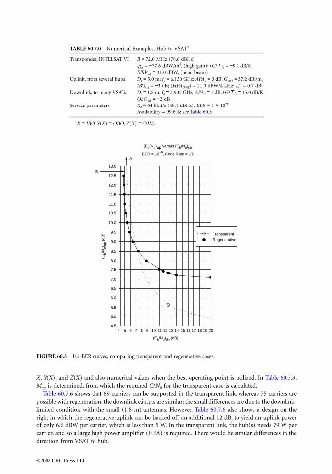
X, Y(X), and Z(X) and also numerical values when the best operating point is utilized. In Table 60.7.3,Msys is determined, from which the required C/N0 for the transparent case is calculated.

Table 60.7.6 shows that 69 carriers can be supported in the transparent link, whereas 75 carriers arepossible with regeneration; the downlink e.i.r.p.s are similar; the small differences are due to the downlink-limited condition with the small (1.8-m) antennas. However, Table 60.7.6 also shows a design on theright in which the regenerative uplink can be backed off an additional 12 dB, to yield an uplink powerof only 6.6 dBW per carrier, which is less than 5 W. In the transparent link, the hub(s) needs 79 W percarrier, and so a large high power amplifier (HPA) is required. There would be similar differences in thedirection from VSAT to hub.

TABLE 60.7.0 Numerical Examples, Hub to VSATa

Transponder, INTELSAT VI B = 72.0 MHz (78.6 dBHz)φsat = −77.6 dBW/m2, (high gain); (G/Τ)s = −9.2 dB/KEIRPsat = 31.0 dBW, (hemi beam)

Uplink, from several hubs Du = 5.0 m; fu = 6.130 GHz; APAu = 0 dB; G1m2 = 37.2 dBi/m2

IBOcci = −3 dB; (HPAIM0L) = 21.0 dBW/4 kHz; Lfu = 0.7 dB;Downlink, to many VSATs Dd = 1.8 m; fd = 3.905 GHz; APAd = 1 dB; (G/Τ)e = 15.0 dB/K

OBOcci = −2 dBService parameters Rb = 64 kbit/s (48.1 dBHz); BER = 1 × 10−6

Availability = 99.6%; see Table 60.3

aX = IBO, Y(X) = OBO, Z(X) = C/IM.

FIGURE 60.3 Iso-BER curves, comparing transparent and regenerative cases.

4 5 6 7 8 9 10 11 12 13 14 15 16 17 18 19 20

13.0

12.5

12.0

11.5

11.0

10.5

10.0

9.5

9.0

8.5

8.0

7.5

7.0

6.5

6.0

5.5

5.0

4.5

(Eb/No)dn (dB)

(Eb/

No)

up (

dB)

B

(Eb/No)up versus (Eb/No)dn

BER = 10−6, Code Rate = 1/2A

TransparentRegenerative


60.9 Other Issues

The link designs and examples are for star VSAT networks, which work with a few large hubs. Even moreinteresting would be a mesh VSAT designs where there is a need to conserve uplink and downlink power,and interference from similar systems is more severe due to lower isolations. Also, these link designs haveexcluded bandwidth improvement factors for intermodulation, which take into account sparse use ofspectrum; likewise, bandwidth allocation factors and overheads have been excluded. In particular forsmall to medium size antennas, outer coding can be usefully applied. These designs have no demand

TABLE 60.7.1 Uplink and Downlink Thermal Equations, Clear Sky


Operatingflux density

dBw/m2

Uplinkcarrier power-to-noise density

dBHz

Pd = 31.0 + Y(X) Downlink EIRP dBW Pd = 31.0 + Y(Xd)

Downlinkcarrier power-to-noise density

dBHz

#2r

˙

TABLE 60.7.2 Interference and Intermodulation Equations


Carrier-to-CCI density up

dBHz

Carrier-to-CCI density down

dBHz

#4r

Total EIRP up dBW

Carrier-to-ASI density up

dBHz

Carrier-to-ASI density down

dBHz

Carrier-to-IM density E/S HPA

dBHz

Carrier-to-IM density (satellite)

dBHz

f 77.6–( ) X 0.0–+=77.6– X+=

f 77.6–( ) Xu 0.0–+=77.6– Xu+=

CN0

------u

f 37.2– 9.2–( ) 228.6–( )–+=

104.6 X #1t+=

CN0

------u

f 37.2– 9.2–( ) 228.6–( )–+=

104.6 Xu #1r+=

CN0

------d

Pd 1.0 15.0 228.6–( )–+ +=

196.4– 0.3–

78.9 Y X( ) #2t+=

CN0

------d

Pd 1.0 15.0 228.6–( )–+ +=

196.4– 0.3–

78.9 Y Xd( )+=

CI0 cci

--------u

X 3.0–( )– 19.3 78.6+ +=

100.9 X #3t+=

CI0cci

--------u

Xu 3.0–( )– 19.3 78.6+ +=

100.9 Xu #3r+=

CI0 cci

--------d

Y X( ) 2.0–( )– 20.1 78.6+ +=

100.7 Y X( ) #4t+=

CI0cci

--------d

Y Xd( ) 2.0–( )– 20.1 78.6+ +=

100.7 Y Xd( ) #4r+=

EIRPtu f 37.2– 200.4 0.3+ +=85.9 X+=

EIRPtu f 37.2– 200.4 0.3+ +=85.9 Xu+=

CI0 asi

--------u

EIRPtu 32.8–( )–=

118.7 X #5t+=

CI0asi

--------u

EIRPtu 32.8–( )–=

118.7 Xu #5r+=

CI0 asi

--------d

Pd 1.0 12.4 43.7–( )–+ +=

88.1 Y X( ) #6t+=

CI0asi

--------d

Pd 1.0 12.4 43.7–( )–+ +=

88.1 Y Xd( ) #6r+=

C/IM0 hpa EIRPtu 21.0– 36.0+=100.9 X #7t+=

C////IM0 hpa EIRPtu 21.0– 36.0+=100.9 Xu #7t+=

C/IM0 Z X( ) 78.6+=78.6 Z X( ) #8t+=

C////IM0 Z Xd( ) 78.6+=78.6 Z Xd( ) #8r+=


TABLE 60.7.3 Allowances, Losses and Margins


AOL = 0.5 + 0.9 = 1.4 TERN and OL dB AOLu/AOLd 1.0/1.3Propagation:

Lp,u = 1.0 & 1.2 = 1.6 Prop losses, up dB Lp,u = Lr,u & Ls,u 1.6/—Lp,u = 1.0 & 1.2 = 1.6 Prop losses, down dB Lp,d = LD,d & Ls,d —/1.6Mm = 1.7 Coded modem margin dB Mm,u/Mm,d 1.5/1.7(C/N0)other;∆ = [74.6 � 76.9] + 1.6 = 80.1 opt Other than thermal dBHz n.a.(C/N0)d;D = 76.9 + 1.6 − 1.6 = 76.9 opt Degraded dBHz n.a.Md;D = 74.6 + 1.6 − (80.1 ⊕ 76.9) = 1.0 opt Available margin, down dB n.a.Msys = 1.6 Up, downlink margins dB Mu = 1.6/Md = 1.6

TABLE 60.7.4 Sums of Link Equations


Sum uplink

C-to-N0

X = −1.3(Figure 60.2)

Y = −2

dBHz

(Figure 60.1)n.a. Available, up

C-to-N0

dBHz (C/N0)a,u = 94.0 − 1.093.0 including Mu

Sum downlinkC-to-N0

Z = 10.3

dBHz

(C/N0)ta = {95.7 ⊗ 76.1}− 1.4= 74.6 (excluding Msys) opt

(Total) AvailableC-to-N0

dBHz(C/N0)a,d = 74.7 − 1.3

= 73.4 including Md opt

Transparent: Xopt = −1.3, Yopt = −2.0, Z = 10.3, Regenerative: Xu = −14.3, Yopt = −2.1, Z = 10.4.

TABLE 60.7.5 Designed BER and Required C/N0


BER = 1.0 × 10−6 Designedbit error ratio

BER = 1.0 × 10−12 + 1.0 × 10−6

Designed BER determines Eb/N0 Energy-per-bitto noise-density

dB (Eb/N0)u = 12.8(Eb/N0)d = 4.8

n.a. Required C/N0 up dBHz

Required C/N0

(total), down

dBHz

C/N0( )su 104.6 X+[ ] 103.3 #1t{=100.9 X+[ ] 99.6 #3t⊕118.7 X+[ ] 117.4 #5t⊕100.9 X+[ ] 99.6 } #7t⊕

97.0 X+( ) = 95.7 opt=

C////N0( )su 104.6 Xu+[ 103.3 #1r{=100.9 Xu+[ 99.6 #3r⊕118.7 Xu+[ 117.4 #5r⊕100.9 Xu+[ ] 1.6– 99.6 } 1.6– #7r⊕

97.6 Xu ]+ 1.6 = – 94.1=

C/N0( )sd 78.9 Y X( )+[ ] 76.9 #2t{=100.7 Y X( )+[ ] 98.7 #4t⊕88.1 Y X( )+[ ] 86.1 #6t⊕78.6 Z X( )+[ ] 88.9 } #8t⊕

76.1 opt=

C/N0)sd 78.9 Y Xd( ) 1.6–+[ ] 75.2 #2r{=100.7 Y Xd( )+[ ] 98.6 #4r⊕88.1 Y Xd( )+[ ] 86.0 #6 r⊕78.6 Z Xd( )+[ ] 89.0 } #8 r⊕

74.7 opt=

CN0

------r ,u

12.8 48.1 1.5+ +=

62.4 excluding Mu=CN0

------r

4.8 48.1 1.7 1.6+ + +=

54.6 including Msys( )=

CN0

------r ,d

4.8 48.1 1.7+ +=

54.6 excluding Md=


assignment multiple access (DAMA) signalling, which would need to be robustly designed. As to otherissues, data-only links can take advantage of automatic repeat request (ARQ) so that throughput andbasic BER can be selected accordingly. Links with voice/video-only can be operated with relatively poorBER, and effective error concealement techniques can be applied.

60.10 Summary

This chapter has presented a unified but simplified set of link designs for transparent and regenerativelinks. Several numerical examples illustrate the methods and the differences in link designs.

All link designs must properly take into account thermal, interference, and intermodulation contri-butions, as well as allowances, losses, and margins. Transparent links, which are most prevalent now,suffer noise power addition of up to ten entries. Regenerative links, which are being developed in manyforms and can be expected in next-generation satellites, separate the uplink and downlink so that eachhas only up to four entries. Regenerative links require an uplink modem margin (for the payloaddemodulator), but other allowances, losses, and margins are generally lower than for transparent links.

Appendix A: Some Calculations

Boltzmann’s constant:

k = −228.6 dBJ/K

Propagation velocity in free space:

c = 2.998 × 108 m/s

Wavelength (Lambda):

where f is the frequency of operation [up fu, down fd], in Hertz.

TABLE 60.7.6 Number of Carriers, EIRP and Power per Carrier

Transparent Name Unit Regenerative Design

n.a. Uplink carriers

n.a. Downlink carriers nd = 75

opt

Number of carriers n = min(nu, nd) = 75 opt

EIRPcu = 85.9 + (−1.3) −18.4 = 66.2 opt

EIRP per carrier, up dBW EIRPcu ==== 85.9 + (−−−−1.3) −18.8 = 65.8

Xu = −12.0EIRPcu = 53.8

Pcu = 66.2 − 47.9 + 0.7= 19.0 {79 W} opt

Power per carrier, up dBW Pcu = 65.8 − 47.9 + 0.7= 18.6 {72 W}

Pcu = 6.6 (5 W)

EIRPcd = 31.0 + (−2.1) −18.4 = 10.6 opt

EIRP per carrier, down

dBW EIRPcd = 31.0 + (−−−−2.1) −18.8 = 10.1 opt

nu 10 93.1�62.4[ ]/ 10=

1174=

nu 10 81.1−62.4–( )/10=

75=

nd 10 73.4−54.6[ ]/ 10=

75=

n 10 74.6−56.2[ ]/ 10=

69=

l cf-- m=


The maximum antenna gain relative to isotropic for a parabolic antenna, up and down:

where η is the antenna efficiency (nominal 0.6) and D is the aperture diameter in meters.Gain of ideal 1 m2:

G1m2 = 21.455 + 20 log F dBi/m2

where F is the (approximate) frequency in gigaHertz.Typical atmospheric loss, up and down:

Free space spreading loss up and down:

Lsp = 32.45 + 20 log10(FR) dB

where R is the (slant-range) distance to the satellite in meters. [Typically, at 10° elevation angle, R =40,587,000 m to geostationary Earth orbit (GEO).]

Appendix B: Calculation of Antenna Discrimination4

Gain mask:

where G is the maximum gain (as previously calculated) and θ is the satellite spacing in degrees (nominal3°).

Antenna discrimination for receive Earth station:

4 Based on International Telecommunications Union (ITU) Rec. 465–4 and Report 391–6.

G 10 log10 h pDl

-------

2

dBi=

La 0.25 dB 2 F 5 GHz< <=0.33 5 F 10 GHz< <0.53 10 F 13 GHz< <0.73 13 F GHz<

Gm G 0.0025 qD/l[ ] 2 mainlobe dBi–=

G1 2 15 log10 D/l( ) first sidelobe+=

Gs 32 25 log10q other sidelobes–=

dm 20l/D( ) G G1–( ) degree=dm max 1°, 100l/D°[ ]=

IF q dm< Γasi,d G Gm– of mainlobe dB=

IF dm q≤ d1< Γasi,d G G1– of first sidelobe dB=

IF d1 q≤ 48< Γasi,d G Gs of other sidelobes dB–=

IF 48 q≤ Γ asi,d G 10–( ) dB–=


Defining Terms

Allowance: An allowance in decibels is subtracted from a sum of carrier-to-noise densities which wouldhave been available in a link; usually, such an allowance accounts for factors external to a givensystem (and beyond the system designer’s control).

Availability: Usually expressed as a percentage of a year, availability is the total time duration overwhich the specified BER is met or exceeded.

Clear-sky condition: Only atmospheric losses are added to spreading losses; this excludes weather effects.Code rate: The code rate (actually a ratio) for forward error correcting codes is the ratio of input to

output bits (or symbols), such as rate 1/2, rate 3/4 for binary codes, and rate 239/255 for a typicalReed–Solomon code.

Degraded-sky condition: In the uplink there is additional attenuation due to rain; in the downlinkthere is rain attenuation and also an increased effective receiver system temperature due to theincreased sky noise.

Discrimination: Antenna discrimination is the differential gain compared to maximum for an antennain the specified direction; usually, masks are provided for the main lobe, the first sidelobe, andother sidelobes.

Interference: The generic term that includes all unwanted signals that affect a telecommunications link,excluding thermal noise and intermodulation products; interference can be man-made or natural;it can be internal or external to a system.

Intermodulation: A generic term; intermodulation products are produced in nonlinear devices (ampli-fiers) and they are dependent on the wanted signal levels, modulation formats, and frequency plan.

Iso-BER curve: A graph of constant (iso) bit error ratio with uplink and downlink parameters on they- and x-axis, respectively; C/N0 or Eb/N0 are usually used.

Isolation: An antenna beam’s minimum discrimination to a co-channel or cross-polarization channel.Margin: In decibel, a margin is added to required values, for example to Eb/N0 required for a target BER,

and reflects uncertainties in equipment performance; this is sometimes called implementation margin.Propagation loss or downlink degradation: In decibel, propagation loss is subtracted from all carrier-

to-noise (equivalent) densities where C (signal power) is affected but Io is not; rain attenuation,increased sky noise, depolarization, and tropospheric scintillation are typical examples of such losses.

Regenerative: A link that, in comparison to transparent, has additional functions in the satellite pay-load, such as demultiplexing and demodulation of the communications signals in the uplink andmodulation for the downlink; this is sometimes called onboard regeneration (OBR). OBR andadditional functions such as possibly FEC decoding, re-encoding, baseband switching or IF routing,and TDM constitute what are usually called onboard processing (OBP).

Transparent: A transparent link uses a transponder that has an output signal format that is exactly thesame as the input format.

Transponder: Consists of a wideband receiver, frequency-translating equipment, and a power amplifier;its associated input and output multiplex filters determine its center frequency and bandwidth; itwould be more correctly called a repeater.

Acknowledgment

The authors wish to acknowledge William Salazar and Luis Gonzales for their dedicated work in preparingthe link budget programs.

References

Brown, M.P., Duesing, R.W., Nguyen, L.N., Sandrin, W.A., and Tehrani, J.A. 1990. INTELSAT VI transmis-sion design and computer system models for FDMA services. COMSAT Tech. Rev., 20(2):373–399.

INTELSAT, 1992. INTELSAT Intersystem Coordination Manual, IICM-314, Rev. 1A, Dec.Mathews, N. 1988. Performance evaluation of regenerative digital satellite links with FEC codecs. Satellite

Integrated Communications Networks, Proc. Tirrenia Workshop, North-Holland, U.K.


Nuspl, P., Peters, R., Abdel-Nabi, T., and Mathews, N., 1987. On-board processing for communicationssatellites: Systems and benefits. Int. J. Satellite Commun., 5(2):65–76.

Further Information

For a general treatment of propagation topics, see the book by J.E. Allnutt, 1989, Satellite-to-GroundRadiowave Propagation, Theory, Practice and System Impact at Frequencies Above 1 GHz, Peter PeregrinusLtd., UK.

For another treatment of (transparent) link budgets, see Chapter 6 of Satellite Communications, byD. Roddy, 1989, Prentice Hall, Englewood Cliffs, NJ.

There was a special issue on on-board processing, edited by P. Nuspl, International Journal of SatelliteCommunications, vol. 5, no. 2, Wiley-Interscience, London, UK, April–June, 1987. See B. Pontano, P. deSantis, L. White, and F. Faris, “On-Board Processing Architectures for International CommunicationsSatellite Applications,” Proceedings of the 13th America Institute of Aeronautics and Astronautics (AIAA)International Communication Satellite Systems Conference and Exhibit, Los Angeles, CA, Paper 90-0853,March 1990. Also, see several sessions in Proceedings of International Conference on Digital SatelliteCommunications ICDSC-8, Guadeloupe, April 1989; ICDSC-9, Copenhagen, May 1992; 14th AIAAConference, Washington, D.C., March 1992; and 15th AIAA Conference, San Diego, March 1994.

Also, trends for future payloads are described in “Advanced Communications Technologies for FutureINTELSAT Systems,” P.P. Nuspl, 1992, Proceedings, Advanced Methods for Satellite and Deep SpaceCommunications, 1992 DLR Seminar, Bonn, Germany, September (DLR is the German AerospaceResearch Center near Munich, Germany).


61The Calculation of

System Temperature fora Microwave Receiver

61.1 Noise, Antenna, and System TemperaturesThermal Noise Density • Noise Temperature • Noise Figure • Networks in Tandem • Antenna Temperature • The General Microwave Receiver

61.1 Noise, Antenna, and System Temperatures

Thermal Noise Density

The ultimate capacity of any communications channel is determined by the ratio C/No of carrier powerto thermal noise density, and the purpose of RF link analysis is to calculate this ratio. No is the compositenoise spectral density and is given by No = kTs , where Ts is the composite system temperature. It is thetemperature to which a resistor at the system input, with the system having only its gain and generatingno noise, would have to be heated to generate the same amount of random noise as is observed at thereal system receiver output. This temperature characterizes the entire system noise performance and isintended to comprise the effects of thermal noise, receiver noise, and noise available at the antennaterminals. The latter noise itself comprises two components, the thermal noise of the surroundings withwhich the antenna interchanges energy and external sources of noise in the sky.

All noise considerations are based on the irreducible thermal noise due to the random motion ofelectrons in conductors. The full quantum expression for the spectral density of this noise is

(61.1)

In the range of frequencies of usual interest in satellite communication kT hf and we have Nyquist’sfamiliar formula for thermal noise density

(61.2)

In a bandwidth B, the resulting voltage across a resistance R is given by Nyquist’s formula . Ifwe consider a source of impedance R generating this voltage, then the power available into a matchedload R is simply kTB. This concept of available power is used almost exclusively in considering the noiseperformance of composite systems.

Nohf

ehfkT------

1–

--------------- hf–=

>>

No kT=

4kTBR

Wilbur PritchardW. L. Pritchard & Co., Inc.


Noise Temperature

Figure 61.1 is an arbitrary two-port network characterized by a power gain G and excess noise charac-terized by parameters to be defined.

We define the noise temperature at a point as that temperature to which a matched resistor must beheated to generate the same available noise as is measured at that point. Thus, the noise at any point xin the chain is given by Nx = kTxB. If the point in question is the input, then the noise temperature isoften written as Ti, and, more specifically, if an antenna is at the input, then the temperature is writtenas Ta.

A different and altogether basic characterization is found in the system temperature Ts, which is thetemperature to which a resistor at the input must be heated to generate a noise equal to the observed totalnoise output. Other sources of noise are neglected. The output noise can now be written as Nx = GkTsB,and GTs = Tx. The system temperature will clearly be higher than the input source temperature by virtueof the extra noise generated by the network. We use this idea to define an excess temperature TE,characteristic of the network itself, and to write the noise temperature at any point Tx, by the equations

(61.3)

Performance figures and noise temperatures quoted by receiver manufacturers are usually this excesstemperature TE, naturally enough, since it is a measure of the receiver quality, but it is a frequent error touse that temperature in the calculation of system performance. That computation must use the systemtemperature, which requires the addition of the antenna temperature, and consideration of other sourcesof noise.

Noise Figure

An older, and still much used, figure of merit for network noise performance is noise figure F. It is basedon the idea that the reduction in available carrier-to-noise ratio (CNR) from the input to the output ofa network is a measure of the noise added to the system by the network and, thus, a measure of its noisequality. The difficulty with that concept in its naive form is that the same network will seem better if theinput CNR is poorer and vice versa. To avoid this anomaly, the definition is based on the assumptionthat the available noise power at the input is always taken at room temperature, arbitrarily taken in radioengineering work to be 290 K.

(61.4)

This can be rewritten several ways. Note that the input and output carrier levels are related by the availablepower gain and, in accordance with our definition, the input noise level is simply kToB. One form,occasionally taken as a definition, is that the output noise is given by

(61.5)

FIGURE 61.1 Noise parameters: basic network.

Ts Tin TE+=

Tx G TE Tin+( )=

FCin/Nin

Cout/Nout

---------------------=

Nout FGkToB=


Note well that, although the definition of noise figure assumes the input at room temperature, it can bemeasured and used at any input temperature if the calculations are made correctly. We can understandthis better by rewriting the preceding equation as

(61.6)

(61.7)

In the form of Eq. (61.6) we can identify the first term as attributable to the amplified input noise andthe second term as the excess noise generated by the network. In fact, we can change the term To to Tin

where Tin is an arbitrary input source temperature, for instance, that of a receiver antenna. By comparingthe second term of Eq. (61.7) to that of Eq. (61.3), we see that they are both terms for the excess noiseand thus write

(61.8)

This is a particularly useful relation inasmuch as the need to go back and forth between the twocharacterizations of excess noise is frequent.

The Hot Pad

A very important special case is the noise characterization of a plain attenuator, at either room temper-ature 290 K or some arbitrary temperature T. Transmission line loss between an antenna and the firststage of RF amplification, typically a low-noise amplifier (LNA), the loss in the atmosphere due toatmospheric gases such as oxygen and water vapor, and the loss due to rain can all be considered hotpads. It can be shown [Mumford and Scheibe, 1968] that the noise temperature of such an attenuator is

(61.9)

Networks in Tandem

To be able to apply our set of definitions and relations to a real microwave receiver, we need a relationbetween the characteristics of two individual networks and their composite characteristics when thenetworks are in tandem or cascade (see Fig. 61.2).

The calculation of the noise performance of two stages in tandem is done by equating the noise outputas calculated from the combined parameters, either F or TE, with the noise output as calculated by takingthe noise output of the first stage as the noise input for the second stage. From Eq. (61.3), we have, forthe output noise in terms of the noise at x,

(61.10)

FIGURE 61.2 Two networks in tandem.

Nout GkTo B F 1–( )GkTo B+=

Nout GkTinB F 1–( )GkTo B+=

TE F 1–( )To=

TN

Tin L 1–( )T+L

----------------------------------=

Tx G1 Tin Te1+( )=

Tout G2 Tx Te2+( )=

Tout G1G2 Tin Te1+( ) G2Te2+=


We can also write the output noise as G1G2(Tin + Te), again by using Eq. (61.3). By equating the twoexpressions for output noise, we arrive at the fundamental relation for the composite

(61.11)

The identical approach can be used with excess noise being characterized by noise figures, or Eq. (61.11)can be converted using the relation between excess noise temperature and the noise figure given by Eq.(61.7). In either case, the result is

(61.12)

Antenna Temperature

We have been using the term “antenna temperature” casually with the understanding that the input to amicrowave receiver is usually connected to an antenna and that in some way the antenna can be consideredas generating an equivalent input temperature. This is indeed the case, and we can make the idea moreprecise by defining the antenna temperature as the weighted average temperature of the surroundingswith which the antenna exchanges energy. For example, if two narrow beam antennas communicatedwith each other with no loss to external radiation, and if one of these antennas were connected to amatched resistor at a temperature TA, then TA would be the antenna temperature of the other antenna.

An Earth station antenna typically exchanges energy with the sky in the vicinity of the satellite at whichit is pointed, the ground via its side lobes, and the sun, usually in the antenna side lobe structure butoccasionally in the main beam. A satellite antenna exchanges energy, principally with the ground, butalso with the sky and occasionally with the moon and sun. Obviously, the satellite orbit and antennacoverage determine the situation. Antenna temperature is much affected by atmospheric losses andespecially by rain attenuation. By way of example, a narrow beam antenna pointed at the clear sky mighthave a temperature of 20 K, but this will increase to more than 180 K with 4.0 dB of rain loss, as is easilycalculated from the hot pad formula (61.9). With a receiver excess temperature of 50 K, the systemtemperature will increase from 70 to 230 K or 5.0 dB. Note that this is a greater loss than that due to thesignal attenuation by the rain. This is a frequently overlooked effect of rain attenuation. The implicationfor system design, at those frequencies where rain loss is anything other than negligible, is significant.The margin achieved using high-performance, low-noise receivers, is something of an illusion. Themargin disappears quickly just when one needs it the most. The performance improvement achievedwith a larger antenna is better than that achieved with a low-noise receiver because the deterioration ofthe former because of rain attenuation is only that due to the signal loss, whereas the latter suffers thesignal loss and the increase in antenna temperature.

The antenna temperature can, in principle, be calculated from the definition by evaluating the integralof the temperature, weighted by the antenna gain, both as a function of solid angle. Due allowance mustbe made for reflections. The exact expression is

(61.13)

where:G1 = antenna gain in a sky directionG2 = antenna gain in a ground directionΩ 1 = solid angle in sky directionsΩ 2 = solid angle in ground directionsTg = ground temperatureTsky = sky temperatureρ = voltage reflection factor of the ground

Te Te1

Te2

G1

-------+=

F F1

F2 1–( )G1

------------------+=

14p------ G1Tsky dΩ

14p------ G2 1 r2–( )Tg r2Tsky+[ ]dΩ∫+∫T=


The sky temperature, the starting point for most calculations of antenna temperature, is found byfirst determining the clear sky temperature, normally very low. The spectral absorption of atmosphericgases raises this temperature in accordance with the hot pad effect and yields a sky temperature that isa function of frequency and angle of elevation. Figure 61.3 is a plot of this sky temperature vs. frequencywith angle of elevation as a parameter. Note the presence of a microwave window in the frequency regionhigh enough for the galactic noise to have fallen to a low value, nominally the 3.5-K microwave background,a remnant of the big bang, and low enough to avoid the increases due to atmospheric gas absorption.The frequency sensitivity largely mirrors the absorption spectra of these gases (shown in Fig. 61.4), andthe dependence on angle of elevation seen in Fig. 61.5 results from the increased path length throughthe atmosphere at low angles. Note that there are regions in the sky where there is radio noise at a higherlevel than shown and generated by various galactic sources. Some of these sources of radio noise are usedto calibrate the noise performance of Earth stations.

Ground and rain temperatures are typically taken to be To = 290 K. The integration requires aknowledge of the antenna pattern in spherical coordinates and the location of ground masses, reflectingsurfaces, reflection factors, and sky temperatures. It can be carried out numerically but normally it iscomplicated and not worth the trouble. A result sufficiently accurate for most practical purposes can befound using

(61.14)

FIGURE 61.3 Sky noise temperature calculated for various elevation angles.

Ta a1Tsky a2Tg a3Tsun+ +=


where the terms a1, a2, and a3 are the relative solid angles covered by the main beam, side lobes lookingat the ground, and side lobe looking at the sun, respectively. They can be approximated by

(61.15)

The idea is to obtain an average of the temperature weighted by the antenna gain. The W and G are thesolid angles and gains, respectively, of the main beam, side lobes that see the ground, and side lobe thatsees the sun. Here, ρ is the voltage reflection factor of the ground, and p is a factor to allow for the sun’sradiation being randomly polarized while the antenna receives linear or circular polarization only; p istypically 1/2. The assumption is that the sun is not in the main beam but rather in a side-lobe where thegain is much lower, and this reduces the effect of the sun’s high temperature. If the sun is in the mainbeam, and if the antenna beam is less than or equal to the sun’s subtended angle (0.5∞), then the increasein temperature is formidable and produces a sun outage. The sun’s apparent temperature can be foundfrom Fig. 61.6.

FIGURE 61.4 One way signal attenuation through troposphere at various elevation angles.

a1

14p------ GskyΩsky r2GgΩg+( )=

a2

Ω g

4p-------Gg 1 r2–( )=

a3 rΩ s

4p-------Gs/Lr=


Note that rain loss Lr has the good effect of shielding the receiver from the sun. On a beam reasonablywide compared to the sun, the margin normally available to protect against rain loss, say 6.0 dB or so atKu band, is sufficient to ameliorate the sun interference to a bearable level even with the sun in the mainbeam. An antenna of 50 cm in diameter for the direct reception of satellite TV has a beamwidth of 3.5–4.0∞and a solid angle 50 times that of the sun. In effect, this reduces the sun’s temperature by 50 times.

The General Microwave Receiver

Figure 61.7 shows the functional diagram of a general microwave receiver. Almost all satellite and Earthstation receivers fit a diagram of this sort.

We can use Eqs. (61.11) and (61.12) pairwise to combine the stages and yield an overall result. Theantenna noise, discussed in the last section, is taken as the input, and we assume that there are nosignificant noise contributions beyond the mixer down converter. An important and useful point con-cerns the noise figure of a matched passive attenuator. Such a device has the result of reducing the available

FIGURE 61.5 Sky noise temperature at 4 GHz vs. elevation angle.


carrier power by its loss in decibels, while not changing at all the available thermal noise. Thus, its noisefigure, defined as the ratio of input to output carrier to noise ratios, is simply equal to its loss. The result,from combining the stages of the receiver two at a time, is

(61.16)

This equation is informative. Besides showing the more or less obvious advantages of low-noise receivers,it highlights the unexpectedly devastating effect of the loss L in the line between the antenna and theLNA. Even 1.0 dB here produces a temperature increase of 75 K. Such a loss is by no means unrealizablein a long line such as might be necessary between a prime focus feed and a convenient receiver locationin a large antenna. The need to place the LNA directly at the horn feed, or to use a Cassegrainian typeof antenna so that the LNA can be placed at the reflector vertex, is clear.

FIGURE 61.6 Noise spectral density of quiet and active sun. (From NASA Propagation Effects Handbook for SatelliteSystem Design, ORI TR 1983.)

FIGURE 61.7 General microwave receiver.

Ts Ta L 1–( )To LTr L F 1–( )To

Gr

-----+ + +=


Defining Terms

Antenna gain: Directivity, ratio of power transmitted in a particular direction to the power that wouldbe transmitted in that direction if the antenna were an isotropic radiator.

Antenna temperature: Noise temperature at the antenna terminals.Carrier to noise ratio: Ratio of carrier to available noise power.Down converter: Mixer to reduce RF carrier frequency to more convenient and constant value for

amplification.Excess noise temperature: Apparent temperature of extra noise above input noise added by any black

box.Hot pad: Input attenuator at some temperature higher than room temperature (rain, for example, at

room temperature compared to sky noise at a few Kelvins).Low-noise amplifier (LNA): First amplifier in receiver, just after antenna, with very good excess noise

characteristics.Noise: Random electrical signals that interface with signal detection.Noise density: Noise in watts per unit bandwidth.Noise figure: Ratio of input to output carrier to noise ratio.Noise temperature: Apparent temperature of resistance producing the observed or calculated noise.Power gain: Ratio of available power at output of a network to available power at the input.Receiver temperature: Excess temperature of entire receiver including low-noise amplifiers and down

converter.Side lobe: Part of the antenna radiation pattern off the main beam but still radiating measurable energy.Sky temperature: Apparent noise temperature of the sky.Sun interference: Increase in antenna noise because antenna is pointed at the sun.Sun outage: Sun interference so great that receiver is blinded completely.System temperature: Apparent temperature of resistance producing the observed noise of the entire

system if connected to the input.Thermal noise: Noise due to random electron motions dependent on temperature.

References

Bousquet, M., Maral, G., and Pares, J. 1982. Les Systémes de Télécommunications par Satellites, Massonet Cie, Éditeurs, Paris.

Ippolito, L.J., 1986. Radio Wave Propagation and Satellite Communication Systems, Van Nostrand, NewYork.

Ippolito, L.J., Kaul, R.D., and Wallace, R.G. 1986. Propagation Effects Handbook for Satellite Systems Design,NASA Ref. Pub. 1082(03), 3rd ed., Washington, D.C., June.

Jasik, J. 1961. Antenna Engineering Handbook, McGraw-Hill, New York.Kraus, J.D. 1950. Antennas, McGraw-Hill, New York.Lin, S.H. 1976. Empirical rain attenuation model for Earth-satellite path. IEEE Trans. Commun. COM-

27(5):812–817.Mumford, W.W. and Scheibe E.H. 1968. Noise Performance Factors in Communications Systems, Horizon

House-Microwave Inc., Dedham, Mass.Pritchard, W.L., Suyderhoud, H.G., and Nelson, R.A. 1993. Satellite Communication Systems Engineering,

2nd ed., PTR Prentice-Hall, Englewood Cliffs, NJ.


62Onboard Switching

and Processing

62.1 IntroductionSatellite Switching (SS) Advantages • Applications

62.2 Onboard Switching TypesReconfigurable Static IF Switching • Regenerative IF Switching • Implementation of Regenerative and Static IF Switches Using Optical Waveguides • Onboard Baseband Switching • Baseband Fast Packet Switches • Photonic Baseband Switches • Asynchronous Transfer Mode (ATM)-Oriented Switches

62.3 Summary

62.1 Introduction

The onboard (OB) combination of satellite switching (SS) and spot beam utilization is intended toenable a large number of small and inexpensive mobile as well as fixed site terminals to communicateand integrate with commercial broadcasting and integrated and various voice, data, and video applica-tions. This interconnection should not only serve as a standby for terrestrial and optical networks, butalso as a competing alternative. With the launching of low Earth orbit satellites (LEOs) [Louie, Rouffet,and Gilhausen, 1992] approaching, the roundtrip satellite propagation delays will become an order ofmagnitude less than those of geostationary Earth orbits (GEOs). Also, ground terminals will be cheaper,thus providing the edge for competing with ground-based networks. The concept of a bent pipe satellitewill be long gone and users now operating in few zones around the globe will be divided into many zoneswith one satellite antenna supporting local communication of each zone and the switch onboard thesatellite routing the traffic from zone to zone within the cluster (Fig. 62.1). If a constellation of LEOs ormedium Earth orbit satellites (MEOs) is to cover the globe, then each satellite will handle one cluster,but intrasatellite links have to be provided by a ground network or by a space-based network for usersbelonging to different clusters to intracommunicate. OBSS systems apply to GEO, LEO, and MEOconstellations. Operating in this environment while accommodating various packet switching (PS) andcircuit switching (CS) types of traffic affects the selection of the OB switch type and technology. Beforelooking at the various OB switch types, details, performance, and fault tolerance, we state their mainadvantages and applications.

Satellite Switching (SS) Advantages

1. Terminal cost is reduced by lowering transmission power (smaller user antennas used). Also,reducing the number of users per zone reduces user bit rate and, hence, cost.

2. Up- and downlinks are decoupled, thus allowing their separate optimization. For example, forstream (CS) and wideband Integrated Services Digital Network (WBISDN) users in a certain zone,

A. K. ElhakeemConcordia University


time-division multiplexing (TDM) uplink and TDM downlink techniques are adequate. On theother hand, for a multiple of bursty Earth stations, in another zone, a demand assignmentmultiple access–time-division multiple access (DAMA–TDMA) uplink/TDM downlink tech-nique allows the optimal sharing of the uplink capacity. A third zone in heavy rain or undershadowing fading conditions might prefer a switching satellite that has code-division multipleaccess (CDMA) in the uplink and/or downlink.

3. The number of possible virtual connections is reduced from an order of N 2 to the order of Nwhere N is the number of users.

4. Flexibility and reconfigurability includes, among other things, reprogramming of onboard process-ing (OBP) control memories, reconfiguration of Earth stations (time/frequency plans for each con-nection setup), accommodation of both circuit and packet switched traffic, adopting different flowand congestion control measures for each zone depending on current traffic loads and types, andaccommodation of multirate and/or dynamically changing bit rate and bit rate conversion on board.

5. SS has natural amenability to DAMA and ISDN services.6. There is enhanced fault tolerance; a single satellite failure handling a cluster of zones can be easily

replaced by another within hours or minutes, thus averting the disasters of losing customers fora few days or months. A single failing antenna onboard the satellite can be easily replaced byanother hopping antenna.

7. SS increases the total capacity of the satellite system in terms of number of circuits and servicesprovided within the same bandwidth.

These advantages come with a price, that is, the cost and complexity of the satellite itself.

Applications

• Internetworking, low-cost and low-power user terminals, fixed site, and mobile communications

• Video conferencing

FIGURE 62.1 Onboard (OB) processing satellite using multiple-beam antennas and onboard switching.


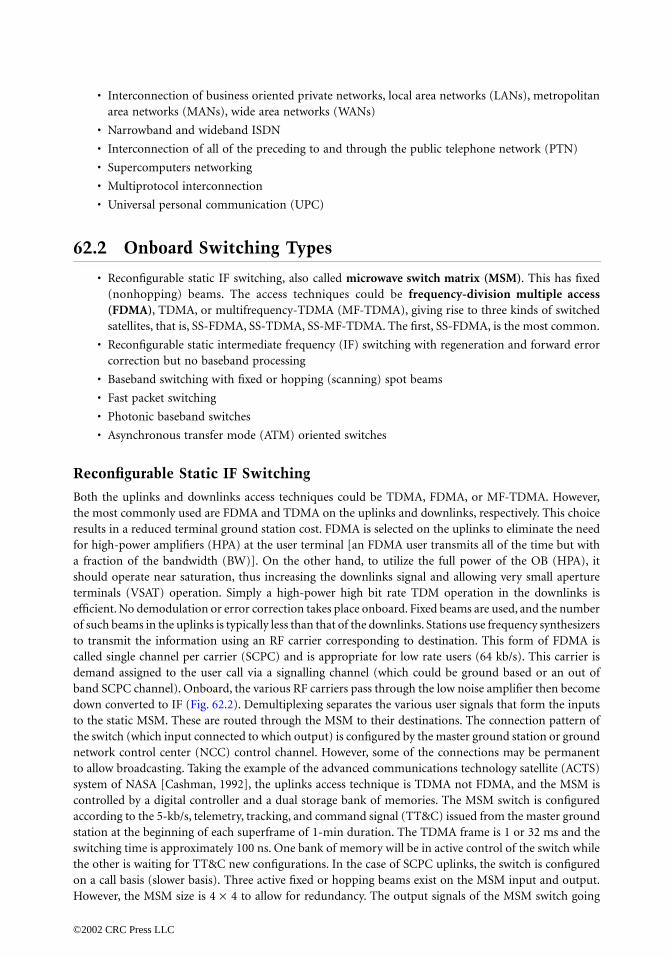
• Interconnection of business oriented private networks, local area networks (LANs), metropolitanarea networks (MANs), wide area networks (WANs)

• Narrowband and wideband ISDN

• Interconnection of all of the preceding to and through the public telephone network (PTN)

• Supercomputers networking

• Multiprotocol interconnection

• Universal personal communication (UPC)

62.2 Onboard Switching Types

• Reconfigurable static IF switching, also called microwave switch matrix (MSM). This has fixed(nonhopping) beams. The access techniques could be frequency-division multiple access(FDMA), TDMA, or multifrequency-TDMA (MF-TDMA), giving rise to three kinds of switchedsatellites, that is, SS-FDMA, SS-TDMA, SS-MF-TDMA. The first, SS-FDMA, is the most common.

• Reconfigurable static intermediate frequency (IF) switching with regeneration and forward errorcorrection but no baseband processing

• Baseband switching with fixed or hopping (scanning) spot beams

• Fast packet switching

• Photonic baseband switches

• Asynchronous transfer mode (ATM) oriented switches

Reconfigurable Static IF Switching

Both the uplinks and downlinks access techniques could be TDMA, FDMA, or MF-TDMA. However,the most commonly used are FDMA and TDMA on the uplinks and downlinks, respectively. This choiceresults in a reduced terminal ground station cost. FDMA is selected on the uplinks to eliminate the needfor high-power amplifiers (HPA) at the user terminal [an FDMA user transmits all of the time but witha fraction of the bandwidth (BW)]. On the other hand, to utilize the full power of the OB (HPA), itshould operate near saturation, thus increasing the downlinks signal and allowing very small apertureterminals (VSAT) operation. Simply a high-power high bit rate TDM operation in the downlinks isefficient. No demodulation or error correction takes place onboard. Fixed beams are used, and the numberof such beams in the uplinks is typically less than that of the downlinks. Stations use frequency synthesizersto transmit the information using an RF carrier corresponding to destination. This form of FDMA iscalled single channel per carrier (SCPC) and is appropriate for low rate users (64 kb/s). This carrier isdemand assigned to the user call via a signalling channel (which could be ground based or an out ofband SCPC channel). Onboard, the various RF carriers pass through the low noise amplifier then becomedown converted to IF (Fig. 62.2). Demultiplexing separates the various user signals that form the inputsto the static MSM. These are routed through the MSM to their destinations. The connection pattern ofthe switch (which input connected to which output) is configured by the master ground station or groundnetwork control center (NCC) control channel. However, some of the connections may be permanentto allow broadcasting. Taking the example of the advanced communications technology satellite (ACTS)system of NASA [Cashman, 1992], the uplinks access technique is TDMA not FDMA, and the MSM iscontrolled by a digital controller and a dual storage bank of memories. The MSM switch is configuredaccording to the 5-kb/s, telemetry, tracking, and command signal (TT&C) issued from the master groundstation at the beginning of each superframe of 1-min duration. The TDMA frame is 1 or 32 ms and theswitching time is approximately 100 ns. One bank of memory will be in active control of the switch whilethe other is waiting for TT&C new configurations. In the case of SCPC uplinks, the switch is configuredon a call basis (slower basis). Three active fixed or hopping beams exist on the MSM input and output.However, the MSM size is 4 × 4 to allow for redundancy. The output signals of the MSM switch going


to same zone are grouped (multiplexed). The resultant is subsequently translated to RF frequency,amplified by solid-state power amplifiers (SSPA), and transmitted via output beams. An in-band or out-of-band signalling scheme is used by the user terminals to establish the call. The master control stationfinally assigns the right resources to the call, for example, one out of a pool on the FDMA uplinks andone time slot of a certain TDMA frame on the downlinks for that call. This reservation goes to the OBS,which becomes correspondingly configured for the call duration. We notice here the isolation betweenthe up- and downlinks provided by OBS, for example, in the preceding case the uplink user transmitscontinuously using the assigned FDMA SCPC, i.e., disjointed from the TDM process taking place on thedownlinks. Amplifying these FDMA signals OB creates intermodulation products (IMP). SCPC alsosuffers from its inability to meet variable bit rate (VBR) services. Multichannel per carrier (MCPC)/TDMAor MF/TDMA is typically employed to reduce these IMP. Here, a number of users (terminals) are allocatedchannels (time slots) on a TDM frame, which is transmitted on a single carrier.

Other disadvantages of FDMA-oriented MSM are the difficulty of dynamic networks reconfigurationwithout data loss, the difficulty of operation with hopping beams, and broadcasting of multiple carriertransmissions to many destinations.

Regenerative IF Switching

This is similar to the previous static IF switching in the following respects: switching of IF signals, employingTDMA, FDMA, or MF-TDMA access techniques with the FDMA uplinks/MF-TDMA downlinks as thepreferred technique, no baseband processing being involved, a station simultaneously transmitting/receivingfrom many stations having to use a different carrier for each source (destination), programming reconfig-uration via fixed connections and/or under the TT&C commands, use of low noise amplifiers (LNAs) andSSPAs, and RF to IF and IF to RF translations.

However, it differs in the following respects. The IF signals (following RF to IF translation anddemultiplexing) are demodulated, forward error corrected, then forward error encoded [using errordetecting and correcting coding (EDAC)] and then modulated [continuous phase shift keying (CPSK)or minimum shift keying (MSK)] again before feeding them to the MSM switch. If both uplinks anddownlinks are of the MF-TDMA kind, then the various uplinks user TDM channels (slots) of eachbeam form the IF inputs to the switch. At the switch output, output IF slots are multiplexed again,

FIGURE 62.2 Nonregenerative onboard IF switching.


and the resultant modulates the RF carrier of the downlinks beam. The regeneration involved in thedemodulation–modulation processes allows the separation of uplinks and downlinks noises, fading,interference effects, and so forth. Also, the decoding–encoding could be done at different rates, thusproviding for more protection against rain in the downlinks, for example, by decreasing the forwarderror correction (FEC) encoding rate. These regenerations lead to better links performances and betteramenability to MF-TDMA generation that needs higher transmission rates. Nevertheless, regenerativeIF switching suffers the same aforementioned disadvantages of static IF switching.

Implementation of Regenerative and Static IF Switches via MSM Technology

Basically, this is a solid-state programmable crossbar switch. Signal switching at the matrix crosspointsis performed using dual-gate field-effect transistor (FET) active switches (employing GaAs technologyfor switches with IF bandwidths equal to or exceeding 2.5 GHz). In recent implementations, such as theNASA ACTS OBS [Cashman, 1992], input signal distribution and output signal combining are performedusing passive recursive couplers (Fig. 62.3).

Among many alternatives, such as single pole, rearrangeable switching, and so forth, the couplercrossbar implementation was selected by both ACTS and other NASA systems for its simple control, lowinsertion loss, and amenability to broadcasting. In this architecture, a switching element [Fig. 62.3(b)]is situated between two directional couplers. If the data is to flow from input i to output j, the switch

FIGURE 62.3(a) N × N IF switch matrix using crossbar configuration.


will be ON and the input and output couplers pass the data; otherwise, the switch is OFF and the datais reflected and absorbed by the coupler loads. To equalize the output power at all N input couplersconnected to the N output lines, the coupler coefficients increase as the output number increases, thatis, α j = 1/(N - j + 2). The same logic α j applies to the output coupler coefficient βi as in Fig. 62.3(b).Switches at the various cross points are independently controlled to provide broadcasting as well as point-to-point connections. Moreover, the switch design could be modular both electrically and mechanically(as in NASA designs); for example, different switch points or parts of the switch can be repaired andtested independently, thus improving cost and reliability, or larger switches can be built from smallermodules.

The switch elements could be built using ferrite switches, p-i-n diodes, or single gate FETs. The firstoption is too slow, the second needs larger amounts of DC power, the third yields no gain during ONstates; dual gate FETs are typically preferred. These use Schottky barrier diodes with very low junctioncapacitance, thus allowing the switching from gain to high insertion loss in about 100 ps. Two FETs areused, with the RF input signal applied to the first and the switch control applied to the second. Thisprovides for excellent isolation between the DC control (which ranges from 30-dB loss to 10-dB gain)and the RF input. One could envision an IF switch with constant coupling coefficients (α j, βi) andvariable switch amplifier gain. Typically, however, the earlier variable coupling gains implementationis preferred.

The switch states (configuration) and latency of each cross point are decided upon by ground controlsignals. This control unit is typically called a control distribution unit (CDU). One bank of the dualcontrol memory will be in active control of the switch states while the other bank receives the freshground control commands. These ground control signals also cause the exchange of the two memorybank identities to take account, for example, termination and/or new call establishments.

The switch sequence (logical signals) that controls the switching state of all cross points is periodicallydumped from the control memory until fresh control commands are loaded to the other memory bankfrom the ground control station, in which case the switch control signals are dumped from the othermemory bank. The reconfiguration rate is a few microseconds and the switching time is in the 2–10 nsrange.

The reliability of the IF switch matrix is highly dependent on the failure rate of the GaAs FET, whichis roughly equal to 23 × 10-9 (including the associated passive elements). This reliability can be improvedby adding extra rows and columns so as to provide alternate routes from inputs to outputs that do notpass by the failed cross points [the dashes of Fig. 62.3(a)]. Additional reliability could be achieved byusing multiple (N × N) switching planes in parallel at the expense of cost and weight. For the switchcontrol unit, using the memory decoder yields a reliability of 0.8331 for 10 years operation. This can beimproved further by using simple forward error correction techniques to correct for possible memoryread or write errors.

For an N × N cross point IF switch, and if the time frame has M data units, the control memory sizeis given by M(N log2 N), since N cross points are controlled by log2 N bits of memory (if decoding is used).

FIGURE 62.3(b) Switch module units: α j = couplering coefficient of jth output cross point on the same input line;βi = couplering coefficient of ith output cross point on the same output line.


Implementation of Regenerative and Static IF SwitchesUsing Optical Waveguides

Future low orbit satellite clusters will probably communicate through intersatellite optical links at datarates of the order of few gigabits per second. This will make the instant and immediate switching of thesesignals in the optical domain a great asset compared to the classic tedious and slow approach of opticalto electric conversion, switching of IF or baseband signals, then electrical to optical conversion at theswitch outputs. In both IF and baseband implementations of optical switches, a directional coupler isthe basic switching element.

The directional coupler (Fig. 62.4) consists of two waveguides situated close enough to allow thepropagating modes (carrying the information signals to be switched) to interact (couple) and transferpower from one waveguide to another. Electrical control is still applied to allow the ON or OFF switchingof the input signal to one or both outputs. This controls the index of refraction and, therefore, thecoupling coefficients.

In the OFF state, a 3-dB optical isolation is achievable between outputs. If the switching voltage is 25 V,coupling lengths lie in the range of 1 to 2 cm, the loss associated with single mode fiber termination is ofthe order of a few decibels, and switching times lie in the 1 to 100 ns range. It is possible, however, tolower these to 50 ps by using traveling wave electrodes or by using free space optical switching techniques.

To reduce the N 2 complexity of MSM cross point switches using optical waveguides, different config-urations are used. The one shown in Fig. 62.4(b) uses only N(N - 1)/2, where N = 6 couplers, thus saving,for example, (36 - 15) = 21 couplers for a (6 × 6) switch.

Optical waveguides are not without disadvantages; for example, switch size is limited by the area ofavailable substrate, high insertion loss (due to fan in losses of waveguides), high level of crosstalk, internalblocking in Benes, Banyan, or general multistage types, which eventually lead to difficulties in operationin broadcasting modes.

To enhance the reliability of optical wave guide IF switching architectures, replication in the case ofN × N cross point structure or addition of a few input and output lines, and dilation (addition of moreparallel lines between stages) in the case of Benes and multistage structures are generally recommended.

FIGURE 62.4(a) A 2 × 2 all optical switch module using direcitonal coupler.

FIGURE 62.4(b) Multistage implementation of an optical N × N switch using N(N - 1)/2.


Onboard Baseband Switching

The uplink signals are downconverted, demodulated (possibly FEC decoded), switched, and then mod-ulated, FEC encoded, upconverted, and transmitted downlink (Fig. 62.5). Switching takes place at base-band level, thus allowing for a much needed flexibility. For example, a station with only one carrier athand can transmit to many destinations via different TDMA slots. These transmissions could reach thedestinations on the different carriers, the different bit and FEC rates, the different modulation formats,and so forth, that best suit the fading environment and other conditions in the downlink. Multicastingand accommodation of a mixture of high and low bit rates without needing multicarriers as in IFswitching are some of the added benefits.

Baseband switching can be oriented toward circuit or packet oriented traffic. When large portions ofthe network traffic and/or most of the users are of the circuit switched type, and/or switch reconfigurationis infrequent and onboard, baseband circuit switching is more efficient. For a satellite network carryingmostly packet switched traffic, and/or circuit switched traffic with frequent configuration, and/or a com-bination thereof, a packet switch is more efficient. Hybrid packet/circuit baseband switching is also aviable alternative that has gained attention recently.

Baseband Circuit Switching Categories

Time–space–time (T–S–T), common memory (T-stage), distributed memory, and high-speed fiber opticring are the main types of this category.

(T–S–T) Baseband Switching. This is used for multigigabit per second operation and has been adoptedin the NASA ACTS system and for European Space Agency (ESA) prototypes. It has also been in use forsome time in terrestrial networks (AT&T no. 4ESS switch). The basic idea is to reduce the space switchcomplexity by premultiplexing n of input data units (e.g., bytes), thus reducing the number of inputs andoutputs of the space switch. However, this reduced switch has to switch data much faster, as will follow.

Following RF to IF conversion, filtering, and data demodulation and forward error decoding in eachof the (N/n) uplink banks [Fig. 62.6(a)], the n baseband data units of each multiplexer (with a combinedrate of nRb b/s) are further multiplexed via the time slot interchange (TSI) box [Fig. 62.6(b)] to yield abit rate at the TSI equal to kRb b/s, where k ≥ 2n to allow for a strictly internally nonblocking switch.

FIGURE 62.5 Building blocks of onboard baseband switching.


Internal nonblocking means that there are enough virtual paths inside the switch to connect any of the(N/n) inputs to any of the (N/n) outputs. The TSI is basically a serial to parallel converter followed by aT-stage (memory), which stores the data units of the uplink frames, followed by a parallel to serialconverter. At the space switch output, another TSI executes a reversed sequence of events that finallyfeeds all data units of the downlink frame to the data forward error encoder and modulator, after whichIF to RF conversion and subsequent transmission in the downlink takes place. To see the reducedcomplexity of this approach compared to a conventional cross point switch, we take N = 1024, multiplexingof n = 128 slots (each can serve one unit of data), k = 2n = 256. The size of the space switch is (N/n ×N/n), that is, (8 × 8) a great simplification compared to the corresponding conventional cross pointswitch of (1024 × 1024) complexity. The relation k ≥ 2n was derived in the 1950s for a class of three-stage Clos space switch, which resembles the T–S–T switch, and it effectively says that the speed of thespace stage inputs (output of TSI unit) should be at least twice as fast as that of the TSI input [Fig.62.6(b)]. Memory read and write from the T stages limit the speed of the external lines (from datademodulator and FEC decoders). If we take the frame time T = 4 ms, 1 byte as the data unit, input datarate of Rb = 4 Mb/s per input beam, the T-stage total memory size should be 2n . T F . Rb ≅ 4 Mb. Thetotal memory requirements for all input and output T-stages become 4(8 + 8) = 64 Mb/s. The totalswitch throughput = NRb = 1024 . 4 Mb/s ª 4 Gb/s, which can be increased by increasing (N/n), that is,the number of pins of the space switch, and the memory access time per word of the input or output T-stages (assuming a 16-b-wide memory bus) is given by 1/(KRb/16) = 16 ns.

FIGURE 62.6(a) T–S–T baseband switching.

FIGURE 62.6(b) Time slot interchange (TSI) reading from T-stage is at least twice as fast as writing into this stage(k ≥ 2n - 1).


If current technology does not permit, one has to reduce n and/or the input data rate Rb. Dual memories(T-stages) of size 2n . T F . Rb bytes are used on both input and output TSIs such that simultaneous readand write to the same memory can be achieved. Also, pipelined operation is assumed such that whilebytes of the new frame are shifted at the input speed and stored in T-stages, bytes of the previous framesare shifted out to the output stage at the output speed.

To accommodate a multiplexity of user terminals of high and low speeds, additional multiplexing oflower rate users [not shown in Fig. 62.6(a)] is implemented at the input lines (prior to input TSI stage).This makes for a square N/n × N/n switch structure.

A sophisticated control processor (consisting mainly of memories and TSI timers) reconfigures theswitch in a conflict free manner during the call establishment period for CS traffic and each frame forPS traffic. This consumes time and hardware since all three stages (input TSI, space switch, output TSI)have to be correspondingly adjusted. For example, if a user input beam 3 has a call in slot 5 of the inputframe to a user in output beam 6 who listens in slot 9 of the output frame, then the space switch controlpart makes sure that input beam (3) is connected to output beam (6) in each frame for one slot time.The TSI control at the switch inputs and outputs makes sure that the input byte is written in the fifthlocation in input memory and the output byte is read from the ninth location.

To improve T–S–T reliability, (N/n) active T-stages and r redundant ones are used in both input andoutput sides of the space switch, which is by itself replicated. Also, error detection and correction can beused to protect the memories from permanent and transient errors. For example, 16 out of 20 (N/n outof N/n + r) redundancy and 1 out of 2 redundancy for space switch yields 99% reliability for 10 years.

It is also noted that the T–S–T architecture could, in principle, be used for routing packet switchedtraffic as well. However, switch control will be derived in this case from the individual input packetheader, a process that slows the switch compared to the case of CS traffic. It is also generally assumedthat all corresponding time slots of all inputs to TSIs are bit synchronized. This requirement will addcostly hardware, especially in the case of hybrid PS/CS traffic; for example, some preambles will bestripped at the switch input, while some central headers will be routed through the switch. Furthermore,T–S–T switching has the advantage of expandability to higher speeds, and the disadvantage of encoun-tering two switching TDM frame delays (corresponding to the input and output TSI stages).

Baseband Memory Switch (MS). This is the simplest and least costly architecture [Evans et al., 1986].During a certain TDM frame, demodulated data bytes from all uplink beams are stored in a single double(dual) data memory (Fig. 62.7) in a sequential manner under the control of a set of counters or control memory.

FIGURE 62.7 A baseband memory switch.


Parallel in time, the stored bytes from the previous switching TDM frame are served to the appro-priate switch output under the supervision of the control memory. For one double dual memoryto replace the many T-stages of the previous T–S–T architecture, this memory has to be large enoughand fast enough to store the data bytes of the synchronized M input TDM frames in one frame time. Ahigh-speed bus and a multiplexer (MUX) are thus used, and a demultiplexer (DEMUX) distributes thedata memory contents into the various output channels under the control of simple counters and theconfiguration memory. Memory switches could be asymmetric (number of inputs π number of outputs)and are internally nonblocking. The data memory size is (2NS), where S is the number of TDM slotsper frame and N is the number of output beams. This is half the memory requirements of the T-stagesof T–S–T switches and is typically organized into 4 or 8 smaller memory blocks.

The contents of control memory serve as the addresses to the data memory and together with a simplecounter associated with each output they read the right location of data memory in the right TDM slotof each output frame. The control memory is reconfigured with each new call. However, this is lessintensive in time and in control hardware compared to the T–S–T case.

This architecture could possibly route packet switched traffic, in which case the switch control isderived from the destination in the packet header, which is more involved and time critical.

Bus speed and memory access time upperbounds the capacity of this architecture compared to theT–S–T that grows independently of these. Also, the memory is a reliability hazard avoided by memoryreplication, and immunity to soft (intermittent) errors is provided by error detection and correctionbetween data memory banks and read and write latches.

Power and weight are important considerations, and in recent designs (for example, the PSDE-SAT2of the ESA), memory switches were approximately four times lighter than T–S–T switches and they tookonly 1/10th of the chips.

Distributed Memory Switch (DMS). To improve the reliability of the memory switch (MS) architec-ture, the memory could be split into N T-stages at the output side (Fig. 62.8). This way, failure of oneor more of the T-stages means that only a few (not all) beams are out of service.

Multiplexing of the uplink baseband TDM frames and sequential writing to the TDM bus takes placeas in MS. All T-stages hear the broadcast TDM data; however, under distributed control and timers, onlythe appropriate data is sequentially written at the right time slot into the applicable T-stage. Readingdata from T-stage to output beams is done via random access in different time slots of the output TDMframe. The memory size is still the same as in MS, and the distributed memory switch (DMS) is a strictlynonblocking switch. Redundancy is achieved by duplicating each T-stage; the MUX is also duplicated.Control units are also distributed and duplicated for fault tolerance. Reconfiguration of the T-stages issimple compared to T–S–T switches.

However, T–S–T architecture has better expansion capabilities than MS or DMS structures. Thoughbus speed is not a problem in the DMS, the bus is overloaded by the presence of the many T-stages, thus

FIGURE 62.8 Distribution memory switch (DMS).


increasing the bus driver power consumption. Error detecting and correcting codes are also applied tothe individual T-stages to protect against reading and writing errors.

Baseband Fast Packet Switches

Circuit switches are more or less amenable to handling packet switched traffic [Inukai and Pontano,1993]. For example, the MS architecture becomes self-routing (and thus able to handle packet switchedtraffic) by stripping the headers of the packets that contain the destination and storing them in the controlmemory, which then selects the appropriate data unit from the data memory to the appropriate outputregister. In the case of the DMS architecture, these stripped packet headers are routed (using an addressbus) to the distributed control units at the various output beams. A fiber optical token access schemering such as that of the fiber distributed data interface (FDDI) standard is directly adaptable to both CSand PS traffic.

MS, DMS, and T–S–T switch throughputs for PS traffic are reduced by the described header stripping,bus contention, memory size, and so forth. A self-routing multistage switch is generally preferred forhandling PS traffic if throughputs higher than a few gigabits per second are required. A control memoryis unnecessary in this case since part of the packet header is used to route the switch through each stage.Error detection and correction are used to protect against misrouting the packet due to header errors.However, complex data and control memories are not used; rather a set of cascaded (2 × 2) moduleswitches is used. A typical multistage switch of the Banyan switch (BS) type is shown in Fig. 62.9(a) [thesorted Banyan network (BN) or Batcher Banyan network] [Hui and Arthurs, 1987].

The heart of this is the Banyan network (also called delta network), which is detailed in Fig. 62.9(b)for a 16 × 16 BN. The packet finds its path automatically by self-routing within the various stages in theN × N rectangular Banyan network, which is composed of (log2N = 4) stages. Each stage consists of(N/2) smaller switching elements. Each element is a small (2 × 2) binary switch. A control bit of 0 or 1moves the input packet to the upper or lower element output, respectively.

A BN has the property that there is exactly one path from any input to any output but has thedisadvantages of exhibiting internal blocking, that is, two packets from two inputs colliding at the sameintermediate switching element output, even if they were destined to different final outputs. All of theprevious CS described earlier have the advantage of being strictly nonblocking in this sense. However,both types (internally blocking and nonblocking switches) may have final output blocking, which is dueto two packets from different inputs destined to same output. To solve the two problems of internal andoutput blocking, the sorting network of Fig. 62.9(a) should be used or one has to replace the whole figureby an alternate buffered Banyan network (Fig. 62.10). In the latter, a limited buffering capacity exists ateach (2 × 2) module input. If two input packets are destined to the same output, one packet is routedto the output and the other is temporarily stored for subsequent routing in the following time slot.

Among recent buffered Banyan implementations is the Caso–Banyan baseband switch of Toshiba[Shobtake and Kodama, 1990]. In that implementation, the FIFO property of the 2 × 2 switch elementwas violated such that when two head of line data units of the two input buffers contended for the sameoutput, only one is forwarded to this output and another packet (not the head of line) of the other inputis forwarded to the other output. It has been found that the unit data (packet, cell, byte) blocking rate is

FIGURE 62.9(a) A sorter-Banyan baseband switch.


1% of that given by conventional buffered Banyan networks at normalized input utilization factor ρ = 0.85.Now the sorting network approach of Fig. 62.9(a) [Hui and Arthurs, 1987] is used to reorder packets atthe N input requests so they appear ordered according to their packet destination at the sorter N outputs(on the first phase). Also, in this phase, only short connection requests are made by various inputs. Thispacket rearrangement guarantees no internal blocking when feeding these to the subsequent BN.

Output blocking is avoided by purging contending packets and acknowledging only the input requeststhat have priority (in the second phase) and forwarding only one of the sorter output packets to the BN(in the third phase).

Unacknowledged inputs will try retransmission of their output blocked packets in subsequent timeslots. This three-phase algorithm slows the switching speed and lowers the achieved throughputs. Otherimplementations, such as the Starlite switch (Fig. 62.11), still have BN and use buffers at the output to storecontending packets that did not win the output contention for subsequent routing in the following timeslots, but do not have a separate request (phase 1) of the three-phase algorithm underlying Fig. 62.9(a).The Starlite approach [Huang and Knauer, 1984], however, has more hardware (buffers and control) andmay produce packets out of sequence at the switch outputs.

Having realized that increasing the speed of Banyan type networks (reducing the blocking) was achievedonly at the expense of increasing the hardware, a straightforward solution of replicated-Banyan switchesprovided modularity as well. Here, the number of internal paths (space diversity) is increased by distrib-uting input traffic among many Banyan switches in different planes, thus reducing internal blockings.Output blocking may still be decreased by incorporating buffers at the various outputs of each switchingplane. Internal speed up could be used to speed the data passage through the switch elements in all of

FIGURE 62.9(b) Banyan network with four stages and 16 input terminals. The dotted path corresponds to a packetheader of 0100.


the previous architectures (sorted Banyan, replicated Banyan, buffered Banyan, etc.) in a manner similarto that used in baseband CS (T–S–T, MS, DM). This leads to an almost strictly internal nonblockingswitch, as was previously outlined, and a space switch component with less inputs and outputs.

Similar to baseband CS, the Banyan switches suffer from both stuck-at and intermittent faults. Toincrease their reliability, replication of switching planes, dilation (addition of parallel links and moreswitching stages within the same plane), and using EDAC codes to protect the packet headers before andafter the baseband switches are the state-of-the-art techniques of fault tolerance in the baseband PS case[Kumar, 1989]. Also, self-testing hardware and testing sequences have been designed and added onboardto detect the presence of stuck-at faults.

Gamma switching networks [sometimes called inverse augmented data manipulator (lADM)] have amultistage structure, which uses a 3 × 3 switching element and allows broadcasting, a property not readilyavailable in the Banyan switching networks presented.

Omega and close switching networks also belong to the multistage group but could be made strictlynonblocking under certain conditions. Lack of amenability to broadcasting is the common thread inmost of the Banyan-based and multistage networks. To have this capability, replicated or dilated Banyannetworks are essential and/or copy networks could be used.

Photonic Baseband Switches

These are ultra fast and efficient switches that can handle a mix of CS and PS traffic and have aninherent broadcasting capability. TDM-based optical rings, optical token rings, wave division multi-plexing (WDM) optical rings, and knockout switches are the basic types in this category. A singlefiber-based ring can support a multitude of switched traffic to a total sum of a few gigabits per second.

FIGURE 62.10 A buffered Banyan network.


Optical technology (fibers, waveguides, free space optical transmission) provides a switching media whosebandwidths lie in the terahertz region and, hence, are bounded only by the processing speed of inputand output interfaces and stringent bit synchronization requirements around the ring, etc. Optical switchthroughput exceeding 80 Gb/s can be accommodated with present day technology.

A TDM Optical Ring Switch

Each beam will have one input and one output processor on the optical ring, see Fig. 62.12, which mainlyshows the baseband stages. The input processor includes not only the optical transmitter, but also EDACdecoding, packet assembly, descrambling, deinterleaving, burst and/or frame synchronization, input trafficdemultiplexing, and possibly bit stuffing for CS traffic. The time frame on the optical ring is divided intoslots (that serve, for example, one byte for CS traffic or one packet for PS traffic) and each input processorof an uplink beam is allocated a certain part of this ring switching frame (say, 8 slots) for its traffic to alloutput processors of the downlink. The optical ring traffic controller, which has a dedicated control packetat the ring TDM frame start, keeps the ring in sync, issues the frame start and ring management commands,and reconfigures (allocates slots) the TDM ring frame among the users (input processors).

For PS traffic, the output processor of each beam receives all packets of the ring frame but processesonly the ones destined to this beam by a filtering mechanism to recognize the destination address in eachpacket. For CS traffic, the output processor selects the appropriate slots of the frame based on thecontroller commands that are updated by the arrival of each CS call. Alternately, the input processor mayinsert dummy destination bits (addresses) in each CS packet only for routing purposes within the switch(TDM ring). These addresses will be filtered by the intended output processor. Note that dummy bitscould be used even in the first approach to have the same packet size for both CS and PS traffic flowingthrough the ring so as to simplify synchronization and control hardware. Broadcasting is easily achievedby having all output processors identifying certain broadcast bits in the packet header and processingthe packet accordingly.

The output processor of each beam will have the optical receiver, modulator, scrambler, interleaver,EDAC encoding circuits, and packet reassembly and multiplexing of the various packets on the TDM

FIGURE 62.11 A Starlite network.


frame to the downlink. The reliability of the ring can be increased by using dual rings as in the FDDIstandard, where failure of some parts or a whole ring does not affect the ring operation. Also, a bypassswitch allows the isolation of faulty input and/or output processors. It is to be noted, however, that theaccess technique in FDDI is token ring and not TDM.

Wave Division Multiplexed (WDM) Baseband Switches

Figure 62.13 shows a WDM switch that uses a star coupler [Hinton, 1990]. This is a device with M opticalinputs and N optical outputs that combines the M optical input signals, then divides them among theN optical outputs. Packetized baseband information is buffered at the various inputs. The input laser

FIGURE 62.12 Onboard TDM optical ring switch.

FIGURE 62.13 A WDM-based onboard baseband switch.


has a fixed wavelength. The output receiver should be tuned to the same wavelength as that of the intendedinput. Once both the transmitter and receiver lasers are triggered by the star controller, the input bufferserially shifts the data bits into the laser transmitter. This controller also resolves the contention for switchoutputs. This way, only one of the input packets is shifted, while the other contending input packet isleft in the input buffer for the next time slot (packet time).

This represents the PS mode of operation, and the amenability to broadcasting is clear: if a certaininput packet wavelength is to be broadcast to a set of outputs, all involved output receivers are tuned tothe same input wavelength. For CS operation, the control commands are received from the ground stationvia out-of-band signalling channels. These reconfigure the star controller of the WDM switch by thearrival or termination of each new call. These commands may also be easily derived from a signallingTDM subframe slots (in-band signalling).

A mix of CS and PS traffic is easily accommodated, however, dummy bits would be inserted into CStraffic or the packet header stripped from PS traffic before entering the switch so as to have the samepacket size passing through the WDM switch. Also, this switch becomes very efficient for directlyswitching CS intersatellite links in the optical domain.

For a cluster of low orbit satellites (LEO) (64 in the Global Star proposal [Louie, Rouffet, and Gilhausen,1992]), optical intersatellite communications may render ground gateways (hubs) unnecessary and will,hence, reduce the end-to-end user delay. However, with an efficient all optical switch such as WDM, wesave the expensive and delay prone optical/electronic and electronic/optical conversions. Reconfigurationcontrol of CS traffic is still done electronically by the arrival of each new call and does not have to beultrafast. This could be achieved by an out-of-band signal emanating from the ground control station.This signal carries the time slot plan to each involved LEO to enable it to communicate with its neigh-boring satellites. WDM technology has reached its maturity in terrestrial applications. Among WDMexperiments is the HYPASS, where receiver wavelengths are fixed and the input laser transmitters arecorrespondingly tuned to the destination address. There is nothing in the weight, size, or cost that willforbid the use of these WDM switches in intersatellite switching applications so as to provide a totalswitch throughput over 50 Gb/s.

Asynchronous Transfer Mode (ATM)-Oriented Switches

Onboard switches handling PS and CS traffic could become more involved with the passing of widebandISDN and multimedia multirate services through the multibeam satellite. With the advent of ATM-basedWBISDN, signals of different kinds (video, voice, data, facsimile, etc.) are all physically transported ona standard size packet called a cell.

Processing a standard size cell through the OB self-routing fast packet switch (multistage or Banyantypes) makes the dummy bits addition and header stripping circuits mentioned earlier unnecessary. Allservices (PS, CS, variable bit rate, etc.) will have the same cell format. The cell has a header part and adata part. The cell size is 53 bytes, and the header mainly consists of two parts (Fig. 62.14). The first isthe 12-b virtual path identifier (VPI) and the second is a 16-b virtual circuit identifier (VCI), which is

FIGURE 62.14 ATM cell user network interface (UNI).


followed by 12 b of error detection. The VPI is used to route the cell from satellite to next satellite or toground, etc., enroute to the destination across the internetwork. The second cell field is a VCI betweenthe two communicating entities. Cells find their way onboard the satellite fast packet switch by a routeidentifier. This route identifier is obtained by feeding the VPI to a translation lookup table.

However, this translation process may become unnecessary if the VPI is configured such that its firstfew bits are the routing tag through the satellite packet type switch. This is one of many possible scenarios.If the VPIs are not permanently assigned to ground user stations, the satellite should also have OBtranslation tables (to obtain switching routing tag) for both the VPI and the VCI of each incoming cell,otherwise different cells from different source–destination pairs may have the same value in their VPIand VCI fields. This implies that the satellite will have the baseband routing switch (ABN type, forexample) as well as an ATM switch. This complicates the OB processing, slows down the operation, andis not recommended. Thus far, we have assumed an ATM type of user station. For stations launchingpackets, not cells, to the satellite, the satellite should still have an ATM switch onboard and a packetprocessing facility to divide the packet into cells, to add VPIs and VCIs to cells, and so forth. For grounduser stations launching CS traffic, the ATM switch onboard will assign a VPI and a VCI to the incomingtraffic and then route the traffic through the onboard baseband switch (BN, photonic, etc.). It is easilyseen that unless the ATM users of the world have the ATM interface, the traffic arriving to the satelliteduring the early migration years of ATM technology may have cell, packet, or CS format, thus compli-cating onboard processing. However, this might be inevitable if satellite vendors are to provide the sameservice to ground-based optical network users on standby or even on a competitive basis. Once ATMsupersedes other switching modes, OB processing will be less cumbersome except for the VPI and VCIprocessors referred to earlier.

62.3 Summary

Numerous switching techniques are in use or being developed for ground-based networks. We have triedto present the most relevant to the satellite environment. Knockout switches, token ring switches, andback-to-back hybrid packet/circuit switching, such as that of the ACTS system, are some of the techniquesthat could find application OB.

To compare the different switching architectures, one has to look at their throughput blocking, queue-ing delay, and reliability performance (see the Further Information section).

Cost of hardware, weight, power consumption, and size of the OB switch are crucial considerations.Comparing the different architectures based on these could be a less quantifiable process. Comparingthem on a basis such as amenability to migration to ATM environments, and to different uplinks anddownlinks access techniques, could be both art and science.

Defining Terms

Banyan network (BN): A self-routing switching technique for baseband signals.Circuit switching (CS): A channel sharing technique where users are assigned physical or virtual circuits

throughout their communications.Demand assignment multiple access (DAMA): A multiaccess technique where each user is assigned a

varying size time and/or frequency slot depending on his call needs.Frequency-division multiple access (FDMA): A multiaccess technique where each user is assigned a

certain frequency band for his call.Memory switch (MS): A baseband switching technique for OB processing.Microwave switch matrix (MSM): A switching technique for microwave signals.Onboard (OB): Part of the satellite payload.Packet switching (PS): A transmission and networking technique where the data units are called

packets.


Satellite switching (SS): A satellite that redirects signals in the time and/or frequency and/or spacedomains.

Time-division multiple access (TDMA): A multiaccess technique where each user is assigned one ormore slots in a certain time frame for his call.

Time–space–time (T–S–T): A baseband switching technique based on multiplexing in the time andspace domains.

Wave-division multiplexing (WDM): A multiplexing technique for optical fiber networks also pro-posed for OB switching.

References

Cashman, W.F. 1992. ACTS multibeam communications package, description and performance charac-terization. In Proc. AIAA 92 Conference, AIAA, Washington, DC, March, 1151–1161.

Evans, B.G. et al. 1986. Baseband switches and transmultiplexers for use in an on-board processingmobile/business satellite system. IEE Proc., Pt. F, 133(4):336–363.

Hinton, S.H. 1990. Photonic switching fabrics. IEEE Commun. Mag., 28(4):71–89.Huang, A. and Knauer. 1984. Starlite—a wideband digital switch. In Proc. IEEE GlobeCom-84, November,

5.3.1–5.3.5.Hui, J.Y. and Arthurs, E. 1987. A broadband packet switch for integrated transport. IEEE J. Selec. Areas

Commun., SAC-5 (8):1264–1273.Inukai, T., Faris, F., and Shyy, D.J. 1992. On-board processing satellite network architectures for broad-

band ISDN. In Proceedings of the AIAA 92 Conference, AIAA, Washington, DC, March, 1471–1483.Inukai, T. and Pontano, A.B. 1993. Satellite unheard baseband switching architectures. European Trans.

Telecomm., 4(1):53–61.Karol, M.J., Hluchyj, M.G., and Morgan, S.P. 1987. Input versus output queueing on a space-division

packet switch. IEEE Trans. Com. Comm., COM-35(Dec.):1347–1356.Kumar, V.P. and Reibman, A.L. 1989. Failure dependent performance analysis of a fault-tolerant multi-

stage interconnection network. IEEE Trans. Comp., 38(12):1703–1713.Kwan, R.K. et al. 1992. Technology requirements for mesh VSAT applications. In Proc. AIAA 92 Conference,

AIAA, Washington, DC, March, 1304–1314.Louie, M., Rouffet, D., and Gilhausen, K.S. 1992. Multiple access techniques and spectrum utilization of

the GlobalStar mobile satellite system. In Proc. AIAA 92 Conference, AIAA, Washington, DC, March,903–911.

Maronicchio, F. et al. 1988. Italsat—The first preoperational SS-TDMA system. In Proc. IEEE GlobeCom88 Conference, March, 53.6.1–53.6.5.

Oie, Y., Suda, S., Murata, M., and Miyahara, H. 1990. Survey of the performance of nonblocking switcheswith FIFO input buffers. In Proc. IEEE ICC 90 Conference, April, 316.1.1–316.1.5.

Saadawi, T., Ammar, M., and Elhakeem, A.K. 1994. Fundamentals of Telecommunications Networks, WileyInterscience, New York, chap. 12.

Shabtake, Y. and Kodama, T. 1990. A cell switching algorithm for the buffored Banyan network. In Proc.IEEE ICC 90 Conference, April, 316.4.1–316.4.7.

Further Information

Kwan et al. [1992] and Cashman [1992] provide a good treatment of the architectures and applicationsof microwave IF switches. Maronicchio et al. [1988], Evans et al. [1986], and Inukai and Pontano[1993] cover on-board baseband switches. The architectures and analysis of Banyan and other terres-trial baseband classes are investigated in Hui and Arthurs [1987], Huang and Knauer [1984], Carol,Hluchyj, and Morgan [1987], Oie et al. [1990], and Saadawi, Ammar, and Elhakeem [1994]. Photonicswitching and LEO satellites are covered in Hinton [1990] and Louie, Rouffet, and Gilhausen [1992].Fault tolerant switches are discussed in Kumar and Reibman [1989], which also contains an exhaustivelist of references.


63Path Diversity

63.1 Concepts63.2 Site Diversity Processing63.3 Site Diversity for Rain-Fade Alleviation

Measurements • Data Presentation • Diversity Improvement Factor and Diversity Gain • Isolation Diversity Gain • Prediction Models • Empirical Models • Analytical Models

63.4 Optical Satellite Site Diversity.63.5 Site Diversity for Land–Mobile Satellite

Communications63.6 Site Diversity for Arctic Satellite

Communications63.7 Microscale Diversity for VSATs63.8 Orbital Diversity

63.1 Concepts

Propagation impairments along the path between a satellite and Earth station are often spatially inho-mogeneous. For example, cells of severe rain are generally a few kilometers in horizontal and verticalextent; the regions of destructive interference due to scintillations or to multipath generally have dimen-sions of a few meters, and so do the field variations due to roadside trees in a satellite communicationssystem for land–mobile use. One way to ameliorate such impairments is to vary the path. When anadditional Earth station is used for this purpose, it is called site diversity [Fig. 63.1(a)]; when an alternatesatellite is used, it is termed orbital diversity [Fig. 63.1(b)].

Site and orbital diversity are not mature disciplines; there are very few data on the operational perfor-mance of complete systems. Research has focused on the propagation aspects and, to a lesser extent, onprocessor design and performance.

In principle, site and orbital diversity may be used on both uplinks and downlinks. In practice, thedownlink problem is usually the more critical because of the limited power available aboard satellites,whereas the uplink problem is the more difficult when the processing is performed on the ground wherethe synchronization of signals at the satellite cannot be observed directly. For these reasons, site diversityprocessing has centered primarily on downlinks. Of course, attenuation data are applicable to bothdownlink and uplink design.

63.2 Site Diversity Processing

For site diversity reception, the signals from the various terminals must be linked to a common point,synchronized, and combined or selected according to some control algorithm. In principle, this can bedone at intermediate frequency (IF), but baseband seems to be the preferred implementation. The linksmust have high reliability, e.g., coaxial lines or fiber optics. For wide-area service using very small aperture

Curt A. LevisThe Ohio State University


terminals (VSATs) accessed through a metropolitan area network (MAN), the MAN itself has been proposedas the link [Spracklen, Hodson, and Heron, 1993].

Sychronization generally involves both a fixed and a variable delay. For low data rates (e.g., 2 Mb/s),the fixed delay may be a digital first-in first-out (FIFO) memory; for higher rates (e.g., 34 Mb/s), a surfaceacoustic wave (SAW) delay line at IF has been proposed. The variable delay may be an elastic digitalmemory, which may be implemented as an addressable latch coupled to a multiplexer [Di Zenobio et al.,1988].

One method of combining signals is to switch to the best of the diversity branches, with carrier-to-noise ratio (C/N) or bit error rate (BER) as criterion. To avoid excessive switching when signal qualitiesare approximately equal, hysteresis in the switching algorithm is helpful. One algorithm causes switchoverwhen

(63.1)

where E0 denotes the number of errors in a given time interval in the channel currently on line, Es is thesame for the current standby channel, and H is a hysteresis parameter appropriate for the current signalquality. The time interval is chosen to give N errors for a desired BER threshold [Russo, 1993].

A second approach is a weighted linear combination of the signals, with the weight for each branchdetermined on the basis of either C/N or BER. Considerable theory is available for designing optimizedweight controls [Hara and Morinaga, 1990a, 1990b]. Such systems should outperform switching; however,their application has been considered only recently. Linear combining techniques developed for base-station site diversity in cellular systems may be adaptable to satellite systems.

63.3 Site Diversity for Rain-Fade Alleviation1

The concept of path diversity for rain-fade alleviation was first utilized on line-of-sight microwave paths;recognition of its applicability to satellites seems to date to the mid-1960s. It is most effective with systemshaving an appreciable rain margin, since cells of heavy rain generally do not extend far horizontally(Fig. 63.2). It is less effective at low elevation angles, for which substantial attenuation may result fromstratiform rain.

FIGURE 63.1 Path diversity concepts: (a) site diversity and (b) orbital diversity.

1This section includes material from Lin, K.T. and Levis, C.A. 1993. Site diversity for satellite Earth terminals andmeasurements at 28 GHz. Proc. IEEE, 81(6):897–904. With permission.

E0 N≥( ) Es N/H≤( )∧ TRUE=


Measurements

An experiment with up- and downlink site diversity using switching based on BER determined from theforward error correcting (FEC) code was conducted in Japan with Intelsat V at approximately 6º elevationat 14 GHz (up) and 11 GHz (down) with a site separation of 97 km. Up- and downlinks were switchedsimultaneously. The data rate was 120 Mb/s. Results during a rain event appear in Fig. 63.3.

Diversity rain-fade measurements have been obtained by four different methods. The most directmeasures the signal from a satellite beacon at two or more Earth stations; unfortunately, opportunitiesfor such measurements have been quite limited. A second approach utilizes the thermodynamic law thatabsorbing materials at a finite temperature emit noise. By pointing radiometers in the proposed satellite

FIGURE 63.2 Probability that a rain-rate will be exceeded simultaneously at two stations, divided by the proba-bility that it will be exceeded at a specific one of the stations. (Source: Adapted from Yokoi, H., Yamada, M., andOgawa, A. 1974. Measurement of precipitation attenuation for satellite communications at low elevation angles.J. Rech. Atmosph. (France), 8:329–338. With permission.)

FIGURE 63.3 Bit error rate probability for an operational experiment in Japan. (Source: Watanabe et al. 1983. Sitediversity and up-path power control experiments for TDMA satellite link in 4/11 GHz bands. In Sixth InternationalConference on Digital Satellite Communications, IEEE, New York, IX-21–IX-28. With permission.)


direction and measuring the excess sky noise, signal attenuation along the path can be inferred. It isdifficult to measure attenuations in excess of about 15 dB by this method, and there are some uncer-tainties in converting the noise to equivalent attenuation; nevertheless, much useful data has beenobtained from sky noise measurements. An efficient third means of data acquisition is to measure theradar reflectivity along the proposed paths. Through careful calibration and data processing, useful datamay be obtained, although some assumptions must be made about the raindrop size distributions inconverting reflectivity data to attenuation. An advantage of this method is that several diversity siteconfigurations can be investigated in one experiment, provided the attenuations on all paths occur withinthe scanned radar volume. Finally, fast-response measurements with rain-gauge networks were theearliest means to infer propagation data, and rain-gauge measurements are still often correlated withpropagation measurements.

A tabulation of site-diversity experiments prior to 1983 appears in the literature [Ippolito, 1989].Table 63.1 lists additional experiments, with no pretension to completeness.

Data Presentation

The natural form of the data is a time series of attenuation samples for each path over one or more years.Statistical means are used to reduce the data to more convenient forms. A common graphical form ofdata presentation is in the form of fade-level statistics, where the ordinate represents the percentage ofthe time during which the attenuation specified by the abscissa is exceeded. Figure 63.4 shows the fade-level statistics for the two individual sites of a specific site diversity experiment and the correspondingstatistics for ideal switching and maximal-ratio combining, both based on C/N. The effectiveness of theuse of diversity is shown by the displacement, downward and to the left, of the combined-signal curvesrelative to those of the individual sites.

Propagation experiments and calculations have been interpreted traditionally in terms of switching tothe best signal, with hysteresis neglected. Unless otherwise indicated, all diversity data presented hereand in the literature should be interpreted accordingly.

For the system designer, statistics of the duration of fades and of the time between fades are also ofinterest. Figure 63.5 shows the fade-duration statistics for single sites and the corresponding diversitystatistics; the interfade interval statistics for the same diversity experiment are shown in Fig. 63.6. Thebenefit of diversity is evident from the general reduction of fade durations and increase in the timebetween fades.

Fade-level statistics for a 3-site diversity configuration are shown in Fig. 63.7. It has been shown thataverage fade durations may be shortened by adding additional diversity sites, even if the fade-level statisticsdo not show a corresponding improvement [Witternig et al., 1993].

TABLE 63.1 Some Site-Diversity Propagation Experiments

Ref. Location Frequency (GHz) Baseline (km)

Bostian et al. [1990] (B, R)a Blacksburg, VA 11.4 7.3Färber et al. [1991] (B)a Netherlands 12.5, 30 10Fionda, Falls, and Westwater [1991] (S)a Denver, CO 20.6, 31.6 50Goldhirsh [1984] (R)a Wallops Island, VA 19.0, 28.6 £35Goldhirsh [1982] (R)a Wallops Island, VA 28.6 £35Goddard and Cherry [1984] (R)a Chilbolton, UK 11.6 £40Lin, Bergmann, and Pursley [1980] (S)a NJ, GA, IL, CO 13–18 11–33b

Lin and Levis [1993] (S)a Columbus, OH 28.6 9.0Pratt, Bostian, and Stutzman [1989] (R, B)a Blacksburg, VA 11.5 7.3Rogers and Allnutt [1990] (S)a Atlanta, GA 12.0 37.5Witternigg et al. [1993] (S)a Graz, Austria 12.0 9–26b

a(B) = satellite beacon, (S) = sky noise, (R) = radar.bIncludes multiple (3- or 4-site) diversity.


Diversity Improvement Factor and Diversity Gain

Two criteria of diversity effectiveness have been defined in terms of fade-level distributions. One is thediversity improvement factor, defined [CCIR, 1990] as the ratio p1/p2, where p1 denotes the percent ofthe time a given attenuation will be exceeded for the single-site distribution, and p2 is the correspondingpercentage for the combined-signal distribution. The diversity improvement factor (many authors usethe term diversity advantage) may be defined with respect to any of the individual sites. If the system isbalanced, that is, if the statistics for all of the participating sites are essentially the same, it is commonpractice to average the single-site attenuations (in decibel) at each probability level for use as the single-site statistics. The diversity improvement factor I is a measure of the vertical distance between thesingle-site and diversity curves, and it is proportional to that distance if the time-percentage scale islogarithmic. In Fig. 63.4, the diversity improvement factor at the 12-dB single-site attenuation level forswitching-combining is shown to be about (0.09/0.021) = 4.3 for that experiment. The diversity improve-ment factor specifies the improvement in system reliability due to use of diversity. For the example ofFig. 63.4, if the system has a 12-dB rain margin, the probability of rain outage would be reduced by afactor of 4.3.

The most commonly used criterion for diversity effectiveness is the diversity gain, defined as theattenuation difference (in decibel) between the single-site attenuation and the diversity system attenuationat a given exceedence level. It is a measure of the horizontal distance between the single-site and diversityfade statistics curves, and it is proportional to that distance if the attenuation scale is linear in decibel.It represents the decrease, due to diversity, in the required rain fade margin. In Fig. 63.4, the distance Gshows the diversity gain for that experiment for switching-combining at the 0.09% exceedence level as(12.0 - 8.7) = 3.3 dB. For an allowed rain failure rate of 0.09%, the fade margin could be reduced from12 dB for single-site operation to 8.7 dB for switching-diversity operation.

Although diversity gain is defined as the attenuation difference between single-site and diversity systemsat a given exceedence level p, it should be stated and graphed as a function of the corresponding single-site attenuation level As(p); for example, in Fig. 63.4, G(12 dB) = 3.3 dB. This point is trivial when dealingwith a single set of fade-level statistics, but it is significant when different sets of statistics are compared.

FIGURE 63.4 Fade-level statistics for single sites and two methods of processing at 28.6 GHz in Columbus, OH,with 9-km site separation and 25.6∞ elevation. (Source: Adapted from Lin, K.-T. and Levis, C.A. 1993. Site diversityfor satellite Earth terminals and measurements at 28 GHz. Proc. IEEE, 81(6):897–904. With permission.)


The dependence of G on AS has been found to be relatively independent of single-site statistics; this isnot true of the dependence of G on p. Conversely, the model adopted by the CCIR for diversity improve-ment factor implies that the diversity improvement factor I is relatively independent of single-site statisticswhen it is specified as a function of p, but not when specified as a function of As.

Diversity gain and improvement are clearly not independent. Given the single-site fade-level statisticsand the diversity improvement factor at all attenuation levels, the diversity fade-level statistics curve can

FIGURE 63.5 Fade-duration statistics for one year at 28.6 GHz in Columbus, OH, with 9-km site separation and25.6∞ elevation: (a) single sites and (b) diversity for two methods of processing. (Source: Adapted from Lin, K.-T. andLevis, C.A. 1993. Site diversity for satellite Earth terminals and measurements at 28 GHz. Proc. IEEE, 81(6):897–904.With permission.)


be determined and, from it, diversity gain. Similarly, the diversity improvement factor can be determinedif the single-site fade-level statistics and the diversity gain are given. An exception occurs in the practicalcase where reception is limited (e.g., by noise considerations) to a certain attenuation level. In this case,diversity data may extend to lower time percentages than the single-site data, and diversity gain will beundefined for such time percentages (e.g., in Fig. 63.4 for p < 0.04%). Diversity gain and improvementfactor can be defined for all methods of diversity signal processing (e.g., both switching and maximal-ratio

FIGURE 63.6 Interfade interval statistics for one year at 28.6 GHz in Columbus, OH, with 9-km site separationand 25.6º elevation: (a) single sites and (b) diversity for two methods of processing. (Source: Adapted from Lin, K.-T.and Levis, C.A. 1993. Site diversity for satellite Earth terminals and measurements at 28 GHz. Proc. IEEE., 81(6):897–904. With permission.)


combining in Fig. 63.4), but current literature references ordinarily imply switching to the best availablesignal.

A relative diversity gain can be defined [Goldhirsh, 1982] as the ratio of the diversity gain for a givensite separation to the diversity gain for a very large site separation, say, 35 km, with other systemparameters held constant. The relative diversity gain is determined by the rain-rate profile along theEarth–satellite path and should be essentially independent of frequency and of rain drop-size distribution.

Isolation Diversity Gain

For systems utilizing polarization diversity to allow frequency reuse, isolation-level statistics, analogousto fade-level statistics, may be generated (Fig. 63.8). Isolation diversity gain may then be defined as

(63.2)

where Ij and Is denote, respectively, the diversity and single-site isolation, both at a selected time per-centage p for which these isolations were not exceeded, for example, the horizontal displacement of thediversity curve with respect to a single-site curve in Fig. 63.8.

Prediction Models

Empirical models have been generated, generally by proposing a mathematical relationship on theoreticalor observational grounds and adjusting the coefficients by regression analysis. Analytical models are basedon theoretical models of the structure of rain or of the attenuation statistics of signals in the presence ofrain. In practice, empirical models are much easier to apply, but they give much less information, beinglimited to a specific parameter, such as diversity gain.

FIGURE 63.7 Single-site, two-site diversity, and triple diversity fade-level statistics at 19 GHz for three sites nearTampa, FL, with separations of 11, 16, and 20 km and 55∞ elevation. (Source: Tang, D.D., Davidson, D., and Bloch,S.C. 1982. Diversity reception of COMSTAR satellite 19/29-GHz beacons with the Tampa Triad, 1978–1981. RadioSci., 17(6):1477–1488. With permission.)

GID p( ) Ij p( ) Is p( )–=


Empirical Models

An empirical model for diversity gain in decibels [Hodge, 1982] has been adopted by the CCIR [1990],

(63.3)

where

(63.4)

(63.5)

(63.6)

(63.7)

(63.8)

(63.9)

where d is the site separation in kilometers, A is the single-site attenuation in decibel, θ is the pathelevation angle in degrees, f is the frequency in gigahertz, and φ ≤ 90º is the baseline orientation angle

FIGURE 63.8 Polarization isolation statistics at 11.6 GHz in Blacksburg, VA, for 7.3 km site separation and 10.7ºelevation. (Source: Towner et al. 1982. Initial results from the VPI & SU SIRIO diversity experiment. Radio Sci.,17(6):1489–1494. With permission.)

GD GdGf GqGf=

Gd a 1 e bd––( )=

a 0.78A 1.94 1 e 0.11A––( )–=

b 0.59= 1 e 0.1A––( )

Gf e 0.025 f–=

Gq 1 0.006q+=

Gf 1 0.002f+=


with respect to the azimuth direction of the propagation path. When tested against the CCIR data set,the arithmetic mean and standard deviation were found to be 0.14 dB and 0.96 dB, respectively, with anrms error of 0.97 dB. Many comparisons of this model with experiments are found in the literature,mostly with good agreement. Two examples are given in Fig. 63.9.

Another empirical model [Rogers and Allnutt, 1984] is based on the typical behavior of diversity gainas a function of single-site attenuation (see Fig. 63.10). In this model, the offset between the ideal andobserved diversity gain is attributed to correlated impairment on both paths due to stratified rain. Formodeling purposes, a time percentage of 0.3% is assumed for the correlation, and the offset is computedas the single-site path attenuation for the rain-rate, which is exceeded 0.3% of the time. A straight lineparallel to the ideal diversity-gain curve (GD = As) is thus determined. The knee is determined by the rainrate at which the two paths become uncorrelated, that is, the onset of the convective regime, which istaken as 25 mm/h. Thus, the knee attenuation is calculated as the single-path attenuation for a rain-rateof 25 mm/h. The model is completed by a straight line from the knee to the origin.

FIGURE 63.9 Comparison of Hodge’s model with experiment: (a) 11.4-GHz, Blacksburg, VA, 7.3-km baseline,18∞ elevation. (Source: Bostian et al. 1990. Satellite path diversity at 11.4 GHz: Direct measurements, radar obser-vations, and model predictions. IEEE Trans. Ant. Prop., AP-38(7):1035–1038. With permission.) (b) 28.6-GHz,Columbus, OH, 25.6∞ elevation, 9-km baseline. (Source: Adapted from Lin, K.T. and Levis, C.A. 1993. Site diversityfor satellite Earth terminals and measurements at 28 GHz. Proc. IEEE, 81(6):897–904. With permission.)


An empirical expression for the relative diversity gain is

(63.10)

where d is the site spacing in kilometer [Goldhirsh, 1982].An empirical model for the diversity improvement factor, which has been adopted by the CCIR [1990]

but is not as widely supported in the literature as the Hodge diversity gain model, is

(63.11)

where

(63.12)

the site separation in kilometer again is d, and P1 represents the single-site time percentage of exceedenceof a given attenuation, that is, the ordinate of a fade-level statistics diagram such as Fig. 63.4. For theusual case of small β2, this reduces to

(63.13)

In Fig. 63.11, experimental data is compared with this model.

Analytical Models

Analytical models are usually more cumbersome and computationally intensive than empirical models,but they are potentially applicable to a wider class of problems, for example, the determination of diversitygain for three or more sites.

FIGURE 63.10 Site diversity model. (Source: Rogers, D.V. and Allnutt, J.E. 1984. Evaluation of a site diversity modelfor satellite communications systems. IEE Proc. F., 131(5):501–506. With permission.)

GD ,rel 1 1.206e 0.531 d– 1 d 30≤ ≤–=

I1

1 b2+--------------- 1

100b2

P1

--------------+ ×=

b 2 10 4–= d1.33

I 1100b 2

P1

---------------+=


Predictionwith distribdeviations oCCIR data b

A model bution was dependent oalso dependmental valuof 0.2 dB an

When a suand a suitabconsideratiomodel resul

A comparMatricciani,attenuations

TABLE 63.2 Mathematically Based Models

Probability Spatial

FIGURE 63.1GHz in ColumSite diversity f

0967-frame_C63 Page 12 Tuesday, March 5, 2002 7:44 PM

©2002 CRC P

s based on a rain model consisting of storm cells and debris which are mutually uncorrelated,utions and parameters based on quite detailed meteorological considerations, show rmsf 59% in attenuation and 222% in probability when compared to 48 diversity pairs in thease [Crane and Shieh, 1989].

based on circularly cylindrical rain cells of constant rain rate and uniform horizontal distri-used in Mass [1987]. The cell diameters are lognormally distributed, with the mediann rain rate, and the cylinder heights are given by four equally probable values, which are

ent on rain rate. Calculated attenuation differences are compared graphically with experi-es for some 20 paths, principally at yearly exceedence levels of 0.1, 0.01, and 0.001%. A biasd rms deviation of 0.9 dB can be calculated from these data.itable n-dimensional joint rain-rate probability distribution is assumed for n diversity paths,le spatial correlation coefficient is assumed for the rain rate, more detailed meteorologicalns can be avoided. Models using this approach are listed in Table 63.2. In most cases, thets are compared with a limited set of experimental data.ison of seven models for diversity gain with numerous measurements [Bosisio, Capsoni, and 1993] should be used with caution because of the weight it accords differences at low, which generally have little influence on system performance.

Ref. Distribution Correlation

Matricciani [1983] lognormal e−βd

Kanellopoulos and Koukoulas [1987] lognormal G/(G2 + d2)1/2

Kanellopoulos and Koukoulasa [1990] lognormal G/(G2 + d2)1/2

Kanellopoulos and Ventouras [1990a] lognormalKanellopoulos and Ventouras [1990b] lognormal G/(G2 + d2)1/2

Kanellopoulos and Ventourasa [1992] gamma G/(G2 + d2)1/2

Koukoulas and Kanellopoulos [1990] gamma, lognormal

aThree-site diversity.

1 Comparison of CCIR diversity improvement factor model, due to Boithias, with experiment at 28.6bus, OH, for 9-km site separation, 25.6° elevation. (Source: Adapted from Lin, K.-T. and Levis, C.A. 1993.

or satellite Earth terminals and measurements at 28 GHz. Proc. IEEE, 81(6):897–904. With permission.)

e α d–

e α d–

ress LLC

63.4 Optical Satellite Site Diversity

For optical distances exsites singly adata; the beto have 98%

63.5 SC

In the UHF ment mechaSite separati

for the diversingle-site fa

Because fAn optimizaand an incoapplications1990a, 1990b

63.6 S

Propagationand enhanceelevation anwell correlaqualitativelymodeling th

where λ is thangle of the

In a systestation via thas switchingtransmitted;at the south

63.7 M

The large sepcost systemsdue to scinti


©2002 CRC P

Earth–space paths, cloud cover is the most serious source of obscuration, with correlationtending, in some cases, to hundreds of miles. The link availability using a number of NASAnd in three- and four-site diversity configurations has been calculated from meteorological

st single-site availability was 75%, although several four-site configurations were predicted availability [Chapman and Fitzmaurice, 1991].

ite Diversity for Land–Mobile Satellite ommunications

and 1.5-GHz frequency bands considered for the land-mobile service, the principal impair-nisms are shadowing (for example, by the woody parts of trees) and multipath due to terrain.ons of 1 to 10 m have been found useful for country roads, and an expression

(63.14)

sity improvement factor has been proposed, where d denotes distance in meters and A thede depth in decibel [Vogel, Goldhirsh, and Hase, 1992].ade margins are likely to be low in these applications, linear signal combining is attractive.tion of weights has been proposed, based on modeling the signal as having a coherent (direct)herent (scattered) component in the presence of fast Rician noise. Land, sea, and aircraft of this model differ in the representation of the incoherent component [Hara and Morinaga,]. A Bayes-test algorithm for weight optimization has also been proposed [Sandström, 1991].

ite Diversity for Arctic Satellite Communications

measurements at 6 GHz in the Canadian arctic at 80°N latitude have shown clear-air fadingments in the summer under conditions of sharply defined temperature inversions at the lowgles required for geostationary satellites [Strickland, 1981]. These variations were equallyted for horizontal site separations of 480 m and vertical separations of 20 m, but were uncorrelated at vertical separations of 180 m. These results appear to be predicted well bye interface as sinusoidally corrugated, resulting in vertical coverage gaps of size

(63.15)

e corrugation wavelength, A its amplitude, h its height above the observer, and φ the elevation path, with g, λ, h, and A in meters, ∆N in N-units, and φ in degrees.ms experiment, a diversity system at this location communicated with a single southerne Anik B satellite in the 6/4-GHz frequency bands. Both C/N and BER were used, separately, criteria, with data rates up to 1.544 Mb/s. On the S–N path, a single frequency was on the N–S path, each diversity site transmitted on its own carrier to allow signal selectionern station. Figure 63.12 shows the experiment configuration and results.

icroscale Diversity for VSATs

arations required for site-diversity protection from rain fades may be too expensive for low- utilizing very small aperture terminals, but smaller separations can protect against fadingllations [Cardoso, Safaai-Jazi, and Stutzman, 1993]. The improvement may be small in cases

I A,d( ) 1 0.2loge d( ) 0.23+[ ]A+=

g 1.039 10 3– λ2

A----- ∆N

φ--------

2

h21/3

×=

ress LLC

where rain fcorrelation o

63.8 O

Orbital divealways is nediversity. ThEarth stationdiversity gai

FIGURE 63.1vertical antenand Smalley, International


©2002 CRC P

ades predominate. Fade-level statistics for a separation of 48 m are shown in Fig. 63.13. Thef the scintillations is examined experimentally and theoretically in Haidara [1993].

rbital Diversity

rsity is likely to be less effective than site diversity because the propagation impairmentar the Earth terminals, so that propagation effects tend to be more correlated for orbitale calculated tradeoff between the required satellite separation angle, as viewed from the, for orbital diversity and the separation of sites for site diversity, which will give identical

n, at 19 GHz at Fucino, Italy, is shown in Fig. 63.14. Economic factors favor putting the

2 Signal-level statistics for a diversity experiment at 4/6 GHz at Eureka, Canada (80°N) with 150-mna separation: (a) experiment configuration and (b) signal statistics. (Source: Adapted from Mimis, V.A. 1982. Low elevation angle site diversity satellite communications for the Canadian arctic. IEEEConference on Communications, 4A.4.1–4.A.4.5. With permission.)

ress LLC

redundancyspare channthe economit was conclpractical.

FIGURE 63.1from a 1-h sacommunicati

FIGURE 63.1for the same gthe rain of thunder rain an


©2002 CRC P

on the ground unless the system is usable by a great many Earth stations. A system utilizingels on the Italsat and Olympus satellites and 100 Earth stations has been analyzed ignoringic aspects [Matricciani, 1987]. Although significant power margin reductions are attainable,uded that many problems remain to be solved before orbital diversity can be considered

3 Microscale attenuation statistics at 20 GHz in Blacksburg, VA, with a 48-m baseline, 14° elevation,mple. (Source: Cardoso, J.C., Safaai-Jazi, A., and Stutzman, W.L. 1993. Microscale diversity in satelliteons. IEEE Trans. Ant. Prop., 41(6):801–805. With permission.)

4 Relationship between site separation (for site diversity) and angular separation (for orbital diversity)ain, calculated from radar data for the Fucino plain, Italy, at 19 GHz. L is the slant-path length through

e site-diversity systems. (Source: Matricciani, E. 1983. An orbital diversity model for earth to space linksd comparisons with site diversity. Radio Sci., 18(4):583–588. With permission.)

ress LLC

Defining Terms

Diversity gain: The difference in the attenuation, measured in decibel, which is exceeded a givenpercenpercen

Diversity imexceedexceed

Interfade inwhile

Isolation disystemcorres

Relative divsite se

Reference

Bosisio, A.Vdivers93), V

Bostian, C.Wdirect1035–

CCIR 1990.systemmedia

Cardoso, J.CIEEE

Chapman, Wsity re

Crane, R.K. perfor

Di Zenobio,site diVol. 1

Färber, K., MexperiIn 7thPubl.

Fionda, E., derive46–50

Goddard, J.Welevat

Goldhirsh, Jtechni

Goldhirsh, Jmode

Haidara, F.MfrequeBradle


©2002 CRC P

tage of the time at a single reference site, and the attenuation which is exceeded the sametage of the time for the combined diversity signal.provement factor: The ratio of the percent of the time that a given attenuation will beed at a single reference site to the percent of the time that the same attenuation will beed for the combined diversity signal.

terval: A time interval during which the attenuation remains less than a given threshold,it is exceeded immediately before and after the interval.

versity gain: The difference between a polarization isolation value in decibel of a diversity, such that the observed isolation is less than this value a given percentage of time, and the

ponding value for a single reference site.ersity gain: The ratio of the diversity gain for a given site separation to that for a very largeparation, typically 35 km, with other system parameters held constant.

s

., Capsoni, C., and Matricciani, E. 1993. Comparison among prediction methods of siteity system performances. In 8th International Conference on Antennas and Propagation (ICAPol. 1, 60–63 (IEE Conf. Publ. No. 370).., Pratt, T., Stutzman, W.L., and Porter, R.E. 1990. Satellite path diversity reception at 11.4 GHz: measurements, radar observations, and model predictions. IEEE Trans. Ant. Prop., AP-38(7):1038. Propagation data and prediction methods required for Earth-space telecommunications. In Reports of the CCIR, 1990, Rept. 564-4, Annex to Vol. V, Propagation in nonionized, International Telecommunication Union, Geneva, Switzerland, 458–463, 486–488.., Safaai-Jazi, A., and Stutzman, W.L. 1993. Microscale diversity in satellite communications.

Trans. Ant. Prop., 41(6):801–805.. and Fitzmaurice, M. 1991. Optical space-to-ground link availability assessment and diver-

quirements. In Free-Space Laser Communications Technology III (Proc. SPIE 1417), 63–74.and Shieh, H.-C. 1989. A two-component rain model for the prediction of site diversitymance. Radio Sci., 24(6):641–665. D., Lombardi, P., Migliorni, P., and Russo, E. 1988. A switching circuit scheme for a satelliteversity system. In Proceedings of 1988 IEEE International Symposium on Circuits and Systems,, 119–122 (IEEE Cat. 88CH2458-8).

awira, A., Quist, J., and Verhoef, G.J.C. 1991. 12 & 30 GHz Olympus propagation beaconment of PTT-Netherlands: space diversity and frequency dependence of the co-polar phase. International Conference on Antennas and Propagation (ICAP 91), Part 1, 476–479 (IEE Conf.333).Falls, M.J., and Westwater, E.R. 1991. Attenuation statistics at 20.6, 31.65, and 52.86 GHzd from emission measurements by ground-based microwave radiometers. IEE Proc., H 138(1):.

.F. and Cherry, S.M. 1984. Site diversity advantage as a function of spacing and satelliteion angle, derived from dual-polarization radar data. Radio Sci., 19(1):231–237.. 1982. Space diversity performance prediction for Earth-satellite paths using radar modelingques. Radio Sci., 17(6):1400–1410.. 1984. Slant path rain attenuation and path diversity statistics obtained through radarling of rain structure. IEEE Trans. Ant. Prop., AP-32(1):54–60.. 1993. Characterization of tropospheric scintillations on Earth-space paths in the Ku and Kancy bands using the results from the Virginia Tech OLYMPUS Experiment. Ph.D. Dissertation,y Dept. of Elect. Eng., Virginia Polytechnic Institute and State University, Blacksburg, VA.

ress LLC

Hara, S. and Morinaga, N. 1990a. Optimum post-detection diversity of binary DPSK system in fast Ricianfading channel. Trans. Inst. Electron. Inf. Commun. Eng. (Japan), E-73(2):220–228.

Hara, S. andsystemfrom

Hodge, D.B.17(6):

Ippolito, L.J1082(

Kanellopoulsystem

Kanellopoulspace

Kanellopouloperfor

KanellopoulperforTech.,

Kanellopoulforma

Koukoulas, forma(Japan

Lin, K.-T. anProc. I

Lin, S.H., Beof 10-

Mass, J. 198Tech.

Matricciani,site di

Matricciani,IEEE

Mimis, V. aCanad0536-

Pratt, T., Bofrom 89), 3

Rogers, D.Vsystem

Rogers, D.V.Georg

Russo, E. 19Procee0-780

Sandström, 9:93–9

Spracklen, CKa baColloq


©2002 CRC P

Morinaga, N. 1990b. Post-detection combining diversity improvement of four-phase DPSK in mobile satellite communications. Electron. Commun. Japan 1, 73(7):68–75. [Translated

Denshi Joho Tsushin Gakkai Ronbunshi, 1989. 72-BII(7):304–309.] 1982. An improved model for diversity gain on earth-space propagation paths. Radio Sci.,1393–1399.. 1989. Propagation Effects Handbook for Satellite Systems Design, 4th ed., NASA Ref. Publ.04):7-78–7-107.os, J.D. and Koukoulas, S.G. 1987. Analysis of the rain outage performance of route diversitys. Radio Sci., 22(4):549–565.

os, J.D. and Koukoulas, S.G. 1990. Prediction of triple-site diversity performance in Earth-communication. J. Electromagn. Waves Appl. (Netherlands), 4(4):341–358.s, J. and Ventouras, S. 1990a. A modification of the predictive analysis for the multiple site diversity

mance taking into account the stratified rain. Eur. Trans. Telecommun. Relat. Tech., 1(1):49–57.os, J. and Ventouras, S. 1990b. A unified analysis for the multiple-site diversity outagemance of single/dual-polarized communication systems. Eur. Trans. Telecommun. Relat.

1(6):625–632.os, J.D. and Ventouras, S. 1992. A model for the prediction of the triple-site diversity per-nce based on the gamma distribution. IEICE Trans. Commun. (Japan), E75-B(4):291–297.S.G. and Kanellopoulos, J.D. 1990. A model for the prediction of the site diversity per-nce based on the two-dimensional gamma distribution. Trans. Inst. Elec. Inf. Commun. Eng.), E-73(2):229–236.d Levis, C.A. 1993. Site diversity for satellite Earth terminals and measurements at 28 GHz.EEE, 81(6):897–904.rgmann, H.J., and Pursley, M.V. 1980. Rain attenuation on Earth-satellite paths—summaryyear experiments and studies. Bell Syst. Tech. J., 59(2):183–228.7. A simulation study of rain attenuation and diversity effects on satellite links. COMSATRev., 17(1):159–188. E. 1983. An orbital diversity model for earth to space links under rain and comparisons withversity. Radio Sci., 18(4):583–588. E. 1987. Orbital diversity in resource-shared satellite communication systems above 10 GHz.J. Sel. Areas Commun., SAC-5(4):714–723.nd Smalley, A. 1982. Low elevation angle site diversity satellite communications for theian arctic. In IEEE International Conference on Communications, 4A.4.1–4A.4.5. (IEEE Cat.

1486/82).stian, C.W., and Stutzman, W.L. 1989. Diversity gain and rain height statistics for slant pathsradar measurements. In 6th International Conference an Antennas and Propagation (ICAP40–344. (IEE Conf. Publ. 301.). and Allnutt, J.E. 1984. Evaluation of a site diversity model for satellite communicationss. IEE Proc. F, 131(5):501–506.

and Allnutt, J.E. 1990. Results of a 12-GHz radiometric site diversity experiment at Atlanta,ia. COMSAT Tech. Rev., 20(1):97–103.93. Implementation of a space diversity system for Ka-band satellite communications. Indings of IEEE International Conference on Communications ’93, 1468–1474. (IEEE Cat.

3-0950-2/93).H., 1991. Optimum processing of QPSK signals for site diversity. Int. J. Satel. Commun.,7..T., Hodson, K., and Heron, R. 1993. The application of wide area diversity techniques tond VSATs. In Electron. Div. Colloq. Future of Ka Band for Satell. Commun., 5/1–5/8. (IEE. Dig. 1993/215).

ress LLC

Strickland, J.I., 1981. Site diversity measurements of low-angle fading and comparison with a theoreticalmodel. Ann. Télécommun. (France), 36(7–8):457–463.

Tang, D.D., beaco

Towner, G.CInitial

Vogel, W.J., Spacec

Watanabe, TpowerConfe

Witternig, NQuad140(5

Yokoi, H., Ycomm

Further I

Louis J. Ippameliorationin Satellite-tin Chapters

The excelincludes a gto the perfo

Althoughfurnish mucalleviation.

A good rediversity in m

A discuss“Statistical rAP-24(4):54


©2002 CRC P

Davidson, D., and Bloch, S.C. 1982. Diversity reception of COMSTAR satellite 19/29-GHzns with the Tampa Triad, 1978–1981. Radio Sci., 17(6):1477–1488.., Marshall, R.E., Stutzman, W.L., Bostian, C.W., Pratt, T., Manus, E.A., and Wiley, P.H. 1982. results from the VPI&SU SIRIO diversity experiment. Radio Sci., 17(6):1489–1494.Goldhirsh, J., and Hase, Y. 1992. Land-mobile-satellite fade measurements in Australia. J.r. Rockets, 29(1):123–128.., Satoh, G., Sakurai, K., Mizuike, T., and Shinonaga, H. 1983. Site diversity and up-path control experiments for TDMA satellite link in 14/11 GHz bands. In Sixth Internationalrence on Digital Satellite Communications, IEEE, New York, IX-21–IX-28.

., Kubista, E., Randeu, W.L., Riedler, W., Arbesser-Rastburg, B., and Allnutt, J.E. 1993.ruple-site diversity experiment in Austria using 12 GHz radiometers. IEE Proc. H,):354–360.amada, M., and Ogawa, A. 1974. Measurement of precipitation attenuation for satelliteunications at low elevation angles. J. Rech. Atmosph. (France), 8:329–338.

nformation

olito, 1989, gives a very comprehensive treatment of propagation impairments and their, including path diversity systems. The fine treatment of the general propagation problem

o-Ground Radiowave Propagation, 1989, by J.E. Allnutt, includes material on path diversity4 and 10.lent text Radiowave Propagation in Satellite Communications, by Louis J. Ippolito, 1986,ood overview of space diversity in Chapter 10, including the application of Hodge’s modelrmance prediction of switching diversity systems. Lin et al., 1980, is limited to the research of one particular organization, it is so broad as toh insight into the general problem of impairments and of space diversity as a means of

view of early work with copious references appears in J.E. Allnutt, 1978, “Nature of spaceicrowave communications via geostationary satellites: a review,” Proc. IEE, 125(5):369–376.

ion of rain storms useful for path diversity applications is found in R.R. Rogers, 1976,ainstorms models; their theoretical and physical foundation,” IEEE Trans. Antennas Propag.,7–566.

ress LLC

64Mobile Satellite

Systems

64.1 Introduction 64.2 The Radio Frequency Environment

and Its Implications64.3 Satellite Orbits64.4 Multiple Access64.5 Modulation and Coding64.6 Trends in Mobile Satellite Systems

64.1 Introduction

Mobile satellite systems are capable of delivering a range of services to a wide variety of terminal types.Examples of mobile satellite terminal platforms include land vehicles, aircraft, marine vessels, and remotedata collection and control sites. Services can also be provided to portable terminals, which can rangein size from that of a briefcase to that of a handheld telephone. Many services include position determi-nation, using a combination of the inherent system signal processing and inputs from a Global PositioningSystem (GPS) receiver, and reporting the position estimates over the mobile satellite communicationssystem. The types of the communication channels available to the user can be subdivided into fourcategories: store-and-forward packet data channels, interactive packet data channels, broadcast channels,and circuit-switched channels. Store-and-forward packet channels, which are the easiest to implement,allow for the transmission of small quantities of user data with delivery times that can be several minutesor more. This channel type is usually acceptable for services such as vehicle position reports (for example,when tracking truck trailers, rail cars, or special cargoes), paging, vehicle routing messaging, telemetry,telexes, and for some emergency and distress signaling. However, for many emergency and distressapplications, as well as for interactive messaging (such as inquiry-based services), a delay of up to severalminutes is unacceptable. For these applications, the second channel type, interactive packet data chan-nels, is required. Services such as television and audio programming are delivered through broadcastchannels, which are point-to-multipoint in nature. The quantities of user data per transmission aretypically quite large, and delivery is relatively delay-insensitive. Finally, for applications involving real-time voice communications or the transmission of large amounts of data (for example, facsimile andfile transfers), circuit-switched channels are needed. In many cases, voice services provide a mobiletelephone capability similar to those offered by cellular telephone, but offering much broader geograph-ical coverage. In these cases, a gateway station, which may provide an interface between the satellitenetwork and the public switched telephone network (PSTN), communicates with the mobile via thesatellite. In other cases, mobile radio voice services can be offered to a closed user group (such as agovernment or large company), with the satellite communications being provided between the mobilesand a base station.

John LodgeCommunications Research Centre

Michael MoherCommunications Research Centre


Mobile satellite systems share many aspects with other satellite systems as well as with terrestrial mobileradio systems. With respect to other satellite systems, the main differences are due to the small size andmobility of the user’s terminal. The largest antennas used by mobile satellite terminals are 1 m parabolicdish antennas for large ship-board installations. At the other extreme are antennas small enough to bepart of a handheld terminal. Also, the transmit power level of the terminal is limited due to small antennasize and often due to restrictions on available battery power. The above factors have the consequence thatmobile satellite systems operate at a significantly lower power margin than most mobile radio systems.Therefore, mobile satellite services are very limited unless there is line-of-sight transmission to the satellite.

64.2 The Radio Frequency Environment and Its Implications

When studying any radio system, it is generally instructive to begin by considering the basic link equation.This is particularly true for mobile satellite systems because the combination of limited electrical power onthe satellite and at the mobile terminals and relatively small antennas on the mobile terminals results in asituation where transmitted power is a critical resource that should be conserved subject to the requirementof providing a sufficiently high signal-to-noise ratio to support the desired grade of service. Here, we onlyconsider a simplified link equation with the objective of providing some context for subsequent issues.

Consider the following simplified link equation:

C/No = Pt + Gt - Lp + Gr - Tr - k - L dB-Hz (64.1)

where:C/No: the ratio of the signal power to the noise power spectral density after being received and

amplified (dB-Hz)Pt: RF power delivered to the transmitting antenna (dBW)Gt: gain of the transmitting antenna relative to isotropic radiation (dBi)Lp: free-space path loss (dB)Gr: gain of the receiving antenna (dBi)Tr: composite noise temperature of the receiving system (dBK)k: Boltzmann’s constant expressed in decibels (-228.6 dBW/K-Hz)L: composite margin accommodating losses due to a variety of transmission impairments (dB)

A link equation of this type can be applied to either the forward direction or the return direction aswell as to the corresponding links between the satellite and the gateway or base station. Many satellitessimply amplify and frequency translate the received signal from the uplink prior to transmission overthe downlink. Therefore, the end-to-end signal-to-noise ratio must incorporate both uplink and downlinknoise. Further examination of some of the constituents of the link equation can provide some interestinginsights. For instance, the transmitting antenna gain is a measure of an antenna’s ability to convert theelectrical radio signal into an electromagnetic waveform and then to focus that energy toward the receivingantenna. Similarly, the receiving antenna gain is a measure of an antennas ability to collect the transmittedenergy and then to convert the energy into an electrical signal that can be amplified and processed by thereceiver. In general, the greater the gain of an antenna, the narrower its beam. As an example, consider acircular parabolic antenna. Its antenna gain is given by the following expression:

G = 10 log10(Ω π2D2/λ2) dBi (64.2)

where:W: efficiency of the antennaD: diameter of the antenna (m)λ: wavelength of the RF signal (m)

While the circular parabolic antenna is only one example of many possible antennas, this equation providesan order-of-magnitude indication of the size of antenna needed to provide a desired amount of gain.


The free space path loss is given by

Lp = 10 log10[(4πr)2/λ2] dB (64.3)

where r is the distance in meters between the terminal and the satellite. Note that the path loss and both the transmitting and receiving antenna gains increase with the square

of the radio frequency. From Eq. (64.1), this would imply that, given constraints on the dimensions of theantennas, there is a net benefit in using relatively high radio frequencies. While there is some truth to this,the benefits are not as great as one might think because the composite propagation losses also tend toincrease with the radio frequency. Frequencies used for delivering mobile satellite services range from about130 MHz up to 30 GHz. Use of the lowest frequency bands is dominated by low data rate store-and-forwardservices provided with low earth-orbit (LEO) satellites. Most mobile satellite telephone services, with typicaltransmission rates ranging from several kbit/s up to 64 kbit/s, are provided in frequency bands locatedbetween 1500 MHz and 2500 MHz. Interactive packet data and circuit-switched services, at transmissionrates up to several Mbit/s, are planned for the higher frequency bands. This correlation between transmis-sion rates and carrier frequencies is a result of both the above link considerations as well as the fact thatlarger spectrum allocations are available in the higher frequency bands than in the lower ones.

Efficient use of the satellite’s two critical resources, spectrum and power, can be achieved if the satellite’santenna system covers the appropriate area of the earth’s surface with multiple beams instead of one largebeam. The total allocated system bandwidth is divided into a number of distinct subbands, which neednot be of equal size, and each beam is then assigned a subband in such a way that some desired minimumisolation between beams with the same subband is maintained. This situation is illustrated in Fig. 64.1.

FIGURE 64.1 An example illustrating frequency re-use with a multiple-beam satellite. Here, the total allocatedsystem frequency band is divided into four subbands. The assignment of the subbands to the beams is denoted bythe number shown in each beam.


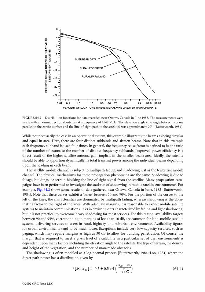
While not necessarily the case in an operational system, this example illustrates the beams as being circularand equal in area. Here, there are four distinct subbands and sixteen beams. Note that in this exampleeach frequency subband is used four times. In general, the frequency reuse factor is defined to be the ratioof the number of beams to the number of distinct frequency subbands. Improved power efficiency is adirect result of the higher satellite antenna gain implicit in the smaller beam area. Ideally, the satelliteshould be able to apportion dynamically its total transmit power among the individual beams dependingupon the loading in each beam.

The satellite mobile channel is subject to multipath fading and shadowing just as the terrestrial mobilechannel. The physical mechanisms for these propagation phenomena are the same. Shadowing is due tofoliage, buildings, or terrain blocking the line-of-sight signal from the satellite. Many propagation cam-paigns have been performed to investigate the statistics of shadowing in mobile satellite environments. Forexample, Fig. 64.2 shows some results of data gathered near Ottawa, Canada in June, 1983 [Butterworth,1984]. Note that these curves exhibit a “knee” between 50 and 90%. For the portion of the curves to theleft of the knee, the characteristics are dominated by multipath fading, whereas shadowing is the dom-inating factor to the right of the knee. With adequate margins, it is reasonable to expect mobile satellitesystems to maintain communications links in environments characterized by fading and light shadowing,but it is not practical to overcome heavy shadowing for most services. For this reason, availability targetsbetween 90 and 95%, corresponding to margins of less than 10 dB, are common for land-mobile satellitesystems delivering services to users in rural, highway, and suburban environments. Availability figuresfor urban environments tend to be much lower. Exceptions include very low-capacity services, such aspaging, which may require margins as high as 30 dB to allow for building penetration. Of course, themargin that is required to meet a given level of availability in a particular set of user environments isdependent upon many factors including the elevation angle to the satellite, the type of terrain, the densityand height of the vegetation, and the number of man-made obstacles.

The shadowing is often modeled as a log-normal process [Butterworth, 1984; Loo, 1984] where thedirect path power has a distribution given by

(64.4)

FIGURE 64.2 Distribution functions for data recorded near Ottawa, Canada in June 1983. The measurements weremade with an omnidirectional antenna at a frequency of 1542 MHz. The elevation angle (the angle between a planeparallel to the earth’s surface and the line-of-sight path to the satellite) was approximately 20º [Butterworth, 1984].

P S xdB<[ ] 0.5 0.5 erf xdB ms–

2ss

------------------- +=


where ms is the received signal strength in dB, S is the average dB shadowing loss, and σs is the dB varianceof the shadowing loss. The parameters of this distribution depend not only on environment but on theelevation angle to the satellite and on frequency. For a variety of situations, estimates of these parameterscan be derived from the empirical results of these propagation campaigns provided in ITU-R Recom-mendation PN.681 and PN.681-1 and Stutzman [1988].

Multipath fading results from interference caused by reflections of the radio signal from the immediateenvironment, with the time-varying nature being caused by motion of the terminal through the environ-ment. In satellite applications, the reflections are generally too weak to be useful by themselves but not soweak as to be ignored. Consequently, the satellite mobile channel is usually modeled as a Rician fadingchannel consisting of an unshadowed direct path and a diffuse component which has a complex Gaussiandistribution (Rayleigh distributed amplitude and uniformly distributed phase). The amplitude distributionof the resulting channel is the non-central Chi-squared distribution with two degrees of freedom,

(64.5)

where a = , b = r/σ, and Ik(.) is the kth order modified Bessel function. The quantity K is the ratioof the direct path power to the average power of the multipath, 2σ2. Rician channels are characterizedby their K-factor. The probability of a fade of a given depth is shown in Fig. 64.3 for various K-factors.Note that there is a greater than 50% probability that the diffuse component will increase the signalstrength. K-factors with vehicle1-mounted antennas are typically 10 dB and higher, with the worst casevalue of 10 dB occurring at low elevation angles. For handheld terminals, where the antenna has littledirectivity, lower K-factors can be expected.

The time-varying nature of the fading, in particular, the duration of the fades, is characterized by itsspectrum. For land-mobile applications, the Clarke model [Clarke, 1968], which assumes uniformlydistributed scatterers in a plane about the moving terminal, is often used. The maximum Doppler fre-quency observed is related to the transmission frequency by the expression fd = v/λ, where v is the velocityof the terminal, and λ is the transmission wavelength. The Clarke model for the diffuse spectrum is given by

(64.6)

FIGURE 64.3 Cumulative fade distribution for the Rician channel as a function of K-factor.

1Vehicle refers to automobile, aircraft, or ship.

P R r<[ ] 1 e a2+b

2( )/2– ab--

k

Ik ab( )k=0

∞

∑–=

K

S f( )1

1 f/fd( )2–

----------------------------=


and the corresponding time correlation of the diffuse component is given by

(64.7)

where Jo(.) is the zeroth order Bessel function.For the land-mobile channel, some effort has been devoted to providing an appropriate model com-

bining the effects of shadowing and multipath fading which is appropriate for satellite applications. Anexample of these is the Lutz-model [Lutz et al., 1991], which consists of two states, a good state and abad state. In the good state, the channel is Rician. In the bad state, the line-of-sight signal is essentiallyblocked due to significant shadowing. The parameters of the model are the distribution of the dwelltimes in each state, the K-factor, and the distribution of the shadowing, which are selected to model theenvironment of interest.

In aeronautical-mobile, the fading spectrum is generally modeled as Gaussian. However, measurementsin this case indicate that the fading bandwidth is not strongly dependent on the aircraft velocity. Thefading tends to be slow and is due to reflections from a limited portion of the earth’s surface and fromthe aircraft’s body. At L-band frequencies (1.6 GHz), the fading bandwidths for aeronautical-mobilechannels range from 20 to 100 Hz with 20 Hz being more prevalent [Neul et al., 1987].

The physics involved in determining an appropriate model for the maritime channel are quite similarto that for the aeronautical case [Moreland, 1987]. Consequently, the fading spectrum is generally modeledas Gaussian. However, the fading bandwidth is typically less than 1 Hz [Schweikert and Hagenauer, 1983].

In general, multipath in satellite-mobile channels is not time-dispersive. Measurements indicate thatfor practical bandwidths (<2 MHz), this is true for wideband channels up to 2 MHz [Jahn et al., 1995].A possible exception to this is the high-altitude aeronautical channel where one may occasionally receivedistant reflections from the sea surface or ice. For this case, the strength of the reflected path is strongenough to be problematic only at elevation angles below 20º .

64.3 Satellite Orbits

Initial mobile satellite systems used geostationary orbits and were generally aimed at mobile terminalswith significant antenna gain (>8 dB). As satellite technology evolved, applications have expanded toinclude terminals with much lower antenna gain (0 dBi). These include a number of regional mobilesatellite services as well as the Inmarsat international service. The geostationary orbits provide goodcoverage in the low- to mid-latitude regions. Service availability to mobile units in the mid- to higher-latitude regions can be compromised due to blockage at the lower elevation angles. To achieve a higherservice availability to a greater portion of the earth’s surface necessitates the use of non-geostationaryorbits.

With non-geostationary orbits, coverage from one satellite is time-varying, although the orbits areoften chosen to be a submultiple of either the solar day (24 h) or the sidereal day (23 h 56 m 4 s). Withthe latter, the satellite ground tracks are periodic, while with the former, the ground tracks drift approx-imately 1º longitudinally each day. As a result of this time-varying behavior, a constellation of satellitesmust be employed to provide continuous coverage.

A variety of non-geostationary orbits and constellations have been proposed. These range from thelow earth orbit (LEO) systems at altitudes from 500 to 2000 km, through the medium earth orbit (MEO)systems at altitudes from 9000 to 14,000 km, to the highly elliptical orbit (HEO) systems. One constrainton orbits is the Van Allen radiation belts which encircle the planet [Hess, 1968]. The primary belt from2000 to 9000 km and the secondary belt from 14,000 to 19,000 km can restrict operation at these altitudesbecause of the greater radiation hardness requirements on the satellite components.

Constellations are generally configured as a number of orbital planes with a number of satellites in eachplane. The number of satellites in the constellation generally decreases with the altitude. Most examplesfall into the category of inclined circular orbits [Ballard, 1980], where the inclination refers to the angle

R t( ) Jo 2pfdt( )=


the orbital plane makes with the equator. The extreme case of these are the polar-orbiting constellations[Adams and Rider, 1987]. The coverage provided by all these constellations is global in nature, but theminimum elevation angle and number of satellites visible simultaneously at any location depends on theconstellation and its altitude. In general, simple constellations can provide good coverage of the earth.As an example, the cumulative distribution of the elevation angles (averaged over time and location) fora twelve satellite constellation is shown in Fig. 64.4. This figure indicates that the elevation to the primaryvisible satellite is always greater than 23º ; and 90% of the time/locations it is always greater than 30º .Figure 64.4 also indicates that a second satellite is always visible with an elevation of at least 10º .

An alternative to the inclined circular orbits are the elliptical orbits of which the Molniya [Ruddy,1981] and Loopus [Dondl, 1984] are well-known examples. A constellation of satellites in highly ellipticalorbits can approximate the effect of an overhead geo-synchronous satellite for high latitude regions.However, the useful coverage with elliptical orbits is restricted (generally they are only active near the orbitapogee), and they are intended for regional services.

While non-geostationary orbits ameliorate a number of the propagation phenomena affecting com-munications with a mobile terminal, they also introduce a number of challenges. In particular, with non-geostationary satellites, a number of quantities such as path delay and Doppler shifts become not onlyposition-dependent but also time-varying, depending on the satellite orbital speed. The period of a satellitein an elliptic or circular orbit around the earth is

(64.8)

where a is the semimajor axis of the orbit (the radius in the case of a circular orbit) and GM is the earth’sgravitational parameter (GM = 3.99 × 1014 m3/s2).

As with a geostationary satellite, the propagation delay and path loss vary with user position (range),and the general expression for satellite range as a function of elevation angle θ is given by

(64.9)

where Re is the earth’s radius (6378 km) and h is the satellite altitude. The corresponding delay is τ = r/c.Unlike geostationary satellite systems, there can be significant Doppler and propagation delay variations

FIGURE 64.4 Cumulative distribution of elevation angle to primary satellite with a constellation of four inclinedplanes of three satellites at an altitude of 10,355 km.

T2pa3/2

GM---------------=

r q( ) R e 1 h/Re+( )2cos2q– sinq–( )=


due to the relative velocity of the user and the satellite with non-geostationary mobile satellite systems.Both of these quantities are proportional to the range rate, with the delay variation given by

(64.10)

where τ is the propagation delay, r is the range, and the Doppler shift is given by

(64.11)

Note that this Doppler frequency is distinct from the maximum Doppler rate used to characterizemultipath fading. The latter corresponds to the mobile terminal velocity relative to its immediate envi-ronment. There are a number of contributors to the range rate. They include the satellite motion, theearth’s rotation, and the velocity of the mobile terminal relative to the earth. In a number of simple casesinvolving circular orbits, the contribution of these various components can be calculated explicitly. Whenthe user lies in the orbital plane, such that the geometry is as shown in Fig. 64.5, then the range rate dueto satellite motion alone is given by

(64.12)

In addition, the velocity of the mobile terminal due to the earth’s rotation is given by

(64.13)

in a direction of constant latitude, where γ is the latitude of the mobile terminal, and Te is the periodof the earth’s rotation (23 h 56 m 4s). In the general case, the range rate is the vector sum of the velocitiesof these different contributors projected along the range vector. This depends on the mobile terminalposition as well as velocity and does not have a simple explicit formula [Vilar and Austin, 1991]. However,the general circular-orbit case can be upperbounded by Eqs. (64.12) and (64.13), projected in the directionof the satellite, to give

(64.14)

This shows that both the Doppler and delay rate are zero at the subsatellite point and increases towardthe satellite horizon, although the Doppler increase depends upon the relative direction. The Doppler can

FIGURE 64.5 Illustration of satellite geometry for calculating range and range rates.

dτdt----- 1

c--

drdt-----=

fs1λ---=

drdt-----

drdt-----

sat

2πRe

T------------– cosθ=

vr

2πRe

Te

------------ γcos=

drdt----- 2πRe cosθ 1

T--- γcos

Te

-----------+ ≤


range from zero for a geostationary orbit to greater than 42 kHz for a LEO satellite (1000 km) at 2.0 GHz.The corresponding delay rate can vary from zero to 21 microseconds per second.

Another parameter of interest is the rate of change of Doppler. There is no simple expression for theDoppler rate but, in a similar manner, it can be upper bounded by

(64.15)

Equations (64.14) and (64.15) do not include the effect of mobile terminal motion relative to the earth.The Doppler rate can range from zero for a geostationary satellite to 100 Hz/sec for a LEO satellite at1000 km at 2.0 GHz depending upon the positions of the user and the satellite.

In addition to these potential influences of non-geostationary satellites on modem design, there canalso be a significant impact on the multiple access strategy due to differential delay and differentialDoppler across a spotbeam. Assuming the differential effects of the earth’s rotation across a spotbeamcan be neglected, the differential delay can be upper bounded by

(64.16)

where θmin and θmax are the minimum and maximum elevations for the spotbeam of interest. The greatestdifferential delay occurs at the edge of coverage. For many scenarios, this differential delay can be of theorder of milliseconds, which can have an impact on multiple access strategies which require the time-synchronization of users.

The differential Doppler across a spotbeam depends upon the location of the spotbeam relative to theorbital plane of the satellite. If one neglects the differential effects of the earth’s rotation across a spotbeam,one can bound the differential Doppler in spotbeams along the orbital plane by

(64.17)

This bound assumes that the whole spotbeam lies completely in either the fore or aft coverage of thesatellite, but indicates that the maximum differential Doppler occurs across a spotbeam covering thesubsatellite point. For many scenarios, the differential Doppler across a spotbeam can be on the orderof kilohertz and, thus, can also influence the design of a multiple access strategy.

It should be noted that lower altitude satellites must provide the same RF power flux density as higheraltitude satellites. Typically, however, higher altitude satellites are used to cover larger areas and, to providean equivalent return link service, must have larger antennas and more spotbeams. Consequently, whilefewer of the higher altitude satellites are required to provide global coverage, they are generally largerand more complex.

64.4 Multiple Access

Satellites intended for mobile services are frequently designed with antennas large enough to providemultiple spotbeams. This not only reduces the power requirements but also allows frequency re-usebetween the beams. The result is a system which is similar to terrestrial cellular systems with the followingdifferences:

1. Isolation between co-channel users is controlled by the spacecraft antenna characteristics and notby propagation losses.

∆τr θmin( ) r θmax( )–

c---------------------------------------≤

∆fs

2πRe

λT------------ θmin θmaxcos–cos( )≤

dfo

dt------

2π( )2Re sinθλT

-------------------------------- 1T--- γcos

Te

-----------+ ≤


2. The near–far problem is less critical so power control is less of a factor. Due to delay constraintsin satellite systems, power control is generally limited to counteracting the effects of variation inantenna gain and average propagation losses. This, however, means that co-beam users in theforward direction will generally be received at different power levels.

3. Due to the distortion caused by the curvature of the earth’s surface, the spotbeams do not coverthe same surface area. In particular, the outer beams can be significantly extended in the radialdirection, as illustrated in Fig. 64.6; this figure is a two-dimensional projection of the coveragepattern on the earth that preserves radial proportions but results in some angular distortion.The consequence of this distortion is that the outer beams may be required to serve significantlymore users. Furthermore, the outer beams are subject to more adjacent beam interference forsimilar reasons. A complicating factor is that the outer beams are also the most likely to be in thefield of view of other satellites in the constellation. The satellite antenna can be designed to provideequal size spotbeams on the earth, but this policy penalizes the communications performance ofa large number of users for the benefit of none.

4. With many constellations there can be significant overlapping coverage from multiple satellites,and this allows the possibility of diversity transmissions. A whole range of diversity techniquesare possible for all multiple access strategies depending on the power, bandwidth, and complexityconstraints. The simplest approach is selection diversity during the call setup. More complexapproaches include dynamic techniques such as switched diversity in the forward direction basedon return-link signal strength and maximal ratio combining in the return direction.

5. This brings up a final difference with respect to terrestrial systems in that, with a fixed antennacluster, the satellite cells and “base station” are moving with respect to the mobile rather than viceversa. This raises issues regarding handover procedures and, in light of multiple satellite coverage,the orthogonality of user accesses.

In general, multiple access techniques for mobile satellite applications can be divided into two groups:wideband techniques, such as CDMA [Gilhousen et al., 1990], and narrowband techniques, such asFDMA and narrowband TDMA. Each technique has its strengths and weaknesses which depend on theapplication and implementation, but there are a number of common aspects. The power efficiency of alltechniques can be improved by adding forward error correction coding but with a bandwidth penalty.The exception to this is asynchronous CDMA, which does not suffer a bandwidth penalty but generallymust tolerate greater co-user interference. There are synchronous versions of all these techniques (synchro-nization at the chip level for CDMA and at the bit and frequency level for FDMA and TDMA) that can beused to improve spectral efficiency on the forward link where one can easily synchronize transmissions.

FIGURE 64.6 Spotbeam pattern projected onto the earth’s surface: 4-db contours with edge of coverage at 10∞elevation.


For applications in the 1 GHz and 2 GHz range, the propagation characteristics of wideband techniques(<2 MHz) and narrowband techniques are similar.

Interference tolerance, in particular multiple access interference, is one aspect which differs betweenwideband and narrowband systems. With CDMA, interference due to co-users is averaged over all co-users and affects all users. With narrowband techniques, interference generally results in greater degra-dation, but only of individual carriers. It is this interference tolerance which determines the frequencyre-use capability and the bandwidth-limited capacity. When comparing the bandwidth-limited capacitiesof various approaches, care must be taken to be equitable. Interference has a probability distribution dueto the random location (and isolation) of co-channel users relative to the desired user. In both widebandand narrowband techniques, it is the tails of this distribution which determine the effect of interferenceon the service availability [Moher et al., 1996].

An additional issue is the design of the ancillary channels for signaling and control for a multi-beamsatellite system and their integration with the traffic services with a minimum of power and bandwidthrequirements.

64.5 Modulation and Coding

Along with the choice of multiple access strategy, modulation and coding schemes must be selected tomeet the stringent bandwidth and power efficiency requirements of the mobile satellite communicationssystem. With respect to the choice of modulation scheme, binary phase-shift keying (BPSK) has beenpopular for low data rate store-and-forward systems due to its simplicity and robustness. However, BPSKis very spectrally inefficient when transmitted from a terminal with a nonlinear power amplifier (e.g., apower-efficient class-C amplifier). Aeronautical satellite communications systems have improved uponthe spectral efficiency, without sacrificing robustness or compatibility with nonlinear amplifiers, by usingππππ/2-BPSK coupled with 40% square-root raised-cosine pulse shaping.

The most popular choice of modulation technique for higher-rate services has been quadrature phase-shift keying (QPSK). QPSK can be considered as two BPSK waveforms orthogonally modulated: one bya sine wave at the carrier frequency, and the other by the corresponding cosine wave. Consequently, fora given choice of pulse shaping filter and for a linear channel, the spectral efficiency (in terms of the ratioof the number of bit/s transmitted to the occupied bandwidth in Hz) for QPSK is twice that for BPSK.With standard QPSK, the symbol timing is identical in the sine and cosine channels. A fairly lineartransmitting power amplifier is required in the mobile terminal if good bandwidth efficiency is to bemaintained with standard QPSK. As is the case for BPSK, variations of QPSK can be used that are rea-sonably tolerant to amplifier nonlinearity. Figure 64.7 [Patenaude and Lodge, 1992] illustrates thetransmitted power spectrum of π/4-QPSK (60% square-root raised-cosine pulse shaping) and offset-QPSK (60% and 100% square-root raised-cosine pulse shaping) after being amplified by a hard-limitingamplifier (which is the extreme example of a nonlinear power amplifier). Note that even in this severecase, offset-QPSK with 60% pulse shaping is quite spectrally efficient. In fact, this is the choice ofmodulation scheme for a number of mobile satellite communications systems including Inmarsat’s M,B, and Aeronautical systems.

The viability of mobile satellite systems is dependent upon excellent power efficiency. Consequently,detection is often based on phase-coherent approaches rather than the less power-efficient options ofdifferentially-coherent and noncoherent detection that are commonly used for terrestrial systems. Increas-ingly, traditional carrier tracking schemes, such as phase-locked loop based techniques, are being replacedby digital schemes such as the one described in [Viterbi and Viterbi, 1983]. The fading and shadowingnature of the channel can result in frequent cycle slips of the carrier recovery algorithm, resulting in aphase ambiguity (which is inherent in the PSK signal) that must be resolved. Differential phase encodingof the transmitted symbols is a fairly traditional approach for eliminating the detrimental effects of thephase ambiguity. However, differential encoding tends to increase the average bit error rate for a givensymbol error rate and is consequently avoided in many mobile satellite system signal designs. A morecommon approach is to periodically insert a known bit or symbol (referred to as a reference symbol) or


group of bits (referred to as a unique word) into the transmitted signal, which can be used to detect theoccurrence of cycle slips and then to resolve the resulting carrier phase ambiguity. In the extreme case,for which the period of insertion is sufficiently greater than the required tracking bandwidths, carriertracking can be based solely on the reference symbols [Moher and Lodge, 1989].

Forward error control (FEC) coding is an important tool for achieving good power and bandwidthefficiency. The choice of FEC coding technique is dependent upon the number of bits that are to becoded as an identifiable group. First, consider the case for which only several tens of bits are to be codedinto a codeword. This situation naturally arises in a number of circumstances including short data packetscontaining signaling information or user data, and for digital voice transmission for which additionaldelays (due to coding) of greater than a couple of voice frames is unacceptable and only the most sensitivebits in the frame are protected with FEC coding. In these cases, block codes such as the Golay code andBose–Chaudhuri–Hocquenghem (BCH) codes are common choices. Another possibility is the use ofconvolutional coding with puncturing [Yasuda et al., 1984] used to achieve the desired code rate. Con-volutional codes with a constraint-length of 7 have been popular choices for early systems, with con-straint-length 9 codes being proposed for later ones. Usually prior to convolutional encoding, a field of“flush bits” is appended to the end of the field of data bits so that the last data bits to be decoded havea similar level of integrity as the rest of the data bits. The field of flush bits can represent a significant(and undesirable) overhead for the transmission of very short data blocks. Fortunately, the requirementfor such a field can be obviated if tail biting [Ma and Wolf, 1986] is used. Usually, convolutional codingis preferable to block coding because it is more amenable to the use of soft decisions.

The second scenario to consider is the transmission of a continuous data stream (e.g., digital voice)or data in large fields. In this case, convolutional coding is a reasonable choice for services for whichhigh average bit error rates (i.e., higher than 10-4) are acceptable. For applications requiring higher qualitydata, reasonable choices include concatenated coding (with a convolutional code as the inner code and

FIGURE 64.7 The transmitted power spectrum of p/4-QPSK (60% square-root raised-cosine pulse shaping) andoffset-QPSK (60% and 100% square-root raised-cosine pulse shaping) following hard-limiting amplification.[Patenaude and Lodge, 1992].


a Reed-Solomon code as the outer code) and turbo coding [Berrou et al., 1993]. As an example of therelative power efficiency, Fig. 64.8 shows the performance of several of these alternatives where the onlychannel impairment is additive white Gaussian noise. Curves A, B, C, and D are all for rate-1/2 coding.Curve D is a constraint length-7 convolutional code. Curve C is the same convolutional code, puncturedto rate-3/5, concatenated with a (255, 213) Reed–Solomon code. Curves A and B represent the perfor-mance of turbo coding for block lengths of 10,000 and 300 data bits, respectively. Curves E and F providean indication of the trade-off between bandwidth and power efficiency. These latter two curves use theconvolutional codec of curve D, so the level of code complexity is fixed. Curve E is punctured to a rate of3/4, while curve F uses pragmatic coding [Viterbi et al., 1989] to achieve a rate of 1 bit per dimension.For the range of spectral efficiencies considered here and for a fixed level of coding complexity, the ruleof thumb is that a 1 dB improvement in bandwidth efficiency results in approximately a 1 dB degradationin power efficiency. Note that trading bandwidth against power efficiency, using puncturing or pragmaticcoding, is equally applicable for concatenated and turbo coding schemes.

Fading and shadowing can cause reductions in the level of the received signal to a point where reliabletransmission is no longer possible. If these signal outages are of short duration, they can successfully becompensated for by interleaving the order of the coded data prior to modulation in the transmitter andthen deinterleaving the data prior to decoding [Clark and Cain, 1981]. This effectively shuffles the receivedbits having low received signal power with received bits having higher signal power. Of course, for thecombination coding and interleaving to eliminate errors in the decoded data bits, the interleaving mustbe performed over a signal duration that is several times greater than the duration of the outage. Inter-leaving adds to the total end-to-end delay, and, consequently, the duration of outages that can be dealtwith is dependent upon the delay constraint of the given mobile satellite service.

Inevitably, some of the outages will have a duration too great to be handled by interleaving and coding.In such cases, many services will simply be unavailable. However, some source codecs (e.g., certain vocoders)have the capability to gracefully handle several sequential missing or erroneous frames. Also, applications

FIGURE 64.8 The performance of various coding schemes in an additive white Gaussian noise environment. A: rate-1/2 turbo code with a block size of 10,000 b; B: rate-1/2 turbo code with a block size of 300 b; C: rate-1/2 concatenatedconvolution/Reed–Solomon code; D: rate-1/2 constraint length 7 convolution code; E: rate-3/4 punctured constraintlength 7 convolutional code; F: rate-1 pragmatic constraint length 7 convolutional code. (Provided by P. Guinand,Communications Research Centre, Ottawa, Canada.)


that can tolerate long delays can overcome fairly long outages by employing automatic repeat request(ARQ) schemes.

64.6 Trends in Mobile Satellite Systems

An increasing variety of services are being offered to travelers via mobile satellite systems, with the datarates for the high-end services increasing steadily. In parallel with this, there is continuing pressure toreduce the size of the mobile terminals. The result is that the size of the system’s space segment is growingthrough some combination of an increased number of satellites and larger, more complex satellites. Fora given orbit altitude, the size of the satellite antenna is growing dramatically. A corresponding increasecan be seen in system complexity, with the apportioning of this complexity between the space segmentand the ground infrastructure varying from one system to another. System designs that place much ofthis complexity in the space segment are characterized by on-board switching and processing and, insome cases, intersatellite links. System designs that place much of the complexity in the ground infra-structure are characterized by a large number of coordinated and very sophisticated gateway stations.

The number of customers for mobile satellite services has begun to grow significantly, and explosivegrowth in the future is forecast. Many organization are designing new systems to meet this anticipateddemand, with new frequency bands being allocated to accommodate them. Even with these new bands,increasing frequency congestion will be experienced if the forecasted traffic volumes materialize. The firstgeneration mobile satellite systems were predominantly power limited. However, subsequent generationswill be increasingly bandwidth limited.

The traffic volumes for many early generation mobile satellite systems are fairly symmetric (in thesense that the volume of traffic in the forward direction is approximately the same as that for the returndirection) because voice telephone applications are dominant. However, it is anticipated that an increasingportion of the traffic will support services such as database access, message retrieval (e.g., e-mail andvoice mail), and broadcast information. In general, these services result in much greater volumes of databeing transmitted in the forward direction than in the return direction. Fortunately, this asymmetrictraffic requirement is a good match with the technological situation in a couple of respects. Firstly, in theforward direction, improved bandwidth efficiency can be achieved by taking advantage of the fact thatthe system can be designed to accurately coordinate the carrier frequency, carrier phase, and symbol timingof each transmission within a beam. Consequently, techniques such as synchronous CDMA, orthogonalfrequency-division multiplexing, and wavelet-packet multiple access can be employed. Secondly, unlikethe return direction for which the mobile terminal’s power amplifier places fairly severe constraints onthe dynamic range of the transmitted waveform, the forward link channel is incrementally linear. Incre-mentally linear means that each carrier appears to be transmitted through a linear channel, with inter-modulation due to the nonlinearity of the satellite transponder’s power amplifier resulting in an additivenoise-like process. Given that both the traffic requirements and the technological situation are asymmet-ric, the transmission schemes selected for these mobile satellite services will differ significantly betweenthe forward and the return direction.

Defining Terms

Forward direction: Direction of transmission that is from the satellite to the mobile.Maximal ratio combining: A combining technique for which signals from two or more communication

paths are aligned in phase, weighted proportional to their voltage-to-noise power ratios, and thensummed [Proakis, 1989].

Narrowband TDMA: A multiple access strategy where a small number of users, typically less than ten,share a single frequency channel in time. Larger numbers of users are accommodated by using anumber of narrowband TDMA carriers of different frequencies.

Offset-QPSK: A variation of QPSK for which the symbol timing in the sine channel is offset by halfof a symbol period relative to that in the cosine channel.


Return direction: Direction of transmission that is from the mobile to the satellite.Switched diversity: The process of switching to the best of two or more communication paths [Jakes,

1974].ππππ/2-BPSK: A variation of BPSK for which consecutive symbols experience a relative phase shift of π/2

radians.ππππ/4-QPSK: A variation of QPSK for which consecutive symbols experience a relative phase shift of π/4

radians.

References

Adams, W.S. and Rider, L., Circular polar constellations providing continuous single or multiple coverageabove a specified latitude, J. Astron. Sci., 35, 155, 1987.

Ballard, A.H., Rosette constellations of earth satellites, IEEE Trans. Aero. Elec. Sys., AES-16(5), 656, 1980.Berrou, C., Glavieux, A., and Thitimajshima, P., Near Shannon limit error-correcting coding and decod-

ing: turbo-codes, Proc. IEEE Int. Conf. Comm., ICC’93, 1064, 1993.Butterworth, J.S., Propagation measurements for land-mobile satellite systems at 1542 MHz, Commu-

nications Research Centre Tech. Note No.: 723, Department of Communications, Canada, August1984.

Clark, G.C., Jr. and Cain, J.B., Interleaver structures for coded systems, Error-Correction Coding for DigitalCommunications, Plenum Press, New York, 1981, Section 8.3.

Clarke, R.H., A statistical theory of mobile radio reception, Bell Syst. Tech. J., 47, 957, 1968.Dondl, P., Loopus opens a new dimension in satellite communications, Int. J. Sat. Comm., 2, 241, 1984.Gilhousen, K.S., Jacobs, I.M., Padovani, R., and Weaver, L.A., Jr., Increased capacity using CDMA for

mobile satellite communications, IEEE J. Sel. Areas Comm., 8, 503, 1990.Hess, W.N., The Radiation Belt and Magnetosphere, Blaisdell, Waltham, MA, 1968.ITU, Propagation data required for the design of earth-space land mobile telecommunication systems,

Recommendation ITU-R PN.681 (1992) and ITU-R PN.681-1 (1995).Jahn A., Lutz, E., Sforza, M., and Buonomo, S., A wideband channel model for land mobile satellite

systems, Proc. Int. Mob. Sat. Conf., Ottawa, June 1995, 122.Jakes, W.C., Ed., Microwave Mobile Communications, IEEE Press, New York, 1993. Loo, C., A statistical model for land-mobile satellite link, Proc. Int. Conf. Comm., 588, 1984.Lutz, E., Cygan, D., Dippold, M., Dolainsky, M., and Papke, W., The land mobile satellite communication

channel—recording, statistics and channel model, IEEE Trans. Veh. Tech., 40(2), 375, 1991.Ma, H.H. and Wolf, J.K., On tail biting convolutional codes, IEEE Trans. Commun., COM-34(2), 104,

1986.Moher, M.L. and Lodge, J.H., TCMP—a modulation and coding strategy for Rician fading channels,

IEEE J. Sel. Areas Commun., 7(9), 1347, 1989.Moher, M.L., Erup, L., and Lyons, R.G., Interference statistics for multi-beam satellites, Proc. 2nd Eur.

Workshop Mobile/Personal Satcom, 366, 1996.Moreland, K.W., Ocean scatter propagation models for aeronautical and maritime satellite communica-

tion applications, M.Sc. Thesis, Carleton University, 1987.Neul, A., Hagenauer, J., Papke, W., Dolainsky, F., and Edbauer, F., Propagation measurements for the

aeronautical satellite channel, Proc. IEEE. Veh. Tech. Conf., Tampa, FL, June 1987, 90.Patenaude, F. and Lodge, J., Non-coherent detection of hardlimited O-QPSK, Proc. 1992 Int. Conf. Sel.

Topics Wireless Comm., Vancouver, Canada, June 1992, 93.Proakis, J.G., Digital Communications, 2nd ed., McGraw-Hill, New York, 1989.Ruddy, J.M., A novel non-geostationary satellite communications system, Proc. Int. Conf. Comm., 3,

Denver, June 1981.Schweikert, R. and Hagenauer, J., Channel modelling and multipath compensation with forward error

correction for small satellite ship earth stations, Proc. 6th Int. Conf. Dig. Sat. Comm., Phoenix, AZ,1983, XII-32.


Stutzman, W.L., Ed., Mobile satellite propagation measurements and modeling: a review of results forsystems engineers, Proc. Int. Mob. Sat. Conf., Pasadena, CA, June 1988, 107.

Vilar, E. and Austin, J., Analysis and correction techniques of Doppler shift for non-geosynchronouscommunication satellites, Int. J. Sat. Comm., 9, 123, 1991.

Viterbi, A.J. and Viterbi, A.M., Nonlinear estimation of PSK-modulated carrier phase with applicationsto burst digital transmission, IEEE Trans. Info. Theory, IT-29(4), 543, 1983.

Viterbi, A.J., Wolf, J.K., Zehavi, E., and Padovani, R., A pragmatic approach to trellis-coded modulation,IEEE Commun. Mag., 11, 1989.

Yasuda, Y., Kashiki, K., and Hirata, Y., High rate punctured convolutional codes for soft decision Viterbidecoding, IEEE Trans. Commun., COM-32, 315, 1984.

Further Information

A number of tutorial paper on mobile satellite systems have appeared in recent years. These include:

Kato, S., Personal communication systems and low earth orbit satellites, Proceedings of the Space andRadio Science Symposium, U.R.S.I., Brussels, Belgium, April 1995, 30.

Lodge, J., Mobile satellite communications systems: toward global personal communications, IEEE Com-mun. Mag., 29(11), 24, 1991.

Wu, W.W., Miller, E.F., Pritchard, W.L., and Pickholtz, R.L., Mobile satellite communications, Proc. IEEE,82(9), 1431, 1994.

Special issues of journals, dedicated to mobile satellite communications, are:

Kucar, A.D., Kato, S., Hirata, Y., and Lundberg, O., Eds., Special Issue on Satellite Systems and Servicesfor Travelers, IEEE J. Sel. Areas Commun., 10(8), 1992.

Maral, E., Ed., Special Issue on Personal Communication via Satellite, Int. J. Sat. Commun., 12(1), 1994.

A comprehensive book that contains a number of sections that are highly relevant to the discussionof multiple access techniques is:

Abramson, N., Ed., Multiple Access Communications: Foundations for Emerging Technologies, IEEE Press,New York, 1993.


65Satellite Antennas

65.1 Introduction65.2 Horn Antennas and Reflector Feeds

Horn Antennas • Cup-Dipole Antennas • Frequency Reuse Feed and Polarization Diversity • Monopulse Feed

65.3 Reflector Antennas65.4 Phased Array Antennas65.5 Tracking, Telemetry, and Command Antennas 65.6 Current and Planned LEO/MEO Mobile

Satellite Antennas65.7 Radiometer Antennas 65.8 Space Qualification65.9 Future Trends and Further Study

65.1 Introduction

Satellite antennas provide not only for telecommunications, but also communications for controlling andcommanding the satellite in a prescribed orbit: an invisible tower in space [Hwang, 1992]. Their capabilitieshave evolved from being only a radio relay station to being an onboard processing base station. Most com-munications satellites are boosted into geosynchronous Earth orbit (GEO). At a particular altitude, with anangular speed exactly matching the Earth’s rotational rate, the satellite is motionless as viewed from the Earth.Three such satellites in synchronous orbit can cover over 90% of all inhabited regions of the Earth. Signalssent up from the ground and transmitted down from the satellite travel 19,300 nmi and suffer large propagationloss. A high-gain antenna is required to compensate for the path loss. The antenna can be a simple one forgenerating a circular pencil beam for Earth coverage or a much more complicated antenna generating multipleshaped beams and/or reconfigurable beams for frequency reuse with spatial and polarization diversities. Asmobile communications services evolve from a regional to a global scale, satellites play an important role inproviding the low-power-transmitters needed to broadcast from relatively unobtrusive base stations distributedthroughout space.

In order to provide low-power, personal handheld telephone services, the coverage area would normallybe divided into cells, each cell covered by a separate antenna beam. For a GEO satellite, this beam wouldrequire a very large antenna, which could not be implemented even with deployable antenna technology.In addition, the time delay of the half-hop propagation for a GEO satellite varies between 119 and 139 µs,becoming a problem in voice communication. This time delay can be reduced by the use of low Earth orbit(LEO) or medium Earth orbit (MEO) satellites. LEO and MEO orbits are particularly suitable for cellularmobile communication systems since the cell size remains constant throughout the orbit. Several LEO andMEO systems have been proposed, among them Iridium, Globalstar, and Odyssey. The range of possiblecommunication distance, propagation loss, propagation delay, and satellite view time vs. orbital attitudeare key parameters in the system tradeoff and design.

Yeongming HwangPinnacle EM Wave

Youn Ho ChoungTRW Space and Electronics Group


To meet these requirements, the antenna radiation pattern varies from omnidirectional to highly direc-tional. It can be fixed or reconfigured to meet the needs for each system configuration. A shaped beam isrequired in order to constrain the energy to conform to the coverage area to improve equivalent isotropicallyradiated power (EIRP) and reduce interference between beams. It can be achieved either by a multiple beamantenna system or a shaped reflector system. Beam reconfiguration is required to accommodate the changeof radiation pattern for a time-domain multiple access (TDMA) system.

Conventional antenna parameters such as half-power beamwidth (HPBW), antenna radiation effi-ciency, and aperture efficiency are insufficient to describe the performance of the system. In addition tothe gain ripple and gain slope over the coverage and frequency band, isolation or interference amongthese beams is important in the system. They are assessed in terms of spatial and polarization isolation,and both must be considered. Figure 65.1 depicts a 27-dB isolation between two transmit beams. Similarly,the receive isolation is defined as the isolation of two received signals of equal incident flux density. Beamshaping efficiency is used to evaluate the gain over a highly shaped coverage. An ideally shaped beam isone that has maximum antenna gain without sidelobes and achieves constant antenna radiation intensityover the area. Therefore, the theoretically achieved maximum gain is

where Acov is the coverage area in degrees square. The performance is evaluated in terms of beam shapingefficiency η defined as

where Gmin is the minimum gain over A cov. Practically, the gain-area product is between 10,000 and18,000, depending on the size of antenna aperture and the shape of coverage.

The tracking, telemetry, and command (TT&C) antenna provides ranging, telemetry, and commandoperation throughout all mission phases after launch vehicle separation. An autotracking antenna is requiredfor two reasons: to improve the pointing accuracy of the highly shaped beam where the performancedegradation is not accepted in the system due to satellite pointing error and to communicate with a movingtarget or user.

Successful observation of weather and climate from satellites has led to other new applications such asthe measurement of atmospheric parameters by seeing through cloud canopies. A microwave radiometeris a good candidate for this application. However, at least a 4.4-m antenna would be required to provide30-km nadir spatial resolution. This type of antenna is still under development. The most common typesof antennas being used to meet these requirements are summarized in Table 65.1.

FIGURE 65.1 Transmit isolation requirements.

G 41253/Acov=

h Gmin Acov/41253=


Satellite antennas differ from other antennas in several respects. A satellite must be designed to with-stand the dynamic mechanical and thermal stress during the launch and in the space environment. Thematerials used become a key factor. Other design constraints are size and weight. The antenna has to fit theshroud of the launching vehicle. As a result, the reflector used for the high-gain antenna must be stowedusing either a solid reflector or a meshed reflector. Weight cannot exceed that weight budget allocated inthe system. The challenge of satellite antenna design for the future will be to make them lighter, smaller,and cheaper.

65.2 Horn Antennas and Reflector Feeds

Currently, the reflector antenna is the most widely used satellite antenna, but future satellites may featurephased array antennas capable of rapid and low-loss beam scan, achievable with the design maturity ofsolid-state microwave amplifiers and receivers. The reflector antenna may have either a single feed ormultiple feeds, depending on the coverage requirement; the phased array antenna, in contrast, has manyradiating elements. The best candidates for feeds and radiating elements are horns and cup dipoles. Above6 GHz, horns are usually used since the waveguide is low loss and small in size. Cup dipoles are typicallyused below 4 GHz since coaxial cables are smaller and lighter than waveguides.

Horn Antennas

There are five types of horn antennas: open-ended waveguide, conical horn, dual-mode horn, corrugatedhorn, and multiflare horn. Table 65.2 compares pros and cons among these five horns. The open-endedwaveguide or the conical horn are most frequently used for multiple beam antennas (MBA) with phased

TABLE 65.1 Satellite Antennas

Area Coverage Function Antenna TypesAntenna

Gain Design Challenge Name of Satellites

Earth coverage ±9∞FOV Corrugated horn Multiflare horn

Medium Single horn with diplexer to coverboth up- anddown-links, withGood axial ratio

Most of all communication satellites

Omni TT&C with 2 Conspiral antenna Low Nearly omni- Most of allcoverage operation Biconical antenna Low directional communication

Spot coverage modes: Horn antenna Medium/ Spacecraft body satellites 1. transfer

orbitlow blockage

2. on-orbit ReliabilityPencil beam

coverageLimited

portion Reflector antennas

Single feedHigh Gimbal Steering INTELSAT-VIIs

of FOV Multiple feeds Beam forming NASA ACTS network (BFN) MILSTAR

Shaped beam coverage

Multiple beams for frequency reuse

Multibeams antennas

Shaped reflector antennas

High Isolation between beams

Switching BFN

INTELSAT-VINTELSAT-VIINTELSAT-VII

Nulling Maximize Reflector antennas High Adaptive nulling MILSTAR coverage signal-to- Multiple feeds algorithm

interference Adaptive BFN Adaptive BFNpower ratio Phased array

antennasCalibration and

characterizationAdaptive BFN of BFN

Finite coverage Passive Reflector antennas High Size of reflectormicrowave Surface tolerenceradiometer


array elements since their apertures can be small. Figure 65.2 shows a 30-GHz feed array for the NASAAdvanced Communication Technology Satellite (ACTS). The advantage of this type of horn is its sim-plicity and ease of fabrication. The disadvantage is that the radiation pattern is not circularly symmetrical,and so antenna efficiency is low and a high axial ratio is obtained for the circular polarization.

The dual-mode horn antenna, also called the Potter horn, generates a circularly symmetric pattern byadding transverse electric (TE11) and transverse magnetic (TM11) modes in proper amplitude and phase[Potter, 1963]. The TM11 mode is excited by a simple waveguide step. However, due to the phase velocitydifference, proper phasing of the two modes occurs only in a limited-frequency band with less than 5%bandwidth. Therefore, the dual-mode horn is only used in narrow bandwidth applications.

The corrugated horn carries a hybrid mixture of TE11 and TM11 modes through the grooved hornwalls; this fundamental hybrid mode is called the hybrid electric (HE11) mode. The TE and TM compo-nents in the HE11 mode have the same cutoff and phase velocity; therefore, the beamwidth limitationof the dual-mode (or multiflare) horn is removed. A detailed theoretical analysis has been given byClarricoats and Saha [1971]. One design problem of the corrugated horn is that without a matchingsection at the horn throat region it has a poor voltage standing wave ratio (VSWR), especially over thelower portion of the operating frequency band. Two kinds of matching sections can be used to improveVSWR: varying groove depths and ring-loaded grooves [James, 1982]. The corrugated horn can easilybe designed up to 60% bandwidth using a varying grooves matching section and, using a ring-loadedmatching section, can even be designed to a 2:1 bandwidth. One drawback of the corrugated horn is that

TABLE 65.2 Comparison Among Various Horns

Open-End Waveguide

ConicalHorn

Dual-Mode Horn Corrugated Horn

MultiflareHorn

Bandwidth Wide Wide Narrow Wide ModeratePattern

SymmetryNo No Yes Yes Yes

Phase Center Location

On the aperture

Inside aperture

Inside aperture Inside aperture On/Inside the aperture

VSWR forLarge Aperture

Good Excellent Frequency sensitive

Poor without matching section

Excellent

Fabrication Easy Easy Easy Difficult EasyApplications Array element Array element High-efficiency

feed for reflector

High-efficiency feed for reflector

High-efficiency feed for reflector

FIGURE 65.2 Feed array for NASA ACTS MBA.


the fabrication of the grooved walls is difficult, resulting in high manufacturing cost. Yet the corrugatedhorn is the most used reflector feed and is the best candidate for the Earth coverage antenna. A corrugatedhorn is classified either as a narrow- or a wide-flare horn. Figure 65.3 shows the antenna geometry andthe normalized radiation patterns for the narrow-flare corrugated horn. Figure 65.4 shows those for thewide-flare corrugated horn.

A multiflare horn is formed of several flared waveguide sections. This mechanically simple structureleads to very low fabrication cost. The smooth wall, as well as the flare structure, provides good RF matchto the waveguide. A low VSWR is always achieved. A conical multiflare horn generates higher order TE1n

and TM1n modes at the flare change. The circularly symmetric pattern is obtained by adding these highermodes (mainly TM11) to the fundamental TE11 in proper ratio. The analysis is based on mode matchingat the flare change to compensate for phase front curvature change. The differential phase shift amongmodes in a multiflare horn is less than that in a dual-mode horn. Thus, the multiflare horn is capable ofachieving about l5% bandwidth. A three-section multiflare horn is comparable (or even smaller) in sizeto a corrugated horn with the same beamwidth [Chen, Choung, and Palma, 1986]. The multiflare horn

FIGURE 65.3 Narrow-flare corrugated horn.

FIGURE 65.4 Wide-flare corrugated horn.


has advantages over the dual-mode horn in terms of bandwidth and over the corrugated horn in termsof manufacturing simplicity. Multiflare horns are currently utilized as spot beam feeds for NASA ACTS.

Cup-Dipole Antennas

A cup-dipole antenna has crossed dipoles in a cylinder and has good axial ratio for circular polarization. Theantenna is compact and easy to manufacture. There are two types, as shown in Fig. 65.5: unequal arms withsingle coaxial cable and equal arms using two coaxial cables and a 90∞ hybrid. The cup dipole with unequalarms is mechanically simple but can only generate single circular polarization with less than 5% frequencybandwidth. The cup dipole with equal arms has dual circular polarization with about 20% bandwidth, butit is mechanically complex. Several design variations of the cup dipole antenna such as the short backfireand cavity-back helix are described in Chapter 4 of Kumar and Hristrov [1989]. The dipole is about 0.45λand the cup diameter is from 0.7λ to 3l depending on the beamwidth and/or the array spacing.

Frequency Reuse Feed and Polarization Diversity

A given frequency band can be used more than once at the satellite to increase the communicationscapability of a given link. Since different communications channels will exist at the same carrier frequen-cies, each reuse channel must be isolated.

There are two techniques to achieve this required isolation. One way is to use two orthogonal polar-izations. One channel carries a vertical polarization [or right-hand circular polarization (RHCP)], andthe other channel carries a horizontal polarization [or left-hand circular polarization (LHCP)] with morethan 30-dB isolation. This can be done using a polarizer (for the CP case) and an orthomode transducerplaced right after the feed horn. Another method is to use two spot beams pointing at different locationswith high (about 30 dB) spatial isolation. This can be achieved using two feeds (or feed clusters) of thereflector to generate low sidelobes. Low sidelobes can be achieved with minimum spillover energy by theuse of a high taper feed on the reflector.

FIGURE 65.5 Two types of CP cup dipole.


Monopulse Feed

Point-to-point satellite communications require a narrow beamwidth to obtain high antenna gain. Butthe satellite jitters, causing a pointing error. In order to maintain reliable communications, a satelliteantenna must be accurately pointed toward a signal source. To achieve accurate pointing, the satelliteemploys an autotracking system, providing tracking signals related to pointing errors in elevation andazimuth. The tracking signals control a feedback servoloop of the satellite to orient the satellite as required,positioning the antenna accurately with respect to the signal source. A block diagram of the monopulsetracking is shown in Fig. 65.6. It is achieved using a single corrugated horn and a tracking coupler. Thecoupler uses a longitudinal traveling wave mechanism and utilizes the circular TE11 and TE21 modes thatprovide the sum and the difference channels, respectively, to achieve wideband monopulse tracking. Themain beam is obtained on the boresight axis of the antenna when only the dominant mode (TE11) isexcited at the aperture of the feed. When the beam is off the boresight axis, higher order modes (TE21)are excited in the feed. The amplitude of the TE21 mode is proportional to the angle of boresight, and anull in the higher order mode is obtained at the boresight.

65.3 Reflector Antennas

The reflector antenna, a high-gain antenna used to support high data rates with low transmitter power,is the most desirable type for communication antennas because of its light weight, structural simplicity,and design maturity. Its disadvantage is that the reflector has to be offset to avoid the aperture blockage.The offset destroys the rational symmetry of the optical aperture and limits the achievable performanceas compared to that of a lens antenna.

A reflector antenna system consists of one or more reflector surfaces. The surface can be solid, gridded,printed substrate, or meshed. It may be paraboloid, hyperboloid, spheroid, ellipsoid, or general in shape.Seven antenna types that have been most commonly used for satellite communication systems are summa-rized in Table 65.3. They include the parabolic reflector and the Cassegrain reflector, both either center fedor offset fed, the overlapped dual-gridded reflector, a multireflector system with a frequency selective surface(FSS) subreflector, and the deployable reflector antenna.

The center-fed parabolic and Cassegrain reflectors are used for a high-gain antenna where the radiationpattern is of circular shape. When the radiation pattern must be shaped to form a contour beam, a multiplebeam reflector antenna system or shaped reflector antenna system can be utilized. One of the mostcomplicated multiple beam antenna systems in use was designed for the INTELSAT V-VII series. TheINTELSAT VII satellite used a 2.44-m graphite fiber reinforced plastic (GFRP) reflector for the 4-GHzfrequency band over the Atlantic, Pacific, and Indian Oceans. The antenna provides shaped hemisphericand zone coverage, as shown in Fig. 65.7. The coverage was determined by the traffic demand in eachregion. The isolation between zone and hemispheric beams is accomplished by polarization diversification,

FIGURE 65.6 Block diagram of monopulse tracking.


whereas the isolation between the east and west hemispheric beams is accomplished by spatial diversifi-cation. There are 110 feeds used in the feed system. Each feed is a 1.13 wavelength GFRP circular hornelement arranged in triangular grid, as depicted in Fig. 65.8. The beam forming network consists of airsupported striplines and power dividers sandwiched between ground planes. The gain of the hemisphericbeam is about 15 dBi, and the gain of the zone beam is 22 dBi (decibels over an isotropic radiator). Theisolation achieved for both polarization and spatial diversification is about 27 dB.

Another complex reflector antenna in flight is NASA ACTS [Choung and Wong, 1968] operating atKa-band (30 GHz for receive and 20 GHz for transmit) (see Fig. 65.9). The MBA is designed to coverthe continental U.S. (CONUS). The coverage and polarization plan are shown in Fig. 65.10. The MBAprovides three fixed spot beams (Cleveland, Atlanta, and Tampa) for high-burst-rate (HBR) operationsand two scanning beams for low-burst-rate (LBR) operations. The scanning beams provide coverage for

TABLE 65.3 Reflector Antenna Configurations Used in Communication Antenna Systems

Type Features and Application Shape

1. Center-fed Simple, symmetrical light weight structureparabolic Aperture blockage causing sidelobe level and

reducing peak gainreflector High feed line loss

Pencil beam

2. Cassegrain Short, low feed line lossreflector Shaped reflector may be used to increase efficiencysystem Aperture blockage causing sidelobe level and

reducing efficiency Pencil beam

3. Offset No aperture blockageparabolicreflector

Convenience for spacecraft mounting with feed embedded below the platform

Shaped beam by using multihorns or shaping reflector surface

4. Offset No or minimum aperture blockageCassegrain Worse scan loss(or Gregorian) Fixed or scanning beamreflector

5. Overlapping Offset configurationdual-gridded Polarization reuse with 33-dB isolationparabolic Shaped beamreflector Thermal distortion of the gridded surface

6. Multiband dual FSS subreflector or overlappingFSS reflector Subreflectors in which one is an FSS

Same main reflector aperture for multifrequency band operation

Compact Thermal distortion of FSS7. Deployable Meshed reflector that can be folded

reflector Allow to use larger reflector aperture size Tradeoff between weight and surface accuracy Passive intermodulation may be generated Use mostly for lower frequency band system


FIGURE 65.7 INTELSAT VII hemi/zone coverage.

FIGURE 65.8 INTELSAT VII transmit feed array.


FIGURE 65.9 NASA ACTS MBA geometry.

FIGURE 65.10 NASA ACTS coverage and polarization plan.


two scan sectors (east and west) and 13 scan spots (Seattle, San Francisco, Los Angeles, Phoenix, Denver,White Sands, Dallas, Kansas City, New Orleans, Memphis, Huntsville, Houston, and Miami). ACTS hastwo electrically identical MBAs (one for transmit and one for receive) with half-power beamwidth(HPBW) on the order of 0.35º . Each MBA shown in Fig. 65.10 has one main reflector, a dual polarizedsubreflector, and two orthogonal feed assemblies. Both the low sidelobe fixed beams and the provisionfor overlapping fixed and scanning beams can be achieved by using an offset Cassegrain antenna with adual-gridded subreflector consisting of two offset hyperbolas arranged in a piggyback configuration. Thefront subreflector is gridded to pass one sense of polarization and reflect the orthogonal polarization.The back subreflector is solid and reflects the polarization transmitted by the front subreflector. The focalaxes of the two subreflectors are symmetrically displaced from the symmetry plane of the main reflectorby an angle of 10° so that two orthogonally polarized feed assemblies can be placed in their respectivefocal regions without mechanical interference.

A multireflector antenna system with an FSS subreflector is used for multiband operation. The FSS isdesigned to be transparent for one frequency band and to be reflective for another band. The feeds areplaced at two foci of the reflector system. The typical FSS antenna has a main reflector, an FSS subreflectorusing etched Jerusalem cross elements, a cluster of receive feeds, and a transmit feed, as shown in Fig. 65.11.The receive feed cluster may allow adaptive nulling, and the main reflector may be gimballed to allow beamscan within the Earth coverage. This design concept is applicable to a MILSTAR MBA.

Successful deployment and application of the 30-ft-diam reflector on the ATS-6 satellite demonstratedthe feasibility of large deployable reflectors. The deployable reflector antenna became a space proventechnology that has been used for satellite applications. The use of a deployable reflector antenna providesan allowable larger aperture that can be stowed for launch, then deployed on orbit. The reflector utilizesGFRP ribs to shape and support the reflective mesh surface, as shown in Fig. 65.12. The number of ribs isbased on a tradeoff considering surface tolerance and weight. As the number of ribs increases, the surfaceerror decreases, while weight increases. This type of antenna has also been used for NASA’s Tracking andData Relay Satellite system (TDRSS) single access (SA) antenna, as shown in Fig. 65.13. Each TDRSSspacecraft has two SA antennas that are used for communication with user satellites in low Earth orbit.

65.4 Phased Array Antennas

The complexity of a phased array is highly dependent on the grating lobe requirements. A phased arrayantenna for a communication satellite, especially for geosynchronous orbit, has a limited field of view(FOV) and, thus, does not require grating lobe free antenna design. It only requires that the gratinglobe be out of the FOV. Thus, the antenna design can be simpler, using high-gain elements with largerspacing.

FIGURE 65.11 A typical FSS reflector antenna.


FIGURE 65.12 TDRSS mesh antenna.

FIGURE 65.13 Tracking and data relay satellite.


The array gain is approximately expressed as

where N is the number of elements and Ge is the element gain in decibels. A larger element has highergain, and, thus, the number of elements is minimized for the given gain. Also, mutual coupling betweenelements is insignificant if the element spacing is larger than two wavelengths. If the gain requirementis stringent, a large number of elements is required and the mechanical complexity increases. In this case,the trade should be performed with comparison to a multibeam antenna.

The most widely used radiating elements in a satellite phased array antenna system are the horn, thedipole, the helix, and the microstrip patch, as summarized in Table 65.4. The horn is most frequentlyused. The helix is used for a high-gain antenna system used in mobile communication or in a multipleaccess (MA) system like TDRSS. The waveguide slot array antenna is also used for a high-gain and high-power communications system. Most of waveguide slot array antennas are linearly polarized. If circularpolarization is required, it can be obtained by putting a layer of meanderline polarizer in front of thearray to transform a linearly polarized wave to a circularly polarized one. The microstrip patch is usedwhere a low profile and compact size are required.

The TDRSS MA antenna [Imbriale and Wong, 1977] is an S-band, 30-element phased array antennafor both transmit and receive. Between transmit and receive, 12 elements are diplexed, and the remaining18 elements are receive only. The MA antenna is spacecraft body mounted with a fixed ground planeand points to the spacecraft nadir, as shown in Fig. 65.13. The radiating elements are helices arrangedin a triangular grid. The circularly polarized helical element is lightweight and provides 13 dB of gainover ±13.5° FOV. Figure 65.14 shows a block diagram of the transmit array. The transmitter splits theinput signal (2.1064 GHz) with a 12-way power divider. Each element is individually phase shifted andamplified to form a transmit beam. Figure 65.15 shows a block diagram of the receive array. The receivesignals (2.2875 GHz) from each of the MA users are received and preamplified at each of the 30 receiveelements. The preamplified signals are then multiplexed. The beam forming is performed at IF level.Recent progress made in the areas of GaAs monolithic microwave integrated circuit (MMIC) design andprocessing in conjunction with advanced microwave packaging techniques has made MMIC phased arrayantennas attractive for the satellite that provides one or more pencil beams capable of being steered atelectronic speed. The beam forming network’s high loss is compensated for by the active devices. COMSATLaboratories has built a 64-element prototype Ku-band active phased array [Zaghloul et al., 1990] forapplication to INTELSAT coverage of the Atlantic Ocean region with four dual-polarized reconfigurableshaped beams. A 3.4λ square horn arranged in a triangular lattice is used. Figure 65.16 shows a singleactive element and the 64-element active phased array system.

TABLE 65.4 Types of Satellite Phased Array Antenna System

Type Features and Applications

Horn array antenna Good electrical performanceUsed as a feed array in a multibeam

antenna systemDipole array antenna Low profile and simpleHelix array antenna High gain is required

Mobile antenna systemWaveguide slot array antenna Low profile

High powerMeanderline polarizer is required for

circular polarizationActive MMIC phased array High gain as the BFN loss is compensated

For by active device

G 10 Log10 N Ge+=


65.5 Tracking, Telemetry, and Command Antennas

The TT&C antenna must provide broad coverage throughout the spacecraft mission, including initialacquisition, transfer orbit, and normal on-orbit operations. It must also provide nearly omnidirectionalcoverage for the unlikely event of altitude failure. If the satellite starts to tumble, satellite control commandsfrom the ground must be received for any arbitrary orientation of the satellite. During on-orbit operation,the antenna provides Earth coverage for the lifetime of the satellite.

FIGURE 65.14 TDRSS MA transmit phased array antenna.

FIGURE 65.15 TDRSS MA receive phased array antenna.


To achieve omnidirectional coverage, two hemispheric antennas can be mounted on opposite sides ofthe satellite and the appropriate antenna selected. For on-orbit Earth coverage, either one of the hemi-spheric antennas or the separate horn antenna can be used. In this case, high system margin is achieved,but switching complexity between antennas remains an issue. The design challenge for the TT&C antennais to use only a single antenna having a broad beam cardioid radiation pattern with lower system margin.

Most frequently used TT&C antennas are conical spiral antennas [Yeh and Mei, 1967] or biconicalantennas [Barrow, Chu, and Jansen, 1939]. A loosely wound four-arm conical spiral antenna mountedat the end of a deployable boom is ideal for the single antenna approach. Figure 65.17 illustrates variousTT&C operation modes using a single antenna. This approach is used for the geostationary operationalenvironmental satellite (GOES) weather satellite. This antenna is simple and lightweight, provides nearlyidentical patterns, and has good polarization purity. During initial acquisition, the antenna is deployed,but no solar panel deployment has taken place. The coverage region of interest is a 45∞ conical regionabout the z-axis. In transfer orbit operation, a single solar panel is deployed, and the coverage region ofinterest is a 45˚ conical region about the x-axis. For on-orbit operation with full deployment of the solarpanels and the solar sail, the coverage region is only a 9˚ cone about the z-axis.

The conical spiral antenna can provide satisfactory coverage under free-space conditions, but theinterference and shadowing caused by the spacecraft could cause serious pattern degradations that resultin inadequate coverage in some regions of space. To calculate the antenna pattern in the presence of thespacecraft, the geometrical theory of diffraction (GTD) [Lee, Schenuum, and Hwang, 1991] is used asthe best method of analysis. The GTD is a high-frequency solution. Using this approach, a ray opticstechnique can be applied to determine the fields incident on the various scatterers such as edges, corners,and curved surfaces. The fields diffracted are found by using the GTD solutions in terms of rays summedwith the geometrical optics components and edge-diffracted components in the far field. The basicapproach is to model the spacecraft with simple structural forms such as flat plates and cylinders; thishas been used very successfully in the past.

65.6 Current and Planned LEO/MEO Mobile Satellite Antennas

Most of the LEO/MEO satellite antennas are designed to provide frequency reuse for cellular systems. Asa result, the coverage areas are divided into cells. Each cell is covered by an antenna beam. The LEO/MEOsatellites orbit in the Van Allen radiation belts, which lie between the magnetosphere and the ionosphere.The environment of these two orbital satellites is somewhat different from that of GEO. The Van Allenbelts consist of two regions containing energetic protons and electrons traveling around the Earth’s

FIGURE 65.16 COMSAT Ku-band MMIC phased array antenna: (a) element and (b) array.


magnetic field lines. LEO satellites are orbiting under the most intense and damaging portions of the lowerVan Allen belts. The energetic particles can damage the exposed antenna components. The eclipse portionsand the eclipse durations of the LEO/MEO satellites are also different from those of GEO. They may spend35% or more of their time in the Earth’s shadow.

The logical choice for the LEO/MEO satellite antennas is the multiple beam antenna system. The typesof antennas selected can be phased arrays or reflector multiple beam antenna systems. Variable beam-width, sidelobe control, and/or power level in each beam can also be incorporated in the system. Thephased array can be an active MMIC phased array with distributed output power amplifiers.

FIGURE 65.17 TT&C antenna and its operation modes: (a) initial acquisition, (b) transfer orbit, and (c) on-orbitoperation.


Even though many mobile communication satellite systems have been proposed, at this writing, commu-nication antennas are still in the design and development phase. The antennas can range from the simplestsystem, such as the VHF/UHF cross-dipole array antenna in Orbcomm’s Microstar satellites, to the verycomplicated Ka-band MBA system in Teledesic satellites. Not all of the proposed antenna systems aredescribed in the open literature. Figure 65.18 depicts the Orbcomm’s spacecraft [Schoen and Locke, 1995]in which the antenna is designed for uplink frequencies from 148 to 150.05 MHz and downlink frequenciesfrom 137 to 138 MHz.

The currently proposed antennas in the Globalstar mobile satellite system [Schindall, 1995] are L- andS-band active MMIC phased array antennas. The antenna design may be changed in the final developmentstage. Each antenna will generate 16 beams that cover the 5760-km-diam circle on Earth. The antennabeam is shaped to yield higher gain at the edge of coverage to compensate for the higher range losses,thus providing nearly constant power throughout the operating region. Figure 65.19 depicts the 91-element transmit array. The receive antenna is separated from the transmit antenna and is almost identicalto the transmit antenna except that high-power amplifiers are replaced by low-noise amplifiers. Theelement consists of microstrip patch, filters, interfacing substrates, and hybrids used for generatingcircular polarization. Heat sink is used for heat dissipation. The beam forming network is implementedin stripline and comprises 32 layer Teflon dielectric substrates with required printed power dividers orcombiners. The transmit antenna operates at 2.4835 to 2.5 GHz with minimum 50-dB gain, whereas thereceive antenna operates at 1.61 to 1.6265 GHz with minimum 40-dB gain.

The counterpart in the Odyssey communication satellite system [Speltz, 1996] is a phased array antennasystem. The antenna design may be changed in the final development stage. Two direct radiating arrayshave been developed: an L-band downlink and an S-band uplink. Each antenna generates 61 spot beams.Hybrid networks driven by amplifiers provide real-time power reconfiguration to meet varying demandsin each region, and the satellite antennas are designed to provide coverage to a portion of the total areavisible to the satellite.

FIGURE 65.18 Orbcomm’s satellite configuration.


65.7 Radiometer Antennas

A satellite passive radiometer has unique properties that are not found in other measurement systems:it provides consistent viewing angles to a given location. The capability to observe the same location fora long time prolongs the sensing dwell time to achieve the required signal-to-noise ratio of the measure-ment within the spectral resolution limits of the instrument. Such an ability to provide a temperatureprofile at frequent intervals has proven significantly beneficial to meteorological analysis and forecastingbased on modeling simulation.

The radiometer is a multichannel microwave (90–230 GHz) system. Temperature profiles are madenear the center and on the wings of the 118-GHz oxygen absorption region. Moisture profiles can bemade using the 183-GHz water vapor absorption band. The determination of precipitation coverage andrate can be done at several frequencies at the atmospheric windows at 92, 104, 150, and 230 GHz. Allchannels can operate simultaneously from the same resolution area using coincidental beams. However,beamwidths of different channels need not be the same.

Key design parameters are beam efficiency, antenna losses, and antenna physical temperature, inaddition to conventional requirements such as directional gain, low sidelobes, mismatch, and polarizationpurity. The beam efficiency is the fraction of total power contained within the main beam of the correctpolarization. It should be greater than 85%.

An antenna of at least 4.4-m aperture is required to provide 30-km nadir spatial resolution. The 4.4 mis also the largest antenna that fits the space shuttle cargo bay without folding. However, it is difficult tobuild a lightweight antenna with dimensional stability and surface accuracy of 2 mils in a space thermalenvironment. The scanning of a 4.4-m antenna generates angular momentum, which must be compen-sated for by the spacecraft attitude control subsystem.

65.8 Space Qualification

Qualification tests of all flight hardware are required to show suitability of the design for the spaceenvironment. Although the space or operating environment cannot be exactly duplicated, the tests areconducted in a controlled manner so that the hardware that passes the tests will function successfully.

FIGURE 65.19 Globalstar active MMIC phased array antenna.


The tests can be grouped into two main categories: external environment during and after launch andoperating environment. The external environment tests include zero gravity, high vacuum, solar radia-tion, g-radiation, neutron radiation, electromagnetic pulse, and mechanical launch environment.

Four main components of the launch environment are steady-state acceleration, low-frequency vibra-tion (5–100 Hz), vibro/acoustic (20–2000 Hz), and pyrotechnic shock. Space is a vacuum with diurnaland seasonal temperature fluctuation; the thermal vacuum test is for survivability in such environment.If the component must survive nuclear weapons effects or laser attack, it may also undergo g-ray testingand electromagnetic compatibility testing.

The operating environment refers to the circumstances in which the components or communicationsystem must operate. Two factors are considered most in the operating environment: multipactor andpassive intermodulation (PIM). Multipactor discharge can cause noise in a sensitive system, heating ofthe surface, and gas discharge into the local atmosphere. The temperature can rise to the point that itdiscolors or burns the components. PIM takes place in high-power applications, especially where theantenna is designed for both transmit and receive functions. PIM may interfere with the receive signals.Careful attention should be paid to the design and fabrication of any junction between microwave com-ponents. Materials play an important role in the design’s ability to meet these stringent requirements.Graphite epoxy is widely used for the reflector and other composite materials.

Space qualification is a lengthy and expensive process. Any new hardware component or system hasto go through a dedicated qualification phase. Components of lesser importance can be qualified bysimilarity, that is, the component and the environment are identical to previously qualified hardware.

65.9 Future Trends and Further Study

Communications satellite antenna systems have undergone drastic changes since the advent of satellites.The changes can be divided into five major phases. In the first phase, antenna systems produced onlysimple circular beams used in the first generation satellites in the early 1960s. The second phase startedin the 1970s. In this phase, a shaped beam directed the energy to the coverage area to improve effectiveisotropic radiation power, reducing the output of the power amplifiers. A major change occurred in thethird phase (1980s), when the demand for increased communication satellite capacity directed frequencyreuse. Typical technology during this period used a multibeam antenna system to provide highly shapedpatterns and several simultaneous beams, such as that used for INTELSAT V. Limited beam reconfigu-ration was required to accommodate the change of radiation pattern from one satellite orbital locationto another. The fourth phase (1990s) was characterized by full exploitation of the beam reconfiguration.Beam reconfiguration was also extended from space to channel. Typical examples are the direct broadcastsatellite and NASA ACTS, which can provide coverage of either half CONUS or full CONUS. The fifthphase (2000s and beyond) will represent rapid antenna pattern control capability, required to provideadaptive nulling and coverage for mobile communications satellites. Table 65.5 summarizes technologydevelopment and risks at each of the five phases.

The design of a satellite antenna system is driven by the system requirements, technology advancement,and maturity of developed components and composite materials. Recent research and development inMMIC technology, photonic array antennas, and superconductive materials in the communications systemwill be incorporated into future satellite antenna systems. Present satellite antenna systems are usuallydesigned separately, then integrated into other subsystems, that is, filters, multiplexers, and power andreceive amplifiers. Future communications systems will be designed and developed as integrated systems.

Communications antenna systems design involves a tradeoff between the space segment and theground segment. Higher EIRP in the space segment enables a lower cost and a smaller ground antennasystem. A lower EIRP satellite antenna system reduces the complexity and cost of the space segment;however, a larger ground antenna system is required to compensate for the space loss. This incurs highercost for the ground segment.


Defining Terms

Antenna performance parameters: Include beam shaping efficiency that is used to indicate how wella beam is shaped as compared to an ideally shaped beam; circular polarizations, right-hand circularpolarization (RHCP), and left-hand circular polarization; copolarization and cross-polarizationisolations/interferences; equivalent isotropically radiated power (EIRP); field of view (FOV); half-power beamwidth (HPBW); and voltage standing wave ratio (VSWR).

Beam: A ray of electromagnetic field, which may be omnidirectional, pencil shaped, and/or reconfig-urable; the beam that will change as a function of time and space.

Frequency reuse: A frequency band can be used more than once via space and/or polarization diver-sifications.

Graphite fiber reinforced plastic surface (GFRP): A perfectly conducting material that is light and hasa very low-thermal-expansion coefficient.

Multipactor and passive intermodulation (PIM): Interference or noises due the heating of the surface,gas discharge, or higher order modes generated in the system.

Orbits: Geosynchronous Earth orbit (GEO), an orbit that is 19,300 nmi away from the Earth; low Earthorbit (LEO); medium Earth orbit (MEO).

Reflector surfaces: Include solid, gridded for polarization purification, frequency selective surface (FSS)that will pass one frequency band and reject another band(s), and meshed.

Space qualification: Qualification test of flight hardware.Types of antennas: Include cup-dipole antennas, deployable reflector antennas that are stowed for

launch and deployed on orbit, horn antennas, monolithic microwave integrated circuit (MMIC)phased array antennas, radiometer antennas, shaped beam antennas whose radiation pattern isshaped to conform the contour of the coverage area, and tracking, telemetry, and command(TT&C) antennas that provide communications during initial acquisition, transfer orbit, and on-orbit operations.

TABLE 65.5 Evolution of Satellite Antenna System Technology

Year Antenna Radiation

Patterns Key Components Required Technology

Development

1960s Simple beam Antenna connectors Lightweight Space qualified materials

1970s Simple shaped beam Reflector LightweightDeployable mesh reflector Space qualified materialsLens

1998s Reconfigurable over Reflector Wider bandwidthSpace Lens Computer-aided

Gridded reflector design (CAD) toolsShaped reflector SwitchesFSS reflectorVariable, power divider (VPD)/

Variable phase shifter (VPS)Beam forming network (BFN)

components,1990s Reconfigurable over Ditto CAD tools

space and channel MMIC LNAs Higher frequency BFNMMIC VPD/VPSBFN controller Switches

MMIC solid-state poweramplifier (SSPA)

2000s and Reconfigurable over Large optics MMIC phased arraybeyond space, channel, and Photonic phased array FSS

time Active MMIC phased array Multiband BFN components


References

Barrow, W., Chu, L., and Jansen, J. 1939. Biconical electromagnetic horns. Proc. IRE, (Dec.):769–779. Chen, C., Choung, Y., and Palma, D. 1986. A compact multiflare horn design for spacecraft reflector

antennas. 1986 IEEE AP-S Symp. Digest, (June):907–910.Choung, Y. and Wong, W. 1986. Multibeam antenna design and development for NASA advanced

communications technology satellite. IEEE/GLOBECOM Conference, Houston, TX, Dec.,16.2.1–16.2.6.

Clarricoats, P. and Saha, P. 1971. Propagation and radiation behavior of corrugated feeds. Proc. IEEE,118(Sept.):1176–1186.

Hwang, Y. 1992. Satellite antennas. IEEE Proc., 80(1):183–193.Imbriale, W. and Wong, G. 1977. An S-band phased array for multiple access communications. NTC’77,

19.3.1–19.3.7.James, G. 1982. TE11 to HE11 mode converters for small angle corrugated horns. IEEE Trans. AP,

AP-30(6):1057–1062.Kumar, A. and Hristov, H. 1989. Microwave Cavity Antennas, Artech House, Norwood, MA.Lee, E., Schenuum, G., and Hwang, Y. 1991. Scattering measurements for I-VII TC&R antennas on a

spacecraft mockup. 1991 IEEE AP-S Symposium, London, Canada, (June):1690–1693.Potter, P. 1963. A new horn antenna with suppressed sidelobes and equal beamwidths. Microwave J.,

VI(June):71–78.Schindall, J. 1995. Concept and implementation of the globalstar mobile satellite system. 1995 Interna-

tional Mobile Satellite Conference, Ottawa, Canada, A-11–16.Schoen, D. and Locke, P. 1995. Orbcomm––initial operations. 1995 International Mobile Satellite Con-

ference, Ottawa, Canada, 397–400.Speltz, L. 1996. Personal communications satellite systems. 18th Annual Pacific Telecommunications

Conference, Honolulu, HI, Jan. 14–18.Yeh, Y. and Mei, K. 1967. Theory of conical equiangular-spiral antennas. IEEE Trans. AP-S., Pt. 1, (Sept.):

634–639.Yeh, Y. and Mei, K. 1968. Theory of conical equiangular-spiral antennas. IEEE Trans. AP-S., Pt. 2, (Jan.):

14–21.Zaghloul, A., Hwang, Y., Sobello, R., and Assal, F. 1990. Advances in multibeam communications satellite

antennas. IEEE Proc., 78(7):1214–1232.


66Tracking and Data

Relay Satellite System

66.1 Introduction66.2 TDRS System Overview66.3 TDRSS Communications Design66.4 First Generation TDRS Relay Satellite Design

White Sands Complex • User Satellite Transponder

66.5 TDRS Link Budget Examples66.6 Summary

66.1 Introduction

The tracking and data relay satellite system (TDRSS) was developed in the late 1970s and early 1980s byNASA Goddard Space Flight Center (GSFC) with an industry team comprising Western Union SpaceCommunication Company, TRW Space & Electronics Group, and Harris Government CommunicationsDivision. Second generation tracking and data relay (TDR) satellites were developed by Boeing SatelliteSystems, Inc. (formerly Hughes Space and Communications) in the late 1990s for launch in 2000, 2001,and 2002. TDRSS is now operated for NASA under the Consolidated Space Operations Contract (CSOC)by contractors under Lockheed Martin Corporation.

The TDRSS mission is to provide communications and tracking services to low-Earth orbiting usersatellites and manned space missions. TDRSS is the primary communication and tracking system for theShuttle Space Transportation System (STS) and the international space station (ISS), providing near-continuous data, voice, and video links for the manned space program. User satellites have included theLandsat 4 and 5 multispectral imaging satellites, the Compton Gamma Ray Observatory (GRO) and theCosmic Background Explorer (COBE). Current user satellites include the Hubble Space Telescope (HST),the Tropical Rain Measurement System (TRMS), and the Terra Multispectral Earth Imaging Mission.

The TDRS system consists of three segments: the space segment encompassing the tracking and datarelay satellite (TDRS) vehicles in geosynchronous orbit; the ground segment, which includes the WhiteSands complex (WSC) in New Mexico and the Guam Rremote Ground Terminal (GRGT) on the islandof Guam; and the user segment, which includes the TDRSS transponders on user satellites orbiting theEarth. As shown in Fig. 66.1, forward links to user satellites are established through the WSC up to aTDRS and then down to the user satellites in low-Earth orbits. Return links from the user satellites arerelayed up through a TDRS and then down to the WSC directly or indirectly via the GRGT.

Prior to TDRSS, NASA’s worldwide network of tracking stations provided communications in 5 to 15 mincontacts as user satellites occasionally passed over a station’s coverage area. The TDRS relay satellites, fromtheir vantage point 35,786 km above the Earth, allow near-continuous long arc coverage of low-Earth orbitingsatellites. TDRSS eliminates the necessity of operating a network of ground-based tracking stations, whileproviding lower cost and higher performance communications for NASA.

Erwin C. HudsonWildBlue Communications, Inc.


TDRS-A, the first TDRS satellite, was carried into orbit on shuttle mission STS-6 in April 1983. TDRS-Bwas lost in the space shuttle Challenger accident in January 1986. With shuttle mission STS-26 in September1988, a second relay satellite, TDRS-C, was deployed, and the TDRS system became fully operational. The firstsecond generation relay satellite, TDRS-H, was launched in June 2000. As of mid-2001, TDRSS is a maturesystem with a constellation of six relay satellites on orbit.

66.2 TDRS System Overview

TDRSS provides command, telemetry, range tracking, Doppler tracking, and wideband data relay servicesto user satellites operating in low-Earth orbits. User satellite payload operations control centers (POCCs)interface with TDRSS through the NASA communications (NASCOM) network. The user satellite oper-ator sends a schedule request to the network control center (NCC), which determines whether TDRSShas the space and ground resources to honor the request. If the schedule request can be honored, theNCC sends a schedule order message through NASCOM to initiate service. At the scheduled time, therequested communication services are established between the user POCC and the user satellite, allautomatically and without manual intervention.

TDRSS provides four user services: command, tracking, telemetry, and mission data communications.Command links are forward services, telemetry and mission data links are return services, and rangetracking is both a forward and return (turn-around) service. TDRSS can also perform Doppler trackingusing only a return service.

Command service. User satellite operators send instructions and other data to their space vehiclesthrough command channels. Command links may be used, for example, to operate sensors andfire thrusters or to reconfigure onboard equipment to recover from failures.

Telemetry service. Satellites are designed to telemeter state-of-health and operational status data totheir controllers. Satellite telemetry typically includes vehicle attitude, temperatures of sensitiveequipment, power system voltages and currents, and other critical parameters.

Tracking service. Space missions such as Earth sensing require accurate knowledge of the orbitalposition of the sensor. In addition to Doppler frequency measurements, which provide an estimateof range rate, TDRSS performs user satellite ranging by sending a pseudonoise (PN) coded rangingsignal on a round-trip path from the TDRSS ground station, to the user satellite, and back to theTDRSS ground station. The round-trip time delay is determined by correlating the transmitted

FIGURE 66.1 Tracking and data relay satellite system concept.


ranging code with the returned version of the code and adjusting time delays until the two copiesmatch. With proper time delay calibration, the round-trip distance can be determined to withina few meters. TDRSS uses ground-based transponders at known locations to perform rapid andhighly accurate orbit determination for each TDRS. The NASA Flight Dynamics Facility preciselydetermines the orbital elements of each user satellite using the TDRS orbital data and the rangingand Doppler measurements to the user transponders.

Mission data relay service. Mission data is the experiment data, scientific measurements, sensor data,or other digital information generated by a satellite in orbit. While many scientific missions havedata rate requirements of 1 Mb/s or less, Earth sensing and imaging missions may require tens tohundreds of megabits per second. A typical TDRSS contact involves a forward link commandservice to a user satellite and a return link data relay service back through the WSC to the userPOCC. Based on the schedule order parameters, the required TDRS and WSC equipment isassigned and configured prior to the contact. At the specified time, the TDRS points the assignedantenna toward the user satellite and activates the forward signal. The forward signal frequencyis initially offset and then continuously adjusted to compensate for Doppler shift so that the userreceives the signal at a constant frequency. The user satellite acquires the forward signal andestablishes simultaneous two-way communications by transmitting a return link signal back tothe TDRS. At the end of the contact, the TDRS and WSC equipment assignments are released,and the equipment is made available to support other users.

66.3 TDRSS Communications Design

TDRSS provides a complete set of communication capabilities for existing, planned, and future usersatellites. The system supports a variety of frequencies, data rates, modulation types, and signal formats[Poza, 1979]. The relay satellites themselves are relatively simple analog repeaters; the communicationsprocessing is done in the ground facilities where the equipment can be maintained, upgraded, andmodified as required.

The primary TDRSS constellation consists of two satellites over the Atlantic Ocean, at 41º West and46º West longitude, and two satellites over the Pacific Ocean, at 171º West and 174º West longitude.These orbital locations were selected to maximize worldwide coverage while providing line-of-sightvisibility to White Sands. The dry desert climate in southern New Mexico results in low rain losses andexcellent link availability, even at low elevation angles; this is one of the principal reasons NASA selectedWhite Sands for the TDRSS ground site.

The primary TDRSS constellation has an oval-shaped zone-of-exclusion (ZOE) centered over theIndian Ocean where coverage is not available below 1200 km due to blockage by the Earth. Since theearly 1990s, NASA has stationed a TDRS over the Indian Ocean at 85º East longitude to provide TDRSSservices in the ZOE. While the original ZOE implementation provided only limited S-band services toGRO using a temporary ground facility in Australia, TDRSS ZOE coverage is now fully operational forall TDRSS services using the GRGT located on Guam.

Each TDRS communicates with its ground control site over Ku-band space-to-ground links. Usersatellites communicate over space-to-space links with the TDRS relay satellites at S-band, Ku-band, and/orKa-band. The TDRSS frequency plan is shown in Fig. 66.2.

TDRSS services are referred to as either single access or multiple access. Single access service isestablished using one of two large reflector antennas on the TDRS. Multiple access service is providedwith an S-band array antenna on each TDRS. Multiple access service supports up to 20 simultaneouscode-division multiple access (CDMA) users in the return direction while providing a single beam inthe forward direction to one user satellite at a time.

Table 66.1 describes the four forward link services available through TDRSS. Multiple access (MA)forward service uses a 6-MHz bandwidth channel centered at a fixed frequency of 2.1064 GHz. S-bandsingle access (SSA) forward channels are 20 MHz wide and are tunable over the 2.0304 to 2.1133 GHzband. Ku-band single access (KSA or KuSA) forward channels are centered at a fixed 13.7750 GHz and


have 50-MHz bandwidths. Ka-band single access forward channels, available only on the second-generationTDR satellites, have a bandwidth of 50 MHz and can be tuned over the 22.550–23.550 GHz band. Theforward link ranging code rates, nominally 3 Mchips/sec, are coherently related to the forward link carrierfrequency by the ratios in Table 66.1. All TDRSS frequency conversions are performed coherently tomaintain this relationship between the code rate and the carrier frequency [Gagliardi, 1979].

Table 66.2 describes the four TDRSS return link services. MA return service provides users with a 5-MHzbandwidth channel centered at a fixed 2.2875 GHz. SSA return channels are 10 MHz wide and tunable overthe 2.2050 to 2.2950 GHz band. KSA return channels, centered at a fixed 15.0034 GHz, are 225 MHz wideand support data rates up to 300 Mb/s. The MA and SSA return carrier frequencies are generated by multi-plying the forward link frequencies by the ratio 240/221. The KSA return carrier is derived in the samemanner using the turn-around ratio 1600/1469. Ka-band single access return channels, available only on thesecond-generation TDR satellites, have a bandwidth of either 225 MHz or 550 MHz and can be tuned overthe 25.250 to 27.500 GHz band. The return link ranging code rates are the same as the forward link ratesand are tied to the carrier frequency by the ratios given in Table 66.2.

TABLE 66.1 TDRSS Forward Service Capabilities

Forward Frequency Bandwidth Forward Link Ranging RateService Ffwd (GHz) (MHz) Data Rate (ª3 Mchips/sec)

MA 2.1064 6 100 b/s–10 kb/s Ffwd × 31/221/96SSA 2.0304–2.1133 20 100 b/s–300 kb/s Ffwd × 31/221/96KSA 13.7750 50 1 kb/s–25 Mb/s Ffwd × 31/1469/96KaSA 22.5500–23.5500 50 Up to 50 Mb/s Ka ranging not available

TABLE 66.2 TDRSS Return Service Capabilities

Return Frequency Bandwidth Return Link Ranging RateService Frtn (GHz) (MHz) Data Rate (ª3 Mchips/sec)a

MA 2.2875 5 100 b/s–50 kb/s Frtn × 31/240/96SSA 2.2050–2.2950 10 100 b/s–6 Mb/s Frtn × 31/240/96KSA 15.0034 225 1 kb/s–300 Mb/s Frtn × 31/1600/96KaSA 25.2500–27.5000 225 or 550 Up to 800 Mb/s Ka ranging not available

aReturn link ranging is not available when the SSA data rate exceeds 3.15 Mb/s or whenthe KSA data rate exceeds 150.15 Mb/s.

FIGURE 66.2 TDRSS misssion communication frequency plan.


Figure 66.3 shows a typical TDRSS forward signal transmitted up from the WSC to a user satellite andthe return signal from the user satellite back down to the WSC. Unlike ground-based satellite trackingsystems, the TDRS transmits high-power signals down from above with the Earth in the background.For data rates below 300 kb/s, TDRSS must use spread-spectrum signals rather than narrowband signalsto avoid violating international limitations on microwave flux density [NASA, 1995, App. G].

A typical TDRSS forward signal is quadrature phase-shift keying (QPSK) modulated with the quadra-ture (Q) channel attenuated 10 dB below the in-phase (I) channel. A short 1023-bit PN-code runningat a chip rate of approximately 3 MHz (per Table 66.1) is modulo-2 added to the command data andmodulated onto the I-channel. The Q-channel is modulated with a long 1023 × 256 bit PN-code runningat the same chip rate as the short code. The starting points or epochs of the short and long codes aresynchronized to simplify user acquisition. The short code is used by the user satellite transponder forinitial acquisition and the long code is used for turn-around ranging.

A typical TDRSS return signal is QPSK modulated with telemetry data on the I-channel and missiondata on the Q-channel. The I-channel may be attenuated up to 6 dB relative to the Q-channel. The returnlink carrier is generated by frequency multiplying the recovered forward link carrier by the appropriateturn-around ratio. The user satellite telemetry data on the I-channel is modulo-2 added to the ranging coderecovered from the forward signal. When the mission data rate on the Q-channel is less than 300 kb/s, aPN-code may be modulo-2 added to the data to improve interference rejection.

Although PN-coded QPSK is the most common TDRSS waveform, additional signal types, waveformdesigns, and communication modes are available. The Space Network (SN) Users Guide [NASA, 1995] isa complete reference for the entire set of frequency bands, waveforms, and data rates available throughTDRSS.

66.4 First Generation TDRS Relay Satellite Design

Each first generation TDRS relay satellite consists of a communications payload module containing theantennas and electronics to perform the TDRSS mission and a spacecraft bus module that provides athree-axis stabilized platform and support functions for the payload [Harper and Woodson, 1981]. Asketch of the first generation TDRS vehicle is shown in Fig. 66.4.

The TDRS frame is constructed primarily of aluminum and consists of a six-sided outer structurebuilt around a cylindrical inner section. The cylindrical section supports the antenna platform on thetop, attaches to the launch vehicle adapter on the bottom, and contains two pressurized fuel tanks in itsinterior. The six-sided enclosure houses the communications payload and spacecraft bus electronics on

FIGURE 66.3 TDRSS forward and return link signal design.

Mod-2Adder

PhaseModulator

White Sands Complex

I-channel

Synthesizer

CodeSync

ShortPN-Code

CommandData

RangingPN-Code

PhaseModulator Q-channel

−10 dB 90

RangingExtraction

RangingData

TelemetryData

MissionData

Return Link Demodulator

RecoveredRanging Code

Q-channelPhase

Modulator

MissionData

90

FrequencyMultiplier

TransmitCarrier

PhaseModulator

Mod-2Adder

I-channel

0 to −6 dBTelemetryData

CommandData

RecoveredRanging Code

RecoveredForward Carrier

TDRS-CompatibleForward Link Demodulator

TDRSUser Satellite

Σ

Σ


the interior facing sides of 12 rectangular panels. The weight of the fully assembled and fueled satellite,including the launch vehicle adapter, is 2230 kg.

Two rectangular solar arrays, each approximately 3.8 × 3.8 m, are attached to the north and south sidesof the spacecraft. The two arrays contain 28,080 silicon solar cells and produce greater than 1700 W at end-of-life. A solar array drive motor slowly rotates each array once per 24 h to track the sun as the TDRS orbitsthe Earth.

The TDRS antenna suite consists of two 4.9-m single access antennas, a 30-element multiple accessarray, and a 2-m space-to-ground link antenna. The single access antennas are mechanically gimbaledand steerable over ±22.5 ˚ East–West and ±31.0 ˚ North–South. The multiple access array is electronicallysteerable over a ±13.0 ˚ conical field-of-view.

Attached directly to the base of each single access antenna is an electronics compartment, which housesthe high-power transmitters and low noise receivers. Placing this equipment at the antenna minimizessignal losses between the antenna and the electronics, improving receiver sensitivity and radiated power.

The block diagram in Fig. 66.5 shows the signal flow through the TDRS communication payload.Backup equipment, frequency generators, TDRS command and telemetry processors, and other supportequipment are not shown.

The TDRS interface with the WSC is at Ku-band through the space-to-ground link antenna. The fre-quency-division multiplexed forward signals from the WSC are downconverted and then demultiplexed inthe forward processor. The forward processor performs automatic level control on the MA, SSA, and KSAforward signals and tunes the SSA signals to the commanded center frequencies. The forward processorthen sends the SSA and KSA signals to the single access antennas and the MA signal to the MA transmitter.

The KSA forward signals are upconverted to 13.7750 GHz in the antenna compartment and transmittedthrough a 1.5-W power amplifier. The SSA forward signals are sent to the antenna centered at thecommanded frequency between 2.0304 and 2.1133 GHz, and are transmitted through a 26-W power

FIGURE 66.4 Tracking and data relay satellite (TDRS-G shown).


amplifier. Both KSA and SSA transmitters may be used simultaneously through one single access antennafor dual-band user service.

The MA phased array has 30 elements, 12 of which can simultaneously transmit and receive; theremaining 18 elements are receive only. The MA transmitter splits the 2.1064-GHz MA forward signal usinga 12-way divider and adjusts each of these components in phase to steer the forward beam. Eight signalsare used for normal operations, and the remaining four are spares. Each transmit signal is routed through a3.6-W power amplifier in the MA transmitter and a composite beam is formed in the direction of theuser satellite.

All 30 MA array antenna elements have low noise amplifiers, providing 30-MA return signals centeredat 2.2875 GHz to the MA receiver. The MA receiver frequency-division multiplexes these 30 signals on7.5-MHz centers into a 225-MHz wide signal. The MA receiver sends the multiplexed MA return signalto the return processor for downlink transmission. MA return array processing is performed on theground rather than onboard to minimize the complexity of the satellite.

The single access antennas have both S-band and Ku-band low noise amplifiers for SSA and KSAreturn services. The KSA return signal at 15.0034 GHz is downconverted in the antenna equipmentcompartment, and both the SSA and KSA return signals are sent to the return processor for downlinktransmission. The return processor tunes the center frequencies of the SSA return channels over the2.2050–2.2950 GHz receive band.

The single access antennas have narrow 0.27˚ half-power beamwidths at Ku-band, and auto-trackingis available to ensure accurate beam pointing. TDRS performs KSA autotracking using four error-sensinghorns around the main Ku-band receive feed. The autotrack modulator scans these error signals andamplitude modulates azimuth and elevation errors onto the KSA return signal. The autotrack modulatorhas a low modulation index so that the autotrack modulation has essentially no effect on the phasemodulated KSA user data. Autotrack error signals are recovered at the TDRS ground site and used togenerate antenna pointing commands that are sent up to the TDRS. Autotrack improves pointing froma 99% circular error probability of 0.22˚ using open-loop pointing alone to better than 0.06˚ withclosed-loop autotrack, reducing potential KSA pointing loss from 9.6 dB to 0.6 dB.

The return processor frequency-division multiplexes the 30-MA return element signals, the SSA returnsignals, and one of the two KSA return signals into a composite downlink. The composite downlink isamplified through a 30-W traveling-wave tube amplifier (TWTA) and transmitted on horizontal polarization.

FIGURE 66.5 Tracking and data relay satellite payload block diagram.

Multiple Access Antenna

Multiple AccessTransmitter

Ku-bandPolarizersand Filters

Ku-band Down-Converter

LNA LNA LNA LNA

1 12 13 30

ForwardProcessor

Ku-band Down-converter

Multiple AccessReciverSpace-to-

Ground LinkAntenna

High Power TWT Amplifier

Ku-bandUpconverter

High Power TWT Amplifier

Ku-bandUpconverter

ReturnProcessor

SSA

KSA

MA

CompositeDownlink

DedicatedDownlink

Common Equipment

MA

KSA

SSA

Ku-band Up-converter

Ku-bandLow Noise Amplifier

Ku-band PowerAmplifier

CouplerAutotrackModulator


S-band Filters

S-bandPower

Amplifier

S-bandLow NoiseAmplifier

Second Single Access Antenna and Equipment Compartment

SingleAccessAntenna

+- Az +- El

EquipmentCompartment


The return processor performs automatic level control on the return signals to keep the TWTA in itshighly linear region, at an output power of approximately 3 W, to avoid intermodulation products betweenthe many composite carriers. The remaining KSA return signal is transmitted on a dedicated downlink.The dedicated downlink uses an identical 30-W TWTA in its quasilinear region, at approximately 12-Woutput power, to prevent suppression of the autotrack modulation on the KSA return carrier. Thededicated downlink band overlaps the MA portion of the composite downlink band, and the dedicateddownlink is transmitted down on vertical polarization to avoid interference.

The first generation TDRSS satellites were launched on the space shuttle and used Boeing’s inertialupper stage (IUS) to fly to geosynchronous orbit. The TDRS/IUS vehicle, in the configuration shown inFig. 66.6, is released from the cargo bay; the IUS performs an initial burn to place the TDRS into anelliptical transfer orbit; the first stage of the IUS is discarded. Several hours later at the peak or apogee of

FIGURE 66.6 TDRS-A launched on shuttle mission STS-6, April 1983.


the transfer orbit, the IUS second stage does an injection burn to insert the TDRS into geosynchronousorbit. The TDRS begins deployment of its solar arrays and antennas while still attached to the IUS to takeadvantage of the combined TDRS/IUS moment of inertia. After the IUS separates, the TDRS completesits deployments and initiates normal spacecraft operations. After approximately a month of on-orbitcalibration and evaluation, the new TDRS is ready to begin providing relay services to user satellites.

White Sands Complex

The White Sands complex consists of two facilities, approximately 5 km apart, located on the westernedge of the White Sands Missile Base in southern New Mexico. To the south is the original White Sandsground terminal (WSGT), which became operational in 1983. A new facility, called the second TDRSSground terminal (STGT), was completed in 1995. As of 2001, WSGT has been upgraded to the STGThardware and software configuration.

A diagram of the original White Sands ground equipment is shown in Fig. 66.7. Three 18-m Ku-bandantennas provide the microwave interface with the TDRS relay satellites. The Ku-band low noise receiversare collocated with the antennas to minimize losses. Each White Sands ground terminal consists of satellitecontrol equipment to operate the TDRS relay satellites and communications/tracking equipment to provideuser services. Racks of command transmission, telemetry reception, and ranging/Doppler equipment per-form the control and monitoring functions required to operate the relay satellites. Forward link user com-munications equipment consist of encoders, modulators, equalizers, transmitters, and multiplexers. Returnlink user communications equipment consists of demultiplexers, demodulators, equalizers, and decoders.

User Satellite Transponder

User satellites carry a TDRSS-compatible transponder to interface with the TDRS system over the space-to-space links. User transponders may be S-band, Ku-band, or have a combination of S-band and Ku-band capabilities. Users with mission data rate requirements below 6 Mb/s may be S-band only; usersabove 6 Mb/s usually have both S-band and Ku-band capabilities.

Figure 66.8 has a diagram of a typical user transponder subsystem capable of both S-band and Ku-bandoperations. The subsystem consists of a two-axis gimbaled antenna module and a signal processing module.

FIGURE 66.7 White Sands ground equipment block diagram.


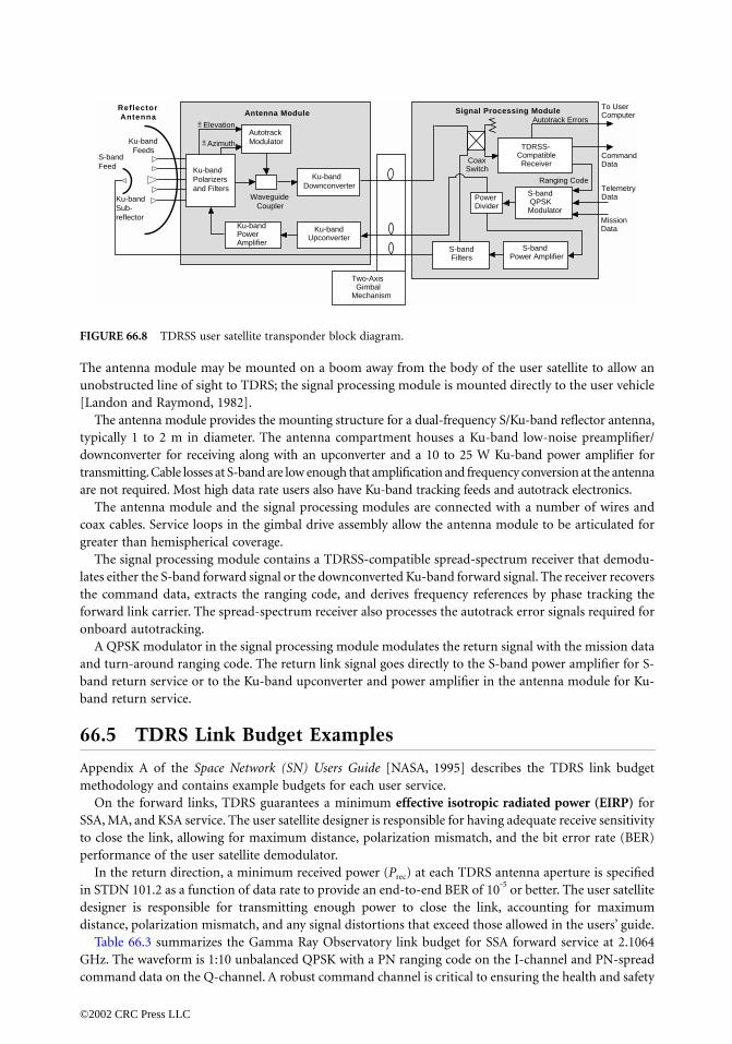
The antenna module may be mounted on a boom away from the body of the user satellite to allow anunobstructed line of sight to TDRS; the signal processing module is mounted directly to the user vehicle[Landon and Raymond, 1982].

The antenna module provides the mounting structure for a dual-frequency S/Ku-band reflector antenna,typically 1 to 2 m in diameter. The antenna compartment houses a Ku-band low-noise preamplifier/downconverter for receiving along with an upconverter and a 10 to 25 W Ku-band power amplifier fortransmitting. Cable losses at S-band are low enough that amplification and frequency conversion at the antennaare not required. Most high data rate users also have Ku-band tracking feeds and autotrack electronics.

The antenna module and the signal processing modules are connected with a number of wires andcoax cables. Service loops in the gimbal drive assembly allow the antenna module to be articulated forgreater than hemispherical coverage.

The signal processing module contains a TDRSS-compatible spread-spectrum receiver that demodu-lates either the S-band forward signal or the downconverted Ku-band forward signal. The receiver recoversthe command data, extracts the ranging code, and derives frequency references by phase tracking theforward link carrier. The spread-spectrum receiver also processes the autotrack error signals required foronboard autotracking.

A QPSK modulator in the signal processing module modulates the return signal with the mission dataand turn-around ranging code. The return link signal goes directly to the S-band power amplifier for S-band return service or to the Ku-band upconverter and power amplifier in the antenna module for Ku-band return service.

66.5 TDRS Link Budget Examples

Appendix A of the Space Network (SN) Users Guide [NASA, 1995] describes the TDRS link budgetmethodology and contains example budgets for each user service.

On the forward links, TDRS guarantees a minimum effective isotropic radiated power (EIRP) forSSA, MA, and KSA service. The user satellite designer is responsible for having adequate receive sensitivityto close the link, allowing for maximum distance, polarization mismatch, and the bit error rate (BER)performance of the user satellite demodulator.

In the return direction, a minimum received power (Prec) at each TDRS antenna aperture is specifiedin STDN 101.2 as a function of data rate to provide an end-to-end BER of 10-5 or better. The user satellitedesigner is responsible for transmitting enough power to close the link, accounting for maximumdistance, polarization mismatch, and any signal distortions that exceed those allowed in the users’ guide.

Table 66.3 summarizes the Gamma Ray Observatory link budget for SSA forward service at 2.1064GHz. The waveform is 1:10 unbalanced QPSK with a PN ranging code on the I-channel and PN-spreadcommand data on the Q-channel. A robust command channel is critical to ensuring the health and safety

FIGURE 66.8 TDRSS user satellite transponder block diagram.


AutotrackModulator

Ku-bandDownconverter

Ku-bandPowerAmplifier

Ku-bandUpconverter

S-band Filters

PowerDivider

TDRSS-Compatible Receiver

S-band QPSKModulator

S-bandPower Amplifier

To UserComputer

CommandData

TelemetryData

MissionData

CoaxSwitch

Ranging Code

Autotrack Errors

Two-Axis GimbalMechanism

Signal Processing ModuleAntenna Module

Elevation+−

+− Azimuth

Waveguide Coupler

Reflector Antenna

Ku-band Feeds

S-bandFeed

Ku-bandSub-reflector


of a satellite in orbit, and, as a result, GRO acquires the command signal with 19-dB margin and demod-ulates command data with almost 15-dB margin.

Table 66.4 shows a GRO link budget for one of several SSA return services that GRO is designed touse. The return center frequency, generated by multiplying the forward carrier frequency by 240/221, is2.2875 GHz. The waveform is 1:4 unbalanced QPSK with ranging and 32 kb/s telemetry data modulatedon the I-channel and with 512 kb/s mission data on the Q-channel. Like the command channel, telemetryis critical to spacecraft operations and is designed for greater than a 10 dB link margin. The mission datachannel has a 4.2-dB margin, which ensures excellent performance while allowing for any uncertaintiesand unexpected variations over temperature and life.

66.6 Summary

TDRSS has established a complete space communications infrastructure, providing command, telemetry,tracking, and wideband data relay services to NASA satellites in low-Earth orbit. Using relatively simplerelay satellites in geosynchronous orbits and a sophisticated ground complex at White Sands, TDRSS usersatellites have access to a full complement of forward and return communication capabilities at S-band

TABLE 66.3 Gamma Ray Observatory SSA Forward Link Budget

Parameter SSA Forward Service

TDRS SSA forward EIRP 43.5 dBWSpace loss from TDRS to user (44,000 km) -191.8 dBPolarization mismatch loss -0.2 dBGRO received power -148.5 dBWiGRO antenna gain (1.5 m, 48% efficiency) 27.6 dBiPointing loss (3σ error of 1.1∞) -0.4 dBEffective received power at GRO -121.3 dBWEffective thermal noise density (81,800 K) -179.8 dBW-HzGRO power received-to-noise ratio (Prec/No) 58.5 dB-HzMinimum Prec/No for acquisition and ranging 39.5 dB-HzAcquisition and ranging link margin 19.0 dBMininium Prec/No for 1-kb/s command data 43.7 dB-HzCommand link margin (10-5 BER) 14.8 dB

TABLE 66.4 Gamma Ray Observatory SSA Return Link Budget

Parameter SSA Return Service

GRO power amplifier (5.2 W) 7.2 dBWPower losses from amplifier to antenna -5.9 dBAntenna gain (1.5 m, 52% efficiency) 27.9 dBiGRO pointing loss (3s error of 1.1∞) -0.4 dBGRO transmitter EIRP 28.8 dBWPolarization mismatch loss -0.2 dBSpace loss from GRO to TDRS (44,000 km) -192.5 dBTDRS received power -163.9 dBWiI-channel power sharing (1/5) -7.0 dBI-channel distortion and interference losses -0.7 dBI-channel received power at TDRS -171.6 dBWiTDRS requirement (10-5 BER) -167.8 dBWiLink margin (Ranging, 32-Kb/s telemetry) 10.2 dBQ-channel power sharing (4/5) -1.0 dBQ-channel distortion and interference losses -1.7 dBQ-channel received power at TDRS -166.6 dBWiTDRS requirement (10-5 BER) -170.8 dBWiLink margin (512 Kb/s mission data) 4.2 dB


and Ku-band. The ZOE of the original satellite constellation has been closed by deploying a TDRS at 85∞East longitude, supported by a new facility (GRGT) on the island of Guam.

NASA has contracted with Boeing Satellite Systems, Inc. for three new TDRS satellites to allow replace-ment of the existing vehicles as they complete their useful lives on orbit. The new satellites, designatedTDRS-H, -I, and -J, are backwards compatible with respect to the services provided by the original TDRsatellites, have enhanced G/T and EIRP performance, and provide expanded user services in the Ka-band.Introduction of these next-generation relay satellites began with the successful Atlas/Centaur launch ofTDRS-H in June 2000. TDRS-I and -J was launched in 2000 and 2001, respectively, allowing NASA tocontinue providing TDRSS communications services to the space shuttle and other user satellites well intothe 21st century.

Defining Terms

Code-division multiple access: Use of families of near-orthogonal codes to allow several data streamsto occupy the same frequency band and pass through a single channel.

Effective isotropic radiated power: Transmitted flux density expressed in terms of the equivalent inputpower to an ideal unity gain transmit antenna.

Geosynchronous orbit: A 24-h orbit, approximately 35,800 km above the Earth, in which a satelliteappears, from the ground, to be almost stationary.

Ka-band: The frequency band between 18.0 and 40.0 GHz, in which several subbands are allocated forspace communications and space research.

Ku-band: The frequency band between 12.5 and 18.0 GHz, in which several subbands are allocated forspace communications and space research.

Pseudonoise code: Binary codes, generated using linear shift registers and sequential feedback, thatappear random and have good correlation properties.

Quadrature phase-shift keying: A modulation technique in which pairs of data bits are encoded ontoa carrier by rotating the phase to one of four biorthogonal positions.

S-band: The frequency band between 1.55 and 5.20 GHz, in which several subbands are allocated forspace communications and space research.

Spread-spectrum: Techniques, such as modulo-2 adding a PN-code to binary communications data,that increase bandwidth and reduce the power density of the signal.

References

Agrawal, B.N. 1986. Design of Geosynchronous Spacecraft, Prentice–Hall, Englewood Cliffs, NJ.Gagliardi, R.M. 1979. Phase coherency in tracking and data relay satellites. IEEE Trans. Comm., COM-

27(10):1527–1537.Gagliardi, R.M. 1984. Satellite Communications, Lifetime Learning Pub., Belmont, CA.Harper, W.R. and Woodson, W.L. 1981. The tracking and data relay satellite. ISA Trans., 20(2):49–62.Landon, R.B. and Raymond, H.G. 1982. Ku-band satellite communications via TDRSS, 9th AIAA Com-

munication Satellite Systems Conference, 82–0457.Martin, D.H. 2000. Communication Satellites, 4th ed., American Institute of Aeronautics.NASA. 1995. Space Network (SN) Users Guide, Rev. 7, Goddard Space Flight Center, Greenbelt, MD. 530-

SNUG (formerly STDN 101.2).Poza, H.B. 1979. TDRSS telecommunications payload: an overview. IEEE Trans. Aero. Elec. Syst., AES-

15(3):414–429.

Further Information

TDRSS was a special topic at the 1977 National Telecommunications Conference (NTC’77), and thecollection of TDRSS-related papers in the NTC’77 Conference Record (IEEE Publication 77CH12922CSCB) provides an excellent overview of the TDRS system. TDRSS user services and the TDRS user


interfaces are fully specified in the Space Network (SN) Users Guide, Rev. 7 [NASA, 1995]. For a generaloverview of spacecraft design, including orbital, launch vehicle, and payload electronics considerations,see Design of Geostationary Spacecraft [Agrawal, 1986]. Satellite Communications [Gagliardi, 1984] is agood introductory text covering digital communications through satellite channels. CommunicationSatellites, 4th ed. [Martin 2000], contains a technical summary of a large number of military, scientific,and commercial satellites, including additional material on the new TDRS-H, -I, and -J satellites.

Acknowledgments

The author wishes to sincerely thank Paul J. Heffernan at NASA Goddard Space Flight Center forproviding updated information on the tracking and data relay satellite system and for supporting thepreparation of the second edition of this material.


VIWireless

67 Wireless Personal Communications: A Perspective Donald C. Cox Introduction • Background and Issues • Evolution of Technologies, Systems,and Services • Evolution Toward the Future and to Low-Tier Personal CommunicationsServices • Comparisons with Other Technologies • Quality, Capacity, and EconomicIssues • Other Issues • Infrastructure Networks • Conclusion

68 Modulation Methods Gordon L. StüberIntroduction • Basic Description of Modulated Signals • Analog FrequencyModulation • Phase Shift Keying (PSK) and π/4-QPSK • Continuous PhaseModulation (CPM) and MSK • Gaussian Minimum Shift Keying • OrthogonalFrequency Division Multiplexing (OFDM) • Conclusions

69 Access Methods Bernd-Peter ParisIntroduction • Relevant Wireless Communication System Characteristics • FrequencyDivision Multiple Access • Time Division Multiple Access • Code DivisionMultiple Access • Comparison and Outlook

70 Rayleigh Fading Channels Bernard SklarIntroduction • The Challenge of a Fading Channel • Mobile-Radio Propagation:Large-Scale Fading and Small-Scale Fading • Signal Time-Spreading Viewed in theTime-Delay Domain: Figure 70.1, Block 7—The Multipath Intensity Profile • SignalTime-Spreading Viewed in the Frequency Domain: Figure 70.1, Block 10—The Spaced-Frequency Correlation Function • Typical Examples of Flat Fading and Frequency-SelectiveFading Manifestations • Time Variance Viewed in the Time Domain: Figure 70.1, Block 13—The Spaced-Time Correlation Function • Time Variance Viewed in the Doppler-ShiftDomain: Figure 70.1, Block 16—The Doppler Power Spectrum • Analogy Between SpectralBroadening in Fading Channels and Spectral Broadening in Digital Signal Keying• Degradation Categories due to Time Variance, Viewed in the Doppler-Shift Domain• Mitigation Methods • Summary of the Key Parameters Characterizing Fading Channels• The Viterbi Equalizer as Applied to GSM • The Rake Receiver Applied to Direct-SequenceSpread-Spectrum (DS/SS) Systems • Conclusion

71 Space-Time Processing Arogyaswami J. PaulrajIntroduction • The Space-Time Wireless Channel • Signal Models• ST Receive Processing (Base) • ST Transmit Processing (Base) • Summary

72 Location Strategies for Personal Communications Services Ravi K. Jain,Yi-Bing Lin and Seshadri MohanIntroduction • An Overview of PCS • IS-41 Preliminaries • Global System for MobileCommunications • Analysis of Database Traffic Rate for IS-41 and GSM • ReducingSignalling During Call Delivery • Per-User Location Caching • Caching ThresholdAnalysis • Techniques for Estimating Users’ LCMR • Discussion • Conclusions


73 Cell Design Principles Michel Daoud YacoubInt roduct ion • Cel lu lar Pr incip les • Per formance Measures and SystemRequirements • System Expansion Techniques • Basic Design Steps • Traffic Engineering• Cell Coverage • Interference • Conclusions

74 Microcellular Radio Communications Raymond SteeleIntroducing Microcells • Highway Microcells • City Street Microcells • IndoorMicrocells • Microcellular Infrastructure • Microcells in CDMA Networks • Discussion

75 Microcellular Reuse Patterns Michel Daoud Yacoub and Paula R. C. GomezIntroduction • Microcellular Reuse Patterns • Performance Analysis Model • Worst CaseCondition • A More Realistic Case Condition • Conclusions • Appendix

76 Fixed and Dynamic Channel Assignment Bijan JabbariI n t ro d u c t i o n • T h e Re s o u r ce A s s i g n m e n t Pro b l e m • F i xe d C h a n n e lAss ig nment • Enhanced Fixed Channe l Ass ig nment • Dynamic Channe lAssignment • CDMA Systems • Conclusion

77 Radiolocation Techniques Gordon L. Stüber and James J. Caffery, JrIntroduction • Description of Radiolocation Methods • Location Algorithms • Measuresof Location Accuracy • Location in Cellular Systems • Sources of LocationError • Summary and Conclusions

78 Power Control Roman Pichna and Qiang Wang In t ro d u c t i o n • C e l l u l a r Sy s te m s a n d Pow e r C o n t ro l • Pow e r C o n t ro lExamples • Summary

79 Enhancements in Second Generation Systems Marc Delprat and Vinod KumarI n t ro d u c t i o n • O ve r v i e w o f S e co n d G e n e r a t i o n Sy s t e m s • C a p a c i t yEnhancement • Quality Enhancement • High Bit Rate Data Transmission • Conclusion

80 The Pan-European Cellular System Lajos HanzoIntroduction • Overview • Logical and Physical Channels • Speech and DataTransmission • Transmission of Control Signals • Synchronization Issues • GaussianMinimum Shift Keying Modulation • Wideband Channel Models • Adaptive LinkControl • Discontinuous Transmission • Summary

81 Speech and Channel Coding for North American TDMA Cellular SystemsPaul MermelsteinIntroduction • Modulation of Digital Voice and Data Signals • Speech CodingFundamentals • Channel Coding Considerations • VSELP Encoder • Linear PredictionAnalysis and Quantization • Bandwidth Expansion • Quantizing and Encoding theRe fl e c t i o n C o e f fi c i e n t s • VS E L P C o d e b o o k S e a rch • Lo n g - Te r m F i l t e rSearch • Orthogonalization of the Codebooks • Quantizing the Excitation and SignalGains • Channel Coding and Interleaving • Bad Frame Masking • ACELPEncoder • Algebraic Codebook Structure and Search • Quantization of the Gains forACELP Encoding • Channel Coding for ACELP Encoding • Conclusions

82 The British Cordless Telephone Standard: CT-2 Lajos HanzoHistory and Background • The CT-2 Standard • The Radio Interface • BurstFormats • Signalling Layer Two (L2) • CPP-Initiated Link Setup Procedures• CFP-Initiated Link Setup Procedures • Handshaking • Main Featuresof the CT-2 System

83 Half-Rate Standards Wai-Yip Chan, Ira Gerson, and Toshio MikiIntroduction • Speech Coding for Cellular Mobile Radio Communications• Codec Selection and Performance Requirements • Speech Coding Techniquesin the Half-Rate Standards • Channel Coding Techniques in the Half-RateStandards • The Japanese Half-Rate Standard • The European GSM Half-RateStandard • Conclusions

84 Wireless Video Communications Madhukar Budagavi and Raj TalluriIntroduction • Wireless Video Communications • Error Resilient Video Coding• MPEG-4 Error Resilience Tools • H.263 Error Resilience Tools • Discussion

85 Wireless LANs Suresh SinghIntroduction • Physical Layer Design • MAC Layer Protocols • Network LayerIssues • Transport Layer Design • Conclusions


86 Wireless Data Allen H. Levesque and Kaveh PahlavanIntroduction • Characteristics of Wireless Data Networks • Market Issues • ModemServices Over Cellular Networks • Packet Data and Paging/Messaging Networks• Cellular Data Networks and Services • Other Developing Standards • Conclusions

87 Wireless ATM: Interworking Aspects Melbourne Barton, Matthew Cheng,and Li Fung ChangIntroduction • Background and Issues • Wireless Interworking With Transit ATMNetworks • The PCS-to-ATM Interworking Scenario • QoS Support • Conclusions

88 Wireless ATM: QoS and Mobility Management Bala Rajagopalan and Daniel ReiningerIntroduction • QoS in Wireless ATM • Mobility Management in Wireless ATM• Summary and Conclusions

89 An Overview of cdma2000, WCDMA, and EDGE Tero Ojanperäand Steven D. GrayI n t ro d u c t i o n • C D M A- B a s e d S c h e m e s • C D M A S y s t e m D e s i g nIssues • WCDMA • cdma2000 • TDMA-Based Schemes • Time Division Duplex(TDD) • Conclusions

90 Multiple-Input Multiple-Output (MIMO) Wireless Systems Helmut Bölcskeiand Arogyaswami J. Paulraj Introduction • The MIMO Fading Channel Model • Capacity of MIMOChannels • Spatial Multiplexing • Transmit Diversity • Summary and Conclusion

91 Near-Instantaneously Adaptive Wireless Transceivers of the Near FutureLie-Liang Yang and Lajos HanzoIntroduction • FH/MC DS-CDMA • Characteristics of the FH/MC DS-CDMASystems • Adaptive Rate Transmission • Software Defined Radio Assisted FH/MCDS-CDMA • Final Remarks

92 Ad-Hoc Routing Techniques for Wireless LANs Ahmed K. ElhakeemIntroduction • AODV (Ad-Hoc On-Demand Distance Vector Routing) • Fisheye Routing(FSR) • Hierarchical State Routing (HSR) • Destination-Sequenced Distance-VectorRouting (DSDV) • Zone Routing Protocol (ZRP) • Dynamic Source Routing (DSR)• Summary


67Wireless PersonalCommunications:

A Perspective

67.1 Introduction67.2 Background and Issues

Mobility and Freedom from Tethers

67.3 Evolution of Technologies, Systems,and ServicesCordless Telephones • Cellular Mobile Radio Systems • Wide-Area Wireless Data Systems • High-Speed Wireless Local-Area Networks (WLANs) •Paging/Messaging Systems • Satellite-Based Mobile Systems • Fixed Point-to-MultipointWireless Loops • Reality Check

67.4 Evolution Toward the Future and to Low-Tier Personal Communications Services.

67.5 Comparisons with Other TechnologiesComplexity/Coverage Area Comparisons • Coverage, Range, Speed, and Environments

67.6 Quality, Capacity, and Economic IssuesCapacity, Quality, and Complexity • Economics, System Capacity, and Coverage Area Size • Loop Evolution and Economics

67.7 Other IssuesImprovement of Batteries • People Only Want One Handset • Other Environments • Speech Quality Issues • New Technology • High-Tier to Low-Tier or Low-Tier to High-Tier Dual Mode

67.8 Infrastructure Networks 67.9 Conclusion

67.1 Introduction

Wireless personal communications has captured the attention of the media and with it, the imaginationof the public. Hardly a week goes by without one seeing an article on the subject appearing in a popularU.S. newspaper or magazine. Articles ranging from a short paragraph to many pages regularly appear inlocal newspapers, as well as in nationwide print media, e.g., The Wall Street Journal, The New York Times,Business Week, and U.S. News and World Report. Countless marketing surveys continue to project enor-mous demand, often projecting that at least half of the households, or half of the people, want wirelesspersonal communications. Trade magazines, newsletters, conferences, and seminars on the subject by

Donald C. CoxStanford University


many different names have become too numerous to keep track of, and technical journals, magazines,conferences, and symposia continue to proliferate and to have ever increasing attendance and numbersof papers presented. It is clear that wireless personal communications is, by any measure, the fastestgrowing segment of telecommunications. The explosive growth of wireless personal communications hascontinued unabated worldwide. Cellular and high-tier PCS pocketphones, pagers, and cordless telephoneshave become so common in many countries that few people even notice them anymore. These items havebecome an expected part of everyday life in most developed countries and in many developing countriesaround the world.

If you look carefully at the seemingly endless discussions of the topic, however, you cannot help butnote that they are often describing different things, i.e., different versions of wireless personal communi-cations [29,50]. Some discuss pagers, or messaging, or data systems, or access to the national informationinfrastructure, whereas others emphasize cellular radio, or cordless telephones, or dense systems of satel-lites. Many make reference to popular fiction entities such as Dick Tracy, Maxwell Smart, or Star Trek. Inaddition to the things noted above, the topic of wireless loops [24,30,32] has also become popular in thewidespread discussions of wireless communications. As discussed in [30], this topic includes several fixedwireless applications as well as the low-tier PCS application that was discussed originally under the wirelessloop designation [24,32]. The fixed wireless applications are aimed at reducing the cost of wireline loop-ends, i.e., the so-called “last mile” or “last km” of wireline telecommunications.

Thus, it appears that almost everyone wants wireless personal communications, but what is it? Thereare many different ways to segment the complex topic into different communications applications, modes,functions, extent of coverage, or mobility [29,30,50]. The complexity of the issues has resulted in con-siderable confusion in the industry, as evidenced by the many different wireless systems, technologies,and services being offered, planned, or proposed. Many different industry groups and regulatory entitiesare becoming involved. The confusion is a natural consequence of the massive dislocations that areoccurring, and will continue to occur, as we progress along this large change in the paradigm of the waywe communicate. Among the different changes that are occurring in our communications paradigm,perhaps the major constituent is the change from wired fixed place-to-place communications to wirelessmobile person-to-person communications. Within this major change are also many other changes, e.g.,an increase in the significance of data and message communications, a perception of possible changes invideo applications, and changes in the regulatory and political climates. The fixed wireless loop applica-tions noted earlier do not fit the new mobile communications paradigm. After many years of decline offixed wireless communications applications, e.g., intercontinental HF radio and later satellites, point-to-point terrestrial microwave radio, and tropospheric scatter, it is interesting to see this rebirth of interestin fixed wireless applications. This rebirth is riding on the gigantic “wireless wave” resulting from therapid public acceptance of mobile wireless communications. It will be interesting to observe this rebirthto see if communications history repeats; certainly mobility is wireless, but there is also considerablehistorical evidence that wireless is also mobility.

This chapter attempts to identify different issues and to put many of the activities in wireless into aframework that can provide perspective on what is driving them, and perhaps even to yield some indicationof where they appear to be going in the future. Like any attempt to categorize many complex interrelatedissues, however, there are some that do not quite fit into neat categories, and so there will remain somedangling loose ends. Like any major paradigm shift, there will continue to be considerable confusion asmany entities attempt to interpret the different needs and expectations associated with the new paradigm.

67.2 Background and Issues

Mobility and Freedom from Tethers

Perhaps the clearest constituents in all of the wireless personal communications activity are the desirefor mobility in communications and the companion desire to be free from tethers, i.e., from physicalconnections to communications networks. These desires are clear from the very rapid growth of mobile


technologies that provide primarily two-way voice services, even though economical wireline voiceservices are readily available. For example, cellular mobile radio has experienced rapid growth. Growthrates have been between 35 and 60% per year in the United States for a decade, with the total numberof subscribers reaching 20 million by year-end 1994. The often neglected wireless companions to cellularradio, i.e., cordless telephones, have experienced even more rapid, but harder to quantify, growth withsales rates often exceeding 10 million sets a year in the United States, and with an estimated usagesignificantly exceeding 50 million in 1994. Telephones in airlines have also become commonplace. Similaror even greater growth in these wireless technologies has been experienced throughout the world. Theexplosive growth in cellular and its identical companion, high-tier PCS, has continued to about 55 millionsubscribers in the U.S. at year-end 1997 and a similar number worldwide. In Sweden the penetration ofcellular subscribers by 1997 was over one-third of the total population, i.e., the total including everyman, woman, and child! And the growth has continued since. Similar penetrations of mobile wirelessservices are seen in some other developed nations, e.g., Japan. The growth in users of cordless telephonesalso has continued to the point that they have become the dominant subscriber terminal on wirelinetelephone loops in the U.S. It would appear that, taking into account cordless telephones and cellularand high-tier PCS phones, half of all telephone calls in the U.S. terminate with at least one end on awireless device.

Perhaps the most significant event in wireless personal communications since the writing of thisoriginal chapter was the widespread deployment and start of commercial service of personal handphone(PHS) in Japan in July of 1995 and its very rapid early acceptance by the consumer market [53]. By year-end 1996 there were 5 million PHS subscribers in Japan with the growth rate exceeding one-half million/month for some months. The PHS “phenomena” was one of the fastest adoptions of a new technologyever experienced. However, the PHS success story [41] peaked at a little over 7 million subscribers in1997 and has declined slightly to a little under 7 million in mid-1998. This was the first mass deploymentof a low-tier-like PCS technology (see later sections of this chapter), but PHS has some significantlimitations. Perhaps the most significant limitation is the inability to successfully handoff at vehicularspeeds. This handoff limitation is a result of the cumbersome radio link structure and control algorithmsused to implement dynamic channel allocation (DCA) in PHS. DCA significantly increases channeloccupancy (base station capacity) but incurs considerable complexity in implementing handoff. Anothersignificant limitation of the PHS standard has been insufficient receiver sensitivity to permit “adequate”coverage from a “reasonably” dense deployment of base stations. These technology deficiencies coupledwith heavy price cutting by the cellular service providers to compete with the rapid advancing of thePHS market were significant contributors to the leveling out of PHS growth. It is again evident, as withCT-2 phone point discussed in a later section, that low-tier PCS has very attractive features that canattract many subscribers, but it must also provide vehicle speed handoff and widespread coverage ofhighways as well as populated regions.

Others might point out the deployment and start of service of CDMA systems as a significant eventsince the first edition. However, the major significance of this CDMA activity is that it confirmed thatCDMA performance was no better than other less-complex technologies and that those, including thisauthor, who had been branded as “unbelieving skeptics” were correct in their assessments of the short-comings of this technology. The overwhelming failure of CDMA technology to live up to the early claimsfor it can hardly be seen as a significant positive event in the evolution of wireless communication. It was,of course, a significant negative event. After years of struggling with the problems of this technology, serviceproviders still have significantly fewer subscribers on CDMA worldwide than there are PHS subscribersin Japan alone! CDMA issues are discussed more in later sections dealing with technology issues.

Paging and associated messaging, although not providing two-way voice, do provide a form of teth-erless mobile communications to many subscribers worldwide. These services have also experiencedsignificant growth and have continued to grow since 1996. There is even a glimmer of a market in themany different specialized wireless data applications evident in the many wireless local area network(WLAN) products on the market, the several wide area data services being offered, and the specializedsatellite-based message services being provided to trucks on highways. Wireless data technologies still


have many supporters, but they still have fallen far short of the rapid deployment and growth of themore voice oriented wireless technologies. However, hope appears to be eternal in the wireless data arena.

The topics discussed in the preceding two paragraphs indicate a dominant issue separating the differentevolutions of wireless personal communications. That issue is the voice versus data communications issue thatpermeates all of communications today; this division also is very evident in fixed networks. The packet-orientedcomputer communications community and the circuit-oriented voice telecommunications (telephone) com-munity hardly talk to each other and often speak different languages in addressing similar issues. Althoughthey often converge to similar overall solutions at large scales (e.g., hierarchical routing with exceptions forembedded high-usage routes), the small-scale initial solutions are frequently quite different. Asynchronoustransfer mode (ATM)–based networks are an attempt to integrate, at least partially, the needs of both thepacket-data and circuit-oriented communities.

Superimposed on the voice-data issue is an issue of competing modes of communications that existin both fixed and mobile forms. These different modes include the following.

Messaging is where the communication is not real time but is by way of message transmission, storage,and retrieval. This mode is represented by voice mail, electronic facsimile (fax), and electronic mail (e-mail),the latter of which appears to be a modern automated version of an evolution that includes telegraph andtelex. Radio paging systems often provide limited one-way messaging, ranging from transmitting only thenumber of a calling party to longer alpha-numeric text messages.

Real-time two-way communications are represented by the telephone, cellular mobile radio telephone,and interactive text (and graphics) exchange over data networks. The two-way video phone alwayscaptures significant attention and fits into this mode; however, its benefit/cost ratio has yet to exceed avalue that customers are willing to pay.

Paging, i.e., broadcast with no return channel, alerts a paged party that someone wants to commu-nicate with him/her. Paging is like the ringer on a telephone without having the capability for completingthe communications.

Agents are new high-level software applications or entities being incorporated into some computernetworks. When launched into a data network, an agent is aimed at finding information by some titleor characteristic and returning the information to the point from which the agent was launched. Therapid growth of the World Wide Web is based on this mode of communications.

There are still other ways in which wireless communications have been segmented in attempts tooptimize a technology to satisfy the needs of some particular group. Examples include (1) user location,which can be differentiated by indoors or outdoors, or on an airplane or a train and (2) degree of mobility,which can be differentiated either by speed, e.g., vehicular, pedestrian, or stationary, or by size of areathroughout which communications are provided. As noted earlier, wireless local loop with stationaryterminals has become a major segment in the pursuit of wireless technology.

At this point one should again ask; wireless personal communications—what is it? The evidencesuggests that what is being sought by users, and produced by providers, can be categorized according tothe following two main characteristics.

Communications portability and mobility on many different scales:

• Within a house or building (cordless telephone, WLANs)

• Within a campus, a town, or a city (cellular radio, WLANs, wide area wireless data, radio paging,extended cordless telephone)

• Throughout a state or region (cellular radio, wide area wireless data, radio paging, satellite-basedwireless)

• Throughout a large country or continent (cellular radio, paging, satellite-based wireless)

• Throughout the world?

Communications by many different modes for many different applications:

• Two-way voice

• Data


• Messaging

• Video?

Thus, it is clear why wireless personal communications today is not one technology, not one system,and not one service but encompasses many technologies, systems, and services optimized for differentapplications.

67.3 Evolution of Technologies, Systems, and Services

Technologies and systems [27,29,30,39,50,59,67,87], that are currently providing, or are proposed toprovide, wireless communications services can be grouped into about seven relatively distinct groups,the seven previous groups are still evident in the technology but with the addition of the fixed point-to-multipoint wireless loops there are now eight, although there may be some disagreement on the groupdefinitions, and in what group some particular technology or system belongs. All of the technologies andsystems are evolving as technology advances and perceived needs change. Some trends are becomingevident in the evolutions. In this section, different groups and evolutionary trends are explored alongwith factors that influence the characteristics of members of the groups. The grouping is generally withrespect to scale of mobility and communications applications or modes.

Cordless Telephones

Cordless telephones [29,39,50] generally can be categorized as providing low-mobility, low-power, two-way tetherless voice communications, with low mobility applying both to the range and the user’s speed.Cordless telephones using analog radio technologies appeared in the late 1970s, and have experiencedspectacular growth. They have evolved to digital radio technologies in the forms of second-generationcordless telephone (CT-2), and digital European cordless telephone (DECT) standards in Europe, andseveral different industrial scientific medical (ISM) band technologies in the United States.1

Personal handyphone (PHS) noted earlier and discussed in later sections and inserts can be consideredeither as a quite advanced digital cordless telephone similar to DECT or as a somewhat limited low-tierPCS technology. It has most of the attributes of similarity of the digital cordless telephones listed laterin this section except that PHS uses π/4 QPSK modulation.

Cordless telephones were originally aimed at providing economical, tetherless voice communicationsinside residences, i.e., at using a short wireless link to replace the cord between a telephone base unitand its handset. The most significant considerations in design compromises made for these technologiesare to minimize total cost, while maximizing the talk time away from the battery charger. For digitalcordless phones intended to be carried away from home in a pocket, e.g., CT-2 or DECT, handset weightand size are also major factors. These considerations drive designs toward minimizing complexity andminimizing the power used for signal processing and for transmitting.

Cordless telephones compete with wireline telephones. Therefore, high circuit quality has become arequirement. Early cordless sets had marginal quality. They were purchased by the millions, and discardedby the millions, until manufacturers produced higher-quality sets. Cordless telephones sales then exploded.Their usage has become commonplace, approaching, and perhaps exceeding, usage of corded telephones.

The compromises accepted in cordless telephone design in order to meet the cost, weight, and talk-time objectives are the following.

• Few users per megahertz

• Few users per base unit (many link together a particular handset and base unit)

1These ISM technologies either use spread spectrum techniques (direct sequence or frequency hopping) or verylow-transmitter power (<~1 mW) as required by the ISM band regulations.


• Large number of base units per unit area; one or more base units per wireline access line (in high-rise apartment buildings the density of base units is very large)

• Short transmission range

There is no added network complexity since a base unit looks to a telephone network like a wirelinetelephone. These issues are also discussed in [29,50].

Digital cordless telephones in Europe have been evolving for a few years to extend their domain of usebeyond the limits of inside residences. Cordless telephone, second generation, (CT-2) has evolved toprovide telepoint or phone-point services. Base units are located in places where people congregate. e.g.,along city streets and in shopping malls, train stations, etc. Handsets registered with the phone-pointprovider can place calls when within range of a telepoint. CT-2 does not provide capability for transferring(handing off) active wireless calls from one phone point to another if a user moves out of range of theone to which the call was initiated. A CT-2+ technology, evolved from CT-2 and providing limitedhandoff capability, is being deployed in Canada. CT-2+ deployment was never completed. Phone-pointservice was introduced in the United Kingdom twice, but failed to attract enough customers to becomea viable service. In Singapore and Hong Kong, however, CT-2 phone point has grown rapidly, reachingover 150,000 subscribers in Hong Kong [75] in mid-1994. The reasons for success in some places andfailure in others are still being debated, but it is clear that the compactness of the Hong Kong and Singaporepopulations make the service more widely available, using fewer base stations than in more spreadoutcities. Complaints of CT-2 phone-point users in trials have been that the radio coverage was not completeenough, and/or they could not tell whether there was coverage at a particular place, and the lack of handoffwas inconvenient. In order to provide the alerting or ringing function for phone-point service, conven-tional radio pagers have been built into some CT-2 handsets. (The telephone network to which a CT-2phone point is attached has no way of knowing from which base units to send a ringing message, eventhough the CT-2 handsets can be rung from a home base unit). CT-2 phone points in Hong Kong peakedat about 170,000 subscribers. There was then a precipitous decline as these subscribers abandoned thelimited service CT-2 in favor of high-tier PCS and cellular services which had reduced their prices tocompete with phone points. Phone points have now been removed from Hong Kong. CT-2 phone pointswere also deployed in Korea, again with initial success followed by decline. The message is clear from theCT-2 and PHS experiences. The attributes of cordless phone-like low-tier PCS are very attractive, but needwidespread coverage and vehicle speed handoff in order to be long term attractive and viable in the market.

Another European evolution of cordless telephones is DECT, which was optimized for use insidebuildings. Base units are attached through a controller to private branch exchanges (PBXs), key telephonesystems, or phone company CENTREX telephone lines. DECT controllers can hand off active calls fromone base unit to another as users move, and can page or ring handsets as a user walks through areascovered by different base units. DECT has increased in deployment in some countries, notably Italy, forseveral applications including cordless telephone and wireless loop. There are reported to be perhaps7 million or more DECT users in Europe.

These cordless telephone evolutions to more widespread usage outside and inside with telepoints andto usage inside large buildings are illustrated in Fig. 67.1, along with the integration of paging intohandsets to provide alerting for phone-point services. They represent the first attempts to increase theservice area of mobility for low-power cordless telephones.

Some of the characteristics of the digital cordless telephone technologies, CT-2 and DECT, are listed inTable 67.1. Additional information can be found in [32,50]. Even though there are significant differencesbetween these technologies, e.g., multiple access technology [frequency division multiple access (FDMA)or time division multiple access (TDMA)/FDMA], and channel bit rate, there are many similarities thatare fundamental to the design objectives discussed earlier and to a user’s perception of them. Thesesimilarities and their implications are as follows.

32-kb/s Adaptive Differential Pulse Code Modulation (ADPCM) Digital Speech Encoding: This is alow-complexity (low-signal processing power) speech encoding process that provides wireline speechquality and is an international standard.


Average Transmitter Power ≤≤≤≤10 mW: This permits many hours of talk time with small, low-cost,lightweight batteries, but provides limited radio range.

Low-Complexity Radio Signal Processing: There is no forward error correction and no complexmultipath mitigation (i.e., no equalization or spread spectrum).

Low Transmission Delay, e.g., <<<<50 ms, and for CT-2 <<<<10-ms Round Trip: This is a speech-qualityand network-complexity issue. A maximum of 10 ms should be allowed, taking into account additionalinevitable delay in long-distance networks. Echo cancellation is generally required for delays >10 ms.

Simple Frequency-Shift Modulation and Noncoherent Detection: Although still being low in com-plexity, the slightly more complex 4QPSK modulation with coherent detection provides significantlymore spectrum efficiency, range, and interference immunity.

Dynamic Channel Allocation: Although this technique has potential for improved system capacity,the cordless-telephone implementations do not take full advantage of this feature for handoff and, thus,cannot reap the full benefit for moving users [15,19].

Time Division Duplex (TDD): This technique permits the use of a single contiguous frequency bandand implementation of diversity from one end of a radio link. Unless all base station transmissions aresynchronized in time, however, it can incur severe cochannel interference penalties in outside environ-ments [15,16]. Of course, for cordless telephones used inside with base stations not having a propagationadvantage, this is not a problem. Also, for small indoor PBX networks, synchronization of base stationtransmission is easier than is synchronization throughout a widespread outdoor network, which can havemany adjacent base stations connected to different geographic locations for central control and switching.

Cellular Mobile Radio Systems

Cellular mobile radio systems are becoming known in the United States as high-tier personal communica-tions service (PCS), particularly when implemented in the new 1.9-GHz PCS bands [20]. These systemsgenerally can be categorized as providing high-mobility, wide-ranging, two-way tetherless voice communi-cations. In these systems, high mobility refers to vehicular speeds, and also to widespread regional tonationwide coverage [27,29,50]. Mobile radio has been evolving for over 50 years. Cellular radio integrateswireless access with large-scale networks having sophisticated intelligence to manage mobility of users.

Cellular radio was designed to provide voice service to wide-ranging vehicles on streets and highways[29,39,50,82], and generally uses transmitter power on the order of 100 times that of cordless telephones

FIGURE 67.1


Low-Power Systems

-Tier PCS Digital Cordless

Handi-Phone DECT CT-2TDMA/FDMA TDMA/FDMA FDMA 1895–1907 1880–1990 864–868

(Japan) (Eur.) (Eur. and Asia)

300 1728 100

π

/4 DQPSK GFSK GFSK

80 mW/10 mW 250 mW/10 mW 10 mW/5 mW

ADPCM ADPCM ADPCM

32 32 32

4 12 1

384 1152 72

CRC CRC None(control)

5 10 2

TABLE 67.1 Wireless PCS Technologies

High-Power Systems

Digital Cellular (High-Tier PCS) Low

System IS-54 IS-95 (DS) GSM DCS-1800 WACS/PACSMultiple Access TDMA/FDMA CDMA/FDMA TDMA/FDMA TDMA/FDMA TDMA/FDMAFreq. band, MHz

Uplink, MHz 869–894 869–894 935–960 1710–1785 Emerg. Tech.*Downlink, MHz 824–849 824–849 890–915 1805–1880

(USA) (USA) (Eur.) (UK) (USA)

RF ch. spacingDownlink, KHz 30 1250 200 200 300Uplink, KHz 30 1250 200 200 300

Modulation π/4 DQPSK BPSK/QPSK GMSK GMSK π/4 QPSK

Portable txmit Power, max./avg.

600 mW/200 mW 600 mW 1 W/125 mW 1 W/125 mW 200 mW/25 mW

Speech coding VSELP QCELP RPE-LTP RPE-LTP ADPCM

Speech rate, kb/s 7.95 8 (var.) 13 13 32/16/8

Speech ch./RF ch. 3 — 8 8 8/16/32

Ch. Bit rate, kb/sUplink, kb/s 48.6 270.833 270.833 384Downlink, kb/s 48.6 270.833 270.833 384

Ch. coding 1/2 rate 1/2 rate fwd. 1/2 rate 1/2 rate CRCconv. 1/3 rate rev. conv. conv.

Frame, ms 40 20 4.615 4.615 2.5

*Spectrum is 1.85–2.2 GHz allocated by the FCC for emerging technologies; DS is direct sequence.


(≈2 W for cellular). Thus, cellular systems can only provide reduced service to handheld sets that aredisadvantaged by using somewhat lower transmitter power (<0.5 W) and less efficient antennas thanvehicular sets. Handheld sets used inside buildings have the further disadvantage of attenuation throughwalls that is not taken into account in system design.

Cellular radio or high-tier PCS has experienced large growth as noted earlier. In spite of the limitationson usage of handheld sets already noted, handheld cellular sets have become very popular, with theirsales becoming comparable to the sales of vehicular sets. Frequent complaints from handheld cellularusers are that batteries are too large and heavy, and both talk time and standby time are inadequate.Cellular and high-tier PCS pocket handsets have continued to decrease in size and weight and moreefficient lithium batteries have been incorporated. This has increased their attractiveness (more on thisin the later section, Reality Check). For several years there have been many more pocket handsets soldthan vehicular mounted sets every year. However, despite the improvements in these handsets andbatteries, the complaints of weight and limited talk time still persist. The electronics have becomeessentially weightless compared to the batteries required for these high-tier PCS and cellular handsets.

Cellular radio at 800 MHz has evolved to digital radio technologies [29,39,50] in the forms of thedeployed systems standards

• Global Standard for Mobile (GSM) in Europe

• Japanese or personal digital cellular (JDC or PDC) in Japan

• U.S. TDMA digital cellular known as USDC or IS-54

and in the form of the code division multiple access (CDMA) standard, IS-95, which is under developmentbut not yet deployed. Since the first edition was published, CDMA systems have been deployed in theU.S., Korea, Hong Kong, and other countries after many months (years) of redesign, reprogramming,and adjustment. These CDMA issues are discussed later in the section “New Technology.”

The most significant consideration in the design compromises made for the U.S. digital cellular orhigh-tier PCS systems was the high cost of cell sites (base stations). A figure often quoted is U.S. $1million for a cell site. This consideration drove digital system designs to maximize users per megahertzand to maximize the users per cell site.

Because of the need to cover highways running through low-population-density regions between cities,the relatively high transmitter power requirement was retained to provide maximum range from highantenna locations.

Compromises that were accepted while maximizing the two just cited parameters are as follows.

• High transmitter power consumption.

• High user-set complexity, and thus high signal-processing power consumption.

• Low circuit quality.

• High network complexity, e.g., the new IS-95 technology will require complex new switching andcontrol equipment in the network, as well as high-complexity wireless-access technology.

Cellular radio or high-tier PCS has also been evolving for a few years in a different direction, towardvery small coverage areas or microcells. This evolution provides increased capacity in areas having highuser density, as well as improved coverage of shadowed areas. Some microcell base stations are beinginstalled inside, in conference center lobbies and similar places of high user concentrations. Of course,microcells also permit lower transmitter power that conserves battery power when power control isimplemented, and base stations inside buildings circumvent the outside wall attenuation. Low-complexitymicrocell base stations also are considerably less expensive than conventional cell sites, perhaps two ordersof magnitude less expensive. Thus, the use of microcell base stations provides large increases in overallsystem capacity, while also reducing the cost per available radio channel and the battery drain on portablesubscriber equipment. This microcell evolution, illustrated in Fig. 67.1, moves handheld cellular sets ina direction similar to that of the expanded-coverage evolution of cordless telephones to phone pointsand wireless PBX.


Some of the characteristics of digital-cellular or high-tier PCS technologies are listed in Table 67.1 forIS-54, IS-95, and GSM at 900 MHz, and DCS-1800, which is GSM at 1800 MHz. The technology listedhere as IS-54 has also become known as IS-136 having more sophisticated digital control channels. Thesetechnologies, IS-54/IS-136 are also sometimes known as DAMPS (i.e., Digital AMPS), as U.S. TDMA orNorth American TDMA, or sometimes just as “TDMA.” Additional information can be found in [29,39,50].The JDC or PDC technology, not listed, is similar to IS-54. As with the digital cordless technologies, thereare significant differences among these cellular technologies, e.g., modulation type, multiple access tech-nology, and channel bit rate. There are also many similarities, however, that are fundamental to the designobjectives discussed earlier. These similarities and their implications are as follows.

Low Bit-Rate Speech Coding ≤≤≤≤13 kb/s with Some ≤≤≤≤8 kb/s: Low bit-rate speech coding obviouslyincreases the number of users per megahertz and per cell site. However, it also significantly reduces speechquality [29], and does not permit speech encodings in tandem while traversing a network; see also thesection on Other Issues later in this chapter.

Some Implementations Make Use of Speech Inactivity: This further increases the number of usersper cell site, i.e., the cell-site capacity. It also further reduces speech quality [29], however, because of thedifficulty of detecting the onset of speech. This problem is even worse in an acoustically noisy environmentlike an automobile.

High Transmission Delay; ≈≈≈≈200-ms Round Trip: This is another important circuit-quality issue. Suchlarge delay is about the same as one-way transmission through a synchronous-orbit communicationssatellite. A voice circuit with digital cellular technology on both ends will experience the delay of a fullsatellite circuit. It should be recalled that one reason long-distance circuits have been removed from satellitesand put onto fiber-optic cable is because customers find the delay to be objectionable. This delay in digitalcellular technology results from both computation for speech bit-rate reduction and from complex signalprocessing, e.g., bit interleaving, error correction decoding, and multipath mitigation [equalization orspread spectrum code division multiple access (CDMA)].

High-Complexity Signal Processing, Both for Speech Encoding and for Demodulation: Signal pro-cessing has been allowed to grow without bound and is about a factor of 10 greater than that used inthe low-complexity digital cordless telephones [29]. Since several watts are required from a battery toproduce the high transmitter power in a cellular or high-tier PCS set, signal-processing power is not assignificant as it is in the low-power cordless telephones; see also the section on Complexity/CoverageArea Comparisons later in this chapter.

Fixed Channel Allocation: The difficulties associated with implementing capacity-increasing dynamicchannel allocation to work with handoff [15,19] have impeded its adoption in systems requiring reliableand frequent handoff.

Frequency Division Duplex (FDD): Cellular systems have already been allocated paired-frequency bandssuitable for FDD. Thus, the network or system complexity required for providing synchronized transmis-sions [15,16] from all cell sites for TDD has not been embraced in these digital cellular systems. Note thatTDD has not been employed in IS-95 even though such synchronization is required for other reasons.

Mobile/Portable Set Power Control: The benefits of increased capacity from lower overall cochannelinterference and reduced battery drain have been sought by incorporating power control in the digitalcellular technologies.

Wide-Area Wireless Data Systems

Existing wide-area data systems generally can be categorized as providing high mobility, wide-ranging,low-data-rate digital data communications to both vehicles and pedestrians [29,50]. These systems havenot experienced the rapid growth that the two-way voice technologies have, even though they have beendeployed in many cities for a few years and have established a base of customers in several countries.Examples of these packet data systems are shown in Table 67.2.


The earliest and best known of these systems in the United States are the ARDIS network developedand run by Motorola, and the RAM mobile data network based on Ericsson Mobitex Technology. Thesetechnologies were designed to make use of standard, two-way voice, land mobile-radio channels, with12.5- or 25-kHz channel spacing. In the United States these are specialized mobile radio services (SMRS)allocations around 450 MHz and 900 MHz. Initially, the data rates were low: 4.8 kb/s for ARDIS and8 kb/s for RAM. The systems use high transmitter power (several tens of watts) to cover large regionsfrom a few base stations having high antennas. The relatively low data capacity of a relatively expensivebase station has resulted in economics that have not favored rapid growth.

The wide-area mobile data systems also are evolving in several different directions in an attempt toimprove base station capacity, economics, and the attractiveness of the service. The technologies used inboth the ARDIS and RAM networks are evolving to higher channel bit rates of 19.2 kb/s.

The cellular carriers and several manufacturers in the United States are developing and deploying a newwide-area packet data network as an overlay to the cellular radio networks. This cellular digital packet data(CDPD) technology shares the 30-kHz spaced 800-MHz voice channels used by the analog FM advancedmobile phone service (AMPS) systems. Data rate is 19.2 kb/s. The CDPD base station equipment alsoshares cell sites with the voice cellular radio system. The aim is to reduce the cost of providing packet dataservice by sharing the costs of base stations with the better established and higher cell-site capacity cellularsystems. This is a strategy similar to that used by nationwide fixed wireline packet data networks that couldnot provide an economically viable data service if they did not share costs by leasing a small amount ofthe capacity of the interexchange networks that are paid for largely by voice traffic. CDPD has been deployedin many U.S. cities for several years. However, it has not lived up to early expectations and has become“just another” wireless data service with some subscribers, but not with the large growth envisioned earlier.

Another evolutionary path in wide-area wireless packet data networks is toward smaller coverage areasor microcells. This evolutionary path also is indicated in Fig. 67.1. The microcell data networks are aimedat stationary or low-speed users. The design compromises are aimed at reducing service costs by makingvery small and inexpensive base stations that can be attached to utility poles, the sides of buildings andinside buildings and can be widely distributed throughout a region. Base-station-to-base-station wirelesslinks are used to reduce the cost of the interconnecting data network. In one network this decreases theoverall capacity to serve users, since it uses the same radio channels that are used to provide service.Capacity is expected to be made up by increasing the number of base stations that have connections toa fixed-distribution network as service demand increases. Another such network uses other dedicatedradio channels to interconnect base stations. In the high-capacity limit, these networks will look morelike a conventional cellular network architecture, with closely spaced, small, inexpensive base stations,i.e., microcells, connected to a fixed infrastructure. Specialized wireless data networks have been built toprovide metering and control of electric power distributions, e.g., Celldata and Metricom in California.

TABLE 67.2 Wide-Area Wireless Packet Data Systems

CDPD1RAM Mobile

(Mobitex) ARDIS2 (KDT)Metricom (MDN)3

Data rate, kb/s 19.2 8 (19.2) 4.8 (19.2) 76Modulation GMSK BT = 0.5 GMSK GMSK GMSKFrequency, MHz 800 900 800 915Chan. spacing, kHz 30 12.5 25 160Status 1994 service Full service Full service In serviceAccess means Unused AMPS

channelsSlotted Aloha

CSMAFH SS (ISM)

Transmit power, W 40 1

Note: Data in parentheses ( ) indicates proposed.1Cellular Digital Packet Data2Advanced Radio Data Information Service3Microcellular Data Network


A large microcell network of small inexpensive base stations has been installed in the lower SanFrancisco Bay Area by Metricom, and public packet-data service was offered during early 1994. Most ofthe small (shoe-box size) base stations are mounted on street light poles. Reliable data rates are about75 kb/s. The technology is based on slow frequency-hopped spread spectrum in the 902–928 MHz U.S.ISM band. Transmitter power is 1 W maximum, and power control is used to minimize interference andmaximize battery life time. The metricom network has been improved and significantly expanded in theSan Francisco Bay Area and has been deployed in Washington, D.C., and a few other places in the U.S.However, like all wireless data services so far, it has failed to grow as rapidly or to attract as manysubscribers as was originally expected. Wireless data overall has had only very limited success comparedto that of the more voice-oriented technologies, systems, and services.

High-Speed Wireless Local-Area Networks (WLANs)

Wireless local-area data networks can be categorized as providing low-mobility high-data-rate datacommunications within a confined region, e.g., a campus or a large building. Coverage range from awireless data terminal is short, tens to hundreds of feet, like cordless telephones. Coverage is limited towithin a room or to several rooms in a building. WLANs have been evolving for a few years, but overallthe situation is chaotic, with many different products being offered by many different vendors [29,59].There is no stable definition of the needs or design objectives for WLANs, with data rates ranging fromhundreds of kb/s to more than 10 Mb/s, and with several products providing one or two Mb/s wirelesslink rates. The best description of the WLAN evolutionary process is: having severe birth pains. An IEEEstandards committee, 802.11, has been attempting to put some order into this topic, but their successhas been somewhat limited. A partial list of some advertised products is given in Table 67.3. Users ofWLANs are not nearly as numerous as the users of more voice-oriented wireless systems. Part of thedifficulty stems from these systems being driven by the computer industry that views the wireless systemas just another plug-in interface card, without giving sufficient consideration to the vagaries and needsof a reliable radio system. This section still describes the WLAN situation in spite of some attempts atstandards in the U.S. and Europe, and continuing industry efforts. Some of the products in Table 67.3have been discontinued because of lack of market and some new products have been offered, but themanufacturers still continue to struggle to find enough customers to support their efforts. Optimismremains high in the WLAN community that “eventually” they will find the “right” technology, service,or application to make WLANs “take off”—but the world still waits. Success is still quite limited.

There are two overall network architectures pursued by WLAN designers. One is a centrally coordinatedand controlled network that resembles other wireless systems. There are base stations in these networksthat exercise overall control over channel access [44].

The other type of network architecture is the self-organizing and distributed controlled network whereevery terminal has the same function as every other terminal, and networks are formed ad hoc by com-munications exchanges among terminals. Such ad hoc networks are more like citizen band (CB) radionetworks, with similar expected limitations if they were ever to become very widespread.

Nearly all WLANs in the United States have attempted to use one of the ISM frequency bands forunlicensed operation under part 15 of the FCC rules. These bands are 902–928 MHz, 2400–2483.5 MHz,and 5725–5850 MHz, and they require users to accept interference from any interfering source that mayalso be using the frequency. The use of ISM bands has further handicapped WLAN development becauseof the requirement for use of either frequency hopping or direct sequence spread spectrum as an accesstechnology, if transmitter power is to be adequate to cover more than a few feet. One exception to theISM band implementations is the Motorola ALTAIR, which operates in a licensed band at 18 GHz. Itappears that ALTAIR has been discontinued because of the limited market. The technical and economicchallenges of operation at 18 GHz have hampered the adoption of this 10–15 Mb/s technology. Thefrequency-spectrum constraints have been improved in the United States with the recent FCC allocationof spectrum from 1910–1930 MHz for unlicensed data PCS applications. Use of this new spectrumrequires implementation of an access etiquette incorporating listen before transmit in an attempt to


provide some coordination of an otherwise potentially chaotic, uncontrolled environment [68]. Also,since spread spectrum is not a requirement, access technologies and multipath mitigation techniquesmore compatible with the needs of packet-data transmission [59], e.g., multipath equalization or mul-ticarrier transmission, can be incorporated into new WLAN designs. The FCC is allocating spectrum at5 GHz for wideband wireless data for internet and next generation data network access, BUT it remainsto be seen whether this initiative is any more successful than past wireless data attempts. Optimism isagain high, BUT…

Three other widely different WLAN activities also need mentioning. One is a large European Tele-communications Standards Institute (ETSI) activity to produce a standard for high performance radiolocal area network (HIPERLAN), a 20-Mb/s WLAN technology to operate near 5 GHz. Other activitiesare large U.S. Advance Research Projects Agency (ARPA)–sponsored WLAN research projects at theUniversities of California at Berkeley (UCB) and at Los Angeles (UCLA). The UCB Infopad project isbased on a coordinated network architecture with fixed coordinating nodes and direct-sequence spreadspectrum (CDMA), whereas, the UCLA project is aimed at peer-to-peer networks and uses frequencyhopping. Both ARPA-sponsored projects are concentrated on the 900-MHz ISM band.

As computers shrink in size from desktop to laptop to palmtop, mobility in data network access isbecoming more important to the user. This fact, coupled with the availability of more usable frequencyspectrum, and perhaps some progress on standards, may speed the evolution and adoption of wirelessmobile access to WLANs. From the large number of companies making products, it is obvious that manybelieve in the future of this market. It should be noted that the objective for 10 MB/s data service withwidespread coverage from a sparse distribution of widely separated base stations equivalent to cellularis unrealistic and unrealizable. This can be readily seen by considering a simple example. Consider acellular coverage area that requires full cellular power of 0.5 watt to cover from a handset. Consider thehandset to use a typical digital cellular bit rate of about 10 kb/s (perhaps 8 kb/s speech coding + overhead).With all else in the system the same, e.g., antennas, antenna height, receiver noise figure, detectionsensitivity, etc., the 10 MB/s data would require 10 MB/s ∏ 10 kb/s = 1000 times as much power as the10 kb/s cellular. Thus, it would require 0.5 × 1000 = 500 watts for the wireless data transmitter. This isa totally unrealistic situation. If the data system operates at a higher frequency (e.g., 5 GHz) than thecellular system (e.g., 1 or 2 GHz) then there will be even more power required to overcome the additionalloss at a higher frequency. The sometimes expressed desire by the wireless data community for a systemto provide network access to users in and around buildings and to provide 10 MB/s over 10 miles with10 milliwatts of transmitter power and costing $10.00 is totally impossible. It requires violation of the“laws of physics.”

Paging/Messaging Systems

Radio paging began many years ago as a one-bit messaging system. The one bit was: someone wants tocommunicate with you. More generally, paging can be categorized as one-way messaging over wide areas.The one-way radio link is optimized to take advantage of the asymmetry. High transmitter power(hundreds of watts to kilowatts), and high antennas at the fixed base stations permit low-complexity,very low-power consumption, pocket paging receivers that provide long usage time from small batteries.This combination provides the large radio-link margins needed to penetrate walls of buildings withoutburdening the user set battery. Paging has experienced steady rapid growth for many years and servesabout 15 million subscribers in the United States.

Paging also has evolved in several different directions. It has changed from analog tone coding for useridentification to digitally encoded messages. It has evolved from the 1-b message, someone wants you,to multibit messages from, first, the calling party’s telephone number to, now, short e-mail text messages.This evolution is noted in Fig. 67.1.

The region over which a page is transmitted has also increased from (1) local, around one transmittingantenna; to (2) regional, from multiple widely-dispersed antennas; to (3) nationwide, from large networksof interconnected paging transmitters. The integration of paging with CT-2 user sets for phone-pointcall alerting was noted previously.


Mod./Coding

Power, mW Network Topology

4-level FSK 25 peak Eight devices/radio; radio to base to ethernet

DQPSK 250 Peer-to-peer

DQPSK 250 PCMCIA w/ant.; radio to hub

16 PSK trellis coding

650 Hub

DQPSK 250 Hub

20 Peer-to-peer

©2002 C

RC

Press LL

C

TABLE 67.3 Partial List of WLAN Products

ProductCompanyLocation

Freq., MHz

Link Rate, Mb/s User Rate Protocol(s) Access

No. of chan. orSpread Factor

Altair PlusMotorolaArlington Hts, IL

18–19GHz

15 5.7 Mb/s Ethernet

WaveLANNCR/AT&TDayton, OH

902–928 2 1.6 Mb/s Ethernet-like DS SS

AirLanSolectekSan Diego, CA

902–928 2 Mb/s Ethernet DS SS

FreeportWindata Inc.Northboro, MA

902–928 16 5.7 Mb/s Ethernet DS SS 32 chips/bit

IntersectPersoft Inc.Madison, WI

902–928 2 Mb/s Ethernet token ring

DS SS

LAWNO’Neill Comm.Horsham, PA

902–928 38.4 kb/s AX.25 SS 20 users/chan.;max. 4 chan.


nconven-tional

30 Peer-to-peer

100 Peer-to-peer

1 W max PCs with ant.; radio to hub

Hub

100

100 Peer-to-peerbridge

Hub

6 PSK trellis coding

100 Hub

©2002 C

RC

Press LL

C

WILANWi-LAN Inc.Calgary, Alberta

902–928 20 1.5 Mb/s/chan.

Ethernet, token ring

CDMA/TDMA

3 chan. 10–15 links each

u

RadioPortALPS ElectricUSA

902–928 242 kb/s Ethernet SS 7/3 channels

ArLAN 600 Telesys. SLWDon Mills, Ont.

902–928; 2.4 GHz

1.35 Mb/s Ethernet SS

Radio LinkCal. MicrowaveSunnyvale, CA

902–928; 2.4 GHz

250 kb/s 64 kb/s FH SS 250 ms/hop500 kHz space

Range LANProxim, Inc.Mountain View, CA

902–928 242 kb/s Ethernet, token ring

DS SS 3 chan.

RangeLAN 2Proxim, Inc.Mountain View, CA

2.4 GHz 1.6 50 kb/s max. Ethernet, token ring

FH SS 10 chan. at 5 kb/s; 15 sub-ch. each

NetwaveXircomCalabasas, CA

2.4 GHz 1/adaptor Ethernet, token ring

FH SS 82 l-MHzchn. or “hops”

FreelinkCabletron Sys.Rochester, NH

2.4 and 5.8 GHz

5.7 Mb/s Ethernet DS SS 32 chips/bit 1


Another evolutionary paging route sometimes proposed is two-way paging. This is an ambiguous andunrealizable concept, however, since the requirement for two-way communications destroys the asymmet-rical link advantage so well exploited by paging. Two-way paging puts a transmitter in the user’s set andbrings along with it all of the design compromises that must be faced in such a two-way radio system.Thus, the word paging is not appropriate to describe a system that provides two-way communications.The two-way paging situation is as unrealistic as that noted earlier for wide-area, high-speed, low-powerwireless data. This can be seen by looking at the asymmetry situation in paging. In order to achievecomparable coverage uplink and downlink, a 500-watt paging transmitter downlink advantage must beovercome in the uplink. Even considering the relatively high cellular handset transmit power levels onthe order of 0.5 watt results in a factor of 1000 disadvantage, and 0.5 watt is completely incompatible withthe low power paging receiver power requirements. If the same uplink and downlink coverage is requiredfor an equivalent set of system parameters, then the only variable left to work with is bandwidth. If thepaging link bit rate is taken to be 10 kb/sec (much higher than many paging systems), then the usableuplink rate is 10 kb/s/1000 = 10 B/s, an unusably low rate. Of course, some uplink benefit can be gainedbecause of better base station receiver noise figure and by using forward error correction and perhapsARQ. However, this is unlikely to raise the allowable rate to greater than 100 B/s which even though likelyoveroptimistic is still unrealistically low and we have assumed an unrealistically high transmit power inthe two-way “pager!”

Satellite-Based Mobile Systems

Satellite-based mobile systems are the epitome of wide-area coverage, expensive base station systems.They generally can be categorized as providing two-way (or one-way) limited quality voice and/or verylimited data or messaging to very wide-ranging vehicles (or fixed locations). These systems can providevery widespread, often global, coverage, e.g., to ships at sea by INMARSAT. There are a few messagingsystems in operation, e.g., to trucks on highways in the United States by Qualcomm’s Omnitracs system.

A few large-scale mobile satellite systems have been proposed and are being pursued: perhaps the bestknown is Motorola’s Iridium; others include Odyssey, Globalstar, and Teledesic. The strength of satellitesystems is their ability to provide large regional or global coverage to users outside buildings. However,it is very difficult to provide adequate link margin to cover inside buildings, or even to cover locationsshadowed by buildings, trees, or mountains. A satellite system’s weakness is also its large coverage area.It is very difficult to provide from Earth orbit the small coverage cells that are necessary for providinghigh overall systems capacity from frequency reuse. This fact, coupled with the high cost of the orbitalbase stations, results in low capacity along with the wide overall coverage but also in expensive service.Thus, satellite systems are not likely to compete favorably with terrestrial systems in populated areas oreven along well-traveled highways. They can complement terrestrial cellular or PCS systems in low-population-density areas. It remains to be seen whether there will be enough users with enough moneyin low-population-density regions of the world to make satellite mobile systems economically viable.Some of the mobile satellite systems have been withdrawn, e.g., Odyssey. Some satellites in the Iridiumand Globalstar systems have been launched. The industry will soon find out whether these systems areeconomically viable.

Proposed satellite systems range from (1) low-Earth orbit systems (LEOS) having tens to hundreds ofsatellites through (2) intermediate- or medium-height systems (MEOS) to (3) geostationary or geosyn-chronous orbit systems (GEOS) having fewer than ten satellites. LEOS require more, but less expensive,satellites to cover the Earth, but they can more easily produce smaller coverage areas and, thus, providehigher capacity within a given spectrum allocation. Also, their transmission delay is significantly less(perhaps two orders of magnitude!), providing higher quality voice links, as discussed previously. Onthe other hand, GEOS require only a few, somewhat more expensive, satellites (perhaps only three) andare likely to provide lower capacity within a given spectrum allocation and suffer severe transmission-delay impairment on the order of 0.5 s. Of course, MEOS fall in between these extremes. The possibleevolution of satellite systems to complement high-tier PCS is indicated in Fig. 67.1.


Fixed Point-to-Multipoint Wireless Loops

Wideband point-to-multipoint wireless loop technologies sometimes have been referred to earlier as“wireless cable” when they were proposed as an approach for providing interactive video services tohomes [30]. However, as the video application started to appear less attractive, the application emphasisshifted to providing wideband data access for the internet, the worldwide web, and future wideband datanetworks. Potentially lower costs are the motivation for this wireless application. As such, these technol-ogies will have to compete with existing coaxial cable and fiber/coax distribution by CATV companies,with satellites, and with fiber and fiber/coax systems being installed or proposed by telephone companiesand other entities [30]. Another competitor is asymmetric digital subscriber line technology, which usesadvanced digital signal processing to provide high-bandwidth digital distribution over twisted copperwire pairs.

In the U.S. two widely different frequency bands are being pursued for fixed point-to-multipointwireless loops. These bands are at 28 GHz for local multipoint distribution systems or services (LMDS)[52] and 2.5 to 2.7 GHz for microwave or metropolitan distribution systems (MMDS) [74]. The goal oflow-cost fixed wireless loops is based on the low cost of point-to-multipoint line-of-sight wirelesstechnology. However, significant challenges are presented by the inevitable blockage by trees, terrain, andhouses, and by buildings in heavily built-up residential areas. Attenuation in rainstorms presents anadditional problem at 28 GHz in some localities. Even at the 2.5-GHz MMDS frequencies, the largebandwidth required for distribution of many video channels presents a challenge to provide adequateradio-link margin over obstructed paths. From mobile satellite investigations it is known that trees canoften produce over 15 dB additional path attenuation [38]. Studies of blockage by buildings in cities haveshown that it is difficult to have line-of-sight access to more than 60% of the buildings from a singlebase station [55]. Measurements in a region in Brooklyn, NY [60], suggest that access from a single basestation can range from 25% to 85% for subscriber antenna heights of 10 to 35 ft and a base station heightof about 290 ft. While less blockage by houses could be expected in residential areas, such numbers wouldsuggest that greater than 90% access to houses could be difficult, even from multiple elevated locations,when mixes of one- and two-story houses, trees, and hills are present. In regions where tree cover isheavy, e.g., the eastern half of the U.S., tree cover in many places will present a significant obstacle. Heavyrainfall is an additional problem at 28 GHz in some regions. In spite of these challenges, the lure of low-cost wireless loops is attracting many participants, both service providers and equipment manufacturers.

Reality Check

Before we go on to consider other applications and compromises, perhaps it would be helpful to see ifthere is any indication that the previous discussion is valid. For this check, we could look at cordlesstelephones for telepoint use (i.e., pocketphones) and at pocket cellular telephones that existed in the 1993time frame.

Two products from one United States manufacturer are good for this comparison. One is a third-generation hand-portable analog FM cellular phone from this manufacturer that represents their secondgeneration of pocketphones. The other is a first-generation digital cordless phone built to the UnitedKingdom CT-2 common air interface (CAI) standard. Both units are of flip phone type with the earpieceon the main handset body and the mouthpiece formed by or on the flip-down part. Both operate near900 MHz and have 1/4 wavelength pull-out antennas. Both are fully functional within their class ofoperation (i.e., full number of U.S. cellular channels, full number of CT-2 channels, automatic channelsetup, etc.). Table 67.4 compares characteristics of these two wireless access pocketphones from the samemanufacturer.

The following are the most important items to note in the Table 67.4 comparison.

1. The talk time of the low-power pocketphone is four times that of the high-power pocket-phone.2. The battery inside the low-power pocketphone is about one-half the weight and size of the battery

attached to the high-power pocketphone.


3. The battery-usage ratio, talk time/weight of battery, is eight times greater, almost an order ofmagnitude, for the low-power pocketphone compared to the high-power pocketphone!

4. Additionally, the lower power (5 mW) digital cordless pocketphone is slightly smaller and lighterthan the high-power (500 mW) analog FM cellular mobile pocketphone.

Similar comparisons can be made between PHS advanced cordless/low-tier PCS phones and advancedcellular/high-tier PCS pocketphones. New lithium batteries have permitted increased talk time in pock-etphones. Digital control/paging channels facilitate significantly extended standby time. Advances insolid-state circuits have reduced the size and weight of cellular pocketphone electronics so that they arealmost insignificant compared to the battery required for the high power transmitter and complex digitalsignal processing. However, even with all these changes, there is still a very significant weight and talktime benefit in the low complexity PHS handsets compared to the most advanced cellular/high-tier PCShandsets. Picking typical minimum size and weight handsets for both technologies results in the followingcomparisons.

From the table, the battery usage ratio has been reduced to a factor of about 4 from a factor of 8, butthis is based on total weight, not battery weight alone as used for the earlier CT-2 and cellular comparison.

Thus, there is still a large talk time and weight benefit for low-power low-complexity low-tier PCScompared to higher power high-complexity, high tier PCS and cellular.

TABLE 67.4 Comparison of CT-2 and Cellular Pocket Size Flip-Phones from the Same Manufacturer

Characteristics/Parameter CT-2 Cellular

Weight, ozFlip phone only 5.2 4.2Battery1 only 1.9 3.6

Total unit 7.1 7.8Size (max.dimensions), in

Flip phone only 5.9 × 2.2 × 0.95 5.5 × 2.4 × 0.98.5 in3 —

Battery1 only 1.9 × 1.3 × 0.5 4.7 × 2.3 × 0.4internal external

Total unit 5.9 × 2.2 × 0.95 5.9 × 2.4 × 1.18.5 in3 11.6 in3

Talk-time, min (h)Rechargeable battery2 180 (3) 45Nonrechargeable battery 600 (10) N/A

Standby time, hRechargeable battery 30 8Nonrechargeable battery 100 N/A

Speech quality 32 kb/s telephone quality 30 kHz FM depends onchannel quality

Transmit power avg., W 0.005 0.5

1Rechargeable battery.2Ni-cad battery.

PHS Cellular

weight, oztotal unit

3 4.5

sizetotal unit

4.2 in3 —

talk-time, h 8 3standby time, h 600 48


The following should also be noted.

1. The room for technology improvement of the CT-2 cordless phone is greater since it is firstgeneration and the cellular phone is second/third generation.

2. A digital cellular phone built to the IS-54, GSM, or JDC standard, or in the proposed United StatesCDMA technology, would either have less talk time or be heavier and larger than the analog FMphone, because: a) the low-bit-rate digital speech coder is more complex and will consume morepower than the analog speech processing circuits; b) the digital units have complex digital signal-processing circuits for forward error correction—either for delay dispersion equalizing or forspread-spectrum processing—that will consume significant amounts of power and that have noequivalents in the analog FM unit; and c) power amplifiers for the shaped-pulse nonconstant-envelope digital signals will be less efficient than the amplifiers for constant-envelope analog FM.Although it may be suggested that transmitter power control will reduce the weight and size of aCDMA handset and battery, if that handset is to be capable of operating at full power in fringeareas, it will have to have capabilities similar to other cellular sets. Similar power control appliedto a CT-2-like low-maximum-power set would also reduce its power consumption and thus alsoits weight and size.

The major difference in size, weight, and talk time between the two pocketphones is directly attributableto the two orders of magnitude difference in average transmitter power. The generation of transmitterpower dominates power consumption in the analog cellular phone. Power consumption in the digitalCT-2 phone is more evenly divided between transmitter-power generation and digital signal processing.Therefore, power consumption in complex digital signal processing would have more impact on talktime in small low-power personal communicators than in cellular handsets where the transmitter-powergeneration is so large. Other than reducing power consumption for both functions, the only alternativefor increasing talk time and reducing battery weight is to invent new battery technology having greaterdensity; see section on Other Issues later in this chapter.

In contrast, lowering the transmitter power requirement, modestly applying digital signal processing,and shifting some of the radio coverage burden to a higher density of small, low-power, low-complexity,low-cost fixed radio ports has the effect of shifting some of the talk time, weight, and cost constraints frombattery technology to solid state electronics technology, which continues to experience orders-of-magnitudeimprovements in the span of several years. Digital signal-processing complexity, however, cannot be per-mitted to overwhelm power consumption in low-power handsets; whereas small differences in complexitywill not matter much, orders-of-magnitude differences in complexity will continue to be significant.

Thus, it can be seen from Table 67.4 that the size, weight, and quality arguments in the precedingsections generally hold for these examples. It also is evident from the preceding paragraphs that they willbe even more notable when comparing digital cordless pocketphones with digital cellular pocketphonesof the same development generations.

67.4 Evolution Toward the Future and to Low-Tier Personal Communications Services

After looking at the evolution of several wireless technologies and systems in the preceding sections itappears appropriate to ask again: wireless personal communications, what is it? All of the technologiesin the preceding sections claim to provide wireless personal communications, and all do to some extent.All have significant limitations, however, and all are evolving in attempts to overcome the limitations. Itseems appropriate to ask, what are the likely endpoints? Perhaps some hint of the endpoints can be foundby exploring what users see as limitations of existing technologies and systems and by looking at theevolutionary trends.

In order to do so, we summarize some important clues from the preceding sections and project them,along with some U.S. standards activity, toward the future.


Digital Cordless Telephones

• Strengths: good circuit quality; long talk time; small lightweight battery; low-cost sets and service.

• Limitations: limited range; limited usage regions.

• Evolutionary trends: phone points in public places; wireless PBX in business.

• Remaining limitations and issues: limited usage regions and coverage holes; limited or no handoff;limited range.

Experience with PHS and CT-2 phone point have provided more emphasis on the need for vehiclespeed handoff and continuous widespread coverage of populated areas and of highways in between.

Digital Cellular Pocket Handsets

• Strength: widespread service availability.

• Limitations: limited talk time; large heavy batteries; high-cost sets and service; marginal circuit quality;holes in coverage and poor in-building coverage; limited data capabilities; complex technologies.

• Evolutionary trends: microcells to increase capacity and in-building coverage and to reduce batterydrain; satellite systems to extend coverage.

• Remaining limitations and issues: limited talk time and large battery; marginal circuit quality;complex technologies.

Wide Area Data

• Strength: digital messages.

• Limitations: no voice, limited data rate; high cost.

• Evolutionary trends: microcells to increase capacity and reduce cost; share facilities with voicesystems to reduce cost.

• Remaining limitations and issues: no voice; limited capacity.

Wireless Local Area Networks (WLANs)

• Strength: high data rate.

• Limitations: insufficient capacity for voice, limited coverage; no standards; chaos.

• Evolutionary trends: hard to discern from all of the churning.

Paging/Messaging

• Strengths: widespread coverage; long battery life; small lightweight sets and batteries; economical.

• Limitations: one-way message only; limited capacity.

• Evolutionary desire: two-way messaging and/or voice; capacity.

• Limitations and issues: two-way link cannot exploit the advantages of one-way link asymmetry.

Fixed Wireless Loops

• Strength: high data rates.

• Limitations: no mobility.

There is a strong trajectory evident in these systems and technologies aimed at providing the followingfeatures.

High Quality Voice and Data

• To small, lightweight, pocket carried communicators.

• Having small lightweight batteries.


• Having long talk time and long standby battery life.

• Providing service over large coverage regions.

• For pedestrians in populated areas (but not requiring high population density).

• Including low to moderate speed mobility with handoff. It has become evident from the experiencewith PHS and CT-2 phone point that vehicle speed handoff is essential so that handsets can beused in vehicles also.

Economical Service

• Low subscriber-set cost.

• Low network-service cost.

Privacy and Security of Communications

• Encrypted radio links.

This trajectory is evident in all of the evolving technologies but can only be partially satisfied by anyof the existing and evolving systems and technologies! Trajectories from all of the evolving technologiesand systems are illustrated in Fig. 67.1 as being aimed at low-tier personal communications systems orservices, i.e., low-tier PCS. Taking characteristics from cordless, cellular, wide-area data and, at leastmoderate-rate, WLANs, suggests the following attributes for this low-tier PCS.

1. 32 kb/s ADPCM speech encoding in the near future to take advantage of the low complexity andlow power consumption, and to provide low-delay high-quality speech.

2. Flexible radio link architecture that will support multiple data rates from several kilobits persecond. This is needed to permit evolution in the future to lower bit rate speech as technologyimprovements permit high quality without excessive power consumption or transmission delayand to provide multiple data rates for data transmission and messaging.

3. Low transmitter power (≤25 mW average) with adaptive power control to maximize talk time anddata transmission time. This incurs short radio range that requires many base stations to cover alarge region. Thus, base stations must be small and inexpensive, like cordless telephone phonepoints or the Metricom wireless data base stations. The lower power will require somewhat closerspacing of base stations in cluttered environments with many buildings, etc. This issue is dealtwith in more detail in Section 67.5. The issues associated with greater base station spacing alonghighways are also considered in Section 67.5.

4. Low-complexity signal processing to minimize power consumption. Complexity one-tenth thatof digital cellular or high-tier PCS technologies is required [29]. With only several tens of milliwatts(or less under power control) required for transmitter power, signal processing power becomessignificant.

5. Low cochannel interference and high coverage area design criteria. In order to provide high-qualityservice over a large region, at least 99% of any covered area must receive good or better coverageand be below acceptable cochannel interference limits. This implies less than 1% of a region willreceive marginal service. This is an order-of-magnitude higher service requirement than the 10%of a region permitted to receive marginal service in vehicular cellular system (high-tier PCS) designcriteria.

6. Four-level phase modulation with coherent detection to maximize radio link performance andcapacity with low complexity.

7. Frequency division duplexing to relax the requirement for synchronizing base station transmis-sions over a large region. PHS uses time division duplexing and requires base station synchroni-zation. In first deployments, one provider did not implement this synchronization. The expectedserious performance degradation prompted system upgrades to provide the needed synchroniza-tion. While this is not a big issue, it does add complexity to the system and decreases the overallrobustness.


8. As noted previously, experience with PHS and CT-2 phone point have emphasized the need forvehicular speed handoff in these low-tier PCS systems. Such handoff is readily implemented inPACS and has been demonstrated in the field [51]. This issue is discussed in more detail later inthis section.

Such technologies and systems have been designed, prototyped, and laboratory and field tested andevaluated for several years [7,23,24,25,26,27,28,29,31,32,50]. The viewpoint expressed here is consistentwith the progress in the Joint Technical Committee (JTC) of the U.S. standards bodies, Telecommuni-cations Industry Association (TIA) and Committee T1 of the Alliance for Telecommunications IndustrySolutions (ATIS). Many technologies and systems were submitted to the JTC for consideration for wirelessPCS in the new 1.9-GHz frequency bands for use in the United States [20]. Essentially all of thetechnologies and systems listed in Table 67.1, and some others, were submitted in late 1993. It was evidentthat there were at least two and perhaps three distinctly different classes of submissions. No systemsoptimized for packet data were submitted, but some of the technologies are optimized for voice.

One class of submissions was the group labeled high-power systems, digital cellular (high-tier PCS)in Table 67.1. These are the technologies discussed previously in this chapter. They are highly optimizedfor low-bit-rate voice and, therefore, have somewhat limited capability for serving packet-data applica-tions. Since it is clear that wireless services to wide ranging high-speed mobiles will continue to be needed,and that the technology already described for low-tier PCS may not be optimum for such services,Fig. 67.1 shows a continuing evolution and need in the future for high-tier PCS systems that are theequivalent of today’s cellular radio. There are more than 100 million vehicles in the United States alone.In the future, most, if not all, of these will be equipped with high-tier cellular mobile phones. Therefore,there will be a continuing and rapidly expanding market for high-tier systems.

Another class of submissions to the JTC [20] included the Japanese personal handyphone system(PHS) and a technology and system originally developed at Bellcore but carried forward to prototypesand submitted to the JTC by Motorola and Hughes Network Systems. This system was known as wirelessaccess communications systems (WACS).2 These two submissions were so similar in their design objec-tives and system characteristics that, with the agreement of the delegations from Japan and the UnitedStates, the PHS and WACS submissions were combined under a new name, personal access communi-cation systems (PACS), that was to incorporate the best features of both. This advanced, low-powerwireless access system, PACS, was to be known as low-tier PCS. Both WACS/PACS and Handyphone(PHS) are shown in Table 67.1 as low-tier PCS and represent the evolution to low-tier PCS in Fig. 67.1.The WACS/PACS/UDPC system and technology are discussed in [7,23,24,25,26,28,29,31,32,50].

In the JTC, submissions for PCS of DECT and CT-2 and their variations were also lumped under theclass of low-tier PCS, even though these advanced digital cordless telephone technologies were somewhatmore limited in their ability to serve all of the low-tier PCS needs. They are included under digital cordlesstechnologies in Table 67.1. Other technologies and systems were also submitted to the JTC for high-tierand low-tier applications, but they have not received widespread industry support.

One wireless access application discussed earlier that is not addressed by either high-tier or low-tierPCS is the high-speed WLAN application. Specialized high-speed WLANs also are likely to find a placein the future. Therefore, their evolution is also continued in Fig. 67.1. The figure also recognizes thatwidespread low-tier PCS can support data at several hundred kilobits per second and, thus, can satisfymany of the needs of WLAN users.

It is not clear what the future roles are for paging/messaging, cordless telephone appliances, or wide-area packet-data networks in an environment with widespread contiguous coverage by low-tier and high-tier PCS. Thus, their extensions into the future are indicated with a question mark in Fig. 67.1.

Those who may object to the separation of wireless PCS into high-tier and low-tier should review thissection again, and note that we have two tiers of PCS now. On the voice side there is cellular radio, i.e., high-tier PCS, and cordless telephone, i.e., an early form of low-tier PCS. On the data side there is wide-area data,

2WACS was known previously as Universal Digital Portable Communications (UDPC).


i.e., high-tier data PCS, and WLANs, i.e., perhaps a form of low-tier data PCS. In their evolutions, theseall have the trajectories discussed and shown in Fig. 67.1 that point surely toward low-tier PCS. It is thislow-tier PCS that marketing studies continue to project is wanted by more than half of the U.S. householdsor by half of the people, a potential market of over 100 million subscribers in the United States alone.Similar projections have been made worldwide.

PACS technology [6] has been prototyped by several manufacturers. In 1995 field demonstrations wererun in Boulder, CO at a U.S. West test site using radio ports (base stations) and radio port control unitsmade by NEC. “Handset” prototypes made by Motorola and Panasonic were trialed. The handsets andports were brought together for the first time in Boulder. The highly successful trial demonstrated theease of integrating the subsystems of the low-complexity PACS technology and the overall advantages ofPACS from a user’s perspective as noted throughout this chapter. Effective vehicular speed operation wasdemonstrated in these tests. Also, Hughes Network Systems (HNS) has developed and tested many setsof PACS infrastructure technology with different handsets in several settings and has many times dem-onstrated highly reliable high vehicular speed (in excess of 70 mi/hr) operation and handoff amongseveral radio ports. Motorola also has demonstrated PACS equipment in several settings at vehicularspeeds as well as for wireless loop applications. Highly successful demonstrations of PACS prototypeshave been conducted from Alaska to Florida, from New York to California, and in China and elsewhere.

A PACS deployment in China using NEC equipment started to provide service in 1998. The U.S.service provider, 21st Century Telesis, is poised to begin a PACS deployment in several states in the U.S.using infrastructure equipment from HNS and handsets and switching equipment from different sup-pliers. Perhaps, with a little more support of these deployments, the public will finally be able to obtainthe benefits of low-tier PCS.

67.5 Comparisons with Other Technologies

Complexity/Coverage Area Comparisons

Experimental research prototypes of radio ports and subscriber sets [64,66] have been constructed todemonstrate the technical feasibility of the radio link requirements in [7]. These WACS prototypesgenerally have the characteristics and parameters previously noted, with the exceptions that (1) theportable transmitter power is lower (10 mW average, 100 mW peak), (2) dynamic power control andautomatic time slot transfer are not implemented, and (3) a rudimentary automatic link-transfer imple-mentation is based only on received power. The experimental base stations transmit near 2.17 GHz; theexperimental subscriber sets transmit near 2.12 GHz. Both operated under a Bellcore experimentallicense. The experimental prototypes incorporate application-specific, very large-scale integrated circuits3

fabricated to demonstrate the feasibility of the low-complexity high-performance digital signal-processingtechniques [63,64] for symbol timing and coherent bit detection. These techniques permit the efficientshort TDMA bursts having only 100 b that are necessary for low-delay TDMA implementations. Otherdigital signal-processing functions in the prototypes are implemented in programmable logic devices.All of the digital signal-processing functions combined require about 1/10 of the logic gates that arerequired for digital signal processing in vehicular digital cellular mobile implementations [42,62,63]; thatis, this low-complexity PCS implementation having no delay-dispersion-compensating circuits and noforward error-correction decoding and is about 1/10 as complex as the digital cellular implementations thatinclude these functions.4 The 32 kb/s ADPCM speech-encoding in the low-complexity PCS implementationis also about 1/10 as complex as the less than 10-kb/s speech encoding used in digital cellular implementations.

3Applications specific integrated circuits (ASIC), very large-scale integration (VLSI).4Some indication of VLSI complexity can be seen by the number of people required to design the circuits. For

the low-complexity TDMA ASIC set, only one person part time plus a student part time were required; the complexCDMA ASIC has six authors on the paper alone.


This significantly lower complexity will continue to translate into lower power consumption and cost.It is particularly important for low-power pocket personal communicators with power control in whichthe DC power expended for radio frequency transmitting can be only tens of milliwatts for significantlengths of time.

The experimental radio links have been tested in the laboratory for detection sensitivity [bit error rate(BER) vs SNR] [18,61,66] and for performance against cochannel interference [1] and intersymbolinterference caused by multipath delay spread [66]. These laboratory tests confirm the performance ofthe radio-link techniques. In addition to the laboratory tests, qualitative tests have been made in severalPCS environments to compare these experimental prototypes with several United States CT-1 cordlesstelephones at 50 MHz, with CT-2 cordless telephones at 900 MHz, and with DCT-900 cordless telephonesat 900 MHz. Some of these comparisons have been reported [8,71,84,85]. In general, depending on thecriteria, e.g., either no degradation or limited degradation of circuit quality, these WACS experimentalprototypes covered areas inside buildings that ranged from 1.4 to 4 times the areas covered by the othertechnologies. The coverage areas for the experimental prototypes were always substantially limited intwo or three directions by the outside walls of the buildings. These area factors could be expected to beeven larger if the coverage were not limited by walls, i.e., once all of a building is covered in one direction,no more area can be covered no matter what the radio link margin. The earlier comparisons [8,84,85]were made with only two-branch uplink diversity before subscriber-set transmitting antenna switchingwas implemented and, with only one radio port before automatic radio-link transfer was implemented.The later tests [71] included these implementations. These reported comparisons agree with similarunreported comparisons made in a Bellcore Laboratory building. Similar coverage comparison resultshave been noted for a 900-MHz ISM-band cordless telephone compared to the 2-GHz experimentalprototype. The area coverage factors (e.g., ×1.4 to ×4) could be expected to be even greater if the cordlesstechnologies had also been operated at 2 GHz since attenuation inside buildings between similar smallantennas is about 7 dB greater at 2 GHz than at 900 MHz [35,36] and the 900 MHz handsets transmittedonly 3 dB less average power than the 2-GHz experimental prototypes. The greater area coverage dem-onstrated for this technology is expected because of the different compromises noted earlier; the follow-ing, in particular.

1. Coherent detection of QAM provides more detection sensitivity than noncoherent detection offrequency-shift modulations [17].

2. Antenna diversity mitigates bursts of errors from multipath fading [66].3. Error detection and blanking of TDMA bursts having errors significantly improves perceived

speech quality [72]. (Undetected errors in the most significant bit cause sharp audio pops thatseriously degrade perceived speech quality.)

4. Robust symbol timing and burst and frame synchronization reduce the number of frames in errordue to imperfect timing and synchronization [66].

5. Transmitting more power from the radio port compared to the subscriber set offsets the lesssensitive subscriber set receiver compared to the port receiver that results from power and com-plexity compromises made in a portable set.

Of course, as expected, the low-power (10-mW) radio links cover less area than high-power (0.5-W)cellular mobile pocketphone radio links because of the 17-dB transmitter power difference resulting fromthe compromises discussed previously. In the case of vehicular mounted sets, even more radio-linkadvantage accrues to the mobile set because of the higher gain of vehicle-mounted antennas and highertransmitter power (3 W).

The power difference between a low-tier PACS handset and a high-tier PCS or cellular pocket handsetis not as significant in limiting range as is often portrayed. Other differences in deployment scenariosfor low-tier and high-tier systems are as large or even larger factors, e.g., base station antenna heightand antenna gain. This can be seen by considering using the same antennas and receiver noise figuresat base stations and looking at the range of high-tier and low-tier handsets. High-tier handsets typicallytransmit a maximum average power of 0.5 watt. The PACS handset average transmit power is 25 milliwatts


(peak power is higher for TDMA, but equal comparisons can be made considering average power andequivalent receiver sensitivities). This power ratio of ×20 translates to approximately a range reductionof a factor of about 0.5 for an environment with a distance dependence of 1/(d)4 or a factor of about 0.4for a 1/(d)3.5 environment. These represent typical values of distance dependence for PCS and cellularenvironments. Thus, if the high-tier handset would provide a range of 5 miles in some environment, thelow-tier handset would provide a range of 2 to 2.5 miles in the same environment, if the base stationantennas and receiver noise figures were the same. This difference in range is no greater than the differencein range between high-tier PCS handsets used in 1.9 GHz systems and cellular handsets with the samepower used in 800 MHz systems. Range factors are discussed further in the next section.

Coverage, Range, Speed, and Environments

Interest has been expressed in having greater range for low-tier PCS technology for low-population-density areas. One should first note that the range of a wireless link is highly dependent on the amountof clutter or obstructions in the environment in which it is operated. For example, radio link calculationsthat result in a 1400-ft base station (radio-port) separation at 1.9 GHz contain over 50-dB margin forshadowing from obstructions and multipath effects [25,37]. Thus, in an environment without obstruc-tions, e.g., along a highway, the base station separation can be increased at least by a factor of 4 to overa mile, i.e., 25 dB for an attenuation characteristic of d -4, while providing the same quality of service,without any changes to the base station or subscriber transceivers, and while still allowing over 25-dBmargin for multipath and some shadowing. This remaining margin allows for operation of a handsetinside an automobile. In such an unobstructed environment, multipath RMS delay spread [21,33] willstill be less than the 0.5 µs in which PACS was designed to operate [28].

Operation at still greater range along unobstructed highways or at a range of a mile along moreobstructed streets can be obtained in several ways. Additional link gain of 6 dB can be obtained by goingfrom omnidirectional antennas at base stations to 90˚ sectored antennas (four sectors). Another 6 dBcan be obtained by raising base station antennas by a factor of 2 from 27 ft to 55 ft in height. Thisadditional 12 dB will allow another factor of 2 increase in range to 2-mile base station separation alonghighways, or to about 3000-ft separation in residential areas. Even higher-gain and taller antennas couldbe used to concentrate coverage along highways, particularly in rural areas. Of course, range could befurther increased by increasing the power transmitted.

As the range of the low-tier PACS technology is extended in cluttered areas by increasing link gain,increased RMS delay spread is likely to be encountered. This will require increasing complexity inreceivers. A factor of 2 in tolerance of delay spread can be obtained by interference-canceling signalcombining [76,77,78,79,80] from two antennas instead of the simpler selection diversity combiningoriginally used in PACS. This will provide adequate delay-spread tolerance for most suburban environ-ments [21,33].

The PACS downlink contains synchronization words that could be used to train a conventional delay-spread equalizer in subscriber set receivers. Constant-modulus (blind) equalization will provide greatertolerance to delay spread in base station receivers on the uplink [45,46,47,48] than can be obtained byinterference-cancellation combining from only two antennas. The use of more base-station antennas andreceivers can also help mitigate uplink delay spread. Thus, with some added complexity, the low-tierPACS technology can work effectively in the RMS delay spreads expected in cluttered environments forbase station separations of 2 miles or so.

The guard time in the PACS TDMA uplink is adequate for 1-mile range, i.e., 2-mile separation betweenbase station and subscriber transceivers. A separation of up to 3 miles between transceivers could beallowed if some statistical outage were accepted for the few times when adjacent uplink timeslots areoccupied by subscribers at the extremes of range (near–far). With some added complexity in assigningtimeslots, the assignment of subscribers at very different ranges to adjacent timeslots could be avoided,and the base station separation could be increased to several miles without incurring adjacent slotinterference. A simple alternative in low-density (rural) areas, where lower capacity could be acceptable


and greater range could be desirable, would be to use every other timeslot to ensure adequate guard timefor range differences of many tens of miles. Also, the capability of transmitter time advance has beenadded to PACS standard in order to increase the range of operation. Such time advance is applied in thecellular TDMA technologies.

The synchronization, carrier recovery, and detection in the low-complexity PACS transceivers will per-form well at highway speeds. The two-receiver diversity used in uplink transceivers also will perform wellat highway speeds. The performance of the single-receiver selection diversity used in the low-complexityPACS downlink transceivers begins to deteriorate at speeds above about 30 mi/h. However, at any speed,the performance is always at least as good as that of a single transceiver without the low-complexity diversity.Also, fading in the relatively uncluttered environment of a highway is likely to have a less severe Riceandistribution, so diversity will be less needed for mitigating the fading. Cellular handsets do not have diversity.Of course, more complex two-receiver diversity could be added to downlink transceivers to provide two-branch diversity performance at highway speeds. It should be noted that the very short 2.5-ms TDMAframes incorporated into PACS to provide low transmission delay (for high speech quality) also make thetechnology significantly less sensitive to high-speed fading than the longer-frame-period cellular technolo-gies. The short frame also facilitates the rapid coordination needed to make reliable high-speed handoffsbetween base stations. Measurements on radio links to potential handoff base stations can be made rapidly,i.e., a measurement on at least one radio link every 2.5 ms. Once a handoff decision is made, signallingexchanges every 2.5 ms ensure that the radio link handoff is completed quickly. In contrast, the long frameperiods in the high-tier (cellular) technologies prolong the time it takes to complete a handoff. As notedearlier, high speed handoff has been demonstrated many times with PACS technology and at speeds over70 mi/h.

67.6 Quality, Capacity, and Economic Issues

Although the several trajectories toward low-tier PCS discussed in the preceding section are clear, it doesnot fit the existing wireless communications paradigms. Thus, low-tier PCS has attracted less attentionthan the systems and technologies that are compatible with the existing paradigms. Some examples arecited in the following paragraphs.

The need for intense interaction with an intelligent network infrastructure in order to manage mobilityis not compatible with the cordless telephone appliance paradigm. In that paradigm, independence ofnetwork intelligence and base units that mimic wireline telephones are paramount.

Wireless data systems often do not admit to the dominance of wireless voice communications and,thus, do not take advantage of the economics of sharing network infrastructure and base station equip-ment. Also, wireless voice systems often do not recognize the importance of data and messaging and,thus, only add them in as bandaids to systems.

The need for a dense collection of many low-complexity, low-cost, low-tier PCS base stations inter-connected with inexpensive fixed-network facilities (copper or fiber based) does not fit the cellular high-tier paradigm that expects sparsely distributed $1 million cell sites. Also, the need for high transmissionquality to compete with wireline telephones is not compatible with the drive toward maximizing users-per-cell-site and per megahertz to minimize the number of expensive cell sites. These concerns, of course,ignore the hallmark of frequency-reusing cellular systems. That hallmark is the production of almostunlimited overall system capacity by reducing the separation between base stations. The cellular paradigmdoes not recognize the fact that almost all houses in the U.S. have inexpensive copper wires connectingtelephones to the telephone network. The use of low-tier PCS base stations that concentrate individualuser services before backhauling in the network will result in less fixed interconnecting facilities thanexist now for wireline telephones. Thus, inexpensive techniques for interconnecting many low-tier basestations are already deployed to provide wireline telephones to almost all houses. The cost of backhaulto many base stations (radio ports) in a low-tier system is often cited as an economic disadvantage thatcannot be overcome. However, this perception is based on existing tariffs for T1 digital lines which are


excessive considering current digital subscriber line technology. These tariffs were established many yearsago when digital subscriber line electronics were very expensive. With modern low-cost high-rate digitalsubscriber line (HDSL) electronics, the cost of backhaul could be greatly reduced. If efforts were madeto revise tariffs for digital line backhaul based on low cost electronics and copper loops like residentialloops, the resulting backhaul costs would more nearly approach the cost of residential telephone lines.As it is now, backhaul costs are calculated based on antiquated high T1 line tariffs that were establishedfor “antique” high cost electronics.

This list could be extended, but the preceding examples are sufficient, along with the earlier sectionsof the paper, to indicate the many complex interactions among circuit quality, spectrum utilization,complexity (circuit and network), system capacity, and economics that are involved in the design com-promises for a large, high-capacity wireless-access system. Unfortunately, the tendency has been to ignoremany of the issues and focus on only one, e.g., the focus on cell site capacity that drove the developmentof digital-cellular high-tier systems in the United States. Interactions among circuit quality, complexity,capacity, and economics are considered in the following sections.

Capacity, Quality, and Complexity

Although capacity comparisons frequently are made without regard to circuit quality, complexity, or costper base station, such comparisons are not meaningful. An example in Table 67.5 compares capacityfactors for U.S. cellular or high-tier PCS technologies with the low-tier PCS technology, PACS/WACS.The mean opinion scores (MOS) (noted in Table 67.5) for speech coding are discussed later. Detectionof speech activity and turning off the transmitter during times of no activity is implemented in IS-95.Its impact on MOS also is noted later. A similar technique has been proposed as E-TDMA for use withIS-54 and is discussed with respect to TDMA system in [29]. Note that the use of low-bit-rate speechcoding combined with speech activity degrades the high-tier system’s quality by nearly one full MOSpoint on the five-point MOS scale when compared to 32 kb/s ADPCM. Tandem encoding is discussedin a later section. These speech quality degrading factors alone provide a base station capacity increasingfactor of ×4 × 2.5 = ×10 over the high-speech-quality low-tier system! Speech coding, of course, directlyaffects base station capacity and, thus, overall system capacity by its effect on the number of speechchannels that can fit into a given bandwidth.

The allowance of extra system margin to provide coverage of 99% of an area for low-tier PCS versus90% coverage for high-tier is discussed in the previous section and [29]. This additional quality factorcosts a capacity factor of ×2. The last item in Table 67.5 does not change the actual system, but onlychanges the way that frequency reuse is calculated. The additional 2-dB margin in standard deviation σ,allowed for coverage into houses and small buildings for low-tier PCS, costs yet another factor of ×1.5in calculation only. Frequency reuse factors affect the number of sets of frequencies required and, thus,the bandwidth available for use at each base station. Thus, these factors also affect the base station capacityand the overall system capacity.

For the example in Table 67.5, significant speech and coverage quality has been traded for a factor of×30 in base station capacity! Whereas base station capacity affects overall system capacity directly, it

TABLE 67.5 Comparison of Cellular (IS-54/IS-95) and Low-Tier PCS (WACS/PACS). Capacity Comparisons Made without Regard to Quality Factors, Complexity, and Costper Base Station Are not Meaningful

Parameter Cellular (High-Tier) Low-Tier PCS Capacity Factor

Speech Coding, kb/s 8 (MOS 3.4)No tandem coding

32 (MOS 4.1) 3 or 4 tandem

×4

Speech activity Yes (MOS 3.2) No (MOS 4.1) ×2.5Percentage of good areas, % 90 99 ×2Propagation σ, dB 8 10 ×1.5Total: trading quality for capacity ×30


should be remembered that overall system capacity can be increased arbitrarily by decreasing the spacingbetween base stations. Thus, if the PACS low-tier PCS technology were to start with a base station capacityof ×0.5 of AMPS cellular5 (a much lower figure than the ×0.8 sometimes quoted [20]), and then weredegraded in quality as described above to yield the ×30 capacity factor, it would have a resulting capacityof ×15 of AMPS! Thus, it is obvious that making such a base station capacity comparison withoutincluding quality is not meaningful.

Economics, System Capacity, and Coverage Area Size

Claims are sometimes made that low-tier PCS cannot be provided economically, even though it is whatthe user wants. These claims are often made based on economic estimates from the cellular paradigm.These include the following.

• Very low estimates of market penetration, much less than cordless telephones, and often even lessthan cellular.

• High estimates of base station costs more appropriate to high-complexity, high-cost cellular tech-nology than to low-complexity, low-cost, low-tier technology.

• Very low estimates of circuit usage time more appropriate to cellular than to cordless/wirelinetelephone usage, which is more likely for low-tier PCS.

• Backhaul costs based on existing T1 line tariffs that are based on “antique” high cost digital loopelectronics. (See discussion in fourth paragraph at start of Section 67.6.)

Such economic estimates are often done by making absolute economic calculations based on veryuncertain input data. The resulting estimates for low-tier and high-tier are often closer together than thelarge uncertainties in the input data. A perhaps more realistic approach for comparing such systems isto vary only one or two parameters while holding all others fixed and then looking at relative economicsbetween high-tier and low-tier systems. This is the approach used in the following examples.

Example 67.1

In the first example (see Table 67.6), the number of channels per megahertz is held constant for cellularand for low-tier PCS. Only the spacing is varied between base stations, e.g., cell sites for cellular andradio ports for low-tier PCS, to account for the differences in transmitter power, antenna height, etc.In this example, overall system capacity varies directly as the square of base station spacing, but basestation capacity is the same for both cellular and low-tier PCS. For the typical values in the example,the resulting low-tier system capacity is ×400 greater, only because of the closer base station spacing.If the two systems were to cost the same, the equivalent low-tier PCS base stations would have to costless than $2,500.

This cost is well within the range of estimates for such base stations, including equivalent infrastructure.These low-tier PCS base stations are of comparable or lower complexity than cellular vehicular subscribersets, and large-scale manufacture will be needed to produce the millions that will be required. Also, land,building, antenna tower and legal fees for zoning approval, or rental of expensive space on top of commercialbuildings, represent large expenses for cellular cell sites. Low-tier PCS base stations that are mounted onutility poles and sides of buildings will not incur such large additional expenses. Therefore, costs of theorder of magnitude indicated seem reasonable in large quantities. Note that, with these estimates, the per-wireless-circuit cost of the low-tier PCS circuits would be only $14/circuit compared to $5,555/circuit forthe high-tier circuits. Even if there were a factor of 10 error in cost estimates, or a reduction of channelsper radio port of a factor of 10, the per-circuit cost of low-tier PCS would still be only $140/circuit, whichis still much less than the per-circuit cost of high-tier.

5Note that the ×0.5 factor is an arbitrary factor taken for illustrating this example. The so-called ×AMPS factorsare only with regard to base station capacity, although they are often misused as system capacity.


Example 67.2

In the second example (see Table 67.6), the overall system capacity is held constant, and the number ofchannels/port, i.e., channels/(base station) is varied. In this example, less than 1/2 channel/port is needed,again indicating the tremendous capacity that can be produced with close-spaced low-complexity base stations.

Example 67.3

Since the first two examples are somewhat extreme, the third example (see Table 67.6) uses a moremoderate, intermediate approach. In this example, some of the cellular high-tier channels/(base station)are traded to yield higher quality low-tier PCS as in the previous subsection. This reduces the channels/port to 11+, with an accompanying increase in cost/circuit up to $222/circuit, which is still much lessthan the $5,555/circuit for the high-tier system. Note, also, that the low-tier system still has ×25 thecapacity of the high-tier system!

Low-tier base station (Port) cost would have to exceed $62,500 for the low-tier per-circuit cost toexceed that of the high-tier cellular system. Such a high port cost far exceeds any existing realistic estimateof low-tier system costs.

It can be seen from these examples, and particularly Example 67.3, that the circuit economics of low-tier PCS are significantly better than for high-tier PCS, if the user demand and density is sufficient tomake use of the large system capacity. Considering the high penetration of cordless telephones, the rapidgrowth of cellular handsets, and the enormous market projections for wireless PCS noted earlier in this

TABLE 67.6 System Capacity/Coverage Area Size/Economics

Example 67.1

Assume channels/MHz are the same for cellular and PCSCell site: spacing = 20.000 ft cost $ = 1 MPCS port: spacing = 1,000 ftPCS system capacity is (20000/1000)2 = 400 × cellular capacity

Then, for the system costs to be the samePort cost = ($1 M/400) $2,500 a reasonable figure

If, cell site and port each have 180 channelsCellular cost/circuit = $1 M/180 = $5,555/circuitPCS cost/circuit = $2500/180 = $14/circuit

Example 67.2

Assume equal cellular and PCS system capacityCell site: spacing = 20,000 ftPCS port: spacing = 1,000 ft

If, a cell site has 180 channelsthen, for equal system capacity, a PCS port needs

180/400 < 1 channel/port

Example 67.3

Quality/cost tradeCell site: Spacing = 20,000 ft cost = $1 M channels = 180PCS port: Spacing = 1,000 ft cost = $2,500

Cellular to PCS, base station spacing capacity factor = ×400PCS to cellular quality reduction factors:

32 to 8 kb/s speech ×4Voice activity (buying) ×299–90% good areas ×2Both in same environment (same σ) ×1Capacity factor traded

180 ch/16 = 11.25 channels/port then, $2500/11.25 = $222/circuit and remainingis ×400/16 = ×25 system capacity of PCS over cellular

×16


chapter, filling such high capacity in the future would appear to be certain. The major problem is providingrapidly the widespread coverage (buildout) required by the FCC in the United States. If this unrealisticregulatory demand can be overcome, low-tier wireless PCS promises to provide the wireless personalcommunications that everyone wants.

Loop Evolution and Economics

It is interesting to note that several wireless loop applications are aimed at reducing cost by replacingparts of wireline or CATV loops with wireless links between transceivers. The economics of theseapplications are driven by the replacing of labor-intensive wireline and cable technologies with mass-produced solid-state electronics in transceivers.

Consider first a cordless telephone base unit. The cordless base-unit transceiver usually serves one or,at most, two handsets at the end of one wireline loop. Now consider moving such a base unit back alongthe copper-wire-pair loop end a distance that can be reliably covered by a low-power wireless link [25,31],i.e., several hundred to a thousand feet or so, and mounting it on a utility pole or a street light pole.This replaces the copper loop end with the wireless link. Many additional copper loop ends to othersubscribers will be contained within a circle around the pole having a maximum usable radius of thiswireless link. Replace all of the copper loop ends within the circle with cordless base units on the samepole. Note that this process replaces the most expensive parts of these many loops, i.e., the many individualloop ends, with the wireless links from cordless handsets to “equivalent” cordless base units on a pole.Of course, being mounted outside will require somewhat stronger enclosures and means of poweringthe base units, but these additional costs are considerably more than offset by eliminating the manycopper wire drops.

It is instructive to consider how many subscribers could be collected at a pole containing base units.Consider, as an example, a coverage square of 1400 ft on a side (PACS will provide good coverage overthis range, i.e., for base unit pole separations of about 1400 ft, at 1.9 GHz). Within this square will be45 houses for a 1 house/acre density typical of low-housing-density areas, or 180 houses for 4 house/acre density more typical of high-density single-family housing areas. These represent significant con-centration of traffic at a pole.

Because of the trunking advantage of the significant number of subscribers concentrated at a pole,they can share a smaller number of base unit, i.e., wireless base unit transceivers, than there are wirelesssubscriber sets. Therefore, the total cost compared with having a cordless base unit per subscriber alsois reduced by the concentration of users.

A single PACS transceiver will support simultaneously eight TDMA channels or circuits at 32 kb/s (or 16at 16 kb/s or 32 at 8 kb/s) [56]. Of these, one channel is reserved for system control. The cost of such moderate-rate transceivers is relatively insensitive to the number of channels supported; i.e., the cost of such an 8-channel (or 16 or 32) transceiver will be significantly less than twice the cost of a similar one-channeltransceiver. Thus, another economic advantage accrues to this wireless loop approach from using time-multiplexed (TDMA) transceivers instead of single-channel-per-transceiver cordless telephone base units.

For an offered traffic of 0.06 Erlang, a typical busy-hour value for a wireline subscriber, a seven-channeltransceiver could serve about 40 subscribers at 1% blocking, based on the Erlang B queuing discipline.From the earlier example, such a transceiver could serve most of the 45 houses within a 1400-ft square.Considering partial penetration, the transceiver capacity is more than adequate for the low-densityhousing.6

Considering the high-density example of 4 houses/acre, a seven-channel transceiver could serve onlyabout 20% of the subscribers within a 1400-ft square. If the penetration became greater than about 20%,either additional transceivers, perhaps those of other service providers, or closer transceiver spacing wouldbe required.

6The range could be extended by using higher base unit antennas, by using higher-gain directional (sectored)antennas, and/or by increasing the maximum power that can be transmitted.


Another advantageous economic factor for wireless loops results when considering time-multiplexedtransmission in the fixed distribution facilities. For copper or fiber digital subscriber loop carrier (SLC),e.g., T1 or high-rate digital subscriber line (HDSL), a demultiplexing/multiplexing terminal and dropinterface are required at the end of the time-multiplexed SLC line to provide the individual circuits foreach subscriber loop-end circuit, i.e., for each drop. The most expensive part of such an SLC terminatingunit is the subscriber line cards that provide per-line interfaces for each subscriber drop. Terminating aT1 or HDSL line on a wireless loop transceiver eliminates all per-line interfaces, i.e., all line cards, themost expensive part of a SLC line termination. Thus, the greatly simplified SLC termination can beincorporated within a TDMA wireless loop transceiver, resulting in another cost savings over the con-ventional copper-wire-pair telephone loop end.

The purpose of the previous discussions is not to give an exact system design or economic analysis, butto illustrate the inherent economic advantages of low-power wireless loops over copper loop ends and overcopper loop ends with cordless telephone base units. Some economic analyses have found wireless loopends to be more economical than copper loop ends when subscribers use low-power wireless handsets.Rizzo and Sollenberger [56] have also discussed the advantageous economics of PACS wireless loop tech-nology in the context of low-tier PCS.

The discussions in this section can be briefly summarized as follows. Replacing copper wire telephoneloop ends with low-complexity wireless loop technology like PACS can produce economic benefits in atleast four ways. These are:

1. Replacing the most expensive part of a loop, the per-subscriber loop-end, with a wireless link.2. Taking advantage of trunking in concentrating many wireless subscriber loops into a smaller

number of wireless transceiver channels.3. Reducing the cost of wireless transceivers by time multiplexing (TDMA) a few (7, 15, or 31)

wireless loop circuits (channels) in each transceiver.4. Eliminating per-line interface cards in digital subscriber line terminations by terminating time-

multiplexed subscriber lines in the wireless loop transceivers.

67.7 Other Issues

Several issues in addition to those addressed in the previous two sections continue to be raised withrespect to low-tier PCS. These are treated in this section.

Improvement of Batteries

Frequently, the suggestion is made that battery technology will improve so that high-power handsets willbe able to provide the desired 5 or 6 hours of talk time in addition to 10 or 12 hours of standby time,and still weigh less than one-fourth of the weight of today’s smallest cellular handset batteries. This hopedoes not take into account the maturity of battery technology, and the long history (many decades) ofconcerted attempts to improve it. Increases in battery capacity have come in small increments, a fewpercent, and very slowly over many years, and the shortfall is well over a factor of 10. In contrast,integrated electronics and radio frequency devices needed for low-power low-tier PCS continue toimprove and to decrease in cost by factors of greater than 2 in time spans on the order of a year or so.It also should be noted that, as the energy density of a battery is increased, the energy release rate pervolume must also increase in order to supply the same amount of power. If energy storage density andrelease rate are increased significantly, the difference between a battery and a bomb become indistin-guishable! The likelihood of a ×10 improvement in battery capacity appears to be essentially zero. If evena modest improvement in battery capacity were possible, many people would be driving electric vehicles.

As noted in the addition to the Reality Check section, new lithium batteries have become the batteriesof choice for the smallest cellular/high-tier PCS handsets. While these lithium batteries have higher energydensity than earlier nickel cadmium batteries, they still fall far short of the factor of 10 improvementthat was needed to make long talk time, small size, and low weight possible. With the much larger advance


in electronics, the battery is even more dominant in the size and weight of the newest cellular handsets.The introduction of these batteries incurred considerable startup pain because of the greater fire andexplosive hazard associated with lithium materials, i.e., closer approach to a bomb. Further attempts inthis direction will be even more hazardous.

People Only Want One Handset

This issue is often raised in support of high-tier cellular handsets over low-tier handsets. Whereas thestatement is likely true, the assumption that the handset must work with high-tier cellular is not. Sucha statement follows from the current large usage of cellular handsets; but such usage results because thatis the only form of widespread wireless service currently available, not because it is what people want.The statement assumes inadequate coverage of a region by low-tier PCS, and that low-tier handsets willnot work in vehicles. The only way that high-tier handsets could serve the desires of people discussedearlier would be for an unlikely breakthrough in battery technology to occur. A low-tier system, however,can cover economically any large region having some people in it. (It will not cover rural or isolatedareas but, by definition, there is essentially no one there to want communications anyway.)

Low-tier handsets will work in vehicles on village and city streets at speeds up to 30 or 40 mi/h, andthe required handoffs make use of computer technology that is rapidly becoming inexpensive. As notedearlier, vehicular speed handoff is readily accomplished with PACS. Reliable handoff has been demon-strated for PACS at speeds in excess of 70 mi/h. Highways between populated areas, and also streetswithin them, will need to be covered by high-tier cellular PCS, but users are likely to use vehicular sets inthese cellular systems. Frequently the vehicular mobile user will want a different communications deviceanyway, e.g., a hands-free phone. The use of hands-free phones in vehicles is becoming a legal requirementin some places now and is likely to become a requirement in many more places in the future. Thus,handsets may not be legally usable in vehicles anyway. With widespread deployment of low-tier PCSsystems, the one handset of choice will be the low-power, low-tier PCS pocket handset or voice/datacommunicator.

As discussed in earlier sections, it is quite feasible economically to cover highways between cities withlow-tier systems, if the low-tier base stations have antennas with the same height and gain as used forcellular and high-tier PCS systems. (The range penalty for the lower power was noted earlier to be onlyon the order of 1/2, or about the same as the range penalty in going from 800 MHz cellular to 1.9 GHzhigh-tier PCS.)

There are approaches for integrating low-tier pocket phones or pocket communicators with high-tier vehicular cellular mobile telephones. The user’s identity could be contained either in memory inthe low-tier set or in a small smart card inserted into the set, as is a feature of the European GSMsystem. When entering an automobile, the small low-tier communicator or card could be inserted intoa receptacle in a high-tier vehicular cellular set installed in the automobile.7 The user’s identity wouldthen be transferred to the mobile set. “Car adapters” that have a cradle for a small cellular handsetproviding battery charging and connection to an outside antenna are quite common—e.g., in Swedenuse of such adapters is commonplace. Thus, this concept has already evolved significantly, even for thedisadvantaged cellular handsets when they are used in vehicles. The mobile set could then initiate adata exchange with the high-tier system, indicating that the user could now receive calls at that mobileset. This information about the user’s location would then be exchanged between the network intelli-gence so that calls to the user could be correctly routed.8 In this approach the radio sets are optimizedfor their specific environments, high-power, high-tier vehicular or low-power, low-tier pedestrian, asdiscussed earlier, and the network access and call routing is coordinated by the interworking of networkintelligence. This approach does not compromise the design of either radio set or radio system. It places

7Inserting the small personal communicator in the vehicular set would also facilitate charging the personalcommunicator’s battery.

8This is a feature proposed for FPLMTS in CCIR Rec. 687.


the burden on network intelligence technology that benefits from the large and rapid advances incomputer technology.

The approach of using different communications devices for pedestrians than for vehicles is consistentwith what has actually happened in other applications of technology in similarly different environments.For example, consider the case of audio cassette tape players. Pedestrians often carry and listen to smallportable tape players with lightweight headsets (e.g., a Walkman).9 When one of these people enters anautomobile, he or she often removes the tape from the Walkman and inserts it into a tape player installedin the automobile. The automobile player has speakers that fill the car with sound. The Walkman isoptimized for a pedestrian, whereas the vehicular-mounted player is optimized for an automobile. Bothuse the same tape, but they have separate tape heads, tape transports, audio preamps, etc. They do notattempt to share electronics. In this example, the tape cassette is the information-carrying entity similarto the user identification in the personal communications example discussed earlier. The main pointsare that the information is shared among different devices but that the devices are optimized for theirenvironments and do not share electronics.

Similarly, a high-tier vehicular-cellular set does not need to share oscillators, synthesizers, signal pro-cessing, or even frequency bands or protocols with a low-tier pocket-size communicator. Only the infor-mation identifying the user and where he or she can be reached needs to be shared among the intelligenceelements, e.g., routing logic, databases, and common channel signalling [26,29] of the infrastructurenetworks. This information exchange between network intelligence functions can be standardized andcoordinated among infrastructure subnetworks owned and operated by different business entities (e.g.,vehicular cellular mobile radio networks and intelligent low-tier PCS networks). Such standardization andcoordination are the same as are required today to pass intelligence among local exchange networks andinterexchange carrier networks.

Other Environments

Low-tier personal communications can be provided to occupants of airplanes, trains, and buses byinstalling compatible low-tier radio access ports inside these vehicles. The ports can be connected tohigh-power, high-tier vehicular cellular mobile sets or to special air-ground or satellite-based mobilecommunications sets. Intelligence between the internal ports and mobile sets could interact with cellularmobile, air-ground, or satellite networks in one direction, using protocols and spectrum allocated forthat purpose, and with low-tier personal communicators in the other direction to exchange user identi-fication and route calls to and from users inside these large vehicles. Radio isolation between the low-power units inside the large metal vehicles and low-power systems outside the vehicles can be ensuredby using windows that are opaque to the radio frequencies. Such an approach also has been consideredfor automobiles, i.e., a radio port for low-tier personal communications connected to a cellular mobileset in a vehicle so that the low-tier personal communicator can access a high-tier cellular network. (Thiscould be done in the United States using unlicensed PCS frequencies within the vehicle.)

Speech Quality Issues

All of the PCS and cordless telephone technologies that use CCITT standardized 32-kb/s ADPCM speechencoding can provide similar error-free speech distortion quality. This quality often is rated on a five-pointsubjective mean opinion score (MOS) with 5 excellent, 4 good, 3 fair, 2 poor, and 1 very poor. The error-free MOS of 32-kb/s ADPCM is about 4.1 and degrades very slightly with tandem encodings. Tandemencodings could be expected in going from a digital-radio PCS access link, through a network using analogtransmission or 64-kb/s PCM, and back to another digital-radio PCS access link on the other end of thecircuit. In contrast, a low-bit-rate (<10-kb/s) vocoder proposed for a digital cellular system was recentlyreported [54] to yield an MOS of 3.4 on an error-free link without speech-activity detection. This score

9Walkman is a registered trademark of Sony Corporation.


dropped to 3.2 when speech-activity detection was implemented to increase system capacity. This nearlyone full point decrease on the five-point MOS score indicates significant degradation below acceptedCCITT wireline speech distortion quality. Either almost half of the population must have rated it as pooror most of the population must have rated it as only fair. It should also be noted that these MOS scoresmay not reflect additional degradation that may occur in low-bit-rate speech encoding when the speechbeing encoded is combined with acoustical noise in a mobile environment, e.g., tire, wind, and enginenoise in automobiles and street noise, background talking, etc., in handheld phone environments alongstreets and in buildings. Comments from actual users of low-bit-rate speech technology in acousticallynoisy environments suggest that the MOS scores just quoted are significantly degraded in these real worldenvironments. Waveform coders, e.g., ADPCM, are not likely to experience degradation from suchbackground noise. In addition, the low-bit-rate speech encoding is not at all tolerant of the tandemspeech encodings that will inevitably occur for PCS for many years. That is, when low-bit-rate speech istranscoded to a different encoding format, e.g., to 64 kb/s as is used in many networks or from an IS-54 phone on one end to a GSM or IS-95 phone on the other end, the speech quality deterioratesprecipitously. Although this may not be a serious issue for a vehicular mobile user who has no choiceother than not to communicate at all, it is likely to be a serious issue in an environment where a wirelinetelephone is available as an alternative. It is also less serious when there are few mobile-to-mobile callsthrough the network, but as wireless usage increases and digital mobile-to-mobile calls become common-place, the marginal transcoded speech quality is likely to become a serious issue. These comments in thisparagraph are generally applicable to speech encoding at rates of 13 kb/s or less. The predictions aboveabout the seriousness of the speech coding quality issues have been proven to be true in virtually all cellulartechnologies [2,5]. The much touted speech quality of the original IS-95 CDMA 8 kb/s QCELP speechcoder proved to be unacceptable to users.

The 8 kb/s speech coder was replaced with a 13 kb/s speech coder when IS-95 CDMA technology wasdeployed for high-tier PCS at 1.9 GHz. Many of the 800 MHz CDMA systems are converting or consideringconverting to the higher bit rate coder to improve their speech quality. This change was accompanied bya base station capacity reduction of 1/3, but the CDMA advocates seldom acknowledge this fact. The GSMeffort to create a “half-rate” speech coder was redirected to develop an improved speech quality coder at13 kb/s that would be less sensitive to acoustic background noise, bit errors, tandem encoding, etc. Thequality of the new coder is better under some conditions. The 8 kb/s North American TDMA/IS-136speech coder was redesigned to improve speech quality. Some improvement has been achieved. In all theserevised coder cases, the issues discussed above in the original article still apply.

In the arena of transmission delay, the short-frame (2-ms) FDMA/TDD and TDMA technologies (e.g.,CT-2 and WACS noted earlier) can readily provide single-radio-link round-trip delays of <10 ms and,perhaps, even <5 ms. The longer frame (10 ms and greater) cordless-phone TDMA technologies, e.g.,DCT-900/CT-3/DECT and some ISM-band implementations, inherently have a single-link round-tripdelay of at least 20 ms and can range 30–40 ms or more in some implementations. As mentioned earlier,the digital vehicular-cellular technologies with low-bit-rate speech encoding, bit interleaving, forwarderror-correction decoding, and relatively long frame time (~16–20 ms) result in single-link round-tripdelays on the order of 200 ms, well over an order of magnitude greater than the short-frame technologies,and on the same order of magnitude as a single-direction synchronous satellite link. Even with thesomewhat improved low bit rate speech coders noted previously, the transmission delay remains excessivefor all of the cellular/high-tier PCS digital technologies. It should be noted that almost all United Statesdomestic long-distance telephone circuits have been removed from such satellite links, and many inter-national satellite links also are being replaced by undersea fiber links. These long-distance-circuit tech-nology changes are made partially to reduce the perceptual impairment of long transmission delay.

New Technology

New technology, e.g., spread spectrum or CDMA, is sometimes offered as a solution to both the higher-tier cell site capacity and transmitter power issues. As these new technologies are pursued vigorously,however, it becomes increasingly evident that the early projections were considerably overoptimistic, that


the base station capacity will be about the same as other technologies [29], and that the high complexitywill result in more, not less, power consumption.

With the continuing problems and delays in initial deployments, there is increasing concern throughoutthe industry as to whether CDMA is a viable technology for high-capacity cellular applications. With thepassage of time, it is becoming more obvious that Viterbi was correct in his 1985 paper in which hequestioned the use of spread spectrum for commercial communications [73].

The IS-95 proposal is considerably more technically sophisticated than earlier spread spectrum proposals.It includes fast feedback control of mobile transmitter power, heavy forward error correction, speech detectionand speech-encoding rate adjustment to take advantage of speech inactivity, and multiple receiver correlatorsto latch onto and track resolvable multipath maxima [57]. The spreading sequence rate is 1.23 MHz.

The near–far problem is addressed directly and elegantly on the uplink by a combination of the fast-feedback power control and a technique called soft handoff that permits the instantaneous selection ofthe best paths between a mobile and two cell sites. Path selection is done on a frame-by-frame basis whenpaths between a mobile and the two cell sites are within a specified average level (perhaps 6–10 dB) foreach other. This soft handoff provides a form of macroscopic diversity [10] between pairs of cell siteswhen it is advantageous. Increasing capacity by soft handoff requires precise time synchronization (onthe order of a microsecond) among all cell sites in a system. An advantage of this proposal is that frequencycoordination is not needed among cell sites since all sites can share a frequency channel. Coordinationof the absolute time delays of spreading sequences among cell sites is required, however, since thesesequence delays are used to distinguish different cell sites for initial access and for soft handoff. Also,handoff from one frequency to another is complicated.

Initially, the projected cell site capacity of this CDMA system, determined by mathematical analysisand computer simulation of simplified versions of the system, was ×20 to ×40 that of the analog AMPS,with a coverage criterion of 99% of the covered area [11]. However, some other early estimates [83]suggested that the factors were more likely to be ×6 to ×8 of AMPS.

A limited experiment was run in San Diego, California, during the fourth quarter of 1991 under theobservation of cellular equipment vendors and service providers. This experiment had 42–62 mobileunits in fewer than that many vehicles,10 and four or five cell sites, one with three sectors. Well over halfof the mobiles needed to provide the interference environment for system capacity tests were simulatedby hardware noise simulation by a method not yet revealed for technical assessment. Estimates of thecell site capacity from this CDMA experiment center around ×10 that of AMPS [12,54]11 with coveragecriteria <99%, perhaps 90–95%, and with other capacity estimates ranging between ×8 and ×15.

This experiment did not exercise several potential capacity-reducing factors; the following, for example:

1. Only four cells participated in capacity tests. The test mobiles were all located in a relatively limitedarea and had limited choices of cell sites with which to communicate for soft handoffs. This excludesthe effects of selecting a strong cell-site downlink for soft handoff that does not have the lowestuplink attenuation because of uncorrelated uplink and downlink multipath fading at slow vehiclespeeds [3].

2. The distribution of time-dispersed energy in hilly environments like San Diego usually is moreconcentrated around one or two delays than is the dispersed energy scattered about in heavilybuilt-up urban areas like downtown Manhattan [13,14], or Chicago. Energy concentrated at oneor two delays is more fully captured by the limited number of receiver correlators than is energymore evenly dispersed in time.

3. Network delay in setting up soft handoff channels can result in stronger paths to other cell sitesthan to the one controlling uplink transmitter power. This effect can be more pronounced whencoming out of shadows of tall buildings at intersections in heavily built-up areas. The effect willnot occur as frequently in a system with four or five cell sites as it will in a large, many cell site system.

10Some vehicles contained more than one mobile unit.11AT&T stated that the San Diego data supported a capacity improvement over analog cellular of at least ×10.


All of these effects and others [4] will increase the interference in a large system, similarly to theincrease in interference that results from additional mobiles and, thus, will decrease cell site capacitysignificantly below that estimated in the San Diego trial. Factors like these have been shown to reducethe San Diego estimate of ×10 to an expected CDMA capacity of ×5 or ×6 of analog AMPS [3,4,13].This further reduction in going from a limited experiment to a large-scale system in a large metropolitanarea is consistent with the reduction already experienced in going from simplified theoretical estimatesto the limited experiment in a restricted environment. There are many “small” effects that decrease theperformance and, thus, the base station capacity of actual mobile CDMA systems compared to calcula-tions of performance based on ideal assumptions—e.g., stationary channel and additive white Gaussiannoise analysis. Some of these effects, in addition to those noted above, included inaccuracy in assigningcorrelators (“fingers”) to time varying statistically nonstationary multiple “paths” at different delays whenmany “paths” exist, and lack of diversity because many environments have delay spreads less than theresolution of correlators.

The San Diego trial also indicated a higher rate of soft(er) handoffs [54] between antenna sectors ata single cell site than expected for sectors well isolated by antenna patterns. This result suggests a lowerrealizable sectorization gain because of reflected energy than would be expected from more idealizedantennas and locations. This could further reduce the estimated cell site capacity of a large-scale system.

Even considering the aforementioned factors, capacity increases of ×5 or ×6 are significant. Theseestimates, however, are consistent with the factor of ×3 obtained from low-bit-rate (<10-kb/s) speechcoding and the ×2 to ×2.5 obtained by taking advantage of speech pauses. These factors result in anexpected increase of ×6–7.5, with none of these speech-processing-related contributions being directlyattributable to the spread-spectrum processing in CDMA. These results are consistent with the factor of×6–8 estimate made earlier [83] and are not far from the factor of ×8 quoted recently [86].

Thus, it is clear that new high-complexity, high-tier technology will not be a substitute for low-complexity, low-power, low-tier PCS.

Since the writing for the first edition of this handbook, IS-95 based CDMA systems have been deployedand are providing service in several parts of the world, e.g., the U.S.A., Korea, and Hong Kong. The “highpriests” and the “disciples” of CDMA continue to espouse their “belief” in the superiority of their CDMAtechnology. Good hard data on system performance is still scarce and of questionable reliability. How-ever, there is sufficient evidence from some “usually reliable sources” and from “conversations in thehalls” to confirm that, not only does CDMA not perform as well as was originally promised, but also inmany places it is likely to be providing performance that is inferior to the other high-tier digital tech-nologies. In spite of the continuing dismal failures of CDMA technology to meet the early claims for it,a significant fraction of the wireless industry appears to be committed to pursuing variations of CDMAfor future applications. At this time it is not obvious how many more redesign and reprogrammingfailures, or perhaps even failures of manufacturing companies and service providers will be needed toovercome the religiously fanatic attachment of a part of the industry to CDMA. It appears that some areheavily committed again to “sweep on to the grand fallacy.” Viterbi may even have been over optimisticabout CDMA in 1985 [73], but he was correct in the way it attracts advocates.

IS-95 CDMA has failed to satisfy any of the major claims made for it in the late 1980s and early 1990s.The listing in Table 67.7 and the following discussion cites specific claims that have NOT been met nowthat reality has set in.

Much of the original CDMA hype was focused on undefined cell site capacity. Information from manysources (e.g., [9], Benjamin and Lusignan, 1997—Benjamin is with Lucent Technologies; Lusignan withStanford University; [40,49,69], etc.) suggest that with 13 kb/s speech coding, “fully loaded” systems mayprovide base station capacities on the order of AMPS ×3 or perhaps ×4. However, the meaning of fullyloaded is not well defined. If it is taken to be at a very high call dropping rate (sometimes said to be ashigh as 40%!), perhaps even these low factors are again unrealistically inflated. A usable system loadingmust provide an acceptable call dropping rate, perhaps 1% or less. If loading is reduced to providesufficient operating margin to prevent too many dropped calls, perhaps the usable base station capacity


may be even significantly less than AMPS ×3. (Note: Publicly presented CDMA claims have been con-sistently inflated in the past. Why should we be any more inclined to believe them now?) The capacitysituation is so bad that the CDMA crowd doesn’t even want to discuss this topic anymore. They nowattempt to shift attention to the fact that there are operating CDMA systems, and try to brush aside thefact CDMA performance is so very poor. Low capacity has a significant negative impact on the economicsof systems; high call dropping rates have a significant negative impact on service quality.

Another big early claim for CDMA was that it was easy to install and expand, that is, that it needed littleengineering and planning for installation because it didn’t require frequency reuse and power coordinationamong base stations. In reality, many parameters require adjustment and critical thresholds require settingfor a system to provide even the low capacity numbers cited above. Many software revisions have beenmade in attempts to cope with fundamental problems that keep appearing and reappearing in new deploy-ments and expansions. Deployments and service starts have been consistently late by many months andeven years. [40,69, and others]. A partial list of late CDMA deployments that required many months oreven years of “parameter adjustment” and/or “software revisions” and/or “redesign” include those in Seattle,WA, U.S.A. (800 MHz); Los Angeles, CA, U.S.A. (800 MHz); Hong Kong, China (800 MHz); Trenton, NJ,U.S.A.; Seoul, Korea (800 MHz); Houston and Dallas, TX, U.S.A. (1.9 GHz); etc. As these systems weredeployed a consistent pattern developed. Announcements would concentrate on a projected future servicedate, e.g., Seattle, 1Q 1994. When that date approached, news focused on yet another service date elsewhere,e.g., after Seattle was Los Angeles, to divert attention from the deployment problems causing large slips inearlier announcements. Sometimes when service date slips became excessive, sizes of deployed areas wererevised downward, and “trials” were substituted for service starts, e.g., Los Angeles. This pattern continuedthrough the early deployments and service eventually was started on systems, even though their performancewas significantly below earlier claims. Excuses for slips were often vague, for example: software problems(e.g., Seattle, Hong Kong, and Korea); adjusting parameters (e.g., Seattle, Houston, and Dallas); too muchinterference from AMPS (e.g., Los Angeles); not enough multipath! (e.g., Seattle). These sound like descrip-tions of attempts to overcome some of the fundamental problems in mobile CDMA systems. In any eventit is obvious that CDMA is not easy to install and is likely more difficult to adjust than other technologies.

The CDMA speech quality issue was discussed earlier in the Speech Quality Issues section. It is justanother example of unrealistic initial claims.

Throughout the CDMA debate over almost 10 years, when unrealistic claims were questioned andeven when sound technical analysis was cited by more conservative members of the wireless technical

TABLE 67.7 CDMA Scoresheet

Early Claim Reality

Easy to install and expand(no frequency planning)

Many “parameters” to adjust; adjustment is verydifficult; many software revisions required

“Capacity” of AMPS ×20(with high expectation ofAMPS ×40)

AMPS ×3 or 4; AMPS × <3?(at unspecified but likely high call dropping rate)(continuously revised downward over time)

No more dropped calls More dropped calls than other technologies (somereports say up to 40% dropped calls when systemis loaded!)

No problem withinterference (CDMA“loves” interference)

Can’t live with interference from AMPS or othersources

Greater range and coveragethan other technologies

System coverage “breathes” as loading increases;range often is less than other technologies

“Toll quality” 8 kb/s QCELPspeech

Original 8 kb/s QCELP speech quality worse thanVSELP in TDMA; required change to 13 kb/scoder (change reduced “capacity”)


community, including this author, these members were immediately branded as heretics and theirconcerns were dismissed with rhetoric by the high priests and their disciples. (In the technical world,“never have so many been misled for so long by so few!”) However, as deployments have proceeded andreality set in, even the more conservative initial assessments have, unfortunately, turned out to besomewhat optimistic. Thus, even the conservative heretics in the community now appear to be in theunfortunate position of having also been overoptimistic in their initial estimates of the performance ofIS-95 CDMA.

Statistical Multiplexing, Speech Activity, CDMA, and TDMA

Factors of ×2–2.5 have been projected for the capacity increase possible by taking advantage of pausesin speech. It has been suggested that implementing statistical multiplexing is easier for CDMA systemsbecause it is sometimes thought to be time consuming to negotiate channels for speech spurts forimplementation in TDMA systems. The most negative quality-impacting factor in implementing statis-tical multiplexing for speech, however, is not in obtaining a channel when needed but is in the detectionof the onset of speech, particularly in an acoustically noisy environment. The effect of clipping at theonset of speech is evident in the MOS scores noted for the speech-activity implementation in the UnitedStates cellular CDMA proposal discussed earlier (i.e., an MOS of 3.4 without statistical multiplexing andof 3.2 with it). The degradation in MOS can be expected to be even greater for encoding that starts witha higher MOS, e.g., 32-kb/s ADPCM.

It was noted earlier that the proposed cellular CDMA implementation was ×10 as complex as theproposed WACS wireless access for personal communications TDMA implementation. From earlierdiscussion, the CDMA round-trip delay approaches 200 ms, whereas the short 2-ms-frame TDMA delayis <10-ms round trip. It should be noted that the TDMA architecture could permit negotiation for timeslots when speech activity is detected. Since the TDMA frames already have capability for exchange ofsignalling data, added complexity for statistical multiplexing of voice could readily be added within lessthan 200 ms of delay and less than ×10 in complexity. That TDMA implementation supports 8 circuitsat 32 kb/s or 16 circuits at 16 kb/s for each frequency. These are enough circuits to gain benefit fromstatistical multiplexing. Even more gain could be obtained at radio ports that support two or threefrequencies and, thus, have 16–48 circuits over which to multiplex.

A statistical multiplexing protocol for speech and data has been researched at Rutgers WINLAB [39].The Rutgers packet reservation multiple access (PRMA) protocol has been used to demonstrate thefeasibility of increasing capacity on TDMA radio links. These PRMA TDMA radio links are equivalentto slotted ALOHA packet-data networks. Transmission delays of less than 50 ms are realizable. Thecapacity increase achievable depends on the acceptable packet-dropping ratio. This increase is soft inthat a small increase in users causes a small increase in packet-dropping ratio. This is analogous to thesoft capacity claimed for CDMA.

Thus, for similar complexity and speech quality, there appears to be no inherent advantage of eitherCDMA or TDMA for the incorporation of statistical multiplexing. It is not included in the personalcommunications proposal but is included in cellular proposals because of the different speech-quality/complexity design compromises discussed throughout this chapter, not because of any inherent ease ofincorporating it in any particular access technology.

High-Tier to Low-Tier or Low-Tier to High-Tier Dual Mode

Industry and the FCC in the United States appear willing to embrace multimode handsets for operatingin very different high-tier cellular systems, e.g., analog FM AMPS, TDMA IS-54, and CDMA IS-95. Suchsets incur significant penalties for dual mode operation with dissimilar air interface standards and, ofcourse, incur the high-tier complexity penalties.

It has been suggested that multimode high-tier and low-tier handsets could be built around one air-interface standard, for example, TDMA IS-54 or GSM. When closely spaced low-power base stations


were available, the handset could turn off unneeded power-consuming circuitry, e.g., the multipathequalizer. The problem with this approach is that the handset is still encumbered with power-consumingand quality-reducing signal processing inherent in the high-tier technology, e.g., error correction decod-ing and low-bit-rate speech encoding and decoding.

With widespread and successful deployment of GSM, perhaps an initial dual-mode strategy of GSM andPACS could be desirable. Of all the high-tier and low-tier technologies, GSM and PACS appear mostcompatible for dual-mode handset and base station implementation. They are considerably more compat-ible than the dual-mode combinations, e.g., AMPS/IS-54/IS-136 and AMPS/IS-95, already implemented.

An alternative dual-mode low-tier, high-tier system based on a common air-interface standard can beconfigured around the low-tier PACS/WACS system, if such a dual-mode system is deemed desirable inspite of the discussion in this chapter. The range of PACS can readily be extended by increasing transmitterpower and/or the height and gain of base station antennas. With increased range, the multipath delayspread will be more severe in some locations [21,22,33]. Two different solutions to the increased delayspread can be employed, one for the downlink and another for the uplink. The PACS radio-link archi-tecture has a specified bit sequence, i.e., a unique word, between each data word on the TDM downlink[7,28]. This unique word can be used as a training sequence for setting the tap weights of a conventionalequalizer added to subscriber sets for use in a high-tier PACS mode. Since received data can be storeddigitally [62,65], tap weights can be trimmed, if necessary, by additional passes through an adaptiveequalizer algorithm, e.g., a decision feedback equalizer algorithm.

The PACS TDMA uplink has no unique word. The high-tier uplink, however, will terminate on a basestation that can support greater complexity but still be no more complex than the high-tier cellulartechnologies. Research at Stanford University has indicated that blind equalization, using constant-modulus algorithms (CMA), [58,70], can be effective for equalizing the PACS uplink. Techniques havebeen developed for converging the CMA equalizer on the short TDMA data burst.

The advantages of building a dual-mode high-tier, low-tier PCS system around the low-tier PACS air-interface standard follow.

1. The interface can still support small low-complexity, low-power, high-speech-quality low-tierhandsets.

2. Both data and voice can be supported in a PACS personal communicator.3. In high-tier low-tier dual mode PACS sets, circuits used for low-tier operation will also be used

for high-tier operation, with additional circuits being activated only for high-tier operation.4. The flexibility built into the PACS radio link to handle different data rates from 8 kb/s to several

hundred kb/s will be available to both modes of operation.

67.8 Infrastructure Networks

It is beyond the scope of this chapter to consider the details of PCS network infrastructures. There are,however, perhaps as many network issues as there are wireless access issues discussed herein [26,32,43,81].With the possible exception of the self-organizing WLANS, wireless PCS technologies serve as accesstechnologies to large integrated intelligent fixed communications infrastructure networks.

These infrastructure networks must incorporate intelligence, i.e., database storage, signalling, process-ing and protocols, to handle both small-scale mobility, i.e., handoff from base station to base station asusers move, and large-scale mobility, i.e., providing service to users who roam over large distances, andperhaps from one network to another. The fixed infrastructure networks also must provide the inter-connection among base stations and other network entities, e.g., switches, databases, and control pro-cessors. Of course, existing cellular mobile networks now contain or are incorporating these infrastructurenetwork capabilities. Existing cellular networks, however, are small compared to the expected size offuture high-tier and low-tier PCS networks, e.g., 20 million cellular users in the United States comparedwith perhaps 100 million users or more each in the future for high-tier and low-tier PCS.


Several other existing networks have some of the capabilities needed to serve as access networks forPCS. Existing networks that could provide fixed base station interconnection include:

• Local exchange networks that could provide interconnection using copper or glass-fiber distribu-tion facilities

• Cable TV networks that could provide interconnection using new glass-fiber and coaxial-cabledistribution facilities

• Metropolitan fiber digital networks that could provide interconnection in some cities in whichthey are being deployed

Networks that contain intelligence, e.g., databases, control processors, and signalling that is suitableor could be readily adapted to support PCS access include:

• Local exchange networks that are equipped with signalling system 7 common channel signalling(SS7 CCS), databases, and digital control processors

• Interexchange networks that are similarly equipped

Data networks, e.g., the internet, could perhaps be adapted to provide the needed intelligence forwireless data access, but they do not have the capacity needed to support large voice/data wireless low-tier PCS access.

Many entities and standards bodies worldwide are working on the access network aspects of wirelessPCS. The signalling, control processing, and database interactions required for wireless access PCS areconsiderably greater than those required for fixed place-to-place networks, but that fact must be acceptedwhen considering such networks.

Low-tier PCS, when viewed from a cellular high-tier paradigm, requires much greater fixed intercon-nection for the much closer spaced base stations. When viewed from a cordless telephone paradigm ofa base unit for every handset and, perhaps, several base units per wireline, however, the requirement ismuch less fixed interconnection because of the concentration of users and trunking that occurs at themultiuser base stations. One should remember that there are economical fixed wireline connections toalmost all houses and business offices in the United States now. If wireless access displaces some of thewireline connections, as expected, the overall need for fixed interconnection could decrease!

67.9 Conclusion

Wireless personal communications embraces about seven relatively distinct groups of tetherless voiceand data applications or services having different degrees of mobility for operation in different envi-ronments. Many different technologies and systems are evolving to provide the different perceived needsof different groups. Different design compromises are evident in the different technologies and systems.The evidence suggests that the evolutionary trajectories are aimed toward at least three large groups ofapplications or services, namely, high-tier PCS (current cellular radio), high-speed wireless local-areanetworks (WLANS), and low-tier PCS (an evolution from several of the current groups). It is not clearto what extent several groups, e.g., cordless telephones, paging, and wide-area data, will remain aftersome merging with the three large groups. Major considerations that separate current cellular technol-ogies from evolving low-tier low-power PCS technologies are speech quality, complexity, flexibility ofradio-link architecture, economics for serving high-user-density or low-user-density areas, and powerconsumption in pocket carried handsets or communicators. High-tier technologies make use of largecomplex expensive cell sites and have attempted to increase capacity and reduce circuit costs by increas-ing the capacity of the expensive cell sites. Low-tier technologies increase capacity by reducing thespacing between base stations, and achieve low circuit cost by using low-complexity, low-cost basestations. The differences between these approaches result in significantly different compromises in circuitquality and power consumption in pocket-sized handsets or communicators. These kinds of differencesalso can be seen in evolving wireless systems optimized for data. Advantages of the low-tier PACS/WACS


technology are reviewed in the chapter, along with techniques for using that technology in high-tierPCS systems.

References

1. Afrashteh, A., Sollenberg, N.R., and Chukurov, D.D., Signal to interference performance for aTDMA portable radio link. IEEE VTC’91, St. Louis, MO, 19–22, May, 1991.

2. Andrews, E.L., When digital doesn’t always mean clear, New York Times, p. C1, 4, Jun. 26, 1995.3. Ariyavisitakul, S., SIR-based power control in a CDMA system. IEEE GLOBECOM’92, Orlando,

FL, Paper 26.3, Dec. 6–9, to be published in IEEE Trans. Comm., 1992. 4. Ariyavisitakul, S., et al., private communications.5. Baugh, C.R., Wireless quality: a ticking time bomb, Telephony, 232(9), 50–58, Mar. 3, 1997.6. Baugh, C.R., Laborde, E., Pandey, V., and Varma, V., Personal access communications system:

fixed wireless local loop and mobile configurations and services, Proc. IEEE, 1498–1506, July,1998.

7. Bellcore Technical Advisories. Generic framework criteria for universal digital personal commu-nications systems (PCS). FA-TSY-001013(1) March and FA-NWT-001013(2) Dec., and Tech. Ref.1993. Generic criteria for version 0.1 wireless access communications systems (WACS). (1) Oct.rev. 1, Jun. 1994.

8. BellSouth Services Inc., Quarterly progress report number 3 for experimental licenses KF2XFOand KF2XFN. To the Federal Communications Commission, Nov. 25, 1991.

9. Benjamin, B. and Lusignan, B., CDMA vs. TDMA, Stanford Univ. Center for Telecom. Symposium,The Acceleration of World Wide Wireless Communication, May 21, 1997.

10. Bernhardt, R.C., Macroscopic diversity in frequency reuse radio systems. IEEE J. Sel. Areas in Comm.,SAC-5, 862–870, Jun. 1987.

11. Cellular Telecommunications Industries Association. CDMA digital cellular technology open forum.Jun. 6, 1989.

12. Cellular Telecommunications Industries Association. CTIA Meeting, Washington, D.C., 5–6, Dec.1991.

13. Chang, L.F., Dispersive fading effects in CDMA radio systems. Elect. Lett., 28(19), 1801–1802, 1992.14. Chang, L.F. and Ariyavisitakul, S., Performance of a CDMA radio communications system with feed-

back power control and multipath dispersion. IEEE GLOBECOM’91, Phoenix, AZ, 1017–1021, Dec.1991.

15. Chuang, J.C.-I., Performance issues and algorithms for dynamic channel assignment. IEEE JSAC,Aug. 1993.

16. Chuang, J.C.-I., Performance limitations of TDD wireless personal communications with asynchro-nous radio ports. Electron. Lett., 28, 532–533, Mar. 1992.

17. Chuang, J.C.-I., Comparison of coherent and differential detection of BPSK and QPSK in a quasistaticfading channel. IEEE Trans. Comm., 565–576, May 1990.

18. Chuang, J.C.-I. and Sollenberger, N.R., Burst coherent detection with robust frequency and timingestimation for portable radio communications. IEEE GLOBECOM’88, Hollywood, FL, 28–30, Nov.1988.

19. Chuang, J.C.-I., Sollenberger, N.R., and Cox, D.C., A pilot based dynamic channel assignment schemefor wireless access TDMA/FDMA systems. Proc. IEEE ICUPC’93, Ottawa, Canada, Oct. 12–15, 706–712,1994. Intl. J. Wireless Inf. Net., 1(1), 37–48, 1993.

20. Cook, C.I., Development of air interface standards for PCS. IEEE Personal Comm., 4th Quarter,30–34, 1994.

21. Cox, D.C., Delay-Doppler characteristics of multipath propagation at 910 MHz in a suburban mobileradio environment. IEEE Trans. on Antennas and Propagation, 625–635, Sep. 1972.

22. Cox, D.C., Multipath delay spread and path loss correlation for 910 MHz urban mobile radio prop-agation. IEEE Trans. on Veh. Tech., 340–344, Nov. 1977.


23. Cox, D.C., Universal portable radio communications. IEEE Trans. on Veh. Tech., 117–121, Aug. 1985.24. Cox, D.C., Research toward a wireless digital loop. Bellcore Exchange, 2, 2–7, Nov./Dec. 1986.25. Cox, D.C., Universal digital portable radio communications. Proc. IEEE, 75, 436–477, Apr. 1987.26. Cox, D.C., Portable digital radio communications—An approach to tetherless access. IEEE Comm.

Mag., 30–40, Jul. 1989.27. Cox, D.C., Personal communications—A viewpoint. IEEE Comm. Mag., 8–20, Nov. 1990.28. Cox, D.C., A radio system proposal for widespread low-power tetherless communications. IEEE Trans.

on Comm., 324–335, Feb. 1991.29. Cox, D.C., Wireless network access for personal communications. IEEE Comm. Mag., 96–115, Dec.

1992.30. Cox, D.C., Wireless loops: what are they. Intl. J. Wireless Inf. Net., 3(3), Plenum Press, 1996.31. Cox, D.C., Arnold, H.W., and Porter, P.T., Universal digital portable communications—a system

perspective. IEEE JSAC, JSAC-5, 764–773, Jun. 1987.32. Cox, D.C., Gifford, W.G., and Sherry, H., Low-power digital radio as a ubiquitous subscriber loop.

IEEE Comm. Mag., 92–95, Mar. 1991.33. Devasirvatham, D.M.J., Radio propagation studies in a small city for universal portable communi-

cations. IEEE VTC’88, Conference Record. Philadelphia, PA, 100–104, Jun. 15–17, 1988.34. Devasirvatham, D.M.J., Radio propagation studies in a small city for universal portable communi-

cations, IEEE VTC’88, Philadelphia, PA, 100–104, Jun. 15–17, 1988.35. Devasirvatham, D.M.J., et al., Radio propagation measurements at 850 MHz, 1.7 GHz and 4 GHz

inside two dissimilar office buildings. Elect. Lett., 26(7), 445–447, 1990a.36. Devasirvatham, D.M.J., et al., Multi-frequency radiowave propagation measurements in the portable

radio environment. IEEE ICC’90, 1334–1340, Apr. 1990b.37. Devasirvatham, D.M.J., Murray, R.R., Arnold, H.W., and Cox, D.C., Four-frequency CW measure-

ments in residential environments for personal communications, symposium on personal indoorand mobile radio communications (PIMRC’93), Yokohama, Japan, 201–205, Sep. 9–11, 1993.

38. Goldhirsh, J. and Vogel, W., Mobile satellite system fade and statistics for shadowing and multipathfrom roadside trees at UFH and L-band, IEEE Transactions on Antennas and Propagation, 37, Apr.1989.

39. Goodman, D.J., Trends in cellular and cordless communications. IEEE Comm. Mag., 31–40, Jun.1991.

40. Hardy, Q., Jacob’s Patter, The Wall Street Journal, Friday, Sep. 6, 1996.41. Hattori, T., PHS system deployment success story, Stanford Univ. Center for Telecom. Symposium,

May 21, 1997.42. Hinderling, J., et al., CDMA mobile station modem ASIC. IEEE CICC 92, Boston, MA, May. Intl. J.

Wireless Info. Net., 1(1), 37–48, Jan. 1994.43. Jabbari, B., et al., Network issues for wireless personal communications. IEEE Comm. Mag., 88–98,

Jan. 1995.44. Katz, R.H., Adaptation and mobility in wireless information systems. IEEE Personal Comm., 1st

Quarter, 6–17, 1994.45. Kim, B.-J. and Cox, D.C., Blind equalization for short burst communications over frequency selective

wireless channels, 1997 IEEE VTC’97, Phoenix, AZ, 2, 544–548, May 4–7, 1997a.46. Kim, B.-J. and Cox, D.C., Blind sequence estimation for short burst communications over time-

varying wireless channels, IEEE ICUPC’97, San Diego, CA, 2, 713–717, Oct. 12–16, 1997b.47. Kim, B.-J. and Cox, D.C., Blind diversity combining equalization for short burst wireless commu-

nications, IEEE Globecom’97, Phoenix, AZ, 3, 1163–1167, Nov. 3–8, 1997c.48. Kim, B.-J., Blind equalization for short burst wireless communications, Stanford University Ph.D.

Thesis, Jan. 1998.49. Korea Mobile Telecom, Article on CDMA, Mobile Communications International, Feb. 1997.50. Padgett, J.E., Hattori, T., and Gunther, C., Overview of wireless personal communications. IEEE

Comm. Mag., 28–41, Jan. 1995.


51. Patel, V., Personal Access Communications System, Stanford Univ. Center for Telecom. Symposium,May 21, 1997.

52. Phillips, B.W., Broadband in the Local Loop, Telecommunications, 37–42, Nov. 1994.53. PHS, World Congress, Singapore, Nov. 18–20, 1996.54. Qualcomm Technology Forum, Open meeting on status of CDMA technology and review of San

Diego experiment. San Diego, CA, Jan. 16–17, 1992.55. Ranade, A., Local access radio interference due to building reflections, IEEE Transaction on Com-

munications, 70–74, Jan. 1989.56. Rizzo, J.F. and Sollenberger, N.R., Multiuser Wireless Access, IEEE Personal Communications Magazine,

18–30, Jun. 1995.57. Salmasi, A. and Gilhousen, K.S., On the system design aspects of code division multiple access

(CDMA) applied to digital cellular and personal communications networks. IEEE VTC’91, St. Louis,MO, 57–62, May 1991.

58. Sato, Y., A method of self-recovering equalization for multilevel amplitude modulation systems. IEEETrans. on Comm., 679–682, Jun. 1975.

59. Schneideman, R., Spread spectrum gains wireless applications. Microwaves and RF, 31–42, May 1992.60. Seidel, S.Y. and Arnold, H.W., Propagation measurements of 28 GHz to investigate the performance

of local multipoint distribution services (LMDS), IEEE Globecom’95, 1995.61. Sollenberger, N.R. and Chuang, J.C-I., Low overhead symbol timing and carrier recovery for TDMA

portable radio systems. Third nordic sem. digital land mobile radio comm., Copenhagen, Denmark,13–15, Sep. 1988.

62. Sollenberger, N.R., An experimental VLSI implementation of low-overhead symbol timing andfrequency offset estimation for TDMA portable radio applications. IEEE Globecom’90, San Diego,CA, 1701–1711, Dec. 1990.

63. Sollenberger, N.R., An experimental TDMA modulation/demodulation CMOS VLSI chip-set. IEEECICC’91, San Diego, CA, May 12–15, 1991.

64. Sollenberger, N.R. and Afrashteh, A., An experimental low-delay TDMA portable radio link. Wire-less’91, Calgary, Canada, Jul. 8–10, 1991.

65. Sollenberger, N.R. and Chuang, J.C.-I., Low-overhead symbol timing and carrier recovery for TDMAportable radio systems. IEEE Trans. on Comm., 1886–1892, Oct. 1990.

66. Sollenberger, N.R., et al., Architecture and implementation of an efficient and robust TDMA framestructure for digital portable communications. IEEE Trans. Veh. Tech., 40, 250–260, Feb. 1991.

67. Steele, R., Deploying personal communications networks. IEEE Comm. Mag., 12–15, Sep. 1990.68. Steer, D.G., Coexistence and access etiquette in the United States unlicensed PCS band. IEEE Personal

Comm. Mag., 4th Quarter, 36–43, 1994.69. Titch, S., Blind Faith, Telephony, Sep. 8, 1997 and Global Telephony, Intertec Publishing Corp., Oct.

30, 1997.70. Treichler, J.R. and Agee, B.G., A new approach to multipath correction of constant modulus signals,

IEEE Trans. on Acoustics, Speech and Signal Processing, 459–472, Apr. 1983.71. Tuthill, J.P., Granger, B.S., and Wurtz, J.L., Request for a pioneer’s preference. Before the Federal

Communications Commission, Pacific Bell submission for FCC General Docket No. 90–314, RM-7140, and RM-7175, May 4, 1992.

72. Varma, V.K., et al., Performance of sub-band and RPE coders in the portable communicationenvironment. Fourth Intl. Conf. on Land Mobile Radio, Coventry, UK, 221–227, Dec. 14–17, 1987.

73. Viterbi, A.J., When not to spread spectrum—A sequel. IEEE Comm. Mag., 12–17, Apr. 1985.74. Weseloh, C., Solutions for Wireless Communications, Stanford University Center for Telecommu-

nications, Symposium, Stanford, CA, May 16, 1995.75. Wong, A., Regulating public wireless networks. Workshop on lightwave, wireless and networking

technologies, Chinese Univ. of Hong Kong, Hong Kong, Aug. 24, 1994.76. Wong, P., Low-power, low-complexity diversity combining algorithm and VLSI circuit chip for hand-

held PCS receivers, Stanford University Ph.D. Thesis, Apr. 1997.


77. Wong, P. and Cox, D.C., Low-complexity cochannel interference cancellation and macroscopic diver-sity for high capacity PCS, IEEE ICC’95 Digest, Seattle, WA, 852–857, Jun. 19–22, 1995.

78. Wong, P. and Cox, D.C., Low-complexity diversity combining algorithms and circuit architecturesfor cochannel interference cancellation and frequency selective fading mitigation, IEEE ICC’96 Digest,Dallas TX, Jun. 23–27, 1996a.

79. Wong, P. and Cox, D.C., Low-complexity diversity combining algorithms and circuit architecturesfor cochannel interference cancellation and frequency-selective fading mitigation, IEEE Trans. onComm., 44(9), 1107–1116, Sep. 1996b.

80. Wong, P. and Cox, D.C., Low-complexity interference cancellation and macroscopic diversity forhigh capacity PCS, IEEE Trans. on Veh. Tech., 124–132, Feb. 1998.

81. Zaid, M., Personal mobility in PCS. IEEE Personal Comm., 4th Quarter, 12–16, 1994.82. Special issue on advanced mobile phone service (AMPS). Bell System Tech. J., (BSTS). 58, Jan. 1979.83. CDMA capacity seen as less than advertised. Adv. Wireless Comm., (AWC). 1–2, Feb. 6, 1991.84. Bellcore’s Wireless Prototype. Microcell News, (MN). 5–6, Jan. 25, 1992.85. Bellcore PCS phone shines in Bellsouth test; others fall short. Adv. Wireless Comm., (AWC). 2–3, Feb.

19, 1992a.86. TDMA accelerates, but CDMA could still be second standard. Adv. Wireless Comm., (AWC). 6, Mar.

4, 1992b.87. Special issue on wireless personal communications. IEEE Comm. Mag., Jan. 1995.


68Modulation Methods

68.1 Introduction68.2 Basic Description of Modulated Signals 68.3 Analog Frequency Modulation 68.4 Phase Shift Keying (PSK) and p/4-QPSK68.5 Continuous Phase Modulation (CPM)

and MSK68.6 Gaussian Minimum Shift Keying68.7 Orthogonal Frequency Division

Multiplexing (OFDM)68.8 Conclusions

68.1 Introduction

Modulation is the process where the message information is added to the radio carrier. Most firstgeneration cellular systems such as the advanced mobile telephone system (AMPS) use analog frequencymodulation (FM), because analog technology was very mature when these systems were first introduced.Digital modulation schemes, however, are the obvious choice for future wireless systems, especially ifdata services such as wireless multimedia are to be supported. Digital modulation can also improvespectral efficiency, because digital signals are more robust against channel impairments. Spectral efficiencyis a key attribute of wireless systems that must operate in a crowded radio frequency spectrum.

To achieve high spectral efficiency, modulation schemes must be selected that have a high bandwidthefficiency as measured in units of bits per second per Hertz of bandwidth. Many wireless communicationsystems, such as cellular telephones, operate on the principle of frequency reuse, where the carrier fre-quencies are reused at geographically separated locations. The link quality in these systems is limited bycochannel interference. Hence, modulation schemes must be identified that are both bandwidth efficientand capable of tolerating high levels of cochannel interference. More specifically, digital modulation tech-niques are chosen for wireless systems that satisfy the following properties.

Compact Power Density Spectrum: To minimize the effect of adjacent channel interference, it isdesirable that the power radiated into the adjacent channel be 60–80 dB below that in the desired channel.Hence, modulation techniques with a narrow main lobe and fast rolloff of sidelobes are desirable.

Good Bit-Error-Rate Performance: A low-bit-error probability should be achieved in the presence ofcochannel interference, adjacent channel interference, thermal noise, and other channel impairments,such as fading and intersymbol interference.

Envelope Properties: Portable and mobile applications typically employ nonlinear (class C) poweramplifiers to minimize battery drain. Nonlinear amplification may degrade the bit-error-rate perfor-mance of modulation schemes that transmit information in the amplitude of the carrier. Also, spectralshaping is usually performed prior to up-conversion and nonlinear amplification. To prevent the regrowth

Gordon L. StüberGeorgia Institute of Technology


of spectral sidelobes during nonlinear amplification, the input signal must have a relatively constantenvelope.

A variety Two of the

shifted quad

former is us(PDC), whechapter provcommunica

68.2 B

With any m

where

v

(

t

) is

digital modu

where

A

is t

baud durati

b

(

t

,

x

i

) and t

are providedthe bandpas

The

powe

the complex

The power dform

where

B

(

f

,

x

m

) is th

signal sets a

the power d

|

m

|

>

K

, the


©2002 CRC P

of digital modulation techniques are currently being used in wireless communication systems.more widely used digital modulation techniques for cellular mobile radio are π/4 phase-rature phase shift keying (π/4-QPSK) and Gaussian minimum shift keying (GMSK). Theed in the North American IS-54 digital cellular system and Japanese Personal Digital Cellularreas the latter is used in the global system for mobile communications (GSM system). Thisides a discussion of these and other modulation techniques that are employed in wireless

tion systems.

asic Description of Modulated Signals

odulation technique, the bandpass signal can be expressed in the form

(68.1)

the complex envelope, fc is the carrier frequency, and Re{z} denotes the real part of z. Forlation schemes v(t) has the general form

(68.2)

he amplitude of the carrier xk = (xk, xk−1,… ,xk−K) is the data sequence, T is the symbol oron, and b(t, xi) is an equivalent shaping function usually of duration T. The precise form ofhe memory length K depends on the type of modulation that is employed. Several examples in this chapter where information is transmitted in the amplitude, phase, or frequency ofs signal. r spectral density of the bandpass signal Sss( f ) is related to the power spectral density of envelope Svv( f ) by

(68.3)

ensity spectrum of the complex envelope for a digital modulation scheme has the general

(68.4)

(68.5)

e Fourier transform of b(t, xm), and E[�] denotes the expectation operator. Usually symmetricre chosen so that the complex envelope has zero mean, i.e., E[b(t, x0)] = 0. This implies thatensity spectrum has no discrete components. If, in addition, xm and x0 are independent forn

(68.6)

s t( ) Re v t( )ej2πfct

{ }=

v t( ) A b t kT– , xk( )k

∑=

Sss f( ) 12-- Svv f fc–( ) Svv f fc+( )+[ ]=

Svv f( ) A2

T----- Sb , m f( )e j2πfmT–

m∑=

Sb , m f( ) 12--E B f, xm( )B∗ f, x0( )[ ]=

Svv f( ) A2

T----- Sb , m f( )e j2πfmT–

m <K

∑=

ress LLC

68.3 Analog Frequency Modulation

With analog

where m(t) iThe bandpa

The instantahence, the nnonlinear awaveform mspectral cha

With the

where ∆f = k

where β = ∆then narrowIf β 1, th2∆f. In gene

which is a rmodulation waveform m

In analogand then hadeviation ∆ f

filter prior tfrequency dcomponent ratio, D = ∆

This approxbandwidth r

>>


©2002 CRC P

frequency modulation the complex envelope is

(68.7)

s the modulating waveform and kf in Hz/v is the frequency sensitivity of the FM modulator.ss signal is

(68.8)

neous frequency of the carrier fi(t) = fc + kfm(t) varies linearly with the waveform m(t),ame frequency modulation. Notice that FM has a constant envelope making it suitable formplification. However, the complex envelope is a nonlinear function of the modulating(t) and, therefore, the spectral characteristics of v(t) cannot be obtained directly from the

racteristics of m(t).sinusoidal modulating waveform m(t) = Am cos(2π fmt) the instantaneous carrier frequency is

(68.9)

f Am is the peak frequency deviation. The complex envelope becomes

(68.10)

f /fm is called the modulation index. The bandwidth of v(t) depends on the value of β. If β < 1,band FM is generated, where the spectral widths of v(t) and m(t) are about the same, i.e., 2fm.en wideband FM is generated, where the spectral occupancy of v(t) is slightly greater thanral, the approximate bandwidth of an FM signal is

(68.11)

elation known as Carson’s rule. Unfortunately, typical analog cellular radio systems use aindex in the range 1 � β � 3 where Carson’s rule is not accurate. Furthermore, the message(t) is not a pure sinusoid so that Carson’s rule does not directly apply. cellular systems the waveform m(t) is obtained by first companding the speech waveformrd limiting the resulting signal. The purpose of the limiter is to control the peak frequency. The limiter introduces high-frequency components that must be removed with a low-passo modulation. To estimate the bandwidth occupancy, we first determine the ratio of theeviation ∆ f corresponding to the maximum amplitude of m(t), and the highest frequencyB that is present in m(t). These two conditions are the most extreme cases, and the resulting

f /B, is called the deviation ratio. Then replace β by D and fm by B in Carson’s rule, giving

(68.12)

imation will overestimate the bandwidth requirements. A more accurate estimate of theequirements must be obtained from simulation or measurements.

v t( ) A j2πkf m τ( ) dτ0

t

∫exp=

s t( ) A 2πfct 2πkf m t( ) dt0

t

∫+cos=

fi t( ) fc ∆f 2πfmt( )cos+=

v t( ) 2π fi t( ) dt0

t

∫exp=

2πfct β 2π fmt( )sin+[ ]exp=

W 2∆f 2fm+≈ 2∆f 11β---+

=

W 2∆f 2B+ 2∆f 11D----+

=≈

ress LLC

68.4 Phase Shift Keying (PSK) and ππππ////4-QPSK

With phase

where hs(t) ialphabet. Nokeying. For alog2 M sourc

Usually, twhere u(t) iroot raised c

The receiverspectrum ΨGaussian nowill optimizrolloff factoβ results in to errors in

The timetransform, r

A typical sqspeaking thexample, in

Unlike cotransmitted θ(n − 1) be rate is 2 b/sy

Since the symdifferences mconvenient a


©2002 CRC P

shift keying (PSK), the equivalent shaping function in Eq. (68.2) has the form

(68.13)

s a phase shaping pulse, ψT(t) an amplitude shaping pulse, and M the size of the modulationtice that the phase varies linearly with the symbol sequence {xk}, hence the name phase shift modulation alphabet size of M, xk ∈ {±1, ±3,…, ±(M − 1)}. Each symbol xk is mapped ontoe bits. A QPSK signal is obtained by using M = 4, resulting in a transmission rate of 2 b/symbol.he phase shaping pulse is chosen to be the rectangular pulse hs(t) = uT(t) u(t) − u(t − T),s the unit step function. The amplitude shaping pulse is very often chosen to be a squareosine pulse, where the Fourier transform of ψ T(t) is

(68.14)

implements the same filter ΨR( f ) = ΨT( f ) so that the overall pulse has the raised cosine( f ) = ΨR( f )ΨT( f ) = |ΨT( f )|2. If the channel is affected by flat fading and additive whiteise, then this partitioning of the filtering operations between the transmitter and receivere the signal to noise ratio at the output of the receiver filter at the sampling instants. Ther β usually lies between 0 and 1 and defines the excess bandwidth 100β%. Using a smallera more compact power density spectrum, but the link performance becomes more sensitivethe symbol timing. The IS-54 system uses β = 0.35, while PDC uses β = 0.5. domain pulse corresponding to Eq. (68.14) can be obtained by taking the inverse Fourieresulting in

(68.15)

uare root raised cosine pulse with a rolloff factor of β = 0.5 is shown in Fig. 68.1. Strictlye pulse is noncausal, but in practice a truncated time domain pulse is used. ForFig. 68.1 the pulse is truncated to 6T and time shifted by 3T to yield a causal pulse.nventional QPSK that has four possible transmitted phases, π/4-QPSK has eight possiblephases. Let θ(n) be the transmitted carrier phase for the nth epoch, and let ∆θ(n) = θ(n) −the differential carrier phase between epochs n and n − 1. With π/4-QPSK, the transmissionmbol and the differential phase is related to the symbol sequence {xn} through the mapping

(68.16)

bol sequence {xn} is random, the mapping in Eq. (68.16) is arbitrary, except that the phaseust be ±π/4 and ±3π/4. The phase difference with the given mapping can be written in the

lgebraic form

(68.17)

b t, xk( ) ψT t( ) jπM----- xkhs t( ) ,exp xk xk= =

=∆

ΨT f( )T 0 f 1 β–( )/2T≤ ≤

T2--- 1 πT

β-------sin f 1

2T------–

– 1 β–( )/2T f 1 β+( )/2T≤ ≤

=

ψT t( ) 4β 1 β+( )πt/T[ ]cos 1 β–( )πt/T[ ]sin+ 4βt/T( ) 1–

π T 1 16β 2t2/T 2–[ ]------------------------------------------------------------------------------------------------------------------=

ψT(t)

θ n( )∆

3π/4, xn 3–=–

π/4, xn 1–=–

π/4, xn +1=3π/4, xn +3=

=

∆θ n( ) xnπ4---=

ress LLC

which allow

The summathe phase chpulse uT (t).Eq. (68.15).

The phasFig. 68.2 tha

FIGURE 68.1

FIGURE 68.2


©2002 CRC P

s us to write the equivalent shaping function of the π/4-QPSK signal as

(68.18)

tion in the exponent represents the accumulated carrier phase, whereas the last term isange due to the kth symbol. Observe that the phase shaping function is the rectangular

The amplitude shaping function ψT (t) is usually the square root raised cosine pulse in

e states of QPSK and π/4-QPSK signals can be summarized by the signal space diagram int shows the phase states and allowable transitions between the phase states. However, it does

Square root raised cosine pulse with rolloff factor β = 0.5.

Signal-space constellations for QPSK and π/4-DQPSK.

b t, xk

( ) ψ t( ) j θ k 1–( ) xkπ4---+

exp=

ψT t( ) jπ4--- xn

n= ∞–

k−1

∑ xk+

exp=

ress LLC

not describeraised cosinthe origin. Tnonlineariti

The poweshaping pulthe complex

With squaredensity specwriting convolutionpulse will rethe power de

68.5 C

Continuousthe carrier pCPM schemThe comple

FIGURE 68.3

ψ̃T(


©2002 CRC P

the actual phase trajectories. A typical diagram showing phase trajectories with square roote pulse shaping is shown in Fig. 68.3. Note that the phase trajectories do not pass throughhis reduces the envelope fluctuations of the signal making it less susceptible to amplifier

es and reduces the dynamic range required of the power amplifier.r density spectrum of QPSK and π /4-QPSK depends on both the amplitude and phase

ses. For the rectangular phase shaping pulse hs(t) = uT(t), the power density spectrum of envelope is

(68.19)

root raised cosine pulse shaping, ΨT ( f ) has the form defined in Eq. (68.14). The powertrum of a pulse that is obtained by truncating ψT(t) to length τ can be obtained by

= ψT(t)rect(t/τ). Then = ΨT( f ) ∗ τ sinc( fτ ), where ∗ denotes the operation of, and the power density spectrum is again obtained by applying Eq. (68.19). Truncation of thegenerate some side lobes, thus causing adjacent channel interference. Figure 68.4 illustratesnsity spectrum of a truncated square root raised cosine pulse for various truncation lengths τ.

ontinuous Phase Modulation (CPM) and MSK

phase modulation (CPM) refers to a broad class of frequency modulation techniques wherehase varies in a continuous manner. A comprehensive treatment of CPM is provided in [1].es are attractive because they have constant envelope and excellent spectral characteristics.x envelope of any CPM signal is

(68.20)

Phase diagram of π/4-QPSK with square root raised cosine pulse; β = 0.5.

Svv f( ) A2

T----- ΨT f( ) 2=

ψ̃T(t)t) Ψ̃T( f )

v t( ) A j2πkf xnhs τ nT–( )n

∑ dτ∞–

t

∫exp=

ress LLC

The instanta

where kf is tequivalent s

where

is the phase Minimum

rectangular

Therefore, th

FIGURE 68.4β = 0.5.


©2002 CRC P

neous frequency deviation from the carrier is

(68.21)

he peak frequency deviation. If the frequency shaping pulse hs(t) has duration T, then thehaping function in Eq. (68.2) has the form

(68.22)

(68.23)

shaping pulse, and h = β(T)/π is called the modulation index. shift keying (MSK) is a special form of binary CPM (xk ∈{−1, +1}) that is defined by a

frequency shaping pulse hs(t) = uT(t), and a modulation index h = 1/2 so that

(68.24)

e complex envelope is

(68.25)

Power density spectrum of truncated square root raised cosine pulse with various truncation lengths;

fdev t( ) kf xnhs t nT–( )n

∑=

b t, xk( ) j β T( ) xn

n= ∞–

k−1

∑ xkβ t( )+

uT t( )exp=

β T( )

0, t 0<

πh

∫0Ths τ( )dτ

----------------------- hs τ( )dτ,0

t

∫ 0 t T≤ ≤

πh, t T≥

=

β T( )0, t 0<πt/2T, 0 t T≤ ≤π/2, t T≥

=

v t( ) A jπ2--- xn

n= ∞–

k−1

∑ π2---xk

t kT–T

--------------+

exp=

ress LLC

A MSK signbehavior of

The MSK

From Eq. (6fU = fc + 1/4This is the monality withtrigonometr

where

Note that ththe half-sinuTherefore, Mamplitude s

FIGURE 68.5

s t( ) A[=


©2002 CRC P

al can be described by the phase trellis diagram shown in Fig. 68.5 which plots the timethe phase

(68.26)

bandpass signal is

(68.27)

8.27) we observe that the MSK signal has one of two possible frequencies fL = fc − 1/4T orT during each symbol interval. The difference between these frequencies is fU − fL = 1/2T.inimum frequency difference between two sinusoids of duration T that will ensure orthog-

coherent demodulation [7], hence, the name minimum shift keying. By applying variousic identities to Eq. (68.27) we can write

(68.28)

e and are independent binary symbols that take on elements from the set {−1, +1}, andsoid amplitude shaping pulse ψ(t) has duration 2T and ψ(t − T) = sin(πt/2T), 0 ≤ t ≤ 2T.SK is equivalent to offset quadrature amplitude shift keying (OQASK) with a half-sinusoid

haping pulse.

Phase-trellis diagram for MSK.

θ t( ) π2--- xn

n= ∞–

k−1

∑ π2---xk

t kT–T

--------------+=

s t( ) A 2π fctπ2--- xn

n= ∞–

k−1

∑ π2---xk

t kT–T

--------------+ +

cos=

A 2π fc

xk

4T------+

tkπ2

------xkπ2--- xn

n= ∞–

k−1

∑+– kT t k 1+( )T≤ ≤cos=

xkI ψ t k2T–( ) 2π fct( )cos xk

Qψ t k2T– T–( ) 2πfct( )sin– ], kT t k 1+( )T≤ ≤

xkI xk−1

Q x2k−1–=

xkQ xk

I x2k=

ψ t( ) πt2T------

, T– t T≤ ≤cos=

xkI xk

Q

ress LLC

To obtain the power density spectrum of MSK, we observe from Eq. (68.28) that the equivalent shapingfunction of MSK has the form

The Fourier

Since the sym

Therefore, thsinusoid am

The power ssidelobes com

68.6 G

MSK signalsspectrum. Tfilter prior tcomponents(1) narrow bvation of th

GMSK us

where B is tabout f = 0through this

FIGURE 68.6


©2002 CRC P

(68.29)

transform of Eq. (68.29) is

(68.30)

bols and are independent and zero mean, it follows from Eqs. (68.5) and (68.6) that

(68.31)

e power density spectrum of MSK is determined solely by the Fourier transform of the half-plitude shaping pulse ψ(t), resulting in

(68.32)

pectral density of MSK is plotted in Fig. 68.8. Observe that an MSK signal has fairly largepared to π/4-QPSK with a truncated square root raised cosine pulse (c.f., Fig. 68.4).

aussian Minimum Shift Keying

have all of the desirable attributes for mobile radio, except for a compact power densityhis can be alleviated by filtering the modulating signal x(t) = ΣnxnuT(t − nT) with a low-passo frequency modulation, as shown in Fig. 68.6. Such filtering removes the higher frequency in x(t) and, therefore, yields a more compact spectrum. The low-pass filter is chosen to haveandwidth and a sharp transition band, (2)low-overshoot impulse response, and (3) preser-

e output pulse area to ensure a phase shift of π/2.es a low-pass filter with the following transfer function:

(68.33)

he 3-dB bandwidth of the filter and A a constant. It is apparent that H( f ) is bell shaped, hence the name Gaussian MSK. A rectangular pulse rect(t/T) = uT(t + T/2) transmitted filter yields the frequency shaping pulse

(68.34)

Premodulation filtered MSK.

b t, xk( ) xkI ψ t( ) jxk

Qψ t T–( )+=

B f, xk( ) xkI jxk

Qe j2π f T–+( )Ψ f( )=

xkI xk

Q

Svv f( ) A2 Ψ f( ) 2

2T------------------------=

Svv f( ) 16A2T

π2--------------- 2π f Tcos

1 16f 2T2–-------------------------

2

=

H f( ) AfB---

2 2ln

2--------–

exp=

hs t( ) A2π

2ln-------- BT( ) 2π2 BT( )2x2

2ln----------------------------–

dxexpt/T−1/2

t/T+1/2

∫=

ress LLC

The phase c

where

The first termintroduced bis maintaine

Notice thplots a GMSnormalized so that ISI isBT results inperformanceis a good ch

The powepublished mfrom Wesolo

68.7 O

Orthogonalsuggested fobasic idea oorthogonal verted into chosen so thsubcarrier ishas practica

FIGURE 68.7


©2002 CRC P

hange over the time interval from −T/2 ≤ t ≤ T/2 is

(68.35)

(68.36)

in Eq. (68.35) is the desired term, and the second term is the intersymbol interference (ISI)y the premodulation filter. Once again, with GMSK h = 1/2 so that a total phase shift of π/2d.at the pulse hs(t) is noncausal so that a truncated pulse must be used in practice. Figure 68.7K frequency shaping pulse that is truncated to τ = 5T and time shifted by 2.5T, for variousfilter bandwidths BT. Notice that the frequency shaping pulse has a duration greater than T introduced. As BT decreases, the induced ISI is increased. Thus, whereas a smaller value of a more compact power density spectrum, the induced ISI will degrade the bit-error-rate. Hence, there is a tradeoff in the choice of BT. Some studies have indicated that BT = 0.25

oice for cellular radio systems [6].r density spectrum of GMSK is quite difficult to obtain, but can be computed by usingethods [3]. Figure 68.8 plots the power density spectrum for BT = 0.2, 0.25, and 0.3, obtainedwski [8]. Observe that the spectral sidelobes are greatly reduced by the Gaussian low-pass filter.

rthogonal Frequency Division Multiplexing (OFDM)

frequency division multiplexing (OFDM) is a modulation technique that has been recentlyr use in cellular radio [2], digital audio broadcasting [4], and digital video broadcasting. Thef OFDM is to transmit blocks of symbols in parallel by employing a (large) number ofsubcarriers. With block transmission, N serial source symbols each with period Ts are con-a block of N parallel modulated symbols each with period T = NTs. The block length N isat NTs >> στ , where στ is the rms delay spread of the channel. Since the symbol rate on each much less than the serial source rate, the effects of delay spread are greatly reduced. This

l advantages because it may reduce or even eliminate the need for equalization. Although the

GMSK frequency shaping pulse for various normalized filter bandwidths BT.

θ T2---

θ T–2

------ – x0β0 T( ) xnβn T( )

n= ∞–n 0≠

∞

∑+=

βn T( ) πh

∫−∞∞ hs ν( )dν

--------------------------- hs ν( )dνT/2−nT–

T/2 nT–

∫=

ress LLC

block lengthoverlap. Thieliminated aleast as long

The comp

where

are orthogonsubcarriers, one symbol At epoch k, often chosen

+ wA key adv

using eitherfast Fourier offset exp{−

FIGURE 68.8

xk ,nI jxk ,n

Q


©2002 CRC P

N is chosen so that NTs >> στ , the channel dispersion will still cause consecutive blocks tos results in some residual ISI that will degrade the performance. This residual ISI can bet the expense of channel capacity by using guard intervals between the blocks that are at as the effective channel impulse response.lex envelope of an OFDM signal is described by

(68.37)

(68.38)

al waveforms and UT(t) is a rectangular shaping function. The frequency separation of the1/T, ensures that the subcarriers are orthogonal and phase continuity is maintained fromto the next, but is twice the minimum required for orthogonality with coherent detection.N-data symbols are transmitted by using the N distinct pulses. The data symbols xk,n are from an M-ary quadrature amplitude modulation (M-QAM) constellation, where xk,n =ith , ∈ {±1, ±3,…,±(N − 1)} and N = .

antage of using OFDM is that the modulation can be achieved in the discrete domain by an inverse discrete Fourier transform (IDFT) or the more computationally efficient inversetransform (IFFT). Considering the data block at epoch k = 0 and ignoring the frequencyj[2π(N − 1)t/2T]}, the complex low-pass OFDM signal has the form

(68.39)

Power density spectrum of MSK and GMSK.

v t( ) A xk , nφn t kT–( )n=0

N−1

∑k

∑=

φn t( ) j2π n N 1–

2-------------–

t

T----------------------------------

UT t( ), n 0,1, …, N 1–=exp=

xk ,nI xk ,n

Q M

v t( ) x0, nj2πntNTs

--------------

, 0 t T≤ ≤expn=0

N−1

∑=

ress LLC

If this signa

Observe thaof the data b

The powemodulation separated bythe overlap ithe waveform

where = spectrum of

FIGURE 68.9

FIGURE 68.1

σx2 1

2--


©2002 CRC P

l is sampled at epochs t = kTs, then

(68.40)

t the sampled OFDM signal has duration N and the samples v0, v1,…,vN−1 are just the IDFTlock x0,0, x0,1,…,x0,N−1. A block diagram of an OFDM transmitter is shown in Fig. 68.9.r spectral density of an OFDM signal can be obtained by treating OFDM as independenton subcarriers that are separated in frequency by 1/T. Because the subcarriers are only 1/T, significant spectral overlap results. Because the subcarriers are orthogonal, however,mproves the spectral efficiency of the scheme. For a signal constellation with zero mean and

s in Eq. (68.38), the power density spectrum of the complex envelope is

(68.41)

E[|xk,n|2] is the variance of the signal constellation. For example, the complex envelope power OFDM with N = 32 subcarriers is shown in Fig. 68.10.

Block diagram of OFDM transmitter using IDFT or IFFT.

0 Power density spectrum of OFDM with N = 32.

vk v kTs( ) x0, nj2πnk

N--------------

, k 0,1, …, N 1–=expn=0

N−1

∑= =

Svv f( ) A2

T-----σ x

2 c f T nN 1–

2-------------–

–sin2

n=0

N−1

∑=

ress LLC

68.8 Conclusions

A variety of schemes muerror-rate peThe most poGSM systemaudio broad

Defining

Bandwidth bits p

ContinuousExcess band

or symFrequency m

with tGaussian m

to freqMinimum s

and aOrthogonal

onal sPhase shift

data sPower spectQuadrature

of the

Reference

1. Anderson1986.

2. Birchler, Proc. 5th

3. Garrison1228–124

4. Le FlochIEEE Tra

5. Murota, mun., CO

6. Murota, K23.8.1, Ju

7. Proakis, 8. Wesolow

Further I

A good discuby K. Feher,


©2002 CRC P

modulation schemes are employed in wireless communication systems. Wireless modulationst have a compact power density spectrum, while at the same time providing a good bit-rformance in the presence of channel impairments such as cochannel interference and fading.pular digital modulation techniques employed in wireless systems are GMSK in the European, π/4-QPSK in the North American IS-54 and Japanese PDC systems, and OFDM in digitalcasting systems.

Terms

efficiency: Transmission efficiency of a digital modulation scheme measured in units ofer second per Hertz of bandwidth. phase modulation: Frequency modulation where the phase varies in a continuous manner.width: Percentage of bandwidth that is in excess of the minimum of 1/2Τ (Τ is the baudbol duration) required for data communication.odulation: Modulation where the instantaneous frequency of the carrier varies linearly

he data signal.inimum shift keying: MSK where the data signal is prefiltered with a Gaussian filter prioruency modulation.

hift keying: A special form of continuous phase modulation having linear phase trajectories modulation index of 1/2. frequency division multiplexing: Modulation by using a collection of low-bit-rate orthog-ubcarriers.keying: Modulation where the instantaneous phase of the carrier varies linearly with theignal.ral density: Relative power in a modulated signal as a function of frequency. amplitude modulation: Modulation where information is transmitted in the amplitude cosine and sine components of the carrier.

s

, J.B., Aulin, T., and Sundberg, C.-E., Digital Phase Modulation, Plenum Press, New York,

M.A. and Jasper, S.C., A 64 kbps digital land mobile radio system employing M-16QAM. Nordic Sem. Dig. Mobile Radio Commun., 237–241, Dec. 1992., G.J., A power spectral density analysis for digital FM, IEEE Trans. Commun., COM-23,3, Nov. 1975.

, B., Halbert-Lassalle, R., and Castelain, D., Digital sound broadcasting to mobile receivers,ns. Consum. Elec., 35, Aug. 1989.K. and Hirade, K., GMSK modulation for digital mobile radio telephony, IEEE Trans. Com-

M-29, 1044–1050, Jul. 1981.., Kinoshita, K., and Hirade, K., Spectral efficiency of GMSK land mobile radio. Proc. ICC’81,

n. 1981.J.G., Digital Communications, 2nd ed., McGraw-Hill, New York, 1989.ski, K., Private Communication, 1994.

nformation

ssion of digital modem techniques is presented in Advanced Digital Communications, edited Prentice-Hall, 1987.

ress LLC

Proceedings of various IEEE conferences such as the Vehicular Technology Conference, InternationalConference on Communications, and Global Telecommunications Conference, document the lastestdevelopmen

Journals snology repor


©2002 CRC P

ts in the field of wireless communications each year.uch as the IEEE Transactions on Communications and IEEE Transactions on Vehicular Tech-t advances in wireless modulation.

ress LLC

69Access Methods

69.1 Introduction69.2 Relevant Wireless Communication

System Characteristics69.3 Frequency Division Multiple Access

Channel Considerations • Influence of Antenna Height • Example 69.1: CT2 • Further Remarks

69.4 Time Division Multiple AccessPropagation Considerations • Initial Channel Assignment • Example 69.2: GSM • Further Remarks

69.5 Code Division Multiple AccessPropagation Considerations • Multiple-Access Interference • Further Remarks

69.6 Comparison and Outlook

69.1 Introduction

The radio channel is fundamentally a broadcast communication medium. Therefore, signals transmittedby one user can potentially be received by all other users within range of the transmitter. Although thishigh connectivity is very useful in some applications, like broadcast radio or television, it requires stringentaccess control in wireless communication systems to avoid, or at least to limit, interference betweentransmissions. Throughout, the term wireless communication systems is taken to mean communicationsystems that facilitate two-way communication between a portable radio communication terminal andthe fixed network infrastructure. Such systems range from mobile cellular systems through personalcommunication systems (PCS) to cordless telephones.

The objective of wireless communication systems is to provide communication channels on demandbetween a portable radio station and a radio port or base station that connects the user to the fixed networkinfrastructure. Design criteria for such systems include capacity, cost of implementation, and quality ofservice. All of these measures are influenced by the method used for providing multiple-access capabil-ities. However, the opposite is also true: the access method should be chosen carefully in light of therelative importance of design criteria as well as the system characteristics.

Multiple access in wireless radio systems is based on insulating signals used in different connectionsfrom each other. The support of parallel transmissions on the uplink and downlink, respectively, is calledmultiple access, whereas the exchange of information in both directions of a connection is referred to asduplexing. Hence, multiple access and duplexing are methods that facilitate the sharing of the broadcastcommunication medium. The necessary insulation is achieved by assigning to each transmission differentcomponents of the domains that contain the signals. The signal domains commonly used to providemultiple access capabilities include the following.

Spatial domain: All wireless communication systems exploit the fact that radio signals experiencerapid attenuation during propagation. The propagation exponent ρ on typical radio channels lies between

Bernd-Peter ParisGeorge Mason University


ρ = 2 and ρ = 6 with ρ = 4 a typical value. As signal strength decays inversely proportional to the ρthpower of the distance, far away transmitters introduce interference that is negligible compared to thestrength of the desired signal. The cellular design principle is based on the ability to reuse signals safelyif a minimum reuse distance is maintained. Directional antennas can be used to enhance the insulationbetween signals. We will not focus further on the spatial domain in this treatment of access methods.

Frequency domain: Signals which occupy nonoverlapping frequency bands can be easily separatedusing appropriate bandpass filters. Hence, signals can be transmitted simultaneously without interferingwith each other. This method of providing multiple access capabilities is called frequency-divisionmultiple access (FDMA).

Time domain: Signals can be transmitted in nonoverlapping time slots in a round-robin fashion. Thus,signals occupy the same frequency band but are easily separated based on their time of arrival. Thismultiple access method is called time-division multiple access (TDMA).

Code domain: In code-division multiple access (CDMA) different users employ signals that have verysmall cross-correlation. Thus, correlators can be used to extract individual signals from a mixture of signalseven though they are transmitted simultaneously and in the same frequency band. The term code-divisionmultiple-access is used to denote this form of channel sharing. Two forms of CDMA are most widelyemployed and will be described in detail subsequently, frequency hopping (FH) and direct sequence (DS).

System designers have to decide in favor of one, or a combination, of the latter three domains tofacilitate multiple access. The three access methods are illustrated in Fig. 69.1. The principal idea in allthree of these access methods is to employ signals that are orthogonal or nearly orthogonal. Then,correlators that project the received signal into the subspace of the desired signal can be employed toextract a signal without interference from other transmissions.

Preference for one access method over another depends largely on overall system characteristics, aswe will see in the sequel. No single access method is universally preferable, and system considerationsshould be carefully weighed before the design decision is made. Before going into the detailed description

FIGURE 69.1 Multiple-access methods for wireless communication systems.

Fre

quen

cy

Fre

quen

cy

Fre

quen

cy

TimeTime

Time

(a) FDMA

(c) CDMA (FH)

(b) TDMA

User 1

User 2

User 3

Use

r 1

Use

r 2

Use

r 3

User 1

User 2

User 3

User 2

User 3

User 1

User 3

User 1

User 2

Guard Band

Gua

rd T

ime

Guard Band Gua

rd T

ime


of the different access methods, we will discuss briefly the salient features of some wireless communicationsystems. This will allow us later to assess the relative merits of the access methods in different scenarios.

69.2 Relevant Wireless Communication System Characteristics

Modern wireless radio systems range from relatively simple cordless telephones to mobile cellular systemsand personal communication systems (PCS). It is useful to consider such diverse systems as cordless tele-phone and mobile cellular radio to illustrate some of the fundamental characteristics of wireless com-munication systems [2].

A summary of the relevant parameters and characteristics for cordless telephone and cellular radio isgiven in Table 69.1. As evident from that table, the fundamental differences between the two systems arespeech quality and the area covered by a base station. The high speech quality requirement in the cordlessapplication is the consequence of the availability of tethered access in the home and office and the resultingdirect competition with wire-line telephone services. In the mobile cellular application, the user has noalternative to the wireless access and may be satisfied with lower, but still acceptable, quality of service.

In cordless telephone applications the transmission range is short because the base station can simplybe moved to a conveniently located wire-line access point (wall jack) to provide wireless network accesswhere desired. In contrast, the mobile cellular base station must provide access for users throughout alarge geographical area of up to approximately 30 km (20 mi) around the base station. This large coveragearea is necessary to economically meet the promise of uninterrupted service to roaming users.

The different range requirements directly affect the transmit power and antenna height for the twosystems. High-power transmitters used in mobile cellular user sets consume far more power than evencomplex signal processing hardware. Hence, sophisticated signal processing, including speech compression,voice activity detection, error correction and detection, and adaptive equalization, can be employed withoutsubstantial impact on the battery life in portable hand sets. Furthermore, such techniques are consistentwith the goals of increased range and support of large numbers of users with a single, expensive basestation. On the other hand, the high mobile cellular base station antennas introduce delay spreads that areone or two orders of magnitude larger than those commonly observed in cordless telephone applications.

Clearly, the two systems just considered are at extreme ends of the spectrum of wireless communica-tions systems. Most notably, the PCS systems fall somewhere between the two. However, the comparisonabove highlights some of the system characteristics that should be considered when discussing accessmethods for wireless communication systems.

69.3 Frequency Division Multiple Access

As mentioned in Section 69.1, in FDMA nonoverlapping frequency bands are allocated to different userson a continuous time basis. Hence, signals assigned to different users are clearly orthogonal, at leastideally. In practice, out-of-band spectral components can not be completely suppressed leaving signalsnot quite orthogonal. This necessitates the introduction of guard bands between frequency bands to

TABLE 69.1 Summary of Relevant Characteristics of Cordless Telephone and Cellular Mobile Radio

Characteristic or Parameter Cordless Telephone Cellular Radio

Speech quality Toll quality Varying with channel quality; possibly decreased by speech pause exploitation

Transmission range <100 m 100 m–30 kmTransmit power Milliwatts Approx. 1 WBase station antenna height Approx. 1 m Tens of metersDelay spread Approx. 1 µs Approx. 10 µsComplexity of base station Low High Complexity of user set Low High


reduce adjacent channel interference, i.e., inference from signals transmitted in adjacent frequency bands;see also Fig. 69.1(a).

It is advantageous to combine FDMA with time-division duplexing (TDD) to avoid simultaneousreception and transmission that would require insulation between receive and transmit antennas. In thisscenario, the base station and portable take turns using the same frequency band for transmission.Nevertheless, combining FDMA and frequency division duplex is possible in principle, as is evident fromthe analog FM-based systems deployed throughout the world since the early 1980s.

Channel Considerations

In principle there exists the well-known duality between TDMA and FDMA; see [1, p. 113]. In the wirelessenvironment, however, propagation related factors have a strong influence on the comparison betweenFDMA and TDMA. Specifically, the duration of a transmitted symbol is much longer in FDMA than inTDMA. As an immediate consequence, an equalizer is typically not required in an FDMA-based systembecause the delay spread is small compared to the symbol duration.

To illustrate this point, consider a hypothetical system that transmits information at a constant rateof 50 kb/s. This rate would be sufficient to support 32-kb/s adaptive differential pulse code modulation(ADPCM) speech encoding, some coding for error protection, and control overhead. If we assume furtherthat some form of QPSK modulation is employed, the resulting symbol duration is 40 µs. In relation todelay spreads of approximately 1 µs in the cordless application and 10 µs in cellular systems, this durationis large enough that only little intersymbol interference is introduced. In other words, the channel isfrequency nonselective, i.e., all spectral components of the signal are affected equally by the channel. Inthe cordless application an equalizer is certainly not required; cellular receivers may require equalizerscapable of removing intersymbol interference between adjacent bits. Furthermore, it is well known thatintersymbol interference between adjacent bits can be removed without loss in SNR by using maximum-likelihood sequence estimation; e.g., [8, p. 622].

Hence, rather simple receivers can be employed in FDMA systems at these data rates. However, there isa flip side to the argument. Recall that the Doppler spread, which characterizes the rate at which the channelimpulse response changes, is given approximately by Bd = v/cfc , where v denotes the speed of the mobileuser, c is the propagation speed of the electromagnetic waves carrying the signal, and fc is the carrierfrequency. Thus, for systems operating in the vicinity of 1 GHz, Bd will be less than 1 Hz in the cordlessapplication and typically about 100 Hz for a mobile traveling on a highway. In either case, the signalbandwidth is much larger than the Doppler spread Bd, and the channel can be characterized as slowlyfading. Whereas this allows tracking of the carrier phase and the use of coherent receivers, it also meansthat fade durations are long in comparison to the symbol duration and can cause long sequences of bitsto be subject to poor channel conditions. The problem is compounded by the fact that the channel isfrequency nonselective because it implies that the entire signal is affected by a fade.

To overcome these problems either time diversity, frequency diversity, or spatial diversity could beemployed. Time diversity can be accomplished by a combination of coding and interleaving if the fadingrate is sufficiently large. For very slowly fading channels, such as the cordless application, the necessaryinterleaving depth would introduce too much delay to be practical. Frequency diversity can be intro-duced simply by slow frequency hopping, a technique that prescribes users to change the carrierfrequency periodically. Frequency hopping is a form of spectrum spreading because the bandwidthoccupied by the resulting signal is much larger than the symbol rate. In contrast to direct sequencespread spectrum discussed subsequently, however, the instantaneous bandwidth is not increased. Thejumps between different frequency bands effectively emulate the movement of the portable and, thus,should be combined with the just described time-diversity methods. Spatial diversity is provided by theuse of several receive or transmit antennas. At carrier frequencies exceeding 1 GHz, antennas are smalland two or more antennas can be accommodated even in the hand set. Furthermore, if FDMA iscombined with time-division duplexing, multiple antennas at the base station can provide diversity onboth uplink and downlink. This is possible because the channels for the two links are virtually identical,


and the base station, using channel information gained from observing the portable’s signal, can transmitsignals at each antenna such that they combine coherently at the portable’s antenna. Thus, signalprocessing complexity is moved to the base station extending the portable’s battery life.

Influence of Antenna Height

In the cellular mobile environment base station antennas are raised considerably to increase the coveragearea. Antennas mounted on towers and rooftops are a common sight, and antenna heights of 50 m aboveground are no exceptions. Besides increasing the coverage area, this has the additional effect that frequentlythere exists a better propagation path between two base station antennas than between a mobile and thebase station; see Fig. 69.2.

Assuming that FDMA is used in conjunction with TDD as specified at the beginning of this section,then base stations and mobiles transmit on the same frequency. Now, unless there is tight synchronizationbetween all base stations, signals from other base stations will interfere with the reception of signalsfrom portables at the base station. To keep the interference at acceptable levels, it is necessary to increasethe reuse distance, i.e., the distance between cells using the same frequencies. In other words, sufficientinsulation in the spatial domain must be provided to facilitate the separation of signals. Note that thesecomments apply equally to cochannel and adjacent channel interference.

This problem does not arise in cordless applications. Base station antennas are generally of the sameheight as user sets. Hence, interference created by base stations is subject to the same propagation condi-tions as signals from user sets. Furthermore, in cordless telephone applications there are frequentlyattenuating obstacles, such as walls, between base stations that reduce intracell interference further. Notethat this reduction is vital for the proper functioning of cordless telephones since there is typically nonetwork planning associated with installing a cordless telephone. As a safety feature, to overcome intercellinterference, adaptive channel management strategies based on sensing interference levels can be employed.

Example 69.1: CT2

The CT2 standard was originally adopted in 1987 in Great Britain and improved with a common airinterface (CAI) in 1989. The CAI facilitates interoperability between equipment from different vendorswhereas the original standard only guarantees noninterference. The CT2 standard is used in home andoffice cordless telephone equipment and has been used for telepoint applications [5].

CT2 operates in the frequency band 864–868 MHz and uses carriers spaced at 100 kHz. FDMA withtime division duplexing is employed. The combined gross bit rate is 72 kb/s, transmitted in frames of 2-ms duration of which the first-half carries downlink and the second-half carries uplink information. Thissetup supports a net bit rate of 32 kb/s of user data (32-kb/s ADPCM encoded speech) and 2-kb/s controlinformation in each direction. The CT2 modulation technique is binary frequency shift keying.

FIGURE 69.2 High base station antennas lead to stronger propagation paths between base stations than betweena user set and its base stations.


Further Remarks

From the preceding discussion it is obvious that FDMA is a good candidate for applications like cordlesstelephone. In particular, the simple signal processing makes it a good choice for inexpensive implemen-tation in the benign cordless environment. The possibility of concentration of signal processing functionsin the base station strengthens this aspect.

In the cellular application, on the other hand, FDMA is inappropriate because of the lack of built-indiversity and the potential for severe intercell interference between base stations. A further complicationarises from the difficulty of performing handovers if base stations are not tightly synchronized.

For PCS the decision is not as obvious. Depending on whether the envisioned PCS applicationresembles more a cordless private branch exchange (PBX) than a cellular system, FDMA may be an ap-propriate choice. We will see later that it is probably better to opt for a combined TDMA/FDMA or aCDMA-based system to avoid the pitfalls of pure FDMA systems and still achieve moderate equipmentcomplexities.

Finally, there is the problem of channel assignment. Clearly, it is not reasonable to assign a uniquefrequency to each user as there are not sufficient frequencies and the spectral resource would be unusedwhenever the user is idle. Instead, methods that allocate channels on demand can make much moreefficient use of the spectrum. Such methods will be discussed further during the description of TDMAsystems.

69.4 Time Division Multiple Access

In TDMA systems users share the same frequency band by accessing the channel in non-overlappingtime intervals in a round-robin fashion [3]. Since the signals do not overlap, they are clearly orthogonal,and the signal of interest is easily extracted by switching the receiver on only during the transmission ofthe desired signal. Hence, the receiver filters are simply windows instead of the bandpass filters requiredin FDMA. As a consequence, the guard time between transmissions can be made as small as the syn-chronization of the network permits. Guard times of 30–50 µs between time slots are commonly usedin TDMA-based systems. As a consequence, all users must be synchronized with the base station to withina fraction of the guard time. This is achievable by distributing a master clock signal on one of the basestation’s broadcast channels.

TDMA can be combined with TDD or frequency-division duplexing (FDD). The former duplexingscheme is used, for example, in the Digital European Cordless Telephone (DECT) standard and is wellsuited for systems in which base-to-base and mobile-to-base propagation paths are similar, i.e., systemswithout extremely high base station antennas. Since both the portable and the base station transmit onthe same frequency, some signal processing functions for the downlink can be implemented in the basestation, as discussed earlier for FDMA/TDD systems.

In the cellular application, the high base station antennas make FDD the more appropriate choice.In these systems, separate frequency bands are provided for uplink and downlink communication. Notethat it is still possible and advisable to stagger the uplink and downlink transmission intervals such thatthey do not overlap, to avoid the situation that the portable must transmit and receive at the same time.With FDD the uplink and downlink channel are not identical and, hence, signal processing functionscan not be implemented in the base station; antenna diversity and equalization have to be realized in theportable.

Propagation Considerations

In comparison to a FDMA system supporting the same user data rate, the transmitted data rate in aTDMA system is larger by a factor equal to the number of users sharing the frequency band. This factoris eight in the pan-European global system for mobile communications (GSM) and three in the advancedmobile phone service (D-AMPS) system. Thus, the symbol duration is reduced by the same factor andsevere intersymbol interference results, at least in the cellular environment.


To illustrate, consider the earlier example where each user transmits 25 K symbols per second. Assum-ing eight users per frequency band leads to a symbol duration of 5 µs. Even in the cordless applicationwith delay spreads of up to 1 µs, an equalizer may be useful to combat the resulting interference betweenadjacent symbols. In cellular systems, however, the delay spread of up to 20 µs introduces severe inter-symbol interference spanning up to 5 symbol periods. As the delay spread often exceeds the symbolduration, the channel can be classified as frequency selective, emphasizing the observation that thechannel affects different spectral components differently.

The intersymbol interference in cellular TDMA systems can be so severe that linear equalizers areinsufficient to overcome its negative effects. Instead, more powerful, nonlinear decision feedback ormaximum-likelihood sequence estimation equalizers must be employed [9]. Furthermore, all of theseequalizers require some information about the channel impulse response that must be estimated fromthe received signal by means of an embedded training sequence. Clearly, the training sequence carriesno user data and, thus, wastes valuable bandwidth.

In general, receivers for cellular TDMA systems will be fairly complex. On the positive side of theargument, however, the frequency selective nature of the channel provides some built-in diversity thatmakes transmission more robust to channel fading. The diversity stems from the fact that the multipathcomponents of the received signal can be resolved at a resolution roughly equal to the symbol duration,and the different multipath components can be combined by the equalizer during the demodulation ofthe signal. To further improve robustness to channel fading, coding and interleaving, slow frequencyhopping and antenna diversity can be employed as discussed in connection with FDMA.

Initial Channel Assignment

In both FDMA and TDMA systems, channels should not be assigned to a mobile on a permanent basis.A fixed assignment strategy would either be extremely wasteful of precious bandwidth or highly suscep-tible to cochannel interference. Instead, channels must be assigned on demand. Clearly, this implies theexistence of a separate uplink channel on which mobiles can notify the base station of their need for atraffic channel. This uplink channel is referred to as the random-access channel because of the type ofstrategy used to regulate access to it.

The successful procedure for establishing a call that originates from the mobile station is outlined inFig. 69.3. The mobile initiates the procedure by transmitting a request on the random-access channel.Since this channel is shared by all users in range of the base station, a random access protocol, like theALOHA protocol, has to be employed to resolve possible collisions. Once the base station has receivedthe mobile’s request, it responds with an immediate assignment message that directs the mobile to tuneto a dedicated control channel for the ensuing call setup. Upon completion of the call setup negotiation,a traffic channel, i.e., a frequency in FDMA systems or a time slot in TDMA systems, is assigned by the

FIGURE 69.3 Mobile-originating call establishment.


base station and all future communication takes place on that channel. In the case of a mobile-terminatingcall request, the sequence of events is preceded by a paging message alerting the base station of the callrequest.

Example 69.2: GSM

Named after the organization that created the system standards (Groupe Speciale Mobile) this pan-European digital cellular system has been deployed in Europe since the early 1990s [6]. GSM uses com-bined TDMA and FDMA with frequency-division duplex for access. Carriers are spaced at 200 kHz andsupport eight TDMA time slots each. For the uplink the frequency band 890–915 MHz is allocated,whereas the downlink uses the band 935–960 MHz. Each time slot is of duration 577 µs, which corre-sponds to 156.26-b periods, including a guard time of 8.25-b periods. Eight consecutive time slots forma GSM frame of duration 4.62 ms.

The GSM modulation is Gaussian minimum shift keying with time-bandwidth product of 0.3, i.e.,the modulator bandpass has a cutoff frequency of 0.3 times the bit rate. At the bit rate of 270.8 kb/s, severeintersymbol interference arises in the cellular environment. To facilitate coherent detection, a 26-bit trainingsequence is embedded into every time slot. Time diversity is achieved by interleaving over 8 frames forspeech signals and 20 frames for data communication. Sophisticated error-correction coding with varyinglevels of protection for different outputs of the speech coder is provided. Note that the round-trip delayintroduced by the interleaver is on the order of 80 ms for speech signals. GSM provides slow frequencyhopping as a further mechanism to improve the efficiency of the interleaver.

Further Remarks

In cellular systems, such as GSM or the North-American D-AMPS, TDMA is combined with FDMA.Different frequencies are used in neighboring cells to provide orthogonal signalling without the need fortight synchronization of base stations. Furthermore, channel assignment can then be performed in eachcell individually. Within a cell, one or more frequencies are shared by users in the time domain.

From an implementation standpoint TDMA systems have the advantage that common radio and signalprocessing equipment at the base station can be shared by users communicating on the same frequency.A somewhat more subtle advantage of TDMA systems arises from the possibility of monitoring sur-rounding base stations and frequencies for signal quality to support mobile assisted handovers.

69.5 Code Division Multiple Access

CDMA systems employ wideband signals with good cross-correlation properties [7]. That means theoutput of a filter matched to one user’s signal is small when a different user’s signal is input. A largebody of work exists on spreading sequences that lead to signal sets with small cross correlations [10].Because of their noise-like appearance such sequences are often referred to as pseudonoise (PN) sequences,and because of their wideband nature CDMA systems are often called spread-spectrum systems.

Spectrum spreading can be achieved mainly in two ways: through frequency hopping as explainedearlier or through direct sequence spreading. In direct sequence spread spectrum, a high-rate, antipodalpseudorandom spreading sequence modulates the transmitted signal such that the bandwidth of theresulting signal is roughly equal to the rate of the spreading sequence. The cross-correlation of thesignals is then largely determined by the cross-correlation properties of the spreading signals. Clearly,CDMA signals overlap in both time and frequency domains but are separable based on their spreadingwaveforms.

An immediate consequence of this observation is that CDMA systems do not require tight synchro-nization between users as do TDMA systems. By the same token, frequency planning and managementare not required as frequencies are reused throughout the coverage area.


Propagation Considerations

Spread spectrum is well suited for wireless communication systems because of its built-in frequencydiversity. As discussed before, in cellular systems the delay spread measures several microseconds and,hence, the coherence bandwidth of the channel is smaller than 1 MHz. Spreading rates can be chosen toexceed the coherence bandwidth such that the channel becomes frequency selective, i.e., different spectralcomponents are affected unequally by the channel and only parts of the signal are affected by fades.Expressing the same observation in time domain terms, multipath components are resolvable at a re-solution equal to the chip period and can be combined coherently, for example, by means of a RAKEreceiver [8]. An estimate of the channel impulse response is required for the coherent combination ofmultipath components. This estimate can be gained from a training sequence or by means of a so-calledpilot signal.

Even for cordless telephone systems, operating in environments with submicrosecond delay spreadand corresponding coherence bandwidths of a few megahertz, the spreading rate can be chosen largeenough to facilitate multipath diversity. If the combination of multipath components already describedis deemed too complex, a simpler, but less powerful, form of diversity can be used that decorrelates onlythe strongest received multipath component and relies on the suppression of other path components bythe matched filter.

Multiple-Access Interference

If it is possible to control the relative timing of the transmitted signals, such as on the downlink, thetransmitted signals can be made perfectly orthogonal, and if the channel only adds white Gaussian noise,matched filter receivers are optimal for extracting a signal from the superposition of waveforms. If thechannel is dispersive because of multipath, the signals arriving at the receiver will no longer be orthogonaland will introduce some multiple-access interference, i.e., signal components from other signals that arenot rejected by the matched filter.

On the uplink, extremely tight synchronization between users to within a fraction of a chip period,which is defined as the inverse of the spreading rate, is generally not possible, and measures to controlthe impact of multiple-access interference must be taken. Otherwise, the near–far problem, i.e., theproblem of very strong undesired users’ signals overwhelming the weaker signal of the desired user, canseverely decrease performance. Two approaches are proposed to overcome the near–far problem: powercontrol with soft handovers and multiuser detection.

Power control attempts to ensure that signals from all mobiles in a cell arrive at the base station withapproximately equal power levels. To be effective, power control must be accurate to within about 1 dBand fast enough to compensate for channel fading. For a mobile moving at 55 mph and transmitting at1 GHz, the Doppler bandwidth is approximately 100 Hz. Hence, the channel changes its characteristicdrastically about 100 times per second and on the order of 1000 b/s must be sent from base station tomobile for power control purposes. As different mobiles may be subject to vastly different fading andshadowing conditions, a large dynamic range of about 80 dB must be covered by power control. Notice,that power control on the downlink is really only necessary for mobiles that are about equidistant fromtwo base stations, and even then neither the update rate nor the dynamic range of the uplink is required.

The interference problem that arises at the cell boundaries where mobiles are within range of two ormore base stations can be turned into an advantage through the idea of soft handover. On the downlink,all base stations within range can transmit to the mobile, which in turn can combine the received signalsto achieve some gain from the antenna diversity. On the uplink, a similar effect can be obtained byselecting the strongest received signal from all base stations that received a user’s signal. The base stationthat receives the strongest signal will also issue power control commands to minimize the transmit powerof the mobile. Note, however, that soft handover requires fairly tight synchronization between basestations, and one of the advantages of CDMA over TDMA is lost.

Multiuser detection is still an emerging technique. It is probably best used in conjunction with powercontrol. The fundamental idea behind this technique is to model multiple-access interference explicitly


and devise receivers that reject or cancel the undesired signals. A variety of techniques have been proposedranging from optimum maximum-likelihood sequence estimation via multistage schemes, reminiscentof decision feedback algorithms, to linear decorrelating receivers. An excellent survey of the theory andpractice of multiuser detection is given by [11].

Further Remarks

CDMA systems work well in conjunction with frequency division duplexing. This arrangement decouplesthe power control problem on the uplink and downlink, respectively.

Signal quality enhancing methods, such as time diversity through coding and interleaving, can beapplied just as with the other access methods. In spread spectrum systems, however, coding can be builtinto the spreading process, avoiding the loss of bandwidth associated with error protection. Additionally,CDMA lends itself naturally to the exploitation of speech pauses that make up more than half the timeof a connection. If no signals are transmitted during such pauses, then the instantaneous interferencelevel is reduced and the total number of users supportable by the system can be approximately doubled.

69.6 Comparison and Outlook

The question of which of the access methods is best does not have a single answer. Based on the precedingdiscussion FDMA is only suited for applications such as cordless telephone with very small cells andsubmicrosecond delay spreads. In cellular systems and for most versions of personal communicationsystems, the choice reduces to TDMA vs. CDMA.

In terms of complexity, TDMA receivers require adaptive, nonlinear equalizers when operating inenvironments with large delay spreads. CDMA systems, in turn, need RAKE receivers and sophisticatedpower control algorithms. In the future, some form of multiple-access interference rejection is likely tobe implemented as well. Time synchronization is required in both systems, albeit for different reasons.The additional complexity for coding and interleaving is comparable for both access methods.

An often quoted advantage of CDMA systems is the fact that the performance will degrade gracefullyas the load increases. In TDMA systems, in turn, requests will have to be blocked once all channels ina cell are in use. Hence, there is a hard limit on the number of channels per cell. There are proposalsfor extended TDMA systems, however, that incorporate reassignment of channels during speech pauses.Not only would such extended TDMA systems match the advantage of the exploitation of speech pausesof CDMA systems, they would also lead to a soft limit on the system capacity. The extended TDMAproposals would implement the statistical multiplexing of the user data, e.g., by means of the packetreservation multiple access protocol [4]. The increase in capacity depends on the acceptable packet lossrate; in other words, small increases in the load lead to small increases in the packet loss probability.

Many comparisons in terms of capacity between TDMA and CDMA can be found in the recentliterature. Such comparisons, however, are often invalidated by making assumptions that favor one accessmethod over the other. An important exception constitutes the recent paper by Wyner [12]. Under asimplified model that nevertheless captures the essence of cellular systems, he computes the Shannoncapacity. Highlights of his results include the following.

• TDMA is distinctly suboptimal in cellular systems.

• When the signal-to-noise-ratio is large, CDMA appears to achieve twice the capacity of TDMA.

• Multiuser detectors are essential to realize near-optimum performance in CDMA systems.

• Intercell interference in CDMA systems has a detrimental effect when the signal-to-noise ratio islarge, but it can be exploited via diversity combining to increase capacity when the signal-to-noiseratio is small.

More research along this avenue is necessary to confirm the validity of the results. In particular,incorporation of realistic channel models into the analysis is required. However, this work represents asubstantial step toward quantifying capacity increases achievable with CDMA.


Defining Terms

Capacity: Shannon originally defined capacity as the maximum data rate which permits error-free com-munication in a given environment. A looser interpretation is normally employed in wireless com-munication systems. Here capacity denotes the traffic density supported by the system underconsideration normalized with respect to bandwidth and coverage area.

Code-division multiple access (CDMA): Systems use signals with very small cross-correlations tofacilitate sharing of the broadcast radio channel. Correlators are used to extract the desired user’ssignal while simultaneously suppressing interfering, parallel transmissions.

Duplexing: Refers to the exchange of messages in both directions of a connection.Frequency-division multiple access (FDMA): Simultaneous access to the radio channel is facilitated

by assigning nonoverlapping frequency bands to different users.Multiple access: Denotes the support of simultaneous transmissions over a shared communication

channel.Random-access channel: This uplink control channel is used by mobiles to request assignment of a

traffic channel. A random access protocol is employed to arbitrate access to this channel.Time-division multiple access (TDMA): Systems assign nonoverlapping time slots to different users

in a round-robin fashion.

References

1. Bertsekas, D. and Gallager, R., Data Networks, Prentice-Hall, Englewood Cliffs, NJ, 1987.2. Cox, D.C., Wireless network access for personal communications, IEEE Comm. Mag., 96–115, 1992.3. Falconer, D.D., Adachi, F., and Gudmundson, B. Time division multiple access methods for wireless

personal communications. IEEE Comm. Mag., 33(1), 50–57, 1995.4. Goodman, D., Trends in cellular and cordless communications. IEEE Comm. Mag., 31–40, 1991a.5. Goodman, D.J., Second generation wireless information networks. IEEE Trans. on Vehicular Tech.,

40(2), 366–374, 1991b.6. Hodges, M.R.L., The GSM radio interface. Br. Telecom Tech. J., 8(1), 31–43, 1990.7. Kohno, R., Meidan, R., and Milstein, L.B., Spread spectrum access methods for wireless communi-

cations. IEEE Comm. Mag., 33(1), 58, 1995.8. Proakis, J.G., Digital Communications. 2nd ed., McGraw-Hill, New York, 1989.9. Proakis, J.G., Adaptive equalization for TDMA digital mobile radio. IEEE Trans. on Vehicular Tech.,

40(2), 333–341, 1991. 10. Sarwate, D.V. and Pursley, M.B., Crosscorrelation properties of pseudorandom and related sequences.

Proceedings of the IEEE, 68(5), 593–619, 1980.11. Verdu, S., Multi-user detection. In Advances in Statistical Signal Processing—Vol. 2: Signal Detection,

JAI Press, Greenwich, CT, 1992.12. Wyner, A.D., Shannon-theoretic approach to a Gaussian cellular multiple-access channel. IEEE Trans.

on Information Theory, 40(6), 1713–1727, 1994.

Further Information

Several of the IEEE publications, including the Transactions on Communications, Journal on Selected Areasin Communications, Transactions on Vehicular Technology, Communications Magazine, and Personal Com-munications Magazine contain articles on the subject of access methods on a regular basis.


70Rayleigh Fading

Channels1

70.1 Introduction 70.2 The Challenge of a Fading Channel70.3 Mobile-Radio Propagation: Large-Scale Fading

and Small-Scale FadingLarge-Scale Fading: Path-Loss Mean and Standard Deviation • Small-Scale Fading: Statistics and Mechanisms

70.4 Signal Time-Spreading Viewed in the Time-Delay Domain: Figure 70.1, Block 7—The MultipathIntensity ProfileDegradation Categories due to Signal Time-Spreading Viewed in the Time-Delay Domain

70.5 Signal Time-Spreading Viewed in the Frequency Domain: Figure 70.1, Block 10—The Spaced-Frequency Correlation Function Degradation Categories due to Signal Time-Spreading Viewed in the Frequency Domain

70.6 Typical Examples of Flat Fading and Frequency-Selective Fading Manifestations

70.7 Time Variance Viewed in the Time Domain: Figure 70.1, Block 13—The Spaced-Time Correlation Function The Concept of Duality • Degradation Categories due to Time Variance Viewed in the Time Domain

70.8 Time Variance Viewed in the Doppler-Shift Domain: Figure 70.1, Block 16—The Doppler Power Spectrum

70.9 Analogy Between Spectral Broadening in Fading Channels and Spectral Broadening in Digital Signal Keying

70.10 Degradation Categories due to Time Variance, Viewed in the Doppler-Shift Domain

70.11 Mitigation Methods Mitigation to Combat Frequency-Selective Distortion • Mitigation to Combat Fast-Fading Distortion • Mitigation to Combat Loss in SNR

1A version of this chapter has appeared as two papers in the IEEE Communications Magazine, September 1997,under the titles “Rayleigh Fading Channels in Mobile Digital Communication Systems, Part I: Characterization” and“Part II: Mitigation.”

Bernard SklarCommunications Engineering Services


70.12 Summary of the Key Parameters CharacterizingFading ChannelsFast-Fading Distortion: Example #1 • Frequency-Selective Fading Distortion: Example #2 • Fast-Fading and Frequency-Selective Fading Distortion: Example #3

70.13 The Viterbi Equalizer as Applied to GSM70.14 The Rake Receiver Applied to Direct-Sequence

Spread-Spectrum (DS/SS) Systems 70.15 Conclusion

70.1 Introduction

When the mechanisms of fading channels were first modeled in the 1950s and 1960s, the ideas wereprimarily applied to over-the-horizon communications covering a wide range of frequency bands. The3–30 MHz high-frequency (HF) band is used for ionospheric communications, and the 300 MHz–3 GHzultra-high-frequency (UHF) and 3–30 GHz super-high-frequency (SHF) bands are used for troposphericscatter. Although the fading effects in a mobile radio system are somewhat different from those inionospheric and tropospheric channels, the early models are still quite useful to help characterize fadingeffects in mobile digital communication systems. This chapter addresses Rayleigh fading, primarily inthe UHF band, that affects mobile systems such as cellular and personal communication systems (PCS).The chapter itemizes the fundamental fading manifestations, types of degradation, and methods tomitigate the degradation. Two particular mitigation techniques are examined: the Viterbi equalizerimplemented in the Global System for Mobile Communication (GSM), and the Rake receiver used inCDMA systems built to meet Interim Standard-95 (IS-95).

70.2 The Challenge of a Fading Channel

In the study of communication systems, the classical (ideal) additive-white-Gaussian-noise (AWGN) chan-nel, with statistically independent Gaussian noise samples corrupting data samples free of intersymbolinterference (ISI), is the usual starting point for understanding basic performance relationships. The primarysource of performance degradation is thermal noise generated in the receiver. Often, external interferencereceived by the antenna is more significant than the thermal noise. This external interference can sometimesbe characterized as having a broadband spectrum and quantified by a parameter called antenna temperature[1]. The thermal noise usually has a flat power spectral density over the signal band and a zero-meanGaussian voltage probability density function (pdf). When modeling practical systems, the next step is theintroduction of bandlimiting filters. The filter in the transmitter usually serves to satisfy some regulatoryrequirement on spectral containment. The filter in the receiver often serves the purpose of a classical“matched filter” [1,2]. Due to the bandlimiting and phase-distortion properties of filters, special signaldesign and equalization techniques may be required to mitigate the filter-induced ISI.

If a radio channel’s propagating characteristics are not specified, one usually infers that the signalattenuation vs. distance behaves as if propagation takes place over ideal free space. The model of freespace treats the region between the transmit and receive antennas as being free of all objects that mightabsorb or reflect radio frequency (RF) energy. It also assumes that, within this region, the atmospherebehaves as a perfectly uniform and nonabsorbing medium. Furthermore, the earth is treated as beinginfinitely far away from the propagating signal (or, equivalently, as having a reflection coefficient that isnegligible). Basically, in this idealized free-space model, the attenuation of RF energy between thetransmitter and receiver behaves according to an inverse-square law. The received power expressed interms of transmitted power is attenuated by a factor, Ls(d), where this factor is called path loss or freespace loss. When the receiving antenna is isotropic, this factor is expressed as [1]:

(70.1)Ls d( ) 4pdl

----------

2

=


In Eq. (70.1), d is the distance between the transmitter and the receiver, and λ is the wavelength of thepropagating signal. For this case of idealized propagation, received signal power is very predictable.

For most practical channels, where signal propagation takes place in the atmosphere and near theground, the free-space propagation model is inadequate to describe the channel and predict systemperformance. In a wireless mobile communication system, a signal can travel from transmitter toreceiver over multiple reflective paths; this phenomenon is referred to as multipath propagation. Theeffect can cause fluctuations in the received signal’s amplitude, phase, and angle of arrival, giving riseto the terminology multipath fading. Another name, scintillation, having originated in radio astron-omy, is used to describe the multipath fading caused by physical changes in the propagating medium,such as variations in the density of ions in the ionospheric layers that reflect high frequency (HF) radiosignals. Both names, fading and scintillation, refer to a signal’s random fluctuations or fading due tomultipath propagation. The main difference is that scintillation involves mechanisms (e.g., ions) thatare much smaller than a wavelength. The end-to-end modeling and design of systems that mitigate theeffects of fading are usually more challenging than those whose sole source of performance degradationis AWGN.

70.3 Mobile-Radio Propagation: Large-Scale Fading and Small-Scale Fading

Figure 70.1 represents an overview of fading channel manifestations. It starts with two types of fadingeffects that characterize mobile communications: large-scale fading and small-scale fading. Large-scalefading represents the average signal power attenuation or the path loss due to motion over large areas.In Fig. 70.1, the large-scale fading manifestation is shown in blocks 1, 2, and 3. This phenomenon isaffected by prominent terrain contours (e.g., hills, forests, billboards, clumps of buildings, etc.) betweenthe transmitter and receiver. The receiver is often represented as being “shadowed” by such prominences.The statistics of large-scale fading provide a way of computing an estimate of path loss as a function ofdistance. This is described in terms of a mean-path loss (nth-power law) and a log-normally distributedvariation about the mean. Small-scale fading refers to the dramatic changes in signal amplitude andphase that can be experienced as a result of small changes (as small as a half-wavelength) in the spatialseparation between a receiver and transmitter. As indicated in Fig. 70.1, blocks 4, 5, and 6, small-scalefading manifests itself in two mechanisms, namely, time-spreading of the signal (or signal dispersion)and time-variant behavior of the channel. For mobile-radio applications, the channel is time-variantbecause motion between the transmitter and receiver results in propagation path changes. The rate ofchange of these propagation conditions accounts for the fading rapidity (rate of change of the fadingimpairments). Small-scale fading is also called Rayleigh fading because if the multiple reflective pathsare large in number and there is no line-of-sight signal component, the envelope of the received signalis statistically described by a Rayleigh pdf. When there is a dominant nonfading signal component present,such as a line-of-sight propagation path, the small-scale fading envelope is described by a Rician pdf [3].A mobile radio roaming over a large area must process signals that experience both types of fading:small-scale fading superimposed on large-scale fading.

There are three basic mechanisms that impact signal propagation in a mobile communication system.They are reflection, diffraction, and scattering [3].

• Reflection occurs when a propagating electromagnetic wave impinges upon a smooth surface withvery large dimensions compared to the RF signal wavelength (λ).

• Diffraction occurs when the radio path between the transmitter and receiver is obstructed by a densebody with large dimensions compared to λ, causing secondary waves to be formed behind theobstructing body. Diffraction is a phenomenon that accounts for RF energy travelling from trans-mitter to receiver without a line-of-sight path between the two. It is often termed shadowing becausethe diffracted field can reach the receiver even when shadowed by an impenetrable obstruction.


FIGURE 70.1 Fading channel manifestations.

• Scattering occurs when a radio wave impinges on either a large rough surface or any surface whosedimensions are on the order of λ or less, causing the reflected energy to spread out (scatter) inall directions. In an urban environment, typical signal obstructions that yield scattering arelampposts, street signs, and foliage.

Figure 70.1 may serve as a table of contents for the sections that follow. We will examine the twomanifestations of small-scale fading: signal time-spreading (signal dispersion) and the time-variant natureof the channel. These examinations will take place in two domains: time and frequency, as indicated inFig. 70.1, blocks 7, 10, 13, and 16. For signal dispersion, we categorize the fading degradation types asbeing frequency-selective or frequency-nonselective (flat), as listed in blocks 8, 9, 11, and 12. For thetime-variant manifestation, we categorize the fading degradation types as fast-fading or slow-fading, aslisted in blocks 14, 15, 17, and 18. The labels indicating Fourier transforms and duals will be explained later.

Figure 70.2 illustrates the various contributions that must be considered when estimating path lossfor a link budget analysis in a cellular application [4]. These contributions are:

• Mean path loss as a function of distance, due to large-scale fading

• Near-worst-case variations about the mean path loss (typically 6–10 dB) or large-scale fading margin

• Near-worst-case Rayleigh or small-scale fading margin (typically 20–30 dB)

In Fig. 70.2, the annotations “≈1–2%” indicate a suggested area (probability) under the tail of each pdfas a design goal. Hence, the amount of margin indicated is intended to provide adequate received signalpower for approximately 98–99% of each type of fading variation (large- and small-scale).

A received signal, is generally described in terms of a transmitted signal s(t) convolved with the impulseresponse of the channel hc(t). Neglecting the degradation due to noise, we write:

(70.2)

where ∗ denotes convolution. In the case of mobile radios, r(t) can be partitioned in terms of twocomponent random variables, as follows [5]:

(70.3)

FIGURE 70.2 Link-budget considerations for a fading channel.

r t( ) s t( ) ∗ hc t( )=

r t( ) m t( ) r0 t( )×=


where m(t) is called the large-scale-fading component, and r0(t) is called the small-scale-fading component.m(t) is sometimes referred to as the local mean or log-normal fading because the magnitude of m(t) isdescribed by a log-normal pdf (or, equivalently, the magnitude measured in decibels has a Gaussian pdf).r0(t) is sometimes referred to as multipath or Rayleigh fading. Figure 70.3 illustrates the relationship betweenlarge-scale and small-scale fading. In Fig. 70.3(a), received signal power r(t) vs. antenna displacement(typically in units of wavelength) is plotted for the case of a mobile radio. Small-scale fading superimposedon large-scale fading can be readily identified. The typical antenna displacement between the small-scalesignal nulls is approximately a half wavelength. In Fig. 70.3(b), the large-scale fading or local mean, m(t),has been removed in order to view the small-scale fading, r0(t), about some average constant power.

In the sections that follow, we enumerate some of the details regarding the statistics and mechanismsof large-scale and small-scale fading.

Large-Scale Fading: Path-Loss Mean and Standard Deviation

For the mobile radio application, Okumura [6] made some of the earlier comprehensive path-lossmeasurements for a wide range of antenna heights and coverage distances. Hata [7] transformed Okumura’sdata into parametric formulas. For the mobile radio application, the mean path loss, (d), as a functionof distance, d, between the transmitter and receiver is proportional to an nth-power of d relative to areference distance d0 [3].

(70.4)

FIGURE 70.3 Large-scale fading and small-scale fading.

Lp

Lp d( ) dd0

----- n

∝


(d) is often stated in decibels, as shown below.

(70.5)

The reference distance, d0, corresponds to a point located in the far field of the antenna. Typically, thevalue of d0 is taken to be 1 km for large cells, 100 m for microcells, and 1 m for indoor channels. (d)is the average path loss (over a multitude of different sites) for a given value of d. Linear regression fora minimum mean-squared estimate (MMSE) fit of (d) vs. d on a log-log scale (for distance greaterthan d0) yields a straight line with a slope equal to 10 n dB/decade. The value of the exponent n dependson the frequency, antenna heights, and propagation environment. In free space, n = 2, as seen in Eq. (70.1).In the presence of a very strong guided wave phenomenon (like urban streets), n can be lower than 2.When obstructions are present, n is larger. The path loss Ls(d0) to the reference point at a distance d0

from the transmitter is typically found through field measurements or is calculated using the free-spacepath loss given by Eq. (70.1). Figure 70.4 shows a scatter plot of path loss vs. distance for measurementsmade in several German cities [8]. Here, the path loss has been measured relative to the free-spacereference measurement at d0 = 100 m. Also shown are straight-line fits to various exponent values.

The path loss vs. distance expressed in Eq. (70.5) is an average, and therefore not adequate to describeany particular setting or signal path. It is necessary to provide for variations about the mean since theenvironment of different sites may be quite different for similar transmitter-receiver separations. Figure 70.4illustrates that path-loss variations can be quite large. Measurements have shown that for any value of d,the path loss Lp(d) is a random variable having a log-normal distribution about the mean distant-dependentvalue (d) [9]. Thus, path loss Lp(d) can be expressed in terms of (d) plus a random variable Xσ, asfollows [3].

(70.6)

FIGURE 70.4 Path loss vs. distance measured in several German cities.

Lp

Lp d( ) dB( ) Ls d0( ) dB( ) 10n logdd0

----- +=

Lp

Lp

Lp Lp

Lp d( ) dB( ) Ls d0( ) dB( ) 10n log10dd0

----- Xs dB( )+ +=


where Xσ denotes a zero-mean, Gaussian random variable (in decibels) with standard deviation σ (alsoin decibels). Xσ is site and distance dependent. The choice of a value for Xσ is often based on measure-ments; it is not unusual for Xσ to take on values as high as 6–10 dB or greater. Thus, the parametersneeded to statistically describe path loss due to large-scale fading for an arbitrary location with a specifictransmitter-receiver separation are:

• The reference distance d0

• The path-loss exponent n

• The standard deviation σ of Xσ

There are several good references dealing with the measurement and estimation of propagation pathloss for many different applications and configurations [3], [7]–[11].

Small-Scale Fading: Statistics and Mechanisms

When the received signal is made up of multiple reflective rays plus a significant line-of-sight (nonfaded)component, the envelope amplitude due to small-scale fading has a Rician pdf, and is referred to asRician fading [3]. The nonfaded component is called the specular component. As the amplitude of thespecular component approaches zero, the Rician pdf approaches a Rayleigh pdf, expressed as:

(70.7)

where r is the envelope amplitude of the received signal, and 2σ 2 is the predetection mean power ofthe multipath signal. The Rayleigh faded component is sometimes called the random, scatter, or diffusecomponent. The Rayleigh pdf results from having no specular component of the signal; thus for a singlelink it represents the pdf associated with the worst case of fading per mean received signal power. Forthe remainder of this chapter, it will be assumed that loss of signal-to-noise ratio (SNR) due to fadingfollows the Rayleigh model described. It will also be assumed that the propagating signal is in the UHFband, encompassing present-day cellular and personal communications services (PCS) frequencyallocations—nominally 1 GHz and 2 GHz, respectively.

As indicated in Fig. 70.1, blocks 4, 5, and 6, small-scale fading manifests itself in two mechanisms:

• Time-spreading of the underlying digital pulses within the signal

• A time-variant behavior of the channel due to motion (e.g., a receive antenna on a moving platform)

Figure 70.5 illustrates the consequences of both manifestations by showing the response of a multipathchannel to a narrow pulse vs. delay, as a function of antenna position (or time, assuming a constantvelocity of motion). In Fig. 70.5, we distinguish between two different time references—delay time τ andtransmission or observation time t. Delay time refers to the time-spreading manifestation which resultsfrom the fading channel’s nonoptimum impulse response. The transmission time, however, is related tothe antenna’s motion or spatial changes, accounting for propagation path changes that are perceived asthe channel’s time-variant behavior. Note that, for constant velocity, as is assumed in Fig. 70.5, eitherantenna position or transmission time can be used to illustrate this time-variant behavior. Figures70.5(a)–(c) show the sequence of received pulse-power profiles as the antenna moves through a successionof equally spaced positions. Here, the interval between antenna positions is 0.4 λ, where λ is thewavelength of the carrier frequency. For each of the three cases shown, the response-pattern differssignificantly in the delay time of the largest signal component, the number of signal copies, theirmagnitudes, and the total received power (area) in the received power profile. Figure 70.6 summarizesthese two small-scale fading mechanisms, the two domains (time or time-delay and frequency orDoppler shift) for viewing each mechanism and the degradation categories each mechanism can exhibit.

p r( )r

s2----- r2

2s2--------– for r 0≥exp

0 otherwise

=


FIGURE 70.5 Response of a multipath channel to a narrow pulse vs. delay, as a function of antenna position.

FIGURE 70.6 Small-scale fading: mechanisms, degradation categories, and effects.


Note that any mechanism characterized in the time domain can be characterized equally well in thefrequency domain. Hence, as outlined in Fig. 70.6, the time-spreading mechanism will be characterizedin the time-delay domain as a multipath delay spread and in the frequency domain as a channel coherencebandwidth. Similarly, the time-variant mechanism will be characterized in the time domain as a channelcoherence time and in the Doppler-shift (frequency) domain as a channel fading rate or Doppler spread.These mechanisms and their associated degradation categories will be examined in greater detail in thesections that follow.

70.4 Signal Time-Spreading Viewed in the Time-Delay Domain: Figure 70.1, Block 7—The MultipathIntensity Profile

A simple way to model the fading phenomenon was introduced by Bello [13] in 1963; he proposed thenotion of wide-sense stationary uncorrelated scattering (WSSUS). The model treats signal variationsarriving with different delays as uncorrelated. It can be shown [4,13] that such a channel is effectivelyWSS in both the time and frequency domains. With such a model of a fading channel, Bello was able todefine functions that apply for all time and all frequencies. For the mobile channel, Fig. 70.7 containsfour functions that make up this model [4], [13]–[16]. We will examine these functions, starting withFig. 70.7(a) and proceeding counter-clockwise toward Fig. 70.7(d).

In Fig. 70.7(a), a multipath-intensity profile, S(τ) vs. time delay τ is plotted. Knowledge of S(τ) helpsanswer the question, “For a transmitted impulse, how does the average received power vary as a functionof time delay, τ ?” The term “time delay” is used to refer to the excess delay. It represents the signal’s

FIGURE 70.7 Relationships among the channel correlation functions and power density functions.


propagation delay that exceeds the delay of the first signal arrival at the receiver. For a typical wirelessradio channel, the received signal usually consists of several discrete multipath components, sometimesreferred to as fingers. For some channels, such as the tropospheric scatter channel, received signals areoften seen as a continuum of multipath components [14,16]. For making measurements of the multipathintensity profile, wideband signals (impulses or spread spectrum) need to be used [16]. For a singletransmitted impulse, the time, Tm, between the first and last received component represents the maximumexcess delay, during which the multipath signal power falls to some threshold level below that of thestrongest component. The threshold level might be chosen at 10 dB or 20 dB below the level of thestrongest component. Note, that for an ideal system (zero excess delay), the function S(τ) would consistof an ideal impulse with weight equal to the total average received signal power.

Degradation Categories due to Signal Time-Spreading Viewed in the Time-Delay Domain

In a fading channel, the relationship between maximum excess delay time, Tm, and symbol time, Ts, canbe viewed in terms of two different degradation categories, frequency-selective fading and frequencynonselective or flat fading, as indicated in Fig. 70.1, blocks 8 and 9, and Fig. 70.6. A channel is said toexhibit frequency-selective fading if Tm > Ts. This condition occurs whenever the received multipathcomponents of a symbol extend beyond the symbol’s time duration. Such multipath dispersion of thesignal yields the same kind of ISI distortion that is caused by an electronic filter. In fact, another namefor this category of fading degradation is channel-induced ISI. In the case of frequency-selective fading,mitigating the distortion is possible because many of the multipath components are resolvable by thereceiver. Later, several such mitigation techniques are described.

A channel is said to exhibit frequency nonselective or flat fading if Tm < Ts. In this case, all of thereceived multipath components of a symbol arrive within the symbol time duration; hence, the compo-nents are not resolvable. Here, there is no channel-induced ISI distortion, since the signal time spreadingdoes not result in significant overlap among neighboring received symbols. There is still performancedegradation since the unresolvable phasor components can add up destructively to yield a substantialreduction in SNR. Also, signals that are classified as exhibiting flat fading can sometimes experiencefrequency-selective distortion. This will be explained later when viewing degradation in the frequencydomain, where the phenomenon is more easily described. For loss in SNR due to flat fading, the mitigationtechnique called for is to improve the received SNR (or reduce the required SNR). For digital systems,introducing some form of signal diversity and using error-correction coding is the most efficient way toaccomplish this.

70.5 Signal Time-Spreading Viewed in the FrequencyDomain: Figure 70.1, Block 10—The Spaced-Frequency Correlation Function

A completely analogous characterization of signal dispersion can begin in the frequency domain. In Fig.70.7(b), the function |R(∆f )| is seen, designated a spaced-frequency correlation function; it is theFourier transform of S(τ). R(∆f) represents the correlation between the channel’s response to two signalsas a function of the frequency difference between the two signals. It can be thought of as the channel’sfrequency transfer function. Therefore, the time-spreading manifestation can be viewed as if it were theresult of a filtering process. Knowledge of R(∆f) helps answer the question, “What is the correlationbetween received signals that are spaced in frequency ∆f = f1 − f2?” R(∆f ) can be measured by transmittinga pair of sinusoids separated in frequency by ∆f, cross-correlating the two separately received signals,and repeating the process many times with ever-larger separation ∆f. Therefore, the measurement ofR(∆f) can be made with a sinusoid that is swept in frequency across the band of interest (a widebandsignal). The coherence bandwidth, f0, is a statistical measure of the range of frequencies over which thechannel passes all spectral components with approximately equal gain and linear phase. Thus, the


coherence bandwidth represents a frequency range over which frequency components have a strongpotential for amplitude correlation. That is, a signal’s spectral components in that range are affected bythe channel in a similar manner, as for example, exhibiting fading or no fading. Note that f0 and Tm arereciprocally related (within a multiplicative constant). As an approximation, it is possible to say that

(70.8)

The maximum excess delay, Tm, is not necessarily the best indicator of how any given system will performon a channel because different channels with the same value of Tm can exhibit very different profiles ofsignal intensity over the delay span. A more useful measurement of delay spread is most often charac-terized in terms of the root mean squared (rms) delay spread, στ , where

(70.9)

is the mean excess delay, ( )2 is the mean squared, is the second moment, and στ is the square rootof the second central moment of S(τ) [3].

An exact relationship between coherence bandwidth and delay spread does not exist, and must bederived from signal analysis (usually using Fourier techniques) of actual signal dispersion measurementsin particular channels. Several approximate relationships have been described. If coherence bandwidthis defined as the frequency interval over which the channel’s complex frequency transfer function has acorrelation of at least 0.9, the coherence bandwidth is approximately [17]

(70.10)

For the case of a mobile radio, an array of radially uniformly spaced scatterers, all with equal-magnitudereflection coefficients but independent, randomly occurring reflection phase angles [18,19] is generallyaccepted as a useful model for urban surroundings. This model is referred to as the dense-scattererchannel model. With the use of such a model, coherence bandwidth has similarly been defined [18] fora bandwidth interval over which the channel’s complex frequency transfer function has a correlation ofat least 0.5 to be

(70.11)

The ionospheric-effects community employs the following definition

(70.12)

A more popular approximation of f0 corresponding to a bandwidth interval having a correlation of atleast 0.5 is [3]

(70.13)

Degradation Categories due to Signal Time-Spreading Viewed in the Frequency Domain

A channel is referred to as frequency-selective if f0 < 1/Ts ≈ W, where the symbol rate 1/Ts is nominallytaken to be equal to the signal bandwidth W. In practice, W may differ from 1/Ts due to system filteringor data modulation type (quaternary phase shift keying, QPSK, minimum shift keying, MSK, etc.) [21].Frequency-selective fading distortion occurs whenever a signal’s spectral components are not all affectedequally by the channel. Some of the signal’s spectral components, falling outside the coherence bandwidth,

f01

Tm

------≈

st t2 t( )2

–=

t t t2

f01

50st-----------≈

f00.276

st------------=

f01

2pst------------=

f01

5st--------≈


will be affected differently (independently) compared to those components contained within the coher-ence bandwidth. This occurs whenever f0 < W and is illustrated in Fig. 70.8(a).

Frequency-nonselective or flat fading degradation occurs whenever f0 > W. Hence, all of the signal’sspectral components will be affected by the channel in a similar manner (e.g., fading or no fading); thisis illustrated in Fig. 70.8(b). Flat-fading does not introduce channel-induced ISI distortion, but perfor-mance degradation can still be expected due to the loss in SNR whenever the signal is fading. In orderto avoid channel-induced ISI distortion, the channel is required to exhibit flat fading by ensuring that

(70.14)

Hence, the channel coherence bandwidth f0 sets an upper limit on the transmission rate that can beused without incorporating an equalizer in the receiver.

For the flat-fading case, where f0 > W (or Tm < Ts), Fig. 70.8(b) shows the usual flat-fading pictorialrepresentation. However, as a mobile radio changes its position, there will be times when the receivedsignal experiences frequency-selective distortion even though f0 > W. This is seen in Fig. 70.8(c), wherethe null of the channel’s frequency transfer function occurs at the center of the signal band. Wheneverthis occurs, the baseband pulse will be especially mutilated by deprivation of its DC component. Oneconsequence of the loss of DC (zero mean value) is the absence of a reliable pulse peak on which toestablish the timing synchronization, or from which to sample the carrier phase carried by the pulse [18].Thus, even though a channel is categorized as flat fading (based on rms relationships), it can still manifest

FIGURE 70.8 Relationships between the channel frequency-transfer function and a signal with bandwidth W.

f0 W1Ts

-----≈>


frequency-selective fading on occasions. It is fair to say that a mobile radio channel, classified as havingflat-fading degradation, cannot exhibit flat fading all of the time. As f0 becomes much larger than W (or Tm

becomes much smaller than Ts), less time will be spent in conditions approximating Fig. 70.8(c). Bycomparison, it should be clear that in Fig. 70.8(a) the fading is independent of the position of the signalband, and frequency-selective fading occurs all the time, not just occasionally.

70.6 Typical Examples of Flat Fading and Frequency-Selective Fading Manifestations

Figure 70.9 shows some examples of flat fading and frequency-selective fading for a direct-sequencespread-spectrum (DS/SS) system [20,22]. In Fig. 70.9, there are three plots of the output of a pseudonoise(PN) code correlator vs. delay as a function of time (transmission or observation time). Each amplitude vs.delay plot is akin to S(τ) vs. τ shown in Fig. 70.7(a). The key difference is that the amplitudes shown inFig. 70.9 represent the output of a correlator; hence, the waveshapes are a function not only of the impulseresponse of the channel, but also of the impulse response of the correlator. The delay time is expressedin units of chip durations (chips), where the chip is defined as the spread-spectrum minimal-durationkeying element. For each plot, the observation time is shown on an axis perpendicular to the amplitudevs. time-delay plane. Figure 70.9 is drawn from a satellite-to-ground communications link exhibiting

FIGURE 70.9 DS/SS matched-filter output time-history examples for three levels of channel conditions, where Tch

is the time duration of a chip.


scintillation because of atmospheric disturbances. However, Fig. 70.9 is still a useful illustration of threedifferent channel conditions that might apply to a mobile radio situation. A mobile radio that movesalong the observation-time axis is affected by changing multipath profiles along the route, as seen in thefigure. The scale along the observation-time axis is also in units of chips. In Fig. 70.9(a), the signaldispersion (one “finger” of return) is on the order of a chip time duration, Tch. In a typical DS/SS system,the spread-spectrum signal bandwidth is approximately equal to 1/Tch; hence, the normalized coherencebandwidth f0Tch of approximately unity in Fig. 70.9(a) implies that the coherence bandwidth is about equalto the spread-spectrum bandwidth. This describes a channel that can be called frequency-nonselectiveor slightly frequency-selective. In Fig. 70.9(b), where f0Tch = 0.25, the signal dispersion is more pronounced.There is definite interchip interference, and the coherence bandwidth is approximately equal to 25% ofthe spread-spectrum bandwidth. In Fig. 70.9(c), where f0Tch = 0.1, the signal dispersion is even morepronounced, with greater interchip-interference effects, and the coherence bandwidth is approximatelyequal to 10% of the spread-spectrum bandwidth. The channels of Figs. 70.9(b) and (c) can be categorizedas moderately and highly frequency-selective, respectively, with respect to the basic signalling element,the chip. Later, we show that a DS/SS system operating over a frequency-selective channel at the chiplevel does not necessarily experience frequency-selective distortion at the symbol level.

70.7 Time Variance Viewed in the Time Domain: Figure 70.1, Block 13—The Spaced-Time Correlation Function

Until now, we have described signal dispersion and coherence bandwidth, parameters that describe thechannel’s time-spreading properties in a local area. However, they do not offer information about thetime-varying nature of the channel caused by relative motion between a transmitter and receiver, or bymovement of objects within the channel. For mobile-radio applications, the channel is time variantbecause motion between the transmitter and receiver results in propagation-path changes. Thus, for atransmitted continuous wave (CW) signal, as a result of such motion, the radio receiver sees variationsin the signal’s amplitude and phase. Assuming that all scatterers making up the channel are stationary,then whenever motion ceases, the amplitude and phase of the received signal remain constant; that is,the channel appears to be time invariant. Whenever motion begins again, the channel appears timevariant. Since the channel characteristics are dependent on the positions of the transmitter and receiver,time variance in this case is equivalent to spatial variance.

Figure 70.7(c) shows the function R(∆t), designated the spaced-time correlation function; it is theautocorrelation function of the channel’s response to a sinusoid. This function specifies the extent towhich there is correlation between the channel’s response to a sinusoid sent at time t1 and the responseto a similar sinusoid sent at time t2, where ∆t = t2 − t1. The coherence time, T0, is a measure of the expectedtime duration over which the channel’s response is essentially invariant. Earlier, we made measurementsof signal dispersion and coherence bandwidth by using wideband signals. Now, to measure the time-variant nature of the channel, we use a narrowband signal. To measure R(∆t) we can transmit a singlesinusoid (∆f = 0) and determine the autocorrelation function of the received signal. The function R(∆t)and the parameter T0 provide us with knowledge about the fading rapidity of the channel. Note that foran ideal time-invariant channel (e.g., a mobile radio exhibiting no motion at all), the channel’s responsewould be highly correlated for all values of ∆t, and R(∆t) would be a constant function. When using thedense-scatterer channel model described earlier, with constant velocity of motion, and an unmodulatedCW signal, the normalized R(∆t) is described as

(70.15)

where J0(⋅) is the zero-order Bessel function of the first kind, V is velocity, V∆t is distance traversed, andk = 2π/λ is the free-space phase constant (transforming distance to radians of phase). Coherence time canbe measured in terms of either time or distance traversed (assuming some fixed velocity of motion).

R ∆t( ) J0 kV∆t( )=


Amoroso described such a measurement using a CW signal and a dense-scatterer channel model [18]. Hemeasured the statistical correlation between the combination of received magnitude and phase sampled ata particular antenna location x0, and the corresponding combination sampled at some displaced locationx0 + ζ, with displacement measured in units of wavelength λ. For a displacement ζ of 0.38λ between twoantenna locations, the combined magnitudes and phases of the received CW are statistically uncorrelated.In other words, the state of the signal at x0 says nothing about the state of the signal at x0 + ζ. For a givenvelocity of motion, this displacement is readily transformed into units of time (coherence time).

The Concept of Duality

Two operators (functions, elements, or systems) are dual when the behavior of one with reference to atime-related domain (time or time-delay) is identical to the behavior of the other with reference to thecorresponding frequency-related domain (frequency or Doppler shift).

In Fig. 70.7, we can identify functions that exhibit similar behavior across domains. For understandingthe fading channel model, it is useful to refer to such functions as duals. For example, R(∆f) inFig. 70.7(b), characterizing signal dispersion in the frequency domain, yields knowledge about the rangeof frequency over which two spectral components of a received signal have a strong potential for amplitudeand phase correlation. R(∆t) in Fig. 70.7(c), characterizing fading rapidity in the time domain, yieldsknowledge about the span of time over which two received signals have a strong potential for amplitudeand phase correlation. We have labeled these two correlation functions as duals. This is also noted inFig. 70.1 as the duality between blocks 10 and 13, and in Fig. 70.6 as the duality between the time-spreading mechanism in the frequency domain and the time-variant mechanism in the time domain.

Degradation Categories due to Time Variance Viewed in the Time Domain

The time-variant nature of the channel or fading rapidity mechanism can be viewed in terms of twodegradation categories as listed in Fig. 70.6: fast fading and slow fading. The terminology “fast fading”is used for describing channels in which T0 < Ts, where T0 is the channel coherence time and Ts is thetime duration of a transmission symbol. Fast fading describes a condition where the time duration inwhich the channel behaves in a correlated manner is short compared to the time duration of a symbol.Therefore, it can be expected that the fading character of the channel will change several times duringthe time that a symbol is propagating, leading to distortion of the baseband pulse shape. Analogous tothe distortion previously described as channel-induced ISI, here distortion takes place because thereceived signal’s components are not all highly correlated throughout time. Hence, fast fading can causethe baseband pulse to be distorted, resulting in a loss of SNR that often yields an irreducible error rate.Such distorted pulses cause synchronization problems (failure of phase-locked-loop receivers), in additionto difficulties in adequately defining a matched filter.

A channel is generally referred to as introducing slow fading if T0 > Ts. Here, the time duration thatthe channel behaves in a correlated manner is long compared to the time duration of a transmissionsymbol. Thus, one can expect the channel state to virtually remain unchanged during the time in whicha symbol is transmitted. The propagating symbols will likely not suffer from the pulse distortion describedabove. The primary degradation in a slow-fading channel, as with flat fading, is loss in SNR.

70.8 Time Variance Viewed in the Doppler-Shift Domain: Figure 70.1, Block 16—The Doppler Power Spectrum

A completely analogous characterization of the time-variant nature of the channel can begin in the Doppler-shift (frequency) domain. Figure 70.7(d) shows a Doppler power spectral density, S(v), plotted as a func-tion of Doppler-frequency shift, v. For the case of the dense-scatterer model, a vertical receive antenna withconstant azimuthal gain, a uniform distribution of signals arriving at all arrival angles throughout the range


(0, 2π), and an unmodulated CW signal, the signal spectrum at the antenna terminals is [19]

(70.16)

The equality holds for frequency shifts of v that are in the range ±fd about the carrier frequency fc andwould be zero outside that range. The shape of the RF Doppler spectrum described by Eq. (70.16) isclassically bowl-shaped, as seen in Fig. 70.7(d). Note that the spectral shape is a result of the dense-scatterer channel model. Equation (70.16) has been shown to match experimental data gathered formobile radio channels [23]; however, different applications yield different spectral shapes. For example,the dense-scatterer model does not hold for the indoor radio channel; the channel model for an indoorarea assumes S(v) to be a flat spectrum [24].

In Fig. 70.7(d), the sharpness and steepness of the boundaries of the Doppler spectrum are due to thesharp upper limit on the Doppler shift produced by a vehicular antenna traveling among the stationaryscatterers of the dense scatterer model. The largest magnitude (infinite) of S(v) occurs when the scattereris directly ahead of the moving antenna platform or directly behind it. In that case the magnitude of thefrequency shift is given by

(70.17)

where V is relative velocity and λ is the signal wavelength. fd is positive when the transmitter and receivermove toward each other and negative when moving away from each other. For scatterers directly broadsideof the moving platform, the magnitude of the frequency shift is zero. The fact that Doppler componentsarriving at exactly 0° and 180° have an infinite power spectral density is not a problem, since the angleof arrival is continuously distributed and the probability of components arriving at exactly these anglesis zero [3,19].

S(v) is the Fourier transform of R(∆t). We know that the Fourier transform of the autocorrelationfunction of a time series is the magnitude squared of the Fourier transform of the original time series.Therefore, measurements can be made by simply transmitting a sinusoid (narrowband signal) and usingFourier analysis to generate the power spectrum of the received amplitude [16]. This Doppler powerspectrum of the channel yields knowledge about the spectral spreading of a transmitted sinusoid (impulsein frequency) in the Doppler-shift domain. As indicated in Fig. 70.7, S(v) can be regarded as the dual ofthe multipath intensity profile, S(τ), since the latter yields knowledge about the time spreading of atransmitted impulse in the time-delay domain. This is also noted in Fig. 70.1 as the duality betweenblocks 7 and 16, and in Fig. 70.6 as the duality between the time-spreading mechanism in the time-delaydomain and the time-variant mechanism in the Doppler-shift domain.

Knowledge of S(v) allows us to glean how much spectral broadening is imposed on the signal as afunction of the rate of change in the channel state. The width of the Doppler power spectrum is referredto as the spectral broadening or Doppler spread, denoted by fd, and sometimes called the fadingbandwidth of the channel. Equation (70.16) describes the Doppler frequency shift. In a typical multipathenvironment, the received signal arrives from several reflected paths with different path distances anddifferent angles of arrival, and the Doppler shift of each arriving path is generally different from that ofanother path. The effect on the received signal is seen as a Doppler spreading or spectral broadening ofthe transmitted signal frequency, rather than a shift. Note that the Doppler spread, fd, and the coherencetime, T0, are reciprocally related (within a multiplicative constant). Therefore, we show the approximaterelationship between the two parameters as

(70.18)

S v( ) 1

pfd 1v fc–

fd

----------- 2

–------------------------------------=

fdVl---=

T01fd

---≈


Hence, the Doppler spread fd or 1/T0 is regarded as the typical fading rate of the channel. Earlier, T0

was described as the expected time duration over which the channel’s response to a sinusoid is essentiallyinvariant. When T0 is defined more precisely as the time duration over which the channel’s response toa sinusoid has a correlation of at least 0.5, the relationship between T0 and fd is approximately [4]

(70.19)

A popular “rule of thumb” is to define T0 as the geometric mean of Eqs. (70.18) and (70.19). This yields

(70.20)

For the case of a 900 MHz mobile radio, Fig. 70.10 illustrates the typical effect of Rayleigh fading on asignal’s envelope amplitude vs. time [3]. The figure shows that the distance traveled by the mobile in thetime interval corresponding to two adjacent nulls (small-scale fades) is on the order of a half-wavelength(λ /2) [3]. Thus, from Fig. 70.10 and Eq. (70.17), the time (approximately, the coherence time) requiredto traverse a distance λ /2 when traveling at a constant velocity, V, is:

(70.21)

Thus, when the interval between fades is taken to be λ/2, as in Fig. 70.10, the resulting expression for T0

in Eq. (70.21) is quite close to the rule-of-thumb shown in Eq. (70.20). Using Eq. (70.21), with the parametersshown in Fig. 70.10 (velocity = 120 km/hr, and carrier frequency = 900 MHz), it is straightforward tocompute that the coherence time is approximately 5 ms and the Doppler spread (channel fading rate) isapproximately 100 Hz. Therefore, if this example represents a voice-grade channel with a typical transmissionrate of 104 symbols/s, the fading rate is considerably less than the symbol rate. Under such conditions, thechannel would manifest slow-fading effects. Note that if the abscissa of Fig. 70.10 were labeled in units ofwavelength instead of time, the figure would look the same for any radio frequency and any antenna speed.

FIGURE 70.10 A typical Rayleigh fading envelope at 900 MHz.

T09

16pfd

-------------≈

T09

16pfd2

--------------0.423

fd

------------= =

T0l/2V

--------≈ 0.5fd

-------=


70.9 Analogy Between Spectral Broadening in Fading Channels and Spectral Broadening in Digital Signal Keying

Help is often needed in understanding why spectral broadening of the signal is a function of fading rateof the channel. Figure 70.11 uses the keying of a digital signal (such as amplitude-shift-keying orfrequency-shift-keying) to illustrate an analogous case. Figure 70.11(a) shows that a single tone, cos 2π fc t(−∞ < t < ∞) that exists for all time is characterized in the frequency domain in terms of impulses (at ± fc).This frequency domain representation is ideal (i.e., zero bandwidth), since the tone is pure and neverend-ing. In practical applications, digital signalling involves switching (keying) signals on and off at a requiredrate. The keying operation can be viewed as multiplying the infinite-duration tone in Fig. 70.11(a) by anideal rectangular (switching) function in Fig. 70.11(b). The frequency-domain description of the idealrectangular function is of the form (sin f )/f. In Fig. 70.11(c), the result of the multiplication yields atone, cos 2π fc t, that is time-duration limited in the interval −T/2 < t < T/2. The resulting spectrum isobtained by convolving the spectral impulses in part (a) with the (sin f )/f function in part (b), yieldingthe broadened spectrum in part (c). It is further seen that, if the signalling occurs at a faster ratecharacterized by the rectangle of shorter duration in part (d), the resulting spectrum of the signal in part(e) exhibits greater spectral broadening. The changing state of a fading channel is somewhat analogousto the keying on and off of digital signals. The channel behaves like a switch, turning the signal “on” and“off.” The greater the rapidity of the change in the channel state, the greater the spectral broadening ofthe received signals. The analogy is not exact because the on and off switching of signals may result inphase discontinuities, but the typical multipath-scatterer environment induces phase-continuous effects.

70.10 Degradation Categories due to Time Variance, Viewed in the Doppler-Shift Domain

A channel is referred to as fast fading if the symbol rate, 1/Ts (approximately equal to the signalling rate orbandwidth W) is less than the fading rate, 1/T0 (approximately equal to fd); that is, fast fading is characterized by

(70.22a)

FIGURE 70.11 Analogy between spectral broadening in fading and spectral broadening in keying a digital signal.

W fd<


or

(70.22b)

Conversely, a channel is referred to as slow fading if the signalling rate is greater than the fading rate.Thus, in order to avoid signal distortion caused by fast fading, the channel must be made to exhibit slowfading by ensuring that the signalling rate must exceed the channel fading rate. That is

W > fd (70.23a)

or

Ts < T0 (70.23b)

In Eq. (70.14), it was shown that due to signal dispersion, the coherence bandwidth, f0, sets an upperlimit on the signalling rate which can be used without suffering frequency-selective distortion. Similarly,Eq. (70.23) shows that due to Doppler spreading, the channel fading rate, fd, sets a lower limit on thesignalling rate that can be used without suffering fast-fading distortion. For HF communicating systems,when teletype or Morse-coded messages were transmitted at a low data rate, the channels were often fastfading. However, most present-day terrestrial mobile-radio channels can generally be characterized asslow fading.

Equation (70.23) doesn’t go far enough in describing what we desire of the channel. A better way to statethe requirement for mitigating the effects of fast fading would be that we desire W fd (or Ts T0). Ifthis condition is not satisfied, the random frequency modulation (FM) due to varying Doppler shiftswill limit the system performance significantly. The Doppler effect yields an irreducible error rate thatcannot be overcome by simply increasing Eb /N0 [25]. This irreducible error rate is most pronounced forany modulation that involves switching the carrier phase. A single specular Doppler path, withoutscatterers, registers an instantaneous frequency shift, classically calculated as fd = V/λ. However, a com-bination of specular and multipath components yields a rather complex time dependence of instanta-neous frequency which can cause much larger frequency swings than ±V/λ when detected by aninstantaneous frequency detector (a nonlinear device) [26]. Ideally, coherent demodulators that lockonto and track the information signal should suppress the effect of this FM noise and thus cancel theimpact of Doppler shift. However, for large values of fd, carrier recovery becomes a problem because verywideband (relative to the data rate) phase-lock loops (PLLs) need to be designed. For voice-gradeapplications with bit-error rates of 10−3 to 10−4, a large value of Doppler shift is considered to be on theorder of 0.01 × W. Therefore, to avoid fast-fading distortion and the Doppler-induced irreducible errorrate, the signalling rate should exceed the fading rate by a factor of 100 to 200 [27]. The exact factordepends on the signal modulation, receiver design, and required error-rate [3], [26]–[29]. Davarian [29]showed that a frequency-tracking loop can help lower, but not completely remove, the irreducible errorrate in a mobile system when using differential minimum-shift keyed (DMSK) modulation.

70.11 Mitigation Methods

Figure 70.12, subtitled “The Good, The Bad, and The Awful,” highlights three major performancecategories in terms of bit-error probability, PB, vs. Eb /N0. The leftmost exponentially-shaped curverepresents the performance that can be expected when using any nominal modulation type in AWGN.Observe that with a reasonable amount of Eb /N0, good performance results. The middle curve, referredto as the Rayleigh limit, shows the performance degradation resulting from a loss in SNR that ischaracteristic of flat fading or slow fading when there is no line-of-sight signal component present. Thecurve is a function of the reciprocal of Eb/N0 (an inverse-linear function), so for reasonable values ofSNR, performance will generally be “bad.” In the case of Rayleigh fading, parameters with overbars areoften introduced to indicate that a mean is being taken over the “ups” and “downs” of the fadingexperience. Therefore, one often sees such bit-error probability plots with mean parameters denoted by

Ts T0>

>> <<


and /N0. The curve that reaches an irreducible level, sometimes called an error floor, represents“awful” performance, where the bit-error probability can approach the value of 0.5. This shows the severedistorting effects of frequency-selective fading or fast fading.

If the channel introduces signal distortion as a result of fading, the system performance can exhibitan irreducible error rate; when larger than the desired error rate, no amount of Eb /N0 will help achievethe desired level of performance. In such cases, the general approach for improving performance is touse some form of mitigation to remove or reduce the distortion. The mitigation method depends onwhether the distortion is caused by frequency-selective fading or fast fading. Once the distortion hasbeen mitigated, the PB vs. Eb /N0 performance should have transitioned from the “awful” bottoming outcurve to the merely “bad” Rayleigh limit curve. Next, we can further ameliorate the effects of fading andstrive to approach AWGN performance by using some form of diversity to provide the receiver with acollection of uncorrelated samples of the signal, and by using a powerful error-correction code.

In Fig. 70.13, several mitigation techniques for combating the effects of both signal distortion and lossin SNR are listed. Just as Figs. 70.1 and 70.6 serve as a guide for characterizing fading phenomena andtheir effects, Fig. 70.13 can similarly serve to describe mitigation methods that can be used to amelioratethe effects of fading. The mitigation approach to be used should follow two basic steps: first, providedistortion mitigation; second, provide diversity.

Mitigation to Combat Frequency-Selective Distortion

• Equalization can compensate for the channel-induced ISI that is seen in frequency-selective fading.That is, it can help move the operating point from the error-performance curve that is “awful” inFig. 70.12 to the one that is “bad.” The process of equalizing the ISI involves some method ofgathering the dispersed symbol energy back together into its original time interval. In effect,

FIGURE 70.12 Error performance: The good, the bad, and the awful.

PB Eb


equalization involves insertion of a filter to make the combination of channel and filter yield a flatresponse with linear phase. The phase linearity is achieved by making the equalizer filter the complexconjugate of the time reverse of the dispersed pulse [30]. Because in a mobile system the channelresponse varies with time, the equalizer filter must also change or adapt to the time-varying channel.Such equalizer filters are, therefore, called adaptive equalizers. An equalizer accomplishes morethan distortion mitigation; it also provides diversity. Since distortion mitigation is achieved bygathering the dispersed symbol’s energy back into the symbol’s original time interval so that itdoesn’t hamper the detection of other symbols, the equalizer is simultaneously providing eachreceived symbol with energy that would otherwise be lost.

• The decision feedback equalizer (DFE) has a feedforward section that is a linear transversal filter[30] whose length and tap weights are selected to coherently combine virtually all of the currentsymbol’s energy. The DFE also has a feedback section which removes energy that remains frompreviously detected symbols [14], [30]–[32]. The basic idea behind the DFE is that once aninformation symbol has been detected, the ISI that it induces on future symbols can be estimatedand subtracted before the detection of subsequent symbols.

• The maximum-likelihood sequence estimation (MLSE) equalizer tests all possible data sequences(rather than decoding each received symbol by itself) and chooses the data sequence that is themost probable of the candidates. The MLSE equalizer was first proposed by Forney [33] when heimplemented the equalizer using the Viterbi decoding algorithm [34]. The MLSE is optimal inthe sense that it minimizes the probability of a sequence error. Because the Viterbi decodingalgorithm is the way in which the MLSE equalizer is typically implemented, the equalizer is oftenreferred to as the Viterbi equalizer. Later in this chapter, we illustrate the adaptive equalizationperformed in the Global System for Mobile Communications (GSM) using the Viterbi equalizer.

• Spread-spectrum techniques can be used to mitigate frequency-selective ISI distortion because thehallmark of any spread-spectrum system is its capability to reject interference, and ISI is a typeof interference. Consider a direct-sequence spread-spectrum (DS/SS) binary phase shift keying(PSK) communication channel comprising one direct path and one reflected path. Assume thatthe propagation from transmitter to receiver results in a multipath wave that is delayed by τk

compared to the direct wave. If the receiver is synchronized to the waveform arriving via the directpath, the received signal, r(t), neglecting noise, can be expressed as

(70.24)

FIGURE 70.13 Basic mitigation types.

r t( ) Ax t( )g t( ) 2p fct( ) aAx t tk–( )g t tk–( ) 2p fct q+( )cos+cos=


where x(t) is the data signal, g(t) is the pseudonoise (PN) spreading code, and τk is the differentialtime delay between the two paths. The angle θ is a random phase, assumed to be uniformlydistributed in the range (0, 2π), and α is the attenuation of the multipath signal relative to thedirect path signal. The receiver multiplies the incoming r(t) by the code g(t). If the receiver issynchronized to the direct path signal, multiplication by the code signal yields

(70.25)

where g2(t) = 1, and if tk is greater than the chip duration, then,

(70.26)

over some appropriate interval of integration (correlation), where � indicates complex conjugate,and τk is equal to or larger than the PN chip duration. Thus, the spread spectrum system effectivelyeliminates the multipath interference by virtue of its code-correlation receiver. Even though channel-induced ISI is typically transparent to DS/SS systems, such systems suffer from the loss in energycontained in all the multipath components not seen by the receiver. The need to gather up thislost energy belonging to the received chip was the motivation for developing the Rake receiver[35]–[37]. The Rake receiver dedicates a separate correlator to each multipath component (finger).It is able to coherently add the energy from each finger by selectively delaying them (the earliestcomponent gets the longest delay) so that they can all be coherently combined.

• Earlier, we described a channel that could be classified as flat fading, but occasionally exhibitsfrequency-selective distortion when the null of the channel’s frequency transfer function occursat the center of the signal band. The use of DS/SS is a good way to mitigate such distortion becausethe wideband SS signal would span many lobes of the selectively faded frequency response. Hence,a great deal of pulse energy would then be passed by the scatterer medium, in contrast to thenulling effect on a relatively narrowband signal [see Fig. 70.8(c)] [18].

• Frequency-hopping spread-spectrum (FH/SS) can be used to mitigate the distortion due to frequency-selective fading, provided the hopping rate is at least equal to the symbol rate. Compared to DS/SS,mitigation takes place through a different mechanism. FH systems avoid the degradation effects dueto multipath by rapidly changing the carrier-frequency band in the transmitter. Interference is avoidedby similarly changing the band position in the receiver before the arrival of the multipath signal.

• Orthogonal frequency-division multiplexing (OFDM) can be used in frequency-selective fadingchannels to avoid the use of an equalizer by lengthening the symbol duration. The signal band ispartitioned into multiple subbands, each one exhibiting a lower symbol rate than the originalband. The subbands are then transmitted on multiple orthogonal carriers. The goal is to reducethe symbol rate (signalling rate), W ≈ 1/Ts, on each carrier to be less than the channel’s coherencebandwidth f0. OFDM was originally referred to as Kineplex. The technique has been implementedin the U.S. in mobile radio systems [38], and has been chosen by the European community underthe name Coded OFDM (COFDM), for high-definition television (HDTV) broadcasting [39].

• Pilot signal is the name given to a signal intended to facilitate the coherent detection of waveforms.Pilot signals can be implemented in the frequency domain as an in-band tone [40], or in the timedomain as a pilot sequence, which can also provide information about the channel state and thusimprove performance in fading [41].

Mitigation to Combat Fast-Fading Distortion

• For fast fading distortion, use a robust modulation (noncoherent or differentially coherent) thatdoes not require phase tracking, and reduces the detector integration time [20].

• Increase the symbol rate, W ≈ 1/Ts, to be greater than the fading rate, fd ≈ 1/T0, by adding signalredundancy.

Ax t( )g2 t( ) 2pfct( ) aAx t tk–( )g t( )g t tk–( ) 2pfct q+( )cos+cos

g∗ t( )g t tk–( ) td∫ << g∗ t( )g t( ) td∫


• Error-correction coding and interleaving can provide mitigation because instead of providingmore signal energy, a code reduces the required Eb/N0. For a given Eb /N0, with coding present, theerror floor will be lowered compared to the uncoded case.

• An interesting filtering technique can provide mitigation in the event of fast-fading distortion andfrequency-selective distortion occurring simultaneously. The frequency-selective distortion can bemitigated by the use of an OFDM signal set. Fast fading, however, will typically degrade conven-tional OFDM because the Doppler spreading corrupts the orthogonality of the OFDM subcarriers.A polyphase filtering technique [42] is used to provide time-domain shaping and duration exten-sion to reduce the spectral sidelobes of the signal set and thus help preserve its orthogonality. Theprocess introduces known ISI and adjacent channel interference (ACI) which are then removedby a post-processing equalizer and canceling filter [43].

Mitigation to Combat Loss in SNR

After implementing some form of mitigation to combat the possible distortion (frequency-selective orfast fading), the next step is to use some form of diversity to move the operating point from the error-performance curve labeled as “bad” in Fig. 70.12 to a curve that approaches AWGN performance. Theterm “diversity” is used to denote the various methods available for providing the receiver with uncor-related renditions of the signal. Uncorrelated is the important feature here, since it would not help thereceiver to have additional copies of the signal if the copies were all equally poor. Listed below are someof the ways in which diversity can be implemented.

• Time diversity—Transmit the signal on L different time slots with time separation of at least T0.Interleaving, often used with error-correction coding, is a form of time diversity.

• Frequency diversity—Transmit the signal on L different carriers with frequency separation of atleast f0. Bandwidth expansion is a form of frequency diversity. The signal bandwidth, W, isexpanded to be greater than f0, thus providing the receiver with several independently fadingsignal replicas. This achieves frequency diversity of the order L = W/f0. Whenever W is made largerthan f0, there is the potential for frequency-selective distortion unless we further provide somemitigation such as equalization. Thus, an expanded bandwidth can improve system performance(via diversity) only if the frequency-selective distortion the diversity may have introduced ismitigated.

• Spread spectrum is a form of bandwidth expansion that excels at rejecting interfering signals. Inthe case of direct-sequence spread-spectrum (DS/SS), it was shown earlier that multipath com-ponents are rejected if they are delayed by more than one chip duration. However, in order toapproach AWGN performance, it is necessary to compensate for the loss in energy contained inthose rejected components. The Rake receiver (described later) makes it possible to coherentlycombine the energy from each of the multipath components arriving along different paths. Thus,used with a Rake receiver, DS/SS modulation can be said to achieve path diversity. The Rakereceiver is needed in phase-coherent reception, but in differentially coherent bit detection, a simpledelay line (one bit long) with complex conjugation will do the trick [44].

• Frequency-hopping spread-spectrum (FH/SS) is sometimes used as a diversity mechanism. TheGSM system uses slow FH (217 hops/s) to compensate for those cases where the mobile user ismoving very slowly (or not at all) and happens to be in a spectral null.

• Spatial diversity is usually accomplished through the use of multiple receive antennas, separatedby a distance of at least 10 wavelengths for a base station (much less for a mobile station). Signalprocessing must be employed to choose the best antenna output or to coherently combine all theoutputs. Systems have also been implemented with multiple spaced transmitters; an example isthe Global Positioning System (GPS).

• Polarization diversity [45] is yet another way to achieve additional uncorrelated samples of thesignal.


• Any diversity scheme may be viewed as a trivial form of repetition coding in space or time.However, there exist techniques for improving the loss in SNR in a fading channel that are moreefficient and more powerful than repetition coding. Error-correction coding represents a uniquemitigation technique, because instead of providing more signal energy it reduces the requiredEb /N0 in order to accomplish the desired error performance. Error-correction coding coupled withinterleaving [20], [46]–[51] is probably the most prevalent of the mitigation schemes used toprovide improved performance in a fading environment.

70.12 Summary of the Key Parameters CharacterizingFading Channels

We summarize the conditions that must be met so that the channel does not introduce frequency-selectivedistortion and fast-fading distortion. Combining the inequalities of Eqs. (70.14) and (70.23), we obtain

f0 > W > fd (70.27a)

or

Tm < Ts < T0 (70.27b)

In other words, we want the channel coherence bandwidth to exceed our signalling rate, which in turnshould exceed the fading rate of the channel. Recall that without distortion mitigation, f0 sets an upperlimit on signalling rate, and fd sets a lower limit on it.

Fast-Fading Distortion: Example #1

If the inequalities of Eq. (70.27) are not met and distortion mitigation is not provided, distortion willresult. Consider the fast-fading case where the signalling rate is less than the channel fading rate, that is,

f0 > W < fd (70.28)

Mitigation consists of using one or more of the following methods. (See Fig. 70.13).

• Choose a modulation/demodulation technique that is most robust under fast-fading conditions.That means, for example, avoiding carrier recovery with PLLs since the fast fading could keep aPLL from achieving lock conditions.

• Incorporate sufficient redundancy so that the transmission symbol rate exceeds the channel fadingrate. As long as the transmission symbol rate does not exceed the coherence bandwidth, the channelcan be classified as flat fading. However, even flat-fading channels will experience frequency-selective distortion whenever a channel null appears at the band center.

Since this happens only occasionally, mitigation might be accomplished by adequate error-correctioncoding and interleaving.

• The above two mitigation approaches should result in the demodulator operating at the Rayleighlimit [20] (see Fig. 70.12). However, there may be an irreducible floor in the error-performancevs. Eb /N0 curve due to the FM noise that results from the random Doppler spreading. The use ofan in-band pilot tone and a frequency-control loop can lower this irreducible performance level.

• To avoid this error floor caused by random Doppler spreading, increase the signalling rate abovethe fading rate still further (100–200 × fading rate) [27]. This is one architectural motive behindtime-division multiple access (TDMA) mobile systems.

• Incorporate error-correction coding and interleaving to lower the floor and approach AWGNperformance.


Frequency-Selective Fading Distortion: Example #2

Consider the frequency-selective case where the coherence bandwidth is less than the symbol rate; that is,

f0 < W > fd (70.29)

Mitigation consists of using one or more of the following methods. (See Fig. 70.13).

• Since the transmission symbol rate exceeds the channel-fading rate, there is no fast-fading distor-tion. Mitigation of frequency-selective effects is necessary. One or more of the following techniquesmay be considered:

• Adaptive equalization, spread spectrum (DS or FH), OFDM, pilot signal. The European GSMsystem uses a midamble training sequence in each transmission time slot so that the receiver canlearn the impulse response of the channel. It then uses a Viterbi equalizer (explained later) formitigating the frequency-selective distortion.

• Once the distortion effects have been reduced, introduce some form of diversity and error-correction coding and interleaving in order to approach AWGN performance. For direct-sequencespread-spectrum (DS/SS) signalling, the use of a Rake receiver (explained later) may be used forproviding diversity by coherently combining multipath components that would otherwise be lost.

Fast-Fading and Frequency-Selective Fading Distortion: Example #3

Consider the case where the coherence bandwidth is less than the signalling rate, which in turn is less thanthe fading rate. The channel exhibits both fast-fading and frequency-selective fading which is expressed as

f0 < W < fd (70.30a)

or

f0 < fd (70.30b)

Recalling from Eq. (70.27) that f0 sets an upper limit on signalling rate and fd sets a lower limit on it,this is a difficult design problem because, unless distortion mitigation is provided, the maximum allow-able signalling rate is (in the strict terms of the above discussion) less than the minimum allowablesignalling rate. Mitigation in this case is similar to the initial approach outlined in example #1.

• Choose a modulation/demodulation technique that is most robust under fast-fading conditions.

• Use transmission redundancy in order to increase the transmitted symbol rate.

• Provide some form of frequency-selective mitigation in a manner similar to that outlined inexample #2.

• Once the distortion effects have been reduced, introduce some form of diversity and error-correction coding and interleaving in order to approach AWGN performance.

70.13 The Viterbi Equalizer as Applied to GSM

Figure 70.14 shows the GSM time-division multiple access (TDMA) frame, having a duration of 4.615 msand comprising 8 slots, one assigned to each active mobile user. A normal transmission burst occupyingone slot of time contains 57 message bits on each side of a 26-bit midamble called a training or soundingsequence. The slot-time duration is 0.577 ms (or the slot rate is 1733 slots/s). The purpose of themidamble is to assist the receiver in estimating the impulse response of the channel in an adaptive way(during the time duration of each 0.577 ms slot). In order for the technique to be effective, the fading


behavior of the channel should not change appreciably during the time interval of one slot. In otherwords, there should not be any fast-fading degradation during a slot time when the receiver is usingknowledge from the midamble to compensate for the channel’s fading behavior. Consider the example ofa GSM receiver used aboard a high-speed train, traveling at a constant velocity of 200 km/hr (55.56 m/s).Assume the carrier frequency to be 900 MHz (the wavelength is λ = 0.33 m). From Eq. (70.21), we cancalculate that a half-wavelength is traversed in approximately the time (coherence time)

(70.31)

Therefore, the channel coherence time is over 5 times greater than the slot time of 0.577 ms. The timeneeded for a significant change in fading behavior is relatively long compared to the time duration ofone slot. Note, that the choices made in the design of the GSM TDMA slot time and midamble wereundoubtedly influenced by the need to preclude fast fading with respect to a slot-time duration, as inthis example.

The GSM symbol rate (or bit rate, since the modulation is binary) is 271 kilosymbols/s and the bandwidthis W = 200 kHz. If we consider that the typical rms delay spread in an urban environment is on the orderof σ = 2µs, then using Eq. (70.13) the resulting coherence bandwidth is f0 ≈ 100 kHz. It should thereforebe apparent that since f0 < W, the GSM receiver must utilize some form of mitigation to combat frequency-selective distortion. To accomplish this goal, the Viterbi equalizer is typically implemented.

Figure 70.15 illustrates the basic functional blocks used in a GSM receiver for estimating the channelimpulse response, which is then used to provide the detector with channel-corrected reference waveforms[52]. In the final step, the Viterbi algorithm is used to compute the MLSE of the message. As stated inEq. (70.2), a received signal can be described in terms of the transmitted signal convolved with the impulseresponse of the channel, hc(t). We show this below, using the notation of a received training sequence,rtr(t), and the transmitted training sequence, str(t), as follows:

(70.32)

where ∗ denotes convolution. At the receiver, rtr(t) is extracted from the normal burst and sent to a filterhaving impulse response, hmf (t), that is matched to str(t). This matched filter yields at its output an

FIGURE 70.14 The GSM TDMA frame and time-slot containing a normal burst.

T0l/2V

-------- 3 ms≈ ≈

rtr t( ) str t( ) ∗ hc t( )=


estimate of hc(t), denoted he(t), developed from Eq. (70.32) as follows.

(70.33)

where Rs(t) is the autocorrelation function of str(t). If Rs(t) is a highly peaked (impulse-like) function,then he(t) ≈ hc(t).

Next, using a windowing function, w(t), we truncate he(t) to form a computationally affordablefunction, hw(t). The window length must be large enough to compensate for the effect of typical channel-induced ISI. The required observation interval L0 for the window can be expressed as the sum of twocontributions. The interval of length LCISI is due to the controlled ISI caused by Gaussian filtering of thebaseband pulses, which are then MSK modulated. The interval of length LC is due to the channel-inducedISI caused by multipath propagation; therefore, L0 can be written as

L0 = LCISI + LC (70.34)

The GSM system is required to provide mitigation for distortion due to signal dispersions of approxi-mately 15–20 µs. The bit duration is 3.69 µs. Thus, the Viterbi equalizer used in GSM has a memory of4–6 bit intervals. For each L0-bit interval in the message, the function of the Viterbi equalizer is to findthe most likely L0-bit sequence out of the possible sequences that might have been transmitted.Determining the most likely L0-bit sequence requires that meaningful reference waveforms be createdby modifying (or disturbing) the ideal waveforms in the same way that the channel has disturbed thetransmitted message. Therefore, the reference waveforms are convolved with the windowed estimate ofthe channel impulse response, hw(t) in order to derive the disturbed or channel-corrected referencewaveforms. Next, the channel-corrected reference waveforms are compared against the receiveddata waveforms to yield metric calculations. However, before the comparison takes place, the received datawaveforms are convolved with the known windowed autocorrelation function w(t)Rs(t), transformingthem in a manner comparable to that applied to the reference waveforms. This filtered message signal iscompared to all possible channel-corrected reference signals, and metrics are computed as required bythe Viterbi decoding algorithm (VDA). The VDA yields the maximum likelihood estimate of the trans-mitted sequence [34].

FIGURE 70.15 The Viterbi equalizer as applied to GSM.

he t( ) rtr t( ) ∗ hmf t( )=str t( ) ∗ hc t( ) ∗ hmf t( )=Rs t( ) ∗ hc t( )=

2L0

2L0

2L0

2L0

2L0


70.14 The Rake Receiver Applied to Direct-SequenceSpread-Spectrum (DS/SS) Systems

Interim Specification 95 (IS-95) describes a DS/SS cellular system that uses a Rake receiver [35]–[37] toprovide path diversity. In Fig. 70.16, five instances of chip transmissions corresponding to the codesequence 1 0 1 1 1 are shown, with the transmission or observation times labeled t−4 for the earliesttransmission and t0 for the latest. Each abscissa shows three “fingers” of a signal that arrive at the receiverwith delay times t1, t2, and t3. Assume that the intervals between the ti transmission times and theintervals between the τi delay times are each one chip long. From this, one can conclude that the fingerarriving at the receiver at time t−4, with delay τ3, is time coincident with two other fingers, namely thefingers arriving at times t−3 and t−2 with delays τ2 and τ1, respectively. Since, in this example, the delayedcomponents are separated by exactly one chip time, they are just resolvable. At the receiver, there mustbe a sounding device that is dedicated to estimating the τi delay times. Note that for a terrestrial mobileradio system, the fading rate is relatively slow (milliseconds) or the channel coherence time large com-pared to the chip time (T0 > Tch). Hence, the changes in τi occur slowly enough so that the receiver canreadily adapt to them.

Once the τi delays are estimated, a separate correlator is dedicated to processing each resolvablemultipath finger. In this example, there would be three such dedicated correlators, each one processinga delayed version of the same chip sequence 1 0 1 1 1. In Fig. 70.16, each correlator receives chips withpower profiles represented by the sequence of fingers shown along a diagonal line. Each correlatorattempts to match these arriving chips with the same PN code, similarly delayed in time. At the end ofa symbol interval (typically there may be hundreds or thousands of chips per symbol), the outputs ofthe correlators are coherently combined, and a symbol detection is made. At the chip level, the Rakereceiver resembles an equalizer, but its real function is to provide diversity.

The interference-suppression nature of DS/SS systems stems from the fact that a code sequence arrivingat the receiver merely one chip time late, will be approximately orthogonal to the particular PN codewith which the sequence is correlated. Therefore, any code chips that are delayed by one or more chiptimes will be suppressed by the correlator. The delayed chips only contribute to raising the noise floor(correlation sidelobes). The mitigation provided by the Rake receiver can be termed path diversity, sinceit allows the energy of a chip that arrives via multiple paths to be combined coherently. Without the Rakereceiver, this energy would be transparent and therefore lost to the DS/SS system. In Fig. 70.16, looking

FIGURE 70.16 Example of received chips seen by a 3-finger Rake receiver.


vertically above point τ3, it is clear that there is interchip interference due to different fingers arrivingsimultaneously. The spread-spectrum processing gain allows the system to endure such interference atthe chip level. No other equalization is deemed necessary in IS-95.

70.15 Conclusion

In this chapter, the major elements that contribute to fading in a communication channel have beencharacterized. Figure 70.1 was presented as a guide for the characterization of fading phenomena. Twotypes of fading, large-scale and small-scale, were described. Two manifestations of small-scale fading(signal dispersion and fading rapidity) were examined, and the examination involved two views, timeand frequency. Two degradation categories were defined for dispersion: frequency-selective fading andflat-fading. Two degradation categories were defined for fading rapidity: fast and slow. The small-scalefading degradation categories were summarized in Fig. 70.6. A mathematical model using correlationand power density functions was presented in Fig. 70.7. This model yields a nice symmetry, a kind of“poetry” to help us view the Fourier transform and duality relationships that describe the fading phe-nomena. Further, mitigation techniques for ameliorating the effects of each degradation category weretreated, and these techniques were summarized in Fig. 70.13. Finally, mitigation methods that have beenimplemented in two system types, GSM and CDMA systems meeting IS-95, were described.

References

1. Sklar, B., Digital Communications: Fundamentals and Applications, 2nd ed., Prentice-Hall, EnglewoodCliffs, NJ, Ch. 4, 2001.

2. Van Trees, H.L., Detection, Estimation, and Modulation Theory, Part I, John Wiley & Sons, New York,Ch. 4, 1968.

3. Rappaport, T.S., Wireless Communications, Prentice-Hall, Upper Saddle River, New Jersey, Chs. 3and 4, 1996.

4. Greenwood, D. and Hanzo, L., Characterisation of Mobile Radio Channels, Mobile Radio Commu-nications, Steele, R., Ed., Pentech Press, London, Ch. 2, 1994.

5. Lee, W.C.Y., Elements of cellular mobile radio systems, IEEE Trans. Vehicular Technol., V-35(2), 48–56,May 1986.

6. Okumura, Y. et al., Field strength and its variability in VHF and UHF land mobile radio service,Rev. Elec. Comm. Lab., 16(9-10), 825–873, 1968.

7. Hata, M., Empirical formulæ for propagation loss in land mobile radio services, IEEE Trans. VehicularTechnol., VT-29(3), 317–325, 1980.

8. Seidel, S.Y. et al., Path loss, scattering and multipath delay statistics in four European cities fordigital cellular and microcellular radiotelephone, IEEE Trans. Vehicular Technol., 40(4), 721–730,Nov. 1991.

9. Cox, D.C., Murray, R., and Norris, A., 800 MHz Attenuation measured in and around suburbanhouses, AT&T Bell Laboratory Technical Journal, 673(6), 921–954, Jul.-Aug. 1984.

10. Schilling, D.L. et al., Broadband CDMA for personal communications systems, IEEE Commun. Mag.,29(11), 86–93, Nov. 1991.

11. Andersen, J.B., Rappaport, T.S., and Yoshida, S., Propagation measurements and models for wirelesscommunications channels, IEEE Commun. Mag., 33(1), 42–49, Jan. 1995.

12. Amoroso, F., Investigation of signal variance, bit error rates and pulse dispersion for DSPN signallingin a mobile dense scatterer ray tracing model, Intl. J. Satellite Commun., 12, 579–588, 1994.

13. Bello, P.A., Characterization of randomly time-variant linear channels, IEEE Trans. Commun. Syst.,360–393, Dec. 1963.

14. Proakis, J.G., Digital Communications, McGraw-Hill, New York, Ch. 7, 1983.15. Green, P.E., Jr., Radar astronomy measurement techniques, MIT Lincoln Laboratory, Lexington, MA,

Tech. Report No. 282, Dec. 1962.


16. Pahlavan, K. and Levesque, A.H., Wireless Information Networks, John Wiley & Sons, New York, Chs.3 and 4, 1995.

17. Lee, W.Y.C., Mobile Cellular Communications, McGraw-Hill, New York, 1989.18. Amoroso, F., Use of DS/SS signalling to mitigate Rayleigh fading in a dense scatterer environment,

IEEE Personal Commun., 3(2), 52–61, Apr. 1996.19. Clarke, R.H., A statistical theory of mobile radio reception, Bell Syst. Tech. J., 47(6), 957–1000, Jul.-

Aug. 1968.20. Bogusch, R.L., Digital Communications in Fading Channels: Modulation and Coding, Mission

Research Corp., Santa Barbara, California, Report No. MRC-R-1043, Mar. 11, 1987.21. Amoroso, F., The bandwidth of digital data signals, IEEE Commun. Mag., 18(6), 13–24, Nov. 1980.22. Bogusch, R.L. et al., Frequency selective propagation effects on spread-spectrum receiver tracking,

Proc. IEEE, 69(7), 787–796, Jul. 1981.23. Jakes, W.C., Ed., Microwave Mobile Communications, John Wiley & Sons, New York, 1974.24. Joint Technical Committee of Committee T1 R1P1.4 and TIA TR46.3.3/TR45.4.4 on Wireless Access,

Draft Final Report on RF Channel Characterization, Paper No. JTC(AIR)/94.01.17-238R4, Jan. 17,1994.

25. Bello, P.A. and Nelin, B.D., The influence of fading spectrum on the binary error probabilities ofincoherent and differentially coherent matched filter receivers, IRE Trans. Commun. Syst., CS-10,160–168, Jun. 1962.

26. Amoroso, F., Instantaneous frequency effects in a Doppler scattering environment, IEEE InternationalConference on Communications, 1458–1466, Jun. 7–10, 1987.

27. Bateman, A.J. and McGeehan, J.P., Data transmission over UHF fading mobile radio channels, IEEEProc., 131, Pt. F(4), 364–374, Jul. 1984.

28. Feher, K., Wireless Digital Communications, Prentice-Hall, Upper Saddle River, NJ, 1995.29. Davarian, F., Simon, M., and Sumida, J., DMSK: A Practical 2400-bps Receiver for the Mobile Satellite

Service, Jet Propulsion Laboratory Publication 85-51 (MSAT-X Report No. 111), Jun. 15, 1985.30. Rappaport, T.S., Wireless Communications, Prentice-Hall, Upper Saddle River, NJ, Ch. 6, 1996.31. Bogusch, R.L., Guigliano, F.W., and Knepp, D.L., Frequency-selective scintillation effects and decision

feedback equalization in high data-rate satellite links, Proc. IEEE, 71(6), 754–767, Jun. 1983.32. Qureshi, S.U.H., Adaptive equalization, Proc. IEEE, 73(9), 1340–1387, Sept. 1985.33. Forney, G.D., The Viterbi algorithm, Proc. IEEE, 61(3), 268–278, Mar. 1978.34. Sklar, B., Digital Communications: Fundamentals and Applications, Prentice-Hall, Englewood Cliffs,

NJ, Ch. 6, 1988.35. Price, R. and Green, P.E., Jr., A communication technique for multipath channels, Proc. IRE, 555–570,

Mar. 1958.36. Turin, G.L., Introduction to spread-spectrum antimultipath techniques and their application to

urban digital radio, Proc. IEEE, 68(3), 328–353, Mar. 1980.37. Simon, M.K., Omura, J.K., Scholtz, R.A., and Levitt, B.K., Spread Spectrum Communications Hand-

book, McGraw-Hill, New York, 1994.38. Birchler, M.A. and Jasper, S.C., A 64 kbps Digital Land Mobile Radio System Employing M-16QAM,

Proceedings of the 1992 IEEE Intl. Conference on Selected Topics in Wireless Communications, Vancou-ver, British Columbia, 158–162, Jun. 25–26, 1992.

39. Sari, H., Karam, G., and Jeanclaude, I., Transmission techniques for digital terrestrial TV broadcast-ing, IEEE Commun. Mag., 33(2), 100–109, Feb. 1995.

40. Cavers, J.K., The performance of phase locked transparent tone-in-band with symmetric phasedetection, IEEE Trans. Commun., 39(9), 1389–1399, Sept. 1991.

41. Moher, M.L. and Lodge, J.H., TCMP—A modulation and coding strategy for Rician fading channel,IEEE J. Selected Areas Commun., 7(9), 1347–1355, Dec. 1989.

42. Harris, F., On the Relationship Between Multirate Polyphase FIR Filters and Windowed, OverlappedFFT Processing, Proceedings of the Twenty Third Annual Asilomar Conference on Signals, Systems, andComputers, Pacific Grove, California, 485–488, Oct. 30 to Nov. 1, 1989.


43. Lowdermilk, R.W. and Harris, F., Design and Performance of Fading Insensitive Orthogonal Fre-quency Division Multiplexing (OFDM) using Polyphase Filtering Techniques, Proceedings of theThirtieth Annual Asilomar Conference on Signals, Systems, and Computers, Pacific Grove, California,Nov. 3–6, 1996.

44. Kavehrad, M. and Bodeep, G.E., Design and experimental results for a direct-sequence spread-spectrum radio using differential phase-shift keying modulation for indoor wireless communica-tions, IEEE JSAC, SAC-5(5), 815–823, Jun. 1987.

45. Hess, G.C., Land-Mobile Radio System Engineering, Artech House, Boston, 1993. 46. Hagenauer, J. and Lutz, E., Forward error correction coding for fading compensation in mobile

satellite channels, IEEE JSAC, SAC-5(2), 215–225, Feb. 1987.47. McLane, P.I. et al., PSK and DPSK trellis codes for fast fading, shadowed mobile satellite commu-

nication channels, IEEE Trans. Commun., 36(11), 1242–1246, Nov. 1988.48. Schlegel, C. and Costello, D.J., Jr., Bandwidth efficient coding for fading channels: code construction

and performance analysis, IEEE JSAC, 7(9), 1356–1368, Dec. 1989.49. Edbauer, F., Performance of interleaved trellis-coded differential 8–PSK modulation over fading

channels, IEEE J. Selected Areas Commun., 7(9), 1340–1346, Dec. 1989.50. Soliman, S. and Mokrani, K., Performance of coded systems over fading dispersive channels, IEEE

Trans. Commun., 40(1), 51–59, Jan. 1992.51. Divsalar, D. and Pollara, F., Turbo Codes for PCS Applications, Proc. ICC’95, Seattle, Washington,

54–59, Jun. 18–22, 1995.52. Hanzo, L. and Stefanov, J., The Pan-European Digital Cellular Mobile Radio System—known as

GSM, Mobile Radio Communications. Steele, R., Ed., Pentech Press, London, Ch. 8, 1992.


71Space-Time Processing

71.1 Introduction71.2 The Space-Time Wireless Channel

Multipath Propagation • Space-Time Channel Model

71.3 Signal ModelsSignal Model at Base Station (Reverse Link) • Signal Model at Mobile (Forward Link) • Discrete Time Signal Model • Signal-Plus-Interference Model

71.4 ST Receive Processing (Base)Receive Channel Estimation (Base) • Multiuser ST Receive Algorithms • Single-User ST Receive Algorithms

71.5 ST Transmit Processing (Base)Transmit Channel Estimation (Base) • ST Transmit Processing • Forward Link Processing at the Mobile

71.6 Summary

71.1 Introduction

Mobile radio signal processing includes modulation and demodulation, channel coding and decoding,equalization and diversity. Current cellular modems mainly use temporal signal processing. Use of spatio-temporal signal processing can improve average signal power, mitigate fading, and reduce cochannel andintersymbol interference. This can significantly improve the capacity, coverage, and quality of wirelessnetworks.

A space-time processing radio operates simultaneously on multiple antennas by processing signalsamples both in space and time. In receive, space-time (ST) processing can increase array gain, spatialand temporal diversity and reduce cochannel interference and intersymbol interference. In transmit, thespatial dimension can enhance array gain, improve diversity, reduce generation of cochannel and inter-symbol interference.

71.2 The Space-Time Wireless Channel

Multipath Propagation

Multipath scattering gives rise to a number of propagation effects described below.

Scatterers Local to Mobile

Scattering local to the mobile is caused by buildings/other scatterers in the vicinity of the mobile (a fewtens of meters). Mobile motion and local scattering give rise to Doppler spread which causes time-selectivefading. For a mobile traveling at 65 mph, the Doppler spread is about 200 Hz in the 1900 MHz band. Whilelocal scatterers contribute to Doppler spread, the delay spread they contribute is usually insignificantbecause of the small scattering radius. Likewise, the angle spread induced at the base station is also small.



Remote Scatterers

The emerging wavefront from the local scatterers may then travel directly to the base or may be scatteredtoward the base by remote dominant scatterers, giving rise to specular multipaths. These remote scattererscan be either terrain features or high-rise building complexes. Remote scattering can cause significantdelay and angle spreads.

Scatterers Local to Base

Once these multiple wavefronts reach the base station, they may be scattered further by local structuressuch as buildings or other structures in the vicinity of the base. Such scattering will be more pronouncedfor low elevation and below roof-top antennas. Scattering local to the base can cause severe angle spreadwhich in turn causes space-selective fading. See Figure 71.1 for a depiction of different types of scattering.

The forward link channel is affected in similar ways by these scatterers, but in a reverse order.

Space-Time Channel Model

The effect of delay, Doppler and angle spreads makes the channel selective in frequency, time, and space.Figure 71.2 shows plots of the frequency response at each branch of a four-antenna receiver operatingwith a 200 Khz bandwidth. We can see that the channel is highly frequency-selective since the delayspread reaches 10 to 15 µs. Also, an angle spread of 30∞ causes variations in the channel from antennato antenna. The channel variation in time depends upon the Doppler spread. As expected, the plots show

FIGURE 71.1 Multipath propagation in macrocells.

FIGURE 71.2 ST channel.


negligible channel variation between adjacent time slots, despite the high velocity of the mobile (100 kph).Use of longer time slots such as in IS-136 will result in significant channel variations over the slot period.Therefore, space-time processing should address the effect of the three spreads on the signal.

71.3 Signal Models

We develop signal models for nonspread modulation used in time division multiple access (TDMA)systems.

Signal Model at Base Station (Reverse Link)

We assume that antenna arrays are used at the base station only and that the mobile has a single omniantenna. The mobile transmits a channel coded and modulated signal which does not incorporate anyspatial (or indeed any special temporal) processing. See Figure 71.3.

The baseband signal xi(t) received by the base station at the ith element of an m element antenna arrayis given by

(71.1)

where L is the number of multipaths, ai(θl) is the response of the ith element for the lth path fromdirection , is the complex path fading, τl is the path delay, ni(t) is the additive noise and u( .)is the transmitted signal that depends on the modulation waveform and the information data stream.

For a linear modulation, the baseband transmitted signal is given by

(71.2)

where g( .) is the pulse shaping waveform and s(k) represents the information bits.In the above model we have assumed that the inverse signal bandwidth is large compared to the travel

time across the array. Therefore, the complex envelopes of the signals received by different antennas froma given path are identical except for phase and amplitude differences that depend on the path angle-of-arrival, array geometry and the element pattern. This angle-of-arrival dependent phase and amplituderesponse at the ith element is ai(θl).

FIGURE 71.3 ST Processing Model.

xi t( ) ai q l( )a lR t( )u t tl–( ) ni t( )+

l=1

L

∑=

ql a lR(t)

u t( ) g t kT–( )s k( )k

∑=


We collect all the element responses to a path arriving from angle θl into an m-dimensional vector,called the array response vector defined as

(71.3)

where x(t) and n(t) are m-dimensional complex vectors. The fading |αR(t)| is Rayleigh or Rician distrib-uted depending on the propagation model.

Signal Model at Mobile (Forward Link)

In this model, the base station transmits different signals from each antenna with a defined relationshipbetween them. In the case of a two element array, some examples of transmitted signals ui(t), i = 1, 2 canbe: (a) delay diversity: u2(t) = u1(t - T) where T is the symbol period; (b)Doppler diversity: u2(t) = u1(t)e jωt

where ω is differential carrier offset; (c) beamforming: u2(t) = w2u1(t) where w2 is complex scalar; and(d) space-time coding: u1(t) = ∑k g(t - kT)s1(k), u2(t) = ∑k g(t - kT)s2(k) where s1(k) and s2(k) are relatedto the symbol sequence s(k) through coding.

The received signal at the mobile is then given by

(71.4)

where the path delay τl and angle parameters θl are the same as those of the reverse link. is thecomplex fading on the forward link. In (fast) TDD systems will be identical to the reverse linkcomplex fading . In a FDD system and will usually have the same statistics but will ingeneral be uncorrelated with each other. We assume is the same for both links. This is onlyapproximately true in FDD systems.

If simple beamforming alone is used in transmit, the signals radiated from the antennas are related bya complex scalar and result in a directional transmit beam which may selectively couple into the multipathenvironment and differentially scale the power in each path.

The signal received by the mobile in this case can be written as

(71.5)

where w is the beamforming vector.

Discrete Time Signal Model

The channel model described above uses physical path parameters such as path gain, delay, and angle ofarrival. In practice these are not known and the discrete time received signal uses a more convenientdiscretized “symbol response” channel model.

We derive a discrete-time signal model at the base station antenna array. Let the continuous-timeoutput from the receive antenna array x(t) be sampled at the symbol rate at instants t = to + kT. Thenthe vector array output may be written as

(71.6)

a q l( ) a1 q l( )a2 q l( )…am q l( )[ ]T=

x t( ) a q l( )a lR t( )u t tl–( ) n t( )+

l=1

L

∑=

x t( ) ail=1

L

∑ ql( )alF t( )ui t tl–( ) n t( )+

i=1

m

∑=

alF(t)

alF(t)

alR(t) al

F(t) alR(t)

ai(ql)

x t( ) wHa q l( )alF t( )u t tl–( ) n t( )+

l=1

L

∑=

x k( ) HRs k( )= n k( )+


where HR is the reverse link symbol response channel (a m × N matrix) that captures the effects of thearray response, symbol waveform and path fading. m is the number of antennas, N is the channel lengthin symbol periods and n(k) the sampled vector of additive noise. Note that n(k) may be colored in spaceand time, as discussed later. HR is assumed to be time invariant. s(k) is a vector of N consecutive elementsof the data sequence and is defined as

(71.7)

Note that we have assumed a sampling rate of one sample per symbol. Higher sampling rates may beused. Also, HR is given by

(71.8)

where g(τl) is a vector defined by T spaced sampling of the pulse shaping function g(.) with an offset of τl.Likewise the forward discrete signal model at the mobile is given by

(71.9)

where is a 1 × N composite channel from the symbol sequence via the ith antenna to the mobilereceiver which includes the effect transmit ST processing at the base station.

In the case of two antenna delay diversity, is given by

(71.10)

and

(71.11)

If spatial beamforming alone is used, the signal model becomes

(71.12)

where HF is the intrinsic forward (F) channel given by

(71.13)

s k( )s k( )�

s k N– 1+( )=

HR a q l( )alRgT tl( )

l=1

L

∑=

x k( ) hiFs k( ) n k( )+

i=1

m

∑=

hiF

hiF

h1F a1

l=1

L

∑ ql( )alFg tl( )=

h2F a2

l=1

L

∑ ql( )alFg tl T–( )=

x k( ) wHHFs k( ) n k( )+

l=1

L

∑=

HFh1

F

h2F

al=1

L

∑ ql( )alFgT tl( )= =


Signal-Plus-Interference Model

The overall received signal-plus-interference-and-noise model at the base station antenna array can bewritten as

(71.14)

where and are channels for signal and CCI, respectively, while ss and sq are the corresponding datasequences. Note that Eq. (71.14) appears to suggest that the signal and interference are baud synchronous.However, this can be relaxed and the time offsets can be absorbed into the channel .

Similarly, the signal at the mobile can also be extended to include CCI. Note that in this case, thesource of interference is from other base stations (in TDMA) and the channel is between the interferingbase station and the desired mobile. It is often convenient to handle signals in blocks. Therefore, we maycollect M consecutive snapshots of corresponding to time instants k,…,k + M - 1, (and droppingsubscripts for a moment), we get

(71.15)

where X(k), S(k) and N(k) are defined appropriately. Similarly the received signal at the mobile in theforward link has a block representation using a row vector.

71.4 ST Receive Processing (Base)

The base station receiver receives the signals from the array antenna which consist of the signals fromthe desired mobile and the cochannel signals along with associated intersymbol interference and fading.The task of the receiver is to maximize signal power and mitigate fading, CCI and ISI. There are twobroad approaches for doing this—one is multiuser detection wherein we demodulate both the cochanneland desired signals jointly, the other is to cancel CCI. The structure of the receiver depends on the natureof the channel estimates available and the tolerable receiver complexity. There are a number of optionsand we discuss only a few salient cases. Before discussing the receiver processing, we discuss how receiverchannel is estimated.

Receive Channel Estimation (Base)

In many mobile communications standards, such as GSM and IS-54, explicit training signals are insertedinside the TDMA data bursts.

Let T be the training sequence arranged in a matrix form (T is arranged to be a Toeplitz matrix).Then, during the training burst, the received data is given by

(71.16)

Clearly HR can be estimated using least squares as

(71.17)

where .The use of training consumes spectrum resource. In GSM, for example, about 20% of the bits are

dedicated to training. Moreover, in rapidly varying mobile channels, we may have to retrain frequently,resulting in even poorer spectral efficiency. There is, therefore, increased interest in blind methods thatcan estimate a channel without an explicit training signal.

x k( ) HsRss k( ) Hq

Rsq k( ) n k( )+q=1

Q-1

∑+=

HsR Hq

R

HqR

x .( )

X k( ) HRS k( ) N k( )+=

X HRT N+=

ΗΗΗΗR XT†=

T† TH(TTH)-1

=


Multiuser ST Receive Algorithms

In multiuser (MU) algorithms, we address the problem of jointly demodulating the multiple signals.Recall the received signal is given by

(71.18)

where HR and S are suitably defined to include multiple users and are of dimensions m × NQ and NQ × M,respectively.

If the channels for all the arriving signals are known, then we jointly demodulate all the user datasequences using multiuser maximum likelihood sequence estimation (MLSE). Starting with the datamodel in Eq. (71.18), we can then search for multiple user data sequences that minimize the ML costfunction

(71.19)

The multiuser MLSE will have a large number of states in the trellis. Efficient techniques for imple-menting this complex receiver are needed. Multiuser MLSE detection schemes outperform all otherreceivers.

Single-User ST Receive Algorithms

In this scheme we only demodulate the desired user and cancel the CCI. Therefore, after CCI cancellationwe can use MLSE receivers to handle diversity and ISI. In this method there is potential conflict betweenCCI mitigation and diversity maximization. We are forced to allocate the available degrees of freedom(antennas) to the competing requirements.

One approach is to cancel CCI by a space-time filter followed by an MLSE receiver to handle ISI. Wedo this by reformulating the MLSE criterion to arrive at a joint solution for the ST-MMSE filter and theeffective channel for the scalar MLSE.

Another approach is to use a ST-MMSE receiver to handle both CCI and ISI. In a space-time filter(equalizer-beamformer), W has the following form

(71.20)

In order to obtain a convenient formulation for the space-time filter output, we introduce the quantitiesW(k) and X(k) as follows

(71.21)

where the operator vec(.)is defined as:

X HRS N+=

minS

X HRS– F2

W k( )

w11 k( ) … w1M k( )

� … �wm1 k( ) … wmM k( )

=

X k( ) vec X k( )( ) mM 1×( )=

W k( ) vec W k( )( ) mM 1×( )=

vec v1…vM[ ]( )

v1

�vM

=


The ST-MMSE filter chooses the filter weights to achieve the minimum mean square error. TheST-MMSE filter takes the familiar form

(71.22)

where is one column of vec(HR). In ST-MMSE the CCI and spatial diversity conflict for the spatialdegrees of freedom. Likewise, temporal diversity and ISI cancellation conflict for the temporal degrees offreedom.

71.5 ST Transmit Processing (Base)

The goal in ST transmit processing is to maximize the average signal power and diversity at the receiveras well as minimize cochannel generation to other mobiles. Note that the base station transmission cannotdirectly affect the CCI seen by its intended mobile. In transmit the space-time processing needs channelknowledge, but since it is carried out prior to transmission and, therefore, before the signal encountersthe channel, this is different from the reverse link where the space-time processing is carried out afterthe channel has affected the signal. Note that the mobile receiver will, of course, need to know the channelfor signal demodulation, but since it sees the signal after transmission through the channel, it can estimatethe forward link channel using training signals transmitted from the individual transmitter antennas.

Transmit Channel Estimation (Base)

The transmit channel estimation at the base of the vector forward channel can be done via feedback byuse of reciprocity principles. In a TDD system, if the duplexing time is small compared to the coherencetime of the channel, both channels are the same and the base station can use its estimate of the reversechannel as the forward channel; i.e., HF = HR, where HR is the reverse channel (we have added superscriptR to emphasize the receive channel). In FDD systems, the forward and reverse channels can potentiallybe very different. This arises from differences in instantaneous complex path gains αR π αF. The otherchannel components a(θl) and g(τl) are very nearly equal.

A direct approach to estimating the forward channel is to feed back the signal from the mobile unitand then estimate the channel. We can do this by transmitting orthogonal training signals through eachbase station antenna. We can feed back from the mobile to the base the received signal for each transmittedsignal and thus estimate the channel.

ST Transmit Processing

The primary goals at the transmitter are to maximize diversity in the link and to reduce CCI generationto other mobiles. The diversity maximization depends on the inherent diversity at the antenna arrayand cannot be created at the transmitter. The role of ST processing is limited to maximizing theexploitability of this diversity at the receiver. This usually leads to use of orthogonal or near orthogonalsignalling at each antenna: Úu1(t)u2(t)dt ª 0. Orthogonality ensures that the transmitted signals areseparable at the mobile which can now combine these signals after appropriate weighting to attainmaximum diversity.

In order to minimize CCI, our goal is to use the beamforming vector w to steer the radiated energyand therefore minimize the interference at the other mobiles while maximizing the signal level at one’sown mobile. Note that the CCI at the reference mobile is not controlled by its own base station but isgenerated by other base stations. Reducing CCI at one’s own mobile requires the cooperation of the otherbase stations.

Therefore we choose w such that

(71.23)

W RXX-1 HR=

HR

maxw

E wHHFs k( )s k( )HHFHw( )∑q=1

Q-1wHHqFHq

FHw-------------------------------------------------------------


where Q - 1 is the number of susceptible outer cell mobiles. is the channel from the base stationto the qth outer cell mobile. In order to solve the above equation, we need to know the forward linkchannel HF to the reference mobile and to cochannel mobiles. In general, such complete channelknowledge may not be available and suboptimum receivers must be designed. Furthermore, we need tofind a receiver that harmonizes maximization of diversity and reduction of CCI. Use of transmit STprocessing affects HF and thus can be incorporated.

Forward Link Processing at the Mobile

The mobile will receive the composite signal from all the base station transmit antennas and will needto demodulate the signal to estimate the symbol sequence. In doing so it usually needs to estimate theindividual channels from each base station antenna to itself. This is usually done via the use of trainingsignals on each transmit antenna. Note that as the number of transmit antennas increases, there is agreater burden of training requirements. The use of transmit ST processing reduces the CCI powerobserved by the mobile as well enhances the diversity available.

71.6 Summary

Use of space-time processing can significantly improve average signal power, mitigate fading, andreduce cochannel and intersymbol interference in wireless networks. This can in turn result in signifi-cantly improved capacity, coverage, and quality of wireless networks.

In this chapter we have discussed applications of ST processing to TDMA systems. The applicationsto CDMA systems follow similar principles, but differences arise due to the nature of the signal andinterference models.

Defining Terms

CCI: Cochannel interference arises from neighboring cells where the frequency channel is reused.ISI: Intersymbol intereference is caused by multipath propagation where one symbol interferes with

other symbols.Maximum Likelihood Sequence Estimation: A technique for channel equalization based on determin-

ing the best symbol sequence that matches the received signal.

References

1. Lindskog, E. and Paulraj, A., A taxonomy of space-time signal processing, IEE Trans. Radar and Sonar,25–31, Feb. 1998.

2. Ng, B.C. and Paulraj, A., Space-time processing for PCS, IEEE PCS Magazine, 5(1), 36–48, Feb.1998.3. Paulraj, A. and Papadias, C.B., Space-time processing for wireless communications, IEEE Signal

Processing Magazine, 14(5), 49–83, Nov. 1997.4. Paulraj, A., Papadias, C., Reddy, V.U., and Van der Veen, A., A Review of Space-Time Signal Processing

for Wireless Communications, in Signal Processing for Wireless Communications, V. Poor, Ed., PrenticeHall, 179–210, Dec. 1997.

HqF

HqF


72Location Strategies

for PersonalCommunications

Services1

72.1 Introduction72.2 An Overview of PCS

Aspects of Mobility—Example 72.1 • A Model for PCS

72.3 IS-41 PreliminariesTerminal/Location Registration • Call Delivery

72.4 Global System for Mobile CommunicationsArchitecture • User Location Strategy

72.5 Analysis of Database Traffic Rate for IS-41and GSMThe Mobility Model for PCS Users • Additional Assumptions • Analysis of IS-41 • Analysis of GSM

72.6 Reducing Signalling During Call Delivery72.7 Per-User Location Caching 72.8 Caching Threshold Analysis72.9 Techniques for Estimating Users’ LCMR

The Running Average Algorithm • The Reset-K Algorithm • Comparison of the LCMR Estimation Algorithms

72.10 DiscussionConditions When Caching Is Beneficial • Alternative Network Architectures • LCMR Estimation and Caching Policy

72.11 Conclusions

72.1 Introduction

The vision of nomadic personal communications is the ubiquitous availability of services to facilitateexchange of information (voice, data, video, image, etc.) between nomadic end users independent oftime, location, or access arrangements. To realize this vision, it is necessary to locate users that move

1” 1996 by Bell Communications Research, Inc. Used with permission. The material in this chapter appeared originallyin the following IEEE publications: S. Mohan and R. Jain. 1994. Two user location strategies for personal commu-nications services, IEEE Personal Communications: The Magazine of Nomadic Communications and Computing,pp. 42–50, Feb., and R. Jain, C.N. Lo, and S. Mohan, 1994. A caching strategy to reduce network impacts of PCS,J-SAC Special Issue on Wireless and Mobile Networks, Aug.

Ravi K. JainTelcordia Technologies

Yi-Bing LinNational Chaio Tung University

Seshadri MohanComverse Network Systems


from place to place. The strategies commonly proposed are two-level hierarchical strategies, whichmaintain a system of mobility databases, home location registers (HLR) and visitor location resisters(VLR), to keep track of user locations. Two standards exist for carrying out two-level hierarchicalstrategies using HLRs and VLRs. The standard commonly used in North America is the EIA/TIA InterimStandard 41 (IS 41) [6] and in Europe the Global System for Mobile Communications (GSM) [15,18].In this chapter, we refer to these two strategies as basic location strategies.

We introduce these two strategies for locating users and provide a tutorial on their usage. We thenanalyze and compare these basic location strategies with respect to load on mobility databases and signallingnetwork. Next we propose an auxiliary strategy, called the per-user caching or, simply, the caching strategy,that augments the basic location strategies to reduce the signalling and database loads.

The outline of this chapter is as follows. In Section 72.2 we discuss different forms of mobility in thecontext of personal communications services (PCS) and describe a reference model for a PCS architecture.In Sections 72.3 and 72.4, we describe the user location strategies specified in the IS-41 and GSM standards,respectively, and in Section 72.5, using a simple example, we present a simplified analysis of the databaseloads generated by each strategy. In Section 72.6, we briefly discuss possible modifications to theseprotocols that are likely to result in significant benefits by either reducing query and update rate todatabases or reducing the signalling traffic or both. Section 72.7 introduces the caching strategy followedby an analysis in the next two sections. This idea attempts to exploit the spatial and temporal locality incalls received by users, similar to the idea of exploiting locality of file access in computer systems [20].A feature of the caching location strategy is that it is useful only for certain classes of PCS users, thosemeeting certain call and mobility criteria. We encapsulate this notion in the definition of the user’s call-to-mobility ratio (CMR), and local CMR (LCMR), in Section 72.8. We then use this definition and ourPCS network reference architecture to quantify the costs and benefits of caching and the threshold LCMRfor which caching is beneficial, thus characterizing the classes of users for which caching should beapplied. In Section 72.9, we describe two methods for estimating users’ LCMR and compare theireffectiveness when call and mobility patterns are fairly stable, as well as when they may be variable. InSection 72.10, we briefly discuss alternative architectures and implementation issues of the strategyproposed and mention other auxiliary strategies that can be designed. Section 72.11 provides someconclusions and discussion of future work.

The choice of platforms on which to realize the two location strategies (IS-41 and GSM) may varyfrom one service provider to another. In this paper, we describe a possible realization of these protocolsbased on the advanced intelligent network (AIN) architecture (see [2,5]), and signalling system 7 (SS7).It is also worthwhile to point out that several strategies have been proposed in the literature for locatingusers, many of which attempt to reduce the signalling traffic and database loads imposed by the need tolocate users in PCS.

72.2 An Overview of PCS

This section explains different aspects of mobility in PCS using an example of two nomadic users whowish to communicate with each other. It also describes a reference model for PCS.

Aspects of Mobility—Example 72.1

PCS can involve two possible types of mobility, terminal mobility and personal mobility, that are explainednext.

Terminal Mobility: This type of mobility allows a terminal to be identified by a unique terminal identifierindependent of the point of attachment to the network. Calls intended for that terminal can thereforebe delivered to that terminal regardless of its network point of attachment. To facilitate terminal mobility,a network must provide several functions, which include those that locate, identify, and validate a terminaland provide services (e.g., deliver calls) to the terminal based on the location information. This impliesthat the network must store and maintain the location information of the terminal based on a unique


identifier assigned to that terminal. An example of a terminal identifier is the IS-41 EIA/TIA cellularindustry term mobile identification number (MIN), which is a North American Numbering Plan (NANP)number that is stored in the terminal at the time of manufacture and cannot be changed. A similar notionexists in GSM (see Section 72.4).

Personal Mobility: This type of mobility allows a PCS user to make and receive calls independent of boththe network point of attachment and a specific PCS terminal. This implies that the services that a user hassubscribed to (stored in that user’s service profile) are available to the user even if the user moves or changesterminal equipment. Functions needed to provide personal mobility include those that identify (authen-ticate) the end user and provide services to an end user independent of both the terminal and the locationof the user. An example of a functionality needed to provide personal mobility for voice calls is the needto maintain a user’s location information based on a unique number, called the universal personal tele-communications (UPT) number, assigned to that user. UPT numbers are also NANP numbers. Anotherexample is one that allows end users to define and manage their service profiles to enable users to tailorservices to suit their needs. In Section 72.4, we describe how GSM caters to personal mobility via smart cards.

For the purposes of the example that follows, the terminal identifiers (TID) and UPT numbers are NANPnumbers, the distinction being TIDs address terminal mobility and UPT numbers address personal mobility.Though we have assigned two different numbers to address personal and terminal mobility concerns, thesame effect could be achieved by a single identifier assigned to the terminal that varies depending on theuser that is currently utilizing the terminal. For simplicity we assume that two different numbers are assigned.

Figure 72.1 illustrates the terminal and personal mobility aspects of PCS, which will be explained viaan example. Let us assume that users Kate and Al have, respectively, subscribed to PCS services fromPCS service provider (PSP) A and PSP B. Kate receives the UPT number, say, 500 111 4711, from PSP A.She also owns a PCS terminal with TID 200 777 9760. Al too receives his UPT number 500 222 4712

FIGURE 72.1 Illustrating terminal and personal mobility.


from PSP B, and he owns a PCS terminal with TID 200 888 5760. Each has been provided a personalidentification number (PIN) by their respective PSP when subscription began. We assume that the twoPSPs have subscribed to PCS access services from a certain network provider such as, for example, a localexchange carrier (LEC). (Depending on the capabilities of the PSPs, the access services provided mayvary. Examples of access services include translation of UPT number to a routing number, terminal andpersonal registration, and call delivery. Refer to Bellcore [3] for further details.) When Kate plugs in herterminal to the network, or when she activates it, the terminal registers itself with the network by providingits TID to the network. The network creates an entry for the terminal in an appropriate database, which,in this example, is entered in the terminal mobility database (TMDB) A. The entry provides a mappingof her terminal’s TID, 200 777 9760, to a routing number (RN), RN1. All of these activities happenwithout Kate being aware of them. After activating her terminal, Kate registers herself at that terminalby entering her UPT number (500 111 4711) to inform the network that all calls to her UPT numberare to be delivered to her at the terminal. For security reasons, the network may want to authenticateher and she may be prompted to enter her PIN number into her terminal. (Alternatively, if the terminalis equipped with a smart card reader, she may enter her smart card into the reader. Other techniques,such as, for example, voice recognition, may be employed.) Assuming that she is authenticated, Kate hasnow registered herself. As a result of personal registration by Kate, the network creates an entry for herin the personal mobility database (PMDB) A that maps her UPT number to the TID of the terminal atwhich she registered. Similarly, when Al activates his terminal and registers himself, appropriate entriesare created in TMDB B and PMDB B. Now Al wishes to call Kate and, hence, he dials Kate’s UPT number(500 111 4711). The network carries out the following tasks.

1. The switch analyzes the dialed digits and recognizes the need for AIN service, determines that thedialed UPT number needs to be translated to a RN by querying PMDB A and, hence, it queriesPMDB A.

2. PMDB A searches its database and determines that the person with UPT number 500 111 4711is currently registered at terminal with TID 200 777 9760.

3. PMDB A then queries TMDB A for the RN of the terminal with TID 200 777 9760. TMDB Areturns the RN (RN1).

4. PMDB A returns the RN (RN1) to the originating switch.5. The originating switch directs the call to the switch RN1, which then alerts Kate’s terminal. The

call is completed when Kate picks up her terminal.

Kate may take her terminal wherever she goes and perform registration at her new location. From thenon, the network will deliver all calls for her UPT number to her terminal at the new location. In fact,she may actually register on someone else’s terminal too. For example, suppose that Kate and Al agreeto meet at Al’s place to discuss a school project they are working on together. Kate may register herselfon Al’s terminal (TID 200 888 9534). The network will now modify the entry corresponding to 4711 inPMDB A to point to B 9534. Subsequent calls to Kate will be delivered to Al’s terminal.

The scenario given here is used only to illustrate the key aspects of terminal and personal mobility;an actual deployment of these services may be implemented in ways different from those suggested here.We will not discuss personal registration further. The analyses that follow consider only terminal mobilitybut may easily be modified to include personal mobility.

A Model for PCS

Figure 72.2 illustrates the reference model used for the comparative analysis. The model assumes thatthe HLR resides in a service control point (SCP) connected to a regional signal transfer point (RSTP).The SCP is a storehouse of the AIN service logic, i.e., functionality used to perform the processingrequired to provide advanced services, such as speed calling, outgoing call screening, etc., in the AINarchitecture (see Bellcore [2] and Berman and Brewster [5]). The RSTP and the local STP (LSTP) arepacket switches, connected together by various links such A links or D links, that perform the signalling


functions of the SS7 network. Such functions include, for example, global title translation for routingmessages between the AIN switching system, which is also referred to as the service switching point (SSP),and SCP and IS-41 messages [6]. Several SSPs may be connected to an LSTP.

The reference model in Fig. 72.2 introduces several terms which are explained next. We have tried tokeep the terms and discussions fairly general. Wherever possible, however, we point to equivalent cellularterms from IS-41 or GSM.

For our purposes, the geographical area served by a PCS system is partitioned into a number of radioport coverage areas (or cells, in cellular terms) each of which is served by a radio port (or, equivalently,base station) that communicates with PCS terminals in that cell. A registration area (also known in thecellular world as location area) is composed of a number of cells. The base stations of all cells in a registrationarea are connected by wireline links to a mobile switching center (MSC). We assume that each registrationarea is served by a single VLR. The MSC of a registration area is responsible for maintaining and accessingthe VLR and for switching between radio ports. The VLR associated with a registration area is responsiblefor maintaining a subset of the user information contained in the HLR.

Terminal registration process is initiated by terminals whenever they move into a new registration area.The base stations of a registration area periodically broadcast an identifier associated with that area. Theterminals periodically compare an identifier they have stored with the identifier to the registration areabeing broadcast. If the two identifiers differ, the terminal recognizes that it has moved from one registrationarea to another and will, therefore, generate a registration message. It also replaces the previous registrationarea identifier with that of the new one. Movement of a terminal within the same registration area willnot generate registration messages. Registration messages may also be generated when the terminals areswitched on. Similarly, messages are generated to deregister them when they are switched off.

PCS services may be provided by different types of commercial service vendors. Bellcore [3] describesthree different types of PSPs and the different access services that a public network may provide to them.For example, a PSP may have full network capabilities with its own switching, radio management, andradio port capabilities. Certain others may not have switching capabilities, and others may have onlyradio port capabilities. The model in Fig. 72.2 assumes full PSP capabilities. The analysis in Section 72.5is based on this model and modifications may be necessary for other types of PSPs.

It is also quite possible that one or more registration areas may be served by a single PSP. The PSP mayhave one or more HLRs for serving its service area. In such a situation users that move within the PSP’sserving area may generate traffic to the PSP’s HLR (not shown in Fig. 72.2) but not to the network’sHLR (shown in Fig. 72.2). In the interest of keeping the discussions simple, we have assumed that there

FIGURE 72.2 Example of a reference model for a PCS.


is one-to-one correspondence between SSPs and MSCs and also between MSCs, registration areas, andVLRs. One impact of locating the SSP, MSC, and VLR in separate physical sites connected by SS7 signallinglinks would be to increase the required signalling message volume on the SS7 network. Our model assumesthat the messages between the SSP and the associated MSC and VLR do not add to signalling load on thepublic network. Other configurations and assumptions could be studied for which the analysis may needto be suitably modified. The underlying analysis techniques will not, however, differ significantly.

72.3 IS-41 Preliminaries

We now describe the message flow for call origination, call delivery, and terminal registration, sometimescalled location registration, based on the IS-41 protocol. This protocol is described in detail in EIA/TIA [6].Only an outline is provided here.

Terminal/Location Registration

During IS-41 registration, signalling is performed between the following pairs of network elements:

• New serving MSC and the associated database (or VLR)

• New database (VLR) in the visited area and the HLR in the public network

• HLR and the VLR in former visited registration area or the old MSC serving area

Figure 72.3 shows the signalling message flow diagram for IS-41 registration activity, focusing only onthe essential elements of the message flow relating to registration; for details of variations from the basicregistration procedure, see Bellcore [3].

FIGURE 72.3 Signalling flow diagram for registration in IS-41.


The following steps describe the activities that take place during registration.

1. Once a terminal enters a new registration area, the terminal sends a registration request to theMSC of that area.

2. The MSC sends an authentication request (AUTHRQST) message to its VLR to authenticate theterminal, which in turn sends the request to the HLR. The HLR sends its response in the authrqstmessage.

3. Assuming the terminal is authenticated, the MSC sends a registration notification (REGNOT)message to its VLR.

4. The VLR in turn sends a REGNOT message to the HLR serving the terminal. The HLR updatesthe location entry corresponding to the terminal to point to the new serving MSC/VLR. The HLRsends a response back to the VLR, which may contain relevant parts of the user’s service profile.The VLR stores the service profile in its database and also responds to the serving MSC.

5. If the user A terminal was registered previously in a different registration area, the HLR sends aregistration cancellation (REGCANC) message to the previously visited VLR. On receiving thismessage, the VLR erases all entries for the terminal from the record and sends a REGCANC messageto the previously visited MSC, which then erases all entries for the terminal from its memory.

The protocol shows authentication request and registration notification as separate messages. If thetwo messages can be packaged into one message, then the rate of queries to HLR may be cut in half.This does not necessarily mean that the total number of messages are cut in half.

Call Delivery

The signalling message flow diagram for IS-41 call delivery is shown in Fig. 72.4. The following stepsdescribe the activities that take place during call delivery.

1. A call origination is detected and the number of the called terminal (for example, MIN) is receivedby the serving MSC. Observe that the call could have originated from within the public network

FIGURE 72.4 Signalling flow diagram for call delivery in IS-41.


from a wireline phone or from a wireless terminal in an MSC/VLR serving area. (If the calloriginated within the public network, the AIN SSP analyzes the dialed digits and sends a queryto the SCP.)

2. The MSC determines the associated HLR serving the called terminal and sends a location request(LOCREQ) message to the HLR.

3. The HLR determines the serving VLR for that called terminal and sends a routing addressrequest (ROUTEREQ) to the VLR, which forwards it to the MSC currently serving theterminal.

4. Assuming that the terminal is idle, the serving MSC allocates a temporary identifier, called atemporary local directory number (TLDN), to the terminal and returns a response to the HLRcontaining this information. The HLR forwards this information to the originating SSP/MSC inresponse to its LOCREQ message.

5. The originating SSP requests call setup to the serving MSC of the called terminal via the SS7signalling network using the usual call setup protocols.

Similar to the considerations for reducing signalling traffic for location registration, the VLR and HLRfunctions could be united in a single logical database for a given serving area and collocated; further, thedatabase and switch can be integrated into the same piece of physical equipment or be collocated. In thismanner, a significant portion of the messages exchanged between the switch, HLR, and VLR as shownin Fig. 72.4 will not contribute to signalling traffic.

FIGURE 72.5 Flow diagram for registration in GSM.


72.4 Global System for Mobile Communications

In this section we describe the user location strategy proposed in the European Global System for MobileCommunications (GSM) standard and its offshoot, digital cellular system 1800 (DCS1800). There hasrecently been increased interest in GSM in North America, since it is possible that early deployment ofPCS will be facilitated by using the communication equipment already available from European manu-facturers who use the GSM standard. Since the GSM standard is relatively unfamiliar to North Americanreaders, we first give some background and introduce the various abbreviations. The reader will findadditional details in Mouley and Pautet [18]. For an overview on GSM, refer to Lycksell [15].

The abbreviation GSM originally stood for Groupe Special Mobile, a committee created within thepan-European standardization body Conference Europeenne des Posts et Telecommunications (CEPT)in 1982. There were numerous national cellular communication systems and standards in Europe at thetime, and the aim of GSM was to specify a uniform standard around the newly reserved 900-MHz frequencyband with a bandwidth of twice 25 MHz. The phase 1 specifications of this standard were frozen in 1990.Also in 1990, at the request of the United Kingdom, specification of a version of GSM adapted to the1800-MHz frequency, with bandwidth of twice 75 MHz, was begun. This variant is referred to asDCS1800; the abbreviation GSM900 is sometimes used to distinguish between the two variations, withthe abbreviation GSM being used to encompass both GSM900 and DSC1800. The motivation forDCS1800 is to provide higher capacities in densely populated urban areas, particularly for PCS. TheDCS1800 specifications were frozen in 1991, and by 1992 all major GSM900 European operators beganoperation.

At the end of 1991, activities concerning the post-GSM generation of mobile communications werebegun by the standardization committee, using the name universal mobile telecommunications system(UMTS) for this effort. In 1992, the name of the standardization committee was changed from GSM tospecial mobile group (SMG) to distinguish it from the 900-MHz system itself, and the term GSM waschosen as the commercial trademark of the European 900-MHz system, where GSM now stands forglobal system for mobile communications.

The GSM standard has now been widely adopted in Europe and is under consideration in severalother non-European countries, including the United Arab Emirates, Hong Kong, and New Zealand. In1992, Australian operators officially adopted GSM.

Architecture

In this section we describe the GSM architecture, focusing on those aspects that differ from the archi-tecture assumed in the IS-41 standard.

A major goal of the GSM standard was to enable users to move across national boundaries and stillbe able to communicate. It was considered desirable, however, that the operational network within eachcountry be operated independently. Each of the operational networks is called a public land mobilenetwork (PLMN) and its commercial coverage area is confined to the borders of one country (althoughsome radio coverage overlap at national boundaries may occur), and each country may have severalcompeting PLMNs.

A GSM customer subscribes to a single PLMN called the home PLMN, and subscription informationincludes the services the customer subscribes to. During normal operation, a user may elect to chooseother PLMNs as their service becomes available (either as the user moves or as new operators enter themarketplace). The user’s terminal [GSM calls the terminal a mobile station (MS)] assists the user inchoosing a PLMN in this case, either presenting a list of possible PLMNs to the user using explicit names(e.g., DK Sonofon for the Danish PLMN) or choosing automatically based on a list of preferred PLMNsstored in the terminal’s memory. This PLMN selection process allows users to choose between the servicesand tariffs of several competing PLMNs. Note that the PLMN selection process differs from the cellselection and handoff process that a terminal carries out automatically without any possibility of user


intervention, typically based on received radio signal strengths and, thus, requires additional intelligenceand functionality in the terminal.

The geographical area covered by a PLMN is partitioned into MSC serving areas, and a registration areais constrained to be a subset of a single MSC serving area. The PLMN operator has complete freedom toallocate cells to registration areas. Each PLMN has, logically speaking, a single HLR, although this may beimplemented as several physically distributed databases, as for IS-41. Each MSC also has a VLR, and a VLRmay serve one or several MSCs. As for IS-41, it is interesting to consider how the VLR should be viewed inthis context. The VLR can be viewed as simply a database off loading the query and signalling load on theHLR and, hence, logically tightly coupled to the HLR or as an ancillary processor to the MSC. This distinctionis not academic; in the first view, it would be natural to implement a VLR as serving several MSCs, whereasin the second each VLR would serve one MSC and be physically closely coupled to it. For GSM, the MSCimplements most of the signalling protocols, and at present all switch manufacturers implement a combinedMSC and VLR, with one VLR per MSC [18].

A GSM mobile station is split in two parts, one containing the hardware and software for the radiointerface and the other containing subscribers-specific and location information, called the subscriberidentity module (SIM), which can be removed from the terminal and is the size of a credit card or smaller.The SIM is assigned a unique identity within the GSM system, called the international mobile subscriberidentity (IMSI), which is used by the user location strategy as described in the next subsection. The SIMalso stores authentication information, services lists, PLMN selection lists, etc., and can itself be protectedby password or PIN.

The SIM can be used to implement a form of large-scale mobility called SIM roaming. The GSMspecifications standardize the interface between the SIM and the terminal, so that a user carrying his orher SIM can move between different terminals and use the SIM to personalize the terminal. This capabilityis particularly useful for users who move between PLMNs which have different radio interfaces. The usercan use the appropriate terminal for each PLMN coverage area while obtaining the personalized facilitiesspecified in his or her SIM. Thus, SIMs address personal mobility. In the European context, the usage oftwo closely related standards at different frequencies, namely, GSM900 and DCS1800, makes this capa-bility an especially important one and facilitates interworking between the two systems.

User Location Strategy

We present a synopsis of the user location strategy in GSM using call flow diagrams similar to those usedto describe the strategy in IS-41.

In order to describe the registration procedure, it is first useful to clarify the different identifiers used inthis procedure. The SIM of the terminal is assigned a unique identity, called the IMSI, as already mentioned.To increase confidentiality and make more efficient use of the radio bandwidth, however, the IMSI is notnormally transmitted over the radio link. Instead, the terminal is assigned a temporary mobile subscriberidentity (TMSI) by the VLR when it enters a new registration area. The TMSI is valid only within a givenregistration area and is shorter than the IMSI. The IMSI and TMSI are identifiers that are internal to thesystem and assigned to a terminal or SIM and should not be confused with the user’s number that wouldbe dialed by a calling party; the latter is a separate number called the mobile subscriber integrated servicedigital network (ISDN) number (MSISDN), and is similar to the usual telephone number in a fixed network.

We now describe the procedure during registration. The terminal can detect when it has moved into thecell of a new registration area from the system information broadcast by the base station in the new cell.The terminal initiates a registration update request to the new base station; this request includes the identityof the old registration area and the TMSI of the terminal in the old area. The request is forwarded to theMSC, which, in turn, forwards it to the new VLR. Since the new VLR cannot translate the TMSI to theIMSI of the terminal, it sends a request to the old VLR to send the IMSI of the terminal corresponding tothat TMSI. In its response, the old VLR also provides the required authentication information. The newVLR then initiates procedures to authenticate the terminal. If the authentication succeeds, the VLR uses theIMSI to determine the address of the terminal’s HLR.


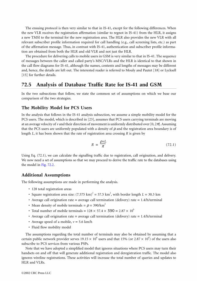
The ensuing protocol is then very similar to that in IS-41, except for the following differences. Whenthe new VLR receives the registration affirmation (similar to regnot in IS-41) from the HLR, it assignsa new TMSI to the terminal for the new registration area. The HLR also provides the new VLR with allrelevant subscriber profile information required for call handling (e.g., call screening lists, etc.) as partof the affirmation message. Thus, in contrast with IS-41, authentication and subscriber profile informa-tion are obtained from both the HLR and old VLR and not just the HLR.

The procedure for delivering calls to mobile users in GSM is very similar to that in IS-41. The sequenceof messages between the caller and called party’s MSC/VLRs and the HLR is identical to that shown inthe call flow diagrams for IS-41, although the names, contents and lengths of messages may be differentand, hence, the details are left out. The interested reader is referred to Mouly and Pautet [18] or Lycksell[15] for further details.

72.5 Analysis of Database Traffic Rate for IS-41 and GSM

In the two subsections that follow, we state the common set of assumptions on which we base ourcomparison of the two strategies.

The Mobility Model for PCS Users

In the analysis that follows in the IS-41 analysis subsection, we assume a simple mobility model for thePCS users. The model, which is described in [23], assumes that PCS users carrying terminals are movingat an average velocity of v and their direction of movement is uniformly distributed over [0, 2π]. Assumingthat the PCS users are uniformly populated with a density of ρ and the registration area boundary is oflength L, it has been shown that the rate of registration area crossing R is given by

(72.1)

Using Eq. (72.1), we can calculate the signalling traffic due to registration, call origination, and delivery.We now need a set of assumptions so that we may proceed to derive the traffic rate to the databases usingthe model in Fig. 72.2.

Additional Assumptions

The following assumptions are made in performing the analysis.

• 128 total registration areas

• Square registration area size: (7.575 km)2 = 57.5 km2, with border length L = 30.3 km

• Average call origination rate = average call termination (delivery) rate = 1.4/h/terminal

• Mean density of mobile terminals = ρ = 390/km2

• Total number of mobile terminals = 128 × 57.4 × 390 = 2.87 × 106

• Average call origination rate = average call termination (delivery) rate = 1.4/h/terminal

• Average speed of a mobile, v = 5.6 km/h

• Fluid flow mobility model

The assumptions regarding the total number of terminals may also be obtained by assuming that acertain public network provider serves 19.15 × 106 users and that 15% (or 2.87 × 106) of the users alsosubscribe to PCS services from various PSPs.

Note that we have adopted a simplified model that ignores situations where PCS users may turn theirhandsets on and off that will generate additional registration and deregistration traffic. The model alsoignores wireline registrations. These activities will increase the total number of queries and updates toHLR and VLRs.

RrvL

p--------=


Analysis of IS-41

Using Eq. (72.1) and the parameter values assumed in the preceding subsection, we can compute the trafficdue to registration. The registration traffic is generated by mobile terminals moving into a new registrationarea, and this must equal the mobile terminals moving out of the registration area, which per second is

This must also be equal to the number of deregistrations (registration cancellations),

The total number of registration messages per second arriving at the HLR will be

The HLR should, therefore, be able to handle, roughly, 750 updates per second. We observe from Fig.72.3 that authenticating terminals generate as many queries to VLR and HLR as the respective numberof updates generated due to registration notification messages.

The number of queries that the HLR must handle during call origination and delivery can be similarlycalculated. Queries to HLR are generated when a call is made to a PCS user. The SSP that receives therequest for a call, generates a location request (LOCREQ) query to the SCP controlling the HLR. Therate per second of such queries must be equal to the rate of calls made to PCS users.

This is calculated as

For calls originated from a mobile terminal by PCS users, the switch authenticates the terminal byquerying the VLR. The rate per second of such queries is determined by the rate of calls originating inan SSP serving area, which is also a registration area (RA). This is given by

This is also the number of queries per second needed to authenticate terminals of PCS users to whichcalls are delivered:

Table 72.1 summarizes the calculations.

Analysis of GSM

Calculations for query and update rates for GSM may be performed in the same manner as for IS-41,and they are summarized in Table 72.2. The difference between this table and Table 72.1 is that in GSMthe new serving VLR does not query the HLR separately in order to authenticate the terminal duringregistration and, hence, there are no HLR queries during registration. Instead, the entry (749 queries)

Rreg, VLR

390 30.3 5.6××3600p

--------------------------------------- 5.85= =

Rdereg, VLR 5.85=

Rreg, HLR Rreg, VLR total No. of registration areas× 749= =

RCallDeliv, HLR call rate per user total number of users×=

1.4 2.87 105××3600

--------------------------------------=

1116=

RCallOrig, VLR

1116128----------- 8.7= =

RCallDeliv, VLR 8.7=


under HLR queries in Table 72.1, corresponding to mobility-related authentication activity at registration,gets equally divided between the 128 VLRs. Observe that with either protocol the total database trafficrates are conserved, where the total database traffic for the entire network is given by the sum of all ofthe entries in the last row total (Network), i.e.,

HLR updates + VLR updates + HLR queries + VLR queries

From Tables 72.1 and 72.2 we see that this quantity equals 7087.The conclusion is independent of any variations we may provide to the assumptions in earlier in the

section. For example, if the PCS penetration (the percentage of the total users subscribing to PCS services)were to increase from 15 to 30%, all of the entries in the two tables will double and, hence, the totaldatabase traffic generated by the two protocols will still be equal.

72.6 Reducing Signalling During Call Delivery

In the preceding section, we provided a simplified analysis of some scenarios associated with user locationstrategies and the associated database queries and updates required. Previous studies [13,16] indicatethat the signalling traffic and database queries associated with PCS due to user mobility are likely to growto levels well in excess of that associated with a conventional call. It is, therefore, desirable to studymodifications to the two protocols that would result in reduced signalling and database traffic. We nowprovide some suggestions.

For both GSM and IS-41, delivery of calls to a mobile user involves four messages: from the caller’sVLR to the called party’s HLR, from the HLR to the called party’s VLR, from the called party’s VLR tothe HLR, and from the HLR to the caller’s VLR. The last two of these messages involve the HLR, whoserole is to simply relay the routing information provided by the called party’s VLR to the caller’s VLR. Anobvious modification to the protocol would be to have the called VLR directly send the routinginformation to the calling VLR. This would reduce the total load on the HLR and on signalling network

TABLE 72.1 IS-41 Query and Update Rates to HLR and VLR

Activity HLR Updates/s VLR Updates/s HLR Queries/s VLR Queries/s

Mobility-relatedactivities atregistration

749 5.85 749 5.85

Mobility-relatedactivities atderegistration

5.85

Call origination 8.7Call delivery 1116 8.7Total (per RA) 5.85 11.7 14.57 23.25Total (Network) 749 1497.6 1865 2976

TABLE 72.2 GMS Query and Update Rates to HLR and VLR

Activity HLR Updates/s VLR Updates/s HLR Queries/s VLR Queries/s

Mobility-relatedactivities atregistration

749 5.85 11.7

Mobility-relatedactivities atderegistration

5.85

Call origination 8.7Call delivery 1116 8.7Total (per VLR) 749 11.7 1116 29.1Total (Network) 749 1497.6 1116 3724.8


links substantially. Such a modification to the protocol may not be easy, of course, due to administrative,billing, legal, or security concerns. Besides, this would violate the query A response model adopted inIS-41, requiring further analysis.

A related question which arises is whether the routing information obtained from the called party’sVLR could instead be stored in the HLR. This routing information could be provided to the HLR, forexample, whenever a terminal registers in a new registration area. If this were possible, two of the fourmessages involved in call delivery could be eliminated. This point was discussed at length by the GSMstandards body, and the present strategy was arrived at. The reason for this decision was to reduce thenumber of temporary routing numbers allocated by VLRs to terminals in their registration area. If atemporary routing number (TLDN in IS-41 or MSRN in GSM) is allocated to a terminal for the wholeduration of its stay in a registration area, the quantity of numbers required is much greater than if anumber is assigned on a per-call basis. Other strategies may be employed to reduce signalling and databasetraffic via intelligent paging or by storing user’s mobility behavior in user profiles (see, for example,Tabbane [22]). A discussion of these techniques is beyond the scope of the paper.

72.7 Per-User Location Caching

The basic idea behind per-user location caching is that the volume of SS7 message traffic and databaseaccesses required in locating a called subscriber can be reduced by maintaining local storage, or cache, ofuser location information at a switch. At any switch, location caching for a given user should be employedonly if a large number of calls originate for that user from that switch, relative to the user’s mobility.Note that the cached information is kept at the switch from which calls originate, which may or may notbe the switch where the user is currently registered.

Location caching involves the storage of location pointers at the originating switch; these point to theVLR (and the associated switch) where the user is currently registered. We refer to the procedure oflocating a PCS user a FIND operation, borrowing the terminology from Awerbuch and Peleg [1]. Wedefine a basic FIND, or BasicFIND( ), as one where the following sequence of steps takes place.

1. The incoming call to a PCS user is directed to the nearest switch.2. Assuming that the called party is not located within the immediate RA, the switch queries the

HLR for routing information.3. The HLR contains a pointer to the VLR in whose associated RA the subscriber is currently situated

and launches a query to that VLR.4. The VLR, in turn, queries the MSC to determine whether the user terminal is capable of receiving

the call (i.e., is idle) and, if so, the MSC returns a routable address (TLDN in IS-41) to the VLR.5. The VLR relays the routing address back to the originating switch via the HLR.

At this point, the originating switch can route the call to the destination switch. Alternately, BasicFIND( )can be described by pseudocode as follows. (We observe that a more formal method of specifying PCSprotocols may be desirable.)

BasicFIND( ){Call to PCS user is detected at local switch;if called party is in same RA then return;Switch queries called party’s HLR;Called party’s HLR queries called party’s current VLR, V;V returns called party’s location to HLR;HLR returns location to calling switch;

}

In the FIND procedure involving the use of location caching, or CacheFIND( ), each switch contains alocal memory (cache) that stores location information for subscribers. When the switch receives a call


origination (from either a wire-line or wireless caller) directed to a PCS subscriber, it first checks itscache to see if location information for the called party is maintained. If so, a query is launched to thepointed VLR; if not, BasicFIND( ), as just described, is followed. If a cache entry exists and the pointedVLR is queried, two situations are possible. If the user is still registered at the RA of the pointed VLR(i.e., we have a cache hit), the pointed VLR returns the user’s routing address. Otherwise, the pointedVLR returns a cache miss.

CacheFIND( ){Call to PCS user is detected at local switch;if called is in same RA then return;if there is no cache entry for called userthen invoke BasicFIND( ) and return;Switch queries the VLR, V, specified in the cache entry;if called is at V, then

V returns called party’s location to calling switch;else {

V returns “miss” to calling switch;Calling switch invokes BasicFIND( );

}}

When a cache hit occurs we save one query to the HLR [a VLR query is involved in both CacheFIND( )and BasicFIND( )], and we also save traffic along some of the signalling links; instead of four messagetransmissions, as in BasicFIND( ), only two are needed. In steady-state operation, the cached pointer forany given user is updated only upon a miss.

Note that the BasicFIND( ) procedure differs from that specified for roaming subscribers in the IS-41standard EIA/TIA [6]. In the IS-41 standard, the second line in the BasicFIND( ) procedure is omitted,i.e., every call results in a query of the called user’s HLR. Thus, in fact, the procedure specified in thestandard will result in an even higher network load than the BasicFIND( ) procedure specified here. Tomake a fair assessment of the benefits of CacheFIND( ), however, we have compared it againstBasicFIND( ). Thus, the benefits of CacheFIND( ) investigated here depend specifically on the use ofcaching and not simply on the availability of user location information at the local VLR.

72.8 Caching Threshold Analysis

In this section we investigate the classes of users for which the caching strategy yields net reductions insignalling traffic and database loads. We characterize classes of users by their CMR. The CMR of a useris the average number of calls to a user per unit time, divided by the average number of times the userchanges registration areas per unit time. We also define a LCMR, which is the average number of callsto a user from a given originating switch per unit time, divided by the average number of times the userchanges registration areas per unit time.

For each user, the amount of savings due to caching is a function of the probability that the cachedpointer correctly points to the user’s location and increases with the user’s LCMR. In this section wequantify the minimum value of LCMR for caching to be worthwhile. This caching threshold is param-eterized with respect to costs of traversing signalling network elements and network databases and canbe used as a guide to select the subset of users to whom caching should be applied. The analysis in thissection shows that estimating user’s LCMRs, preferably dynamically, is very important in order to applythe caching strategy. The next section will discuss methods for obtaining this estimate.

From the pseudocode for BasicFIND( ), the signalling network cost incurred in locating a PCS userin the event of an incoming call is the sum of the cost of querying the HLR (and receiving the response),


and the cost of querying the VLR which the HLR points to (and receiving the response). Let

α = cost of querying the HLR and receiving a responseβ = cost of querying the pointed VLR and receiving a response

Then, the cost of BasicFIND( ) operation is

(72.2)

To quantify this further, assume costs for traversing various network elements as follows.

Al = cost of transmitting a location request or response message on A link between SSP and LSTPD = cost of transmitting a location request on response message or D linkAr = cost of transmitting a location request or response message on A link between RSTP and SCPL = cost of processing and routing a location request or response message by LSTPR = cost of processing and routing a location request or response message by RSTP

HQ = cost of a query to the HLR to obtain the current VLR locationVQ = cost of a query to the VLR to obtain the routing address

Then, using the PCS reference network architecture

(72.3)

(72.4)

From Eqs. (72.2)–(72.4)

(72.5)

We now calculate the cost of CacheFIND( ). We define the hit ratio as the relative frequency with whichthe cached pointer correctly points to the user’s location when it is consulted. Let

p = cache hit ratioCH = cost of the CacheFIND( ) procedure when there is a hitCM = cost of the CacheFIND( ) procedure when there is a miss

Then the cost of CacheFIND( ) is

(72.6)

For CacheFIND( ), the signalling network costs incurred in locating a user in the event of an incomingcall depend on the hit ratio as well as the cost of querying the VLR, which is stored in the cache; thisVLR query may or may not involve traversing the RSTP. In the following, we say a VLR is a local VLR ifit is served by the same LSTP as the originating switch, and a remote VLR otherwise. Let

q = Prob (VLR in originating switch’s cache is a local VLR)δ = cost of querying a local VLR� = cost of querying a remote VLRη = cost of updating the cache upon a miss

Then,

(72.7)

(72.8)

(72.9)

CB a b+=

a 2 Al D Ar L R+ + + +( ) HQ+=

b 2 Al D Ar L R+ + + +( ) VQ+=

CB 4 Al D Ar L R+ + + +( ) HQ VQ+ +=

CC pCH 1 p–( )CM+=

d 4Al 2L VQ+ +=

� 4 Al D L+ +( ) 2R VQ+ +=

CH qd 1 q–( )�+=


Since updating the cache involves an operation to a fast local memory rather than a database operation,we shall assume in the following that η = 0. Then,

(72.10)

From Eqs. (72.6), (72.9), and (72.10) we have

(72.11)

For net cost savings we require CC < CB, or that the hit ratio exceeds a hit ratio threshold pT , derived usingEqs. (72.6), (72.9), and (72.2),

(72.12)

(72.13)

Equation (72.13) specifies the hit ratio threshold for a user, evaluated at a given switch, for which localmaintenance of a cached location entry produces cost savings. As pointed out earlier, a given user’s hitratio may be location dependent, since the rates of calls destined for that user may vary widely acrossswitches.

The hit ratio threshold in Eq. (72.13) is comprised of heterogeneous cost terms, i.e., transmission linkutilization, packet switch processing, and database access costs. Therefore, numerical evaluation of thehit ratio threshold requires either detailed knowledge of these individual quantities or some form ofsimplifying assumptions. Based on the latter approach, the following two possible methods of evaluationmay be employed.

1. Assume one or more cost terms dominate, and simplify Eq. (72.13) by setting the remaining termsto zero.

2. Establish a common unit of measure for all cost terms, for example, time delay. In this case, Al ,Ar , and D may represent transmission delays of fixed transmission speed (e.g., 56 kb/s) signallinglinks, L and R may constitute the sum of queueing and service delays of packet switches (i.e.,STPs), and HQ and VQ the transaction delays for database queries.

In this section we adopt the first method and evaluate Eq. (72.13) assuming a single term dominates. (InSection 72.9 we present results using the second method.) Table 72.3 shows the hit ratio threshold requiredto obtain net cost savings, for each case in which one of the cost terms is dominant.

TABLE 72.3 Minimum Hit Ratios and LCMRs for Various Individual Dominant Signalling Network Cost Terms

DominantCost Term

Hit ratioThreshold, pT

LCMR Threshold,

LCMRT

LCMR Threshold(q = 0.043)

LCMR Threshold(q = 0.25)

Al 1 ∞ ∞ ∞Ar 0 0 0 0D 1 - q 1/q - 1 22 3L 1 - q/2 2/q - 1 45 7R 1 - q/2 2/q - 1 45 7HQ 0 0 0 0VQ 1 ∞ ∞ ∞

CM CH CB+ qd 1 q–( )� a b+ ++= =

CC a b � p a b+( ) q d �–( )+–+ +=

p pT>CH

CB

------ � q d �–( )+a b+

-----------------------------= =

4Al 4D 4L 2R VQ q 4D 2L 2R+ +( )–+ + + +4Al 4D 4Ar 4L 4R HQ VQ+ + + + + +

--------------------------------------------------------------------------------------------------------------=


In Table 72.3 we see that if the cost of querying a VLR or of traversing a local A link is the dominantcost, caching for users who may move is never worthwhile, regardless of users’ call reception and mobilitypatterns. This is because the caching strategy essentially distributes the functionality of the HLR to theVLRs. Thus, the load on the VLR and the local A link is always increased, since any move by a user resultsin a cache miss. On the other hand, for a fixed user (or telephone), caching is always worthwhile. Wealso observe that if the remote A links or HLR querying are the bottlenecks, caching is worthwhile evenfor users with very low hit ratios.

As a simple average-case calculation, consider the net network benefit of caching when HLR accessand update is the performance bottleneck. Consider a scenario where u = 50% of PCS users receive c =80% of their calls from s = 5 RAs where their hit ratio p > 0, and s′ = 4 of the SSPs at those RAs containsufficiently large caches. Assume that caching is applied only to this subset of users and to no other users.Suppose that the average hit ratio for these users is p = 80%, so that 80% of the HLR accesses for callsto these users from these RA are avoided. Then the net saving in the accesses to the system’s HLR isH = (ucs′p)/s = 25%.

We discuss other quantities in Table 72.3 next. It is first useful to relate the cache hit ratio to users’calling and mobility patterns directly via the LCMR. Doing so requires making assumptions about thedistribution of the user’s calls and moves. We consider the steady state where the incoming call streamfrom an SSP to a user is a Poisson process with arrival rate λ, and the time that the user resides in anRA has a general distribution F(t) with mean 1/µ. Thus,

(72.14)

Let t be the time interval between two consecutive calls from the SSP to the user and t1 be the timeinterval between the first call and the time when the user moves to a new RA. From the random observerproperty of the arrival call stream [7], the hit ratio is

If F(t) is an exponential distribution, then

(72.15)

and we can derive the LCMR threshold, the minimum LCMR required for caching to be beneficialassuming incoming calls are a Poisson process and intermove times are exponentially distributed,

(72.16)

Equation (72.16) is used to derive LCMR thresholds assuming various dominant costs terms, as shownin Table 72.3.

Several values for LCMRT in Table 72.3 involve the term q, i.e., the probability that the pointed VLRis a local VLR. These values may be numerically evaluated by simplifying assumptions. For example,assume that all of the SSPs in the network are uniformly distributed amongst l LSTPs. Also, assume thatall of the PCS subscribers are uniformly distributed in location across all SSPs and that each subscriberexhibits the same incoming call rate at every SSP. Under those conditions, q is simply 1/l. Consider thecase of the public switched telephone network. Given that there are a total of 160 local access transport

LCMRlm-----=

Pr t t1<[ ] le lt–

t=0

∞∫= = m 1 F t 1( )–[ ]dt1dtt1=t

∞∫

pl

l m+-------------=

LCMRT

pT

1 pT–--------------=


area (LATA) across the 7 Regional Bell Operating Company (RBOC) regions [4], the average number ofLATAs, or l, is 160/7 or 23. Table 72.3 shows the results with q = 1/l in this case.

We obseris extremelycantly moreworthwhile deployed in be significan

It is possiin this way astrategy appnet increasesection discu

72.9 T

Here we sketthese quantiis high enoudominant coif it is knowinstalled at t

One possuser’s callingoff-peak hou

In this seccaching is torunning aveto obtain a malgorithms nand mobilit

The Run

The runningthe hit ratioprocedure ulocation for of the hit ratthat pM = p. of the hit rathe basic schthe basic sch

We consiPoisson prodistributionstate is

0967_frame_C72.fm Page 19 Tuesday, March 5, 2002 9:17 PM

©2002 CRC P

ve that the assumption that all users receive calls uniformly from all switches in the network conservative. In practice, we expect that user call reception patterns would display signifi- locality, so that q would be larger and the LCMR thresholds required to make cachingwould be smaller. It is also worthwhile to consider the case of a RBOC region with PCSa few LATA only, a likely initial scenario, say, 4 LATAs. In either case the value of q wouldtly higher; Table 72.3 shows the LCMR threshold when q = 0.25.ble to quantify the net costs and benefits of caching in terms of signalling network impactsnd to determine the hit ratio and LCMR threshold above which users should have the cachinglied. Applying caching to users whose hit ratio and LCMR is below this threshold results ins in network impacts. It is, thus, important to estimate users’ LCMRs accurately. The nextsses how to do so.

echniques for Estimating Users’ LCMR

ch some methods of estimating users’ LCMR. A simple and attractive policy is to not estimateties on a per-user basis at all. For instance, if the average LCMR over all users in a PCS systemgh (and from Table 72.3, it need not be high depending on which network elements are thests), then caching could be used at every SSP to yield net system-wide benefits. Alternatively,n that at any given SSP the average LCMR over all users is high enough, a cache can behat SSP. Other variations can be designed. ibility for deciding about caching on a per-user basis is to maintain information about a and mobility pattern at the HLR and to download it periodically to selected SSPs duringrs. It is easy to envision numerous variations on this idea.tion we investigate two possible techniques for estimating LCMR on a per-user basis when be deployed. The first algorithm, called the running average algorithm, simply maintains a

rage of the hit ratio for each user. The second algorithm, called the reset-K algorithm, attemptseasure of the hit ratio over the recent history of the user’s movements. We describe the two

ext and evaluate their effectiveness using a stochastic analysis taking into account user callingy patterns.

ning Average Algorithm

average algorithm maintains, for every user that has a cache entry, the running average of. A running count is kept of the number of calls to a given user, and, regardless of the FINDsed to locate the user, a running count of the number of times that the user was at the sameany two consecutive calls; the ratio of these numbers provides the measured running averageio. We denote the measured running average of the hit ratio by pM; in steady state, we expectThe user’s previous location as stored in the cache entry is used only if the running averagetio pM is greater than the cache hit threshold pT . Recall that the cache scheme outperformseme if p > pT = CH/CB. Thus, in steady state, the running average algorithm will outperformeme when pM > pT.

der, as before, the steady state where the incoming call stream from an SSP to a user is acess with arrival rate λ, and the time that the user resides in an RA has an exponential with mean 1/µ. Thus LCMR = λ/µ [Eq. (72.14)] and the location tracking cost at steady

(72.17)CCpMCH 1 pM–( )CB,+ pM pT>CB, otherwise

=

ress LLC

Figure 72.6 uniform unSection 72.8the caching caching strathe basic schsavings of 2

Equation (cf., dashed of the outputo study the to time [wh

One probpast historyreflect the re

The Rese

We may moevery K incocounts the nthe cache is

FIGURE 72.6


©2002 CRC P

plots the cost ratio CC/CB from Eq. (72.17) against LCMR. (This corresponds to assigningits to all cost terms in Eq. (72.13), i.e., the second evaluation method as discussed in. Thus, the ratio CC/CB may represent the percentage reduction in user location time withstrategy compared to the basic strategy.) The figure indicates that in the steady state, thetegy with the running average algorithm for estimating LCMR can significantly outperformeme if LCMR is sufficiently large. For instance with LCMR ∼ 5, caching can lead to cost

0–60% over the basic strategy.(72.17) (cf., solid curves in Fig. 72.6) is validated against a simple Monte Carlo simulationcurves in Fig. 72.6). In the simulation, the confidence interval for the 95% confidence levelt measure CC/CB is within 3% of the mean value. This simulation model will later be usedrunning average algorithm when the mean of the movement distribution changes from timeich cannot be modeled by using Eq. (72.17)].lem with the running average algorithm is that the parameter p is measured from the entire of the user’s movement, and the algorithm may not be sufficiently dynamic to adequatelycent history of the user’s mobility patterns.

t-K Algorithm

dify the running average algorithm such that p is measured from the recent history. Defineming calls as a cycle. The modified algorithm, which is referred to as the reset-K algorithm,umber of cache hits n in a cycle. If the measured hit ratio for a user, pM = n/K ≥ pT , then

enabled for that user, and the cached information is always used to locate the user in the

The location tracking cost for the running average algorithm.

ress LLC

next cycle. Otherwise, the cache is disabled for that user, and the basic scheme is used. At the beginningof a cycle, the cache hit count is reset, and a new pM value is measured during the cycle.

To study by a Markovthe time perwhere i > j, cycle. A pairi incoming difference bthen the prothe user moconsecutive

Figure 72from (i − 1, from (i, 0) tprobability o

Figure 72.7(the state (i, phone call. such a state.to (i + 1, i −the transitio

Figure 72.7(move into stfrom (i, j) to

Figure 72.7(arrives whenrepresent th

so that the hmoves fromOtherwise, t


©2002 CRC P

the performance of the reset-K algorithm, we model the number of cache misses in a cycle process. Assume as before that the call arrivals are a Poisson process with arrival rate λ andiod the user resides in an RA has an exponential distribution with mean 1/µ. A pair (i, j),represents the state that there are j cache misses before the first i incoming phone calls in a (i, j)∗, where i ≥ j ≥ 1, represents the state that there are j − 1 cache misses before the firstphone calls in a cycle, and the user moves between the ith and the i + 1 phone calls. Theetween (i, j) and (i, j)∗ is that if the Markov process is in the state (i, j) and the user moves,cess moves into the state (i, j + 1)∗. On the other hand, if the process is in state (i, j)∗ whenves, the process remains in (i, j)∗ because at most one cache miss occurs between two

phone calls..7(a) illustrates the transitions for state (i, 0) where 2 < i < K + 1. The Markov process moves0) to (i, 0) if a phone call arrives before the user moves out. The rate is λ. The process moveso (i, 1)∗ if the user moves to another RA before the i + 1 call arrival. Let π(i, j) denote thef the process being in state (i, j). Then the transition equation is

(72.18)

b) illustrates the transitions for state (i, i − 1) where 1 < i < K + 1. The only transition intoi − 1) is from (i − 1, i − 1)∗, which means that the user always moves to another RA after a[Note that there can be no state (i − 1, i − 1) by definition and, hence, no transition from] The transition rate is λ. The process moves from (i, i − 1) to (i, i)∗ with rate µ, and moves 1) with rate λ. Let π∗(i, j) denote the probability of the process being in state (i, j)∗. Thenn equation is

(72.19)

c) illustrates the transitions for state (i, j) where 2 < i < K + 1, 0 < j < i − 1. The process mayate (i, j) from two states (i − 1, j) and (i − 1, j)∗ with rate λ, respectively. The process moves (i, j + 1)∗ or (i + 1, j) with rates µ and λ, respectively. The transition equation is

(72.20)

d) illustrates the transitions for state (K + 1, j) where 0 < j < K + 1. Note that if a phone call the process is in (K, j) or (K, j)∗, the system enters a new cycle (with rate λ), and we could

e new state as (1, 0). In our model, we introduce the state (K + 1, j) instead of (1, 0), where

it ratio, and thus the location tracking cost, can be derived [see Eq. (72.25)]. The process (K + 1, j) [i.e., (1, 0)] to (1, 1)∗ with rate µ if the user moves before the next call arrives.he process moves to (2, 0) with rate λ. The transition equation is

(72.21)

π i,0( ) λλ µ+------------- π i 1– , 0( ), 2 i K 1+< <=

π i, i 1–( ) λλ µ+-------------π∗ i 1– , i 1–( ), 1 i K 1+< <=

π i, j( ) λλ µ+------------- π i 1,– j( ) π∗ i 1– , j( )+[ ], 2 i K 1, 0 j i 1–< <+< <=

π K 1,+ j( )0 j K≤ ≤∑ π 1, 0( )=

π K 1+ , j( ) λλ µ+------------- π K, j( ) π∗ K, j( )+[ ], 0 j K 1+< <=

ress LLC

FIGURE 72.7


©2002 CRC P

State transitions.

ress LLC

For j = 0, the transition from (K, j)∗ to (K + 1, 0) should be removed in Fig. 72.7(d) because the state(K, 0)∗ does not exist. The transition equation for (K + 1, 0) is given in Eq. (72.18). Figure 72.7(e)illustrates th ∗ ∗

from (i, j − 1the process transition eq

The transitioreplaced by

Finally, the (1, 0) is repl

Suppose thacache misses

Thus, the pr

and the loca

The first terthreshold excache is enabwhich misseduring the c

CC CBP=


©2002 CRC P

e transitions for state (i, j) where 0 < j < i, 1 < i < K + 1. The process can only move to (i, j)) (with rate µ). From the definition of (i, j)∗, if the user moves when the process is in (i, j)∗,

remains in (i, j)∗ (with rate µ). Otherwise, the process moves to (i + 1, j) with rate λ. Theuation is

(72.22)

ns for (2, 0) are similar to the transitions for (i, 0) except that the transition from (1, 0) is(K + 1, 0),…,(K + 1, K) [cf., Fig. 72.7(f)]. The transition equation is

(72.23)

transitions for (1, 1)∗ is similar to the transitions for (i, j)∗ except that the transition fromaced by (K + 1, 0),…,(K + 1, K) [cf., Fig. 72.7(g)]. The transition equation is

(72.24)

t at the beginning of a cycle, the process is in state (K + 1, j), then it implies that there are j in the previous cycle. The cache is enabled if and only if

obability that the measured hit ratio pM < pT in the previous cycle is

tion tracking cost for the reset-K algorithm is

(72.25)

m Eq. (72.25) represents the cost incurred when caching is disabled because the hit ratioceeds the hit ratio measured in the previous cycle. The second term is the cost when theled and consists of two parts, corresponding to calls during which hits occur and calls during

s occur. The ratio in square brackets is the conditional probability of being in state urrent cycle.

π∗ i, j( ) µλ---π i, j 1–( ), 0 j i, 1 i K 1, i 2≥+< <≤<=

π 2, 0( ) λλ µ+------------- π K 1, j+( )

0≤ j≤K

∑=

π∗ 1, 1( ) µλ--- π K 1, j+( )

0≤ j≤K

∑=

pM pT≥CH

CB

------ 1jK---–

CH

CB

------ 0 j K 1CH

CB

------– ≤ ≤⇒≥⇒=

Pr pM pT<[ ]∑k 1− CH/CB( )[ ] j K≤< π K 1,j+( )

∑0≤ j≤Kπ K 1, j+( )--------------------------------------------------------------------=

r pM pT<[ ] 1 Pr pM pT<[ ]–( )K j–( )CH

K-----------------------

j CH CB+( )K

--------------------------+ π K 1, j+( )

∑0≤i≤Kπ K 1+ , i( )-----------------------------------------

0≤ j≤K

∑

+

π K 1+ , j( )

ress LLC

The num

defined in E

we have

and using Eq. (7

The analythe 98% concurves for Eqand CH = 0simulation m

Comparis

If the distribwould expecsmall) becauvalue p in thas the runnifor the runn

FIGURE 72.8

π i, j( ) ai=

π K 1+(


©2002 CRC P

erical computation of can be done as follows. First, compute ai,j and bi,j where and . Note that ai,j = 0(bi,j = 0) if is not

qs. (72.18)–(72.24). Since

can be computed and the location tracking cost for the reset-K algorithm is obtained2.25).sis is validated by a Monte Carlo simulation. In the simulation, the confidence interval forfidence level of the output measure CC /CB is within 3% of the mean value. Figure 72.8 plots. (72.25) (the solid curves) against the simulation experiments (the dashed curves) for K = 20

.5CB and 0.3CB, respectively. The figure indicates that the analysis is consistent with theodel.

on of the LCMR Estimation Algorithms

utions for the incoming call process and the user movement process never change, then wet the running average algorithm to outperform the reset-K algorithm (especially when K isse the measured hit ratio pM in the running average algorithm approaches the true hit ratioe steady state. Surprisingly, the performance for the reset-K algorithm is roughly the same

ng average algorithm even if K is as small as 10. Figure 72.9 plots the location tracking costsing average algorithm and the reset-K algorithm with different K values.

The location tracking costs for the reset-K algorithm; K = 20.

π K 1+ , j( ), jπ

∗ 1, 1( ) π∗ i, j( ) bi , jπ∗ 1, 1( )= π i, j( ) π∗ i, j( )[ ]

π i, j( ) π∗ i, j( )+[ ]i , j∑ 1=

π∗ 1,1( ) 1∑i , j ai , j bi , j+( )---------------------------------=

, j)

ress LLC

The figuruser movemvalue of K o

If the disttime, we expthis proposirate changessimilar resulthe confidenmean value.By changingthan the run

72.10 D

In this sectioa number oftecture and assumptionssome of the

FIGURE 72.9


©2002 CRC P

e indicates that in steady state, when the distributions for the incoming call process and theent process never change, the running average algorithm outperforms reset K, and a largeutperforms a small K but the differences are insignificant.ributions for the incoming call process or the user movement process change from time toect that the reset-K algorithm outperforms the running average algorithm. We have examinedtion experimentally. In the experiments, 4000 incoming calls are simulated. The call arrival from 0.1 to 1.0, 0.3, and then 5.0 for every 1000 calls (other sequences have been tested andts are observed). For every data point, the simulation is repeated 1000 times to ensure thatce interval for the 98% confidence level of the output measure CC/CB is within 3% of the

Figure 72.10 plots the location tracking costs for the two algorithms for these experiments. the distributions of the incoming call process, we observe that the reset-K algorithm is betterning average algorithm for all CH/CB values.

iscussion

n we discuss aspects of the caching strategy presented here. Caching in PCS systems raises issues not encountered in traditional computer systems, particularly with respect to archi-locality in user call and mobility patterns. In addition, several variations in our reference are possible for investigating the implementation of the caching strategies. Here we sketch

issues involved.

The location tracking costs for the running average algorithm and the reset-K algorithm; CH = 0.5CB.

ress LLC

Conditio

We summarour analysis.

The cachis the perfodatabase loaload and trato the VLRsis the perfoupgraded.

The beneRSTP, and Lexponentialcaching to threshold coestimate theissue furthesystem studcould also pthe LSTP ar

We observthe issues ramobility and

FIGURE 72.1


©2002 CRC P

ns When Caching Is Beneficial

ize the conditions for which the auxiliary strategies are worthwhile, under the assumptions of

ing strategy is very promising when the HLR update (or query load) or the remote A linkrmance bottleneck, since a low LCMR(LCMR > O) is required. For caching, the totald and signalling network traffic is reduced whenever there is a cache hit. In addition,ffic is redistributed from the HLR and higher level SS7 network elements (RSTP, D links) and lower levels where excess network capacity may be more likely to exist. If the VLRrmance bottleneck, the caching strategy is not promising, unless the VLR capacity is

fits of the caching strategy depend on user call and mobility patterns when the D link,STP are the performance bottlenecks. We have used a Poisson call arrival model and

intermove time to estimate this dependence. Under very conservative assumptions, forbe beneficial requires relatively high LCMR (25–50); we expect that in practice thisuld be lowered significantly (say, LCMR > 7). Further experimental study is required to amount of locality in user movements for different user populations to investigate thisr. It is possible that for some classes of users data obtained from active badge locationies (e.g., Fishman and Mazer [8]) could be useful. In general, it appears that cachingotentially provide benefits to some classes of users even when the D link, the RSTP, ore the bottlenecks.e that more accurate models of user calling and mobility patterns are required to help resolveised in this section. We are currently engaged in developing theoretical models for user estimating their effect on studies of various aspects of PCS performance [10].

0 Comparing the running average algorithm and the reset-K algorithm under unstable call traffic.

ress LLC

Alternative Network Architectures

The reference architecture we have assumed (Fig. 72.2) is only one of several possible architectures. It ispossible to cat a local SCnumber of Htelecommunof databasesplacement o

Rather thtecture to illChanges in tour qualitat

LCMR Es

It is possiblea relatively accurate estidetermining

We have and short-rais fairly conbe employedchapter.

An alternmovements approach is

A related deploying a selecting theratio threshouseful to mathe thresholused (LRU) offer some g

72.11 C

We began thregistration,strategies fostandard GSto which damade that a

Previous suggest a higactivities fordatabase loauser location


©2002 CRC P

onsider variations in the placement of the HLR and VLR functionality, (e.g., placing the VLRP associated with the LSTP instead of at the SSP), the number of SSPs served by an LSTP, the

LRs deployed, etc. It is quite conceivable that different regional PCS service providers andications companies will deploy different signalling network architectures, as well as placement for supporting PCS within their serving regions [19]. It is also possible that the number andf databases in a network will change over time as the number of PCS users increases.an consider many possible variations of the architecture, we have selected a reference archi-ustrate the new auxiliary strategies and our method of calculating their costs and benefits.he architecture may result in minor variations in our analysis but may not significantly affective conclusions.

timation and Caching Policy

that for some user populations estimating the LCMR may not be necessary, since they displayhigh-average LCMR. For some populations, as we have shown in Section 72.9, obtainingmates of user LCMR in order to decide whether or not to use caching can be important in the net benefits of caching.presented two simple distributed algorithms for estimating LCMR, based on a long-rangenge running calculation; the former is preferable if the call and mobility pattern of users

sistent. Tuning the amount of history that is used to determine whether caching should for a particular user is an obvious area for further study but is outside the scope of this

ative approach is to utilize some user-supplied information, by requesting profiles of user(e.g., see Tabbane [22] and to integrate this with the caching strategy. A variation of thisto use some domain knowledge about user populations and their characteristics.issue is that of cache size and management. In practice it is likely that the monetary cost ofcache may limit its size. In that case, cache entries may not be maintained for some users;se users carefully is important to maximize the benefits of caching. Note that the cache hitld cannot necessarily be used to determine which users have cache entries, since it may be

intain cache entries for some users even though their hit ratios have temporarily fallen belowd. A simple policy that has been found to be effective in computer systems in the least recentlypolicy [20] in which cache entries that have been least recently used are discarded; LRU mayuidance in this context.

onclusions

is chapter with an overview of the nuances of PCS, such as personal and terminal mobility, deregistration, call delivery, etc. A tutorial was then provided on the two most commonr locating users in PCS, in North American interim standard IS-41 and the Pan-EuropeanM. A simplified analysis of the two standards was then provided to show the reader the extenttabase and signalling traffic is likely to be generated by PCS services. Suggestions were thenre likely to result in reduced traffic.studies [12,13,14,16] of PCS-related network signalling and data management functionalitiesh level of utilization of the signalling network in supporting call and mobility management PCS systems. Motivated by the need to evolve location strategies to reduce signalling andds, we then presented an auxiliary strategy, called per-user caching, to augment the basic strategy proposed in standards [6,18].

ress LLC

Using a reference system architecture for PCS, we quantified the criteria under which the cachingstrategy produces reductions in the network signalling and database loads in terms of users’ LCMRs. Wehave shown caching is ubottlenecks,of locality inthe system-wand stable clocation straprocedure wuser location

We have examined thdesigner to tthe benefits with variatioapproach caof the cachinstrategies su

Recently, compared thfor enablinglow CMRs, aand databas

Acknowl

We acknowlthe authors

Reference

1. AwerbuComm.

2. BellcoreSR-NPL

3. BellcoreReport

4. Bellcoregrated cations

5. Berman27–32,

6. Electroncommu

7. Feller, W1966.

8. FishmaWorksh

9. Harjonstrategy


©2002 CRC P

that, if the HLR or the remote A link in an SS7 architecture is the performance bottleneck,seful regardless of user call and mobility patterns. If the D link or STPs are the performance caching is potentially beneficial for large classes of users, particularly if they display a degree their call reception patterns. Depending on the numbers of PCS users who meet these criteria,ide impacts of these strategies could be significant. For instance, for users with LCMR ~ 5

all and move patterns, caching can result in cost reduction of 20–60% over the basic usertegy BasicFIND( ) under our analysis. Our results are conservative in that the BasicFIND( )e have used for comparison purposes already reduces the network impacts compared to the strategy specified in PCS standards such as IS-41.

also investigated in detail two simple on-line algorithms for estimating users’ LCMRs ande call and mobility patterns for which each would be useful. The algorithms allow a systemune the amount of history used to estimate a users’ LCMR and, hence, to attempt to optimizedue to caching. The particular values of cache hit ratios and LCMR thresholds will changens in the way the PCS architecture and the caching strategy is implemented, but our general

n still be applied. There are several issues deserving further study with respect to deploymentg strategy, such as the effect of alternative PCS architectures, integration with other auxiliary

ch as the use of user profiles, and effective cache management policies.we have augmented the work reported in this paper by a simulation study in which we havee caching and basic user location strategies [9]. The effect of using a time-based criterion

use of the cache has also been considered [11]. We have proposed elsewhere, for users withn auxiliary strategy involving a system of forwarding pointers to reduce the signalling traffic

e loads [10], a description of which is beyond the scope of this chapter.

edgment

edge a number of our colleagues in Bellcore who have reviewed several previous papers byand contributed to improving the clarity and readability of this work.

s

ch, B. and Peleg, D., Concurrent online tracking of mobile users. In Proc. SIGCOMM Symp. Arch. Prot., Oct. 1991.., Advanced intelligent network release 1 network and operations plan, Issue 1. Tech. Rept.-001623. Bell Communications Research, Morristown, NJ, Jun. 1991.., Personal communications services (PCS) network access services to PCS providers, SpecialSR-TSV-002459, Bell Communications Research, Morristown, NJ, Oct. 1993.., Switching system requirements for interexchange carrier interconnection using the inte-

services digital network user part (ISDNUP). Tech. Ref. TR-NWT-000394. Bell Communi- Research. Morristown, NJ, Dec. 1992., R.K. and Brewster, J.H., Perspectives on the AIN architecture. IEEE Comm. Mag., 1(2),

1992.ic Industries Association/Telecommunications Industry Association., Cellular radio tele-

nications intersystem operations. Tech. Rept. IS-41. Rev. B. Jul. 1991.., An Introduction to Probability Theory and Its Applications. John Wiley & Sons, New York,

n, N. and Mazer, M., Experience in deploying an active badge system. In Proc. Globecomop on Networking for Pers. Comm. Appl., Dec. 1992.o, H., Jain, R., and Mohan, S., Analysis and simulation of a cache-based auxiliary location for PCS. In Proc. IEEE Conf. Networks Pers. Comm., 1994.

ress LLC

10. Jain, R. and Lin Y.-B., An auxiliary user location strategy employing forwarding pointers to reducenetwork impacts of PCS. ACM Journal on Wireless Info. Networks (WINET), 1(2), 1995.

11. Lin, Y.-BTech., 4

12. Lo, C., commu002424

13. Lo, C.Nsuppor

14. Lo, C. adata co

15. Lycksel16. Meier-H

commu17. Mohan

42–50, 18. Mouly,

Brunea19. Russo, P

United 20. Silbersc21. Tabban

strategy22. Tabban

nication23. Thoma

a radio


©2002 CRC P

., Determining the user locations for personal communications networks. IEEE Trans. Vehic.66–473, Aug. 1994.Mohan, S., and Wolff, R., A comparison of data management alternatives for personalnications applications. Second Bellcore Symposium on Performance Modeling, SR-TSV-, Bell Communications Research, Morristown, NJ, Nov. 1993.., Wolff, R.S., and Bernhardt, R.C., An estimate of network database transaction volume to

t personal communications services. In Proc. Intl. Conf. Univ. Pers. Comm., 1992.nd Wolff, R., Estimated network database transaction volume to support wireless personal

mmunications applications. In Proc. Intl. Conf. Comm., May 1993.l, E., GSM system overview. Tech. Rept. Swedish Telecom. Admin., Jan. 1991.

ellstern, K. and Alonso, E., The use of SS7 and GSM to support high density personalnications. In Proc. Intl. Conf. Comm., 1992., S. and Jain, R., Two user location strategies for PCS. IEEE Pers. Comm. Mag., Premiere issue.Feb. 1994.M. and Pautet, M.B., The GSM System for Mobile Communications. M. Mouly, 49 rue Louiseu, Palaiseau, France, 1992.., Bechard, K., Brooks, E., Corn, R.L., Honig, W.L., Gove, R., and Young, J., In rollout in theStates. IEEE Comm. Mag., 56–63, Mar. 1993.hatz, A. and Peterson, J., Operating Systems Concepts. Addison-Wesley, Reading, MA, 1988.e, S., Comparison between the alternative location strategy (AS) and the classical location (CS). Tech. Rept. Rutgers Univ. WINLAB. Rutgers, NJ, Jul. 1992.e, S., Evaluation of an alternative location strategy for future high density wireless commu-s systems. Tech. Rept. WINALAB-TR-51, Rutgers Univ. WINLAB. Rutgers, NJ, Jan. 1993.

s, R., Gilbert, H., and Mazziotto, G., Influence of the mobile station on the performance of mobile cellular network. In Proc. 3rd Nordic Seminar. Sep. 1988.

ress LLC

73Cell Design Principles

73.1 Introduction73.2 Cellular Principles73.3 Performance Measures and System

Requirements73.4 System Expansion Techniques73.5 Basic Design Steps73.6 Traffic Engineering73.7 Cell Coverage

Propagation Model • Base StationCoverage • Application Examples

73.8 Interference Adjacent Channel Interference • Cochannel Interference

73.9 Conclusions

73.1 Introduction

Designing a cellular network is a challenging task that invites engineers to exercise all of their knowledgein telecommunications. Although it may not be necessary to work as an expert in all of the fields, theinterrelationship among the areas involved impels the designer to naturally search for a deeper under-standing of the main phenomena. In other words, the time for segregation, when radio engineers andtraffic engineers would not talk to each other, at least through a common vocabulary, is probably gone.

A great many aspects must be considered in a cellular network planning. The main ones include thefollowing.

Radio Propagation: Here the topography and the morphology of the terrain, the urbanization factorand the clutter factor of the city, and some other aspects of the target geographical region underinvestigation will constitute the input data for the radio coverage design.

Frequency Regulation and Planning: In most countries there is a centralized organization, usuallyperformed by a government entity, regulating the assignment and use of the radio spectrum. Thefrequency planning within the assigned spectrum should then be made so that interferences are mini-mized and the traffic demand is satisfied.

Modulation: As far as analog systems are concerned, the narrowband FM is widely used due to itsremarkable performance in the presence of fading. The North American Digital Cellular Standard IS-54proposes the π/4 differential quadrature phase-shift keying (π/4 DQPSK) modulation, whereas the GlobalStandard for Mobile Communications (GSM) establishes the use of the Gaussian minimum-shift keying(GMSK).

Antenna Design: To cover large areas and for low-traffic applications omnidirectional antennas are rec-ommended. Some systems at their inception may have these characteristics, and the utilization of

Michel Daoud YacoubFEEC/UNICAMP


omnidirectional antennas certainly keeps the initial investment low. As the traffic demand increases, the useof some sort of capacity enhancement technique to meet the demand, such as replacing the omnidirectionalby directional antennas, is mandatory.

Transmission Planning: The structure of the channels, both for signalling and voice, is one of theaspects to be considered in this topic. Other aspects include the performance of the transmission com-ponents (power capacity, noise, bandwidth, stability, etc.) and the design or specification of transmittersand receivers.

Switching Exchange: In most cases this consists of adapting the existing switching network for mobileradio communications purposes.

Teletraffic: For a given grade of service and number of channels available, how many subscribers canbe accommodated into the system? What is the proportion of voice and signalling channels?

Software Design: With the use of microprocessors throughout the system there are software applica-tions in the mobile unit, in the base station, and in the switching exchange.

Other aspects, such as human factors, economics, etc., will also influence the design.This chapter outlines the aspects involving the basic design steps in cellular network planning. Topics,

such as traffic engineering, cell coverage, and interference, will be covered, and application examples willbe given throughout the section so as to illustrate the main ideas. We start by recalling the basic conceptsincluding cellular principles, performance measures and system requirements, and system expansion techniques.

73.2 Cellular Principles

The basic idea of the cellular concept is frequency reuse in which the same set of channels can be reusedin different geographical locations sufficiently apart from each other so that cochannel interference bewithin tolerable limits. The set of channels available in the system is assigned to a group of cells consti-tuting the cluster. Cells are assumed to have a regular hexagonal shape and the number of cells per clusterdetermines the repeat pattern. Because of the hexagonal geometry only certain repeat patterns cantessellate. The number N of cells per cluster is given by

(73.1)

where i and j are integers. From Eq. (73.1) we note that the clusters can accommodate only certainnumbers of cells such as 1, 3, 4, 7, 9, 12, 13, 16, 19, 21, … , the most common being 4 and 7. The numberof cells per cluster is intuitively related with system capacity as well as with transmission quality. Thefewer cells per cluster, the larger the number of channels per cell (higher traffic carrying capacity) andthe closer the cocells (potentially more cochannel interference). An important parameter of a cellularlayout relating these entities is the D/R ratio, where D is the distance between cocells and R is the cellradius. In a hexagonal geometry it is found that

(73.2)

73.3 Performance Measures and System Requirements

Two parameters are intimately related with the grade of service of the cellular systems: carrier-to-cochannel interference ratio and blocking probability.

A high carrier-to-cochannel interference ratio in connection with a low-blocking probability is thedesirable situation. This can be accomplished, for instance, in a large cluster with a low-traffic condition.In such a case the required grade of service can be achieved, although the resources may not be efficientlyutilized. Therefore, a measure of efficiency is of interest. The spectrum efficiency ηs expressed in erlangper square meter per hertz, yields a measure of how efficiently space, frequency, and time are used, and

N i2= ij j2+ +

D/R 3N=


it is given by

Another measure of interest is the trunking efficiency in which the number of subscribers per channelis obtained as a function of the number of channels per cell for different values of blocking probability.As an example, assume that a cell operates with 40 channels and that the mean blocking probability isrequired to be 5%. Using the erlang-B formula (refer to the Traffic Engineering section of this chapter),the traffic offered is calculated as 34.6 erlang. If the traffic per subscriber is assumed to be 0.02 erl, a totalof 34.6/0.02 = 1730 subscribers in the cell is found. In other words, the trunking efficiency is 1730/40 =43.25 subscribers per channel in a 40-channel cell. Simple calculations show that the trunking efficiencydecreases rapidly when the number of channels per cell falls below 20.

The basic specifications require cellular services to be offered with a fixed telephone network quality.Blocking probability should be kept below 2%. As for the transmission aspect, the aim is to provide goodquality service for 90% of the time. Transmission quality concerns the following parameters:

• Signal-to-cochannel interference (S/Ic) ratio

• Carrier-to-cochannel interference ratio (C/Ic)

• Signal plus noise plus distortion-to-noise plus distortion (SINAD) ratio

• Signal-to-noise (S/N) ratio

• Adjacent channel interference selectivity (ACS)

The S/Ic is a subjective measure, usually taken to be around 17 dB. The corresponding C/Ic dependson the modulation scheme. For instance, this is around 8 dB for 25-kHz FM, 12 dB for 12.5-kHz FM,and 7 dB for GMSK, but the requirements may vary from system to system. A common figure for SINADis 12 dB for 25-kHz FM. The minimum S/N requirement is 18 dB, whereas ACS is specified to be no lessthan 70 dB.

73.4 System Expansion Techniques

The obvious and most common way of permitting more subscribers into the network is by allowing asystem performance degradation but within acceptable levels. The question is how to objectively definewhat is acceptable. In general, the subscribers are more likely to tolerate a poor quality service ratherthan not having the service at all. Some alternative expansion techniques, however, do exist that can beapplied to increase the system capacity. The most widely known are as follows.

Adding New Channels: In general, when the system is set up not all of the channels need be used, andgrowth and expansion can be planned in an orderly manner by utilizing the channels that are still available.

Frequency Borrowing: If some cells become more overloaded than others, it may be possible toreallocate channels by transferring frequencies so that the traffic demand can be accommodated.

Change of Cell Pattern: Smaller clusters can be used to allow more channels to attend a bigger trafficdemand at the expense of a degradation of the transmission quality.

Cell Splitting: By reducing the size of the cells, more cells per area, and consequently more channels perarea, are used with a consequent increase in traffic capacity. A radius reduction by a factor of f reducesthe coverage area and increases the number of base stations by a factor of f 2. Cell splitting usually takesplace at the midpoint of the congested areas and is so planned in order that the old base stations are kept.

Sectorization: A cell is divided into a number of sectors, three and six being the most common arrange-ments, each of which is served by a different set of channels and illuminated by a directional antenna.The sector, therefore, can be considered as a new cell. The base stations can be located either at the centeror at the corner of the cell. The cells in the first case are referred to as center-excited cells and in the

hs

number of reusescoverage area

----------------------------------------- ×number of channelsbandwidth available------------------------------------------------ ×

time the channel is busytotal time of the channel----------------------------------------------------------=


second as corner-excited cells. Directional antennas cut down the cochannel interference, allowing thecocells to be more closely spaced. Closer cell spacing implies smaller D/R ratio, corresponding to smallerclusters, i.e., higher capacity.

Channel Allocation Algorithms: The efficient use of channels determines the good performance ofthe system and can be obtained by different channel assignment techniques. The most widely usedalgorithm is based on fixed allocation. Dynamic allocation strategies may give better performance butare very dependent on the traffic profile and are usually difficult to implement.

73.5 Basic Design Steps

Engineering a cellular system to meet the required objectives is not a straightforward task. It demands a greatdeal of information, such as market demographics, area to be served, traffic offered, and other data notusually available in the earlier stages of system design. As the network evolves, additional statistics will helpthe system performance assessment and replanning. The main steps in a cellular system design are as follows.

Definition of the Service Area: In general, the responsibility for this step of the project lies on theoperating companies and constitutes a tricky task, because it depends on the market demographics and,consequently, on how much the company is willing to invest.

Definition of the Traffic Profile: As before, this step depends on the market demographics and isestimated by taking into account the number of potential subscribers within the service area.

Choice of Reuse Pattern: Given the traffic distribution and the interference requirements a choice ofthe reuse pattern is carried out.

Location of the Base Stations: The location of the first base station constitutes an important step. Asignificant parameter to be taken into account in this is the relevance of the region to be served. Thebase station location is chosen so as to be at the center of or as close as possible to the target region.Data, such as available infrastructure and land, as well as local regulations are taken into considerationin this step. The cell radius is defined as a function of the traffic distribution. In urban areas, where thetraffic is more heavily concentrated, smaller cells are chosen so as to attend the demand with the availablechannels. In suburban and in rural areas, the radius is chosen to be large because the traffic demandtends to be small. Once the placement of the first base station has been defined, the others will beaccommodated in accordance with the repeat pattern chosen.

Radio Coverage Prediction: Given the topography and the morphology of the terrain, a radio pre-diction algorithm, implemented in the computer, can be used to predict the signal strength in thegeographic region. An alternative to this relies on field measurements with the use of appropriateequipment. The first option is usually less costly and is widely used.

Design Checkup: At this point it is necessary to check whether or not the parameters with which thesystem has been designed satisfy the requirements. For instance, it may be necessary to re-evaluate thebase station location, the antenna height, etc., so that better performance can be attained.

Field Measurements: For a better tuning of the parameters involved, field measurements (radiosurvey) should be included in the design. This can be carried out with transmitters and towers provi-sionally set up at the locations initially defined for the base station.

The cost assessment may require that a redesign of the system should be carried out.

73.6 Traffic Engineering

The starting point for engineering the traffic is the knowledge of the required grade of service. This isusually specified to be around 2% during the busy hour. The question lies on defining the busy hour.There are usually three possible definitions: (1) busy hour at the busiest cell, (2) system busy hour, and(3) system average over all hours.


The estimate of the subscriber usage rate is usually made on a demographic basis from which thetraffic distribution can be worked out and the cell areas identified. Given the repeat pattern (cluster size),the cluster with the highest traffic is chosen for the initial design. The traffic A in each cell is estimatedand, with the desired blocking probability E(A, M), the erlang-B formula as given by Eq. (73.3) is usedto determine the number of channels per cell, M

(73.3)

In case the total number of available channels is not large enough to provide the required grade ofservice, the area covered by the cluster should be reduced in order to reduce the traffic per cell. In sucha case, a new study on the interference problems must be carried out. The other clusters can reuse thesame channels according to the reuse pattern. Not all channels need be provided by the base stations ofthose cells where the traffic is supposedly smaller than that of the heaviest loaded cluster. They willeventually be used as the system grows.

The traffic distribution varies in time and space, but it is commonly bell shaped. High concentrationsare found in the city center during the rush hour, decreasing toward the outskirts. After the busy hourand toward the end of the day, this concentration changes as the users move from the town center totheir homes. Note that because of the mobility of the users handoffs and roaming are always occurring,reducing the channel holding times in the cell where the calls are generated and increasing the traffic inthe cell where the mobiles travel. Accordingly, the erlang-B formula is, in fact, a rough approximationused to model the traffic process in this ever-changing environment. A full investigation of the trafficperformance in such a dynamic system requires all of the phenomena to be taken into account, makingany traffic model intricate. Software simulation packages can be used so as to facilitate the understandingof the main phenomena as well as to help system planning. This is a useful alternative to the complexmodeling, typically present in the analysis of cellular networks, where closed-form solutions are notusually available.

On the other hand, conventional traffic theory, in particular, the erlang-B formula, is a handy toolwidely used in cellular planning. At the inception of the system the calculations are carried out basedon the best available traffic estimates, and the system capacity is obtained by grossly exaggerating thecalculated figures. With the system in operation some adjustments must be made so that the requirementsare met.

The approach just mentioned assumes the simplest channel assignment algorithm: the fixed alloca-tion. It has the maximum spatial efficiency in channel reuse, since the channels are always assigned atthe minimum reuse distance. Moreover, because each cell has a fixed set of channels, the channel assign-ment control for the calls can be distributed among the base stations.

The main problem of fixed allocation is its inability to deal with the alteration of the traffic pattern.Because of the mobility of the subscribers, some cells may experience a sudden growth in the trafficoffered, with a consequent deterioration of the grade of service, whereas other cells may have free channelsthat cannot be used by the congested cells.

A possible solution for this is the use of dynamic channel allocation algorithms in which the channelsare allocated on a demand basis. There is an infinitude of strategies using the dynamic assignmentprinciples, but they are usually complex to implement. An interim solution can be exercised if the changeof the traffic pattern is predictable. For instance, if a region is likely to have an increase of the traffic ona given day (say, a football stadium on a match day), a mobile base station can be moved toward sucha region in order to alleviate the local base.

Another specific solution uses the traffic available at the boundary between cells that may well com-municate with more than one base station. In this case, a call that is blocked in its own cell can bedirected to the neighboring cell to be served by its base station. This strategy, called directed retry, isknown to substantially improve the traffic capacity. On the other hand, because channels with marginally

E M, A( )AM/M!

∑i=0M Ai/i!

----------------------=


acceptable transmission quality may be used, an increase in the interference levels, both for adjacentchannel and cochannel, can be expected. Moreover, subscribers with radio access only to their own basewill experien

73.7 C

The propagincluding thcharacterizaods, such asare restrictedpropagationuse curves anwith varioustype of terradeterministiwe may treagiven probareceived sign

Suppose be known. Gsignal abovemined eithemobile radioand Nakagavariations) distributioncalculationsin a like manthen the effe

Propagati

Define mw a

where α is t

Define thdensity funclognormal d

0967_frame_C73 Page 6 Tuesday, March 5, 2002 9:24 PM

©2002 CRC P

ce an increase in blocking probability.

ell Coverage

ation of energy in a mobile radio environment is strongly influenced by several factors,e natural and artificial relief, propagation frequency, antenna heights, and others. A precisetion of the signal variability in this environment constitutes a hard task. Deterministic meth- those described by the free space, plane earth, and knife-edge diffraction propagation models,

to very simple situations. They are useful, however, in providing the basic mechanisms of. Empirical methods, such as those proposed by many researchers (e.g., [1,4,5,8]; and others),d/or formulas based on field measurements, some of them including deterministic solutions correction factors to account for the propagation frequency, antenna height, polarization,in, etc. Because of the random characteristics of the mobile radio signal, however, a single

c treatment of this signal will certainly lead the problem to a simplistic solution. Therefore,t the signal on a statistical basis and interpret the results as random events occurring with ability. The cell coverage area is then determined as the proportion of locations where theal is greater than a certain threshold considered to be satisfactory.

that at a specified distance from the base station the mean signal strength is considered toiven this we want to determine the cell radius such that the mobiles experience a received a certain threshold with a stipulated probability. The mean signal strength can be deter-r by any of the prediction models or by field measurements. As for the statistics of the signal, five distributions are widely accepted today: lognormal, Rayleigh, Suzuki [11], Rice,

mi. The lognormal distribution describes the variation of the mean signal level (large-scalefor points having the same transmitter–receiver antennas separation, whereas the others characterize the instantaneous variations (small-scale variations) of the signal. In the that follow we assume a lognormal environment. The other environments can be analyzed

ner; although this may not be of interest if some sort of diversity is implemented, becausects of the small-scale variations are minimized.

on Model

nd k as the mean powers at distances x and x0, respectively, such that

(73.4)

he path loss coefficient. Expressed in decibels, Mw = 10 log mw , K = 10 log k and

(73.5)

e received power as w = v2/2, where v is the received envelope. Let p(W) be the probabilitytion of the received power W, where W = 10 logw. In a lognormal environment, v has aistribution and

(73.6)

mw kxx0

---- α–

=

Mw K 10α xx0

---- log–=

p W( ) 1

2πσw

-----------------expW Mw–( )2

2σw2

----------------------------–

=

ress LLC

where MW is the mean and σw is the standard deviation, all given in decibels. Define wT and WT = 10 log wT

as the threshold above which the received signal is considered to be satisfactory. The probability that thereceived sign

where erf( )

Base Stat

The problemwe may wishthe thresholdefined by xthe perimetecircular area

The prop

Using Eqs. (

This probab

FIGURE 73.1corresponds t


©2002 CRC P

al is below this threshold is its probability distribution function P(WT), such that

(73.7)

is the error function defined as

(73.8)

ion Coverage

of estimating the cell area can be approached in two different ways. In the first approach, to determine the proportion β of locations at x0 where the received signal power w is above

d power wT . In the second approach, we may estimate the proportion µ of the circular area

0 where the signal is above this threshold. In the first case, this proportion is averaged overr of the circumference (cell border); whereas in the second approach, the average is over the (cell area).ortion β equals the probability that the signal at x0 is greater than this threshold. Hence,

(73.9)

73.5) and (73.7) in Eq. (73.9) we obtain

(73.10)

ility is plotted in Fig. 73.1, for x = x0 (cell border).

Proportion of locations where the received signal is above a given threshold; the dashdot lineo the β approach and the other lines to the µ approach.

P WT( ) p W( )dW∞–

WT

∫ 12-- 1

2-- erf

WT MW–( )2

2σw2

-------------------------------+= =

erf y( ) 2

π------- exp t2–( ) dt

0

y

∫=

β prob W WT≥( ) 1 P WT( )–= =

β 12--

12-- erf

WT K– 10α x/x0( )log+2σ w

-----------------------------------------------------------–=

ress LLC

Let prob(W ≥ WT) be the probability of the received power W being above the threshold WT withinan infinitesimal area dS. Accordingly, the proportion µ of locations within the circular area S experiencingsuch a cond

where

where u = xInserting

where a = (KThese pro

coefficients.

Applicati

From the thand µ for ceWT , and a c

The appli8 dB. We assto be −116 dthat at the cefor the specsignal-to-no(1 mW) = −

Three cas

Case 1: Wthreshold (1probability µ

Case 2: Igiven thresharea. This prborder) of tsignal strengestimated.

Case 3: Ta signal stredistance, proreceived signK already ca

The calcu

S =


©2002 CRC P

ition is

(73.11)

and dS = x dxdθ. Note that 0 ≤ x ≤ x0 and 0 ≤ θ ≤ 2π. Therefore, solving for dθ, we obtain

(73.12)

/x0 is the normalized distance.Eq. (73.10) in Eq. (73.12) results in

(73.13)

− WT)/ and b = 10α log(e)/ .babilities are plotted in Fig. 73.1 for different values of standard deviation and path loss

on Examples

eory that has been developed it can be seen that the parameters affecting the probabilities βll coverage are the path loss coefficient α, the standard deviation σw , the required thresholdertain power level K, measured or estimated at a given distance from the base station.cations that follow are illustrated for two different standard deviations: σw = 5 dB and σw =ume the path loss coefficient to be α = 4 (40 dB/decade), the mobile station receiver sensitivityB (1 mW), and the power level estimated at a given distance from the base station as beingll border, K = −102 dB (1 mW). The receiver is considered to operate with a SINAD of 12 dB

ified sensitivity. Assuming that cochannel interference levels are negligible and given that aise ratio S/N of 18 dB is required, the threshold WT will be −116 dB (1 mW) + (18 − 12) dB110 dB (1 mW).es will be explored as follows.

e want to estimate the probabilities β and µ that the received signal exceeds the given) at the border of the cell, probability β and (2) within the area delimited by the cell radius,.

t may be interesting to estimate the cell radius x0 such that the received signal be above theold with a given probability (say 90%) (1) at the perimeter of the cell and (2) within the celloblem implies the calculation of the mean signal strength K at the distance x0 (the new cellhe base station. Given K and given that at a distance x0 (the former cell radius) the meanth Mw is known [note that in this case Mw = −102 dB (1 mW)], the ratio x0/x can be

o fulfill the coverage requirement, rather than calculating the new cell radius, as in Case 2,ngth at a given distance can be estimated such that a proportion of the locations at thisportion β, or within the area delimited by this distance, proportion µ, will experience aal above the required threshold. This corresponds to calculating the value of the parameterrried out in Case 2 for the various situations. lation procedures are now detailed for σw = 5 dB. Results are also shown for σw = 8 dB.

µ 1S-- 1 P WT( )–[ ] dS

S∫=

πr2

µ 2 uβ du0

1

∫=

µ 0.5 1 erf a( ) exp2ab 1+

b2------------------

1 erfab 1+

b---------------

–+ +

=

2σw 2σw

ress LLC

Case 1: Uobtain the the cell bord

Note, froprobability fin the area respectively.

Case 2: FBecause Mw σw = −0.48, results are supower is abofrom the bas

Note, fromcan be increrequirementpower is ach90% coveragcoverage, an

Case 3: Tshows the siabove −116

73.8 In

Radio-frequand mainteninterferenceis mainly co

TABLE 73.1 Case 1 Coverage Probability

Standard Deviation, β Approach µ Approach


©2002 CRC P

sing the given parameters we obtain (WT − K)/σw = −1.6. With this value in Fig. 73.1, weprobability that the received signal exceeds −116 dB (1 mW) for S/N = 18 dB given that ater the mean signal power is −102 dB (1 mW) given in Table 73.1.

m Table 73.1, that the signal at the cell border exceeds the receiver sensitivity with 97%or σw = 5 dB and with 84% probability for σw = 8 dB. If, on the other hand, we are interestedcoverage rather than in the border coverage, then these figures change to 100% and 95%,

rom Fig. 73.1, with β = 90% we find (WT − K)/σw = −1.26. Therefore, K = −103.7 dB (1 mW).− K = −10α log (x/x0), then x0/x = 1.10. Again, from Fig. 73.1, with µ = 90% we find (WT − K)/yielding K = −107.6 dB (1 mW). Because Mw − K = −10α log(x/x0), then x0/x = 1.38. Thesemmarized in Table 73.2, which shows the normalized radius of a cell where the received signalve −116 dB (1 mW) with 90% probability for S/N = 18 dB, given that at a reference distancee station (the cell border) the received mean signal power is −102 dB (1 mW).

Table 73.2, that in order to satisfy the 90% requirement at the cell border the cell radiusased by 10% for σw = 5 dB. If, on the other hand, for the same standard deviation the 90% is to be satisfied within the cell area, rather than at the cell border, a substantial gain inieved. In this case, the cell radius can be increased by a factor of 1.38. For σw = 8 dB ande at the cell border, the cell radius should be reduced to 88% of the original radius. For area increase of 27% of the cell radius is still possible.

he values of the mean signal power K are taken from Case 2 and shown in Table 73.3, whichgnal power at the cell border such that 90% of the locations will experience a received signaldB for S/N = 18 dB.

terference

ency interference is one of the most important issues to be addressed in the design, operation,ance of mobile communication systems. Although both intermodulation and intersymbol

s also constitute problems to account for in system planning, a mobile radio system designerncerned about adjacent channel and cochannel interferences.

dB (Border Coverage), % (Area Coverage), %

5 97 1008 84 95

TABLE 73.2 Case 2 Normalized Radius

Standard Deviation,dB

β Approach(Border Coverage)

µ Approach(Area Coverage)

5 1.10 1.388 0.88 1.27

TABLE 73.3 Case 3 Signal Power

StandardDeviation

β Approach(Border Coverage),

µ Approach (Area Coverage),

dB dB (1 mW) dB (1 mW)

5 −103.7 −107.6 8 −99.8 −106.2

ress LLC

Adjacent Channel Interference

Adjacent channel interference occurs due to equipment limitations, such as frequency instability, receiverbandwidth, spectrum efthis problem

Some simIn narrowbacomposing tstation to mthe two halvlevels, is accadjacent chain adjacent pattern. For cells.

Cochann

Undoubtedlplanning is of the frequ

A parameinterferenceand, consequsuch as (1) In this subsadequate recAs can be in

Cochanneminimum rConsequent

The total

where p(n) iIn the cal

signals to beto-noise rati

where xm is and xm = imj


©2002 CRC P

filtering, etc. Moreover, because channels are kept very close to each other for maximumficiency, the random fluctuation of the signal, due to fading and near–far effect, aggravates.ple, but efficient, strategies are used to alleviate the effects of adjacent channel interference.nd systems, the total frequency spectrum is split into two halves so that the reverse channels,he uplink (mobile to base station) and the forward channels, composing the downlink (baseobile), can be separated by half of the spectrum. If other services can be inserted betweenes, then a greater frequency separation, with a consequent improvement in the interferenceomplished. Adjacent channel interference can also be minimized by avoiding the use ofnnels within the same cell. In the same way, by preventing the use of adjacent channels

cells a better performance is achieved. This strategy, however, is dependent on the cellularinstance, if a seven-cell cluster is chosen, adjacent channels are inevitably assigned to adjacent

el Interference

y the most critical of all interferences that can be engineered by the designer in cellularcochannel interference. It arises in mobile radio systems using cellular architecture becauseency reuse philosophy.ter of interest to assess the system performance in this case is the carrier-to-cochannel

ratio C/Ic . The ultimate objective of estimating this ratio is to determine the reuse distanceently, the repeat pattern. The C/Ic ratio is a random variable, affected by random phenomena

location of the mobile, (2) fading, (3) cell site location, (4) traffic distribution, and others.ection we shall investigate the outage probability, i.e., the probability of failing to achieveeption of the signal due to cochannel interference. This parameter will be indicated by p(CI).ferred, this is intrinsically related to the repeat pattern.l interference will occur whenever the wanted signal does not simultaneously exceed the

equired signal level s0 and the n interfering signals, i1, i2,… ,in, by some protection ratio r.ly, the conditional outage probability, given n interferers, is

(73.14)

outage probability can then be evaluated by

(73.15)

s the distribution of the number of active interferers.culations that follow we shall assume an interference-only environment, i.e., s0 = 0, and the Rayleigh faded. In such a fading environment the probability density function of the signal-o x is given by

(73.16)

the mean signal-to-noise ratio. Note that x = s and xm = sm for the wanted signal, and x = ij

for the interfering signal j, with sm and imj being the mean of s and ij, respectively.

p CI | n( ) 1 p s( ) p i1( ) p i2( )…0

s/r( )−i1

∫0

s/r

∫s0

∞

∫–=

p in( )din…

0

s/r( )−i1−… in−1–

∫× di2 di1 ds

p CI( ) p CI | n( )p n( )n

∑=

p x( ) 1xm

-----expx

xm

-----– =

ress LLC

By using

where zk = rIf the inte

Define Z (73.18) is pinterferers a

If the prothe binomiainterferers w

For equalgiven by

where B is t

FIGURE 73.2and in a Suzu


©2002 CRC P

the density of Eq. (73.16) in Eq. (73.14) we obtain

(73.17)

sm/imk.rferers are assumed to be equal, i.e., zk = z for k = 1, 2,… ,n, then

(73.18)

= 10 log z, Sm = 10 log sm , Im = 10 log im, and Rr = 10 log r. Then, Z = Sm − (Im + Rr). Equationlotted in Fig. 73.2 as a function of Z for n = 1 and n = 6, for the situation in which there equal.bability of finding an interferer active is p, the distribution of active interferers is given byl distribution. Considering the closest surrounding cochannels to be the most relevante then have six interferers. Thus

(73.19)

capacity cells and an evenly traffic distribution system, the probability p is approximately

(73.20)

he blocking probability and M is the number of channels in the cell.

Conditional and unconditional outage probability for n = 6 interferes in a Rayleigh environmentki environment with σ = 6 dB.

p CI | n( )zk

1 zk+-------------

k=1

j

∏j=1

n

∑=

p CI | n( ) 1z

1 z+-----------

–n

=

p n( ) 6n

pn 1 p–( )6−n=

p BM=

ress LLC

Now Eqs. (73.20), (73.19), and (73.18) can be combined into Eq. (73.15) and the outage probabilityis estimated as a function of the parameter Z and the channel occupancy p. This is shown in Fig. 73.2for p = 75%

A similarNote that inthe interferiwanted signbinations. Aprobability awith σ = 6 d

Note thatwhich, in tua function o

The ratio their respect

where α is tbase stationmobile is po

or, equivalen

In fact, Sm −

With Eq. cluster sizesThe protectito 20 dB [si

Note, frooutage prob


©2002 CRC P

and p = 100%., but much more intricate, analysis can be carried out for the other fading environments. our calculations we have considered only the situation in which both the wanted signal andng signals experience Rayleigh fading. For a more complete analysis we may assume theal to fade differently from the interfering signals, leading to a great number of possible com- case of interest is the investigation of the influence of the standard deviation in the outagenalysis. This is illustrated in Fig. 73.2 for the Suzuki (lognormal plus Rayleigh) environmentB. by definition the parameter z is a function of the carrier-to-cochannel interference ratio,rn, is a function of the reuse distance. Therefore, the outage probability can be obtained asf the cluster size, for a given protection ratio.between the mean signal power sm and the mean interfering power im equals the ratio betweenive distances ds and di such that

(73.21)

he path loss coefficient. Now, (1) let D be the distance between the wanted and interferings, and (2) let R be the cell radius. The cochannel interference worst case occurs when thesitioned at the boundary of the cell, i.e., ds = R and di = D − R. Then,

(73.22a)

tly,

(73.22b)

Im = Z + Rr . Therefore,

(73.23)

(73.23) and the curves of Fig. 73.2, we can compare some outage probabilities for different. The results are shown in Table 73.4 where we have assumed a protection ratio Rr = 0 dB.on ratio depends on the modulation scheme and varies typically from 8 dB (25-kHz FM)

ngle sideband (SSB) modulation].m Table 73.4, that the standard deviation has a great influence in the calculations of theability.

TABLE 73.4 Probability of Cochannel Interference in Different Cell Clusters

Outage Probability, %

Rayleigh Suzuki σ = 6 dB

N Z + R, dB p = 75% p = 100% p = 75% p = 100%z

1 −4.74 100 100 100 1003 10.54 31 40 70 864 13.71 19 26 58 747 19.40 4.7 7 29 42

12 24.46 1 2.1 11 2413 25.19 0.9 1.9 9 22

sm

im

-----ds

di

----

α–

=

im

sm

----- DR---- 1–

α–

=

Sm Im– 10α DR---- 1–

log=

Z Rr+ 10α 3N 1–( )log=

ress LLC

73.9 Conclusions

The interrelabelonging toantenna des

Designingpartially andwhole proce

Defining

Outage probinstan

Spectrum efin erla

Trunking efchann

Reference

1. Egli, J., 2. Hata, M

Tech., V3. Ho, M.J

fading c4. Ibrahim

strength5. Lee, W.C6. Leonard

systemsDec. 19

7. Leonardof the I

8. OkumuUHF la

9. Reudink79–131

10. Sowerbferers in

11. Suzuki,1977.

Further I

The fundamcations as wMobile Radi


©2002 CRC P

tionship among the areas involved in a cellular network planning is substantial. Vocabularies topics, such as radio propagation, frequency planning and regulation, modulation schemes,ign, transmission, teletraffic, and others, are common to all cellular engineers. a cellular network to meet system requirements is a challenging task which can only be roughly accomplished at the design desk. Field measurements play an important role in thess and constitute an essential step used to tune the parameters involved.

Terms

ability: The probability of failing to achieve adequate reception of the signal due to, force, cochannel interference.ficiency: A measure of how efficiently space, frequency, and time are used. It is expressedng per square meter per hertz.ficiency: A function relating the number of subscribers per channel and the number ofels per cell for different values of blocking probability.

s

Radio above 40 Mc over irregular terrain. Proc. IRE., 45(10), 1383–1391, 1957.., Empirical formula for propagation loss in land-mobile radio services. IEEE Trans. VehicularT-29, 317–325, 1980.. and Stüber, G.L., Co-channel interference of microcellular systems on shadowed Nakagamihannels. Proc. IEEE Vehicular Tech. Conf., 568–571, 1993., M.F. and Parsons, J.D., Signal strength prediction in built-up areas, Part I: median signal. Proc. IEEE. Pt. F. (130), 377–384, 1983..Y., Mobile Communications Design Fundamentals, Howard W. Sams, Indianapolis, IN, 1986.o, E.J. and Yacoub, M.D., A statistical approach for cell coverage area in land mobile radio

. Proceedings of the 7th IEE. Conf. on Mobile and Personal Comm., Brighton, UK, 16–20,93a.o, E.J. and Yacoub, M.D., (Micro) Cell coverage area using statistical methods. Proceedings

EEE Global Telecom. Conf. GLOBECOM’93, Houston, TX, 1227–1231, Dec. 1993b.ra, Y., Ohmori, E., Kawano, T., and Fukuda, K., Field strength and its variability in VHF andnd mobile service. Rev. Elec. Comm. Lab., 16, 825–873, Sept.-Oct. 1968., D.O., Large-scale variations of the average signal. In Microwave Mobile Communications,

, John Wiley & Sons, New York, 1974.y, K.W. and Williamson, A.G., Outage probability calculations for multiple cochannel intercellular mobile radio systems. IEE Proc., Pt. F. 135(3), 208–215, 1988.

H., A statistical model for urban radio propagation. IEEE Trans. Comm., 25(7), 673–680,

nformation

entals of mobile radio engineering in connection with many practical examples and appli-ell as an overview of the main topics involved can be found in Yacoub, M.D., Foundations ofo Engineering, CRC Press, Boca Raton, FL, 1993.

ress LLC

74Microcellular Radio

Communications

74.1 Introducing Microcells 74.2 Highway Microcells

Spectral Efficiency of Highway Microcellular Network

74.3 City Street MicrocellsTeletraffic Issues

74.4 Indoor Microcells74.5 Microcellular Infrastructure

Radio over Fiber • Miniaturized Microcellular BSs

74.6 Microcells in CDMA Networks 74.7 Discussion

74.1 Introducing Microcells

In mobile radio communications, an operator will be licenced a specific bandwidth in which to operatea service. The operator will, in general, not design the mobile equipment, but purchase equipment thathas been designed and standardized by others. The performance of this equipment will have a profoundeffect on the number of subscribers the network can support. To shoehorn us into the our subject ofmicrocellular radio communications we will commence with the simplist of systems; namely, circuit-switched frequency division multiple access (FDMA) where each user is assigned a unique radio frequency(RF) bandwidth (B) for the duration of their call. If an operator has been assigned a bandwidth W forcalls from the network to the mobile stations (MSs), i.e., handsets carried by subscribers, then the operatorcan deploy NT = W/B channels. The operator must also be assigned another bandwidth W in order thatthere are NT channels to be used by MSs to transmit their messages to the network. The two bands ofWHz must be spaced apart so that the high level transmit signals will be miniscule at the transceiversreceiver ports.

Communications with MSs are made from fixed sites, known as base stations (BSs). Should a mobiletravel too far from its BS, the quality of the communications link becomes unacceptable. The perimeteraround the BS where acceptable communications occur is called a cell and, hence, the term cellular radio.BSs are arranged so that their radio coverage areas, or cells, overlap, and each BS may be given N = NT/Mchannels. This implies that there are M BS and each BS uses a different set of channels.

The number NT is typically relatively low, suppose only 1000. As radio channels cannot operate with100% utilization, the cluster of BSs or cells has fewer than 1000 simultaneous calls. In order to make thebusiness viable, more users must be supported by the network. This is achieved by repeatedly reusingthe channels. Clusters of BSs are tessellated with each cluster using the same NT channels. This meansthat there are users in each cluster using the same frequency band at the same time, and inevitably therewill be interference. This interference is known as cochannel interference. Cochannel cells, i.e., cells using

Raymond SteeleMultiple Access Communications


the same channels, must be spaced sufficiently far apart for the interference levels to be acceptable. AnMS will therefore receive the wanted signal of power S and a total interference power of I, and the signal-to-interference ratio (SIR) is a key system design parameter.

Suppose we have large cells, a condition that occurs during the initial stages of deploying a networkwhen coverage is important. For a given geographical area GA we may have only one cluster of sevencells, and this may support some 800 simultaneous calls in our example. As the subscriber base grows,the number of clusters increases to, say, 100 with the area of each cluster being appropriately decreased.The network can now support some 80,000 simultaneous calls in the area GA. As the number of subscriberscontinues to expand, we increase the number of clusters. The geographical area occupied by each clusteris now designed to match the number of potential users residing in that area. Consequently, the smallestclusters having the highest density of channels per area is found in the center of cities. As each clusterhas the same number of channels, the smaller the clusters and, therefore, the smaller the cells, the greaterthe spectral efficiency measured in erlang per hertz per square meter. Achieving this higher spectralefficiency requires a concomitant increase in the infrastructure that connects the small cell BSs to theirbase station controller (BSC). The BSCs are connected to other switches and data bases required to registermobiles, page them when they are being called, or to allow them to make calls. The mobile operatorsusually lease high capacity trunk links from the national and international fixed network operators tosupport their teletraffic. The consequence is that roving MSs can be connected to other MSs, or to fixedterminals, who are anywhere in the world.

As we make the cells smaller, we change from locating the BS antennas on top of tall buildings or hills,where they produce large cells or macrocells, to the tops of small buildings or the sides of large buildings,where they form minicells, to lamp post elevations (several metres), where they form street microcells.Each decrease in cell size is accompanied by a reduction in the radiated power levels from the BSs andfrom the mobiles. As the BS antenna height is lowered, the neighboring buildings and streets increasinglycontrol the radio propagation. This chapter is concerned with microcells and microcellular networks.We commence with the simplest type of microcells, namely, those used for highways.

74.2 Highway Microcells

Since their conception by Steele and Prabhu [1], many papers have been published on highway microcells,ranging from propagation measurements to teletraffic issues. Figure 74.1 shows the basic concepts for ahighway microcellular system having two cells per cluster where microcells 1 use channel set 1 while microcells2 use channel set 2. Mobile stations using channel set 1 are always separated in distance by at least the lengthof microcell 2, and this distance, we assume, provides an acceptable SIR for all MSs. Similar commentsapply for MSs using channel set 2. The highway is partitioned into contiguous cigar-shaped segments formedby directional antennas. Omnidirectional antennas can be used at junctions, roundabouts, cloverleafs, andother road intersections. The BS antennas are sited at elevations of some 6–12 m. Figure 74.2 shows receivedsignal levels as a function of the distance d between BS and MS for different roads [2]. The average loss inreceived signal level, or path loss, is approximately inversely proportional to d4. The path loss is associated

FIGURE 74.1 Highway microcellular clusters. Microcells with the same number use the same channel set.


with a slow fading component that is due to the variations in the terrain, the road curvature and cuttings,and the presence of other vehicles.

The curves in the figure are plotted for an 18-element yagi BS antenna having a gain of 15 dB and afront-to-back ratio of 25 dB. In Fig. 74.2, reference is made to junctions on different motorways, e.g.,junction 5 on motorway M4. This is because the BS antennas are mounted at these road junctions with theyagi antenna pointing along the highway in order to create a cigar-shaped cell. The flat part of the curvenear the BS is due to the MS receiver being saturated by high-signal levels. Notice that the curve related toM25, junction 11, decreases rapidly with distance when the MS leaves the immediate vicinity of the BS.This is due to the motorway making a sharp turn into a cutting, causing the MS to lose line of sight (LOS)with the BS. Later the path loss exponent is approximately 4. Experiments have shown that using thearrangement just described, with each BS transmitting 16 mW at 900 MHz, 16 kb/s noncoherent frequencyshift keying, two-cell clusters could be formed where each cell has a length along the highway ranging from1 to 2 km. For MSs traveling at 110 km/h the average handover rate is 1.2 per minute [2].

Spectral Efficiency of Highway Microcellular Network

Spectral efficiency is a key system parameter. The higher the efficiency, the greater will be the teletrafficcarried by the network for the frequency band assigned by the regulating authorities per unit geographicalarea. We define the spectral efficiency in mobile radio communications in erlang per hertz per squaremeter as

(74.1)

although erlang per megahertz per square kilometer is often used. In this equation, ACT is the total trafficcarried by the microcellular network,

(74.2)

where C is the number of microcells in the network and AC the carried traffic by each microcellular BS.The total area covered by the tessellated microcells is

(74.3)

FIGURE 74.2 Overlayed received signal strength profiles of various highway cells including the inverse fourth powerlaw curve for both the front and back antenna lobes. (Source: Chia et al. 1987. Propagation and bit error ratiomeasurements for a microcellular system. JIERE. 57(6), 5255–5266. With permission.)

h ∆= ACT/STW

ACT CAC=

ST CS=


where S is the average area of a microcell, whereas the total bandwidth available is

(74.4)

whose terms M, N, and B were defined in Section 74.1. Substituting Eqs. (74.2)–(74.4) into Eq. (74.1)yields

(74.5)

where

(74.6)

is the utilization of each BS channel.If the length of each microcell is L, there are n up-lanes and n down-lanes, and each vehicle occupies

an effective lane length V, which is speed dependent, then the total number of vehicles in a highwaymicrocell is

(74.7)

Given that all vehicles have a mobile terminal, the maximum number of MSs in a microcell is K. In ahighway microcell we are not interested in the actual area S = 2nL but in how many vehicles can occupythis area, namely, the effective area K. Notice that K is largest in a traffic jam when all vehicles arestationary and V only marginally exceeds the vehicle length. Given that N is sufficiently large, η is in-creased when the traffic flow is decreased.

The traffic carried by a microcellular BS is

(74.8)

where Pbn is the probability of a new call being blocked, Pf hm is the probability of handover failure whenmobiles enter the microcell while making a call and concurrently no channel is available, λN and λH arethe new call and handover rates, respectively, and is the mean channel holding time of all calls. Forthe simple case where no channels are exclusively reserved for handovers, Pbn = Pf hm, and

(74.9)

where

(74.10)

and A is the total offered traffic. The mathematical complexity resides in calculating A and Pbn, and thereader is advised to consult El-Dolil, Wong, and Steele [3] and Steele and Nofal [4].

Priority schemes have been proposed whereby N channels are available for handover, but only N - Nh

for new calls. Thus Nh channels are exclusively reserved for handover [3,4]. While Pbn marginally increases,Pf hm decreases by orders of magnitude for the same average number of new calls per sec per microcell.This is important as people prefer to be blocked while attempting to make a call compared to having acall in progress terminated due to no channel being available on handover. An important enhancementis to use an oversailing macrocellular cluster, where each macrocell supports a microcellular cluster. Therole of the macrocell is to provide channels to support microcells that are overloaded and to providecommunications to users who are in areas not adequately covered by the microcells [3,4]. When vehiclesare in a solid traffic jam, there are no handovers and so Nh should be zero. When traffic is flowing fast,Nh should be high. Accordingly, a useful strategy is to make Nh adaptive to the new call and handoverrates [5].

W MNB=

hr

SMB------------=

r AC/N=

K 2nL/V=

AC lN 1 Pbn–( ) lH 1 Pfhm–( )+[ ]TH=

TH

AC lTTH 1 Pbn–( ) A 1 Pbn–( )= =

l T lN lH+=


74.3 City Street Microcells

We will define a city street microcell as one where the BS antenna is located below the lowest building.As a consequence, the diffraction over the buildings can be ignored, and the heights of the buildings areof no consequence. Roads and their attendant buildings form trenches or canyons through which themobiles travel. If there is a direct line-of-sight path between the BS and a MS and a ground-reflectedpath, the received signal level vs. BS–MS distance is as shown in Fig. 74.3. Should there be two additionalpaths from rays reflected from the buildings, then the profile for this four-ray situation is also shown inFig. 74.3. These theoretical curves show that as the MS travels from the BS the average received signallevel is relatively constant and then decreases relatively rapidly. This is a desirable characteristic as it offersa good signal level within the microcell, while the interference into adjacent microcells falls off rapidlywith distance.

In practice there are many paths, but there is often a dominant one. As a consequence the fading isRician [6,7]. The Rician distribution approximates to a Gaussian one when the received signal is from adominant path with the power in the scattered paths being negligible, to a Rayleigh one when there isno dominant path. Macrocells usually have Rayleigh fading, whereas in microcells the fading only occa-sionally becomes Rayleigh and is more likely to be closer to Gaussian. This means that the depth of thefades in microcells are usually significantly smaller than in macrocells enabling microcellular communi-cations to operate closer to the receiver noise floor without experiencing error bursts and to accommodatehigher cochannel interference levels. Because of the small dimensions of the microcells, the delays betweenthe first and last significant paths is relatively small compared to the corresponding delays in macrocells.Consequently, the impulse response is generally shorter in microcells and, therefore, the transmittedbit rate can be significantly higher before intersymbol interference is experienced compared to thesituation in macrocells. Microcells are, therefore, more spectrally efficient with an enhanced propagationenvironment.

We may classify two types of city street microcells, one for pedestrians and the other for vehicles. Ingeneral, there are more MSs carried by pedestrians than in cars. Also, as cars travel more quickly thanpeople, street microcells for cars are accordingly larger than those for pedestrians. The handover ratesfor MSs in pedestrian and vehicular street microcells may be similar, and networks must be capable ofhandling the many handovers per call that may occur. In addition, the time available to complete ahandover may be very short compared to those in macrocells.

FIGURE 74.3 Signal level profiles for the two- and four-path models. Also shown are the free space and inversefourth power laws. (Source: Green. 1990. Radio link design for microcellular system, British Telecom. Tech. J., 8(1),85–96. With permission.)


City street microcells are irregular when the streets are irregular as demonstrated by the NP WorkPlace1

coverage plot for the microcellular BS in Southampton city area displayed in Fig. 74.4. The microcell isrepresented by the white arrow in the plot, the buildings are in light grey, the vegetation in green, and openspaces in black. The other colours are received signal strength zone defined by the legend. Having sited thefirst BS and observed its signal level contours we still do not know the microcell boundary, as this boundaryis not set by coverage but by the minimum acceptable SIR level for the system being deployed. For FDMAor time division multiple access (TDMA) networks [code division multiple access (CDMA) networks willbe addressed later], the SIR levels cannot be computed until we have a frequency plan and hence knowwhich other BSs are using the same channel set as assigned to our microcell. However, coverage is a pre-requisite, i.e., first we must obtain coverage and then we will decide on the “frequency plan” to yield ourcell shapes. Figure 74.5 shows the highest received level at any location due to a cluster of microcells. Againwe observe the white arrows signifying the microcellular BSs, and the high signal levels around each BS(represented by the colour red). Using a planning tool, like the NPWorkPlace, a frequency plan is assigned.This process is too complex to be described here, but intuitively it is apparent that if two adjacent BSs areassigned the same channel set then the SIR values are likely to be <8 dB at juctions where both BSs have ahigh signal level. Indeed if adjacent BSs were assigned the same channel set then the microcell for each BSwould be a island around it, with areas between the BSs unusable because of the unacceptably low SIRvalues. However, if the cochannel BSs are sufficiently far apart, and we take care with the siting of our BSs,we can tailor the cells to suit the teletraffic requirements. In Fig. 74.5, the BSs at the top-left hand andbottom right-hand corner of the cluster could be cochanneled.

In the middle of cities, microcell clusters will be tesselated to form a mosaic of concatenated microcells.They will probably be assigned their own channel set, as distinct from the set used by macrocells. Argumentsfor channel set partitioning are presented in reference [8]. Channel set partitioning or not, macrocells over-sailing microcellular clusters are needed to remove radio dead spots, enables the channel utilisation of microcellchannels to be high as well as providing support for MSs that cannot handover to another microcellular BS.

There are important differences between highway microcells and city microcells, which relate to theirone- and two-dimensional characteristics. A similar comment applies to street microcells and hexagonalcells. Basically, the buildings have a profound effect on cochannel interference. The buildings shield much

FIGURE 74.4 NP WorkPlace coverage plot of a city street microcell. The map gridsize is 500 meters.

1NP WorkPlace is a propriety software outdoor planning tool developed by Multiple Access Communications Ltd.


of the cochannel interference, and the double regression path loss law of microcells [6] also decreasesinterference if the break-distance constitutes the notional microcell boundary. City microcellular clustersmay have as few as two microcells, but generally more are required, and in some topologies six or moremay be deployed [9]. The irregularity of city streets means that some signals can find paths throughbuilding complexes to give cochannel interference where it is least expected.

In highway microcells two-cell clusters can be used with TDMA and FDMA. Street microcells havecomplex shapes, see Figs. 74.4 and 74.5, and when fixed channel assignment (FCA) is used with TDMAand FDMA, there is a danger that high levels of interference will be ducted through streets and causehigh-interference levels in a small segment of a microcell. To accommodate this phenomenon, the systemmust have a rapid handover (HO) capability, with HO to either a different channel at the same BS, tothe interfering cell, or to an oversailing macrocell. The irregularity of street microcells, except in regularlyshaped cities, such as midtown Manhattan, suggests that FCA should not be used. If it is, it requires M ≥ 4.Instead, dynamic channel assignment (DCA) should be employed. For example, when DCA is used withTDMA we abandon the notion of clusters of microcells. We may arrange for all microcells to have thesame frequency set and design the system with accurate power control to contain the cochannel inter-ference, and to encourage a MS to switch to another channel at the current BS or switch to a new BSdirectly when the SIR becomes below a threshold at either end of the duplex link. The application ofDCA increases the capacity and can also deal with the situation where a MS suddenly experiences a rapidpeak of cochannel interference during its travels.

TDMA/DCA is appropriate for indoor microcells, where the complexity of the DCA is easier toimplement compared to street microcells. FDMA should be considered for indoor microcells where it iswell suited to provide high-bit-rate services since the transmitted rate is the same as the source rate. Italso benefits from the natural shielding that exists within buildings to contain the cochannel interferenceand the low-power levels that simplify equipment design.

Teletraffic Issues

Consider the arrangement where each microcellular cluster is overlaid by a macrocell. The macrocellsare also clustered.The arrangement is shown in Fig. 74.6 [10]. The total traffic carried is

(74.11)

FIGURE 74.5 Cluster of microcells in a city centre. The map gridsize is 500 meters.

ACT CmAcm CMACM+=


where Cm anBS has N chACM. The ch

where M is The spect

where Bc is thThe traffic c

over an area

where Sm is The spect

We note thaoperate the

FIGURE 74.6particular mitimode mobil

Microcell


©2002 CRC P

d CM are number of microcells and macrocells in the network, respectively. Each microcellularannels and carries Acm erlang. The corresponding values for the macrocellular BSs are N0 andannel utilization for the network is

(74.12)

the number of microcells per cluster.ral efficiency is found by noting that the total bandwidth is

(74.13)

e effective channel bandwidth, and M0 is the number of macrocells per macrocellular cluster.arried by a macrocellular cluster and its cluster of microcells is

(74.14)

of

(74.15)

the area of each microcell.ral efficiency is, therefore,

(74.16)

t by using oversailing macrocells to assist microcells experiencing overloading we are able tomicrocells at high levels of channel utilization. However, the channel utilization of the

Microcellular clusters with oversailing macrocellular clusters. Each macrocell is associated with acrocellular cluster. (Source: Steele and Williams. 1993. Third generation PCN and the intelligent mul-e portable. IEE Elect. and Comm. Eng. J., 5(3), 147–156. With permission.)

(a) Microcell (b) Macrocell overlaying cluster of microcells

cluster of microcells

cluster of microcells

(c) a PCN

ρ2

CmAcm CMACM+CmN CMN0+

---------------------------------------MAcm ACM+

MN N0+------------------------------= =

BT Bc MN M0N0+( )=

AM ACMM0 M0 AcmM( )+=

SM SmM( )M0=

ηACM AcmM+

Bc MN M0N0+( )SmM----------------------------------------------------=

ρ2

BcSmM-----------------

MN N0+MN M0N0+------------------------------

=

ress LLC

macrocells must not be high if the probability of calls forced to terminate due to handover failure is tobe minuscule.

74.4 Indoor Microcells

Microcellular BSs may be located within buildings to produce indoor microcells often called picocells,whose dimensions may extend from a small office, to part of larger offices, to a complete floor, or to anumber of floors. The microcells are box-like for a single office microcell; or may contain many boxes,e.g., when a microcell contains contiguous offices. Furniture, such as bookcases, filing cabinets, and desksmay represent large obstacles that will introduce shadowing effects. The signal attenuation through walls,floors, and ceilings may vary dramatically depending on the construction of the building. There is elec-tromagnetic leakage down stairwells and through service ducting, and signals may leave the building andre-enter it after reflection and diffractions from other buildings.

Predicting the path loss in office microcells is, therefore, fraught with difficulties. At the outset it maynot be easy to find out the relevant details of the building construction. Even if these are known, anestimation of the attenuation factors for walls, ceilings, and floors from the building construction is farfrom simple. Then there is a need to predict the effect of the furniture, effect of doors, the presence ofpeople, and so on. Simple equations have been proposed. For example, the one by Keenan and Motley[11], who represent the path loss in decibels by

(74.17)

where d is the straight line distance between the BS and the MS, af and aw are the attenuation of a floorand a wall, respectively, nf and nw are the number of floors and walls along the line d, respectively, andL(V ) is a so-called clutter loss, which is frequency dependent. This equation should be used with caution.Researchers have made many measurements and found that computer ray tracing techniques give dis-parate results. Prediction errors having a standard deviation of 8–12 dB are not unusual. Given the widerange of path loss in mobile communications, however, and the expense of making measurements,particularly when many BS locations are examined, means that there is nevertheless an important rolefor planning tools to play, albeit their poorer accuracy compared to street microcellular planning tools.

As might be expected, the excess path delays in buildings is relatively small. The maximum delay spreadwithin rooms and corridors may be <200 and 300 ns, respectively [12]. The digitally enhanced cordlesstelecommunication (DECT) indoor system operates at 1152 kb/s without either channel coding or equal-ization [13]. This means that the median rms values are relatively low, and 25 ns has been measured[12]. When the delay spread becomes too high resulting in bit errors, the DECT system hops the user toa better channel using DCA.

74.5 Microcellular Infrastructure

An important requirement of first and second generation mobile networks is to restrict the number ofbase stations to achieve sufficient network capacity with an acceptably low probability of blocking. Thisapproach is wise given the cost of base stations and their associated equipment, plus the cost anddifficulties in renting sites. It is somewhat reminiscent of the situation faced by early electronic circuitdesigners who needed to minimize the number of tubes and later the number of discrete transistors intheir equipment. It was the introduction of microelectronics that freed the circuit designer. We are nowapproaching an analogous situation where we can free the network designers of the third generation(3G) communication networks, allowing the design to have microcellular BSs in the position where theyare required, without being concerned if they are rarely used, and knowing that the cost of the micro-cellular network is a minor one compared to the overall network cost. This approach is equivalent toinstalling electric lighting where we are not unduly concerned if not all the lights are switched on at anyparticular time, preferring to be able to provide illumination where and when it is needed.

PL L V( ) 20 log10 d nf af nwaw+ + +=


To realize high-capacity mobile communications we need to design microcellular BSs of negligiblecosts, of match-box to coffee mug dimensions and to interconnect them with their infrastructure usingeither a fibre network or a wireless local area network (W-LAN). At one extreme we could deploydistribution points (DPs) that only have optical-to-microwave converters, microwave-to-optical convert-ers, and linear amplifiers, with the remainder of the BS at another location. In between the miniaturized,fully functional BSs and the DPs there is a range of options that depends on how much complexity isbuilt into the microcellular BS and how the intelligence of the network is distributed.

Radio over Fiber

The method of using DPs to form microcells is often referred to as radio over fiber (ROF) [14]. Figure 74.7(a)shows a microcellular BS transmitting to a MS. When the DP concept is evoked, the microcellular BScontains electrical-to-optical (E/O) and optical-to-electrical (O/E) converters as shown in Fig. 74.7(b).The microwave signal that would have been radiated to the mobile is now applied, after suitable atten-uation, to a laser transmitter. Essentially, the microwave signal amplitude modulates the laser, and themodulated signal is conveyed over a single-mode optical fiber to the distribution point. O/E conversionensues followed by power amplification, and the resulting signal is transmitted to the MS. Signals fromthe MS are low-noise amplified and applied to the laser transmitter in the DP. Optical signals are sentfrom the DP to the BS where O/E conversion is performed followed by radio reception.

In general, the BS transceiver will be handling multicarrier signals for many mobiles, and the DP willaccordingly be transceiving signals with many mobiles whose power levels may be significantly different,even when power control is used. Care must be exercised to avoid serious intermodulation productsarising in the optical components.

Figure 74.7(c) shows the cositing of n microcellular BSs for use with DPs. This cositing may beconveniently done at a mobile switching center (MSC). Shown in the figure are the DPs and their irregularshaped overlapping microcells. The DPs can be attached to lamp posts in city streets, using electricalpower from the electric light supply and the same ducting as used by the electrical wiring, or localtelephone ducting. The DPs can also be attached to the outside of buildings. DPs within buildings maybe conveniently mounted on ceilings.

FIGURE 74.7 Creating microcells using DPs: (a) microcellular BS communicating with MS, (b) radio over fiberto distribution point, and (c) microcellular clusters using DPs.

MICROCELLULAR BS

MICROCELLULAR BS USING DP DISTRIBUTION POINT (DP)

(a)

(b)

(c)

OTHERPARTS

TX

RX

TX

RX

MS

MS

PA

LNA

O/E

E/O

E/O

FIBRE

O/E

BS1

BS2

BS3

BSn

DP1

DP2

DP3

DPn


The DP concept allows small, lightweight equipment in the form of DPs to be geographically distrib-uted to form microcells; however, there are problems. The N radio carriers cause intermodulationproducts (IMPs), which may be reduced by decreasing the depth of amplitude modulation for each radiochannel. Unfortunately this also decreases the carrier-to-noise ratio (CNR) and the dynamic range ofthe link. With TDMA having many channels per carrier, we can decrease the number of radio carriersand make the IMPs more controllable. CDMA is particularly adept at coping with IMPs. The signalsarriving from the MSs may have different power levels, in spite of power control. Because of the smallsize cells, the dynamic range of the signals arriving from MSs having power control should be <20 dB.If not, the power levels of the signals arriving at the DP from the MSs may need to be made approximatelysimilar by individual amplification at the DP. We also must be careful to limit the length of the fiber asoptical signals propagate along fibers more slowly than radio signals propagate in free space. This shouldnot be a problem in microcells, unless the fiber makes many detours before arriving at its DP.

Miniaturized Microcellular BSs

The low-radiated power levels used by BSs and MSs in microcells have important ramifications on BSequipment design. Small fork combiners can be used along with linear amplifiers. Even FDMA BSsbecome simple when the high-radiated power levels are abandoned. It is the changes to the size of theRF components that enables the size of the microcellular BSs to be small.

The interesting question that next arises is, how much baseband signal processing complexity shouldthe microcellular BS have? If the microcellular BSs are connected to nodes in an optical LAN, we canconvey the final baseband signals to the BS, leaving the BS with the IF and front-end RF components.This means that processing of the baseband signals will be done at the group station (GS), which maybe a MSC connected to the LAN. The GS will, therefore, transcode the signals from the ISDN into asuitable format. Using an optical LAN, however, and with powerful microelectronics, the transcoding andfull BS operations could be done at each microcellular BS. Indeed, the microcellular BS may eventuallyexecute many of the operations currently handled by the MSC.

74.6 Microcells in CDMA Networks

Cellular radio operates in an intentional interference environment where the level of interference is acompromise between an acceptable received signal quality and a sufficiently high network capacity.Because CDMA was conceived to operate in military environments where enemy jamming interferenceis expected, it follows that CDMA technology is well suited to handling interference in cellular radio. Asa consequence of CDMA technology’s robustness to interference, CDMA networks are able to operatewith single cell clusters (M = 1). In principle, an entire CDMA network can work with the same radiofrequency carrier in every sector, although the more likely strategy is to assign one carrier to, say, allindoor microcells, another to all outdoor microcells, and a further carrier to all macrocells. The problemwith this scenario is that the adjacent channel interference from the macrocells to the microcells mustbe carefully managed. Failure to do this will result in radio deserts where few or no calls can be made.Should sufficient carriers be available then frequency planning can be used with effect in CDMA networks.

The International Telecommunications Union (ITU) is supporting a family of 3G networks to providemultimedia mobile services on a global basis. The leading 3G systems are IMT DS, also known as UTRAFDD or wideband CMDA (W-CDMA); and IMT MC which is another name for cdma2000 [9]. Thereare another three members of the 3G terrestrial system family, but they will not be considered here. Themain point is that W-CDMA is the dominant 3G technology.

Let us consider a CDMA network of BSs in a city centre. In our discussions on FDMA and TDMAwe showed a coverage plot in Fig. 74.5 of a cluster of microcells. The NPWorkPlace planning tool willplan small 3-D cells in cities [15] using 3-D map data having a building data resolution of 1m. BSs canbe placed on the tops or the sides of buildings at any elevation, yielding SIR horizontal profiles at theelevations of interest. This means, for example, that the SIR values on the outside of buildings at ground


and at any other floor can be predicted. As a consequence we can have both microcells in the street canyons,and oversailing minicells (i.e., small macrocells) covering buildings and their neighbouring streets belowthe minicell antennas.

Figure 74.8 shows an NPWorkPlace plot of minimum path loss, i.e., highest received signal level for fourmicrocells; and for three 3-sector minicells and two 2-sector minicells whose antennas are located on topof the buildings (shown in grey). This plot, when coupled with a frequency plan, will yield the cells withsuitable SIR values for a TDMA network. But, the situation is different for CDMA, and is further differentfrom second generation TDMA systems due to the presence of multimedia services with their specific bitrates and quality-of-service (QoS) agreements. In CDMA planning we also need to consider the numberand behaviour of the 3G MSs.

Consider a simple example of a single cell and only one user. The cell boundary is identified by theuser travelling away from the BS in a specific direction until the quality of reception is just acceptable,and then repeating this procedure for different directions from the BS. If a second user closer to the BSthan the original user now communicates with the BS, its received power will be interference to the firstuser, whose position on the boundary was previously just able to sustain communications. The first userwill have his call dropped unless he moves toward the BS until his received power matches the receivedpower of the second user. Notice that in CDMA each user is power controlled in an attempt to deliverthe same power S as the BS. The effect of the first user needing to move towards the BS means that thepresence of the second user has shrunk the cell. Further users, each delivering a powers at the BS, willcause the cell to get smaller as the interference to any user is (N − 1)S, where N is the number of usersin the cell. The cell boundary depends on the user on the boundary having sufficient radiated power todeliver the power S at the BS. The received power S is simply related to the received energy per bit Eb,and the interference power (N − 1)S is related via the transmission bandwidth to the power spectraldensity (Io) of the total interference. The quotient Eb/Io is a key system parameter in CDMA.

Notice that for a given number of users N, their position in the cell is unimportant, provided theycan all deliver the power S at the BS. However, the profile of Eb/Io versus mobile speed is far from constant,being low when the MS is stationary when power control is effective, and low at higher speeds whenchannel coding and interleaving combats errors. For intermediate speeds a higher Eb/Io is required. Ifthe user is allowed to increase its power the interference to other users increases. Also, even if all usersmove at the same speed, perfect power control is not realised. Consequently the Eb/Io has a distributionabout its target value, and the larger the standard deviation of this distribution the greater the decreasein capacity for a given data erasure rate [9].

FIGURE 74.8 The minimum path loss from all sites.


In a multicellular environment there is intercellular interference in addition to the intracellular inter-ference just discussed. The intercellular interference is difficult to control, and generally each BS doesthe best it can for its own users rather than the network attempting a global optimisation of mitigatingall forms of interference. The important point to appreciate is that the cell boundary is a system variable,with the cell size increasing as the interference levels decrease, and vice versa. So if there are few users,as in a start-up scenario, the cell size may be large, but as traffic builds up the cell size decreases; and asusers clear-down calls, or additional users in the cell make new calls, or change their behaviour (e.g.,speed), or the intercellular interference changes, then the cell size also changes.

This interference modulated cell size is difficult to manage, and matters are exacerbated by otherfactors. For example, in 3G networks the chip rate may be constant, but the bit rate varies with the typeof service. This means the spreading factor, which is equal to the CDMA code length, decreases withincreasing bit rate. Consequently, the processing gain of the CDMA receiver is decreased, and this in turndecreases the link budget. Hence increasing the bit rate results in the cell size contracting. This has anotherknock-on effect, namely, if the cells become islands for high bit rate services, then soft handover (SHO)that requires more than one BS involvement cannot be used, and this makes matters worse. There areother major difficulties, such as if the QoS requires a lower bit error rate, or guaranteed packet delivery,etc., then these factors also decrease the effective size of the cell for this service.

Our above comments lead us to the opinion that because cell shapes and sizes are so variable, dependingas they do on a myriad of factors, then the basic concept of a cell may have become out-moded. Insteadwe may adopt the notion of 3-D space in which MSs roam and may be connected to one or more BSs,and that for some services there is a continuum of space for communications, and at other times onlyislands that will support particular services, and that these islands have continuously changing bound-aries. One BS does not have one island, but more like an archipelago, small volumes of space where theservice is best from this BS.

In the plots that follow we will illustrate some of these ideas. Cells will not be specifically shown.Rather areas where communications can be supported by a family of BSs. The plots were made usingthe MACdma planning tool,2 which will highlight some of the key phenomena for the exemplaryconditions given in Table 74.1.

The table displays the downlink (forward link) transmission rates for three services. The probabilitythat the service will be used is given by the penetration column, and hence the sum of the numbers inthis column is unity. From the penetration column we observe that 80% of all calls are for speech, whileonly 5% and 15% of the calls are for high-rate (384 kb/s) and medium rate (144 kb/s) data, respectively.Consequently an average user is 0.8/0.05 = 16 times more likely to make a voice call than a high-rateuser. A voice call is 0.8/0.15 = 5.3 times more probable than a medium-rate call. Because most calls donot have data to transmit continuously we need to introduce the source activity factor (SAF). We seethat the speech service has a SAF of 0.5, which may be interpreted as a speaker requiring the channel onaverage for half the time. For the remainder of the time the other person will speak. The system per-formance is enhanced if the SAF is low as less interference is generated to other users. The symmetrycolumn gives the ratio of the uplink (UL) to downlink (DL) data rates. We observe that for the high-rateand medium-rate services, the DL rate is 384 kb/s and 144 kb/s. The corresponding UL rate from the MSsis also 384 kb/s and 144 kb/s. However, because these services have large asymmetry, the uplinks transmit

TABLE 74.1 The Assumed Service Mix Within the Network

Service Type Bit Rate PenetrationSource

Activity FactorSymmetry (UL/DL)

High-rate data 384 kb/s 0.05 0.8 0.026Medium-rate data 144 kb/s 0.15 0.8 0.026Speech 12.2 kb/s 0.8 0.5 1

2MACdma planning tool developed by Multiple Access Communications Ltd.


relatively infrequently, and the long-term average data rate is 384 × 0.026 = 9.984 kb/s and 144 × 0.026 =3.744 kb/s, respectively.

We now need a map of how we expect the traffic density measured in E/m2 to be distributed throughoutthe city. Generating such a map is difficult, but as a first approximation it could be based on 2G telephonytraffic, and then modified by measurements as the network capacity grows and the popularity of differentservices becomes apparent. Let us utilise the arbitrary traffic distribution shown in Fig. 74.9, where thehighest traffic of 128 µE/m2 is carried by the microcellular cluster. Other parameters now need to beconsidered, such as the channel holding time for each service, the mean call arrival rate and its distri-bution, and so on. We will refrain from entering into such detail, but emphasise that the carried trafficfor a specific service is independent of the bit rate.

In the plots that follow we will assume that the three services listed in Table 74.1 are being used con-currently, and that the traffic density for each service depends on where the MSs are located, i.e., in accor-dance with Fig. 74.9. Our first step is to assure ourselves that the plot (not shown) of downlink pilotchannel energy per chip-to-interference PSD, namely, Ec/Io, is in excess of −16 dB throughout the completecoverage area. The condition (Ec/Io) > −16 dB is a number we assume the system requires in order for anMS to register on the network. Whether an MS is allowed to make a call depends on a number of factors,such as whether the BS is able to allocate sufficient transmit power to a traffic channel in the presence ofmany calls in progress.

At any instant we may have one to all of the service types being handled by each BS. It may be thatthe required MS transmit power is sufficient for a particular service as the received Eb /Io is acceptable,given the current level of prevailing interference. Such a situation is shown in Fig. 74.10 for the speechservice. Scrutiny of the plot may lead the observer to consider that the buildings are displayed in orange.But this is not so. MSs are uniformly distributed and some are therefore located within buildings. Theseusers have to transmit sufficient power to overcome the electromagnetic shielding of the buildings theyare in, and as a consequence there is a considerable difference in the transmit power from an MS withina building and another on the street outside. However, we observe that for some buildings additionaltransmit power is required (shown in red), while for buildings close to a cell site the transmit power isat a minimum irrespective of whether an MS is within or outside the building (see the green areas).

Consideration must also be given to the consequences of granting access to the network. To this end, callaccess control (CAC) is employed, and if the network considers that by granting access to an MS the level

FIGURE 74.9 Variation of traffic density across the network. Red represents 128 µE/m2, green represents 64 µE/m2,light blue represents 32 µE/m2, and dark blue represents 16 µE/m2.


of interference will become unacceptably high to other users then the access request fails. Figure 74.11displays the probability of blocking for the speech service. The dimensions of this plot are smaller than inthe previous ones as for our traffic levels and service mix the blocking only occurs close to the microcellularBSs. This may seem surprising but it is due to the path losses between MSs and their BSs being so smallthat when the MSs are power controlled to their lowest specified levels they deliver a power at the cellsite that is unacceptably high, causing unwanted interference to other MSs. Accordingly the system’s CACblocks these calls. Interestingly, MSs located within buildings close to the cell sites may not be blocked ifthe building penetration losses are sufficiently high to cause the received power at the BS to be broughtclose to the specified received power by the power control system. Fortunately this high level of blockingaround the cell site is small, ranging from a few meters to usually less than 80 metres. We note that all ofthe plots in Section 74.6 relate to the same carrier being deployed at all cell sites, be they microcellular orminicellular. If an additional carrier is available then MSs in the high blocking probability areas would behanded over to the other carrier, probably used by the minicells.

To appreciate how the degree of traffic effects the MS transmit power and the probability of blocking ofan access call for the speech service, we increase the variation of teletraffic density shown in Fig. 74.9 by afactor of four for all services. So the red area where the microcells reside now supports 512 µE/m2 of traffic.

FIGURE 74.10 The required transmit power for the speech service.

FIGURE 74.11 The probability of blocking for the speech service.


Figures 74.12 and 74.13 apply for this fourfold increase in traffic. We observe in Fig. 74.12 that at manylocations the MSs are required to transmit more power to make a speech call compared to the situation inFig. 74.10 where the offered traffic is four times less. The MS transmit values of Fig. 74.12 (and Fig. 74.10)relate to MSs that are able to make a call. More significantly, the probability of blocking for speech usersis dramatically increased as shown in Fig. 74.13. Notice that the plot size in Fig. 74.13 is much larger thanin Fig. 74.11 where blocking is confined to areas close to the microcellular sites. Comparing the traffic mapof Fig. 74.9 (with traffic levels now four times higher) with the probability of blocking map of Fig. 74.13we observe that in spite of the traffic being highest in the vicinity of the microcells, the blocking probabilityis low (except in the immediate vicinity of the cell sites, as previously described) because of the high capacityper metre squared offered by the microcellular cluster. The minicells on the right hand side of Fig. 74.13are able to accommodate the increase in traffic. Unacceptably high blocking levels occur on the left half ofthe plot where the traffic is high and the network capacity is insufficient.

FIGURE 74.12 The required transmit power for MSs using the speech service, when the level of offered traffic hasbeen increased by a factor of four.

FIGURE 74.13 The probability of blocking for speech users when the offered traffic has been increased by a factorof four. For the key see Fig. 74.11.


We now return to the offered traffic levels shown in Fig. 74.9. An important feature of CDMA is softhandover (SHO), a form of macro-diversity, where a MS communicates with more than one BS when itsreceived signal levels from its current and another BS differs by a sufficiently small amount (a system para-meter [9]). By communicating with more than one BS, diversity combining occurs enabling the transmitpower to be decreased, the overall interference power to fall, and the capacity and coverage to increase. Thebenefits of SHO, only applied to our speech service, are present in all of our plots. A useful plot for anoperator to have is one showing SHO regions, i.e., those areas of a city in which SHOs can be implemented.Figure 74.14 shows those areas where SHO can be achieved using two BSs, and more rarely with three BSs.Observe that there are large areas in our example where SHOs cannot be implemented.

Let us now consider the high-rate service operating at 384 kb/s. Figure 74.15 displays the required MStransmit power. The processing gain for the high-rate services is much lower than for the speech servicebecause the energy contained in each data bit is lower. This means that more signal energy must be

FIGURE 74.14 Soft handover regions for MSs using the speech service. The dark blue, cyan, and green areasrepresent regions in which an MS can be served by one, two or three BSs, respectively.

FIGURE 74.15 Required MS transmit power for the 384 kb/s high rate service. Original traffic levels shown inFig. 74.9 apply.


provided to overcome the interference in the system, and we observe that the required MS transmitpowers are generally higher than the corresponding values for the speech service displayed in Fig. 74.10.

74.7 Discussion

In the first generation (1G) FDMA networks, microcells were and remain rare, except in dense urbanconurbations like Hong Kong. Microcells began to be more widely deployed in 2G networks but confinedto cities. There are now small microcellular GSM BSs and they are to be found in city streets and withinbuildings. Sections 74.1 to 74.4 discussed microcells for highways, city streets and for buildings, while inSection 74.5 we commented on microcellular infrastructures. These FDMA and TDMA microcells arerelatively straight forward to design, but in Section 74.6 we introduced microcells and oversailing minicellsfor cities having 3G CDMA networks. Designing these networks is difficult and we trust that the figuresin Section 74.6 will give the reader an indication of the magnitude of the problem. These high user densityCDMA networks providing multimedia service have not been fully deployed yet, so this brief chapter haslooked back to the origins of microcells and moved forward to glimpse how they may be deployed inthe future. We live in rapidly changing times.

References

1. R. Steele and V. K. Prabhu, “Mobile radio cellular structures for high user density and large datarates,” Proceedings of the IEE, vol. Pt. F, no. 5, pp. 396–404, 1985.

2. S. T. S. Chia, R. Steele, E. Green, and A. Baran, “Propagation and bit error ratio measurements fora microcellular system,” JIERE, Supplement, vol. 57, no. 6, pp. 5255–5266, 1987.

3. S. A. El-Dolil, W. C. Wong, and R. Steele, “Teletraffic performance of highway microcells with overlaymacrocell,” IEEE Journal on Selected Areas of Communications, vol. 7, no. 1, pp. 71–78, 1989.

4. R. Steele and M. Nofal, “Teletraffic performance of microcellular personal communication networks,”IEE Proceedings -I, vol. 139, no. 4, pp. 448–461, 1992.

5. R. Steele, M. Nofal, and S. El-Dolil, “An adaptive algorithm for variable teletraffic demand in highwaymicrocells,” IEE Electronic Letters, vol. 26, no. 14, pp. 988–990, 1990.

6. E. Green, “Radio link design for microcellular systems,” British Telecom Technical Journal, vol. 8, no. 1,pp. 85–96, 1990.

7. R. Steele and L. Hanzo, Mobile Radio Communications, 2nd edition, London, John Wiley, 1999.8. R. Coombs and R. Steele, “Introducing microcells into macrocellular networks: a case study,” IEEE

Transactions on Communications, vol. 47, no. 4, pp. 568–576.9. R. Steele, C.-C. Lee, and P. Gould, GSM, cdmaOne and 3G Systems, John Wiley, 2001.

10. R. Steele and J. E. B. Williams, “Third generation pcn and the intelligent multimode mobile portable,”IEE Electronics and Communications Engineering Journal, vol. 5, no. 3, pp. 147–156, 1990.

11. J. M. Keenan and A. J. Motley, “Radio coverage in buildings,” British Telecom Technical Journal, vol. 8,no. 1, pp. 19–24, 1990.

12. A. A. M. Saleh and R. A. Valenzula, “A statistical model for indoor multipath propagation,” IEEEJournal on Selected Areas of Communications, vol. 5, no. 2, pp. 128–137, 1987.

13. C. Phongphanphanee, T. Mitchell, and R. Steele, “DECT coverage of indoor-outdoor environments,”IEEE Communications Letters, vol. 3, no. 6, pp. 161–163, June 1999.

14. R. P. Merrett, A. J. Cooper, and I. C. A. Symington, “A cordless access system using radio-over-fibertechniques,” in IEEE 41st VTS Conference, (Missouri, USA), pp. 921–924, May 1991.

15. S. Dehghan and R. Steele, “Small cell city,” IEEE Communications Magazine, vol. 30, pp. 52–59,August 1997.

The IEEE Communications Magazine Special Issue on an update on personal communication,Vol. 30, No. 12, December 1992, provides a good introduction to microcells, particularly the paperby L. J. Greenstein et al.


FIGURE 74.4 NP WorkPlace coverage plot of a city street microcell. The map gridsize is 500 meters.

0967 COLOR.qxd 3/12/02 6:57 PM Page 1

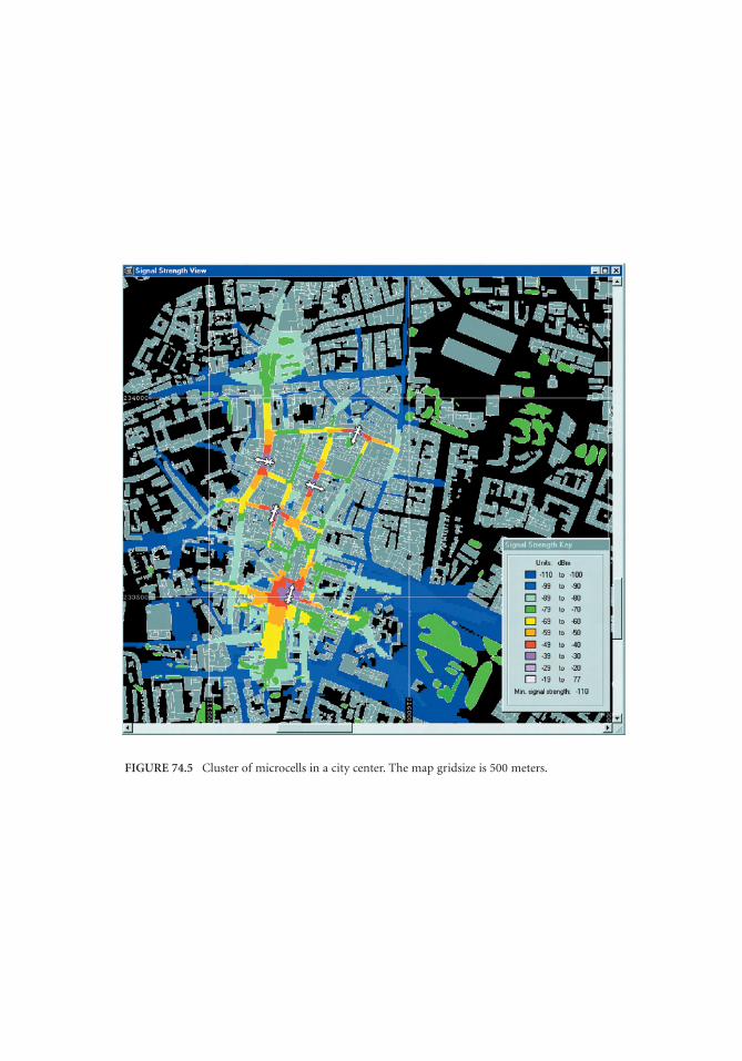
FIGURE 74.5 Cluster of microcells in a city center. The map gridsize is 500 meters.

0967 COLOR.qxd 3/12/02 6:57 PM Page 2

FIGURE 74.8 The minimum pathloss from all sites.

0967 COLOR.qxd 3/12/02 6:57 PM Page 3

FIGURE 74.9 Variation of traffic density across the network. Red represents 128 µE/m2,green represents 64 µE/m2, light blue represents 32 µE/m2, and dark blue represents16 µE/m2.

0967 COLOR.qxd 3/12/02 6:58 PM Page 4

FIGURE 74.10 The required transmit power for the speech service.

0967 COLOR.qxd 3/12/02 6:58 PM Page 5

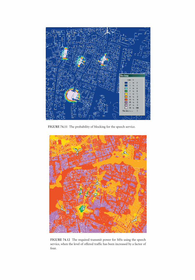
FIGURE 74.11 The probability of blocking for the speech service.

FIGURE 74.12 The required transmit power for MSs using the speechservice, when the level of offered traffic has been increased by a factor offour.

0967 COLOR.qxd 3/12/02 6:58 PM Page 6

FIGURE 74.13 The probability of blocking for speech users whenthe offered traffic has been increased by a factor of four. For the key,see Figure 74.11.

FIGURE 74.14 Soft handover regions for MSs using the speech service.The dark blue, cyan, and green areas represent regions in which an MScan be served by one, two, or three BSs, respectively.

0967 COLOR.qxd 3/12/02 6:58 PM Page 7

FIGURE 74.15 Required MS transmit power for the 384 kb/s high rate service. Original trafficlevels shown in Figure 74.9 apply.

0967 COLOR.qxd 3/12/02 6:58 PM Page 8

75Microcellular Reuse

Patterns

75.1 Introduction75.2 Microcellular Reuse Patterns75.3 Performance Analysis Model75.4 Worst Case Condition

Carrier-to-Interference Ratio • An Application Example

75.5 A More Realistic Case ConditionCarrier-to-Interference Ratio • An Application Example

75.6 ConclusionsAppendixGeneral Formulation for the Positioning of the Interferers

This chapter addresses the basic principles underlying the construction and performance of reuse patternsapplied to microcellular networks. These reuse patterns are based on a square grid and the performance ofthe system is assessed by means of the carrier-to-interference (C/I) ratio. Initially, the worst case conditionis considered, in which the system is assumed to operate at full load and all mobiles are positioned for thehighest interference situation. Following, in a more realistic condition, the mobiles are assumed to berandomly positioned within the network with the channel activity of each call connection varying in accor-dance with a given traffic intensity.

Amongst the possible reuse patterns (1, 2, 4, 5, 8, 9, 10, 13, 16... microcells per cluster), the performanceanalysis carried out here explores systems with clusters of 5, 8, 9, 10, and 13 microcells. General andclosed-form formulas are presented for all possible reuse patterns. The chapter also addresses the perti-nence of the use of simple but approximate formulas for the overall performance evaluation.

A substantial difference in performance for the uplink and downlink can be noticed, with the formerperforming less satisfactorily than the latter and with this difference diminishing as the size of the clusterincreases. Some peculiarities of each reuse pattern, such as sudden degradation in the performance atcertain points of the service area, are outlined. Both the 10- and the 9-microcell clusters exhibit anoutstanding performance. On the other hand, if appropriately explored, a remarkable trade-off betweencapacity and interference may be encountered for the 5-microcell cluster.

75.1 Introduction

The expansion and the evolution of the wireless network shall be supported by an ample microcellularstructure, not only to satisfy the high traffic demand in the dense urban regions but also to provide for theservices requiring low mobility. The microcellular network concept is rather different from that of themacrocellular one widely employed in wireless networks. In particular, the macrocellular network makesuse of a hexagonal cell array with reuse pattern being established with the supposition that reuse distances

Michel Daoud Yacoub FEEC/UNICAMP

Paula R. C. GomezFEEC/UNICAMP


are isotropic and that a cluster is comprised of a contiguous group of cells. In theory, the high-power sitescombined with base station antennas being positioned well above the rooftops provide for a propagationsymmetry, in which case, for system planning purposes, the hexagonal coverage grid has proven appropriate.

In microcellular systems, with low-power sites and antennas mounted at the street level (below therooftops), the supposed propagation symmetry of the macrocellular network no longer applies and thehexagonal cell pattern does not make sense. The ‘‘microscopic’’ structure of the environment (e.g., streetorientation, width of the streets, layout of the buildings, among others) constitutes a decisive elementinfluencing the system performance.

The ubiquitous coverage of a service area based on a microcellular network will have to make use of anexceedingly greater number of base stations as compared with that of the macrocellular systems. Therefore,among the important factors to be accounted for in the microcellular system planning (cost of the site, sizeof the service area, etc.), the per-subscriber cost is determinant. This cost is intimately related to how efficientlythe radio resources are reutilized in a given service area. The reuse efficiency depends on the interfering en-vironment of the network and on the ability of the involved technology to cope with the interfering sources.

The studies of interference in macrocellular systems is greatly eased by the intrinsic symmetry of theproblem. In the microcellular case, the inherent asymmetry due to the microscopic structures involvedimplies an additional complication. In such a case, the interference is dependent not only on the distancebetween transmitter and receiver but also, and mainly, on the line-of-sight (LOS) condition of the radiopath. For instance, assuming base stations located at street intersections, mobiles on streets running radiallyfrom the base station may experience an interference pattern changing along the street as they depart fromthe vicinity of their serving base station, where the desired signal is strong and the relevant interferingsignals are obstructed by buildings (non LOS—NLOS), and approach new intersections, where they mayhave an LOS condition not only to their serving base station but also to the interfering ones. The interferingsituation will then follow a completely distinct pattern on the perpendicular streets. Again, the asymmetryof the problem is stressed by the traffic distribution, which is more likely to comply with an unevenconfiguration with the main streets accommodating more mobile users than the secondary ones.

75.2 Microcellular Reuse Patterns

A number of field measurements and investigations [1–6] show that an urban microcell service area canbe reasonably well-approximated by a square diamond. Assuming a square cellular grid, as in Fig. 75.1,where R is the cell radius and [10] is the unit in the respective set of coordinates and the distanceD between the centers of the cells is given by D2 = i2 + j2, where i = u2 - u1 and j = v2 - v1 range over theintegers. Considering that reuse distances are isotropic and that a cluster is a contiguous group of cells,the format of the clusters must be of a square type, whose area is given by D2. Given that the area of thecell equals 2R2, the number N of cells per cluster is found to be N = i2 + j2, leading to clusters accom-modating 1, 2, 4, 5, 8, 9, 10, 13, 16... cells.

FIGURE 75.1 Square cell geometry.

2R

v

u

R

(u1,v1)

(u2,v2)

√2R

D


The layout of the cells within the cluster is attained having as principal target symmetry and compact-ness. Figure 75.2 shows some of the suggested repeat patterns. The tessellation over the entire plane isthen achieved by replicating the cluster in an isotropic manner. In other words, if the chosen reuse patternis such that i = p and j = q, then, for the reference cell located at the coordinates (0, 0), the fourcorresponding equidistant cocells are positioned at (p, q), (-q, p), (-p, -q), and (q, -p). Figure 75.2illustrates this for the case i = 1 and j = 2 (N = 5). Figure 75.3 shows a partial tessellation for the reusesof 5 (i = 1, j = 2) and 13 (i = 2, j = 3).

In the performance analysis of the various reuse patterns, a parameter of interest is the distance betweenthe interferers positioned at the co-cell of the Lth co-cell layer and at the target cell, the target cell takenas the reference cell. We define such a parameter as nL and, for ease of manipulation, normalize it withrespect to the cell radius, i.e., nL is given in number of cell radii. We observe that this parameter is greatlydependent on the reuse pattern. It can be obtained by a simple visual inspection, but certainly for a verylimited number of cell layers. For the general case, a more general formulation is required, and this isshown in the appendix.

FIGURE 75.2 Some possible reuse patterns (N = 1, 2, 4, 5, 8, 9, 10, 13 microcells per cluster).

FIGURE 75.3 Partial tessellation for the reuse of 5 and 13.

(1,2)(−2,1)

(−1,−2)

i

j

(2,−1)

(2,3)

(−3,2)

(3,−2)

j

i

(−2,−3)

(1,2) (−2,1)

(2,−1)

i

j

(−1,−2)


75.3 Performance Analysis Model

The performance analysis to be carried out here considers a square cellular pattern with base stationspositioned at every other intersection of the streets. This means that base stations are collinear and thateach microcell covers a square area comprised of four 90∞-sectors, each sector corresponding to one-half of a block, with the streets running on the diagonals of this square. Figure 75.4 shows the cellularlayout with respect to the streets. In Fig. 75.4, the horizontal and vertical lines represent the streets andthe diagonal lines represent the microcells’ borders. The central microcell is highlighted in the figure inorder to evidence its location.

In order to give an insight into how the performance calculations are carried out, Figs. 75.5 and 75.6illustrate the complete tessellation for clusters containing 5 (Fig. 75.5), 8, 9, 10, and 13 (Fig. 75.6) microcells,in which the highlighted cluster accommodates the target cell, and the other dark cells correspond to the

FIGURE 75.4 Cellular layout in an urban area.

FIGURE 75.5 Five-microcell cluster tesselation—Prime Non-Collinear Group (see appendix).

A

BC

D E

A

BC

D E

A

BC

D E

A

BC

D E

A

BC

D E A

BC

D E

A

BC

D E

A

BC

D E

A

BC

D E

A

BC

D E

A

BC

D E A

BC

D E A

BC

D E A

BC

D E

A

BC

D E

A

BC

D E

A

BC

D E A

BC

D E

A

BC

D E A

BC

D E

A

BC

D E

A

BC

D E

A

BC

D E

A

BC

D E

A

BC

D E

A

BC

D E

A

BC

D E

A

BC

D E

A

B

E

A

D E

ABC

A

C

D

A

BC

D E


co-microcells that, at a certain time, may interfere with the mobile or base station of interest. Within amicrocellular structure, distinct situations are found that affect in a different manner the performanceof the downlink and of the uplink. In general, the set of microcells affecting the downlink constitutes asubset of those influencing the uplink. In Figs. 75.5 and 75.6, the stars indicate the sites contributing tothe C/I performance of the downlink, whereas the circles point the worst case location of the mobileaffecting the C/I performance of the uplink. The cluster attribute (collinear, non-collinear, etc.) indicatedin the captions of these figures are defined in the appendix.

It is noteworthy that some of the patterns tessellate into staggered configurations with the closerinterferers being either completely obstructed or obstructed for most of the time with an LOS interfererappearing many blocks away. It is also worth emphasizing that for clusters with a prime number ofconstituent cells, as is the case of the 5-cell cluster of Fig. 75.5, the base stations that interfere with thetarget mobile in the downlink change as the mobile moves along the street.

Concerning the radio coverage aspects, it is well known [1–6] that the LOS and the NLOS modes ofpropagation are very distinct from each other. The respective propagation losses at a distance d from thebase station and for a wavelength λ, a transmitting antenna height ht, and a receiving antenna height hr

are then given by

(75.1)

(75.2)

where KLOS = (λ/4π)2, dB = 4hthr/λ is the breakpoint distance, KNLOS = 0.16 for 900 MHz and 0.0015 for2 GHz, and α = 4.3 for 900 MHz and α = 3.8 for 2 GHz [4].

FIGURE 75.6 (a) Eight-microcell cluster tessellation—Collinear i = j Group; (b) Nine-microcell cluster tessellation—Collinear Group; (c) Ten-microcell cluster tessellation—Even Non-Collinear; (d) Thirteen-microcell clustertessellation—Prime Non-Collinear Group (see appendix).

(a) (b)

(c) (d)

N Z∈

L LOS

KLOS

d2----------- 1

ddB

-----

2

+–

=

LNLOS

KNLOS

da--------------=


The following two sections of this chapter analyze the performance of a microcellular network systemfor the worst case condition and also for a more realistic condition. In the first case, the system is assumedto operate at full load and all mobiles are positioned for the highest interference situation. In the secondcase, the mobiles are assumed to be randomly positioned within the network with the channel activityof each call connection varying in accordance with a given traffic intensity. Because the contribution ofthe obstructed interferers to the overall C/I performance is negligible if compared to that of the LOSinterferers, only the LOS condition of the interferers is used for the calculations. In such a case, the resultsfor the worst case condition express the lower bound performance of the system whereas the realisticcase condition express the upper bound performance.

75.4 Worst Case Condition

Carrier-to-Interference Ratio

Defining r as the serving base station-to-mobile station distance normalized with respect to the cell radius(0 < r ≤ 1) and k as the ratio between the cell radius and the breakpoint distance (k ≥ 0), it is possible toshow that, for the interferers positioned at the worst case condition, the uplink C/I parameter is given by [7]

(75.3)

where nL = 1, 2, 3... is the distance between the interferers at the Lth layer and the target cell site, givenin number of units of the cell radius. The parameter nL is dependent on the reuse pattern, as shown inthe appendix.

In the same way, a C/I can be found for the downlink. However, this ratio depends on the positionof the target mobile with respect to its serving base station because, as the mobile moves from the cellcenter toward the next corner, it acquires a new LOS, and it may find new interfering base stations.Therefore, for the downlink and for the mobile at the vicinity of its serving base station, more specifically,at the intersection of the streets (r ≤ normalized distance from the site to the beginning of the street),the C/I ratio [7] is

(75.4)

Away from the vicinity of the serving base station, which corresponds to most of the path, the C/I ratio[7] is

(75.5)

At the border of the cell (very end of the corner), new interferers may appear in an LOS condition. However,this is not the case for all reuse patterns. This phenomenon only happens for clusters with a prime numberof cells, as, for example, in the case of 5-cell clusters as illustrated in Fig. 75.5. Hence, for clusters with a primenumber of cells and the mobile away from its serving base station (1 - r ≤ normalized distance from the site

CI--- 1 rk( )2+[ ]

1–

4r2∑L=1∞ nL

2– 1 nLk( )2+[ ]1–

------------------------------------------------------------=

CI--- =

1 rk( )2+[ ]1–

r2∑L=1∞ nL r+( ) 2–

1 nL r+( )2k2+[ ]

1–nL r–( ) 2–

1+ nL r–( )2k2[ ]

1–2 nL

2 r2+( )1–

1+ nL2 r2+( )k2[ ]

1–++{ }

---------------------------------------------------------------------------------------------------------------------------------------------------------------------------------------------------------------------------------------------

CI--- 1 rk( )2+[ ]

1–

r2∑L=1∞ nL r+( ) 2–

1 nL r+( )2k2+[ ]

1–nL r–( ) 2–

1 nL r–( )2k2+[ ]

1–+{ }

-----------------------------------------------------------------------------------------------------------------------------------------------------------------=


to the beginning of the street), the C/I ratio [7] is

where = 1

An Appli

This section has been evathe center togray, the co-m

For the nuof 15 m, thefrequency of(in practice,

Figures 758-, 9-, 10-, acluster the bnotably outs(lower curveextension oflatter occurr

There is abecoming pin Fig. 75.8,

It is interFor this purpFigures 75.9normalized (one layer) mfor the infincalculations.

FIGURE 75.7

CI---

r2 ∑L=1∞[

----------------=

r

10

20

30

40

50

60

70

80

90

100

Car

rier/

Inte

rfer

ence

[dB

]


©2002 CRC P

(75.6)

− r and is defined in the appendix.

cation Example

illustrates the C/I performance for clusters with 5, 8, 9, 10, and 13 microcells. The performanceluated having the central microcell as the target cell and for the mobile subscriber departing fromward its edge, as shown by the arrow in the respective cell in Fig. 75.5. Figure 75.5 also shows, in

icrocells that, at a certain time, may interfere with the wanted mobile in an LOS condition.merical results, the calculations consider the radius of the microcell as 100 m, a street width

transmitter and receiver antennas heights, respectively, equal to 4 m and 1.5 m, an operation 890 MHz, which leads to k = 1.405, and a network consisting of an infinite number of cells 600 layers of interfering cells)..7a and 75.7b show, respectively, the uplink and downlink performances for the cases of 5-,

nd 13-microcell clusters as a function of the normalized distance. In general, the bigger theetter the carrier-to-interference ratio, as expected. However, the 5-microcell cluster has atanding behavior, with its C/I coinciding with that of the 8-microcell cluster for the uplink in Fig. 75.7a) and with that of the 10-microcell cluster for the downlink for most of the the path (curve below the upper one in Fig. 75.7b), with the separation of the curves in theing at the edge of the microcell, where two new interferers appear in an LOS condition. significant difference between the performance for the uplink and downlink, this differencerogressively smaller with the increase of the size of the cluster. This can be better observedwhere the 5- and 10-microcell clusters are compared.

esting to examine the influence of the number of interfering layers in the C/I performance.ose, we analyze the performance of a one-layer network (L = 1 in Eqs. (75.3) through (75.6)).a and 75.9b show the performances for the uplink and downlink as a function of the

distance to the base station using both the exact (infinite number of layers) and the simplifiedethods for clusters of 5 and 8 cells, respectively. The dotted lines correspond to the results

ite number of interferers case, and the solid lines represent the results for the simplified Analyzing the graphs and the numerical results, one observes that the difference between

Carrier-to-interference ratio as a function of normalized distance: (a) uplink; (b) downlink.

1 rk( )2+[ ] 1–

nL r+( ) 2–1 nL r+( )2

k2+[ ] 1–nL r–( ) 2–

1 nL r–( )2k2+[ ] 1–+{ } ∑L ′=1

∞ nL ′′

2r

2+( ) 1–1 n

L ′′2

r2+( ) k2( )+[ ] 1–{ }+ ]

------------------------------------------------------------------------------------------------------------------------------------------------------------------------------------------------------------------------------------------

nL′

0.2 0.4 0.6 0.8 1.0

Uplink 5 Uplink 8 Uplink 9 Uplink 10 Uplink 13

Normalized Distance from Site0.2 0.4 0.6 0.8 1.0

10

20

30

40

50

60

70

80

90 Downlink 5 Downlink 8 Downlink 9 Downlink 10 Downlink 13

Car

rier/

Inte

rfer

ence

[dB

]

Normalized Distance from Site

(a) (b)

ress LLC

the C/I raticonclusion areuse pattern

Thereforelayer that isformulas. Homust be con

75.5 A

Carrier-to

This sectionchannel to bthe locationsubset of theare not activLOS conditiiACT&LOS inteinterference

FIGURE 75.8

FIGURE 75.9(a) 5-cell clu

70

Uplink 5 Downlink 5 Uplink 10 B

]


©2002 CRC P

o for an infinite-cell network and for a one-interfering-layer network is negligible. Thislso applies to the other patterns, with the biggest difference found in both methods for alls being less than 0.35 dB.

, for the worst case condition, the C/I ratio can be estimated by considering only the interfering closest to the target cell. In such a case, Eqs. (75.3) through (75.6) reduce to very simplewever, as will be discussed in the following section, for a more realistic condition more layers

sidered in the performance analyses.

More Realistic Case Condition

-Interference Ratio

considers the interferer to be randomly positioned within the microcell network and thee active according to a given traffic intensity. Assume a uniform probability distribution for of a mobile within a cell. Let i be the number of interferers and iACT&LOS (0 ≤ iACT&LOS ≤ i) a interferers that are active and in an LOS condition, and iNACT or NLOS = i − iACT&LOS those thate or that are in an obstructed situation. Let pLOS be the probability of a mobile being in anon, pACT the probability of a channel being active, and pACT&LOS the probability of havingrferers simultaneously active and in an LOS condition. Let E[C/I|iACT&LOS] be the carrier-to- ratio estimated in such a case. The overall mean carrier-to-interference ratio is, therefore [8],

(75.7)

Carrier-to-interference ratio as a function of normalized distance for uplink and downlink compared.

Performance considering an infinite number of interferers and a single layer of interferers forsters and (b) 8-cell clusters.

0.2 0.4 0.6 0.8 1.0

10

20

30

40

50

60 Downlink 10

Car

rier/

Inte

rfer

ence

[dNormalized Distance from Site

S

0.2 0.4 0.6 0.8 1.0

10

20

30

40

50

60

70

5 Cell Cluster Uplink oo layers Uplink 1 layer Downlink oo layers Downlink 1 layer

Car

rier/

Inte

rfer

ence

[dB

]

Normalized Distance from Site0.2 0.4 0.6 0.8 1.0

10

20

30

40

50

608 Cell Cluster

Uplink oo layers Uplink 1 layer Downlink oo layers Downlink 1 layer

Car

rier/

Inte

rfer

ence

[dB

]


(a) (b)

E C/I[ ] E C/I |iACT&LOS[ ]pACT&LOS

iACT&LOS=0

i

∑=

ress LLC

where

or, equivalen

There is afrom the celhand, for clFrom Fig. 7layers are inare in an LOnumber of Eq. (75.9) fo

An Appli

The results probability pthe street ofonly at the ceach microcnumber of mof interfererspurposes, thcell (inner lathe former ahas been foureliable resu

Figures 75normalized dcases: for thelayers (solidwhereas the condition ca

Figure 75.and 8-cell clucases. It is n


©2002 CRC P

(75.8)

tly,

(75.9)

(75.10)

(75.11)

unique value for pLOS for clusters with a non-prime number of microcells, as can be observedlular layout. Therefore, Eq. (75.8) is used to evaluate pACT&LOS in these cases. On the otherusters with a prime number of microcells, there is more than one possible value for pLOS.5.5, one can observe that mobile interferers affecting the uplink (circles) from the first two an LOS condition only when positioned at the corner, whereas mobiles from the third layerS condition at any point along the entire street. This is the case for all clusters with a prime

cells. Therefore, calculations of the performance of the uplink for such cases make use ofr the value of pACT&LOS.

cation Example

to be shown here consider clusters of 5 and 8 cells for the parameters as given before. The

LOS is different for each tessellation because for some of them there are co-microcells wherefers an LOS condition at any of its points, whereas for others, the LOS condition is offeredorner of the street of the co-microcell. The calculations of the C/I ratio shown here assumeell to have 8 channels and a grade of service of 2% and they are performed for an ‘‘infinite’’

icrocells. Certainly, performing the calculations outlined in Eq. (75.7) for an infinite number is impracticable. Limiting the number of interferers may compromise the results. For practicale interferers are then divided into two groups: those belonging to the layers closer to the targetyers) and those belonging to the other layers (outer layers). Again for practical purposes, onlyre given random properties, whereas the latter are positioned for the worst case condition. Itnd [9] that the minimum number of layers within the inner layers necessary to yield statisticallylts is 7. As before, the calculations take into account 600 layers of interfering cells. .10a and 75.10b show the performances for the uplink and the downlink as a function of theistance to the base station for clusters with 5 and 8 microcells, respectively, for the two limiting inner layers containing one layer only (dotted lines) and for the inner layers containing seven

lines). Note that a remarkable difference between the two cases is found. This implies that,worst case condition can be easily modeled by means of a one-layer network, a more realisticn only be analyzed if a significantly greater number of layers is considered.11 compares the lower bound performance and the upper bound performance for 5-cell clusterssters. The plots show an outstanding increase in performance for both the uplink and downlink

oteworthy that this increase is enhanced for the case of 5-cell clusters, and this applies to all

pACT&LOS

i

iACT&LOS pLOS pACT×( )

iACT&LOS 1 pLOS pACT×–( )i iACT&LOS–

=

pACT&LOS

i 1( )

iACT&LOS1( )

pLOS1( ) pACT×( )

iACT&LOS1( )

1 pLOS1( ) pACT×–( )

1 iACT&LOS1( )

–⋅=

i 2( )

iACT&LOS2( )

pLOS2( ) pACT×( )

iACT&LOS2( )

1 pLOS2( ) pACT×–( )

iACT&LOS2( )

⋅×

i 1( ) i 2( )+ i=

iACT&LOS1( ) iACT&LOS

2( )+ iACT&LOS=

ress LLC

clusters withmost of the cells have thattention shofor the casescase, and no

75.6 C

This chapterapplied to mcarried out condition anwith probabchannel actihere, the woaccount the to improve dare assumednection vari

Among thanalysis conformulas we

When comcan observe

FIGURE 75.10(a) 5-cell clus

FIGURE 75.1lower and up

70

8 Cell Cluster

[dB

]805 Cell Cluster

Uplink - 7 inner layersUplink - 1 inner layer

Uplink - 7 inner layersUplink - 1 inner layer[d

B]


©2002 CRC P

prime number of cells. The reason for this is that, for clusters with prime number of cells,co-microcells have only their corners in LOS, whereas the clusters with non-prime number ofe co-microcells collinear with the target cell, therefore, having a whole street in LOS. Specialuld be paid to the enhancement in efficiency at the corner opposite the serving base station

of clusters with a prime number of cells. Those points showed a poor C/I ratio for the worstw, considering a more realistic situation, they show a drastic improvement.

onclusions

addressed the basic principles underlying the construction and performance of reuse patternsicrocellular networks. An initial assessment of these patterns, based on a square grid, was

by means of the carrier-to-interference ratio for the mobiles positioned at the worst cased the system operating at a full load. It is noteworthy that the worst case condition occurs

ility of (pACT × pLOS)4L, where L is the number of interfering layers, pACT is the probability of

vity, and pLOS is the probability of LOS condition. Roughly speaking, for the geometry exploredrst case condition occurs with probability (3 × 10−5)L × (pACT)4L. Therefore, by taking intorandom distribution of the users and the channel occupancy, the mean C/I ratio is expectedrastically. This motivates the examination of a more realistic condition in which the mobiles to be randomly positioned within the network and the channel activity of each call con-es in accordance with a given traffic intensity. e possible reuse patterns (1, 2, 4, 5, 8, 9, 10, 13, 16... microcells per cluster), the performancesidered systems with clusters of 5, 8, 9, 10, and 13 microcells. General and closed-formre presented for all possible reuse patterns for all cases.

paring the performance for the worst case condition and the more realistic condition, onean outstanding increase in the carrier-to-interference ratio for the latter case. An analysis of

Upper bound performance as a function of normalized distance for the uplink and downlink forters; (b) 8-cell clusters.

1 Carrier-to-interference ratio as a function of normalized distance for uplinks and downlinks forper bound performances compared: (a) 5-cell clusters; (b) 8-cell clusters.

0.2 0.4 0.6 0.8 1.0

20

30

40

50

60

Car

rier/

Inte

rfer

ence

0.2 0.4 0.6 0.8 1.020

30

40

50

60

70 Downlink - 7 inner layersDownlink - 1 inner layer

Downlink - 7 inner layersDownlink - 1 inner layer

Car

rier/

Inte

rfer

ence


(a)


(b)

0.2 0.4 0.6 0.8 1.010

20

30

40

50

60

708 Cell Cluster

Car

rier/

Inte

rfer

ence

[dB

]

Normalized Distance from Site 0.2 0.4 0.6 0.8 1.0

10

20

30

40

50

60

70

80

5 Cell ClusterUplink - Upper boundUplink - Lower bound Downlink - Upper boundDownlink - Lower bound

Uplink - Upper boundUplink - Lower bound Downlink - Upper boundDownlink - Lower bound

Car

rier/

Inte

rfer

ence

[dB

]

(a)Normalized Distance from Site

(b)

ress LLC

a microcellular system can be made by considering the results of the equations presented for the worstcase condition as the lower bound performance and the results of the equations presented for the morerealistic con

Finally, thoverall perfoand the appthat the firsthand, if moThe conditiofor the numconditions dBoth the 10appropriatelfor the 5-mi

Append

General F

In the perforinterferers atnormalize itparameter iscertainly for and this is sh

The reuseaccording togroups. Givethe classifica

• Collin

• Non-

Figures 7tessellation with an evensubgroups isas in Fig. 75.of its servincells per clu

The relatcell and itsminimum dunits of thefor base sta


©2002 CRC P

dition as the upper bound performance.e chapter addressed the pertinence of the use of simple but approximate formulas for thermance evaluation. The graphs showed a remarkable similarity in the C/I ratio for the exact

roximate methods when considering the worst case condition, from which it can be inferred layer of interferers play the most influential role in the overall performance. On the otherre realistic conditions are to be considered, then this influence just mentioned is not valid.n that yields statistically reliable results was discussed. It was found that convergence occursber of interfering layers approaching seven. It could be observed that the more realisticrastically improves the performance of the system as compared to the worst case condition.- and the 9-microcell clusters exhibit an outstanding performance. On the other hand, ify explored, a remarkable trade-off between capacity and interference may be encounteredcrocell cluster.

ix

ormulation for the Positioning of the Interferers

mance analysis of the various reuse patterns, a parameter of interest is the distance between the the Lth layer and the target cell. We define such a parameter as nL and, for ease of manipulation, with respect to the cell radius, i.e., nL is given in number of cell radii. We observe that this greatly dependent on the reuse pattern. It can be obtained by a simple visual inspection, buta very limited number of cell layers. For the general case, a more general formulation is required,own here. patterns of the square grid cell configurations can be divided into four different groups the shape into which their cells tesselate [9]. Figures 75.5 and 75.6 illustrate samples of somen that the number of cells per cluster is defined by N = i2 + j2, where i and j are integers,tion of reuse patterns for square cells is as follows:

ear

Collinear ˙

5.6a and 75.6b show the tessellations of the first case (collinear). From the non-collineargroup, there are three different subgroups: clusters with a prime number of cells, clusters number of cells, and clusters with an odd and non-prime number of cells. The first of these represented by a 5-cell cluster tessellation, as in Fig. 75.5, and by the 13-cell cluster tesselation,6d, and is characterized by the appearance of new interferers as the mobile reaches the borderg base station. A member of the group of non-collinear tessellation with an even number ofster is illustrated in Fig. 75.6c.ions below show, for each of the groups defined above, the distance between the target interferers for the uplink and for the downlink, for the worst case condition. Theistance between collinear co-cells is represented by the variable d, given in number of cell radius. In these relations, L is the number of the interfering layer and BS standstion.

• N Z, i.e., i∈ 0 or j 0 (square clusters)= =or

• i j, i.e., N x2 where x Z and Z defines the integer set∈= =

• N is prime

• N is non-prime

ress LLC

1. Collinear

• d = 2i

• obs

• Up

• Do

2. Even

• d =• Up

• Do

3. Odd

•

• nL

whdis

4. Prim

• d =

• Up

wh

• Do

Reference

1. J.H. WhIEEE Tr

2. A.J. Rusgation lConfere

3. V. ErcegcoveragVeh. Tec

4. M.V. ClTrans. V

5. A. Goldurban m

6. V. Erceg1992.

N∀


©2002 CRC P

: when ∈ Z, if i = 0, d = 2j

link: nL = 2iL − 1

wnlink:

Non-Collinear

N

link: nL = N⋅L − 1

wnlink:

and Non-Prime Non-Collinear

= rNR

= r ⋅nL(R)

ere r ∈Z, NR < N, NR = number of cells per cluster of another reuse pattern R, and nL(R) is thetance between the interferers at the Lth layer and the target cell for reuse pattern Re Non-Collinear

2N

link:

ere p designates the prime number immediately prior to N

wnlink:

s

itteker, Measurements of path loss at 910 MHz for proposed microcell urban mobile systems,ans. Veh. Technol., 37, 125, 1988.tako, V. Erceg, R.S. Roman, T.M. Willis, and J. Ling, Measurements of microcellular propa-oss at 6 GHz and 2 GHz over nonline-of-sight paths in the city of Boston, in GLOBECOM’95nce, Singapore, 758., A.J. Rustako, Jr., and R.S. Roman, Diffraction around corners and its effects of the microcelle area in urban and suburban environments at 900 MHz, 2 GHz, and 6 GHz, IEEE Trans.hnol., 43, 762, 1994.ark, V. Erceg, and L.J. Greenstein, Reuse efficiency in urban microcellular networks, IEEEeh. Technol., 46, 279, 1994.smith and L.J. Greenstein, A measurement-based model for predicting coverage areas oficrocells, IEEE J. Select. Areas Commun., 11, 1013, 1993.

et al., Urban/suburban out-of-sight propagation modeling, IEEE Commun. Mag., 30, 56,

N

Near BS: nL 2iL=Far from BS: nL 2iL=

Near BS: nL N⋅L=Far from BS: nL N⋅L=

n3(L−1)+1 p 2N L 1–( )+=n3(L−1)+2 2N p–( ) 2N L 1–( )+=n3(L−1)+3 2NL 1–=

Near BS: nL 2NL=Far from BS: nL 2NL=

Near cell border:

nL 2NL=n′2 L−1( )+1 p 2N L 1–( )+=n′2 L−1( )+ 2 2N p–( ) 2N L 1–( )+=

ress LLC

7. M.D. Yacoub, A.F. Toledo, P.R.C. Gomez, P.J.E. Jeszensky, and E.B.R. Féris, Reuse pattern for micro-cellular networks, Int. J. Wireless Inf. Networks, 6(1), 1, 1999.

8. P.R.C. GrealisticCommu

9. P.R.C. GBraziliaES, Braz

10. M.D. Ya


©2002 CRC P

omez, M.D. Yacoub, and A.F. Toledo, Performance of a microcellular network in a more condition, The 11th IEEE International Symposium on Personal Indoor and Mobile Radionications, 2000.omez, M.D. Yacoub, and A.F. Toledo, Interference in wireless networks with a new reuse pattern,

n Telecommunications Symposium (Simpósio Brasileiro de Telecomunicações), SBT99, Vitória,il, 1999 (in Portuguese).coub, Wireless Technology, CRC Press, Boca Raton, FL, 2001.

ress LLC

76Fixed and Dynamic

Channel Assignment

76.1 Introduction76.2 The Resource Assignment Problem76.3 Fixed Channel Assignment 76.4 Enhanced Fixed Channel Assignment 76.5 Dynamic Channel Assignment 76.6 CDMA Systems76.7 Conclusion

76.1 Introduction

One of the important aspect of frequency reuse-based cellular radio as compared to early land mobiletelephone systems is the potential for dynamic allocation of channels to traffic demand. This fact hadbeen recognized from the early days of research (e.g., see [18, Chapter 7], [7,8]) in this field. With theemergence of wireless personal communications and use of microcell with nonuniform traffic, radioresource assignment becomes essential to network operation and largely determines the available spec-trum efficiency. The primary reason for this lies in the use of microcell in dense urban areas wheredistinct differences exist as compared to large cell systems due to radio propagation and fading effectsthat affect the interference conditions.

In this chapter, we will first review the channel reuse constraint and then describe methods to accom-plish the assignment. Subsequently, we will consider variations of fixed channel assignment and discussdynamic resource assignment. Finally, we will briefly discuss the traffic modeling aspect.

76.2 The Resource Assignment Problem

The resources in a wireless cellular network are derived either in frequency division multiple access(FDMA), time division multiple access (TDMA), or joint frequency–time (MC-TDMA) [1]. In thesechannel derivation techniques, the frequency reuse concept is used throughout the service areas com-prised of cells and microcells. The same channel is used by distinct terminals in different cells, with theonly constraint of meeting a given interference threshold. In spread spectrum multiple access (SSMA)such as the implemented code division multiple access (CDMA) system (IS-95) [24] each subscriberspreads its transmitted signal over the same frequency band by using a pseudorandom sequence simul-taneously. As any active channel is influenced by the others, a new channel can be set up only if theoverall interference is below a given threshold. Thus, the problem of resource assignment in CDMArelates to transmission power control in forward (base station to mobile terminal) and reverse (mobileterminal to base station) channels. Of course, the problem of power control applies to TDMA and FDMAas well, but not to the extent that it impacts the capacity of CDMA. Here we first focus on time- and

Bijan JabbariGeorge Mason University


frequency-based access methods. We subsequently present some preliminary discussion on spread spec-trum CDMA systems.

Fixed channel assignment (FCA) and dynamic channel assignment (DCA) techniques are the twoextremes of allocating radio channels to mobile subscribers. For a specific grade of service and qualityof transmission, the assignment scheme provides a tradeoff between spectrum utilization and implemen-tation complexity. The performance parameters from a radio resource assignment point of view areinterference constraints (quality of transmission link), probability of call blocking (grade of service), andthe system capacity (spectrum utilization) described by busy hour erlang traffic that can be carried bythe network. In a cellular system, however, there exist other functions, such as handoff and its executionor radio access control. These functions may be facilitated by the use of specific assignment schemes and,therefore, they should be considered in such a tradeoff [14].

The problem of channel assignment can be described as the following: Given a set of channels derivedfrom the specified spectrum, assign the channels and their transmission power such that for every set ofassigned channels to cell i, (C/I)i > (C/I)0. Here, (C/I)0 represents the minimum allowed carrier to interfer-ence and (C/I)i represents carrier to interference at cell i.

76.3 Fixed Channel Assignment

In fixed channel assignment the interference constraints are ensured by a frequency plan independent ofthe number and location of active mobiles. Each cell is then assigned a fixed number of carriers, dependenton the traffic density and cell size. The corresponding frequency plan remains fixed on a long-term basis.In reconfigurable FCA (sometimes referred to as flexible FCA), however, it is possible to reconfigure thefrequency plan periodically in response to near/medium term changes in predicted traffic demand.

In FCA, for a given set of communications system parameters, (C/I)0 relates to a specific quality oftransmission link (e.g., probability of bit error or voice quality). This parameter in turn relates to thenumber of channel sets [18] (or cluster size) given by K = 1/3 (D/R)2. Thus, the ratio D/R is determinedby (C/I)0. Here D is the cochannel reuse distance and R is the cell radius. For example, in the NorthAmerican cellular system advanced mobile phone service (AMPS), (C/I)0 = 18 dB, which results in K = 7or D = 4.6R. Here, we have used a propagation attenuation proportional to the fourth power of thedistance. The radius of the cell is determined mainly by the projected traffic density. In Fig. 76.1 a seven

FIGURE 76.1 Fixed channel assignment.


cell cluster with frequency sets F1 through F7 (in cells designated A–G) has been illustrated. It is seenthat the same set of frequencies is repeated two cells away.

The number of channels for each cell can be determined through the erlang-B formula (for example,see Cooper, 1990 [6]) by knowing the busy hour traffic and the desired probability of blocking (gradeof service). Probability of blocking PB is related to offered traffic A, and the number of channels per cellN by

This applies to the case of blocked calls cleared. If calls are delayed, the grade of service becomes theprobability of calls being delayed PQ and is given by the erlang-C formula [6],

FCA is used in almost all existing cellular mobile networks employing FDMA or TDMA. To illustrateresource assignment in FCA, we describe the FCA schemes used in global system for mobile communi-cations (GSM or DCS) [17]. Here, the mobile terminal continuously monitors the received signal strengthand quality of a broadcast channel along with the identity of the transmitting base station. This mech-anism allows both the mobile and the network to keep track of the subscriber movements throughoutthe service area. When the mobile terminal tries and eventually succeeds in accessing the network (seeFig. 76.2), a two way control channel is assigned that allows for both authentication and ciphering modeestablishment. On completion of these two phases, the setup phase initiates and a traffic channel iseventually assigned to the mobile terminal. Here, the terminal only knows the identity of the serving cell;the (control and traffic) radio channel assignment is a responsibility of the network and fulfills the originalcarrier to cell association, while simplifying the control functions during normal system operation.

FIGURE 76.2 Radio resource assignment in GSM/DCS. Source: Jabbari, B. et al., Network issues for wirelesspersonal communications. IEEE Commun. Mag., 33(1), 1995.

PB

AN/N!

∑i=0N Ai/i!

---------------------=

PQ

AN

N! 1 A/N–( )-------------------------

∑i=0N-1Ai/i!

AN

N! 1 A/N–( )--------------------------------+

-------------------------------------------------------=


76.4 Enhanced Fixed Channel Assignment

FCA has the advantage of having simple realization. Since the frequency sets are preassigned to cellsbased on long-term traffic demand, however, it cannot adapt to traffic variation across cells and, therefore,FCA will result in poor bandwidth utilization. To improve the utilization while maintaining the imple-mentation simplicity, various strategies have been proposed as enhancements to FCA and deployed inexisting networks. Two often used methods are channel borrowing and directed retry, which are describedhere.

In the channel borrowing strategy [11,12,18,29], channels that are not in use in their cells may beborrowed by adjacent cells with high offered traffic on a call-by-call basis. Borrowing of channels allowsthe arriving calls to be served in their own cell. This implies that there will be further restrictions inusing the borrowed channels in other cells. Various forms of borrowing have been surveyed in Tekinayand Jabbari [23].

In directed retry [10,13,14], a call to or from a mobile subscriber may try other cells with channelswith sufficient signal strength meeting the C/I constraint if there are no channels available in its own cellto be served. In some cases it may be necessary to direct some of the calls in progress in a given congestedcell to adjacent lightly loaded cells (those calls that can be served by adjacent cells) in order to accom-modate the new calls in that given cell. This is referred to as directed handoff [13,20]. The combinationof these two capabilities provides a significant increase in bandwidth utilization.

76.5 Dynamic Channel Assignment

In dynamic channel assignment [2,3,4,7,8,9,12,21], the assignment of channels to cells occurs based onthe traffic demand in the cells. In other words, channels are pooled together and assignments are madeand modified in real time. Therefore, this assignment scheme has the potential to achieve a significantlyimproved bandwidth utilization when there are temporal or spatial traffic variations.

In DCA, the interference constraints are ensured by a real-time evaluation of the most suitable (lessinterfered) channels that can be activated in a given cell (reassignment may be needed). That is, thesystem behaves as if the frequency plan was dynamically changing to meet the actual radio link qualityand traffic loads, realizing an implicit sharing of the frequency band under interference constraints.

The implementation of DCA generally is more complex due to the requirement for system-wide stateinformation where the state refers to which channel in which cell is being used. Obviously, it is impracticalto update the system state in a large cellular network at any time, especially those based on microcells,as the controller will be overloaded or call set delay will be unacceptable. Therefore, methods have beendevised based on a limited state space centralized control [15] or based on a distributed control to performthe necessary updating. A method referred to as maximum packing, suggested in Everitt and Macfadyen[15], records only the number of channels in use. Distributed control schemes, however, where channelassignments are made at mobile stations or base stations may be attractive. These schemes are particularlysuitable for a mobile controlled resource assignment where each mobile measures the actually perceivedinterference and decides to utilize a radio resource in a completely decentralized way.

Design of DCA algorithms is critical to achieve the potential advantages in efficiency and robustnessto traffic heterogeneity throughout cells as compared to FCA and enhanced FCA. Poor DCA algorithms,however, might lead to an uncontrolled global situation, i.e., the locally selected channel might be verygood for the specific mobile terminal and at the same time very poor for the interference level inducedto other traffic sources.

Two classes of regulated DCA and segregation DCA are discussed here due to their importance. In aregulated DCA, appropriate thresholds tend to maintain the current channel, avoiding useless handoffsthat can tie up channels; in a segregation DCA, channel acquisition obeys priorities assigned to eachchannel. In the latter, the channels successfully activated in a cell have a higher assignment probabilitythan those found to have a high interference in the cell; of course, priorities change in time dependingon changes in the system status. These types of assignment lead to a (frequency) plan still changing


dynamically but more slowly and, in general, only because of substantial load imbalance. In steady-stateconditions, the plan either tends to be confirmed or fluctuates around a basic configuration, proven tobe suboptimal in terms of bandwidth efficiency.

Both digital European cordless telecommunications (DECT) and cordless technology known as CT2are employing the DCA technique [25], and the next generation cellular systems are foreseen to deployit. In CT2 the handset and the base station jointly determine a free suitable channel to serve the call. InDECT, the mobile terminal (portable handset) not only recognizes the visited base station (radio fixedpart) through a pilot signal but continuously scans all of the system channels and holds a list of the lessinterfered ones. The potentially available channels are ordered by the mobile terminal with respect tothe measured radio parameters, namely, the radio signal strength indicator, measuring and combiningcochannel, adjacent-channel, and intermodulation interference. When a connection has to be established,the best channel is used to communicate on the radio interface.

It is possible to have a hybrid of DCA and FCA in a cellular network in which a fraction of channelsare fixed assigned and the remainder are allocated based on FCA. This scheme has less system imple-mentation complexity than the DCA scheme but provides performance improvement (lower probabilityof call blocking) depending on the DCA–FCA channel partitioning [19].

In general, DCA schemes cannot be considered independently of the adopted power control mecha-nism because the transmitted power from both mobile terminal and base station substantially affects theinterference within the network. For a detailed discussion of DCA and power control, the readers arereferred to [5]. Despite the availability of several power control algorithms, much work is needed toidentify realizable power and channel control algorithms that maximize bandwidth efficiency. Neverthe-less, realization of power control mechanisms would require distribution of the system status informationand information exchange between mobile terminal and network entities. This in turn will involveoverhead and terminal power usage.

The performance of DCA depends on the algorithm implementing this capability [13,16]. In general,due to interactions between different cells the performance of the system will involve modeling the systemas a whole, as opposed to in FCA where cells are treated independently. Therefore, mathematical modelingand performance evaluation of DCA becomes quite complex. Simplifying assumptions may, therefore,be necessary to obtain approximate results [15,22]. Simulation techniques have been widely used inevaluation of DCA performance. For a representative performance characteristics of DCA and a com-parison to enhanced FCA schemes the readers are referred to [14].

76.6 CDMA Systems

Now we turn our attention to systems based on direct sequence spread spectrum CDMA. Examplesinclude the second generation system based on IS-95 and the proposed third generation system basedon Wideband CDMA (W-CDMA) [28]. Due to the simultaneous availability and reuse of the entirefrequency spectrum in every cell, opportunity for dynamic channel assignment exists inherently. However,the problem of dynamic channel allocation turns into the problem of allocation of resources such asspreading codes, equipment limitations, intracell and intercell interference. Added to this is the practicalimplication of the soft capacity, which allows temporary degradation of the links. Furthermore, the useof voice activity compression technique allows increase in channel utilization while adding new perfor-mance measures such as speech freeze-out fraction.

The capacity of the CDMA system in terms of Erlang for both forward and reverse directions has beenderived in [27]. The effect of imperfect power control, other cell interference has been taken into accountfor traffic sources with a given user activity. This capacity reflects the average traffic load the system cancarry under a specified performance measure. This measure, although it is treated similar to the proba-bility of blocking, in actuality is somewhat different from those commonly used in orthogonal time andfrequency systems and indeed reflects the outage probability. The performance measure has been definedin [27] as the ratio of background noise density to total interference density, N0/I0, being greater than aspecified value (for example, 0.1). For the simple equally loaded cells case where the limiting direction


is the reverse link, with a bandwidth of W, source data rate of R bits/second, required energy to interferenceratio of Eb/I0, and ratio of other cells to own cell (sector) interference of f, the condition to have an outageis given by [27]:

In the above formula, vi represents the event the bi-state source is in the active state and K is the numberof sources in a single cell. Note that (Eb/I0)i is the energy per bit-to-interference ratio of source i asreceived at the observed base station. Additional scenarios and some approximations for special caseshave been further carried out and discussed in [26]. Such analysis can be used to evaluate the systemcapacity for when traffic is nonuniformly distributed across the cells/sectors.

76.7 Conclusion

In this chapter we have classified and reviewed channel assignment techniques. We have emphasized theadvantages of DCA schemes over FCA in terms of bandwidth utilization in a heterogeneous trafficenvironment at the cost of implementation complexity. The DCA schemes are expected to play an essentialrole in future cellular and microcellular networks.

CDMA inherently provides the DCA capability. However, the system capacity depends on factorsincluding power control accuracy and other cell interference. We presented a brief discussion of capacityof CDMA.

References

1. Abramson, N., Multiple access techniques for wireless networks. Proc. of IEEE, 82(9), 1994.2. Anderson, L.G., A simulation study of some dynamic channel assignment algorithms in a high

capacity mobile telecommunications system. IEEE Trans. on Comm., COM-21(11), 1973.3. Beck, R. and Panzer, H., Strategies for handover and dynamic channel allocation in micro-cellular

mobile radio systems. Proceedings of the IEEE Vehicular Technology Conference, 1989.4. Chuang, J.C.-I., Performance issues and algorithms for dynamic channel assignment. IEEE J. on

Selected Areas in Comm., 11(6), 1993.5. Chuang, J.C.-I., Sollenberger, N.R., and Cox, D.C., A pilot-based dynamic channel assignment

schemes for wireless access TDMA/FDMA systems. Internat. J. of Wireless Inform. Networks, Jan.1994.

6. Cooper, R.B., Introduction to Queueing Theory, 3rd ed., CEEPress Books, 1990.7. Cox, D.C. and Reudnik, D.O., A comparison of some channel assignment strategies in large-scale

mobile communications systems. IEEE Trans. on Comm., COM-20(2), 1972.8. Cox, D.C. and Reudnik, D.O., Increasing channel occupancy in large-scale mobile radio environ-

ments: dynamic channel reassignment. IEEE Trans. on Comm., COM-21(11), 1973.9. Dimitrijevic, D. and Vucetic, J.F., Design and performance analysis of algorithms for channel

allocation in cellular networks. IEEE Trans. on Vehicular Tech., 42(4), 1993.10. Eklundh, B., Channel utilization and blocking probability in a cellular mobile telephone system

with directed retry. IEEE Trans. on Comm., COM 34(4), 1986.11. Elnoubi, S.M., Singh, R., and Gupta, S.C., A new frequency channel assignment algorithm in high

capacity mobile communications. IEEE Trans. on Vehicular Techno., 31(3), 1982.12. Engel, J.S. and Peritsky, M.M., Statistically-optimum dynamic server assignment in systems with

interfering servers. IEEE Trans. on Comm., COM-21(11), 1973.13. Everitt, D., Traffic capacity of cellular mobile communications systems. Computer Networks and

ISDN Systems, ITC Specialist Seminar, Sept. 25–29, 1989, 1990.

Poutage Pr vi Eb/I0( )i W/R( ) 1 N0/I0–( )>i=1

K 1+ f( )

∑=


14. Everitt, D., Traffic engineering of the radio interface for cellular mobile networks. Proc. of IEEE,82(9), 1994.

15. Everitt, D.E. and Macfadyen, N.W., Analysis of multicellular mobile radiotelephone systems withloss. BT Tech. J., 2, 1983.

16. Everitt, D. and Manfield, D., Performance analysis of cellular mobile communication systems withdynamic channel assignment. IEEE J. on Selected Areas in Comm., 7(8), 1989.

17. Jabbari, B., Colombo, G., Nakajima, A., and Kulkarni, J., Network issues for wireless personalcommunications. IEEE Comm. Mag., 33(1), 1995.

18. Jakes, W.C. Ed. Microwave Mobile Communications, Wiley, New York, 1974, reissued by IEEE Press,1994.

19. Kahwa, T.J. and Georganas, N.D., A hybrid channel assignment scheme in Large scale, cellular-structured mobile communications systems. IEEE Trans. on Comm., COM-26(4), 1978.

20. Karlsson, J. and Eklundh, B., A cellular mobile telephone system with load sharing—an enhance-ment of directed retry. IEEE Trans. on Comm., COM 37(5), 1989.

21. Panzer, H. and Beck, R., Adaptive resource allocation in metropolitan area cellular mobile radiosystems. Proceedings of the IEEE Vehicular Technology Conference, 1990.

22. Prabhu, V. and Rappaport, S.S., Approximate analysis for dynamic channel assignment in largesystems with cellular structure. IEEE Trans. on Comm., COM-22(10), 1974.

23. Tekinay, S. and Jabbari, B., Handover and channel assignment in mobile cellular networks. IEEEComm. Mag., 29(11), 1991.

24. Telecommunications Industry Association. TIA Interim Standard IS-95, CDMA Specifications,1993.

25. Tuttlebee, W.H.W., Cordless personal communications. IEEE Comm. Mag., Dec. 1992.26. Viterbi, A.J., CDMA—Principles of Spread Spectrum Communication, Addison Wesley, Reading,

MA, 1995.27. Viterbi, A.J. and Viterbi, A.J., Erlang capacity of a power controlled CDMA system. IEEE JSAC,

11(6), 892–900, 1993.28. W-CDMA. Feature topic. IEEE Communications Magazine, Sept. 1998.29. Zhang, M. and Yum, T.-S.P., Comparison of channel-assignment strategies in cellular mobile tele-

phone systems. IEEE Trans. on Vehicular Tech., 38(4), 1989.


77Radiolocation

Techniques

77.1 Introduction77.2 Description of Radiolocation Methods

Angle of Arrival • Signal Strength • Time-Based Location

77.3 Location Algorithms Problem Formulation • Location Solutions

77.4 Measures of Location AccuracyCramér-Rao Lower Bound • Circular Error Probability • Geometric Dilution of Precision

77.5 Location in Cellular Systems77.6 Sources of Location Error

Multipath • NLoS Propagation • Multiple-Access Interference


77.1 Introduction

Several location technologies have been developed and commercially deployed for locating wireless radiosincluding Decca, Loran, Omega, the Global Positioning System (GPS), and the Global Navigation SatelliteSystem(GLONASS). GPS, originally developed for military use, is perhaps the most popular commerciallocation system today, providing location accuracies to within 100 m.

All of the above systems use a location technique known as radiolocation. A radiolocation systemoperates by measuring radio signals traveling between a mobile station (MS) and a set of fixed stations(FSs). The measurements are then used to determine the length and/or direction of the radio paths, andthe MS’s position is derived from known geometrical relationships. In general, measurements from n +1 FSs are necessary to locate an MS in n dimensions. To achieve high accuracy in a radiolocation system,it is necessary that a line-of-sight (LoS) exist between the MS and FSs. Otherwise, large errors are likelyto be incurred.

With the above mentioned radiolocation technologies, the MS formulates its own position by usingsignals received from the FSs. This form of location is often referred to as self-positioning. In these systems,a special receiver is placed in the MS to calculate the MS’s position. Alternatively, the position of the MScould be calculated at a remote location by using signals received at the FSs. This form of radiolocationis known as remote-positioning and requires a transmitter for the MS.

Over the last several years, there has been increased interest in developing location services for wirelesscommunications systems. An array of applications for such technology exists including location sensitivebilling, fraud detection, cellular system design and resource management, fleet management, and Intel-ligent Transportation Services (ITS)[8]. The greatest driving force behind location system developmentin wireless systems has been the FCC’s Emergency-911 (E-911) requirements, where a wireless E-911

Gordon L. StüberGeorgia Institute of Technology

James J. Caffery, Jr.University of Cincinnati


caller must be located within an rms accuracy of 125 m in 67% of the cases [4]. Adding GPS to thehandset is not a universal solution because of the large pool of existing handsets. Remote-positioningradiolocation is a natural choice since it requires no modification of existing MS handsets and most, ifnot all, of the complexity could be incorporated into the network side.

In this chapter, techniques for locating wireless users using measurements from radio signals aredescribed. A few algorithms for location estimation are developed along with a discussion of measuresof accuracy. The radiolocation methods that are appropriate for wireless location and the major sourcesof error in various mobile cellular networks are discussed.

77.2 Description of Radiolocation Methods

Radiolocation systems can be implemented that are based on angle-of-arrival (AoA), signal strength,time-of-arrival (ToA), time-difference-of-arrival (TDoA), or their combinations. These are briefly dis-cussed below.

Angle of Arrival

AoA techniques estimate the MS location by first measuring the arrival angles of a signal from a MS atseveral FSs (Fig. 77.1). The AoA can be determined through the use of directive antennas or antennaarrays. Simple geometric relationships are then used to determine the location by finding the intersectionsof the lines-of-position (see Fig. 77.1). To generate a position fix, the AoA method requires that the signaltransmitted from the MS be received by a minimum of two FSs.

Signal Strength

Radiolocation based on signal strength measurements uses a known mathematical model describing thepath loss attenuation with distance. Since measurement of signal strength provides a distance estimatebetween a MS and FS, the MS must lie on a circle centered at the FS. Hence, for signal strength basedradiolocation, the lines-of-position are defined by circles. By using measurements from multiple FSs, thelocation of the MS can be determined from the intersection of circles (Fig. 77.2).

A second method makes use of premeasured signal strength contours around each FS. Received signalstrength measured at multiple FSs can be mapped to a location by overlaying the contours for each FS.This technique can be used to combat shadowing, as discussed in Section 77.6.

Time-Based Location

The final class of radiolocation techniques are those based on estimating the ToAs of a signal transmittedby the MS and received at multiple FSs or the TDoAs of a signal received at multiple pairs of FSs. In theToA approach, the distance between a MS and FS is measured by finding the one-way propagation time

FIGURE 77.1 The measured angles, φi, determine the position of the MS for a given FS geometry.


between the MS and FS. Geometrically, this provides a circle, centered at the FS, on which the MS mustlie. Given a ToA at FS i, the equation for the circle is given by

(77.1)

where xi is the position of ith FS, xs is the position of MS and c is the speed oflight. By using at least three base stations to resolve ambiguities, the MS’s position is given by theintersection of circles (Fig. 77.2). Since the ToA and path loss based signal strength methods are basedon distance measurements between the MS and FSs, they are often referred to as ranging systems.

In the TDoA approach, time differences of arrival are used. Hence, the time of signal transmissionneed not be known. Since the hyperbola is a curve of constant time difference of arrival for two FSs, aTDoA measurement defines a line-of-position as a hyperbola, with the foci located at one of the twoFSs. For FSs i and j, the equation of the hyperbola, ρi,j, for a given TDoA is

(77.2)

The location of the MS is at the intersection of the hyperbolas (Fig. 77.3). In general, for N FSs receivingthe signal from the MS, N - 1 non-redundant TDoA measurements can be made. Thus, a MS can belocated in N - 1 dimensions.

77.3 Location Algorithms

When there are no measurement errors, the lines-of-position intersect at a point and a geometric solutioncan be obtained for the MS’s location by finding the intersection of the lines of position. However, inpractice, measurement errors occur and the lines of position do not intersect at a point. Consequently,other solution methods must be utilized. In the following, a solution approach is developed for two-dimensional location systems where the MS is located at xs = [xs, ys]

T and the FSs are located at xi =[xi, yi]

T for i = 1,… ,N .

Problem Formulation

In general, the N × 1 vector of noisy measurements, r, from a set of N FSs can be modeled by

(77.3)

FIGURE 77.2 For signal strength and ToA based radiolocation systems the location of the MS is at the intersectionof circles of radius di.

ti Di xs( )/c=

Di(xs) xi xs– ,=

ri , j

Di xs( ) Dj xs( )–c

------------------------------------=

r C xs( ) n+=


where

n

is a

covariance m

where

The terms

τ

without loss

to form the

and

y

s

. The measuremen

The AoAs

Although no

FIGURE 77.3

represent con


©2002 CRC P

n N × 1 measurement noise vector, generally assumed to have zero mean and an N × Natrix ΣΣΣΣ. The system measurement model C(xs) depends on the location method used:

(77.4)

(77.5)

(77.6)

(77.7)

i and ρi,1 are the ToAs and TDoAs defined in Eqs. (77.1) and (77.2), respectively, where of generality, the TDoAs are referenced to the first FS. If the time of transmission τs is neededToA estimates, it can be incorporated into xs as a parameter to be estimated along with xs

unknown parameter vector can then be modified to , while the systemt model becomes . are defined by

(77.8)

t explicitly shown in the above equations, τi, ρi,1 and φi are nonlinear functions of xs.

For TDoA based radiolocation the position of the MS is at the intersection of hyperbolas. The curvesstant differences in distance to the MS with respect to the first FS, ρi,1 = di − d1.

C xs( )D xs( ) for ToA

R xs( ) for TDoA

ΦΦΦΦ xs( ) for AoA

=

D xs( ) τ1,τ2,…,τN[ ]T=

R xs( ) ρ2,1, ρ3,1,…ρN ,1[ ]T=

ΦΦΦΦ xs( ) φ1, φ2,…,φN[ ]T=

xs [xs, ys, τs]T=

C(xs) D(xs, ys) τs1+=

φi

yi ys–xi xs–--------------

−1tan=

ress LLC

A well-known approach for determining an estimate from a noisy set of measurements is the methodof least squares (LS) estimation. The weighted least squares (WLS) solution is formed as the vector that minimi

LS methodsGaussian wigives the ML

Location

As Eq. (77.4LS problem of the functilocation and

where the mthe gradient

In order tby using a T

where H is t

This approaestimate. A k

The Tayloapproximateization by traare given by

where

The term that has r in

xsˆ

D


©2002 CRC P

zes the cost function

(77.9)

can achieve the maximum likelihood (ML) estimate when the measurement noise vector isth E[n] = 0 and equal variances, i.e., . For unequal variances, WLS with W = estimate. In the following, W = I will be assumed.

Solutions

) indicates, is a nonlinear function of the unknown parameter vector xs so that theis a nonlinear one. One straightforward approach is to iteratively search for the minimumon using a gradient descent method. With this approach, an initial guess is made of the MS successive estimates are updated according to

(77.10)

atrix νννν = diag(νx, νy) is the step size, is the estimate at time k, and ∇ = ∂/∂x denotes vector with respect to the vector x.o mold the problem into a linear LS problem, the nonlinear function C(xs) can be linearizedaylor series expansion about some reference point x0 so that

(77.11)

he Jacobian matrix of . Then the LS solution can be formed as

(77.12)

ch can be performed iteratively, with each successive estimate being closer to the finaley drawback to this approach is that an initial guess, x0, must be made of the MS’s position.r series approach introduces error when the linearized function C(xs) does not accurately the nonlinear function. Other approaches have been developed for TDoA that avoid linear-nsforming the TDoA measurements into “pseudo-measurements.” The pseudo-measurements

[5]

(77.13)

(77.14)

is nonlinear in the unknown vector xs and can be removed by using a projection matrix its null space. A suggested projection is where Z is a circular shift

E xsˆ( ) r − C xsˆ( )[ ]TW r C xsˆ( )–[ ]=

ΣΣΣΣ σn2I= ΣΣΣΣ 1–

C(xs)

xsˆk+1( )

xsˆk( ) νννν ∇E xsˆ

k( )

–=

xsˆk( )

C xs( ) C x0( ) H xs x0–( )+≈

C(xs)

xsˆ x0 HTH( )−1+ HT

r C x0( )–[ ] =

ϕϕϕϕ xs∆∆∆∆ D1 xs( )r+=

∆∆∆∆x2 x1–( )T

�

xN x1–( )T

ϕϕϕϕ 12--

x22 x1

2 ρ2,12––

�

xN2 x1

2 ρN ,12––

==

1(xs)P (I Z) diag(r)[ ]−1–=

ress LLC

matrix [5]. Projecting Eq. (77.13) with P, the following linear equation results:

which leads

77.4 M

To evaluate measure of the Cramér-geometric d

Cramér-R

For location

where E[⋅] dgiven by thethe inverse o

where r is thr conditionewith mean r

Circular

A simple methe mean anin the locatia measure ovector is bouB + CEP fro

Because iwithin 10%


©2002 CRC P

(77.15)

to the following linear LS solution for the location of the MS

(77.16)

easures of Location Accuracy

the performance of a location method, several benchmarks have been proposed. A commonaccuracy is the comparison of the mean-squared-error (MSE) of the location estimate withRao lower bound (CRLB) [10]. The concepts of circular error probability (CEP) [9] andilution of precision (GDOP) [6] have also been used as accuracy measures.

ao Lower Bound

in M dimensions, the MSE of the position estimate is given by

(77.17)

enotes expectation. The calculated MSE is often compared to the theoretical minimum MSE CRLB which sets a lower bound on the variance of any unbiased estimator. The CRLB isf the information matrix J defined as [10]

(77.18)

e vector of TDoA, ToA, or AoA estimates and is the probability density function ofd on the parameter vector x. Assuming Gaussian measurement noise, is Gaussian

0 and covariance matrix Q, and the CRLB reduces to

(77.19)

Error Probability

asure of accuracy is the CEP which is defined as the radius of the circle that has its center atd contains half the realizations of a random vector. The CEP is a measure of the uncertaintyon estimator relative to its mean E . If the location estimator is unbiased, the CEP isf the estimator uncertainty relative to the true MS position. If the magnitude of the biasnded by B, then with a probability of one-half, a particular estimate is within a distance of

m the true position.t is difficult to derive an exact expression for the CEP, an approximation that is accurate tois often used. The approximation for CEP is given as [9]

(77.20)

(77.21)

Pϕϕϕϕ P∆∆∆∆xs=

xsˆ ∆∆∆∆TPTP∆∆∆∆( )−1∆∆∆∆TPTPϕϕϕϕ=

MSE E xs xsˆ –( )T

xs xsˆ –( )[ ]=

J E∂p r x( )

∂x-------------------

∂p r x( )∂x

-------------------

T

x=xs

=

p(r x)p(r x)

CRLB J 1– c2 ∂roT

∂x--------Q−1 ∂r0 )

∂xT---------

−1

x=xs

= =

xsˆ xsˆ[ ]

CEP 0.75 E xsˆ µµµµ̂ –( )T

xsˆ µµµµ̂–( )[ ]≈

0.75 σx̂s ,i

2

i=1

M

∑=

ress LLC

where is the mean location estimate and is the variance of the ith estimated coordinate,i = 1, . . . ,M.

Geometr

The GDOP estimate. It iunbiased est

where σr denvariance of

The GDOgeometric rethe CEP and

The GDOP slocation errlocation serv

77.5 L

The locationsystems, butalgorithms oTDMA, GSMof those systhe large vaSection 77.6The AoA meof cellular sbe obtained cellular systethe TDoA apTDoA locati

The mostthe use of sreceived at prequires thatin AMPS sin

For CDMthe uplink, tthe BSs in ISMS can servprocessing othe ToA/TDreverse traffi

µµµµ̂ E xsˆ [ ]= σx̂s ,i

2


©2002 CRC P

ic Dilution of Precision

provides a measure of the effect of the geometric configuration of the FSs on the locations defined as the ratio of the rms position error to the rms ranging error [9,6]. Hence, for animator, the GDOP is given by

(77.22)

otes the fundamental ranging error for ToA and TDoA systems. For AoA, is the averagethe distance between each FS and a reference point near the true position of the MS.P is an indicator of the extent to which the fundamental ranging error is magnified by thelation between the MS and FSs. Furthermore, comparing (77.21) and (77.22), we find that GDOP are related by

(77.23)

erves as a useful criterion for selecting the set of FSs from a large set to produce the minimumor. In addition, it may aid cell site planning for cellular networks which plan to provideices to their users.

ocation in Cellular Systems

requirements set forth by the FCC [4] must be met not only by the new digital cellular the older analog system as well. In cellular networks, the BSs serve the role of the FSs in thef Section 77.3. With several different wireless systems on the market (AMPS, IS-54/136, IS-95 CDMA), different methods may be necessary to implement location services in each

tems. The signal strength method is often not implemented for cellular systems because ofriability of received signal strength resulting from shadowing and multipath fading (see). AoA requires the placement of antenna arrays at the BSs which may be extremely costly.asurements can be obtained from array signal processing and is not dependent on the type

ystem deployed. Unlike AoA, the ToA and TDoA methods require that timing informationfrom the signals transmitted by a MS which may be implemented in different ways for eachm. The time-based methods may also require strict synchronization of the BSs, especiallyproach. The remainder of this section discusses implementation strategies for the ToA and

on methods in current and future generation cellular systems. straightforward approach for obtaining timing information for ToA or TDoA location isignal correlation methods. Specifically, maximizing cross-correlations between the signalsairs of BSs will provide an estimate of the TDoAs for each pair of BSs. Of course, this approach the BSs be synchronized. These techniques are necessary for implementing a location systemce no system message parameters provide useful radiolocation information.A, different methods can be used for the uplink (MS to BS) and downlink (BS to MS). Onhe timing information for ToA or TDoA can be obtained using correlation techniques. Since-95 are synchronized to a GPS time reference, the time of detection of the signal from thee as a ToA time stamp. Similarly, segments of the detected signal can be sent to a centralffice for cross-correlation in order to determine the set TDoAs for the BSs. The signals foroA measurements can come from the reverse traffic channel or the access channel. Thec channel could be used for E-911 calls, for example, since a voice call must be initially made.

GDOPE xsˆ µµµµ̂ –( )

Txsˆ µµµµ̂–( )[ ]

σr

----------------------------------------------------------=

σ n2

CEP 0.75σr( ) GDOP≈

ress LLC

For other location applications, the location may be desired when the MS is not actively transmitting.In these cases, the MS could be prompted to transmit messages on the access channel in response tocommands from its serving BS on the paging channels. Unfortunately, it may be impossible to detectthe MS transmissions at other BSs due to the near–far effect (see Section 77.6), although this problemcan be alleviated by having the MS power-up to its maximum power for a short time. However, the useof the power up function must be limited to emergencies (such as E-911) in order to avoid excessiveinterference to other users.

An alternative for location in CDMA is to utilize pilot monitoring in the MS on the downlink. Toassist in the handoff process, the MS monitors the strongest pilots from the surrounding BSs. The servingBS can send a pilot measurement request order (PMRO) causing the BS to respond with a message whichincludes the magnitudes of the pilots in the candidate set as well as the code phase of each pilot relativeto its serving BS [2]. Hence, it is possible to construct TDoA estimates from these system messages. Theaccuracy of the TDoA estimates is dependent on the resolution of the code phase and the synchronizationof the BSs. Fortunately, for IS-95, the BSs are synchronized to a GPS time reference. However, the codephase resolution is limited to a chip time, Tc, which implies a TDoA resolution of approximately 244 m.Finally, the soft handoff, during which the MS communicates with nearby BSs during a handoff, can beused for location in CDMA systems as long as at least three BSs are in a soft handoff with the MS.

The TDMA-based systems also provide timing information in their system messages that can be usedfor ToA or TDoA location. The time alignment parameter in IS-54/136 and timing advance in GSM(both abbreviated TA) are used by each of those networks to ensure that the transmissions of MSs arriveat their serving BSs in the appropriate time slots. Each BS sends the MSs a TA value which is the amountthe MS must advance or retard the timing of its transmissions. Additionally, the TA serves as a measureof the propagation time between the MS and BS. By artificially forcing the MS to handoff to two ormore BSs, the location of the MS could be found using the ToA method. A primary consideration is theaccuracy of the TA. For IS-54, the timing of MS transmissions are advanced or retarded in units of Tb /2,where Tb = 20.6 µs is the bit duration [1]. Hence, the TAs are accurate to Tb /4, or 1543 m. For GSM,the TA messages are reported in units of bits, with Tb = 3.7 µs, which gives a TA resolution of Tb /2, or554 m, in GSM [3].

An alternative for GSM is to use the observed time difference (OTD) measurements which are madeat the MS without forcing additional handoffs. The OTDs are used to facilitate handoffs by estimatingthe amount the timing of the MS would have to be advanced or retarded if it were to be handed over toanother BS. With a synchronized network, the OTDs could be used to implement a TDoA locationsystem. Unfortunately, the GSM standard does not require that the network be synchronized. Additionally,the OTD measurements are made to the same accuracy of the TA measurements, 554 m.

Because of the high chip rate and good correlation properties of the spreading code sequences usedin CDMA systems, these systems have greater potential than the other systems for accurate locationestimates. It is apparent that the resolution of the timing parameters in the system messages needs to beimproved in order to provide more accurate estimates of location.

77.6 Sources of Location Error

In all cellular systems, several factors can introduce error in the location estimates. Sources of error thatare common to all cellular systems include multipath propagation, non-line-of-sight (NLoS) propagationand multiple-access interference (MAI). However, MAI poses a more significant problem in CDMAsystems because of power control and the near–far effect. These effects are described below.

Multipath

Multipath propagation can introduce error in signal strength, AoA, ToA, and TDoA measurements. Forsignal-strength-based location systems, multipath fading and shadowing cause variations in the signalstrength that can be as great as 30–40 dB over distances in the order of a half wavelength. Signal strength


averaging can help, but low mobility MSs may not be able to average out the effects of multipath fadingand there will still be the variability due to shadowing. The errors due to shadowing can be combatedby using premeasured signal strength contours that are centered at the BSs. However, this approachassumes a constant physical topography since shadows will change with the tree foliage, construction/destruction of structures, etc.

For AoA-based systems, scattering near and around the MS and BS will affect the measured AoA.Multipath will interfere with the angle measurement even when a LoS component is present. For mac-rocells, scattering objects are primarily within a small distance of the MS and the BSs are usually elevatedwell above the local terrain. Consequently, the signals arrive with a relatively narrow AoA spread at theBSs. For microcells, the BSs may be placed below roof top level. Consequently, the BSs will often be sur-rounded by local scatterers such that the signals arrive at the BSs with a large AoA spread. Thus, the AoAmethod may be impractical for microcells.

In time-based location systems, the ToA or TDoA estimates can be in error even when there is a LoSpath between the MS and BS. Conventional delay estimators, which are usually based on correlationtechniques, are influenced by the presence of multipath fading. The result is a shift in the peak of thecorrelation away from the true value. Conventional delay estimators will detect a delay in the vicinity ofthese later arriving rays.

NLoS Propagation

With NLoS propagation, the signal transmitted from the MS (or BS) is reflected or diffracted and takesa path that is longer than the direct path or received at a different angle (Fig. 77.4). Obviously, the effecton an AoA system can be disastrous if the received AoAs are in a much different direction than the trueAoAs. For the time-based systems, the measured distances can be considerably greater than true distances.For instance, for ToA location in the GSM system, the typical ranging error introduced by NLoS prop-agation can average 400–700 meters [7]. NLoS propagation will corrupt the ToA or TDoA measurementseven when high resolution timing techniques are employed and even if there is no multipath fading.

Multiple-Access Interference

All cellular systems suffer from cochannel interference. The transmissions of other users interfere withthe signal of the desired user reducing the accuracy with which location measurements can be made.The problem is most evident in CDMA systems where the users share the same frequency band. As aresult, signals from higher-powered users may mask the signals of the lower-powered users, a phenom-enon known as the near–far effect. To combat the near–far effect, power control is used. However, for a

FIGURE 77.4 Propagation in a NLoS environment where signals are received from a reflection rather than a direct(LoS) path.


location system where multiple BSs must receive the transmission from the MS, the near–far problemstill exists because the MS is not power-controlled to the other BSs. Consequently, the signal from theMS may not be detected at enough BSs to form a location estimate. As mentioned in Section 77.5, it maybe possible, for instance, in E-911 situations, for the MS to power up to maximum level and, therefore,mitigate the near–far effect. A further possibility is to take advantage of soft handoffs. However, the MSmust be in position for a three-way soft handoff to be located.


This chapter has provided a brief introduction to radiolocation techniques for wireless systems. Severalalgorithms were developed for locating a MS using AoA, ToA, and TDoA, and measures of locator accuracywere described. For location services in mobile cellular networks, many possibilities exist. However, it isapparent that none has the current capability of providing high accuracy location estimates to meet theFCC requirements.

Defining Terms

AMPS (advanced mobile phone service): Analog cellular system in North America.CDMA (code-division multiple-access): A technique for spread-spectrum multiple-access digital com-

munications that separates users through the use of unique code sequences.Gradient descent method: A minimization technique which searches for the minimum of an error

surface by taking steps along the direction of greatest slope.GSM (global system for mobile communications): Pan-European digital cellular standard.Least squares estimation: A method whose estimate is chosen as the value that minimizes the sum of

squares of the measured error.Maximum likelihood estimation: A method whose estimate is chosen as the parameter value from

which the observed data was most likely to come.Multipath fading: Rapid fluctuation of the complex envelope of the received signal caused by reception

of multiple copies of the transmitted signal, each with different amplitude, phase, and delay.Near–far effect: A phenomenon that arises from unequal received power levels from the MSs. Stronger

signals mask the weaker signals.Path loss: Description of the attenuation of signal power with distance from a transmitter.Power control: System for controlling the transmission power of the MS. Used to reduce cochannel

interference and mitigate the near–far effect on the uplink.Shadowing: Slow variation in the mean envelope over a distance corresponding to tens of wavelengths.Soft handoff: Reception and transmission of radio signals between an MS and two or more BSs to

achieve a macrodiversity gain.TDMA (time-division multiple access): A form of multiple access giving each user a different time

slot for transmission and reception of signals.

References

1. EIA/TIA Interim Standard, IS-54., Cellular System Dual Mode Mobile Station–Land Station Com-patibility Specifications, May 1990.

2. EIA/TIA Interim Standard IS-95., Mobile Station–Base Station Compatibility Standard for Dual-Mode Wideband Spread Spectrum Cellular System, May 1992.

3. ETSI-SMG., GSM 05.10 Technical Specification, Version 4.0.1, Apr. 1992.4. FCC Docket No.96-254., Report and Order and Further Notice of Proposed Rulemaking in the

Matter of Revision of the Commission’s Rules to Ensure Compatibility with Enhanced 911 Emer-gency Calling Systems, Jun. 12, 1996.


5. Friedlander, B., A passive location algorithm and its accuracy analysis, IEEE Journal of OceanicEngineering, 234–244, Jan. 1987.

6. Massatt, P. and Rudnick, K., Geometric formulas for dilution of precision calculations, Journal ofthe Institute of Navigation, 37, 379–391, Winter, 1991.

7. Silventoinen, M. and Rantalainen, T., Mobile station emergency locating in GSM, in Proceedingsof the IEEE International Conference on Personal Wireless Communications, 232–238, 1996.

8. Stilp, L., Carrier and end-user applications for wireless location systems. Proc. SPIE, 119–126, 1996.9. Torrieri, D.J., Statistical theory of passive location systems, IEEE Trans. on Aerospace and Electronic

Systems, AES-20, 183–197, Mar. 1984.10. Van Trees, H.L., Detection, Estimation and Modulation Theory, Part I, John Wiley & Sons, New

York, Ch. 2, 1968.

Further Information

More information on radiolocation can be found in the April, 1998, issue of IEEE CommunicationsMagazine, which provided several articles regarding location service issues for wireless communicationsnetworks.

Articles discussing location techniques and algorithms can be found in many IEEE journals includingTransactions on Vehicular Technology, Transactions on Aerospace and Electronic Systems, and the Journalof Oceanic Engineering.

Proceedings of various IEEE conferences such as the Vehicular Technology Conference document someof the latest developments for location in cellular networks.


78Power Control

78.1 Introduction78.2 Cellular Systems and Power Control78.3 Power Control Examples78.4 Summary

78.1 Introduction

The growing demand for mobile communications is pushing the technological barriers of wireless com-munications. The available spectrum is becoming crowded and the old analog FDMA (frequency divisionmultiple access) cellular systems no longer meet the growing demand for new services, higher quality,and spectral efficiency. A second generation of digital cellular mobile communication systems are beingdeployed all around the world. The second generation systems are represented by three major standards:the GSM, IS-136, and IS-95. The first two are TDMA-based digital cellular systems and offer a significantincrease in spectral efficiency and quality of service as compared to the first generation systems, e.g.,AMPS, NMT, and TACS. IS-95 is based on DS/CDMA technology. The standardization of the thirdgeneration systems, IMT-2000 (formerly known as FPLMTS), is being pursued at ITU. Similar effortsare being conducted at regional standardization bodies.

The channel capacity of any cellular system is significantly influenced by the cochannel interference.To minimize the cochannel interference, several techniques are proposed: frequency reuse patterns,which ensure that the same frequencies are not used in adjacent cells; efficient power control, whichminimizes the transmitted power; cochannel interference cancellation techniques; and orthogonal sig-nalling (time, frequency, or code). All of these are being intensively researched, and some have alreadybeen implemented.

This chapter provides a short overview of power control. Since power control is a very broad topic, itis not possible to exhaustively cover all facets associated with power control. The interested reader canfind additional information in the recommended reading that is appended at the end of this chapter.

The following section (Section 78.2) provides a brief introduction into cellular networks and demon-strates the necessity of power control. The various types of power control are presented in this section.The next section (Section 78.3) illustrates some applications of power control employed in varioussystems such as analog AMPS, GSM, DS/CDMA cellular standard IS-95, and digital cordless telephonestandard CT2. A glossary of definitions is provided at the end of the chapter.

78.2 Cellular Systems and Power Control

In cellular communication systems, the service area is divided into cells, each covered by a single basestation. If, in the forward link (base station to mobile), all users served by all base stations share thesame frequency, each communication between a base station and a particular user would also reach allother users in the form of cochannel interference. However, the greater the distance between the mobile

Roman PichnaNokia

Qiang WangUniversity of Victoria


and the interfering transmitter, the weaker the interference becomes due to the propagation loss. Toensure a good quality of service throughout the cell, the received signal in the fringe area of the cellmust be strong. Once the signal has crossed the boundary of a cell, however, it becomes interferenceand is required to be as weak as possible. Since this is difficult, the channel frequency is usually not re-used in adjacent cells in most of the cellular systems. If the frequency is reused, the cochannel inter-ference impairs the signal reception in the adjacent cell, and the quality of service severely degradesunless other measures are taken to mitigate the interference. Therefore, a typical reuse pattern reusesthe frequency in every seventh cell (frequency reuse factor = 1/7). The only exception is for CDMA-based systems where the users are separated by codes, and the allocated frequency may be shared by allusers in all cells.

Even if the frequency is reused in every seventh cell, there is still some cochannel interference arrivingat the receiver. It is, therefore, very important to maintain a minimal transmitted level at the base stationto keep the cochannel interference low, frequency reuse factor high, and therefore the capacity of thesystem and quality of service high.

The same principle applies in the reverse link (mobile to base station)—the power control maintainsthe minimum necessary transmitted power for reliable communication. Several additional benefits canbe gained from this strategy. The lower transmitted power conserves the battery energy allowing themobile terminal (the portable) to be lighter and stay on the air longer. Furthermore, recent concernsabout health hazards caused by the portable’s electromagnetic emissions are also alleviated.

In the reverse link, the power control also serves to alleviate the near–far effect. If all mobiles trans-mitted at the same power level, the signal from a near mobile would be received as the strongest. Thedifference between the received signal strength from the nearest and the farthest mobile can be in therange of 100 dB, which would cause saturation of the weaker signals’ receivers or an excessive amountof adjacent channel interference. To avoid this, the transmitted power at the mobile must be adjustedinversely proportional to the effective distance from the base station. The term effective distance is usedsince a closely located user in a propagation shadow or in a deep fade may have a weaker signal than amore distant user having excellent propagation conditions.

In a DS/CDMA system, power control is a vital necessity for system operation. The capacity of aDS/CDMA cellular system is interference limited since the channels are separated neither in frequencynor in time, and the cochannel interference is inherently strong. A single user exceeding the limit ontransmitted power could inhibit the communication of all other users.

The power control systems have to compensate not only for signal strength variations due to thevarying distance between base station and mobile but must also attempt to compensate for signal strengthfluctuations typical of a wireless channel. These fluctuations are due to the changing propagationenvironment between the base station and the user as the user moves across the cell or as some elementsin the cell move. There are two main groups of channel fluctuations: slow (i.e., shadowing) and fastfading.

As the user moves away from the base station, the received signal becomes weaker because of thegrowing propagation attenuation with the distance. As the mobile moves in uneven terrain, it often travelsinto a propagation shadow behind a building or a hill or other obstacle much larger than the wavelengthof the frequency of the wireless channel. This phenomenon is called shadowing. Shadowing in a land-mobile channel is usually described as a stochastic process having log-normal distributed amplitude. Forother types of channels other distributions are used, e.g., Nakagami.

Electromagnetic waves transmitted from the transmitter may follow multiple paths on the way fromthe transmitter to the receiver. The different paths have different delays and interfere at the antenna ofthe receiver. If two paths have the same propagation attenuation and their delay differs in an odd numberof half-wavelengths (half-periods), the two waves may cancel each other at the antenna completely. Ifthe delay is an even multiple of the half-wavelengths (half-periods), the two waves may constructivelyadd, resulting in a signal of double amplitude. In all other cases (nonequal gains, delays not a multipleof half-wavelength), the resultant signal at the antenna of the receiver is between the two mentionedlimiting cases. This fluctuation of the channel gain is called fading. Since the scattering and reflecting


surfaces in the service area are randomly distributed (buildings, trees, furniture, walls, etc.), the amplitudeof the resulting signal is also a random variable. The amplitude of fading is usually described by a Rayleigh,Rice, or Nakagami distributed random variable.

Since the mobile terminal may move at the velocity of a moving car or even of a fast train, the rateof channel fluctuations may be quite high and the power control has to react very quickly in order tocompensate for it.

The performance of the reverse link of DS/CDMA systems is most affected by the near–far effect and,therefore, very sophisticated power control systems in the reverse link that attempt to alleviate the effects ofchannel fluctuations must be used. Together with other techniques, such as micro- and macrodiversity,interleaving and coding, interference cancellation, multiuser detection, and adaptive antennae, the DS/CDMAcellular system is able to cope with the wireless channel extremely well.

The effective use of the power control in DS/CDMA cellular system enables the frequency to be reusedin every cell, which in turn enables features such as the soft hand-off and base station diversity. Alltogether, these help enhance the capacity of the system.

In the forward link of a DS/CDMA system, power control may also be used. It may vary the trans-mitted power to the mobile, but the dynamic range is smaller due to the shared spectrum and, thus,shared interference.

We can distinguish between two kinds of power control, the open-loop power control and the closed-loop power control. The open-loop power control estimates the channel and adjusts the transmittedpower accordingly but does not attempt to obtain feedback information on its effectiveness. Obviously,the open-loop power control is not very accurate, but since it does not have to wait for the feedbackinformation it may be relatively fast. This can be advantageous in the case of a sudden channel fluctuation,such as a mobile driving from behind a big building or in case it should provide only the initial or roughtransmitted power setting.

The principle operation of open-loop power control is shown in Fig. 78.1. The open-loop powercontrol must base its action on the estimation of the channel state. In the reverse link it estimates thechannel by measuring the received power level of the pilot from the base station in the forward link and

FIGURE 78.1 Reverse link open-loop power control.


sets the transmitted power level inversely proportional to it. Estimating the power of pilot is, in general,more reliable than estimating the power of the voice (or data) channel since the pilot is usually trans-mitted at higher power levels. Using the estimated value for setting the transmitted power ensures thatthe average power level received from the mobile at the base station remains constant irrespective of thechannel variations. However, this approach assumes that the forward and the reverse link signal strengthsare closely correlated. Although forward and reverse link may not share the same frequency and, therefore,the fading is significantly different, the long-term channel fluctuations due to shadowing and propagationloss are basically the same.

The closed-loop power control system (Fig. 78.2a) may base its decision on an actual communica-tion link performance metric, e.g., received signal power level, received signal-to-noise ratio, receivedbit-error rate, or received frame-error rate, or a combination of them. In the case of the reverse linkpower control, this metric may be forwarded to the mobile as a base for an autonomous power controldecision, or the metric may be evaluated at the base station and only a power control adjustmentcommand is transmitted to the mobile. If the reverse link power control decision is made at the basestation, it may be based on the additional knowledge of the particular mobile’s performance and/or agroup of mobiles’ performance (such as mobiles in a sector, cell, or even in a cluster of cells). If thepower control decision for a particular mobile is made at the base station or at the switching officefor all mobiles and is based on the knowledge of all other mobile’s performance, it is called a centralizedpower control system. A centralized power control system may be more accurate than a distributedpower control system, but it is much more complex in design, more costly, and technologicallychallenging.

In principle, the same categorization may be used for the power control in the forward link (Fig. 78.2b)except that in the reverse link pilots from the mobiles are usually unavailable and only closed-loop powercontrol is applied.

A special case for the design of power control are TDD-based systems [3]. In TDD systems, the forwardand reverse link are highly correlated, and therefore a very good estimate of the channel gain in the

FIGURE 78.2a Reverse link closed-loop power control.


forward linkpower contrfeedback inf

In the ideHowever, thfinite delayscommand trpower contrconditions sof these conthe system w

Some resultThe autho

loop on pow

TABLE 78.1

Capacity Reduction versus Power Control Error

σ

E

=

0.5 dB, %

σ

E

=

1 dB, %

σ

E

=

2 dB, %

σ

E

=

3 dB, %

FIGURE 78.2


©2002 CRC P

can be obtained from the estimate of the reverse link gain and vice versa. An open-loopol then performs with the precision of a closed-loop power control but much faster since noormation has to be transmitted.al case, power control compensates for the propagation loss, shadowing, and fast fading.

ere are many effects that prevent the power control from becoming ideal. Fast fading rate, of the power control system, nonideal channel estimation, error in the power controlansmission, limited dynamic range, etc., all contribute to degrading the performance of theol system. It is very important to examine the performance of power control under nonidealince the research done has shown that the power control system is quite sensitive to someditions [11]. Kudoh [5] simulated a nonideal closed-loop power control system. Errors inere represented by a log-normal distributed control error with standard deviation σE (dB).

s on capacity reduction are presented in Table 78.1.rs have also studied the effects of Doppler and delay and feedback errors in power controler control [8].

Forward link 10 29 64 83Reverse link 10 31 61 81

Source: Kudoh, E., On the capacity of DS/CDMA cellular mobile radios underimperfect transmitter power control. IEICE Trans. Commun., E76-B, 886–893,Apr. 1993.

b Forward link closed-loop power control.

ress LLC

78.3 Power Control Examples

In the followpresented.

In the analink [6]. Pow

• reduc

• reduc

• reduc

The powe

• reduc

• reduc

One examsystem. Thepower at thepower contrinterferencethe capacity

Another eTIA standarthe present

The analo

radiated poweight power command thper step. (Se

IS-95 supmitted powe

As for thCT2/CT2PLfor digital ce


©2002 CRC P

ing section, several applications of power control of analog and digital cellular systems are

log networks we may see power control implemented in both the reverse link and forwarder control in the reverse link:

es the chance of receiver saturation by a closely located mobile

es the cochannel interference and thus increases the frequency-reuse factor and capacity, and

es the average transmitted power at the mobile thus conserving battery energy at the mobile.

r control in the forward link:

es cochannel interference and thus increases the frequency reuse factor and capacity and

es adjacent-channel interference and improves the quality of service.

ple of a power control system shown by Lee [7] was of an air-to-ground communication relevant airspace is divided into six zones based on the aircraft altitude. The transmitted aircraft is then varied in six steps based on the zone in which the aircraft is located. The

ol system exhibits a total of approximately 28 dB of dynamic range. This reduces the cochannel and, due to the excellent propagation conditions in the free air, has a significant effect on of the system.xample of a power control system in an analog wireless network is in the analog part of the

d IS-95 [10]. IS-95 standardizes a dual-mode FDMA/CDMA cellular system compatible withday AMPS analog FDMA cellular system.g part of IS-95 divides the mobiles into three classes according to nominal ERP (effectiveer with respect to half-wave dipole) at the mobile. For each class, the standard specifies

levels. Based on the propagation conditions, the mobile station may receive a power controlat specifies at what power level the mobile should transmit. The maximum change is 4 dB

e Table 78.2.)ports further discontinuous transmission. This feature allows the mobile to vary its trans-r between two states: low and high. These two states must be at least 8 dB apart.e power control in a digital wireless system, three examples will be shown: GSM [1],US standard [2] for digital cordless telephones of second generation, and the IS-95 standardllular DS/CDMA system [10].

TABLE 78.2 Nominal ERP of the Mobile

Nominal ERP (dBW) of Mobile

Power Level I II III

0 6 2 −21 2 2 −22 −2 −2 −23 −6 −6 −64 −10 −10 −105 −14 −14 −146 −18 −18 −187 −22 −22 −22

Source: Telecommunications Industry Association/Electronic Industries Association. Mobile Station-Base Station Compatibility Standard for Dual-ModeWideband Spread Spectrum Cellular System, TIA/EIA/IS-95 Interim Standard, Jul. 1993.

ress LLC

GSM is a1992–1993 pin GSM enscommunicaaccording to

The transthe transmitand capacity

The powepower contrby 2 dB. Anycontrol in Gwould cause

The dynanear–far proaddition to

The CT2P

allow powerrelatively slothe power clevels:

norm

The IS-95code divisionallocation, thmay cause tdisastrous fosequences. Thigh rate sinsystem mustlink.

The rever

• Equasysteminterfeffect

• Minimthe c

TABLE 78.3

GSM Transmitter Classes

Power Class Base Station Power (W) Mobile Station Power (W)


©2002 CRC P

Pan-European digital cellular system that was introduced in many countries during theeriod. GSM is a digital TDMA system with a frequency hopping feature. The power controlures that the mobile station uses only the minimum power level necessary for reliable

tion with the base station. GSM defines eight classes of base stations and five classes of mobiles their power output, as shown in Table 78.3.mitted power at the base station is controlled, nominally in 2-dB steps. The adjustment ofted power reduces the intercell interference and, thus, increases the frequency reuse factor. The transmitted power at the base station may be decremented to a minimum of 13 dBm.r control of the mobile station is a closed-loop system controlled from the base station. Theol at the mobile sets the transmitted power to one of 15 transmission power levels spaced change can be made only in steps of 2 dB during each time slot. Another task for the powerSM is to control graceful ramp-on and ramp-off of the TDMA bursts since too steep slopes spurious frequency emissions.mic range of the received signal at the base station may be up to 116 dB [1] and, thus, theblem may also by experienced, especially if the problem occurs in adjacent time slots. In

power control, a careful assignment of adjacent slots can also alleviate the near–far effect.LUS standard [2] is a Canadian enhancement of the ETSI CT2 standard. Both these standards control in the forward and in the reverse link. Due to the expected small cell radius andw signal level fluctuation rate, given by the fact that the user of the portable is a pedestrian,ontrol specifications are relatively simple. The transmission at the portable can have twoal (full) and low. The low–normal difference is up to 20 dB. standard represents a second generation digital wireless cellular system using direct-sequence multiple access (DS/CDMA). Since in a DS/CDMA system all users have the same frequencye cochannel interference is crucial for the performance of the system [4]. The near–far effect

he received signal level to change up to 100 dB [12]. This considerable dynamic range isr a DS/CDMA where the channels are separated by a finite correlation between spreadinghis is further aggravated by the shadowing and the fading. The fading may have a relativelyce the mobile terminal is expected to move at the speed of a car. Therefore, the power control be very sophisticated. Power control is employed in both the reverse link and in the forward

se link power control serves to do the following:

lizes the received power level from all mobiles at the base station. This function is vital for operation. The better the power control performs, the more it reduces the cochannel

erence and, thus, increases the capacity. The power control compensates for the near–far, shadowing, and partially for slow fading.

izes the necessary transmission power level to achieve good quality of service. This reducesochannel interference, which increases the system capacity and alleviates health concerns.

1 320 202 160 83 80 54 40 25 20 0.86 107 58 2.5

Source: Balston, D.M. and Macario, R.C.V., Cellular Radio Systems, ArtechHouse, Norwood, MA, 1993.

ress LLC

In addition, it saves the battery power. Viterbi [12] has shown up to 20–30 dB average powerreduction compared to the AMPS mobile user as measured in field trials.

The forw

• Equacase a

• Provihighw

• Minimthe coconce

The reverloop. The syinactive. Thethe open-loothen sets the

where NOMsequent protransmission

Once the fir

The ranges oThe close

the base statcommand cmobile mus

mea

m

mean outp


©2002 CRC P

ard link power control serves to:

lize the system performance over the service area (good quality signal coverage of the worst-reas),

de load shedding between unequally loaded cells in the service areas (e.g., along a busyay) by controlling the intercell interference to the heavy loaded cells, and

ize the necessary transmission power level to achieve good quality of service. This reduceschannel interference in other cells, which increases the system capacity and alleviates healthrns in the area around the base station.

se link power control system is composed of two subsystems: the closed-loop and the open-stem operates as follows. Prior to the application to access, closed-loop power control is mobile estimates the mean received power of the received pilot from the base station andp power control estimates the mean output power at the access channel [10]. The system closed-loop probing and estimates the mean output power,

(78.1)

_PWR and INIT_PWR are parameters obtained by the mobile prior to transmission. Sub-bes are sent at increased power levels in steps until a response is obtained. The initial on the reverse traffic channel is estimated as

(78.2)

st closed-loop power control bit is received the mean output power is estimated as

(78.3)

f the parameters NOM_PWR and INIT_PWR are shown in Table 78.4.d-loop power control command arrives at the mobile every 1.25 ms (i.e., 800 b/s). Therefore,ion estimates the received power level for approximately 1.25 ms. A closed-loop power controlan have only two values: 0 to increase the power level and 1 to decrease the power level. Thet respond to the power control command by setting the required transmitted power level

TABLE 78.4 NOM_PWR and INIT_PWR Parameters

Nominal Value, dB Range, dB

NOM_PWR 0 −8−7INIT_PWR 0 −16−15

Source: Telecommunications Industry Association/ElectronicIndustries Association. Mobile Station-Base Station Compatibil-ity Standard for Dual-Mode Wideband Spread Spectrum CellularSystem. TIA/EIA/IS-95 Interim Standard, Jul. 1993.

n output power (dBm) mean input power (dBm) – 73– NOM_PWR (dB)+=INIT_PWR (dB)+

ean output power (dBm) mean input power (dBm) – 73–=NOM_PWR (dB) INIT_PWR (dB)+ +the sum of all access probe corrections (dB)+

ut power (dBm) mean input power (dBm) – 73– NOM_PWR (dB)+=INIT_PWR (dB) the sum of all access probe corrections (dB)+ +the sum of all closed-loop power control corrections dB( )+

ress LLC

within 500

µ

s. The total range of the closed-loop power control system is

±

24 dB. The total supportedrange of power control (closed-loop and open-loop) must be at least

±

32 dB.The beha

transmissionthe transmitleast one ba

The systegate-off stat

the other usrate voice en

The forwarriving frommode of opestation evaluway, the bas

A systemcontrol is aband achieve

Power conis crucial to the theoretic

78.4 S

We have shosome examp

In a wirelin the system

In the revwith all othesince the usstation may received signof the receivphenomeno

The nearshared by allTherefore, fo

The mostway that thethe received

The use oThe controllthe cochann

Since the power contrhave also sh

Althoughthe most effiand channel


©2002 CRC P

vior of the closed-loop power control system while the mobile receives base station diversitys is straightforward. If all diversity transmitting base stations request the mobile to increaseted power (all power control commands are 0), the mobile increases the power level. If at

se station requests the mobile to decrease its power, the mobile decreases its power level.m also offers a feature of gated transmitted power for variable rate transmission mode. Thee reduces the output power by at least 20 dB within 6 µs. This reduces the interference toers at the expense of transmitted bit rate. This feature may be used together with variablecoder or voice activated keying of the transmission.ard link power control works as follows. The mobile monitors the errors in the frames

the base station. It reports the frame-error rate to the base station periodically. (Anotherration may report the error rate only if the error rate exceeds a preset threshold.) The baseates the received frame-error rate reports and slightly adjusts its transmitting power. In this

e station may equalize the performance of the forward links in the cell or sector. conforming with the standard has been field tested, and the results show that the powerle to combat the channel fluctuation (together with other techniques such as RAKE reception)the bit energy to interference power density (Eb/I0) necessary for a reliable service [12].trol together with soft handoff determines the feasibility of the DS/CDMA cellular system and

its performance. QUALCOMM, Inc. has shown on field trials that their system conforms withal predictions and surpasses the capacity of other currently proposed cellular systems [12].

ummary

wn the basic principles of power control in wireless cellular networks and have presentedles of power control systems employed in some networks.

ess channel the channel transmission or channel gain is a random variable. If all transmitters transmitted at equal and constant power levels, the received powers would be random.

erse link (mobile to base station) each user has its own wireless channel, generally uncorrelatedr users. The received signals at the base station are independent and random. Furthermore,ers are randomly distributed over the cell, the distance between the mobiles and the basevary and so does the propagation loss. The differences between the strongest and the weakestal level may approach the order of 100 dB. This power level difference may cause saturationers at the base station even if they are allocated a different frequency or time slot. This

n is called the near–far effect.–far effect is especially detrimental for a DS/CDMA system where the frequency band is users and, for any given user, all other users’ transmissions form the cochannel interference.r the DS/CDMA system it is vitally important to efficiently mitigate the near–far effect.

natural way to mitigate the near–far effect is to power control the transmission in such a transmitted power counterfollows the channel fluctuations and compensates for them. Then signal at the base station arrives at a constant amplitude.f power control is not limited to the reverse link, but is also employed in the forward link.ed transmission maintaining the transmitted level at the minimum acceptable level reducesel interference, which translates into an increased capacity of the system.DS/CDMA systems are most vulnerable to the near–far effect they have a very sophisticatedol system. In giving examples, we have concentrated on the DS/CDMA cellular system. Weown the power control used in other systems such as GSM, AMPS, and CT2. there are more techniques available for mitigation of the near–far effect, power control iscacious. As such, power control forms the core in the effort in combatting the near–far effect fluctuations in general [12].

ress LLC

Defining Terms

AMPS:

Advanced Mobile Phone Service. Analog cellular system in North America.

CT2:

Cord

DS/CDMA:

DOC:

Dep

ERP:

Effec

ETSI:

Euro

Fading:

Famultip

FDMA:

Fr

Forward

lin

GSM:

Gro

for di

NMT:

NorPower contr

interfeReverse linkShadowing:

tion oTACS: TotTDD: TimTDMA: Ti

Reference

1. Balston2. Departm

ment 1.Telepho

3. EsmailzIEEE Pe

4. Gilhouscapacity

5. Kudoh,control

6. Lee, W.7. Lee, W.

1993.8. Pichna,

SoftwarCommu

9. Simon, book, M

10. TelecomStationTIA/EIA

11. Viterbi,nication

12. Viterbi,cation.


©2002 CRC P

less Telephone, Second Generation. A digital FDMA/TDD system.Direct Sequence Code Division Multiple Access.

artment of Communications.tive Radiated Power.pean Telecommunications Standard Institute.st varying fluctuations of the wireless channel mainly due to the interference of time-delayedaths.

equency Division Multiple Access.k: Link from the base (fixed) station to the mobile (user, portable).upe Spéciale Mobile, recently referred to as the Global System for Mobility. An ETSI standardgital cellular and microcellular systems.dic Mobile Telephone. A cellular telephony standard used mainly in Northern Europe.ol: Control system for controlling the transmission power. Used to reduce the cochannelrence and mitigate the near–far effect in the reverse link.: Link from the mobile (user, portable) to the base (fixed) station.

Slowly varying fluctuations of the wireless channel due mainly to the shades in propaga-f electromagnetic waves. Often described by log-normal probability density function.al Access Communication System. An analogue cellular system used mainly in UK.e Division Duplex.me Division Multiple Access.

s

, D.M. and Macario, R.C.V., Cellular Radio Systems, Artech House, Norwood, MA, 1993.ent of Communications. ETI Interim Standard # I-ETS 300 131, Annex 1, Issue 2, Attach-

In CT2PLUS Class 2: Specification for the Canadian Common Air Interface for Digital Cordlessny, Including Public Access Services, RS-130. Communications Canada, Ottawa, ON, 1993.adeh, R., Nakagawa, M., and Sourour, E.A., Time-division duplex CDMA communications,rsonal Comm., 4(3), 51–56, Apr. 1997.en, K.S., Jacobs, I.S., Padovani, R, Viterbi, A.J., Weaver, L.A., and Wheatley III, C.E., On the of cellular CDMA system. IEEE Trans. Veh. Tech., 40, 303–312, May 1991.

E., On the capacity of DS/CDMA cellular mobile radios under imperfect transmitter power. IEICE Trans. Commun., E76-B, 886–893, Apr. 1993.C.L., Mobile Cellular Telecommunications Systems, McGraw-Hill, New York, 1989.C.L., Mobile Communications Design Fundamentals, 2nd ed., John Wiley & Sons, New York,

R., Kerr, R., Wang, Q., Bhargava, V.K., and Blake, I.F., CDMA Cellular Network Analysise. Final Rep. Ref. No. 36-001-2-3560/01-ST, prepared for Department of Communications,nications Research Centre, Ottawa, ON, Mar. 1993.M.K., Omura, J.K., Scholtz, R.A., and Levitt, B.K., Spread Spectrum Communication Hand-cGraw-Hill, New York, 1994.munications Industry Association/Electronic Industries Association. Mobile Station-Base

Compatibility Standard for Dual-Mode Wideband Spread Spectrum Cellular System./IS-95 Interim Standard, Jul. 1993.

A.J. and Zehavi, E., Performance of power-controlled wideband terrestrial digital commu-. IEEE Trans. Comm., 41, 559–569, Apr. 1993.

A.J., The orthogonal-random waveform dichotomy for digital mobile personal communi-IEEE Personal Comm., 1(1st qtr.), 18–24, 1994.

ress LLC

Further Information

For general information see the following overview books:

1. Balsto2. Simo

book,

For more

3. Gilhothe caor:

4. Viterbmuni

Readers dtions, IEEE TCommunica


©2002 CRC P

n, D.M. and Macario, R.C.V., Cellular Radio Systems, Artech House, Norwood, MA, 1993.n, M.K., Omura, J.K., Scholtz, R.A., and Levitt, B.K., Spread Spectrum Communication Hand- McGraw-Hill, New York, 1994.

details on power control in DS/CDMA systems consult the following:

usen, K.S., Jacobs, I.S., Padovani, R., Viterbi, A.J., Weaver, L.A., and Wheatley C.E., III., Onpacity of cellular CDMA system. IEEE Trans. Veh. Tech., 40, 303–312, May 1991.

i, A.J. and Zehavi, E., Performance of power-controlled wideband terrestrial digital com-cation. IEEE Trans. Comm., 41, 559–569, Apr. 1993.

eeply interested in power control are recommended the IEEE Transactions on Communica-ransactions on Vehicular Technology, and relevant issues of IEEE Journal on Selected Areas in

tions.

ress LLC

79Enhancements in

Second GenerationSystems

79.1 Introduction79.2 Overview of Second Generation

Systems79.3 Capacity Enhancement

Capacity Enhancement Through Increasein Number of Carriers and/or Voice Circuits • Improved Interference Management Techniques • Novel Cellular Configurations

79.4 Quality EnhancementQuality Aspects and Definitions • Speech Quality Enhancements • Coverage Quality Enhancements

79.5 High Bit Rate Data TransmissionCircuit Mode Techniques • Packet ModeTechniques • New Modulation Schemes

79.6 Conclusion

79.1 Introduction

Present digital cellular and cordless systems were optimized for voice services. At the very best, they canprovide low and medium bit rate information services. The development of enhanced versions of theseradio interfaces is motivated by the following:

• Provision of additional services, including high bit rate circuit-switched and packet-switchedservices that meet the short-term needs of mobile multimedia services.

• Improvements in the radio coverage of existing cellular systems. An extension to allow cordlesscoverage in the home is also being considered.

• Even more efficient utilization of the available frequency spectrum, which is a valuable but limitedresource.

This chapter deals mainly with the air interface of second generation systems. The subject of enhance-ment in system performance is addressed from two directions. On the one hand, system features likeadaptive multirate coders, packet transmission, which have been explicitly included in the standard, arediscussed in detail. On the other hand, methods of equipment design or network design possible withthe new or already existing features of the air interface are presented.

Marc DelpratAlcatel Mobile Network Division

Vinod KumarAlcatel Research & Innovation


79.2 Overview of Second Generation Systems

Initially the need of a pan-European system to replace a large variety of disparate analog cellular systemswas the major motivating factor behind the creation of the Global System for Mobile communications(GSM). In North America and Japan, where unique analog systems existed, the need to standardizerespectively IS-54, IS-95, and Personal Digital Cellular (PDC) for digital cellular applications arose fromthe lack of spectrum to serve the high traffic density areas [3]. Additionally, some of the second generationsystems like Digital European Cordless Telecommunications (DECT) and Personal Handy Phone Systems(PHS) are the result of a need to offer wireless services in residential and office environments with lowcost subscriber equipment [16].

The physical layer characteristics of all these systems offer robust radio links paired with good spectralefficiency. The network related functionalities have been designed to offer secure communication toauthenticated users even when roaming between various networks based on the same system. Table 79.1provides the essential characteristics of the second generation systems as initially designed in the lateeighties and early nineties. Since then several additions have been made to those standards. Enhancementsof air interface as well as network subsystem functionalities have been incorporated.

79.3 Capacity Enhancement

The capacity of a mobile network can be defined as the Erlangs throughput by a cell, a cluster of cells, orby a portion of a network. For a given radio interface, the achievable capacity is a function of the robustnessof the physical layer, the effectiveness of the medium access control (MAC) layer and the multiple accesstechnique. Moreover, it is strongly dependent on the radio spectrum available for network planning. If wedefine:

BW Available radio spectrumWc Spectrum occupied by a single radio carrier Nc Number of circuits handled by a single carrier (e.g., number of time slots per frame in a TDMA

system)Cs Permissible cluster size which guarantees a good quality for a vast majority of active calls (like

90 to 95%)

The number of circuits per cell is given by (BW/Wc) × (Nc/Cs).The Erlang capacity can be derived from this expression after consideration of the signalling overhead

required by the pilot channel, signalling and traffic channel overheads for handover, and the specifiedcall blocking rate.

This definition of capacity is applicable in case of TDMA/FDMA air interfaces and when the networksare designed using “deterministic frequency allocation.” A slightly different approach to the problem isnecessary in systems like DECT which use dynamic channel selection and for DS-CDMA systems. IS-95networks pretend to use a cluster size (Cs) of one. However, the number of good quality circuits in a cellis a function of the available noninterfered spreading codes.

Capacity enhancement can be obtained through:

• An increase in number of radio carriers and/or the number of traffic channels (e.g., voice circuits)

• Improved interference management techniques

• Novel cellular configurations

Capacity Enhancement Through Increase in Numberof Carriers and/or Voice Circuits

This family of relatively simple solutions can be subdivided in three categories related to the availability ofspectrum in the same band, or in a different band where the same radio interface can be utilized or thesituation in which the number of voice circuits can be increased by the introduction of multiple speech codecs.


TABLE 79.1 Air Interface Characteristics of Second Generation Systems

Standard

Cellular Cordless

GSM IS-54 IS-95 PDC DECT PHS

Frequency band (MHz)

Europe USA USA Japan Europe Japan

Uplink 890–915(1710–1785)

824–849 824–849 940–956(1429–1441)

1880–1900 1895–1907

Downlink 935–960(1805–1880)

869–894 869–894 810–826(1477–1489)

Duplex Spacing (MHz)

45(95)

45 45 130(48)

— —

Carrier spacing (kHz)

200 30 1250 25 1728 300

Number of radio channels in the frequency band

124(374)

832 20 640(480)

10 77

Multiple access TDMA TDMA CDMA TDMA TDMA TDMA

Duplex mode FDD FDD FDD FDD TDD TDD

Number of channels per carrier

8(half rate: 16)

3(half rate: 6)

128 3(half rate: 6)

12 4

Modulation GMSK II/4 DQPSK QPSK BPSK II/4 DQPSK GFSK II/4 DQPSK

Carrier bit rate (kb/s)

270.8 48.6 1288 42 1152 384

Speech coder(full rate)

RPE-LTP VSELP QCELP VSELP ADPCM ADPCM

Net bit rate (kb/s) 13 7.95 (var.rate: 8, 4, 2, 0.8)

6.7 32 32

Channel coder for speech channels

1/2 rate convolutional + CRC

1/2 rate convolutional + CRC

1/2 (downlink), 1/3 (uplink) convolutional + CRC

1/2 rate con-volutional + CRC

no no

Gross bit rate speech + channel coding (kb/s)

22.8 13 var. rate 19.2, 9.6, 4.8, 2.4

11.2 — —

Frame size (ms) 4.6 40 20 20 10 5

Peak Aver. Pak Aver.

MS transmission power (W)

8 12 0.25

(1) (0.125)

9 34.8 1.61.8 0.6

0.6Peak Aver.

2 0.66Peak Aver.0.25 0.01

Peak Aver.0.08 0.01

Power controlMSBS

YY

YY

YY

YY

NN

YY

Operational C/I(dB)

9 16 6 17 21 26

Equalizer Needed Needed Rake receiver Option Option No

Handover Y Y Soft handoff Y Y Y


Increased Spectrum Availability

In such a fortunate situation, extra carriers can be added to the already installed base stations (BS). Theexisting Cs is maintained and the increase in capacity is according to the added carriers/circuits. Anadditional gain in Erlang capacity is available due to increased trunking efficiency.

Supplementary Spectrum Availability (in Different Frequency Bands)

Most of the second generation systems were implemented in the 800 and 900 MHz frequency bands.Their application has been extended to the 1800 and 1900 MHz bands too (e.g., GSM 1800 and PCS1900).Carriers from both the bands can be used at the same BSs—either according to a common or independentfrequency reuse scheme. Increase in traffic throughput can be maximized by using dual band mobilestations (MSs) and by providing adequate handover mechanisms between the carriers of two bands. Also,due to difference in propagation for carriers from two widely separated bands, certain adjustments relatedto coverage planning might be required when the carriers are co-sited.

Multiple Speech Codecs for Increased Number of Voice Circuits

Originally, only full rate (FR) speech codecs were used in second generation systems. Hence, a one-to-onecorrespondence between the physical channels on the air interface and the available voice circuits wasestablished. If the number of installed carriers in a cell is kept unchanged, the introduction of half rate (HR)codecs will double the number of voice circuits in the cell and a more than two-fold increase in Erlangcapacity in the cell will be achievable. A similar possibility is offered by the adaptive multirate codec (AMR).The output bit rates of speech codec and channel codec can be adapted in order to minimize the carrieroccupancy time necessary to offer a predetermined call quality. The statistical multiplexing gain thusobtained can be exploited to enhance the traffic throughput.

Such capacity enhancement methods can be implemented only if corresponding MSs or MSs withmultiple codec capabilities are commercialized. Moreover, every cell site in a network will have to maintaina certain number of FR voice circuits necessary to offer downwards compatibility. Table 79.2 providesan applicability matrix related to the above mentioned capacity enhancement methods.

Improved Interference Management Techniques

Initially, the design of a cellular network is based on some simplifying assumptions like uniformlydistributed subscriber density and traffic patterns or homogeneous propagation conditions. Usually, suchdesign results in a worst case value of Cs. The situation can be improved through better management ofcochannel interference by implementing one or a combination of the following:

• Slow frequency hopping (SFH)

• Voice activity detection (VAD) and discontinuous transmission (DTx)

TABLE 79.2 Applicability Matrix of Methods for Capacity Enhancements Based on Increased Spectrum Availability

Second Generation System

Method for Capacity Enhancement

AdditionalSpectrum inSame Band

AdditionalSpectrum in

Another BandMultiple Speech

Codecs

GSM Family Available Under trial inreal networks

Under trial inreal networks

IS-54/IS-136 Available Applicable Applicable PDC Available Applicable ApplicableIS-95 Family using

DS-CDMASome of these solutions are applicable. However, their implementation shall adversely

effect the functioning of soft handover which is an essential feature of DS-CDMA networks.

DECT Available Under Consideration Under ConsiderationPHS Available Not Applicable Applicable


• Transmit power control (PC)

• Antenna beamforming

Slow Frequency Hopping

Every call is “spread” over all the carrier frequencies available in the cell. To avoid intracell interference,orthogonal (random or pseudo random) frequency hopping laws are used for different calls. Also, theworst-case intercell interference situation can last only one hop and an averaging out of cochannelinterference in the network occurs. Statistically, the distribution of carrier-to-cochannel interference ratioin the network is more compact with frequency hopping than without it, and this can be exploited toreduce the cluster size Cs and increase capacity.

Voice Activity Detection (VAD) and Discontinuous Transmission (DTx)

Collection of statistics related to telephone conversations has demonstrated that the duty cycle of voicesources is around 40%. With DTx, the radio signal is transmitted according to the activity of voice source.An overall reduction in the averaged cochannel interference experienced by the calls can thus be observed.This offers the possibility of implementing smaller Cs. Also, saving energy with DTx in the up-link (UL)results in a prolonged autonomy for the MS.

Transmit Power Control

Usually, the full available transmit power is necessary for the initial access and for a short duration aftercall establishment. For the rest of the call, both DL and UL transmit powers can be reduced to a levelnecessary to maintain a good link quality. The overall improvement in radio interference in the networkthus obtained is helpful for the reduction of cluster size. Like VAD/DTx, the DL transmit power controlis not permitted for pilot carriers if the mobile assisted handover is implemented in the system.

Antenna Beamforming

Interference related to every call can be individually managed by “dynamic cell sectorization.” Actually, thebase station receiver captures the up-link signal in a narrow antenna beam dynamically “placed” around theMS. Similarly, the down-link signal is transmitted in a beam focused towards the MS. This sort of spatialfiltering of cochannel interference is useful for implementing very compact frequency reuse schemes. Gen-erally, both the down-link and up-link beamforming capabilities are placed at the BS where an antenna arrayand signal processing algorithms related to direction finding, signal source separation, and beam synthesishave to be implemented. Table 79.3 provides an applicability matrix for the second generation systems.

Capacity enhancements of 200% or more have been reported [10,13] through the implementation ofcombinations of SFH, VAD/DTx, and PC in GSM networks. With SFH and antenna beam forming, Csof three is achievable for GSM networks [1]. Since VAD/DTx and PC cannot be applied to the pilot

TABLE 79.3 Applicability Matrix of Methods for Capacity Enhancements Based on Improved Interference Management



Slow Frequency Hopping VAD/DTx Power Control

Antenna Beam Forming

GSM Family AAP AAP AAP APPIS-95 (DS-CDMA) Not Applicable Essential requirements for satisfactory system

operation and not capacity enhancement features APP

IS-54/IS-136 ANP ANP AAP APPPDC ANP ANP AAP APPDECT ANP ANP ANP APPPHS ANP ANP ANP APP

Note: AAP Applicable and already provided by the standard.ANP Applicable but not explicitly provided by the standard.APP Applicable depending on BS equipment design.


carriers, most of the operational networks deploy a dual cluster scheme where Cs for pilot carriers isslightly higher than Cs for traffic carriers. Moreover, some other issues related to pilot channels/carriershave somewhat impeded the introduction of antenna beamforming in GSM or IS-95 (DS-CDMA)networks for cellular applications. However, in wireless local loop applications, substantial capacity gainshave been reported for IS-95 [12].

Novel Cellular Configurations

The traffic capacity throughput by a regular grid of homogeneous cells can be increased by cell splitting.Theoretically speaking, if the cell size is divided by two by adding base stations in the middle of existingones and the current frequency reuse scheme is maintained the achievable traffic capacity is multipliedby four. However, a reduction in cell size beyond a limit leads to excessive overlap between cells due toincreased difficulty of coverage prediction. Moreover, since the dwelling time of MS in a cell is reduced,the average number of handovers per call increases. Conventional cellular organizations can no longermeet the requirements for good quality of service due to the failure of handover mechanisms. For highcapacity coverage, the following novel cellular configurations have been suggested/implemented:

• Microcells and the associated hierarchical network organization

• Concentric cells

• Frequency reuse of one through generalized slow frequency hopping

Microcells and Associated Hierarchical Network Organization

Hot spot coverage in dense urban areas is realized in the form of isolated islands of microcells. This isimplemented through micro-BS antennas placed below the roof tops of the surrounding buildings. Eachantenna radiates very low power. Each island is covered by an umbrella cell which is a part of a continuousmacrocellular network over a wider area. Traffic throughput is optimized by intelligent spectrum man-agement performed either off-line or on-line. A set of carriers is assigned to the macrocellular layerorganized in a conventional manner. The remaining carriers are repeatedly used in the islands of micro-cells. Cell selection parameters in the MS and the call admission control algorithms (e.g., Forced DirectedRetry) in the base station controllers are adjusted such that a maximum of traffic in the hot spot is takenby the microcells. The umbrella cells are dimensioned to handle the spill-over traffic. This can be thefast moving MS which could generate too many handovers if kept with the microcells. An MS whichexperiences a sudden degradation of link budget with respect to its serving microcell and/or in the absenceof a good target microcell can be temporarily handed over to the umbrella cell.

Despite its difficulty related to spectrum management, this technique has proved to be quite popularfor the densification of parts of existing networks based on second generation systems usingTDMA/FDMA. [6,11] provide analysis and guidelines for spectrum management for optimized efficiencyin hierarchical networks.

Concentric Cells

A concentric cell coverage is implemented by splitting the available traffic carriers in two groups. Onegroup transmits at full power required to cover the complete cell and the other group transmits at alower level thus providing the coverage of an inner zone concentric with the original cell. The pilot carrieris transmitted at full power. The localized transmission in the inner zone creates a lower level of inter-ference for other cells. Hence, a smaller cluster size can be used for the frequencies of the inner zoneleading to traffic capacity enhancement. Call admission control is designed to keep the MSs near the BSon the carriers of inner zone. Simple intracell handover mechanisms are used to ensure call continuityfor the MSs moving across the boundary of the inner zone. Analysis and simulations have shown thatoptimized capacity enhancement is achieved if the inner zone is limited to 40% of the total cell area.Field trials of concentric cell networks have demonstrated 35% higher spectrum efficiency as comparedto single cell networks.


Reuse of One Through Generalized Frequency Hopping and Fractional Loading

Micro- or picocellular networks with TDMA/FDMA systems can be deployed with frequency “reuse of one.”Every base station has the capability of using all the available carriers by slow frequency hopping. Theallocation of frequency hopping laws for MSs in clusters of adjacent cells is managed by a centralized control.

During the steady state of operation in a loaded network, only a fraction of the total available bandwidthis in active use in every cell (fractional loading). The level of interference for active calls, for unusedcircuits and the availability of noninterfered frequency hopping laws is constantly monitored by thenetwork. New calls in a cell are accepted according to the availability of interference-free circuits. In caseof unevenly distributed traffic load, an average circuit occupancy in the network is maintained at a levelnecessary to keep the interference level for active calls below a predetermined threshold. Extreme situa-tions where the same circuit and/or same frequency hopping law is used in two adjacent cells are remediedby intracell handover of one of the two calls. Very high capacity enhancement has been demonstrated inoperational GSM networks by using this technique.

Table 79.4 provides the applicability matrix for novel cellular configurations.

79.4 Quality Enhancement

Quality Aspects and Definitions

The quality of service in a telecommunications network can simply be defined as the average performanceperceived by the end user in setting up and maintaining a communication. However, its assessment is complexsince it is influenced by many parameters, especially in digital wireless systems. In these systems the qualityis primarily based on the end-to-end bit error rate and on the continuity of radio links between the two ends.Interference-free radio coverage with sufficient desired signal strength needs to be provided to achieve theabove. Moreover, communication continuity has to be ensured between coverage areas with high trafficdensity (microcells) and low/medium traffic density (macrocells). Three main quality aspects will be distin-guished in the following, namely the call handling quality, the communication quality, and the coveragequality.

For speech transmission, the communication quality strongly depends on the intrinsic performanceof the speech coder, and its evaluation normally requires intensive listening tests. When it is comparableto the quality achieved on modern wire-line telephone networks, it is called “toll quality.” But the speechquality is also influenced by other parameters linked to the communication characteristics like radiochannel impairments (bit error rate), transmission delay, echo, background noise and tandeming (i.e.,when several coding/decoding operations exist in the link).

TABLE 79.4 Applicability Matrix of Methods for Capacity Enhancements Based on Novel Cellular Configurations



Micro-cells andHierarchical N/W Concentric Cells Reuse of One with GSFH

GSM Family AAP AAP AAPIS-54/IS-136 AAP AAP ANPPDC AAP AAP ANPIS-95 Family using

DS-CDMANot applicable due to the resulting near–far problem

and the power control complexityInherent due to

DS-CDMADECT AAP AAP ANP. Reuse of one

possible with DCSPHS AAP AAP ANP

Note: AAP Applicable and already provided by the standard.ANP Applicable but not explicitly provided by the standard.APP Applicable depending on BS equipment design.


For data transmission, the communication quality can be more easily quantified based on bit errorrate and transmission delay. In synchronous circuit mode, delay is fixed and bit error rate depends onradio channel quality. In packet mode, bit error rate can be kept low thanks to retransmission mecha-nisms, but average delay increases and throughput decreases as the radio channel degrades.

The coverage quality is the percentage of the served area where a communication can be established.It is determined by the acceptable path loss of the radio link and by the propagation characteristics inthe area. The radio link budget generally includes some margin depending on the type of terrain (forshadowing effects) and on operator’s requirements (for indoor penetration). A coverage quality of 90%is a typical value for cellular networks.

The call handling quality mainly depends on the capacity of the mobile network. When the user isunder coverage of the network, the call set-up performance is measured by the blocking rate whichdepends on the network load. Since in cellular networks mobility of the users is high, capacity require-ments are less predictible than in fixed networks which results in a higher blocking rate (typically 1%).Requirements are even more stringent in cordless systems.

A last call-handling quality attribute specific to mobile networks is the success rate in maintaining thecommunication for mobile users. The handover procedure triggered in cellular networks when the usermoves from one cell to another implies the establishment of a new link with some risk to lose the call.The performance is here given by the handover success rate. It must be noted that even if successful, ahandover generally results in a short transmission break which degrades the communication quality.

In fact, capacity and quality are dual parameters and a compromise is needed when designing a mobilenetwork. The call handling quality is strongly linked to the correct dimensioning of the network capacity.On the other hand, offering a high capacity in a mobile network implies an intensive use of the availableradio spectrum and hence a high average interference level, which may in turn degrade the communi-cation quality. In the following, some major enhancements in speech quality and coverage qualitystandardized or implemented in second generation systems are reviewed.

Speech Quality Enhancements

In digital cellular systems the first generation of speech coders (full rate) were standardized in the late1980s to provide good communication quality at medium bit rate (6.7 to 13 kb/s). Operation at a fixedbit rate matched to the intended communication channel was the most important requirement in creatingthese standards. The main characteristics of the full rate speech coders standardized for second generationcellular systems are listed in Table 79.1 together with other air interface parameters.

With the recent advances in speech coding techniques, low delay toll quality at 8 kb/s and near-toll qualitybelow 6 kb/s are now available [2]. This has enabled the standardization of half rate codecs in cellular systems,though with an increased complexity of implementation. In GSM/DCS, IS-54, and PDC this evolution wasanticipated at an early stage, so the need for a half rate speech channel was taken into account in the designof the TDMA frame structure. Half rate codecs provide a doubling of the systems capacity (in terms ofnumber of voice circuits per cell site) while maintaining a speech quality comparable to that available fromrelated full rate codecs. A 5.6 kb/s VSELP coder for GSM and a 3.45 kb/s PSI-CELP coder for PDC werestandardized in 1993. However, they have not been widely introduced up to now because of their slightlylower quality in some conditions (e.g., background noise, tandeming) compared to their full rate counterpart.

On the contrary, operators have pushed toward speech quality enhancements, and a new generationof speech coders has emerged. In 1996 ETSI standardized the GSM EFR (enhanced full rate) coder,adopting without any competitive selection process the US1 coder defined for PCS1900 in the U.S. TheEFR coder has the remarkable feature of keeping the same channel coding as for the full rate channel,hence simplifying its implementation in the infrastructure. The ACELP coder (using an algebraic code-book with some benefits in computational efficiency like in the the 8 kb/s G.729 ITU standard) has anet bit rate of 12.2 kb/s which leaves room for additional protection (CRC).

Similarly the IS-641 coder has been standardized for IS-54 cellular systems. Its structure is very similarto that of G.729 but with a frame size of 20 ms and a bit rate of 7.4 kb/s. Also a 13 kb/s QCELP coder hasbeen standardized for IS-95. These new coders provide near toll quality in ideal transmission conditions.


Concerning cordless systems, both DECT and PHS use 32 kb/s ADPCM and, therefore, provide tollquality in normal conditions thanks to their relatively high operational C/I. For these systems the concernis rather to introduce lower rate coders with equivalent quality in some kind of half rate mode, allowingfor capacity increase, but such coders have not been standardized yet.

With the emergence of variable bit rate (VBR) techniques, some further developments in speech codingare now taking place to satisfy the requirements of cellular operators for toll quality speech with betterrobustness to radio channel impairments, combined with the capacity increase achievable with half rateoperation. One VBR approach is to adapt the bit rate according to the source requirements, takingadvantage of silence and stationary segments in the speech signal. Another VBR approach is to adapt thebit rate according to the radio channel quality, either by varying the bit rate allocation between speechand channel coding within a constant gross bit rate (for better quality) or by reducing the gross bit ratein good transmission conditions (for higher capacity). Adaptation to the source characteristics is fast (ona frame-by-frame basis) and adaptation to the channel quality is slower (maximum, a few times persecond). In all cases, the underlying idea is that current coders are dimensioned for worst-case operationso that the system quality and capacity can be increased by exploiting the large variations over time ofthe bit rate requirements (for a given quality).

VBR capabilities with source driven adaptation were introduced since the beginning in IS-95. In CDMAsystems the resulting average bit rate reduction directly translates into increased capacity. The initial IS-96BQCELP coder supports four bit rates (8, 4, 2, and 0.8 kb/s) with a scalable CELP architecture, and bitrate adjustment is performed based on adaptive energy thresholds. In practice the two extreme rates areused most frequently. The achievable speech quality was estimated to be lower than that of the IS-54VSELP coder. Subsequently an enhanced variable rate coder (EVR) was standardized as IS-127. It is basedon the relaxed CELP (RCELP) coding technique and supports three rates (8.5, 4, and 0.8 kbit/s).

In Europe, ETSI has launched in 1997 the standardization of an Adaptive Multirate coder (AMR) forGSM systems. Its output bit rate is continuously adapted to radio channel conditions and traffic load.The objective is to find the best compromise between speech quality and capacity by selecting an optimumcombination of channel mode and codec mode. The AMR codec can operate in two channel modes, fullrate and half rate. For each channel mode there are several possible codec modes (typically three) withdifferent bit rate allocations between speech and channel coding. An adaptation algorithm tracks thevariations in speech quality using specific metrics and decides upon the changes in codec mode (up toseveral times per second). Changes in codec mode is detected by the receiver either via in-band signallingor by automatic mode identification. As shown in Fig. 79.1, the multiplicity of codec modes givessignificant performance improvement over any of the corresponding fixed rate codecs.

FIGURE 79.1 AMR codec quality as a function of C/I. (Typical results derived from the first AMR selection tests.Quality is given on the equivalent MNRU scale in dB.)


AMR codec will also allow handovers between half rate and full rate channels using intracell handovermechanisms. The AMR codec was selected by October 1998 and the full standard was available inmid-1999. A potential extension is wideband coding, which could be added later to AMR as an option.The wideband option would extend the audio bandwidth from the current 300–3400 Hz to 50–5000 Hzor even 50–7000 Hz.

Speech quality enhancements in cellular networks do not concern only the speech coder itself. First, itis well known that tandeming (i.e., several cascaded coding/decoding operations) can be a source ofsignificant degradation of speech quality. In the case of mobile-to-mobile calls there is no need to decodethe speech signal in the network (assuming both mobiles use the same speech codec). Therefore, a tandem-free operation (TFO) will soon be introduced for GSM using in-bandsignalling between peer transcoders.The benefit of TFO, however, will largely depend on the percentage of intra-GSM mobile-to-mobilecalls.

In CDMA systems like IS-95, the soft handoff feature enables a smooth transition from one cell toanother. On the contrary in TDMA systems, handovers produce short breaks in the communicationwhich locally degrade the speech quality in spite of the speech extrapolation mechanism used in thedecoder. In GSM the duration of the transmission break can be as long as 160 ms due to the necessarytime alignment of the mobile in the new cell. The speech interruption can be reduced by 40 ms in asynchronized network, but in practice local synchronization is only offered for co-sited cells. The sameperformance can be more easily achieved with the presynchronized handover where the mobile receivesan indication of the distance to the base station together with the handover command. Some improvementcan also be obtained on the uplink by switching at the right point in time and on the downlink bybroadcasting the speech information to both the old and the new cell. As a result of all these improve-ments, the interruption time can be reduced down to 60 ms.

Some advances have also been made concerning the robustness to radio channel impairments. Unequalerror protection (UEP) is now used in most codecs designed for cellular systems and it is often based onrate-compatible punctured convolutional codes. UEP enables the adjustment of the protection rate as afunction of the sensitivity of bits output by the speech coder. Besides, most linear predictive coders usea speech extrapolation procedure, replacing potentially corrupted information in the current frame withmore reliable information from a previously received frame. More sophisticated error concealmenttechniques, using both reliability information at the output of the channel decoder and a statistical sourcemodel (a priori knowledge), have been reported to provide up to 3 dB improvement in Eb/N0 underadverse channel conditions [5].

Robustness to background noise is another topic of interest. Speech quality improvements in medium-to low-bit rate coders have been obtained with coding algorithms optimized for speech signals. Suchalgorithms may produce poor results in the presence of background noise. Therefore, optional noisecancellation processing has been introduced in recent standards. This can be performed either in thetime domain (Kalman filtering) as in JDC half rate or in the frequency domain (spectral subtraction) asin IS-127 EVR.

Coverage Quality Enhancements

Various second generation systems provide the possibility of implementing mechanisms like slow fre-quency hopping (as in GSM), antenna diversity (also called microdiversity), macrodiversity or multisitetransmission, and dynamic channel selection (as in DECT). Such mechanisms are useful to alleviate theeffects of radio transmission phenomena like shadowing, fading, and cochannel interference. They are,therefore, particularly interesting to enhance the coverage quality in interference-limited or strong mul-tipath environments (e.g., urban areas). Optional equalizers have been defined for cordless systems(DECT and PHS) with the introduction of a suitable training sequence (“prolonged preamble” in DECT),allowing for channel estimation in the presence of longer delay spread and thus providing increasedcoverage and/or quality.


Operators also have to face network planning issues linked to natural or artificial obstacles. Varioussolutions have been designed for the cases where the coverage cannot be efficiently ensured with regularbase stations. Radiating cables (leaky feeders) are typically used for the coverage of tunnels. Radiorepeaters have been standardized for GSM and for DECT (Wireless Relay Station, WRS) and are usefulto fill coverage holes and to provide outdoor-to-indoor or outdoor-to-underground coverage extensions.Microcells (and microbase stations) may also be used as “gap fillers.”

The use of smart antennas at cell sites helps to extend the cell range. In rural environments where trafficis low, the required number of cell sites is minimized by using antenna arrays and signal processingalgorithms to ensure high sensitivity reception at the base station. Algorithms that implement either n-foldreceive diversity or mobile station direction finding followed by beamforming for mobile station trackinghave been shown to perform well in such radio channels. Adaptive beamforming techniques with an M-element antenna array generally provide a directivity gain of M, e.g., 9 dB with M = 8 (plus some diversitygain depending on channel type). It results in a significant increase of the uplink range (typically by afactor >1.5 with M = 8), but an increased range in the downlink is also needed to get an effectivereduction of the number of cell sites. An increased downlink range can be achieved using adaptivebeamforming (but with a much higher complexity compared to the uplink-only implementation), amultibeam antenna (i.e., a phased array doing fixed beamforming), or an increased transmit power ofthe base station. However, the success of smart antenna techniques for range extension applications insecond generation systems has been slowed down by their complexity of implementation and by oper-ational constraints (multiple feeders, large antenna panels).

79.5 High Bit Rate Data Transmission

Circuit Mode Techniques

All second generation wireless systems support circuit mode data services with basic rates typicallyranging from 9.6 kb/s (in cellular systems) to 32 kb/s (in cordless systems) for a single physical radioresource. With the growing needs for higher rates, new services have been developed based on multipleallocation or grouping of physical resource.

In GSM, HSCSD (High Speed Circuit Switched Data) enables multiple Full Rate Traffic Channels(TCH/F) to be allocated to a call so that a mobile subscriber can use n times the transmission capacityof a single TCH/F channel (Fig. 79.2). The n full rate channels over which the user data stream is splitare handled completely independently in the physical layer and for layer 1 error control. The HSCSDchannel resulting from the logical combination of n TCH/F channels is controlled as a single radio linkduring cellular operations such as handover. At the A interface, calls will be limited to a single 64 kb/scircuit. Thus HSCSD will support transparent (up to 64 kb/s) and nontransparent modes (up to 4 ×9.6 = 38.4 kb/s and, later, 4 × 14.4 = 57.6 kb/s). The initial allocation can be changed during a call if

FIGURE 79.2 Simplified GSM network configuration for HSCSD.


required by the user and authorized by the network. Initially the network allocates an appropriate HSCSDconnection according to the requested user bit rate over the air interface. Both symmetric and asymmetricconfigurations for bidirectional HSCSD operation are authorized. The required TCH/F channels areallocated over consecutive or nonconsecutive timeslots.

Similar multislot schemes are envisaged or standardized for other TDMA systems. In IS-54 and PDC,where radio channels are relatively narrowband, no more than three time slots can be used per carrierand the achievable data rate is therefore limited to, say, 32 kb/s. On the contrary, in DECT up to 12 timeslots can be used at 32 kb/s each, yielding a maximum data rate of 384 kb/s. Moreover, the TDD accessmode of DECT allows asymmetric time slot allocation between uplink and downlink, thus enabling evenhigher data rates in one direction.

Packet Mode Techniques

There is a growing interest for packet data services in second generation wireless systems to support dataapplications with intermittent and bursty transmission requirements like the Internet, with a better usageof available radio resources, thanks to the multiplexing of data from several mobile users on the samephysical channel. Cellular Digital Packet Data (CDPD) has been defined in the U.S. as a radio access overlayfor AMPS or D-AMPS (IS-54) systems, allowing packet data transmission on available radio channels.However, CDPD is optimized for short data transmission and the bit rate is limited to 19.2 kb/s. A CDMApacket data standard has also been defined (IS-657) which supports CDPD and Internet protocols witha similar bit rate limitation but allowing use of the same backhaul as for voice traffic.

In Europe, ETSI has almost completed the standardization of GPRS (General Packet Radio Service) forGSM. A GPRS subscriber will be able to send and receive in an end-to-end packet transfer mode. Bothpoint-to-point and point-to-multipoint modes are defined. A GPRS network coexists with a GSM PLMNas an autonomous network. In fact, the Serving GPRS Support Node (SGSN) interfaces with the GSM BaseStation Controller (BSC), an MSC and a Gateway GPRS Service Node (GGSN). In turn, the GGSN interfaceswith the GGSNs of other GPRS networks and with public Packet Data Networks (PDN). Typically, GPRStraffic can be set up through the common control channels of GSM, which are accessed in slotted ALOHAmode. The layer 2 protocol data units, which are about 2 kbytes in length, are segmented and transmittedover the air interface using one of the four possible channel coding schemes. The system is highly scaleableas it allows from one mobile using 8 radio time slots up to 16 mobiles per time slot, with separate allocationin up- and downlink. The resulting peak data rate per user ranges from 9 kb/s up to 170 kb/s. Time slotconcatenation and variable channel coding to maximize the user information bit rate are envisaged forfuture implementations. This is indicated by the mobile station, which provides information concerningthe desire to initiate in-call modifications and the channel coding schemes that can be used during the callset up phase. It is expected that use of the GPRS service will initially be limited and traffic growth willdepend on the introduction of GPRS capable subscriber terminals. Easy scalability of the GPRS backbone(e.g., by introducing parallel GGSNs) is an essential feature of the system architecture (Fig. 79.3).

FIGURE 79.3 Simplified view of the GPRS architecture.


New Modulation Schemes

New modulation schemes are being studied as an option in several second generation wireless standards.The aim is to offer higher rate data services equivalent or close to the 2 Mb/s objective of the forthcomingthird generation standards. Multilevel modulations (i.e., several bits per modulated symbol) represent astraightforward means to increase the carrier bit rate. However, it represents a significant change in theair interface characteristics, and the increased bit rate is achieved at the expense of a higher operationalsignal-to-noise plus interference ratio, which is not compatible with large cell dimensions. Therefore, thenew high bit rate data services are mainly targetting urban areas, and the effective bit rate allocated todata users will depend on the system load.

Such a new air interface option is being standardized for GSM under the name of EDGE (EnhancedData rates for GSM Evolution). The selected modulation scheme is 8-PSK, suitable coding schemes areunder study, whereas the other air interface parameters (carrier spacing, TDMA frame structure,…)are kept unchanged. Reusing HSCSD (for circuit data) and GPRS (for packet data) protocols and servicecapabilities, EDGE will provide similar ECSD and EGPRS services but with a three-fold increase of theuser bit rate. The higher level modulation requires better radio link performances, typically a loss of3 to 4 dB in sensitivity and a C/I increased by 6 to 7 dB. Operation will also be restricted to environmentswith limited time dispersion and limited mobile speed. Nevertheless, EGPRS will roughly double themean throughput compared to GPRS (for the same average transmitted power). EDGE will alsoincrease the maximum achievable data rate in a GSM system to 553.6 kb/s in multislot (unprotected)operation. Six different protection schemes are foreseen in EGPRS using convolutional coding with arate ranging from 1/3 to 1 and corresponding to user rates between 22.8 and 69.2 kb/s per time slot.This is in addition to the four coding schemes already defined for GPRS. An intelligent link adaptationalgorithm will dynamically select the most appropriate modulation and coding schemes, i.e., thoseyielding the highest throughput for a given channel quality. The first phase of EDGE standardizationwas completed by end 1999. It should be noted that a similar EDGE option is being studied for IS-54/IS-136 (and their PCS derivatives). Initially, the 30 kHz channel spacing will be maintained and thenextension to a 200 kHz channel will be provided in order to offer a convergence with its GSMcounterpart.

A higher bit rate option is also under standardization for DECT. Here it is seen as an essentialrequirement to maintain backward compatibility with existing equipment so the new multilevel modu-lation will only affect the payload part of the bursts, keeping the control and signalling parts unchanged.This ensures that equipment with basic modulation and equipment with a higher rate option canefficiently share a common base station infrastructure. Only 4-level and 8-level modulations are consid-ered and the symbol length, carrier spacing, and slot structure remain unchanged. The requirements ontransmitter modulation accuracy need to be more stringent for 4- and 8-level modulation than for thecurrent 2-level scheme. An increased accuracy can provide for coherent demodulation, whereby some(or most) of the sensitivity and C/I loss when using the multilevel mode can be regained. In combinationwith other new air interface features like forward error correction and double slots (with reducedoverhead), the new modulation scheme will provide a wide range of data rates up to 2 Mb/s. For instanceusing (II /4-DQPSK modulation (a possible/suitable choice), an unprotected connection with two doubleslots in each direction gives a data rate of 384 kb/s. Asymmetric connections with a maximum of 11double slots in one direction will also be supported.

79.6 Conclusion

Since their introduction in the early 1990s, most of the second generation systems have been enjoyingexponential growth. With more than 100 million subscribers acquired worldwide in less than ten yearsof lifetime, the systems based on the GSM family of standards have demonstrated the most spectaculardevelopment. Despite a more regional implementation of other second generation systems, each one ofthose can boast a multimillion subscriber base in mobile or fixed wireless networks.


A variety of service requirements of third generation mobile communication systems are being alreadymet by the upcoming enhancements of second generation systems. Two important trends are reflected by this:

• The introduction of third generation systems like Universal Mobile Telecommunication System(UMTS) or International Mobile Telecommunication-2000 (IMT-2000) might be delayed to apoint in time where the evolutionary capabilities of second generation systems have beenexhausted.

• The deployment of networks based on third generation systems will be progressive. Any new radiointerface will be imposed worldwide if and only if it provides substantial advantages as comparedto the present systems. Another essential requirement is the capability of downward compatibilityto second generation systems.

Defining Terms

Capacity: In a mobile network it can be defined as the Erlangs throughput by a cell, a cluster of cells,or by a portion of a network. For a given radio interface, the achievable capacity is a function ofthe robustness of the physical layer, the effectiveness of the medium access control (MAC) layerand the multiple access technique. Moreover, it is strongly dependent on the radio spectrumavailable for network planning.

Cellular: Refers to public land mobile radio networks for generally wide area (e.g., national) coverage,to be used with medium- or high-power vehicular mobiles or portable stations and for providingmobile access to the Public Switched Telephone Network (PSTN). The network implementationexhibits a cellular architecture which enables frequency reuse in nonadjacent cells.

Cordless: These are systems to be used with simple low power portable stations operating within ashort range of a base station and providing access to fixed public or private networks. There arethree main applications, namely, residential (at home, for Plain Old Telephone Service, POTS),public-access (in public places and crowded areas, also called Telepoint), and Wireless PrivateAutomatic Branch eXchange (WPABX, providing cordless access in the office environment), plusemerging applications like radio access for local loop.

Coverage quality: It is the percentage of the served area where a communication can be established.It is determined by the acceptable path loss of the radio link and by the propagation characteristicsin the area. The radio link budget generally includes some margin depending on the type of terrain(for shadowing effects) and on operator’s requirements (for indoor penetration). A coverage qualityof 90% is a typical value for cellular networks.

Speech quality: It strongly depends on the intrinsic performance of the speech coder and its evaluationnormally requires intensive listening tests. When it is comparable to the quality achieved on modernwire-line telephone networks, it is called “toll quality.” In wireless systems it is also influenced byother parameters linked to the communication characteristics like radio channel impairments (biterror rate), transmission delay, echo, background noise, and tandeming (i.e., when several coding/decoding operations are involved in the link).

References

1. Anderson, S., Antenna Arrays in Mobile Communication Systems, Proc. Second Workshop on SmartAntennas in Wireless Mobile Communications, Stanford University, Jul. 1995.

2. Budagavi, M. and Gibson, J.D., Speech coding in mobile radio communications, Proceedings of theIEEE, 86(7), 1402–1412, Jul. 1998.

3. Cox, D.C., Wireless network access for personal communications, IEEE Communications Magazine,96–115, Dec. 1992.

4. DECT, Digital European Cordless Telecommunications Common Interface, ETS-300–175, ETSI, 1992.5. Fingscheidt, T. and Vary, P., Robust Speech Decoding: A Universal Approach to Bit Error Conceal-

ment, Proc. IEEE ICASSP, 1667–1670, Apr. 1997.


6. Ganz, A., et al., On optimal design of multitier wireless cellular systems, IEEE CommunicationsMagazine, 88–93, Feb. 1997.

7. GSM, GSM Recommendations Series 01-12, ETSI, 1990.8. IS-54, Cellular System, Dual-Mode Mobile Station-Base Station Compatibility Standard, EIA/TIA

Interim Standard, 1991.9. IS-95, Mobile Station-Base Station Compatibility Standard for Dual-Mode Wideband Spread Spec-

trum Cellular System, EIA/TIA Interim Standard, 1993.10. Kuhn, A., et al., Validation of the Feature Frequency Hopping in a Live GSM Network, Proc. 46th

IEEE Vehic. Tech. Conf., 321–325, Apr. 1996.11. Lagrange, X., Multitier cell design, IEEE Communications Magazine, 60–64, Aug. 1997.12. Lee, D. and Xu, C., The effect of narrowbeam antenna and multiple tiers on system capacity in

CDMA wireless local loop, IEEE Communications Magazine, 110–114, Sep. 1997.13. Olofsson, H., et al., Interference Diversity as Means for Increased Capacity in GSM, Proc. EPMCC’95,

97–102, Nov. 1995.14. PDC, Personal Digital Cellular System Common Air Interface, RCR-STD27B, 1991.15. PHS, Personal Handy Phone System: Second Generation Cordless Telephone System Standard, RCR-

STD28, 1993.16. Tuttlebee, W.H.W., Cordless personal communications, IEEE Communications Magazine, 42–53, Dec.

1992.

Further Information

European standards (GSM, CT2, DECT, TETRA) are published by ETSI Secretariat, 06921 Sophia Anti-polis Cedex, France.

U.S. standards (IS-54, IS-95, APCO) are published by Electronic Industries Association, EngineeringDepartment, 2001 Eye Street, N.W., Washington D.C. 20006, U.S.A.

Japanese standards (PDC, PHS) are published by RCR (Research and Development Center for RadioSystems), 1-5-16, Toranomon, Minato-ku, Tokyo 105, Japan.


80The Pan-European

Cellular System

80.1 Introduction80.2 Overview80.3 Logical and Physical Channels80.4 Speech and Data Transmission80.5 Transmission of Control Signals80.6 Synchronization Issues80.7 Gaussian Minimum Shift Keying Modulation80.8 Wideband Channel Models80.9 Adaptive Link Control80.10 Discontinuous Transmission80.11 Summary

80.1 Introduction

Following the standardization and launch of the Pan-European digital mobile cellular radio system knownas GSM, it is of practical merit to provide a rudimentary introduction to the system’s main features forthe communications practitioner. Since GSM operating licenses have been allocated to 126 serviceproviders in 75 countries, it is justifiable that the GSM system is often referred to as the Global Systemof Mobile communications.

The GSM specifications were released as 13 sets of recommendations [1], which are summarized inTable 80.1, covering various aspects of the system [3].

After a brief system overview in Section 80.2 and the introduction of physical and logical channels inSection 80.3 we embark upon describing aspects of mapping logical channels onto physical resources forspeech and control channels in Sections 80.4 and 80.5, respectively. These details can be found inrecommendations R.05.02 and R.05.03. These recommendations and all subsequently enumerated onesare to be found in [1]. Synchronization issues are considered in Section 80.6. Modulation (R.05.04),transmission via the standardized wideband GSM channel models (R.05.05), as well as adaptive radiolink control (R.05.06 and R.05.08), discontinuous transmission (DTX) (R.06.31), and voice activitydetection (VA D) (R.06.32) are highlighted in Sections 80.7–80.10, whereas a summary of the fundamentalGSM features is offered in Section 80.11.

80.2 Overview

The system elements of a GSM public land mobile network (PLMN) are portrayed in Fig. 80.1, wheretheir interconnections via the standardized interfaces A and Um are indicated as well. The mobile station(MS) communicates with the serving and adjacent base stations (BS) via the radio interface Um, whereasthe BSs are connected to the mobile switching center (MSC) through the network interface A. As seen

Lajos HanzoUniversity of Southampton


in Fig. 80.1, the MS includes a mobile termination (MT) and a terminal equipment (TE). The TE maybe constituted, for example, by a telephone set and fax machine. The MT performs functions needed tosupport the physical channel between the MS and the base station, such as radio transmissions, radiochannel management, channel coding/decoding, speech encoding/decoding, and so forth.

TABLE 80.1 GSM Recommendations [R.01.01]

R.00 Preamble to the GSM recommendationsR.01 General structure of the recommendations, description of a GSM network, associated recom-

mendations, vocabulary, etc.R.02 Service aspects: bearer-, tele- and supplementary services, use of services, types and features of

mobile stations (MS), licensing and subscription, as well as transferred and international accounting, etc.

R.03 Network aspects, including network functions and architecture, call routing to the MS, technical performance, availability and reliability objectives, handover and location registration procedures, as well as discontinuous reception and cryptological algorithms, etc.

R.04 Mobile/base station (BS) interface and protocols, including specifications for layer 1 and 3aspects of the open systems interconnection (OSI) seven-layer structure.

R.05 Physical layer on the radio path, incorporating issues of multiplexing and multiple access, channel coding and modulation, transmission and reception, power control, frequency allocation and synchronization aspects, etc.

R.06 Speech coding specifications, such as functional, computational and verification procedures for the speech codec and its associated voice activity detector (VAD) and other optionalfeatures.

R.07 Terminal adaptors for MSs, including circuit and packet mode as well as voiceband dataservices.

R.08 Base station and mobile switching center (MSC) interface, and transcoder functions.R.09 Network interworking with the public switched telephone network (PSTN), integrated services

digital network (ISDN) and, packet data networks.R.10 Service interworking, short message service.R.11 Equipment specification and type approval specification as regards to MSs, BSs, MSCs, home

(HLR) and visited location register (VLR), as well as system simulator.R.12 Operation and maintenance, including subscriber, routing tariff and traffic administration, as

well as BS, MSC, HLR and VLR maintenance issues.

FIGURE 80.1 Simplified structure of GSM PLMN, ETT [4].

TE MTUm

BTS

BSC

NMC

MS

ADC

TE MT

TE MT

TE MT

MS

MS

MS

Um

Um

Um

BTS

BTS

BTS

BTS

BTS

BSC

BS

BS

OMC

MSC

HLR

AUC

OMC

MSC

VLR

EIR

A

©


The BS is divided functionally into a number of base transceiver stations (BTS) and a base stationcontroller (BSC). The BS is responsible for channel allocation (R.05.09), link quality and power budgetcontrol (R.05.06 and R.05.08), signalling and broadcast traffic control, frequency hopping (FH)(R.05.02), handover (HO) initiation (R.03.09 and R.05.08), etc. The MSC represents the gateway toother networks, such as the public switched telephone network (PSTN), integrated services digitalnetwork (ISDN) and packet data networks using the interworking functions standardized in recom-mendation R.09. The MSC’s further functions include paging, MS location updating (R.03.12), HOcontrol (R.03.09), etc. The MS’s mobility management is assisted by the home location register (HLR)(R.03.12), storing part of the MS’s location information and routing incoming calls to the visitor locationregister (VLR) (R.03.12) in charge of the area, where the paged MS roams. Location update is asked forby the MS, whenever it detects from the received and decoded broadcast control channel (BCCH)messages that it entered a new location area. The HLR contains, amongst a number of other parameters,the international mobile subscriber identity (IMSI), which is used for the authentication (R.03.20) ofthe subscriber by his authentication center (AUC). This enables the system to confirm that the subscriberis allowed to access it. Every subscriber belongs to a home network and the specific services that thesubscriber is allowed to use are entered into his HLR. The equipment identity register (EIR) allows forstolen, fraudulent, or faulty mobile stations to be identified by the network operators. The VLR is thefunctional unit that attends to a MS operating outside the area of its HLR. The visiting MS is automaticallyregistered at the nearest MSC, and the VLR is informed of the MSs arrival. A roaming number is thenassigned to the MS, and this enables calls to be routed to it. The operations and maintenance center(OMC), network management center (NMC) and administration center (ADC) are the functional entitiesthrough which the system is monitored, controlled, maintained and managed (R.12).

The MS initiates a call by searching for a BS with a sufficiently high received signal level on the BCCHcarrier; it will await and recognize a frequency correction burst and synchronize to it (R.05.08). Now theBS allocates a bidirectional signalling channel and also sets up a link with the MSC via the network. Howthe control frame structure assists in this process will be highlighted in Section 80.5. The MSC uses theIMSI received from the MS to interrogate its HLR and sends the data obtained to the serving VLR. Afterauthentication (R.03.20) the MS provides the destination number, the BS allocates a traffic channel, andthe MSC routes the call to its destination. If the MS moves to another cell, it is reassigned to anotherBS, and a handover occurs. If both BSs in the handover process are controlled by the same BSC, thehandover takes place under the control of the BSC, otherwise it is performed by the MSC. In case ofincoming calls the MS must be paged by the BSC. A paging signal is transmitted on a paging channel(PCH) monitored continuously by all MSs, and which covers the location area in which the MS roams.In response to the paging signal, the MS performs an access procedure identical to that employed whenthe MS initiates a call.

80.3 Logical and Physical Channels

The GSM logical traffic and control channels are standardized in recommendation R.05.02, whereas theirmapping onto physical channels is the subject of recommendations R.05.02 and R.05.03. The GSMsystem’s prime objective is to transmit the logical traffic channel’s (TCH) speech or data information.Their transmission via the network requires a variety of logical control channels. The set of logical trafficand control channels defined in the GSM system is summarized in Table 80.2. There are two generalforms of speech and data traffic channels: the full-rate traffic channels (TCH/F), which carry informationat a gross rate of 22.8 kb/s, and the half-rate traffic channels (TCH/H), which communicate at a grossrate of 11.4 kb/s. A physical channel carries either a full-rate traffic channel, or two half-rate trafficchannels. In the former, the traffic channel occupies one timeslot, whereas in the latter the two half-ratetraffic channels are mapped onto the same timeslot, but in alternate frames.

For a summary of the logical control channels carrying signalling or synchronisation data, seeTable 80.2. There are four categories of logical control channels, known as the BCCH, the commoncontrol channel (CCCH), the stand-alone dedicated control channel (SDCCH), and the associated


control channel (ACCH). The purpose and way of deployment of the logical traffic and control channelswill be explained by highlighting how they are mapped onto physical channels in assisting high-integritycommunications.

A physical channel in a time division multiple access (TDMA) system is defined as a timeslot with atimeslot number (TN) in a sequence of TDMA frames. The GSM system, however, deploys TDMAcombined with frequency hopping (FH) and, hence, the physical channel is partitioned in both time andfrequency. Frequency hopping (R.05.02) combined with interleaving is known to be very efficient incombatting channel fading, and it results in near-Gaussian performance even over hostile Rayleigh-fadingchannels. The principle of FH is that each TDMA burst is transmitted via a different RF channel (RFCH).If the present TDMA burst happened to be in a deep fade, then the next burst most probably will notbe. Consequently, the physical channel is defined as a sequence of radio frequency channels and timeslots.Each carrier frequency supports eight physical channels mapped onto eight timeslots within a TDMAframe. A given physical channel always uses the same TN in every TDMA frame. Therefore, a timeslotsequence is defined by a TN and a TDMA frame number FN sequence.

80.4 Speech and Data Transmission

The speech coding standard is recommendation R.06.10, whereas issues of mapping the logical speechtraffic channel’s information onto the physical channel constituted by a timeslot of a certain carrier arespecified in recommendation R.05.02. Since the error correction coding represents part of this mappingprocess, recommendation R.05.03 is also relevant to these discussions. The example of the full-rate speechtraffic channel (TCH/FS) is used here to highlight how this logical channel is mapped onto the physicalchannel constituted by a so-called normal burst (NB) of the TDMA frame structure. This mapping isexplained by referring to Figs. 80.2 and 80.3. Then this example will be extended to other physical burstssuch as the frequency correction (FCB), synchronization (SB), access (AB), and dummy burst (DB)carrying logical control channels, as well as to their TDMA frame structures, as seen in Figs. 80.2 and 80.6.

The regular pulse excited (RPE) speech encoder is fully characterized in the following references: [3,5,7].Because of its complexity, its description is beyond the scope of this chapter. Suffice to say that, as it can beseen in Fig. 80.3, it delivers 260 b/20 ms at a bit rate of 13 kb/s, which are divided into three significanceclasses: class 1a (50 b), class 1b (132 b) and class 2 (78 b). The class-1a bits are encoded by a systematic (53,50) cyclic error detection code by adding three parity bits. Then the bits are reordered and four zero tailing

TABLE 80.2 GSM Logical Channels, ETT [4]

Logical Channels

Duplex BS ´ MS Traffic Channels:TCH Control Channels: CCH

FEC-coded Speech

FEC-codedData

Broadcast CCH BCCHBS → MS

Common CCH CCCH

Stand-alone Dedicated CCH SDCCHBS ´ MS

Associated CCH ACCHBS ´ MS

TCH/F22.8 kb/s

TCH/F9.6 TCH/F4.8 TCH/F2.422.8 kb/s

Freq. Corr. Ch: FCCH

Paging Ch: PCH BS → MS

SDCCH/4 Fast ACCH: FACCH/F FACCH/H

TCH/H11.4 kb/s

TCH/H4.8 TCH/H2.411.4 kb/s

Synchron. Ch: SCH

Random Access Ch: RACHMS → BS

SDCCH/8 Slow ACCH: SACCH/TF SACCH/TH SACCH/C4 SACCH/C8

General Inf. Access Grant Ch: AGCHBS → MS

©


bits are added to periodically reset the memory of the subsequent half-rate, constraint length five convolutionalcodec (CC) CC(2, 1, 5), as portrayed in Fig. 80.3. Now the unprotected 78 class-2 bits are concatenated toyield a block of 456 b/20 ms, which implies an encoded bit rate of 22.8 kb/s. This frame is partitioned intoeight 57-b subblocks that are block diagonally interleaved before undergoing intraburst interleaving. At thisstage each 57-b subblock is combined with a similar subblock of the previous 456-b frame to construct a 116-b burst, where the flag bits hl and hu are included to classify whether the current burst is really a TCH/FSburst or it has been stolen by an urgent fast associated control channel (FACCH) message. Now the bits areencrypted and positioned in an NB, as depicted at the bottom of Fig. 80.2, where three tailing bits (TB)are added at both ends of the burst to reset the memory of the Viterbi channel equalizer (VE), which isresponsible for removing both the channel-induced and the intentional controlled intersymbol interference [6].

The 8.25-b interval duration guard period (GP) at the bottom of Fig. 80.2 is provided to prevent burstoverlapping due to propagation delay fluctuations. Finally, a 26-b equalizer training segment is includedin the center of the normal traffic burst. This segment is constructed by a 16-b Viterbi channel equalizertraining pattern surrounded by five quasiperiodically repeated bits on both sides. Since the MS has tobe informed about which BS it communicates with, for neighboring BSs one of eight different trainingpatterns is used, associated with the so-called BS color codes, which assist in identifying the BSs.

This 156.25-b duration TCH/FS NB constitutes the basic timeslot of the TDMA frame structure, whichis input to the Gaussian minimum shift keying (GMSK) modulator to be highlighted in Section 80.7, ata bit rate of approximately 271 kb/s. Since the bit interval is 1/(271 kb/s) = 3.69 µs, the timeslot durationis 156.25 . 3.69 ≈ 0.577 ms. Eight such normal bursts of eight appropriately staggered TDMA users aremultiplexed onto one radio frequency (RF) carrier giving a TDMA frame of 8 . 0.577 ≈ 4.615-ms duration,as shown in Fig. 80.2. The physical channel as characterized earlier provides a physical timeslot with athroughput of 114 b/4.615 ms = 24.7 kb/s, which is sufficiently high to transmit the 22.8 kb/s TCH/FSinformation. It even has a reserved capacity of 24.7 - 22.8 = 1.9 kb/s, which can be exploited to transmitslow control information associated with this specific traffic channel, i.e., to construct a so-called slowassociated control channel (SACCH), constituted by the SACCH TDMA frames, interspersed with trafficframes at multiframe level of the hierarchy, as seen in Fig. 80.2.

FIGURE 80.2 The GSM TDMA frame structure, ETT [4].

1 hyperframe = 2048 superframes = 2,715,648 TDMA frames (3 hours, 28 minutes, ...)

1 superframe = 1326 TDMA frames (6.12 s)

1 multiframe = 51 TDMA frames (235 ms)1 multiframe = 26 TDMA frames (120 ms)

1 TDMA frame = 8 timeslots (4.615 ms)

1 timeslot = (156.25 bit durations − 0.577 ms)

(1 bit duration − 3.69 us)

0 1 2 3 20472046

0 1 2

0 1

49 50

24 25

0 1 11 SACCH 12 13 24 0 1 2 49 50

0 1 2 7

3 58 Encrypted bits 26 bits Training Seg. 58 Encrypted bits 3 8.25TB TB GP

Idle/SACCH

e. g. TCH / FS

e. g.TCH / FS

e. g. BCCH

e. g.BCCH

∼

∼

©


Mapping logical data traffic channels onto a physical channel is essentially carried out by the channelcodecs [8], as specified in recommendation R.05.03. The full- and half-rate data traffic channels stan-dardized in the GSM system are: TCH/F9.6, TCH/F4.8, TCH/F2.4, as well as TCH/H4.8, TCH/H2.4, aswas shown earlier in Table 80.2. Note that the numbers in these acronyms represent the data transmissionrate in kilobits per second. Without considering the details of these mapping processes we now focusour attention on control signal transmission issues.

80.5 Transmission of Control Signals

The exact derivation, forward error correcting (FEC) coding and mapping of logical control channelinformation is beyond the scope of this chapter, and the interested reader is referred to ETSI, 1988(R.05.02 and R.05.03) and Hanzo and Stefanov [4] for a detailed discussion. As an example, the mappingof the 184-b SACCH, FACCH, BCCH, SDCCH, PCH, and access grant control channel (AGCH)messages onto a 456-b block, i.e., onto four 114-b bursts is demonstrated in Fig. 80.4. A double-layerconcatenated FIRE-code/convolutional code scheme generates 456 bits, using an overall coding rate ofR = 184/456, which gives a stronger protection for control channels than the error protection of trafficchannels.

Returning to Fig. 80.2 we will now show how the SACCH is accommodated by the TDMA framestructure. The TCH/FS TDMA frames of the eight users are multiplexed into multiframes of 24 TDMA

FIGURE 80.3 Mapping the TCH/FS logical channel onto a physical channel, ETT [4].

0 1 2 3 4 5 6 7 0 1 2 3 4 5 6 7

57 hl hu 57 57 hl hu 57

114 114 114 114

block (n − 1)

C1a50 bits

C1b132 bits

C278 bits

50 3 132 4

189 bits

Convolutional Code r = 1/2, k = 5

78

ParityCheck

260 bits/20 ms = 13 kbps

block (n)

©


frames, but the 13th frame will carry a SACCH message, rather than the 13th TCH/FS frame, whereasthe 26th frame will be an idle or dummy frame, as seen at the left-hand side of Fig. 80.2 at the multiframelevel of the traffic channel hierarchy. The general control channel frame structure shown at the right of Fig.80.2 is discussed later. This way 24-TCH/FS frames are sent in a 26-frame multiframe during 26 . 4.615 =120 ms. This reduces the traffic throughput to (24/26) . 24.7 = 22.8 kb/s required by TCH/FS, allocates(1/26) . 24.7 = 950 b/s to the SACCH and wastes 950 b/s in the idle frame. Observe that the SACCHframe has eight timeslots to transmit the eight 950-b/s SACCHs of the eight users on the same carrier.The 950-b/s idle capacity will be used in case of half-rate channels, where 16 users will be multiplexed ontoalternate frames of the TDMA structure to increase system capacity. Then 16, 11.4-kb/s encoded half-ratespeech TCHs will be transmitted in a 120-ms multiframe, where also 16 SACCHs are available.

The FACCH messages are transmitted via the physical channels provided by bits stolen from theirown host traffic channels. The construction of the FACCH bursts from 184 control bits is identical tothat of the SACCH, as also shown in Fig. 80.4 but its 456-b frame is mapped onto eight consecutive114-b TDMA traffic bursts, exactly as specified for TCH/FS. This is carried out by stealing the evenbits of the first four and the odd bits of the last four bursts, which is signalled by setting hu = 1, hl =0 and hu = 0, hl = 1 in the first and last bursts, respectively. The unprotected FACCH information rateis 184 b/20 ms = 9.2 kb/s, which is transmitted after concatenated error protection at a rate of 22.8kb/s. The repetition delay is 20 ms, and the interleaving delay is 8 . 4.615 = 37 ms, resulting in a totalof 57-ms delay.

In Fig. 80.2 at the next hierarchical level, 51-TCH/FS multiframes are multiplexed into one superframelasting 51. 120 ms = 6.12 s, which contains 26 .51 = 1326 TDMA frames. In the case of 1326 TDMA frames,however, the frame number would be limited to 0 ≤ FN ≤ 1326 and the encryption rule relying on such alimited range of FN values would not be sufficiently secure. Then 2048 superframes were amalgamated toform a hyperframe of 1326 . 2048 = 2,715,648 TDMA frames lasting 2048 . 6.12 s ≈ 3 h 28 min, allowinga sufficiently high FN value to be used in the encryption algorithm. The uplink and downlink traffic-framestructures are identical with a shift of three timeslots between them, which relieves the MS from having totransmit and receive simultaneously, preventing high-level transmitted power leakage back to the sensitivereceiver. The received power of adjacent BSs can be monitored during unallocated timeslots.

In contrast to duplex traffic and associated control channels, the simplex BCCH and CCCH logicalchannels of all MSs roaming in a specific cell share the physical channel provided by timeslot zero of theso-called BCCH carriers available in the cell. Furthermore, as demonstrated by the right-hand side sectionof Fig. 80.2, 51 BCCH and CCCH TDMA frames are mapped onto a 51 .4.615 = 235-ms durationmultiframe, rather than on a 26-frame, 120-ms duration multiframe. In order to compensate for theextended multiframe length of 235 ms, 26 multiframes constitute a 1326-frame superframe of 6.12-sduration. Note, in Fig. 80.5, that the allocation of the uplink and downlink frames is different, sincethese control channels exist only in one direction.

FIGURE 80.4 FEC in SACCH, FACCH, BCCH, SDCCH, PCH, and AGCH, ETT [4].

tailing

184 bits

Fire-Code (224, 184)

information bits: 184

CC (2, 1, 5)

456

G5(D) = D40 + D26 + D23 + D17 + D3 + 1

parity: 40 4

©


Specifically, the random access channel (RACH) is only used by the MSs in the uplink direction ifthey request, for example, a bidirectional SDCCH to be mapped onto an RF channel to register with thenetwork and set up a call. The uplink RACH has a low capacity, carrying messages of 8-b/235-msmultiframe, which is equivalent to an unprotected control information rate of 34 b/s. These messagesare concatenated FEC coded to a rate of 36 b/235 ms = 153 b/s. They are not transmitted by the NBderived for TCH/FS, SACCH, or FACCH logical channels, but by the AB, depicted in Fig. 80.6 incomparison to a NB and other types of bursts to be described later. The FEC coded, encrypted 36-b ABmessages of Fig. 80.6 contain among other parameters, the encoded 6-b BS identifier code (BSIC)constituted by the 3-b PLMN color code and 3-b BS color code for unique BS identification. These 36 bare positioned after the 41-b synchronization sequence, which has a high wordlength in order to ensurereliable access burst recognition and a low probability of being emulated by interfering stray data. Thesemessages have no interleaving delay, while they are transmitted with a repetition delay of one controlmultiframe length, i.e., 235 ms.

Adaptive time frame alignment is a technique designed to equalize propagation delay differencesbetween MSs at different distances. The GSM system is designed to allow for cell sizes up to 35 km radius.The time a radio signal takes to travel the 70 km from the base station to the mobile station and backagain is 233.3 µs. As signals from all the mobiles in the cell must reach the base station without overlappingeach other, a long guard period of 68.25 b (252 µs) is provided in the access burst, which exceeds themaximum possible propagation delay of 233.3 µs. This long guard period in the access burst is neededwhen the mobile station attempts its first access to the base station or after a handover has occurred.When the base station detects a 41-b random access synchronization sequence with a long guard period,it measures the received signal delay relative to the expected signal from a mobile station of zero range.This delay, called the timing advance, is signalled using a 6-b number to the mobile station, whichadvances its timebase over the range of 0–63 b, i.e., in units of 3.69 µs. By this process the TDMA burstsarrive at the BS in their correct timeslots and do not overlap with adjacent ones. This process allows the

FIGURE 80.5 The control multiframe, ETT [4].

51 time frames51.4,615 = 235 ms

(a) Uplink Direction

R R R R R R R R R R R R R R R R R R R R R R R R R R R R R R R R

R: Random Access Channel

F : Frequency Correction Channel

S : Synchronisation Channel

B : Broadcast Control Channel

C: Access Grant/Paging Channel

I : Idle Frame

51 time frames 235 ms

(b) Downlink Direction

F S B B B B C C C C F S C C C C C C C C F S C C C C C C C C C I

1 2 3 4 51

©


guard period in all other bursts to be reduced to 8.25 . 3.69 µs ≈ 30.46 µs (8.25 b) only. During normaloperation, the BS continuously monitors the signal delay from the MS and, if necessary, it will instructthe MS to update its time advance parameter. In very large traffic cells there is an option to actively utilizeevery second timeslot only to cope with higher propagation delays, which is spectrally inefficient, but inthese large, low-traffic rural cells it is admissible.

As demonstrated by Fig. 80.2, the downlink multiframe transmitted by the BS is shared amongst anumber of BCCH and CCCH logical channels. In particular, the last frame is an idle frame (I), whereasthe remaining 50 frames are divided in five blocks of ten frames, where each block starts with afrequency correction channel (FCCH) followed by a synchronization channel (SCH). In the first blockof ten frames the FCCH and SCH frames are followed by four BCCH frames and by either four AGCHor four PCH. In the remaining four blocks of ten frames, the last eight frames are devoted to eitherPCHs or AGCHs, which are mutually exclusive for a specific MS being either paged or granted a controlchannel.

The FCCH, SCH, and RACH require special transmission bursts, tailored to their missions, as depictedin Fig. 80.6. The FCCH uses frequency correction bursts (FCB) hosting a specific 142-b pattern. Inpartial response GMSK it is possible to design a modulating data sequence, which results in a near-sinusoidal modulated signal imitating an unmodulated carrier exhibiting a fixed frequency offset fromthe RF carrier utilized. The synchronization channel transmits SB hosting a 16 .4 = 64-b extendedsequence exhibiting a high-correlation peak in order to allow frame alignment with a quarter-bit accu-racy. Furthermore, the SB contains 2 .39 = 78 encrypted FEC-coded synchronization bits, hosting theBS and PLMN color codes, each representing one of eight legitimate identifiers. Lastly, the AB containan extended 41-b synchronization sequence, and they are invoked to facilitate initial access to the system.Their long guard space of 68.25-b duration prevents frame overlap, before the MS’s distance, i.e., thepropagation delay becomes known to the BS and could be compensated for by adjusting the MS’s timingadvance.

FIGURE 80.6 GSM burst structures, ETT [4].

1 TDMA FRAME = 8 TIME SLOTS

1 TIME SLOT = 156.25 BIT DURATIONS

NORMAL BURST

FREQUENCY CORRECTION BURST

SYNCHRONISATION BURST

ACCESS BURST

0 1 2 3 4 5 6 7

TAIL BITS 3

ENCRYPTED BITS 58

TRAINING SEQUENCE 26

TAIL BITS 3

GUARD PERIOD 8.25

ENCRYPTED BITS 58

TAIL BITS 3

FIXED BITS 142

TAIL BITS 3

GUARD PERIOD 8.25

TAIL BITS 3

ENCRYPTED SYNC BITS 39

EXTENDED TRAINING SEQUENCE 64

TAIL BITS 3

GUARD PERIOD 8.25

ENCRYPTED SYNC BITS 39

TAIL BITS 8

SYNCHRO SEQUENCE 41

ENCRYPTED BITS 36

TAIL BITS 3

GUARD PERIOD 68.25

©


80.6 Synchronization Issues

Although some synchronization issues are standardized in recommendations R.05.02 and R.05.03, theGSM recommendations do not specify the exact BS-MS synchronization algorithms to be used, these areleft to the equipment manufacturers. A unique set of timebase counters, however, is defined in order toensure perfect BS-MS synchronism. The BS sends FCB and SB on specific timeslots of the BCCH carrierto the MS to ensure that the MS’s frequency standard is perfectly aligned with that of the BS, as well asto inform the MS about the required initial state of its internal counters. The MS transmits its uniquelynumbered traffic and control bursts staggered by three timeslots with respect to those of the BS to preventsimultaneous MS transmission and reception, and also takes into account the required timing advance(TA) to cater for different BS-MS-BS round-trip delays.

The timebase counters used to uniquely describe the internal timing states of BSs and MSs are thequarter-bit number (QN = 0–624) counting the quarter-bit intervals in bursts, bit number (BN = 0–156),timeslot number (TN = 0–7) and TDMA Frame Number (FN = 0–26 . 51 . 2048), given in the orderof increasing interval duration. The MS sets up its timebase counters after receiving a SB by determiningQN from the 64-b extended training sequence in the center of the SB, setting TN = 0 and decoding the78-encrypted, protected bits carrying the 25-SCH control bits.

The SCH carries frame synchronization information as well as BS identification information to the MS,as seen in Fig. 80.7, and it is provided solely to support the operation of the radio subsystem. The first 6 bof the 25-b segment consist of three PLMN color code bits and three BS color code bits supplying a uniqueBS identifier code (BSIC) to inform the MS which BS it is communicating with. The second 19-bit segmentis the so-called reduced TDMA frame number (RFN) derived from the full TDMA frame number FN,constrained to the range of [0 - (26 . 51 . 2048) -1] = (0–2, 715, 647) in terms of three subsegments T1, T2,and T3. These subsegments are computed as follows: T1(11 b) = [FN div (26 . 51)], T2(5 b) = (FN mod26) and T3′(3 b) = [(T3 - 1) div 10], where T3 = (FN mod 5), whereas div and mod represent the integerdivision and modulo operations, respectively. Explicitly, in Fig. 80.7 T1 determines the superframe indexin a hyperframe, T2 the multiframe index in a superframe, T3 the frame index in a multiframe, whereasT3′ is the so-called signalling block index [1–5] of a frame in a specific 51-frame control multiframe, andtheir roles are best understood by referring to Fig. 80.2. Once the MS has received the SB, it readily computesthe FN required in various control algorithms, such as encryption, handover, etc., as

80.7 Gaussian Minimum Shift Keying Modulation

The GSM system uses constant envelope partial response GMSK modulation [6] specified in recommen-dation R.05.04. Constant envelope, continuous-phase modulation schemes are robust against signalfading as well as interference and have good spectral efficiency. The slower and smoother are the phasechanges, the better is the spectral efficiency, since the signal is allowed to change less abruptly, requiringlower frequency components. The effect of an input bit, however, is spread over several bit periods,leading to a so-called partial response system, which requires a channel equalizer in order to remove thiscontrolled, intentional intersymbol interference (ISI) even in the absence of uncontrolled channel dis-persion.

FIGURE 80.7 Synchronization channel (SCH) message format, ETT [4].

PLMNcolour3 bits

BScolour3 bits

T1 : superframe index

11 bits

T2 : multiframe index

5 bits

T1 : block frame index

3 bits

BSIC 6 bits RFN 19 bits

©

N 51 T3 T2–( ) mod 26[ ] T3 51 26 T1, where T3. .+ + 10 T3′. +1= =


The widely employed partial response GMSK scheme is derived from the full response minimumshift keying (MSK) scheme. In MSK the phase changes between adjacent bit periods are piecewise linear,which results in discontinuous-phase derivative, i.e., instantaneous frequency at the signalling instants,and hence widens the spectrum. Smoothing these phase changes, however, by a filter having a Gaussianimpulse response [6], which is known to have the lowest possible bandwidth, this problem is circum-vented using the schematic of Fig. 80.8, where the GMSK signal is generated by modulating and addingtwo quadrature carriers. The key parameter of GMSK in controlling both bandwidth and interferenceresistance is the 3-dB down filter-bandwidth × bit interval product (B . T), referred to as normalizedbandwidth. It was found that as the B . T product is increased from 0.2 to 0.5, the interference resistanceis improved by approximately 2 dB at the cost of increased bandwidth occupancy, and best compromisewas achieved for B . T = 0.3. This corresponds to spreading the effect of 1 b over approximately 3-bintervals. The spectral efficiency gain due to higher interference tolerance and, hence, more densefrequency reuse was found to be more significant than the spectral loss caused by wider GMSK spectrallobes.

The channel separation at the TDMA burst rate of 271 kb/s is 200 kHz, and the modulated spectrummust be 40 dB down at both adjacent carrier frequencies. When TDMA bursts are transmitted in an on-offkeyed mode, further spectral spillage arises, which is mitigated by a smooth power ramp up and downenvelope at the leading and trailing edges of the transmission bursts, attenuating the signal by 70 dBduring a 28- and 18-µs interval, respectively.

80.8 Wideband Channel Models

The set of 6-tap GSM impulse responses [2] specified in recommendation R.05.05 is depicted in Fig. 80.9,where the individual propagation paths are independent Rayleigh fading paths, weighted by the appro-priate coefficients hi corresponding to their relative powers portrayed in the figure. In simple terms thewideband channel’s impulse response is measured by transmitting an impulse and detecting the receivedechoes at the channel’s output in every D-spaced so-called delay bin. In some bins no delayed andattenuated multipath component is received, whereas in others significant energy is detected, dependingon the typical reflecting objects and their distance from the receiver. The path delay can be easily relatedto the distance of the reflecting objects, since radio waves are travelling at the speed of light. For example,at a speed of 300,000 km/s, a reflecting object situated at a distance of 0.15 km yields a multipathcomponent at a round-trip delay of 1 µs.

The typical urban (TU) impulse response spreads over a delay interval of 5 µs, which is almost two3.69-µs bit-intervals duration and, therefore, results in serious ISI. In simple terms, it can be treated asa two-path model, where the reflected path has a length of 0.75 km, corresponding to a reflector locatedat a distance of about 375 m. The hilly terrain (HT) model has a sharply decaying short-delay sectiondue to local reflections and a long-delay path around 15 µs due to distant reflections. Therefore, in

FIGURE 80.8 GMSK modulator schematic diagram, ETT [4].

phase pulse shaping

frequencypulse shaping

dt

sin [φ (t, α )]n

cos [φ (t, α )]n

−sin ωt

cos [ωt + φ (t, α )]n

φ (t, α )n

Gaussian filter

cos

sin

cos ωt

©


practical terms it can be considered a two- or three-path model having reflections from a distance ofabout 2 km. The rural area (RA) response seems the least hostile amongst all standardized responses,decaying rapidly inside 1-b interval and, therefore, is expected to be easily combated by the channelequalizer. Although the type of the qualizer is not standardized, partial response systems typically useVEs. Since the RA channel efffectively behaves as a singlepath nondispersive channel, it would notrequire an equalizer. The fourth standardized impulse response is artificially contrived in order to testthe equalizer’s performance and is constituted by six equidistant unit-amplitude impulses representingsix equal-powered independent Rayleigh-fading paths with a delay spread over 16 µs. With these impulseresponses in mind, the required channel is simulated by summing the appropriately delayed and weightedreceived signal components. In all but one case the individual components are assumed to have Rayleighamplitude distribution, whereas in the RA model the main tap at zero delay is supposed to have a Riciandistribution with the presence of a dominant line-of-sight path.

FIGURE 80.9 Typical GSM channel impulse responses, ETT [4].

××

××

××

××

DELAY (us)

REL. POWER1.2

1

0.8

0.6

0.4

0.2

00 105 15 20

TYPICAL URBAN (TU) IMPULSE RESPONSE

××

DELAY (us)

REL. POWER1.2

1

0.8

0.6

0.4

0.2

00 105 15 20

HILLY TERRAIN (HT) IMPULSE RESPONSE

××

××

××

DELAY (us)

REL. POWER1.2

1

0.8

0.6

0.4

0.2

00 105 15 20

RURAL AREA (RA) IMPULSE RESPONSE

××

DELAY (us)

REL. POWER1.2

1

0.8

0.6

0.4

0.2

00 105 15 20

EQUALISER TEST (EQ) IMPULSE RESPONSE

××

××

××

××

××

××

×× ×× ×× ×× ××

©


80.9 Adaptive Link Control

The adaptive link control algorithm portrayed in Fig. 80.10 and specified in recommendation R.05.08allows for the MS to favor that specific traffic cell which provides the highest probability of reliablecommunications associated with the lowest possible path loss. It also decreases interference with othercochannel users and, through dense frequency reuse, improves spectral efficiency, whilst maintaining an

FIGURE 80.10 Initial cell selection by the MS, ETT [4].

MSselects new PLMN

BCCHSfor PLMN known

HomePLMN

Switch ON

Measure RXLEVfor all GSM carriers

Hop to strongestcarrier & await FCB

Recognise FCB

Sychronise &await BCCh data

Decode BSIC(PLMN & BS colour bits)

BCCHfrom selected PLMN

Barred cell

Pathlossacceptable

Idle Mode

Save BCCH list for this PLMN

Hop to next strongest carrier

All124 carriers tested

Time out

Time out

Measure & store RXLEV for all GSM carriers

Hop to strongest BCCH carrier & await FCB

Sychronise &await BCCh data

Decode BSIC Time out

BCCHfrom selected PLMN

Barred cell

Pathlossacceptable

Hop to next strongest BCCH

AnyBCCH decoded

Hop to strongest BCCH

AllBCCHS tested

N

N

Y

Y

YY

N

N

Y

N

Y Y

N

N

Y

N

N

Y

Y

N

N

©


adequate communications quality, and facilitates a reduction in power consumption, which is particularlyimportant in hand-held MSs. The handover process maintains a call in progress as the MS moves betweencells, or when there is an unacceptable transmission quality degradation caused by interference, in whichcase an intracell handover to another carrier in the same cell is performed. A radio-link failure occurswhen a call with an unacceptable voice or data quality cannot be improved either by RF power controlor by handover. The reasons for the link failure may be loss of radio coverage or very high-interferencelevels. The link control procedures rely on measurements of the received RF signal strength (RXLEV),the received signal quality (RXQUAL), and the absolute distance between base and mobile stations(DISTANCE).

RXLEV is evaluated by measuring the received level of the BCCH carrier which is continuouslytransmitted by the BS on all time slots of the B frames in Fig. 80.5 and without variations of the RF level.A MS measures the received signal level from the serving cell and from the BSs in all adjacent cells bytuning and listening to their BCCH carriers. The root mean squared level of the received signal is measuredover a dynamic range from -103 to -41 dBm for intervals of one SACCH multiframe (480 ms). Thereceived signal level is averaged over at least 32 SACCH frames (≈15 s) and mapped to give RXLEV valuesbetween 0 and 63 to cover the range from -103 to -41 dBm in steps of 1 dB. The RXLEV parameters arethen coded into 6-b words for transmission to the serving BS via the SACCH.

RXQUAL is estimated by measuring the bit error ratio (BER) before channel decoding, using theViterbi channel equalizer’s metrics [6] and/or those of the Viterbi convolutional decoder [8]. Eight valuesof RXQUAL span the logarithmically scaled BER range of 0.2–12.8% before channel decoding.

The absolute DISTANCE between base and mobile stations is measured using the timing advanceparameter. The timing advance is coded as a 6-b number corresponding to a propagation delay from0 to 63 . 3.69 µs = 232.6 µs, characteristic of a cell radius of 35 km.

While roaming, the MS needs to identify which potential target BS it is measuring, and the BCCHcarrier frequency may not be sufficient for this purpose, since in small cluster sizes the same BCCHfrequency may be used in more than one surrounding cell. To avoid ambiguity a 6-b BSIC is transmittedon each BCCH carrier in the SB of Fig. 80.6. Two other parameters transmitted in the BCCH data provideadditional information about the BS. The binary flag called PLMN_PERMITTED indicates whether themeasured BCCH carrier belongs to a PLMN that the MS is permitted to access. The second Boolean flag,CELL_BAR_ACCESS, indicates whether the cell is barred for access by the MS, although it belongs to apermitted PLMN. A MS in idle mode, i.e., after it has just been switched on or after it has lost contactwith the network, searches all 125 RF channels and takes readings of RXLEV on each of them. Then ittunes to the carrier with the highest RXLEV and searches for FCB in order to determine whether or notthe carrier is a BCCH carrier. If it is not, then the MS tunes to the next highest carrier, and so on, untilit finds a BCCH carrier, synchronizes to it and decodes the parameters BSIC, PLMN_PERMITTED andCELL_BAR_ACCESS in order to decide whether to continue the search. The MS may store the BCCHcarrier frequencies used in the network accessed, in which case the search time would be reduced. Again,the process described is summarized in the flowchart of Fig. 80.10.

The adaptive power control is based on RXLEV measurements. In every SACCH multiframe the BScompares the RXLEV readings reported by the MS or obtained by the base station with a set of thresholds.The exact strategy for RF power control is determined by the network operator with the aim of providingan adequate quality of service for speech and data transmissions while keeping interferences low. Clearly,adequate quality must be achieved at the lowest possible transmitted power to keep cochannel interfer-ences low, which implies contradictory requirements in terms of transmitted power. The criteria forreporting radio link failure are based on the measurements of RXLEV and RXQUAL performed by boththe mobile and base stations, and the procedures for handling link failures result in the re-establishmentor the release of the call, depending on the network operator’s strategy.

The handover process involves the most complex set of procedures in the radio-link control. Handoverdecisions are based on results of measurements performed both by the base and mobile stations. Thebase station measures RXLEV, RXQUAL, DISTANCE, and also the interference level in unallocated timeslots, whereas the MS measures and reports to the BS the values of RXLEV and RXQUAL for the serving


cell and RXLEV for the adjacent cells. When the MS moves away from the BS, the RXLEV and RXQUALparameters for the serving station become lower, whereas RXLEV for one of the adjacent cells increases.

80.10 Discontinuous Transmission

Discontinuous transmission (DTX) issues are standardized in recommendation R.06.31, whereas theassociated problems of voice activity detection VAD are specified by R.06.32. Assuming an average speechactivity of 50% and a high number of interferers combined with frequency hopping to randomize theinterference load, significant spectral efficiency gains can be achieved when deploying discontinuoustransmissions due to decreasing interferences, while reducing power dissipation as well. Because of thereduction in power consumption, full DTX operation is mandatory for MSs, but in BSs, only receiverDTX functions are compulsory.

The fundamental problem in voice activity detection is how to differentiate between speech and noise,while keeping false noise triggering and speech spurt clipping as low as possible. In vehicle-mountedMSs the severity of the speech/noise recognition problem is aggravated by the excessive vehicle back-ground noise. This problem is resolved by deploying a combination of threshold comparisons and spectraldomain techniques [1,3]. Another important associated problem is the introduction of noiseless inactivesegments, which is mitigated by comfort noise insertion (CNI) in these segments at the receiver.

80.11 Summary

Following the standardization and launch of the GSM system its salient features were summarized inthis brief review. Time division multiple access (TDMA) with eight users per carrier is used at a multiuserrate of 271 kb/s, demanding a channel equalizer to combat dispersion in large cell environments. Theerror protected chip rate of the full-rate traffic channels is 22.8 kb/s, whereas in half-rate channels it is11.4 kb/s. Apart from the full- and half-rate speech traffic channels, there are 5 different rate data trafficchannels and 14 various control and signalling channels to support the system’s operation. A moderatelycomplex, 13 kb/s regular pulse excited speech codec with long term predictor (LTP) is used, combinedwith an embedded three-class error correction codec and multilayer interleaving to provide sensitivity-matched unequal error protection for the speech bits. An overall speech delay of 57.5 ms is maintained.Slow frequency hopping at 217 hops/s yields substantial performance gains for slowly moving pedestrians.

TABLE 80.3 Summary of GSM Features

System feature Specification

Up-link bandwidth, MHz 890–915 = 25Down-link bandwidth, MHz 935–960 = 25Total GSM bandwidth, MHz 50Carrier spacing, KHz 200No. of RF carriers 125Multiple access TDMANo. of users/carrier 8Total No. of channels 1000TDMA burst rate, kb/s 271Modulation GMSK with BT = 0.3Bandwidth efficiency, b/s/Hz 1.35Channel equalizer yesSpeech coding rate, kb/s 13FEC coded speech rate, kb/s 22.8FEC coding Embedded block/convolutionalFrequency hopping, hop/s 217DTX and VAD yesMaximum cell radius, km 35


Constant envelope partial response GMSK with a channel spacing of 200 kHz is deployed to support125 duplex channels in the 890–915-MHz up-link and 935–960-MHz down-link bands, respectively. Ata transmission rate of 271 kb/s a spectral efficiency of 1.35-bit/s/Hz is achieved. The controlled GMSK-induced and uncontrolled channel-induced intersymbol interferences are removed by the channel equal-izer. The set of standardized wideband GSM channels was introduced in order to provide bench markersfor performance comparisons. Efficient power budgeting and minimum cochannel interferences areensured by the combination of adaptive power and handover control based on weighted averaging of upto eight up-link and down-link system parameters. Discontinuous transmissions assisted by reliablespectral-domain voice activity detection and comfort-noise insertion further reduce interferences andpower consumption. Because of ciphering, no unprotected information is sent via the radio link. As aresult, spectrally efficient, high-quality mobile communications with a variety of services and interna-tional roaming is possible in cells of up to 35 km radius for signal-to-noise and interference ratios inexcess of 10–12 dBs. The key system features are summarized in Table 80.3.

Defining Terms

A3: Authentication algorithm.A5: Cyphering algorithm.A8: Confidential algorithm to compute the cyphering key.AB: Access burst.ACCH: Associated control channel.ADC: Administration center.AGCH: Access grant control channel.AUC: Authentication center.AWGN: Additive Gaussian noise.BCCH: Broadcast control channel.BER: Bit error ratio.BFI: Bad frame indicator flag.BN: Bit number.BS: Base station.BS-PBGT: BS powerbudget; to be evaluated for power budget motivated handovers.BSIC: Base station identifier code.CC: Convolutional codec.CCCH: Common control channel.CELL_BAR_ACCESS: Boolean flag to indicate if the MS is permitted to access the specific traffic cell.CNC: Comfort noise computation.CNI: Comfort noise insertion.CNU: Comfort noise update state in the DTX handler.DB: Dummy burst.DL: Down link.DSI: Digital speech interpolation to improve link efficiency.DTX: Discontinuous transmission for power consumption and interference reduction.EIR: Equipment identity register.EOS: End of speech flag in the DTX handler.FACCH: Fast associated control channel.FCB: Frequency correction burst.FCCH: Frequency correction channel.FEC: Forward error correction.FH: Frequency hopping.FN: TDMA frame number.GMSK: Gaussian minimum shift keying.


GP: Guard space.HGO: Handover in the VAD.HLR: Home location register.HO: Handover.HOCT: Handover counter in the VAD.HO_MARGIN: Handover margin to facilitate hysteresis.HSN: Hopping sequence number; frequency hopping algorithm’s input variable.IMSI: International mobile subscriber identity.ISDN: Integrated services digital network.LAI: Location area identifier.LAR: Logarithmic area ratio.LTP: Long term predictor.MA: Mobile allocation; set of legitimate RF channels, input variable in the frequency hopping algorithm.MAI: Mobile allocation index; output variable of the FH algorithm.MAIO: Mobile allocation index offset; initial RF channel offset, input variable of the FH algorithm.MS: Mobile station.MSC: Mobile switching center.MSRN: Mobile station roaming number.MS_TXPWR_MAX: Maximum permitted MS transmitted power on a specific traffic channel in a

specific traffic cell.MS_TXPWR_MAX(n): Maximum permitted MS transmitted power on a specific traffic channel in the

nth adjacent traffic cell.NB: Normal burst.NMC: Network management center.NUFR: Receiver noise update flag.NUFT: Noise update flag to ask for SID frame transmission.OMC: Operation and maintenance center.PARCOR: Partial correlation.PCH: Paging channel.PCM: Pulse code modulation.PIN: Personal identity number for MSs.PLMN: Public land mobile network.PLMN_PERMITTED: Boolean flag to indicate if the MS is permitted to access the specific PLMN.PSTN: Public switched telephone network.QN: Quarter bit number.R: Random number in the authentication process.RA: Rural area channel impulse response.RACH: Random access channel.RF: Radio frequency.RFCH: Radio frequency channel.RFN: Reduced TDMA frame number; equivalent representation of the TDMA frame number that is

used in the synchronization channel.RNTABLE: Random number table utilized in the frequency hopping algorithm.RPE: Regular pulse excited.RPE-LTP: Regular pulse excited codec with long term predictor.RS-232: Serial data transmission standard equivalent to CCITT V24. interface.RXLEV: Received signal level; parameter used in handovers.RXQUAL: Received signal quality; parameter used in handovers.S: Signed response in the authentication process.SACCH: Slow associated control channel.SB: Synchronization burst.


SCH: Synchronization channel.SCPC: Single channel per carrier.SDCCH: Stand-alone dedicated control channel.SE: Speech extrapolation.SID: Silence identifier.SIM: Subscriber identity module in MSs.SPRX: Speech received flag.SPTX: Speech transmit flag in the DTX handler.STP: Short term predictor.TA: Timing advance.TB: Tailing bits.TCH: Traffic channel.TCH/F: Full-rate traffic channel.TCH/F2.4: Full-rate 2.4-kb/s data traffic channel.TCH/F4.8: Full-rate 4.8-kb/s data traffic channel.TCH/F9.6: Full-rate 9.6-kb/s data traffic channel.TCH/FS: Full-rate speech traffic channel.TCH/H: Half-rate traffic channel.TCH/H2.4: Half-rate 2.4-kb/s data traffic channel.TCH/H4.8: Half-rate 4.8-kb/s data traffic channel.TDMA: Time division multiple access.TMSI: Temporary mobile subscriber identifier.TN: Time slot number.TU: Typical urban channel impulse response.TXFL: Transmit flag in the DTX handler.UL: Up link.VAD: Voice activity detection.VE: Viterbi equalizer.VLR: Visiting location register.

References

1. European Telecommunications Standardization Institute. Group Speciale Mobile or Global System ofMobile Communication (GSM) Recommendation, ETSI Secretariat, Sophia Antipolis Cedex, France,1988.

2. Greenwood, D. and Hanzo, L., Characterisation of mobile radio channels, In Mobile Radio Commu-nications, Steele, R. and Hanzo, L., Eds., Chap. 2, IEEE Press–John Wiley, 1999.

3. Hanzo, L. and Stefanov, J., The Pan-European digital cellular mobile radio system—known as GSM.In Mobile Radio Communications, Steele, R. and Hanzo, L., Eds., Chap. 8, IEEE Press–John Wiley, 1999.

4. Hanzo, L. and Steele, R., The Pan-European mobile radio system, Pts. 1 and 2, European Trans. onTelecomm., 5(2), 245–276, 1994.

5. Salami, R.A., Hanzo, L., et al., Speech coding. In Mobile Radio Communications, Steele, R. and Hanzo,L., Eds., Chap. 3, IEEE Press–John Wiley, 1999.

6. Steele, R. and Hanzo, L., Eds., Mobile Radio Communications, IEEE Press–John Wiley, 1999.7. Vary, P. and Sluyter, R.J., MATS-D speech codec: Regular-pulse excitation LPC, Proceedings of Nordic

Conference on Mobile Radio Communications, 257–261, 1986.8. Wong, K.H.H. and Hanzo, L., Channel coding. In Mobile Radio Communications, Steele, R. and Hanzo,

L., Eds., Chap. 4, IEEE Press–John Wiley, 1999.


81Speech and Channel

Coding for NorthAmerican TDMACellular Systems

81.1 Introduction81.2 Modulation of Digital Voice and Data Signals81.3 Speech Coding Fundamentals81.4 Channel Coding Considerations81.5 VSELP Encoder81.6 Linear Prediction Analysis and Quantization81.7 Bandwidth Expansion81.8 Quantizing and Encoding the

Reflection Coefficients81.9 VSELP Codebook Search 81.10 Long-Term Filter Search81.11 Orthogonalization of the Codebooks81.12 Quantizing the Excitation and Signal Gains81.13 Channel Coding and Interleaving81.14 Bad Frame Masking81.15 ACELP Encoder81.16 Algebraic Codebook Structure and Search81.17 Quantization of the Gains for ACELP

Encoding81.18 Channel Coding for ACELP Encoding81.19 Conclusions

81.1 Introduction

The goals of this chapter are to give the reader a tutorial introduction and high-level understanding ofthe techniques employed for speech transmission by the IS-54 digital cellular standard. It builds on theinformation provided in the standards document but is not meant to be a replacement for it. Separatestandards cover the control channel used for the setup of calls and their handoff to neighboring cells, aswell as the encoding of data signals for transmission. For detailed implementation information the readershould consult the most recent standards document [9].

IS-54 provides for encoding bidirectional speech signals digitally and transmitting them over cellularand microcellular mobile radio systems. It retains the 30-kHz channel spacing of the earlier advanced

Paul MermelsteinINRS-TélécommunicationsUniversity of Québec


mobile telephone service (AMPS), which uses analog frequency modulation for speech transmission andfrequency shift keying for signalling. The two directions of transmission use frequencies some 45 MHzapart in thedirection, a tmultiple acceach frequenin each direstandard em30-kHz freq

Each freqdifferential qdivided into13 kb/s for coccupying ocall carryingAll digital trin intercell ipattern of seat a given blnumber of sservice were

In 1996 thcoding followcoding. Theintroduced bquality and the improve

two trained predictive qthe number

81.2 M

The modula

(DPSK). Symstream is co

respectively.

where

I

k

−

1

an

π

/

4, 3

π

/

4,

−

results in a

encoding av

carrier phasThe signa

±

as indof the

I

and

Q

The generic

1/ 2


©2002 CRC P

band between 824 and 894 MHz. AMPS employs one channel per conversation in eachechnique known as frequency division multiple access (FDMA). IS-54 employs time divisioness (TDMA) by allowing three, and in the future six, simultaneous transmissions to sharecy band. Because the overall 30-kHz channelization of the allocated 25 MHz of spectrum

ction is retained, it is also known as a FDMA-TDMA system. In contrast, the later IS-95ploys code division multiple access (CDMA) over bands of 1.23 MHz by combining severaluency channels.uency channel provides for transmission at a digital bit rate of 48.6 kb/s through use ofuadrature-phase shift key (DQPSK) modulation at a 24.3-kBd channel rate. The channel is

six time slots every 40 ms. The full-rate voice coder employs every third time slot and utilizesombined speech and channel coding. The six slots provide for an eventual half-rate channelne slot per 40 ms frame and utilizing only about 6.5 kb/s for each call. Thus, the simultaneous capacity with IS-54 is increased by a factor 3 (factor 6 in the future) above that of AMPS.ansmission is expected to result in a reduction in transmitted power. The resulting reductionnterference may allow more frequent reuse of the same frequency channels than the reuseven cells for AMPS. Additional increases in erlang capacity (the total call-carrying capacityocking rate) may be available from the increased trunking efficiency achieved by the largerimultaneously available channels. The first systems employing dual-mode AMPS and TDMA put into operation in 1993.e TIA introduced the IS-641 enhanced full rate codec. This codec consists of 7.4 kb/s speeching the algebraic code-excited linear prediction (ACELP) technique [7], and 5.6 kb/s channel

13 kb/s coded information replaces the combined 13 kb/s for speech and channel codingy the IS-54 standard. The new codec provides significant enhancements in terms of speech

robustness to transmission errors. The quality enhancement for clear channels results fromd modeling of the stochastic excitation by means of an algebraic codebook instead of theVSELP codebooks. Improved robustness to transmission errors is achieved by employing

uantization techniques for the linear-prediction filter and gain parameters, and increasing of bits protected by forward error correction.

odulation of Digital Voice and Data Signals

tion method used in IS-54 is π/4 shifted differentially encoded quadrature phase-shift keyingbols are transmitted as changes in phase rather than their absolute values. The binary data

nverted to two binary streams Xk and Yk formed from the odd- and even-numbered bits, The quadrature streams Ik and Qk are formed according to

d Qk−1 are the amplitudes at the previous pulse time. The phase change ∆φ takes the valuesπ/4, and −3π/4 for the dibit (Xk, Yk) symbols (0,0), (0,1), (1,0), and (1,1), respectively. Thisrotation by π/4 between the constellations for odd and even symbols. The differential

oids the problem of 180° phase ambiguity that may otherwise result in estimation of thee.ls Ik and Qk at the output of the differential phase encoder can take one of five values, 0, ±1,icated in the constellation of Fig. 81.1. The corresponding impulses are applied to the inputs baseband filters, which have linear phase and square root raised cosine frequency responses.

modulator circuit is shown in Fig. 81.2. The rolloff factor α determines the width of the

Ik Ik−1 ∆φ Xk, Yk( )[ ]cos Qk−1 ∆φ Xk, Yk( )[ ]sin–=Qk Ik−1 ∆φ Xk, Yk( )[ ]sin Qk−1 ∆φ Xk, Yk( )[ ]cos+=

ress LLC

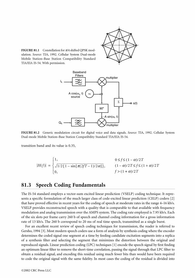
transition ba

81.3 S

The IS-54 stsents a specithat have proVSELP provmodulation of the six slorate of 13 kb

For an exGersho, 1994determines tof a synthesreproduced san optimumobtain a resito code the

FIGURE 81.1

ulation.

Sourc

Mobile StatioTIA/EIA IS-5

FIGURE 81.2

Dual-mode M

H


©2002 CRC P

nd and its value is 0.35,

peech Coding Fundamentals

andard employs a vector-sum excited linear prediction (VSELP) coding technique. It repre-fic formulation of the much larger class of code-excited linear prediction (CELP) coders [2]ved effective in recent years for the coding of speech at moderate rates in the range 4–16 kb/s.

ides reconstructed speech with a quality that is comparable to that available with frequencyand analog transmission over the AMPS system. The coding rate employed is 7.95 kb/s. Eachts per frame carry 260 b of speech and channel coding information for a gross information/s. The 260 b correspond to 20 ms of real time speech, transmitted as a single burst.

cellent recent review of speech coding techniques for transmission, the reader is referred to [3]. Most modern speech coders use a form of analysis by synthesis coding where the encoderhe coded signal one segment at a time by feeding candidate excitation segments into a replicais filter and selecting the segment that minimizes the distortion between the original andignals. Linear prediction coding (LPC) techniques [1] encode the speech signal by first finding linear filter to remove the short-time correlation, passing the signal through that LPC filter todual signal, and encoding this residual using much fewer bits than would have been requiredoriginal signal with the same fidelity. In most cases the coding of the residual is divided into

Constellation for π/4 shifted QPSK mod-e: TIA, 1992. Cellular System Dual-moden–Base Station Compatibility Standard

4. With permission.

Generic modulation circuit for digital voice and data signals. Source: TIA, 1992. Cellular Systemobile Station–Base Station Compatibility Standard TIA/EIA IS-54.

~

Baseband Filters

multiplier

A cos(ω t) source

c

multiplier

−A sin(ωc t)

s(t)

lk

Qk

90

Σ

f( )1,

1/2 1 π 2fT 1–( )/2α[ ]sin–{ },

0,

=0 f 1 α–( )/2T≤ ≤1 α–( )/2T f 1 α+( )/2T≤ ≤

f 1 α+( )/2T>

ress LLC

two steps. First, the long-time correlation due to the periodic pitch excitation is removed by means of anoptimum one-tap filter with adjustable gain and lag. Next, the remaining residual signal, which now closelyresembles a wwhich they stechnique. Tallow the speStarting withcoding a largmore effectiv

The speecof the orderanalysis of taccurate detframe is divoperations a

The speecpossible. It absence of trerror at the ence. Since tection is pr

81.4 C

The sharp lisensitivity oand convolumission errocorrection werrors. Grouand is proteonly. The th

The speechave been dbad-frame mreceived paris made to hreception.

81.5 V

A block diagfrom three cA weighted sThe weighteprocess. Thinoise compoby adjustingclosely and gsynthesis filtenhance the


©2002 CRC P

hite-noise signal, is encoded. Code-excited linear predictors use one or more codebooks fromelect replicas of the residual of the input signal by means of a closed-loop error-minimizationhe index of the codebook entry as well as the parameters of all the filters are transmitted toech signal to be reconstructed at the receiver. Most code-excited coders use trained codebooks. a codebook containing Guassian signal segments, entries that are found to be used rarely ine body of speech data are iteratively eliminated to result in a smaller codebook that is considerede.h signal can be considered quasistationary or stationary for the duration of the speech frame, of 20 ms. The parameters of the short-term filter, the LPC coefficients, are determined byhe autocorrelation function of a suitably windowed segment of the input signal. To allowermination of the time-varying pitch lag as well as simplify the computations, each speechided into four 5-ms subframes. Independent pitch filter computations and residual codingre carried out for each subframe.h decoder attempts to reconstruct the speech signal from the received information as best

employs a codebook identical to that of the encoder for excitation generation and, in theansmission errors, would produce an exact replica of the signal that produced the minimizedencoder. Transmission errors do occur, however, due, to signal fading and excessive interfer-any attempt at retransmission would incur unacceptable signal delays, sufficient error pro-ovided to allow correction of most transmission errors.

hannel Coding Considerations

mitations on available bandwidth for error protection argue for careful consideration of thef the speech coding parameters to transmission errors. Pairwise interleaving of coded blockstional coding of a subset of the parameters permit correction of a limited number of trans-rs. In addition, a cyclic redundancy check (CRC) is used to determine whether the erroras successful. The coded information is divided into three blocks of varying sensitivity to

p 1 contains the most sensitive bits, mainly the parameters of the LPC filter and frame energy,cted by both error detection and correction bits. Group 2 is provided with error correctionird group, comprising mostly the fixed codebook indices, is not protected at all.h signal contains significant temporal redundancy. Thus, speech frames within which errorsetected may be reconstructed with the aid of previously correctly received information. Aasking procedure attempts to hide the effects of short fades by extrapolating the previously

ameters. Of course, if the errors persist, the decoded signal must be muted while an attemptand off the connection to a base station to/from which the mobile may experience better

SELP Encoder

ram of the VSELP speech encoder [4] is shown in Fig. 81.3. The excitation signal is generatedomponents, the output of a long term or pitch filter, as well as entries from two codebooks.ynthesis filter generates a synthesized approximation to the frequency-weighted input signal.d mean square error between these two signals is used to drive the error minimizations weighted error is considered to be a better approximation to the perceptually importantnents than the unweighted mean square error. The total weighted square error is minimized

the pitch lag and the codebook indices as well as their gains. The decoder follows the encoderenerates the excitation signal identically to the encoder but uses an unweighted linear-predictioner to generate the decoded signal. A spectral postfilter is added after the synthesis filter to quality of the reconstructed speech.

ress LLC

The preci20 ms of sig(2) frame en

81.6 L

The purposematched by speech spectis given by

The filter prcients coefficients u

A variety signal. One lattice stage minimized bcentered witis 20 samplesthe reflection

The FLAT

Define the frelation of thresidual B0(i

FIGURE 81.3Mobile Statio

Longterm s(n)

β

r1,…


©2002 CRC P

se data rate of the speech coder is 7950 b/s or 159 b per time slot, each corresponding tonal in real time. These 159 b are allocated as follows: (1) short-term filter coefficients, 38 bits;ergy, 5 bits; (3) pitch lag, 28 bits; (4) codewords, 56 bits; and (5) gain values, 32 bits.

inear Prediction Analysis and Quantization

of the LPC analysis filter is to whiten the spectrum of the input signal so that it can be betterthe codebook outputs. The corresponding LPC synthesis filter A(z) restores the short-time

rum characteristics to the output signal. The transfer function of the tenth-order synthesis filter

edictor parameters are not transmitted directly. Instead, a set of reflection coeffi- are computed and quantized. The predictor parameters are determined from the reflection

sing a well-known backward recursion algorithm [6].of algorithms are known that determine a set of reflection coefficients from a windowed inputsuch algorithm is the fixed point covariance lattice, FLAT, which builds an optimum inverseby stage. At each stage j, the sum of the mean-squared forward and backward residuals isy selection of the best reflection coefficient rj. The analysis window used is 170 samples long,

h respect to the middle of the fourth 5-ms subframe of the 20-ms frame. Since this centerpoint from the end of the frame, 65 samples from the next frame to be coded are used in computing coefficient of the current frame. This introduces a lookahead delay of 8.125 ms. algorithm first computes the covariance matrix of the input speech for NA = 170 and Np = 10,

orward residual out of stage j as fj(n) and the backward residual as bj(n). Then the autocor-e initial forward residual F0(i, k) is given by φ(i, k). The autocorrelation of the initial backward, k) is given by φ(i + 1, k + 1) and the initial cross correlation of the two residuals is given

Block diagram of the speech encoder in VSELP. Source: TIA, 1992. Cellular system Dual-moden–Base Station Compatibility Standard TIA/EIA IS-54.

+ −

filter state

Codebook

Codebook

weighted synthesis filter

1

2

weighting filter

Totalweighted error

Select indices L, I or H to minimize total weighted error. ERROR MINIMIZATION

L

I

H

p(n)

p'(n)ex(n)H(z)

W(z)

γ1

γ2

Σ( )2

A z( ) 1

1 ∑i=1

Np αizi––

------------------------------=

α1,…,αNp

,rNp

φ i, k( ) s n i–( )s n k–( ), 0n=Np

NA−1

∑ i, k Np≤≤=

ress LLC

by C0(i, k) =determined the computaloops, reflecerrors of the

and

Use of two computed re

FIGURE 81.4

Fj − 1B j − 1

Fj

B j


©2002 CRC P

φ(i, k + 1) for 0 ≤ i, k ≤ Np−1. Initially j is set to 1. The reflection coefficient at each stage isas the ratio of the cross correlation to the mean of the autocorrelations. A block diagram oftions is shown in Fig. 81.4. By quantizing the reflection coefficients within the computationtion coefficients at subsequent stages are computed taking into account the quantization previous stages. Specifically,

sets of correlation values separated by Np − j samples provides additional stability to theflection coefficients in case the input signal changes form rapidly.

Block diagram for lattice covariance computations.

F (i + 1, k + 1)j − 1

F (i, k + 1)

C (k + 1, i)j − 1

F (i, k)j − 1

B (i, k)j

C j − 1

B (i, k)j − 1

C (k, i)j − 1

C (i, k) +j − 1

C (k + 1, i + 1)j − 1

C (i + 1, k + 1) +j − 1

B (i + 1, k + 1)j − 1

j − 1

C (i, k + 1)j − 1

B (i, k + 1)j − 1

F (i, k)j

C (i, k)j

r j

r j

r j

F (i, k)j + 1

B (i, k)j + 1

C (i, k)j + 1

r j + 1

r j + 1

r j + 1

Cj

C′j−1 Cj−1 0, 0( ) Cj−1 Np j, Np j––( )+=F′j−1 Fj−1 0, 0( ) Fj−1 Np j, Np j––( )+=B′j−1 Bj−1 0, 0( ) Bj−1 Np j, Np j––( )+=

rj

2C′j−1–

Fj−1′ Bj−1

′+------------------------=

ress LLC

Once a quantized reflection coefficient rj has been determined, the resulting auto- and cross corre-lations can be determined iteratively as

and

These comp

81.7 B

Poles with vUse of a binfilter and resubsequent fby use of a w

81.8 Q

The distortias we movelower order Scalar quantquantizatio

It is impoand decoderusing the covalues comp

81.9 V

The codebooI and H so acomplex parplexity of thzation of ththe long-tercodebooks afollows in seand makes terrors.

Entries frorthogonaliz

Fj i, k( )

Bj i, k( )

C


©2002 CRC P

utations are carried out iteratively for rj, j = 1,…,Np.

andwidth Expansion

ery narrow bandwidths may introduce undesirable distortions into the synthesized signal.omial window with effective bandwidth of 80 Hz suffices to limit the ringing of the LPCduce the effect of the LPC filter selected for one frame on the signal reconstructed forrames. To achieve this, prior to searching for the reflection coefficients, the φ(i, k) is modifiedindow function w( j), j = 1,…,10, as follows:

uantizing and Encoding the Reflection Coefficients

on introduced into the overall spectrum by quantizing the reflection coefficients diminishes to higher orders in the reflection coefficients. Accordingly, more bits are assigned to thecoefficients. Specifically, 6, 5, 5, 4, 4, 3, 3, 3, 3, and 2 b are assigned to r1,…,r10, respectively.ization of the reflection coefficients is used in IS-54 because it is particularly simple. Vector

n achieves additional quantizing efficiencies at the cost of significant added complexity.rtant to preserve the smooth time evolution of the linear prediction filter. Both the encoder linearly interpolate the coefficients αi for the first, second, and third subframes of each frameefficients determined for the previous and current frames. The fourth subframe uses theuted for that frame.

SELP Codebook Search

k search operation selects indices for the long-term filter (pitch lag L) and the two codebookss to minimize the total weighted error. This closed-loop search is the most computationallyt of the encoding operation, and significant effort has been invested to minimize the com-ese operations without degrading performance. To reduce complexity, simultaneous optimi-e codebook selections is replaced by a sequential optimization procedure, which considersm filter search as the most significant and therefore executes it first. The two vector-sumre considered to contribute less and less to the minimization of the error, and their searchquence. Subdivision of the total codebook into two vector sums simplifies the processinghe result less sensitive to errors in decoding the individual bits arising from transmission

om each of the two vector-sum codebooks can be expressed as the sum of basis vectors. Bying these basis vectors to the previously selected codebook component(s), one ensures that

Fj−1 i, k( ) rj Cj−1 i, k( ) Cj−1 k, i( )+[ ] rj2Bj−1 i, k( )+ +=

Bj−1 i 1+ , k 1+( ) rj Cj−1 i 1+ , k 1+( ) Cj−1 k 1+ , i 1+( )+[ ] rj2Fj−1 i 1+ , k 1+( )+ +=

j i, k( ) Cj−1 i, k 1+( ) rj Bj−1 i, k 1+( ) Fj−1 i, k 1+( )+[ ] rj2Cj−1 k 1+ , i( )+ +=

φ′ i, k( ) φ i, k( )w i k–( )=

ress LLC

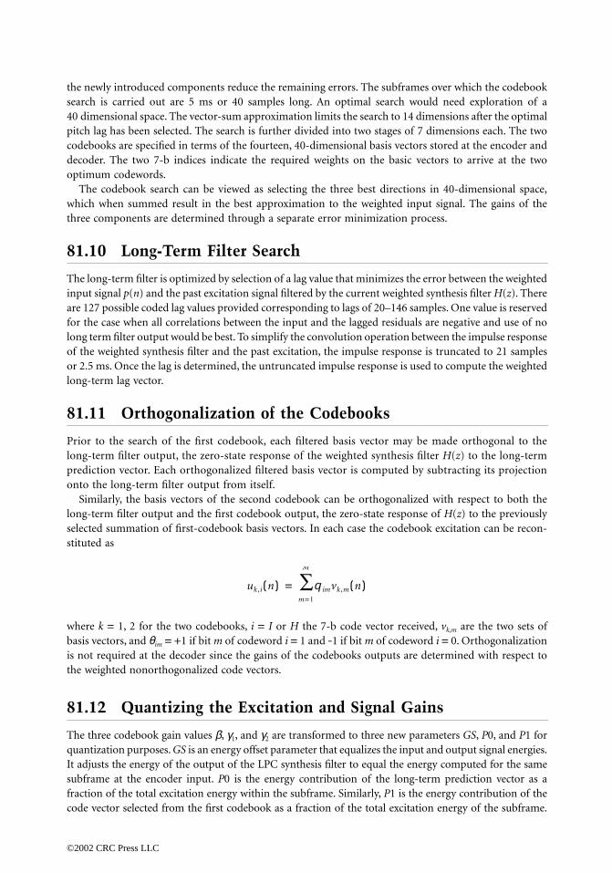
the newly introduced components reduce the remaining errors. The subframes over which the codebooksearch is carried out are 5 ms or 40 samples long. An optimal search would need exploration of a40 dimensional space. The vector-sum approximation limits the search to 14 dimensions after the optimalpitch lag has been selected. The search is further divided into two stages of 7 dimensions each. The twocodebooks are specified in terms of the fourteen, 40-dimensional basis vectors stored at the encoder anddecoder. The two 7-b indices indicate the required weights on the basic vectors to arrive at the twooptimum codewords.

The codebook search can be viewed as selecting the three best directions in 40-dimensional space,which when summed result in the best approximation to the weighted input signal. The gains of thethree components are determined through a separate error minimization process.

81.10 Long-Term Filter Search

The long-term filter is optimized by selection of a lag value that minimizes the error between the weightedinput signal p(n) and the past excitation signal filtered by the current weighted synthesis filter H(z). Thereare 127 possible coded lag values provided corresponding to lags of 20–146 samples. One value is reservedfor the case when all correlations between the input and the lagged residuals are negative and use of nolong term filter output would be best. To simplify the convolution operation between the impulse responseof the weighted synthesis filter and the past excitation, the impulse response is truncated to 21 samplesor 2.5 ms. Once the lag is determined, the untruncated impulse response is used to compute the weightedlong-term lag vector.

81.11 Orthogonalization of the Codebooks

Prior to the search of the first codebook, each filtered basis vector may be made orthogonal to thelong-term filter output, the zero-state response of the weighted synthesis filter H(z) to the long-termprediction vector. Each orthogonalized filtered basis vector is computed by subtracting its projectiononto the long-term filter output from itself.

Similarly, the basis vectors of the second codebook can be orthogonalized with respect to both thelong-term filter output and the first codebook output, the zero-state response of H(z) to the previouslyselected summation of first-codebook basis vectors. In each case the codebook excitation can be recon-stituted as

where k = 1, 2 for the two codebooks, i = I or H the 7-b code vector received, vk,m are the two sets ofbasis vectors, and θim = +1 if bit m of codeword i = 1 and -1 if bit m of codeword i = 0. Orthogonalizationis not required at the decoder since the gains of the codebooks outputs are determined with respect tothe weighted nonorthogonalized code vectors.

81.12 Quantizing the Excitation and Signal Gains

The three codebook gain values β, γ1, and γ2 are transformed to three new parameters GS, P0, and P1 forquantization purposes. GS is an energy offset parameter that equalizes the input and output signal energies.It adjusts the energy of the output of the LPC synthesis filter to equal the energy computed for the samesubframe at the encoder input. P0 is the energy contribution of the long-term prediction vector as afraction of the total excitation energy within the subframe. Similarly, P1 is the energy contribution of thecode vector selected from the first codebook as a fraction of the total excitation energy of the subframe.

uk ,i n( ) qimvk ,m n( )m=1

M

∑=


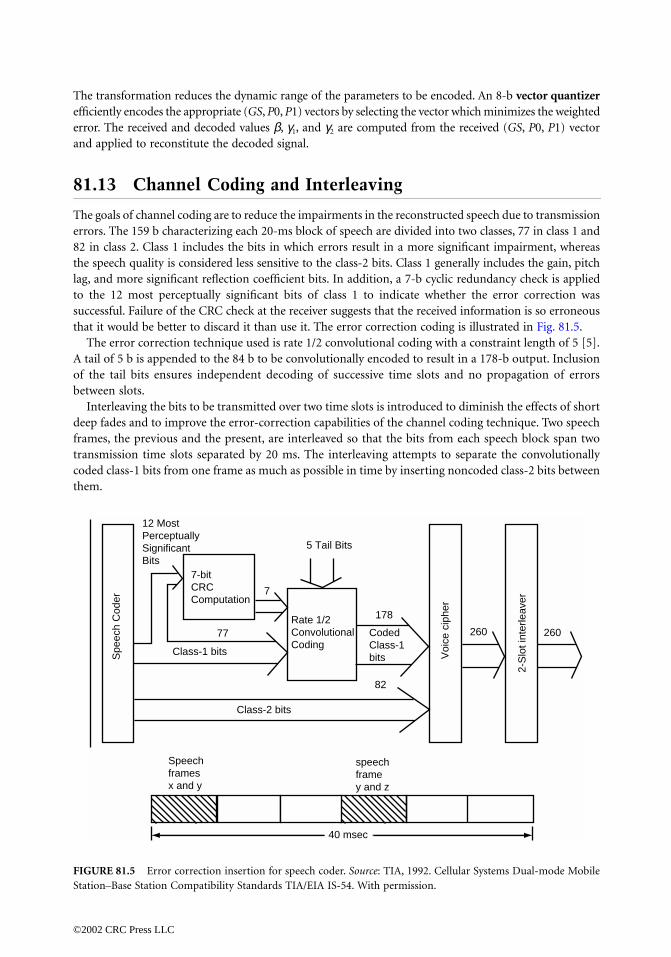
The transformation reduces the dynamic range of the parameters to be encoded. An 8-b vector quantizerefficiently encodes the appropriate (GS, P0, P1) vectors by selecting the vector which minimizes the weightederror. The received and decoded values β, γ1, and γ2 are computed from the received (GS, P0, P1) vectorand applied to reconstitute the decoded signal.

81.13 Channel Coding and Interleaving

The goals of channel coding are to reduce the impairments in the reconstructed speech due to transmissionerrors. The 159 b characterizing each 20-ms block of speech are divided into two classes, 77 in class 1 and82 in class 2. Class 1 includes the bits in which errors result in a more significant impairment, whereasthe speech quality is considered less sensitive to the class-2 bits. Class 1 generally includes the gain, pitchlag, and more significant reflection coefficient bits. In addition, a 7-b cyclic redundancy check is appliedto the 12 most perceptually significant bits of class 1 to indicate whether the error correction wassuccessful. Failure of the CRC check at the receiver suggests that the received information is so erroneousthat it would be better to discard it than use it. The error correction coding is illustrated in Fig. 81.5.

The error correction technique used is rate 1/2 convolutional coding with a constraint length of 5 [5].A tail of 5 b is appended to the 84 b to be convolutionally encoded to result in a 178-b output. Inclusionof the tail bits ensures independent decoding of successive time slots and no propagation of errorsbetween slots.

Interleaving the bits to be transmitted over two time slots is introduced to diminish the effects of shortdeep fades and to improve the error-correction capabilities of the channel coding technique. Two speechframes, the previous and the present, are interleaved so that the bits from each speech block span twotransmission time slots separated by 20 ms. The interleaving attempts to separate the convolutionallycoded class-1 bits from one frame as much as possible in time by inserting noncoded class-2 bits betweenthem.

FIGURE 81.5 Error correction insertion for speech coder. Source: TIA, 1992. Cellular Systems Dual-mode MobileStation–Base Station Compatibility Standards TIA/EIA IS-54. With permission.

Speechframesx and y

speechframey and z

40 msec

5 Tail Bits

77

7-bitCRCComputation

178

CodedClass-1bits V

oice

cip

her

2-S

lot i

nter

leav

er

260Rate 1/2ConvolutionalCoding

Spe

ech

Cod

er

Class-1 bits

7

Class-2 bits

82

12 MostPerceptuallySignificantBits

260


81.14 Bad Frame Masking

A CRC failure indicates that the received data is unusable, either due to transmission errors resultingfrom a fade, or from pre-emption of the time slot by a control message (fast associated control channel,FACCH). To mask the effects that may result from leaving a gap in the speech signal, a masking operationbased on the temporal redundancy between adjacent speech blocks has been proposed. Such maskingcan at best bridge over short gaps but cannot recover loss of signal of longer duration. The bad framemasking operation may follow a finite state machine where each state indicates an operation appropriateto the elapsed duration of the fade to which it corresponds. The masking operation consists of copyingthe previous LPC information and attenuating the gain of the signal. State 6 corresponds to errorsequences exceeding 100 ms, for which the output signal is muted. The result of such a masking operationis generation of an extrapolation in the gap to the previously received signal, significantly reducing theperceptual effects of short fades. No additional delay is introduced in the reconstructed signal. At thesame time, the receiver will report a high frequency of bad frames leading the system to explore handoffpossibilities immediately. A quick successful handoff will result in rapid signal recovery.

81.15 ACELP Encoder

The ACELP encoder employs linear prediction analysis and quantization techniques similar to those usedin VSELP and discussed in Section 81.6. The frame structure of 20 ms frames and 5 ms subframes ispreserved. Linear prediction analysis is carried out for every frame. The ACELP encoder uses a long-term filter similar to the one discussed in Section 81.10 and represented as an adaptive codebook. Thenonpredictable part of the LPC residual is represented in terms of ACELP codebooks, which replace thetwo VSELP codebooks shown in Fig. 81.3.

Instead of encoding the reflection coefficients as in VSELP, the information is transformed into line-spectral frequency pairs (LSP) [8]. The LSPs can be derived from linear prediction coefficients, a 10thorder analysis generating 10 line-spectral frequencies (LSF), 5 poles, and 5 zeroes. The LSFs can be vectorquantized and the LPC coefficients recalculated from the quantized LSFs. As long as the interleaved orderof the poles and zeroes is preserved, quantization of the LSPs preserves the stability of the LPC synthesisfilters. The LSPs of any frame can be better predicted from the values calculated and transmitted corre-sponding to previous frames, resulting in additional advantages. The long-term means of the LSPs arecalculated for a large body of speech data and stored at both the encoder and decoder. First-order moving-average prediction is then used for the mean-removed LSPs. The time-prediction technique also permitsuse of predicted values for the LSPs in case uncorrectable transmissions errors are encountered, resultingin reduced speech degradation. To simplify the vector quantization operations, each LSP vector is splitinto 3 subvectors of dimensions 3, 3, and 4. The three subvectors are quantized with 8, 9, and 9 bitsrespectively, corresponding to a total bit assignment of 26 bits per frame for LPC information.

81.16 Algebraic Codebook Structure and Search

Algebraic codebooks contain relatively few pulses having nonzero values leading to rapid search of thepossible innovation vectors, the vectors which together with the ACB output form the excitation of theLPC filter for the current subframe. In this implementation the 40-position innovation vector containsonly four nonzero pulses and each can take on only values +1 and -1. The 40 positions are divided intofour tracks and one pulse is selected from each track. The tracks are generally equally spaced but differin their starting value, thus the first pulse can take on positions 0, 5, 10, 15, 20, 25, 30, or 35 and thesecond has possible positions 1, 6, 11, 16, 21, 26, 31, or 36. The first three pulse positions are coded with3 bits and the fourth pulse position (starting positions 3 or 4) with 4 bits, resulting in a 17-bit sequencefor the algebraic code of each subframe.

The algebraic codebook is searched by minimizing the mean square error between the weighted inputspeech and the weighted synthesized speech over the time span of each subframe. In each case the weighting


is that produced by a perceptual weighting filter that has the effect of shaping the spectrum of the synthesiserror signal so that it is better masked by spectrum of the current speech signal.

81.17 Quantization of the Gains for ACELP Encoding

The adaptive codebook gain and the fixed (algebraic) codebook gains are vector quantized using a 7-bitcodebook. The gain codebook search is performed by minimizing the mean-square of the weighted errorbetween the original and the reconstructed speech, expressed as a function of the adaptive codebookgain and a fixed codebook correction factor. This correction factor represents the log energy differencebetween a predicted gain and an estimated gain. The predicted gain is computed using fourth-ordermoving-average prediction with fixed coefficients on the innovation energy of each subframe. The resultis a smoothed energy profile even in the presence of modest quantization errors. As discussed above incase of the LSP quantization, the moving-average prediction serves to provide predicted values even whenthe current frame information is lost due to transmission errors. Degradations resulting from loss of oneor two frames of information are thereby mitigated.

81.18 Channel Coding for ACELP Encoding

The channel coding and interleaving operations for ACELP speech coding are similar to those discussedin Section 81.13 for VSELP coding. The number of bits protected by both error-detection (parity) anderror-correction convolutional coding is increased to 48 from 12. Rate 1/2 convolutional coding isused on the 108 more significant bits, 96 class-1 bits, 7 CRC bits and the 5 tail bits of the convolutionalcoder, resulting in 216 coded class-1 bits. Eight of the 216 bits are dropped by puncturing, yielding208 coded class-1 bits which are then combined with 52 nonprotected class-2 bits. As compared tothe channel coding of the VSELP encoder, the numbers of protected bits is increased and the numberof unprotected bits is reduced while keeping the overall coding structure unchanged.

81.19 Conclusions

The IS-54 digital cellular standard specifies modulation and speech coding techniques for mobile cellularsystems that allow the interoperation of terminals built by a variety of manufacturers and systems operatedacross the country by a number of different service providers. It permits speech communication withgood quality in a transmission environment characterized by frequent multipath fading and significantintercell interference. Generally, the quality of the IS-54 decoded speech is better at the edges of a cell thanthe corresponding AMPS transmission due to the error mitigation resulting from channel coding. Neara base station or in the absence of significant fading and interference, the IS-54 speech quality is reportedto be somewhat worse than AMPS due to the inherent limitations of the analysis–synthesis model inreconstructing arbitrary speech signals with limited bits. The IS-641 standard coder achieves higher speechquality, particularly at the edges of heavily occupied cells where transmission errors may be more numer-ous. At this time no new systems following the IS-54 standard are being introduced. Most base stationshave been converted to transmit and receive on the IS-641 standard as well and use of IS-54 transmissionsis dropping rapidly. At the time of its introduction in 1996 the IS-641 coder represented the state of theart in terms of toll quality speech coding near 8 kb/s, a significant improvement over the IS-54 coderintroduced in 1990. These standards represent reasonable engineering compromises between high per-formance and complexity sufficiently low to permit single-chip implementations in mobile terminals.

Both IS-54 and IS-641 are considered second generation cellular standards. Third generation cellularsystems promise higher call capacities through better exploitation of the time-varying transmissionrequirements of speech conversations, as well as improved modulation and coding in wider spectrumbandwidths that achieve similar bit-error ratios but reduce the required transmitted power. Until suchsystems are introduced, the second generation TDMA systems can be expected to provide many years ofsuccessful cellular and personal communications services.


Defining Terms

Codebook: A set of signal vectors available to both the encoder and decoder.Covariance lattice algorithm: An algorithm for reduction of the covariance matrix of the signal con-

sisting of several lattice stages, each stage implementing an optimal first-order filter with a singlecoefficient.

Reflection coefficient: A parameter of each stage of the lattice linear prediction filter that determines(1) a forward residual signal at the output of the filter-stage by subtracting from the forwardresidual at the input a linear function of the backward residual, also (2) a backward residual atthe output of the filter stage by subtracting a linear function of the forward residual from thebackward residual at the input.

Vector quantizer: A quantizer that assigns quantized vectors to a vector of parameters based on theircurrent values by minimizing some error criterion.

References

1. Atal, B.S. and Hanauer, S.L., Speech analysis and synthesis by linear prediction of the speech wave.J. Acoust. Soc. Am., 50, 637–655, 1971.

2. Atal, B.S. and Schroeder, M., Stochastic coding of speech signals at very low bit rates. Proc. Int.Conf. Comm., 1610–1613, 1984.

3. Gersho, A., Advances in speech and audio compression. Proc. IEEE, 82, 900–918, 1994.4. Gerson, I.A. and Jasiuk, M.A., Vector sum excited linear prediction (VSELP) speech coding at 8

kbps. Int. Conf. Acoust. Speech and Sig. Proc., ICASSP90, 461–464, 1990.5. Lin S. and Costello, D., Error Control Coding: Fundamentals and Application, Prentice Hall, Engle-

wood Cliffs, NJ, 1983.6. Makhoul, J., Linear prediction, a tutorial review. Proc. IEEE, 63, 561–580, 1975.7. Salami, R., Laflamme, C., Adoul, J.P., and Massaloux, D., A toll quality 8 kb/s speech codec for the

personal communication system (PCS). IEEE Trans. Vehic. Tech., 43, 808–816, 1994.8. Soong, F.K. and Juang, B.H., Line spectrum pair (LSP) and speech data compression. Proc.

ICASSP’84, 1.10.1–1.10.4, 1984.9. Telecommunications Industry Association, EIA/TIA Interim Standard, Cellular System Dual-mode

Mobile Station–Base Station Compatibility Standard IS-54B, TIA/EIA, Washington, D.C., 1992.

Further Information

For a general treatment of speech coding for telecommunications, see N.S. Jayant and P. Noll, DigitalCoding of Waveforms, Prentice Hall, Englewood, NJ, 1984. For a more detailed treatment of linearprediction techniques, see J. Markel and A. Gray, Linear Prediction of Speech, Springer–Verlag, New York,1976.


82The British

Cordless TelephoneStandard: CT-2

82.1 History and Background82.2 The CT-2 Standard82.3 The Radio Interface

Transmission Issues • Multiple Access and Burst Structure • Power Ramping, Guard Period, and Propagation Delay • Power Control

82.4 Burst Formats82.5 Signalling Layer Two (L2)

General Message Format • Fixed Format Packet

82.6 CPP-Initiated Link Setup Procedures82.7 CFP-Initiated Link Setup Procedures82.8 Handshaking82.9 Main Features of the CT-2 System

82.1 History and Background

Following a decade of world-wide research and development (R&D), cordless telephones (CT) are nowbecoming widespread consumer products, and they are paving the way toward ubiquitous, low-costpersonal communications networks (PCN) [7,8]. The two most well-known European representativesof CTs are the digital European cordless telecommunications (DECT) system [1,5] and the CT-2 system[2,6]. Three potential application areas have been identified, namely, domestic, business, and publicaccess, which is also often referred to as telepoint (TP).

In addition to conventional voice communications, CTs have been conceived with additional dataservices and local area network (LAN) applications in mind. The fundamental difference betweenconventional mobile radio systems and CT systems is that CTs have been designed for small to verysmall cells, where typically benign low-dispersion, dominant line-of-sight (LOS) propagation condi-tions prevail. Therefore, CTs can usually dispense with channel equalizers and complex low-ratespeech codecs, since the low-signal dispersion allows for the employment of higher bit rates beforethe effect of channel dispersion becomes a limiting factor. On the same note, the LOS propagationscenario is associated with mild fading or near-constant received signal level, and when combinedwith appropriate small-cell power-budget design, it ensures a high average signal-to-noise ratio(SNR). These prerequisites facilitate the employment of high-rate, low-complexity speech codecs,which maintain a low battery drain. Furthermore, the deployment of forward error correction codecs

Lajos Hanzo University of Southampton


can often also be avoided, which reduces both the bandwidth requirement and the power consumptionof the portable station (PS).

A further difference between public land mobile radio (PLMR) systems [3] and CTs is that whereasthe former endeavor to standardize virtually all system features, the latter seek to offer a so-called accesstechnology, specifying the common air interface (CAI), access and signalling protocols, and some networkarchitecture features, but leaving many other characteristics unspecified. By the same token, whereas PLMRsystems typically have a rigid frequency allocation scheme and fixed cell structure, CTs use dynamicchannel allocation (DCA) [4]. The DCA principle allows for a more intelligent and judicious channelassignment, where the base station (BS) and PS select an appropriate traffic channel on the basis of theprevailing traffic and channel quality conditions, thus minimizing, for example, the effect of cochannelinterference or channel blocking probability.

In contrast to PLMR schemes, such as the Pan-European global system of mobile communications(GSM) system [3], CT systems typically dispense with sophisticated mobility management, which accountsfor the bulk of the cost of PLMR call charges, although they may facilitate limited hand-over capabilities.Whereas in residential applications CTs are the extension of the public switched telephone network(PSTN), the concept of omitting mobility management functions, such as location update, etc., leads totelepoint CT applications where users are able to initiate but not to receive calls. This fact drasticallyreduces the network operating costs and, ultimately, the call charge at a concomittant reduction of theservices rendered.

Having considered some of the fundamental differences between PLMR and CT systems let us nowreview the basic features of the CT-2 system.

82.2 The CT-2 Standard

The European CT-2 recommendation has evolved from the British standard MPT-1375 with the aim ofensuring the compatibility of various manufacturers’ systems as well as setting performance requirements,which would encourage the development of cost-efficient implementations. Further standardizationobjectives were to enable future evolution of the system, for example, by reserving signalling messagesfor future applications and to maintain a low PS complexity even at the expense of higher BS costs. TheCT-2 or MPT 1375 CAI recommendation is constituted by the four following parts.

1. Radio interface: Standardizes the radio frequency (RF) parameters, such as legitimate channelfrequencies, the modulation method, the transmitter power control, and the required receiversensitivity as well as the carrier-to-interference ratio (CIR) and the time division duplex (TDD)multiple access scheme. Furthermore, the transmission burst and master/slave timing structuresto be used are also laid down, along with the scrambling procedures to be applied.

2. Signalling layers one and two: Defines how the bandwidth is divided among signalling, traffic data,and synchronization information. The description of the first signalling layer includes the dynamicchannel allocation strategy, calling channel detection, as well as link setup and establishmentalgorithms. The second layer is concerned with issues of various signalling message formats, aswell as link establishment and re-establishment procedures.

3. Signalling layer three: The third signalling layer description includes a range of message sequencediagrams as regards to call setup to telepoint BSs, private BSs, as well as the call clear down procedures.

4. Speech coding and transmission: The last part of the standard is concerned with the algorithmicand performance features of the audio path, including frequency responses, clipping, distortion,noise, and delay characteristics.

Having briefly reviewed the structure of the CT-2 recommendations let us now turn our attention toits main constituent parts and consider specific issues of the system’s operation.


82.3 The Radio Interface

Transmission Issues

In our description of the system we will adopt the terminology used in the recommendation, where thePS is called cordless portable part (CPP), whereas the BS is referred to as cordless fixed part (CFP). Thechannel bandwidth and the channel spacing are 100 kHz, and the allocated system bandwidth is 40 MHz,which is hosted in the range of 864.15–868.15 MHz. Accordingly, a total of 40 RF channels can be utilizedby the system.

The accuracy of the radio frequency must be maintained within ±10 kHz of its nominal value for boththe CFP and CPP over the entire specified supply voltage and ambient temperature range. To counteractthe maximum possible frequency drift of 20 kHz, automatic frequency correction (AFC) may be usedin both the CFP and CPP receivers. The AFC may be allowed to control the transmission frequency ofonly the CPP, however, in order to prevent the misalignment of both transmission frequencies.

Binary frequency shift keying (FSK) is proposed, and the signal must be shaped by an approximatelyGaussian filter in order to maintain the lowest possible frequency occupancy. The resulting scheme isreferred to as Gaussian frequency shift keying (GFSK), which is closely related to Gaussian minimumshift keying (GMSK) [7] used in the DECT [1] and GSM [3] systems.

Suffice to say that in M-arry FSK modems the carrier’s frequency is modulated in accordance with theinformation to be transmitted, where the modulated signal is given by

and E represents the bit energy, T the signalling interval length, ωi has M discrete values, whereas thephase Φ is constant.

Multiple Access and Burst Structure

The so-called TDD multiple access scheme is used, which is demonstrated in Fig. 82.1. The simpleprinciple is to use the same radio frequency for both uplink and downlink transmissions between theCPP and the CFP, respectively, but with a certain staggering in time. This figure reveals further detailsof the burst structure, indicating that 66 or 68 b per TDD frame are transmitted in both directions.

There is a 3.5- or 5.5-b duration guard period (GP) between the uplink and downlink transmissions,and half of the time the CPP (the other half of the time the CFP) is transmitting with the other partlistening, accordingly. Although the guard period wastes some channel capacity, it allows a finite time forboth the CPP and CFP for switching from transmission to reception and vice versa. The burst structureof Fig. 82.1 is used during normal operation across an established link for the transmission of adaptivedifferential pulse code modulated (ADPCM) speech at 32 kb/s according to the CCITT G721 standard in

FIGURE 82.1 M1 burst and TDD frame structure.

Si t( ) 2ET------ w it Φ+[ ]cos i 1,…, M= =


a so-called B channel or bearer channel. The D channel, or signalling channel, is used for the transmissionof link control signals. This specific burst structure is referred to as a multiplex one (M1) frame.

Since the speech signal is encoded according to the CCITT G721 recommendation at 32 kb/s the TDDbit rate must be in excess of 64 kb/s in order to be able to provide the idle guard space of 3.5- or 5.5-binterval duration plus some signalling capacity. This is how channel capacity is sacrificed to provide theGP. Therefore, the transmission bit rate is stipulated to be 72 kb/s and the transmission burst length is2 ms, during which 144-b intervals can be accommodated. As it was demonstrated in Fig. 82.1, 66 or 68b are transmitted in both the uplink and downlink burst, and taking into account the guard spaces, thetotal transmission frame is constituted by (2 . 68) + 3.5 + 4.5 = 144 b or equivalently, by (2 . 66) + 5.5+ 4.5 = 144 b. The 66-b transmission format is compulsory, whereas the 68-b format is optional. In the66-b burst there is one D bit dedicated to signalling at both ends of the burst, whereas in the 68-b burstthe two additional bits are also assigned to signalling. Accordingly, the signalling rate becomes 2 b/2 msor 4 b/2 ms, corresponding to 1 kb/s or 2 kb/s signalling rates.

Power Ramping, Guard Period, and Propagation Delay

As mentioned before and suggested in Fig. 82.1, there is a 3.5- or 5.5-b interval duration GP between trans-mitted and received bursts. Since the signalling rate is 72 kb/s, the bit interval becomes about 1/(72 kb/s) ≈13.9 µs and, hence, the GP duration is about 49 µs or 76 µs. This GP serves a number of purposes. Primarily,the GP allows the transmitter to ramp up and ramp down the transmitted signal level smoothly over a finitetime interval at the beginning and end of the transmitted burst. This is necessary, because if the transmittedsignal is toggled instantaneously, that is equivalent to multiplying the transmitted signal by a rectangulartime-domain window function, which corresponds in the frequency domain to convolving the transmittedspectrum with a sinc function. This convolution would result in spectral side-lobes over a very wide frequencyrange, which would interfere with adjacent channels. Furthermore, due to the introduction of the guardperiod, both the CFP and CPP can tolerate a limited propagation delay, but the entire transmitted burst mustarrive within the receivers’ window, otherwise the last transmitted bits cannot be decoded.

Power Control

In order to minimize the battery drain and the cochannel interference load imposed upon cochannelusers, the CT-2 system provides a power control option. The CPPs must be able to transmit at two differentpower levels, namely, either between 1 and 10 mW or at a level between 12 and 20 dB lower. Themechanism for invoking the lower CPP transmission level is based on the received signal level at the CFP.If the CFP detects a received signal strength more than 90 dB relative to 1 µV/m, it may instruct the CPPto drop its transmitted level by the specified 12–20 dB. Since the 90-dB gain factor corresponds to abouta ratio of 31,623, this received signal strength would be equivalent for a 10-cm antenna length to anantenna output voltage of about 3.16 mV. A further beneficial ramification of using power control is thatby powering down CPPs that are in the vicinity of a telepoint-type multiple-transceiver CFP, the CFP’sreceiver will not be so prone to being desensitised by the high-powered close-in CPPs, which wouldseverely degrade the reception quality of more distant CPPs.

82.4 Burst Formats

As already mentioned in the previous section on the radio interface, there are three different subchannelsassisting the operation of the CT-2 system, namely, the voice/data channel or B channel, the signallingchannel or D channel, and the burst synchronization channel or SYN channel. According to the momentarysystem requirements, a variable fraction of the overall channel capacity or, equivalently, a variable fractionof the bandwidth can be allocated to any of these channels. Each different channel capacity or bandwidthallocation mode is associated with a different burst structure and accordingly bears a different name.The corresponding burst structures are termed as multiplex one (M1), multiplex two (M2), and multiplexthree (M3), of which multiplex one used during the normal operation of established links has already


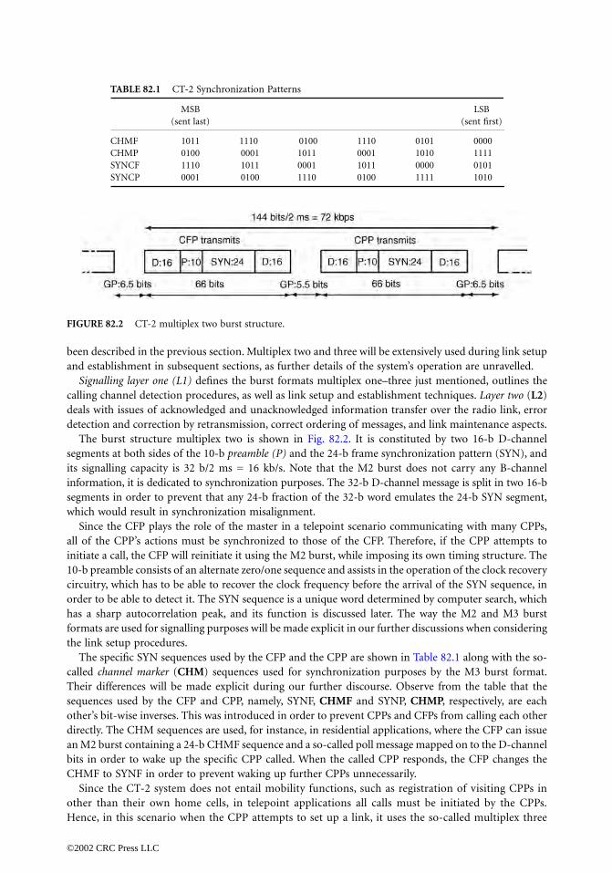
been described in the previous section. Multiplex two and three will be extensively used during link setupand establishment in subsequent sections, as further details of the system’s operation are unravelled.

Signalling layer one (L1) defines the burst formats multiplex one–three just mentioned, outlines thecalling channel detection procedures, as well as link setup and establishment techniques. Layer two (L2)deals with issues of acknowledged and unacknowledged information transfer over the radio link, errordetection and correction by retransmission, correct ordering of messages, and link maintenance aspects.

The burst structure multiplex two is shown in Fig. 82.2. It is constituted by two 16-b D-channelsegments at both sides of the 10-b preamble (P) and the 24-b frame synchronization pattern (SYN), andits signalling capacity is 32 b/2 ms = 16 kb/s. Note that the M2 burst does not carry any B-channelinformation, it is dedicated to synchronization purposes. The 32-b D-channel message is split in two 16-bsegments in order to prevent that any 24-b fraction of the 32-b word emulates the 24-b SYN segment,which would result in synchronization misalignment.

Since the CFP plays the role of the master in a telepoint scenario communicating with many CPPs,all of the CPP’s actions must be synchronized to those of the CFP. Therefore, if the CPP attempts toinitiate a call, the CFP will reinitiate it using the M2 burst, while imposing its own timing structure. The10-b preamble consists of an alternate zero/one sequence and assists in the operation of the clock recoverycircuitry, which has to be able to recover the clock frequency before the arrival of the SYN sequence, inorder to be able to detect it. The SYN sequence is a unique word determined by computer search, whichhas a sharp autocorrelation peak, and its function is discussed later. The way the M2 and M3 burstformats are used for signalling purposes will be made explicit in our further discussions when consideringthe link setup procedures.

The specific SYN sequences used by the CFP and the CPP are shown in Table 82.1 along with the so-called channel marker (CHM) sequences used for synchronization purposes by the M3 burst format.Their differences will be made explicit during our further discourse. Observe from the table that thesequences used by the CFP and CPP, namely, SYNF, CHMF and SYNP, CHMP, respectively, are eachother’s bit-wise inverses. This was introduced in order to prevent CPPs and CFPs from calling each otherdirectly. The CHM sequences are used, for instance, in residential applications, where the CFP can issuean M2 burst containing a 24-b CHMF sequence and a so-called poll message mapped on to the D-channelbits in order to wake up the specific CPP called. When the called CPP responds, the CFP changes theCHMF to SYNF in order to prevent waking up further CPPs unnecessarily.

Since the CT-2 system does not entail mobility functions, such as registration of visiting CPPs inother than their own home cells, in telepoint applications all calls must be initiated by the CPPs.Hence, in this scenario when the CPP attempts to set up a link, it uses the so-called multiplex three

TABLE 82.1 CT-2 Synchronization Patterns

MSB LSB(sent last) (sent first)

CHMF 1011 1110 0100 1110 0101 0000CHMP 0100 0001 1011 0001 1010 1111SYNCF 1110 1011 0001 1011 0000 0101SYNCP 0001 0100 1110 0100 1111 1010

FIGURE 82.2 CT-2 multiplex two burst structure.


burst format displayed in Fig. 82.3. The design of the M3 burst reflects that the CPP initiating the callis oblivious of the timing structure of the potentially suitable target CFP, which can detect accessattempts only during its receive window, but not while the CFP is transmitting. Therefore, the M3format is rather complex at first sight, but it is well structured, as we will show in our furtherdiscussions. Observe in the figure that in the M3 format there are five consecutive 2-ms long 144-btransmitted bursts, followed by two idle frames, during which the CPP listens in order to determinewhether its 24-b CHMP sequence has been detected and acknowledged by the CFP. This process canbe followed by consulting Fig. 82.6, which will be described in depth after considering the detailedconstruction of the M3 burst.

The first four of the five 2-ms bursts are identical D-channel bursts, whereas the fifth one serves asa synchronization message and has a different construction. Observe, furthermore, that both the firstfour 144-b bursts as well as the fifth one contain four so-called submultiplex segments, each of whichhosts a total of (6 + 10 + 8 + 10 + 2) = 36 b. In the first four 144-b bursts there are (6 + 8 + 2) = 16one/zero clock-synchronizing P bits and (10 + 10) = 20 D bits or signalling bits. Since the D-channelmessage is constituted by two 10-b half-messages, the first half of the D-message is marked by the +sign in Fig. 82.3. As mentioned in the context of M2, the D-channel bits are split in two halves andinterspersed with the preamble segments in order to ensure that these bits do not emulate valid CHMsequences. Without splitting the D bits this could happen upon concatenating the one/zero P bits withthe D bits, since the tail of the SYNF and SYNP sequences is also a one/zero segment. In the fifth 144-bM3 burst, each of the four submultiplex segments is constituted by 12 preamble bits and 24 CPP channelmarker (CHMP) bits.

The four-fold submultiplex M3 structure ensures that irrespective of how the CFP’s receive windowis aligned with the CPP’s transmission window, the CFP will be able to capture one of the four submul-tiplex segments of the fifth M3 burst, establish clock synchronization during the preamble, and lock onto the CHMP sequence. Once the CFP has successfully locked on to one of the CHMP words, thecorresponding D-channel messages comprising the CPP identifier can be decoded. If the CPP identifierhas been recognized, the CFP can attempt to reinitialize the link using its own master synchronization.

FIGURE 82.3 CT-2 multiplex three burst structure.


82.5 Signalling Layer Two (L2)

General Message Format

The signalling L2 is responsible for acknowledged and un-acknowledged information transfer over theair interface, error detection and correction by retransmission, as well as for the correct ordering ofmessages in the acknowledged mode. Its further functions are the link end-point identification and linkmaintenance for both CPP and CFP, as well as the definition of the L2 and L3 interface.

Compliance with the L2 specifications will ensure the adequate transport of messages between theterminals of an established link. The L2 recommendations, however, do not define the meaning ofmessages, this is specified by L3 messages, albeit some of the messages are undefined in order to accom-modate future system improvements.

The L3 messages are broken down to a number of standard packets, each constituted by one or morecodewords (CW), as shown in Fig. 82.4. The codewords have a standard length of eight octets, and eachpacket contains up to six codewords. The first codeword in a packet is the so-called address codeword(ACW) and the subsequent ones, if present, are data codewords (DCW). The first octet of the ACW ofeach packet contains a variety of parameters, of which the binary flag L3_END is indicated in Fig. 82.4,and it is set to zero in the last packet. If the L3 message transmitted is mapped onto more than onepacket, the packets must be numbered up to N. The address codeword is always preceded by a 16-b D-channel frame synchronization word SYNCD. Furthermore, each eight-octet CW is protected by a 16-bparity-check word occupying its last two octets. The binary Bose–Chaudhuri–Hocquenghem BCH (63,48)code is used to encode the first six octets or 48 b by adding 15 parity b to yield 63 b. Then bit 7 of octet8 is inverted and bit 8 of octet 8 added such that the 64-b codeword has an even parity. If there are noD-channel packets to send, a 3-octet idle message IDLE_D constituted by zero/one reversals is transmit-ted. The 8-octet format of the ACWs and DCWs is made explicit in Fig. 82.5, where the two parity checkoctets occupy octets 7 and 8. The first octet hosts a number of control bits. Specifically, bit 1 is set tological one for an ACW and to zero for a DCW, whereas bit 2 represents the so-called format type (FT)bit. FT = 1 indicates that variable length packet format is used for the transfer of L3 messages, whereasFT = 0 implies that a fixed length link setup is used for link end point addressing end service requests.FT is only relevant to ACWs, and in DCWs it has to be set to one.

FIGURE 82.4 General L2 and L3 message format.


Fixed Format Packet

As an example, let us focus our attention on the fixed format scenario associated with FT = 0. Thecorresponding codeword format defined for use in M1, M2, and M3 for link initiation and in M1 andM2 for handshaking is displayed in Fig. 82.5. Bits 1 and 2 have already been discussed, whereas the 2-bit link status (LS) field is used during call setup and handshaking. The encoding of the four possibleLS messages is given in Table 82.2. The aim of these LS messages will become more explicit during ourfurther discussions with reference to Fig. 82.6 and Fig. 82.7. Specifically, link_request is transmitted fromthe CPP to the CFP either in an M3 burst as the first packet during CPP-initiated call setup and link re-establishment, or returned as a poll response in an M2 burst from the CPP to the CFP, when the CPPis responding to a call. Link_grant is sent by the CFP in response to a link_request originating from theCPP. In octets 5 and 6 it hosts the so-called link identification (LID) code, which is used by the CPP, forexample, to address a specific CFP or a requested service. The LID is also used to maintain link referenceduring handshake exchanges and link re-establishment. The two remaining link status handshake mes-sages, namely, ID_OK and ID_lost, are used to report to the far end whether a positive confirmation ofadequate link quality has been received within the required time-out period. These issues will be revisitedduring our further elaborations. Returning to Fig. 82.5, we note that the fixed packet format (FT = 0)also contains a 19-b handset identification code (HIC) and an 8-b manufacturer identification code(MIC). The concatenated HIC and MIC fields jointly from the unique 27-b portable identity code (PIC),serving as a link end-point identifier. Lastly, we have to note that bit 5 of octet 1 represents the signallingrate (SR) request/response bit, which is used by the calling party to specify the choice of the 66- or 68-b M1 format. Specifically, SR = 1 represents the four bit/burst M1 signalling format. The first 6 octetsare then protected by the parity check information contained in octets 7 and 8.

TABLE 82.2 Encoding of Link Status Messages

LS1 LS0 Message

0 0 Link_request0 1 Link_grant1 0 ID_OK 1 1 ID_lost

FIGURE 82.5 Fixed format packets mapped on M1, M2, and M3 during link initialization and on M1 and M2during handshake.


82.6 CPP-Initiated Link Setup Procedures

Calls can be initiated at both the CPP and CFP, and the call initiation and detection procedures invokeddepend on which party initiated the call. Let us first consider calling channel detection at the CFP, whichensues as follows. Under the instruction of the CFP control scheme, the RF synthesizer tunes to alegitimate RF channel and after a certain settling time commences reception. Upon receiving the M3bursts from the CPP, the automatic gain control (AGC) circuitry adjusts its gain factor, and during the12-b preamble in the fifth M3 burst, bit synchronization is established. This specific 144-b M3 burst, istransmitted every 14 ms, corresponding to every seventh 144-b burst. Now the CFP is ready to bit-synchronously correlate the received sequences with its locally stored CHMP word in order to identifyany CHMP word arriving from the CPP. If no valid CHMP word is detected, the CFP may retune itselfto the next legitimate RF channel, etc.

As mentioned, the call identification and link initialization process is shown in the flowchart ofFig. 82.6. If a valid 24-b CHMP word is identified, D-channel frame synchronization can take place usingthe 16-b SYNCD sequence and the next 8-octet L2 D-channel message delivering the link_requesthandshake portrayed earlier in Fig. 82.5 and Table 82.2 is decoded by the CFP. The required 16 + 64 =80 D bits are accommodated in this scenario by the 4 . 20 = 80 D bits of the next four 144-b bursts of

FIGURE 82.6 Flowchart of the CT-2 link initialization by the CPP.


the M3 structure, where the 20 D bits of the four submultiplex segments are transmitted four timeswithin the same burst before the D message changes. If the decoded LID code of Fig. 82.5 is recognizedby the CFP, the link may be reinitialized based on the master’s timing information using the M2 burstassociated with SYNF and containing the link_grant message addressed to the specific CPP identified byits PID.

Otherwise the CFP returns to its scanning mode and attempts to detect the next CHMP message. Thereception of the CFP’s 24-b SYNF segment embedded in the M2 message shown previously in Fig. 82.2allows the CPP to identify the position of the CFP’s transmit and receive windows and, hence, the CPPnow can respond with another M2 burst within the receive window of the CFP. Following a number ofM2 message exchanges, the CFP then sends a L3 message to instruct the CPP to switch to M1 bursts,which marks the commencement of normal voice communications and the end of the link setup session.

FIGURE 82.7 Flowchart of the CT-2 link initialization by the CFP.


82.7 CFP-Initiated Link Setup Procedures

Similar procedures are followed when the CPP is being polled. The CFP transmits the 24-b CHMFwords hosted by the 24-b SYN segment of the M2 burst shown in Fig. 82.2 in order to indicate thatone or more CPPs are being paged. This process is displayed in the flowchart of Fig. 82.7, as well as inthe timing diagram displayed in Fig. 82.8. The M2 D-channel messages convey the identifiers of thepolled CPPs.

The CPPs keep scanning all 40 legitimate RF channels in order to pinpoint any 24-b CHMF words.Explicitly, the CPP control scheme notifies the RF synthesizer to retune to the next legitimate RF channelif no CHMF words have been found on the current one. The synthesizer needs a finite time to settle onthe new center frequency and then starts receiving again. Observe in Fig. 82.8 that at this stage only theCFP is transmitting the M2 bursts; hence, the uplink-half of the 2-ms TDD frame is unused.

Since the M2 burst commences with the D-channel bits arriving from the CFP, the CPP receiver’s AGCwill have to settle during this 16-b interval, which corresponds to about 16 . 1/[72 kb/s] ≈ 0.22 ms. Uponthe arrival of the 10 alternating one–zero preamble bits, bit synchronization is established. Now the CPPis ready to detect the CHMF word using a simple correlator circuitry, which establishes the appropriateframe synchronization. If, however, no CHMF word is detected within the receive window, the synthesizerwill be retuned to the next RF channel, and the same procedure is repeated, until a CHMF word isdetected.

When a CHMF word is correctly decoded by the CPP, the CPP is now capable of frame and bitsynchronously decoding the D-channel bits. Upon decoding the D-channel message of the M2 burst, theCPP identifier (ID) constituted by the LID and PID segments of Fig. 82.5 is detected and compared tothe CPP’s own ID in order to decide as to whether the call is for this specific CPP. If so, the CPP ID isreflected back to the CFP along with a SYNP word, which is included in the SYN segment of an uplinkM2 burst. This channel scanning and retuning process continues until a legitimate incoming call isdetected or the CPP intends to initiate a call.

More precisely, if the specific CPP in question is polled and its own ID is recognized, the CPPsends its poll_response message in three consecutive M2 bursts, since the capacity of a single M2burst is 32 D bits only, while the handshake messages of Fig. 82.5 and Table 82.2 require 8 octetspreceded by a 16-b SYNCD segment. If by this time all paged CPPs have responded, the CFP changesthe CHMF word to a SYNF word, in order to prevent activating dormant CPPs who are not beingpaged. If any of the paged CPPs intends to set up the link, then it will change its poll_response to aL2 link_request message, in response to which the CFP will issue an M2 link_grant message, as seenin Fig. 82.7, and from now on the procedure is identical to that of the CPP-initiated link setupportrayed in Fig. 82.6.

FIGURE 82.8 CT-2 call detection by the CPP.


82.8 Handshaking

Having established the link, voice communications is maintained using M1 bursts, and the link qualityis monitored by sending handshaking (HS) signalling messages using the D-channel bits. The requiredfrequency of the handshaking messages must be between once every 400 ms and 1000 ms. The CT-2codewords ID_OK, ID_lost, link_request and link_grant of Table 82.2 all represent valid handshakes.When using M1 bursts, however, the transmission of these 8-octet messages using the 2- or 4-b/2 msD-channel segment must be spread over 16 or 32 M1 bursts, corresponding to 32 or 64 ms.

Let us now focus our attention on the handshake protocol shown in Fig. 82.9. Suppose that the CPP’shandshake interval of Thtx_p = 0.4 s since the start of the last transmitted handshake has expired, andhence the CPP prepares to send a handshake message HS_p. If the CPP has received a valid HS_f messagefrom the CFP within the last Thrx_p = 1s, the CPP sends an HS_p = ID_OK message to the CFP, otherwisean ID_Lost HS_p. Furthermore, if the valid handshake was HS_f = ID_OK, the CPP will reset its HS_flost timer Thlost_p to 10 s. The CFP will maintain a 1-s timer referred to as Thrx_f, which is reset to itsinitial value upon the reception of a valid HS_p from the CPP.

The CFP’s actions also follow the structure of Fig. 82.9 upon simply interchanging CPP with CFP andthe descriptor _p with _f. If the Thrx_f = 1 s timer expires without the reception of a valid HS_p from

FIGURE 82.9 CT-2 handshake algorithms.


the CPP, then the CFP will send its ID_Lost HS_f message to the CPP instead of the ID_OK messageand will not reset the Thlost_f = 10 s timer. If, however, the CFP happens to detect a valid HS_p, whichcan be any of the ID_OK, ID_Lost, link_request and link_grant messages of Table 82.2, arriving fromthe CPP, the CFP will reset its Thrx_f = 1 s timer and resumes transmitting the ID_OK HS_f messageinstead of the ID_Lost. Should any of the HS messages go astray for more than 3 s, the CPP or the CFPmay try and re-establish the link on the current or another RF channel. Again, although any of theID_OK, ID_Lost, link_request and link_grant represent valid handshakes, only the reception of theID_OK HS message is allowed to reset the Thlost = 10 s timer at both the CPP and CFP. If this timerexpires, the link will be relinquished and the call dropped.

The handshake mechanism is further augmented by referring to Fig. 82.10, where two differentscenarios are examplified, portraying the situation when the HS message sent by the CPP to the CFP islost or, conversely, that transmitted by the CFP is corrupted.

Considering the first scenario, during error-free communications the CPP sends HS_p = ID_OK,and upon receiving it the CFP resets its Thlost_f timer to 10 s. In due course it sends an HS_f = ID_OKacknowledgement, which also arrives free from errors. The CPP resets the Thlost_f timer to 10 s and,after the elapse of the 0.4–1 s handshake interval, issues an HS_p = ID_OK message, which does notreach the CFP. Hence, the Thlost_f timer is now reduced to 9 s and an HS_f = ID_Lost message is sentto the CPP. Upon reception of this, the CPP now cannot reset its Thlost_p timer to 10 s but can respondwith an HS_p = ID_OK message, which again goes astray, forcing the CFP to further reduce its Thlost_ftimer to 8 s. The CFP issues the valid handshake HS_f = ID_Lost, which arrives at the CPP, where thelack of HS_f = ID_OK reduces Thlost_p to 8 s. Now the corruption of the issued HS_p = ID_OKreduces Thlost_f to 7 s, in which event the link may be reinitialized using the M3 burst. The portrayedsecond example of Fig. 82.10 can be easily followed in case of the scenario when the HS_f message iscorrupted.

FIGURE 82.10 Handshake loss scenarios.


82.9 Main Features of the CT-2 System

In our previous discourse we have given an insight in the algorithmic procedures of the CT-2 MPT 1375recommendation. We have briefly highlighted the four-part structure of the standard dealing with theradio interface, signalling layers 1 and 2, signalling layer 3, and the speech coding issues, respectively.There are forty 100-kHz wide RF channels in the band 864.15–868.15 MHz, and the 72 kb/s bit streammodulates a Gaussian filtered FSK modem. The multiple access technique is TDD, transmitting 2-msduration, 144-b M1 bursts during normal voice communications, which deliver the 32-kb/s ADPCM-coded speech signal. During link establishment the M2 and M3 bursts are used, which were also portrayedin this treatise, along with a range of handshaking messages and scenarios.

Defining Terms

AFC: Automatic frequency correction.CAI: Common air interface.CFP: Cordless fixed part.CHM: Channel marker sequence. CHMF: CFP channel marker. CHMP: CPP channel marker. CPP: Cordless portable part.CT: Cordless telephone.DCA: Dynamic channel allocation. DCW: Data code word.DECT: Digital European cordless telecommunications system. FT: Frame format type bit.GFSK: Gaussian frequency shift keying. GP: Guard period.HIC: Handset identification code. HS: Handshaking.ID: Identifier.L2: Signalling layer 2. L3: Signalling layer 3. LAN: Local area network. LID: Link identification.LOS: Line of sight.LS: Link status.M1: Multiplex one burst format. M2: Multiplex two burst format.M3: Multiplex three burst format. MIC: Manufacturer identification code. MPT-1375: British CT2 standard.PCN: Personal communications network .PIC: Portable identification code.PLMR: Public land mobile radio.SNR: Signal-to-noise ratio.SR: Signalling rate bit.SYN: Synchronization sequence. SYNCD: 16-b D-channel frame synchronization word. TDD: Time division duplex multiple access scheme. TP: Telepoint.


References

1. Asghar, S., Digital European cordless telephone (DECT), In The Mobile Communications Handbook,Chap. 30, CRC Press, Boca Raton, FL, 1995.

2. Gardiner, J.G., Second generation cordless (CT-2) telephony in the UK: telepoint services and thecommon air-interface, Elec. & Comm. Eng. J., 71–78, Apr. 1990.

3. Hanzo, L., The Pan-European mobile radio system, In The Mobile Communications Handbook, Chap.25, CRC Press, Boca Raton, FL, 1995.

4. Jabbari, B., Dynamic channel assignment, In The Mobile Communications Handbook, Chap. 21,CRC Press, Boca Raton, FL, 1995.

5. Ochsner, H., The digital European cordless telecommunications specification DECT. In CordlessTelecommunication in Europe, Tuttlebee, W.H.M., Ed., 273–285, Springer-Verlag, Berlin, 1990.

6. Steedman, R.A.J., The Common Air Interface MPT 1375. In Cordless Telecommunication in Europe,Tuttlebee, W.H.W. Ed., 261–272, Springer-Verlag, Berlin, 1990.

7. Steele, R. and Hanzo, L., Eds., Mobile Radio Communications, IEEE Press and John Wiley, 1999.8. Tuttlebee, W.H.W., Ed., Cordless Telecommunication in Europe, Springer-Verlag, Berlin, 1990.


83Half-Rate Standards

83.1 Introduction83.2 Speech Coding for Cellular Mobile Radio

Communications83.3 Codec Selection and Performance

Requirements83.4 Speech Coding Techniques in the

Half-Rate Standards83.5 Channel Coding Techniques in the

Half-Rate Standards83.6 The Japanese Half-Rate Standard83.7 The European GSM Half-Rate Standard83.8 Conclusions

83.1 Introduction

A half-rate speech coding standard specifies a procedure for digital transmission of speech signals in adigital cellular radio system. The speech processing functions that are specified by a half-rate standardare depicted in Fig. 83.1. An input speech signal is processed by a speech encoder to generate a digitalrepresentation at a net bit rate of Rs bits per second. The encoded bit stream representing the input speechsignal is processed by a channel encoder to generate another bit stream at a gross bit rate of Rc bits persecond, where Rc > Rs. The channel encoded bit stream is organized into data frames, and each frame istransmitted as payload data by a radio-link access controller and modulator. The net bit rate Rs countsthe number of bits used to describe the speech signal, and the difference between the gross and net bitrates (Rc - Rs) counts the number of error protection bits needed by the channel decoder to correct anddetect transmission errors. The output of the channel decoder is given to the speech decoder to generatea quantized version of the speech encoder’s input signal. In current digital cellular radio systems that usetime-division multiple access (TDMA), a voice connection is allocated a fixed transmission rate (i.e., Rc

is a constant). The operations performed by the speech and channel encoders and decoders and theirinput and output data formats are governed by the half-rate standards.

Globally, three major TDMA cellular radio systems have been developed and deployed. The initialdigital speech services offered by these cellular systems were governed by full-rate standards. Because ofthe rapid growth in demand for cellular services, the available transmission capacity in some areas isfrequently saturated, eroding customer satisfaction. By providing essentially the same voice quality butat half the gross bit rates of the full-rate standards, half-rate standards can readily double the number ofcallers that can be serviced by the cellular systems. The gross bit rates of the full-rate and half-ratestandards for the European Groupe Speciale Mobile (GSM), Japanese Personal Digital Cellular1 (PDC),and North American cellular (IS-54) systems are listed in Table 83.1. The three systems were developed

1Personal Digital Cellular was formerly Japanese Digital Cellular (JDC).

Wai-Yip ChanIllinois Institute of Technology

Ira GersonAuvo Technologies, Inc.

Toshio MikiNTT Mobile CommunicationsNetwork, Inc.


and deployed under different time tables. Their disparate full- and half-bit rates partly reflect this difference.At the time of writing (January, 1995), the European and the Japanese systems have each selected analgorithm for their respective half-rate codec. Standardization of the North American half-rate codec hasnot reached a conclusion as none of the candidate algorithms has fully satisfied the standard’s require-ments. Thus, we focus here on the Japanese and European half-rate standards and will only touch uponthe requirements of the North American standard.

83.2 Speech Coding for Cellular Mobile RadioCommunications

Unlike the relatively benign transmission media commonly used in the public-switched telephone network(PSTN) for analog and digital transmission of speech signals, mobile radio channels are impaired byvarious forms of fading and interference effects. Whereas proper engineering of the radio link elements(modulation, power control, diversity, equalization, frequency allocation, etc.) ameliorates fading effects,burst and isolated bit errors still occur frequently. The net effect is such that speech communication maybe required to be operational even for bit-error rates greater than 1%. In order to furnish reliable voicecommunication, typically half of the transmitted payload bits are devoted to error correction and detection.

It is common for low-bit-rate speech codecs to process samples of the input speech signal one frameat a time, e.g., 160 samples processed once every 20 ms. Thus, a certain amount of time is required togather a block of speech samples, encode them, perform channel encoding, transport the encoded dataover the radio channel, and perform channel decoding and speech synthesis. These processing stepsof the speech codec add to the overall end-to-end transmission delay. Long transmission delay hampersconversational interaction. Moreover, if the cellular system is interconnected with the PSTN and afour-wire to two-wire (analog) circuit conversion is performed in the network, feedbacks called echoesmay be generated across the conversion circuit. The echoes can be heard by the originating talker asa delayed and distorted version of his/her speech and can be quite annoying. The annoyance levelincreases with the transmission delay and may necessitate (at additional costs) the deployment of echocancellers.

A consequence of user mobility is that the level and other characteristics of the acoustic backgroundnoise can be highly variable. Though acoustic noise can be minimized through suitable acoustic trans-duction design and the use of adaptive filtering/cancellation techniques [9,13,15], the speech encodingalgorithm still needs to be robust against background noise of various levels and kinds (e.g., babble,music, noise bursts, and colored noise).

Processing complexity directly impacts the viability of achieving a circuit realization that is compactand has low-power consumption, two key enabling factors of equipment portability for the end user.

TABLE 83.1 Gross Bit Rates Used for Digital Speech Transmission in Three TDMA Cellular Radio Systems

Gross Bit Rate, b/s

Standard Organization and Digital Cellular System Full Rate Half Rate

European Telecommunications Standards Institute (ETSI), GSM 22,800 11,400Research & Development Center for Radio Systems (RCR), PDC 11,200 5,600Telecommunication Industries Association (TIA), IS-54 13,000 6,500

FIGURE 83.1 Digital speech transmission for digital cellular radio. Boxes with solid outlines represent processingmodules that are specified by the half-rate standards.


Factors that tend to result in low complexity are fixed-point instead of floating-point computation, lackof complicated arithmetic operations (division, square roots, transcendental functions), regular algorithmstructure, small data memory, and small program memory. Since, in general, better speech quality canbe achieved with increasing speech and channel coding delay and complexity, the digital cellular mobile-radio environment imposes conflicting and challenging requirements on the speech codec.

83.3 Codec Selection and Performance Requirements

The half-rate speech coding standards are drawn up through competitive testing and selection. Froma set of candidate codec algorithms submitted by contending organizations, the one algorithm thatmeets basic selection criteria and offers the best performance is selected to form the standard. The codecperformance measures and codec testing and selection procedures are set out in a test plan under theauspices of the organization (Table 83.1) responsible for the standardization process (see, e.g., [16]).Major codec characteristics evaluated are speech quality, delay, and complexity. The full-rate codec isalso evaluated as a reference codec, and its evaluation scores form part of the selection criteria for thecodec candidates.

The speech quality of each candidate codec is evaluated through listening tests. To conduct the tests,each candidate codec is required to process speech signals and/or encoded bit streams that have beenpreprocessed to simulate a range of operating conditions: variations in speaker voice and level, acousticbackground noise type and level, channel error rate, and stages of tandem coding. During the tests,subjects listen to processed speech signals and judge their quality levels or annoyance levels on a five-point opinion scale. The opinion scores collected from the tests are suitably averaged over all trials andsubjects for each test condition (see [11], for mean opinion score (MOS) and degradation mean opinionscore). The categorical opinion scales of the subjects are also calibrated using modulated noise referenceunits (MNRUs) [3]. Modulated noise better resembles the distortions created by speech codecs than noisethat is uncorrelated with the speech signal. Modulated noise is generated by multiplying the speech signalwith a noise signal. The resultant modulated noise is scaled to a desired power level and then added tothe uncoded (clean) speech signal. The ratio between the power level of the speech signal and that ofthe modulated noise is expressed in decibels and given the notation dBQ. Under each test condition,subjects are presented with speech signals processed by the codecs as well as speech signals corrupted bymodulated noise. Through presenting a range of modulated-noise levels, the subjects’ opinions arecalibrated on the dBQ scale. Thereafter, the mean opinion scores obtained for the codecs can also beexpressed on that scale.

For each codec candidate, a profile of scores is compiled, consisting of speech quality scores, delaymeasurements, and complexity estimates. Each candidate’s score profile is compared with that of thereference codec, ensuring that basic requirements are satisfied [see, e.g., [12]). An overall figure of meritfor each candidate is also computed from the profile. The candidates, if any, that meet the basic require-ments then compete on the basis of maximizing the figure of merit.

Basic performance requirements for each of the three half-rate standards are summarized in Table 83.2.In terms of speech quality, the GSM and PDC half-rate codecs are permitted to underperform theirrespective full-rate codecs by no more than 1 dBQ averaging over all test conditions and no more than

TABLE 83.2 Basic Performance Requirements for the Three Half-Rate Standards

Basic Performance Requirements

Min. Speech Quality, Max. Delay, Max. ComplexityDigital Cellular Systems dBQ Rel. to Full Rate ms Rel. to Full Rate

Japanese (PDC) -1 average, -3 maximum 94.8 3×European (GSM) -1 average, -3 maximum 90 4× North American (IS-54) Statistically equivalent 100 4×


3 dBQ within each test condition. More stringently, the North American half-rate codec is required tofurnish a speech-quality profile that is statistically equivalent to that of the North American full-rate codecas determined by a specific statistical procedure for multiple comparisons [16]. Since various requirementson the half-rate standards are set relative to their full-rate counterparts, an indication of the relative speechquality between the three half-rate standards can be deduced the test results of De Martino [2] comparingthe three full-rate codecs. The maximum delays in Table 83.2 apply to the total of the delays through thespeech and channel encoders and decoders (Fig. 83.1). Codec complexity is computed using a formula thatcounts the computational operations and memory usage of the codec algorithm. The complexity of thehalf-rate codecs is limited to 3 or 4 times that of their full-rate counterparts.

83.4 Speech Coding Techniques in the Half-Rate Standards

Existing half-rate and full-rate standard coders can be characterized as linear-prediction based analysis-by-synthesis (LPAS) speech coders [4]. LPAS coding entails using a time-varying all-pole filter in thedecoder to synthesize the quantized speech signal. A short segment of the signal is synthesized by drivingthe filter with an excitation signal that is either quasiperiodic (for voiced speech) or random (for unvoicedspeech). In either case, the excitation signal has a spectral envelope that is relatively flat. The synthesisfilter serves to shape the spectrum of the excitation input so that the spectral envelope of the synthesizedoutput resembles the filter’s magnitude frequency response. The magnitude response often has prominentpeaks; they render the formants that give a speech signal its phonetic character. The synthesis filter hasto be adapted to the current frame of input speech signal. This is accomplished with the encoder per-forming a linear prediction (LP) analysis of the frame: the inverse of the all-pole synthesis filter is appliedas an LP error filter to the frame, and the values of the filter parameters are computed to minimize theenergy of the filter’s output error signal. The resultant filter parameters are quantized and conveyed tothe decoder for it to update the synthesis filter.

Having executed an LP analysis and quantized the synthesis filter parameters, the LPAS encoderperforms analysis-by-synthesis (ABS) on the input signal to find a suitable excitation signal. An ABSencoder maintains a copy of the decoder. The encoder examines the possible outputs that can be producedby the decoder copy in order to determine how best to instruct (using transmitted information) theactual decoder so that it would output (synthesize) a good approximation of the input speech signal.The decoder copy tracks the state of the actual decoder, since the latter evolves (under ideal channelconditions) according to information received from the encoder. The details of the ABS procedure varywith the particular excitation model employed in a specific coding scheme. One of the earliest seminalLPAS schemes is code excited linear prediction (CELP) [4]. In CELP, the excitation signal is obtained froma codebook of code vectors, each of which is a candidate for the excitation signal. The encoder searchesthe codebook to find the one code vector that would result in a best match between the resultant synthesisoutput signal and the encoder’s input speech signal. The matching is considered best when the energyof the difference between the two signals being matched is minimized. A perceptual weighting filter isusually applied to the difference signal (prior to energy integration) to make the minimization morerelevant to human perception of speech fidelity. Regions in the frequency spectrum where humanlisteners are more sensitive to distortions are given relatively stronger weighting by the filter and viceversa. For instance, the concentration of spectral energy around the formant frequencies gives rise tostronger masking of coder noise (i.e., rendering the noise less audible) and, therefore, weaker weightingcan be applied to the formant frequency regions. For masking to be effective, the weighting filter has tobe adapted to the time-varying speech spectrum. Adaptation is achieved usually by basing the weightingfilter parameters on the synthesis filter parameters.

The CELP framework has evolved to form the basis of a great variety of speech coding algorithms,including all existing full- and half-rate standard algorithms for digital cellular systems. We outline nextthe basic CELP encoder-processing steps, in a form suited to our subsequent detailed descriptions ofthe PDC and GSM half-rate coders. These steps have accounted for various computational efficiency


considerations and may, therefore, deviate from a conceptual functional description of the encoderconstituents.

1. LP analysis on the current frame of input speech to determine the coefficients of the all-polesynthesis filter;

2. quantization of the LP filter parameters;3. determination of the open-loop pitch period or lag;4. adapting the perceptual weighting filter to the current LP information (and also pitch information

when appropriate) and applying the adapted filter to the input speech signal;5. formation of a filter cascade (which we shall refer to as perceptually weighted synthesis filter)

consisting of the LP synthesis filter, as specified by the quantized parameters in step 2, followedby the perceptual weighting filter;

6. subtraction of the zero-input response of the perceptually weighted synthesis filter (the filter’s decayingresponse due to past input) from the perceptually weighted input speech signal obtained in step 4;

7. an adaptive codebook is searched to find the most suitable periodic excitation, i.e., when theperceptually weighted synthesis filter is driven by the best code vector from the adaptive codebook,the output of the filter cascade should best match the difference signal obtained in step 6;

8. one or more nonadaptive excitation codebooks are searched to find the most suitable randomexcitation vectors that, when added to the best periodic excitation as determined in step 7 andwith the resultant sum signal driving the filter cascade, would result in an output signal bestmatching the difference signal obtained in step 6.

Steps 1–6 are executed once per frame. Steps 7 and 8 are executed once for each of the subframes thattogether constitute a frame. Step 7 may be skipped depending on the pitch information from step 3, orif step 7 were always executed, a nonperiodic excitation decision would be one of the possible outcomes ofthe search process in step 7. Integral to steps 7 and 8 is the determination of gain (scaling) parametersfor the excitation vectors. For each frame of input speech, the filter and excitation and gain parametersdetermined as outlined are conveyed as encoded bits to the speech decoder.

In a properly designed system, the data conveyed by the channel decoder to the speech decoder shouldbe free of errors most of the time, and the speech signal synthesized by the speech decoder would beidentical to that as determined in the speech encoder’s ABS operation. It is common to enhance thequality of the synthesized speech by using an adaptive postfilter to attenuate coder noise in the perceptuallysensitive regions of the spectrum. The postfilter of the decoder and the perceptual weighting filter of theencoder may seem to be functionally identical. The weighting filter, however, influences the selection ofthe best excitation among available choices, whereas the postfilter actually shapes the spectrum of thesynthesized signal. Since postfiltering introduces its own distortion, its advantage may be diminished iftandem coding occurs along the end-to-end communication path. Nevertheless, proper design can ensurethat the net effect of postfiltering is a reduction in the amount of audible codec noise [1]. Exceptingpostfiltering, all other speech synthesis operations of an LPAS decoder are (effectively) duplicated in theencoder (though the converse is not true). Using this fact, we shall illustrate each coder in the sequel byexhibiting only a block diagram of its encoder or decoder but not both.

83.5 Channel Coding Techniques in the Half-Rate Standards

Crucial to the maintenance of quality speech communication is the ability to transport coded speech dataacross the radio channel with minimal errors. Low-bit-rate LPAS coders are particularly sensitive to channelerrors; errors in the bits representing the LP parameters in one frame, for instance, could result in thesynthesis of nonsensical sounds for longer than a frame duration. The error rate of a digital cellular radiochannel with no channel coding can be catastrophically high for LPAS coders. The amount of tolerabletransmission delay is limited by the requirement of interactive communication and, consequently, forwarderror control is used to remedy transmission errors. “Forward” means that channel errors are remedied in


the receiver, with no additional information from the transmitter and, hence, no additional transmissiondelay. To enable the channel decoder to correct channel errors, the channel encoder conveys more bits thanthe amount generated by the speech encoder. The additional bits are for error protection, as errors may ormay not occur in any particular transmission epoch. The ratio of the number of encoder input (information)bits to the number of encoder output (code) bits is called the (channel) coding rate. This is a number nomore than one and generally decreases as the error protection power increases. Though a lower channelcoding rate gives more error protection, fewer bits will be available for speech coding. When the channelis in good condition and, hence, less error protection is needed, the received speech quality could be betterif bits devoted to channel coding were used for speech coding. On the other hand, if a high channel codingrate were used, there would be uncorrected errors under poor channel conditions and speech quality wouldsuffer. Thus, when nonadaptive forward error protection is used over channels with nonstationary statistics,there is an inevitable tradeoff between quality degradation due to uncorrected errors and that due toexpending bits on error protection (instead of on speech encoding).

Both the GSM and PDC half-rate coders use convolutional coding [14] for error correction. Convolu-tional codes are sliding or sequential codes. The encoder of a rate m/n, m < n convolutional code can berealized using m shift registers. For every m information bits input to the encoder (one bit to each of them shift registers), n code bits are output to the channel. Each code bit is computed as a modulo-2 sumof a subset of the bits in the shift registers. Error protection overhead can be reduced by exploiting theunequal sensitivity of speech quality to errors in different positions of the encoded bit stream. A familyof rate-compatible punctured convolutional codes (RCPCCs) [10] is a collection of related convolutionalcodes; all of the codes in the collection except the one with the lowest rate are derived by puncturing(dropping) code bits from the convolutional code with the lowest rate. With an RCPCC, the channelcoding rate can be varied on the fly (i.e., variable-rate coding) while a sequence of information bits isbeing encoded through the shift registers, thereby imparting on different segments in the sequencedifferent degrees of error protection.

For decoding a convolutional coded bit stream, the Viterbi algorithm [14] is a computationally efficientprocedure. Given the output of the demodulator, the algorithm determines the most likely sequence ofdata bits sent by the channel encoder. To fully utilize the error correction power of the convolutionalcode, the amplitude of the demodulated channel symbol can be quantized to more bits than the minimumnumber required, i.e., for subsequent soft decision decoding. The minimum number of bits is given bythe number of channel-coded bits mapped by the modulator onto each channel symbol; decoding basedon the minimum-rate bit stream is called hard decision decoding. Although soft decoding gives bettererror protection, decoding complexity is also increased.

Whereas convolutional codes are most effective against randomly scattered bit errors, errors on cellularradio channels often occur in bursts of bits. These bursts can be broken up if the bits put into the channelare rearranged after demodulation. Thus, in block interleaving, encoded bits are read into a matrix byrow and then read out of the matrix by column (or vice versa) and then passed on to the modulator;the reverse operation is performed by a deinterleaver following demodulation. Interleaving increases thetransmission delay to the extent that enough bits need to be collected in order to fill up the matrix.

Owing to the severe nature of the cellular radio channel and limited available transmission capacity,uncorrected errors often remain in the decoded data. A common countermeasure is to append an errordetection code to the speech data stream prior to channel coding. When residual channel errors aredetected, the speech decoder can take various remedial measures to minimize the negative impact onspeech quality. Common measures are repetition of speech parameters from the most recent good framesand gradual muting of the possibly corrupted synthesized speech.

The PDC and GSM half-rate standard algorithms together embody some of the latest advances inspeech coding techniques, including: multimodal coding where the coder configuration and bit alloca-tion change with the type of speech input; vector quantization (VQ) [5] of the LP filter parameters;higher precision and improved coding efficiency for pitch-periodicg excitation; and postfiltering withimproved tandeming performance. We next explore the more distinctive features of the PDC and GSMspeech coders.


83.6 The Japanese Half-Rate Standard

An algorithm was selected for the Japanese half-rate standard in April 1993, following the evaluation of12 submissions in a first round, and four final candidates in a second round [12]. The selected algorithm,called pitch synchronous innovation CELP2 (PSI-CELP), met all of the basic selection criteria and scoredthe highest among all candidates evaluated. A block diagram of the PSI-CELP encoder is shown in Fig. 83.2and bit allocations are summarized in Table 83.3. The complexity of the coder is estimated to be approx-imately 2.4 times that of the PDC full-rate coder. The frame size of the coder is 40 ms, and its subframesize is 10 ms. These sizes are longer than those used in most existing CELP-type standard coders. However,LP analysis is performed twice per frame in the PSI-CELP coder.

TABLE 83.3 Bit Allocations for the PSI-CELPHalf-Rate PDC Speech Coder

Parameter Bits Error Protected Bits

LP synthesis filter 31 15Frame energy 7 7 Periodic excitation 8 × 4 8 × 4Stochastic excitation 10 × 4 0Gain 7 × 4 3 × 4

Total 138 66

FIGURE 83.2 Basic structure of the PSI-CELP encoder.

2There were two candidate algorithms named PSI-CELP in the PDC half-rate competition. The algorithmdescribed here was contributed by NTT Mobile Communications Network, Inc. (NTT DoCoMo).


A distinctive feature of the PSI-CELP coder is the use of an adaptive noise canceller [13,15] to suppressnoise in the input signal prior to coding. The input signal is classified into various modes, dependingon the presence or absence of background noise and speech and their relative power levels. The currentactive mode determines whether Kalman filtering [9] is applied to the input signal and whether theparameters of the Kalman filter are adapted. Kalman filtering is applied when a significant amount ofbackground noise is present or when both background noise and speech are strongly present. The filterparameters are adapted to the statistics of the speech and noise signals in accordance with whether theyare both present or only noise is present.

The LP filter parameters in the PSI-CELP coder are encoded using VQ. A tenth-order LP analysis isperformed every 20 ms. The resultant filter parameters are converted to 10 line spectral frequencies (LSFs).3

The LSF parameters have a naturally increasing order, and together are treated as the ordered componentsof a vector. Since the speech spectral envelope tends to evolve slowly with time, there is intervector depen-dency between adjacent LSF vectors that can be exploited. Thus, the two LSF vectors for each 40-ms frameare paired together and jointly encoded. Each LSF vector in the pair is split into three subvectors. The pairof subvectors that cover the same vector component indexes are combined into one composite vector andvector quantized. Altogether, 31 b are used to encode a pair of LSF vectors. This three-way split VQ4 schemeembodies a compromise between the prohibitively high complexity of using a large vector dimension andthe performance gain from exploiting intra- and intervector dependency.

The PSI-CELP encoder uses a perceptual weighting filter consisting of a cascade of two filter sections.The sections exploit the pitch-harmonic structure and the LP spectral-envelope structure of the speech signal,respectively. The pitch-harmonic section has four parameters, a pitch lag and three coefficients, whosevalues are determined from an analysis of the periodic structure of the input speech signal. Pitch-harmonicweighting reduces the amount of noise in between the pitch harmonics by aggregating coder noise to becloser to the harmonic frequencies of the speech signal. In high-pitched voice, the harmonics are spacedrelatively farther apart, and pitch-harmonic weighting becomes correspondingly more important.

The excitation vector x (Fig. 83.2) is updated once every subframe interval (10 ms) and is constructedas a linear combination of two vectors

(83.1)

where g0 and g1 are scalar gains, y is labeled as the periodic component of the excitation and z as thestochastic or random component. When the input speech is voiced, the ABS operation would find avalue for y from the adaptive codebook (Fig. 83.2). The codebook is constructed out of past samples ofthe excitation signal x; hence, there is a feedback path into the adaptive codebook in Fig. 83.2. Each codevector in the adaptive codebook corresponds to one of the 192 possible pitch lag L values available forencoding; the code vector is populated with samples of x beginning with the Lth sample backward intime. L is not restricted to be an integer, i.e., fractional pitch period is permitted. Successive values of Lare more closely spaced for smaller values of L; short, medium, and long lags are quantized to one-quarter, one-half, and one sampling-period resolution, respectively. As a result, the relative quantizationerror in the encoded pitch frequency (which is the reciprocal of the encoded pitch lag) remains roughlyconstant with increasing pitch frequency. When the input speech is unvoiced, y would be obtained fromthe fixed codebook (Fig. 83.2). To find the best value for y, the encoder searches through the aggregate of256 code vectors from both the adaptive and fixed codebooks. The code vector that results in a synthesisoutput most resembling the input speech is selected. The best code vector thus chosen also implicitlydetermines the voicing condition (voiced/unvoiced) and the pitch lag value L* most appropriate to thecurrent subframe of input speech. These parameters are said to be determined in a closed-loop search.

The stochastic excitation z is formed as a sum of two code vectors, each selected from a conjugatecodebook (Fig. 83.2) [13]. Using a pair of conjugate codebooks each of size 16 code vectors (4 b) has been

3Also known as line spectrum pairs (LSPs).4Matrix quantization is another possible description.

x g0y g1z+=


found to improve robustness against channel errors, in comparison with using one single codebook ofsize 256 code vectors (8 b). The synthesis output due to z can be decomposed into a sum of two orthogonalcomponents, one of which points in the same direction as the synthesis output due to the periodicexcitation y and the other component points in a direction orthogonal to the synthesis output due to y.The latter synthesis output component of z is kept, whereas the former component is discarded. Suchdecomposition enables the two gain factors g0 and g1 to be separately quantized. For voiced speech, theconjugate code vectors are preprocessed to produce a set of pitch synchronous innovation (PSI) vectors.The first L* samples of each code vector are treated as a fundamental period of samples. The fundamentalperiod is replicated until there are enough samples to populate a subframe. If L* is not an integer,interpolated samples of the code vectors are used (upsampled versions of the code vectors can be precom-puted). PSI has been found to reinforce the periodicity and substantially improve the quality of synthesizedvoiced speech.

The postfilter in the PSI-CELP decoder has three sections, for enhancing the formants, the pitchharmonics, and the high frequencies of the synthesized speech, respectively. Pitch-harmonic enhancementis applied only when the adaptive codebook has been used. Formant enhancement makes use of thedecoded LP synthesis filter parameters, whereas a refined pitch analysis is performed on the synthesizedspeech to obtain the values for the parameters of the pitch-harmonic section of the postfilter. A first-order high-pass filter section compensates for the low-pass spectral tilt [1] of the formant enhancementsection.

Of the 138 speech data bits generated by the speech encoder every 40-ms frame, 66 b (Table 83.3)receive error protection and the remaining 72 speech data bits of the frame are not error protected. Anerror detection code of 9 cyclic redundancy check (CRC) bits is appended to the 66 b and then submittedto a rate 1/2, punctured convolutional encoder to generate a sequence of 152 channel coded bits. Of theunprotected 72 b, the 40 b that index the excitation codebooks (Table 83.3) are remapped or pseudo-Gray coded [17] so as to equalize their channel error sensitivity. As a result, a bit error occurring in anindex word is likely to cause about the same amount of degradation regardless of the bit error positionin the index word. For each speech frame, the channel encoder emits 224 b of payload data. The payloaddata from two adjacent frames are interleaved before transmission over the radio link.

Uncorrected errors in the most critical 66 b are detected with high probability as a CRC error. A finitestate machine keeps track of the recent history of CRC errors. When a sequence of CRC errors is encoun-tered, the power level of the synthesized speech is progressively suppressed, so that muting is reachedafter four consecutive CRC errors. Conversely, following the cessation of a sequence of CRC errors, thepower level of the synthesized speech is ramped up gradually.

83.7 The European GSM Half-Rate Standard

A vector sum excited linear prediction (VSELP) coder, contributed by Motorola, Inc., was selected inJanuary 1994 by the main GSM technical committee as a basis for the GSM half-rate standard. Thestandard was finally approved in January 1995. VSELP is a generic name for a family of algorithms fromMotorola; the North American full-rate and the Japanese full-rate standards are also based on VSELP.All VSELP coders make use of the basic idea of representing the excitation signal by a linear combinationof basis vectors [6]. This representation renders the excitation codebook search procedure very compu-tationally efficient. A block diagram of the GSM half-rate decoder is depicted in Fig. 83.3 and bitallocations are tabulated in Table 83.4. The coder’s frame size is 20 ms, and each frame comprises foursubframes of 5 ms each. The coder has been optimized for execution on a processor with 16-b wordlength and 32-b accumulator. The GSM standard is a bit exact specification: in addition to specifying thecodec’s processing steps, the numerical formats and precisions of the codec’s variables are also specified.

The synthesis filter coefficients in GSM VSELP are encoded using the fixed point lattice technique(FLAT)[8] and vector quantization. FLAT is based on the lattice filter representation of the linear pre-diction error filter. The tenth-order lattice filter has 10 stages, with the ith stage, i , con-taining a reflection coefficient parameter ri. The lattice filter has an order-recursion property such that the

1, …,10{ }∈


best prediction error filters of all orders less than ten are all embedded in the best tenth-order latticefilter. This means that once the values of the lower order reflection coefficients have been optimized, theydo not have to be reoptimized when a higher order predictor is desired; in other words, the coefficientscan be optimized sequentially from low to high orders. On the other hand, if the lower order coefficientswere suboptimal (as in the case when the coefficients are quantized), the higher order coefficients could
TABLE 83.4 Bit Allocations for the VSELP Half-Rate GSM Coder

Parameter Bits/Subframe Bits/Frame

LP synthesis filter 28 Soft interpolation 1 Frame energy 5 Mode selection 2 Mode 0

Excitation code I 7 28Excitation code H 7 28Gain code Gs, P0 5 20

Mode 1, 2, and 3 Pitch lag L (first subframe) 8 Difference lag (subframes 2, 3, 4) 4 12Excitation code J 9 36 Gain code Gs, P0 5 20

Total 112

FIGURE 83.3 Basic structure of the GSM VSELP decoder. Top is for mode 0 and bottom is for modes 1, 2, and 3.


still be selected to minimize the prediction residual (or error) energy at the output of the higher orderstages; in effect, the higher order stages can compensate for the suboptimality of lower order stages.

In the GSM VSELP coder, the ten reflection coefficients {r1,… ,r10} that have to be encoded for eachframe are grouped into three coefficient vectors v1 = [r1r2r3], v2 = [r4r5r6], v3 = [r7r8r9r10]. The vectors arequantized sequentially, from v1 to v3, using a bi-bit VQ codebook Ci for vi, where bi, i = 1, 2, 3 are 11, 9, and8 b, respectively. The vector vi is quantized to minimize the prediction error at the energy output of thejth stage of the lattice filter where rj is the highest order coefficient in the vector vi. The computationalcomplexity associated with quantizing vi is reduced by searching only a small subset of the code vectorsin Ci. The subset is determined by first searching a prequantizer codebook of size ci bits, where ci, i = 1,…,3are 6, 5, and 4 b, respectively. Each code vector in the prequantizer codebook is associated with code vectors in the target codebook. The subset is obtained by pooling together all of the code vectorsin Ci that are associated with the top few best matching prequantizer code vectors. In this way, a factorof reduction in computational complexity of nearly is obtained for the quantization of vi.

The half-rate GSM coder changes its configuration of excitation generation (Fig. 83.3) in accordancewith a voicing mode [7]. For each frame, the coder selects one of four possible voicing modes dependingon the values of the open-loop pitch-prediction gains computed for the frame and its four subframes.Open loop refers to determining the pitch lag and the pitch-predictor coefficient(s) via a direct analysisof the input speech signal or, in the case of the half-rate GSM coder, the perceptually weighted (LP-weighting only) input signal. Open-loop analysis can be regarded as the opposite of closed-loop analysis,which in our context is synonymous with ABS. When the pitch-prediction gain for the frame is weak,the input speech signal is deemed to be unvoiced and mode 0 is used. In this mode, two 7-b trainedcodebooks (excitation codebooks 1 and 2 in Fig. 83.3) are used, and the excitation signal for each subframeis formed as a linear combination of two code vectors, one from each of the codebooks. A trained codebookis one designed by applying the coder to a representative set of speech signals while optimizing thecodebook to suit the set. Mode 1, 2, or 3 is chosen depending on the strength of the pitch-predictiongains for the frame and its subframes. In these modes, the excitation signal is formed as a linear combi-nation of a code vector from an 8-b adaptive codebook and a code vector from a 9-b trained codebook(Fig. 83.3). The code vectors that are summed together to form the excitation signal for a subframe areeach scaled by a gain factor (β and γ in Fig. 83.3). Each mode uses a gain VQ codebook specific to that mode.

As depicted in Fig. 83.3, the decoder contains an adaptive pitch prefilter for the voiced modes and anadaptive postfilter for all modes. The filters enhance the perceptual quality of the decoded speech andare not present in the encoder. It is more conventional to locate the pitch prefilter as a section of thepostfilter; the distinctive placement of the pitch prefilter in VSELP was chosen to reduce artifacts causedby the time-varying nature of the filter. In mode 0, the encoder uses an LP spectral weighting filter inits ABS search of the two excitation codebooks. In the other modes, the encoder uses a pitch-harmonicweighting filter in cascade with an LP spectral weighting filter for searching excitation codebook 0, whereasonly LP spectral weighting is used for searching the adaptive codebook. The pitch-harmonic weightingfilter has two parameters, a pitch lag and a coefficient, whose values are determined in the aforementionedopen-loop pitch analysis.

A code vector in the 8-b adaptive codebook has a dimension of 40 (the duration of a subframe) and ispopulated with past samples of the excitation signal beginning with the Lth sample back from the presenttime. L can take on one of 256 different integer and fractional values. The best adaptive code vector foreach subframe can be selected via a complete ABS; the required exhaustive search of the adaptive codebookis, however, computationally expensive. To reduce computation, the GSM VSELP coder makes use of theaforementioned open-loop pitch analysis to produce a list of candidate lag values. The open-loop pitch-prediction gains are ranked in decreasing order, and only the lags corresponding to top-ranked gains arekept as candidates. The final decisions for the four L values of the four subframes in a frame are madejointly. By assuming that the four L values can not vary over the entire range of all possible 256 values inthe short duration of a frame, the L of the first subframe is coded using 8 b, and the L of each of theother three subframes is coded differentially using 4 b. The 4 b represent 16 possible values of deviationrelative to the lag of the previous subframe. The four lags in a frame trace out a trajectory where the change

2bi-ci

2bi-ci


from one time point to the next is restricted; consequently, only 20 b are needed instead of 32 b forencoding the four lags. Candidate trajectories are constructed by linking top ranked lags that are com-mensurate with differential encoding. The best trajectory among the candidates is then selected via ABS.

The trained excitation codebooks of VSELP have a special vector sum structure that facilitates fastsearching [6]. Each of the 2b code vectors in a b-bit trained codebook is formed as a linear combinationof b basis vectors. Each of the b scalar weights in the linear combination is restricted to have a binaryvalue of either 1 or -1. The 2b code vectors in the codebook are obtained by taking all 2b possiblecombinations of values of the weights. A substantial storage saving is incurred by storing only b basisvectors instead of 2b code vectors. Computational saving is another advantage of the vector-sum structure.Since filtering is a linear operation, the synthesis output due to each code vector is a linear combinationof the synthesis outputs due to the individual basis vectors, where the same weight values are used in theoutput linear combination as in forming the code vector. A vector sum codebook can be searched by firstperforming synthesis filtering on its b basis vectors. If, for the present subframe, another trained codebook(mode 0) or an adaptive codebook (mode 1, 2, 3) had been searched, the filtered basis vectors are furtherorthogonalized with respect to the signal synthesized from that codebook, i.e., each filtered basis vectoris replaced by its own component that is orthogonal to the synthesized signal. Further complexityreduction is obtained by examining the code vectors in a sequence such that two successive code vectorsdiffer in only one of the b scalar weight values; that is, the entire set of 2b code vectors is searched in aGray coded sequence. With successive code vectors differing in only one term in the linear combination,it is only necessary in the codebook search computation to progressively track the difference [6].

The total energy of a speech frame is encoded with 5 b (Table 83.4). The two gain factors (β and γin Fig. 83.3) for each subframe are computed after the excitation codebooks have been searched andare then transformed to parameters Gs and P0 to be vector quantized. Each mode has its own 5-b gainVQ codebook. Gs represents the energy of the subframe relative to the total frame energy, and P0

represents the fraction of the subframe energy due to the first excitation source (excitation codebook1 in mode 0, or the adaptive codebook in the other modes).

An interpolation bit (Table 83.4) transmitted for each frame specifies to the decoder whether the LPsynthesis filter parameters for each subframe should be obtained from interpolating between the decodedfilter parameters for the current and the previous frames. The encoder determines the value of this bitaccording to whether interpolation or no interpolation results in a lower prediction residual energy for theframe. The postfilter in the decoder operates in concordance with the actual LP parameters used for synthesis.

The speech encoder generates 112 b of encoded data (Table 83.4) for every 20-ms frame of the speechsignal. These bits are processed by the channel encoder to improve, after channel decoding at the receiver,the uncoded bit-error rate and the detectability of uncorrected errors. Error detection coding in the formof 3 CRC bits is applied to the most critical 22 data bits. The combined 25 b plus an additional 73 speechdata bits and 6 tail bits are input to an RCPCC encoder (the tail bits serve to bring the channel encoderand decoder to a fixed terminal state at the end of the payload data stream). The 3 CRC bits are encodedat rate 1/3 and the other 101 b are encoded at rate 1/2, generating a total of 211 channel coded bits.These are finally combined with the remaining 17 (uncoded) speech data bits to form a total of 228 bfor the payload data of a speech frame. The payload data from two speech frames are interleaved fortransmission over four timeslots of the GSM TDMA channel.

With the Viterbi algorithm, the channel decoder performs soft decision decoding on the demodulatedand deinterleaved channel data. Uncorrected channel errors may still be present in the decoded speechdata after Viterbi decoding. Thus, the channel decoder classifies each frame into three integrity categories:bad, unreliable, and reliable, in order to assist the speech decoder in undertaking error concealmentmeasures. A frame is considered bad if the CRC check fails or if the received channel data is close tomore than one candidate sequence. The latter evaluation is based on applying an adaptive threshold tothe metric values produced by the Viterbi algorithm over the course of decoding the most critical 22speech data bits and their 3 CRC bits. Frames that are not bad may be classified as unreliable, dependingon the metric values produced by the Viterbi algorithm and on channel reliability information suppliedby the demodulator.


Depending on the recent history of decoded data integrity, the speech decoder can take various errorconcealment measures. The onset of bad frames is concealed by repetition of parameters from previousreliable frames, whereas the persistence of bad frames results in power attenuation and ultimately mutingof the synthesized speech. Unreliable frames are decoded with normality constraints applied to the energyof the synthesized speech.

83.8 Conclusions

The half-rate standards employ some of the latest techniques in speech and channel coding to meet thechallenges posed by the severe transmission environment of digital cellular radio systems. By halving thebit rate, the voice transmission capacity of existing full-rate digital cellular systems can be doubled.Although advances are still being made that can address the needs of quarter-rate speech transmission,much effort is currently devoted to enhancing the speech quality and robustness of full-rate (GSM andIS-54) systems, aiming to be closer to toll quality. On the other hand, the imminent introduction ofcompeting wireless systems that use different modulation schemes [e.g., coded division multiple access(CDMA)] and/or different radio frequencies [e.g., personal communications systems (PCS)] is poisedto alleviate congestion in high-user-density areas.

Defining Terms

Codebook: An ordered collection of all possible values that can be assigned to a scalar or vector variable.Each unique scalar or vector value in a codebook is called a codeword, or code vector where appropriate.

Codec: A contraction of (en)coder–decoder, used synonymously with the word coder. The encoder anddecoder are often designed and deployed as a pair. A half-rate standard codec performs speech aswell as channel coding.

Echo canceller: A signal processing device that, given the source signal causing the echo signal,generates an estimate of the echo signal and subtracts the estimate from the signal being interferedwith by the echo signal. The device is usually based on a discrete-time adaptive filter.

Pitch period: The fundamental period of a voiced speech waveform that can be regarded as periodicover a short-time interval (quasiperiodic). The reciprocal of pitch period is pitch frequency orsimply, pitch.

Tandem coding: Having more than one encoder–decoder pair in an end-to-end transmission path. Incellular radio communications, having a radio link at each end of the communication path couldsubject the speech signal to two passes of speech encoding–decoding. In general, repeated encodingand decoding increases the distortion.

Acknowledgment

The authors would like to thank Erdal Paksoy and Mark A. Jasiuk for their valuable comments.

References

1. Chen, J.-H. and Gersho, A., Adaptive postfiltering for quality enhancement of coded speech. IEEETrans. Speech & Audio Proc., 3(1), 59–71, 1995.

2. De Martino, E., Speech quality evaluation of the European, North-American and Japanese speechcodec standards for digital cellular systems. In Speech and Audio Coding for Wireless and NetworkApplications, Atal, B.S., Cuperman, V., and Gersho, A., Eds., 55–58, Kluwer Academic Publishers,Norwell, MA, 1993.

3. Dimolitsas, S., Corcoran, F.L., and Baraniecki, M.R., Transmission quality of North Americancellular, personal communications, and public switched telephone networks. IEEE Trans. Veh. Tech.,43(2), 245–251, 1994.

4. Gersho, A., Advances in speech and audio compression. Proc. IEEE, 82(6), 900–918, 1994.


5. Gersho, A. and Gray, R.M., Vector Quantization and Signal Compression, Kluwer Academic Pub-lishers, Norwell, MA, 1991.

6. Gerson, I.A. and Jasiuk, M.A., Vector sum excited linear prediction (VSELP) speech coding at8 kbps. In Proceedings, IEEE Intl. Conf. Acoustics, Speech, & Sig. Proc., 461–464, April, 1990.

7. Gerson, I.A. and Jasiuk, M.A., Techniques for improving the performance of CELP-type speechcoders. IEEE J. Sel. Areas Comm., 10(5), 858–865, 1992.

8. Gerson, I.A., Jasiuk, M.A., Nowack, J.M., Winter, E.H., and Müller, J.-M., Speech and channel codingfor the half-rate GSM channel. In Proceedings, ITG-Report 130 on Source and Channel Coding,225–232. Munich, Germany, Oct., 1994.

9. Gibson, J.D., Koo, B., and Gray, S.D., Filtering of colored noise for speech enhancement and coding.IEEE Trans. Sig. Proc., 39(8), 1732–1742, 1991.

10. Hagenauer, J., Rate-compatible punctured convolutional codes (RCPC codes) and their applica-tions. IEEE Trans. Comm., 36(4), 389–400, 1988.

11. Jayant, N.S. and Noll, P., Digital Coding of Waveforms, Prentice-Hall, Englewood Cliffs, NJ, 1984. 12. Masui, F. and Oguchi, M., Activity of the half rate speech codec algorithm selection for the personal

digital cellular system. Tech. Rept. of IEICE, RCS93-77(11), 55–62 (in Japanese), 1993.13. Ohya, T., Suda, H., and Miki, T., 5.6 kbits/s PSI-CELP of the half-rate PDC speech coding standard.

In Proceedings, IEEE Veh. Tech. Conf., 1680–1684, June, 1994.14. Proakis, J.G., Digital Communications, 3rd ed., McGraw-Hill, New York, 1995.15. Suda, H., Ikeda, K., and Ikedo, J., Error protection and speech enhancement schemes of PSI-CELP,

NTT R&D. (Special issue on PSI-CELP speech coding system for mobile communications), 43(4),373–380, (in Japanese), 1994.

16. Telecommunication Industries Association (TIA). Half-rate speech codec test plan V6.0. TR45.3.5/93.05.19.01, 1993.

17. Zeger, K. and Gersho, A., Pseudo-Gray coding. IEEE Trans. Comm., 38(12), 2147–2158, 1990.

Further Information

Additional technical information on speech coding can be found in the books, periodicals, and conferenceproceedings that appear in the list of references. Other relevant publications not represented in the listare Speech Communication, Elsevier Science Publishers; Advances in Speech Coding, B. S. Atal, V. Cuperman,and A. Gersho, Eds., Kluwer Academic Publishers; and Proceedings of the IEEE Workshop on Speech Coding.


84Wireless Video

Communications

84.1 Introduction84.2 Wireless Video Communications

Recommendation H.223

84.3 Error Resilient Video CodingA Standard Video Coder • Error Resilient VideoDecoding • Classification of Error-Resilience Techniques

84.4 MPEG-4 Error Resilience ToolsResynchronization • Data Partitioning • Reversible Variable Length Codes (RVLCs) • Header Extension Code (HEC) • Adaptive Intra Refresh (AIR)

84.5 H.263 Error Resilience ToolsSlice Structure Mode (Annex K) • Independent Segment Decoding (ISD) (Annex R) • Error Tracking(Appendix I) • Reference Picture Selection (Annex N)

84.6 Discussion

84.1 Introduction

Recent advances in technology have resulted in a rapid growth in mobile communications. With thisexplosive growth, the need for reliable transmission of mixed media information—audio, video, text,graphics, and speech data—over wireless links is becoming an increasingly important application require-ment. The bandwidth requirements of raw video data are very high (a 176 × 144 pixels, color videosequence requires over 8 Mb/s). Since the amount of bandwidth available on current wireless channelsis limited, the video data has to be compressed before it can be transmitted on the wireless channel. Thetechniques used for video compression typically utilize predictive coding schemes to remove redundancyin the video signal. They also employ variable length coding schemes, such as Huffman codes, to achievefurther compression.

The wireless channel is a noisy fading channel characterized by long bursts of errors [8]. Whencompressed video data is transmitted over wireless channels, the effect of channel errors on the videocan be severe. The variable length coding schemes make the compressed bitstream sensitive to channelerrors. As a result, the video decoder that is decoding the corrupted video bitstream can easily losesynchronization with the encoder. Predictive coding techniques, such as block motion compensation,which are used in current video compression standards, make the matter worse by quickly propagatingthe effects of channel errors across the video sequence and rapidly degrading the video quality. This mayrender the video sequence totally unusable.

Error control coding [5], in the form of Forward Error Correction (FEC) and/or AutomaticRepeat reQuest (ARQ), is usually employed on wireless channels to improve the channel conditions.

Madhukar BudagaviTexas Instruments

Raj TalluriTexas Instruments


FEC techniques prove to be quite effective against random bit errors, but their performance is usuallynot adequate against longer duration burst errors. FEC techniques also come with an increasedoverhead in terms of the overall bitstream size; hence, some of the coding efficiency gains achievedby video compression are lost. ARQ techniques typically increase the delay and, therefore, might notbe suitable for real-time videoconferencing. Thus, in practical video communication schemes, errorcontrol coding is typically used only to provide a certain level of error protection to the compressedvideo bitstream, and it becomes necessary for the video coder to accept some level of errors in thevideo bitstream. Error-resilience tools are introduced in the video codec to handle these residualerrors that remain after error correction.

The emphasis in this chapter is on discussing relevant international standards that are making wirelessvideo communications possible. We will concentrate on both the error control and source coding aspectsof the problem. In the next section, we give an overview of a wireless video communication system thatis a part of a complete wireless multimedia communication system. The International TelecommunicationUnion—Telecommunications Standardization Sector (ITU-T) H.223 [1] standard that describes a methodof providing error protection to the video data before it is transmitted is also described. It should benoted that the main function of H.223 is to multiplex/demultiplex the audio, video, text, graphics, etc.,which are typically communicated together in a videoconferencing application—error protection of thetransmitted data becomes a requirement to support this functionality on error-prone channels. In Section84.3, an overview of error-resilient video coding is given. The specific tools adopted into the InternationalStandards Organization (ISO)/International Electrotechnical Commission (IEC) Motion Picture ExpertsGroup (MPEG) v.4 (i.e., MPEG-4) [7] and the ITU-T H.263 [3] video coding standards to improve theerror robustness of the video coder are described in Sections 84.4 and 84.5, respectively.

Table 84.1 provides a listing of some of the standards that are described or referred to in this chapter.

84.2 Wireless Video Communications

Figure 84.1 shows the basic block diagram of a wireless video communication system [10]. Input videois compressed by the video encoder to generate a compressed bitstream. The transport coder convertsthe compressed video bitstream into data units suitable for transmission over wireless channels. Typicaloperations carried out in the transport coder include channel coding, framing of data, modulation, andcontrol operations required for accessing the wireless channel. At the receiver side, the inverse operationsare performed to reconstruct the video signal for display.

In practice, the video communication system is part of a complete multimedia communication systemand needs to interact with other system components to achieve the desired functionality. Hence, it becomesnecessary to understand the other components of a multimedia communication system in order to designa good video communication system. Figure 84.2 shows the block diagram of a wireless multimediaterminal based on the ITU-T H.324 set of standards [4]. We use the H.324 standard as an example becauseit is the first videoconferencing standard for which mobile extensions were added to facilitate use onwireless channels. The system components of a multimedia terminal can be grouped into three processingblocks: (1) audio, video, and data (the word data is used here to mean still images/slides, shared files,documents, etc.), (2) control, and (3) multiplex-demultiplex blocks.

TABLE 84.1 List of Relevant Standards

ISO/IEC 14496-2 (MPEG-4) Information Technology—Coding of Audio-Visual Objects: VisualH.263 (Version 1 and Version 2) Video coding for low bitrate communication H.261 Video codec for audiovisual services at p X 64 kbit/sH.223 Multiplexing protocol for low bitrate multimedia communicationH.324 Terminal for low bitrate multimedia communicationH.245 Control protocol for multimedia communication G.723.1 Dual rate speech coder for multimedia communication transmitting

at 5.3 and 6.3 kbit/s


1. Audio, video, and data processing blocks—These blocks basically produce/consume the multime-dia information that is communicated. The aggregate bitrate generated by these blocks is restricteddue to limitations of the wireless channel and, therefore, the total rate allowed has to be judiciouslyallocated among these blocks. Typically, the video blocks use up the highest percentage of theaggregate rate, followed by audio and then data. H.324 specifies the use of H.261/H.263 for videocoding and G.723.1 for audio coding.

2. Control block—This block has a wide variety of responsibilities all aimed at setting up andmaintaining a multimedia call. The control block facilitates the set-up of compression methodsand preferred bitrates for audio, video, and data to be used in the multimedia call. It is alsoresponsible for end-to-network signalling for accessing the network and end-to-end signalling forreliable operation of the multimedia call. H.245 is the control protocol in the H.324 suite ofstandards that specifies the control messages to achieve the above functionality.

FIGURE 84.1 A wireless video communication system.

FIGURE 84.2 Configuration of a wireless multimedia terminal.


3. Multiplex-Demultiplex (MUX) block—This block multiplexes the resulting audio, video, data,and control signals into a single stream before transmission on the network. Similarly, the receivedbitstream is demultiplexed to obtain the audio, video, data, and control signals, which are thenpassed to their respective processing blocks. The MUX block accesses the network through asuitable network interface. The H.223 standard is the multiplexing scheme used in H.324.

Proper functioning of the MUX is crucial to the operation of the video communication system, as allthe multimedia data/signals flow through it. On wireless channels, transmission errors can lead to abreakdown of the MUX resulting in, for example, nonvideo data being channeled to the video decoderor corrupted video data being passed on to the video decoder. Three annexes were specifically added toH.223 to enable its operation in error-prone environments. Below, we give a more detailed overview ofH.223 and point out the levels of error protection provided by H.223 and its three annexes. It shouldalso be noted that MPEG-4 does not specify a lower-level MUX like H.223, and thus H.223 can also beused to transmit MPEG-4 video data.

Recommendation H.223

Video, audio, data, and control information is transmitted in H.324 on distinct logical channels. H.223determines the way in which the logical channels are mixed into a single bitstream before transmissionover the physical channel (e.g., the wireless channel). The H.223 multiplex consists of two layers—themultiplex layer and the adaptation layer, as shown in Fig. 84.2. The multiplex layer is responsible formultiplexing the various logical channels. It transmits the multiplexed stream in the form of packets. Theadaptation layer adapts the information stream provided by the applications above it to the multiplex layerbelow it by adding, where appropriate, additional octets for the purposes of error control and sequencenumbering. The type of error control used depends on the type of information (audio/video/data/control)being conveyed in the stream. The adaptation layer provides error control support in the form of bothFEC and ARQ.

H.223 was initially targeted for use on the benign general switched telephone network (GSTN). Lateron, to enable its use on wireless channels, three annexes (referred to as Levels 1–3, respectively), weredefined to provide improved levels of error protection. The initial specification of H.223 is referred toas Level 0. Together, Levels 0–3 provide for a trade-off of error robustness against the overhead required,with Level 0 being the least robust and using the least amount of overhead and Level 3 being the mostrobust and also using the most amount of overhead.

1. H.223 Level 0—Default mode. In this mode the transmitted packet sizes are of variable lengthand are delimited by an 8-bit HDLC (High-level Data Link Control) flag (01111110). Each packetconsists of a 1-octet header followed by the payload, which consists of a variable number ofinformation octets. The header octet includes a Multiplex Code (MC) which specifies, by indexingto a multiplex table, the logical channels to which each octet in the information field belongs. Toprevent emulation of the HDLC flag in the payload, bitstuffing is adopted.

2. H.223 Level 1 (Annex A)—Communication over low error-prone channels. The use of bitstuffingleads to poor performance in the presence of errors; therefore in Level 1, bitstuffing is not performed.The other improvement incorporated in Level 1 is the use of a longer 16-bit pseudo-noise synchro-nization flag to allow for more reliable detection of packet boundaries. The input bitstream iscorrelated with the synchronization flag and the output of the correlator is compared with a corre-lation threshold. Whenever the correlator output is equal to or greater than the threshold, a flag isdetected. Since bitstuffing is not performed, it is possible to have this flag emulated in the payload.However, the probability of such an emulation is low and is outweighed by the improvement gainedby not using bitstuffing over error-prone channels.

3. H.223 Level 2 (Annex B)—Communication over moderately error-prone channels. When com-pared to the Level 1 operation, Level 2 increases the protection on the packet header. A MultiplexPayload Length (MPL) field, which gives the length of the payload in bytes, is introduced into theheader to provide additional redundancy for detecting the length of the video packet. A (24,12,8)


extended Golay code is used to protect the MC and the MPL fields. Use of error protection in theheader enables robust delineation of packet boundaries. Note that the payload data is not protectedin Level 2.

4. H.223 Level 3 (Annex C)—Communication over highly error-prone channels. Level 3 goes onestep above Level 2 and provides for protection of the payload data. Rate Compatible PuncturedConvolutional (RCPC) codes, various CRC polynomials, and ARQ techniques are used for pro-tection of the payload data. Level 3 allows for the payload error protection overhead to varydepending on the channel conditions. RCPC codes are used for achieving this adaptive level oferror protection because RCPC codes use the same channel decoder architecture for all the allowedlevels of error protection, thereby reducing the complexity of the MUX.

84.3 Error Resilient Video Coding

Even after error control and correction, some amount of residual errors still exist in the compressedbitstream fed to the video decoder in the receiver. Therefore, the video decoder should be robust to theseerrors and should provide acceptable video quality even in the presence of some residual errors. In thissection, we first describe a standard video coder configuration that is the basis of many internationalstandards and also highlight the potential problems that are encountered when compressed video fromthese systems is transmitted over wireless channels. We then give an overview of the strategies that canbe adopted to overcome these problems. Most of these strategies are incorporated in the MPEG-4 videocoding standard and the H.263 (Version 2) video coding standard [3]. The original H.263 standard [2]which was standardized in 1996 for use in H.324 terminals connected to GSTN is referred to as Version 1.Version 2 of the H.263 standard provides additional improvements and functionalities (which includeerror-resilience tools) over the Version 1 standard. We will use H.263 to refer to both Version 1 andVersion 2 standards and a distinction will be made only when required.

A Standard Video Coder

Redundancy exists in video signals in both spatial and temporal dimensions. Video coding techniquesexploit this redundancy to achieve compression. A plethora of video compression techniques have beenproposed in the literature, but a hybrid coding technique consisting of block motion compensation (BMC)and discrete cosine transforms (DCT) has been found to be very effective in practice. In fact, most ofthe current video coding standards such as H.263 and MPEG-4, which provide state-of-the-art compres-sion performance, are all based on this hybrid coding technique. In this hybrid BMC/DCT codingtechnique, BMC is used to exploit temporal redundancy and the DCT is used to reduce spatial redundancy.

Figure 84.3 illustrates a standard hybrid BMC/DCT video coder configuration. Pictures are coded ineither of two modes—interframe (INTER) or intraframe (INTRA) mode. In intraframe coding, the videoimage is encoded without any relation to the previous image, whereas in interframe coding, the currentimage is predicted from the previous image using BMC, and the difference between the current imageand the predicted image, called the residual image, is encoded. The basic unit of data which is operatedon is called a macroblock (MB) and is the data (both luminance and chrominance components) corre-sponding to a block of 16 × 16 pixels. The input image is split into disjoint macroblocks and the processingis done on a macroblock basis. Motion information, in the form of motion vectors, is calculated foreach macroblock. The motion compensated prediction residual error is then obtained by subtractingeach pixel in the macroblock with its motion shifted counterpart in the previous frame. Depending onthe mode of coding used for the macroblock, either the image macroblock or the corresponding residualimage macroblock is split into blocks of size 8 × 8 and an 8 × 8 DCT is applied to each of these 8 × 8blocks. The resulting DCT coefficients are then quantized. Depending on the quantization step-size, thiswill result in a significant number of zero-valued coefficients. To efficiently encode the DCT coefficientsthat remain nonzero after quantization, the DCT coefficients are zig-zag scanned, and run-length encodedand the run-lengths are variable length encoded before transmission. Since a significant amount of


correlation exists between the neighboring macroblocks’ motion vectors, the motion vectors are them-selves predicted from already transmitted motion vectors and the motion vector prediction error isencoded. The motion vector prediction error and the mode information are also variable length codedbefore transmission to achieve efficient compression.

The decoder uses a reverse process to reconstruct the macroblock at the receiver. The variable lengthcodewords present in the received video bitstream are decoded first. For INTER macroblocks, the pixelvalues of the prediction error are reconstructed by inverse quantization and inverse DCT and are thenadded to the motion compensated pixels from the previous frame to reconstruct the transmitted mac-roblock. For INTRA macroblocks, inverse quantization and inverse DCT directly result in the transmittedmacroblock. All macroblocks of a given picture are decoded to reconstruct the whole picture.

Error Resilient Video Decoding

The use of predictive coding and variable length coding (VLC), though very effective from a compressionpoint of view, makes the video decoding process susceptible to transmission errors. In VLC, the boundarybetween codewords is implicit. The compressed bitstream has to be read until a full codeword is encountered;the codeword is then decoded to obtain the information encoded in the codeword. When there are trans-mission errors, the implicit nature of the boundary between codewords typically leads to an incorrectnumber of bits being used in VLC decoding and, thus, subsequently results in a loss of synchronizationwith the encoder. In addition, the use of predictive coding leads to the propagation of these transmissionerrors to neighboring spatial blocks and to subsequently decoded frames, which leads to a rapid degra-dation in the reconstructed video quality.

To minimize the disastrous impact that transmission errors can have on the video decoding process,the following stages are incorporated in the video decoder to make it more robust:

• Error detection and localization

• Resynchronization

• Data recovery

• Error concealment

Figure 84.4 shows an error resilient video decoder configuration. The first step involved in robustvideo coding is the detection of errors in the bitstream. The presence of errors in the bitstream can besignaled by the FEC used in the multiplex layer. The video coder can also detect errors whenever illegalVLC codewords are encountered in the bitstream or when the decoding of VLC codewords leads to anillegal value of the decoded information (e.g., occurrence of more than 64 DCT coefficients for an 8 ×8 DCT block). Accurate detection of errors in the bitstream is a very important step, since most of theother error resilience techniques can only be invoked if an error is detected.

FIGURE 84.3 A standard video coder.


Due to the use of VLC, the location in the bitstream where the decoder detects an error is not thesame location where the error has actually occurred but some undetermined distance away from it. Thisis shown in Fig. 84.5. Once an error is detected, it also implies that the decoder is not in synchronizationwith the encoder. Resynchronization schemes are then employed for the decoder to fall back into lockstep with the encoder. While constructing the bitstream, the encoder inserts unique resynchronizationwords into the bitstream at approximately equally spaced intervals. These resynchronization words arechosen such that they are unique from the valid video bitstream. That is, no valid combination of thevideo algorithm’s VLC tables can produce these words. The decoder, upon detection of an error, seeksforward in the bitstream looking for this known resynchronization word. Once this word is found, thedecoder then falls back in synchronization with the encoder. At this point, the decoder has detected anerror, regained synchronization with the encoder, and isolated the error to be between the two resyn-chronization points. Since the decoder can only isolate the error to be somewhere between the resyn-chronization points but not pinpoint its exact location, all of the data that corresponds to the macroblocksbetween these two resynchronization points needs to be discarded. Otherwise, the effects of displayingan image reconstructed from erroneous data can cause highly annoying visual artifacts.

Some data recovery techniques, such as “reversible decoding,” enable the decoder to salvage some ofthe data between the two resynchronization points. These techniques advocate the use of a special kindof VLC table at the encoder in coding the DCTs and motion vector information. These special VLCs havethe property that they can be decoded both in the forward and reverse directions. By comparing the

FIGURE 84.4 Error resilient video decoder.

FIGURE 84.5 At the decoder, it is usually not possible to detect the error at the actual error occurrence location;hence, all the data between the two resynchronization points may need to be discarded.


forward and reverse decoded data, the exact location of the error in the bit stream can be localized moreprecisely and some of the data between the two resynchronization points can be salvaged. The use ofthese reversible VLCs (RVLCs) is part of the MPEG-4 standard and will be described in greater detail inthe following sections.

After data recovery, the impact of the data that is deemed to be in error needs to be minimized. Thisis the error concealment stage. One simple error concealment strategy is to simply replace the luminanceand chrominance components of the erroneous macroblocks with the luminance and chrominance ofthe corresponding macroblocks in the previous frame of the video sequence. While this technique worksfairly well and is simple to implement, more complex techniques use some type of estimation strategiesto exploit the local correlation that exists within a frame of video data to come up with a better estimateof the missing or erroneous data. These error concealment strategies are essentially postprocessing algo-rithms and are not mandated by the video coding standards. Different implementations of the wirelessvideo systems utilize different kinds of error concealment strategies based on the available computationalpower and the quality of the channel.

If there is support for a decoder feedback path to the encoder as shown in Fig. 84.3, this path can beused to signal detected errors. The feedback information from the decoder can be used to retransmitdata or to influence future encoder action so as to stop the propagation of detected errors in the decoder.Note that for the feedback to take place, the network must support a back channel.

Classification of Error-Resilience Techniques

In general, techniques to improve the robustness of the video coder can be classified into three categoriesbased on whether the encoder or the decoder plays a primary part in improving the error robustness[10]. Forward error resilience techniques refer to those techniques where the encoder plays the primarypart in improving the error robustness, typically by introducing redundancy in the transmitted infor-mation. In postprocessing techniques, the decoder plays the primary part and does concealment of errorsby estimation and interpolation (e.g., spatial-temporal filtering) using information it has already received.In interactive error resilience techniques, the decoder and the encoder interact to improve the errorresilience of the video coder. Techniques that use decoder feedback come under this category.

84.4 MPEG-4 Error Resilience Tools

MPEG-4 is an ISO/IEC standard being developed by the Motion Pictures Expert Group. Initially MPEGwas aimed primarily at low-bit-rate communications; however, its scope was later expanded to be muchmore of a multimedia coding standard [7]. The MPEG-4 video coding standard is the first video codingstandard to address the problem of efficient representation of visual objects of arbitrary shape. MPEG-4was also designed to provide “universal accessibility,” i.e., the ability to access audio-visual informationover a wide range of storage and transmission media. In particular, because of the proliferation of wirelesscommunications, this implied development of specific tools to enable error-resilient transmission ofcompressed data over noisy communication channels.

A number of tools have been incorporated into the MPEG-4 video coder to make it more error resilient.All these tools are basically forward error resilience tools. We describe below each of these tools and itsadvantages.

Resynchronization

As mentioned earlier, a video decoder that is decoding a corrupted bitstream may lose synchronizationwith the encoder (i.e., it is unable to identify the precise location in the image where the current databelongs). If remedial measures are not taken, the quality of the decoded video rapidly degrades andbecomes unusable. One approach is for the encoder to introduce resynchronization markers in the bit-stream at various locations. When the decoder detects an error, it can then look for this resynchronizationmarker and regain synchronization.


Previous video coding standards such as H.261 and H.263 (Version 1) logically partition each of theimages to be encoded into rows of macroblocks called Group Of Blocks (GOBs). These GOBs correspondto a horizontal row of macroblocks for QCIF images. Figure 84.6 shows the GOB numbering scheme forH.263 (Version 1) for QCIF resolution. For error resilience purposes, H.263 (Version 1) provides the encoderan option of inserting resynchronization markers at the beginning of each of the GOBs. Hence, for QCIFimages these resynchronization markers are allowed to occur only at the left edge of the images. The smallestregion that the error can be isolated to and concealed in this case is thus one row of macroblocks.

In contrast, the MPEG-4 encoder is not restricted to inserting the resynchronization markers only atthe beginning of each row of macroblocks. The encoder has the option of dividing the image into videopackets. Each video packet is made up of an integer number of consecutive macroblocks in raster scanorder. These macroblocks can span several rows of macroblocks in the image and can even include partialrows of macroblocks. One suggested mode of operation for the MPEG-4 encoder is for it to insert a resyn-chronization marker periodically at approximately every K bits. Note that resynchronization markers canonly be placed at a macroblock boundary and, hence, the video packet length cannot be constrained tobe exactly equal to K bits. When there is a significant activity in one part of the image, the macroblockscorresponding to these areas generate more bits than other parts of the image. If the MPEG-4 encoderinserts the resynchronization markers at uniformly spaced bit intervals, the macroblock interval betweenthe resynchronization markers is a lot closer in the high activity areas and a lot farther apart in the lowactivity areas. Thus, in the presence of a short burst of errors, the decoder can quickly localize the errorto within a few macroblocks in the important high activity areas of the image and preserve the imagequality in these important areas. In the case of H.263 (Version 1), where the resynchronization markersare restricted to be at the beginning of the GOBs, it is only possible for the decoder to isolate the errorsto a fixed GOB independent of the image content. Hence, effective coverage of the resynchronizationmarker is reduced when compared to the MPEG-4 scheme. The recommended spacing of the resynchro-nization markers in MPEG-4 is based on the bitrates. For 24 Kb/s, it is recommended to insert them atintervals of 480 bits and for bitrates between 25 Kb/s to 48 Kb/s, it is recommended to place them atevery 736 bits. Figures 84.7(a) and (b) illustrate the placement of resynchronization markers for H.263(Version 1) and MPEG-4.

Note that in addition to inserting the resynchronization markers at the beginning of each videopacket, the encoder also needs to remove all data dependencies that exist between the data belongingto two different video packets within the same image. This is required so that even if one of the videopackets in the current image is corrupted due to errors, the other packets can be decoded and utilizedby the decoder. In order to remove these data dependencies, the encoder inserts two additional fieldsin addition to the resynchronization marker at the beginning of each video packet, as shown in Fig. 84.8.These are (1) the absolute macroblock number of the first macroblock in the video packet, Mb. No.,

FIGURE 84.6 H.263 GOB numbering for a QCIF image.


(which indicates the spatial location of the macroblock in the current image), and (2) the quantizationparameter, QP, which denotes the initial quantization parameter used to quantize the DCT coefficientsin the video packet. The encoder also modifies the predictive encoding method used for coding the motionvectors such that there are no predictions across the video packet boundaries. Also shown in Fig. 84.8 isa third field, labeled HEC. Its use is discussed in a later section.

Data Partitioning

Data partitioning in MPEG-4 provides enhanced error localization and error concealment capabilities.The data partitioning mode partitions the data within a video packet into a motion part and a texturepart (DCT coefficients) separated by a unique Motion Marker (MM), as shown in Fig. 84.9. All thesyntactic elements of the video packet that have motion-related information are placed in the motionpartition and all the remaining syntactic elements that relate to the DCT data are placed in the texturepartition. If the texture information is lost, data partitioning enables the salvation of motion information,which can then be used to conceal the errors in a more effective manner.

The motion marker is computed from the motion VLC tables using a search program such that it isHamming distance 1 from any possible valid combination of the motion VLC tables [9]. The motionmarker is uniquely decodable from the motion VLC tables, and it indicates to the decoder the end of themotion information and the beginning of the DCT information. The number of macroblocks in thevideo packet is implicitly known after encountering the motion marker. Note that the motion marker isonly computed once based on the VLC tables and is fixed in the standard. Based on the VLC tables inMEPG-4, the motion marker is a 17-bit word whose value is 1 1111 0000 0000 0001.

Reversible Variable Length Codes (RVLCs)

As was shown in Fig. 84.5, if the decoder detects an error during the decoding of VLC codewords, itloses synchronization and hence typically has to discard all the data up to the next resynchronizationpoint. RVLCs are designed such that they can be instantaneously decoded both in the forward and thebackward direction. When the decoder detects an error while decoding the bitstream in the forward

FIGURE 84.7 Position of resynchronization markers in the bitstream for (a) H.263 (Version 1) encoder with GOBheaders and for (b) an MPEG-4 encoder with video packets.

FIGURE 84.8 An MPEG-4 video packet.

FIGURE 84.9 A data partitioned MPEG-4 video packet.


direction, it jumps to the next resynchronization marker and decodes the bitstream in the backwarddirection until it encounters an error. Based on the two error locations, the decoder can recover someof the data that would have otherwise been discarded. This is shown in Fig. 84.10, which shows only thetexture part of the video packet—only data in the shaded area is discarded. Note that if RVLCs were notused, all the data in the texture part of the video packet would have to be discarded. RVLCs thus enablethe decoder to better isolate the error location in the bitstream.

Figure 84.11 shows the comparison of performance of resynchronization, data partitioning, and RVLCtechniques for 24 Kb/s QCIF video data. The experiments involved transmission of three video sequences,each of duration 10 s, over a bursty channel simulated by a 2-state Gilbert model [6]. The burst durationon the channel is 1 ms and the burst occurrence probability is 10-2. Figure 84.11, which plots the averagepeak signal-to-noise ratios of the received video frames, shows that data partitioning and RVLC provideimproved performance when compared to using only resynchronization markers.

Header Extension Code (HEC)

Some of the most important information that the decoder needs in order to decode the video bitstreamis in the video frame header data. This data includes information about the spatial dimensions of thevideo data, the time stamps associated with the decoding and the presentation of this video data, andthe type of the current frame (INTER/INTRA). If some of this information is corrupted due to channelerrors, the decoder has no other recourse but to discard all the information belonging to the current

FIGURE 84.10 Use of reversible variable length codes.

FIGURE 84.11 Performance comparison of resynchronization, data partitioning, and RVLC over a bursty channelsimulated by a 2-state Gilbert model. Burst durations are 1 ms long and the probability of occurrence of a burst is10-2. Legend: RM—resynchronization marker; DP—data partitioning; RVLC—reversible variable length codes.


video frame. In order to reduce the sensitivity of this data, a technique called Header Extension Code(HEC) was introduced into the MPEG-4 standard. In each video packet, a 1-bit field called HEC ispresent. The location of HEC in the video packet is shown in Fig. 84.8. For each video packet, whenHEC is set, the important header information that describes the video frame is repeated in the bitsfollowing the HEC. This information can be used to verify and correct the header information of thevideo frame. The use of HEC significantly reduces the number of discarded video frames and helpsachieve a higher overall decoded video quality.

Adaptive Intra Refresh (AIR)

Whenever an INTRA macroblock is received, it basically stops the temporal propagation of errors at itscorresponding spatial location. The procedure of forcefully encoding some macroblocks in a frame inINTRA mode to flush out possible errors is called INTRA refreshing. INTRA refresh is very effective instopping the propagation of errors, but it comes at the cost of a large overhead. Coding a macroblockin INTRA mode typically requires many more bits when compared to coding the macroblock in INTERmode. Hence, the INTRA refresh technique has to be used judiciously.

For areas with low motion, simple error concealment by just copying the previous frame’s macroblocksworks quite effectively. For macroblocks with high motion, error concealment becomes very difficult.Since the high motion areas are perceptually the most significant, any persistent error in the high motionarea becomes very noticeable. The AIR technique of MPEG-4 makes use of the above facts and INTRArefreshes the motion areas more frequently, thereby allowing the corrupted high motion areas to recoverquickly from errors.

Depending on the bitrate, the AIR approach only encodes a fixed and predetermined number ofmacroblocks in a frame in INTRA mode (the exact number is not standardized by MPEG-4). This fixednumber might not be enough to cover all the macroblocks in the motion area; hence, the AIR techniquekeeps track of the macroblocks that have been refreshed (using a “refresh map”) and in subsequent framesrefreshes any macroblocks in the motion areas that might have been left out.

84.5 H.263 Error Resilience Tools

In this section, we discuss four error resilience techniques which are part of the H.263 standard—slicestructure mode and independent segment decoding, which are forward error resilience features, and errortracking and reference picture selection, which are interactive error resilience techniques. Error tracking wasintroduced in H.263 (Version 1) as an appendix, whereas the remaining three techniques were introducedin H.263 (Version 2) as annexes.

Slice Structure Mode (Annex K)

The slice structured mode of H.263 is similar to the video packet approach of MPEG-4 with a slicedenoting a video packet. The basic functionality of a slice is the same as that of a video packet—providingperiodic resynchronization points throughout the bistream. The structure of a slice is shown in Fig. 84.12.Like an MPEG-4 video packet, the slice consists of a header followed by the macroblock data. The SSCis the slice start code and is identical to the resynchronization marker of MPEG-4. The MBA field, which

FIGURE 84.12 Structure of a slice in H.263/Annex K.


denotes the starting macroblock number in the slice, and the SQUANT field, which is the quantizer scalecoded nonpredictively, allow for the slice to be coded independently.

The slice structured mode also contains two submodes which can be used to provide additional func-tionality. The submodes are

• Rectangular slice submode (RSS)—This allows for rectangular shaped slices. The rectangularregion contained in the slice is specified by SWI+1 (See Fig. 84.12 for the location of the SWI fieldin the slice header), which gives the width of the rectangular region, and MBA, which specifiesthe upper left macroblock of the slice. Note that the height of the rectangular region gets specifiedby the number of macroblocks contained in the slice. This mode can be used, for example, tosubdivide images into rectangular regions of interest for region-based coding.

• Arbitrary slice submode (ASO)—The default order of transmission of slices is such that the MBAfield is strictly increasing from one slice to the next transmitted slice. When ASO is used, the slicesmay appear in any order within the bitstream. This mode is useful when the wireless networksupports prioritization of slices which might result in out-of-order arrival of video slices at thedecoder.

Independent Segment Decoding (ISD) (Annex R)

Even though the slice structured mode eliminates decoding dependency between neighboring slices,errors in slices can spatially propagate to neighboring slices in subsequent frames due to motion com-pensation. This happens because motion vectors in a slice can point to macroblocks of neighboring slicesin the reference picture. Independent segment decoding eliminates this from happening by restrictingthe motion vectors within a predefined segment of the picture from pointing to other segments in thepicture, thereby helping to contain the error to be within the erroneous segment. This improvement inthe localization of errors, however, comes at a cost of a loss of coding efficiency. Because of this restrictionon the motion vectors, the motion compensation is not as effective, and the residual error images usemore bits.

For ease of implementation, the ISD mode puts restrictions on segment shapes and on the changesof segment shapes from picture to picture. The ISD mode cannot be used with the slice structured mode(Annex K) unless the rectangular slice submode of Annex K is active. This prevents the need for treatingawkward shapes of slices that can otherwise arise when Annex K is not used with rectangular slicesubmode. The segment shapes are not allowed to change from picture to picture unless an INTRA frameis being coded.

Error Tracking (Appendix I)

The error tracking approach is an INTRA refresh technique but uses decoder feedback of errors to decidewhich macroblocks in the current image to code in INTRA mode to prevent the propagation of theseerrors. When there are no errors on the channel, normal coding (which usually results in the bit-efficientINTER mode being selected most of the time) is used. The use of decoder feedback allows the system toadapt to varying channel conditions and minimizes the use of forced INTRA updates to situations whenthere are channel errors.

Because of the time delay involved in the decoder feedback, the encoder has to track the propagationof an error from its original occurrence to the current frame to decide which macroblocks should beINTRA coded in the current frame. A low complexity algorithm was proposed in Appendix I of H.263to track the propagation of errors. However, it should be noted that the use of this technique is notmandated by H.263. Also, H.263 itself does not standardize the mechanism by which the decoder feedbackof error can be sent. Typically, H.245 control messages are used to signal the decoder feedback for errortracking purposes.


Reference Picture Selection (Annex N)

The Reference Picture Selection (RPS) mode of H.263 also relies on decoder feedback to efficiently stopthe propagation of errors. The back channel used in RPS mode can be a separate logical channel (e.g.,by using H.245), or if two-way communication is taking place, the back channel messages can be sentmultiplexed with the encoded video data. In the presence of errors, the RPS mode allows the encoder tobe instructed to select one of the several previously correctly received and decoded frames as the referencepicture for motion compensation of the current frame being encoded. This effectively stops the propa-gation of error. Note that the use of RPS requires the use of multiple frame buffers at both the encoderand the decoder to store previously decoded frames. Hence, the improvement in performance in the RPSmode has come at the cost of increased memory requirements.

84.6 Discussion

In this chapter we presented a broad overview of the various techniques that enable wireless video trans-mission. Due to the enormous amount of bandwidth required, video data is typically compressed beforebeing transmitted, but the errors introduced by the wireless channels have a severe impact on the compressedvideo information. Hence, special techniques need to be employed to enable robust video transmission.International standards play a very important role in communications applications. The two current stan-dards that are most relevant to video applications are ISO MPEG-4 and ITU H.263. In this chapter,we detailed these two standards and explained the error resilient tools that are part of these standardsto enable robust video communication over wireless channels. A tutorial overview of these tools hasbeen presented and the performance of these tools has been described.

There are, however, a number of other methods that further improve the performance of a wirelessvideo codec that the standards do not specify. If the encoder and decoder are aware of the limitationsimposed by the communication channel, they can further improve the video quality by using thesemethods. These methods include encoding techniques such as rate control to optimize the allocation ofthe effective channel bit rate between various parts of video to be transmitted and intelligent decisionson when and where to place INTRA refresh macroblocks to limit the error propagation. Decodingmethods such as superior error concealment strategies that further conceal the effects of erroneousmacroblocks by estimating them from correctly decoded macroblocks in the spatiotemporal neighbor-hood can also significantly improve the effective video quality.

This chapter has mainly focused on the error resilience aspects of the video layer. There are a numberof error detection and correction strategies, such as Forward Error Correction (FEC), that can furtherimprove the reliability of the transmitted video data. These FEC codes are typically provided in thesystems layer and the underlying network layer. If the video transmission system has the ability to monitorthe dynamic error characteristics of the communication channel, joint source-channel coding techniquescan also be effectively employed. These techniques enable the wireless communication system to performoptimal trade-offs in allocating the available bits between the source coder (video) and the channel coder(FEC) to achieve superior performance.

Current video compression standards also support layered coding methods. In this approach, thecompressed video information can be separated into multiple layers. The base layer, when decoded,provides a certain degree of video quality and the enhancement layer, when received and decoded, thenadds to the base layer to further improve the video quality. In wireless channels, these base and enhance-ment layers give a natural method of partitioning the video data into more important and less importantlayers. The base layer can be protected by a stronger level of error protection (higher overhead channelcoder) and the enhancement layer by a lesser strength coder. Using this Unequal Error Protection (UEP)scheme, the communication system is assured of a certain degree of performance most of the time throughthe base layer, and when the channel is not as error prone and the decoder receives the enhancementlayer, this scheme provides improved quality.

Given all these advances in video coding technology, coupled with the technological advances in pro-cessor technology, memory devices, and communication systems, wireless video communications is fast


becoming a very compelling application. With the advent of higher bandwidth third generation wirelesscommunication systems, it will be possible to transmit compressed video in many wireless applications,including mobile videophones, videoconferencing systems, PDAs, security and surveillance applications,mobile Internet terminals, and other multimedia devices.

Defining Terms

Automatic Repeat reQuest (ARQ): An error control system in which notification of erroneouslyreceived messages is sent to the transmitter which then simply retransmits the message. The useof ARQ requires a feedback channel and the receiver must perform error detection on receivedmessages. Redundancy is added to the message before transmission to enable error detection atthe receiver.

Block motion compensation (BMC): Motion compensated prediction that is done on a block basis;that is, blocks of pixels are assumed to be displaced spatially in a uniform manner from one frameto another.

Forward Error Correction: Introduction of redundancy in data to allow for correction of errors withoutretransmission.

Luminance and chrominance: Luminance is the brightness information in a video image, whereaschrominance is the corresponding color information.

Motion vectors: Specifies the spatial displacement of a block of pixels from one frame to another.QCIF: Quarter Common Intermediate Format (QCIF) is a standard picture format that defines the

image dimensions to be 176 × 144 (pixels per line × lines per picture) for luminance and 88 × 72for chrominance.

References

1. International Telecommunications Union—Telecommunications Standardization Sector, Recom-mendation H.223: Multiplexing protocol for low bitrate multimedia communications, Geneva, 1996.

2. International Telecommunications Union—Telecommunications Standardization Sector, Recom-mendation H.263: Video coding for low bitrate communication, Geneva, 1996.

3. International Telecommunications Union—Telecommunications Standardization Sector, Draft Rec-ommendation H.263 (Version 2): video coding for low bitrate communication, Geneva, 1998.

4. International Telecommunications Union—Telecommunications Standardization Sector, Recom-mendation H.324: terminal for low bit rate multimedia communications, Geneva, 1996.

5. Lin, S. and Costello, D.J., Jr., Error Control Coding: Fundamentals and Applications, Prentice-Hall,Englewood Cliffs, NJ, 1983.

6. Miki, T., et al., Revised error pattern generation programs for core experiments on error resilience,ISO/IEC JTC1/SC29/WG11 MPEG96/1492, Maceio, Brazil, Nov. 1996.

7. International Organization for Standardization, Committee draft of Tokyo (N2202): informationtechnology—coding of audio-visual objects: visual, ISO/IEC 14496-2, Mar. 1998.

8. Sklar, B., Rayleigh fading channels in mobile digital communication systems, Pt. I: Characterization,IEEE Commun. Mag., 35, 90–100, 1997.

9. Talluri, R., et al., Error concealment by data partitioning, to appear in Signal Processing: ImageCommun., 1998.

10. Wang, Y. and Zhu, Q., Error control and concealment for video communication: a review, IEEETrans. Circuits Syst. Video Technol., 86(5), 974–997, May 1998.

Further Information

A broader overview of wireless video can be found in the special issue of IEEE Communications Magazine,June 1998. Wang and Zhu [10] provide an exhaustive review of error concealment techniques for videocommunications. More details on MPEG-4 and ongoing Version 2 activities in MPEG-4 can be found


on the web page http://drogo.cselt.it/mpeg/standards/mpeg-4/mpeg-4.htm. H.263 (Version 2) activitiesare tracked on the web page http://www.ece.ubc.ca/spmg/research/motion/h263plus/. Most of the ITU-Trecommendations can be obtained from the web site http://www.itu.org. The special issue of IEEECommunications Magazine, December 1996, includes articles on H.324 and H.263.

Current research relevant to wireless video communications is reported in a number of journalsincluding IEEE Transactions on Circuits and Systems for Video Technology, IEEE Transactions on ImageProcessing, IEEE Transactions on Vehicular Technology, Signal Processing: Image Communication. The IEEECommunications Magazine regularly reports review articles relevant to wireless video communications.Conferences of interest include the IEEE International Conference on Image Processing (ICIP), IEEEVehicular Technology Conference (VTC), and IEEE International Conference on Communications (ICC).


85Wireless LANs

85.1 Introduction85.2 Physical Layer Design85.3 MAC Layer Protocols

Reservation-TDMA (R-TDMA) • Distributed Foundation Wireless MAC (DFWMAC) • Randomly AddressedPolling (RAP)

85.4 Network Layer IssuesAlternative View of Mobile Networks • A Proposed Architecture • Networking Issues

85.5 Transport Layer Design85.6 Conclusions

85.1 Introduction

A proliferation of high-performance portable computers combined with end-user need for communi-cation is fueling a dramatic growth in wireless local area network (LAN) technology. Users expect tohave the ability to operate their portable computer globally while remaining connected to communica-tions networks and service providers. Wireless LANs and cellular networks, connected to high-speednetworks, are being developed to provide this functionality.

Before delving deeper into issues relating to the design of wireless LANs, it is instructive to considersome scenarios of user mobility.

1. A simple model of user mobility is one where a computer is physically moved while retainingnetwork connectivity at either end. For example, a move from one room to another as in a hospitalwhere the computer is a hand-held device displaying patient charts and the nurse using thecomputer moves between wards or floors while accessing patient information.

2. Another model situation is where a group of people (at a conference, for instance) set up anad-hoc LAN to share information as in Fig. 85.1.

3. A more complex model is one where several computers in constant communication are in motionand continue to be networked. For example, consider the problem of having robots in space collab-orating to retrieve a satellite.

A great deal of research has focused on dealing with physical layer and medium access control (MAC)layer protocols. In this chapter we first summarize standardization efforts in these areas. The remainderof the chapter is then devoted to a discussion of networking issues involved in wireless LAN design. Someof the issues discussed include routing in wireless LANs (i.e., how does data find its destination whenthe destination is mobile?) and the problem of providing service guarantees to end users (e.g., error-freedata transmission or bounded delay and bounded bandwidth service, etc.).

Suresh SinghPortland State University


85.2 Physical Layer Design

Two media are used for transmission over wireless LANs, infrared and radio frequency. RF LANs aretypically implemented in the industrial, scientific, and medical (ISM) frequency bands 902–928 MHz,2400–2483.5 MHz, and 5725–5850 MHz. These frequencies do not require a license allowing the LANproduct to be portable, i.e., a LAN can be moved without having to worry about licensing.

IR and RF technologies have different design constraints. IR receiver design is simple (and thusinexpensive) in comparison to RF receiver design because IR receivers only detect the amplitude of thesignal not the frequency or phase. Thus, a minimal of filtering is required to reject interference. Unfor-tunately, however, IR shares the electromagnetic spectrum with the sun and incandescent or fluorescentlight. These sources of modulated infrared energy reduce the signal-to-noise ratio of IR signals and, ifpresent in extreme intensity, can make the IR LANs inoperable. There are two approaches to buildingIR LANs.

1. The transmitted signal can be focused and aimed. In this case the IR system can be used outdoorsand has an area of coverage of a few kilometers.

2. The transmitted signal can be bounced off the ceiling or radiated omnidirectionally. In either case,the range of the IR source is 10–20 m (i.e., the size of one medium-sized room).

RF systems face harsher design constraints in comparison to IR systems for several reasons. Theincreased demand for RF products has resulted in tight regulatory constraints on the allocation and useof allocated bands. In the U.S., for example, it is necessary to implement spectrum spreading for operationin the ISM bands. Another design constraint is the requirement to confine the emitted spectrum to aband, necessitating amplification at higher carrier frequencies, frequency conversion using precisionlocal oscillators, and selective components. RF systems must also cope with environmental noise that iseither naturally occurring, for example, atmospheric noise or man-made, for example, microwave ovens,copiers, laser printers, or other heavy electrical machinery. RF LANs operating in the ISM frequencyranges also suffer interference from amateur radio operators.

Operating LANs indoors introduces additional problems caused by multipath propagation, Rayleighfading, and absorption. Many materials used in building construction are opaque to IR radiationresulting in incomplete coverage within rooms (the coverage depends on obstacles within the room thatblock IR) and almost no coverage outside closed rooms. Some materials, such as white plasterboard,can also cause reflection of IR signals. RF is relatively immune to absorption and reflection problems.Multipath propagation affects both IR and RF signals. The technique to alleviate the effects of multipathpropagation in both types of systems is the same use of aimed (directional) systems for transmissionenabling the receiver to reject signals based on their angle of incidence. Another technique that may beused in RF systems is to use multiple antennas. The phase difference between different paths can beused to discriminate between them.

Rayleigh fading is a problem in RF systems. Recall that Rayleigh fading occurs when the difference inpath length of the same signal arriving along different paths is a multiple of half a wavelength. This causesthe signal to be almost completely canceled out at the receiver. Because the wavelengths used in IR areso small, the effect of Rayleigh fading is not noticeable in those systems. RF systems, on the other hand,

FIGURE 85.1 Ad-hoc wireless LAN.


use wavelengths of the order of the dimension of a laptop. Thus, moving the computer a small distancecould increase/decrease the fade significantly.

Spread spectrum transmission technology is used for RF-based LANs and it comes in two varieties:direct-sequence spread spectrum (DSSS) and frequency-hopping spread spectrum (FHSS). In a FHSSsystem, the available band is split into several channels. The transmitter transmits on one channel for afixed time and then hops to another channel. The receiver is synchronized with the transmitter and hopsin the same sequence; see Fig. 85.2(a). In DSSS systems, a random binary string is used to modulate thetransmitted signal. The relative rate between this sequence and user data is typically between 10 and 100;see Fig. 85.2(b).

The key requirements of any transmission technology is its robustness to noise. In this respect DSSSand FHSS show some differences. There are two possible sources of interference for wireless LANs: thepresence of other wireless LANs in the same geographical area (i.e., in the same building, etc.) andinterference due to other users of the ISM frequencies. In the latter case, FHSS systems have a greaterability to avoid interference because the hopping sequence could be designed to prevent potential inter-ference. DSSS systems, on the other hand, do exhibit an ability to recover from interference because ofthe use of the spreading factor [Fig. 85.2(b)].

It is likely that in many situations several wireless LANs may be collocated. Since all wireless LANsuse the same ISM frequencies, there is a potential for a great deal of interference. To avoid interference inFHSS systems, it is necessary to ensure that the hopping sequences are orthogonal. To avoid interferencein DSSS systems, on the other hand, it is necessary to allocate different channels to each wireless LAN.The ability to avoid interference in DSSS systems is, thus, more limited in comparison to FHSS systemsbecause FHSS systems use very narrow subchannels (1 MHz) in comparison to DSSS systems that usewider subchannels (for example, 25 MHz), thus, limiting the number of wireless LANs that can becollocated. A summary of design issues can be found in [1].

85.3 MAC Layer Protocols

MAC protocol design for wireless LANs poses new challenges because of the in-building operatingenvironment for these systems. Unlike wired LANs (such as the ethernet or token ring), wireless LANsoperate in strong multipath fading channels where channel characteristics can change in very short dis-tances resulting in unreliable communication and unfair channel access due to capture. Another featureof the wireless LAN environment is that carrier sensing takes a long time in comparison to wired LANs;it typically takes between 30 and 50 µs (see [4]), which is a significant portion of the packet transmissiontime. This results in inefficiencies if the CSMA family of protocols is used without any modifications.

FIGURE 85.2 Spread spectrum.


Other differences arise because of the mobility of users in wireless LAN environments. To provide abuilding (or any other region) with wireless LAN coverage, the region to be covered is divided into cells asshown in Fig. 85.3. Each cell is one wireless LAN, and adjacent cells use different frequencies to minimizeinterference. Within each cell there is an access point called a mobile support station (MSS) or base stationthat is connected to some wired network. The mobile users are called mobile hosts (MH). The MSSperforms the functions of channel allocation and providing connectivity to existing wired networks; seeFig. 85.4. Two problems arise in this type of an architecture that are not present in wired LANs.

1. The number of nodes within a cell changes dynamically as users move between cells. How canthe channel access protocol dynamically adapt to such changes efficiently?

2. When a user moves between cells, the user has to make its presence known to the other nodes inthe cell. How can this be done without using up too much bandwidth? The protocol used to solvethis problem is called a handoff protocol and works along the following lines: A switching station(or the MSS nodes working together, in concert) collects signal strength information for eachmobile host within each cell. Note that if a mobile host is near a cell boundary, the MSS node inits current cell as well as in the neighboring cell can hear its transmissions and determine signalstrengths. If the mobile host is currently under the coverage of MSS M1 but its signal strength atMSS M2 becomes larger, the switching station initiates a handoff whereby the MH is consideredas part of M2’s cell (or network).

The mode of communication in wireless LANs can be broken in two: communication from themobile to the MSS (called uplink communication) and communication in the reverse direction (calleddownlink communication). It is estimated that downlink communication accounts for about 70–80%of the total consumed bandwidth. This is easy to see because most of the time users request files ordata in other forms (image data, etc.) that consume much more transmission bandwidth than the

FIGURE 85.3 Cellular structure for wireless LANs (note frequency reuse).

FIGURE 85.4 In-building LAN (made up of several wireless LANs).


requests themselves. In order to make efficient use of bandwidth (and, in addition, guarantee servicerequirements for real-time data), most researchers have proposed that the downlink channel be con-trolled entirely by the MSS nodes. These nodes allocate the channel to different mobile users basedon their current requirements using a protocol such as time division multiple access (TDMA). Whatabout uplink traffic? This is a more complicated problem because the set of users within a cell isdynamic, thus making it infeasible to have a static channel allocation for the uplink. This problem isthe main focus of MAC protocol design.

What are some of the design requirements of an appropriate MAC protocol? The IEEE 802.11 recom-mended standard for wireless LANs has identified almost 20 such requirements, some of which arediscussed here (the reader is referred to [3], for further details). Clearly any protocol must maximizethroughput while minimizing delays and providing fair access to all users. In addition to these require-ments, however, mobility introduces several new requirements.

1. The MAC protocol must be independent of the underlying physical layer transmission technologyadopted (be it DSSS, FHSS or IR).

2. The maximum number of users can be as high as a few hundred in a wireless LAN. The MAC pro-tocol must be able to handle many users without exhibiting catastrophic degradation of service.

3. The MAC protocols must provide secure transmissions because the wireless medium is easy to tap.4. The MAC protocol needs to work correctly in the presence of collocated networks.5. It must have the ability to support ad-hoc networking (as in Fig. 85.1).6. Other requirements include the need to support priority traffic, preservation of packet order, and

an ability to support multicast.

Several contention-based protocols currently exist that could be adapted for use in wireless LANs. Theprotocols currently being looked at by IEEE 802.11 include protocols based on carrier sense multipleaccess (CSMA), polling, and TDMA. Protocols based on code division multiple access (CDMA) andfrequency division multiple access (FDMA) are not considered because the processing gains obtainedusing these protocols are minimal while, simultaneously, resulting in a loss of flexibility for wireless LANs.

It is important to highlight an important difference between networking requirements of ad-hocnetworks (as in Fig. 85.1) and networks based on cellular structure. In cellular networks, all communi-cation occurs between the mobile hosts and the MSS (or base station) within that cell. Thus, the MSS canallocate channel bandwidth according to requirements of different nodes, i.e., we can use centralizedchannel scheduling for efficient use of bandwidth. In ad-hoc networks there is no such central scheduleravailable. Thus, any multiaccess protocol will be contention based with little explicit scheduling. In theremainder of this section we focus on protocols for cell-based wireless LANs only.

All multiaccess protocols for cell-based wireless LANs have a similar structure; see [3].

1. The MSS announces (explicitly or implicitly) that nodes with data to send may contend for thechannel.

2. Nodes interested in sending data contend for the channel using protocols such as CSMA.3. The MSS allocates the channel to successful nodes.4. Nodes transmit packets (contention-free transmission).5. MSS sends an explicit acknowledgment (ACK) for packets received.

Based on this model we present three MAC protocols.

Reservation-TDMA (R-TDMA)

This approach is a combination of TDMA and some contention protocol (see PRMA in [7]). The MSSdivides the channel into slots (as in TDMA), which are grouped into frames. When a node wants totransmit it needs to reserve a slot that it can use in every consecutive frame as long as it has data totransmit. When it has completed transmission, other nodes with data to transmit may contend for that


free slot. There are four steps to the functioning of this protocol.

a. At the end of each frame the MSS transmits a feedback packet that informs nodes of the currentreservation of slots (and also which slots are free). This corresponds to steps 1 and 3 from thepreceding list.

b. During a frame, all nodes wishing to acquire a slot transmit with a probability ρ during a freeslot. If a node is successful it is so informed by the next feedback packet. If more than one nodetransmits during a free slot, there is a collision and the nodes try again during the next frame.This corresponds to step 2.

c. A node with a reserved slot transmits data during its slot. This is the contention-free transmission(step 4).

d. The MSS sends ACKs for all data packets received correctly. This is step 5.

The R-TDMA protocol exhibits several nice properties. First and foremost, it makes very efficient use ofthe bandwidth, and average latency is half the frame size. Another big benefit is the ability to implementpower conserving measures in the portable computer. Since each node knows when to transmit (nodestransmit during their reserved slot only) it can move into a power-saving mode for a fixed amount oftime, thus increasing battery life. This feature is generally not available in CSMA-based protocols.Furthermore, it is easy to implement priorities because of the centralized control of scheduling. Onesignificant drawback of this protocol is that it is expensive to implement (see [2]).

Distributed Foundation Wireless MAC (DFWMAC)

The CSMA/CD protocol has been used with great success in the ethernet. Unfortunately, the sameprotocol is not very efficient in a wireless domain because of the problems associated with cell interference(i.e., interference from neighboring cells), the relatively large amount of time taken to sense the channel(see [6]) and the hidden terminal problem (see [12,13]). The current proposal is based on a CSMA/collision avoidance (CA) protocol with a four-way handshake; see Fig. 85.5.

The basic operation of the protocol is simple. All MH nodes that have packets to transmit competefor the channel by sending ready to transmit (RTS) messages using nonpersistent CSMA. After a stationsucceeds in transmitting a RTS, the MSS sends a clear to transmit (CTS) to the MH. The MH transmitsits data and then receives an ACK. The only possibility of collision that exists is in the RTS phase of theprotocol and inefficiencies occur in the protocol, because of the RTS and CTS stages. Note that unlikeR-TDMA it is harder to implement power saving functions. Furthermore, latency is dependent on systemload making it harder to implement real-time guarantees. Priorities are also not implemented. On thepositive side, the hardware for this protocol is very inexpensive.

FIGURE 85.5 CSMA/CA and four-way handshaking protocol.


Randomly Addressed Polling (RAP)

In this scheme, when a MSS is ready to collect uplink packets it transmits a READY message. At thispoint all nodes with packets to send attempt to grab the channel as follows.

a. Each MH with a packet to transmit generates a random number between 0 and P.b. All active MH nodes simultaneously and orthogonally transmit their random numbers (using

CDMA or FDMA). We assume that all of these numbers are received correctly by the MSS.Remember that more than one MH node may have selected the same random number.

c. Steps a and b are repeated L times.d. At the end of L stages, the MSS determines a stage (say, k) where the total number of distinct

random numbers was the largest. The MSS polls each distinct each random number in this stagein increasing order. All nodes that had generated the polled random number transmit packets tothe MSS.

e. Since more than one node may have generated the same random number, collisions are possible.The MSS sends a ACK or NACK after each such transmission. Unsuccessful nodes try again duringthe next iteration of the protocol.

The protocol is discussed in detail in [4] and a modified protocol called GRAP (for group RAP) isdiscussed in [3]. The authors propose that GRAP can also be used in the contention stage (step 2) forTDMA- and CSMA-based protocols.

85.4 Network Layer Issues

An important goal of wireless LANs is to allow users to move about freely while still maintaining all oftheir connections (network resources permitting). This means that the network must route all packetsdestined for the mobile user to the MSS of its current cell in a transparent manner. Two issues need tobe addressed in this context.

• How can users be addressed?

• How can active connections for these mobile users be maintained?

Ioanidis, Duchamp, and Maguire [8] propose a solution called the IPIP (IP-within-IP) protocol. Hereeach MH has a unique internet protocol (IP) address called its home address. To deliver a packet to aremote MH, the source MSS first broadcasts an address resolution protocol (ARP) request to all otherMSS nodes to locate the MH. Eventually some MSS responds. The source MSS then encapsulates eachpacket from the source MH within another packet containing the IP address of the MSS in whose cellthe MH is located. The destination MSS extracts the packet and delivers it to the MH. If the MH hasmoved away in the interim, the new MSS locates the new location of the MH and performs the sameoperation. This approach suffers from several problems as discussed in [11]. Specifically, the method isnot scaleable to a network spanning areas larger than a campus for the following reasons.

1. IP addresses have a prefix identifying the campus subnetwork where the node lives; when the MHmoves out of the campus, its IP address no longer represents this information.

2. The MSS nodes serve the function of routers in the mobile network and, therefore, have theresponsibility of tracking all of the MH nodes globally causing a lot of overhead in terms of messagepassing and packet forwarding; see [5].

Teraoka and Tokoro [11], have proposed a much more flexible solution to the problem called virtual IP(VIP). Here every mobile host has a virtual IP address that is unchanging regardless of the location ofthe MH. In addition, hosts have physical network addresses (traditional IP addresses) that may changeas the host moves about. At the transport layer, the target node is always specified by its VIP addressonly. The address resolution from the VIP address to the current IP address takes place either at thenetwork layer of the same machine or at a gateway. Both the host machines and the gateways maintain


a cache of VIP to IP mappings with associated timestamps. This information is in the form of a tablecalled address mapping table (AMT). Every MH has an associated home gateway. When a MH moves intoa new subnetwork, it is assigned a new IP address. It sends this new IP address and its VIP address to itshome gateway via a VipConn control message. All intermediate gateways that relay this message updatetheir AMT tables as well. During this process of updating the AMT tables, all packets destined to theMH continue to be sent to the old location. These packets are returned to the sender, who then sendsthem to the home gateway of the MH. It is easy to see that this approach is easily scaleable to largenetworks, unlike the IPIP approach.

Alternative View of Mobile Networks

The approaches just described are based on the belief that mobile networks are merely an extension ofwired networks. Other authors [10] disagree with this assumption because there are fundamental differ-ences between the mobile domain and the fixed wired network domain. Two examples follow.

1. The available bandwidth at the wireless link is small; thus, end-to-end packet retransmission fortransmission control protocol (TCP)–like protocols (implemented over datagram networks) is abad idea. This leads to the conclusion that transmission within the mobile network must beconnection oriented. Such a solution, using virtual circuits (VC), is proposed in [5].

2. The bandwidth available for a MH with open connections changes dynamically since the numberof other users present in each cell varies randomly. This is a feature not present in fixed high-speed networks where, once a connection is set up, its bandwidth does not vary much. Sincebandwidth changes are an artifact of mobility and are dynamic, it is necessary to deal with theconsequences (e.g., buffer overflow, large delays, etc.) locally to both, i.e., shield fixed networkhosts from the idiosyncrasies of mobility as well as to respond to changing bandwidth quickly(without having to rely on end-to-end control). Some other differences are discussed in [10].

A Proposed Architecture

Keeping these issues in mind, a more appropriate architecture has been proposed in Ghai and Singh [5],and Singh [10]. Mobile networks are considered to be different and separate from wired networks.Within a mobile network is a three-layer hierarchy; see Fig. 85.6. At the bottom layer are the MHs. Atthe next level are the MSS nodes (one per cell). Finally, several MSS nodes are controlled by a supervisorhost (SH) node (there may be one SH node per small building). The SH nodes are responsible for flowcontrol for all MH connections within their domain; they are also responsible for tracking MH nodesand forwarding packets as MH nodes roam. In addition, the SH nodes serve as a gateway to the wirednetworks. Thus, any connection setup from a MH to a fixed host is broken in two, one from the MH

FIGURE 85.6 Proposed architecture for wireless networks.


to the SH and another from the SH to the fixed host. The MSS nodes in this design are simply connectionendpoints for MH nodes. Thus, they are simple devices that implement the MAC protocols and littleelse. Some of the benefits of this design are as follows.

1. Because of the large coverage of the SH (i.e., a SH controls many cells) the MH remains in thedomain of one SH much longer. This makes it easy to handle the consequences of dynamicbandwidth changes locally. For instance, when a MH moves into a crowded cell, the bandwidthavailable to it is reduced. If it had an open ftp connection, the SH simply buffers undeliveredpackets until they can be delivered. There is no need to inform the other endpoint of this connec-tion of the reduced bandwidth.

2. When a MH node sets up a connection with a service provider in the fixed network, it negotiatessome quality of service (QOS) parameters such as bandwidth, delay bounds, etc. When the MHroams into a crowded cell, these QOS parameters can no longer be met because the availablebandwidth is smaller. If the traditional view is adopted (i.e., the mobile networks are extensionsof fixed networks) then these QOS parameters will have to be renegotiated each time the bandwidthchanges (due to roaming). This is a very expensive proposition because of the large number ofcontrol messages that will have to be exchanged. In the approach of Singh [10], the service providerwill never know about the bandwidth changes since it deals only with the SH that is accessedvia the wired network. The SH bears the responsibility of handling bandwidth changes by eitherbuffering packets until the bandwidth available to the MH increases (as in the case of the ftpexample) or it could discard a fraction of real-time packets (e.g., a voice connection) to ensuredelivery of most of the packets within their deadlines. The SH could also instruct the MSS toallocate a larger amount of bandwidth to the MH when the number of buffered packets becomeslarge. Thus, the service provider in the fixed network is shielded from the mobility of the user.

Networking Issues

It is important for the network to provide connection-oriented service in the mobile environment (asopposed to connectionless service as in the internet) because bandwidth is at a premium in wirelessnetworks, and it is, therefore, inadvisable to have end-to-end retransmission of packets (as in TCP). Theproposed architecture is well suited to providing connection-oriented service by using VCs.

In the remainder of this section we look at how virtual circuits are used within the mobile networkand how routing is performed for connections to mobile hosts. Every connection set up with one ormore MH nodes as a connection endpoint is routed through the SH nodes and each connection is givena unique VC number. The SH node keeps track of all MH nodes that lie within its domain. When apacket needs to be delivered to a MH node, the SH first buffers the packet and then sends it to the MSSat the current location of the MH or to the predicted location if the MH is currently between cells. TheMSS buffers all of these packets for the MH and transmits them to the MH if it is in its cell. The MSSdiscards packets after transmission or if the SH asks it to discard the packets. Packets are delivered in thecorrect order to the MH (without duplicates) by having the MH transmit the expected sequence number(for each VC) during the initial handshake (i.e., when the MH first enters the cell). The MH sends ACKsto the SH for packets received. The SH discards all packets that have been acknowledged. When a MHmoves from the domain of SH1 into the domain of SH2 while having open connections, SH1 continuesto forward packets to SH2 until either the connections are closed or until SH2 sets up its own connectionswith the other endpoints for each of MH’s open connections (it also gives new identifiers to all theseopen connections). The detailed protocol is presented in [5].

The SH nodes are all connected over the fixed (wired) network. Therefore, it is necessary to routepackets between SH nodes using the protocol provided over the fixed networks. The VIP protocol appearsto be best suited to this purpose. Let us assume that every MH has a globally unique VIP address. TheSHs have both a VIP as well as a fixed IP address. When a MH moves into the domain of a SH, the IPaddress affixed to this MH is the IP address of the SH. This ensures that all packets sent to the MH arerouted through the correct SH node. The SH keeps a list of all VIP addresses of MH nodes within its


domain and a list of open VCs for each MH. It uses this information to route the arriving packets alongthe appropriate VC to the MH.

85.5 Transport Layer Design

The transport layer provides services to higher layers (including the application layer), which include con-nectionless services like UDP or connection-oriented services like TCP. A wide variety of new serviceswill be made available in the high-speed networks, such as continuous media service for real-time dataapplications such as voice and video. These services will provide bounds on delay and loss while guar-anteeing some minimum bandwidth.

Recently variations of the TCP protocol have been proposed that work well in the wireless domain.These proposals are based on the traditional view that wireless networks are merely extensions of fixednetworks. One such proposal is called I-TCP [2] for indirect TCP. The motivation behind this work stemsfrom the following observation. In TCP the sender times out and begins retransmission after a timeoutperiod of several hundred milliseconds. If the other endpoint of the connection is a mobile host, it ispossible that the MH is disconnected for a period of several seconds (while it moves between cells and per-forms the initial greeting). This results in the TCP sender timing out and transmitting the same dataseveral times over, causing the effective throughput of the connection to degrade rapidly. To alleviate thisproblem, the implementation of I-TCP separates a TCP connection into two pieces—one from the fixedhost to another fixed host that is near the MH and another from this host to the MH (note the similarityof this approach with the approach in Fig. 85.6). The host closer to the MH is aware of mobility and hasa larger timeout period. It serves as a type of gateway for the TCP connection because it sends ACKsback to the sender before receiving ACKs from the MH. The performance of I-TCP is far superior totraditional TCP for the mobile networks studied.

In the architecture proposed in Fig. 85.6, a TCP connection from a fixed host to a mobile host wouldterminate at the SH. The SH would set up another connection to the MH and would have the respon-sibility of transmitting all packets correctly. In a sense this is a similar idea to I-TCP except that in thewireless network VCs are used rather than datagrams. Therefore, the implementation of TCP service ismade much easier.

A problem that is unique to the mobile domain occurs because of the unpredictable movement ofMH nodes (i.e., a MH may roam between cells resulting in a large variation of available bandwidth ineach cell). Consider the following example. Say nine MH nodes have opened 11-kb/s connections in acell where the available bandwidth is 100 kb/s. Let us say that a tenth mobile host M10, also with anopen 11-kb/s connection, wanders in. The total requested bandwidth is now 110 kb/s while the availablebandwidth is only 100 kb/s. What is to be done? One approach would be to deny service to M10. However,this seems an unfair policy. A different approach is to penalize all connections equally so that eachconnection has 10-kb/s bandwidth allocated.

To reduce the bandwidth for each connection from 11 kb/s to 10 kb/s, two approaches may be adopted:

1. Throttle back the sender for each connection by sending control messages.2. Discard 1-kb/s data for each connection at the SH. This approach is only feasible for applications

that are tolerant of data loss (e.g., real-time video or audio).

The first approach encounters a high overhead in terms of control messages and requires the senderto be capable of changing the data rate dynamically. This may not always be possible; for instance, considera teleconference consisting of several participants where each mobile participant is subject to dynamicallychanging bandwidth. In order to implement this approach, the data (video or audio or both) will have tobe compressed at different ratios for each participant, and this compression ratio may have to be changeddynamically as each participant roams. This is clearly an unreasonable solution to the problem. Thesecond approach requires the SH to discard 1-kb/s of data for each connection. The question is, howshould this data be discarded? That is, should the 1 kb of discarded data be consecutive (or clustered)or uniformly spread out over the data stream every 1 s? The way in which the data is discarded has


an effect on the final perception of the service by the mobile user. If the service is audio, for example, arandom uniform loss is preferred to a clustered loss (where several consecutive words are lost). If thedata is compressed video, the problem is even more serious because most random losses will cause theencoded stream to become unreadable resulting in almost a 100% loss of video at the user.

A solution to this problem is proposed in Seal and Singh [9], where a new sublayer is added to thetransport layer called the loss profile transport sublayer (LPTSL). This layer determines how data is to bediscarded based on special transport layer markers put by application calls at the sender and based onnegotiated loss functions that are part of the QOS negotiations between the SH and service provider.Figure 85.7 illustrates the functioning of this layer at the service provider, the SH, and the MH. Theoriginal data stream is broken into logical segments that are separated by markers (or flags). When thisstream arrives at the SH, the SH discards entire logical segments (in the case of compressed video, onelogical segment may represent one frame) depending on the bandwidth available to the MH. The purposeof discarding entire logical segments is that discarding a part of such a segment of data makes the rest ofthe data within that segment useless—so we might as well discard the entire segment. Observe also thatthe flags (to identify logical segments) are inserted by the LPTSL via calls made by the application layer.Thus, the transport layer or the LPTSL does not need to know encoding details of the data stream. Thisscheme is currently being implemented at the University of South Carolina by the author and his researchgroup.

85.6 Conclusions

The need for wireless LANs is driving rapid development in this area. The IEEE has proposed standards(802.11) for the physical layer and MAC layer protocols. A great deal of work, however, remains to bedone at the network and transport layers. There does not appear to be a consensus regarding subnetdesign for wireless LANs. Our work has indicated a need for treating wireless LAN subnetworks as beingfundamentally different from fixed networks, thus resulting in a different subnetwork and transport layerdesigns. Current efforts are under way to validate these claims.

Defining Terms

Carrier sense multiple access (CSMA): Protocols such as those used over the ethernet.Medium access control (MAC): Protocols arbitrate channel access between all nodes on a wireless LAN.Mobile host (MH) nodes: The nodes of wireless LAN.Supervisor host (SH): The node that takes care of flow-control and other protocol processing for all

connections.

FIGURE 85.7 LPTSL, an approach to handle dynamic bandwidth variations.


References

1. Bantz, D.F. and Bauchot, F.J., Wireless LAN design alternatives. IEEE Network, 8(2), 43–53, 1994.2. Barke, A. and Badrinath, B.R., I-TCP: indirect TCP for mobile hosts. Tech. Rept. DCS-TR-314, Dept.

Computer Science, Rutgers University, Piscataway, NJ, 1994.3. Chen, K.-C., Medium access control of wireless LANs for mobile computing. IEEE Network, 8(5),

50–63, 1994.4. Chen, K.-C. and Lee, C.H., RAP: a novel medium access control protocol for wireless data networks.

Proc. IEEE GLOBECOM’93, IEEE Press, Piscataway, NJ, 08854. 1713–1717, 1993.5. Ghai, R. and Singh, S., An architecture and communication protocol for picocellular networks. IEEE

Personal Comm. Mag., 1(3), 36–46, 1994.6. Glisic, S.G., 1-Persistent carrier sense multiple access in radio channel with imperfect carrier sensing.

IEEE Trans. on Comm., 39(3), 458–464, 1991.7. Goodman, D.J., Cellular packet communications. IEEE Trans. on Comm., 38(8), 1272–1280, 1990.8. Ioanidis, J., Duchamp, D., and Maguire, G.Q., IP-based protocols for mobile internetworking. Proc.

of ACM SIGCOMM’91, ACM Press, New York, NY, 10036 (Sept.), 235–245, 1991.9. Seal, K. and Singh, S., Loss profiles: a quality of service measure in mobile computing. J. Wireless

Networks, 2, 45–61, 1996.10. Singh, S., Quality of service guarantees in mobile computing. J. of Computer Comm., 19, 359–371,

1996.11. Teraoka, F. and Tokoro, M., Host migration transparency in IP networks: the VIP approach. Proc.

of ACM SIGCOMM, ACM Press, New York, NY, 10036 (Jan.), 45–65, 1993.12. Tobagi, F. and Kleinrock, L., Packet switching in radio channels: Part I carrier sense multiple access

models and their throughput delay characteristic. IEEE Trans. on Comm., 23(12), 1400–1416, 1975a.13. Tobagi, F. and Kleinrock, L., Packet switching in radio channels: Part II the hidden terminal problem

in CSMA and busy-one solution. IEEE Trans. on Comm., 23(12), 1417–1433, 1975b.

Further Information

A good introduction to physical layer issues is presented in Bantz and Bauchot [1] and MAC layer issuesare discussed in Chen [3]. For a discussion of network and transport layer issues, see Singh [10] andGhai and Singh [5].


86Wireless Data

86.1 Introduction86.2 Characteristics of Wireless Data Networks

Radio Propagation Characteristics

86.3 Market Issues86.4 Modem Services Over Cellular Networks86.5 Packet Data and Paging/Messaging Networks

ARDIS (Motient Data Network) • MOBITEX (Cingular Wireless) • Paging and Messaging Networks

86.6 Cellular Data Networks and ServicesCellular Digital Packet Data (CDPD) • Digital Cellular Data Services

86.7 Other Developing StandardsTerrestrial Trunked Radio (TETRA)

86.8 Conclusions

86.1 Introduction

Wireless data services and systems represent a steadily growing and increasingly important segment ofthe communications industry. While the wireless data industry is becoming increasingly diverse, one canidentify two mainstreams that relate directly to users’ requirement for data services. On one hand, thereare requirements for relatively low-speed data services provided to mobile users over wide geographicalareas, as provided by private mobile data networks and by data services implemented on common-carriercellular telephone networks. On the other hand, there are requirements for high-speed data services inlocal areas, as provided by cordless private branch exchange (PBX) systems and wireless local area networks(LANs), as well as by the emerging personal communications services (PCS). Wireless LANs are treatedin Chapter 85. In this chapter we mainly address wide-area wireless data systems, commonly called mobiledata systems, and touch upon data services to be incorporated into the emerging digital cellular systems.We also briefly address paging and messaging services.

Mobile data systems provide a wide variety of services for both business users and public safety or-ganizations. Basic services supporting most businesses include electronic mail, enhanced paging, modemand facsimile transmission, remote access to host computers and office LANs, information broadcastservices and, increasingly, Internet access. Public safety organizations, particularly law-enforcement agen-cies, are making increasing use of wireless data communications over traditional VHF and UHF radiodispatch networks, over commercial mobile data networks, and over public cellular telephone networks.In addition, there are wireless services supporting vertical applications that are more or less tailored tothe needs of specific companies or industries, such as transaction processing, computer-aided deliverydispatch, customer service, fleet management, and emergency medical services. Work currently inprogress to develop the national Intelligent Transportation System (ITS) includes the definition of a widearray of new traveler services, many of which will be supported by standardized mobile data networks.

Allen H. LevesqueWorcester Polytechnic Institute

Kaveh PahlavanWorcester Polytechnic Institute


Much of the growth in use of wireless data services has been spurred by the rapid growth of the pagingservice industry and increasing customer demand for more advanced paging services, as well as the desireto increase work productivity by extending to the mobile environment the suite of digital communicationsservices readily available in the office environment. There is also a desire to make more cost-efficient useof the mobile radio and cellular networks already in common use for mobile voice communications byincorporating efficient data transmission services into these networks. The services and networks thathave evolved to date represent a variety of specialized solutions and, in general, they are not interoperablewith each other. As the wireless data industry expands, there is an increasing demand for an array ofattractively priced standardized services and equipment accessible to mobile users over wide geographicareas. Thus, we see the growth of nationwide privately operated service networks as well as new dataservices built upon the first and second generation cellular telephone networks. The implementation ofPCS networks in the 2-GHz bands as well as the eventual implementation of third generation (3G)wireless networks will further extend this evolution.

In this chapter we describe the principal existing and evolving wireless data networks and the relatedstandards activities now in progress. We begin with a discussion of the technical characteristics of wirelessdata networks.

86.2 Characteristics of Wireless Data Networks

From the perspective of the data user, the basic requirement for wireless data service is convenient,reliable, low-speed access to data services over a geographical area appropriate to the user’s pattern ofdaily business operation. By low speed we mean data rates comparable to those provided by standarddata modems operating over the public switched telephone network (PSTN). This form of service willsupport a wide variety of short-message applications, such as notice of electronic mail or voice mail, aswell as short file transfers or even facsimile transmissions that are not overly lengthy. The user’s require-ments and expectations for these types of services are different in several ways from the requirementsplaced on voice communication over wireless networks. In a wireless voice service, the user usuallyunderstands the general characteristics and limitations of radio transmission and is tolerant of occasionalsignal fades and brief dropouts. An overall level of acceptable voice quality is what the user expects. In adata service, the user is instead concerned with the accuracy of delivered messages and data, the time-delay characteristics of the service network, the ability to maintain service while traveling about, and, ofcourse, the cost of the service. All of these factors are dependent on the technical characteristics ofwireless data networks, which we discuss next.

Radio Propagation Characteristics

The chief factor affecting the design and performance of wireless data networks is the nature of radiopropagation over wide geographic areas. The most important mobile data systems operate in variousland-mobile radio bands from roughly 100 to 200 MHz, the specialized mobile radio (SMR) band around800 MHz, and the cellular telephone bands at 824–894 MHz. In these frequency bands, radio transmissionis characterized by distance-dependent field strength, as well as the well-known effects of multipath fading,signal shadowing, and signal blockage. The signal coverage provided by a radio transmitter, which inturn determines the area over which a mobile data receiving terminal can receive a usable signal, isgoverned primarily by the power–distance relationship, which gives signal power as a function of distancebetween transmitter and receiver. For the ideal case of single-path transmission in free space, the rela-tionship between transmitted power Pt and received power Pr is given by

(86.1)

where Gt and Gr are the transmitter and receiver antenna gains, respectively, d is the distance betweenthe transmitter and the receiver, and λ is the wavelength of the transmitted signal. In the mobile radio

Pr/Pt GtGr l/4pd( )2=


environment, the power-distance relationship is in general different from the free-space case just given.For propagation over an Earth plane at distances much greater than either the signal wavelength or theantenna heights, the relationship between Pt and Pr is given by

(86.2)

where h1 and h2 are the transmitting and receiving antenna heights. Note here that the received powerdecreases as the fourth power of the distance rather than the square of distance seen in the ideal free-space case. This relationship comes from a propagation model in which there is a single signal reflectionwith phase reversal at the Earth’s surface, and the resulting received signal is the vector sum of the directline-of-sight signal and the reflected signal. When user terminals are deployed in mobile situations, thereceived signal is generally characterized by rapid fading of the signal strength, caused by the vectorsummation of reflected signal components, the vector summation changing constantly as the mobileterminal moves from one place to another in the service area. Measurements made by many researchersshow that when the fast fading is averaged out, the signal strength is described by a Rayleigh distributionhaving a log-normal mean. In general, the power-distance relationship for mobile radio systems is a morecomplicated relationship that depends on the nature of the terrain between transmitter and receiver.

Various propagation models are used in the mobile radio industry for network planning purposes,and a number of these models are described in [1]. Propagation models for mobile communicationsnetworks must take account of the terrain irregularities existing over the intended service area. Most ofthe models used in the industry have been developed from measurement data collected over variousgeographic areas. A very popular model is the Longley–Rice model [8,14]. Many wireless networks areconcentrated in urban areas. A widely used model for propagation prediction in urban areas is one usuallyreferred to as the Okumura–Hata model [4,9].

By using appropriate propagation prediction models, one can determine the range of signal coveragefor a base station of given transmitted power. In a wireless data system, if one knows the level of receivedsignal needed for satisfactory performance, the area of acceptable performance can, in turn, be deter-mined. Cellular telephone networks utilize base stations that are typically spaced 1–5 mi apart, thoughin some mid-town areas, spacings of 1/2 mi or less are now being used. In packet-switched data networks,higher power transmitters are used, spaced about 5–15 mi apart.

An important additional factor that must be considered in planning a wireless data system is the in-building penetration of signals. Many applications for wireless data services involve the use of mobiledata terminals inside buildings, for example, for trouble-shooting and servicing computers on customers’premises. Another example is wireless communications into hospital buildings in support of emergencymedical services. It is usually estimated that in-building signal penetration losses will be in the range of15–30 dB. Thus, received signal strengths can be satisfactory in the outside areas around a building buttotally unusable inside the building. This becomes an important issue when a service provider intendsto support customers using mobile terminals inside buildings.

One important consequence of the rapid fading experienced on mobile channels is that errors tendto occur in bursts, causing the transmission to be very unreliable for short intervals of time. Anotherproblem is signal dropouts that occur, for example, when a data call is handed over from one base stationto another, or when the mobile user moves into a location where the signal is severely attenuated. Becauseof this, mobile data systems employ various error-correction and error-recovery techniques to ensureaccurate and reliable delivery of data messages.

86.3 Market Issues

There are two important trends that are tending to propel growth in the use of wireless data services.The first is the rapidly increasing use of portable devices such as laptop computers, pen-pads, notebookcomputers, and other similar devices. Increasingly, the laptop or notebook computer is becoming astandard item of equipment for traveling professional or business person, along with the cellular telephone

Pr/Pt GtGr h12h2

2/d4( )=


and pager. This trend has been aided by the steady decrease in prices, increases in reliability, andimprovements in capability and design for such devices. The second important trend tending to drivegrowth in wireless data services is the explosive growth in the use of the Internet. As organizations becomeincreasingly reliant upon the Internet for their everyday operations, they will correspondingly want theiremployees to have convenient access to the Internet while travelling, just as they do in the office envi-ronment. Wireless data services can provide the traveler with the required network access in many situa-tions where wired access to the public network is impractical or inconvenient. Mobile data communicationservices and newer messaging services discussed here provide a solution for wireless access over wide areas.Recent estimates of traffic composition indicate that data traffic now accounts for less than 1% of thetraffic on wireless networks, compared to 50% for wireline networks. Therefore, the potential for growthin the wireless data market continues to be strong.

86.4 Modem Services Over Cellular Networks

A simple form of wireless data communication now in common use is data transmission using modemsor facsimile terminals over analog cellular telephone links. In this form of communication, the mobileuser simply accesses a cellular channel just as he would in making a standard voice call over the cellularnetwork. The user then operates the modem or facsimile terminal just as would be done from office tooffice over the PSTN. A typical connection is shown in Fig. 86.1, where the mobile user has a laptopcomputer and portable modem in the vehicle, communicating with another modem and computer inthe office. Typical users of this mode of communication include service technicians, real estate agents,and traveling sales people. In this form of communication, the network is not actually providing a dataservice but simply a voice link over which the data modem or fax terminal can interoperate with acorresponding data modem or fax terminal in the office or service center. The connection from themobile telephone switching office (MTSO) is a standard landline connection, exactly the same as isprovided for an ordinary cellular telephone call. Many portable modems and fax devices are now availablein the market and are sold as elements of the so-called ‘‘mobile office’’ for the traveling business person.Law enforcement personnel are also making increasing use of data communication over cellular telephoneand dispatch radio networks to gain rapid access to databases for verification of automobile registrationsand drivers’ licenses. Portable devices are currently available that operate at transmission rates up to 9.6or 14.4 kb/s. Error-correction modem protocols such as MNP-10, V.34, and V.42 are used to providereliable delivery of data in the error-prone wireless transmission environment.

In another form of mobile data service, the mobile subscriber uses a portable modem or fax terminalas already described but now accesses a modem provided by the cellular service operator as part of amodem pool, which is connected to the MTSO. This form of service is shown in Fig. 86.2. The modempool might provide the user with a choice of several standard modem types. The call connection fromthe modem pool to the office is a digital data connection, which might be supported by any of a numberof public packet data networks, such as those providing X.25 service. Here, the cellular operator is providinga special service in the form of modem pool access, and this service in general carries a higher tariff thandoes standard cellular telephone service, due to the operator’s added investment in the modem pools.

FIGURE 86.1 Modem operation over an analog cellular voice connection.


In this form of service, however, the user in the office or service center does not require a modem butinstead has a direct digital data connection to the desk-top or host computer.

Each of the types of wireless data transmission just described is in effect an appliqué onto an underlyingcellular telephone service and, therefore, has limitations imposed by the characteristics of the underlyingvoice-circuit connection. That is, the cellular segment of the call connection is a circuit-mode service,which might be cost effective if the user needs to send long file transfers or fax transmissions but mightbe relatively costly if only short messages are to be transmitted and received. This is because the subscriberis being charged for a circuit-mode connection, which stays in place throughout the duration of thecommunication session, even if only intermittent short message exchanges are needed. The need forsystems capable of providing cost-effective communication of relatively short message exchanges led tothe development of wireless packet data networks, which we describe next.

86.5 Packet Data and Paging/Messaging Networks

Here we describe two packet data networks that provide mobile data services to users in major metro-politan areas of the United States and briefly discuss paging/messaging networks.

ARDIS (Motient Data Network)

ARDIS is a two-way radio service developed as a joint venture between IBM and Motorola and firstimplemented in 1983. In mid-1994, IBM sold its interest in ARDIS to Motorola and early in 1998 ARDISwas acquired by the American Mobile Satellite (now Motient Corporation). The ARDIS network consistsof four network control centers with 32 network controllers distributed through 1250 base stations in400 cities in the U.S. The service is suitable for two-way transfers of data files of size less than 10 kilobytes,and much of its use is in support of computer-aided dispatching, such as is used by field service personnel,often while they are on customers’ premises. Remote users access the system from laptop radio terminals,which communicate with the base stations. Each of the ARDIS base stations is tied to one of the 32 radionetwork controllers, as shown in Fig. 86.3. The backbone of the network is implemented with leasedtelephone lines. The four ARDIS hosts, located in Chicago, New York, Los Angeles, and Lexington, KY,serve as access points for a customer’s mainframe computer, which can be linked to an ARDIS host usingasync, bisync, SNA, or X.25 dedicated circuits.

The operating frequency band is 800 MHz, and the RF links use separate transmit and receive frequen-cies spaced by 45 MHz. The system was initially implemented with an RF channel data rate 4800 b/s per25-kHz channel, using the MDC-4800 protocol. In 1993 the access data rate was upgraded to 19.2 kb/s,using the RD-LAP protocol, which provides a user data rate of about 8000 b/s. In the same year, ARDISimplemented a nationwide roaming capability, allowing users to travel between widely separated regionswithout having to preregister their portable terminals in each new region. The ARDIS system architectureis cellular, with cells overlapped to increase the probability that the signal transmission from a portable

FIGURE 86.2 Cellular data service supported by modem pools in the network.


transmitter will reach at least one base station. The base station power is 40 W, which provides line-of-sight coverage up to a radius of 10–15 miles. The portable units operate with 4 W of radiated power.The overlapping coverage, combined with designed power levels, and error-correction coding in thetransmission format, ensures that the ARDIS can support portable communications from inside build-ings, as well as on the street. This capability for in-building coverage is an important characteristic ofthe ARDIS service. The modulation technique is frequency-shift keying (FSK), the access method isfrequency division multiple access (FDMA), and the transmission packet length is 256 bytes.

Although the use of overlapping coverage, almost always on the same frequency, provides reliable radioconnectivity, it poses the problem of interference when signals are transmitted simultaneously from twoadjacent base stations. The ARDIS network deals with this by turning off neighboring transmitters, for0.5–1 s, when an outbound transmission occurs. This scheme has the effect of constraining overallnetwork capacity.

The laptop portable terminals access the network using a random access method called data sense multipleaccess (DSMA) [11]. A remote terminal listens to the base station transmitter to determine if a ‘‘busy bit’’is on or off. When the busy bit is off, the remote terminal is allowed to transmit. If two remote terminalsbegin to transmit at the same time, however, the signal packets may collide, and retransmission will beattempted, as in other contention-based multiple access protocols. The busy bit lets a remote user knowwhen other terminals are transmitting and, thus, reduces the probability of packet collision.

MOBITEX (Cingular Wireless)

The MOBITEX system is a nationwide, interconnected trunked radio network developed by Ericssonand Swedish Telecom. The first MOBITEX network went into operation in Sweden in 1986, and networkshave either been implemented or are being deployed in 22 countries. A MOBITEX operations associationoversees the open technical specifications and coordinates software and hardware developments [6]. Inthe U.S., MOBITEX service was introduced by RAM Mobile Data in 1991. In 1992 Bell South Enterprisesbecame a partner with RAM. Currently, MOBITEX data service in the U.S. is operated by CingularWireless, formerly known as Bell South Wireless Data, LP. The Cingular MOBITEX service now coversover 90% of the U.S. urban business population with about 2000 base stations, and it provides automatic‘‘roaming’’ across all service areas. By locating its base stations close to major business centers, the systemprovides a degree of in-building signal coverage. Although the MOBITEX system was designed to carryboth voice and data service, the U.S. and Canadian networks are used to provide data service only.

FIGURE 86.3 ARDIS network architecture.


MOBITEX is an intelligent network with an open architecture that allows establishing virtual networks.This feature facilitates the mobility and expandability of the network [7,12].

The MOBITEX network architecture is hierarchical, as shown in Fig. 86.4. At the top of the hierarchyis the network control center (NCC), from which the entire network is managed. The top level of switchingis a national switch (MHX1) that routes traffic between service regions. The next level comprises regionalswitches (MHX2s), and below that are local switches (MOXs), each of which handles traffic within agiven service area. At the lowest level in the network, multichannel trunked-radio base stations commu-nicate with the mobile and portable data sets. MOBITEX uses packet-switching techniques, as doesARDIS, to allow multiple users to access the same channel at the same time. Message packets are switchedat the lowest possible network level. If two mobile users in the same service area need to communicatewith each other, their messages are relayed through the local base station, and only billing informationis sent up to the network control center.

The base stations are laid out in a grid pattern using the same frequency reuse rules as are used forcellular telephone networks. In fact, the MOBITEX system operates in much the same way as a cellulartelephone system, except that handoffs are not managed by the network. That is, when a radio connectionis to be changed from one base station to another, the decision is made by the mobile terminal, not bya network computer as in cellular telephone systems.

To access the network, a mobile terminal finds the base station with the strongest signal and thenregisters with that base station. When the mobile terminal enters an adjacent service area, it automaticallyre-registers with a new base station, and the user’s whereabouts are relayed to the higher level networknodes. This provides automatic routing of messages bound for the mobile user, a capability known asroaming. The MOBITEX network also has a store-and-forward capability.

The mobile units transmit at 896 to 901 MHz and the base stations at 935 to 940 MHz. The basestations use a trunked radio design employing 2 to 30 radio channels in each service area. The systemuses dynamic power setting, in the range of 100 mW–10 W for mobile units and 100 mW–4 W forportable units. The Gaussian minimum shift keying (GMSK) modulation technique is used, with BT = 0.3and noncoherent demodulation. The transmission rate is 8000 b/s half-duplex in 12.5-kHz channels,and the service is suitable for file transfers up to 20 kilobytes. The MOBITEX system uses a proprietarynetwork-layer protocol called MPAK, which provides a maximum packet size of 512 bytes and a 24-baddress field. Forward-error correction, as well as retransmissions, are used to ensure the bit-error-rate

FIGURE 86.4 MOBITEX network architecture.


quality of delivered data packets. Figure 86.5 shows the packet structure at various layers of the MOBITEXprotocol stack. The system uses the reservation-slotted ALOHA (R-S-ALOHA) random access method.

Paging and Messaging Networks

The earliest paging networks, first launched in the early 1960s, supported simple one-way tone pagers. Tonepaging was soon replaced by special paging codes, beginning with numeric codes introduced in NorthAmerican networks in the 1970s [19]. In 1976, European and U.S. manufacturers and paging industryrepresentatives formed the Post Office Code Advisory Group (POCSAG), and they subsequently definedthe POCSAG code. The POCSAG code supported tone, numeric, and alpha-text services and was widelyadopted for paging networks. In 1985 the organization of European Post, Telephone and Telegraph admin-istrations, known as CEPT, began work to develop a unified European paging code standard. In 1993 theirrecommendation for an enhanced protocol was approved by the European Telecommunications StandardsInstitute (ETSI) as the Enhanced Radio Message System (ERMES). The ERMES code was based upon thePOCSAG code, and incorporated enhancements for multicasting and multifrequency roaming as well asfor transmission of longer text messages. However, ERMES protocol did not receive widespread support,and the market demands for simpler short numeric message paging tended to prevail.

At present, a suite of alphanumeric paging protocols called FLEXTM, developed by Motorola in 1993, hasbecome the de facto world standard for paging services. While the FLEX protocols bear some similarity tothe POCSAG and ERMES protocols, they overcome many of the weaknesses of those protocols. FLEX carriesless transmission overhead than does ERMES, providing improved alphanumeric messaging capacity. TheFLEX protocol is a synchronous time-slotted protocol referenced to a GPS time base. Each pager is assignedto a base frame in a set of 128 frames transmitted during a 4-minute cycle (32 frames per minute, 1.875seconds per frame.) Fifteen FLEX cycles occur each hour and are synchronized to the start of the GPS hour.Each FLEX frame consists of a synchronization portion and a data portion. The synchronization portionconsists of a sync signal and an 11-bit frame information word allowing the pager to identify the frame andcycle in which it resides. A second sync signal indicates the rate at which the data portion is transmitted.

FIGURE 86.5 MOBITEX packet and frame structure at three layers of the protocol stack.


Three data rates are provided, 1600, 3200, or 6400 bps, and the modulation used is either 2-level or 4-levelfrequency-shift keying (FSK). For two-way paging service, which is becoming increasingly popular in theU.S., the FLEX forward channel (in the 931 MHz band) protocol is combined with a return channel (901MHz band) protocol called ReFLEXTM.

86.6 Cellular Data Networks and Services

Cellular Digital Packet Data (CDPD)

The cellular digital packet data (CDPD) system was designed to provide packet data services as an overlayonto the existing analog cellular telephone network, which is called advanced mobile phone service(AMPS). CDPD was developed by IBM in collaboration with the major cellular carriers. Any cellularcarrier owning a license for AMPS service is free to offer its customers CDPD service without any needfor further licensing. A basic concept of the CDPD system is to provide data services on a noninterferingbasis with the existing analog cellular telephone services using the same 30-kHz channels. This is accom-plished in either of two ways. First, one or a few AMPS channels in each cell site can be devoted to CDPDservice. Second, CDPD is designed to make use of a cellular channel that is temporarily not being usedfor voice traffic and to move to another channel when the current channel is assigned to voice service.In most of the CDPD networks deployed to date, the fixed-channel implementation is being used.

The compatibility of CDPD with the existing cellular telephone system allows it to be installed in anyAMPS cellular system in North America, providing data services that are not dependent on support of adigital cellular standard in the service area. The participating companies issued release 1.0 of the CDPDspecification in July 1993, and release 1.1 was issued in late 1994 [2]. At this writing (early 2002), CDPDservice is implemented in many of the major market areas in the U.S. Typical applications for CDPD serviceinclude: electronic mail, field support servicing, package delivery tracking, inventory control, credit cardverification, security reporting, vehicle theft recovery, traffic and weather advisory services, and a widerange of information retrieval services. Some CDPD networks support Palm Handheld devices.

Although CDPD cannot increase the number of channels usable in a cell, it can provide an overallincrease in user capacity if data customers use CDPD instead of voice channels. This capacity increaseresults from the inherently greater efficiency of a connectionless packet data service relative to a connection-oriented service, given bursty data traffic. That is, a packet data service does not require the overheadassociated with setup of a voice traffic channel in order to send one or a few data packets. In the followingparagraphs we briefly describe the CDPD network architecture and the principles of operation of thesystem. Our discussion follows [13], closely.

The basic structure of a CDPD network (Fig. 86.6) is similar to that of the cellular network with whichit shares transmission channels. Each mobile end system (M-ES) communicates with a mobile data basestation (MDBS) using the protocols defined by the air-interface specification, to be described subse-quently. The MDBSs are typically collocated with the cell equipment providing cellular telephone serviceto facilitate the channel-sharing procedures. All of the MDBSs in a service area are linked to a mobiledata intermediate system (MD-IS) by microwave or wireline links. The MD-IS provides a functionanalogous to that of the mobile switching center (MSC) in a cellular telephone system. The MD-IS maybe linked to other MD-ISs and to various services provided by end systems outside the CDPD network.The MD-IS also provides a connection to a network management system and supports protocols fornetwork management access to the MDBSs and M-ESs in the network.

Service endpoints can be local to the MD-IS or remote, connected through external networks. A MD-IScan be connected to any external network supporting standard routing and data exchange protocols. AMD-IS can also provide connections to standard modems in the PSTN by way of appropriate modeminterworking functions (modem emulators). Connections between MD-ISs allow routing of data to andfrom M-ESs that are roaming, that is, operating in areas outside their home service areas. These con-nections also allow MD-ISs to exchange information required for mobile terminal authentication, serviceauthorization, and billing.


CDPD employs the same 30-kHz channelization as used in existing AMPS cellular systems throughoutNorth America. Each 30-kHz CDPD channel supports channel transmission rates up to 19.2 kb/s.Degraded radio channel conditions, however, will limit the actual information payload throughput rateto lower levels, and will introduce additional time delay due to the error-detection and retransmissionprotocols.

The CDPD radio link physical layer uses GMSK modulation at the standard cellular carrier frequencies,on both forward (base-to-mobile) and reverse (mobile-to-base) links. The Gaussian pulse-shaping filteris specified to have bandwidth-time product BbT = 0.5. The specified BbT product ensures a transmittedwaveform with bandwidth narrow enough to meet adjacent-channel interference requirements, whilekeeping the intersymbol interference small enough to allow simple demodulation techniques. The choiceof 19.2 kb/s as the channel bit rate yields an average power spectrum that satisfies the emission require-ments for analog cellular systems and for dual-mode digital cellular systems.

The forward channel carries data packets transmitted by the MDBS, whereas the reverse channel carriespackets transmitted by the M-ESs. In the forward channel, the MDBS forms data frames by addingstandard high level data link control (HDLC) terminating flags and inserted zero bits, and then segmentseach frame into blocks of 274 b. These 274 b, together with an 8-b color code for MDBS and MD-ISidentification, are encoded into a 378-b coded block using a (63, 47) Reed–Solomon code over a 64-aryalphabet. A 6-b synchronization and flag word is inserted after every 9 code symbols. The flag words areused for reverse link access control. The forward link block structure is shown in Fig. 86.7.

In the reverse channel, when an M-ES has data frames to send, it formats the data with flags andinserted zeros in the same manner as in the forward link. That is, the reverse link frames are segmentedand encoded into 378-b blocks using the same Reed–Solomon code as in the forward channel. The M-ESmay form up to 64 encoded blocks for transmission in a single reverse channel transmission burst. Duringthe transmission, a 7-b transmit continuity indicator is interleaved into each coded block and is set to

FIGURE 86.6 Cellular digital packet data network architecture.


all ones to indicate that more blocks follow, or all zeros to indicate that this is the last block of the burst.The reverse channel block structure is shown in Fig. 86.8.

The media access control (MAC) layer in the forward channel is relatively simple. The receiving M-ESremoves the inserted zeros and HDLC flags and reassembles data frames that were segmented into multipleblocks. Frames are discarded if any of their constituent blocks are received with uncorrectable errors.

On the reverse channel (M-ES to MDBS), access control is more complex, since several M-ESs mustshare the channel. CDPD uses a multiple access technique called digital sense multiple access (DSMA),which is closely related to the carrier sense multiple access/collision detection (CSMA/CD) access technique.

The network layer and higher layers of the CDPD protocol stack are based on standard ISO andInternet protocols. The CDPD specification stipulates that there be no changes to protocols above thenetwork layer of the seven-layer ISO model, thus ensuring the compatibility of applications software usedby CDPD subscribers.

The selection of a channel for CDPD service is accomplished by the radio resource management entityin the MDBS. Through the network management system, the MDBS is informed of the channels in itscell or sector that are available either as dedicated data channels or as potential CDPD channels whenthey are not being used for analog cellular service, depending on which channel allocation method isimplemented. For the implementation in which CDPD service is to use ‘‘channels of opportunity,’’ thereare two ways in which the MDBS can determine whether the channels are in use. If a communicationlink is provided between the analog system and the CDPD system, the analog system can inform theCDPD system directly about channel usage. If such a link is not available, the CDPD system can use aforward power monitor (‘‘sniffer’’ antenna) to detect channel usage on the analog system. Circuitry toimplement this function can be built into the cell sector interface.

Another version of CDPD called circuit-switched CDPD (C-SCDPD) is designed to provide serviceto subscribers traveling in areas where the local cellular service provider has not implemented the CDPDservice. With C-SCDPD, the subscriber establishes a standard analog cellular circuit connection to a

FIGURE 86.7 Cellular digital packet data forward link block structure.

FIGURE 86.8 Cellular digital packet data reverse link block structure.


prescribed number, and then transmits and receives CDPD data packets over that circuit connection.The called number is a gateway that provides connection to the CDPD backbone packet network.

Digital Cellular Data Services

In response to the rapid growth in demand for cellular telephone service throughout the U.S and Canada,the Cellular Telecommunications Industry Association (CTIA) and the Telecommunications IndustryAssociation (TIA) have developed standards for new digital cellular systems to replace the existing analogcellular system (advanced mobile phone system or AMPS). Two air-interface standards have now beenpublished. The IS-54 standard specifies a three-slot TDMA system, and the I-95 standard specifies aCDMA spread spectrum system. In both systems, a variety of data services are provided or planned.

Following the development of the IS-95 standard for CDMA voice service, the cellular industry hasworked on defining various data services to operate in the same networks. The general approach taken inthe definition of IS-95 data services has been to base the services on standard data protocols, to the greatestextent possible [17]. The previously-specified physical layer of the IS-95 protocol stack was adopted for thephysical layer of the data services, with an appropriate radio link protocol (RLP) overlaid. The first CDMAdata service to be defined was asynchronous (‘‘start-stop’’ interface) data and Group-3 facsimile. This serviceprovides for interoperability with many standard PSTN data modems as well as standard office fax machines.This service is in the category of circuit-mode service, since a circuit connection is first established, just aswith a voice call, and the circuit connection is maintained until the user disconnects.

Following the standardization of the asynchronous data service, the industry defined a service thatcarries packet-formatted data over a CDMA circuit connection. It is important to note that this is not atrue packet-data service over the radio link, since the full circuit connection is maintained regardless ofhow little packet data is transmitted. One potential application for this type of service is to providesubscribers with CDPD access from a CDMA network.

It is recognized that in order to make use more efficient, it will be highly desirable to provide acontention-based packet data service in CDMA cellular networks. This is currently a subject of study inCDMA data services standardization groups.

In parallel with the CDMA data services efforts, another TIA task group, TR45.3.2.5, has definedstandards for digital data services for the TDMA digital cellular standard IS-54 [15,18]. As with the IS-95data services effort, initial priority was given to standardizing circuit-mode asynchronous data andGroup-3 facsimile services [16].

86.7 Other Developing Standards

Terrestrial Trunked Radio (TETRA)

As has been the case in North America, there is interest in Europe in establishing fixed wide-area standardsfor mobile data communications. Whereas the Pan-European standard for digital cellular, termed GlobalSystems for Mobile communications (GSM), will provide an array of data services, data will be handledas a circuit-switched service, consistent with the primary purpose of GSM as a voice service system.Therefore, the European Telecommunications Standards Institute (ETSI) began developing a publicstandard in 1988 for trunked radio and mobile data systems, and this standardization process continuestoday. The standards, which are now known generically as Terrestrial Trunked Radio (TETRA) (formerlyTrans-European Trunked Radio), were made the responsibility of the ETSI RES 6 subtechnical committee[3]. In 1996, the TETRA standardization activity was elevated within RES-6 with the creation of projectTETRA.

TETRA is being developed as a family of standards. One branch of the family is a set of radio andnetwork interface standards for trunked voice (and data) services. The other branch is an air-interfacestandard optimized for wide-area packet data services for both fixed and mobile subscribers and supportingstandard network access protocols. Both versions of the standard will use a common physical layer, based


on π/4 differential quadrature phase shift keying (π/4-DQPSK) modulation operating at a channel rateof 36 kb/s in each 25-kHz channel. The composite data rate of 36 kb/s comprises four 9 kb/s user channelsmultiplexed in a TDMA format. The TETRA standard provides both connection-oriented and connec-tionless data services, as well as mixed voice and data services.

TETRA has been designed to operate in the frequency range from VHF (150 MHz) to UHF (900 MHz).The RF carrier spacing in TETRA is 25 kHz. In Europe, harmonized bands have been designated in thefrequency range 380–400 MHz for public safety users. It is expected that commercial users will adoptthe 410–430 MHz band. The Conference of European Posts and Telecommunications Administrations(CEPT) has made additional recommendations for use in the 450–470 MHz and 870–876/915–921 MHzfrequency bands.

Table 86.1 compares the chief characteristics and parameters of the wireless data services described.

86.8 Conclusions

Mobile data radio systems have grown out of the success of the paging-service industry and the increasingcustomer demand for more advanced services. The growing use of portable, laptop, and palmtop computersand other data services will propel a steadily increasing demand for wireless data services. Today, mobiledata services provide length-limited wireless connections with in-building penetration to portable users inmetropolitan areas. The future direction is toward wider coverage, higher data rates, and capability forwireless Internet access.

References

1. Bodson, D., McClure, G.F., and McConoughey, S. R., Eds., Land-Mobile Communications Engineering,Selected Reprint Ser., IEEE Press, New York, 1984.

2. CDPD Industry Coordinator. Cellular Digital Packet Data Specification, Release 1.1, November 1994,Pub. CDPD, Kirkland, WA, 1994.

3. Haine, J.L., Martin, P.M., and Goodings, R.L.A., A European standard for packet-mode mobile data,Proceedings of Personal, Indoor, and Mobile Radio Conference (PIMRC’92), Boston, MA. Pub. IEEE,New York, 1992.

TABLE 86.1 Characteristics and Parameters of Five Mobile Data Services

System: ARDIS MOBITEX CDPD IS-95b TETRAb

Frequency bandBase to mobile, (MHz). (800 band,

45-kHz sep.)935–940a

896–901869–894

824–849869–894

824–849(400 and

900 Bands)Mobile to base, (MHz).RF channel spacing 25 kHz (U.S.) 12.5 kHz 30 kHz 1.25 MHz 25 kHzChannel access/

multiuser accessFDMA/DSMA FDMA/

dynamic-R-S-ALOHA

FDMA/DSMA FDMA/CDMA-SS

FDMA/DSMA& SAPRc

Modulation method FSK, 4-FSK GMSK GMSK 4-PSK/DSSS π/4-QDPSKChannel bit rate, kb/s 19.2 8.0 19.2 9.6 36Packet length Up to 256 bytes

(HDLC)Up to

512 bytes24–928 b (Packet

service-TBD)192 b (short)

384 b (long)Open architecture No Yes Yes Yes YesPrivate or Public Carrier Private Private Public Public PublicService Coverage Major metro.

areas in U.S.Major metro.

areas in U.S.All AMPS

areasAll CDMA

cellular areasEuropean

trunked radioType of coverage In-building

& mobileIn-building

& mobileMobile Mobile Mobile

a Frequency allocation in the U.S. In the U.K., 380–450 MHz band is used.b IS-95 and TETRA data services standardization in progress.c Slotted-ALOHA packet reservation.


4. Hata, M., Empirical formula for propagation loss in land-mobile radio services. IEEE Trans. onVehicular Tech., 29(3), 317–325, 1980.

5. International Standards Organization (ISO), Protocol for providing the connectionless-mode net-work service. Pub. ISO 8473, 1987.

6. Khan, M. and Kilpatrick, J., MOBITEX and mobile data standards. IEEE Comm. Maga., 33(3), 96– 101,1995.

7. Kilpatrick, J.A., Update of RAM Mobile Data’s packet data radio service. Proceedings of the 42nd IEEEVehicular Technology Conference (VTC’92), Denver, CO, 898–901, Pub. IEEE, New York, 1992.

8. Longley, A. G. and Rice, P. L., Prediction of tropospheric radio transmission over irregular terrain.A computer method—1968, Environmental Sciences and Services Administration Tech. Rep. ERL79-ITS 67, U.S. Government Printing Office, Washington, D.C., 1968.

9. Okumura, Y., Ohmori, E., Kawano, T., and Fukuda, K., Field strength and its variability in VHF andUHF land-mobile service. Review of the Electronic Communication Laboratory, 16, 825–873, 1968.

10. Pahlavan, K. and Levesque, A.H., Wireless data communications. Proceedings of the IEEE, 82(9),1398–1430, 1994.

11. Pahlavan, K. and Levesque, A.H., Wireless Information Networks, J. Wiley & Sons, New York, 1995.12. Parsa, K., The MOBITEX packet-switched radio data system. Proceedings of the Personal, Indoor and

Mobile Radio Conference, (PIMRC’92), Boston, MA, 534–538. Pub. IEEE, New York, 1992.13. Quick, R.R., Jr. and Balachandran, K., Overview of the cellular packet data (CDPD) system. Pro-

ceedings of the Personal, Indoor and Mobile Radio Conference, (PIMRC’93), Yokohama, Japan, 338–343. Pub. IEEE, New York, 1993.

14. Rice, P.L., Longley, A.G., Norton, K.A., and Barsis, A.P., Transmission loss predictions for tropo-spheric communication circuits. National Bureau of Standards, Tech. Note 101, Boulder, CO, 1967.

15. Sacuta, A., Data standards for cellular telecommunications—a service-based approach. Proceedingsof the 42nd IEEE Vehicular Technology Conference, Denver CO, 263–266. Pub. IEEE, New York, 1992.

16. Telecommunications Industry Association. Async data and fax. Project No. PN-3123, and Radio linkprotocol 1. Project No. PN-3306, Nov. 14. Issued by TIA, Washington, D.C., 1994.

17. Tiedemann, E., Data services for the IS-95 CDMA standard. Presented at Personal, Indoor andMobile Radio Conf. PIMRC’93. Yokohama, Japan, 1993.

18. Weissman, D., Levesque, A.H., and Dean, R.A., Interoperable wireless data. IEEE Comm. Mag., 31(2),68–77, 1993.

19. Beaulieu, M., Wireless Internet Applications and Architecture, Addison-Wesley, Boston, MA, 2002.

Further Information

Reference [11] provides a comprehensive survey of the wireless data field as of mid-1994. Reference [19]covers the wireless data field up to 2001, with emphasis on current and emerging applications for wirelessdata networking technology. The monthly journals IEEE Communications Magazine and IEEE PersonalCommunications Magazine, and the bimonthly journal IEEE Transactions on Vehicular Technology reportadvances in many areas of mobile communications, including wireless data. For subscription informationcontact: IEEE Service Center, 445 Hoes Lane, P.O. Box 1331, Piscataway, NJ, 08855-1131. Phone (800)678-IEEE.


87Wireless ATM:

Interworking Aspects

87.1 Introduction87.2 Background and Issues87.3 Wireless Interworking With Transit

ATM NetworksIntegrated Wireless–Wireline ATM Network Architecture • Wireless Access Technology Options

87.4 The PCS-to-ATM Interworking ScenarioArchitecture and Reference Model • Signalling Link Evolution

87.5 QoS Support87.6 Conclusions

87.1 Introduction

The ATM Forum’s wireless asynchronous transfer mode (WATM) Working Group (WG) is developingspecifications intended to facilitate the use of ATM technology for a broad range of wireless networkaccess and interworking scenarios, both public and private. These specifications are intended to coverthe following two broad WATM application scenarios:

• End-to-End WATM—This provides seamless extension of ATM capabilities to mobile terminals,thus providing ATM virtual channel connections (VCCs) to wireless hosts. For this application,high data rates are envisaged, with limited coverage, and transmission of one or more ATM cellsover the air.

• WATM Interworking—Here the fixed ATM network is used primarily for high-speed transport byadding mobility control in the ATM infrastructure network, without changing the non-ATM airinterface protocol. This application will facilitate the use of ATM as an efficient and cost-effectiveinfrastructure network for next generation non-ATM wireless access systems, while providing asmooth migration path to seamless end-to-end WATM.

This chapter focuses on the ATM interworking application scenario. It describes various interworkingand non-ATM wireless access options and their requirements. A generic personal communications ser-vices (PCS)1-to-ATM interworking scenario is described which enumerates the architectural features,protocol reference models, and signalling issues that are being addressed for mobility support in the ATM

1The term PCS is being used in a generic sense to mean emerging digital wireless systems, which support mobilityin microcellular and other environments. It is currently defined in ANSI T1.702-1995 as “a set of capabilities thatallows some combination of terminal mobility, personal mobility, and service profile management.”

Melbourne BartonTelcordia Technologies

Matthew ChengMobilink Telecom

Li Fung ChangMobilink Telecom


infrastructure network. Evolution strategies intended to eventually provide end-to-end WATM capabilitiesand a methodology to consistently support a range of quality of service (QoS) levels on the radio link arealso described.

87.2 Background and Issues

ATM is the switching and multiplexing standard for broadband integrated services digital network(BISDN), which will ultimately be capable of supporting a broad range of applications over a set of highcapacity multiservice interfaces. ATM holds out the promise of a single network platform that cansimultaneously support multiple bandwidths and latency requirements for fixed access and wireless accessservices without being dedicated to any one of them. In today’s wireline ATM network environment, theuser network interface (UNI) is fixed and remains stationary throughout the connection lifetime of acall. The technology to provide fixed access to ATM networks has matured. Integration of fixed andwireless access to ATM will present a cost-effective and efficient way to provide future tetherless multi-media services, with common features and capabilities across both wireline and wireless network envi-ronments. Early technical results [19,20,25] have shown that standard ATM protocols can be used tosupport such integration and extend mobility control to the subscriber terminal by incorporating wirelessspecific layers into the ATM user and control planes.

Integration of wireless access features into wireline ATM networks will place additional demands onthe fixed network infrastructure due primarily to the additional user data and signalling traffic that willbe generated to meet future demands for wireless multimedia services. This additional traffic will allowfor new signalling features including registration, call delivery, and handoff during the connection lifetimeof a call. Registration keeps track of a wireless user’s location, even though the user’s communicationlink might not be active. Call delivery, establishes a connection link to/from a wireless user with the helpof location information obtained from registration. The registration and call delivery functions arereferred to as location management. Handoff is the process of switching (rerouting) the communicationlink from the old coverage area to the new coverage area when a wireless user moves during activecommunication. This function is also referred to as mobility management.

In June 1996 the ATM Forum established a WATM WG to develop requirements and specificationsfor WATM. The WATM standards are to be compatible with ATM equipment adhering to the (then)current ATM Forum specifications. The technical scope of the WATM WG includes development of: (1)radio access layer (RAL) protocols for the physical (PHY), medium access control (MAC), and data linkcontrol (DLC) layers; (2) wireless control protocols for radio resource management; (3) mobile protocolextensions for ATM (mobile ATM) including handoff control, routing considerations, location manage-ment, traffic and QoS control, and wireless network management; and (4) wireless interworking functionsfor mapping between non-ATM wireless access and ATM signalling and control entities. Phase-1 WATMspecifications are being developed for short-range, high-speed, end-to-end WATM devices using wirelessterminals that operate in the 5 GHz frequency band. Operating speeds will be up to 25 Mb/s, with arange of 30 m–50 m indoor and 200 m–300 m outdoor. The European Telecommunications StandardsInstitute (ETSI) Broadband Radio Access Networks (BRAN) project is developing the RAL for Phase-1WATM specifications using the High Performance Radio LAN (HIPERLAN) functional requirements.The ATM Forum plans to release the Phase-1 WATM specifications by the second quarter of 1999.

There are a number of emerging wireless access systems (including digital cellular, PCS, legacy LANsbased on the IEEE 802.11 standards, satellite, and IMT-2000 systems), that could benefit from access to,and interworking with, the fixed ATM network. These wireless systems are based on different accesstechnologies and require development of different interworking functions (IWFs) at the wireless accessnetwork and fixed ATM network boundaries to support WATM interworking. For example, a set ofnetwork interfaces have already been identified to support PCS access to the fixed ATM network infra-structure, without necessarily modifying the PCS air interface protocol to provide end-to-end ATMcapabilities [4,6,28]. The WATM WG might consider forming sub-working groups which could work inparallel to identify other network interfaces and develop IWF specifications for each of (or each subset of)


the wireless access options that are identified. These WATM interworking specifications would be availablein the Phase-2 and later releases of the WATM standards.

Some service providers and network operators see end-to-end WATM as a somewhat limited serviceoption at this time because it is being targeted to small enterprise networks requiring high-speed dataapplications, with limited coverage and low mobility. On the other hand, WATM interworking canpotentially support a wider range of services and applications, including low-speed voice and data access,without mandatory requirements to provide over-the-air transmission of ATM cells. It will allow forwider coverage, possibly extending to macrocells, while supporting higher mobility. WATMinterworking will provide potential business opportunities, especially for public switched telephone net-work (PSTN) operators and service providers, who are deploying emerging digital wireless technologiessuch as PCS. Existing wireless service providers (WSPs) with core network infrastructures in place cancontinue to use them while upgrading specific network elements to provide ATM transport. On the otherhand, a new WSP entrant without such a network infrastructure can utilize the public (or private) ATMtransport network to quickly deploy the WATM interworking service, and not be burdened with the costof developing an overlay network. If the final goal is to provide end-to-end WATM services and appli-cations, then WATM interworking can provide an incremental development path.

87.3 Wireless Interworking With Transit ATM Networks

Figure 87.1 shows one view of the architectural interworking that will be required between public/privatewireless access networks and the fixed ATM network infrastructure. It identifies the network interfaceswhere modifications will be required to allow interworking between both systems. A desirable objectivein formulating WATM specifications for this type of wireless access scenario should be to minimizemodifications to the transit ATM network and existing/emerging wireless access system specifications.This objective can be largely met by limiting major modifications to the network interfaces between theboundaries of the transit ATM network and public/private wireless networks, and where possible, adopt-ing existing network standard processes (i.e., SS7, IS-41, MAP, AIN.3, Q.931, Q.932, Q.2931, etc.) tominimize development costs and upgrades to existing service providers’ network infrastructure. Devel-opment of standard network interfaces that allow interworking of a reasonable subset of non-ATM digitalwireless access systems with the fixed ATM network infrastructure ensure that:

• Large-scale revisions and modifications are not necessary to comply with later versions of theWATM specifications to accommodate other emerging digital wireless access systems that do notrequire end-to-end ATM connectivity

• WATM systems are supported by open interfaces with a rich set of functionality to provide accessto both ATM and non-ATM wireless access terminal devices

FIGURE 87.1 Wireless ATM interworking architecture.


• WATM services can reach a much larger potential market including those markets providing tra-ditional large-scale support for existing voice services and vertical voice features

Integrated Wireless–Wireline ATM Network Architecture

Figure 87.2 shows one example of a mature, multifunctional ATM transport network platform, whichprovides access to fixed and mobile terminals for wide-area coverage. Four distinct network interfacesare shown supporting: (1) fixed access with non-ATM terminal, (2) fixed access with ATM terminal, (3)wireless access with non-ATM terminal (WATM interworking), and (4) wireless access with ATM terminal(end-to-end WATM).

International Telecommunications Union (ITU) and ATM Forum standard interfaces either exist todayor are being developed to support fixed access to ATM networks through various network interfaces.These include frame relay service (FRS) UNI, cell relay service (CRS) UNI, circuit emulation service(CES) UNI, and switched multimegabit data service (SMDS) subscriber NI (SNI). The BISDN intercar-rier interface (B-ICI) specification [1] provides examples of wired IWFs that have been developed forimplementation above the ATM layer to support intercarrier service-specific functions developed at thenetwork nodes, and distributed in the public ATM/BISDN network. These distributed, service-specificfunctions are defined by B-ICI for FRS, CRS, CES, and SMDS. Examples of such functions include ATMcell conversion, clock recovery, loss of signal and alarm indication detection, virtual channel identifier(VCI) mapping, access class selection, encapsulation/mapping, and QoS selection. In addition to the B-ICI, the private network–network interface (PNNI) specification [2] defines the basic call control sig-nalling procedures (e.g., connection setup and release) in private ATM networks. It also has capabilitiesfor autoconfiguration, scalable network hierarchy formation, topology information exchange, anddynamic routing.

On the wireless access side, existing ITU specifications provide for the transport of wireless serviceson public ATM networks (see, e.g., [10,11]). For example, if the ATM UNI is at the mobile switchingcenter (MSC), then message transfer part (MTP) 1 and 2 would be replaced by the PHY and ATM layers,respectively, the broadband ISDN user part (BISUP) replaced by MTP 3, and a common channel signalling(CCS) interface deployed in the ATM node. BISUP is used for ATM connection setup and any requiredfeature control. If the ATM UNI is at the base station controller (BSC), then significant modificationsare likely to be required. Equipment manufacturers have not implemented, to any large degree, thefeatures that are available with the ITU specifications. In any case, these features are not sufficient tosupport the WATM scenarios postulated in this chapter.

FIGURE 87.2 Wireless and wireline system integration with transit ATM Network.


The two sets of WATM scenarios postulated in this chapter are shown logically interfaced to the ATMnetwork through a mobility-enabled ATM (ME-ATM) switch. This enhanced ATM access switch willhave capabilities to support mobility management and location management. In addition to supportinghandoff and rerouting of ATM connections, it will be capable of locating a mobile user anywhere in thenetwork.

It might be desirable that functions related to mobility not be implemented in standard ATM switchesso that network operators and service providers are not required to modify their ATM switches in orderto accommodate WATM and related services. A feasible strategy that has been proposed is to implementmobility functions in servers (i.e., service control modules or SCMs) that are logically separated fromthe ATM switch. In these servers, all mobility features, service creation logic, and service managementfunctions will be implemented to allow logical separation of ATM switching and service control frommobility support, service creation, and management. The open network interface between the ATM accessswitch and SCM will be standardized to enable multivendor operation. It would be left up to the switchmanufacturer to physically integrate the SCM into a new ATM switching fabric, or implement the SCMas a separate entity.

Wireless Access Technology Options

Figure 87.3 identifies various digital wireless systems that could be deployed to connect mobile terminalsto the transit ATM network through IWFs that have to be specified. The main emphasis is on developingmobility support in the transit ATM infrastructure network to support a range of wireless access tech-nologies. Significant interests have been expressed, through technical contributions and related activitiesin the WATM WG, in developing specifications for the IWFs shown in Fig. 87.3 to allow access to thefixed ATM network through standard network interfaces. The main standardization issues that need tobe addressed for each wireless access system are described below.

PCS

This class of digital wireless access technologies include the low-tier PCS systems as described in Cox[8]. Digital cellular systems which are becoming known in the U.S. as high-tier PCS, especially whenimplemented in the 1.8-1.9 GHz PCS frequency bands, are addressed in the Digital Cellular section below.The PCS market has been projected to capture a significant share of the huge potential revenues to be

FIGURE 87.3 Various wireless access technologies supported by wireless ATM interworking.


generated by business and residential customers. In order to provide more flexible, widespread, tetherlessportable communications than can be provided by today’s limited portable communications approaches,low-power exchange access radio needs to be integrated with network intelligence provided by the wirelinenetwork.

Today, the network for supporting PCS is narrowband ISDN, along with network intelligence basedon advanced intelligent network (AIN) concepts, and a signalling system for mobility/location manage-ment and call control based on the signalling system 7 (SS7) network architecture. It is expected that thecore network will evolve to BISDN/ATM over time with the capability to potentially integrate a widerange of network services, both wired and wireless, onto a single network platform. Furthermore,there will be no need for an overlay network for PCS. In anticipation of these developments, the WATMWG included the development of specifications and requirements for PCS access to, and interworkingwith, the ATM transit network in its charter and work plan. To date, several contributions have beenpresented at WATM WG meetings that have identified some of the key technical issues relating to PCS-to-ATM interworking. These include (1) architectures, (2) mobility and location management signalling,(3) network evolution strategies, and (4) PCS service scenarios.

Wireless LAN

Today, wireless LAN (WLAN) is a mature technology. WLAN products are frequently used as LANextensions to access areas of buildings with wiring difficulties and for cross-building interconnect andnomadic access. Coverage ranges from tens to a few hundreds of meters, with data rates ranging fromhundreds of kb/s to more than 10 Mb/s. Several products provide 1 or 2 Mb/s. ATM LAN productsprovide LAN emulation services over the connection-oriented (CO) ATM network using various archi-tectural alternatives [24]. In this case, the ATM network provides services that permit reuse of existingLAN applications by stations attached directly to an ATM switch, and allow interworking with legacyLANs. Furthermore, the increasing importance of mobility in data access networks and the availabilityof more usable spectrum are expected to speed up the evolution and adoption of mobile access to WLANs.Hence, it is of interest to develop wireless LAN products that have LAN emulation capabilities similarto wireline ATM LANs.

The ETSI BRAN project is developing the HIPERLAN RAL technology for wireless ATM access andinterconnection. It will provide short-range wireless access to ATM networks at approximately 25 Mb/sin the 5 GHz frequency band. HIPERLAN is an ATM-based wireless LAN technology that will have end-to-end ATM capabilities. It does not require the development of an IWF to provide access to ATM. Aprevious version of HIPERLAN (called HIPERLAN I), which has been standardized, supports data ratesfrom 1–23 Mb/s in the 5 GHz band using a non-ATM RAL [27]. This (and other non-ATM HIPERLANstandards being developed) could benefit from interworking with the backbone ATM as a means ofextending the marketability of these products in the public domain such as areas of mass transit andcommuter terminals.

Several proposals have been submitted to IEEE 802.11 to provide higher speed extensions of currentIEEE 802.11 systems operating in the 2.4 GHz region and the development of specifications for newsystems operating in the 5 GHz frequency band. The proposed 2.4 GHz extensions support differentmodulation schemes, but are interoperable with the current IEEE 802.11 low rate PHY and are fullycompliant with the IEEE 802.11 defined MAC. The 5 GHz proposals are not interoperable with thecurrent 2.4 GHz IEEE 802.11 systems. One of the final three 5 GHz proposals being considered is basedon orthogonal frequency division multiplexing (OFDM), or multicarrier modulation. The other two aresingle carrier proposals using offset QPSK (OQPSK)/offset QAM (OQAM), and differential pulse positionmodulation (DPPM). The OFDM proposal has been selected. With 16-QAM modulation on each sub-carrier and rate-3/4 convolutional coding, the OFDM system has a peak data rate capability of 30 Mb/s.

It is clear that a whole range of WLAN systems either exist today, or are emerging, that are not based onATM technology, and therefore cannot provide seamless access to the ATM infrastructure network. Thedevelopment of IWF specifications that allow these WLANs to provide such access through standard networkinterfaces will extend the range of applications and service features provided by WLANs. In Pahlavan [17],


a number of architectural alternatives to interconnect WLAN and WATM to the ATM and/or LAN back-bone are discussed, along with service scenarios and market and product issues.

Digital Cellular

Digital cellular mobile radio systems include the 1.8–1.9 GHz (high-tier PCS) and the 800–900 MHz systemsthat provide high-mobility, wide-area coverage over macrocells. Cellular radio systems at 800–900 MHzhave evolved to digital in the form of Global System for Mobile Communications (GSM) in Europe,Personal Digital Cellular (PDC) in Japan, and IS-54 Time Division Multiple Access (TDMA) and IS-95Code Division Multiple Access (CDMA) in the U.S. The capabilities in place today for roaming betweencellular networks provide for even wider coverage. Cellular networks have become widespread, withcoverage extending beyond some national boundaries. These systems integrate wireless access with large-scale mobile networks having sophisticated intelligence to manage mobility of users.

Cellular networks (e.g., GSM) and ATM networks are evolving somewhat independently. The devel-opment of IWFs that allow digital cellular systems to utilize ATM transport will help to bridge the gap.Cellular networks have sophisticated mechanisms for authentication and handoff, and support for rerout-ing through the home network. In order to facilitate the migration of cellular systems to ATM transport,one of the first issues that should be addressed is that of finding ways to enhance the basic mobilityfunctions already performed by them for implementation in WATM. Contributions presented at WATMWG meetings have identified some basic mobility functions of cellular mobile networks (and cordlessterminal mobility) which might be adopted and enhanced for WATM interworking. These basic mobilityfunctions include rerouting scenarios (including path extension), location update, call control, andauthentication.

Satellite

Satellite systems are among the primary means of establishing connectivity to untethered nodes for long-haul radio links. This class of applications has been recognized as an essential component of the NationalInformation Infrastructure (NII) [16]. Several compelling reasons have been presented in the ATM Forum’sWATM WG for developing standard network interfaces for satellite ATM (SATATM) networks. Theseinclude (1) ubiquitous wide area coverage, (2) topology flexibility, (3) inherent point-to-multipoint andbroadcast capability, and (4) heavy reliance by the military on this mode of communications. Althoughthe geostationary satellite link represents only a fraction of satellite systems today, WATM WG contribu-tions that have addressed this interworking option have focused primarily on geostationary satellites.Some of these contributions have also proposed the development of WATM specifications for SATATMsystems having end-to-end ATM capabilities.

Interoperability problems between satellite systems and ATM networks could manifest themselves inat least four ways.

1. Satellite links operate at much higher bit error rates (BERs) with variable error rates and burstyerrors.

2. The approximately 540 ms round trip delay for geosynchronous satellite communications canpotentially have adverse impacts on ATM traffic and congestion control procedures.

3. Satellite communications bandwidth is a limited resource, and might be incompatible with lessbandwidth efficient ATM protocols.

4. The high availability rates (at required BERs) for delivery of ATM (e.g., 99.95%) is costly, hencethe need to compromise between performance relating to availability levels and cost.

A number of experiments have been performed to gain insights into these challenges [21]. The resultscan be used to guide the development of WATM specifications for the satellite interworking scenario.Among the work items that have been proposed for SATATM access using geostationary satellites linksare (1) identification of requirements for RAL and mobile ATM functions; (2) study of the impact ofsatellite delay on traffic management and congestion control procedures; (3) development of require-ments and specifications for bandwidth efficient operation of ATM speech over satellite links; (4) inves-tigation of various WATM access scenarios; and (5) investigation of frequency spectrum availability issues.


One interesting SATATM application scenario has been proposed to provide ATM services to multiuserairborne platforms via satellite links for military and commercial applications. In this scenario, a satelliteconstellation is assumed to provide contiguous overlapping coverage regions along the flight path of theairborne platforms. A set of interworked ground stations form the mobile enhanced ATM network thatprovides connectivity between airborne platforms and the fixed terrestrial ATM network via bent-pipesatellite links. Key WATM requirements for this scenario have been proposed, which envisage amongother things modifications to existing PNNI signalling and routing mechanisms to allow for mobility of(ATM) switches.

In related work, the Telecommunications Industry Association (TIA) TR34.1 WG has also proposedto develop technical specifications for SATATM networks. Three ATM network architectures are proposedfor bent-pipe satellites and three others for satellites with onboard ATM switches [23]. Among the tech-nical issues that are likely to be addressed by TR34.1 are protocol reference models and architecturespecifications, RAL specifications for SATATM, and support for routing, rerouting, and handoff of activeconnections. A liaison has been established between the ATM Forum and TR34.1, which is likely to leadto the WATM WG working closely with TR34.1 to develop certain aspects of the TR34.1 SATATMspecifications.

Ad Hoc Networks

The term ad hoc network is used to characterize wireless networks that do not have dedicated terminalsto perform traditional BS and/or wireless resource control functions. Instead, any mobile terminal (or asubset of mobile terminals) can be configured to perform these functions at any time. Ad hoc networkingtopologies have been investigated by wireless LAN designers, and are part of the HIPERLAN and IEEE802.11 wireless LAN specifications [13]. As far as its application to WATM is concerned, low-cost, plug-and-play, and flexibility of system architecture are essential requirements. Potential application servicecategories include rapidly deployable networks for government use (e.g., military tactical networks, rescuemissions in times of natural disasters, law enforcement operations, etc.), ad hoc business conferencingdevoid of any dedicated coordinating device, and ad hoc residential network for transfer of informationbetween compatible home appliances.

There are some unique interworking features inherent in ad hoc networks. For example, there is aneed for location management functions not only to identify the location of terminals but also to identifythe current mode of operation of such terminals. Hence, the WATM WG is considering proposals todevelop separate requirements for ad hoc networks independent of the underlying wireless access tech-nology. It is likely that requirements will be developed for an ad hoc RAL, mobility management signallingfunctions, and location management functions for supporting interworking of ad hoc networks thatprovide access to ATM infrastructure networks.

The range of potential wireless access service features and wireless interworking scenarios presentedin the five wireless access technologies discussed above is quite large. For example, unlicensed satellitesystems could provide 32 kb/s voice, and perhaps up to 10 Mb/s for wireless data services. The mainproblem centers around the feasibility of developing specifications for IWFs to accommodate the range ofapplications and service features associated with the wireless access options shown in Fig. 87.3. TheWATM WG might consider forming sub-working groups which would work in parallel to develop thenetwork interface specifications for each (or a subset of each) of the above non-ATM wireless accessoptions.

87.4 The PCS-to-ATM Interworking Scenario

This section presents a more detailed view of potential near-term and longer-term architectures andreference models for PCS-to-ATM interworking. A signalling link evolution strategy to support mobilityis also described. Mobility and location management signalling starts with the current CCS network,which is based on the SS7 protocol and 56 kb/s signalling links, and eventually migrates to ATM signalling.The system level architectures, and the mobility and location management signalling issues addressed in


this section serve to illustrate the range of technical issues that need to be addressed for the other WATMinterworking options.

Architecture and Reference Model

The near-term approach for the PCS-to-ATM interworking scenario is shown in Fig. 87.4. The near-termapproach targets existing PCS providers with network infrastructures in place, who wish to continue touse them while upgrading specific network elements (e.g., MSCs) to provide ATM transport for userdata. The existing MSCs in the PCS network are upgraded to include fixed ATM interfaces. ATM is usedfor transport and switching of user data, while mobility/location management and call control signallingis carried by the SS7 network. No mobility support is required in the ATM network. Synchronizationproblems might develop because different traffic types relating to the same call may traverse the narrow-band SS7 network and the broadband ATM network and arrive at the destination in an uncoordinatedmanner. Upgrading the SS7 network to broadband SS7 (e.g., T1 speeds or higher) should partially alleviatethis potential problem.

A longer-term approach for PCS-to-ATM interworking has been proposed in some technical contri-butions to the WATM WG. This is illustrated in Fig. 87.5, together with the protocol stacks for both dataand signalling. The ATM UNI is placed at the BSC, which acts as the PCS-to-ATM gateway. The ATMnetwork carries both data and signalling. ATM cells are not transmitted over the PCS link. Communi-cations between the BS and BSC are specific to the PCS access network, and could be a proprietaryinterface. Compared with existing/emerging BSCs, additional protocol layer functionality is required inthe BSC to provide (1) transfer/translation and/or encapsulation of PCS protocol data units (PDUs),(2) ATM to wireless PDU conversion, and (3) a limited amount of ATM multiplexing/demultiplexingcapabilities.

The BSC is connected to the ATM network through a ME-ATM access switch instead of a MSC. TheME-ATM switch provides switching and signalling protocol functions to support ATM connectionstogether with mobility and location management. These functions could be implemented in servers thatare physically separate from, but logically connected to, the ME-ATM switch. The WATM WG is expectedto formulate requirements and specifications for these mobile-specific functions. On the other hand, anIWF can be introduced between the BSC and the ME-ATM switch shown in Fig. 87.5. In this case, theUNI is between the IWF and the ME-ATM switch, and another standard interface (not necessarily ATM)can be used to connect the BSC to the IWF. The BSC then requires no modification, but a new entity(i.e., the IWF) is required. The IWF will perform protocol conversion and it may serve multiple BSCs.

FIGURE 87.4 A near-term architecture for PCS-to-ATM interworking.


A unique feature of this architecture is that modifications to network entities to allow for interworkingof PCS with the transit ATM network are only required at the edges of the ATM and wireless accessnetworks, i.e., to the BSC and the ME-ATM access switch. In order to minimize the technical impact ofmobility on existing/emerging transit ATM networks and PCS specifications, an initial interworkingscenario is envisaged in which there are no (or only very limited) interactions between PCS and ATMsignalling entities. PCS signalling would be maintained over the air interface, traditional ATM signallingwould be carried in the control plane (C-Plane), and PCS signalling would be carried over the ATMnetwork as user traffic in the user plane (U-Plane). In the long term, this architecture is expected toeventually evolve to an end-to-end ATM capability.

On the ATM network side, mobility and location management signalling is implemented in the userplane as the mobile application part (MAP) layer above the ATM adaptation layer (AAL), e.g., AAL5.The MAP can be based on the MAP defined in the existing PCS standards (e.g., IS41-MAP or GSM-MAP), or based on a new set of mobile ATM protocols. The U-plane is logically divided into two parts,one for handling mobility and location management signalling messages and the other for handlingtraditional user data. This obviates the need to make modifications to the ATM UNI and NNI signallingprotocols, currently being standardized. The MAP layer also provides the necessary end-to-end reliabilitymanagement for the signalling because it is implemented in the U-Plane, where reliable communicationis not provided in the lower layers of the ATM protocol stack as is done in the signalling AAL (SAAL)layer. The MAP functionality can be distributed at individual BSCs or ME-ATM access switches orcentralized in a separate server to further reduce modifications to existing implementations. The setupand release of ATM connections are still handled by the existing ATM signalling layer. This approachallows easy evolution to future wireless ATM architectures, which will eventually integrate the ATM andPCS network segments to form a homogeneous network to carry both mobility/location managementand traditional ATM signalling in the C-Plane. Issues relating to mobility support for PCS interworkingwith ATM networks are addressed in more detail in Cheng [7].

FIGURE 87.5 A longer-term architecture and reference model PCS-to-ATM interworking.† NNI here is used in a generic sense, to refer to both public and private networks. In public networks, there will be

an additional MTP3 layer between the NNI and SAAL layers.‡ MM—Mobility Management, LM—Location Management.


Signalling Link Evolution

Signalling will play a crucial role in supporting end-to-end connections (without location restrictions) in anintegrated WATM network infrastructure. The signalling and control message exchanges required to supportmobility will occur more frequently than in wireline ATM networks. Today’s CCS network, which is largelybased on the SS7 protocol and 56 kb/s signalling links, will not be able to support the long-term stringentservice and reliability requirements of WATM. Two broad deployment alternatives have been proposed formigrating the CCS/SS7 network (for wireline services) to using the broadband signalling platform [22].

• Migration to high-speed signalling links using the narrowband signalling platform supported bycurrent digital transmission (e.g., DS1) facilities. The intent of this approach is to support migra-tion to high-speed signalling links using the existing CCS infrastructure with modified signallingnetwork elements. This would allow the introduction of high-speed (e.g., 1.5 Mb/s) links withpossible minimal changes in the CCS network. One option calls for modifications of existingMTP2 procedures while maintaining the current protocol layer structure. Another option replacesMTP2 with some functionality of the ATM/SAAL link layer, while continuing to use the sametransport infrastructure as DS1 and transport messages over the signalling links in variable lengthsignal units delimited by flags.

• Alternative 2 supports migration of signalling links to a broadband/ATM signalling networkarchitecture. Signaling links use both ATM cells and the ATM SAAL link layer, with signallingmessage transported over synchronous optical network (SONET) or existing DS1/DS3 facilitiesat rates of 1.5 Mb/s or higher. This alternative is intended primarily to upgrade the current CCSnetwork elements to support an ATM-based interface, but could also allow for the inclusion ofsignalling transfer point (STP) functions in the ATM network elements to allow for internetwork-ing between ATM and existing CCS networks.

The second alternative provides a good vehicle for the long-term goal of providing high-speed signal-ling links on a broadband signalling platform supported by the ATM technology. One signalling networkconfiguration and protocol option is the extended Q.93B signalling protocol over ATM in associatedmode [22]. The PSTN’s CCS networks are currently quasi-associated signalling networks. Q.93B isprimarily intended for point-to-point bearer control in user-to-network access, but can also be extendedfor (link-to-link) switch-to-switch and some network-to-network applications. Standards activities todefine high-speed signalling link characteristics in the SS7 protocol have been largely finalized. Standardsto support SS7 over ATM are at various stages of completion. These activities provide a good basis forfurther evolving the SS7 protocol to provide the mobility and location management features that will berequired to support PCS (and other wireless systems) access to the ATM network.

The functionality required to support mobility in cellular networks is currently defined as part of theMAP. Both IS-41 and GSM MAPs are being evolved to support PCS services with SS7 as the signallingtransport protocol [14]. Quite similar to the two alternatives described above, three architectural alter-natives have been proposed for evolving today’s IS-41 MAP on SS7 to a future modified (or new) IS-41on ATM signalling transport platform [28]. They are illustrated in Fig. 87.6. In the first (or near-term)approach, user data is carried over the ATM network, while signalling is carried over existing SS7 links.The existing SS7 network can also be upgraded to broadband SS7 network (e.g., using T1 links) toalleviate some of the capacity and delay constraints in the narrowband SS7 network. This signallingapproach can support the near-term PCS-to-ATM interworking described in the previous subsection. Inthe second (or midterm) approach, a hybrid-mode operation is envisaged, with the introduction ofbroadband SS7 network elements into the ATM network. This results in an SS7-over-ATM signallingtransport platform. Taking advantage of the ATM’s switching and routing capabilities, the MTP3 layercould also be modified to utilize these capabilities and eliminate the B-STP functionality from thenetwork. In the third phase (or long-term approach), ATM replaces the SS7 network with a unifiednetwork for both signalling and user data. No SS7 functionality exists in this approach. Here, routing ofsignalling messages is completely determined by the ATM layer, and the MAP may be implemented in a


format other than the transaction capability application part (TCAP), so that the unique features ofATM are best utilized. The longer-term PCS-to-ATM interworking approach is best supported for thissignalling approach. The performance of several signalling protocols for PCS mobility support for thislong-term architecture is presented in Cheng [6,7]. The above discussion mainly focuses on publicnetworks. In private networks, there are no existing standard signalling networks. Therefore, the thirdapproach can be deployed immediately in private networks.

There are several ways to achieve the third signalling approach in ATM networks. The first approach isto overlay another “network layer” protocol (e.g., IP) over the ATM network, but this requires the manage-ment of an extra network. The second approach is to enhance the current ATM network-network interface

FIGURE 87.6 Signalling link evolution for mobility/location management over a public ATM network.


(e.g., B-ICI for public networks and PNNI for private networks) to handle the new mobility/location man-agement signalling messages and information elements, but this requires modifications in the existing ATMnetwork. The third approach is to use dedicated channels (PVCs or SVCs) between the mobility controlsignalling points. This does not require any modifications in existing ATM specifications. However, signallinglatency may be high in the case of SVCs, and a full mesh of PVCs between all mobility control signallingpoints is difficult to manage. The fourth approach is to use the generic functional protocols (e.g., connectionoriented-bearer independent (CO-BI) or connectionless-BI (CL-BI) transport mechanism) defined in ITU-T’s Q.2931.2 [12]. This cannot be done in existing ATM networks without modifications, but these functionsare being included in the next version of PNNI (PNNI 2.0) to provide a generic support for supplementaryservices. There are also technical contributions to the ATM Forum proposing “connectionless ATM” [26],which attempt to route ATM cells in a connectionless manner by using the routing information obtainedthrough the PNNI protocol. However, the “connectionless ATM” concept is still being debated.

87.5 QoS Support

One immediate impact of adding mobility to an otherwise fixed ATM infrastructure network is the needto manage the changing QoS levels that are inherent in a mobile environment due to the vagaries of thewireless link, the need for rerouting of traffic due to handoff, and available bandwidth, etc. DynamicQoS negotiation and flow control will be required to flexibly support QoS guarantees for multimediaservice applications that are likely to be encountered in this environment. QoS provisioning is based onthe notion that the wireless channel is likely to demand more stringent measures than the fixed ATMnetwork to support end-to-end QoS. QoS metrics include (1) throughput, (2) delay sensitivity, (3) losssensitivity, and (4) BER performance. Issues relating to end-to-end QoS provisioning in multimediawireless networks are discussed in Naghshineh [15] and articles therein. Here, the focus is on BERmaintenance in the context of PCS-to-ATM interworking using forward error correction (FEC) at theradio PHY layer. This is the first step toward developing a hybrid automatic repeat request (ARQ)/FECprotocol for error control of the wireless link, with FEC at the PHY supplemented by ARQ at the DLClayer. A comparison of commonly used FEC and ARQ techniques and their potential application toWATM is presented in Ayanoglu [3].

One adaptive FEC coding scheme that has been proposed for PCS-to-ATM interworking is based onthe use of rate-compatible punctured convolution (RCPC), punctured Bose-Chaudhuri-Hocquenghem(BCH) or Reed-Solomon (RS) coding at the wireless PHY layer to provide unequal error protection ofthe wireless PDU [5]. These coding schemes can support a broad range of QoS levels consistent with therequirements of multimedia services, minimize the loss of information on the wireless access segment,and prevent misrouting of cells on the fixed ATM network. Code rate puncturing is a procedure used toperiodically discard a set of predetermined coded bits from the sequence generated by an encoder forthe purposes of constructing a higher rate code. With the rate-compatibility restriction, higher rate codesare embedded in the lower rate codes, allowing for continuous code rate variation within a data frame.

An example set of three wireless PDU formats that might be appropriate for a PCS system that providesaccess to the ATM network is shown in Table 87.1. It is desirable to establish a tight relationship betweenthe wireless PDU and wireline ATM cell to minimize incompatibilities between them. This will reduce

TABLE 87.1 Examples of Wireless Protocol Data Unit (PDU) Formats

PDU type

PDU header (bits)

Information payload (bits)

PDU trailer (bits)

PDU size (bits)

PDU-1 24 128 — 152PDU-2 40 256 8 304PDU-3 56 384 16 456

Note: Information payloads are limited to submultiples of a 48-byte ATM cellinformation payload.


the complexity of the IWF at the PCS-to-ATM gateway by limiting the amount of processing requiredfor protocol conversion. The wireless PDU can be tightly coupled to the wireline ATM cell in two ways.

1. Encapsulate the equivalent of a full 48-byte ATM information payload, along with wireless-specificoverhead (and a full/compressed ATM header, if required by the mobile terminal), in the wirelessPDU (e.g., PDU-3).

2. Transmit a submultiple of 48-byte ATM information payload, along with wireless-specific overhead(and a compressed ATM header, if required by the mobile terminal), in the wireless PDU (e.g.,PDU-1 and PDU-2).

If the second option is used, then the network has to decide whether to send partially filled ATM cellsover the ATM infrastructure network, or wait until enough wireless PDUs arrive to fill an ATM cell.

The performance of RCPC and punctured BCH (and RS) codes have been evaluated in terms of thedecoded bit BER [5] on a Rayleigh fading channel. For RCPC coding, the Viterbi upper bound on thedecoded BER is given by:

(87.1)

where P is the puncturing period, βd is the weight coefficient of paths having distance d, Pd is the probabilityof selecting the wrong path, and df is the free distance of the RCPC code. Closed-form expressions for Pd arepresented in Hagenauer [9] for a flat Rayleigh fading channel, along with tables for determining βd. Sincethe code weight structure of BCH codes is known only for a small subset of these codes, an upper BERperformance bound is derived in the literature independent of the structure. Assume that for a t-errorcorrecting BCH(n,k) code, a pattern of i channel errors (i > t) will cause the decoded word to differ fromthe correct word in i + t bit positions. For flat Rayleigh fading channel conditions and differential quadraturephase-shift keying (DQPSK) modulation, the decoded BER for the BCH(n, k) code is [18]:

(87.2)

where Ps is the raw symbol error rate (SER) on the channel. An upper bound on the decoded BER for at-error correcting RS(n,k) code with DQPSK signalling on a flat Rayleigh fading channel is similar inform to Eq. (87.2). However, Ps should be replaced with the RS-coded digit error rate Pe, and the unitof measure for the data changed from symbols do digits. A transmission system that uses the RS code[from GF(2m)]2 with M-ary signalling generates r = m/log2 M symbols per m-bit digit. For statisticallyindependent symbol errors, Pe = 1 - (1 - Ps)

r. For the binary BCH(n,k) code, n = 2m - 1.Table 87.2 shows performance results for RCPC and punctured BCH codes that are used to provide

adaptive FEC on the PHY layer of a simulated TDMA-based PCS system that accesses the fixed ATMnetwork. The FEC codes provide different levels of error protection for the header, information payload,and trailer of the wireless PDU. This is particularly useful when the wireless PDU header containsinformation required to route cells in the fixed ATM network, for example. Using a higher level ofprotection for the wireless PDU header increases the likelihood that the PDU will reach its destination,and not be misrouted in the ATM network.

The numerical results show achievable average code rates for the three example PDU formats inTable 87.1. The PCS system operates in a microcellular environment at 2 GHz, with a transmission bitrate of 384 kb/s, using DQPSK modulation. The channel is modeled as a time-correlated Rayleigh fadingchannel. The PCS transmission model assumes perfect symbol and frame synchronization, as well as

2GF(2m) denotes the Galois Field of real numbers from which the RS code is constructed. Multiplication andaddition of elements in this field are based on modulo-2 arithmetic, and each RS code word consists of m bits.

Pb 1P--- bdPd

d=df

∞

∑≤

Pb

23-- i t+

n---------- 1 Ps–( )n-1

Psi

i=t+1

n

∑=


perfect frequency tracking. Computed code rates are shown with and without the use of diversitycombining. All overhead blocks in the wireless PDUs are assumed to require a target BER of 10-9. Onthe other hand, the information payload has target BERs of 10-3 and 10-6, which might be typical forvoice and data, respectively. Associated with this target BERs is a design goal of 20 dB for the SNR. Themother code rate for the RCPC code is R = 1/3, the puncturing period P = 8, and the memory lengthM = 6. For BCH coding, the parameter m ≥ 8.

The numerical results in Table 87.2 show the utility of using code rate puncturing to improve the QoSperformance of the wireless access segment. The results for punctured RS coding are quite similar tothose for punctured BCH coding. Adaptive PHY layer FEC coding can be further enhanced by imple-menting an ARQ scheme at the DLC sublayer, which is combined with FEC to form a hybrid ARQ/FECprotocol [9] to supplement FEC at the PHY layer. This approach allows adaptive FEC to be distributedbetween the wireless PHY and DLC layers.

87.6 Conclusions

The ATM Forum is developing specifications intended to facilitate the use of ATM technology for a broadrange of wireless network access and interworking scenarios, both public and private. These specificationsare intended to cover requirements for seamless extension of ATM to mobile devices and mobility controlin ATM infrastructure networks to allow interworking of non-ATM wireless terminals with the fixedATM network. A mobility-enhanced ATM network that is developed from specifications for WATMinterworking may be used in near-term cellular/PCS/satellite/wireless LAN deployments, while providinga smooth migration path to the longer-term end-to-end WATM application scenario. It is likely to becost-competitive with other approaches that adopt non-ATM overlay transport network topologies.

This chapter describes various WATM interworking scenarios where the ATM infrastructure might bea public (or private) transit ATM network, designed primarily to support broadband wireline services. Adetailed description of a generic PCS-to-ATM architectural interworking scenario is presented, alongwith an evolution strategy to eventually provide end-to-end WATM capabilities in the long term. Oneapproach is described for providing QoS support using code rate puncturing at the wireless PHY layer, alongwith numerical results. The network architectures, protocol reference models, signalling protocols, and QoSmanagement strategies described for PCS-to-ATM interworking can be applied, in varying degrees, tothe other WATM interworking scenarios described in this chapter.

Defining Terms

BISDN intercarrier interface (B-ICI): A carrier-to-carrier public interface that supports multiplexingof different services such as SMDS, frame relay, circuit emulation, and cell relay services.

Broadband integrated services digital network (BISDN): A cell-relay-based information transfer tech-nology upon which the next-generation telecommunications infrastructure is to be based.

TABLE 87.2 Average Code Rates for RCPC Codinga and Punctured BCH Codingb for a2-GHz TDMA-Based PCS System with Access to an ATM Infrastructure Network

Average code rate (10-3

BER for informationpayload)

Average code rate (10-6 BER for information

payload)

Coding scheme PDU-1 PDU-2 PDU-3 PDU-1 PDU-2 PDU-3

RCPC: no diversity 0.76 0.77 0.78 0.61 0.62 0.63RCPC: 2-branch diversity 0.91 0.93 0.93 0.83 0.84 0.85Punctured BCH: no diversity 0.42 0.44 0.51 0.34 0.39 0.46Punctured BCH: 2-branch

diversity0.83 0.81 0.87 0.75 0.76 0.82

a with soft decision decoding and no channel state information at the receiver.b with and without 2-branch frequency diversity.


High-Performance Radio LAN (HIPERLAN): Family of standards being developed by the EuropeanTelecommunications Standards Institute (ETSI) for high-speed wireless LANs, to provide short-range and remote wireless access to ATM networks and for wireless ATM interconnection.

Interworking functions (IWFs): A set of network functional entities that provide interaction betweendissimilar subnetworks, end systems, or parts thereof, to support end-to-end communications.

Location management: A set of registration and call delivery functions.Mobile application part (MAP): Application layer protocols and processes that are defined to support

mobility services such as intersystem roaming and handoffs.Mobility-enabled ATM (ME-ATM): An ATM switch with additional capabilities and features to support

location and mobility management. Mobility management: The handoff process associated with switching (rerouting) of the communica-

tion link from the old coverage area to the new coverage area when a wireless user moves duringactive communication.

Personal communications services (PCS): Emerging digital wireless systems which support mobilityin microcellular and other environments, which have a set of capabilities that allow some combi-nation of terminal mobility, personal mobility, and service profile management.

Protocol data units (PDUs): The physical layer message structure used to carry information across thecommunications link.

Private network–network interface (PNNI): The interface between two private networks.Radio access layer (RAL): A reference to the physical, medium access control, and data link control

layers of the radio link.Rate-compatible punctured convolution (RCPC): Periodic discarding of predetermined coded bits

from the sequence generated by a convolutional encoder for the purposes of constructing a higherrate code. The rate-compatibility restriction ensures that the higher rate codes are embedded inthe lower rate codes, allowing for continuous code rate variation to change from low to high errorprotection within a data frame.

Satellite ATM (SATATM): A satellite network that provides ATM network access to fixed or mobileterminals, high-speed links to interconnect fixed or mobile ATM networks, or form an ATMnetwork in the sky to provide user access and network interconnection services.

User network interface (UNI): A standardized interface providing basic call control functions forsubscriber access to the telecommunications network.

Wireless asynchronous transfer mode (WATM): An emerging wireless networking technology thatextends ATM over the wireless access segment, and/or uses the ATM infrastructure as a transportnetwork for a broad range of wireless network access scenarios, both public and private.

References

1. ATM. B-ICI Specification, V 2.0. ATM Forum, 1995.2. ATM. Private Network-Network Interface (PNNI) Specification, Version 1.0. ATM Forum, 1996.3. Ayanoglu, E., et al., Wireless ATM: Limits, challenges, and protocols. IEEE Personal Commun., 3(4),

18–34, Aug. 1996.4. Barton, M., Architecture for wireless ATM networks. PIMRC’95. 778–782, Sep. 1995.5. Barton, M., Unequal error protection for wireless ATM applications. GLOBECOM’96, 1911–1915,

Nov. 1996.6. Cheng, M., Performance comparison of mobile assisted network controlled, and mobile-controlled

hand-off signalling for TDMA PCS with an ATM backbone. ICC’97. Jun. 1997a.7. Cheng, M., Rajagopalan, S., Chang, L.F., Pollini, G.P., and Barton, M., PCS mobility support over

fixed ATM networks. IEEE Commun. Mag., 35(11), 82–92, Nov. 1997b.8. Cox, D.C., Wireless personal communications: what is it? IEEE Personal Commun. Mag., 2(2), 20–35,

Apr. 1995.9. Hagenauer, J., Rate-compatible punctured convolution codes (RCPC codes) and their applications.

IEEE Trans. Commun., COM-36(4), 389–400, Apr. 1988.


10. ITU. Message Transfer Part Level 3 Functions and Messages Using the Service of ITU-T Recom-mendations, Q.2140. International Telecommunications Union-Telecommunications Standardiza-tion Sector, Geneva, Switzerland. TD PL/11–97. 1995a.

11. ITU. B-ISDN Adaptation Layer—Service Specific Coordination Function for Signaling at the NetworkNode Interface (SCCF) at NNI. ITU-T Q.2140. International Telecommunications Union, Telecom-munications Standardization Sector, Geneva, Switzerland. 1995b.

12. ITU. Digital Subscriber Signaling System No. 2—Generic Functional Protocol: Core Functions.ITU-T Recommendation Q.2931.2. International Telecommunications Union, TelecommunicationsStandardization Sector, Geneva, Switzerland. 1996.

13. LaMaire, R.O., Krishna, A., Bhagwat, P., and Panian, J., Wireless LANs and mobile networking:standards and future directions. IEEE Commun. Mag., 34(8), 86–94, Aug. 1996.

14. Lin, Y.B. and Devries, S.K., PCS network signalling using SS7. IEEE Commun. Mag., 2(3), 44–55,Jun. 1995.

15. Naghshineh, M. and Willebeek-LeMair, M., End-to-end QoS provisioning in multimedia wireless/mobile networks using an adaptive framework. IEEE Commun. Mag., 72–81, Nov. 1997.

16. NSTC. Strategic Planning Document—Information and Communications, National Science and Tech-nology Council. 10, Mar. 1995.

17. Pahlavan, K., Zahedi, A., and Krishnamurthy, P., Wideband local wireless: wireless LAN and wirelessATM. IEEE Commun. Mag., 34–40, Nov. 1997.

18. Proakis, J.G., Digital Communications. McGraw-Hill, New York. 1989.19. Raychaudhuri, D. and Wilson, N.D., ATM-based transport architecture for multiservices wireless

personal communication networks. IEEE J. Select. Areas Commun., 12(8), 1401–1414, Oct. 1994.20. Raychaudhuri, D., Wireless ATM networks: architecture, system design, and prototyping. IEEE

Personal Commun., 3(4), 42–49, Aug. 1996.21. Schmidt, W.R., et al., Optimization of ATM and legacy LAN for high speed satellite communications.

Transport Protocols for High-Speed Broadband Networks Workshop. GLOBECOM’96. Nov. 1996.22. SR. Alternatives for Signaling Link Evolution. Bellcore Special Report. Bellcore SR-NWT-002897. (1),

Feb. 1994.23. TIA. TIA/EIA Telecommunications Systems Bulletin (TSB)—91. Satellite ATM Networks: Architec-

tures and Guidelines. Telecommunications Industry Association. TIA/EIA/TSB-91. Apr. 1998.24. Truong, H.L. et al., LAN emulation on an ATM network. IEEE Commun. Mag., 70–85, May 1995.25. Umehira, M. et al., An ATM wireless system for tetherless multimedia services. ICUPC’95. Nov. 1995.26. Veeraraghavan, M., Pancha, P., and Eng, K.Y., Connectionless Transport in ATM Networks. ATM

Forum Contribution. ATMF/97-0141, 9–14, Feb. 1997.27. Wilkinson, T. et al., A report on HIPERLAN standardization. Intl. J. Wireless Inform. Networks. 2(2),

99–120, 1995.28. Wu, T.H. and Chang, L.F., Architecture for PCS mobility management on ATM transport networks.

ICUPC’95. 763–768, Nov. 1995.

Further Information

Information supplementing the wireless ATM standards work may be found in the ATM Forum docu-ments relating to the Wireless ATM Working Group’s activities (web page http://www.atmforum.com).Special issues on wireless ATM have appeared in the August 1996 issue of IEEE Personal Communications,the January 1997 issue of the IEEE Journal on Selected Areas in Communications, and the November 1997issue of IEEE Communications Magazine.

Reports on proposals for higher speed wireless LAN extensions in the 2.4 GHz and 5 GHz bands canbe found at the IEEE 802.11 web site (http://grouper.ieee.org/groups/802/11/Reports). Additional infor-mation on HIPERLAN and related activities in ETSI BRAN can be obtained from their web site(http://www.etsi.fr/bran).


88Wireless ATM: QoS and

Mobility Management

88.1 Introduction88.2 QoS in Wireless ATM

ATM QoS Model • QoS Approach in Wireless ATM • MAC Layer Functions • Network and Application Layer Functions

88.3 Mobility Management in Wireless ATM Location Management in Wireless ATM • Network Entities Involved in LM • Location Management Functions and Control Flow • Connection Handover in Wireless ATM


88.1 Introduction

Wireless ATM (WATM) refers to the technology that enables ATM end-system mobility as well astetherless access to ATM core networks. Wireless ATM has two distinct components: the radio accesstechnology, and enhancements to existing ATM technology to support end-system mobility. The lattercomponent is referred to as “MATM” (mobility-enhanced ATM) and it is independent of the radio accesstechnology. The rationale for wireless ATM has been discussed at length elsewhere [1,2]. In this chapter,we restrict our discussion to two challenging issues in wireless ATM: the provisioning of ATM quality ofservice (QoS) for connections that terminate on mobile end systems over a radio link, and the protocolsfor mobility management in the MATM infrastructure.

Figure 88.1 illustrates the WATM reference model considered in this chapter [3]. “W” UNI in thisfigure indicates the ATM user-network interface established over the wireless link. “M” NNI refers to theATM network-node interface supporting mobility management protocols. The figure depicts the scenariowhere an MATM network has both end system mobility-supporting ATM switches (EMAS) and tradi-tional ATM switches with no mobility support. Thus, one of the features of mobility managementprotocols in an MATM network is the ability to work transparently over switches that do not implementmobility support.

88.2 QoS in Wireless ATM

The type of QoS guarantees to be provided in wireless ATM systems is debatable [4]. On the one hand,the QoS model for traditional ATM networks is based on fixed terminals and high quality links. Terminalmobility and error-prone wireless links introduce numerous problems [5]. On the other hand, main-taining the existing QoS model allows the transparent extension of fixed ATM applications into thedomain of mobile networking. Existing prototype implementations have chosen the latter approach[6]–[8]. This is also the decision of the ATM Forum wireless ATM working group [9]. Our discussion,

Bala RajagopalanTellium, Inc.

Daniel ReiningerSemandex Networks, Inc.


therefore, is oriented in the same direction, and to this end we first briefly summarize the existing ATMQoS model.

ATM QoS Model

Five service categories have been defined under ATM [10]. These categories are differentiated accordingto whether they support constant or variable rate traffic, and real-time or non-real-time constraints. Theservice parameters include a characterization of the traffic and a reservation specification in the form ofQoS parameters. Also, traffic is policed to ensure that it conforms to the traffic characterization, andrules are specified for how to treat nonconforming traffic. ATM provides the ability to tag nonconformingcells and specify whether tagged cells are policed (and dropped) or provided with best-effort service.

Under UNI 4.0, the service categories are constant bit rate (CBR), real-time variable bit rate (rt-VBR),non-real-time variable bit rate (nrt-VBR), unspecified bit rate (UBR) and available bit rate (ABR). Thedefinition of these services can be found in [10]. Table 88.1 summarizes the traffic descriptor parametersand QoS parameters relevant to each service category in ATM traffic management specifications version4.0 [11]. Here, the traffic parameters are peak cell rate (PCR), cell delay variation tolerance (CDVT),sustainable cell rate (SCR), maximum burst size (MBS) and minimum cell rate (MCR). The QoSparameters are cell loss ratio (CLR), maximum cell transfer delay (max CTD) and cell delay variation(CDV). The explanation of these parameters can be found in [11].

Functions related to the implementation of QoS in ATM networks are usage parameter control (UPC)and connection admission control (CAC). In essence, the UPC function (implemented at the networkedge) ensures that the traffic generated over a connection conforms to the declared traffic parameters.Excess traffic may be dropped or carried on a best-effort basis (i.e., QoS guarantees do not apply). TheCAC function is implemented by each switch in an ATM network to determine whether the QoSrequirements of a connection can be satisfied with the available resources. Finally, ATM connections canbe either point-to-point or point-to-multipoint. In the former case, the connection is bidirectional, with

TABLE 88.1 ATM Traffic and QoS Parameters

Attribute

ATM Service Category

CBR rt-VBR nrt-VBR UBR ABR

Traffic ParametersPCR and CDVT Yes Yes Yes Yes YesSCR and MBS N/A Yes Yes N/A N/AMCR N/A N/A N/A N/A Yes

QoS ParametersCDV Yes Yes No No NoMaximum CTD Yes Yes No No NoCLR Yes Yes Yes No No

FIGURE 88.1 WATM reference model.


separate traffic and QoS parameters for each direction, while in the latter case it is unidirectional. In thischapter, we consider only point-to-point connections for the sake of simplicity.

QoS Approach in Wireless ATM

QoS in wireless ATM requires a combination of several mechanisms acting in concert. Figure 88.2illustrates the various points in the system where QoS mechanisms are needed:

• At the radio interface: A QoS-capable medium access control (MAC) layer is required. The mech-anisms here are resource reservation and allocation for ATM virtual circuits under various servicecategories, and scheduling to meet delay requirements. Furthermore, an error control function isneeded to cope with radio link errors that can otherwise degrade the link quality. Finally, a CACmechanism is required to limit access to the multiple access radio link in order to maintain QoSfor existing connections.

• In the network: ATM QoS mechanisms are assumed in the network. In addition, a capability forQoS renegotiation will be useful. This allows the network or the mobile terminal (MT) to rene-gotiate the connection QoS when the existing connection QoS cannot be maintained duringhandover. Renegotiation may also be combined with soft QoS mechanisms, as described later.Finally, mobility management protocols must include mechanisms to maintain QoS of connectionsrerouted within the network during handover.

• At the MT: The MT implements the complementary functions related to QoS provisioning in theMAC and network layers. In addition, application layer functions may be implemented to dealwith variations in the available QoS due to radio link degradation and/or terminal mobility. Similarfunctions may be implemented in fixed terminals communicating with MTs.

In the following, we consider the QoS mechanisms in some detail. We focus on the MAC layer andthe new network layer functions such as QoS renegotiation and soft QoS. The implementation of existingATM QoS mechanisms have been described in much detail by others (for example, see [12]).

MAC Layer Functions

The radio link in a wireless ATM system is typically a broadcast multiple access channel shared by anumber of MTs. Different multiple access technologies are possible, for instance frequency, time, or codedivision multiple access (FDMA, TDMA, and CDMA, respectively). A combination of FDMA and

FIGURE 88.2 QoS mechanisms in wireless ATM.


dynamic TDMA is popular in wireless ATM implementations. That is, each radio port (RP) operates ona certain frequency band and this bandwidth is shared dynamically among ATM connections terminatingon multiple MTs using a TDMA scheme [13]. ATM QoS is achieved under dynamic TDMA using acombination of a resource reservation/allocation scheme and a scheduling mechanism. This is furtherexplained using the example of two wireless ATM implementations: NEC’s WATMnet 2.0 prototype [13]and the European Union’s Magic WAND (Wireless ATM Network Demonstrator) project [8].

Resource Reservation and Allocation Mechanisms (WATMnet 2.0)

WATMnet utilizes a TDMA/TDD (time division duplexing) scheme for medium access. The logicaltransmission frame structure under this scheme is shown in Fig. 88.3. As shown, this scheme allows theflexibility to partition the frame dynamically for downlink (from EMAS to MTs) and uplink (from MTsto EMAS) traffic, depending on the traffic load in each direction. Other notable features of this scheme are:

• A significant portion of each slot is used for forward error control (FEC)

• A separate contention region in the frame is used for MTs to communicate with the EMAS

• 8-byte control packets are used for bandwidth request and allocation announcements. An MT cantag request packets along with the WATM cells it sends or in the contention slots

• WATM cells are modified ATM cells with data link control (DLC) and cyclic redundancy check(CRC) information added

In the downlink direction, the WATM cells transported belong to various ATM connections terminat-ing on different MTs. After such cells arrive at the EMAS from the fixed network, the allocation of TDMAslots for specific connections is done at the EMAS based on the connections’ traffic and QoS parameters.This procedure is described in the next section. In the uplink direction, the allocation is based on requestsfrom MTs. For bursty traffic, an MT makes a request only after each burst is generated. Once uplinkslots are allocated to specific MTs, the transmission of cells from multiple active connections at an MTis again subject to the scheduling scheme. Both the request for uplink slot allocation from the MTs andthe results from the EMAS are carried in control packets whose format is shown in Fig. 88.4. Here, thenumbers indicate the bits allocated for various fields. The sequence number is used to recover fromtransmission losses. Request and allocation types indicate one of four types: CBR, VBR, ABR or UBR.The allocation packet has a start slot field which indicates where in the frame the MT should starttransmission. The number of allocated slots is also indicated.

FIGURE 88.3 TDMA logical frame format.


The DLC layer implementation in WATMnet is used to reduce the impact of errors that cannot becorrected using the FEC information. The DLC layer is responsible for selective retransmission of cellswith uncorrectable errors or lost cells. Furthermore, the DLC layer provides request/reply control interfaceto the ATM layer to manage the access to the wireless bandwidth, based on the instantaneous amountof traffic to be transmitted. The wireless ATM cell sent over the air interface is a modified version of thestandard ATM cell with DLC and CRC information, as shown in Fig. 88.5. The same figure also showsthe acknowledgment packet format for implementing selective retransmission. In this packet, the VCIfield specifies the ATM connection for which the acknowledgment is being sent. The sequence numberfield indicates the beginning sequence number from which the 16-bit acknowledgment bitmap indicatesthe cells correctly received (a “1” in the bit map indicates correct reception).

The TDMA/TDD scheme thus provides a mechanism for dynamic bandwidth allocation to multipleATM connections. How active connections are serviced at the EMAS and the MTs to maintain their QoSneeds is another matter. This is described next using Magic WAND as the example.

Scheduling (Magic WAND)

The Magic WAND system utilizes a TDMA scheme similar to that used by the WATM-net. This is shownin Fig. 88.6. Here, each MAC Protocol Data Unit (MPDU) consists of a header and a sequence of WATMcells from the same MT (or the EMAS) referred to as a cell train. In the Magic WAND system, thescheduling of both uplink and downlink transmissions is done at the EMAS. Furthermore, the schedulingis based on the fact that the frame length is variable. A simplified description of the scheduling schemeis presented below. More details can be found in [14,15].

At the beginning of each TDMA frame, the scheduling function at the EMAS considers pendingtransmission requests, uplink and downlink, from active connections. The scheduler addresses two issues:

1. The determination of the number of cells to be transmitted from each connection in the frame, and2. The transmission sequence of the selected cells within the frame

FIGURE 88.4 Bandwidth control packet formats.

FIGURE 88.5 WATM formats at the DLC layer.


The objective of the scheduler is to regulate the traffic over the radio interface as per the declared ATMtraffic parameters of various connections and to ensure that the delay constraints (if any) are met forthese connections over this interface.

The selection of cells for transmission is done based on the service categories of active connections aswell as their traffic characteristics. First, for each connection, a priority based on its service category isassigned. CBR connections are assigned the highest priority, followed by rt-VBR, nrt-VBR, ABR. Inaddition, for each active connection that is not of type UBR, a token pool is implemented. Tokens for aconnection are generated at the declared SCR of the connection and tokens may be accumulated in thepool as long as their number does not exceed the declared MBS for the connection. The scheduler servicesactive connections in two passes: in the first pass, connections are considered in priority order from CBRto ABR (UBR is omitted) and within each priority class only connections with a positive number oftokens in their pools are considered. Such connections are serviced in the decreasing order of the numberof tokens in their pools. Whenever a cell belonging to a connection is selected for transmission, a tokenis removed from its pool. At the end of the first pass, either all the slots in the downlink portion of theframe are used up or there are still some slots available. In the latter case, the second pass is started. Inthis pass, the scheduler services remaining excess traffic in each of CBR, rt and nrt-VBR and ABR classes,and UBR traffic in the priority order. It is clear that in order to adequately service active connections,the mean bandwidth requirement of the connections cannot exceed the number of downlink slotsavailable in each frame. The CAC function is used to block the setting up of new connections over aradio interface when there is a danger of overloading. Another factor that can result in overloading isthe handover of connections. The CAC must have some knowledge of the expected load due to handoversso that it can limit new connection admissions. Preserving the QoS for handed over connections whilenot degrading existing connections at a radio interface requires good network engineering. In addition,mechanisms such as QoS renegotiation and soft QoS (described later) may be helpful.

Now, at the end of the selection phase, the scheduler has determined the number of cells to betransmitted from each active connection. Some of these cells are to be transmitted uplink while the othersare to be transmitted downlink. The scheduler attempts to place a cell for transmission within the framesuch that the cell falls in the appropriate portion of the frame (uplink or downlink, Fig. 88.6) and thedelay constraint (CDT) of the corresponding connection is met. To do this, first the delay allowed overthe radio segment is determined for each connection with a delay constraint (it is assumed that this valuecan be obtained during the connection routing phase by decomposing the path delay into delays for eachhop). Then, for downlink cells, the arrival time for the cell from the fixed network is marked. Foruplink cells, the arrival time is estimated from the time at which the request was received from the MT.

FIGURE 88.6 Magic WAND TDMA frame structure.


The deadline for the transmission of a cell (uplink or downlink) is computed as the arrival time plus thedelay allowed over the radio link.

The final placement of the cells in the frame is based on a three-step process, as illustrated by anexample with six connections (Fig. 88.7). Here, Dn and Un indicate downlink and uplink cells withdeadline = slot n, respectively, and and indicate downlink and uplink cells of the ith connectionwith deadline = slot j, respectively. In the first step, the cells are ordered based on their deadlines[Fig. 88.7(a)]. Several cells belonging to the same connection may have been selected for transmissionin a frame. When assigning a slot for the first cell of such a “cell train” the scheduler positions the cellsuch that its transmission will be before and as close to its deadline as possible. Some cells may have tobe shifted from their previously allocated slots to make room for the new allocation. This is done onlyif the action does not violate the deadline of any cell. When assigning a slot for another cell in the train,the scheduler attempts to place it in the slot next to the one allocated to the previous cell. This may

FIGURE 88.7 Scheduling example.

Dji Uj

i


require shifting of existing allocations as before. This is shown in Figs. 88.7(b)–88.7(d). Here, the trans-mission frame is assumed to begin at slot 5.

At the end of the first step, the cell sequencing may be such that uplink and downlink cells may beinterleaved. The second step builds the downlink portion of the frame by first shifting all downlink cellsoccurring before the first uplink cell as close to the beginning of the frame as possible. In the spacebetween the last such downlink cell and the first uplink cell, as many downlink cells as possible arepacked. This is illustrated in Fig. 88.7(e). A slot for period overhead (PO) is added between the downlinkand uplink portions. Finally, in the last step, the uplink cells are packed, by moving all uplink cellsoccurring before the next downlink cell as shown in Fig. 88.7(f). The contention slots are added afterthe last uplink cell and the remaining cells are left for the next frame.

Thus, scheduling can be a rather complicated function. The specific scheduling scheme used in theMagic WAND system relies on the fact that the frame length is variable. Scheduling schemes for otherframe structures could be different.

Network and Application Layer Functions

Wireless broadband access is subject to sudden variations in bandwidth availability due to the dynamicnature of the service demand (e.g., terminals moving in and out of RPs coverage area, variable bit-rateinteractive multimedia connections) and the natural constraints of the physical channel (e.g., fading andother propagation conditions). QoS control mechanisms should be able to handle efficiently both themobility and the heterogeneous and dynamic bandwidth needs of multimedia applications. In addition,multimedia applications themselves should be able to adapt to terminal heterogeneity, computing limi-tations, and varying availability of network resources [16].

In this section, the network and application layer QoS control functions are examined in the contextof NECs WATMnet system [6]. In this system, a concept called soft-QoS is used to effectively supportterminal mobility, maintain acceptable application performance and high network capacity utilization.Soft-QoS relies on a QoS control framework that permits the allocation of network resources to dynam-ically match the varying demands of mobile multimedia applications. Network mechanisms under thisframework for connection admission, QoS renegotiation, and handoff control are described. The soft-QoS concept and the realization of the soft-QoS controller based on this concept are described next.Finally, experimental results on the impact of network utilization and soft-QoS provisioning for videoapplications are discussed.

A Dynamic Framework for QoS Control

The bit-rates of multimedia applications vary significantly among sessions and within a session due touser interactivity and traffic characteristics. Contributing factors include the presence of heterogeneousmedia (e.g., video, audio, and images) compression schemes (e.g., MPEG, JPEG), presentation qualityrequirements (e.g., quantization, display size), and session interactivity (e.g., image scaling, VCR-likecontrol). Consider, for example, a multimedia application using several media components or mediaobjects (such as a multiwindow multimedia user interface or future MPEG-4 encoded video) whichallows users to vary the relative importance-of-presence (IoP) of a given media object to match thecurrent viewing priorities. In this case there would be a strong dependency of user/application interactionon the bandwidth requirements of individual media components. Figure 88.8 shows the bit-rate whenthe user changes the video level-of-detail (LoD) during a session. A suitable network service for theseapplications should support bandwidth renegotiation to simultaneously achieve high network utilizationand maintain acceptable performance. For this purpose, an efficient network service model shouldsupport traffic contract renegotiation during a session. It has been experimentally verified that bandwidthrenegotiation is key for efficient QoS support of network-aware adaptive multimedia applications, andthat the added implementation complexity is reasonable [17,18].

In the mobile multimedia communication scenario, bandwidth renegotiation is particularly important.Conventional network services use static bandwidth allocation models that lack the flexibility needed to


cope with multimedia interactivity and session mobility. These session properties enlarge the dynamicrange of bandwidth requirements and make dynamic bandwidth management protocols a requirementfor effective end-to-end QoS support. Renegotiation may be required during handover, as well as whenresource allocation changes are warranted due to instantaneous application needs and sudden changesin network resource availability.

Figure 88.9 shows the system and API model for QoS control with bandwidth renegotiation. Theapplication programming interface (API) between the adaptive application and the QoS control moduleis dynamic, i.e., its parameters can be modified during the session. For example, the Winsock 2 APIunder Microsoft Windows [19] allows the dynamic specification of QoS parameters suitable for theapplication. In addition, the API between the QoS controller and the network allows the traffic descriptor

FIGURE 88.8 Video bit-rate changes on an interactive multimedia session.

FIGURE 88.9 System and API model for QoS control with bandwidth renegotiation.


to be varied to track the bit-rate requirements of the bitstream. A new network service, called VBR+

allows renegotiation of traffice descriptors between the network elements and the terminals [20]. VBR+

allows multimedia applications to request “bandwidth-on-demand” suitable for their needs.

Soft-QoS Model

Although multimedia applications have a wide range of bandwidth requirements, most can gracefullyadapt to sporadic network congestion while still providing acceptable performance. This graceful adap-tation can be quantified by a softness profile [17]. Figure 88.10 shows the characteristics of a softnessprofile. The softness profile is a function defined on the scales of two parameters: satisfaction index andbandwidth ratio. The satisfaction index is based on the subjective mean-opinion-score (MOS), gradedfrom 1 to 5; a minimum satisfaction divides the scale in two operational regions: the acceptable satis-faction region and the low satisfaction region. The bandwidth ratio is defined by dividing the currentbandwidth allocated by the network to the bandwidth requested to maintain the desired applicationperformance. Thus, the bandwidth ratio is graded from 0 to 1; a value of 1 means that the allocatedbandwidth is sufficient to achieve the desired application performance. The point indicated as B is calledthe critical bandwidth ratio since it is the value that results in minimum acceptable satisfaction. As shownin Fig. 88.10, the softness profile is approximated by piecewise linear “S-shaped” function consisting ofthree linear segments. The slope of each linear segment represents the rate at which applications perfor-mance degrades (satisfaction index decreases) when the network allocates only a portion of the requestedbandwidth: the steeper the slope is, the “harder” the corresponding profile is.

The softness profile allows efficient match of application requirements to network resource availability.With the knowledge of the softness profile, network elements can perform soft-QoS control—QoS-fairallocation of resources among contending applications when congestion arises. Applications can definea softness profile that best represents their needs. For example, the softness profile for digital compressedvideo is based on the nonlinear relationship between coding bit-rate and quality, and the satisfactionindex is correlated to the user perception of quality [21,22]. While video-on-demand (VoD) applicationsmay, in general, tolerate bit-rate regulations within a small dynamic range, applications such as surveil-lance or teleconference may have a larger dynamic range for bit-rate control. Other multimedia appli-cations may allow a larger range of bit-rate control by resolution scaling [18]. In these examples, VoDapplications are matched to a “harder” profile than the other, more adaptive multimedia applications.Users on wireless mobile terminals may select a “softer” profile for an application in order to reduce theconnection’s cost, while a “harder” profile may be selected when the application is used on wired desktopterminal. Thus, adaptive multimedia applications able to scale their video quality could specify their soft-QoS requirements dynamically to control the session’s cost.

Figure 88.11 conceptually illustrates the role of application QoS/bandwidth renegotiation, servicecontract, and session cost in the service model. The soft-QoS service model is suitable for adaptive

FIGURE 88.10 Example softness profile.


multimedia applications capable of gracefully adjusting their performance to variable network conditions.The service definition is needed to match the requirements of the application with the capabilities of thenetwork. The service definition consists of two parts: a usage profile that specifies the target regime ofoperation and the service contract that statistically quantifies the soft-QoS service to be provided by thenetwork. The usage profile, for example, can describe the media type (e.g., MPEG video), interactivitymodel (e.g., multimedia browsing, video conference), mobility model (indoors, urban semi-mobile,metropolitan coverage area), traffic, and softness profiles. The service contract quantifies soft-QoS interms of the probability that the satisfaction of a connection will fall outside the acceptable range (givenin its softness profile), the expected duration of “satisfaction outage,” and the new connection blockingprobability.

Network resource allocation is done in two phases. First, a connection admission control procedure,called soft-CAC, checks the availability of resources on the terminals coverage area at connection set-uptime. The necessary resources are estimated based on the service definition. The new connection isaccepted if sufficient resources are estimated to be available for the connection to operate within theservice contract without affecting the service of other ongoing connections. Otherwise the connectionis blocked. Second, while the connection is in progress, dynamic bandwidth allocation is performed tomatch the requirements of interactive variable bit-rate traffic. When congestion occurs, the soft-QoScontrol mechanism (re)-allocates bandwidth among connections to maintain the service of all ongoingconnections within their service contracts. The resulting allocation improves the satisfaction of undersat-isfied connections while maintaining the overall satisfaction of other connections as high as possible [17].Under this model, connections compete for bandwidth in a “socially responsible” manner based on theirsoftness profiles. Clearly, if a cost model is not in place, users would request the maximum QoS possible.The cost model provides feedback on session cost to the applications; the user can adjust the long-termQoS requirements to maintain the session cost within budget.

Soft-QoS Control in the WATMnet System

In the WATMnet system, soft-QoS control allows effective support of mobile multimedia applicationswith high network capacity utilization. When congestion occurs, the soft-QoS controller at the EMASsallocates bandwidth to connections based on their relative robustness to congestion given by the appli-cations softness profiles. This allocation improves the satisfaction of undersatisfied connections whilemaintaining the overall satisfaction of other connections as high as possible. Within each EMAS, con-nections compete for bandwidth in a “socially responsible” manner based on their softness profiles.

ATM UNI signalling extensions are used in the WATMnet system to support dynamic bandwidthmanagement. These extensions follow ITU-T recommendations for ATM traffic parameter modification

FIGURE 88.11 Service model for dynamic bandwidth allocation with soft-QoS.


while the connection is active [23]. Although these procedures are not finalized at the time of this writing,an overview of the current state of the recommendation is given next with an emphasis on its use tosupport soft-QoS in the mobile WATM scenario.

ITU-T Q.2963 allows all three ATM traffic parameters, PCR, SCR, and MBS, to be modified duringa call. All traffic parameters must be increased or decreased; it is not possible to increase a subset of theparameters while decreasing the others. The user who initiates the modification request expects to receivefrom the network a new set of traffic parameters that are greater than or equal to (or less than) theexisting traffic parameters if the modification request is an increase (or decrease). Traffic parametermodification is applicable only to point-to-point connections and may be requested only by the terminalthat initiated the connection while in the active state.

The following messages are added to the UNI:

• MODIFY REQUEST message is sent by the connection owner to request modification of the trafficdescriptor; its information element (IE) is the ATM traffic descriptor.

• MODIFY ACKNOWLEDGE message is sent by the called user or network to indicate that themodify request is accepted. The broadband report type IE is included in the message when thecalled user requires confirmation of the success of modification.

• CONNECTION AVAILABLE is an optional message issued by the connection owner to confirmthe connection modification performed in the addressed user to requesting user direction. Theneed for explicit confirmation of modification is indicated by the “modification confirmation”field in the MODIFY ACKNOWLEDGE broadband report IE.

• MODIFY REJECT message is sent by the called user or network to indicate that the modifyconnection request is rejected. The cause of the rejection is informed through the cause IE.

Figures 88.12, 88.13, and 88.14 show the use of these messages for successful, addressed user rejectionand network rejection of modification request, respectively.

Additionally, the soft-QoS control framework of the WATMnet system uses the following modificationsto the Q2963 signalling mechanisms:

• BANDWIDTH CHANGE INDICATION (BCI) message supports network-initiated and calleduser-initiated modification. The message is issued by the network or called user to initiate amodification procedure. The traffic descriptor to be used by the connection owner when issuingthe corresponding MODIFY REQUEST message is specified in the BCIs ATM traffic descriptorIE. Figure 88.15 illustrates the use of BCI for called user–initiated modification. Timer T362 is setwhen issuing the BCI message and cleared when the corresponding MODIFY REQUEST message

FIGURE 88.12 Successful Q2963 modification of ATM traffic parameters with (optional) confirmation.


is received; if T362 expires, the terminal and/or network element can modify the traffic policersto use the ATM traffic descriptor issued in the BCI message.

• Specification of softness profile and associated minimum acceptable satisfaction level (satmin) inthe MODIFY REQUEST message. The softness profile and satmin are used for QoS-fair allocationwithin the soft-QoS control algorithm.

FIGURE 88.13 Addressed user rejection of modification.

FIGURE 88.14 Network rejection of modification request.

FIGURE 88.15 Use of BCI message for addressed user–initiated modification.


• Specification of available bandwidth fraction (ABF) for each ATM traffic descriptor parameter.ABF is defined as the ratio of the available to requested traffic descriptor parameter. This resultsin ABF-PCR, ABF-SCR, and ABF-MBS for the peak, sustained, and maximum burst size, respec-tively. These parameters are included in the MODIFY REJECT message. Using the ABF informa-tion, the connection owner may recompute the requested ATM traffic descriptor and reissue anappropriate MODIFY REQUEST message.

Two additional call states are defined to support modification. An entity enters the modify requeststate when it issues a MODIFY REQUEST of BCI message to the other side of the interface. An entityenters the modify received state when it receives a MODIFY REQUEST of BCI message from the otherside of the interface.

Soft-QoS control is particularly useful during the handover procedure as a new MT moves into a celland places demands on resources presently allocated to connections from other MTs. A flexible way ofprioritizing the bandwidth allocation to various session VCs is through their softness profiles. If a mobileterminal faces significant drop in bandwidth availability as it moves from one cell to another, rather thandropping the handover connections, the EMAS might be able to reallocate bandwidth among selectedactive connections in the new cell.

Within the soft-QoS framework, the soft-QoS controller selects a set of connections, called donors,and changes their bandwidth reservation so as to ensure satisfactory service for all [17]. This processis called network-initiated renegotiation. Network-initiated renegotiation improves the session handoversuccess probability since multiple connections within and among sessions can share the availableresources at the new EMAS, maintaining the satisfaction of individual connections above the minimumrequired. This mechanism allows multimedia sessions to transparently migrate the relative priority ofconnections as the MT moves across cells without a need to further specify details of the media session’scontent.

Figure 88.16 shows an MT moving into the coverage area of a new RP under a new EMAS and issuinga MODIFY REQUEST message (MRE). As a result, the EMAS might have to reallocate bandwidth ofother connections under the RP to successfully complete the handover. This is accomplished by issuingBCI messages to a selected set of connections, called donors. At the time of receiving the first MREmessage for a connection being handed over, no state exists for that connection within the new EMAS.This event differentiates the MRE messages from ongoing connections and connections being handedover. Different algorithmic provisions can be made to expedite bandwidth allocation to MRE messagesof connections being handed over, reducing the probability of handover drop. For example, uponidentifying a MRE from such connection, the soft QoS controller can use cached bandwidth reserves tomaintain the satisfaction of the connection above the minimum. The size of the bandwidth cache is madeadaptive to the ratio of handed-over to local bandwidth demand. The bandwidth cache for each RP can

FIGURE 88.16 Handover procedure with soft-QoS in the WATMnet system.


be replenished off-line using the network-initiated modification procedure. In this way, a handed-overconnection need not wait for the network-initiated modification procedure to end before being able touse the bandwidth. The outcome of the reallocation enables most connections to sustain a better thanminimum application performance while resources become available. Short-term congestion may occurdue to statistical multiplexing. If long-term congestion arises due to the creation of a hot spot, dynamicchannel allocation (DCA) may be used to provide additional resources. It is also possible that if connectionrerouting is required inside the network for handover, the required resources to support the original QoSrequest may not be available within the network along the new path. Renegotiation is a useful feature inthis case also.

An important performance metric for the soft-QoS service model is the low satisfaction rate (LSR).LSR measures the probability of failing to obtain link capacity necessary to maintain acceptable appli-cation performance. Figure 88.17 compares the LSR with and without network-initiated modificationover a wide range of link utilization for an MPEG-based interactive video application. The softnessprofiles for MPEG video were derived from empirical results reported in [21,22]. The figure shows thatnetwork-initiated modification has an important contribution to soft-QoS control performance: robustoperation (LSR < 10-3) is achievable while maintaining 70 to 80% utilization. In the WATM scenario,the handoff success probability with soft-QoS control is related to the LSR by Prob(handoff success) =P(sat+ > satmin) > 1 - LSR >> 1 - Pb, where sat+ represents the satisfaction after handover to the new APcompletes. Since it is better to block a new connection than to drop an existing connection for lack ofcapacity, the condition LSR << Pb is used, where Pb is the connection blocking probability. The operatinggoal for the system is to maintain utilization >70%, LSR ~ 10-5, Pb ~ 10-3.

Although the results presented are based on softness profiles for video, the definition of soft-QoS isappropriate for adaptive multimedia applications in general. Various representative softness profiles canbe defined and refined as users’ experience with distributed multimedia applications grows. New profilescan easily be incorporated within the framework as they become available.

88.3 Mobility Management in Wireless ATM

Allowing end system mobility in ATM networks gives rise to the problem of mobility management, i.e.,maintaining service to end systems regardless of their location or movement. A fundamental designchoice here is whether mobility management deals with user mobility or terminal mobility. When anetwork supports user mobility, it recognizes the user as the subscriber with an associated service profile.

FIGURE 88.17 Effect of soft-QoS control with and without network-initiated modification.


The user can then utilize any MT for access to the subscribed services. This results in flexibility in serviceprovisioning and usage, but some extra complexity is introduced in the system implementation, asexemplified by the GSM system [24]. Support for user mobility implies support for terminal mobility.A network may support only terminal mobility and not recognize the user of the terminal, resulting ina simpler implementation. In either case, the mobility management tasks include:

• Location Management: Keeping track of the current location of an MT in order to permit corre-spondent systems to set up connections to it. A key requirement here is that the correspondentsystems need not be aware of the mobility or the current location of the MT.

• Connection Handover: Maintaining active connections to an MT as it moves between differentpoints of attachment in the network. The handover function requires protocols at both the radiolayer and at the network layer. The issue of preserving QoS during handovers was described earlierand this introduces some complexity in handover implementations.

• Security Management: Authentication of mobile users (or terminals) and establishing crypto-graphic procedures for secure communications based on the user (or terminal) profile [25].

• Service Management: Maintaining service features as a user (or terminal) roams among networksmanaged by different administrative entities. Security and service management can be incorpo-rated as part of location management procedures.

Early wireless ATM implementations have considered only terminal mobility [6,7]. This has been to focusthe initial effort on addressing the core technical problems of mobility management, i.e., location manage-ment and handover [26]. Flexible service management in wide-area settings, in the flavor of GSM, has notbeen an initial concern in these systems. The mobility management protocol standards being developed bythe ATM Forum WATM working group may include support for user mobility. In the following, therefore,we concentrate on the location management and handover functions required to support terminal mobilityin wireless ATM.

Location Management in Wireless ATM

Location management (LM) in WATM networks is based on the notions of permanent and temporaryATM addresses. A permanent ATM address is a location-invariant, unique address assigned to each MT.As the MT attaches to different points in a WATM network, it may be assigned different temporary ATMaddresses. As all ATM end system addresses, both permanent and temporary addresses are derived fromthe addresses of switches in the network, in this case EMASs. This allows connection set-up messages tobe routed toward the MT, as described later. The EMAS whose address is used to derive the permanentaddress of an MT is referred to as the home EMAS of that MT. The LM function in essence keeps trackof the current temporary address corresponding to the permanent address of each MT. Using thisfunction, it becomes possible for correspondent systems to establish connections to an MT using onlyits permanent address and without knowledge of its location.

Network Entities Involved in LM

The LM functions are distributed across four entities:

• The Location Server (LS): This is a logical entity maintaining the database of associations betweenthe permanent and temporary addresses of mobile terminals. The LS responds to query and updaterequests from EMASs to retrieve and modify database entries. The LS may also keep track ofservice-specific information for each MT.

• The AUthentication Server (AUS): This is a logical entity maintaining a secure database of authen-tication and privacy related information for each MT. The authentication protocol may be imple-mented between EMASs and the AUS, or directly between MTs and the AUS.


• The Mobile Terminal: The MT is required to execute certain functions to initiate location updatesand participate in authentication and privacy protocols.

• The EMAS: Certain EMASs are required to identify connection set-up messages destined to MTsand invoke location resolution functions. These can be home EMASs or certain intermediateEMASs in the connection path. All EMASs in direct contact with MTs (via their RPs) may berequired to execute location update functions. Home EMASs require the ability to redirect aconnection set-up message. In addition, all EMASs may be required to participate in the redirectionof a connection set-up message to the current location of an MT.

There could be multiple LSs and AUSs in a WATM network. Specifically, an LS and an AUS may beincorporated with each home EMAS, containing information on all the MTs that the EMAS is home to.On the other hand, an LS or an AUS may be shared between several EMASs, by virtue of being separateentities. These choices are illustrated in Fig. 88.18, where the terms “integrated” and “modular” are usedto indicate built-in and separated LS and AUS. In either case, protocols must be implemented for reliablyquerying and updating the LS, and mechanisms to maintain the integrity and security of the AUS. NEC’sWATMnet [6] and BAHAMA [7] are examples of systems implementing integrated servers. The modularapproach is illustrated by GSM [24] and next-generation wireless network proposals [27].

Location Management Functions and Control Flow

At a high level, the LM functions are registration, location update, connection routing to home or gatewayEMAS, location query, and connection redirect.

Registration and Location Update

When an MT connects to a WATM network, a number of resources must be instantiated for that mobile.This instantiation is handled by two radio layer functions: association, which establishes a channel forthe MT to communicate with the edge EMAS, and registration, which binds the permanent address ofthe MT to a temporary address. In addition, the routing information pertaining to the mobile at one ormore location servers must be updated whenever a new temporary address is assigned. This is done usinglocation updates.

The authentication of a mobile terminal and the establishment of encryption parameters for furthercommunication can be done during the location updating procedure. This is illustrated in Fig. 88.19 whichshows one possible control flow when an MT changes location from one EMAS to another. Here, theBroadcast_ID indicates the identity of the network, the location area, and the current radio port. Basedon this information, e.g., by comparing its access rights and the network ID, the MT can decide to accessthe network. After an association phase, which includes the setting up of the signalling channel to theEMAS, the MT sends a registration message to the switch. This message includes the MT’s home addressand authentication information. The location update is initiated by the visited EMAS and the furtherprogression is as shown. The LS/AUS are shown logically separate from the home EMAS for generality.

FIGURE 88.18 Server organizations.


They can be integrated with the home EMAS. Details on the implementation of a similar location updatescheme can be found in [28].

Now, there are other possible configurations of LSs that give rise to different control message flow.For example, a two-level hierarchical LS arrangement can be used. Under this organization, the LS inthe visiting network is updated as long as the MT remains in this network, and the home LS is updatedonly when the MT moves to a different WATM network. The information kept in the home LS must,therefore, point to a gateway EMAS in the visited network, since precise location in the visited networkwill not be available at the home LS. GSM location management is an example of this scheme [24].

Connection Forwarding, Location Query, and Connection Redirect

After a location update, a location server handling the MT has the correct association between itspermanent and temporary ATM addresses. When a new connection to the MT is established, the set-upmessage must be routed to some EMAS that can query the LS to determine the current address of theMT. This is the connection forwarding function. Depending on how MT addresses are assigned, thelocation query can occur very close to the origination of the connection or it must progress to the homeEMAS of the MT. For instance, if MT addresses are assigned from a separately reserved ATM addressspace within a network, a gateway EMAS in the network can invoke location query when it processes aset-up message with a destination address known to be an MT address. To reach some EMAS that caninterpret an MT address, it is sufficient to always forward connection set-up messages toward the homeEMAS. This ensures that at least the home EMAS can invoke the query if no other EMAS enroute cando this. The location query is simply a reliable control message exchange between an EMAS and an LS.If the LS is integrated with the EMAS, this is a trivial operation. Otherwise, it requires a protocol toexecute this transaction.

The control flow for connection establishment when the MT is visiting a foreign network is shown inFig. 88.20. The addresses of various entities shown have been simplified for illustration purposes. Here,a fixed ATM terminal (A.1.1.0) issues a SETUP toward the MT whose permanent address is C.2.1.1. TheSETUP message is routed toward the home EMAS whose address is C.2.1. It is assumed that no otherEMAS in the path to the home EMAS can detect MT addresses. Thus, the message reaches the homeEMAS which determines that the end system whose address is C.2.1.1 is an MT. It then invokes a locationquery to the LS which returns the temporary address for the MT (B.3.3). The home EMAS issues aredirected SETUP toward the temporary address. In this message, the MT is identified by its permanent

FIGURE 88.19 Location update control flow.


address thereby enabling the visited EMAS to identify the MT and proceed with the connection SETUPsignalling.

It should be noted that in the topology shown in Fig. 88.20, the redirection of the connection set-updoes not result in a nonoptimal path. But, in general, this may not be the case. To improve the overallend-to-end path, redirection can be done with partial teardown in which case a part of the establishedpath is released and the connection set-up is redirected from an EMAS that occurs further upstream ofthe home EMAS. This is shown in Fig. 88.21. Here, the EMAS labelled COS (Cross Over Switch) occursin the original connection path upstream of the home EMAS. To redirect the set-up to B.3.3, theconnection already established to the home EMAS is torn down up to COS, and new segment isestablished from the COS to B.3.3. This requires additional signalling procedures.

Finally, in Fig. 88.22, the case of hierarchical location servers is illustrated. Here, as long as the MT isin the visited network, the address of the gateway EMAS (B.1.1) is registered in its home LS. The connection

FIGURE 88.20 MT in foreign network.

FIGURE 88.21 Connection redirect.


set-up is sent via the home EMAS to the gateway EMAS. The gateway then queries its local LS to obtainthe exact location (B.3.3) of the MT. It is assumed that the gateway can distinguish the MT address(C.2.1.1) in a SETUP message from the fact that this address has a different network prefix (C) than theone used in the visited network (B).

Signalling and Control Messages for LM

The signalling and control messages required can be derived from the scenarios above. Specifically,interactions between the EMAS and the LS require control message exchange over a VC established forthis purpose. The ATM signalling support needed for connection set-up and redirection is described in[28].

Connection Handover in Wireless ATM

Wireless ATM implementations rely on mobile-initiated handovers whereby the MT is responsible formonitoring the radio link quality and decides when to initiate a handover [26]. A handover process typicallyinvolves the following steps:

1. Link quality monitoring: When there are active connections, the MT constantly monitors thestrength of the signal it receives from each RP within range.

2. Handover trigger: At a given instance, all the connections from/to the MT are routed through thesame RP, but deterioration in the quality of the link to this RP triggers the handover procedure.

3. Handover initiation: Once a handover is triggered, the MT initiates the procedure by sending asignal to the edge EMAS with which it is in direct contact. This signal indicates to the EMAS thelist of candidate RPs to which active connections can be handed over.

4. Target RP selection: The edge EMAS selects one RP as the handover target from the list of candi-dates sent by the MT. This step may make use of network-specific criteria for spreading thetraffic load among various RPs and interaction between the edge EMAS and other EMASshousing the candidate RPs.

5. Connection rerouting: Once the target RP is selected, the edge EMAS initiates the rerouting ofall connections from/to the MT within the MATM network to the target RP. The complexity of

FIGURE 88.22 Hierarchical LS configuration.


this step depends on the specific procedures chosen for rerouting connections, as described next.Due to constraints on the network or radio resources, it is possible that not all connections aresuccessfully rerouted at the end of this step.

6. Handover completion: The MT is notified of the completion of handover for one or more activeconnections. The MT may then associate with the new RP and begin sending/receiving data overthe connections successfully handed over.

Specific implementations may differ in the precise sequence of events during handover. Furthermore,the handover complexity and capabilities may be different. For instance, some systems may implementlossless handover whereby cell loss and missequencing of cells are avoided during handover by bufferingcells inside the network [29]. The handover control flow is described in detail below for two types ofhandovers:

• Backward handover: The MT initiates handover through the current RP it is connected to. Thisis the normal scenario.

• Forward handover: The MT loses connectivity to the current RP due to a sudden degenerationof the radio link. It then chooses a new RP and initiates the handover of active connections.

The following description allows only hard handovers, i.e., active connections are routed via exactlyone RP at a given instance, as opposed to soft handovers in which the MT can receive data for activeconnections simultaneously from more than one RP during handover.

Backward Handover Control Flow

Figure 88.23 depicts the control sequence for backward handover when the handover involves twodifferent EMASs. Here, “old” and “new” EMAS refer to the current EMAS and the target EMAS, respec-tively. The figure does not show handover steps (1) and (2), which are radio layer functions, but startswith step (3). The following actions take place:

1. The MT initiates handover by sending an HO_REQUEST message to the old EMAS. With thismessage, the MT identifies a set of candidate RPs. Upon receiving the message, the old EMASidentifies a set of candidate EMASs that house the indicated RPs. It then sends an HO_REQUEST_QUERY to each candidate EMAS, identifying the candidate RP as well as the set ofconnections (including the traffic and QoS parameters) to be handed over. The connection iden-tifiers are assumed to be unique within the network [28].

2. After receiving the HO_REQUEST_QUERY message, a candidate EMAS checks the radio resourcesavailable on all the candidate RPs it houses and selects the one that can accommodate the mostnumber of connections listed. It then sends an HO_REQUEST_RESPONSE message to the oldEMAS identifying the target RP chosen and a set of connections that can be accommodated (thismay be a subset of connections indicated in the QUERY message).

3. After receiving an HO_REQUEST_RESPONSE message from all candidate EMASs, the old EMASselects one target RP, based on some local criteria (e.g., traffic load spreading). It then sends anHO_RESPONSE message to the MT, indicating the target RP. At the same time, it also sends anHO_COMMAND to the new EMAS. This message identifies the target RP and all the connectionsto be handed over along with their ATM traffic and QoS parameters. This message may alsoindicate the connection rerouting method. Rerouting involves first the selection of a cross-overswitch (COS) which is an EMAS in the existing connection path. A new connection segment iscreated from the new EMAS to the COS and the existing segment from the COS to the old EMASis deleted. Some COS selection options are:

VC Extension: The old EMAS-E itself serves as the COS.Anchor-Based Rerouting: The COS is determined apriori (e.g., a designated EMAS in thenetwork) or during connection set-up (e.g., the EMAS that first served the MT when the


connection was set up). The selected COS is used for all handovers during the lifetime of theconnection.Dynamic COS Discovery: The COS is dynamically determined during each handover.

These procedures are illustrated in Fig. 88.24. While anchor-based rerouting and VC extensionresult in the same COS being used for all the connections being handed over, dynamic COSselection may result in different COSs for different connections. The HO_COMMAND messageindicates which COS selection method is used, and if VC extension or anchor-based rerouting isused, it also includes the identity of the COS. If dynamic COS selection is used, the messageincludes the identity of the first EMAS in the connection path from the source (this informationis collected during connection set-up [28]). For illustrative purposes, we assume that the dynamicCOS selection procedure is used.

4. Upon receiving the HO_COMMAND message, the new EMAS allocates radio resources in thetarget RP for as many connections in the list as possible. It then sends a SETUP message towardthe COS of each such connection. An EMAS in the existing connection path that first processesthis message becomes the actual COS. This is illustrated in Fig. 88.25. This action, if successful,establishes a new segment for each connection from the new EMAS to the COS.

FIGURE 88.23 Backward handover control flow.


FIGURE 88.24 COS discovery.

FIGURE 88.25 COS selection when MT moves.


5. If the set-up attempt is not successful, new EMAS sends an HO_FAILURE message to the oldEMAS, after releasing all the local resources reserved in step (4). This message identifies theconnection in question and it is forwarded by the old EMAS to the MT. What the MT does inresponse to an HO_FAILURE message is not part of the backward handover specification.

6. If the COS successfully receives the SETUP message, it sends a CONNECT message in reply, therebycompleting the partial connection establishment procedure. It then sends an HO_COMPLETEmessage to old EMAS-E. The HO_COMPLETE message is necessary to deal with the situationwhen handover is simultaneously initiated by both ends of the connection when two MTs com-municate (for the sake of simplicity, we omit further description of this situation, but the readermay refer to [30] for further details).

7. The old EMAS-E waits to receive HO_COMPLETE messages for all the connections being handedover. However, the waiting period is limited by the expiry of a timer. Upon receiving theHO_COMPLETE message for the last connection, or if the timer expires, the old EMAS sends anHO_RELEASE message to MT. Waiting for the HO_RELEASE message allows the MT to utilizethe existing connection segment as long as possible thereby minimizing data loss. However, if theradio link deteriorates rapidly, the MT can switch over to the new RP without receiving theHO_RELEASE message.

8. The old EMAS initiates the release of each connection for which an HO_COMPLETE was receivedby sending a RELEASE message to the corresponding COS.

9. Upon receiving the RELEASE message, the COS sends a RELEASE COMPLETE to the previousswitch in the path (as per regular ATM signalling) and switches the data flow from the old to thenew connection segment.

10. Meanwhile, after receiving the HO_RELEASE message from the old EMAS or after link deterio-ration, the MT dissociates from the old RP and associates with the new RP. This action triggersthe assignment of radio resources for the signalling channel and user data connections for whichresources were reserved in step (4).

11. Finally, the MT communicates to the new EMAS its readiness to send and receive data on allconnections that have been handed over by sending a CONN_ACTIVATE message.

12. Upon receiving the CONN_ACTIVATE message from the MT, new EMAS responds with aCONN_ACTIVE message. This message contains the identity of the connections that have beenhanded over, including their new ATM VC identifiers. Multiple CONN_ACTIVE messages maybe generated, if all the connections have not been handed over when the CONN_ACTIVATEmessage was received. However, handover of remaining connections and the subsequent gener-ation of CONN_ACTIVE signals are timer-bound: if the MT does not receive information abouta connection in a CONN_ACTIVE message before the corresponding timer expires, it assumesthat the connection was not successfully handed over. The recovery in this case is left up to theMT.

The description above has left open some questions. Among them: what mechanisms are used toreliably exchange control messages between the various entities that take part in handover? What actionsare taken when network or radio link failures occur during handover? How can lossless handover beincluded in the control flow? What effect do transient disruptions in service during handover have onapplication behavior?, and what are the performance impacts of signalling for handover? The shortanswers to these questions are: reliability can be incorporated by implementing a reliable transfer protocolfor those control messages that do not already use such a transport (SETUP, RELEASE, etc., do, butHO_REQUEST_QUERY for example, requires attention). Actions taken during network failures requirefurther analysis, but forward handover can be used to recover from radio link failures during handover.Lossless handover requires inband signalling within each connection and buffering in the network. Detailson this can be found in [29]. The effect of transient disruptions on applications can be minimal,depending on how rerouting is implemented during handover. This is described in detail in [31]. Finally,some of the performance issues related to mobility management are investigated in [32].


Forward Handover

Forward handover is considered as the measure of last resort, to be invoked when the current radio linkdeteriorates suddenly. The forward handover procedure is simpler than backward handover, as illustratedin Fig. 88.26. Here,

1. The radio link with the old EMAS degrades abruptly. This results in the MT being dissociatedwith the old RP. The MT then chooses a new RP and associates with it. In the example shown,the new RP is housed by a different EMAS (the new EMAS).

2. The MT initiates forward handover by sending a FW_HO_REQUEST message to the new EMAS.This message indicates the active connections by their network-wide unique identifiers, along withtheir ATM traffic and QoS parameters, the identity of the previous EMAS (the “old” EMAS), andthe COS information (this information may be obtained when the connection is initially set up).

3. The new EMAS sends an HO_NOTIFY message to the old EMAS indicating the initiation ofhandover. This serves to keep the old EMAS from prematurely releasing the existing connections.

4. The new EMAS reserves radio resources for as many listed connections as possible on the radioport to which the MT is associated. It then sends a FW_HO_RESPONSE message to the MTidentifying the connections that can be handed over.

5. For each such connection, the new EMAS generates a SETUP message toward the COS to establishthe new connection segment. This message includes the identity of the new EMAS. An EMAS inthe existing connection path that first processes this message becomes the COS (Fig. 88.25).

6. Upon receiving the SETUP message, the COS completes the establishment of the new connectionsegment by sending a CONNECT message to the new EMAS.

FIGURE 88.26 Forward handover control flow.


7. After receiving the CONNECT message, new EMAS sends a CONN_ACTIVE message to the MT,indicating the connection has become active. Reception of CONN_ACTIVE by the MT is subjectto a timer expiry: if it does not receive information about a connection in any CONN_ACTIVEmessage before the corresponding timer expires, it may initiate any locally defined recoveryprocedure.

8. If the new connection segment cannot be setup, the new EMAS sends an HO_FAILURE messageto the old EMAS and the MT, after releasing all the local resources reserved for the connection.Recovery in this case is left up to the MT.

9. If the COS did send a CONNECT in step 7, it switches the connection data to the new segmentand sends an HO_COMPLETE message to old EMAS. As in the case of backward handover, theHO_COMPLETE message is necessary to resolve conflicts in COS selection when handover issimultaneously initiated by both ends of the connection when two MTs communicate.

10. Upon receiving the HO_COMPLETE message, the old EMAS releases the existing connectionsegment by sending a RELEASE message to the COS. In response, the COS sends a RELEASECOMPLETE to the previous switch.


In this chapter, the QoS and mobility management aspects of wireless ATM were described. WATMimplementations, as well as the WATM standards being developed, allow the same ATM service categoriesin WATM networks as found in fixed ATM networks. The support for these classes of service in wirelessATM requires a variety of QoS control mechanisms acting in concert. The implementation of QoS inthe wireless MAC layer, as well as the new QoS control mechanisms in the network and application layers,were described. The role of QoS renegotiation during handover was also described.

While mobility management in wide area involves various service-related aspects, the wireless ATMimplementations and the standards efforts have so far focused on the core technical problems of locationmanagement and connection handover. These were described in some detail, along the lines of the speci-fications being developed by the ATM Forum with examples from WATM implementations. In conclusion,we note that wireless ATM is still an evolving area and much work is needed to fully understand how toefficiently support QoS and mobility management.

References

1. Raychaudhuri, D. and Wilson, N., ATM based transport architecture for multiservices wirelesspersonal communication network, IEEE J. Selected Areas in Commun., 1401–1414, Oct. 1994.

2. Raychaudhuri, D., Wireless ATM: An enabling technology for personal multimedia communications,in Proc. Mobile Multimedia Commun. Workshop, Bristol, U.K., Apr. 1995.

3. Raychaudhuri, D., Wireless ATM networks: Architecture, system design and prototyping, IEEEPersonal Commun., 42–49, Aug. 1996.

4. Singh, S., Quality of service guarantees in mobile computing, Computer Communications, 19,359–371, 1996.

5. Naghshineh, M., Schwartz, M., and Acampora, A.S., Issues in wireless access broadband networks,in Wireless Information Networks, Architecture, Resource Management, and Mobile Data, Holtzman,J.M., Ed., Kluwer, 1996.

6. Raychaudhuri, D., French, L.J., Siracusa, R.J., Biswas, S.K., Yuan, R., Narasimhan, P., and Johnston,C.A., WATMnet: A prototype wireless ATM system for multimedia personal communication, IEEEJ. Selected Areas in Commun., 83–95, Jan. 1997.

7. Veeraraghavan, M., Karol, M.J., and Eng, K.Y., Mobility and connection management in a wirelessATM LAN, IEEE J. Selected Areas in Commun., 50–68, Jan. 1997.

8. Ala-Laurila, J. and Awater, G., The magic WAND: Wireless ATM network demonstrator, in Proc.ACTS Mobile Summit 97, Denmark, Oct. 1997.


9. The ATM Forum, Wireless ATM Capability Set O Spec, 2002.10. The ATM Forum Technical Committee, ATM User-Network Signalling Specification, Version 4.0, AF-

95-1434R9, Jan. 1996.11. The ATM Forum Technical Committee, Traffic Management Specification, Version 4.0, AF-95-

0013R11, Mar. 1996.12. Liu, K., Petr, D.W., Frost, V.S., Zhu, H., Braun, C., and Edwards, W.L., A bandwidth management

framework for ATM-based broadband ISDN, IEEE Communications Mag., 138–145, May 1997.13. Johnston, C.A., Narasimhan, P., and Kokudo, J., Architecture and implementation of radio access

protocols in wireless ATM networks, in Proc. IEEE ICC 98, Atlanta, Jun. 1998.14. Passas, N., Paskalis, S., Vali, D., and Merakos, L., Quality-of-service-oriented medium access control

for wireless ATM networks, IEEE Communications Mag., 42–50, Nov. 1997.15. Passas, N., Merakos, L., and Skyrianoglou, D., Traffic scheduling in wireless ATM networks, in Proc.

IEEE ATM 97 Workshop, Lisbon, May 1997.16. Raychaudhuri, D., Reininger, D., Ott, M., and Welling, G., Multimedia processing and transport for

the wireless personal terminal scenario, Proceedings SPIE Visual Communications and Image Process-ing Conference, VCIP95, May 1995.

17. Reininger, D. and Izmailov, R., Soft Quality-of-Service with VBR+ video, Proceedings of 8th Interna-tional Workshop on Packet Video (AVSPN97), Aberdeen, Scotland, Sept. 1997.

18. Ott, M., Michelitsch, G., Reininger, D., and Welling, G., An architecture for adaptive QoS and itsapplication to multimedia systems design Computers and Communications, 1997.

19. Microsoft Corporation., Windows Quality of Service Technology, White paper available on-line athttp://www.microsoft.com/ntserver/

20. Reininger, D., Raychaudhuri, D., and Hui, J., Dynamic bandwidth allocation for VBR video overATM networks, IEEE Journal on Selected Areas in Communications, 14(6), 1076–1086, Aug. 1996.

21. Lourens, J.G., Malleson, H.H., and Theron, C.C., Optimization of bit-rates, for digitally compressedtelevision services as a function of acceptable picture quality and picture complexity, ProceedingsIEE Colloquium on Digitally Compressed TV by Satellite, 1995.

22. Nakasu, E., Aoi, K., Yajima, R., Kanatsugu, Y., and Kubota, K., A statistical analysis of MPEG-2picture quality for television broadcasting, SMPTE Journal, 702–711, Nov. 1996.

23. ITU-T, ATM Traffic Descriptor Modification by the connection owner, ITU-T Q.2963.2, Sept. 1997.24. Mouly, M. and Pautet, M.-B., The GSM System for Mobile Communications, Cell & Sys, Palaiseau,

France, 1992.25. Brown, D., Techniques for privacy and authentication in personal communication systems, IEEE

Personal Comm., Aug. 1985.26. Acharya, A., Li, J., Rajagopalan, B., and Raychaudhuri, D., Mobility management in wireless ATM

networks, IEEE Communications Mag., 100–109, Nov. 1997.27. Tabbane, S., Location management methods for third-generation mobile systems, IEEE Communi-

cations Mag., Aug. 1997.28. Acharya, A., Li, J., Bakre, A., and Raychaudhuri, D., Design and prototyping of location management

and handoff protocols for wireless ATM networks, in Proc. ICUPC, San Diego, Nov. 1997.29. Mitts, H., Hansen, H., Immonen, J., and Veikkolainen, Lossless handover in wireless ATM, Mobile

Networks and Applications, 299–312, Dec. 1996.30. Rajagopalan, B., Mobility management in integrated wireless ATM networks, Mobile Networks and

Applications, 273–286, Dec. 1996.31. Mishra, P. and Srivastava, M., Effect of connection rerouting on application performance in mobile

networks, in Proc. IEEE Conf. on Distributed Computing Syst., May 1997.32. Pollini, G.P., Meier-Hellstern, K.S., and Goodman, D.J., Signalling traffic volume generated by mobile

and personal communications, IEEE Communications Mag., Jun. 1995.


89An Overview

of cdma2000, WCDMA,and EDGE

89.1 Introduction89.2 CDMA-Based Schemes89.3 CDMA System Design Issues

Bandwidth • Chip Rate • Multirate • Spreading and Modulation Solutions • Coherent Detection in the Reverse Link • Fast Power Control in Forward Link • Additional Pilot Channel in the Forward Link forBeamforming • Seamless Interfrequency Handover • Multiuser Detection • Transmit Diversity

89.4 WCDMASpreading Codes • Coherent Detection and Beamforming • Multirate • Packet Data

89.5 cdma2000Multicarrier • Spreading Codes • Coherent Detection• Multirate Scheme • PacketData • Parametric Comparison

89.6 TDMA-Based SchemesCarrier Spacing and Symbol Rate • Modulation • Frame Structures • Multirate Scheme • Radio Resource Management

89.7 Time Division Duplex (TDD)89.8 Conclusions

In response to the International Telecommunications Union’s (ITU) call for proposals, third generationcellular technologies are evolving at a rapid pace where different proposals are vying for the future marketplace in digital wireless multimedia communications. While the original intent for third generation wasto have a convergence of cellular based technologies, this appears to be an unrealistic expectation. Assuch, three technologies key for the North American and European markets are the third generationextension of TIA/EIA-95B based Code Division Multiple Access (CDMA) called cdma2000, the Europeanthird generation CDMA called WCDMA, and the third generation Time Division Multiple Access (TDMA)system based on EDGE. For packet data, EDGE is one case where second generation technologies convergedto a single third generation proposal with convergence of the US TDMA system called TIA/EIA-136 andthe European system GSM. This chapter provides an overview of the air interfaces of these key technol-ogies. Particular attention is given to the channel structure, modulation, and offered data rates of eachtechnology. A comparison is also made between cdma2000 and WCDMA to help the reader understandthe similarities and differences of these two CDMA approaches for third generation.

Tero Ojanperä Nokia Group

Steven D. Gray Nokia Research Center


89.1 Introduction

The promise of third generation is a world where the subscriber can access the World Wide Web (WWW)or perform file transfers over packet data connections capable of providing 144 kbps for high mobility,384 kbps with restricted mobility, and 2 Mbps in an indoor office environment [1]. With these guidelineson rate from the ITU, standards bodies started the task of developing an air interface for their thirdgeneration system. In North America, the Telecommunications Industry Association (TIA) evaluatedproposals from TIA members pertaining to the evolution of TIA/EIA-95B and TIA/EIA-136. In Europe,the European Telecommunications Standards Institute (ETSI) evaluated proposals from ETSI memberspertaining to the evolution of GSM.

While TIA and ETSI were still discussing various targets for third generation systems, Japan began toroll out their contributions for third generation technology and develop proof-of-concept prototypes.In the beginning of 1997, the Association for Radio Industry and Business (ARIB), a body responsiblefor standardization of the Japanese air interface, decided to proceed with the detailed standardization ofa wideband CDMA system. The technology push from Japan accelerated standardization in Europe andthe U.S. During 1997, joint parameters for Japanese and European wideband CDMA proposals wereagreed. The air interface is commonly referred to as WCDMA. In January 1998, the strong support behindwideband CDMA led to the selection of WCDMA as the UMTS terrestrial air interface scheme for FDD(Frequency Division Duplex) frequency bands in ETSI. In the U.S., third generation CDMA came througha detailed proposal process from vendors interested in the evolution of TIA/EIA-95B. In February 1998,the TIA committee TR45.5 responsible for TIA/EIA-95B standardization adopted a framework thatcombined the different vendors’ proposals and later became known as cdma2000.

For TDMA, the focus has been to offer IS-136 and GSM operators a competitive third generation evolution.WCDMA is targeted toward GSM evolution; however, Enhanced Data Rates for Global TDMA Evolution(EDGE) allows the operators to supply IMT-2000 data rates without the spectral allocation requirements ofWCDMA. Thus, EDGE will be deployed by those operators who wish to maintain either IS-136 or GSM forvoice services and augment these systems with a TDMA-based high rate packet service. TDMA convergenceoccurred late in 1997 when ETSI approved standardization of the EDGE concept and in February 1998 whenTIA committee TR45.3 approved the UWC-136 EDGE-based proposal.

The push to third generation was initially focused on submission of an IMT-2000 radio transmissiontechniques (RTT) proposal. To date, the evaluation process has recently started in ITU [2] where Fig. 89.1depicts the time schedule of the ITU RTT development. Since at the same time regional standards havestarted the standards writing process, it is not yet clear what is the relationship between the ITU andregional standards. Based upon actions in TIA and ETSI, it is reasonable to assume that standards willexist for cdma2000, WCDMA, and EDGE and all will be deployed based upon market demands.

FIGURE 89.1 ITU timelines: 1, 2, 3—RTTs request, development, and submission; 4—RTT evaluation; 5—reviewoutside evaluation; 6—assess compliance with performance parameters; 7—consideration of evaluation results andconsensus on key characteristics; 8—development of detailed radio interface specifications.


The chapter is organized as follows: issues effecting third generation CDMA are discussed followedby a brief introduction of cdma2000, WCDMA, and EDGE. A table comparing cdma2000 and WCDMAis given at the end of the CDMA section. For TDMA, an overview of the IS-136-based evolution is givenincluding the role played by EDGE.

89.2 CDMA-Based Schemes

Third generation CDMA system descriptions in TIA and ETSI have similarities and differences. Some ofthe similarities between cdma2000 and WCDMA are variable spreading, convolutional coding, and QPSKdata modulation. The major differences between cdma2000 and WCDMA occur with the channel structure,including the structure of the pilot used on the forward link. To aid in comparison of the two CDMAtechniques, a brief overview is given to some important third generation CDMA issues, the dedicatedchannel structure of cdma2000 and WCDMA, and a table comparing air interface characteristics.

89.3 CDMA System Design Issues

Bandwidth

An important design goal for all third generation proposals is to limit spectral emissions to a 5 MHzdual-sided passband. There are several reasons for choosing this bandwidth. First, data rates of 144 and384 kbps, the main targets of third generation systems, are achievable within 5 MHz bandwidth withreasonable coverage. Second, lack of spectrum calls for limited spectrum allocation, especially if thesystem has to be deployed within the existing frequency bands already occupied by the second generationsystems. Third, the 5 MHz bandwidth improves the receiver’s ability to resolve multipath when comparedto narrower bandwidths, increasing diversity and improving performance. Larger bandwidths of 10, 15,and 20 MHz have been proposed to support highest data rates more effectively.

Chip Rate

Given the bandwidth, the choice of chip rate depends on spectrum deployment scenarios, pulse shaping,desired maximum data rate and dual-mode terminal implementation. Figure 89.2 shows the relationbetween chip rate (CR), pulse shaping filter roll-off factor (α) and channel separation (Df ). If raised cosinefiltering is used, spectrum is zero (in theory) after CR/2(1 + α). In Fig. 89.2, channel separation is selectedsuch that two adjacent channel spectra do not overlap. Channel separation should be selected this way, ifthere can be high power level differences between the adjacent carriers. For example, for WCDMA parametersminimum channel separation (Dfmin) for nonoverlapping carriers is Dfmin = 4.096(1 + 0.22) = 4.99712 MHz.If channel separation is selected in such a way that the spectrum of two adjacent channel signals overlap,

FIGURE 89.2 Relationship between chip rate (CR), roll-off factor (α ), and channel separation (Df ).


some power leaks from one carrier to another. Partly overlapping carrier spacing can be used, for example,in micro cells where the same antenna masts are used for both carriers.

A designer of dual-mode terminals needs to consider the relation between the different clock frequen-cies of different modes. Especially important are the transmitter and receiver sampling rates and thecarrier raster. A proper selection of these frequencies for the standard would ease the dual mode terminalimplementation. The different clock frequencies in a terminal are normally derived from a commonreference oscillator by either direct division or synthesis by the use of a PLL. The use of a PLL will addsome complexity. The WCDMA chip rate has been selected based on consideration of backward com-patibility with GSM and PDC. cdma2000 chip rate is a direct derivation of the TIA/EIA-95B chip rate.

Multirate

Multirate design means multiplexing different connections with different quality of service requirementsin a flexible and spectrum efficient way. The provision for flexible data rates with different quality ofservice requirements can be divided into three subproblems: how to map different bit rates into theallocated bandwidth, how to provide the desired quality of service, and how to inform the receiver aboutthe characteristics of the received signal. The first problem concerns issues like multicode transmissionand variable spreading. The second problem concerns coding schemes. The third problem concernscontrol channel multiplexing and coding.

Multiple services belonging to the same session can be either time- or code-multiplexed as depictedin Fig. 89.3. The time multiplexing avoids multicode transmissions thus reducing peak-to-average powerof the transmission. A second alternative for service multiplexing is to treat parallel services completelyseparate with separate channel coding/interleaving. Services are then mapped to separate physical datachannels in a multicode fashion as illustrated in the lower part of Fig. 89.3. With this alternative scheme,the power, and consequently the quality, of each service can be controlled independently.

Spreading and Modulation Solutions

A complex spreading circuit as shown in Fig. 89.4 helps to reduce the peak-to-average power and thusimproves power efficiency.

FIGURE 89.3 Time and code multiplexing principles.


The spreading modulation can be either balanced- or dual-channel QPSK. In the balanced QPSKspreading the same data signal is split into I and Q channels. In dual-channel QPSK spreading the symbolstreams on the I and Q channels are independent of each other. In the forward link, QPSK datamodulation is used in order to save code channels and allow the use of the same orthogonal sequencefor I and Q channels. In the reverse link, each mobile station uses the same orthogonal codes; this allowsfor efficient use of BPSK data modulation and balanced QPSK spreading.

Coherent Detection in the Reverse Link

Coherent detection can improve the performance of the reverse link up to 3 dB compared to noncoherentreception used by the second generation CDMA system. To facilitate coherent detection a pilot signal isrequired. The actual performance improvement depends on the proportion of the pilot signal power tothe data signal power and the fading environment.

Fast Power Control in Forward Link

To improve the forward link performance fast power control is used. The impact of the fast power controlin the forward link is twofold. First, it improves the performance in a fading multipath channel. Second,it increases the multiuser interference variance within the cell since orthogonality between users is notperfect due to multipath channel. The net effect, however, is improved performance at low speeds.

Additional Pilot Channel in the Forward Link for Beamforming

An additional pilot channel on the forward link that can be assigned to a single mobile or to a group ofmobiles enables deployment of adaptive antennas for beamforming since the pilot signal used for channelestimation needs to go through the same path as the data signal. Therefore, a pilot signal transmittedthrough an omnicell antenna cannot be used for the channel estimation of a data signal transmittedthrough an adaptive antenna.

Seamless Interfrequency Handover

For third generation systems hierarchical cell structures (HCS), constructed by overlaying macro cellson top of smaller micro or pico cells, have been proposed to achieve high capacity. The cells belongingto different cell layers will be in different frequencies, and thus an interfrequency handover is required.A key requirement for the support of seamless interfrequency handover is the ability of the mobile station

FIGURE 89.4 Complex spreading.


to carry out cell search on a carrier frequency different from the current one, without affecting theordinary data flow. Different methods have been proposed to obtain multiple carrier frequency measure-ments. For mobile stations with receiver diversity, there is a possibility for one of the receiver branchesto be temporarily reallocated from diversity reception and instead carry out reception on a differentcarrier. For single-receiver mobile stations, slotted forward link transmission could allow interfrequencymeasurements. In the slotted mode, the information normally transmitted during a certain time, e.g., a10 ms frame, is transmitted in less than that time, leaving an idle time that the mobile can use to measureon other frequencies.

Multiuser Detection

Multiuser detection (MUD) has been the subject of extensive research since 1986 when Verdu formulatedan optimum multiuser detector for AWGN channel, maximum likelihood sequence estimation (MLSE) [3].In general, it is easier to apply MUD in a system with short spreading codes since cross-correlations do notchange every symbol as with long spreading codes. However, it seems that the proposed CDMA schemeswould all use long spreading codes. Therefore, the most feasible approach seems to be interference cancel-lation algorithms that carry out the interference cancellation at the chip level, thereby avoiding explicitcalculation of the cross-correlation between spreading codes from different users [4]. Due to complexity,MUD is best suited for the reverse link. In addition, the mobile station is interested in detecting its ownsignal in contrast to the base station, which needs to demodulate the signals of all users. Therefore, a simplerinterference suppression scheme could be applied in the mobile station. Furthermore, if short spreadingcodes are used, the receiver could exploit the cyclostationarity, i.e., the periodic properties of the signal, tosuppress interference without knowing the interfering codes.

Transmit Diversity

The forward link performance can be improved in many cases by using transmit diversity. For directspread CDMA schemes, this can be performed by splitting the data stream and spreading the two streamsusing orthogonal sequences or switching the entire data stream between two antennas. For multicarrierCDMA, the different carriers can be mapped into different antennas.

89.4 WCDMA

To aid in the comparison of cdma2000 and WCDMA, the dedicated frame structure of WCDMA isillustrated in Figs. 89.5 and 89.6. The approach follows a time multiplex philosophy where the DedicatedPhysical Control Channel (DPCCH) provides the pilot, power control, and rate information and theDedicated Physical Data Channel (DPDCH) is the portion used for data transport. The forward and

FIGURE 89.5 Forward link dedicated channel structure in WCDMA.


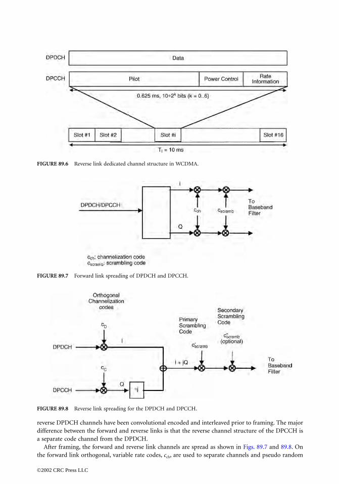
reverse DPDCH channels have been convolutional encoded and interleaved prior to framing. The majordifference between the forward and reverse links is that the reverse channel structure of the DPCCH isa separate code channel from the DPDCH.

After framing, the forward and reverse link channels are spread as shown in Figs. 89.7 and 89.8. Onthe forward link orthogonal, variable rate codes, cch, are used to separate channels and pseudo random

FIGURE 89.6 Reverse link dedicated channel structure in WCDMA.

FIGURE 89.7 Forward link spreading of DPDCH and DPCCH.

FIGURE 89.8 Reverse link spreading for the DPDCH and DPCCH.


scrambling

different baslink to separstations andto group mo

Spreading

WCDMA emforward link

truncated to

short code mGold code olong code gcorrespondiimplementathe numbershort codesmultiuser deproperties. Tbeneficial inimplementa

Orthogoncodes whoseaccording to

FIGURE 89.9


©2002 CRC P

sequences, cscramb, are used to spread the signal evenly across the spectrum and separatee stations. On the reverse link, the orthogonal channelization codes are used as in the forwardate CDMA channels. The scrambling codes, and , are used to identify mobile to spread the signal evenly across the band. The optional scrambling code is used as a meansbiles under a common scrambling sequence.

Codes

ploys long spreading codes. Different spreading codes are used for cell separation in the and user separation in the reverse link. In the forward link Gold codes of length 218 are form cycles of 216 times 10 ms frames. In order to minimize the cell search time, a specialask is used. The synchronization channel of WCDMA is masked with an orthogonal short

f length 256 chips spanning one symbol. The mask symbols carry information about the BSroup. Thus, the mobile station first acquires the short mask code and then searches theng long code. A short VL-Kasami code has been proposed for the reverse link to ease thetion of multiuser detection. In this case, code planning would also be negligible because of VL-Kasami sequences is more than one million. However, in certain cases, the use of may lead to bad correlation properties, especially with very small spreading factors. Iftection were not used, adaptive code allocation could be used to restore the cross-correlationhe use of short codes to ease the implementation of advanced detection techniques is more the forward link since the cyclostationarity of the signal could be utilized for adaptivetion of the receiver.ality between the different spreading factors can be achieved by tree-structured orthogonal construction is illustrated in Fig. 89.9 [5]. The tree-structured codes are generated recursively the following equation,

Construction of orthogonal spreading codes for different spreading factors.

c′scramb c″scramb

c2n

c2n ,1

c2n ,2

�

c2n ,2n

cn ,1 cn ,1

cn ,1 c– n ,1

�

cn ,n cn ,n

cn ,n c– n ,n

= =

ress LLC

where C2n is the orthogonal code set of size 2n. The generated codes within the same layer constitute aset of orthogonal functions and are thus orthogonal. Furthermore, any two codes of different layers arealso orthogonal except for the case that one of the two codes is a mother code of the other. For examplecode c4,4 is not orthogonal with codes c1,1 and c2,2.

Coherent Detection and Beamforming

In the forward link, time-multiplexed pilot symbols are used for coherent detection. Because the pilotsymbols are user dedicated, they can be used for channel estimation with adaptive antennas as well. Inthe reverse link, WCDMA employs pilot symbols multiplexed with power control and rate informationfor coherent detection.

Multirate

WCDMA traffic channel structure is based on a single code transmission for small data rates and multicodefor higher data rates. Multiple services belonging to the same connection are, in normal cases, time multi-plexed as was depicted in the upper part of Fig. 89.3. After service multiplexing and channel coding, themultiservice data stream is mapped to one or more dedicated physical data channels. In the case of multicodetransmission, every other data channel is mapped into Q and every other into I channel. The channel codingof WCDMA is based on convolutional and concatenated codes. For services with BER = 10-3, convolutionalcode with constraint length of 9 and different code rates (between 1/2-1/4) is used. For services with BER= 10-6, a concatenated coding with an outer Reed-Solomon code has been proposed. Typically, blockinterleaving over one frame is used. WCDMA is also capable of interframe interleaving, which improvesthe performance for services allowing longer delay. Turbo codes for data services are under study. Ratematching is performed by puncturing or symbol repetition.

Packet Data

WCDMA has two different types of packet data transmission possibilities. Short data packets can beappended directly to a random access burst. The WCDMA random-access burst is 10 ms long, it istransmitted with fixed power, and the access principle is based on the slotted Aloha scheme. Thismethod, called common channel packet transmission, is used for short infrequent packets, where thelink maintenance needed for a dedicated channel would lead to an unacceptable overhead. Larger ormore frequent packets are transmitted on a dedicated channel. A large single packet is transmitted usinga single-packet scheme where the dedicated channel is released immediately after the packet has beentransmitted. In a multipacket scheme the dedicated channel is maintained by transmitting power controland synchronization information between subsequent packets.

89.5 cdma2000

The dedicated channels used in cdma2000 system are the fundamental, supplemental, pilot,1 and dedi-cated control channels. Shown for the forward link in Fig. 89.10 and for the reverse in Fig. 89.11, thefundamental channel provides for the communication of voice, low rate data, and signalling where powercontrol information for the reverse channels is punctured on the forward fundamental channel. For highrate data services, the supplemental channel is used where one important difference between the sup-plemental and the fundamental channel is the addition of parallel-concatenated turbo codes. For differentservice options, multiple supplemental channels can be used. The code multiplex pilot channel allowsfor phase coherent detection. In addition, the pilot channel on the forward link is used for determiningsoft handoff and the pilot channel on the reverse is used for carrying power control information for the

1Dedicated for the reverse link and common for the forward link.


forward channels. Finally, the dedicated control channel, also shown in Fig. 89.10 for the forward linkand in Fig. 89.11, for the reverse, is used primarily for exchange of high rate Media Access Control (MAC)layer signalling.

Multicarrier

In addition to direct spread, a multicarrier approach has been proposed for the cdma2000 forward linksince it would maintain orthogonality between the cdma2000 and TIA/EIA-95B carriers [6]. The mul-ticarrier variant is achieved by using three 1.25 MHz carriers for a 5 MHz bandwidth where all carriershave separate channel coding and are power controlled in unison.

FIGURE 89.10 Forward link channel structure in cdma2000 for direct spread. (Note: dashed line indicates that itis only used for the fundamental channel).

FIGURE 89.11 Reverse link channel structure in cdma2000.


Spreading Codes

On the forward link, the cell separation for cdma2000 is performed by two M-sequences of length 3 × 215,one for I and one for Q channel, which are phase shifted by PN-offset for different cells. Thus,during the cell search process only these sequences are searched. Because there are a limited numberof PN-offsets, they need to be planned in order to avoid PN-confusion [7]. In the reverse link, userseparation is performed by different phase shifts of M-sequence of length 241. The channel separation isperformed using variable spreading factor Walsh sequences, which are orthogonal to each other.

Coherent Detection

In the forward link, cdma2000 has a common pilot channel, which is used as a reference signal forcoherent detection when adaptive antennas are not employed. When adaptive antennas are used, anauxiliary pilot is used as a reference signal for coherent detection. Code multiplexed auxiliary pilots aregenerated by assigning a different orthogonal code to each auxiliary pilot. This approach reduces thenumber of orthogonal codes available for the traffic channels. This limitation is alleviated by expandingthe size of the orthogonal code set used for the auxiliary pilots. Since a pilot signal is not modulated bydata, the pilot orthogonal code length can be extended, thereby yielding an increased number of availablecodes, which can be used as additional pilots. In the reverse link, the pilot signal is time multiplexed withpower control and erasure indicator bit (EIB).

Multirate Scheme

cdma2000 has two traffic channel types, the fundamental and the supplemental channel, which are codemultiplexed. The fundamental channel is a variable rate channel which supports basic rates of 9.6 kbpsand 14.4 kbps and their corresponding subrates, i.e., Rate Set 1 and Rate Set 2 of TIA/EIA-95B. It conveysvoice, signalling, and low rate data. The supplemental channel provides high data rates. Services withdifferent QoS requirements are code multiplexed into supplemental channels. The user data framelength of cdma2000 is 20 ms. For the transmission of control information, 5 and 20 ms frames can beused on the fundamental channel or dedicated control channel. On the fundamental channel a convo-lutional code with constraint length 9 is used. On supplemental channels convolutional coding is usedup to 14.4 kbps. For higher rates Turbo codes with constraint length 4 and rate 1/4 are preferred. Ratematching is performed by puncturing, symbol repetition, and sequence repetition.

Packet Data

cdma2000 also allows short data burst using the slotted Aloha principle. However, instead of fixed trans-mission power it increases the transmission power for the random access burst after an unsuccessfulaccess attempt. When the mobile station has been allocated a traffic channel, it can transmit withoutscheduling up to a predefined bit rate. If the transmission rate exceeds the defined rate, a new accessrequest has to be made. When the mobile station stops transmitting, it releases the traffic channel butnot the dedicated control channel. After a while it also releases the dedicated control channel as well butmaintains the link layer and network layer connections in order to shorten the channel set-up time whennew data needs to be transmitted.

Parametric Comparison

For comparison, Table 89.1 lists the parameters of cdma2000 and WCDMA. cdma2000 uses a chip rateof 3.6864 Mcps for the 5 MHz band allocation with the direct spread forward link option and a1.2288 Mcps chip rate with three carriers for the multicarrier option. WCDMA uses direct spread with achip rate of 4.096 Mcps. The multicarrier approach is motivated by a spectrum overlay of cdma2000carriers with existing TIA/EIA-95B carriers [6]. Similar to EIA/TIA-95B, the spreading codes of cdma2000are generated using different phase shifts of the same M-sequence. This is possible due to the synchronous


network operation. Since WCDMA has an asynchronous network, different long codes rather than differentphase shifts of the same code are used for the cell and user separation. The code structure determines howcode synchronization, cell acquisition, and handover synchronization are performed.

89.6 TDMA-Based Schemes

As discussed, TIA/EIA-136 and GSM evolution have similar paths in the form of EDGE. The UWC-136IMT 2000 proposal contains, in addition to the TIA/EIA-136 30 kHz carriers, the high rate capabilityprovided by the 200 kHz and 1.6 MHz carriers shown in Table 89.2. The targets for the IS-136 evolutionwere to meet IMT-2000 requirements and an initial deployment within 1 MHz spectrum allocation.UWC-136 meets these targets via modulation enhancement to the existing 30 kHz channel (136+) andby defining complementary wider band TDMA carriers with bandwidths of 200 kHz for vehicular/outdoorenvironments and 1.6 MHz for indoor environments. The 200 kHz carrier, 136 HS (vehicular/outdoor)

TABLE 89.1 Parameters of WCDMA and cdma2000

WCDMA cdma2000

Channel bandwidth 5, 10, 20 MHz 1.25, 5, 10, 15, 20 MHz Forward link RF channel

structure Direct spread Direct spread or multicarrier

Chip rate 4.096/8.192/16.384 Mcps 1.2288/3.6864/7.3728/11.0593/14.7456 Mcps for direct spread

n × 1.2288 Mcps (n = 1,3,6,9,12) for multicarrier

Roll-off factor 0.22 Similar to TIA/EIA-95B Frame length 10 ms/20 ms (optional) 20 ms for data and control/5 ms for

control information on the fundamentaland dedicated control channel

Spreading modulation Balanced QPSK (forward link) Balanced QPSK (forward link)Dual channel QPSK (reverse link) Dual channel QPSK (reverse link) Complex spreading circuit Complex spreading circuit

Data modulation QPSK (forward link) QPSK (forward link) BPSK (reverse link) BPSK (reverse link)

Coherent detection User dedicated time multiplexed pilot(forward link and reverse link),common pilot in forward link

Pilot time multiplexed with PC and EIB(reverse link)

Common continuous pilot channel andauxiliary pilot (forward link)

Channel multiplexing in reverse link

Control and pilot channel timemultiplexed

Control, pilot fundamental, andsupplemental code multiplexed

I&Q multiplexing for data and control channel

I&Q multiplexing for data and control channels

Multirate Variable spreading and multicode Variable spreading and multicode Spreading factors 4-256 (4.096 Mcps) 4-256 (3.6864 Mcps) Power control Open and fast closed loop (1.6 kHz) Open loop and fast closed loop (800 Hz) Spreading (forward link) Variable length orthogonal sequences for

channel separation. Gold sequences for cell and user separation

Variable length Walsh sequences for channel separation, M-sequence 3 × 215

(same sequence with time shift utilized in different cells different sequence in I&Q channel)

Spreading (reverse link) Variable length orthogonal sequences for channel separation. Gold sequence 241 for user separation (different time shifts in I and Q channel, cycle 216 10 ms radio frames)

Variable length orthogonal sequences for channel separation, M-sequence 215

(same for all users different sequences in I&Q channels), M-sequence 241 for user separation (different time shifts for different users)

Handover Soft handover Soft handover Interfrequency handover Interfrequency handover


with the same parameters as EDGE provides medium bit rates up to 384 kbps and the 1.6 MHz carrier,136 HS (indoor), highest bit rates up to 2 Mbps. The parameters of the 136 HS proposal submitted toITU are listed in Table 89.2 and the different carrier types of UWC-136 are shown in Fig. 89.12.

Carrier Spacing and Symbol Rate

The motivation for the 200 kHz carrier is twofold. First, the adoption of the same physical layer for136 HS (Vehicular/Outdoor) and GSM data carriers provides economics of scale and therefore cheaperequipment and faster time to market. Second, the 200 kHz carrier with higher order modulation canprovide bit rates of 144 and 384 kbps with reasonable range and capacity fulfilling IMT-2000 requirementsfor pedestrian and vehicular environments. The 136 HS (Indoor) carrier can provide 2 Mbit/s user datarate with a reasonably strong channel coding.

Modulation

First proposed modulation methods were Quaternary Offset QAM (Q-O-QAM) and Binary Offset QAM(B-O-QAM). Q-O-QAM could provide higher data rates and good spectral efficiency. For each symboltwo bits are transmitted and consecutive symbols are shifted by π/2. An offset modulation was proposed,

TABLE 89.2 Parameters of 136 HS

136 HS (Vehicular/Outdoor) 136 HS (Indoor)

Duplex method FDD FDD and TDD Carrier spacing 200 kHz 1.6 MHz Modulation Q-O-QAM Q-O-QAM

B-O-QAM B-O-QAM 8 PSKGMSK

Modulation bit rate 722.2 kbps (Q-O-QAM) 5200 kbps (Q-O-QAM) 361.1 kbps (B-O-QAM) 2600 kbps (B-O-QAM)812.5 kbps (8 PSK)270.8 kbps (GMSK)

Payload 521.6 kbps (Q-O-QAM) 4750 kbps (Q-O-QAM) 259.2 kbps (B-O-QAM) 2375 kbps (B-O-QAM) 547.2 kbps (8 PSK) 182.4 kbps (GMSK)

Frame length 4.615 ms 4.615 ms Number of slots 8 64 (72 µs)

16 (288 µs) Coding Convolutional Convolutional

1/2, 1/4, 1/3, 1/1 1/2, 1/4, 1/3, 1/1 ARQ Hybrid Type II ARQ

Frequency hopping Optional Optional Dynamic channel allocation Optional Optional

FIGURE 89.12 UWC-136 carrier types.


because it causes smaller amplitude variations than 16QAM, which can be beneficial when using ampli-fiers that are not completely linear. The second modulation B-O-QAM has been introduced, which hasthe same symbol rate of 361.111 ksps, but where only the outer signal points of the Q-O-QAM modulationare used. For each symbol one bit is transmitted and consecutive symbols are shifted by π/2. A secondmodulation scheme with the characteristic of being a subset of the first modulation scheme and havingthe same symbol rate as the first modulation allows seamless switching between the two modulationtypes between bursts. Both modulation types can be used in the same burst. From a complexity pointof view the addition of a modulation, which is subset of the first modulation, adds no new requirementsfor the transmitter or receiver.

In addition to the originally proposed modulation schemes, Quaternary Offset QAM (Q-O-QAM)and Binary Offset QAM (B-O-QAM), other modulation schemes, CPM (Continuous Phase Modu-lation) and 8-PSK, have been evaluated in order to select the modulation best suited for EDGE. Theoutcome of this evaluation is that 8 PSK was considered to have implementation advantages overQ-O-QAM. Parties working on EDGE are in the process of revising the proposals so that 8 PSKwould replace the Q-O-QAM and GMSK can be used as the lower level modulation instead of B-O-QAM. The symbol rate of the 8 PSK will be the same as for GMSK and the detailed bit rates will bespecified early in 1999.

Frame Structures

The 136 HS (Vehicular/Outdoor) data frame length is 4.615 ms and one frame consists of eight slots.The burst structure is suitable for transmission in a high delay spread environment. The frame and slotstructures of the 136 HS (Indoor) carrier were selected for cell coverage for high bit rates. The HS-136Indoor supports both FDD and TDD duplex methods. Figure 89.13 illustrates the frame and slotstructure. The frame length is 4.615 ms and it can consist of

• 64 1/64 time slots of length 72 µs

• 16 1/16 time slots of length 288 µs

In the TDD mode, the same burst types as defined for the FDD mode are used. The 1/64 slot can beused for every service from low rate speech and data to high rate data services. The 1/16 slot is to beused for medium to high rate data services. Figure 89.13 also illustrates the dynamic allocation of resourcesbetween the reverse link and the forward link in the TDD mode.

The physical contents of the time slots are bursts of corresponding length. Three types of trafficbursts are defined. Each burst consists of a training sequence, two data blocks, and a guard period.The bursts differ in the length of the burst (72 µs and 288 µs) and in the length of the training sequence

FIGURE 89.13 Wideband TDMA frame and slot structure.


(27 symbols and 49 symbols) leading to different numbers of payload symbols and different multipathdelay performances (Fig. 89.14). The number of required reference symbols in the training sequencedepends on the length of the channel’s impulse response, the required signal-to-noise ratio, the expectedmaximum Doppler frequency shift, and the number of modulation levels. The number of referencesymbols should be matched to the channel characteristics, remain practically stable within the correlationwindow, and have good correlation properties. All 136 based schemes can use interference cancellation asa means to improve performance [8]. For 136 HS (Indoor), the longer sequence can handle about 7 µsof time dispersion and the shorter one 2.7 µs. It should be noted that if the time dispersion is larger, thedrop in performance is slow and depends on the power delay profile.

Multirate Scheme

The UWC-136 multirate scheme is based on a variable slot, code, and modulation structure. Data ratesup to 43.2 kbps can be offered using the 136+ 30 kHz carrier and multislot transmission. Depending onthe user requirements and channel conditions a suitable combination of modulation, coding, and numberof data slots is selected. 136 HS can offer packet switched, and both transparent and nontransparentcircuit switched data services. Asymmetrical data rates are provided by allocating a different number oftime slots in the reverse and forward links. For packet switched services the RLC/MAC protocol providesfast medium access via a reservation based medium access scheme, supplemented by selective ARQ forefficient retransmission.

Similar to 136 HS (Outdoor/Vehicular), the 136 HS (Indoor) uses two modulation schemes and differentcoding schemes to provide variable data rates. In addition, two different slot sizes can be used. For delaytolerant packet data services, error control is based on a Type II hybrid ARQ (automatic repeat request)scheme [5]. The basic idea is to first send all data blocks using a simple error control coding scheme. Ifdecoding at the receiver fails, a retransmission is requested using a stronger code. After the secondretransmission, diversity combining can be performed between the first and second transmissions priorto hard decisions. This kind of ARQ procedure can be used due to the ability of the RLC/MAC protocolto allocate resources fast and to send transmission requests reliably in the feedback channel [5].

Radio Resource Management

The radio resource management schemes of UWC-136 include link adaptation, frequency hopping, powercontrol, and dynamic channel allocation. Link adaptation offers a mechanism for choosing the bestmodulation and coding alternative according to channel and interference conditions. Frequency hoppingaverages interference and improves link performance against fast fading. For 136 HS (Indoor) fast powercontrol (frame-by-frame) could be used to improve the performance in cases where frequency hoppingcannot be applied, for example, when only one carrier is available. Dynamic channel allocation can beused for channel assignments. However, when deployment with minimum spectrum is desired, reuse 1/3and fractional loading with fixed channel allocation is used.

FIGURE 89.14 Burst structure.


89.7 Time Division Duplex (TDD)

The main discussion about the IMT-2000 air interface has been concerned with technologies for FDD.However, there are several reasons why TDD would be desirable. First, there will likely be dedicatedfrequency bands for TDD within the identified UMTS frequency bands. Furthermore, FDD requiresexclusive paired bands and spectrum is, therefore, hard to find. With a proper design including powerfulFEC, TDD can be used even in outdoor cells. The second reason for using TDD is flexibility in radioresource allocation, i.e., bandwidth can be allocated by changing the number of time slots for the reverselink and forward link. However, the asymmetric allocation of radio resources leads to two interferencescenarios that will impact the overall spectrum efficiency of a TDD scheme:

• asymmetric usage of TDD slots will impact the radio resource in neighboring cells, and

• asymmetric usage of TDD slots will lead to blocking of slots in adjacent carriers within their owncells.

Figure 89.15 depicts the first scenario. MS2 is transmitting at full power at the cell border. Since MS1has a different asymmetric slot allocation than MS2, its forward link slots received at the sensitivity limitare interfered by MS1, which causes blocking. On the other hand, since the BS1 can have much higherEIRP (effective isotropically radiated power) than MS2, it will interfere BS2’s ability to receive MS2.Hence, the radio resource algorithm needs to avoid this situation.

In the second scenario, two mobiles would be connected into the same cell but using differentfrequencies. The base station receives MS1 on the frequency f1 using the same time slot it uses on thefrequency f2 to transmit into MS2. As shown in Table 89.3, the transmission will block the reception dueto the irreducible noise floor of the transmitter regardless of the frequency separation between f1 and f2.

Both TDMA- and CDMA-based schemes have been proposed for TDD. Most of the TDD aspects arecommon to TDMA- and CDMA-based air interfaces. However, in CDMA-based TDD systems the slotduration on the forward and reverse links must be equal to enable the use of soft handoff and preventthe interference situation described in the first scenario. Because TDMA systems do not have soft handoffon a common frequency, slot imbalances from one BS to the next are easier to accommodate. Thus,TDMA-based solutions have higher flexibility. The frame structure for the wide band TDMA for theTDD system was briefly discussed in the previous section. WCDMA has been proposed for TDD in Japanand Europe. The frame structure is the same as for the FDD component, i.e., a 10 ms frame split into16 slots of 0.625 ms each. Each slot can be used either for reverse link or forward link. For cdma2000,the TDD frame structure is based on a 20 ms frame split into 16 slots of 1.25 ms each.

TABLE 89.3 Adjacent Channel Interference Calculation

BTS transmission power for MS2 in forward link 1W 30 dBm Received power for MS1 -100 dBm Adjacent channel attenuation due to irreducible noise floor 50 to 70 dBSignal to adjacent channel interference ratio -60 to -80 dB

FIGURE 89.15 TDD interference scenario.


89.8 Conclusions

Third generation cellular systems are a mechanism for evolving the telecommunications business basedprimarily on voice telephony to mobile wireless datacomm. In light of events in TIA, ETSI, and ARIB,cdma2000, WCDMA, and EDGE will be important technologies used to achieve the datacomm goal.Standardization related to radio access technologies discussed in this chapter were under way at the timeof writing and will offer the European, U.S., and Japanese markets both CDMA and TDMA third-generation options. In comparing CDMA evolution, the European, U.S., and Japanese based systemshave some similarities, but differ in the chip rate and channel structure. In the best circumstances, someharmonization will occur between cdma2000 and WCDMA making deployment of hardware capable ofsupporting both systems easier. In TDMA, the third generation paths of GSM and TIA/EIA-136 arethrough a common solution. This alignment will offer TDMA systems an advantage in possible globalroaming for data services. In spite of the regional standards differences, third generation will be themechanism for achieving wireless multimedia enabling services beyond the comprehension of secondgeneration systems.

Acknowledgments

The authors would like to thank Harri Holma, Pertti Lukander, and Antti Toskala from Nokia Telecom-munications, George Fry, Kari Kalliojarvi, Riku Pirhonen, Rauno Ruismaki, and Zhigang Rong fromNokia Research Center, Kari Pehkonen from Nokia Mobile Phones, and Kari Pulli from the Universityof Stanford for helpful comments. In addition, contributions related to spectrum and modulation aspectsfrom Harri Lilja from Nokia Mobile Phones are acknowledged.

References

1. ITU-R M.1225, Guidelines for Evaluation of Radio Transmission Technologies for IMT-2000, 1998.2. Special Issue on IMT-2000: Standards Efforts of the ITU, IEEE Pers. Commun., 4(4), Aug. 1997.3. Verdu, S., Minimum probability of error for asynchronous gaussian multiple access, IEEE Trans. on

IT., IT-32(1), 85–96, Jan. 1986.4. Monk, A.M. et al., A noise-whitening approach to multiple access noise rejection—Pt I: Theory and

background, IEEE J. Select. Areas Commun., 12(5), 817–827, Jun. 1997.5. Nikula, E., Toskala, A., Dahlman, E., Girard, L., and Klein, A., FRAMES multiple access for UMTS

and IMT-2000, IEEE Pers. Commun., Apr. 1998.6. Tiedemann, E.G., Jr., Jou, Y.-C., and Odenwalder, J.P., The evolution of IS-95 to a third generation

system and to the IMT-2000 era, Proc. ACTS Summit, Aalborg, Denmark, 924–929, Oct. 1997.7. Chang, C.R., Van, J.Z., and Yee, M.F., PN offset planning strategies for nonuniform CDMA networks,

Proc. VTC’97, 3, Phoenix, Arizona, 1543–1547, May 4–7, 1997.8. Ranta, P., Lappetelainen, A., and Honkasalo, Z.-C., Interference cancellation by joint detection in

random frequency hopping TDMA networks, Proc. ICUPC96, 1, Cambridge, MA, 428–432, Sept./Oct.1996.


90Multiple-Input

Multiple-Output(MIMO) Wireless

Systems1

90.1 IntroductionDiversity Gain • Multiplexing Gain

90.2 The MIMO Fading Channel Model90.3 Capacity of MIMO Channels

The Deterministic Case • The Random Case

90.4 Spatial MultiplexingZero Forcing Receiver • Minimum Mean-Square Error Receiver • V-BLAST Receiver • Maximum Likelihood Receiver

90.5 Transmit DiversityIndirect Transmit Diversity • Direct Transmit Diversity

90.6 Summary and Conclusion

90.1 Introduction

Wireless transmission is impaired by signal fading and interference. The increasing requirements on datarate and quality of service for wireless communications systems call for new techniques to increasespectrum efficiency and to improve link reliability. The use of multiple antennas at both ends of a wirelesslink promises significant improvements in terms of spectral efficiency and link reliability. This technologyis known as multiple-input multiple-output (MIMO) wireless (see Fig. 90.1). MIMO systems offer diver-sity gain and multiplexing gain.

Diversity Gain

Diversity is used in wireless systems to combat small scale fading caused by multipath effects. The basicprinciple of diversity is that if several replicas of the information signal are received through independentlyfading links (branches), then with high probability at least one or more of these links will not be in a fadeat any given instant. Clearly, this probability will increase if the number of diversity branches increases.In a noise limited link, without adequate diversity, the transmit power will need to be higher or the range

1This work was supported in part by FWF-grant J1868-TEC.

Helmut BölcskeiETH Zurich



smaller to protect the link against fading. Likewise in co-channel interference limited links, withoutadequate diversity, the reuse factor will have to be increased to make co-channel interference well belowthe signal average level. Diversity processing that reduces fading is a powerful tool to increase capacity andcoverage in radio networks. The three main forms of diversity traditionally exploited in wireless commu-nications systems are temporal diversity, frequency diversity, and spatial (or antenna) diversity.

Temporal diversity is applicable in a channel that has time selective fading. The information is trans-mitted with spreading over a time span that is larger than the coherence time of the channel. Thecoherence time is the minimum time separation between independent channel fades. Time diversity isusually exploited via interleaving, forward error correction coding (FEC), and automatic repeat request(ARQ). One drawback of time diversity is the inherent delay incurred in time spreading.

Frequency diversity is effective when the fading is frequency-selective. This diversity can be exploited byspreading the information over a frequency span larger than the coherence bandwidth of the channel. Thecoherence bandwidth is the minimum frequency separation between independent channel fades and isinversely dependent on the delay spread in the channel. Frequency diversity can be exploited through spreadspectrum techniques or through interleaving and FEC in conjunction with multicarrier modulation [1].

Spatial diversity. In this chapter, we are mostly concerned with spatial (or antenna) diversity. In spacediversity we receive or transmit information signals from antennas that are spaced by more than thecoherence distance apart. The coherence distance is the minimum spatial separation of antennas forindependent fading and depends on the angle spread of the multipaths arriving at or departing from anantenna array. For example, if the multipath signals arrive from all directions in the azimuth, antennaspacing on the order of 0.4λ-0.6λ is adequate [2] for independent fading. On the other hand, if themultipath angle spread is smaller, the coherence distance is larger. Empirical measurements show a strongcoupling between antenna height and coherence distance for base station antennas. Higher antennaheights imply larger coherence distances. At the terminal end, which is usually low and buried in scatterers,a 0.4λ-0.6λ separation will be adequate. Receive diversity, i.e., the use of multiple antennas only at thereceive side, is a well-studied subject [3]. Driven mostly by mobile wireless applications, where it is difficultto employ multiple antennas in the handset, the use of multiple antennas at the base station in combi-nation with transmit diversity has become an active area of research in the past few years [4,5,6,7,8,9].Transmit diversity in the case where the channel is known at the transmitter involves transmission suchthat the signals launched from the individual antennas arrive in phase at the receiver antenna. In thecase where the channel is not known at the transmitter, transmit diversity requires more sophisticatedmethods such as space-time coding which use coding across antennas (space) and time. Here, the basicidea is to send the information bitstream with different preprocessing (coding, modulation, delay, etc.)from different antennas such that the receiver can combine these signals to obtain diversity.

In a MIMO system both transmit and receive antennas combine to give a large diversity order.Assuming MT transmit and MR receive antennas, a maximum of MTMR links are available; if all of theselinks fade independently, we get MT MRth order diversity. The value of spatial MIMO diversity is dem-onstrated in Figs. 90.2(a) and (b), where the signal level at the output of a 1-input 1-output (SISO) and

FIGURE 90.1 Schematic representation of a MIMO wireless system.

TX H RX


of a 2-input 2-output system, respectively, is shown, assuming that the channel is known at the receiverand proper diversity combining is employed. Clearly, the use of multiple antennas reduces the signalfluctuations and eliminates deep fades.

Transmit and receive diversity are both similar and different in many ways. While receive diversityneeds merely multiple antennas which fade independently, and is independent of coding/modulationschemes, transmit diversity needs special modulation/coding schemes in order to be effective. Also, receivediversity provides array gain, whereas transmit diversity does not provide array gain when the channelis unknown in the transmitter (the usual case).

Multiplexing Gain

While spatial diversity gain can be obtained when multiple antennas are present at either the transmitor the receive side, spatial multiplexing requires multiple antennas at both ends of the link [10,11]. Theidea of spatial multiplexing is that the use of multiple antennas at the transmitter and the receiver inconjunction with rich scattering in the propagation environment opens up multiple data pipes withinthe same frequency band to yield a linear (in the number of antennas) increase in capacity. This increasein capacity comes at no extra bandwidth or power consumption and is therefore very attractive. Thebasic principle of spatial multiplexing is illustrated in Fig. 90.3. The symbol stream to be transmitted isbroken up into several parallel symbol streams which are then transmitted simultaneously and withinthe same frequency band from the antennas. Due to multipath propagation, each transmit antennainduces a different spatial signature at the receiver. The receiver exploits these signature differences to

FIGURE 90.2 The value of spatial diversity. Signal level as a function of time for a (a) 1-input 1-output, and a (b)2-input 2-output system.

FIGURE 90.3 Schematic of a spatial multiplexing system. S/P and P/S denote serial-to-parallel and parallel-to-serial conversion, respectively.

0 100 200 300 400 500 600 700 800 90030

20

10

0

10

(a)

0 100 200 300 400 500 600 700 800 90030

20

10

0

10

(b)

S/P TX RX P/S


separate the individual data streams. The price to be paid for multiplexing gain is increased hardwarecost due to the use of multiple antennas.

We concluplexing, and

90.2 T

We focus onis equipped

discussion tochannel moentries are i.an independthe transmitbe obtainedchannel is kfeedback froand is theref

The inpu

where

r

=

[

r

s

=

[

s

0

s

1

…

vector. The

with zero mevariable

z

=

Equivalently

model is typthe transmit

CN

(0, 1). Threceive anten

ρ

regardless

90.3 C

As discussedthe capacityMIMO chan

The Dete

The formula

where

ρ

is t

It is evident that the traneach with a

s

0967_Frame_C90 Page 4 Tuesday, March 5, 2002 10:35 PM

©2002 CRC P

de by noting that MIMO systems can be used for transmit–receive diversity, spatial multi- combinations of diversity and multiplexing.

he MIMO Fading Channel Model

a single-user communication model and consider a point-to-point link where the transmitterwith MT antennas and the receiver employs MR antennas (see Fig. 90.1). We restrict our the case where the channel is frequency-flat (narrowband assumption). A commonly used

del in MIMO wireless communications is the block fading model, where the channel matrixi.d. complex Gaussian (Rayleigh fading), constant during a block of symbols, and change inent fashion from block to block. We furthermore assume that the channel is unknown atter and perfectly known (and tracked) at the receiver. Channel knowledge in the receiver can by sending training data and estimating the channel. We do not discuss the case where thenown at the transmitter. Acquiring channel knowledge at the transmitter requires the use ofm the receiver or the use of transmit-receive duplexing based channel mapping methodsore often hard to realize in practice.

t-output relation of the MR × MT matrix channel can be written as

, (90.1)

0 r1… ]T is the MR × 1 receive signal vector, H is the MR × MT channel transfer matrix,]T is the MT × 1 transmit signal vector, and n = [n0 n1… ]T is the MR × 1 noise

elements of the channel transfer matrix H are i.i.d. circularly symmetric complex Gaussianan and unit variance. A circularly symmetric complex Gaussian random variable is a random(x + jy) ∼ CN (0, σ2), in which x and y are i.i.d. real Gaussian distributed with N (0, σ2/2)., each entry of H has uniformly distributed phase and Rayleigh distributed magnitude. Thisical of an environment with rich scattering and enough separation between the antennas atter and the receiver. The noise components ni (i = 0, 1, …, MR − 1) are assumed to be i.i.d.e average transmitted power across all antennas, which is equal to the average SNR at eachna with this normalization of noise power and channel loss, is limited to be no greater than

of MT. The transmit power is assumed to be equally distributed across the transmit antennas.

apacity of MIMO Channels

earlier, MIMO systems offer significant capacity gains over SISO channels. Before analyzing of random i.i.d. MIMO fading channels, let us briefly consider deterministic SISO andnels.

rministic Case

for Shannon capacity for a deterministic SISO channel with input-output relation r = Hs + n,he average transmit power and E{|n|2} = 1, is given by [12]

(90.2)

that for high SNRs, a 3dB increase in ρ gives an increase in capacity of one bps/Hz. Assumingsmitted signal vector is composed of MT statistically independent equal power components,circularly symmetric complex Gaussian distribution, the capacity of a deterministic MIMO

r Hs n+=

rMR 1–

MT 1– nMR 1–

C log2 1 ρ H 2+( ) bps/Hz= .

ress LLC

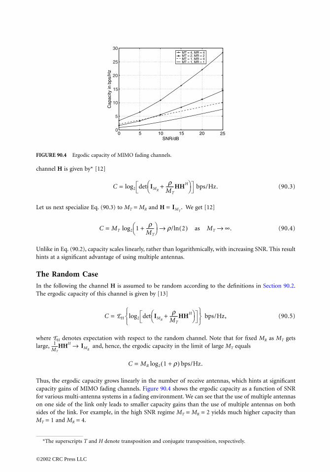
channel H i

Let us next

Unlike in Eqhints at a sig

The Rand

In the followThe ergodic

where EH delarge, HH

Thus, the ercapacity gainfor various mon one sidesides of the MT = 1 and

FIGURE 90.4

*The supe

30MT = 4, MR = 4MT = 2, MR = 2MT = 1, MR = 4

1MT

-------


©2002 CRC P

s given by* [12]

(90.3)

specialize Eq. (90.3) to MT = MR and H = We get [12]

(90.4)

. (90.2), capacity scales linearly, rather than logarithmically, with increasing SNR. This resultnificant advantage of using multiple antennas.

om Case

ing the channel H is assumed to be random according to the definitions in Section 90.2. capacity of this channel is given by [13]

(90.5)

notes expectation with respect to the random channel. Note that for fixed MR as MT getsH → and, hence, the ergodic capacity in the limit of large MT equals

godic capacity grows linearly in the number of receive antennas, which hints at significants of MIMO fading channels. Figure 90.4 shows the ergodic capacity as a function of SNRulti-antenna systems in a fading environment. We can see that the use of multiple antennas

of the link only leads to smaller capacity gains than the use of multiple antennas on bothlink. For example, in the high SNR regime MT = MR = 2 yields much higher capacity thanMR = 4.

Ergodic capacity of MIMO fading channels.

rscripts T and H denote transposition and conjugate transposition, respectively.

10

25

20

15

5

00 5 10 15 20 25

SNR/dB

Cap

acity

in b

ps/H

z

MT = 1, MR = 1

C log2 det IMR

ρMT

-------HHH+ bps/Hz= .

IMT.

C MT log2 1ρ

MT

-------+ ρ/ln 2( ) as MT ∞→→= .

C EH log2 det IMR

ρMT

-------HHH+

bps/Hz= ,

IMR

C MR log2 1 ρ+( ) bps/Hz= .

ress LLC

90.4 Spatial Multiplexing

We recall froand receive which allow

In a spatilower rate stmodulation.Each receiveinto constituClearly, the sarchitecturereceiver stru

Zero Forc

A simple linmatrix, i.e., vector s is o

The ZF receiH, the ZF rethe receiver employed, s

Minimum

The ZF recealternative loverall errorof s is obtai

where it wasto noise at tgeneral not receiver.

V-BLAST

An attractivthe cost of inrather than this strongetransmit sig


©2002 CRC P

m Section 90.1 that multiplexing gain is available if multiple antennas are used at the transmitside of the wireless link. In this section, we describe various signal processing techniques realization of this gain.al multiplexing system [10,11] the data stream to be transmitted is demultiplexed into MT

reams which are then simultaneously sent from the MT transmit antennas after coding and Note that these streams occupy the same frequency band (i.e., they are co-channel signals). antenna observes a superposition of the transmitted signals. The receiver then separates thement data streams and remultiplexes them to recover the original data stream (see Fig. 90.3).eparation step determines the computational complexity of the receiver. Competing receiver

s have different performance-complexity tradeoffs. In the following, we discuss variousctures.

ing Receiver

ear receiver is the zero forcing (ZF) receiver which basically inverts the channel transferassuming that H is square and invertible. An estimate of the MT × 1 transmitted data symbolbtained as

(90.6)

ver hence perfectly separates the co-channel signals si(i = 0, 1, …, MT − 1). For ill-conditionedceiver incurs significant noise enhancement. In practice, if H is rank-deficient or non squareleft-multiplies r by the pseudo-inverse of H to recover rank(H) symbol streams. If FEC is

patial and temporal redundancy can be exploited to recover lost data.

Mean-Square Error Receiver

iver yields perfect separation of the co-channel signals at the cost of noise enhancement. Aninear receiver is the minimum mean-square error (MMSE) receiver, which minimizes the due to noise and mutual interference between the co-channel signals. In this case, an estimatened according to

(90.7)

assumed that E{ssH} = and E{nnΗ} = The MMSE receiver is less sensitivehe cost of reduced signal separation quality. In other words, the co-channel signals are inperfectly separated. In the high SNR case ≈ 0), the MMSE receiver converges to the ZF

Receiver

e alternative to ZF and MMSE receivers which, in general, yields improved performance atcreased computational complexity is the so-called V-BLAST algorithm [14,15]. In V-BLAST

jointly decoding all the transmit signals, we first decode the “strongest” signal, then subtractst signal from the received signal, proceed to decode the strongest signal of the remainingnals, and so on. The optimum detection order in such a nulling and cancellation strategy is

ŝ H 1– r=

ŝ ρMT

-------HH σn2IMR

ρMT

-------HHH+ 1–

r= ,

ρMT

------- IMTσn

2IMR.

(σn2

ress LLC

from the strongest to the weakest signal [14]. Assuming that the channel H is known, the main steps ofthe V-BLAST algorithm can be summarized as follows:

• Nullintrans

• Slicin

• Cancesignavecto

For a more

Maximum

The receiverreceiver. Hoexponential been acquire

where the mscalar constea set of size even for a smto enumerat

90.5 T

Transmit divantennas wifirst discuss diversity sch

Indirect T

In indirect tcan then reashall discusdiversity, an

Delay diveunderlying dmitting the antenna (seeseen by the

where h0 anrespectively.

Q


©2002 CRC P

g: An estimate of the strongest transmit signal is obtained by nulling out all the weakermit signals (e.g., using the zero forcing criterion).

g: The estimated signal is detected to obtain the data bits.

llation: These data bits are remodulated and the channel is applied to estimate its vectorl contribution at the receiver. The resulting vector is then subtracted from the received signalr and the algorithm returns to the nulling step until all transmit signals are decoded.

in-depth treatment of the V-BLAST algorithm the interested reader is referred to [14,15].

Likelihood Receiver

which yields the best performance in terms of error rate is the maximum likelihood (ML)wever, this receiver also has the highest computational complexity which moreover exhibitsgrowth in the number of transmit antennas. Assuming that channel state information hasd, the ML receiver computes the estimate according to

inimization is performed over all possible codeword vectors s. Note that if the size of thellation used is Q (e.g., Q = 4 for QPSK), the receiver has to perform an enumeration over

. For higher-order modulation such as 64-QAM, this complexity can become prohibitiveall number of transmit antennas. For example, for 64-QAM and MT = 3, the receiver has

e over 262,144 different vectors on the symbol rate.

ransmit Diversity

ersity is a technique which realizes spatial diversity gain in systems with multiple transmitthout requiring channel knowledge in the transmitter [4,5,6,7,8,16]. In this section, we shallindirect transmit diversity schemes and then proceed with a discussion of direct transmitemes such as space-time block and space-time Trellis codes.

ransmit Diversity

ransmit diversity schemes we convert spatial diversity into time or frequency diversity, whichdily be exploited by the receiver (often using FEC and interleaving). In the following, we

s two techniques, namely delay diversity, which converts spatial diversity into frequencyd intentional frequency offset diversity, which converts spatial diversity into time diversity.rsity. In order to simplify the presentation let us assume that MT = 2 and MR = 1. The principleelay diversity is to convert the available spatial diversity into frequency diversity by trans-

data bearing signal from the first antenna and a delayed replica thereof from the second Fig. 90.5) [4,5]. Assuming that the delay is one symbol interval, the effective SISO channel

receiver is given by

(90.8)

d h1 denote the channel gains between transmit antennas 1 and 2, and the receive antenna,We assume that h0 and h1 are i.i.d. CN (0, 1). Therefore, the channel transfer function He(e j2πθ)

ŝ

ŝ argsmin r Hs– 2= ,

MT

He e j2πθ( ) h0 h1e j2πθ–+= ,

ress LLC

is random acompute the

The functioν = are fufades and sain the system

Intentionaspatial diverMR = 1. Aftefrequency shSISO chann

where θ1 wiassumed thtemporal di

FIGURE 90.5from the seco

FIGURE 90.6

h0

12--


©2002 CRC P

s well. In order to see how the spatial diversity is converted into frequency diversity we frequency correlation function R(e j2πν) = E{He(e j2πθ) He

∗(e j2π(θ−ν))}. Using Eq. (90.8) we get

(90.9)

n |R(e j2πν)| in Eq. (90.9) is depicted in Fig. 90.6. We can see that frequencies separated bylly decorrelated. Such a channel looks exactly like a 2-paths channel with independent pathme average path energy. Therefore a Viterbi (ML) sequence detector will capture the diversity

. The extension of delay diversity to more than two transmit antennas is described in [5].l frequency offset diversity. An alternative indirect transmit diversity scheme which converts

sity into temporal diversity was first described in [17]. Let us again assume that MT = 2 andr coding and modulation, we transmit the data bearing signal from the first antenna and aifted (phase rotated) version thereof from the second antenna (see Fig. 90.7). The effective

el seen by the receiver is given by

(90.10)

th |θ1| < 1/2 is the intentional frequency offset introduced at the second antenna. It is againat h0 and h1 are i.i.d. CN(0, 1). In order to see how spatial diversity is converted intoversity, we compute the temporal correlation function of the stochastic channel he[n] given

Schematic representation of delay diversity. A delayed version of the data bearing signal is transmittednd antenna.

The correlation function |R(e j2πν)| for a delay of one symbol interval.

Dh1

−0.5 −0.4 −0.3 −0.2 −0.1 0 0.1 0.2 0.3 0.4 0.50

0.1

0.2

0.3

0.4

0.5

0.6

0.7

0.8

0.9

1

normalized frequency

corr

elat

ion

12--

R e j2πν( ) 12-- 1 e j– 2πν+( )=

he n[ ] h0 h1ej2πnθ1, n Z∈+= ,

ress LLC

by R[k] =

If |R[k]| is smresulting temas we may d

Direct Tr

Space-time b[8,18]. A simmum-ratio receive or trreview receivrespectively,the two recetransmitted

Clearly, if eishall next deused at the t

FIGURE 90.7version of the

FIGURE 90.8

h0

12--


©2002 CRC P

E{he[n] [n − k]}. Using Eq. (90.10), we get

all data symbols spaced k symbol intervals apart undergo close to independent fading. Theporal diversity can be exploited by using FEC in combination with time interleaving just

o in naturally time fading channels.

ansmit Diversity

lock coding. Space-time block coding has attracted much attention for practical applicationsple space-time block code known as Alamouti scheme [18] performs very similar to maxi-

combining (MRC), a technique which realizes spatial diversity gain by employing multipleansmit antennas (but needs channel knowledge in the transmitter for the latter). We brieflye MRC for MT = 1 and MR = 2. The receive signals are given by r0 = h0s + n0 and r1 = h1s + n1,

where h0 and h1 denote the CN (0, 1) i.i.d. channel gains between the transmit antenna andive antennas and n0 and n1 are CN (0, 1) i.i.d. noise samples. The receiver estimates thedata symbols by forming the decision variable

ther h0 or h1 is not faded, we have a good channel. Thus, we get second order diversity. Wescribe Alamouti’s scheme where MT = 2 and MR = 1. Note that now the two antennas areransmitter rather than at the receiver. Figure 90.8 shows a schematic of Alamouti’s scheme,

Conversion of spatial diversity into time diversity through intentional frequency offset. A modulated data bearing signal is transmitted from the second antenna.

Schematic of the Alamouti scheme.

h1

s0 s1

−s1∗ s0

∗

h1h0

he∗

R k[ ] 12-- 1 e

j2πkθ1+( )=

y h0∗r0 h1

∗r1+ h02 h1

2+( )s h0∗n0 h1

∗n1+ += = .

ress LLC

which consists of three steps:

• Encoding and transmitting. At a given symbol period, two signals are simultaneously transmitted fromthe twtransmis tran

whereantensampform

where

is thecolum

• The cthe ve

The e

where

• ML d

We can see toverall transa 3 dB SNR does not offantenna is eFigure 90.9 schannel usin

The Alamachieve full ddecouples in


©2002 CRC P

o antennas. In the first time instant, the signal transmitted from antenna 1 is s0 and the signalitted from antenna 2 is s1. In the next time instant, is transmitted from antenna 1 and

smitted from antenna 2. The received signals r0 and r1 are, hence, given by

(90.11)

h0 and h1 denote the CN(0, 1) i.i.d. channel gains between transmit antenna 1 and the receivena and transmit antenna 2 and the receive antenna, respectively. Furthermore, the noiseles n0 and n1 are CN(0, 1) i.i.d. The equations in Eq. (90.11) can be rewritten in vector-matrix as

is the received signal vector (note that r1 was conjugated),

(90.12)

equivalent channel matrix, s = [s0 s1]T, and n = [n0 ] is the noise vector. Note that the

ns of the channel matrix Ha are orthogonal irrespective of the specific values of h0 and h1.

ombining step. In the receiver, assuming that perfect channel knowledge has been acquired,ctor r is left-multiplied by which results in

stimates of the symbols s0 and s1 are now given by

and

etection. The symbols and are independently sent to an ML detector.

hat the Alamouti scheme yields the same diversity order as MRC. Note, however, that if themit power in the Alamouti scheme is kept the same as in MRC, the Alamouti scheme incursloss compared to MRC [18]. This 3 dB difference is due to the fact that the Alamouti schemeer array gain since it does not know the channel in the transmitter. If more than one receivemployed, the Alamouti scheme realizes 2MR-fold diversity, i.e., full spatial diversity gain.hows the bit error rate obtained for the Alamouti scheme in comparison to the SISO fadingg BPSK modulation.outi scheme is a special case of so-called space-time block codes [8]. Space-time block codesiversity gain and drastically simplify the receiver structure since the vector detection problemto simpler scalar detection problems.

s– 1∗ s0

∗

r0 h0s0 h1s1 n0+ +=

r1 h– 0s1∗ h1s0

∗ n1+ += ,

r Has n+= ,

r [r0 r1∗]

T=

Ha

h0 h1

h1∗ h0

∗–=

n1∗

HaH

ŝ HaHr

h02 h1

2+ 0

0 h02 h1

2+s Ha

Hnñ

+= = .

ŝ0 h02 h1

2+( )s0 ñ0+=

ŝ1 h02 h1

2+( )s1 ñ1+= ,

ñ0 h0∗n0 h1n1

∗+= ñ1 h1∗n0 h0n1

∗.–=ŝ0 ŝ1

ress LLC

Space-timmultiple traencoded by the channel 1) of size MT

energy of th0, 1,…,T − 1perfect chanaccording to

where C = [Let us ne

has perfect cand E = [e0

transmitted.the receiver

where*

and r(Bc,e) dThe desig

• The rfull ra

FIGURE 90.9

*The supe

100


©2002 CRC P

e trellis codes. Space-time Trellis codes are an extension of Trellis codes [19] to the case ofnsmit and receive antennas. In space-time Trellis coding, the bit stream to be transmitted isthe space-time encoder into blocks of size MT × T, where T is the size of the burst over whichis assumed to be constant. One data burst therefore consists of T vectors ck(k = 0, 1,…, T − × 1 with the data symbols taken from a finite complex alphabet chosen such that the averagee constellation elements is 1. The kth receive symbol vector is given by rk = Hck + nk(k =) where nk is complex-valued Gaussian noise satisfying E{nk = δ[k − l]. Assumingnel state information, the ML decoder computes the vector sequence (k = 0, 1,…,T − 1)

c0 c1 … cT−1] and the minimization is over all possible codeword matrices C.xt briefly review the design criteria for space-time Trellis codes assuming that the receiverhannel state information. We consider the pairwise error probability. Let C = [c0 c1 … cT−1]

e1 … eT−1] be two different space-time codewords of size MT × T and assume that C was In the high SNR case, the average probability (averaged over all channel realizations) thatdecides erroneously in favor of the signal E is upper bounded by [7]

(90.13)

enotes the rank of the matrix Bc,e and λi(Bc,e) denotes the nonzero eigenvalues of Bc,e.n criteria for space-time Trellis codes can now be summarized as follows [7]:

ank criterion: In order to achieve the maximum diversity MT MR, the matrix Bc,e has to benk for every pair of distinct codewords C and E.

Bit error rate for Alamouti scheme in comparison to the SISO fading channel.

rscript ∗ stands for elementwise conjugation.

10−5

10−4

10−3

10−2

10−1

0 5 10 15 20 25SNR/dB

Bit

erro

r ra

te

1 Tx, 1 Rx2 Tx, 1 Rx2 Tx, 2 Rx

10−6

Es

nlH} IMR

ĉk

ĉk argCmin rk EsHck–

2

k=0

T−1

∑= ,

P C E→( )Es

4----

r Bc ,e( )MR–

λi Bc ,e( )MR–

i=0

r Bc ,e( )−1

∏≤

Bc ,e C E–( )T C E–( )∗= ,

ress LLC

• The determinant criterion: If a diversity advantage of MT MR is the design target, the minimum ofthe determinant of Bc,e taken over all pairs of distinct codewords C and E must be maximized.

The design criteria for arbitrary diversity order can be found in [7]. Space-time Trellis codes generallyoffer better performance than space-time block codes at the cost of increased decoding complexity [7].Figure 90.10 shows a schematic of a space-time Trellis coding system, and Fig. 90.11 shows the Trellisdiagram for a simple 4-PSK, 4-state space-time Trellis code for MT = 2 with rate 2 bps/Hz. The Trellisdiagram is to be read as follows. The symbols to the left of the nodes correspond to the encoder outputfor the two transmit antennas. For example, in state 0, if the incoming two bits are 10, the encoderoutputs a zero on antenna 1 and a 2 on antenna 2 and changes to state 2. The encoder outputs 0, 1, 2,3 are mapped to the symbols 1, j, -1, -j, respectively.

90.6 Summary and Conclusion

The use of multiple antennas at both ends of a wireless radio link provides significant gains in terms ofspectral efficiency and link reliability. Spatial multiplexing is a technique which requires multiple antennasat both sides of the link and is capable of increasing the spectral efficiency. Rich scattering in thepropagation environment is, however, needed in order to obtain multiplexing gain. MIMO diversitytechniques realize spatial diversity gain from the transmit and receive antennas. Space-time block codescan realize full diversity gain and decouple the vector-ML decoding problem into scalar problems, whichdramatically reduces receiver complexity. Space-time Trellis codes yield better performance than space-time block codes at the cost of increased receiver complexity.

The area of MIMO communication theory is new and full of challenges. Some promising MIMOresearch areas are MIMO in combination with OFDM and CDMA, new coding, modulation and receivers,combinations of space-time coding and spatial multiplexing, MIMO technology for cellular communi-cations, and adaptive modulation and link adaptation in the context of MIMO.

FIGURE 90.10 Schematic of space-time Trellis coding.

FIGURE 90.11 Trellis diagram for 4-PSK, 4 state Trellis code for MT = 2 with rate 2 bps/Hz.

00 01 02 03

10 11 12 13

20 21 22 23

30 31 32 33


Defining Terms

Array gain: Improvement in SNR obtained by coherently combining the signals on multiple transmitor multiple receive antennas.

Automatic request for repeat: An error control mechanism in which received packets that cannot becorrected are retransmitted.

Diversity gain: Improvement in link reliability obtained by transmitting the same data on indepen-dently fading branches.

Fading: Fluctuation in the signal level due to shadowing and multipath effects.Forward error correction (FEC): A technique that inserts redundant bits during transmission to help

detect and correct bit errors during reception.Interleaving: A form of data scrambling that spreads bursts of bit errors evenly over the received data

allowing efficient forward error correction.Multiplexing gain: Capacity gain at no additional power or bandwidth consumption obtained through

the use of multiple antennas at both sides of a wireless radio link.Space-time coding: Coding technique that realizes spatial diversity gain without knowing the channel

in the transmitter by spreading information across antennas (space) and time.Spatial multiplexing: Technique to realize multiplexing gain.Transmit diversity: Simple technique to realize spatial diversity gain without knowing the channel in

the transmitter by sending modified versions of the data bearing signal from multiple transmitantennas.

References

1. B. LeFloch, M. Alard, and C. Berrou, Coded orthogonal frequency division multiplex, Proc. IEEE,83, 982, 1995.

2. W. C. Y. Lee, Mobile Communications Engineering, McGraw-Hill, New York, 1982.3. W. C. Jakes, Microwave Mobile Communications, Wiley, New York, 1974.4. A. Wittneben, Base station modulation diversity for digital SIMULCAST, Proc. IEEE VTC, May 1993,

505–511.5. N. Seshadri and J. Winters, Two signaling schemes for improving the error performance of frequency-

division-duplex (FDD) transmission systems using transmitter antenna diversity, Int. J. Wireless Inf.Networks, 1(1), 49–60 1994.

6. J. Guey, M. Fitz, M. Bell, and W. Kuo, Signal design for transmitter diversity wireless communicationsystems over Rayleigh fading channels, Proc. IEEE VTC, 1996, 136–140.

7. V. Tarokh, N. Seshadri, and A. R. Calderbank, Space-time codes for high data rate wireless com-munication: Performance criterion and code construction, IEEE Trans. Inf. Theory, 44, 744–765,1998.

8. V. Tarokh, H. Jafarkhani, and A. R. Calderbank, Space-time block codes from orthogonal designs,IEEE Trans. Inf. Theory, 45, 1456–1467, 1999.

9. T. L. Marzetta and B. M. Hochwald, Capacity of a mobile multiple-antenna communication link inRayleigh flat fading, IEEE Trans. Inf. Theory, 45, 139–157, 1999.

10. A. J. Paulraj and T. Kailath, Increasing capacity in wireless broadcast systems using distributedtransmission/directional reception, U.S. Patent no. 5,345,599, 1994.

11. G. J. Foschini, Layered space-time architecture for wireless communication in a fading environmentwhen using multi-element antennas, Bell Labs Tech. J., 41–59, Autumn 1996.

12. G. J. Foschini and M. J. Gans, On limits of wireless communications in a fading environment whenusing multiple antennas, Wireless Personal Communications, 6, 311–335, 1998.

13. I. E. Telatar, Capacity of multi-antenna Gaussian channels, European Trans. Telecommunications,10(6), 585–595, 1999.


14. G. D. Golden, G. J. Foschini, R. A. Valenzuela, and P. W. Wolniansky, Detection algorithm and initiallaboratory results using the V-BLAST space-time communication architecture, Electron. Lett., 35(1),14–15, 1999.

15. G. J. Foschini, G. D. Golden, R. A. Valenzuela, and P. W. Wolniansky, Simplified processing for highspectral efficiency wireless communication employing multi-antenna arrays, IEEE J. Sel. AreasComm., 17(11), 1841–1852, 1999.

16. B. M. Hochwald and T. L. Marzetta, Unitary space-time modulation for multiple-antenna commu-nications in Rayleigh flat fading, IEEE Trans. Inf. Theory, 46(2), 543–564, 2000.

17. A. Hiroike, F. Adachi, and N. Nakajima, Combined effects of phase sweeping transmitter diversityand channel coding, IEEE Trans. Veh. Technol., 41, 170–176, 1992.

18. S. M. Alamouti, A simple transmit diversity technique for wireless communications, IEEE J. Sel. AreasComm., 16, 1451–1458, 1998.

19. E. Biglieri, D. Divsalar, P. J. McLane, and M. K. Simon, Introduction to Trellis-Coded Modulation withApplications. Macmillan, New York, 1991.


91Near-Instantaneously

Adaptive WirelessTransceivers

of the Near Future*

91.1 Introduction91.2 FH/MC DS-CDMA91.3 Characteristics of the FH/MC

DS-CDMA Systems91.4 Adaptive Rate Transmission

Why Adaptive Rate Transmission? • What Is Adaptive Rate Transmission? • Adaptive Rate Transmission in FH/MC DS-CDMA Systems

91.5 Software Defined Radio Assisted FH/MC DS-CDMA

91.6 Final Remarks

91.1 Introduction1

There is a range of activities in various parts of the globe concerning the standardization, research, anddevelopment of the third-generation (3G) mobile systems known as the Universal Mobile Telecommu-nications System (UMTS) in Europe, which was termed as the IMT-2000 system by the InternationalTelecommunications Union (ITU) [1,2]. This is mainly due to the explosive expansion of the Internetand the continued dramatic increase in demand for all types of advanced wireless multimedia services,including video telephony as well as the more conventional voice and data services. However, advancedhigh-rate services such as high-resolution interactive video and ‘‘telepresence’’ services require data ratesin excess of 2Mb/s, which are unlikely to be supported by the 3G systems [3–7]. These challenges remainto be solved by future mobile broadband systems (MBS).

The most recent version of the IMT-2000 standard is, in fact, constituted by a range of five independentstandards. These are the UTRA Frequency Division Duplex (FDD) Wideband Code Division MultipleAccess (W-CDMA) mode [8], the UTRA Time Division Duplex (TDD) CDMA mode, the Pan-Americanmulti-carrier CDMA configuration mode known as cdma2000 [8], the Pan-American Time DivisionMultiple Access (TDMA) mode known as UWT-136, and the Digital European Cordless Telecommuni-cations (DECT) [8] mode. It would be desirable for future systems to become part of this standard

1This chapter is based on L.-L. Yang and L. Hanzo, Software Defined Radio Assisted Adaptive Broadband FrequencyHopping Multicarrier DS-CDMA, ©IEEE [11].

Lie-Liang YangUniversity of Southampton

Lajos HanzoUniversity of Southampton


framework without having to define new standards. The framework proposed in this contribution iscapable of satisfying this requirement.

More specifically, these future wireless systems are expected to cater for a range of requirements. Firstly,MBSs are expected to support extremely high bitrate services while exhibiting different traffic character-istics and satisfying the required quality of service guarantees [3]. The objective is that mobile usersbecome capable of accessing the range of broadband services available for fixed users at data rates up to155 Mb/s. Multi-standard operation is also an essential requirement. Furthermore, these systems are expectedto be highly flexible, supporting multimode and multiband operation as well as global roaming, while achiev-ing the highest possible spectral efficiency. These features have to be sustained under adverse operating con-ditions, i.e., for high-speed users, for dynamically fluctuating traffic loads, and over hostile propagationchannels. These requirements can be conveniently satisfied with the aid of broadband mobile wirelesssystems based on the concept of adaptive software defined radio (SDR) architectures [9,10].

In the first part of this chapter, a broadband multiple access candidate scheme meeting the aboverequirements is presented, which is constituted by frequency-hopping (FH) based multicarrier DS-CDMA(FH/MC DS-CDMA) [16–19]. Recent investigations demonstrated that channel-quality controlled rateadaptation is an efficient strategy for attaining the highest possible spectral efficiency in terms of b/s/Hz[20–24], while maintaining a certain target integrity. Hence, in the second part of the chapter we consideradaptive rate transmission (ART) schemes associated with supporting both time-variant rate and multirateservices. These ART techniques are discussed in the context of the proposed FH/MC DS-CDMA system,arguing that SDRs constitue a convenient framework for their implementation. Therefore, in the final partof this contribution, the concept of SDR-assisted broadband FH/MC DS-CDMA is presented and the rangeof reconfigurable parameters are described with the aim of outlining a set of promising research topics. Letus now commence our detailed discourse concerning the proposed FH/MC DS-CDMA system.

91.2 FH/MC DS-CDMA

The transmitter schematic of the proposed FH/MC DS-CDMA arrangement is depicted in Fig. 91.1. Eachsubcarrier of a user is assigned a pseudo-noise (PN) spreading sequence. These PN sequences can be simul-taneously assigned to a number of users, provided that only one user activates the same PN sequence on thesame subcarrier. These PN sequences produce narrow-band DS-CDMA signals. In Fig. 91.1, C(Q, U)represents a constant-weight code having U number of 1s and (Q - U) number of 0s. Hence, the weight ofC(Q, U) is U. This code is read from a so-called constant-weight code book, which represents the frequency-hopping patterns. The constant-weight code C(Q, U) plays two different roles. Its first role is that its weight—namely U—determines the number of subcarriers invoked, while its second function is that the positions of

FIGURE 91.1 Transmitter diagram of the frequency-hopping multicarrier DS-CDMA system using adaptive trans-mission, ©IEEE [11].

Side information

Constellationmapping


Serialdata

Serial/parallelconverterandgrouping

Constant-weightcode book


C (Q,U)

Carrier selection

Frequency synthesizer

1 32 ...

...

Q

f1(t)

b0(t)

b1(t)

bU−1(t)

f2(t) fU(t)

U

1

2

...

C0

d0

d1

dU−1

C1

CU−1

Spreading Multicarrier modulation

Transmittedsignal

Σx

x

x


the U number of binary 1s determines the selection of a set of U number of subcarrier frequencies from theQ outputs of the frequency synthesizer. Furthermore, in the transmitter, side-information reflecting thechannel’s instantaneous quality might be employed in order to control its transmission and coding mode sothat the required target throughput and transmission integrity requirements are met.

As shown in Fig. 91.1, the original bit stream having a bit duration of Tb is first serial-to-parallel (S-P)converted. Then, these parallel bit streams are grouped and mapped to the potentially time-variantmodulation constellations of the U active subcarriers. Let us assume that the number of bits transmittedby an FH/MC DS-CDMA symbol is M, and let us denote the symbol duration of the FH/MC DS-CDMAsignal by Ts. Then, if the system is designed for achieving a high processing gain and for mitigating theinter-symbol-interference (ISI) in a constant-rate transmission scheme, the symbol duration can beextended to a multiple of the bit duration, i.e., Ts = MTb. In contrast, if the design aims to supportmultiple transmission rates or channel-quality matched variable information rates, then a constant bitduration of T0 = Ts can be employed. Both multirate and variable rate transmissions can be implementedby employing a different number of subcarriers associated with different modulation constellations aswell as different spreading gains. As seen in Fig. 91.1, after the constellation mapping stage, each branchis DS spread using the assigned PN sequence, and then this spread signal is carrier modulated using oneof the active subcarrier frequencies derived from the constant-weight code C(Q, U). Finally, all U activebranch signals are multiplexed in order to form the transmitted signal.

In the FH/MC DS-CDMA receiver of Fig. 91.2, the received signal associated with each active subcarrieris detected using, for example, a RAKE combiner. Alternatively, multiuser detection (MUD) can beinvoked in order to approach the single-user bound. In contrast to the transmitter side, where only Uout of Q subcarriers are transmitted by a user, at the receiver different detector structures might beimplemented based on the availability [19] or lack [25] of the FH pattern information. During the FHpattern acquisition stage, which usually happens at the beginning of transmission or during handover,tentatively all Q subcarriers can be demodulated. The transmitted information can be detected and theFH patterns can be acquired simultaneously by using blind joint detection algorithms exploiting the char-acteristics of the constant-weight codes [17,18]. If, however, the receiver has the explicit knowledge of theFH patterns, then only U subcarriers have to be demodulated. However, if fast Fourier transform (FFT)techniques are employed for demodulation, as often is the case in multicarrier CDMA [26] or OFDM [27]systems, then all Q subcarriers might be demodulated, where the inactive subcarriers only output noise.In the decision unit of Fig. 91.2, these noise-output-only branches can be eliminated by exploiting theknowledge of the FH patterns [19,25]. Hence, the decision unit only outputs the information transmitted

FIGURE 91.2 Receiver block diagram of the frequency-hopping multicarrier DS-CDMA system using conventionalRAKE receiver, ©IEEE [11].

Carrier demodulation

receivedsignal

1 2 3 ...

...

Q

Carrier selection

Frequency synthesizer

Frequency-hopping information

Outputdata

Parallel/serial

converterDecision

unit

Channel states (to transmitter)

Z1

f1(t ) f2(t ) fU(t )

d0

d1

dU −1

Z2

ZU

Rakecombiner 1

Rakecombiner 2

Rakecombiner U

x

x

x


by the active subcarriers. Finally, the decision unit’s output information is parallel-to-serial converted toform the output data.

At the receiver, the channel states associated with all the subchannels might be estimated or predictedusing pilot signals [22,24]. This channel state information can be utilized for coherent demodulation. Itcan also be fed back to the transmitter as highly protected side-information in order to invoke a rangeof adaptive transmission schemes including power control and adaptive-rate transmission.

91.3 Characteristics of the FH/MC DS-CDMA Systems

In the proposed FH/MC DS-CDMA system, the entire bandwidth of future broadband systems can bedivided into a number of subbands, and each subband can be assigned a subcarrier. According to theprevalent service requirements, the set of legitimate subcarriers can be distributed in line with the users’instantaneous information rate requirements. FH techniques are employed for each user in order toevenly occupy the whole system bandwidth available and to efficiently utilize the available frequencyresources. In this respect, FH/MC DS-CDMA systems exhibit compatibility with the existing 2nd- and3rd-generation CDMA systems and, hence, constitute a highly flexible air interface.

Broadband Wireless Mobile System—To elaborate a little further, our advocated FH/MC DS-CDMAsystem is a broadband wireless mobile system constituted by multiple narrow-band DS-CDMA subsystems.Again, FH techniques are employed for each user in order to evenly occupy the whole system bandwidthand to efficiently utilize the available frequency resources. The constant-weight code based FH patternsused in the schematic of Fig. 91.1 are invoked in order to control the number of subcarriers invokedwhich is kept constant during the FH procedure. In contrast to single-carrier broadband DS-CDMAsystems such as wideband CDMA (W-CDMA) [2] exhibiting a bandwidth in excess of 5 MHz—whichinevitably results in extremely high-chip-rate spreading sequences and high-complexity—the proposedFH/MC DS-CDMA system does not have to use high chip-rate DS spreading sequences since eachsubcarrier conveys a narrow-band DS-CDMA signal. In contrast to broadband OFDM systems [6]—which have to use a high number of subcarriers and usually result in a high peak-to-average powerfluctuation—due to the associated DS spreading, the number of subcarriers of the advocated broadbandwireless FH/MC DS-CDMA system may be significantly lower. This potentially mitigates the crest-factorproblem. Additionally, with the aid of FH, the peak-to-average power fluctuation of the FH/MC DS-CDMA system might be further decreased. In other words, the FH/MC DS-CDMA system is capable ofcombining the best features of single-carrier DS-CDMA and OFDM systems while avoiding many oftheir individual shortcomings. Finally, in comparison to the FH/MC DS-CDMA system, both broadbandsingle-carrier DS-CDMA systems and broadband OFDM systems are less amenable to interworking withthe existing 2nd- and 3rd-generation wireless communication systems. Let us now characterize some ofthe features of the proposed system in more depth.

Compatibility—The broadband FH/MC DS-CDMA system can be rolled out over the bands of the 2nd-and 3rd-generation mobile wireless systems and/or in the band licensed for future broadband wirelesscommunication systems. In FH/MC DS-CDMA systems, the subbands associated with different subcarriersare not required to be of equal bandwidth. Hence, existing 2nd- and 3rd-generation CDMA systems canbe supported using one or more subcarriers. For example, Fig. 91.3 shows the spectrum of a frequencyhopping, orthogonal multicarrier DS-CDMA signal using a subchannel bandwidth of 1.25 MHz, whichconstitutes the bandwidth of a DS-CDMA signal in the IS-95 standard [1]. In Fig. 91.3, we also show thatseven subchannels, each having a bandwidth of 1.25 MHz, can be replaced by one subchannel with a band-width of 5 MHz (= 8 × 1.25/2 MHz). Hence, the narrow-band IS-95 CDMA system can be supported bya single subcarrier, while the UMTS and IMT-2000 W-CDMA systems might be supported using sevensubchannels’ bandwidth amalgamated into one W-CDMA channel. Moreover, with the aid of SDRs, FH/MCDS-CDMA is also capable of embracing other existing standards, such as the time-division multiple-access(TDMA) based global system of mobile communications known as GSM [8].


FH Strategy—In FH/MC DS-CDMA systems, both slow FH and fast FH techniques can be invoked, depend-ing on the system’s design and the state-of-the-art. In slow FH, several symbols are transmitted after eachfrequency hopping, while in fast FH, several frequency hops take place in a symbol duration, i.e., each symbolis transmitted using several subcarriers. Moreover, from a networking point of view, random FH, uniformFH, and adaptive FH [19] schemes can be utilized in order to maximize the efficiency of the network. In thecontext of random FH [19], the subcarriers associated with each transmission of a user are determined bythe set of pre-assigned FH patterns constituting a group of constant-weight codewords [25]. The activesubcarriers are switched from one group of frequencies to another without the knowledge of the FH patternsof the other users. In contrast, for the FH/MC DS-CDMA system using uniform FH [19], the FH patternsof all users are determined jointly under the control of the base station (BS), so that each subcarrier is activatedby a similar number of users. It can be shown that for the downlink (DL), uniform FH can be readilyimplemented since the BS has the knowledge of the FH patterns of all users. However, for implementinguplink (UL) transmissions, the FH patterns to be used must be signalled by the BS to each mobile station(MS) in order to be able to implement uniform FH. Finally, if the near-instantaneous channel qualityinformation is available at the transmitter, advanced adaptive FH can be invoked, where information is onlytransmitted over a group of subchannels exhibiting a satisfactory signal-to-interference ratio (SIR).

Implementation of Multicarrier Modulation—The multicarrier modulation block in Fig. 91.1 and themulticarrier demodulation block in Fig. 91.2 can be implemented using FFT techniques, provided thateach of the subchannels occupies the same bandwidth. Since not all of the subcarriers are activated ateach transmission in the proposed FH/MC DS-CDMA system, the deactivated subcarriers can be set tozero in the FFT or IFFT algorithm. However, if an unequal bandwidth is associated with the subchannels,multicarrier modulation/demodulation can only be implemented using less efficient conventional, ratherthan FFT based carrier modulation/demodulation, schemes.

Access Strategy—When a new user attempts to access the channel and commences his/her transmission,a range of different access strategies might be offered by the FH/MC DS-CDMA system in order to minimizethe interference inflicted by the new user to the already active users. Specifically, if there are subchannelswhich are not occupied by any other users, or if there are subchannels that exhibit a sufficiently high SIR,then the new user can access the network using these passive subchannels or the subchannels exhibiting ahigh SIR. However, if all the subchannels have been occupied and the SIR of each of the subchannels isinsufficiently high, then the new user accesses the network by spreading its transmitted energy evenly acrossthe subchannels. This access scheme imposes the minimum possible impact on the QoS of the users alreadyactively communicating. However, the simplest strategy for a new user to access the network is by randomlyselecting one or several subchannels.

Multirate and Variable Rate Services—In FH/MC DS-CDMA systems, multirate and variable rate ser-vices can be implemented using a variety of approaches. Specifically, the existing techniques, such asemploying a variable spreading gain, multiple spreading codes, a variable constellation size, variable-rateforward error correction (FEC) coding, etc., can be invoked to provide multirate and variable rate services.Furthermore, since the proposed FH/MC DS-CDMA systems use constant-weight code based FH patterns,

FIGURE 91.3 Spectrum of FH/MC DS-CDMA signal using subchannel bandwidth of 1.25 MHz and/or 5 MHz,©IEEE [11].

................

Frequency5 MHz1.25 MHz(IS-95)

(W-CDMA)


multirate and variable rate services can also be supported by using constant-weight codes having differentweights, i.e., by activating a different number of subcarriers. Note that the above-mentioned techniquescan be implemented either separately or jointly in a system.

Diversity—The FH/MC DS-CDMA system includes frequency hopping, multicarrier modulation, aswell as direct-sequence spreading, hence a variety of diversity schemes and their combinations can beimplemented. The possible diversity schemes include the following arrangements.

• If the chip-duration of the spreading sequences is lower than the maximum delay spread of thefading channels, then frequency diversity can be achieved on each of the subcarrier signals.

• Frequency diversity can also be achieved by transmitting the same signal using a number ofdifferent subcarriers.

• Time diversity can be achieved by using slow frequency hopping in conjunction with error controlcoding as well as interleaving.

• Time-frequency diversity can be achieved by using fast frequency hopping techniques, where thesame symbol is transmitted using several time slots assigned to different frequencies.

• Spatial diversity can be achieved by using multiple transmit antennas, multiple receiver antennas,and polarization.

Initial Synchronization—In our FH/MC DS-CDMA system, initial synchronization can be implementedby first accomplishing DS code acquisition. The fixed-weight code book index of the FH pattern used can bereadily acquired once DS code acquisition is achieved. During DS code acquisition, the training signal sup-porting the initial synchronization, which is usually the carrier modulated signal without data modulation,can be transmitted using a group of subcarriers. These subcarrier signals can be combined at the receiverusing, for example, equal gain combining (EGC) [28]. Hence, frequency diversity can be employed duringthe DS code acquisition stage of the FH/MC DS-CDMA system’s operation, and, consequently, the initialsynchronization performance can be significantly enhanced. Following the DS code acquisition phase, datatransmission can be activated and the index of the FH pattern used can be signalled to the receiver using agiven set of fixed subchannels. Alternatively, the index of the FH pattern can be acquired blindly from thereceived signal with the aid of a group of constant-weight codes having a given minimum distance [18].

Interference Resistance—The FH/MC DS-CDMA system concerned can mitigate the effects of inter-symbol interference encountered during high-speed transmissions, and it readily supports partial-bandand multitone interference suppression. Moreover, the multiuser interference can be suppressed by usingmultiuser detection techniques [20], potentially approaching the single-user performance.

Advanced Technologies—The FH/MC DS-CDMA system can efficiently amalgamate the techniques ofFH, OFDM, and DS-CDMA. Simultaneously, a variety of performance enhancement techniques, suchas multiuser detection [29], turbo coding [30], adaptive antennas [31], space-time coding and transmitterdiversity [32], near-instantaneously adaptive modulation [21], etc., might be introduced.

Flexibility—The future generation broadband mobile wireless systems will aim to support a wide rangeof services and bit rates. The transmission rates may vary from voice and low-rate messages to very high-rate multimedia services requiring rates in excess of 100 Mb/s [3]. The communications environmentsvary in terms of their grade of mobility, the cellular infrastructure, the required symmetric and asym-metric transmission capacity, and whether indoor, outdoor, urban, or rural area propagation scenariosare encountered. Hence, flexible air interfaces are required which are capable of maximizing the areaspectrum efficiency expressed in terms of bits/s/Hz/km2 in a variety of communication environments.Future systems are also expected to support various types of services based on ATM and IP, which requirevarious levels of quality of service (QoS). As argued before, FH/MC DS-CDMA systems exhibit a highgrade of compatibility with existing systems. These systems also benefit from the employment of FH,MC, and DS spreading-based diversity assisted adaptive modulation [27]. In short, FH/MC DS-CDMAsystems constitute a high-flexibility air interface.


91.4 Adaptive Rate Transmission

Why Adaptive Rate Transmission?

There are a range of issues which motivate the application of adaptive rate transmissions (ART) in thebroadband mobile wireless communication systems of the near future. The explosive growth of the Internetand the continued dramatic increase in demand for all types of wireless services are fueling the demand forincreasing the user capacity, data rates, and the variety of services supported. Typical low-data-rate appli-cations include audio conferencing, voice mail, messaging, email, facsimile, and so on. Medium- to high-data-rate applications encompass file transfer, Internet access, high-speed packet- and circuit-based networkaccess, as well as high-quality video conferencing. Furthermore, the broadband wireless systems in thefuture are also expected to support real-time multimedia services, which provide concurrent video, audio,and data services to support advanced interactive applications. Hence, in the future generation mobilewireless communication systems, a wide range of information rates must be provided in order to supportdifferent services which demand different data rates and different QoS. In short, an important motivationfor using ART is to support a variety of services, which we refer to as service-motivated ART (S-ART).However, there is a range of other motivating factors which are addressed below.

The performance of wireless systems is affected by a number of propagation phenomena: (1) path-loss variation vs. distance; (2) random slow shadowing; (3) random multipath fading; (4) inter-symbolinterference (ISI), co-channel interference, and multiuser interference; and (5) background noise. Forexample, mobile radio links typically exhibit severe multipath fading, which leads to serious degradationin the link’s signal-to-noise ratio (SNR) and, consequently, a higher bit error rate (BER). Fading com-pensation techniques such as an increased link budget margin or interleaving with channel coding aretypically required to improve the link’s performance. However, today’s cellular systems are designed forthe worst-case channel conditions, typically achieving adequate voice quality over 90–95% of the coveragearea for voice users, where the signal-to-interference plus noise ratio (SINR) is above the designed target[21]. Consequently, the systems designed for the worst-case channel conditions result in poor exploitationof the available channel capacity a good percentage of the time. Adapting the transmitter’s certainparameters to the time-varying channel conditions leads to better exploitation of the channel capacityavailable. This ultimately increases the area spectral efficiency expressed in terms of b/s/Hz/km2. Hence,the second reason for the application of ART is constituted by the time-varying nature of the channel,which we refer to as channel quality motivated ART (C-ART).

What Is Adaptive Rate Transmission?

Broadly speaking, ART in mobile wireless communications implies that the transmission rates at both thebase stations and the mobile terminals can be adaptively adjusted according to the instantaneous opera-tional conditions, including the communication environment and service requirements. With the expectedemployment of SDR-based wireless systems, the concept of ART might also be extended to adaptivelycontrolling the multiple access schemes—including FDMA, TDMA, narrow-band CDMA, W-CDMA, andOFDM—as well as the supporting network structures—such as local area networks and wide area net-works. In this contribution, only C-ART and S-ART are concerned in the context of the proposed FH/MCDS-CDMA scheme. Employing ART in response to different service requests indicates that the transmissionrate of the base station and the mobile station can be adapted according to the requirements of the servicesconcerned, as well as to meet their different QoS targets. In contrast, employing ART in response to thetime-varying channel quality implies that for a given service supported, the transmission rate of the basestation and that of the mobile station can be adaptively controlled in response to their near-instantaneouschannel conditions. The main philosophy behind C-ART is the real-time balancing of the link budgetthrough adaptive variation of the symbol rate, modulation constellation size and format, spreading factor,coding rate/scheme, etc., or, in fact, any combination of these parameters. Thus, by taking advantage ofthe time-varying nature of the wireless channel and interference conditions, the C-ART schemes can provide


a significantly higher average spectral efficiency than their fixed-mode counterparts. This takes placewithout wasting power, without increasing the co-channel interference, or without increasing the BER.We achieve these desirable properties by transmitting at high speeds under favorable interference/channelconditions and by responding to degrading interference and/or channel conditions through a smoothreduction of the associated data throughput. Procedures that exploit the time-varying nature of the mobilechannel are already in place for all the major cellular standards worldwide [21], including IS-95 CDMA,cdma2000, and UMTS W-CDMA [8], IS-136 TDMA, the General Packet Radio Service of GSM, and theEnhanced Data rates for Global Evolution (EDGE) schemes. The rudimentary portrayal of a range ofexisting and future ART schemes is given below. Note that a system may employ a combination of severalART schemes, listed below, in order to achieve the desired data rate, BER, or the highest possible areaspectrum efficiency.

• Multiple Spreading Codes—In terms of S-ART, higher rate services can be supported in CDMAbased systems by assigning a number of codes. For example, in IS-95B, each high-speed user canbe assigned one to eight Walsh codes, each of which supports a data rate of 9.6 kb/s. In contrast,multiple codes cannot be employed in the context of C-ART in order to compensate for channelfading, path-loss, and shadowing unless they convey the same information, and, hence, achievediversity gain. However, if the co-channel interference is low—which usually implies in CDMAbased systems that the number of simultaneously transmitting users is low—then multiple codescan be transmitted by an active user in order to increase the user’s transmission rate.

• Variable Spreading Factors—In the context of S-ART, higher rate services are supported by usinglower spreading factors without increasing the bandwidth required. For example, in UMTS W-CDMA [1], the spreading factors of 4/8/16/32/64/128/256 may be invoked to achieve the correspond-ing data rates of 1024/512/256/128/64/32/16 kb/s. In terms of C-ART, when the SINR experiencedis increased, reduced spreading factors are assigned to users for the sake of achieving higher data rates.

• Variable Rate FEC Codes—In a S-ART scenario, higher rate services can be supported by assigningless powerful, higher rate FEC codes associated with reduced redundancy. In a C-ART scenario,when the SINR improves, a higher-rate FEC code associated with reduced redundancy is assignedin an effort to achieve a higher data rate.

• Different FEC Schemes—The range of coding schemes might entail different classes of FEC codes,code structures, encoding/decoding schemes, puncturing patterns, interleaving depths and patterns,and so on. In the context of S-ART, higher rate services can be supported by coding schemes havinga higher coding rate. In the context of C-ART, usually an appropriate coding scheme is selected inorder to maximize the spectrum efficiency. The FEC schemes concerned may entail block or con-volutional codes, block or convolutional constituent code based turbo codes, trellis codes, turbotrellis codes, etc. The implementational complexity and error correction capability of these codescan be varied as a function of the coding rate, code constraint length, the number of turbo decodingiterations, the puncturing pattern, etc. A rule of thumb is that the coding rate is increased towardunity, as the channel quality improves, in order to increase the system’s effective throughput.

• Variable Constellation Size—In S-ART schemes, higher rate services can be supported by trans-mitting symbols having higher constellation sizes. For example, an adaptive modem may employBPSK, QPSK, 16QAM, and 64QAM constellations [27], which corresponds to 1, 2, 4, and 6 bitsper symbol. The highest data rate provided by the 64QAM constellation is a factor six higher thanthat provided by employing the BPSK constellation. In C-ART scenarios, when the SINR increases,a higher number of bits per symbol associated with a higher order constellation is transmitted forincreasing the system’s throughput.

• Multiple Time Slots—In a S-ART scenario, higher rate services can also be supported by assigninga corresponding number of time slots. A multiple time slot based adaptive rate scheme is usedin GPRS-136 (1–3 time slots/20 ms) and in enhanced GPRS (EGPRS) (1–8 time slots/4.615GSMframe) in order to achieve increased data rates. In the context of C-ART, multiple time slots associated


with interleaving or frequency hopping can be implemented for achieving time diversity gain.Hence, C-ART can be supported by assigning a high number of time slots for the compensationof severe channel fading at the cost of tolerating a low data throughput. In contrast, assigning alow number of time slots over benign non-fading channels allows us to achieve a high throughput.

• Multiple Bands—In the context of S-ART, higher rate services can also be supported by assigninga higher number of frequency bands. For example, in UMTS W-CDMA [1], two 5 MHz bandsmay be assigned to a user in order to support the highest data rate of 2 Mb/s (=2 × 1024 kb/s),which is obtained by using a spreading factor of 4 on each subband signal. In the context of C-ART associated with multiple bands, frequency-hopping associated with time-variant redundancyand/or variable rate FEC coding schemes or frequency diversity techniques might be invoked inorder to increase the spectrum efficiency of the system. For example, in C-ART schemes associatedwith double-band assisted frequency diversity, if the channel quality is low, the same signal canbe transmitted in two frequency bands for the sake of maintaining a diversity order of two.However, if the channel quality is sufficiently high, two independent streams of information canbe transmitted in these bands and, consequently, the throughput can be doubled.

• Multiple Transmit Antennas—Employing multiple transmit antennas based on space-time coding[32] is a novel method of communicating over wireless channels which was also adapted for use inthe 3rd-generation mobile wireless systems. ART can also be implemented using multiple transmitantennas associated with different space-time codes. In S-ART schemes, higher rate services can besupported by a higher number of transmit antennas associated with appropriate space-time codes. Interms of C-ART schemes, multiple transmit antennas can be invoked for achieving a high diversitygain. Therefore, when the channel quality expressed in terms of the SINR is sufficiently high, thediversity gain can be decreased. Consequently, two or more symbols can be transmitted in eachsignalling interval, and each stream is transmitted by only a fraction of the transmit antennas associatedwith the appropriate space-time codes. Hence, the throughput is increased. However, when the channelquality is poor, all the transmit antennas can be invoked for transmitting one stream of data, henceachieving the highest possible transmit diversity gain of the system while decreasing the throughput.

Above we have summarized the philosophy of a number of ART schemes which can be employed inwireless communication systems. An S-ART scheme requires a certain level of transmitted power in orderto achieve the required QoS. Specifically, a relatively high transmitted power is necessitated for supportinghigh-data rate services, and a relatively low transmitted power is required for offering low-data rate services.Hence, a side effect of an S-ART scheme supporting high data rate services is the concomitant reductionof the number of users supported due to the increased interference or/and increased bandwidth. Bycontrast, a cardinal requirement of a C-ART scheme is the accurate channel quality estimation or predictionat the receiver as well as the provision of a reliable side-information feedback between the channel qualityestimator or predictor of the receiver and the remote transmitter [22,24] where the modulation/codingmode requested by the receiver is activated. The parameters capable of reflecting the channel quality mayinclude BER, SINR, transmission frame error rate, received power, path loss, automatic repeat request(ARQ) status, etc. A C-ART scheme typically operates under the constraint of constant transmit power andconstant bandwidth. Hence, without wasting power and bandwidth, or without increasing the co-channelinterference compromising the BER performance, C-ART schemes are capable of providing a significantlyincreased average spectral efficiency by taking advantage of the time-varying nature of the wireless channelwhen compared to fixed-mode transmissions.

Adaptive Rate Transmission in FH/MC DS-CDMA Systems

Above we have discussed a range of ART schemes which were controlled by the prevalent servicerequirements and the channel quality. Future broadband mobile wireless systems are expected to pro-vide a wide range of services characterized by highly different data rates while achieving the highestpossible spectrum efficiency. The proposed FH/MC DS-CDMA based broadband mobile wireless system


constitutes an attractive candidate system since it is capable of efficiently utilizing the available frequencyresources, as discussed previously, and simultaneously achieving a high grade of flexibility by employingART techniques. More explicitly, the FH/MC DS-CDMA system can provide a wide range of data ratesby combining the various ART schemes discussed above. At the same time, for any given service, theFH/MC DS-CDMA system may also invoke a range of adaptation schemes in order to achieve the highestpossible spectrum efficiency in various propagation environments such as indoor, outdoor, urban, ruralscenarios at low to high speeds. Again, the system is expected to support different services at a varietyof QoS, including voice mail, messaging, email, file transfer, Internet access, high-speed packet- andcircuit-based network access, real-time multimedia services, and so on. As an example, a channel-qualitymotivated burst-by-burst ART assisted FH/MC DS-CDMA system is shown in Fig. 91.4, where we assumethat the number of subcarriers is three, the bandwidth of each subchannel is 5 MHz and the channelquality metric is the SINR. In response to the SINR experienced, the transmitter may transmit a frameof symbols selected from the set of BPSK, QPSK, 16QAM, or 64QAM constellations or may simply curtailtransmitting information if the SINR is too low.

91.5 Software Defined Radio Assisted FH/MC DS-CDMA

The range of existing wireless communication systems is shown in Fig. 91.5. Different legacy systemswill continue to coexist, unless ITU, by some miracle, succeeds in harmonizing all the forthcomingstandards under a joint framework while at the same time ensuring compatibility with the existingstandards. In the absence of the perfect standard, the only solution is employing multiband, multimode,multistandard transceivers based on the concept of software defined radios (SDR) [9,10].

In SDRs, the digitization of the received signal is performed at some stage downstream from theantenna, typically after wideband filtering, low-noise amplification, and down-conversion to a lowerfrequency. The reverse processes are invoked by the transmitter. In contrast to most wireless communi-cation systems which employ digital signal processing (DSP) only at baseband, SDRs are expected toimplement the DSP functions at an intermediate frequency (IF) band. An SDR defines all aspects of theair interface, including RF channel access and waveform synthesis in software. In SDRs, wide-band analog-to-digital and digital-to-analog converters (ADC and DAC) transform each RF service band from digitaland analog forms at IF. The wideband digitized receiver stream of bandwidth Ws accommodates allsubscriber channels, each of which has a bandwidth of Wc(Wc << Ws). Because they use programmableDSP chips at both the intermediate frequency as well as at baseband, SDRs can efficiently support

FIGURE 91.4 A frame structure of burst-by-burst adaptive modulation in multicarrier DS-CDMA systems, ©IEEE[11].

64QAM

QPSK

BPSK

0

Frequency (MHz)

A frame

Subcarrier 1

Subcarrier 2

Subcarrier 3

16QAM16QAM

10

15

5Time

BPSK

QPSK

16QAM

64QAM

No info.

SINR


multiband and multistandard communications. An SDR employs one or more reconfigurable processorsembedded in a real-time multiprocessing fabric, permitting flexible reprogramming and reconfigurationusing software downloaded, for example, with the aid of a signalling channel from the base station.Hence, SDRs offer an elegant solution to accommodating various modulation formats, coding, and radioaccess schemes. They also have the potential of reducing the cost of introducing new technology super-seding legacy systems and are amenable to future software upgrades, potentially supporting sophisticatedfuture signal processing functions such as array processing, multiuser detection, and as yet unknowncoding techniques.

FH/MC DS-CDMA systems will be designed in order to provide the maximum grade of compatibilitywith the existing CDMA based systems, such as IS-95 and W-CDMA based systems. For example, thefrequency bands of the IS-95 CDMA system in North America are 824–849 MHz (uplink) and 869–894 MHz(downlink), respectively. The corresponding frequency bands for the UMTS-FDD wideband CDMA systemare 1850–1910 MHz (uplink) and 1930–1990 MHz (downlink) in North America, and 1920–1980 MHz(uplink) and 2110–2170 MHz (downlink) in Europe. In order to ensure compatibility with these systems,the proposed FH/MC DS-CDMA system’s spectrum can be assigned according to Fig. 91.6. Specially, in thefrequency band of IS-95, 39 orthogonal subcarriers are assigned, each having a bandwidth of 1.25 MHz,while in the frequency band of UMTS-FDD W-CDMA, 23 orthogonal subcarriers are allocated, eachwith a bandwidth of 5 MHz. The multicarrier modulation used in the FH/MC DS-CDMA system obeyingthe above spectrum allocation can be readily implemented using two IFFT subsystems at the transmitterand two FFT subsystems at the receiver, where a pair of IFFT-FFT subsystems carries out modulation/demodulation in the IS-95 band, while another pair of IFFT-FFT subsystems transmits and receives in theUMTS-FDD band. If the chip rate for the 1.25 MHz bandwidth subcarriers is 1.2288M chips per second(cps) and for the 5 MHz bandwidth subcarriers is 3.84 Mcps, then the FH/MC DS-CDMA system will becompatible with both the IS-95 and the UMTS-FDD W-CDMA systems.

However, the terminals of future broadband mobile wireless systems are expected not only to supportmultimode and multistandard communications, but also to possess the highest possible grade of flexibilitywhile achieving a high spectrum efficiency. Hence, these systems are expected to be capable of softwarereconfiguration both between different standards as well as within a specific standard. In contrast toreconfiguration between different standards invoked, mainly for the sake of compatibility, the objectiveof reconfiguration within a specific standard is to support a variety of services at the highest possible

FIGURE 91.5 Software defined radio assisted FH/MC DS-CDMA and its reconfiguration modes, ©IEEE [11].

CDMA based systems:IS-95A(B), CDMA I,CDMA II, W-CDMA(/NA)cdma2000, TD-CDMA,WIMS W-CDMA, UTRA

Compatibility

FH/MC DS-CDMA

IS-95: Digital cellular standards in the United StatesIS-95B: Enhanced version of IS-95CDMA I: Multiband synchronous DS-CDMACDMA II: Asynchronous DS-CDMAW-CDMA: Wideband CDMAW-CDMA/NA: North American Wideband CDMAcdma2000: Multicarrier CDMA system based on IS-95TD-CDMA: Time-Division synchronous CDMAWIMS W-CDMA: Wireless Multimedia and Messaging Services Wideband CDMAUTRA: UMTS Terrestrial Radio Access

Non-CDMA based system:GSM/DCS-1800, PDC,IS-54/136, UWC-136(+),DECT, EDGE, ......

Software Defined Radio (SDR) controlled re-configuration unit

GSM: Global System of Mobile communicationsDCS-1800: GSM system in the 1800 MHz bandPDC: Japanese Personal Digital Cellular systemIS-54: American digital advanced mobile phone system (DAMPS)IS-136: North American TDMA systemUWC-136: Universal Wireless Communications based on IS-136UWC-136+: Enhanced version of UWC-136DECT: Digital Enhanced Cordless TelecommunicationsEDGE: Enhanced Data Rates for Global Evolution


spectrum efficiency. The SDR assisted broadband FH/MC DS-CDMA system is operated under the controlof the software reconfiguration unit shown in Fig. 91.5. The set of reconfigured parameters of the broad-band FH/MC DS-CDMA system may include:

• Services: data rate, QoS, real-time or non-real-time transmission, and encryption/decryptionschemes and parameters

• Error Control: CRC, FEC codes, coding/decoding schemes, coding rate, number of turbo decodingsteps, and interleaving depth and pattern

• Modulation: modulation schemes, signal constellation, and partial response filtering

• PN Sequence: spreading sequences (codes), chip rate, chip waveform, spreading factor, and PNacquisition and tracking schemes

• Frequency Hopping: FH schemes (slow, fast, random, uniform, and adaptive), FH patterns, andweight of constant-weight codes

• Detection: detection schemes (coherent or non-coherent, etc.) and algorithms (maximum likeli-hood sequence detection (MLSD) or minimum mean square estimation (MMSE), etc.), param-eters associated with space/time as well as frequency diversity, beam-forming, diversity combiningschemes, equalization schemes as well as the related parameters (such as the number of turboequalization iterations, etc.), and channel quality estimation algorithms

• Others: subchannel bandwidth and power control parameters

In the context of different standards—in addition to the parameters listed above—the transceiverparameters that must be reconfigurable have to include the clock rate, the radio frequency (RF) bands,and air interface modes.

91.6 Final Remarks

We have presented a flexible broadband mobile wireless communication system based on FH/MC DS-CDMA and reviewed the existing as well as a range of forthcoming techniques which might be required todevelop broadband mobile wireless systems exhibiting high flexibility and high efficiency. We argued thatthis broadband FH/MC DS-CDMA system exhibits a high grade of compatibility with the existing CDMA

FIGURE 91.6 Exhibition of spectrum compatibility of the broadband FH/MC DS-CDMA system with IS-95 andUMTS-FDD wideband CDMA systems, ©IEEE [11].

..............

1920

1 232

......

824

1 2

..............

1 232

......

1 2

39

849

869 894

39

2110

1980 (Europe)1910 (USA)

(MHz)

2170 (Europe)1990 (USA)

(MHz)

1850

19301.25 MHz

1.25 MHz

......

......

(a) Uplink

(b) Downlink

5 MHz

5 MHz

IS-95: 25 MHz

IS-95: 25 MHz

......

UMTS-FDD W-CDMA: 60 MHz

UMTS-FDD W-CDMA: 60 MHz

......


based systems since it is capable of incorporating a wide range of techniques developed for the 2nd- and3rd-generation mobile systems. At the time of this writing, research is well under way toward the SDR-based implementation of a range of existing systems [33]. It is expected that these efforts will soon encompassa generic scheme not too different from the FH/MC DS-CDMA scheme advocated in this chapter. For arange of related topics, the interested reader is referred to [34–36].

References

1. M. Zeng, A. Annamalai, and V. K. Bhargava, Recent advances in cellular wireless communications,IEEE Commun. Mag., 128–138, 1999.

2. P. Chaudhury, W. Mohr, and S. Onoe, The 3GPP proposal for imt-2000, IEEE Commun. Mag., 72–81,1999.

3. M. Progler, C. Evci, and M. Umehira, Air interface access schemes for broadband mobile systems,IEEE Commun. Mag., 106–115, 1999.

4. L. Kleinrock, On some principles of nomadic computing and multi-access communications, IEEECommun. Mag., 46–50, 2000.

5. P. Bender, P. Black, M. Grob, R. Padovani, N. Sindhushayana, and A. Viterbi, CDMA/HDR: Abandwidth-efficient high-speed wireless data service for nomadic users, IEEE Commun. Mag., 70–77,2000.

6. J. Chuang and N. Sollenberger, Beyond 3G: wideband wireless data access based on OFDM anddynamic packet assignment, IEEE Commun. Mag., 78–87, 2000.

7. N. Dimitriou, R. Tafazolli, and G. Sfikas, Quality of service for multimedia CDMA, IEEE Commun.Mag., 88–94, 2000.

8. R. Steele and L. Hanzo, Eds., Mobile Radio Communications, 2nd ed., IEEE Press–John Wiley, NewYork, 1999.

9. J. Mitola III, The software radio architecture, IEEE Commun. Mag., 26–38, 1995.10. J. Mitola III, Technical challenges in the globalization of software radio, IEEE Commun. Mag., 84–89,

1999.11. L. L. Yang and L. Hanzo, Software defined radio assisted adaptive broadband frequency hopping

multicarrier DS-CDMA, IEEE Commun. Mag., to appear March 2002.12. H. Tsurumi and Y. Suzuki, Broadband RF stage architecture for software-defined radio in handheld

terminal applications, IEEE Commun. Mag., 90–95, 1999.13. R. H. Walden, Performance trends for analogy-to-digital converters, IEEE Commun. Mag., 96–101,

1999.14. S. Srikanteswara, J. H. Reed, P. Athanas, and R. Boyle, A soft radio architecture for reconfigurable

platforms, IEEE Commun. Mag., 140–147, 2000.15. D. Murotake, J. Oates, and A. Fuchs, Real-time implementation of a reconfiguable imt-2000 base

station channel modem, IEEE Commun. Mag., 148–152, 2000.16. E. A. Sourour and M. Nakagawa, Performance of orthogonal multicarrier CDMA in a multipath

fading channel, IEEE Trans. Commun., 44, 356–367, 1996.17. L. L. Yang and L. Hanzo, Blind soft-detection assisted frequency-hopping multicarrier DS-CDMA

systems, Proceedings of IEEE GLOBECOM’99, Rio de Janeiro, Brazil, December 5–9, 1999, 842–846.18. S. B. Slimane, MC-CDMA with quadrature spreading for wireless communication systems, Eur.

Trans. Telecommun., 9, 371–378, 1998.19. L. L. Yang and L. Hanzo, Slow frequency-hopping multicarrier ds-cdma over Nakagami multipath

fading channels, submitted to IEEE J. Sel. Areas Commun., 19(7), 1211–1222, 1999.20. S. Verdu, Wireless bandwidth in the making, IEEE Commun. Mag., 53–58, 2000.21. S. Nanda, K. Balachandran, and S. Kumar, Adaptation techniques in wireless packet data services,

IEEE Commun. Mag., 54–64, 2000.22. A. J. Goldsmith and S. G. Chua, Variable-rate variable-power MQAM for fading channels, IEEE

Trans. Commun., 45, 1218–1230, 1997.


23. M. S. Alouini and A. J. Goldsmith, Capacity of Rayleigh fading channels under different adaptivetransmission and diversity-combining techniques, IEEE Trans. Vehicular Technol., 48, 1165–1181,1999.

24. A. Duel-Hallen, S. Hu, and H. Hallen, Long-range prediction of fading signals, IEEE Signal Proc.Mag., 62–75, 2000.

25. L. L. Yang and L. Hanzo, Blind joint soft-detection assisted slow frequency-hopping multicarrierDS-CDMA, IEEE Trans. Commun., 48, 1520–1529, 2000.

26. R. Prasad and S. Hara, Overview of multicarrier CDMA, IEEE Commun. Mag., 126–133, 1997.27. L. Hanzo, W. T. Webb, and T. Keller, Single- and Multi-carrier Quadrature Amplitude Modulation:

Principles and Applications for Personal Communications, WLANs and Broadcasting, 2nd ed., IEEEPress and John Wiley & Sons, London, 1999.

28. L. L. Yang and L. Hanzo, Parallel code-acquisition for multicarrier DS-CDMA systems communicatingover multipath Nakagami fading channels, Proceedings of IEEE GLOBECOM’99, San Francisco,California, November 27–December 1, 2000, 890–894.

29. S. Verdu, Multiuser Detection. Cambridge University Press, London, 1998.30. C. Berrou and A. Glavieux, Near optimum error correcting coding and decoding: turbo codes, IEEE

Trans. Commun., 44, 1261–1271, 1996.31. Y. Li and N. R. Sollenberger, Adaptive antenna arrays for OFDM systems with cochannel interference,

IEEE Trans. Commun., 47, 217–229, 1999.32. V. Tarokh, N. Seshadri, and A. R. Calderbank, Space-time codes for high data rate wireless commu-

nication: performance criterion and code construction, IEEE Trans. Inf. Theory, 44, 744–765, 1998.33. W. Tuttlebee, Ed., Software Defined Radio, vol. I and II, John Wiley & Sons, New York, 2002.34. L. Hanzo, C. Wong, and M. Yee, Adaptive Wireless Transceivers, John Wiley, IEEE Press, 2002.35 L. Hanzo, P. Cherriman, and J. Streit, Wireless Video Communications: From Second to Third Generation

Systems, WLANs and beyond, IEEE Press.36. L. Hanzo, T. Liew, and B. Yeap, Turbo Coding, Turbo Equalisation and Space-Time Coding, John Wiley,

IEEE Press, 2002.


92Ad-Hoc Routing

Techniques forWireless LANs

92.1 Introduction92.2 AODV (Ad-Hoc On-Demand Distance

Vector Routing)The Routing Algorithm • The Build-up of the Routing Table of AODV • Performance of AODV • Notes

92.3 Fisheye Routing (FSR)The Routing Algorithm • Performance of FSR

92.4 Hierarchical State Routing (HSR)The Routing Algorithm • Performance of HSR • Drawbacks

92.5 Destination-Sequenced Distance-VectorRouting (DSDV) Description • Performance of DSDV • Comments

92.6 Zone Routing Protocol (ZRP)Description • Performance of ZRP • Comments

92.7 Dynamic Source Routing (DSR) Description • Performance of DSR • Comments

92.8 Summary

92.1 Introduction

There has been a growing interest in providing mobile users traversing nested wireless LANs with freeroaming and minimum call blocking. Existing IEEE 802.11 based wireless LANs [Gier, 1999] haveminimal capabilities when it comes to providing wireless connectivity among neighboring wireless LANsegments. These networks have always found applications in the military and disasterous relief fields.However, the future may carry more surprises given the need to deploy the cellular based macrosystemsin remote areas, e.g., underground stations of public transportation. The high bandwidth these wirelessLANs provide is another attribute to their utilization and interconnection to the generally narrower bandmacrosystems. This paves the way to wider deployment of the bandwidth-thirsty multimedia applicationssuch as full IP Web access and many other services of the intelligent transportation systems [Elhakeem,2000]. Many such LAN segments may be interconnected by means of a terrestrial ethernet or othernetworks utilizing the standard access point (AP) mode of operation. However, such connectivity islacking within the IEEE 802.11 ad-hoc mode. In the latter, users establish peer-to-peer communicationswithout seeking the help of a central station AP. One can envision that the distributed ad-hoc mode willbe adopted by the multivendor multidesign based deployment of such nested LANs. This will make the

Ahmed K. ElhakeemConcordia University


need for efficient routing of users’ packets by wireless means even greater. For mobile users, faster roamingbetween the microcells of the nested wireless LANs necessitates the devising of efficient routing techniquesso as to mitigate the combined effects of logical and physical link failures.

Ad-hoc networks are easier to deploy compared to cellular counterparts which necessitate expensiveplanning, support ground networks, and expensive base stations. Failure of a few access points (wirelessLAN base stations) may not lead to overall network failure. On the other hand, the limited communicationrange wireless LANs may have is more than offset by the high rate and cheaper operations in theunlicensed 900 MHz, 1900 MHz, 2.4 GHz, and 6 GHz bands. Ad-hoc routing techniques for wirelessLANs can be categorized as follows [Iwata, 1999]:

• Global precomputed routing (sometimes called flat or proactive): All routes to all nodes arecomputed a priori and updated periodically at each node. Distance vector routing DSDV [Perkins,1994] and links state LS [Jaquet, 2000] routing fit into this category.

• Hierarchical routing [Kasera, 1997]: Here, two kinds of nodes exist: end points and switches.End points select the switch (similar to the BS of the cellular system) and form a cell around it.In turn, the switches form clusters among themselves. Cluster heads are appointed and form ahigher level cluster and so on.

• Flooding and limited flooding techniques: A node hearing a data racket rebroadcasts to allneighbors and so on. To limit the amount of overhead traffic, limited flooding techniques areproposed [Elhakeem, 2000].

• On-demand routing techniques (sometimes called reactive): Here, nodes issue route requestsand receive route replies as the need arises with no build-up of routing tables nor a forwardingdata basis.

92.2 AODV (Ad-Hoc On-Demand Distance Vector Routing) [Perkins, 1997; Assad, 1998]

The Routing Algorithm

This technique is a mix of proactive/reactive ad-hoc routing approaches. It establishes a balance betweenfull proactivity where the wireless node stores all information about every node in the wireless Internet(complete routing tables) and full reactivity where there is no information about any node. In the lattercase, excessive routing query-response will have to be carried out leading to long latency (call waitingdelay).

The routing algorithm can be summarized as follows:

1. The source node consults its routing table for the intended call destination. If it finds this desti-nation, the call will commence, otherwise a route request (R-request) packet is sent. Figure 92.1shows the routing related fields in this packet. Other typical fields such as SYNC, length, CRC,etc., are not shown.

2. Every intermediate node hearing one or more R-request packets for the lifetime of the same source-destination will flood only the first heard request (and if and only if it does not know the routeto destination). Each intermediate node will also update its routing table to include the source ofthe R-request in preparation for the reverse-path setup (Fig. 92.2). By flooding, multicast, or broad-cast we mean that the packet is physically heard by all neighbors and processed by all neighbors.

FIGURE 92.1 A typical route request packet of AODV.

Dest Source Seq_noSource Dest Seq_no # of Hops Prev Hop


3. If the node hearing the R-request finds a route to the specified destination in its routing tables orfinds itself as the requested destination, it will unicast (unicast means that the packet is physicallyheard by all neighbors but processed only by the intended node) back an R-reply packet to theimmediate source through which the R-request was heard; it will not multicast the R-request.Figure 92.3 shows a typical R-reply packet, again not showing the SYNC, CRC, and other fieldsnot related to routing. The sequence number in Fig. 92.2 is the same as that of the correspondingR-request packet.

4. An intermediate node hearing an R-reply packet will repeat it only unicast to the neighboringnode through which it has heard the corresponding R-request packet in the first place. It will alsoinsert the destination of the R-reply and the corresponding intermediate node that delivered thisR-reply in its routing table. The later information forms the forward path, Fig. 92.4, which issubsequently used for forwarding regular data packets from source to destination.

5. Intermediate nodes hearing an R-request but no corresponding R-reply will time out after a certaintime and discard the bending R-request and the corresponding reverse path.

6. Intermediate nodes receiving an R-reply for which no corresponding R-request was received willdiscard it. However, they will update their routing tables to include the source and destination ofthe heard R-reply.

7. The source may finally receive many R-reply and, so, many routes to the same destination. Theroute with smallest number of hops is then selected. However, discovered routes with a morerecent sequence number are preferred even if they have more hops as compared to an R-replywith older sequence numbers.

8. Nodes store route information for certain source-destination pairs for a certain lifetime beyondwhich these routes are eliminated.

FIGURE 92.2 Route request propagation: reverse path setup.

FIGURE 92.3 A typical route reply message in AODV.

FIGURE 92.4 Route reply propagation: forward path setup.

Broadcast Rreqto neighbors

Source

7

4 2

1

3

5

8

6

Relay Rreq only ifdestination not

found

Source Dest DestSeq no

Prev Hop# of

HopsReply To

Unicast Route Replyalong shorter path &delete pending Rreq

Source

7

4 2

1

3

5

8

6

Update RoutingTables with

Forward Path

Timeout & DeletePending Route Request

Dest


The Build-up of the Routing Table of AODV

1. Every node periodically sends a hello packet to its neighbors (Fig. 92.5). AODV also has R-requesterror and other types of packets [Perkins, 1997].

2. All neighbors update their lists of neighbors reacheability set and their routing tables for eachhello packet received.

3. Each entry in the reacheability set formed at each node has a lifetime. Upon exceeding this, theentry and all involved routes are erased unless a fresh hello packet is received before expiry of thislifetime. The expiry of these entries is an indication that certain nodes have moved out of reach,in which case link failure may occur and involved source-destination pairs have to be notified.

Performance of AODV

Figures 92.6 and 92.7 show the simulation results in Assad [1998], namely, the control and data perfor-mances. The average mobility is the node speed averaged over all nodes and all simulation iterations(time). The number of hello packets does not change much with mobility as compared to numbers ofR-request and R-reply packets. Comparing Fig. 92.6 to Fig. 92.7, it seems that the number of control(routing) packets are higher than that of data packets. However, considering the length of control packetsfinally leads to 1.6% of node time spent on control and 36% spent on data.

Notes

AODV [Perkins, 1997] has other types of packets such as route error (RERR) packets, route reply ACK,and RREP-ACK packets. AODV offers features such as local repair of a route (due to intermediate orend node mobilities). A gratitutous mode, where an intermediate node who knows the route to a certain

FIGURE 92.5 A typical “hello” message in AODV.

FIGURE 92.6 Routing messages vs. mobility of AODV [Assad, 1998].

FIGURE 92.7 Data messages vs. mobility of AODV [Assad, 1998].

Source Seq_no List of neighbors

0

20

40

60

80

100

120

140

0 0.15 0.3 0.44 0.59 0.74 9 1.05 1.21 1.35 1.46

Mobility (m/s)

# of

Rou

ting

Mes

sage

s

Hello

Rreq

Rrep

30

35

40

45

50

55

60

0 0.15 0.3 0.44 0.59 0.74 0.9 1.05 1.21 1.35 1.46

Mobility (m/s)

Avg

# o

f Dat

a an

d A

ck M

essa

ges

data sent

data rcvd

ack sent

ack rcvd


destination would unicast this back immediately to the requesting source without further broadcastingthe R-request to the destination, also exists in AODV.

92.3 Fisheye Routing (FSR) [Iwata, 1999; Kleinrock, 1971]


Though the subject node stores routing entries in its table for all possible nodes, it communicates itsrouting table contents less frequently to more distant nodes. As in Fig. 92.8, the subject node #11 issurrounded by the nodes in the first oval (first scope). Routing information (table of contents) betweennode #11 and nodes of first scope is exchanged at the highest rate. Routing information is exchanged ata lesser rate between node #11 and member nodes of 2nd scope (2nd oval or second hop) and so on.This way, large latencies (waiting for routes to be exchanged) will occur if the applicable node #11 wishesto communicate with nodes in 2nd or 3rd scopes (hops), but the flooding overhead of link state routing(LS) [Jaquet, 2000] for all nodes (near and far) is eliminated in FSR. This link state LS flooding is causedby the fact that each node has to transmit its routing table contents at the same rate irrespective ofdistance from the applicable node meaning more routing overhead.

Performance of FSR

The computer simulations in Iwata [1999] are conducted for 5 kinds of routing techniques includingFSR. Two scopes (hops) were taken, for a network of 200 nodes. Data packets were generated from aPossion kind of traffic with an inter-arrival period of 2 seconds amounting to a data rate of 4 Kbps pernode source. Arriving data packets consist of 10K bits, nodes moved at a speed of 60 km/hour, max radiorange is 100 m, and the data rate on channel is 2 Mbps. The routing tables are refreshed at a rate of onceevery 2 seconds for 1st scope and once every 6 seconds for 2nd scope nodes.

Figures 92.9–92.13 show the routing performance results obtained. Figures 92.9 and 92.10 show thatthe routing overhead (control) per cluster does not change much with active nodes’ numbers or theirmobilities (speeds). However, FSR control overhead is relatively higher than the other routing techniques(to be discussed).

Figure 92.11 shows that the average data packet delay does not rise much with nodes’ mobilities. FSRperformance is the best in this regard compared to other techniques. Similar results are drawn fromFig. 92.12 which shows the average number of hops traveled by a typical data packet.

Figure 92.13 shows that the FSR overhead ratio does not increase as much as other techniques as thenetwork size increases (while keeping the same user density). In comparison, Fig. 92.9 uses the samegeographical area while increasing the number of users.

FIGURE 92.8 Scope of fisheye [Iwata, 1999].

15 36 14

24

3031

26

Hop=1

Hop=2

Hop>2

25

9

8

2

3 9

6

5

12

16 17 23

27

20

2832

343529

22

21191811

7

4 10

1

13


FIGURE 92.9 Control O/H vs. traffic pairs fixed area [Iwata, 1999].

FIGURE 92.10 Control O/H vs. mobility (100 pairs) [Iwata, 1999].

FIGURE 92.11 Average delay vs. mobility (100 pairs) [Iwata, 1999].

FIGURE 92.12 Average hops vs. mobility (100 pairs) [Iwata, 1999].

0.001

0.01

0.1

1

10

10 20 30 40 50 100 200 300 400 500

# of Pairs (mobility = 60.0 km/hr)

Con

trol

O/H

(M

bits

/Clu

ster

)

DSDV Routing

Fisheye Routing

Hierarchical Routing

On Demand Routing-B

On Demand Routing-A

0.001

0.01

0.1

1

10

20 30 40 50 60 70 80 90

Mobility (km/hr) (100 pairs)

Con

trol

O/H

(M

pbs/

Clu

ster

)

DSDV Routing

Fisheye Routing

Ondemand Routing-A


Ondemand Routing-B

10

100

1000

10000

20 30 40 50 60 70 80 90

Mobility (km/hr) (100 pairs)

Ave

rage

Del

ay (

ms)

On Demand Routing-A

On Demand Routing-B


DSDV Routing

Fisheye Routing

3

4

5

6

7

8

9

10

11

12

20 30 40 50 60 70 80 90

Mobility (km/hr) (100 Pairs)

Ave

rage

Num

ber

of H

ops

On Demand Routing-A

On Demand Routing-B


DSDV Routing

Fisheye Routing


Figures 92.9–92.13 also show the performance of simulated on-demand routing techniques such asAODV, DSR, and TORA (to be presented). In types A and B, the on-demand routing tables are updatedevery 3 and 6 s, respectively.

92.4 Hierarchical State Routing (HSR) [Iwata, 1999]


HSR combines dynamic, distributed multilevel hierarchical grouping (clustering) and efficient locationmanagement. Clustering (dividing nodes into groups and different kinds of nodes) at the MAC and networklayers helps the routing of data as the number of nodes grow and, subsequently, the cost of processing(nodes memory and processing required).

HSR keeps a hierarchical topology, where selected cluster heads at the lowest level become membersof the next higher level and so on. While this clustering is based on network topology (i.e., physical),further logical partitioning of nodes eases the location management problem in HSR. Figure 92.14 showsfour physical level clusters, namely, CO-1, CO-2, CO-3, and CO-4. Cluster heads are selected eithermanually (by the network administrator) or via the appropriate real time distributed voting mechanism,e.g., [Chiang, 1997 and Gerla, 1995]. In Fig. 92.14, nodes 1, 2, 3, and 4 are assumed to be cluster heads,nodes 5, 9, and 10 are internal nodes, and nodes 6, 7, 8, and 11 are gateway nodes.

Gateway nodes are those belonging to more than one physical cluster. At the physical cluster level, allcluster heads, gateways, and internal nodes use the MAC address, but each also has a hierarchical addressas will be discussed.

Cluster heads exchange the link state LS information with other cluster heads via the gateway nodes.For example, in Fig. 92.14, cluster heads 2 and 3 exchange LS information via gateway 8. Cluster heads 4and 3 via gateway 11 and so on. In the sequel, logical level C1-1 is formed of cluster heads 1, 2, 3, and 4.However, in level C1-1, only 1 and 3 are cluster heads.

Similarly, at level C2-1, only 1 is a cluster head while node 3 is an ordinary node at the C1-2 level.Routing table storage at each node is reduced by the aforementioned hierarchical topology. For example,for node 5 to deliver a packet to node 10, it will forward it to cluster head 1 which has a tunnel (route)to cluster head 3, which finally delivers the packet to node 10. But how would cluster head 1 know thatnode 10 is a member of a cluster headed by 3? The answer is that nodes in each cluster exchange virtualLS information about the cluster (who is the head, who are the members) and lower cluster (with lessdetails), and the process repeats at lower clusters. Each virtual node floods this LS information down tonodes within its lower level cluster. Consequently, each physical node would have hierarchical topologyinformation (actually, summary of topology including cluster heads and member nodes) rather than the

FIGURE 92.13 Control O/H vs. number of nodes (area increases with number of hops) [Iwata, 1999].

0

0.2

0.4

0.6

0.8

1

1.2

1.4

1.6

1.8

2

0 50 100 150 200 250 300 350 400 450

# of nodes (Mobility = 22.5 km/hr, 100 pairs)

Con

trol

O/H

(M

bits

/Clu

ster

)

On Demand Routing-B

DSDV Routing


Fisheye Routing


full topology of flat routing where all individual routes to each node in the networks are stored at allnodes and are exchanged at the same rate to all nodes.

The hierarchical address (a sequence of MAC addresses) is sufficient for packet delivery to any nodein the network. For example, in Fig. 92.13, node HID (5) = (1, 1, 5) going from the top to the lowestcluster, 1 is the cluster head of clusters C1-1 and CO-1, and node 5 is an interior node of CO-1. Similarly,HID (6) = (3, 2, 6) and HID (10) = (3, 3, 10). Returning back to the example above where node 5 seeksa route to node 10, it will ask 1 (its cluster head). Node 1 has a virtual link or tunnel, i.e., the successionof nodes (1, 6, 2, 8, 3) to node 3 which is the cluster head of the final destination. This tunnel is computedfrom the LS information flooded down from higher cluster heads, as above. Finally, node 3 delivers thepacket to node 10 along the downward hierarchical path which is a mere single hop. Gateways have multipleHID since they belong to more than one physical cluster.

Performance of HSR

Figures 92.9–92.13 show the performance of HSR. The refresh rate of routing tables is 2 seconds.Figure 92.9 reveals that the overheard ratio in HSR is a relatively constant (w.r.t) number of communi-cating pairs. Also, it is better than that of FSR or DSVD. Figure 92.9 shows that the HSR overhead ratiois better than FSR and DSDV as the nodes increase their speed. Figure 92.11 also shows better delay forHSR, but the average number of hops in Fig. 92.12 does not reveal marked improvement compared toother routing techniques. Finally, Fig. 92.13 shows a superior overhead ratio performance of HSR, as thenumber of communicating nodes rises (while keeping the user density the same). Figures 92.9–92.13also show the performance of simulated on-demand routing techniques such as AODV, DSR, and TORA.In types A and B, the on-demand routing tables are updated every 3 and 6 s, respectively.

Drawbacks

Utilization of long hierarchical addresses and the cost of continuously updating the cluster hierarchicaland hierarchical addresses as nodes move (memory and processing of nodes) are the shortcomings ofHSR. Also, clustering and voting for cluster heads may consume more overhead not to mention creatingprocessing, security, and reliability hazards at cluster heads at different hierarchical levels.

FIGURE 92.14 An example of physical/virtual clustering [Iwata, 1999].

Virtual node

Level = 2 C2-1

Level = 1

C1-3C1-1

4

11

7C0-4

3C0-3

1C0-1

C0-2

6

5

2

8 9

10 < 3,3,10>

<1,1,5>

Level = 0(Physical level)

<x,y,z> Hierarchical ID

Cluster Head

Gateway Node

Internal node

Physical radio link

Virtual link


92.5 Destination-Sequenced Distance-Vector Routing (DSDV) [Hedrick, 1988; Perkins, 1994; Iwata, 1999]

Description

DSDV is based on the routing information protocol (RIP) [Hedrick, 1988] used within the Internet. Eachnode keeps a routing table containing routes (next hop nodes) to all possible destination nodes in thewireless network. Data packets are routed by consulting this routing table. Each entry in the table (Fig. 92.15)contains a destination node address, the address of the next hop node enroute to this destination, thenumber of hops (metric) between destination and next hop node, and the lifetime of this entry (calledthe sequence number). Each node must periodically transmit its entire routing table to its neighborsusing update packets.

Build-up and update of routing tables is done via the update packets to be described shortly. Figure92.15 shows how a typical data packet is forwarded from node 1 to final destination node 3. Node 1consults its routing table and finds node 4 as the immediate node to reach destination node 3. Node 1then forwards the data packet (Fig. 92.16a) with the destination field equal to 3 and the next hop fieldset to 4. All nodes in the neighborhood of node 1 hear this data packet (recall the physical broadcast natureof wireless channels), but only node 4 processes this packet. Node 4 consults its routing table (Fig. 92.16b)and finds the next hop node 5 corresponding to destination field set to 3. Node 4 builds a new packetwith the destination field set to 3 and the next hop field set to 5 and transmits this packet. This packetis similarly processed upon its reception at node 5 and so on until the packet reaches the final destination.

Routing tables, as such, are updated at a slower rate within the terrestrial based Internet. However, inthe case of the mobile wireless LANs and due to nodes mobility, the routing table’s update has to occurat faster rate. A great deal of DSDV processing and bandwidth (overhead) is consumed by table man-agement (generation and maintenance). Routing tables have to react faster to topology changes or routingloops may result. The route update packets (Fig. 92.15) contain a destination field which has either theaddress of the 1st node (called destination) originating the route update or the address of one of itsneighbors. The metric field is set to 1 by the 1st node originating the route update. This field denotesthe number of wireless hops to the declared destination. This field is incremented by 1 by each nodereceiving this update and repeating it to its neighbors. The next hop field has the address of the node

FIGURE 92.15 A node receiving three update packets.

(a) UPDATE PKT Routing Table

(b)

(c)

Dest Metrc Seq#

2 4 1 24

3 5 5 19

7 1 7 56… … … …

UpdateIgnored

Destination 3

Metric

Next Hop 1

Sequence 19

Dest Metrc Next Hop

Next Hop

Seq#

2 4 1 24

3 5 5 19

7 1 7 56… … … …

Destination 3

Metric 6

1

Sequence 20

Dest Metrc Seq#

2 4 1 24

3 5 5 19

7 1 7 56… … … …

Dest Metrc Seq#

2 4 1 24

3 6 1 20

7 1 7 56… … … …

UpdateIgnored

3

6

1

Sequence 18

Next Hop

Next Hop

Metric

Next Hop

Destination

6

Next Hop


which has just retransmitted the route update packet. The sequence number is set by the originatingnode. As the node moves, it sends fresh route update packets with higher sequence numbers. Nodeshearing these will update their tables according to the information in the newer packets from the sameoriginator (destination), i.e., from packets having higher sequence numbers (for same destination). Figure92.15 shows three scenarios corresponding to a certain intermediate node receiving three different updatepackets from neighboring nodes. In Fig. 92.15a, the received sequence (18) is less than what the subjectnode has already in routing table (19) to the same destination (3), i.e., it is older and so is discarded.

In Fig. 92.15b, the sequence number is the same in both of the route update packets and the routingtable, but the metric is higher in the route update packet. In this case, the route update packet is discarded(meaning that this update packet looped too much and so the smaller metric already existing in the tableis preferred).

In Fig. 92.15c, the received route update packet has a sequence number (20) which is higher than theexisting value in the routing table (for the same destination). In this case, the received route updatepacket replaces the existing entry in the routing table even if the metric in the table is smaller than thatin the received route update packet. Higher sequence numbers mean fresh information and are preferredeven if this new routing information has a shorter path to its destination, i.e., a smaller metric.

Performance of DSDV

This is shown in Figs. 92.9–92.13. Figure 92.9 shows that the DSDV overhead performance is worse thanFSR, HSR, etc. Figure 92.10 shows that the DSDV overhead performance vs. speed of nodes is prohibitive.Figures 92.9 and 92.10 also show that DSDV performance is somewhat independent of the nodes trafficconditions; this is due to the fact that all nodes are busy with the transmission of their routing tables.DSDV exhibits good delay and an average number of hops (Figs. 92.11 and 92.12). However, for highlydeployed networks where the number of nodes increases as the area enlarges, the overhead ratio is muchworse than FSR, HSR, etc. (Fig. 92.13). Figures 92.9–92.13 also show the performance of simulated on-demand routing techniques such as AODV, DSR, and TORA. In types A and B, the on-demand routingtables are updated every 3 and 6 s, respectively.

Comments

DSDV is a flat routing technique that propagates 100% of the routing table contents of all nodes andwith the same frequency for all table entries. The frequency of transmitting the routing tables becomeshigher as node speeds increase. Perkins [1994] contains procedures for handling different network layeraddresses, damping routing oscillations due to topology changes, etc. For example, broken links (a node

FIGURE 92.16 Routing example in DSDV: (a) node 1 transmits packet to node 4 for forwarding; (b) node 4 looksup the destination in its routing table.

(a)

(b)

Node 4

Node 4

Dest Next Hop

2 13 57 7… …

Next Hop Destination …

5 3 …4 3 …

Node 5

Node 1

Node 1

Dest Next Hop

2 13 47 7… …

Next Hop Destination …

4 3 …

Node 4


does not hear from a neighbor for some time) are repaired by transmitting a new route update packetwith a larger sequence number and a metric of ∞.

92.6 Zone Routing Protocol (ZRP) [Pearlman, 1999]

Description

This is a hybrid reactive/proactive routing technique. Routing is flat and not hierarchical (as in HSR)thus leading to reducing the processing and overhead. Nodes keep routing tables of a node’s neighborhoodand not of the whole network.

Query/reply messaging is needed if the destination is not found in the routing table. The query/replyprocess is handled only by certain selected nodes (called border nodes of the zone). On the other hand,all interior nodes repeat (physical broadcast) the query/reply packet but do not process it. The bordernodes are not gateways nor cluster heads such as the case in HSR. They are plain nodes located at theborders of the routing zone of the applicable node. The routing zone of a certain node of radius r > 1is defined as the collection of these nodes which can be reached via 1, 2, or 4, , r hops from the applicablenode. Nodes within one hop from the center node (e.g., node S in Fig. 92.17) are those that can directlyhear the radio transmission of node S. These are nodes A, B, C, D, and E (one-hop nodes). The higherthe power of a typical node S, the larger the number of one hop nodes. This may lead to increasing thecontrol traffic necessary for these nodes to exchange their routing tables. Also, this increases the level ofcontention of the IEEE 802.11 CSMA based access [Gier, 1999]. The routing zone in Fig. 92.17 corre-sponds to a routing zone of two hops (r = 2). Each node in this routing zone exchanges routing packetsonly with members in its routing zone (nodes A–K in Fig. 92.17). This takes place according to theIntrazone protocol (IARP) which forms the proactive part of the ZRP routing protocol.

Nodes G–K in Fig. 92.17 are called the peripheral nodes of node S. These again are ordinary nodesbut just happened to be at 2 hops, i.e., at the border of the routing zone of node S (r = 2, zone radiusof routing zone of Fig. 92.17). For a different node, the peripheral nodes will change. The IARP protocolprovides nodes with routing tables with a limited number of entries corresponding to nodes in the samerouting zone (nodes A–K in Fig. 92.17). If the destination lies outside the routing zone such as node Lin Fig. 92.17, the calling node (say node S) will issue a query to search for a route to node L. This querypacket will be retransmitted by nodes A–E to the peripheral nodes. These are the only nodes that willprocess and respond to the route query packet.

This process is called bordercasting and the underlying protocol is called interzone routing protocol(IERP). The identities, distances, and number of hops of the peripheral nodes of the applicable node aswell as all other nodes (interior nodes) in its routing zone are assumed to be known to each node in thewireless Internet. Query packets are sent unicast or broadcast to all peripheral nodes if the applicablenode does not find the destination in its routing tables. Further, if these peripheral nodes do not findthe required destination in their zone, they would forward the query to their own peripheral nodes andso on. If one of the peripheral nodes know the route to destination, it will return a route-reply packet tothe node that sent the query. In Fig. 92.18 node S does not find the destination node D in its routing zone.

S bordercasts a query packet to nodes C, G, and H. Each of these retransmits this query packet to itsperipheral nodes after finding that D is not in their routing zones. The process repeats until node B findsthe destination node D in its routing zone. Node B returns a reply containing the ID sequence S–H–B–D.

FIGURE 92.17 A routing zone of two hops radius[Pearlman, 1999].

…

L

C B

SDG

H

E

IF

A

J

K


In this route accumulation routine process, each node adds its ID to the query packets then transmits itto its peripheral nodes. The destination node uses the reversed accumulated sequence of node IDs tosend a route reply back to the source node.

The accumulated ID sequence is likened to source routing techniques in terrestrial networks. Toalleviate longer route reply packets due to this accumulation, intermediate peripheral nodes may storetemporary short routing tables. These contain the IDs of the previous peripheral nodes who have sentthe query. The intermediate peripheral nodes will also overwrite the ID of the previous peripheral nodefrom which they have received the query before retransmitting the query packet rather than appendingits ID to the query packet. Once this intermediate node receives a route reply, it will send it to the previousperipheral node whose ID is stored in the short temporary table. Needless to say, even with bordercasting,there is still some flooding of the route query (but less than pure flooding) and the source node of thequery may select the route with minimum number of hops.

Performance of ZRP

Figures 92.19–92.23 show some of the simulation results in Pearlman [1999]. In all of these, v denotesthe speed of the node expressed in neighbor acquisition per second, d is the distance from transmitterto call destination, and Rrout_failure is the rate of route failure per second. Figure 92.19 shows the volumeof traffic in packets generated by a neighbor node vs. the zone radius r due to the proactive IARP trafficwhich increases with the number of neighboring nodes. Figure 92.20 shows a similar result for the IERP

FIGURE 92.18 An example of IERP operation[Pearlman, 1999].

FIGURE 92.19 IARP traffic generated per neighbor [Pearlman, 1999].

FIGURE 92.20 IERP traffic received by each node per query [Pearlman, 1999].

EF

C

S

HBD

GA

0

2000

4000

6000

8000

10000

12000

1 2 3 4 5 6 7 8

zone radius

pack

ets

3 neighbors

5 neighbors

6 neighbors

7 neighbors

9 neighbors

0123456789

1 2 3 4 5 6 7 8

zone radius

pack

ets

3 neighbors

5 neighbors

6 neighbors

7 neighbors

9 neighbors


traffic volumes (due to route query/reply traffic). However, the IERP traffic decreases with the zone radiusas opposed to Fig. 92.19, thus reflecting one of the trade-offs in ZRP and other ad-hoc routingtechniques (i.e., proactivity vs. reactivity). Figure 92.21 shows the route failure rate, which decreases withr. The route failure is caused by node mobilities and topology changes. Failure rate increases slightly forhigher numbers of nodes. Figure 92.22 shows the ZRP traffic per node vs. r. Optimal values for r arepossible, as shown (yielding minimum traffic in packets/s). The dependence of optimal values of zoneradius r on nodes speeds is shown in Fig. 92.23.

FIGURE 92.21 Route failure rate traffic (normalized to node velocity) [Pearlman, 1999].

FIGURE 92.22 ZRP traffic per node (N = 1000 nodes, v = 0.5 neighbor/s) [Pearlman, 1999].

(A) N = 1000 nodes

0.10.150.2

0.250.3

0.350.4

0.450.5

0.550.6

1 2 3 4 5 6 7 8

zone radiusfa

ilure

s/se

c 5 neighbors

6 neighbors

7 neighbors

9 neighbors

(B) N = 500 nodes

0.10.20.30.40.50.60.70.80.9

1 2 3 4 5 6 7 8

zone radius

failu

res/

sec

5 neighbors6 neighbors7 neighbors9 neighbors

(A) Rroute_usage << Rroute_failure

0

1000

2000

3000

4000

5000

6000

1 2 3 4 5 6 7 8

zone radius

pack

ets/

sec 5 neighbors

6 neighbors

7 neighbors

9 neighbors

0

1000

2000

3000

4000

5000

6000

1 2 3 4 5 6 7 8

zone radius

pack

ets/

sec 5 neighbors

6 neighbors

7 neighbors

9 neighbors

(B) Rroute_usage >> Rroute_failure


Comments

ZRP is a good example of an ad-hoc routing technique that tries to strike a balance between proactivityand reactivity. The MAC layer neighbor discovery control overhead (which may not be belittled) is calledassociation traffic in IEEE 802.11 [Gier, 1999]. This overhead, being related to the MAC layer, was notaccounted for in all of the results above. Bordercasting is seen to decrease the volumes of IARP traffic.Pearlman [1999] also presents excellent ways of adapting/adjusting the zone radius depending on theratio of reactive IARP traffic to proactive IARP traffic volumes. However, it was noted [Pearlman, 1999]that accuracy of the optimal zone radius is a very complex function of underlying wireless Internet andits too many parameters (mobilities, user density, traffic volumes and types, etc.).

92.7 Dynamic Source Routing (DSR) [Broch, 1998; Maltz, 1999]

Description

In source routing techniques (wireless and wire based), each data packet contains the complete routeidentification (list of nodes addresses, IDs, or route paths) from source to destination node (Fig. 92.24)DSR does not require periodic route advertisement or link status packets, implying less routing overhead.An intermediate node hearing a data packet, and finding its ID within, preceded by the ID of the nodethat transmitted the packet will retransmit this data packet. Otherwise this intermediate node discardsthe data packet. If the intermediate node is listed as the final destination of the data packet, the packetwill not be retransmitted. This is seen as an example of physical multicast (broadcast), due to the natureof the wireless channel, but logical unicast since the lonely node meant by this data packet repeats it.Each node has to find and store an end-to-end route to each destination it wishes to communicate with.

Route discovery is the second axiom of DSR, where the source node broadcasts a route requestwhenever it places a call to this destination. Each node hearing this route request and not finding itselfthe destination of this request nor finding its address within the route list of the packet (series ofintermediate node addresses) will append its address (ID) to the route list then multicasts this packet(physically and logically). The route request hops this way until the destination is reached or one inter-mediate node has the information regarding the route to destination. In both cases, the route request is

FIGURE 92.23 ZRP traffic per node (N = 1000 nodes, d = 6.0 neighbors) [Pearlman, 1999].

0

500

1000

1500

2000

2500

1 2 3 4 5 6 7 8

zone radiuspa

cket

s/se

c

v=0.1 neighbors/sec

v=0.5 neighbors/sec

v=1.0 neighbors/sec

v=1.5 neighbors/sec

(A) Rroute_usage << Rroute_failure

0100020003000400050006000700080009000

10000

1 2 3 4 5 6 7 8

zone radius

pack

ets/

sec v=0.1 neighbors/sec

v=0.5 neighbors/sec

v=1.0 neighbors/sec

v=1.5 neighbors/sec

(B) Rroute_usage >> Rroute_failure


not retransmitted but a route-reply packet is sent back to the source node along the same (but reversed)path of the route list of the route-request packet which the subject destination node has received. Eachintermediate node multicasts a certain route request from a certain source to a certain destination onlyonce and discards similar route requests.

All nodes maintain complete routing information (route path) to the destination they recently com-municated with as well as routes for which they have handled the route requests. Similar to wire basednetworks, the processes above may generate multiple route paths, but the destination node has the optionof returning only the first discovered route. Other options include the returning of all possible routes orthe best route (which has the minimum number of hops) to the source node.

The third axiom of DSR is route maintenance. Here, a node receiving a data or route request typepacket and detecting a route error (e.g., an intermediate node moved and can no longer handle certainroutes) will send a route error packet to the source. All intermediate nodes hearing a route error packetwill remove from their routing tables the broken link for all involved routes (of other source-destinationpairs) which use this broken link. All such routes will then become truncated at this point.

In networks with full duplex connections, route error packets follow the reverse path back to the source.If only half duplex connections are available, Broch [1998] and Maltz [1999] provide other mechanismsfor returning route error packets back to the source node.

Route maintenance packets are acknowledged either end-to-end (via the TCP transport layer software,for example) or on a hop-by-hop basis (via the MAC layer).

Performance of DSR

A network with 50 nodes was simulated [Maltz, 1999]. The nodes moved at variable speeds from 0 to 20 m/s.Figure 92.25 shows the packet delivery ratio and routing overhead vs. node mobility (900 in Fig. 92.25means a stationary node and 0 means a continuously moving node).

Routing overhead include all kinds of route-request, route-reply, etc. Packet delivery ratio is the totalnumber of packets delivered to all destinations during simulations divided by total number of packetsactually generated.

Table 92.1 shows the latency of first route-reply (time for route discovery). “Neighbor” refers to allnodes which are at one hop from the subject node. “Cache replies” refers to all route replies returnedback by an intermediate rather than the destination node. “Target reply” is the route returned by thedestination node. Table 92.2 summarizes the route discovery costs. Non-propagated route requests aredefined as those requests forwarded only to neighbors and not transmitted further. Propagated routerequests are forwarded to all nodes and are transmitted hop-by-hop until the destination.

“Request Og” is the number of route request originators. “Fw Rep” is the number of replies forwardedand so on. Containment is defined as the percentage of nodes that are not neighbors of the source node.The cost is defined as:

FIGURE 92.24 Path based routing from node 9 to node 5 in DSR.

Packet

9

1

4

3

2

5

8

4

1

7

93

6

2

5

ΣOg Req ΣFw Req ΣOg Rep ΣFw Rep+++( )/Og Req


Comments

Intelligent caching techniques [Broch, 1998; Maltz, 1999] can be used to reduce the route discovery androute maintenance overheads at the expense of memory and CPU times of nodes. Yet the greatest overheadloss of DSR is attributed to the long route path in each packet. Compression techniques may be used tocut such overhead, with the penalty of more frequent occurrence of long bursts of bit errors. The securityof DSR is also inferior compared to other non-source coding routing techniques.

TABLE 92.1 Latency of First Route Reply by Type (All Optimal DSR, Rectangular Site, Constant Motion) [Maltz, 1999]

Latency

#Replies Mean Min 99 Percentile Max

Neighbor Replies 3136 7.1 ms 1.3 ms 457 ms 1.78 sCache Replies 1524 45.9 ms 1.3 ms 752 ms 2.4 sTarget Replies 12 87.6 ms 23.6 ms 458 ms 458.3 s

TABLE 92.2 Summary of Route Discovery Costs (All Optimal DSR, Rectangular Site, Constant Motion) [Maltz, 1999]

Nonpropagating Propagating Total

Request Og 957 316 1273Request Fw 0 6115 6115Reply Og 3912 3215 7127Reply Fw 0 7002 7002Containment 77.0% 41.0% 68.0%Cost 5.06 52.69 16.90

FIGURE 92.25a Baseline DSR packet delivery ratio (all-optimal DSR, rectangular site) [Maltz, 1999].

FIGURE 92.25b Baseline DSR routing packet overhead (all-optimal DSR, rectangular site) [Maltz, 1999].

00.10.20.30.40.50.60.70.80.9

1

0 100 200 300 400 500 600 700 800 900

pause time (secs), mobility

pack

et d

eliv

ery

ratio

packet delivering ratio

0

4000

8000

12000

16000

2000024000

28000

32000

36000

40000

0 100 200 300 400 500 600 700 800 900

pause time (secs), mobility

rout

ing

over

head

(pk

ts)

routing overhead


92.8 Summary

A variety of ad-hoc routing techniques were presented. The ideal or standard ad-hoc routing techniquedoes not exist yet. Extensive research activities are still going on in this important area. Pure proactiveor pure reactive routing did not provide the efficiency nor the dynamicity required in interconnectedwireless LANs, so most of the recent works are concentrated around hybrid techniques (partly proactive/partly reactive). Establishing the best mix of proactive and reactive techniques is a complex function ofthe traffic amounts and types, the channel, required QoS, etc.

The difficulty of standardizing the routing performance criteria over the various routing techniquesis one of the main obstacles standing in the way of adapting a standard for ad-hoc wireless routing.The processing speeds and memory requirement of the real-time operation of routing candidateremains to be evaluated. It is not uncommon to discard good routing techniques that are too complexfor the small battery power, small processors, and memories these handheld devices have. As a matterof fact, for these devices, routing is just one of the many functions the portable node is supposed tohandle.

Defining Terms

Access point (AP) mode: Centralized mode of operation of wireless LANs where the AP resembles thefunctionalities of the cellular system BS.

Ad-hoc routing: Routing techniques amenable to wireless LANs with no predefined borders, no basestations, and with all nodes performing the same distributed routing algorithms based on peer-to-peer communications.

Hierarchical routing: Nodes are sorted into logical groupings; certain nodes assume the functionalityof cluster heads and gateways so as to reduce the routing overhead.

Media access control (MAC): Set of techniques and standards for controlling the right to transmit ona certain shared channel such as TDMA, FDMA, CSMA, etc.

On-demand routing: Similar to reactive routing, e.g., AODV [Perkins, 1997; Assad, 1998] and DSR[Broch, 1998].

Proactive (flat) routing: Where modes build and update complete routing tables with entries corre-sponding to all nodes in the wireless Internet.

Reactive routing: Where nodes issue route requests and receive route replies as the need arises, withno build-up of routing tables nor forwarding data basis.

Unicast: The packet is physically heard by all neighbors but processed by only one intended node anddiscarded by the other nodes.

References

Assad, S., 1998, http://www.ctr.columbia.edu.Bellur, B., Ogier, R.G., and Templin, F.L., 2000, Topology broadcast based on reverse-path forwarding

(TBRPF), ITEF, Internet draft, draft-itef-manet-tbrpf-00.txt.Broch, J., Johnson, D.B., and Maltz, D.A., 1998, The dynamic source routing protocol for mobile ad-hoc

networks, Internet draft, draft-itef-manet-dsr-01.txt.Chiang, C.C., Wu, H.K., Liu, W., and Gerla, M., 1997, Routing in clustered multihop, mobile, wireless

networks, Proceedings of IEEE Singapore International Conference on Networks, 197.Elhakeem, A.K., Ali, S.M., Aquil, F., Li, Z., and Zeidi, S.R.A., 2000, New forwarding data basis and ad-

hoc routing techniques for nested clusters of wireless LANs, submitted to Wireless Comm. J.Gerla, M. and Tsai, J., 1995, Multiuser, mobile, multimedia radio network, ACM Baltzer J. Wireless

Networks, 1(3), 255.


http://www.ctr.columbia.edu

Gier, J., 1999, Wireless LANs, Implementing Interoperable Networks, Macmillan Technical Publishing,New York.

Hedrick, C., 1988, Routing information protocol, RFC1058, June.Iwata, A., Chiang, C.C., Pei, G., Gerla, M., and Chan, T.W., 1999, Scalable routing strategies for ad-hoc

wireless networks, IEEE J. Sel. Areas Comm., 17(8), 1369.Jaquet, P., Muhlethaler, M., and Qayyum, A., 2000, Optimized link state routing protocol, ITEF, Internet

draft, draft-itef-manet-olsr-01.txt.Ji, L. and Corson, M.S., 2000, Differential destination multicast (DDM) specification, ITEF, Internet

draft, draft-itef-manet-ddm-00.txt.Kasera, K. K. and Ramanathan, R., 1997, A location management protocol for hierarchically organized

multihop mobile wireless networks, Proceedings of IEEE ICUPC’97, 158.Kleinrock, L. and Stevens, K., 1971, Fisheye: a lenslike computer display transformation, Tech. Report,

University of California, Los Angeles, CA.Lee, S.J., Su, W., and Gerla, M., 2000, On-demand multicast routing protocol (ODMRP) for ad-hoc

networks, ITEF, Internet-draft, draft-itef-manet-odmrp-02.txt.Lin, C.R. and Lui, J.S., 1999, QoS routing in ad-hoc wireless networks, IEEE J. Sel. Areas Comm., 17(8),

1426.Maltz, D.A, Broch, J., Jetcheva, J., and Johnson, D., 1999, The efforts of on-demand behavior in routing

protocols for multihop wireless ad-hoc networks, IEEE J. Sel. Areas Comm., 17(8), 1439.McDonald, A.B. and Znati, T.F., 1999, A mobilty-based framework for adaptive clustering in wireless ad-

hoc networks, IEEE J. Sel. Areas Comm., 17(8), 1466.Ng, M.J. and Lu, I.T., 1999, A peer-to-peer zone-based two-level link state routing for mobile ad-hoc

networks, IEEE J. Sel. Areas Comm., 17(8), 1415.Park, V.D. and Corson, M.S., 1997, A highly adaptive distributed routing algorithm for mobile wireless

networks, Proceedings of INFOCOM ’97, 1405. Pearlman, M.R. and Haas, Z.J., 1999, Determining the optimal configuration for the zone routing

protocol, IEEE J. Sel. Areas Comm., 17(8), Aug.Perkins, C. E., 1997, Ad-hoc demand distance vector routing, ITEF, Internet draft, draft-itef-manet-adov-

00.txt.Perkins, C.E. and Bhagwat, P., 1994, Highly dynamic destination-sequenced distance-vector routing

(DSDV) for mobile computers, Proceedings of the SIGCOM’94 Conference on CommunicationArchitectures, Protocols and Applications, Aug., 234.

Sivakumar, R., Sinha, P., and Bharghavan, V., 1999, CEDAR: a core-extraction distributed ad-hoc routingalgorithm, IEEE J. Sel. Areas Comm., 17(8), 1454.

Wu, C.W., Tay, Y.C., and Toh, C.K., 2000, Ad-hoc multicast routing protocol utilizing increasing id-numbers (AMRIS) functional specifications, ITEF, Internet draft, draft-itef-manet-amris-spec-00.txt.

Further Information

A core extraction routing algorithm, CEDAR, is presented in Sivakumar [1999]. Both description andQoS performance are presented. GPS facilities are used in Ng [1999] to improve the routing performanceof ad-hoc networks. Performance of a new clustering technique that improves the availability of linksand leads to route stability is presented in McDonald [1999]. An adaptive routing technique for largeand dense wireless networks (TORA) is presented in Park [1999], while Lin [1999] presents a QoS routingfor asynchronous transfer mode (ATM) based ad-hoc networks. Miscellaneous Internet drafts such asTBRPF [Belhur, 2000], DDM [Ji, 2000], ODMRP [Lee, 2000], OLSR [Jaquet, 2000], and AMRIS [Wu,2000] provide a multitude of new algorithms for routing in ad-hoc wireless LANs.


VII

Source Compression

93 Lossless Compression

Khalid Sayood and Nasir D. Memon

Introduction • Entropy Coders • Universal Codes • Text Compression • ImageCompression • Lossless Compression Standards • Compression Packages

94 Facsimile

Nasir D. Memon and Khalid Sayood

Introduction • Facsimile Compression Techniques • International Standards

95 Speech

Boneung Koo

Int roduct ion • Proper t ies of Speech S ig nals • Ty pes of Speech CodingAlgorithms • Quantization • Predictive Coders • Frequency-Domain Coders• Analysis-by-Synthesis Coders • Vocoders • Variable Bit Rate (VBR) Coding• Performance Evaluation • Speech Coding Standards • Concluding Remarks

96 Video

Eric Dubois

Introduction • Source Characteristics and Viewer Requirements • CodingAlgorithms • Standards • Perspectives

97 High Quality Audio Coding

Peter Noll

Introduction • Auditory Masking • Noise Shaping and Perception-Based Coding • MeanOpinion Score • Low Bit Rate Coding • ITU-T G.722 Wideband Speech Coder• Transform Coding • Subband Coding and Hybrid Frequency Mappings• ISO/MPEG Audio Coding • MPEG-1 and MPEG-2 Audio • MPEG Advanced AudioCoding • Proprietary Audio Coding • Multichannel Standards • MPEG-4 AudioCoding • Lossless Coding • Conclusion

98 Cable

Jeff Hamilton, Mark Kolber, Charles E. Schell, and Len Taupier

Introduction • Cable System Architecture • Source Origination and Head End• Transmission Channel • Consumer Premises Equipment • Access Control and Security

99 Video Servers

A. L. Narasimha Reddy and Roger Haskin

Introduction • Data Server • Video Networks • Network Multimedia

100 Videoconferencing

Madhukar Budagavi

Introduction • Overview • Videoconferencing over Integrated Services Digital Network (ISDN) • Videoconferencing over General Switched Telephone Networks (GSTN) • Videoconferencing over Internet Protocol (IP) Networks• Recent Developments and Extensions to Videoconferencing Standards


93.1 In

Lossless

com

in which thecompressionsource

S

wit

where

and {

X

1

,

X

2

,

structure thidentically d

Gn

i1=1

i1=m

∑–=

Khalid Sa

University of

Nasir D. M

Polytechnic U

0967_Frame_C93 Page 1 Sunday, July 28, 2002 7:26 PM

©2002 CRC P

93Lossless Compression

93.1 Introduction 93.2 Entropy Coders

Huffman Codes • Arithmetic Codes • Adaptive Huffman Coding • Adaptive Arithmetic Coding

93.3 Universal CodesLynch–Davisson–Schalkwijk–CoverCodes • Syndrome Source Coding • GolombCodes • Rice Codes • Ziv–Lempel Codes

93.4 Text Compression Context Models • State Models • Dictionary-Based Coding • Block Sorting

93.5 Image Compression Prediction Models • Modeling Prediction Errors

93.6 Lossless Compression StandardsJoint Bilevel Image Experts Group • Joint Photographic Experts Group

93.7 Compression Packages

troduction

pression or reversible compression, as the name implies, denotes compression approaches decompressed or reconstructed data exactly match the original. Theoretically, the lossless rate in terms of bits per symbol is bounded below by the entropy of the source. For a generalh alphabet A = {1, 2,…,m}, which generates a sequence {X1, X2,…}, the entropy is given by

(93.1)

(93.2)

…,Xn} is a sequence of length n from the source. The reason for the limit is to capture anyat may exist in the source output. In the case where the source puts out independent,istributed (i.i.d.) symbols, Eq. (93.2) collapses to

(93.3)

H S( ) 1n---

n→∞lim Gn=

… P X1 i1, X2 i2,…, Xn in= = =( ) P X1 i1, X2 i2,…, Xn in= = =( )log×in=1

in=m

∑i2=1

i2=m

∑

Gn n P X1 i1=( ) P X1 i1=( )logi1=1

in=m

∑=

yoodNebraska–Lincoln

emonniversity

ress LLC

and the entropy of the source is given by

(93.4)

Although taking longer and longer blocks of symbols is certainly a valid method for extracting thestructure in the data, it is generally not a feasible approach. Consider an alphabet of size m. If we encodedthe output of this source in blocks of n, we would effectively be dealing with an alphabet of size mn.Besides being impractical, if we assume the source generates strings of finite length, then it has beenshown that extending the alphabet by taking longer and longer blocks of symbols turns out to beinherently inefficient.

A more effective strategy is to use a model to capture the inherent structure in the source. This modelcan be used in a number of different ways. One approach is to use the model to generate a residualsequence that is the difference between the actual source output, and the model predictions. If the modelaccurately reflects the structure in the source output, the residual sequence can be considered to be i.i.d.Often, a second stage model is used to further extract any structure that may remain in the residualsequence. The second stage modeling is often referred to as error modeling. Once we get (or assumethat we have) an i.i.d. sequence, we can use entropy coding to obtain a coding rate close to the entropyas defined by Eq. (93.4).

Another approach is to use the model to provide a context for the encoding of the source output andencode sequences by using the statistics provided by the model. The sequence is encoded symbol bysymbol. At each step, the model provides a probability distribution for the next symbol to the encoder,based on which the encoding of the next symbol is performed.

These approaches separate the task of lossless compression into a modeling task and a coding task. Aswe shall see in the next section, encoding schemes for i.i.d. sequences are known that perform optimallyand, hence, the critical task in lossless compression is that of modeling. The model that is imposed onthe source determines the rate at which we would be able to encode a sequence emitted by the source.Naturally, the model is highly dependent on the type of data being compressed. Later in this chapter wedescribe some popular modeling schemes for text and image data.

This chapter is organized as follows. We first describe two popular techniques for encoding theresiduals which assume knowledge of the probabilities of the symbols, followed by adaptive versions ofthese techniques. We then describe universal coding techniques, which do not require any a prioriknowledge of the statistics of the source. Finally, we look at two of the three most popular areas forlossless compression, text, and images. The third area, compression of facsimile, is covered in the nextchapter.

93.2 Entropy Coders

The idea behind entropy coding is very simple: use shorter codes for more frequently occurringsymbols (or sets of symbols). This idea has been around for a long time and was used by SamuelMorse in the development of Morse code. As the codes generated are of variable length, it is essentialthat a sequence of codewords be decoded to a unique sequence of symbols. One way of guaranteeingthis is to make sure that no codeword is a prefix of another code. This is called the prefix condition,and codes that satisfy this condition are called prefix codes. The prefix condition, while sufficient, isnot necessary for unique decoding. However, it can be shown that given any uniquely decodable codethat is not a prefix code, we can always find a prefix code that performs at least as well in terms ofcompression. Because prefix codes are also easier to decode, most of the work on lossless coding hasdealt with prefix codes.

H S( ) P X i=( ) P X i=( )logi=1

m

∑=


Huffman Codes

The

Huffman coding

algorithm was developed by David A. Huffman as part of a class assignment[Huffman, 1

1. In ansymb

2. In an

The Huffmato the two l

probable sym

be

m

∗

0. H

First, the lby combininprobabilitiesare identicallowest probaletters. We asAt each stepwill have a p93.2, where

The rate

p

max

+

0.086

bound is achone symbol

Thus, we can

an exponenexponential

TA

C(C(a

a

0967_Frame_C93 Page 3 Sunday, July 28, 2002 7:26 PM

©2002 CRC P

952]. The algorithm is based on two observations about optimum prefix codes:

optimum code, symbols that occur more frequently will have shorter codewords thanols that occur less frequently. optimum code, the two symbols that occur least frequently will have the same length.

n procedure is obtained by adding the simple requirement that the codewords correspondingowest probability symbols differ only in the last bit. That is, if γ and δ are the two least

bols in an alphabet, then, if the codeword for γ was m ∗ 1, then the codeword for δ wouldere m is a string of 1s and 0s and ∗ denotes concatenation.etters of the alphabet are sorted in order of decreasing probability. A new alphabet is generatedg the two lowest probability letters into a single letter whose probability is the sum of the two. When this composite letter is decomposed, its constituent letters will have codewords, which except in the final bit. The process of sorting and then combining the two letters with thebilities to generate a new alphabet is continued until the new alphabet contains only twosign a codeword of 0 to one and 1 to the other, and we then proceed to decompose the letters. of the decomposition we will get a bit each of two codewords. At the end of the process werefix code for the entire alphabet. An example of this process is shown in Tables 93.1 and

C(ak) is the codeword for ak.for the Huffman code in bits per symbol can be shown to lie in the interval [H(S), H(S) +], where pmax is the probability of the most probable symbol [Gallagher, 1978]. The lowerieved when the probabilities of the source symbols are all powers of two. If, instead of codingat a time, we block n symbols together, the bounds on the coding rate are

(93.5)

get the coding rate arbitrarily close to the entropy. Unfortunately, this approach also meanstial growth in the size of the source alphabet. A technique that avoids this problem ofgrowth with block length is arithmetic coding, which is described in the next section.

TABLE 93.1 Composition Process for Huffman Coding

Alphabet Sorted Composite Composite Sorted Composite Sorted(Prob.) (Prob.) (Prob.) (Prob.) (Prob.) (Prob.) (Prob.)

al(0.2) a2(0.4) a2(0.4) a2(0.4) a2(0.4) a2(0.4) (0.6)a2(0.4) a1(0.2) a1(0.2) a1(0.2) (0.4) (0.6) a2(0.4)

, a1

a3(0.2) a3(0.2) a3(0.2) (0.4) a1(0.2) ⇐ a3,

a4(0.1) a4(0.1) (0.2) ⇐ a4, a5

a5(0.1) a5(0.1)

BLE 93.2 Code Assignment in Huffman Coding

⇒ , a1 ⇒ a3, ⇒ a4, a5

) = 0 C( ) = C( ) ∗ 0 = 00 C(a3) = C( ) ∗ 0 = 000 C(a4) = C( ) ∗ 0 = 0010

2) = 1 C(a1) = C( ) ∗ 1 = 01 C( ) = C( ) ∗ 1 = 001 C(a5) = C( ) ∗ 1 = 0011

H S( ) RH H S( )Pmax

n 0.086+n

-----------------------------+≤ ≤

a3″a3′ a3″

a3″ a3′⇐a3′a3′ a4′

a4′a4′

a3″ a3′ a3′ a4′ a4′

3″ a3′ a3″ a3′ a4′a3″ a4′ a3′ a4′

ress LLC

Arithmetic Codes

Encoding sequences of symbols is more efficient than encoding individual symbols in terms of codingrate. However, Huffman encoding of sequences becomes impractical because to Huffman code a particularsequence of length m we need codewords for all possible sequences of length m. This latter fact causesan exponential growth in the size of the codebook. What we need is a way of assigning codewords toparticular sequences without having to generate codes for all sequences of that length.

If we assume that all letters in a given alphabet occur with nonzero probability, the value of thecumulative density function cdf FX(X) of a sequence X is distinct from the value of the cdf for any othersequence of symbols. If we could impose an ordering on the sequences such that Xi < Xj if i < j, then thehalf-open sets [FX(Xi-1), Fx(Xi)] are disjoint, and any element in this set can be used as a unique tag for thesequence Xi. It can be shown that the binary representation of this number truncated to [log(l/(P(X))] +1 bits is a unique code for this sequence [Cover and Thomas, 1991].

Arithmetic coding is a procedure that generates this unique code in an incremental fashion. That is,the code is developed and transmitted (or stored) as the sequence of symbols develops. The decodingprocedure is also incremental in nature. Elements of the sequence can be identified as the code is received,without having to wait for the entire code to be received. The coding and decoding procedure requiresthe knowledge of the cdf FX(x) of the source (note that we need the cdf of the source, not of the sequences).

It can be shown [Cover and Thomas, 1991] that the bounds on the coding rate for arithmetic codingRA for a sequence of length n are

(93.6)

On comparing the upper bound to Eq. (93.5), it seems that Huffman coding will always have an advantageover arithmetic coding. However, recall that Huffman coding is not a realistic alternative for sequencesof any reasonable length.

In terms of implementation, Huffman encoding is easier to implement, although the decoding com-plexities for the two are comparable. On the other hand, arithmetic coding can generally provide a codingrate closer to the entropy than Huffman coding, the exception being when the symbol probabilities arepowers of 2, in which case the Huffman code exactly achieves entropy. Other cases where arithmeticcoding does not provide much advantage over Huffman coding are when the alphabet size is relativelylarge. In these cases, Pmax is generally small, and Huffman coding will generate a rate close to the entropy.However, when there is a substantial imbalance in probabilities, especially in small alphabets, arithmeticcoding can provide significant advantage. This is especially true in the coding of facsimile informationwhere the base alphabet size is two with highly uneven probabilities. Arithmetic coding is also easier touse when multiple codes are to be used for the same source, as the setup cost is simply the generationof multiple cdfs. This situation occurs often in text compression where context modeling may require theuse of a different arithmetic code for different contexts.

Adaptive Huffman Coding

The Huffman code relies on knowledge of source statistics for its efficiency. In many applications, thesource statistics are not known a priori and the Huffman code is implemented as a two-pass procedure.The statistics of the source are collected in the first pass. These statistics are used to generate the Huffmancode, which is then used to encode the source in the second pass. In order to convert this algorithm intoa one-pass procedure, the probabilities need to be estimated adaptively and the code altered to reflectthese estimates. Theoretically, if we wanted to encode the (k + 1)st symbol using the statistics of the firstk symbols, we could recompute the code using the Huffman coding procedure each time a symbol istransmitted. However, this would not be a very practical approach due to the large amount of computationinvolved. The adaptive Huffman coding procedure is a computationally efficient procedure for estimatingthe probabilities and updating the Huffman code.

H S( ) RA H S( )2n---+≤ ≤


In the adaptive Huffman coding procedure, at the start of transmission neither transmitter nor receiverknows anything about the statistics of the source sequence. The tree at both the transmitter and thereceiver consists of a single node, which corresponds to all symbols not yet transmitted and has a weightof zero. As transmission progresses, nodes corresponding to symbols transmitted will be added to thetree, and the tree is reconfigured using a computationally efficient update procedure [Gallagher, 1978].Prior to the beginning of transmission, a fixed code for each symbol is agreed upon between transmitterand receiver and is used upon the first occurrence of the symbol.

The adaptive Huffman coding procedure provides an excellent alternative to Huffman coding in caseswhere the source statistics are unknown. The drawbacks are increased complexity and substantiallyincreased vulnerability to channel errors. As both transmitter and receiver are building the code as thetransmission proceeds, a single error can cause the building of different codes at the transmitter andreceiver, effectively stopping any transfer of information. There is some overhead involved in transmit-ting the fixed codes for the first occurrence of each symbol; however, if the transmission is sufficientlylong, the effect of this overhead on the average transmission rate is minimal. Of course, if we try tocombat the effect of channel errors with frequent resynchronization, the overhead can become a majorfactor.

Adaptive Arithmetic Coding

Adapting the arithmetic coder to changing statistics is relatively easy. The simplest way to do this is touse the number of times a symbol is encountered as an estimate of the probability and, hence, thecumulative distribution function. This approach can be refined to provide efficient implementationalgorithms. More sophisticated algorithms have been developed for the particular case of binary alphabets.One of the more well-known adaptive arithmetic coders is the Q-coder, which is part of the jointphotographic expert group (JPEG) and joint bilevel image experts group (JBIG) standards.

93.3 Universal Codes

The coding schemes we have described previously depend on the source statistics being stationary, or atworst, slowly varying. In situations where this assumption does not hold, these coding schemes mightprovide undesirable results. Coding schemes, which optimally code sources with unknown parameters,are generally known as universal coding schemes [Davisson, 1973]. Although proofs of optimality forthese schemes generally rely on asymptotic results, several universal coding schemes have also been shownto perform well in practical situations. We describe some of these in the following.

Lynch–Davisson–Schalkwijk–Cover Codes

In this approach, the input is divided into blocks of n bits where n = 2m [Cover and Thomas, 1991]. Foreach block, the Hamming weight w (the number of 1s in the n-bit long sequence) of the block istransmitted using m bits followed by Èlog2((n/w) - 1)˘ bits to indicate a specific sequence out of all ofthe possible n bit sequences with w ones.

Syndrome Source Coding

This approach entails using a block error correcting decoder as a source encoder [Ancheta, 1977]. Thesource output is represented in binary form and divided into blocks of length n. Each block is thenviewed as an error pattern and represented by the syndrome vector of an error correcting code. Asdifferent error correcting codes will correct a different number of errors, the syndrome vector is precededby an index pointing to the code being used.


Golomb Codes

Golomb [1966] codes are unary codes, which are optimal for certain distributions. Given the parameterg for the Golomb code, any integer n is represented by a prefix and a suffix. The prefix is the unaryrepresentation of [n/g], and the suffix is the binary representation of n mod m. Although these codes areoptimal for certain exponential distributions, they are not universal in the sense that sources can befound for which the average code length diverges.

Rice Codes

The Rice code can be seen as a universal version of the Golomb codes [Rice, Yeh, and Miller, 1991]. TheRice algorithm first converts the input into a sequence of nonnegative integers. This sequence is thencoded in blocks of length J (a suggested choice for J is 16). Each block is coded using a variety of binaryand unary codes depending on the properties of the particular block. The Rice code has been shown tobe optimal over a range of entropies.

Ziv–Lempel Codes

The Ziv-Lempel (LZ) codes are a family of dictionary-based coding schemes that encode strings ofsymbols by sending information about their location in a dictionary. The basic idea behind thesedictionary-based schemes is that for certain sources, certain patterns recur very frequently. These patternscan be made into entries in a dictionary. Then, all future occurrences of these patterns can be encodedvia a pointer to the relevant entry in the dictionary. The dictionary can be static or adaptive. Most ofthe adaptive schemes have been inspired by two papers by Ziv and Lempel in 1977 and 1978 [Bell, Cleary,and Witten, 1990].

The 1977 algorithm and its derivatives use a portion of the already encoded string as the dictionary.For example, consider the encoding of the string abra, where the underlined portion of thestring has already been encoded. The string abra could then be encoded by simply sending the pair (7,4),where the first number is the location of the previous occurrence of the string relative to the currentposition and the second number is the length of the match. How far back we search for a match dependson the size of a prespecified window and may include all of the history.

The 1978 algorithm actually builds a dictionary of all strings encountered. Each new entry in thedictionary is a previous entry followed by a letter from the source alphabet. The dictionary is seededwith the letters of the source alphabet. As the coding progresses, the entries in the dictionary will consistof longer and longer strings. The most popular derivative of the 1978 algorithm is the LZW algorithm,a variant of which is used in the UNIX compress command, as well as the GIF image compression format,and the V.42-bis compression standard.

We now describe the LZW algorithm. The LZW algorithm starts with a dictionary containing all ofthe letters of the alphabet [Bell, Cleary, and Witten, 1990]. Accumulate the output of the source in astring s as long as the string s is in the dictionary. If the addition of another letter a from the sourceoutput creates a string s * a that is not in the dictionary, send the index in the dictionary for s, add thestring s * a to the dictionary, and start a new string that begins with the letter a. The easiest way todescribe the LZW algorithm is through an example. Suppose we have a source that transmits symbolsfrom the alphabet A = {a, b, c}, and we wish to encode the sequence aabaabc…. Assuming we are using4 bits to represent the entries in the codebook, our initial dictionary may look like this

a 0000b 0001c 0010

We will first look at what happens at the encoder. As we begin to encode the given sequence we havethe string s = a, which is in the dictionary. The next letter results in the string s * a = aa, which is not

abr acad


in the dictionary. Therefore, we send 0000, which is the code for a, and add aa to our dictionary, whichis now

a 0000b 0001c 0010

aa 0000

and we begin a new string s = a. This string is in our dictionary and so we read the next letter and updateour string to s * b = ab, which is not in our dictionary. Thus, we add ab to our dictionary, send the code fora to the receiver and start a new string s = b. Again, reading in the next letter, we have the string s * a = ba.This is not in our dictionary and so we send 0001, which is the code for b, add ba to our dictionary, andstart a new string s = a. This time when we read a new letter, the new string s * a = aa is in our dictionaryand so we continue with the next letter to obtain the string s * b = aab. The string aab is not in thedictionary and so we send the 0011, which is the code for aa, and add the string aab into the dictionary.The dictionary at this stage looks like this:

a 0000b 0001c 0010

aa 0011ab 0100ba 0101

aab 0110

Notice that the entries in the dictionary are getting longer. The decoder starts with the same initialdictionary. When it receives the first codeword 0000, it decodes it as a and sets its string equal to a. Uponreceipt of the next 4 bits (which would again be 0000), it adds the string aa to the dictionary and initializesthe string s to a. The update procedure at the decoder is the same as the update procedure at the encoderand so the decoder dictionary tracks the encoder, albeit with some delay. The only time this delay causesa problem is when the encoder encounters a sequence of the form a * r * a * r * a * b is to be encoded,where a and b are symbols, r is a string, and a * r is already in the dictionary. The encoder sends thecode for a * r, and then adds a * ra to the encoder dictionary. The next code transmitted by the encoderis the code for a * ra, which the decoder does not yet have. This problem can easily be handled as anexception.

We can see that after a while we will have exhausted all the 4 bit combinations. At this point we cando one of several things. We can flush the dictionary and restart, treat the dictionary as a static dictionary,or add 1 bit to our code and continue adding entries into the dictionary.

93.4 Text Compression

A text source has several very distinctive characteristics, which can be taken advantage of when designingtext compression schemes. The most important characteristic from the point of view of compression is thefact that a text source generally contains a large number of recurring patterns (words). Because of this,directly encoding the output of a text source with an entropy coder would be highly inefficient. Considerthe letter u. The probability of this letter occurring in a fragment of English text is 0.02. Therefore, if wedesigned an entropy coder for this source we would assign a relatively long codeword to this letter.However, if we knew that the preceding letter was q, the probability of the current letter being u is closeto one. Therefore, if we designed a number of entropy coders, each being indexed by the previous characterencoded, the number of bits used to represent u would be considerably less. Thus, to be efficient, it isimportant that we treat each symbol to be encoded in the context of the past history, and context modelinghas become an important approach to text compression.


Another technique for modeling recurring patterns is the use of finite state machines. Although thisapproach has been less fruitful in terms of generating compression algorithms, it holds promise for thefuture.

Finally, an obvious approach to text compression is by the use of dictionaries. We have described someadaptive dictionary-based techniques in the section on universal coding. We now briefly describe someof the more popular methods. Descriptions that are more complete can be found in Bell, Cleary, andWitten [1990].

Context Models

In lossless compression, both the encoder and decoder are aware of the same past history. In other words,they are aware of the context in which the current symbol occurs. This information can, therefore, beused to increase the efficiency of the coding process. The context is used to determine the probabilitydistribution for the next symbol. This probability distribution can then be used by an entropy coder toencode the symbol. In practice, this might mean that the context generates an pointer to a code tabledesigned for that particular distribution. Thus, if the letter u follows a space it will be encoded usingconsiderably more bits than if it followed the letter q.

Context-based schemes are generally adaptive as different text fragments can vary considerably interms of repeating patterns. The probabilities for different symbols in the different contexts are updatedas they are encountered. This means that one will often encounter symbols that have not beenencountered before for any of the given contexts (this is known as the zero frequency problem). Inadaptive Huffman coding, this problem was resolved by sending a code to indicate that the followingsymbol was being encountered for the first time followed by a prearranged code for that symbol.There was a certain amount of overhead associated with it, but for a sufficiently long symbol stringthe additional rate due to the overhead was negligible. Unfortunately, in context-based encoding, thezero-frequency problem is encountered often enough for overhead to be a problem. This is especiallytrue for longer contexts. Consider a context model of order four (the context is determined by thelast four symbols). If we take an alphabet size of 95, the possible number of contexts is 954, which ismore than 81 million! Of course, most of these contexts will never occur, but still the zero-frequencyproblem will occur often enough for the effect of the overhead to be substantial. One way to at leastreduce the size of the problem would be to reduce the order of the context. However, longer contextsare more likely to generate accurate predictions. This problem can be resolved by a process calledexclusion, which approximates a blending strategy for combining the probabilities of a symbol withrespect to contexts of different orders. The exclusion approach works by first attempting to find if thesymbol to be encoded has a nonzero probability with respect to the maximum context length. If thisis so, the symbol is encoded and transmitted. If not, an escape symbol is transmitted and the contextsize is reduced by one and the process is repeated. This procedure is repeated until a context is foundwith respect to which the symbol has a nonzero probability. To guarantee that this process converges,a null context is always included, with respect to which all symbols have equal probability. Theprobability of the escape symbol can be computed in a number of different ways leading to differentimplementations.

Context modeling-based text compression schemes include: PPMC [prediction by partial match(PPM), PPMC is a descendant of PPMA and PPMB], DAFC, which uses a maximum context order ofone, and WORD, which uses two alphabets, one which only contains alphanumeric characters, with theother containing the rest. A performance comparison is shown in Table 93.3.

State Models

Context models discard sequential information beyond the size of the context. This information canbe preserved and used by finite-state models. However, there is relatively less work available in thisarea. An adaptive technique for finite-state modeling named dynamic Markov compression (DMC)was given by Cormack and Horspool [Bell, Cleary, and Witten, 1990]. In DMC, one starts with some


fixed initial model and rapidly adapts it to the input data. Adaptation is done by maintaining countson the transitions from each state and cloning a state when the count exceeds a certain threshold.The size of the model grows rapidly and, hence, this technique has been found to be feasible only forbinary input data, in which case each state in the model has only two output transitions. Althoughat first sight DMC seems to offer the full generality of Markov models, it has been proven that theyonly generate finite-context models and, hence, are no more powerful then the techniques describedearlier. Despite this fact, DMCs provide an attractive and efficient way of implementing finite-contextmodels.

Dictionary-Based Coding

Dictionary-based coding techniques have always been popular for text compression. The dictionary canbe static or it can adapt to the source characteristics. Most current adaptive dictionary-based coders arevariations of the 1977 and 1978 algorithms due to Ziv and Lempel (LZ77 and LZ78). The LZ77 and LZ78algorithms are described in the section on universal coding.

The most popular static dictionary-based coding scheme is diagram coding. The dictionary consistsof the letters of the alphabet followed by the most popular pairs of letters. For example, an 8-bit dictionaryfor printable ASCII characters could be constructed by following the 95 printable ASCII characters by161 most frequently occurring pairs of characters. The algorithm would parse the input a pair of charactersat a time. If the pair existed in the dictionary, it would put out the code for the pair and advance thepointer by two characters. If not, it would encode the first element of the pair and then advance thepointer by one character. This is a very simple compression scheme; however, compared to the otherschemes described here, the compression performance is not very good.

Table 93.3 shows a comparison of the various schemes described here. The LZB algorithm is a particularimplementation of the LZ77 approach, whereas the LZFG algorithm is an implementation of the LZ78approach.

Block Sorting

The block sorting transform (also known as Burrows–Wheeler transform, or BWT) is a relatively recentcompression technique. It achieves speeds comparable to fast dictionary-based methods and enablescompression competitive with the best context-based like PPM. The BWT transforms a string S containingN characters by forming the N rotations (cyclic shifts) of S, sorting them lexicographically, and extractingthe last character of each of the rotations. A string L is formed from these characters, where the ithcharacter of L is the last character of the ith sorted rotation. The algorithm also computes the index I

TABLE 93.3 Results of Compression Experiments (bits per character)

Text Size Diagram LZB LZFG Huffman DAFC PPMC WORD DMC

Bib (technical bibliography)

111261 6.42 3.17 2.90 5.24 3.84 2.11 2.19 2.28

Book (Far from the Madding Crowd)

768771 5.52 3.86 3.62 4.58 3.68 2.48 2.70 2.51

Geo (seismic data 32-b numbers)

102400 7.84 6.17 5.70 5.70 4.64 4.78 5.06 4.77

News (USENET batch file)

377109 6.03 3.55 3.44 5.23 4.35 2.65 3.08 2.89

Obj (executable Macintosh file)

246814 6.41 3.14 2.96 6.80 5.77 2.69 4.34 3.08

Paper (technical, troff format)

82199 5.60 3.43 3.16 4.65 3.85 2.45 2.39 2.68

Progc (source code in C)

39611 6.25 3.08 2.89 5.26 4.43 2.49 2.71 2.98

Source: Bell, T.C., Witten, I.H., and Cleary, J.C. 1989. Modeling for text compression. ACM Comput. Surveys, Dec.


which is the location of the original string S in the sorted list of rotations. We clarify the algorithm bymeans of an example. With the input string abraca, the rotated strings and the lexicographically sortedlist of rotations is as follows:

abraca aabracbracaa abracaracaab acaabr⇒acaabr bracaacaabra caabraaabrac racaab

The string of last letters, L, in the sorted list is caraab, and, as the original string is the second entry inthe sorted list, the index I is 1 (the lowest index value is 0). The original string S can be reconstructedusing just L and I. To do this, the inverse transform sorts the string L to form the string F. For thisexample, the string caraab would be sorted to obtain the string aaabcr: caraab fi aaabcr. The algorithmalso forms the array T, where T[m] is the index of the first occurrence of L[m] in F added to the numberof previous occurrences of L[m] in L. In the above example, T is [4 0 5 1 2 3]. Let J be an index thatinitially points to the last letter in the reconstructed string R. The inverse BWT procedure copies thevalue of L[I] to R[J] and sets J to J-1 and I to T[I]. This procedure is repeated until R is filled from backto front. Applying this procedure to the example string, we have J = 5. Therefore, R[5] = L[1] = a. Thenthe values of I and J are updated; I = T[1] = 0, and J = J - 1 = 4. Then the penultimate reconstructedletter R[4] = L[0] = c. The next value for I is T[0] which is 4, therefore, R[3] = L[4] = a. We have recoveredthe last three letters of the original string. Continuing in this fashion, we can recover the entire originalstring.

The structure of the string L that comprises BWT output is similar for typical text files: it has manydiscrete regions, each with a group of characters with high probability. This is because BWT arrangessymbols lexicographically according to their suffixes. For example, strings beginning with heº in the listof lexicographically sorted roations of S would be most often t. This is because the letter t most oftenprecedes he. As another example, the suffixes to WT…would be most often B. For this reason, BWT canbe considered a context-based scheme like PPM, with a context of the entire block.

The transform presented thus far only makes its input more compressible. There are many approachesemployed for actually compressing BWT output. A simple way of doing this is by using the move-to-front (MTF) coding technique that exploits the locality of occurrence in BWT output. MTF initializesan array with the entire alphabet of L, inputs a character, outputs the position of the character in thearray, and moves it to the front of the array. With the string caraab, the MTF output is 2 1 3 1 0 3.

93.5 Image Compression

Algorithms for text compression do not work well when applied to images. This is because such algorithmsexploit the frequent recurrence of certain exact patterns that are very typical of textual data. In imagedata, there are no such exact patterns common to all images. Also, in image data, correlation amongpixels exists along both the horizontal and vertical dimensions. Text compression algorithms, when appliedto images, invariably fail to exploit some of these correlations. Hence, specific algorithms need to bedesigned for lossless compression of images.

As mentioned before, there are two basic components in a lossless compression technique, modelingand coding. In lossless image compression, the task of modeling is usually split into two stages. In thefirst step, a prediction model is used to predict pixel values and replace them by the error in prediction.If prediction is based on previously transmitted values, then knowing the prediction error and theprediction scheme, the receiver can recover the value of the original pixel.

In the second step, a prediction error model is constructed, which is used to drive a variable lengthcoder for encoding prediction errors. As we have already mentioned, coding schemes are known that can


code at rates very close to the model entropy. Hence, it is important to build accurate prediction errormodels. In the next two sections, we describe various schemes that have been proposed in literature foreach of these two steps.

Prediction Models

Linear Predictive Models

Linear predictive techniques (also known as lossless DPCM) usually scan the image in raster order,predicting each pixel value by taking a linear combination of pixel values in a casual neighborhood. Forexample, we could use (P[i - 1, j] + P[i, j - 1])/2 as the prediction value for P[i, j], where P[i, j] is thepixel value in row i, column j. Despite their apparent simplicity, linear predictive techniques are quiteeffective and give performance surprisingly close to more state-of-the-art techniques. If we assume thatthe image is being generated by an autoregressive (AR) model, coefficients that best fit given data in thesense of the L2 norm can be computed. One problem with such a technique is that the implicit assumptionof the data being generated by a stationary source is, in practice, seldom true for images. Hence, suchschemes yield very little improvement over the simpler linear predictive techniques such as the examplein the previous paragraph [Rabbani and Jones, 1991].

Significant improvements can be obtained for some images by adaptive schemes that compute optimalcoefficients on a block-by-block basis or by adapting coefficients to local changes in image statistics.Improvements in performance can also be obtained by adaptively selecting from a set of predictors. Anexample scheme that adapts in the presence of local edges is given by the median edge detection (MED)predictor used in the JPEG-LS lossless image compression standard. MED detects horizontal or verticaledges by examining the north, west, and northwest neighbors of the current pixel. The north (west) pixelis used as a prediction in the case of a vertical (horizontal) edge. In case of neither, planar interpolationis used to compute the prediction value. The MED predictor has also been called the median adaptivepredictor (MAP) and was first proposed by Martucci [1990]. Martucci proposed the MAP predictor as anonlinear adaptive predictor that selects the median of a set of three predictions in order to predict thecurrent pixel. One way of interpreting such a predictor is that it always chooses either the best or the secondbest predictor among the three candidate predictors. Martucci reported the best results with the followingthree predictors: (1) P[i, j - 1], (2) P[i - 1, j], and (3) P[i, j - 1] + P[i - 1, j] - P[i - 1, j - 1]. In this case,it is easy to see that MAP turns out to be the MED predictor. In an extensive evaluation [Memon andWu, 1997], it was observed that the MED predictor gives superior or almost as good a performance asmany standard prediction techniques, many of which are significantly more complex. It should also benoted that, strictly speaking, MED is not a linear predictor but it does select adaptively from one of threedifferent linear predictors.

Context Models

In context-based models, data is partitioned into contexts, and statistics are collected for each context.These statistics are then used to perform prediction. One problem with such schemes when compressinggray-scale images is that the number of different contexts grows exponentially with the size of the context.Given the large alphabet size of image data, such schemes quickly become infeasible even for small contextsizes. Some clever schemes have been devised for partitioning the large number of contexts to a moremanageable size [Wu and Memon, 1997; Todd, Langdon, and Rissanen, 1985]. Such schemes, however,have all been for modeling the prediction errors after using a simple linear predictive scheme. We shalldescribe them in more detail in the next section. An exception to this rule is binary images, for whichcontext-based prediction schemes are among the most efficient.

Multiresolution Models

Multiresolution models generate representations of an image with varying spatial resolution. This usuallyresults in a pyramid like representation of the image with each layer of the pyramid serving as a pre-diction model for the layer immediately below. The pyramid can be generated in either a top-down or


a bottom-up manner. Transmission is generally done in a top-down manner. One advantage of such ascheme is that the receiver recovers the image level by level. After reconstructing each level, the receivercan get an approximation of the entire image by interpolating unknown pixels. This leads to progressivetransmission, a technique that is useful in many applications.

One of the more popular such techniques is known as hierarchical interpolation (HINT) and was proposedby Endoh and Yamakazi [Rabbani and Jones, 1991]. The specific steps involved in HINT are as follows. First,the pixels labeled D in Fig. 93.1 are decorrelated using DPCM. In the second step, the intermediate pixels(o) are estimated by linear interpolation and replaced by the error in estimation. Then, the pixels X areestimated from D and o and replaced by the error. Finally, the pixels labeled and then � are estimated fromknown neighbors and replaced. The reconstruction process proceeds in a similar manner.

Lossy Plus Lossless Models

Given the success of lossy compression schemes for efficiently constructing a low-bit-rate approximation,one way of obtaining a prediction model for an image is to use a lossy representation of an image as theprediction model. Such schemes are called lossy plus lossless schemes (LPL). Here, a low-rate lossy repre-sentation of the image is first transmitted. Subsequently, the difference between the lossy and the originalis transmitted to yield lossless reconstruction. Although the lossy image and its residual are usuallyencoded independently, making use of the lossy image to encode the residual can lead to significantsavings in bit rates. Generally, LPL schemes do not give as good compression as other standard methods.However, they are found to be very useful in certain applications. One application is when a user isbrowsing through a database of images, looking for a specific image of interest.

Modeling Prediction Errors

If the residual image that comprises prediction errors can be treated as an i.i.d. source, then it can beefficiently coded using any of the standard variable length techniques such as Huffman coding orarithmetic coding. Unfortunately, even after applying the most sophisticated prediction techniques,generally the residual image has ample structure that violates the i.i.d. assumption. Hence, in order toencode prediction errors efficiently, we need a model that captures the structure that remains afterprediction. This step is often referred to as error modeling [Howard and Vitter, 1992]. A very simpletechnique for modeling and coding the prediction residual in lossless image compression based on theRice encoder described previously is given in [Rice, Yeh, and Miller, 1991]. However, the error modelingtechniques employed by most lossless compression schemes proposed in the literature use a contextmodeling framework first described in Rissanen and Langdon [1981] and applied in an increasinglyrefined manner in Todd et al. [1985], Howard and Vitter [1992], Wu and Memon [1997], and Weinbergeret al. [1996]. In this approach, the prediction error at each pixel is encoded with respect to a conditioningstate or context, which is arrived at from the values of previously encoded neighboring pixels. Viewedin this framework, the role of the error model is essentially to provide estimates of the conditionalprobability of the prediction error given the context in which it occurs. This can be done by estimatingthe pdf by maintaining counts of symbol occurrences within each context [Todd et al., 1985; Wu and

FIGURE 93.1 The HINT scheme for hierarchical prediction.

*


Memon, 1997] or by estimating the parameters (variance for example) of an assumed pdf (Laplacian, forexample) as in Howard and Vitter [1992] and Weinberger et al. [1996]. Each of these uses some clevermechanisms to reduce the number of possible contexts. We describe the technique by Weinberger et al.in more detail as it is used in the lossless compression standard JPEG-LS that is described in more detailin a later section. Contexts in JPEG-LS are formed by first computing the following differences: (1) D1 =NE-N (2) D2 = N-NW and (3) D3 = NW-W. Here N, W, NE, and NW represent the north, west, northeast,and northwest neighbors of the current pixel, respectively. The differences D1, D2, and D3 are thenquantized into 9 regions (labeled -4 to +4) symmetric about the origin with one of the quantizationregions (region 0) containing only the difference value 0. Further, contexts of the type (q1, q2, q3) and (-q1, -q2, -q3) are merged based on the assumption that P(e | q1, q2, q3) = P(-e | -q1, -q2, -q3). The totalnumber of contexts turns out to be 93 - 1/2 = 364. These contexts are then mapped to the set of integers[0, 363] in a one-to-one fashion.

As described earlier, contexts are used as conditioning states for encoding prediction errors. Withineach state, the pdf of the associated set of events is adaptively estimated by events by keeping occurrencecounts for each context. Clearly, to better capture the structure preset in the prediction residuals, onewould like to use a large number of contexts or conditioning states. However, the larger the number ofcontexts, the greater the number of parameters (conditional probabilities in this case) that need to beestimated based on the same data set. This can lead to the “sparse context” or “high model cost” problem.Typically (for example, in the JPEG lossless standard—arithmetic coding version), this problem isaddressed by keeping the number of contexts small. One problem with this approach is that keeping thenumber of conditioning states to a small number fails to effectively capture the structure present in theprediction errors and results in poor performance. Hence, the JPEG-LS baseline algorithm employs adifferent solution for this problem. First, it uses a relatively large number of contexts to capture the structurepresent in the prediction errors. However, instead of estimating the pdf of prediction errors, p(e | C), withineach context C, only the conditional expectation E{e | C} is estimated using the corresponding sample meanswithin each context. These estimates are then used to further refine the prediction prior to entropy codingby an error feedback mechanism that cancels prediction biases in different contexts. This process is calledbias-cancellation. Furthermore, for encoding the bias-cancelled prediction errors, instead of estimating theprobabilities of each possible prediction error, baseline JPEG-LS essentially estimates a parameter that servesto characterize the specific pdf to be employed from a fixed set of pdfs.

A straightforward implementation of bias-cancellation would require accumulating prediction errorswithin each context and keeping frequency counts of the number of occurrences for each context. Theaccumulated prediction error within a context divided by its frequency count would then be used as anestimate of prediction bias within the context. However, this division operation can be avoided by asimple and clever operation that updates the variables in a suitable manner, producing average predictionresiduals in the interval [-0.5, 0.5]. For details, the reader is referred to Weinberger et al. [1996] and tothe Draft International Standard. In addition, since JPEG-LS uses Rice codes that assign shorter codesto negative residual values than to positive ones, the bias is adjusted such that it produces averageprediction residuals in the interval [-1, 0], instead of [-0.5, 0.5]. For a detailed justification of thisprocedure and other details pertaining to bias estimation and cancellation mechanisms, the reader isreferred to Weinberger et al. [1996].

93.6 Lossless Compression Standards

Joint Bilevel Image Experts Group

The JBIG algorithm proposed by the joint bilevel image experts group defines a standard for losslessimage compression. The algorithm is mainly designed for bilevel or binary data such as facsimile, butcan also be used for image data with up to 256 b/pixel by encoding individual bit planes. The algorithmperforms best for data up to 6 b/pixel, and beyond 6 b, other algorithms such as lossless JPEG give betterperformance. JBIG is described in more detail in the next chapter.


Joint Photographic Experts Group

The JPEG committee has developed two standards for lossless image compression. One, which we referto as the JPEG lossless standard, was developed in conjunction with the well-known DCT based lossycompression standard in 1988. A more recent standard named JPEG-LS was finalized in 1997. Below webriefly describe both.

JPEG Lossless

The well-known JPEG still compression standard [Wallace, 1991] has a lesser-known lossless componentthat uses linear predictive techniques followed by either Huffman or arithmetic coding of predictionerrors. It provides eight different predictive schemes from which the user can select. Table 93.4 lists theeight predictors. The first scheme makes no prediction. The next three are one-dimensional predictors,and the last four are two-dimensional prediction schemes.

In the Huffman coding version, essentially no error model is used. Prediction errors are assumed i.i.d.and are encoded using the Huffman table specified in the bit stream using the specified syntax. TheHuffman coding procedure specified by the standard for encoding prediction errors is identical to theone used for encoding DC coefficient differences in the lossy codec.

Unlike the Huffman coding version, which assumes the prediction errors to be i.i.d., the arithmeticcoding version uses quantized prediction errors at neighboring pixels as contexts for conditioning theencoding the prediction error. This is a simplified form of error modeling which attempts to capture theremaining structure in the prediction residual. Encoding within each context is done with a binaryarithmetic coder by decomposing the prediction error into a sequence of binary decisions. The firstbinary decision determines if the prediction error is zero. If it is not zero, then the second step determinesthe sign of the error. The subsequent steps assist in classifying the magnitude of the prediction error intoone of a set of ranges, and the final bits that determine the exact prediction error magnitude within therange are sent uncoded. The QM-Coder is used for encoding each binary decision. A detailed descriptionof the coder and the standard can be found in Pennebaker and Mitchell [1993]. Since the arithmeticcoded version of the standard is rarely used, we do not delve in the details of the procedures used forarithmetic coding but refer the interested reader to Pennebaker and Mitchell [1993].

JPEG-LS

The JPEG-LS algorithm, like its predecessor, is a predictive technique. However, there are significantdifferences, as enumerated below:

• Instead of using a simple linear predictor, JPEG-LS uses the MED predictor described earlier,which attempts to detect the presence of edges passing through the current pixel and accordinglyadjusts prediction. This results in a significant improvement in performance in the prediction stepas compared to the old JPEG lossless standard.

• Like JPEG lossless arithmetic, JPEG-LS uses some simple but very effective context modeling ofthe prediction errors prior to encoding.

TABLE 93.4 JPEG Predictors for Lossless Coding

Mode Prediction for P[I, j ]

0 0 (No Prediction)1 P[i - 1, j]2 P[i, j - 1]3 P[i – 1, J - 1]4 P[i, j - 1] + P[i - 1, j] - P[i - 1, j - 1]5 P[i, j - 1] + (P[i - 1, j] - P[i - 1, j - 1)/26 P[i - 1, j] + (P[i, j - 1] - P[i - 1, j - l])/27 (P[i, j - 1] + P[i - 1, j])/2


• Baseline JPEG-LS uses Golomb–Rice codes for encoding prediction errors. Golomb–Rice codesare Huffman codes for certain geometric distributions, which serve well in characterizing thedistribution of prediction errors. Although Golomb–Rice codes have been known for a long time,JPEG-LS uses some novel and highly effective techniques for adaptively estimating the parameterfor the Golomb–Rice code to be used in a given context.

• In order to effectively code low entropy images or regions, JPEG-LS uses a simple alphabetextension mechanism by switching to a run-length mode when a uniform region is encountered.The run-length coding used is again an extension of Golomb codes and provides significantimprovement in performance for highly compressible images.

• For applications that require higher compression, JPEG-LS provides a near-lossless mode, whichguarantees each reconstructed pixel to be within k counts of the original. Near-lossless compressionis achieved by a simple uniform quantization of the prediction error.

The baseline JPEG-LS algorithm described above was subsequently extended in many ways, and thedifferent extensions are collectively known as JPEG-LS Part 2. Part 2 includes many additional featuresthat improve compression but were considered to be too application oriented. Some of the key featuresthat are part of this set of extensions are:

• Arithmetic Coding: The biggest difference between JPEG-LS and JPEG-LS Part 2 is in the entropycoding stage. Part 2 uses a binary arithmetic coder for encoding prediction errors, which are binarizedby a Golomb code. The Golomb code tree is produced based on the activity class of the contextcomputed from its current average prediction error magnitude. Twelve activity levels are defined. Inthe arithmetic coding procedure, numerical data is treated in radix 255 representation, with eachsample expressed as eight bit data. Probabilities of the more probable symbol (MPS) and the lessprobable symbol (LPS) are estimated by keeping occurrence counts. Multiplication and division areavoided by approximations that make use of table look-up operations.

• Prediction: JPEG-LS baseline is not suitable for images with sparse histograms. In order to dealwith such images, Part 2 defines an optional prediction value control mode wherein it is ensuredthat a predicted value is always a symbol that has actually occurred in the past. This is done byforming the same prediction as JPEG baseline using the MED predictor, then adjusting thepredictor to a value that has been seen before.

• Context Formation: In order to better model prediction errors, Part 2 uses additional contexts ascompared to the baseline.

• Bias Cancellation: In baseline JPEG-LS, in the bias cancellation step, prediction errors within eachcontext are centered on -0.5 instead of 0. This, we said, was done as the prediction error mappingtechnique and Rice–Golomb coding used in the baseline algorithm assigns shorter code words tonegative errors as opposed to a positive error of the same magnitude. However, if arithmetic codingis employed, then there is no such imbalance and bias cancellation is used to center the predictionerror distribution in each context around zero.

• Alphabet Extension: If arithmetic coding is used, then alphabet extension is clearly not required.Hence, in the arithmetic coding mode, the coder does not switch to run-mode on encounteringthe all zeroes context. However, in addition to this change, Part 2 also specifies some small changesto the run length-coding mode of the original baseline algorithm. For example, when the under-lying alphabet is binary, Part 2 does away with the redundant encoding of sample values thatterminated a run, as required by the baseline.

• Near-Lossless Mode: The near-lossless mode is another area where Part 2 differs significantly fromthe baseline. Essentially, Part 2 provides mechanisms for a more versatile application of the near-lossless mode. The two main features enabled by Part 2 in the near-lossless mode are:

• Visual Quantization: Near-lossless compression can often lead to annoying artifacts at largervalues of k. Furthermore, the baseline does not provide any graceful degradation mechanismbetween step size of k and k + 1. Hence, JPEG-LS Part 2 defines a new visual quantization mode.


In this mode, the quantization step size is allowed to be either k or k + 1 depending on the context.Contexts with a larger gradients use a step size of k + 1 and contexts with smaller gradients usea step size of k. The user specifies a threshold based on which this decision is made. The standarddoes not specify how to arrive at the threshold. It only provides syntax for its specification.

• Rate Control: By allowing the user to change the quantization step size while encoding an image,Part 2 essentially provides a rate-control mechanism whereby the coder can keep track of the codedbytes, based on which appropriate changes to the quantization step size could be made. Theencoder, for example, can compress the image to less than a bounded size with a single sequentialpass over the image. Other uses of this feature are possible, including region-of-interest losslesscoding, etc.

• Fixed Length Coding: There is a possibility that Golomb code causes data expansion and resultsin a compressed image larger than the source image. To avoid such a case, an extension to thebaseline is defined where the encoder could switch to a fixed length coding technique by insertingan appropriate marker in the bit-stream. Another marker is used to signal the end of fixed lengthcoding.

93.7 Compression Packages

The past few years have seen a rapid proliferation of compression packages for use in reducing storagerequirements. Most of these are based on the LZ algorithms with a secondary variable length encoder,which is generally a Huffman encoder. These include the following:

• LZ77-based schemes: arj, lha, Squeeze, UC2, pkzip, zip, zoo

• LZ78 based schemes: gif, compress, pak, Stacker, arc, pkarc

• PPMC based schemes: ha

• BWT based schemes: bzip, bzip2

Defining Terms

Arithmetic coding: A coding technique that maps source sequences to intervals on the real line.Compression ratio: Size of original data/size of compressed data.Context model: A modeling technique often used for text and image compression in which the encod-

ing of the current symbol is conditioned on its context.Entropy: The average information content (usually measured in bits per symbol) of a data source.Entropy coding: A fixed to variable length coding of statistically independent source symbols that

achieves or approaches optimal average code length.Error model: A model used to capture the structure in the residual sequence which represents the

difference between the source sequence and source model predictions.Huffman coding: Entropy coding using Huffman’s algorithm, which maps source symbols to binary

codewords of integral length such that no codeword is a prefix of a longer codeword.Predictive coding: A form of coding where a prediction is made for the current event based on previous

events and the error in prediction is transmitted.Universal code: A source coding scheme that is designed without knowledge of source statistics but

that converges to an optimal code as the source sequence length approaches infinity.Ziv–Lempel coding: A family of dictionary coding-based schemes that encode strings of symbols by

sending information about their location in a dictionary. The LZ77 family uses a portion of thealready encoded string as dictionary, and the LZ78 family actually builds a dictionary of stringsencountered.


References

Ancheta, T.C., Jr. 1977. Joint source channel coding. Ph.D. Thesis, University of Notre Dame.Bell, T.C., Cleary, J.C., and Witten, I.H. 1990. Text Compression. Advanced reference series. Prentice-Hall,

Englewood Cliffs, NJ.Cover, T.M. and Thomas, J.A. 1991. Elements of Information Theory, Wiley series in telecommunications.

Wiley, New York.Davisson, L.D. 1973. Universal noiseless coding. IEEE Trans. Inf. Th., 19:783–795.Gallagher, R.G. 1978. Variations on a theme by Huffman. IEEE Trans. Inf. Th., IT-24(6):668–674.Golomb, S.W. 1966. Run-length encodings. IEEE Trans. Inf. Th., IT-12(July):399–401.Howard, P.G. and Vitter, J.S. 1992. New methods for lossless image compression using arithmetic coding.

In Proceedings of the Data Compression Conference, Eds. J.H. Reif and J.A. Storer, IEEE ComputerSociety Press, New York, 257–266.

Huffman, D.A. 1952. A method for the construction of minimum redundancy codes. Proc. IRE,40:1098–1101.

Martucci, S.A. 1990. Reversible compression of HDTV images using median adaptive prediction andarithmetic coding. In IEEE International Symposium on Circuits and Systems, IEEE Press, New York,1310–1313.

Memon, N.D. and Sayood, K. 1995. Lossless image compression—a comparative study. In Still ImageCompression, SPIE Proceedings, Volume 2418, 8–20.

Memon, N.D. and Wu, X. 1997. Recent developments in lossless image compression. Computer J.,40(2):31–40.

Pennebaker, W.B. and Mitchell, J.L. 1993. JPEG Still Image Data Compression Standard. Van NostrandReinhold, New York.

Rabbani, M. and Jones, P.W. 1991. Digital Image Compression Techniques, Vol. TT7, Tutorial texts series.SPIE Optical Engineering Press.

Rice, R.F., Yeh, P.S., and Miller, W. 1991. Algorithms for a very high speed universal noiseless codingmodule. Tech. Rept. 91–1, Jet Propulsion Lab., California Institute of Technology, Pasadena.

Rissanen, J. and Langdon, G.G., Jr. 1981. Compression of black-white images with arithmetic coding.IEEE Trans. Commun., COM-29(6):858–867.

Todd, S., Langdon, G.G., and Rissanen, J.J. 1985. Parameter reduction and context selection for com-pression of gray scale images. IBM J. Res. Dev., 29(March):88–193.

Wallace, G.K. 1991. The JPEG still picture compression standard. Commun. ACM, 34(April):31–44.Weinberger, M.J., Seroussi, G., and Sapiro, G. 1996. LOCO-I: a low complexity context-based lossless

image compression algorithm. In Proceedings of the IEEE Data Compression Conference, IEEE Press,New York, 140–149.

Wu, X. and Memon, N.D. 1997. Context-based adaptive lossless image coding. IEEE Trans. on Commun.,45(4):437–444.

Further Information

A source for further information on the topics covered in this chapter is the book Introduction to DataCompression, by K. Sayood.

A good place to obtain information about compression packages as well as information about recentcommercial developments is the frequently asked questions (FAQ) for the group comp.compression in thenetnews hierarchy. This FAQ is maintained by Jean-Loup Gailly and is periodically posted in the comp.com-pression newsgroup. The FAQ can also be obtained by ftp from rtfm.mit.edu in pub/usenet/news.answers/compression-faq/part [1–3]. The information about compression packages was obtained from the FAQ.


94Facsimile

94.1 Introduction94.2 Facsimile Compression Techniques

One-Dimensional Coding • Two-Dimensional Coding Schemes • Multilevel Facsimile Coding • Lossy Techniques • Pattern Matching Techniques

94.3 International StandardsCCITT Group 3 and 4—Recommendations T.4 and T.6• The Joint Bilevel Image Processing Group (JBIG) • The JBIG Standard—T.82 • The JBIG2 Standard—T.88• Comparison of MH, MR, MMR, JBIG, and JBIG2

94.1 Introduction

A facsimile (fax) image is formed when a document is raster scanned by a light sensitive electronic device,which generates an electrical signal with a strong pulse corresponding to a dark dot on the scan line anda weak pulse for a white dot. In digital fax machines, the electrical signal is subsequently digitized to twolevels and processed, before transmission over a telephone line. Modern digital fax machines partition apage into 2376 scan lines, with each scan line comprising 1728 dots. A fax document can, therefore, beviewed as a two-level image of size 2376 × 1728, which corresponds to 4, 105, 728 bits of data. The timerequired to transmit this raw data over a telephone channel could be substantial. To reduce the bit rates,some form of compression technique is required. Fortunately, fax images contain sufficient redundancies,and even higher than 15:1 compression can be achieved by state-of-the-art compression techniques.

Facsimile image compression provides one of the finest examples of the importance of the develop-ment of efficient compression technology in modern day communication. The field of facsimile imagetransmission has seen explosive growth in the last decade. One of the key factors behind this proliferationof fax machines has been the development and standardization of effective compression techniques. Inthe rest of this chapter we describe the different approaches that have been developed for the compressionof fax data. For the purpose of discussion, we classify the compression techniques into five differentcategories and give one or two representative schemes for each. We then describe international standardsfor facsimile encoding, the development of which has played a key role in the establishment of facsimiletransmission as we know it today.

94.2 Facsimile Compression Techniques

Over the last three decades, numerous different techniques have been developed for the compression offacsimile image data. For the purpose of discussion, we classify such compression techniques into fivedifferent categories: (1) one-dimensional coding, (2) two-dimensional techniques, (3) multilevel tech-niques, (4) lossy techniques, and (5) pattern matching techniques. We discuss each approach in a separatesubsection and describe one or two representative schemes.

Nasir D. MemonPolytechnic University

Khalid SayoodUniversity of Nebraska—Lincoln


One-Dimensional Coding

Figure 94.1 shows two sample documents that are typically transmitted by a fax machine. One propertythat clearly stands out is the clustered nature of black (b) and white (w) pixels. The b and w pixels occurin bursts. It is precisely this property that is exploited by most facsimile compression techniques. A naturalway to exploit this property is by run length coding, a technique used in some form or another by a majorityof the earlier schemes for facsimile image coding.

In run length coding, instead of coding individual pixels, the lengths of the runs of pixels of the samecolor are encoded, following an encoding of the color itself. With a two-level image, just encodingalternating runs is sufficient. To efficiently encode the runlengths we need an appropriate model. A simpleway to obtain a model for the black and white runs is by regarding each scan line as being generated bythe first-order Markov process, shown in Fig. 94.2, known as the Capon model for binary images [Capon,1959]. The two states Sw and Sb shown in the figure represent the events that the current pixel is a whitepixel or a black pixel, respectively. P(w/b) and P(b/w) represent transition probabilities. P(w/b) is theprobability of the next pixel being a white pixel when the current pixel is black, and P(b/w) is vice versa.

FIGURE 94.1 Example documents from the CCITT group 3 test images.

FIGURE 94.2 The Capon model for binary images.


If we denote the probabilities

P

(

w

/

b

) and

P

(

b

/

w

) by

t

w

and

t

b

, respectively, then the probability of a runof length

r

k

in a state

s

is given by

which gives

runs then tu

appropriate maps [Kuntprinted textdocuments iand optimalUsually, twothe two are tables is wor

Two-Dim

The amountsection is usuthat is, the care especiallThere have bfew that are

One way

simultaneou

block coding,

Yasuda [1980aries of the bcorrelations encounteredthree such te

Relative E

Since two adwhite and blengths of thlate 1970s. P

technique th[Yasuda, 198

current and

identified as

•

a

0

: Tencod

it ofte

•

a

1

: T

•

a

2

: T

•

b

l

: Tof

a

0

•

b

2

: T

0967-Frmae_C94 Page 3 Sunday, July 28, 2002 7:30 PM

©2002 CRC P

us a geometric distribution for the run lengths. The expected run length of black and whiterns out to be l/tb and l/tw , respectively. The geometric distribution has been found to be anmodel for the run lengths encountered in special classes of facsimile images such as weather and Johnsen, 1980]. However, for more structured documents such as letters that contain, it turns out to be inadequate. Getting analytical models for run lengths of structureds difficult. In practice, models are obtained empirically by analyzing a set of typical images, variable length codes are then constructed based on the statistics of run lengths in this set. distinct sets of codewords are constructed for the black and white runs as the statistics forfound to be significantly different. The extra cost involved in maintaining two separate codeth the improvement in compression obtained.

ensional Coding Schemes

of compression obtained by one-dimensional coding schemes described in the previous sub-ally quite limited. This is because such schemes do not take into account vertical correlations,orrelation between adjacent scan lines, typically found in image data. Vertical correlations

y prominent in high-resolution images that contain twice the number of scan lines per page.een many schemes proposed for taking vertical correlations into account. We will discuss a

representative.to take vertical correlations into account is by encoding pixels belonging to k successive linessly. Many different techniques of this nature have been proposed in the literature, including cascade division coding, quad-tree encoding, etc. (for a review, see Kunt and Johnsen [1980] and]). However, such techniques invariably fail to utilize correlations that occur across the bound-locks or bundles of lines that are being encoded simultaneously. A better way to exploit verticalis to process pixels line by line, as in one-dimensional coding, and make use of the information in previous scan lines in order to encode the current pixel or sequence of pixels. Next we listchniques that have proven to be very successful.

lement Address Designate (READ) Coding

jacent scan lines of a fax image are highly correlated, so are their corresponding runs oflack pixels. Hence, the run lengths of one scan line can be encoded with respect to the rune previous scan line. A number of schemes based on this approach were developed in the

erhaps the best known among them is the relative element address designate (READ) codingat was a part of Japan’s response to a call for proposals for an international standard0]. In READ coding, prior to encoding a run length, we locate five reference pixels on the

previous scan line. These pixels are denoted by a0, a1, a2, b1, and b2, respectively, and are follows:

his is the last pixel whose value is known to both encoder and decoder. At the beginning ofing each line, a0 refers to an imaginary white pixel to the left of the first actual pixel. Althoughn is a transition pixel, it does not have to be one.

his is the first transition pixel to the right of a0.

his is the second transition pixel to the right of a0.

his is the first transition pixel on the line above the line currently being encoded to the rightwhose color is the opposite of the color of a0.

his is the first transition pixel to the right of b1 and on the same line as b1.

P rK s( ) ts 1 ts–( )rk−1

s Sw, Sb{ }∈=

ress LLC

For exampleto the seconboth the tra

and

a

2

are kpositions of between

a

1

a

the distance

the distance

better to en

encoding is

when the co

completing encoded to lengths, a cospecific code

Two-Dime

In predictivpixel based prediction cto as two-direceiver, onlsequence is made. If thezeroes than othen, given aerror can bethe practicaoften enhan[Yasuda, 198

Model-Bas

If we impos

where s1,…,taken to be prior to x. Garithmetic co

FIGURE 94.3


©2002 CRC P

, if the second row is the one being currently encoded, and we have encoded the pixels upd pixel, then the assignment of the different pixels is shown in Fig. 94.3. Note that whilensmitter (encoder) and receiver (decoder) know the positions a0, b1, and b2, the positions a1

nown only to the encoder. Coding is done in one of three modes depending on the relativethese pixels. If the run lengths on the current and previous lines are similar, then the distancend b1 would typically be much smaller than the distance between a0 and a1. Hence, encoding (a1, b1) can specify the current length. This is called vertical mode coding. However, when between a1 and b1 is large, that is, if there is no similar run on the previous line, then it iscode the runs (a0, a1) and (a1, a2) using one-dimensional run length coding. This type ofknown as horizontal mode coding. A third type of coding, known as pass mode, is performedndition a0 ≤ b1 < b2 < a1 occurs. That is, we go through two runs in the previous line beforethe current run on the current line. In this case, we simply advance the next pixel to be

, which is the pixel on the current line that is exactly under b2. Before sending any rundeword specifying the mode being used is transmitted. Additional details, including thewords to be used, are given in Yasuda [1980].

nsional Predictive Coding

e coding, the image is scanned in some fixed order and a prediction is made of the currenton the values of previously transmitted pixels. If the neighborhood employed to performontains pixels from both the previous and current scan lines, then the technique is referredmensional prediction. Since prediction is being made on the basis of pixels known to they the prediction error needs to be transmitted. With binary images, the prediction erroragain binary, with a 0 indicating no error and a 1 indicating that an error in prediction was prediction scheme is effective, then the prediction error sequence will contain many morenes and, hence, can be coded more efficiently. If we fix the neighborhood used for prediction,

specific image, the optimum prediction function that minimizes the probability of prediction computed. However, such an optimum function varies from image to image. This fact limitsl utility of predictive schemes. Prediction when used as a preprocessing step, however, cance the performance of other facsimile compression techniques such as run length coding0].

ed Coding

e an nth-order Markov model on a binary source, then its entropy is given by

sn are the states and x is the current pixel. When coding binary images, the states si are simplythe different bit patterns that can occur in a particular neighborhood of n pixels that occuriven the conditional probabilities mentioned, the source can be optimally encoded by usingding [Rissanen and Langdon, 1979]. Note that since Huffman coding uses an integral number

Two rows of an image; the transition pixels are marked with a dot.

a0′

P Sk( ) P x 0 sk=( ) log2P x 0 sk=( ) P x 1 sk=( ) log2P x 1 sk=( )⋅+⋅( )k=1

n

∑

ress LLC

of bits to encode each source symbol, it is of little utility for encoding a binary source unless some formof alphabet extension is performed that blocks individual bits to build an extended alphabet set. Hence,model-basedsophisticatedthe entropieother schemhowever, wecan be adaptcorrespondi[Hampel et standards fois especially [Arps and T

Multileve

The techniqusing more tinto n differeBetter compas comparedguarantees ta single bit p

The bit-ptwo-level bicompressed arbitrary onA comparisoperforms be(typically, 2–

Another abeen developrevious chencoding wh

Compresslossless combeen acquirnoninformaniques can description

Lossy Te

Besides mullossy techniqand postprotwo-level imably leads tobesides reduratios that cthat filter oupreprocessin


©2002 CRC P

coding was not used for binary images until the early 1980s when the development of arithmetic coding techniques enabled the encoding of sources at rates arbitrarily close to

s. In fact, it has been proven that model-based arithmetic coding is essentially superior to anye that may encode more than one bit at a time [Langdon and Rissanen, 1981]. In practice, do not have the exact conditional probabilities needed by the model. An estimate of theseively maintained by keeping track of the counts of black and white pixels encountered so far

ng to every state. The recently finalized joint bilevel image processing group (JBIG) standardal., 1992] uses model-based arithmetic coding and significantly outperforms the previous

r facsimile image compression for a wide variety of test images. The compression ratio obtainedsuperior when encoding half-tone images or mixed documents that contain graphics and textruong, 1994].

l Facsimile Coding

ues we have discussed so far can also be applied to facsimile images that have been digitizedhan two amplitude levels. An image containing 2n gray levels, with n ≥ 2, can be decomposednt bit planes, each of which can then be compressed by any two-level compression technique.ression can be obtained if pixel intensities are expressed by using a Gray code representation to the standard binary number representation. This is because the Gray code representationhat two numbers that differ in magnitude by one will differ in their representations in onlyosition.

lane approach for coding multilevel images can be taken to its extreme by constructing at plane for each of the 2n gray levels in the image. The 2n resulting level planes can then beby some two-level compression technique. Among the 2n different level planes, a single

e need not be encoded as it can be completely determined by the remaining 2n – 1 level planes.n of level plane and bit plane coding has been made, and it appears that level plane codingtter than bit plane coding for images that contain a relatively small number of gray levels4 b per pixel) [Yasuda et al., 1985].pproach to coding multilevel facsimile images is to use one of the many techniques that haveped for encoding gray scale video images. These techniques have been described in theapter. Such techniques typically perform better than bit-plane encoding and level-planeen the number of gray levels present is relatively large (more than 6 b per pixel).ion ratios achieved by lossless techniques are usually very modest. Typical state-of-the-artpression techniques can only achieve between 2–1 and 3–1 compression for images that haveed by a camera or some similar sensory device. Hence, it is quite common to use lossy ortion preserving compression techniques for multilevel images. State-of-the-art lossy tech-easily achieve more than 15–1 compression while preserving excellent visual fidelity. Aof lossy techniques for multilevel images is given in a later section of this chapter.

chniques

tilevel facsimile images, lossy techniques can also be used for two-level images. Two types ofues have been used on two-level images. The first type consists of a large number of pre-

cessing techniques that are primarily used for enhancing subsequent lossless compression ofages. The scanning and spatial sampling process inherent in digital facsimile systems invari- a high degree of jaggedness in the boundaries between black and white pixels. This jaggedness,cing the visual quality of the reconstructed document, also severely effects the compressionan be obtained by breaking up long runs of uniform color. Hence, preprocessing techniquest noise would not only improve picture quality but also reduce transmission time. Variousg techniques have been developed, a survey of which is given in Yasuda [1980].

ress LLC

A simple preprocessing technique is to remove isolated black points and bridge small gaps of whitepixels between a sequence of black pixels. More sophisticated techniques employ morphological operatorsto modify lointroduce siimage at theequipment athat flip pixeare describe

An alternis used to obsuch quantizadjusts the qby using the

The seconthe input imSuch schemcussed in th

Pattern M

Since digitizsuch imagesStandard CoUnfortunatemakes charabe transmittscheme thatmentioned. different alget al., 1980;

Techniquedocument wThis patternmatch is forThe library i

If a close is transmitteto spatially lwhich repreto be transmpreserving, tin order to o

Althoughto be taken cand matchinthe library, acloseness ofThe differengood survey

The internthe level of


©2002 CRC P

cal patterns such that subsequent compression is increased. Such techniques, however, maygnificant degradations in the image and, hence, require postprocessing of the reconstructed receiving end. This fact limits their utility in commercial systems, as they require the facsimilet the receiving end to be equipped with circuitry to perform postprocessing. Two approachesls when the change will result in higher compression but without a significant loss in quality

d in Martins and Forchhammer [1997].ative approach to reduce jaggedness in a facsimile image is by modifying the quantizer thattain a two-level image from electrical impulses generated while scanning a document. Oneer, called the notchless bilevel quantizer, has been proposed [Yasuda, 1980] which adaptivelyuantization level on the basis of preceding pixels. It has been shown that images obtained notchless quantizer have considerably lower entropy and better visual quality.d class of lossy compression techniques for facsimile image data attempts to approximateage by replacing patterns extracted from the image with appropriate patterns from a library.es form an important special class of facsimile image compression techniques and are dis-e next subsection.

atching Techniques

ed images used in facsimile transmission often contain mostly text, one way of compressing is to perform optical character recognition (OCR) and encode characters by their Americande for Information Interchange (ASCII) code along with an encoding of their position.ly, the large variety of fonts that may be encountered, not to mention handwritten documents,cter recognition very unreliable. Furthermore, such an approach limits documents that caned to specific languages, making international communication difficult. However, an adaptive develops a library of patterns as the document is being scanned circumvents the problemsGiven the potentially high compression that could be obtained with such a technique, manyorithms based on this approach have been proposed and continue to be investigated [PrattJohnsen, Segen, and Cash, 1983; Witten, Moffat, and Bell, 1994].s based on pattern matching usually contain a pattern isolater that extracts patterns from thehile scanning it in raster order. A pattern is defined to be a connected group of black pixels. is then matched with the library of patterns that has been accumulated thus far. If no closemed, then an encoding of the pattern is transmitted and the pattern is added to the library.s empty at the beginning of coding and gradually builds up as encoding progresses.match for the current pattern is found in the library, then the index of the library symbold followed by an encoding of an offset with respect to the previous pattern that is neededocate the current pattern in the document. Since the match need not be exact, the residue,sents the difference between the current pattern and its matching library symbol, also needsitted if lossless compression is required. However, if the transmission need not be informationhen the residue can be discarded. Most practical schemes discard at least part of the residuebtain high compression ratios.

the steps just outlined represent the basic approach, there are a number of details that needare of for any specific implementation. Such details include the algorithm used for isolatingg patterns, the encoding technique used for the patterns that do not find a close match inlgorithms for fast identification of the closest pattern in the library, distortion measures for

match between patterns, heuristics for organizing and limiting the size of the library, etc.t techniques reported in the literature differ in the way they tackle the issues listed. For a of such techniques, the reader is referred to Witten, Moffat, and Bell [1994].ational standard ITU T.88, commonly referred to as JBIG2, uses pattern matching to increase

compression.

ress LLC

94.3 International Standards

Several standspecific stand297 mm) is ttional Telecobased on theinto four groto transmit a

• Grouphon

• Grou3 minThe a

• Grouschemin ab

• Grouomm

CCITT G

The recomma two-dimento encode alfirst pixel is (EOL) codewhite runs. length r1, th

A run lengthcodes, and thto be used. generally represcribed b[1980]. Onehow they ar

For the rpixels per scprovide for white runs.

The two-READ (MR)READ, the dIf |a1b1| ≤ 3, a k factor thscanned at loerrors to no


©2002 CRC P

ards for facsimile transmission have been developed over the past few decades. These includeards for compression. The requirements on how fast the facsimile of an A4 document (210 ×ransmitted has changed over the last two decades, and the CCITT, a committee of the Interna-mmunications Union (ITU) of the United Nations, has issued a number of recommendations speed requirements at a given time. The CCITT classifies the apparatus for facsimile transmissionups. Although several considerations are used in this classification, if we only consider the timen A4 size document over the phone lines, the four groups are described as follows:

p 1. This apparatus is capable of transmitting an A4 size document in about 6 min over thee lines using an analog scheme. The apparatus is standardized in Recommendation T.2.

p 2. This apparatus is capable of transmitting an A4 document over the phone lines in about. Group 2 apparatus also use an analog scheme and, therefore, do not use data compression.pparatus is standardized in Recommendation T.3.

p 3. This apparatus uses a digitized binary representation of the facsimile. As it is a digitale it can, and does, use data compression and is capable of transmitting an A4 size document

out one minute. The apparatus is standardized in Recommendation T.4.

p 4. The speed requirement is the same as group 3. The apparatus is standardized in Rec-endations T.6, T.503, T.521, and T.563.

roup 3 and 4—Recommendations T.4 and T.6

endations for group 3 facsimile include two coding schemes: a one-dimensional scheme andsional scheme. In the one-dimensional coding mode, a run-length coding scheme is used

ternating white and black runs on each scan line. The first run is always a white run. If thea black pixel, then we assume that we have a white run of length zero. A special end-of-line is transmitted at the end of every line. Separate Huffman codes are used for the black andSince the number of runlengths is high, instead of generating a Huffman code for each rune run length is expressed in the form

(94.1)

rl is then represented by the codes for m and t. The codes for t are called the terminatinge codes for m are called the make-up codes. If rl < 63, then only a terminating code needs

Otherwise, both a make-up code and a terminating code are used. This coding scheme isferred to as a modified Huffman (MH) scheme. The specific codewords to be used arey the standard and can be found in a variety of sources including Hunter and Robinson special property of the codewords is that a sequence of six zeroes cannot result no mattere concatenated. Hence, the codeword 0000001 is used to indicate end-of-line.ange of m and t given, lengths of up to 1728 can be represented, which is the number ofan line in an A4 size document. However, if the document is wider, the recommendationsthose with an optional set of 13 codes. The optional codes are the same for both black and

dimensional encoding scheme specified in the group 3 standard is known as the modified coding. It is essentially a simplification of the READ scheme described earlier. In modifiedecision to use the horizontal mode or the vertical mode is made based on the distance a1bl.

then the vertical mode is used, otherwise the horizontal mode is used. The codec also specifiesat no more than k − 1 successive lines are two-dimensionally encoded; k is 2 for documentsw resolution and 4 for high resolution documents. This prevents vertical propagation of bit

more than k lines.

r1 64 ∗ m t for t+ 0, 1,…,63, and m 1, 2,…,27= = =

ress LLC

The group 4 encoding algorithm, as standardized in CCITT recommendation T.6, is identical to thetwo-dimensional encoding algorithm in recommendation T.4. The main difference between T.6 and T.4from the commeans that present. Thimodified REwhich was indifference inlengths are than 2560. Tgroup 3 tech

Handling T

If facsimile itransmissionremaining bresynchronione-dimensspecified resdocument sc

To handlecorrecting mpixels is divian all white the nonwhitfrom propag

The errorcode to eachthe entire panot exceed f

The Joint

The JBIG isElectrotechnestablish a sto two stanstandard comthe approachThe JBIG2 s

The JBIG

The JBIG stalgorithm another.

Lossless C

The lossless particular arof neighborto be used a


©2002 CRC P

pression point of view is that T.6 does not have a one-dimensional coding algorithm, whichthe restriction specified by the k factor as described in the previous paragraph is also nots slight modification of the modified READ algorithm has earned it the name modifiedAD (MMR). The group 4 encoding algorithm also does away with the end-of-line code,tended to be a form of redundancy to avoid image degradation due to bit errors. Another

the group 4 algorithm is the ability to encode lines having more than 2623 pixels. Such runencoded by using a mark-up code(s) of length 2560 and a terminating code of length lesshe terminating code itself may consist of mark-up and terminating codes as specified by thenique.

ransmission Errors

mages are transmitted over the existing switched telephone network, techniques for handling errors are needed. This is because an erroneous bit causes the receiver to interpret theits in a different manner. With the one-dimensional modified Huffman coding scheme,

zation can quickly occur. Extensive studies of the resynchronization period for the group 3ional coding schemes have been made. It was shown that in most cases the Huffman codeynchronizes quickly, with the number of lost pixels being typically less than 50. For aanned at high resolution, this corresponds to a length of 6.2 mm on a scan line. transmission errors, CCITT has defined an optional error limiting mode and an error-ode. In the error-limiting mode, which is used only with MH coding, each line of 1728

ded into 12 groups of 144 pixels each. A 12-b header is then constructed for the line, indicatinggroup with a 0 and a nonwhite group with a one. The all white groups are not encoded ande groups are encoded separately by using MH. This technique limits the effect of bit errorsating through an entire scan line.

correction mode breaks up the coded data stream into packets and attaches an error detecting packet. Packets received in error are retransmitted as requested by the receiver but only afterge has first been transmitted. The number of retransmissions for any packet is restricted toour.

Bilevel Image Processing Group (JBIG)

a joint experts group of the International Standards Organization (ISO), Internationalical Commission (IEC), and the CCITT. This experts group was jointly formed in 1988 totandard for the progressive encoding of bilevel images. The work of the committee has leddards, the ITU T.82 standard commonly known as the JBIG standard and the ITU T.88

monly referred to as the JBIG2 standard. While both standards address the same problem,es taken are markedly different. In the following subsection we describe the JBIG standard.

tandard is discussed in the subsection after that.

Standard—T.82

andard can be viewed as a combination of two algorithms: a progressive transmissiond a lossless compression algorithm. Each of these can be understood independently of the

ompression

compression algorithm uses a simple context model to capture the structure in the data. Aithmetic coder is then selected for each pixel based on its context. The context is made up

ing pixels. For example, in Fig. 94.4, the pixel to be coded is marked X, whereas the pixelss the context are marked O or A. The A and O pixels are previously encoded pixels and are

ress LLC

available to structure thpixels are usto the decod

The arithmas the QM ccoder [Pennmetic coderand 1s put oprobable symimage, 1 wilthe implemarithmetic cto be used foboth hardwathe interval tation. The context C is of qc is chanwas caused symbol assigsituation, thvice versa. Tin much the

Progressive

In progressilow-resolutithe desired transmissionhigher resoleach two bylayers) is no10–25 dots pfrom a highrecommendresolution rcircles reprepixels.

Each pixe

FIGURE 94.4


©2002 CRC P

both encoder and decoder. The A pixel can be moved around in order to better capture anyat might exist in the image. This is especially useful in half-toned images in which the Aed to capture the periodic structure. The location and movement of the A pixel is transmitteder as side information.

etic coder specified in the JBIG standard is a special binary adaptive arithmetic coder knownoder. The QM coder is a modification of an adaptive binary arithmetic coder called the Qebaker and Mitchell, 1993], which in turn is an extension of another binary adaptive arith- called the skew coder [Langdon and Rissanen, 1981]. Instead of dealing directly with the 0sut by the source, the QM coder maps them into a more probable symbol (MPS) and lessbol (LPS). If 1 represents black pixels and 0 represents white pixels, then, in a mostly black

l be the MPS, whereas in an image with mostly white regions, 0 will be the MPS. To makeentation simple, the JBIG committee recommended several deviations from the standardoding algorithm. The update equations in arithmetic coding that keep track of the subintervalr representing the current string of symbols involve multiplications, which are expensive inre and software. In the QM coder, expensive multiplications are avoided and rescalings of

take the form of repeated doubling, which corresponds to a left shift in the binary represen-probability qc of the LPS for context C is updated each time a rescaling takes place and theactive. An ordered list of values for qc is kept in a table. Every time a rescaling occurs, the valueged to the next lower or next higher value in the table, depending on whether the rescalingby the occurrence of an LPS or MPS. In a nonstationary situation, it may happen that thened to an LPS actually occurs more often than the symbol assigned to an MPS. In this

e assignments are reversed; the symbol assigned the LPS label is assigned the MPS label andhe test is conducted every time a rescaling takes place. The decoder for the QM coder operates same way as the encoder, by mimicking the encoder operation.

Transmission

ve transmission of an image, a low-resolution representation of the image is first sent. Thison representation requires very few bits to encode. The image is then updated, or refined, tofidelity by transmitting more and more information. To encode an image for progressive, we need to create a sequence of progressively lower resolution images from the original

ution image. The JBIG specification recommends generating one lower resolution pixel for two block in the higher resolution image. The number of lower resolution images (calledt specified by JBIG. However, there is a suggestion that the lowest resolution image is roughlyer inch (dpi). There are a variety of ways in which the lower resolution image can be obtaineder resolution image, including sampling and filtering. The JBIG specification contains aation against the use of sampling. The specification provides a table-based method foreduction. The table is indexed by the neighboring pixels shown in Fig. 94.5 in which thesent the lower resolution layer pixels and the squares represent the higher resolution layer

l contributes a bit to the index. The table was formed by computing the expression

4e + 2(b + d + f + h) + (a + c + g + i) − 3(B + C) − A

(a) Three line and (b) two line model template for lowest resolution layer.

ress LLC

If the value certain excepoperation. T

When theused to imprused to encothose shownIn each contbeing used, 1

The standstructed. Indbe single-probetween thecan be decodcannot be deby partitiondefined heigEach stripe iinto the out

FIGURE 94.5

FIGURE 94.6


©2002 CRC P

of this expression is greater than 4.5, the pixel X is tentatively declared to be 1. The table hastions to this rule to reduce the amount of edge smearing generally encountered in a filteringhere are also exceptions that preserve periodic patterns and dither patterns. progressive mode is used for transmission, information from lower resolution layers can beove compression. This is done by including pixels from lower resolution layers in the contextde a pixel in the current layer. The contexts used for coding the lowest resolution layer are in Fig. 94.4. The contexts used in coding the higher resolution layer are shown in Fig. 94.6.ext, 10 pixels are used. If we include the 2 b required to indicate which context template is2 b will be used to indicate the context. This means that we can have 4096 different contexts.ard does not impose any restrictions on D, the number of resolution layers that are con-eed, D can be set to zero if progressive coding is of no utility. In this case, coding is said togression sequential or just sequential. The algorithm allows some degree of compatibility

progressive and sequential modes. Images that have been encoded in a progressive mannered sequentially, that is, as just one layer. Images that have been encoded sequentially, however,coded progressively. This compatibility between progressive and sequential modes is achieveding an image into stripes, with each stripe representing a sequence of image rows with userht. If the image has multiple bit planes, then stripes from each bit plane can be interleaved.s separately encoded, with the user defining the order in which these stripes are concatenatedput data stream.

Pixels used to determine value of lower level pixel.

Contexts used in the coding of higher resolution layers.

ress LLC

The JBIG2 Standard—T.88

Unlike the JBIG standard, the JBIG2 standard, provides for lossy compression of bilevel images, thusproviding sithe JBIG2 stdata transmi

The algoran “other” recolumns. Inencoded exawhere the mregion on thperiodic bitmThe data constandard pro

The standof a segmenin two wayssequential oall the segmorganized in

The standthe existencare stored inprinting or progressive may hold st

The standresults in thdecoding pr

Generic Re

There are twalgorithm dfor decodingwith the size

The standregion of pcontexts arerefined.

Text Regio

The text regiof symbols using the geof multiple dictionary a

Halftone R

The halftonpattern dictindex inform


©2002 CRC P

gnificantly higher compression. Along with facsimile compression, the target applications ofandard include document storage and archiving, image compression on the Internet, wirelessssion, and print spooling. ithm first partitions the page into three kinds of regions: a text region, a half-tone region, andgion. The text region contains characters of approximately the same size arranged in rows and the JBIG2 terminology, these characters are referred to as symbols. These symbols can bectly in a lossless fashion or in a lossy fashion by sending the index in a dictionary of symbolsatch to an entry in the dictionary can be approximate. The halftone region will generally be ae page where a grayscale image has been dithered to generate a bilevel representation. Theap cells in this region are called patterns. The remaining region consists of what is left over.

tained in this region is referred to as generic data. The regions can overlap on a page and thevides a syntax for recombining the overlapping regions to reconstitute the page. ard requires that all the information be organized into segments where each segment consistst header, a data header, and segment data. The compressed representation can be organized: sequential or random access. In the sequential organization, the segments are arranged inrder with each segment containing all three components. In the random access organization,ent headers are collected in the beginning of the file followed by the data and data headers the same order as the segment headers.ard assumes that the decoded data will be stored before display or printing. This allows for

e of internal buffers and considerable processing. As the various regions are decoded, they the page buffer. When the entire page has been decoded, it can be sent to an output file or

display device. The standard does not preclude sending out partial pages to accommodatetransmission schemes or in response to user input. There are also auxiliary buffers whichructures such as dictionaries or other intermediate results. ard specifies a control decoding procedure that decodes segment headers. The decoding

e identification of the segment type, which then results in the invocation of the appropriateocedures.

gion Decoding

o main generic decoding procedures. One is for decoding regions encoded using the MMRescribed previously. The second decoding algorithm is similar to the algorithm used in JBIG the bottom layer. Which algorithm is to be used is indicated in the segment header along of the rectangular region of pixels to be decoded.ard also provides a generic region refinement procedure that is used to refine an existing

ixels in the buffer. The refinement procedure uses context based arithmetic coding. The made up of decoded pixels from the refinement pass as well as pixels from the region being

n Decoding

on decoding procedure is a dictionary-based procedure. The decoder first creates a dictionarywhich is an indexed set of symbol bitmaps. The symbol bitmaps may have been encodedneric procedure or they may be constructed as a refinement of a symbol, or as an aggregationsymbols, already in the dictionary. The text region segment contains indices to the symbolnd the location at which the symbols are to be placed.

egion Decoding

e decoding functions in a manner similar to the text region decoding procedure. First, aionary consisting of fixed size bitmaps is created. These are then placed using location and

ation from the halftone region segment.

ress LLC

Comparis

In the previdifferent intalgorithm, writhm, whichsame trend, first four sch

The modadaptive 3 lithe one-dimin file size foan adaptive two-dimensdimensional

The comphalf-tone imnot valid forsuch drawba

Another sThe sourc

generated frthe two JBIGalgorithms. compression

Defining

CompressioFacsimile:Facsimile im

a facsFax: AbbreGray code:

only oGroup 3: F

appar

TABLE 94.1 Comparison of Binary Image Coding Schemes [Arps and Truong, 1994]

Source Description Original Size, pixels MH, bytes MR, bytes MMR, bytes JBIG, bytes

LettSpaDen


©2002 CRC P

on of MH, MR, MMR, JBIG, and JBIG2

ous subsection we have seen several different facsimile coding algorithms that are part ofernational standards. As we might, expect the JBIG2 algorithm performs better than the JBIGhich performs better than the MMR algorithm, which performs better than the MR algo- in turn performs better than the MH algorithm. The level of complexity also follows the

though one could argue that MMR is actually less complex than MR. A comparison of theemes for some facsimile sources is shown in Table 94.1.

ified READ algorithm was used with K = 4, whereas the JBIG algorithm was used with anne template and adaptive arithmetic coder to obtain the results in this table. As we go fromensional MH coder to the two-dimensional MMR coder, we get a factor of two reductionr the sparse text sources. We get even further reduction when we use an adaptive coder andmodel, as is true for the JBIG coder. When we come to the dense text, the advantage of theional MMR over the one-dimensional MH is not as significant because the amount of two- correlation becomes substantially less.ression schemes specified in T.4 and T.6 break down when we try to use them to encodeages. This is to be expected as the model that was used to develop these coding schemes is half tone images. The JBIG algorithm, with its adaptive model and coder, suffers from nocks and performs well for half-tone images as well [Arps and Truong, 1994]. et of comparisons is shown in Table 94.2. e images are images scanned using different resolutions and four mask images that were

om segmenting a page of an electronics catalog. The results clearly show the superiority of algorithms. However, there does not seem to be much difference between the two JBIG

One should note, however, that these comparisons are only for lossless compression. If lossy were allowed, the result could be substantially different.

Terms

n ratio: Size of original data/size of compressed data.The process by which a document is optically scanned and converted to electrical signals.age: The quantized digital image corresponding to the document that has been input to

imile machine.viation for facsimile.A binary code for integers in which two integers that differ in magnitude by one differ in

ne bit position.acsimile apparatus capable of transmitting an A4 size document in about one minute. The

atus is standardized in Recommendation T.4.

er 4352 × 3072 20,605 14,290 8531 6682rse text 4352 × 3072 26,155 16,676 9956 7696se text 4352 × 3072 135,705 105,684 92,100 70,703

TABLE 94.2 Comparison of Different Bilevel Coding Standards

Source Description Group 3, bits Group 4, bits JBIG, bits JBIG2, bits

9200 dpi bilevel images 647,348 400,382 254,223 236,0539300 dpi bilevel images 1,344,030 749,674 588,418 513,4954 mask bilevel images 125,814 67,116 54,443 51,453

ress LLC

Group 4: Facsimile apparatus for sending a document over public data networks with virtually error-free reception. Standardized in Recommendations T.6, T.503, T.521, and T.563.

Joint Bileve(ISO)jointlyterm J

Modified HModified mModified REPredictive c

eventsProgressive

imagemore

Quantizer:

Reference

Arps, R. andProc. I

Capon, J. 19163.

Hampel, H. Sig. P

Hunter, R. aJohnsen, O.

substiKunt, M. anLangdon, G

IEEE Martins, B.

the ISPennebaker,

New YPratt, W., Ca

data cRissanen, J.JWitten, I., M

ImageYasuda, Y. 19Yasuda,Y., Ya

Further I

FAX—FacsimR. Schaphorof facsimile

Two comfacsimile hamarize mostof referenceissues on fac


©2002 CRC P

l Image Processing Group (JBIG): A group from International Standards Organization, International Electrotechnical Commission (IEC), and the CCITT. This expert group was formed in 1988 to establish a standard for the progressive encoding of bilevel images. TheBIG is also used to refer to the coding algorithm proposed by this committee.

uffman code (MH): One-dimensional coding scheme used by Group 3 equipment.odified READ code (MMR): Two-dimensional coding scheme used by Group 4 equipment.

AD code (MR): Two-dimensional coding scheme used by Group 3 equipment.oding: A form of coding where a prediction is made for the current event based on previous and the error in prediction is transmitted.

transmission: A form of transmission in which a low-resolution representation of the is first sent. The image is then updated, or refined, to the desired fidelity by transmittingand more information.

The process of converting analog data to digital form.

s

Troung, T. 1994. Comparison of international standards for lossless still image compression.EEE, 82(6):889–899.59. A probabilistic model for run-length coding of pictures. IRE Trans. Inf. Th. (Dec.):157–

et al. 1992. Technical features of the JBIG standard for progressive bi-level image compression.roc., 4(2):103–111.nd Robinson, A.H. 1980. International digital facsimile standards. Proc. IEEE, 68(7):855–865., Segen, J., and Cash, G.L. 1983. Coding of two-level pictures by pattern matching andtution. Bell Sys. Tech. J., 62(8):2513–2545.d Johnsen, O. 1980. Block coding of graphics: a tutorial review. Proc. IEEE, 68(7):770–786..G., Jr. and Rissanen, J. 1981. Compression of black-white images with arithmetic coding.Trans. Commun., COM-29(6):858–867.and Forchhammer, S. 1997. Lossless/lossy compression of bi-level images. In Proceedings of&T/SPIE Symposium on Electronic Imaging: Science and Technology 1997, 3018, 38–49, 1997. W.B. and Mitchell, J.L. 1993. JPEG Still Image Compression Standard. Van Nostrand Reinhold,ork.pitant, P., Chen, W., Hamilton, E., and Wallis, R. 1980. Combined symbol matching facsimileompression system. Proc. IEEE, 68(7):786–796.. and Langdon, G.G. 1979. Arithmetic coding. IBM J. Res. Dev., 23(2):149–162.offat, A., and Bell, T.C. 1994. Managing Gigabytes: Compressing and Indexing Documents ands. Van Nostrand Reinhold, New York.80. Overview of digital facsimile coding techniques in Japan. Proc. IEEE, 68(7):830–845.makazi, Y., Kamae, T., and Kobayashi, K. 1985. Advances in fax. Proc. IEEE, 73(4):707–731.

nformation

ile Technology and Applications Handbook, 2nd edition, by K. McConnell, D. Bodson, andst, published by Artech House, Norwood, MA, is an excellent single source on various aspectstechnology, including compression.prehensive surveys by Yasuhiko Yasuda et al. and Yasuhiko Yasuda on coding techniques forve appeared in Proceedings of the IEEE in 1980 and 1985, respectively. These surveys sumof the research that has been conducted on facsimile coding and contain an extensive list

s. In addition, the two issues that they appear in, July 1980 and April 1985, are both specialsimile coding.

ress LLC

For a description of the CCITT standards, the best sources are the original documents containing therecommendations:

Standardi1980.

Facsimilemend

ITU-T ReJBIG

ITU-T RJBIG2

These doc1211, Genev1201 Seven

A more rstandards.


©2002 CRC P

zation of Group 3 Facsimile Apparatus for Document Transmission, Recommendation T.4,

Coding Schemes and Coding Control Functions for Group 4 Facsimile Apparatus, Recom-ation T.6, 1984.commendation T.82 Information Technology—Progressive Bi-Level Image Compression,Recommendation, 1993.ecommendation T.88 Information Technology—Lossy/Lossless Coding Bi-Level Images, Recommendation, 2000.

uments can be ordered from the International Telecommunication Union, Place Des Nationsa 20, Switzerland. They are also available from Omnicom, Phillips Business Information,

Locks Road, Suite 300, Potomac, Maryland 20854, fax: 1-800-666-4266.ecent survey by Arps and Troung (see reference list) compares the performance of different

ress LLC

95Speech

95.1 Introduction95.2 Properties of Speech Signals95.3 Types of Speech Coding Algorithms95.4 Quantization95.5 Predictive Coders95.6 Frequency-Domain Coders95.7 Analysis-by-Synthesis Coders95.8 Vocoders95.9 Variable Bit Rate (VBR) Coding95.10 Performance Evaluation 95.11 Speech Coding Standards95.12 Concluding Remarks

95.1 Introduction

Speech compression refers to the compact representation of speech signals, and speech coding refers tothe digital representation of speech signals. Since the primary goal of speech coding is to compress thesignal, that is, to reduce the number of bits required to represent it, the two terms, speech compressionand speech coding, can be used interchangeably.

Coded speech will be transmitted or stored for a specific application. As the number of bits used inthe representation of a signal is reduced, the effective bandwidth of the transmission channel will beincreased and the memory space will be reduced. Coded speech must be decoded back to analog format the receiver. In this coding/decoding process, some amount of distortion results inevitably in thereconstructed speech. Hence, the ultimate goal of speech coding is to compress the signal while main-taining a prescribed level of reconstructed speech quality. Various coding algorithms differ in how toselect signals or parameters that represent the speech efficiently. Those selected signals and/or param-eters are then quantized and transmitted to the receiver for decoding.

Typical applications of speech coding include the conventional telephone network, wireless personalcommunication systems, and secure military communications. Speech over the Internet has applicationsin multimedia, videoconferencing, and Internet phones. Even though prices of processors, memories,and transmission media have become cheaper and processing speed higher than in the past, the impor-tance of speech coding or compression has not diminished because demands for more efficient use ofhardware resources are ever increasing.

Since the introduction of 64 kb/s log-pulse-code modulation (PCM) in the AT&T long-distance tele-phone network in the 1970s, speech coding has been a major research area in telecommunications. In 1984,adaptive differential PCM (ADPCM) was adopted by the Consultative Committee on International Tele-phony and Telegraphy (CCITT) [now, the International Telecommunications Union—Telecommunications(ITU-T)] as a 32 kb/s international standard. Since the mid-1980s, there have been tremendous activities

Boneung KooKyonggi University


in applications and standardization of medium-to-low rate speech coding. An important contributionwas made by code-excited linear prediction (CELP), introduced in 1985. Advances in VLSI technologyhave made it possible to implement complicated coding and signal processing algorithms in real-time.Versions of CELP in the range of 1.6–4.8 kb/s have been adopted in a variety of standards and cellularnetworks around the world.

Principles and applications of typical speech coding algorithms are reviewed in this chapter. Propertiesof the speech signal are briefly reviewed, followed by a classification of coder types. Principles of quan-tization and coding algorithms are then presented. This presentation is not exhaustive; emphasis is givento coders employed in standards. Criteria to be considered for speech coder evaluation and subjectiveand objective measures for speech quality evaluation are presented. A summary of speech coding stan-dards is given, followed by concluding remarks.

95.2 Properties of Speech Signals

Since speech signal is nonstationary with slowly time-varying characteristics, a speech signal is processedin short time segments, typically of 5–30 ms. Each segment or frame can be classified as voiced, unvoiced,or silence. Voiced sounds are generated by passing quasiperiodic air pulses through the glottis, causingvibrations in the vocal cords. This results in a quasiperiodic nature in the time domain and harmonicstructure in the frequency domain. An unvoiced sound is generated by constricting the vocal tract andforcing air through the constriction to create turbulence. This leads to a near-white noise source to excitethe vocal tract such that the unvoiced segment looks like random noise in the time domain and broadbandin the frequency domain.

In its simplest form, the speech production system can be modeled as a source-system model, that is,a linear system driven by an excitation source. In the conventional two-state approach, the excitation isa train of pulses for voiced segments and white noise for unvoiced segments. In the more recent mixedexcitation approach, a segment can be a consequence of both voiced and unvoiced excitation.

In general, energy of the voiced segment is higher than that of the unvoiced one. A speech segmentthat is not a consequence of speech activity is classified as silence or nonspeech. In telephone speech,approximately 50% of the talk time is known to be silence. This fact is utilized in some wireless cellularsystems to increase the effective channel bandwidth via voice activity detection.

The period of the quasiperiodicity in the voiced segment is referred to as the pitch period in the timedomain or the pitch or fundamental frequency in the frequency domain. The pitch of the voiced segmentsis an important parameter in many speech coding algorithms. It can be identified as the periodicity of thepeak amplitudes in the time waveform and the fine structure of the spectrum. The pitch frequency of menand women usually lies in the range 50–250 Hz (4–20 ms), and 120–500 Hz (2–8.3 ms), respectively.

The bandwidth of speech rarely extends beyond 8 kHz. In wideband speech coding, bandwidth islimited to 7 kHz, and speech is sampled at 16 kHz. In telephony, bandwidth is limited to below 4 kHz(0.2–3.4 kHz, typically) and speech is sampled, usually, at 8 kHz. It is assumed throughout this chapterthat input speech is bandlimited to below 4 kHz and sampled at 8 kHz unless otherwise specified.

The coded speech quality can be roughly classified into the following four categories. Broadcast qualityrefers to wideband speech, toll or network to narrowband (telephone) analog speech, communications todegraded but natural and highly intelligible quality, and, finally, synthetic to unnatural but intelligiblequality typically represented by the linear predictives coding (LPC) vocoder. Speech quality producedby coders to be discussed in this chapter belongs to one of the last three categories.

95.3 Types of Speech Coding Algorithms

Speech coders studied so far can be classified broadly into three categories: waveform coders, vocoders,and hybrid coders. Waveform coders are intended directly at approximating the original waveform. Thereconstructed sound may or may not be close to the original. On the other hand, vocoders are primarilyaimed at approximating the sound and, consequently, the reconstructed waveform may or may not be


close to the original. Coders that employ features of both waveform coders and vocoders are called hybridcoders. A classification of coders is shown in Table 95.1.

In waveform coders, all or parts of the original waveform are quantized for transmission. For example,in PCM, input speech sample itself is quantized, and in DPCM and ADPCM, the prediction residual isquantized. Also, adaptive delta modulation (ADM), continuously variable-slope delta modulation (CVSD),adaptive predictive coding (APC), residual-excited linear prediction (RELP), subband coding (SBC), andadaptive transform coding (ATC) are waveform coders. Coders that employ predictors, such as ADPCM,ADM, APC, and RELP, are called predictive coders. SBC and ATC are frequency-domain coders in thatcoding operations can best be described in the frequency domain. Speech quality produced by waveformcoders is generally high, however, at higher bit rates than vocoders.

In vocoders, the speech production model or other acoustic feature parameters that represent percep-tually important elements of speech are estimated, quantized, and transmitted to the receiver, where speechis reconstructed based on these parameters. For this reason, vocoders are also called parametric coders andare speech specific in many cases. Vocoder types include channel, formant, phase, cepstral, hormomorphicvocoders, and LPC, sinusoidal transform coding (STC), and multiband excitation (MBE) vocoders. Vocod-ers can generally achieve higher compression ratios than waveform coders; however, they are known forartificial or unnatural speech quality, except for the recent improvements in STC, MBE, and MELP.

In hybrid coders, the high compression efficiency of vocoders and high-quality speech reproductioncapability of waveform coders are combined to produce good quality speech at medium-to-low bit rates.The so-called analysis-by-synthesis coders such as MPLP, RPE, VSELP, and CELP are hybrid coders.

95.4 Quantization

The input to the quantizer is generally modeled as a random process with a continuous amplitude. Thefunction of the quantizer is to produce an output with a discrete amplitude such that it can be encodedwith a finite number of bits. Depending on the coding algorithm, the quantizer input can be raw speechsamples, the prediction residual, or some parameters estimated at the transmitter and required at thereceiver to reconstruct the speech. There are two types of quantizers: scalar and vector.

The scalar quantizer operates on a sample-by-sample basis. Parameters of a scalar quantizer are dynamicrange, stepsize, input/output step values, and the number of output levels or the number of bits requiredto represent each output level. The difference between the input and output is called quantization noise.

TABLE 95.1 A Classification of Speech Coders

Type Coding Algorithm

Waveform Coders PCM (pulse-code modulation), APCM (adaptive PCM)DPCM (differential PCM), ADPCM (adaptive DPCM)DM (delta modulation), ADM (adaptive DM)CVSD (continuously variable-slope DM)APC (adaptive predictive coding)RELP (residual-excited linear prediction)SBC (subband coding)ATC (adaptive transform coding)

Hybrid coders MPLP (multipulse-excited linear prediction)RPE (regular pulse-excited linear prediction)VSELP (vector-sum excited linear prediction)CELP (code-excited linear prediction)ACELP (algebraic CELP)

Vocoders Channel, Formant, Phase, Cepstral, or HomomorphicLPC (linear predictive coding)MELP (mixed-excitation linear prediction)STC (sinusoidal transform coding)MBE (multiband excitation), Improved MBE, Advanced MBE


The quantizer should be designed such that the quantization noise power is minimized for the specifiedclass of input signals. Usually, quantizers are designed according to the probability density function (pdf)of the signal to be quantized. The uniform quantizer works best for a uniform input. Otherwise, alogarithmic or pdf-optimized nonuniform quantizer should be used. Quantizer adaptations to changinginput characteristics can take several forms, however, the stepsize adaptation to account for the changingdynamic range or variance is the most common. Detailed information can be found in Jayant and Noll[1984].

According to rate distortion theory, coding vectors is more efficient than coding scalars, and theefficiency is increased as the dimension of the vector is increased at the expense of computationalcomplexity. The input to the vector quantizer (VQ) is a vector formed from consecutive samples of speechor prediction residual or from model parameters. The incoming vector is compared to each codewordin the codebook, and the address of the closest codeword is selected for transmission. The distance ismeasured with respect to a distortion measure. The simplest and the most common distortion measureis the sum of squared errors. Entries of the codebook are selected by dividing the vector space intononoverlapping and exhaustive cells. Each cell, called the centroid, is assigned a unique address in thecodebook. The quantization process is to find the address of the centroid of the cell that the input vectorfalls in.

Two important issues associated with vector quantization are the codebook design and the code searchprocedure. An iterative codebook design procedure of importance is called the Linde, Buzo, and Gray(LBG) algorithm, which involves an initial guess and iterative improvement by using training vectors.The complexity of VQ increases exponentially with the vector dimension and codebook size, however,the code search time can be significantly reduced by using a structured codebook. See Makhoul et al.[1985] for more information.

95.5 Predictive Coders

Speech samples have redundancy due to correlation among samples. In predictive coders, redundancyis removed by using predictors. The difference between the input sample and the predictor output iscalled the prediction residual. There are two types of predictors widely used in speech coders for removingthe redundancy: the short-term predictor (STP) and the long-term predictor (LTP). The STP and LTPmodel the short-term correlation and the long-term correlation (due to pitch), respectively. The synthesisfilter associated with the STP reproduces the spectral coarse or formant structure (spectral envelope).The synthesis filter associated with the LTP is used to reconstruct the spectral fine structure of the voicedsegment.

The STP can be used to obtain the prediction residual e(n) shown in Fig. 95.1(a). The differenceequation and the transfer function of the loop in Fig. 95.1(a) are e(n) = s(n) - sp(n) and 1 - A(z),respectively. The filter A(z) produces a linear combination of past samples according to the relation

FIGURE 95.1 Linear predictor applications: (a) analysis and (b) synthetics.

sp n( ) ais n i–( )i=1

p

∑=


and its transfer function is

(95.1)

where p is the prediction order and the ai are linear prediction (LP) coefficients. Figure 95.1(b) is the STPsynthesis loop, where the original signal is reconstructed by inserting back the redundancy. The transferfunction of the synthesis loop in Fig. 95.1(b) is {1 - A(z)}-1. A variety of algorithms are available forestimating the LP coefficients, and details can be found in Rabiner and Schafer [1978].

Other types of predictors are the all-zero predictor and the pole-zero predictor. The output of an all-zeropredictor is a linear combination of past prediction residuals. The pole-zero predictor is a combinationof the all-pole predictor and the all-zero predictor. The pole-zero predictor, employed in ADPCM adoptedin the CCITT standard, has been known to best model the speech signal. In practice, however, the all-pole predictor has been more widely used because of its adequate performance and computationaladvantage.

Redundancy due to long-term correlations can be reduced by using the LTP. A general form of theLTP transfer function is given by

(95.2)

where τ is the pitch period in samples and the bi are parameters called the pitch gain. Here j is usuallya small integer of 0 or 1. Several algorithms are available for open-loop estimation of the LTP parameters.In analysis-by-synthesis coding, closed-loop estimation can be used to produce significantly better resultsthan open-loop estimation [Spanias, 1994].

In DPCM coding, the prediction residual instead of the original speech is computed, quantized, andtransmitted. The STP is used to compute prediction residual. Because the variance of the predictionresidual should be substantially smaller than that of the original speech, a quantizer with fewer bits canbe used with little drop in reconstructed speech quality. The transmission rate or the data rate is thusdetermined by the number of bits required to represent the number of quantizer output levels. Thedecoder synthesizes the output by adding the quantized prediction residual and the predicted value.

Adaptation of the quantizer stepsize and predictor parameters improves the reconstructed speechquality, which is called ADPCM. The predictor can be forward adaptive or backward adaptive. In forwardadaptation, predictor parameters are estimated at the encoder and transmitted to the receiver as sideinformation. In backward adaptation, predictor parameters are estimated from the reconstructed data,which are also available at the receiver, and thus are not required to be transmitted. A variety of adaptiveprediction algorithms can be found in Gibson [1980, 1984].

ADPCM was employed in the 32-kb/s CCITT standard, G.721. The coder consists of a 4-b adaptivequantizer and a backward-adaptive predictor with 2 poles and 6 zeros. The coder provides for toll qualitycomparable to that of 64-kb/s log PCM. The G.721 was replaced by the G.726, which operates at one ofthe four rates, 40-, 32-, 24-, and 16-kb/s.

DM can be viewed as DPCM with a 1-b quantizer and a first-order predictor. ADM employs anadaptive stepsize to track varying statistics in the input signal. Because of its simple structure in quan-tization and prediction, ADM generally requires a higher sampling rate than ADPCM. ADM generatesvery high-quality speech in the range of 32–48 kb/s using a very simple algorithm. A 48-kb/s ADM canproduce toll-quality speech with a mean opinion score (MOS) rating of 4.3. A well-known version ofADM is CVSD. More information on ADM and CVSD can be found in Jayant and Noll [1984].

In APC, the LTP or pitch predictor is used in addition to the STP in DPCM, reducing the variance ofthe prediction residual and allowing fewer bits to be used in the quantizer. Except for the LTP loop, theAPC encoder in Fig. 95.2(a) is the same as the ADPCM encoder with an all-pole predictor. Transferfunctions of the STP and LTP are shown in Eqs. (95.1) and (95.2), respectively. The prediction residual

A z( ) aizi–

i=1

p

∑=

AL z( ) bizi t––

i=- j

j

∑=


computed by using the predictors is encoded by a scalar quantized on a sample-by-sample basis andtransmitted to the receiver. Predictor parameters are estimated, quantized, and also transmitted to thereceiver as side information. At the receiver shown in Fig. 95.2(b), speech is reconstructed by passing thequantized prediction residual through the LTP synthesizer and the STP synthesizer. APC provides tollquality speech at 16 kb/s and communications quality at 9.6 kb/s. The International Maritime SatelliteOrganization (Inmarsat)-B standard employs a 16-kb/s APC coder.

RELP has been studied to reduce the number of bits required for encoding the residual in APC. RELPis basically the same as APC except that only the low-frequency part of the residual is transmitted to thereceiver with a decimation factor of 3 or 4. This is based on the observation that perceptually importantpitch information is in the low-frequency band. At the receiver, the residual is recovered by nonlinearinterpolation and used as an excitation to synthesize speech. The estimated acceptable subjective perfor-mance of RELP is limited to 9.6 kb/s or higher.

95.6 Frequency-Domain Coders

SBC and ATC are classified as frequency-domain coders in that coding operations rely on a frequency-domain representation of signals. The basic idea is to divide the speech spectrum into several frequencybands and encode each band separately.

In SBC, the signal is divided into several subbands by filter banks. Each band is then low-pass trans-lated, decimated to the Nyquist sampling rate, encoded, and multiplexed for transmission. The numberof bits allocated to each subband is determined by perceptual importance. Usually, more bits are assignedto lower bands to preserve pitch and format information. Any coding scheme such as APCM, ADPCM,or VQ can be used to encode each subband. At the receiver, subband signals are demultiplexed, decoded,interpolated, translated back to their original spectral bands, and then summed up to reproduce thespeech. The filter bank is a very important consideration for the implementation and speech quality ofthe SBC. An important class of filters is quadrature mirror filters (QMF), which deliberately allows aliasingbetween subbands in the analysis stage and eliminates it in the reconstruction stage, thus resulting inperfect reconstruction except for quantization noise.

An SBC/APCM coder operating at 16 and 24 kb/s was employed in the AT&T voice store-and-forwardsystem, where a five-band nonuniform QMF is used as a filter bank and APCM coders are used asencoders.

More complicated frequency analysis than in SBC is involved in ATC. In ATC, a windowed frame ofspeech samples is unitary transformed into the frequency domain, and the transform coefficients are

FIGURE 95.2 APC coder: (a) encoder and (b) decoder.


quantized and transmitted. At the receiver, the coefficients are inverse transformed and joined togetherto reproduce the synthesized speech. The unitary transform produces decorrelated spectral samples, thevariances of which are slowly time varying so that redundancy can be removed. The Karhunen–Loevetransform (KLT) is the optimal unitary transform that maximally decorrelates the transform components,however, the discrete cosine transform (DCT) is the most popular in practice because of its near-optimality for first-order autoregressive (AR) processes and computational advantage. The DCT can becomputed efficiently by using the fast fourier transform (FFT) algorithm.

The transform block size is typically in the range of 128–256, which is much greater than the numberof subbands of the SBC, which is usually 4–16. Bit allocation to each band or transform coefficient canbe fixed or adaptive. More bits are allocated to the coefficient that has more variance. Adaptive bitallocation is incorporated in ATC. ATC provides toll quality speech at 16 kb/s and communicationsquality at 9.6 kb/s.

95.7 Analysis-by-Synthesis Coders

A common feature of coders described so far is that they operate in open-loop fashion. Hence, there isno look back and control over the distortion in the reconstructed speech. Such coders are called analysis-and-synthesis coders.

In the analysis-by-synthesis class of coders, an excitation sequence is selected in a closed-loop fashionby minimizing the perceptually weighted error energy between the original speech and the reconstructedspeech. The conceptual block diagram of an analysis-by-synthesis coder is shown in Fig. 95.3. The coderconsists of the excitation generator, pitch synthesis filter, linear prediction synthesis filter, and perceptualweighting filter. The pitch and the LP synthesis filters are, respectively, the same as the LTP and the STPsynthesis loops shown in Fig. 95.2(b). The weighting filter is used to perceptually shape the error spectrumby de-emphasizing noise in the formant nulls. The transfer function of the weighting filter often used isgiven by

where A(z) is the transfer function of the STP in Eq. (95.1). The value of (γ1, γ2) is typically (1, 0.8) inconventional CELP coders and (0.9, 0.4) in the low-delay CELP coder to be described later.

The excitation generator forms or selects the excitation sequence that minimizes the perceptuallyweighted error criterion, which is usually a weighted sum of squares. The STP and LTP parameters areupdated, typically every 10–30 ms and 5–15 ms, respectively. The STP is usually all-pole with a typicalorder of 10, and parameters are usually converted to another format (line spectrum pairs, for example)and vector quantized for coding efficiency. The pitch lag is usually searched over the range of 20–147 insamples (for 8-kHz sampling). There are several versions of coders depending on the type of excitationmodel, namely, MPLP, RPE, and CELP coders.

FIGURE 95.3 Analysis-by-synthesis coder.

W z( )1 A z/g 1( )–

1 A z/g 2( )–---------------------------- , 0 g 2 g 1 1≤< <=


In MPLP coding, an excitation sequence is obtained by forming multiple non-uniformly spaced pulsesof different amplitudes. The location and amplitude of each pulse is determined sequentially such that theweighted mean square error is minimized. Typically, 4–6 pulses in each 5-ms frame are used. The pulseamplitudes and locations are transmitted to the receiver. The multipulse technique is used in the 9.6-kb/sSkyphone, an airline communication service, and, in the recent 6.3 kb/s G.723-1, a dual rate (6.3/5.3 kb/s)ITU-T standard for multimedia network applications.

In RPE coding, an excitation sequence is formed by combining multiple pulses of different amplitudesas in MPLP coding; however, pulses are uniformly spaced. Hence, pulse positions are determined byspecifying the location of the first pulse. The amplitude of each pulse is determined by solving a set oflinear equations such that the weighted mean square error is minimized. Typically, 10–13 pulses in each5-ms frame are used, and the pulse spacing is 3 or 4. A 13-kb/s RPE-LTP coder, an association of RPEwith LTP, is used in the ETSI GSM FR (full-rate) digital cellular standard.

In CELP coding, the optimum excitation sequence is selected from a codebook, perhaps of randomGaussian sequences, which minimizes the perceptually weighted mean squared error. The first CELPcoder [Schroeder and Atal, 1985] used 1024 codes (vectors), each of length 40 samples (5 ms in 8-kHzsampling). Early CELP algorithms required heavy computations for the exhaustive codebook search andspeech synthesis for each candidate code. A great deal of work followed to reduce computational com-plexity. Notable developments have been made in structured codebooks, such as sparse, overlapping, andvector-sum excitation, and in the associated fast search algorithms. CELP can provide good quality speechat low rates down to 4.8 kb/s. With the recent developments of high-speed and high-capacity DSP pro-cessors, CELP algorithms have become practical and actually adopted in several standards.

A typical example of CELP coding is the 4.8-kb/s U.S. FS-1016 coder. The 10th-order STP parameters arecomputed every 30 ms over the Hamming windowed frame of incoming speech. Excitation parameters areupdated every 7.5 ms. The synthesis part is shown in Fig. 95.4, where the excitation is a combination of codesfrom a stochastic codebook and an adaptive codebook. The adaptive codebook, which consists of past ex-citation codes, replaces the LTP synthesis, and the search for the optimum adaptive code is equivalent tosearch for the optimal pitch lag. The LP synthesis in Fig. 95.4 is same as the STP synthesis loop as shown inFig. 95.1(b). In this coder and in many modern coders as well, the line spectrum pairs (LSPs), also calledthe line spectrum frequencies (LSFs), are used as the STP parameters for stability and quantization efficiency.The additive white-type noise contained in the CELP-coded speech can be reduced by using the postfilterof the form (1 + cz-1)W (z), which essentially deemphasizes spectral valleys. The range 0.2 ≤ c ≤ 0.4 has beenfound to give reasonable subjective results.

The bit allocation scheme of the 4.8-kb/s DoD-CELP coder is shown in Table 95.2. It can be seen thatmore than two-thirds of the total bits are allocated to the codebook indices and gains that specify theexcitation signal.

VSELP and low-delay CELP (LD-CELP) are versions of CELP coding. In the 8-kb/s VSELP algorithm,adopted in the time-domain multiple access (TDMA) North American digital cellular standard, IS-54, bythe Cellular Telecommunications Industry Association (CTIA), the excitation is a combination of vectors(codes) from a pitch adaptive codebook and two highly structured codebooks. The VSELP algorithm wasadopted in the 6.4 kb/s Japanese digital cellular standard and the 6.3 kb/s GSM HR (half-rate) coder.The LD-CELP algorithm is employed as a low-delay 16-kb/s international standard, G.728. The LD-CELPhas a unique feature in that LTP is not used, and instead, the order of STP is increased to 50 to compensate

FIGURE 95.4 Speech synthesis in the FS-1016 CELP.


for the lack of pitch information. The speech quality of LD-CELP is comparable to that of G.721, 32-kb/sADPCM, and coding delay is less than 5 ms. More information on DoD-CELP, VSELP, and LD-CELPcoders can be found in Atal, Cuperman, and Gersho [1991].

Probably the most prevailing version in recent years is the algebraic CELP (ACELP), which uses analgebraically structured codebook for efficient search. The ACELP is used in the 5.3 kb/s mode of G.723.1.The 8 kb/s G.729 employs ACELP along with the conjugate-structured codebook to reduce complexity.Other examples which adopt ACELP structure include the TIA IS-127 EVRC coder based on the RCELP(relaxed CELP) algorithm and the GSM EFR (enhanced full-rate) coder.

95.8 Vocoders

LPC, probably the most widely-studied of the very low rate vocoding, will be described here due to itshistorical importance. A classic example is the 2.4-kb/s LPC-10 algorithm adopted as the U.S. FS-1015standard in 1977, which has been used for secure voice communications. The LPC-10 algorithm uses a10th-order all-pole predictor and relies on the two-state (voiced and unvoiced) source excitation model.The speech synthesis model of LPC is shown in Fig. 95.5. The linear prediction parameters, gain, pitchperiod, and voicing/unvoicing (V/U) decision parameters are estimated, quantized, and transmitted tothe receiver. At the receiver, speech is synthesized by using the impulse train for the voiced frame andwhite noise for the unvoiced frame. The impulse train, defined in the standard, is a periodic sequencethat has a pitch period similar to a glottal pulse.

Reconstructed speech of an LPC vocoder operating at very low rates such as 2.4 kb/s is of syntheticquality due to the inaccuracy of the source excitation. The quality of the speech produced by LPC-10is also synthetic in that it sounds artificial, unnatural, and buzzy. The two-state excitation model wasimproved later by the mixed excitation source model, which reduced the buzziness and breathiness inthe synthesized speech. A 2.4 kb/s mixed excitation LPC, called the MELP, became the new UnitedStates federal standard [McCree et al., 1996]. A 400 b/s LPC vocoder based on LPC-10 was also reported[Atal et al., 1991].

TABLE 95.2 Bit Allocations in the FS-1016 CELP

Parameters Bits Update, ms Bit Rate, b/s

STP (10-LSPs) 34 30 1133.33Stochastic codebook 7.5 1866.67

Index 9Gain 5

Adaptive Codebook 7.5 1600Index 7Gain 5

Miscellaneous 200Total 4800

Source: Atal et al. [1991].

FIGURE 95.5 LPC synthesis model.


Other types of vocoding are STC and MBE, which belong to the class of sinusoidal coding. In sinusoidalcoding, speech is analyzed and synthesized by using sinusoidal components. These coders have receivedattention recently because of their potential for high-quality speech coding at low bit rates.

The MBE takes a mixed excitation approach in that the short-time spectrum of a speech frame is treatedas a collection of multiple bands, each of which is either voiced or unvoiced. The voiced bands are centeredaround the pitch harmonics and the unvoiced bands contribute to the random nature of the spectrum. Theparameters of the MBE speech model consist of fundamental (pitch) frequency, the V/U decision for eachband, and spectral magnitudes (envelope). An analysis-by-synthesis technique is used to estimate theparameters that minimize weighted error between the original spectrum and the synthetic spectrum. Atthe receiver, the voiced bands are synthesized in the time domain using a bank of harmonic sinusoids.

where Ak , kωo , and φk are magnitudes, frequencies, and phases of L pitch harmonics respectively, ωo isthe pitch frequency, and N is the frame size. The unvoiced bands are synthesized in the frequency domainby scaling the normalized white noise spectrum by the spectral magnitude. Synthesized speech is obtainedby adding the voiced bands and inverse Fourier transform of the unvoiced bands spectra. The phaseinformation of the voiced harmonics is determined at the receiver by using partial information trans-mitted from the encoder and a phase prediction algorithm.

The 4.15 kb/s IBME (improved MBE) coder was adopted as a 6.4-kb/s Inmarsat-M standard, whichincludes an additional 2.25 kb/s for forward error correction. In this coder, most of the bits are used forscalar quantization of spectral envelope parameters. Bit rate reduction was made possible by representingand vector quantizing the spectral envelope with LSPs that correspond to 10-pole LPC parameters. A newAMBE (advanced MBE) coder reportedly produced near-toll quality at 4-kb/s. Refer to Atal, Cuperman,and Gersho [1991] for details on MBE coders. Information on the STC can be found in Gersho [1994]and Spanias [1994].

95.9 Variable Bit Rate (VBR) Coding

In variable bit rate (VBR) coding, different speech segments are encoded at different bit rates. Variablerate coding can be effective for storage, packet voice, and multiple access channel applications. The twotypical approaches for the VBR coding are in the variable update rates and the variable bit allocationsfor parameters from different speech segments. The VBR coding algorithms are usually based on con-ventional coders such as ADPCM, SBC, and CELP. A key element of VBR coding is the voice activitydetection (VAD) used for voicing decisions and speech/nonspeech classifications.

An example of a VBR coder is a variation of the CELP, called QCELP, which is used in the CDMA NorthAmerican digital cellular standard, IS-96, adopted by the TIA. QCELP operates at one of four predeterminedrates, 8, 4, 2, or 1 kb/s, for each 20-ms analysis frame. Another example is the IS-127 EVRC coder, which en-codes speech signals at 8, 4, or 0.8 kb/s depending on the speech activity determined by the VAD algorithm.

95.10 Performance Evaluation

Performance of a coding algorithm is primarily specified by the speech quality at the prescribed codingrate. When a particular speech coder is to be designed or selected for a particular application, otherfactors should also be considered. Those are coding delay (due to algorithmic and computational factors),complexity [of algorithm and implementation, often measured in million instructions per second (MIPS)of a computing processor], cost (of system and terminal), robustness (to background noise or channelimpairments), tandeming (with itself or other coders), transcoding (into another coding format), andvoiceband data compatibility (e.g., modem and facsimile). The priority of consideration will depend onthe target application. For example, in the public switched telephone network (PSTN), coding delay and

n n( ) Ak kwon fk+( ), ncosk=1

L

∑ 0, 1, …, N= =


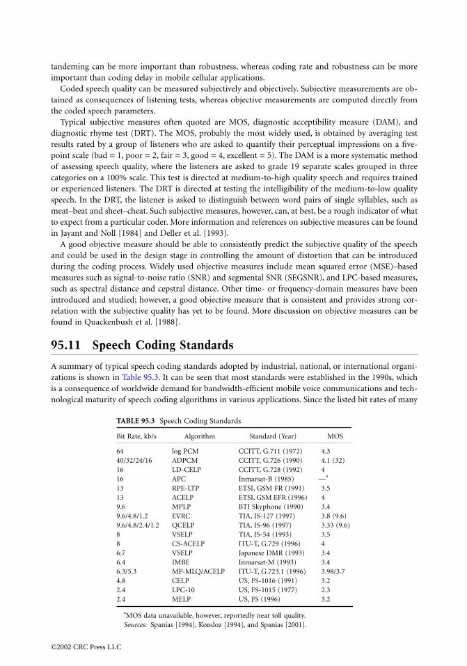
tandeming can be more important than robustness, whereas coding rate and robustness can be moreimportant than coding delay in mobile cellular applications.

Coded speech quality can be measured subjectively and objectively. Subjective measurements are ob-tained as consequences of listening tests, whereas objective measurements are computed directly fromthe coded speech parameters.

Typical subjective measures often quoted are MOS, diagnostic acceptibility measure (DAM), anddiagnostic rhyme test (DRT). The MOS, probably the most widely used, is obtained by averaging testresults rated by a group of listeners who are asked to quantify their perceptual impressions on a five-point scale (bad = 1, poor = 2, fair = 3, good = 4, excellent = 5). The DAM is a more systematic methodof assessing speech quality, where the listeners are asked to grade 19 separate scales grouped in threecategories on a 100% scale. This test is directed at medium-to-high quality speech and requires trainedor experienced listeners. The DRT is directed at testing the intelligibility of the medium-to-low qualityspeech. In the DRT, the listener is asked to distinguish between word pairs of single syllables, such asmeat–beat and sheet–cheat. Such subjective measures, however, can, at best, be a rough indicator of whatto expect from a particular coder. More information and references on subjective measures can be foundin Jayant and Noll [1984] and Deller et al. [1993].

A good objective measure should be able to consistently predict the subjective quality of the speechand could be used in the design stage in controlling the amount of distortion that can be introducedduring the coding process. Widely used objective measures include mean squared error (MSE)–basedmeasures such as signal-to-noise ratio (SNR) and segmental SNR (SEGSNR), and LPC-based measures,such as spectral distance and cepstral distance. Other time- or frequency-domain measures have beenintroduced and studied; however, a good objective measure that is consistent and provides strong cor-relation with the subjective quality has yet to be found. More discussion on objective measures can befound in Quackenbush et al. [1988].

95.11 Speech Coding Standards

A summary of typical speech coding standards adopted by industrial, national, or international organi-zations is shown in Table 95.3. It can be seen that most standards were established in the 1990s, whichis a consequence of worldwide demand for bandwidth-efficient mobile voice communications and tech-nological maturity of speech coding algorithms in various applications. Since the listed bit rates of many

TABLE 95.3 Speech Coding Standards

Bit Rate, kb/s Algorithm Standard (Year) MOS

64 log PCM CCITT, G.711 (1972) 4.340/32/24/16 ADPCM CCITT, G.726 (1990) 4.1 (32)16 LD-CELP CCITT, G.728 (1992) 416 APC Inmarsat-B (1985) —a

13 RPE-LTP ETSI, GSM FR (1991) 3.513 ACELP ETSI, GSM EFR (1996) 49.6 MPLP BTI Skyphone (1990) 3.49.6/4.8/1.2 EVRC TIA, IS-127 (1997) 3.8 (9.6)9.6/4.8/2.4/1.2 QCELP TIA, IS-96 (1997) 3.33 (9.6)8 VSELP TIA, IS-54 (1993) 3.58 CS-ACELP ITU-T, G.729 (1996) 46.7 VSELP Japanese DMR (1993) 3.46.4 IMBE Inmarsat-M (1993) 3.46.3/5.3 MP-MLQ/ACELP ITU-T, G.723.1 (1996) 3.98/3.74.8 CELP US, FS-1016 (1991) 3.22.4 LPC-10 US, FS-1015 (1977) 2.32.4 MELP US, FS (1996) 3.2

aMOS data unavailable, however, reportedly near toll quality.Sources: Spanias [1994], Kondoz [1994], and Spanias [2001].


coders in Table 95.3 include error control bits, actual source coding rates of such coders are smaller thanthose listed. Coders with MOS ratings of close to or more than 4 can be considered to provide toll quality,whereas the rest provide near-toll or communications quality except for the LPC-10.


Principles and applications of typical coding algorithms for telephone speech have been reviewed in thischapter. Major research efforts in the last decade have concentrated on the analysis-by-synthesis tech-nique in the bit range of 4–16 kb/s, and some of the results have turned into standards in cellular andmobile voice communications. Important advances can be typified by the standardization of CELPcoders in the range of 4.8–16 kb/s and emergence of the sinusoidal vocoding approach (STC, MBE) andMELP in the 2.4–4.8 kb/s range.

Major research efforts in the future are expected to be concentrated on low bit range coding, say4 kb/s or below, where perceptual factors of the human auditory system become more important[Jayant, 1992]. Continued activities for enhanced coder performance are also expected in the range of4–8 kb/s for specific applications. In a practical aspect, speech coding algorithms to be included in thenext generation of mobile communication systems will be a major issue for the next few years.

Defining Terms

Analysis-and-synthesis: Refers to open-loop operation where the analysis cannot be affected or changedby the synthesis.

Analysis-by-synthesis: Refers to closed-loop operation where the analysis can be affected or changedby the synthesis.

Hybrid coders: Coders that employ features of both waveform coders and vocoders.Mixed excitation: A speech segment is modeled as a consequence of both voiced and unvoiced excitation.Vocoders: Coders that are primarily aimed at reproducing the original sound.Waveform coders: Coders that are primarily aimed at reproducing the original time-domain waveform.

References

Atal, B.S., Cuperman, V., and Gersho, A., Eds. 1991. Advances in Speech Coding, Kluwer, Dordrecht, theNetherlands.

Deller, J.R. Jr., Proakis, J.G., and Hansen, J.H.L. 1993. Discrete-Time Processing of Speech Signals,Macmillan, New York.

Gersho, A. 1994. Advances in speech and audio compression. Proc. IEEE, 82(6):900–918.Gibson, J.D. 1980. Adaptive prediction in speech differential encoding systems. Proc. IEEE, (April):488–525.Gibson, J.D. 1984. Adaptive prediction for speech encoding. ASSP Mag., 1: 12–26.Jayant, N.S. 1992. Signal compression: technology targets and research directions. IEEE Trans. Selec. Areas

Commun., 10(5):796–818.Jayant, N.S. and Noll, P. 1984. Digital Coding of Waveforms: Principles and Applications to Speech and

Video, Prentice–Hall, Englewood Cliffs, NJ.Kondoz, A.M. 1994. Digital Speech: Coding for Low Bit Rate Communications Systems, Wiley, Chichester,

England.Makhoul, J., Roucos, S., and Gish, H. 1985. Vector quantization in speech coding. Proc. IEEE, 73(11):

1551–1588.McCree, A.V., George, E. B., Barnwell, T., and Viswanathan, V. R. 1996. A 2.4 kbit/s MELP coder candidate

for the new U.S. federal standard. In Proc. ICASSP.Quackenbush, S.R., Barnwell, T.P., and Clements, M.A. 1988. Objective Measures of Speech Quality,

Prentice–Hall, Englewood Cliffs, NJ.


Rabiner, L.R. and Schafer, R.W. 1978. Digital Processing of Speech Signals, Prentice–Hall, Englewood Cliffs,NJ.

Schroeder, M.R. and Atal, B.S. 1985. Code-excited linear prediction (CELP): high quality speech at verylow bit rates. In Proc. ICASSP, Tampa, FL, April, 937–940.

Spanias, A.S. 1994. Speech coding: a tutorial review. Proc. IEEE, 82(10):1541–1582.Spanias, A.S. 2001. Speech coding standards. In Multimedia Communications: Directions and Innovations,

Gibson, J.D., Ed., Academic Press, New York.

Further Information

A comprehensive tutorial can be found in Spanias [1994]. Speech coding standards and references arewell summarized in Spanias [2001]. Journals specialized in speech coding are IEEE Transactions on Speechand Audio Processing (since 1993), IEEE Transactions on Signal Processing (1991–1993), IEEE Transactionson Acoustics, Speech and Signal Processing (1974–1990), and IEEE Transactions on Communications. Themost recent activities can be found in the annual Proceedings of the International Conference onAcoustics, Speech, and Signal Processing (ICASSP).


96Video

96.1 Introduction96.2 Source Characteristics and Viewer Requirements96.3 Coding Algorithms

Motion Compensation • Predictive Coding • Interpolative Coding • Residual Coding • Buffer Control • Pyramidal Coding

96.4 Standards 96.5 Perspectives

96.1 Introduction

Time-varying imagery is a highly effective medium in a variety of applications including entertainment,interpersonal communication, information presentation and retrieval, and many others. We refer to atime-varying image signal in electronic form as a video signal. Until recently, video signals were storedand transmitted exclusively in analog form, and this continues to be the most common situation. Theprincipal storage medium is analog video tape, and the main transmission channels are the over-the-airbroadcast channel, cable, and satellite. However, due to recent advances in digital hardware and in imagecompression technology, systems for digital storage and transmission of video signals are becoming morecommon. It can be expected that digital representations of video will be predominant in the future. Videowill be stored in digital form on disks and tape, and will be transmitted digitally over broadband networksas well as wireless networks and broadcast channels.

Video signals are notorious for consuming huge amounts of bandwidth. For example, an analog NationalTelevision System Committee (NTSC) video signal uses a 6-MHz bandwidth, whereas an uncompresseddigital NTSC video signal requires a bit rate of about 100 Mb/s. To allow economical storage and/or trans-mission, more efficient representations are required. This process is often viewed as a compression operation,wherein quality is sacrificed; an alternative view is that we seek a representation that will deliver maximumvideo quality for a given available data rate. At rates of 20–30 Mb/s, this would yield large images of highquality [high-definition television (HDTV)], whereas at low rates such as 64 kb/s and below, this wouldresult in a system providing small pictures of rather low quality and with limited capability to render motion(videophone).

The techniques of source coding seek to exploit both redundancy in the source and the fidelity require-ments of the receiver of the information in order to minimize distortion for a given data rate. If a stochasticmodel of the source and a fidelity criterion for the receiver are known, the optimal performance can befound using rate-distortion theory. However, an implementable coder with acceptable delay giving thisoptimal performance may not be available. In the case of time-varying imagery, neither general purposestochastic models of the source nor mathematical fidelity criteria that capture all of the known propertiesof source and receiver are known at this time. Thus, optimal source coding for time-varying imagery doesnot currently rest on a firm theoretical basis. Rather, we have available an arsenal of tools that work welland that address, at least qualitatively, the known properties of the source and receiver.

Eric DuboisUniversity of Ottawa


The purpose of this chapter is to identify the properties of source and receiver that are exploited byvideo source coding algorithms and to describe the tools that are available for source coding. The em-phasis is on those aspects that are specific to time-varying imagery, since a previous chapter deals withstill imagery. Thus, the use of motion information in the processing and compression of time-varyingimagery is a pivotal element for this contribution. An overview of video compression standards is alsogiven, followed by some perspectives for the future. An extensive treatment of video coding can be foundin Netravali and Haskell [1995].

96.2 Source Characteristics and Viewer Requirements

A number of factors determine the source characteristics and the level of redundancy that can beexploited. These include the scanning format, the signal-to-noise ratio, the amount of detail, and thecharacteristics of the motion. Note that the source signal to be coded may not necessarily be the directoutput of a video camera; it may be the result of some scan conversion or other preprocessing operations.

The scanning format encompasses the picture size and the sampling structure. We assume that theinput to the source coder is fully digital, that is, an ordered sequence of fixed length binary codewordsrepresenting the image color at a discrete set of points Ψ. This is denoted

(96.1)

where u1, u2, u3 represent coordinates in a suitable color space. These could be red–green–blue orluminance-chrominance components. Clearly, black and white images would be represented by a singlecomponent. The sampling structure Ψ is a regular array of points such as a lattice, cropped spatially tothe image frame size. Picture size may range from small windows on a videophone or workstation, say,of size 64 by 64, to HDTV pictures of size 1920 by 1080 and beyond. Two vertical-temporal scanningstructures are widely used for video: progressive scanning and interlaced scanning. These scanningstructures are shown in vertical-temporal profile in Fig. 96.1. In analog systems, where the capture,transmission, and display formats are the same, interlace is a method to achieve higher vertical resolutionfor a given vertical scan rate and system bandwidth. The vertical scan rate of 50 or 60 Hz used in majorworldwide systems is largely determined by the requirement to minimize the visibility of flicker at thedisplay. Although interlace is a good technique in the context of analog systems, it usually leads tospatiotemporal aliasing in the presence of vertical motion, which makes subsequent processing, andespecially source coding, much more difficult. (See Dubois [1992] for a discussion.) For this reason, therehas been increasing focus on progressive scanning in recent system proposals. A detailed discussion ofsampling structures and video signal sampling is given in Dubois [1985].

FIGURE 96.1 Profile view of scanning structures: (a) progressive and (b) interlace.

ui x, y, t( ), x, y, t( ) Ψi, i 1, 2, 3=∈


Although some standards allow considerable flexibility in the choice of picture format, a number ofspecific formats are in common use or have been proposed. Table 96.1 shows the parameters of some ofthese formats. The final coded bit rate is very directly related to the source sampling rate, although notlinearly.

The signal-to-noise ratio of the source has a significant impact on compression efficiency. In general,noise has little redundancy and cannot be compressed very much; thus, it should be removed prior tocoding if possible. There is, of course, a trade-off between coding efficiency and the introduction ofartifacts due to noise reduction. Valid assumptions must be made or the processing may remove desiredpicture content such as snowstorms, fireworks, etc. Motion compensated processing is required for themost effective noise reduction [Dubois, 1992]. However, good image and noise models are necessary.The principle is to filter out those deviations from an assumed image model (e.g., that image intensityis constant along trajectories of motion) that match the characteristics of an assumed noise model (e.g.,white noise with a specified variance).

The characteristics of the motion in the scene affect the amount of compression that is possible.Apparent motion in the image can be due to either camera motion (including zooming), object motion,or both. In a videophone application, most apparent motion may be due to movement of the person infront of the camera. In a surveillance application, most of it may be due to the scanning motion of thecamera (except during an incident), whereas in a sports scene, both camera motion and scene motionmay be significant. Motion may, in general, be low, as in a videophone application, or very active, as ina sports application; it may be highly structured (rigid-body motion) or pseudorandom (rustling leaves).Knowledge of the motion characteristics can affect the coding algorithm; if there is unrestricted motion,a worst-case assumption must be made.

Redundancy in a source is related to the concept of predictability (although they are not the same).Given that a certain portion of the source signal has already been transmitted, the coder may attempt topredict what comes next. If the prediction is at all reliable, it is better to transmit information concerningthe deviation from the prediction than the raw information. Predictability implies a certain regularityin the data that can be captured in statistical models. In the spatial dimension, if a certain pattern appearsover a certain area, one may assume that the pattern will continue and make the prediction on this basis.Of course, at an object boundary, the prediction will be wrong. However, if it is right most of the time,an overall coding gain can be achieved. In a moving picture, the assumption is that if an object is movingwith a certain velocity and acceleration, it will continue to do so. Thus, if the velocity and acceleration areknown, the coder can predict what the next frame will look like and only transmit the error between thisprediction and reality. This is the essence of motion-compensated coding. Again, at a scene change, theprediction will be completely wrong, and more information must be transmitted. However, on average,there will be a substantial compression. Temporal change is not due solely to motion. The illumination maychange, and the luminance of scene points may change as the angles between object surface, illuminationsource, and camera change. If we can model these effects as well, we can make better predictions and therebyimprove coding performance.

In addition to the structural or statistical redundancy in the source, there is perceptual redundancy(also called irrelevancy). Specifically, information that cannot be perceived by the viewer need not betransmitted. The main phenomena related to this are spatial and temporal masking. Spatial masking is

TABLE 96.1 Typical Scanning Formats Used for Digital Video Communications

Luminance Size Chrominance Size Scanning Structure

Identifier Hor. Vert. Hor. Vert. Interlace Pict. Rate

QCIF 176 144 88 72 1:1 29.97CIF 352 288 176 144 1:1 29.97ITU-R 601 720 480 360 480 2:1 59.94HDTV-P 1280 720 640 360 1:1 60.0HDTV-I 1920 1080 960 540 2:1 60.0


the effect whereby certain types of distortion are less visible in the vicinity of high-contrast image detailthan in flat low-contrast areas. Temporal masking is the effect where distortions are less visible in areasof the image that are newly exposed or contain fast motion. An important case here is the scene change.The viewer can tolerate a significant reduction in resolution just after a scene change. This is fortuitous,because this is exactly where the temporal motion-compensated prediction breaks down.

The goal of an efficient source coder is to maximize quality (or minimize distortion) subject to anumber of constraints. In most applications of video compression, the quality or distortion are subjectivemeasures determined by the visual properties of the viewer. However, if further signal processing ormanipulation of the image sequence is to be performed, a more stringent objective criterion may be moreappropriate, since impairments invisible to a viewer could have a negative effect on a signal processingoperation such as chroma key. If subjective quality is the main concern, it would be very desirable to havea mathematical function that measures the subjective distortion. This distortion function could then beminimized during the optimization of the coding algorithm. Unfortunately, such a general purpose andwidely accepted perceptual distortion measure is not available. Thus, properties of the human visual systemare usually ex-ploited based on qualitative or empirical considerations that are obtained under restrictedconditions. However, this approach may still be quite effective [Schreiber, 1993; Jayant et al., 1993]. Thecoding algorithm can then be evaluated using formal subjective testing under controlled conditions[Allnutt, 1983].

Other requirements may affect the type of coding algorithm that can be used. These include delay,random access, playback control, and scalability. Both the coding algorithm and the transmission channelintroduce delay. Depending on the application, there may be tight bounds on this delay, especially in inter-active applications. The most stringent application is in face-to-face communication, where a maximumend-to-end delay of about 200 ms can be tolerated. If the delay is longer than this, spontaneous interactionbecomes difficult. In a database access application, somewhat longer delays of up to a few seconds may beacceptable. Finally, in an application such as video on demand, the delay constraint may be of no practicalconsequence, that is, any reasonable encoding system would meet the delay constraint.

Random access and playback control are requirements that may exist in services such as database accessand video on demand. Some coding schemes are recursive in nature and require that the sequence be de-coded continuously from the beginning in order to view a particular frame. This may be acceptable in anapplication such as video conferencing, but it precludes random access and channel switching. Thus, theencoding algorithm must have finite memory in some sense to allow such a random access feature. Theplayback controls include fast-forward, reverse, and fast-reverse playback as well as pause functions. Again,general coding algorithms may not permit such features, and they must be incorporated as constraints ifthey are desired.

The coding algorithm must account for the properties of the channel or storage medium. The channelmay allow only constant bit rate (CBR) operation, or it may permit variable bit rate (VBR) operation.In the former case, the coder must be designed to produce a fixed number of bits over a specified unitof time. In the latter case, the bit rate may vary over time, although some constraints negotiated at setuptime must be respected (e.g., ratio of peak to average bit rate). Another requirement of a coding algorithmis acceptable performance in the presence of typical channel impairments. These channel impairmentsmay vary considerably for different types of channels. For example, a dedicated digital link may haverandom errors with a very low probability of occurrence, whereas a wireless link may have bursty errorswith a high probability of occurrence. Also, depending on the transport mechanism, the errors may occurin isolated bits, or they may involve an entire packet consisting of a large number of bits. In general,when the coding efficiency for redundancy reduction is higher, the coded data is more vulnerable totransmission errors. Thus, overall system performance must be evaluated with the channel impairmentstaken into account in order to be realistic. If possible, joint source/channel coding should be considered.

In some situations, the same video signal must be delivered to a variety of receivers having differentcapabilities. Some examples include the broadcast of entertainment television to a population of receiv-ers ranging from small tabletop units to large high-definition displays. Similarly, a database containingvideo data might be accessed by terminals ranging from relatively inexpensive home computers to


powerful workstations, perhaps with three-dimensional display. The capability to transmit only thatportion of the data required by the terminal, or to extract a subset of the data, is known as scalability.The most straightforward approach to this is simulcasting or multiple storage of the coded data for eachtype of receiver. This is complex and wasteful of storage or transmission capacity. Thus, a more efficientapproach is the concept of embedded coding, whereby a subset of the encoded data can be used to decodea lower version of the sequence suitable for display on the lower capability display.

Most of the preceding requirements can reduce the coding efficiency achievable, as compared to anunconstrained situation. In each case, the system designer must decide whether the benefits of the featurejustify the additional complexity or performance loss.

96.3 Coding Algorithms

The goal of a source coding algorithm is usually to provide the best image quality for a given channel or datarate, subject to constraints on complexity, delay, or other requirements, as discussed. In some circumstances,a certain quality may be prescribed, and a coding algorithm is sought that provides this quality at the lowestpossible rate (again, subject to constraints). In time-varying imagery, most incremental information overtime is carried by the motion occurring in the scene. Thus, the most highly efficient coding algorithms arebased on motion estimation and compensation. This is the main feature distinguishing video coding fromstill image coding, and it represents the focus of this section. An image sequence is usually encoded by bothintraframe coding techniques and interframe coding techniques. The intraframe coding algorithms are verysimilar to the still picture coding algorithms. They are used for several reasons, including: to permit randomaccess into the sequence, to allow fast forward and reverse playback, to provide robustness to channel errors,and as fallback when temporal coding fails (for example, at a scene change).

Motion Compensation

The three-dimensional motion of objects in a scene induces two-dimensional motion in the image plane.The relationship between them depends on the perspective transformation of the camera and may becomplex. The image of a given scene point traces out over time a trajectory in the space–time coordinatesof the time-varying image (Fig. 96.2). The basic principle of motion-compensated coding is that the

FIGURE 96.2 Trajectory in space time of a scene point.


redundancy is very high along this trajectory. This is exploited using the coder structure of Fig. 96.3. Theinput signal is applied to a motion estimation module that determines a motion field. This motion fieldestablishes the correspondences between image samples lying on the same trajectory in successive imagepictures. Although the motion field specifies estimated displacements for each pixel in the image sequence,it may be specified parametrically over regions, as will be described subsequently. The motion field isthen encoded with a lossless code for transmission to the receiver at rate RM. Any quantization of themotion field is assumed to take place within the motion estimation module. The motion field is alsosupplied to the motion-compensated coding module, which performs a conditional coding of the imagesequence given the estimated and quantized motion field. The output of this module (which includesany lossless coding) is transmitted to the receiver at rate RI. It is possible for the motion estimator toalso make use of previously coded/decoded data. This can be accommodated (conceptually) by thestructure of Fig. 96.3 by assuming that the motion estimation module contains a copy of the motion-compensated coder. Of course, the motion-compensated coder would not be duplicated in a practicalimplementation; common elements would be shared between the motion estimation and motion-compensated coding modules.

The total rate R for coding the video sequence is the sum of RM, the rate to transmit the motioninformation, and RI, the rate to transmit the conditionally coded video information. The best way topartition the overall rate between these two components is an open problem. A greater precision in themotion field may lead to a lower rate RI for the motion-compensated video but a higher rate RM for themotion information. The optimal point will depend on the motion coding scheme and the motion-compensated video coding scheme. An extreme situation is when RM = 0, where either no motioninformation is used, or motion is only computed from previously encoded video data. At the otherextreme, we can imagine a situation where the motion field is coded very precisely, so that RI << RM.

There are two basic approaches for estimating the motion field: the pixel-based approach and the para-metric approach. In the pixel-based approach, a displacement vector is estimated for each pixel in the pictureusing some robust algorithm. The resulting motion field is then encoded efficiently to achieve the desiredrate. Significant compression is possible since the motion field is, in general, highly redundant (it is verysmooth except at object boundaries). The decoded motion field is used in the motion-compensated coder.The parametric approach is more common in video coding, where the motion field is represented para-metrically over image regions. The most common technique is to assume a constant displacement over arectangular block of pixels. Higher order models such as the affine model have also been used. A moregeneral approach is to assume that the motion is represented parametrically over nonrectangular regions.In this case, the specification of region boundaries is part of the motion representation. There are manyalgorithms to actually estimate the motion, including region matching, gradient-based optimization, andtransform domain methods. See Mitiche and Bouthemy [1996] for a survey.

FIGURE 96.3 General structure of a motion-compensated video coder.


The two main techniques to perform conditional coding given motion, predictive coding and inter-polative coding, are discussed in the next two sections.

Predictive Coding

The principle of predictive coding is that, given the motion information and previous decoded pictures,it is possible to form a good estimate of the next picture to be coded. Then, only the deviation from thisestimate needs to be encoded and transmitted. A structure well suited to this is differential pulse codemodulation (DPCM), shown in Fig. 96.4. In this system, the prediction is formed on the basis of previouslyreconstructed pictures using a local decoder at the transmitter. The prediction error is then spatiallyquantized and losslessly encoded at a variable rate for transmission. The types of spatial quantizationused are discussed in the section on residual coding.

In the basic mode of operation, the image information at time t is predicted from the suitably displacedinformation in the previous vertical scan at time t - T, where T is the vertical scan time. The predictionof the sampled input image u(x, y, t) is given by

(96.2)

where (dx (x, y, t), dy(x, y, t)) is the estimated displacement at (x, y, t) and is the locally reconstructedoutput of the codec. If (x - dx, y - dy , t - T) does not lie on the sampling grid, spatial interpolationmust be used to compute u from existing samples of at time t - T. If the video signal is in interlacedformat, each vertical scan of the image contains only part of the spatial information. Thus, a moreelaborate prediction using at least the two previous pictures is very advantageous, as used in movingpictures experts group-2 (MPEG-2) standards [ISO/IEC, 1994].

A disadvantage of predictive coding is that the quantization error of the residual encoder is fed backto the predictor. This limits the compression efficiency, even if the source is very highly correlatedalong motion trajectories. One way to counteract this effect is to use interpolative coding for somepictures.

FIGURE 96.4 Motion-compensated DPCM encoder.

û x, y, t( ) ũ x dx x, y, t( ), y dy x, y, t( ), t T–––( )=

ũ

ũ


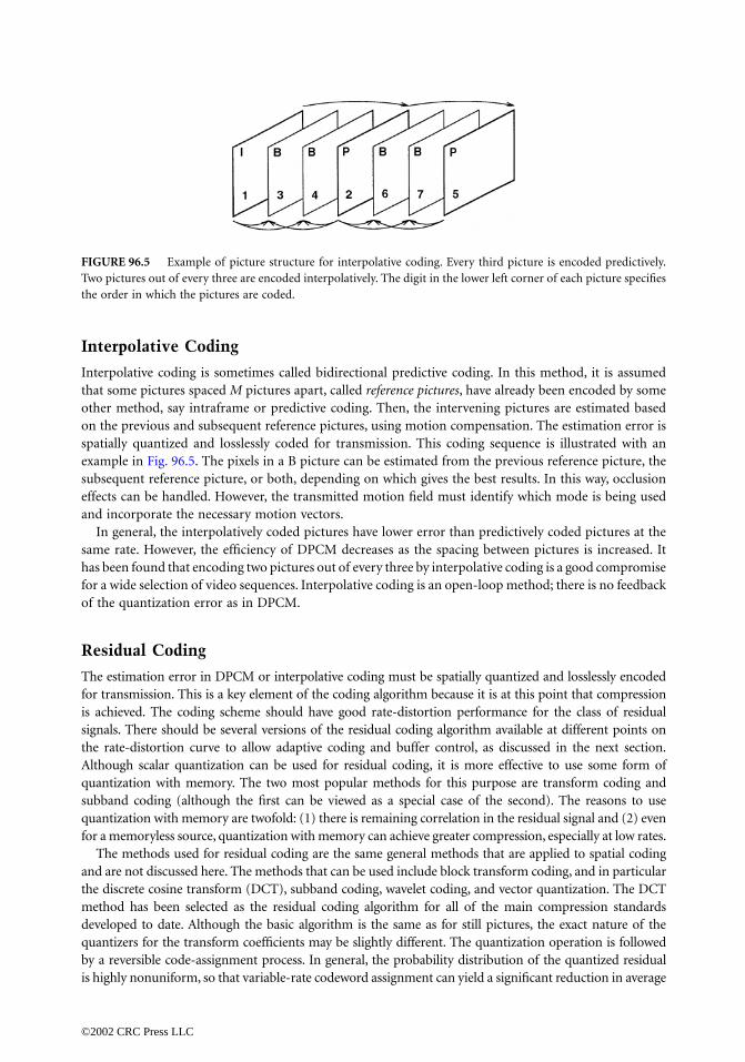
Interpolative Coding

Interpolative coding is sometimes called bidirectional predictive coding. In this method, it is assumedthat some pictures spaced M pictures apart, called reference pictures, have already been encoded by someother method, say intraframe or predictive coding. Then, the intervening pictures are estimated basedon the previous and subsequent reference pictures, using motion compensation. The estimation error isspatially quantized and losslessly coded for transmission. This coding sequence is illustrated with anexample in Fig. 96.5. The pixels in a B picture can be estimated from the previous reference picture, thesubsequent reference picture, or both, depending on which gives the best results. In this way, occlusioneffects can be handled. However, the transmitted motion field must identify which mode is being usedand incorporate the necessary motion vectors.

In general, the interpolatively coded pictures have lower error than predictively coded pictures at thesame rate. However, the efficiency of DPCM decreases as the spacing between pictures is increased. Ithas been found that encoding two pictures out of every three by interpolative coding is a good compromisefor a wide selection of video sequences. Interpolative coding is an open-loop method; there is no feedbackof the quantization error as in DPCM.

Residual Coding

The estimation error in DPCM or interpolative coding must be spatially quantized and losslessly encodedfor transmission. This is a key element of the coding algorithm because it is at this point that compressionis achieved. The coding scheme should have good rate-distortion performance for the class of residualsignals. There should be several versions of the residual coding algorithm available at different points onthe rate-distortion curve to allow adaptive coding and buffer control, as discussed in the next section.Although scalar quantization can be used for residual coding, it is more effective to use some form ofquantization with memory. The two most popular methods for this purpose are transform coding andsubband coding (although the first can be viewed as a special case of the second). The reasons to usequantization with memory are twofold: (1) there is remaining correlation in the residual signal and (2) evenfor a memoryless source, quantization with memory can achieve greater compression, especially at low rates.

The methods used for residual coding are the same general methods that are applied to spatial codingand are not discussed here. The methods that can be used include block transform coding, and in particularthe discrete cosine transform (DCT), subband coding, wavelet coding, and vector quantization. The DCTmethod has been selected as the residual coding algorithm for all of the main compression standardsdeveloped to date. Although the basic algorithm is the same as for still pictures, the exact nature of thequantizers for the transform coefficients may be slightly different. The quantization operation is followedby a reversible code-assignment process. In general, the probability distribution of the quantized residualis highly nonuniform, so that variable-rate codeword assignment can yield a significant reduction in average

FIGURE 96.5 Example of picture structure for interpolative coding. Every third picture is encoded predictively.Two pictures out of every three are encoded interpolatively. The digit in the lower left corner of each picture specifiesthe order in which the pictures are coded.


bit rate compared with fixed codeword length assignment. The methods that have been found effectiveinclude Huffman coding, run length coding, and arithmetic coding. These techniques are discussed inprevious chapters. Because of the additional variability in residual statistics due to changing motion, thebit rate process can have significantly more variability in interframe coding than in spatial coding.

Buffer Control

The video coding algorithms described in preceding sections are characterized by a number of parameters,such as the quantizer scale factors, the input sampling structure, prefilter characteristics, etc. These param-eters establish the rate and quality at which the coder operates. However, because of the time-varying natureof the video signal characteristics and the use of variable length codes, the short-term rate and qualitychange with time for a fixed set of parameter values. The rate can also vary as the coding mode changes,for example, the rate in intrapicture mode will be considerably higher than the rate in interpolative mode.

The transmission channel can be either a CBR link or a VBR link. In the former case, the variable ratedata emitted by the coder must be smoothed out by a rate buffer (as in Fig. 96.4) to deliver data to thechannel at a fixed constant rate. Because of constraints on delay and complexity, the buffer size is limited.As a result, there is a significant probability of buffer overflow or underflow. A control mechanism isrequired to adapt the coder parameters in order avoid buffer overflow while maintaining the highest andmost uniform image quality possible. Even for a VBR channel, there will be constraints on the coderoutput bit rate process that must be satisfied, so that a rate buffer and control algorithm are still required.

The control algorithm periodically monitors the rate buffer occupancy and changes the coder param-eters to avoid potential overflow or underflow in such a way as to give the best overall image quality.Large or overly frequent parameter changes causing uneven quality should be avoided. Most techniquesfor buffer control have been heuristically derived. The occupancy of the rate buffer is used to determinethe coding parameters (often only one, a scale factor for the DCT coefficient quantizers). At prespecifiedtime intervals, the buffer fullness is evaluated, and, if it crosses certain thresholds in a given direction, thecoding parameters are changed in a way to counteract the change in buffer occupancy. For example, ifthe buffer level is increasing, the quantization in the coder can be made coarser in order to reduce thenumber of bits being put into the buffer. The choices of coding modes and buffer switch points are madeheuristically. More sophisticated techniques attempt to formulate a cost function that measures perfor-mance of the buffer control algorithm and to use the history of the buffer occupancy and the statisticsof the bit rate process in different coding modes to choose an optimal parameter adaptation strategy.See Zdepski, Raychaudhuri, and Joseph [1992] and Leduc [1994] for recent work.

Pyramidal Coding

Pyramidal coding is a method that can be used to perform embedded coding for scalable videoapplications [Girod, 1993]. It is capable of producing coded versions of a given video sequence atdifferent levels of spatial, temporal, and amplitude resolution. The general structure of a pyramidalcoder is shown in Fig. 96.6. The input is first coded at the lowest supported rate R1 by the level 1 coder.The resulting bit stream can be decoded by any decoder supported by the service. This level 1 sequencewould be at the lowest spatial, temporal, and amplitude resolution, whereas the input would have fullspatial, temporal, and amplitude resolution. Thus, the level 1 coder would need to incorporate appro-priate spatial and/or temporal downsampling. To obtain the next highest level in the hierarchy, the level1 signal is locally decoded and used as a priori information in the conditional coding of the input. Theincremental information is coded at a rate R2, and together with the level 1 bit stream specifies the level2 output. This process is repeated for as many levels as are desired. Conditional coding is usually achievedby interpolating a lower level signal to the same spatial and temporal resolution as the next level. Thisis then used to form a prediction of this higher level signal; the residual is then further coded fortransmission.


96.4 Standards

Standards play a major role in ensuring the wide availability of image communication products thatpermit interoperability between equipment provided by different manufacturers. The first importantstandard for compressed video was the International Telecommunications Union–TelecommunicationsStandardization Sector (ITU-T) [formerly the Consultative Committee on International Telephony andTelegraphy (CCITT)] H.261 standard for videoconferencing. This was followed by the InternationalStandards Organization (ISO)/IEC MPEG 1 and 2 standards. These standards are summarized inTable 96.2. A brief description of each follows. A more detailed overview of these standards is given inAravind et al. [1993].

The ITU-T Recommendation H.261 specifies the video codec system as part of a group of standardsfor audiovisual telecommunication services [ITU-T, 1990]. In 1984, CCITT Study Group XV establisheda specialist group on coding for visual telephony, and the recommendation was completed and approvedin December 1990. This transmission standard was developed for use in videophone and videoconfer-encing applications. The standard specifies bit rates of the form p × 64 kb/s, where p is an integer between1 and 30. The standard defines only the functionality of the decoder; the encoder is not explicitly defined,but it must produce a bit stream compatible with the standard decoder. The input signals are in QCIFor CIF format (Table 96.1). The coding algorithm uses motion-compensated temporal DPCM with DCTcoding of the residual. The motion compensation is block oriented, with a single motion vector for each16 × 16 block of luminance pixels (referred to as a macroblock). The DCT is applied to 8 × 8 blocks ofthe residual signal. To meet the strict delay requirements, the prediction is always based on the imme-diately preceding picture. It is possible to set the temporal prediction to zero, so that the residual is equalto the input signal (interframe coding mode), or to force the motion vector to be zero (interframe codingwithout motion compensation). The bit stream has a layered structure, with layers for the picture, groupof blocks (defined as 3 × 11 macroblocks), macroblock, and block. The top three layers consist of a

FIGURE 96.6 Pyramidal coder for embedded scalable video coding.


header containing synchronization information, parameter values, and user defined bits, followed by anumber of units of the next lower layer. The lowest layer (block) simply contains encoded transformcoefficients and an end-of-block (EOB) code. The coder designer must decide how to regulate theparameters to optimize quality, avoid buffer overflow or underflow, and meet certain constraints imposedby a hypothetical reference decoder (HRD).

MPEG, under the ISO-IEC/JTC1/SC29/WG11, undertook, in 1988, the development of a standard forvideo coding adapted to rates of about 1–1.5 Mb/s and suitable for digital storage media. The strict delayrequirement of H.261 was relaxed, whereas additional features such as random access, fast forward/reverse, etc., were desired. This standard, referred to as MPEG-1, has now been approved as an interna-tional standard [ISO/IEC, 1993]. It builds considerably on the H.261 standard and has much common-ality. It supports a wider range of input signal formats, although the input sequences are assumed to beprogressively scanned. The basic techniques of motion-compensated temporal DPCM and DCT codingof the residual are maintained from H.261. However, the technique of interpolative coding has beenadded. The concepts of layers used in H.261 has been augmented with the sequence layer and the groupof pictures layer. The group of pictures layer is the unit allowing random access into the sequence. Thegroup of blocks layer is replaced with a more flexible slice layer. The macroblock and block layers are similarto H.261. The bit stream is characterized at the sequence layer by a bit rate and buffer size. The MPEGstandard establishes constraints on the bit stream to ensure that decoding will occur without buffer over-flow for the given buffer size. See Le Gall [1992] for a more detailed overview of the MPEG algorithm.

In the second phase of MPEG, the algorithms have been extended to work with interlaced sequencesand to integrate various forms of scalability [ISO/IEC, 1994]. It is considered for application to interlacedvideo such as the studio standard of ITU-R Recommendation 601 or HDTV. It extends the bit rate rangeof MPEG-1 up to about 20 Mb/s in currently studied implementations. MPEG-2 has introduced theconcept of profiles and levels. A profile is a collection of signal processing tools (i.e., subset of the globalsyntax), whereas a level is related to the processing complexity and defines constraints on parameter values.

96.5 Perspectives

The video coding techniques described in the previous sections are well understood and will form thebasis for many video services in the coming years. However, they do not approach fundamental limitsof compression performance. Standards activity is currently addressing high-compression video codingunder the phase 4 of MPEG. Techniques such as analysis-by-synthesis, object-oriented coding, andpossibly even fractal coding will be brought to bear on the problem.

Defining Terms

Aliasing: An artifact caused by sampling a continuous signal with too low a sampling rate.Interlaced scanning: A video scanning structure where the vertical position of horizontal scan lines in

a given pass through the image is midway between the position of adjacent lines in the previouspass through the image.

Interpolative coding: A compression technique in which the coded signal is given by the quantizeddifference between the input signal and an estimation based on previously transmitted informationoccurring before and after the current input in time.

Masking: Reduction of the visibility of distortion by the image content.

TABLE 96.2 Standards for Compressed Video

Name Identifier Application Typical Bit Rates

p × 64 ITU-T Rec. H.261 Teleconferencing 64 kbit/s–1.92 Mbit/sMPEG-1 ISO/IEC 11172-2 Digital storage media 1.0–1.5 Mbit/sMPEG-2 ISO/IEC 13818-2 Broad range 1.5–20 Mbit/s


Motion field: A vector field that determines the correspondences between image samples lying on thesame trajectory in successive image pictures.

Predictive coding: A compression technique in which the coded signal is given by the quantized errorbetween the input signal and a prediction based on previously transmitted information that occursearlier in time.

Progressive scanning: A video scanning structure consisting of horizontal scan lines that lie in thesame vertical position on each pass through the image.

Rate buffer: A first-in–first-out buffer memory that accepts the coded data from the codec at a variablerate and emits it to the channel at a fixed rate (or possibly at a variable rate but with smallervariability).

Scalability: The capability to easily derive multiple versions of the input signal at different spatial,temporal, and amplitude resolutions from the same coded data.

Video signal: A time-varying image signal in electronic form.

References

Allnutt, J. 1983. Transmitted-Picture Assessment, Wiley, Chichester, U.K.Aravind, R., Cash, G.L., Duttweiler, D.L., Hang, H.M., Haskell, B.G., and Puri, A. 1993. Image and video

coding standards. AT&T Tech. J., 72(l):67–89.Dubois, E. 1985. The sampling and reconstruction of time-varying imagery with application in video

systems. Proc. IEEE, 73(4):502–522.Dubois, E. 1992. Motion-compensated filtering of time-varying images, Multidimensional Sys. Signal Proc.,

3:211–239.Girod, B. 1993. Scalable video for multimedia workstations, Comp. Graphics, 17(3):269–276.ISO/IEC. 1993. Information technology—coding of moving pictures and associated audio for digital

storage media at up to about 1.5 Mbit/s. ISO/IEC 11172, International Standards Organization.ISO/IEC. 1994. Information technology—generic coding of moving pictures and associated audio.

JTC1/SC29, ISO/IEC 13818-2 Committee Draft, International Standards Organization.ITU-T. 1990. Recommendation H.261—video codec for audiovisual services at p ¥ 64 kbit/s. International

Telecommunications Union–Telecommunications Standardization Sector, Geneva, Switzerland.Jayant, N., Johnston, J., and Safranek, R. 1993. Signal compression based on models of human perception.

Proc. IEEE, 81(10):1385–1422.Leduc, J.P. 1994. Bit-rate control for digital TV and HDTV codecs. Sig. Proc. Image Commun., 6(l):25–45.Le Gall, D.J. 1992. The MPEG video compression algorithm, Sig. Proc. Image Commun., 4(2):129–140.Mitiche, A. and Bouthemy, P. 1996. Computation and analysis of visual motion: A synopsis of current

problems and methods. Int. J. Comp. Vision, to be published.Netravali, A.N. and Haskell, B.G. 1995. Digital Pictures: Representation, Compression, and Standards, 2nd ed.,

Plenum, New York.Schreiber, W.F. 1993. Fundamentals of Electronic Imaging Systems: Some Aspects of Image Processing, 3rd ed.,

Springer–Verlag, Berlin.Zdepski, J., Raychaudhuri, D., and Joseph, K. 1992. Statistically based buffer control policies for constant

rate transmission of compressed digital video. IEEE Trans. Commun., 39(6):947–957.

Further Information

More details on the various aspects of video compression can be found in Netravali and Haskell [1995]and Schreiber [1993]. Current research is reported in a number of journals, including IEEE Transactionson Image Processing, IEEE Transactions on Circuits and Systems for Video Technology, and Signal Processing:Image Communication. Annual conferences of interest include the SPIE International Conference onVisual Communication and Image Processing, the IEEE International Conference on Image Processing,the European Conference on Signal Processing, and many more.


97High Quality Audio

Coding

97.1 Introduction97.2 Auditory Masking97.3 Noise Shaping and Perception-Based Coding97.4 Mean Opinion Score97.5 Low Bit Rate Coding97.6 ITU-T G.722 Wideband Speech Coder97.7 Transform Coding97.8 Subband Coding and Hybrid Frequency

Mappings97.9 ISO/MPEG Audio Coding97.10 MPEG-1 and MPEG-2 Audio97.11 MPEG Advanced Audio Coding97.12 Proprietary Audio Coding97.13 Multichannel Standards97.14 MPEG-4 Audio Coding97.15 Lossless Coding97.16 Conclusion

97.1 Introduction

On a compact disc (CD), today’s quasi standard of digital audio, signals with a 10 to 20,000 Hz band-width and 44.1 kHz sampling rate are stored with a resolution of 16 bits per sample. The resulting netbit rate is 2 × 44.1 × 16 = 1412 kb/s per stereo channel.1

The compact disc has made digital audio popular and serves still as an accepted audio representationstandard. [In audio production, higher resolutions up to and above 24 bits per sample and sampling ratesup to 192 kHz are in use.] Lower bit rates than those given by the 16-bit PCM format of the CD aremandatory if audio signals are to be transmitted over channels of limited capacity, in particular over mobileradio channels, or are to be stored on storage media of limited capacity. Basic requirements in the design oflow bit rate audio coders are: (1) high quality of the decoded signals; (2) robustness to random and burstychannel bit errors and to packet (cell) losses; (3) graceful degradation of quality with increasing bit errorrates in mobile radio and broadcast applications; and (4) low complexity and power consumption.

Typical application areas for digital audio with bandwidths of not less than 20 kHz are in the fields ofaudio production, distribution and program exchange, digital audio broadcasting (DAB), digital storage

1The CD needs a significant overhead for a runlength-limited line code, for synchronization, and error correc-tion, resulting in a 49-bit representation of each 16-bit audio sample. Hence, the total stereo bit rate is 1.41 × 49/16 =4.32 Mb/s.

Peter NollTechnische Universität


(archives, studios, consumer electronics), digital audio on PCs, video-conferencing, multipoint interac-tive audiovisual communications, and in the field of enhanced quality TV systems.

In the case of digital storage of compressed audio, a number of consumer products are on the market.The coded bit streams are stored on magnetic discs or on chip-based memory cards. For example, variousMP3 players make use of the MP3 coding algorithm, a member of a collection of MPEG audio codingstandards. A second example is Sony’s magneto-optical MiniDisc (MD), which makes use of the adaptivetransform acoustic coding (ATRAC) compression algorithm.

Delivery of digital audio signals must be possible over a wide variety of digital channels. In the caseof broadcasting, its network chains will include sections with different quality requirements ranging fromproduction quality, where editing, cutting, postprocessing, etc., have to be taken into account, down toemission quality. ITU-R has recommended the use of ISO/MPEG-1 Layers II and III (MP3) audio codingalgorithms for broadcasting digital audio to the end user.

Of great interest is a high quality transmission of audio bit streams through narrowband ISDNnetworks operating at rates of 64 or 128 kb/s (1 or 2 B channels, respectively). These channels are veryuseful for a practical distribution of audio signals. Major problems have to be solved to provide highquality for listeners using mobile and portable receivers since multipath interference and selective fadingcan otherwise cause severe impairments. Recently, the Internet network has become popular for trans-mitting audio and broadcast programs despite its inherent (and statistical) packet delays and packetlosses. The problems of adjusting coders to channel impairments will not be covered in this chapter.

97.2 Auditory Masking

Digital representations of analog waveforms introduce some kind of distortions. A basic problem in thedesign of source coders is to achieve a given acceptable level of distortion with the smallest possibleencoding bit rate. To reach this goal the encoding algorithm must be adapted both to the changingstatistics of the source and to auditory perception. Unlike speech, there is no production model for audiosignals, therefore audio coding can only exploit auditory perception by transmitting only those detailsof the signal which are perceptible by ear. Such coders provide high coding quality without providinghigh signal-to-noise ratios.

Auditory perception is based on critical band analyses in the inner ear where frequency-to-placetransformations occur along the basilar membrane. The power spectra are not represented on a linearfrequency scale but on frequency bands called critical bands with bandwidths in the order of 100 Hzbelow 500 Hz and with increasing bandwidths (up to 5000 Hz) at high signal frequencies [Zwicker, 1982].Within critical bands, the intensities of individual tones are summed by the ear. Up to 24,000 Hzbandwidth, twenty-six critical bands have to be taken into account.2 All audio coders are based on critical-band structured signal processing.

Auditory masking plays a major role in the design of bit-rate efficient coders. It describes the effectthat a low level audio signal (the maskee) can become inaudible when a louder signal (the masker) occurssimultaneously. Without a masker, a signal is inaudible if its sound pressure level (SPL)3 is below theabsolute hearing threshold, called threshold in quiet. It depends on frequency and covers a dynamic rangeof more than 60 dB, as shown in the lower curve of Fig. 97.1. In the presence of a masker, a maskingthreshold can be measured, below which any signal will not be audible. This masking threshold, in thecontext of source coding also known as the threshold of just noticeable distortion, depends on the soundpressure level (SPL), the frequency of the masker, and on characteristics of the masker and maskee. Ifmany maskers are present simultaneously in different frequency bands a global masking threshold can bederived from the individual masking thresholds.

Consider the example of the masking threshold for the SPL = 60 dB smallband noise masker in Fig. 97.1:around 1 kHz, the SPL of any maskee can be surprisingly high; it will be masked as long as its SPL is within

2Telephone bandwidth (up to 3400 Hz) can be described by fifteen or sixteen critical bands.3SPL = 0 dB relates to a sound pressure of 0.02 mN/m2.


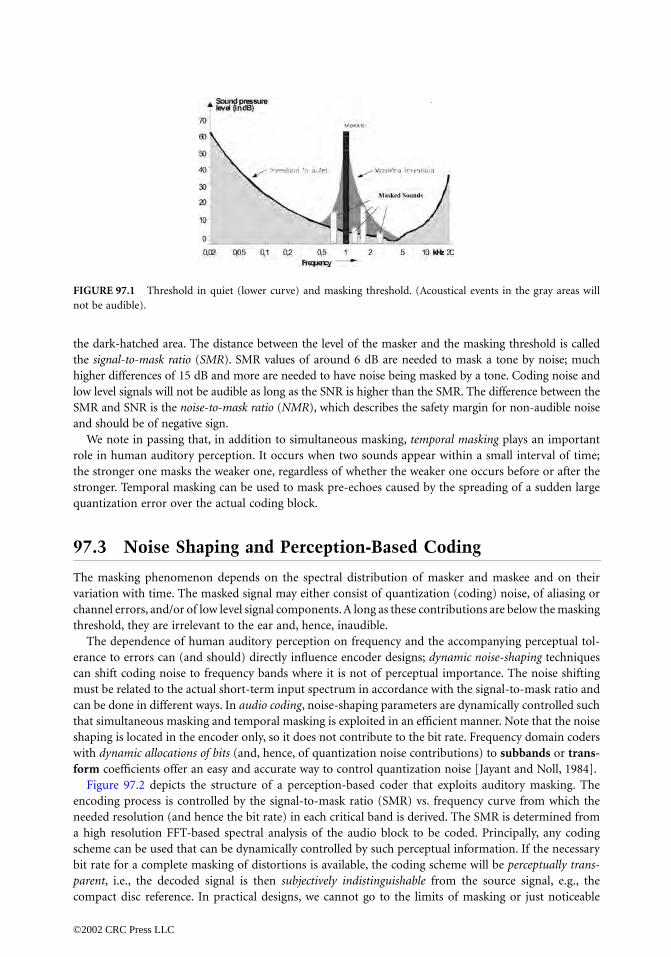
the dark-hatched area. The distance between the level of the masker and the masking threshold is calledthe signal-to-mask ratio (SMR). SMR values of around 6 dB are needed to mask a tone by noise; muchhigher differences of 15 dB and more are needed to have noise being masked by a tone. Coding noise andlow level signals will not be audible as long as the SNR is higher than the SMR. The difference between theSMR and SNR is the noise-to-mask ratio (NMR), which describes the safety margin for non-audible noiseand should be of negative sign.

We note in passing that, in addition to simultaneous masking, temporal masking plays an importantrole in human auditory perception. It occurs when two sounds appear within a small interval of time;the stronger one masks the weaker one, regardless of whether the weaker one occurs before or after thestronger. Temporal masking can be used to mask pre-echoes caused by the spreading of a sudden largequantization error over the actual coding block.

97.3 Noise Shaping and Perception-Based Coding

The masking phenomenon depends on the spectral distribution of masker and maskee and on theirvariation with time. The masked signal may either consist of quantization (coding) noise, of aliasing orchannel errors, and/or of low level signal components. A long as these contributions are below the maskingthreshold, they are irrelevant to the ear and, hence, inaudible.

The dependence of human auditory perception on frequency and the accompanying perceptual tol-erance to errors can (and should) directly influence encoder designs; dynamic noise-shaping techniquescan shift coding noise to frequency bands where it is not of perceptual importance. The noise shiftingmust be related to the actual short-term input spectrum in accordance with the signal-to-mask ratio andcan be done in different ways. In audio coding, noise-shaping parameters are dynamically controlled suchthat simultaneous masking and temporal masking is exploited in an efficient manner. Note that the noiseshaping is located in the encoder only, so it does not contribute to the bit rate. Frequency domain coderswith dynamic allocations of bits (and, hence, of quantization noise contributions) to subbands or trans-form coefficients offer an easy and accurate way to control quantization noise [Jayant and Noll, 1984].

Figure 97.2 depicts the structure of a perception-based coder that exploits auditory masking. Theencoding process is controlled by the signal-to-mask ratio (SMR) vs. frequency curve from which theneeded resolution (and hence the bit rate) in each critical band is derived. The SMR is determined froma high resolution FFT-based spectral analysis of the audio block to be coded. Principally, any codingscheme can be used that can be dynamically controlled by such perceptual information. If the necessarybit rate for a complete masking of distortions is available, the coding scheme will be perceptually trans-parent, i.e., the decoded signal is then subjectively indistinguishable from the source signal, e.g., thecompact disc reference. In practical designs, we cannot go to the limits of masking or just noticeable

FIGURE 97.1 Threshold in quiet (lower curve) and masking threshold. (Acoustical events in the gray areas willnot be audible).


distortion, since post-processing of the acoustic signal (e.g., filtering in equalizers) by the end-user andmultiple encoding/decoding processes have to be considered. In addition, our current knowledge aboutauditory masking is very limited. For example, generalizations of masking results, derived for simple andstationary maskers and for limited bandwidths, may be appropriate for most source signals but may failfor others. Therefore, as an additional requirement, we need a sufficient safety margin in practical designsof such perception-based coders.

97.4 Mean Opinion Score

Perceptual coding techniques ask for a distortion measure that specifies perceptual similarity betweenthe source signal and its reconstructed version. In audio coding, the mean opinion score (MOS) isusually being applied to measure this similarity. Listeners classify the quality of coders on an N-pointquality or impairment scale. Table 97.1 shows the signal impairment scale and its associated numbering[ITU-R Rec. 562]; see also Jayant and Noll [1984]. The impairment scale is extremely useful if coderswith only small impairments have to be graded. The final result of such tests is an averaged judgmentcalled the mean opinion score. In assessing the value of a given MOS rating, the standard deviation ofthis rating is also important.

Recent results have shown that perception-based objective distortion measures that make use of resultsfrom psychoacoustics are quite promising measures of quality. A recent ITU-R standard recommends a“method for objective measurements of subjectively perceived audio quality” [ITU-R, 1999; Thiede, 1999].

97.5 Low Bit Rate Coding

Digital coding at high bit rates is dominantly waveform-preserving, i.e., the amplitude-vs.-time waveformof the decoded signal approximates that of the input signal. At lower bit rates, the error criterion has tobe in favor of an output signal that is useful to the human receiver rather than favoring a decoded signalthat follows and preserves the input waveform. Basically, any efficient source coding algorithm will

FIGURE 97.2 Block diagram of perception-based coders.

TABLE 97.1 5-Point MOS Impairment Scale

MOS Score Impairment Scale

5 Imperceptible4 Perceptible, but not annoying3 Slightly annoying2 Annoying1 Very annoying


• remove redundant components of the source signal by exploiting correlations between its sampleseither in time domain by employing adaptive linear prediction (LPC) or in frequency domain byemploying high-resolution bandwidth splitting in subband coding (SBC) or transform coding (TC)schemes. Combinations thereof are also used.

• remove components of the source signal, which are irrelevant to the auditory system, i.e., to the ear.Irrelevancy manifests itself as unnecessary amplitude or frequency resolution; all portions of thesource signal which are masked are irrelevant. Recently obtained results in audio bit rate compressionsresult from an efficient identification and subsequent removal of such irrelevant components priorto transmission.

Redundancy reduction can easily be achieved by using frequency-domain coding, such as transformcoding, subband coding, and hybrid forms thereof. In addition—and more importantly—frequency-domain coding offers an easy and direct way for perceptual coding, i.e., for noise shaping and suppressionof frequency components that need to be transmitted. In the following, we offer brief summaries of anumber of audio coding algorithms which are based on such frequency mappings as a first stage of audiocoding. The differences are in the number of spectral components, the type of mapping (subband splittingvs. discrete transform), and in the strategies for an efficient quantization of spectral components andmasking of the resulting coding errors.

97.6 ITU-T G.722 Wideband Speech Coder

This 64 kb/s wideband speech coder can code signals with a 3 dB-bandwidth of 50–7000 Hz [Mermelstein,1988]. The ITU-T standard employs a two-band subband technique and a backward-adaptive ADPCMcoding in each of the two subbands. The subband splitting is based on two identical quadrature mirrorfilters (QMF) to divide the wideband signal, sampled at 16 kHz, into two 8-kHz sampled components,called low subband and high subband. The filters overlap, and aliasing will occur because of subsamplingof each of the components; the synthesis QMF filterbank at the receiver ensures that aliasing productsare canceled. However, quantization error components on the two subbands will not be eliminatedcompletely. Therefore 24-tap QMF filters with a stop-band rejection of 60 dB are employed.

The coding of the subband signals is based on ADPCM with backward-adaptive predictors andquantizers, their design is borrowed from [ITU-T Rec.G.726]. The quantizers, however, do not supportthe slowly adapting mode. High quality coding is provided by a fixed bit allocation, where the low andhigh subband ADPCM coders use a 6-b/sample and a 2-b/sample quantizer, respectively. In the lowsubband, the signal resembles the narrowband speech signal in most of its properties. A reduction of thequantizer resolution to 5 or 4 b/sample is possible to support transmission of auxiliary data at rates of8 and 16 kb/s. Embedded encoding is used in the low subband ADPCM coding, i.e., the adaptations ofpredictor and quantizer are always based only on the four most significant bits of each ADPCM codeword.Hence, a stripping of one of two least significant bits from the ADPCM codewords does not affect theadaptation processes and cannot lead to mistracking effects caused by different decoding processes inthe receiver and transmitter.

Subjective speech coding tests have shown that the 64 kb/s ADPCM-coded version has the same MOSrating (MOS = 4.3) as the uncoded source, implying no measurable difference in subjective quality. Inaddition, the coder shows a graceful degradation of subjective quality with decreasing bit rate and increas-ing bit error rate. The coder also provides a good to fair quality for coding of audio signals. Table 97.2

TABLE 97.2 MOS Performance of ITU-T G.722 Coder(7 kHz bandwidth) [Mermelstein, 1988]

Bit Rate in kb/s MOS Value for Speech MOS Value for Audio

48 3.8 3.264 4.2 3.9


compares MOS values for speech and audio signals at two bit rates. The resulting subjective quality ispartly limited by the restriction on the bandwidth. Current activities in wideband speech coding con-centrate on coding at 16 kb/s and below, with the 64 kb/s ITU-T standard serving as reference.

MPEG-1 Layer I and II coders are examples of subband coders with a high number of subbands. Theyare more suitable for perceptual coding; details will be given in a later section.

97.7 Transform Coding

The conventional adaptive transform coding (ATC), as proposed in the midseventies [Zelinski and Noll,1975 and 1977],4 employs a discrete cosine transform (DCT) which maps blocks of N samples into anequivalent number of transform coefficients. The logarithm of the absolute values of these coefficientsform the DCT-based short-term log-spectral envelope; its encoded version is used to calculate, for eachaudio block, the optimum number of bits for each of the N quantizers for the transform coefficients(dynamic bit allocation). The encoder transmits the quantized transform coefficients and the encodedspectral envelope.

The conventional ATC has a number of shortcomings; it produces aliasing effects due to spectral overlap,and it produces pre-echoes because the inverse transform in the decoder spreads large quantization errors—possibly resulting from a sudden attack in the source signal—over the reconstructed block. In addition,inappropriate bit allocations occur if these allocations are based on an unweighted mean-squared codingerror criterion. However, it was already stated in the first publication that the ATC performance could beimproved if emphasis would be laid on irrelevancy reduction, and that the available bits had to be allocateddynamically such that the perceived distortion is minimal [Zelinski and Noll, 1975].

The problem of aliasing can be partly solved by introducing a modified discrete cosine transform(MDCT) with an 50% overlap between adjacent audio blocks. Pre-echoes can be reduced or avoided byusing blocks of short lengths. However, shorter blocks cause an insufficient frequency resolution, and alarger percentage of the total bit rate is required for the transmission of side information. A solution tothis problem is to switch between block sizes of different lengths of, say, N = 64 to N = 1024 (windowswitching). The small blocks are only used to control pre-echo artifacts during nonstationary periods ofthe signal, otherwise the coder switches back to long blocks. It is clear that the block size selection hasto be based on an analysis of the characteristics of the actual audio coding block. In addition, windowswitching has to be carried out such that the aliasing cancellation property of the transform is maintained.MDCT and window switching are used in all advanced audio coders.

97.8 Subband Coding and Hybrid Frequency Mappings

Subband coding and transform coding were first introduced in the context of speech coding. Thedifferentiation between these two categories is mainly due to historical reasons. Both use an analysisfilterbank in the encoder to produce subsampled spectral coefficients. In the case of subband coding, thisfilterbank consists of a typically small number of bandpass filters and each output is critically sampledat a rate that is twice the nominal bandwidth of each bandpass. It is easy to show that an N-valuedtransform can be viewed as a critically decimated bank of N finite impulse response bandpass filters.

Hybrid structures are cascades of a subband and a transform filterbank. MPEG’s MP3 and Sony’sATRAC coders employ such hybrid mappings (see later sections). One of the advantages is that differentfrequency resolutions can be provided in a flexible way and with low complexity.

4The conventional ATC used, for the first time, DCT as the appropriate linear transform for speech, it intro-ducedthe technique of adaptive bit allocation, and it showed that a log-spectral envelope should be computed andparameterized to derive the appropriate bit allocation.


97.9 ISO/MPEG Audio Coding

The moving pictures expert group within the International Organization of Standardization (ISO/MPEG)has provided a generic source coding method (MPEG 1) for storing audio-visual information on digitalstorage media at bit rates up to about 1.5 Mb/s [ISO/MPEG 1993; Brandenburg and Stoll, 1994; Noll,1997]. MPEG-1 Audio has been the first international standard in the field of digital audio compression,useful both for audio-visual and audio-only applications.

In all MPEG standards (see next sections), each spectral component is quantized and coded with thegoal to keep the quantization noise below the masking threshold. The number of bits for each subband anda scale factor are determined on a block-by-block basis. The number of quantizer bits is obtained from adynamic bit allocation algorithm that is controlled by a psychoacoustical model. The subband codewords,the scale factors, and bit allocation information are multiplexed into one bitstream, together with a headerand optional ancillary data. In the decoder, the synthesis filterbank reconstructs a block of 32 audio outputsamples from the demultiplexed bitstream.

It is worthwhile to note that the normative part of all MPEG standards describes the decoder and themeaning of the encoded bitstream, but that the encoders are not defined, thus leaving room for evolu-tionary improvements of the encoders. In particular, different psychoacoustic models can be used rangingfrom very simple (or none at all) to very complex based on quality and implementability requirements(the standard gives two examples of such models). In addition, encoders can be optimized for certainapplications. It should be noted that the model is only needed in the encoder which makes the decoderless complex, a desirable feature for audio playback and audio broadcasting applications.

The structure of MPEG coders follows that of perception-based coders. In the first step, the audiosignal is converted into spectral components via an analysis filterbank; Layers I and II make use of asubband filterbank, Layer III employs a hybrid transform, and MPEG AAC is purely transform-based.

97.10 MPEG-1 and MPEG-2 Audio

The MPEG 1 standard consists of three layers I, II, and III of increasing complexity and subjectiveperformance. It supports sampling rates of 32, 44.1, and 48 kHz and bit rates per monophonic channelbetween 32 and 448 kb/s in 32 kb/s steps (Layer I). An additional free format mode allows for any bitrate below 448 kb/s. The coder provides a quality that is subjectively equivalent to compact disc (CD)quality (16 bit PCM) at a stereo rate of 256 kb/s for most audio items.

The MPEG-1 coder uses perception-based frequency-domain coding. In the first stage, the audio signalis converted into 32 spectral subbands components via an analysis filterbank. Each spectral componentis quantized, whereby the number of quantizer levels for each component is controlled by a psychoacousticmodel that computes signal-to-mask ratios and obtains its information about the short-term spectrumby running an FFT in parallel to the encoder (see Fig. 97.2).

MPEG-1 Layer I contains the basic mapping of the digital audio input into 32 subbands via equallyspaced bandpass filters (Fig. 97.3), fixed segmentation to format the data into blocks (8 ms at 48 kHzsampling rate), and quantization with block companding.

FIGURE 97.3 Structure of MPEG-1 Audio filterbank, Layers I and II.


At 48 kHz sampling rate, each band has a width of 750 Hz. A polyphase filter structure is used for thefrequency mapping; its filters are of order 511, which implies an impulse response of 5.33 ms length (at48 kHz). In each subband, blocks of 12 decimated samples are formed, and for each block, signal-to-mask ratios are calculated via an 512-point FFT. For each subband, the bit allocation selects a quantizer(out of a set of 15) such that both the bit rate requirement and the masking requirement are being met.

The decoding is straightforward: the subband sequences are reconstructed on the basis of 12-samplesubband blocks taking into account the decoded scalefactor and bit allocation information. If a subbandhas no bits allocated to it, the samples in that subband are set to zero. Each time the subband samplesof all 32 subbands have been calculated, they are applied to the synthesis filterbank, and 32 consecutive16-bit PCM format audio samples are calculated.

The MPEG-1 Layer II coder is basically similar to the Layer I coder but achieves a better performancethrough three modifications. First, the input to the psychoacoustic model is a 1024-point FFT leadingto a finer frequency resolution for the calculation of the global masking threshold. Second, the overallscalefactor side information is reduced by exploiting redundancies between the scale factors of threeadjacent 12-sample blocks. Third, a finer quantization with a maximum of 16-bit amplitude resolutionis provided (which reduces the coding noise).

MPEG-1 Layer III introduces many new features. The Layer III approach has become quite popular,in particular in Internet applications (MP3). MP3 achieves its improvement mainly by an improvedfrequency mapping, an analysis-by-synthesis approach for the noise allocation, an advanced pre-echocontrol, and by nonuniform quantization with entropy (Huffman) coding. Finally, a buffer technique,called bit reservoir, leads to further savings in bit rate. In order to achieve a higher frequency resolutioncloser to critical band partitions, the 32 subband signals are subdivided further in frequency content byapplying a switched 6-point or 18-point modified DCT (MDCT) with 50% overlap to each of thesubbands (see Fig. 97.4). The maximum number of frequency components is 32 × 18 = 576 eachrepresenting a bandwidth of only 24000/576 = 41.67 Hz. The term hybrid filterbank is used to describesuch a cascade of polyphase filterbank and MDCT transform. The decoding follows that of the encodingprocess.

The MPEG-2 standard includes an extension that adds sampling frequencies of 24, 22.05 and 16 kHz[ISO/MPEG 1995; Stoll, 1996]. These sampling frequencies are useful for the transmission of widebandspeech and medium quality audio signals. In addition, a reduction in sampling frequency by a factor oftwo doubles the frequency solution of the filterbanks and transforms and will therefore improve theperformance of the coders, in particular those of low frequency resolution (MPEG-1, Layers I and II).Only small modifications of ISO/MPEG-1 are needed for this extension; the bitstream syntax still complieswith the standard.

97.11 MPEG Advanced Audio Coding

More recently, MPEG advanced audio coding (AAC) has been standardized [ISO/MPEG 1997; Bosi et al.,1997]. This standard offers the highest subjective quality and is about to become a universal standard inmany application areas with totally different requirements such as consumer electronics, professionalaudio processing, telecommunications, and broadcasting.

FIGURE 97.4 Hybrid filterbank of MPEG-1 Layer III (MP3) encoder.


The MPEG-2 AAC standard employs high resolution filterbanks, prediction techniques, and noiselesscoding. It is based on recent evaluations and definitions of tools (or modules) each having been selectedfrom a number of proposals. The self-contained tools include an optional preprocessing, a filterbank, aperceptual model, temporal noise shaping, intensity multichannel coding, time domain prediction, M/Sstereo coding, quantization, noiseless (Huffman) coding, and a bitstream multiplexer. The filterbank isa 1024-point modified discrete cosine transform (due to an 50% overlap, the transform is taken over2048 windowed samples). In case of transient signals, the filterbank can switch to a 128-point mode.The perceptual model can be taken from MPEG-1.

The temporal noise shaping (TNS) tool plays an important role in improving the overall performanceof the coder (see Fig. 97.5). It performs a prediction of the spectral coefficients of each audio frame.Instead of the coefficients, the prediction residual is transmitted. TNS is very effective in case of transientaudio signals since such transients (signal attacks) imply a high predictability in the spectral domain.(Recall that peaky spectra lead to a high predictability in the time domain.) Therefore, the TNS toolcontrols the time dependence of the quantization noise. Time domain prediction is applied to subsequentsubband samples in a given subband in order to further improve coding efficiency, in particular forstationary sounds (see Fig. 97.5). Second-order backward-adaptive predictors are used for this purpose.Finally, for quantization, an iterative method keeps the quantization noise in all critical bands below theglobal masking threshold.

The MPEG-2 AAC standard offers high quality at lowest possible bit rates. For example, when operatingat a 128 kb/s stereo rate, AAC has a mean opinion score (MOS) only 0.2 off the reference value. At thatrate, the popular MPEG-1 Layer III coder (MP3) is almost one full score value below the reference value[Meares et al., 1998].

AAC, a joint effort of AT&T, Dolby Laboratories, Fraunhofer Institute, and Sony Corporation providesup to 48 channels (see below) and sampling rates up to 96 kHz. It is supported by a growing number ofhardware and software manufacturers.

97.12 Proprietary Audio Coding

Dolby’s AC-3 coder (Dolby Digital) is a transform coder with sampling rates of 32, 44.1, and 48 kHzand nineteen mono channel bit rates in the range from 32 to 640 kb/s. The coder supports variousmultichannel configurations and provides the option of channel down-mixing adjustable by the end user[Fielder et al., 1996]. Unlike other approaches, Dolby’s AC-3 coder makes use of hybrid backward/forwardadaptive bit allocation to reduce the necessary bit rate for transmitting bit allocation side information.The bit allocation routine, called parametric bit allocation, runs both in the encoder and the decoder,

FIGURE 97.5 Spectral and time domain prediction in MPEG-2 advanced audio coding (AAC).


based on a psychoacoustic model. The forward mode of the algorithm allows the decoder to be re-adjusted by the encoder. If the encoder uses an improved bit allocation routine, it can compare its resultwith that of the routine used by the decoder and send correction information to fine-tune the decoder’sbit allocation. The final bit allocations of the encoder and decoder are, of course, identical. [An earlierversion, AC-2, uses a purely backward-adaptive bit allocation based on quantized information. In caseof an error-free transmission, this information is also available at the decoder, therefore no side infor-mation is required to inform the decoder about the actual bit allocation.] Applications will be coveredin the section about multichannel standards.

AC-3 coding serves as an emission or storage coding format optimized for maximum quality at lowbit rates, typically for one encode/decode cycle. Within broadcast and postproduction infrastructures,other formats have to be employed. One example is the Dolby E distribution coding system with asampling rate of 48 kHz and a resolution of 16, 20, and 24 bits per audio sample.

Sony’s Adaptive Transform Acoustic Coding (ATRAC) uses a hybrid frequency mapping: the signal isfirst split into three subbands (0–5.5, 5.5–11.0, and 11.0–22.0 kHz) reflecting auditory perception [Iwadareet al., 1992]. An MDCT with 50% overlap is then applied to all subbands with dynamic window switching:the regular block size is N = 512, to provide optimum frequency resolution, but in the case of possiblepre-echoes, N is switched to 64 in the high frequency bands and to N = 128 otherwise. The coder withits 44.1 kHz sampling rate and its 256 kb/s stereo bit rate has been developed for portable digital audio,specifically for the 64 mm optical or magneto-optical disc which has approximately one-fifth of the byte-capacity of a standard CD [Tsutsui et al., 1992].

More recently, ATRAC3 was released. It achieves a higher compression rate mainly by splitting theaudio signal into four bands (instead of three) and by employing a 256-point MDCT to all four bands(see Fig. 97.6). In addition, tonal audio components are identified and coded separately from otherspectral components. Entropy coding reduces the bit rate further. Finally, a joint stereo coding schemetakes advantage of the correlations between stereo channels.

97.13 Multichannel Standards

In multichannel coding, redundancies and irrelevancies such as intra- and interchannel correlations andmasking effects are exploited to reduce the overall bit rate. In addition, stereo-irrelevant components ofthe multichannel signal may be identified and reproduced in a monophonic format to bring the bit ratesfurther down. A typical multichannel system may employ five channels (L = left, C = center, R = right,LS = left surround, RS = right surround) but up to 48 channels are supported by the AAC standard.

The MPEG standards include two classes of multichannel audio coding, one of which is forward- andbackward-compatible with MPEG-1 Audio [ISO/MPEG 1993]. Forward compatibility means that anMPEG-2 multichannel decoder is able to properly decode MPEG-1 mono- or stereophonic signals.Backwards compatibility means that existing MPEG-1 stereo decoders, which can only handle two-channel audio, are able to reproduce a meaningful basic stereo signal from an MPEG-2 multichannel

FIGURE 97.6 Block diagram of Sony’s ATRAC3 audio encoder.


bitstream so as to serve the needs of users with simple mono or stereo equipment. However, due to itsconstraints caused by matrixing and dematrixing procedures,5 the compatible coder will need a higherbit rate for a given audio quality.

Non-backward-compatible multichannel coders will not be able to feed a meaningful bitstream intoan MPEG-1 stereo decoder. On the other hand, these codecs have more freedom in producing highquality audio signals. Therefore, we will only cover the standard that supports applications which do notrequest compatibility with the existing MPEG-1 stereo format. Within the MPEG-2 standard, the mul-tichannel advanced audio coding technique (AAC) offers highest performance at comparably low overallbit rates (see Fig. 97.7).

In extensive formal subjective tests, it turned out that the non-backward-compatible 320 kb/s MPEG-2AAC coder performed slightly better than the backward-compatible 640 kb/s MPEG-2 Layer II coder.From these subjective tests, it became clear that the concept of backward compatibility implies the needfor significantly higher bit rates. The AAC coder satisfies requirements for ITU-R broadcast quality at320 kbit/s for 5 channels.

As mentioned above, Dolby’s AC-3 coding supports up to nineteen mono channel bit rates from 32to 640 kb/s which allow for a high number of multichannel configurations. A first multichannel appli-cation of AC-3 has been for digital optical soundtracks in 35 mm cinema. The soundtrack consists ofdata between the sprocket hole perforation and presents a 5.1 multichannel audio system operating at abit rate of only 320 kb/s. AC-3 has been selected as the audio coding standard in the US DTV systemwith a typical bit rate of 384 kb/s [ATSC, 1995; Fielder et al., 1996]. In DVD Video, it is mandatory tosupport linear PCM (see section on lossless coding) and AC-3 coded audio (whereas MPEG audio is oneof the mandatory audio coding modes for TV systems with 625 lines and 25 frames only).

If bit rates are not of highest concern, a simulcast transmission may be employed, where a full stereobitstream is multiplexed with a full non-backward-compatible multichannel bitstream in order to supportbackward compatibility without matrixing techniques (Fig. 97.8).

FIGURE 97.7 MPEG-2 advanced audio coding (multichannel configuration; T = transmission channels).

FIGURE 97.8 Backward-compatible multichannel audio coding (simulcast mode).

5Matrixing describes a down-mix technique of, say, five-channel audio signals into two compatible stereo sig-nals.Three additional transmission channels carry audio information that has to be chosen such that the decoder canrecompute the complete 5-channel audio signal (dematrixing).


97.14 MPEG-4 Audio Coding

Activities within the MPEG-4 standardization process have aimed at proposals for a broad field of applica-tions including communication services, interactive services, and broadcast services. The new standard[ISO/MPEG 1999] takes into account that a growing part of information is read, seen, and heard ininteractive ways. It supports new forms of communications, in particular for Internet and multimediaapplications and in mobile communications. MPEG-1 and MPEG-2 offer only a very limited interaction andcontrol over the presentation and configuration of the system. In addition, an integration of natural andsynthetic content is difficult, and access and transmission across heterogeneous networks is not well-supported. MPEG-4 is different: it represents an audiovisual scene as a composition of (potentially mean-ingful) objects and supports the evolving ways in which audiovisual material is produced, delivered, andconsumed. For example, computer-generated content may become part of the production of an audio-visual scene. In addition, interaction of objects with scene is possible, so it will be possible to associate a Webaddress to a person in a scene.

In the case of audio, MPEG-4 merges the whole range of audio from high fidelity audio coding andspeech coding down to synthetic speech and synthetic audio, supporting applications from high-fidelityaudio systems down to mobile-access multimedia terminals [Brandenburg et al., 2000; Johnston et al.,2000; Scheirer et al., 2000]. Figure 97.9 indicates the potential of MPEG-4; it describes an audiovisualscene with a number of audio objects: the noise of an incoming train, an announcement, a conversation,and background music. For example, the noise of the train can be described by an eight-channelrepresentation. On the other hand, if the necessary bandwidth is not available, a one-channel represen-tation—or no representation at all—might be used instead. Such a form of scalability will be very usefulin future applications whenever audiovisual signals have to be transmitted to and via receivers of differingcomplexity and channels of differing capacity. In the case of the announcement, one-channel pseudo 3-D and echo effects could be added. The background music may have an AAC format, or it is of syntheticorigin [ISO/MPEG 1998].

MPEG-4 supports compression of speech and audio signals at monophonic bit rates ranging from 2to 64 kb/s. Three core coders are used:

• a parametric coding scheme (vocoder) for low bit rate speech coding (2 to 10 kbit/s)

• a CELP-based analysis-by-synthesis coding scheme for medium bit rates (4 to 16 kb/s)

• a transform-based coding scheme for higher bit rates (up to 64 kbit/s)

The transform-based coder is an AAC coder with a number of modifications. Important examples are(1) a less complex longterm prediction tool, (2) a perceptual noise substitution tool which allows a veryefficient coding of noiselike signal components, and (3) bit rate scalability with the potential of adaptingthe rate dynamically to the time-varying capacity of a channel.

FIGURE 97.9 Audiovisual scene and its audio channels [ISO/MPEG 1998].


MPEG-4 not only offers simple means of manipulation of coded data such as time scale control andpitch change, but also a flexible access to coded data and subsets thereof, i.e., scalability of bit rate,bandwidth, complexity, and of error robustness. In addition, MPEG-4 supports not only natural audiocoding at rates between 2 and 64 kb/s, but also text-to-speech conversion (TTS) and structured audio[Scheirer et al., 2000]. The standard offers also an interface between TTS and facial animation for syntheticface models to be driven from speech (talking heads).

Figure 97.10 indicates the range of quality and bit rates offered by the new standard. Transform-basedaudio coders show a very good performance at bit rates down to 16 kb/s, whereas speech coders performclearly better at rates between 2.4 kb/s and 16 kb/s.

97.15 Lossless Coding

For archiving and processing of audio signals, the coding will have to be lossless. Lossless coding does notalter the final decoded audio signal in any way (i.e., in any bit). Digital versatile discs for audio (DVD Audio),with their capacity of 4.7 GB (single layer) or 8.5 GB (double layer) (or up to 17 GB if both sides of thediscs are readable), allow storage of audio material without any source coding [Fuchigami et al., 2000].Therefore, linear PCM was adopted for DVD Audio as one of the mandatory audio coding schemes. Sixsampling rates in the range between 44.1 and 192 kHz and amplitude resolutions of 16, 20, and 24 bitsper audio sample have been specified.

Lossless coding compresses (packs) PCM-format audio signals in a way that the decoded versions arebit-precise replica of the PCM format. Packed PCM was specified as an additional mandatory codingalgorithm for DVD Audio discs [Stuart et al., 2000]. The encoder employs

• a lossless matrix technique to reduce inter-channel correlations

• prediction for each channel

• entropy coding

• buffering to smooth the encoded data rate

In addition, it exploits unused capacity from audio data that is not full scale.Lossless coding, when applied to 16-bit linear PCM (CD format), results in average bit rates of around

8 bits per sample depending on the audio material. Average values for the complete audio material ofthe SQAM CD [SQAM, 1988] are 5.0 for the popular linear predictive coding algorithm “Shorten”[Robinson, 1994], and 4.6 for the lossless transform audio compression (LTAC) algorithm of TU Berlin[Liebchen et al., 1999]. Table 97.3 compares coding results for the audio categories of the CD. The resultsare optimistic since all audio examples start and end with a pause. Please note that data rates in losslesscoding are typically variable; the presented values are averages.

FIGURE 97.10 Range of audio quality and bit rates in MPEG-4.


97.16 Conclusion

Low bit rate digital audio is being applied in many different fields such as consumer electronics, profes-sional audio processing, telecommunications, and broadcasting. Perceptual coding in the frequencydomain has paved the way to high compression rates. The ISO/MPEG audio coding algorithms are widelyaccepted international standards. However, other (propriatory) coding schemes serving different goalsand meeting other requirements have evolved and have found many applications. More recently, losslesscoding has gained interest for both professional and consumer use where data integrity is mandatory.

Defining Terms

ADPCM: Adaptive differential pulse code modulation, a predictive coding technique with adaptationof quantizer step sizes and predictor coefficients based on the short-term statistics of the sourcesignal.

Auditory masking: Simultaneous masking describes the effect that a low level audio signal (the maskee)can become inaudible when a louder signal (the masker) occurs simultaneously. Temporal maskingdescribes the effect that a low level audio signal can become inaudible before and after a loudersignal has been switched on and off.

ISDN: Integrated services digital networks offer end-to-end digital connectivity to support a wide rangeof communication applications. Customers have physical access to one or two 64 kb/s bearer (B)channels and one data (D) channel (the latter supports signaling at 16 kb/s but can also carry userinformation). Higher rates than 64 or 128 kb/s are achievable using multiple calls with channelaggregation and may be more generally available in the future as multiple-rate services.

ITU: International Telecommunication Union, a worldwide standardization organization. ITU-R is itsradiocommunication section, formerly called CCIR, and ITU-T is its telecommunication section,formerly called CCITT.

Mean opinion score (MOS): A distortion measure that specifies perceptual similarity between anuncoded source signal and its coded version.

MPEG: The moving pictures expert group is the working group 11 of the ISO/IEC/JTC1/SC2 standard-ization body. Its task is to propose algorithms for coding of moving pictures and associated audio.

MP3: Acronym for the MPEG-1, Layer III audio coding standard.Subband coding: Division of the source signal into bandpass signals (subbands) via a filterbank fol-

lowed by individual coding of the subband signals.Transform coding: Deriving transform (spectral) coefficients from blocks of the source signal via a

linear transform followed by individual coding of the transform (spectral) coefficients.

TABLE 97.3 Coding Results in Bits per Sample for the Audio Material of the SQAM Disc[Liebchen et al., 1999]

CategoryShorten

(Public Domain)LTAC

(TU Berlin)

Alignment signals 6.29 6.06Artificial signals 2.84 2.60Single instruments 4.60 4.15Vocal 5.35 4.83Speech 5.45 5.36Solo instruments 5.09 4.52Vocal & orchestra 6.73 6.14Orchestra 5.33 5.07Pop music 6.37 6.03CD average 4.98 4.56


References

ACATS (Advisory Committee on Advanced Television Service), 1994, Grand Alliance HDTV System Spec-ification, Version 1.0.

ATSC Doc. A/52, 1995, ATSC Digital Audio Compression Standard (AC-3). [ATSC = Advanced TelevisionStandardization Committee.]

Bosi, M. et al., 1997, ISO/IEC MPEG-2 advanced audio coding, J. Audio Eng. Soc., 45(10), S789–S814.Brandenburg, K., Kunz, O., and Sugiyama, A., 2000, MPEG-4 natural audio coding, Signal Proc. Image

Commun., 15, 423–444.Brandenburg, K. and Stoll, G., 1994, The ISO/MPEG-audio codec: a generic standard for coding of high

quality digital audio, J. Audio Eng. Soc., 42, 780–792.Fielder, L.D. et al., 1996, AC-2 and AC-3: low complexity transform-based audio coding, in Gilchrist, N.

and Grewin, C., Eds., Collected Papers on Digital Audio Bit-Rate Reduction, Audio EngineeringSociety, Inc., New York, 73–82.

Fuchigami, N., Kuroiwa, T., and Suzuki, B.H., 2000, DVD—Audio Specifications, J. Audio Eng. Soc., 48(12).ISO/MPEG 1993, International Standard ISO/IEC 11172 Part 3 (MPEG-1 Audio). ISO/MPEG 1995, International Standard ISO/IEC 13818 Part 3 (MPEG-2 Audio).ISO/MPEG 1997, International Standard ISO/IEC 13818 Part 7 (AAC).ISO/MPEG 1998, MPEG Document 98/N2431.ISO/MPEG 1999, International Standard ISO/IEC 14496 Part 3 (MPEG-Audio).ITU-R BS. 1387, 1999, Method for Objective Measurements of Subjectively Perceived Audio Quality.Iwadare, M. et al., 1992, A128 kb/s hi-fi audio codec based on adaptive transform coding with adaptive

block size, IEEE J. Sel. Areas Commun., 10(1), 138–144.Jayant, N.S. and Noll, P., 1984, Digital Coding of Waveforms: Principles and Applications to Speech and

Video, Prentice-Hall, Englewood Cliffs, NJ.Johnston, J.D. et al., 2000, Review of MPEG-4 general audio coding, in Puri, A. and Chen, T., Eds.,

Multimedia Systems, Standards, and Networks, Marcel Dekker Inc., New York–Basel, 131–156.Liebchen, T., Purat, M., and Noll, P., 1999, Improved lossless transform coding of audio signals, in Impulse

und Antworten, Wissenschaft & Technik Verlag, Berlin, 159–170.Meares, D., Watanabe, K., and Scheirer, E., 1998, Report on the MPEG-2 AAC Stereo Verification Tests,

MPEG Document 98/N2006.Mermelstein, P., 1988, G722, a new CCITT coding standard for digital transmission of wideband audio

signals, IEEE Commun. Mag., 8–15. Noll, P., 1997, MPEG digital audio coding, IEEE Signal Proc. Mag., 14–59–81.Robinson, T., 1994, Shorten: simple lossless and near-lossless waveform compression, Technical report

CUED/F-INFENG/TR.156, Cambridge University Engineering Department.Scheirer, E.D., Lee, Y., and Yang, J.W., 2000, Synthetic audio and SNHC audio in MPEG-4, in Puri, A.

and Chen, T., Eds., Multimedia Systems, Standards, and Networks, Marcel Dekker Inc., NewYork–Basel, 157–178.

SQAM (Sound Quality Assessment Material—Recordings for Subjective Tests), 1988, Technical Centreof the European Broadcasting Union (EBU).

Stoll, G., 1996, ISO-MPEG2 audio: a generic standard for the coding of two-channel and multichannelsound, in Gilchrist, N. and Grewin, C., Eds., Collected Papers on Digital Audio Bit-Rate Reduction,Audio Engineering Society, Inc., New York, 43–53.

Stuart, J.R. et al., 2000, MLP lossless compression, AES 9th Regional Convention Tokyo, preprint H-6,152–155.

Thiede, T., 1999, Perceptual audio quality assessment using a non-linear filterbank, PhD Thesis, Berlin.Tsutsui, K. et al., 1992, Adaptive transform acoustic coding for MiniDisc, 93rd AES-Convention, San

Francisco, preprint 3456.Zelinski, R. and Noll, P., 1977, Adaptive transform coding of speech signals, IEEE Trans. Acoustics Speech

Signal Proc., 299–309.


Zelinski, R. and Noll, P., 1975, Adaptive Blockquantisierung von Sprachsignalen, Heinrich-Hertz-Institute,Technical Report No. 181, Berlin.

Zwicker, E., 1982, Psychoacoustics, Springer-Verlag, New York.

Further Information

For audio coding, the state of the art, as of 1996, is well documented in Gilchrist, N. and Grewin, C.,Eds., 1996, Collected Papers on Digital Audio Bit-Rate Reduction, Audio Engineering Society, Inc., NewYork. The MPEG-4 standard (including audio) is covered in Puri, A. and Chen, T., Eds., 2000, MultimediaSystems, Standards, and Networks, Marcel Dekker Inc., New York–Basel.

There is a significant overlap between speech and audio coding. Therefore we recommend consultingthe chapter on speech signal processing in this handbook and overview papers, such as “Advances inSpeech and Audio Compression,” Proc. IEEE, 82(6), 900–918, 1994, by A. Gersho.

Actual contributions to all aspects of digital audio processing and coding can be found at the biannualconventions of the Audio Engineering Society (AES) and the IEEE ASSP Workshops on Applications ofSignal Processing to Audio and Acoustics.


98Cable

98.1 Introduction98.2 Cable System Architecture

Frequency Plans • Cable TV Frequency Plans • Control Data Channel

98.3 Source Origination and Head EndOff-the-Air Broadcast Signals • Direct Fiber Links • Analog and Digital Satellite Signals • AM and FM Microwave Signals • Commercial Insertion • Character Generators • Live Local Programming • Digital Satellite to Digital Cable Transcoding • Digital Video Servers

98.4 Transmission ChannelChannel Characteristics • Modulation and Error Correction (Analog and Digital)

98.5 Consumer Premises EquipmentThe First Converters • The First Set-Top Converters • Set-Top Designs • Interdiction

98.6 Access Control and SecurityAccess Control • Security Systems

98.1 Introduction

Cable TV, or community antenna TV (CATV), began shortly after World War II. Television broadcaststations were established in most major cities. The frequencies used for transmission were and are primarilyline-of-sight transmission and of a power sufficient to reach consumers in the city and close-in suburbs.As television caught on, this gave rise to a large number of consumers who could not receive good qualitypictures because they were in the shadow of a hill or too far from the transmitters.

The answer was to place a large antenna at a good receive site, on top of a mountain, for example, anddistribute the signals to an entire community. The earliest such sites were in Astoria, OR and Williamsport,PA. The original cable was RG-11 military surplus from World War II.

Early CATV systems carried only 3 channels in the low-VHF band of 54–88 MHz. Over the years, thisevolved to 174, 220, 270, 300, 330, 450, and 550 as broadcast TV added the UHF band channels, pay TVarrived with such services as HBO, and distribution electronics improved to allow high-quality deliveryof the ever larger number of channels. The typical new plant is designed for 750 MHz, with a capacityfor over one hundred analog video channels.

The advent of digital video compression, based on the moving pictures expert group-2 (MPEG-2)standard, promises to increase this capacity by an order of magnitude. Initially, digital services will bedeployed on hybrid plants which carry a mix of analog and digital video signals. Typical plans are to offer77 analog channels in the 50–550 MHz band which can be received by consumers with only analogequipment in the home. Added to this will be a band of digital audio and video services from 550 to 750MHz. This 200-MHz digital cable band will provide the same capacity as the popular 32 transponder high-power DBS services.

Jeff HamiltonGeneral Instrument Corporation

Mark KolberGeneral Instrument Corporation

Charles E. SchellGeneral Instrument Corporation

Len TaupierGeneral Instrument Corporation


New hybrid set-top converters will be deployed to subscribers of these services that receive both theanalog and digital transmissions. Current compression technology provides, typically, 4–10 channels ineach 6-MHz band, allowing well over 200 new video services in the initial 200-MHz digital band. Asdigital receiving equipment rolls out to more and more consumers, cable has the option of evolving toall digital transmission by progressively replacing analog channels with digital carriers.

From the early days of TV, the consumer’s choice has been to select from what’s playing on a fewchannels. Cable added dozens more channels and, through its ability to charge on a per channel basis,created the higher value subscription movie channels. Digital compression combined with the deliveryof signals over fiber to neighborhoods of a few hundred homes now makes possible an efficient path toprovide dedicated bandwidth to each subscriber. This capability amounts to infinite bandwidth in whicheverything a subscriber might want to view is on, by request. Instead of the consumers choosing amongwhat programmers decide to send them, they will have the ability to tell the system what they want to see.

98.2 Cable System Architecture

The distribution system or cable plant that carries the signals from the head end to the subscribers can usevarious architectures. The common tree and branch architecture uses one inch or larger diameter solidaluminum outer conductor coaxial cable to carry the signal from the head end. This trunk cable runsthrough the system, distributing the broadband signal to each neighborhood. Feeder lines that branch offthe trunk typically use smaller diameter cable to carry the signal into the neighborhoods passing eachsubscriber’s home. Drop cables lead from the curb side to each home and are typically 1/4 inch flexiblecoaxial cable. All CATV cables are 75-W characteristic impedance, which is near optimum for low loss.

Devices called taps are used to extract a portion of the signal from a feeder to supply a drop cable.For example, a 20-dB tap extracts 1/100 of the power from the feeder, causing a 20-dB loss at the tappedoutput but only a 0.04-dB loss to the main path.

CATV signals are measured in decibels relative to 1 millivolt (dBmV). For example, 0 dBmV corre-sponds to 1 mV, and +60 dBmV to 1 V. Signals are normally distributed on the trunk cable at a level from+30 to +50 dBmV per channel. The signal level delivered to the home is usually from 0 to +15 dBmVper channel. In order to maintain the signal level, trunk amplifiers and feeder amplifiers, also known asline extenders, are spaced along the lines about every 1/2 mi. This corresponds to 20–30 dB loss at thehighest design frequency. A trunk line may have 40 or more amplifiers in cascade. Since the attenuationof the cables increases with increasing frequency, the amplifiers are equipped with equalizers to providemore gain to the higher frequencies. The ratio of cable loss in decibels between two frequencies isapproximately equal to the square root of the ratio of the two frequencies. A cable with 7-dB loss at 55MHz will have about 20-dB loss at 450 MHz. Some amplifiers include automatic gain control (AGC) tomaintain the desired output level. The amplifier cases can also include diplexers and small upstreamamplifiers to separate and amplify the typically 5–30 MHz return path signals. Amplifiers are usuallypowered by 60 or 90 V AC signals, which are carried along the same coaxial lines.

Many CATV systems now use a hybrid fiber coax (HFC) architecture. To minimize the number oftrunk amplifiers through which the signal must pass, the signal is carried via fiber optic cables from thehead end to multiple remote locations known as a nodes. The head-end optical transmitter normallyuses a distributed feedback (DFB) laser diode generating a few milliwatts of optical power at 1310 nm.The entire RF spectrum is used to intensity modulate the optical output of the laser. Since the fiber lossis only about 0.4 dB/km, the node can be located a relatively large distance from the head end, eliminatingthe need to cascade many amplifiers along a trunk. At the node, a photodetector receiver converts theoptical signal back to RF for distribution on the coax. Return path signals are sent from the node backtoward the head end through a separate fiber using less expensive Fabry–Perot laser sources.

The HFC architecture improves on the classic tree and branch in several areas. It provides many feweractive devices between the head end and home, which greatly improves system reliability. This reductionin the number of active devices also reduces maintenance costs, problem location, and recovery time.


The fiber cables are not susceptible to noise ingress, which impairs TV pictures, nor do they radiate RFpower, which can interfere with nearby radio communications.

The star configuration of HFC fiber plant design provides individual fiber runs to each neighbor-hood. This means the plant supports dedicated bandwidth from the head end to each node of as few asa few hundred homes. Currently, HFC plants carry the same broadcast TV signals to every node. Asinteractive and on-demand services are rolled out, the HFC plant will carry the unique signals demandedby the subscribers in each neighborhood on their node alone. This effectively multiplies bandwidth byas many times as there are nodes in a system. Telephony is a primary example of an interactive, on-demand service. A tree and branch cable plant could provide only a limited number of telephone channelsbefore running out of shared bandwidth, particularly upstream. The HFC star architecture can providededicated bandwidth to and from each node with ample resources for full service.

Frequency Plans

The 5–30 MHz range, called the subband, is commonly used for return path or upstream (from subscriberto head end) transmissions. This is used for the relaying of remote broadcasts to the head end and forthe return of billing and other information from the subscribers’ set-top. It can also be used for theupstream portion of telephony and interactive TV applications.

The range of frequencies used by CATV operators for downstream (sending video from the head endto the subscribers home) ranges from 50–200 MHz for older 23-channel systems to 50–550 MHz for 77-channel system. Newer systems are designed to pass up to 750 MHz or even 1000 MHz. Each analogNational Television Systems Committee (NTSC) TV channel occupies 6 MHz. Using digital compres-sion, several video programs can be transmitted in each 6-MHz channel.

The bands for downstream transmission are:

• Low band: 54–88 MHz (off the air VHF channels 2–6)

• Mid band: 88–174 MHz

• High band: 174–216 MHz (off the air VHF channels 7–13)

• Super band: 216–300 MHz

• Hyper band: above 300 MHz

There are multiple plans for assigning channels within the available frequencies. The Electronics IndustryAssociation (EIA) plan assigns channels to agree with the VHF off the air channel numbers where possible.Additional channels are spaced 6 MHz from these. The harmonically related carriers (HRC) plan placesvideo carriers near multiples of 6 MHz. This helps reduces the visibility of interference from harmonicand intermodulation distortion created in the distribution equipment because the distortion productsfall directly on and zero beat with other video carriers. The incrementally related carriers (IRC) plan issimilar to the EIA plan except for channels 5 and 6. This plan reduces the visibility of intermodulationdistortion products but not harmonic distortion products.

Since many of the frequencies used for CATV channels are assigned to various over-the-air services,it is important for the cable system to maintain shielding integrity, both to keep outside signals frominterfering with the CATV system (ingress) and to keep CATV signals from radiating and causinginterference to local radio traffic, such as the aircraft communication bands.

Cable TV Frequency Plans

EIA Standard Plan: The standard plan uses xxx.250 MHz for analog video carriers for most channels.Digital center frequencies are 1.75 MHz above the analog video carrier so they will typically fall onxxx.000 MHz. For example, Channel 3 analog video carrier = 61.250 MHz. Channel 3 digital centerfrequency = 63.000 MHz. This corresponds to the NTSC over the air frequency plan for analog carriers.Analog channels that fall in the aircraft bands are given a +12.5 kHz offset up to xxx.2625 to reduce theprobability of interference to aircraft. These aeronautical offsets are not needed for digital carriers because


there is no concentration of energy at the carrier frequency. None of the standard plan carriers are phaselocked, therefore all intermodulation and harmonic distortion products can produce visible beats. Thecarriers are spaced nominally at 6 MHz. Due to the small frequency tolerance errors, the compositesecond order (CSO) intermodulation products and the composite triple beat (CTB) third order distortionproducts typically will create visible interference beats.

IRC: Incrementally Related Carrier: Nearly all IRC channels are xxx.2625 and all the carriers are phaselocked to a common reference. This causes the CTB products to be nearly invisible because they falldirectly on and zero beat the picture carrier. The CTB products are zero beats and invisible in the IRCsystem, but the CSO products fall 1.25 MHz above and below the analog video carriers and can producevisible interference.

HRC: Harmonically Related Carrier: HRC carriers are all phase locked and are multiples of 6.0003MHz. This relationship causes both CTB and CSO products to be zero beat and nearly invisible. The300 Hz or 50 ppm offset provides for protection of aviation services. HRC analog carriers are about 1.25MHz below the standard analog carriers except channels 5 and 6 which are 0.75 MHz above.

Control Data Channel

In some CATV systems, another signal, known as the out-of-band signal, is also sent from the head endto the subscriber. This signal is used to control addressable set-top converters. The converter contains areceiver that is always tuned to this signal regardless of which in-band channel is being viewed or poweron/off. This signal is usually located in the FM radio band (88–108 MHz). The dedicated frequency andcontinuous reception by set-tops provides a reliable path for access control and user features such asprogram guides and downloaded graphical user interfaces.

98.3 Source Origination and Head End

The signals and programs that are to be delivered to CATV subscribers are all collected at a centrallocation known as the head end. There can be many sources of signals including VHF and UHF off-the-air broadcast signals, analog and digital satellite signals, AM and FM microwave signals, prerecordedvideo tapes, character generators, digital video servers, and live locally originated programs.

Off-the-Air Broadcast Signals

The reception of distant off-the-air broadcast signals was the original need that created the CATVindustry. Today, as populated areas become more spread out, many people subscribe to CATV to improvethe quality of their reception of broadcast signals.

At the head end, off-the-air signals are received using high-gain Yagi antennas mounted on a hill ortower to provide the maximum signal. The directional characteristics of the Yagi antenna also help todiscriminate against reflections which cause ghosting. Advanced digital techniques are also availableto cancel ghosting. A known reference signal is transmitted in the invisible vertical blanking intervalsection of the TV signal. The receiver compares the received version of the signal to the known referencesignal and calculates a ghost profile. This profile is then subtracted from the entire video signal tocancel the ghost effect. Using these techniques, good off-the-air pictures can be received over 60–100 miaway.

Second Order CSO Products Third Order CTB Products

Standard plan +/-750 kHz or +/-1.25 MHz +/-15 kHzIRC Plan +/-750 kHz or +/-1.25 MHz zero beatHRC Plan zero beat zero beat


Direct Fiber Links

The penetration of cable to the majority of TV viewers in the U.S. means more people watch networkTV on cable than off-the-air. This has made direct delivery of broadcast programming to the cable headend an attractive way to maximize the quality of these channels. Fiber is run from either the local broadcaststudio or transmitter to the cable head end. There it is directly modulated onto a cable channel fordistribution to subscribers.

Analog and Digital Satellite Signals

As the CATV industry grew, the concept of superstations and premium movie channels developed. Theseare distributed nationwide via geostationary communications satellites located 22,500 mi above theequator. Each programmer transmits their signal up to a satellite via an uplink, usually in the 5.9–6.4 GHzband. The satellite then transmits the signal back to Earth in the 3.7–4.2 GHz range or C band. Mostanalog CATV programming is concentrated on a few satellites known as cable birds. The transponderson these satellites generate 16–30 W of RE power, which usually requires a 10–30 ft diameter dish antennaat the cable head end. Each satellite contains 24 transponders and can carry 24 analog programs. Although,typically, a separate parabolic dish antenna is needed to receive each satellite, a specially shaped antennacan be used with multiple feeds to simultaneously receive multiple satellites.

Analog satellite signals are received in integrated receiver decoders (IRDs) at the cable head end. Thesedevices tune the desired transponder frequency, demodulate the FM video signal, descramble the videosignal, and decrypt and convert the digital audio back to analog form. They are authorized by the programproviders access control and security system. The output analog video and audio go to a cable scrambler,modulator, and channel converter for transmission on the cable plant.

The enormous expense of satellite transponders drove the development of digital video compressionfor satellite transmission. Digital transmission of compressed video signals provides more efficient useof satellite transponders. Compression systems currently offer 4–10 video programs over a single trans-ponder, greatly reducing the programmer’s satellite link costs.

Digital compressed satellite signals are received in a digital IRD, which connects to the head-end systemsin much the same way as an analog IRD. The digital IRD performs many more functions than an analogIRD but delivers similar outputs of analog video and audio signals. Differences include higher quality videosignals due to digital transmission with no quality degradation of weak signals, high security due to digitalencryption, and the availability of many more programs due to the efficiency of transmission.

AM and FM Microwave Signals

In some locations, it is impossible to receive off-the-air broadcast signals with the desired quality. Inthese cases, a dedicated point-to-point microwave link can be installed. The desired off-the-air signal isreceived at a location close to the transmitter or, sometimes, the microwave signal can be sent out fromthe TV station directly. The signal is beamed via very directional antennas directly to the head end. BothAM and FM modulation are used for microwave links.

Commercial Insertion

As special programming intended solely for CATV became available, the concept of local advertisementinsertion developed. Local business can purchase advertising air time from the CATV operator. Thesecommercials are inserted during defined commercial breaks in the programming. In the past, advertise-ments were pre-recorded on video tape and automatically controlled to run at the correct time. Locallyoriginated programs such as locally produced news, school board or local government meetings, andpublic access programming can also be recorded on video tape for transmission via CATV. New com-mercial insertion equipment uses compressed digital video sources. This provides greatly enhanced videoquality, reliability, insertion tracking, scheduling, and methods for delivery of the program material to


the insertion equipment. Commercial insertion into digital video channels on cable will require a newdevice called an add–drop multiplexer. This device will replace the compressed video bits of a satellitedelivered advertisement with a local ad. This is all accomplished in the digital domain without any needto decompress the content.

Character Generators

Character generators are used to create bulletin board style information channels. Programming, adver-tising, local government, and weather information can be displayed. Usually, several screens worth ofdata are stored in the character generator and these are sequentially displayed. Computer graphics canalso be included to enhance visual appeal. Expanded forms include characters generated over video stillsor live video.

Live Local Programming

Many CATV operators carry local school or government meetings live. Often, a subband frequency (5–30 MHz) is used to carry the signal from the town hall, for example, via the cable plant return path backto the head end. At the head end, the signal is converted to a normal forward path channel and sent tothe subscribers via the distribution system.

Digital Satellite to Digital Cable Transcoding

Just as the integrated device called the IRD receives an analog or digital satellite service for use on cable,a device called an integrated receiver transcoder (IRT) receives a compressed digital video multiplex fordirect transmission to digital video subscribers without decompression at the head end. The IRT performsalmost all of the functions required to pass a compressed multiplex of signals from a digital satellite channelto a digital cable channel.

The IRT tunes a digital satellite signal, demodulates it, performs satellite link error correction, decryptsthe multiple video and audio services in the multiplex, replaces the satellite access control informationwith new cable system control data, re-encrypts the services with cable security, inserts cable error controlbits, and modulates the data onto a 64 quadrature amplitude modulation (QAM) carrier. Only a channelconverter is required to prepare the signal for CATV transmission. This high density of signal processingmeans it takes much less rack space in the cable head end to add a channel of digital programming froma satellite than an analog channel. At the same time, the digital channel provides many simultaneousvideo programs to the subscriber.

Digital Video Servers

An expanded version of the video equipment used for digital commercial insertion can provide full lengthprograms such as pay-per-view movies and movies with multiple start times. Video servers can be usedto create programming for analog cable plants in place of video tape, but their most efficient applicationis in digital cable plants. When digital set-tops are deployed, a digital video server can output precom-pressed services to them for preprogrammed or video on-demand services. The output is encrypted,multiplexed, and modulated in equipment that can also process streams from real-time video encoders.

98.4 Transmission Channel

Channel Characteristics

In order to deliver a high-quality signal, the CATV distribution plant must be designed to add a minimumof noise, distortion, and spurious signals. Various defects in the channel can cause visible impairmentsto the picture. The in-channel gain and group delay must be constant vs. frequency to avoid ringing orloss of vertical detail. Excessive thermal noise causes snow or graininess in the picture. Spurious signals


or intermodulation can cause herringbones or diagonal lines that move randomly through the picture.Table 98.1 is a list of some of the relevant parameters and values required for an excellent picture.

Degradation from each part of the system is additive. The consumer’s video signal has passed througha great number of active and passive components, each of which degrades the signal. Within the economicconstraints on real products, each system component must be designed to minimize its contribution tototal impairment.

Digital transmission on cable will, in general, be much more robust, reliable, and easy to monitor thananalog transmission. There are a few impairments that will affect digital transmission more than analog.The best example is burst noise. This shows up as a loss of signal for a fraction of one TV scan line inanalog TV. This is fleeting and rarely objectionable. With digital compression, all of the redundantinformation in the video signal has been removed. Any lost data will likely be noticeable. For this reason,the QAM transmission for the cable channels has been designed to be highly robust even for bursts ofnoise over a full scan line long. Within the design limits, digital video will contain no degradation frompassing through the distribution system.

Modulation and Error Correction (Analog and Digital)

Analog Modulation

Unscrambled analog video signals are carried in exactly the same modulation, vestigial sideband–amplitudemodulation (AM-VSB) format as broadcast TV. This facilitates the use of TVs as the CATV receptiondevice for simple services. The simplest forms of analog scrambling modify the modulation format byreducing signal power during the synchronizing periods of the video signal. Sync suppression has theadded benefit of reducing peak load on the distribution system as the modulated TV signal is designedfor peak power during these sync periods. More complex scrambling systems also perform various formsof video inversion. Both of these modified forms of modulation are suitable for CATV applicationsbecause of the robust and well-controlled reception conditions. High sync power, for example, is notrequired because there is no need to receive signals in the microvolt level from distant broadcast stations.

Digital Modulation

Just as analog satellite signals use frequency modulation (FM) digital satellite transmissions use quante-nary phase-shift keying (QPSK). Both are wide bandwidth low carrier-to-noise modulation formats.Digital CATV systems use bandwidth-efficient high carrier-to-noise modulation called 64QAM and256QAM. QAM is similar to QPSK in that two quadrature carriers are used but it adds amplitudemodulation on each of the quadrature carriers. For example, 64QAM has eight states for each carrierinstead of QPSK’s two states. This results in 64 combinations and, therefore, each modulation symbolcarries 6 bits of data. For 256QAM, 8 bits are delivered for each symbol. These digital modulation formatsdeliver about 30 and 43 million bits per second (Mb/s) in each 6-MHz CATV channel.

Digital Forward Error Correction (FEC)

A great advantage of digital transmission is its ability to build on the well-developed field of errorcorrection. Sufficient redundancy is designed into the transmitted signal to allow correction of virtuallyall errors caused by transmission impairments. The International Telecommunications Union (ITU)

TABLE 98.1 Typical Maximum Impairments to Analog Video Signals

Gain flatness ±1dBGroup delay variation ±170 nsHum modulation ±1% maxSignal to noise ratio 48 dBComposite second order (CSO) -50 dBComposite triple beat (CTB) -50 dB


standard J.83 annex B is the standard for digital cable transmission in North America. It defines aconcatenated coding system of Reed–Solomon (RS) block error correction with convolutional trelliscoded modulation for highly robust performance in the cable channel. Interleaving is provided to correctbursts of errors of up to 95 µs.

After error correction, the 64 and 256QAM modulation modes deliver 27 and 39 Mb/s of near error-free information, respectively, to the receiver.

98.5 Consumer Premises Equipment

The First Converters

The earliest cable systems had trouble carrying VHF channels 7–13 at their broadcast frequencies of174–216 MHz. Because signal loss in coaxial cable increases at higher frequencies, many more amplifierswere required, causing much higher distortion, than delivering channels 2–6 at 54–88 MHz. To solve thisproblem, the early systems carried channels 7–13 in the frequency band below channel 2 (54 MHz). Thisfrequency range is called the subband and is numbered T7–T13. The earliest converters block convertedthese subband frequencies back to the broadcast channels 7–13 near the subscribers’ location for receptionon standard TVs.

The First Set-Top Converters

Early CATV set-top converters solved two technical problems: cochannel interference and the need formore channels. Without a set-top converter, each channel was received by the TV on its cable channelfrequency. Because TVs do not have effective RF shielding, many subscribers received one or morebroadcast channels strongly enough at the TVs’ input terminals to cause direct pick-up interference. Thiscauses a ghost to be displayed on top of the signal received from the CATV system. Set-top convertersallowed the CATV channel to be received in a well-shielded tuner and converted to a TV channel notbroadcast in the local area. If the local stations transmitted on channels 2, 4, and 6, the output of theset-top would use channel 3 to the TV set. This eliminated the ghost effect and is still important today.

The second, and possibly most important, use of the set-top was to extend channel capacity. The useof the UHF broadcast channel frequencies was not viable for early CATV systems due to their muchhigher transmission loss in coaxial cable. To go beyond the 12-VHF channels required the use of non-broadcast channels. This required the use of a new tuner that could tune these cable-only channels. Thisalso provided a rudimentary form of access control. Only those subscribers who had paid for the extendedservice were given a set-top that could tune the added channels.

Set-Top Designs

Modern CATV converters serve many additional functions. One of these is to provide tuners with goodperformance in the cable environment. To this day, almost all TV tuners are single conversion with onemixer and one oscillator. TV stations are allocated licenses on nonadjacent channels in each broadcastmarket. This means, for example, that if channel 3 is active in a certain market, channels 2 and 4 willnot be used. In addition, TV tuners are required to receive very low-signal levels in the low-microvoltrange to receive distant stations. For this reason, TV tuners must be high-gain, low-noise devices. Whenpresented with strong signals on every channel as occurs in CATV transmission, standard TV tunersoverload and generate distortion products, which range from imperceptible to very annoying in the TVpicture. The signals in a properly maintained cable system are maintained at above 1 mV.

By around 1978, descrambling converters were given unique addresses to enable their control bycomputers located at the CATV system offices. At the same time, 400-MHz distribution plants wereintroduced; this boosted channel capacity to 52 channels and added the capability for two-way commu-nications over the cable. At about the same time, wireless remote control of converter channel tuning


was becoming available. By 1980, infrared (IR) control of converters was available to CATV operators.Microprocessors were added to converters that converted the remote control signals to tuning voltagesand could interpret the addressable data sent from the cable companies’ computers. This was really thestart of the modern descrambling converter as we know it today.

Addressable Converters

The addressable cable converter offers many advantages over the older preprogrammed converter. Ini-tially, the most important advantage was the ability to change services at the subscriber location, withoutrequiring a technician to visit the home and replace the equipment. A service representative at the cablesystem office could enter the subscriber service change into the billing computer and the change wasmade immediately. It had an added benefit of upgrading the subscribers’ billing information at the sametime. By about 1983, video demodulators were added to the converter. This allowed processing of basebandvideo and audio and added volume control as a converter feature. This was a major convenience for themany subscribers who did not have remote control TV sets. Baseband processing added the capability todescramble the higher security baseband scrambled video signals and provide audio privacy capability,which removes the possibly offensive audio signals of channels not wanted by the subscriber. This wasalso the time many cable plants and converters increased bandwidth to 550 MHz with 77-channel capacity.

Impulse Pay-per-View Converters

The introduction of addressability simplified the process of ordering a one-time event over the cable. Ifa special event, such as a championship boxing match or a live concert, was offered on cable, a subscribercould order the event by calling the cable company, have it transmitted to his home or place of business,and pay a one-time charge for the viewing. This system of pay-per-view was relatively successful butrequired planning by the subscriber well in advance of the event. It also required a large number ofservice representatives be made available to staff the telephones.

Between 1983 and 1985, a new technology, impulse pay-per-view, was introduced using store-and-forward technology. This allowed a cable company to offer special events or movies 7 days a week, 24hours a day. Subscribers could purchase the event shortly before or after the event started, using onlytheir handheld remote control. The number of subscriber purchases increased dramatically. The converterbecame a two-way device transmitting the subscriber purchase information back to the cable system viaa telephone modem or RF transmitter built into the converter. A record was made of every purchasemade by the subscriber. Periodically, the system polled all of its converters and uploaded purchases tothe master billing computer at the cable office.

Over the years, many user-friendly features were added to the converter. On-screen displays and down-loadable electronic program guides are becoming common. Digital audio reception capability is beingadded to provide high-quality radio-type services as well as digital transmission of the audio signals fortelevision channels. These added functions continue to make converters easier to use and improve theoperators’ ability to provide enhanced services.

Digital Cable Converters

Digital cable converters add the ability to receive digital video transmissions on CATV plants. Thesesophisticated devices start with the most advanced form of analog converter and add QAM reception,MPEG-2 video decompression, Advanced Television System Committee (ATSC) or MPEG audio decom-pression, and secure digital decryption capabilities. One way to look at them is as a combination of anadvanced analog converter and a digital DBS receiver.

Digital cable converters will finally remove the limits on channel capacity and picture quality to thehome that have defined cable since its inception. The high security enabled by digital encryption tech-nology will allow new services with very high value, while compression dramatically increases the channelcapacity to carry them.


Cable Modems

Cable modems deliver high-bandwidth data service to consumers over the CATV plant. Typical rates fordata delivery run to 27 Mb/s for downstream delivery to the consumer. Upstream rates for the variousmodem products vary widely from symmetrical service, where the upstream transmission matches thedownstream rate, to products using telephone return channels limited to 28.8 kb/s. With as much as1000 times the maximum rate available on dial-up telephone lines, cable modems seek to provide en-hanced Internet access and linked digital video and data services to personal computers.

Interdiction

Interdiction is an alternative to scrambling channels as a means to selectively deliver CATV services topaying subscribers. It has the advantages of using no set-top converter and delivering all paid services toany cable outlet in the home. This allows the unrestricted and direct connection of multiple VCRs andTVs and the ability to simultaneously watch and record two pay services. Modern interdiction systemsare addressable and offer the same services as conventional cable systems. The common interdictionmethod injects a jamming oscillator onto the interdicted channel, making it unwatchable. Interdictiondisadvantages include the need for an interdiction module for every subscriber, not just those buyingenhanced services as with scrambling, and the piracy threat of delivering clear services to every homeup to the point of interdiction.

Each subscriber in an interdiction system will have a complete access control and jamming modulein an off-premises enclosure. Enclosures typically service between 1 and 16 subscribers. Each subscribermodule has a unique address, which can be addressed by the cable system’s master computer. Each modulecan be authorized for any number of channels or disconnect service entirely.

The heart of the interdiction system is the jamming oscillator. Each oscillator consists of agile voltagecontrolled oscillators (VCOs) which sweep a band of channel frequencies. The number of VCOs is deter-mined by the number of channel bands or the total bandwidth of the cable system to be processed. TypicalVCO range is limited to approximately 50 MHz or 8 channels in an NTSC system. Lengthening the VCOrange will reduce the on-channel time and will start degrading the effect of jamming on each channel. TheVCO will inject a carrier between -250 and +750 kHz of the video carrier of the interdicted channel andskip those channels which the subscriber is authorized to view. Each subscriber module will consist ofthe jamming oscillator, an oscillator injector, phase lock loop (PLL) circuitry to control the oscillator,AGC control of the incoming channel signals, and a microprocessor.

98.6 Access Control and Security

Access control is applied to cable television systems to provide the means to offer services on a individuallycontrolled basis. It allows consumers to choose, and pay for, only those services they desire. Varioustechniques enable the commonly encountered cable services such as subscriptions, events, pay-per-viewmovies, and near video on-demand movies. Access control has developed from simple physical schemesto sophisticated computer-controlled techniques.

Access control techniques themselves do not prevent unauthorized individuals from stealing services.That is the job of the security measures. When piracy becomes widespread, the delivery of enhancedservices can become either too expensive for the paying consumer and uneconomical for the operator.The inherent trade-off of a security system is in how much to invest to hold off the pirates who woulddefeat it. Security measures protect revenues and make it worth deploying new services but increase theinvestment in set-tops and operating procedures.

Access Control

Access control is a combination of access requirements and authorization rights, thought of as lockand key, where access requirements are the lock and authorization rights are the key. Access controlregulates access to system services, each identified by one or more service codes. These services, typically,


are those for which cable customers must pay. Typically, the installation of a set-top in the home enablesthe system’s access control capability.

Service codes are tokens used by the system to identify a particular service. The maximum number ofservice code values determines the maximum number of services supported by the system at any particulartime. For example, if a typical system provides 256 service codes, then it supports up to 256 uniqueservices. Since a single service might use more than one service code, however, the actual number ofsupported services is often less than 256. Access control systems for digital video offer many thousandsof service codes to support the much larger number of digital channels and services.

Access Requirements

In order to access a service, that service must have a service code assigned and be authorized within theset-top box. Fundamentally, these are the only access requirements.

Authorization Rights

The system grants authorization rights to a service by turning on the service code assigned to that servicein the set-top. Alternately, the system rescinds authorization rights to a service by turning off that servicecode.

Physical Access Control Techniques

The physical presence (or absence) of an electronic trap located between the cable itself and the converteris an early form of access control used to authorize subscription-type services. Typically, traps are on theutility pole where the residential drop originates. In that case, a set-top, converter may not be required.The cable installer provides access control by inserting or removing the trap device.

Computer-Controlled Access Control Techniques

In modern systems, a microcomputer in the set-top enforces access control by communicating electron-ically with head-end computers. The set-top only sends services to the television monitor if the servicecode is authorized. Depending on the type of service and on the capabilities of the set-top, the controlsystem can either directly or indirectly authorize services.

Head-End Authorization. Direct authorizations originate from the system head end. In this case, thehead end sends a message to the set-top to authorize or to deauthorize a particular service code.The control computer tags the service by attaching this same service code to the signal. When theviewer ultimately selects the tagged service, the set-top reads the attached service code and checksto see if it is authorized. To make a subscription request, for example, the viewer calls an advertisedtelephone number and speaks to a service representative who makes the authorization. To cancel thesubscription (or event), the viewer requests the service representative to deauthorize the service.For subscriptions, the tag value never changes and an authorized viewer always has access. Forevents, the head end changes the tag value at the end of the event, forcing the set-top boxes todeauthorize and switch to a different screen. After the tag changes, head-end computers transmitmessages to deauthorize the service code in all set-top boxes to allow the service code to be usedagain at a later time.

Self-Authorization. Self-authorizations schemes also exist for viewers to purchase services on impulsewithout any communication with the head-end. The set-top self-authorizes for a period of timeand then either self-deauthorizes or waits for the head-end computer to deauthorize it. This tech-nology requires the set-top to have some means to inform head-end computers of such impulsepurchases by the viewer, such as a telephone modem or RF return transmitter. With this capability,the set-top self-authorizes services at any time, knowing that head-end computers will later readthem and bill viewers appropriately.

Some form of deauthorization always follows self-authorization so the set-top terminates the serviceafter it is completed, for example, when the movie ends. In a manner similar to authorization there aretwo forms of deauthorization: deauthorization by the head-end or self-deauthorization via a control timer.


The head-end deauthorization scheme enables services such as impulse pay-per-view. The viewer, onimpulse, purchases a movie (or other offering) merely by requesting it via the handheld remote controlunit or the set-top’s front panel. The set-top tunes the service, reads the service code from the tag, andauthorizes it. The box then delivers the service and stores the purchase in memory for later transfer tohead-end computers.

At the end of the movie, the head-end changes the tag to a currently deauthorized value, forcing theset-top to stop delivering the service. As in the pay-per-view case previously discussed, head-end com-puters then deauthorize the service code in all set-tops.

The last case, where the set-top both authorizes and deauthorizes itself, enables a service type knownas near video on-demand. In this service, the viewer purchases a movie that is actually running at staggeredintervals on multiple cable channels. For example, a 2 hour movie might be running on five cablechannels spaced out at half-hour intervals. At the time of the purchase request, the set-top waits for thenearest movie start time (no more than one-half hour away) and automatically tunes the correct channel.

After tuning the movie’s channel, the set-top reads the service code carried in the tag, self-authorizes,and stores purchase information for later transfer to the head end. The authorization time carried in thetag determines how long the authorization is valid. After the authorization time expires, the set-topautomatically terminates that service by deauthorizing its service code.

While the timer is running and since all channels carrying the movie have the same tag, the viewercan, in effect, fast-forward or reverse the movie in 1/2 hour intervals by tuning to these different channelsuntil the self-deauthorization occurs.

Security Systems

A security system can be defined as a series of techniques applied to the distribution of cable servicesthat prohibit users from bypassing the system’s access control facilities. Optimum security in cable systemsis accomplished through two primary venues, legal actions (both litigation and legislation) and securetechniques (both physical and electronic schemes).

Legal Actions

The threat of legal action against the perpetrators is an important part of anti-piracy efforts. The federallaw making cable theft a felony is a principle piece of legislation enabling law enforcement agencies tointervene in piracy cases. Many state statutes and some municipal codes also prohibit the sale, and a feweven prohibit possession, of pirate devices. Cable equipment suppliers and cable operators support theselaws by assisting law enforcement agencies at all levels of government wherever possible.

Secure Techniques

Secure techniques include both physical and electronic means. Physical schemes are used primarily withinthe head-end and in the distribution paths for set-tops. They are primarily directed at keeping convertersaway from pirates who may modify them to provide service without payment. Electronic measures arebased on coordination between installed set-top boxes and head-end equipment. They are performed intwo primary areas:

• Security of the authorizations stored in specific set-top boxes

• Security of the signals transmitted downstream on the cable itself

The cable operator enters the set-top box’s serial number into the access control computer. This numberrelates to a specific physical unit which is now known to the system. During a configuration process, thecontrol computer gives the set-top a unique address along with a system specifier. Using this uniqueaddress, the system then authorizes access to services ordered by the viewer.

To scramble an analog television signal, cable operators modify one or more of its key characteristics.Typical scrambled pictures appear faded or torn with the left-hand side of the picture on the right-handside of the screen and vice versa. Techniques giving rise to these effects suppress the picture synchronization

1/2


signals or invert the video information. Less common techniques change the order of the video lines inthe picture, individually shift them right or left, or rotate them around a dynamically changing split point.Scrambling techniques may also modify the audio portion of the signal.

Electronic security for digital video signals is implemented as digital encryption of the compressed bitstream. The advanced art of encryption and key delivery can provide very high signal security on all ofthe digital services when well implemented.

Defining Terms

Access control: A scheme utilized in cable television systems to determine access rights as a functionof predefined access requirements.

Access requirements: A set of conditions that must be satisfied prior to granting access to certainservices carried on cable television systems. The system first assigns a service code to the serviceand then grants authorization rights for the service to the set-top box.

Authorization rights: A generic term describing the system’s response to various authorization statesof a service. If the state is ON, then the system delivers the service. If the state is OFF, then thesystem blocks the service.

Authorization state: Each service exists within the set-top box in one of two authorization states: on(or authorized) and off (or deauthorized).

Automatic gain control (AGC): An electronic circuit that detects the level of a signal and either increasesor decreases its amplitude before passing the signal to the next stage.

Converter: A generic term referring to any device interposed between a cable system and a service-rendering device (for example, a television monitor) which changes the cable signals into a formusable by the rendering device.

Decibel-millivolts (dBmV): A measure of power levels of a signal common in the cable TV field. Itcan be stated as the level at any point in a system expressed in decibels relative to 1 mV.

Descrambler: An element of some cable converters that is capable of descrambling secure cable signals.Dither: The repeated sweep in frequency between two extremes.Event: A type of service available on modern cable systems characterized by fixed start and stop times

which typically occurs once. Viewers purchase this service by calling a service agent who authorizesthe service for that viewer and who records the purchase for later billing purposes.

Frequency shift keyed (FSK): A type of digital modulation in which a carrier is varied in frequency.Head end: The point of origination of the cable TV signals before they are transmitted out on the

system. Typically, this equipment is located near the business office of the cable company.Impulse pay-per-view: A type of service available on modern cable systems that enables viewers to

purchase the service using their handheld remote units or the set-top front panel. The set-top boxtypically stores the purchase in memory and transfers it to the control computer at a later time.

Interdiction: The process of denying a particular service to a subscriber.Jamming: Adding interference to a signal, making it unusable.National Television Systems Committee (NTSC): The U.S. broadcast standard for TV video transmis-

sion also used in Japan and many other countries.Near video on-demand: A type of service available on modern cable systems that enables viewers to

purchase a service at nearly any time and that is always available on the system within a shortinterval. The set-top box stores the purchase in memory and transfers it to the control computerat a later time.

Pay-per-view: A type of service in which viewers pay to view a specific event, e.g., a movie.Phase lock loop (PLL): A circuit used to stabilize oscillator circuits to some predetermined frequency

by monitoring the actual oscillator frequency and sending a correction voltage to the oscillatortuning circuits.

Purchase: A viewer makes a purchase in one of two ways: either by calling a service agent or on impulseby using the set-top remote unit or front panel controls.


Scrambling: Modifying standard video signals so they can only be received by authorized devices,typically set-top converters.

Security: A generic term referring to one of many techniques used on cable systems to prohibit viewersfrom bypassing the normal access control feature. Example techniques include legislation, litiga-tion, and various electronic guises.

Service code: A symbol (or token) used by a cable system to identify and control access to a particularservice. Service codes are authorized and deauthorized within the set-top box by the controlcomputer.

Set-top: A specific type of converter that follows a cable system’s access control constraints. Often, set-tops include a descrambler and/or decryptor for changing scrambled or encrypted cable signalsinto a form usable by the subscriber.

Subscription: A type of service that, after being authorized, is available to the viewer 24 h per daythroughout the billing cycle. Typically, the viewer places a request with a service agent whoauthorizes the service for the viewer and who records the purchase for later billing purposes. Earlysystems implemented subscriptions using traps.

Synthesizer: An oscillator capable of producing multiple frequencies from a single clock source.Tag: Multiple symbols added to a service signal that are detected and used by a set-top box to deliver

services. Signals are tagged with, at a minimum, the service code assigned to the service and areused in the set-top box to determine if delivery to the viewer is authorized.

Trap: A device used to control access to subscription services by blocking them at the point of deliveryinto the home, usually on the telephone pole where the cable drop originates.

Voltage controlled oscillator (VCO): An oscillator whose tank circuit contains a varacter diode, whichchanges capacity as its bias changes; the most common form of oscillator control in TV receiversand other communication equipment.


99Video Servers

99.1 Introduction 99.2 Data Server

Disk Scheduling • Multiprocessor Communication Scheduling • Network Delivery • Other Issues

99.3 Video Networks99.4 Network Multimedia

Servers for Network Multimedia • Internet Video Servers • Video Multicast

99.1 Introduction

The recent dramatic advances in communications technology, compression techniques, and computersystems have led to a demand to support multimedia data (digitized video and audio) across datanetworks. In part, this demand comes from the personal computer marketplace, where the use of videoand audio in PC applications and games is now pervasive, and, in part, the demand comes from theentertainment marketplace, where there is a move to use digital video to supplant the traditional analogmethods of content creation and broadcast. This intersection of technologies and markets has led to thedevelopment of video servers. Several telephone companies and cable companies are planning to installvideo servers that would serve video streams to customers over telephone lines or television cable. Theseprojects aim to store movies in a compressed digital format and route the compressed video to thecustomer (through cable, telephone lines, or local area networks) where it can be uncompressed anddisplayed. Several Web sites already provide low quality video content in compressed digital format thatcan be viewed by Web browsers.

These projects aim to compete with the local video rental stores with better service: offering the abilityto watch any movie at any time, avoiding the situation of all of the copies of the desired movie alreadybeing rented out, offering a wider selection of movies, offering other services such as tele-shopping, anddelivery of other video content such as interactive video games.

A number of business models have been proposed for such video servers. The business models includecomplete interactive video games and near-video-on-demand in hotels, among others. The systems’requirements vary considerably depending on the targeted markets. Near-video-on-demand envisionssupplying popular/recent movies at regular intervals, say every 5 min, to requesting customers over somedelivery medium. This form of service is expected to be popular in hotels, replacing the existing situationof making movies available at only few times during the day. Dozens of movies are expected to be availablethrough such a server. Video-on-demand (VOD) envisions replacing conventional pay-per-view pro-gramming (as available on cable TV), which allows customers to view a small number of movies at widelyspaced intervals, with a system that allows customers to choose from a large number of movies and playthem within a few minutes or seconds of when the customers request them. Some of these servers planto provide the ability to supply VCR-like capabilities to pause/resume and fast forward/reverse a moviestream. Such servers are said to provide interactive TV (ITV) service. Interactive video servers could have

A. L. Narasimha ReddyTexas A&M University

Roger HaskinIBM Almaden Research Center


wide applications. Some of the planned applications of interactive video servers include training, edu-cation, travel planning, etc. These interactive video servers play a predetermined set of video sequencesbased on the user’s input. Interactive video games require a higher level of interaction with the videoserver since the playout of the video sequence varies more rapidly based on the user’s input. Videoteleconferencing requires two-way interactive response between the users. Near video-on-demand,which delivers video at discrete times, is already avaiable in hotels in large cities. Which of these businessmodels will predominate remains to be seen.

Digital video broadcast (DVB) systems replace analog video channels with compressed digital video.DVB allows more channels to occupy the same frequency spectrum and allows expensive and failure-prone electromechanical devices (e.g., video tape players) to be replaced with more reliable digital storage.In a DVB system, the video storage and transmission are identical to those in a VOD or ITV system. InDVB, however, instead of the video being under the control of a user, a piece of automation equipmentcontrols the sequencing of video playback. Here, sequencing means creating a smooth, continuous videostream out of multiple independent pieces of stored video, for example, a series of commercials followedby a segment of a TV program, a station break, more commercials, etc. A DVB system is actually, in thisrespect, more comparable to an ITV system than to VOD since the system is required to respond intimely fashion to commands from the automation equipment. Video servers are also being utilized fordigital video productions. This includes the management of uncompressed and lightly compressed(HDTV) digital data.

A number of pilot projects have been under way to study the feasibility of these approaches. Severalmajor companies in the computer systems business (IBM, SGI, HPDEC), computer software (Oracle,Microsoft, IBM), telephone carriers (AT&T, US West, Bell Atlantic, Ameritech), cable companies (TCI,Time Warner, Cox Cable), and equipment manufacturers (Scientific Atlanta, General Instrument) havebeen actively participating in these trials. The technical challenges in making these projects economic/business successes are daunting. In this chapter, we highlight some of the technical problems/approachesin building such video servers, with an emphasis on communication aspects of the problem.

Currently, with motion pictures expert group-2 (MPEG-2) compression at 6 Mb/s, a movie of roughly90 min duration takes about 4 gigabytes of storage space. Storing a movie at uncompressed HDTV qualitytakes 260MB/s of storage space. Storing such large data sets in memory is very expensive except for themost frequently requested movies. To limit the costs of storage, movies are typically stored on disks. Itis possible to store infrequently accessed movies on tapes or other tertiary media. However, it has beenshown that these media are not as cost-effective as magnetic disk drives even for infrequently accessedmovies [Chervenak, 1994].

A video server storing about 1000 movies (a typical video rental store carries more) would have to spendabout $100,000 just for storing the movies on disk at the current cost of $100/gigabyte for managed storagesystems. If higher quality picture is desired and MPEG-2 compression is used at 6.0 Mb/s, then the cost ofstorage space goes up to $400,000. Other nonrecurring costs include costs for enhancing the deliverymedium and providing a set-top box for controlling the video delivery. Even as the costs of storage keepfalling, requirements for storing larger data sets through better quality standards emerge. This requirementof large amounts of investment implies that the service providers need to centralize the resources and provideservice to a large number of customers to amortize costs. However, the ever-decreasing costs of magneticstorage (at the rate of 50% every 18 mo) and computing power (at the rate of 54% every year) may makethese cost considerations less of a problem if the technical challenges can be overcome.

99.2 Data Server

A large video server may be organized as shown in Fig. 99.1. A number of nodes act as storage nodes.Storage nodes are responsible for storing video data either in memory, disk, tape, or some other mediumand delivering the required input/output (I/O) bandwidth to this data. The system also has networknodes. These network nodes are responsible for requesting appropriate data blocks from storage nodesand routing them to the customers. Both these functions can reside on the same node, that is, a node


can be a storage node, a network node, or both at the same time. Each request stream would originateat one of the several network nodes in the system, and this network node would be responsible forobtaining the required data for this stream from the various storage nodes in the system. The design ofnetwork nodes will change based on the delivery medium. The logical separation (whether or not theyare physically separated) of nodes into network nodes and storage nodes makes it easier to adapt thevideo server organization to different delivery mediums.

The delivered data stream is fed to a set-top box (STB) at the customer’s site. The STB decompressesthe digitally enoded data into a suitable input form for the TV monitor. The STB may provide additionalfeatures such as the ability to pause/resume and fast forward/reverse an incoming video stream. Thedesign of the STB is a hotly discussed topic with proposals ranging from a dumb decoder to intelligentcontroller with most of the functions of a personal computer. The design of the STB depends on thefunctions provided, compression standard, bandwidth of the compressed stream, and input standard ofthe TV monitor, among other things. To enable future adaptation to evolving compression technology,some projects envision doing decompression completely in software by a processor in the set-top box.

To obtain high I/O bandwidth, data has to be striped (distributed) across a number of storage nodes.If a movie is completely stored on a single disk, the number of streams requesting that movie will belimited by the disk bandwidth. To enable serving a larger number of streams of a single movie, eachmovie has to be striped across a number of nodes. As we increase the number of nodes for striping, weincrease the bandwidth for a single movie. If all of the movies are striped across all of the nodes, we alsoimprove the load balance across the system since every node in the system has to participate in providingaccess to each movie. A number of related issues such as fault-tolerance and incremental growth of the

FIGURE 99.1 System model of a multiprocessor video server.


system are closely linked to striping characteristics, and we will discuss these issues later in the chapter.The unit of striping across the storage nodes is called a block. In earlier studies on disk scheduling [Reddyand Wyllie, 1993], 64–256 kilobytes is found to be a suitable disk block size for delivering high real-timebandwidth from the disk subsystem.

As a result of striping, a network node that is responsible for delivering a movie stream to the usermay have to communicate with all of the storage nodes in the system during the playback of that movie.This results in a point-to-point communication from all of the storage nodes to the network node(possibly multiple times depending on the striping block size, the number of nodes in the system, andthe length of the movie) during the playback of the movie. Each network node will be responsible for anumber of movie streams. Hence, the resulting communication pattern is random point-to-point com-munication among the nodes of the system. It is possible to achieve some locality by striping the moviesamong a small set of nodes and restricting that the network nodes for a movie be among this smallerset of storage nodes.

The service for a video stream can be broken up into three components: (1) reading the requested blockfrom the disk to a buffer in the storage node, (2) transferring this block from the storage node buffer to abuffer in the network node across the multiprocessor interconnection network, and (3) delivering the re-quested block to the user over the delivery medium. The critical issues in these three components of serviceare disk scheduling, interconnection network scheduling, and delivery guarantees over the delivery medium,respectively. We discuss each of these service components briefly here.

Disk Scheduling

Traditionally, disks have used seek optimization techniques such as SCAN or shortest seek time first(SSTF) for minimizing the arm movement in serving the requests. These techniques reduce the disk armutilization by serving requests close to the disk arm. The request queue is ordered by the relative positionof the requests on the disk surface to reduce the seek overheads. Even though these techniques utilizethe disk arm efficiently, they may not be suitable for real-time environments since they do not have anotion of time or deadlines in making a scheduling decision.

In real-time systems, when requests have to be satisfied within deadlines, algorithms such as earliestdeadline first (EDF) and least slack time first are used. The EDF algorithm is shown to be optimal [Liuand Layland, 1973] if the service times of the requests are known in advance. However, the disk servicetime for a request depends on the relative position of the request from the current position of theread–write head. Moreover, due to the overheads of seek time, strict real-time scheduling of the disk armmay result in excessive seek time cost and poor utilization of the disk.

New disk scheduling algorithms have been proposed recently that combine the real-time schedulingpolicies with the disk seek-optimizing techniques. Some of these algorithms include SCAN-EDF [Reddyand Wyllie, 1993] and grouped sweeping scheduling [Yu, Chen, and Kandlur, 1993]. These algorithmsbatch requests into rounds or groups based on request deadlines, serving requests within a round basedon their disk track locations to optimize the seek time. These algorithms are shown to significantlyimprove real-time performance at smaller request blocks and improve nonreal-time performance at largerrequest blocks [Reddy and Wyllie, 1993]. Figure 99.2 shows the impact of request block size on variousscheduling algorithms. Other factors to be considered include multiple data stream rates and variablebit rates.

Multiprocessor Communication Scheduling

The communication scheduling problem deals with the issue of scheduling the network resources of themultiprocessor computer system for minimizing the communication delays. If the nodes in the multi-processor system are interconnected by a complete crossbar network, there is no communication sched-uling problem since any pair of nodes in the system can communicate without a conflict in the network.Regular distribution of video data over the storage networks enables us to guarantee that if source and


destination pairs are scheduled without a conflict for the transmission of the first block of data then theentire playback of that video stream will not see any source and destination conflicts [Reddy, 1995].Providing similar guarantees within the multiprocessor network depends on the network organization.Some interconnection networks such as Omega networks and hypercubes have been shown to exhibitproperties that make it amenable to provide guarantees of no conflicts within the network. A simplesolution such as a round-robin distribution of data blocks among the storage nodes suffices to providesuch guarantees [Reddy, 1995] in these networks.

The basic approach to providing guarantees of conflict-free transfers relies on time-division multi-plexing of the network resources. The network usage is divided into a number of slots. Each slot providessufficient time to transfer a fixed block across the network under no conflicts. Each stream is assigned afixed slot. The transfers are repeated after a fixed amount of time (a frame) to transfer the next block ofeach stream. The regular data distribution and the network properties ensure that if the first block of astream is scheduled without any conflicts at the source or destination and within the network, the entirestream of blocks of that video stream can be transferred without any conflicts. When the cluster networkhas a higher bandwidth than the delivery network, the delays across the cluster network may not addsignificant delays to the end-to-end delay in delivering the data.

FIGURE 99.2 Performance impact of scheduling policies and request block size.

FIGURE 99.3 IBM’s Hong Kong video server setup.


Network Delivery

The actual delivery of video data blocks to the customer depends significantly on the network employed.Performance guarantees such as guaranteed bandwidth and delay bounds are necessary to provide highquality video picture to the customer. The current Internet network does not provide any performanceguarantees, hence, the resulting low-quality delivery of Web-based video content. It is possible to providededicated bandwidth over various networks. These issues will be discussed further in Section 99.4.

Other Issues

In this section, we briefly touch upon a number of issues that have significant impact on the design ofa video server. The intent is to give the reader a feel of the problems and to provide starting pointers forfurther reading.

Buffering

Buffering can make a significant impact on the video server design. Once the video stream is started onthe consumer’s monitor, the delivery of the video stream has a real-time nature, that is, the data has tobe supplied at a constant rate. However, the system can control when the first block of the stream isdelivered to the consumer’s monitor (latency). Buffering can be used effectively to control the latency ofdelivery in video-on-demand applications. The more the data is buffered, the greater the stream startuplatency and the longer the time to serve a request block at the server. In more interactive applications,long latencies cannot be tolerated. Buffering can be used to increase the request block size or to provideextra time for serving a request of a video stream (deadline extension). Both these options, larger requestblocks and deadline extensions, are shown to improve the number of video streams that can be supported[Reddy and Wyllie, 1993].

Interactive Response

Providing a VCR-like capability of pause/resume and fast forward/reverse requires that sufficient resourcesbe available at the server to absorb the variations in bandwidth demands due to such operations [Jayantaet al., 1994]. Pause operation may reduce the bandwidth demand at the server, and the other threeoperations may increase the bandwidth requirement. To support such operations, the server has todetermine that these bandwidth variations do not affect the delivery of other scheduled streams. It isalso possible to keep the bandwidth requirements at the server constant by serving alternate copies ofvideo streams that have less quality encoding at the higher frame rates required by the fast-forward andreverse operations [Chen, Kandlur, and Yu, 1994]. Then the server can serve the alternate copies of videodata during fast-forward and reverse operations without altering the schedule of the scheduled streams.When interactivity is dominant, EDF-like scheduling may be employed at the cost of lower throughput.

Fault Tolerance

Bandwidth considerations, load balancing, and other issues favor striping data across multiple disks andnodes in a multiprocessor video server. However, this increases the probability of losing service due toa failure of one of the disks or nodes in the system. In line of business applications such as ITV, VOD,and DVB, the video server must be highly reliable and tolerate hardware failures with minimal or nosystem downtime. To illustrate the importance of this, consider a large ITV system supporting 30,000users (systems of this size were considered in early trials [WSJ, 1995; Comput. Int., 1995; Bus. Wire,1995]). Assuming the primary application is pay-per-view movies at $5 apiece, the system is generatingapproximately $75,000/h! This is approximately one year’s pay for the service person, who undoubtedlywould not collect it for long if outages were frequent or prolonged.

Multilevel encoding has been proposed to tolerate against failures in the delivery medium. In theseschemes, the video data is stored in the server in two layers: a base layer and an enhancement layer. Whenthe available bandwidth is affected due to failures, the server can continue to provide a lower qualitypicture to the consumer by sending only the base layer and thereby putting less load on the network.


A similar idea can be used for reducing the disk overhead by protecting against the loss of the baselayer only and by not providing redundancy to protect against the loss of the enhancement layer.

As opposed to a conventional file or database system, loading from tape is not a desirable way torecover from storage device failures. At the 6-Mb/s video data rate common in most ITV systems, a 2-hmovie requires 5.2 gigabyte of storage, which takes 1/2 h to restore even from a relatively high-performance3 megabyte/s tape drive. Some ITV systems in use by customer trials have 1 tetrabyte online [WWW],which would require 97 h (or many tape drives) to restore. This makes redundant storage [mirroring orredundant arrays of inexpensive disks (RAID)] a requirement.

Disk failures can be protected either by making duplicate copies of data (disk mirroring) or by parityprotection (RAID) techniques [Patterson, Gibson, and Katz, 1988]. These fault-tolerance techniquesincrease the availability of data and typically can tolerate the loss of a disk without losing access to data.However, these data protection techniques incur extra load under a failure, and this extra workload needsto be factored into the design for providing guarantees after an failure. To protect against the failure ofan SCSI bus (bus that interconnects multiple disks to a system’s memory bus), it is possible to connectthe disks to two SCSI buses such that the disks may be accessible through a second bus after a failure.

These techniques can guarantee availability of data but cannot guarantee availability of the necessaryI/O bandwidth for timely delivery of data after a failure. Scheduling data delivery after a componentfailure is a difficult problem. Much work needs to be done in this area. Overdesigning the system is oneof the possible options so that even after a failure the data can be delivered in a timely fashion. Dynamicresource allocation for tolerating failures is another possible option. In certain cases, only statisticalguarantees may be provided as to the capability of providing the required real-time bandwidth after afailure.

Variable Bit Rate Streams

Video can be compressed into constant bit rate (CBR) streams or variable bit rate (VBR) streams. Whileit is easier to schedule CBR streams, VBR streams tend to produce higher quality at the same bit rates.VBR streams complicate resource scheduling because of the inherent variations in demand. A numberof approaches can be taken to account for these variations. The peak bit rate of the video can be consideredfor scheduling purposes. However, such an approach leads to underutilization of the server and networkresources. VBR streams can be smoothed [Salehi, Zhang, Kurose, and Towsley, 1996] to reduce rate vari-ability and to improve the delivered throughput. It is also possible to adjust the starting times of thevideos to reduce the overall system load variability over time [Reddy and Wijayaratne, 1999] to improvethe total throughput.

Variable Bandwidth Devices

Some of the current disks utilize zone-bit recording, which makes the track capacity a variable dependingon the location of the track on the disk. This results in a variable data rate depending on the tracklocation. The variable data rate makes it harder to utilize the disk bandwidth efficiently. To guaranteethe real-time requirements, the minimum supportable bandwidth can be assumed to be the averagedeliverable bandwidth. However, this results in inefficient use of the disk bandwidth. It is possible touse the remaining bandwidth for nonreal-time requests while utilizing the minimum disk bandwidth forreal-time requests. Request spreading techniques [Birk, 1995] can be used to make sure that the requestsare spread uniformly over the surface of the disk to utilize the disk at its average bandwidth.

Integrated Service

Much work has been done recently to enable servers to provide integrated service simultaneously tomultiple types of data. While video playback requires periodic guarantees, interactive operations such asfast forward or rewind require quick response from the server. Similarly, interactive video games requirethe server to provide a quick respone to a user’s commands. Providing different guarantees to differenttypes of requests is more challenging than providing bandwidth guarantees required for video playback. Anumber of projects have recently shown that it is possible to design servers that can provide integrated service.


Fellini [Ozden, Rastogi, and Silberschatz, 1994], Symphony [Shenoy, 1998], and Prism [Wijayaratne, 2001]are examples of experimental file servers that have been designed to provide integrated service to multipledata types.

99.3 Video Networks

The most prominent types of digital networks used for ITV are asynchronous digital subscriber loop(ADSL), hybrid fiber coax (HFC), asynchronous transfer mode (ATM), and high-speed ethernet.Although there are major differences between these networks, they all support both a high bandwidthvideo channel for sending video to the set-top box, and a lower bandwidth control channel (usually bidi-rectional) for communicating user commands and other control information with the server. ADSLmultiplexes the downstream video channel, a bidirectional 16-Kb/s control channel (which usuallyemploys X.25 packet switching), and the existing analog telephone signal over the same copper twistedpair [Bell, 1993a, 1993b]. ADSL is designed to leverage the existing telephone company (telco) wiringinfrastructure and, as such, has been used in several VOD trials conducted by telcos [WNT, 1993; Plumb,1993; Patterson, 1994].

ADSL is used for the connection between the customer premises and the telephone company centralswitching office. The server can either be located in the central office or at some centralized metropolitanor regional center, in which case the data travels between the server and the customer’s central officeover the telephone company’s digital trunk lines. The video bandwidth the ADSL is capable of supportingdepends on the length of the subscriber loop (i.e., the distance between the central office and the customerpremises). At present, an ADSL will support 1.544 Mb/s (T1 bandwidth), correspondingly higher band-widths over shorter distances. MPEG compressed at T1 bandwidth can deliver VCR quality video but ismarginal for applications such as sports. The choice of T1 bandwidth is convenient because it is widelyused in the telco trunk system and because T1 modems are readily available to connect the video serverto the digital network.

As ADSL attempts to leverage the existing telephony infrastructure, hybrid fiber coax [Ciciora, 1995]leverages the existing cable TV plant and, as such, is popular for ITV systems deployed by cable serviceproviders. Standard cable plants deliver some number of analog TV channels (typically 70 channels usinga total bandwidth of 450 MHz) which are fanned out to all subscribers. The cable system is structuredas a large tree, with repeaters at each of the nodes and subscriber cable decoders at the leaves. However,70 channels is barely a sufficient number for broadcast and is not nearly sufficient for VOD or ITV. Thebasic idea behind HFC is to subdivide the tree into smaller subtrees (for example, one subtree perneighborhood) and feed each subtree independently by fiber from the cable company head end. Somenumber of channels in this subtree are still reserved for broadcast, and the remainder are available forinteractive services. A segment of the cable’s frequency range (typically 5–30 MHz) is reserved forupstream control signalling, and LAN-like packet switching is used on this upstream channel.

In an HFC system, each user of interactive services is assigned a channel for the period during whichhe is using the system. The server sends a command over the control channel to tell the STB whichchannel to select and, subsequently, sends video to the STB over this channel. For security, STBs canprevent interactive channels from being selected manually.

In some early trials, a subset of the analog TV channels were reserved for ITV [UPI, 1993]. MPEGvideo from the server was converted to analog at the cable head end and multiplexed onto fiber. Sinceonly a small number of channels (those not used for broadcast) on each subtree are available for ITV,the area covered by a subtree is small, and therefore a completely analog system is expensive.

New techniques [vestigial sideband (VSB), quadrature amplitude modulation (QAM)] have been devel-oped that allow sending high-bandwidth digital data over analog TV channels. QAM-64, for example, allows27 Mb/s of digital data to be carried by one 6-MHz analog TV channel. This payload can carry one high-bandwidth program [e.g., high-definition television (HDTV)], but is normally used to carry an MPEG-2transport stream with a number of lower-bandwidth programs. For example, QAM-64 allows four 6-Mb/sMPEG-2 programs to be carried on a single 6-MHz analog TV channel, allowing a 70-channel cable TV


plant to carry 280 channels. Higher bandwidth fiber-based systems are being deployed that support adownstream bandwidth of 750 MHz, which supports over 400 6 Mb/s MPEG programs. This is suitablefor carrying a full complement of broadcast channels as well as a sufficient number of interactive channelsfor a neighborhood of 1000 households.

The downstream video path of an HFC video server is somewhat more complicated than its ADSLcounterpart. The server sends individual MPEG programs to an MPEG multiplexor, which combines theindependent programs into a single MPEG transport stream. The transport stream is then converted(e.g., by a QAM modulator) to a 6-MHz analog signal and then multiplexed onto one of the cable system’sanalog channels. The STB selects its MPEG program under control of the server from one of the MPEGtransport streams.

A number of alternatives exist for transporting video over ATM. ATM defines one standard [ATMadaptive layer-1 (AAL1)] for continuous bit rate traffic and another standard (AAL5) for packet-baseddata. Perhaps surprisingly, most ITV systems have used the packet-based approach. Even using AAL5,several alternatives exist: the ATM fabric can be used as a fast Internet protocol (IP) network, or aspecialized video streaming protocol can be used [ATM, 1995]. Most ATM-based ITV systems implementthe ATM Forum standard; examples of IP-based systems are discussed in a later section. Time–Warner’sfull-service network (FSN) ITV system, deployed in Orlando, Florida [Time, 1993], uses a combinationof ATM and HFC. The server sends multiple MPEG program streams via ATM to a QAM modulator.From there, they are transmitted by fiber to the customer STB, as previously discussed. Here, ATM isused primarily as a head-end switching fabric rather than as a distribution mechanism. ATM has beendeployed in select campuses and corporations to the desktop but has not found widespread deploymentto the curb in residential access.

99.4 Network Multimedia

During the last several years, the cost of computer power, storage devices, and storage media has droppedradically in the personal computer marketplace. This has led to the proliferation of interactive multimediaapplications and games for the PC. To date, most multimedia applications run on stand-alone PCs, withdigitized video and audio coming from local hard disks and compact disc read-only memories (CD-ROMs). Increasingly, there has been a demand for file servers that support capture, storage, and playbackof multimedia data. The reasons for this are identical to the ones that motivate the use of file servers forconventional data: sharing, security, data integrity, and centralized administration.

Servers for Network Multimedia

Although interactive TV is the glamor application for video servers, video playback over a local areanetwork (LAN) is the bread and butter of the industry. A LAN multimedia system includes one or moreservers, some number of multimedia client workstations, and a video-capable LAN. Applications forLAN multimedia include training videos, information kiosks, desktop news, and digital libraries. Theclient workstation software architecture has much to do with the design of the multimedia LAN server.There are two basic client architectures, depending on whether or not the manufacturer-supplied driversoftware provided with the video codec is used.

Normally, the video codec (e.g., MPEG card and Indeo software codec) comes packaged with driversoftware that allows video to be played through the operating system multimedia support (e.g., theWindows Media Player interface). The loop to read a buffer of video data and present it on the display isimplemented in this driver, which is a black box executable file supplied by the decoder manufacturer. Sincethis driver reads data through the file system interface, the server must make video available through thatinterface. With advances in PC speeds, MPEG-2 DVDs are now decoded in software entirely. Figure 99.4shows a typical multimedia LAN server.

Most client platforms (Windows, Macintosh, UNIX) support the notion of an installable file system(IFS), which the multimedia LAN server can use to provide video data. However, the performance


characteristics of the multimedia IFS driver must be equivalent to local disk or CD-ROM. In particular,any read-ahead or extra buffering to smooth out variations in the network transfer rate must be imple-mented in the IFS driver, not in the video codec device driver (which is unaware that video is comingfrom the server as opposed to from local disk).

This file-based approach has the advantage of allowing the server to support almost any video codec.Furthermore, applications that use the operating system media player or multimedia programminginterfaces (most multimedia applications fall into this class) need not be modified to use the server. Forexample, such servers allow copying a multimedia CD-ROM to the server, after which it can transparentlybe used by any number of clients simultaneously.

The server can either implement its own proprietary installable file system or can use one designedto support a standard network operating system (NOS) protocol (e.g., Netware, LAN Manager, or NFS).A proprietary file system allows using more aggressive read-ahead and buffering or a network transportprotocol tuned for video. However, a number of commercially available servers use standard NOS IFSdrivers (or NOS clients). This has obvious advantages: it allows the server to support a large variety ofplatforms and makes it unnecessary for the user to install special software to use the server. Severalcommercial servers have been built using standard NOS clients: examples include IBM OS/2 LAN ServerUltimedia [IBM, 1993], Panasonic Video NFS [MEI, 1995], and IBM Multimedia LAN Server for AIX[IBM, 1996].

Standard NOS network protocols work acceptably for video over a suitable LAN, that is, one withsufficiently high throughput, low latency, and low error rate. The need for throughput is obvious; lowlatency is required to prevent buffer starvation with the limited amount of read-ahead done by moststandard NOS clients. For example, the NFS protocol supports a maximum 8 K read size. Application(e.g., codec driver) read requests larger than 8 K are broken up by the NOS client and sent to the serveras multiple 8-K requests. If the NOS client sends these requests synchronously (i.e., one at a time), thetime to complete a request must average less than 54 ms to maintain a data rate of 1.2 Mb/s (the datarate for most CD-ROM MPEG). By supporting read-ahead (sending successive requests before previousones complete), an NOS client can relax this latency requirement somewhat. Most NOS clients supportread-ahead. The final requirement for low error rate stems from the fact that in most NOS clients, errorrecovery is driven by timeouts. These timeouts are typically short enough to allow the occasional droppedpacket without a visible interruption in video, but bursts of errors will cause video to degrade.

Modern technology allows configuring LANs to support video in a cost-effective manner. Switchedethernet, fiber distributed data interface (FDDI), and ATM LAN emulation are all suitable for video andwith high-performance routers can be scaled up to support a large building or campus. A number of projectshave developed technology for ensuring sufficient bandwidth over LAN, for example, Venkataramani andChiueh [1995].

FIGURE 99.4 A multimedia LAN server.


A number of multimedia LAN server vendors have taken the approach of implementing proprietarystreaming protocols to transport video over LANs. Typically, this forces the server vendor to supplyspecial driver software for each video codec it wishes to support. This usually restricts such servers to alimited number of codecs and increases the time required to support new ones. However, a proprietarystreaming protocol can, in principle, be designed to work better with a less-than-perfect network. StarlightNetworks’ Star Works and its MTP protocol is an example of this approach [Starlight, 1996a, 1996b].

Internet Video Servers

The recent explosion of interest in the Internet and the World Wide Web have resulted in a number ofattempts to support video over long distances using the Internet. These range from modest attempts tosupport low-resolution video over dial-up and integrated services digital network (ISDN) connectionsto more ambitious attempts to transport high-resolution video over the MBONE wide-area network(WAN) and high-speed networks, for example, Numtv [2001].

The earliest attempts to support video and audio over the World Wide Web used store-and-forward.Using this technique, the video file is downloaded to the client workstation in its entirety, after whichthe operating system media player is launched to play the file. For all but the shortest videos, the delayto download before viewing is unacceptable.

Recently, a number of systems have become available that play video and audio in real-time over theInternet. Most are implemented as a Web browser external viewer or plug-in (the distinction is notimportant to this discussion), and most work more or less the same way. When the user clicks on a linkto video (or audio) on a Web page, the browser loads the contents of the file pointed to by the link andlaunches the viewer (or plug-in). This file, instead of containing the video data itself, contains a URLpointer to the data, often on a separate, dedicated video server. The viewer starts transferring data fromthe server, buffering it in random access memory (RAM) until it has a sufficient amount to begin playback.Video is decoded in software and displayed in a window; accompanying audio is played from the databuffer using the low-level audio subsystem programming interfaces (e.g., WaveOutWrite on Windows).

In contrast to the file-based approach, this type of viewer usually does not take advantage of specialhardware (e.g., MPEG cards) that might be on the system or that supports a limited number of cardsusing special drivers. Given the low video data rates possible over the Internet at present, this is usuallynot a serious consideration. On the other hand, rather than using a conventional network file systemprotocol (e.g., NFS) or even a conventional streaming protocol [e.g., transport control protocol (TCP)],these viewers usually implement special-purpose network transport protocols (layered on UDP) that aredesigned specifically for audio or video. Much work has been done in devising suitable protocols forvideo transmission across networks [for example, Smith, 1996; Dwyer et al., 1998; Floyd et al., 2000].Some additionally implement proprietary compression algorithms tailored to the Internet’s low data rateand high error rate. Commercial products implementing proprietary transport protocols and/or com-pression algorithms include VDO Live [VDOnet, 1995], Real Audio, and Microsoft Windows Media.

The research community and standards organizations have also been active in transporting multimediaover the Internet. Real-time transport protocol (RTP) defines an encapsulation of any of a number ofaudio or video data formats into UDP datagrams that allow it to be streamed over the Internet. Ratherthan retransmitting lost packets as does TCP, RTP timestamps packets to allow missing packets to bedetected. RTP contains no flow-control mechanism and leaves the task of recovering from lost packetsto the video/audio codec. A number of commercial products are based on RTP (Apple’s QuickTime,Precept FlashWare, Netscape LiveMedia, Microsoft’s Netmeeting and Real Player). A number of multi-media servers are available from major vendors, for example, IBM’s videocharger.

Video Multicast

Since video puts considerable demands on the network bandwidth, there has been much interest infinding efficient ways of distributing video across the network. For transmission of live or stored videosthat may be of interest to multiple receivers, multicasting may significantly reduce the bandwidth demands


on the network. Much work has been done recently in devising efficient encoding, transmission tech-niques for multicasting video. We briefly discuss some of these issues.

The vic video conferencing system supports real-time video multicast using RTP [Schulzrinne et al.,1996]. Although the original version of vic supported only live video, Argonne National Laboratories hasextended vic to support playback of stored video at high bandwidth (6 Mb/s) via RTP from IBM’s TigerShark video server [Haskin, 1998] on an IBM SP-2 parallel computer [IBM, 1995]. Several such exper-imental video tools, including Xerox PARC’s Network Video, INRIA’s IVS, and CuseeMe, have beendeveloped for videoconferencing across networks.

When video is multicast across the Internet, receivers with different network bandwidths may wish toparticipate in the multicast. To accommodate such heterogeneity in network connectivity, video may betransmitted in multiple layers [Brown et al., 1996; McCanne, Jacobson, and Vetterli, 1996]. A receiverwould then subscribe to as many layers of video as possible in order to maximize the received videoquality within the bandwidth constraints of his/her network connection. Significant amounts of researchwork have been done to optimize the delivered quality in the presence of receiver heterogeneity andvariability in network bandwidth.

In the context of video servers, it is possible to multicast popular videos to several receivers simulta-neously. Videos or video objects may be multicast in the form of channels, and a user would subscribeto particular channel(s) to receive the requested video. Depending on the available bandwidth and thepopularity of the videos, a video may be multicast at regular intervals to satisfy the user requests. A userwould then wait for the beginning of the multicast of the requested video. A number of such videobroadcasting schemes have been proposed with various assumptions about network bandwidth, popu-larity of videos, receivers’ network connectivity [Hua and Sheu, 1997; Dan, Sitaram, and Shahabuddin,1994]. These schemes try to combine as many user requests as possible into one batch to be served by asingle multicast channel. In such schemes, a user’s latency tolerance for the beginning of a video is asignificant factor in determining the multicast efficiency. A number of techniques have been proposedto reduce the user perceived latency in such multicast schedules [Hua, Cai, and Sheu, 1998].

Defining Terms

Asynchronous digital subscriber loop (ADSL): Technology that allows video to be delivered overregular phone lines.

Data server: Computer system that stores and retrieves digital video.Earliest deadline first (EDF): A real-time scheduling policy.Hybrid fiber coax (HFC): Technology that allows bidirectional data transfer over cable.Interactive TV (ITV): Video delivery depends on the interactive commands from the customer.MPEG: A video compression standard proposed by the motion picture experts group.Real-time/continuous media: Data that requires delivery within deadlines.SCAN: A seek optimizing disk scheduling policy.Set-top box: A decoder used to decompress and convert digital video to an appropriate input form

suitable for a customer’s monitor.Striping: Distribution of data over several storage nodes (or disks).Video on demand (VOD): A service where a video stream is delivered on demand.

References

ATM. 1995. Doc. 95-0012r5. ATM Forum.Bell, 1993a. ADSL video dial tone network interface requirements. TR-72535, Bell Atlantic, Inc., Dec.Bell, 1993b. Signalling specification for video dial tone. TR-72540, Bell Atlantic Inc., Dec.Birk, Y. 1995. Track pairing: a novel data layout for VOD servers with multi-zone recording disks. Proc.

IEEE Conf. Multimedia Comput. Sys.


Brown, T., Sazzad, S., Schoeder, C., Cantrell, P., and Gibson, J. 1996. Packet video for heterogeneousnetwork using CU-seeme, Proc. IEEE Int. Conf. Image Proc., Sept.

Business Wire, 1995. NEC to supply set-top boxes to Hong Kong telecom IMS. Business Wire, Nov. 14.Chen, M.S., Kandlur, D., and Yu, P.S. 1994. Support for fully interactive playout in a disk-array-based

video server. Proc. ACM Multimedia Conf., Oct., 391–398.Chen, Z., Tan, S.M., Campbell, R.H., and Li, Y. 1995. Real time video and audio in the world wide web.

Proc. 4th Int. World Wide Web Conf., Dec. 11.Chervenak, A. 1994. Tertiary storage: an evaluation of new applications. Ph.D Thesis, University of

California, Berkeley, CA.Ciciora, W.S. 1995. Cable television in the United States—an overview. Cable Television Labs., Inc.Computergram International. 1995. Hong Kong to get world’s first multimedia service. Computergram

Int., Nov.Dan, A., Sitaram, D., and Shahabuddin, P. 1994. Scheduling policies for an on-demand video server with

batching, Proc. ACM Multimedia.Dwyer, D., Ha, S., Li, J.R., and Bhargavan, V. 1998. An adaptive transport protocol for multimedia

communication, Proc. IEEE Multimedia Comput. Sys.Floyd, S., Handley, M., Padhye, J., and Widmer, J. 2000. Equation-based congestion control for unicast

applications, Proc. ACM SIGCOMM, August.Haskin, R. 1998. Tiger Shark: a scalable file system for multimedia. IBM J. Res. Dev., 42(2), 185–198.Haskin, R. and Stein, F. 1995. A system for the delivery of interactive television programming. Proc. IEEE

1995 Spring COMPCON, San Francisco, CA, March, 209–216.Hua, K., Cai, Y., and Sheu, S. 1998. Patching: a multicast technique for true video-on-demand services,

Proc. ACM Multimedia, Sept.Hua, K. and Sheu, S. 1997. A new broadcasting scheme for metropolitan video-on-demand systems, Proc.

ACM SIGCOMM, Sept.IBM. 1993. IBM LAN server Ultimedia—multimedia for OS/2, DOS, and Windows clients. IBM Doc.

96F8520, Nov.IBM. 1995. The medium is the message: IBM, Argonne National Lab. host first bi-coastal “internews”

conference. IBM Corp. press release IBM US 490, San Diego, CA, Dec. 6.IBM. 1996. IBM multimedia server for AIX, version 1.1. IBM Doc. 5967-213, Feb. 20.Insoft. 1996. Insoft targets internet real time multimedia users and developers with first interactive

collaborative environment. Insoft Inc. press release, Mechanicsburg, PA, Jan. 8. Jayanta, K.D., Salehi, J.D., Kurose, J.F., and Towsley, D. 1994. Providing VCR capabilities in large-scale

video server. Proc. ACM Multimedia Conf., Oct., 25–32.Liu, C.L. and Layland, J.W. 1973. Scheduling algorithms for multiprogramming in a hard real-time

environment. J. ACM, 46–61.McCanne, S., Jacobson, V., and Vetterli, M. 1996. Receiver-driven layered multicast, Proc. ACM SIG-

COMM.MEI. 1995. Matsushita develops “video server” technology for use on standard computer networks.

Matsushita Electric Industrial Co., Ltd. press release, March 22.Numtv.com. 2001. www.numtv.com.Ozden, B., Rastogi, R., and Silberschatz, A. 1994. Fellini—a file system for continuous media, Tech. Report

113880-941028-30, AT&T Bell Labs.Patterson, A. 1994. Hong Kong Telecom, IBM map video effort. Electron. Eng. Times, Aug. 1. Patterson, D.A., Gibson, G., and Katz, R.H. 1988. A case for redundant arrays of inexpensive disks (RAID).

ACM SIGMOD Conf., June.Plumb, L. 1993. Bell Atlantic demonstrates video on demand over existing telephone network. Bell

Atlantic press release, June 14.Reddy, A.L.N. 1995. Scheduling and data distribution in a multiprocessor video server. Proc. Int. Conf.

Multimedia Comput. Sys., 256–263.


Reddy, A.L.N. and Wijayaratne, R. 1999. Techniques for improving the throughput of VBR streams. Proc.Int. Conf. Multimedia Comput. Networking, Jan.

Reddy, A.L.N. and Wyllie, J. 1993. Disk scheduling in a multimedia I/O system. Proc. ACM MultimediaConf., Aug.

Salehi, J., Zhang, Z.L., Kurose, J., and Towsley, D. 1996. Supporting stored video: reducing rate variabilityand end-to-end resource requirements through optimal smoothing. Proc. ACM SIGMETRICS, May.

Schulzrinne, H., Casner, S., Frederick, R., and Jacobson, V. 1996. A transport protocol for real-timeapplications. Internet RFC 1889, Internet Engineering Task Force, Jan.

Shenoy, P. 1998. Symphony: an integrated multimedia file system, Ph.D. Thesis, Dept. of ComputerScience, University of Texas.

Smith, B. 1996. Cyclic UDP: a priority-driven best-effort protocol, Tech. Report, Cornell University.Starlight. 1996a. The challenges of networking video applications. Starlight Networks Tech. Rep., Starlight

Networks Inc., Mountain View, CA, April 22.Starlight. 1996b. Effect of video on LAN data traffic. Starlight Networks Tech. Rep., Starlight Networks

Inc., Mountain View, CA, April 22.Time. 1993. Time Warner cable completes first phase of full service network. Time Warner press release,

Dec. 16.UPI. 1993. Cox to launch interactive tests in Omaha. United Press International, Dec. 1.VDOnet. 1995. VDOlive will enable motion video on the internet. VDOnet Corp. press release

(http://www.vdolive.com), Oct. 27.Venkataramani, C. and Chiueh, T.C. 1995. Design, implementation and evaluation of a software driven

real-time ethernet protocol, Proc. ACM SIGCOMM.Wijayaratne, R. 2001. Prism: a file server architecture for providing integrated services, Ph.D. Thesis,

Dept. of Computer Science, Texas A & M University.WNT. 1993. Bell Atlantic, IBM announce agreement for video on demand server. World News Today, Jan. 8.WSJ. 1995. Wall Street Journal, Nov. 10.WWW. Basic plan for the multimedia experiments at the Tokyo metropolitan waterfront subcenter

multimedia experiments. http://www.tokyo-teleport.co.jp/english/atms/atmsj20l.htm.Yu, P.S., Chen, M.S., and Kandlur, D.D. 1993. Grouped sweeping scheduling for DASD-based multimedia

storage management. Multimedia Sys., 1:99–109.

Further Information

Readers are encouraged to refer to Readings in Multimedia Computing and Networking, edited by K. Jeffayand H. Zhang, published by Morgan Kaufmann publishers, August 2001.


100Videoconferencing

100.1 Introduction100.2 Overview

Videoconferencing Terminal • Network • Multipoint Control Unit/Multicast Router

100.3 Videoconferencing over Integrated ServicesDigital Network (ISDN)Audio • Video • Multiplex • Control • Other Standards related to H.320

100.4 Videoconferencing over General Switched Telephone Networks (GSTN)Audio • Video • Multiplex • Control

100.5 Videoconferencing over InternetProtocol (IP) NetworksH.323 • Session Initiation Protocol (SIP)

100.6 Recent Developments and Extensions to Videoconferencing StandardsWireless Extensions to H.324 • Extensions to H.323

100.1 Introduction

Videoconferencing enables groups of people and individuals in different locations to communicate witheach other using the following media: (1) video, with which participants can see motion pictures of eachother, (2) audio, with which participants can hear each other, and (3) data, with which participants canexchange still images/slides and share files, documents, and applications. Early videoconferencing systemswere expensive and required large amounts of bandwidth (mainly because of the bandwidth requiredfor transmitting video). Also, high speed networks necessary to transfer videoconferencing data were notwidely available. All these factors hindered widespread deployment of videoconferencing systems. Butwith advances in microelectronics, video and audio compression techniques, and network technologies,videoconferencing is becoming more and more economical and popular. Current videoconferencingsystems can be broadly divided into room-based systems and desktop-based systems. In room-basedvideoconferencing, participants at a site have to go to conference rooms specially fitted with videocon-ferencing equipment (typically with a large television monitor) in order to videoconference with othersin similarly equipped rooms at remote sites. In contrast, desktop videoconferencing takes videoconfer-encing to the familiar desktop personal computers (PC) of the users. Desktop videoconferencing enablesusers to sit at their own desk and videoconference with others using their personal computers. It leadsto a cheaper, more convenient, and flexible way of implementing a system for videoconferencing. Withthe proliferation of advanced wireless networks, another way of videoconferencing—wireless videocon-ferencing using mobile handheld terminals—is slowly emerging now.

The next section gives an overview of the various components that make up a videoconferencingsystem. Videoconferencing over the integrated services digital network (ISDN), over the common analog

Madhukar BudagaviTexas Instruments


general switched telephone network (GSTN), and over packet-based networks (specifically over networksbased on the Internet protocol [IP]) are described next. The emphasis of this chapter will be on discussingrelevant standards for videoconferencing, since videoconferencing standards have played a very significantrole in accelerating the widespread acceptance of videoconferencing. Table 100.1 lists the videoconferencingstandards discussed in this chapter. Both room-based and desktop-based videoconferencing systems usethe same set of videoconferencing standards. The chapter concludes with a list of recent developmentsand extensions to the videoconferencing standards—one of the extensions that standardizes videocon-ferencing over wireless networks is discussed in more detail.

100.2 Overview

A videoconferencing system consists of three important components: the videoconferencing terminals,the network, and the multipoint control unit/multicast router (MCU/MR). Figure 100.1 shows a typicalvideoconferencing system configuration. The videoconferencing terminal is the device that provides thenecessary videoconferencing facilities to the users. It interfaces with input/output devices producing/consuming videoconferencing data for/from other users. In the case of desktop-based systems, the video-conferencing terminal is usually the user’s desktop computer or workstation. In the case of room-basedvideoconferencing, the videoconferencing terminal is housed in cabinets or on carts that can be wheeledinto conference rooms. The network is used for transporting videoconferencing data between partici-pants, whereas the MCU/MR is responsible for coordinating and directing the flow of informationbetween three or more videoconferencing users who wish to simultaneously communicate to each other.

Videoconferencing Terminal

The videoconferencing terminal consists of four processing blocks: (1) audio and video, (2) data, (3)control, and (4) multiplex–demultiplex-synchronization blocks, as shown in Fig. 100.1.

• Audio and video processing block. This block interfaces with audio and video (AV) input/output(I/O) devices. In the case of desktop-based systems, video input is usually through a desktop video

TABLE 100.1 Videoconferencing Standards Discussed in This Chapter

Standard Name Networks Supported

H.320 Narrowband visual telephone systems and terminal equipment

ISDN

H.324 Terminal for low bit rate multimediacommunication

GSTN, Circuit-switched wirelessnetwork, ISDN

H.323 Packet-based multimedia communications systems

IP Networks

SIP Session Initiation Protocol IP Networks, Packet-switchedwireless networks

FIGURE 100.1 A general videoconferencing system configuration.

Videoconferencing terminal

User/System control

Control protocols

Network

MCU/MR

Multiplex/Demultiplex

&Synchonization

NetworkInterface

User data applications

Data protocols

Other terminals/ MCU/MRs

Audio-Video I/O equipment

Audio-Video processing


camera connected to the PC through special purpose video processing cards inside the PC. In thecase of room-based systems, the video camera is more sophisticated and, typically, its directionof focus can be controlled by electronic means. The users at the remote end (and also at the localend) can change the direction the camera is pointing to in order to focus on different people.Electronic controllability also enables implementation of advanced features such as voice activatedcamera control, where the camera automatically trains on the person speaking. The video outputis usually on the display monitor of the PC for desktop-based systems and on a large televisionmonitor for room-based systems. The audio I/O equipment usually consists of microphones andheadphones for desktop-based systems. For room-based systems, the audio output is usuallythrough speakerphones. The AV processing block performs another important function: compression/decompression of the AV signals. Compression is necessitated by the fact that current networksused to transport videoconferencing data have limited bandwidth. Compression/decompressionis typically done using AV codec chips or special purpose digital signal processing chips. In thecase of desktop-based systems, compression/decompression can be done in software too, usingthe local processor of the PC.

• Data processing block. The term data here is used to specify information arising out of applicationssuch as electronic whiteboards, still images/slides, shared files and applications, and documents. Thedata processing block enables users to exchange such information and to work jointly on applica-tions. Since applications usually reside on the PC of the user, data sharing is more convenient indesktop videoconferencing when compared to the room-based videoconferencing systems.

• Control block. As visible to the user, control is in the form of some graphical user interface (GUI)window on the PC screen or on the television monitor, with which a user can initiate conferencesand set up preferred data rates and compression methods for audio and video. The user can typi-cally select the options on the GUI using a mouse for desktop-based systems or through a wirelesskeypad for room-based systems. At the system level, the control unit is responsible for end-to-network signaling for accessing the network and end-to-end signaling for proper operation ofthe desktop terminal.

• Multiplex–demultiplex-synchronization block. This block multiplexes the resulting audio, video,data, and control signals into a single stream before transmission on the network. Similarly, thereceived bit stream is demultiplexed to obtain the audio, video, data, and control signals whichare then passed on to their respective processing blocks. This block is also responsible for syn-chronization of the different media (audio/video/data) being transmitted and for receiver feedbackfor quality of service (QoS) monitoring. The multiplex–demultiplex block accesses the networkthrough a suitable network interface. Depending on the network interface, multiplexing anddemultiplexing may not be required sometimes.

Network

The network is the entity used for transporting videoconferencing data between participants. For vid-eoconferencing applications it is desirable that the network provide a low and predictable delay connec-tion; this is essential for transmission of audio and video data, which are real-time signals with strictdelay requirements. There are two types of networks, circuit-switched networks and packet-switchednetworks, for which videoconferencing standards and applications currently exist. Circuit-switched net-works, which allocate a dedicated amount of bandwidth, provide a predictable delay connection, whereaspacket-switched networks, which packetize data and transmit them over shared nondedicated bandwidthnetworks, cannot guarantee predictable timing of data delivery. Commonly used networks are the ISDNand GSTN (which are circuit-switched networks) and local area networks (LANs) and the Internet (whichare packet-switched networks). The network interfaces provided by ISDN and GSTN networks mandatethe use of a multiplex/demultiplex block in videoconferencing terminals. However, for packet-switchednetworks, the network interface is such that the multiplex/demultiplex block is not essential—multiplexingand demultiplexing occurs at networking layers below the layer exposed at the network interface.


Multipoint Control Unit ////Multicast Router

Videoconferencing can be classified as point-to-point or multipoint, based on the number of participantsin a given session. A point-to-point videoconference has only two users who communicate with eachother via audio, video, and shared data applications, whereas multipoint conferencing involves morethan two participants and multimedia information from each participant has to be multicast to all others.Special network servers are required to coordinate the distribution of the videoconferencing data amongstthe multiple participants in a multipoint videoconference. These servers are called multipoint controlunits in the terminology of circuit-switched networks. The equivalent function in packet-switched net-works can be carried out by multicast routers. Note that some packet-switched networks such as LANsinherently have multicasting capabilities.

100.3 Videoconferencing over Integrated Services Digital Network (ISDN)

The integrated services digital network (ISDN), a digital communication channel, is currently the mostwidely used channel in videoconferencing for business related purposes. Most of the videoconferencingsystems over ISDN incorporate the H.320 standard [1], proposed by the International Telecommunica-tions Union—Telecommunications Standardization Sector (ITU-T). ITU-T H.320 is a suite of standardsand operates at rates from 64 kb/s to about 1920 kb/s. H.320 makes use of a number of other ITU-Tstandards, which can be integrated, as shown in Fig. 100.2, to form the complete videoconferencingsystem. The standards for audio, video, control, and multiplex are summarized in Table 100.2.

TABLE 100.2 H.320 Series of Recommendations

H.320 Narrowband visual telephone systems and terminal equipmentH.261 Video codec for audiovisual services at p × 64 kb/sG.711 Pulse coded modulation of voice frequenciesG.722 7-kHz audio coding within a 64-kb/s channelG.728 Coding of speech at 16 kb/s using low-delay code excited linear

predictionH.221 Frame structure for a 64–1920 kb/s channel in audiovisual

teleservicesH.242 System for establishing communication between audiovisual

terminals using digital channels up to 2 Mb/sH.230 Frame synchronous control and indication signals for

audiovisual systems

FIGURE 100.2 H.320 protocol stack.

I.400-Series Recs.

Recs. H.242, H.230, H.221

Rec. H.320

Rec. H.261

Video codec

MUX/DMUX

NetworkInterface

Rec. H.221 I.400-Series

Systemcontrol

End-to-end signalling

End-to-network signalling

Recs. G.711, G.722, G.728

Audio codec

Rec. T.120

Data


Audio

H.320 supports both telephone quality (G.711 and G.728) as well as wideband quality (G.722) speech [2].G.711 does the traditional A-law/µ-law quantization of speech whereas G.728 is based on the analysis-by-synthesis approach and makes use of the low-delay code excited linear prediction (LD-CELP) algorithmto compress speech to 16 kb/s. The wideband standard, G.722, splits the wideband speech into low andhigh bands and does adaptive differential pulse code modulation (ADPCM) encoding of the two subbandsequences. The type of audio coding used in a videoconferencing session is signaled by using proceduresdefined in the control standards of H.320 described later. For further details on G.722 and G.728 and otherspeech coding standards, the reader is referred to [2].

Video

H.261 specifies the video coding standard for use in H.320. H.261 operates on video signals, which haveto be in either of the two standard picture formats: the common intermediate format (CIF) or the quarter-CIF (QCIF). The luminance and chrominance resolutions of the CIF and QCIF formats are summarizedin Table 100.3. Pictures in H.261 are coded either in intraframe or in interframe modes. In intraframecoding, the image is encoded without any relation to the previous image, whereas in interframe coding,the current image is predicted from the previous image using block motion compensation and thedifference between the current image, and the predicted image is encoded. A single motion vector isused for each macroblock (data corresponding to 16 × 16 blocks in an image). Depending on the modeof coding used, the macroblocks of either the image or the residual image are split into blocks of size8 × 8, which are then transformed using a two-dimensional discrete cosine transform (DCT). Theresulting DCT coefficients are quantized, run-length encoded, and finally Huffman encoded to give abit rate of p × 64 kb/s, where p is an integer between 1 to 30. An overview of the H.261 standard isgiven in [3].

Multiplex

The H.221 standard determines the way in which audio, video, data, and control is multiplexed in H.320before transmission on the ISDN line. Data on each 64 kb/s ISDN channel is transmitted in 80 octet(bytes) frames, as specified in H.221. Each 80 octet frame is split into 8 subchannels, as shown in Fig. 100.3.Multiplexing is achieved by allocating video, audio, data, and control information to different subchannels.For example, if G.728 (16 kbps) is used for speech coding, the resulting compressed speech would betransmitted in subchannels 1 and 2, and video, data, and control would be sent in the remainingsubchannels. A fixed part of subchannel 8 is always reserved for signaling the service channel (SC) in allH.221 frames. The SC in a frame consists of 8 bits each of bit-rate allocation signal (BAS), frame alignmentsignal (FAS), and encryption control signal (ECS), as shown in Fig. 100.3; the remaining bits (bits 25–80)of the SC can be used for transmitting videoconferencing data. The first 8 bits of the SC form the FAS,which helps the receiver synchronize to the H.221 frame boundaries. The BAS channel consists of bits9–16 of SC and is used to signal commands and capabilities to the other end. It is also used to transmitinformation describing the bit allocation between video, audio, and data channels in H.221 frames.

TABLE 100.3 Picture Formats for H.261 and H.263

Picture Format Recommendations

Luminance (pixels per line ¥ lines)

Chrominance(pixels per line ¥ lines)

Sub-QCIF H.263 128 × 96 64 × 48QCIF H.261 and H.263 176 × 144 88 × 72CIF H.261 and H.263 352 × 288 176 × 1444 CIF H.263 704 × 576 352 × 28816 CIF H.263 1408 × 1152 704 × 576


Control

ITU-T H.242 defines the procedure and protocols to be used for negotiating capabilities of the terminalsin order to determine the mode of operation (i.e., the type of audio/video codec, etc.) to use. It uses BAScodes defined in H.221 to negotiate the mode.

Other Standards Related to H.320

ITU-T H.231 and H.243 cover procedures for use by MCUs for multipoint conferences. Figure 100.4shows a topology of H.320 terminals in a multipoint conference. ITU-T H.233 and H.234 specifyencryption and key exchange for H.320. Encryption is used if secure videoconferencing, conferences thatcannot be monitored as they pass through the network, is desired.

100.4 Videoconferencing over General Switched Telephone Networks (GSTN)

General switched telephone networks (GSTN) are the common analog telephone line networks. ITU-TH.324 specifies the standard for videoconferencing over the GSTN by using V.34 data modems [4,5]. Thebit rate targeted is very low at around 33.6 kb/s. The H.324 protocol stack is shown in Fig. 100.5. LikeH.320, H.324 also invokes other ITU-T standards to provide complete videoconferencing functionality.Table 100.4 gives a list of these standards. The audio coding standard G.723.1 [6] and the video coding

FIGURE 100.3 H.221 frame.

FIGURE 100.4 Multipoint videoconferencing using H.320.

Bit number8 (SC)

1 Octet numberFAS :

89

BAS :1617

ECS :2425...80

FAS Frame alignment signalBAS Bit-rate allocation signalECS Encryption control signal

Sub-channel#1

Sub-channel#2

Sub-channel#3

Sub-channel#4

Sub-channel#5

Sub-channel#6

Sub-channel#7

#8

1 2 3 4 5 6 7

H.231MCU

H.231MCU

H.231MCU

H.320Terminal

H.320Terminal

H.320Terminal

H.320Terminal


standard H.263 [7] were specifically developed for the low bit rate operation on GSTN targeted by H.324.All H.324 terminals should support at least the V.34 modem, H.223 multiplex, and H.245 system controlprotocol and, depending on the application, could support audio and video codecs and data protocols.

Audio

G.723.1 is the recommendation for speech coding in the H.324 family of standards [6]. G.723.1 specifiesa dual rate speech coder with bit rates of 5.3 and 6.3 kb/s. The higher bit rate coder provides betterquality than the lower bit rate coder. Both rates are a mandatory part of the encoder and decoder. Thevariable bit rate operation allows for dynamic adjustment of the speech bit rate depending on therequirements of other bit streams (such as video) which have to be simultaneously transmitted. G.723.1is based on the principles of linear prediction (LP) and analysis-by-synthesis coding. The coder operateson speech frames of 30 ms duration (which, in turn, is split into four subframes of 7.5 ms each). TheLP coefficients are vector quantized and transmitted once per frame. The excitation to the LP filter ismodeled as a combination of two components: one from a fixed codebook and the other from an adaptivecodebook. The adaptive codebook contribution corresponds to long-term prediction and reduces redun-dancy present in the speech signal due to the pitch periodicities. A fifth-order pitch predictor is used,and information concerning the pitch predictor (pitch lags and gains) is transmitted once every subframe.The main difference in coding for the two rates comes from the type of excitation used in the fixedcodebook. The high rate coder uses multipulse maximum likelihood quantization (MP-MLQ) and thelow rate coder uses algebraic codebook excited linear prediction (ACELP). Both schemes essentially modelthe excitation as a sequence of pulses, and information regarding the fixed codebook excitation istransmitted in the form of pulse position and pulse signs once every subframe.

Video

H.263 is the video coding standard for low bit rate communication in H.324 [7]. H.263 is based on theH.261 recommendation and improves upon it to provide an equivalent subjective quality at less thanhalf the bit rate. H.263 consists of a base level coder and four optional modes that are defined in four


H.324 Terminal for low bit rate multimedia communicationH.263 Video coding for low bit rate communicationG.723.1 Dual rate speech coder for multimedia

communication transmitting at 5.3 and 6.3 kb/sH.223 Multiplexing protocol for low bit rate multimedia

communicationH.245 Control protocol for multimedia communication


End-to-network signaling – National Standards

NetworkInterface(Analog

TelephoneLine

Interface)

ModemV.34/V.8

Multiplex/Demultiplex

H.223

Video codecH.263/H.261

Audio codecG.723.1

Data protocolsT.120 (V.14, LAPM, etc.)

End-to-end signalling

SRP/LAPM

procedures

Control protocol

H.245SystemControl


annexes to the standard. H.263 specifies five standardized picture formats, as listed in Table 100.3. TheH.263 recommendation mandates that all decoders be able to operate using at least the sub-QCIF andQCIF formats and that the encoder be able to operate on at least either of the two formats, sub-QCIFor QCIF. Use of other picture formats is optional. Most of the improvements at the base level come fromusing motion vectors with half-pixel resolution and from using improved variable length coding forcoding DCT coefficients. Also, motion vectors and other overhead information are coded more efficientlythan in H.261. The four optional modes of H.263 further improve compression efficiency. The reader isreferred to [7] for more details on the optional modes.

Multiplex

Video, audio, data, and control information is transmitted in H.324 on distinct logical channels. ITU-TH.223 determines the way in which the logical channels are mixed into a single bit stream beforetransmission over the GSTN. The H.223 multiplex consists of two layers, the adaptation layer that sitson top of the multiplex layer. The adaptation layer adapts the information stream provided by theapplications above it to the multiplex layer below it by adding, where appropriate, additional octets forthe purposes of error control and sequence numbering. The type of error control used depends on thetype of information (audio/video/data/control) being conveyed in the stream. The adaptation layerprovides error control support in the form of cyclic redundancy check (CRC) bits and retransmissionprotocols. The multiplex layer is responsible for multiplexing the various logical channels. It transmitsthe multiplexed stream in the form of packets. Each packet transmitted by the multiplex layer containsa one octet header and a payload consisting of a variable number of information field octets carryingvideoconferencing information. The packets are delimited by an 8 bit HDLC (high-level data link control)flag (01111110). The header octet includes a multiplex code, which specifies, by indexing to a multiplextable, the logical channels to which each octet in the information field belongs. To prevent emulation ofthe HDLC flag in the payload, bitstuffing is adopted.

Control

H.324 systems contain exactly one control channel in each direction. The messages and procedures usedon these channels are specified in Recommendation H.245. The control channel is always carried onlogical channel 0. The information carried on the control channel includes capabilities data, multiplextable entries, and mode preferences and flow control messages. The control channel is also used foropening and closing logical channels. More details on H.245 are provided in the next section.

100.5 Videoconferencing over Internet Protocol (IP) Networks

Unlike videoconferencing over ISDN and GSTN discussed earlier, videoconferencing over the Internetis through packet-switched networks. Connectivity on the Internet is provided through the Internetprotocol (IP). Two transport layer protocols were developed for use with IP: the transmission controlprotocol (TCP) and the user datagram protocol (UDP). TCP was designed to provide a reliable point-to-point service for delivery of packet information in proper sequence, whereas the UDP was designedto simply provide a service for delivering packets to the destination without bothering about congestioncontrol. TCP uses retransmission of lost packets to guarantee delivery. TCP is found to be inappropriatefor real-time transport of audio and video information because retransmissions may result in indeter-minate delays leading to discernible distortions and gaps in the real-time playout of the audio and videostreams. In contrast, UDP does not have the problem of indeterminate delays because it does not useretransmission. However, the problem in using UDP for transmitting media is that UDP does not providesequence numbers to transmitted packets. Hence, UDP packets can get delivered out-of-order and packetloss might go undetected.

Another important factor in determining the transport to use for media transmission purposes istheir support for multicasting. The problem that was initially faced in using IP directly for large-scale


videoconferencing was that IP was a unicast (point-to-point) protocol and did not support efficientmulticasting. Clearly, unicasting separate copies of videoconferencing data to each of the recipients ishighly inefficient and leads to flooding of the network with redundant data. To overcome this problem,the IP multicast model was proposed by Deering and Cheriton [8]. In IP multicast, the network doesthe replication as paths to different receivers diverge. Support for IP multicast is required both innetwork routers and switches and in the end terminals. TCP does not support multicast, whereas UDPsupports it.

In practice, UDP is used in videoconferencing for transmitting audio and video because it does nothave the problem of indeterminate delays (as in TCP) and because it supports multicasting. However,as was noted earlier, UDP does not provide information about sequencing of packets. It also does notprovide support for intermedia and intramedia synchronization. These problems motivated the devel-opment of the real-time transport protocol (RTP) [9] for transporting real-time audio and video dataover the Internet. RTP was proposed by the Audio Video Transport Working Group (AVTWG) of theInternet Engineering Task Force (IETF). RTP is typically layered over UDP and relies on the UDP toprovide it services such as framing and multiplexing. RTP consists of two parts: a data part and a controlpart. The data part handles the transportation of the actual videoconferencing media (audio and video)and takes care of timing and sequencing of media packets. The control part, real-time transport controlprotocol (RTCP), is responsible for sending control information related to the RTP streams. RTCP packetsinclude information that helps in synchronizing different media (e.g., lip-syncing of audio and video).They also include receiver feedback of packet loss. The receiver feedback is used to monitor QoS of thenetwork. The QoS information may be used to adaptively change the source coder parameters so as toeither decrease or increase the data rate as required.

Based on these developments, videoconferencing standards have since been standardized both inITU-T, which standardized the H.323 protocol [10–12], and in IETF, which standardized the sessioninitiation protocol (SIP) [13,14]. Both these standards are described in this section. Both these standardsmake use of RTP for transporting the videoconferencing media.

H.323

Unlike H.320 and H.324, H.323 describes not only the videoconferencing terminals but also othercomponents on the network. Hence, before going into the details of H.323, it is useful to first look atthe various components in a H.323 enabled network. Figure 100.6 shows a H.323 enabled network. Thefour main components are: (1) H.323 terminal: the videoconferencing terminal where the user initiatesa videoconference or receives a videoconferencing call, (2) MCU: the multipoint control unit responsiblefor multipoint videoconferencing, (3) Gatekeeper: controls access of H.323 terminals to the network andregulates the bandwidth that the terminals can use, and (4) Gateway: the endpoint in the network that

FIGURE 100.6 H.323 enabled network.

H.323 enabled network

Packet based network

Other networks (GSTN, ISDN etc.)

H.323Terminal

H.323MCU

H.323gatekeeper

H.323gateway

H.323Terminal


provides services for H.323 terminals to interoperate with other terminals on other networks (such asISDN, GSTN etc.). The H.323 standard basically specifies the signaling between all these entities and italso specifies the media codecs that can be used. Table 100.5 lists the main standards that fall under theumbrella of H.323. Figure 100.7 shows the H.323 protocol stack.

Audio and Video

The video and audio coding standards described in the previous sections are supported in H.323 too.ITU-T G.729 is an additional audio codec that is supported in H.323. G.729 is a 8 kbps speech coderbased on a linear prediction analysis-by-synthesis technique that uses ACELP. More details on G.729 canbe found in [15].

Media Transmission

Standard H.225.0 specifies that RTP should be used for media transmission. There is no multiplexing ofaudio and video data within a RTP packet. Audio and video data are sent separately in different RTPpackets in separate streams. Multiplexing of audio and video packets occurs at the network level.

Control

There are basically three control and signaling protocols:

• Registration admission and status (RAS): This protocol is defined in H.225.0 and takes care ofterminal to gatekeeper signaling. The messages exchanged deal with bandwidth allocation, calladmission, etc.


H.323 Packet-based multimedia communications systemsH.261, H.263 Video coding standards. See Tables 100.2 and 100.4G.711, G.722,

G.723.1, G.728Speech coding standards. See Tables 100.2 and 100.4

G.729 Coding of speech at 8 kbit/s using conjugate structure algebraic code-excited linear-prediction (CS-ACELP)

H.225.0 Call signaling protocols and media stream packetization for packet based multimedia communication systems

H.245 Control protocol for multimedia communication


System Control

Network Interface

RTP(H.225.0)

UDP

IP

Video codecH.261/H.263

H.245 ControlTCP

Audio codecG.711, G.722,

G.723.1, G.728,G.729

RAS Control(H.225.0)

Q.931 Call Control(H.225.0)

Data protocolT.120


•

Call control signaling:

This protocol is defined in H.225.0 and is used for call-setup and teardownbetween H.323 terminals. This protocol makes use of the Q.931 signaling protocol that is com-monl

•

End-

opena mesdefina H.2and tfrom abilitof a

µ

field. to usopen

The interFigure 100.9There are sethe gatekeependpoint to H.245 is alsosaid to haveto send audiencing convclosed usingQ.931. In th

FIGURE 100.

H.203

H.2req

}


©2002 CRC P

y used for signaling in ISDN and GSTN.

to-end control using H.245: H.245 is used in H.323, too, for exchanging terminal capability,ing and closing of logical channels, and other control purposes. The H.245 standard definessage syntax and a set of protocols to exchange multimedia messages. The message syntax is

ed using ASN.1 [16]. ASN.1 encodes messages in a binary format. It is instructive to look at45 message. Figure 100.8 shows an example H.245 message where both the binary encodinghe corresponding decoded message are shown (both were obtained using the H323 stackwww.openh323.org). The decoded message has been printed in a form that aids user read-y. The H.245 message shown is an open logical channel message that requests the opening-law quantized G.711 audio channel. The media codec information is sent in the data typeThis open logical channel message also includes other information such as the IP address

e for the RTCP connection (this appears in the media control channel field). Note that the logical channel message in a H.324 system will be different from the one shown in Fig. 100.8.

play of the various protocols can be understood by tracing the steps of a typical H.323 call. shows a typical call sequence where two H.323 endpoints place a call through the gatekeeper.ven phases. In the first phase, the endpoints make use of RAS to request permission fromer to make/receive a call. In the second phase, Q.931 is used to place a call from the callingthe called endpoint. H.245 is then used to negotiate capabilities between the two endpoints. used to open the logical channels for transmitting audio and video using RTP. The call is

been established at this stage. In the next phase (the fourth phase), the endpoints use RTPo and video data to each other to achieve two-way communications. Once the videoconfer-ersation is over, the call can be shutdown by either endpoints. The logical channels are first H.245. This forms the fifth phase of the call. In the sixth phase, the call is torn down usinge final phase of the call, the endpoints signal the gatekeeper using RAS to indicate that the

8 An H.245 message example.

45 – actual sequence of bytes transmitted (Hex notation):00 00 64 0c 60 1d 80 0b 0d 00 01 00 80 f7 63 23 13 89 80

45 Decoded message: uest openLogicalChannel {forwardLogicalChannelNumber = 101forwardLogicalChannelParameters = {

dataType = audioData g711Ulaw64k 30multiplexParameters = h2250LogicalChannelParameters {

sessionID = 1mediaGuaranteedDelivery = FALSEmediaControlChannel = unicastAddress iPAddress {

network = 4 octets {80 f7 63 23

}tsapIdentifier = 5001

}silenceSuppression = TRUE

}}

ress LLC

resources (e.g., bandwidth) used for the call are no longer in use. The gatekeeper then captures theresources and waits for the next call.

Session Initiation Protocol (SIP)

SIP was standardized by IETF [13,14]. The videoconferencing functionality supported by SIP is more orless the same as that supported by H.323. SIP is becoming popular because it is simpler than H.323 andcan be more easily modified to support newer features. The SIP protocol is basically a call signalingprotocol and, as such, does not mandate the procedures to use in deciding on the media streams to usein the videoconference nor does it specify the audio and video codecs to use. Current implementationsof SIP use the session description protocol (SDP) [17] to describe multimedia sessions and use RTP totransmit audio and video. SDP provides the functionality of H.245 in SIP. Note, however, that H.245 ismuch more sophisticated, and also much more complex, than SDP. A videoconferencing terminal in SIPis called a user agent. SIP uses textual encoding of its messages with a syntax very similar to HTTP [18].The working of SIP is explained using the message trace of a simplified call between two user agents—UA1 and UA2, as shown in Fig. 100.10 (Note that the messages shown in Fig. 100.10 have been truncated

FIGURE 100.9 A gatekeeper enabled H.323 call.

FIGURE 100.10 A simple SIP call.

H.323Gatekeeper7

RAS

Terminal 2(H.323)

Terminal 1(H.323)

4-RTP

Q.9312

6

H.2453

5

RAS

7

11

3Capabilityexchange, logicalchannel setup

2 Call setup

1 Call admission

4 Stable call

5 Channel closing

6 Call teardown

7 Call disengage

“200 OK”response

INVITErequest

INVITE sip:[email protected] SIP/2.0To: sip:[email protected]: sip:[email protected]: [email protected]

v=0m=audio 3456 RTP/AVP 0m=video 4180 RTP/AVP 34

SIP

SIP/2.0 200 OKTo: sip:[email protected]: sip:[email protected]: [email protected]

v=0m=audio 3456 RTP/AVP0m=video 0 RTP/AVP 34

SIPUser Agent UA1([email protected])

SIPUser Agent UA2([email protected])

ACK sip:[email protected] SIP/2.0

RTP

BYE sip:[email protected] SIP/2.0

SIP/2.0 200 OK

SDP


to simplify the narrative and to highlight the important parts). UA1 places a call to UA2 by sending anINVITE message. The “From” field indicates the originator of the call, the “To” field indicates the recipientof the call, and the “Call-ID” field provides a unique session ID for the call. The INVITE message alsoincludes the SDP message in its body, as shown in Fig. 100.10. The “m=” lines in the SDP message indicatethe type of media that UA1 is able to receive and transmit. In this case “m=audio 3456 RTP/AVP 0”indicates capability to receive G.711 audio using RTP and “m=video 4180 RTP/AVP 34” indicates capabilityto receive and transmit H.263 video using RTP. On receipt of the INVITE message, UA2, if it decides toaccept the call, returns a “200 OK” message indicating willingness to participate in the call. The “200 OK”response also contains an SDP message indicating the media that UA2 can receive and transmit. UA1acknowledges the receipt of “200 OK” message from UA2 by sending an “ACK” message. At this stage,the videoconferencing call is considered to be established. Media transmission using RTP then takes placebetween the two user agents. At the time of termination of the call, the user agent that wants to terminatethe call sends a “BYE” message. More details on SIP can be found in [14].

SIP is also being standardized for use on third generation packet-switched wireless networks [19].

100.6 Recent Developments and Extensions to Videoconferencing Standards

Many of the videoconferencing standards described in the previous section have been extended from thetime they were first finalized. These extensions include addition of new features, support for other networktypes, and modifications for improvement in calling speed. They also include support for newer mediacodecs such as MPEG-4 for video [20], H.263 Version 2 (which includes more optional annexes) forvideo [21], and some GSM speech coders [22]. This section highlights some of the extensions.

Wireless Extensions to H.324

The wireless channel is a noisy fading channel characterized by long bursts of errors on the channel.Hence, the data that is transmitted on the wireless channel needs to be error protected. H.324 was initiallydesigned for use on the benign GSTN. It was later extended to cover mobile wireless networks by addingerror protection to H.223 [20,23]. Three annexes (referred to as Levels 1–3, respectively) were definedto provide improved levels of error protection. The initial specification of H.223 (See Section 100.4) isreferred to as Level 0. Together, Levels 0–3 provide for a trade-off of error robustness against the overheadrequired, with Level 0 being the least robust and using the least amount of overhead and Level 3 beingthe most robust and also using the most amount of overhead.

• H.223 Level 1 (Annex A)—Communication over low error-prone channels—A longer 16-bitpseudo-noise synchronization flag was introduced in Level 1 to allow for more reliable detectionof packet boundaries. The input bitstream is correlated with the synchronization flag and theoutput of the correlator is compared with a correlation threshold. Whenever the correlator outputis equal to or greater than the threshold, a flag is detected. The other improvement incorporatedin Level 1 is that bitstuffing is removed. The use of bitstuffing leads to poor performance in thepresence of errors. Since bitstuffing is not performed, it is possible to have the synchronizationflag emulated in the payload. However, the probability of such an emulation is low and is out-weighed by the improvement gained by not using bitstuffing over error-prone channels.

• H.223 Level 2 (Annex B)—Communication over moderate error-prone channels—When com-pared to the Level 1 operation, Level 2 increases the protection on the packet header. A multiplexpayload length (MPL) field, which gives the length of the payload in bytes, is introduced into theheader to provide additional redundancy for detecting the length of the video packet. A (24,12,8)extended Golay code is used to protect the multiplex code and the MPL fields. Use of errorprotection in the header enables robust delineation of packet boundaries. Note that the payloaddata is not protected in Level 2.


• H.223 Level 3 (Annex C)—Communication over highly error-prone channels—Level 3 goes onestep above Level 2 and provides for protection of the payload data. Rate compatible puncturedconvolutional (RCPC) codes, various CRC polynomials, and ARQ techniques are used for pro-tection of the payload data. Level 3 allows for the payload error protection overhead to varydepending on the channel conditions. RCPC codes are used for achieving this adaptive level oferror protection.

The wireless extensions of H.324 have been adopted for use on third-generation circuit-switched wirelessnetworks [24].

Extensions to H.323

H.323 has been updated three times so far, resulting in specifications commonly called H.323 Version 2,H.323 Version 3, and H.323 Version 4. The original H.323 is called Version 1. Some of the modificationsand improvements have been:

• Fast Connect: Reduces call setup time by combining the Q.931 and H.245 phases of the call.

• Supplementary services: A new set of standards—the H.450 series of standards—was defined tosupport supplementary services such as call transfer, call forwarding, call waiting, name identifi-cation, etc., in H.323 enabled networks. These services are similar to those available on GSTNcurrently.

• Use of UDP for call signaling transport (Annex E/H.323): Signaling in H.323 (H.245 and Q.931)is normally transferred on top of TCP. Because of the handshake mechanism inherent in estab-lishing a TCP connection, TCP takes more time to connect to a remote endpoint when comparedto UDP. Therefore, use of UDP reduces call setup time.

• Simple endpoint type (SET) (Annex F/H.323): The SET was introduced to reduce the cost ofapplication-specific hardware devices that do not require the full functionality and generality ofH.323. A SET device utilizes only a small portion of the full H.323 protocol stack but is still ableto establish audio calls with other H.323 endpoints.

• Multiplexed stream transmission: Currently, both audio and video are sent in separate RTPpackets in two separate RTP streams. Synchronization of audio and video becomes difficult becauseof this. Annex F of H.225.0 allows both audio and video to be multiplexed into a single RTPstream. This enables endpoints to achieve better synchronization of audio and video. The H.223multiplex is basically used for this multiplexing. The multiplexed packets that come out of H.223are encapsulated in RTP packets and transmitted.

Defining Terms

Analysis-by-synthesis technique: In this technique, the excitation to the linear prediction filter ischosen from a (predefined) set of possible excitation vectors such that the perceptually weightederror between the input speech signal and its reconstructed version (which is the output of thelinear prediction filter) is minimized.

Block motion compensation: Motion compensated prediction is done on a block basis, that is, blocksof pixels are assumed to be displaced spatially in an uniform manner from one frame to another.

Capability: Describes the terminal’s ability to process a particular kind of information stream.Code excited linear prediction (CELP): Uses a “codebook”—a set of vectors available at both the

encoder and the decoder. An index into this codebook is used to signal the excitation vector to beused for reconstructing the speech.

Data: This term is also used to specify information arising in applications such as electronic white-boards, application sharing, and still images/slides transmission.

End-to-network and end-to-end signaling: End-to-network signaling is the signaling between theterminal and the network access point to gain access to the network. End-to-network signaling isused to place calls to the remote end. End-to-end signaling consists of system messages that are


exchanged between terminal endpoints, e.g., capability messages exchanged to determine a com-mon mode of operation.

Linear prediction: Models the speech as parameters of a linear filter wherein the current sample ofspeech is predicted from the past (typically) 10–12 samples of speech.

Luminance and chrominance: Luminance is the brightness information in a video image, whereaschrominance is the corresponding color information. For H.261 and H.263, color is encoded astwo color differences commonly called Cb and Cr components.

Motion vector: Specifies the spatial displacement of a block of pixels from one frame to another.Multicast: Transmission of the same information to multiple recipients. Terminology more commonly

used in packet-switched networks such as the Internet.Multipoint communication: Simultaneous communication between more than two participants. Ter-

minology usually used in circuit-switched network applications.Quality of service (QoS): Provided by Internet, is measured in terms of parameters such as packet loss

and packet delay variation.Wideband speech: Traditional telephone quality speech is bandlimited to about 3 kHz. Wideband

speech is bandlimited to 7 kHz and gives more natural sounding speech.

References

1. International Telecommunications Union-Telecommunications Standardization Sector, Narrow-band visual telephone systems and terminal equipment, Recommendation H.320, 1993.

2. Spanias, A.S., Speech coding: a tutorial review, Proc. IEEE, 82, 1541–1582, Oct. 1994.3. Schafer, R. and Sikora, T., Digital video coding standards and their role in video communications,

Proc. IEEE, 83, 907–924, June 1995.4. International Telecommunications Union-Telecommunications Standardization Sector, Terminal for

low bit rate multimedia communications, Recommendation H.324, 1998.5. Lindbergh, D., The H.324 multimedia communication standard, IEEE Commun. Mag., 34, 46–51,

Dec. 1996.6. Cox, R.V. and Kroon, P., Low bit-rate speech coders for multimedia communication, IEEE Commun.

Mag., 34, 34–51, Dec. 1996.7. Rijkse, K., H.263: video coding for low-bit-rate communication, IEEE Commun. Mag., 34, 42–45,

Dec. 1996.8. Deering, S.E. and Cheriton, D.R., Multicast routing in datagram internetworks and extended LANs.

ACM Trans. Comp. Sys., 8, 85–110, May 1990.9. Schulzrinne, H., Casner, S., Frederick, R., and Jacobson, V., RTP: a transport protocol for real-time

applications, Request for Comments 1889, Internet Engineering Task Force, Jan. 1996.10. International Telecommunications Union–Telecommunications Standardization Sector, Packet-

based multimedia communications systems, Recommendation H.323, 1999.11. Thom, G.A., H323: the multimedia communications standard for local area networks, IEEE Com-

mun. Mag., 34, 52–56, Dec. 1996.12. Liu, H. and Mouchtaris, P., Voice over IP signaling: H.323 and beyond, IEEE Commun. Mag., 38,

142–148, Oct. 2000.13. Handley, M., Schulzrinne, H., Schooler, E., and Rosenberg, J., SIP: Session initiation protocol,

Request for Comments 2543, Internet Engineering Task Force, Mar. 1999.14. Schulzrinne, H. and Rosenberg, J., The session initiation protocol: Internet-centric signaling, IEEE

Commun. Mag., 38, 134–141, Oct. 2000.15. Salami, R. et al., Design and description of CS-ACELP: a toll quality 8 kb/s speech coder, IEEE Trans.

Speech Audio Proc., 6, 116–130, Mar. 1998.16. International Telecommunications Union–Telecommunications Standardization Sector, Information

technology—Abstract Syntax Notation One (ASN.1)—Specification of basic notation, Recommen-dation X.680, 1994.


17. Handley, M. and Jacobson, V., SDP: session description protocol, Request for Comments 2327,Internet Engineering Task Force, Apr. 1998.

18. Fielding, R. et al., Hypertext Transfer Protocol—HTTP/1.1, Request for Comments 2616, InternetEngineering Task Force, June 1999.

19. 3rd Generation Partnership Project, Packet switched conversational multimedia applications: defaultcodecs, Technical Specification 26.235 V5.0.0, 2001.

20. Budagavi, M. and Talluri, R., Wireless video communications, in The Mobile Communications Hand-book, Gibson, J.D., Ed., CRC Press, Boca Raton, FL, 1996, Chap. 31.

21. Cote, G. et al., H.263+: video coding at low bit rates, IEEE Trans. Circuits Syst. Video Technol., 8,849–866, Nov. 1998.

22. Budagavi, M. and Gibson, J.D., Speech coding in mobile radio communications, Proc. IEEE, 86,1402–1412, July 1998.

23. Farber, N., Girod, B., and Villasenor, J., Extensions of ITU-T recommendation H.324 for error-resilient video transmission, IEEE Commun. Mag., 36, 120–128, Jun. 1998.

24. 3rd Generation Partnership Project, Codec for circuit switched multimedia telephony service: Mod-ification to H.324, Technical Specification 26.111 V3.4.0, 2000.

25. Netravali, A.N. and Haskell, B.G., Digital Pictures: Representation and Compression, Plenum, NewYork, 1988.

26. Deller, J.R., Jr., Proakis, J.G., and Hansen, J.H.L., Discrete-Time Processing of Speech Signals, Macmillian,New York, 1993.

27. Schaphorst, R., Videoconferencing and Videotelephony: Technology and Standards, 2nd ed., ArtechHouse, Norwood, MA, 1999.

28. Gibson, J.D. et al., Digital Compression for Multimedia: Principles and Standards, Morgan Kaufmann,San Francisco, CA, 1998.

29. Sun, M.T. and Reibman, A.R., Eds., Compressed Video over Networks, Marcel Dekker, New York, 2001.

Further Information

The ITU-T standards covered in this chapter can be procured from http://www.itu.int/ and the IETFstandards referred to in this chapter can be found at http://www.ietf.org/. Third-generation partnershipproject (3GPP) standards for wireless videoconferencing [19,24] can be found at http://www.3gpp.org/.Fundamental level books on video and speech processing include the books by Netravali and Haskell[25] and by Deller, Proakis, and Hansen [26], respectively. Books containing more information onvideoconferencing include those by Schaphorst [27], Gibson et al. [28], and the book edited by Sun andReibman [29].

Current research relevant to desktop videoconferencing is reported in a number of journals includingIEEE Transactions on Speech and Audio Processing, IEEE Transactions on Image Processing, IEEE Transac-tions on Circuit and Systems for Video Technology, and Signal Processing. Conferences of interest includethe IEEE International Conference on Image Processing (ICIP), the IEEE International Conference onAcoustics Speech and Signal Processing (ICASSP), the IEEE Infocomm, and ACM Multimedia.


VIIIData Recording

101 Magnetic Storage Jaekyun MoonIntroduction • Communication Channel Model of the Read /Write Process • SNRDefinition and Code Rate Penalty • Coding and Detection • Glimpse of the Future• Other Considerations • Summary

102 Magneto-Optical Disk Data Storage Masud MansuripurIntroduction • Preliminaries and Basic Definitions • The Optical Path • AutomaticFocusing • Automatic Tracking • Thermomagnetic Recording Process• Magneto-Optical Readout • Materials of Magneto-Optical Data Storage


101Magnetic Storage

101.1 Introduction101.2 Communication Channel Model

of the Read/Write ProcessMedia Noise • Nonlinearity

101.3 SNR Definition and Code Rate PenaltySNR Definition in AWGN • SNR Definition in the Presence of Transition Noise

101.4 Coding and DetectionThe State-of-the Art Detector: EPR4ML Combined with Parity Code • Post ECC Performance Metric • Distance-Enhancing Codes

101.5 Glimpse of the FutureLow Density Parity Check Codes • Pattern-Dependent Noise Prediction

101.6 Other Considerations101.7 Summary

101.1 Introduction

Magnetic data storage is a critical component in modern computers, taking up a significant fraction ofthe overall computer system cost. From the early 1990s to around 1997, the storage density of commercialhard disk drives grew at an annual compound rate of 60% a year. In more recent years, the growth ratehas been over 100% a year. The demand for increased storage capacity will continue in the Internet era,given the need to store massive amounts of data, including graphics and images, on central servers aswell as personal computers. The growth of the E-commerce industry will only stimulate the appetite formore storage space. Magnetic storage is also competing with flash memory in portable electronics devices.Microdrives are available that weigh just 20 grams and store 1 gigabyte of data. The size of a quarter,these miniature drives are poised for deployment in digital cameras and various handheld devices.Application to future mobile phones is an intriguing possibility. Personal TV is another visible andgrowing application area for magnetic disk storage.

In the year 2000, commercial disk drives could store up to 18 gigabits of data per square inch of disksurface. Internal media transfer rates are up to 700 Mbits/sec. The reliability requirement is stringent:after rereads and full error correction, the unrecoverable bit error rate is kept below 10-14 while theprobability of miscorrection is typically less than 10-21.

For a successful design of high-performance, high-capacity magnetic storage devices, advanced signalprocessing techniques are playing an increasingly important role. There are several important factors onemust consider in developing signal processing schemes suitable for magnetic storage systems. Amongthem are cost constraint, power consumption, and the data rate requirement.

Jaekyun MoonUniversity of Minnesota


Starting with the communication channel modeling of the read/write process, this chapter reviewssome of the important coding and detection techniques employed in today’s magnetic storage devices.Techniques that have a potential for improving future storage systems are also discussed.

101.2 Communication Channel Model of the Read/Write Process

Figure 101.1 shows a block diagram of general data storage systems. Error correction coding (ECC) is firstapplied to information bits. In commercial magnetic storage devices, the Reed–Solomon (RS) codes areused almost universally for outer error correction. The information bits and the RS parity bits are thensubject to modulation coding. The modulation code imposes runlength constraints on the bit sequence tofacilitate gain control and timing recovery during the retrieval operation. Constrained codes can also bedesigned to improve distance properties at the detector output. The modulation encoded bits or the symbolsequence are converted into a rectangular current waveform and then written in the medium in the formof a magnetization waveform. This “write” process is accomplished by a small magnetic element called thewrite head, moving at a constant velocity above the magnetic storage medium. In modern digital recording,the written magnetization takes the form of a rectangular waveform as the medium is saturated either alongor opposite to the track direction. At the time of data retrieval, the stored bit sequence is reproduced as theread head senses the magnetic flux (either the flux itself or its gradient depending on the type of read head)emitted from the written magnetization pattern. The signal at the output of the read head appears as acontinuous time voltage waveform. The amplified version of the read head output waveform is then passedthrough what is generally called the read channel in the data storage community. The read channel consistsof some type of bandlimiting filter, a sampler driven by a timing circuit, an equalizer, and a symbol detector(in a broader definition, the read channel also includes the modulation encoder/decoder and, possibly, aninner error correction or error detection encoder/decoder). The detected symbol or written bit sequence isthen applied to the modulation decoder and finally to the error correction decoder.

A mathematical model of the read/write (R/W) process is useful in design, analysis, and simulationof signal processing schemes. To begin, note that there are two different formats for generating the currentwaveform given a binary data pattern. With the non-return-to-zero-interleaved (NRZI) format, a binary1 in the data pattern produces a transition and a binary 0 results in the absence of transition. This isshown in Fig. 101.2a. With the non-return-to-zero (NRZ) method, the amplitude level in the waveformdirectly reflects the given binary information, as shown in Fig. 101.2b. In the past, data recovery wastypically carried out by a simple peak detector which determined whether a transition was present withinthe given symbol interval. The NRZI recording format is a preferred method with this peak detection,as an error made in a given interval has no effect in the future decisions (i.e., no error propagation). Incontrast, serious error propagation will result when the NRZ waveform is reconstructed based on thepeak detector outputs. With more sophisticated partial response maximum likelihood (PRML) detectors,however, the NRZI method offers no distinct advantage over the NRZ recording format.

FIGURE 101.1 Block diagram of a data storage system.

write head/medium/readhead assembly

error-correctionencoder

modulationencoder

Information bits

Recorded bits

Reproduced bits

Readback voltagewaveform

modulationdecoder

Estimatedinformation bits

modulator

read channel

Rectangular currentwaveform

error-correctionencoder


In digital communication systems based on pulse amplitude modulation (PAM), the received waveformis commonly expressed as

(101.1)

where bk is the digital data sequence transmitted, s(t) is the channel impulse response, n(t) representsthe additive noise observed at the receiver, and T is the symbol period. An analogous mathematicaldescription exists for the R/W process of magnetic recording. The rectangular current waveform generatedaccording to the given binary data pattern (whether NRZI or NRZ) is viewed as the input to the write-head/medium/read-head assembly. The voltage waveform generated at the output of the read head duringthe read process is taken as the output of the same write-head/medium/read-head assembly and is ess-entially a differentiated and low-pass-filtered version of the applied input waveform. See Fig. 101.3. Thereproduced waveform is also corrupted by noise. The overall write/read process can be modeled math-ematically as:

(101.2)

where z(t) is the reproduced or readback voltage waveform; w(t) denotes the rectangular current wave-form that swings between 1/2 to –1/2; h(t) represents the low-pass filter type of response arising fromthe frequency dependent signal loss terms due to the head-medium spacing in the read process, the read

FIGURE 101.2 NRZI and NRZ recording formats.

FIGURE 101.3 A typical step response in disk drive systems.

current waveform

Input data

(a) NRZI

1 0 1 0 10 0 0 1

(b) NRZ

current waveform

Input data 1 0 1 0 10 0 0 1

Time/PW50

Nor

mal

ized

Am

plitu

de

−5 −4 −3 −2 −1 0 1 2 3 4 5

10.90.80.70.60.50.40.30.20.1

−0.10

z t( ) bks t kT–( ) n t( )+k

∑=

z t( )dw t( )

dt-------------- * h t( ) n t( )+=


head gap effect, the medium thickness effect and the imperfect writing of magnetic transitions;

n

(

t

) isthe additive white Gaussian noise due to the read head and electronics; and

∗

denotes the convolution.The respons

magnetic ste

differentiatioessentially bthin-film mnoise shortly

Let us forform,

w

(

t

), i

pulse of dur

Combining

we can expr

Comparing channel is [

h

to a rectangu

in magnetic nonzero NR

where

The symbol

transition, r

symbols. The step

where

E

t

is theight. Figurfilm disk an


©2002 CRC P

e h(t) can be obtained experimentally by measuring the read voltage after writing a singlep or transition. In this sense, h(t) is called the transition response or step response. Then occurs under the assumption of an inductive read element, but the modeling results will

e the same with the shielded magneto-resistive (MR) read head. Recording systems usingedia also exhibit a highly localized, non-additive type of noise. We shall discuss this type of.

the time being assume that the NRZ recording format is used. Then, the input current wave-s generated by multiplying each bipolar input bk taking the value +1 or −1 by a rectangularation T and height 1/2:

(101.3)

Eqs. (101.2) and (101.3) and realizing that

(101.4)

ess the readback waveform as

(101.5)

Eqs. (101.1) and (101.5), we see that the effective impulse response of the magnetic recording(t) − h(t − T)]/2. This is usually called the pulse response since it is the head/medium responselar current pulse. Note that the response h(t) − h(t − T) is traditionally called the dibit responserecording community since it is the response to two consecutive magnetic transitions or twoZI bits. Equation (101.5) can be alternatively written as

(101.6)

(101.7)

ak takes values 1, 0, and −1, which represent a positive transition, no transition, and a negativeespectively. Note that the polarity must alternate between any two successive nonzero ak

response is often analytically modeled as the Lorentzian function:

(101.8)

he energy of a transition, i.e., , and PW50 is the width of the pulse at halfe 101.3 shows a more realistic step response arising from micromagnetic modeling of a thin-

d a magneto-resistive (MR) head.

w t( ) bkp t kT–( )k

∑=

dwdt------- bk

δ t kT–( ) δ t T– kT–( )–2

------------------------------------------------------------⋅k

∑=

z t( ) bkh t kT–( ) h t T– kT–( )–

2------------------------------------------------------------- n t( )+⋅

k

∑=

z t( ) akh t kT–( ) n t( )+k

∑=

ak bk bk−1–( )/2=

h t( )4Et

πPW50------------------

1

1 2t/PW50( )2+---------------------------------------⋅=

∫|h(t)|2dt Et=

ress LLC

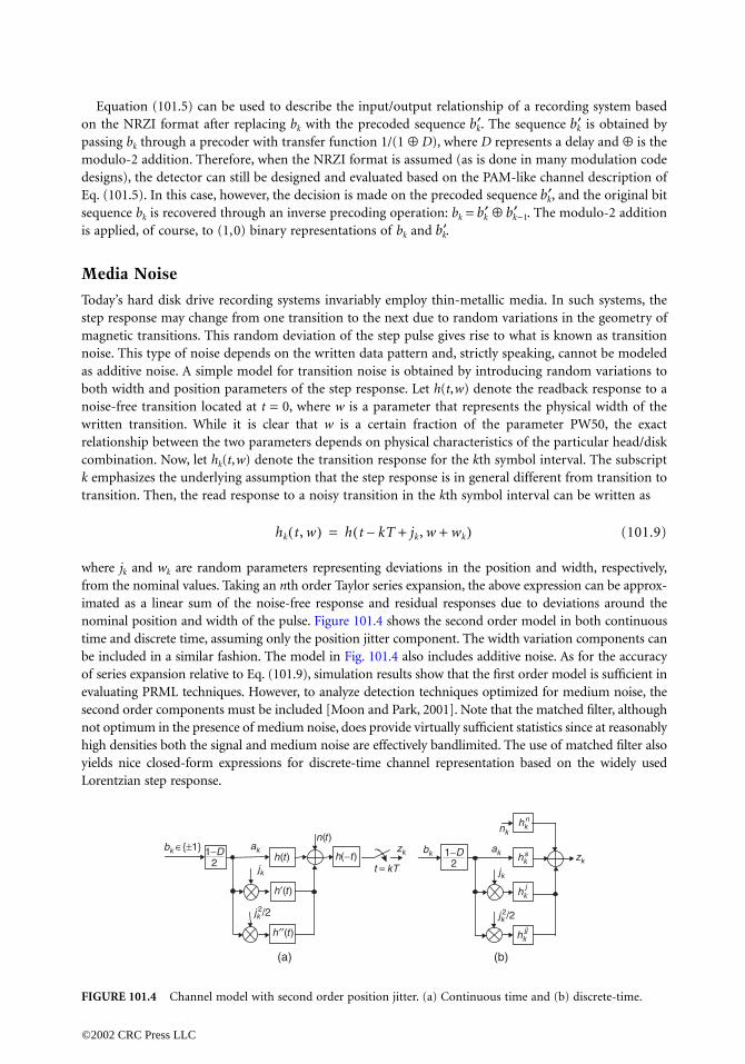
Equation (101.5) can be used to describe the input/output relationship of a recording system basedon the NRZI format after replacing bk with the precoded sequence . The sequence is obtained bypassing bk thmodulo-2 addesigns), theEq. (101.5). sequence bk is applied, o

Media No

Today’s hardstep responsmagnetic tranoise. This tas additive nboth width noise-free trwritten tranrelationshipcombinationk emphasizetransition. T

where jk andfrom the nomimated as a nominal postime and disbe included of series expevaluating Psecond ordernot optimumhigh densitieyields nice cLorentzian s

FIGURE 101.

b′k b′k


©2002 CRC P

rough a precoder with transfer function 1/(1 ⊕ D), where D represents a delay and ⊕ is thedition. Therefore, when the NRZI format is assumed (as is done in many modulation code detector can still be designed and evaluated based on the PAM-like channel description ofIn this case, however, the decision is made on the precoded sequence , and the original bitis recovered through an inverse precoding operation: bk = ⊕ . The modulo-2 additionf course, to (1,0) binary representations of bk and .

ise

disk drive recording systems invariably employ thin-metallic media. In such systems, thee may change from one transition to the next due to random variations in the geometry ofnsitions. This random deviation of the step pulse gives rise to what is known as transitionype of noise depends on the written data pattern and, strictly speaking, cannot be modeledoise. A simple model for transition noise is obtained by introducing random variations to

and position parameters of the step response. Let h(t,w) denote the readback response to aansition located at t = 0, where w is a parameter that represents the physical width of thesition. While it is clear that w is a certain fraction of the parameter PW50, the exact

between the two parameters depends on physical characteristics of the particular head/disk. Now, let hk(t,w) denote the transition response for the kth symbol interval. The subscript

s the underlying assumption that the step response is in general different from transition tohen, the read response to a noisy transition in the kth symbol interval can be written as

(101.9)

wk are random parameters representing deviations in the position and width, respectively,inal values. Taking an nth order Taylor series expansion, the above expression can be approx-

linear sum of the noise-free response and residual responses due to deviations around theition and width of the pulse. Figure 101.4 shows the second order model in both continuouscrete time, assuming only the position jitter component. The width variation components canin a similar fashion. The model in Fig. 101.4 also includes additive noise. As for the accuracyansion relative to Eq. (101.9), simulation results show that the first order model is sufficient inRML techniques. However, to analyze detection techniques optimized for medium noise, the components must be included [Moon and Park, 2001]. Note that the matched filter, although in the presence of medium noise, does provide virtually sufficient statistics since at reasonably

s both the signal and medium noise are effectively bandlimited. The use of matched filter alsolosed-form expressions for discrete-time channel representation based on the widely usedtep response.

4 Channel model with second order position jitter. (a) Continuous time and (b) discrete-time.

b′kb′k b′k−1

b′k

hk t, w( ) h t kT– jk, w wk+ +( )=

jk

akbk ∈{±1} zk

n(t)

h(−t)h(t)

h′(t)

h ′′(t)

kTt =1−D

2

jk2/2

jk

ak

nk

bk zk1−D

2

jk2/2

hkjj

hkj

hks

hkn

(a) (b)

ress LLC

Nonlinearity

The above channel model assumes that the signal portion of the received waveform can be constructedfrom linear start to intershift in transthe head fieltransition asThus, a tranin the previoapproach eavoltage, thisis a repeatabseries. Othestanding of are geared ssystems, nonshifts.

101.3 S

Care must bvarious codiratio, whichPart of the rnor peak) cfact that thedensity.

SNR Defi

First consid(AWGN) annoise spectrarates. Assumthe ratio

where Es is tis sometimeto the rate o

The magntransition rehead/mediuto medium SNR of an o


©2002 CRC P

superposition of isolated step responses. However, as density increases, nearby transitionsact, resulting in significant nonlinear distortion. An important source of nonlinearity is theition positions, which occurs as the demagnetizing field of the previous transition influences

d writing the current transition. Another type of nonlinearity is the broadening of the current the head field gradient is reduced by the demagnetizing field from a previous transition.

sition is shifted earlier in time and tends to broaden due to the effect of the transition writtenus symbol interval. Yet another form of nonlinearity, which becomes significant as transitionsch other even more closely, corresponds to partial erasure of adjacent transitions. In the read appears as a sudden reduction of the signal amplitude. Unlike transition noise, nonlinearityle phenomenon. The nonlinear distortion can be characterized using the Volterra functionalr nonlinearity characterization methods exist which rely more heavily on physical under-the write process. While different signal processing techniques have been developed whichpecifically toward nonlinearity, they are mostly exploratory at present. In today’s recordinglinear precompensation is aimed only at mitigating pattern-dependent transition position

NR Definition and Code Rate Penalty

e taken in defining the signal to noise ratio (SNR) that can provide a basis for comparingng and modulation strategies that operate at different symbol rates or densities. The Eb /No

is universally used in power-constraint communication channels, cannot be employed here.eason is that saturation recording is not a power-constrained (in the sense of neither averagehannel. Furthermore, finding the right SNR definition is particularly confusing due to the statistical properties of medium noise depend on the written pattern as well as the symbol

nition in AWGN

er only additive noise. In communication channels with additive white Gaussian noised an average transmitter power constraint, the Eb /No ratio, the information bit energy tol height ratio, can be used to compare coding/modulation schemes based on different symboling the transmitted symbol is binary, the symbol error probability is mainly determined by

(101.10)

he symbol energy, r is the code rate, and Ps denotes the average transmitter power. This ratios referred to as the detection SNR. For a given Eb /No ratio, the detection SNR is proportionalf the code r.etic recording channel should be viewed as the h(t)-constrained channel, where h(t) is thesponse discussed above; there is no average or peak power constraint here, but for a givenm interface, h(t) is fixed and coding and signal processing engineers must live with it. At lowrecording densities (where single errors are more likely than multiple errors), the detectionptimal sequence detector is given by

(101.11)

βcom

Es

No

------rEb

No

-------Ps

No/T------------= = =

βmag

∫ ∞–

∞h t( ) h t T–( )–[ ]2 td

4No

------------------------------------------------------=

ress LLC

For the Lorentzian channel, this reduces to

where Ds deEquation (1play the Eb /proportionarecording thmultiple err

SNR Defi

The Et /N0 radependent c

where M0 isM0, and α de

We can furtSNR reducetransition, th

where the stto assume thamong transthen the tota

and M0 can noise for thi

For the fi

∫ ∞–

∞nm

2 (t) t/d


©2002 CRC P

(101.12)

notes the symbol density defined as PW50/T and Du is the user density given by r ⋅ Ds.01.12) suggests that Et /No, the isolated transition pulse energy to noise spectral height ratio,No-like role for magnetic recording. It can be seen that for a given Eb /No, βmag is roughlyl to r2 (assuming >> r2), indicating that the code rate penalty is more severe with magnetican with the average-power-constrained communication channel. At high densities where

ors dominate, βmag drops even faster than r2.

nition in the Presence of Transition Noise

tio, however, does not provide a meaningful SNR definition when noise includes a signal-omponent. The following SNR definition can handle mixed noise channels:

(101.13)

twice the average energy of the medium noise associated with each transition, Nα = N0 +notes the medium noise power expressed as a percentage of the total in-band noise power, i.e.,

(101.14)

her write N0 = [(100 − α)/100]Nα and M0 = (α/100)Nα with 0 ≤ α ≤ 100. With α = 0, thes to Et /N0. Letting nm(t) denote the medium noise voltage waveform associated with a given

e average medium noise energy per transition can be defined as

(101.15)

atistical average is taken over transitions written at different positions in the disk. It is safeat the right hand side of Eq. (101.15) is finite. If the medium noise is statistically independentitions (as in the case of disks exhibiting a linear increase of noise power vs. linear density),l medium noise power arising from the all-transitions (or 1T) pattern is easily shown to be

. This means that

(101.16)

be viewed as the equivalent (single-sided) band-limited white noise spectrum of the mediums pattern.rst-order position jitter and width variation (1PW) noise model, M0 can be written as

(101.17)

βmag1

Ds2 1+

---------------Et

No

------⋅ r2

Du2 r2+

----------------Et

No

------⋅= =

Du2

SNREt

N0 M0+-------------------

Et

Nα------= =

αM0

N0 M0+------------------- 100×=

M0/2 nm2 t( ) td

∞–

∞

∫=

T

M0

2T------- total medium noise power in 1T pattern( )=

M0 2σ j2It 2σ w

2 Iw+=

ress LLC

where and are the variances of position jitter and width variation, respectively, and

With the ab[assuming hlation or anais known, prspecified, onoperating at of the symbthat the Et /Nsystems whechannel and

As a point oEPR4ML wiwith medium

101.4 C

The magnetfor ISI chanfeedback eqeliminate ercannot be useems that thheads and m

A well-kntechnique, wbasic idea ofequalizer, wh(1 + D)n po1987]. The correspondinatural chansignal levelscombined w

FIGURE 101.

σ j2 σ w

2

∞


©2002 CRC P

(101.18)

(101.19)

ove definitions, specifying Et /Nα with a particular value of α determines both No and M0

(t, w) is given as well]. Once M0 is determined, the noise parameters necessary for BER simu-lysis are specified. For example, with the 1PW model, both and are specified once M0

ovided the ratio / is also known. Once No, , and as well as the symbol period aree can proceed with performance analysis or BER simulations to compare codes/detectorsdifferent symbol or user densities. Note that the key assumption here is that M0 is independentol period T so that the noise composition parameter α is also independent of T. This means

α definition is free of symbol density, as desired. This assumption will hold for any recordingre the total integrated medium noise power increases linearly with 1/T. For the Lorentzian assuming w = PW50/2, it can be shown that

(101.20)

f reference, to meet a 10−5 target BER for the 1PW Lorentzian channel at user density 2.5,th a rate 16/17 RLL code requires an Et /No slightly above 24 dB and an Et /N90 around 23 dB

noise comprised only of independent position jitter.

oding and Detection

ic recording channel can be characterized as a severe ISI channel. It has been suggested thatnels, the capacity can be approached through coding with the relatively simple decision

ualizer (DFE) replacing complex sequence detectors and utilizing transmitter precoding toror. However, transmitter precoding is applicable only to multi-level input channels andsed for modern magnetic storage channels, which are binary-input channels. At present, ite only way to utilize a considerable fraction of the channel capacity available from the givenedia technologies is to rely on some type of sequence detection. own example of the application of a sequence detector to magnetic storage is the PRMLhich combines Viterbi detection with partial response linear equalization [Fisher, 1996]. The the PRML method is illustrated in Fig. 101.5. The sampled read signal is applied to a linearich forces the transfer function of the combined channel filter and equalizer to a (1 − D) ×

lynomial, where D represents a symbol delay and n is a positive integer [Thapar and Patel,equalizer output signal is then fed to the Viterbi detector tuned to the ISI coefficientsng to the (1 − D)(1 + D)n target function. While offering a reasonably good match to thenel response, this particular family of target functions yields a smaller number of distinct

at the equalizer output than more general target functions with the same ISI length. This,ith the feature that the signal levels are integer-valued, significantly reduces the number of

5 Partial response maximum likelihood (PRML) detection.

It ∂h/∂t[ ]2 td∞–∫=

Iw ∂h/∂w[ ]2 td∞–

∞

∫=

σ j2 σ w

2

σ j2 σ w

2 σ j2 σ w

2

It Iw

2Et

PW502-----------------= =

filtered & sampledread signal

Viterbi detectortuned to

equalized PR channel

Partial responselinear equalizer

ress LLC

multiplies required in the implementation of the Viterbi detector. In the absence of noise enhancementand noise correlation, the Viterbi detector will perform maximum likelihood detection. But, there is anobvious lossand the natufractional copossible, sucdone using asampling ocare stored ina constant atravels fromacross the enis called zonpractical readivided intoin practice, tas the head

The State

Although vais based on eincorporatinconstraint lipoint to aid (1 − D)(1 + user data (asuser blocks aan increasedthis strategycontaminateblocks if it othe error cocheck (SPC)constructed 32/33 (0,k +

The singlnumber of Nindeed reprebe used to hwhenever tha list of likeWhen the paactual patteaccordingly.the corresporequired har

Another aconstraint inrecent inputparity constr


©2002 CRC P

of optimality associated with the PR equalizer. A close match between the target functionral channel will make this loss small. For this reason, more general PR targets that allowefficients are also being considered. Other types of PR targets with integer-coefficients areh as (1 − D)(1 + D)(2 + 2D + D2) considered in Conway [1998]. Equalization is typically finite impulse response (FIR) digital filter, but it can also be done in continuous time beforecurs. In disk drives, equalizers are typically trained at the factory floor and the trained taps shift registers that reside within the read channel IC. In disk recording, as the disk spins at

ngular velocity, the linear velocity of the head relative to the data track is reduced as the head the inner tracks to the outer ones. Despite this, storage density is kept more or less constanttire surface of the platter by forcing the data rate to increase at outer tracks. This technology

e bit recording (ZBR) and is crucial in achieving the maximum possible storage density. Forsons, however, the data rate is not allowed to change in every track; rather, entire tracks are a number of bands and the data rate changes only from one band of tracks to another. Thus,he equalizer taps are trained and stored for each band separately. At the time of data retrieval,travels to the target track, the right set of taps is loaded from the shift register.

-of-the Art Detector: EPR4ML Combined with Parity Code

riations exist, it is fair to say that the current industry standard in the read channel architecturextended class IV (EPR4) equalization followed by the Viterbi algorithm (dubbed EPR4ML),g a single bit parity code on top of the usual (0,k) runlength-limited (RLL) code. The (0,k)

mits the runs of consecutive NRZI 0s to k to ensure frequent non-zero signal levels at the readgain control and timing recovery [Siegel and Wolf, 1991]. EPR4 equalization is based on theD)2 target polynomial. The basic RLL code is a block code that converts one or two bytes of well as the RS parity bits) to 9 or 17 bit-long codewords, respectively. In some cases, uncodedre interspersed among the RLL codewords to effectively raise the code rate at the expense of k parameter. In addition to allowing a lower complexity encoder/decoder for a given rate, mitigates error propagation associated with long codewords. A single error event typicallys the whole code block after modulation decoding, but it may also corrupt two consecutiveccurs on the codeword boundary. As the block gets large, error propagation will underminerrection capability of the outer RS code. Once the RLL code is determined, a single parity bit is appended to each RLL codeword. For example, a rate 32/34 RLL/SPC code can beby first attaching two uncoded user bytes to a 16/17 (0,k) RLL code to effectively form a rate 16) RLL code and then appending a single parity bit to the resulting RLL codeword. e bit parity is able to detect isolated occurrences of all error events consisting of an oddRZ bit errors, such as ±{2}, ±{2, −2, 2},±{2, −2, 2, −2, 2}, and so on. These types of error eventssent the errors frequently observed in high density recording. Two different methods mayandle detected errors. One way is to add a post processor that attempts to correct errorse error flag is raised [Conway, 1998]. The attempt for error correction is based on keepingly error patterns and their associated metrics for all positions within the parity code block.rity is violated at the end of a given block, the post processor identifies the position and the

rn of the most likely error event from the stored list and attempt to correct the error The metric or the likelihood of a candidate error pattern can easily be obtained by correlatingnding noiseless signal pattern with the noisy received signal [Conway, 1998]. While thedware complexity is relatively small with this approach, associated latency may be an issue. pproach to error correction for the single parity code is to directly incorporate the parity the Viterbi trellis. In the conventional EPR4 trellis, the state at time k is given by three most bits {bk−1, bk−2, bk−3}. With binary inputs, this gives rise to an 8-state trellis. With the singleaint, however, the state is completely specified by {bk−1, bk−2, bk−3; S}, where S is the modulo-2

ress LLC

running sum of input bits since the beginning of the block. At the end of each block, S is forced to take oneither 1 or 0, depending on the type of parity imposed. The result is a time-varying trellis that starts with8-states at ththe end of thpost processdepending oparity code t

Attempts the detectorerror propag

Post ECC

It is importaideal metricrate (SRR), any reread. Wa BER to anbyte error stinner codingmore or lesstend to prodwith burst ereasons whysearch with commercial nificant SNRwell suited togains over P

Distance

It is easy to way of ensuris the maximcode is to elthe MTR coding current event that coclass of neadistance-enhMTR codescrowded tranthe rate 4/5 to the magn


©2002 CRC P

e beginning of each parity code block, grows to 16 states, and then reduces back to 8 states ate block. While the difference may be small, this approach yields a better performance than the

or technique since the probability of miscorrection is smaller. Although the actual gain variesn the channel properties including operating linear density and noise characteristics, the singleypically provides a dB or so SNR gain. have been made to use more than one parity bit, but the additional SNR gain observed at

output tends to disappear at the output of the RS decoder. The reason might be the increasedation associated with multiple parity bits [Feng et al., 2000].

Performance Metric

nt to realize that the performance measure based on detector symbol error rates is not the for the read channel reliability. A more meaningful performance metric is the sector retrythe probability that the RS code fails to correct all the errors in a sector before attempting

hen the byte errors observed at the detector output are independent, the translation from SRR is straightforward using the binomial probability distribution for the byte errors. If theatistics are the same for all code/detector strategies, the BER can be used to rank different/detection strategies since the SNR gain of one scheme over another at a given BER remains intact at the corresponding SRR level. However, in reality certain read channel strategiesuce more burst errors than others. Since the RS code performance degrades more rapidly

rrors, a BER level gain does not necessarily translate to an SRR level gain. This is one of the feedback-based detectors such as the DFE [Tyner and Proakis, 1993] and fixed delay treedecision feedback (FDTS/DF) [Moon and Carley, 1990] have not found much success inapplications so far. These techniques are prone to error propagation, although they offer sig- advantages over PRML techniques at a given BER. While feedback-based detectors are not the ECC parameters of today’s hard disk systems, they can provide meaningful performance

RML techniques with more aggressive ECC parameters.

-Enhancing Codes

see that the single bit parity code itself does not have any error correction capability. Oneing that given types of error events never occur is to apply a constrained code. One exampleum transition run (MTR) code [Moon and Brickner, 1996]. The basic idea of the MTR

iminate critical bit patterns that cause most errors in sequence detectors. More specifically,e eliminates input patterns that contain j or more consecutive transitions in the correspond-

waveform. As a result, for j = 2, the NRZ error events of the form ±{2, −2, 2} (and any errorntains this pattern) are eliminated. This substantially improves the performance of a broad

r-optimal sequence detectors at high linear densities. The code can be viewed as having aancing property for high linear density recording. In addition to enhancing distances, the

are useful in controlling nonlinearities and other write-side anomalies associated withsitions. As a simple example of an MTR code with j = 2, 16 codewords required to implement

block code are given in Table 101.1. The NRZI format is assumed in mapping the codewordsetization waveform. It can be seen that consecutive runs of 1s are limited to 2 both within

TABLE 101.1 Codewords for a Rate 4/5 MTR Block Code with k = 8

00001 00110 01100 1001000010 01000 01101 1010000100 01001 10000 1010100101 01010 10001 10110

ress LLC

the codewords and at the codeword boundaries. The runs of consecutive 0s are also limited (to 8 in thisexample) for timing recovery purposes. Bit error rate (BER) simulation results indicate that the MTRcode can yiePRML and Fencoding strbeen design[Fitzpatrick,

There alsohigh-order Pcomprehens

101.5 G

In order forread channeyield large SN

Low Den

As in a widecommunity Fan et al., 1Unlike turbosolution to the decodin

Figure 10density of 2of the code column weigmation is gebelief-propathe LDPC dnoise [in themedium no

FIGURE 101.


©2002 CRC P

ld significant performance improvement over the uncoded case when used with high-orderDTS detectors. The rate 6/7 MTR j = 2 code has been constructed using a state-dependentategy [Brickner and Moon, 1997]. A higher-rate location-dependent MTR code has also

ed which allows three or more consecutive transitions starting at every other bit position 1997]. exist other types of code constraints that posses similar distance-enhancing properties forRML and other ISI channels. For the interested reader, Karabed et al. [1999] provides a

ive treatment on general distance-enhancing codes for severe ISI channels.

limpse of the Future

the data storage industry to sustain the growth rate trend in density, it is important that thel provides substantial SNR gains in future storage systems. Two techniques that will potentially

R gains are low density parity check (LDPC) codes and pattern-dependent noise prediction.

sity Parity Check Codes

variety of communication channels, there is considerable interest in the magnetic recordingin employing turbo [Berrou et al., 1993; Ryan et al., 1998] or LDPC codes [Gallager, 1962;999] to data storage devices. This interest is driven by the promise of very large SNR gain. codes, LDPC codes do not seem to exhibit error floors and, thus, may offer a more attractive

storage systems where the error rate requirements are very low. Also, the overall latency ing operation is considerably smaller in LDPC codes. 1.6a shows the BER simulation results of uncoded EPR4ML vs. LDPC coded EPR4 at a user.5, assuming the noise is 100% AWGN. The Lorentzian step response is assumed. The rateis 8/9, and the frame length is about 5000 bits. The encoder is an irregular LDPC code withht four and an overlap constraint that removes the length-4 cycles. The soft channel infor-nerated using the forward-backward trellis search algorithm. The decoder is based on thegation/message-passing algorithm. There is no iteration between the channel detector andecoder. Figure 101.6b shows similar curves except that the medium noise is 90% of the total sense of Eq. (101.14)]. It can be seen that the relative gain of the LDPC code is larger with

ise than with additive noise. Results on turbo code suggest similar gains.

6 BER vs. SNR for (a) 100% AWGN and (b) 10% AWGN/90% medium noise (all position jitter).

Uncoded

LDPC−2

−3

−4

−5

−1

17 19 21 23 25

log10(BER)

Et/N0 (dB)

16 18 20 22 24−5

−4

−3

−2

Uncoded

log10(BER)

Et/N90 (dB)

LDPC

(a) (b)

ress LLC

Both fundamental and practical issues must be addressed to overcome major obstacles in employingthese types of codes in real storage systems. With turbo or LDPC coding, a large coding gain is achievedonly when tthe sector faLDPC codeswithout furtsystems are rates of typiIn light of reet al., 2000]bounds, althWith the strthese codes mentation. TLDPC code,As for decodmessage-pashigh. Variatipossible. Oncan be viewtecture optioalgorithm [O

Another rized. Thermlead to totallnot fail in thare needed i

Pattern-D

Unless the cthe severe rachieve an Sthere is a sidirection is t1997; Kavcicthe noise pothe pattern-each branchmedium nofuture high

101.6 O

Although nohead over ththe processina major sourcomponentstape, signal


©2002 CRC P

he block size becomes comparable to the present sector size of 512 K bytes. In disk drives,ilure rate is more important than the BER. This means that the block error rate of turbo or must be low enough to meet the demanding reliability requirement of storage systemsher error correction. Therefore, the error flooring effects that are common in turbo codedsimply not acceptable here. As computer simulation is not feasible at the low target errorcal disk drives, the performance must be reasonably ensured using error bound approaches.cent developments in algebraic LDPC codes with known minimum distance properties [Kou, it might be possible to ensure a desired level of error probability through analytical errorough more work is needed in this direction. Another issue is the implementation complexity.ingent power and speed constraint, the complexity is a major obstacle to the deployment ofin commercial storage devices. Efforts must be directed to both decoder and encoder imple-

he encoder complexity, which is a major issue in the implementation of Gallager’s original seems to be no longer a problem with, for example, the cyclic encoder of Kou et al. [2000].ing, while the implementation speed can be made extremely fast using the inherently parallelsing algorithm, the complexity is proportional to the frame length and can be excessivelyons of the turbo/LDPC code that allow both practical encoding and decoding may also bee example is a turbo product code based on the single parity constituent codes. This code

ed as an LDPC code whose generator matrix is also sparse, allowing flexible decoder archi-ns ranging from a serial forward-backward operation to a massively parallel message-passingenning and Moon, 2001].

emaining question is robustness. Not all recording channel impairments are well character-al asperity and offtrack interference are just two examples of channel disturbances that cany unexpected results on read channel performance testing. It is important that the code doese presence of some unforeseen disturbances. Performance verification and sensitivity studiesn the presence of thermal asperity, offtrack, and nonlinearity.

ependent Noise Prediction

ode is extremely powerful as in turbo and LDPC coded systems, it is difficult to overcomeate penalty of the magnetic channel. In light of this observation, one effective strategy toNR gain is to improve the detector capability. Especially when medium noise dominates,gnificant room for improvement in detection performance. A viable strategy along thiso incorporate pattern-dependent noise prediction into the Viterbi algorithm [Caroselli et al., and Moura, 2000; Moon and Park, 2001]. This approach is based on the observation thatwer changes from one branch (state-transition) to the next in the Viterbi trellis because ofdependent nature of medium noise. It can be shown that if the noise can be predicted on separately based on predetermined local noise statistics, the overall immunity against

ise can be improved significantly. This method is particularly promising in the design ofdensity storage systems where medium noise is likely to be a major limiting factor.

ther Considerations

t discussed here, servo signal processing is important to achieve accurate positioning of thee given track. As track density increases, data written in adjacent tracks may interfere withg of the main track signal. This type of interference, called offtrack interference, may becomece of errors in future storage systems. Gain control and timing recovery loops are also critical in the overall read channel design. In storage systems that employ flexible media such asfades due to medium asperity and mechanical fluctuation of head-tape spacing can be a

ress LLC

major cause of errors. For these channels, requirements on equalization and ECC can be considerablydifferent from the hard disk channel.

101.7 S

A brief descdependent tmagnetic stodiscussed.

Reference

Berrou, C., decod

Brickner, B. 33(5).

Caroselli, J.,system

Conway, T. 1IEEE

Fan, J. L., Kustorag

Feng, W., Virecord

Fisher, K. D.capac

Fitzpatrick, Tel. C

Gallager, R. Karabed, R.

intersKavcic, A. a

InformKou, Y., Lin

rediscMoon, J. an

MagnMoon, J. and

IEEE Moon, J. an

IEEE Oenning, T.

singleRyan, W., M

PR4-eSiegel, P. H.

29(12Thapar, H. a

magnTyner, D. J. a

chann


©2002 CRC P

ummary

ription is given on the characteristics of the magnetic recording channel including signal-ransition noise and nolinearity. Some of the coding and detection techniques of today’srage systems are reviewed. Future possibilities for the read channel strategy also have been

s

Glavieux, A., and Thitimajshima, P. 1993. Near Shannon limit error-correcting coding anding: turbo-codes. Proc. IEEE Intl. Conf. Commun., Geneva, May, 1064.and Moon, J. 1997. Design of a rate 6/7 maximum transition run code. IEEE Trans. Magnet.,

Altekar, S. A., McEwen, P., and Wolf, J. K. 1997. Improved detection for magnetic recordings with media noise. IEEE Trans. Magnet., 33(5), 2779.998. A new target response with parity coding for high density magnetic recording channels.

Trans. Magnet., 34(4), 2382.rtas, E., Friedman, A., and McLaughlin, S. 1999. Low-density parity-check codes for magnetice. Allerton Conference, Sept.tyaev, A., Burd, G., and Nazari, N. 2000. On the performance of parity codes in magneticing systems. Proc. IEEE Global. Tel. Comm. Conf., Abbott, W. L., Sonntag, J. L., and Nelson, R. 1996. PRML detection boosts hard-disk driveity. IEEE Spectrum, 70.K. K. 1997. Time-varying MTR codes for high density magnetic recording. Proc. IEEE Global.omm. Conf.G. 1962. Low-density parity check codes. IRE Trans. Inform. Theory, IT-8, 21., Siegel, P. H., and Soljanin, E. 1999. Constrained coding for binary channels with highymbol interference. IEEE Trans. Inform. Theory, 45(6), 1777.nd Moura, J. M. F. 2000. The Viterbi algorithm and Markov noise memory. IEEE Trans.. Theory, 46, 291.

, S., and Fossorier, M. 2000. Low-density parity-check codesbased on finite geometries: aovery. Proc. IEEE Int. Symp. on Inform. Theory.d Brickner, B. 1996. Maximum transition run codes for data storage systems. IEEE Trans.et., 32(5). Carley, L. R. 1990. Performance comparison of detection methods in magnetic recording.

Trans. Magnet., 26(6), 3155.d Park, J. 2001. Near-maximum likelihood sequence detection in pattern dependent noise.J. Sel. Areas Commun., to appear. and Moon, J. 2001. A low density generator matrix interpretation of parallel concatenated bit parity codes. IEEE Trans. Magnet.cPheters, L., and McLaughlin, S. 1998. Combined turbo coding and turbo equalization forqualized Lorentzian channels. Proc. Conf. on Information Systems and Sciences.and Wolf, J. K. 1991. Modulation and coding for information storage. IEEE Commun. Mag.,), 68.nd Patel, A. M. 1987. A class of partial response systems for increasing storage density in

etic recording. IEEE Trans. Magnet., 23(5).nd Proakis, J. G. 1993. Partial response equalizer performance in digital magnetic recordingels. IEEE Trans. Magnet., 29(6), 4194.

ress LLC

Further Information

For a comprehensive treatment on constrained codes used for data storage channels, see Codes for MassData Storagmagnetic reand audio rDaniel, Secoprocessing iCommunicaAlso, each ymunicationsissue of the ference on processing isis devoted tprocessing wissue of the


©2002 CRC P

e Systems, K. A. S. Immink, Shannon Foundation Publishers, 1999. For an overview ofcording technology including computer tape and disk recording as well as consumer videoecording, consult Magnetic Recording Technology and Magnetic Storage Handbook, Mee andnd Edition, McGraw-Hill, 1996. For more detailed information on some coding and signaldeas for data storage, see the January 1992 issue of the IEEE Journal on Selected Areas intions. A new JSAC issue devoted to the same topic will appear sometime early in the year 2001.ear, the Global Telecommunications Conference and the International Conference on Com- run sessions dedicated to data storage. In addition, either the September or the NovemberIEEE Transactions on Magnetics includes papers presented at the annual International Con-Magnetics and contains a significant number of papers on communications and signalsues of data storage technology. Finally, every third year, the Magnetic Recording Conferenceo systems and signal processing issues for storage. The last TMRC dedicated to signalas in the year 2000, and some of the papers presented there appeared in the January 2001

IEEE Transactions on Magnetics.

ress LLC

102Magneto-Optical Disk

Data Storage

102.1 Introduction102.2 Preliminaries and Basic Definitions

The Concept of Track • Disk RotationSpeed • Access Time

102.3 The Optical PathCollimation and Beam-Shaping • Focusingby the Objective Lens

102.4 Automatic Focusing102.5 Automatic Tracking

Tracking on Grooved Regions • Sampled Tracking

102.6 Thermomagnetic Recording ProcessRecording by Laser Power Modulation(LPM) • Recording by Magnetic Field Modulation

102.7 Magneto-Optical ReadoutDifferential Detection

102.8 Materials of Magneto-Optical Data Storage

102.1 Introduction

Since the early 1940s, magnetic recording has been the mainstay of electronic information storageworldwide. Audio tapes provided the first major application for the storage of information on magneticmedia. Magnetic tape has been used extensively in consumer products such as audio tapes and videocassette recorders (VCRs); it has also found application in backup/archival storage of computer files,satellite images, medical records, etc. Large volumetric capacity and low cost are the hallmarks of tapedata storage, although sequential access to the recorded information is perhaps the main drawback of thistechnology. Magnetic hard disk drives have been used as mass storage devices in the computer industryever since their inception in 1957. With an areal density that has doubled roughly every other year, harddisks have been and remain the medium of choice for secondary storage in computers.1 Another magneticdata storage device, the floppy disk, has been successful in areas where compactness, removability, andfairly rapid access to the recorded information have been of prime concern. In addition to providingbackup and safe storage, inexpensive floppies with their moderate capacities (2 megabyte on a 3.5-in-diam platter is typical nowadays) and reasonable transfer rates have provided the crucial function of file/data transfer between isolated machines. All in all, it has been a great half-century of progress and market

1At the time of this writing, achievable densities on hard disks are in the range of 107 b/cm2. Random access toarbitrary blocks of data in these devices can take on the order of 10 ms, and individual read/write heads can transferdata at the rate of several megabits per second.

Masud MansuripurUniversity of Arizona


dominance for magnetic recording devices, which are only now beginning to face a potentially seriouschallenge from the technology of optical recording.

Like magnetic recording, a major application area for optical data storage systems is the secondarystorage of information for computers and computerized systems. Like the high-end magnetic media,optical disks can provide recording densities in the range of 107 b/cm2 and beyond. The added advantageof optical recording is that, like floppies, these disks can be removed from the drive and stored on theshelf. Thus, the functions of the hard disk (i.e., high capacity, high data transfer rate, rapid access) maybe combined with those of the floppy (i.e., backup storage, removable media) in a single optical diskdrive. Applications of optical recording are not confined to computer data storage. The enormouslysuccessful audio compact disc (CD), which was introduced in 1983 and has since become the de factostandard of the music industry, is but one example of the tremendous potential of the optical technology.

A strength of optical recording is that, unlike its magnetic counterpart, it can support read-only, write-once, and erasable/rewritable modes of data storage. Consider, for example, the technology of opticalaudio/video disks. Here the information is recorded on a master disk, which is then used as a stamperto transfer the embossed patterns to a plastic substrate for rapid, accurate, and inexpensive reproduction.The same process is employed in the mass production of read-only files [CD read only memory (CD-ROM), and optical ROM (O-ROM)], which are now being used to distribute software, catalog, and otherlarge data bases. Or consider the write-once read-many (WORM) technology, where one can permanentlystore massive amounts of information on a given medium and have rapid, random access to themafterwards. The optical drive can be designed to handle read only, WORM, and erasable media all in oneunit, thus combining their useful features without sacrificing performance and ease of use or occupyingtoo much space. What is more, the media can contain regions with prerecorded information as well asregions for read/write/erase operations, both on the same platter. These possibilities open new vistas andoffer opportunities for applications that have heretofore been unthinkable; the interactive video-disk isperhaps a good example of such applications.

In this chapter, we lay out the conceptual basis for optical data storage systems; the emphasis will beon disk technology in general and magneto-optical disk in particular. The next section is devoted to adiscussion of some elementary aspects of disk data storage including the concept of track and definitionof the access time. Section 102.3 describes the basic elements of the optical path and its functions; includedare the properties of the semiconductor laser diode, characteristics of the beam shaping optics, and certainfeatures of the focusing objective lens. Because of the limited depth of focus of the objective and theeccentricity of tracks, optical disk systems must have a closed-loop feedback mechanism for maintainingthe focused spot on the right track. These mechanisms are described in Sections 102.4 and 102.5 forautomatic focusing and automatic track-following, respectively. The physical process of thermomagneticrecording in magneto-optic (MO) media is described next, followed by a discussion of the MO readoutprocess in Section 102.7. The final section describes the properties of the MO media.

102.2 Preliminaries and Basic Definitions

A disk, whether magnetic or optical, consists of a number of tracks along which the information isrecorded. These tracks may be concentric rings of a certain width, Wt , as shown in Fig. 102.1. Neighboringtracks may be separated from each other by a guard band whose width we shall denote by Wg . In theleast sophisticated recording scheme imaginable, marks of length ∆0 are recorded along these tracks.Now, if each mark can be in either one of two states, present or absent, it may be associated with a binarydigit, 0 or 1. When the entire disk surface of radius R is covered with such marks, its capacity C0 will be

(102.1)

Consider the parameter values typical of current optical disk technology: R = 67 mm corresponding to5.25-in.-diam platters, ∆0 = 0.5 µm, which is roughly determined by the wavelength of the read/write laser

C0πR2

Wt Wg+( )∆0

------------------------------- bits per surface=


diodes, and Wt + Wg = 1 µm for the track-pitch. The disk capacity will then be around 28 × 109 b, or3.5 gigabytes. This is a reasonable estimate and one that is fairly close to reality, despite the many sim-plifying assumptions made in its derivation. In the following paragraphs, we examine some of theseassumptions in more detail.

The disk was assumed to be fully covered with information-carrying marks. This is generally not thecase in practice. Consider a disk rotating at N revolutions per second (r/s). For reasons to be clarifiedlater, this rotational speed should remain constant during the disk operation. Let the electronic circuitryhave a fixed clock duration Tc. Then only pulses of length Tc (or an integer multiple thereof) may beused for writing. Now, a mark written along a track of radius r, with a pulse-width equal to Tc, will havelength �, where

(102.2)

Thus, for a given rotational speed N and a fixed clock cycle Tc, the minimum mark length � is a linearfunction of track radius r, and � decreases toward zero as r approaches zero. One must, therefore, picka minimum usable track radius, rmin, where the spatial extent of the recorded marks is always greaterthan the minimum allowed mark length, ∆0 . Equation (102.2) yields

(102.3)

One may also define a maximum usable track radius rmax, although for present purposes rmax = R is aperfectly good choice. The region of the disk used for data storage is thus confined to the area betweenrmin and rmax. The total number N of tracks in this region is given by

(102.4)

The number of marks on any given track in this scheme is independent of the track radius; in fact, thenumber is the same for all tracks, since the period of revolution of the disk and the clock cycle uniquelydetermine the total number of marks on any individual track. Multiplying the number of usable tracks

FIGURE 102.1 Physical appearance and general features of an optical disk. The read/write head gains access to thedisk through a window in the jacket; the jacket itself is for protection purposes only. The hub is the mechanicalinterface with the drive for mounting and centering the disk on the spindle. The track shown at radius r0 is of theconcentric-ring type.

� 2π NrTc=

rmin

∆0

2πNTc

----------------=

Nrmax rmin–Wt Wg+-----------------------=


N with the capacity per track, we obtain for the usable disk capacity

(102.5)

Replacing for N from Eq. (102.4) and for N Tc from Eq. (102.3), we find

(102.6)

If the capacity C in Eq. (102.6) is considered a function of rmin with the remaining parameters heldconstant, it is not difficult to show that maximum capacity is achieved when

(102.7)

With this optimum rmin, the value of C in Eq. (102.6) is only half that of C0 in Eq. (102.1). In otherwords, the estimate of 3.5 gigabyte per side for 5.25-in disks seems to have been optimistic by a factorof two.

One scheme often proposed to enhance the capacity entails the use of multiple zones, where eitherthe rotation speed N or the clock period Tc are allowed to vary from one zone to the next. In general,zoning schemes can reduce the minimum usable track radius below that given by Eq. (102.7). Moreimportantly, however, they allow tracks with larger radii to store more data than tracks with smallerradii. The capacity of the zoned disk is somewhere between C of Eq. (102.6) and C0 of Eq. (102.1), theexact value depending on the number of zones implemented.

A fraction of the disk surface area is usually reserved for preformat information and cannot be usedfor data storage. Also, prior to recording, additional bits are generally added to the data for error-correction coding and other housekeeping chores. These constitute a certain amount of overhead onthe user data and must be allowed for in determining the capacity. A good rule of thumb is that overheadconsumes approximately 20% of the raw capacity of an optical disk, although the exact number mayvary among the systems in use. Substrate defects and film contaminants during the deposition processcan create bad sectors on the disk. These are typically identified during the certification process and aremarked for elimination from the sector directory. Needless to say, bad sectors must be discounted whenevaluating the capacity.

Modulation codes may be used to enhance the capacity beyond what has been described so far. Mod-ulation coding does not modify the minimum mark length of ∆0 but frees the longer marks from theconstraint of being integer multiples of ∆0. The use of this type of code results in more efficient datastorage and an effective number of bits per ∆0 that are greater than unity. For example, the popular (2, 7)modulation code has an effective bit density of 1.5 b per ∆0. This or any other modulation code canincrease the disk capacity beyond the estimate of Eq. (102.6).

The Concept of Track

The information on magnetic and optical disks is recorded along tracks. Typically, a track is a narrowannulus at some distance r from the disk center. The width of the annulus is denoted by Wt, whereas thewidth of the guard band, if any, between adjacent tracks is denoted by Wg. The track pitch is the center-to-center distance between neighboring tracks and is therefore equal to Wt + Wg. A major difference betweenthe magnetic floppy disk, the magnetic hard disk, and the optical disk is that their respective track-pitchesare presently of the order of 100, 10, and 1 µm. Tracks may be fictitious entities, in the sense that noindependent existence outside the pattern of recorded marks may be ascribed to them. This is the case,for example, with the compact audio disk format where prerecorded marks simply define their own

CN

NTc

---------=

C2πrmin rmax rmin–( )

Wt Wg–( )∆0

-------------------------------------------=

rmin12--rmax=


tracks and help guide the laser beam during readout. In the other extreme are tracks that are physicallyengraved on the disk surface before any data is ever recorded. Examples of this type of track are providedby pregrooved WORM and magneto-optical disks. Figure 102.2 shows micrographs from several recordedoptical disk surfaces. The tracks along which the data are written are clearly visible in these pictures.

It is generally desired to keep the read/write head stationary while the disk spins and a given track isbeing read from or written onto. Thus, in an ideal situation, not only should the track be perfectly circular,but the disk must also be precisely centered on the spindle axis. In practical systems, however, tracks areneither precisely circular, nor are they concentric with the spindle axis. These eccentricity problems aresolved in low-performance floppy drives by making tracks wide enough to provide tolerance for misreg-istrations and misalignments. Thus, the head moves blindly to a radius where the track center is nominallyexpected to be and stays put until the reading or writing is over. By making the head narrower than thetrack pitch, the track center is allowed to wobble around its nominal position without significantly

FIGURE 102.2 Micrographs of several types of optical storage media. The tracks are straight and narrow (trackpitch = 1.6 µm), with an orientation angle of �−45º. (a) ablative, write-once tellurium alloy; (b) ablative, write-once organic dye; (c) amorphous-to-crystalline, write-once phase-change alloy GaSb; (d) erasable, amorphousmagneto-optic alloy GdTbFe; (e) erasable, crystalline-to-amorphous phase-change tellurium alloy; and (f) read-onlyCD-audio, injection-molded from polycarbonate with a nickel stamper. (Source: Ullmann’s Encylopedia of IndustrialChemistry, 5th ed., Vol A14, VCH, Weinheim, 1989, 196. With permission.)


degrading the performance during the read/write operation. This kind of wobble, however, is unaccept-able in optical disk systems, which have a very narrow track, about the same size as the focused beamspot. In a typical situation arising in practice, the eccentricity of a given track may be as much as +50 µmwhile the track pitch is only about 1 µm, thus requiring active track-following procedures.

One method of defining tracks on an optical disk is by means of pregrooves that are either etched,stamped, or molded onto the substrate. In grooved media of optical storage, the space between neigh-boring grooves is the so-called land [see Fig. 102.3(a)]. Data may be written in the grooves with the landacting as a guard band. Alternatively, the land regions may be used for recording while the groovesseparate adjacent tracks. The groove-depth is optimized for generating an optical signal sensitive to theradial position of the read/write laser beam. For the push–pull method of track error detection, the groovedepth is in the neighborhood of λ/8, where λ is the wavelength of the laser beam.

In digital data storage applications, each track is divided into small segments or sectors intended forthe storage of a single block of data (typically either 512 or 1024 bytes). The physical length of a sectoris thus a few millimeters. Each sector is preceded by header information such as the identity of the sector,identity of the corresponding track, synchronization marks, etc. The header information may be prefor-matted onto the substrate, or it may be written on the storage layer prior to shipping the disk. Pregroovedtracks may be carved on the optical disk either as concentric rings or as a single continuous spiral. Thereare certain advantages to each format. A spiral track can contain a succession of sectors without inter-ruption, whereas concentric rings may each end up with some empty space that is smaller than therequired length for a sector. Also, large files may be written onto (and read from) spiral tracks withoutjumping to the next track, which occurs when concentric tracks are used. On the other hand, multiple

FIGURE 102.3 (a) Lands and grooves in an optical disk. The substrate is transparent, and the laser beam mustpass through it before reaching the storage medium. (b) Sampled-servo marks in an optical disk. These marks, whichare offset from the track-center, provide information regarding the position of focused spot.


path operations, such as write-and-verify or erase-and-write, which require two paths each for a givensector or still-frame video are more conveniently handled on concentric-ring tracks.

Another track format used in practice is based on the sampled-servo concept. Here the tracks are identifiedby occasional marks placed permanently on the substrate at regular intervals, as shown in Fig. 102.3(b).Details of track-following by the sampled-servo scheme will follow shortly; suffice it to say at this point thatservo marks help the system identify the position of the focused spot relative to the track-center. Once theposition is determined it is fairly simple to steer the beam and adjust its position.

Disk Rotation Speed

When a disk rotates at a constant angular velocity ω, a track of radius r moves with the constant linearvelocity V = rω. Ideally, one would like to have the same linear velocity for all of the tracks, but this isimpractical except in a limited number of situations. For instance, when the desired mode of access tothe various tracks is sequential, such as in audio and video disk applications, it is possible to place thehead in the beginning at the inner radius and move outward from the center thereafter while contin-uously decreasing the angular velocity. By keeping the product of r and ω constant, one can thus achieveconstant linear velocity for all of the tracks.* Sequential access mode, however, is the exception ratherthan the norm in data storage systems. In most applications, the tracks are accessed randomly with suchrapidity that it becomes impossible to adjust the rotation speed for constant linear velocity. Under thesecircumstances, the angular velocity is best kept constant during the normal operation of the disk. Typicalrotation speeds are 1200 and 1800 r/m for slower drives and 3600 r/m for the high-data-rate systems.Higher rotation rates (5000 r/m and beyond) are certainly feasible and will likely appear in future storagedevices.

Access Time

The direct-access storage-device (DASD) used in computer systems for the mass storage of digitalinformation is a disk drive capable of storing large quantities of data and accessing blocks of this datarapidly and in arbitrary order. In read/write operations, it is often necessary to move the head to newlocations in search of sectors containing specific data-items. Such relocations are usually time consumingand can become the factor that limits performance in certain applications. The access time τa is definedas the average time spent in going from one randomly selected spot on the disk to another. Also, τa canbe considered the sum of a seek time τs, which is the average time needed to acquire the target track, anda latency τl, which is the average time spent on the target track while waiting for the desired sector. Thus,

τa = τs + τl (102.8)

The latency is half the revolution period of the disk, since a randomly selected sector is, on the average,halfway along the track from the point where the head initially lands. Thus for a disk rotating at 1200 r/m,τl = 25 ms, whereas at 3600 r/m, τl � 8.3 ms. The seek time, on the other hand, is independent of therotation speed of the disk but is determined by the traveling distance of the head during an average seek,as well as by the mechanism of head actuation. It can be shown that the average length of travel in arandom seek is one-third of the full stroke. (In our notation, the full stroke is rmax – rmin.) In magneticdisk drives where the head/actuator assembly is relatively light-weight (a typical Winchester head weighsabout 5 g), the acceleration and deceleration periods are short, and seek times are typically around 10 msin small format drives (i.e., 5.25 and 3.5 in). In optical disk systems, on the other hand, the head, beingan assembly of discrete elements, is fairly large and heavy (typical weight � 100 g), resulting in values ofτs that are several times greater than those obtained in magnetic recording systems. The seek times reported

*In compact audio disk players, the linear velocity is kept constant at 1.2 m/s. The starting position of the headis at the inner radius rmin = 25 mm, where the disk spins at 460 r/m. The spiral track ends at the outer radius rmax =58 mm, where the disk’s angular velocity is 200 r/m.


for commercially available optical drives presently range from 20 ms in high performance 3.5-in. drivesto about 80 ms in larger (and slower) drives. We emphasize, however, that the optical disk technology isstill in its infancy; with the passage of time, the integration and miniaturization of the elements withinthe optical head will surely produce lightweight devices capable of achieving seek times of the order ofonly a few milliseconds.

102.3 The Optical Path

The optical path begins at the light source which, in practically all laser disk systems in use today, is asemiconductor GaAs diode laser. Several unique features have made the laser diode indispensable inoptical recording technology, not only for the readout of stored information but also for writing anderasure. The small size of this laser has made possible the construction of compact head assemblies, itscoherence properties have enabled diffraction-limited focusing to extremely small spots, and its directmodulation capability has eliminated the need for external modulators. The laser beam is modulated bycontrolling the injection current; one applies pulses of variable duration to turn the laser on and offduring the recording process. The pulse duration can be as short as a few nanoseconds, with rise andfall times typically less than 1 ns. Although readout can be accomplished at constant power level, thatis, in continuous wave (CW) mode, it is customary for noise reduction purposes to modulate the laserat a high frequency (e.g., several hundred megahertz during readout).

Collimation and Beam-Shaping

Since the cross-sectional area of the active region in a laser diode is only about 1 µm, diffraction effectscause the emerging beam to diverge rapidly. This phenomenon is depicted schematically in Fig. 102.4(a).In practical applications of the laser diode, the expansion of the emerging beam is arrested by a collimat-ing lens, such as that shown in Fig. 102.4(b). If the beam happens to have aberrations (astigmatism isparticularly severe in diode lasers), then the collimating lens must be designed to correct this defect as well.

In optical recording, it is most desirable to have a beam with circular cross-section. The need forshaping the beam arises from the special geometry of the laser cavity with its rectangular cross-section.Since the emerging beam has different dimensions in the directions parallel and perpendicular to thejunction, its cross-section at the collimator becomes elliptical, with the initially narrow dimensionexpanding more rapidly to become the major axis of the ellipse. The collimating lens thus produces abeam with elliptical cross-section. Circularization may be achieved by bending various rays of the beamat a prism, as shown in Fig. 102.4(c). The bending changes the beam’s diameter in the plane of incidencebut leaves the diameter in the perpendicular direction intact.

Focusing by the Objective Lens

The collimated and circularized beam of the diode laser is focused on the surface of the disk using anobjective lens. The objective is designed to be aberration free so that its focused spot size is limited onlyby the effects of diffraction. Figure 102.5(a) shows the design of a typical objective made from sphericaloptics. According to the classical theory of diffraction, the diameter of the beam, d, at the objective’sfocal plane is given by

(102.9)

where λ is the wavelength of light, and NA is the numerical aperture of the objective.*

*Numerical aperture is defined as NA = n sinθ, where n is the refractive index of the image space and θ is thehalf-angle subtended by the exit pupil at the focal point. In optical recording systems, the image space is air whoseindex is very nearly unity; thus, for all practical purposes NA = sinθ.

d � λNA--------


In optical recording it is desired to achieve the smallest possible spot, since the size of the spot isdirectly related to the size of marks recorded on the medium. Also, in readout, the spot size determinesthe resolution of the system. According to Eq. (102.9) there are two ways to achieve a small spot: first,by reducing the wavelength and second, by increasing the numerical aperture of the objective. Thewavelengths currently available from GaAs lasers are in the range of 670–840 nm. It is possible to use anonlinear optical device to double the frequency of these diode lasers, thus achieving blue light. Goodefficiencies have been demonstrated by frequency doubling. Also recent developments in II–VI materialshave improved the prospects for obtaining green and blue light directly from semiconductor lasers.Consequently, there is hope that in the near future, optical storage systems will operate in the wavelengthrange of 400–500 nm. As for the numerical aperture, current practice is to use a lens with NA � 0.5−0.6.Although this value might increase slightly in the coming years, much higher numerical apertures areunlikely, since they put strict constraints on the other characteristics of the system and limit the toler-ances. For instance, the working distance at high numerical aperture is relatively short, making access tothe recording layer through the substrate more difficult. The smaller depth of focus of a high numericalaperture lens will make attaining /maintaining proper focus more of a problem, whereas the limited

FIGURE 102.4 (a) Away from the facet, the output beam of a diode laser diverges rapidly. In general, the beamdiameter along X is different from that along Y, which makes the cross-section of the beam elliptical. Also, the radiiof curvature Rx and Ry are not the same, thus creating a certain amount of astigmatism in the beam. (b) Multielementcollimator lens for laser diode applications. Aside from collimating, this lens also corrects astigmatic aberrations ofthe beam. (c) Beam-shaping by deflection at a prism surface. θ1 and θ2 are related by Snell’s law, and the ratio d2 /d1

is the same as cosθ2 /cosθ1. Passage through the prism circularizes the elliptical cross-section of the beam.


field of view might restrict automatic track-following procedures. A small field of view also places con-straints on the possibility of read/write/erase operations involving multiple beams.

The depth of focus of a lens, δ, is the distance away from the focal plane over which tight focus canbe maintained [see Fig. 102.5(b)]. According to the classical diffraction theory,

(102.10)

Thus for a wavelength of λ = 700 nm and NA = 0.6, the depth of focus is about ±1 µm. As the diskspins under the optical head at the rate of several thousand revolutions per minute, the objective lensmust stay within a distance of f ± δ from the active layer if proper focus is to be maintained. Given theconditions under which drives usually operate, it is impossible to make rigid enough mechanical sys-tems to yield the required positioning tolerances. On the other hand, it is fairly simple to mount the

FIGURE 102.5 (a) Multielement lens design for a high numerical aperture video disc objective. (Source: Kuntz, D.1984. Specifying laser diode optics, Laser Focus, March. With permission.) (b) Various parameters of the objectivelens. The numerical aperture is NA = sinθ. The spot diameter d and the depth of focus δ are given by Eqs. (102.9)and (102.10), respectively. (c) Focusing through the substrate can cause spherical aberration at the active layer. Theproblem can be corrected if the substrate is taken into account in the design of the objective.

δ � λNA2----------


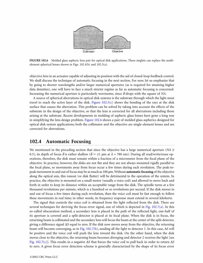
objective lens in an actuator capable of adjusting its position with the aid of closed-loop feedback control.We shall discuss the technique of automatic focusing in the next section. For now, let us emphasize thatby going to shorter wavelengths and/or larger numerical apertures (as is required for attaining higherdata densities), one will have to face a much stricter regime as far as automatic focusing is concerned.Increasing the numerical aperture is particularly worrisome, since δ drops with the square of NA.

A source of spherical aberrations in optical disk systems is the substrate through which the light musttravel to reach the active layer of the disk. Figure 102.5(c) shows the bending of the rays at the disksurface that causes the aberration. This problem can be solved by taking into account the effects of thesubstrate in the design of the objective, so that the lens is corrected for all aberrations including thosearising at the substrate. Recent developments in molding of aspheric glass lenses have gone a long wayin simplifying the lens design problem. Figure 102.6 shows a pair of molded glass aspherics designed foroptical disk system applications; both the collimator and the objective are single-element lenses and arecorrected for aberrations.

102.4 Automatic Focusing

We mentioned in the preceding section that since the objective has a large numerical aperture (NA ≥0.5), its depth of focus δ is rather shallow (δ � ±1 µm at λ = 780 nm). During all read/write/erase op-erations, therefore, the disk must remain within a fraction of a micrometer from the focal plane of theobjective. In practice, however, the disks are not flat and they are not always mounted rigidly parallel tothe focal plane, so movements away from focus occur a few times during each revolution. The peak-to-peak movement in and out of focus may be as much as 100 µm. Without automatic focusing of the objectivealong the optical axis, this runout (or disk flutter) will be detrimental to the operation of the system. Inpractice, the objective is mounted on a small motor (usually a voice coil) and allowed to move back andforth in order to keep its distance within an acceptable range from the disk. The spindle turns at a fewthousand revolutions per minute, which is a hundred or so revolutions per second. If the disk moves inand out of focus a few times during each revolution, then the voice coil must be fast enough to followthese movements in real time; in other words, its frequency response must extend to several kilohertz.

The signal that controls the voice coil is obtained from the light reflected from the disk. There areseveral techniques for deriving the focus error signal, one of which is depicted in Fig. 102.7(a). In thisso-called obscuration method, a secondary lens is placed in the path of the reflected light, one-half ofits aperture is covered and a split-detector is placed at its focal plane. When the disk is in focus, thereturning beam is collimated and the secondary lens will focus the beam at the center of the split detector,giving a difference signal ∆S equal to zero. If the disk now moves away from the objective, the returningbeam will become converging, as in Fig. 102.7(b), sending all the light to detector 1. In this case, ∆S willbe positive and the voice coil will push the lens toward the disk. On the other hand, when the diskmoves close to the objective, the returning beam becomes diverging and detector 2 receives the light [seeFig. 102.7(c)]. This results in a negative ∆S that forces the voice coil to pull back in order to return ∆Sto zero. A given focus error detection scheme is generally characterized by the shape of its focus error

FIGURE 102.6 Molded glass aspheric lens pair for optical disk applications. These singlets can replace the multi-element spherical lenses shown in Figs. 102.4(b) and 102.5(a).


signal ∆S vs. the amount of defocus ∆z ; one such curve is shown in Fig. 102.7(d). The slope of the focuserror signal (FES) curve near the origin is of particular importance since it determines the overallperformance and stability of the servo loop.

102.5 Automatic Tracking

Consider a track at a certain radial location, say r0, and imagine viewing this track through the accesswindow shown in Fig. 102.1. It is through this window that the head gains access to arbitrarily selectedtracks. To a viewer looking through the window, a perfectly circular track centered on the spindle axiswill look stationary, irrespective of the rotation rate. However, any eccentricity will cause an apparentradial motion of the track. The peak-to-peak distance travelled by a track (as seen through the window)depends on a number of factors including centering accuracy of the hub, deformability of the substrate,mechanical vibrations, manufacturing tolerances, etc. For a typical 3.5-in. disk, for example, this peak-to-peak motion can be as much as 100 µm during one revolution. Assuming a revolution rate of 3600 r/m,the apparent velocity of the track in the radial direction will be several millimeters per second. Now, if thefocused spot remains stationary while trying to read from or write to this track, it is clear that the beamwill miss the track for a good fraction of every revolution cycle.

Practical solutions to the described problem are provided by automatic tracking techniques. Here theobjective is placed in a fine actuator, typically a voice-coil, which is capable of moving the necessary

FIGURE 102.7 Focus error detection by the obscuration method. In (a) the disk is in focus and the two halves ofthe split detector receive equal amounts of light. When the disk is too far from the objective (b), or too close to it(c), the balance of detector signals shifts to one side or the other. A plot of the focus error signal (FES) vs. defocusis shown in (d), and its slope near the origin is identified as the FES gain G.


radial distances and maintaining a lock on the desired track. The signal that contols the movement ofthis actuator is derived from the reflected light itself, which carries information about the position ofthe focused spot. There exist several mechanisms for extracting the track-error signal (TES); all of thesemethods require some sort of structure on the disk surface in order to identify the track. In the case ofread-only disks (CD, CD-ROM, and video disk), the embossed pattern of data provides ample informa-tion of tracking purposes. In the case of write-once and erasable disks, tracking guides are carved on thesubstrate in the manufacturing process. As mentioned earlier, the two major formats for these trackingguides are pregrooves (for continuous tracking) and sampled-servo marks (for discrete tracking). Acombination of the two schemes, known as continuous /composite format, is often used in practice. Thisscheme is depicted in Fig. 102.8, which shows a small section containing five tracks, each consisting ofthe tail-end of a groove, synchronization marks, a mirror area used for adjusting focus/track offsets, apair of wobble marks for sampled tracking, and header information for section identification.

Tracking on Grooved Regions

As shown in Fig. 102.3(a), grooves are continuous depressions that are either embossed, etched, or moldedonto the substrate prior to deposition of the storage medium. If the data is recorded on the grooves, thenthe lands are not used except for providing a guard band between neighboring grooves. Conversely, theland regions may be used to record the information, in which case grooves provide the guard band.Typical track-widths are about one wavelength of the light. The guard bands are somewhat narrowerthan the tracks; their exact shape and dimensions depending on the beam size, the required track-servoaccuracy, and the acceptable levels of cross talk between adjacent tracks. The groove depth is usuallyaround one-eighth of one wavelength (λ/8), since this depth can be shown to give the largest TES in thepush–pull method. Cross-sections of the grooves may be rectangular, trapezoidal, or triangular.

When the focused spot is centered on the track, it is diffracted symmetrically from the two edges of thetrack, resulting in a balanced far-field pattern. As soon as the spot moves away from the center, the symmetrybreaks down and the light distribution in the far field tends to shift to one side or the other. A splitphotodetector placed in the path of the reflected light can therefore sense the relative position of the spotand provide the appropriate feedback signal. This strategy is depicted schematically in Fig. 102.9(a); alsoshown in the figure are intensity plots at the detector plane for light reflected from various regions ofthe disk. Note how the intensity shifts to one side or the other depending on the direction of motion of thespot.

Sampled Tracking

Since dynamic track runout is usually a slow and gradual process, there is actually no need for continuoustracking as done on grooved media.A pair of embedded marks, offset from the track center as in Fig. 102.3(b),can provide the necessary information for correcting the relative position of the focused spot. The reflectedintensity will indicate the positions of the two servo marks as two successive short pulses. If the beam happensto be on track, the two pulses will have equal magnitudes and there shall be no need for correction. If, onthe other hand, the beam is off track, one of the pulses will be stronger than the other. Depending on whichpulse is the strong one, the system will recognize the direction in which it has to move and will correct theerror accordingly. The servo marks must appear frequently enough along the track to ensure proper track

FIGURE 102.8 Servo fields in continuous/composite format contain a mirror area and offset marks for tracking.(Source: Marchant, A.B. 1990. Optical Recording, Addison–Wesley, Reading, MA, 264. With permission.)


following. In a typical application, the track might be divided into groups of 18 bytes, 2 bytes dedicatedas servo offset areas and 16 bytes filled with other format information or left blank for user data.

102.6 Thermomagnetic Recording Process

Recording and erasure of information on a magneto-optical disk are both achieved by the thermomag-netic process. The essence of thermomagnetic recording is shown in Fig. 102.10. At the ambient tem-perature, the film has a high magnetic coercivity* and, therefore, does not respond to the externallyapplied field. When a focused beam raises the local temperature of the film, the hot spot becomesmagnetically soft (i.e., its coercivity drops). As the temperature rises, coercivity drops continuously untilsuch time as the field of the electromagnet finally overcomes the material’s resistance to reversal andswitches its magnetization. Turning the laser off brings the temperatures back to normal, but the reverse-magnetized domain remains frozen in the film. In a typical situation in practice, the film thickness maybe around 300 Å, laser power at the disk 10 � mW, diameter of the focused spot �1 µm, laser pulseduration �50 ns, linear velocity of the track �10 m/s, and the magnetic field strength �200 G. Thetemperature may reach a peak of 500 K at the center of the spot, which is sufficient for magnetization

FIGURE 102.9 (a) Push–pull sensor for tracking on grooves. (Source: Marchant, A.B. 1990. Optical Recording,Addison–Wesley, Reading, MA, 1990, 175. With permission.) (b) Calculated distribution of light intensity at thedetector plane when the disk is in focus and the beam is centered on track. (c) Calculated intensity distribution atthe detector plane with disk in focus but the beam centered on the groove edge. (d) Same as (c) except for the spotbeing focused on the opposite edge of the groove.

*Coercivity of a magnetic medium is a measure of its resistance to magnetization reversal. For example, considera thin film with perpendicular magnetic moment saturated in the +Z direction. A magnetic field applied along −Zwill succeed in reversing the direction of magnetization only if the field is stronger than the coercivity of the film.


reversal but is not nearly high enough to melt or crystalize or in any other way modify the material’satomic structure.

The materials of magneto-optical recording have strong perpendicular magnetic anisotropy. This typeof anisotropy favors the up and down directions of magnetization over all other orientations. The diskis initialized in one of these two directions, say, up, and the recording takes place when small regions areselectively reverse magnetized by the thermomagnetic process. The resulting magnetization distributionthen represents the pattern of recorded information. For instance, binary sequences may be representedby a mapping of 0s to up-magnetized regains and 1s to down magnetized regions [nonreturn to zero(NRZ)]. Alternatively, the NRZI scheme might be used, whereby transitions (up-to-down and down-to-up) are used to represent the 1s in the bit sequence.

Recording by Laser Power Modulation (LPM)

In this traditional approach to thermomagnetic recording, the electromagnet produces a constant field,whereas the information signal is used to modulate the power of the laser beam. As the disk rotates underthe focused spot, the on/off laser pulses create a sequence of up/down domains along the track. TheLorentz electron micrograph in Fig. 102.10(b) shows a number of domains recorded by laser powermodulation (LPM). The domains are highly stable and may be read over and over again withoutsignificant degradation. If, however, the user decides to discard a recorded block and to use the spacefor new data, the LPM scheme does not allow direct overwrite; the system must erase the old data duringone disk revolution cycle and record the new data in a subsequent revolution cycle.

During erasure, the direction of the external field is reversed so that up-magnetized domains inFig. 102.10(a) now become the favored ones. Whereas writing is achieved with a modulated laser beam, inerasure the laser stays on for a relatively long period of time, erasing an entire sector. Selective erasureof individual domains is not practical, nor is it desired, since mass data storage systems generally dealwith data at the level of blocks, which are recorded onto and read from individual sectors. Note that atleast one revolution period elapses between the erasure of an old block and its replacement by a newblock. The electromagnet therefore need not be capable of rapid switchings. (When the disk rotates at3600 r/m, for example, there is a period of 16 ms or so between successive switchings.) This kind of slowreversal allows the magnet to be large enough to cover all of the tracks simultaneously, thereby eliminatingthe need for a moving magnet and an actuator. It also affords a relatively large gap between the disk andthe magnet, which enables the use of double-sided disks and relaxes the mechanical tolerances of thesystem without overburdening the magnet’s driver.

FIGURE 102.10 (a) Thermomagnetic recoding process: the field of the electromagnet helps reverse the directionof magnetization in the area heated by the focused laser beam; (b) Lorentz micrograph of domains written thermo-magnetically. The various tracks shown here were written at different laser powers, with power level decreasing fromtop to bottom. (Source: Greidanus, F. et al., 1989. Paper 26B-5, International Symposium on Optical Memory, Kobe,Japan, Sept. With permission.)


The obvious disadvantage of LPM is its lack of direct overwrite capability. A more subtle concern isthat it is perhaps unsuitable for the pulse width modulation (PWM) scheme of representing binarywaveforms. Because of fluctuations in the laser power, spatial variations of material properties, and lackof perfect focusing and track following, etc., the length of a recorded domain along the track may fluctuatein small but unpredictable ways. If the information is to be encoded in the distance between adjacentdomain walls (i.e., PWM), then the LPM scheme of thermomagnetic writing may suffer from excessivedomain-wall jitter. Laser power modulation works well, however, when the information is encoded inthe position of domain centers [i.e., pulse position modulation (PPM)]. In general, PWM is superior to PPMin terms of the recording density, and, therefore, recording techniques that allow PWM are preferred.

Recording by Magnetic Field Modulation

Another method of thermomagnetic recording is based on magnetic field modulation (MFM) and isdepicted schematically in Fig. 102.11(a). Here the laser power may be kept constant while the informationsignal is used to modulate the magnetic field. Photomicrographs of typical domain patterns recorded inthe MFM scheme are shown in Fig. 102.11(b). Crescent-shaped domains are the hallmark of the fieldmodulation technique. If one assumes (using a much simplified model) that the magnetization alignsitself with the applied field within a region whose temperature has passed a certain critical value, Tcrit,then one can explain the crescent shape of these domains in the following way: with the laser operating

FIGURE 102.11 (a) Thermomagnetic recording by magnetic field modulation. The power of the beam is keptconstant, while the magnetic field direction is switched by the data signal. (b) Polarized-light microphotograph ofrecorded domains. (c) Computed isotherms produced by a CW laser beam, focused on the magnetic layer of a disk.The disk moves with constant velocity under the beam. The region inside the isotherm marked as Tcrit is above thecritical temperature for writing, that is, its magnetization aligns with the direction of the applied field. (d) Magne-tization within the heated region (above Tcrit) follows the direction of the applied field, whose switchings occur attimes tn. The resulting domains are crescent shaped.


in the CW mode and the disk moving at constant velocity, temperature distribution in the magneticmedium assumes a steady-state profile, such as that shown in Fig. 102.11(c). Of course, relative to thelaser beam, the temperature profile is stationary, but in the frame of reference of the disk, the profilemoves along the track with the linear track velocity. The isotherm corresponding to Tcrit is identified assuch in the figure; within this isotherm, the magnetization aligns itself with the applied field. Figure102.11(d) shows a succession of critical isotherms along the track, each obtained at the particular instantof time when the magnetic field switches direction. From this picture it is easy to infer how the crescent-shaped domains form and also understand the relation between the waveform that controls the magnetand the resulting domain pattern.

The advantages of magnetic field modulation recording are that (1) direct overwriting is possible, and(2) domain wall positions along the track, being rather insensitive to defocus and laser power fluctuations,are fairly accurately controlled by the timing of the magnetic field switchings. On the negative side, themagnet must now be small and fly close to the disk surface if it is to produce rapidly switched fields witha magnitude of a hundred gauss or so. Systems that utilize magnetic field modulation often fly a smallelectromagnet on the opposite side of the disk from the optical stylus. Since mechanical tolerances aretight, this might compromise the removability of the disk. Moreover, the requirement of close proximitybetween the magnet and the storage medium dictates the use of single-sided disks in practice.

102.7 Magneto-Optical Readout

The information recorded on a perpendicularly magnetized medium may be read with the aid of thepolar magneto-optical Kerr effect. When linearly-polarized light is normally incident on a perpendicularmagnetic medium, its plane of polarization undergoes a slight rotation upon reflection. This rotation ofthe plane of polarization, whose sense depends on the direction of magnetization in the medium, isknown as the polar Kerr effect. The schematic representation of this phenomenon in Fig. 102.12 showsthat if the polarization vector suffers a counterclockwise rotation upon reflection from an up-magnetizedregion, then the same vector will rotate clockwise when the magnetization is down. A magneto-optical(MO) medium is characterized in terms of its reflectivity R and its Kerr rotation angle θk. R is a realnumber (between 0 and 1) that indicates the fraction of the incident power reflected back from themedium at normal incidence. Here θk is generally quoted as a positive number, but is understood to bepositive or negative depending on the direction of magnetization; in MO readout, it is the sign of θk

that carries the information about the state of magnetization, that is, the recorded bit pattern.The laser used for readout is usually the same as that used for recording, but its output power level

is substantially reduced in order to avoid erasing (or otherwise obliterating) the previously recorded

FIGURE 102.12 Schematic diagram describing the polar magneto-optical Kerr effect. Upon reflection from thesurface of a perpendicularly magnetized medium, the polarization vector undergoes a rotation. The sense of rotationdepends on the direction of magnetization M and switches sign when M is reversed.


information. For instance, if the power of the write/erase beam is 20 mW, then for the read operation thebeam is attenuated to about 3 or 4 mW. The same objective lens that focuses the write beam is now used tofocus the read beam, creating a diffraction-limited spot for resolving the recorded marks. Whereas in writingthe laser was pulsed to selectively reverse magnetize small regions along the track, in readout it operates withconstant power, that is, in CW mode. Both up- and down-magnetized regions are read as the track passesunder the focused spot. The reflected beam, which is now polarization modulated, goes back through theobjective and becomes collimated once again; its information content is subsequently decoded by polariza-tion-sensitive optics, and the scanned pattern of magnetization is reproduced as an electronic signal.

Differential Detection

Figure 102.13 shows the differential detection system that is the basis of magneto-optical readout in prac-tically all erasable optical storage systems in use today. The beam-splitter (BS) diverts half of the reflectedbeam away from the laser and into the detection module.* The polarizing beam-splitter (PBS) splits thebeam into two parts, each carrying the projection of the incident polarization along one axis of the PBS,as shown in Fig. 102.13(b). The component of polarization along one of the axes goes straight through,whereas the component along the other axis splits off and branches to the side. The PBS is oriented suchthat, in the absence of the Kerr effect, its two branches will receive equal amounts of light. In other words,if the polarization, upon reflection from the disk, did not undergo any rotations whatsoever, then the beamentering the PBS would be polarized at 45° to the PBS axes, in which case it would split equally betweenthe two branches. Under this condition, the two detectors generate identical signals, and the differentialsignal ∆S will be zero. Now, if the beam returns from the disk with its polarization rotated clockwise (rotationangle = θk), then detector 1 will receive more light than detector 2, and the differential signal will be positive.Similarly, a counterclockwise rotation will generate a negative ∆S. Thus, as the disk rotates under the focusedspot, the electronic signal ∆S reproduces the pattern of magnetization along the scanned track.

102.8 Materials of Magneto-Optical Data Storage

Amorphous rare earth transition metal alloys are presently the media of choice for erasable optical datastorage applications. The general formula for the composition of the alloy may be written (TbyGd1−y)x

(FezCo1−z)1−x, where terbium and gadolinium are the rare earth (RE) elements, whereas iron and cobaltare the transition metals (TM). In practice, the transition metals constitute roughly 80 atomic percentof the alloy (i.e., x � 20). In the transition metal subnetwork, the fraction of cobalt is usually small,typically around 10%, and iron is the dominant element (z � 90). Similarly, in the rare earth subnetwork,Tb is the main element (y � 90), whereas the gadolinium content is small or it may even be absent insome cases. Since the rare earth elements are highly reactive to oxygen, RE-TM films tend to have poorcorrosion resistance and, therefore, require protective coatings. In multilayer disk structures, the dielectriclayers that enable optimization of the medium for the best optical/thermal behavior also perform thecrucial function of protecting the MO layer from the environment.

The amorphous nature of the material allows its composition to be continuously varied until a numberof desirable properties are achieved. In other words, the fractions x, y, z of the various elements are notconstrained by the rules of stoichiometry. Disks with very large areas can be coated uniformly with thinfilms of these media, and, in contrast to polycrystalline films whose grains and grain boundaries scatterthe beam and cause noise, amorphous films are continuous, smooth, and substantially free from noise.The films are deposited either by sputtering from an alloy target or by cosputtering from multipleelemental targets. In the latter case, the substrate moves under the various targets and the fraction of agiven element in the alloy is determined by the time spent under each target as well as the power appliedto that target. During film deposition, the substrate is kept at a low temperature (usually by chilled water)

*The use of an ordinary beam-splitter is an inefficient way of separating the incoming and outgoing beams sincehalf the light is lost in each pass through the splitter. One can do much better by using a so-called leaky beam-splitter.


in order to reduce the mobility of deposited atoms and to inhibit crystal growth. The type of the sputteringgas (argon, krypton, xenon, etc.) and its pressure during sputtering, the bias voltage applied to thesubstrate, deposition rate, nature of the substrate and its pretreatment, and temperature of the substrateall can have dramatic effects on the composition and short-range order of the deposited film. A com-prehensive discussion of the factors that influence film properties will take us beyond the intended scopehere; the interested reader may consult the vast literature in this field for further information.

Defining Terms

Automatic focusing: The process in which the distance of the disk from the objective’s focal plane iscontinuously monitored and fed back to the system in order to keep the disk in focus at all times.

Automatic tracking: The process in which the distance of the focused spot from the track center iscontinuously monitored and the information fed back to the system in order to maintain theread/write beam on track at all times.

FIGURE 102.13 Differential detection scheme (a) utilizes a polarizing beam splitter and two photodetectors inorder to convert the rotation of polarization to an electronic signal. E|| and are the reflected components ofpolarization; they are, respectively, parallel and perpendicular to the direction of incident polarization. The diagramin (b) shows the orientation of the PBS axes relative to the polarization vectors.

E⊥


Compact disc (CD): A plastic substrate embossed with a pattern of pits that encode audio signals indigital format. The disk is coated with a metallic layer (to enhance its reflectivity) and read in adrive (CD player) that employs a focused laser beam and monitors fluctuations of the reflectedintensity in order to detect the pits.

Error correction coding (ECC): Systematic addition of redundant bits to a block of binary data asinsurance against possible read/write errors. A given error correcting code can recover the originaldata from a contaminated block, provided that the number of erroneous bits is less than themaximum number allowed by that particular code.

Grooved media of optical storage: A disk embossed with grooves of either the concentric-ring type orthe spiral type. If grooves are used as tracks, then the lands (i.e., regions between adjacent grooves)are the guard bands. Alternatively, lands may be used as tracks, in which case the grooves act asguard bands. In a typical grooved optical disk in use today, the track width is 1.1 µm, the widthof the guard band is 0.5 µm, and the groove depth is 70 nm.

Magneto-optical Kerr effect: The rotation of the plane of polarization of a linearly polarized beam oflight upon reflection from the surface of a perpendicularly magnetized medium.

Objective lens: A well-corrected lens of high numerical aperture, similar to a microscope objective,used to focus the beam of light onto the surface of the storage medium. The objective also collectsand recollimates the light reflected from the medium.

Optical path: Optical elements in the path of the laser beam in an optical drive. The path begins atthe laser itself and contains a collimating lens, beam shaping optics, beam splitters, polarization-sensitive elements, photodetectors, and an objective lens.

Preformat: Information such as sector address, synchronization marks, servo marks, etc., embossedpermanently on the optical disk substrate.

Sector: A small section of track with the capacity to store one block of user data (typical blocks areeither 512 or 1024 bytes). The surface of the disk is covered with tracks, and tracks are dividedinto contiguous sectors.

Thermomagnetic process: The process of recording and erasure in magneto-optical media, involvinglocal heating of the medium by a focused laser beam, followed by the formation or annihilationof a reverse-magnetized domain. The successful completion of the process usually requires anexternal magnetic field to assist the reversal of the magnetization.

Track: A narrow annulus or ringlike region on a disk surface, scanned by the read/write head duringone revolution of the spindle; the data bits of magnetic and optical disks are stored sequentiallyalong these tracks. The disk is covered either with concentric rings of densely packed circular tracksor with one continuous, fine-pitched spiral track.

References

Arimoto, A., Ojima, M., Chinone, N., Oishi, A., Gotoh, T., and Ohnuki, N. 1986. Optimum conditionsfor the high frequency noise reduction method in optical video disk players. Appl. Opt., 25:1398.

Beck, J.W. 1970. Noise considerations of optical beam recording. Appl. Opt., 9:2559.Bouwhuis, G., Braat, J., Huijser, A., Pasman, J., Van Rosmalen, G., and Immink, K.S. 1985. Principles of

Optical Disk Systems, Adam Hilger, Bristol, Chaps. 2 and 3.Carslaw, H.S. and Jaeger, J.C. 1954. Conduction of Heat in Solids, Oxford University Press, London.Chikazumi, S. and Charap, S.H. 1964. Physics of Magnetism, Wiley, New York.Egashira, K. and Yamada, R. 1974. Kerr effect enhancement and improvement of readout characteristics

in MnBi film memory. J. Appl. Phys., 45:3643–3648.Hansen, P. and Heitman, H. 1989. Media for erasable magneto-optic recording. IEEE Trans. Mag.,

25:4390–4404.Heemskerk, J. 1978. Noise in a video disk system: experiments with an (AlGa) As laser. Appl. Opt., 17:2007.Huth, B.G. 1974. Calculation of stable domain radii produced by thermomagnetic writing IBM J. Res.

Dev., pp. 100–109.


Immink, K.A.S. 1986. Coding methods for high-density optical recording. Philips J. Res., 41:410–430.Kivits, P., deBont, R., and Zalm, P. 1981. Superheating of thin films for optical recording. Appl. Phys.,

24:273–278.Kryder, M.H. 1987. Data-storage technolgoies for advanced computing. Sci. Am., 257:116–125.Maissel, L.I. and Glang, R., Eds. 1970. Handbook of Thin Film Technology, McGraw–Hill, New York.Malozemoff, A.P. and Slonczewski, J.C. 1979. Magnetic Domain Walls in Bubble Materials, Academic Press,

New York.Mansuripur, M. 1989. Certain computational aspects of vector diffraction problem. J. Opt. Soc. Am. A,

6:786–806.Mansuripur, M., Connell, G.A.N., and Goodman, J.W. 1982a. Laser-induced local heating of multilayers.

Appl. Opt., 21:1106.Mansuripur, M., Connell, G.A.N., and Goodman, J.W. 1982b. Signal and noise in magneto-optical read-

out. J. Appl. Phys., 53:4485.Marchant, A.B. 1990. Optical Recording, Addison–Wesley, Reading, MA.Patel, A.M. 1988. Signal and error-control coding. In Magnetic Recording, Vol. II, Eds. C.D. Mee and E.D.

Daniel, McGraw–Hill, New York. Pershan, P.S. 1967. Magneto-optic effects. J. Appl. Phys., 38:1482–1490.Smith, D.O. 1965. Magneto-optical scattering multilayer magnetic and dielectric films. Opt. Acta, 12:13.Special Issue. 1978. Appl. Opt., July 1 (video disks).Weissler, G.L. and Carlson, R.W., Eds. 1979. Vaccum Physics and Technology, Vol. 14, Methods of Experi-

mental Physics, Academic Press, New York.Wolf, E. 1959. Electromagnetic diffraction in optical systems. I. An integral representation of the image

field. Proc. R. Soc. Ser. A, 253:349–357.

Further Information

Proceedings of the Optical Data Storage Conference are published annually by SPIE, the InternationalSociety for Optical Engineering. These proceedings document the latest developments in the field ofoptical recording each year. Two other conferences in this field are the International Symposium onOptical Memory (ISOM), whose proceedings are published as a special issue of the Japanese Journal ofApplied Physics, and the Magneto-Optical Recording International Symposium (MORIS), whose pro-ceedings appear in a special issue of the Journal of the Magnetics Society of Japan.


SECOND EDITION - Government Arts College Coimbatore

Documents

Transcript of SECOND EDITION - Government Arts College Coimbatore