Seattle City Light Electrification Assessment
244
2022 TECHNICAL REPORT Seattle City Light Electrification Assessment
-
Upload
khangminh22 -
Category
Documents
-
view
4 -
download
0
Transcript of Seattle City Light Electrification Assessment

2022 TECHNICAL REPORT
Seattle City Light Electrification Assessment


Authors: M. Alexander D. Bowermaster B. Clarin J. Deboever A. Dennis J. Dunckley M. Duvall B. Johnson S. Krishnamoorthy J. Kwong I. Laaguidi R. Narayanamurthy A. O’Connell E. Porter S. Sankaran R. Schurhoff J. Smith D. Trinko B. Vairamohan
EPRI 3420 Hillview Avenue, Palo Alto, California 94304-1338 ▪ PO Box 10412, Palo Alto, California 94303-0813 ▪ USA
800.313.3774 ▪ 650.855.2121 ▪ [email protected] ▪ www.epri.com
Seattle City Light Electrification Assessment Final Report, January 2022

DISCLAIMER OF WARRANTIES AND LIMITATION OF LIABILITIES THIS DOCUMENT WAS PREPARED BY THE ORGANIZATION(S) NAMED BELOW AS AN ACCOUNT OF WORK SPONSORED OR COSPONSORED BY THE ELECTRIC POWER RESEARCH INSTITUTE, INC. (EPRI). NEITHER EPRI, ANY MEMBER OF EPRI, ANY COSPONSOR, THE ORGANIZATION(S) BELOW, NOR ANY PERSON ACTING ON BEHALF OF ANY OF THEM:
(A) MAKES ANY WARRANTY OR REPRESENTATION WHATSOEVER, EXPRESS OR IMPLIED, (I) WITH RESPECT TO THE USE OF ANY INFORMATION, APPARATUS, METHOD, PROCESS, OR SIMILAR ITEM DISCLOSED IN THIS DOCUMENT, INCLUDING MERCHANTABILITY AND FITNESS FOR A PARTICULAR PURPOSE, OR (II) THAT SUCH USE DOES NOT INFRINGE ON OR INTERFERE WITH PRIVATELY OWNED RIGHTS, INCLUDING ANY PARTY'S INTELLECTUAL PROPERTY, OR (III) THAT THIS DOCUMENT IS SUITABLE TO ANY PARTICULAR USER'S CIRCUMSTANCE; OR
(B) ASSUMES RESPONSIBILITY FOR ANY DAMAGES OR OTHER LIABILITY WHATSOEVER (INCLUDING ANY CONSEQUENTIAL DAMAGES, EVEN IF EPRI OR ANY EPRI REPRESENTATIVE HAS BEEN ADVISED OF THE POSSIBILITY OF SUCH DAMAGES) RESULTING FROM YOUR SELECTION OR USE OF THIS DOCUMENT OR ANY INFORMATION, APPARATUS, METHOD, PROCESS, OR SIMILAR ITEM DISCLOSED IN THIS DOCUMENT.
REFERENCE HEREIN TO ANY SPECIFIC COMMERCIAL PRODUCT, PROCESS, OR SERVICE BY ITS TRADE NAME, TRADEMARK, MANUFACTURER, OR OTHERWISE, DOES NOT NECESSARILY CONSTITUTE OR IMPLY ITS ENDORSEMENT, RECOMMENDATION, OR FAVORING BY EPRI.
THE ELECTRIC POWER RESEARCH INSTITUTE (EPRI) PREPARED THIS REPORT.
NOTE For further information about EPRI, call the EPRI Customer Assistance Center at 800.313.3774 or e-mail [email protected].
Together…Shaping the Future of Energy®
© 2022 Electric Power Research Institute (EPRI), Inc. All rights reserved. Electric Power Research Institute, EPRI, and TOGETHER…SHAPING THE FUTURE OF ENERGY are registered marks of the Electric Power Research Institute, Inc. in the U.S. and worldwide.

Planning for an Electrified Future A letter from Emeka Anyanwu, Energy Innovation and Resources Officer Seattle City Light
The City of Seattle has made significant commitments to address the climate crisis through decarbonization, and the key means of achieving those goals is electrification – the transition from other forms of energy to electricity for various end uses. Recent pivotal technological advances around electric vehicles in all sectors and the development of efficient cold climate heat pumps have been gamechangers that set the stage for electrification at scale. These advancements will bring many customer benefits and improve local air quality. And thanks to Seattle City Light’s (SCL) carbon-free generation resources, electrification will be a major contributor to regional decarbonization.
As the utility serving Seattle and other nearby franchise cities, it is imperative that we at SCL understand the potential impacts of electrification so that we can prepare to meet our customers’ evolving needs, now and into the future. To gain important insights on these impacts, SCL worked with the industry-leading Electric Power Research Institute (EPRI) to conduct this Electrification Assessment that takes a wide-ranging look at simulated scenarios of electrification to ask and answer two primary questions: (1) How will electrification impact SCL’s load over time? and (2) How can SCL’s distribution grid and resources best serve this load?
This Electrification Assessment provides analysis that will help SCL better understand the energy needed for the electrification of buildings, transportation, and commercial and industrial applications within SCL’s service territory. It also provides insight into the available capacity on our existing distribution grid.
The completion of this Electrification Assessment concludes a key initial phase of work for SCL – but is hardly the end of these efforts. The results will be used to inform SCL’s other planning and forecasting efforts, such as the Integrated Resource Plan and the load forecast. It will also be used to inform our strategic objectives and policy and program decisions as SCL considers how it can best facilitate equitable electrification.
Again, while this study is extensive in what it covers, it does not account for all aspects of our future, so there is still work to be done. Specifically, this Electrification Assessment does not address potential for energy savings through conservation or demand response. It also does not address SCL’s generation resource and transmission needs, nor the costs to achieve electrification. We expect to build on this effort in future phases to look into some of these additional questions and continue to build solutions into our long-term plans.
City Light is committed to creating a shared energy future with our customers and to meeting their energy needs in whatever way they choose. This Electrification Assessment is an important step that helps frame our planning and forecasting efforts as we build toward a decarbonized future. We look forward to the additional work to come.


This publication is a corporate document that should be cited in the literature in the following manner:
Seattle City Light Electrification Assessment. EPRI, Palo Alto, CA: 2022.
iii
ACKNOWLEDGMENTS
The Electric Power Research Institute (EPRI) prepared this report.
Principal Investigators M. Alexander D. Bowermaster B. Clarin J. Deboever A. Dennis J. Dunckley M. Duvall B. Johnson S. Krishnamoorthy J. Kwong I. Laaguidi R. Narayanamurthy A. O’Connell E. Porter S. Sankaran R. Schurhoff J. Smith D. Trinko B. Vairamohan
This report describes research sponsored by EPRI.


v
ABSTRACT
Seattle is leading the way with a vision for a fully electrified economy by 2030. To achieve an accelerated, transformational shift from end-use combustion to electrification, Seattle City Light (SCL) will need to plan for and supply energy to its customers for both existing and emerging electric technologies.
This assessment examines the high-level impacts of electrification in Seattle City Light’s Service Territory under multiple adoption scenarios that extend to 2042 to understand the electrification needs. Specifically, it looks at:
• Energy needed for the electrification of buildings, transportation, and commercial and industrial applications within SCL’s service territory under several adoption scenarios
• SCL’s current grid load, grid capacity, and future grid load
• Flexibility of new electric loads due to technology advances
• Different strategies to help tackle electrification adoption challenges
Keywords Electrification Grid impacts Load flexibility

EXECUTIVE SUMMARY
vii
Deliverable Number: 3002023248 Product Type: Technical Report
Product Title: Seattle City Light Electrification Assessment
PRIMARY AUDIENCE: Utilities SECONDARY AUDIENCE: Cities
KEY RESEARCH QUESTION
The City of Seattle has aggressive policy goals related to decarbonization. This assessment helps SCL begin to understand the potential future load and demand related to electrification, as well as the available capacity of SCL’s existing distribution system. Additionally, this assessment provides an overview of opportunities for flexibility, and other strategies related to electrification.
RESEARCH OVERVIEW
This assessment examines the high-level impacts of electrification in Seattle City Light’s Service Territory under multiple adoption scenarios, in a timeframe that extends a little more than a decade beyond 2030, until 2042, to understand the lasting electrification needs. Specifically, it looks at:
• Energy needed for the electrification of buildings, transportation, and commercial and industrial applications within SCL’s service territory under several adoption scenarios,
• SCL’s current grid load, grid capacity, and future grid load, • Flexibility of new electric loads due to technology advances, and • Different strategies to help tackle electrification adoption challenges.
KEY FINDINGS
Transportation • Light-duty vehicles will be the dominant load when compared to medium- and heavy-duty (MDHD)
vehicles over all scenarios and all years. Although heavier vehicles consume more energy individually, the population of passenger vehicles is at least 20 times greater than any other vehicle class.
• MDHD vehicles have smaller energy needs than light-duty over time, but some technologies such as electric transit buses are available now and with high levels of adoption could impact the grid sooner than light-duty because of their centralized charging locations.
• In the 100% electrification scenario, the energy required to fuel electric vehicles (both light-duty and MDHD) is approximately 90 times greater than it is today.
• Due to the high number of multiple unit dwellings in Seattle, charging solutions for those without a dedicated charger need to be a priority.
• MDHD transportation may be a challenge due to their aggregated depot charging and the high-power charging required for long-distance travel.
Buildings and Industry • Over all years modeled in this study, residential and commercial buildings will account for the majority
of the energy use in Seattle as a result of electrification.

EXECUTIVE SUMMARY
Together...Shaping the Future of EnergyTM
EPRI 3420 Hillview Avenue, Palo Alto, California 94304-1338 • PO Box 10412, Palo Alto, California 94303-0813 USA
800.313.3774 • 650.855.2121 • [email protected] • www.epri.com © 2022 Electric Power Research Institute (EPRI), Inc. All rights reserved. Electric Power Research Institute, EPRI, and TOGETHER…SHAPING THE FUTURE OF ENERGY
are registered marks of the Electric Power Research Institute, Inc. in the U.S. and worldwide.
• Without any energy efficiency or peak mitigation strategies, expect significant increases in the system peak, primarily due to space heating, space cooling, and water heating. Use of dual-fuel space heating options (i.e., auxiliary heat at lower temperatures) can also greatly help limit impacts on system peak.
• Due to advances in load management technologies, new technologies entering the market can be more controllable and therefore flexible to help reduce peak demand when grid capacity may be constrained.
• Energy efficiency analysis found that conversions of resistance heat to heat pump technologies could potentially provide a significant offset to increases in peak due to electrification.
Grid • The existing SCL distribution grid has significant capacity available for additional electrified load. There
are, however, areas of the grid and times of the day/year when the available capacity may be limited. • Awareness of when and where loads are emerging, and implementing strategies to impact how they
align with grid capacity, is critical. • Local monitoring together with flexible load strategies may prove key to ensuring that electric
technology adoption is not limited anywhere on SCL’s grid.
WHY THIS MATTERS
Seattle is leading the way with a vision for a fully electrified economy by 2030. To achieve an accelerated, transformational shift from end-use combustion to electrification, Seattle City Light will need to plan for and supply energy to its customers for both existing and emerging electric technologies.
HOW TO APPLY RESULTS
The analysis presented here quantifies the energy and power needs for different technologies under different adoption scenarios. It also quantifies the available capacity of the grid to be able to support increased electrified technologies. Careful attention must be paid to emerging loads on a local level because technologies may be adopted in clusters and in areas where grid capacity may be very limited.
EPRI CONTACTS: Jamie Dunckley, Sr. Project Manager, [email protected]
PROGRAMS: Electrification (199), Electric Transportation (18), Distribution Operations and Planning (200) and Advanced Buildings (204)

ix
ACRONYMS
ACS American Community Survey
AEO annual energy outlook
AER all electric range
ASHP air-source heat pump
BEV battery electric vehicle
BTM behind-the-meter
BYOD bring your own device
CAGR compound annual growth rate
CAP City of Seattle Climate Action Plan
CBECS Commercial Buildings Energy Consumption Survey
CBP county business patterns
CBSA Commercial Building Stock Assessment
CHP combined heat and power
CPA conservation potential assessment
DER distributed energy resources
DG distributed generation
DOE Department of Energy
DR demand response
DSM demand side management
EER energy efficiency ratio
EIA Energy Information Administration
EPA Environmental Protection Agency
EV electric vehicle

x
eVMT electrified vehicle miles traveled
EPRI Electric Power Research Institute
GEB grid-interactive efficient buildings
GSHP ground-source heat pump
HPWH heat pump water heater
HVAC heating, ventilation, and air conditioning
IC internal combustion
ICCT International Council for Clean Transportation
IEER integrated energy efficiency ratio
IR infrared
KCM King County Metro Transit
LCT light commercial truck
LODES LEHD Origin-Destination Employment Statistics
MDHD Medium-duty and heavy-duty
MECS Manufacturing Energy Consumption Survey
MOVES motor vehicle emission simulator
NAICS North American Industry Classification System
NEEA Northwest Energy Efficiency Alliance
NEI National Emissions Inventory
NHTS National Household Travel Survey
NREL National Renewable Energy Laboratory
NWA non-wires alternatives
OEM original equipment manufacturer
OSE City of Seattle Office of Sustainability and the Environment
PHEV plug-in hybrid vehicle
PSE Puget Sound Energy
PSRC Puget Sound Regional Council
PV photovoltaics
RBSA Residential Building Stock Assessment
RECS Residential Energy Consumption Survey
xi
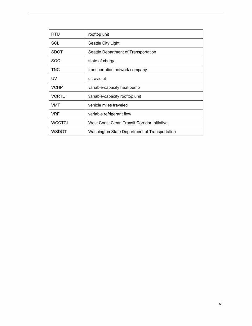
RTU rooftop unit
SCL Seattle City Light
SDOT Seattle Department of Transportation
SOC state of charge
TNC transportation network company
UV ultraviolet
VCHP variable-capacity heat pump
VCRTU variable-capacity rooftop unit
VMT vehicle miles traveled
VRF variable refrigerant flow
WCCTCI West Coast Clean Transit Corridor Initiative
WSDOT Washington State Department of Transportation


xiii
CONTENTS
ABSTRACT .................................................................................................................................. V
EXECUTIVE SUMMARY ............................................................................................................ VII
1 OVERVIEW AND EXECUTIVE SUMMARY ........................................................................... 1-1
Scenarios .............................................................................................................................. 1-1
Scenario Analysis Results: Total Energy Needed ................................................................. 1-3
Scenario 1: Moderate Market Advancement Scenario ..................................................... 1-3
Scenario 2: Rapid Market Advancement Scenario ........................................................... 1-5
Scenario 3: Full Adoption of Electrification Technologies ................................................. 1-6
Scenario Analysis Results: Power Demand .......................................................................... 1-7
Grid Capacity Analysis .......................................................................................................... 1-8
Key Findings ....................................................................................................................... 1-10
Transportation ................................................................................................................ 1-10
Buildings and Industry .................................................................................................... 1-11
Grid ................................................................................................................................. 1-11
Report Format ..................................................................................................................... 1-12
2 ON-ROAD TRANSPORTATION ............................................................................................ 2-1
Executive Summary .............................................................................................................. 2-1
Introduction ........................................................................................................................... 2-1
Scenario Definitions .............................................................................................................. 2-3
Scenario 1: Moderate Market Advancement .................................................................... 2-5
Scenario 2: Rapid Market Advancement .......................................................................... 2-5
Scenario 3: Full Electrification .......................................................................................... 2-6
Vehicle Population, Charging Infrastructure, and Activity Data ............................................. 2-6
Vehicle Classes and EV Types ........................................................................................ 2-6
Vehicle Population ............................................................................................................ 2-8
Current Electric Vehicle Population .................................................................................. 2-9
xiv
Growth Rates .................................................................................................................. 2-10
Vehicle Miles Traveled ................................................................................................... 2-10
Travel Data: Daily Driving Patterns ................................................................................ 2-11
Data Limitations .............................................................................................................. 2-12
Electric Vehicle Population Projections ............................................................................... 2-13
Electrification Rates ........................................................................................................ 2-14
Electric Vehicle Population ............................................................................................. 2-14
Share of Electric Vehicles in Operation .......................................................................... 2-15
VMT and Electrified VMT Trends ................................................................................... 2-16
Load Profiles ....................................................................................................................... 2-18
Overview of Simulation Approach .................................................................................. 2-18
Interim Load Profile Result: Per-EV 24-Hour Load Profiles ............................................ 2-20
Long-Haul Vehicles: Trucks and Intercity Buses ............................................................ 2-22
Final Load Profile Result: Aggregate 8,760-Hour Load Profiles ..................................... 2-23
Annual Energy Consumption............................................................................................... 2-25
Charging Infrastructure Analysis for Passenger Vehicles ................................................... 2-25
Seattle Infrastructure Ratio Comparison ........................................................................ 2-27
Home Charging .............................................................................................................. 2-28
Workplace Charging ....................................................................................................... 2-30
Public Charging .............................................................................................................. 2-32
Recommendations for Infrastructure .............................................................................. 2-34
Charging Infrastructure Analysis for Light Commercial Trucks and MDHD Vehicles .......... 2-34
Infrastructure Demand for Short-Haul MDHD Vehicle Types ......................................... 2-34
Infrastructure Demand for Long-Haul MDHD Vehicle Types .......................................... 2-34
Conclusion .......................................................................................................................... 2-35
3 BUILDINGS ............................................................................................................................ 3-1
Executive Summary .............................................................................................................. 3-1
Introduction ........................................................................................................................... 3-2
Scenario Definitions .............................................................................................................. 3-3
Modeling Methodology .......................................................................................................... 3-3
Data Sources .................................................................................................................... 3-3
Baseline Technology Saturation and Energy Consumption ............................................. 3-5
Market Growth Projections ............................................................................................... 3-7
Key Electrification Opportunities ........................................................................................... 3-8

xv
Residential Space and Water Heating .............................................................................. 3-9
Air-Source Heat Pumps (ASHPs) ................................................................................ 3-9
Ducted Variable-Capacity Heat Pumps (VCHPs) ................................................... 3-9
Ductless Mini-Split and Multi-Split Heat Pumps ...................................................... 3-9
Ground-Source Heat Pumps (GSHPs) ...................................................................... 3-10
Resistance and Heat Pump Water Heaters (HPWHs) ............................................... 3-10
Applications, Benefits, and Barriers: Residential Space and Water Heating ............. 3-10
Commercial Space and Water Heating .......................................................................... 3-11
Air-Source Heat Pumps (ASHPs) .............................................................................. 3-11
Variable-Capacity Rooftop Heat Pumps (VCRTUs) ................................................... 3-12
Variable-Refrigerant Flow (VRF) Heat Pumps ...................................................... 3-12
Ground-Source Heat Pumps (GSHPs) ...................................................................... 3-13
Resistance and Heat Pump Water Heaters (HPWHs) ............................................... 3-13
Applications, Benefits, and Barriers: Commercial Space and Water Heating ............ 3-13
Commercial Cooking ...................................................................................................... 3-14
Commercial Fryers, Griddles, and Combi-Ovens ...................................................... 3-14
Applications, Benefits, and Barriers: Commercial Cooking ........................................ 3-15
Energy and Demand Impacts of Electrification ................................................................... 3-15
Scenario 1: Moderate Market Advancement .................................................................. 3-16
Scenario 2: Rapid Market Advancement ........................................................................ 3-19
Scenario 3: Full Electrification by 2030 .......................................................................... 3-21
Energy Efficiency and Electrification ................................................................................... 3-23
Conclusion .......................................................................................................................... 3-25
4 INDUSTRY AND NON-ROAD EQUIPMENT .......................................................................... 4-1
Executive Summary .............................................................................................................. 4-1
Introduction ........................................................................................................................... 4-2
Scenario Definitions .............................................................................................................. 4-3
Modeling Methodology .......................................................................................................... 4-3
Data Sources .................................................................................................................... 4-3
Baseline Energy Consumption ......................................................................................... 4-4
Market Growth Projections ............................................................................................... 4-5
Key Electrification Opportunities ........................................................................................... 4-5
Industrial Boilers/CHP ...................................................................................................... 4-5
Electric Resistance Boilers .......................................................................................... 4-5
xvi
Electrode Boilers .......................................................................................................... 4-5
Applications, Benefits, and Barriers: Industrial Boilers/CHP ........................................ 4-6
Industrial Process Heating ................................................................................................ 4-6
Resistance Heating and Melting .................................................................................. 4-6
Induction Heating and Melting ..................................................................................... 4-6
IR Curing and Drying ................................................................................................... 4-7
UV Curing .................................................................................................................... 4-7
Vacuum Carburizing Furnace ...................................................................................... 4-7
Applications, Benefits, and Barriers: Industrial Process Heating ................................. 4-8
Non-Road Equipment ..................................................................................................... 4-10
Forklifts ...................................................................................................................... 4-10
Terminal Trucks ......................................................................................................... 4-10
Lawn and Garden Equipment .................................................................................... 4-10
Construction Equipment............................................................................................. 4-11
Seaport Electrification ................................................................................................ 4-11
Applications, Benefits, and Barriers: Non-Road Equipment ........................................... 4-11
Energy and Demand Impacts of Electrification ................................................................... 4-12
Scenario 1: Moderate Market Advancement .................................................................. 4-13
Scenario 2: Rapid Market Advancement ........................................................................ 4-15
Scenario 3: Full Electrification by 2030 .......................................................................... 4-17
Energy Efficiency and Electrification ................................................................................... 4-19
Conclusion .......................................................................................................................... 4-20
5 HIGH-LEVEL GRID IMPACTS ASSESSMENT ..................................................................... 5-1
Executive Summary .............................................................................................................. 5-1
Introduction ........................................................................................................................... 5-2
Hosting Capacity Using DRIVE ............................................................................................. 5-3
Grid Data Collection .............................................................................................................. 5-4
SCL Distribution Grid ........................................................................................................ 5-4
Data Collection ................................................................................................................. 5-5
Feeder Models: Looped Radial System Only .............................................................. 5-5
Feeder and Substation Limits ...................................................................................... 5-5
Time-Series Load Data ................................................................................................ 5-7
Results ................................................................................................................................ 5-11
Looped Radial Feeders .................................................................................................. 5-12

xvii
Distributed Load Deployment..................................................................................... 5-12
Centralized Load Deployment.................................................................................... 5-18
Network Feeders ............................................................................................................ 5-24
Substations and System ................................................................................................. 5-27
Conclusion .......................................................................................................................... 5-30
6 FLEXIBILITY OF NEW ELECTRIC LOADS .......................................................................... 6-1
Introduction ........................................................................................................................... 6-1
Flexibility of Electric Loads .................................................................................................... 6-3
Opportunities, Challenges, and Market Readiness ............................................................... 6-7
Commercial Buildings ....................................................................................................... 6-7
Residential Buildings: Single Family ............................................................................... 6-11
Residential Buildings: Multi-Family ................................................................................. 6-14
Flexibility as a Distribution Grid Resource ...................................................................... 6-15
Summary: Conclusions, Recommendations, Next Steps .................................................... 6-16
7 STRATEGY AND IMPLEMENTATION .................................................................................. 7-1
Overall Objectives and Drivers of Increased Electrification ................................................... 7-1
Policy Drivers .................................................................................................................... 7-2
Market Drivers .................................................................................................................. 7-3
Technology Drivers ........................................................................................................... 7-4
Considerations for Equitable Electrification ...................................................................... 7-4
Background and Challenges ................................................................................................. 7-5
On-Road Electric Transportation Background and Challenges ........................................ 7-5
Up-Front Cost .............................................................................................................. 7-9
Charging Infrastructure ................................................................................................ 7-9
Building Electrification Background and Challenges ........................................................ 7-9
Commercial Cooking Equipment Background and Challenges ...................................... 7-10
Industrial Process Heating Electrification Background and Challenges ......................... 7-11
Non-Road Electric Transportation Background and Challenges .................................... 7-11
Strategies for Increasing Electrification ............................................................................... 7-12
Reducing First Cost ........................................................................................................ 7-13
Technology-Specific Strategies for Increasing Electrification .............................................. 7-14
Strategies for Increasing Electric Vehicle Adoption ........................................................ 7-14
Other Utility Investments and Programs in On-road Electrification ............................ 7-18
xviii
Strategies for Increasing Heat Pump Adoption in Buildings ........................................... 7-21
Strategies for Increasing Commercial Cooking Electrification ........................................ 7-21
Strategies for Increasing Electrification in Industrial Process Heating ........................... 7-22
Strategies for Increasing Adoption of Non-road Electric Transportation Technologies .................................................................................................................. 7-22
Conclusion .......................................................................................................................... 7-23
A ELECTRIC TRANSPORTATION ASSUMPTIONS............................................................... A-1
B ELECTRIC TRANSPORTATION LOAD PROFILES ............................................................ B-1
Load Profile Simulation Process .......................................................................................... B-1
Travel Data ...................................................................................................................... B-1
Charging Simulation ........................................................................................................ B-2
Initialization Phase ........................................................................................................... B-2
Simulation Phase ............................................................................................................. B-3
Aggregation Phase .......................................................................................................... B-3
Special Commercial and MDHD Cases ........................................................................... B-3
Implicit Assumptions ........................................................................................................ B-4
Detailed Assumptions........................................................................................................... B-5
Charging Power Access Probabilities .............................................................................. B-5
Home Charging ............................................................................................................... B-6
Workplace Charging ........................................................................................................ B-6
Public Charging ............................................................................................................... B-6
En Route Charging .......................................................................................................... B-7
Nominal Electric Energy Consumption Rates .................................................................. B-7
Adjustments to Energy Consumption to Account for Ambient Temperature ................... B-8
Adjusting for Temperatures Greater Than 78 Degrees Fahrenheit ............................... B-10
Adjusting for Temperatures Less Than 69 Degrees Fahrenheit .................................... B-12
Accounting for Commuter Travel ................................................................................... B-12
Vehicle Class Definitions ............................................................................................... B-12
Sources for Vehicle Population, Growth Rate, and VMT Data ...................................... B-14
Passenger Vehicle BEV/PHEV Proportion .................................................................... B-15
eVMT by Scenario, Vehicle Class, and Year ................................................................. B-15
C BUILDINGS SATURATION DATA ....................................................................................... C-1

xix
D GRID SUPPORTING ANALYSIS TABLES .......................................................................... D-1
E FLEXIBILITY OPPORTUNITIES AND CHALLENGES IN COMMERCIAL, RESIDENTIAL, AND MULTI-UNIT DWELLINGS .................................................................... E-1
F METRICS FOR IMPLEMENTING ELECTRIFICATION PROGRAMS FOR END-USE TECHNOLOGIES ...................................................................................................................... F-1


xxi
LIST OF FIGURES
Figure 1-1 Scenarios explored in the study together with their basis and assumptions used for electric transportation as well as commercial and industrial ................................ 1-2
Figure 1-2 Moderate Market Advancement scenario (Scenario 1) colored by the end-use sector. The totals over the colored area show the total TWh of electric energy required over time. ............................................................................................................. 1-3
Figure 1-3 Rapid Market Advancement scenario (Scenario 2) colored by the end-use sector. The totals over the colored area show the total TWh of electric energy required over time. ............................................................................................................. 1-5
Figure 1-4 Full Adoption of Electrification Technologies (Scenario 3) colored by the end-use sector. The totals over the colored area show the total TWh of electric energy required over time. ............................................................................................................. 1-6
Figure 1-5 Yearly load of Full Adoption scenario (Scenario 3) colored by transportation, buildings and commercial and industrial load in the year 2030. The black dotted lines indicate SCL’s 2020 load. .......................................................................................... 1-7
Figure 1-6 Available system capacity in SCL’s service territory (in blue) over a year-long period and the system load (2019 data) (in orange) .......................................................... 1-8
Figure 1-7 Left: SCL system capacity for each feeder (looped radial feeders only) during the peak load hour and minimum load hour. Analysis for networked feeders is not performed using feeder models; therefore, results are not available in geographical plot format. Right: Available capacity (MW) during peak load and minimum load subdivided by substation (includes networked substations). Note full page graphics are available in the Section 5. ............................................................................................ 1-9
Figure 1-8 Left: Annual energy capacity calculated as the sum of each feeder’s capacity across a full year (MWh). Right: Minimum daily energy capacity calculated as the sum of each feeder’s capacity for the day with the lowest energy availability.................. 1-10
Figure 2-1 Number of passenger electric vehicles (both PHEV and BEV) available from 2010 to 2024. The vehicle segment is specified by the color. Graphic generated by EPRI. .................................................................................................................................. 2-2
Figure 2-2 SCL electric vehicle population ................................................................................ 2-9 Figure 2-3 Vehicle population growth rates by class for Seattle (2020–2042) ......................... 2-10 Figure 2-4 Electrification rates of new vehicles for each vehicle class .................................... 2-14 Figure 2-5 Electric vehicle population by vehicle class over time. Yellow line in Moderate
and Rapid scenarios corresponds to the right y-axis, which shows percentage of passenger vehicles in operation that is electric. Note that the passenger vehicle population includes commuter vehicles, which account for approximately 20% of the total passenger vehicle population. .................................................................................. 2-15
Figure 2-6 Percent of vehicles in operation that is electric by vehicle class. Left: Moderate scenario. Right: Rapid scenario. ...................................................................... 2-16

xxii
Figure 2-7 Diagram of the process for estimating load profiles ............................................... 2-19 Figure 2-8 Example set of average per-EV unmanaged charging loads (passenger cars
in 2030) with and without home charging ......................................................................... 2-21 Figure 2-9 Example set of per-EV charging loads (LCT and MDHD classes in 2030)............. 2-22 Figure 2-10 Combination truck traffic for an average week in 2019 ........................................ 2-23 Figure 2-11 Aggregate load projected on the coldest weekday (December 16), 2030 and
2042, for each of the market projection scenarios ........................................................... 2-24 Figure 2-12 Annual electricity consumption (GWh) by vehicle class groups for all
scenarios .......................................................................................................................... 2-25 Figure 2-13 Current public EV charging connectors in Seattle ................................................ 2-26 Figure 2-14 Number of home charge ports required by housing type and power level ........... 2-30 Figure 2-15 Workplace charge ports required by power level ................................................. 2-31 Figure 2-16 Public charge ports required by power level ......................................................... 2-33 Figure 2-17 Total number of charge ports required by location type ....................................... 2-33 Figure 2-18 Load shape for long-haul trucks ........................................................................... 2-35 Figure 3-1 Comparison of 2020 and 2042 final energy consumption (Scenarios 1, 2, and
3) ........................................................................................................................................ 3-1 Figure 3-2 Baseline technology saturation assumptions for residential buildings ...................... 3-5 Figure 3-3 Baseline technology saturation assumptions for commercial buildings .................... 3-6 Figure 3-4 Baseline final energy consumption for residential buildings ..................................... 3-7 Figure 3-5 Baseline final energy consumption for commercial buildings ................................... 3-7 Figure 3-6 Scenario 1: Change in electric consumption for residential and commercial
buildings ........................................................................................................................... 3-17 Figure 3-7 Scenario 1: Projected 2042 load shape for residential and commercial
buildings based on a typical meteorological year ............................................................. 3-18 Figure 3-8 Scenario 1: Projected final energy consumption for residential and
commercial buildings ........................................................................................................ 3-18 Figure 3-9 Scenario 2: Change in electric consumption for residential and commercial
buildings ........................................................................................................................... 3-19 Figure 3-10 Scenario 2: Projected 2042 load shape for residential and commercial
buildings based on a typical meteorological year ............................................................. 3-20 Figure 3-11 Scenario 2: Projected final energy consumption for residential and
commercial buildings ........................................................................................................ 3-21 Figure 3-12 Scenario 3: Net change in electric consumption for residential and
commercial buildings ........................................................................................................ 3-21 Figure 3-13 Scenario 3: Projected 2042 load shape for residential and commercial
buildings based on a typical meteorological year ............................................................. 3-22 Figure 3-14 Scenario 3: Projected final energy consumption for residential and
commercial buildings ........................................................................................................ 3-23 Figure 3-15 Scenarios 1, 2, and 3: Projected 2042 load shape for residential and
commercial buildings based on a typical meteorological year (with EPRI energy efficiency assumptions applied) ....................................................................................... 3-25
xxiii
Figure 3-16 Comparison of 2020 and 2042 final energy consumption (Scenarios 1, 2, and 3) ............................................................................................................................... 3-26
Figure 4-1 Comparison of 2020 and 2042 final energy consumption (Scenarios 1, 2, and 3) ........................................................................................................................................ 4-1
Figure 4-2 Baseline final energy consumption for industry ........................................................ 4-4 Figure 4-3 Baseline final energy consumption for non-road equipment .................................... 4-4 Figure 4-4 Scenario 1: Change in electric consumption for industry and non-road
equipment ........................................................................................................................ 4-13 Figure 4-5 Scenario 1: Projected 2042 load shape for industry and non-road equipment
based on a typical meteorological year ............................................................................ 4-14 Figure 4-6 Scenario 1: Projected final energy consumption for industry and non-road
equipment ........................................................................................................................ 4-14 Figure 4-7 Scenario 2: Change in electric consumption for industry and non-road
equipment ........................................................................................................................ 4-15 Figure 4-8 Scenario 2: Projected 2042 load shape for industry and non-road equipment
based on a typical meteorological year ............................................................................ 4-16 Figure 4-9 Scenario 2: Projected final energy consumption for industry and non-road
equipment ........................................................................................................................ 4-16 Figure 4-10 Scenario 3: Change in electric consumption for industry and non-road
equipment ........................................................................................................................ 4-17 Figure 4-11 Scenario 3: Projected 2042 load shape for industry and non-road equipment
based on a typical meteorological year ............................................................................ 4-18 Figure 4-12 Scenario 3: Projected final energy consumption for industry and non-road
equipment ........................................................................................................................ 4-18 Figure 4-13 Scenario 1, 2, and 3: Projected 2042 load shape for industry and non-road
equipment based on a typical meteorological year (with EPRI energy efficiency assumptions applied) ....................................................................................................... 4-20
Figure 4-14 Comparison of 2020 and 2042 final energy consumption (Scenarios 1, 2, and 3) ............................................................................................................................... 4-21
Figure 5-1 Available system capacity in SCL’s service territory (in blue) over a year-long period and the system load (2019 data) (in orange). ......................................................... 5-1
Figure 5-2 Example of (a) centralized and (b) distributed load deployments for hosting capacity calculations .......................................................................................................... 5-4
Figure 5-3 Range of 2019 load for each of the looped radial feeders (Feeder 2687 is not included because it is a large dedicated load) ................................................................... 5-8
Figure 5-4 Range of 2019 load for each of the network feeders ................................................ 5-9 Figure 5-5 Hourly system load data for 2019 ........................................................................... 5-10 Figure 5-6 Hosting capacity for additional distributed load for each feeder during (a)
system peak load hour and (b) system minimum load hour ............................................. 5-13 Figure 5-7 Load exceeding planning limit for feeders with minimum capacity of 0 MW
(Feeder 2687 is not included because it is a large dedicated load) ................................. 5-14 Figure 5-8 (a) Location of feeders 2612 and 2644 on SCL system and minimum capacity
for additional distributed load for Feeders (b) 2612 and (c) 2644 ...................................... 5-15
xxiv
Figure 5-9 Existing load and remaining capacity for additional distributed load for Feeders 2612 and 2644 for each hour of the year ........................................................... 5-16
Figure 5-10 Example showing calculation of annual energy capacity and minimum daily energy capacity for Feeder 2612 ..................................................................................... 5-17
Figure 5-11 (a) Annual energy capacity and (b) minimum daily energy capacity for each feeder for distributed load deployment ............................................................................. 5-18
Figure 5-12 Hosting capacity for additional centralized load for each feeder during the system minimum load hour for (a) feeder head location and (b) average of all three-phase locations ................................................................................................................ 5-19
Figure 5-13 Capacity for additional centralized load for every location on Feeder 2620 during (a) system minimum load and (b) system peak load ............................................. 5-20
Figure 5-14 Capacity for additional centralized load for every hour of the year for feeder head and lateral location on Feeder 2620 ........................................................................ 5-21
Figure 5-15 Average of centralized hosting capacity for all three-phase locations for each feeder during (a) system peak load hour and (b) system minimum load hour ........ 5-22
Figure 5-16 (a) Annual energy capacity and (b) minimum daily energy capacity for centralized load deployment taking average capacity of all three-phase locations for each feeder ...................................................................................................................... 5-23
Figure 5-17 Minimum and maximum capacity for additional load for each of the network feeders based on network feeder ratings and 2019 load ................................................. 5-25
Figure 5-18 Minimum and maximum capacity for additional load for each of the subnets based on subnet ratings and 2019 load ........................................................................... 5-26
Figure 5-19 Overall substation capacity at each hour .............................................................. 5-28 Figure 5-20 Existing load and capacity for additional load for SCL system ............................. 5-29 Figure 6-1 8760 Load curves in SCL’s service territory colored by transportation and
buildings in a Full Electrification Adoption scenario (in 2030) ............................................ 6-2 Figure 6-2 8760 Load curves in SCL’s service territory colored by transportation and
buildings in a Rapid Market Advancement scenario .......................................................... 6-2 Figure 6-3 Flexibility to address energy system needs .............................................................. 6-4 Figure 6-4 The 4 S’s of Demand Response ............................................................................... 6-4 Figure 6-5 Representative 50,000 sq. ft. commercial building winter load shape (average
load shape). Left graph represents 2020 average load shape. Right graph represents 2030 average load shape for the Rapid Market Advancement scenario (Scenario 2). ....................................................................................................................... 6-8
Figure 6-6 Commercial building energy management system schematic.................................. 6-9 Figure 6-7 Controllability feasibility and potential customer impact of end uses found in
commercial building ......................................................................................................... 6-10 Figure 6-8 Average winter load shape of a single-family home. Left graph represents
2020 average load shape. Right graph represents 2030 average load shape in the Rapid Market Advancement scenario (Scenario 2). ......................................................... 6-12
Figure 6-9 Example load shape of a zero net energy home from 6:00PM to 9:00AM ............. 6-13 Figure 6-10 Average winter load shape of a 100-unit multi-unit dwelling. Left graph
represents 2020 average load shape. Right graph represents 2030 average load shape in the Rapid Market Advancement scenario (Scenario 2). .................................... 6-14
xxv
Figure 7-1 U.S. GHG Emissions by Sector in 2019 ................................................................... 7-2 Figure 7-2 Shading of the number of policy levers in the form of carbon targets set at
state, city, and utility scale ................................................................................................. 7-3 Figure 7-3 Strata of energy impact on disadvantaged communities. ......................................... 7-5 Figure 7-4 USA EV sales since December 2010. 2.1 million EVs have been sold. ................... 7-6 Figure 7-5 Heat map of percentage of new EV sales in the Unites States by county from
June 2020 through June 2021. The top 5 counties in California and the top 15 counties outside of California have been highlighted. ........................................................ 7-7
Figure 7-6 Decarbonization actions that can help achieve overall system cost reduction objectives ......................................................................................................................... 7-13
Figure 7-7 Outline for the utility role in electric transportation from business as usual to equipment owner and operator ........................................................................................ 7-15
Figure 7-8 Incentives tested for in EPRI’s PEV preferences study. The blue coloring highlights incentives that have a more direct monetary value whereas the green highlights incentives that have varying values depending on specific driver situations or preferences. ................................................................................................. 7-16
Figure 7-9 2025 EV share of new vehicle sales with incentives. This example is from national average statistics; specific utility results varied depending on their unique circumstances. Each incentive percentage is above the assumed 8.1% baseline adoption projected in 2025. .............................................................................................. 7-17
Figure 7-10 EV share of new vehicle sales with incentive portfolio (national average). .......... 7-18 Figure 7-11 Utility investment in the EV space in 2020, EPRI generated ................................ 7-19 Figure B-1 Transit bus charging profiles obtained from King County Metro ............................. B-4 Figure B-2 Illustration of charging probability assumptions used for passenger cars in
2030. Probabilities vary with respect to home charging access, EV type, power level, and charging location. Additional probability assumptions apply in other years and for passenger trucks. .................................................................................................. B-5
Figure B-3 Visualization of energy consumption rates over time for each modeled vehicle class .................................................................................................................................. B-8
Figure B-4 Total passenger EV charging load for every day in the year 2042 shown on the same axes. Load profiles are shown in different colors depending on the average temperature of the day on which they occur (measured between 8 am and 5 pm). ................................................................................................................................ B-9
Figure B-5 Total LCT and MDHD EV charging load for every day in the year 2042 shown on the same axes. Load profiles are shown in different colors depending on the average temperature of the day on which they occur (measured between 8 am and 5 pm). .............................................................................................................................. B-10
Figure B-6 Energy consumption rate temperature model from FleetCarma/CHARGED magazine ......................................................................................................................... B-11
Figure B-7 Linear models of energy consumption change as a function of temperature for separate groups of vehicles in the Southern study .................................................... B-12
Figure B-8 BEV/PHEV Proportions of New EV Sales ............................................................. B-15

xxvii
LIST OF TABLES
Table 1-1 Moderate Market Advancement scenario (Scenario 1) total TWh needed in 2020 and 2042, by total TWh and % of total energy .......................................................... 1-4
Table 1-2 Rapid Market Advancement scenario (Scenario 2) total TWh needed in 2020 and 2042 segmented by end use and ordered with the largest % at the top in 2042 (Commercial and residential are combined) ...................................................................... 1-5
Table 1-3 Full Adoption of Electrification Technologies (Scenario 3). Total energy [TWhr] required in 2042 segmented by end use. Year 2020 is not included in this table because this scenario runs from 2030 to 2042. ................................................................. 1-6
Table 1-5 Energy needs for both light-duty and medium- and heavy-duty vehicle classes in 2020 as well as 2042 for the 100% electrification scenario .......................................... 1-11
Table 2-1 Scenarios, their underlying bases, and assumptions explored in this analysis ......... 2-4 Table 2-2 Vehicle class definitions ............................................................................................. 2-7 Table 2-3 SCL service territory vehicle population (2020) ......................................................... 2-8 Table 2-4 Estimated annual VMT by vehicle class .................................................................. 2-11 Table 2-5 Electrified VMT estimates (in millions of miles) ....................................................... 2-17 Table 2-6 Moderate market advancement, electrified VMT estimates (in millions of miles)
divided by vehicle type ..................................................................................................... 2-17 Table 2-7 Rapid market advancement, electrified VMT estimates (in millions of miles)
divided by vehicle type ..................................................................................................... 2-18 Table 2-8 Attributes distinguishing segments of the passenger vehicle population over
time. 24-hour load profiles were obtained for every combination of values. .................... 2-20 Table 2-9 Attributes distinguishing segments of the LCT/MDHD vehicle population over
time. 24-hour load profiles were obtained for every combination of values. .................... 2-20 Table 2-10 Home charging availability by housing type ........................................................... 2-28 Table 2-11 Total housing and distribution of housing by type over time in SCL ...................... 2-28 Table 2-12 Vehicle distribution by housing type over time ....................................................... 2-29 Table 2-13 Vehicle distribution by home charging availability (regardless of housing type) .... 2-29 Table 2-14 Home charging power level distribution by housing type ....................................... 2-29 Table 2-15 Access to workplace charging over time ............................................................... 2-31 Table 2-16 Key impacts of on-road electric transportation, 2030 ............................................ 2-36 Table 3-1 Scenarios explored in this analysis and their underlying basis .................................. 3-3 Table 3-2 Summary of data sources used and their geospatial granularity ............................... 3-4 Table 3-3 Baseline building stock (residential) and building floorspace (commercial)
assumptions ....................................................................................................................... 3-4
xxviii
Table 3-4 Building stock (residential) and building floorspace (commercial) growth projections .......................................................................................................................... 3-8
Table 3-5 Residential space and water heating technology benefits ....................................... 3-11 Table 3-6 Commercial space and water heating technology benefits ..................................... 3-14 Table 3-7 Baseline final energy consumption and technology saturation assumptions for
nonelectric equipment in residential and commercial buildings ....................................... 3-16 Table 3-8 Scenario 1: Change in electric consumption for residential and commercial
buildings ........................................................................................................................... 3-17 Table 3-9 Scenario 2: Change in electric consumption for residential and commercial
buildings ........................................................................................................................... 3-20 Table 3-10 Scenario 3: Change in electric consumption for residential and commercial
buildings ........................................................................................................................... 3-22 Table 3-11 Scenarios 1, 2, and 3: Change in electric consumption for residential and
commercial buildings (with EPRI energy efficiency assumptions applied) ....................... 3-24 Table 4-1 Scenarios explored in this analysis and their underlying basis. ................................. 4-3 Table 4-2 Summary of data sources used and their geospatial granularity ............................... 4-3 Table 4-3 Industrial process heating applications ...................................................................... 4-8 Table 4-4 Industrial process heating technology benefits .......................................................... 4-9 Table 4-5 Baseline final energy consumption for nonelectric equipment in industry and
non-road ........................................................................................................................... 4-12 Table 4-6 Scenario 1: Change in electric consumption for industry and non-road
equipment ........................................................................................................................ 4-13 Table 4-7 Scenario 2: Change in electric consumption for industry and non-road
equipment ........................................................................................................................ 4-15 Table 4-8 Scenario 3: Change in electric consumption for industry and non-road
equipment ........................................................................................................................ 4-17 Table 4-9 Scenario 1, 2, and 3: Change in electric consumption for industry and non-
road equipment (with EPRI energy efficiency assumptions applied) ............................... 4-19 Table 5-1 Year of grid model and load data used for grid impacts analysis .............................. 5-2 Table 5-2 Characteristics of looped radial and networked parts of SCL medium-voltage
distribution grid ................................................................................................................... 5-5 Table 5-3 Summer and winter ratings for substations ............................................................... 5-6 Table 5-4 Subnet ratings ............................................................................................................ 5-6 Table 5-5 Description of summary results ............................................................................... 5-11 Table 5-6 Minimum and maximum capacity for additional load for each substation ................ 5-27 Table 5-7 Feeders grouped by minimum capacity for additional distributed load .................... 5-30 Table 6-1 Four S Categories of Demand Response Described ................................................. 6-5 Table 7-1 Examples of city electric vehicle goals and strategies. .............................................. 7-8 Table B-1 Methods by which load profiles for each LCT/MDHD vehicle class were
obtained ............................................................................................................................ B-2 Table B-2 Data required as input to charging simulation tool ................................................... B-2

xxix
Table B-3 Example set of charging probabilities (home charging by cars in 2030). More probabilities were assumed for other subpopulations and charging locations. ................. B-5
Table B-4 Energy consumption rates assumed for each vehicle class and year (Wh/mile) ..... B-7 Table B-5 Breakdown of MOVES vehicle classes by regulatory class ................................... B-13 Table B-6 Vehicle class regulatory names and definitions ..................................................... B-14 Table B-7 Data Sources .......................................................................................................... B-14 Table B-8 eVMT, in millions of miles, Moderate Market Advancement................................... B-15 Table B-9 eVMT, in millions of miles, Rapid Market Advancement ........................................ B-16 Table B-10 Estimated VMT by vehicle class and year ............................................................ B-16 Table C-1 Baseline space heating saturation assumptions (residential) .................................. C-1 Table C-2 Baseline space cooling saturation assumptions (residential) ................................... C-1 Table C-3 Baseline water heating, cooking, and clothes dryer saturation assumptions
(residential) ....................................................................................................................... C-2 Table C-4 Baseline space heating saturation assumptions (commercial) ................................ C-2 Table C-5 Baseline space cooling saturation assumptions (commercial) ................................. C-3 Table C-6 Baseline water heating and cooking saturation assumptions (commercial) ............. C-3 Table D-1 Winter and summer ratings for all looped radial feeders in Amps ............................ D-1 Table D-2 Ratings for all network feeders in Amps ................................................................... D-4 Table D-3 Minimum, mean, and maximum capacity for additional distributed load for
each feeder in MW ............................................................................................................ D-5 Table E-1 Flexibility opportunities and challenges in commercial, residential, and multi-
unit dwellings ..................................................................................................................... E-1 Table F-1 Actionable metrics for implementing electrification programs for end-use
technologies ....................................................................................................................... F-1

1-1
1 OVERVIEW AND EXECUTIVE SUMMARY
Seattle is leading the way with a vision for a fully electrified economy. To achieve an accelerated, transformational shift from end-use combustion to electrification, Seattle City Light (SCL) will need to plan for and supply energy to its customers for both existing and emerging electric technologies at scale.
This assessment examines the high-level impacts of electrification in SCL’s service territory under multiple adoption scenarios in a timeframe that extends until 2042, in order to understand the lasting electrification needs. Specifically, it looks at:
• Energy needed for the electrification of buildings, transportation, and commercial and industrial applications within SCL’s service territory under several adoption scenarios, and
• SCL’s current distribution grid load and capacity, and future distribution grid load. Additionally, the assessment provides a high-level overview of other key components of an electrified future, including:
• Flexibility of new electric loads due to technology advances, and
• Different strategies to help tackle electrification adoption challenges.
Scenarios To undertake this electrification assessment, EPRI worked with SCL as well as other City of Seattle departments (Seattle Department of Transportation (SDOT), the Seattle Office of Sustainability and the Environment (OSE), and the Department of Construction and Inspection (SDCI)) to define scenarios. The scenarios were chosen, where possible, to align with existing City of Seattle planning, strategies, and policies. Three electrification scenarios were explored for this analysis, and are described in additional detail below.
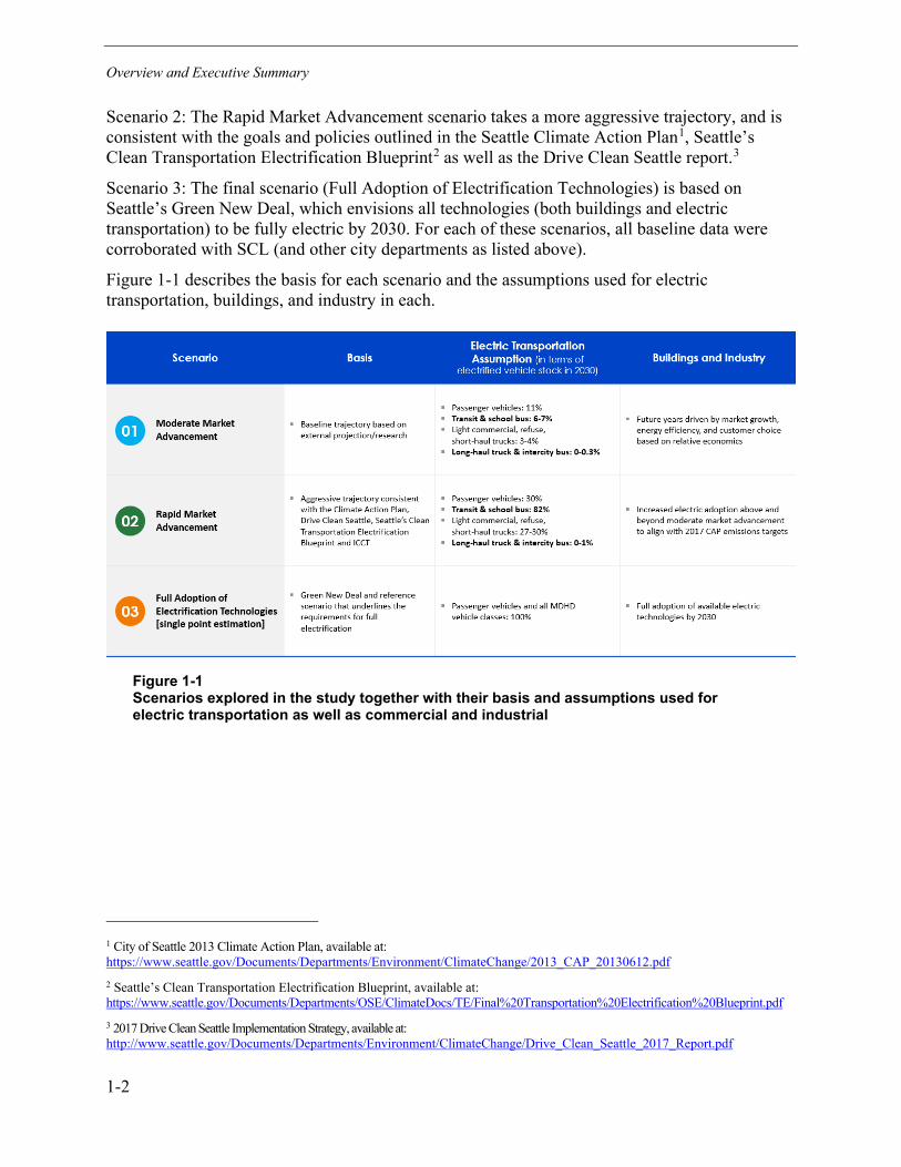
Scenario 1: The Moderate Market Advancement scenario is the closest to a “business as usual” scenario. In this scenario, electric transportation adoption continues to grow based on past trajectories and includes any incentives that may have been offered prior to 2020. In this scenario, electrification of buildings and industry are driven by customer choice as well as relative economics.
Overview and Executive Summary
1-2
Scenario 2: The Rapid Market Advancement scenario takes a more aggressive trajectory, and is consistent with the goals and policies outlined in the Seattle Climate Action Plan1, Seattle’s Clean Transportation Electrification Blueprint2 as well as the Drive Clean Seattle report.3
Scenario 3: The final scenario (Full Adoption of Electrification Technologies) is based on Seattle’s Green New Deal, which envisions all technologies (both buildings and electric transportation) to be fully electric by 2030. For each of these scenarios, all baseline data were corroborated with SCL (and other city departments as listed above).
Figure 1-1 describes the basis for each scenario and the assumptions used for electric transportation, buildings, and industry in each.
Figure 1-1 Scenarios explored in the study together with their basis and assumptions used for electric transportation as well as commercial and industrial
1 City of Seattle 2013 Climate Action Plan, available at: https://www.seattle.gov/Documents/Departments/Environment/ClimateChange/2013_CAP_20130612.pdf 2 Seattle’s Clean Transportation Electrification Blueprint, available at: https://www.seattle.gov/Documents/Departments/OSE/ClimateDocs/TE/Final%20Transportation%20Electrification%20Blueprint.pdf 3 2017 Drive Clean Seattle Implementation Strategy, available at: http://www.seattle.gov/Documents/Departments/Environment/ClimateChange/Drive_Clean_Seattle_2017_Report.pdf
Overview and Executive Summary
1-3
The summaries that follow show an overview of the results of the scenario analysis on both Total Energy and Power Demand.
Scenario Analysis Results: Total Energy Needed To calculate the energy needed each year to support each of the scenarios, a yearly load shape was generated for each of the electrified technologies. The load shape was then multiplied by the total electrified stock each year out to 2042 to find the energy required each year to support the electrification scenarios.
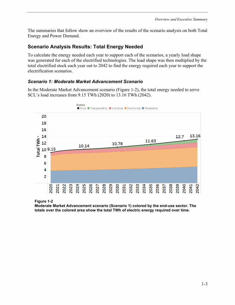
Scenario 1: Moderate Market Advancement Scenario In the Moderate Market Advancement scenario (Figure 1-2), the total energy needed to serve SCL’s load increases from 9.15 TWh (2020) to 13.16 TWh (2042).
Figure 1-2 Moderate Market Advancement scenario (Scenario 1) colored by the end-use sector. The totals over the colored area show the total TWh of electric energy required over time.
Overview and Executive Summary
1-4
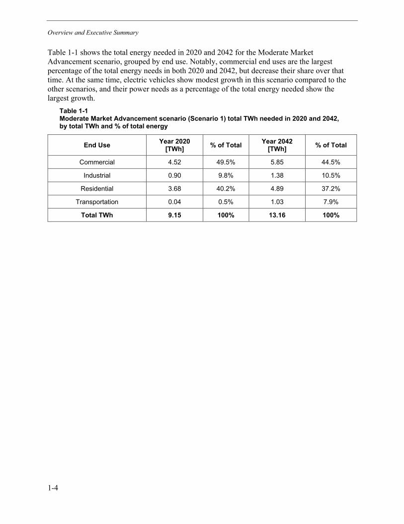
Table 1-1 shows the total energy needed in 2020 and 2042 for the Moderate Market Advancement scenario, grouped by end use. Notably, commercial end uses are the largest percentage of the total energy needs in both 2020 and 2042, but decrease their share over that time. At the same time, electric vehicles show modest growth in this scenario compared to the other scenarios, and their power needs as a percentage of the total energy needed show the largest growth.
Table 1-1 Moderate Market Advancement scenario (Scenario 1) total TWh needed in 2020 and 2042, by total TWh and % of total energy
End Use Year 2020 [TWh] % of Total Year 2042
[TWh] % of Total
Commercial 4.52 49.5% 5.85 44.5%
Industrial 0.90 9.8% 1.38 10.5%
Residential 3.68 40.2% 4.89 37.2%
Transportation 0.04 0.5% 1.03 7.9%
Total TWh 9.15 100% 13.16 100%

Overview and Executive Summary
1-5
Scenario 2: Rapid Market Advancement Scenario In the Rapid Market Advancement scenario (Figure 1-3), there is a significant increase in the energy needed over time to support electrified technologies – from 9.15 TWh in 2020 to 16.25 TWh in 2042. Due to the sharp increase in the number of electrified passenger vehicles in this scenario, transportation-related energy need increases to a total of 3.28 TWh to support them (approximately 750,000 passenger vehicles). While the commercial, industrial, and residential segments all show overall growth in energy use from 2020 to 2042, their percentage of the total drops due to the larger growth in energy use for transportation. See Table 1-2 for specifics.
Figure 1-3 Rapid Market Advancement scenario (Scenario 2) colored by the end-use sector. The totals over the colored area show the total TWh of electric energy required over time.
Table 1-2 Rapid Market Advancement scenario (Scenario 2) total TWh needed in 2020 and 2042 segmented by end use and ordered with the largest % at the top in 2042 (Commercial and residential are combined)
End Use Year 2020 [TWh] % of Total Year 2042
[TWh] % of Total
Commercial 4.52 49.5% 6.10 37.6%
Industrial 0.90 9.8% 1.72 10.6%
Residential 3.68 40.2% 5.14 31.6%
Transportation 0.04 0.5% 3.28 20.2%
Total TWh 9.15 100% 16.25 100%
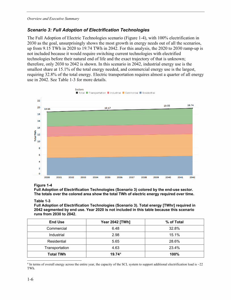
Overview and Executive Summary
1-6
Scenario 3: Full Adoption of Electrification Technologies The Full Adoption of Electric Technologies scenario (Figure 1-4), with 100% electrification in 2030 as the goal, unsurprisingly shows the most growth in energy needs out of all the scenarios, up from 9.15 TWh in 2020 to 19.74 TWh in 2042. For this analysis, the 2020 to 2030 ramp-up is not included because it would require switching current technologies with electrified technologies before their natural end of life and the exact trajectory of that is unknown; therefore, only 2030 to 2042 is shown. In this scenario in 2042, industrial energy use is the smallest share at 15.1% of the total energy needed, and commercial energy use is the largest, requiring 32.8% of the total energy. Electric transportation requires almost a quarter of all energy use in 2042. See Table 1-3 for more details.
Figure 1-4 Full Adoption of Electrification Technologies (Scenario 3) colored by the end-use sector. The totals over the colored area show the total TWh of electric energy required over time.
Table 1-3 Full Adoption of Electrification Technologies (Scenario 3). Total energy [TWhr] required in 2042 segmented by end use. Year 2020 is not included in this table because this scenario runs from 2030 to 2042.
End Use Year 2042 [TWh] % of Total Commercial 6.48 32.8%
Industrial 2.98 15.1% Residential 5.65 28.6%
Transportation 4.63 23.4% Total TWh 19.744 100%
4 In terms of overall energy across the entire year, the capacity of the SCL system to support additional electrification load is ~22 TWh.
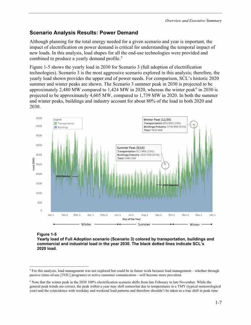
Overview and Executive Summary
1-7
Scenario Analysis Results: Power Demand Although planning for the total energy needed for a given scenario and year is important, the impact of electrification on power demand is critical for understanding the temporal impact of new loads. In this analysis, load shapes for all the end-use technologies were provided and combined to produce a yearly demand profile.5
Figure 1-5 shows the yearly load in 2030 for Scenario 3 (full adoption of electrification technologies). Scenario 3 is the most aggressive scenario explored in this analysis; therefore, the yearly load shown provides the upper end of power needs. For comparison, SCL’s historic 2020 summer and winter peaks are shown. The Scenario 3 summer peak in 2030 is projected to be approximately 2,480 MW compared to 1,424 MW in 2020, whereas the winter peak6 in 2030 is projected to be approximately 4,605 MW, compared to 1,739 MW in 2020. In both the summer and winter peaks, buildings and industry account for about 80% of the load in both 2020 and 2030.
Figure 1-5 Yearly load of Full Adoption scenario (Scenario 3) colored by transportation, buildings and commercial and industrial load in the year 2030. The black dotted lines indicate SCL’s 2020 load.
5 For this analysis, load management was not explored but could be in future work because load management—whether through passive (time-of-use [TOU] programs) or active customer comunication—will become more prevalent. 6 Note that the winter peak in the 2030 100% electrification scenario shifts from late February to late November. While the general peak trends are correct, the peak within a year may shift somewhat due to temperatures in a TMY (typical meteorological year) and the coincidence with weekday and weekend load patterns and therefore shouldn’t be taken as a true shift in peak time

Overview and Executive Summary
1-8
Although extreme temperature variations will lead to larger variations in SCL’s load, extreme weather events were not modeled explicitly in this analysis. Extreme temperature effects are explored for buildings, commercial and industrial applications, and electric transportation in their respective sections. For example, for the light-duty passenger fleet, charging load increases approximately 0.9–1% for every degree beyond the coldest or hottest expected temperatures. For buildings in extreme temperatures, due to the operating characteristics of heat pump–based technologies (which operate more efficiently at milder temperatures and less efficiently at lower temperatures), SCL can expect that its peak loads will increase while average load may remain the same or decrease without additional mitigation strategies to manage peaks. Impacts to peak demand due to temperature may vary greatly, depending on the future technology mix, with dual-fuel heating options lessening these impacts.
Grid Capacity Analysis To understand the impact of electrification on SCL’s distribution system7, an assessment of the available grid capacity is needed. This assessment looked at historic grid load and the available capacity across the system as a whole, as well as more granularly by location and time to see how much unused grid capacity is free to meet increased power needs due to electrification.
Figure 1-6 shows the 2019 total SCL system load and the total available capacity of SCL’s existing distribution system for each hour of the year. Peak load of 1800 MW (1.8 GW) occurred in February 2019 as such, available capacity was at its lowest during this time. Due to seasonal variations in equipment ratings, the overall capacity of the distribution system is higher during winter at ~2600 MW (2.6 GW), while in summer this value reduces to ~2300 MW (2.3 GW).
Figure 1-6 Available system capacity in SCL’s service territory (in blue) over a year-long period and the system load (2019 data) (in orange)
7 Note, this analysis did not look at the transmission system capacity

Overview and Executive Summary
1-9
SCL’s summer system capacity is approximately 2300 MW, and the winter capacity is 2600 MW. SCL’s 2019 summer and winter peaks fit well within that capacity. However, when the total grid capacity is compared to the results of the electrification scenario analysis, the projected Scenario 3 winter peak is significantly larger (4605 MW) than the existing capacity and the current system winter capacity (2600 MW). The Scenario 3 Summer peak is closer to the total capacity of SCL’s system, however, it also exceeds the total capacity. Thus, technologies that help manage load will be key to avoiding large system peaks in the winter.
It is crucial for SCL to also understand its system capacity on a more granular level, as loads and available capacity will vary by location and time. The available capacity for each feeder and substation during the system peak and minimum load hours is shown in Figure 1-7. The color of each feeder represents the capacity, with warmer colors indicating lower capacity and cooler colors representing higher capacity. These results show the diversity in capacity across the feeders and substations as well as the range in available capacity as load conditions vary over time. This demonstrates that even though a particular feeder or substation can have limited capacity during peak load, it may have significantly higher capacity at other hours of the year. Additionally, the majority of feeders that have limited available capacity during peak load are not constrained by the equipment ratings, but instead by planning limits that are imposed to ensure that capacity is available for switching and maintenance. It is acceptable to exceed these thresholds for short durations during the year as needed for operational flexibility.
Figure 1-7 Left: SCL system capacity for each feeder (looped radial feeders only) during the peak load hour and minimum load hour. Analysis for networked feeders is not performed using feeder models; therefore, results are not available in geographical plot format. Right: Available capacity (MW) during peak load and minimum load subdivided by substation (includes networked substations). Note full page graphics are available in the Section 5.

Overview and Executive Summary
1-10
Figure 1-8 shows each feeder’s annual energy capacity, which is the sum of the feeder’s available capacity at each hour of the year, and the minimum daily energy capacity, which is found by summing the energy capacity for each day and finding the day with the lowest energy capacity. Similar to the snapshot results during peak and minimum load, there is a significant range in energy capacity among the feeders. Although the minimum daily energy capacity plot shows many feeders in the lower range of the scale, it is worth noting that the primary red color represents 50 MWh of energy per day, which is more than 2 MW per hour. In general, the feeders have a significant level of capacity available for additional electrified load.
Figure 1-8 Left: Annual energy capacity calculated as the sum of each feeder’s capacity across a full year (MWh). Right: Minimum daily energy capacity calculated as the sum of each feeder’s capacity for the day with the lowest energy availability.
Key Findings While there are more details provided in each subsequent section of the report, a high-level summary of the key findings can be found below.
Transportation
• Light-duty vehicles will be the dominant load when compared to medium- and heavy-duty (MDHD) vehicles over all scenarios and all years. Although heavier vehicles consume more energy individually, the population of passenger vehicles is at least 20 times greater than any other vehicle class.
• MDHD vehicles have smaller energy needs than light-duty over time, but some technologies such as electric transit buses are available now, and with high levels of adoption could impact the grid sooner than light-duty because of their centralized charging locations.
• In the 100% electrification scenario, the energy required to fuel electric vehicles (both light-duty and MDHD) is approximately 90 times greater than it is today.
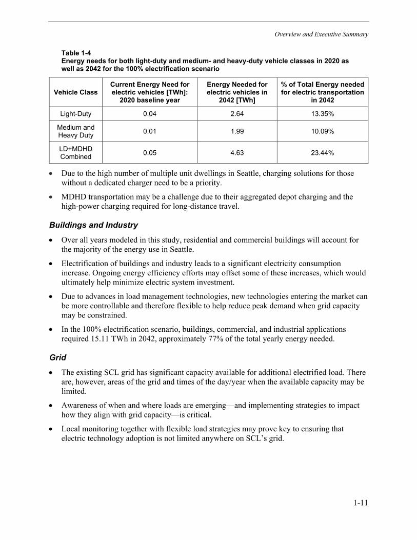
Overview and Executive Summary
1-11
Table 1-4 Energy needs for both light-duty and medium- and heavy-duty vehicle classes in 2020 as well as 2042 for the 100% electrification scenario
Vehicle Class Current Energy Need for electric vehicles [TWh]:
2020 baseline year
Energy Needed for electric vehicles in
2042 [TWh]
% of Total Energy needed for electric transportation
in 2042
Light-Duty 0.04 2.64 13.35%
Medium and Heavy Duty 0.01 1.99 10.09%
LD+MDHD Combined 0.05 4.63 23.44%
• Due to the high number of multiple unit dwellings in Seattle, charging solutions for those without a dedicated charger need to be a priority.
• MDHD transportation may be a challenge due to their aggregated depot charging and the high-power charging required for long-distance travel.
Buildings and Industry
• Over all years modeled in this study, residential and commercial buildings will account for the majority of the energy use in Seattle.
• Electrification of buildings and industry leads to a significant electricity consumption increase. Ongoing energy efficiency efforts may offset some of these increases, which would ultimately help minimize electric system investment.
• Due to advances in load management technologies, new technologies entering the market can be more controllable and therefore flexible to help reduce peak demand when grid capacity may be constrained.
• In the 100% electrification scenario, buildings, commercial, and industrial applications required 15.11 TWh in 2042, approximately 77% of the total yearly energy needed.
Grid
• The existing SCL grid has significant capacity available for additional electrified load. There are, however, areas of the grid and times of the day/year when the available capacity may be limited.
• Awareness of when and where loads are emerging—and implementing strategies to impact how they align with grid capacity—is critical.
• Local monitoring together with flexible load strategies may prove key to ensuring that electric technology adoption is not limited anywhere on SCL’s grid.
Overview and Executive Summary
1-12
Report Format The following sections of this assessment provide the analysis undertaken to support this work as well as detail the potential for flexibility of new electric loads and strategies to achieve full electrification:
• Section 2: Electric transportation: The total energy needed to support electrification, vehicle growth by vehicle type and dwelling type is provided. This section also provides detailed analysis on the charging infrastructure required to support large growth in electric vehicle (EV) fleets.
• Sections 3 and 4: Buildings, commercial, and industrial technologies: Provides an analysis of existing energy consumption as well as key opportunities for electrifying various end-use technologies. Future changes in consumption considering market growth, energy efficiency, and electrification are also discussed.
• Section 5: Grid capacity: Models distribution grid capacity down to the feeder level with time series data, which allows temporal and locational analysis for when and where the grid may become constrained.
• Section 6: New load flexibility: Discusses how new load flexibility has great potential to help decrease the sizable grid impact due to growing electric load; many factors must be considered—from customer comfort to cost considerations as well as how codes and standards impact the need for flexibility.
• Section 7: Strategies to achieve full electrification: Effective electrification strategies will be central to SCL’s consideration of next steps in its efforts to meet the policy goals of the City of Seattle. The strategies provided in this assessment point to specific technology gaps and ways to overcome them as well as examples of what other cities are doing to achieve their own electrification goals. No city or utility is the same; therefore, it is likely that there is a unique solution (or grouping of solutions that will need to adapt over time) that will help SCL achieve its electrification goals.
2-1
2 ON-ROAD TRANSPORTATION
Executive Summary Section 2 of the Electrification Assessment provides analysis for the three transportation electrification scenarios. For each scenario, the total energy, power, and charging infrastructure required is calculated. The underlying assumptions that are used in these scenarios are also discussed.
Over all scenarios and years (2020-2042), passenger vehicles will be the dominant load. Although heavier vehicles consume more energy individually, the population of passenger vehicles is at least 20 times greater than any other vehicle class. In the Full Electrification scenario, which has 100% adoption of all vehicle classes, passenger vehicles are about 55% of the total annual EV consumption. The energy required to support electric transportation in SCL’s service territory in 2030 ranges from 117 GWh (in the Moderate Market Advancement scenario) to 4,312 GWh (in the Full Electrification Scenario).
This analysis also provided analysis on the number of charging ports needed to support these vehicles which included home, work and public charging. Due to the high number of MUDs (multiple unit dwellings) in Seattle, alternatives to home charging need to be accessible. The recommended amount of fast (over 50 kW) public charging ports needed to support the three scenarios presented here in 2030 range from 683 to 17,670 depending on the scenario.
The vehicle load shapes provided were based on local travel data that was supplemented, where needed, with national survey data. A load shape was assumed for a variety of electric vehicle types (both BEVs and PHEVs) and then was combined and multiplied based on a yearly vehicle count to achieve a load shape across all electrified transportation. It is unknown how transportation may change in the near and far future due to shifts in TNC (transportation network company) miles, vehicle autonomy, increased transit use and remote and flexible work options thus this analysis may need to be revisited as transportation conditions shift significantly. Using the assumptions in this analysis, for 100% electrification scenario, the energy required to fuel electric vehicles (both light-duty and medium and heavy duty) is projected to be approximately 90 times greater than it is today.
Introduction SCL has been a leader in efforts to decarbonize the power sector, becoming the first carbon-neutral utility in the nation in 2005.8 With transportation accounting for 60% of Seattle’s
8 https://www.seattle.gov/city-light/energy-and-environment/environment/climate-change-and-energy
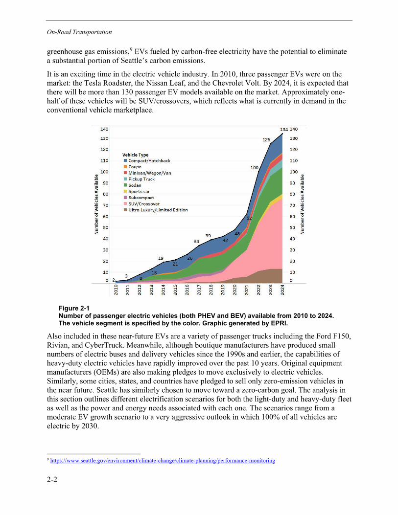
On-Road Transportation
2-2
greenhouse gas emissions,9 EVs fueled by carbon-free electricity have the potential to eliminate a substantial portion of Seattle’s carbon emissions.
It is an exciting time in the electric vehicle industry. In 2010, three passenger EVs were on the market: the Tesla Roadster, the Nissan Leaf, and the Chevrolet Volt. By 2024, it is expected that there will be more than 130 passenger EV models available on the market. Approximately one-half of these vehicles will be SUV/crossovers, which reflects what is currently in demand in the conventional vehicle marketplace.
Figure 2-1 Number of passenger electric vehicles (both PHEV and BEV) available from 2010 to 2024. The vehicle segment is specified by the color. Graphic generated by EPRI.
Also included in these near-future EVs are a variety of passenger trucks including the Ford F150, Rivian, and CyberTruck. Meanwhile, although boutique manufacturers have produced small numbers of electric buses and delivery vehicles since the 1990s and earlier, the capabilities of heavy-duty electric vehicles have rapidly improved over the past 10 years. Original equipment manufacturers (OEMs) are also making pledges to move exclusively to electric vehicles. Similarly, some cities, states, and countries have pledged to sell only zero-emission vehicles in the near future. Seattle has similarly chosen to move toward a zero-carbon goal. The analysis in this section outlines different electrification scenarios for both the light-duty and heavy-duty fleet as well as the power and energy needs associated with each one. The scenarios range from a moderate EV growth scenario to a very aggressive outlook in which 100% of all vehicles are electric by 2030.
9 https://www.seattle.gov/environment/climate-change/climate-planning/performance-monitoring

On-Road Transportation
2-3
On-road vehicles—which include personally owned cars and trucks as well as publicly or privately owned commercial trucks and buses—are responsible for approximately 50% of the greenhouse gas emissions in the SCL territory. In 2020, less than 2% of Seattle’s on-road vehicles were electric.10
This section of the Electrification Assessment is focused on the electrification of on-road transportation, and includes the following:
• Scenario definitions. Describes the factors underlying the three different adoption scenarios and presents the trajectories of EV adoption in terms of the share of new vehicles that are electric.
• Vehicle population and activity data. Presents the quantitative assessment of the existing population of various classes of on-road vehicles; the various data sources of activity data, which include daily driving patterns and annual mileage; and the annual growth rates of these vehicle populations in future years.
• Electric vehicle projections. Presents the future electric vehicle population according to the three scenarios.
• Load shapes. Discusses the modeling approach and methodology used to determine the hourly demand of uncontrolled and unmanaged electric vehicle charging. The results include 24-hour and 8760-hour load shapes.
• Annual energy consumption. This brief section presents the assumptions and methodology for calculating the total electricity consumption of EVs on an annual basis.
• Charging infrastructure. This section explains the methodology used to determine the amount of charging infrastructure required to support the future population of EVs within Seattle, along with numerical estimates for the number of charging ports in future years.
• Conclusion. The section ends with a recap of the most relevant high-level impacts of EVs on the SCL system.
Scenario Definitions The City of Seattle aims to create jobs and advance an equitable transition from fossil fuels to renewable energy. Seattle’s 2013 Climate Action Plan11 is the main policy framework for the City’s climate-related actions. The recent transportation sector components of this effort have been documented in various utility, city planning, and implementation documents, including the EV Charging Roadmap for Shared Mobility,12 the Shared Mobility Playbook,13 the SCL Transportation Electrification Strategic Investment Plan,14 the Clean Transportation
10 Based on EPRI’s analysis of vehicle registration data.
11 http://www.seattle.gov/documents/departments/ose/2013_cap_20130612.pdf
12 https://www.seattle.gov/Documents/Departments/OSE/ClimateDocs/TE/SDOT_EVSE_Roadmap_for_Shared_Mobility_Hubs.pdf 13 https://www.seattle.gov/Documents/Departments/SDOT/NewMobilityProgram/NewMobility_Playbook_9.2017.pdf 14 https://www.seattle.gov/documents/Departments/CityLight/TESIP.pdf
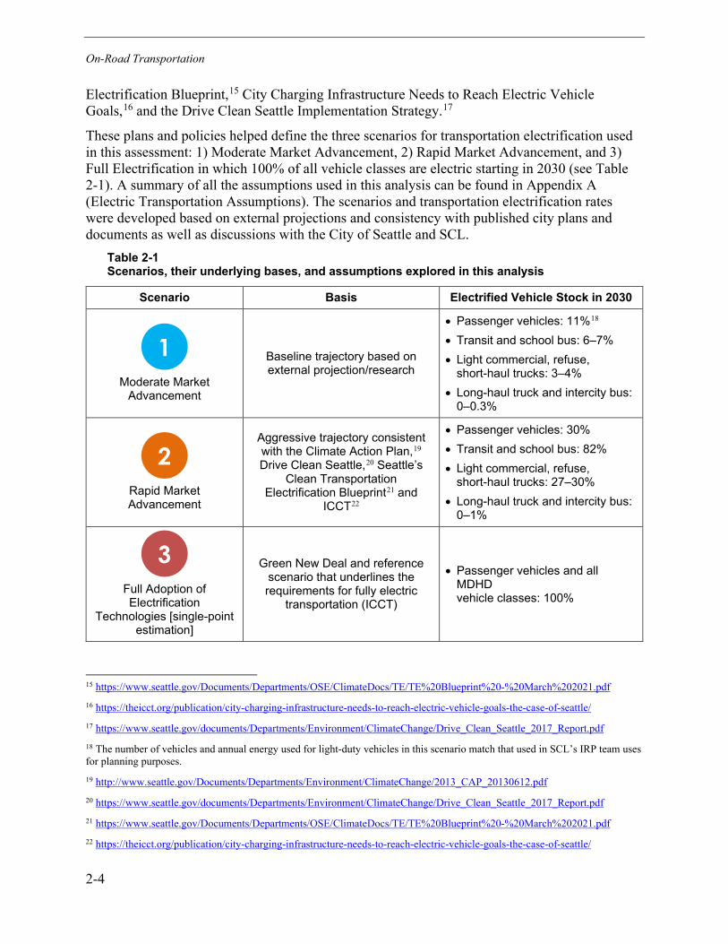
On-Road Transportation
2-4
Electrification Blueprint,15 City Charging Infrastructure Needs to Reach Electric Vehicle Goals,16 and the Drive Clean Seattle Implementation Strategy.17
These plans and policies helped define the three scenarios for transportation electrification used in this assessment: 1) Moderate Market Advancement, 2) Rapid Market Advancement, and 3) Full Electrification in which 100% of all vehicle classes are electric starting in 2030 (see Table 2-1). A summary of all the assumptions used in this analysis can be found in Appendix A (Electric Transportation Assumptions). The scenarios and transportation electrification rates were developed based on external projections and consistency with published city plans and documents as well as discussions with the City of Seattle and SCL.
Table 2-1 Scenarios, their underlying bases, and assumptions explored in this analysis
Scenario Basis Electrified Vehicle Stock in 2030
Moderate Market
Advancement
Baseline trajectory based on external projection/research
• Passenger vehicles: 11%18 • Transit and school bus: 6–7% • Light commercial, refuse,
short-haul trucks: 3–4% • Long-haul truck and intercity bus:
0–0.3%
Rapid Market Advancement
Aggressive trajectory consistent with the Climate Action Plan,19 Drive Clean Seattle,20 Seattle’s
Clean Transportation Electrification Blueprint21 and
ICCT22
• Passenger vehicles: 30% • Transit and school bus: 82% • Light commercial, refuse,
short-haul trucks: 27–30% • Long-haul truck and intercity bus:
0–1%
Full Adoption of Electrification
Technologies [single-point estimation]
Green New Deal and reference scenario that underlines the requirements for fully electric
transportation (ICCT)
• Passenger vehicles and all MDHD vehicle classes: 100%
15 https://www.seattle.gov/Documents/Departments/OSE/ClimateDocs/TE/TE%20Blueprint%20-%20March%202021.pdf 16 https://theicct.org/publication/city-charging-infrastructure-needs-to-reach-electric-vehicle-goals-the-case-of-seattle/ 17 https://www.seattle.gov/documents/Departments/Environment/ClimateChange/Drive_Clean_Seattle_2017_Report.pdf 18 The number of vehicles and annual energy used for light-duty vehicles in this scenario match that used in SCL’s IRP team uses for planning purposes. 19 http://www.seattle.gov/Documents/Departments/Environment/ClimateChange/2013_CAP_20130612.pdf 20 https://www.seattle.gov/documents/Departments/Environment/ClimateChange/Drive_Clean_Seattle_2017_Report.pdf 21 https://www.seattle.gov/Documents/Departments/OSE/ClimateDocs/TE/TE%20Blueprint%20-%20March%202021.pdf 22 https://theicct.org/publication/city-charging-infrastructure-needs-to-reach-electric-vehicle-goals-the-case-of-seattle/
1
2
3

On-Road Transportation
2-5
Scenario 1: Moderate Market Advancement The Moderate Market Advancement scenario is a baseline trajectory based on a combination of EPRI analysis and external projections. This scenario assumes that transportation electrification will continue to advance but that EVs do not become the dominant technology by 2042. In general, this scenario assumes continued EV and charging infrastructure cost reductions, increasing customer awareness around EVs, moderate levels of charging infrastructure outside of the SCL territory, and limited incentivization from the City of Seattle.
Passenger vehicles are estimated to be approximately 11% EV stock by 2030, according to EPRI projections.23 Market projections and cost parity estimates for MDHD vehicles are based on third-party sources, including the North American Council for Freight Efficiency,24 McKinsey,25 BloombergNEF,26 the Department of Energy’s Annual Energy Outlook (AEO),27 and other EPRI analyses. Approximately 10% of passenger vehicles are assumed to be plug-in hybrid vehicles through 2045,28 while all electrified29 MDHD vehicles are assumed to be battery electric vehicles without a combustion engine component. Compared to the West Coast Clean Transit Corridor Initiative (WCCTCI) 2020 report, this study’s Moderate Market Advancement scenario’s electrification rate of new short-haul trucks is between the WCCTCI report’s low and high estimates for medium-duty trucks in the state of Washington, and the Moderate Market Advancement scenario for long-haul trucks is similar to the WCCTCI Low-with-Incentives scenario for heavy-duty trucks.30
Scenario 2: Rapid Market Advancement The Rapid Market Advancement scenario represents a more aggressive electrification strategy, reflective of political drivers and City of Seattle policy goals. It was developed to be consistent with the City of Seattle’s Climate Action Plan, Drive Clean Seattle report, and the 2016 City Council resolution that set a goal that 30% of vehicles in the City will be electric by 2030.31 Under the Drive Clean Seattle Implementation Strategy report, 30% of all light-duty vehicles in Seattle should be electric by 2030. Consistent with the Drive Clean report, the Rapid Market Advancement scenario targets 30% of the passenger vehicle stock to be electrified by 2030. This
23 The tool estimates and projects the composition of the United States on-road vehicle fleet, calculates energy use, greenhouse gas emissions reduction, and other results that are important to utilities. https://www.epri.com/research/programs/053122/results/3002018552 24 “Electric Trucks: Where They Make Sense” (2018 report) https://nacfe.org/future-technology/electric-trucks/) 25 “What’s sparking electric-vehicle adoption in the truck industry?” (2017 article) https://www.mckinsey.com/industries/automotive-and-assembly/our-insights/whats-sparking-electric-vehicle-adoption-in-the-truck-industry#) 26 Electric Vehicle Outlook 2019 https://about.bnef.com/electric-vehicle-outlook/ 27 Annual Energy Outlook 2020 https://www.eia.gov/outlooks/aeo/ 28 Please refer to Page A-2 in Appendix A for more information. 29 Some media refer to hybrid-electric vehicles, which do not recharge from the grid, as “electrified” vehicles. Here “electrified” specifically denotes plug-in electric vehicles. 30 West Coast Clean Transit Corridor Initiative, Interstate 5 Corridor, California, Oregon, Washington, FINAL REPORT, June 2020. https://westcoastcleantransit.com/resources/Final%20Report%20Files.zip 31 Seattle City Council resolution 31696. http://seattle.legistar.com/LegislationDetail.aspx?ID=2811912&GUID=9E735C1F-A4C2-4358-B5EF-6007CE47D037&FullText=1
On-Road Transportation
2-6
is also in line with the trajectory established in the 30% of passenger vehicle stock scenario in the 2021 ICCT/SDOT report on charging infrastructure needs for the City of Seattle.32 Light commercial trucks and MDHD trucks vary based on class. In the Rapid Market Advancement scenario, 50% of new sales for light commercial and short-haul trucks are assumed to be electrified by 2026, and 98% of new sales by 2030. This is an extension of Seattle’s Clean Transportation Electrification Blueprint33 goal that 30% of all goods delivery be zero emissions, expanding the goal to include the stock of all other short-haul heavy-duty vehicles. Long-haul trucks electrify at slower rates, reaching approximately 50% of new sales by 2040.34 Transit buses are assumed to reach 100% electric stock by 2040, based on King County Metro goals; however, this may require early retirement of vehicles in operation.35 The Electric Vehicle Population Projections section below presents the electrification rates for the Moderate Market Advancement scenario and the Rapid Market Advancement scenario.
Scenario 3: Full Electrification Full electrification of all transportation is modeled in Scenario 3 and was developed to be consistent with the ideas laid out in City of Seattle’s Green New Deal and the 100% adoption by 2030 scenario within the 2021 ICCT report. This scenario assumes that 100% of all vehicle classes are battery electric vehicle (BEV) starting in 2030. For this scenario, electrification over time is shown only from 2030 onward and assumes the goal of 100% electrification by 2030.
Vehicle Population, Charging Infrastructure, and Activity Data As a first step for analysis, available data for current vehicles and charging infrastructure in the City of Seattle were inventoried to develop a baseline estimate of the fleet of vehicles presently operating in Seattle.
Vehicle Classes and EV Types The current vehicle fleet operating in SCL’s service territory was divided into two high-level vehicle categories: 1) passenger vehicles and 2) light commercial, MDHD trucks. Each of these categories is further subdivided according to the vehicle classes used by EPA’s Motor Vehicle Emission Simulator (MOVES).36
Passenger vehicles include the following vehicle classes: passenger cars, passenger trucks, and motorcycles. Passenger cars include both personal and commercial/fleet cars. Passenger trucks include light trucks, vans, and SUVs that are primarily used for personal transportation. Light
32 International Council for Clean Transportation. City charging infrastructure needs to reach electric vehicle goals: The case of Seattle. https://theicct.org/publication/city-charging-infrastructure-needs-to-reach-electric-vehicle-goals-the-case-of-seattle/ 33 https://www.seattle.gov/Documents/Departments/OSE/ClimateDocs/TE/TE%20Blueprint%20-%20March%202021.pdf 34 Compared to the West Coast Clean Transit Corridor Initiative (WCCTCI) 2020 report, this study’s Rapid scenario for new short-haul trucks is higher than the WCCTCI report’s High-with-Incentives scenario for medium-duty trucks in the state of Washington, and our Rapid scenario for long-haul trucks is slightly lower than the WCCTCI High projection for heavy-duty trucks. West Coast Clean Transit Corridor Initiative, Interstate 5 Corridor, California, Oregon, Washington, FINAL REPORT, June 2020. https://westcoastcleantransit.com/resources/Final%20Report%20Files.zip 35 This depends on the age of the transit bus fleet and if Seattle area transit bus life spans are greater than 12 years. 36 https://www.epa.gov/moves

On-Road Transportation
2-7
commercial trucks (LCT) cover commercial or fleet light trucks, vans, and SUVs. The passenger truck and light commercial truck categories overlap: both include Class 1 and Class 2 trucks in their definition.37 They differ based on whether they are owned as a personal vehicle or by a commercial operator. The MDHD trucks vehicle category includes the following vehicle classes: transit buses, school buses, intercity buses, refuse trucks, motor home, short-haul MDHD trucks, and long-haul MDHD trucks. Table 2-2 provides additional descriptions of each vehicle class.
Table 2-2 Vehicle class definitions38
Vehicle Class Description
Motorcycle Motorcycles
Passenger Car Personal or commercial/fleet passenger cars
Passenger Truck Minivans, pickups, SUVs, and other 2-axle/4-tire trucks used primarily for personal transportation
Light Commercial Truck
Minivans, pickups, SUVs, and other 2-axle/4-tire trucks used primarily for commercial applications
Intercity Bus Buses that are not transit buses or school buses, for example, those used primarily by commercial carriers for city-to-city transport
Transit Bus Buses used for public transit
School Bus School and church buses
Refuse Truck Garbage and recycling trucks
Single-Unit Short-Haul Truck Single-unit trucks with majority of operation within 200 miles of home base
Single-Unit Long-Haul Truck Single-unit trucks with majority of operation outside of 200 miles of home base
Motor Home Motor home
Combination Short-Haul Truck
Combination trucks towing at least 1 trailer with majority of operation within 200 miles of home base. Includes drayage trucks
Combination Long-Haul Truck
Combination trucks towing at least 1 trailer with majority of operation outside of 200 miles of home base
For passenger vehicles, the projected electric vehicle types used include plug-in hybrids (PHEVs) with 10-, 20-, and 40-mile electric ranges and BEVs, with 100- and 250-mile ranges. For light commercial and MDHD trucks, all vehicles are assumed to be BEVs, with no plug-in hybrids. In addition, the electrified vehicle ranges of LCT and MDHD trucks are assumed to be consistent with the current vehicle operating ranges.
37 Class 2b vehicles, with gross vehicle weight ratings between 8,501 and 10,000 lb, are considered “light-duty” by the Federal Highway Administration and the U.S. Census Bureau but are treated as MDHD vehicles by the EPA’s emissions regulations. For more information, refer to https://afdc.energy.gov/data/10380. 38 Motor Vehicle Emission Simulator (MOVES) 2014 Software Design and Reference Manual. United States Environmental Protection Agency, Washington, DC: 2014. EPA-420-B-14-056.

On-Road Transportation
2-8
Vehicle Population The total vehicle population for SCL’s service territory in 2020 is estimated to be approximately 837,400 vehicles, with the majority composed of passenger vehicles.
Table 2-3 SCL service territory vehicle population (2020)
Vehicle Class Vehicle Population
Passenger Vehicle 771,486
Light Commercial Truck 33,659
Intercity Bus 45
Transit Bus 1,252
School Bus 405
Refuse Truck 204
Short-Haul Truck39 24,136
Long-Haul Truck 2,400
Motor Home 3,795
Data for on-road vehicles in 2020 were assembled from a variety of sources, and EPRI used local sources when available. The passenger vehicle population was derived from PSRC’s household travel survey and SoundCast40 model outputs and included vehicles that reside outside of Seattle but commute into Seattle for work.41 The transit bus count was based on King County Metro reports.42 It excludes buses that are operated out of the East Campus depot in Bellevue because this depot is outside of SCL service territory. School bus data were provided directly from First Student, the bus operator for Seattle Public Schools.43 Refuse trucks were estimated based on the published size of the Waste Management and Recology fleets in Seattle, which are the only two operators within the city.44 The vehicle population for the remaining classes was derived from analysis based on the EPA’s 2017 National Emissions Inventory (NEI),45 the most recent available, which provides data at the county level for different vehicle classes in 2017. This was then scaled by the fraction of vehicle activity for each category that is estimated to take place in the SCL service territory versus the rest of King County.
39 Short-Haul Trucks include drayage trucks 40 SoundCast is a travel demand model system built for the Puget Sound Region. The model was designed to depict diverse human travel behavior and include travel sensitivity to land use and the built environment. (Link: https://www.psrc.org/activity-based-travel-model-soundcast). 41 These commuter vehicles have their home location outside of Seattle but take at least one work-related trip into Seattle in the day. 42 Metro Facilities Master Plan (https://epri.app.box.com/file/799427857531?s=ydjn3fsg5hfz764xfhg5p1628l94moip) 43 E-mail from Seattle Public Schools to EPRI. 44 https://www.geekwire.com/2019/seattle-rolls-nations-first-fully-electric-garbage-trucks-transition-fossil-fuel-free-fleet/ 45 https://www.epa.gov/air-emissions-inventories/2017-national-emissions-inventory-nei-data, accessed in November, in conjunction with results from MOtor Vehicle Emission Simulator version 2014b (MOVES2014b), United States Environmental Protection Agency.
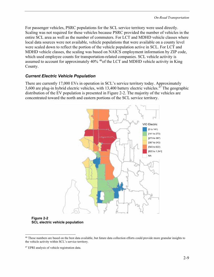
On-Road Transportation
2-9
For passenger vehicles, PSRC populations for the SCL service territory were used directly. Scaling was not required for these vehicles because PSRC provided the number of vehicles in the entire SCL area as well as the number of commuters. For LCT and MDHD vehicle classes where local data sources were not available, vehicle populations that were available on a county level were scaled down to reflect the portion of the vehicle population active in SCL. For LCT and MDHD vehicle classes, the scaling was based on NAICS employment information by ZIP code, which used employee counts for transportation-related companies. SCL vehicle activity is assumed to account for approximately 40% 46of the LCT and MDHD vehicle activity in King County.
Current Electric Vehicle Population There are currently 17,000 EVs in operation in SCL’s service territory today. Approximately 3,600 are plug-in hybrid electric vehicles, with 13,400 battery electric vehicles.47 The geographic distribution of the EV population is presented in Figure 2-2. The majority of the vehicles are concentrated toward the north and eastern portions of the SCL service territory.
Figure 2-2 SCL electric vehicle population
46 These numbers are based on the best data available, but future data collection efforts could provide more granular insights to the vehicle activity within SCL’s service territory. 47 EPRI analysis of vehicle registration data.
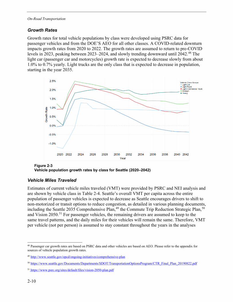
On-Road Transportation
2-10
Growth Rates Growth rates for total vehicle populations by class were developed using PSRC data for passenger vehicles and from the DOE’S AEO for all other classes. A COVID-related downturn impacts growth rates from 2020 to 2022. The growth rates are assumed to return to pre-COVID levels in 2023, peaking between 2023–2024, and slowly trending downward until 2042.48 The light car (passenger car and motorcycles) growth rate is expected to decrease slowly from about 1.0% to 0.7% yearly. Light trucks are the only class that is expected to decrease in population, starting in the year 2035.
Figure 2-3 Vehicle population growth rates by class for Seattle (2020–2042)
Vehicle Miles Traveled Estimates of current vehicle miles traveled (VMT) were provided by PSRC and NEI analysis and are shown by vehicle class in Table 2-4. Seattle’s overall VMT per capita across the entire population of passenger vehicles is expected to decrease as Seattle encourages drivers to shift to non-motorized or transit options to reduce congestion, as detailed in various planning documents, including the Seattle 2035 Comprehensive Plan,49 the Commute Trip Reduction Strategic Plan,50 and Vision 2050.51 For passenger vehicles, the remaining drivers are assumed to keep to the same travel patterns, and the daily miles for their vehicles will remain the same. Therefore, VMT per vehicle (not per person) is assumed to stay constant throughout the years in the analyses
48 Passenger car growth rates are based on PSRC data and other vehicles are based on AEO. Please refer to the appendix for sources of vehicle population growth rates. 49 http://www.seattle.gov/opcd/ongoing-initiatives/comprehensive-plan 50 https://www.seattle.gov/Documents/Departments/SDOT/TransportationOptionsProgram/CTR_Final_Plan_20190822.pdf 51 https://www.psrc.org/sites/default/files/vision-2050-plan.pdf
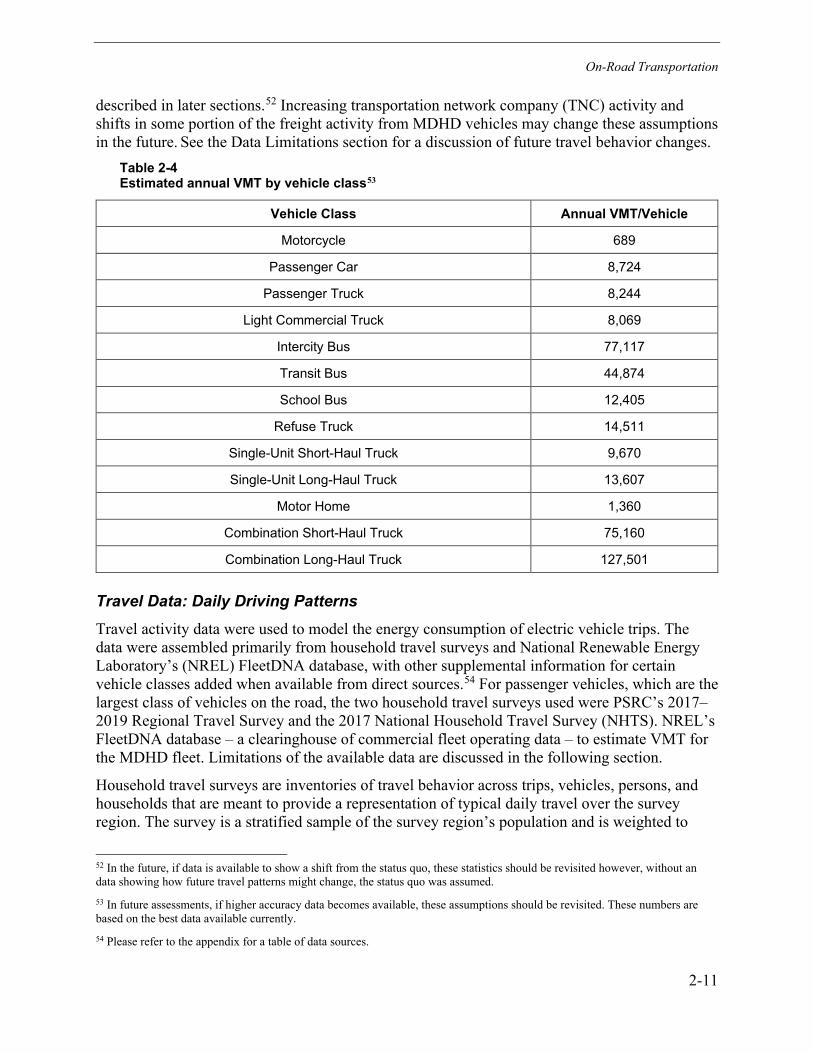
On-Road Transportation
2-11
described in later sections.52 Increasing transportation network company (TNC) activity and shifts in some portion of the freight activity from MDHD vehicles may change these assumptions in the future. See the Data Limitations section for a discussion of future travel behavior changes.
Table 2-4 Estimated annual VMT by vehicle class53
Vehicle Class Annual VMT/Vehicle
Motorcycle 689
Passenger Car 8,724
Passenger Truck 8,244
Light Commercial Truck 8,069
Intercity Bus 77,117
Transit Bus 44,874
School Bus 12,405
Refuse Truck 14,511
Single-Unit Short-Haul Truck 9,670
Single-Unit Long-Haul Truck 13,607
Motor Home 1,360
Combination Short-Haul Truck 75,160
Combination Long-Haul Truck 127,501
Travel Data: Daily Driving Patterns Travel activity data were used to model the energy consumption of electric vehicle trips. The data were assembled primarily from household travel surveys and National Renewable Energy Laboratory’s (NREL) FleetDNA database, with other supplemental information for certain vehicle classes added when available from direct sources.54 For passenger vehicles, which are the largest class of vehicles on the road, the two household travel surveys used were PSRC’s 2017–2019 Regional Travel Survey and the 2017 National Household Travel Survey (NHTS). NREL’s FleetDNA database – a clearinghouse of commercial fleet operating data – to estimate VMT for the MDHD fleet. Limitations of the available data are discussed in the following section.
Household travel surveys are inventories of travel behavior across trips, vehicles, persons, and households that are meant to provide a representation of typical daily travel over the survey region. The survey is a stratified sample of the survey region’s population and is weighted to
52 In the future, if data is available to show a shift from the status quo, these statistics should be revisited however, without an data showing how future travel patterns might change, the status quo was assumed. 53 In future assessments, if higher accuracy data becomes available, these assumptions should be revisited. These numbers are based on the best data available currently. 54 Please refer to the appendix for a table of data sources.

On-Road Transportation
2-12
match the total population and total trips over a full travel day for the region. The PSRC survey was a longitudinal study that included data from consecutive days and focused primarily on weekday travel, though weekend travel data were included. It covers the four-county Puget Sound region—which consists of King, Pierce, Snohomish, and Kitsap counties—and is the most recent Seattle-specific travel survey available. The NHTS was designed to provide an accurate representation of all seven days of the week across the entire United States, though each respondent provides data for only one day. The two household surveys were compared for consistency between the data sets. Due to the focus of the PSRC survey on weekday travel over weekend travel, weekend travel data were supplemented with NHTS data.
The same attributes were used from both surveys to model energy consumption and are described below. Trip purposes at the origin and destination (for example, home, work, school, drop off) informed whether a charging event could occur and whether it was at a home, work, or public charger. Trip start and end times were used to determine when a charging event would be as well as trip mileages (when paired with additional data about vehicle operating efficiency and characteristics).
FleetDNA was used to help provide a representation of a typical weekday for MDHD vehicles. To obtain an estimate of weekend energy consumption, the data were scaled by the difference between weekend and weekday truck counts in the Seattle region via truck counts from WSDOT.55 There are a total of six count locations56 with vehicle weight class information and time across all the major ingress and egress roads and highways around SCL’s service territory. These locations were used as a representative cordon, and the available hourly counts for the year 2017 were used to estimate the split between weekday and weekend truck activity. Weekend truck counts consisted of approximately 13% of the total observed truck counts, and weekdays accounted for the other 87%. This estimate was checked for validity against a medium-duty and heavy-duty data set from INRIX57 for the Seattle region, which had similar percentages for the split of truck trip activity on weekdays and weekends. Driving data for long-haul trucks were also derived from WSDOT travel data for I-5. None of the sensors within Seattle had the ability to distinguish truck types,58 so data from a sensor north of Seattle were used to estimate the volume of trucks during different time periods. This was scaled by the total VMT estimated in the NEI analysis to determine VMT per hour.
Data Limitations Passenger car data were based on the PSRC regional travel model and survey, which has known limitations, including that the survey design focuses primarily on residential-based driving and that the results are calibrated to past trends. In addition, the PSRC survey sample size is small, covering approximately 1,200 of the 344,000 Seattle households, which may not adequately
55 Using PTR sites from https://www.wsdot.wa.gov/data/tools/geoportal/?config=traffic 56 Count locations: D10, D14, R082S, R117, S837, S839 57 The INRIX data set is an anonymized data set collected from road sensors, cell phone, and fleet vehicle records. The data set used covered every other month of 2017, starting in February, and all vehicles that stopped in the SCL service territory at least once within the available data’s time frame. 58 The City of Seattle is actively working on collection more data, and there may be more insights available soon
On-Road Transportation
2-13
represent Seattle driving patterns. Employment-based driving via LODES59 was used to help validate the percentage of VMT for Seattle, but neither data set can capture known changes coming in the near and far future for transportation in the form of electric vehicles, TNCs, autonomous vehicles, increased transit use, remote and flexible work options, and other unknown changes.
This analysis assumes that per capita vehicle ownership will drop in the future but that driving patterns will stay consistent for the remaining vehicles. VMT per remaining vehicle may increase in the future due to a shift from personal trips to rideshare and gig delivery, but there are insufficient data available to support specific assumptions. Seattle currently has one of the lowest percentages of rideshare VMT in the nation. A 2019 study by Fehr and Peers estimated that only 1.9% of Seattle’s VMT was due to rideshare VMT, far lower than cities such as San Francisco (12.8%) and Washington, D.C. (6.9%).60 Therefore, the chances that ridesharing will increase in the future is likely.
In addition, though gig delivery VMT may be rising, insufficient data from operators are available to determine the rate that person trips are shifting to delivery services and how much of an increase may be occurring. The effects may also vary based on locale, especially based on future urban planning design and actions by cities to limit the congestion due to last-mile freight delivery.
Furthermore, TNCs and gig delivery effectively reroute the transportation of people or goods from one vehicle into a different vehicle. It is not clear whether the net change in energy or electricity consumption due to this shift is positive or negative.
For this analysis, it seemed preferable to limit estimates to known quantities and the changes due to electrification proposed in these scenarios, though further analysis could be performed to test a range of scenarios with increased rideshare and delivery VMT—especially as more data are collected. Future data collection efforts for the effects of electrification on rideshare, e-commerce, and gig delivery could include obtaining data on the driving pattern distribution of e-commerce and gig vehicles (arrival and departure times and distances on weekends and weekdays), including information about whether the driver resides at an apartment or single-family house and whether they travel from suburban or exurban communities into the central core of the city for gig work.
Electric Vehicle Population Projections Each of the three scenarios considered has different adoption rates of electric vehicles in each vehicle class over time. The primary distinction between the scenarios is the rate at which different vehicle classes electrify. The electrification rates as well as the various life spans of each type of vehicle contribute to the total number of electric vehicles in the population. The number of electric vehicles in operation contributes to the annual energy consumption from transportation electrification based on the electric vehicle miles traveled. Furthermore, the number of EVs in the population is a critical variable in determining the number of EV charge ports that are required to provide this energy.
59 LEHD Origin-Destination Employment Statistics, Census 60 https://www.fehrandpeers.com/what-are-tncs-share-of-vmt/
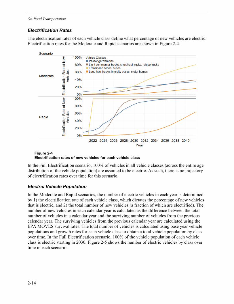
On-Road Transportation
2-14
Electrification Rates The electrification rates of each vehicle class define what percentage of new vehicles are electric. Electrification rates for the Moderate and Rapid scenarios are shown in Figure 2-4.
Figure 2-4 Electrification rates of new vehicles for each vehicle class
In the Full Electrification scenario, 100% of vehicles in all vehicle classes (across the entire age distribution of the vehicle population) are assumed to be electric. As such, there is no trajectory of electrification rates over time for this scenario.
Electric Vehicle Population In the Moderate and Rapid scenarios, the number of electric vehicles in each year is determined by 1) the electrification rate of each vehicle class, which dictates the percentage of new vehicles that is electric, and 2) the total number of new vehicles (a fraction of which are electrified). The number of new vehicles in each calendar year is calculated as the difference between the total number of vehicles in a calendar year and the surviving number of vehicles from the previous calendar year. The surviving vehicles from the previous calendar year are calculated using the EPA MOVES survival rates. The total number of vehicles is calculated using base year vehicle populations and growth rates for each vehicle class to obtain a total vehicle population by class over time. In the Full Electrification scenario, 100% of the vehicle population of each vehicle class is electric starting in 2030. Figure 2-5 shows the number of electric vehicles by class over time in each scenario.
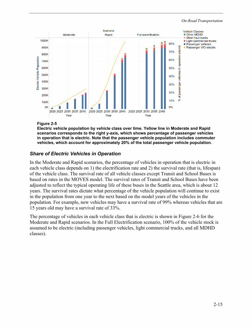
On-Road Transportation
2-15
Figure 2-5 Electric vehicle population by vehicle class over time. Yellow line in Moderate and Rapid scenarios corresponds to the right y-axis, which shows percentage of passenger vehicles in operation that is electric. Note that the passenger vehicle population includes commuter vehicles, which account for approximately 20% of the total passenger vehicle population.
Share of Electric Vehicles in Operation In the Moderate and Rapid scenarios, the percentage of vehicles in operation that is electric in each vehicle class depends on 1) the electrification rate and 2) the survival rate (that is, lifespan) of the vehicle class. The survival rate of all vehicle classes except Transit and School Buses is based on rates in the MOVES model. The survival rates of Transit and School Buses have been adjusted to reflect the typical operating life of these buses in the Seattle area, which is about 12 years. The survival rates dictate what percentage of the vehicle population will continue to exist in the population from one year to the next based on the model years of the vehicles in the population. For example, new vehicles may have a survival rate of 99% whereas vehicles that are 15 years old may have a survival rate of 33%.
The percentage of vehicles in each vehicle class that is electric is shown in Figure 2-6 for the Moderate and Rapid scenarios. In the Full Electrification scenario, 100% of the vehicle stock is assumed to be electric (including passenger vehicles, light commercial trucks, and all MDHD classes).
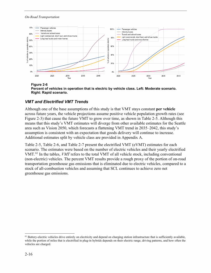
On-Road Transportation
2-16
Figure 2-6 Percent of vehicles in operation that is electric by vehicle class. Left: Moderate scenario. Right: Rapid scenario.
VMT and Electrified VMT Trends Although one of the base assumptions of this study is that VMT stays constant per vehicle across future years, the vehicle projections assume positive vehicle population growth rates (see Figure 2-3) that cause the future VMT to grow over time, as shown in Table 2-5. Although this means that this study’s VMT estimates will diverge from other available estimates for the Seattle area such as Vision 2050, which forecasts a flattening VMT trend in 2035–2042, this study’s assumption is consistent with an expectation that goods delivery will continue to increase. Additional estimates split by vehicle class are provided in Appendix A.
Table 2-5, Table 2-6, and Table 2-7 present the electrified VMT (eVMT) estimates for each scenario. The estimates were based on the number of electric vehicles and their yearly electrified VMT.61 In the tables, VMT refers to the total VMT of all vehicle stock, including conventional (non-electric) vehicles. The percent VMT results provide a rough proxy of the portion of on-road transportation greenhouse gas emissions that is eliminated due to electric vehicles, compared to a stock of all-combustion vehicles and assuming that SCL continues to achieve zero net greenhouse gas emissions.
61 Battery-electric vehicles drive entirely on electricity and depend on charging station infrastructure that is sufficiently available, while the portion of miles that is electrified in plug-in hybrids depends on their electric range, driving patterns, and how often the vehicles are charged.
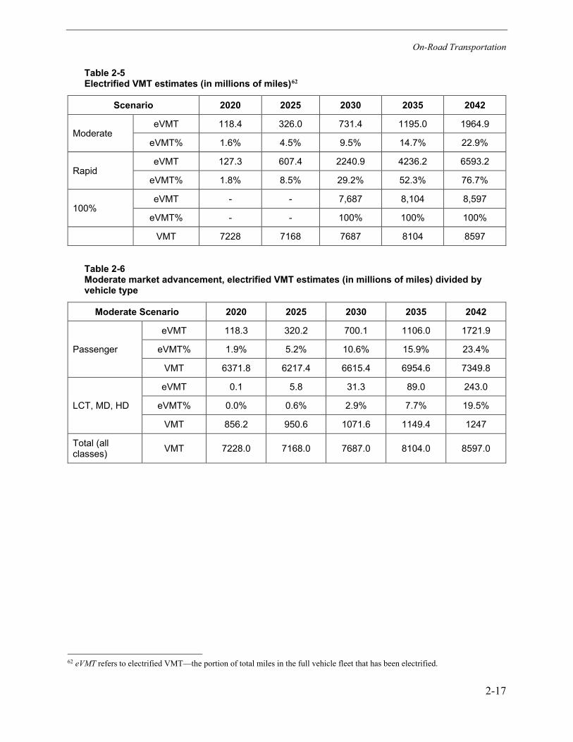
On-Road Transportation
2-17
Table 2-5 Electrified VMT estimates (in millions of miles)62
Scenario 2020 2025 2030 2035 2042
Moderate eVMT 118.4 326.0 731.4 1195.0 1964.9
eVMT% 1.6% 4.5% 9.5% 14.7% 22.9%
Rapid eVMT 127.3 607.4 2240.9 4236.2 6593.2
eVMT% 1.8% 8.5% 29.2% 52.3% 76.7%
100% eVMT - - 7,687 8,104 8,597
eVMT% - - 100% 100% 100%
VMT 7228 7168 7687 8104 8597
Table 2-6 Moderate market advancement, electrified VMT estimates (in millions of miles) divided by vehicle type
Moderate Scenario 2020 2025 2030 2035 2042
Passenger
eVMT 118.3 320.2 700.1 1106.0 1721.9
eVMT% 1.9% 5.2% 10.6% 15.9% 23.4%
VMT 6371.8 6217.4 6615.4 6954.6 7349.8
LCT, MD, HD
eVMT 0.1 5.8 31.3 89.0 243.0
eVMT% 0.0% 0.6% 2.9% 7.7% 19.5%
VMT 856.2 950.6 1071.6 1149.4 1247
Total (all classes) VMT 7228.0 7168.0 7687.0 8104.0 8597.0
62 eVMT refers to electrified VMT—the portion of total miles in the full vehicle fleet that has been electrified.
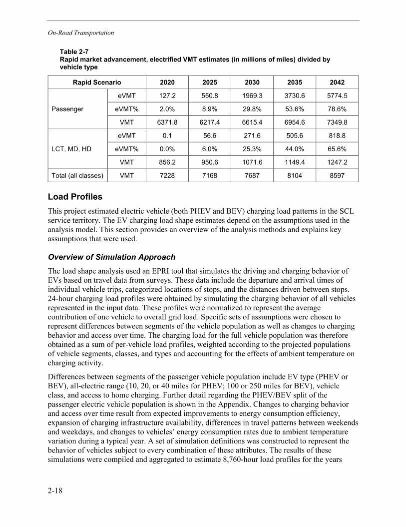
On-Road Transportation
2-18
Table 2-7 Rapid market advancement, electrified VMT estimates (in millions of miles) divided by vehicle type
Rapid Scenario 2020 2025 2030 2035 2042
Passenger
eVMT 127.2 550.8 1969.3 3730.6 5774.5
eVMT% 2.0% 8.9% 29.8% 53.6% 78.6%
VMT 6371.8 6217.4 6615.4 6954.6 7349.8
LCT, MD, HD
eVMT 0.1 56.6 271.6 505.6 818.8
eVMT% 0.0% 6.0% 25.3% 44.0% 65.6%
VMT 856.2 950.6 1071.6 1149.4 1247.2
Total (all classes) VMT 7228 7168 7687 8104 8597
Load Profiles This project estimated electric vehicle (both PHEV and BEV) charging load patterns in the SCL service territory. The EV charging load shape estimates depend on the assumptions used in the analysis model. This section provides an overview of the analysis methods and explains key assumptions that were used.
Overview of Simulation Approach The load shape analysis used an EPRI tool that simulates the driving and charging behavior of EVs based on travel data from surveys. These data include the departure and arrival times of individual vehicle trips, categorized locations of stops, and the distances driven between stops. 24-hour charging load profiles were obtained by simulating the charging behavior of all vehicles represented in the input data. These profiles were normalized to represent the average contribution of one vehicle to overall grid load. Specific sets of assumptions were chosen to represent differences between segments of the vehicle population as well as changes to charging behavior and access over time. The charging load for the full vehicle population was therefore obtained as a sum of per-vehicle load profiles, weighted according to the projected populations of vehicle segments, classes, and types and accounting for the effects of ambient temperature on charging activity.
Differences between segments of the passenger vehicle population include EV type (PHEV or BEV), all-electric range (10, 20, or 40 miles for PHEV; 100 or 250 miles for BEV), vehicle class, and access to home charging. Further detail regarding the PHEV/BEV split of the passenger electric vehicle population is shown in the Appendix. Changes to charging behavior and access over time result from expected improvements to energy consumption efficiency, expansion of charging infrastructure availability, differences in travel patterns between weekends and weekdays, and changes to vehicles’ energy consumption rates due to ambient temperature variation during a typical year. A set of simulation definitions was constructed to represent the behavior of vehicles subject to every combination of these attributes. The results of these simulations were compiled and aggregated to estimate 8,760-hour load profiles for the years
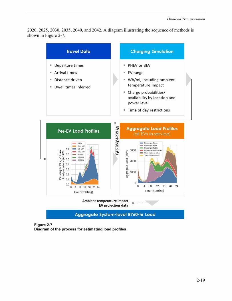
On-Road Transportation
2-19
2020, 2025, 2030, 2035, 2040, and 2042. A diagram illustrating the sequence of methods is shown in Figure 2-7.
Figure 2-7 Diagram of the process for estimating load profiles

On-Road Transportation
2-20
Interim Load Profile Result: Per-EV 24-Hour Load Profiles The outputs of a single charging simulation represent average per-vehicle load for a specific segment of the vehicle population. (Details of the charging simulation can be found in Appendix B.) The vehicle population was divided into subpopulations according to the attributes in Table 2-8, for passenger vehicles, and Table 2-9, for commercial and MDHD vehicles. The simulation year was used to determine the base energy consumption rate. The charging access probabilities were determined as a function of simulation year, vehicle type, home charging access, and EV type. Details on the energy consumption rate and the charging access probabilities are provided in Appendix B.
Table 2-8 Attributes distinguishing segments of the passenger vehicle population over time. 24-hour load profiles were obtained for every combination of values.
Category Attribute Value
Vehicle
Vehicle class car, truck
EV type PHEV10/20/40, BEV100/250
Home charging access yes, no
Time
Year 2020, 2030, 2040
Energy consumption rate adjustment 0.9, 1.0, 1.1, 1.2, 1.3
Day of week weekend, weekday
Table 2-9 Attributes distinguishing segments of the LCT/MDHD vehicle population over time. 24-hour load profiles were obtained for every combination of values.
Category Attribute Value
Vehicle Vehicle class All MDHD classes except long-haul trucks and intercity buses
Time Year 2020, 2030, 2040
Energy consumption rate adjustment Varies by class
24-hour load profiles were simulated for every combination of the attributes in Table 2-8 and Table 2-9 to represent each subpopulation throughout the time scope of the study. For passenger vehicles, this came to 600 iterations; for LCT and MDHD, the total was 198 iterations. A subset of these outputs is shown in Figure 2-8, for passenger cars, and Figure 2-9, for LCT and MDHD vehicles, on weekdays in 2030.
Load profiles represent the power drawn by vehicles at the point of the charging station with no interventions and therefore do not consider the possibility of customer-side power or charging management. Managed charging, which is not modeled, might include customer-owned energy

On-Road Transportation
2-21
storage applied to shift or flatten load or other charging management approaches, such as “smart charging” or customer behaviors to avoid high time-of-use prices or peak demand charges.63
Differences in load between types of housing, broadly categorized as single-unit and multi-unit dwellings (SUD and MUD), were modeled. All SUD with EVs were assumed to have some level of home charging availability. In contrast, MUD in the Seattle area were modeled to host some combination of EVs with and without access to home charging, where an increasing fraction has access to home charging in later years. At the per-EV stage of the process, these were modeled separately, as 1) EVs that do have access to home charging and 2) EVs that do not have access to home charging. Then, at the aggregation stage, assumptions about the fraction of MUD EVs with home charging were applied by weighting sums of the respective load profiles (home charging and no home charging) to generate aggregate profiles for the MUD EV population. A sample of the results is shown in Figure 2-8. As shown, vehicles with access to home charging contribute to an afternoon/evening peak in home charging load, whereas vehicles without home charging contribute to a morning peak in workplace charging load.
Figure 2-8 Example set of average per-EV unmanaged charging loads (passenger cars in 2030) with and without home charging
63 Vehicles with access to home charging were assumed to charge at every home stop. If the actual likelihood of charging during a home stop is significantly lower, the result would likely be a flatter, more spread-out home charging peak. This is because, on average, more energy would be replenished during each home charging session.

On-Road Transportation
2-22
Figure 2-9 is analogous to Figure 2-8 but represents per-EV load for each class of LCT and MDHD vehicle. As with passenger vehicles, these loads result from an assumption that no load management is applied. With the exception of the transit bus profile, all load profiles in Figure 2-9 were simulated using travel data from Fleet DNA (see Travel Data: Daily Driving Patterns). Transit bus load profiles were obtained directly from King County Metro and scaled, as shown in the figure. The following section describes the modeling approach for long-haul vehicle classes, which does not involve estimating per-vehicle loads.
Figure 2-9 Example set of per-EV charging loads (LCT and MDHD classes in 2030)
Long-Haul Vehicles: Trucks and Intercity Buses Charging profiles for combination long-haul, single-unit long-haul, and intercity buses were estimated using road sensor data. These vehicles are defined in the NEI analysis data set as those that generally operate more than 200 miles from their home base. This activity is dominated by combination trucks, which are articulated “semi” trucks. There are currently no production electric vehicles in these categories and therefore no operational data. The load shape for these was derived from road activity data for conventional combination trucks at the WSDOT R082S sensor north of Seattle because none of the sensors within Seattle was equipped to measure vehicle type. Because these vehicles do not generally return to a home base, it was assumed that charging activity would scale with driving activity, which is shown in Figure 2-10 for an average week in 2019. A normalized load shape was calculated based on the average vehicle volume in each hour for weekdays only. This load shape was then scaled to a per-vehicle load based on the average daily energy usage for each vehicle type. It is also possible that charging will be offered at parking areas for long-haul vehicles and, if so, some of the daytime energy will be shifted into
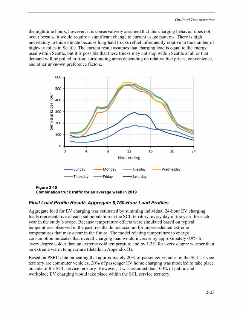
On-Road Transportation
2-23
the nighttime hours; however, it is conservatively assumed that this charging behavior does not occur because it would require a significant change to current usage patterns. There is high uncertainty in this estimate because long-haul trucks refuel infrequently relative to the number of highway miles in Seattle. The current result assumes that charging load is equal to the energy used within Seattle, but it is possible that these trucks may not stop within Seattle at all or that demand will be pulled in from surrounding areas depending on relative fuel prices, convenience, and other unknown preference factors.
Figure 2-10 Combination truck traffic for an average week in 2019
Final Load Profile Result: Aggregate 8,760-Hour Load Profiles Aggregate load for EV charging was estimated by summing individual 24-hour EV charging loads representative of each subpopulation in the SCL territory, every day of the year, for each year in the study’s scope. Because temperature effects were simulated based on typical temperatures observed in the past, results do not account for unprecedented extreme temperatures that may occur in the future. The model relating temperature to energy consumption indicates that overall charging load would increase by approximately 0.9% for every degree colder than an extreme cold temperature and by 1.3% for every degree warmer than an extreme warm temperature (details in Appendix B).
Based on PSRC data indicating that approximately 20% of passenger vehicles in the SCL service territory are commuter vehicles, 20% of passenger EV home charging was modeled to take place outside of the SCL service territory. However, it was assumed that 100% of public and workplace EV charging would take place within the SCL service territory.
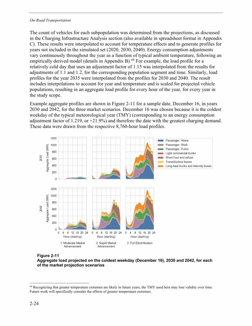
On-Road Transportation
2-24
The count of vehicles for each subpopulation was determined from the projections, as discussed in the Charging Infrastructure Analysis section (also available in spreadsheet format in Appendix C). These results were interpolated to account for temperature effects and to generate profiles for years not included in the simulated set (2020, 2030, 2040). Energy consumption adjustments vary continuously throughout the year as a function of typical ambient temperature, following an empirically derived model (details in Appendix B).64 For example, the load profile for a relatively cold day that uses an adjustment factor of 1.15 was interpolated from the results for adjustments of 1.1 and 1.2, for the corresponding population segment and time. Similarly, load profiles for the year 2035 were interpolated from the profiles for 2030 and 2040. The result includes interpolations to account for year and temperature and is scaled for projected vehicle populations, resulting in an aggregate load profile for every hour of the year, for every year in the study scope.
Example aggregate profiles are shown in Figure 2-11 for a sample date, December 16, in years 2030 and 2042, for the three market scenarios. December 16 was chosen because it is the coldest weekday of the typical meteorological year (TMY) (corresponding to an energy consumption adjustment factor of 1.219, or +21.9%) and therefore the date with the greatest charging demand. These data were drawn from the respective 8,760-hour load profiles.
Figure 2-11 Aggregate load projected on the coldest weekday (December 16), 2030 and 2042, for each of the market projection scenarios
64 Recognizing that greater temperature extremes are likely in future years, the TMY used here may lose validity over time. Future work will specifically consider the effects of greater temperature extremes.
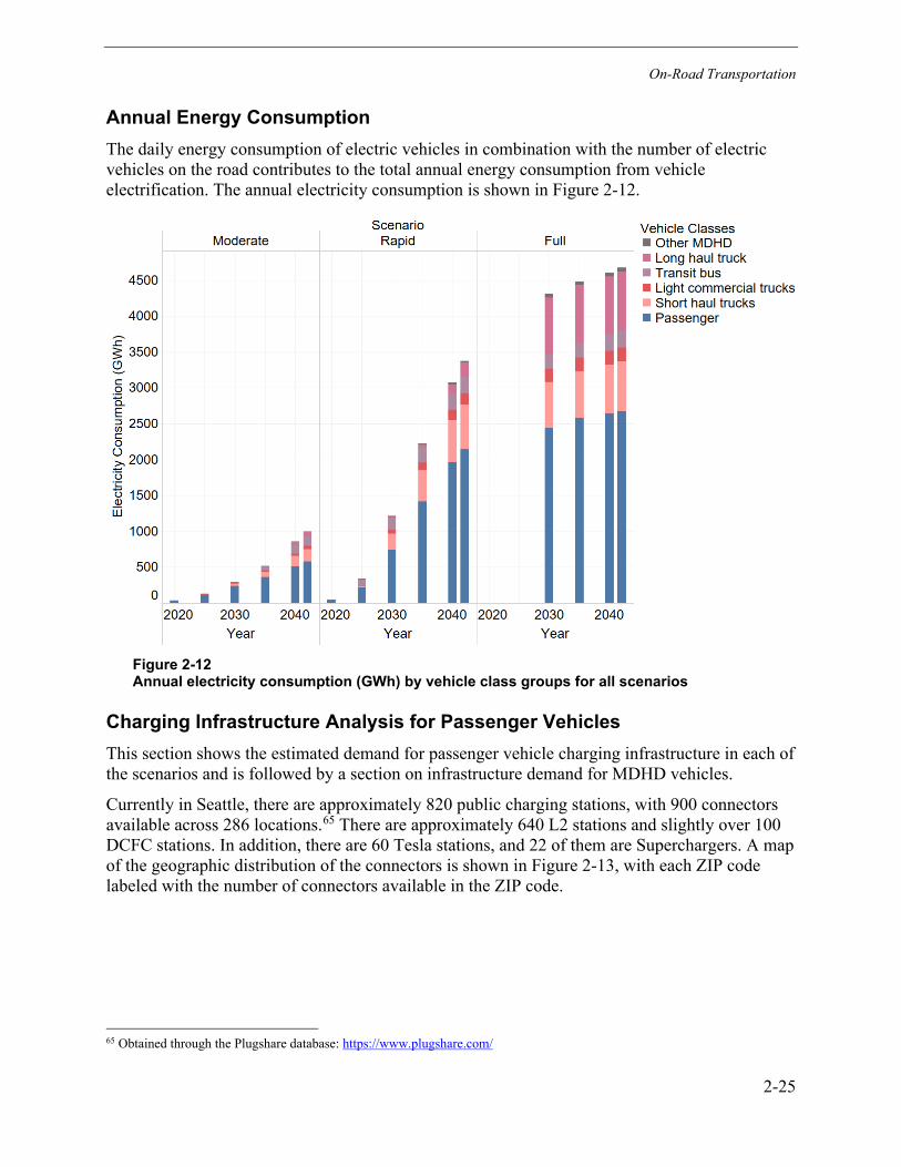
On-Road Transportation
2-25
Annual Energy Consumption The daily energy consumption of electric vehicles in combination with the number of electric vehicles on the road contributes to the total annual energy consumption from vehicle electrification. The annual electricity consumption is shown in Figure 2-12.
Figure 2-12 Annual electricity consumption (GWh) by vehicle class groups for all scenarios
Charging Infrastructure Analysis for Passenger Vehicles This section shows the estimated demand for passenger vehicle charging infrastructure in each of the scenarios and is followed by a section on infrastructure demand for MDHD vehicles.
Currently in Seattle, there are approximately 820 public charging stations, with 900 connectors available across 286 locations.65 There are approximately 640 L2 stations and slightly over 100 DCFC stations. In addition, there are 60 Tesla stations, and 22 of them are Superchargers. A map of the geographic distribution of the connectors is shown in Figure 2-13, with each ZIP code labeled with the number of connectors available in the ZIP code.
65 Obtained through the Plugshare database: https://www.plugshare.com/
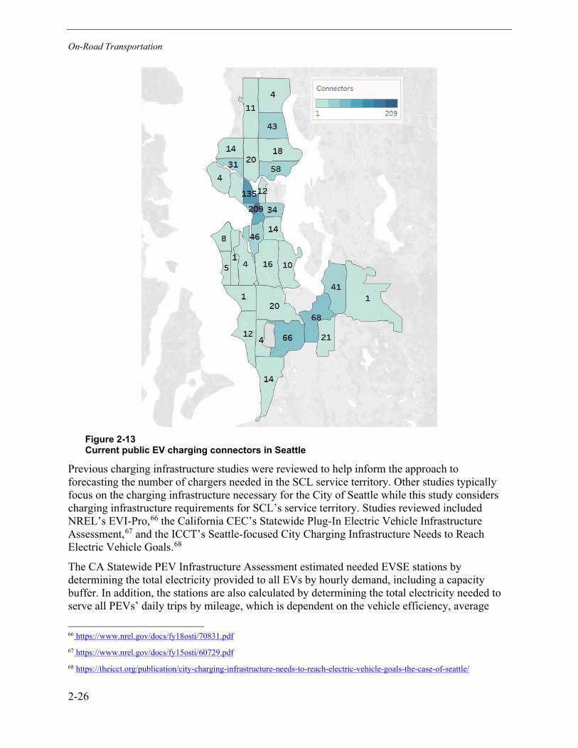
On-Road Transportation
2-26
Figure 2-13 Current public EV charging connectors in Seattle
Previous charging infrastructure studies were reviewed to help inform the approach to forecasting the number of chargers needed in the SCL service territory. Other studies typically focus on the charging infrastructure necessary for the City of Seattle while this study considers charging infrastructure requirements for SCL’s service territory. Studies reviewed included NREL’s EVI-Pro,66 the California CEC’s Statewide Plug-In Electric Vehicle Infrastructure Assessment,67 and the ICCT’s Seattle-focused City Charging Infrastructure Needs to Reach Electric Vehicle Goals.68
The CA Statewide PEV Infrastructure Assessment estimated needed EVSE stations by determining the total electricity provided to all EVs by hourly demand, including a capacity buffer. In addition, the stations are also calculated by determining the total electricity needed to serve all PEVs’ daily trips by mileage, which is dependent on the vehicle efficiency, average
66 https://www.nrel.gov/docs/fy18osti/70831.pdf 67 https://www.nrel.gov/docs/fy15osti/60729.pdf 68 https://theicct.org/publication/city-charging-infrastructure-needs-to-reach-electric-vehicle-goals-the-case-of-seattle/

On-Road Transportation
2-27
number of charge points per station, and average number of charging events per charge point per day.
EVI-Pro simulates individual PEV driving/charging simulations with data derived from real-world driving days, then processes the events to derive ratios of charge plugs to PEVs, and then scales said ratios by a PEV stock goal or projection. These ratios are used to estimate the percentage of vehicles participating in non-residential charging, derive aggregate load profiles, and investigate spatial distribution of demand.
The ICCT Seattle study used an energy needs–based estimation to project the number of chargers needed at home, work, and public locations. It assigned a ratio of vehicles to each charger and estimated a number of charging events per vehicle per day and the energy per charging event. Charging behavior was based on whether the vehicle was an EV or PHEV, housing characteristics, and if the vehicle was a commuting vehicle.
Similar to previous studies, a model was created for this study to estimate the charging infrastructure needed based on projected EV growth, levels of existing infrastructure, and assumed future changes. These estimates consider characteristics local to the City of Seattle, including city planning scenarios and policies, considerations for multi-family dwellings, and local commute and driving patterns. The assumptions and results are discussed separately for each charging location.
Seattle Infrastructure Ratio Comparison Progress toward achieving adequate charging access can be measured in terms of chargers per population, chargers per land area, total number of chargers, or other metrics, but it is currently unclear which measure is best. In a previous report, the ICCT summarized electrification goals and metrics for other cities.69 Germany has laid out ambitious goals for 1 million public charge points by 2030 and, in the state of Baden-Wurttemberg, a minimum of one 20-kW charger for every 100 km2 (38.6 square miles) and one 55-kW charger for every 400 km2 (154 square miles). The United Kingdom is aiming for 95% of motorways and A-roads to be within 20 miles of a charger. France’s current goal is to have one charging station for every 10 electric vehicles.
However, other metrics have been proposed for charger availability—including weighting chargers based on their power and accessibility in terms of hours of public access per day,70 a charging opportunity metric based on local travel data and likelihood that drivers will find a charger during their typical daily travel,71 and evaluating sufficiency of charger coverage based on utilization, spatial concentration, and energy use.72
69 https://theicct.org/publications/EV_charging_metrics_aug2020 70 https://www.transportenvironment.org/sites/te/files/publications/01%202020%20Draft%20TE% 20Infrastructure%20Report%20Final.pdf 71 https://www.researchgate.net/publication/329281412_Understanding_the_linkage_between_ electric_vehicle_charging_network_coverage_and_charging_opportunity_using_GPS_travel_data 72 https://www.researchgate.net/publication/326495345_Indicator-Based_Methodology_for_Assessing_EV_Charging_Infrastructure_Using_Exploratory_Data_Analysis
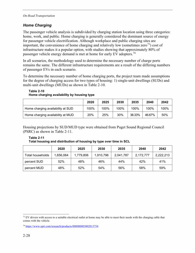
On-Road Transportation
2-28
Home Charging The passenger vehicle analysis is subdivided by charging station location using three categories: home, work, and public. Home charging is generally considered the dominant source of energy for passenger vehicle electrification. Although workplace and public charging sites are important, the convenience of home charging and relatively low (sometimes zero73) cost of infrastructure makes it a popular option, with studies showing that approximately 80% of passenger vehicle energy demand is met at home for early EV adopters.74
In all scenarios, the methodology used to determine the necessary number of charge ports remains the same. The different infrastructure requirements are a result of the differing numbers of passenger EVs in each scenario.
To determine the necessary number of home charging ports, the project team made assumptions for the degree of charging access for two types of housing: 1) single-unit dwellings (SUDs) and multi-unit dwellings (MUDs) as shown in Table 2-10.
Table 2-10 Home charging availability by housing type
2020 2025 2030 2035 2040 2042
Home charging availability at SUD 100% 100% 100% 100% 100% 100%
Home charging availability at MUD 20% 25% 30% 38.33% 46.67% 50%
Housing projections by SUD/MUD type were obtained from Puget Sound Regional Council (PSRC) as shown in Table 2-11.
Table 2-11 Total housing and distribution of housing by type over time in SCL
2020 2025 2030 2035 2040 2042
Total households 1,656,064 1,779,806 1,910,796 2,041,787 2,172,777 2,222,213
percent SUD 52% 48% 46% 44% 42% 41%
percent MUD 48% 52% 54% 56% 58% 59%
73 EV drivers with access to a suitable electrical outlet at home may be able to meet their needs with the charging cable that comes with the vehicle. 74 https://www.epri.com/research/products/000000003002013754
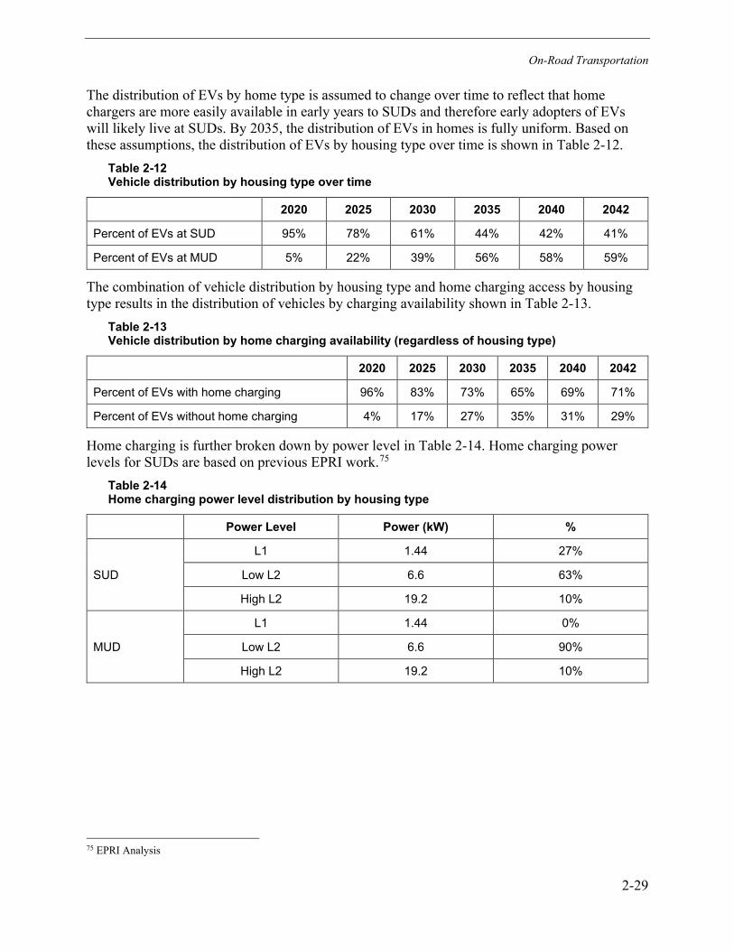
On-Road Transportation
2-29
The distribution of EVs by home type is assumed to change over time to reflect that home chargers are more easily available in early years to SUDs and therefore early adopters of EVs will likely live at SUDs. By 2035, the distribution of EVs in homes is fully uniform. Based on these assumptions, the distribution of EVs by housing type over time is shown in Table 2-12.
Table 2-12 Vehicle distribution by housing type over time
2020 2025 2030 2035 2040 2042
Percent of EVs at SUD 95% 78% 61% 44% 42% 41%
Percent of EVs at MUD 5% 22% 39% 56% 58% 59%
The combination of vehicle distribution by housing type and home charging access by housing type results in the distribution of vehicles by charging availability shown in Table 2-13.
Table 2-13 Vehicle distribution by home charging availability (regardless of housing type)
2020 2025 2030 2035 2040 2042
Percent of EVs with home charging 96% 83% 73% 65% 69% 71%
Percent of EVs without home charging 4% 17% 27% 35% 31% 29%
Home charging is further broken down by power level in Table 2-14. Home charging power levels for SUDs are based on previous EPRI work.75
Table 2-14 Home charging power level distribution by housing type
Power Level Power (kW) %
SUD
L1 1.44 27%
Low L2 6.6 63%
High L2 19.2 10%
MUD
L1 1.44 0%
Low L2 6.6 90%
High L2 19.2 10%
75 EPRI Analysis
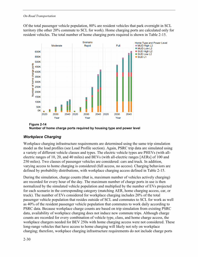
On-Road Transportation
2-30
Of the total passenger vehicle population, 80% are resident vehicles that park overnight in SCL territory (the other 20% commute to SCL for work). Home charging ports are calculated only for resident vehicles. The total number of home charging ports required is shown in Table 2-15.
Figure 2-14 Number of home charge ports required by housing type and power level
Workplace Charging Workplace charging infrastructure requirements are determined using the same trip simulation model as the load profiles (see Load Profile section). Again, PSRC trip data are simulated using a variety of different vehicle classes and types. The electric vehicle types are PHEVs (with all-electric ranges of 10, 20, and 40 miles) and BEVs (with all-electric ranges [AERs] of 100 and 250 miles). Two classes of passenger vehicles are considered: cars and truck. In addition, varying access to home charging is considered (full access, no access). Charging behaviors are defined by probability distributions, with workplace charging access defined in Table 2-15.
During the simulation, charge counts (that is, maximum number of vehicles actively charging) are recorded for every hour of the day. The maximum number of charge ports in use is then normalized by the simulated vehicle population and multiplied by the number of EVs projected for each scenario in the corresponding category (matching AER, home charging access, car, or truck). The number of EVs considered for workplace charging includes 20% of the total passenger vehicle population that resides outside of SCL and commutes to SCL for work as well as 40% of the resident passenger vehicle population that commutes to work daily according to PSRC data. Because workplace charge counts are based on trip simulation from existing PSRC data, availability of workplace charging does not induce new commute trips. Although charge counts are recorded for every combination of vehicle type, class, and home charge access, the workplace chargers needed for BEV 250s with home charging access were not considered. These long-range vehicles that have access to home charging will likely not rely on workplace charging; therefore, workplace charging infrastructure requirements do not include charge ports
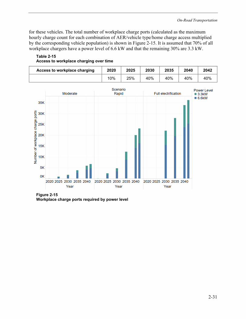
On-Road Transportation
2-31
for these vehicles. The total number of workplace charge ports (calculated as the maximum hourly charge count for each combination of AER/vehicle type/home charge access multiplied by the corresponding vehicle population) is shown in Figure 2-15. It is assumed that 70% of all workplace chargers have a power level of 6.6 kW and that the remaining 30% are 3.3 kW.
Table 2-15 Access to workplace charging over time
Access to workplace charging 2020 2025 2030 2035 2040 2042 10% 25% 40% 40% 40% 40%
Figure 2-15 Workplace charge ports required by power level

On-Road Transportation
2-32
Public Charging Public charging infrastructure requirements are computed in a similar manner to workplace charging based on PSRC trip simulation and charge counts. Further detail regarding the trip simulation can be found in the Load Profiles section. To obtain charge counts for public charging infrastructure, the following scenarios are considered:
Access to Home Charging Power Level Charging Behavior Type
Yes 6.6 kW Destination charging
No 6.6 kW Destination charging
Yes 19.2 kW Destination charging
No 19.2 kW Destination charging
Yes 50 kW Mid-trip charging
No 50 kW Mid-trip charging
Yes 250 kW Mid-trip charging
No 250 kW Mid-trip charging
The 6.6 kW charge power scenarios are designed specifically for PHEVs, which often charge at a lower power level compared to BEVs. Destination charge counts capture the maximum number of vehicles charging during each hour at public locations. The PSRC trip data for these vehicles indicate that a stop occurred, so no behavioral change is required for these vehicles to charge at these times. In contrast, en route charges may require a behavioral change in which an additional stop is made specifically to charge the vehicle.76 Because en route charging requires a stop to charge, the power levels are high to ensure that vehicles can replenish their batteries rapidly and therefore inconvenience the driver less. Charge counts from these scenarios are multiplied by the projected vehicle populations in the corresponding categories to determine the total number of public charge ports. The public charging infrastructure is designed to ensure adequate lower power public charging that can be used while drivers are stopped in locations where they would typically stop in conventional vehicles in addition to adequate higher power public charging that can be used when vehicles are making a stop specifically to charge. The total number of public charge ports required is shown in Figure 2-16.
76 It is likely that the trip data do not include most of the conventional refueling stops, and therefore the behavioral change for EV charging may (or may not) be a potentially longer stop.
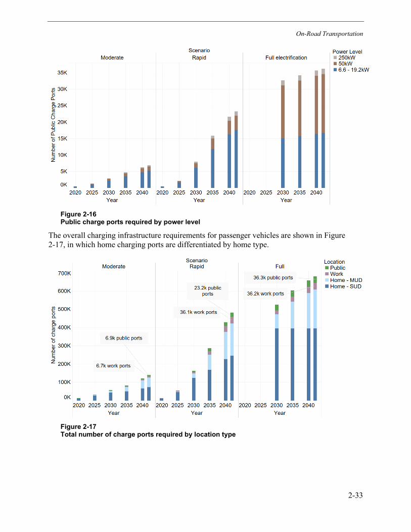
On-Road Transportation
2-33
Figure 2-16 Public charge ports required by power level
The overall charging infrastructure requirements for passenger vehicles are shown in Figure 2-17, in which home charging ports are differentiated by home type.
Figure 2-17 Total number of charge ports required by location type
On-Road Transportation
2-34
Recommendations for Infrastructure Charging infrastructure is required to support the electrification of passenger vehicles. In areas where there is a high concentration of MUDs, it is critical to ensure that these MUDs have home charging or that there is adequate public charging available in the area. For widespread passenger vehicle electrification to occur in places with diverse housing types, public and workplace charging infrastructure becomes more important. However, inducing new vehicle commute trips to access workplace charging contradicts ongoing efforts to shift commute trips toward transit and active forms of transportation and should be avoided.
In all cases where SCL is the owner, operator, or overseer of public charging infrastructure, it is critical to keep track of charger use and, if possible, customer satisfaction. Customer surveys and crowdsourced data such as PlugShare scores can help SCL understand customer satisfaction. In this way, SCL can determine if more charge ports are needed in certain locations.
In addition to charging infrastructure requirements in the SCL territory, widespread passenger vehicle electrification requires public charging access over a wide geographic area to enable long-distance travel. Although early adopters have shown a willingness to electrify their personal vehicles in an era of relatively low public charging access, Full Electrification will require widespread public charging infrastructure.
Charging Infrastructure Analysis for Light Commercial Trucks and MDHD Vehicles At this time, there are few production light commercial truck and MDHD electric vehicles and the charging standards are still being developed, so there is little usage data for these vehicles—including how they will be charged. Therefore, this analysis of charging infrastructure demand uses relatively simple assumptions.
Infrastructure Demand for Short-Haul MDHD Vehicle Types For the current analysis, it is assumed that short-haul vehicles, including light commercial trucks, will return to base each night and will have a dedicated charger, meaning that there is a 1:1 ratio between vehicles and chargers and that a given vehicle usage pattern will be electrified only when the vehicle range is long enough to satisfy the full daily driving needs. There will be some vehicles with routine driving patterns that will enable en route charging, such as transit buses that charge at some bus stops, but this is expected to represent relatively few chargers. Charger sharing at a home base could also occur, but this would require additional manual management and is likely to be less cost-effective than dedicated chargers as the market scales. Automated capacity sharing between chargers is likely to be cost-effective but will still result in a dedicated charger for each vehicle.
Infrastructure Demand for Long-Haul MDHD Vehicle Types For long-haul vehicles, it is assumed that vehicles do not usually return to base each night and so must charge en route. As discussed above, load for long-haul vehicles is derived from measured traffic flow data. The resulting total load for each scenario is shown in Figure 2-18 for 2042. It is uncertain how this will translate into the number of chargers required because the charging standards for these vehicle types are still being developed, and it is unclear how much
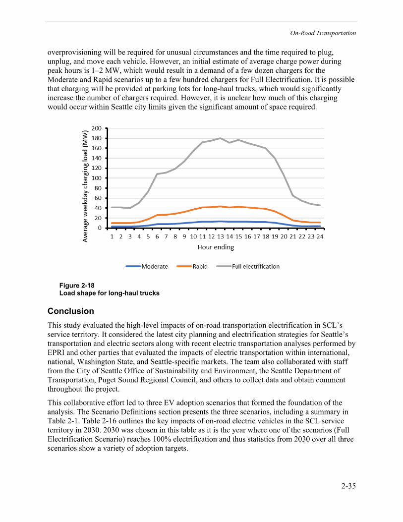
On-Road Transportation
2-35
overprovisioning will be required for unusual circumstances and the time required to plug, unplug, and move each vehicle. However, an initial estimate of average charge power during peak hours is 1–2 MW, which would result in a demand of a few dozen chargers for the Moderate and Rapid scenarios up to a few hundred chargers for Full Electrification. It is possible that charging will be provided at parking lots for long-haul trucks, which would significantly increase the number of chargers required. However, it is unclear how much of this charging would occur within Seattle city limits given the significant amount of space required.
Figure 2-18 Load shape for long-haul trucks
Conclusion This study evaluated the high-level impacts of on-road transportation electrification in SCL’s service territory. It considered the latest city planning and electrification strategies for Seattle’s transportation and electric sectors along with recent electric transportation analyses performed by EPRI and other parties that evaluated the impacts of electric transportation within international, national, Washington State, and Seattle-specific markets. The team also collaborated with staff from the City of Seattle Office of Sustainability and Environment, the Seattle Department of Transportation, Puget Sound Regional Council, and others to collect data and obtain comment throughout the project.
This collaborative effort led to three EV adoption scenarios that formed the foundation of the analysis. The Scenario Definitions section presents the three scenarios, including a summary in Table 2-1. Table 2-16 outlines the key impacts of on-road electric vehicles in the SCL service territory in 2030. 2030 was chosen in this table as it is the year where one of the scenarios (Full Electrification Scenario) reaches 100% electrification and thus statistics from 2030 over all three scenarios show a variety of adoption targets.
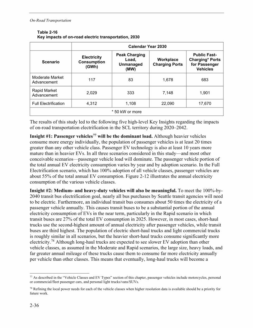
On-Road Transportation
2-36
Table 2-16 Key impacts of on-road electric transportation, 2030
Calendar Year 2030
Scenario Electricity
Consumption (GWh)
Peak Charging Load,
Unmanaged (MW)
Workplace Charging Ports
Public Fast-Charging* Ports for Passenger
Vehicles
Moderate Market Advancement 117 83 1,678 683
Rapid Market Advancement 2,029 333 7,148 1,901
Full Electrification 4,312 1,108 22,090 17,670
* 50 kW or more
The results of this study led to the following five high-level Key Insights regarding the impacts of on-road transportation electrification in the SCL territory during 2020–2042.
Insight #1: Passenger vehicles77 will be the dominant load. Although heavier vehicles consume more energy individually, the population of passenger vehicles is at least 20 times greater than any other vehicle class. Passenger EV technology is also at least 10 years more mature than in heavier EVs. In all three scenarios considered in this study—and most other conceivable scenarios—passenger vehicle load will dominate. The passenger vehicle portion of the total annual EV electricity consumption varies by year and by adoption scenario. In the Full Electrification scenario, which has 100% adoption of all vehicle classes, passenger vehicles are about 55% of the total annual EV consumption. Figure 2-12 illustrates the annual electricity consumption of the various vehicle classes.
Insight #2: Medium- and heavy-duty vehicles will also be meaningful. To meet the 100%-by-2040 transit bus electrification goal, nearly all bus purchases by Seattle transit agencies will need to be electric. Furthermore, an individual transit bus consumes about 50 times the electricity of a passenger vehicle annually. This causes transit buses to be a substantial portion of the annual electricity consumption of EVs in the near term, particularly in the Rapid scenario in which transit buses are 27% of the total EV consumption in 2025. However, in most cases, short-haul trucks use the second-highest amount of annual electricity after passenger vehicles, while transit buses are third highest. The population of electric short-haul trucks and light commercial trucks is roughly similar in all scenarios, but the heavier short-haul trucks consume significantly more electricity.78 Although long-haul trucks are expected to see slower EV adoption than other vehicle classes, as assumed in the Moderate and Rapid scenarios, the large size, heavy loads, and far greater annual mileage of these trucks cause them to consume far more electricity annually per vehicle than other classes. This means that eventually, long-haul trucks will become a
77 As described in the “Vehicle Classes and EV Types” section of this chapter, passenger vehicles include motorcycles, personal or commercial/fleet passenger cars, and personal light trucks/vans/SUVs. 78 Refining the local power needs for each of the vehicle classes when higher resolution data is available should be a priority for future work.

On-Road Transportation
2-37
substantial load on the SCL system, and individual charging stations will require several MW of service unless on-site energy storage is used.
Insight #3: The quantitative results are highly dependent on assumptions around customer behavior. The extent and timing of EV adoption levels across the various classes directly affects the number of EVs in operation, which in turn affects all other aspects of Seattle’s EV ecosystem. In addition, the extent of charging access at residences, which is a greater challenge at multi-unit dwellings, has a direct impact on the number of workplace and public EV charging stations that are required within Seattle’s territory. And although workplace charging that is free or very low cost to the driver may be an effective incentive for commuters to adopt EVs, once EV adoption reaches high levels this can lead to unnecessary workplace infrastructure costs and increase the daytime charging load beyond desirable levels.
Insight #4: Long-distance travel requires widespread EV charging outside of the SCL territory. The most impactful vehicle classes—passenger vehicles and long-haul trucking—will require widespread access to EV charging beyond the borders of the SCL service territory. Some early adopters of passenger vehicles may get by without this requirement depending on their destinations or their access to conventional vehicles or other forms of transportation. However, high passenger vehicle adoption requires a network of charge stations outside of the SCL territory. Furthermore, long-haul trucking cannot function without an adequate system of en route charging stations to support these vehicles.
SCL should continue to engage in and support efforts that help to plan and implement charging infrastructure outside of SCL’s territory. For example, to support light-duty vehicle charging, SCL could coordinate with the Washington State DOT and Oregon DOT in efforts to continue to upgrade and expand the West Coast Electric Highway. Further, that effort could expand to include other regional utilities, creating a collaboration similar to the Electric Highway Coalition in the Southwestern and Northeastern US. Beyond these collaborations, SCL can continue its work with efforts such as the West Coast Clean Transit Corridor Initiative to enable long haul electrified trucks easy access through Seattle.79
Insight #5: Much of EV charging is a flexible load. Most passenger vehicles and some other types of vehicles are parked for the majority of the day, which provides ample opportunity to charge these vehicles at times that are convenient for the electric grid. This topic is explored further in Section 6, Flexibility of New Electric Loads.
79 https://www.prnewswire.com/news-releases/electric-highway-coalition-grows-to-14-members-more-than-doubling-participation-301340996.html

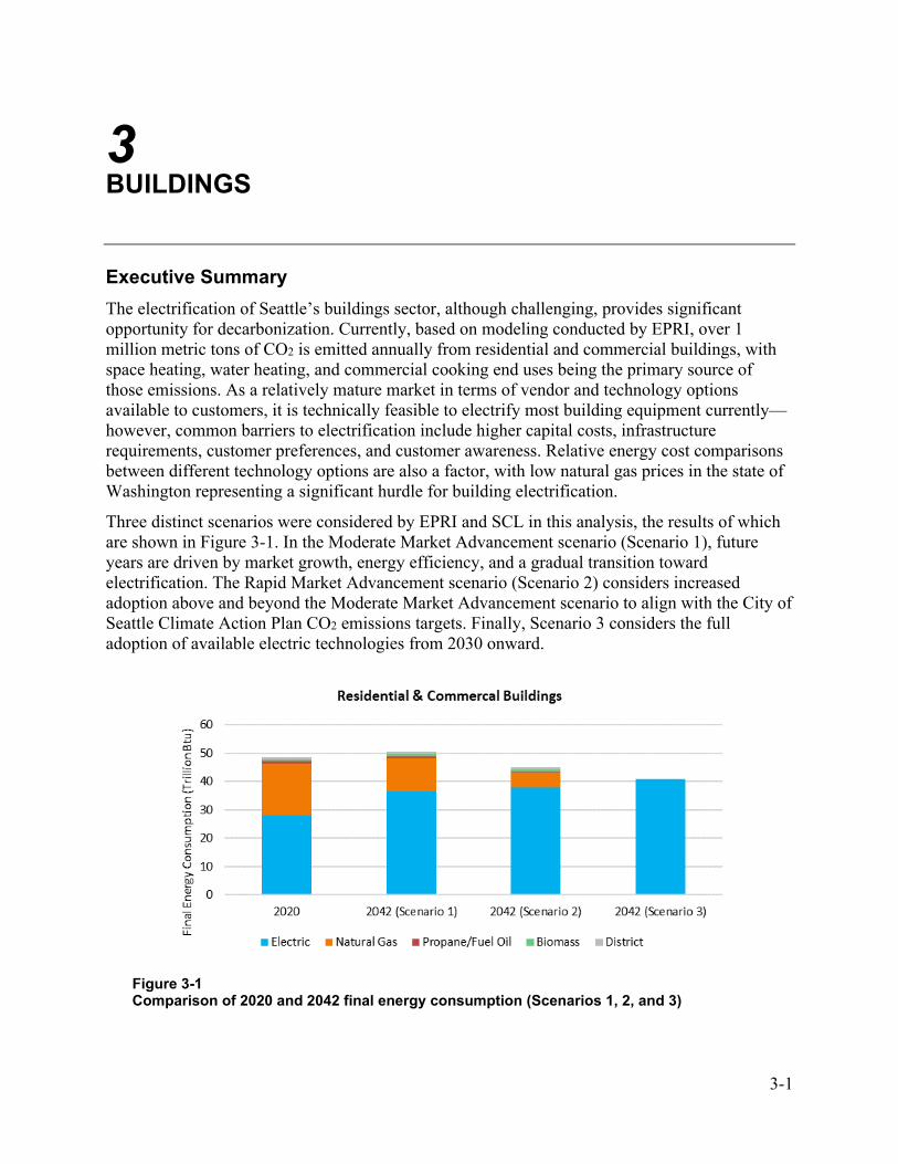
3-1
3 BUILDINGS
Executive Summary The electrification of Seattle’s buildings sector, although challenging, provides significant opportunity for decarbonization. Currently, based on modeling conducted by EPRI, over 1 million metric tons of CO2 is emitted annually from residential and commercial buildings, with space heating, water heating, and commercial cooking end uses being the primary source of those emissions. As a relatively mature market in terms of vendor and technology options available to customers, it is technically feasible to electrify most building equipment currently—however, common barriers to electrification include higher capital costs, infrastructure requirements, customer preferences, and customer awareness. Relative energy cost comparisons between different technology options are also a factor, with low natural gas prices in the state of Washington representing a significant hurdle for building electrification.
Three distinct scenarios were considered by EPRI and SCL in this analysis, the results of which are shown in Figure 3-1. In the Moderate Market Advancement scenario (Scenario 1), future years are driven by market growth, energy efficiency, and a gradual transition toward electrification. The Rapid Market Advancement scenario (Scenario 2) considers increased adoption above and beyond the Moderate Market Advancement scenario to align with the City of Seattle Climate Action Plan CO2 emissions targets. Finally, Scenario 3 considers the full adoption of available electric technologies from 2030 onward.
Figure 3-1 Comparison of 2020 and 2042 final energy consumption (Scenarios 1, 2, and 3)

Buildings
3-2
Due to the inherent efficiency advantages of electric technologies compared to their fossil-fueled alternatives (for example, all-electric heat pumps can be 2–3 times more efficient (commonly referred as coefficient of performance, COP, of 2.0 or above) than comparable natural gas furnaces), final energy consumption across all fuels is expected to remain relatively flat or decline depending on the scenario considered. In contrast, electric energy consumption is likely to increase due to electrification, with an additional 2.5 to 3.8 TWh of growth through 2042. Along with increases in electric energy consumption, significant increases in summer and winter peak demand may also be expected, with winter peaks doubling in all scenarios without additional mitigation strategies. Ongoing energy efficiency efforts (specifically conversions of resistance-based space and water heating equipment to heat pump-based systems) provide an opportunity for offsetting these impacts. Although multiple challenges exist, building electrification efforts offer a viable pathway to meeting Seattle’s future decarbonization goals.
Introduction Today, residential and commercial building end uses account for much of the existing electricity consumption within Seattle. Of the approximately 48.5 trillion Btu of energy consumed by buildings, electricity accounts for 28 trillion Btu, or just under 58% based on EPRI’s modeling. Natural gas is the second most common fuel type used within the Seattle buildings segment, representing 38% of all energy consumed and just over 1 million metric tons of CO2 emissions. As a relatively mature market, with numerous vendor and technology options available to customers, it is technically feasible to electrify most building equipment currently—however, economic feasibility may vary by end use and building application (with different thermal characteristics depending on the type of building considered). Common barriers to electrification include higher capital costs, energy costs, infrastructure requirements, customer preferences, and customer awareness.
Section 3 of the Electrification Assessment is focused on the electrification of major residential and commercial building end uses such as space heating, water heating, cooking, and clothes dryers. Specifically, the analysis considers the following:
• Scenario definitions. Provides a description of the three scenarios considered: Moderate Market Advancement, Rapid Market Advancement, and Full Electrification by 2030.
• Modeling methodology. A review of the various data sources used within this study as well as the approach used to align estimates with baseline consumption data. Market growth projections for residential and commercial buildings are also included.
• Key electrification opportunities. A summary of key electric technology options, along with an overview of their applications, benefits, and barriers from the customer perspective.
• Energy and demand impacts of electrification. Provides energy and demand impacts for each of the three electrification scenarios considered, identifying the incremental impact of electrification to SCL.
• Electrification and energy efficiency. Examines how energy efficiency improvements may offset growth from electrification.
• Conclusion. Review of the potential impacts of widespread building electrification on the SCL electric system.

Buildings
3-3
Scenario Definitions Within this analysis, EPRI and SCL considered three distinct scenarios. In the Moderate Market Advancement scenario, future years are driven by market growth, energy efficiency, and a gradual transition toward electrification. The Rapid Market Advancement scenario considers increased adoption above and beyond the Moderate Market Advancement scenario to align with the Climate Action Plan CO2 emissions targets. Finally, a third scenario considers the full adoption of available electric technologies from 2030 onward (Table 3-1). These scenarios are further detailed in the Energy and Demand Impacts of Electrification subsection below.
Table 3-1 Scenarios explored in this analysis and their underlying basis
Scenario Description
1. Moderate Market Advancement Future years driven by market growth, energy efficiency, and electrification
2. Rapid Market Advancement Increased adoption above and beyond the Moderate Market Advancement scenario to align with the City of Seattle Climate Action Plan CO2 emissions targets
3. Full Electrification by 2030 Full adoption of available electric technologies by 2030
Modeling Methodology Because buildings represent such a large portion of existing energy consumption, significant emphasis was placed on developing baseline estimates of current consumption that closely align with available end-use surveys and utility sales data. This effort included aligning the building stock/floorspace and technology saturation assumptions used within EPRI’s modeling framework with similar metrics found in SCL’s internal load forecasting tools. In addition, all estimates were optimized against SCL’s 2020 end-use forecasting model and sector-level 2019 natural gas sales data provided by Puget Sound Energy.
Data Sources Descriptions of the data sources used within this study as well as the approach used to align estimates with baseline consumption data is provided in additional detail below. A summary of the data sources used along with their geospatial granularity are given in Table 3-2.

Buildings
3-4
Table 3-2 Summary of data sources used and their geospatial granularity
Data Source Geospatial Granularity
2016-2017 Residential Building Stock Assessment SCL Service Territory
2014 Commercial Building Stock Assessment SCL Service Territory
2019 American Community Survey City of Seattle
2015 Residential Energy Consumption Survey Census Division
2012 Commercial Buildings Energy Consumption Survey Census Division
2021 Annual Energy Outlook Census Division
Existing stock and floorspace assumptions for residential and commercial buildings were provided by SCL and are summarized in Table 3-3. Due to the significantly different end-use mix found within the industrial sector (that is, manufacturing, construction, and agriculture), those segments are excluded from this analysis and are instead evaluated separately in Section 4.
Table 3-3 Baseline building stock (residential) and building floorspace (commercial) assumptions
Building Type Baseline Stock/Floorspace
Single-Family 198,727 households
Multi-Family80 207,836 dwellings
Assembly 18,877,016 ft2
Education 46,874,108 ft2
Food Sales 6,043,758 ft2
Food Service 6,928,078 ft2
Health Care 13,411,716 ft2
Lodging 21,324,523 ft2
Office: Large 87,884,318 ft2
Office: Small 25,172,774 ft2
Mercantile/Service 30,303,693 ft2
Warehouse 32,932,775 ft2
Other Commercial Buildings 52,059,519 ft2
80 Within EPRI’s modeling framework, multi-family dwellings, including all common area spaces, fall within the residential buildings segment.

Buildings
3-5
One of the primary pieces of information provided by SCL was electric technology saturation data collected in NEEA’s 2016–2017 Residential Building Stock Assessment (RBSA) and 2014 Commercial Building Stock Assessment (CBSA). Both the RBSA and CBSA provide SCL-specific data related to the existing equipment mix of electric technologies (such as the percentage of customers using heat pump-based systems for water heating rather than traditional resistance-based systems). Where more geographically granular data were not available (particularly for fossil-fueled end uses), saturation data from the U.S. Energy Information Administration’s (EIA) 2015 Residential Energy Consumption Survey and 2012 Commercial Buildings Energy Consumption Survey for the Pacific census division were used. In addition, saturation data for residential space heating fuels used in the city of Seattle were obtained from the U.S. Census Bureau’s 2019 American Community Survey.
Baseline Technology Saturation and Energy Consumption Utilizing the data provided above, baseline technology saturation assumptions were calculated, and are summarized in Figure 3-2 and Figure 3-3, with additional detail for electric end-use technologies provided in Appendix C.
Figure 3-2 Baseline technology saturation assumptions for residential buildings81
81 Baseline residential cooking saturation across all fuel types is greater than 100% (that is, based on survey data, on average more than one piece of equipment is utilized per household).
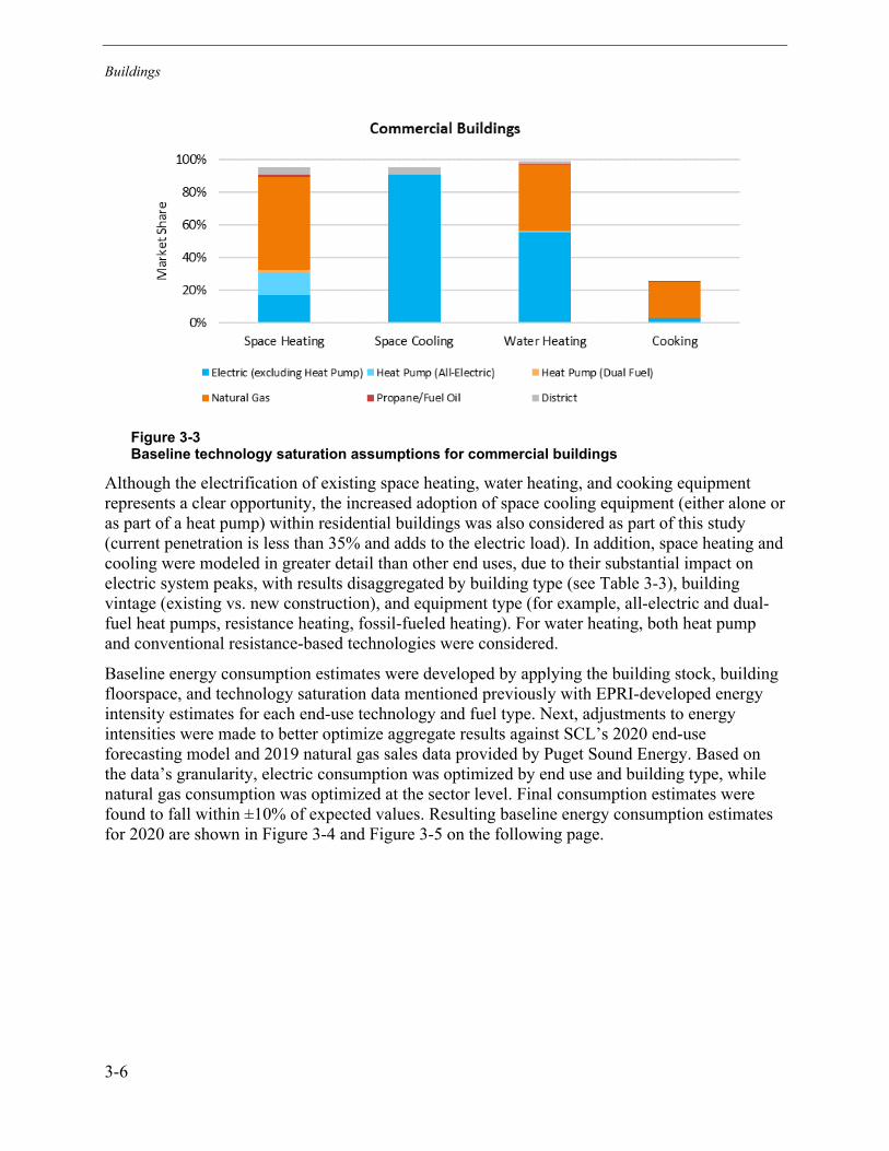
Buildings
3-6
Figure 3-3 Baseline technology saturation assumptions for commercial buildings
Although the electrification of existing space heating, water heating, and cooking equipment represents a clear opportunity, the increased adoption of space cooling equipment (either alone or as part of a heat pump) within residential buildings was also considered as part of this study (current penetration is less than 35% and adds to the electric load). In addition, space heating and cooling were modeled in greater detail than other end uses, due to their substantial impact on electric system peaks, with results disaggregated by building type (see Table 3-3), building vintage (existing vs. new construction), and equipment type (for example, all-electric and dual-fuel heat pumps, resistance heating, fossil-fueled heating). For water heating, both heat pump and conventional resistance-based technologies were considered.
Baseline energy consumption estimates were developed by applying the building stock, building floorspace, and technology saturation data mentioned previously with EPRI-developed energy intensity estimates for each end-use technology and fuel type. Next, adjustments to energy intensities were made to better optimize aggregate results against SCL’s 2020 end-use forecasting model and 2019 natural gas sales data provided by Puget Sound Energy. Based on the data’s granularity, electric consumption was optimized by end use and building type, while natural gas consumption was optimized at the sector level. Final consumption estimates were found to fall within ±10% of expected values. Resulting baseline energy consumption estimates for 2020 are shown in Figure 3-4 and Figure 3-5 on the following page.
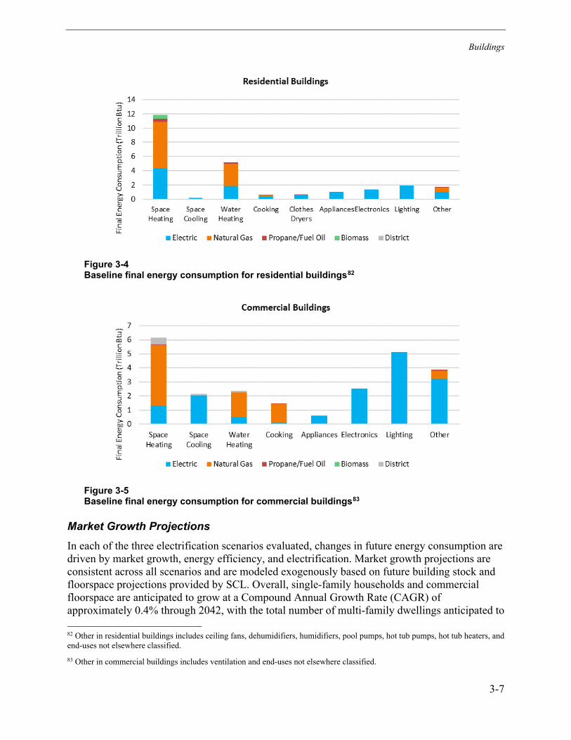
Buildings
3-7
Figure 3-4 Baseline final energy consumption for residential buildings82
Figure 3-5 Baseline final energy consumption for commercial buildings83
Market Growth Projections In each of the three electrification scenarios evaluated, changes in future energy consumption are driven by market growth, energy efficiency, and electrification. Market growth projections are consistent across all scenarios and are modeled exogenously based on future building stock and floorspace projections provided by SCL. Overall, single-family households and commercial floorspace are anticipated to grow at a Compound Annual Growth Rate (CAGR) of approximately 0.4% through 2042, with the total number of multi-family dwellings anticipated to
82 Other in residential buildings includes ceiling fans, dehumidifiers, humidifiers, pool pumps, hot tub pumps, hot tub heaters, and end-uses not elsewhere classified. 83 Other in commercial buildings includes ventilation and end-uses not elsewhere classified.

Buildings
3-8
grow more rapidly at a CAGR of 1.4% through 2042 (Table 3-4). Within EPRI’s modeling framework, these growth projections are used to define the total addressable market as well as the total number of new construction buildings over the study’s time horizon. Finally, changes in future energy prices use projections from the EIA’s 2021 Annual Energy Outlook.
Table 3-4 Building stock (residential) and building floorspace (commercial) growth projections
Building Type 2020 2025 2030 2035 2040 2042
Single-Family 198,727 households
202,566 households
206,813 households
211,035 households
215,361 households
217,118 households
Multi-Family 207,836 dwellings
224,706 dwellings
242,123 dwellings
259,324 dwellings
276,936 dwellings
284,185 dwellings
Assembly 18,877,016 ft2 19,324,681 ft2 19,810,004 ft2 20,218,070 ft2 20,493,119 ft2 20,595,993 ft2
Education 46,874,108 ft2 47,985,425 ft2 49,190,229 ft2 50,203,243 ft2 50,886,047 ft2 51,141,426 ft2
Food Sales 6,043,758 ft2 6,187,036 ft2 6,342,369 ft2 6,472,973 ft2 6,561,003 ft2 6,593,926 ft2
Food Service 6,928,078 ft2 7,092,370 ft2 7,270,484 ft2 7,420,244 ft2 7,521,186 ft2 7,558,940 ft2
Health Care 13,411,716 ft2 13,731,342 ft2 14,077,853 ft2 14,369,205 ft2 14,565,585 ft2 14,639,036 ft2
Lodging 21,324,523 ft2 21,829,841 ft2 22,377,669 ft2 22,838,287 ft2 23,148,758 ft2 23,264,879 ft2
Office: Large 87,884,318 ft2 89,968,923 ft2 92,228,888 ft2 94,129,096 ft2 95,409,897 ft2 95,888,939 ft2
Office: Small 25,172,774 ft2 25,769,682 ft2 26,416,803 ft2 26,960,912 ft2 27,327,658 ft2 27,464,826 ft2
Mercantile /Service 30,303,693 ft2 31,019,477 ft2 31,795,474 ft2 32,447,942 ft2 32,887,722 ft2 33,052,204 ft2
Warehouse 32,932,775 ft2 33,713,682 ft2 34,560,281 ft2 35,272,112 ft2 35,751,909 ft2 35,931,362 ft2
Other Commercial Buildings
52,059,519 ft2 53,224,520 ft2 54,487,523 ft2 55,549,471 ft2 56,265,258 ft2 56,532,974 ft2
Key Electrification Opportunities As shown in the previous section, space heating, water heating, and commercial cooking equipment represent the bulk of the opportunity for electrification within the buildings segment. Within the residential sector, significant opportunity exists for electrifying space heating in single-family homes, while a large percentage of multi-family is already electrified (primarily with resistance heating). Penetration of electric systems within commercial buildings varies by application (and is lower overall than the residential sector); however, due to their occupancy and thermal characteristics, less heating is generally required.
For each of these areas, a variety of options exist that make it technically feasible to electrify most equipment today, although economic feasibility may vary by application. Key electric technology options for each of these end-use areas, along with their applications, benefits, and barriers, are described next.

Buildings
3-9
Residential Space and Water Heating Heat pump-based technologies for residential space and water heating offer significant efficiency improvements compared to traditional electric resistance and fossil-fueled equipment while providing a similar level of comfort to customers. A major secondary benefit of heat pumps is their ability to provide cooling, particularly in Seattle where many homes lack air conditioning (current penetration is less than 40%). Natural gas space and water heating technologies are the primary alternatives used in Seattle, with fuel oil and biomass heating accounting for a much smaller market share. There are multiple types of heat pump technologies available for space and water heating, defined next.
Air-Source Heat Pumps (ASHPs)
ASHPs typically provide space conditioning (heating and cooling) through ductwork and are ideal for the replacement of existing ducted heating, ventilation, and air conditioning (HVAC) systems. Standard efficiency ASHPs cycle between fully on or off to meet a home’s heating and cooling load. Energy savings for minimum efficiency ASHPs will be moderate, and auxiliary heat (electric resistance or fossil fuel) is typically required for lower temperatures. Due to the nature of their operation, ASHPs operate more efficiently at milder temperatures and less efficiently at lower temperatures and, depending on the fuel source of the auxiliary heat, may or may not add to the system peak.
High-efficiency options include inverter-driven units that have a higher first cost but more significant energy savings, offsetting nearly all need for auxiliary heating. Two high-efficiency options are described in the following sections.
Ducted Variable-Capacity Heat Pumps (VCHPs)
Inverter-driven compressors allow VCHPs to have a continuously variable output, closely matching the heating and cooling loads of the home. VCHPs are capable of a range of heating and cooling outputs and provide higher heating output and efficiency at lower temperatures compared to standard-efficiency ASHPs.
Space conditioning systems are typically sized to meet location specific design conditions (hottest or coldest days of the year). The greatest advantage of inverter-driven systems is their ability to run efficiently at part-load conditions, and because this is typically most of the operating time, these systems can offer significant energy savings compared to traditional ASHPs.
Ductless Mini-Split and Multi-Split Heat Pumps
Mini- or multi-split heat pumps are also inverter-driven ASHPs with the same advantages as VCHPs. Mini- or multi-split systems have an outdoor compressor/condenser unit and, instead of distributing air through ductwork like ASHPs and VCHPs, the refrigerant is piped to one or more indoor air-handling units located throughout the home. Additional savings are realized with the elimination of ductwork, which is the source of significant energy losses.
Mini-split refers to a system with a single indoor unit; multi-split typically refers to a system with multiple indoor units. Each indoor unit is often attached to an interior wall and is controlled by a thermostat enabling zoned conditioning.

Buildings
3-10
Ground-Source Heat Pumps (GSHPs)
GSHPs are a high-efficiency heat pump system that transfers heat from the ground instead of the outside air. The use of the ground’s heat as an alternative, non-varying thermal source leads to a more stable heating and cooling process year-round. GSHPs have great energy savings, but the biggest barriers are the high first cost and the space and time needed for installation.
Resistance and Heat Pump Water Heaters (HPWHs)
Although resistance water heaters can offer energy savings for customers, operating costs may be a limiting factor, particularly compared to natural gas–based systems. In contrast, heat pump water heaters have an integrated ASHP to provide high-efficiency water heating. The units typically include both resistance elements and a heat pump with several operating modes, giving customers options that meet comfort needs as well as provide energy savings.
Applications, Benefits, and Barriers: Residential Space and Water Heating
The following describe “best-fit” applications for residential space and water heating equipment. Note: heat pump technologies used for space heating are also capable of providing space cooling (which may help drive customer adoption).
• ASHP and VCHP. Single- and multi-family homes, both new and existing construction, well suited where there is existing ductwork. Also well suited for homes that have centralized heating but lack air conditioning.
• Ductless mini-split system. For existing homes, a single mini-split may be used in home additions to provide heating and cooling without extending ductwork or overtaxing the existing system. May also be added to the main living space as the primary space conditioning system, offsetting a portion of the heating and cooling provided by an inefficient centralized system.
• Ductless multi-split system. Well suited for new construction with no existing ductwork, mitigating the need for fuel-handling infrastructure. These systems are typically sized to eliminate the need for auxiliary heating.
• GSHP. Single and multi-family homes, both new and existing construction, well suited where there is existing ductwork. If sized appropriately, these high-efficiency heat pumps may not require auxiliary heating, eliminating the need for fuel piping for heating purposes.
• Resistance water heater. May be used to replace existing fossil-fueled water heaters of similar capacity (gallons).
• HPWH. Can be a drop-in replacement for fossil-fueled units; depending on the size, there may be space constraints in the existing install location.
The primary benefit of heat pumps for residential space and water heating are energy savings. In all cases, electric technologies reduce or eliminate direct combustion of fossil fuels, reducing site emissions and increasing safety for homeowners. Inverter-driven (high-efficiency) ASHPs offer a customer experience similar to fossil fuel furnaces with higher output temperatures than standard heat pumps. HPWHs typically have multiple operating modes that allow customers to maximize energy savings with heat pump only mode, or a mixed mode using resistance backup

Buildings
3-11
for faster reheat. In addition, a major secondary benefit of heat pumps is their ability to provide cooling, particularly in Seattle where many homes lack air conditioning, and the frequency of high-temperature days is expected to increase. A summary of the main benefits associated with electric residential space and water heating equipment is provided in Table 3-5.
Table 3-5 Residential space and water heating technology benefits
Efficiency/ Energy Savings
Customer Experience Similar to
Alternative
Reduced Site Emissions and
Increased Safety Reduced
Maintenance
ASHP
VCHP
Mini- or Multi-Split
GSHP
Resistance WH
HPWH
Common market barriers for heat pumps for residential space heating include:
• Higher first cost for high-efficiency technologies
• Lack of customer familiarity with heat pumps and existing perception that heat pumps do not work well in colder climates in particular
• Installers may not be familiar with customer benefits and therefore may not propose heat pumps as an alternative
• Additional space and time needed for installation of GSHPs
The primary barrier for residential electric resistance water heaters is the lack of familiarity with the performance of electric and the propensity for customers to replace existing equipment with the same technology option upon failure.
Commercial Space and Water Heating Similar to residential buildings, a significant portion of space and water heating in the commercial segment is provided by natural gas–fueled equipment, with a small amount coming from fuel oil and district heating systems. Within this customer segment, cost-effectiveness of electric systems may vary greatly by end use and building application, and building-specific energy consumption should be considered in economic assessments to understand best fits. Key commercial sector space and water heating technologies are described next.
Air-Source Heat Pumps (ASHPs)
Standard-efficiency ASHPs are similar in cost to fossil-fueled alternatives, providing moderate energy savings for heating, with auxiliary heat (electric resistance or fossil fuel) typically

Buildings
3-12
required for lower temperatures. High-efficiency options include inverter-driven units that have a higher first cost but significant energy savings, offsetting nearly all need for auxiliary heating.
Traditional ASHPs are well suited for buildings with existing ductwork. A packaged system including both air conditioning (AC) and space heating is commonly used in commercial settings to provide both space heating and cooling. Packaged systems are commonly referred to as rooftop units (RTUs), although they are not always located on rooftops.
Standard ASHPs include single-speed components (compressor, fans, etc.) and cycle between fully on or off to meet a building’s heating and cooling load. Two high-efficiency options are described in the following sections.
Variable-Capacity Rooftop Heat Pumps (VCRTUs)
In response to the U.S. Department of Energy (DOE’s) RTU Challenge issued in 2011,84 RTU manufacturers have begun integrating inverter-driven compressors into RTUs to meet the goal of an integrated energy efficiency ratio (IEER85) of 18 or higher. The federal minimum efficiency for rooftop ACs is currently 11.2 EER, and these minimum efficiency units typical have an IEER of about 11.86
Inverter-driven compressors allow RTUs to have a continuously variable output, closely matching the heating and cooling loads of the building. VCRTUs are capable of a range of heating and cooling outputs and provide higher heating output and efficiency at lower temperatures compared to standard ASHPs.
Space conditioning systems are typically sized to meet location specific design conditions (hottest or coldest days of the year). The greatest advantage of inverter-driven systems is their ability to run efficiently at part-load conditions, and because this is typically most of the operating time, VCRTUs offer significant energy savings compared to traditional ASHPs.
Variable-Refrigerant Flow (VRF) Heat Pumps
Unlike conventional HVAC systems, which supply conditioned air through centralized ducts or heated/chilled water through pipes to heat or cool spaces within a building, VRF technology transports heat via refrigerant through an internal piping network to smaller heat exchangers mounted in the conditioned space. A VRF system uses a single outdoor compressor that can operate as an evaporator in heating mode or as a condenser in cooling mode.
There are two VRF types: heat pump (HP) and heat recovery (HR). VRF-HP systems operate all indoor units in either heating or cooling mode, while VRF-HR systems enable simultaneous heating and cooling within a building. VRF technology enables precise, room-to-room temperature control (similar to residential multi-split systems), with some systems even offering
84 U.S. DOE EERE, Better Buildings Alliance. https://www4.eere.energy.gov/alliance/activities/technology-solutions-teams/space-conditioning/rtu 85 IEER is a measure of part-load cooling efficiency as opposed to the energy efficiency ratio (EER), which evaluates full-load cooling efficiency at an outdoor temperature of 95°F. 86 Assessment of Commercial Space Conditioning Technologies: Variable Capacity Rooftop Units. EPRI, Palo Alto, CA: 2013. 3002001380.

Buildings
3-13
humidity control. For these reasons, VRF heat pumps are an attractive option for many commercial buildings including offices, retail, schools, and medical facilities.
Ground-Source Heat Pumps (GSHPs)
GSHPs may also be applied in commercial settings offering significant energy savings; however, they may be cost prohibitive due to the higher first cost and the space and time needed for installation. GSHPs are an inherently high-efficiency heat pump system that transfers heat from the ground instead of the outside air. The use of the ground’s heat as an alternative, non-varying thermal source leads to a more stable heating and cooling process year-round.
Resistance and Heat Pump Water Heaters (HPWHs)
Although electric resistance water heaters can offer energy savings, operating costs may be a limiting factor—particularly compared to natural gas–based systems. In contrast, heat pump water heaters have an integrated ASHP to provide high-efficiency water heating. The units typically include both resistance elements and a heat pump with several operating modes, giving customers options that meet comfort needs as well as energy savings.
Applications, Benefits, and Barriers: Commercial Space and Water Heating
The following describe “best-fit” applications for commercial space and water heating equipment:
• ASHP and VCRTU. May be used in a variety of commercial building spaces; the type of equipment applied will vary depending on building size and configuration. In particular, RTUs and VCRTUs may be applied for a variety of commercial activities including office and retail space. RTUs and VCRTUs are typically not applied in high-rise buildings.
• VRF. Well suited for new construction applications, with no need to remove existing ductwork; mitigates need for fuel-handling infrastructure. These systems are typically sized to eliminate the need for auxiliary heating.
• GSHP. Nearly any commercial space, both new and existing construction; well suited where there is existing ductwork. If sized appropriately, these high-efficiency heat pumps may not require auxiliary heating, eliminating the need for fuel piping for heating purposes.
• Resistance water heater. May be used to replace existing fossil-fueled water heaters of similar capacity (gallons).
• HPWH. Integrated heat pump provides high-efficiency water heating. The units include resistance elements for backup heating, and the extent of resistance heating depends on the user-chosen settings. Depending on the size, there may be space constraints in the existing install location.
The primary benefit of heat pumps for commercial space and water heating is energy savings. In all cases, electric technologies reduce or eliminate direct combustion of fossil fuels, reducing site emissions and increasing safety for end-use customers. Inverter-driven (high-efficiency) ASHPs offer a customer experience similar to fossil fuel furnaces with higher output temperatures than standard heat pumps. Equipment manufacturers have plans for enhanced monitoring of VCRTUs, which would likely reduce maintenance while improving equipment performance and

Buildings
3-14
customer experience. HPWHs typically have multiple operating modes that allow customers to maximize energy savings or achieve faster water reheat. A summary of the main benefits associated with electric commercial space and water heating equipment is provided in Table 3-6.
Table 3-6 Commercial space and water heating technology benefits
Efficiency/
Energy Savings
Customer Experience Similar to
Alternative
Reduced Site Emissions and
Increased Safety Reduced
Maintenance
ASHP
VCRTU
VRF
GSHP
Resistance WH
HPWH
Common market barriers for heat pumps for commercial space heating include:
• Higher first cost for high-efficiency equipment
• Lack of customer familiarity with heat pumps and existing perception that heat pumps do not work well in colder climates in particular
• Installers may not be familiar with customer benefits and therefore may not propose heat pumps as a beneficial alternative
• Additional space and time needed for installation of GSHPs
The primary barrier for commercial electric resistance water heaters is the lack of familiarity with the performance of electric and the propensity for customers to replace existing equipment with the same technology option upon failure.
Commercial Cooking In the commercial sector, electric fryers, griddles, and combination ovens (combi-ovens) have inherent advantages over natural gas equipment in both energy savings and productivity. Unlike heat pumps, the non-energy benefits of these electric technologies are the primary driver for adoption in place of gas-fired equipment. Natural gas tends to be dominant in the U.S. commercial cooking market; gas fryers and griddles have an estimated 80% share of the U.S. market, while combi-ovens have an estimated 65% share.
Commercial Fryers, Griddles, and Combi-Ovens
Fryers and griddles are ubiquitous in commercial kitchens and may be found in nearly every commercial cooking space. Depending on the types of foods sold by an establishment, fryers or griddles may be a bottleneck for productivity. In these cases, replacing natural gas equipment

Buildings
3-15
with electric options that can improve productivity is an attractive option to reduce bottlenecks and increase revenue.
Combi-ovens provide steam and convection cooking, either separately or together. They prepare food more quickly than traditional methods, for instance, reducing cooking time by almost half for a rotisserie chicken. Combi-ovens are a larger piece of equipment (larger physical footprint) with a relatively high cost compared to other appliances. Combi-ovens are often applied in institutional settings such as schools. In some cases, there are lower cost products with functionality similar to combi-ovens that may be a more economic option.
Applications, Benefits, and Barriers: Commercial Cooking
The primary benefits of electric cooking equipment – and what drives adoption – are the increased quality of the final product as well as increased throughput.
• Electric fryers. Have a faster reheat than similar gas products, which both reduces cooking time and increases the quality of the finished product (for instance, crispier French fries).
• Electric griddles. Can provide consistent even heat from edge to edge, whereas gas equipment may develop hot spots over time. Where griddles are used for higher volume foods (for instance, hamburger patties in a burger restaurant), throughput may be increased due to the consistency of heat across an increased surface area.
• Electric combi-ovens. Also have fewer hot spots, resulting in more even cooking and better performance than comparable gas versions.
In addition, electric fryers have the added benefit of reducing oil usage, which has significant cost savings potential over the life of the equipment (on the order of hundreds to thousands of dollars per year).
Common market barriers for electric cooking equipment include:
• Higher capital cost (except for combi-ovens)
• Lack of understanding of benefits compared to gas
• Preference for and familiarity with cooking on gas equipment
• Equipment type may be mandated by parent company
• Lack of adequate electrical service and cost to upgrade
Energy and Demand Impacts of Electrification Building electrification was modeled based on an evaluation of relevant electric technologies, assuming customers adopt more beneficial electric options over time. The results of the scenario analysis presented in Section 3 build upon the baseline energy consumption estimates and market growth projections described previously and show the incremental impact of electrification for each of the three scenarios.
To allow SCL to better assess the net impacts of electrification on a standalone basis, this analysis looked only at the impact of the fuel transitions, and the resulting load impacts do not account for potential impacts of energy efficiency. This was done because energy efficiency and
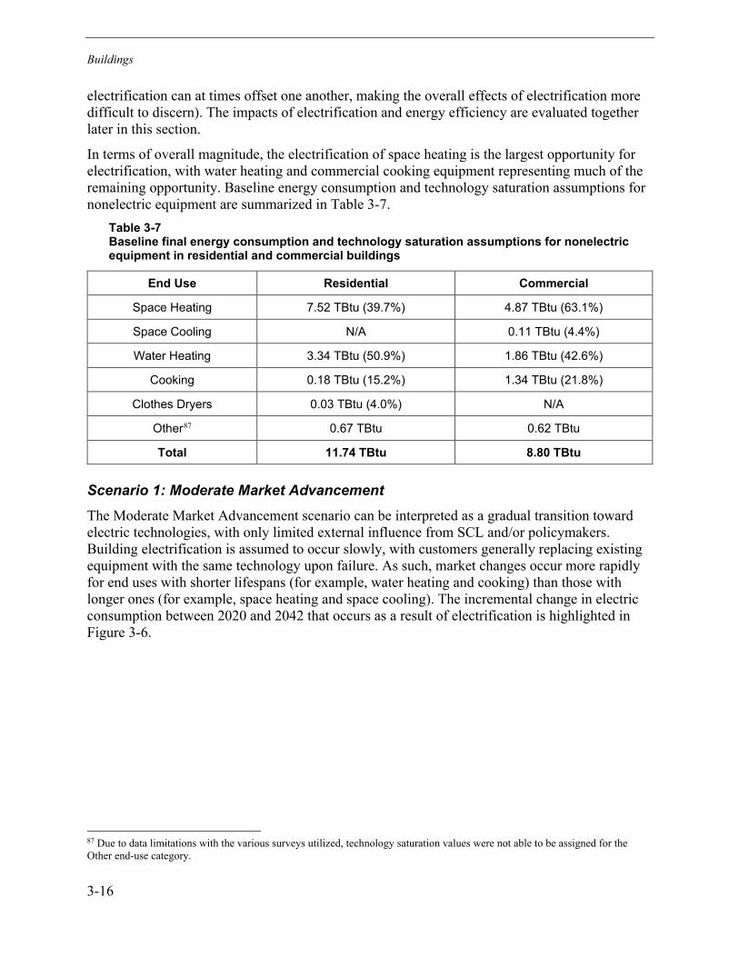
Buildings
3-16
electrification can at times offset one another, making the overall effects of electrification more difficult to discern). The impacts of electrification and energy efficiency are evaluated together later in this section.
In terms of overall magnitude, the electrification of space heating is the largest opportunity for electrification, with water heating and commercial cooking equipment representing much of the remaining opportunity. Baseline energy consumption and technology saturation assumptions for nonelectric equipment are summarized in Table 3-7.
Table 3-7 Baseline final energy consumption and technology saturation assumptions for nonelectric equipment in residential and commercial buildings
End Use Residential Commercial
Space Heating 7.52 TBtu (39.7%) 4.87 TBtu (63.1%)
Space Cooling N/A 0.11 TBtu (4.4%)
Water Heating 3.34 TBtu (50.9%) 1.86 TBtu (42.6%)
Cooking 0.18 TBtu (15.2%) 1.34 TBtu (21.8%)
Clothes Dryers 0.03 TBtu (4.0%) N/A
Other87 0.67 TBtu 0.62 TBtu
Total 11.74 TBtu 8.80 TBtu
Scenario 1: Moderate Market Advancement The Moderate Market Advancement scenario can be interpreted as a gradual transition toward electric technologies, with only limited external influence from SCL and/or policymakers. Building electrification is assumed to occur slowly, with customers generally replacing existing equipment with the same technology upon failure. As such, market changes occur more rapidly for end uses with shorter lifespans (for example, water heating and cooking) than those with longer ones (for example, space heating and space cooling). The incremental change in electric consumption between 2020 and 2042 that occurs as a result of electrification is highlighted in Figure 3-6.
87 Due to data limitations with the various surveys utilized, technology saturation values were not able to be assigned for the Other end-use category.
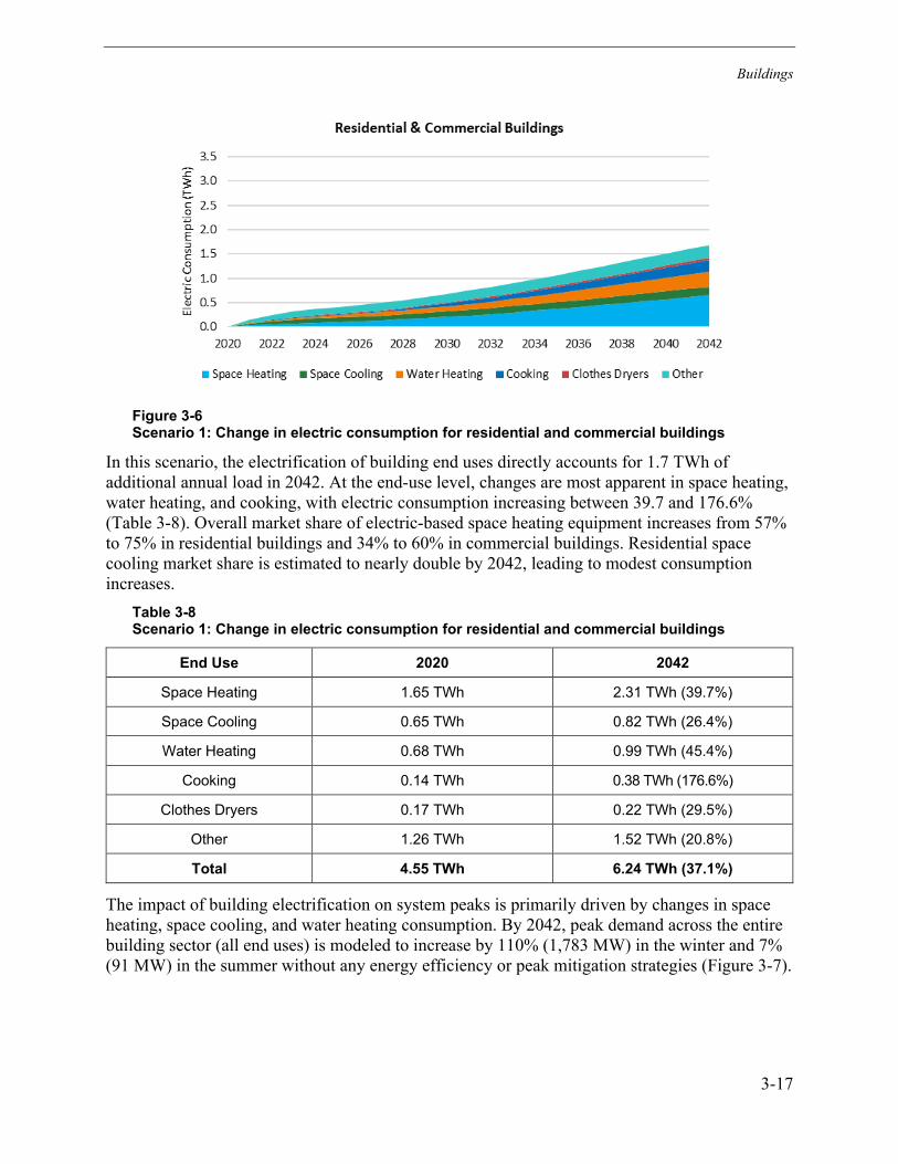
Buildings
3-17
Figure 3-6 Scenario 1: Change in electric consumption for residential and commercial buildings
In this scenario, the electrification of building end uses directly accounts for 1.7 TWh of additional annual load in 2042. At the end-use level, changes are most apparent in space heating, water heating, and cooking, with electric consumption increasing between 39.7 and 176.6% (Table 3-8). Overall market share of electric-based space heating equipment increases from 57% to 75% in residential buildings and 34% to 60% in commercial buildings. Residential space cooling market share is estimated to nearly double by 2042, leading to modest consumption increases.
Table 3-8 Scenario 1: Change in electric consumption for residential and commercial buildings
End Use 2020 2042
Space Heating 1.65 TWh 2.31 TWh (39.7%)
Space Cooling 0.65 TWh 0.82 TWh (26.4%)
Water Heating 0.68 TWh 0.99 TWh (45.4%)
Cooking 0.14 TWh 0.38 TWh (176.6%)
Clothes Dryers 0.17 TWh 0.22 TWh (29.5%)
Other 1.26 TWh 1.52 TWh (20.8%)
Total 4.55 TWh 6.24 TWh (37.1%)
The impact of building electrification on system peaks is primarily driven by changes in space heating, space cooling, and water heating consumption. By 2042, peak demand across the entire building sector (all end uses) is modeled to increase by 110% (1,783 MW) in the winter and 7% (91 MW) in the summer without any energy efficiency or peak mitigation strategies (Figure 3-7).
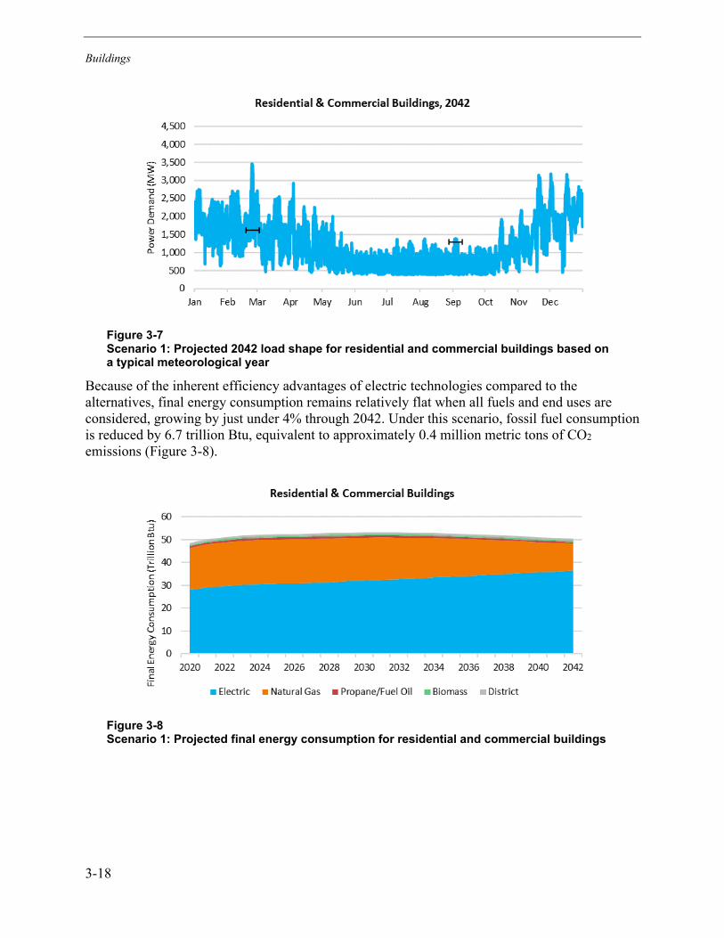
Buildings
3-18
Figure 3-7 Scenario 1: Projected 2042 load shape for residential and commercial buildings based on a typical meteorological year
Because of the inherent efficiency advantages of electric technologies compared to the alternatives, final energy consumption remains relatively flat when all fuels and end uses are considered, growing by just under 4% through 2042. Under this scenario, fossil fuel consumption is reduced by 6.7 trillion Btu, equivalent to approximately 0.4 million metric tons of CO2 emissions (Figure 3-8).
Figure 3-8 Scenario 1: Projected final energy consumption for residential and commercial buildings
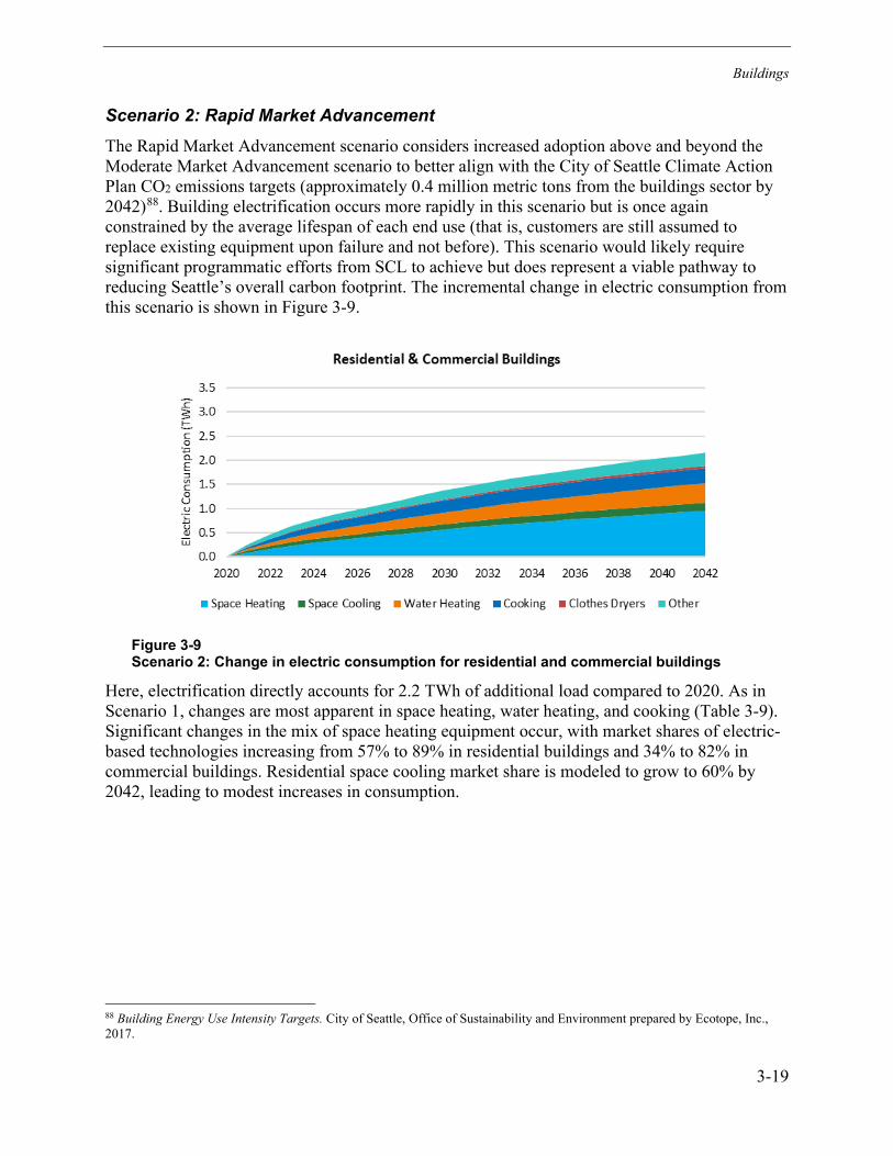
Buildings
3-19
Scenario 2: Rapid Market Advancement The Rapid Market Advancement scenario considers increased adoption above and beyond the Moderate Market Advancement scenario to better align with the City of Seattle Climate Action Plan CO2 emissions targets (approximately 0.4 million metric tons from the buildings sector by 2042)88. Building electrification occurs more rapidly in this scenario but is once again constrained by the average lifespan of each end use (that is, customers are still assumed to replace existing equipment upon failure and not before). This scenario would likely require significant programmatic efforts from SCL to achieve but does represent a viable pathway to reducing Seattle’s overall carbon footprint. The incremental change in electric consumption from this scenario is shown in Figure 3-9.
Figure 3-9 Scenario 2: Change in electric consumption for residential and commercial buildings
Here, electrification directly accounts for 2.2 TWh of additional load compared to 2020. As in Scenario 1, changes are most apparent in space heating, water heating, and cooking (Table 3-9). Significant changes in the mix of space heating equipment occur, with market shares of electric-based technologies increasing from 57% to 89% in residential buildings and 34% to 82% in commercial buildings. Residential space cooling market share is modeled to grow to 60% by 2042, leading to modest increases in consumption.
88 Building Energy Use Intensity Targets. City of Seattle, Office of Sustainability and Environment prepared by Ecotope, Inc., 2017.
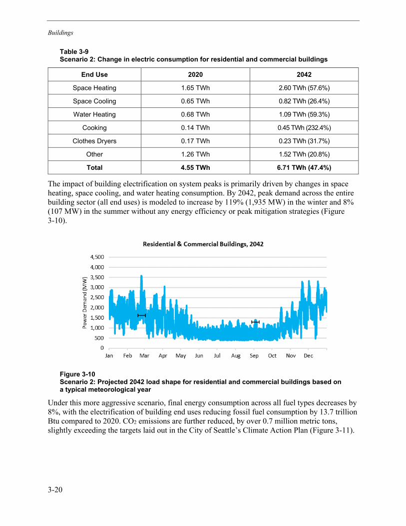
Buildings
3-20
Table 3-9 Scenario 2: Change in electric consumption for residential and commercial buildings
End Use 2020 2042
Space Heating 1.65 TWh 2.60 TWh (57.6%)
Space Cooling 0.65 TWh 0.82 TWh (26.4%)
Water Heating 0.68 TWh 1.09 TWh (59.3%)
Cooking 0.14 TWh 0.45 TWh (232.4%)
Clothes Dryers 0.17 TWh 0.23 TWh (31.7%)
Other 1.26 TWh 1.52 TWh (20.8%)
Total 4.55 TWh 6.71 TWh (47.4%)
The impact of building electrification on system peaks is primarily driven by changes in space heating, space cooling, and water heating consumption. By 2042, peak demand across the entire building sector (all end uses) is modeled to increase by 119% (1,935 MW) in the winter and 8% (107 MW) in the summer without any energy efficiency or peak mitigation strategies (Figure 3-10).
Figure 3-10 Scenario 2: Projected 2042 load shape for residential and commercial buildings based on a typical meteorological year
Under this more aggressive scenario, final energy consumption across all fuel types decreases by 8%, with the electrification of building end uses reducing fossil fuel consumption by 13.7 trillion Btu compared to 2020. CO2 emissions are further reduced, by over 0.7 million metric tons, slightly exceeding the targets laid out in the City of Seattle’s Climate Action Plan (Figure 3-11).
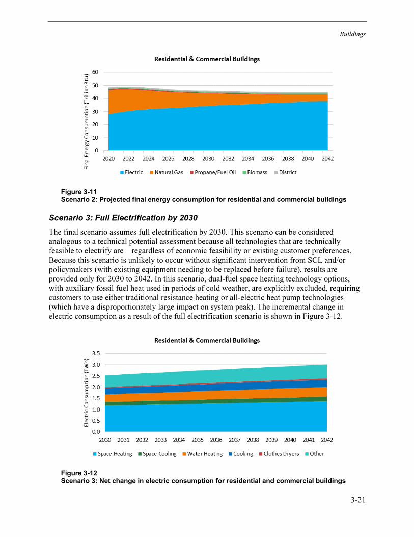
Buildings
3-21
Figure 3-11 Scenario 2: Projected final energy consumption for residential and commercial buildings
Scenario 3: Full Electrification by 2030 The final scenario assumes full electrification by 2030. This scenario can be considered analogous to a technical potential assessment because all technologies that are technically feasible to electrify are—regardless of economic feasibility or existing customer preferences. Because this scenario is unlikely to occur without significant intervention from SCL and/or policymakers (with existing equipment needing to be replaced before failure), results are provided only for 2030 to 2042. In this scenario, dual-fuel space heating technology options, with auxiliary fossil fuel heat used in periods of cold weather, are explicitly excluded, requiring customers to use either traditional resistance heating or all-electric heat pump technologies (which have a disproportionately large impact on system peak). The incremental change in electric consumption as a result of the full electrification scenario is shown in Figure 3-12.
Figure 3-12 Scenario 3: Net change in electric consumption for residential and commercial buildings
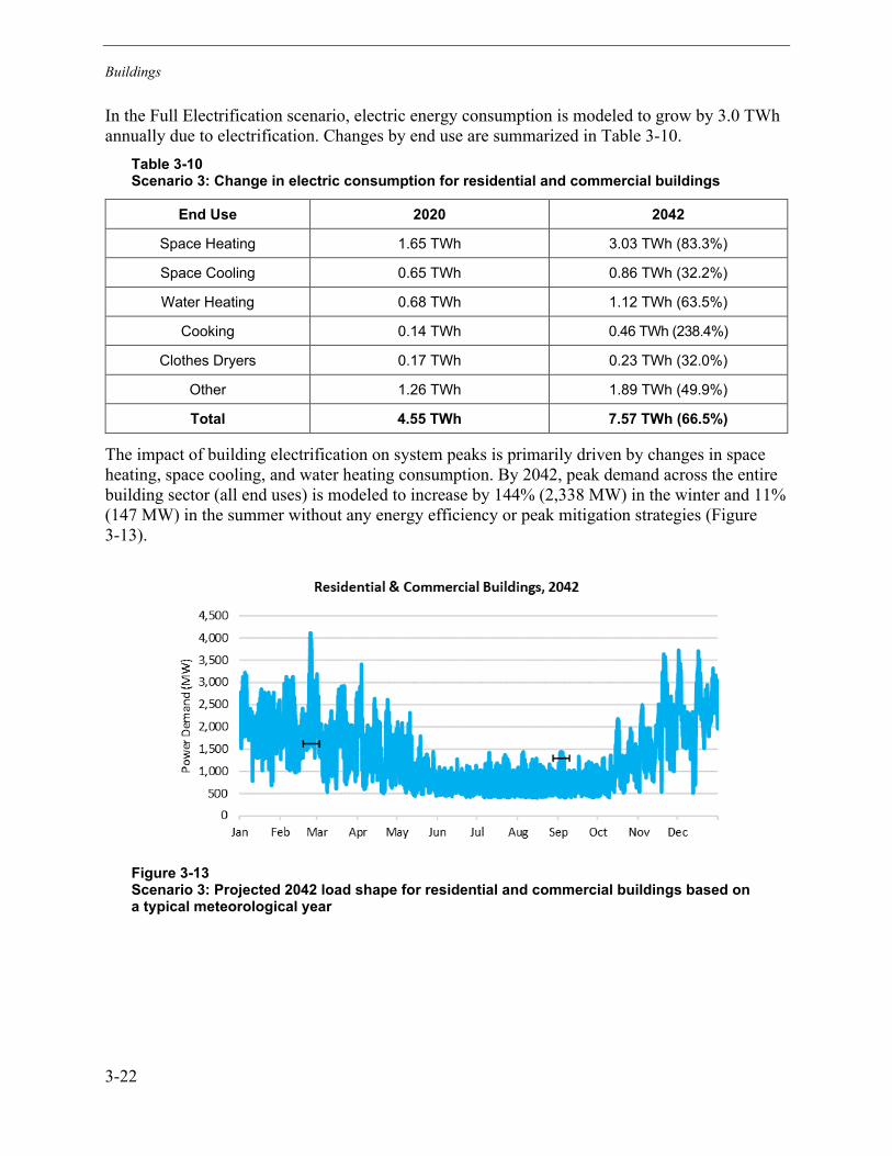
Buildings
3-22
In the Full Electrification scenario, electric energy consumption is modeled to grow by 3.0 TWh annually due to electrification. Changes by end use are summarized in Table 3-10.
Table 3-10 Scenario 3: Change in electric consumption for residential and commercial buildings
End Use 2020 2042
Space Heating 1.65 TWh 3.03 TWh (83.3%)
Space Cooling 0.65 TWh 0.86 TWh (32.2%)
Water Heating 0.68 TWh 1.12 TWh (63.5%)
Cooking 0.14 TWh 0.46 TWh (238.4%)
Clothes Dryers 0.17 TWh 0.23 TWh (32.0%)
Other 1.26 TWh 1.89 TWh (49.9%)
Total 4.55 TWh 7.57 TWh (66.5%)
The impact of building electrification on system peaks is primarily driven by changes in space heating, space cooling, and water heating consumption. By 2042, peak demand across the entire building sector (all end uses) is modeled to increase by 144% (2,338 MW) in the winter and 11% (147 MW) in the summer without any energy efficiency or peak mitigation strategies (Figure 3-13).
Figure 3-13 Scenario 3: Projected 2042 load shape for residential and commercial buildings based on a typical meteorological year
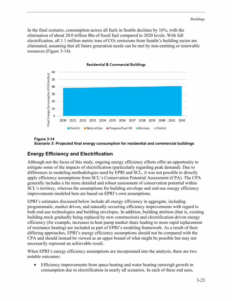
Buildings
3-23
In the final scenario, consumption across all fuels in Seattle declines by 16%, with the elimination of about 20.0 trillion Btu of fossil fuel compared to 2020 levels. With full electrification, all 1.1 million metric tons of CO2 emissions from Seattle’s building sector are eliminated, assuming that all future generation needs can be met by non-emitting or renewable resources (Figure 3-14).
Figure 3-14 Scenario 3: Projected final energy consumption for residential and commercial buildings
Energy Efficiency and Electrification Although not the focus of this study, ongoing energy efficiency efforts offer an opportunity to mitigate some of the impacts of electrification (particularly regarding peak demand). Due to differences in modeling methodologies used by EPRI and SCL, it was not possible to directly apply efficiency assumptions from SCL’s Conservation Potential Assessment (CPA). The CPA generally includes a far more detailed and robust assessment of conservation potential within SCL’s territory, whereas the assumptions for building envelope and end-use energy efficiency improvements modeled here are based on EPRI’s own assumptions.
EPRI’s estimates discussed below include all energy efficiency in aggregate, including programmatic, market driven, and naturally occurring efficiency improvements with regard to both end-use technologies and building envelopes. In addition, building attrition (that is, existing building stock gradually being replaced by new construction) and electrification-driven energy efficiency (for example, increases in heat pump market share leading to more rapid replacement of resistance heating) are included as part of EPRI’s modeling framework. As a result of their differing approaches, EPRI’s energy efficiency assumptions should not be compared with the CPA and should instead be viewed as an upper bound of what might be possible but may not necessarily represent an achievable result.
When EPRI’s energy efficiency assumptions are incorporated into the analysis, there are two notable outcomes:
• Efficiency improvements from space heating and water heating outweigh growth in consumption due to electrification in nearly all scenarios. In each of these end uses,
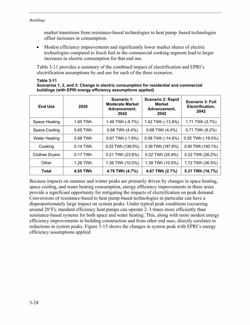
Buildings
3-24
market transitions from resistance-based technologies to heat pump–based technologies offset increases in consumption.
• Modest efficiency improvements and significantly lower market shares of electric technologies compared to fossil fuel in the commercial cooking segment lead to larger increases in electric consumption for that end use.
Table 3-11 provides a summary of the combined impact of electrification and EPRI’s electrification assumptions by end use for each of the three scenarios. Table 3-11 Scenarios 1, 2, and 3: Change in electric consumption for residential and commercial buildings (with EPRI energy efficiency assumptions applied)
End Use 2020 Scenario 1:
Moderate Market Advancement,
2042
Scenario 2: Rapid Market
Advancement, 2042
Scenario 3: Full Electrification,
2042
Space Heating 1.65 TWh 1.49 TWh (-9.7%) 1.42 TWh (-13.8%) 1.71 TWh (3.7%)
Space Cooling 0.65 TWh 0.68 TWh (4.4%) 0.68 TWh (4.4%) 0.71 TWh (9.2%)
Water Heating 0.68 TWh 0.67 TWh (-1.9%) 0.58 TWh (-14.9%) 0.55 TWh (-19.0%)
Cooking 0.14 TWh 0.33 TWh (139.5%) 0.39 TWh (187.8%) 0.40 TWh (193.1%)
Clothes Dryers 0.17 TWh 0.21 TWh (23.8%) 0.22 TWh (25.9%) 0.22 TWh (26.2%)
Other 1.26 TWh 1.39 TWh (10.0%) 1.39 TWh (10.0%) 1.72 TWh (36.5%)
Total 4.55 TWh 4.76 TWh (4.7%) 4.67 TWh (2.7%) 5.31 TWh (16.7%)
Because impacts on summer and winter peaks are primarily driven by changes in space heating, space cooling, and water heating consumption, energy efficiency improvements in these areas provide a significant opportunity for mitigating the impacts of electrification on peak demand. Conversions of resistance-based to heat pump-based technologies in particular can have a disproportionately large impact on system peaks. Under typical peak conditions (occurring around 20°F), standard efficiency heat pumps can operate 2–3 times more efficiently than resistance-based systems for both space and water heating. This, along with more modest energy efficiency improvements in building construction and from other end uses, directly corelates to reductions in system peaks. Figure 3-15 shows the changes in system peak with EPRI’s energy efficiency assumptions applied.

Buildings
3-25
Figure 3-15 Scenarios 1, 2, and 3: Projected 2042 load shape for residential and commercial buildings based on a typical meteorological year (with EPRI energy efficiency assumptions applied)
Although only relatively small changes in summer peaks occur when energy efficiency is applied, significant impacts are present with regard to winter peaks across all scenarios. Once again, this is primarily driven by transitions from resistance heating to heat pumps, particularly in the residential sector where over 50% of households use resistance heating today. Utilizing EPRI’s efficiency assumptions, this market share drops to less than 10–33%, depending on the scenario considered. The use of dual-fuel space heating options (which employ fossil-fueled auxiliary heat at lower temperatures and do not affect peak hours) helps limit impacts on system peak. Overall, with energy efficiency and dual-fuel heating options included (Scenarios 1 and 2), peak demand impacts can be minimized.
Conclusion Due to the inherent efficiency advantages of electric technologies compared to their fossil-fueled alternatives, the electrification of Seattle’s building sector provides significant opportunity for decarbonization.
Key Insights from the Buildings analysis include:
Insight #1: In the three scenarios considered by EPRI and SCL, final energy consumption across all fuels is expected to remain relatively flat or decline depending on the scenario considered, with electric consumption increasing by 2.5 to 3.8 TWh compared to 2020 (Figure 3-16). Although the Moderate Market Advancement scenario (Scenario 1) assumes a more gradual transitions toward electrification, more aggressive pathways—such as those seen in the Rapid Market Advancement scenario (Scenario 2) and Full Electrification by 2030 scenario (Scenario 3) —allow SCL to meet the City of Seattle Climate Action Plan CO2 emissions targets.
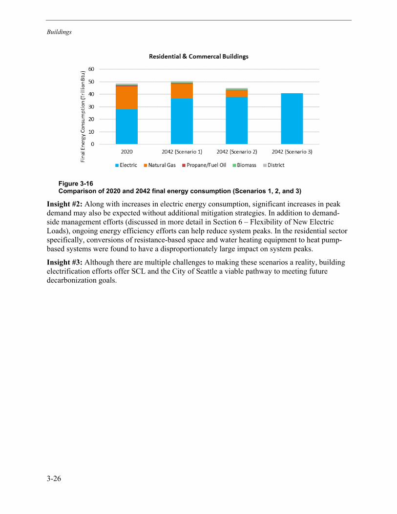
Buildings
3-26
Figure 3-16 Comparison of 2020 and 2042 final energy consumption (Scenarios 1, 2, and 3)
Insight #2: Along with increases in electric energy consumption, significant increases in peak demand may also be expected without additional mitigation strategies. In addition to demand-side management efforts (discussed in more detail in Section 6 – Flexibility of New Electric Loads), ongoing energy efficiency efforts can help reduce system peaks. In the residential sector specifically, conversions of resistance-based space and water heating equipment to heat pump-based systems were found to have a disproportionately large impact on system peaks.
Insight #3: Although there are multiple challenges to making these scenarios a reality, building electrification efforts offer SCL and the City of Seattle a viable pathway to meeting future decarbonization goals.
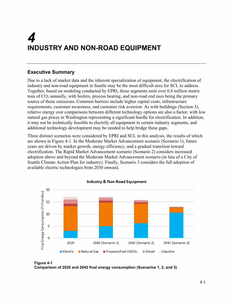
4-1
4 INDUSTRY AND NON-ROAD EQUIPMENT
Executive Summary Due to a lack of market data and the inherent specialization of equipment, the electrification of industry and non-road equipment in Seattle may be the most difficult area for SCL to address. Together, based on modeling conducted by EPRI, these segments emit over 0.8 million metric tons of CO2 annually, with boilers, process heating, and non-road end uses being the primary source of those emissions. Common barriers include higher capital costs, infrastructure requirements, customer awareness, and customer risk aversion. As with buildings (Section 3), relative energy cost comparisons between different technology options are also a factor, with low natural gas prices in Washington representing a significant hurdle for electrification. In addition, it may not be technically feasible to electrify all equipment in certain industry segments, and additional technology development may be needed to help bridge these gaps.
Three distinct scenarios were considered by EPRI and SCL in this analysis, the results of which are shown in Figure 4-1. In the Moderate Market Advancement scenario (Scenario 1), future years are driven by market growth, energy efficiency, and a gradual transition toward electrification. The Rapid Market Advancement scenario (Scenario 2) considers increased adoption above and beyond the Moderate Market Advancement scenario (in lieu of a City of Seattle Climate Action Plan for industry). Finally, Scenario 3 considers the full adoption of available electric technologies from 2030 onward.
Figure 4-1 Comparison of 2020 and 2042 final energy consumption (Scenarios 1, 2, and 3)
Industry and Non-Road Equipment
4-2
Due to the efficiency advantages of electric technologies compared to their fossil-fueled alternatives, final energy consumption across all fuels is expected to remain relatively flat or decline depending on the scenario considered. In contrast, electric energy consumption is likely to increase due to electrification, with an additional 0.6 to 2.2 TWh of growth through 2042. Along with increases in electric energy consumption, increases in summer and winter peak demand may also be expected without additional mitigation strategies. Ongoing energy efficiency efforts provide an opportunity for offsetting these impacts.
Introduction Although not as large as residential and commercial buildings, based on EPRI’s modeling, the industrial segment within Seattle accounts for approximately 13.7 trillion Btu of energy consumption. In contrast to buildings which rely heavily on electricity, natural gas is the most common fuel used, accounting for nearly 74% of all energy consumption and just over 0.5 million metric tons of CO2 emissions. Electricity is the second most common fuel type, accounting for 3.0 trillion Btu or just under 22% of the total. Common barriers to electrification in the industrial segment include higher capital costs, infrastructure requirements, customer awareness, and customer risk aversion. In addition, in certain industry segments it may not be technically feasible to electrify all equipment, and additional technology development may be needed to help bridge these gaps. Non-road, which is defined to include heavy-duty commercial and industrial equipment as well as residential and commercial lawn and garden equipment, is expected to follow a similar development trajectory to that of MDHD on-road transportation.
Section 4 of the Electrification Assessment is focused on the electrification of major industrial end uses such as boilers, process heating, and non-road equipment. This section follows a similar layout to Section 3 in how the information is presented:
• Scenario definitions. Provides a description of the three scenarios considered: Moderate Market Advancement, Rapid Market Advancement, and Full Electrification by 2030.
• Modeling methodology. Includes a review of the various data sources used within this study as well as the approach used to align estimates with baseline consumption data. Market growth projections for industry and non-road equipment are also included.
• Key electrification opportunities. Provides a summary of key electric technology options, along with an overview of their applications, benefits, and barriers from the customer perspective.
• Energy and demand impacts of electrification. Provides energy and demand impacts for each of the three electrification scenarios considered, identifying the incremental impact of electrification to SCL.
• Electrification and energy efficiency. Examines how energy efficiency improvements may offset growth from electrification.
• Conclusion. Review of the potential impacts of widespread industry and non-road electrification on the SCL system.

Industry and Non-Road Equipment
4-3
Scenario Definitions Within this analysis, EPRI and SCL considered three distinct scenarios. In the Moderate Market Advancement scenario, future years are driven by market growth, energy efficiency, and a gradual transition toward electrification. The Rapid Market Advancement scenario considers increased adoption above and beyond the Moderate Market Advancement scenario (in lieu of a City of Seattle Climate Action Plan for industry). Finally, a third scenario considers the full adoption of available electric technologies from 2030 onward (Table 4-1). Additional detail for these scenarios is discussed in the Energy and Demand Impacts of Electrification subsection.
Table 4-1 Scenarios explored in this analysis and their underlying basis.
Scenario Description
Moderate Market Advancement Future years driven by market growth, energy efficiency, and electrification
Rapid Market Advancement Increased adoption above and beyond the Moderate Market Advancement scenario (in lieu of a City of Seattle Climate Action Plan for industry)
Full Electrification by 2030 Full adoption of available electric technologies by 2030
Modeling Methodology
Data Sources Due to the lack of available saturation surveys and data sources pertaining to the industrial segment in Seattle, baseline estimates of current consumption employ a “top down” approach, relying directly on aggregate 2019 electricity and natural gas sales provided by SCL and Puget Sound Energy. Next, survey data from the EIA’s Manufacturing Energy Consumption Survey for the West census region were used to develop end-use level estimates for industry. Non-road estimates use county-level data from the EPA’s MOtor Vehicle Emission Simulator, with the City of Seattle’s share estimated using the Census Bureau’s 2019 American Community Survey and 2019 County Business Patterns. A summary of the data sources used, and their geospatial granularity, is given in Table 4-2.
Table 4-2 Summary of data sources used and their geospatial granularity
Data Source Geospatial Granularity
2019 American Community Survey County
2019 County Business Patterns County
2014 MOtor Vehicle Emission Simulator County
2021 Annual Energy Outlook Census Division
2018 Manufacturing Energy Consumption Survey Census Region
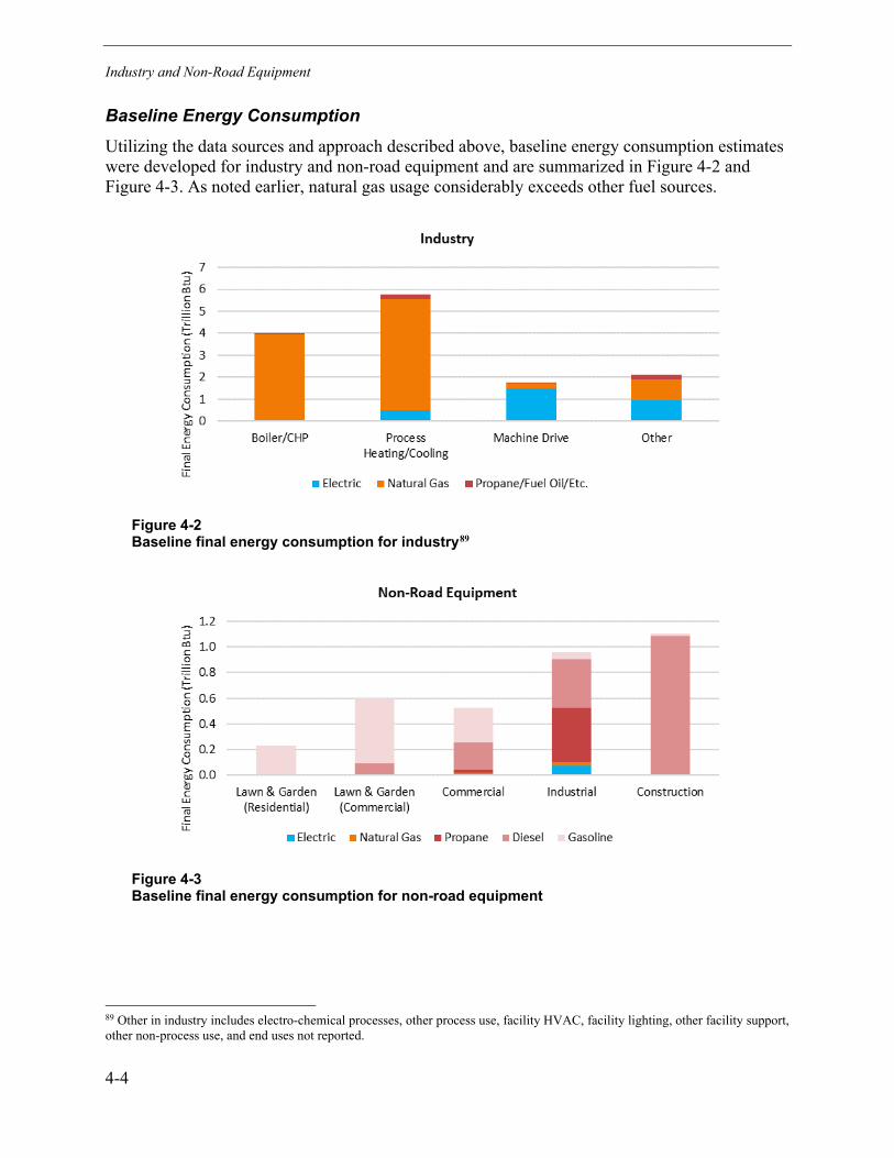
Industry and Non-Road Equipment
4-4
Baseline Energy Consumption Utilizing the data sources and approach described above, baseline energy consumption estimates were developed for industry and non-road equipment and are summarized in Figure 4-2 and Figure 4-3. As noted earlier, natural gas usage considerably exceeds other fuel sources.
Figure 4-2 Baseline final energy consumption for industry89
Figure 4-3 Baseline final energy consumption for non-road equipment
89 Other in industry includes electro-chemical processes, other process use, facility HVAC, facility lighting, other facility support, other non-process use, and end uses not reported.

Industry and Non-Road Equipment
4-5
Market Growth Projections In each of the three electrification scenarios evaluated, changes in future energy consumption are driven by market growth, energy efficiency, and electrification. Market growth projections are consistent across all scenarios and are modeled exogenously, with growth in the industrial sector assumed to remain flat through 2042 and growth in relevant residential and commercial non-road equipment indexed to future building stock and floorspace projections provided by SCL (Table 3-4). Within EPRI’s modeling framework, these growth projections are used to define the total addressable market as well as the total number of new equipment installations over the study’s time horizon. Changes in future energy prices use projections from the EIA’s 2021 Annual Energy Outlook.
Key Electrification Opportunities Based on the baseline energy consumption estimates presented in the previous section, boilers/combined heat and power (CHP), process heating, and non-road equipment represent the bulk of the opportunity for electrification within this segment. In certain industrial applications, it may not be technically feasible to electrify all equipment, and additional technology development may help bridge these gaps. Key electric technology options for each of these end-use areas, along with their applications, benefits, and barriers, are described next.
Industrial Boilers/CHP Boilers burn fossil fuels such as natural gas, oil, and solid fuels or use electricity to heat water to produce hot water or steam. Boilers are essential in many energy-intensive industries and maintain a major role in manufacturing, heating, and electricity generation. Electric boilers use current to heat water and produce steam at different temperatures and pressures. The two primary types of electric boilers on the market today are described next.
Electric Resistance Boilers
Electric resistance boilers use an electrically resistive heating element and thermostat to maintain temperature to produce hot water or steam. These boilers are available in capacities up to ~4 MW and have high efficiency (>90%) in converting water to steam as well as low standby losses.
Electrode Boilers
Electrode boilers use specific electrodes to apply current to the water stream to generate steam for applications that require high heat output and fast recovery. For applications >4 MW, electrode boilers are attractive because they can quickly provide higher heat output. Although electrode boilers are usually less expensive to install than electric resistance boilers, economic comparisons to gas or fuel-oil boilers remain a major hurdle.

Industry and Non-Road Equipment
4-6
Applications, Benefits, and Barriers: Industrial Boilers/CHP
Industrial electric boilers are broadly applicable in industries that require steam for either heating or process use, including most manufacturing.
Electric boilers have several advantages over fossil-fuel-fired boilers:
• Clean firing: no emissions of products of combustion
• No venting or stack required
• High efficiency with minimal losses
• Compact size: smaller volume and footprint than fossil-fired boilers
• Available in wide range of sizes as boiler only or in tank-type models
Higher annual energy costs compared to gas boilers remains the primary barrier to adoption. As such, little electrification is expected to occur naturally.
Industrial Process Heating Heat is used in nearly every industrial process to cure, dry, heat treat, and melt materials used in making various products. Multiple electric technology options can be employed for industrial process heating including resistance, induction, infrared (IR), and ultraviolet (UV). These technologies tend to be highly efficient compared to natural gas–fired alternatives and can provide significant non-energy benefits for customers, including increased productivity and product quality. The following examples describe the different types of process heating and electric technologies that may be employed.
Resistance Heating and Melting
Heating and melting using electric resistance can be a low-cost option, providing freedom from noise and excessive heat of combustion processes. This simplistic heating method results in a high-quality melt with low oxidation losses.
Resistance heating may be used in place of natural gas batch furnaces to heat-treat metal parts such as wire, gears, shafts, fasteners, and automotive transmission parts and various housings. Resistance heating has high thermal efficiency, offering customers energy savings while increasing productivity, reducing waste, and freeing up floor space for other use. The operating cost of resistance heating equipment may be high compared to natural gas ovens, and there may be reliability issues with electric element breakage and the integrity of clamped connections.
Induction Heating and Melting
Induction provides rapid and targeted heating, allowing for much faster (less than 10% of the time) and more precise results than is possible with natural gas carburizing furnaces. Complex part geometry may inhibit application of induction heating. Induction heat treating may be best applied for production of large quantities of the same part or parts with similar geometry.
Induction melting is an efficient alternative to fossil-fueled furnaces in foundries for both primary metal melting and alloys. Removal of direct combustion of natural gas eliminates site emissions and can provide a more comfortable work environment for employees. Coreless

Industry and Non-Road Equipment
4-7
induction furnaces are used to melt metal, while channel induction furnaces are used to hold the molten metal. Channel furnaces must be kept on all the time while holding molten metal. There may be increased maintenance costs for induction furnaces associated with refractory cracks when processing some alloys.
IR Curing and Drying
IR may be used in place of natural gas convection ovens or in addition to convection ovens as a “boost” oven, providing curing and drying for myriad applications. Electric IR equipment is highly efficient and allows for productivity increases and improved product quality. In some cases, IR equipment will cost less than convection ovens; however, larger units may have a higher capital cost compared to convection ovens. IR curing and drying is a “line-of-sight” technology; therefore, the shape of parts will impact the efficacy of infrared equipment. The surface to be cured or dried must be “visible” to the IR emitters for desired results. The most common applications for IR include paint on car bodies and appliances, paint and powder coating on light fixtures, and paint and varnish on sheets of hardboard, particleboard, and chipboard.
UV Curing
UV curing (also known as radiation curing or energy curing) is a photochemical process in which high-intensity ultraviolet light is used to instantly cure or “dry” inks, coatings, or adhesives. UV curing is not actually drying but is a polymerization process that hardens the material, whether the material is applied to another or is a built-up product. UV has demonstrated increased production speed, reduced rejection rates, and improved scratch and solvent resistance compared to other drying technologies. It also is used to facilitate high-performance bonding.
UV curing technology is used across a wide range of industrial applications. Products that are closer to consumers and other end users are increasingly incorporating UV cure coatings due to their unique benefits of reduced and solvent-free formulations, fast curing times, low-temperature processing, and, most recently, scratch resistance and chemical resistance.
Vacuum Carburizing Furnace
A vacuum carburizing furnace is a resistance furnace in which carbon atoms are added to the part being treated to cause desired phase transformations, which results in improved strength of the material. This is done in a vacuum where air has been removed and inert gases added as the part is being heat treated. This differs from induction surface heat treating in which no hydrocarbons are added during heat treating.
Vacuum furnaces may be used in the same applications as induction and resistance heating including machinery and appliance manufacturing as well as automotive engineering. Additional benefits of using vacuum carburizing as opposed to atmospheric carburizing ovens are fewer deformations of parts, reduced process times, and minimal to no post-processing requirements.
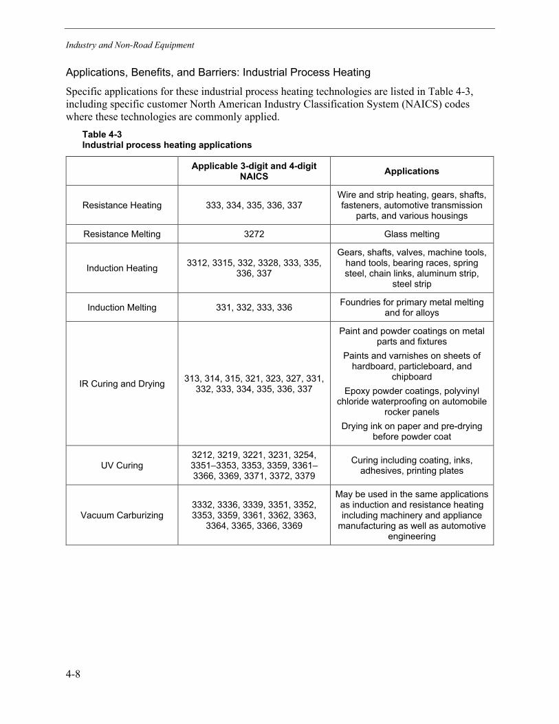
Industry and Non-Road Equipment
4-8
Applications, Benefits, and Barriers: Industrial Process Heating
Specific applications for these industrial process heating technologies are listed in Table 4-3, including specific customer North American Industry Classification System (NAICS) codes where these technologies are commonly applied.
Table 4-3 Industrial process heating applications
Applicable 3-digit and 4-digit NAICS Applications
Resistance Heating 333, 334, 335, 336, 337 Wire and strip heating, gears, shafts, fasteners, automotive transmission
parts, and various housings
Resistance Melting 3272 Glass melting
Induction Heating 3312, 3315, 332, 3328, 333, 335, 336, 337
Gears, shafts, valves, machine tools, hand tools, bearing races, spring steel, chain links, aluminum strip,
steel strip
Induction Melting 331, 332, 333, 336 Foundries for primary metal melting and for alloys
IR Curing and Drying 313, 314, 315, 321, 323, 327, 331, 332, 333, 334, 335, 336, 337
Paint and powder coatings on metal parts and fixtures
Paints and varnishes on sheets of hardboard, particleboard, and
chipboard Epoxy powder coatings, polyvinyl
chloride waterproofing on automobile rocker panels
Drying ink on paper and pre-drying before powder coat
UV Curing 3212, 3219, 3221, 3231, 3254, 3351–3353, 3353, 3359, 3361–3366, 3369, 3371, 3372, 3379
Curing including coating, inks, adhesives, printing plates
Vacuum Carburizing 3332, 3336, 3339, 3351, 3352, 3353, 3359, 3361, 3362, 3363,
3364, 3365, 3366, 3369
May be used in the same applications as induction and resistance heating including machinery and appliance
manufacturing as well as automotive engineering
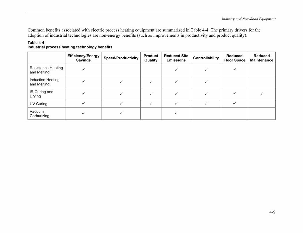
Industry and Non-Road Equipment
4-9
Common benefits associated with electric process heating equipment are summarized in Table 4-4. The primary drivers for the adoption of industrial technologies are non-energy benefits (such as improvements in productivity and product quality). Table 4-4 Industrial process heating technology benefits
Efficiency/Energy Savings Speed/Productivity Product
Quality Reduced Site
Emissions Controllability Reduced Floor Space
Reduced Maintenance
Resistance Heating and Melting
Induction Heating and Melting
IR Curing and Drying
UV Curing
Vacuum Carburizing

Industry and Non-Road Equipment
4-10
In general, the high upfront cost of process heating equipment may be a barrier if customer access to capital is limited or the capital approval process is burdensome. More importantly, downtime needed to install new equipment—electric or otherwise—is a hurdle to be addressed in planning stages because loss of productivity is a primary barrier for installing new equipment.
Non-Road Equipment Significant electrification opportunities exist within the non-road equipment segment. In most cases, electric equipment will offset the direct combustion of petroleum-based fuels (propane, diesel, or gasoline), providing substantial environmental and health benefits. Near-term solutions include material handling and logistics equipment (such as forklifts and terminal trucks) with larger, more heavy-duty equipment (such as that used in construction) to become more commercially viable in the long term. Outside the industrial sector, residential and commercial lawn and garden equipment are also near-term opportunities.
Forklifts
With adequate usage, electric forklifts can quickly pay back additional first costs compared to fossil-fueled alternatives. Forklifts are applied in many business operations to transport materials, ranging from occasional use at commercial businesses to nearly round-the-clock use in warehouse facilities. The primary opportunity for electrification is conversion of Class 4 and 5 internal combustion (IC) forklifts to Class 1 (electric) units.
Class 1 and Class 4 cushion-tired forklifts are interchangeable in application—they differ only in fuel type; electric and propane, respectively. Because of this, Class 1 electric units are expected to have the potential to capture all the Class 4 market. Class 1 pneumatic tire is similar to Class 5; again they differ in fuel type—electric and diesel, respectively—and they may differ in the lifting capacities (20,000 lb for electric to 100,000 lb for diesel). It is estimated by lift truck original equipment manufacturers (OEMs) that 50–80% of the current Class 5 market could be converted to Class 1 electric trucks.
Terminal Trucks
Terminal trucks, also known as yard hostlers, move semi-trailers in a cargo yard, warehouse, or intermodal facility. Electric terminal trucks, like their diesel counterparts, can bear up to 80,000 pounds of gross weight (including the weight of the truck). These trucks come with up to 160-kWh batteries, which can be opportunity-charged during breaks or fully charged overnight using onboard chargers. Although current options cost more to deploy, they can eliminate on-site emissions, improve worker health and safety, and reduce noise.
Lawn and Garden Equipment
Market penetration of electric lawn and garden equipment is increasing, with many options available in retail stores across the country. Electric mowers can be corded or cordless. They are simple and easy to use because they are battery powered and there is no maintenance required, unlike gasoline lawn mowers. Therefore, this equipment saves significant maintenance time and cost. Ancillary equipment—such as leaf blowers, edgers, and trimmers—has a lower level of usage and consumes only a fraction of the energy consumed by lawn mowers.

Industry and Non-Road Equipment
4-11
Construction Equipment
Just as electric vehicles are a growing trend in on-road transportation, electric equipment is an emerging area in the construction industry. Several major OEMs are producing electric equipment for various construction applications. Examples of emerging electric equipment include excavators, backhoe loaders, earthmovers, skid steer loaders, mobile cranes, cement mixers, and bulldozers. Hybrid diesel-electric equipment options are also being developed.
Seaport Electrification
At the Port of Seattle, electrification has been used as one strategy to achieve its emissions reduction goals. The Port and/or its tenants own several electric cranes, electric forklifts, and electric pallet jacks in addition to other cargo-handling equipment that has been traditionally powered by fossil fuels. Additional cargo handling equipment that may be electrified includes rail mounted gantry cranes, rubber tire gantry cranes, top handlers, and refrigerated cargo containers.
Shore power, or cold ironing, is the process of providing shoreside electrical power to a ship (cargo, cruise, or other ships) at berth while its main and auxiliary engines are turned off. It allows emergency equipment, refrigeration, cooling, heating, lighting, and other equipment to receive continuous electrical power while the ship loads or unloads its cargo. Significant investment in electrical infrastructure may be necessary to use shore power at the Port of Seattle. For ships and cruise liners not currently equipped to plug into shore power, certain onboard modifications are necessary. In most cases, the terminals at which these ships berth also need to be modified with electric infrastructure. Electrical transformers are also necessary at the terminal or on board the ship.
Applications, Benefits, and Barriers: Non-Road Equipment Although the applications are specific, there are several common non-energy benefits of electric non-road equipment that play a critical role in the conversion of these technologies:
• Elimination of local emissions
• Reduced noise
• Reduced maintenance and increased reliability
• Ability to turn on/off quickly, reducing or eliminating idle time
• Improved worker health and safety and customer impacts – Reduced exposure to diesel and jet fuel emissions – Reduced noise levels and noise pollution
In addition to customer preferences, higher upfront costs and infrastructure requirements may be a barrier to electrifying non-road equipment.

Industry and Non-Road Equipment
4-12
Energy and Demand Impacts of Electrification Electrification was modeled based on an evaluation of relevant electric technologies by EPRI subject matter experts, with customers adopting more beneficial options over time. Future scenarios build upon the baseline energy consumption estimates and market growth projections described previously. Results showing the incremental impact of electrification for each of the three scenarios are presented in this section. To allow SCL to better assess the net impacts of electrification on a standalone basis, energy efficiency impacts are excluded here (energy efficiency and electrification can at times offset one another, making the overall effects of electrification more difficult to discern). These impacts are evaluated together later in this section.
In terms of overall magnitude, the electrification of process heating is the largest opportunity, with boilers/CHP and non-road equipment representing much of the remaining opportunity. Baseline energy consumption estimates for nonelectric equipment in industry and non-road are summarized in Table 4-5.
Table 4-5 Baseline final energy consumption for nonelectric equipment in industry and non-road
End Use Industry & Non-Road
Boiler/CHP 3.97 TBtu
Process Heating/Cooling 5.37 TBtu
Machine Drive 0.29 TBtu
Non-Road Equipment 3.34 TBtu
Other 1.16 TBtu
Total 14.04 TBtu
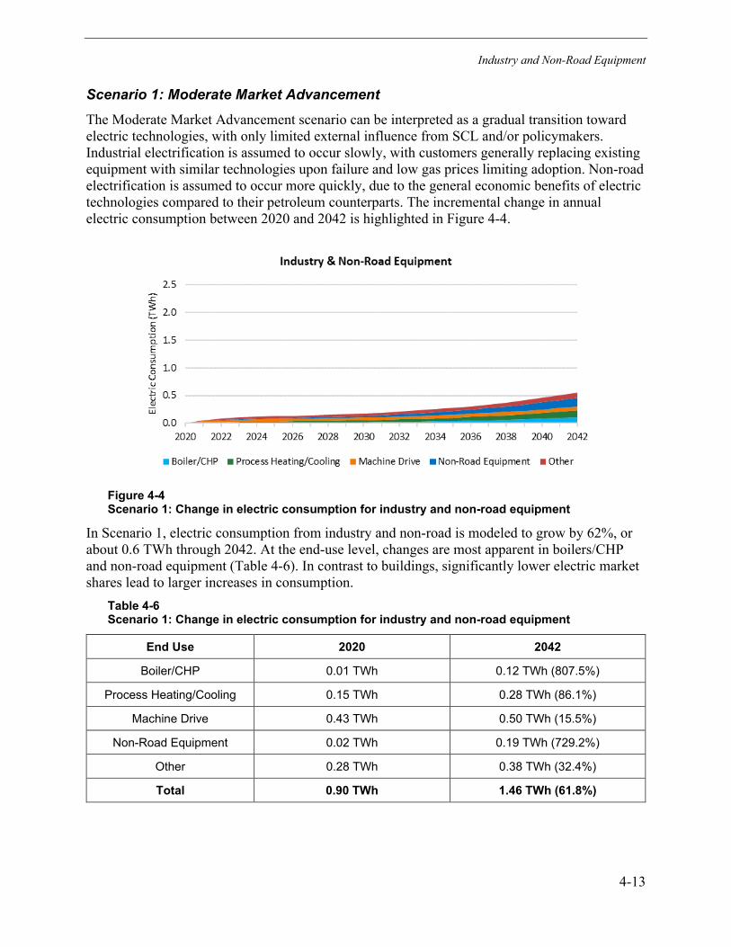
Industry and Non-Road Equipment
4-13
Scenario 1: Moderate Market Advancement The Moderate Market Advancement scenario can be interpreted as a gradual transition toward electric technologies, with only limited external influence from SCL and/or policymakers. Industrial electrification is assumed to occur slowly, with customers generally replacing existing equipment with similar technologies upon failure and low gas prices limiting adoption. Non-road electrification is assumed to occur more quickly, due to the general economic benefits of electric technologies compared to their petroleum counterparts. The incremental change in annual electric consumption between 2020 and 2042 is highlighted in Figure 4-4.
Figure 4-4 Scenario 1: Change in electric consumption for industry and non-road equipment
In Scenario 1, electric consumption from industry and non-road is modeled to grow by 62%, or about 0.6 TWh through 2042. At the end-use level, changes are most apparent in boilers/CHP and non-road equipment (Table 4-6). In contrast to buildings, significantly lower electric market shares lead to larger increases in consumption.
Table 4-6 Scenario 1: Change in electric consumption for industry and non-road equipment
End Use 2020 2042
Boiler/CHP 0.01 TWh 0.12 TWh (807.5%)
Process Heating/Cooling 0.15 TWh 0.28 TWh (86.1%)
Machine Drive 0.43 TWh 0.50 TWh (15.5%)
Non-Road Equipment 0.02 TWh 0.19 TWh (729.2%)
Other 0.28 TWh 0.38 TWh (32.4%)
Total 0.90 TWh 1.46 TWh (61.8%)
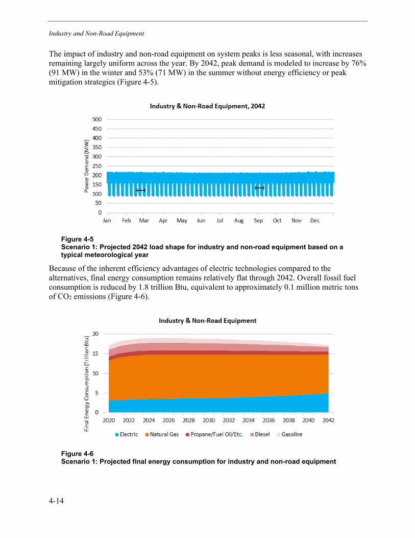
Industry and Non-Road Equipment
4-14
The impact of industry and non-road equipment on system peaks is less seasonal, with increases remaining largely uniform across the year. By 2042, peak demand is modeled to increase by 76% (91 MW) in the winter and 53% (71 MW) in the summer without energy efficiency or peak mitigation strategies (Figure 4-5).
Figure 4-5 Scenario 1: Projected 2042 load shape for industry and non-road equipment based on a typical meteorological year
Because of the inherent efficiency advantages of electric technologies compared to the alternatives, final energy consumption remains relatively flat through 2042. Overall fossil fuel consumption is reduced by 1.8 trillion Btu, equivalent to approximately 0.1 million metric tons of CO2 emissions (Figure 4-6).
Figure 4-6 Scenario 1: Projected final energy consumption for industry and non-road equipment
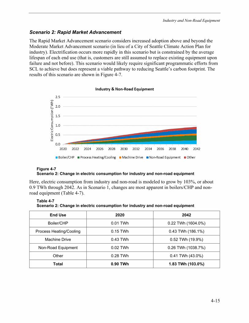
Industry and Non-Road Equipment
4-15
Scenario 2: Rapid Market Advancement The Rapid Market Advancement scenario considers increased adoption above and beyond the Moderate Market Advancement scenario (in lieu of a City of Seattle Climate Action Plan for industry). Electrification occurs more rapidly in this scenario but is constrained by the average lifespan of each end use (that is, customers are still assumed to replace existing equipment upon failure and not before). This scenario would likely require significant programmatic efforts from SCL to achieve but does represent a viable pathway to reducing Seattle’s carbon footprint. The results of this scenario are shown in Figure 4-7.
Figure 4-7 Scenario 2: Change in electric consumption for industry and non-road equipment
Here, electric consumption from industry and non-road is modeled to grow by 103%, or about 0.9 TWh through 2042. As in Scenario 1, changes are most apparent in boilers/CHP and non-road equipment (Table 4-7).
Table 4-7 Scenario 2: Change in electric consumption for industry and non-road equipment
End Use 2020 2042
Boiler/CHP 0.01 TWh 0.22 TWh (1604.0%)
Process Heating/Cooling 0.15 TWh 0.43 TWh (186.1%)
Machine Drive 0.43 TWh 0.52 TWh (19.9%)
Non-Road Equipment 0.02 TWh 0.26 TWh (1038.7%)
Other 0.28 TWh 0.41 TWh (43.0%)
Total 0.90 TWh 1.83 TWh (103.0%)
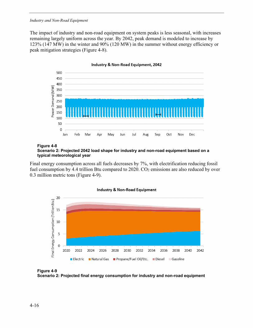
Industry and Non-Road Equipment
4-16
The impact of industry and non-road equipment on system peaks is less seasonal, with increases remaining largely uniform across the year. By 2042, peak demand is modeled to increase by 123% (147 MW) in the winter and 90% (120 MW) in the summer without energy efficiency or peak mitigation strategies (Figure 4-8).
Figure 4-8 Scenario 2: Projected 2042 load shape for industry and non-road equipment based on a typical meteorological year
Final energy consumption across all fuels decreases by 7%, with electrification reducing fossil fuel consumption by 4.4 trillion Btu compared to 2020. CO2 emissions are also reduced by over 0.3 million metric tons (Figure 4-9).
Figure 4-9 Scenario 2: Projected final energy consumption for industry and non-road equipment
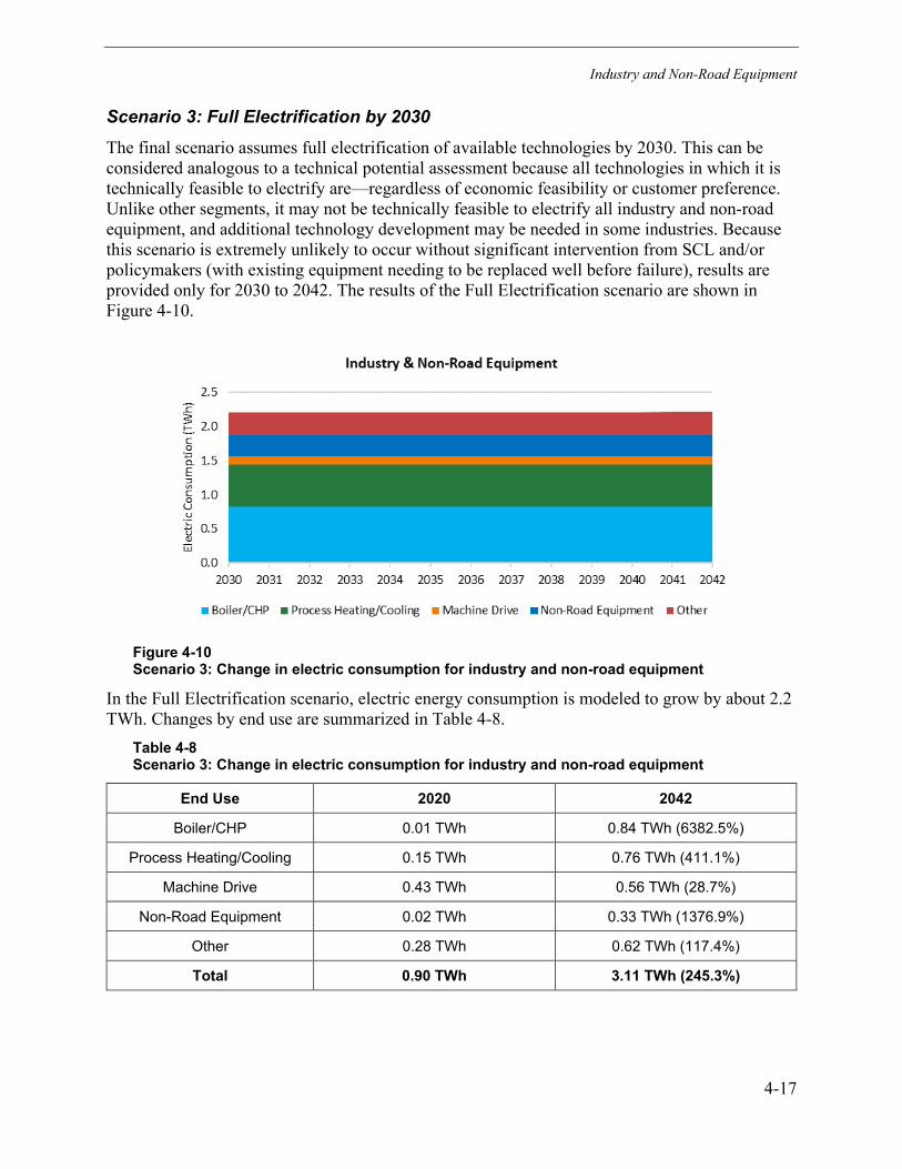
Industry and Non-Road Equipment
4-17
Scenario 3: Full Electrification by 2030 The final scenario assumes full electrification of available technologies by 2030. This can be considered analogous to a technical potential assessment because all technologies in which it is technically feasible to electrify are—regardless of economic feasibility or customer preference. Unlike other segments, it may not be technically feasible to electrify all industry and non-road equipment, and additional technology development may be needed in some industries. Because this scenario is extremely unlikely to occur without significant intervention from SCL and/or policymakers (with existing equipment needing to be replaced well before failure), results are provided only for 2030 to 2042. The results of the Full Electrification scenario are shown in Figure 4-10.
Figure 4-10 Scenario 3: Change in electric consumption for industry and non-road equipment
In the Full Electrification scenario, electric energy consumption is modeled to grow by about 2.2 TWh. Changes by end use are summarized in Table 4-8.
Table 4-8 Scenario 3: Change in electric consumption for industry and non-road equipment
End Use 2020 2042
Boiler/CHP 0.01 TWh 0.84 TWh (6382.5%)
Process Heating/Cooling 0.15 TWh 0.76 TWh (411.1%)
Machine Drive 0.43 TWh 0.56 TWh (28.7%)
Non-Road Equipment 0.02 TWh 0.33 TWh (1376.9%)
Other 0.28 TWh 0.62 TWh (117.4%)
Total 0.90 TWh 3.11 TWh (245.3%)

Industry and Non-Road Equipment
4-18
The impact of industry and non-road equipment on system peaks is less seasonal, with increases remaining largely uniform across the year. By 2042, peak demand is modeled to increase by 270% (323 MW) in the winter and 229% (304 MW) in the summer without energy efficiency or peak mitigation strategies (Figure 4-11).
Figure 4-11 Scenario 3: Projected 2042 load shape for industry and non-road equipment based on a typical meteorological year
In the final scenario, consumption across all fuels in Seattle declines by 23%, with the elimination of about 11.6 trillion Btu of fossil fuel compared to 2020 levels. Overall, approximately 0.7 million metric tons of CO2 emissions are eliminated in this scenario, assuming that all future generation needs can be met by non-emitting or renewable resources (Figure 4-12).
Figure 4-12 Scenario 3: Projected final energy consumption for industry and non-road equipment

Industry and Non-Road Equipment
4-19
Energy Efficiency and Electrification Although not the focus of this study, ongoing energy efficiency improvements offer an opportunity to mitigate some of the impacts of electrification (particularly with regard to peak demand). As discussed in the Buildings section, due to differences in modeling methodologies used by EPRI and SCL, it was not possible to directly apply efficiency assumptions from SCL’s Conservation Potential Assessment (CPA). The CPA generally includes a far more detailed and robust assessment of conservation potential within SCL’s territory, whereas the assumptions for end-use energy efficiency improvements modeled here are based on EPRI’s own assumptions.
EPRI’s estimates include all energy efficiency in aggregate—including programmatic, market driven, and naturally occurring efficiency improvements—and should not be directly compared with the CPA. In contrast to buildings, sizable increases in electric consumption are projected when efficiency assumptions are applied, as only modest efficiency improvements anticipated, and significantly lower market shares of existing electric technologies can be retrofitted to become more efficient. A summary of these changes in electric consumption for each of the three scenarios compared to 2020 is provided by end use in Table 4-9.
Table 4-9 Scenario 1, 2, and 3: Change in electric consumption for industry and non-road equipment (with EPRI energy efficiency assumptions applied)
End Use 2020 Scenario 1:
Moderate Market Advancement, 2042
Scenario 2: Rapid Market
Advancement, 2042 Scenario 3: Full
Electrification, 2042
Boiler/CHP 0.01 TWh 0.11 TWh (726.8%) 0.20 TWh (1452.4%) 0.77 TWh (5806.1%)
Process Heating/Cooling 0.15 TWh 0.25 TWh (69.6%) 0.39 TWh (160.7%) 0.70 TWh (365.7%)
Machine Drive 0.43 TWh 0.46 TWh (5.2%) 0.47 TWh (9.3%) 0.51 TWh (17.3%)
Non-Road Equipment 0.02 TWh 0.14 TWh (503.4%) 0.19 TWh (728.7%) 0.24 TWh (974.8%)
Other 0.28 TWh 0.34 TWh (20.6%) 0.37 TWh (30.3%) 0.56 TWh (98.1%)
Total 0.90 TWh 1.29 TWh (43.6%) 1.62 TWh (79.8%) 2.77 TWh (207.8%)
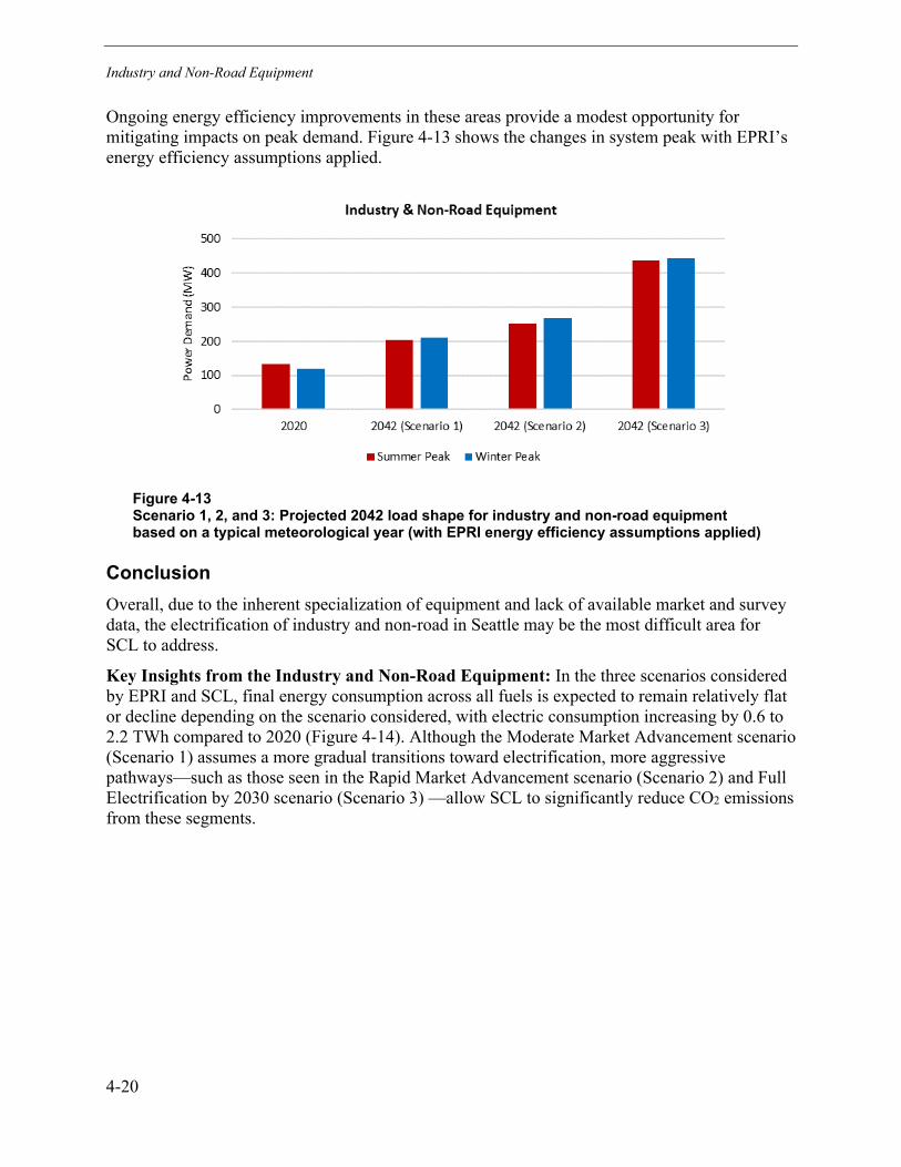
Industry and Non-Road Equipment
4-20
Ongoing energy efficiency improvements in these areas provide a modest opportunity for mitigating impacts on peak demand. Figure 4-13 shows the changes in system peak with EPRI’s energy efficiency assumptions applied.
Figure 4-13 Scenario 1, 2, and 3: Projected 2042 load shape for industry and non-road equipment based on a typical meteorological year (with EPRI energy efficiency assumptions applied)
Conclusion Overall, due to the inherent specialization of equipment and lack of available market and survey data, the electrification of industry and non-road in Seattle may be the most difficult area for SCL to address.
Key Insights from the Industry and Non-Road Equipment: In the three scenarios considered by EPRI and SCL, final energy consumption across all fuels is expected to remain relatively flat or decline depending on the scenario considered, with electric consumption increasing by 0.6 to 2.2 TWh compared to 2020 (Figure 4-14). Although the Moderate Market Advancement scenario (Scenario 1) assumes a more gradual transitions toward electrification, more aggressive pathways—such as those seen in the Rapid Market Advancement scenario (Scenario 2) and Full Electrification by 2030 scenario (Scenario 3) —allow SCL to significantly reduce CO2 emissions from these segments.
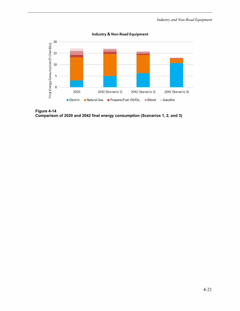
Industry and Non-Road Equipment
4-21
Figure 4-14 Comparison of 2020 and 2042 final energy consumption (Scenarios 1, 2, and 3)

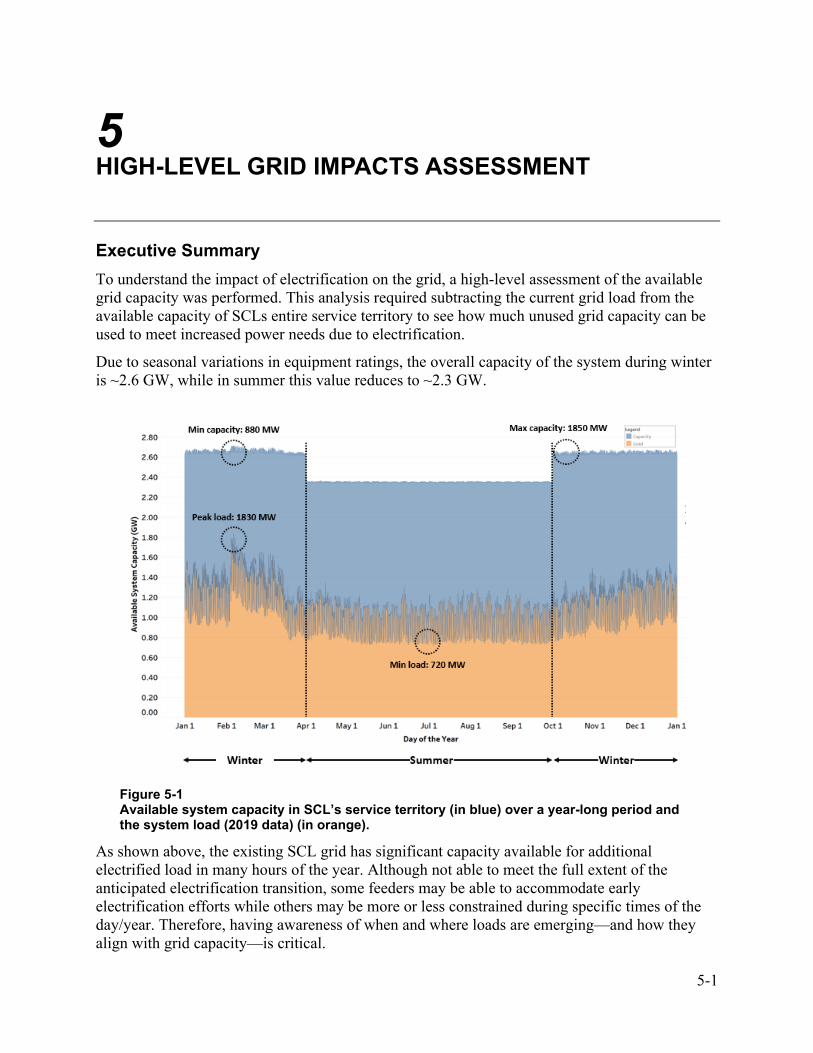
5-1
5 HIGH-LEVEL GRID IMPACTS ASSESSMENT
Executive Summary To understand the impact of electrification on the grid, a high-level assessment of the available grid capacity was performed. This analysis required subtracting the current grid load from the available capacity of SCLs entire service territory to see how much unused grid capacity can be used to meet increased power needs due to electrification.
Due to seasonal variations in equipment ratings, the overall capacity of the system during winter is ~2.6 GW, while in summer this value reduces to ~2.3 GW.
Figure 5-1 Available system capacity in SCL’s service territory (in blue) over a year-long period and the system load (2019 data) (in orange).
As shown above, the existing SCL grid has significant capacity available for additional electrified load in many hours of the year. Although not able to meet the full extent of the anticipated electrification transition, some feeders may be able to accommodate early electrification efforts while others may be more or less constrained during specific times of the day/year. Therefore, having awareness of when and where loads are emerging—and how they align with grid capacity—is critical.

High-Level Grid Impacts Assessment
5-2
Local monitoring together with flexible load strategies may prove key to ensuring that electric technology adoption is not limited anywhere on SCL’s grid. Careful attention must be paid to both energy and power needs on a local level as technologies may be adopted in clusters (such as with MDHD electric transportation) and in areas where grid capacity may be more limited.
Introduction The Grid Assessment Approach
The objective of this grid assessment is to understand the capacity of SCL’s existing distribution grid for electrification of future load. To achieve this, the analysis undertaken for the grid assessment consists of a detailed system-wide hosting capacity assessment using EPRI’s DRIVE tool.90 Hosting capacity can be defined as the amount of load or generation that can be accommodated without adversely impacting power quality or reliability, under current configurations, and without requiring infrastructure upgrades. For this study, hosting capacity for additional new load is calculated for each location, feeder, and substation in the SCL territory as well as for the system as a whole. The results are also time-specific to ensure that capacity can be aligned with the needs of new electrification load. The analysis in this task is independent of the Moderate Market Advancement, Rapid Market Advancement, and Full Electrification scenarios outlined for previous tasks, because this effort determines how much additional electrification load can be accommodated based on the grid in its modeled state, under those configurations and load levels.
As shown in Table 5-1, for this study, the grid model used is from 2017/2018 because this was the most up-to-date grid model available, while the load data are from 2019. Load data from 2020 were not used because 2020 load levels may not be representative of typical loading due to altered consumption patterns as a result of the COVID-19 pandemic.
Table 5-1 Year of grid model and load data used for grid impacts analysis
Year
Grid Model 2017/2018
Load Data 2019
The hosting capacity analysis encompasses all lines and equipment in service in the model of the distribution system and uses both equipment and operational planning limits. Projected or known new loads that are not in the system model are not included. Similarly, special conditions on specific feeders are not included as planning models periodically updated; that is, the analysis does not include dedicated feeders to customers, future reserved capacity. While this could nuance the analysis, the results represented the available capacity based on the planning models which may not include these special conditions.
90 https://www.epri.com/DRIVE

High-Level Grid Impacts Assessment
5-3
Hosting Capacity Using DRIVE EPRI’s DRIVE tool has been developed based on a history of prior stochastic-based studies and analyses to overcome the computational burden of stochastic and iterative-based approaches while still capturing critical grid responses for determining location-based hosting capacity. Although the tool has evolved to include other applications such as mitigation analysis and locational value, hosting capacity analysis is the core functionality of the tool. It can calculate hosting capacity considering voltage, thermal, and protection limitations for various load and DER technologies and efficiently scales from location-specific, node-by-node analysis to distribution system wide analysis in an automated fashion.
There are two components in EPRI’s DRIVE tool. The first is the interface to the utility planning tool, which for SCL is CYME. In this component, each feeder is analyzed to extract information from the model via power flows and short-circuit studies. The second component is the DRIVE hosting capacity assessment module in which the extracted data from the first component are analyzed and examined for hosting capacity. Hosting capacity is calculated based on whether the specific condition exceeds a user-defined threshold for two different load/distributed energy resources (DER) deployments, centralized (single-site) and distributed (multiple-site). For this study, only hosting capacity for load is analyzed considering voltage and thermal limits; that is, hosting capacity for generation is not assessed. Additional operational planning limits for each feeder, are also included.
Centralized load deployment (single-site): The hosting capacity for centralized load depicts how much load at a specific location can be accommodated as depicted in Figure 5-2(a). When the hosting capacity analysis is performed, each location on the feeder is considered independently, and the feeder-wide impact of the load at that location is observed. The resulting hosting capacity describes what each location on the feeder can host; that is, there is a capacity for every location on the feeder. These results can help inform specific interconnection requests for large loads or DER.
Distributed load deployment (multi-site): The hosting capacity for distributed load depicts how much load dispersed across the feeder can be accommodated as depicted in Figure 5-2(b). When the hosting capacity analysis is performed, a distribution of load across the feeder is assumed and the feeder-wide impact of that load distribution is observed. For this study, the distribution is across all three-phase locations, with the size of the load weighted by the impedance to the location. The resulting hosting capacity describes what the feeder can host; that is, there is single capacity for the feeder as a whole. The distributed results are most applicable when planning for organic load growth or electrification of dispersed loads, as is the case for this study.
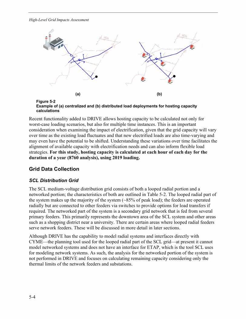
High-Level Grid Impacts Assessment
5-4
(a) (b)
Figure 5-2 Example of (a) centralized and (b) distributed load deployments for hosting capacity calculations
Recent functionality added to DRIVE allows hosting capacity to be calculated not only for worst-case loading scenarios, but also for multiple time instances. This is an important consideration when examining the impact of electrification, given that the grid capacity will vary over time as the existing load fluctuates and that new electrified loads are also time-varying and may even have the potential to be shifted. Understanding these variations over time facilitates the alignment of available capacity with electrification needs and can also inform flexible load strategies. For this study, hosting capacity is calculated at each hour of each day for the duration of a year (8760 analysis), using 2019 loading.
Grid Data Collection
SCL Distribution Grid The SCL medium-voltage distribution grid consists of both a looped radial portion and a networked portion; the characteristics of both are outlined in Table 5-2. The looped radial part of the system makes up the majority of the system (~85% of peak load); the feeders are operated radially but are connected to other feeders via switches to provide options for load transfers if required. The networked part of the system is a secondary grid network that is fed from several primary feeders. This primarily represents the downtown area of the SCL system and other areas such as a shopping district near a university. There are certain areas where looped radial feeders serve network feeders. These will be discussed in more detail in later sections.
Although DRIVE has the capability to model radial systems and interfaces directly with CYME—the planning tool used for the looped radial part of the SCL grid—at present it cannot model networked systems and does not have an interface for ETAP, which is the tool SCL uses for modeling network systems. As such, the analysis for the networked portion of the system is not performed in DRIVE and focuses on calculating remaining capacity considering only the thermal limits of the network feeders and substations.
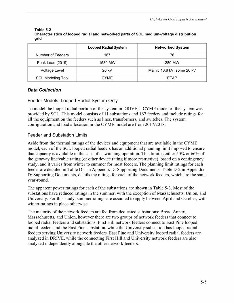
High-Level Grid Impacts Assessment
5-5
Table 5-2 Characteristics of looped radial and networked parts of SCL medium-voltage distribution grid
Looped Radial System Networked System
Number of Feeders 167 76
Peak Load (2019) 1580 MW 280 MW
Voltage Level 26 kV Mainly 13.8 kV, some 26 kV
SCL Modeling Tool CYME ETAP
Data Collection
Feeder Models: Looped Radial System Only
To model the looped radial portion of the system in DRIVE, a CYME model of the system was provided by SCL. This model consists of 11 substations and 167 feeders and include ratings for all the equipment on the feeders such as lines, transformers, and switches. The system configuration and load allocation in the CYME model are from 2017/2018.
Feeder and Substation Limits
Aside from the thermal ratings of the devices and equipment that are available in the CYME model, each of the SCL looped radial feeders has an additional planning limit imposed to ensure that capacity is available in the case of a switching operation. This limit is either 50% or 66% of the getaway line/cable rating (or other device rating if more restrictive), based on a contingency study, and it varies from winter to summer for most feeders. The planning limit ratings for each feeder are detailed in Table D-1 in Appendix D: Supporting Documents. Table D-2 in Appendix D: Supporting Documents, details the ratings for each of the network feeders, which are the same year-round.
The apparent power ratings for each of the substations are shown in Table 5-3. Most of the substations have reduced ratings in the summer, with the exception of Massachusetts, Union, and University. For this study, summer ratings are assumed to apply between April and October, with winter ratings in place otherwise.
The majority of the network feeders are fed from dedicated substations: Broad Annex, Massachusetts, and Union, however there are two groups of network feeders that connect to looped radial feeders and substations. First Hill network feeders connect to East Pine looped radial feeders and the East Pine substation, while the University substation has looped radial feeders serving University network feeders. East Pine and University looped radial feeders are analyzed in DRIVE, while the connecting First Hill and University network feeders are also analyzed independently alongside the other network feeders.

High-Level Grid Impacts Assessment
5-6
Table 5-3 Summer and winter ratings for substations
Substation Winter (MVA) Summer (MVA) Broad 219 182
Broad Annex* 208 170 Canal 160 153
Creston 242 201 Delridge 241 200
Duwamish 338 276 East Pine** 200 160
Massachusetts* 60 60 North 238 193
Shoreline 165 127 South 388 314 Union* 160 160
University** 188 188 Viewland 217 178
* Network substation ** Substation feeds looped radial and network feeders
The network feeders on the SCL system are also grouped into subnets, with each subnet consisting of three to six feeders. The subnet ratings are calculated by summing all the corresponding feeder ratings, excluding the highest rated feeder (see Table 5-4).
Table 5-4 Subnet ratings
Subnet Rating (Amps) Rating (MVA) Broad Center 2179 52 Broad East 2213 53
Broad Middle 2264 54 Broad North 2250 54 Broad South 2245 54
First Hill* 1600 72 Massachusetts Middle 1260 30 Massachusetts North 2061 49 Massachusetts South 1300 31
Union East 2452 59 Union North 2270 54 Union South 2217 53
Union Waterfront 2342 56 University Dist* 678 31
* Fed from looped radial feeders

High-Level Grid Impacts Assessment
5-7
As well as thermal limits, upper and lower voltage limits are also imposed for all locations on the looped radial system when running the DRIVE analysis. Based on SCL planning limits, these have been implemented as 0.95 p.u. and 1.034 p.u.
Time-Series Load Data
To calculate hosting capacity for additional load for each hour of the year, hourly loading is required. Given that 2020 load levels may not be representative of typical loading due to altered consumption patterns as a result of the COVID-19 pandemic, it was agreed that 2019 load data would be used for this study. SCL provided measured 2019 load data at hourly resolution for all feeders where available. Following are some caveats:
• Feeders 3401 and 3402 are used for dedicated load and are therefore not analyzed for feeder hosting capacity. Their load, however, is included when determining substation and system hosting capacities.
• For Feeders 2657, 2660, 2687, and 2752, load measurements for 2019 are unavailable. The closest available measurements are used for these feeders (typically from 2018). As such, load peaks may be mis-aligned for these feeders, but it should not significantly impact the overall results.
• Feeders 2643 and 2651 have measurements of zero for the year. SCL confirmed that these feeders do not currently have any load; however, they are in the process of being repurposed for known future loads. It is likely that the results will show high capacity for additional load for these feeders; however, part of this capacity will be consumed by the planned future loads.
• Network feeders for Denny Triangle and SLU1 subnets are new and do not have any load data; therefore, they are not included in the analysis. They will likely provide additional capacity in future.
• Load measurements for 2019 are unavailable for the First Hill network feeders. Because these feeders are connected to the East Pine looped radial feeders, loading is estimated based on corresponding East Pine feeder data and peak load in the CYME model. The actual First Hill load may vary slightly, but it should not significantly impact the overall results.

High-Level Grid Impacts Assessment
5-8
Figure 5-3 and Figure 5-4 show the range in 2019 load for the looped radial and network feeders, respectively. The range in load for the network feeders is relatively similar for many of the feeders, typically between 1 MW and 5 MW. The looped radial feeders are more varied in their loading, with several of feeders having peak load of greater than 20 MW.
Figure 5-3 Range of 2019 load for each of the looped radial feeders (Feeder 2687 is not included because it is a large dedicated load)
0
5
10
15
20
2526
0026
0226
0426
0626
0826
1026
1226
1426
1926
2126
2326
2526
2726
2926
3126
3326
3526
3726
3926
4126
4326
4526
4726
4926
5126
5326
5626
5826
6026
6426
6626
6826
7226
7426
7626
7826
8026
8226
8426
8626
8926
9126
9327
0227
0427
0627
0827
1027
1227
2227
2427
2927
3227
3427
3627
3827
4027
4227
4427
4627
4827
5027
5227
5427
5627
5827
6127
6327
6527
7427
7627
7827
8027
8227
8427
8627
8827
9128
0328
0828
13
Pow
er (M
W)
Feeder
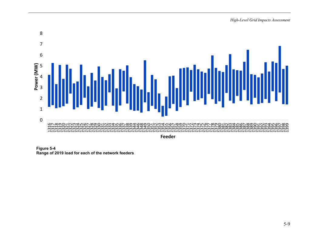
High-Level Grid Impacts Assessment
5-9
Figure 5-4 Range of 2019 load for each of the network feeders
0
1
2
3
4
5
6
7
8
1316
1317
1318
1319
1320
1321
1322
1323
1324
1325
1326
1327
1328
1329
1330
1331
1332
1333
1334
1335
1336
1337
1338
1339
1344
1346
1348
1349
1350
1351
1352
1353
1354
1355
1356
1357
1358
1359
1370
1371
1372
1373
1374
1375
1376
1377
1378
1379
1380
1381
1382
1383
1384
1385
1386
1387
1388
1389
1390
1391
1392
1393
1394
1395
1396
1397
1398
1399
Pow
er (M
W)
Feeder
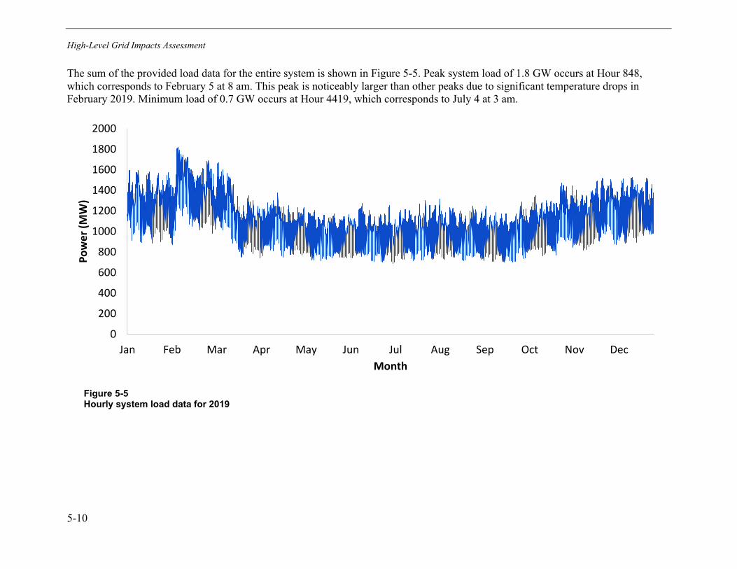
High-Level Grid Impacts Assessment
5-10
The sum of the provided load data for the entire system is shown in Figure 5-5. Peak system load of 1.8 GW occurs at Hour 848, which corresponds to February 5 at 8 am. This peak is noticeably larger than other peaks due to significant temperature drops in February 2019. Minimum load of 0.7 GW occurs at Hour 4419, which corresponds to July 4 at 3 am.
Figure 5-5 Hourly system load data for 2019
0
200
400
600
800
1000
1200
1400
1600
1800
2000
Jan Feb Mar Apr May Jun Jul Aug Sep Oct Nov Dec
Pow
er (M
W)
Month

High-Level Grid Impacts Assessment
5-11
Results The results of the analysis are broken down as follows:
• Looped radial feeders: These are the results of the time-series (8760) DRIVE analysis for each of the looped radial feeders. They are further broken down by whether the analysis examined distributed or centralized load deployment.
• Network feeders: These are the results of the time-series analysis for each of the network feeders as well as the subnets, considering the thermal limits of each feeder and subnet.
• Substation: These are the results of the time-series analysis, considering only the substation thermal capacity and the load of all the feeders connected to that substation.
• Overall substation: These results combine the substation and feeder results to find the most limiting capacity for each substation for each hour.
• System: These results are the sum of the overall substation results for each hour.
The raw results of the analysis consist of a hosting capacity value for each hour of the year, which can be difficult to portray for every location and/or feeder on the system. Some results are therefore aggregated or summarized as detailed in Table 5-5.
Table 5-5 Description of summary results
Summary Result Description
System peak load hosting capacity snapshot (MW)
The hosting capacity for additional load during the system peak load hour (Feb 5th 8 am as shown in Figure 5-5). This metric is beneficial for examining the worst-case capacity from a system perspective. When looking at multiple feeders it represents each feeder’s capacity at that hour, rather than the worst-case capacity for each feeder.
System minimum load hosting capacity snapshot (MW)
The hosting capacity for additional load during the system minimum load hour (July 4th 3 am as shown in Figure 5-5). This metric is beneficial for examining the best-case capacity from a system perspective. When looking at multiple feeders it represents each feeder’s capacity at that hour, rather than the best-case capacity for each feeder.
Feeder minimum hosting capacity (MW)
The minimum hosting capacity for additional load for a specific feeder across all hours of the year. This represents the capacity of load that can be accommodated at every hour of the year.
Feeder maximum hosting capacity (MW)
The maximum hosting capacity for additional load for a specific feeder across all hours of the year. This metric is useful as a bookend to the minimum hosting capacity to show the range in capacity over time for a specific feeder.
Minimum daily energy capacity (MWh)
The sum of the hourly capacity for additional load for the 24-hour period with the lowest available energy. There will be at least this amount of energy available on any given day of the year. This can help inform whether flexible load might be a viable option if there is insufficient capacity available at a particular time of day.
Annual energy capacity (MWh)
The sum of the hourly capacity across all hours of the year. Alongside the minimum and maximum hosting capacities, this metric gives an indication of the variations in capacity across the year. It facilitates comparison between feeders and also can help inform where flexible load may be viable.

High-Level Grid Impacts Assessment
5-12
Although ratings for feeders/substations are shown in MVA, the hosting capacity results in this section are all shown in MW, assuming a power factor of 1. There may be lower MW capacity available for loads with a large reactive power component.
Looped Radial Feeders
Distributed Load Deployment
Figure 5-6 shows the hosting capacity for additional distributed load for each of the looped radial feeders during the system peak load hour (Hour 848) and minimum load hour (Hour 4419). The color of each feeder represents the capacity, with warmer colors indicating lower capacity and cooler colors representing higher capacity. Minimum, maximum, and average capacity results for each feeder are also detailed in Table D-3 in Appendix D: Supporting Documents.
These results show the diversity in capacity across the feeders, even during peak load, with some feeders having no capacity for additional load and others having 10–20 MW. The difference between Figure 5-6 (a) and (b) highlights the range in capacity as load conditions vary over time, so even though a particular feeder may have limited capacity during peak load, it may have significantly higher capacity at other hours of the year.
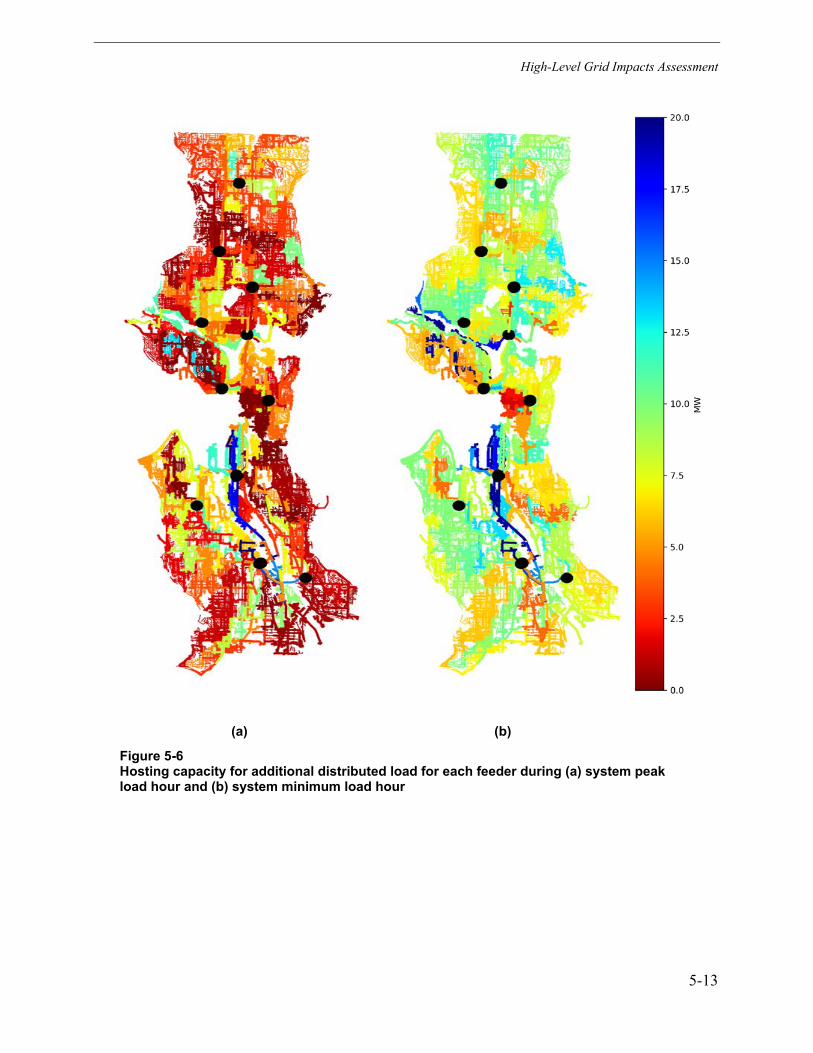
High-Level Grid Impacts Assessment
5-13
(a) (b)
Figure 5-6 Hosting capacity for additional distributed load for each feeder during (a) system peak load hour and (b) system minimum load hour
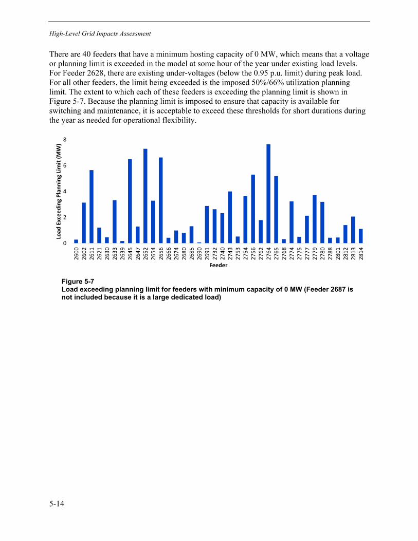
High-Level Grid Impacts Assessment
5-14
There are 40 feeders that have a minimum hosting capacity of 0 MW, which means that a voltage or planning limit is exceeded in the model at some hour of the year under existing load levels. For Feeder 2628, there are existing under-voltages (below the 0.95 p.u. limit) during peak load. For all other feeders, the limit being exceeded is the imposed 50%/66% utilization planning limit. The extent to which each of these feeders is exceeding the planning limit is shown in Figure 5-7. Because the planning limit is imposed to ensure that capacity is available for switching and maintenance, it is acceptable to exceed these thresholds for short durations during the year as needed for operational flexibility.
Figure 5-7 Load exceeding planning limit for feeders with minimum capacity of 0 MW (Feeder 2687 is not included because it is a large dedicated load)
0
2
4
6
8
2600
2602
2611
2621
2630
2633
2639
2645
2647
2652
2654
2656
2666
2674
2680
2685
2690
2691
2732
2740
2743
2753
2754
2756
2762
2764
2765
2768
2774
2775
2777
2779
2780
2788
2801
2812
2813
2814
Load
Exc
eedi
ng P
lann
ing
Lim
it (M
W)
Feeder
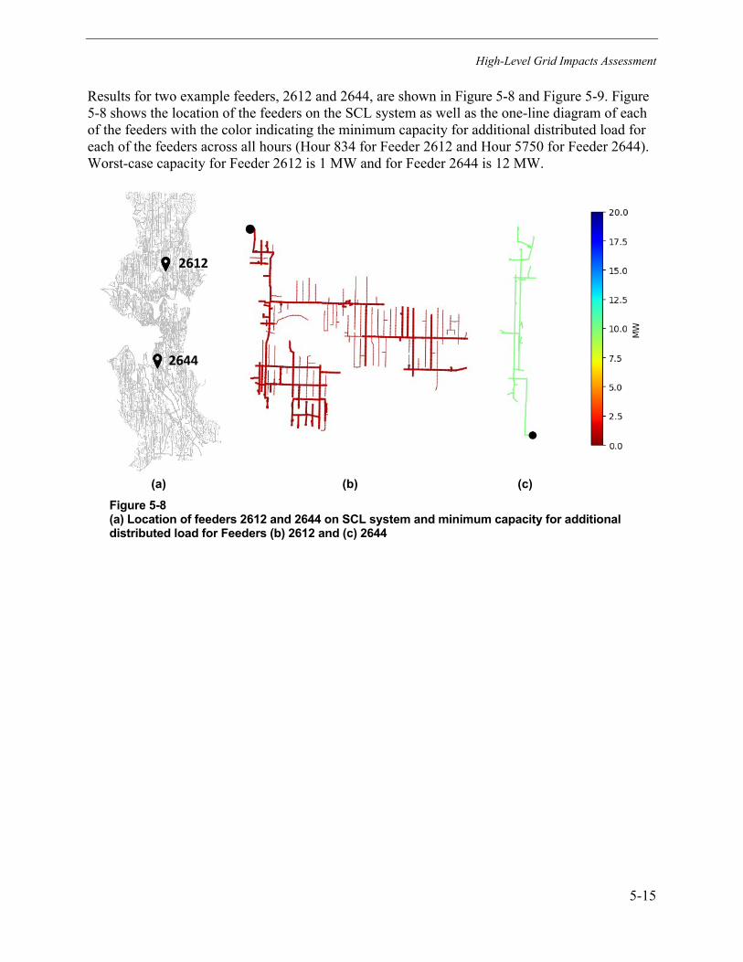
High-Level Grid Impacts Assessment
5-15
Results for two example feeders, 2612 and 2644, are shown in Figure 5-8 and Figure 5-9. Figure 5-8 shows the location of the feeders on the SCL system as well as the one-line diagram of each of the feeders with the color indicating the minimum capacity for additional distributed load for each of the feeders across all hours (Hour 834 for Feeder 2612 and Hour 5750 for Feeder 2644). Worst-case capacity for Feeder 2612 is 1 MW and for Feeder 2644 is 12 MW.
(a) (b) (c)
Figure 5-8 (a) Location of feeders 2612 and 2644 on SCL system and minimum capacity for additional distributed load for Feeders (b) 2612 and (c) 2644
2612
2644
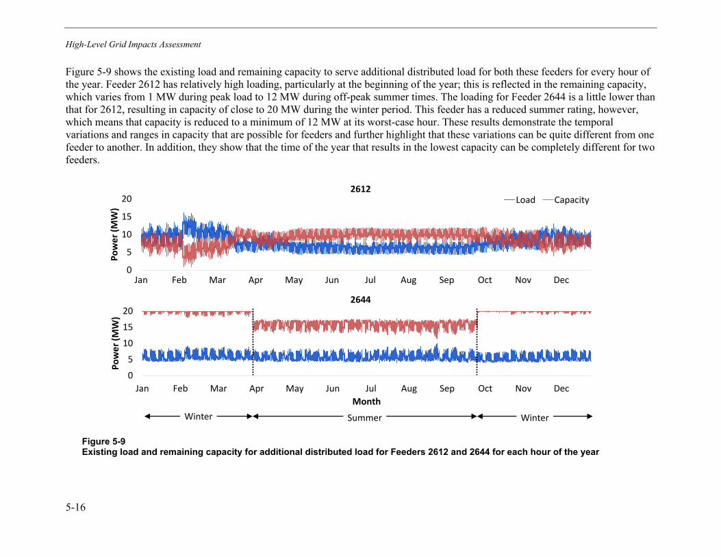
High-Level Grid Impacts Assessment
5-16
Figure 5-9 shows the existing load and remaining capacity to serve additional distributed load for both these feeders for every hour of the year. Feeder 2612 has relatively high loading, particularly at the beginning of the year; this is reflected in the remaining capacity, which varies from 1 MW during peak load to 12 MW during off-peak summer times. The loading for Feeder 2644 is a little lower than that for 2612, resulting in capacity of close to 20 MW during the winter period. This feeder has a reduced summer rating, however, which means that capacity is reduced to a minimum of 12 MW at its worst-case hour. These results demonstrate the temporal variations and ranges in capacity that are possible for feeders and further highlight that these variations can be quite different from one feeder to another. In addition, they show that the time of the year that results in the lowest capacity can be completely different for two feeders.
Figure 5-9 Existing load and remaining capacity for additional distributed load for Feeders 2612 and 2644 for each hour of the year
0
5
10
15
20
Jan Feb Mar Apr May Jun Jul Aug Sep Oct Nov Dec
Pow
er (M
W)
Month
2644
0
5
10
15
20
Jan Feb Mar Apr May Jun Jul Aug Sep Oct Nov Dec
Pow
er (M
W)
2612Load Capacity
SummerWinter Winter
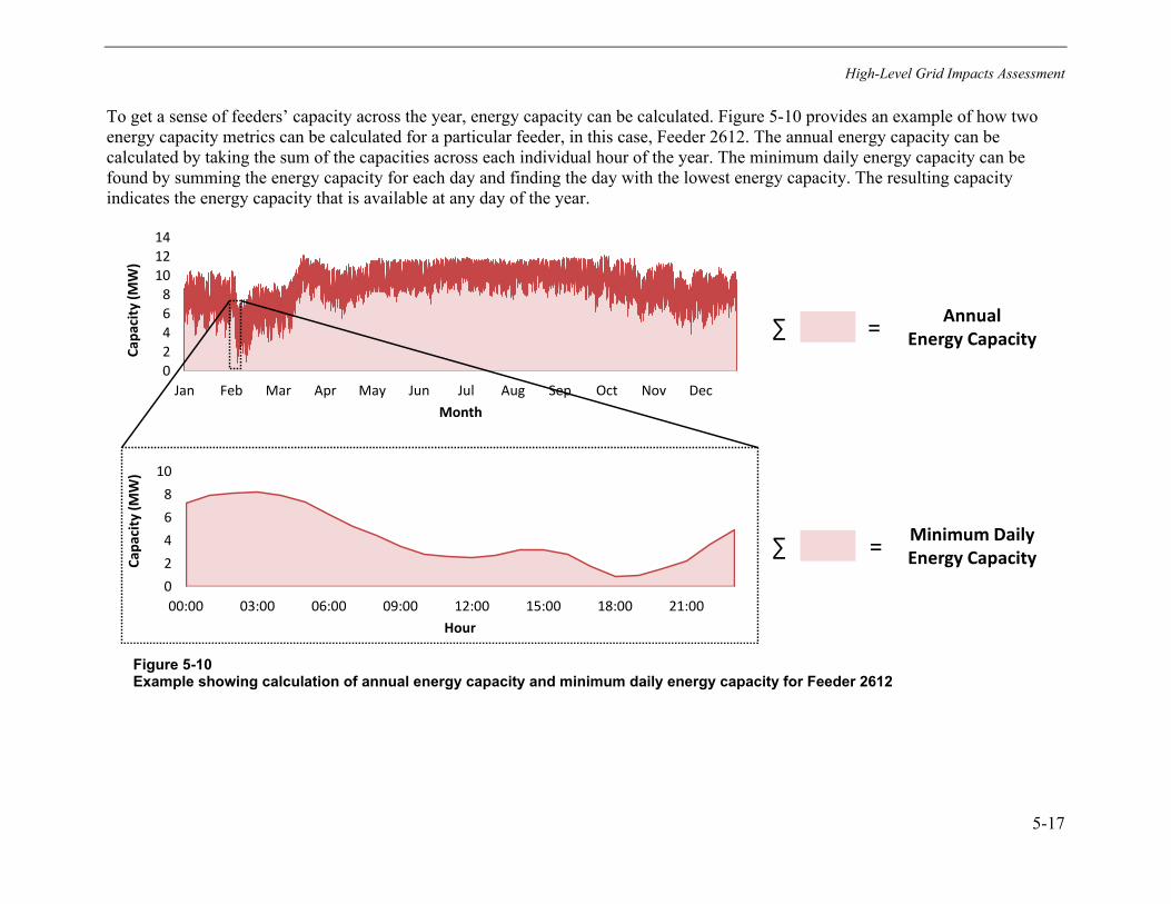
High-Level Grid Impacts Assessment
5-17
To get a sense of feeders’ capacity across the year, energy capacity can be calculated. Figure 5-10 provides an example of how two energy capacity metrics can be calculated for a particular feeder, in this case, Feeder 2612. The annual energy capacity can be calculated by taking the sum of the capacities across each individual hour of the year. The minimum daily energy capacity can be found by summing the energy capacity for each day and finding the day with the lowest energy capacity. The resulting capacity indicates the energy capacity that is available at any day of the year.
Figure 5-10 Example showing calculation of annual energy capacity and minimum daily energy capacity for Feeder 2612
02468
10
00:00 03:00 06:00 09:00 12:00 15:00 18:00 21:00
Capa
city
(MW
)
Hour
02468
101214
Jan Feb Mar Apr May Jun Jul Aug Sep Oct Nov Dec
Capa
city
(MW
)
Month
∑
∑
=
=
AnnualEnergy Capacity
Minimum Daily Energy Capacity
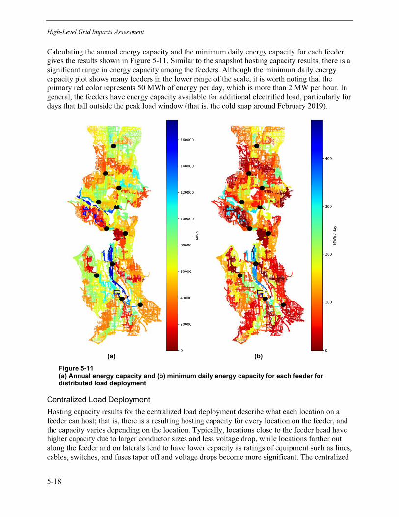
High-Level Grid Impacts Assessment
5-18
Calculating the annual energy capacity and the minimum daily energy capacity for each feeder gives the results shown in Figure 5-11. Similar to the snapshot hosting capacity results, there is a significant range in energy capacity among the feeders. Although the minimum daily energy capacity plot shows many feeders in the lower range of the scale, it is worth noting that the primary red color represents 50 MWh of energy per day, which is more than 2 MW per hour. In general, the feeders have energy capacity available for additional electrified load, particularly for days that fall outside the peak load window (that is, the cold snap around February 2019).
(a) (b)
Figure 5-11 (a) Annual energy capacity and (b) minimum daily energy capacity for each feeder for distributed load deployment
Centralized Load Deployment Hosting capacity results for the centralized load deployment describe what each location on a feeder can host; that is, there is a resulting hosting capacity for every location on the feeder, and the capacity varies depending on the location. Typically, locations close to the feeder head have higher capacity due to larger conductor sizes and less voltage drop, while locations farther out along the feeder and on laterals tend to have lower capacity as ratings of equipment such as lines, cables, switches, and fuses taper off and voltage drops become more significant. The centralized
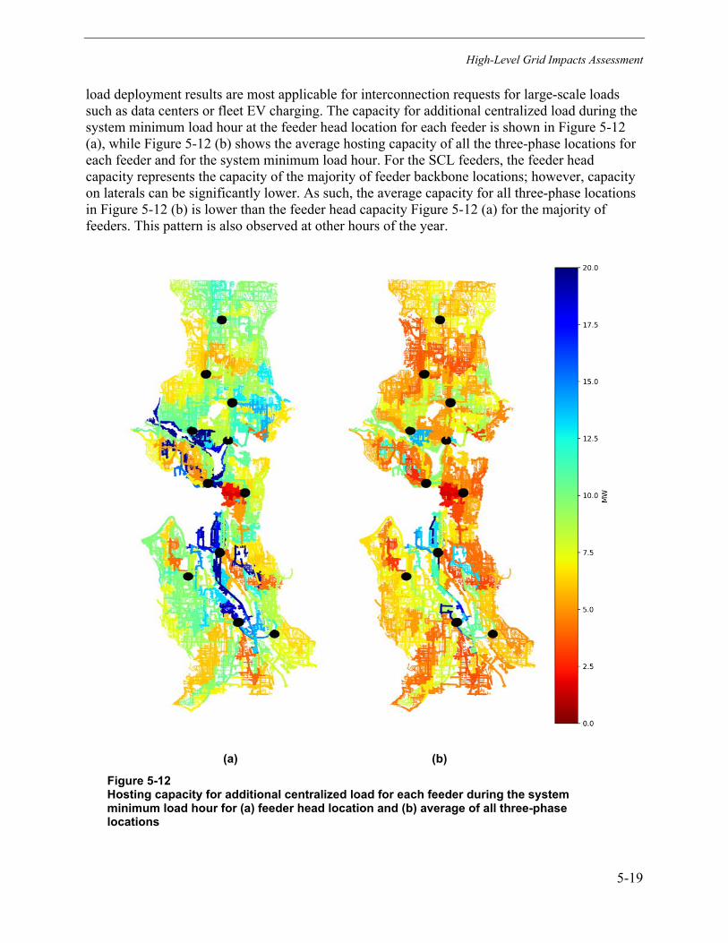
High-Level Grid Impacts Assessment
5-19
load deployment results are most applicable for interconnection requests for large-scale loads such as data centers or fleet EV charging. The capacity for additional centralized load during the system minimum load hour at the feeder head location for each feeder is shown in Figure 5-12 (a), while Figure 5-12 (b) shows the average hosting capacity of all the three-phase locations for each feeder and for the system minimum load hour. For the SCL feeders, the feeder head capacity represents the capacity of the majority of feeder backbone locations; however, capacity on laterals can be significantly lower. As such, the average capacity for all three-phase locations in Figure 5-12 (b) is lower than the feeder head capacity Figure 5-12 (a) for the majority of feeders. This pattern is also observed at other hours of the year.
(a) (b)
Figure 5-12 Hosting capacity for additional centralized load for each feeder during the system minimum load hour for (a) feeder head location and (b) average of all three-phase locations
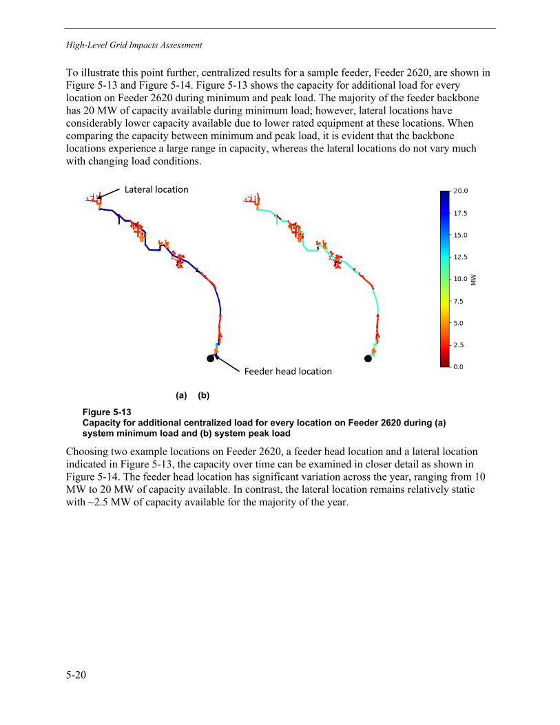
High-Level Grid Impacts Assessment
5-20
To illustrate this point further, centralized results for a sample feeder, Feeder 2620, are shown in Figure 5-13 and Figure 5-14. Figure 5-13 shows the capacity for additional load for every location on Feeder 2620 during minimum and peak load. The majority of the feeder backbone has 20 MW of capacity available during minimum load; however, lateral locations have considerably lower capacity available due to lower rated equipment at these locations. When comparing the capacity between minimum and peak load, it is evident that the backbone locations experience a large range in capacity, whereas the lateral locations do not vary much with changing load conditions.
(a) (b)
Figure 5-13 Capacity for additional centralized load for every location on Feeder 2620 during (a) system minimum load and (b) system peak load
Choosing two example locations on Feeder 2620, a feeder head location and a lateral location indicated in Figure 5-13, the capacity over time can be examined in closer detail as shown in Figure 5-14. The feeder head location has significant variation across the year, ranging from 10 MW to 20 MW of capacity available. In contrast, the lateral location remains relatively static with ~2.5 MW of capacity available for the majority of the year.
Feeder head location
Lateral location

High-Level Grid Impacts Assessment
5-21
Figure 5-14 Capacity for additional centralized load for every hour of the year for feeder head and lateral location on Feeder 2620
Figure 5-15 shows the average capacity of all the three-phase locations for each feeder during the system peak (a) and minimum (b) load hours. Capacity under this analysis is a little lower than the distributed load deployment case because the plot shows the average capacity of all three-phase locations. The same plot for the feeder head location would show much higher capacity and for an end-of-the-feeder location would show much lower capacity.
0
5
10
15
20
Jan Feb Mar Apr May Jun Jul Aug Sep Oct Nov Dec
Capa
city
for A
dditi
onal
Load
(MW
)
Month
Feeder Head Lateral

High-Level Grid Impacts Assessment
5-22
(a) (b)
Figure 5-15 Average of centralized hosting capacity for all three-phase locations for each feeder during (a) system peak load hour and (b) system minimum load hour
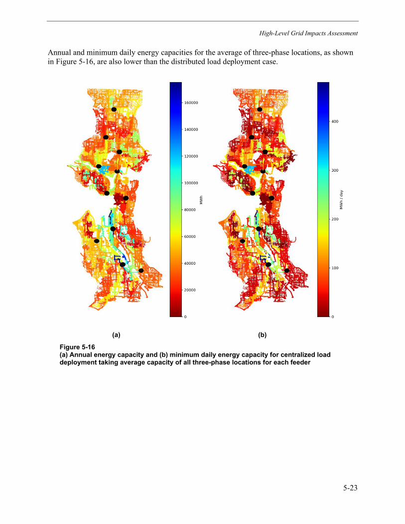
High-Level Grid Impacts Assessment
5-23
Annual and minimum daily energy capacities for the average of three-phase locations, as shown in Figure 5-16, are also lower than the distributed load deployment case.
(a) (b)
Figure 5-16 (a) Annual energy capacity and (b) minimum daily energy capacity for centralized load deployment taking average capacity of all three-phase locations for each feeder

High-Level Grid Impacts Assessment
5-24
Network Feeders As previously discussed, the analysis for the networked portion of the system is not performed in DRIVE, but rather consists of finding the remaining capacity of network feeders and subnets by subtracting the 2019 hourly load data from the feeder ratings, which are given in Table D-2 in Appendix D: Supporting Documents, and the subnet ratings in Table 5-4. Because the network feeders are not modeled, ratings of equipment located along the feeders are not taken into account, which for some feeders may limit capacity for additional load more than the feeder ratings used for this study. Planning limits for contingency scenarios are not imposed for individual feeders but are captured in the subnet ratings in Table 5-4, where the rating of the feeder with the largest capacity is excluded. As previously mentioned, the First Hill and University network feeders are fed from the East Pine and University looped radial feeders and substations, respectively. These looped radial feeders have been analyzed using DRIVE alongside the other looped radial feeders. The results shown in this section for the First Hill and University network feeders consider only the network feeder ratings and the subnet ratings and not any of the upstream looped radial limits because these have been considered in the DRIVE analysis. Because capacities are aggregated to the substation and system level, the looped radial results for the East Pine and University feeders are used because they are more limited than the network feeder and subnet capacities shown here.
Figure 5-17 shows the minimum and maximum capacity for additional load for each of the network feeders. The results are quite similar for many of the feeders with minimum capacities typically between 4 MW and 6 MW and maximum capacities between 8 MW and 10 MW. In general, considering only the feeder ratings, there is capacity available on all feeders.
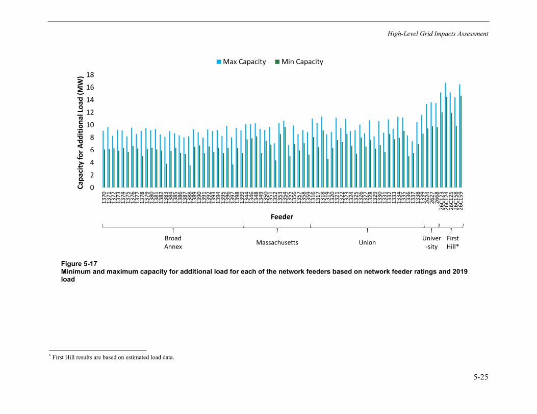
High-Level Grid Impacts Assessment
5-25
Figure 5-17 Minimum and maximum capacity for additional load for each of the network feeders based on network feeder ratings and 2019 load*
* First Hill results are based on estimated load data.
0
2
4
6
8
10
12
14
16
18
1370
1371
1372
1373
1374
1375
1376
1377
1378
1379
1380
1381
1382
1383
1384
1385
1386
1387
1388
1389
1390
1391
1392
1393
1394
1395
1396
1397
1398
1399
1344
1346
1348
1349
1350
1351
1352
1353
1354
1355
1356
1357
1358
1359
1316
1317
1318
1319
1320
1321
1322
1323
1324
1325
1326
1327
1328
1329
1330
1331
1332
1333
1334
1335
1336
1337
1338
1339
2624
2627
2668
26C1
2326
C124
26C1
2526
C158
26C1
59
Capa
city
for A
dditi
onal
Load
(MW
)
Feeder
Max Capacity Min Capacity
Broad Annex Massachusetts Union Univer
-sityFirst Hill*

High-Level Grid Impacts Assessment
5-26
A similar trend is noted when looking at results for the subnets, with capacities ranging between 15 MW and 60 MW (see Figure 5-18). The First Hill subnet has higher capacity than others; however, the First Hill loading is estimated based on East Pine load—therefore, results may not be accurate. These results indicate that the networked portion of the SCL system has significant capacity available; however, it should be noted that neither ratings of downstream equipment nor voltages are considered for this analysis and may result in less available capacity than shown here.
Figure 5-18 Minimum and maximum capacity for additional load for each of the subnets based on subnet ratings and 2019 load*
* First Hill results are based on estimated load data.
010203040506070
Capa
city
for A
dditi
onal
Load
(MW
)
Subnet
Max capacity Min capacity

High-Level Grid Impacts Assessment
5-27
Substations and System The minimum and maximum capacity for additional load for each substation is shown in Table 5-6. These results consider only each substation’s rating alongside the hourly load data. As with the feeder results, there is a significant range in capacity both among the substations and for each individual substation over time. The substations with the lowest capacity are generally substations that feed network feeders; the ones with the highest capacity generally have higher ratings than others.
Table 5-6 Minimum and maximum capacity for additional load for each substation
Substation Minimum (MW) Maximum (MW) Broad 48 156
Broad Annex* 44 143 Canal 65 129
Creston 160 223 Delridge 120 202
Duwamish 140 262 East Pine** 36 133
Massachusetts* 16 45 North 120 205
Shoreline 44 131 South 90 266 Union* 64 123
University** 72 124 Viewland 77 173
* Network substation ** Substation feeds looped radial and network feeders
To find overall substation capacities, both the corresponding feeder capacities as well as the substation capacity itself must be considered. For a given hour, the overall capacity for a particular substation is the lesser of either the sum of the capacity for additional distributed load for each of the feeders connected to that substation at that hour or the calculated substation capacity for that hour. For the network substations, the subnet capacities are also summed, and the minimum of the feeders/subnets/substation is the overall substation capacity. The overall substation capacities at each hour are shown in Figure 5-19 and are stacked to show the overall system capacity for additional load with network substations stacked on the bottom; the black line denotes the total capacity of the network substations. The Duwamish substation has the most significant capacity available across the year, while the Massachusetts substation has the least. The overall shape of the aggregated capacity is in some ways the inverse of the system load shown in Figure 5-5. The reduced summer ratings for many of the feeders and substations are reflected in the drop-off in capacity during the middle of the year. The minimum capacity of 0.9 GW coincides with peak load; however, the maximum capacity of 1.8 GW does not align with minimum load because summer ratings are in place, but it occurs around Hour 6600 when load is still relatively low and winter ratings apply.
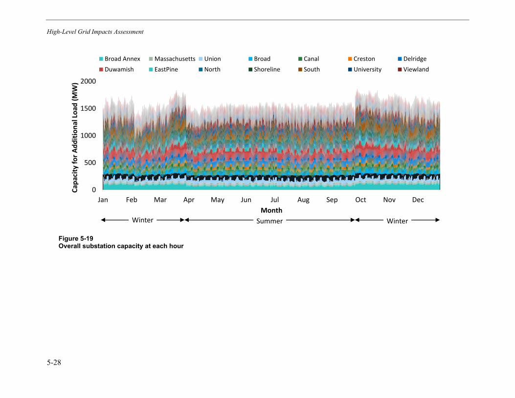
High-Level Grid Impacts Assessment
5-28
Figure 5-19 Overall substation capacity at each hour
0
500
1000
1500
2000
Jan Feb Mar Apr May Jun Jul Aug Sep Oct Nov Dec
Capa
city
for A
dditi
onal
Load
(MW
)
Month
Broad Annex Massachusetts Union Broad Canal Creston DelridgeDuwamish EastPine North Shoreline South University Viewland
SummerWinter Winter

High-Level Grid Impacts Assessment
5-29
Figure 5-20 shows the sum of the substation capacities from Figure 5-19 layered on top of the existing system load. These results indicate that during winter, the overall capacity of the system is ~2.6 GW, while in summer this value reduces to ~2.3 GW. In terms of overall energy across the year, the capacity of the SCL system for future electrification is ~22 TWh,which exceeds the identified capacity required for any of the electrification scenarios (Moderate, Rapid, or Full Electrification) both with and without energy efficiency. Although the overall system has sufficient energy to support electrification, the time and location of load and its alignment with the locally available capacity identified in earlier results is a critical consideration.
Figure 5-20 Existing load and capacity for additional load for SCL system
0
500
1000
1500
2000
2500
3000
Jan Feb Mar Apr May Jun Jul Aug Sep Oct Nov Dec
Pow
er (M
W)
Month
Load Capacity
SummerWinter Winter
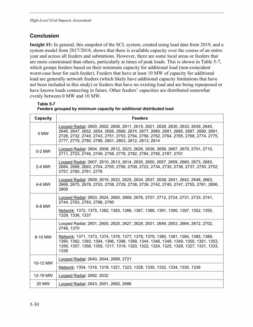
High-Level Grid Impacts Assessment
5-30
Conclusion Insight #1: In general, this snapshot of the SCL system, created using load data from 2019, and a system model from 2017/2018, shows that there is available capacity over the course of an entire year and across all feeders and substations. However, there are some local areas or feeders that are more constrained than others, particularly at times of peak loads. This is shown in Table 5-7, which groups feeders based on their minimum capacity for additional load (non-coincident worst-case hour for each feeder). Feeders that have at least 10 MW of capacity for additional load are generally network feeders (which likely have additional capacity limitations that have not been included in this study) or feeders that have no existing load and are being repurposed or have known loads connecting in future. Other feeders’ capacities are distributed somewhat evenly between 0 MW and 10 MW.
Table 5-7 Feeders grouped by minimum capacity for additional distributed load
Capacity Feeders
0 MW
Looped Radial: 2600, 2602, 2606, 2611, 2615, 2621, 2628, 2630, 2633, 2639, 2645, 2646, 2647, 2652, 2654, 2656, 2666, 2674, 2677, 2680, 2681, 2685, 2687, 2690, 2691, 2728, 2732, 2740, 2743, 2751, 2753, 2754, 2756, 2762, 2764, 2765, 2768, 2774, 2775, 2777, 2779, 2780, 2788, 2801, 2803, 2812, 2813, 2814
0-2 MW Looped Radial: 2604, 2608, 2612, 2623, 2626, 2636, 2658, 2667, 2679, 2701, 2710, 2711, 2723, 2746, 2749, 2758, 2778, 2782, 2784, 2785, 2787, 2791
2-4 MW Looped Radial: 2607, 2610, 2613, 2614, 2635, 2650, 2657, 2659, 2660, 2673, 2683, 2684, 2688, 2693, 2704, 2705, 2706, 2709, 2722, 2734, 2735, 2736, 2737, 2750, 2752, 2757, 2760, 2761, 2776
4-6 MW Looped Radial: 2609, 2619, 2622, 2625, 2634, 2637, 2638, 2641, 2642, 2648, 2663, 2668, 2675, 2678, 2703, 2708, 2729, 2738, 2739, 2742, 2745, 2747, 2755, 2781, 2806, 2808
6-8 MW
Looped Radial: 2603, 2624, 2665, 2669, 2676, 2707, 2712, 2724, 2731, 2733, 2741, 2744, 2763, 2783, 2786, 2790
Network: 1372, 1375, 1382, 1383, 1386, 1387, 1388, 1391, 1395, 1397, 1352, 1355, 1329, 1336, 1337
8-10 MW
Looped Radial: 2601, 2605, 2620, 2627, 2629, 2631, 2649, 2653, 2664, 2672, 2702, 2748, 1370
Network: 1371, 1373, 1374, 1376, 1377, 1378, 1379, 1380, 1381, 1384, 1385, 1389, 1390, 1392, 1393, 1394, 1396, 1398, 1399, 1344, 1346, 1348, 1349, 1350, 1351, 1353, 1356, 1357, 1358, 1359, 1317, 1319, 1320, 1322, 1324, 1325, 1326, 1327, 1331, 1333, 1338
10-12 MW Looped Radial: 2640, 2644, 2689, 2721
Network: 1354, 1316, 1318, 1321, 1323, 1328, 1330, 1332, 1334, 1335, 1339
12-19 MW Looped Radial: 2692, 2632
20 MW Looped Radial: 2643, 2651, 2682, 2686

High-Level Grid Impacts Assessment
5-31
Insight #2: It is important to consider the timing of new loads and how that aligns with the capacity of an individual feeder. For some feeders, capacity can vary significantly across hours, days, and seasons, as highlighted by the range in capacities between system peak and minimum load in Figure 5-6 and Figure 5-15. For those feeders that have limited capacity at particular times of the day or year, the implementation of demand response or load shifting may help alleviate constraints.
Insight #3: Considering that the results of this analysis are based on the grid in its modeled state, using the 2017/2018 system model and 2019 load levels and not accounting for any planned future load, it would be prudent for SCL to reassess the system as updated data become available. Updated data may include:
• A more recent system model
• Load data for the current year (assuming that load patterns are representative of SCL load)
• Planned future loads (location and time-series profile)
A more detailed study of the network system including more granular data on downstream equipment and ratings would also be beneficial to provide greater accuracy to the results. It may also be of interest to perform detailed impact analysis on certain feeders/areas using the profiles generated for the electrification scenarios in Sections 2, 3, and 4 alongside more localized growth and adoption forecasts, if available. Such analysis could also provide insights into the feasibility of demand response schemes for cases in which sufficient capacity is not available. Finally, the inclusion of transmission capacity limits in future analysis could help provide a more holistic view of grid capacity for the system as a whole.


6-1
6 FLEXIBILITY OF NEW ELECTRIC LOADS
Introduction Load growth associated with the electrification of the transportation sector and the ever-changing load shape associated with a combination of increases in efficiency and the introduction of new electric loads in the buildings sector results in brand new load shapes at the utility level. As electric utilities manage these changes, many are exploring programs, policies, and mechanisms that can help minimize costs while still maintaining reliable service for customers. This paradigm of increases in load associated with vehicle and building electrification alongside improvements in efficiency has resulted in energy companies evaluating new mechanisms to manage the grid and leverage flexibility potentially enabled by many of these building and transportation technologies.
Specifically, electrification initiatives have the potential to assist with these efforts by introducing new electric loads that can utilize flexibility to provide certain grid functions that would historically be completed by utility-owned assets As discussed in the Grid Analysis section, SCL has distribution system capacity to accommodate for both the electrification of the transportation and the building sector; however, the availability of capacity will vary across locations, hours, and seasons.
Flexibility in these new loads potentially allows SCL to use the existing utility infrastructure more effectively. The more aggressive the electrification initiative, the greater the need for flexibility to meet changing demand and to manage the electrical grid. As shown in the electrification scenarios in Figure 6-1 and Figure 6-2, SCL can anticipate considerable increases to its peak load under both Scenario 2: Rapid Market Advancement and Scenario 3: Full Electrification. There is potential to reduce the periods of peak demand, by shifting energy consumption to different hours or seasons through load flexibility.
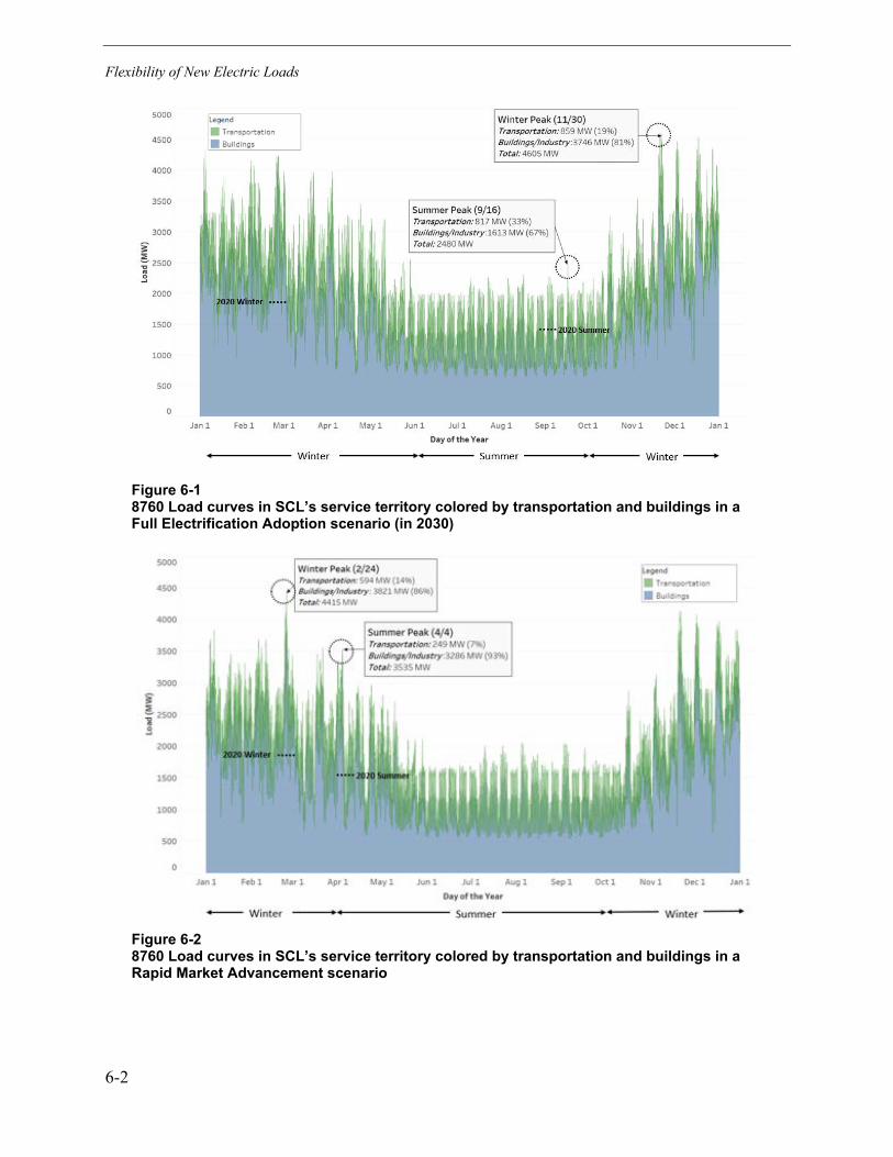
Flexibility of New Electric Loads
6-2
Figure 6-1 8760 Load curves in SCL’s service territory colored by transportation and buildings in a Full Electrification Adoption scenario (in 2030)
Figure 6-2 8760 Load curves in SCL’s service territory colored by transportation and buildings in a Rapid Market Advancement scenario

Flexibility of New Electric Loads
6-3
These loads can enable new program opportunities for electric utilities. Load flexibility has been estimated to potentially become a 200 GW resource in the United States by 203091. Although the technical potential for flexibility is high, there are still quite a few challenges, industry wide, to enable flexibility programs that: 1) can be scaled, 2) minimize impact on occupant comfort and convenience, 3) are done in a way that is both secure for the grid and maintains customer privacy and security, and 4) are part of greater electrification strategies.
To better understand how SCL can incorporate flexibility in its new electric loads, this section covers the following:
• Flexibility of new electric loads. This section defines what is meant by flexibility of new electric loads in greater detail as well as what specific grid challenges they are intended to solve.
• Opportunities, challenges, and market readiness. The section provides high-level discussions on technologies and infrastructure that enable new electric load flexibility. The section also discusses current feasibility and market maturity of those loads to provide grid flexibility.
• Conclusions, next steps, and recommendations: This section intends to start a discussion on the topic of flexibility of new electric loads and the need as part of SCL’s electrification strategies. A set of high-level conclusions, next steps, and recommendations for future activities around flexibility of new electric loads is provided.
Flexibility of Electric Loads Flexibility is enabled through reducing the use of energy consuming technologies and curtailing energy generating technologies when the energy system is reaching capacity—shifting energy usage or storing energy generated to increasing usage when the energy system is underused. Figure 6-3 provides an illustration of how SCL’s load is spread across hours of the year, sorted from highest load hour to lowest load hour.
91 Hledik, Ryan et. al. The National Potential for Load Flexibility. The Brattle Group. Washington, D.C. 2019.
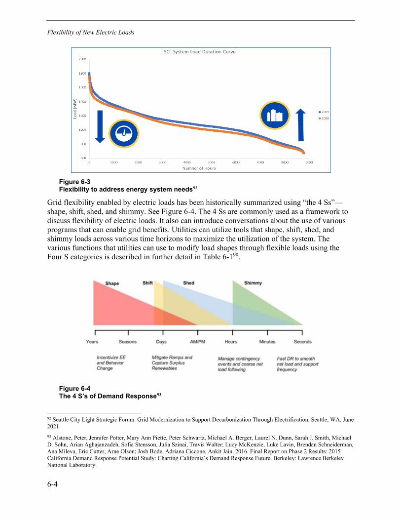
Flexibility of New Electric Loads
6-4
Figure 6-3 Flexibility to address energy system needs92
Grid flexibility enabled by electric loads has been historically summarized using “the 4 Ss”—shape, shift, shed, and shimmy. See Figure 6-4. The 4 Ss are commonly used as a framework to discuss flexibility of electric loads. It also can introduce conversations about the use of various programs that can enable grid benefits. Utilities can utilize tools that shape, shift, shed, and shimmy loads across various time horizons to maximize the utilization of the system. The various functions that utilities can use to modify load shapes through flexible loads using the Four S categories is described in further detail in Table 6-190.
Figure 6-4 The 4 S’s of Demand Response93
92 Seattle City Light Strategic Forum. Grid Modernization to Support Decarbonization Through Electrification. Seattle, WA. June 2021. 93 Alstone, Peter, Jennifer Potter, Mary Ann Piette, Peter Schwartz, Michael A. Berger, Laurel N. Dunn, Sarah J. Smith, Michael D. Sohn, Arian Aghajanzadeh, Sofia Stensson, Julia Szinai, Travis Walter; Lucy McKenzie, Luke Lavin, Brendan Schneiderman, Ana Mileva, Eric Cutter, Arne Olson; Josh Bode, Adriana Ciccone, Ankit Jain. 2016. Final Report on Phase 2 Results: 2015 California Demand Response Potential Study: Charting California’s Demand Response Future. Berkeley: Lawrence Berkeley National Laboratory.

Flexibility of New Electric Loads
6-5
Table 6-1 Four S Categories of Demand Response Described
Category Function
Shape Modifying customer load profiles through price response, or through behavioral programs. These commands are not tied to load control system and do not have direct automation functions. Customers are given advance notice of months to days.
Shift Promotes the use of energy from times of high demand to times of day when there is a surplus of generation and/or lower demand. Addresses ramping attributed solar generation or other renewable generating resource patterns.
Shed
Reduction of energy used at certain times through control of flexible loads. Used to support the energy system to avoid system upgrades and generation facility through challenges related to peak capacity. Also used in emergency or contingency events—broadly across the grid, in local areas of high load, and on the distribution system.
Shimmy Flexible loads used to dynamically adjust demand on the system to alleviate short (timescales ranging from seconds to an hour) energy system ramping and disturbances.
The functions outlined above can potentially be solutions to maintaining reliability of electric system and keeping energy costs low amid increasing demand of electrification. To enable these functions, energy companies historically have used the following tactics:
• Demand response: The NW Power Planning Council defines demand response as “a non-persistent intentional change in net electricity usage by end-use customers from normal consumptive patterns in response to a request on behalf of, or by, a power and/or distribution/transmission system operator. This change is driven by an agreement, potentially financial, or tariff between two or more participating parties.”94 Demand response (DR) programs have developed over decades. These programs focus on the reduction or limitation of energy consumption of buildings and communities over a period of time. Historically focused on manual communication and control of large commercial and industrial facilities, technology advancement has resulted in more automated methods to manage customer and building loads.
• Time-of-use rates: Developing energy costs that more accurately resemble the cost of generating, transmitting, and distributing energy to customers at the time the energy is consumed is a method to help balance electricity system supply with energy demand. This can be accomplished through the adoption of time-of-use (TOU) rates, demand charges, and/or other mechanisms to economically signal customers and their devices. Western utilities such as Pacific Gas and Electric (PG&E)95 and Southern California Edison (SCE)96 have recently introduced TOU rates as a default rate plan for residential customers while
94 7th Northwest Electric Power Plan [https://www.nwcouncil.org/reports/seventh-power-plan] 95 Pacific Gas and Electric, “Residential Time of Use Rate Plans (Current)”. Microsoft Excel file.. [https://www.pge.com/tariffs/Res_Inclu_TOU_Current.xlsx]. Accessed October 2021. 96 Southern California Edison. “Time-of-Use Residential Rate Plans.” [https://www.sce.com/residential/rates/Time-Of-Use-Residential-Rate-Plans]. Accessed October 2021.
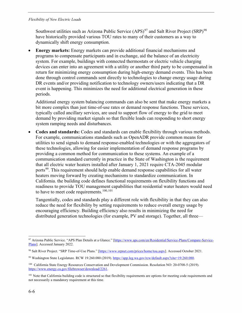
Flexibility of New Electric Loads
6-6
Southwest utilities such as Arizona Public Service (APS)97 and Salt River Project (SRP)98 have historically provided various TOU rates to many of their customers as a way to dynamically shift energy consumption.
• Energy markets: Energy markets can provide additional financial mechanisms and programs to compensate participants and in exchange, aid the balance of an electricity system. For example, buildings with connected thermostats or electric vehicle charging devices can enter into an agreement with a utility or another third party to be compensated in return for minimizing energy consumption during high-energy demand events. This has been done through control commands sent directly to technologies to change energy usage during DR events and/or providing notification to technology owners/users indicating that a DR event is happening. This minimizes the need for additional electrical generation in these periods. Additional energy system balancing commands can also be sent that make energy markets a bit more complex than just time-of-use rates or demand response functions. These services, typically called ancillary services, are used to support flow of energy to the grid to meet demand by providing market signals so that flexible loads can responding to short energy system ramping needs and disturbances.
• Codes and standards: Codes and standards can enable flexibility through various methods. For example, communications standards such as OpenADR provide common means for utilities to send signals to demand response-enabled technologies or with the aggregators of these technologies, allowing for easier implementation of demand response programs by providing a common method for communication to these systems. An example of a communication standard currently in practice in the State of Washington is the requirement that all electric water heaters installed after January 1, 2021 require CTA-2045 modular ports99. This requirement should help enable demand response capabilities for all water heaters moving forward by creating mechanisms to standardize communication. In California. the building code defines functional requirements on flexibility functions and readiness to provide TOU management capabilities that residential water heaters would need to have to meet code requirements.100,101 Tangentially, codes and standards play a different role with flexibility in that they can also reduce the need for flexibility by setting requirements to reduce overall energy usage by encouraging efficiency. Building efficiency also results in minimizing the need for distributed generation technologies (for example, PV and storage). Together, all three—
97 Arizona Public Service. “APS Plan Details at a Glance.” [https://www.aps.com/en/Residential/Service-Plans/Compare-Service-Plans]. Accessed January 2022. 98 Salt River Project. “SRP Time-of-Use Plans.” [https://www.srpnet.com/prices/home/tou.aspx]. Accessed October 2021. 99 Washington State Legislature. RCW 19.260.080 (2019). https://app.leg.wa.gov/rcw/default.aspx?cite=19.260.080. 100 California State Energy Resources Conservation and Development Commission. Resolution NO: 20-0708-5 (2019). https://www.energy.ca.gov/filebrowser/download/2261. 101 Note that California building code is structured so that flexibility requirements are options for meeting code requirements and not necessarily a mandatory requirement at this time.

Flexibility of New Electric Loads
6-7
distributed generation, energy efficiency, and flexibility loads—play a role in system decarbonization.
Opportunities, Challenges, and Market Readiness As discussed above, aggressive electrification can introduce a much greater need for load flexibility. This section focuses on potential opportunities, challenges, and market readiness of tools and technologies that enable and scale flexibility. Flexibility opportunities will be discussed and described based on building segment.
Commercial Buildings Opportunities for utility commercial building flexibility programs focus on four main initiatives:102
• Historic commercial building demand response programs. These programs are the most common flexibility programs found in the industry today. They rely on “dispatching” commercial load shed or load reduction through manual messaging. Commercial building owners and/or operators are notified of load shed requirements through e-mail, text, or other forms of communication. They would reduce energy consumption and be compensated for load reduction through some form of contract between the building owner and/or operator and the utility. Most commercial building demand response problems also put in place penalties in the event that a commercial building does not meet specific targets as defined by the contract.
• Time-of-use rates and/or tariffs. This work involves the development of rates, tariffs, and/or other economic agreements between the commercial building(s) and the utility to develop price-based “signaling.”
• Automated demand response programs. Advancements in connectivity have enabled more automated demand response capabilities. These can be direct load control or behavioral programs and opt-in or opt-out designs. These systems usually rely on automatic mechanisms to send grid signals to buildings and/or devices and, in some instances, provide information on system response to these grid signals. This can be done through building energy management systems connected to aggregators or other supervisory platforms. Although these programs have been around for quite some time, these types of automated demand response programs and tools that enable them to have limited uptake compared to historic commercial building demand response programs.
• Emerging services. These utility-offered services take the form of energy audits or other consultative-type activities around enhancing or maintaining grid reliability and resiliency through the use of microgrids and connected technologies and distributed energy resources (DER) and enabling energy-related services such as predictive maintenance programs.
The benefit of these opportunities for flexibility are demonstrated below. Figure 6-5 depicts average daily winter load shape103 of a representative 50,000 sq. ft. commercial office building
102 Utilities and Commercial Customers. EPRI, Palo Alto, CA: 2019. 3002017238. 103 Note that winter load shapes are used because that is the current and predicted SCL system peak.
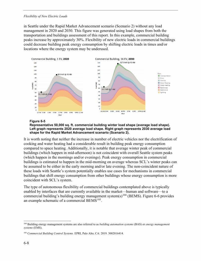
Flexibility of New Electric Loads
6-8
in Seattle under the Rapid Market Advancement scenario (Scenario 2) without any load management in 2020 and 2030. This figure was generated using load shapes from both the transportation and buildings assessment of this report. In this example, commercial building peaks increase by approximately 30%. Flexibility of new electric loads in commercial buildings could decrease building peak energy consumption by shifting electric loads in times and/or locations where the energy system may be underused.
Figure 6-5 Representative 50,000 sq. ft. commercial building winter load shape (average load shape). Left graph represents 2020 average load shape. Right graph represents 2030 average load shape for the Rapid Market Advancement scenario (Scenario 2).
It is worth noting that neither the increase in number of electric vehicles nor the electrification of cooking and water heating had a considerable result in building peak energy consumption compared to space heating. Additionally, it is notable that average winter peak of commercial buildings (which happen in mid-afternoon) is not coincident with overall Seattle system peaks (which happen in the mornings and/or evenings). Peak energy consumption in commercial buildings is estimated to happen in the mid-morning on average whereas SCL’s winter peaks can be assumed to be either in the early morning and/or late evening. The non-coincident nature of these loads with Seattle’s system potentially enables use cases for mechanisms in commercial buildings that shift energy consumption from other buildings whose energy consumption is more coincident with SCL’s system.
The type of autonomous flexibility of commercial buildings contemplated above is typically enabled by interfaces that are currently available in the market—human and software—to a commercial building’s building energy management system(s)104 (BEMS). Figure 6-6 provides an example schematic of a commercial BEMS105.
104 Building energy management systems are also referred to as building automation systems (BAS) or energy management systems (EMS). 105 Commercial Building Control Systems. EPRI, Palo Alto, CA: 2019. 3002016414.
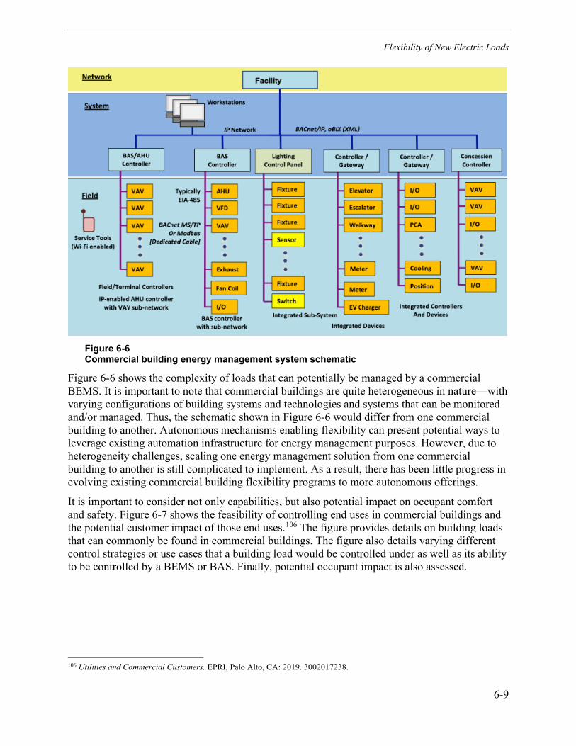
Flexibility of New Electric Loads
6-9
Figure 6-6 Commercial building energy management system schematic
Figure 6-6 shows the complexity of loads that can potentially be managed by a commercial BEMS. It is important to note that commercial buildings are quite heterogeneous in nature—with varying configurations of building systems and technologies and systems that can be monitored and/or managed. Thus, the schematic shown in Figure 6-6 would differ from one commercial building to another. Autonomous mechanisms enabling flexibility can present potential ways to leverage existing automation infrastructure for energy management purposes. However, due to heterogeneity challenges, scaling one energy management solution from one commercial building to another is still complicated to implement. As a result, there has been little progress in evolving existing commercial building flexibility programs to more autonomous offerings.
It is important to consider not only capabilities, but also potential impact on occupant comfort and safety. Figure 6-7 shows the feasibility of controlling end uses in commercial buildings and the potential customer impact of those end uses.106 The figure provides details on building loads that can commonly be found in commercial buildings. The figure also details varying different control strategies or use cases that a building load would be controlled under as well as its ability to be controlled by a BEMS or BAS. Finally, potential occupant impact is also assessed.
106 Utilities and Commercial Customers. EPRI, Palo Alto, CA: 2019. 3002017238.
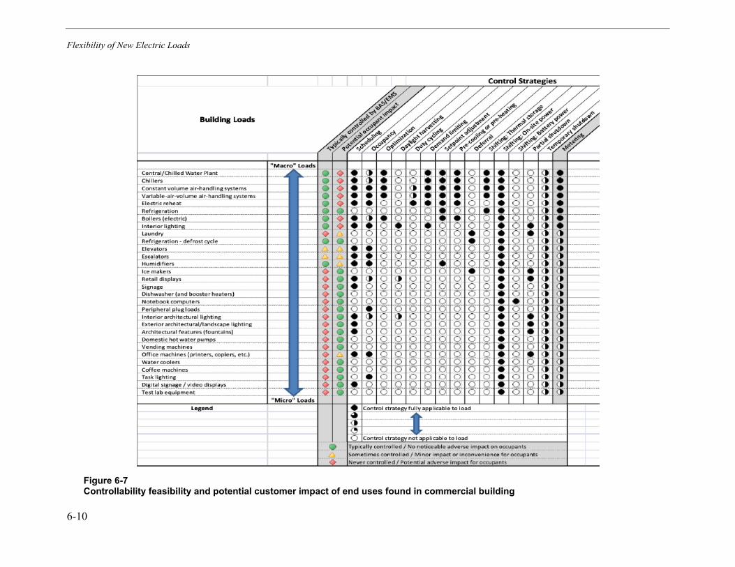
Flexibility of New Electric Loads
6-10
Figure 6-7 Controllability feasibility and potential customer impact of end uses found in commercial building

Flexibility of New Electric Loads
6-11
Two main items can be deduced from Figure 6-7: 1) large loads such as HVAC are the main controllable loads by the BEMS and 2) although controllable, these loads also have a higher probability of customer impact.
Additionally, workplace charging programs can provide additional opportunities for flexibility in commercial buildings by shifting EV charging electricity needs from periods of time that are more coincident to system peak (that is, evenings and mornings) to midday off-peak hours. However, although not necessarily coincident with overall system peak, the grid system analysis in this report does show scenarios in which peak loads of campuses or commercial buildings located at specific feeders would result in local energy system constraints, and these factors would need to be taken into account when considering these programs.
In summary, commercial buildings provide ways to provide grid flexibility as part of an overall building decarbonization strategy—especially in large commercial buildings. BEMS or BAS and the building automation functions they provide can be a potential integration point, enabling energy management for the utility with this infrastructure. However, with the heterogeneity of building loads found within commercial buildings and limitations from signals sent by utilities, aggregators, and/or supervisory systems to control a set of commercial buildings, commercial building flexibility programs remain very similar to the historic commercial building demand response programs offered. A table summarizing the approach, description, opportunity, and challenges of flexibility approaches for commercial, residential, and MUDs is provided in Appendix E (Table E-1).
Residential Buildings: Single Family Although Seattle has not historically required demand response programs in residential buildings, nationally, residential buildings flexibility has historically focused on leveraging direct load control switches to manage the use of air conditioning in the summertime. Although some programs have been successful, overall, this method has resulted in limited market uptake because customer value was relatively low compared to risk of occupant inconvenience. However, as home automation and advancements in connected technologies have become more widely available in the market, opportunities for flexibility in single-family homes has been more widely enabled. This market interest and availability addresses one of the main barriers that has hampered flexibility program adoption in the past: the large program cost of customer recruitment and device installation. The “Bring-Your-Own-Device” (BYOD) model that has been leveraged over the last 10 years provides an opportunity to increase a targeted set of homes for flexibility programs.
Figure 6-8 shows an average winter load shape for single-family homes in the Rapid Market Advancement scenario (Scenario 2). Similar to the shift seen in commercial buildings under this electrification scenario, peaks increase by approximately 30% in single-family buildings. As an outcome of electrification, the load factor107 of single-family homes decreases. This means the peak demand of residential buildings will be considerably higher than the average energy demands across the entire year, requiring a system capacity more than what is needed under most
107 Load factor can be defined as the peak power used (or exported to the grid in instances where the building can generate more electricity than it consumes) divided by the average energy a building consumes over a period of time. A group of homes or buildings all with high load factors can result in high system utilization for the grid.
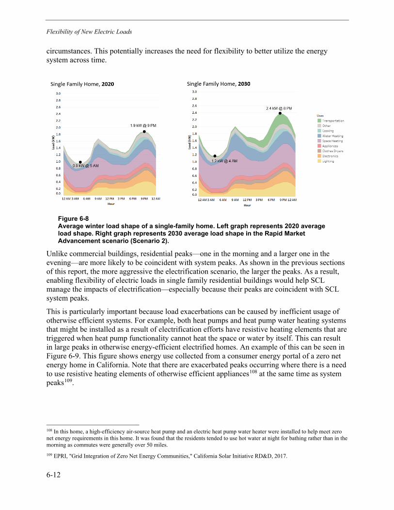
Flexibility of New Electric Loads
6-12
circumstances. This potentially increases the need for flexibility to better utilize the energy system across time.
Figure 6-8 Average winter load shape of a single-family home. Left graph represents 2020 average load shape. Right graph represents 2030 average load shape in the Rapid Market Advancement scenario (Scenario 2).
Unlike commercial buildings, residential peaks—one in the morning and a larger one in the evening—are more likely to be coincident with system peaks. As shown in the previous sections of this report, the more aggressive the electrification scenario, the larger the peaks. As a result, enabling flexibility of electric loads in single family residential buildings would help SCL manage the impacts of electrification—especially because their peaks are coincident with SCL system peaks.
This is particularly important because load exacerbations can be caused by inefficient usage of otherwise efficient systems. For example, both heat pumps and heat pump water heating systems that might be installed as a result of electrification efforts have resistive heating elements that are triggered when heat pump functionality cannot heat the space or water by itself. This can result in large peaks in otherwise energy-efficient electrified homes. An example of this can be seen in Figure 6-9. This figure shows energy use collected from a consumer energy portal of a zero net energy home in California. Note that there are exacerbated peaks occurring where there is a need to use resistive heating elements of otherwise efficient appliances108 at the same time as system peaks109.
108 In this home, a high-efficiency air-source heat pump and an electric heat pump water heater were installed to help meet zero net energy requirements in this home. It was found that the residents tended to use hot water at night for bathing rather than in the morning as commutes were generally over 50 miles. 109 EPRI, "Grid Integration of Zero Net Energy Communities," California Solar Initiative RD&D, 2017.
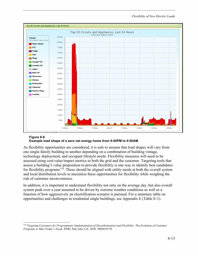
Flexibility of New Electric Loads
6-13
Figure 6-9 Example load shape of a zero net energy home from 6:00PM to 9:00AM
As flexibility opportunities are considered, it is safe to assume that load shapes will vary from one single-family building to another depending on a combination of building vintage, technology deployment, and occupant lifestyle needs. Flexibility measures will need to be assessed using cost/value/impact metrics to both the grid and the customer. Targeting tools that assess a building’s value proposition to provide flexibility is one way to identify best candidates for flexibility programs110. These should be aligned with utility needs at both the overall system and local distribution levels to maximize these opportunities for flexibility while weighing the risk of customer inconvenience.
In addition, it is important to understand flexibility not only on the average day, but also overall system peak over a year assumed to be driven by extreme weather conditions as well as a function of how aggressively an electrification scenario is pursued. For a summary table on opportunities and challenges in residential single buildings, see Appendix E (Table E-1).
110 Targeting Customers for Programmatic Implementation of Decarbonization and Flexibility: The Evolution of Customer Programs to Meet Today’s Needs. EPRI, Palo Alto, CA: 2020. 3002019170.
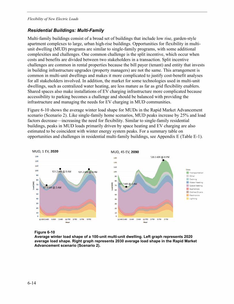
Flexibility of New Electric Loads
6-14
Residential Buildings: Multi-Family Multi-family buildings consist of a broad set of buildings that include low rise, garden-style apartment complexes to large, urban high-rise buildings. Opportunities for flexibility in multi-unit dwelling (MUD) programs are similar to single-family programs, with some additional complexities and challenges. One common challenge is the split incentive, which occur when costs and benefits are divided between two stakeholders in a transaction. Split incentive challenges are common in rental properties because the bill payer (tenant) and entity that invests in building infrastructure upgrades (property managers) are not the same. This arrangement is common in multi-unit dwellings and makes it more complicated to justify cost-benefit analyses for all stakeholders involved. In addition, the market for some technologies used in multi-unit dwellings, such as centralized water heating, are less mature as far as grid flexibility enablers. Shared spaces also make installations of EV charging infrastructure more complicated because accessibility to parking becomes a challenge and should be balanced with providing the infrastructure and managing the needs for EV charging in MUD communities.
Figure 6-10 shows the average winter load shape for MUDs in the Rapid Market Advancement scenario (Scenario 2). Like single-family home scenarios, MUD peaks increase by 25% and load factors decrease—increasing the need for flexibility. Similar to single-family residential buildings, peaks in MUD loads primarily driven by space heating and EV charging are also estimated to be coincident with winter energy system peaks. For a summary table on opportunities and challenges in residential multi-family buildings, see Appendix E (Table E-1).
Figure 6-10 Average winter load shape of a 100-unit multi-unit dwelling. Left graph represents 2020 average load shape. Right graph represents 2030 average load shape in the Rapid Market Advancement scenario (Scenario 2).

Flexibility of New Electric Loads
6-15
Flexibility as a Distribution Grid Resource Efforts to enable electric load flexibility have historically focused on providing balancing for the broader energy system. However, many electric utilities are seeking to leverage load flexibility for additional purposes now, including as a means to provide distribution grid support and services. As new electric loads come online as a result of electrification, there is an opportunity to deploy flexibility mechanisms that can address specific distribution grid needs. These needs are driven by two main factors:
• Locational variations in grid conditions. As the grid assessment included in Section 5 of this report notes, different areas of SCL’s distribution system have varying capacity levels to support electrification and decarbonization activities. Flexibility of building and transportation loads is a potential alternative to additional capital investments in locations where the grid is becoming more constrained.
• Customer decarbonization initiatives. Increasing numbers of utility customers—residential, commercial, and industrial—have established decarbonization goals and targets. For example, the University of Washington aims to reduce its greenhouse gas emissions by 45% by 2030111. A combination of renewable energy deployment, energy conservation measures, and electrification of transportation and buildings are all parts of the solution to meet the University of Washington’s goals. As customers electrify as part of their efforts to decarbonize, it will have considerable impacts on the specific portions of the grid serving those customers.
At this time, distribution system flexibility programs, such as capacity deferral and managing distribution voltage issues are less mature than the programs designed for the bulk energy system. Generally, wholesale electricity markets have had well-defined market products that can be used to assign value to flexibility.112 Although bulk system flexibility objectives still require amendments, they are building on significant industry experience to enable greater participation from DER in the bulk market.
Although there are similarities with bulk system flexibility objectives, addressing distribution constraints requires additional components, including a higher level of certainty of participation. This is because consequences of not meeting the expected outcomes put distribution systems at risk because when one site fails to perform in the bulk system, there is usually a larger pool of alternatives to maintain grid reliability across the wider grid than there are to meet a need on a local level. As a result, penalties for nonparticipation may be considerable compared for the incentives for building owners to provide the distribution services. In addition, “settlement-based” approaches used in the bulk market do not provide the rapid feedback or the predictive metrics necessary to support staggered-stop events and other dynamic load-modification strategies found within distribution grid services. New mechanisms for compensating customer
111 University of Washington Sustainability Action Plan, available at: https://green.uw.edu/sustainability-plan 112 Ancillary Services in the United States: Technical Requirements, Market Designs and Price Trends. EPRI, Palo Alto, CA: 2019. 30020156
Flexibility of New Electric Loads
6-16
participation in these distribution programs are needed. Although these approaches are currently being explored, they are still in nascent stages113
Summary: Conclusions, Recommendations, Next Steps Electrification will increase electric load in SCL’s service territory. As electrification is pursued, some portion of that increase can be offset through efficiency programs, as discussed in the previous sections. However, flexibility will also be a tool for SCL to ensure that it is maximizing the usage of its existing system. As this transition occurs, three primary questions should be addressed:
• How can SCL enable electric loads as flexible resources? Specifically, SCL will need to know the existing and developing technical, market, and programmatic approaches that enable grid flexibility objectives.
• What are considerations for scalability? This includes how replicable a technical, market, and/or program approach is, as well as likelihood of engagement and ongoing participation of building owners and occupants.
• What is the maturity of the industry that provides support? Incorporating flexibility will require technical capabilities and infrastructure to operate and maintain specific programs, technologies, and systems.
As electrification accelerates, the following considerations and recommendations for how to incorporate flexibility should include:
• Coordination with other activities at SCL. Decarbonization strategies require tighter coordination of DSM approaches that have traditionally had their own targets and metrics with other utility activities. For example, the flexibility of new electric loads found in GEBs (HVAC, water heating, lighting, EVs) can align and be integrated with other related programs. Additionally, because decarbonization strategies require a more decentralized set of potential energy resources coordinating with planning and operations activities is important in order to efficiency planning, operating, and managing an energy system behind that.
• Understand Application and Value of Flexibility. Flexibility of electric loads can potentially be a low-cost non-wires alternative for areas of congestion on SCL’s distribution grid. However, it is important to understand the application and value of flexibility, understanding the available and achievable capacity value that can be obtained in the context of greater electrification initiatives. Considerations should include the following: – SCL should consider signaling by both active controls signaling (for example, demand
response) or passive rate signaling (for example, TOU) to achieve flexibility. Signaling strategies should consider consumer and occupant impact and technology readiness to respond such active or passive utility signals.
– Flexibility enabled by connected HVAC, water heating, appliances, and EVs should be considered in a portfolio of strategies that include energy efficiency and efficiency
113 Measurement and Verification for DERs Providing Grid Services: Approaches and Challenges. EPRI, Palo Alto, CA: 2021 (expected).

Flexibility of New Electric Loads
6-17
conservation measures, distributed generation sources such as solar and storage, and advanced and current wired alternatives.
– Because many of these new electric loads have customer and occupant value propositions other than being an energy resource, it is important to understand the stacked value that energy-related customer value propositions provide.
– Flexibility strategies do not just include active or passive load management/control strategies. Application of energy conservation programs, or updates to applicable codes and standards to minimize the need for flexibility, should be considered.
• Evaluate Cost and Benefits of flexibility measures. Cost-benefit analyses of flexibility measures will allow SCL to understand when, where, and at what point of inflection flexibility measures make sense. This type of analysis and sequencing of potential projects and programs is important because the value of the same project will vary depending on where it is deployed on the grid. For example, there may be few system benefits to enabling flexibility in areas where there is excess capacity because there is no need to defer large electric system investments to accommodate for electrification initiatives. As demand increases as a result of aggressive localized electrification efforts, utilizing flexibility to decrease energy system peaks and to maximize the use of the overall energy system will provide greater benefits as an alternative to potential infrastructure or resource upgrades.
• Utilize “market pull” and “policy push” to deploy flexibility. On the large scale, understanding corporate sustainability policies and decarbonization efforts as drivers of electrification will offer opportunities for SCL to partner with customers making these changes so that flexibility can be incorporated in these transitions. On a smaller scale, the popularity of connected building technologies such as smart thermostats and connected water heaters and programs like deferred charging programs can be a low cost way to enable flexibility in more homes and buildings throughout SCL’s service territory.
• Develop functional requirements. Distributed energy resources, and building and vehicle electric technologies, combined with the increased interest in distribution services have resulted in the development of commercially ready platforms to enable flexibility of these new electrified loads. Commonly referred to as distributed energy resource management systems (DERMS) in the industry, these platforms can offer electric utilities the ability to manage flexibility initiatives. To help de-risk these capital investments, when sourcing and implementing the platforms it is important to develop functional requirements and to assess the feasibility of devices and systems used to interface with these platforms.

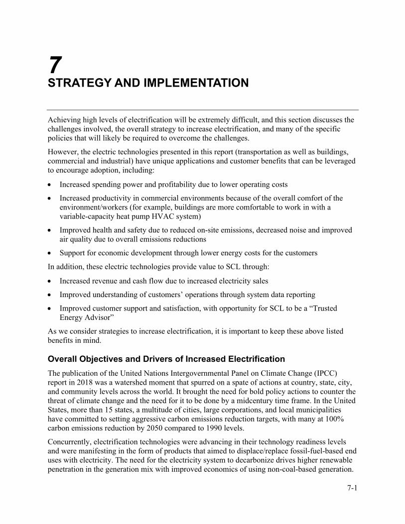
7-1
7 STRATEGY AND IMPLEMENTATION
Achieving high levels of electrification will be extremely difficult, and this section discusses the challenges involved, the overall strategy to increase electrification, and many of the specific policies that will likely be required to overcome the challenges.
However, the electric technologies presented in this report (transportation as well as buildings, commercial and industrial) have unique applications and customer benefits that can be leveraged to encourage adoption, including:
• Increased spending power and profitability due to lower operating costs
• Increased productivity in commercial environments because of the overall comfort of the environment/workers (for example, buildings are more comfortable to work in with a variable-capacity heat pump HVAC system)
• Improved health and safety due to reduced on-site emissions, decreased noise and improved air quality due to overall emissions reductions
• Support for economic development through lower energy costs for the customers
In addition, these electric technologies provide value to SCL through:
• Increased revenue and cash flow due to increased electricity sales
• Improved understanding of customers’ operations through system data reporting
• Improved customer support and satisfaction, with opportunity for SCL to be a “Trusted Energy Advisor”
As we consider strategies to increase electrification, it is important to keep these above listed benefits in mind.
Overall Objectives and Drivers of Increased Electrification The publication of the United Nations Intergovernmental Panel on Climate Change (IPCC) report in 2018 was a watershed moment that spurred on a spate of actions at country, state, city, and community levels across the world. It brought the need for bold policy actions to counter the threat of climate change and the need for it to be done by a midcentury time frame. In the United States, more than 15 states, a multitude of cities, large corporations, and local municipalities have committed to setting aggressive carbon emissions reduction targets, with many at 100% carbon emissions reduction by 2050 compared to 1990 levels.
Concurrently, electrification technologies were advancing in their technology readiness levels and were manifesting in the form of products that aimed to displace/replace fossil-fuel-based end uses with electricity. The need for the electricity system to decarbonize drives higher renewable penetration in the generation mix with improved economics of using non-coal-based generation.
Strategy and Implementation
7-2
Although these trends continue, the relative importance of transportation, buildings, and industry as contributors to GHG emissions in the United States (Figure 7-1) underscored the need for these sectors to take actions to decarbonize.
Figure 7-1 U.S. GHG Emissions by Sector in 2019
The driving forces for electrification can be categorized in three major buckets: policy, market, and technology drivers.
Policy Drivers Policy drivers for electrification comprise federal, state, local jurisdictional decarbonization goals and associated state and local laws. As an example, Figure 7-2 shows actions toward building decarbonization, with the darker shades of green indicating statewide actions and lighter shades of green indicating city- and utility-driven actions. States like California, New York, and Washington have instituted several laws on reducing carbon pollution and promoting energy efficiency in buildings. Seattle and New York have developed their own climate action plans that specifically identify requirements for energy efficiency for the building stock. Many cities—for example, New York and San Francisco and Berkeley, California—have also taken legislative

Strategy and Implementation
7-3
action to enact a wide array of measures including a ban on natural gas hookups for new buildings. Seattle has enacted ordinances114 of what is being termed a “partial gas ban” comprising a ban on natural gas for space heating in new construction of commercial buildings and high-rise apartment buildings including for replacement of heating systems in older buildings. The ordinance also bans the use of natural gas for water heating in hotels and large apartment buildings and has instituted code that will allow for improved energy conservation including efficient electric heating and cooling systems.
Figure 7-2 Shading of the number of policy levers in the form of carbon targets set at state, city, and utility scale115
Market Drivers Decarbonization will require consumer-driven decarbonization and customer participation in demand response/flexibility type programs. This can be enhanced through customer programs that incentivize the use of lower carbon resources for home heating, incentives/rebates for electrification of end uses such as space heating cooling, water heating, cooking, electric vehicle purchases, and industrial electrification. Market transformation can also be enhanced through incentives for improvements to non-electric pathways such as building envelope weatherization. More recently, more direct economics-driven conservation measures are being enacted using variable rates, such as time-of-use rates, in many utility service territories.
114 Source: https://www.seattletimes.com/seattle-news/seattle-city-council-passes-measure-to-end-most-natural-gas-use-in-commercial-buildings-and-some-apartments/ 115 EPRI internal research
Strategy and Implementation
7-4
Technology Drivers Technology drivers for electrification include supply-side measures such as the investment made by vendors of end-use equipment into R&D to achieve higher efficiencies and lower costs. These include significant improvements in the efficiency of space heating/cooling, water heating, cooking convenience appliances, electric vehicles, and industrial equipment. In buildings, heat pump–based HVAC systems have seen significant improvement in their minimum efficiency levels while emerging technologies such as 120 V heat pump and package terminal heat pumps (PTHPs) are potential game-changers in the space conditioning landscape. The use of low to very-low GWP refrigerants has also helped address the need for water heating applications in unitary and garden-style (low-rise) multifamily dwellings. Energy Star–rated appliances also have significant potential for energy conservation.116 In transportation, the availability of electric vehicles has increased tremendously while costs have decreased to the point where up-front cost parity has already been achieved in some segments.
Considerations for Equitable Electrification In addition to general policy implementation, it will be important to ensure that equity is increased by focusing efforts on traditionally overlooked and underserved communities. According to 2019 Census data, about 11% of Seattle’s population had incomes below the poverty threshold.117 Given the nascent state of most technologies, there is still a significant cost burden for customers to adopt efficient electrified technologies. Therefore, there is a considerable need for policy-driven measures to address electrification with equity and affordability in the forefront.
The notion of the energy burden becomes a principal consideration for stakeholders in the energy market transformation. The nexus of poverty, high energy costs, and access—or lack thereof—to affordable clean energy leads to a stratified impact on disadvantaged communities (see Figure 7-3). A comprehensive energy market transformation strategy must consider all tiers of the energy impact on disadvantaged communities.
116 https://www.energysage.com/energy-efficiency/costs-benefits/energy-star-rebates/ 117 https://www.census.gov/quickfacts/fact/table/seattlecitywashington,US/PST045219
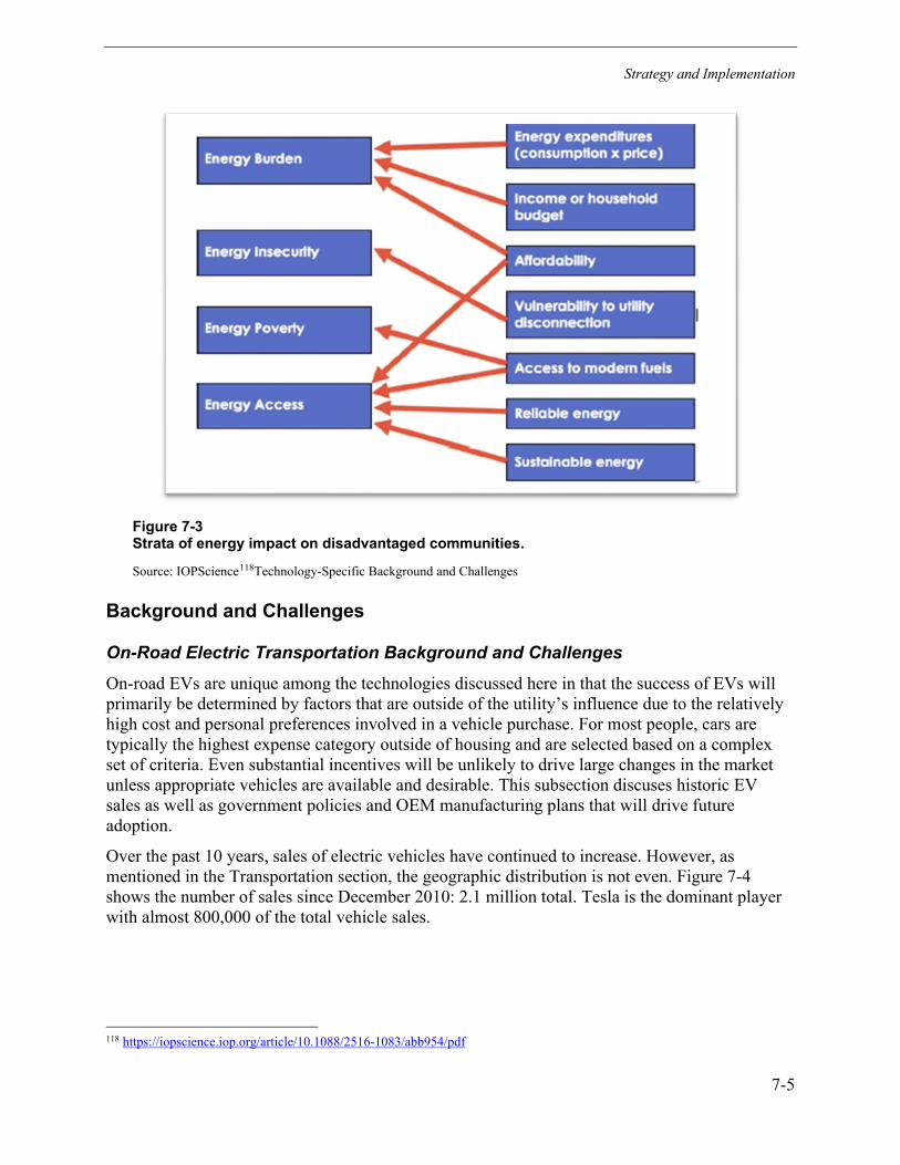
Strategy and Implementation
7-5
Figure 7-3 Strata of energy impact on disadvantaged communities.
Source: IOPScience118Technology-Specific Background and Challenges
Background and Challenges
On-Road Electric Transportation Background and Challenges On-road EVs are unique among the technologies discussed here in that the success of EVs will primarily be determined by factors that are outside of the utility’s influence due to the relatively high cost and personal preferences involved in a vehicle purchase. For most people, cars are typically the highest expense category outside of housing and are selected based on a complex set of criteria. Even substantial incentives will be unlikely to drive large changes in the market unless appropriate vehicles are available and desirable. This subsection discuses historic EV sales as well as government policies and OEM manufacturing plans that will drive future adoption.
Over the past 10 years, sales of electric vehicles have continued to increase. However, as mentioned in the Transportation section, the geographic distribution is not even. Figure 7-4 shows the number of sales since December 2010: 2.1 million total. Tesla is the dominant player with almost 800,000 of the total vehicle sales.
118 https://iopscience.iop.org/article/10.1088/2516-1083/abb954/pdf
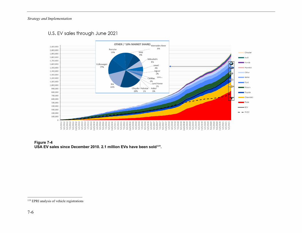
Strategy and Implementation
7-6
Figure 7-4 USA EV sales since December 2010. 2.1 million EVs have been sold119.
119 EPRI analysis of vehicle registrations

Strategy and Implementation
7-7
Figure 7-5 shows the percent of new vehicle sales that are EV in 2020. Many of the counties with high concentrations of new EV sales are located in zero-emission vehicle states (ZEV) states, especially California where the ZEV program originated. However, Washington State has 3 of the 15 highest-share counties outside of California despite not being a ZEV state, although there are plans to join the ZEV program in 2023.
Figure 7-5 Heat map of percentage of new EV sales in the Unites States by county from June 2020 through June 2021. The top 5 counties in California and the top 15 counties outside of California have been highlighted.

Strategy and Implementation
7-8
Tesla has been dominating the EV space for some time, but there have been many recent announcements from OEMs pledging to electrify a significant portion of the vehicles they produce. These include announcements by Audi (20 EVs available by 2025), BMW (15–25% of global sales will be EVs by 2025), Ford (will invest 29 billion in EVs by 2025), GM (20 EVs on the market in North America by 2025), and many others.120 This shift in the market is evident already, as there are 18 new EVs set to hit the market this year, offering consumers more choice when they consider their next vehicle purchase.
OEMs are national and global companies, so as electrification policies and targets are adopted by cities, states, and countries across the globe, the impacts can be more widespread than the local or national policy. As OEMs comply with new emissions standards imposed by specific states or countries, there will be more EVs available for purchase for all consumers, regardless of their location—which will help accelerate the market transition as a whole. Policies range from local, state, and national policies which reduce emissions or encourage EV adoption to outright bans on sales of new internal combustion engine (ICE) vehicles.
Recently, President Joe Biden announced a national target for electric vehicles to make up half of all new vehicle sales in the United States by 2030. In addition, the bipartisan infrastructure package currently (as of August 2021) under debate in Congress would include funding for EV infrastructure.121
Detailed examples of city goals, including Seattle, and strategies employed there, are provided in Table 7-1. Potential strategies and their anticipated impacts are discussed in further detail in the Technology – Specific Strategies section.
Table 7-1 Examples of city electric vehicle goals and strategies122.
120 https://www.caranddriver.com/news/g35562831/ev-plans-automakers-timeline/ 121 https://www.whitehouse.gov/briefing-room/statements-releases/2021/06/24/fact-sheet-president-biden-announces-support-for-the-bipartisan-infrastructure-framework/ (accessed 7/27/2021) 122 https://theicct.org/publication/update-on-electric-vehicle-adoption-across-u-s-cities/

Strategy and Implementation
7-9
Although there is considerable momentum toward electrification of on-road vehicles, there are significant challenges to overcome, particularly up-front cost and availability of charging infrastructure.
Up-Front Cost
As with many efficiency and electrification technologies, EVs are generally cheaper to operate than conventional vehicles due to higher efficiency but are more expensive up front. This is primarily due to the cost of batteries, which make up a significant fraction of the cost of EVs. These costs are coming down, and some analysts expect up-front cost parity to be achieved by 2025.123 However, this is mainly for vehicles with relatively low energy use per mile, such as sedans and smaller crossovers, and vehicles with higher energy use intensity, such as pickups and larger vehicles, will continue to be more expensive. This is a significant barrier to customer adoption because customers are less likely to pay more for an uncertain return.
The higher cost for current vehicles is particularly a problem for low-income customers, who typically buy used vehicles. Because widespread EV manufacturing is still in early phases, there is not yet a large inventory of used EVs. There will be a lag of 5−10 years between when there is a significant change in the new market and when there is availability for lower-income customers. In addition, policies like up-front incentives that are available to drive the new vehicle market often are not available to used vehicle buyers.
Charging Infrastructure
A second main challenge for EV market adoption is the availability of charging infrastructure. Drivers need to be able to charge on long trips and during their daily activities. There has been significant investment in charging networks that has resulted in good coverage for many driving profiles, but much of the market development to date has assumed that charging is available at home to meet most routine energy needs overnight. However, this will not currently be true for drivers who park on the street or who park in garages of apartments and multiunit dwellings where charging is not available. There is a significant share of these drivers in Seattle, so increasing adoption will require installing chargers in these locations or increasing the availability of charging at workplaces and other common destinations. These chargers may also have to be DCFC to ensure that charging is possible in the time available.
Building Electrification Background and Challenges In Seattle, fossil-fuel-based space heating technologies account for 63% of the total space heating energy consumption (~7.5 trillion Btu) each year. Heat pumps offer an excellent electric replacement option that can aid in city decarbonization goals. Currently only a small percentage of heat pumps are used in the residential and commercial customer segments. Heat pumps can lower energy requirements by as much as three times those of fossil-fuel-based heating systems. A similar trend exists for commercial buildings in which the fossil-fuel-based heating systems dominate the space heating and consume 79% of the energy used for heating per year.
For water heating, heat pumps offer similar benefits to customers over fossil-fuel-based systems. In Seattle, only about 35% of water heating energy consumption is electric based (predominately
123 https://about.bnef.com/blog/electric-cars-reach-price-parity-2025/

Strategy and Implementation
7-10
resistance) in single- and multi-family buildings, and only 21% is electric (dominated by electric resistance) in commercial buildings. Heat pumps used for space and water heating in residential and commercial buildings offer energy efficiency benefits, decarbonization solutions, and lower energy costs to the customers.
Some of the common market challenges faced by heat pump technologies are as follows:
• Higher first cost for high-efficiency technologies.
• Lack of familiarity with heat pumps and existing perception that heat pumps do not work well in colder climates in particular.
• Installers may not be familiar with customer benefits and therefore may not propose heat pumps as an alternative.
• Customers have the propensity to replace their HVAC or water heater systems with in-kind technologies.
• The HVAC or water heater replacement is not typically a planned event. In other words, the customer typically looks for an HVAC or water heater system when the current system breaks unexpectedly. They sometimes are forced to install the systems that the contractors carry with them. If the contractors are not educated about the benefits of heat pump systems, they often sell the cheapest system to the customer.
In many cases, customers may not be familiar with the performance of electric equipment or possible benefits. If electric technology options are not offered and compared to alternatives, there is little incentive for customers to convert.
Commercial Cooking Equipment Background and Challenges In Seattle, the commercial cooking energy is dominated by natural-gas-based systems. Nearly 92% of the energy consumed for commercial cooking is fossil-fuel-based, and only 8% is electric. In commercial buildings, the cooking equipment provides a great electrification opportunity. The primary benefits of commercial cooking equipment—and what drives adoption—are the increased quality of the final product as well as increased throughput. In addition to these benefits, there are other non-energy benefits such as oil savings, flexibility of the operations, and lower space cooling requirements that favor the electric commercial cooking options. The reason some of the fast food chains prefer electric over natural gas is that electric fryers have a faster reheat than similar gas products, which both reduces cooking time and increases the quality of the finished product (for instance, crispier French fries). It is also worth noting that the electric griddles used in restaurants provide even heat from edge to edge, whereas gas equipment develops hot spots over time. Where griddles are used for higher volume foods (for instance, hamburger patties in a burger restaurant), throughput may be increased due to the consistency of heat across an increased surface area. Electric combi-ovens also have fewer hot spots, resulting in more even cooking and better performance than gas versions. The electric cooking equipment can meet or exceed the restaurant food quality specifications compared to the gas cooking equipment and offers many benefits to the customers.

Strategy and Implementation
7-11
Some of the common challenges for electric cooking equipment are as follows:
• Higher capital cost (except for combi-ovens)
• Lack of understanding of benefits compared to gas
• Preference for and familiarity with cooking on gas equipment
• Equipment type possibly mandated by parent company
• Lack of adequate electrical service and cost to upgrade
Industrial Process Heating Electrification Background and Challenges In Seattle, the industrial customers within Seattle account for approximately 13.7 trillion Btu of energy consumption. The heating is primarily done with steam from boilers, convection ovens, or furnaces. Nearly 90% of the energy used for boilers and process heating is by natural gas, propane, or fuel oil. Heat is used in nearly every industrial process to cure, dry, heat treat, and melt materials used in making parts and consumer goods. Multiple electric technologies are employed in industrial process heating, including resistance, induction, infrared (IR), and ultraviolet (UV) heat. These electric technologies tend to be high-efficiency compared to the natural-gas-fired alternatives and provide significant non-energy benefits that are the primary drivers for electric equipment adoption—including increased productivity and product quality.
In performing research and analysis for various utilities, EPRI found that there are four major barriers, expressed by customers and the equipment vendors, that need to be addressed to achieve significant market expansion of these technologies:
• Lack of upfront capital: In today’s economic environment, many customers are capital constrained and allocating these scarce resources for new technology investments is difficult.
• Long sales cycle: A long sales cycle is usually caused by significant capital requirements, the intricacy of the application, and the impact of a technology on current operations. In addition, in working with customers on long sales projects, key personnel change due to restructurings, retirements, and so on can cause significant time delays.
• Resistance to adopt technologies without knowing the impact to a customer’s production: One of the most significant barriers to adoption of these technologies is the customer’s concern about how it will impact their current operations. Typically, customers are skeptical of changing their production to accommodate new technologies. A small decrease in productivity can lead to a substantial revenue and earnings impact to the customer.
• Equipment downtime: More importantly, the downtime needed to install new equipment—electric or otherwise—is a hurdle to be addressed in planning stages because loss of productivity is a primary barrier for installing new equipment.
Non-Road Electric Transportation Background and Challenges Non-road electric transportation technologies are used widely at commercial as well as industrial facilities. Some of the technologies that fall under this category are residential and commercial lawn and garden, material handling equipment used in warehouses, ports and industries, and

Strategy and Implementation
7-12
construction and agricultural equipment. In Seattle, the electric technologies account for only about 1% in lawn and garden (both residential and commercial); 7% in industrial technologies such as forklifts, terminal tractors, and so on; and almost none in construction and agricultural equipment. The electric options are growing, although at a lower rate, in the non-road transportation segment as the research from the light-, medium-, and heavy-duty on-road transportation is spilling over to this industry. Although the applications are specific, there are several common non-energy benefits of non-road transportation technologies that play a critical role in the conversion:
• Elimination of local emissions
• Reduced noise
• Reduced maintenance; increased reliability
• Ability to turn on/off quickly—reduce or eliminate idle time
• Improved worker safety and customer impacts – Reduced exposure to diesel and jet fuel emissions – Reduced noise levels and noise pollution
Electric forklifts are a key opportunity for electrification; with adequate usage, electric forklifts quickly pay back additional first costs, typically in less than two years (based on usage). Electrification of heavy-duty vehicle idling provides the ability for trucks and trailers to shut down diesel engines while parked at rest stops, truck centers, distribution centers, warehouses, food manufacturers, terminals, or other areas where trucks congregate. Airport electrification is also an attractive option for emissions and cost reductions where applicable.
Strategies for Increasing Electrification This section covers the implementation strategies that SCL could consider for the various electrification technologies discussed in this report.
The objective of the actions outlined here is to enable electrification scenarios studied as part of the analysis in a way that is cost optimized for the scenario. The formulation used here has two market actions that utilities can take: rate adjustments and customer programs to incentivize electrification.
Utilities can also engage by using policy actions such as influencing the evolving codes and standards and/or updates to distribution planning approaches to take advantage of enhanced demand-side flexibility that may be available through electrification. Although direct economics can be explicitly modeled and optimized, it is necessary to include non-economic benefits (or non-energy benefits) in the form of improved air quality and enhanced comfort/convenience (see Figure 7-6).
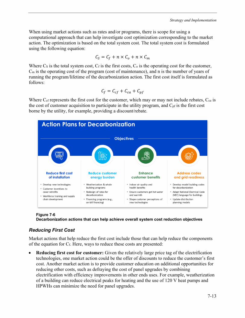
Strategy and Implementation
7-13
When using market actions such as rates and/or programs, there is scope for using a computational approach that can help investigate cost optimization corresponding to the market action. The optimization is based on the total system cost. The total system cost is formulated using the following equation:
𝐶𝐶𝑆𝑆 = 𝐶𝐶𝑓𝑓 + 𝑛𝑛 × 𝐶𝐶𝑜𝑜 + 𝑛𝑛 × 𝐶𝐶𝑚𝑚
Where CS is the total system cost, Cf is the first costs, Co is the operating cost for the customer, Cm is the operating cost of the program (cost of maintenance), and n is the number of years of running the program/lifetime of the decarbonization action. The first cost itself is formulated as follows:
𝐶𝐶𝑓𝑓 = 𝐶𝐶𝑐𝑐𝑓𝑓 + 𝐶𝐶𝑐𝑐𝑎𝑎 + 𝐶𝐶𝑝𝑝𝑓𝑓
Where Ccf represents the first cost for the customer, which may or may not include rebates, Cca is the cost of customer acquisition to participate in the utility program, and Cpf is the first cost borne by the utility, for example, providing a discount/rebate.
Figure 7-6 Decarbonization actions that can help achieve overall system cost reduction objectives
Reducing First Cost Market actions that help reduce the first cost include those that can help reduce the components of the equation for Cf. Here, ways to reduce these costs are presented:
• Reducing first cost for customer: Given the relatively large price tag of the electrification technologies, one market action could be the offer of discounts to reduce the customer’s first cost. Another market action is to provide customer education on additional opportunities for reducing other costs, such as defraying the cost of panel upgrades by combining electrification with efficiency improvements in other ends uses. For example, weatherization of a building can reduce electrical peaks for heating and the use of 120 V heat pumps and HPWHs can minimize the need for panel upgrades.
Strategy and Implementation
7-14
• Extending On-Bill Financing Programs: A specific program to reduce up-front cost without net expenditure is the use of on-bill financing (OBF) programs for electrification upgrades. Several utilities (especially California IOUs and SoCalGas) have on-bill financing programs that provide loans to pay for energy efficiency upgrades. Programs such as Meter Energy Efficiency Transaction Structure (MEETS) may be extended to add other types of buildings (especially multifamily housing) where there are challenges to performing efficient electrification upgrades due to split incentives and/or other dissuading factors.
• Reducing the cost of customer acquisition: Reducing the cost of customer acquisition requires marketing actions such as customer segmentation, program alignment to the customer segment, and customer targeting. Tools are available for segmenting customers based on their energy use profile and to perform virtual energy audits and get recommendations on specific upgrades. These types of tools will help reduce the cost of customer acquisition by optimizing program rollout.
• Reducing the first cost of programs: Reducing the first cost of programs includes reducing the need for distribution network upgrades. Although energy efficiency measures are a sound method to reduce the need for distribution upgrades, electrified end uses often induce needle-peak behaviors due to inefficient operating regimes for otherwise high-efficiency technologies as mentioned in the previous section. To prevent the need for distribution upgrades because of coincident demand, better modeling techniques may be used to understand the diversity factor of electrified end uses. In addition, by understanding and attributing load peaks to specific end uses, demand flexibility measures may be employed to shift peaks toward less peaky times of the day.
Reducing Operating Costs
The operating cost of electrified end use depends on both the usage patterns (conservative vs. excessive use) and the rate plans for customers who have made the fuel-switching/electrification decisions. Tiered rate structures tend to provide reliable baselines that customers can use to understand the economics of their energy use, but with increased thrust toward electrification it may be necessary to allocate additional energy quotas as part of baseline usage in the first tier. If customers are being switched to a time-of-use rate, additional measures to inform them of rate changes and providing them with tools to view and manage their energy use especially during peak times become requirements. Rate structures form a reliable and direct method to help improve customer economics with or without associated behavioral changes.
Technology-Specific Strategies for Increasing Electrification This section discusses technology-specific strategies for increasing adoption of the electric technologies discussed in this report. As discussed above, incentives to reduce capital and operating costs are important for each technology.
Strategies for Increasing Electric Vehicle Adoption Many factors can influence EV adoption, including cost, convenience, EV availability, access to charging and many more. Electric utilities are uniquely suited to address some of these considerations, depending on an individual utility’s interest and ability to participate in EV-related activities in the EV space. Figure 7-7 shows the different levels of engagement for
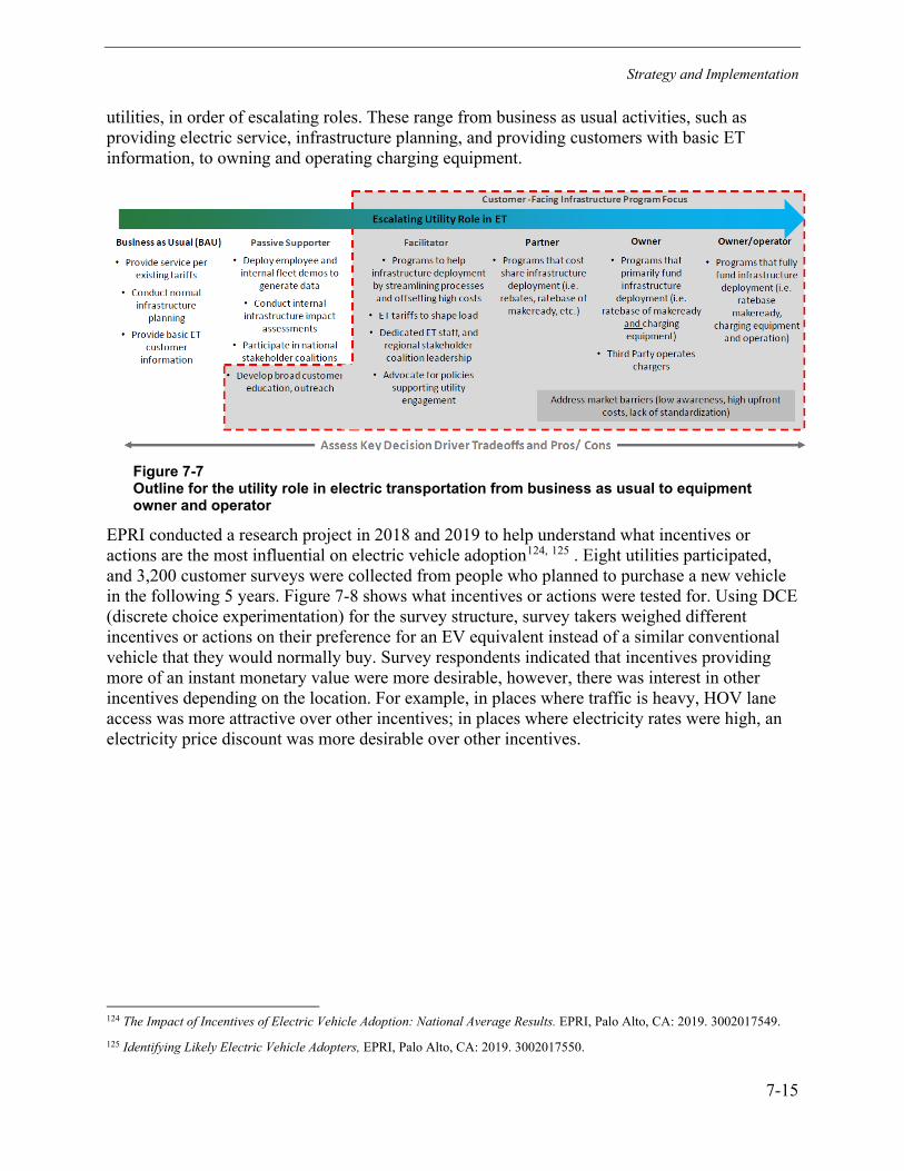
Strategy and Implementation
7-15
utilities, in order of escalating roles. These range from business as usual activities, such as providing electric service, infrastructure planning, and providing customers with basic ET information, to owning and operating charging equipment.
Figure 7-7 Outline for the utility role in electric transportation from business as usual to equipment owner and operator
EPRI conducted a research project in 2018 and 2019 to help understand what incentives or actions are the most influential on electric vehicle adoption124, 125 . Eight utilities participated, and 3,200 customer surveys were collected from people who planned to purchase a new vehicle in the following 5 years. Figure 7-8 shows what incentives or actions were tested for. Using DCE (discrete choice experimentation) for the survey structure, survey takers weighed different incentives or actions on their preference for an EV equivalent instead of a similar conventional vehicle that they would normally buy. Survey respondents indicated that incentives providing more of an instant monetary value were more desirable, however, there was interest in other incentives depending on the location. For example, in places where traffic is heavy, HOV lane access was more attractive over other incentives; in places where electricity rates were high, an electricity price discount was more desirable over other incentives.
124 The Impact of Incentives of Electric Vehicle Adoption: National Average Results. EPRI, Palo Alto, CA: 2019. 3002017549. 125 Identifying Likely Electric Vehicle Adopters, EPRI, Palo Alto, CA: 2019. 3002017550.

Strategy and Implementation
7-16
Figure 7-8 Incentives tested for in EPRI’s PEV preferences study. The blue coloring highlights incentives that have a more direct monetary value whereas the green highlights incentives that have varying values depending on specific driver situations or preferences.
The results of the DCE survey analysis was combined with a vehicle adoption model to be able to show the effects of an incentive (or a few incentives) on future EV adoption. An example scenario is shown for illustrative purposes. The incentives chosen for this scenario include:126
• Purchase price discount: $500 at the point of sale.
• Home charging station: Assuming a national average of $1,500 per home charging station including installation, a home charging station was offered to the customer for $1,000— roughly a benefit of $500.
• Electricity price discount: Discount of 20%. At a retail rate of $0.10 kWh, over a 10-year vehicle lifetime, and a total kWh/year of 2700, this amounted to savings of ~$550.
• Workplace charging.
• Charging station density increase.
• Green rate: An option to choose renewable energy for an additional cost.
• HOV access.
• Free workplace EV parking.
The results of this scenario are shown in Figure 7-9. In this example, workplace charging, electricity price discount, and green rate all have similar projected impacts when looking at the national average–level results, while purchase price discounts, HOV access, and free workplace parking show potential impacts at a lower level. The analysis for this scenario showed that the home charging station incentive of $500 was not high enough to offset the total cost of the installation.
126 In this example, where possible, an equal value was chosen for each incentive. For example, an electricity discount of 20%, a benefit of approximately $550 dollars over 10 years, is similar to a vehicle purchase price discount of $500.
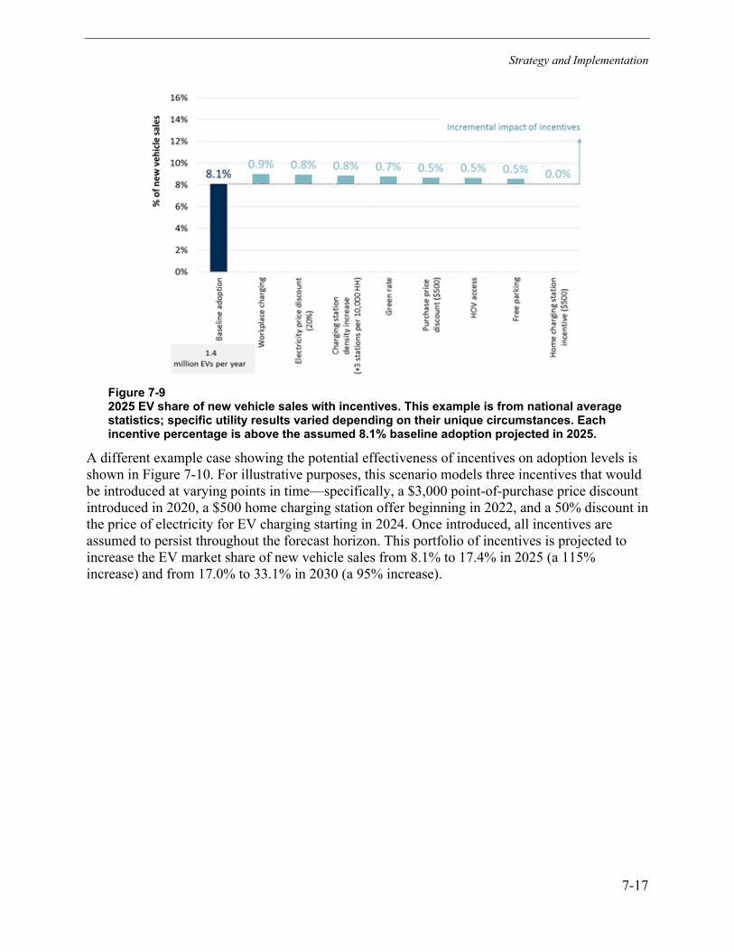
Strategy and Implementation
7-17
Figure 7-9 2025 EV share of new vehicle sales with incentives. This example is from national average statistics; specific utility results varied depending on their unique circumstances. Each incentive percentage is above the assumed 8.1% baseline adoption projected in 2025.
A different example case showing the potential effectiveness of incentives on adoption levels is shown in Figure 7-10. For illustrative purposes, this scenario models three incentives that would be introduced at varying points in time—specifically, a $3,000 point-of-purchase price discount introduced in 2020, a $500 home charging station offer beginning in 2022, and a 50% discount in the price of electricity for EV charging starting in 2024. Once introduced, all incentives are assumed to persist throughout the forecast horizon. This portfolio of incentives is projected to increase the EV market share of new vehicle sales from 8.1% to 17.4% in 2025 (a 115% increase) and from 17.0% to 33.1% in 2030 (a 95% increase).
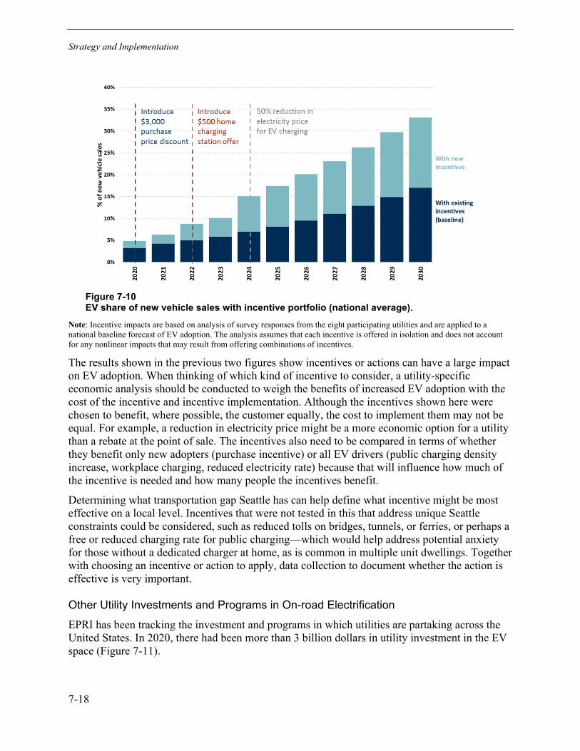
Strategy and Implementation
7-18
Figure 7-10 EV share of new vehicle sales with incentive portfolio (national average).
Note: Incentive impacts are based on analysis of survey responses from the eight participating utilities and are applied to a national baseline forecast of EV adoption. The analysis assumes that each incentive is offered in isolation and does not account for any nonlinear impacts that may result from offering combinations of incentives.
The results shown in the previous two figures show incentives or actions can have a large impact on EV adoption. When thinking of which kind of incentive to consider, a utility-specific economic analysis should be conducted to weigh the benefits of increased EV adoption with the cost of the incentive and incentive implementation. Although the incentives shown here were chosen to benefit, where possible, the customer equally, the cost to implement them may not be equal. For example, a reduction in electricity price might be a more economic option for a utility than a rebate at the point of sale. The incentives also need to be compared in terms of whether they benefit only new adopters (purchase incentive) or all EV drivers (public charging density increase, workplace charging, reduced electricity rate) because that will influence how much of the incentive is needed and how many people the incentives benefit.
Determining what transportation gap Seattle has can help define what incentive might be most effective on a local level. Incentives that were not tested in this that address unique Seattle constraints could be considered, such as reduced tolls on bridges, tunnels, or ferries, or perhaps a free or reduced charging rate for public charging—which would help address potential anxiety for those without a dedicated charger at home, as is common in multiple unit dwellings. Together with choosing an incentive or action to apply, data collection to document whether the action is effective is very important.
Other Utility Investments and Programs in On-road Electrification
EPRI has been tracking the investment and programs in which utilities are partaking across the United States. In 2020, there had been more than 3 billion dollars in utility investment in the EV space (Figure 7-11).
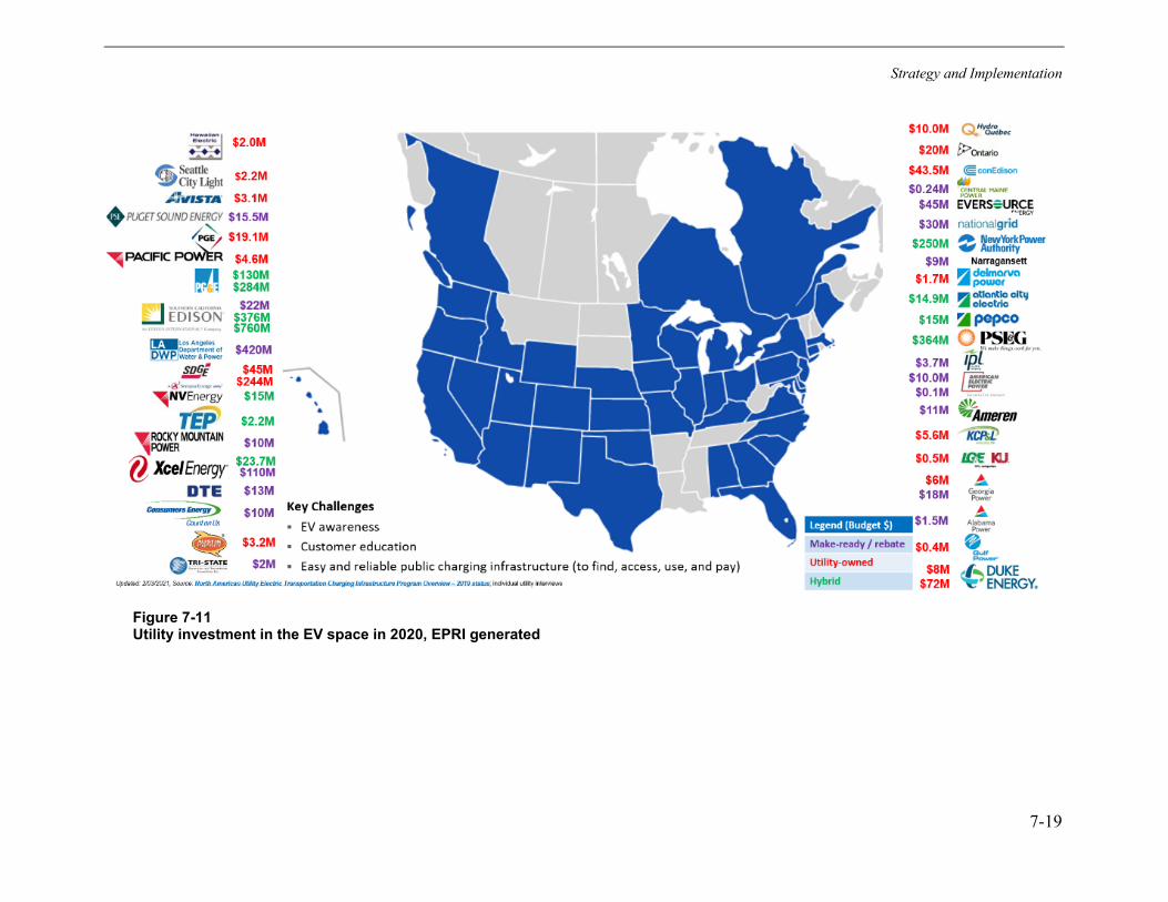
Strategy and Implementation
7-19
Figure 7-11 Utility investment in the EV space in 2020, EPRI generated

Strategy and Implementation
7-20
More information on specific utility programs can be found in the North American Utility Electric Transportation Charging Infrastructure Program Overview;127 however, some examples include:
• Rebates for installation, network fees, and purchase of public L2 and DCFC (10% low income) [Example from AEP, OH]
• Corridor DCFC funding [Example from Alabama Power]
• Incentives for workplace charging [Avista, WA and many others]
• Incentive in exchange for charging data [Smart Charging Infrastructure Pilot, Dominion, VA]
• Incentives available for installation of DCFC chargers for MDHD fleets [Medium-Heavy Duty Fleet Pilot make-ready program, ConEd]
• Incentive for enrollment in a demand response program [EE/DR Program, Dominion, VA]
• Funds for customer education [DTE and many others]
• Electric school bus rebate program [Duke Energy, OH]
• On-bill financing for public and home EV charging infrastructure [Gulf Power, FL]
• Low- to moderate-income home sales incentives to cover panel upgrade costs for L2 charging equipment [PG&E]
Each utility is different, so looking at some other examples of potentially similar utilities may be useful as SCL thinks about what next steps may be pertinent. Utility programs are widely varying and range from a $50 dollar gift card offered to any EV sold at a vehicle dealership in exchange for the vehicle buyers’address, contact info and vehicle information, to smart charging incentives to help manage EV load. Although a smart charging incentive seems like it would not directly affect EV adoption rates, a happy customer who can boast about money saved by changing EV charging habits can only help knowledge transfer among work colleagues, neighbors, and friends—a good way to spread EV knowledge.
EPRI is working with utilities (under the program ETIPS, or Electric Transportation Infrastructure Program Support) to help identify what role they should play in the EV market and types of program design options that support the chosen role. From this work, a set of guiding principles is defined to help guide future program design. This might be a possible next step for SCL to outline a future program design.
127 https://www.epri.com/research/products/000000003002020283
Strategy and Implementation
7-21
Strategies for Increasing Heat Pump Adoption in Buildings Some strategies to increase adoption of heat pumps in the space and water heating market include the following:
• To increase market growth for these heat pump technologies, higher first costs may be addressed where applicable via utility and local or federal incentives.
• Education on equipment benefits may be used for contractors/installers who are the touch point for customers.
• Additional education and training for equipment installers and maintenance personnel will help ensure customer satisfaction through optimally operating equipment.
• Heat pump campaigns can be set up in conjunction with big box retailers and the manufacturers.
Similar to the residential market, the majority of space and water heating in commercial spaces is provided by fossil-fueled equipment, primarily natural-gas-fueled, but also including a small amount of distillate fuel oil and propane. Although commercial customers’ natural gas prices tend to be lower than residential, electric technologies still tend to be more cost-competitive with fuel oil or propane in the commercial sector.
To increase market capture for these heat pump technologies, higher first costs may be addressed where applicable, possibly through incentives to customers. However, as mentioned before, a split incentive barrier exists for commercial spaces and multiple unit dwellings where the building owner purchases the equipment while the occupant realizes any energy savings.
Strategies for Increasing Commercial Cooking Electrification The strategies to increase adoption for cooking equipment include:
• Education of equipment suppliers as well as customers is needed to understand the benefits of electric equipment. As with other process-specific equipment, a detailed assessment of the impacts and benefits of electric equipment instead of gas should be considered.
• SCL may want to work with local contractors to encourage specification of electric equipment in kitchen design. Demonstration of equipment and resulting product quality is a powerful tool to encourage adoption of electric equipment. For example, Alabama Power has a demonstration kitchen at its Technology Applications Center (TAC) located near Birmingham128 where it invites its customers to test its sample products with electric cooking equipment to compare the results.
• Incentives may be useful in reducing the first costs for adoption of electric equipment for the customer. Small incentives to equipment providers can help encourage electric as an option for customers as well as helping to track electric sales.
128 Source: https://www.alabamapower.com/business/business-customers-and-services/food-service.html
Strategy and Implementation
7-22
Strategies for Increasing Electrification in Industrial Process Heating The strategies to increase adoption of industrial process heating equipment include:
• Strategies to help reduce the lack of upfront capital impact include: – Aligning with “third-party” financing/leasing companies. – Working with vendors that provide leasing options for the sale of their equipment. – In certain cases, utilities have provided financing options for customers including third-
party leasing arrangement for this equipment.
• Strategies to help reduce the barrier of long sales cycle include: – Developing strong technology vendor relationships. – Creating marketing materials including robust examples of related case studies and
technology applications. – Engaging key customer decision makers throughout the sales cycle.
• Strategies to mitigate the barrier of resistance to adopt technologies include: – Aligning with vendors that can model the customer’s production using the electric
technology. – Working with vendors and other utilities to find similar customer applications that are
currently operating. – A strategy to mitigate the barrier of equipment downtime can be engaging the customer
from the beginning and helping them install the equipment in phases to minimize operational disruptions.
Strategies for Increasing Adoption of Non-road Electric Transportation Technologies Strategies to overcome market barriers for non-road electric transportation technologies are as follows:
• To increase adoption of electric forklifts, SCL can help by increasing end-use awareness, offering incentives, offering technical support to customers and dealers, and leveraging existing communication channels between technology manufacturers, dealers, and end users—an important aspect during program implementation. These are general next steps that may be applied to increase non-road electric transportation technologies adoption.
• For electric forklifts, training and educating account managers about the details of the program along with program goals, and training and educating employees about the program to help facilitate the message to customers and end users.
• Leveraging existing relationships between account managers and key commercial and, in the case of forklifts, industrial accounts to help with scheduling of meetings and presentations with customers and targeted end users.

Strategy and Implementation
7-23
• To increase customer confidence and reduce perceived risk of electric technologies, SCL may consider marketing that emphasizes the high reliability of electric service and, where applicable, the low volatility of electricity prices.
• SCL may also consider sponsoring a demonstration facility to conduct blind testing or to provide unbiased technology evaluations, similar to what Southern Company provides for customers at its TAC (Alabama Power).
• SCL can develop a process for vetting a select group of vendors that serve these markets and working closely with them to reach customers. Joint marketing plans and goals may be developed with interested vendors to encourage a structured approach to market capture.
Defining what metrics are helpful to measure program effectiveness is necessary. Table F-1 outlines some of the EPRI-suggested actions and metrics and how to define success for each metric. Unlike energy efficiency programs that are well established in the industry, the electrification programs are relatively new. These actions are not part of implementation plans from other utilities, but rather recommendations based on discussions with several utilities in the Electrification program on the steps that could lead to a successful outcome.
Conclusion In summary, the development of effective electrification programs is a journey, and the establishment of program teams ensures focused engagements while the technologies are new and need more support while they are still unfamiliar. The experience gained from the successful implementations results in higher confidence level for the staff and helps in the scaling efforts of the electrification of the technologies. By focusing on the areas with lower electric technology adoption, insights will be gained on strategies that work and those that do not. The strategies described here should be revisited after a few years to make necessary changes to reflect positive outcomes. The effectiveness of many programs will depend on the resources allocated to their execution. A customer team that can respond quickly to support the customer will further encourage adoption through these great experiences and word of mouth. Effective programs that target the metrics in Table F-1 will build long-term benefits for a member utility, its customers, and stakeholders.

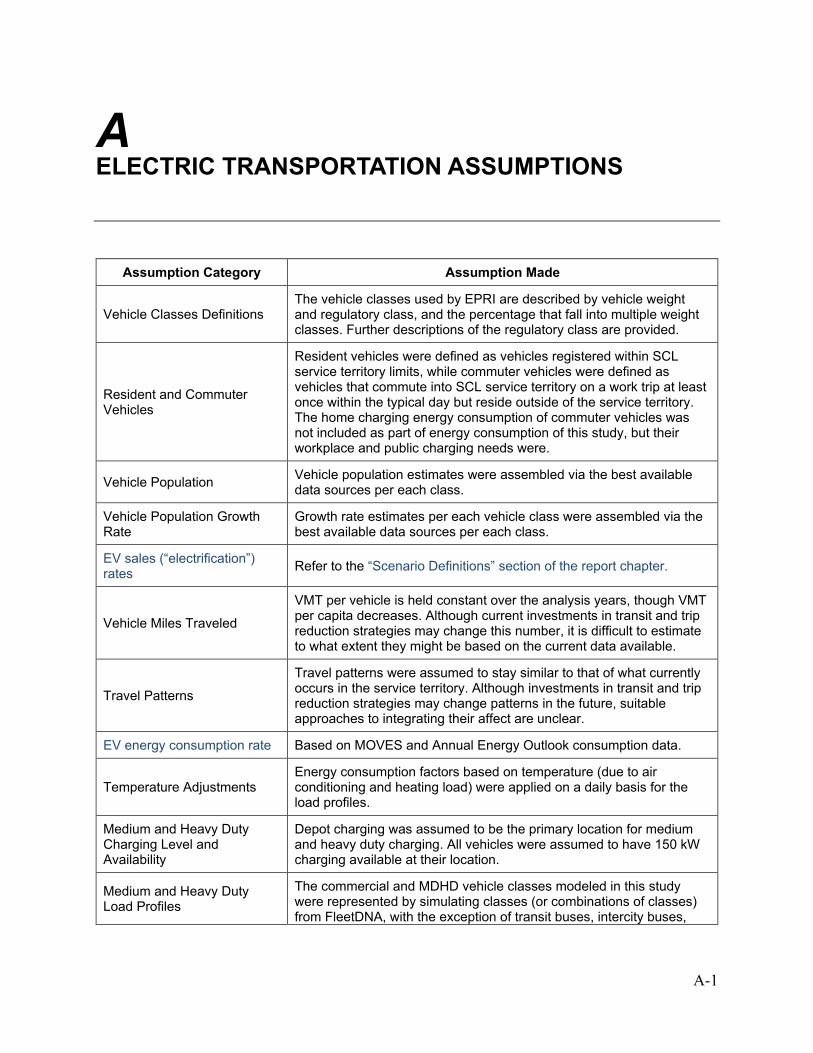
A-1
A ELECTRIC TRANSPORTATION ASSUMPTIONS
Assumption Category Assumption Made
Vehicle Classes Definitions The vehicle classes used by EPRI are described by vehicle weight and regulatory class, and the percentage that fall into multiple weight classes. Further descriptions of the regulatory class are provided.
Resident and Commuter Vehicles
Resident vehicles were defined as vehicles registered within SCL service territory limits, while commuter vehicles were defined as vehicles that commute into SCL service territory on a work trip at least once within the typical day but reside outside of the service territory. The home charging energy consumption of commuter vehicles was not included as part of energy consumption of this study, but their workplace and public charging needs were.
Vehicle Population Vehicle population estimates were assembled via the best available data sources per each class.
Vehicle Population Growth Rate
Growth rate estimates per each vehicle class were assembled via the best available data sources per each class.
EV sales (“electrification”) rates Refer to the “Scenario Definitions” section of the report chapter.
Vehicle Miles Traveled
VMT per vehicle is held constant over the analysis years, though VMT per capita decreases. Although current investments in transit and trip reduction strategies may change this number, it is difficult to estimate to what extent they might be based on the current data available.
Travel Patterns
Travel patterns were assumed to stay similar to that of what currently occurs in the service territory. Although investments in transit and trip reduction strategies may change patterns in the future, suitable approaches to integrating their affect are unclear.
EV energy consumption rate Based on MOVES and Annual Energy Outlook consumption data.
Temperature Adjustments Energy consumption factors based on temperature (due to air conditioning and heating load) were applied on a daily basis for the load profiles.
Medium and Heavy Duty Charging Level and Availability
Depot charging was assumed to be the primary location for medium and heavy duty charging. All vehicles were assumed to have 150 kW charging available at their location.
Medium and Heavy Duty Load Profiles
The commercial and MDHD vehicle classes modeled in this study were represented by simulating classes (or combinations of classes) from FleetDNA, with the exception of transit buses, intercity buses,

Electric Transportation Assumptions
A-2
Assumption Category Assumption Made and long-haul trucks, for which load profiles were estimated using a different method.
Long Haul Vehicles Long haul charging load is assumed to be equal to the energy used within Seattle.
Home Charging Level The majority of home charging is assumed to be 6.6 kW, with some Level 1 (1.44 kW) and Level 2 (19.2 kW)
Home Charging Availability Access to home charging across the electric vehicle population was assumed to vary by year.
Workplace Charging Level All workplace chargers are assumed to provide 6.6 kW of charging.
Workplace Charging Availability
Workplace charging was assumed to increase from 10% availability in 2020 to 40% availability in 2030 and staying constant thereafter.
Public Charging Level Public charging availability varied but included 6.6 kW and 19.2 kW at destinations and 50 kW and 250 kW for en route charging.
Public Charging Availability Public charging probabilities were modeled to vary over time as a function of EV type, vehicle class (car or truck), and access to home charging.
En Route Charging Level For passenger cars and trucks, available power via en route charging is modeled to increase gradually over time.
En Route Charging Availability
Long range BEVs will use en route charging as needed, while PHEVs do not.
BEV/PHEV Distribution 90% of EVs will be BEVs; the remaining are PHEVs.

B-1
B ELECTRIC TRANSPORTATION LOAD PROFILES
Load Profile Simulation Process
Travel Data Four sets of travel data were used for different aspects of this study. As discussed in the report, these are:
• PSRC 2017–2019 travel surveys – Weekday passenger vehicle travel
• NHTS 2017 – Weekend passenger vehicle travel
• FleetDNA – Commercial and MDHD travel
• WSDOT road sensor data from 2019 – Long-haul travel
The PSRC travel surveys provide a rich and localized set of passenger vehicle travel data for weekdays but were not designed to capture weekend travel. Although NHTS is not localized, it is a long-trusted survey that was designed to capture both weekend and weekday travel at a national level. Travel data for commercial trucks and MDHD vehicles do not exist as public travel surveys on the scale of the PSRC and NHTS, but the National Renewable Energy Laboratory hosts a public data set of travel patterns representing several commercial and MDHD classes (FleetDNA).
The commercial and MDHD vehicle classes modeled in this study were represented by simulating classes (or combinations of classes) from FleetDNA, with the exception of transit buses, intercity buses, and long-haul trucks, for which load profiles were estimated using a different method. The sources for charging load for LCT/MDHD are detailed in Table B-1.

ELectric Transportation Load Profiles
B-2
Table B-1 Methods by which load profiles for each LCT/MDHD vehicle class were obtained
Vehicle Class Charging Load Profile Source
Light Commercial Truck
Charging simulation using the FleetDNA
class to the right:
Straight Truck + Step Van Single-Unit Short-Haul Truck
Combination Short-Haul Truck Tractor
Refuse Truck Refuse Truck
School Bus School Bus
Transit Bus King County Metro charging profile
Intercity Bus
Long-haul charging profile Single-Unit Long-Haul Truck
Combination Long-Haul Truck
Charging Simulation The charging simulation, which takes travel data as input, proceeds in three phases: initialization, simulation, and aggregation. Each phase is detailed in the sections below.
Initialization Phase In the initialization phase, input data are filtered and prepared for simulation. Input data must include, at minimum, the columns listed in Table B-2, where each row represents a single trip record. Filtering removes records with missing or implausible data (for example, a distance of 1000 miles during a trip lasting 10 minutes). Data are organized in chronological order and grouped by vehicle.
Table B-2 Data required as input to charging simulation tool
Column Description
Trip Start Datetime Date and time of departure from origin
Trip End Datetime Date and time of arrival at destination
Trip Distance Travel distance between origin and destination
Vehicle Identifier Unique identifier for individual vehicles
Destination Location Category Home, workplace, public location
Weight Survey record weighting
The charging power available at every destination, and en route during each trip, is determined stochastically based on the access probabilities defined for a simulation.

ELectric Transportation Load Profiles
B-3
Simulation Phase In the simulation phase, the timing, duration, and energy provided during each charging session are determined. The energy provided via charging replenishes energy consumed while driving, which is determined as a function of distance and vehicles’ assumed energy consumption rate. Charging can occur en route, where vehicles stop at a charging station at some point during a trip, and at destinations.
Driving energy is allocated as electric energy, petroleum energy, or a mix of the two based on the availability of battery energy throughout the simulation for each vehicle. Petroleum energy is used only in two instances: 1) a PHEV has insufficient remaining AER to complete a trip using electric energy and 2) a BEV has insufficient remaining AER to complete a trip using electric energy. In Instance 1, the energy deficit is provided by burning fuel in the PHEV’s internal combustion engine (ICE). In Instance 2, the entire “trip chain” (sequence of trips beginning and ending at home) is assumed to be driven by an ICE-powered vehicle because the BEV range was insufficient to complete the chain with the charging available.
The available power en route and at each destination was determined during initialization. Charging behavior differs slightly for en route and destination charging. At a destination, vehicles are simulated to charge at the available power for as long as possible, beginning immediately upon arrival. Charging ends when the battery is fully charged or the vehicle departs on its next trip. In contrast, a vehicle will stop for en route charging only if its battery state of charge (SOC) falls below a specified threshold (10% for 250-mile BEVs, 20% for 100-mile BEVs) and will stop charging when the battery SOC reaches 80%. The time at which en route charging starts is chosen at random between the time when SOC reaches the lower (10% or 20%) threshold and when it would be fully depleted (or arrive at the destination).
Aggregation Phase The key outcome of the simulation phase is the timing and power level of every charging session for every vehicle. These are used in the aggregation phase to construct average per-vehicle charging profiles.
This average per-vehicle charging profile is the total aggregate charging load for a simulation divided by the total population of vehicles, including undriven vehicles (for data from travel surveys, vehicles that were owned but not operated during the survey window). The aggregate charging load is obtained by constructing a weighted sum of the individual charging session loads, regularized into a single 24-hour window. The weights for summing are from the travel surveys. For vehicles with data spanning multiple days, the summing weight is divided by the number of days of data so that the contribution to aggregate load is that vehicle’s mean daily charging load during the survey period.
Special Commercial and MDHD Cases Load profiles for some MDHD classes were estimated differently, separate from the charging simulation. Transit bus charging profiles were obtained directly from King County Metro. The unmanaged charging case, shown in red in Figure B-1, was scaled to match the expected energy per day per vehicle estimated from data described in the Electric Vehicle Population Projections and Annual Energy Consumption sections of the main text.
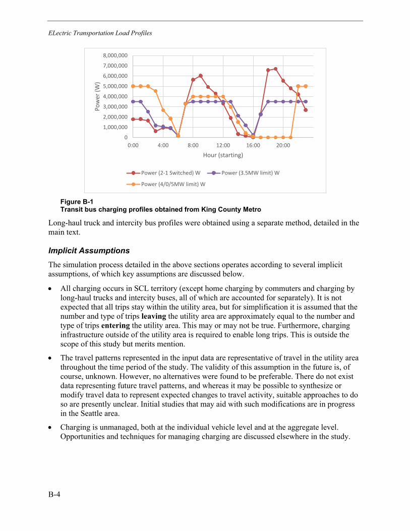
ELectric Transportation Load Profiles
B-4
Figure B-1 Transit bus charging profiles obtained from King County Metro
Long-haul truck and intercity bus profiles were obtained using a separate method, detailed in the main text.
Implicit Assumptions The simulation process detailed in the above sections operates according to several implicit assumptions, of which key assumptions are discussed below.
• All charging occurs in SCL territory (except home charging by commuters and charging by long-haul trucks and intercity buses, all of which are accounted for separately). It is not expected that all trips stay within the utility area, but for simplification it is assumed that the number and type of trips leaving the utility area are approximately equal to the number and type of trips entering the utility area. This may or may not be true. Furthermore, charging infrastructure outside of the utility area is required to enable long trips. This is outside the scope of this study but merits mention.
• The travel patterns represented in the input data are representative of travel in the utility area throughout the time period of the study. The validity of this assumption in the future is, of course, unknown. However, no alternatives were found to be preferable. There do not exist data representing future travel patterns, and whereas it may be possible to synthesize or modify travel data to represent expected changes to travel activity, suitable approaches to do so are presently unclear. Initial studies that may aid with such modifications are in progress in the Seattle area.
• Charging is unmanaged, both at the individual vehicle level and at the aggregate level. Opportunities and techniques for managing charging are discussed elsewhere in the study.
0
1,000,000
2,000,000
3,000,000
4,000,000
5,000,000
6,000,000
7,000,000
8,000,000
0:00 4:00 8:00 12:00 16:00 20:00
Pow
er (W
)
Hour (starting)
Power (2-1 Switched) W Power (3.5MW limit) W
Power (4/0/5MW limit) W

ELectric Transportation Load Profiles
B-5
Detailed Assumptions
Charging Power Access Probabilities The charging power available to simulated vehicles at every stop, and between stops, is determined probabilistically. This process is dictated by a set of assumed probabilities, which are defined as a function of EV type, vehicle class, home charging access, and year, for every type of location. The relevant set of probabilities is applied at each stop to determine power level. This means that, if the probability of workplace charging at 6.6 kW is 40%, vehicles will charge at 6.6 kW at approximately 40% of workplace stops. An example set of probabilities, for home charging by cars in 2030, is shown in Table B-3 and illustrated in Figure B-2.
Table B-3 Example set of charging probabilities (home charging by cars in 2030). More probabilities were assumed for other subpopulations and charging locations.
Charge Power (kW)
0 1.44 6.6 19.2 50 150 350
EV Type
PHEV10 0 0.27 0.73 0 0 0 0
PHEV20 0 0.27 0.73 0 0 0 0
PHEV40 0 0.27 0.73 0 0 0 0
BEV100 0 0.27 0.73 0 0 0 0
BEV250 0 0.27 0.63 0.1 0 0 0
Figure B-2 Illustration of charging probability assumptions used for passenger cars in 2030. Probabilities vary with respect to home charging access, EV type, power level, and charging location. Additional probability assumptions apply in other years and for passenger trucks.

ELectric Transportation Load Profiles
B-6
Home Charging Home charging access probabilities were estimated based on the results of ongoing vehicle tracking studies and were assumed to stay constant over time for those who have access to home charging. (Those without home charging access always have a 100% probability of 0 kW available at home.) The most common charging capabilities installed in homes are Level 1 (1.44 kW), which is estimated to account for 27% of home charging, and low-power Level 2 (6.6 kW), which is estimated to account for the other 73% of home charging for most EV types. Owners of long-range BEVs may install high-power Level 2 (19.2 kW), which is assumed to displace a portion of low-power Level 2 to account for 10% of home charging, for long-range BEVs. Passenger truck BEVs are assumed to have slightly higher charging power availabilities than passenger cars so that 20% are Level 1, 60% are low-power Level 2, and 20% are high-power Level 2.
For commercial and MDHD vehicles, “home” charging (or depot charging) is the primary charging location. All vehicles are assumed to have 150-kW charging available at their home location. (Long-haul trucks, intercity buses, and transit buses are modeled differently.)
Workplace Charging Workplace charging access probabilities were estimated based on two factors: assumed availability of workplace charging in the future and the likelihood of drivers to use workplace charging if it is available. For EVs with access to home charging, the likelihood of charging at the workplace was assumed to be 10% in 2020, increasing to 40% in 2030 and staying constant thereafter, with all chargers assumed to provide 6.6 kW. However, it was also assumed that vehicles without access to home charging would always have access to, and use, workplace charging. The exceptions to this are BEV250s, which follow the same likelihoods for workplace charging (10% to 40%) regardless of access to home charging.
Public Charging The access probabilities for home and workplace charging can broadly be interpreted as (and are meant to represent) the probability that a given vehicle has a charger, at a specific power level, available at home or at work. In contrast, public charging probabilities encompass a broader set of considerations:
• Availability and suitable placement of charging stations: How many chargers exist? How are they placed relative to travel patterns? Do they require significant detouring to access?
• Behavior: Even if a charger is convenient and nearby, what is the probability that a driver will use it? What if they can just charge at home? If driving a PHEV, how important are electric miles to the driver?
• Pricing: How does the cost of charging in public compare to alternatives, such as home charging or powering a PHEV with fuel?
With these considerations in mind, public charging probabilities were modeled to vary over time as a function of EV type, vehicle class (car or truck), and access to home charging. In general, vehicles without access to home charging, with longer AER and higher rates of energy
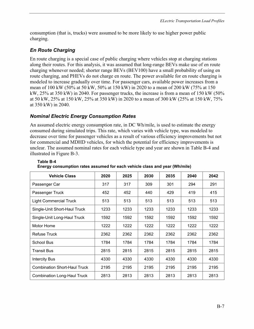
ELectric Transportation Load Profiles
B-7
consumption (that is, trucks) were assumed to be more likely to use higher power public charging.
En Route Charging En route charging is a special case of public charging where vehicles stop at charging stations along their routes. For this analysis, it was assumed that long-range BEVs make use of en route charging whenever needed; shorter range BEVs (BEV100) have a small probability of using en route charging, and PHEVs do not charge en route. The power available for en route charging is modeled to increase gradually over time. For passenger cars, available power increases from a mean of 100 kW (50% at 50 kW, 50% at 150 kW) in 2020 to a mean of 200 kW (75% at 150 kW, 25% at 350 kW) in 2040. For passenger trucks, the increase is from a mean of 150 kW (50% at 50 kW, 25% at 150 kW, 25% at 350 kW) in 2020 to a mean of 300 kW (25% at 150 kW, 75% at 350 kW) in 2040.
Nominal Electric Energy Consumption Rates An assumed electric energy consumption rate, in DC Wh/mile, is used to estimate the energy consumed during simulated trips. This rate, which varies with vehicle type, was modeled to decrease over time for passenger vehicles as a result of various efficiency improvements but not for commercial and MDHD vehicles, for which the potential for efficiency improvements is unclear. The assumed nominal rates for each vehicle type and year are shown in Table B-4 and illustrated in Figure B-3.
Table B-4 Energy consumption rates assumed for each vehicle class and year (Wh/mile)
Vehicle Class 2020 2025 2030 2035 2040 2042
Passenger Car 317 317 309 301 294 291
Passenger Truck 452 452 440 429 419 415
Light Commercial Truck 513 513 513 513 513 513
Single-Unit Short-Haul Truck 1233 1233 1233 1233 1233 1233
Single-Unit Long-Haul Truck 1592 1592 1592 1592 1592 1592
Motor Home 1222 1222 1222 1222 1222 1222
Refuse Truck 2362 2362 2362 2362 2362 2362
School Bus 1784 1784 1784 1784 1784 1784
Transit Bus 2815 2815 2815 2815 2815 2815
Intercity Bus 4330 4330 4330 4330 4330 4330
Combination Short-Haul Truck 2195 2195 2195 2195 2195 2195
Combination Long-Haul Truck 2813 2813 2813 2813 2813 2813
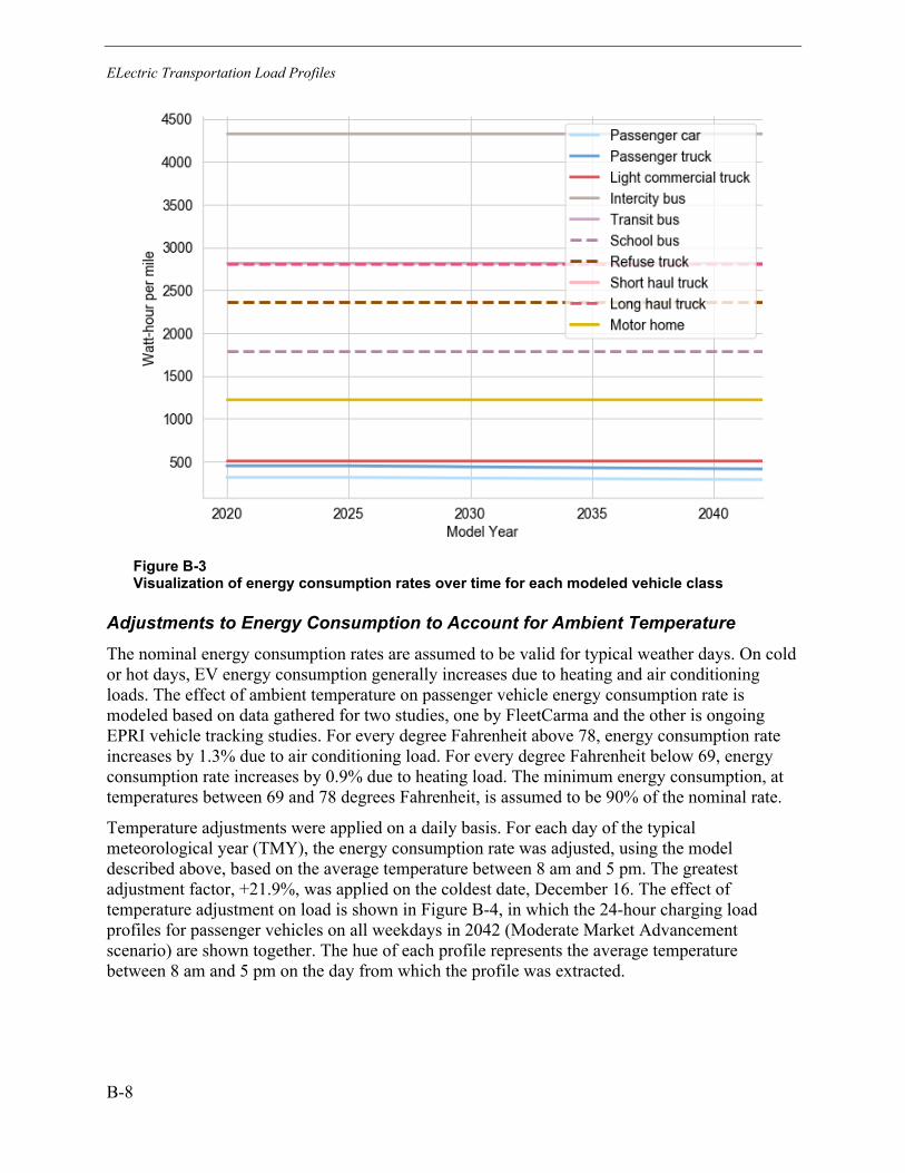
ELectric Transportation Load Profiles
B-8
Figure B-3 Visualization of energy consumption rates over time for each modeled vehicle class
Adjustments to Energy Consumption to Account for Ambient Temperature The nominal energy consumption rates are assumed to be valid for typical weather days. On cold or hot days, EV energy consumption generally increases due to heating and air conditioning loads. The effect of ambient temperature on passenger vehicle energy consumption rate is modeled based on data gathered for two studies, one by FleetCarma and the other is ongoing EPRI vehicle tracking studies. For every degree Fahrenheit above 78, energy consumption rate increases by 1.3% due to air conditioning load. For every degree Fahrenheit below 69, energy consumption rate increases by 0.9% due to heating load. The minimum energy consumption, at temperatures between 69 and 78 degrees Fahrenheit, is assumed to be 90% of the nominal rate.
Temperature adjustments were applied on a daily basis. For each day of the typical meteorological year (TMY), the energy consumption rate was adjusted, using the model described above, based on the average temperature between 8 am and 5 pm. The greatest adjustment factor, +21.9%, was applied on the coldest date, December 16. The effect of temperature adjustment on load is shown in Figure B-4, in which the 24-hour charging load profiles for passenger vehicles on all weekdays in 2042 (Moderate Market Advancement scenario) are shown together. The hue of each profile represents the average temperature between 8 am and 5 pm on the day from which the profile was extracted.

ELectric Transportation Load Profiles
B-9
Figure B-4 Total passenger EV charging load for every day in the year 2042 shown on the same axes. Load profiles are shown in different colors depending on the average temperature of the day on which they occur (measured between 8 am and 5 pm).
For commercial and MDHD vehicles, the same model for temperature adjustment was applied but was scaled differently as a function of vehicle class. Relative to passenger vehicles, the heating and air conditioning loads for most MDHD classes make up a smaller proportion of total energy consumption. The exceptions to this are transit and school buses, which have large cabins with frequent entry and exit and therefore high climate control loads. To model this, the temperature adjustment factor for all commercial and MDHD classes except transit and school buses was scaled by 0.25. Transit and school bus temperature adjustments were doubled relative to passenger adjustment values. Because transit and school buses make up a small proportion of the 2042 fleet, the variation in load profile due to temperature is small, as shown in Figure B-5.
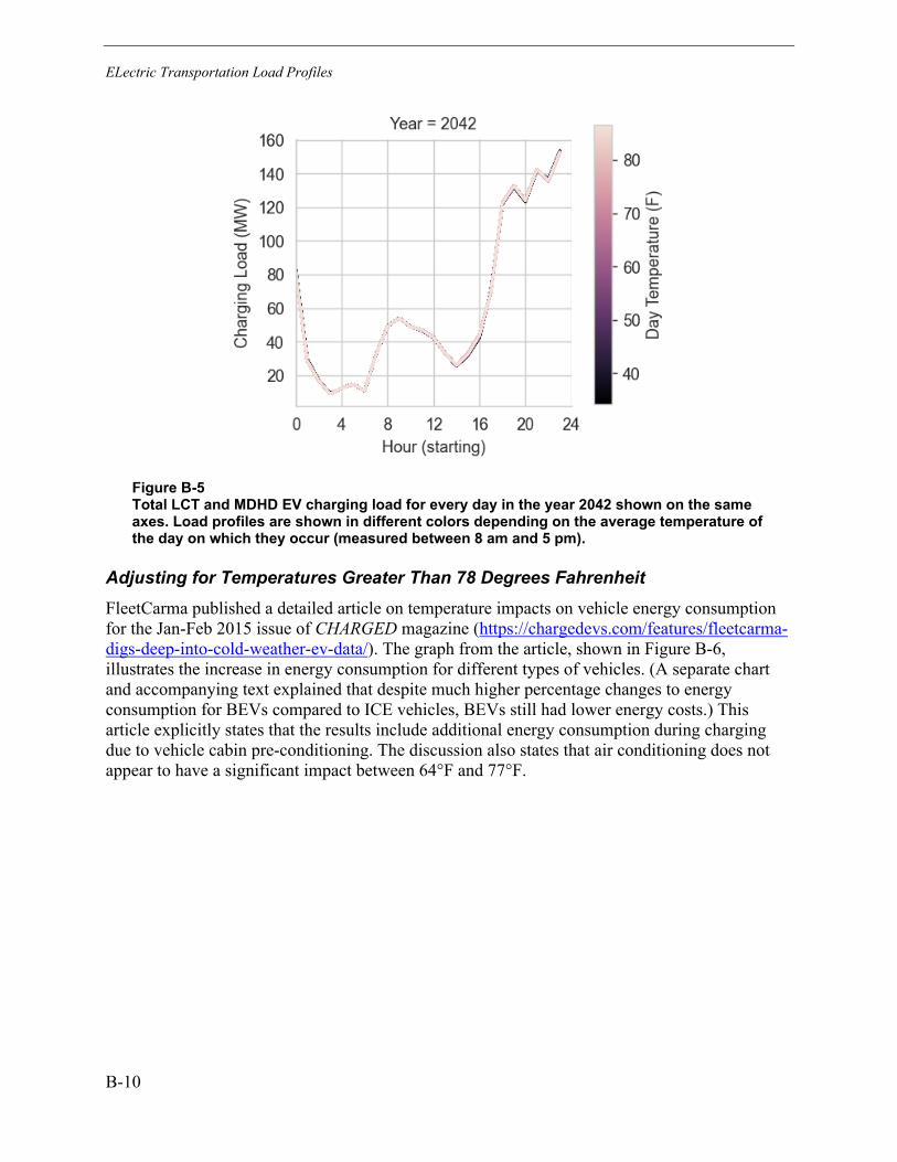
ELectric Transportation Load Profiles
B-10
Figure B-5 Total LCT and MDHD EV charging load for every day in the year 2042 shown on the same axes. Load profiles are shown in different colors depending on the average temperature of the day on which they occur (measured between 8 am and 5 pm).
Adjusting for Temperatures Greater Than 78 Degrees Fahrenheit FleetCarma published a detailed article on temperature impacts on vehicle energy consumption for the Jan-Feb 2015 issue of CHARGED magazine (https://chargedevs.com/features/fleetcarma-digs-deep-into-cold-weather-ev-data/). The graph from the article, shown in Figure B-6, illustrates the increase in energy consumption for different types of vehicles. (A separate chart and accompanying text explained that despite much higher percentage changes to energy consumption for BEVs compared to ICE vehicles, BEVs still had lower energy costs.) This article explicitly states that the results include additional energy consumption during charging due to vehicle cabin pre-conditioning. The discussion also states that air conditioning does not appear to have a significant impact between 64°F and 77°F.
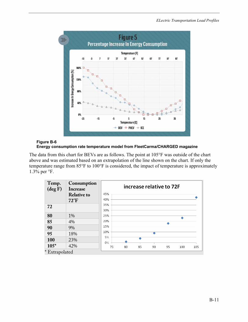
ELectric Transportation Load Profiles
B-11
Figure B-6 Energy consumption rate temperature model from FleetCarma/CHARGED magazine
The data from this chart for BEVs are as follows. The point at 105°F was outside of the chart above and was estimated based on an extrapolation of the line shown on the chart. If only the temperature range from 85°F to 100°F is considered, the impact of temperature is approximately 1.3% per °F.
Temp. (deg F)
Consumption Increase Relative to 72°F
72
80 1% 85 4% 90 9% 95 18% 100 23% 105* 42%
* Extrapolated

ELectric Transportation Load Profiles
B-12
Adjusting for Temperatures Less Than 69 Degrees Fahrenheit Ongoing EPRI analysis indicates some representation of consumption at lower temperatures and was used to estimate the temperature adjustment model for temperatures below 69 degrees. Depending on EV type, vehicles exhibited rates of temperature dependence from 0.8% to 1.1% per degree below 69, as shown in Figure B-7. The adjustment factor was chosen to be 0.9% per degree below 69 degrees Fahrenheit.
Figure B-7 Linear models of energy consumption change as a function of temperature for separate groups of vehicles in the Southern study
Accounting for Commuter Travel Approximately 20% of travel in the SCL territory is commuter activity. To account for this, it is assumed that 20% of simulated passenger vehicles’ home charging occurs outside of SCL territory; that is, it does not contribute to the reported load profiles. Workplace, public, and en route activity, however, are assumed to be accurately represented by the travel survey, and therefore the load profiles for workplace and public charging are not adjusted to account for commuters.
Vehicle Class Definitions The vehicle classes used in this study are from EPA’s MOVES. These vehicle classes are based on vehicle activity, and classes are defined to capture groups of vehicles that have similar travel patterns. Because of this, some MOVES vehicle classes contain vehicles that belong in numerous gross vehicle weight rating (GVWR) categories. Table B-5 shows the breakdown of MOVES vehicle classes by regulatory class, and Table B-6 shows regulatory class definitions with associated GVWR.
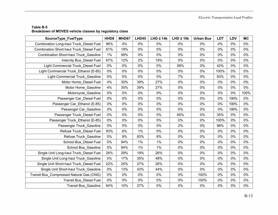
ELectric Transportation Load Profiles
B-13
Table B-5 Breakdown of MOVES vehicle classes by regulatory class
SourceType_FuelType HHD8 MHD67 LHD45 LHD ≤ 14k LHD ≤ 10k Urban Bus LDT LDV MC Combination Long-haul Truck_Diesel Fuel 96% 4% 0% 0% 0% 0% 0% 0% 0% Combination Short-haul Truck_Diesel Fuel 81% 19% 0% 0% 0% 0% 0% 0% 0%
Combination Short-haul Truck_Gasoline 1% 99% 0% 0% 0% 0% 0% 0% 0% Intercity Bus_Diesel Fuel 67% 12% 2% 19% 0% 0% 0% 0% 0%
Light Commercial Truck_Diesel Fuel 0% 0% 0% 0% 58% 0% 42% 0% 0% Light Commercial Truck_Ethanol (E-85) 0% 0% 0% 0% 0% 0% 100% 0% 0%
Light Commercial Truck_Gasoline 0% 0% 0% 0% 7% 0% 93% 0% 0% Motor Home_Diesel Fuel 4% 30% 39% 27% 0% 0% 0% 0% 0%
Motor Home_Gasoline 4% 30% 39% 27% 0% 0% 0% 0% 0% Motorcycle_Gasoline 0% 0% 0% 0% 0% 0% 0% 0% 100%
Passenger Car_Diesel Fuel 0% 0% 0% 0% 0% 0% 0% 100% 0% Passenger Car_Ethanol (E-85) 0% 0% 0% 0% 0% 0% 0% 100% 0%
Passenger Car_Gasoline 0% 0% 0% 0% 0% 0% 0% 100% 0% Passenger Truck_Diesel Fuel 0% 0% 0% 0% 65% 0% 35% 0% 0%
Passenger Truck_Ethanol (E-85) 0% 0% 0% 0% 0% 0% 100% 0% 0% Passenger Truck_Gasoline 0% 0% 0% 0% 2% 0% 98% 0% 0%
Refuse Truck_Diesel Fuel 93% 6% 1% 0% 0% 0% 0% 0% 0% Refuse Truck_Gasoline 0% 9% 83% 8% 0% 0% 0% 0% 0% School Bus_Diesel Fuel 5% 94% 1% 1% 0% 0% 0% 0% 0%
School Bus_Gasoline 5% 94% 1% 1% 0% 0% 0% 0% 0% Single Unit Long-haul Truck_Diesel Fuel 26% 29% 19% 26% 0% 0% 0% 0% 0%
Single Unit Long-haul Truck_Gasoline 0% 17% 35% 48% 0% 0% 0% 0% 0% Single Unit Short-haul Truck_Diesel Fuel 22% 25% 27% 26% 0% 0% 0% 0% 0%
Single Unit Short-haul Truck_Gasoline 0% 13% 43% 44% 0% 0% 0% 0% 0% Transit Bus_Compressed Natural Gas (CNG) 0% 0% 0% 0% 0% 100% 0% 0% 0%
Transit Bus_Diesel Fuel 0% 0% 0% 0% 0% 100% 0% 0% 0% Transit Bus_Gasoline 64% 10% 27% 0% 0% 0% 0% 0% 0%

ELectric Transportation Load Profiles
B-14
Table B-6 Vehicle class regulatory names and definitions
Regulatory Class Name Description
MC Motorcycles
LDV Light-Duty Vehicles
LDT Light-Duty Trucks
Urban Bus Urban Bus
LHD <= 10k Class 2b Trucks with 2 Axles and 4 Tires (8,500 lb < GVWR <= 10,000 lb)
LHD <= 14k Class 2b Trucks with 2 Axles and at least 6 Tires or Class 3 Trucks (8,500 lb < GVWR <= 14,000 lb)
LHD45 Class 4 and 5 Trucks (14,000 lb < GVWR <= 19,500 lb)
MHD67 Class 6 and 7 Trucks (19,500 lb < GVWR <= 33,000 lb)
HHD8 Class 8a and 8b Trucks (GVWR > 33,000 lb)
Sources for Vehicle Population, Growth Rate, and VMT Data Data for the vehicle population, growth rate, and VMT were assembled across multiple sources, as stated in the section Vehicle Population, Charging Infrastructure, and Activity Data. Table B-7 is included below for reference.
Table B-7 Data Sources
Vehicle Classes Base Year Population
Vehicle Population Growth Rate VMT
Passenger Vehicle PSRC PSRC EPA NEI
Light Commercial Truck PSRC PSRC EPA NEI
Single Unit Short Haul Truck EPA NEI DOE AEO EPA NEI
Combination Short Haul Truck EPA NEI DOE AEO EPA NEI
Refuse Truck WM/Recology DOE AEO EPA NEI
School Bus Seattle Schools DOE AEO EPA NEI
Transit Bus King County Metro DOE AEO EPA NEI
Intercity Bus King County Metro DOE AEO EPA NEI
Single Unit Long Haul Truck EPA NEI DOE AEO EPA NEI
Combination Long Haul Truck EPA NEI DOE AEO EPA NEI

ELectric Transportation Load Profiles
B-15
Passenger Vehicle BEV/PHEV Proportion Based on available registration data for the SCL service territory, in 2020, 87% of the EVs were BEVs, and the remaining 13% were PHEVs. This was used to determine the assumption that approximately 10% of the vehicle population would be PHEV in future years because approximately 18% of passenger vehicles are pickup trucks or larger SUVs in Seattle. The 100–150 mile range BEV is assumed to gain popularity as a lower cost option in the future. These assumptions remained the same for both the moderate and rapid scenarios.
Figure B-8 BEV/PHEV Proportions of New EV Sales
eVMT by Scenario, Vehicle Class, and Year The electrified vehicle miles traveled and total vehicle miles traveled estimates for both scenarios by year and class are presented in Table B-8. eVMT refers to electrified VMT—the portion of total miles in the full vehicle fleet that has been electrified.
Table B-8 eVMT, in millions of miles, Moderate Market Advancement
Vehicle Class 2020 2025 2030 2035 2042 Passenger Vehicles 118.30 320.24 700.11 1105.98 1721.89
Light Commercial Truck 0.02 2.20 12.40 32.86 77.45 Intercity Bus 0.00 0.00 0.00 0.00 0.07 Transit Bus 0.04 1.33 5.01 15.41 49.64 School Bus 0.00 0.11 0.41 1.36 4.27
Refuse Truck 0.00 0.01 0.12 0.32 0.83 Single-Unit Short Haul Truck 0.01 1.50 8.98 25.05 67.72 Single-Unit Long Haul Truck 0.00 0.00 0.04 0.23 1.17
Motor Home 0.00 0.00 0.02 0.10 0.48 Combination Short Haul Truck 0.00 0.60 3.49 9.63 24.66 Combination Long Haul Truck 0.00 0.00 0.84 4.04 16.72

ELectric Transportation Load Profiles
B-16
Table B-9 eVMT, in millions of miles, Rapid Market Advancement
Vehicle Class 2020 2025 2030 2035 2042
Passenger Vehicles 127.23 550.81 1969.31 3730.57 5774.47
Light Commercial Truck 0.04 10.21 101.22 199.54 302.87
Intercity Bus 0.00 0.00 0.00 0.08 0.78
Transit Bus 0.04 33.13 59.11 74.52 85.44
School Bus 0.00 2.75 5.07 6.62 7.31
Refuse Truck 0.00 0.10 1.03 2.05 3.33
Single-Unit Short Haul Truck 0.03 7.00 73.13 152.06 262.57
Single-Unit Long Haul Truck 0.00 0.01 0.11 0.66 4.07
Motor Home 0.00 0.01 0.06 0.28 1.58
Combination Short Haul Truck 0.00 2.99 29.20 58.96 96.75
Combination Long Haul Truck 0.00 0.40 2.66 10.87 54.04
Table B-10 Estimated VMT by vehicle class and year
Vehicle Class 2020 2025 2030 2035 2042
Passenger Vehicles 6372.0 6218.0 6615.0 6955.0 7351.0
Light Commercial Truck 271.6 300.1 335.2 356.5 372.7
Intercity Bus 3.5 3.8 4.3 4.6 5.1
Transit Bus 56.2 63.5 71.9 74.8 85.4
School Bus 5.0 5.3 6.2 6.6 7.3
Refuse Truck 3.0 3.4 3.8 4.1 4.4
Single-Unit Short Haul Truck 221.2 237.7 269.9 295.2 337.2
Single-Unit Long Haul Truck 13.2 14.3 15.9 17.1 19.7
Motor Home 5.2 5.5 6.1 6.7 7.6
Combination Short Haul Truck 95.1 104.0 112.8 119.1 128.4
Combination Long Haul Truck 182.3 212.9 245.7 264.7 279.5
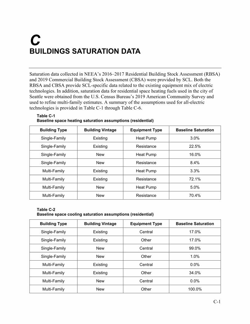
C-1
C BUILDINGS SATURATION DATA
Saturation data collected in NEEA’s 2016–2017 Residential Building Stock Assessment (RBSA) and 2019 Commercial Building Stock Assessment (CBSA) were provided by SCL. Both the RBSA and CBSA provide SCL-specific data related to the existing equipment mix of electric technologies. In addition, saturation data for residential space heating fuels used in the city of Seattle were obtained from the U.S. Census Bureau’s 2019 American Community Survey and used to refine multi-family estimates. A summary of the assumptions used for all-electric technologies is provided in Table C-1 through Table C-6.
Table C-1 Baseline space heating saturation assumptions (residential)
Building Type Building Vintage Equipment Type Baseline Saturation
Single-Family Existing Heat Pump 3.0%
Single-Family Existing Resistance 22.5%
Single-Family New Heat Pump 16.0%
Single-Family New Resistance 8.4%
Multi-Family Existing Heat Pump 3.3%
Multi-Family Existing Resistance 72.1%
Multi-Family New Heat Pump 5.0%
Multi-Family New Resistance 70.4%
Table C-2 Baseline space cooling saturation assumptions (residential)
Building Type Building Vintage Equipment Type Baseline Saturation
Single-Family Existing Central 17.0%
Single-Family Existing Other 17.0%
Single-Family New Central 99.0%
Single-Family New Other 1.0%
Multi-Family Existing Central 0.0%
Multi-Family Existing Other 34.0%
Multi-Family New Central 0.0%
Multi-Family New Other 100.0%
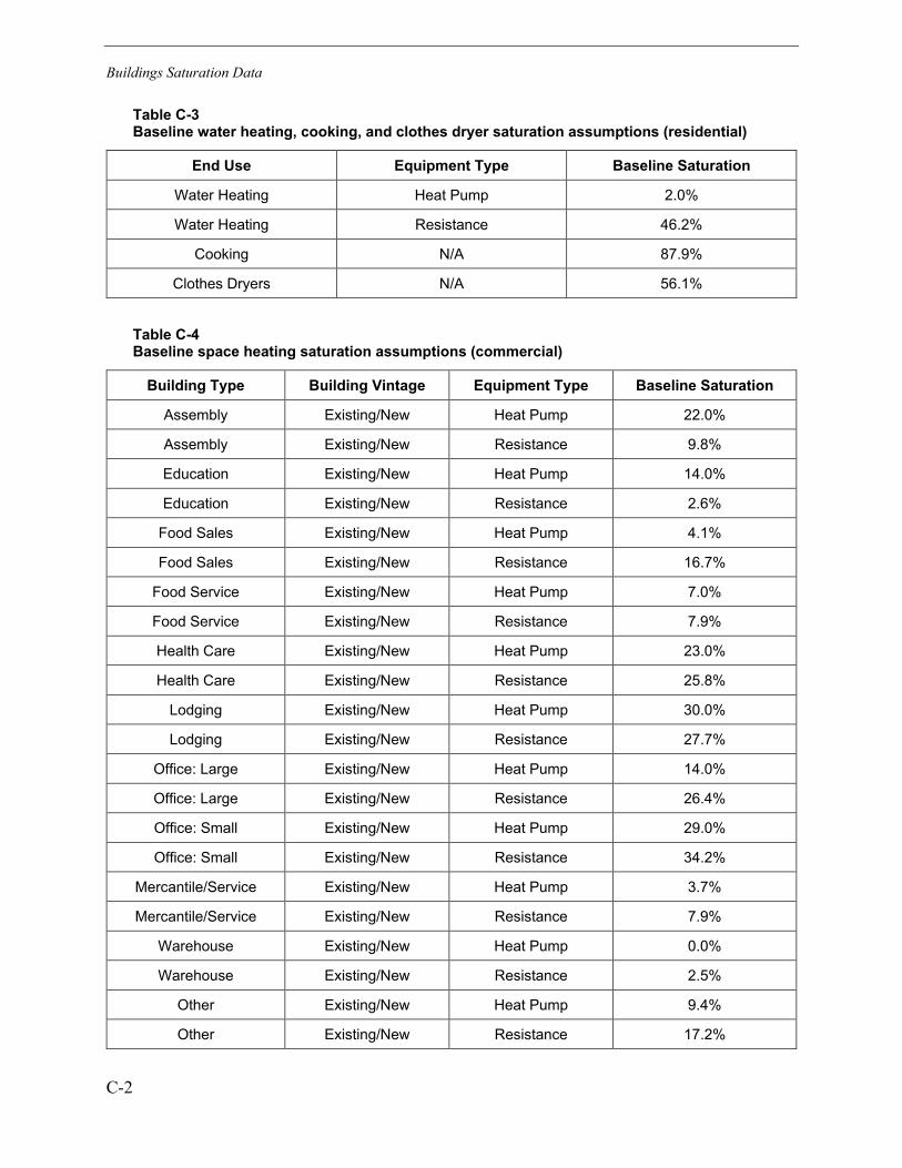
Buildings Saturation Data
C-2
Table C-3 Baseline water heating, cooking, and clothes dryer saturation assumptions (residential)
End Use Equipment Type Baseline Saturation
Water Heating Heat Pump 2.0%
Water Heating Resistance 46.2%
Cooking N/A 87.9%
Clothes Dryers N/A 56.1%
Table C-4 Baseline space heating saturation assumptions (commercial)
Building Type Building Vintage Equipment Type Baseline Saturation
Assembly Existing/New Heat Pump 22.0%
Assembly Existing/New Resistance 9.8%
Education Existing/New Heat Pump 14.0%
Education Existing/New Resistance 2.6%
Food Sales Existing/New Heat Pump 4.1%
Food Sales Existing/New Resistance 16.7%
Food Service Existing/New Heat Pump 7.0%
Food Service Existing/New Resistance 7.9%
Health Care Existing/New Heat Pump 23.0%
Health Care Existing/New Resistance 25.8%
Lodging Existing/New Heat Pump 30.0%
Lodging Existing/New Resistance 27.7%
Office: Large Existing/New Heat Pump 14.0%
Office: Large Existing/New Resistance 26.4%
Office: Small Existing/New Heat Pump 29.0%
Office: Small Existing/New Resistance 34.2%
Mercantile/Service Existing/New Heat Pump 3.7%
Mercantile/Service Existing/New Resistance 7.9%
Warehouse Existing/New Heat Pump 0.0%
Warehouse Existing/New Resistance 2.5%
Other Existing/New Heat Pump 9.4%
Other Existing/New Resistance 17.2%

Buildings Saturation Data
C-3
Table C-5 Baseline space cooling saturation assumptions (commercial)
Building Type Building Vintage Equipment Type Baseline Saturation
Assembly Existing/New Central 91.2%
Assembly Existing/New Other 2.7%
Education Existing/New Central 90.0%
Education Existing/New Other 1.5%
Food Sales Existing/New Central 90.4%
Food Sales Existing/New Other 0.0%
Food Service Existing/New Central 78.6%
Food Service Existing/New Other 16.8%
Health Care Existing/New Central 87.3%
Health Care Existing/New Other 0.0%
Lodging Existing/New Central 75.0%
Lodging Existing/New Other 19.4%
Office: Large Existing/New Central 92.1%
Office: Large Existing/New Other 0.0%
Office: Small Existing/New Central 91.8%
Office: Small Existing/New Other 3.3%
Mercantile/Service Existing/New Central 95.0%
Mercantile/Service Existing/New Other 2.0%
Warehouse Existing/New Central 76.6%
Warehouse Existing/New Other 6.4%
Other Existing/New Central 81.3%
Other Existing/New Other 5.2%
Table C-6 Baseline water heating and cooking saturation assumptions (commercial)
End Use Equipment Type Baseline Saturation
Water Heating Heat Pump 1.3%
Water Heating Resistance 55.3%
Cooking N/A 3.3%

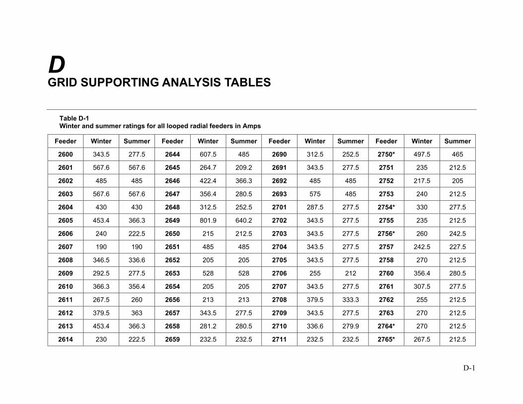
D-1
D GRID SUPPORTING ANALYSIS TABLES
Table D-1 Winter and summer ratings for all looped radial feeders in Amps
Feeder Winter Summer Feeder Winter Summer Feeder Winter Summer Feeder Winter Summer
2600 343.5 277.5 2644 607.5 485 2690 312.5 252.5 2750* 497.5 465
2601 567.6 567.6 2645 264.7 209.2 2691 343.5 277.5 2751 235 212.5
2602 485 485 2646 422.4 366.3 2692 485 485 2752 217.5 205
2603 567.6 567.6 2647 356.4 280.5 2693 575 485 2753 240 212.5
2604 430 430 2648 312.5 252.5 2701 287.5 277.5 2754* 330 277.5
2605 453.4 366.3 2649 801.9 640.2 2702 343.5 277.5 2755 235 212.5
2606 240 222.5 2650 215 212.5 2703 343.5 277.5 2756* 260 242.5
2607 190 190 2651 485 485 2704 343.5 277.5 2757 242.5 227.5
2608 346.5 336.6 2652 205 205 2705 343.5 277.5 2758 270 212.5
2609 292.5 277.5 2653 528 528 2706 255 212 2760 356.4 280.5
2610 366.3 356.4 2654 205 205 2707 343.5 277.5 2761 307.5 277.5
2611 267.5 260 2656 213 213 2708 379.5 333.3 2762 255 212.5
2612 379.5 363 2657 343.5 277.5 2709 343.5 277.5 2763 270 212.5
2613 453.4 366.3 2658 281.2 280.5 2710 336.6 279.9 2764* 270 212.5
2614 230 222.5 2659 232.5 232.5 2711 232.5 232.5 2765* 267.5 212.5

Grid Supporting Analysis Tables
D-2
Table D-1 (continued) Winter and summer ratings for all looped radial feeders in Amps
Feeder Winter Summer Feeder Winter Summer Feeder Winter Summer Feeder Winter Summer
2615 262.5 255 2660 528 528 2712 255 255 2768 294 277.5
2619 215 215 2663 425 425 2721 501.6 501.6 2774 215 215
2620 565 565 2664 485.1 485.1 2722 343.5 277.5 2775 227.5 227.5
2621 264 264 2665 300.3 300.3 2723 281.5 277.5 2776 300.3 300.3
2622 200 200 2666 273.9 273.9 2724 281.5 277.5 2777 200 200
2623 220 220 2667 250 250 2728 320 320 2778 270.6 270.6
2624** 485.1 485.1 2668** 452.1 452.1 2729 270 212.5 2779 215 215
2625 453.4 366.3 2669 452.5 452.5 2731 453.4 366.3 2780 215 215
2626 275 275 2672 343.5 277.5 2732 371.6 366.3 2781 215 215
2627** 514.8 514.8 2673 287.5 277.5 2733 801.9 640.2 2782 270.6 270.6
2628 801.9 640.2 2674 260 212.5 2734 686.4 640.2 2783 264 264
2629 801.9 640.2 2675 465 465 2735 281.5 277.5 2784 250 250
2630 450 450 2676 356.4 280.5 2736 356.4 280.5 2785 232.5 232.5
2631 561 561 2677 312.5 252.5 2737 212 212 2786 225 225
2632 450 450 2678 343.5 277.5 2738 343.5 277.5 2787 215 215
2633 303.6 280.5 2679 343.5 277.5 2739 205 205 2788 215 215
2634 447.5 348.5 2680 232.5 232.5 2740 200 200 2790 215 215
2635 561 561 2681 255 212.5 2741 453.4 366.3 2791 215 215
2636 380 380 2682 574.2 574.2 2742 355 355 2801 282.5 277.5
2637 380 380 2683 567.6 567.6 2743 182.5 182.5 2803 250 250
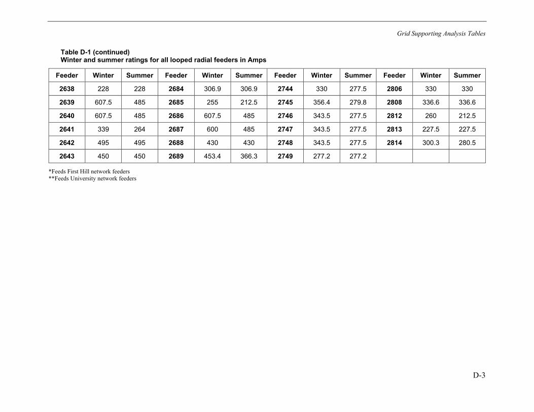
Grid Supporting Analysis Tables
D-3
Table D-1 (continued) Winter and summer ratings for all looped radial feeders in Amps
Feeder Winter Summer Feeder Winter Summer Feeder Winter Summer Feeder Winter Summer
2638 228 228 2684 306.9 306.9 2744 330 277.5 2806 330 330
2639 607.5 485 2685 255 212.5 2745 356.4 279.8 2808 336.6 336.6
2640 607.5 485 2686 607.5 485 2746 343.5 277.5 2812 260 212.5
2641 339 264 2687 600 485 2747 343.5 277.5 2813 227.5 227.5
2642 495 495 2688 430 430 2748 343.5 277.5 2814 300.3 280.5
2643 450 450 2689 453.4 366.3 2749 277.2 277.2
*Feeds First Hill network feeders **Feeds University network feeders
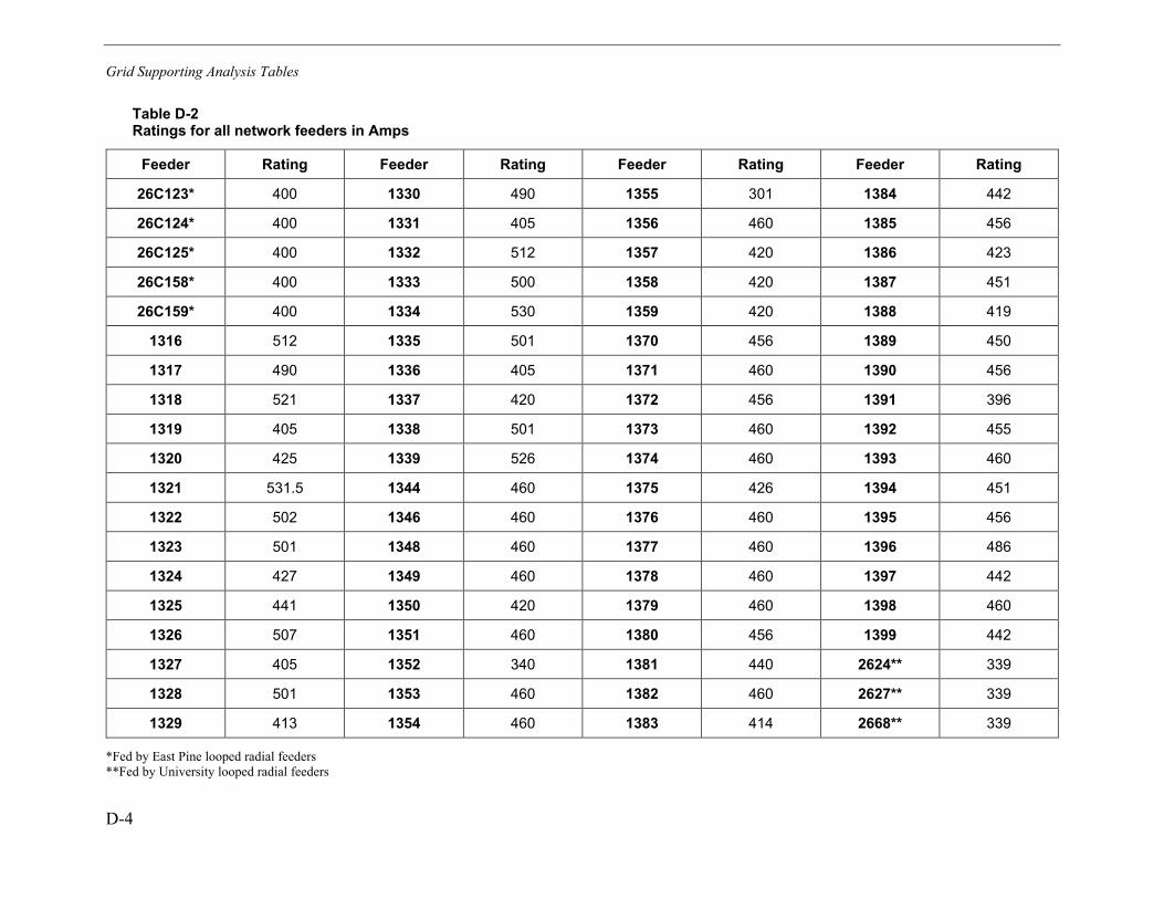
Grid Supporting Analysis Tables
D-4
Table D-2 Ratings for all network feeders in Amps
Feeder Rating Feeder Rating Feeder Rating Feeder Rating
26C123* 400 1330 490 1355 301 1384 442
26C124* 400 1331 405 1356 460 1385 456
26C125* 400 1332 512 1357 420 1386 423
26C158* 400 1333 500 1358 420 1387 451
26C159* 400 1334 530 1359 420 1388 419
1316 512 1335 501 1370 456 1389 450
1317 490 1336 405 1371 460 1390 456
1318 521 1337 420 1372 456 1391 396
1319 405 1338 501 1373 460 1392 455
1320 425 1339 526 1374 460 1393 460
1321 531.5 1344 460 1375 426 1394 451
1322 502 1346 460 1376 460 1395 456
1323 501 1348 460 1377 460 1396 486
1324 427 1349 460 1378 460 1397 442
1325 441 1350 420 1379 460 1398 460
1326 507 1351 460 1380 456 1399 442
1327 405 1352 340 1381 440 2624** 339
1328 501 1353 460 1382 460 2627** 339
1329 413 1354 460 1383 414 2668** 339
*Fed by East Pine looped radial feeders **Fed by University looped radial feeders
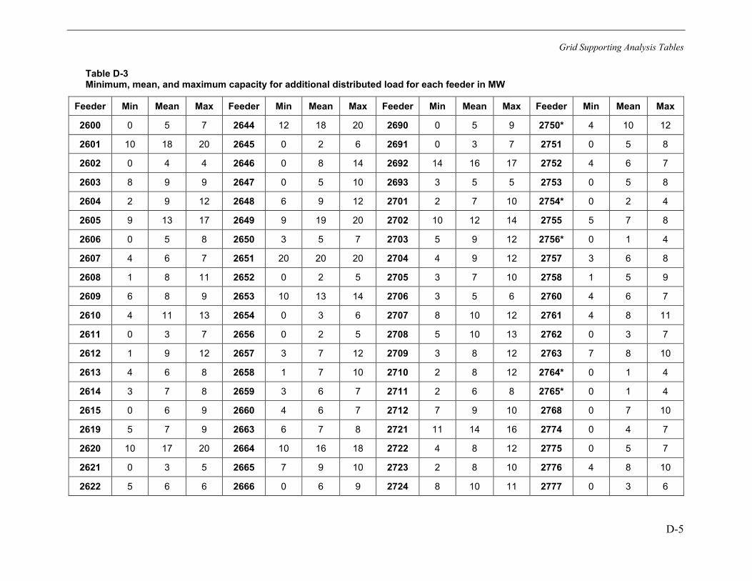
Grid Supporting Analysis Tables
D-5
Table D-3 Minimum, mean, and maximum capacity for additional distributed load for each feeder in MW
Feeder Min Mean Max Feeder Min Mean Max Feeder Min Mean Max Feeder Min Mean Max
2600 0 5 7 2644 12 18 20 2690 0 5 9 2750* 4 10 12
2601 10 18 20 2645 0 2 6 2691 0 3 7 2751 0 5 8
2602 0 4 4 2646 0 8 14 2692 14 16 17 2752 4 6 7
2603 8 9 9 2647 0 5 10 2693 3 5 5 2753 0 5 8
2604 2 9 12 2648 6 9 12 2701 2 7 10 2754* 0 2 4
2605 9 13 17 2649 9 19 20 2702 10 12 14 2755 5 7 8
2606 0 5 8 2650 3 5 7 2703 5 9 12 2756* 0 1 4
2607 4 6 7 2651 20 20 20 2704 4 9 12 2757 3 6 8
2608 1 8 11 2652 0 2 5 2705 3 7 10 2758 1 5 9
2609 6 8 9 2653 10 13 14 2706 3 5 6 2760 4 6 7
2610 4 11 13 2654 0 3 6 2707 8 10 12 2761 4 8 11
2611 0 3 7 2656 0 2 5 2708 5 10 13 2762 0 3 7
2612 1 9 12 2657 3 7 12 2709 3 8 12 2763 7 8 10
2613 4 6 8 2658 1 7 10 2710 2 8 12 2764* 0 1 4
2614 3 7 8 2659 3 6 7 2711 2 6 8 2765* 0 1 4
2615 0 6 9 2660 4 6 7 2712 7 9 10 2768 0 7 10
2619 5 7 9 2663 6 7 8 2721 11 14 16 2774 0 4 7
2620 10 17 20 2664 10 16 18 2722 4 8 12 2775 0 5 7
2621 0 3 5 2665 7 9 10 2723 2 8 10 2776 4 8 10
2622 5 6 6 2666 0 6 9 2724 8 10 11 2777 0 3 6

Grid Supporting Analysis Tables
D-6
Table D-3 (continued) Minimum, mean, and maximum capacity for additional distributed load for each feeder in MW
Feeder Min Mean Max Feeder Min Mean Max Feeder Min Mean Max Feeder Min Mean Max
2623 2 2 3 2667 2 8 9 2728 0 10 12 2778 1 6 9
2624** 7 11 13 2668** 6 10 12 2729 5 8 10 2779 0 4 7
2625 5 10 15 2669 8 12 14 2731 7 9 10 2780 0 3 7
2626 2 3 3 2672 9 11 13 2732 0 7 10 2781 5 7 9
2627** 9 13 14 2673 3 8 10 2733 8 9 10 2782 1 7 10
2628 0 12 20 2674 0 5 8 2734 4 6 7 2783 7 10 11
2629 10 18 20 2675 6 8 9 2735 4 9 11 2784 2 6 9
2630 0 9 14 2676 8 10 13 2736 4 9 13 2785 1 6 9
2631 10 16 20 2677 0 6 9 2737 3 6 9 2786 8 9 10
2632 15 20 20 2678 6 9 12 2738 5 9 13 2787 1 5 7
2633 0 4 7 2679 2 8 12 2739 5 7 8 2788 0 4 6
2634 5 11 16 2680 0 5 8 2740 0 4 7 2790 7 9 9
2635 3 12 17 2681 0 5 8 2741 7 12 17 2791 2 6 7
2636 2 9 13 2682 20 20 20 2742 6 8 9 2801 0 5 8
2637 5 5 6 2683 3 8 8 2743 0 2 4 2803 0 6 9
2638 5 7 9 2684 3 8 11 2744 8 9 10 2806 6 11 12
2639 0 8 15 2685 0 4 8 2745 6 10 13 2808 6 7 9
2640 12 15 20 2686 20 20 20 2746 2 9 13 2812 0 5 8
2641 6 11 14 2687 0 17 20 2747 6 9 13 2813 0 5 8
2642 5 6 7 2688 3 4 5 2748 9 12 14 2814 0 6 9
2643 20 20 20 2689 11 15 18 2749 2 7 11
*Feeds First Hill network feeders **Feeds University network feeders
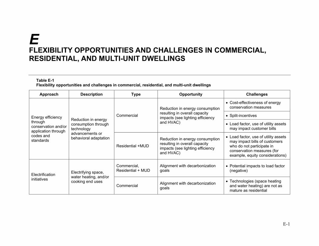
E-1
E FLEXIBILITY OPPORTUNITIES AND CHALLENGES IN COMMERCIAL, RESIDENTIAL, AND MULTI-UNIT DWELLINGS
Table E-1 Flexibility opportunities and challenges in commercial, residential, and multi-unit dwellings
Approach Description Type Opportunity Challenges
Energy efficiency through conservation and/or application through codes and standards
Reduction in energy consumption through technology advancements or behavioral adaptation
Commercial
Reduction in energy consumption resulting in overall capacity impacts (see lighting efficiency and HVAC)
• Cost-effectiveness of energy conservation measures
• Split-incentives
• Load factor, use of utility assets may impact customer bills
Residential +MUD
Reduction in energy consumption resulting in overall capacity impacts (see lighting efficiency and HVAC)
• Load factor, use of utility assets may impact bills of customers who do not participate in conservation measures (for example, equity considerations)
Electrification initiatives
Electrifying space, water heating, and/or cooking end uses
Commercial, Residential + MUD
Alignment with decarbonization goals
• Potential impacts to load factor (negative)
Commercial Alignment with decarbonization goals
• Technologies (space heating and water heating) are not as mature as residential

Flexibility Opportunities and Challenges in Commercial, Residential, and Multi-Unit Dwellings
E-2
Table E-1 (continued) Flexibility opportunities and challenges in commercial, residential, and multi-unit dwellings
Approach Description Type Opportunity Challenges
Electrification initiatives
Electrifying space, water heating, and/or cooking end uses
Residential + MUD
• Impacts to load factor (positive)
• Potential increase in energy bills if not aligned with rates
• Non-energy benefits (for example, improvement in indoor air quality)
MUD Only Non-energy benefits
• Split incentives or bills should be considered (for example, tenant pays electricity and manager pays gas)
• Technologies available but not as mature as single-family applications
Electrification + efficiency
Electrification and efficiency, using metrics of decarbonization
Commercial, Residential + MUD
Benefits of both efficiency and electrification
• Can result in inefficient use of otherwise efficient loads (HVAC, water heating)
Commercial Only Benefits of both efficiency and electrification
• May increase peak and decrease load factor
Residential + MUD Benefits of both efficiency and electrification.
• Potential increase in energy bills if not aligned with rates
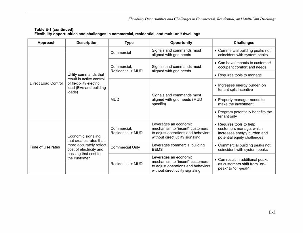
Flexibility Opportunities and Challenges in Commercial, Residential, and Multi-Unit Dwellings
E-3
Table E-1 (continued) Flexibility opportunities and challenges in commercial, residential, and multi-unit dwellings
Approach Description Type Opportunity Challenges
Direct Load Control
Utility commands that result in active control of flexibility electric load (EVs and building loads)
Commercial Signals and commands most aligned with grid needs
• Commercial building peaks not coincident with system peaks
Commercial, Residential + MUD
Signals and commands most aligned with grid needs
• Can have impacts to customer/ occupant comfort and needs
• Requires tools to manage
MUD Signals and commands most aligned with grid needs (MUD specific)
• Increases energy burden on tenant split incentive
• Property manager needs to make the investment
• Program potentially benefits the tenant only
Time of Use rates
Economic signaling that creates rates that more accurately reflect cost of electricity and passing that cost to the customer
Commercial, Residential + MUD
Leverages an economic mechanism to “incent” customers to adjust operations and behaviors without direct utility signaling
• Requires tools to help customers manage, which increases energy burden and potential equity challenges
Commercial Only Leverages commercial building BEMS
• Commercial building peaks not coincident with system peaks
Residential + MUD
Leverages an economic mechanism to “incent” customers to adjust operations and behaviors without direct utility signaling
• Can result in additional peaks as customers shift from “on-peak” to “off-peak”
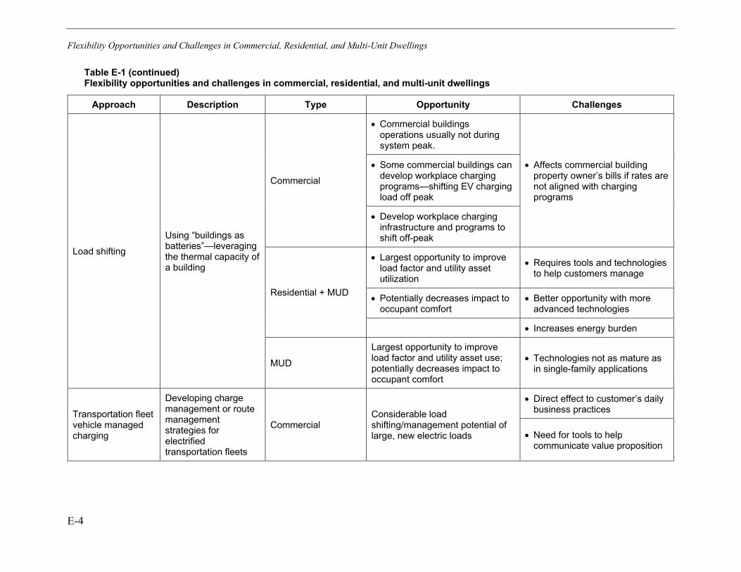
Flexibility Opportunities and Challenges in Commercial, Residential, and Multi-Unit Dwellings
E-4
Table E-1 (continued) Flexibility opportunities and challenges in commercial, residential, and multi-unit dwellings
Approach Description Type Opportunity Challenges
Load shifting
Using “buildings as batteries”—leveraging the thermal capacity of a building
Commercial
• Commercial buildings operations usually not during system peak.
• Affects commercial building property owner’s bills if rates are not aligned with charging programs
• Some commercial buildings can develop workplace charging programs—shifting EV charging load off peak
• Develop workplace charging infrastructure and programs to shift off-peak
Residential + MUD
• Largest opportunity to improve load factor and utility asset utilization
• Requires tools and technologies to help customers manage
• Potentially decreases impact to occupant comfort
• Better opportunity with more advanced technologies
• Increases energy burden
MUD
Largest opportunity to improve load factor and utility asset use; potentially decreases impact to occupant comfort
• Technologies not as mature as in single-family applications
Transportation fleet vehicle managed charging
Developing charge management or route management strategies for electrified transportation fleets
Commercial Considerable load shifting/management potential of large, new electric loads
• Direct effect to customer’s daily business practices
• Need for tools to help communicate value proposition
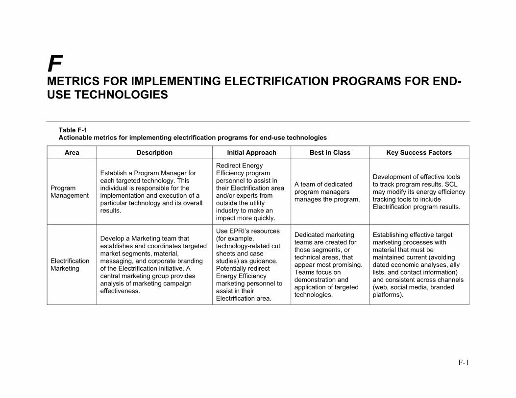
F-1
F METRICS FOR IMPLEMENTING ELECTRIFICATION PROGRAMS FOR END-USE TECHNOLOGIES
Table F-1 Actionable metrics for implementing electrification programs for end-use technologies
Area Description Initial Approach Best in Class Key Success Factors
Program Management
Establish a Program Manager for each targeted technology. This individual is responsible for the implementation and execution of a particular technology and its overall results.
Redirect Energy Efficiency program personnel to assist in their Electrification area and/or experts from outside the utility industry to make an impact more quickly.
A team of dedicated program managers manages the program.
Development of effective tools to track program results. SCL may modify its energy efficiency tracking tools to include Electrification program results.
Electrification Marketing
Develop a Marketing team that establishes and coordinates targeted market segments, material, messaging, and corporate branding of the Electrification initiative. A central marketing group provides analysis of marketing campaign effectiveness.
Use EPRI’s resources (for example, technology-related cut sheets and case studies) as guidance. Potentially redirect Energy Efficiency marketing personnel to assist in their Electrification area.
Dedicated marketing teams are created for those segments, or technical areas, that appear most promising. Teams focus on demonstration and application of targeted technologies.
Establishing effective target marketing processes with material that must be maintained current (avoiding dated economic analyses, ally lists, and contact information) and consistent across channels (web, social media, branded platforms).
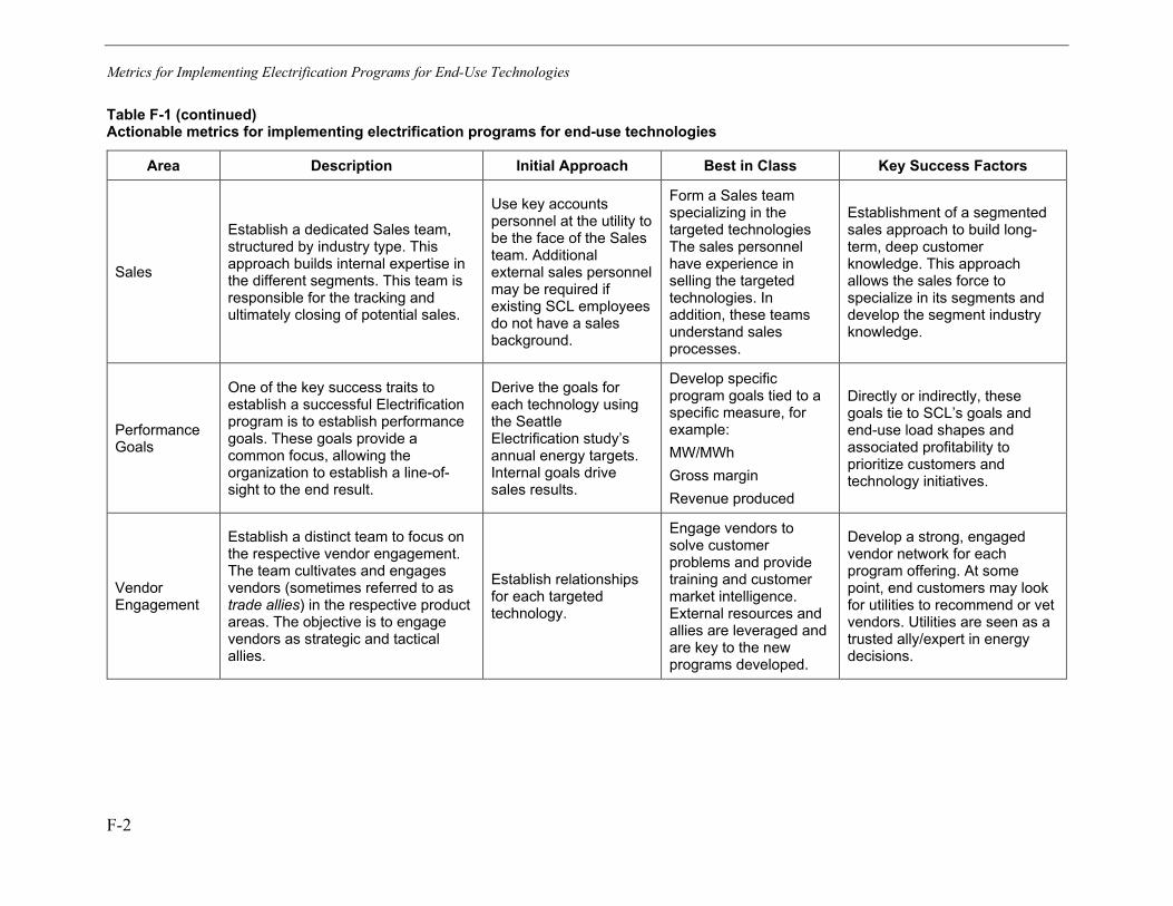
Metrics for Implementing Electrification Programs for End-Use Technologies
F-2
Table F-1 (continued) Actionable metrics for implementing electrification programs for end-use technologies
Area Description Initial Approach Best in Class Key Success Factors
Sales
Establish a dedicated Sales team, structured by industry type. This approach builds internal expertise in the different segments. This team is responsible for the tracking and ultimately closing of potential sales.
Use key accounts personnel at the utility to be the face of the Sales team. Additional external sales personnel may be required if existing SCL employees do not have a sales background.
Form a Sales team specializing in the targeted technologies The sales personnel have experience in selling the targeted technologies. In addition, these teams understand sales processes.
Establishment of a segmented sales approach to build long-term, deep customer knowledge. This approach allows the sales force to specialize in its segments and develop the segment industry knowledge.
Performance Goals
One of the key success traits to establish a successful Electrification program is to establish performance goals. These goals provide a common focus, allowing the organization to establish a line-of-sight to the end result.
Derive the goals for each technology using the Seattle Electrification study’s annual energy targets. Internal goals drive sales results.
Develop specific program goals tied to a specific measure, for example: MW/MWh Gross margin Revenue produced
Directly or indirectly, these goals tie to SCL’s goals and end-use load shapes and associated profitability to prioritize customers and technology initiatives.
Vendor Engagement
Establish a distinct team to focus on the respective vendor engagement. The team cultivates and engages vendors (sometimes referred to as trade allies) in the respective product areas. The objective is to engage vendors as strategic and tactical allies.
Establish relationships for each targeted technology.
Engage vendors to solve customer problems and provide training and customer market intelligence. External resources and allies are leveraged and are key to the new programs developed.
Develop a strong, engaged vendor network for each program offering. At some point, end customers may look for utilities to recommend or vet vendors. Utilities are seen as a trusted ally/expert in energy decisions.

Metrics for Implementing Electrification Programs for End-Use Technologies
F-3
Table F-1 (continued) Actionable metrics for implementing electrification programs for end-use technologies
Area Description Initial Approach Best in Class Key Success Factors
Effectiveness
Establish an Effectiveness Monitoring team that continually monitors the effectiveness of technology sales. The effectiveness of these sales is typically measured by cost effectiveness, energy and/or capacity impacts, and potentially emissions benefits. SCL may want to engage a third party it is currently using or a new one to perform the targeted technologies evaluation, measurement, and verification. This ensures that there is not an internal bias to the results.
Use utility metrics, such as RIM (Rate Impact Measure Test) and TRC (Total Resource Cost Test),129 to establish key performance indicators (KPIs) and gauge effectiveness.
Establish benchmarking for results.
Establish key performance indicators and metrics of success. It is crucial that appropriate weighting of the different KPIs be established at the outset and adjusted carefully as conditions change.
Program Development
Establish a Program Development team that researches, develops, and implements new programs. New technologies, changes in technologies, and understanding barriers to market adoption constantly require the development of new programs. This team also develops any internal/external incentives, performance goals, and initial targeted markets and provides the electrification program impacts to a utility’s resource planning process.
Develop a legislative/commission filing for each of the targeted technologies. This will enable SCL to advance its electrification goals. Ensure that program costs are allocated reasonably to reflect true merits/profitability for technologies in the targeted markets.
Establish dedicated Program Development team.
The Program Development team develops accurate market intelligence/feedback from the field sales staff. Primary and secondary customer program research is needed for success.
129 https://regulationbodyofknowledge.org/wp-content/uploads/2013/04/CUPC_California_Standard_Practice.pdf


Export Control RestrictionsAccess to and use of this EPRI product is granted with the specific understanding and requirement that respon-sibility for ensuring full compliance with all applicable U.S. and foreign export laws and regulations is being
undertaken by you and your company. This includes an obligation to ensure that any individual receiving access hereunder who is not a U.S. citizen or U.S. permanent resident is permitted access under applicable U.S. and foreign export laws and regulations.
In the event you are uncertain whether you or your company may law-fully obtain access to this EPRI product, you acknowledge that it is your obligation to consult with your company’s legal counsel to determine whether this access is lawful. Although EPRI may make available on a case by case basis an informal assessment of the applicable U.S. ex-port classification for specific EPRI products, you and your company acknowledge that this assessment is solely for informational purposes and not for reliance purposes. Your obligations regarding U.S. export control requirements apply dur-ing and after you and your company’s engagement with EPRI. To be clear, the obligations continue after your retirement or other departure from your company, and include any knowledge retained after gaining access to EPRI products. You and your company understand and acknowledge your obligations to make a prompt report to EPRI and the appropriate authorities regard-ing any access to or use of this EPRI product hereunder that may be in violation of applicable U.S. or foreign export laws or regulations.
EPRI 3420 Hillview Avenue, Palo Alto, California 94304-1338 • PO Box 10412, Palo Alto, California 94303-0813 USA
800.313.3774 • 650.855.2121 • [email protected] • www.epri.com
About EPRI
Founded in 1972, EPRI is the world’s preeminent independent, non-profit energy research and development organization, with offices around the world. EPRI’s trusted experts collaborate with more than 450 companies in 45 countries, driving innovation to ensure the public has clean, safe, reliable, affordable, and equitable access to electricity across the globe. Together, we are shaping the future of energy.
© 2022 Electric Power Research Institute (EPRI), Inc. All rights reserved. Electric Power Research Institute, EPRI, and TOGETHER…SHAPING THE FUTURE OF ENERGY are registered marks of the Electric Power Research Institute, Inc. in the U.S. and worldwide.
Program:Program Title 1Program Title 1
Program Title 2Program Title 2
Program Title 3Program Title 3
XXXXXXXXXXXXXXXXXXXX


![[Automation, Electrification, and Shared Mobility in Freight]](https://static.fdokumen.com/doc/165x107/632813a2e491bcb36c0b98fc/automation-electrification-and-shared-mobility-in-freight.jpg)