Seasonal and Synoptic Variations in Near-Surface Air Temperature Lapse Rates in aMountainous Basin

TROY R. BLANDFORD, KAREN S. HUMES, BRIAN J. HARSHBURGER, BRANDON C. MOORE, AND

VON P. WALDEN

Department of Geography, University of Idaho, Moscow, Idaho

HENGCHUN YE

Department of Geography and Urban Analysis, California State University, Los Angeles, Los Angeles, California

(Manuscript received 29 August 2006, in final form 14 March 2007)

ABSTRACT

To accurately estimate near-surface (2 m) air temperatures in a mountainous region for hydrologicprediction models and other investigations of environmental processes, the authors evaluated daily andseasonal variations (with the consideration of different weather types) of surface air temperature lapse ratesat a spatial scale of 10 000 km2 in south-central Idaho. Near-surface air temperature data (Tmax, Tmin, andTavg) from 14 meteorological stations were used to compute daily lapse rates from January 1989 to De-cember 2004 for a medium-elevation study area in south-central Idaho. Daily lapse rates were grouped bymonth, synoptic weather type, and a combination of both (seasonal–synoptic). Daily air temperature lapserates show high variability at both daily and seasonal time scales. Daily Tmax lapse rates show a distinctseasonal trend, with steeper lapse rates (greater decrease in temperature with height) occurring in summerand shallower rates (lesser decrease in temperature with height) occurring in winter. Daily Tmin and Tavg

lapse rates are more variable and tend to be steepest in spring and shallowest in midsummer. Differentsynoptic weather types also influence lapse rates, although differences are tenuous. In general, warmer airmasses tend to be associated with steeper lapse rates for maximum temperature, and drier air masses haveshallower lapse rates for minimum temperature. The largest diurnal range is produced by dry tropicalconditions (clear skies, high solar input). Cross-validation results indicate that the commonly used envi-ronmental lapse rate [typically assumed to be �0.65°C (100 m)�1] is solely applicable to maximum tem-perature and often grossly overestimates Tmin and Tavg lapse rates. Regional lapse rates perform better thanthe environmental lapse rate for Tmin and Tavg, although for some months rates can be predicted moreaccurately by using monthly lapse rates. Lapse rates computed for different months, synoptic types, andseasonal–synoptic categories all perform similarly. Therefore, the use of monthly lapse rates is recom-mended as a practical combination of effective performance and ease of implementation.

1. Introduction

Surface air temperature is a controlling factor ofmany environmental processes. Therefore, it is impor-tant to many fields of research, including hydrology(Blöschl 1991; De Scally 1997; Richard and Gratton2001; Zuzel and Cox 1975), glaciology (Singh and Singh2001), ecology (Lechowicz 1984; Peacock 1975;Stoutjesdijk and Barkman 1992), and agricultural andnatural resource management (Bibby et al. 1982;

Régnière and Bolstad 1994). Accurate spatially distrib-uted estimates of surface air temperature are critical tomany hydrological (Ferguson 1999; Martinec andRango 1998; Wigmosta et al. 1994) and ecological mod-els (Thornton et al. 1997). Additionally, the field ofweather forecasting has much to gain from researchregarding the spatial behavior of near-surface air tem-perature. Gridded graphical forecasts developed overthe past few years by the National Weather Service area good example of how lapse rates are being applied tocoarse model grids in order to generate more realistictemperature distributions in mountainous terrain(Glahn and Ruth 2003).

Linear lapse rates are commonly used in hydrologic

Corresponding author address: Troy Blandford, Department ofGeography, University of Idaho, Moscow, ID 83844.E-mail: troy.blandford@uidaho.edu

JANUARY 2008 B L A N D F O R D E T A L . 249

DOI: 10.1175/2007JAMC1565.1

© 2008 American Meteorological Society

JAM2604

and terrestrial models to interpolate near-surface airtemperature measurements from meteorological sta-tions to locations at different elevations where mea-surements do not exist (Martinec and Rango 1998;Régnière 1996; Running et al. 1987; Thornton et al.1997). The commonly used average environmentallapse rate of �0.65°C (100 m)�1 (Barry and Chorely1987) is a spatially global and temporally climatic av-erage (or standard); it should be applied with caution atother scales (e.g., changes with latitude; De Scally 1997;Tabony 1985). Its use may be particularly problematicat short temporal and fine spatial scales because lapserates show significant variability (De Scally 1997; Dod-son and Marks 1997; Pepin et al. 1999; Rolland 2003).This variability should be accounted for when usinglapse rates to extrapolate air temperature.

A distinction should be made between free-air lapserates and near-surface lapse rates (Harlow et al. 2004;McCutchan 1983; Pepin et al. 2005; Richner and Phil-lips 1984). Because they are impacted by different pro-cesses, near-surface and free-air lapse rates may be verydifferent at a given time and place. This is an especiallyimportant distinction to make in mountainous regionswhere the “heated” land surface is essentially projected(in the form of mountains) into the free air. Near-sur-face lapse rates are more variable than free-air lapserates (Harlow et al. 2004). This analysis is concernedwith near-surface lapse rates.

Near-surface temperatures typically decrease with in-creasing elevation. However, under certain conditionsthe opposite effect may occur. The influences of inver-sion, insolation, katabatic wind, and cold air drainageon the air temperature gradient in mountainous basins,especially on minimum temperature, are well docu-mented (Barry 1992; Clements et al. 2003; Mahrt et al.2001; Whiteman et al. 1999).

Near-surface lapse rates vary diurnally and season-ally. Pepin et al. (1999) and Rolland (2003) investigatedlapse rate variations in the Pennines of northern En-gland and throughout the Italian and Austrian Alps,respectively. Lapse rates were generally steeper(greater decrease in temperature with height) duringthe day than at night and during warmer months thancolder months. Increased inversion frequency duringcolder months partially explains the seasonal trend inlapse rates (Whiteman et al. 1999).

Several studies have investigated the impacts of syn-optic weather conditions, or large-scale weather pat-terns, on lapse rates (Pepin et al. 1999; Stahl et al. 2005).Pepin et al. (1999) conducted a study in the uplands ofnorthern England evaluating the relationships betweenlapse rates and solar radiation, humidity, wind speed,and synoptic types. Steeper lapse rates occurred with

higher levels of solar radiation. At night, wind speedalso steepened the lapse rates, but during the day thisrelationship was weak. At high wind speeds (�5 m s�1),the near-surface lapse rate tended to converge towardthe dry adiabatic lapse rate [�0.98°C (100 m)�1]. Anti-cyclones, typically associated with clear, calm weather,tended to increase the magnitude of the diurnal lapserate cycle. Daytime lapse rates were steep under anti-cyclonic conditions because of increased solar radiationreceipt, and nocturnal lapse rates were shallow (lesserdecrease in temperature with height) because of higherinversion frequencies during cloud-free nights. Moisteratmospheres produced shallower lapse rates. Lapserates during humid conditions approximated the moistadiabatic lapse rate [usually near �0.40°C (100 m)�1].Southerly airflow also produced shallower lapse ratesbecause of the advection of warmer air into higher el-evations, thereby decreasing the temperature–elevation(T–E) relationship. In contrast to Pepin et al. (1999),Stahl et al. (2005) found that the steepest lapse rates inBritish Columbia, Canada, were associated with a lowpressure system characterized by strong westerly tosouthwesterly winds and high amounts of precipitation.Clearly, the impacts of synoptic weather types on lapserates vary by season and by location.

The objective of this work is to quantify seasonal andsynoptic variations in near-surface air temperaturelapse rates. As described previously, Pepin et al. (1999),Rolland (2003), and Stahl et al. (2005) have investi-gated these aspects of lapse rates before, but primarilyat regional scales. Many ecologic and hydrologic mod-eling efforts require spatial interpolation of air tem-perature at the scale of smaller basins. One factor thathas limited past examinations of lapse rates at land-scape scale is the relatively small number of meteoro-logical stations typically available in mountainous wa-tersheds. However, with the advent and recent expan-sion of the Natural Resources Conservation Service(NRCS) snowpack telemetry (SNOTEL) network,there are now an increasing number of stations with along enough data record that are suitable for analysis.

The new elements of work presented here include thefollowing: (i) lapse rates are evaluated at a landscape scale(�10 000 km2) and, therefore, represent local phenom-ena; and (ii) errors incurred using the standard envi-ronmental lapse rate [ELR, assumed to be �0.65°C(100 m)�1] and a locally computed regional lapse rateare compared through cross-validation with errors in-curred using monthly and synoptic mean lapse rates.

2. Study area

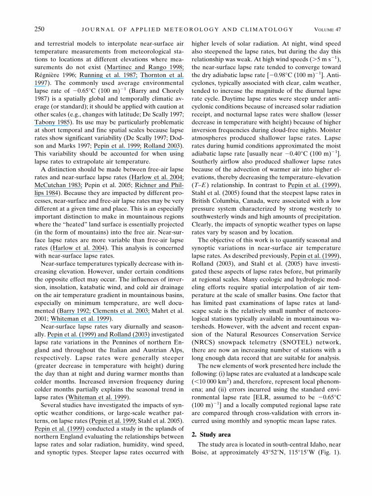
The study area is located in south-central Idaho, nearBoise, at approximately 43°52�N, 115°15�W (Fig. 1).

250 J O U R N A L O F A P P L I E D M E T E O R O L O G Y A N D C L I M A T O L O G Y VOLUME 47

The area is circular because a 1⁄2°-radius search ellipsewas used to identify meteorological stations to use inthe study. This ensured that all stations were within 1°of each other, which was suggested by Rolland (2003)as the largest spatial extent over which lapse ratesshould be expected to remain consistent. Assuming astationary lapse rate beyond this spatial extent is ques-tionable. The circle encompasses an area of approxi-mately 10 000 km2. This is a smaller spatial extent thanother daily air temperature spatial interpolation studies[e.g., 830 000 km2 for Dodson and Marks (1997),260 000 km2 for Harlow et al. (2004), and 400 000 km2

for Thornton et al. (1997)].The study area ranges in elevation from 970 m in the

west to 3390 m in the east (relief of �2400 m). Theregion is typical of much of the central and northernportions of the Rocky Mountain region with wet win-ters and dry summers. Annual normal temperatureranges from 5°C in higher elevations to 16°C in lowerelevations. The study area is practical for developingand testing techniques for generating daily spatial fieldsof temperature in small, mountainous regions, becauseit contains enough meteorological stations that devel-oping temperature–elevation regressions is feasible, butnot so many that it is atypical of station density in otherareas of the Pacific Northwest.

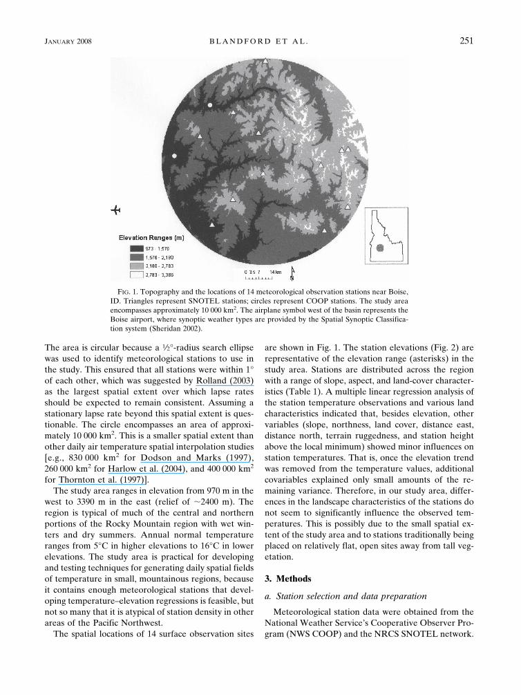
The spatial locations of 14 surface observation sites

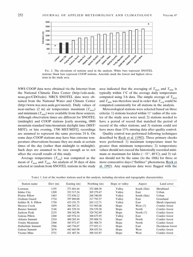
are shown in Fig. 1. The station elevations (Fig. 2) arerepresentative of the elevation range (asterisks) in thestudy area. Stations are distributed across the regionwith a range of slope, aspect, and land-cover character-istics (Table 1). A multiple linear regression analysis ofthe station temperature observations and various landcharacteristics indicated that, besides elevation, othervariables (slope, northness, land cover, distance east,distance north, terrain ruggedness, and station heightabove the local minimum) showed minor influences onstation temperatures. That is, once the elevation trendwas removed from the temperature values, additionalcovariables explained only small amounts of the re-maining variance. Therefore, in our study area, differ-ences in the landscape characteristics of the stations donot seem to significantly influence the observed tem-peratures. This is possibly due to the small spatial ex-tent of the study area and to stations traditionally beingplaced on relatively flat, open sites away from tall veg-etation.

3. Methods

a. Station selection and data preparation

Meteorological station data were obtained from theNational Weather Service’s Cooperative Observer Pro-gram (NWS COOP) and the NRCS SNOTEL network.

FIG. 1. Topography and the locations of 14 meteorological observation stations near Boise,ID. Triangles represent SNOTEL stations; circles represent COOP stations. The study areaencompasses approximately 10 000 km2. The airplane symbol west of the basin represents theBoise airport, where synoptic weather types are provided by the Spatial Synoptic Classifica-tion system (Sheridan 2002).

JANUARY 2008 B L A N D F O R D E T A L . 251

NWS COOP data were obtained via the Internet fromthe National Climatic Data Center (http://cdo.ncdc.noaa.gov/CDO/cdo). NRCS SNOTEL data were ob-tained from the National Water and Climate Center(http://www.wcc.nrcs.usda.gov/snotel). Daily values ofnear-surface (2 m) air temperature maximum (Tmax)and minimum (Tmin) were available from these sources.Although observation times are different for SNOTEL(midnight) and COOP stations [early morning, 0800mountain standard time/mountain daylight time (MST/MDT), or late evening, 1700 MST/MDT], recordingsare assumed to represent the same previous 24 h. Onsome days COOP stations may have bias extreme tem-perature observations because they are made at certaintimes of the day (rather than midnight to midnight).Such days are assumed to be rare enough as to notaffect the overall results of this study.

Average temperature (Tavg) was computed as themean of Tmax and Tmin. An analysis of 30 days of dataselected at random from SNOTEL stations in the study

area indicated that the averaging of Tmax and Tmin istypically within 1°C of the average daily temperaturecomputed using 3-h data. The simple average of Tmax

and Tmin was therefore used in order that Tavg could becomputed consistently for all stations in the analysis.

Meteorological stations were selected based on threecriteria: 1) stations located within 1⁄2° radius of the cen-ter of the study area were used; 2) stations needed tohave a period of record that matched the period ofrecord of the other stations; and 3) stations could nothave more than 15% missing data after quality control.

Quality control was performed following techniquesdescribed by Reek et al. (1992). Three primary checkswere performed: 1) maximum temperature must begreater than minimum temperature; 2) temperaturevalues should not exceed the historically recorded mini-mum or maximum for Idaho (�51°, 48°C); and 3) val-ues should not be the same (to the 10th) for three ormore consecutive days (“flatliner” phenomena; Reek etal. 1992). Any suspicious data were flagged with the

TABLE 1. List of the weather stations used in this analysis, including elevation and topographic characteristics.

Station name Elev (m) Easting (m) Northing (m) Slope or valley Aspect Land cover

Lowman 1195 371 601.64 332 488.38 Valley South (flat) ShrublandIdaho City 1209 352 517.24 305 279.47 Valley East UrbanPrairie Pillow 1463 372 836.12 268 340.09 Valley South (flat) UrbanGraham Guard 1734 397 809.00 317 792.57 Valley East GrasslandSoldier R. S. Pillow 1750 433 191.75 265 112.71 Valley East Shrub (riparian)Moores Creek 1859 366 287.31 315 905.08 Slope West (?) Conifer forestBanner Summit 2146 401 529.10 356 539.20 Slope North Conifer forestJackson Peak 2155 384 362.96 328 762.89 Slope North (?) Conifer forestGalena Pillow 2268 445 974.14 308 675.95 Valley East Conifer forestAtlanta Summit 2310 400 265.44 295 808.74 Slope North Conifer forestTrinity Mountain 2368 383 972.47 281 908.75 Slope North Conifer forestDollarhide Summit 2566 445 756.07 277 852.11 Slope East Deciduous forestGalena Summit 2676 442 665.98 308 435.54 Slope West Conifer forestVienna Mine 2731 431 407.36 300 163.87 Slope West Conifer forest

FIG. 2. The elevations of stations used in the analysis. White bars represent SNOTELstations; black bars represent COOP stations. Asterisks mark the lowest and highest eleva-tions in the study area.

252 J O U R N A L O F A P P L I E D M E T E O R O L O G Y A N D C L I M A T O L O G Y VOLUME 47

value �9999 and confirmed manually before deletionfrom the dataset.

The aforementioned selection criteria resulted in 14meteorological stations (2 NWS COOP and 12 NRCSSNOTEL) with an overlapping period of record from 1January 1989 to 31 December 2004 (station locationsshown in Fig. 1). A day was removed from the entiredataset only if more than one station was missing datafor that day. This maximized the number of days avail-able to compute T–E regressions while ensuring thatthey were consistently computed with at least 90% ofthe stations (13 or 14). Days that did not have a syn-optic classification (discussed later) also had to be re-moved. Of the 5844 days between 1 January 1989 and31 December 2004, approximately 5% were removed.This resulted in a working dataset of 5527 days.

b. Synoptic classification

Synoptic conditions, or general weather types, mayexplain day-to-day variations in lapse rates (Pepin et al.1999; Stahl et al. 2005). Many classification methodsranging from manual and subjective to automated andobjective have been developed (Jones et al. 1993; Kid-son 1994; Lamb 1972; Mayes 1991; Muller 1977;Schwartz 1991). The Spatial Synoptic Classification(SSC2) system was used in this research (Sheridan2002) because it is spatially transferable and has a longperiod of record available for Boise, Idaho.

The SSC2 is spatially transferable, and its classifica-tion scheme is relative to each particular geographiclocation (i.e., a dry moderate classification in Texas isdifferent than dry moderate in Idaho). Likewise, drymoderate conditions are cooler in winter than in sum-mer at all locations. Seed days (days that typify aweather type) are identified from a historical record ateach station and allow the classification to concern it-self with local meteorological character (Sheridan2002). This was valuable to this analysis because it al-lowed the determination of a local lapse rate responseto the weather type. The SSC2 was also chosen becausea historic record (1948 to 2005) of day-by-day weathertypes is readily available (http://sheridan.geog.kent.edu/ssc.html).

The weather conditions for each day are categorizedinto six different types, or as transition between twotypes. The weather types are 1) dry moderate (DM), 2)dry polar (DP), 3) dry tropical (DT), 4) moist moderate(MM), 5) moist polar (MP), and 6) moist tropical (MT).

Because these weather conditions are fashioned to aparticular station, they are described below primarily inrelevance to the Boise, Idaho, airport weather station(SSC2 code BOI), located approximately 30 km west ofthe study area (airplane symbol in Fig. 1). Although the

SSC2 classification is not provided directly in the studyarea, synoptic conditions a short distance to the east areassumed to be similar, because weather patterns in thearea typically traverse west to east, and “synoptics” bydefinition capture large-scale, general conditions.

DM conditions are typified by mild and dry air.Zonal flow aloft is common during DM conditions andallows the air to dry and warm adiabatically, which mayproduce a steeper T–E gradient than normal.

DP conditions are typified by cool or cold, dry airoriginating in Canada or Alaska. Northerly winds arecommon and cloud cover is minimal. Inversions may setup for extended periods during DP as the cold air sinksand displaces warmer air, especially at night.

DT weather is hot, dry, and sunny. It is typicallypushed into Idaho from the southwest. Violent down-slope winds may also produce DT conditions. Becauseof the extreme heat and associated dryness the T–Egradient may approach the dry adiabatic lapse rate[�0.98°C (100 m)�1].

MM conditions are cloudy, warm, and humid. Theyare common during mild winters and may persist formany days. MP conditions are similar to MM but arecooler and less humid. Light precipitation is common.MP conditions are common during winter in Idaho, asis typical of a Mediterranean climate.

MT weather occurred only 2.3% of the days at theBoise station and was, therefore, not used in the analy-sis. The frequency of occurrence of the other weathertypes is shown in Fig. 3 and summarized by month inFig. 4. DM conditions occur most frequently except insummer, and are common during all months. In gen-eral, relatively dry conditions (DM, DP, and DT) domi-nate the study area for nine months of the year.

c. Computing T–E regressions and comparinggroup means

Near-surface lapse rates were estimated from ob-served temperature (2 m) data using linear regression[Eq. (1)], where elevation is the independent variableand air temperature is the dependent variable (Harlowet al. 2004; Rolland 2003). From here forward, the near-surface lapse rate will be used synonymously with “T–Erelationship,” or “regression,” to signify how it is com-puted:

Tobs, j � �1hj � t0, �1

where Tobs, j is the observed air temperature (°C) atstation j, 1 is the slope coefficient/lapse rate (°C m�1),hj is the latitude (m) at station j, and t0 is the tempera-ture (°C) at sea level (0 m, y intercept).

T–E regressions were computed on a daily basis andthen grouped by month, synoptic type, and a combina-

JANUARY 2008 B L A N D F O R D E T A L . 253

tion of these two groupings (seasonal–synoptic). Theseasonal–synoptic groups were created using four sea-sons (December–February, March–May, June–August,and September–November) and the synoptic groupsthat occurred within them. There were 12 monthgroups, 6 synoptic groups, and 24 seasonal–synopticgroups. Although the sample sizes of the month groupswere all relatively the same, the sizes of the othergroups varied, as described by the frequency histo-grams in Figs. 3 and 4.

Student’s t test of difference in mean, which takesdifferent sample sizes into account, and one-way analy-sis of variance (ANOVA) were then used to comparethe population means of different groups. First, a one-sample t test was performed to determine if groupmeans were statistically different from the average at-mospheric lapse rate [�0.65°C (100 m)�1]. A secondone-sample t test was then performed to determine if

the mean of each group was different from a regionallapse rate (an average lapse rate computed from all5527 days, i.e., the mean of the total population). Third,one-way ANOVA was used to compare one group toeach of the others, iteratively. These three steps respec-tively determined (a) if a lapse rate other than the av-erage atmospheric lapse rate was necessary for thestudy area; (b) if a lapse rate other than a regional lapserate was necessary; and (c) if divisions amongst differ-ent groups were necessary.

One-way ANOVA essentially extends the two-sample t test (which compares the equality of two popu-lation means) to compare more than two means. It isequivalent to a t test when only two groups are com-pared. Since many groups were being analyzed,ANOVA was preferable in terms of efficiency. For ex-ample, instead of performing numerous t tests (e.g.,January versus February, January versus March, Janu-

FIG. 4. The number of occurrences of synoptic weather types in the study area by month.

FIG. 3. The number of occurrences of synoptic weather types in the study area from 1 Jan1989 to 31 Dec 2004. The frequency of occurrence of each synoptic weather types is shownabove each bar.

254 J O U R N A L O F A P P L I E D M E T E O R O L O G Y A N D C L I M A T O L O G Y VOLUME 47

ary versus May) all of the months were analyzed againsteach other at once. This was done in a two-step process.

First, one-way ANOVA was used to test whether ornot all of the groups were equivalent based on an Fstatistic. This initial test indicated only that differencesexisted among the group means; it did not indicatewhich groups were different. Therefore, a post hoc testwas necessary to make multiple comparisons. Usingconfidence intervals (alpha � 0.05) set on the differ-ence between group means, the post hoc comparisonidentified which groups were significantly differentfrom each other.

d. Cross-validation

To evaluate how well the group mean lapse ratespredicted daily observed lapse rates, a cross-validationwas performed. Each of the 16 yr was left out succes-sively. The remaining data were grouped as before andthe mean lapse rates were computed (predicted lapserate dataset). Daily lapse rates for the year that was leftout also were computed (observed lapse rate dataset)and then compared with the predicted lapse ratedataset. Results were summarized with mean error(ME; a bias indicator), mean absolute error (MAE),and RMSE (all in units of degrees Celsius per 100meters).

4. Results and discussion

a. Daily lapse rate variation

As shown by the time series in Fig. 5, daily Tavg airtemperature lapse rates showed high variability [stan-dard deviation � 0.22°C (100 m)�1] within a given year.Errors in the temperature observations may explain

some of this variation; however, 7-day (dashed grayline) and 30-day (solid gray line) running averages,which smooth out much of this error, also show highvariability (Fig. 5). Additionally, because the daily T–Elinear regressions showed strong measures of goodness-of-fit (average r2 � 0.6, and RMSE � 1.3°C), the scat-ter in the time series is primarily reflecting real phe-nomena in day-to-day lapse rate behavior, as opposedto reflecting errors in the temperature observations andanalysis.

Daily Tmax lapse rate variation (not shown) waslower than Tavg variability; Tmin variation was higher.High variability in the daily lapse rates indicates thatthe ELR and regional lapse rate (RL) may performpoorly when used at subannual time scales.

b. Seasonal variations

Monthly values for Tmax lapse rates have a distinctseasonal trend (Fig. 6a). Steeper lapse rates occurredduring warmer months, while shallower lapse rates oc-curred during colder months. These findings are con-sistent with other literature (Harding 1979; Rolland2003).

Mean Tmin lapse rates are significantly shallower thanmean Tmax lapse rates for all months (Fig. 6b). Theyare also more variable, with a range from �0.03°C(100 m)�1 in August and September to �0.36°C(100 m)�1 in April. The distinct, gradual seasonal pat-tern observed in mean Tmax lapse rates is not observedin Tmin lapse rates. Instead, a general sinusoidal patternemerges (steeper Tmin lapse rates in spring, shallowerlapse rates in late summer and early fall). This patternis consistent with nighttime inversions, which fre-quently occur at night following warm, clear-sky days insummer and autumn. During warm months (July–Sep-

FIG. 5. The daily variation of Tavg lapse rates. The 7- and 30-day running averages are alsoshown. The T–E regression resulting in the extreme inversion value [�0.80°C (100 m)�1] seenin mid-February had a strong fit (r2 � 0.80), and is therefore not suspected to be in error.

JANUARY 2008 B L A N D F O R D E T A L . 255

tember), the box plots show an extremely shallow meanTmin lapse rate (even positive in August and Septem-ber). Steeper Tmin lapse rates did occur in August andSeptember, as indicated by the extent of the box plotwhiskers; however, extremely shallow or positive lapserates are the norm (�60% of the study days). DailyTmin lapse rates from July to September equal or ex-ceed the ELR (dotted black line) just 0.01% of the

days. Daily Tmin lapse rates are difficult to predict inwinter—any mean lapse rate is a grossly smooth pre-dictor.

As would be expected, Tavg lapse rates vary morethan Tmax and less than Tmin lapse rates (Fig. 6c); Tavg

lapse rates are shallowest in January and December[�0.28°C (100 m)�1] and steepest in April [�0.49°C(100 m)�1]. Additionally, cold months (November–February) are noticeably more variable than warmermonths (May–August), as indicated by the bowtie-likepattern of the box plot whiskers. The seasonal trendseen in Tmax lapse rates is not observed in Tavg lapserates; instead, the pattern seen in Tmin is prevalent, al-beit more gradual.

c. Variations by synoptic weather type

Differences between Tmax lapse rates for differentsynoptic categories are tenuous (Fig. 7a). Box plots foreach synoptic category largely overlap. Dry moderateand moist moderate conditions have statistically iden-tical means, as do dry polar and moist polar (shown bysimilar shading in the box plots). This is surprising con-sidering relative moisture levels (dry versus moist) areexpected to impact lapse rates. For example, Pepin etal. (1999) found significant positive correlations be-tween lapse rates and humidity. Our study suggests thatairmass temperature (polar versus moderate) impactsTmax lapse rates more than humidity level. This is fur-ther indicated by the stark difference between box plotsfor dry polar and dry tropical conditions.

Dry tropical conditions produced mean lapse ratesthat are significantly steeper than all other categories,except the “transition” category. Predictably, the tran-sitional category results in a lapse rate statistically iden-tical to the ELR, because both represent a wide rangeof conditions. During the summer, when dry tropicalconditions are most common, strong surface heatingcauses the atmosphere to mix vertically through con-vection and leads to a dry adiabatic lapse rate (Pepin etal. 1999).

In contrast to Tmax, dry tropical conditions result in ashallow, even slightly positive [0.09°C (100 m)�1], meanvalue for Tmin (Fig. 7b). Cold air drainage likely occursat night during clear sky (DT) conditions (Gustavssonet al. 1998). Also, unlike Tmax, box plots for Tmin showa difference between dry and moist air masses. This isespecially shown by differences between dry moderateand moist moderate conditions. Box plots for DM con-ditions indicate markedly shallower rates than do thebox plots for MM conditions, possibly due to the inso-lating effects of clouds observed during MM conditions.In general, steeper lapse rates occur during wetter con-

FIG. 6. Seasonal variations in lapse rates for (a) Tmax, (b) Tmin,and (c) Tavg. Dotted line represents the constant average environ-mental lapse rate; dot–dashed gray line represents the computedregional lapse rate. Shading shows box plots with statistically simi-lar means.

256 J O U R N A L O F A P P L I E D M E T E O R O L O G Y A N D C L I M A T O L O G Y VOLUME 47

ditions, while shallower lapse rates occur during drierconditions.

d. Seasonal–synoptic variations

Synoptic types appear to impact Tmax lapse rates fordifferent seasons similarly (Fig. 8a). For example, drytropical and transition weather types consistently pro-

duce the steepest mean Tmax lapse rate for all seasons,except June–August. Dry polar and moist polar condi-tions consistently produce the shallowest mean lapserates. This pattern is similar to that shown in the boxplots for the grouping by synoptic type alone (Fig. 7a).

FIG. 7. Lapse rate variation by synoptic weather type for (a)Tmax, (b) Tmin, and (c) Tavg. Dotted line represents the averageatmospheric lapse rate constant; dot–dashed gray line representsthe computed regional lapse rate. Shading shows box plots withstatistically similar means.

FIG. 8. Lapse rate variation by seasonal–synoptic groupings for(a) Tmax, (b) Tmin, and (c) Tavg. Dotted line represents the averageenvironmental lapse rate constant; dot–dashed gray line repre-sents the computed regional lapse rate. The asterisk in Decem-ber–February notes a low sample size (n � 13) for DT. Shadingshows box plots with statistically similar means (DM � dry mod-erate; DP � dry polar; DT � dry tropical; MM � moist moderate;MP � moist polar; T � transition).

JANUARY 2008 B L A N D F O R D E T A L . 257

The box plots in Fig. 8b indicate that, like with Tmax,the impact of synoptic types on Tmin lapse rates is simi-lar for different seasons. Drier conditions (DM, DP,and DT) consistently produce shallower mean lapserates than wetter conditions (MM, MP) for all seasons,except December–February. Cold air masses, whetherdry polar or moist polar, produce the shallowest meanlapse rates during December–February. This is consis-tent with the expectation that cold air may invert basintemperatures for an extended period of time during thewinter. In the Boise study area, there are times in mid-winter that deep inversions setup and only the highestmountains extend above the inversion. When this pat-tern sets up, low clouds and temperatures below freez-ing persist in the valleys, while mountain tops are sunnywith above-freezing temperatures (J. Breidenbach2006, personal communication). Such conditions maylast for days and are likely the cause of the extremeextent of the box plots seen during polar conditions(DP, MP) in December–February.

e. Cross-validation results

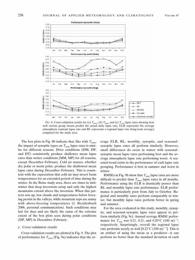
Cross-validation results are plotted in Fig. 9. The plotof performance for Tmax (Fig. 9a) indicates that the av-

erage ELR, RL, monthly, synoptic, and seasonal–synoptic lapse rates all perform similarly. However,small differences do occur in winter with seasonal–synoptic mean lapse rates performing best and the av-erage atmospheric lapse rate performing worst. A sea-sonal trend exists in the performance of each lapse rategrouping. Performance is best in summer and worst inwinter.

RMSEs in Fig. 9b show that Tmin lapse rates are moredifficult to predict than Tmax lapse rates in all months.Performance using the ELR is drastically poorer thanRL and monthly lapse rate performance. ELR perfor-mance is particularly poor from July to October. Re-gional and monthly rates perform comparably in win-ter, but monthly lapse rates perform better in springand summer.

For the area evaluated in this study, monthly, synop-tic, and seasonal–synoptic lapse rates appear to per-form similarly (Fig. 9c). Annual average RMSE perfor-mance for Tavg was 0.21, 0.21, and 0.20°C (100 m)�1,respectively. Surprisingly, overall the regional lapserate performs nearly as well [0.22°C (100 m)�1]. This isan artifact of using the mean as a predictor—it canperform no better than the standard deviation of each

FIG. 9. Cross-validation results for (a) Tmax, (b) Tmin, and (c) Tavg lapse rates showing howwell various group means predict the actual daily lapse rate. ELR represents the averageatmospheric constant lapse rate and RL represents a regional lapse rate (long-term average)computed for the study area.

258 J O U R N A L O F A P P L I E D M E T E O R O L O G Y A N D C L I M A T O L O G Y VOLUME 47

grouping. We hypothesized that grouped lapse rates(subsets of the population) would have significantlylower sample standard deviations than the populationas a whole (i.e., all 5527 daily lapse rates). This did notoccur consistently—some groups had standard devia-tions lower than the population while others werehigher. For example, the variability of Tavg lapse ratesremained high even for the most strict subset (season-al–synoptic grouping), with standard deviations rangingfrom 0.14° to 0.34°C (100 m)�1. In cases where thewithin-group variation remains high, the subset meanwill perform no better than the population mean. Nev-ertheless, the plots of performance (Fig. 9) identify timeperiods when different groupings are advantageousover the others. This is significant in terms of applica-tion because it indicates that the relevance and effi-ciency of the ELR and RL depends on the season andtemperature variable (Tmax, Tmin, or Tavg) for which it isbeing used.

f. Recommended lapse rates

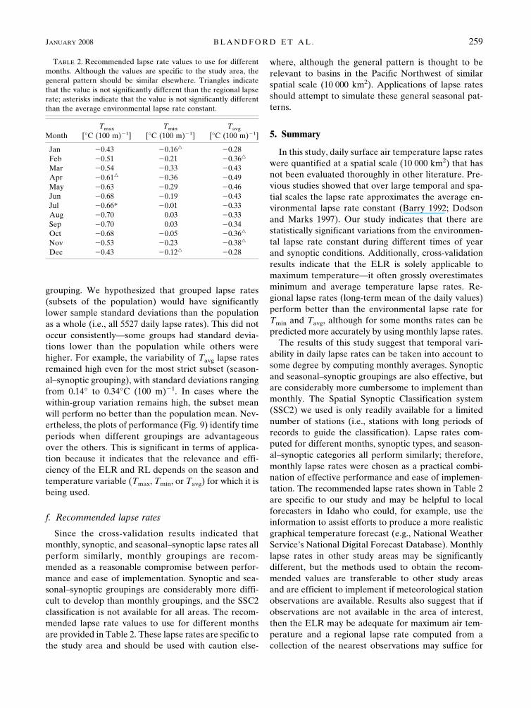
Since the cross-validation results indicated thatmonthly, synoptic, and seasonal–synoptic lapse rates allperform similarly, monthly groupings are recom-mended as a reasonable compromise between perfor-mance and ease of implementation. Synoptic and sea-sonal–synoptic groupings are considerably more diffi-cult to develop than monthly groupings, and the SSC2classification is not available for all areas. The recom-mended lapse rate values to use for different monthsare provided in Table 2. These lapse rates are specific tothe study area and should be used with caution else-

where, although the general pattern is thought to berelevant to basins in the Pacific Northwest of similarspatial scale (10 000 km2). Applications of lapse ratesshould attempt to simulate these general seasonal pat-terns.

5. Summary

In this study, daily surface air temperature lapse rateswere quantified at a spatial scale (10 000 km2) that hasnot been evaluated thoroughly in other literature. Pre-vious studies showed that over large temporal and spa-tial scales the lapse rate approximates the average en-vironmental lapse rate constant (Barry 1992; Dodsonand Marks 1997). Our study indicates that there arestatistically significant variations from the environmen-tal lapse rate constant during different times of yearand synoptic conditions. Additionally, cross-validationresults indicate that the ELR is solely applicable tomaximum temperature—it often grossly overestimatesminimum and average temperature lapse rates. Re-gional lapse rates (long-term mean of the daily values)perform better than the environmental lapse rate forTmin and Tavg, although for some months rates can bepredicted more accurately by using monthly lapse rates.

The results of this study suggest that temporal vari-ability in daily lapse rates can be taken into account tosome degree by computing monthly averages. Synopticand seasonal–synoptic groupings are also effective, butare considerably more cumbersome to implement thanmonthly. The Spatial Synoptic Classification system(SSC2) we used is only readily available for a limitednumber of stations (i.e., stations with long periods ofrecords to guide the classification). Lapse rates com-puted for different months, synoptic types, and season-al–synoptic categories all perform similarly; therefore,monthly lapse rates were chosen as a practical combi-nation of effective performance and ease of implemen-tation. The recommended lapse rates shown in Table 2are specific to our study and may be helpful to localforecasters in Idaho who could, for example, use theinformation to assist efforts to produce a more realisticgraphical temperature forecast (e.g., National WeatherService’s National Digital Forecast Database). Monthlylapse rates in other study areas may be significantlydifferent, but the methods used to obtain the recom-mended values are transferable to other study areasand are efficient to implement if meteorological stationobservations are available. Results also suggest that ifobservations are not available in the area of interest,then the ELR may be adequate for maximum air tem-perature and a regional lapse rate computed from acollection of the nearest observations may suffice for

TABLE 2. Recommended lapse rate values to use for differentmonths. Although the values are specific to the study area, thegeneral pattern should be similar elsewhere. Triangles indicatethat the value is not significantly different than the regional lapserate; asterisks indicate that the value is not significantly differentthan the average environmental lapse rate constant.

MonthTmax

[°C (100 m)�1]Tmin

[°C (100 m)�1]Tavg

[°C (100 m)�1]

Jan �0.43 �0.16� �0.28Feb �0.51 �0.21 �0.36�

Mar �0.54 �0.33 �0.43Apr �0.61� �0.36 �0.49May �0.63 �0.29 �0.46Jun �0.68 �0.19 �0.43Jul �0.66* �0.01 �0.33Aug �0.70 0.03 �0.33Sep �0.70 0.03 �0.34Oct �0.68 �0.05 �0.36�

Nov �0.53 �0.23 �0.38�

Dec �0.43 �0.12� �0.28

JANUARY 2008 B L A N D F O R D E T A L . 259

average and minimum temperature (similar implica-tions are made by Harlow et al. 2004). However, themajor advantage described herein is that local, monthlylapse rates will perform with more consistency (i.e.,smaller error for short time periods).

A better approach than lapse rates to distributingsurface air temperature may be to use geostatisticalspatial interpolation techniques, such as detrended or-dinary kriging (Garen et al. 1994). However, oneshould be cautious about immediately accepting themore complex, spatially explicit methods as “better,”because the computational intensity associated withthese methods may outweigh the improvementsbrought to the model of interest. For example, semid-istributed models, such as the Snowmelt Runoff Model,require mean areal temperature for zones rather thandistributed values. The effect of averaging may sup-plant the benefits of a finer spatial resolution (i.e., fullydistributed approach). A temperature interpolationmethod that simplistically considers spatial and tempo-ral variability, such as the approach described herein,may perform comparably similar without the addedcomputational time and effort. Trade-offs between per-formance and complexity should be investigated.

Acknowledgments. This research was funded by thePacific Northwest Regional Collaboratory as part ofRaytheon Corporation’s Synergy project, funded byNASA through NAS5-03098, Task No. 110. Partial sup-port was also provided by the NSF-Idaho EPSCoR pro-gram under Award Number EPS-0447689. The data forthis project were provided by the Natural ResourcesConservation Service and the National Weather Ser-vice. We thank Ron Abramovich (NRCS) and JayBreidenbach (NWS) for helpful discussions, and Dr.Scott Sheridan provided the Spatial Synoptic Classifi-cation system and assistance in classifying weathertypes. Author Blandford thanks Dr. Stanley Miller forhis review of the master’s thesis that preceded this ar-ticle. We also express our appreciation for the threeanonymous reviewers whose comments improved thequality of this manuscript.

REFERENCES

Barry, R. G., 1992: Mountain Weather and Climate. 2nd ed. Rout-ledge, 402 pp.

——, and R. J. Chorley, 1987: Atmosphere, Weather, and Climate.5th ed. Methuen, 460 pp.

Bibby, J. S., H. A. Douglas, A. J. Thomasson, and J. S. Robertson,1982: Land capability classification for agriculture. TheMacaulay Institute for Soil Research, 75 pp.

Blöschl, G., 1991: The influence of uncertainty in air temperatureand albedo on snowmelt. Nord. Hydrol., 22, 95–108.

Clements, C. B., C. D. Whiteman, and J. D. Horel, 2003: Cold-air-

pool structure and evolution in a mountain basin: Peter Sinks,Utah. J. Appl. Meteor., 42, 752–768.

De Scally, F. A., 1997: Deriving lapse rates of slope air tempera-ture for meltwater runoff modeling in subtropical mountains:An example from the Punjab Himalaya, Pakistan. Mt. Res.Dev., 17, 353–362.

Dodson, R., and D. Marks, 1997: Daily air temperature interpo-lated at high spatial resolution over a large mountainous re-gion. Climate Res., 8, 1–20.

Ferguson, R. I., 1999: Snowmelt runoff models. Prog. Phys.Geogr., 32, 205–227.

Garen, D. C., G. L. Johnson, and C. L. Hanson, 1994: Mean arealprecipitation for daily hydrologic modeling in mountainousregions. Water Resour. Bull., 30, 481–491.

Glahn, H. R., and D. P. Ruth, 2003: The new digital forecast da-tabase of the National Weather Service. Bull. Amer. Meteor.Soc., 84, 195–201.

Gustavsson, T., M. Karlsson, J. Bogren, and S. Lindqvist, 1998:Development of temperature patterns during clear nights. J.Appl. Meteor., 37, 559–571.

Harding, R. J., 1979: Altitudinal gradients of temperature in thenorthern Pennines. Weather, 34, 190–201.

Harlow, R. C., E. J. Burke, R. L. Scott, W. J. Shuttleworth, C. M.Brown, and J. R. Petti, 2004: Derivation of temperature lapserates in semi-arid southeastern Arizona. Hydrol. Earth Syst.Sci., 8, 1179–1185.

Jones, P. D., M. Hulme, and K. R. Briffa, 1993: A comparison ofLamb circulation types with an objective classification de-rived from grid-point mean sea-level pressure data. Int. J.Climatol., 13, 655–663.

Kidson, J. W., 1994: An automated procedure for the identifica-tion of synoptic types applied to the New Zealand region. Int.J. Climatol., 14, 711–721.

Lamb, H. H., 1972: British Isles Weather Types and a Register ofthe Daily Sequence of Weather Patterns, 1861–1971. Geo-physical Memoir, No. 116, HMSO Met Office, 85 pp.

Lechowicz, M. J., 1984: Why do temperate deciduous trees leafout at different times? Adaptation and ecology of forest com-munities. Amer. Nat., 124, 821–842.

Mahrt, L., D. Vickers, R. Nakamura, M. R. Soler, J. L. Sun, S.Burns, and D. H. Lenschow, 2001: Shallow drainage flows.Bound.-Layer Meteor., 101, 243–260.

Martinec, J. A., and A. Rango, 1998: Snowmelt Runoff Model(SRM) user’s manual. USDA-ARS Hydrology and RemoteSensing Laboratory, 84 pp.

Mayes, J. C., 1991: Regional airflow patterns in the British Isles.Int. J. Climatol., 11, 473–491.

McCutchan, M. H., 1983: Comparing temperature and humidityon a mountain slope and in the free air nearby. Mon. Wea.Rev., 111, 836–845.

Muller, R. A., 1977: A synoptic climatology for environmentalbaseline analysis: New Orleans. J. Appl. Meteor., 16, 20–33.

Peacock, J. M., 1975: Temperature and leaf growth in Loliumperenne. I. The thermal microclimate: Its measurement andrelation to crop growth. J. Appl. Ecol., 12, 99–114.

Pepin, N., D. Benham, and K. Taylor, 1999: Modeling lapse ratesin the maritime uplands of northern England: Implicationsfor climate change. Arct. Antarct. Alp. Res., 31, 151–164.

——, M. Losleben, M. Hartman, and K. Chowanski, 2005: A com-parison of SNOTEL and GHCN/CRU surface temperatureswith free-air temperatures at high elevations in the westernUnited States: Data compatibility and trends. J. Climate, 18,1967–1985.

260 J O U R N A L O F A P P L I E D M E T E O R O L O G Y A N D C L I M A T O L O G Y VOLUME 47

Reek, T., S. R. Doty, and T. W. Owen, 1992: A deterministic ap-proach to the validation of historical daily temperature andprecipitation data from the cooperative network. Bull. Amer.Meteor. Soc., 73, 753–762.

Régnière, J., 1996: A generalized approach to landscape-wide sea-sonal forecasting with temperature-driven simulation models.Environ. Entomol., 25, 869–881.

——, and P. Bolstad, 1994: Statistical simulation of daily air tem-perature patterns in eastern North America to forecast sea-sonal events in pest management. Environ. Entomol., 23,1368–1380.

Richard, C., and D. J. Gratton, 2001: The importance of the airtemperature variable for the snowmelt runoff modelling us-ing SRM. Hydrol. Processes, 15, 3357–3370.

Richner, H., and P. D. Phillips, 1984: A comparison of tempera-tures from mountaintops and the free atmosphere—their di-urnal variation and mean difference. Mon. Wea. Rev., 112,1328–1340.

Rolland, C., 2003: Spatial and seasonal variations of air tempera-ture lapse rates in alpine regions. J. Climate, 16, 1032–1046.

Running, S. W., R. R. Nemani, and R. D. Hungerford, 1987: Ex-trapolation of synoptic meteorological data in mountainousterrain and its use for simulating forest evapotranspirationand photosynthesis. Can. J. For. Res., 17, 472–483.

Schwartz, M. D., 1991: An integrated approach to air mass clas-sification in the north central United States. Prof. Geogr., 43,77–91.

Sheridan, S. C., 2002: The redevelopment of a weather-type clas-sification scheme for North America. Int. J. Climatol., 22,51–68.

Singh, P., and V. P. Singh, 2001: Snow and Glacier Hydrology.Kluwer Academic, 742 pp.

Stahl, K., R. D. Moore, and I. G. McKendry, 2005: Lapse rates ofclimate variables for different atmospheric circulation condi-tions. Headwater 2005: Hydrology, Ecology and Water Re-sources in Headwaters. Preprints, Sixth Int. Conf. on Head-water Control, Bergen, Norway.

Stoutjesdijk, P., and J. J. Barkman, 1992: Microclimate, Vegeta-tion, and Fauna. Opulus Press, 216 pp.

Tabony, R. C., 1985: The variation of surface temperature withaltitude. Meteor. Mag., 114, 37–48.

Thornton, P. E., S. W. Running, and M. A. White, 1997: Gener-ating surfaces of daily meteorological variables over largeregions of complex terrain. J. Hydrol., 190, 214–251.

Whiteman, C. D., X. Bian, and S. Zhong, 1999: Wintertime evo-lution of the temperature inversion in the Colorado PlateauBasin. J. Appl. Meteor., 38, 1103–1117.

Wigmosta, M. S., L. W. Vail, and D. P. Lettenmaier, 1994: A dis-tributed hydrology–vegetation model for complex terrain.Water Resour. Res., 30, 1665–1679.

Zuzel, J. F., and L. M. Cox, 1975: Relative importance of meteo-rological variables in snowmelt. Water Resour. Res., 11, 174–176.

JANUARY 2008 B L A N D F O R D E T A L . 261