Seasonal and Spatial Variations in Demand for and Elasticities of Fish Products in the United...

Seasonal and Spatial Variations in Demand for andElasticities of Fish Products in the United States:

An Analysis Based on Market-Level Scanner Data

Kehar Singh,1,∗ Madan M. Dey2 and Prasanna Surathkal3,∗1Department of Health Management, Atlantic Veterinary College, Charlottetown, PE,C1A 4P3, Canada (corresponding author: phone: 902–566–6056; fax: 902-620-5053;

e-mail: [email protected]).2Aquaculture/Fisheries Centre, University of Arkansas at Pine Bluff, Pine Bluff, AR 71601

(phone: 870–575–8108; fax: 870-575-4637;e-mail: [email protected]).

3Department of Agricultural Economics, Oklahoma State University, Stillwater, OK 74078(phone: 405–744–9987;

e-mail: [email protected]).

Seasonally and spatially varying demand elasticities would provide important information to seafoodproducers and marketers as well as policy makers. We analyzed the effects of season and space on(i) demand (translation effects) and (ii) price as well as expenditure elasticities of demand (scalingeffects) for 13 finfish species in the United States. The paper used market-level scanner data for52 U.S. markets. Results suggest that not only the quantity demanded, but also the demand elasticitiesvary across species, seasons, and geography; not only does the degree of competition among finfishproducts vary considerably over space, but substituting products themselves change. These resultshighlight the importance of studying consumer demand behavior at species level, across seasons andgeography, particularly as it sheds important light on some important policy issues such as the potentialsubstitution between catfish and tilapia in the U.S. markets.

Des elasticites de la demande de fruits de mer determinees en fonction des periodes et des en-droits fourniraient de l’information importante aux producteurs et aux commercants de ces produitsainsi qu’aux responsables des orientations politiques. Dans le present article, nous avons analyse lesrepercussions des periodes et des endroits sur (i) la demande (ajustement via l’ordonnee de chaqueequation), (ii) le prix, ainsi que sur l’elasticite de la demande par rapport aux depenses (ajustementvia une normalisation des prix) de 13 especes de poissons a nageoires aux Etats-Unis. Nous avonsutilise les donnees scanographiques relevees aupres de 52 marches aux Etats-Unis. Nos resultats au-torisent a penser que la quantite demandee de meme que l’elasticite de la demande varient selon lesespeces, les periodes et les endroits. Le degre de concurrence entre les produits de poissons a nageoiresvarie considerablement par rapport aux endroits, mais les produits de substitution changent aussi. Nosresultats font ressortir l’importance d’etudier le comportement du consommateur et la demande selonles especes, les periodes et les endroits, particulierement parce qu’ils apportent des eclaircissements surdes enjeux politiques importants tels que la substitution possible entre la barbue de riviere et le tilapiasur les marches aux Etats-Unis.

INTRODUCTION

The number of studies on the demand structure for seafood markets has increased consid-erably in the last two decades. Asche et al (2007) present a comprehensive review of studies

∗Kehar Singh and Prasanna Surathkal were a Research Associate and Graduate Assistant, respec-tively, at the Aquaculture/Fisheries Centre, University of Arkansas at Pine Bluff, AR 71601, USAwhen the study was conducted.

Canadian Journal of Agricultural Economics 62 (2014) 343–363

DOI: 10.1111/cjag.12032

343

344 CANADIAN JOURNAL OF AGRICULTURAL ECONOMICS

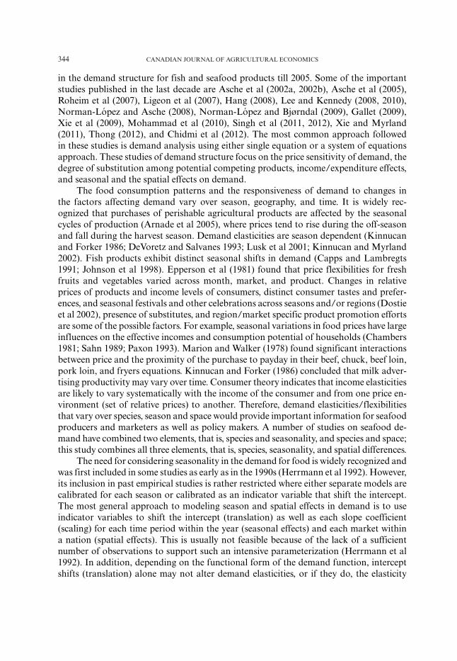
in the demand structure for fish and seafood products till 2005. Some of the importantstudies published in the last decade are Asche et al (2002a, 2002b), Asche et al (2005),Roheim et al (2007), Ligeon et al (2007), Hang (2008), Lee and Kennedy (2008, 2010),Norman-Lopez and Asche (2008), Norman-Lopez and Bjørndal (2009), Gallet (2009),Xie et al (2009), Mohammad et al (2010), Singh et al (2011, 2012), Xie and Myrland(2011), Thong (2012), and Chidmi et al (2012). The most common approach followedin these studies is demand analysis using either single equation or a system of equationsapproach. These studies of demand structure focus on the price sensitivity of demand, thedegree of substitution among potential competing products, income/expenditure effects,and seasonal and the spatial effects on demand.

The food consumption patterns and the responsiveness of demand to changes inthe factors affecting demand vary over season, geography, and time. It is widely rec-ognized that purchases of perishable agricultural products are affected by the seasonalcycles of production (Arnade et al 2005), where prices tend to rise during the off-seasonand fall during the harvest season. Demand elasticities are season dependent (Kinnucanand Forker 1986; DeVoretz and Salvanes 1993; Lusk et al 2001; Kinnucan and Myrland2002). Fish products exhibit distinct seasonal shifts in demand (Capps and Lambregts1991; Johnson et al 1998). Epperson et al (1981) found that price flexibilities for freshfruits and vegetables varied across month, market, and product. Changes in relativeprices of products and income levels of consumers, distinct consumer tastes and prefer-ences, and seasonal festivals and other celebrations across seasons and/or regions (Dostieet al 2002), presence of substitutes, and region/market specific product promotion effortsare some of the possible factors. For example, seasonal variations in food prices have largeinfluences on the effective incomes and consumption potential of households (Chambers1981; Sahn 1989; Paxon 1993). Marion and Walker (1978) found significant interactionsbetween price and the proximity of the purchase to payday in their beef, chuck, beef loin,pork loin, and fryers equations. Kinnucan and Forker (1986) concluded that milk adver-tising productivity may vary over time. Consumer theory indicates that income elasticitiesare likely to vary systematically with the income of the consumer and from one price en-vironment (set of relative prices) to another. Therefore, demand elasticities/flexibilitiesthat vary over species, season and space would provide important information for seafoodproducers and marketers as well as policy makers. A number of studies on seafood de-mand have combined two elements, that is, species and seasonality, and species and space;this study combines all three elements, that is, species, seasonality, and spatial differences.

The need for considering seasonality in the demand for food is widely recognized andwas first included in some studies as early as in the 1990s (Herrmann et al 1992). However,its inclusion in past empirical studies is rather restricted where either separate models arecalibrated for each season or calibrated as an indicator variable that shift the intercept.The most general approach to modeling season and spatial effects in demand is to useindicator variables to shift the intercept (translation) as well as each slope coefficient(scaling) for each time period within the year (seasonal effects) and each market withina nation (spatial effects). This is usually not feasible because of the lack of a sufficientnumber of observations to support such an intensive parameterization (Herrmann et al1992). In addition, depending on the functional form of the demand function, interceptshifts (translation) alone may not alter demand elasticities, or if they do, the elasticity

SEASONAL AND SPATIAL VARIATIONS IN DEMAND ELASTICITIES OF FISH PRODUCTS IN THE U.S. 345

changes (scaling) may occur in restricted and functionally dependent ways (Herrmannet al 1992). Commercial scanner data provide researchers an opportunity to use revealedpreference data from a large number of observations for this purpose.

The availability of commercial scanner data allows significant advances in under-standing food marketing (Cheng and Capps 1988; Nayga 1992; Cotterill 1994; Roheimet al 2007). Some of the important studies using scanner data for food demand analy-sis include Capps (1989), Capps and Nayga (1990), Bergtold et al (2004), Chidmi et al(2005), Torrisi et al (2006), Anders and Moser (2010), and Ahmad and Anders (2012).Capps (1989) used a scanner data set from a retail food firm located in Houston, Texaslooking into the demand relationships for steak, ground beef, roast beef, chicken, porkchops, ham, and pork loin products. Capps and Nayga (1990) examined the role of timeon price and expenditure elasticity estimates for disaggregated fresh beef products. Theresults indicated the importance of inventory adjustment over habit formation as thetime interval is shortened. Using scanner data, Bergtold et al (2004) estimated a set ofunconditional own-price and expenditure elasticities across time for 49 processed foodcategories. Chidmi et al (2005) assessed the impacts of the Northeast Dairy Compact andretail oligopoly power on fluid milk prices in Boston. Torrisi et al (2006) estimated Italiandemand for selected brands of red table wine econometrically using scanner data. Andersand Moser (2010) applied Nielsen household and retail-level scanner data to investigateCanadian consumers’ preferences and retail demand for ground meat products differen-tiated by fat content. Ahmad and Anders (2012) applied a hedonic pricing model to alarge panel of consumer packaged food products to estimate monetary value of brand,convenience, and other quality attributes in processed meat and seafood products using2000–2006 Nielsen aggregate weekly scanner data.

While utilization of scanner data for food demand analyses has become increasinglypopular in the United States, few studies of seafood demand have utilized scanner data.Exceptions include Capps and Lambregts (1991), Wessells and Wallstrom (1999), Chidmiet al (2012), and Singh et al (2012). Capps and Lambregts (1991) studied demand fordisaggregated finfish and shellfish products using scanner data from a single retail firmin Houston, Texas using a multiproduct retail demand function. Wessells and Wallstrom(1999) utilized panel data across 34 U.S. cities from 1988 through 1992 consisting ofscanner data to test the stability of canned salmon demand with a random coefficientmodel. Using national store-level scanner data, Chidmi et al (2012) estimated substitutionpatterns across seafood categories at the U.S. retail market level. Singh et al (2012) usedweekly national store-level scanner data, acquired from A. C. Nielsen Inc., to analyzedemand for 14 unbreaded frozen seafood products in the United States.

This paper used market-level commercial scanner data obtained covering 52 U.S.cities to study the effects of season and space on the demand structure of importantfinfish species. We analyzed the effects of season and space on (1) demand (translationeffects) and (2) price as well as expenditure elasticities of demand (scaling effects) for13 unbreaded frozen finfish species in the United States. The U.S. finfish markets trade anumber of various species in various product forms. The markets are made up of manyspecies that compete with one another as well as competing with imports of similarproducts from other nations. Hence, there is considerable substitutability between somefinfish species.


DATA AND METHODOLOGY

DataThe four-week aggregated market-level scanner data set used in the paper were acquiredfrom A. C. Nielsen Inc. covering the period of June 19, 2005 through June 12, 2010.1

The number of data points is 3,380 (1 data point per city × 52 cities per four-week× 13 four weeks per year × 5 years). A. C. Nielsen Inc. collects weekly scanner datafrom food/grocery, drug, and mass channels2 across the United States for frozen seafoodexcluding random-weight fresh products. The data used are from the food/grocery chan-nels that include most of the major chains (more than 130 chains with the exception ofWalmart) in the United States, and account for the majority of food-for-home consump-tion sales in the United States. The finfish species considered in this study are: salmon,tilapia, whiting, cod, flounder, pollock, catfish, halibut, orange roughy, mahi mahi, tuna,swordfish, perch, and other finfish. Table 1 presents market shares (by volume) of thesefinfish product in different U.S. census divisions. The term “catfish” included “channelcatfish” (Ictalurus punctatus), “basa/tra,” and “swai” (Pangasius spp.). The data do notdifferentiate between domestically produced and imported products. We point out herethat finfish products are sold in different product forms; however, a number of marketintegration studies have shown that the markets for different product forms are highlyintegrated (Asche et al 2002a, 2002b, 2005).

The data set contains “zero consumption” values across the studied species exceptfor salmon, tilapia, whiting, and cod. Of the 3,380 observations flounder has 33 zerovalues, pollock has 37, catfish has 65, halibut has 90, orange roughy has 66, mahi mahihas 101, tuna has 220, swordfish has 291, perch has 324, and other finfish category has83 zero values.

In direct demand models, prices are used as explanatory variables. Using zero pricesfor missing values is inappropriate. We used 13 four-week average price of a city (= averagevalue/average quantity) for missing prices in that city. In order to avoid the problem ofselection bias due to zero consumption, that is, zero values in dependent variable, we haveused the Inverse Mills ratio (IMR; Heckman, 1976) explained in next section.

We divided the data into quarters to capture the effects of season on demand: Novem-ber to January, February to April (Lent), May to July, and August to October. Duringthe period of Lent, fish is the most popular protein consumed in certain geographiesdominated by the Catholics. Fish is not considered as a meat by some Christian groupsand, therefore, is approved for consumption during this holy period. Hence, we expectthat during the period of Lent the demand for fish is higher than other quarters. Ouranalysis is on frozen products; therefore, we do not expect seasonality in demand due toseasonal cycles of production. We considered November to January quarter of the yearas base period.

1 A. C. Nielsen Inc. provided data for 5 years, and we purchased data during June, 2010.2 A. C. Nielsen Inc. defines (1) grocery channels as independent grocers or food stores having lessthan four stores with individual store with sales of over $2 million; (2) drug channels as independentdrug stores as having less than four store with sales of over $1 million; and (3) mass channels as astore having at least 10,000 square feet of selling space, at least three mass merchandise lines, noone line accounting for 80% of selling area (50% in case of food) and high volume, fast turnover,and an image of selling merchandise for less than conventional prices.


Table 1. Market share (%) of different finfish species in the U.S. finfish market

Division Salmon Tilapia Whiting Cod Flounder Pollock Catfish

South Atlantic 9.99 33.83 23.75 2.92 7.53 0.85 2.84East South Central 7.68 23.31 33.39 3.07 3.52 1.12 20.20New England 15.83 20.01 19.72 5.38 7.40 11.84 0.64East North Central 11.96 34.61 17.61 6.60 2.32 5.43 7.34West South Central 10.43 42.25 10.40 3.69 3.88 4.23 16.52Mountain 20.05 40.74 7.49 7.60 3.18 4.68 6.79West North Central 22.10 34.48 6.63 6.77 3.15 9.21 4.44Pacific 14.22 46.58 11.54 3.12 3.52 2.75 10.05Mid Atlantic 20.25 25.47 29.10 2.21 10.25 2.53 1.11United States 13.92 34.59 19.57 3.97 5.50 3.33 6.93

Division Halibut Orange roughy Mahi mahi Tuna Swordfish Perch Others

South Atlantic 0.54 1.99 2.30 1.95 0.67 4.58 6.25East South Central 0.55 0.88 0.43 0.63 0.22 4.03 0.97New England 0.36 0.39 1.28 0.83 0.93 1.25 14.15East North Central 0.70 3.49 0.74 0.90 0.47 5.22 2.59West South Central 0.62 2.01 1.21 1.49 0.56 1.90 0.84Mountain 1.56 2.13 0.76 0.83 0.59 1.37 2.22West North Central 1.03 3.57 1.67 1.98 0.58 2.19 2.18Pacific 1.20 0.54 0.87 0.42 0.24 2.26 2.69Mid Atlantic 0.25 1.00 0.54 0.47 0.34 1.09 5.37United States 0.71 1.75 1.16 1.05 0.47 3.08 3.97

As mentioned earlier, we have used market-level data for analysis. However, wehave considered U.S. census divisions to examine the spatial variations in the quantitydemanded and the demand elasticities for different finfish products. This is because ofcomputational limitations. The U.S. census divisions are: South Atlantic, East SouthCentral, New England, East North Central, West South Central, Mountain, West NorthCentral, Mid Atlantic, and Pacific.

Theoretical Framework and Empirical ModelEquation (1) is the standard form of the Almost Ideal Demand System (AIDS) (Deatonand Muellbauer 1980)

wi = ∝i +n∑

j=1

γi j ln p j + βi (ln Xt − ln Pt) (1)

where wi (= pi qi∑ni=1 pi qi

) is the expenditure share of seafood product i, pi is the retail price

of commodity i, qi is the purchase quantity of seafood product i, ln denotes naturallogarithmic values of variables, Xt (= ∑n

i=1 pi qi ) is the total expenditure, ln P is the priceindex defined in Equation (2), and ∝i , γi j , andβi are the parameters of the model.

ln P =∝0 +n∑

j �=i

∝ j ln p j + 0.5n∑

i=1

∑j �=i

γ ∗i j ln pi ln p j (2)


Due to the nonlinearity of ln P (Equation [2]), the Stone’s price index is used to developa linear approximate AIDS. Some authors have argued for using some other indices(Pashardes 1993; Buse 1994; Moschini 1995). Eales and Unnevehr (1988) suggested usinglagged shares instead of the current share in the Stone’s price index in linear approximateAIDS to overcome the problem of simultaneity. We have used a log linear version ofthe Paasche’s index (Moschini 1995) with lagged shares. Equation (3) gives the dynamicversion of the AIDS model

wi,t = ∝i,t +n∑

j=1

γi j ln p j,t + βi

⎡⎣ln Xt −

n∑j=1

(w j,t−1 ln

p j,t

p j,0

)⎤⎦ (3)

We have modified ∝i (intercept) in Equation (3) to account for the effects of season anddemography on the demand for fish products (i.e., season and demographic translation)

∝i,t = ∝∗i,t +

K∑k=1

τi SkSk +L∑

l=1

τi Rl Rl + μi,t (4)

where S denotes a dummy variable for season, and R is the dummy variable used for U.S.census division, which captures the effects of division specific social, demographic, andeconomic consumer characteristics, and other factors on seafood demand structure. Thecontrol season is November to January, and the Mid Atlantic division as a base division.The term μt,i is the error term, which accounts for random variation in the dependentvariable.

It is important to note that when using the Stone’s price index, the constant term forthe price index is moved from the price index term to the constant term in the demandsystem as discussed by Asche and Wessells (1997). This implies that the season anddemographic translations cause shift/translation in the price index.

In order to capture the effects of season (Sks) and U.S. census division (Rls) on priceand expenditure elasticities, we have introduced interactions terms in Equation (3) asgiven in Equation (5) (i.e., season and demographic scaling)

wi = ∝∗∗i +

⎡⎣ N∑

j=1

γi j ln p j +N∑

j=1

K∑k=1

γi j Sk(ln p j ∗ Sk) +N∑

j=1

L∑l=1

γi j Rl (ln p j ∗ Rl )

⎤⎦

+⎡⎣βi

{ln Xt −

n∑j=1

(w j,t−1 ln

p j,t

p j,0

)}+

K∑k=1

βSk

{ln Xt −

n∑j=1

(w j,t−1 ln

p j,t

p j,0

)}∗ Sk

+L∑

l=1

βRl

{ln Xt −

n∑j=1

(w j,t−1 ln

p j,t

p j,0

)}∗ Rl

⎤⎦ (5)

As mentioned earlier, there is a problem of zero consumption in the data set used.This makes some observations of the dependent variable (wi ) equal to zero and would


cause sample selection bias in the model. To overcome this we used the Heckman (1976)two-step procedure.

In the first step, we estimated a probit model for finfish products having zero con-sumption (Heien and Wessells, 1990) using city specific demographic characteristics asexplanatory variables that include: household income (% of household having householdincome <$10,000, $10,000–$25,000, $25,000–$50,000, and $50,000–$100,000), ethnicity(% of White, Black or African American, American Indian and Alaska Native, Asian,and Native Hawaiian and Other Pacific Islander), and aggregate travel time to work3 (inminutes) of workers 16 years and over who did not work at home. In the second step, wecomputed the IMR (estimated expected error) as a ratio of the normal probability densityfunction to the normal cumulative density function of predicted probabilities in the firststep.

We introduced estimated IMRs in share equations. Equation (6) gives the final modelwith a modified intercept (Equation [4]), interactions of demography and seasonal dummyvariables with the prices and the modified price index (Equation [5]), and IMRs

wi = ∝∗∗∗i,t +

K∑k=1

τi SkSk +L∑

l=1

τi Rl Rl +⎡⎣ N∑

j=1

γi j ln p j +N∑

j=1

K∑k=1

γi j Sk(ln p j ∗ Sk)

+N∑

j=1

L∑l=1

γi j Rl (ln p j ∗ Rl )

⎤⎦ +

⎡⎣βi

⎧⎨⎩ln Xt −

n∑j=1

(w j,t−1 ln

p j,t

p j,0

)⎫⎬⎭

+K∑

k=1

βSk

⎧⎨⎩ln Xt −

n∑j=1

(w j,t−1 ln

p j,t

p j,0

)⎫⎬⎭ ∗ Sk

+L∑

l=1

βRl

⎧⎨⎩ln Xt −

n∑j=1

(w j,t−1 ln

p j,t

p j,0

)⎫⎬⎭ ∗ Rl

⎤⎦ + ∂i I MRi + μi,t (6)

For the sake of brevity, we have used the same symbols for parameters in Equations(1) and (3)–(6). However, the parameters of Equation (6) differ from those of other equa-tions. Equations (7.1)–(7.3) present the modified theoretical restrictions on final model(Equation [6])

Homogeneity restrictions

n∑j=1

γi j = 0,

n∑j=1

γi j +N∑

j=1

γi j Sk = 0,

N∑j=1

γi j Rl = 0 (7.1)

Symmetry restrictions

γi j = γ j i , γi j Sk = γ j i Sk, γi j Rl = γ j i Rl , i �= j (7.2)

3 The data is on fish products consumed at home. We assume that with an increase in the traveltime to work, the infrequency of consuming fish at home, that is, probability of zero consumption,increases.


Adding-up restrictions

n∑i=1

∝∗∗∗i,t = 1,

n∑i=1

τi Sk = 0,

n∑i=1

τi Rl = 0,

n∑i=1

γi j = 0,

n∑i=1

γi j Sk = 0,

n∑i=1

γi j Rl

= 0,

n∑i=1

βi = 0,

n∑i=1

βi Sk = 0,

n∑i=1

βi Rl = 0, andn∑

i=1

∂i 0

(7.3)

Model EstimationEstimation of the system of equations given in Equation [6] as a complete system alongwith the theoretical restrictions imposed will have a singularity problem. This is becausethe sum of left-hand side variables (

∑nj=1 wi ) is equal to the sum of the right-hand side

of the system of equations (due to adding-up restrictions). The most commonly usedapproach in the literature to overcome this problem is the Barten (1969) method, that is,estimating the system of equations by dropping one of the equations. We dropped the“other finfish” equation. We estimated the model given in Equation (6) using the IterativeSeemingly Unrelated Regression procedure in STATA(S/E) 12 software (StataCorp LP,College Station, TX). Using adding-up restrictions (Equation [7.3]) we obtained theparameters of the dropped equation.

Before having the theoretical restrictions imposed in the final model (Equation [6]),we used the log-likelihood ratio test to test the significance of imposing: (a) homogeneityrestrictions alone, (b) symmetry restrictions alone, and (c) homogeneity and symmetryrestrictions together. We found that both restrictions together were highly significant;therefore, we imposed them while estimating the system.

We computed the uncompensated price elasticities (ξi j ), expenditure elasticities (ηi ),and compensated price elasticities (ζi j ) as follows

ξi j Sk = −δ + (γi j + γi j Sk)wi

− (βi + βi Sk) × w j

wi; ξi j Rl = −δ + (γi j + γi j Rl )

wi− (βi + βi Rl )

×w j

wi; ηi Sk = (βi + βi Sk)

wi+ 1; ηi Rl = (βi + βi Rl )

wi+ 1; and ζi j = ξi j + w j × ηi (8)

where δ is the Kronecker delta, which is equal to one for own-price elasticities (i = j) andzero for cross-price elasticities (i �= j). If subscript k = 0, then γi j Sk and βi Sk = 0, and ifsubscript l = 0, then γi j Rl and βi Rl = 0

RESULTS AND DISCUSSION

Model Specification TestsWe have tested all series (wi , ln pi , and ln X) for unit root using the Harris–Tzavalis (HT)(Harris and Tzavalis 1999) panel unit root test. The HT test examines the null hypotheses(H0) that panels contain unit root, against the alternate hypothesis (H1) that they arestationary. The HT test assumes that all panels have the same autoregressive parameterso that the alternative hypothesis is simply ρ < 1, and the number of time periods, T,is fixed. Estimated HT test statistics “ρ” ranged between 0.37 and 0.85. Given that the


Table 2. R2, average prices, and expenditure shares of different finfish species

Average Average

Species R2 Price ($/lb) Expend. share Species R2 Price ($/lb) Expend. share

Salmon 0.4728 6.61 22.32 Halibut 0.4793 13.85 2.82Tilapia 0.4769 3.57 27.36 Orange roughy 0.4557 9.60 4.50Whiting 0.6436 2.27 10.13 Mahi mahi 0.5163 8.00 2.06Cod 0.5016 5.93 6.39 Tuna 0.3305 7.67 2.03Flounder 0.5924 4.16 4.72 Swordfish 0.3546 10.16 1.20Pollock 0.6351 2.73 2.77 Perch 0.6090 4.96 3.43Catfish 0.5167 3.18 6.02 Others 4.74 4.25

number of panels equal to 52, and periods equal to 65, these values are highly significantat 0.00. Therefore, the null hypothesis that panels contain unit root are rejected for allseries under study.

In order to capture any possible multicollinearity problems associated with highcorrelation, we checked all variance-inflation factors (VIFs). Generally individual VIFsgreater than 10 and with an average VIF greater than 6 are generally seen as an indicationof severe multicollinearity. Estimated VIFs ranged between 1.02 and 1.46 with an averageof 1.20 suggesting multicollinearity is not a problem in the model.

We have used the Hausman test (Hausman 1978) to examine the exogeneity ofthe variables on the right-hand side of the Equation [6]. The test results indicated thatendogeneity is not a problem in the model.

Model EstimatesTable 2 depicts R2 values of the fitted model, average prices and average expenditure sharesfor different finfish. The fitted model explains 33–64% of the variation in the expenditureshares of different finfish species. Tilapia and salmon contributes almost 50% to totalconsumer expenditure on finfish products. Among all, halibut is the most expensivefinfish followed by swordfish, orange roughy, and mahi mahi. On the other hand, whitingis the cheapest followed by pollock. The average prices for tilapia are marginally higherthan catfish prices.

It is important to note that coefficients of the IMRs were significant for all equations.Hence, this implies that deleting observations with zero expenditure for some items wouldhave caused biased estimates. Some other studies also reported similar results such asHeien and Wessells (1990), Wellman (1992), and Salvanes and Devoretz (1997) to namea few.

Seasonal and Spatial Variations in DemandA large majority of coefficients of the dummies used for the U.S. census divisions werehighly significant suggesting different patterns of demand for finfish in different divisions.Also a few coefficients of the dummies used for season were found significant up to the0.10 level of significance. We do not expect seasonality in demand due to seasonality inproduction cycles of different finfish products, as mentioned earlier, because our analysis


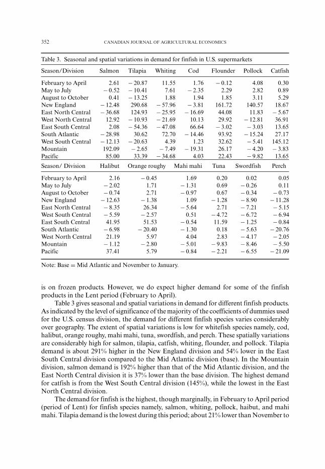
Table 3. Seasonal and spatial variations in demand for finfish in U.S. supermarkets

Season/Division Salmon Tilapia Whiting Cod Flounder Pollock Catfish

February to April 2.61 − 20.87 11.55 1.76 − 0.12 4.08 0.30May to July − 0.52 − 10.41 7.61 − 2.35 2.29 2.82 0.89August to October 0.41 − 13.25 1.88 1.94 1.85 3.11 5.29New England − 12.48 290.68 − 57.96 − 3.81 161.72 140.57 18.67East North Central − 36.68 124.93 − 25.95 − 16.69 44.08 11.83 − 5.67West North Central 12.92 − 10.93 − 21.69 10.13 29.92 − 12.81 36.91East South Central 2.08 − 54.36 − 47.08 66.64 − 3.02 − 3.03 13.65South Atlantic − 28.98 30.62 72.70 − 14.46 93.92 − 15.24 27.17West South Central − 12.13 − 20.63 4.39 1.23 32.62 − 5.41 145.12Mountain 192.09 − 2.65 − 7.49 − 19.31 26.17 − 4.20 − 3.83Pacific 85.00 33.39 − 34.68 4.03 22.43 − 9.82 13.65

Season/ Division Halibut Orange roughy Mahi mahi Tuna Swordfish Perch

February to April 2.16 − 0.45 1.69 0.20 0.02 0.05May to July − 2.02 1.71 − 1.31 0.69 − 0.26 0.11August to October − 0.74 2.71 − 0.97 0.67 − 0.34 − 0.73New England − 12.63 − 1.38 1.09 − 1.28 − 8.90 − 11.28East North Central − 8.35 26.34 − 5.64 2.71 − 7.21 − 5.15West South Central − 5.59 − 2.57 0.51 − 4.72 − 6.72 − 6.94East South Central 41.95 51.53 − 0.54 11.59 − 1.25 − 0.84South Atlantic − 6.98 − 20.40 − 1.30 0.18 − 5.63 − 20.76West North Central 21.19 5.97 4.04 2.83 − 4.17 − 2.05Mountain − 1.12 − 2.80 − 5.01 − 9.83 − 8.46 − 5.50Pacific 37.41 5.79 − 0.84 − 2.21 − 6.55 − 21.09

Note: Base = Mid Atlantic and November to January.

is on frozen products. However, we do expect higher demand for some of the finfishproducts in the Lent period (February to April).

Table 3 gives seasonal and spatial variations in demand for different finfish products.As indicated by the level of significance of the majority of the coefficients of dummies usedfor the U.S. census division, the demand for different finfish species varies considerablyover geography. The extent of spatial variations is low for whitefish species namely, cod,halibut, orange roughy, mahi mahi, tuna, swordfish, and perch. These spatially variationsare considerably high for salmon, tilapia, catfish, whiting, flounder, and pollock. Tilapiademand is about 291% higher in the New England division and 54% lower in the EastSouth Central division compared to the Mid Atlantic division (base). In the Mountaindivision, salmon demand is 192% higher than that of the Mid Atlantic division, and theEast North Central division it is 37% lower than the base division. The highest demandfor catfish is from the West South Central division (145%), while the lowest in the EastNorth Central division.

The demand for finfish is the highest, though marginally, in February to April period(period of Lent) for finfish species namely, salmon, whiting, pollock, haibut, and mahimahi. Tilapia demand is the lowest during this period; about 21% lower than November to


Table 4. Seasonal and spatial variations in own-price elasticities of finfish products in U.S.supermarkets


November to January −1.11 −1.27 −2.08 −0.97 −1.19 −1.23 −1.10February to April −1.21 −1.23 −1.92 −1.12 −1.24 −0.58 −1.13May to July −1.24 −1.19 −2.03 −1.07 −1.27 −0.95 −1.22August to October −1.21 −1.21 −2.03 −1.07 −1.42 −1.15 −1.23Mid Atlantic −1.11 −1.27 −2.08 −0.97 −1.19 −1.23 −1.10New England −1.92 −1.32 −3.25 −0.07 −2.30 −0.21 −1.10East North Central −1.15 −1.66 −2.18 −2.36 −1.62 −1.79 −2.03West South Central −0.83 −1.09 −1.36 −1.31 −1.12 −1.78 −1.46East South Central −1.13 −1.53 −3.37 −1.69 −1.37 −1.79 −5.00South Atlantic −0.97 −1.87 −1.83 −1.07 −2.22 −1.14 −0.70West North Central −1.65 −1.58 −1.67 −2.45 −1.60 −2.77 −1.07Mountain −2.17 −2.31 −1.97 −2.35 −1.33 −1.03 −1.16Pacific −1.03 −2.05 −1.53 −0.91 −1.17 −1.23 −1.54

Season/ Division Halibut Orange roughy Mahi mahi Tuna Swordfish Perch

November January −0.80 −0.98 −1.34 −0.96 −1.07 −1.98February to April −0.80 −0.97 −1.23 −0.96 −1.07 −2.03May to July −0.89 −0.96 −1.29 −1.03 −1.02 −1.91August to October −0.90 −1.02 −1.38 −1.04 −1.00 −1.80Mid Atlantic −0.80 −0.98 −1.34 −0.96 −1.07 −1.98New England −0.90 −0.95 −1.15 −0.97 −1.00 −0.63East North Central −0.87 −0.88 −0.98 −0.88 −0.96 −1.97West South Central −0.99 −0.91 −0.58 −1.21 −0.56 −1.69East South Central −1.03 −1.06 −0.91 −0.97 −1.01 −2.55South Atlantic −0.73 −1.06 −0.90 −0.89 −0.96 −1.23West North Central −1.11 −1.05 −0.96 −2.89 −0.98 −1.17Mountain −1.23 −1.01 −1.09 −1.04 −0.96 −1.18Pacific −0.73 −1.05 −1.20 −1.16 −1.14 −1.05

January quarter. Hang (2008) also found a sharp decline in the budget share of importedsalmon and tilapia in the first quarter. He observed that the budget share of importedsalmon decreased at 5% level of statistical significance in the first and second quarters,while the shares of tilapia and catfish imports decline in the months from January toMarch.

Seasonal and Spatial Variations in Price Elasticities of DemandThe majority of coefficients of the interactions between the division and the prices werehighly significant showing spatially varying responsiveness of demand to changes in prices.A few coefficients of the interactions between the season and the prices were significantindicating low extent of seasonal effects on price elasticities of demand for a majorityof the finfish products. Table 4 presents the own-price elasticities, and Tables 5 and 6gives ranges of own- and cross-price elasticities of different finfish products in different

354 CANADIAN JOURNAL OF AGRICULTURAL ECONOMICST

able

5.Se

ason

alva

riat

ions

inco

mpe

nsat

edcr

oss-

pric

eel

asti

citi

esof

finf

ish

prod

ucts

inU

.S.s

uper

mar

kets

Equ

atio

n→

Salm

onT

ilapi

aW

hiti

ngC

odF

loun

der

Pollo

ckC

atfi

sh

Salm

on−

1.24

to−1

.11

0.09

to0.

180.

56to

0.65

0.17

to0.

231.

08to

1.13

0.65

to0.

75−

0.14

to−0

.07

Tila

pia

0.11

to0.

22−

1.27

to−1

.19

0.92

to1.

120.

26to

0.40

−1.

29to

−1.2

2−

0.21

to0.

601.

33to

1.71

Whi

ting

0.25

to0.

300.

34to

0.42

−2.

08to

−1.9

20.

25to

0.41

0.55

to0.

760.

00to

0.29

−1.

45to

−1.3

4C

od0.

05to

0.07

0.06

to0.

090.

16to

0.26

−1.

12to

−0.9

70.

12to

0.18

−0.

13to

−0.0

80.

32to

0.38

Flo

unde

r0.

23to

0.24

−0.

22to

−0.2

10.

26to

0.35

0.09

to0.

13−

1.42

to−1

.19

0.85

to1.

13−

0.74

to−0

.63

Pollo

ck0.

08to

0.09

−0.

02to

0.06

0.00

to0.

08−

0.06

to−0

.04

0.50

to0.

66−

1.23

to−0

.58

−0.

16to

−0.0

7C

atfi

sh−

0.04

to−0

.02

0.29

to0.

38−

0.86

to−0

.80

0.30

to0.

35−

0.95

to−0

.80

−0.

34to

−0.1

5−

1.23

to−1

.10

Hal

ibut

0.03

to0.

04−

0.01

to0.

02−

0.01

to0.

05−

0.10

to−0

.06

0.00

to0.

08−

0.11

to−0

.01

0.11

to0.

16O

rang

ero

ughy

0.10

to0.

110.

00to

0.01

0.05

to0.

11−

0.06

to−0

.04

−0.

04to

0.02

−0.

08to

0.02

0.12

to0.

19M

ahim

ahi

−0.

02to

0.01

−0.

04to

0.03

0.14

to0.

20−

0.05

to0.

020.

11to

0.17

−0.

15to

−0.0

3−

0.01

to0.

28T

una

0.00

to0.

020.

00to

0.03

0.08

to0.

11−

0.09

to−0

.04

0.01

to0.

03−

0.08

to0.

040.

00to

0.09

Swor

dfis

h−

0.01

to0.

00−

0.01

to0.

000.

05to

0.08

−0.

02to

0.02

−0.

05to

0.01

−0.

07to

0.00

0.04

to0.

08P

erch

−0.

02to

0.00

0.00

to0.

030.

01to

0.10

−0.

07to

0.00

0.08

to0.

160.

50to

0.72

0.02

to0.

13

Hal

ibut

Ora

nge

roug

hyM

ahim

ahi

Tun

aSw

ordf

ish

Per

ch

Salm

on0.

24to

0.31

0.49

to0.

56−

0.17

to0.

060.

05to

0.22

−0.

13to

−0.0

2−

0.14

to0.

02T

ilapi

a−

0.12

to0.

22−

0.02

to0.

05−

0.51

to0.

390.

01to

0.38

−0.

23to

0.11

−0.

03to

0.26

Whi

ting

−0.

02to

0.17

0.12

to0.

250.

69to

0.96

0.39

to0.

530.

45to

0.69

0.03

to0.

28C

od−

0.22

to−0

.15

−0.

08to

−0.0

5−

0.14

to0.

07−

0.28

to−0

.11

−0.

13to

0.10

−0.

13to

−0.0

1F

loun

der

−0.

01to

0.14

−0.

04to

0.02

0.26

to0.

390.

02to

0.06

−0.

19to

0.05

0.11

to0.

22Po

llock

−0.

10to

−0.0

1−

0.05

to0.

01−

0.21

to−0

.04

−0.

11to

0.06

−0.

16to

0.01

0.41

to0.

58C

atfi

sh0.

23to

0.34

0.16

to0.

25−

0.02

to0.

82−

0.01

to0.

270.

20to

0.40

0.04

to0.

22H

alib

ut−

0.90

to−0

.80

0.00

to0.

02−

0.07

to−0

.01

0.01

to0.

110.

17to

0.21

0.02

to0.

05O

rang

ero

ughy

0.00

to0.

02−

1.02

to−0

.96

−0.

06to

0.01

0.07

to0.

120.

16to

0.22

−0.

04to

0.03

Mah

imah

i−

0.05

to−0

.01

−0.

03to

0.00

−1.

38to

−1.2

3−

0.04

to0.

02−

0.25

to−0

.21

0.04

to0.

09T

una

0.01

to0.

080.

03to

0.05

−0.

04to

0.02

−1.

04to

−0.9

6−

0.09

to−0

.02

−0.

05to

0.03

Swor

dfis

h0.

07to

0.09

0.04

to0.

06−

0.15

to−0

.12

−0.

05to

−0.0

1−

1.07

to−1

.00

0.02

to0.

04P

erch

0.02

to0.

06−

0.03

to0.

030.

07to

0.15

−0.

08to

0.05

0.06

to0.

11−

2.03

to−1

.80

Not

e:F

igur

esin

bold

are

unco

mpe

nsat

edow

n-pr

ice

elas

tici

ties

.

SEASONAL AND SPATIAL VARIATIONS IN DEMAND ELASTICITIES OF FISH PRODUCTS IN THE U.S. 355T

able

6.Sp

atia

lvar

iati

ons

inco

mpe

nsat

edcr

oss-

pric

eel

asti

citi

esof

finf

ish

prod

ucts

inU

.S.s

uper

mar

kets

Equ

atio

n→Sa

lmon

Tila

pia

Whi

ting

Cod

Flo

unde

rPo

llock

Cat

fish

Salm

on−

2.17

to−0

.83

0.08

to0.

840.

21to

1.78

−0.

12to

1.39

0.11

to1.

14−

0.63

to3.

02−

4.61

to0.

67T

ilapi

a0.

10to

1.04

−2.

31to

−1.0

90.

01to

2.08

−0.

81to

0.95

−0.

18to

2.18

−0.

01to

1.67

−0.

57to

1.14

Whi

ting

0.10

to0.

810.

00to

0.77

−3.

37to

−1.3

6−

1.38

to0.

63−

1.87

to3.

69−

4.90

to0.

93−

1.10

to1.

32C

od−

0.03

to0.

40−

0.19

to0.

22−

0.87

to0.

40−

2.45

to−0

.07

−1.

51to

0.60

−0.

69to

4.49

−0.

20to

2.09

Flo

unde

r0.

02to

0.24

−0.

03to

0.38

−0.

87to

1.72

−1.

11to

0.44

−2.

30to

−1.1

2−

0.14

to1.

32−

0.26

to2.

08Po

llock

−0.

08to

0.38

0.00

to0.

17−

1.34

to0.

25−

0.30

to1.

95−

0.08

to0.

77−

2.77

to−0

.21

−0.

29to

0.51

Cat

fish

−1.

24to

0.18

−0.

12to

0.25

−0.

65to

0.78

−0.

19to

1.97

−0.

33to

2.65

−0.

64to

1.11

−5.

00to

−0.7

0H

alib

ut−

0.08

to0.

100.

00to

0.06

−0.

02to

0.28

−0.

26to

0.14

−0.

04to

0.18

−0.

27to

0.46

−0.

20to

0.28

Ora

nge

roug

hy−

0.07

to0.

06−

0.03

to0.

15−

0.10

to0.

18−

0.10

to0.

10−

0.16

to0.

11−

0.11

to0.

16−

0.14

to0.

75M

ahim

ahi

−0.

04to

0.03

−0.

07to

0.10

−0.

10to

0.12

−0.

11to

0.20

−0.

09to

0.18

−0.

58to

0.11

−0.

20to

0.24

Tun

a0.

00to

0.06

−0.

04to

0.09

0.00

to0.

18−

0.15

to0.

19−

0.17

to0.

43−

1.19

to0.

53−

0.04

to0.

23Sw

ordf

ish

−0.

03to

0.06

−0.

03to

0.05

−0.

09to

0.11

−0.

15to

0.31

−0.

16to

0.06

−0.

41to

0.05

−0.

23to

0.28

Per

ch−

0.03

to0.

270.

01to

0.16

−0.

24to

0.43

−0.

47to

0.21

−0.

93to

0.28

−0.

24to

0.47

−0.

31to

0.93

Equ

atio

nH

alib

utO

rang

ero

ughy

Mah

imah

iT

una

Swor

dfis

hP

erch

Salm

on−

0.67

to0.

80−

0.36

to0.

32−

0.39

to0.

330.

01to

0.68

−0.

55to

1.08

−0.

21to

1.75

Tila

pia

−0.

03to

0.58

−0.

17to

0.90

−0.

91to

1.35

−0.

50to

1.16

−0.

69to

1.18

0.10

to1.

24W

hiti

ng−

0.09

to0.

99−

0.23

to0.

41−

0.50

to0.

59−

0.02

to0.

89−

0.75

to0.

90−

0.70

to1.

27C

od−

0.60

to0.

31−

0.14

to0.

14−

0.34

to0.

63−

0.47

to0.

61−

0.81

to1.

65−

0.88

to0.

39F

loun

der

−0.

06to

0.31

−0.

17to

0.12

−0.

22to

0.42

−0.

39to

1.01

−0.

62to

0.24

−1.

28to

0.39

Pollo

ck−

0.26

to0.

45−

0.07

to0.

10−

0.77

to0.

15−

1.63

to0.

73−

0.95

to0.

13−

0.19

to0.

38C

atfi

sh−

0.42

to0.

60−

0.19

to1.

00−

0.58

to0.

69−

0.11

to0.

68−

1.17

to1.

42−

0.54

to1.

63H

alib

ut−

1.23

to−0

.73

−0.

10to

0.06

−0.

13to

0.17

−0.

31to

0.10

−0.

34to

0.23

−0.

09to

0.17

Ora

nge

roug

hy−

0.16

to0.

09−

1.06

to−0

.88

−0.

04to

0.18

−0.

11to

0.16

−0.

14to

0.27

−0.

03to

0.16

Mah

imah

i−

0.09

to0.

13−

0.02

to0.

08−

1.20

to−0

.58

−0.

10to

0.26

−0.

02to

0.45

−0.

22to

0.34

Tun

a−

0.23

to0.

07−

0.05

to0.

07−

0.09

to0.

26−

2.89

to−0

.88

−0.

12to

0.27

−0.

15to

0.26

Swor

dfis

h−

0.15

to0.

10−

0.04

to0.

07−

0.01

to0.

26−

0.07

to0.

16−

1.14

to−0

.56

−0.

10to

0.08

Per

ch−

0.11

to0.

21−

0.02

to0.

12−

0.36

to0.

57−

0.25

to0.

44−

0.29

to0.

22−

2.55

to−0

.63

Not

e:F

igur

esin

bold

are

unco

mpe

nsat

edow

n-pr

ice

elas

tici

ties

.


seasons and division, respectively. Own-price elasticities are compensated and cross-priceelasticities are compensated.

Own-price elasticities are negative in all divisions and seasons for all the species(Tables 4). The demand for a majority of finfish products are either relatively own-priceelastic or unitary elastic in most of the seasons and divisions. Whiting demand is the mostelastic and halibut demand the least elastic in majority of seasons and divisions. Estimatesof average (mostly national level) own-price elasticities from other studies for differentseafood products fall within the elasticity ranges of this study. For example Norman-Lopez and Asche (2008) estimated the own-price elasticities of frozen and fresh filletsof U.S. catfish at −0.773 and −1.029, respectively. Similarly Kinnucan and Miao (1999)and Kouka (1995) found own-price elasticity of catfish fillet at the levels of −0.706 and−1.17, respectively. Ligeon et al (2007) conducted an import demand study for tilapia andtilapia products in the United States. They estimated the own-price elasticity of frozenfillets from Jamaica, Thailand, Indonesia, and China at −0.23, −0.14, −0.18, and −0.96levels, respectively. Chidmi et al (2012) found own-price elastic demand for catfish andsalmon, and own-price inelastic demand for tilapia. Singh et al (2012) estimated own-priceelasticities of demand for salmon, catfish, tilapia, flounder, and tuna lower than one, andfor cod, whiting, perch, and pollock greater than one.

Season does not affect the responsiveness of demand to changes in own-prices formajority of finfish species (Table 4 and 5). There are significant seasonal variations in theown-price elasticities of pollock (Tables 4 and 5). Overall, the extent of spatial variationsin own-price elasticities for the finfish products is higher than seasonal variations (Tables 4and 6), and present in all species under study. For example salmon demand is own-priceinelastic in the West South Central division, almost unitary elastic in the South Atlanticand Pacific divisions and elastic in other divisions. Catfish demand is own-price inelasticin the South Atlantic division and almost unitary elastic in the West North Centraldivision. Own-price elasticity of catfish demand is very high (−5) in the East SouthCentral division.

Like own-price elasticities, the degree of seasonal effects on cross-price elasticitiesof demand for finfish products is very low (Table 5). There are complementarities be-tween some species in some seasons but substitutability in other seasons. The cross-priceelasticities of demand for mahi mahi with respect to tilapia are −0.05, 0.39, −0.48,and −0.51 for November to February, February to April, May to July and August toOctober quarters, respectively; elasticity for November to February quarter is nonsignif-icant. This shows that tilapia is a substitute to mahi mahi in February to April quarter,that is, the Lent period, has no relationship in November to February quarter, and has acomplementary relationship for the rest of the year. Tilapia and salmon are substitutes inall seasons; however, the degree of substitutability is very low (Table 5). Tilapia is a verystrong substitute to catfish in all seasons, but the substitutability of catfish for tilapia isvery weak. Salmon has a stronger substitutability for whiting, orange roughy, flounder,Pollock, and halibut in all seasons as compared to substitutability of these products forsalmon. Pollock and flounder, catfish and cod, whiting and tilapia are other substitutingproducts. The responsiveness of demand for finfish species namely, halibut, mahi mahi,and swordfish to the changes in prices of tilapia varied considerably over seasons.

Seasonal variations in cross-price elasticities show that tilapia is a strong substitutingproduct for catfish. However, spatial analysis reveals that their relationship varies between


complementarity and substitutability (Table 6). Tilapia is a substituting product for catfishin East North Central division (cross-price elasticity = 1.14), New England division(cross-price elasticity = 0.89), and Pacific division (cross-price elasticity = 0.45), and hasa complementarity for catfish in Mountain division (cross-price elasticity = −0.41), WestNorth Central division (cross-price elasticity = −0.57), and East South Central division(cross-price elasticity = −0.41). In other divisions, tilapia is a weak substitute productfor catfish. The magnitude of cross-price elasticity of demand for tilapia with catfish ispositive but very low in most of the divisions indicating very weak substitutability, if any,of catfish for tilapia in the supermarkets of the United States.

Norman-Lopez and Asche (2008) found that demand for fresh and frozen importedtilapia was independent of the demand for fresh and frozen domestic catfish. However,Muhammad et al (2010) found tilapia as a substitute for domestic catfish in the UnitedStates. Chidmi et al (2012) found tilapia and catfish as substituting products in the UnitedStates; however, catfish sales were more affected by the price movements of tilapia thantilapia sales were affected by price movements of catfish. Singh et al (2012) did not find anysignificant relationship between catfish and tilapia. The Norman-Lopez and Asche (2008),Muhammad et al (2010), and Chidmi et al (2012) studies did not consider the seasonalor regional variations in demand and price and expenditure elasticities of demand. Singhet al (2012) modified the intercept of the AIDS model to examine the seasonality indemand; this accounted for translation effects only.

Similar to the tilapia and catfish relationship, the relationship between pollock andcatfish also varies between complementarity and substitutability. Catfish is a strong sub-stitute for pollock in the West North Central division (cross-price elasticity = 1.11), anda complementary product in the Pacific division (cross-price elasticity = −0.64) and theNew England division (cross-price elasticity =−0.48). Pollock substitutes for catfish in theWest North Central division (cross-price elasticity = 0.51). Singh et al (2012) did not findany significant relationship between catfish and pollock, which is a national-level study.

Important substitutes of catfish are perch, flounder and cod in the East SouthCentral division (cross-price elasticity = 0.93, 2.08, and 2.09, respectively), tilapia andwhiting in the New England division (cross-price elasticity = 0.89 and 0.82, respec-tively), salmon and tilapia the East North Central division (cross-price elasticity = 0.67and 1.14, respectively), whiting in the West South Central division (cross-price elastic-ity = 1.32), pollock and orange roughy the West North Central division (cross-priceelasticity = 0.51 and 0.44, respectively), and tilapia in the Pacific division (cross-priceelasticity = 0.45). This shows that not only the degree of competition between finfishproducts varies over the divisions, but also the competing products. Singh et al (2012)found salmon and whiting as substituting products for catfish; salmon and whiting arestronger substitutes to catfish than catfish for salmon and whiting.

We found the complementarity relationships (cross-price elasticities that are negativeand highly significant) between some of the fish species. Using national-level retail scannerdata, Singh et al (2012) also found a few complementary relationships between fishproducts in the United States. For example, whiting as a complementary product toflounder (cross-price elasticity = −0.44), flounder as a complementary product to pollock(cross-price elasticity = −0.20), and catfish as a complementary product to tuna (cross-price elasticity = −0.31).


Table 7. Seasonal and spatial variations in expenditure elasticities of finfish products in U.S.supermarkets


November to January 0.94 1.23 0.95 0.83 1.56 0.71 1.23February to April 0.94 1.29 0.86 0.82 1.54 0.62 1.21May to July 0.96 1.26 0.89 0.85 1.51 0.63 1.20August to October 0.95 1.27 0.94 0.80 1.53 0.63 1.14Mid Atlantic 0.94 1.23 0.95 0.83 1.56 0.71 1.23New England 1.02 0.84 1.51 0.87 0.22 -1.99 1.14East North Central 1.05 1.03 1.14 1.09 0.93 0.42 1.43West South Central 0.92 1.33 0.90 0.79 1.04 0.74 0.39East South Central 0.89 1.47 1.41 0.26 1.51 0.73 1.30South Atlantic 1.00 1.18 0.59 1.01 0.52 1.11 0.98West North Central 0.88 1.28 1.09 0.78 1.03 1.23 0.95Mountain 0.58 1.23 0.94 1.18 1.11 0.82 1.38Pacific 0.71 1.16 1.30 0.77 1.18 0.96 1.18

Season/Division Halibut Orange roughy Mahi mahi Tuna Swordfish Perch

November to January 0.81 0.86 0.96 0.83 0.48 0.75February to April 0.75 0.88 0.89 0.82 0.50 0.74May to July 0.86 0.84 1.03 0.82 0.52 0.75August to October 0.83 0.82 1.01 0.81 0.52 0.76Mid Atlantic 0.81 0.86 0.96 0.83 0.48 0.75New England 1.19 0.87 0.91 0.90 1.16 0.99East North Central 1.04 0.54 1.12 0.71 0.88 0.98West South Central 0.99 0.93 0.82 1.09 0.79 0.99East South Central − 0.08 0.18 0.91 0.43 0.53 0.89South Atlantic 1.00 1.26 1.05 0.90 0.81 1.29West North Central 0.34 0.86 0.71 0.74 0.71 0.79Mountain 1.01 0.98 1.13 1.26 1.04 0.88Pacific 0.06 0.78 0.94 0.90 0.87 1.27

Seasonal and Spatial Variations in Expenditure Elasticities of DemandMost of coefficients of the interactions between the division dummies and the real ex-penditure were highly significant indicating spatially varying effects of changes in realexpenditure on demand for finfish in the United States. However, only a few coefficientsof interactions between the seasonal dummies and the real expenditure were significant inany of the expenditure share equation indicating absence of seasonality in the expenditureelasticities of finfish products in the United States.

The estimated expenditure elasticities are positive in all seasons and divisions exceptfor Pollock in New England division (−1.99) and halibut in East South Central divi-sion (−0.08) (Table 7). The coefficient of interaction between halibut price and SouthCentral division was nonsignificant in halibut equation; however, the coefficient of inter-action between pollock price and New England division was highly significant in pollockequation.


The expenditure elasticity of demand is greater than one for tilapia, flounder, andcatfish, and less than one for salmon, whiting, cod, pollock, halibut, orange roughy, tuna,swordfish, and perch in all seasons (Table 7).

Parallel to own- and cross-price elasticities, the spatial effects on expenditure elastic-ities of demand for finfish products are more prominent as compared to seasonal effects.The expenditure elasticity of demand for salmon varied between 0.58 (Mountain division)and 1.05 (East North Central). The expenditure elasticity of demand for tilapia is greaterthan one in all divisions except for New England division with the highest in East SouthCentral division. South Atlantic and West North Central divisions have expenditure elas-ticity of demand for catfish near to one; other divisions have expenditure elasticity ofdemand for catfish greater than one except for West South Central division where it is aslow as 0.39.

Kinnucan and Thomas (1997) and Kinnucan and Mio (1999) estimated expendi-ture elasticity of demand for catfish at the levels of 1.08 and 1.58, respectively. Ligeonet al (2007) indicated that fresh tilapia fillet, frozen tilapia fillet, and whole tilapia are allnormal goods in the U.S. market. Norman-Lopez and Asche (2008) estimated the incomeelasticity of frozen fillets of U.S. catfish at the 0.540 level, while fresh and frozen importedtilapia fillets at the 0.157 and 0.564 levels, respectively. Xie et al (2009) estimated theworld demand curves faced by major exporters of fresh farmed salmon, that is, Norway,the United Kingdom, Chile, and rest of the world (ROW), and frozen farmed salmon.The results suggested that the demand for farmed salmon has become less price elas-tic over time. The estimated expenditure elasticities were less than one for fresh farmedsalmon from the United Kingdom (0.85), Chile (0.92), ROW (0.69), and frozen farmedsalmon (0.83); whereas the expenditure elasticity was greater than one for Norwegianfresh farmed salmon (1.25). The demand for Norwegian fresh farmed salmon and frozenfresh farmed salmon were found own-price inelastic. Chidmi et al (2012) estimated expen-diture elasticities of demand for salmon, catfish, and tilapia at the levels 0.84, 1.37, and1.61, respectively. Using national retail-level scanner data, Singh et al (2012) found thatdemand for finfish (i.e., salmon, catfish, tilapia, flounder, cod, whiting, perch, tuna, andpollock) was expenditure inelastic in the United States; however, expenditure elasticity ofdemand for salmon was lower than catfish and tilapia. The Chidmi et al (2012) and Singhet al (2012) studies used the national store-level weekly scanner data acquired from A. C.Nielsen Inc. The differences in elasticity of demand estimates can be attributed to thespecies and exogenous variables considered, model used, and time period in the studies.However, both studies found that expenditure elasticity of demand for salmon is lowerthan that of tilapia and catfish; which is in line with the results of the present study.

CONCLUDING REMARKS

The food consumption patterns and the price and expenditure elasticities change overspecies, season, and space. A number of studies on seafood demand have combined twoelements, that is, species and seasonality, and species and spatial differences; however, themajority of the studies considered effects of season/space on demand, that is, translationeffects. This study combines all three elements, that is, species, seasonality and spatialdifferences in demand (translation effects), and price as well as expenditure elasticitiesof demand (scaling effects) for 13 finfish products in the United States. The paper used


market-level scanner data acquired from A. C. Nielsen Inc. for 52 U.S. markets. Wehave computed the finfish demand and the demand elasticities for all (nine) U.S. censusdivisions.

The demand for the majority of finfish products are either relatively own-priceelastic or unitary elastic in most of the seasons and divisions. The results show thatseasonal variations are less important than spatial variations in the quantity demandedand the elasticities of demand for the finfish products in the United States. Own- andcross-price elasticities as well as expenditure elasticities of demand for different finfishproducts varied significantly across species and divisions. The analysis shows that notonly the degree of competition among finfish product varies over the divisions, but alsothe competing products change. The spatially variations in demand elasticities may bebecause of ethnic composition of populations and/or historical reasons. For example,for traditional ethnic consumers (Asians and Africans) tilapia is more a staple. Thus,own-price elasticity of demand for tilapia is lower in markets (Mid Atlantic division)where proportions of ethnic populations are higher as compared to the markets withlower proportions of ethnic populations (Mountain division). People in the mountainregion may have had a history of little contact with salmon but more exposure to catfish,so catfish is more of a staple and salmon is bought only if it is cheap which may explainwhy it has high price elasticity.

These results highlight the importance of studying consumer demand behavior atspecies level, across seasons and geography, particularly as it sheds important light onsome important policy issue such as the potential substitution between catfish and tilapiain the U.S. markets. These types of analyses may be more useful to different stakeholderssuch as seafood marketers and consumer groups, because it underlines the fact that eachregion, and sometimes each season, has demands for different products. These demandsare tied to dominant cultures of consumption in different regions. The analyses consider-ing seasonal, spatial, and species effects on demand using system approach require a largenumber of observations which permits more intensive parameterization. For example, thetotal number of parameters in the model used in this study is 2,698 with 1,092 constraints.Availability of commercial scanner data was the key to us being able to perform such anextensive analysis.

ACKNOWLEDGMENTS

The authors gratefully acknowledge funding provided by the Southern Regional AquacultureCenter through USDA/NIFA grant nos. 2006–38500–16977 and 2007–38500–18470 (Prime). Thefindings, opinions, and recommendations expressed are those of the authors and not necessarilythose of the Southern Regional Aquaculture Center, the Mississippi Agricultural and ForestryExperiment Station, or the U.S. Department of Agriculture. The authors would like to thankanonymous reviewers for helpful suggestions and comments. Any remaining errors or omissionsare the authors’ responsibility.

REFERENCES

Ahmad, W. and S. Anders. 2012. The value of brand and convenience attributes in highly processedfood products. Canadian Journal of Agricultural Economics 60 (1): 113–33.Anders, S. and A. Moser. 2010. Consumer choice and health: The importance of health attributesfor retail meat demand in Canada. Canadian Journal of Agricultural Economics 58 (2): 249–71.


Arnade, C., D. Pick and M. Gehlhar. 2005. Testing and incorporating seasonal structures intodemand models for fruit. Agricultural Economics 33(Suppl.): 527–32.Asche, F., T. Bjørndal and D. V. Gordon. 2007. Studies in the demand structure for fish and seafoodproducts. In Handbook of Operation Research in Natural Resources, edited by A. Weintraub, C.Romero, T. Bjørndal and R. Epstein, pp. 295–314. New York: Springer.Asche, F., O. Flaaten, J. R. Isaksen and T. Vassdal. 2002a. Derived demand and relationshipsbetween prices at different levels in the value chain: A note. Journal of Agricultural Economics 53(1): 101–107.Asche, F., D. V. Gordon and R. Hannesson. 2002b. Searching for price parity in the Europeanwhitefish market. Applied Economics 34 (8): 1017–24.Asche, F., A. G. Guttormsen, T. Sebulonsen and E. H. Sissener. 2005. Competition between farmedand wild salmon: The Japanese Salmon Market. Agricultural Economics 33: 333–40.Asche, F. and C. R. Wessells. 1997. On price indices in the almost ideal demand system. AmericanJournal of Agricultural Economics 79 (4): 1182–85.Barten, A. P. 1969. Maximum likelihood estimation of a complete system of demand equations.European Economic Review 1 (1): 7–73.Bergtold, J., E. Akobundu and E. B. Peterson. 2004. The FAST method: Estimating unconditionaldemand elasticities for processed foods in the presence of fixed effects. Journal of Agricultural andResource Economics 29 (2): 276–95.Buse, A. 1994. Evaluating the linearized almost ideal demand system. American Journal of Agricul-tural Economics 76 (4): 781–93.Capps, O. Jr. 1989. Utilizing scanner data to estimate retail demand functions for meat products.American Journal of Agricultural Economics 71 (3): 750–60.Capps, O. Jr. and J. A. Lambregts. 1991. Assessing effects of prices and advertising on purchases offinfish and shellfish in a local market in Texas. Southern Journal of Agricultural Economics 23 (1):181–94.Capps, O. Jr., and R. M. Nayga Jr. 1990. Effect of length of time on measured demand elasticities:The problem revisited. Canadian Journal of Agricultural Economics 38 (3): 499–512.Chambers, R. 1981. Introduction. In Seasonal Dimensions to Rural Poverty, edited by R. Chambers,R. Longhurst and A. Pacey, pp. 1–8. London: Frances Pinter.Cheng, H. and O. Capps Jr. 1988. Demand analysis of fresh and frozen finfish and shellfish in theUnited States. American Journal of Agricultural Economics 70 (3): 533–42.Chidmi, B., T. Henson and G. Nguyen. 2012. Substitutions between fish and seafood products at theUS national retail level. Marine Resource Economics 27 (4): 359–70.Chidmi, B., R. A. Lopez and R. W. Cotterill. 2005. Retail oligopoly power, dairy compact, andBoston milk prices. Agribusiness 21 (4): 477–91.Cotterill, R. W. 1994. Scanner data: New opportunities for demand and competitive strategyanalysis. Agricultural and Resource Economics Review 232 (2): 125–39.Deaton, A. S. and J. Muellbauer. 1980. An almost ideal demand system. The American EconomicReview 70 (3): 312–26.DeVoretz, D. J. and K. G. Salvanes. 1993. Market structure for farmed salmon. American Journalof Agricultural Economics 75 (1): 227–33.Dostie, B., S. Haggblade and J. Randriamamonjy. 2002. Seasonal poverty in Madagascar: Magnitudeand solutions. Food Policy 27 (5&6): 493–518.Eales, J. S. and L. J. Unnevehr. 1988. Demand for beef and chicken products: Separability andstructural change. American Journal of Agricultural Economics 70 (3): 521–32.Epperson, J. E., H. L. Tyan and C. L. Huang. 1981. Applications of demand relations in the freshfruit and vegetable industry. Journal of Food Distribution Research 12 (1): 135–42.Gallet, C. A. 2009. The demand for fish: A meta-analysis of the own-price elasticity. AquacultureEconomics and Management 13 (3): 235–45.


Hang, T. T. K. 2008. Competition between domestic and imported farmed fish—a demand system analysis. M.S. thesis, Auburn University. http://etd.auburn.edu/etd/bitstream/handle/10415/1138/To_Hong_42.pdf?sequen3ce=1 (accessed May 12, 2012).Harris, R. D. F. and E. Tzavalis. 1999. Inference for unit roots in dynamic panels where the timedimension is fixed. Journal of Econometrics 91 (2): 201–26.Hausman, J. A. 1978. Specification tests in econometrics. Econometrica 46 (6): 1251–71.Heckman, J. J. 1976. The common structure of statistical models of truncation, sample selectionand limited dependent variables and a simple estimator for such models. Annals of Economic andSocial Measurement 5 (4): 475–92.Heien, D. and C. R. Wessells. 1990. Demand estimation with microdata: A censored regressionapproach. Journal of Business and Economic Statistics 8 (3): 65–71.Herrmann, M., R. C. Mittelhammer and B. H. Lin. 1992. Applying Almon-type polynomials inmodeling seasonality of the Japanese demand for salmon. Marine Resource Economics 7 (1): 3–13.Johnson, A. J., C. A. Durham and C. R. Wessells. 1998. Seasonality in Japanese household demandfor meat and seafood. Agribusiness 14 (4): 337–51.Kinnucan, H. and O. D. Forker. 1986. Seasonality in the consumer response to milk advertisingwith implications for milk promotion policy. American Journal of Agricultural Economics 68 (3):562–71.Kinnucan, H. and O. Myrland. 2002. Seasonal allocation of an advertising budget. Marine ResourceEconomics 17 (2): 103–20.Kinnucan, H. W. and Y. Miao. 1999. Media-specific returns to generic advertising: The case ofcatfish. Agribusiness 15 (1): 81–99.Kinnucan, H. W. and M. Thomas. 1997. Optimal media allocation decisions for generic advertisers.Journal of Agricultural Economics 48 (1–3): 425–41.Kouka, P. J. 1995. An empirical model of pricing in the catfish industry. Marine Resource Economics10 (2): 161–69.Lee, Y. and P. L. Kennedy. 2008. An examination of inverse demand models: An application to theU.S. crawfish industry. Agricultural and Resource Economics Review 37 (2): 243–56.Lee, Y. and P. L. Kennedy. 2010. An empirical investigation of interproduct relationships betweendomestic and imported seafood in the U.S. Journal of Agricultural and Applied Economics 42 (4):631–42.Ligeon, C., B. Bayard, J. Clark and C. Jolly. 2007. U.S. import demand for tilapia from selectedFTAA countries. Farm & Business: The Journal of the Caribbean Agro-Economic Society (CAES)7 (1): 139–56.Lusk, J. L., T. L. Marsh, T. C. Schroeder and J. A. Fox. 2001. Wholesale demand for USDA qualitygraded boxed beef and effects of seasonality. Journal of Agricultural and Resource Economics 26(1): 91–106.Marion, B. W. and F. E. Walker. 1978. Short-run predictive models for retail meat sales. AmericanJournal of Agricultural Economics 60 (4): 667–73.Moschini, G. 1995. Units of measurement and the stone index in demand system estimation.American Journal of Agricultural Economics 77 (1): 63–68.Muhammad, A., S. J. Neal, T. R. Hanson and K. G. Jones. 2010. The impact of catfish imports onthe U.S. wholesale and farm sectors. Agricultural and Resource Economics Review 39 (3): 429–41.Nayga, R. M. Jr. 1992. Scanner data in super markets: Untapped data source for agriculturaleconomists. Review of Marketing and Agricultural Economics 60 (2): 205–12.Norman-Lopez, A. and F. Asche. 2008. Competition between imported tilapia and US catfish in theUS market. Marine Resource Economics 23 (3): 199–214.Norman-Lopez, A. and T. Bjørndal. 2009. Is tilapia the same product worldwide or are marketssegmented? Aquaculture Economics and Management 13 (2): 138–54.


Pashardes, P. 1993. Bias in estimating the almost ideal demand system with stone index approxi-mation. The Economic Journal 103 (419): 908–15.Paxon, C. H. 1993. Consumption and income seasonality in Thailand. Journal of Political Economy101 (1): 39–72.Roheim, C., L. Gardiner and F. Asche. 2007. Value of brands and other attributes: Hedonic analysisof retail frozen fish in the UK. Marine Resource Economics 22 (3): 239–53.Sahn, E. 1989. Seasonal Variability in Third World Agriculture: The Consequences for Food Security.Baltimore and London: John Hopkins University Press.Salvanes, K. G. and D. J. Devoretz. 1997. Household demand for fish and meat products: Separabilityand demographic effects. Marine Resource Economics 12 (1): 37–55.Singh, K., M. M. Dey and P. Surathkal. 2012. Analysis of a demand system for unbreaded frozenseafood in the United States using store-level scanner data. Marine Resource Economics 27 (4):371–87.Singh, K., M. M. Dey and G. Thapa. 2011. An error corrected almost ideal demand system forcrustaceans in the United States. Journal of International Food & Agribusiness Marketing 23 (3):271–84.Thong, N. T. 2012. An inverse almost ideal demand system for mussels in Europe. Marine ResourceEconomics 27 (4): 149–64.Torrisi, F., G. Stefani and C. Seghieri. 2006. Use of scanner data to analyze the table wine demandin the Italian major retailing trade. Agribusiness 22 (3): 391–403.Wellman, K. F. 1992. The U.S. retail demand for fish products: An application of the almost idealdemand system. Applied Economics 24 (1): 445–57.Wessells, C. R. and P. Wallstrom. 1999. Modeling demand structure using scanner data: Implicationsfor salmon enhancement policies. Agribusiness 15 (4): 449–61.Xie, J., H. W. Kinnucan and O. Myrland. 2009. Demand elasticities for farmed salmon in worldtrade. European Review of Agricultural Economics 36 (3): 425–45.Xie, J. and O. Myrland. 2011. Consistent aggregation in fish demand: A study of French salmondemand. Marine Resource Economics 26 (4): 267–80.

Seasonal and Spatial Variations in Demand for and Elasticities of Fish Products in the United...

Documents

Transcript of Seasonal and Spatial Variations in Demand for and Elasticities of Fish Products in the United...