Searching with Autocompletion:An Indexing Scheme with Provably Fast Response Time

Holger Bast1, Christian W. Mortensen2, and Ingmar Weber1

1 Max-Planck-Institut fur Informatik, Saarbrucken, Germany2 IT University of Copenhagen, Denmark

Abstract. We study the following autocompletion problem, which is at the core of anew full-text search technology that we have developed over the last year. The problemis, for a given document collection, to precompute a data structure using as little space aspossible such that queries of the following kind can be processed as quickly as possible:given a range of words and an arbitrary set of documents, compute the set of those wordsfrom the given range, which occur in at least one of the given documents, as well asthe subset of the given documents, which contain at least one of these words. With astandard inverted index, one inverted list has to be processed for each word from thegiven range. We propose a new indexing scheme that without using more space than aninverted index has a guaranteed query processing time that is independent of the size ofthe given word range. Experiments on real-world data confirm our theoretical analysisand show the practicability of our new scheme.

1 Introduction

Autocompletion, in its most basic form, is the following mechanism: the user types the first few letters ofsome word, and either by pressing a dedicated key (traditionally the tabulator key) or automatically after eachkey stroke a procedure is invoked that displays all words from some precompiled list that are continuationsof the typed sequence.

The precompiled word list depends on the application. In a Unix shell, it is by default the list of all filesin all directories listed in the PATH environment variable. In an editor like Vim, it is the list of all words thatappear somewhere in the edited document(s). In a Windows Help file, it is the list of all words that are usedsomewhere in the help text. In the recently launched Google Suggest service [11], it is an extract of frequentqueries from Google’s query log.

Algorithmically, this basic form of autocompletion is easy: it requires two simple searches (one for eachof the two endpoints of the range of words starting with the typed in sequence) in a sorted list of strings, andan ordinary binary search will be more than fast enough even for millions of strings [4].

We here consider a context-sensitive version of this mechanism used in full-text search. This is a newtechnology that we have developed over the last year [3]. Think of a Google-like search interface and that wehave typed one query word or more already. When beginning to type the next word, the new autocompletionmechanism is then such that only those completions of the partially typed last word are displayed whichtogether with the previous part of the query would actually lead to a hit. At the same time, a selection ofthese hits is displayed.

For example, if we have already typed sympos, and then start to type alg, we would get only thosecompletions of algwhich actually occur (and let us say close in this case) together with words starting withsympos. That is, we would get a relatively short list of words like algorithms or algebraic but noneof the large number of other words starting with alg, which occur somewhere in the collection but nowhereclose to a word starting with sympos.

We have in fact engineered a complete web-service around this feature, with several instances up andrunning [3]. The example from the previous paragraph can be checked out under http://search.mpi-inf.mpg.de, where the complete English Wikipedia is indexed. Type sympos..alg slowly, let-ter by letter, watching the changing lists of completions and hits. The two dots indicate the desired proximityof the words. Typing ? at any point in the query will provide some quick help.

The subject and contribution of this paper is the formulation of the main algorithmic problem underlyingthis web service, and the design and analysis of an efficient indexing and query processing scheme. Morespecifically, our goal is to provide the sketched autocompletion functionality with a guaranteed short re-sponse time for each and every query. As we will see, this is a challenging problem, and it cannot be solvedefficiently with existing indexing techniques.

1.1 Formal problem definition and main result

The autocompletion problem we investigate in this paper is, given a collection of documents, to build a datastructure using as little space as possible such that the following autocompletion queries can be processedas quickly as possible:

Definition: An autocompletion query is given by a range of words W (all possible completions of the lastword which the user has started typing), and a a set of documents D (the hits for the preceding part of thequery). To process the query means to compute the subset W ′ ⊆ W of words that occur in at least onedocument from D as well as the subset D ′ ⊆ D of documents that contain at least one of these words. Athreshold value T may be specified, in which case it suffices to compute, instead of W ′, a subset W ′′ ⊆ W ′

of size minT, |W ′|. In other words, if W ′ contains more than T words it suffices to compute any T

1

of these. Thresholded autocompletion queries contain the unthresholded ones as a special case by settingT = ∞.

Two points should be very clear about this definition.First, note that the process of typing a query (letter by letter) corresponds to a chain of autocompletion

queries according to the definition above. Namely, the set W is always readily obtained from a sorted wordlist, in fact, this is just an instance of the basic form of autocompletion, which we described at the beginningof the introduction and which can be dealt with by a straightforward binary search. The set D, on the otherhand, is simply the set of all documents as long as the user is typing the first query word, and for any furtherword it is just the output set D′ of the instance solved when the last letter of the previous word was typed.

Second, note that, from the point of view of the user, it is good enough to process autocompletion querieswith a constant threshold. If there are few (say up to 30) completions that would lead to a hit, a user wouldcertainly like to see all of them, in order to check which of them make sense with regard to what he or she islooking for. For many completions (say more than 30), however, in practice no more than a small selectioncan and will be visually scanned anyway.

Our main result is as follows. The number N of word-in-document pairs is just the number of distinctwords in each document, summed over all documents. The restrictions on N and W will always be metin practice and help us to keep the formulas simple and focused on the main performance aspects at thispoint. Details on the space-time tradeoff and the exact dependencies on W and the threshold are provided inSection 5, Lemmas 7 and 8. In our conclusions, we will also briefly comment on the I/O-complexity of ournew scheme.

Theorem 1. Given a collection with n documents, m distinct words, and N ≥ 16m word-in-documentpairs, there is a data structure and query processing scheme TREE+++ with the following properties:

(a) The data structure can be constructed in O(N) time.(b) It uses at most N log n bits of space (which is the space used by an ordinary inverted index).(c) Autocompletion queries with word range W of size O(mn/N), document set D, and a constant thresh-

old, can be processed in time O(|D| log(mn/N)).

1.2 The BASIC scheme and outline for the rest of the paper

To clarify the achievement of Theorem 1 above, it will be instructive to first take a closer look at thestraightforward solution to our autocompletion problem, which we will refer to as BASIC. It is based onthe standard indexing data structure from information retrieval, the so-called inverted index [18], for whichwe simply precompute for each word from the collection the list of documents containing that word. For aquery-efficient processing, these lists are typically sorted. Here we assume a sorting by document numberin ascending order. With such an inverted index, an (unthresholded) autocompletion query given by a wordrange W and a set of documents D can be processed as follows.

1. For each word w ∈ W , fetch the list Dw of documents that contain w and compute the intersectionD∩Dw. For the set W ′ of actual completions, report all words for which this intersection is non-empty.

2. Compute the subset D′ of documents from D that contain at least one word from W as the union of thenon-empty intersections D ∩Dw computed in step 1.

Lemma 1. Scheme BASIC uses time at least Ω(∑

w∈W min|D|, |Dw|) to process a query. The invertedlists can be stored using a total of at most N · dlog2 ne bits, where n is the total number of documents, andN is the total number of word-in-document pairs.

2

Proof. In step 1, one intersection is computed for each w ∈ W and any algorithm for intersecting D and Dw

has to differentiate between 2min|D|,|Dw| possible outputs. For the space usage, it suffices to observe that theelements of the inverted lists are just a rearrangement of the sets of distinct words from all documents, andthat each document number can be encoded with dlog2 ne bits (for compression issues, see our conclusions).

ut

Lemma 1 points out the inherent problem of the BASIC scheme, that its query processing time dependson W , and can be on the order of |W| · |D| in the worst case. In particular, no scheme along the linesof BASIC (and this includes standard string search indexing approaches; see the following Section 1.3)can process thresholded autocompletion queries any faster than unthresholded ones, because in general theinverted list Dw of each and every word from W has to be inspected to produce the correct W ′′ and D′. Forour web service [3], this would mean tangible delays (seconds) for certain queries, which for an interactiveapplication is very undesirable.

In the following sections, we develop a new indexing scheme that without using more space than aninverted index enables a query processing time independent of W , as stated in Theorem 1.3 Four main ideaswill lead us to this new scheme: a tree over the words (Section 2), relative bit vectors (Section 3), pushingup the words (Section 4), and dividing into blocks (Section 5).

In all these sections, we will consider unthresholded autocompletion queries. At the end of Section 5 wewill comment on the minor modifications required to make our scheme work for thresholded autocompletionqueries and in particular, how thus to obtain the result stated in Theorem 1. We have opted to use much ofthe available space for intuitive explanations and examples of the various data structures. Their space andtime bounds are concisely stated in formal lemmas, the proofs of all of which can be found in the Appendix.

In Section 6, we will complement our theoretical findings with experiments on real-world data.

1.3 Related work

To the best of our knowledge, the autocompletion problem, as we have defined it above based on the re-quirements of our web service, has not been explicitly studied in the literature.

We have already seen, in the previous subsection, that for bounds independent of W , we cannot justfirst compute the set of all matches in W , and then check which of these matches actually occur in docu-ments from D. In particular, this excludes the use of the many indexing schemes for one-dimensional stringmatching [10] [14] [12].

On the other hand, our problem is not as hard as the various multi-dimensional indexing problems, wherea given query-tuple has to be matched against a collection of tuples. The difference is that for an autocom-pletion query with multiple words (and their number may be arbitrary), we already have the informationabout the set of documents matching the part of the query before the last word, because we computed itwhen this part had been typed. Indeed, none of the state-of-the-art multi-dimensional indexing schemes thatwe are aware of can achieve a provably fast query processing time with a space consumption on the orderof N [9] [8] [1]. As we will point out, however, our data structure shows some interesting analogies to thegeometric range-search data structures from [5] and [15].

The large body of work on string searching concerned with data structures such as PAT/suffix tree/arrayscan be seen as orthogonal to the problem we are discussing here. Namely, in the context of our autocomple-tion problem these data structures would serve to get from mere prefix search to full substring search. Forexample, our Theorem 1 could be enhanced to full substring search (find all words from a given subset ofdocuments containing a given substring and all documents from that subset containing such words) by firstbuilding a suffix data structure like that of [7], and then building our data structure on top of the sorted listof all suffixes (instead of on top of the list of all words).

3 We remark that there is little hope that one can also remove the dependency on D, since D is an arbitrary subset of documents,while the set of possible values for the W , which are ranges, is much more constrained.

3

2 Building a tree over the words (TREE)

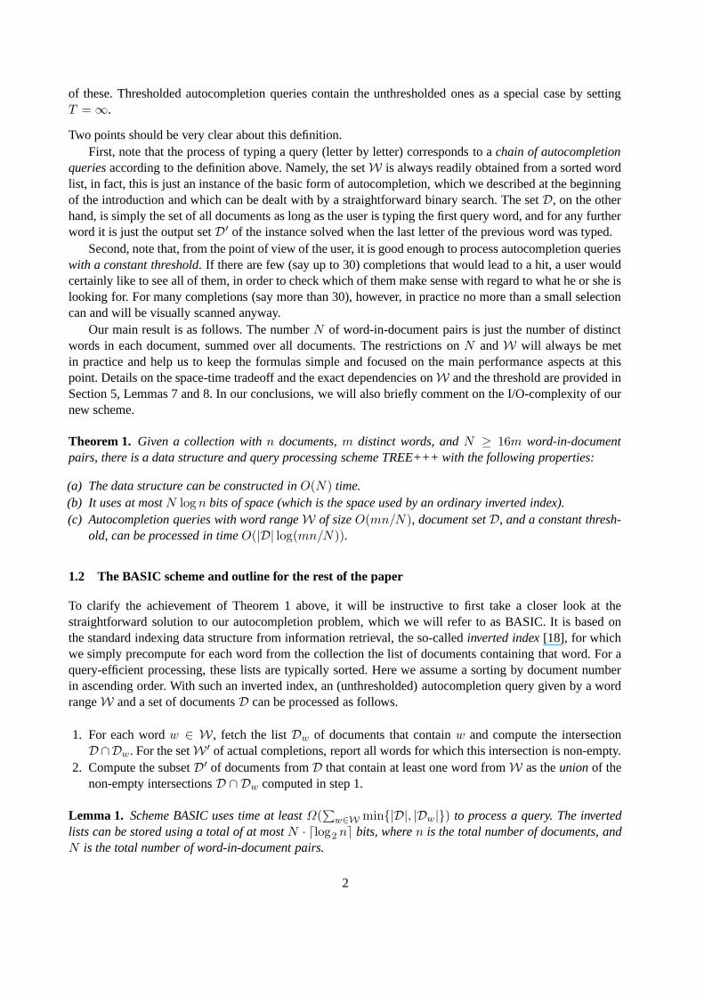
This section is about TREE, our first scheme on the way to Theorem 1, and the idea behind it is to increasethe amount of preprocessing by precomputing inverted lists not only for words but also for their prefixes.More precisely, we construct a complete binary tree with m leaves, where m is the number of distinct wordsin the collection. We assume here and throughout the paper that m is a power of two. For each node v of thetree, we then precompute the list Dv of documents which contain at least one word from the subtree of thatnode, and as for the inverted index, we sort this list by ascending document number. The lists of the leavesare then exactly the lists of an ordinary inverted index, and the list of an inner node is exactly the union ofthe lists of its two children. The list of the root node is exactly the set of all non-empty documents. A simpleexample is given in Figure 1.

Fig. 1. Toy example for the data structure of scheme TREE with 10 documents and 4 different words.

Given this tree data structure, an (unthresholded) autocompletion query given by a word range W and a setof documents D is then processed as follows.

1. Compute the unique minimal sequence v1, . . . , vl of nodes with the property that their subtrees coverexactly the range of words W . Process these l nodes from left to right, and for each node v invoke thefollowing procedure.

2. Fetch the list Dv of v and compute the intersection D ∩ Dv . If the intersection is empty, do nothing. Ifthe intersection is non-empty, then if v is a leaf, report the corresponding word, otherwise invoke thisprocedure (step 2) recursively for each of the two children of v.

3. Compute D′ as the union of the D ∩Dv , for the nodes v computed in step 1.

Scheme TREE can save us time for the following reason. If the intersection computed at an inner node vin step 2 is empty, we know that none of the words in the whole subtree of v is a completion leading to ahit, that is, with a single intersection we are able to rule out a large number of potential completions. Thisdoes not work in the other direction, however: if the intersection at v is non-empty, we know nothing morethan that there is at least one word in the subtree which will lead to a hit, and we will have to examine bothchildren recursively. The following lemma shows the potential of TREE to make the query processing timedepend on W ′ instead of on W like for BASIC. Since TREE is just a step on the way to our final scheme,we do not bother to give the exact query processing time here but just the number of nodes visited, becausewe need exactly this information in the next section.

Lemma 2. When processing a query with TREE, at most 2(|W ′| + 1) log2 |W| nodes are visited.

The price TREE pays in terms of space is large. In an extreme worst case, each level of the tree woulduse just as much space as the inverted index stored at the leaf level, which would give a blow-up factor oflog2 M . For the collections we consider in Section 6, the actual blowup factor would be about 6.

4

3 Relative Bitvectors (TREE+BITVEC)

In this section, we describe and analyze TREE+BITVEC, which reduces the space usage of algorithm TREEfrom the last section, while maintaining as much as possible its potential for a query processing time de-pending on W ′ instead of on W . The basic trick will be to store the inverted lists via bit vectors, morespecifically, via relative bit vectors. The resulting data structure turns out to have similarities with the static2-dimensional orthogonal range counting structure of Chazelle [5].

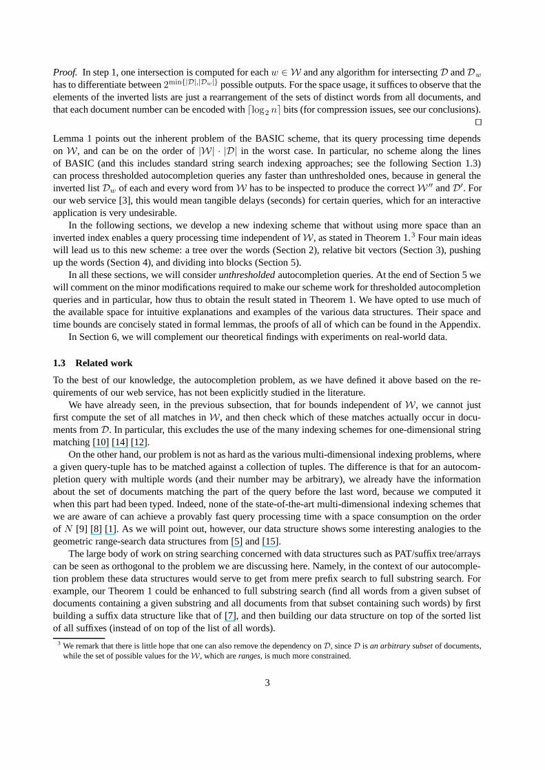
In the root node, the list of all non-empty documents is stored as a bit vector in the obvious way: when Nis the number of documents, there are N consecutive bits, and the ith bit corresponds to document numberi, and the bit is set to 1 if and only if that document contains at least one word from the subtree of the node.In the case of the root node this means that the ith bit is 1 if and only if document number i contains anyword at all.

Now consider any one child v of the root node, and with it store a vector of N ′ bits, were N ′ is thenumber of 1-bits in the parent’s bit vector. To make it interesting already at this point in the tree, assume thatindeed some documents are empty, so that not all bits of the parent’s bit vector are set to one, and N ′ < N .Now the jth bit of v corresponds to the jth 1-bit of its parent, which in turn corresponds to a documentnumber ij . We then set the jth bit of v to 1 if and only if document number ij contains a word in the subtreeof v.

The same principle is now used for every node v that is not the root: the jth bit of the bit vector of vcorresponds to that document to which the jth 1-bit of the parent of v corresponds, and that bit is set to 1 ifand only if that document contains a word from the subtree of v. Constructing these bit vectors is relativelystraightforward; it will be part of the construction given in Appendix B.

Fig. 2. The data structure of TREE+BITVEC for the toy collection from Figure 1.

Lemma 3. Let stree denote the total lengths of the inverted lists of algorithm TREE. The total number ofbits used in the bit vectors of algorithm TREE+BITVEC is then at most 2stree plus the number of emptydocuments (which cost a 0-bit in the root each).

The procedure for processing a query with TREE+BITVEC is, in principle, the same as we gave it for TREEin the previous section (before Lemma 2). The only difference comes from the fact that the bit vectors, exceptthat of the root, cannot be interpreted in isolation but only relative to their respective parents.

We deal with this as follows. We ensure that whenever we visit a node v, we have the set Iv of thosepositions of the bit vector stored at v that correspond to documents from the given set D, as well as the |Iv|numbers of those documents. For the root node, this is trivial to compute. For any other node v, Iv can becomputed from its parent u as follows: for each i ∈ Iu check if the ith bit of u is set to 1, if so computethe number of 1-bits at positions less than i, and add this number to the set Iv and store by it the number of

5

the document from D that was stored by i. With this enhancement, we can follow the same steps as in theprocedure for TREE, except that we have to ensure now that whenever we visit a node that is not the root,we have visited its parent before. The lemma below shows that we have to visit an additional number of upto 2 log2 M nodes because of this.

We also observe here that we can compute the output set D ′ of documents containing at least one wordfrom W ′ on the fly as follows. We associate with each element from the given D a single bit, initialized tozero. When we visit a node v and use Iv for random accesses to v’s bit vector as described above, then foreach i ∈ Iv for which the ith bit of v is set to 1, set the bit of the document in D to which i points to 1. Itis not hard to see that the subset of elements D for which eventually a 1-bit is set, is exactly D ′. Since W isfully covered by the v1, . . . , vl (see step 1 of the query processing procedure in Section 2), it suffices to dothis for the nodes v1, . . . , vl only.

Lemma 4. When processing a query with TREE+BITVEC, at most 2(|W ′| + 1) log2 |W |+ 2 log2 m nodesare visited.

4 Pushing Up the Words (TREE+BITVEC+PUSHUP)

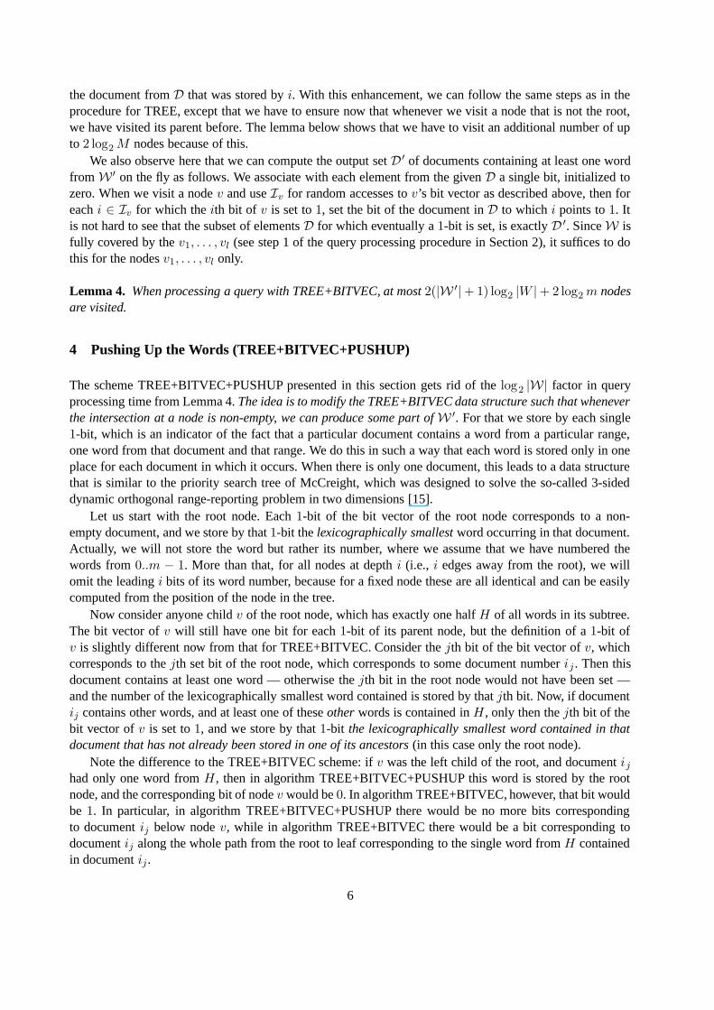
The scheme TREE+BITVEC+PUSHUP presented in this section gets rid of the log2 |W| factor in queryprocessing time from Lemma 4. The idea is to modify the TREE+BITVEC data structure such that wheneverthe intersection at a node is non-empty, we can produce some part of W ′. For that we store by each single1-bit, which is an indicator of the fact that a particular document contains a word from a particular range,one word from that document and that range. We do this in such a way that each word is stored only in oneplace for each document in which it occurs. When there is only one document, this leads to a data structurethat is similar to the priority search tree of McCreight, which was designed to solve the so-called 3-sideddynamic orthogonal range-reporting problem in two dimensions [15].

Let us start with the root node. Each 1-bit of the bit vector of the root node corresponds to a non-empty document, and we store by that 1-bit the lexicographically smallest word occurring in that document.Actually, we will not store the word but rather its number, where we assume that we have numbered thewords from 0..m − 1. More than that, for all nodes at depth i (i.e., i edges away from the root), we willomit the leading i bits of its word number, because for a fixed node these are all identical and can be easilycomputed from the position of the node in the tree.

Now consider anyone child v of the root node, which has exactly one half H of all words in its subtree.The bit vector of v will still have one bit for each 1-bit of its parent node, but the definition of a 1-bit ofv is slightly different now from that for TREE+BITVEC. Consider the jth bit of the bit vector of v, whichcorresponds to the jth set bit of the root node, which corresponds to some document number ij . Then thisdocument contains at least one word — otherwise the jth bit in the root node would not have been set —and the number of the lexicographically smallest word contained is stored by that jth bit. Now, if documentij contains other words, and at least one of these other words is contained in H , only then the jth bit of thebit vector of v is set to 1, and we store by that 1-bit the lexicographically smallest word contained in thatdocument that has not already been stored in one of its ancestors (in this case only the root node).

Note the difference to the TREE+BITVEC scheme: if v was the left child of the root, and document ij

had only one word from H , then in algorithm TREE+BITVEC+PUSHUP this word is stored by the rootnode, and the corresponding bit of node v would be 0. In algorithm TREE+BITVEC, however, that bit wouldbe 1. In particular, in algorithm TREE+BITVEC+PUSHUP there would be no more bits correspondingto document ij below node v, while in algorithm TREE+BITVEC there would be a bit corresponding todocument ij along the whole path from the root to leaf corresponding to the single word from H containedin document ij .

6

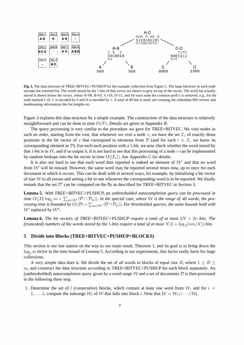
Fig. 3. The data structure of TREE+BITVEC+PUSHUP for the example collection from Figure 1. The large bitvector in each nodeencodes the inverted list. The words stored by the 1-bits of that vector are shown in grey on top of the vector. The word list actuallystored is shown below the vector, where A=00, B=01, C=10, D=11, and for each node the common prefix is removed, e.g., for thenode marked C-D, C is encoded by 0 and D is encoded by 1. A total of 49 bits is used, not counting the redundant 000 vectors andbookkeeping information like list lengths etc.

Figure 3 explains this data structure by a simple example. The construction of the data structure is relativelystraightforward and can be done in time O(N). Details are given in Appendix B.

The query processing is very similar to the procedure we gave for TREE+BITVEC. We visit nodes insuch an order, starting from the root, that whenever we visit a node v, we have the set Iv of exactly thosepositions in the bit vector of v that correspond to elements from D (and for each i ∈ Iv we know itscorresponding element in D). For each such position with a 1-bit, we now check whether the word stored bythat 1-bit is in W , and if so output it. It is not hard to see that this processing of a node v can be implementedby random lookups into the bit vector in time O(|Iv|). See Appendix C for details.

It is also not hard to see that each word thus reported is indeed an element of W ′ and that no wordfrom W ′ will be missed. However, the same word may be reported several times now, up to once for eachdocument in which it occurs. This can be dealt with in several ways, for example, by initializing a bit vectorof size W to all zeroes and setting a bit to one whenever the corresponding word is to be reported. We finallyremark that the set D′ can be computed on the fly as described for TREE+BITVEC in Section 3.

Lemma 5. With TREE+BITVEC+PUSHUP, an unthresholded autocompletion query can be processed intime O(|D| log2 m +

∑w∈W ′ |D ∩ Dw|). In the special case, where W is the range of all words, the pro-

cessing time is bounded by O(|D|+∑

w∈W ′ |D∩Dw|). For thresholded queries, the same bounds hold withW ′ replaced by W ′′.

Lemma 6. The bit vectors of TREE+BITVEC+PUSHUP require a total of at most 2N + 2n bits. The(truncated) numbers of the words stored by the 1-bits require a total of at most N(2 + log2(nm/N)) bits.

5 Divide into Blocks (TREE+BITVEC+PUSHUP+BLOCKS)

This section is our last station on the way to our main result, Theorem 1, and its goal is to bring down thelog2 m factor in the time bound of Lemma 5. According to our experiments, this factor really hurts for largecollections.

A very simple idea does it. We divide the set of all words in blocks of equal size B, where 1 ≤ B ≤m, and construct the data structure according to TREE+BITVEC+PUSHUP for each block separately. An(unthresholded) autocompletion query given by a word range W and a set of documents D is then processedin the following three step.

1. Determine the set of l (consecutive) blocks, which contain at least one word from W , and for i =1, . . . , l, compute the subrange Wi of W that falls into block i. Note that W = W1∪ · · · ∪Wl.

7

2. For i = 1, . . . , l, process the query given by Wi and D according to TREE+BITVEC+PUSHUP, result-ing in a set of hits D′

i ⊆ D and a set of completions W ′i ⊆ Wi.

3. Compute the union of the sets of completions W ′1∪ · · · ∪W ′

l (a simple concatenation). Compute theunion of the hit sets D1 ∪ · · · ∪ Dl on the fly during step 2, as described for TREE+BITVEC andTREE+BITVEC+PUSHUP before.

Lemma 7. With TREE+BITVEC+PUSHUP+BLOCKS and block size B, an unthresholded autocompletionquery can be processed in time O(|D|(log2 B + |W|/B)+

∑w∈W ′ |D ∩Dw|). For a thresholded query, the

same bound holds with W ′ replaced by W ′′.

Lemma 8. TREE+BITVEC+PUSHUP+BLOCKS with block size B requires at most 2N + n · dm/Be bitsfor its bit vectors and at most Ndlog2 Be bits for the word numbers stored by the 1-bits. For B ≥ mn/N ,this adds up to at most N(3 + dlog2 Be) bits.

Parts (b) and (c) of Theorem 1 now follow directly from Lemmas 7 and 8, by choosing B to be nm/N . Thischoice of B minimizes the space bound of Lemma 8. For |W| = O(nm/N), the |W|/B term of Lemma 7then is a constant. Note that N/n is the average number of distinct words per document, so that the condition|W| ≤ C · nm/N rules out only very large word ranges. In our web service, this condition is maintainedby enabling the autocompletion functionality only for prefixes of a certain minimal length (say 2). Part (a)of Theorem 1 is established by the construction given in Appendix B. This finishes the proof of our mainresult.

6 Experiments

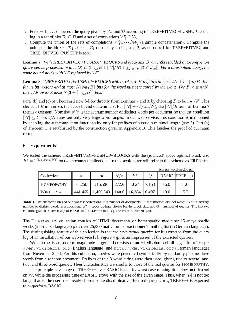
We tested the scheme TREE+BITVEC+PUSHUP+BLOCKS with the (rounded) space-optimal block sizeB∗ = 2dlog2(nm/N)e on two document collections. In this section, we will refer to this scheme as TREE+++.

bits per word-in-doc pair

Collection n m N/n B∗ Q BASIC TREE+++

HOMEOPATHY 33,250 216,596 272.6 1,024 7,168 16.0 11.6

WIKIPEDIA 441,465 1,456,349 140.6 16,384 6,497 19.0 15.2

Table 1. The characteristics of our two test collections: n = number of documents, m = number of distinct words, N/n = averagenumber of distinct words in a document, B∗ = space-optimal choice for the block size, and Q = number of queries. The last twocolumns give the space usage of BASIC and TREE+++ in bits per word-in-document pair.

The HOMEOPATHY collection consists of HTML documents on homeopathic medicine: 15 encyclopedicworks (in English language) plus over 25,000 mails from a practitioner’s mailing list (in German language).The distinguishing feature of this collection is that we have actual queries for it, extracted from the querylog of an installation of our web service [3]. Figure 4 gives an impression of the extracted queries.

WIKIPEDIA is an order of magnitude larger and consists of an HTML dump of all pages from http://en.wikipedia.org (English language) and http://de.wikipedia.org (German language)from November 2004. For this collection, queries were generated synthetically by randomly picking threewords from a random document. Prefixes of this 3-word string were then used, giving rise to several one,two, and three word queries. Their characteristics are similar to those of the real queries for HOMEOPATHY.

The principle advantage of TREE+++ over BASIC is that its worst case running time does not dependon W , while the processing time of BASIC grows with the size of the given range. Thus, when |D| is not toolarge, that is, the user has already chosen some discriminative, focused query terms, TREE+++ is expectedto outperform BASIC.

8

(a) (b) (c)

Fig. 4. Histograms of three characteristic values of the 7168 queries to our HOMEOPATHY collection. (a): the number |W ′| ofcompletions leading to a hit (shown for the window [1, 100]; the histogram for the window [100, 1000] is very similar). (b): the size|W| of the given word range (shown, again representatively, for the window [1, 100]). (c): the length of the last prefix.

For our experiments, BASIC and TREE+++ were implemented in Perl (our web service is implemented inC++, however not yet with the full-fledged TREE+++). Since Perl incurs large unpredictable overheads inthe actual running times, we opted to compare the following, more objective operation counts: for each inter-section of lists X and Y of BASIC, we charged min|X|, |Y |(1 + log(max|X|, |Y |/min|X|, |Y |)).This corresponds to the worst case running time of the best known algorithm for intersecting two sorted lists[2] [6] [13]. In the case where one list consists of all documents, we charged only the length of the shorterlist. For TREE+++, we charged for each visited node v the size of the set Iv of indices into the bit vector ofv. For both schemes, we charged only for the last prefix of each query, because the first part of a multi-wordquery appears as a separate query and the resulting document hits and completions are cached by the systemand do not need to be recomputed.

The results from Figure 5 conform nicely to our theoretical analysis. Three main observations can bemade: (1) For a significant fraction of the queries, BASIC takes a very long time (Figure 5(b)). This is dueto the dependency of its running time on W , which is typically very large when only few letters have beentyped of the last query word. (2) The maximal query processing time for TREE+++ is a factor 4 below thatfor BASIC (Figure 5(b)). (3) For a considerable fraction of the queries, BASIC is very fast (Figure 5(a)).This is the case when W is very small or when we are dealing with a single prefix as a query.

(a) (b)

Fig. 5. Histogram of the operation counts of TREE+++ and BASIC for all HOMEOPATHYqueries: (a) distribution of the counts≤ 2 · 105; (b) distribution of the counts ≥ 2 · 105.

9

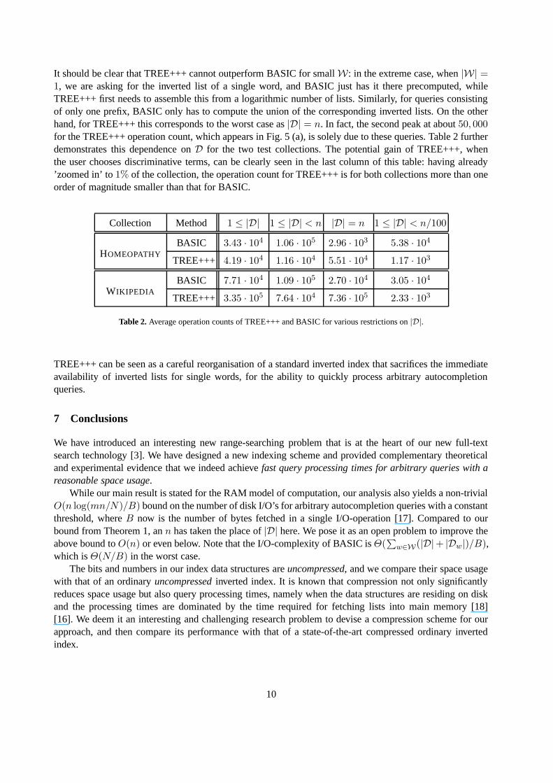
It should be clear that TREE+++ cannot outperform BASIC for small W: in the extreme case, when |W| =1, we are asking for the inverted list of a single word, and BASIC just has it there precomputed, whileTREE+++ first needs to assemble this from a logarithmic number of lists. Similarly, for queries consistingof only one prefix, BASIC only has to compute the union of the corresponding inverted lists. On the otherhand, for TREE+++ this corresponds to the worst case as |D| = n. In fact, the second peak at about 50, 000for the TREE+++ operation count, which appears in Fig. 5 (a), is solely due to these queries. Table 2 furtherdemonstrates this dependence on D for the two test collections. The potential gain of TREE+++, whenthe user chooses discriminative terms, can be clearly seen in the last column of this table: having already’zoomed in’ to 1% of the collection, the operation count for TREE+++ is for both collections more than oneorder of magnitude smaller than that for BASIC.

Collection Method 1 ≤ |D| 1 ≤ |D| < n |D| = n 1 ≤ |D| < n/100

BASIC 3.43 · 104 1.06 · 105 2.96 · 103 5.38 · 104

HOMEOPATHYTREE+++ 4.19 · 104 1.16 · 104 5.51 · 104 1.17 · 103

BASIC 7.71 · 104 1.09 · 105 2.70 · 104 3.05 · 104

WIKIPEDIATREE+++ 3.35 · 105 7.64 · 104 7.36 · 105 2.33 · 103

Table 2. Average operation counts of TREE+++ and BASIC for various restrictions on |D|.

TREE+++ can be seen as a careful reorganisation of a standard inverted index that sacrifices the immediateavailability of inverted lists for single words, for the ability to quickly process arbitrary autocompletionqueries.

7 Conclusions

We have introduced an interesting new range-searching problem that is at the heart of our new full-textsearch technology [3]. We have designed a new indexing scheme and provided complementary theoreticaland experimental evidence that we indeed achieve fast query processing times for arbitrary queries with areasonable space usage.

While our main result is stated for the RAM model of computation, our analysis also yields a non-trivialO(n log(mn/N)/B) bound on the number of disk I/O’s for arbitrary autocompletion queries with a constantthreshold, where B now is the number of bytes fetched in a single I/O-operation [17]. Compared to ourbound from Theorem 1, an n has taken the place of |D| here. We pose it as an open problem to improve theabove bound to O(n) or even below. Note that the I/O-complexity of BASIC is Θ(

∑w∈W(|D|+ |Dw|)/B),

which is Θ(N/B) in the worst case.The bits and numbers in our index data structures are uncompressed, and we compare their space usage

with that of an ordinary uncompressed inverted index. It is known that compression not only significantlyreduces space usage but also query processing times, namely when the data structures are residing on diskand the processing times are dominated by the time required for fetching lists into main memory [18][16]. We deem it an interesting and challenging research problem to devise a compression scheme for ourapproach, and then compare its performance with that of a state-of-the-art compressed ordinary invertedindex.

10

References

1. S. Alstrup, G. S. Brodal, and T. Rauhe. New data structures for orthogonal range searching. In IEEE Symposium on Foundationsof Computer Science, pages 198–207, 2000.

2. R. Baeza-Yates. A fast set intersection algorithm for sorted sequences. Lecture Notes in Computer Science, 3109:400–408,2004.

3. H. Bast, T. Warken, and I. Weber. Searching with autocompletion: a new interactive web search technology. Demo instancesare accessible under http://search.mpi-inf.mpg.de (Wikipedia), http://www.homeonet.org (Homeopathy), http://www.mpi-inf.mpg.de (MPII webpages).

4. J. L. Bentley and R. Sedgewick. Fast algorithms for sorting and searching strings. In ACM-SIAM Symposium on DiscreteAlgorithms, pages 360–369, 1997.

5. B. Chazelle. A functional approach to data structures and its use in multidimensional searching. SIAM Journal on Computing,17(3):427–462, 1988.

6. E. D. Demaine, A. Lopez-Ortiz, and J. I. Munro. Adaptive set intersections, unions, and differences. In ACM-SIAM Symposiumon Discrete Algorithms, pages 743–752, 2000.

7. P. Ferragina and R. Grossi. The string b-tree: a new data structure for string search in external memory and its applications.Journal of the ACM, 46(2):236–280, 1999.

8. P. Ferragina, N. Koudas, S. Muthukrishnan, and D. Srivastava. Two-dimensional substring indexing. Journal of Computer andSystem Science, 66(4):763–774, 2003.

9. V. Gaede and O. G unther. Multidimensional access methods. ACM Computing Surveys, 30(2):170–231, 1998.10. G. H. Gonnet, R. A. Baeza-Yates, and T. Snider. New indices for text: PAT Trees and PAT arrays. Prentice-Hall, Inc., 1992.11. Google suggest beta service, November 2004. http://www.google.com/webhp?complete=1&hl=en.12. R. Grossi and J. S. Vitter. Compressed suffix arrays and suffix trees with applications to text indexing and string matching

(extended abstract). In ACM Symposium on the Theory of Computing, pages 397–406, 2000.13. F. K. Hwang and S. Lin. A simple algorithm for merging two disjoint linearly ordered sets. SIAM Journal on Computing,

1(1):31–39, 1972.14. U. Manber and G. Myers. Suffix arrays: a new method for on-line string searches. SIAM Journal on Computing, 22(5):935–948,

1993.15. E. M. McCreight. Priority search trees. SIAM Journal on Computing, 14(2):257–276, 1985.16. F. Scholer, H. E. Williams, J. Yiannis, and J. Zobel. Compression of inverted indexes for fast query evaluation. In ACM SIGIR

Conference on Research and Development in Information Retrieval, pages 222–229, 2002.17. J. S. Vitter and E. A. M. Shriver. Optimal disk i/o with parallel block transfer. In ACM Symposium on Theory of Computing,

pages 159–169, 1990.18. I. H. Witten, T. C. Bell, and A. Moffat. Managing Gigabytes: Compressing and Indexing Documents and Images, 2nd edition.

Morgan Kaufmann, 1999.

11

A Proofs of Lemmas 2, 3, 4, 5, 6, 7, and 8

For convenience, we restate before each proof the lemma as stated in the corresponding section of the paper.

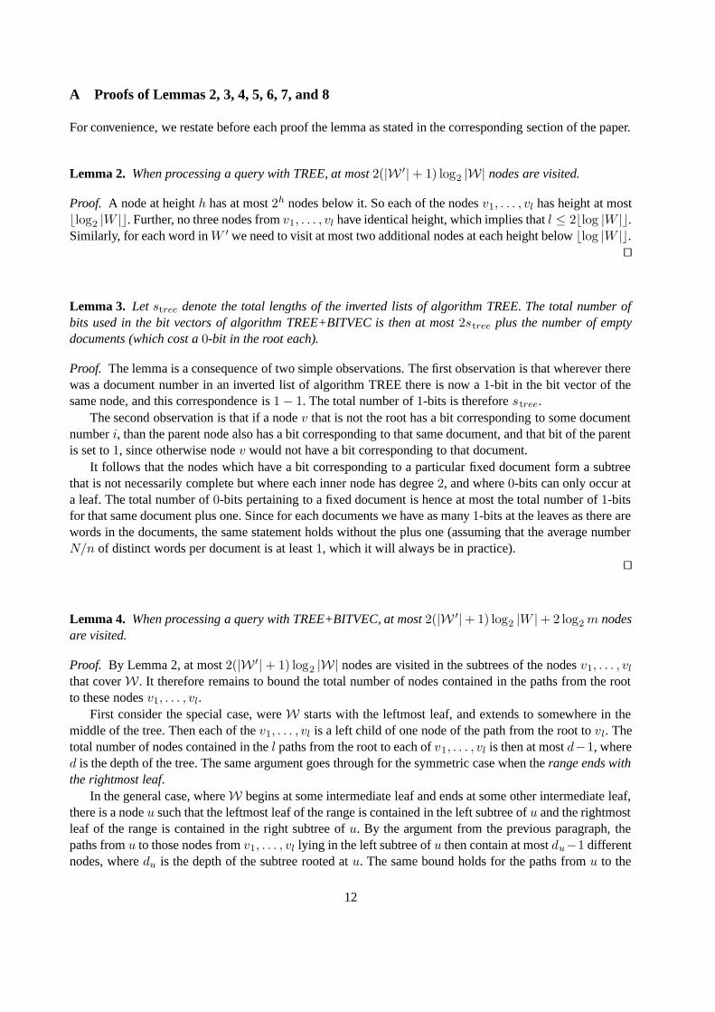
Lemma 2. When processing a query with TREE, at most 2(|W ′| + 1) log2 |W| nodes are visited.

Proof. A node at height h has at most 2h nodes below it. So each of the nodes v1, . . . , vl has height at mostblog2 |W |c. Further, no three nodes from v1, . . . , vl have identical height, which implies that l ≤ 2blog |W |c.Similarly, for each word in W ′ we need to visit at most two additional nodes at each height below blog |W |c.

ut

Lemma 3. Let stree denote the total lengths of the inverted lists of algorithm TREE. The total number ofbits used in the bit vectors of algorithm TREE+BITVEC is then at most 2stree plus the number of emptydocuments (which cost a 0-bit in the root each).

Proof. The lemma is a consequence of two simple observations. The first observation is that wherever therewas a document number in an inverted list of algorithm TREE there is now a 1-bit in the bit vector of thesame node, and this correspondence is 1 − 1. The total number of 1-bits is therefore stree.

The second observation is that if a node v that is not the root has a bit corresponding to some documentnumber i, than the parent node also has a bit corresponding to that same document, and that bit of the parentis set to 1, since otherwise node v would not have a bit corresponding to that document.

It follows that the nodes which have a bit corresponding to a particular fixed document form a subtreethat is not necessarily complete but where each inner node has degree 2, and where 0-bits can only occur ata leaf. The total number of 0-bits pertaining to a fixed document is hence at most the total number of 1-bitsfor that same document plus one. Since for each documents we have as many 1-bits at the leaves as there arewords in the documents, the same statement holds without the plus one (assuming that the average numberN/n of distinct words per document is at least 1, which it will always be in practice).

ut

Lemma 4. When processing a query with TREE+BITVEC, at most 2(|W ′| + 1) log2 |W |+ 2 log2 m nodesare visited.

Proof. By Lemma 2, at most 2(|W ′| + 1) log2 |W| nodes are visited in the subtrees of the nodes v1, . . . , vl

that cover W . It therefore remains to bound the total number of nodes contained in the paths from the rootto these nodes v1, . . . , vl.

First consider the special case, were W starts with the leftmost leaf, and extends to somewhere in themiddle of the tree. Then each of the v1, . . . , vl is a left child of one node of the path from the root to vl. Thetotal number of nodes contained in the l paths from the root to each of v1, . . . , vl is then at most d−1, whered is the depth of the tree. The same argument goes through for the symmetric case when the range ends withthe rightmost leaf.

In the general case, where W begins at some intermediate leaf and ends at some other intermediate leaf,there is a node u such that the leftmost leaf of the range is contained in the left subtree of u and the rightmostleaf of the range is contained in the right subtree of u. By the argument from the previous paragraph, thepaths from u to those nodes from v1, . . . , vl lying in the left subtree of u then contain at most du−1 differentnodes, where du is the depth of the subtree rooted at u. The same bound holds for the paths from u to the

12

other nodes from v1, . . . , vl, lying in the right subtree of u. Adding the length of the path from the root to u,this gives a total number of at most 2d − 3 ut

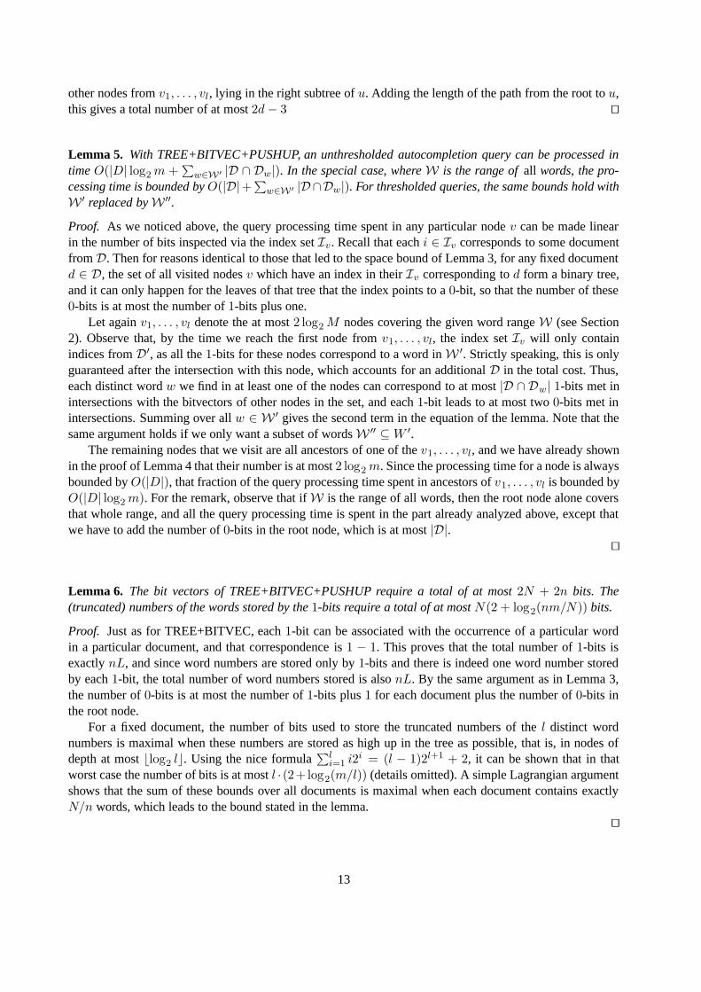
Lemma 5. With TREE+BITVEC+PUSHUP, an unthresholded autocompletion query can be processed intime O(|D| log2 m +

∑w∈W ′ |D ∩ Dw|). In the special case, where W is the range of all words, the pro-

cessing time is bounded by O(|D|+∑

w∈W ′ |D∩Dw|). For thresholded queries, the same bounds hold withW ′ replaced by W ′′.

Proof. As we noticed above, the query processing time spent in any particular node v can be made linearin the number of bits inspected via the index set Iv . Recall that each i ∈ Iv corresponds to some documentfrom D. Then for reasons identical to those that led to the space bound of Lemma 3, for any fixed documentd ∈ D, the set of all visited nodes v which have an index in their Iv corresponding to d form a binary tree,and it can only happen for the leaves of that tree that the index points to a 0-bit, so that the number of these0-bits is at most the number of 1-bits plus one.

Let again v1, . . . , vl denote the at most 2 log2 M nodes covering the given word range W (see Section2). Observe that, by the time we reach the first node from v1, . . . , vl, the index set Iv will only containindices from D′, as all the 1-bits for these nodes correspond to a word in W ′. Strictly speaking, this is onlyguaranteed after the intersection with this node, which accounts for an additional D in the total cost. Thus,each distinct word w we find in at least one of the nodes can correspond to at most |D ∩ Dw| 1-bits met inintersections with the bitvectors of other nodes in the set, and each 1-bit leads to at most two 0-bits met inintersections. Summing over all w ∈ W ′ gives the second term in the equation of the lemma. Note that thesame argument holds if we only want a subset of words W ′′ ⊆ W ′.

The remaining nodes that we visit are all ancestors of one of the v1, . . . , vl, and we have already shownin the proof of Lemma 4 that their number is at most 2 log2 m. Since the processing time for a node is alwaysbounded by O(|D|), that fraction of the query processing time spent in ancestors of v1, . . . , vl is bounded byO(|D| log2 m). For the remark, observe that if W is the range of all words, then the root node alone coversthat whole range, and all the query processing time is spent in the part already analyzed above, except thatwe have to add the number of 0-bits in the root node, which is at most |D|.

ut

Lemma 6. The bit vectors of TREE+BITVEC+PUSHUP require a total of at most 2N + 2n bits. The(truncated) numbers of the words stored by the 1-bits require a total of at most N(2 + log2(nm/N)) bits.

Proof. Just as for TREE+BITVEC, each 1-bit can be associated with the occurrence of a particular wordin a particular document, and that correspondence is 1 − 1. This proves that the total number of 1-bits isexactly nL, and since word numbers are stored only by 1-bits and there is indeed one word number storedby each 1-bit, the total number of word numbers stored is also nL. By the same argument as in Lemma 3,the number of 0-bits is at most the number of 1-bits plus 1 for each document plus the number of 0-bits inthe root node.

For a fixed document, the number of bits used to store the truncated numbers of the l distinct wordnumbers is maximal when these numbers are stored as high up in the tree as possible, that is, in nodes ofdepth at most blog2 lc. Using the nice formula

∑li=1 i2i = (l − 1)2l+1 + 2, it can be shown that in that

worst case the number of bits is at most l · (2+log2(m/l)) (details omitted). A simple Lagrangian argumentshows that the sum of these bounds over all documents is maximal when each document contains exactlyN/n words, which leads to the bound stated in the lemma.

ut

13

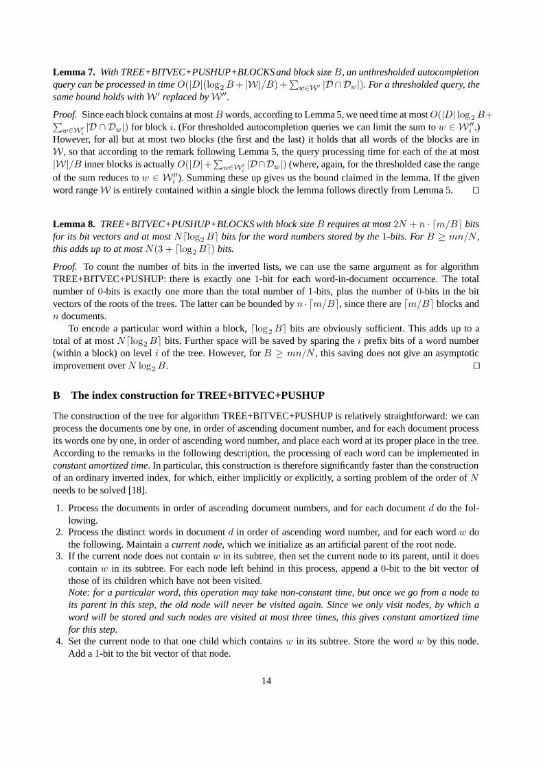
Lemma 7. With TREE+BITVEC+PUSHUP+BLOCKS and block size B, an unthresholded autocompletionquery can be processed in time O(|D|(log2 B + |W|/B)+

∑w∈W ′ |D ∩Dw|). For a thresholded query, the

same bound holds with W ′ replaced by W ′′.

Proof. Since each block contains at most B words, according to Lemma 5, we need time at most O(|D| log 2 B+∑

w∈W ′

i

|D ∩ Dw|) for block i. (For thresholded autocompletion queries we can limit the sum to w ∈ W ′′i .)

However, for all but at most two blocks (the first and the last) it holds that all words of the blocks are inW , so that according to the remark following Lemma 5, the query processing time for each of the at most|W|/B inner blocks is actually O(|D|+

∑w∈W ′

i

|D∩Dw|) (where, again, for the thresholded case the rangeof the sum reduces to w ∈ W ′′

i ). Summing these up gives us the bound claimed in the lemma. If the givenword range W is entirely contained within a single block the lemma follows directly from Lemma 5. ut

Lemma 8. TREE+BITVEC+PUSHUP+BLOCKS with block size B requires at most 2N + n · dm/Be bitsfor its bit vectors and at most Ndlog2 Be bits for the word numbers stored by the 1-bits. For B ≥ mn/N ,this adds up to at most N(3 + dlog2 Be) bits.

Proof. To count the number of bits in the inverted lists, we can use the same argument as for algorithmTREE+BITVEC+PUSHUP: there is exactly one 1-bit for each word-in-document occurrence. The totalnumber of 0-bits is exactly one more than the total number of 1-bits, plus the number of 0-bits in the bitvectors of the roots of the trees. The latter can be bounded by n · dm/Be, since there are dm/Be blocks andn documents.

To encode a particular word within a block, dlog2 Be bits are obviously sufficient. This adds up to atotal of at most Ndlog2 Be bits. Further space will be saved by sparing the i prefix bits of a word number(within a block) on level i of the tree. However, for B ≥ mn/N , this saving does not give an asymptoticimprovement over N log2 B. ut

B The index construction for TREE+BITVEC+PUSHUP

The construction of the tree for algorithm TREE+BITVEC+PUSHUP is relatively straightforward: we canprocess the documents one by one, in order of ascending document number, and for each document processits words one by one, in order of ascending word number, and place each word at its proper place in the tree.According to the remarks in the following description, the processing of each word can be implemented inconstant amortized time. In particular, this construction is therefore significantly faster than the constructionof an ordinary inverted index, for which, either implicitly or explicitly, a sorting problem of the order of Nneeds to be solved [18].

1. Process the documents in order of ascending document numbers, and for each document d do the fol-lowing.

2. Process the distinct words in document d in order of ascending word number, and for each word w dothe following. Maintain a current node, which we initialize as an artificial parent of the root node.

3. If the current node does not contain w in its subtree, then set the current node to its parent, until it doescontain w in its subtree. For each node left behind in this process, append a 0-bit to the bit vector ofthose of its children which have not been visited.Note: for a particular word, this operation may take non-constant time, but once we go from a node toits parent in this step, the old node will never be visited again. Since we only visit nodes, by which aword will be stored and such nodes are visited at most three times, this gives constant amortized timefor this step.

4. Set the current node to that one child which contains w in its subtree. Store the word w by this node.Add a 1-bit to the bit vector of that node.

14

C Query processing in TREE+BITVEC+PUSHUP

First, it is easy to intersect D with the documents in the root node, because we can simply lookup thedocument numbers in the bitvector at the root. Consider then a child v of the root. What we want to do is tomake a new set Sv of document indices, which gives the numbering of the document indices of D in termsof the numbering used in v. This is possible, if we in v store an additional array, where we in entry i storethe number of ones which are in the bitvector of v up to index iα where α ≥ 1 is a parameter. For one suchentry we need log n bits. Sv can then be computed in constant time per entry from D if we for each entrylook up in this array and scan through at most α bits of the original vector. If α is in the order of numberof bits in a machine-word, it is reasonable to assume that this can be done in constant time. We can thencontinue down the tree in a similar way. The total space usage for the document lists will be increased by afactor 1 + (log n)/α.

15