Searching for feasible stationary states in reaction networksby solving a Boolean constraint satisfaction problem

A. Seganti1, F. Ricci-Tersenghi1,2,3 and A. De Martino1,2,41 Dipartimento di Fisica, Sapienza Universita di Roma, p.le A. Moro 2, 00185 Rome (Italy)2 IPCF-CNR, UOS di Roma, Dipartimento di Fisica, Sapienza Universita di Roma (Italy)3 INFN, Sezione di Roma 1, Dipartimento di Fisica, Sapienza Universita di Roma (Italy)

4 Center for Life Nano Science@Sapienza, Istituto Italiano di Tecnologia, Viale Regina Elena 291, 00161 Roma (Italy)

We analyze the solutions, on single network instances, of a recently introduced class of constraint-satisfaction problems (CSPs), describing feasible steady states of chemical reaction networks. First,we show that the CSPs generalize the scheme known as Network Expansion, which is recovered in aspecific limit. Next, a full statistical mechanics characterization (including the phase diagram anda discussion of physical origin of the phase transitions) for Network Expansion is obtained. Finally,we provide a message-passing algorithm to solve the original CSPs in the most general form.

I. INTRODUCTION

The mathematical theory of chemical reaction networks is mainly concerned with issues like the existence, numberand stability of fixed points for realistic (e.g. mass-action based) dynamics of continuous state variables representingthe concentrations of chemical compounds. In many real-world cases, however, full-fledged dynamical approaches areprevented either by lack of knowledge about kinetic constants or by sheer size considerations. It is so, for instance,for cellular metabolic networks at genome-scale [1, 2]. On the other hand, being able to describe viable steady statesof the network in terms of coarse-grained, discrete variables might be a useful (albeit less comprehensive) alternative.

At the simplest level, the operation of networks of chemical reactions can be thought to depend on the availabilityof reaction substrates and of the enzymes required to process them. In particular, one can think that reactions mayoccur whenever all of the required substrates are available, which in turn makes the reaction products available, andso on. Likewise, compound availability can be assumed to depend at least on there being an active reaction producingit. Using these ideas, it is possible to associate to a given reaction network (i.e. to a given bipartite graph encodingfor reaction/compounds interactions) a set of logical constraints to be satisfied by Boolean state variables indicatingwhether a reaction is active or inactive and whether a compound is available or not. This type of reasoning hasled to the formulation of the Network Expansion (NE) framework [3–6], which aims at quantifying the amount ofactivity in the network bulk that is generated upon assuming the availability of a seed of compounds. For cellularmetabolic networks, the seed usually includes both external species (e.g. nutrients) and internal ones (e.g. water,currency metabolites like ATP, etc.). In concrete terms, given a seed, one would like to retrieve the pattern(s) ofreaction activation/compound availability that are induced via the topology (or, more properly, the stoichiometry) ofthe reaction network.

Network Expansion is basically a Boolean Constraint Satisfaction Problem (CSP), possibly one of several typesthat can be reasonably defined to describe the operation of chemical systems, in analogy with those used in the pastto describe other biological mechanisms like transcriptional regulation [7–9]. Despite their ‘natural’ appeal, however,they have received little attention from the statistical mechanics perspective. Besides the general theoretical interest,extracting biologically significant information from them requires being able to explore (in a controlled way) theirvery large and rich space of solutions. Devising algorithms that are able to carry out this task, even for the basic NEscheme, is however far from trivial.

Recently [10], we have proposed a class of CSPs inspired by the so-called constraint-based models for flux analysis[11] which aims at describing the space of configurations of a chemical reaction network through minimal Booleanfeasibility constraints. These CSPs have been defined on random reaction networks (RRN), i.e. bipartite graphs(the two classes of nodes corresponding to ‘reactions’ and ‘reagents’, respectively) characterized by the parameters λ,representing the mean of the Poisson distributed degrees of metabolites, and q (resp. 1−q), giving the probability that areaction has two (resp. one) input or output compounds. The structure of a RRN is described by a M×N connectivity

matrix ξ, with ξmi ∈ {1, 0,−1} depending on whether compound m ∈ {1, . . . ,M} is a substrate (ξmi = −1), a product(ξmi = 1) or is not involved (ξmi = 0) in reaction i ∈ {1, . . . , N}. In this kind of networks, a nutrient is a compoundwith in-degree 0, while a sink has out-degree 0. Denoting by νi ∈ {0, 1} (inactive/active) the state associated toreaction i and by µm ∈ {0, 1} (unavailable/available) that associated to compound m, for a given RRN feasible

arX

iv:1

310.

5637

v1 [

q-bi

o.M

N]

21

Oct

201

3

2

assignments (µ = {µm},ν = {νi}) are defined to be such that Γm = 1 ∀m and ∆i = 1 ∀i, where

Γm = δµm,0δxm,0(δym,0)α + δµm,1(1− δxm,0)(1− δym,0)α (1)

∆i = δνi,0 + δνi,1∏

m∈∂iin

µm , (2)

∂iin is the set of substrates of reaction i, α ∈ {0, 1} is a fixed parameter, and

xm ≡∑

i∈∂min

νi and ym ≡∑

i∈∂mout

νi , (3)

with ∂min (resp. ∂mout) the set of reactions producing (resp. consuming) chemical species m. Condition (2) says thatreactions can always be inactive, while they can activate only if all input compounds are available; likewise, condition(1) allows for a compound m to be available if at least one reaction produces it (for α = 0) or if at least one reactionproduces it and one consumes it (for α = 1). As explained in detail in [10], the case α = 0 (‘Soft Mass Balance’ orSoft-MB) describes steady states that allow for a net production of compounds, while the case α = 1 (‘Hard MassBalance’ or Hard-MB) corresponds, in this coarse-grained view, to a fully mass-balanced scenario.

Once the topology of the reaction network, encoded in an adjacency matrix ξ, is given, the setup presented in [10]aims at retrieving Boolean patterns of activity of reactions (or of metabolite availabilities) induced by the fact thata certain seed of metabolites (in our case, formed by nutrients only) is available from the outset. The cavity-basedpopulation dynamics technique developed in [10] allows in particular to sample configurations (µ,ν) with a probabilitygiven by

P (µ,ν) ∝M∏m=1

Γm

N∏i=1

∆ieθνi , (4)

with a ‘chemical potential’ θ that allows to select states according to the overall number of active processes and, inturn, compute network ensemble-averaged quantities. This study has revealed a rich phase structure characterized byhysteresis, which might potentially hinder the retrieval of individual solutions.

Here we extend the previous analysis in a direction hopefully more useful for applications to quantitative biology(which will be our next step), by searching for solutions to the above CSP on a given reaction network. In this contextwe are going to discuss the statistical properties of the solutions found by several search methods (including NE) andto introduce an improved decimation-based technique. Furthermore, we will compare the statistical properties of thesolutions found on the single instance with the ensemble-averaged results obtained in [10]. The details of the cavitytheory on which our algorithms are based, as well as of the algorithms themselves (Belief Propagation complementedby decimation), are reported in the Appendices.

II. NETWORK EXPANSION REVISITED

A. The problem

The basic idea behind NE is that, given a seed compound (e.g. a nutrient), a reaction can (and will) activatewhen all its substrates are available (AND-like constraint), whereas a compound will be available if at least one ofthe reactions that produce it is active (OR-like constraint). The numerical procedure of NE transfers the informationabout the availability of certain metabolites across the network links, as explained pictorially in Fig. 1. We shall termthis type of process a Propagation of External Inputs (PEI).

It is simple to understand that, as soon as the reaction network departs from a linear topological structure, thepropagation will likely stop after a small number of steps unless the availability of additional compounds is invoked.Indeed, in Network Expansion PEI is aided by the assumption that highly connected metabolites like water areabundant. Because of its intuitive appeal, it is useful to analyze briefly the properties of PEI in somewhat moredetail.

One can write down equations for the probability 〈νi〉 that reaction i will be active and for the probability 〈µm〉that metabolite m will be available by simply considering that, under PEI in a given network, a reaction can activatewhen all of its inputs are available and a metabolite becomes available when at least one reaction is producing it.

3

step 1 step 2 step 3 step 4

Figure 1: Sketch of four steps of the Propagation of External Inputs (PEI) algorithm (serving as the basis of the NetworkExpansion method [3]). Black squares represent compounds initially available. In step 1, reaction i is activated by virtue ofthe availability of compound 1; in step 2, metabolite 2 becomes available by virtue of the activation of reaction i; in step 3,reaction j activates as both 2 and 3 are available; and so on.

This implies that

〈νi〉 =∏

n∈∂iin

〈µn〉 , (5)

1− 〈µm〉 =∏

k∈∂min

(1− 〈νk〉) . (6)

To prove the link between PEI and the CSPs defined above, note that, using the definition (4) one can easily computethe mean values

〈νj〉 =

∑µ,ν

νjM∏m=1

ΓmN∏i=1

∆ieθνi

∑µ,ν

M∏m=1

ΓmN∏i=1

∆ieθνi, (7)

〈µn〉 =

∑µ,ν

µnM∏m=1

ΓmN∏i=1

∆ieθνi

∑µ,ν

M∏m=1

ΓmN∏i=1

∆ieθνi(8)

Under the Mean Field Approximation, we can set

Γm(µm, {νi}) = Γm(µm, {〈νi〉}) , (9)

∆i(νi, {µm}) = ∆i(νi, {〈µm〉}) , (10)

which in turn implies

〈νi〉 =

eθ∏

n∈∂iin〈µn〉

1 + eθ∏

n∈∂iin〈µn〉

(11)

〈µm〉 = 1−∏

k∈∂min

(1− 〈νj〉) . (12)

In the limit θ →∞ we have

〈νi〉 =

1 if

∏n∈∂iin

〈µn〉 = 1 ,

0 if∏

n∈∂iin〈µn〉 = 0 .

(13)

4

0

0.5

1

1.5

2

2.5

3

3.5

4

0 0.2 0.4 0.6 0.8 1

λ

q

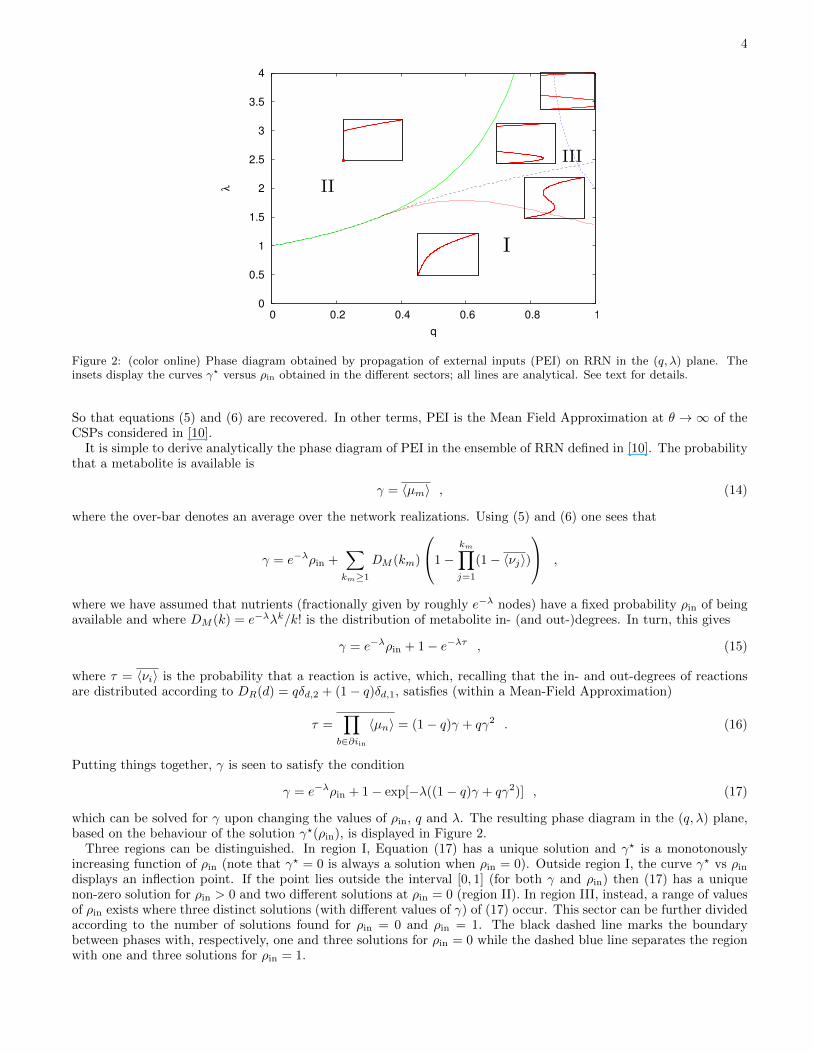
Figure 2: (color online) Phase diagram obtained by propagation of external inputs (PEI) on RRN in the (q, λ) plane. Theinsets display the curves γ? versus ρin obtained in the different sectors; all lines are analytical. See text for details.

So that equations (5) and (6) are recovered. In other terms, PEI is the Mean Field Approximation at θ →∞ of theCSPs considered in [10].

It is simple to derive analytically the phase diagram of PEI in the ensemble of RRN defined in [10]. The probabilitythat a metabolite is available is

γ = 〈µm〉 , (14)

where the over-bar denotes an average over the network realizations. Using (5) and (6) one sees that

γ = e−λρin +∑km≥1

DM (km)

1−km∏j=1

(1− 〈νj〉)

,

where we have assumed that nutrients (fractionally given by roughly e−λ nodes) have a fixed probability ρin of beingavailable and where DM (k) = e−λλk/k! is the distribution of metabolite in- (and out-)degrees. In turn, this gives

γ = e−λρin + 1− e−λτ , (15)

where τ = 〈νi〉 is the probability that a reaction is active, which, recalling that the in- and out-degrees of reactionsare distributed according to DR(d) = qδd,2 + (1− q)δd,1, satisfies (within a Mean-Field Approximation)

τ =∏b∈∂iin

〈µn〉 = (1− q)γ + qγ2 . (16)

Putting things together, γ is seen to satisfy the condition

γ = e−λρin + 1− exp[−λ((1− q)γ + qγ2)] , (17)

which can be solved for γ upon changing the values of ρin, q and λ. The resulting phase diagram in the (q, λ) plane,based on the behaviour of the solution γ?(ρin), is displayed in Figure 2.

Three regions can be distinguished. In region I, Equation (17) has a unique solution and γ? is a monotonouslyincreasing function of ρin (note that γ? = 0 is always a solution when ρin = 0). Outside region I, the curve γ? vs ρindisplays an inflection point. If the point lies outside the interval [0, 1] (for both γ and ρin) then (17) has a uniquenon-zero solution for ρin > 0 and two different solutions at ρin = 0 (region II). In region III, instead, a range of valuesof ρin exists where three distinct solutions (with different values of γ) of (17) occur. This sector can be further dividedaccording to the number of solutions found for ρin = 0 and ρin = 1. The black dashed line marks the boundarybetween phases with, respectively, one and three solutions for ρin = 0 while the dashed blue line separates the regionwith one and three solutions for ρin = 1.

5

0

0.2

0.4

0.6

0.8

1

0 0.2 0.4 0.6 0.8 1

<µ>

ρin

PEIreverse-PEI

0

0.2

0.4

0.6

0.8

1

0 0.2 0.4 0.6 0.8 1

<µ>

ρin

λ=3,q=0.87

Figure 3: Theoretical solution of Equation (17) (solid line) versus ρin, together with the results obatined by PEI and reverse-PEI.

For any fixed ρin, whenever solutions with different values of 〈µ〉 coexist, those with the smallest 〈µ〉 can be retrievedby straightforward PEI starting from a configuration where no metabolite is available except for nutrients. Solutionswith larger 〈µ〉, on the other hand, can be found by ‘reverse-PEI’. In this procedure a configuration where internalmetabolites are all available and nutrients are fixed with probability ρin is initially selected, and then a solution isfound by enforcing the constraints in an iterative way. The results for both procedures are presented in Figure 3 forλ = 3 and q = 0.87 (deep into region III in Figure 2).

B. Origin of the phase transition within the Mean-Field Approximation in PEI

We show here that, as might have been intuitive, the phase transitions occurring in PEI (see Figure 2) are, from aphysical viewpoint, of a percolation type.

To analyze the effectiveness of PEI, we start by identifying the so-called Propagation of External Regulation (PER)Core of the system [12], that is the sub-network obtained by fixing the nutrient availability (with probability ρin) andthen propagating this information inside the network. In this way, some variables will be assigned a definite value(either 1 or 0). At convergence, a fraction γ1 (resp. γ0) of metabolites will be fixed to 1 (resp. 0), while a fractionτ1 (resp. τ0) of reactions will be fixed to 1 (resp. 0). One easily sees that, at the fixed point, the following equationshold:

1− τ0 = q(1− γ0)2 + (1− q)(1− γ0) , (18)

γ0 =∑k 6=0

DM (k)τk0 + (1− ρin)DM (0) , (19)

τ1 = qγ21 + (1− q)γ1 , (20)

1− γ1 =∑k 6=0

DM (k)(1− τ1)k + (1− ρin)DM (0) . (21)

In turn, one obtains

τ0 = 1− q(1− γ0)2 − (1− q)(1− γ0) , (22)

γ0 = e−λeλτ0 − ρine−λ , (23)

τ1 = qγ21 + (1− q)γ1 , (24)

γ1 = 1− e−λτ1 + ρine−λ . (25)

6

0

0.2

0.4

0.6

0.8

1

0 0.2 0.4 0.6 0.8 1

γ

ρin

γmax=1-γ0γ1γ0

γPER

0

0.2

0.4

0.6

0.8

1

0 0.2 0.4 0.6 0.8 1

γ

ρin

Figure 4: Weights of the different components of the PER core for a graph with λ = 3 and q = 0.87. The red line correspondsto the solution of equation (17).

Unsurprisingly, the equations for γ1 and τ1 take us back to (17). On the other hand, the fraction of metabolites inthe PER core is given by

γPER = γ1 + γ0 . (26)

Hence the fraction of metabolites that are not fixed by propagating nutrient availability is given by 1 − γPER, andthe maximum achievable availability for metabolites (that we will often call ‘magnetization’ in the following using astatistical physics jargon) is given by γmax = 1− γ0. Figure 4 displays the different contributions for a specific choiceof the parameters, together with the corresponding solution of Eq. (17).

The excellent agreement of γ1 with the analytical line for the feasible values of the magnetization suggests thatstraightforward PEI will be able to recover solutions with lower magnetization when the latter coexist with high-magnetization solutions. On the other hand, the highest magnetizations coincide, expectedly, with the largest achiev-able average metabolite availability. Finally, depending on the value of λ and q, one obtains a single solution whenno PER core exists, and two solutions (with magnetizations γmax and γ1) in presence of a PER core. Hence thetransition is a typical percolation transition between a phase in which the internal variables are trivially determinedby the nutrients (in absence of a PER core) to one in which the internal variables are not univocally determined (inpresence of a PER core).

III. SOLUTIONS ON INDIVIDUAL NETWORKS BY BELIEF PROPAGATION AND DECIMATION

We turn now to the analysis of the Soft-MB and Hard-MB CSPs (1) and (2) for general θ. In essence, we have derivedthe cavity equations for the CSPs, presented in Appendix 1, and used the Belief Propagation (BP) algorithm discussedin Appendix 2 a to compute the statistics of solutions on single instances of RRNs. Next, in order to obtain individualconfigurations of variables that satisfy our CSPs, we resorted to the decimation scheme presented in Appendix 2 b.Results are presented in Figures 5 and 6 for Soft-MB (α = 0) and in Figures 7 and 8 for Hard-MB (α = 1). Resultsfrom Belief propagation, labeled as ‘BP’, are compared with results retrieved by the population dynamics algorithmdeveloped in [10] (labeled ‘POP’ and corresponding to the ensemble average) and with the decimation results (labeled‘DEC’). In [10], the solution space was explored by two different protocols, which we also use here: by reducing θstarting from a large positive value (+∞→ −∞ in the Figure legends) and by doing the reverse (−∞→ +∞ in theFigure legends). If the decimation scheme does not converge, the corresponding point is absent.

It is clear that decimation generically fails to converge close to the transitions both in the Soft-MB and, moreseverely, in the Hard-MB case. Apart from this, the three methods give results that are in remarkable qualitative

7

0

0.2

0.4

0.6

0.8

1

-4 -2 0 2 4

<µ—>,

<µ>

θ

λ=1, q =0.5

POP +∞ → −∞BP +∞ → −∞

DEC +∞ → −∞POP −∞ → +∞BP −∞ → +∞

DEC −∞ → +∞

0

0.1

0.2

0.3

0.4

0.5

0.6

0.7

0.8

0.9

1

-4 -2 0 2 4

<ν—>,

<ν>

θ

λ=1, q=0.5

POP +∞ → −∞BP +∞ → −∞

DEC +∞ → −∞POP −∞ → +∞BP −∞ → +∞

DEC −∞ → +∞

Figure 5: Soft-MB for λ = 1, q = 0.5 and ρin = 1. Left: average fraction of available metabolites, 〈µ〉 (〈µ〉 for population

dynamics) versus θ. Right: average fraction of active reactions, 〈ν〉 (〈ν〉 for population dynamics) versus θ.

0

0.2

0.4

0.6

0.8

1

-4 -2 0 2 4

<µ—>,

<µ>

θ

λ=3, q =0.8

POP +∞ → −∞BP +∞ → −∞

DEC +∞ → −∞POP −∞ → +∞BP −∞ → +∞

DEC −∞ → +∞

0

0.1

0.2

0.3

0.4

0.5

0.6

0.7

0.8

0.9

1

-4 -2 0 2 4

<ν—>,

<ν>

θ

λ=3, q=0.8

POP +∞ → −∞BP +∞ → −∞

DEC +∞ → −∞POP −∞ → +∞BP −∞ → +∞

DEC −∞ → +∞

Figure 6: Soft-MB for λ = 3, q = 0.8 and ρin = 1. Left: average fraction of available metabolites, 〈µ〉 (〈µ〉 for population

dynamics) versus θ. Right: average fraction of active reactions, 〈ν〉 (〈ν〉 for population dynamics) versus θ.

agreement, including the ability to describe discontinuities in 〈µ〉 and 〈ν〉 upon varying θ. It is noteworthy thatmany different configurations appear to be feasible. These configurations are spread over a broad range of densities,especially in the Soft-MB case. So our method based on BP and decimation is able to sample the solution space byjust varying a single parameter (the chemical potential θ in the present case), even in cases when only “extremal”solutions seem to satisfy the CSP for metabolite nodes (as e.g. in the left panel in Fig. 8) while the density of activereaction is varying in a more continuous manner (see the right panel in the same figure).

0

0.2

0.4

0.6

0.8

1

-4 -2 0 2 4

<µ—>,

<µ>

θ

λ=1, q =0.5

POP +∞ → −∞BP +∞ → −∞

DEC +∞ → −∞POP −∞ → +∞BP −∞ → +∞

DEC −∞ → +∞

0

0.1

0.2

0.3

0.4

0.5

0.6

0.7

0.8

0.9

1

-4 -2 0 2 4

<ν—>,

<ν>

θ

λ=1, q=0.5

POP +∞ → −∞BP +∞ → −∞

DEC +∞ → −∞POP −∞ → +∞BP −∞ → +∞

DEC −∞ → +∞

Figure 7: Hard-MB for λ = 1, q = 0.5 and ρin = 1. Left: average fraction of available metabolites, 〈µ〉 (〈µ〉 for population

dynamics) versus θ. Right: average fraction of active reactions, 〈ν〉 (〈ν〉 for population dynamics) versus θ.

8

0

0.2

0.4

0.6

0.8

1

-4 -2 0 2 4

<µ—>,

<µ>

θ

λ=3, q =0.8

POP +∞ → −∞BP +∞ → −∞

DEC +∞ → −∞POP −∞ → +∞BP −∞ → +∞

DEC −∞ → +∞

0

0.1

0.2

0.3

0.4

0.5

0.6

0.7

0.8

0.9

1

-4 -2 0 2 4

<ν—>,

<ν>

θ

λ=3, q=0.8

POP +∞ → −∞BP +∞ → −∞

DEC +∞ → −∞POP −∞ → +∞BP −∞ → +∞

DEC −∞ → +∞

Figure 8: Hard-MB for λ = 3, q = 0.8 and ρin = 1. Left: average fraction of available metabolites, 〈µ〉 (〈µ〉 for population

dynamics) versus θ. Right: average fraction of active reactions, 〈ν〉 (〈ν〉 for population dynamics) versus θ.

0

0.2

0.4

0.6

0.8

1

-4 -2 0 2 4

<µ—>,

<µ>

θ

POP ρin=0.5DEC ρin=0.3DEC ρin=0.4DEC ρin=0.8DEC ρin=0.6DEC ρin=1

0

0.2

0.4

0.6

0.8

1

-4 -2 0 2 4

<µ—>,

<µ>

θ

POP ρin=0.5DEC ρin=0.3DEC ρin=0.4DEC ρin=0.8DEC ρin=0.6DEC ρin=1

Figure 9: Soft-MB: behaviour of the average fraction of available metabolites, 〈µ〉 (〈µ〉 for population dynamics) for λ = 1and q = 0.5 (Left) and λ = 3 and q = 0.8 (Right) at various ρin.

As detailed in Appendix 1, during decimation nutrients must be treated with special care. This is because theprior assignment of availability for each nutrient (which, as said above, follows a probabilistic rule with parameterρin) does not always coincide, after decimation, with the frequency with which the nutrient is available in the finalassignments (i.e. the actual solutions retrieved), which we denote as 〈µ〉EXT . We analyze the relation between theaverage magnetization of reactions and metabolites and both ρin and 〈µ〉EXT in Figures 9 and 10. We first note thatin this way we are able to obtain solutions at various 〈µ〉EXT clearly different from the corresponding values of ρin.

0

0.2

0.4

0.6

0.8

1

0 0.2 0.4 0.6 0.8 1

<µ>

<µ>EXT

ρin(t=0)=0.3ρin(t=0)=0.4ρin(t=0)=0.5ρin(t=0)=0.6ρin(t=0)=0.8ρin(t=0)=1

0

0.2

0.4

0.6

0.8

1

0 0.2 0.4 0.6 0.8 1

<µ>

<µ>EXT

ρin(t=0)=0.3ρin(t=0)=0.4ρin(t=0)=0.5ρin(t=0)=0.6ρin(t=0)=0.8ρin(t=0)=1

Figure 10: Soft-MB: Behaviour of 〈µ〉 vs 〈µ〉EXT for various ρin, for θ = (−5,−4.5, .., 4.5, 5) and for λ = 1 and q = 0.5 (Left)and λ = 3 and q = 0.8 (Right).

9

0

0.2

0.4

0.6

0.8

1

0 0.2 0.4 0.6 0.8 1

<ν>

<µ>

+∞ → −∞ <ν>+∞ → −∞ <ν>MAX+∞ → −∞ <ν>+∞ → −∞ <ν>MAXMF <ν>

0

0.2

0.4

0.6

0.8

1

0 0.2 0.4 0.6 0.8 1

<ν>

<µ>

+∞ → −∞ <ν>+∞ → −∞ <ν>MAX+∞ → −∞ <ν>+∞ → −∞ <ν>MAXMF <ν>

Figure 11: Plot of 〈µ〉 versus 〈ν〉 for λ = 1 and q = 0.5 (Left) and λ = 3 and q = 0.8 (Right).

Moreover, solutions are rather stable against changes in ρin, as is to be expected expected in random networks, atleast for the Soft-MB problem. Hard-MB presents however more difficulties (not shown): because it typically admitssolutions with either very high or very low magnetization, it turns out to be hard to obtain solutions with 〈µ〉EXT 6= 1,apart from the trivial case when the whole network is inactive.

Finally we would like to compare the solutions of the complete problem to the solutions obtained using the MeanField Approximation (MF) presented in the previous Section. Indeed in Section II A we showed how to obtainsolutions for the MF problem at θ → ∞ using the PEI or reverse-PEI procedure. However in order to compare thetwo approaches, MF solutions at all θ have to be studied. This can be done by searching for solutions to the MFequations (11) at finite θ, and then using the same decimation procedure presented in Appendix 2 b. It is importantto notice, however, that in the MF case both BP and decimation algorithm can be written in a simpler form as onlyone message per variable is needed; furthermore, for θ →∞, BP and decimation together behave exactly as a WarningPropagation Algorithm [13].

Thus in Figure 11 we present the magnetizations 〈µ〉 and 〈ν〉 for solutions obtained using both MF and the completeproblem for various θ ∈ (−∞,∞). Here MF solutions are represented by crosses, while squares represent the densitiesof the solutions obtained by the complete decimation algorithm. The 〈ν〉 density in the latter solutions seems to bealways smaller than in MF. However we have to remind that our CSP allows for configurations where a reaction isinactive even if all its neighbouring metabolites are present. In these cases, the reaction can be switched on withoutviolating any constraint. The data marked 〈ν〉MAX in Fig. 11 have been obtained by switching on all possible reactionwithout changing the configuration of metabolites. This is the upper bound for the reaction activity in the completeproblem.

From data shown in Figure 11 it is clear that the complete problem allows for a wider variability in the valuesof 〈µ〉 and 〈ν〉. Moreover the solutions sampled at MF level are a subpart of the solutions found in the completeproblem. Nevertheless, the MF approach may be useful for real networks, being simpler to solve and hence muchfaster to sample.

IV. CONCLUSIONS

Stationary states of chemical reaction networks can be often described in a compact way through the informationregarding reaction activity/inactivity and reagent availability/inavailability. In these conditions, Boolean CSPs pro-vide a framework to describe feasible operation states of chemical reaction networks. The problem posed by samplingtheir solution space (even for an individual network, as discussed here) is however substantial. We have presented anefficient computational method to generate solutions for a class of CSPs inspired by constraint-based models of cellmetabolism. Extending previous work concerned with ensemble properties, we have focused here on characterizingthe solution space for single instances of RRNs, and on clarifying the connection between the CSPs discussed in [10]and the Network Expansion scheme [3]. Concerning the latter point, we have shown that NE is recovered as a limitingcase of the present CSPs, and that our method permits a thorough exploration of its solution space, much beyond thestraightforward computational approaches employed previously. Moreover, after computing the exact phase diagramof NE, we have quantitatively connected the transitions one observes to percolation phenomena. Moving on to thegeneral CSPs, our results for single instances turn out to be in remarkable agreement with the population dynamicsstudy of [10]. As expected for a RRN, the solution space is robust to changes in the availability of nutrients, a feature

10

that is unlikely to be transferred over to more realistic networks (e.g. cellular metabolic networks).The method presented here can be generalized to include a certain fraction of reversible reactions in a straightforward

way, and applicability to more realistic (real) network topologies could mainly be limited by convergence issues. Futurework will be exploring this aspect and, more importantly, the emerging picture of the solution space on bacterialmetabolic networks.

Acknowledgments

This work is supported by the Italian Research Minister through the FIRB Project No. RBFR086NN1 and bythe DREAM Seed Project of the Italian Institute of Technology (IIT). The IIT Platform Computation is gratefullyacknowledged.

[1] D A Beard and H Qian. Chemical biophysics: quantitative analysis of cellular systems. Cambridge University Press, 2008.[2] B O Palsson. Systems biology: Simulation of Dynamics Network States. Cambridge University Press, 2011.[3] T Handorf, O Ebenhoh, and R Heinrich. Expanding metabolic networks: scopes of compounds, robustness, and evolution.

J. Mol. Evol., 61:498, 2005.[4] O Ebenhoh, T Handorf, and R Heinrich. Structural analysis of expanding metabolic networks. Genome Inf., 15:35, 2004.[5] K Kruse and O Ebenhoh. Comparing flux balance analysis to network expansion: producibility, sustainability and the

scope of compounds. Genome Informatics, 20:299, 2008.[6] T Handorf and O Ebenhoh. Metapath online: a web server implementation of the network expansion algorithm. Nucl.

Acids Res., 35:W613, 2007.[7] Z Burda, A Krzywicki, O C Martin, and M Zagorski. Motifs emerge from function in model gene regulatory networks.

Proc. Nat. Acad. Sci. USA, 108:17263, 2011.[8] P Francois and V Hakim. Design of genetic networks with specified functions by evolution in silico. Proc. Nat. Acad. Sci.

USA, 101:580, 2004.[9] L Correale, M Leone, A Pagnani, M Weigt, and R Zecchina. Core percolation and onset of complexity in boolean networks.

Phys. Rev. Lett., 96:018101, 2006.[10] A Seganti, A De Martino, and F Ricci-Tersenghi. Boolean constraint satisfaction problems for reaction networks. J. Stat.

Mech., 2013:P09009, 2013.[11] B O Palsson. Systems biology: properties of reconstructed networks. Cambridge University Press, 2006.[12] L Correale, M Leone, A Pagnani, M Weigt, and R Zecchina. Computational core and fixed-point organisation in boolean

networks. J. Stat. Mech., 2006:P03002, 2006.[13] A Braunstein, M Mezard, and R Zecchina. Survey propagation: An algorithm for satisfiability. Random Structures &

Algorithms, 27(2):201–226, 2005.[14] J Pearl. Probabilistic Reasoning in Intelligent Systems: Networks of Plausible Inference (2nd edition). Morgan Kaufmann

Publishers, San Francisco, 1988.[15] M Mezard and G Parisi. The cavity method at zero temperature. J. Stat. Phys., 111:1, 2003.[16] F Ricci-Tersenghi and G Semerjian. On the cavity method for decimated random constraint satisfaction problems and the

analysis of belief propagation guided decimation algorithms. J. Stat. Mech., page P09001, 2009.[17] A Decelle and F Ricci-Tersenghi. Decimation based method to improve inference using the pseudo-likelihood method.

preprint arxiv:1304.0942, 2013.

Appendix

1. Cavity equations

In general a CSP, as Soft-MB or Hard-MB, can be solved efficiently on random networks by the belief propagationalgorithm [14] or equivalently by the replica symmetric cavity method [15]. In this method, the marginal of a variableis computed by creating a “cavity” inside the system, removing a subpart of the network. Thus it is possible to obtaina “cavity marginal” and then reintroduce the variables removed. Finally the complete marginal of the variables followsdirectly from the cavity marginals.

In this kind of approach the system is divided between “variable” and “function” nodes. In the RRN this amountsto add two types of function nodes (constraint Γ and ∆) as presented in Figure 12. In the following we will use lettersa, b, .. for the metabolite constraint and e, f, .. for the reaction constraint. Furthermore we introduce the condensednotations: ∂aR = ∂a\m, as the reaction neighbours of the metabolite constraint a; ∂eM = ∂e\i, as the metabolites

11

a a

Figure 12: Schema of the cavity method for Soft-MB (left) and Hard-MB (right) constraints.

neighbours of the reaction constraint e; ∂aRi represents the reaction neighbours of a that are in the same group as iwithout i and ∂aR¬i the reaction neighbours of a that are in the opposite group of i.

The resulting equations for the system are (for a full derivation refer to [10]):

ψm→aµm=

∏f∈∂mR

ηf→mµm/Zm→a

ψa→mµm=

[δµm,0

∏j∈∂aRin

ψj→a0

( ∏j∈∂aRout

ψj→a0

)α+ δµm,1

(1−

∏j∈∂aRin

ψj→a0

)(1−

∏j∈∂aRout

ψj→a0

)α]/Za→m

Za→m =

1−∏

j∈∂aRin

ψj→a0

1−∏

j∈∂aRout

ψj→a0

α

+∏

j∈∂aRin

ψj→a0

∏j∈∂aRout

ψj→a0

α

ψi→aνi = ηe→iνi

( ∏b∈∂iMin\a

ψb→iνi

)α ∏b∈∂iMout\a

ψb→iνi /Zi→a

ψa→iνi .Za→i = ψm→a0 (1− νi)∏

j∈∂aRin\iψj→a0

( ∏j∈∂aRout\i

ψj→a0

)α+

+ψm→a1

(1−

∏j∈∂aR¬i

ψj→a0

)α((1−

∏j∈∂aRi

ψj→a0 ) + νi∏

j∈∂aRi

ψj→a0

)

Za→i = ψm→a0

∏j∈∂aRi

ψj→a0

∏j∈∂aR¬i

ψj→a0

α

+ ψm→a1

1−∏

j∈∂aR¬i

ψj→a0

α2−∏

j∈∂aRi

ψj→a0

12

and, for the reaction constraints,ηi→eνi =

( ∏b∈∂iMin

ψb→iνi

)α ∏b∈∂iMout

ψb→iνi /Zi→e

ηe→iνi =

[δνi,0 + eθδνi,1

∏n∈∂eM

ηn→e1

]/Ze→i

Ze→i = 1 + eθ∏

m∈∂eMηm→e1

ηm→eµm= ψa→mµm

∏f∈∂mR\e

ηf→mµm/Zm→e

ηe→mµm=

[ηi→e0 + eθηi→e1 µm

∏n∈∂eM\m

ηn→e1

]/Ze→m

Ze→m = 2ηi→e0 + eθηi→e1

∏n∈∂eM\m

ηn→e1

It is important to note that nutrients are treated differently from the rest of the network. In fact in the last articlewe decided that nutrients shouldn’t have associated metabolite-constraint while sinks have it (Figure 13). Hencelooking at constraint (2), it is immediately clear that in this setting if a nutrient is present, its neighbouring reactionscan be either active or not, whereas if nutrient is absent no neighbouring reaction can function. Indeed this is hownutrients are used in real networks.

A B

a

Figure 13: Representation of the external metabolites in our network. A is the product while B is the nutrient.

2. Methods

a. Belief Propagation Algorithm

Belief Propagation is an algorithm for efficient unbiased sampling of the solutions of a set of equations [14]. In anutshell, in BP it is considered that each variable sends a message to its neighbours. This message represents thebelief that the variables has about the state of its neighbours. The outcome of this algorithm is the BP-marginal forvariables, µ and ν.

It is worth noting that while in the complete case many different messages exist between the variables (see Appendix1), in a Mean Field approximation, the messages are the same for all neighbours and correspond to 〈µm〉 and 〈νi〉.

13

Nevertheless the functioning of the algorithm is similar in the two cases: first we generate a RRN with a given q andλ, then we initialize the messages (to a random value or to the last value computed) and we iterate the equationsuntil convergence. Finally for the complete problem (in Mean Field the BP-marginal is equal to the marginal) atconvergence it is possible to recover the marginals as:

p(µm) = ψa→mµm

∏f∈∂mR

ηf→mµm/Zm,

(27)

p(νi) = ηe→iνi

∏b∈∂iMin

ψb→iνi

α ∏b∈∂iMout

ψb→iνi /Zi,

where:

Zm =∑µm

ψa→mµm

∏f∈∂mR

ηf→mµm.

(28)

Zi =∑νi

ηe→iνi

∏b∈∂iMin

ψb→iνi

α ∏b∈∂iMout

ψb→iνi .

All networks in this paper have M = 104 while N = λM/(1 + q).The simplest way to sample the solutions is by fixing one of the two free variables remained: θ or ρin. By

changing ρin we can see how the configuration of the solutions changes when the nutrients have a probability ρin offunctioning. Whereas by changing θ we can observe what happens if we constrain the system to switch on (or off)the reactions. Each behaviour is interesting to understand how the system is organized. In each case the mean overthe metabolites,〈µ〉, and the reactions, 〈ν〉 (〈x〉 is the average over the measure P (µ, ν), (4)) has been computed.

b. Decimation Procedure

The BP algorithm is an efficient way for obtaining the probability that a variable take a certain state. Neverthelessone is generally confronted with the problem of obtaining actual configurations of variables that satisfy a CSP. Inorder to find it, we resorted to a decimation procedure already used with success in other cases [16, 17].

In decimation, first BP is run and then the BP marginal is used as the real marginal of the variable, thus setting thevariable to 0 or 1 according to the marginal. Hence during decimation, variables are set one at a time, starting fromthe most polarized (with BP-marginal near 0 or 1) then running BP to make sure that the constraints are satisfiedand that no contradiction occurs. This procedure is then iterated until all variables are decimated or until someconstraint is violated.

Using this procedure it is thus possible to obtain a Boolean configuration that is a solution of the CSP problemunder study. It is important to note that while BP is an unbiased way of sampling the solution space (at leastfor problems on random graphs), the decimation process is highly dependent on the procedure used to decimate.Nevertheless, if the procedure converges, the configuration found will be a solution of the CSP. Furthermore assumingBP marginals are unbiased for a RRN it is possible to understand whether we are sampling fairly well the solutionspace with decimation.

In order to reproduce the behaviour already observed in [10], the algorithm that we used to obtain the resultspresented in Figures 5–8 is an extension of the standard decimation procedure presented above. In our algorithm, fora given θ, first a BP solution is found and stored, then the system is decimated Ndec times, each time starting fromthe same BP solution stored. Finally BP solution for the next θ is obtained by initializing the messages with the laststored BP solution. For each system under study we applied this procedure following the two protocols (+∞→ −∞or −∞ → +∞) presented in [10]. All the results in this article have been obtained with Ndec = 5 for the completeproblem and Ndec = 10 for MF.