Search-Based Automated Testing of ContinuousControllers: Framework, Tool Support, and Case Studies

Reza Matinnejad, Shiva Nejati, Lionel Briand

SnT center, University of Luxembourg, 4 rue Alphonse Weicker, L-2721 Luxembourg, Luxembourg

Thomas Bruckmann, Claude Poull

Delphi Automotive Systems, Avenue de Luxembourg, L-4940 Bascharage, Luxembourg

Abstract

Context. Testing and verification of automotive embedded software is a major chal-lenge. Software production in automotive domain comprises three stages: Developingautomotive functions as Simulink models, generating code from the models, and de-ploying the resulting code on hardware devices. Automotive software artifacts are sub-ject to three rounds of testing corresponding to the three production stages: Model-in-the-Loop (MiL), Software-in-the-Loop (SiL) and Hardware-in-the-Loop (HiL) testing.

Objective. We study testing of continuous controllers at the Model-in-Loop (MiL)level where both the controller and the environment are represented by models andconnected in a closed loop system. These controllers make up a large part of automotivefunctions, and monitor and control the operating conditions of physical devices.

Method. We identify a set of requirements characterizing the behavior of continu-ous controllers, and develop a search-based technique based on random search, adap-tive random search, hill climbing and simulated annealing algorithms to automaticallyidentify worst-case test scenarios which are utilized to generate test cases for theserequirements.

Results. We evaluated our approach by applying it to an industrial automotive con-troller (with 443 Simulink blocks) and to a publicly available controller (with 21 Simulinkblocks). Our experience shows that automatically generated test cases lead to MiLlevel simulations indicating potential violations of the system requirements. Further,not only does our approach generate significantly better test cases faster than randomtest case generation, but it also achieves better results than test scenarios devised bydomain experts. Finally, our generated test cases uncover discrepancies between envi-ronment models and the real world when they are applied at the Hardware-in-the-Loop

Email addresses: reza.matinnejad@uni.lu (Reza Matinnejad), shiva.nejati@uni.lu(Shiva Nejati), lionel.briand@uni.lu (Lionel Briand), thomas.bruckmann@delphi.com(Thomas Bruckmann), claude.poull@delphi.com (Claude Poull)

Preprint submitted to Information and Software Technology January 10, 2015

(HiL) level.

Conclusion. We propose an automated approach to MiL testing of continuous con-trollers using search. The approach is implemented in a tool and has been successfullyapplied to a real case study from the automotive domain.

Keywords: Search-Based Testing, Continuous Controllers, Model-in-the-LoopTesting, Automotive Software Systems, Simulink Models

1. IntroductionModern vehicles are increasingly equipped with Electronic Control Units (ECUs).

The amount and the complexity of software embedded in the ECUs of today’s vehi-cles is rapidly increasing. To ensure the high quality of software and software-basedfunctions on ECUs, the automotive and ECU manufacturers have to rely on effectivetechniques for verification and validation of their software systems. A large group ofautomotive software functions require to monitor and control the operating conditionsof physical components. Examples are functions controlling engines, brakes, seatbelts,and airbags. These controllers are widely studied in the control theory domain as con-tinuous controllers [1, 2] where the focus has been to optimize their design for a specificapplication or a specific hardware configuration [3, 4, 5]. Yet a complementary and im-portant problem, of how to systematically and automatically test controllers to ensuretheir correctness and safety, has received almost no attention in control engineeringresearch [1].

In this article, we concentrate on the problem of automatic and systematic testcase generation for continuous controllers. The principal challenges when analyzingsuch controllers stem from their continuous interactions with the physical environment,usually through feedback loops where the environment impacts computations and viceversa. We study the testing of controllers at an early stage where both the controllerand the environment are represented by models and connected in a closed feedbackloop process. In model-based approaches to embedded software design, this level isreferred to as Model-in-the-Loop (MiL) testing.

Testing continuous aspects of control systems is challenging and is not yet sup-ported by existing tools and techniques [1, 3, 4]. There is a large body of research ontesting mixed discrete-continuous behaviors of embedded software systems where thesystem under test is represented using state machines, hybrid automata, and hybrid petrinets [6, 7, 8]. For these models, test case generation techniques have been introducedbased on meta-heuristic search and model checking [9, 10]. These techniques, how-ever, are not amenable to testing purely continuous properties of controllers describedin terms of mathematical models, and in particular, differential equations. A numberof commercial verification and testing tools have been developed, aiming to generatetest cases for MATLAB/Simulink models, namely the Simulink Design Verifier soft-ware [11], and Reactis Tester [12]. Currently, these tools handle only combinatorialand logical blocks of the MATLAB/Simulink models, and fail to generate test casesthat specifically evaluate continuous blocks (e.g., integrators) [1].

Contributions. In this article, we propose a search-based approach to automategeneration of MiL level test cases for continuous controllers. This article extends and

2

refines an earlier version of this work which appeared in [13], making the followingcontributions: We identify a set of common requirements characterizing the desired be-havior of such controllers. We develop a search-based technique to generate stress testcases attempting to violate these requirements by combining explorative and exploita-tive search algorithms [14]. Specifically, we first apply a purely explorative randomsearch to evaluate a number of input signals distributed across the search space. Com-bining the domain experts’ knowledge and random search results, we select a numberof regions that are more likely to lead to critical requirement violations in practice. Wethen start from the worst-case input signals found during exploration, and apply an ex-ploitative single-state search [14] to the selected regions to identify test cases for thecontroller requirements. Our search algorithms rely on objective functions created byformalizing the controller requirements.

We have implemented our approach in a tool, called Continuous Controller Tester(CoCoTest). We evaluated our approach by applying it to an automotive air compres-sor module and to a publicly available controller model. Our experiments show thatour approach automatically generates several test cases for which the MiL level sim-ulations indicate potential errors in the controller model or in the environment model.Furthermore, the resulting test cases had not been previously found by manual testingbased on domain expertise. In addition, our approach computes test cases better andfaster than a random test case generation strategy. Finally, our generated test casesuncover discrepancies between environment models and the real world when they areapplied at the Hardware-in-the-Loop (HiL) level.

Organization. This article is organized as follows. Section 2 introduces the indus-trial background of our research. Section 3 precisely formulates the problem we aim toaddress in this article. Section 4 outlines our solution approach and describes how wecast our MiL testing approach as a search problem. Our MiL testing tool, CoCoTest,and the results of our evaluation of the proposed MiL testing approach are presented inSections 5 and 6, respectively. Section 7 compares our contributions with related work.Finally, Section 8 concludes the article.

2. MiL Testing of Continuous Controllers: Practice and ChallengesControl system development involves building of control software (controllers) to

interact with mechatronic systems usually referred to as plants or environment [2]. Anabstract view of such controllers and their plant models is shown in Figure 1(a). Thesecontrollers are commonly used in many domains such as manufacturing, robotics, andautomotive. Model-based development of control systems is typically carried out inthree major levels described below. The models created through these levels becomeincreasingly more similar to real controllers, while verification and testing of thesemodels becomes successively more complex and expensive.

Model-in-the-Loop (MiL): At this level, a model for the controller and a model forthe plant are created in the same notation and connected in the same diagram. Inmany sectors and in particular in the automotive domain, these models are created inMATLAB/Simulink. The MiL simulation and testing is performed entirely in a virtualenvironment and without any need for any physical component. The focus of MiLtesting is to verify the control behavior or logic, and to ensure that the interactionsbetween the controller and the plant do not violate the system requirements.

3

+- error(t)

actual(t

)

desired(t)

⌃

KDde(t)

dt

P

I

D

output(t)

KP e(t)

KI

Re(t) dt

++

+⌃

Plant Model

+-

⌃

(a) (b)

DesiredValue

ActualValue

System Output

Controller(SUT)

Plant Model

Error

Figure 1: Continuous controllers: (a) A MiL level controller-plant model, and (b) a generic PID formulationof a continuous controller.

Software-in-the-Loop (SiL): At this level, the controller model is converted to code(either autocoded or manually). This often includes the conversion of floating pointdata types into fixed-point values as well as addition of hardware-specific libraries.The testing at the SiL level is still performed in a virtual and simulated environmentlike MiL, but the focus is on controller code which can run on the target platform.Further, in contrast to verifying the behavior, SiL testing aims to ensure correctness offloating point to fixed-point conversion and the conformance of code to control models,especially in contexts where coding is (partly) manual.Hardware-in-the-Loop (HiL): At this level, the controller software is fully installedinto the final control system (e.g., in our case, the controller software is installed onthe ECUs). The plant is either a real piece of hardware, or is some software (HiL plantmodel) that runs on a real-time computer with physical signal simulation to lead thecontroller into believing that it is being used on a real plant. The main objective of HiLis to verify the integration of hardware and software in a more realistic environment.HiL testing is the closest to reality, but is also the most expensive among the threetesting levels and performing the test takes the longest at this level.

In this article, among the above three levels, we focus on the MiL level testing.MiL testing is the primary level intended for verification of the control behavior andensuring the satisfaction of their requirements. Development and testing at this levelis considerably fast as the engineers can quickly modify the control model and im-mediately test the system. Furthermore, MiL testing is entirely performed in a virtualenvironment, enabling execution of a large number of test cases. Finally, the MiL leveltest cases can later be used at SiL and HiL levels either directly or after some adapta-tions.

Currently, in most companies, MiL level testing of controllers is limited to runningthe controller-plant Simulink model (e.g., Figure 1(a)) for a small number of simula-tions, and manually inspecting the results of individual simulations. The simulationsare often selected based on the engineers’ domain knowledge and experience, but in arather ad hoc way. Such simulations are useful for checking the overall sanity of thecontrol behavior, but cannot be taken as a substitute for systematic MiL testing. Man-ual simulations fail to find erroneous scenarios that the engineers might not be awareof a priori. Identifying such scenarios later during SiL/HiL is much more difficult andexpensive than during MiL testing. Also, manual simulation is by definition limited in

4

scale and scope.Our goal is to develop an automated MiL testing technique to verify controller-plant

systems. To do so, we formalize the properties of continuous controllers regarding thefunctional, performance, and safety aspects. We develop an automated test case gener-ation approach to evaluate controllers with respect to these properties. In our work, thetest inputs are signals, and the test outputs are measured over the simulation diagramsgenerated by MATLAB/Simulink plant models. The simulations are discretized wherethe controller output is sampled at a rate of a few milliseconds. To generate test cases,we combine two search algorithms: (1) An explorative random search that allows usto achieve high diversity of test inputs in the space, and to identify the most criticalregions that need to be explored further. (2) An exploitative search that enables us tofocus our search and compute worst-case scenarios in the identified critical regions.

3. Problem FormulationFigure 1(a) shows an overview of a controller-plant model at the MiL level. Both

the controller and the plant are captured as models and linked via virtual connections.We refer to the input of the controller-plant system as desired or reference value. Forexample, the desired value may represent the location we want a robot to move to,the speed we require an engine to reach, or the position we need a valve to arrive at.The system output or the actual value represents the actual state/position/speed of thehardware components in the plant. The actual value is expected to reach the desiredvalue over a certain time limit, making the Error, i.e., the difference between the actualand desired values, eventually zero. The task of the controller is to eliminate the errorby manipulating the plant to obtain the desired effect on the system output.

The overall objective of the controller in Figure 1(a) may sound simple. In re-ality, however, the design of such controllers requires calculating proper correctiveactions for the controller to stabilize the system within a certain time limit, and fur-ther, to guarantee that the hardware components will eventually reach the desired statewithout oscillating too much around it and without any damage. A controller designis typically implemented via complex differential equations known as proportional-integral-derivative (PID) [2]. Figure 1(b) shows the generic (most basic) formulationof a PID equation. Let e(t) be the difference between desired(t) and actual(t) (i.e.,error). A PID equation is a summation of three terms: (1) a proportional term KP e(t),(2) an integral term KI

∫e(t)dt, and (3) a derivative term KD

de(t)dt . Note that the PID

formulation for real world controllers are more complex than the formula shown inFigure 1(b). Figure 2 shows a typical output diagram of a PID controller. As shown inthe figure, the actual value starts at an initial value (here zero), and gradually moves toreach and stabilize at a value close to the desired value.

Continuous controllers are characterized by a number of generic requirements dis-cussed in Section 3.1. Having specified the requirements of continuous controllers, weshow in Section 3.2 how we define testing objectives based on these requirements, andhow we formulate MiL testing of continuous controllers as a search problem.

3.1. Testing Continuous Controller RequirementsTo ensure that a controller design is satisfactory, engineers perform several simula-

tions, and analyze the output simulation diagram (Figure 2) with respect to a number

5

time

Des

ired

& Ac

tual

Val

ue

Desired Value

Actual Value

Figure 2: A typical example of a continuous controller output.

of requirements. After careful investigations, we identified the following requirementsfor controllers:

Liveness (functional): The controller shall guarantee that the actual value will reachthe desired value within t1 seconds. This is to ensure that the controller indeed satisfiesits main functional requirement.

Stability (safety, functional): The actual value shall stabilize at the desired value aftert2 seconds. This is to make sure that the actual value does not divert from the desiredvalue or does not keep oscillating around the desired value after reaching it.

Smoothness (safety): The actual value shall not change abruptly when it is close tothe desired one. That is, the difference between the actual and desired values shallnot exceed v2, once the difference has already reached v1 for the first time. This is toensure that the controller does not damage any physical devices by sharply changingthe actual value when the error is small.

Responsiveness (performance): The difference between the actual and desired valuesshall be at most v3 within t3 seconds, ensuring the controller responds within a timelimit.

The above four requirement templates are illustrated on a typical controller outputdiagram in Figure 3 where the parameters t1, t2, t3, v1, v2, and v3 are represented. Thefirst three parameters represent time while the last three are described in terms of thecontroller output values. As shown in the figure, given specific controller requirementswith concrete parameters and given an output diagram of a controller under test, we candetermine whether that particular controller output satisfies the given requirements.

Having discussed the controller requirements and outputs, we now describe howwe generate input test values for a given controller. Typically, controllers have a largenumber of configuration parameters that affect their behaviors. For the configurationparameters, we use a value assignment commonly used for HiL testing because it en-ables us to compare the results of MiL and HiL testing. In our approach, we focuson two essential controller inputs in our MiL testing approach: (1) the initial actualvalue, and (2) the desired value. Among these two inputs, the desired value can beeasily manipulated externally. However, since the controller is a closed loop system,it is not generally possible to modify the initial actual value and start the system froman arbitrary initial state. In general, the initial actual state, which is usually set to zero,

6

v3

t3

(a) Liveness

(C) Smoothness (d) Responsiveness

Des

ired

& Ac

tual

Val

ues

Des

ired

& Ac

tual

Val

ues

v1

v2

time time

Desired Value

Actual Value

t1

⇡ 0

t2

No Oscilation

(b) Stability

tc

Figure 3: The controller requirements illustrated on the controller output: (a) Liveness, (b) Stability, (c)Smoothness, and (d) Responsiveness.

depends on the plant model and cannot be manipulated externally. Assuming that thesystem always starts from zero is like testing a cruise controller only for positive carspeed increases, and missing a whole range of speed decreasing scenarios.

To eliminate this restriction, we provide a step signal for the desired value of thecontroller (see examples of step signals in Figure 3 and Figure 4(a)). The step signalconsists of two consecutive constant signals such that the first one sets the controller atthe initial desired value, and the second one moves the controller to the final desiredvalue. The lengths of the two signals in a step signal are equal (see Figure 4(a)), andshould be sufficiently long to give the controller enough time to stabilize at each of theinitial and final desired values. Figure 4(b) shows an example of a controller outputdiagram for the input step signal in Figure 4(a).

3.2. Formulating MiL Testing as a Search ProblemGiven a controller-plant model and a set of controller requirements, the goal of MiL

testing is to generate controller input values such that the resulting controller outputvalues violate, or become close to violating, the given requirements. Based on thisdescription, any MiL testing strategy has to perform the following common tasks: (1) Itshould generate input signals to the controller, i.e., step signal in Figure 4(a). (2) Itshould receive the output, i.e., Actual in Figure 4(b), from the controller model, andevaluate the output against the controller requirements. Below, we first formalize thecontroller input and output, and then, we derive five objective functions from the fourrequirements introduced in Section 3.1. Specifically, we develop one objective function

7

InitialDesired Value

FinalDesired Value

time time

Desired Value

Actual Value

T/2 T T/2 T

Desired Value

Figure 4: Controller input step signals: (a) Step signal. (b) Output of the controller (actual) given the inputstep signal (desired).

for each of the liveness, stability and responsiveness requirements, and two objectivefunctions for the smoothness requirement.Controller input and output: Let T = {0, . . . , T} be a set of time points duringwhich we observe the controller behavior, and let min and max be the minimum andmaximum values for the Actual and Desired attributes in Figure 1(a). In our work,since input is assumed to be a step signal, the observation time T is chosen to belong enough so that the controller can reach and stabilize at two different Desired po-sitions successively (e.g., see Figure 4(b)). Note that Actual and Desired are of thesame type and bounded within the same range, denoted by [min . . . max]. As dis-cussed in Section 3, the test inputs are step signals representing the Desired values(e.g. Figure 4(a)). We define an input step signal in our approach to be a functionDesired : T → {min, . . . , max} such that there exists a pair Initial Desired andFinal Desired of values in [min . . . max] that satisfy the following conditions:

∀t · 0 ≤ t < T2 ⇒ Desired(t) = Initial Desired

∧

∀t · T2 ≤ t < T ⇒ Desired(t) = Final Desired

We define the controller output, i.e., Actual, to be a functionActual : T → {min, . . . , max} that is produced by the given controller-plant model,e.g., in MATLAB/Simulink environment.

The search space in our problem is the set of all possible input functions, i.e., theDesired function. Each Desired function is characterized by the pair Initial Desiredand Final Desired values. In control system development, it is common to use float-ing point data types at MiL level. Therefore, the search space in our work is the set ofall pairs of floating point values for Initial Desired and Final Desired within the[min . . . max] range.Objective Functions: Our goal is to guide the search to identify input functions in thesearch space that are more likely to break the properties discussed in Section 3.1. Todo so, we create the following five objective functions:

• Liveness: Let t1 be the liveness property parameter in Section 3.1. We definethe liveness objective function OL as:

max t1+T2 <t≤T {|Desired(t)− Actual(t)|}

That is, OL is the maximum of the difference between Desired and Actual

after time t1 + T2 .

• Stability: Let t2 be the stability property parameter in Section 3.1. We define

8

the stability objective function OSt as:

StdDev t2+T2 <t≤T {Actual(t)}

That is, OSt is the standard deviation of the values of Actual function betweent2 +

T2 and T .

• Smoothness: Let v1 be the smoothness property parameter in Section 3.1. Lettc ∈ T be such that tc > T

2 and|Desired(tc)− Actual(tc)| ≤ v1

∧

∀t · T2 ≤ t < tc⇒ |Desired(t)− Actual(t)| > v1

That is, tc is the first point in time after T2 where the difference between Actual

and Final Desired values has reached v1. We then define the smoothness ob-jective function OSm as:

max tc<t≤T {|Desired(t)− Actual(t)|}That is, the function OSm is the maximum difference between Desired andActual after tc.

Note thatOSm measures the absolute value of undershoot/overshoot. We noticedin our work that in addition to finding the largest undershoot/overshoot scenarios,we need to identify scenarios where the overshoot/undershoot is large comparedto the step size in the input step signal. In other words, we are interested inscenarios where a small change in the position of the controller, i.e., a smalldifference between Initial Desired and Final Desired, yields a relativelylarge overshoot/undershoot. These latter scenarios cannot be identified if we onlyuse theOSm function for evaluating the Smoothness requirement. Therefore, wedefine the next objective function, normalized smoothness, to help find such testscenarios.

• Normalized Smoothness: We define the normalized smoothness objective func-tion ONs, by normalizing the OSm function:

ONs =OSm

OSm + |Final Desired− Initial Desired|ONs evaluates the overshoot/undershoot values relative to the step size of theinput step signal.

• Responsiveness: Let v3 be the responsiveness parameter in Section 3.1. Wedefine the responsiveness objective function OR to be equal to tr such that tr ∈T and tr > T

2 and|Desired(tr)− Actual(tr)| ≤ v3

∧

∀t · T2 ≤ t < tr ⇒ |Desired(t)− Actual(t)| > v3

That is,OR is the first point in time after T2 where the difference between Actual

and Final Desired values has reached v3.We did not use v2 from the smoothness and t3 from the responsiveness properties

in definitions of OSm and OR. These parameters determine pass/fail conditions fortest cases, and are not required to guide the search. Further, v2 and t3 depend on thespecific hardware characteristics and vary from customer to customer. Hence, they are

9

not known at the MiL level. Specifically, we define OSm to measure the maximumovershoot rather than to determine whether an overshoot exceeds v2, or not. Similarly,we define OR to measure the actual response time without comparing it with t3.

The above five objective functions are heuristics and provide quantitative estimatesof the controller requirements, allowing us to compare different test inputs. The higherthe objective function value, the more likely it is that the test input violates the require-ment corresponding to that objective function. We use these objective functions in oursearch algorithms discussed in the next section.

In the next section, we describe our automated search-based approach to MiL test-ing of controller-plant systems. Our approach automatically generates input step sig-nals such as the one in Figure 4(a), produces controller output diagrams for each inputsignal, and evaluates the five controller objective functions on the output diagram. Oursearch is guided by a number of heuristics to identify the input signals that are morelikely to violate the controller requirements. Our approach relies on the fact that, duringMiL, a large number of simulations can be generated quickly and without breaking anyphysical devices. Using this characteristic, we propose to replace the existing manualMiL testing with our search-based automated approach that enables the evaluation of alarge number of output simulation diagrams and the identification of critical controllerinput values.

4. Solution Approach

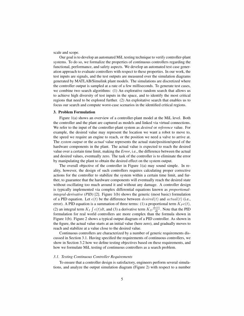
In this section, we describe our search-based approach to MiL testing of controllers,and show how we employ and combine different search algorithms to guide and auto-mate MiL testing of continuous controllers. Figure 5 shows an overview of our auto-mated MiL testing approach. In the first step, we receive a controller-plant model (e.g.,in MATLAB/Simulink) and a set of objective functions derived from requirements. Wepartition the input search space into a set of regions, and for each region, compute avalue indicating the evaluation of a given objective function on that region based on ran-dom search (exploration). We refer to the result as a HeatMap diagram [15]. HeatMapdiagrams are graphical 2-D or 3-D representations of data where a matrix of valuesare represented by colors. In this paper, we use grayscale 2-D HeatMap diagrams (seeFigure 6(b) for an example). These diagrams are intuitive and easy to understand bythe users of our approach. In addition, our HeatMap diagrams are divided into equalregions (squares), making it easier for engineers to delineate critical parts of the in-put space in terms of these equal and regular-shape regions. Based on domain expertknowledge, we select some of the regions that are more likely to include critical andrealistic errors. In the second step, we focus our search on the selected regions andemploy a single-state heuristic search to identify, within those regions, the worst-casescenarios to test the controller. Single-state search optimizers only keep one candidatesolution at a time, as opposed to population-based algorithms that maintain a set ofsamples at each iteration [14].

In the first step of our approach in Figure 5, we apply a random (unguided) searchto the entire search space in order to identify high risk areas. The search exploresdiverse test inputs to provide an unbiased estimate of the average objective functionvalues in different regions of the search space. In the second step, we apply a heuristic

10

+Controller-plant

model

Objective Functionsbased on

Requirements

HeatMap Diagram

Worst-Case Scenarios

List of Critical RegionsDomain

Expert

1.Exploration 2.Single-StateSearch

Figure 5: An overview of our automated approach to MiL testing of continuous controllers.

single-state search to a selection of regions in order to find worst-case test scenariosthat are likely to violate the controller properties. In the following two sections, wediscuss these two steps.

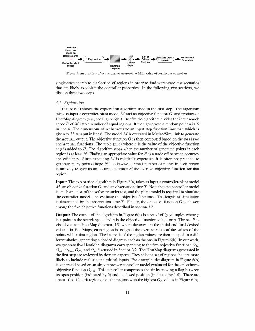
4.1. ExplorationFigure 6(a) shows the exploration algorithm used in the first step. The algorithm

takes as input a controller-plant model M and an objective function O, and produces aHeatMap diagram (e.g., see Figure 6(b)). Briefly, the algorithm divides the input searchspace S of M into a number of equal regions. It then generates a random point p in Sin line 4. The dimensions of p characterize an input step function Desired which isgiven toM as input in line 6. The modelM is executed in Matlab/Simulink to generatethe Actual output. The objective function O is then computed based on the Desiredand Actual functions. The tuple (p, o) where o is the value of the objective functionat p is added to P . The algorithm stops when the number of generated points in eachregion is at leastN . Finding an appropriate value forN is a trade off between accuracyand efficiency. Since executing M is relatively expensive, it is often not practical togenerate many points (large N ). Likewise, a small number of points in each regionis unlikely to give us an accurate estimate of the average objective function for thatregion.

Input: The exploration algorithm in Figure 6(a) takes as input a controller-plant modelM , an objective function O, and an observation time T . Note that the controller modelis an abstraction of the software under test, and the plant model is required to simulatethe controller model, and evaluate the objective functions. The length of simulationis determined by the observation time T . Finally, the objective function O is chosenamong the five objective functions described in section 3.2.

Output: The output of the algorithm in Figure 6(a) is a set P of (p, o) tuples where pis a point in the search space and o is the objective function value for p. The set P isvisualized as a HeatMap diagram [15] where the axes are the initial and final desiredvalues. In HeatMaps, each region is assigned the average value of the values of thepoints within that region. The intervals of the region values are then mapped into dif-ferent shades, generating a shaded diagram such as the one in Figure 6(b). In our work,we generate five HeatMap diagrams corresponding to the five objective functions OL,OSt,OSm,ONs andOR discussed in Section 3.2. The HeatMap diagrams generated inthe first step are reviewed by domain experts. They select a set of regions that are morelikely to include realistic and critical inputs. For example, the diagram in Figure 6(b)is generated based on an air compressor controller model evaluated for the smoothnessobjective function OSm. This controller compresses the air by moving a flap betweenits open position (indicated by 0) and its closed position (indicated by 1.0). There areabout 10 to 12 dark regions, i.e., the regions with the highest OS values in Figure 6(b).

11

(a)Algorithm. EXPLORATION

Input: A controller-plant model M with input search space S.An objective function O.An observation time T .

Output: An overview diagram (HeatMap) HM .The set P of HM points.

1. Partition S into equal sub-regions2. Let P = {}3. repeat4. Let p = (Initial Desired, Final Desired) be

a random point in S5. Let Desired be a step function generated based on p and T6. Run M with the Desired input to obtain the Actual output7. o = O(Desired, Actual)8. P = {(p, o)} ∪ P9. until there are at least N points in each region of S do10. Create a HeatMap diagram HM based on P11. Return HM and P

(b)

Initial Desired Value

Fina

l Des

ired

Valu

e

0.0

0.1

0.2

0.3

0.4

0.5

0.6

0.7

0.8

0.9

1.0

0.0 0.1 0.2 0.3 0.4 0.5 0.6 0.7 0.8 0.9 1.0

Figure 6: The first step of our approach in Figure 5: (a) The exploration algorithm. (b) An example HeatMapdiagram produced by the algorithm in (a)

These regions have initial flap positions between 0.5 and 1.0, and final flap positionsbetween 0.1 and 0.6. Among these regions, domain experts tend to focus on regionswith initial values between 0.8 and 1.0, or final values between 0.8 and 1.0. This isbecause, in practice, there is more probability of damage when a closed (or a nearlyclosed) flap is being moved, or when a flap is about to be closed.

Search heuristics: Figure 6(a) shows a generic description of our exploration algo-rithm. This algorithm can be implemented in different ways by devising various heuris-tics for generating random points in the input search space S (line 4 in Figure 6(a)).In our work, we use two alternative heuristics for line 4 of the algorithm: (1) a simplerandom search, which we call naive random search, and (2) an adaptive random searchalgorithm [14]. The naive random search simply calls a random function to generatepoints in line 4 in Figure 6(a). Adaptive random search is an extension of the naiverandom search that attempts to maximize the euclidean distance between the selectedpoints. Specifically, it explores the space by iteratively selecting points in areas of thespace where fewer points have already been selected. To implement adaptive randomsearch, the algorithm in Figure 6(a) changes as follows: Let Pi be the set of points se-lected by adaptive random search at iteration i (line 8 in Figure 6(a)). At iteration i+1,at line 4, instead of generating one point, adaptive random search randomly generatesa set X of candidate points in the input space. The search computes distances betweeneach candidate point p ∈ X and the points in Pi. Formally, for each point p = (v1, v2)in X , the search computes a function dist(p) as follows:

dist(p) = MIN(v′1,v

′2)∈Pi

√(v1 − v′1)2 + (v2 − v′2)2

The search algorithm then picks a point p ∈ X such that dist(p) is the largest, andproceeds to the lines 5 to 7. Finally, the selected p together with the value o of objectivefunction at point p is added to Pi to generate Pi+1 in line 8.

The algorithm in Figure 6(a) stops when at least N points have been selected ineach region. We anticipate the adaptive random heuristic reaches this termination con-dition faster than a naive random heuristic because it generates points that are more

12

evenly distributed across the entire space. Our work is similar to quasi-random num-ber generators that are available in some languages, e.g., MATLAB [16]. Similar toour adaptive random search algorithm, these number generators attempt to minimizethe discrepancy between the distribution of generated points. We evaluate efficiency ofnaive random search and adaptive random search in generating HeatMap diagrams inSection 6.

Note that a simple and faster solution to build HeatMap diagrams could have beento simply generate equally spaced points in the search space. However, assuming thesoftware under test might have some regularity in its behavior, such a strategy mightmake it impossible to collect a statistically, unbiased representative subset of observa-tions in each region.

4.2. Single-State SearchFigure 7(a) presents our single-state search algorithm for the second step of the

procedure in Figure 5. The single-state search algorithm starts with the point with theworst (highest) objective function value among those computed by the random searchin Figure 6(a). It then iteratively generates new points by tweaking the current point(line 6) and evaluates the given objective function on the newly generated points. Fi-nally, it reports the point with the worst (highest) objective function value. In contrastto random search, the single-state search is guided by an objective function and per-forms a tweak operation. Since the search is driven by the objective function, we haveto run the search five times separately for OL, OSt, OSm, ONs and OR.

At this step, we rely on single-state exploitative algorithms. These algorithmsmostly make local improvements at each iteration, aiming to find and exploit localgradients in the space. In contrast, explorative algorithms, such as the adaptive randomsearch we used in the first step, mostly wander about randomly and make big jumpsin the space to explore it. We apply explorative search at the beginning to the entiresearch space, and then focus on a selected area and try to find worst case scenarios inthat area using exploitative algorithms.

Input: The input to the single-state search algorithm in Figure 7(a) is the controller-plant model M , an objective function O, an observation time T , a HeatMap region r,and the set P of points generated by exploration algorithm in Figure 6(a). We alreadyexplained the input values M , O and T in Section 4.1. Region r is chosen amongthe critical regions of the HeatMap identified by the domain expert. The single-statesearch algorithm focuses on the input region r to find a worst-case test scenario of thecontroller. The algorithm, further, requires P to identify its starting point in r, i.e., thepoint with the worst (highest) objective function in r.

Output: The output of the single-state search algorithm is a worst-case test scenariofound by the search after K iterations. For instance Figure 7(b) shows the worst-casescenario computed by our algorithm for the smoothness objective function applied toan air compressor controller. As shown in the figure, the controller has an undershootaround 0.2 when it moves from an initial desired value of 0.8 and is about to stabilizeat a final desired value of 0.3.

Search heuristics: In our work, evaluating fitness functions takes a relatively long

13

(a)Algorithm. SINGLESTATESEARCHInput: A controller-plant model M with input search space S.

A region r.The set P computed by the algorithm in Figure 6(a).An objective function O.An observation time T .

Output: The worst-case test scenario testCase.1. P ′ = {(p, o) ∈ P | p ∈ r}2. Let (p, o) ∈ P ′ s.t. for all (p′, o′) ∈ P ′, we have o ≥ o′

3. worstFound = o4. AdaptParameteres(r, P )5. for K iterations :6. newp = Tweak(p)7. Let Desired be a step function generated by newp8. Run M with the Desired input to obtain

the Actual output9. v = O(Desired, Actual)10. if v > worstFound :11. worstFound = v12. testCase = newp13. p = Replace(p, newp)14. return testCase

(b)

time

Desired ValueActual Value

0 1 20.0

0.1

0.2

0.3

0.4

0.5

0.6

0.7

0.8

0.9

1.0

Initial Desired

Final Desired

undershoot

Des

ired

& Ac

tual

Val

ue

Figure 7: The second step of our approach in Figure 5: (a) The single-state search algorithm. (b) An exampleoutput diagram produced by the algorithm in (a)

time. Each fitness computation requires us to generate a T second simulation of thecontroller-plant model. This can take up to several minutes. For this reason, for thesecond step of our approach in Figure 5, we opt for a single-state search method incontrast to a population-based search such as Genetic Algorithms (GA) [14]. Notethat in population-based approaches, we have to compute fitness functions for a set ofpoints (a population) at each iteration.

The algorithm in Figure 7(a) represents a generic single-state search algorithm.Specifically, there are two placeholders in this figure: Tweak() at line 6, and Replace()at line 13. To implement different single-state search heuristics, one needs to definehow the existing point p should be modified (the Tweak() operator), and to determinewhen the existing point p should be replaced with a newly generated point newp (theReplace operator).

In our work, we instantiate the algorithm in Figure 7(a) based on three single-statesearch heuristics: standard Hill-Climbing (HC), Hill-Climbing with Random Restarts(HCRR), and Simulated Annealing (SA). Specifically, the Tweak() operator for HCshifts p in the space by adding values x′ and y′ to the dimensions of p. The x′ andy′ values are selected from a normal distribution with mean µ = 0 and variance σ2.The Replace operator for HC replaces p with newp, if and only if newp has a worse(higher) objective function than p. HCRR and SA are different from HC only in theirreplacement policy. HCRR restarts the search from time to time by replacing p witha randomly selected point. Like HC, SA always replaces p with newp if newp hasa worse (higher) objective function. However, SA may replace p with newp even ifnewp has a better (lower) objective function. This latter situation occurs only if anothercondition based on a random variable (temperature t) holds. Temperature is initializedto some value at the beginning of the search and decreases over time, meaning that SAreplaces p with newp more often at the beginning and less often towards the end of the

14

0.20

0.21

0.22

0.23

0.24

0.25

0.26

0.27

0.28

0.29

0.30

0.80 0.81 0.82 0.83 0.84 0.85 0.86 0.87 0.88 0.89 0.90

(a) (b)

120.0

122.0

124.0

126.0

128.0

130.0

132.0

134.0

136.0

138.0

140.0

0.0 2.0 4.0 6.0 8.0 10.0 12.0 14.0 16.0 18.0 20.0

Initial DesiredInitial Desired

Fina

l Des

ired

Fina

l Des

ired

Figure 8: Diagrams representing the landscape for regular and irregular HeatMap regions: (a) A regularregion with a clear gradient between the initial point of the search and the worst-case point. (b) An irregularregion with several local optima.

search. That is, SA is more explorative during the first iterations, but becomes moreand more exploitative over time.

In general, single-state search algorithms, including HC, HCRR, and SA, have anumber of configuration parameters (e.g., variance σ in HC, and the initial temperaturevalue and the speed of decreasing the temperature in SA). These parameters serveas knobs with which we can tune the degree of exploitation (or exploration) of thealgorithms. To be able to effectively tune these parameters in our work, we visualizedthe landscape of several regions from our HeatMap diagrams. We noticed that theregion landscapes can be categorized into two groups: (1) Regions with a clear gradientbetween the initial point of the search and the worst-case point (see e.g., Figure 8(a)).(2) Regions with a noisier landscape and several local optima (see e.g., Figure 8(b)).We refer to the regions in the former group as regular regions, and to the regions inthe latter group as irregular regions. As expected, for regular regions, like the regionin Figure 8(a), exploitative heuristics work best, while for irregular regions, like theregion in Figure 8(b), explorative heuristics are most suitable [14].

Note that the number of points generated and evaluated in each region in the firststep (the exploration step) is not sufficiently large so that we can conclusively deter-mine whether a given region belongs to the regular group or to the irregular groupabove. Therefore, in our work, we rely on a heuristic that attempts to predict the re-gion group based on the information available in HeatMap diagrams. Specifically, ourobservation shows that dark regions mostly surrounded by dark shaded regions belongto regular regions, while dark regions located in generally light shaded areas belong toirregular regions. Using this heuristic, we determine whether a given region belongsto a regular group or to an irregular group. For regular regions, we need to use algo-rithms that exhibit a more exploitative search behavior, and for irregular regions, werequire algorithms that are more explorative. In Section 6, we evaluate our single-statesearch algorithms, HC, HCRR and SA, by applying them to both groups of regions,and comparing their performance in identifying worst-case scenarios in each regiongroup.

15

5. Tool Support

We have fully automated and implemented our approach in a tool called CoCoTest(https://sites.google.com/site/cocotesttool/). CoCoTest implements the en-tire MiL testing process shown in Figure 5. Specifically, CoCoTest provides users withthe following main functions: (1) Creating a workspace for testing a desired Simulinkmodel. (2) Specifying the information about the input and output of the model undertest. (3) Specifying the number of regions in a HeatMap diagram and the number of testcases to be run in each region. (4) Allowing engineers to identify the critical regions ina HeatMap diagram. (5) Generating HeatMap diagrams for each requirement. (6) Re-porting a list of worst-case test scenarios for a number of regions. (7) Enabling usersto run the model under test for any desired point in the input search space. In addition,CoCoTest can be run in a maintenance mode, allowing an advanced user to configuresophisticated features of the tool. This, in particular, includes choosing and configur-ing the algorithms used for the exploration and single-state search steps. Specifically,the user can choose between random search or adaptive random search for exploration,and between Hill-Climbing, Hill-Climbing with Random Restarts and Simulated An-nealing for single-state search. Finally, the user can configure the specific parametersof each of these algorithms as discussed in Section 4.2.

As shown in Figure 5, the input to CoCoTest is a controller-plant model imple-mented in Matlab/Simulink and provided by the user. We have implemented the fivegeneric objective functions discussed in Section 3.2 in CoCoTest. The user can retrievethe HeatMap diagrams and the worst-case scenarios for each of these objective func-tions separately. In addition, the user can specify the critical operating regions of acontroller under test either by way of excluding HeatMap regions that are not of inter-est, or by including those that he wants to focus on. The worst-case scenarios can becomputed only for those regions that the user has included, or has not excluded. Theuser also specifies the number of regions for which a worst-case scenario should begenerated. CoCoTest sorts the regions that are picked by the user based on the resultsfrom the exploration step, and computes the worst-case scenarios for the ones that aretop in the sorting depending on the number of worst-case scenarios requested by theuser. The final output of CoCoTest is five HeatMap diagrams for the five objectivefunctions specified in the tool, and a list of worst-case scenarios for each HeatMap di-agram. The user can examine the HeatMap diagram and run worst-case test scenariosin Matlab individually. Further, the user can browse the HeatMap diagrams, pick anypoint in the diagram, and run the test scenario corresponding to that point in Matlab.

CoCoTest is implemented in Microsoft Visual Studio 2010 and Microsoft .NET 4.0.It is an object-oriented program in C# with 65 classes and roughly 30K lines of code.The main functionalities of CoCoTest have been tested with a test suite containing 200test cases. CoCoTest requires Matlab/Simulink to be installed and operational on thesame machine to be able to execute controller-plant model simulations. We have testedCoCoTest on Windows XP and Windows 7, and with Matlab 2007b and Matlab 2012b.Matlab 2007 was selected because Delphi Simulink models were compatible with thisversion of Matlab. We have made CoCoTest available to Delphi, and have presented itin a hands-on tutorial to Delphi function engineers.

16

6. Evaluation

In this section, we present the research questions that we set out to answer (Sec-tions 6.1), relevant information about the industrial case study (Section 6.2), and thekey parameters in setting our experiment and tuning our search algorithms (Section 6.3).We then provide answers to our research questions based on the results obtained fromour experiment (Section 6.4). Finally, we discuss practical usability of the HeatMapdiagrams and the worst-case test scenarios generated by our approach (Section 6.5).

6.1. Research Questions

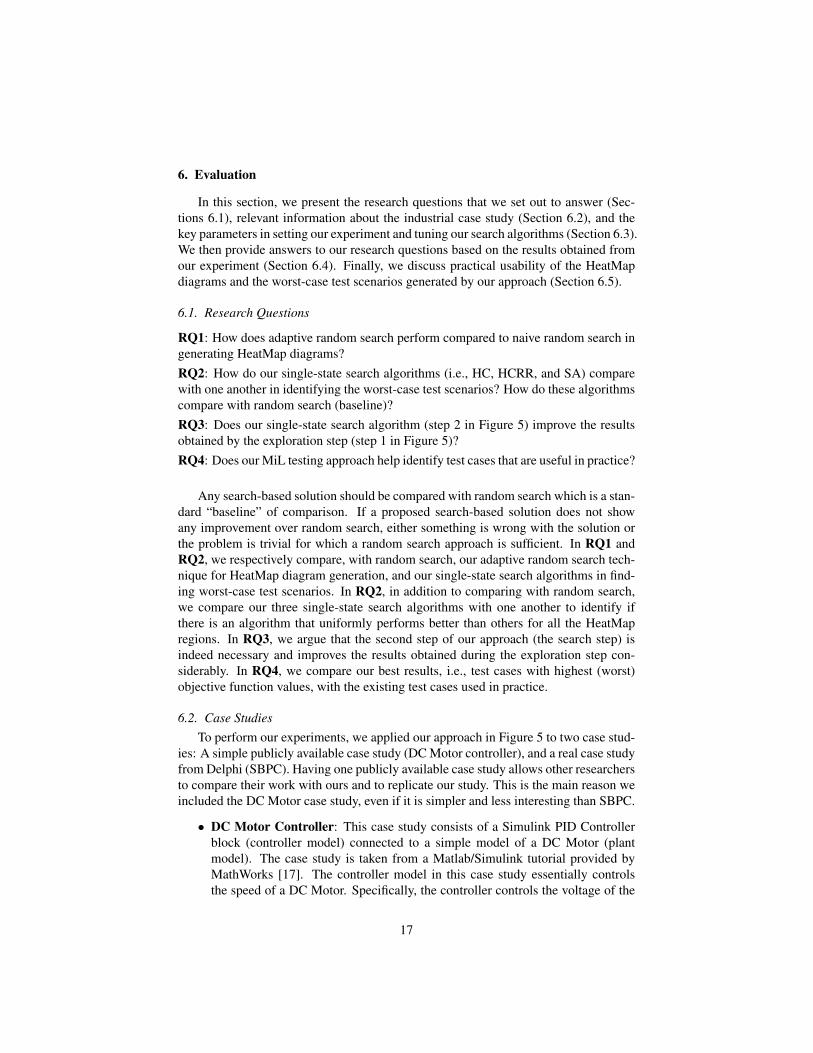
RQ1: How does adaptive random search perform compared to naive random search ingenerating HeatMap diagrams?RQ2: How do our single-state search algorithms (i.e., HC, HCRR, and SA) comparewith one another in identifying the worst-case test scenarios? How do these algorithmscompare with random search (baseline)?RQ3: Does our single-state search algorithm (step 2 in Figure 5) improve the resultsobtained by the exploration step (step 1 in Figure 5)?RQ4: Does our MiL testing approach help identify test cases that are useful in practice?

Any search-based solution should be compared with random search which is a stan-dard “baseline” of comparison. If a proposed search-based solution does not showany improvement over random search, either something is wrong with the solution orthe problem is trivial for which a random search approach is sufficient. In RQ1 andRQ2, we respectively compare, with random search, our adaptive random search tech-nique for HeatMap diagram generation, and our single-state search algorithms in find-ing worst-case test scenarios. In RQ2, in addition to comparing with random search,we compare our three single-state search algorithms with one another to identify ifthere is an algorithm that uniformly performs better than others for all the HeatMapregions. In RQ3, we argue that the second step of our approach (the search step) isindeed necessary and improves the results obtained during the exploration step con-siderably. In RQ4, we compare our best results, i.e., test cases with highest (worst)objective function values, with the existing test cases used in practice.

6.2. Case StudiesTo perform our experiments, we applied our approach in Figure 5 to two case stud-

ies: A simple publicly available case study (DC Motor controller), and a real case studyfrom Delphi (SBPC). Having one publicly available case study allows other researchersto compare their work with ours and to replicate our study. This is the main reason weincluded the DC Motor case study, even if it is simpler and less interesting than SBPC.

• DC Motor Controller: This case study consists of a Simulink PID Controllerblock (controller model) connected to a simple model of a DC Motor (plantmodel). The case study is taken from a Matlab/Simulink tutorial provided byMathWorks [17]. The controller model in this case study essentially controlsthe speed of a DC Motor. Specifically, the controller controls the voltage of the

17

Table 1: Size and complexity of our case study models.

Model features DC Motor (M ) SBPC (M )Controller Plant Controller Plant

Blocks 8 13 242 201Levels 1 1 6 6Subsystems 0 0 34 21Input Var. 1 1 21 6Output Var. 1 2 42 7LOC 150 220 8900 6700

DC Motor so that it reaches a desired angular velocity. Hence, the desired andactual values (see Figure 1(a)) represent the desired and actual angular velocitiesof the motor, respectively. The angular velocity of the DC Motor is a float valuebounded within [0...160].

• Suppercharger Bypass Position Controller: Supercharger is an air compres-sor blowing into a turbo-compressor to increase the air pressure supplied to theengine and, consequently, increase the engine torque at low engine speeds. Theair pressure can be rapidly adjusted by a mechanical bypass flap. When the flapis completely open, supercharger is bypassed and the air pressure is minimum.When the flap is completely closed, the air pressure is maximum. SuperchargerBypass Flap Position Controller (SBPC) is a component that determines the po-sition of the bypass flap to reach to a desired air pressure. In SBPC, the desiredand actual values (see Figure 1(a)) represent the desired and actual positions ofthe flap, respectively. The flap position is a float value bounded within [0...1](open when 0 and closed when 1.0).

The DC Motor controller, the SBPC controller, and their corresponding plant modelsare all implemented in Matlab/Simulink. Table 1 provides some metrics representingthe size and complexity of the Simulink models for these two case studies. The tableshows the number of Simulink blocks, hierarchy levels, subsystems, and input/outputvariables in each controller and in each plant model. In addition, we generated C codefrom each model using Matlab auto-coding tool [18], and have reported the (estimated)number of lines of code (excluding comments) generated from each model in the lastrow of Table 1.

Note that the desired and actual angular velocities of the DC Motor, and the de-sired and actual bypass flap positions are among the input and output variables of thecontroller and plant models. Recall that desired values are input variables to controllermodels, and actual values are output variables of plant models. SBPC models haveseveral more input/output variables representing configuration parameters.

6.3. Experiments Setup.

Before running the experiments, we need to set the controller requirements param-eters introduced in Figure 3. Table 2 shows the requirements parameter values, theobservation time T used in our experiments, and the actual simulation times of ourcase study models. For SBPC, the requirements parameters were provided as part ofthe case study, but for DC Motor, we chose these parameters based on the maximum

18

Table 2: Requirements parameters and simulation time for the DC Motor and SBPC case studiesRequirements Parame-ters

DC Motor SBPC

Liveness t1 = 3.6s t1 = 0.8sStability t2 = 3.6s t2 = 0.8sSmoothness NormalizedSmoothness

v1 = 8 v1 = 0.05

Responsiveness v3 = 4.8 v3 = 0.03Observation Time T = 8s T = 2sActual Simulation Run-ning Time on Amazon

50ms 31s

Table 3: Parameters for the Exploration stepParameters for Explo-ration

DC Motor SBPC

Size of search space [0..160]× [0..160] [0..1]× [0..1]HeatMap dimensions 8× 8 10× 10Number of points per re-gion (N in Figure 6(a))

10 10

value of the DC Motor speed. Specifically, T is chosen to be large enough so that theactual value can stabilize at the desired value. Note that as we discussed in Section 3.2,since we do not have pass/fail conditions, we do not specify v2 from the smoothnessand t3 from the responsiveness properties.

We ran the experiments on Amazon micro instance machines which are equal totwo Amazon EC2 compute units. Each EC2 compute unit has a CPU capacity ofa 1.0-1.2 GHz 2007 Xeon processor. A single 8-second simulation of the DC Motormodel and a single 2-second simulation of the SBPC Simulink model (e.g., Figure 7(b))respectively take about 50 msec and 31 sec on the Amazon machine (See Table 2 lastrow).

We now discuss the parameters of the exploration and search algorithms in Fig-ures 6(a) and 7(a). Table 3 summarizes the parameters we used in our experiment torun the exploration algorithm. Specifically, these include the size of the search space,the dimensions of the HeatMap diagrams, and the minimum number of points that areselected and simulated in each HeatMap region during exploration. Note that the inputsearch spaces of both case studies are the set of floating point values within the searchspaces specified in Table 3 first row.

We chose the HeatMap dimensions and the number of points per region, i.e., thevalue of N , (lines 2 and 3 in Table 3) by balancing and satisfying the following crite-ria: (1) The region shades should not change across different runs of the explorationalgorithms. (2) The HeatMap regions should not be so fine grained such that we haveto generate too many points during exploration. (3) The HeatMap regions should notbe too coarse grained such that the points generated within one region have drasticallydifferent objective function values.

For both case studies, we decided to generate at least 10 points in each region duringexploration (N = 10). We divided the search space into 100 regions in SBPC (10×10),and into 64 regions in DC Motor (8 × 8), generating a total of at least 1000 points

19

Table 4: Parameters for the Search stepSingle-State Search Parameters DC Motor SBPCNumber of Iterations (HC, HCRR, SA) 100 100Exploitative Tweak (σ) (HC, HCRR, SA) 2 0.01Explorative Tweak (σ) (HC) - 0.03Distribution of Restart Iteration Intervals (HCRR) U(20, 40) U(20, 40)

Initial Temperature (SA)

Liveness 0.3660831 0.0028187Stability 0.0220653 0.000161Smoothness 12.443589 0.0462921NormalizedSmoothness

0.08422266 0.1197671

Responsiveness 0.0520161 0.0173561

Schedule (SA)

Liveness 0.0036245851 0.000027907921Stability 0.0002184 0.0000015940594Smoothness 0.12320385 0.00045833762NormalizedSmoothness

0.00083388772 0.0011858129

Responsiveness 0.00051501089 0.00017184257

and 640 points for SBPC and DC Motor, respectively. We executed our explorationalgorithms a few times for SBPC and DC Motor case studies, and for each of ourfive objective functions. For each function, the region shades remained completelyunchanged across the different runs. In all the resulting HeatMap diagrams, the pointsin the same region have close objective function values. On average, the variance overthe objective function values for an individual region was small. Hence, we concludethat our selected parameter values are suitable for our case studies, and satisfy theabove three criteria.

Table 4 shows the list of parameters for the search algorithms that we used in thesecond step of our work, i.e., HC, HCRR, and SA. Here, we discuss these parametersand justify the selected values in Table 4:

Number of Iterations (K): We ran each single-state search algorithm for 100 iter-ations, i.e., K = 100 in Figure 7(a). This is because the search has alwaysreached a plateau after 100 iterations in our experiments. On average, iteratingeach of HC, HCRR, and SA for 100 times takes a few seconds for DC Motorand around one hour for SBPC on the Amazon machine. Note that the time foreach iteration is dominated by the model simulation time. Therefore, the timerequired for our experiment was roughly equal to multiplying 100 by the timerequired for one single simulation of each model identified in Table 2 (50 msecfor DC Motor and 31 sec for SBPC).

Exploitative and Explorative Tweak (σ): Recall that in Section 4.2, we discussedthe need for having two Tweak operators: One for exploration, and one for ex-ploitation. Specifically, each Tweak operator is characterized by a normal dis-tribution with µ (mean) and σ (variance) values from which random values areselected. We set µ = 0 in our experiment. For an exploitative Tweak, we chooseσ = 2.0 for DC Motor, and σ = 0.01 for SBPC. As intended, with a probabilityof 99% the result of tweaking a point in the center of a HeatMap region stays in-side that region in both case studies. Obviously, this probability decreases when

20

the point moves closer to the borders. In our search, we discard the result ofTweak when it generates points outside of the regions, and never generate sim-ulations for them. In addition, with these values for σ, the search tends to beexploitative. Specifically, the Tweak has a probability of 70% to modify individ-ual points’ dimensions within a range defined by σ.

To obtain an explorative Tweak operator, we triple the above values for σ. Notethat in our work, we use the explorative Tweak option only with the HC algo-rithm. HCRR and SA are turned into explorative search algorithms using restartand temperature options discussed below. In addition, in the DC Motor casestudy, we do not need an explorative Tweak operator because all the HeatMapregions belong to regular regions for which an exploitative Tweak is expected towork best.

Restart for HCRR: HCRR is similar to HC 3except that from time to time it restartsthe search from a new point in the search space. For this algorithm, we need todetermine how often the search is restarted. In our work, the number of itera-tions between each two consecutive restarts is randomly selected from a uniformdistribution between 20 and 40, denoted by U(20, 40).

Initial Temperature and Schedule: The SA algorithm requires a temperature that isinitialized at the beginning of the search, and is incremented iteratively based onthe value of a schedule parameter. The values for the temperature and scheduleparameters should satisfy the following criteria [14]: (1) The initial value of tem-perature should be comparable with differences between the objective functionvalues of pairs of points in the search space. (2) The temperature should con-verge towards zero without reaching it. We set the initial value of temperature tobe the standard deviation of the objective function values computed during theexploration step. The schedule is then computed by dividing the initial value oftemperature by 101, ensuring that the final value of temperature after 100 itera-tions does not become equal to zero.

6.4. Results Analysis

RQ1. How does adaptive random search perform compared to naive randomsearch in generating HeatMap diagrams? To answer this question, we compare (1)the HeatMap diagrams generated by naive random search and adaptive random search,and (2) the time these two algorithms take to generate their output HeatMap diagrams.

For each of our case studies, we compared three HeatMap diagrams randomly gen-erated by naive random search with three HeatMap diagrams randomly generated byadaptive random search. Specifically, we compared the region colors and value rangesrelated to each color. We noticed that all the HeatMap diagrams related to DC Motor(resp. SBPC) were similar. Hence, we did not observe any differences between thesetwo algorithms by comparing their generated HeatMap diagrams.

Figures 9 and 10 represent example sets of HeatMap diagrams generated for DCMotor and SBPC case studies, respectively. In each figure, there are five diagramscorresponding to our five objective functions. Note that as we discussed above, because

21

160.0140.0120.0100.080.060.040.020.00.0

0.0

20.0

40.0

60.0

80.0

100.0

120.0

140.0

160.0

(a) Liveness (b) Stability

(e) Responsiveness

(c) Smoothness

(d) Normalized Smoothness

160.0140.0120.0100.080.060.040.020.00.0

0.0

20.0

40.0

60.0

80.0

100.0

120.0

140.0

160.0

160.0140.0120.0100.080.060.040.020.00.0

0.0

20.0

40.0

60.0

80.0

100.0

120.0

140.0

160.0

160.0140.0120.0100.080.060.040.020.00.0

0.0

20.0

40.0

60.0

80.0

100.0

120.0

140.0

160.0

160.0140.0120.0100.080.060.040.020.00.0

0.0

20.0

40.0

60.0

80.0

100.0

120.0

140.0

160.0

Figure 9: HeatMap diagrams generated for DC Motor for the (a) Liveness, (b) Stability, (c) Smoothness, (d)Normalized Smoothness and (e) Responsiveness requirements. Among the regions in these diagrams, weapplied our single-state search algorithms to the region specified by a white dashed circle.

1.00.90.80.70.60.50.40.30.20.10.00.0

0.1

0.2

0.3

0.4

0.5

0.6

0.7

0.8

0.9

1.0

1.00.90.80.70.60.50.40.30.20.10.00.0

0.1

0.2

0.3

0.4

0.5

0.6

0.7

0.8

0.9

1.0

1.00.90.80.70.60.50.40.30.20.10.00.0

0.1

0.2

0.3

0.4

0.5

0.6

0.7

0.8

0.9

1.0

1.00.90.80.70.60.50.40.30.20.10.00.0

0.1

0.2

0.3

0.4

0.5

0.6

0.7

0.8

0.9

1.0

1.00.90.80.70.60.50.40.30.20.10.00.0

0.1

0.2

0.3

0.4

0.5

0.6

0.7

0.8

0.9

1.0

(a) Liveness (b) Stability

(e) Responsiveness

(c) Smoothness

(d) Normalized Smoothness

Figure 10: HeatMap diagrams generated for SBPC for the (a) Liveness, (b) Stability, (c) Smoothness, (d)Normalized Smoothness and (e) Responsiveness requirements. Among the regions in these diagrams, weapplied our single-state search algorithms to the two regions specified by white dashed circles.

22

1000

1250

1500

1750

2000

2250

2500

2750

3000

700

800

900

1000

1100

1200

1300

1400

1500

1600

1700

1800

1900(b) SBPC(a) DC Motor

Naive Random Adaptive Random Naive Random Adaptive Random

Num

ber o

f gen

erat

ed te

st c

ases

nee

ded

to g

ener

ate

the

Hea

tMap

Num

ber o

f gen

erat

ed te

st c

ases

nee

ded

to g

ener

ate

the

Hea

tMap

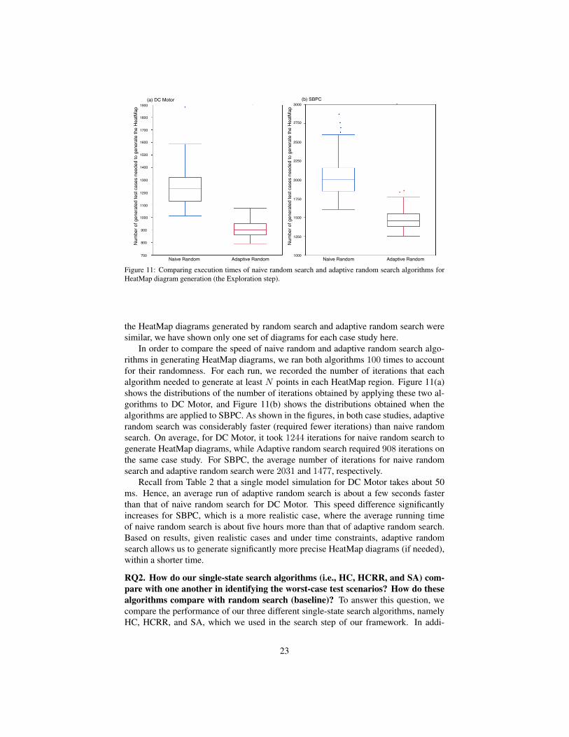
Figure 11: Comparing execution times of naive random search and adaptive random search algorithms forHeatMap diagram generation (the Exploration step).

the HeatMap diagrams generated by random search and adaptive random search weresimilar, we have shown only one set of diagrams for each case study here.

In order to compare the speed of naive random and adaptive random search algo-rithms in generating HeatMap diagrams, we ran both algorithms 100 times to accountfor their randomness. For each run, we recorded the number of iterations that eachalgorithm needed to generate at least N points in each HeatMap region. Figure 11(a)shows the distributions of the number of iterations obtained by applying these two al-gorithms to DC Motor, and Figure 11(b) shows the distributions obtained when thealgorithms are applied to SBPC. As shown in the figures, in both case studies, adaptiverandom search was considerably faster (required fewer iterations) than naive randomsearch. On average, for DC Motor, it took 1244 iterations for naive random search togenerate HeatMap diagrams, while Adaptive random search required 908 iterations onthe same case study. For SBPC, the average number of iterations for naive randomsearch and adaptive random search were 2031 and 1477, respectively.

Recall from Table 2 that a single model simulation for DC Motor takes about 50ms. Hence, an average run of adaptive random search is about a few seconds fasterthan that of naive random search for DC Motor. This speed difference significantlyincreases for SBPC, which is a more realistic case, where the average running timeof naive random search is about five hours more than that of adaptive random search.Based on results, given realistic cases and under time constraints, adaptive randomsearch allows us to generate significantly more precise HeatMap diagrams (if needed),within a shorter time.

RQ2. How do our single-state search algorithms (i.e., HC, HCRR, and SA) com-pare with one another in identifying the worst-case test scenarios? How do thesealgorithms compare with random search (baseline)? To answer this question, wecompare the performance of our three different single-state search algorithms, namelyHC, HCRR, and SA, which we used in the search step of our framework. In addi-

23

1.38

1.39

1.40

1.41

1.42

1.43

1.44

1.45

1.46

0 10 20 30 40 50 60 70 80 90 100

(a) (b)1.47

HC HCRR SA RandomIteration

Live

ness

Obj

ectiv

e Fu

nctio

n

1.38

1.39

1.40

1.41

1.42

1.43

1.44

1.45

1.46

1.47

Live

ness

Obj

ectiv

e Fu

nctio

n+ + + + + + ++

^ ^ ^ ^ ^ ^ ^ ^ ^

+HCHCRRSARandom

+^ ^

Figure 12: The result of applying HC, HCRR, SA and random search to a regular region from DC Motor(specified by a dashed white circle in Figure 9(a)): (a) The averages of the output values (i.e., the highestobjective function values) of each algorithm obtained across 100 different runs over 100 iterations. (b) Thedistributions of the output values obtained across 100 different runs of each algorithm after completion, i.e.,at iteration 100.

tion, we compare these algorithms with random search which is used as a baselineof comparison for search-based algorithms. Recall that in section 4.2, we identifiedtwo different groups of HeatMap regions. Here, we compare the performance of HC,HCRR, SA, and random search in finding worst-case test scenarios for both groups ofHeatMap regions, separately. As shown in Figure 7(a) and mentioned in section 4.2,for each region, we start the search from the worst point found in that region duringthe exploration step. This not only allows us to reuse the results from the explorationstep, but also makes it easier to compare the performance of the single-state search al-gorithms as these algorithms all start the search from the same point in the region andthe same objective function value.

We selected three regions from the set of high risk regions of each one of theHeatMap diagrams in Figures 9 and 10, and applied HC, HCRR, SA, and randomsearch to each of these regions. In total, we applied each single-state search algorithmto 15 regions from DC Motor and to 15 regions from SBPC. For DC Motor, we selectedthe three worst (darkest) regions in each HeatMap diagram, and for SBPC case study,the domain expert chose the three worst (darkest) regions among the critical operatingregions of the SBPC controller.

We noticed that all the HeatMap regions in the DC Motor case study were fromgroup regular with a clear gradient from light to dark. Therefore, for the DC Motorregions, we ran our single-state search algorithms only with the exploitative parametersin Table 4. For the SBPC case study, we ran the search algorithms with the exploitativeparameters for nine regions (regions from smoothness, normalized smoothness, andresponsiveness HeatMap diagrams), and with the explorative parameters for six otherregions (regions from liveness and stability HeatMap diagrams).

Figure 12 shows the results of comparing our three single-state search algorithmsas well as random search using a representative region from the DC Motor case study.Specifically, the results in this figure were obtained by applying these algorithms to theregion specified by a white dashed circle in Figure 9(a). The results of applying ouralgorithms to the other 14 HeatMap regions selected from the DC Motor case studywere similar. As before, we ran each of these algorithms 100 times. Figure 12(a) showsthe averages of the highest (worst) objective function values for 100 different runs of

24

1.88

1.90

1.91

1.92

1.93

1.94

0 10 20 30 40 50 60 70 80 90 100

(a) (b)

0.00931

0.00932

0.00933

0.00934

0.00935

0.00936

0.00937

0 10 20 30 40 50 60 70 80 90 100

(c) (d)Iteration

Iteration

Smoo

thne

ss O

bjec

tive

Func

tion

Live

ness

Obj

ectiv

e Fu

nctio

n

HC HCRR SA Random

HC HCRR SA Random

1.89

1.88

1.90

1.91

1.92

1.93

1.94

1.89

Smoo

thne

ss O

bjec

tive

Func

tion

0.00931

0.00932

0.00933

0.00934

0.00935

0.00936

0.00937

Live

ness

Obj

ectiv

e Fu

nctio

n

+HCHCRRSARandom

+^ ^

+ + + + + + + +

^ ^ ^ ^ ^ ^ ^ ^^

+HCHCRRSARandom

+^ ^

+

++

+ +

^ ^ ^ ^ ^ ^ ^ ^ ^

+ + + + +

Figure 13: The result of applying HC, HCRR, SA and random search to a regular and an irregular regionfrom SBPC: (a) and (c) show the averages of the output values (i.e., the highest objective function values) ofeach algorithm obtained across 100 different runs over 100 iterations. (b) and (d) show the distributions ofthe output values obtained across 100 different runs of each algorithm over 100 iterations. Diagrams (a,b)are related to the region specified by a dashed white circle in Figure 10(c), and Diagrams (c,d) are related tothe region specified by a dashed white circle in Figure 10(a).

each of our algorithms over 100 iterations. Figure 12(b) compares the distributions ofthe highest (worst) objective function values produced by each of our algorithms oncompletion (i.e., at iteration 100) over 100 runs.

Figure 13 represents the results of applying our algorithms to two representativeHeatMap regions from the SBPC case study. Specifically, Figures 13(a) and (b) showthe results related to a regular region, (i.e., regions with clear gradients from light todark), and Figures 13(c) and (d) represent the results related to an irregular region, (i.e.,regions with several local optima and no clear gradient landscape). The former regionis from Figure 10(c), and the latter is from Figure 10(a). Both regions are specified bya white dashed circle in Figures 10 (c) and (a), respectively. For the regular region, weexecuted HC, HCRR, and SA with the exploitative tweak parameter in Table 4, and forthe irregular region, we used the explorative tweak parameter for HC from the sametable.

Similar to Figure 12(a), Figures 13(a) and (c) represent the averages of the algo-rithms’ output values obtained from 100 different runs over 100 iterations, and similarto Figure 12(b), Figures 13(b) and (d) represent the distributions of the algorithms’output values obtained from 100 different runs. As before, the results in Figures 13(a)and (b) were representative of the results we obtained from other eight SBPC regularregions in our experiment, while the results in Figures 13(c) and (d) were representative

25

for the other five SBPC irregular regions.The diagrams in Figures 12 and 13 show that HC and HCRR perform better than

random search and SA for regular regions. Specifically, these two algorithms requirefewer iterations to find better output values, i.e., higher objective function values, com-pared to SA and random search. HC performs better than HCRR on the regular regionfrom DC Motor. As for the irregular region from SBPC, HCRR performs better thanother algorithms.

To statistically compare the algorithms, we performed a two-tailed, student t-test [19]and other non-parametric equivalent tests, but only report the former as results wereconsistent. The chosen level of significance (α) was set to 0.05. Applying t-test tothe regular region from DC Motor (Figures 12 (a) and (b)) resulted in the followingorder for the algorithms, from best to worst, with significant differences between allpairs: HC, HCRR, random search, and SA. The statistical test for both regular andirregular regions from SBPC (Figures 13(a) to (d)) showed that the algorithms are di-vided into two equivalence classes: (A) HC and HCRR, and (B) random search andSA. The p-values between pairs of algorithms in the same class are above 0.05, andthe p-values between those in different classes are below 0.05. Table 5 provides the p-values comparing HC with other algorithms for regular regions, and comparing HCRRwith other algorithms for an irregular region from SBPC. In addition, to computingp-values, we provide effect sizes comparing HC and HCRR with other algorithms forregular and irregular regions, respectively. In [20], it was noted that it is inadequate tomerely show statistical significance alone. Rather we need to determine whether theeffect size is noticeable. Therefore, in Table 5, we show effect sizes computed basedon Cohen’s d [21]. The effect sizes are considered small for 0.2 ≤ d < 0.5, mediumfor 0.5 ≤ d < 0.8, and high for d ≥ 0.8.

To summarize, for regular regions exploitative algorithms work best. Specifically,HC, which is the most exploitative algorithm, performs better than other algorithms onregular regions from DC Motor. For the regular region from SBPC, HCRR managesto be as good as HC because it can reach its plateau early enough before it is restartedfrom a different point. Hence, HCRR and HC perform the same on the regular regionsfrom SBPC.

For irregular regions, search algorithms that are more explorative do better. Specif-ically, HCRR is slightly better than HC on irregular regions from SBPC. The histogramdiagrams in Figure 14 compare the distributions of the highest objective function valuesfound by HC and HCRR. Specifically, with 50% probability, HCRR finds an objectivefunction value larger than 0.00933. If we run HCRR for three times, with a probabilityof 87.5%, HCRR finds at least one value around or higher than 0.00933. For HC, how-ever, the probability of finding an objective function value higher than 0.00933 is lessthan 20% in one run, and less than 49% in three runs. That is, even though we do notobserve a statistically significant difference between the results of HC and HCRR forthe irregular region of SBPC, by running these algorithms three times, we have a higherchance to find a larger value by HCRR than by HC. Finally, even though we chose SAparameters according to the guidelines in the literature (see Section 6.3, and [14]), onour case study models, SA is never better than random. This can be due to the factthat SA merely explores the space at the beginning of its search and becomes totallyexploitative at the end of its search, but the exploitation is not necessarily performed

26

0.10

0.20

0.30

0.40

0.50

0.60

(a) HC

Prob

abilit

y

0.05

0.10

0.15

0.20

0.25

0.30

Prob

abilit

y

0.0093 0.00931 0.00932 0.00933 0.00934 0.00935 0.00936 0.00937 0.00938 0.0093 0.00931 0.00932 0.00933 0.00934 0.00935 0.00936 0.00937 0.00938

(b) HCRR

Figure 14: The distribution of the highest objective function values found after 100 iterations by HC andHCRR related to the region specified by a dashed white circle in Figure 10(a)

Table 5: The p-values obtained by applying t-test to the results in Figures 12 and 13 and the effect sizes mea-suring the differences between these results: Each algorithm is compared with HC (i.e., the best candidatefor regular regions) for the regular DC Motor and SBPC regions, and with HCRR (i.e., the best candidate forirregular regions) for the irregular SBPC region.

Algorithm DC Motor Reg-ular Region

SBPC RegularRegion

SBPC IrregularRegion

p-value with HC (effect size)HCRR <0.0001(High) 0.2085(Low) -SA <0.0001(High) <0.0001(High) -Random <0.0001(High) <0.0001(High) -

p-value with HCRR (effect size)HC - - 0.0657(Medium)SA - - 0.0105(High)Random - - 0.0014(High)

close to a local optimum. However, HCRR periodically spends a number of iterationsimproving its candidate solution (exploitation) after each random restart (exploration).As a result, HCRR is more likely to perform some exploitation in parts of the searchspace close to a local optimum.

RQ3. Does our single-state search algorithm (step 2 in Figure 5) improve the re-sults obtained by the exploration step (step 1 in Figure 5)? To answer this question,we compare the output of single-state search algorithm with the output of explorationstep for two regular regions from DC Motor and SBPC, and one irregular region fromSBPC. Relying on RQ1 and RQ2 results, for this comparison, we use the adaptive ran-dom search algorithm for the exploration step, HC for the single-state search in regularregions, and HCRR for the single-state search in irregular regions.

Let A be the highest objective function value computed by adaptive random searchin each region, and let Bi be the output (highest objective function value) of HC andHCRR at run i on regular and irregular regions, respectively. We compute the relativeimprovement that the search step could bring about over the results of the explorationstep for run i of the search by Bi−A

A . Figure 15 shows the distribution of these relativeimprovements for the three selected regions and across 100 different runs.

The results show that the final test cases computed by our best single-state searchalgorithm have higher objective function values compared to the best test cases iden-tified by adaptive random search during the exploration step. The average relativeimprovement, for regular regions, is around 5.5% for DC Motor, and 7.8% for SBPC,which is a larger and more realistic case study and has a more complex search space.

27

0.05

0.10

0.15

0.20

0.25

0.30

(a)

Prob

abilit

y

0.05 0.051 0.052 0.053

(b)

0.35

0.054 0.055 0.056 0.057 0.0778 0.078 0.0782 0.0784 0.0786 0.0788

(c)

0.033 0.034 0.035 0.036 0.037 0.038 0.0390.058

Figure 15: The distribution of the improvements of the single-state search output compared to the explorationoutput across 100 different runs of the search algorithm: (a) and (b) show the improvements obtained byapplying HC to two regular regions from DC Motor and SBPC, and (c) shows the improvements obtained byapplying HCRR to an irregular region from SBPC. The results are related to the three regions specified bydashed white circles in Figures 9(a), 10(a), and 10(c), respectively.

This value, for the irregular region form SBPC is about 3.5%.

RQ4. Does our MiL testing approach help identify test cases that are useful inpractice? To demonstrate practical usefulness of our approach, we show that the testcases generated by our MiL testing approach had not been previously found by man-ual testing based on domain expertise. Specifically in our industry-strength case study(SBPC), we were able to generate 15 worst-case test scenarios for the SBPC controller.Figure 7(b) shows the simulation for one of these test scenarios concerning smooth-ness. Delphi engineers reviewed the simulation diagrams related to these worst-casescenarios to determine which ones are acceptable as they exhibit small deviations thatcan be tolerated in practice, and which ones are critical and have to be further investi-gated. Among the 15 worst-case test scenarios, those related to liveness and stabilityrequirements were considered acceptable by the domain expert. The other nine testscenarios, however, indicated violations of the controller requirements. None of thesecritical test cases had been previously found by manual, expertise-based MiL testingby Delphi engineers. For example, Figure 7(b) shows an undershoot scenario around0.2 for the SBPC controller. The maximum undershoot/overshoot for the SBPC con-troller identified by manual testing was around 0.05. Similarly, for the responsivenessproperty, we found a scenario in which it takes 150ms for the actual value to get closeenough to the desired value while the maximum corresponding value in manual testingwas around 50ms.

6.5. Practical UsabilityTo better understand practical usability of our work, we made our case study results

and tool support available to Delphi engineers through interactive tutorial sessions andour frequent meetings with them. In general, the engineers believe that our approachcan help them effectively identify bugs in their controller models, and in addition, canbe seen as a significant aid in designing controllers.

To receive feedback on specific output items of our work, we presented HeatMapdiagrams shown in Figure 10 to Delphi engineers. They found the diagrams visuallyappealing and useful. They noted that the diagrams, in addition to enabling the iden-tification of critical regions, can be used in the following ways: (1) The engineers cangain confidence about the controller behaviors over the light shaded regions of the di-agrams. (2) The diagrams enable the engineers to investigate potential anomalies in

28

the controller behavior. Specifically, since controllers have continuous behaviors, weexpect a smooth shade change over the search space going from white to black. Asharp contrast such as a dark region immediately neighboring a light shaded regionmay potentially indicate an abnormal behavior that needs to be further investigated.

As discussed in response to RQ4, we identified 15 worst case scenarios (test cases)for SBPC in total. Nine out of these 15 test cases indicated requirements violations atthe MiL level. According to Delphi engineers, the violations revealed by our nine testcases could be due to a lack of precision or errors in the controller or plant models.In order to determine whether these MiL level errors arise in more realistic situations,Delphi engineers applied these nine test scenarios at the Hardware-in-the-Loop (HiL)level where the MiL level plant model is replaced with a combination of hardwaredevices and more realistic HiL plant models running on a real-time simulator. Thisstudy showed that:

• Three (out of nine) errors that were related to the responsiveness requirementdisappeared at the HiL level. This indicates that the responsiveness MiL levelerrors were due to lack of precision or abstractions made in the plant model, asthey do not arise in a more realistic HiL environment.

• Six (out of nine) errors that were related to the smoothness and normalizedsmoothness requirements repeated at the HiL level. Since Delphi engineers werenot able to identify defects in the controller model causing these errors, theyconjecture that these errors might be due to configuration parameters of the con-trollers, and disappear once the controller is configured with proper parameterstaken from real cars. As discussed in Section 3.1, we do not focus on controllerconfiguration parameters in this paper.

In addition, we also applied at the HiL level the six test cases out of the original 15test cases that had passed the MiL testing stage. These six test cases were related toliveness and stability. The HiL testing results for these test cases were consistent withthose obtained on MiL. That is, these test cases passed the HiL testing stage as well.To summarize, our approach is effective in finding worst-case scenarios that cannotbe identified manually. Furthermore, such scenarios constitute effective test cases todetect potential errors in the controller model or in the plant model or in controllerconfiguration parameters.

7. Related Work

Testing continuous controllers presents a number of challenges, and is not yet fullysupported by existing tools and techniques [4, 3, 1, 22]. There are many approaches totesting and analysis of MATLAB/Simulink models [22]. We discuss these approachesand compare them with our work under the following categories:

Formal methods. The modeling languages that have been developed to capture em-bedded software systems mostly deal with discrete-event or mixed discrete-continuoussystems [6, 23, 8]. Examples of these languages include timed automata [24], hybridautomata [7, 25], and Stateflow [26]. Automated reasoning tools built for these lan-guages largely rely on formal methods. Specifically, these tools either exhaustively

29

verify the model under analysis, e.g., using model checkers [4, 27], or generate testcases from counter-examples produced by model checkers [28, 29, 10]. None of thesetools, however, are directly applicable to Simulink models, and they require a pre-requisite translation step to convert simulink models into a formal intermediate nota-tion (e.g., hybrid automata or the SAL notation [30]) [10]. Existing translation mecha-nisms apply to a subset of the Simulink notation and cannot handle the entire Simulinkblocks [10]. In general, formal methods are more amenable to verification of logicaland state-based behaviors such as invariance and reachability properties. Further, theirscalability to large and realistic systems is still unknown. In our work, we focused ontesting pure continuous controllers which have not previously been captured by anydiscrete-event or formal mixed discrete-continuous notation. Moreover, we demon-strated usefulness and scalability of our approach by evaluating it on a representativeindustrial case study.

Search-based approaches. Search-based techniques have been applied to Matlab/Simulinkmodels for two different purposes:

1. Generation of complex input signals that are as close as possible to real-worldsignals, and can be used for testing continuous aspects of Simulink models [31].Such signals can be generated either by sequencing parameterized base sig-nals [32, 33], or by modifying parameters of Fourier series [33]. Meta-heuristicsearch algorithms are used to build such close-to-real-world signals by compos-ing simpler input signals where the search objective is to match a user-defineddescription of the signal [32] or to satisfy certain signal constraints specified intemporal logic [34]. This approach does not address generation of test cases withrespect to system requirements. Neither does it provide any insight as to how onecan develop test oracles for the generated input signals. In our work, we focuson continuous controllers for which step functions are used as input signals. Inaddition, we derive test cases and test objectives from system requirements, en-abling engineers to find worst-case test scenarios and develop test oracles basedon each requirement.

There has been also some approaches to automated signal analysis where simu-lation outputs of Simulink models are verified against customized boolean prop-erties implemented via Matlab blocks [35]. Such boolean properties fail to cap-ture complex requirements such as smoothness or responsiveness. Hence, in ourwork, we use quantitative objective functions over controller outputs. In addi-tion, the signal analysis method in [35] does neither address systematic testing,nor does it include identification of test cases or formalization of test oracles.

2. Generation of test input data with the goal of maximizing coverage or adequacycriteria of test suites [36, 37]. Different meta-heuristic search techniques havebeen used to maximize coverage or adequacy criteria for MATLAB/Simulinkmodels [37], e.g., they are used to maximize path coverage of Simulink mod-els [38, 39], or the number of killed mutants by test cases [40], or coverage ofthe Stateflow statecharts [9]. This approach does not take into account system re-quirements. In addition, the coverage/adequacy criteria listed above do not apply

30

to continuous blocks of MATLAB/Simulink models. Finally, coverage/adequacycriteria satisfaction alone is a poor indication of test suite effectiveness [41]. Ourwork enables generation of test cases based on controller requirements. More-over, our approach is not limited to MATLAB/Simulink and is applicable totesting continuous controllers, implemented in any modelling or programminglanguage.

Control Theory. Continuous controllers have been widely studied in the control theorydomain [2, 5, 42], where the focus has been to optimize the controller behavior for aspecific application by design optimization [43], or a specific hardware configurationby configuration optimization [5]. Overall existing work in control theory deals withoptimizing the controller design or configuration rather than testing. They normallycheck and optimize the controller behavior over one, or a few number of test cases andcannot substitute systematic testing as addressed by our approach.

Commercial Tools. Finally, a number of commercial verification and testing toolshave been developed, aiming to generate test cases for MATLAB/Simulink models.The Simulink Design Verifier software [11] and Reactis Tester [12] are perhaps themost well-known tools but there are a few other competitors as well [44]. To eval-uate requirements using these tools, the MATLAB/Simulink models need to be aug-mented with boolean assertions. The existing assertion checking mechanism, however,handles combinatorial and logical blocks only, and fails to evaluate the continuousMATLAB/Simulink blocks (e.g., integrator blocks) [23]. As for the continuous be-haviors, these tools follow a methodology that considers the MiL models to be thetest oracles [23]. Under this assumption, MiL level testing can never identify the dis-crepancies between controller-plant models and their high-level requirements. In ourwork, however, we rely on controller requirements as test oracles, and are able to iden-tify requirement violations in the MiL level models. Another major issue about thesecommercial tools is a lack of detailed publicly available and research-based documen-tation [45, 46].

8. Conclusions

Testing and verification of the software embedded into cars is a major challengein automotive industry. Software production in the automotive domain typically com-prises three stages: Developing automotive control functions as Simulink models, gen-erating C code from the Simulink models, and deploying the resulting code on hard-ware devices. The artifacts produced at each stage should be sufficiently tested be-fore moving to the subsequent stage. Hence, automotive software artifacts are subjectto (at least) the following three rounds of testing: Model-in-the-Loop (MiL) testing,Software-in-the-Loop (SiL) testing, and Hardware-in-the-Loop (HiL) testing. In thisarticle, we proposed a search-based approach to automate generation of Model-in-the-loop (MiL) level test cases for continuous controllers. These controllers make up alarge part of automotive functions. We identified and formalized a set of commonrequirements for this class of controllers. Our proposed technique relies on a combina-tion of explorative and exploitative search algorithms, which aim at finding worst-case

31

scenarios in the input space with respect to the controller requirements. Our techniqueis implemented in a tool, named CoCoTest. We evaluated our approach by applying itto an automotive air compressor module and to a publicly available controller model.Our experiments showed that our approach automatically generates several worst-casescenarios, which can be used for testing purposes, that had not been previously foundby manual testing based on domain expertise. The test cases indicated potential viola-tions of the requirements at the MiL level, and were applied by Delphi engineers at theHiL level to identify potential discrepancies between plant models, and the HiL plantmodel and hardware. In addition, we demonstrated the effectiveness and efficiencyof our search strategy by showing that our approach computes significantly better testcases and is significantly faster than a pure random test case generation strategy.

In future, we plan to perform more case studies with various controllers and fromdifferent domains to demonstrate generalizability and scalability of our work. In addi-tion, we want to extend our approach to include configuration parameters of continuouscontrollers in our test case generation strategy. To do so, we need to find effective andscalable techniques that can search through large and multi-dimensional search spaces,and effectively help engineers visualize such spaces. Furthermore, we intend to eval-uate our tool, CoCoTest, to assess its abilities and performance in bug finding andfault localization of Simulink models. Extending our search-based testing approach toother types of embedded Simulink components such as state machine controllers andcomponents calculating physical properties is another avenue for future work. Finally,in collaboration with Delphi engineers, we intend to empirically and systematicallyevaluate our tool with respect to detecting and localizing real-world faults in Simulinkmodels.

AcknowledgmentsSupported by the Fonds National de la Recherche - Luxembourg (FNR/P10/03 and

FNR 4878364), and Delphi Automotive Systems, Luxembourg.

References

[1] J. Zander, I. Schieferdecker, P. J. Mosterman, Model-based testing for embeddedsystems, volume 13, CRC Press, 2012.

[2] N. S. Nise, Control Systems Engineering, 4th ed., John-Wiely Sons, 2004.

[3] E. Lee, S. Seshia, Introduction to Embedded Systems: A Cyber-Physical SystemsApproach, http://leeseshia.org, 2010.

[4] T. Henzinger, J. Sifakis, The embedded systems design challenge, in: FormalMethods (FM), Springer, 2006, pp. 1–15.

[5] M. Araki, PID control, Control systems, robotics and automation 2 (2002) 1–23.

[6] A. Pretschner, M. Broy, I. Kruger, T. Stauner, Software engineering for auto-motive systems: A roadmap, in: Future of Software Engineering (FOSE), IEEEComputer Society, 2007, pp. 55–71.

[7] T. A. Henzinger, The Theory of Hybrid Automata, Springer, 2000.

32

[8] T. Stauner, Properties of hybrid systems-a computer science perspective, FormalMethods in System Design 24 (2004) 223–259.

[9] A. Windisch, Search-based test data generation from Stateflow statecharts, in:Genetic and Evolutionary Computation (GECCO), ACM, 2010, pp. 1349–1356.

[10] S. Mohalik, A. A. Gadkari, A. Yeolekar, K. Shashidhar, S. Ramesh, Automatictest case generation from Simulink/Stateflow models using model checking, Soft-ware Testing, Verification and Reliability (2013).

[11] The MathWorks Inc., Simulink, http://www.mathworks.nl/products/simulink,2003. [Online; accessed 25-Nov-2013].

[12] Reactive Systems Inc., Reactis Tester, http://www.reactive-systems.com/

simulink-testing-validation.html, 2010. [Online; accessed 25-Nov-2013].

[13] R. Matinnejad, S. Nejati, L. Briand, T. Bruckmann, C. Poull, Automated model-in-the-loop testing of continuous controllers using search, in: Search Based Soft-ware Engineering, Springer, 2013, pp. 141–157.

[14] S. Luke, Essentials of Metaheuristics, Lulu, 2009. http://cs.gmu.edu/˜sean/book/metaheuristics/.

[15] G. Grinstein, M. Trutschl, U. Cvek, High-dimensional visualizations, in: Pro-ceedings of the 7th Data Mining Conference (KDD), 2001, pp. 7–19.

[16] The MathWorks Inc., Matlab quasi random numbers, http://www.mathworks.nl/

help/stats/generating-quasi-random-numbers.html, 2003. [Online; accessed 17-Mar-2014].

[17] The MathWorks Inc., DC Motor Simulink Model, http://www.mathworks.com/

matlabcentral/fileexchange/11587-dc-motor-model-simulink, 2009. [Online; ac-cessed 25-Nov-2013].

[18] The MathWorks Inc., Embedded Coder, http://www.mathworks.nl/products/

embedded-coder/, 2011. [Online; accessed 25-Nov-2013].

[19] J. Capon, Elementary Statistics for the Social Sciences: Study Guide, WadsworthPublishing Company, 1991.

[20] A. Arcuri, L. Briand, A hitchhiker’s guide to statistical tests for assessing ran-domized algorithms in software engineering, Software Testing, Verification andReliability (2012).

[21] J. Cohen, Statistical power analysis for the behavioral sciences, Lawrence Erl-baum Associates, Inc, 1977.

[22] F. Elberzhager, A. Rosbach, T. Bauer, Analysis and testing of Matlab Simulinkmodels: A systematic mapping study, in: Proceedings of the 2013 InternationalWorkshop on Joining AcadeMiA and Industry Contributions to testing Automa-tion (JAMAICA’13), ACM, 2013, pp. 29–34.

33

[23] P. Skruch, M. Panek, B. Kowalczyk, Model-based testing in embedded automo-tive systems, Model-Based Testing for Embedded Systems (2011) 293–308.

[24] R. Alur, Timed automata, in: Computer Aided Verification (CAV), Springer,1999, pp. 8–22.

[25] J.-F. Raskin, An introduction to hybrid automata, in: Handbook of networkedand embedded control systems, Springer, 2005, pp. 491–517.

[26] A. Sahbani, J. Pascal, Simulation of hyibrd systems using Stateflow, in: EuropeanSimulation Multiconference on Simulation and Modelling (ESM), 2000, pp. 271–275.

[27] M. Mazzolini, A. Brusaferri, E. Carpanzano, Model-checking based verificationapproach for advanced industrial automation solutions, in: IEEE Conference onEmerging Technologies and Factory Automation (ETFA), IEEE, 2010, pp. 1–8.

[28] A. A. Gadkari, A. Yeolekar, J. Suresh, S. Ramesh, S. Mohalik, K. Shashidhar,Automotgen: Automatic model oriented test generator for embedded control sys-tems, in: Computer Aided Verification (CAV), Springer, 2008, pp. 204–208.

[29] M. Satpathy, A. Yeolekar, P. Peranandam, S. Ramesh, Efficient coverage of par-allel and hierarchical Stateflow models for test case generation, Software Testing,Verification and Reliability 22 (2012) 457–479.

[30] Symbolic Analysis Laboratory Homepage, http://sal.csl.sri.com, 2001. [On-line; accessed 25-Nov-2013].

[31] T. E. Vos, F. F. Lindlar, B. Wilmes, A. Windisch, A. I. Baars, P. M. Kruse,H. Gross, J. Wegener, Evolutionary functional black-box testing in an industrialsetting, Software Quality Journal 1 (2013) 1–30.

[32] A. Baresel, H. Pohlheim, S. Sadeghipour, Structural and functional sequence testof dynamic and state-based software with evolutionary algorithms, in: Geneticand Evolutionary Computation (GECCO), Springer, 2003, pp. 2428–2441.

[33] A. Windisch, N. Al Moubayed, Signal generation for search-based testing of con-tinuous systems, in: International Conference on Software Testing, Verificationand Validation Workshops (ICSTW), IEEE, 2009, pp. 121–130.

[34] B. Wilmes, A. Windisch, Considering signal constraints in search-based testingof continuous systems, in: International Conference on Software Testing, Verifi-cation, and Validation Workshops (ICSTW), IEEE, 2010, pp. 202–211.

[35] J. Zander-Nowicka, Model-based Testing of Real-Time Embedded Systems inthe Automotive Domain, Ph.D. thesis, Elektrotechnik und Informatik der Tech-nischen Universitat, Berlin, 2009.

[36] Y. Zhan, J. A. Clark, A search-based framework for automatic testing of MatlabSimulink models, Journal of Systems and Software 81 (2008) 262–285.

34

[37] K. Ghani, J. A. Clark, Y. Zhan, Comparing algorithms for search-based testdata generation of Matlab Simulink models, in: IEEE Congress on EvolutionaryComputation (CECCO), IEEE, 2009, pp. 2940–2947.

[38] Y. Zhan, J. Clark, Search based automatic test-data generation at an architecturallevel, in: Genetic and Evolutionary Computation (GECCO), Springer, 2004, pp.1413–1424.

[39] Y. Zhan, J. A. Clark, The state problem for test generation in Simulink, in:Genetic and Evolutionary Computation (GECCO), ACM, 2006, pp. 1941–1948.

[40] Y. Zhan, J. A. Clark, Search-based mutation testing for Simulink models, in:Genetic and Evolutionary Computation (GECCO), ACM, 2005, pp. 1061–1068.

[41] M. Staats, G. Gay, M. Whalen, M. Heimdahl, On the danger of coverage di-rected test case generation, in: Fundamental Approaches to Software Engineering(FASE), Springer, 2012, pp. 409–424.

[42] T. Wescott, PID without a PhD, Embedded Systems Programming 13 (2000)1–7.

[43] Wikipedia, PID controller, http://en.wikipedia.org/wiki/PID_controller, 2004.[Online; accessed 25-Nov-2013].

[44] Berner and Mattner Inc., http://www.berner-mattner.com/de/berner-mattner-home/unternehmen/index.html, 2011. [Online; accessed 25-Nov-2013].

[45] S. Sims, D. C. DuVarney, Experience report: the Reactis validation tool, ACMSIGPLAN Notices 42 (2007).

[46] J. Wegener, P. M. Kruse, Search-based testing with in-the-loop systems, in: In-ternational Symposium on Search Based Software Engineering (SSBSE), IEEE,2009, pp. 81–84.

35