1

Copy accepted for publication. Reference for the article:

A. Piacentino, E. Cardona. Scope Oriented Thermoeconomic analysis of energy systems. Part II: Formation structure of optimality for robust design. Applied Energy, 2010, Vol. 87, Issue 3, p. 957-970.

Scope Oriented Thermoeconomic analysis of energy systems. Part II: Formation structure of optimality for robu st design

Antonio Piacentino*, Ennio Cardona DREAM – Dpt. of Energy and Environmental Researches, University of Palermo

Viale delle Scienze, 90128, Palermo (Italy)

Abstract This paper represents the Part II of a paper in two parts. In Part I the fundamentals of Scope Oriented

Thermoeconomics have been introduced, showing a scarce potential for the cost accounting of existing plants;

in this Part II the same concepts are applied to the optimization of a small set of design variables for a vapour

compression chiller. The method overcomes the limit of most conventional optimization techniques, which are

usually based on hermetic algorithms not enabling the energy analyst to recognize all the margins for

improvement. The Scope Oriented Thermoeconomic optimization allows us to disassemble the optimization

process, thus recognizing the Formation Structure of Optimality, i.e. the specific influence of any

thermodynamic and economic parameter in the path toward the optimal design. Finally, the potential

applications of such an in-depth understanding of the inner driving forces of the optimization are discussed in

the paper, with a particular focus on the sensitivity analysis to the variation of energy and capital costs and on

the actual operation-oriented design.

Keywords: Energy systems, vapour compression chiller, optimization, thermoeconomics, formation structure of optimality, Scope

1. Introduction Thermoeconomic approaches to the optimization of energy systems have been developed since the seventies

and earlier, due to the pioneristic contributions by Tribus, Evans and El-Sayed. In the early eighties a group of

scientists developed a reference optimization problem, the well known CGAM problem [1], in order to compare

and reciprocally validate their methodologies for thermoeconomic optimization; the research on

thermoeconomics received a strong impulse, with hundreds research articles and some insightful review articles

published in little more than two decades. The Thermoeconomic Functional Approach [2] is based on a

functional analysis of the system and on the adoption of the Lagrange multipliers method: a set of non linear

equations is usually obtained, which may be solved by numerical techniques. Approaches based on the

Lagrange multipliers method are also used for the optimization of energy systems by the Exergetic Cost Theory

[3] and the Engineering Functional Analysis [4]; while the former approach has revealed particularly explicative

for the cost accounting of existing systems [5] and has posed the bases for the modern thermoeconomic

diagnosis of malfunctions [6], the latter still identifies the thermoeconomic optimization as a best application. A

different approach was proposed in [7], which consists of an iterative procedure based on exergoeconomic

variables like the relative cost difference and the relative exergetic efficiency difference, whose values suggest

to the energy analyst the best path toward the optimal design. Actually, however, thermoeconomic optimization

is not as widely used as it could be expected. The obstacles encountered in real world applications are related to:

* Corresponding author. Tel.: +39 091 236 302; fax: +39 091 484 425. E-mail address: piacentino@dream.unipa.it (A. Piacentino)

2

Nomenclature AESC Average Exergy Saving Cost [ ex€/kW ]

B, b Exergy flow [kW] and specific exergy content [kJex/kg]

B* Exergetic cost [kW] c Unit exergoeconomic cost [€/kWh]

condPTdCost Cost unbalance term at the PT

function of the condenser EE Embodied Exergy F Fuel [kW] h Specific enthalpy [kJ/kg]

k Marginal unit exergetic cost, dimensionless

⋅m Mass flow rate [kg/s] P Product [kW] PM, PT Product Maker and Product Taker s Specific entropy [kJ/kgK] SOT Scope Oriented Thermoeconomics T Temperature [K, °C] T0 Ambient temperature TV Throttling valve W Shaft work Z, z Capital cost [€] and unit capital cost Greek letters Γ Design option ψ Generic path between two design options

∆ Variation in the value of the associated magnitude

componentcauseδ Cost associated with an exergy

destruction in a certain component, related to a specific cause η Isoentropic efficiency

Superscripts comp Compressor cond Condenser opt Optimal value p,T Mechanical and Thermal fractions of exergy exp Expander ev Evaporator throttle At the throttling valve Subscripts Cold uses Cooling exergy delivered to the final users dest Destroyed economic. Economically dominated effect marg Marginal thermod. Thermodinamically dominated effect

4thr Final point of an irreversible expansion occurring in a TV

1. The complexity of the analytical model in case of complex lay-outs. This aspect often induces the plant

designer to adopt thermoeconomic approaches more for optimization at single

component/subcomponent level [8,9] than at system level;

2. The scarce benefits that could be exploited, which are related to the abatement of the computational

resources consumed due to the identification of more accurate solution search directions;

3. The presence of several available alternatives, represented by large scale optimization techniques like

linear and non linear programming and evolutionary search algorithms.

As concerns the optimization algorithms, a main distinction can be made between those which use feasible

points only during the iterations and those which explore also regions outside the feasibility space. Several

applications of both typologies can be found in literature [10-12]; most of them, however, share a common limit

represented by the hermetic behaviour with respect to the optimization problem.

Let us clarify this concept. When the analyst introduces the objective function and the constraints (either

represented by equalities and inequalities), the optimal solution is determined; also, depending on whether the

designer has a full knowledge of the optimization algorithm, he could eventually associate to the solution some

additional informations concerning its reliability and stability. In most cases, however, the algorithm does not

enable the analyst to recognize all the margins for improvement; this is a great limit because in a typical

optimization problem we have both physical constraints, with an intrinsically binding nature, and “auxiliary”

constraints (related to socio-economic or environmental issues) which could eventually be removed at a non-

3

null cost. Hence, providing the energy analyst with an in-depth understanding of the inner driving forces of the

optimization is a premise for the implementation of enhanced optimization processes.

In this paper, representing the 2nd part of a paper in two parts, a very explicative approach to thermoeconomic

optimization will be presented, which is essentially based on the Scope Oriented Thermoconomic (SOT)

method introduced in [13]. In the Part I the SOT approach revealed inadequate for the cost accounting of

existing plants, due to its intrinsically “marginal” (i.e. differential) syntax; with reference to the same case study

adopted in Part I, a large potential will emerge in this paper for the optimization of plant design. After having

introduced the marginal approach to SOT analysis and having applied it to the optimization of a small set of

design variables, the potential applications will be discussed.

2. The case study and the optimization problem

The energy system examined in this paper is the same 1.5 MWc vapour compression chiller presented in [13],

operating with R134a as working fluid; its schematic lay-out is shown in fig. 1. As observed in [13], the scheme

includes a generic component named “expander”, whose behaviour is assumed to range from the irreversibility-

dominated expansion occurring in a Throttling Valve (TV, which obviously covers almost the totality of the

practical applications) to the isentropic efficiency occurring in an ideal turbine (expisη =1), which represents a

reference thermodynamic condition in the Carnot inverse cycle. Just few practical applications of active

expanders have been proposed [14,15], achieving very low exergetic efficiencies; however, coherently with the

methodological purpose of this paper, the technological/economical feasibility of the component “turbine” will

not be discussed here.

The optimization problem is formulated as follows: basing on the cost figures for purchasing and installing each

component given in Appendix A, let us determine the values of the condensation temperature T3 and the

isentropic efficiencies compη of the compressor and expη of the expander that minimize the Total Exergetic

Cost (TEC) of the 1.5 MWc cooling energy rate delivered to the user at a -20°C temperature. The concept of

TEC will be explained in the next section. As concerns the boundary conditions, which in terms of

mathematical modelling represent the constraints, we assume:

– Absence of subcooling of the condensate (i.e. saturated liquid at state 3) and absence of superheating of

the vapour (i.e. dry saturated vapour at state 1);

– Fixed 1.5 MWc cooling capacity;

– Absence of irreversibility due to heat transfer across a finite ∆T at the evaporator, that means

12c1c TTT ≅= . This hypothesis is evidently non realistic. It is introduced because of the explicative

purpose of this paper, aimed at offering an innovative representation of the interactions between the

design variables. As the effect of exergy destruction due to the heat transfer across a finite ∆T will be

kept into account at the condenser, by this non-realistic assumption we just intend to avoid duplicating

the description of a same phenomenon. Evidently, in any practical application this hypothesis should be

excluded;

– Negligible sensitiveness of the pressure drop at the condenser to T3.

The values of T3, ηexp and ηcomp will be discretized over an imposed range; the T3 values in the range [40°C,

60°C] will be discretized assuming a 2°C step, the ηexp will be assumed to vary in the range [0, 0.45], step 0.05,

and finally as concerns ηcomp the range [0.65, 0.86] will be explored, assuming a step ∆η

comp=0.03. This discrete

4

approach is suggested by the availability in tabular form of the R134a thermodynamic properties in the

saturation region: it does not represent a great limit, being in general possible to reduce the width of each

interval according to the desired accuracy level.

3. Basic concepts about Scope Oriented Thermoeconomics and conventional optimization

The genesis of Scope Oriented Thermoconomics was described in [13]. It is essentially based on the following

concept: “when creating a thermoeconomic model, we should always avoid identifying fictitious products for

the components. When we are not able to identify a product to charge with the cost of the resources consumed,

we should extend the boundaries around the component so as to identify at least a Scope for the consumption of

those resources”. This apparently cryptic definition becomes absolutely clear when we consider, for instance, a

typical dissipative component like a condenser. According to the above approach, we should avoid introducing

concepts like negentropy so as to allocate on the other components the cost of the residue dissipated (i.e. the

exergy associated with the heat discarded at T≠T0). We should preferably observe that the scope associated with

the finite “∆T=T-T0” at the condenser is the availability of a finite driving force for heat transfer, so as to install

an heat exchanger with a finite size and cost; in simple words, we may affirm that we destroy some exergy with

the purpose to save money. Evidently, extending the analysis to the economic implications we were able to

identify the actual purpose for destroying that exergy.

Also, SOT analysis differs from the conventional thermoeconomic approaches for adopting a higher

disaggregation level of the system, where the specific functions of a component are not classified as

productive/dissipative, but as:

1. Product Makers (PM): active functions (and the related physical subprocesses) for which a “quality of

the energy conversion process” can be identified and the values of the involved physical parameters

are influenced by endogenous (related to the same quality indicator) factors;

2. Product Takers (PT): passive functions that, once clearly defined, are allowed for a unique evolution

of the energy conversion process. The variations of the involved physical parameters are consequently

determined by the boundary conditions.

Details on the aforementioned concepts can be found in [13].

Before passing to examine in detail the optimization process, some general concepts about the optimization of

energy systems should be introduced. In [16] the authors observe that any system converting energy requires

resources to make it and resources to operate it; an ideal system requires least operating resources but the largest

making resources since the approach to reversibility implies quasi-stationary processes occurring in infinite

time and/or by infinite surfaces as concerns heat exchange processes. We should distinguish whether we intend

to refer to an exergoeconomic model [7] or to a model derived by the Exergetic Cost Theory [3]. A typical

exergoeconomic cost balance for an energy system is:

{ } { } { }

∑∑∑∈∈

⋅

∈

=+productsm

mPcomponentsj

j

inputsiiF PcZFc

mi (1)

Where c represents a unit exergoeconomic cost and the fuel F and the product P are expressed in kW; ⋅Z

indicates the consumption rate of capital resources for owning and operating the component.

If we refer, for the sake of simplicity, to a mono-product energy system, minimizing cp (at fixed P) evidently

leads us to find the optimal compromise between the need for efficient components (F being expected to

5

decrease while ⋅Z will increase) and the need for lower capital costs (cheaper and less efficient components).

The optimization problem is well formulated. If we now refer to the minimization of the exergetic cost, being a

typical cost balance expressed as:

{ } { }

∑∑∈∈

=productsm

*m

inputsi

*i PF (2)

we observe that minimizing P* (at a fixed P) in a mono-product system will induce us to purchase the most

efficient components, with no regard to the capital cost of the components. This occurs whenever F* and P* do

not keep into account, in any way, the monetary nor the exergetic externalities. Following the approach

proposed in [13], we here assume a different approach, oriented to minimize the Total Exergetic Cost (TEC) of

the product, intended as an exergetic cost which includes the cost of externalities. In fact, installing very

efficient components produces two negative effects:

1. Very large components, with large amounts of raw materials consumed in making them;

2. Very high purchase cost.

These two aspects can be converted into exergetic units by introducing:

– The Embodied Exergy EE, i.e. the exergetic cost associated with the exergetic resources consumed

in making the component. This cost can be determined by procedures like Life Cycle Costing;

– The exergetic equivalent of a money saving, to be determined by means of an Average Exergy

Saving Cost [13], AESC, which represents “the cost of alternative exergy saving initiatives that

could be surely implemented” by the plant owner/manager. Details on the values typically assumed

by the AESC can be found in [13].

Let us consider a system whose fuel cost rate in input is F (in kWex) and whose output rate is P, to be kept

constant. Passing from a design option ( )1n

12

11

1 x,...,x,x=Γ to a more efficient design option

( )2n

22

21

2 x,...,x,xΓ = , we expect to have an increase of both the embodied exergy EE of the plant and its capital

cost Z. Calculating a consumption rate of these resources ⋅

EE and ⋅Z by the conventional procedure suggested

in [17], we might determine the Total Exergetic Cost of the product P as follows:

*PEEAESC

Z*F =++

⋅⋅

(3)

Obviously, if a multi-objective optimization was performed [18], oriented to minimize a Total Exergo-

Environmental Cost, a new term ⋅

Env γ should be added on the left hand of Eq. 3, obtained multiplying a

“consumption rate of environmental resources consumed” ⋅

Env (to be calculated again by a Life Cycle

accounting of the environmental externalities) by a γ factor representing the arbitrary weighting index between

the environmental and the exergetic resources consumed. Such an extended approach should be preferred

whenever the environmental costs are particularly high, like in nuclear plants; evidently, this is not our case.

Focusing again on Eq. 3, minimizing P* will no longer lead to adopt the most efficient equipment and design

solutions, because as long as F* reduces, the other two fractions of the resources consumed will increase. In

many applications the embodied exergy rate ⋅

EE is negligible with respect to the term ⋅Z /AESC; this

assumption will be also made in the rest of this paper.

6

The above analysis is just oriented to recognize that as long as we include the externalities related to the capital

costs, we make the minimization of the Total Exergetic Cost of the product to represent an absolutely dual

problem with respect to the minimization of the exergoeconomic cost PcP . This duality is more evident when

we look at the parallel role played by the variables cF in Eq. 1 and AESC in Eq. 3: both of them represent the

link between exergetics and economics. Low values of cF, in fact, will reduce the incidence of the cost fraction

FcF on the total cost (see Eq. 1), leading to an optimal design characterised by a lower energy conversion

efficiency. Similarly, when AESC decreases the incidence of the term ⋅Z /AESC increases and the optimal

design (characterised by the minimum Total Exergetic Cost of the product) will converge toward a less efficient

solution. In this latter case, in fact, the plant owner/manager has margins for cheap exergy saving alternatives

(AESC is expressed in savedex€/kW ) and a small reduction in the capital cost of the system will offer margins for

alternative actions ensuring higher exergy savings than a slightly more efficient design of our system could have

achieved.

The perfect duality between the minimization of the Total Exergetic Cost and that of the exergoeconomic cost

was here underlined because the former approach, adopted in the following of this paper, could appear more

theoretical than the latter (that is actually adopted in most of the practical thermoeconomic optimizations);

however, due to the duality between the two problems, any of the conclusions that will be achieved while

minimizing the TEC could be conceptually extended (following the rules of the aforementioned parallelism) to

the minimization of the exergoeconomic cost of the product. In our case-study the product is the cooling exergy

delivered to the users; consequently the TEC will be indicated as *uses coldB .

Before passing to examine the benefits of a SOT optimization, let us verify the results that could be easily

achieved by an ordinary optimization/simulation algorithm. According to [13], four AESC values are

considered, i.e. AESC=300, 700, 1600 €/kWex and the limit for AESC→ + ∞; the following results are easily

determined:

( ) 0.71) 0, 54,η,η,TOpt

ex300€/kWAESCcompexp

3 (== ( ) 0.77) 0, 50,η,η,TOpt

ex00€/kW7AESCcompexp

3 (== (4.a,b)

( ) 0.83) 0, ,44η,η,TOpt

ex00€/kW16AESCcompexp

3 (== ( ) 0.86) 0.45, ,40η,η,TOpt

AESCcompexp

3 (=+∞→ (4.c,d)

In fig. 2.a-d some iso- *uses coldB surfaces are plotted for the AESC values considered. We may observe that, as

expected, when AESC increases the optimal solution is forced toward more efficient design options; also, we

may note that even at high AESC (up to 1,600 €/kWex) the optimal solution lies on the plane ηexp=0, testifying

that the inclusion of an active component for the production of some shaft work from fluid expansion is far

from feasibility. The presented results offer to the analyst just a generic idea about the role played by the

different variables; the SOT approach that will be proposed in the next sections offers a much more explicative

representation of the problem and of the mutual interactions between design variables and boundary conditions.

4. Application of Scope Oriented Thermoeconomics to the optimization of the 1.5 MWc chiller

In the Part I of this paper several cost balances were written, according to the principles resumed at the

beginning of the previous section. However, differently than average costs, marginal costs are not conservative

and balances for each specific component or function cannot be written in marginal terms. The first step of SOT

optimization consists of expressing analytically the marginal variation of each relevant thermodynamic

7

parameter with the design variables; for an exergy flow B, for instance, considering the design variables T3, ηexp

and ηcomp, we get:

comp

expη,3Tcomp

exp

compη,3Texp3

compη,expη3

dηη

Bdη

η

BdT

T

BdB

∂∂+

∂∂+

∂∂= (5)

As a second step of the analysis, the marginal resources consumed in a component due to an infinitesimal

variation of a design variable are compared with the marginal products (do note: the two quantities are not

imposed to be equal a priori) and, if needed, a disequilibrium term is introduced. This apparently complex

approach will result immediately clear with reference to the examined example. The equations that follow will

be briefly commented in the next subsections; a complete understanding of their origin, however, requires

reading accurately the premises of SOT analysis and examining the SOT cost structure of the 1.5 MWc chiller

presented in [13]. Let us here briefly remind the plant disaggregation level proposed for the examined chiller in

the Part I of this paper:

− The compressor only consists of a PM function: it is fed by electricity with the purpose to increase the

thermal and mechanical exergy of the vapour from State 1 to State 2;

− The condenser consists of a PM function and a PT function. The PM function consumes mechanical

exergy (related to the pressure drop) to allow the fluid to pass into the tube bundle to release heat. The

PT function is responsible for all the marginal resources consumed throughout the plant with the

purpose to have a finite ∆T (driving force for heat transfer) at the condenser. Its scope is “saving

money” to purchase a condenser with a limited heat exchange surface;

− The expander consists of a PM and a PT function. The PT function is represented by the throttling

valve, which allows an irreversibility-dominated expansion whose useful result, the thermal exergy

associated with the fluid exiting the valve at T<T0, depends only on external parameters. The PM

function, included just when we adopt an expander with ηexp>0, is assumed to consume additional

money to purchase the component, while its products are represented by the shaft work expWB and the

additional cooling exergy “ Tthr4

T4 BB − ”, produced in a fixed proportion;

− The functional structure of the evaporator is very similar to that of the condenser. Again we have a PM

function related to the pressure drop for fluid circulation, and a PT function whose objective is

transferring cooling exergy to the users.

A last preliminary note concerns the most intuitive way to present the analytical model: for each component or

function a complex equation could be written, where we compare combinately the additional resources

consumed due to the marginal dT3, dηexp and dηcomp; however, since the error introduced by comparing these

effects separately is negligible (being a higher order differential, as the quantity dT3dηexpdη

comp would appear),

the equations expressing the marginal effects of an infinitesimal variation of each design variable will be

presented separately.

4.1 SOT model for a marginal dT3 variation

The marginal cost equation at the compressor (which represents a PM function, being characterised by its

efficiency ηcomp) is:

8

( )

3expη ,compη3

0W

3expη ,compη

3

expW

3

T2

p2comp

dTT

B dT

T

B

T

BBk

∂∂

=

∂∂

−∂

+∂⋅ (6)

The cost associated with the marginal feed electricity 0WB consumed and with the marginal input from the

expander are allocated on the marginal exergy of the fluid at the state 2. Any non-null variation in the purchase

cost of the compressor is not considered here, because it is generated by a dT3 whose scope is related to the PT

function of the condenser.

No marginal cost equation is written for the PM function of the condenser. According to [13] the scope of this

component consists of “allowing the fluid to pass in the tube bundle of the condenser to reject heat”. Having

assumed to neglect the variation of the pressure drop at the condenser with dT3, dηexp and dηcomp, neither the PM

function of the condenser nor the PM function of the evaporator (for the same reason) will appear in our

marginal analysis. The marginal cost equation at the PT function of the condenser is:

( ) ( )

{ }3

η,η

3

componentsi

i

condPT3

η,η3

throttleilityirreversib

3

η,η3

expW

3

T4thr

T4

3

T3

T2comp

dTT

Z

AESC

1

dCostdTT

δdT

T

B

T

BB

T

BBk

expcomp

expcompexpcomp

∂

∂

⋅−=

=−

∂∂

+

∂∂

−∂

−∂−

∂−∂

⋅

∑∈

(7)

Here several marginal effects of a dT3 are compared. The positive effects of a dT3>0 are the increase in the shaft

work produced at the expander and in the exergy associated to the additional cooling effect from the state 4 to

the state 4thr (characterised by h4thr=h3 and p4thr≈p4); another positive effect is the money saving for the

installation of a cheaper condenser (the driving force of heat transfer has increased). Negative effects are related

to the higher purchase cost of the compressor and the expander and to the increased exergy destruction at the

throttling valve. We cannot affirm, a priori, whether or not these effects are balanced: consequently, a

disequilibrium term condPTdCost is introduced.

The marginal cost equation at the throttling valve is just introduced to indicate how to compute the cost

associated with the exergy destruction:

( ) ( )[ ]

0dTT

δdT

T

BBBB k 3

η,η3

throttleilityirreversib

3

η,η3

T4thr

p4thr

T3

p3comp

expcompexpcomp

=

∂∂

−

∂+−+∂

⋅ (8)

Eq. 8 suggests that the unit cost of the marginal exergy destroyed at the TV coincides with the unit marginal

cost of the compressor [13]. Finally, the marginal cost equation at the PT function of the evaporator indicates

that the marginal cost of the final product reflects the net sum of the marginal contributes from all the plant

components:

( )

0dBdTT

BBkdCost *

uses cold3

η,η3

T4thr

T4compcond

PTcompexp

=−

∂−∂⋅+ (9)

We can observe the absence of a marginal unit cost exp

k of the product of the expander. This is justified by the

assumptions made: having considered the component “expander” (in fig. 1) as the sum of a throttling valve and

a turbine (or active part of the expander, included just when ηexp>0), this last component will be charged with a

9

marginal cost only when it will be responsible for marginal effects on the cycle, i.e. when we will impose a

dηexp

≠0 (see next subsection).

4.2 SOT model for a marginal dηexp variation The marginal cost equation at the compressor is given by:

( ) exp

3T,compη

exp

0Wexp

3T,compη

exp

expW

expexp

3T,compη

exp

T2

p2

compdη

η

Bdη

η

Bkdη

η

BBk

∂∂=

∂∂⋅−

∂+∂⋅ (10)

It suggests that the cost of the marginal resources consumed (both exergy of feed electricity and shaft work

from the expander) are allocated on the marginal product ( )T2

p2 BBd + , which is non-null because at a constant

cooling 1.5 MWc production rate we have a negative exp

η,T

exp

R134adη

η

m

comp3

∂∂

⋅

.

The cost equation at the PT function of the condenser is quite simple and intuitive:

( )

0dCostdηη

BBk cond

PTexp

compη,3T

exp

T3

T2comp

=−

∂−∂⋅ (11)

The marginal cost equation at the turbine (or active part of the expander) is:

( ) { } exp

compη,3T

exp

componentsi

i

exp

compη,3T

exp

T4thr

T4

exp

expWexp

dηη

Z

AESC

1dη

η

BB

η

Bk

∂

∂⋅=

∂−∂+

∂∂ ∑

∈ (12)

The exergy equivalent of the monetary savings/costs for purchasing each component are all allocated on the

product of the responsible component. No disequilibrium term is here included, because having included one at

the PT function of the condenser already allows us to account for the non-null marginal cost/benefit associated

with a dηexp and to charge it on the useful product of the plant.

The cost equation at the evaporator is:

( )

0dBdηη

BBdCost *

uses coldexp

compη,3T

exp

T4thr

T4cond

PT =−

∂−∂+ (13)

It could be noted the absence of the term throttleilityirreversibδ ; this is because we neglect the effect of a dη

exp on the

exergy destruction at the throttling valve. This concept should not be surprising: the TV is modelled as a PT

function, whose performance only depends on the condensation/evaporation temperatures/pressures of the

cycle, which are not influenced by a dηexp.

4.3 SOT model for a marginal dηcomp variation

The marginal cost equation at the compressor is:

( ) comp

expη,3T

comp

0Wcomp

expη,3Tcomp

compcomp

expη,3T

comp

T2

p2

compdη

η

Bdη

η

Z

AESC

1dη

η

BBk

∂∂+

∂∂⋅=

∂+∂⋅ (14)

Both the contributes of a marginal purchase cost of the compressor and a marginal variation in the feed

electricity consumed (these contributes are expected to have opposite signs) are charged on the marginal

product of the compressor. The cost equation at the PT function of the condenser is expressed as follows:

10

( )

0dCostdηη

BBk cond

PTcomp

expη,3T

comp

T3

T2comp

=−

∂−∂⋅ (15)

Finally, the disequilibrium term condPTdCost , which has been charged with all the marginal effects related to

dηcomp, is allocated on the final product of the plant:

0dBdCost *uses cold

condPT =− (16)

5. Preliminary results of a SOT optimization

The analytical thermoeconomic model synthesised by Eqq. 6-16 could appears quite complex; its physical

interpretation will result absolutely clear in this section, where some preliminary results are presented. The

equations were solved by implementing a simulator in Engineering Equation Solver environment [19] which

extracts R134a thermodynamic properties from a REFPROP 7.0 library [20].

Because of the limits of 3-D plots, we will represent the results obtained by assuming combined variations of

two design variables (being the third kept constant). Let us start by considering the combined effects of T3 and

ηexp variations; evidently, we had to use combinately Eq. 5 and Eqq. 6-13. The results are plotted in fig. 3.a-e. In

fig. 3.a-d the behaviour of the Total Exergetic Cost *uses coldB is plotted versus T3 and ηexp, assuming different

values of AESC and for a fixed ηcomp=0.65; we may observe that, as expected, when AESC increases *

uses coldB

becomes less sensitive to the design option and more efficient solutions are gradually privileged (the

coordinates corresponding to the optimal configuration are indicated in the figure, for each AESC). The

diagrams confirm that the inclusion of the expander, with an ηexp>0, is always inconvenient, but for the

hypothetical case of AESC→+∞; the optimal ηexp at different T3 is in fact always equal to 0 at any finite AESC.

The optimal condensation temperature at different ηexp is also identified (see projections in the figure), defined

as follows:

( ) { }min0.65)ηα,η,(TB:TT compexp3

*uses cold3αη0.65,η

opt3 expcomp ====== (17)

The physical meaning is evident; in fig. 3.a, for instance, it is clearly shown that ( )αη0.65,η

opt3 expcompT == with

α=0.3 represents the minimum of the dashed bold line plotted on the surface (its value is 52 °C). While

( )αη0.65,η

opt3 expcompT == undergoes large fluctuations at low AESC (in the range 44÷54 °C, see fig. 3.a), this range

of fluctuations reduces at higher AESC. Also, in order to explore the sensitiveness to ηcomp of the above

described costη

exp3

*colduses comp)η,(TB == f behaviour, in fig. 3.e a similar graph is plotted for the cases

AESC=300 €/kWex and ηcomp=0.86. Comparing the diagrams 3.a and 3.e, obtained at a same AESC, we observe

that ( )αηcost,η

opt3 expcompT == slightly reduces with ηcomp in the low-ηexp region; on the contrary, ( )

αηcost,η

opt3 expcompT ==

is almost insensitive to ηcomp in the high-ηexp region. An interpretation of this behaviour can be easily provided.

At low ηexp the “thermodynamic” effect of a dηexp is prevalent with respect to the effect related to the capital

cost; at higher ηexp the latter effect becomes prevalent, due to the supposed exponential behaviour of Zexp with

ηexp. In the high-ηexp region, consequently, the value of ( )

αη0.65,η

opt3 expcompT == is dominated by the function

Zexp=Zexp(T3, ηexp) and is insensitive to η

comp. In the low-ηexp region the reduction of ( )αη0.65,η

opt3 expcompT == with

11

ηcomp is due to the fact that the shaft work produced at the expander (which increases with T3) contributes to

save a lower amount of feed electricity, because of the better performance of the compressor.

Let us now consider the combined effects of T3 and ηcomp; in this case we had to use combinately Eqq. 5-9 and

14-16; the results are plotted in fig. 4.a-d. In particular, in fig. 4.a-c the diagrams obtained for AESC=300

€/kWex, AESC=700 €/kWex and AESC→+∞ are respectively plotted, assuming in all cases ηexp=0 ; in fig. 4.d

the results for AESC=300 €/kWex and ηexp=0.4 are presented, in order to verify the sensitiveness to the

efficiency of the expander. As expected, when AESC increases the optimal solution moves from high T3 – low

ηcomp solutions to low T3 – high ηcomp ones; the optimal condensation temperature (at constant ηcomp):

( ) { }min0)ηα,η,(TB:TT expcomp3

*uses cold30η,η

opt3 expcomp ======α (18)

reveals scarcely sensitive to ηcomp (see projections in the figures). As concerns the sensitiveness to η

exp (do

compare the figures 4.a and 4.d, both plotted assuming a 300 €/kWex AESC), the optimal condensation

temperature significantly reduces when ηexp increases; this behaviour is evidently associated with the very high

unit cost of the expander (characterised by ηexp=0.4), which contributes to increase * uses coldB when the nominal

shaft work capacity expWB increases (at higher condensation temperatures).

Let us now discuss the combined effects of ηexp and ηcomp; in this case we had to use combinately Eq. 5 and Eqq.

10-16; the results of the analysis are plotted in fig. 5.a,b for a same T3=40°C and for two values of AESC (i.e.

300 and 1600 €/kWex). The optimal ηcomp at a fixed ηexp:

( ) { }minα)η,ηC,40(TB:ηηexpcomp

3*

uses coldcomp

αηC,40Toptcomp,

exp3

==°===°= (19)

is absolutely insensitive to ηexp (see projections in the figure) and it gradually increases with AESC, as expected.

Similar diagrams obtained for T3=60°C, not plotted here, could show that the above behaviour is also scarcely

sensitive to T3.

The figures presented in this section allow us to recognize more properly the mutual interactions among the

design variables; we may for instance recognize the flat regions of the surfaces, which reveal a scarce

sensitiveness of *uses coldB to the local value of the design variables or, in case we subtracted the values obtained

for two homogeneous sets of data by assuming two different AESC, we could eventually assess the

sensitiveness of the solution to the AESC. However, a very large number of diagrams should be plotted to cover

the whole (T3, ηexp, ηcomp) region investigated.

Although the presented results are more analytical than those presented in fig. 2 (and obtained by any

conventional optimization approach), they do not exploit the full disaggregation potential of Eqq. 6-13. Being

based on Eq. 5, in fact, in the figures 3-5 the * uses cold∆B between two generic points A and B, characterised by

different values of two design variables var1 and var2 and by a same value of the remaining design variable var3,

is calculated by

costvar

22

*uses cold

Ψpath

11

*uses cold

Ψpath

*uses cold

*uses cold

3

dvarvar

Bdvar

var

BdB∆B

=

∂∂+

∂∂== ∫∫ (20)

where the path Ψ is a generic path between A and B. Eq. 20 does not allow us to recognize the origin of a high

or low value of 1

*uses cold

var

B

∂∂

and 2

*uses cold

var

B

∂∂

; hence, in the next section a higher disaggregation level will be

12

adopted to fully exploit the potential of SOT optimization and of Eqq. 6-16 in the analysis of the Formation

Structure of Optimality.

6. Formation Structure of Optimality by Scope Oriented Thermoeconomics

In this subsection the disaggregation of the optimization problem by SOT analysis will be applied at the highest

level. Let us assume the plant owner/manager to be characterised by an AESC=700 €/kWex; evidently, from fig.

2.b we may recognize that any optimization algorithm would provide the optimal solution

( ( )0.77 0, C, 50)η,η,T optcomp,optexp,opt3 °= . Of course, in proximity of this optimal solution, quasi-optimal

options will be found (see iso-cost surfaces ex*

uses cold kW 840B = and ex*

uses cold kW 900B = in fig. 2.b); we

could be interested in assessing the sensitiveness of *uses coldB to the three design variables in this region. In fig.

6 a region close to optimality is shown by a zooming representation; for each of the design options

characterized by C 56] [44,T3 °∈ , 0.1] [0,ηexp ∈ and 0.83] [0.71,ηcomp∈ , the value of *uses coldB is indicated.

Understanding the Formation Structure of Optimality, i.e. recognizing the driving force locally dominating the

optimization process, could allow to recognize asymmetries between apparently similar design options. Let us

consider, for instance, the three options indicated in fig. 6:

1. Option A: ( ( )0.8 0, C, 44)η,η,T compexp3 °= , ex

*uses cold kW 873.1B = ;

2. Option B: ( ( )0.83 0.1, C, 48)η,η,T compexp3 °= , ex

*uses cold kW 871.4B = ;

3. Option C: ( ( )0.77 0.05, C, 54)η,η,T compexp3 °= , ex

*uses cold kW 868.4B = .

They are quite equivalent as concerns the value of *uses coldB ; with respect to the minimum 835.1 kWex cost at

the optimal design point, they provoke an additional cost slightly variable between 33.3 and 38.0 kWex.

According to Eq. 20, we could recognize the presence of different contributes due to the deviation ∆T3, ∆ηexp

and ∆ηcomp from optimality; basing on Eqq. 6-16, however, we can do something more.

Let us consider, for instance, a curve ( ) costηexp

3*

uses cold compη,TB = , like the larger diagram in fig. 7; it is

absolutely similar to those presented in fig. 3, being just restricted to the examined region of quasi-optimal

solutions (T3 ∈ [44, 56] °C, ηexp∈ [0, 0.1]). According to Eqq. 6-9, the contributes related to dT3 can be

classified by the following expressions:

− dT3 effect n. 1 = ( )

3

η,η3

T3

T2comp

dTT

BBk

expcomp

∂−∂

⋅ ;

− dT3 effect n. 2 =( )

3

η,η3

T4thr

T4comp

dTT

BB k

expcomp

∂−∂

⋅ ;

− dT3 effect n. 3 = 3

η,η3

expWcomp

dTT

Bk

expcomp

∂∂

⋅ ;

− dT3 effect n. 4 =( )[ ]

33

34thr0comp3

η,η3

throttleilityirreversib

dTT

ssT kdT

T

δ

expcomp∂

−∂⋅=

∂∂

;

13

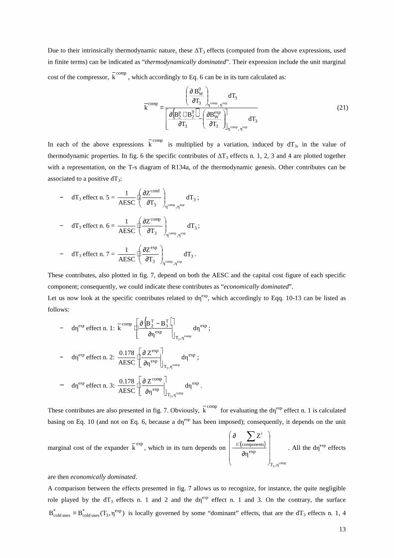
Due to their intrinsically thermodynamic nature, these ∆T3 effects (computed from the above expressions, used

in finite terms) can be indicated as “thermodynamically dominated”. Their expression include the unit marginal

cost of the compressor, comp

k , which accordingly to Eq. 6 can be in its turn calculated as:

( )3

η ,η3

expW

3

T2

p2

3

η ,η3

0W

comp

dTT

B

T

BB

dTT

B

k

expcomp

expcomp

∂∂−

∂+∂

∂∂

= (21)

In each of the above expressions comp

k is multiplied by a variation, induced by dT3, in the value of

thermodynamic properties. In fig. 6 the specific contributes of ∆T3 effects n. 1, 2, 3 and 4 are plotted together

with a representation, on the T-s diagram of R134a, of the thermodynamic genesis. Other contributes can be

associated to a positive dT3:

− dT3 effect n. 5 = 3

η,η3

cond

dTT

Z

AESC

1

expcomp

∂∂⋅ ;

− dT3 effect n. 6 = 3

η,η3

comp

dTT

Z

AESC

1

expcomp

∂∂⋅ ;

− dT3 effect n. 7 = 3

η,η3

exp

dTT

Z

AESC

1

expcomp

∂∂⋅ .

These contributes, also plotted in fig. 7, depend on both the AESC and the capital cost figure of each specific

component; consequently, we could indicate these contributes as “economically dominated”.

Let us now look at the specific contributes related to dηexp, which accordingly to Eqq. 10-13 can be listed as

follows:

− dηexp effect n. 1:

( ) exp

η,Texp

T3

T2comp

dηη

BB k

comp3

∂−∂

⋅ ;

− dηexp effect n. 2: exp

η,Texp

exp

dηη

Z

AESC

0.178

comp3

∂∂⋅ ;

− dηexp effect n. 3: exp

η,Texp

comp

dηη

Z

AESC

0.178

comp3

∂∂⋅ .

These contributes are also presented in fig. 7. Obviously, comp

k for evaluating the dηexp effect n. 1 is calculated

basing on Eq. 10 (and not on Eq. 6, because a dηexp has been imposed); consequently, it depends on the unit

marginal cost of the expander exp

k , which in its turn depends on { }

comp3 η,T

exp

componentsi

i

η

Z

∂

∂ ∑∈

. All the dηexp effects

are then economically dominated.

A comparison between the effects presented in fig. 7 allows us to recognize, for instance, the quite negligible

role played by the dT3 effects n. 1 and 2 and the dηexp effect n. 1 and 3. On the contrary, the surface

)η,(TBB exp3

*uses cold

*uses cold = is locally governed by some “dominant” effects, that are the dT3 effects n. 1, 4

14

and 5. The same procedure here adopted to disaggregate the examined surface could be repeated for different

values of ηcomp and for the profiles )η,(TBB comp3

*uses cold

*uses cold = and )η,(ηBB expcomp*

uses cold*

uses cold = . In

particular, these two profiles involve two dηcomp effects, not presented yet:

− dηcomp effect n. 1:

( ) ( ) comp

η,Tcomp

T3

T2

1

η,Tcomp

T2

p2

η,Tcomp

comp

dηη

BB

η

BB

η

Z

AESC

1

exp3

exp3

exp3

∂−∂⋅

∂+∂

⋅

∂∂⋅

−

. This

economically dominated effect was quantified accordingly to Eqq. 14-16;

− dηcomp effect n. 2:

( ) ( ) comp

η,Tcomp

T3

T2

1

η,Tcomp

T2

p2

η,Tcomp

0W dη

η

BB

η

BB

η

B

exp3

exp3

exp3

∂−∂⋅

∂+∂

⋅

∂∂

−

. Also this

thermodynamically dominated effect was quantified accordingly to Eqq. 14-16.

7. Rational and potential application of the Formation Structure of Optimality

As expected, a potential application of the proposed disaggregation method is the sensitivity analysis for a

robust design of energy systems. Let us attempt answering the question presented in the previous subsection:

what are the intrinsic differences between the paths Opt→A, Opt→B and Opt→C, in fig. 6? Following the

classification of any marginal ( )compexp3

*uses cold dη,dη,dT dB f= into the 12 distinct effects identified in the

previous section (7 related to dT3, 3 to dηexp and 2 to dηcomp), for the three examined paths the disaggregated

results are shown in fig. 8. The black bars represent “ *Optuses, cold

*juses, cold BB − ”, with j representing the

examined design option (either A, B or C); they assume similar values, testifying the need for additional

analyses in order to classify them. The first two bars represent, for each path, the positive and the negative

contributes to the *uses cold∆B , respectively; some of the 12 effects identified are always negligible. Let us

classify the effects depending on whether they are thermodynamically or economically dominated; this

classification is not the only possible option, but the best one for a sensitivity analysis to the AESC value.

The following approximate results are obtained (for each path, the effects with a very small influence have been

neglected):

a. Path Opt. → A:

� Thermodinamically dominated effects:

( ) exAOpt.

thermod.*

uses cold kW 69.9416.0726.3827.49∆B −=−−−≅→

(22)

� Economically dominated effects:

( ) exAOpt.

economic.*

uses cold kW 07.1083.1516.39106.98∆B =−++≅→

(23)

b. Path Opt. → B:

� Thermodinamically dominated effects:

( ) exBOpt.

thermod.*

uses cold kW 38.5512.3434.1010.92∆B −=−−−≅→

(24)

� Economically dominated effects:

( ) exBOpt.

economic.*

uses cold kW 07.9114.334.584.3069.69218.43.41∆B =−−++++≅→

(25)

c. Path Opt. → C:

� Thermodinamically dominated effects:

15

( ) exCOpt.

thermod.*

uses cold kW 39.6003.3236.28∆B =++≅→

(26)

� Economically dominated effects:

( ) exCOpt.

economic.*

uses cold kW 19.2541.5814.1531.431.346.01∆B −=−++++≅→

(27)

The following main aspects can be underlined:

− The paths Opt.→A and Opt.→B indicate deviations from optimality toward more expensive and

energetically efficient solutions; on the contrary, the path Opt.→C indicates a deviation oriented to

save some capital resources for purchasing cheaper components, thus increasing the feed electricity

consumption;

− As concerns the sensitivity to the AESC, the quantities “108.07 kWex”, “91.07 kWex” and “-25.19

kWex” can be expected to increase (in terms of absolute values, i.e. maintaining their sign) when AESC

increases. This makes the path Opt.→C the most robust with respect to the sensitiveness to the AESC,

because of the lowest value assumed by ( )economic.*

uses cold∆B ; also it is preferable when the AESC is

expected to decrease in the future, because a negative ∆AESC would lead to reduce the total

*uses coldB∆ (black bars). As concerns the remaining two options, the path Opt.→A appears the most

sensitive to the AESC and it can be preferred to the path Opt.→B just when the AESC is expected to

decrease in the future.

The results of this analysis could have been someway expected by a very expert analyst; however, SOT analysis

allowed us to evaluate them “quantitatively”, not only “qualitatively”. The relevance of the proposed study is

evident when we consider the duality, discussed in section 3, between the minimization of the Total Exergetic

Cost *uses coldB and the minimization of the exergoeconomic cost of the plant product. Several analysis have

been presented in literature, focused on the sensitivity of similar energy systems to the unit price of electricity;

understanding the origin and the relative weight of each specific cost fraction allows us to predict the results of

a sensitivity analysis.

Let us consider another example. Among the effects of a dT3, the variation of the condenser’s purchase cost is

one of the most relevant. Let us ask: in which direction would the ( ) 0.77η0,η

opt.3 compexpT == vary if we assumed to

obtain a 5% discount on the purchase cost of the condenser and to achieve a 10% reduction in the AESC. The

two factors play a concurrent role: the negative cond∆Z favours a decrease in ( ) 0.77η0,η

opt.3 compexpT == , the negative

∆AESC induces an increase in it. A conventional approach would require performing a new simulation based

on the new test conditions; our analysis, however, allows to predict the answer. Looking at the general

expression:

( )∑=

=7

1jj n.effect 3∆T

*uses cold

*uses cold ∆B∆B (28)

we immediately observe that the ∆T3 effects n. 2, 3 and 7 are null, as we are assuming ηexp=0. The answer to our

question will derive from the local balance of the remaining ∆T3 effects. The data available from SOT analysis

indicate us that, at the previous optimum (identified with the boundary conditions AESC=700 €/kWex and with

no discount on the condenser’s purchase cost):

16

− ∆T3 effect n. 1: ( )

expcomp η,η3

T3

T2comp

T

BBk

∂−∂⋅ is approximately equal to 5.82 kWex/°C;

− ∆T3 effect n. 4: ( )[ ]

3

34thr0comp

η,η3

throttleilityirreversib

T

ssT k

T

δ

expcomp∂

−∂⋅=

∂∂

is approximately equal to 6.15

kWex/°C;

− ∆T3 effect n. 5: expcomp η,η3

cond

T

Z

AESC

1

∂∂⋅ is approximately equal to -15.06 kWex/°C;

− ∆T3 effect n. 6: expcomp η,η3

comp

T

Z

AESC

1

∂∂⋅ is approximately equal to 3.09 kWex/°C.

Obviously, the sum of the above values is null (at optimality 3*

uses cold T/B ∂∂ is null). However, when we

introduce the aforementioned changes in the boundary conditions:

− the ∆T3 effects n. 1 and 4 do not change their local values, being insensitive to AESC and Zcond;

− the ∆T3 effect n. 5 decreases up to -15.89 kWex/°C;

− the ∆T3 effect n. 5 increases up to 3.43 kWex/°C.

Evidently, at the new test conditions we have:

0C/kW 0.49T

Bex

0.77η0,ηC,50T3

*uses cold

compexp3

<°−≅

∂∂

==°=

(29)

and we are able to predict that a new optimization process, performed assuming the new test conditions and

keeping ηexp and ηcomp constant, will converge toward a solution characterised by T3>50°C.

The two, simple examples presented in this section were just intended to show some possible applications of

SOT analysis; both of them, however, are focused on the crucial item of sensitiveness analysis where external

factors like the AESC (or, in the dual problem of exergoeconomic optimization, the unit cost of electricity) play

a primary role. Consequently, in both the examined applications we basically distinguished between

thermodynamically dominated and economically dominated cost fractions. However, by this approach we

exploit just a small part of the large potential of SOT analysis. Let us briefly examine another field worthing

further investigation, which is the plant design based on real operating conditions. This aspect is particularly

relevant for vapour compression refrigerating machines, because their operation is highly influenced by external

conditions such as the fluctuations of the load and the external temperature; designing the system at fixed point

(i.e. focusing just on the nominal operating conditions) has been revealing a quite unsatisfactory approach.

Determining a condensation temperature, for instance, is non-realistic because of its dependence from the

external temperature. As an example, for an air-cooled condenser in winter operation the lower T0 induces a

reduction in the condensation pressure, eventually limited by backing liquid into the condenser to avoid

unacceptable reductions in the flow rate [21,22]; disaggregating the mutual interactions among the operating

variables would allow to account for all these effects separately, thus providing more refined and robust

optimization tools. Evidently, much more accurate physical model will be needed, with respect to the simplified

one adopted in this paper.

17

Although several approaches (see, for instance, the Integral Part Load Value) have been formulated to deal with

the actual operating conditions, progresses are needed in the real operation-based design. In the previous

analysis the ∆T effects n. 1, 2, 3 and 4 and the ∆ηcomp effect n. 2 have been threaten similarly, all of them being

thermodynamically dominated; however, they are related to different thermodynamic effects, which all depend

on fluid properties, condensation and evaporation temperatures, presence or absence of subcooling of the

condensate and superheating of the evaporate, etc.. Being capable to evaluate separately any of these effects,

eventually by less approximate models than the one presented in this paper, could open new frontiers as

concerns design approaches accounting for the off-design annual operation expected. This perspective is not in

contradiction with the conclusions achieved in Part I of this paper, where SOT analysis resulted unsuitable for

the Cost Accounting of existing plants. Accounting for the off-design operation of a pre-defined geometry, in

fact, can be achieved by imposing a marginal variation to a design parameter to evaluate its immediate effects,

basing on the marginal syntax proposed in this Part II. Future research works will be focused on this new

investigation field.

Finally, a brief note on the rational of SOT optimization. Being SOT analysis based on a classification between

Product Makers, whose energy conversion process is associated with efficiency indicators and with inherent

design variables, and Product Takers, whose efficiency is dominated by external factors, it allowed us to focus

more strictly on the crucial parameters and transformations. The Product Makers represent the active section of

the plant lay-out, which governs entirely the performance of the energy system; on the contrary, the Product

Takers are just characterised by secondary effects, which must however be kept into account when attempting

to identify optimal design solutions. In this paper a simplified scheme was examined, because of the

demonstrative purpose of the analysis. The same concepts, however, could be easily applied to more realistic

schemes, including subcooling of the condensate, two stage intercooled compression and other solutions.

8. Conclusions

In this paper, representing the Part II of a paper in two parts, the Scope Oriented Thermoeconomic analysis was

adopted to optimize a set of design variable for an 1.5 MWc vapour compression chiller operating with R134a.

The proposed approach revealed very rational, being based on a functional distinction of plant devices and

processes between Product Makers and Product Takers. SOT analysis revealed useful for the optimization

process, where it allows an in-depth understanding of the sub-contributes leading to optimality; it opens new

horizons in the comprehension of the driving forces of the design parameters towards their optimal value. The

marginal analysis, based on evaluating disaggregated results, allows us to perform efficient sensitivity analysis

toward more robust approached to plant design; also, in the future progresses are expected for a real-operation

based design, which could fully exploit the potential of the disaggregated results offered by SOT analysis.

Acknowledgements

This research was developed in the framework of a National Interest Research Project, PRIN, Contract. Cod. N.

2007YYHMWH, coordinated by Prof. E. Cardona, with the financial support of MIUR, Italian Ministry of

Instruction, University and Research.

Appendix A – Capital cost figures Compressor:

18

( )[ ] 0.5

compis

compis

comp0

1C50T2aR134comp0

comp

η0.9

η

P

bbmzZ 3

−⋅

−⋅⋅= °=−

⋅

(A.1)

with comp0z =26,400 € and kW 100Pcomp

0 =

Condenser:

( ) ( )[ ] ( ) C50T320R134acond

cond0

condcwpcw

cond0

cond3

ssTmε1lnAU

cmzZ °=

⋅⋅

−⋅⋅⋅

−−⋅⋅= (A.2)

with kW

€ 240zcond

0 = , K m

kW 0.15U

2cond= , 2cond

0 m 100A = and ( )cwpcw cm

⋅ determined from

( ) C50T32R134a3

hhm °=

⋅−⋅

Throttling valve:

( ) C503TT3

T4R134a

TV0

TV bbmzZ °=

⋅−⋅= with

kW

€ 30zTV

0 = (A.3)

Turbine:

( )

+

−⋅+

−⋅⋅−⋅⋅= °=

⋅exp

expexp

2

expexp

C50T43R134aexp0

exp cη0.6

1b

η0.6

1ahhmzZ

3 (A.4)

with €/kW 2,000z turb0 = , aexp=-0.006, bexp=0.8012 and cexp=-0.1823. Eq. A.4 is not validated by any

commercial auditing, because of the pilot-level diffusion of stationary devices for the work extraction from the expansion of a low-quality (in the range 0÷0.3) vapour. According to the typical trends, Zturb was supposed to be

a function of turbis

ref ηη

1

−, where the quite low value for reference efficiency ηexp was suggested by the analysis

of pilot applications [18,19]. Evaporator: The analytical expression provided in [16] could be adopted; however, due to the assumption not to include, in our analysis, the secondary circuit (cold user) at the evaporator, the cost of the evaporator has been calculated by the following approximate expression:

( )T1

T4R134

ev0

ev bbmzZ −⋅⋅=⋅

, with ex

ev0 kW

€1,350z = (A.5)

References 1. A. Valero, M.A. Lozano, L. Serra, G. Tsatsaronis, J. Pisa, C. Frangopoulos, M. Von Spakovsky, CGAM

problem: definition and conventional solution, Energy, 1994, Vol. 19, pp. 279-286 2. C.A. Frangopoulos, Thermo-economic functional analysis and optimization, Energy, 1987, Vol. 12, pp.

563-571 3. A. Valero, M.A. Lozano, L. Serra, C. Torres, Application of the Exergetic Cost Theory to the CGAM

problem, Energy, 1994, Vol. 19, pp. 365-381 4. M. Von Spakovsky, Application of engineering functional analysis to the analysis and optimization of the

CGAM problem, Energy, 1994, Vol. 19, pp. 343-364 5. C. Zhang, Y. Wang, C. Zheng, X. Lou, Exergy cost analysis of a coal fired power plant based on structural

theory of thermoeconomics, Energy Conversion and Management, 2006, Vol. 47, pp. 817-843 6. A. Valero, L. Correas, A. Zaleta, A. Lazzaretto, V. Verda, M. Reini, V. Ranger, On the thermoeconomic

approach to the diagnosis of energy system malfunctions: Part 2. Malfunction definitions and assessment, Energy, 2004, Vol. 29, pp. 1889-1907

7. G. Tsatsaronis, J. Pisa, Exergoeconomic evaluation and optimization of energy systems – Application to the CGAM problem, Energy, 1994, Vol. 19, pp. 287-321

8. M. Dentice d'Accadia, L. Vanoli, Thermoeconomic optimisation of the condenser in a vapour compression heat pump, International Journal of Refrigeration, 2004, Vol. 27, pp. 433-441

9. D. Eryener, Thermoeconomic optimization of baffle spacing for shell and tube heat exchangers, Energy Conversion and Management, 2006, Vol. 47, pp. 1478-1489

19

10. H.J- Husmann, H.J. Tantau, Integrated optimization of energy supply systems in horticulture using genetic algorithms, Computers and Electronics in Agriculture, 2001, Vol. 31, pp. 47-59

11. D. Chinese, A. Meneghetti, Optimisation models for decision support in the development of biomass-based industrial district-heating networks in Italy, Applied Energy, 2005, Vol. 82, pp. 228-254

12. K.F. Fong, V.I. Hanby, T.T. Chow, System optimization for HVAC energy management using the robust evolutionary algorithm, Applied Thermal Engineering, 2009, Vol. 29, pp. 2327-2334

13. A. Piacentino, F. Cardona, Scope Oriented Thermoeconomic analysis of energy systems. Part I: Looking for a non-postulated cost accounting for the dissipative devices of a vapor compression chiller. Is it feasible?, Applied Energy, jointly accepted for publication

14. Brasz JJ, Improving the refrigeration cycle with Turbo-Expanders, Proceedings of the 19th International Congress of Refrigeration, The Hague, International Institute of Refrigeration, 1995, Vol. III a, pp. 246-253

15. Cho SY, Cho CH, Kim C, Performance characteristics of a turbo expander substituted for expansion valve on air-conditioner, Experimental Thermal and Fluid Science, 2008, Vol. 32, pp. 1655-1665

16. K.S. Spiegler, Y.M. El-Sayed, The energetics of desalination processes, Desalination, 2001, Vol. 134, pp. 109-128

17. A. Bejan, G. Tsatsaronis, M. Moran, Thermal Design & Optimization, Wiley, 1996 18. Gebreslassie BH, Guillén-Gosàlbez G, Jiménez L, Boer D, Design of environmentally conscious absorption

cooling systems via multi-objective optimization and life cycle assessment, Applied Energy, 2009, Vol. 86, pp. 1712-1722

19. Engineering Equation Solver, Academic version, Produced by F-Chart Software 20. REFPROP version 7.0, Reference Fluid Thermodynamic and Transport Properties, NIST Standard

Reference Database 23, Gaithersbug, MD 20899, USA, 2002 21. Yu FW, Chan KT, Improved condenser design and condenser-fan operation for air-cooled chillers, Applied

Energy, 2006, Vol. 83, pp. 628-648 22. Stoecker WF, Industrial Refrigeration Handbook, McGraw-Hill, New York, 1998

20

Figure captions Figure 1: simplified scheme of the examined refrigeration cycle

Figure 2: iso- *uses coldB surfaces for a. AESC=300 €/kWex, b. AESC=700 €/kWex, c. AESC=1600 €/kWex, d.

AESC→ +∞

Figure 3: variation of *uses coldB with T3 amd ηexp, for a. AESC=300 €/kWex and ηcomp=0.65, b. AESC=700

€/kWex and ηcomp=0.65, c. AESC=1600 €/kWex and ηcomp=0.65, d. AESC→+∞ and ηcomp=0.65, e. AESC=300 €/kWex and ηcomp=0.86

Figure 4: variation of *uses coldB with T3 amd ηcomp, for a. AESC=300 €/kWex and ηexp=0, b. AESC=700 €/kWex

and ηexp=0, c. AESC→+∞ and ηexp=0, d. AESC=300 €/kWex and ηexp=0.4

Figure 5: variation of *uses coldB with ηexp and ηcomp, for a. AESC=300 €/kWex and T3=40°C, b. AESC=1600

€/kWex and T3=40°C

Figure 6: zooming representation of * uses coldB in a region close to optimality

Figure 7: decomposition of a zooming representation of compη

exp3

*colduses )η,(TB into a number of specific

effects of dT3 and dηexp

Figure 8: decomposition of *uses cold∆B into 12 specific effects for sensitivity analysis

21

Figure 1: simplified scheme of the examined refrigeration cycle

22

a. b.

c. d.

Figure 2: iso- *uses coldB surfaces for a. AESC=300 €/kWex, b. AESC=700 €/kWex, c. AESC=1600 €/kWex, d. AESC→ +∞

23

a. b. c. d. e.

Figure 3: variation of *uses coldB with T3 amd ηexp, for a. AESC=300 €/kWex and ηcomp=0.65, b. AESC=700

€/kWex and ηcomp=0.65, c. AESC=1600 €/kWex and ηcomp=0.65, d. AESC→+∞ and ηcomp=0.65, e. AESC=300 €/kWex and ηcomp=0.86

24

a. b. c. d.

Figure 4: variation of *uses coldB with T3 amd ηcomp, for a. AESC=300 €/kWex and ηexp=0, b. AESC=700 €/kWex

and ηexp=0, c. AESC→+∞ and ηexp=0, d. AESC=300 €/kWex and ηexp=0.4

25

a. b.

Figure 5: variation of *uses coldB with ηexp and ηcomp, for a. AESC=300 €/kWex and T3=40°C, b. AESC=1600

€/kWex and T3=40°C

Figure 6: zooming representation of * uses coldB in a region close to optimality

26

Figure 7: decomposition of a zooming representation of compη

exp3

*colduses )η,(TB into a number of specific effects of dT3 and dηexp

27

Figure 8: decomposition of *uses cold∆B into 12 specific effects for sensitivity analysis