Scilab Manual for Antenna Design Lab by Dr Dharmavaram ...

Scilab Manual forAntenna Design Lab

by Dr Dharmavaram Asha DeviElectronics Engineering

Sreenidhi Institute Of Science AndTechnology1

Solutions provided byDr Dharmavaram Asha Devi

Electronics EngineeringSreenidhi Institute Of Science And Technology

March 28, 2022

1Funded by a grant from the National Mission on Education through ICT,http://spoken-tutorial.org/NMEICT-Intro. This Scilab Manual and Scilab codeswritten in it can be downloaded from the ”Migrated Labs” section at the websitehttp://scilab.in

Contents

List of Scilab Solutions 3

1 Design array to achieve optimum pattern 4

2 Design array of 5 elements to achieve optimum pattern 6

3 Design of Simple End Fire Array 8

4 Design of Equiangular Spiral Antenna 10

5 Design of Log Periodic Dipole 12

6 Design of Rhombic Antenna 14

7 Design of 3 element of Yagi Uda Antenna 15

8 Design of 6 element of Yagi Uda Antenna 17

9 Design of a 5 element Broad Side Array which has optimumpattern 19

10 Four Patch Array 21

2

List of Experiments

Solution 1.1 Ex1 . . . . . . . . . . . . . . . . . . . . . . . . . . 4Solution 2.2 Ex2 . . . . . . . . . . . . . . . . . . . . . . . . . . 6Solution 3.3 Ex3 . . . . . . . . . . . . . . . . . . . . . . . . . . 8Solution 4.4 Ex4 . . . . . . . . . . . . . . . . . . . . . . . . . . 10Solution 5.5 Ex5 . . . . . . . . . . . . . . . . . . . . . . . . . . 12Solution 6.6 Ex6 . . . . . . . . . . . . . . . . . . . . . . . . . . 14Solution 7.7 Ex7 . . . . . . . . . . . . . . . . . . . . . . . . . . 15Solution 8.8 Ex8 . . . . . . . . . . . . . . . . . . . . . . . . . . 17Solution 9.9 Ex9 . . . . . . . . . . . . . . . . . . . . . . . . . . 19Solution 10.10 Ex10 . . . . . . . . . . . . . . . . . . . . . . . . . 21

3

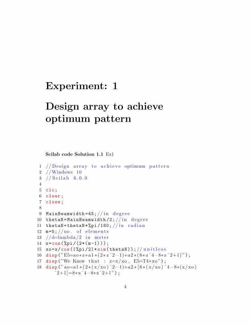
Experiment: 1

Design array to achieveoptimum pattern

Scilab code Solution 1.1 Ex1

1 // Des ign a r r ay to a c h i e v e optimum pa t t e r n2 //Windows 103 // S c i l a b 6 . 0 . 04

5 clc;

6 clear;

7 close;

8

9 MainBeamwidth =45; // i n d eg r e e10 thetaN=MainBeamwidth /2; // i n deg r e e11 thetaN=thetaN*%pi /180; // i n r ad i an12 m=5; //no . o f e l emen t s13 //d=lambda /2 in meter14 x=cos(%pi /(2*(m-1)));

15 xo=x/cos((%pi/2)*sin(thetaN));// u n i t l e s s16 disp(”E5=ao ∗ z+a1 ∗ (2∗ z ˆ2−1)+a2 ∗ (8∗ z ˆ4−8∗ z ˆ2+1)”);17 disp(”We Know tha t : z=x/xo , E5=T4∗xo”);18 disp(” ao=a1 ∗ ( 2∗ ( x/xo ) ˆ2−1)+a2 ∗ [ 8 ∗ ( x/xo ) ˆ4−8∗(x/xo )

ˆ2+1]=8∗xˆ4−8∗xˆ2+1”);

4

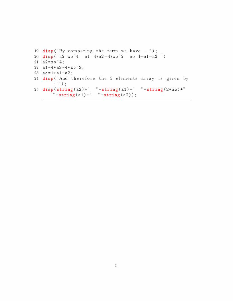
19 disp(”By comparing the term we have : ”);20 disp(” a2=xo ˆ4 a1=4∗a2−4∗xo ˆ2 ao=1+a1−a2 ”)21 a2=xo^4;

22 a1=4*a2 -4*xo^2;

23 ao=1+a1-a2;

24 disp(”And t h e r e f o r e the 5 e l ement s a r r ay i s g i v en by: ”);

25 disp(string(a2)+” ”+string(a1)+” ”+string (2*ao)+””+string(a1)+” ”+string(a2));

5

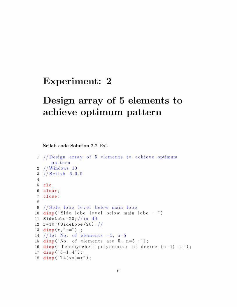
Experiment: 2

Design array of 5 elements toachieve optimum pattern


1 // Des ign a r r ay o f 5 e l emen t s to a c h i e v e optimumpa t t e r n

2 //Windows 103 // S c i l a b 6 . 0 . 04

5 clc;

6 clear;

7 close;

8

9 // S ide l ob e l e v e l below main l ob e10 disp(” S ide l o b e l e v e l below main l ob e : ”)11 SideLobe =20; // i n dB12 r=10^( SideLobe /20);//13 disp(r,” r=”) ;

14 // l e t No . o f e l emen t s =5 , n=515 disp(”No . o f e l emen t s a r e 5 , n=5 : ”);16 disp(” Tcheby s ch e f f p o l ynom ia l s o f d e g r e e ( n−1) i s ”);17 disp(”5−1=4”);18 disp(”T4( xo )=r ”);

6

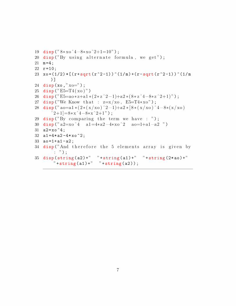
19 disp(” 8∗ xoˆ4−8∗xoˆ2+1=10”);20 disp(”By u s i n g a l t e r n a t e formula , we ge t ”);21 m=4;

22 r=10;

23 xo =(1/2) *[(r+sqrt(r^2-1))^(1/m)+(r-sqrt(r^2-1))^(1/m

)]

24 disp(xo,”xo=”);25 disp(”E5=T4( xo ) ”)26 disp(”E5=ao ∗ z+a1 ∗ (2∗ z ˆ2−1)+a2 ∗ (8∗ z ˆ4−8∗ z ˆ2+1)”);27 disp(”We Know tha t : z=x/xo , E5=T4∗xo”);28 disp(” ao=a1 ∗ ( 2∗ ( x/xo ) ˆ2−1)+a2 ∗ [ 8 ∗ ( x/xo ) ˆ4−8∗(x/xo )

ˆ2+1]=8∗xˆ4−8∗xˆ2+1”);29 disp(”By comparing the term we have : ”);30 disp(” a2=xo ˆ4 a1=4∗a2−4∗xo ˆ2 ao=1+a1−a2 ”)31 a2=xo^4;

32 a1=4*a2 -4*xo^2;

33 ao=1+a1-a2;

34 disp(”And t h e r e f o r e the 5 e l ement s a r r ay i s g i v en by: ”);

35 disp(string(a2)+” ”+string(a1)+” ”+string (2*ao)+””+string(a1)+” ”+string(a2));

7

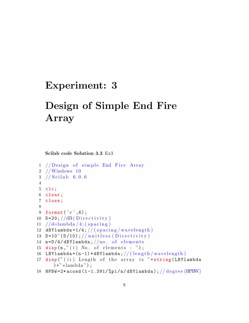
Experiment: 3

Design of Simple End FireArray


1 // Des ign o f s imp l e End F i r e Array2 //Windows 103 // S c i l a b 6 . 0 . 04

5 clc;

6 clear;

7 close;

8

9 format( ’ v ’ ,6);10 D=20; //dB( D i r e c t i v i t y )11 //d=lambda / 4 ; ( s p a c i n g )12 dBYlambda =1/4; // ( s pa c i n g / wave l ength )13 D=10^(D/10);// u n i t l e s s ( D i r e c t i v i t y )14 n=D/4/ dBYlambda;//no . o f e l emen t s15 disp(n,” ( i ) No . o f e l emen t s : ”);16 LBYlambda =(n-1)*dBYlambda;// ( l e n g t h / wave l ength )17 disp(” ( i i ) Length o f the a r r ay i s ”+string(LBYlambda

)+”∗ lambda”);18 HPBW =2* acosd (1 -1.391/ %pi/n/dBYlambda);// deg r e e (HPBW)

8

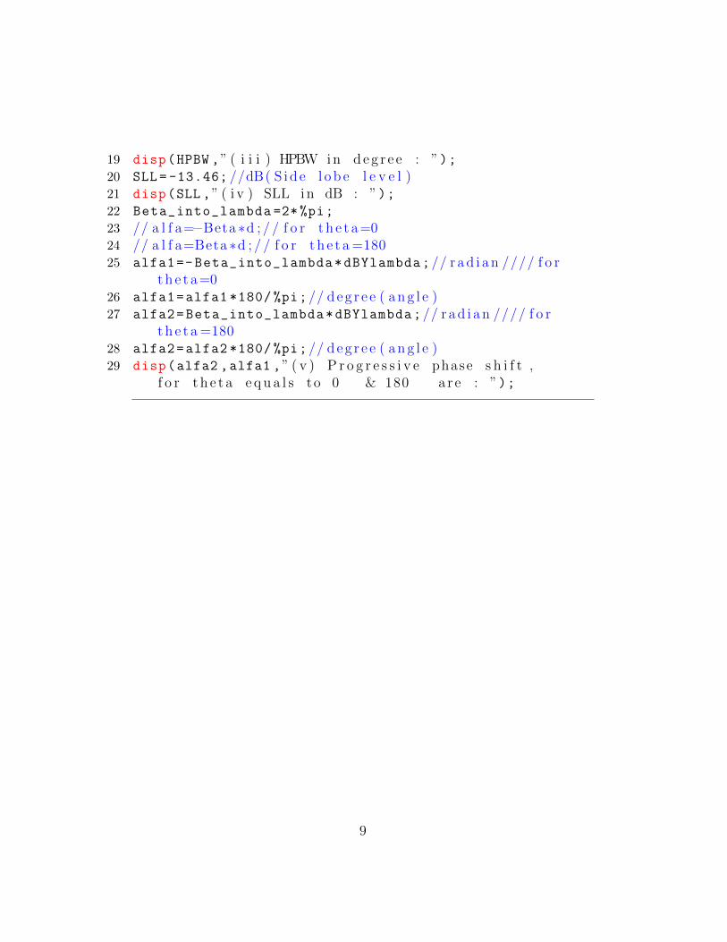
19 disp(HPBW ,” ( i i i ) HPBW in deg r e e : ”);20 SLL = -13.46; //dB( S ide l o b e l e v e l )21 disp(SLL ,” ( i v ) SLL in dB : ”);22 Beta_into_lambda =2* %pi;

23 // a l f a=−Beta ∗d ; / / f o r t h e t a=024 // a l f a=Beta ∗d ; / / f o r t h e t a =18025 alfa1=-Beta_into_lambda*dBYlambda;// r ad i an //// f o r

t h e t a=026 alfa1=alfa1 *180/ %pi;// deg r e e ( ang l e )27 alfa2=Beta_into_lambda*dBYlambda;// r ad i an //// f o r

t h e t a =18028 alfa2=alfa2 *180/ %pi;// deg r e e ( ang l e )29 disp(alfa2 ,alfa1 ,” ( v ) P r o g r e s s i v e phase s h i f t ,

f o r t h e t a e qu a l s to 0 & 180 a r e : ”);

9

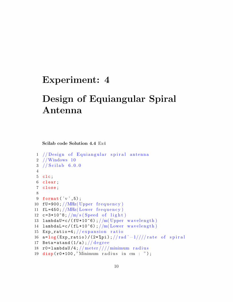
Experiment: 4

Design of Equiangular SpiralAntenna


1 // Des ign o f Equ iangu la r s p i r a l antenna2 //Windows 103 // S c i l a b 6 . 0 . 04

5 clc;

6 clear;

7 close;

8

9 format( ’ v ’ ,5);10 fU=900; //MHz( Upper f r e qu en cy )11 fL=450; //MHz( Lower f r e qu en cy )12 c=3*10^8; //m/ s ( Speed o f l i g h t )13 lambdaU=c/(fU *10^6);//m( Upper wave l ength )14 lambdaL=c/(fL *10^6);//m( Lower wave l ength )15 Exp_ratio =4; // expans i on r a t i o16 a=log(Exp_ratio)/(2* %pi);// rad ˆ−1//// r a t e o f s p i r a l17 Beta=atand (1/a);// deg r e e18 r0=lambdaU /4; //meter ////minimum r ad i u s19 disp(r0*100,”Minimum r ad i u s i n cm : ”);

10

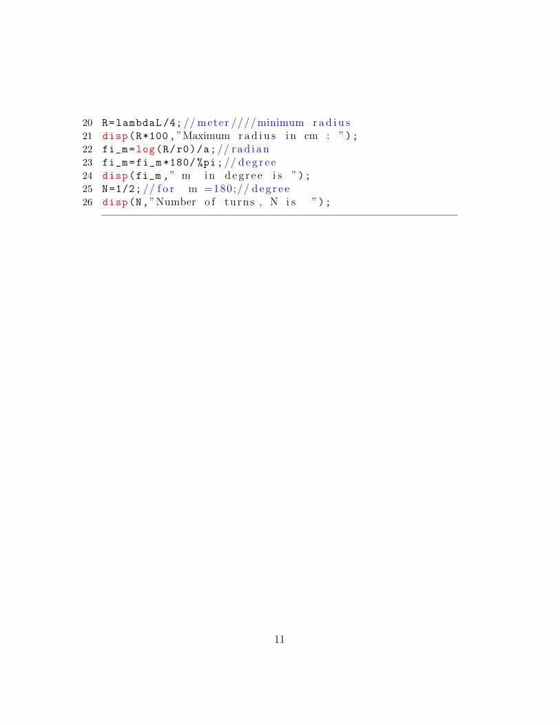
20 R=lambdaL /4; //meter ////minimum r ad i u s21 disp(R*100,”Maximum r ad i u s i n cm : ”);22 fi_m=log(R/r0)/a;// r ad i an23 fi_m=fi_m *180/ %pi;// deg r e e24 disp(fi_m ,” m in deg r e e i s ”);25 N=1/2; // f o r m =180;// d eg r e e26 disp(N,”Number o f turns , N i s ”);

11

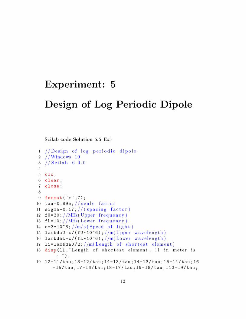
Experiment: 5

Design of Log Periodic Dipole


1 // Des ign o f l o g p e r i o d i c d i p o l e2 //Windows 103 // S c i l a b 6 . 0 . 04

5 clc;

6 clear;

7 close;

8

9 format( ’ v ’ ,7);10 tau =0.895; // s c a l e f a c t o r11 sigma =0.17; // ( s pa c i n g f a c t o r )12 fU=30; //MHz( Upper f r e qu en cy )13 fL=10; //MHz( Lower f r e qu en cy )14 c=3*10^8; //m/ s ( Speed o f l i g h t )15 lambdaU=c/(fU *10^6);//m( Upper wave l ength )16 lambdaL=c/(fL *10^6);//m( Lower wave l ength )17 l1=lambdaU /2; //m( Length o f s h o r t e s t e l ement )18 disp(l1,”Length o f s h o r t e s t e lement , l 1 i n meter i s

: ”);19 l2=l1/tau;l3=l2/tau;l4=l3/tau;l4=l3/tau;l5=l4/tau;l6

=l5/tau;l7=l6/tau;l8=l7/tau;l9=l8/tau;l10=l9/tau;

12

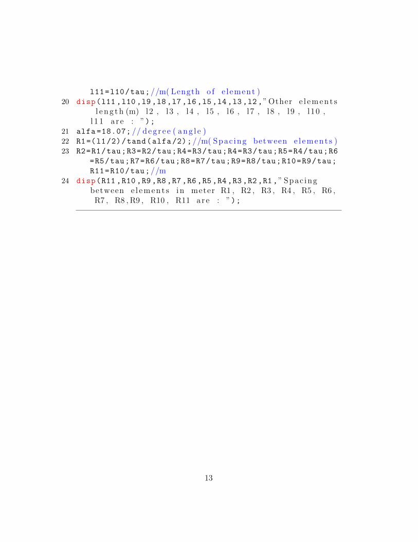
l11=l10/tau;//m( Length o f e l ement )20 disp(l11 ,l10 ,l9 ,l8,l7,l6 ,l5 ,l4,l3,l2 ,”Other e l emen t s

l e n g t h (m) l2 , l3 , l4 , l5 , l 6 , l7 , l 8 , l9 , l 10 ,l 1 1 a r e : ”);

21 alfa =18.07; // deg r e e ( ang l e )22 R1=(l1/2)/tand(alfa /2);//m( Spac ing between e l emen t s )23 R2=R1/tau;R3=R2/tau;R4=R3/tau;R4=R3/tau;R5=R4/tau;R6

=R5/tau;R7=R6/tau;R8=R7/tau;R9=R8/tau;R10=R9/tau;

R11=R10/tau;//m24 disp(R11 ,R10 ,R9 ,R8,R7,R6 ,R5 ,R4,R3,R2 ,R1,” Spac ing

between e l ement s i n meter R1 , R2 , R3 , R4 , R5 , R6 ,R7 , R8 , R9 , R10 , R11 a r e : ”);

13

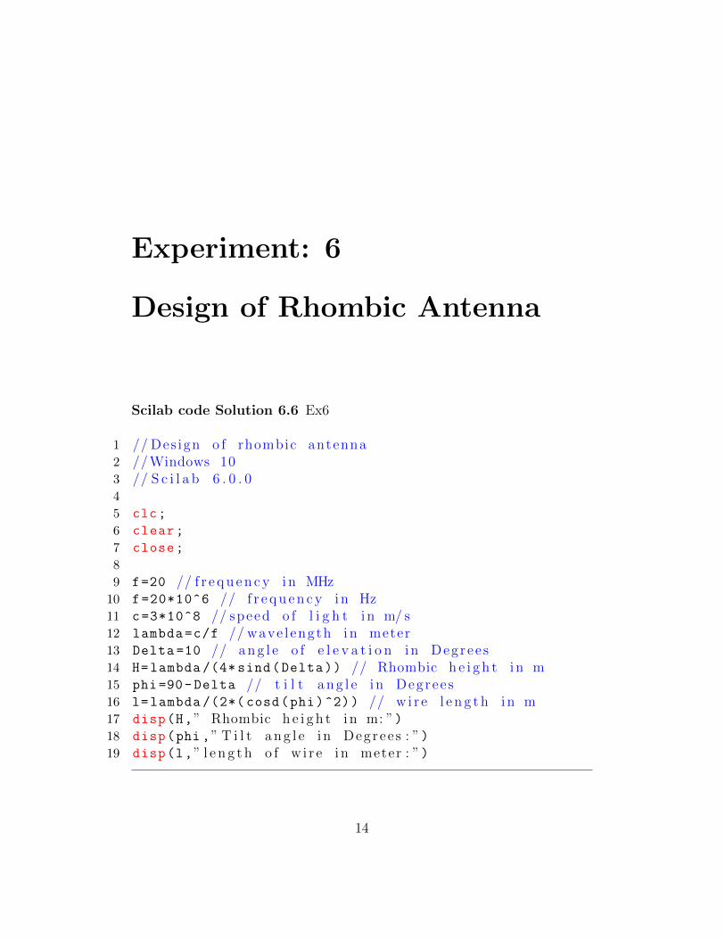
Experiment: 6

Design of Rhombic Antenna


1 // Des ign o f rhombic antenna2 //Windows 103 // S c i l a b 6 . 0 . 04

5 clc;

6 clear;

7 close;

8

9 f=20 // f r e qu en cy i n MHz10 f=20*10^6 // f r e qu en cy in Hz11 c=3*10^8 // speed o f l i g h t i n m/ s12 lambda=c/f // wave l ength i n meter13 Delta =10 // ang l e o f e l e v a t i o n i n Degree s14 H=lambda /(4* sind(Delta)) // Rhombic h e i g h t i n m15 phi=90-Delta // t i l t ang l e i n Degree s16 l=lambda /(2*( cosd(phi)^2)) // w i r e l e n g t h i n m17 disp(H,” Rhombic h e i g h t i n m: ”)18 disp(phi ,” T i l t ang l e i n Degree s : ”)19 disp(l,” l e n g t h o f w i r e i n meter : ”)

14

Experiment: 7

Design of 3 element of YagiUda Antenna


1 // Des ign o f 3 e l ement yag i uda antenna2 //Windows 103 // S c i l a b 6 . 0 . 04

5 clc;

6 clear;

7 close;

8

9 f_MHz =172 // f r e qu en cy in MHz10 c=3*10^8 // speed o f l i g h t i n m/ s11 lambda=c/f_MHz // wave l ength i n m12 La=478/ f_MHz // l e n g t h o f d r i v en e l ement i n f e e t13 Lr=492/ f_MHz // l e n g t h o f r e f l e c t o r i n f e e t14 Ld =461.5/ f_MHz // l e n g t h o f d i r e c t o r i n f e e t15 S=142/ f_MHz // e l ement s pa c i n g i n f e e t16 disp(La,” l e n g t h o f d r i v en e l ement i n f e e t : ”)17 disp(Lr,” l e n g t h o f r e f l e c t o r i n f e e t : ”)18 disp(Ld,” l e n g t h o f d i r e c t o r i n f e e t : ”)19 disp(S,” e l ement s pa c i n g i n f e e t : ”)

15

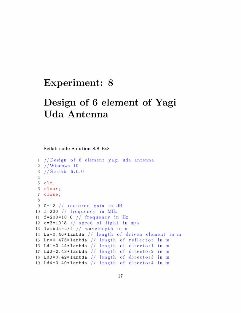
Experiment: 8

Design of 6 element of YagiUda Antenna


1 // Des ign o f 6 e l ement yag i uda antenna2 //Windows 103 // S c i l a b 6 . 0 . 04

5 clc;

6 clear;

7 close;

8

9 G=12 // r e q u i r e d ga in i n dB10 f=200 // f r e qu en cy in MHz11 f=200*10^6 // f r e qu en cy in Hz12 c=3*10^8 // speed o f l i g h t i n m/ s13 lambda=c/f // wave l ength i n m14 La =0.46* lambda // l e n g t h o f d r i v en e l ement i n m15 Lr =0.475* lambda // l e n g t h o f r e f l e c t o r i n m16 Ld1 =0.44* lambda // l e n g t h o f d i r e c t o r 1 i n m17 Ld2 =0.43* lambda // l e n g t h o f d i r e c t o r 2 i n m18 Ld3 =0.42* lambda // l e n g t h o f d i r e c t o r 3 i n m19 Ld4 =0.40* lambda // l e n g t h o f d i r e c t o r 4 i n m

17

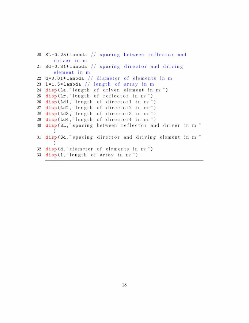
20 SL =0.25* lambda // spa c i n g between r e f l e c t o r andd r i v e r i n m

21 Sd =0.31* lambda // spa c i n g d i r e c t o r and d r i v i n ge l ement i n m

22 d=0.01* lambda // d iamete r o f e l emen t s i n m23 l=1.5* lambda // l e n g t h o f a r r ay i n m24 disp(La,” l e n g t h o f d r i v en e l ement i n m: ”)25 disp(Lr,” l e n g t h o f r e f l e c t o r i n m: ”)26 disp(Ld1 ,” l e n g t h o f d i r e c t o r 1 i n m: ”)27 disp(Ld2 ,” l e n g t h o f d i r e c t o r 2 i n m: ”)28 disp(Ld3 ,” l e n g t h o f d i r e c t o r 3 i n m: ”)29 disp(Ld4 ,” l e n g t h o f d i r e c t o r 4 i n m: ”)30 disp(SL,” spa c i n g between r e f l e c t o r and d r i v e r i n m: ”

)

31 disp(Sd,” spa c i n g d i r e c t o r and d r i v i n g e l ement i n m: ”)

32 disp(d,” d iamete r o f e l emen t s i n m: ”)33 disp(l,” l e n g t h o f a r r ay i n m: ”)

18

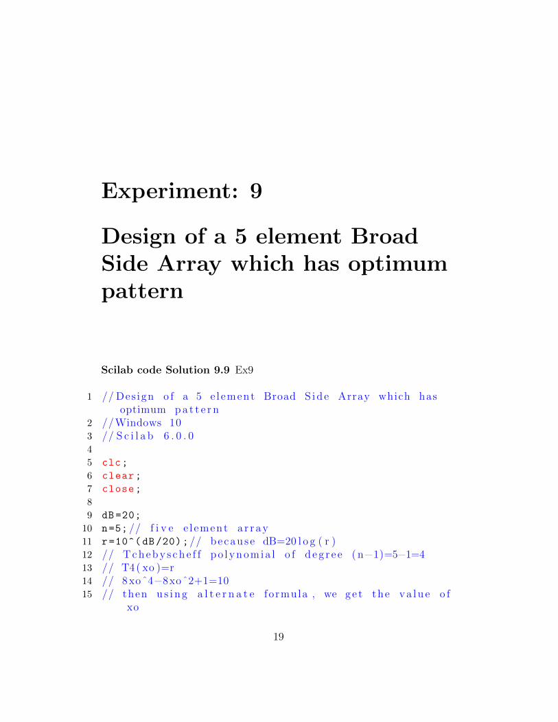
Experiment: 9

Design of a 5 element BroadSide Array which has optimumpattern


1 // Des ign o f a 5 e l ement Broad S ide Array which hasoptimum pa t t e r n

2 //Windows 103 // S c i l a b 6 . 0 . 04

5 clc;

6 clear;

7 close;

8

9 dB=20;

10 n=5; // f i v e e l ement a r r ay11 r=10^( dB/20);// because dB=20 l o g ( r )12 // Tcheby s ch e f f po l ynomia l o f d e g r e e ( n−1)=5−1=413 // T4( xo )=r14 // 8xoˆ4−8xoˆ2+1=1015 // then u s i n g a l t e r n a t e formula , we ge t the va lu e o f

xo

19

16 m=4; // deg r e e o f the equa t i on17 a=sqrt(r^2-1);

18 A=(r+a)^(1/m);

19 B=(r-a)^(1/m);

20 xo=.5*(A+B);

21 // E5=aoz+a1 (2 z ˆ2−1)+a2 (8 zˆ4−8z ˆ2+1) , where z=(x/xo )22 // E5=T4( xo )23 // ao ( x/xo )+a1 ( 2 ( x/xo ) ˆ2−1)+a2 ( 8 ( x/xo ) ˆ4−8(x/xo )

ˆ2+1)=8xˆ4−8xˆ2+124 // Now equa t i ng terms , we have25 // a2 ( x/xo ) ˆ4=xˆ426 a2=xo^4;

27 // a1 ∗2( x/xo ) ˆ2−a2 ∗8( x/xo )ˆ2=−8xˆ228 a1=4*a2 -4*xo^2;

29 // ao−a1+a2=130 ao=1+a1-a2;

31 // The r e f o r e the r e l a t i v e ampl i tude o f the a r r ay a r e32 a11=a1/a1;// the r a t i o o f the a1 to a133 a12=a1/a2;// the r a t i o o f the a1 to a234 a02 =2*ao/a2;// the r a t i o o f the 2 ao to a235 printf(”The va lu e o f the parameter r= %d”, r);

36 printf(”\n The va lu e o f the parameter xo= %f”, xo);

37 printf(”\n The va lu e o f the c u r r e n t ampl i tudeparameter 2∗ ao= %f”, 2*ao);

38 printf(”\n The va lu e o f the c u r r e n t ampl i tudeparameter a1= %f”, a1);

39 printf(”\n The va lu e o f the c u r r e n t ampl i tudeparameter a2= %f”, a2);

40 printf(”\n The va lu e o f the r e l a t i v e ampl i tudeparameter a11= %f”, a11);



20

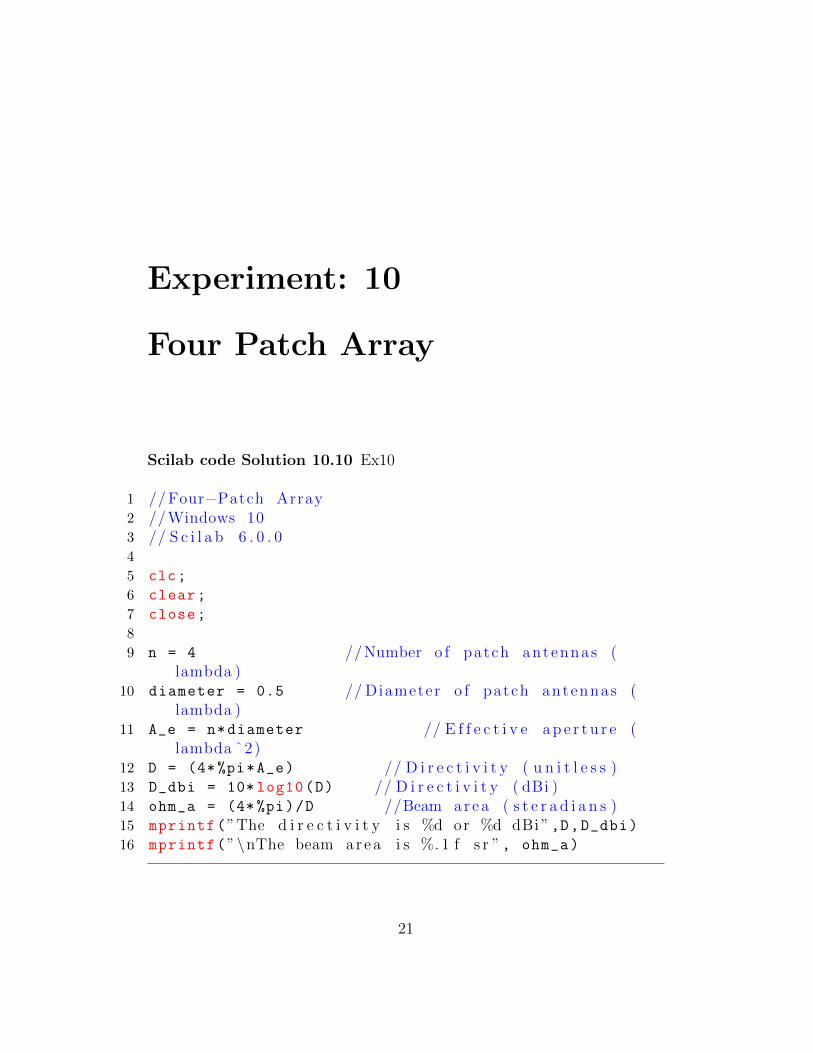
Experiment: 10

Four Patch Array


1 //Four−Patch Array2 //Windows 103 // S c i l a b 6 . 0 . 04

5 clc;

6 clear;

7 close;

8

9 n = 4 //Number o f patch antennas (lambda )

10 diameter = 0.5 // Diameter o f patch antennas (lambda )

11 A_e = n*diameter // E f f e c t i v e ap e r t u r e (lambda ˆ2)

12 D = (4*%pi*A_e) // D i r e c t i v i t y ( u n i t l e s s )13 D_dbi = 10* log10(D) // D i r e c t i v i t y ( dBi )14 ohm_a = (4* %pi)/D //Beam area ( s t e r a d i a n s )15 mprintf(”The d i r e c t i v i t y i s %d or %d dBi ”,D,D_dbi)16 mprintf(”\nThe beam area i s %. 1 f s r ”, ohm_a)

21

Scilab Manual for Antenna Design Lab by Dr Dharmavaram ...

Documents

Transcript of Scilab Manual for Antenna Design Lab by Dr Dharmavaram ...