Schwarzian derivatives and a linearly invariant family in ℂ n
199
Pacific Pacific Pacific Pacific Pacific Pacific Pacific Pacific Pacific Pacific Pacific Pacific Pacific Pacific Pacific Pacific Pacific Pacific Pacific Pacific Pacific Pacific Pacific Pacific Pacific Pacific Pacific Pacific Pacific Pacific Pacific Pacific Pacific Pacific Pacific Pacific Pacific Pacific Pacific Pacific Pacific Pacific Pacific Pacific Pacific Pacific Pacific Pacific Pacific Pacific Pacific Pacific Pacific Pacific Pacific Pacific Pacific Pacific Journal of Journal of Journal of Journal of Journal of Journal of Journal of Journal of Journal of Journal of Journal of Journal of Journal of Journal of Journal of Journal of Journal of Journal of Journal of Journal of Journal of Journal of Journal of Journal of Journal of Journal of Journal of Journal of Journal of Journal of Journal of Journal of Journal of Journal of Journal of Journal of Journal of Journal of Journal of Journal of Journal of Journal of Journal of Journal of Journal of Journal of Journal of Journal of Journal of Journal of Journal of Journal of Journal of Journal of Journal of Journal of Journal of Journal of Mathematics Mathematics Mathematics Mathematics Mathematics Mathematics Mathematics Mathematics Mathematics Mathematics Mathematics Mathematics Mathematics Mathematics Mathematics Mathematics Mathematics Mathematics Mathematics Mathematics Mathematics Mathematics Mathematics Mathematics Mathematics Mathematics Mathematics Mathematics Mathematics Mathematics Mathematics Mathematics Mathematics Mathematics Mathematics Mathematics Mathematics Mathematics Mathematics Mathematics Mathematics Mathematics Mathematics Mathematics Mathematics Mathematics Mathematics Mathematics Mathematics Mathematics Mathematics Mathematics Mathematics Mathematics Mathematics Mathematics Mathematics Mathematics Volume 228 No. 2 December 2006
Transcript of Schwarzian derivatives and a linearly invariant family in ℂ n

PACIFIC JOURNAL OF MATHEMATICS
Volume 228 No. 2 December 2006
PacificJournalofM
athematics
2006Vol.228,N
o.2
PacificPacificPacificPacificPacificPacificPacificPacificPacificPacificPacificPacificPacificPacificPacificPacificPacificPacificPacificPacificPacificPacificPacificPacificPacificPacificPacificPacificPacificPacificPacificPacificPacificPacificPacificPacificPacificPacificPacificPacificPacificPacificPacificPacificPacificPacificPacificPacificPacificPacificPacificPacificPacificPacificPacificPacificPacificPacificJournal ofJournal ofJournal ofJournal ofJournal ofJournal ofJournal ofJournal ofJournal ofJournal ofJournal ofJournal ofJournal ofJournal ofJournal ofJournal ofJournal ofJournal ofJournal ofJournal ofJournal ofJournal ofJournal ofJournal ofJournal ofJournal ofJournal ofJournal ofJournal ofJournal ofJournal ofJournal ofJournal ofJournal ofJournal ofJournal ofJournal ofJournal ofJournal ofJournal ofJournal ofJournal ofJournal ofJournal ofJournal ofJournal ofJournal ofJournal ofJournal ofJournal ofJournal ofJournal ofJournal ofJournal ofJournal ofJournal ofJournal ofJournal ofMathematicsMathematicsMathematicsMathematicsMathematicsMathematicsMathematicsMathematicsMathematicsMathematicsMathematicsMathematicsMathematicsMathematicsMathematicsMathematicsMathematicsMathematicsMathematicsMathematicsMathematicsMathematicsMathematicsMathematicsMathematicsMathematicsMathematicsMathematicsMathematicsMathematicsMathematicsMathematicsMathematicsMathematicsMathematicsMathematicsMathematicsMathematicsMathematicsMathematicsMathematicsMathematicsMathematicsMathematicsMathematicsMathematicsMathematicsMathematicsMathematicsMathematicsMathematicsMathematicsMathematicsMathematicsMathematicsMathematicsMathematicsMathematics
Volume 228 No. 2 December 2006

PACIFIC JOURNAL OF MATHEMATICS
http://www.pjmath.org
Founded in 1951 by
E. F. Beckenbach (1906–1982) F. Wolf (1904–1989)
EDITORS
Vyjayanthi ChariDepartment of Mathematics
University of CaliforniaRiverside, CA 92521-0135
Robert FinnDepartment of Mathematics
Stanford UniversityStanford, CA [email protected]
Kefeng LiuDepartment of Mathematics
University of CaliforniaLos Angeles, CA 90095-1555
V. S. Varadarajan (Managing Editor)Department of Mathematics
University of CaliforniaLos Angeles, CA 90095-1555
Darren LongDepartment of Mathematics
University of CaliforniaSanta Barbara, CA 93106-3080
Jiang-Hua LuDepartment of Mathematics
The University of Hong KongPokfulam Rd., Hong Kong
Sorin PopaDepartment of Mathematics
University of CaliforniaLos Angeles, CA 90095-1555
Jie QingDepartment of Mathematics
University of CaliforniaSanta Cruz, CA 95064
Jonathan RogawskiDepartment of Mathematics
University of CaliforniaLos Angeles, CA 90095-1555
Paulo Ney de Souza, Production Manager Silvio Levy, Senior Production Editor Alexandru Scorpan, Production Editor
SUPPORTING INSTITUTIONS
ACADEMIA SINICA, TAIPEI
CALIFORNIA INST. OF TECHNOLOGY
INST. DE MATEMÁTICA PURA E APLICADA
KEIO UNIVERSITY
MATH. SCIENCES RESEARCH INSTITUTE
NEW MEXICO STATE UNIV.OREGON STATE UNIV.PEKING UNIVERSITY
STANFORD UNIVERSITY
UNIVERSIDAD DE LOS ANDES
UNIV. OF ARIZONA
UNIV. OF BRITISH COLUMBIA
UNIV. OF CALIFORNIA, BERKELEY
UNIV. OF CALIFORNIA, DAVIS
UNIV. OF CALIFORNIA, IRVINE
UNIV. OF CALIFORNIA, LOS ANGELES
UNIV. OF CALIFORNIA, RIVERSIDE
UNIV. OF CALIFORNIA, SAN DIEGO
UNIV. OF CALIF., SANTA BARBARA
UNIV. OF CALIF., SANTA CRUZ
UNIV. OF HAWAII
UNIV. OF MONTANA
UNIV. OF NEVADA, RENO
UNIV. OF OREGON
UNIV. OF SOUTHERN CALIFORNIA
UNIV. OF UTAH
UNIV. OF WASHINGTON
WASHINGTON STATE UNIVERSITY
These supporting institutions contribute to the cost of publication of this Journal, but they are not owners or publishers and have no respon-sibility for its contents or policies.
See inside back cover or www.pjmath.org for submission instructions.
Regular subscription rate for 2006: $425.00 a year (10 issues). Special rate: $212.50 a year to individual members of supporting institutions.Subscriptions, requests for back issues from the last three years and changes of subscribers address should be sent to Pacific Journal ofMathematics, P.O. Box 4163, Berkeley, CA 94704-0163, U.S.A. Prior back issues are obtainable from Periodicals Service Company, 11Main Street, Germantown, NY 12526-5635. The Pacific Journal of Mathematics is indexed by Mathematical Reviews, Zentralblatt MATH,PASCAL CNRS Index, Referativnyi Zhurnal, Current Mathematical Publications and the Science Citation Index.
The Pacific Journal of Mathematics (ISSN 0030-8730) at the University of California, c/o Department of Mathematics, 969 Evans Hall,Berkeley, CA 94720-3840 is published monthly except July and August. Periodical rate postage paid at Berkeley, CA 94704, and additionalmailing offices. POSTMASTER: send address changes to Pacific Journal of Mathematics, P.O. Box 4163, Berkeley, CA 94704-0163.
PUBLISHED BY PACIFIC JOURNAL OF MATHEMATICSat the University of California, Berkeley 94720-3840
A NON-PROFIT CORPORATIONTypeset in LATEX
Copyright ©2007 by Pacific Journal of Mathematics

PACIFIC JOURNAL OF MATHEMATICSVol. 228, No. 2, 2006
SCHWARZIAN DERIVATIVESAND A LINEARLY INVARIANT FAMILY IN Cn
RODRIGO HERNÁNDEZ R.
We use Oda’s definition of the Schwarzian derivative for locally univalentholomorphic maps F in several complex variables to define a Schwarzianderivative operator SF. We use the Bergman metric to define a norm‖SF‖ for this operator, which in the ball is invariant under compositionwith automorphisms. We study the linearly invariant family
Fα = {F : Bn→ Cn
| F(0) = 0, DF(0) = Id, ‖SF‖ ≤ α},
estimating its order and norm order.
1. Introduction
The link between the Schwarzian derivative of a locally univalent holomorphicmap in one complex variable, given by
S f =
(f ′′
f ′
)′
−12
(f ′′
f ′
)2
,
with the univalence of f and distortion problems has been studied extensively;see [Chuaqui and Osgood 1993; Epstein 1986; Kraus 1932; Nehari 1949], forexample. S f vanishes identically if and only if f is a Mobius mapping, and we haveS( f ◦ g)= (S f ◦ g)(g′)2 + Sg. An analytic function f with Schwarzian derivativeS f = 2p has the form f = u/v, where u and v are any linearly independentsolutions of the equation u′′
+ pu = 0. If f is defined in the unit disk D, the norm
‖S f ‖ = sup|z|=1
(1 − |z|2)2|S f (z)|
is invariant under precomposition with automorphisms of the disk.Some analogues of the Schwarzian derivative in several complex variables are
available, but results relating it to the aforementioned problems of univalence and
MSC2000: primary 32A17, 32W50; secondary 32H02, 30C35.Keywords: Several complex varaibles, Schwarzian derivative, Linearly invariant families, Sturm
comparison.
201

202 RODRIGO HERNÁNDEZ R.
distortion are less satisfactory than in one variable [Molzon and Pinney Mortensen1997]. Consider the overdetermined system of partial differential equations
(1-1)∂2u∂zi∂z j
=
n∑k=1
Pki j (z)
∂u∂zk
+ P0i j (z)u, i, j = 1, 2, . . . , n,
where z = (z1, z2, . . . , zn) ∈ Cn . The system is called completely integrable if(1-1) has n + 1 linearly independent solutions. The system (1-1) is said to be incanonical form (see [Yoshida 1976]) if the coefficients satisfy
n∑j=1
P ji j (z)= 0, i = 1, 2, . . . , n.
T. Oda [1974] defined the Schwarzian derivative Ski j of a locally injective holomor-
phic mapping F(z1, z2, . . . , zn)= (w1, w2, . . . , wn) as
Ski j F =
n∑l=1
∂2wl
∂zi∂z j
∂zk
∂wl−
1n + 1
(δk
i∂
∂z j+ δk
j∂
∂zi
)log1,
where i, j, k = 1, 2, . . . , n, 1= det(∂F/∂z), and δki is the Kronecker symbol. For
n > 1 these Schwarzian derivatives satisfy
Ski j F = 0 for all i, j, k = 1, 2, . . . , n
if and only if F(z) is a Mobius transformation, that is, if it has the form
F(z)=
(l1(z)l0(z)
, . . . ,ln(z)l0(z)
),
where li (z) = ai0 + ai1z1 + · · · + ainzn with det(ai j ) 6= 0. For a composition wehave
(1-2) Ski j (G ◦ F)(z)= Sk
i j F(z)+n∑
l,m,r=1
SrlmG(w)
∂wl
∂zi
∂wm
∂z j
∂zk
∂wr, w = F(z).
Thus, precomposition with a Mobius transformation G leads to Ski j (G ◦ F)= Sk
i j F .The coefficients S0
i j F are given by
S0i j F(z)=11/(n+1)
(∂2
∂zi∂z j1−1/(n+1)
−
n∑k=1
∂
∂zk1−1/(n+1)Sk
i j F(z)).
The function u =1−1/n+1 is always a solution of (1-1) with Ski j F = Pk
i j .
Remark 1.1. For n = 1, S111 f = 0 for all locally injective f , but S0
11 f = −12 S f .

SCHWARZIAN DERIVATIVES AND A LINEARLY INVARIANT FAMILY IN Cn 203
Proposition 1.2 [Yoshida 1976]. Let (1-1) be a completely integrable system incanonical form and consider a set u0(z), u1(z), . . . , un(z) of linearly independentsolutions. Then
Pki j (z)= Sk
i j F(z), i, j, k = 1, 2, . . . , n,
where F(z)= (w1(z), . . . , wn(z)) and wi (z)= ui (z)/u0(z).
Remark 1.3. In contrast to the one-dimensional case, when n > 1 the Schwarzianderivatives Sk
i j F are differential operators of order 2. One way to understand thisphenomenon is through a dimensional argument: For n = 1 the Mobius group hasdimension 3, which allows one to choose f (z0), f ′(z0) and f ′′(z0) for a holomor-phic mapping f at a given point z0 arbitrarily. It would therefore be pointless toseek a Mobius-invariant differential operator of order 2. But for n > 1 the numberof parameters involved in the value and all derivatives of order 1 and 2 of a locallybiholomorphic mapping is n2(n + 1)/2 + n2
+ n, which exceeds the dimensionn2
+ 2n of the corresponding Mobius group in Cn . Moreover, since Ski j F = Sk
ji Ffor all k and
n∑j=1
S ji j F = 0,
there are exactly n(n − 1)(n + 2)/2 independent terms Ski j F , which is equal to the
excess mentioned above.
In this paper we employ the Oda Schwarzian derivatives Ski j to propose a Schwar-
zian derivative operator SF . Using the Bergman metric, we will define a norm forSF , which for mappings defined in the ball B turns out to be invariant under thegroup of automorphisms. We then focus on the study of geometric properties ofthe linearly invariant family given by bounded Schwarzian norm. We will appeal tothe relationship with the completely integrable system (1-1) and Sturm comparisontechniques adapted to this special situation.
2. The Schwarzian derivative operator
For � ⊂ Cn open, let F : � → Cn , F(z1, . . . , zn) = (w1, . . . , wn), be a locallyunivalent holomorphic mapping, and set1= det(∂F/∂z). For k = 1, . . . , n, definean n × n matrix
Sk F = (Ski j F), i, j = 1, . . . , n.
Proposition 2.1. Let F be a locally injective holomorphic mapping and let w =
G(z) be a Möbius transformation. Then
Sk(F ◦ G)=
n∑r=1
∂zk
∂wrDG t((Sr F) ◦ G
)DG for k = 1, . . . , n.

204 RODRIGO HERNÁNDEZ R.
Proof. From (1-2) and the Mobius property of G we have
Ski j (F ◦ G)(z)=
n∑l,m,r=1
Srlm F(w)
∂wl
∂zi
∂wm
∂z j
∂zk
∂wr+ Sk
i j G(z)
=
n∑r=1
∂zk
∂wr
n∑m,l=1
∂wl
∂ziSr
lm F(w)∂wm
∂z j+ Sk
i j G(z)
=
n∑r=1
∂zk
∂wr
n∑m,l=1
∂wl
∂ziSr
lm F(w)∂wm
∂z j.
The proposition follows after rewriting this in terms of matrices. �
Definition 2.2. The Schwarzian derivative operator is the operator SF(z) : Tz�→
TF(z)� given by
SF(z)(Ev)=(Ev t S1 F(z)Ev, Ev t S2 F(z)Ev, . . . , Ev t Sn F(z)Ev
),
where Ev ∈ Tz�.
Recall that the Bergman metric on Bn is the hermitian product defined by
(2-1) gi j (z)=n + 1
(1 − |z|2)2((1 − |z|2)δi j + zi z j
).
Any automorphism of the ball is an isometry of the Bergman metric.We define the norm of the Schwarzian derivative operator by
‖SF(z)‖ = sup‖Ev‖=1
‖SF(z)(Ev )‖,
where ‖Ev‖ =(∑
gi jvi v j)1/2 is the Bergman norm of Ev ∈ TzBn .
A routine calculation using the fact that u0 =1−1/n+1 is a solution of (1-1) withPk
i j = Ski j F allows one to rewrite the Schwarzian derivative operator as
SF(z)(Ev, Ev)= (DF(z))−1 D2 F(z)(Ev, Ev)−2
n + 1
(11
n∑j=1
1 j (z) v j
)Ev,
or yet
(2-2) SF(z)(Ev, Ev)= (DF(z))−1 D2 F(z)(Ev, Ev)+ 211/n+1 (∇u0 · Ev) Ev,
where 1 j =∑n
k=1(−1) j−1 δ jk and δ jk is the determinant of DF(z) with the k-thcolumn replaced by the column(
∂2 f1
∂z j∂zk, . . . ,
∂2 fn
∂z j∂zk
)tr
(z).

SCHWARZIAN DERIVATIVES AND A LINEARLY INVARIANT FAMILY IN Cn 205
The operator (DF(z))−1 D2 F(z)(z, ·) was considered by Pfaltzgraff [1974] in hisgeneralization of the Becker criterion.
Theorem 2.3. Let F : Bn→ Cn be a locally injective holomorphic mapping and
let σ be an automorphism of Bn . Then∥∥S(F ◦ σ)(z)∥∥ =
∥∥SF(σ (z))∥∥.
Proof. We know that
Sk(F ◦ σ)=
n∑l=1
∂zk
∂wl(Dσ)t Sl F ◦ σ(Dσ)
=
(∂zk
∂w1, . . . ,
∂zk
∂wn
) (Dσ)t S1 F ◦ σ(Dσ)
...
(Dσ)t Sn F ◦ σ(Dσ)
.
Hence
(SF◦σ)(z)(Ev)= Dσ−1
Evt(Dσ)t S1 F(σ (z))(Dσ)Ev...
Evt(Dσ)t Sn F(σ (z))(Dσ)Ev
= Dσ−1
Eut S1 F(σ (z))Eu...
Eut Sn F(σ (z))Eu
,where Eu = Dσ(z)(Ev). Then
‖S(F ◦ σ)(z)(Ev)‖ = ‖DGσ−1SF(σ (z))(Eu)‖ = ‖SF(σ (z))(Eu)‖,
and since σ is a isometry in the Bergman metric, the theorem follows after takingsupremum over all unit vectors Ev. �
The definition of norm for the Schwarzian operator can be given using any her-mitian metric or even a Finsler metric. Since in ball the Bergman metric coincidesup to constant multiples with the Kobayashi or the Caratheodory metric, the re-sulting norm for SF is the same. This will certainly not be the case on arbitrarydomains. Theorem 2.3 will also fail on arbitrary domains because it requires theautomorphisms to be Mobius.
3. The family Fα
Definition 3.1. Consider the family
L S = {F : Bn→ Cn
| F(0)= 0, DF(0)= Id}
of normalized locally biholomorphic mappings on the ball Bn , and the Koebe trans-formations 3σ (F) of the ball, given by
3σ (F)(z)=(Dσ(0)
)−1(DF(σ (0)))−1(F(σ (z))− F(σ (0))
)
206 RODRIGO HERNÁNDEZ R.
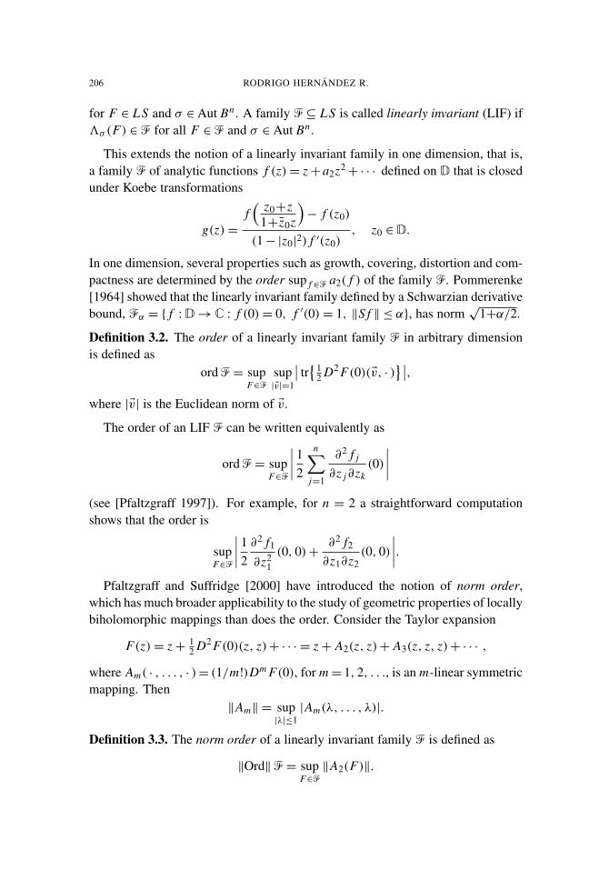
for F ∈ L S and σ ∈ Aut Bn . A family F ⊆ L S is called linearly invariant (LIF) if3σ (F) ∈ F for all F ∈ F and σ ∈ Aut Bn .
This extends the notion of a linearly invariant family in one dimension, that is,a family F of analytic functions f (z)= z +a2z2
+· · · defined on D that is closedunder Koebe transformations
g(z)=
f( z0+z
1+z0z
)− f (z0)
(1 − |z0|2) f ′(z0), z0 ∈ D.
In one dimension, several properties such as growth, covering, distortion and com-pactness are determined by the order sup f ∈F a2( f ) of the family F. Pommerenke[1964] showed that the linearly invariant family defined by a Schwarzian derivativebound, Fα = { f : D → C : f (0)= 0, f ′(0)= 1, ‖S f ‖ ≤ α}, has norm
√1+α/2.
Definition 3.2. The order of a linearly invariant family F in arbitrary dimensionis defined as
ord F = supF∈F
sup|Ev|=1
∣∣ tr{1
2 D2 F(0)(Ev, · )}∣∣,
where |Ev| is the Euclidean norm of Ev.
The order of an LIF F can be written equivalently as
ord F = supF∈F
∣∣∣∣ 12
n∑j=1
∂2 f j
∂z j∂zk(0)
∣∣∣∣(see [Pfaltzgraff 1997]). For example, for n = 2 a straightforward computationshows that the order is
supF∈F
∣∣∣∣ 12∂2 f1
∂z21(0, 0)+
∂2 f2
∂z1∂z2(0, 0)
∣∣∣∣.Pfaltzgraff and Suffridge [2000] have introduced the notion of norm order,
which has much broader applicability to the study of geometric properties of locallybiholomorphic mappings than does the order. Consider the Taylor expansion
F(z)= z +12 D2 F(0)(z, z)+ · · · = z + A2(z, z)+ A3(z, z, z)+ · · · ,
where Am( · , . . . , · )= (1/m!)Dm F(0), for m = 1, 2, . . ., is an m-linear symmetricmapping. Then
‖Am‖ = sup|λ|≤1
|Am(λ, . . . , λ)|.
Definition 3.3. The norm order of a linearly invariant family F is defined as
‖Ord‖ F = supF∈F
‖A2(F)‖.

SCHWARZIAN DERIVATIVES AND A LINEARLY INVARIANT FAMILY IN Cn 207
We define
Fα = {F : Bn→ Cn
| F(0)= 0, DF(0)= Id, ‖SF(z)‖ ≤ α}.
By Theorem 2.3, this is an LIF.
Remark 3.4. The task of calculating the exact value of the norm of SF is, ingeneral, not easy, especially because the Bergman and the Euclidean metrics arenot conformal. For example, define a locally univalent holomorphic mapping inthe ball Bn by Fδ = ( f (z1), zg(z1)), where z = (0, z2, . . . , zn),
g(z1)=1
1−z1and f (z1)=
12δ
((1+z11−z1
)δ− 1
).
For n = 2 a direct calculation shows that
S1 Fδ(z)=
2(δ−1)3(1−z2
1)0
0 0
, S2 Fδ(z)=
2z2(1−δ)
(1−z1)2(1+z1)−
2(δ−1)3(1−z2
1)
−2(δ−1)3(1−z2
1)0
.
ThenSFδ(z)(Ev)=
2(δ−1)3(1−z2
1)
(v2
1,−3z21−z1
v21 − 2v1v2
).
Is easy to see that for z2 = 0 the norm of the Schwarzian operator is
‖SFδ(z)‖ =49(δ− 1), δ > 1,
while for z1 = 0 with a little bit more effort one can show that
‖SFδ(z)‖2
√3(δ− 1), δ > 1.
For arbitrary z ∈ B2 we had to resort to a numerical calculation in AMPL [Foureret al. 2003]. The numerical results show that
‖SFδ(z)‖ ≤2
√3(δ− 1), δ > 1.
On the other hand, Pfaltzgraff and Suffridge [2000] have shown that the norm orderof the linear family generated for Fδ is equal to δ; then for δ =
√3
2 α+ 1 the normof Schwarzian operator of Fδ is α, so that Fδ ∈ Fα and
‖Ord‖ Fα ≥
√3
2α+ 1.
Pfaltzgraff and Suffridge [2000] show that an LIF is normal if and only if thenorm order is bounded. Our aim is to study the family Fα, and we shall prove thatit is normal. We begin with some lemmas.

208 RODRIGO HERNÁNDEZ R.
Lemma 3.5. Let F be a holomorphic mapping in Fα. For z1 = (z1, 0, . . . , 0)∈ Bn ,
(i)∣∣S1
11F(z1)∣∣ ≤
√n+1α
1 − |z1|2,
(ii)∣∣S1
i i F(z1)∣∣ ≤
√n+1α for i = 2, 3, . . . , n,
(iii)∣∣Sk
11F(z1)∣∣ ≤
√n+1α
(1 − |z1|2)3/2for k = 2, 3, . . . , n,
(iv)∣∣Sk
1 jF(z1)∣∣ ≤
2√
n+1α1 − |z1|2
for k, j = 2, 3, . . . , n,
(v)∣∣S1
1 jF(z1)∣∣ ≤
2√
n+1α(1 − |z1|2)1/2
for j = 2, 3, . . . , n,
(vi)∣∣S1
i j F(z1)∣∣ ≤ 2
√n+1α for i 6= j 6= 1,
(vii)∣∣Sk
ii F(z1)∣∣ ≤
√n+1α
(1 − |z1|2)1/2for k, i = 2, 3, . . . , n,
(viii)∣∣Sk
i j F(z1)∣∣ ≤
2√
n+1α(1 − |z1|2)1/2
for k 6= 1, i 6= j 6= 1.
Proof. From (2-1) we have
g11(z1, 0, 0, . . . , 0)=n + 1
(1 − |z1|2)2and gi j (z1, 0, 0, . . . , 0)=
n + 1(1 − |z1|2)
,
for all i, j 6=1. Let Ev be a unit vector in the Bergman metric. Since ‖SF(z1)(Ev )‖≤
α, by setting Ev = (λ, 0, . . . , 0) with λ= (1 − |z1|2)/
√n+1 we obtain
∥∥SF(z1, 0, . . . , 0)(Ev)∥∥2
= (n+1)(
|S111λ
2|2
(1−|z1|2)2+
|S211λ
2|2
1−|z1|2+· · ·+
|Sn11λ
2|2
1−|z1|2
)≤ α2,
whence (i) and (iii) follow. Now consider Ev = (0, 0, . . . , λk, 0, . . . , 0) with λ2k =
(1−|z1|2)/(n+1). As above we have that Ev is a unit vector in the Bergman metric.
Since ‖SF(z1, 0, . . . , 0)(Ev )‖≤α then (ii) and (vii) follow. We obtain (vi) and (vii)analogously, by setting Ev = (0, . . . , λi , 0, . . . , λ j , 0, . . . , 0), where
λi = λ j =1
√2
(1 − |z1|2)1/2
√n+1
.
Finally, (iv) and (v) are established by letting Ev = (λ1, . . . , λ j , 0, . . . , 0), with
λ1 =1
√2
(1 − |z1|2)
√n+1
and λ2 =1
√2
(1 − |z1|2)1/2
√n+1
. �

SCHWARZIAN DERIVATIVES AND A LINEARLY INVARIANT FAMILY IN Cn 209
Lemma 3.6. If F ∈ Fα we have
(3-1)∣∣S0
11 F(z1, 0, . . . , 0)∣∣ ≤
C(n, α)(1 − |z1|2)2
with
C(n, α)=
(4n2
+ 2n − 2 +n+1n−1
)α2
+
(4√
n+1 + 8√
n+1n−1
)α,
and
(3-2)∣∣S0
1 j F(z1, 0, . . . , 0)∣∣ ≤
K (n, α)(1 − |z1|2)3/2
,
withK (n, α)= (16 + 3
√2)
√n+1α+ 6(n2
− 1) α.
Proof. Differentiating (1-1) and using Proposition 1.2 we get
S0i i F(z)= −
1n−1
n∑k=1
∂
∂zkSk
ii F(z)+1
n−1
n∑k=1
n∑j=1
Ski j F(z)S j
ki F(z),
S0i j F(z)=
∂
∂z jSi
i i F(z)−∂
∂ziSi
i j F(z)+n∑
k=1
Skii F(z)Si
k j F(z)−n∑
k=1
Ski j F(z)Si
ki F(z)
for i 6= j . Thus, the coefficients S0i j depend on the Sk
i j . Let F(z1)= F(z1, 0, . . . , 0),so that for all mappings in Fα we have∣∣S0
11 F(z1)∣∣ ≤
1n − 1
n∑k=1
∣∣∣∣ ∂∂zkSk
11 F(z1)
∣∣∣∣ + 1n − 1
n∑k=1
n∑j=1
|Sk1 j F(z1)||S
jk1 F(z1)|,
=1
n − 1
n∑k=1
∣∣∣∣ ∂∂zkSk
11 F(z1)
∣∣∣∣ + 1n − 1
n∑k=2
n∑j=2
|Sk1 j F(z1)||S
jk1 F(z1)|
+1
n − 1
n∑k=2
∣∣Sk11 F(z1)
∣∣ ∣∣S1k1 F(z1)
∣∣ + 1n − 1
∣∣S111 F(z1)
∣∣2.
Therefore Lemma 3.5 implies∣∣S011 F(z1, 0, . . . , 0)
∣∣≤
4(n+1)(n−1)α2
(1 − |z1|2)2+
2(n + 1)α2
(1 − |z1|2)2+
n+1n−1 α
2
(1 − |z1|2)2+
1n − 1
n∑k=1
∣∣∣∣ ∂∂zkSk
11 F(z1)
∣∣∣∣ .Since F ∈ Fα, by taking the unit vector Ev = (λ, 0, . . . , 0) where
|λ|2 =(1 − |z1|
2− |zk |
2)2
(n + 1)(1 − |zk |2)

210 RODRIGO HERNÁNDEZ R.
in the Bergman metric, a straightforward calculation shows that
∣∣Sk11 F(z1, 0, . . . 0, zk, 0, . . . , 0)
∣∣ ≤
√n+1α(1 − |zk |
2)
(1 − |z1|2 − |zk |2)3/2
for k 6= 1.
By considering Sk11 F(z1, 0, . . . 0, zk, 0, . . . , 0) as a holomorphic function of zk we
deduce from Cauchy’s integral formula that∣∣∣∣ ∂∂zkSk
11 F(z1, 0, . . . , 0)∣∣∣∣ ≤
4√
n+1α(1 − |z1|2)2
for k 6= 1.
Similarly, ∣∣∣∣ ∂∂z1S1
11 F(z1, 0, . . . , 0)∣∣∣∣ ≤
8√
n+1α(1 − |z1|2)2
.
Using these two inequalities we conclude that∣∣S011 F(z1, 0, . . . , 0)
∣∣≤(4n2
+ 2n − 2)α2
(1 − |z1|2)2+
n+1n−1 α
2
(1 − |z1|2)2+
4√
n+1α(1 − |z1|2)2
+1
n − 18√
n+1α(1 − |z1|2)2
.
For j 6= 1 we have
∣∣S01 j F(z1)
∣∣ ≤
∣∣∣∣ ∂∂z jS1
11 F(z1)
∣∣∣∣ + ∣∣∣∣ ∂∂z1S1
1 j F(z1)
∣∣∣∣n∑
k=1
∣∣Sk11 F(z1)
∣∣∣∣S1k j F(z1)
∣∣ + ∣∣Sk1 j F(z1)
∣∣∣∣S1k1 F(z1)
∣∣,The contribution of the last two summands is at most
2α(n + 1)(n − 1)(1 − |z1|2)3/2
+4α(n + 1)(n − 1)(1 − |z1|2)3/2
,
while the first two can be estimated using Cauchy’s integral formula:∣∣∣∣ ∂∂z1S1
1 j F(z1)
∣∣∣∣ ≤16
√n+1α
(1 − |z1|2)3/2,
∣∣∣∣ ∂∂z jS1
11 F(z1)
∣∣∣∣ ≤3√
2√
n+1α(1 − |z1|2)3/2
.
Putting it all together,
∣∣S01 j F(z1)
∣∣ ≤6α(n2
− 1)(1 − |z1|2)3/2
+16
√n+1α
(1 − |z1|2)3/2+
3√
2√
n+1α(1 − |z1|2)3/2
,
proving the theorem. �

SCHWARZIAN DERIVATIVES AND A LINEARLY INVARIANT FAMILY IN Cn 211
It is clear that if u(z1, . . . , zn) is a solution of the system (1-1) then u(z1) =
u(z1, 0, . . . , 0) satisfies
u′′= S1
11u′+
n∑j=2
S j11φ j + S0
11u and φ′
k = S11ku′
+
n∑j=2
S j1kφ j + S0
1ku
for k = 2, 3, . . . , n, where φk(z)= ∂u/∂zk .
Lemma 3.7. Let P = P(x), Q = Q(x) be continuous functions defined on [0, 1),with Q(x)≥ 0. Let u = u(x), v = v(x) satisfy
u′′+ Pu + Q ≥ 0, u(0)= 1, u′(0)= 0,
v′′+ Pv+ Q = 0, v(0)= 1, v′(0)= 0.
Then u ≥ v on [0, x0), where x0 is the first zero of v.
Proof. For ε > 0, let uε = u + εy, where y is solution of y′′+ Py = 0, y(0) = 0,
y′(0)= 1. Thenw= u′εv−v
′uε satisfiesw(0)= ε>0 andw′≥ Q(uε−v). Because
of the initial conditions of uε and v, the function w has w′> 0 on an interval (0, r).But then w > 0 (in fact, ≥ ε) on that interval, which implies that u′
ε/uε > v′/v if
v > 0, thus uε > v. It follows from this argument that the first zero of uε cannotoccur before the first zero of v, and the lemma obtains after letting ε→ 0. �
Lemma 3.8. Let u be a solution of the system (1-1) satisfying u(0, . . . , 0) = 1,∇u(0, . . . , 0)= 0 and Pk
i j = Ski j F with F ∈ Fα. Then there exists r > 0 and δ > 0
such that |u|> δ > 0 for |z|< r .
Proof. Let z0 ∈ Bn be a zero of u of smallest euclidean norm, that is, u(z0) =
0 and u(z) 6= 0 for |z| < |z0| = r0. Since Fα is a linearly invariant family wecan assume that z0 = (x0, 0, . . . , 0). We shall study the zeros of the functionu(x) = u(x, 0, . . . , 0) in 0 < x < 1. If F(x) = F(x, 0, . . . , 0), then u(x) andϕk(x)= (∂u/∂zk)(x, 0, . . . , 0) satisfies the system
(3-3)
u′′(x)=
n∑k=1
Sk11 F(x)ϕk(x)+ S0
11 F(x)u(x),
ϕ′
j (x)=
n∑k=1
Sk1 j F(x)ϕk(x)+ S0
1 j F(x)u(x), j = 2, . . . , n,
with initial conditions u(0) = 1 and ϕk(0) = 0. With θ = (ϕ1, . . . , ϕn, u), we canrewrite the system (3-3) as
(3-4) θ ′(x)= A(x) · θ(x), θ(0)= (0, 0, . . . , 1),
where A(x) is the (n+1)×(n+1)matrix of coefficients of the system. Let f 2(x)=‖θ(x)‖2 be the square of the Euclidean norm of θ(x). Using · to represent the

212 RODRIGO HERNÁNDEZ R.
Euclidean inner product of vectors in Cn+1= R2n+2, we have
f ′(x) f (x)= θ ′(x) · θ(x)= A(x)θ(x) · θ(x);
therefore f ′(x) f (x)≤ ‖A(x)‖‖θ(x)‖2= ‖A(x)‖ f 2(x), so
f ′(x)f (x)
≤ ‖A(x)‖.
Since f (0) = 1 we conclude that f (x) ≤ e∫ x
0 p(s) ds , where p(s) stands for thebounds obtained for ‖A(s)‖ from Lemmas 3.5 and 3.6. In particular, we have
|u′(x)| ≤ e∫ x
0 p(s) ds, |ϕk(x)| ≤ e∫ x
0 p(s) ds for k = 2, . . . , n.
Setting U 2(x) = |u(x)|2, we obtain 2UU ′= 2 Re(u′u), hence (U ′)2 + UU ′′
=
Re(u′′u)+ |u′|2, U (0)= 1, U ′(0)= 0. Since |U ′
| ≤ |u′|, we have
UU ′′≥ Re(u′′u).
Using this in (3-3) we get
UU ′′≥ Re{S0
11 F(x)}U 2+ Re
(q(x)u
),
where q(x)= S111 F(x)u′(x)+
∑nk=2 Sk
11 F(x)ϕk(x); hence
U ′′≥ −
∣∣S011 F(x)
∣∣ U − |q(x)|,
or U ′′+ P(x)U +Q(x)≥ 0, where P and Q are the bounds obtained from Lemmas
3.5 and 3.6 for |S011 F(x, 0, . . . , 0)| and |q(x)|, respectively. It follows now from
Lemma 3.7 that U ≥ v on [0, x0), where x0 is the first zero of v, which is solutionof v′′
+ Pv+ Q = 0, v(0)= 1, v′(0)= 0. The lemma follows taking r < x0. �
Remark 3.9. It is clear that we need to estimate the first zero of the functionv. In fact, we proved that |S0
11 F(x, 0, . . . , 0)| ≤ c(n, α)(1 − x2)−2= P , where
c = c(n, α) is a constant. Also one can obtain from Lemmas 3.5 and 3.6 a boundof |q(x)| of the form
|q(x)| ≤M
(1 − x2)δ+1 = Q,
where M =√
n(n+1) α and δ also depends on n and α. Then v is a solution of
v′′+
c(1 − x2)2
v+M
(1 − x2)δ+1 = 0, v(0)= 1, v′(0)= 0.
In general, for given constants c,M, δ, one will be able to estimate the first zeroof v only numerically. However, if δ < 1 then by comparison, it follows that thefirst zero of v does not occur before the first zero of the solution w of
w′′+
c(1 − x2)2
w+M
(1 − x2)2= 0, w(0)= 1, w′(0)= 0,

SCHWARZIAN DERIVATIVES AND A LINEARLY INVARIANT FAMILY IN Cn 213
and this can be determined analytically. Indeed we have w = (M + 1) yc − M ,where yc is the solution of
y′′+
c(1 − x2)2
y = 0, y(0)= 1, y′(0)= 0,
which can be found, for example, in [Kamke 1930]. Thus the first zero of w is thesolution of the (transcendental) equation yc(x)= M/(1+M).
Theorem 3.10. Fix α <∞. The family
Fα ={
F : Bn→ Cn
| F(0)= 0, DF(0)= Id, ‖SF(z)‖ ≤ α}
is a normal family.
Proof. Let F ∈ Fα. From Proposition 1.2 we have
(3-5) F =
(u1
u0, . . . ,
un
u0
)= ( f1, . . . , fn),
where ui and u0 = 1−1/n+1 are linearly independent solutions of (1-1) such that(∂ui/∂zk)(0)= 0 for all k 6= i and (∂ui/∂zi )(0)= 1 for i = 1, . . . , n; see [Yoshida1984]. From equation (2-2) we deduce that
D2 F(0)(Ev, Ev)= SF(0)(Ev, Ev)+ 2 (∇u0(0) · Ev) Ev.
Hence |A2(z)| will be uniformly bounded for F in the family Fα provided that thesame holds for the derivatives
∣∣(∂u0/∂z j )(0)∣∣ for j = 1, . . . , n. To show the latter,
consider the composition G = T ◦ F with the Mobius transformation given by
T (z)=z
1 + z · a,
where we have introduced the inner product 〈z, w〉 = z1w1 + · · · + znwn . Using(3-5), we get
G(z)=F(z)
1 + 〈F(z), a〉=
( u1
u0 + a1u1 + · · · + anun, . . . ,
un
u0 + a1u1 + · · · + anun
)=
( u1
u0, . . . ,
un
u0
),
where u0 = u0 + a1u1 + · · · + anun and ui = ui for i = 1, . . . , n. Differentiatingand setting ak = (∂u0/∂zk)(0) for k = 1, . . . , n, we obtain ∇(u0)(0) = 0. Thismay introduce a pole of G but away from the origin. The function u0 satisfies thesystem
∂2u0
∂zi∂z j(z)=
n∑k=1
Ski j F(z)
∂ u0
∂zk+ S0
i j F(z)u0(z), u0(0)= 1, ∇u0(0)= 0,

214 RODRIGO HERNÁNDEZ R.
and in view of Lemma 3.8, u0 does not vanish on Br for some r > 0. At the sametime, since satisfies ui (0) = 0 and |∇ui (0)| = 1 for each i = 1, . . . , n, it is easyto see from (1-1) and the bounds in Lemmas 3.5 and 3.6 that the functions ui willbe uniformly bounded on compact subsets. Therefore, the class of mappings Gobtained with this normalization is normal on |z|< r0 with r0< r ; then there existss0 > 0 such that G(Bn
r0)⊃ Bn
s0. Since the image of G := ( f1, . . . , fn) covers a ball
of radius s0 and
F =G
1 − 〈a, f 〉
is holomorphic, we conclude that |a1|2
+ · · · + |an|2
≤ 1/s20 . This shows that
|∇u0(0)| =√
|a1|2 + · · · + |an|2 is uniformly bounded and the theorem follows. �
In analogy to the result of Pommerenke cited on page 206, we have:
Theorem 3.11. ‖Ord‖ Fα ≤
√n+12
α+ λα, where λα =2√
nn + 1
ord Fα.
Proof. Equation (2-2) yields D2 F(0)(Ev, Ev) = SF(0)(Ev, Ev)+ 2 (∇u0(0) · Ev) Ev. Isnot difficult to see that
∂u0
∂zk(0)= −
1n + 1
n∑j=1
∂2 f j
∂z j∂zk(0);
hence, taking the Euclidean norm and the supremum over all unit vectors Ev, weobtain
|A2(F)| ≤
√n+12
‖SF(0)‖ + |∇u0(0)|,
where ‖ · ‖ is the Bergman metric. Therefore
‖Ord‖ Fα ≤
√n+12
α+ λα. �
Nehari [1949] proved that if f belongs to the univalent class in the unit disk,the Schwarzian derivative of f has norm at most 6; but this has no counterpart inhigher dimensions, since the norm order of univalent mappings is infinite.
Corollary 3.12. Let F be a convex holomorphic mapping in B2, then
‖SF(z)‖ ≤ αK , where αK =2
√3
+4√
2
3√
3· 1.761.
Proof. Barnard, FitzGerald and Gong [Barnard et al. 1994] established that 32 ≤
ord K (B2) ≤ 1.761 for the family of convex mappings K (B2). Using (2-2) andsetting the Bergman norm in the origin, we deduce that
‖SF(0)(Ev)‖ ≤√
3 |D2 F(0)(Ev)| + 2|∇u0(0) · Ev|,

SCHWARZIAN DERIVATIVES AND A LINEARLY INVARIANT FAMILY IN Cn 215
where | · | is the Euclidean norm. Thus, taking the supremum over all vectors with‖Ev‖ = 1, we obtain
‖SF(0)‖ ≤2
√3
‖Ord‖ K (B2)+4√
2
3√
3ord K (B2)≤
2√
3+
4√
2
3√
3· 1.761.
To establish the estimate at an arbitrary point in the ball, apply the appropriateKoebe transform and Theorem 2.3. �
The order of K (Bn) for n ≥ 2 is unknown, but Liu [1989] has establishedan upper bound in any dimension. The conjecture in [Barnard et al. 1994] thatord K (Bn)= 1
2(n +1) for n ≥ 2 was shown to be false by Pfaltzgraff and Suffridge[2000].
Definition 3.13. A holomorphic mapping F ∈ Fα is an extremal order function forFα if its order is equal to the order of family Fα.
Theorem 3.14. Let F be a extremal order function for the family Fα. There exists{zk} ∈ Bn with |zk | → 1 when k → ∞, such that
limk→∞
|F(zk)| = ∞.
Proof. Let F = ( f1, . . . , fn)= (u1/u0, . . . , un/u0) be an extremal order mappingand consider the Mobius transformation
G =
(f1
1 + ε f1, . . . ,
fn
1 + ε f1
),
for ε > 0. We have SF(z) = SG(z), G(0) = 0, DG(0) = Id and we can writeG = (u1/u0, . . . , un/u0), where u0 = u0 + εu1. Differentiating with respect to z1
and evaluating in the origin, we obtain
∂ u0
∂z1(0)=
∂u0
∂z1(0)+ ε.
But is easy to see that
∂u0
∂z1(0)=
1n + 1
n∑j=1
∂2 f j
∂z1∂z j(0)=
2n + 1
ord Fα.
If G were holomorphic in the ball, it would lie in Fα, contradicting the fact that F isan extremal order function. Hence there must exist a point zε such that 1+ε f1(zε)=0, that is, f1(zε)= −1/ε. It is also clear that |zε| → 1 when ε→ 0, which finishesthe proof. �

216 RODRIGO HERNÁNDEZ R.
4. An estimate for λα
To find explicit bounds for λα in terms of α we have to estimate the radius s0 ofa ball covered by the function G = (u1/u0, . . . , un/u0) considered in the proof ofTheorem 3.10. Recall that the ui formed a set of linearly independent solutions of(1-1) with initial conditions u0(0) = 1, ∇u0(0) = 0, ui (0) = 0 and |∇ui (0)| = 1for i = 1, . . . , n. Set u(x)= uk(x, 0, . . . , 0) and
θ(x)=
(∂u∂z1
(x),∂u∂z2
(x)(1 − x2)−12 , . . . ,
∂u∂zn
(x)(1 − x2)−12 , u(x)(1 − x2)−1
).
It follows from Lemmas 3.5 and 3.6 that θ ′= Bθ for some modification B of the
matrix A of (3-4), such that
‖B(x)‖ ≤k
1 − x2 with k = δ(n, α)+ 2,
where δ(n, α)→ 0 when α → 0. As in the proof of Lemma 3.8 we obtain
(4-1) ‖θ(x)‖ ≤
(1 + x1 − x
)k/2
.
In particular, taking u = u0 we get |u0(x)| ≤ (1 − x2)(1+x
1−x
)k/2. Now we need to
find a lower bound for |ui |, i = 1, . . . , n. Consider the real function U (x)= |u(x)|,for which
U ′′≥ −
∣∣∣∣S111G(x)
∂u∂z1
(x)+ · · · + Sn11G(x)
∂u∂zn
(x)+ S011G(x)u(x)
∣∣∣∣.Using (4-1) and Lemmas 3.5 and 3.6, we obtain
U ′′+
C(1 − x2)2
U ≥ −
√n(n + 1) α1 − x2
(1 + x1 − x
)k/2
, U (0)= 0, U ′(0)= 1.
Then U ≥ y until the first zero x = xα of the solution y of
y′′+
C(1 − x2)2
y = −
√n(n + 1) α1 − x2
(1 + x1 − x
)k/2
, y(0)= 0, y′(0)= 1.
Hence
|G(x)| ≥
√n y(x)
(1 − x2)( 1+x
1−x
)k/2 = φ(x).
It follows that G(Bxα ) covers a ball of radius Mα = max{φ(x) : 0< x ≤ xα}. Fromthe proof of Theorem 3.10 we finally see that
λα ≤1
Mα
.

SCHWARZIAN DERIVATIVES AND A LINEARLY INVARIANT FAMILY IN Cn 217
Acknowledgment
We thank the referee for useful suggestions and an interesting discussion.
References
[Barnard et al. 1994] R. W. Barnard, C. H. FitzGerald, and S. Gong, “A distortion theorem forbiholomorphic mappings in C2”, Trans. Amer. Math. Soc. 344:2 (1994), 907–924. MR 94k:32034Zbl 0814.32004
[Chuaqui and Osgood 1993] M. Chuaqui and B. Osgood, “Sharp distortion theorems associatedwith the Schwarzian derivative”, J. London Math. Soc. (2) 48:2 (1993), 289–298. MR 94g:30005Zbl 0792.30013
[Epstein 1986] C. L. Epstein, “The hyperbolic Gauss map and quasiconformal reflections”, J. ReineAngew. Math. 372 (1986), 96–135. MR 88b:30029 Zbl 0591.30018
[Fourer et al. 2003] R. Fourer, D. M. Gay, and B. W. Kernighan, AMPL: a modeling language formathematical programming, 2nd ed., Duxbury Press and Brooks/Cole, 2003.
[Kamke 1930] E. Kamke, Differentialgleichungen reeller Funktionen, Akademische Verlagsgesell-schaft, Leipzig, 1930. Reprinted Chelsea, New York, 1948. JFM 56.0375.03
[Kraus 1932] W. Kraus, “Ueber den Zusammenhang einiger Charakteristiken eines einfach zusam-menhangenden bereiches mit der Kreisabbildung”, Mitt. Math. Sem. Giessen 21 (1932), 1–28.Zbl 0005.30104
[Liu 1989] T. Liu, “The distortion theorem for biholomorphic mappings in Cn”, Preprint, 1989.
[Molzon and Pinney Mortensen 1997] R. Molzon and K. Pinney Mortensen, “Univalence of holo-morphic mappings”, Pacific J. Math. 180:1 (1997), 125–133. MR 98k:32034 Zbl 0898.32015
[Nehari 1949] Z. Nehari, “The Schwarzian derivative and schlicht functions”, Bull. Amer. Math. Soc.55 (1949), 545–551. MR 10,696e Zbl 0035.05104
[Oda 1974] T. Oda, “On Schwarzian derivatives in several variables”, Surikaisekikenkyusho Kokyu-roku (RIMS, Kyoto) 226 (1974). In Japanese.
[Pfaltzgraff 1974] J. A. Pfaltzgraff, “Subordination chains and univalence of holomorphic mappingsin Cn”, Math. Ann. 210 (1974), 55–68. MR 50 #4997 Zbl 0275.32012
[Pfaltzgraff 1997] J. A. Pfaltzgraff, “Distortion of locally biholomorphic maps of the n-ball”, Com-plex Variables Theory Appl. 33:1-4 (1997), 239–253. MR 99a:32030 Zbl 0912.32017
[Pfaltzgraff and Suffridge 2000] J. A. Pfaltzgraff and T. J. Suffridge, “Norm order and geometricproperties of holomorphic mappings in Cn”, J. Anal. Math. 82 (2000), 285–313. MR 2001k:32028Zbl 0978.32017
[Pommerenke 1964] C. Pommerenke, “Linear-invariante Familien analytischer Funktionen, I, II”,Math. Ann. 155 (1964), 108–154 and 156 (1964), 226–262. MR 1513275 Zbl 0128.30105
[Yoshida 1976] M. Yoshida, “Canonical forms of some systems of linear partial differential equa-tions”, Proc. Japan Acad. 52:9 (1976), 473–476. MR 54 #13962 Zbl 0378.35013
[Yoshida 1984] M. Yoshida, “Orbifold-uniformizing differential equations”, Math. Ann. 267 (1984),125–142. MR 85j:14013 Zbl 0521.58052
Received March 7, 2005. Revised September 4, 2006.

218 RODRIGO HERNÁNDEZ R.
RODRIGO HERNANDEZ R.UNIVERSIDAD ADOLFO IBANEZ
FACULTAD DE CIENCIA Y TECNOLOGIA
AVENIDA LAS TORRES 2640PENALOLEN
CHILE

PACIFIC JOURNAL OF MATHEMATICSVol. 228, No. 2, 2006
HILBERT SPACE REPRESENTATIONS OF THE ANNULARTEMPERLEY–LIEB ALGEBRA
VAUGHAN F. R. JONES AND SARAH A. REZNIKOFF
The set of diagrams consisting of an annulus with a finite family of curvesconnecting some points on the boundary to each other defines a category inwhich a contractible closed curve counts for a certain complex number δ.For δ = 2 cos(π/n) this category admits a C∗-structure and we determineall Hilbert space representations of this category for these values, at least inthe case where the number of internal boundary points is even. This resulthas applications to subfactors and planar algebras.
1. Introduction
The annular Temperley–Lieb algebra ATL has a parameter δ and is linearlyspanned by isotopy classes of (m, n) diagrams. For m and n nonnegative integers,an (m, n) diagram consists of an annulus with m marked points on the inside circleand n marked points on the outside connected to each other by a family of smoothdisjoint curves, called strings, inside the annulus. There may also be (necessarilyclosed) curves that do not connect boundary points. If such a curve is homologi-cally trivial in the annulus, the diagram may be replaced by the same one with theclosed curve removed, but multiplied in the algebra by δ. By definition a basis ofATL consists of such diagrams with no homologically trivial circles. Multiplicationof an (m, p) diagram T by a (p, n) diagram S is achieved by identifying the outsideboundary T with the inside boundary of S in such a way that the boundary pointscoincide, smoothing the strings at the p common marked boundary points, andremoving the common boundary to produce the annular diagram ST .
To the best of our knowledge, the first explicit investigation of ATL appeared in[Jones 1994], where it was encountered in a concrete form as an algebra of lineartransformations on the tensor powers of the n×n matrices (and δ= n2). This studywas relatively simple because of the concrete situation and the fact that as soon as
MSC2000: primary 46L37; secondary 16D60, 57M27.Keywords: planar algebras, subfactors, annular Temperley–Lieb, category, affine Hecke.Jones’ research was supported in part by NSF Grants DMS 9322675 and 0401734 and the Marsdenfund UOA520. This research was conducted in part while Reznikoff was a postdoctoral fellow withJohn Phillips at the University of Victoria and supported by NSERC of Canada, and in part while shewas a visiting assistant professor at Reed College.
219

220 VAUGHAN F. R. JONES AND SARAH A. REZNIKOFF
n is greater than 2 the algebra is “generic” and the structure of the representationsdoes not depend on n. Also, homologically nontrivial circles in the annulus are nodifferent from contractible ones, which, as we shall see, is quite special.
The second explicit analysis of ATL appeared in [Graham and Lehrer 1998],where the abstract algebra more or less as defined in the first paragraph was definedand studied in its own right. One can no longer avoid homologically nontrivialstrings, and the version of ATL in that article introduced a second parameter toaccount for this. Graham and Lehrer produced an impressively complete analysisand we have been greatly inspired by their results. In [Jones 2001] we showedhow to use ATL to obtain results about subfactors. It was recognized that, fora general planar algebra P , the operadic concept of a module over P is the samething as an ordinary module over a canonically defined algebra spanned by annulartangles in P . This led to the perhaps confusing notion of “TL-module” in [Jones2001], which in fact means an ordinary module over the annular algebra. Here wework with a generalization of ATL, which permits shadings on tangles of eitherparity. The affine TL algebroid AffTL with parameter δ ∈ C is the category withobjects the elements of N ×{+,−}, and morphisms from (m, sgn) to (n, sgn′) theelements of the vector space AffTL(m,sgn),(n,sgn′) having as basis the set of shadedaffine (2m, 2n)-diagrams. Multiplication between composable morphisms is thelinear extension of the map on basis elements given by βα = δc(β◦α)(β ◦α). Aconvention determines how a diagram is shaded according to the sign in its index.
A representation of AffTL is a covariant functor from this category into thecategory of vector spaces. Applications to subfactors require that we restrict atten-tion to representations on vector spaces with positive-definite and AffTL-invariantnatural sesquilinear forms — these are the “Hilbert” modules. The main result ofthis paper is a complete characterization of the irreducible Hilbert AffTL modules.
In analogy with the situation for the ordinary Temperley–Lieb algebra, the nat-ural candidates for the irreducible modules of AffTL are the quotients of
AffTL(k,sgn′),(n,sgn)
by diagrams with fewer than k through strings (for k ∈ 2N). It makes sense torestrict to sgn′
= +, and in this annular situation we also need to introduce aparameterω to correspond to the effect of rotation on the internal annulus boundary,and quotient by this relation as well. (In the case k = 0, which is slightly differentbut no more complicated, factors of ω correspond instead to pairs of homologicallynontrivial curves in the annulus.) The resulting vector spaces are denoted V k,ω
n,sgn.It turns out that every irreducible representation of the algebroid is isomorphic toa quotient of some V k,ω
n,sgn; on the other hand, if the natural sesquilinear form onV k,ω
n,sgn is positive semidefinite, then in fact its quotient by the length zero vectors isan irreducible representation (denoted Vk,ω
n ).

HILBERT SPACE REPRESENTATIONS OF THE ANNULAR TEMPERLEY–LIEB 221
In [Jones 2001] it was shown that in the generic case the form is actually positivedefinite on V k,ω
n,sgn. Here we determine the exact set of parameter values corre-sponding to the irreducibles in the nongeneric case. The main result (for the casek positive; again, k = 0 is similar) is that when δ = 2 or 2 cos πa , then Vk,ω existsif and only if δ = 2 and ω = 1, or ω = q2r where r is such that k < r ≤ a/2 andq + q−1
= δ. As a corollary to the proof, we obtain the generating functions forthe dimensions of the irreducible modules in terms of Tchebychev polynomials.
The first main ingredient in our proof, which was used in the paper just men-tioned, is the observation that Vk,ω
n can be viewed as an ordinary Temperley–Liebmodule, and thus decomposed into a direct sum of the irreducible modules ofthis algebra. Positive definiteness of the sesquilinear form is checked on thesesummands individually. Checking the form on the copy of the trivial Temperley–Lieb representation, which is the image of the Jones–Wenzl idempotent, is thedifficult part. A formula of Graham and Lehrer [1998] settles this question at eachlevel n of the module; one of the main components of our paper is a reworking oftheir result to suit our context. There are some simple nongeneric cases in whichthis formula alone serves to prove or disprove the existence of Vk,ω
n , but for thegeneral case, once n is large enough so that the abstract Temperley–Lieb algebrais no longer semisimple we need to pass to a quotient of V k,ω
n before we can usethe formula. Once we obtain the suitable quotient, the inductive proof of positivityon the summands goes through, and determining when the trivial representation ispresent can be done as usual with the Graham–Lehrer formula.
The paper is structured as follows. In Chapter 2 we establish notation and recallthe relevant background material concerning the ordinary Temperley–Lieb alge-bra. Chapter 3 introduces the affine algebra and the family of vector spaces V k,ω
n .Chapter 4 is devoted to Graham and Lehrer’s theorem. In Chapter 5 we stateand prove a necessary condition on ω for Vk,ω
n to exist in the nongeneric case;namely, that ω = e
π ia for some integer r with k < r ≤ a/2, where δ = 2 cos πa .
In Chapter 6 it is shown that this condition is in fact sufficient, and thus, togetherwith the results of [Jones 2001] (along with a brief analysis of the case δ = 2), itcompletely characterizes the nongeneric irreducible Hilbert space representationsof the algebra AffTL.
2. Notation
We use the notation [n] =qn
− q−n
q − q−1 throughout this paper.
The Tchebychev polynomials Pn(x) = [n] with x = q + q−1 satisfy Pn+1 =
x Pn(x)−Pn−1(x) and we define essentially the same polynomials Qn(z) by Q0 =0,Q1 = 1 and Qn+1(z)= Qn(z)− zQn−1(z). Note that xn−1 Qn(x−2)= [n].

222 VAUGHAN F. R. JONES AND SARAH A. REZNIKOFF
For the entirety of this paper, if µ is a complex number we let ω be such thatµ=
√ω+
√ω
−1. We have ω = −1 if and only if µ= 0.It will be important to distinguish clearly between the abstract Temperley–Lieb
algebra defined by multiplication on a basis of diagrams, and a quotient of it whichsupports a C∗-algebra structure, and is only defined for special values of the param-eter. So let TLm(δ) be the *-algebra over C with basis formed by systems of disjointcurves (called strings) in a rectangle with m boundary points on the top and bottomas usual, with multiplication of diagrams α and β defined by stacking α on top ofβ and removing closed strings with a multiplicative factor δ. See [Kauffman 1987]and [Jones 1999] for details. (The ∗ structure is defined by reflecting diagrams ina straight line half way between the bottom and top of a rectangle.)
It is important to note that there is a natural inclusion of TLn in TLn+1, obtainedby adding a new through string to the right of a basis element of TLn . We will oftenmake the identification of TLn with a subalgebra of TLn+1 without comment.
Here is a picture of an element Ei in TLn , where i = 1, . . . , n − 1:
Ei =
i1 2
In [Jones 1983], for δ ≥ 2 and δ= 2 cosπ/a for each integer a = 3, 4, 5, . . . weconstructed a tower of C∗-algebras, which we will call TLn for n = 1, 2, 3, . . .generated by the identity and orthogonal projections ei , i = 1, 2, . . . , n −1, whichsatisfy the relations ei ei±1ei = δ−2ei and ei e j = e j ei for |i − j | ≥ 2. It is wellknown (see [Goodman et al. 1989]) that there is a *-algebra homomorphism 8n
from TLn onto TLn sending Ei onto δei . This homomorphism is compatible withthe inclusions of TLn ⊆TLn+1 and TLn ⊆TLn+1. 8 is “generically” (i.e. for δ≥2)an isomorphism. When 8 is not an isomorphism it is known (see below) that itskernel is the ideal generated by the “Jones–Wenzl” (JW) idempotent pn ∈ TLn
defined in [Wenzl 1987] by the inductive formula
p1 = 1, pn+1 = pn −[n]
[n + 1]pn En pn,
with δ = q + q−1 as long as [ j] 6= 0 for j = 1, 2, . . . , n + 1.The unique irreducible representation of TLn on which E1 (hence all Ei ) acts by
zero will be called the trivial representation. Note that this passes to TLn exactlywhen n < a − 1.

HILBERT SPACE REPRESENTATIONS OF THE ANNULAR TEMPERLEY–LIEB 223
For the convenience of the reader we give a proof that the kernel of 8 is theideal generated by the JW idempotent. Our proof will actually give a set of basiselements of TLn that span a subalgebra mapped isomorphically onto TLn by 8.
Theorem 2.1 (Goodman–Wenzl). The kernel of the map 8 : TLn → TLn is theideal generated by pa−1 for n ≥ a − 1.
Proof. First we construct a sequence An of subalgebras of TLn . For n < a − 1let An = TLn and proceed inductively, setting An+1 = An En An for n ≥ a − 2.(Clearly An has a basis consisting of words on the Ei ’s.) Although the An arenot included in one another, each is individually an algebra. To see this use themaps (“conditional expectations”) En : TLn+1 → TLn defined on the diagram basisby connecting the rightmost top and bottom boundary points of a TLn+1 diagramto give a TLn diagram. It is clear that En(x En y) = xy for x, y ∈ TLn and thatEnx En = En−1(x)En for x ∈ TLn .
One then proves inductively the following three assertions:
(i) An is a subalgebra of TLn .(ii) En(An+1)⊆ An .(iii) An is an An−1-An−1 bimodule under multiplication in TLn .
Now let In be the ideal in TLn generated by the JW idempotent pa−1 definedabove. Observe that In ⊆ In+1. It follows immediately from the standard formof words on the Ei ’s (see e.g. [Jones 1983]) that TLn+1 = (TLn)En(TLn)⊕ C idfor all n. So since 1 − pa−1 ∈ (TLn)En(TLn) for n ≥ a − 1, we have TLn+1 =
(TLn)En(TLn) mod (In+1) for n ≥ a − 1. Thus by induction
(*) TLn+1 = An En An mod (In+1) for n ≥ a − 1.
We now show, also by induction, that 8|An is an isomorphism onto TLn . Thisassertion for n = a − 1 is in some sense the main point of [Jones 1983] sinceker(8a−1) is spanned by 1 − pa−1. Now consider the commutative diagram
An ⊗An−1 Anx ⊗ y 7→ x En y- An+1
TLn ⊗TLn−1 TLn
8⊗8
? x ⊗ y 7→ xen y- TLn+1
8
?
All the maps in this diagram are A-bimodule homomorphisms where TL be-comes an A-A bimodule by transport of structure. It is shown in [Goodman et al.1989] that the bottom horizontal arrow is an isomorphism. The top horizontal arrowis surjective. It follows that the restriction of 8n+1 to An+1 is an isomorphism.
Together with (∗), this proves the theorem. �

224 VAUGHAN F. R. JONES AND SARAH A. REZNIKOFF
Thus the tower of algebras TLn admits a Bratteli diagram, which was shown in[Jones 1983] to be of the form below (exhibited for δ = 2 cosπ/7).
47
1 1
1
2 1
1
1
32
45
5 9 5
14 514
2814 19
1942
This Bratteli diagram can alternatively be thought of as giving the Hilbert spacerepresentations of TL, which may be obtained explicitly as follows. For each n =
0, 1, 2, . . . and each t ≤ n with t ≡ n mod 2, a (t, n) planar diagram is definedto be a rectangle with n marked points on the top and t on the bottom joinedpairwise by disjoint smooth curves inside the rectangle. A curve is a throughstring if it connects the bottom to the top of the rectangle. W t
n is defined to be thevector space whose basis is the set of (t, n) planar diagrams with t through strings.TLn acts on W t
n by concatenation of diagrams (as multiplication is defined in TLn
itself), except that the result is zero if there are fewer than t through strings in theconcatenated diagram. There is an invariant inner product 〈 · , · 〉 on W t
n definedby 〈α, β〉 = β∗α, which is an element of the one dimensional vector space W t
t .This inner product is positive semidefinite and the quotient Wt
n is a Hilbert spaceaffording a representation of TLn . This result is well known to the experts butprobably does not appear anywhere in the literature.
Since the source of positivity for our annular Temperley–Lieb modules will bethat of this inner product, we give a reasonably detailed proof here — trackingpositivity down to its von Neumann algebraic origin.

HILBERT SPACE REPRESENTATIONS OF THE ANNULAR TEMPERLEY–LIEB 225
Theorem 2.2. For δ ≥ 2 or δ = 2 cosπ/a, for a = 3, 4, 5, . . . , the inner producton W t
n defined in the previous paragraph is positive semidefinite; that is, 〈α, α〉 ≥ 0for all α.
Proof. We will effectively identify the representation on Wtn with the action on
a principal left ideal in TLn , which has a positive definite inner product comingfrom the Markov trace of [Jones 1983].
The algebra TLn was analyzed in [Jones 1983] using the basic construction.Adopting that technique, by induction, the irreducible representations ψt for 0 ≤
t ≤ a −2 with t ≡ n mod 2 so obtained are uniquely defined up to equivalence bythe following property: if p is the largest integer such that ψt(e1e3e5 . . . .e2p−1) isnot zero, then p =
12(n−t). For each such t let qt be the minimal central idempotent
in TLn corresponding to ψt and define another inner product { · , · } on W tn by
{α, β} = tr(8(β∗α)qt)
where tr denotes the Markov trace of [Jones 1983] and, given a basis diagramγ ∈ W t
n , we write γ for the TLn,n diagram obtained from γ in the following fashion:
t strings
γ
p caps
Now observe that if β∗α has fewer than t through strings then 8(β∗α)qt = 0.This is because β∗α may be written in the form γ1 E1 E3 E5 . . . .E2k−1γ2 with k >12(n − t). On the other hand if β∗α has t through strings then
β∗α = 〈α, β〉8(E1 E3 E5 . . . E2p−1).
Thus in this case the Markov trace of (β∗α)qt is a positive multiple, K , dependingonly on n, δ, and t , of 〈α, β〉. Combining the two possibilities for the number ofthrough strings we see that in any case there is a K ≥ 0 such that {α, β} = K 〈α, β〉.Since the trace on a II1 factor gives a positive definite inner product, { · , · } ispositive semidefinite and so is 〈 · , · 〉. �
We shall now obtain formulae for the dimensions of the individual Wtn for δ =
2 cosπ/a. To this end let dt,m = dim(Wtt+2m) for t = 0, 1, 2, . . . , a − 2 and m =
0, 1, 2, . . . . Then the meaning of the Bratteli diagram is precisely that
dt,m = dt−1,m + dt+1,m−1,

226 VAUGHAN F. R. JONES AND SARAH A. REZNIKOFF
with dt,−1 = 0 for all t , da−1,n = 0 for all n and d−1,0 = 1 but d−1,n = 0 for n > 0.By induction these relations uniquely determine the dt,n . If we form the generatingfunctions
Dt(z)=
∞∑n=0
dt,nzn
then these relations are equivalent to
zDt+1 = Dt − Dt−1,
with Da−1 = 0 and D−1 = 1.Thus any power series Dt(z) satisfying these conditions must be the generating
functions for the dt,n . But if Qr are the modified Tchebychev polynomials definedabove then setting Dt(z)= Qa−t−1(z)/Qa(z)we see that the relations are satisfied.
We see we have proved the following.
Theorem 2.3. For δ = 2 cosπ/a and all integers t ≥ 0, the generating functionDt(z)=
∑∞
n=0 dim Wtt+2nzn is equal to Qa−t−1/Qa .
Remark 2.4. The ordinary Temperley–Lieb algebras may be turned into an al-gebroid in the obvious way with objects being the nonnegative integers and mor-phisms from m to n being linear combinations rectangular Temperley–Lieb dia-grams with m points on the bottom boundary and n on the top. (So the morphismsare the zero vector space if m and n are different modulo 2.) It is clear that if wedefine for each t the vector space (graded by m), Wt
= {Wtm} to be zero if t < m
or t and m are not equal modulo 2, then these are the Hilbert space modules overthe algebroid.
3. Affine Temperley–Lieb
Motivated by a conjecture of Freedman and Walker, we are going to define aslightly different version of the annular Temperley–Lieb algebra from that of [Jones2001]. It will be essentially the same as that of [Graham and Lehrer 1998]. Thedifference is in how isotopies are required to act on the boundary. In order to avoidconfusion with the definitions of [Jones 2001], we will here call our diagrams“affine” rather than annular.
In the following definition, for a positive integer k, {k} will denote the set ofk-th roots of unity in C. “The” annulus A will mean the set of complex numbers zwith 1 ≤ |z| ≤ 2.
Definition 3.1. Let m and n be two nonnegative integers equal mod 2. An affine(m, n) TL diagram is the intersection with the annulus of a system of smooth closedcurves (strings) in C that meet the boundary of the annulus transversally, precisely
HILBERT SPACE REPRESENTATIONS OF THE ANNULAR TEMPERLEY–LIEB 227
in the points {m} and 2{n}. Such diagrams are considered to be the same if theydiffer by isotopies of the annulus which are the identity on the boundary.
An affine TL diagram is called connected if it has no closed curves in the interiorof the annulus.
A through string in an affine TL diagram is a string whose end points lie ondifferent boundary components of A.
To make the set of all affine TL diagrams into a category we compose an (m, p)diagram α with a (p, n) diagram β by β◦α= O(2β∪α), where we have smoothedthe strings of α and 2β where they meet and O is the transformation of C whichsends reiθ to
√reiθ . (Smoothing could be avoided by requiring the isotopies to be
the identity in a neighborhood of the boundary and insisting that the strings be C∞
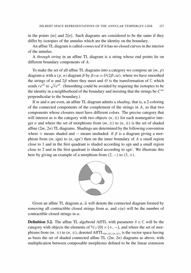
perpendicular to the boundary.)If m and n are even, an affine TL diagram admits a shading, that is, a 2-coloring
of the connected components of the complement of the strings in A, so that twocomponents whose closures meet have different colors. The precise category thatwill interest us is the category with two objects (n,±) for each nonnegative inte-ger n and where the set of morphisms from (m,±) to (n,±) is the set of shadedaffine (2m, 2n) TL diagrams. Shadings are determined by the following conventionwhere + means shaded and − means unshaded: if β is a diagram giving a mor-phism from (m, sgn) to (n, sgn′) then on the inner boundary of A a small regionclose to 1 and in the first quadrant is shaded according to sgn and a small regionclose to 2 and in the first quadrant is shaded according to sgn′. We illustrate thishere by giving an example of a morphism from (2,−) to (3,+).
Given an affine TL diagram α, α will denote the connected diagram formed byremoving all contractible closed strings from α, and c(α) will be the number ofcontractible closed strings in α.
Definition 3.2. The affine TL algebroid AffTL with parameter δ ∈ C will be thecategory with objects the elements of N ∪{0}× {+,−}, and where the set of mor-phisms from (m,±) to (n,±), denoted AffTL(m,±),(n,±), is the vector space havingas basis the set of shaded connected affine TL (2m, 2n) diagrams as above, withmultiplication between composable morphisms defined to be the linear extension

228 VAUGHAN F. R. JONES AND SARAH A. REZNIKOFF
of the map on basis elements given by
βα = δc(β◦α)β ◦α.
A representation of AffTL will be a covariant functor from this category into thecategory of vector spaces.
The transformation z 7→ 2/z of C preserves affine TL diagrams and so definesa conjugate-linear antiinvolution ∗ of the algebroid AffTL. A representation π ofAffTL will be called a Hilbert representation if the representing vector spaces areHilbert spaces and π(α∗)= π(α)∗ for all diagrams α.
Remark 3.3. Having taken linear combinations of annular diagrams we can nowgive a meaning to an annular diagram which also contains a (contractible) rectanglewith 2m boundary points labeled by an element x ∈ TLm . Such a diagram willmean the linear combination of annular diagrams obtained by writing x as a linearcombination of basis elements and inserting those basis elements in the rectangleto obtain a linear combination of AffTL elements. The beginning boundary pointon the rectangle would need to be marked if there were any ambiguity.
Hilbert representations admit an obvious direct sum operation and in this paperwe wish to classify all Hilbert representations into the category of finite dimen-sional Hilbert spaces. They will all be quotients of a universal family which wenow define.
For the rest of this section we suppose that sgn is a fixed sign, + or −, and allstatements are to be true for both values of sgn.
Definition 3.4. For any positive integer k and complex number ω let V k,ωn,sgn be the
graded vector space (graded by the subscripts, in (N ∪ {0})× {+,−}) that is thequotient of AffTL(k,+),(n,sgn) by the subspace spanned by all diagrams with fewerthan 2k through strings (so that V k,ω
n,sgn = 0 for n < k) and all elements of the formαρ−ωα, where ρ ∈AffTL(k,+),(k,+) is the diagram all of whose strings are throughstrings and for which 1 is connected to 2e4π i/2k . (We will use the notation ρk if weneed to specify the actual number of strings ρ has. Note that ρk
k is the rotation by2π .)
For ω 6= −1 and µ 6= δ we let V 0,ωn,sgn be the graded vector space (graded by
(N ∪ {0})× {+,−}) that is the quotient of the vector space AffTL(0,+),(n,sgn) bythe linear span of elements of the form ασ ∗σ − µµα, where σ is the diagram inAffTL(0,+),(0,−) having exactly one closed homologically nontrivial (in A) string.
For k = 0 and µ = δ we let V 0,ωn,sgn be the vector space with basis the set of all
ordinary Temperley–Lieb diagrams in a disc with boundary points being the 2n-throots of unity, and having the shading determined by sgn. This is acted on in theobvious way by AffTL. Note also that it is the quotient of AffTL(0,sgn),(n,sgn) by

HILBERT SPACE REPRESENTATIONS OF THE ANNULAR TEMPERLEY–LIEB 229
the relation that sets a diagram equal to any other diagram with the same systemof connections between boundary points.
For ω = −1 (hence µ= 0) we let
(a) V 0,−1,sgnn,sgn be the quotient of the vector space AffTL(0,sgn),(n,sgn) by the linear
span of elements of the form ασ ∗σ , and
(b) V 0,−1,−sgnn,sgn be the quotient of the vector space AffTL(0,−sgn),(n,sgn) by the linear
span of elements of the form ασ ∗ (or ασ according to sgn).
Remark 3.5. Note that V 0,ωn,sgn depends on µ only through ω (as µ=
√ω+
√ω
−1),so using ω in the notation is justified.
The special treatment of the case ω= −1 is unfortunate but unavoidable. If onedefined two different such representations in all cases, then if k 6= 0 they wouldbe isomorphic via either ρ or a diagram with one homologically nontrivial circle,but this last map is not invertible if µ = 0. Also of course these two represen-tations V 0,−1,± are inequivalent since the two spaces graded by 0 have differentdimensions.
Remark 3.6. Since composition of tangles does not increase the number of throughstrings and the action of tangles on the inside annular boundary commutes with theaction on the outside, the V k,ω become modules over AffTL by composition in thatcategory.
Remark 3.7. Observe that V k,ωn,± is finite dimensional for fixed k and n. We will
need their dimensions, which can be calculated by counting diagrams exactly as in[Jones 2001]:
(a) For k > 0 and n ≥ k, dim V k,ωn,± =
(2n
n − k
).
(b) For k = 0, µ= 0 and n> 0, we have dim V 0,ω,±n,± =
12
(2nn
), dim V 0,−1,sgn
0,sgn = 1,
and dim V 0,−1,sgn0,−sgn = 0.
(c) For k = 0 and µ= δ, dim V 0,ωn,± =
1n + 1
(2nn
).
(d) For k = 0 and 0< µ< δ, dim V 0,ωn,± =
(2nn
).
For uniformity of notation, in the case k = 0, µ= 0 we will use the superscriptω to denote the pair (−1,±) in the above formulae.
We now define the key ingredient of this paper, a sesquilinear form on each V k,ωn,± .
To this end note that the quotient Affk,sgn of AffTL(k,sgn),(k,sgn) by the subspacespanned by diagrams with fewer than k through strings is a unital ∗-algebra freelygenerated by the element ρ when k > 0, and σ ∗σ when k = 0. These generators

230 VAUGHAN F. R. JONES AND SARAH A. REZNIKOFF
are unitary and self-adjoint, respectively. Thus if |ω| = 1 and µ∈ C we may defineunital ∗-algebra homomorphisms φ : Affk,sgn → C by φ(ρ) = ω, and φ(σ ∗σ) =
µµ respectively. We also use the letter φ for the ∗-algebra homomorphism fromAffTL(k,sgn),(k,sgn) to C obtained by composing with the quotient map.
Definition 3.8. With notation as in the last paragraph, define the sesquilinear forms〈 · , · 〉 on each AffTL(k,+),(n,sgn) by 〈v,w〉 = φ(w∗v).
Proposition 3.9. The sesquilinear form of Definition 3.8 is invariant; that is,〈αv,w〉 = 〈v, α∗w〉.
Proof. This follows immediately from w∗αv = (αw)∗v and the fact that φ is a∗-algebra homomorphism. �
Proposition 3.10. The sesquilinear form of Definition 3.8 passes to the quotientV k,ω
n,sgn.
Proof. If δ 6=µ it follows from the ∗-homomorphism property of φ that the elementsdefined in Definition 3.4 spanning the subspace by which the quotient was taken areorthogonal to all diagrams in AffTL(k,+),(n,sgn). Case (b) of the definition requirescare. One observes that if v=ασ andw is any diagram in the same space thenw∗v
is actually a multiple of δ times an element of the form βσ ∗σ . This is because, afterthe removal of homologically trivial circles, w∗v has a homologically nontrivialcircle, hence at least two because the shadings near the inner and outer boundarieshave to match.
Finally in the case µ = δ, if two diagrams v and v′ define the same systemof connections among boundary points, the diagrams for w∗v and w∗v′ are boththe same system of closed curves with the inner annulus boundary possibly indifferent regions. The homologically nontrivial closed curves must occur in pairsfor the annulus boundary shadings to match, and since µ= δ, such a pair will countthe same if it is dealt with by φ or if it is homologically trivial. �
The element 1 ∈ V k,ωk,+ clearly generates V k,ω as a representation of AffTL. We
will call it the vacuum vector and write it vω . It satisfies the following properties,where the εi are as in Definition 2.8 of [Jones 2001].
(a) When k > 0, we have 〈vω, vω〉 = 1, ρ(vω)= ωvω, and εi (vω)= 0 for 0 ≤ i ≤
2k − 1.
(b) When k > 0, we have 〈vω, vω〉 = 1 and σ ∗σ(vω)= µµvω.
The following fundamental lemma was poorly treated in [Jones 2001]. Thiswas because the conclusion was obvious from spherical invariance in the planaralgebras to which it was applied. We give a careful proof here.
Lemma 3.11. The inner products in V k,ω can be calculated using just properties(a) and (b) above.

HILBERT SPACE REPRESENTATIONS OF THE ANNULAR TEMPERLEY–LIEB 231
Proof. Since any vector in V k,ω is a linear combination of affine diagrams appliedto vω, it suffices by invariance to show how the equations can be used to calculate〈αvω, vω〉, with α connected. First consider the case k > 0. Then α is a connectedaffine tangle with 2k inner and outer boundary points. If all the strings are notthrough strings, α = α′εi for some i , and the inner product is zero. If all thestrings are through strings α is necessarily some power of ρ so the inner productis determined by properties 〈vω, vω〉 = 1 and ρ(vω)= ωvω.
Now suppose k = 0. Then by connectedness α consists of a certain numberof strings which may be isotoped into concentric circles. They must be even innumber since the inner and outer boundaries have the same shading. This meansprecisely that α is a power of σ ∗σ . �
Corollary 3.12. Any Hilbert representation of AffTL is isomorphic to a quotientof V k,ω for some root of unity ω, and the corresponding 〈 · , · 〉 of Definition 3.8 ispositive semidefinite. If k = 0, then 0 ≤ µ≤ δ.
Proof. As in [Jones 2001], if U is an irreducible Hilbert space representation, allthe Um,sgn have to be irreducible AffTL(m,sgn),(m,sgn) modules. Let k be the smallestinteger for which Uk,± is nonzero (this k is called the lowest weight and U(k,±) iscalled the lowest weight space). Then AffTL(k,sgn),(k,sgn) acts on the lowest weightspace via the abelian quotient AffTLk,sgn defined before Definition 3.8. By someversion of Schur’s lemma the lowest weight space is thus one dimensional and theunitary ρ must act by some ω, with |ω| = 1, or, if k = 0, σ ∗σ must act by somenonnegative real — choose µ to be a nonnegative square root of that constant andthen choose ω accordingly. A lowest weight vector of unit length in Uk,+ will thensatisfy all the conditions of (a) or (b) above so we may define a 〈 · , · 〉-preservingmap from the corresponding V t,ω onto U by sending, for any connected α, α(vω)onto the α applied to a lowest weight unit vector u ∈ U. So 〈 · , · 〉 is positivesemidefinite, since the inner product in U is.
The case k = 0, ω=−1 does not quite work as above. Then either U0,+ or U0,−
must be nonzero; suppose that it is U0sgn and choose u therein. Then ‖σ(u)‖ = 0(or ‖σ ∗(u)‖ = 0), so by irreducibility U0,sgn vanishes. Then proceed as before toobtain an isomorphism between U and V 0,−1sgn.
That µ≤ δ follows as in [Jones 2001]. �
Conversely, if 〈 · , · 〉 is positive semidefinite on some V k,ω, the quotient by itskernel is a Hilbert space representation of AffTL, which we call Vk,ω.
Lemma 3.13. Vk,ω is irreducible.
Proof. Suppose v ∈ Vk,ω is nonzero. Then 〈v, v〉 6= 0. But v =∑
α cαα vω forsome affine diagrams α and constants cα. So
⟨∑α cαα∗v, vω
⟩6= 0; since AffTLksgn
is one-dimensional it follows that vω, hence all of Vk,ω, is in the AffTL span of v.�

232 VAUGHAN F. R. JONES AND SARAH A. REZNIKOFF
Definition 3.14. If U is an irreducible representation of AffTL isomorphic to Vk,ω
then k will be called the lowest weight of U and ω will be called the chirality.
The determination of the set of values of δ, ω and µ for which the sesquilinearform 〈 · , · 〉 is positive semidefinite is the subject of the next sections.
Finally remark that the representations V k,ω are all mutually inequivalent exceptwhen k = 0 (when clearly V k,ω and V k,ω−1
are the same). Also V 0,0,+ and V 0,0,−
are inequivalent since the dimensions of the spaces graded by (0,+) and (0,−)are different. Thus at the end of this paper we will have obtained a complete listof irreducible Hilbert representations of AffTL.
4. The formula of Graham and Lehrer
Let V k,ω, with |ω| = 1 or 0 ≤ µ ≤ δ, be the affine Temperley–Lieb module con-structed in the previous section and let vω be a lowest weight unit vector therein.
Definition 4.1. For k ≤n we will call αn the element of AffTL(k,+),(n,+) containingone copy of the JW idempotent p2n in a rectangle whose first boundary point isconnected to −2 and the next 2n − 1 (in cyclic order) are also connected to theoutside boundary of A. The 2k boundary points on the inside boundary of A areconnected to the middle 2k of the remaining boundary points of the rectangle andthe other boundary points of the rectangle are connected to each other in the unique(planar) way so that none is connected to its nearest neighbor.
We illustrate this definition in Figure 1 for k = 2 and n = 5. The boundary pointsof the inner circle are the fourth roots of unity and the ones on the outer circle arethe tenth ( = 2n-th) roots of unity. The order of shaded regions on the boundary
p2nαn =Figure 1

HILBERT SPACE REPRESENTATIONS OF THE ANNULAR TEMPERLEY–LIEB 233
of the rectangle containing p2n will depend on the parity of n, but the ordinary TLalgebra makes sense without shading the regions.
Note that Figure 1 represents a (nonzero) linear combination of annular (2, 6)tangles obtained by expanding the J-W idempotent p2n in the rectangle.
For each r ≥ 0 we set 2n = 2k + 2r and define the vector wn ∈ V k,ωn to be the
result of applying the annular element αn of Figure 1 to vω.Let Cn = 〈wn, wn〉 for n > k and Ck = 1. Our main task in this paper will be to
establish whether Cn is positive, negative or zero.
Theorem 4.2. Suppose δ (= q + q−1) and n satisfy δ > 2 cosπ/2n ≥ 0 (so that inparticular the map8 : TL2n−1 → TL2n−1 is an isomorphism, and the JW idempo-tent p2n is defined). Then with r = n − k,
Cn =[r ][r + k]
[2n][2n − 1](q2n
+ q−2n−ω−ω−1)Cn−1
Proof. First note that neither [2n] nor [2n − 1] is zero. If δ > 2 this is obvious.Otherwise write δ = 2 cosπ/a (a not necessarily an integer) so that the conditionbecomes π/2n > π/a, or 2nπ/a < π . Then [2n] = sin(2nπ/a)/sin(π/a), whichis strictly positive.
We want to calculate Cn = 〈αn(vω), αn(vω)〉. By invariance it will suffice toexpress α∗
nαn in terms of α∗
n−1αn−1, which we proceed to do.Case (i), k > 0.In Figure 2 we have drawn α∗
nαn (with n = 4 for clarity, rather than 5 as in theprevious figure).
The first step is to introduce a JW idempotent on one less string. Because ofthe order on these idempotents, the AffTL element in Figure 3 is the same as inFigure 2.
p2nFigure 2

234 VAUGHAN F. R. JONES AND SARAH A. REZNIKOFF
p2np2n−1Figure 3
It is easily seen that there are only 3 tangles in the expansion of p2m that givenonzero contributions in Figure 3. There must be at least 2n − 2 through stringsinside the rectangle, or two adjacent boundary points on the left side of the rec-tangle containing p2n−1 would be connected — giving zero. So the only adjacentboundary points on the right side of the p2n rectangle that can be connected arethe top two. Then it is easy to check that the only two pairs of adjacent boundarypoints on the left side of the p2n rectangle that can be connected are the ones havingexactly one point connected to the inner boundary circle of A. Thus we see that
α∗
nαn = X + cY Y + cZ Z
where X, Y and Z are given in Figures 4, 5, and 6, respectively.
p2n−1
Figure 4

HILBERT SPACE REPRESENTATIONS OF THE ANNULAR TEMPERLEY–LIEB 235
p2n−1
Figure 5
p2n−1
Figure 6
We deal first with the situation in Figure 4. Here after an isotopy we see thatthe bottom left and right boundary points of the p2n−1 rectangle are connected toeach other. The result is well known to be a multiple of p2n−2. By comparing thecoefficient of the identity in the expansion of the idempotent, the multiple is seento be [2n]/[2n − 1], so that
X = ([2n]/[2n − 1]) α∗
n−1αn−1.
The arguments for Y and Z are structurally identical and differ only in theconstants and the direction in which the inner circle is rotated. In Figure 5, thediagram inside the rectangle for p2n is Er Er−1 · · · E1, which has a coefficient of

236 VAUGHAN F. R. JONES AND SARAH A. REZNIKOFF
(−1)r [r+2k]/[2n] in JW; see [Jones 2001], for example. In Figure 6, the diagramis Er+2k Er+2k−1 Er+2k−2 · · · E1; this diagram’s coefficient is (−1)r [r ]/[2n]. Sincewe will be doing many of these calculations, we record the relevant coefficient inthe JW idempotent pictorially:
Coefficient in JW of
r−1
is (−1)r[r+2k]
[2n].
Figure 7
Thus at this stage we have
α∗
nαn =[2n]
[2n − 1]α∗
n−1αn−1 + (−1)r(
[r + 2k]
[2n]Y +
[r ]
[2n]Z).
If we now start with Figure 6 and insert a p2n−2 we obtain Figure 8.
p2n−1
p2n−2Figure 8
For Z , consideration of all possible TL diagrams inside the p2n−1 rectangleshows that the only ones with a nonzero contribution are those with 2n−2 throughstrings and the top and bottom boundary points of the inner annulus boundary con-nected down and up respectively to their nearest neighbors, as in Figures 9 and 10.
The coefficient of the TL diagram from Figure 9 is, again by Figure 7,
(−1)r+1[r + 2k]
[2n − 1]
and the coefficient of the TL diagram from Figure 10 is
(−1)r+1[r ]
[2n − 1].

HILBERT SPACE REPRESENTATIONS OF THE ANNULAR TEMPERLEY–LIEB 237
p2n−2Figure 9
p2n−2Figure 10
But notice that Figure 9 is just α∗
n−1αn−1 composed with ρ and Figure 10 is justα∗
n−1αn−1 . So we have
Z = (−1)r+1α∗
n−1αn−1
([r +2k]
[2n−1]ρ+
[r ]
[2n−1]
).
Doing the corresponding calculation for Figure 5 we obtain that
Y = (−1)r+1α∗
n−1αn−1
([r +2k]
[2n−1]+
[r ]
[2n−1]ρ−1
).

238 VAUGHAN F. R. JONES AND SARAH A. REZNIKOFF
So CY Y + CZ Z equals
−1[2n][2n − 1]
α∗
n−1αn−1([r ]2+ [2k + r ]
2− [r ][r + 2k](ρ+ ρ−1)).
Altogether,
α∗
nαn =[r ][r + 2k]
[2n][2n − 1]α∗
n−1αn−1
([2n]
2
[r ][r + 2k]−
[r ]
[r + 2k]−
[r + 2k]
[r ]− ρ− ρ−1
).
But we have the identity [2n]2−[r ]
2−[2n −r ]
2= (q2n
+q−2n)[r ][2n −r ], andon V k,ω
k , ρ = ω so that
Cn =[n − k][n + k]
[2n][2n − 1]
(q2n
+ q−2n−ω−ω−1)Cn−1
This proves the theorem when k > 0.The case µ= δ needs no consideration since in this case ordinary TL diagrams
inside a disc provide a Hilbert representation.Case (ii); 0< µ< δ.We may consider Figure 3 when k = 0. In this case there are only two ways to
fill in the p2n rectangle to obtain nonzero diagrams. The first is with the identity
which gives[2n]
[2n − 1]as before, and the second, which is the common case r = n
of the terms Y and Z in the previous argument , so we have:
α∗
nαn =[2n]
[2n − 1]α∗
n−1αn−1 + (−1)n[n]
[2n]Y ′
where Y ′ is the tangle with the inner annulus boundary surrounded by a homolog-ically nontrivial circle as illustrated in Figure 11.
Introducing a p2n−2 as before there is only one contributing diagram that can beput in the p2n−1 rectangle and its coefficient is
(−1)n−1[n]
[2n − 1].
The resulting annular diagram is Figure 12.Note that the innermost circle is an annulus boundary and the next two are
strings, which contribute precisely σ ∗σ . Thus we have
α∗
nαn = α∗
n−1αn−1
([2n]
[2n − 1]−
[n]2
[2n][2n − 1]σ ∗σ
).
But σ ∗σ acts as µ2 on V 0,ω0 so that
Cn =
([2n]
[2n − 1]−
µ2[n]
2
[2n][2n − 1]
)Cn−1.

HILBERT SPACE REPRESENTATIONS OF THE ANNULAR TEMPERLEY–LIEB 239
p2n−1Figure 11
p2n−2Figure 12
Using [m] =qm
− q−m
q − q−1and µ2
= 2 +ω+ω−1 we get
Cn =[n]
2
[2n][2n − 1]
(q2n
+ q−2n−ω−ω−1)Cn−1.
This proves the theorem in case (ii).The only remaining case is k = 0, ω = 0, where of course ω+ω−1 is taken to
mean zero. In this case the argument is extremely simple as the term Y in case (ii)already acts by zero. Note that in fact there are two cases for wn in this situationaccording to the shading on the inside annulus boundary. This does not change theargument in any way. �

240 VAUGHAN F. R. JONES AND SARAH A. REZNIKOFF
5. Restrictions on δ, k and ω when δ < 2
Theorem 5.1. Suppose U is an irreducible Hilbert space AffTL module with low-est weight k and chirality ω. Suppose δ = 2 cosπ/a for a = 3, 4, . . . (chooseq = eπ i/a). Then
ω = q±2r for some integer r with k < r ≤ a/2.
Proof. Our first job is to show that k < a/2. Suppose 2k ≥ a and let u be a unitvector spanning Uk . Then consider the a annular tangles νl , l = 1, . . . , a with 2kinner boundary points and 2k + 2 outer ones, 2k through strings, with 2elπ i/(k+1)
connected to 2e(l+1)π i/(k+1) and 1 connected to 2. The matrix of inner productsof the vectors νl(u) is the a × a matrix with δ on the diagonal, one on the firstoff-diagonals and 0 elsewhere. The determinant of this matrix is well known to be
(5-1) [a + 1] =sin(a + 1)π/a
sinπ/a,
which is negative. This is impossible in a Hilbert space, so k < a/2.Since the rotation is unitary and 0 ≤ µ ≤ δ we know that |ω| = 1 and we
may suppose, by taking the complex conjugate if necessary, that Im(ω) ≥ 0. Letθ = arg(ω). We know from Corollary 3.12 that U is a quotient of a V k,ω so thatit makes sense to talk about vk , wn etc. Then if θ is not 2rπ/a for some r withk < r ≤ a/2 then let r0 be the largest value of r with θ ≥ 2rπ/a. Suppose first that2(r0 + 1) < a. Then by Theorem 4.2 we have Cm > 0 for k ≤ m ≤ r0 but Cm < 0for m = r0 + 1, which is disallowed by positivity. So we may suppose 2r0 < a but2(r0 + 1)≥ a. We will divide the proof into two cases.
Case (i) a odd so that 2r0 + 1 = a.The difficulty is clear: using Theorem 4.2 we get Cm > 0 for 1 ≤ m ≤ r0, but
we cannot apply the theorem for r0 + 1 since its hypotheses are no longer valid.But the vector wr0 still exists and by Theorem 4.2 it is nonzero. Now form, as
above, 2r0 +1 vectors in Ur0+1 from wr0 by applying 2r0 +1 annular (2r0, 2r0 +2)diagrams in which one pair of outer boundary points is connected to its nearestneighbor and all other strings are through strings, excluding the one in which −2is connected to the neighboring boundary point with negative imaginary part. Ifthe vector wr0 is normalized to be a unit vector, we get vectors whose matrix ofinner products is the (2r0 + 1)× (2r0 + 1) matrix with δ on the diagonal, one onthe first off-diagonals and 0 elsewhere. (Careless choice of how the inside annulusboundary is connected to the outside will lead to powers of ω on the off-diagonalbut they can be removed by renormalizing the vectors one after another.) Thedeterminant of this matrix is well known to be [2r0 + 2] = [a + 1], given in (5-1),and hence negative. This is impossible in a Hilbert space.

HILBERT SPACE REPRESENTATIONS OF THE ANNULAR TEMPERLEY–LIEB 241
p2a−1Figure 13
Case (ii) a even so that 2r0 = a − 2.We will suppose that k > 0. The case k = 0 goes in exactly the same way but
the diagrams need to be modified a little. We leave the details to the reader.Here we will use the tangle encountered midway through the proof of Theorem
4.2. First let β be the (2k, a) annular tangle with the 2k internal boundary pointsconnected to a JW idempotent on a − 1 strings (the last one for which the induc-tive definition works) in a rectangle, a − 2k − 2 boundary points of the rectangleconnected pairwise by strings that go around the internal annulus boundary andone rectangle boundary point connected to −2, as shown in Figure 13 for a = 8and k = 1. The other a − 1 rectangle boundary points are connected to the outerannulus boundary points.
The first thing we want to show is that β(vω) = 0. We do this by calculating〈β∗β(vω), vω〉. Since pa−1 is a projection, β∗β is as in Figure 14.
But in Figure 14 we see the JW idempotent with two boundary points cappedoff. In general this would be nonzero since the boundary points are not on thesame side of the rectangle, but since this JW idempotent is the last one to exist,it spans the kernel of the natural inner product on TL diagrams so is invariant (atleast up to a scalar) under the rotation. Thus if any two adjacent boundary pointsare connected the result is zero. (One can also show this by Wenzl’s inductiveformula.)
Thus β(vω)= 0.We will now derive a contradiction by showing that the inner product of β(vω)
with another vector is nonzero. This vector will be obtained from applying a (2k, a)tangle called γ to vω where γ is obtained from the (2k, a − 2) tangle αa−2 of

242 VAUGHAN F. R. JONES AND SARAH A. REZNIKOFF
p2a−1Figure 14
pa−2Figure 15
Definition 4.1 by connecting −2 to −2e(a+1)π i/a and the other outer boundarypoints to the boundary points of the rectangle, as indicated in Figure 15.
To calculate the inner product 〈β(vω), γ (vω)〉 we use the tangle γ ∗β, which wehave drawn in Figure 16.
As in the proof of Theorem 4.2, there are only two diagrams that can be put inthe rectangle which give nonzero contributions- those in which the boundary pointsconnected to the first and last internal annular boundary points are connected totheir neighbors (which are not connected to the inner annulus boundary). Thecoefficients of these diagrams are (from Figure 7)
[a/2 − k]
[a − 1]and
[a/2 + k]
[a − 1].

HILBERT SPACE REPRESENTATIONS OF THE ANNULAR TEMPERLEY–LIEB 243
p2n−1
p2n−2Figure 16
But these are both equal tocos kπ/a
sin(a − 1)π/a,
which is nonzero. On the other hand, the two resulting tangles are (δ times)α∗
a−2αa−2ρ and α∗
a−2αa−2. Since ω 6= −1 (by the assumption on θ ) , the sum ofthese two tangles applied to vω is nonzero. Hence, by Theorem 4.2, 〈β(vω), γ (vω)〉is nonzero, a contradiction. �
We point out two corollaries of Theorem 5.1. The first is immediate but some-how surprising.
Corollary 5.2. Let U be a Hilbert space representation of AffTL. Then none ofthe rotations ρt for t ≥ 1 acts by the identity.
Proof. One may reduce to the irreducible case by using a maximal abelian subal-gebra in the commutant of the algebra acting on the lowest weight space. Then theresult follows from Theorem 5.1. �
In [Jones 2001] we studied representations of the quotient AnnTL of our AffTLin which the rotations by 2π , ρt
t , act by the identity. We know that any Hilbertspace representation of AnnTL will give one of AffTL, so we now identify thoseones allowed by Theorem 5.1.
Corollary 5.3. Let U be an irreducible Hilbert space representation of AffTL withchirality ω and lowest weight k > 0. Then U passes to AnnTL if and only if thereis an integer b such that a = rk/b.

244 VAUGHAN F. R. JONES AND SARAH A. REZNIKOFF
Proof. The main thing is that ρkk = 1 on Uk,± implies that ρn
n = 1 on Un,± for alln ≥ k. This is because U is a quotient of V k,ω and it is clear that ρn
nα = αρkk for
any α ∈ AffTL(ksgn),(n,±sgn).So whenever ω is a k-th root of unity, U passes to AnnTL. This is the condition
a = rk/b combined with the conclusion of Theorem 5.1. �
6. Construction of the allowed Hilbert space representations
In this section we will undertake the most difficult part of this paper, namely theexplicit construction of a representation Vk,ω for each pair (k, ω) allowed by The-orem 5.1.
Theorem 6.1. Let (k, ω) be a pair where k is a nonnegative integer and ω is acomplex number (or ω = (−1,±), if k = 0). Then Vk,ω exists if
(i) δ ≥ 2 and either k = 0 and 0 ≤ µ≤ δ,or k > 0 and |ω| = 1, or
(ii) δ = 2 cosπ/a for a = 3, 4, 5, . . . , and ω = q±2r for some integer r withk < r ≤ a/2 (where by −1 we mean (−1,±) if k = 0).
Proof. As observed in Section 3, it suffices to show that the sesquilinear forms〈 · , · 〉 of Definition 3.8 are positive semidefinite on V k,ω. The method, as in [Jones2001], where it is done for the generic case, is to inductively decompose the rep-resentation V k,ω
(n,±) with respect to a large ordinary TL subalgebra, which we willsoon define.
First let us completely handle the case q =1 (so that δ=2). When ω 6=1, we caninductively decompose the representation as is done for δ > 2 in [Jones 2001], andthen confirm positive definiteness on the span of the vector ωn by using Theorem4.2. The case ω= 1 is quite different, as the form is only positive semidefinite andwe must identify the kernel. In this case, it follows from the same theorem thatCn = 0 for all n ≥ k + 1, so that in fact Vk,ω is generated by V k,1
k .In the case δ < 2, the large ordinary TL subalgebra will eventually fail to be
semisimple. Semisimplicity is so important to our analysis — it allows us to usethe inductive technique of [Jones 2001] — that we begin our proof by taking aquotient of V k,ω on which, by Theorem 2.1, the action of TL passes to the C∗
quotient, TLn .It will be convenient to consider only the spaces V k,ω
n,+ . The rotation providesan isometry between this and V k,ω
n,− in all but a special case when k = 0, where thesituation is clear.
Thus let δ=2 cosπ/a for a =3, 4, 5, . . . and letω and k be as in the statement ofthe theorem. Define the subspace JW k,ω
n,± of V k,ωn,± to be the span of the image of vω
under annular diagrams containing a rectangle labeled by the JW idempotent pa−1

HILBERT SPACE REPRESENTATIONS OF THE ANNULAR TEMPERLEY–LIEB 245
(see Remark 3.3). The subspaces JW k,ωn,±, as n varies, are clearly invariant under
the action of AffTL. We claim that they are in the kernel of 〈 · , · 〉. To see this, itsuffices to show that an annular (k, k) diagram containing the JW idempotent pa−1
in a rectangle is zero modulo diagrams with fewer than k through strings. Let αbe such a diagram. We shall show that it has the same form as the element α∗
nαn
of Theorem 4.2 and then apply the Graham–Lehrer formula.If α had a string connecting the inside annulus boundary to the outside, then,
cutting along that string, the rectangle would lie in a disc (after isotopy) with 4k−2boundary points. The rectangle itself has 2a − 2 boundary points and k < a/2 sosome boundary point on the rectangle must be connected to its nearest neighbor,which gives zero. So all of the strings from the inner annulus boundary are con-nected to the rectangle as are all those from the exterior annulus boundary. In factk ≤ a/2 − 1 so that 4k ≤ 2a − 4 so there are boundary points on the rectangle thatare not connected to the annulus boundary. If these points were not connected sym-metrically around the interior of the annulus there would be a rectangle boundarypoint connected to its nearest neighbor.
Let us first treat the case where a is odd so the rectangle has an even numberof boundary points at the top and at the bottom. Since the JW idempotent is ro-tationally invariant (up to a scalar, as observed in the proof of Theorem 5.1), andsince vω is invariant up to a scalar, we may suppose that α is as in Figure 2 (whichillustrates the case a = 9, n = 3). Thus 〈α(vω), vω〉 is equal to C(a−1)/2 and thus,by Theorem 4.2, proportional to Cr since r ≤ (a − 1)/2. But, again by the sametheorem, Cr = 0 since ω = q2r .
Now turn to the case where a is even. Then by rotational invariance as abovewe may suppose that α is as in Figure 16.
First suppose r = a/2 so ω = −1. Then by the argument after Figure 16 weget that 〈α(vω), vω〉 = 0 precisely because ω = −1 (which is the value it did nottake there). The case k = 0 is slightly different. In this case there is only onediagram, shown in Figure 17, that can be put into the rectangle to give a nonzerocontribution, and that results in a homologically nontrivial circle surrounding theinner annulus boundary. This will give zero for 〈α(vω), vω〉.
Finally if r < a/2 we also get the situation of Figure 16, and again by theargument after that figure, we see that 〈α(vω), vω〉 is proportional to Ca/2−1. ByTheorem 4.2, Ca/2−1 is proportional to Cr , but as ω= q2r and k < r , Theorem 4.2applies again to give Cr = 0.
At this stage we have shown that in all cases allowed by the theorem, JW iscontained in the kernel of 〈 · , · 〉, so that 〈 · , · 〉 defines an invariant form on thequotient AffTL-module 2k,ω
= V k,ω/JW k,ω. Positive semidefiniteness of 〈 · , · 〉
on 2k,ω would therefore imply it on V k,ω. We will establish this positivity byrestricting to a large ordinary TL algebra of AffTL(n,+),(n,+) for n ≥ 1.

246 VAUGHAN F. R. JONES AND SARAH A. REZNIKOFF
p2n−2
Figure 17
The intersection of the annulus A with the complement of the wedge{reiθ
∈ C :
(1 +
1n+2
)π < θ <
(1 +
1n+1
)π
}is isotopic to a rectangle with 2n marked points on the top and on the bottom. Thusthe subalgebra of AffTL(n,+),(n,+) spanned by isotopy classes of tangles that lieoutside the wedge is isomorphic to the Temperley–Lieb algebra TL2n . We will callit t`2n . Define Fn ∈ AffTL(n,+),(n,+) to be the unique diagram in t`2n with 2n − 2through strings and −1 connected to ei(1−1/n)π . One may jiggle the boundarypoints to exhibit an isomorphism between Fnt`2n Fn and t`2(n−1), which makesFnV k,ω
(n,+) into a t`2(n−1)-module isomorphic to V k,ω(n−1,+).
All this is as in [Jones 2001]. Moreover, these isomorphisms take the sub-space JW k,ω
(n,+) to the subspace JW k,ω(n−1,+) and the ideal I2n generated in t`2n by
pa−1 (which we take to be zero when 2n < a − 1) onto I2n−2. It is obviousthat the ideal I2n preserves JW k,ω
(n,+) so that the quotients Xk,ωn = V k,ω
(n,+)/JW k,ω(n,+)
become modules over the quotients T`2n = t`2n/I2n . But by Theorem 2.1, T`2n
is a finite-dimensional C∗-algebra (with irreducible representations as described inSection 2). Further, by using the isomorphisms established above, we see that forevery value of t , FnWt
2n is isomorphic to Wt2n−2 as a T`2n−2-module.
Thus Xk,ωn as a T`2n-module is a direct sum of as many copies of each Wt
2n asXk,ω
n−1 is of Wt2n−2, plus a certain number of copies of the trivial representation if
2n<a−1 (and none if 2n ≥a−1). The form 〈 · , · 〉 is invariant under t` and there isonly one such form (up to a scalar) on W, so positive semidefiniteness on the spanof the nontrivial representations follows by induction as soon as it is establishedon the trivial ones as they appear. (The statement for the generic case is [Jones

HILBERT SPACE REPRESENTATIONS OF THE ANNULAR TEMPERLEY–LIEB 247
2001, Proposition 4.10], the proof of which goes through as long as 2n ≤ a − 1.)But the JW idempotent p2n projects onto the trivial representation for 2n < a − 1,and annihilates all vectors in V k,ω
n,+ except for
w =
where all strings that connect the outside boundary to itself go through the wedgedefined above.
Thus there is exactly one copy of the trivial representation for 2n < a − 1 andnone for 2n ≥a−1. Inspection of the preceding figure shows that p2n(w)=αn(vω)
so that positive semidefiniteness of 〈 · , · 〉 follows from Cn ≥ 0. This follows fromTheorem 4.2 and the choice of k, ω and δ, which force Cn to be zero before it hasa chance to be negative. �
We see in the proof of the theorem that we have in fact determined the structureof the Hilbert space representations as modules over the large Temperley–Lieb sub-algebra. In fact the Vk,ω
n,+ become modules over the TL algebroid discussed in Re-mark 2.4. The ordinary TL algebroid is spanned by all diagrams in AffTL(m,+),(n,+)that do not intersect the wedge{
reiθ∈ C :
(1 +
1r +2
)π < θ <
(1 +
1r +1
)π
},
where r = max(m, n). The Hilbert space representations of this algebroid areprecisely the modules Wt .
Scholium 6.2. Suppose ω and k satisfy the conditions of Theorem 6.1. For anyn ≥ k, as a module over the ordinary TL algebroid, Vk,ω
(n,+) is
(i) W2k2k if δ = 2 and q = 1,
(ii)r−1⊕j=k
W2 j2n if k ≥ 0, or k = 0 and ω 6= (−1,±).
(iii)⊕
0≤ j≤mj+1∈2N
W2 j2n if k = 0 and ω = (−1,+),
(iv)⊕
1≤ j≤mj∈2N
W2 j2n if k = 0 and ω = (−1,−),

248 VAUGHAN F. R. JONES AND SARAH A. REZNIKOFF
where in (iii) and (iv) m = a/2−1. (Note that for these values of ω, a is guaranteedto be even, so m is indeed an integer.)
Proof. The first statement follows immediately from the remarks at the beginningof this section.
Item (ii) follows from the inductive procedure used to decompose Vk,ω(n,+) as a
module over the ordinary TL algebroid, which relies on the following two factsfrom [Jones 2001]. First, when 2n ≤ a − 1 and 0 ≤ j < n, a representation πof T`2n contains a copy of W
2 j2m if and only if π restricted to E2n−1(T`2n)E2n−1
contains a copy of W2 j2n−2: this is Proposition 4.10 of [Jones 2001] (with a weak-
ened assumption on the genericity of the index, which does not affect the proof).Second, Theorem B1 of the same paper says that if Vk,ω
(m,+) has dimension( 2m
m−k
)−1
then for all n ≥ m, as a T`2n module, Vk,ω(n,+) is isomorphic to
⊕m−1j=k W
2 j2n . (Note
that the hypothesis on the dimension is satisfied since r ≤ a/2.)Parts (iii) and (iv) are proved by introducing a second copy of the ordinary
Temperley–Lieb algebroid, T`2n , and arguing that (for n > 1) W2n2 j is present in
Vk,ω(n,+) as a T`2n-module when j is odd and as a T`2n module when j is even. The
induction is as in Theorem 5.23 of [Jones 2001]. An adjustment of the dimensionhypothesis of Theorem B.1 of the same paper can be made for this case so that thatproof guarantees the form of the Vk,ω
(n,+) when n ≥ a. �
Corollary 6.3. The dimension of Vk,ω is
(i) zk C(z)2k− zC(z)2k+2
√1 − 4z
if δ = 2 and q = 1,
(ii)1
Qa(z)
r−1∑j=k
z j Qa−2 j−1(z) if ω = q±2r ,
(iii)12
+1
2Qa(z)
a/2−1∑j=0
z j Qa−2 j−1(z) if k = 0, ω = (−1,+),
(iv) −12
+1
2Qa(z)
a/2−1∑j=0
z j Qa−2 j−1(z) if k = 0, ω = (−1,−).
Proof. To prove part (i), note that dim W tn =
( 2nn−t
)−
( 2nn−t−1
), so by [Graham et al.
1994, page 203], we obtain the result. Part (ii) follows directly from Theorem 2.3and the scholium. For (iii) and (iv) use the fact that Vk,ω is isomorphic to both⊕
1≤ j≤mj∈2N
W2 j2n and
⊕1≤ j≤mj+1∈2N
W2 j2n,
so these must have equal dimension. �

HILBERT SPACE REPRESENTATIONS OF THE ANNULAR TEMPERLEY–LIEB 249
References
[Goodman et al. 1989] F. M. Goodman, P. de la Harpe, and V. F. R. Jones, Coxeter graphs andtowers of algebras, Mathematical Sciences Research Institute Publications 14, Springer, New York,1989. MR 91c:46082 Zbl 0698.46050
[Graham and Lehrer 1998] J. J. Graham and G. I. Lehrer, “The representation theory of affineTemperley–Lieb algebras”, Enseign. Math. (2) 44:3-4 (1998), 173–218. MR 99i:20019 Zbl 0964.20002
[Graham et al. 1994] R. L. Graham, D. E. Knuth, and O. Patashnik, Concrete mathematics, 2nded., Addison-Wesley, Reading, MA, 1994. A foundation for computer science. MR 97d:68003Zbl 0836.00001
[Jones 1983] V. F. R. Jones, “Index for subfactors”, Invent. Math. 72:1 (1983), 1–25. MR 84d:46097Zbl 0508.46040
[Jones 1994] V. F. R. Jones, “A quotient of the affine Hecke algebra in the Brauer algebra”, Enseign.Math. (2) 40:3-4 (1994), 313–344. MR 95j:20038 Zbl 0852.20035
[Jones 1999] V. F. R. Jones, “Planar algebras, I”, preprint, 1999. To appear in New Zealand J. Math.math.QA/9909027
[Jones 2001] V. F. R. Jones, “The annular structure of subfactors”, pp. 401–463 in Essays on geom-etry and related topics, edited by E. Ghys et al., Monogr. Enseign. Math. 38, Enseignement Math.,Geneva, 2001. MR 2003j:46094 Zbl 1019.46036
[Kauffman 1987] L. H. Kauffman, “State models and the Jones polynomial”, Topology 26:3 (1987),395–407. MR 88f:57006 Zbl 0622.57004
[Wenzl 1987] H. Wenzl, “On sequences of projections”, C. R. Math. Rep. Acad. Sci. Canada 9:1(1987), 5–9. MR 88k:46070 Zbl 0622.47019
Received March 12, 2005.
VAUGHAN F. R. JONES
DEPARTMENT OF MATHEMATICS
UNIVERSITY OF CALIFORNIA, BERKELEY
BERKELEY, CA 94720-3840UNITED STATES
[email protected]://math.berkeley.edu/~vfr/
SARAH A. REZNIKOFF
DEPARTMENT OF MATHEMATICS AND STATISTICS
UNIVERSITY OF VICTORIA
VICTORIA, BC V8W 3P4CANADA
[email protected]://www.math.uvic.ca/~sarah

PACIFIC JOURNAL OF MATHEMATICSVol. 228, No. 2, 2006
KNOT ADJACENCY, GENUS AND ESSENTIAL TORI
EFSTRATIA KALFAGIANNI AND XIAO-SONG LIN
A knot K is called n-adjacent to another knot K ′ if K admits a projectioncontaining n generalized crossings such that changing any 0 < m ≤ n ofthem yields a projection of K ′. We apply techniques from the theory ofsutured 3-manifolds, Dehn surgery and the theory of geometric structures of3-manifolds to study the extent to which nonisotopic knots can be adjacentto each other. A consequence of our main result is that if K is n-adjacentto K ′ for all n ∈ N, then K and K ′ are isotopic. This provides a partialverification of the conjecture of V. Vassiliev that finite type knot invariantsdistinguish all knots. We also show that if no twist about a crossing circleL of a knot K changes the isotopy class of K , then L bounds a disc in thecomplement of K . This leads to a characterization of nugatory crossings onknots.
1. Introduction
A crossing disc for a knot K ⊂ S3 is an embedded disc D ⊂ S3 such that Kintersects int D twice with zero algebraic number. Let q ∈ Z. Performing 1
q -surgery on L1 := ∂D1, changes K to another knot K ′
⊂ S3. We say that K ′ isobtained from K by a generalized crossing change of order q (see Figure 1).
An n-collection for a knot K is a pair (D, q), such that
(i) D := {D1, . . . , Dn} is a set of disjoint crossing discs for K ,
(ii) q :={ 1
q1, . . . , 1
qn
}, with qi ∈ Z \ {0}, and
(iii) the knots L1 := ∂D1, . . . , Ln := ∂Dn are labeled by 1q1, . . . , 1
qn .
The link L :=⋃n
i=1 L i is called the crossing link associated to (D, q).We will use the notation
i := (i1, . . . , in) ∈ {0, 1}n
MSC2000: 57M25, 57M27, 57M50.Keywords: knot adjacency, essential tori, finite type invariants, Dehn surgery, sutured 3-manifolds,
Thurston norm, Vassiliev’s conjecture.Kalfagianni was supported in part by NSF grants DMS-0104000 and DMS-0306995 and by a grantthrough the Institute for Advanced Study. Lin was supported in part by the Overseas Youth Cooper-ation Research Fund of NSFC and by NSF grants DMS-0102231 and DMS-0404511.
251

252 EFSTRATIA KALFAGIANNI AND XIAO-SONG LIN
K K ′
Figure 1. The knots K and K ′ differ by a generalized crossingchange of order q = −4.
for an n-tuple with i j ∈ {0, 1} for j = 1, . . . , n. We also set 0 := (0, . . . , 0),1 := (1, . . . , 1), and i j := (0, . . . , 0, 1, 0, . . . , 0) with the nonzero entry at the j-thplace.
Given a knot K and an n-collection (D, q), for every i , denote by K (i) the knotobtained from K by a surgery modification of order q j along each L j for whichi j = 1, and of order 0 along each L j for which i j = 0.
Definition 1.1. K is n-adjacent to K ′ if there exists an n-collection (D, q) for Ksuch that the knot K (i) is isotopic to K ′ for every i 6= 0. In this situation we writeK n
−→ K ′ and we say that (D, q) transforms K to K ′.
Our main result is this:
Theorem 1.2. Suppose that K and K ′ are nonisotopic knots. There exists a con-stant C(K , K ′) such that if K n
−→ K ′, then n ≤ C(K , K ′).
The quantity C(K , K ′) can be expressed in terms of computable invariants ofthe knots K and K ′. Let g(K ) and g(K ′) denote the genera of K and K ′ and letg := max {g(K ), g(K ′)}. The constant C(K , K ′) encodes information about therelative size of g(K ), g(K ′) and the behavior of the satellite structures of K and K ′
under the Dehn surgeries imposed by knot adjacency. In many cases C(K , K ′) canbe made explicit. For example, when g(K ) > g(K ′) we have C(K , K ′)= 6g − 3.Thus, in this case, Theorem 1.2 can be restated as follows:
Theorem 1.3. Suppose that K , K ′ are knots with g(K ) > g(K ′). If K n−→ K ′,
then n ≤ 6g(K )− 3.
In the case that K ′ is the trivial knot Theorem 1.3 was proved by H. Howardsand J. Luecke [2002].
A crossing of a knot K , with crossing disc D, is called nugatory if and onlyif ∂D bounds a disc that is disjoint from K . The techniques used in the proof ofTheorem 1.2 have applications to the question of whether a crossing change that

KNOT ADJACENCY, GENUS AND ESSENTIAL TORI 253
doesn’t change the isotopy class of the underlying knot is nugatory [Kirby 1997,Problem 1.58]. As a corollary of the proof of Theorem 1.2 we obtain the followingcharacterization of nugatory crossings:
Corollary 1.4. For a crossing disc D of a knot K let K (r) denote the knot obtainedby a twist of order r along D. The crossing is nugatory if and only if K (r) isisotopic to K for all r ∈ Z.
Definition 1.1 is equivalent to the definition of n-adjacency given in [Kalfagianniand Lin 2004b] (and in the abstract of this paper). With this reformulation, it fol-lows that n-adjacency implies n-similarity in the sense of [Ohyama 1990], which inturn, as shown in [Ng and Stanford 1999], implies n-equivalence. Gussarov showedthat two knots are n-equivalent precisely when all of their finite type invariants oforders<n are the same. Vassiliev [1990] has conjectured that if two oriented knotshave all of their finite type invariants the same then they are isotopic. In the lightof Gussarov’s result, this conjecture can be reformulated as follows:
Conjecture 1.5 (Vassiliev). Suppose that K and K ′ are knots that are n-equivalentfor all n ∈ N. Then K is isotopic to K ′.
Theorem 1.2 implies the following corollary, which provides a partial verifica-tion to Vassiliev’s conjecture:
Corollary 1.6. If K n−→ K ′ for all n ∈ N, then K and K ′ are isotopic.
We now describe the contents of the paper and the idea of the proof of the maintheorem. Let K be a knot and let (D, q) be a n-collection with associated crossinglink L . Since the linking number of K and every component of L is zero, K boundsa Seifert surface in the complement of L . Thus, we can define the genus of K inthe complement of L , say gn
L(K ). In Section 2 we study the extent to which aSeifert surface of K that is of minimal genus in the complement of L remains ofminimal genus under various surgery modifications along the components of L .Using a result of from [Gabai 1987] we show that if K n
−→ K ′, and (D, q) is ann-collection that transfers K to K ′ then gn
L(K )= g := max { g(K ), g(K ′) }, whereg(K ), g(K ′) denotes the genus of K , K ′ respectively. This is done in Theorem 2.1.
In Section 3 we prove Theorem 1.3. In Section 4, we finish the proof of Theorem1.2: We begin by defining a notion of m-adjacency between knots K , K ′ withrespect to an one component crossing link L1 of K (see Definition 4.1). To describeour approach in more detail, set N := S3
\ η(K ∪ L1), and let τ(N ) denote thenumber of disjoint, pairwise nonparallel, essential embedded tori in N . We employresults of Cooper and Lackenby [1998], Gordon [1998] and McCullough [2006]and an induction argument on τ(N ) to show the following: Given knots K , K ′,there exists a constant b(K , K ′)∈ N such that if K is m-adjacent to K ′ with respectto a crossing link L1 then either m ≤ b(K , K ′) or L1 bounds an embedded disc

254 EFSTRATIA KALFAGIANNI AND XIAO-SONG LIN
in the complement of K . This is done in Theorem 4.3. Theorem 2.1 implies thatif K n
−→ K ′ and n > m(6g − 3), then an n-collection that transforms K to K ′
gives rise to a crossing link L1 such that K is m-adjacent to K ′ with respect to L1.Combining this with Theorem 4.3 yields Theorem 1.2.
In Section 5, we present some applications of the results of Section 4 and themethods used in their proofs. Also, for every n ∈ N, we construct examples ofnonisotopic knots K , K ′ such that K n
−→ K ′.Throughout the entire paper we work in the PL or the smooth category. In
[Kalfagianni 2006], the techniques of this paper are refined and used to study ad-jacency to fibered knots and the problem of nugatory crossings in fibered knots.In [Kalfagianni and Lin 2004a] the results of this paper are used to obtain criteriafor detecting nonfibered knots and for detecting the nonexistence of symplecticstructures on certain 4-manifolds. Further applications include, in the same paper,constructions of 3-manifolds that are indistinguishable by certain Cochran–Melvinfinite type invariants, and in [Kalfagianni 2004] constructions of hyperbolic knotswith trivial Alexander polynomial and arbitrarily large volume.
2. Taut surfaces, knot genus and multiple crossing changes
Let K be a knot and (D, q) an n-collection for K with associated crossing linkL . Since the linking number of K and every component of L is zero, K bounds aSeifert surface S in the complement of L . Define
gLn (K ) := min { genus(S) | S a Seifert surface of K as above }.
Our main result in this section is the following:
Theorem 2.1. Suppose that K n−→ K ′, for some n ≥ 1. Let (D, q) be an n-
collection that transforms K to K ′ with associated crossing link L. We have
gLn (K )= max { g(K ), g(K ′) }.
In particular, gLn (K ) is independent of L and n.
Before we prove this we need some preparation. For a link L ⊂ S3 we will useη(L) to denote a regular neighborhood of L . For a knot K ⊂ S3 and an n-collection(D, q), let
ML := S3\ η(K ∪ L),
where L is the crossing link associated to (D, q).
Lemma 2.2. Suppose that K , K ′ are knots such that K n−→ K ′ for some n ≥ 1.
Let (D, q) be an n-collection that transforms K to K ′. If ML is reducible then acomponent of L bounds an embedded disc in the complement of K . In particular,K is isotopic to K ′.

KNOT ADJACENCY, GENUS AND ESSENTIAL TORI 255
Proof. Let 6 be an essential 2-sphere in ML . Assume that 6 has been isotopedso that the intersection I :=6 ∩
(⋃ni=1 Di
)is minimal. Notice that we must have
I 6= ∅ since otherwise 6 would bound a 3-ball in ML . Let c ∈ (6 ∩ Di ) denote acomponent of I that is innermost on 6; that is c bounds a disc E ⊂ 6 such thatint E ∩
(⋃ni=1 Di
)= ∅. Since 6 is separating in ML , the disc E can’t contain just
one point of K ∩ Di . Also E can’t be disjoint from K or c could be removed byisotopy. Hence E contains both points of K ∩ Di and so c = ∂E is parallel to ∂Di
in Di \ K . It follows that L i bounds an embedded disc in the complement of K .Since 1
qi-surgery on L i turns K into K ′, we conclude that K is isotopic to K ′. �
Definition 2.3 [Thurston 1986]. Let M be a compact, oriented 3-manifold withboundary ∂M. For a compact, connected, oriented surface (S, ∂S) ⊂ (M, ∂M),the complexity χ−(S) is defined byχ−(S) := max { 0,−χ(S) }, where χ(S) denotes the Euler characteristic of S.
If S is disconnected then χ−(S) is defined to be the sum of the complexities ofall the components of S. Let η(∂S) denote a regular neighborhood of ∂S in ∂M.The Thurston norm x(z) of a homology class z ∈ H2(M, η(∂S)) is the minimalcomplexity over all oriented, embedded surfaces representing z. The surface S iscalled taut if it is incompressible and we have x([S, ∂S]) = χ−(S); that is S isnorm-minimizing.
The proof of the next lemma follows from the definitions:
Lemma 2.4. Let (D, q) be an n-collection for a knot K with associated crossinglink L and ML := S3
\η(K ∪L). A compact, connected, oriented surface (S, ∂S)⊂(ML , ∂η(K )), such that ∂S = K , is taut if and only if among all Seifert surfaces ofK in the complement of L , S has the minimal genus.
For i ∈ {0, 1}n as above, let ML(i) denote the 3-manifold obtained from ML
by performing Dehn filling on ∂ML with slope 1q j
for the components ∂η(L j ) forwhich i j = 1, and slope ∞ :=
10 for the components where i j = 0. Clearly we have
ML(i) = S3\ η(K (i)), where K (i) is as in Definition 1.1. Also let M+
L (i) andM−
L (i) denote the 3-manifolds obtained from ML by only performing Dehn fillingwith slope 1
q jand ∞, respectively, on the components ∂η(L j ) for which i j = 1.
Lemma 2.5. Let (D, q) be an n-collection for a knot K such that ML is irreducible.Let (S, ∂S)⊂ (ML , ∂η(K )) be an oriented surface with ∂S = K that is taut. Then atleast one of M+
L (i j ), M−
L (i j ) is irreducible and S remains taut in that 3-manifold.
(The notation i j is defined on page 252.)
Proof. The proof uses a result of [Gabai 1987] in the spirit of [Scharlemann andThompson 1989]: For j ∈ {1, . . . , n} set M+
:= M+
L (i j ) and M−:= M−
L (i j ). Alsoset L j
:= L \ L j and T j := ∂η(L j ). We distinguish two cases:

256 EFSTRATIA KALFAGIANNI AND XIAO-SONG LIN
Case 1: Suppose that every embedded torus that is incompressible in ML and itseparates L j
∪S from L j , is parallel to T j . Then ML is SL j -atoroidal (see Definition1.6 of [Gabai 1987]). By Corollary 2.4 of the same reference, there is at most oneDehn filling along T j that yields a 3-manifold which is either reducible or in whichS doesn’t remain taut. Thus the desired conclusion follows.
Case 2: There exists an embedded torus T ⊂ ML such that (i) T is incompressiblein ML ; (ii) T separates L j
∪ S from L j ; and (iii) T is not parallel to T j . In S3, Tbounds a solid torus V , with ∂V = T . Suppose, for a moment, that L j lies in int Vand L j
∪ S lies in S3\ V . If V is knotted in S3 then, since L j is unknotted, L j
is homotopically inessential in V . But then T compresses in V and thus in ML ; acontradiction. If V is unknotted in S3 then the longitude of V bounds a disc E inS3
\V . Since S is disjoint from T , K intersects E at least twice. At the same time,since T is incompressible in ML and K intersects D j twice, L j is isotopic to thecore of V . Hence, T is parallel to T j in ML ; a contradiction. Hence L j
∪ S lies inint V while L j lies in S3
\ V . We will show that M+, M− are irreducible and thatS remains taut in both of these 3-manifolds.
Among all tori in ML that have properties (i)–(iii) stated above, choose T to beone that minimizes |T ∩ D j |. Then D j ∩T consists of a single curve which boundsa disc D∗
⊂ int D j , such that (K ∩ D j ) ⊂ int D∗ and D∗ is a meridian disc of V .See Figure 2.
��
�����
���
����
T S
D j
Figure 2. The intersection of T and S with D j .
Since T is not parallel to T j , V must be knotted. For r ∈ Z, let M(r) denotethe 3-manifold obtained from ML by performing Dehn filling along ∂η(L j ) withslope 1
r . Since the core of V intersects D j once, the Dehn filling doesn’t unknotV and T = ∂V remains incompressible in M(r) \ V . On the other hand, T isincompressible in V \ (K ∪ L j ) by definition. Notice that both M(r) \ V and

KNOT ADJACENCY, GENUS AND ESSENTIAL TORI 257
V \ (K ∪ L j ) are irreducible and
M(r)= (M(r) \ V )⋃
T (V \ (K ∪ L j )).
We conclude that T remains incompressible in M(r) and M(r) is irreducible. Inparticular M+ and M− are both irreducible.
Next we show that S remains taut in M+ and M−. By Lemma 2.4, we mustshow that S is a minimal genus surface for K in M+ and in M−. To that end,let S1 be a minimal genus surface for K in M+ or in M−. We may isotope sothat S1 ∩ T is a collection of parallel essential curves on T . Since the linkingnumber of K and L j is zero, S1 ∩ T is homologically trivial in T . Thus, we mayattach annuli along the components of S1 ∩ T and then isotope off T in int V , toobtain a Seifert surface S′
1 for K that is disjoint from L j . Thus S′
1 is a surfacein the complement of L . Since T is incompressible, no component of S1 \ V isa disc. Thus, genus(S′
1) ≤ genus(S1). On the other hand, by the definition of S,genus(S)≤ genus(S′
1) and thus genus(S)≤ genus(S1). �
Lemma 2.6. Let (D, q) be an n-collection for a knot K such that ML is irreducible.Let (S, ∂S)⊂ (ML , ∂η(K )) be an oriented surface with ∂S = K that is taut. Thereexists at least one sequence i := (i1, . . . in), with i j ∈ {1, 0}, such that S remainstaut in ML(i). Thus g(K (i))= genus(S).
Proof. The proof is by induction on n. For n = 1, the conclusion follows fromLemma 2.5. Suppose the conclusion is true for every m< n and every m-collection(D1, q1) of a knot K1 such that ML1 is irreducible, where L1 denotes the crossinglink associated to D1 and ML1 := S3
\ η(K1 ∪ L1).Let K , (D, q) and S be as in the statement of the lemma. By Lemma 2.5, at least
one of M±
L (i1), say M−
L (i1), is irreducible and S remains taut in that 3-manifold.Let
D1 := {D2, . . . , Dn} and q1 := {q2, . . . , qn}.
Let L1:= L \ L1 and let K1 denote the image of K in M−
L (i1). Clearly, ML1 =
M−
L (i1) and thus ML1 is irreducible. By the induction hypothesis, applied to K1
and the (n−1)-collection (D1, q1), it follows that there is at least one sequenceı := (ı2, . . . ın) ∈ {0, 1}
n−1 such that S remains taut in ML1(ı). Since ML1(ı) =
ML(i), where i := (0, ı2, . . . ın), the desired conclusion follows. �
Proof of Theorem 2.1. Suppose K n−→ K ′and let L and ML be as in the statement
of the theorem. Let S be a Seifert surface for K in the complement of L such thatgenus(S) = gL
n (K ). First, assume that ML is irreducible. By Lemma 2.4, S givesrise to a surface (S, ∂S)⊂ (ML , η(∂S)) that is taut. By Lemma 2.6, there exists atleast one sequence i ∈ {0, 1}
n such that S remains taut in ML(i). There are threecases to consider, depending on the relation between g(K ) and g(K ′).

258 EFSTRATIA KALFAGIANNI AND XIAO-SONG LIN
If g(K ) > g(K ′), for every i 6= 0, we have
g(K ′)= g(K (i)) < g(K )≤ genus(S).
Therefore S doesn’t remain taut in ML(i) = S3\ η(K (i)). Hence S must remain
taut in ML(0)= S3\ η(K ) and we have gL
n (K )= g(K ).If g(K ) < g(K ′), we have a n-collection (D′, q ′) for K ′ where D′
= D andq ′
= −q, such that K ′(i) = K ′ for all i 6= 1 and K ′(1) = K . So we may arguesimilarly as in case (1) that gL
n (K ) = g(K ′). In fact, in this case, S must remaintaut in ML(i) for all i 6= 0.
Finally, if g(K ) = g(K ′), S remains taut in ML(i) for all i , and it follows thatgL
n (K )= g(K ′)= g(K ).Now suppose that ML is reducible. By Lemma 2.2, there is at least one compo-
nent of L that bounds an embedded disc in the complement of K . Let L1 denotethe union of the components of L that bound disjoint discs in the complementof K and let L2
:= L \ L1. We may isotope S so that it is disjoint from thediscs bounded by the components of L1. Now S can be viewed as taut surface inML2 := S3
\ η(K ∪ L1). If L2= ∅, the conclusion is clearly true. Otherwise ML2
is irreducible and the argument described above applies. �
3. Genus reducing n-collections
The purpose of this section is to prove Theorem 1.2 in the case that g(K ) > g(K ′).The argument is essentially that in the proof of the main result of [Howards andLuecke 2002].
Proof of Theorem 1.3. Let K , K ′ be as in the statement of the theorem. Let (D, q)be an n-collection that transforms K to K ′ with associated crossing link L . Let Sbe a Seifert surface for K that is of minimum genus among all surfaces boundedby K in the complement of L . By Theorem 2.1 we have genus(S)= g(K ). SinceS is incompressible, after an isotopy, we can arrange so that for i = 1, . . . , n, eachclosed component of S ∩ int Di is essential in Di \ K and thus parallel to L i = ∂Di
on Di . Then, after an isotopy of L i in the complement of K , we may assume thatS ∩ int Di consists of a single properly embedded arc (αi , ∂αi ) ⊂ (S, ∂S) (Figure3). Notice that αi is essential on S. For, otherwise, Di would bound a disc in thecomplement of K and thus the genus of K could not be lowered by surgery on L i .
We claim that no two of the arcs α1, . . . αn, can be parallel on S. For supposeto the contrary that the arcs αi := int Di ∩ S and α j := int D j ∩ S are parallel on S.Then the crossing circles L i and L j cobound an embedded annulus that is disjointfrom K . Let
M := S3\ η(K ∪ L i ) and M1 := S3
\ η(K ∪ L i ∪ L j ).

KNOT ADJACENCY, GENUS AND ESSENTIAL TORI 259
αi
S
Di
Figure 3. The intersection of S with int Di .
For r, s ∈ Z let M(r) be the 3-manifold obtained from M by filling in ∂η(L i )
with slope 1r , and let M1(r, s) be the manifold obtained from M1 by filling in
∂η(L i ∪ L j ) with slopes 1r and 1
s . By assumption, S doesn’t remain taut in anyM(qi ) or M1(qi , q j ). Since L i , L j are coannular we see that M1(qi , q j )= M(qi +
q j ). Notice that qi + q j 6= qi since otherwise we would conclude that a twist oforder q j along L j cannot reduce the genus of K . Hence we would have two distinctDehn fillings of M along ∂η(L i ) under which S doesn’t remain taut, contradictingCorollary 2.4 of [Gabai 1987]. Therefore, we conclude that no two of the arcsα1, . . . αn, can be parallel on S. Now the conclusion follows since a Seifert surfaceof genus g contains 6g − 3 essential arcs no pair of which is parallel. �
4. Knot adjacency and essential tori
In this section we complete the proof of Theorem 1.2. For this we need to study thecase of n-adjacent knots K n
−→ K ′ in the special situation where all the crossingchanges from K to K ′ are supported on a single crossing circle of K . UsingTheorem 2.1, we will see that the general case is reduced to this special one.
Knot adjacency with respect to a crossing circle. We begin with a refined versionof the knot adjacency notion:
Definition 4.1. Let K , K ′ be knots and let D1 be a crossing disc for K . We willsay that K is m-adjacent to K ′ with respect to the crossing circle L1 := ∂D1, ifthere exist nonzero integers s1, . . . , sm such that the following is true: For everynonempty J ⊂ {1, . . . ,m}, the knot obtained from K by a surgery modification oforder sJ :=
∑j∈J s j along L1 is isotopic to K ′. We will write
K m,L1−→ K ′.

260 EFSTRATIA KALFAGIANNI AND XIAO-SONG LIN
Suppose that K m,L1−→ K ′ and consider the m-collection obtained by taking m
parallel copies of D1 and labeling the i-th copy of L1 by 1si
. As follows immediatelyfrom the definitions, this m-collection transforms K to K ′ in the sense of Definition1.1; thus K m
−→ K ′. Here is a converse that’s needed for the proof of Theorem 1.2:
Lemma 4.2. Let K , K ′ be knots and set g := max { g(K ), g(K ′) }. Suppose thatK n
−→ K ′. If n > m(6g − 3) for some m > 0, there exists a crossing link L1 for Ksuch that K m+1,L1
−→ K ′.
Proof. Let (D, q) be an n-collection that transforms K to K ′ and let L denote theassociated crossing link. Let S be a Seifert surface for K that is of minimal genusamong all surfaces bounded by K in the complement of L . Isotope so that, fori = 1, . . . , n, the intersection S ∩ int Di is an arc αi that is properly embedded andessential on S. By Theorem 2.1, we have genus(S)= g. Since n >m(6g −3), theset {αi | i = 1, . . . , n} contains at least m + 1 arcs that are parallel on S. Suppose,without loss of generality, that these are the arcs αi , i = 1, . . . ,m + 1. It followsthat the components L1, . . . , Lm+1 of L are isotopic in the complement of K ; thusany surgery along any of these components can be realized as surgery on L1. Itnow follows from Definitions 1.1 and 4.1 that K m+1,L1
−→ K ′. �
The main ingredient needed to complete the proof of Theorem 1.2 is providedby the following theorem:
Theorem 4.3. Given knots K , K ′, there exists a constant b(K , K ′)∈ N such that ifL1 is a crossing circle of K and K m,L1
−→ K ′, then either m ≤ b(K , K ′) or L1 boundsan embedded disc in the complement of K .
Proof of Theorem 1.2 assuming Theorem 4.3. Suppose that K , K ′ are nonisotopicknots with K n
−→ K ′. If g(K ) > g(K ′) the conclusion follows from Theorem 1.3by simply taking C(K , K ′) := 6g − 3. In general, let
C(K , K ′) := b(K , K ′) (6g − 3),
where b := b(K , K ′) is the constant of Theorem 4.3. We claim that n ≤ C(K , K ′).Suppose, to the contrary, that n>C(K , K ′). By Lemma 4.2, there exists a crossingcircle L1 for K such that K b+1,L1
−→ K ′. By Theorem 4.3, L1 bounds an embeddeddisc in the complement of K . But this implies that K is isotopic to K ′ contrary toour assumption. �
The rest of this section will be devoted to the proof of Theorem 4.3. For that weneed to study whether the complement of K ∪ L1 contains essential tori and howthese tori behave under the crossing changes from K to K ′. Given K , K ′ and L1
such that K m,L1−→ K ′, set N := S3
\η(K ∪L1) and N ′:= S3
\η(K ′). By assumption,N ′ is obtained by Dehn filling along the torus T1 := ∂η(L1). If N is reducible,

KNOT ADJACENCY, GENUS AND ESSENTIAL TORI 261
Lemma 2.2 implies that L1 bounds a disc in the complement of K ; thus Theorem4.3 holds. For irreducible N , as it turns out, there are three basic cases to consider:
(a) K ′ is a composite knot.
(b) N is atoroidal.
(c) N is toroidal and K ′ is not a composite knot.
By [Thurston 1979], if N is atoroidal it is either hyperbolic (it admits a completehyperbolic metric of finite volume) or it is a Seifert fibered space. To handle thehyperbolic case we will use a result of Cooper and Lackenby [1998]. The Seifertfibered spaces that occur are known to be very special and this case is handled by acase-by-case analysis. Case (c) is handled by induction on the number of essentialtori contained in N . To set up this induction one needs to study the behavior ofthese essential tori under the Dehn fillings from N to N ′. In particular, one needsto know the circumstances under which these Dehn fillings create essential tori inN ′. For this step, we will employ a result of Gordon [1998].
Composite knots. Here we examine the circumstances under which a knot K isn-adjacent to a composite knot K ′. We will need the following theorem.
Theorem 4.4 [Torisu 1999]. Let K ′:= K ′
1#K ′
2 be a composite knot and K ′′ a knotobtained from K ′ by a generalized crossing change with corresponding crossingdisc D. If K ′′ is isotopic to K ′ then either ∂D bounds a disc in the complement ofK ′ or the crossing change occurs within K ′
1 or K ′
2.
Proof. For an ordinary crossing the result is [Torisu 1999, Theorem 2.1]. The proofgiven there works for generalized crossings. �
The next lemma handles possibility (a) above (K ′ is composite), reducing The-orem 4.3 to the case that K ′ is a prime knot.
Lemma 4.5. Let K , K ′ be knots such that K m,L1−→ K ′, where L1 is a crossing circle
for K . Suppose that K ′:= K ′
1#K ′
2 is a composite knot. Then either L1 bounds adisc in the complement of K or K is a connect sum K = K1#K2 and there existJ ∈ {K1, K2} and J ′
∈ {K ′
1, K ′
2} such that J m,L1−→ J ′.
Proof. By assumption there is an integer r 6= 0 so that the knot K ′′ obtained fromK ′ by a generalized crossing change of order r is isotopic to K ′. By Theorem4.4, either L1 bounds a disc in the complement of K ′ or the crossing changeoccurs on one of K ′
1, K ′
2; say on K ′
1. Thus, in particular, in the latter case L1
is a crossing link for K ′
1. Since K is obtained from K ′ by twisting along L1, K isa, not necessarily nontrivial, connect sum of the form K1#K ′
2. By the uniquenessof knot decompositions it follows that K1
m,L1−→ K ′
1. �

262 EFSTRATIA KALFAGIANNI AND XIAO-SONG LIN
Dehn surgeries that create essential tori. Suppose M is a compact orientable 3-manifold. For a collection T of disjointly embedded, pairwise nonparallel, es-sential tori in M we will use |T| to denote the number of components of T. ByHaken’s finiteness theorem [Hempel 1976, Lemma 13.2], the number
τ(M)= max{|T|
∣∣ T is a collection of tori as above}
is well defined. A collection T for which τ(M) = |T| will be called a Hakensystem.
We will study the behavior of essential tori under the various Dehn fillings fromN := S3
\ η(K ∪ L1) to N ′:= S3
\ η(K ′). Since N ′ is obtained from N by Dehnfilling along T1 := ∂η(L1), essential tori in N ′ occur in two ways:
Type I: An essential torus T ′⊂ N ′ that can be isotoped in N ⊂ N ′; thus such a
torus is the image of an essential torus T ⊂ N .
Type II: An essential torus T ′⊂ N ′ that is the image of an essential punctured
torus (P, ∂P)⊂ (N , T1), such that each component of ∂P is parallel on T1 tothe curve along which the Dehn filling from N to N ′ is done.
We begin with a lemma that examines circumstances under which twisting aknot that is geometrically essential inside a knotted solid torus V yields a knotthat is geometrically inessential inside V . In the notation of Definition 4.1, thelemma implies that an essential torus in N either remains essential in N (sJ ), forall nonempty J ⊂ {1, . . . ,m}, or it becomes inessential in all N (sJ ).
Lemma 4.6. Let V ⊂ S3 be a knotted solid torus and let K1 ⊂ V be a knot thatis geometrically essential in V . Let D ⊂ int V be a crossing disc for K1 and letK2 be a knot obtained from K1 by a nontrivial twist along D. Suppose that K1 isisotopic to K2 in S3. Then K2 is geometrically essential in V . Furthermore, if K1
is not the core of V then K2 is not the core of V .
Proof. Suppose that K2 is not geometrically essential in V . Then there is anembedded 3-ball B ⊂ int V that contains K2. Since making crossing changes onK2 doesn’t change the homology class it represents in V , the winding numberof K1 in V must be zero. Set L := ∂D and N := S3
\ η(K ∪ L). Let S be aSeifert surface for K1 such that among all the surfaces bounded by K1 in N , Shas minimum genus. As usual we isotope S so that S ∩ D is an arc α properlyembedded on S. As in the proof of Theorem 2.1, S gives rise to Seifert surfacesS1, S2 of K1, K2, respectively. Now K1 can be recovered from K2 by twisting ∂S2
along α.
Claim. L can be isotoped inside B in the complement of K1.
Assume this for the moment. Since K1 is obtained from K2 by a generalizedcrossing change supported on L it follows that K1 lies in B. Since this contradicts

KNOT ADJACENCY, GENUS AND ESSENTIAL TORI 263
our assumption that K1 is geometrically essential in V , K2 must be geometricallyessential in V . To finish the proof of the lemma, assuming the claim, observe thatif K1 is not the core C of V , then C is a companion knot of K1. If K2 is the coreof V , C and K1 are isotopic in S3 which by [Schubert 1953] is impossible.
We now prove the claim. Since K1, K2 are isotopic in S3 by Corollary 2.4 of[Gabai 1987] (as used in the proof of Theorem 2.1), we see that S1 and S2 areminimum genus surfaces for K1 and K2 in S3. By assumption ∂V is a nontrivialcompanion torus of K1. Since the winding number of K1 in V is zero, the intersec-tions S1 ∩ ∂V and S2 ∩ ∂V are homologically trivial in ∂V . Thus, for i = 1, 2, wemay replace the components of Si ∩ S3 \ V with boundary parallel annuli in int Vto obtain a Seifert surface S′
i inside V . It follows that Si ∩ S3 \ V is a collection ofannuli and S′
i is a minimum genus Seifert surface for Ki . Now S′
2 is a minimumgenus Seifert surface for K2 such that α ⊂ S′
2. By assumption, K2 lies insideB. Since S′
2 is incompressible and V is irreducible, S′
2 can be isotoped in B by asequence of disc trading isotopies in int V . But this isotopy will also bring α insideB and thus L . �
Next we focus on the case that N ′ is toroidal and examine the circumstancesunder which N ′ contains type II tori.
Proposition 4.7. Let K , K ′ be knots such that K ′ is a nontrivial satellite but notcomposite. Suppose that K m,L1
−→ K ′, where L1 is a crossing circle for K and let thenotation be as in Definition 4.1. At least one of the following is true:
(a) L1 bounds an embedded disc in the complement of K .
(b) For every nonempty J ⊂ {1, . . . ,m}, there is in N (sJ ) a Haken system thatdoesn’t contain tori of type II.
(c) We have m ≤ 6.
Proof. For s ∈ Z, let N (s) be the 3-manifold obtained from N by Dehn fillingalong T1 with slope 1
s . Assume that L1 doesn’t bound an embedded disc in thecomplement of K and that, for some nonempty J1 ⊂ {1, . . . ,m}, N (sJ1) admitsa Haken system that contains tori of type II. We claim that, for every nonemptyJ ⊂ {1, . . . ,m}, N (sJ ) has such a Haken system. To see this, first assume thatN doesn’t contain essential embedded tori. Then, since N ′
= N (sJ ) and K ′ isa nontrivial satellite, the conclusion follows. Suppose that N contains essentialembedded tori. By Lemma 4.6 it follows that an essential torus in N either remainsessential in N (sJ ), for all nonempty J ⊂ {1, . . . ,m}, or it becomes inessential inall N (sJ ) as above. Thus the number of type I tori in a Haken system of N (sJ )
is the same for all J as above. Thus, since we assume that N (sJ1) has a Hakensystem containing tori of type II, a Haken system of N (sJ ) must contain tori oftype II, for every nonempty J ⊂ {1, . . . ,m}. We distinguish two cases:

264 EFSTRATIA KALFAGIANNI AND XIAO-SONG LIN
Case 1: Suppose that s1, . . . , sm > 0 or s1, . . . , sm < 0. Let s :=∑m
j=1 s j andrecall that we assumed that N is irreducible. By our discussion above, both ofN (s1), N (s) contain essential embedded tori of type II. By [Gordon 1998, Theorem1.1], we must have
1(s, s1)≤ 5,
where 1(s, s1) denotes the geometric intersection on T1 of the slopes representedby 1
s1and 1
s . Since 1(s, s1)=∣∣∑m
j=2 s j∣∣, and |s j | ≥ 1, in order for 1(s, s1) to be
at least 5 we must have m − 1 ≤ 5 or m ≤ 6.
Case 2: Suppose that not all of s1, . . . , sm have the same sign. Suppose, withoutloss of generality, that s1, . . . , sk > 0 and sk+1, . . . , sm < 0. Let s :=
∑kj=1 s j and
t :=∑m
j=k+1 s j . Since both of N (s), N (t) contain essential embedded tori of typeII, by [Gordon 1998, Theorem 1.1]
1(s, t)≤ 5.
But 1(t, s)= s − t =∑m
j=1 |s j |. Thus, in order for 1(s, t)≤ 5 to be true, we musthave m ≤ 5. The result follows. �
Proposition 4.7 and Lemma 4.5 yield:
Corollary 4.8. Let K , K ′ be knots and let L1 be a crossing circle for K . Supposethat the 3-manifold N contains no essential embedded torus and that K m,L1
−→ K ′. IfK ′ is a nontrivial satellite, then either m ≤ 6 or L1 bounds an embedded disc inthe complement of K .
Hyperbolic and Seifert fibered manifolds. We now deal with the case that themanifold N is atoroidal. As already mentioned, by Thurston’s uniformization the-orem for Haken manifolds [Thurston 1979], N is either hyperbolic or a Seifertfibered manifold.
First we recall some terminology about hyperbolic 3-manifolds. Let N be ahyperbolic 3-manifold with boundary and let T1 a component of ∂N . In int Nthere is a cusp, which is homeomorphic to T1 × [1,∞), associated with the torusT1. The cusp lifts to an infinite set, say H, of disjoint horoballs in the hyperbolicspace H3 which can be expanded so that each horoball in H has a point of tangencywith some other. The image of these horoballs under the projection H3
→ int N isthe maximal horoball neighborhood of T1. The boundary R2 of each horoball inH inherits a Euclidean metric from H3 which in turn induces a Euclidean metricon T1. A slope s on T1 defines a primitive element in π1(T1) corresponding to aEuclidean translation in R2. The length of s, denoted by l(s), is the length of thecorresponding translation vector.
Given a slope s on T1, let us use N [s] to denote the manifold obtained from Nby Dehn filling along T1 with slope s. We remind the reader that in the case that

KNOT ADJACENCY, GENUS AND ESSENTIAL TORI 265
the slope s is represented by 1s , for some s ∈ Z, we use the notation N (s) instead.
Next we recall a result of Cooper and Lackenby the proof of which relies on workof Thurston and Gromov. We only state the result in the special case needed here:
Theorem 4.9 [Cooper and Lackenby 1998]. Let N ′ be a compact orientable man-ifold, with ∂N ′ a collection of tori. Let N be a hyperbolic manifold and let s bea slope on a toral component T1 of ∂N such that N [s] is homeomorphic to N ′.Suppose that the length of s on the maximal horoball of T1 in int N is at least2π + ε, for some ε > 0. Then, for any given N ′ and ε > 0, there is only a finitenumber of possibilities (up to isometry) for N and s.
Remark 4.10. With the notation of Theorem 4.9, let E denote the set of all slopes son T1, such that l(s)≤2π . It is a consequence of the Gromov–Thurston 2π theoremthat E is finite. More specifically, the Gromov–Thurston theorem (a proof of whichis found in [Bleiler and Hodgson 1996]) states that if l(s) > 2π , then N [s] admitsa negatively curved metric. But in Theorem 11 of [Bleiler and Hodgson 1996],Bleiler and Hodgson show that there can be at most 48 slopes on T1 for whichN [s] admits no negatively curved metric. Thus, there can be at most 48 slopes onT1 with length ≤ 2π .
Using Theorem 4.9 we will prove the following proposition which is a specialcase of Theorem 4.3 (compare possibility (b) on page 261):
Proposition 4.11. Let K , K ′ be knots such that K m,L1−→ K ′, where L1 is a cross-
ing circle for K and m > 0. Suppose that N := S3\ η(K ∪ L1) is a hyperbolic
manifold. Then there is a constant b(K , K ′), depending only on K , K ′, such thatm ≤ b(K , K ′).
Proof. We will apply Theorem 4.9 for the manifolds N := S3\ η(K ∪ L1), N ′
:=
S3\ η(K ′) and the component T1 := ∂η(L1) of ∂N . Let s1, . . . , sm be integers
satisfying Definition 4.1. That is, for every nonempty J ⊂ {1, . . . ,m}, N (sJ ) ishomeomorphic to N ′. By abusing the notation, for r ∈ Z we will write l(r) for thelength on T1 of the slope represented by 1
r . Also, as in the proof of Proposition4.7, we will use 1(r, t) to denote the geometric intersection on T1 of the slopesrepresented by 1
r and 1t . Let A(r, t) denote the area of the parallelogram in R2
spanned by the lifts of these slopes and let A(T1) denote the area of a fundamentaldomain of the torus T1. It is known that A(T1)≥
√3/2 (see [Bleiler and Hodgson
1996]) and that1(r, t) is the quotient of A(r, t) by A(T1). Thus, for every r, t ∈ Z,we have
l(r)l(t)≥1(r, t)
√3
2.
Let λ > 0 denote the length of a meridian of T1; in fact it is known that λ≥ 1. As-sume to the contrary that no constant b(K , K ′) as in the statement of the proposition

266 EFSTRATIA KALFAGIANNI AND XIAO-SONG LIN
exists. Then there exist infinitely many integers s such that N (s) is homeomorphicto N ′. Applying the preceding displayed inequality (to l(s) and λ) we obtain
l(s)≥ |s|
√3
2λ.
Thus, for |s| ≥(4πλ+ 2λ
)/√
3, we have l(s) ≥ 2π + 1. But then, for ε = 1, wehave infinitely many integers such that l(s)≥ 2π+ε and N (s) is homeomorphic toN ′. Since this contradicts Theorem 4.9 the proof of the proposition is finished. �
Next we turn our attention to the case where N := S3\η(K ∪ L1) is an atoroidal
Seifert fibered space. Since N is embedded in S3 it is orientable. It is know that anorientable, atoroidal Seifert fibered space with two boundary components is eithera cable space or a trivial torus bundle T 2
× I . Let us recall how a cable spaceis formed: Let V ′′
⊂ V ′⊂ S3 be concentric solid tori. Let J be a simple closed
curve on ∂V ′′ having slope ab , for some a, b ∈ Z with |b| ≥ 2. The complement
X := V ′\int η(J ) is a a
b -cable space. Topologically, X is a Seifert fibered space overthe annulus with one exceptional fiber of multiplicity |b|. We show the following:
Lemma 4.12. Let K , K ′ be knots such that K m,L1−→ K ′, where L1 is a crossing circle
for K and m > 0. Suppose that N := S3\ η(K ∪ L1) is an irreducible, atoroidal
Seifert fibered space. Then there is a constant b(K , K ′) such that m ≤ b(K , K ′).
Proof. As discussed above, N is either a cable space or a torus bundle T 2× I . Note,
however, that in a cable space the cores of the solid tori bounded in S3 by the twocomponents of ∂N have nonzero linking number. Thus, since the linking numberof K and L1 is zero, N cannot be a cable space. Hence, we only have to considerthe case where N ∼= T 2
× I . Suppose T1 = T 2×{1} and T2 := ∂η(K )= T 2
×{0}. Byassumption there is a slope s on T1 such that the Dehn filling of T1 along s producesN ′. Now s corresponds to a simple closed curve on T2 that must compress in N ′.By Dehn’s Lemma, K ′ must be the unknot. It follows that either g(K ) > g(K ′) orK is the unknot. In the later case, we obtain that L1 bounds a disc disjoint fromK , contrary to our assumption that N is irreducible. Thus, g(K ) > g(K ′) and theconclusion follows from Theorem 1.3. �
The next result complements nicely Corollary 4.8; however, it is not needed forthe proof of the main result. A reader eager to get to the proof of Theorem 4.3 canmove to the next page without loss of continuity.
Proposition 4.13. Let K , K ′ be nonisotopic hyperbolic knots. Suppose there existsa crossing circle L1 for K such that K m,L1
−→ K ′, for some m ≥ 6. Then, for given Kand K ′, there is only a finite number of possibilities for m and for L1 up to isotopyin the complement of K .
KNOT ADJACENCY, GENUS AND ESSENTIAL TORI 267
Proof. As before, set N := S3\η(K ∪L1), N ′
:= S3\η(K ′) and let D be a crossing
disc for L1. Since K is not isotopic to K ′, N is irreducible and ∂-irreducible.
Claim. N is atoroidal.
Proof. Suppose that N contains an embedded essential torus T and let V denotethe solid torus bounded by T in S3. If L1 cannot be isotoped to lie in int V thenD ∩ T contains a component whose interior in D is pierced exactly once by K .This implies that T is parallel to ∂η(K ) in N ; a contradiction. Thus, L1 can beisotoped to lie inside V . Now let S be a Seifert surface of K that is taut in N .After isotopy, D ∩ S is an arc α that is essential on S. By Theorem 2.1, S remainsof minimum genus in at least one of N ′′
:= S3\ η(K ), N ′. Assume S remains of
minimum genus in N ′; the other case is completely analogous. Since K , K ′ arehyperbolic T becomes inessential in both of N ′′, N ′. But since K , K ′ are related bya generalized crossing change, either T becomes boundary parallel in both of N ′′,N ′ or it becomes compressible in both of them. First suppose that T is boundaryparallel in both of N ′′, N ′: Then it follows that the arc α is inessential on S and Kis isotopic to K ′; a contradiction. Now suppose that T is compressible in both ofN ′′, N ′: Then both of K , K ′ are inessential in V and they can be isotoped to lie ina 3-ball B ⊂ int V . By an argument similar to this in the proof of Lemma 4.6 wecan conclude that α, and thus L1, can be isotoped to lie in B. But this contradictsthe assumption that T is essential in N and finishes the proof of the claim.
To continue with the proof of the proposition, observe that the argument of theproof of Lemma 4.12 shows that if N is a Seifert fibered space then K ′ is the unknot.But this is impossible since we assumed that K ′ is hyperbolic. Thus, by [Thurston1979], N is hyperbolic. Let s1, . . . , sm be integers that satisfy Definition 4.1 forK , K ′. Thus we have 2m
−1 integers s, with N (s)= N ′. Now [Bleiler and Hodgson1996] implies that we can have at most 48 integers so that the corresponding slopeshave lengths ≤ 2π on T1. Since m ≥ 6 we have 2m
− 1 > 48. Thus we havekm := 2m
− 49 > 0 integers s such that l(s) > 2π and N (s) = N ′. By Theorem4.9, there is only a finite number of possibilities (up to isometry) for N and s. Theproposition follows. �
Remark 4.14. Proposition 4.13 implies Theorem 4.3, and thus also Theorem 1.2,if K , K ′ are hyperbolic.
We now turn to the proof of Theorem 4.3. We will need the following theorem,a special case of a result proved in [McCullough 2006].
Theorem 4.15 [McCullough 2006]. Let M be a compact orientable 3-manifold,and let C be a simple loop in ∂M. Suppose that h : M → M is a homeomorphismwhose restriction to ∂M is isotopic to a nontrivial power of a Dehn twist about C.Then C bounds a disc in M.

268 EFSTRATIA KALFAGIANNI AND XIAO-SONG LIN
Recall also that for a compact orientable 3-manifold M , τ(M) denotes the car-dinality of a Haken system of tori (page 262). In particular, M is atoroidal if andonly if τ(M)= 0.
Proof of Theorem 4.3. Let K , K ′ be knots and let L1 be a crossing circle of K suchthat K m,L1
−→ K ′. As before we set N := S3\ η(K ∪ L1) and N ′
:= S3\ η(K ′). If
g(K ) > g(K ′), by Theorem 1.3, we have m ≤ 3g(K )− 1. Thus, in this case, wecan take b(K , K ′) := 3g(K )− 1 and Theorem 4.3 holds. Hence, we only have toconsider that case that g(K )≤ g(K ′).
Next we consider the complexity
ρ = ρ(K , K ′, L1) := τ(N ).
First, suppose that ρ= 0, that is N is atoroidal. Then N is either hyperbolic or aSeifert fibered manifold [Thurston 1979]. In the former case, the conclusion of thetheorem follows from Proposition 4.11; in the later case it follows from Lemma4.12.
Assume now that τ(N ) > 0; that is N is toroidal. Suppose, inductively, that forevery triple K1, K ′
1, L ′
1, with ρ(K1, K ′
1, L ′
1)< r , there is a constant d = d(K1, K ′
1)
satisfying the following condition:
If K1m,L ′
1−→ K ′
1, then either m ≤ d or L ′
1 bounds an embedded disc in the comple-ment of K1.
Let K , K ′, L1 be knots and a crossing circle for K such that K m,L1−→ K ′ and
ρ(K , K ′, L1) = r . Let s1, . . . , sm be integers satisfying Definition 4.1 for K , K ′
and L1. For every nonempty J ⊂{1, . . . ,m}, let N (sJ ) be the 3-manifold obtainedfrom N by Dehn filling of ∂η(L1) with slope 1
sJ. By assumption, N ′
= N (sJ ).Assume, for a moment, that for some nonempty J1 ⊂ {1, . . . ,m}, N (sJ1) containsessential embedded tori of type II. Then Proposition 4.7 implies that either m ≤ 6or L1 bounds an embedded disc in the complement of K . Hence, in this case, theconclusion of the theorem is true for K , K ′, L1, with b(K , K ′) := 6. Thus we mayassume that, for every nonempty J ⊂ {1, . . . ,m}, N (sJ ) doesn’t contain essentialembedded tori of type II.
Claim. There exist knots K1, K ′
1 and a crossing circle L ′
1 for K1 such that
(1) K1m,L ′
1−→ K ′
1 and ρ(K1, K ′
1, L ′
1) < ρ(K , K ′, L1)= r , and
(2) if L ′
1 bounds an embedded disc in the complement of K1 then L1 bounds anembedded disc in the complement of K .
Assume the claim for the moment. By induction, there is d = d(K1, K ′
1) suchthat either m ≤ d or L ′
1 bounds a disc in the complement of K1. Let Km denotethe set of all pairs of knots K1, K ′
1 such that there exists a crossing circle L ′
1 for

KNOT ADJACENCY, GENUS AND ESSENTIAL TORI 269
K1 satisfying properties (1) and (2) of the claim. Define
b = b(K , K ′) := min { d(K1, K ′
1) | K1, K ′
1 ∈ Km }.
Clearly b satisfies the conclusion of the statement of the theorem. �
Proof of the claim. Let T be an essential embedded torus in N . Since T is essentialin N , T has to be knotted. Let V denote the solid torus component of S3
\T . Notethat K must lie inside V . For, otherwise L1 must be geometrically essential in Vand thus it can’t be the unknot. There are various cases to consider according towhether L1 lies outside or inside V .
Case 1: Suppose that L1 lies outside V and it cannot be isotoped to lie inside V .Now K is a nontrivial satellite with companion torus T . Let D1 be a crossingdisc bounded by L1. Notice that if all the components of D1 ∩ T were eitherhomotopically trivial in D1 \(D1 ∩ K ) or parallel to ∂D1, then we would be able toisotope L1 inside V , contrary to our assumption. Thus D1∩T contains a componentthat encircles a single point of the intersection K ∩ D1. This implies that thewinding number of K in V is one. Since T is essential in N we conclude that Kis composite, say K := K1#K2, and T is the follow-swallow torus. Moreover, thegeneralized crossings realized by the surgeries on L1 occur along a summand ofK , say along K1. By the uniqueness of prime decompositions of knots, it followsthat there exists a (not necessarily nontrivial) knot K ′
1, such that K ′= K ′
1#K2 andK1
m,L1−→ K ′
1. Set N1 := S3\η(K1∪L1) and N ′
1 := S3\η(K ′
1). Clearly, τ(N1)<τ(N ).Thus, ρ(K1, K ′
1, L1) < ρ(K , K ′, L1) and part (1) of the claim has been proved inthis case. To see part (2) notice that if L1 bounds a disc D in the complement ofK1, we may assume D ∩ K = ∅.
Case 2: Suppose that L1 can be isotoped to lie inside V . Now the link K ∪ L1 isa nontrivial satellite with companion torus T . We can find a standardly embeddedsolid torus V1 ⊂ S3, and a 2-component link (K1 ∪ L ′
1)⊂ V1 such that (i) K1 ∪ L ′
1is geometrically essential in V1, (ii) L ′
1 is a crossing disc for K1, and (iii) thereis a homeomorphism f : V1 −→ V such that f (K1) = K and f (L ′
1) = L1 andf preserves the longitudes of V1 and V . In other words, K1 ∪ L ′
1 is the modellink for the satellite. Let T be a Haken system for N containing T . We willassume that the torus T is innermost; i.e. the boundary of the component of N \T
that contains T also contains ∂η(K ). By twisting along L1 if necessary, we maywithout loss of generality assume that V := V \ (K ∪ L1) is atoroidal. Then V1 :=
V1 \ (K1 ∪ L ′
1) is also atoroidal. For every nontrivial J ⊂ {1, . . . ,m}, let K (sJ )
denote the knot obtained from K1 by performing 1sJ
-surgery on L ′
1. By assumptionthe knots f (K (sJ )) are all isotopic to K ′.

270 EFSTRATIA KALFAGIANNI AND XIAO-SONG LIN
Case 2a: There is a nonempty J1 ⊂ {1, . . . ,m} such that ∂V is compressiblein V \ f (K (sJ1)). By Lemma 4.6, for every nonempty J ⊂ {1, . . . ,m}, ∂V iscompressible in V \ f (K (sJ )). It follows that there is an embedded 3-ball B ⊂ int Vsuch that (i) f (K (sJ ))⊂ int(B), for every nonempty J ⊂ {1, . . . ,m}; and (ii) theisotopy from f (K (sJ1)) to f (K (sJ2)) can be realized inside B, for every J1 6= J2
as above. From this observation it follows that there is a knot K ′
1 ⊂ int V1 such that
f (K ′
1)= K ′ and K1m,L ′
1−→ K ′
1
in V1. Set N1 := S3\ η(K1 ∪ L ′
1) and N ′
1 := S3\ η(K ′
1). Clearly, τ(N1) < τ(N ).Hence, ρ(K1, K ′
1, L1) < ρ(K , K ′, L1) and the part (1) of the claim has beenproved.
We will prove part (2) of the claim for Case 2a together with the next case.
Case 2b: For every nonempty J ⊂{1, . . . ,m}, f (K (sJ )) is geometrically essentialin V . By Lemma 4.5, the conclusion of the claim is true if K ′ is composite. Thus,we may assume that K ′ is a prime knot. In this case, we claim that, for everynonempty J1, J2 ⊂ {1, . . . ,m}, there is an orientation preserving homeomorphismφ : S3
−→ S3 such that φ(V ) = V and φ( f (K (sJ1))) = f (K (sJ2)). Since we as-sumed that N (sJ1), N (sJ1) do not contain essential tori of type II, T remains inner-most in the complement of f (K (sJ1)), f (K (sJ2)). By the uniqueness of the torusdecomposition of knot complements [Jaco and Shalen 1979] or the uniquenessof satellite structures of knots [Schubert 1953], there is an orientation preservinghomeomorphism φ : S3
−→ S3 such that φ(V )∩V = ∅ and K := φ( f (K (sJ1)))=
f (K (sJ2)) (compare [Motegi 1993, Lemma 2.3]). Since T is innermost in V , wehave S3
\ int V ⊂ intφ(S3\ int V ) or φ(S3
\ int V ) ⊂ int(S3\ int V ). In both
cases, by Haken’s finiteness theorem, it follows that T and φ(T ) are parallel inthe complement of K . Thus after an ambient isotopy, leaving K fixed, we haveφ(V ) = V . Let h = f ◦ φ ◦ f −1
: V1 −→ V1. Then h preserves the longitude ofV1 up to a sign and h(K (sJ1)) = K (sJ2). So, in particular, the knots K (sJ1) andK (sJ2) are isotopic in S3. Let K ′
1 denote the knot type in S3 of {K (sJ )}J⊂{1,...,m}.By our earlier assumptions, we have K1
m,L ′
1−→ K ′
1. Set N1 := S3\ η(K1 ∪ L ′
1) andN ′
1 := S3\ η(K ′
1). Clearly, τ(N1) < τ(N ). Thus part (1) of the claim has beenproved also in this subcase.
We now prove part (2) of the claim for both subcases. Note that it is enough toshow that if L ′
1 bounds an embedded disc, say D′, in the complement of K1 in S3,then it bounds one inside V1.
Let D′
1 ⊂ V1 be a crossing disc bounded by L ′
1 and such that int D′∩int D′
1 = ∅.Since ∂V1 is incompressible in V1 \ K1, after a cut and paste argument, we mayassume that E = D′
1 ∪ (D ∩ V1) is a proper annulus whose boundary componentsare longitudes of V1.

KNOT ADJACENCY, GENUS AND ESSENTIAL TORI 271
K (s) K (s+r)
E EL ′
1 L ′
1
A twist of order r
Figure 4. The annulus E contains the crossing circle L ′
1 and sep-arates V1 into solid tori V ′
1 (part above E) and V ′′
1 (part below E).In V ′′
1 the knots K (s) and K (s + r) differ by a twist of order ralong D′
1.
By assumption, in both subcases, there exist nonzero integers s, r , such thatK (s) and K (s + r) are isotopic in S3. Here, K (s) and K (s + r) denotes theknots obtained from K1 by a twist along L ′
1 of order s and s + r respectively.Let h : S3
−→ S3 denote the extension of h : V1 −→ V1 to S3. We assume thath fixes the core circle C1 of the complementary solid torus of V1. Since the 2-sphere D ∪ D′
1 gives the same (possible trivial) connected sum decomposition ofK ′
1 = K (s)= K (s + r) in S3, we may assume that h(D)= D and h(D′
1)= D′
1 upto an isotopy. During this isotopy of h, h(C1) and h(V1) remain disjoint. So wemay assume that at the end of the isotopy, we still have h(V1)= V1. Thus, we canassume that h(E)= E .
The annulus E cuts V1 into two solid tori V ′
1 and V ′′
1 . See Figure 4, where thesolid torus above E is V ′
1 and below E is V ′′
1 . We have either h(V ′
1) = V ′
1 andh(V ′′
1 ) = V ′′
1 or h(V ′
1) = V ′′
1 and h(V ′′
1 ) = V ′
1. In the case when h(V ′
1) = V ′
1 andh(V ′′
1 )= V ′′
1 , we may assume that h|∂V1 = id and h|E = id. Thus K (s +r)∩ V ′
1 =
K (s) ∩ V ′
1 and K (s + r) ∩ V ′′
1 is equal to K (s) ∩ V ′′
1 twisted by a twist of orderr along L ′
1. Let M denote the 3-manifold obtained from V ′′
1 \ (V ′′
1 ∩ K (s)) byattaching a 2-handle to ∂V ′′
1 ∩ E along K (s)∩ V ′′
1 . Now h|∂M can be realized bya Dehn twist of order r along L ′
1. By Theorem 4.15, L ′
1 must bound a disc in M .In order words, L ′
1 bounds a disc in V1 \ K (s). This implies that L ′
1 bounds a discin V1 \ K1.

272 EFSTRATIA KALFAGIANNI AND XIAO-SONG LIN
In the case when h(V ′
1)= V ′′
1 and h(V ′′
1 )= V ′
1, we may assume that h|∂V1 andh|E are rotations of 180◦ with an axis on E passing through the intersection pointsof D′
1 with K (s) and K (s + r). Thus K (s + r) ∩ V ′
1 and K (s) ∩ V ′′
1 differ by arotation, and K (s + r) ∩ V ′′
1 is equal to K (s) ∩ V ′
1 twisted by a twist of order ralong L ′
1 followed by a rotation. Now we consider the 3-manifold N obtained fromV ′
1 \ (V ′
1 ∩ K (s)) by attaching a 2-handle to ∂V ′
1 ∩ E along K (s)∩ V ′
1. As abovewe conclude that a Dehn twist of order r along L ′
1 extends to N and we completethe argument by applying Theorem 4.15. �
5. Applications and examples
Applications to nugatory crossings. Recall that a crossing of a knot K with cross-ing disc D is called nugatory if ∂D bounds a disc disjoint from K . This disc andD bound a 2-sphere that decomposes K into a connected sum, where some of thesummands may be trivial. Clearly, changing a nugatory crossing doesn’t changethe isotopy class of a knot. An outstanding question is whether the converse istrue:
Question 5.1 [Kirby 1997, Problem 1.58]. If a crossing change in a knot K yieldsa knot isotopic to K , is the crossing nugatory?
The answer is known to be yes when K is the unknot [Scharlemann and Thomp-son 1989] or a 2-bridge knot [Torisu 1999]. Torisu conjectures that the answer isalways yes. Our results in Section 5 yield the following corollary, which showsthat an essential crossing circle of a knot K can admit at most finitely many twiststhat do not change the isotopy type of K :
Corollary 5.2. For a crossing of a knot K, with crossing disc D, let K (r) denotethe knot obtained by a twist of order r along D. The crossing is nugatory if andonly if K (r) is isotopic to K for all r ∈ Z.
Proof. One direction of the corollary is clear. To obtain the other direction applyTheorem 4.3 for K = K ′. �
In the view of this corollary, Question 5.1 is reduced to the following: In thesame setting of Corollary 5.2, let K+ := K and K− := K (1). If K− is isotopic toK+ is it true that K (r) is isotopic to K , for all r ∈ Z?
Examples. Here we outline some methods that for every n > 0 construct knotsK , K ′ with K n
−→ K ′. It is known that given n ∈ N there exists a plethora ofknots that are n-adjacent to the unknot. In fact, [Askitas and Kalfagianni 2002]provides a method for constructing all such knots. It is easy to see that given knotsK , K ′ such that K1 is n-adjacent to the unknot, the connected sum K := K1#K ′
is n-adjacent to K ′. Clearly, if K1 is nontrivial then g(K ) > g(K ′). To construct

KNOT ADJACENCY, GENUS AND ESSENTIAL TORI 273
examples K , K ′ in which K is not composite, at least in an obvious way, one canproceed as follows: For n > 0 let K1 be a knot that is n-adjacent to the unknotand let V1 ⊂ S3 be a standard solid torus. We can embed K1 in V1 so that it hasnonzero winding number and is n-adjacent to the core of V1 inside V1. Note thatthere might be many different ways of doing so. Now let f : V1 −→ S3 be anyembedding that knots V1. Set V := f (V1), K := f (K1) and let K ′ denote the coreof V . By construction, K n
−→ K ′. Since K1 has nonzero winding number in V1
we have g(K ) > g(K ′) (see, for example, [Burde and Zieschang 1985]).We will say that two ordered pairs of knots (K1, K ′
1), (K2, K ′
2) are isotopic ifand only if K1 is isotopic to K2 and K ′
1 is isotopic to K ′
2. From our discussionabove we obtain:
Proposition 5.3. For every n ∈ N there exist infinitely many nonisotopic pairs ofknots (K , K ′) such that K n
−→ K ′ and g(K ) > g(K ′).
Remark 5.4. We don’t know of any examples of knots (K , K ′) such that K n−→ K ′
and g(K ) ≤ g(K ′). In fact the results of [Kalfagianni 2006], and further exam-ples constructed in [Torisu 2006], prompt the following question: Is it true that ifK n
−→ K ′ for some n > 1, then either g(K ) > g(K ′) or K is isotopic to K ′?
Acknowledgments
We thank Tao Li, Katura Miyazaki and Ying-Qing Wu for their interest in this workand for their helpful comments on an earlier version of the paper. We thank DarrylMcCullough for his comments and his result [2006] about homeomorphisms of3-manifolds needed for the proof the main result of this paper. We also thank IanAgol, Steve Bleiler, Dave Gabai, Marc Lackenby, Marty Scharlemann and OlegViro for useful conversations or correspondence. Finally, we thank the referee fora very thoughtful and careful review that has led to significant improvements inexposition.
References
[Askitas and Kalfagianni 2002] N. Askitas and E. Kalfagianni, “On knot adjacency”, Topology Appl.126:1-2 (2002), 63–81. MR 2004f:57008 Zbl 1012.57018
[Bleiler and Hodgson 1996] S. A. Bleiler and C. D. Hodgson, “Spherical space forms and Dehnfilling”, Topology 35:3 (1996), 809–833. MR 97f:57007 Zbl 0863.57009
[Burde and Zieschang 1985] G. Burde and H. Zieschang, Knots, Studies in Mathematics 5, deGruyter, Berlin, 1985. MR 87b:57004 Zbl 0568.57001
[Cooper and Lackenby 1998] D. Cooper and M. Lackenby, “Dehn surgery and negatively curved3-manifolds”, J. Differential Geom. 50:3 (1998), 591–624. MR 2000g:57030 Zbl 0931.57014
[Gabai 1987] D. Gabai, “Foliations and the topology of 3-manifolds, II”, J. Differential Geom. 26:3(1987), 461–478. MR 89a:57014a Zbl 0627.57012

274 EFSTRATIA KALFAGIANNI AND XIAO-SONG LIN
[Gordon 1998] C. M. Gordon, “Boundary slopes of punctured tori in 3-manifolds”, Trans. Amer.Math. Soc. 350:5 (1998), 1713–1790. MR 98h:57032 Zbl 0896.57011
[Hempel 1976] J. Hempel, 3-Manifolds, Ann. of Math. Studies 86, Princeton University Press,Princeton, NJ, 1976. MR 54 #3702 Zbl 0345.57001
[Howards and Luecke 2002] H. Howards and J. Luecke, “Strongly n-trivial knots”, Bull. LondonMath. Soc. 34:4 (2002), 431–437. MR 2003c:57008 Zbl 1027.57004
[Jaco and Shalen 1979] W. H. Jaco and P. B. Shalen, Seifert fibered spaces in 3-manifolds, Mem.Amer. Math. Soc. 220, Amer. Math. Soc., Providence, 1979. MR 81c:57010 Zbl 0415.57005
[Kalfagianni 2004] E. Kalfagianni, “Alexander polynomial, finite type invariants and volume ofhyperbolic knots”, Algebr. Geom. Topol. 4 (2004), 1111–1123. MR 2005k:57017 Zbl 1078.57014
[Kalfagianni 2006] E. Kalfagianni, “Crossing changes in fibered knots”, preprint, 2006. Available atmath.GT/0610440
[Kalfagianni and Lin 2004a] E. Kalfagianni and X.-S. Lin, “Knot adjacency and fibering”, preprint,2004. To appear in Trans. Amer. Math. Soc. Available at math.GT/0403026
[Kalfagianni and Lin 2004b] E. Kalfagianni and X.-S. Lin, “Knot adjacency and satellites”, Topol-ogy Appl. 138:1-3 (2004), 207–217. MR 2005e:57019 Zbl 1045.57002
[Kirby 1997] R. Kirby, “Problems in low-dimensional topology”, pp. 35–473 in Geometric topology(Athens, GA, 1993), vol. 2, edited by W. H. Kazez, AMS/IP Studies in Advanced Mathematics 2.2,American Mathematical Society, Providence, RI, 1997. MR 98f:57001 Zbl 0882.00041
[McCullough 2006] D. McCullough, “Homeomorphisms which are Dehn twists on the boundary”,Algebr. Geom. Topol. 6 (2006), 1331–1340. MR MR2253449
[Motegi 1993] K. Motegi, “Knotting trivial knots and resulting knot types”, Pacific J. Math. 161:2(1993), 371–383. MR 94h:57012 Zbl 0788.57004
[Ng and Stanford 1999] K. Y. Ng and T. Stanford, “On Gusarov’s groups of knots”, Math. Proc.Cambridge Philos. Soc. 126:1 (1999), 63–76. MR 2000d:57007 Zbl 0961.57006
[Ohyama 1990] Y. Ohyama, “A new numerical invariant of knots induced from their regular dia-grams”, Topology Appl. 37:3 (1990), 249–255. MR 92a:57009 Zbl 0724.57006
[Scharlemann and Thompson 1989] M. Scharlemann and A. Thompson, “Link genus and the Con-way moves”, Comment. Math. Helv. 64:4 (1989), 527–535. MR 91b:57006 Zbl 0693.57004
[Schubert 1953] H. Schubert, “Knoten und Vollringe”, Acta Math. 90 (1953), 131–286. MR 17,291dZbl 0051.40403
[Thurston 1979] W. P. Thurston, “The geometry and topology of three-manifolds”, lecture notes,Princeton University, 1979, Available at http://msri.org/publications/books/gt3m.
[Thurston 1986] W. P. Thurston, “A norm for the homology of 3-manifolds”, Mem. Amer. Math. Soc.59:339 (1986), i–vi and 99–130. MR 88h:57014 Zbl 0585.57006
[Torisu 1999] I. Torisu, “On nugatory crossings for knots”, Topology Appl. 92:2 (1999), 119–129.MR 2000b:57015 Zbl 0926.57004
[Torisu 2006] I. Torisu, “On 2-adjacency relations of 2-bridge knots and links”, preprint, 2006.
[Vassiliev 1990] V. A. Vassiliev, “Cohomology of knot spaces”, pp. 23–69 in Theory of singularitiesand its applications, Adv. Soviet Math. 1, Amer. Math. Soc., Providence, RI, 1990. MR 92a:57016Zbl 0727.57008
Received April 6, 2005. Revised June 26, 2006.

KNOT ADJACENCY, GENUS AND ESSENTIAL TORI 275
EFSTRATIA KALFAGIANNI
DEPARTMENT OF MATHEMATICS
WELLS HALL
MICHIGAN STATE UNIVERSITY
EAST LANSING, MI 48824UNITED STATES
[email protected]://www.math.msu.edu/~kalfagia
XIAO-SONG LIN
DEPARTMENT OF MATHEMATICS
UNIVERSITY OF CALIFORNIA, RIVERSIDE
RIVERSIDE, CA 92521-0135UNITED STATES
[email protected]://math.ucr.edu/~xl

PACIFIC JOURNAL OF MATHEMATICSVol. 228, No. 2, 2006
NOTES ON THE CONTACT OZSVÁTH–SZABÓ INVARIANTS
PAOLO LISCA AND ANDRÁS I. STIPSICZ
We prove various results on contact structures obtained by contact surgeryon a single Legendrian knot in the standard contact three-sphere. Our maintools are the contact Ozsváth–Szabó invariants.
1. Introduction
According to a result of Ding and Geiges [2004], any closed contact three-manifoldis obtained by contact surgery along a Legendrian link L in the standard contactthree-sphere (S3, ξst), where the surgery coefficients on the individual componentsof L can be chosen to be ±1 relative to the contact framing. (For additional dis-cussion on this theorem, see [Ding et al. 2004].) It is an intriguing question how toestablish interesting properties of a contact structure from one of its surgery presen-tations. More precisely, we would like to find a way to determine whether the resultof a certain contact surgery is tight or fillable. Recall that contact (−1)-surgery(also called Legendrian surgery) on a Legendrian link L produces a Stein fillable,hence tight contact three-manifold.
Given a Legendrian knot K ⊂ (S3, ξst), the result of contact (+1)-surgery alongK is denoted by (YK , ξK ). Here is a first result, which has an elementary proof:
Theorem 1.1. Let K be a Legendrian knot in the standard contact three-sphere.Assume that, for some orientation of K , a front projection of K contains the con-figuration of Figure 1, with an odd number of cusps from the strand U to the strandU ′ as the knot is traversed in the direction of the orientation. Then (YK , ξK ) isovertwisted.
Corollary 1.2. Let K be a Legendrian knot in the standard contact three-sphere.If K is smoothly isotopic to a negative torus knot, then (YK , ξK ) is overtwisted.
Notice the contrast: when the Legendrian knot K satisfies tb(K )= 2gs(K )− 1(where tb(K ) is the Thurston–Bennequin invariant of K , and gs(K ) denotes itsslice genus) — for example, if K is a positive torus knot — then (YK , ξK ) is tight
MSC2000: 57R17.Keywords: contact surgery, Legendrian knots, overtwisted contact structures, Ozsváth–Szabó
invariants.Lisca was partially supported by MURST. Stipsicz was partially supported by OTKA T049449.
277

278 PAOLO LISCA AND ANDRÁS I. STIPSICZ
U
U ′
Figure 1. Configuration producing an overtwisted disk.
[Lisca and Stipsicz 2004a]. The tightness question for contact structures can befruitfully attacked with the use of the contact Ozsvath–Szabo invariants [Ozsvathand Szabo 2005]. In fact, the nonvanishing of these invariants implies tightness,while their computation can sometimes be performed (see, e.g., [Lisca and Stipsicz2004a; 2004b]) using a contact surgery presentation in conjunction with the surgeryexact triangle established in Heegaard Floer theory by Peter Ozsvath and ZoltanSzabo [2003a]. Such ideas can be used to prove the next theorem.
Let S3n(K ) denote the three-manifold obtained by performing Dehn surgery
along the knot K ⊂ S3 with surgery coefficient n.
Theorem 1.3. Let K ⊂ S3 be a smooth knot. Suppose that, for some integer n > 0,the three-manifold S3
n(K ) is a lens space. Let L ⊂ (S3, ξst) be a Legendrian knotsmoothly isotopic to K . Then L has Thurston–Bennequin invariant at most n.
In the proof of Theorem 1.3 we will assume only that S3n(K ) is an L-space, a
weaker condition specified in Section 2 and known to be satisfied by lens spaces.It should be noted that, in view of [Lisca and Stipsicz 2004a, Proposition 4.1], ifS3
n(K ) is an L-space for some n>0, then S32gs(K )−1(K ) is an L-space as well, where
gs(K ) is the four-ball genus of K . Therefore, the upper bounds on the Thurston–Bennequin invariants of Legendrian knots coming from Theorem 1.3 are neverstrictly weaker than the ones coming from the slice Bennequin inequality [Rudolph1993]. On the other hand, the authors do not know of an example for which suchbounds are strictly stronger than the ones coming from the slice Bennequin in-equality. We also observe that the same bounds easily follow from [Ozsvath andSzabo 2004a, Theorem 1.4], which requires a more involved machinery.
In our investigations we prove tightness by establishing the nonvanishing of theappropriate contact Ozsvath–Szabo invariant. Therefore, we are interested in caseswhen this invariant vanishes although overtwistedness does not obviously hold.
Proposition 1.4. Let L1, L2 ⊂ (S3, ξst) be two smoothly isotopic Legendrian knotswhose Thurston–Bennequin invariants satisfy
tb(L1) < tb(L2).

NOTES ON THE CONTACT OZSVÁTH–SZABÓ INVARIANTS 279
Then the result of contact (+1)-surgery along L1 has a vanishing contact Ozsváth–Szabó invariant. If tb(L) ≤ −2, the contact Ozsváth–Szabó invariant c+(YL , ξL)
vanishes.
Remark. The hypotheses of Proposition 1.4 do not imply that either L1 or L2 is astabilization of other Legendrian knots. In fact, examples of Legendrian knots L1
and L2 satisfying the assumptions of Proposition 1.4 without being stabilizationswere found by Etnyre and Honda [2005].
In many cases the contact invariants can be explicitly computed. We performsuch computations for the Chekanov–Eliashberg knots, a subfamily of Legendrianknots; see [Epstein et al. 2001]. These knots are of particular interest because theyhave equal classical invariants (i.e., knot type, Thurston–Bennequin invariant androtation number), but are not Legendrian isotopic. Our computation shows that,at least when combined with the particular surgery approach we adopt here, thecontact Ozsvath–Szabo invariant is not strong enough to distinguish these knotsup to Legendrian isotopy. For the precise formulation of this fact, see Section 4.
As a further application, we present examples where the contact Ozsvath–Szaboinvariants distinguish contact structures defined on a fixed three-manifold. In par-ticular, by a simple calculation we recover the main result of [Lisca and Matic1997]:
Theorem 1.5 [Lisca and Matic 1997]. The Brieskorn integral homology sphere−6(2, 3, 6n − 1) admits at least (n−1) nonisotopic tight contact structures.
Remark. O. Plamenevskaya [2004] obtained the same result in a more generalform.
Section 2 is devoted to the necessary (and brief) recollection of backgroundinformation about contact surgery and Ozsvath–Szabo invariants. Proofs of mostof the statements announced in the Introduction are given in Section 3. Section 4is devoted to the Legendrian Chekanov–Eliashberg knots. In Section 5 we proveTheorem 1.5.
2. Preliminaries
For the basics of contact geometry and topology we refer the reader to [Etnyre2003; Geiges 2006].
Contact surgery. Let (Y, ξ) be a closed, contact three-manifold and L ⊂ (Y, ξ) aLegendrian knot. The contact structure ξ can be extended from the complementof a neighborhood of L to the three-manifold obtained by (±1)-surgery along L(with respect to the contact framing). In fact, by the classification of tight contactstructures on the solid torus S1
× D2 [Honda 2000], such an extension is uniquely

280 PAOLO LISCA AND ANDRÁS I. STIPSICZ
specified by requiring that its restriction to the surgered solid torus be tight. Thesame uniqueness property holds for all surgery coefficients of the form 1/k withk ∈ Z. For a general nonzero rational surgery coefficient, there is a finite numberof choices for the tight extension. Consequently, a Legendrian knot L ⊂ (S3, ξst)
decorated with +1 or −1 gives rise to a well-defined contact three-manifold, whichwe denote by (YL , ξL) and (Y L , ξ L), respectively. For a more extensive discussionon contact surgery, see [Ding and Geiges 2004].
Heegaard Floer theory. In this subsection we recall the basics of the Ozsvath–Szabo homology groups. For a more detailed treatment, see [Ozsvath and Szabo2004b; 2004c; 2006].
According to [Ozsvath and Szabo 2004c], one can associate to a closed, ori-ented spinc three-manifold (Y, t) a finitely generated abelian group HF(Y, t) anda finitely generated Z[U ]-module HF+(Y, t). A spinc cobordism (W, s) between(Y1, t1) and (Y2, t2) gives rise to homomorphisms
FW,s : HF(Y1, t1)→ HF(Y2, t2) and F+
W,s : HF+(Y1, t1)→ HF+(Y2, t2),
with F+
W,s U -equivariant.Let Y be a closed, oriented three-manifold and K ⊂ Y a framed knot with
framing f . Let Y (K ) denote the three-manifold given by surgery along K ⊂ Ywith respect to this framing. The surgery can be viewed at the four-manifold levelas a two-handle addition. The resulting cobordism X induces a homomorphism
FX :=
∑s∈Spinc(X)
FX,s : HF(Y )→ HF(Y (K )),
where
HF(Y ) :=
⊕t∈Spinc(Y )
HF(Y, t).
Similarly, there is a cobordism Z defined by adding a two-handle to Y (K ) alonga normal circle N to K with framing −1 with respect to a normal disk to K . Theboundary components of Z are Y (K ) and the three-manifold Y ′(K ) obtained fromY by a surgery along K with framing f +1. As before, Z induces a homomorphism
FZ : HF(Y (K ))→ HF(Y ′(K )).
The construction above can be repeated starting with Y (K ) and N ⊂Y (K ) equippedwith the framing specified above: we get Z (playing the role of X ) and a newcobordism W starting from Y ′(K ), given by attaching a four-dimensional two-handle along a normal circle C to N with framing −1 with respect to a normaldisk. It is easy to check that this last operation yields Y at the three-manifold level.

NOTES ON THE CONTACT OZSVÁTH–SZABÓ INVARIANTS 281
Theorem 2.1 [Ozsvath and Szabo 2004b, Theorem 9.16]. The homomorphismsFX , FZ and FW fit into an exact triangle
HF(Y )FX - HF(Y (K ))
HF(Y ′(K ))�
F Z
�
FW
�
For a torsion spinc structure (i.e., a spinc structure whose first Chern class istorsion), the homology theories HF and HF+ come with a relative Z-grading thatadmits a lift to an absolute Q-grading [Ozsvath and Szabo 2003a]. The action ofU shifts this degree by −2.
For a ∈ Q, define T+a :=
⊕b(T
+a )b as the graded Z[U ]-module such that, for
every b ∈ Q,
(T+
a )b =
{Z for b ≥ a and b − a ∈ 2Z,
0 otherwise,
and the U -action (T+a )b → (T+
a )b−2 is an isomorphism for every b 6=a. The follow-ing proposition can be extracted from [Ozsvath and Szabo 2003a, Propositions 4.2and 4.10; 2004b, Theorem 10.1].
Proposition 2.2. Let Y be a rational homology sphere. Then, for each t∈Spinc(Y ),
HF+(Y, t)= T+
a ⊕ A(Y ),
where a ∈ Q, and A(Y )=⊕
d Ad(Y ) is a graded, finitely generated abelian group.Moreover,
HF+(−Y, t)= T+
−a ⊕ A(−Y ),
with Ad(−Y )∼= A−d−1(Y ). If b1(Y )= 1 and t ∈ Spinc(Y ) is torsion then
HF+(Y, t)= T+
a ⊕ T+
a′ ⊕ A′(Y ),
where a −a′ is an odd integer, and A′(Y )=⊕
d A′
d(Y ) is a graded, finitely gener-ated abelian group. Moreover,
HF+(−Y, t)= T+
−a ⊕ T+
−a′ ⊕ A′(Y ),
with A′
d(−Y )∼= A′
−d−1(Y ). �
The two theories HF and HF+ are related by a long exact sequence, whichtakes the form
(2–1) · · · → HFa(Y, t)f
−→ HF+
a (Y, t) U−→ HF+
a−2(Y, t)→ HFa−1(Y, t)→ · · ·

282 PAOLO LISCA AND ANDRÁS I. STIPSICZ
for a torsion spinc structure t, where the map U denotes multiplication by U . Allthe gradings appearing in the sequence can be worked out from the definitions andthe construction of the exact sequence [Ozsvath and Szabo 2003a, Section 2].
Corollary 2.3. Let Y be a rational homology three-sphere. Then HF+(Y, t)∼= T+a
if and only if HF(Y, t) ∼= Z. If b1(Y ) = 1 and t is a torsion spinc structure, thenHF+(Y, t)∼= T+
a1⊕ T+
a2if and only if HF(Y, t)∼= Z2.
Proof. We sketch the proof of the statement for b1(Y ) = 0; the other case canbe proved by similar arguments. Clearly, if HF+(Y, t) ∼= T+
a then it followsimmediately from Exact Sequence (2–1) that HF(Y, t) = HFa(Y, t) ∼= Z. Con-versely, if HF(Y, t) ∼= Z, then Exact Sequence (2–1) and Proposition 2.2 implyHF+(Y, t)∼= T+
a . �
Observe that, in view of Corollary 2.3, if Y is a rational homology three-sphere,the two conditions are equivalent:
(i) For each spinc structure t ∈ Spinc(Y ), we have HF+(Y, t)∼= T+a for some a.
(ii) For each spinc structure t ∈ Spinc(Y ), we have HF(Y, t)∼= Z.
Definition. A rational homology three-sphere satisfying these two equivalent con-ditions is called an L-space.
It follows from Proposition 2.2 that an oriented rational homology three-sphereY is an L-space if and only if −Y is an L-space. Moreover, lens spaces are L-spaces [Ozsvath and Szabo 2004b, Section 3].
We use the following fact regarding the maps connecting the Ozsvath–Szabohomology groups. Suppose that W is a cobordism defined by a single two-handleattachment.
Proposition 2.4 [Lisca and Stipsicz 2004a]. Let W be a cobordism containing asmooth, closed, oriented surface 6 of genus g, with 6 · 6 > 2g − 2. Then theinduced maps FW,s and F+
W,s vanish for all spinc structures s on W . �
Contact Ozsváth–Szabó invariants. Let (Y, ξ) be a closed, contact three-manifold.Then the contact Ozsvath–Szabo invariants
c(Y, ξ) ∈ HF(−Y, tξ )/〈±1〉 and c+(Y, ξ) ∈ HF+(−Y, tξ )/〈±1〉
are defined [Ozsvath and Szabo 2005], with f (c(Y, ξ))= c+(Y, ξ), where f is thehomomorphism appearing in Exact Sequence (2–1) and tξ is the spinc structureinduced by the contact structure ξ .
To simplify notation, we will ignore the sign ambiguity in the definition of thecontact invariants, and treat them as honest elements of the appropriate homologygroups rather than equivalence classes. The reader should have no problem check-ing that there is no loss in making this abuse of notation. Alternatively, one could

NOTES ON THE CONTACT OZSVÁTH–SZABÓ INVARIANTS 283
work with Z/2Z coefficients to make the sign ambiguity disappear altogether. Therelevant properties of c and c+ can be summarized as follows.
Theorem 2.5 [Ozsvath and Szabo 2005]. Let (Y, ξ) be a closed, contact three-manifold, and denote by c(Y, ξ) either one of the contact invariants c(Y, ξ) andc+(Y, ξ).
(i) The class c(Y, ξ) is an invariant of the isotopy class of the contact structure ξon Y .
(ii) If (Y, ξ) is overtwisted then c(Y, ξ) = 0, while if (Y, ξ) is Stein fillable thenc(Y, ξ) 6= 0.
(iii) Suppose that (Y2, ξ2) is obtained from (Y1, ξ1) by a contact (+1)-surgery.Then we have
F−X (c(Y1, ξ1))= c(Y2, ξ2),
where −X is the cobordism induced by the surgery with orientation reversed,and F−X is the sum of F−X,s over all spinc structures s extending the spinc
structures induced on −Yi by ξi for i = 1, 2. In particular, if c(Y2, ξ2) 6= 0then (Y1, ξ1) is tight.
(iv) Suppose that tξ is torsion. Then c(Y, ξ) is a homogeneous element of degree−h(ξ) ∈ Q, where h(ξ) is the Hopf-invariant of the two-plane field defined bythe contact structure ξ . �
Remark. The Hopf-invariant can be easily determined for a contact structure de-fined by a contact (±1)-surgery diagram along the Legendrian link L ⊂ (S3, ξst)
[Ding et al. 2004]. In fact, fix an orientation of L and consider the four-manifold Xdefined by the Kirby diagram specified by the surgery [Gompf and Stipsicz 1999].Let c ∈ H 2(X; Z) denote the cohomology class that evaluates as rot(L) on thehomology class determined by a component L of the link L. If tξ is torsion, thenc2
∈ Q is defined, and h(ξ) is equal to (1/4)(c2−3σ(X)−2χ(X)+2)+q , where
q is the number of (+1)-surgeries made along L to get (Y, ξ).
3. Proofs
Now we can turn to the proofs of the statements announced in Section 1.
Proof of Theorem 1.1. Consider the Legendrian push-off K ′ of K drawn as adotted line in Figure 2, left. The obvious annulus between K and K ′ inducesframing tb(K ) on both K and K ′. Consider the modification K ′′ of K ′ illustratedin Figure 2, right. Since the total number of cusps of any front projection is even,it is easy to check that the parity assumption on the number of cusps betweenthe strands U and U ′ ensures that the obvious surface S between K ′′ and K isoriented. Moreover, S has genus 1 and it induces framing tb(K )+ 1 on K and

284 PAOLO LISCA AND ANDRÁS I. STIPSICZ
K
K ′
K
K ′′
S
Figure 2. Modification of the Legendrian push-off.
K ′′. In particular, S extends to a meridian disk D inside the surgered solid torus.Since S induces framing tb(K )+1 on K ′′, while tb(K ′′)= tb(K ′)+3 = tb(K )+3,we have tbS∪D(K ′′) = 2, that is, the Legendrian knot K ′′
= ∂(S ∪ D) violates theBennequin–Eliashberg inequality with respect to the punctured torus S ∪ D. Weconclude that (YK , ξK ) is overtwisted. �
To prove Theorem 1.3, Corollary 1.2 and Proposition 1.4, we shall need the fol-lowing lemma (for a different proof of a more general result, see [Ozbagci 2005]).
Lemma 3.1. Let K be a Legendrian knot in the standard contact three-sphere. IfK is the stabilization of another Legendrian knot, then (YK , ξK ) is overtwisted.
Proof. By assumption, K admits a front projection containing one of the config-urations of Figure 3. Without loss we may assume that we are in the situation ofthe left-hand side of the figure. Consider the Legendrian push-off K ′ of K drawn
Figure 3. The two possible “zig-zags”.
as a dotted line in Figure 4, left. The obvious annulus between K and K ′ inducesframing tb(K ) on both K and K ′. Consider the modification K ′′ of K ′ illustratedin Figure 4, right. There still is an obvious annulus A between K ′′ and K , exceptthat now it induces framing tb(K ′′)= tb(K )+ 1 on K and K ′′. Since we performcontact (+1)-surgery on K , the annulus A extends to a meridian disk D inside thesurgered solid torus. Therefore, D ∪ A is an overtwisted disk in (YK , ξK ). �

NOTES ON THE CONTACT OZSVÁTH–SZABÓ INVARIANTS 285
K
K ′
K
K ′′
Figure 4. Modification of the Legendrian push-off.
The proof of Lemma 3.1 clearly applies to establish the following proposition,which shows that Lemma 3.1 holds if K is a Legendrian knot in a general contactthree-manifold:
Proposition 3.2. Suppose that the Legendrian link L ⊂ (S3, ξst) is obtained bystabilizing some components of another Legendrian link. Let (YL, ξL) be the resultof contact (±1)-surgeries along the components of L. If the surgery coefficient onone of the stabilized components is (+1), then (YL, ξL) is overtwisted. �
Proof of Corollary 1.2. Examining [Etnyre and Honda 2001, Figure 8], we eas-ily check that any Legendrian negative torus knot K with maximal Thurston–Bennequin invariant contains the configuration of Figure 1, with an odd num-ber of cusps between the two strands U and U ′. Therefore, by Theorem 1.1,(YK , ξK ) is overtwisted. On the other hand, according to the results of [Etnyre andHonda 2001], any Legendrian negative torus knot K ′ with nonmaximal Thurston–Bennequin invariant is isotopic to the stabilization of one with maximal Thurston–Bennequin invariant. Thus, by Lemma 3.1, (YK ′, ξK ′) is overtwisted. �
Proof of Theorem 1.3. By contradiction, suppose that S3n(K ) is an L-space (recall
that lens spaces are L-spaces), and L1 ⊂ (S3, ξst) is a Legendrian knot smoothlyisotopic to K with tb(L1)>n. Let L be obtained by stabilizing L1 tb(L1)−n times,so that tb(L)= n. Denote by (YL , ξL) the result of contact (+1)-surgery along L .By Lemma 3.1 (YL , ξL) is overtwisted, hence c(YL , ξL)= 0. On the other hand, wecan compute c(YL , ξL) using Theorem 2.5, getting c(YL , ξL) = F−X (c(S3, ξst)),where X is the appropriate cobordism. The map F−X fits into the exact triangle
HF(S3)F−X - HF(S3
−n−1(K ))
HF(S3−n(K ))
�
�
FW

286 PAOLO LISCA AND ANDRÁS I. STIPSICZ
where K is the mirror image of K , and S3r (K ) denotes the result of r -surgery along
K . Since S3−n(K )= −S3
n(K ) is an L-space, we have
rk HF(S3−n(K ))=
∣∣H1(S3−n(K ))
∣∣ = n,
while by Proposition 2.2
rk HF(S3−n−1(K ))≥
∣∣H1(S3−n−1(K ))
∣∣ = n + 1.
Exactness of the triangle immediately implies FW = 0, therefore F−X must beinjective. Since c(S3, ξst) 6= 0, this shows c(YL , ξL) 6= 0, which contradicts the factthat (YL , ξL) is overtwisted. �
Proof of Proposition 1.4. Consider a Legendrian knot L ′ obtained by stabilizingL2 until tb(L1) = tb(L ′). Since L ′ and L1 are smoothly isotopic and have thesame contact framing, the cobordisms associated with the contact (+1)-surgeriesalong L1 and L ′ can be identified. Since c(YL1, ξL1) and c(YL ′, ξL ′) are imagesof c(S3, ξst) under the same map, c(YL1, ξL1) = 0 if and only if c(YL ′, ξL ′) = 0.Lemma 3.1 gives c(YL ′, ξL ′)= 0, and the first statement follows.
For the second statement consider the exact triangle in the HF+-theory providedby the surgery along L . (The Thurston–Bennequin invariant tb(L) is denoted byt .) After reversing orientation the triangle takes the shape
HF+(S3)F+
−X - HF+(S3−t−1(L))
HF+(S3−t(L))
�F+
V
�
F +−W
Now the assumption t <−1, or −t −1> 0, implies the cobordism −X inducingthe first map is positive definite. It is known that the map F∞
−X on the HF∞-theoryvanishes if b+
2 (−X) > 0 [Ozsvath and Szabo 2004b]. Since for S3 the natural mapHF∞(S3)→ HF+(S3) is onto, this implies that F+
−X = 0. Since
c+(YL , ξL)= F+
−X (c+(S3, ξst)),
the vanishing of the contact invariant c+(YL , ξL) follows. �
4. Examples
Given a Legendrian knot L ⊂ (S3, ξst), denote by (YL , ξL), respectively (Y L , ξ L),the contact three-manifold obtained by contact (+1)-, respectively (−1)-surgery.
Let L i = L i (n), where i = 1, . . . , n −1, be the Legendrian knot given by Figure5, right. The knots L i (n) (n fixed and ≥2) were considered in [Epstein et al. 2001].

NOTES ON THE CONTACT OZSVÁTH–SZABÓ INVARIANTS 287
.
.
....
L(n)L i (n)
n negativehalf-twists i
crossingsn − i
crossings
Figure 5. The n-twist knot and its Legendrian realizations.
They are all smoothly isotopic to the n-twist knot of Figure 5, left (having n nega-tive half-twists). The knots L i were the first examples of smoothly isotopic Legen-drian knots having equal classical invariants (i.e., Thurston–Bennequin invariantsand rotation numbers), but are not Legendrian isotopic [Chekanov 2002; Epsteinet al. 2001]. The reader should be aware that our convention for representing aLegendrian knot via its front projection differs from the one used in [Epstein et al.2001]: we use the contact structure given by the one-form dz+x dy rather than theone-form −dz+ y dx used in that paper. However, the contactomorphism betweenthe two contact structures given by sending (x, y, z) to (y,−x, z) induces a one-to-one correspondence between the corresponding front projections, and under thiscorrespondence Figure 1 from [Epstein et al. 2001] is sent to our Figure 5, right.
Proposition 4.1. For every 1 ≤ i, j ≤ n − 1 we have
c(YL i , ξL i )= c(YL j , ξL j ).
Proof. The statement follows easily from basic properties of the contact invari-ant: by the surgery formula for contact (+1)-surgeries, we have c(YL i , ξL i ) =
F−X (c(S3, ξst)), where X is the cobordism induced by the four-dimensional handleattachment dictated by the surgery. Since X depends only on the smooth isotopyclass of the Legendrian knot and its Thurston–Bennequin invariant, and is thereforeindependent of i , the claim trivially follows. �
According to the main result of this section, Theorem 4.2, the same equalityholds if we perform Legendrian surgeries along L i (n); that is, the contact Ozsvath–Szabo invariants of the results of contact (±1)-surgeries do not distinguish theChekanov–Eliashberg knots.

288 PAOLO LISCA AND ANDRÁS I. STIPSICZ
Theorem 4.2. Let n ≥ 2 be an even integer, and let 1 ≤ i, j ≤ n − 1 be both odd.Then
c(Y L i , ξ L i )= c(Y L j , ξ L j ).
The proof of Theorem 4.2 rests on the following two lemmas.
Lemma 4.3 [Ozsvath and Szabo 2003b]. Let n ≥ 2 be an even integer, and denoteby L(n) the mirror image of L(n). Then
HF+(S3
0(L(n)
))∼= T+
1/2 ⊕ T+
3/2 ⊕ Z(n/2)−1(1/2) .
Proof. Let k = n/2. Choosing a suitable oriented basis for an obvious Seifertsurface for L(n), one can easily compute the Seifert matrix(
−k k−1k −k
),
with eigenvalues −k ±√
k2 − k < 0. This immediately gives signature σ(L(n))=−2 and Alexander polynomial
1L(n)(t)= kt−1− (2k − 1)+ kt.
Since L(n) is an alternating knot with genus g(L(n))= 1, applying [Ozsvath andSzabo 2003b, Theorem 1.4] we get{
HF+(S3
0
(L(n)
), s
)∼= T+
−1/2 ⊕ T+
−3/2 ⊕ Z(n/2)−1(−3/2) if c1(s)= 0,
HF+(S3
0
(L(n)
), s
)= 0 if c1(s) 6= 0.
By Proposition 2.2 this implies the result. �
Lemma 4.4. Let k ≥ 0 be an integer, and let V (k) be the oriented three-manifolddefined by the surgery diagram of Figure 6. Then
HF(V (k))∼= Z2k+2 and HF+(V (k))=
2k+2⊕i=1
T+
aifor some ai ∈ Q.
Proof. In order to compute HF(V (k)) we will use the exact triangle defined bythe (k+1)-framed unknot of Figure 6. It is easy to see that this unknot boundsa punctured torus smoothly embedded in the complement of the knot K . Thus,the cobordism we get by attaching this last two-handle contains a torus with self-intersection (k+1), and the induced map in the surgery triangle vanishes by Propo-sition 2.4. Consequently, the surgery triangle is actually a short exact sequence.Notice that K is the (left-handed) trefoil knot, hence HF(S3
0(K )) = Z2 [Ozsvathand Szabo 2003b, Theorem 1.4]. Arguing by induction we get
HF(V (k + 1))∼= HF(V (k))⊕ Z2

NOTES ON THE CONTACT OZSVÁTH–SZABÓ INVARIANTS 289
0
k+1
K
Figure 6. Surgery diagram for V (k).
for every k ≥ 0. On the other hand, for k = 0 the unknot can be blown down,showing that V (0)∼= S1
× S2. This fact immediately implies
(4–1) HF(V (k))∼= Z2k+2
for every k ≥ 0. Using the surgery presentation of Figure 6 it is easy to check that
H1(V (k); Z)∼= Z ⊕ Z/(k + 1)Z,
therefore V (k) admits (k+1) different torsion spinc structures. By Proposition 2.2and Exact Sequence (2–1) we have
rk HF(V (k), t)≥ 2
if t is a torsion spinc structure. Therefore, using (4–1), we see that HF(V (k), t)∼=Z2 for each torsion spinc structure t and
HF(V (k), t)= 0
if t is not torsion. The statement now follows from Proposition 2.2 and Corollary2.3. �
Proof of Theorem 4.2. The idea of the proof is this: First we find a contactthree-manifold (Y, ξ) such that contact (+1)-surgery along some Legendrian knotK ⊂ (Y, ξ) gives (Y L i , ξ L i ) and A(Y )⊂ HF+(Y, tξ ) (as it is defined in Proposition2.2) vanishes. Therefore c+(Y, ξ) is an element of some T+
a . The U -equivariance
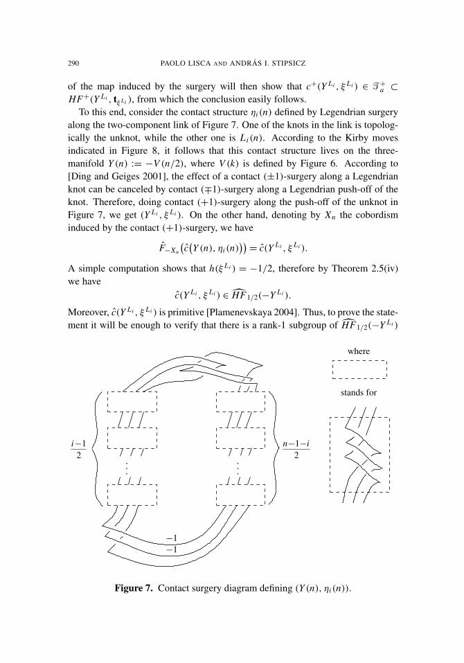
290 PAOLO LISCA AND ANDRÁS I. STIPSICZ
of the map induced by the surgery will then show that c+(Y L i , ξ L i ) ∈ T+a ⊂
HF+(Y L i , tξ Li ), from which the conclusion easily follows.To this end, consider the contact structure ηi (n) defined by Legendrian surgery
along the two-component link of Figure 7. One of the knots in the link is topolog-ically the unknot, while the other one is L i (n). According to the Kirby movesindicated in Figure 8, it follows that this contact structure lives on the three-manifold Y (n) := −V (n/2), where V (k) is defined by Figure 6. According to[Ding and Geiges 2001], the effect of a contact (±1)-surgery along a Legendrianknot can be canceled by contact (∓1)-surgery along a Legendrian push-off of theknot. Therefore, doing contact (+1)-surgery along the push-off of the unknot inFigure 7, we get (Y L i , ξ L i ). On the other hand, denoting by Xn the cobordisminduced by the contact (+1)-surgery, we have
F−Xn
(c(Y (n), ηi (n)
))= c(Y L i , ξ L i ).
A simple computation shows that h(ξ L i ) = −1/2, therefore by Theorem 2.5(iv)we have
c(Y L i , ξ L i ) ∈ HF1/2(−Y L i ).
Moreover, c(Y L i , ξ L i ) is primitive [Plamenevskaya 2004]. Thus, to prove the state-ment it will be enough to verify that there is a rank-1 subgroup of HF1/2(−Y L i )
. .....
i−12
n−1−i2
−1−1
where
stands for
Figure 7. Contact surgery diagram defining (Y (n), ηi (n)).

NOTES ON THE CONTACT OZSVÁTH–SZABÓ INVARIANTS 291
...
k fulltwists
−1 − k
0 0
k
−111
1
00
−k
1
−k−1
−V (k)
Figure 8. Kirby moves for Y (n).
containing
F−Xn
(c(Y (n), ηi (n)
))for every i . An easy computation shows that (since we assumed n to be even)the Thurston–Bennequin numbers of the knots L i (n) are all equal to 1, thanks to[Epstein et al. 2001]. Hence each of the three-manifolds Y L i is diffeomorphic toS3
0(L(n)). By Lemma 4.3,
HF+(−S3
0(L(n)))∼= T+
1/2 ⊕ T+
3/2 ⊕ A,
where A is a finitely generated abelian group, while by Lemma 4.4 we have
HF+(−Y (n))=
n+2⊕i=1
T+
ai

292 PAOLO LISCA AND ANDRÁS I. STIPSICZ
for some ai ∈ Q. Since F+
−Xnis U -equivariant and for sufficiently large h the action
of U h vanishes on A, we have
Im(F+
−Xn)⊆ T+
1/2 ⊕ T+
3/2 ⊆ HF+(−S3
0(L(n)
)).
Therefore, up to sign, there is a unique primitive element in Im(F+
−Xn) of degree
1/2, implying that c+(Y L i , ξ L i ) = c+(Y L j , ξ L j ) for i, j as in the statement ofTheorem 4.2. Since
HF+
−1/2
(−S3
0(L(n)
))= 0,
it follows that the homomorphism
f : HF1/2(−S3
0(L(n)
))→ HF+
1/2
(−S3
0(L(n)
))from Exact Sequence (2–1) is injective. Since
f (c(Y L i , ξ L i ))= c+(Y L i , ξ L i ) ∈ Im(F+
−Xn)
for every i , this concludes the proof. �
5. Distinguishing tight contact structures
Definition. Let ξi , for i =1, . . . , n−1, denote the contact structure on the Brieskornsphere −6(2, 3, 6n − 1) defined by the contact surgery specified by Figure 9.
Theorem 5.1. The contact invariants c+(ξ1), . . . , c+(ξn−1) are linearly indepen-dent over Z.
.
.
....i
left cuspsn−i−1
left cusps
−1
K1 −1
Figure 9. Contact structures on the three-manifold −6(2, 3, 6n−1).

NOTES ON THE CONTACT OZSVÁTH–SZABÓ INVARIANTS 293
.
.
....i
left cuspsn−i−1
left cusps
−1
Figure 10. The contact structure ηi on L(n, 1).
Proof. Consider the Legendrian push-off K1 of the Legendrian trefoil K1 of thefigure. Attach a four-dimensional two-handle along K1 to −6(2, 3, 6n − 1) withframing equal to the contact framing +1. Since contact (+1)-surgery along aLegendrian push-off cancels contact (−1)-surgery, we get a cobordism W suchthat F−W (c+(ξi )) = c+(ηi ), where ηi is the contact structure on L(n, 1) definedby Figure 10. The contact invariants c+(ηi ) are linearly independent because theybelong to groups corresponding to different spinc structures on the same lens spaceL(n, 1). Therefore, the invariants c+(ξi ) are also linearly independent, concludingthe proof. �
Corollary 5.2. The contact structures ξ1, . . . , ξn−1 are pairwise nonisotopic. �
This was first proved by Lisca and Matic [1997] using Seiberg–Witten theory.For a different Heegaard Floer theoretic proof (of a more general statement), see[Plamenevskaya 2004].
Remark. It is known [Ozsvath and Szabo 2003a] that HF+(−6(2, 3, 6n − 1))=T+
−2 ⊕ Zn−1(−2), therefore by Proposition 2.2, HF+(6(2, 3, 6n − 1)) = T+
2 ⊕ Zn−1(1) .
It follows from Theorem 5.1 that the elements c+(ξi ) (i = 1, . . . , n − 1) spanHF+
1 (6(2, 3, 6n − 1)).
If the trefoil knot of Figure 9 is replaced by any Legendrian knot L , the statementof Theorem 5.1 holds with the same proof. If tb(L) = 1 and rot(L) = 0, then thecontact resulting structures ξ1, . . . , ξn−1 are all homotopic as two-plane fields.
Acknowledgment
We thank Peter Ozsvath and Zoltan Szabo for many useful discussions regardingour joint work, and the referee for several useful comments and suggestions.

294 PAOLO LISCA AND ANDRÁS I. STIPSICZ
References
[Chekanov 2002] Y. Chekanov, “Differential algebra of Legendrian links”, Invent. Math. 150:3(2002), 441–483. MR 2003m:53153 Zbl 1029.57011
[Ding and Geiges 2001] F. Ding and H. Geiges, “Symplectic fillability of tight contact structures ontorus bundles”, Algebr. Geom. Topol. 1 (2001), 153–172. MR 2002b:53134 Zbl 0974.53061
[Ding and Geiges 2004] F. Ding and H. Geiges, “A Legendrian surgery presentation of contact3-manifolds”, Math. Proc. Cambridge Philos. Soc. 136:3 (2004), 583–598. MR 2005m:57038Zbl 1069.57015
[Ding et al. 2004] F. Ding, H. Geiges, and A. I. Stipsicz, “Surgery diagrams for contact 3-manifolds”,Turkish J. Math. 28:1 (2004), 41–74. MR 2005c:57028 Zbl 1077.53071
[Epstein et al. 2001] J. Epstein, D. Fuchs, and M. Meyer, “Chekanov–Eliashberg invariants andtransverse approximations of Legendrian knots”, Pacific J. Math. 201:1 (2001), 89–106. MR 2002h:57020 Zbl 1049.57005
[Etnyre 2003] J. B. Etnyre, “Introductory lectures on contact geometry”, pp. 81–107 in Topologyand geometry of manifolds (Athens, GA, 2001), edited by G. Matic and C. McCrory, Proc. Sympos.Pure Math. 71, Amer. Math. Soc., Providence, RI, 2003. MR 2005b:53139 Zbl 1045.57012
[Etnyre and Honda 2001] J. B. Etnyre and K. Honda, “Knots and contact geometry, I: Torus knotsand the figure eight knot”, J. Symplectic Geom. 1:1 (2001), 63–120. MR 2004d:57032 Zbl 1037.57021
[Etnyre and Honda 2005] J. B. Etnyre and K. Honda, “Cabling and transverse simplicity”, Ann. ofMath. (2) 162:3 (2005), 1305–1333. MR 2006j:57051
[Geiges 2006] H. Geiges, “Contact geometry”, pp. 315–382 in Handbook of differential geometry,vol. 2, edited by F. J. E. Dillen and L. C. A. Verstraelen, Elsevier, Amsterdam, 2006.
[Gompf and Stipsicz 1999] R. E. Gompf and A. I. Stipsicz, 4-manifolds and Kirby calculus, Grad-uate Studies in Mathematics 20, Amer. Math. Soc., Providence, RI, 1999. MR 2000h:57038Zbl 0933.57020
[Honda 2000] K. Honda, “On the classification of tight contact structures, I”, Geom. Topol. 4 (2000),309–368. MR 2001i:53148 Zbl 0980.57010
[Lisca and Matic 1997] P. Lisca and G. Matic, “Tight contact structures and Seiberg–Witten invari-ants”, Invent. Math. 129:3 (1997), 509–525. MR 98f:57055 Zbl 0882.57008
[Lisca and Stipsicz 2004a] P. Lisca and A. I. Stipsicz, “Ozsváth-Szabó invariants and tight contactthree-manifolds, I”, Geom. Topol. 8 (2004), 925–945. MR 2005e:57069 Zbl 1059.57017
[Lisca and Stipsicz 2004b] P. Lisca and A. I. Stipsicz, “Ozsváth-Szabó invariants and tight contactthree-manifolds, II”, preprint, 2004. To appear in J. Differential Geom. math.SG/0404136
[Ozbagci 2005] B. Ozbagci, “A note on contact surgery diagrams”, Internat. J. Math. 16:1 (2005),87–99. MR 2005k:57052 Zbl 1068.57026
[Ozsváth and Szabó 2003a] P. Ozsváth and Z. Szabó, “Absolutely graded Floer homologies and in-tersection forms for four-manifolds with boundary”, Adv. Math. 173:2 (2003), 179–261. MR 2003m:57066 Zbl 1025.57016
[Ozsváth and Szabó 2003b] P. Ozsváth and Z. Szabó, “Heegaard Floer homology and alternatingknots”, Geom. Topol. 7 (2003), 225–254. MR 2004f:57040
[Ozsváth and Szabó 2004a] P. Ozsváth and Z. Szabó, “Holomorphic disks and genus bounds”,Geom. Topol. 8 (2004), 311–334. MR 2004m:57024 Zbl 1056.57020

NOTES ON THE CONTACT OZSVÁTH–SZABÓ INVARIANTS 295
[Ozsváth and Szabó 2004b] P. Ozsváth and Z. Szabó, “Holomorphic disks and three-manifold invari-ants: properties and applications”, Ann. of Math. (2) 159:3 (2004), 1159–1245. MR 2006b:57017Zbl 1081.57013
[Ozsváth and Szabó 2004c] P. Ozsváth and Z. Szabó, “Holomorphic disks and topological invari-ants for closed three-manifolds”, Ann. of Math. (2) 159:3 (2004), 1027–1158. MR 2006b:57016Zbl 1073.57009
[Ozsváth and Szabó 2005] P. Ozsváth and Z. Szabó, “Heegaard Floer homology and contact struc-tures”, Duke Math. J. 129:1 (2005), 39–61. MR 2006b:57043 Zbl 1083.57042
[Ozsváth and Szabó 2006] P. Ozsváth and Z. Szabó, “Holomorphic triangles and invariants forsmooth four-manifolds”, Adv. Math. 202:2 (2006), 326–400.
[Plamenevskaya 2004] O. Plamenevskaya, “Contact structures with distinct Heegaard Floer invari-ants”, Math. Res. Lett. 11:4 (2004), 547–561. MR 2005f:53159 Zbl 1064.57031
[Rudolph 1993] L. Rudolph, “Quasipositivity as an obstruction to sliceness”, Bull. Amer. Math. Soc.(N.S.) 29:1 (1993), 51–59. MR 94d:57028 Zbl 0789.57004
Received February 12, 2005. Revised May 13, 2005.
PAOLO LISCA
DIPARTIMENTO DI MATEMATICA
UNIVERSITA DI PISA
LARGO BUONARROTI 5I-56127 PISA
ITALY
ANDRAS I. STIPSICZ
RENYI INSTITUTE OF MATHEMATICS
HUNGARIAN ACADEMY OF SCIENCES
H-1053 BUDAPEST
REALTANODA UTCA 13–15HUNGARY
[email protected] address:Institute for Advanced Study1 Einstein Drive Princeton, NJ 08540United States

PACIFIC JOURNAL OF MATHEMATICSVol. 228, No. 2, 2006
AN EXPLICIT EXAMPLE OF RIEMANN SURFACES WITHLARGE BOUNDS ON CORONA SOLUTIONS
BYUNG-GEUN OH
By modifying Cole’s example, we construct explicit Riemann surfaces withlarge bounds on corona solutions in an elementary way.
1. Introduction
For a given Riemann surface R, consider the algebra H∞(R) of bounded analyticfunctions on R separating the points in R. The corona problem asks whether ι(R)is dense in the maximal ideal space M(R) of H∞(R), where ι : R → M(R) is thenatural inclusion defined by the point evaluation. If ι(R) is dense in M(R), we saythat the corona theorem holds for R. Otherwise R is said to have corona.
The corona theorem holds for R if and only if the following statement is true (see[Gamelin 1978, Chapter 4] or [Garnett 1981, Chapter VIII]): for every collectionF1, . . . , Fn ∈ H∞(R) and any δ ∈ (0, 1) with the property
(1-1) δ ≤ maxj
|F j (ζ )| ≤ 1 for all ζ ∈ R,
there exist G1, . . . ,Gn ∈ H∞(R) such that
(1-2) F1G1 + F2G2 + · · · + FnGn = 1.
We refer to G1, . . . ,Gn as corona solutions, F1, . . . , Fn as corona data, andmax{‖G1‖, . . . , ‖Gn‖} as a bound on the corona solutions or corona constant.Here the notation ‖ · ‖ indicates the uniform norm. Throughout this paper, weassume that the corona data satisfies (1-1) for the given δ. The letter δ is reservedonly for this use.
Theorem 1 (B. Cole; see [Gamelin 1978, Theorem 4.1, pp. 47–49]). For anyδ ∈ (0, 1) and M > 0, there exist a finite bordered Riemann surface R and coronadata F1, F2 ∈ H∞(R) such that any corona solutions G1,G2 ∈ H∞(R) have abound at least M ; that is, max{‖G1‖, ‖G2‖} ≥ M.
MSC2000: 30H05, 30D55.Keywords: corona problem, bounded analytic function.
297

298 BYUNG-GEUN OH
The purpose of this paper is to construct the Riemann surface R in Theorem 1in an elementary way and describe it explicitly. Once Theorem 1 is proved, it ispossible to construct a Riemann surface with corona.
Theorem 2 (B. Cole; see [Gamelin 1978, Theorem 4.2, pp. 49–52]). There existsan open Riemann surface with corona.
The basic idea of the proof of Theorem 2 is that if a Riemann surface R isobtained by connecting two Riemann surfaces R1 and R2 with a thin strip, thenany holomorphic function on R behaves almost independently on R1 and R2.
The corona theorem holds for the unit disc [Carleson 1962], finitely connecteddomains in C [Gamelin 1970], Denjoy domains [Garnett and Jones 1985], and var-ious other classes of planar domains and Riemann surfaces [Alling 1964; Behrens1970; 1971; Jones and Marshall 1985; Stout 1965]. On the other hand, examplesof Riemann surfaces with corona (other than Cole’s) can be found in [Barrett andDiller 1998] and [Hayashi 1999]. Furthermore, by modifying the proof of Theorem2, Cole’s example can be used to obtain a Riemann surface R with corona that is ofParreau–Widom type [Nakai 1982]. (This means that
∑z∈E G(z, w)<+∞, where
G( · , w) is the Green’s function on R with the polew and E ={z : ∇G(z, w)= 0}.)The corona problem for a general domain in C is still open, and the answer is
also unknown for a polydisc or a unit ball in Cn , for n ≥ 2.
2. Proof of Theorem 1
For given δ ∈ (0, 1) and M > 0, we choose a natural number n such that δn≤
min{(16M)−1, 1
4
}. Let d = 4δn2
+n and c = 2δn2. Since 2δn2
< 2δn≤
12 , we have
(2-1)4δn+1
1 − c≤ 8δn+1 < 8δn
≤1
2M.
Moreover,
(2-2)d
c − d=
4δn2+n
2δn2− 4δn2+n
=2δn
1 − 2δn ≤ 4δn <1
2M.
The important features in our choice of c, d and n are that d1/n is small (equation(2-1)), d/c is small (equation (2-2)), and (d/c)1/n is not small — say greater thanδ.
Let D be the unit disc in C, B := B(0, d) = {z ∈ C : |z| < d}, and A := D\B.Further, define
D := {z : (z + c)/(1 + cz) ∈ A},
D1 := {z : zn∈ A} = {z : d/zn
∈ A},
D2 := {z : zn2∈ D}.

RIEMANN SURFACES WITH LARGE CORONA CONSTANTS 299
Thus D is the image of A under the Mobius transformation L(z) := (z−c)/(1−cz),and D1 and D2 are preimages of A and D under h1(z) := d/zn and h2(z) := zn2
.Finally we define the bordered Riemann surface
(2-3) R :=
{(z1, z2) ∈ C2
: z1 ∈ D1, z2 ∈ D2 andzn
1 − c1 − czn
1= zn2
2
}.
preimages of c
c
F2(z1, z2)= z2
h2(z)= zn2
h1(z)=dzn
F1(z1, z2)=d1/n
z1
A
D2D1
R
L(z)=z − c
1 − cz
B
D
Scheme of the construction of R, for n = 4.

300 BYUNG-GEUN OH
Note that R is an n-sheeted covering of D2 and an n2-sheeted branched coveringof D1. This is because D1 is an n-sheeted covering of A and D2 is an n2-sheetedbranched covering of D.
We claim that the Riemann surface R, together with the holomorphic functions
F1(z1, z2)=d1/n
z1and F2(z1, z2)= z2,
satisfies the conditions in Theorem 1.First, note that F1 and F2 have values in D1 and D2, respectively. Thus we have
max{‖F1‖, ‖F2‖} ≤ 1. Furthermore, if |F2(z1, z2)| = |z2|< δ, we have
|zn1 − c| = |z2|
n2|1 − czn
1 |< 2δn2,
and hence |z1|n < c + 2δn2
= 4δn2. Therefore
|F1(z1, z2)| =d1/n
|z1|>
41/nδn+1
41/nδn = δ,
and the inequality max{|F1(z1, z2)|, |F2(z1, z2)|}≥ δ holds for all (z1, z2)∈ R; i.e.,(F1, F2) becomes a pair of corona data for the given δ.
It remains to show that max{‖G1‖, ‖G2‖} ≥ M for any corona solutions G1,G2
such that
(2-4) F1G1 + F2G2 = 1.
In fact, we will show that ‖G1‖≥ M . To prove this claim, we assume, without lossof generality, that G1 and G2 are holomorphic across the boundary of R. Then wedefine for all z ∈ A,
f (z) :=1n3
∑F1(z1, z2)G1(z1, z2),
where the summation is over all the points (z1, z2) ∈ R such that zn1 = z, counting
multiplicity. (Note that the map (z1, z2) 7→ zn1 is an n3-sheeted branched covering
from R to A.) Then f is analytic in (a neighborhood of) A.Since F2(z1, z2)= z2 = 0 when zn
1 = c, it is easy to see from (2-4) that f (c)= 1.On the other hand, | f (z)| ≤ ‖G1‖ for all z ∈ A since ‖F1‖ ≤ 1, and | f (z)| ≤
4δn+1‖G1‖ for |z| = 1 since on {|z1| = 1} we have
|F1(z1, z2)| =d1/n
|z1|= 41/nδn+1
≤ 4δn+1.

RIEMANN SURFACES WITH LARGE CORONA CONSTANTS 301
Therefore, by Cauchy’s integral formula,
1 = | f (c)| =
∣∣∣∣ 12π i
∫|ξ |=1
f (ξ)ξ − c
dξ −1
2π i
∫|ξ |=d
f (ξ)ξ − c
dξ∣∣∣∣
≤4δn+1
‖G1‖
1 − c+
2πd‖G1‖
2π(c − d).
This inequality, together with (2-1) and (2-2), proves the claim. This completesthe proof.
3. Further remarks
1. In the construction of R, one can take F1 as the projection map (z1, z2) 7→ z1,but then it is necessary to modify the definition (2-3) of R to
R :=
{(z1, z2) ∈ C2
: z1 ∈ D1, z2 ∈ D2 andd/zn
1 − c1 − cd/zn
1= zn2
2
}because we want to make the pair (F1, F2) a set of corona data satisfying (1-1).
2. Consider the function h(z) := zn defined on D1. It is not difficult to see that theRiemann surface R constructed in Section 2 is nothing but the Riemann surface ofthe multivalued function
h−1◦ L−1
◦ h2(z)=
(zn2
+ c1 + czn2
)1/n
defined on D2. This function takes values in D1. Similarly, one can consider R asa Riemann surface of the multivalued function
h−12 ◦ L ◦ h(z)=
(zn
− c1 − czn
)1/n2
defined on D1.
3. We can construct R by cutting and pasting. For example, we can construct theRiemann surface of h−1
◦ L−1◦h2 over D2 in the following way: we make n2 cuts
on D2 radially so that each cut connects a hole to the outer boundary of D2 (i.e., tothe unit circle). We denote this region (D2 minus cuts) by D(1), and enumerate thecuts by e(1, k, l), k =1, . . . , n2, l =1, 2 so that e(1, k, 1)=e(1, k, 2) as sets, and asz approaches e(1, k, 1) the argument of z increases. Let D( j), j = 1, . . . , n, be thecopies of D(1) with the corresponding cuts e( j, k, l), j = 1, . . . , n, k = 1, . . . , n2,l = 1, 2. For all j (mod n), paste D( j) and D( j +1) by identifying e( j, k, 1) withe( j + 1, k, 2), k = 1, 2, . . . , n2. The resulting surface is conformally equivalentto R with the natural projection map π ≈ F2. By analytic continuation, the map

302 BYUNG-GEUN OH
h−1◦ L−1
◦h2 ◦π is well-defined on R, hence analytic. We leave the details to thereader.
4. One can recover the same Riemann surface R via interpolation problems. Fixε ∈ (0, 1
2) and let D′
1 := {z : ε < |z| < 1}. Choose a natural number n sufficientlylarge so that 2−n < ε, and let En be the set of n-th roots of 2−n . Note that |z| =
12
for all z ∈ En .We consider two interpolation problems:
(1) Find G1 ∈ H∞(D′
1) (with the smallest uniform norm) such that G1(z)= z forall z ∈ En .
(2) Find F2 ∈ H∞(D′
1) (with the largest δ0 := minz∈D′
1{|F2(z)|, |z|}) such that
‖F2‖ = 1 and F2(z)= 0 for all z ∈ En .
Any solution G1 of (1) has uniform norm greater than C/ε, for some absoluteconstant C . To see this, one can repeat the argument in Section 2; thus, for w suchthat εn < |w|< 1, define
f (w)=1n
∑zG1(z),
where the summation is over all z ∈ D′
1 such that (ε/z)n =w. Note that f (2nεn)= 14
since zG1(z) equals 14 for z ∈ En , and then Cauchy’s integral formula gives a lower
bound estimate ‖G1‖ ≥ C/ε.On the other hand, any solution F2 of (2) should yield a small δ0 =o(1) as ε→0.
To see this, let F1 = z and F2 be the solution of (2). Now if δ0 were not o(1), thepair (F1, F2) would become a set of corona data on D′
1 with corresponding 0<δ≤
lim infε→0 δ0. But then any corona solutions G1 and G2 such that F1G1+F2G2 =1would have a bound ≥C/ε, because G1/4 should be a solution of (1). This violatesthe corona theorem on annuli [Scheinberg 1963; Stout 1965]. (In fact, it violatesa statement slightly stronger than the corona theorem, which is true for annuli;namely, for any annulus D′
1 and corona data defined on D′
1, there always existcorona solutions with bound ≤ M = M(δ), where M does not depend on D′
1. See[Gamelin 1978, p. 47] for details.) Therefore to make F1 and F2 corona data, or toget a solution for (2) with large δ0, we take a number N such that the multivaluedfunction
F(z)=
(zn
− 2−n
1 − 2−nzn
)1/N
,
has modulus ≥14 for |z| < 1
4 . (Such an N should be asymptotically greater thana fixed multiple of n2 as n → ∞, as we have seen in Section 2. Also note thatF N is a solution for (2).) Now since F is not analytic on D′
1, we consider theRiemann surface of F over D′
1, which gives us the Riemann surface R constructedin Section 2 (with δ =
14 ).
RIEMANN SURFACES WITH LARGE CORONA CONSTANTS 303
Acknowledgement
The author deeply thanks Donald Marshall for his invaluable assistance with thiswork. He also thanks D. Drasin, A. Eremenko, T. Gamelin, M. Hayashi, andS. Rohde for their helpful suggestions and encouragement.
References
[Alling 1964] N. L. Alling, “A proof of the corona conjecture for finite open Riemann surfaces”,Bull. Amer. Math. Soc. 70 (1964), 110–112. MR 28 #209 Zbl 0124.04202
[Barrett and Diller 1998] D. E. Barrett and J. Diller, “A new construction of Riemann surfaces withcorona”, J. Geom. Anal. 8:3 (1998), 341–347. MR 2000j:30076 Zbl 0956.30023
[Behrens 1970] M. Behrens, “The corona conjecture for a class of infinitely connected domains”,Bull. Amer. Math. Soc. 76 (1970), 387–391. MR 41 #825 Zbl 0197.11502
[Behrens 1971] M. F. Behrens, “The maximal ideal space of algebras of bounded analytic functionson infinitely connected domains”, Trans. Amer. Math. Soc. 161 (1971), 359–379. MR 55 #8380Zbl 0234.46057
[Carleson 1962] L. Carleson, “Interpolations by bounded analytic functions and the corona prob-lem”, Ann. of Math. (2) 76 (1962), 547–559. MR 25 #5186 Zbl 0112.29702
[Gamelin 1970] T. W. Gamelin, “Localization of the corona problem”, Pacific J. Math. 34 (1970),73–81. MR 43 #2482 Zbl 0199.18801
[Gamelin 1978] T. W. Gamelin, Uniform algebras and Jensen measures, London MathematicalSociety Lecture Note Series 32, Cambridge University Press, Cambridge, 1978. MR 81a:46058Zbl 0418.46042
[Garnett 1981] J. B. Garnett, Bounded analytic functions, Pure and Applied Mathematics 96, Aca-demic Press, New York, 1981. MR 83g:30037 Zbl 0469.30024
[Garnett and Jones 1985] J. B. Garnett and P. W. Jones, “The corona theorem for Denjoy domains”,Acta Math. 155:1-2 (1985), 27–40. MR 87e:30044 Zbl 0578.30043
[Hayashi 1999] M. Hayashi, “Bounded analytic functions on Riemann surfaces”, pp. 45–59 in As-pects of complex analysis, differential geometry, mathematical physics and applications (St. Kon-stantin, 1998), edited by K. S. Stancho Dimiev, World Sci., River Edge, NJ, 1999. MR 2001i:30045Zbl 0962.30023
[Jones and Marshall 1985] P. W. Jones and D. E. Marshall, “Critical points of Green’s function,harmonic measure, and the corona problem”, Ark. Mat. 23:2 (1985), 281–314. MR 87h:30101Zbl 0589.30028
[Nakai 1982] M. Nakai, “Corona problem for Riemann surfaces of Parreau–Widom type”, Pacific J.Math. 103:1 (1982), 103–109. MR 85c:30047 Zbl 0565.30028
[Scheinberg 1963] S. Scheinberg, Hardy spaces and boundary problems in one complex variable,Ph.D. thesis, Princeton University, 1963.
[Stout 1965] E. L. Stout, “Bounded holomorphic functions on finite Reimann surfaces”, Trans. Amer.Math. Soc. 120 (1965), 255–285. MR 32 #1358 Zbl 0154.32903
Received June 12, 2005.

304 BYUNG-GEUN OH
BYUNG-GEUN OH
KOREA INSTITUTE FOR ADVANCED STUDY
207-43 CHEONGNYANGNI 2-DONG
DONGDAEMUN-GU
SEOUL 130-722KOREA

PACIFIC JOURNAL OF MATHEMATICSVol. 228, No. 2, 2006
CLOSED SUBSETS OF THE WEYL ALCOVE AND TQFTS
STEPHEN F. SAWIN
For an arbitrary simple Lie algebra g and an arbitrary root of unity q, weclassify the closed subsets of the Weyl alcove of the quantum group Uq(g).Here a closed subset is a set such that if any two weights in the Weyl alcoveare in the set, so is any weight in the Weyl alcove which corresponds to anirreducible summand of the tensor product of a pair of representations withhighest weights the two original weights. The ribbon category associated toeach closed subset admits a “quotient” by a trivial subcategory as describedby Bruguières and Müger, to give a modular category and a framed three-manifold invariant or a spin modular category and a spin three-manifoldinvariant, as proved by the author.
Most of these theories are equivalent to theories defined in Sawin, Adv.Math. 165 (2002), 1–70, but several exceptional cases represent the firstnontrivial examples of theories that contain noninvertible trivial objects,making the theory much richer and more complex.
Introduction
Quantum groups, that is, quantized universal enveloping algebras of simple Liealgebras, together with their representation theory, have been the subject of muchfruitful investigation, and are of interest from many perspectives, but one partic-ularly important application is to link and three-manifold invariants. The generalsetting is that these quantum groups are ribbon Hopf algebras, and hence theirrepresentation theory forms a ribbon category, from which one can construct aninvariant of links and more generally labeled graphs embedded in S3 with similarproperties to the original Jones polynomial. When the complex parameter q onwhich these algebras depend is a root of unity, their representation theory satisfiesthe more restrictive requirements of a modular category, from which one can con-struct a three-manifold invariant which satisfies Atiyah’s axioms for topologicalquantum field theory. More specifically, the set of representations spanned bythe subset of the irreducible representations in the Weyl alcove, with the ordinary
MSC2000: primary 17B37; secondary 57M27.Keywords: TQFT, quantum groups, Weyl alcove, ribbon category.
305

306 STEPHEN F. SAWIN
tensor product of representations replaced by the truncated tensor product, formsa modular category.
Any subset of the Weyl alcove which spans a set of representations closed underboth duality and the truncated tensor product determines a new ribbon categorywhich is a full subcategory of the original. Of course this subcategory encodesonly a subset of the link information of the original theory, and on this basis doesnot seem of interest. However, if this ribbon subcategory happens to be modular,there is no reason to think that the resulting three-manifold invariant is determinedby the original three-manifold invariant, and in fact it is not apparent that it hasany connection with the original. Thus finding closed subsets of the Weyl alcovewhich are modular is an important question.
In fact, the modularity requirement can be relaxed quite a bit. Muger [2000] andBruguieres [2000] have shown that under favorable circumstances which hold forthe quantum group examples (e.g., the existence of a unitary structure) a ribbon cat-egory admits a kind of quotient which yields a modular category in the absence of acertain easily identifiable obstruction. In fact, even in the presence of this obstruc-tion [Sawin 2002a] a similar process yields an invariant of spin three-manifolds.Thus a classification of the closed subsets of the Weyl alcove, together with anidentification of the quotient and when the quotient yields a modular category,would give a complete summary of the invariants of three-manifolds which can beconstructed out of the Weyl alcove in this fashion. The present article classifiesthe closed subsets of the Weyl alcove and describes the subcategory of so calleddegenerate objects by which one quotients.
A second reason for considering the closed subsets of the Weyl alcove is thatthey might plausibly correspond to quotients of the quantum group, or at least ofa subalgebra. In fact in the classical case the closed subsets of the Weyl chambercorrespond exactly to quotients of the simply connected groups by a subgroup ofthe center: i.e., there is a one-to-one correspondence between closed subsets of theWeyl chamber on the one hand and Lie groups with the given Lie algebra on theother. Thus quotients associated to closed subsets of the Weyl alcove, if they exist,might be viewed as quantum analogues of the nonsimply connected groups.
Finally, in the course of the classification we shall construct some unexpectedtheories at level k = 2. Some of these theories (associated to the quantum group oftype Bn and Dn) appear to give new invariants and admit skein relations that suggestwe might be able to compute for these theories much of what can be computed inthe SU(2) (i.e., A1) theory. Nevertheless, these theories exhibit novel behavior(specifically, the subcategory of degenerate objects is the representation categoryof a nonabelian group) worthy of further study.
The analysis of the closed subsets of the Weyl alcove was begun in [Sawin2002b]. There closed subsets which correspond precisely to the classical closed

CLOSED SUBSETS OF THE WEYL ALCOVE AND TQFTS 307
subsets, i.e., to nonsimply connected Lie groups, were found and their invariantsidentified. These subsets correspond to Chern–Simons theories for nonsimply con-nected Lie groups conjectured by Dijkgraaf and Witten [1990]. A second collectionof closed subsets was also identified and classified there. These subsets, associatedwith certain corners of the Weyl alcove, formed very simple ribbon categories (infact the category associated to the group algebra of an abelian group, with a mildlydeformed R-matrix) and manifold invariants depending only on homology whichhad been studied by Murakami, Ohtsuki and Okada [Murakami et al. 1992]. Herewe complete the identification of the closed subsets of the Weyl alcove, demon-strating that the closed subsets given above are the only ones except for certainspecial cases at level k = 2.
The paper is organized as follows. Section 1 introduces the needed facts aboutLie algebras, quantum groups and the truncated tensor product, which can allbe found in [Humphreys 1972; Kirillov 1996; Kassel 1995; Turaev 1994; Sawin2002b]. Sections 2 and 3 give the classification of the closed subsets, and Section4 identifies when the quotient is modular and what the resulting invariant is for theexceptional cases not discussed in [Sawin 2002b]. Finally Section 5 shows that theclosure under duality condition on closed subsets is implied by the closure undertensor products. This observation is fairly independent of the rest of the paper, butis a natural question. In particular it is of great relevance when using skein theoryand cabling to explore link and three-manifold invariants; see for example [Turaevand Wenzl 1993; Wenzl 1993].
1. Quantum groups and the Weyl alcove
Let g be a simple Lie algebra and let {αi }i≤r be the simple roots of g. Theweight lattice3 is spanned by the fundamental weights {λi }i≤r given by (λi , α j )=
δi, j (αi , αi )/2.The Weyl group is denoted by W, and the set of weights in the fundamental Weyl
chamber is called 3+ (we will loosely refer to this set itself as the Weyl chamber).Half the sum of the positive roots is called ρ, the unique short root in the Weylchamber is called β, and the unique long root in the Weyl chamber is called θ (inthe simply laced case either will refer to the unique root in the Weyl alcove). Theroot θ is the highest weight of the adjoint representation of g. The dual Coxeternumber h is defined to be (ρ, θ)+ 1, the value of the quadratic Casimir on theadjoint representation.
Let q = e2π i/(k+h), for some natural number k. Recall that there is an irreduciblerepresentation Vλ of the quantum group Uq(g) for each weight λ in the Weyl al-cove 30, i.e., weights λ ∈ 3+ such that (λ, θ) ≤ k. Kirillov [1996] shows thatthe category of representations of the quantum group which are a direct sum of

308 STEPHEN F. SAWIN
representations in the Weyl alcove forms a semisimple ribbon ∗-category if theordinary tensor product is replaced by the truncated tensor product, ⊗, whichis the maximal subspace of the ordinary tensor product isomorphic to a directsum of representations in the Weyl alcove (since we will never use the ordinarytensor product in this article, we use ⊗ for the truncated tensor product withoutconfusion). Kirillov’s q is normalized a bit differently from what we use here,which follows the conventions of [Sawin 2002b], but because of differences inthe normalization of the quantum group defining relations, the above sentence stillholds, and determines the normalization. The truncated tensor product operationon the lattice of isomorphism classes of representations in the category (with directsum as addition) forms a commutative, distributive, associative multiplication withthe trivial representation V0 acting as identity, determined by
Vλ⊗Vγ ∼=
⊕η∈30
N ηλ,γ � Vη,
where N ηλ,γ are nonnegative integers and N � V indicates the direct sum of N
copies of the representation V (or equivalently, the tensor product of V with an N -dimensional trivial representation). In [Sawin 2006] we gave the following formulafor these numbers, generalizing a result from [Andersen and Paradowski 1995]:
(1–1) N ηλ,γ =
∑σ∈W0
(−1)σmγ (λ− σ(η)),
where mλ(µ) is the dimension of the µ weight space inside the classical represen-tation of highest weight λ and W0 is the quantum Weyl group, which is generatedby reflection about the hyperplanes {x |(x + ρ, αi ) = 0} for each simple root αi
together with {x |(x, θ)= k + 1}. Also
Cλ = q(λ,λ+2ρ)/2
and qdim(λ) > 0, where qdim(λ) is the invariant of the unknot and Cλ is the factorwhich a full twist applies to the link invariant.
For simplicity, since we will only ever need to consider representations up toisomorphism, we will confuse the (isomorphism class of the) representation Vλwith the weight λ, for example writing λ⊗γ =
⊕η N η
λ,γ � η. Caution should beused with the operations ⊕ and �, because the weights are elements of the weightlattice and therefore admit a lattice addition and scalar multiplication denoted byλ+ γ and nλ, respectively, which we will also make frequent use of. Note thatλ+γ 6= λ⊕γ , and nλ 6= n�λ. In particular, 0 is the additive identity in the lattice,but is the multiplicative identity for ⊗. We hope that the brevity of the notationoutweighs this modest awkwardness.

CLOSED SUBSETS OF THE WEYL ALCOVE AND TQFTS 309
Theorem 0 [Sawin 2002b]. There is an injection ` from Z(G), the center of thesimply connected Lie group with Lie algebra g, to the fundamental weights of theWeyl alcove such that z acts on the classical representation Vγ as
exp(2π i(γ, `(z))) · idγ .
The fundamental weights λi in the image of ` are exactly those for which (λi , θ)=1and the associated root αi is long, and are also exactly those for which there is aunique element τi of the classical Weyl group sending the standard base to the base{α j } j 6=i ∪{−θ}. If we define φi (γ )= kλi +τi (γ ), then φi is an isometry of the Weylalcove and of the simplex {λ : (λ, α j )≥ 0 and (λ, θ)≤ k} and φi (λ⊗γ )=φi (λ)⊗γ
If we use k also to represent the map on the weight lattice which multiplies eachweight by the number k, then k` is a homomorphism in the sense that k`(zz′) =
k`(z)⊗k`(z′). Weights in the range of k` can be characterized as extreme points ofthe simplex {λ : (λ, α j )≥ 0 and (λ, θ)≤ k} such that a neighborhood of the weight0 intersected with the simplex is isometric to a neighborhood of the extreme pointintersected with the alcove, the isometry being given by φi .
If Z is a subgroup of Z(G), let 1Z be the image of Z under k`. The subsetof the Weyl chamber consisting of weights γ such that Z acts trivially on Vγ isthe intersection of the Weyl chamber with a sublattice of the weight lattice, and itselements are in one-to-one correspondence with representations of the Lie groupG/Z . The intersection 0Z of this set with the Weyl alcove may be thought ofloosely as the “Weyl alcove for quantized G/Z ,” and consists of those weights γin the alcove for which (γ, `(z)) is an integer for all z ∈ Z.
A few key facts about the truncated tensor product were proven in [Sawin2002b].
Lemma 1. For any σ in the classical Weyl group W, and any weights γ , λ in theWeyl alcove, if λ+ σ(γ ) is in the Weyl alcove, then λ⊗γ contains λ+ σ(γ ) as asummand.
Lemma 2. λ⊗λ† contains as a summand θ if k ≥ 2 and λ is not a corner (i.e.a multiple of a fundamental weight such that (λ, θ) = k). In the nonsimply lacedcase it contains as a summand β unless (λ, αi )= 0 for every short simple root αi .
We say a fundamental weight λi is long or short according to whether αi is longor short. We say a long weight λi is sharp or dull according to whether 〈λi , θ〉 = 1or not. Finally, we say that a weight λ is a long, short, sharp or dull corner if〈λ, θ〉 = k and it is a multiple of a fundamental weight with the correspondingproperty. Thus for example the above lemmas tell us that λ⊗ λ† contains θ or βas a summand unless λ is a dull corner.

310 STEPHEN F. SAWIN
2. Closed subsets
Following [Sawin 2002b], we say that a subset 0 of the set of representations inthe Weyl alcove30 is closed if it is closed under duals (for every γ ∈0, the weightγ † of the dual representation is in 0) and under the truncated tensor product (ifλ, γ ∈ 0 then every η such that N η
λ,γ 6= 0, i.e. such that η corresponds to a directsummand of λ⊗γ , is in 0). We will see in Section 5 that in the quantum groupscase the second condition implies the first. Such subsets correspond exactly toribbon subcategories, and Muger [2000] showed that if they meet a certain easilychecked condition they admit a quotient which is modular and gives a TQFT andthree-manifold invariant. The following theorem gives a complete classificationof closed subsets of the Weyl alcove. The proof encompasses this and the nextsection.
Theorem 1. The closed subsets of the Weyl alcove are:
(a) For any subgroup Z ⊂ Z(G), the set 0Z .
(b) For any subgroup Z ⊂ Z(G), the set 1Z .
(c) For k = 2,(1) E7 the set {0, λ6},(2) E7 with set {0, λ2, 2λ7},(3) E8 with set {0, λ1},(4) Bl with set {0, 2λ1, λ j , λ2 j , . . . , λ(n−1) j/2} where j > 2 and 2l + 1 = nj ,(5) Dl with set {0, 2λ1, λ j , λ2 j , . . . , λ(n−1) j , 2λl−1, 2λl} where j > 2 and l =
nj ,(6) Dl with set {0, 2λ1, λ j , λ2 j , . . . , λ(n−1) j/2} where j > 2 and 2l = nj for n
odd.Here the λi are the fundamental weights ordered as in [Humphreys 1972]. Wewill call (1)–(6) the exceptional closed subsets.
Before embarking on a proof of the theorem, some general discussion is in order.Equation (1–1) is difficult to use in general, but we will find it suffices for most ofour purposes to examine it carefully only when one of the factors is θ or β. Ourstrategy will be to show that for any λ which is not in one of these exceptionalcases and not a sharp corner(and therefore not in the image of k`) an appropriatetensor product of factors of λ and λ† contains θ or β. It will be easy to see that anyclosed subset containing θ or β is of the first type in the theorem. By Lemma 2, θor β is contained in a tensor product of copies of λ and λ† unless λ is a long corner.
By Lemma 1, λ⊗β will contain as a summand with multiplicity one everyweight λ+ α for which α is a root (or a short root in the nonsimply laced case)and λ+ α is in the Weyl alcove. Thus a crucial question is this : Given any dullcorner λ, for which α is λ+ α in the Weyl alcove? Of course if λi + α is in the

CLOSED SUBSETS OF THE WEYL ALCOVE AND TQFTS 311
Weyl alcove for k = (θ, λi ) (i.e. when λi is a corner), then nλi +α is in the Weylalcove whenever nλi is a corner.
Below we list for each dull λi the roots (or in the nonsimply laced case shortroots) α such that λi +α is in the Weyl alcove for k = (λi , θ). The labeling of theroots and fundamental weights are as in [Humphreys 1972]. The roots are writtenout as a sum of simple roots and θ in such a way that each additional simple roothas negative inner product with the sum up to that point (as can be checked usingthe Cartan matrix: see Humphreys, p. 59), confirming recursively that the sum is aroot. That the root is short in the nonsimply laced case and that the entire sum hasnonnegative inner product with each simple root and inner product with θ less thanor equal to that of λi can be checked from the Cartan matrix and the expansion ofθ (Humphreys, p. 66).
Bl : For 2 ≤ i ≤ l − 1. λi +αi+1 +αi+2 + · · · +αl , λi − (αi +αi+1 + · · · +αl).
Cl : λl +α1 +α2 + · · · +αl−1, λl − (α1 + · · · +αl).
Dl : For 2 ≤ i ≤ l −2. λi − (αi−1 +αi +· · ·+αl−2 +αl−1 +αl +αl−2 +· · ·+αi ),λi +αi+1+αi+2+· · ·+αl−2+αl−1+αl +αl−2+αl−3+· · ·+αi+2 (for the cases i =
l−2, and i = l−3 the last formula should read λl−2+αl−1 and λl−3+αl−2+αl−1+αl
respectively).
E6: λ2 + α1 + α3 + α4 + α5 + α6, λ2 − θ . λ3 + α1, λ3 − θ + α2 + α4 + α5 + α6,λ4 +α1 +α3, λ4 +α5 +α6, λ4 − θ +α2. λ5 +α6, λ5 − θ +α2 +α4 +α3 +α1.
E7: λ1+α3+α4+α5+α6+α7+α2+α4+α5+α6, λ1−θ . λ2−θ+α1+α3+α4+
α5 +α6 +α7. λ3 +α2 +α4 +α5 +α6 +α7, λ3 −θ−α1. λ4 +α2, λ4 +α5 +α6 +α7.λ5+α6+α7, λ5−θ+α1+α3+α4+α2. λ6+α7, λ6−θ+α1+α3+α4+α5+α4+α3.
E8: λ1 − θ + α8 + α7 + α6 + α5 + α4 + α3 + α2 + α4 + α5 + α6 + α7, λ1 −
(α3 + α4 + α2 + α5 + α6 + α7 + α8 + α4 + α5 + α6 + α7). λ2 − θ + α1 + α3 +
α4 + α5 + α6 + α7 + α8, λ2 − (α2 + α4 + α3 + α1 + α5 + α6 + α4 + α3 + α5 +
α4 + α2). λ3 + α1, λ3 − (α1 + α3 + α4 + α2 + α5 + α4 + α3). λ4 + α1 + α3,λ4 + α2. λ5 + α1 + α3 + α4 + α2, λ5 − θ + α6 + α7 + α8. λ6 + α1 + α3 + α4 + α2,λ6 − θ + α7 + α8. λ7 + α1 + α3 + α4 + α2 + α5 + α6 + α4 + α3 + α5 + α4 + α2,λ7 − θ +α8. λ8 + θ −α8 −α7 −α6 −α5 −α4 −α3 −α2 −α4 −α5 −α6 −α7 −α8,λ8 − θ .
F4: λ1 +α2 +α3 +α4 +α3, λ1 − (α1 +α2 +α3). λ2 +α3 +α4, λ2 − (α2 +α3).
G2: λ2 +α1, λ2 − (α1 +α2).
We see from this list that for each of the nonsimply laced algebras except Bl thereis a short root α such that θ + α is in the Weyl alcove for k ≥ 2 (For Cl we haveθ = λl and α= α1 +α2 +· · ·+αl−1; for F4, θ = λ1 and α= α2 +α3 +α4 +α3; andfor G2, θ = λ2 and α= α1). Thus by Equation (1–1) N θ+α
θ,θ contains a contribution

312 STEPHEN F. SAWIN
from σ = 1 since mθ (α)= 1. In order for it to contain a contribution for some otherσ , that σ would have to be a reflection about a short root αi such that (θ+α, αi )=0and α − αi is long. If α − αi is long then (α, αi ) = 0. One can easily check bydirect computation that there is no such αi in any of these case. Therefore θ⊗θcontains θ + α, so θ⊗θ⊗θ contains (θ + α)⊗θ , which by Lemma 1 contains β.For Bl when k > 2 the same argument applies to θ + β. When k = 2 we will seebelow that a power of θ contains 2λl , which is a short corner and hence a higherpower contains β. We conclude that if a closed subset of the Weyl alcove containsθ , it also contains β.
Lemma 3. If a closed subset of the Weyl alcove contains β, it is of the form 0Z forsome Z.
Proof. Consider λ in the root lattice and in the Weyl alcove, and choose a pathin the root lattice connecting λ to 0 such that the difference between successivepoints in the path is a short root. By reflecting about hyperplanes of reflectionin the quantum Weyl group we can replace it by such a path crossing fewer suchhyperplanes, and by induction can find such a path entirely within the alcove. Thenby Lemma 1 λ is contained in β⊗n , where n is the length of this path. Thus if aclosed subset contains β it contains all of the root lattice 3r .
If λ, γ are in the Weyl alcove and in the same coset of 3/3r , their difference isin the root lattice, and thus any closed subset containing one of these and β containsthe other. So any closed subset containing β is a union of cosets intersected withthe Weyl alcove. The tensor product of two weights is a nonempty sum (becausethe quantum dimensions are nonzero) and is in the product of their cosets, so the setof cosets making up such a closed subset is a subgroup of 3/3r . This proves thatthe closed subset is in the intersection of the preimage of a subgroup of3/3r withthe Weyl alcove. By Theorem 0 the map sending z ∈ Z(G) to exp(2π i(`(z), ·)) ∈
(3/3r )∗ is a group isomorphism. So such a subgroup is dual to some subgroup
Z ⊂ Z(G), and the closed subset is exactly 0Z . �
Now if λ is a dull corner it is a multiple of one of the weights in the chart above.If λi +α is in the Weyl alcove for k = (λi , θ), then nλi +α is in the Weyl alcove fork = n(λi , θ). So from the chart there are at least two elements of the Weyl alcovea short root away from λ, except if λ is a multiple of λ2 for E7. In this exceptionalcase λ2/2 −α2 is in the Weyl alcove, so there are still at least two elements of thealcove a short root away from λ except when λ = λ2 and k = 2. Thus with thisexception if λ is a dull corner then by Lemma 1 λ⊗β contains two weights. Buteach of these weights when tensored with β contain λ, so λ⊗β⊗β contains λ withmultiplicity at least 2. Therefore λ⊗λ† contains two weights in β⊗β. Of courseone is the trivial weight, so the other must be of the form β +α for α a short root

CLOSED SUBSETS OF THE WEYL ALCOVE AND TQFTS 313
different from −β. If this β+α is not a corner dual to a long root, a tensor powerof it then contains β.
3. Proof of the Theorem
Proof of Theorem 1. It was shown in [Sawin 2002b] that the subsets of the form0Z and 1Z are closed . We will see below that the exceptional cases are closed bycomputing the truncated tensor product completely. So we have only to show thatevery closed subset is of this form.
We will assume the closed set contains some λ not in the image of k`, and showit is either the exceptional case or it contains θ or β, in which case by Lemma 3 itfalls into the first category. By Lemma 2 we may assume λ is a corner dual to along root.
Case k = 1. There are no dull corners, so there is nothing to prove.
Case k = 2. Except for λ2 of E7 if λ is a corner dual to a long root and not in therange of k` then λ⊗λ† contains something nontrivial in β⊗β, so we may assumethat λ is a such a corner and λ⊗λ† contains a summand of the form β+α for α ashort root.
• For Al , there are no dull corners.
• For Bl , there is nothing to prove if l = 2, so assume l > 2. The Weyl alcoveconsists of λi for i ≤ l and 2λ1 and 2λl . By checking which differences amongthese are short roots and noting λ1 = β we conclude
λi⊗λ1 =
λi−1 ⊕ λi+1 for 1< i < l − 1,
0 ⊕ 2λ1 ⊕ λ2 for i = 1,
2λl ⊕ λl−2 for i = l − 1,
λl for i = l,
2λl⊗λ1 = 2λl ⊕ λl−1,
2λ1⊗λ1 = λ1,
2λ1⊗2λ1 = 0.
From this we conclude recursively that
2λ1⊗λi = λi for i ≤ l,
2λ1⊗2λl = 2λl,

314 STEPHEN F. SAWIN
λi⊗λ j =
λi− j ⊕ λi+ j for l > i > j and i + j < l
λi− j ⊕ 2λl for l > i > j and i + j = l, l + 1
λi− j ⊕ λ2l+1−i− j for l > i > j and i + j > l + 1
0 ⊕ 2λ1 ⊕ λ2i for l > i = j and 2i < l
0 ⊕ 2λ1 ⊕ 2λl for l > i = j and 2i = l, l + 1
0 ⊕ 2λ1 ⊕ λ2l+1−2i for l > i = j and 2i > l + 1.
Notice first of all that a closed subset containing λ2 = θ will contain λi for alleven i < l. In particular it must contain either λl−2 or λl−1, so it must contain 2λl ,and therefore since this is a short corner it must contain β. Thus we recover ourpromised assertion that even for Bl at level k = 2, a closed subset containing θcontains β and therefore is of the from 0Z .
Let 0 be a closed subset which is not of the form 0Z or 1Z . We know that 0cannot contain λ1, λ2, λl or 2λl , or else it would be of the form 0Z , and 0 mustcontain something other than 0 and 2λ1. So let j be the least j such that λ j ∈ 0.Necessarily l > j > 2. By the product rules above λ j , λ2 j , λ3 j , . . . ∈ 0Z . Supposem is the largest such that λmj ∈0. Then every summand of λmj⊗λ j is in 0. Clearly(m + 1) j ≥ l, and in fact (m + 1) j > l + 1, or else 2λl ∈ 0. So we conclude thatλ2l+1−(m+1) j ∈ 0. Now mj < l < (m +1) j so 2l +1− (m +1) j is within j of mj .If they are not equal then λmj⊗λ2l+1−(m+1) j contains λi where i is this difference,contradicting the minimality of j . Thus we conclude mj = 2l +1− (m +1) j , and0 contains set (4) in the statement of the theorem, with n = 2m +1. If it containedany λi not in this set, there would be p such that |i − pj | < j , and hence λ|i−pj |
would be in the set, contradicting the minimality of j .
• For Cl there is nothing to prove since θ is the only dull corner.
• For Dl at k = 2 the weights are λi for 1 ≤ i ≤ l, 2λ1, 2λl−1, 2λl , and λl−1 + λl .By checking which differences among these are roots we see
λi⊗θ =
λ1 ⊕ λ3 for i = 1
0 ⊕ 2λ1 ⊕ λ4 for i = 2
λi−2 ⊕ λi+2 for 2< i < l − 3
λl−5 ⊕ (λl−1 + λl) for i = l − 3
λl−4 ⊕ 2λl ⊕ 2λl−1 for i = l − 2.
Since 2λ1 is in the range of k` and hence invertible, it follows 2λ1⊗θ = θ .Since λ1⊗λ1 contains 2λ1 by Lemma 1, we conclude 2λ1⊗λ1 = λ1 so inductively

CLOSED SUBSETS OF THE WEYL ALCOVE AND TQFTS 315
2λ1⊗λi = λi for i < l − 1. Similarly
2λl⊗θ = λl−2,
2λl−1⊗θ = λl−2,
2λl⊗2λ1 = 2λl−1,
2λl−1⊗2λ1 = 2λl .
Since λ1⊗θ contains λ1, it is clear that λ1⊗λ1 contains 0, θ , and 2λ1, each withmultiplicity one. Notice that by Equation (1–1), η is not a direct summand of λ⊗γif the distance between λ and η is more than ‖γ ‖ (this is argued explicitly in theproof of [Sawin 2002b, Lemma 2]). Noting that ‖λ1‖ = 1 and computing ‖λ−λ1‖
for λ= λi with 2< i < l − 1 and λ= λl−1, λl, (λl−1 + λl) we conclude
λ1⊗λ1 = 0 ⊕ θ ⊕ 2λ1.
It then follows recursively that
λi⊗λ1 =
λi−1 ⊕ λi+1 for 1< i < l − 2
λl−3 ⊕ (λl−1 + λl) for i = l − 2,
(λl−1 + λl)⊗λ1 = λl−2 ⊕ 2λl−1 ⊕ 2λl,
2λl−1⊗λ1 = λl−1 + λl,
2λl⊗λ1 = λl−1 + λl .
Finally, we get recursively from this
λi⊗λ j =
λi− j ⊕ λi+ j for j < i < l − 1 and i + j < l − 1
λi− j ⊕ (λl−1 + λl) for j < i < l − 1 and i + j = l − 1, l + 1
λi− j ⊕ 2λl−1 ⊕ 2λl for j < i < l − 1 and i + j = l
λi− j ⊕ λ2l−i− j for l > i > j and i + j > l + 1
0 ⊕ 2λ1 ⊕ λi+ j for j = i < l − 1 and i + j < l − 1
0 ⊕ 2λ1 ⊕ (λl−1 + λl) for j = i < l − 1 and 2i = l − 1, l + 1
0 ⊕ 2λ1 ⊕ 2λl−1 ⊕ 2λl for j = i < l − 1 and 2i = l
0 ⊕ 2λ1 ⊕ λ2l−2i for j = i < l and 2i > l + 1,
λ⊗λ j =
λl−1 + λl for λ= 2λl−1 or λ= 2λl and j = 1
λl− j for λ= 2λl−1 or λ= 2λl and 1< j < l − 1.

316 STEPHEN F. SAWIN
Thus if the closed subset 0 contains λ1, λ2, λl−1, λl or λl−1 + λl it contains θand is of the form 0Z . If it contains only a subset of 0, 2λ1, 2λl−1, and 2λl it is ofthe form 1Z . If 0 is not of the form 0Z or 1Z then it must contain λ j for some2 < j < l − 1, so suppose j is the least such. Then 0 contains λ j , λ2 j , . . . , λmj ,where m is the greatest such that mj < l−1. Again 0 must contain every summandof λmj⊗λ j . Then by the maximality of m we know (m + 1) j > l − 2, and since 0cannot contain λl−1 + λl we know (m + 1) j 6= l − 1, l + 1. If (m + 1) j = l, then0 contains {0, 2λ1, λ j , λ2 j , . . . , λmj , 2λl−1, 2λl}. If it contained any other λi for2 < i < l − 1 then there would be p with |i − pj | < j , so λ|i−pj | would be in theset, contradicting the minimality of j . Since 0 cannot contain any other weights inthe alcove, we conclude 0 is of the form of set (5) in the theorem, with m = n −1.
On the other hand if (m+1) j 6= l, the (m+1) j> l+1, and therefore λ2l+1−(m+1) j .Of course 2l + 1 − (m + 1) j is a distance less than j from mj , so if the differenceis nonzero then again we contradict the minimality of j . Therefore the distancebetween them is zero, so 2l +1 = (2m+1) j , and 0 contains {0, 2λ1, λ j , · · · , λmj }.Again it cannot contain any other weight in the Weyl alcove without contradictingthe minimality of j (if it contained 2λl or 2λl−1 it would contain λl− j , which isdistinct from λmj but l − j is less than j away from mj) so 0 is set (6) in thetheorem, with n = 2m + 1.
• For E6, the weights of the Weyl alcove are 0, λ1, 2λ1, λ2, λ3, λ5, λ6, 2λ6, andλ1 +λ6. A closed subset containing a dull corner must contain a nontrivial weightof the form θ +α, but the only such weight is λ1 + λ6, which is not a corner.
• For E7, the weights in the alcove are those in k` (0 and 2λ7), the other corners(λ1 = θ , λ2 and λ6) and one other (λ7). We have
2λ7⊗θ = λ6,
θ⊗θ = 0 ⊕ λ6,
λ6⊗θ = θ ⊕ 2λ7,
λ2⊗θ = λ7,
λ7⊗θ = λ2 ⊕ λ7,
soλ6⊗λ6 = 0 ⊕ λ6, λ2⊗λ6 = λ7, λ7⊗λ6 = λ2 ⊕ λ7.
Since every weight in E7 is self-dual, λ7⊗λ7 consists of weights in the root lattice,and since N δ
λ,γ = N γ ∗
λ,δ∗ we can read off from the previous equations
λ7⊗λ7 = 0 ⊕ θ ⊕ 2λ7 ⊕ λ6,
soλ2⊗λ7 = θ ⊕ λ6 and λ2⊗λ2 = 0 ⊕ 2λ7.

CLOSED SUBSETS OF THE WEYL ALCOVE AND TQFTS 317
Thus the smallest closed subset containing λ6 is {0, λ6}, the smallest one con-taining λ2 is {0, λ2, 2λ7}, and the smallest one containing any other nonunit is asubset containing θ .
• For E8, the only weights are 0, λ1 and λ8 =θ . As above we see that θ⊗θ=0⊕λ1,λ1⊗θ = θ , and hence λ1⊗λ1 = 0. Thus λ1 is invertible, {λ1, 0} is a closed subset,and every other closed subset contains θ .
• For F4 and G2 there is nothing to prove since the only elements are 0, θ , β, and2β, where 2β is a short weight.
Case k = 3. Since now for all dull corners we know λ⊗λ† contains somethingnontrivial in β⊗β, we may assume our closed set contains a corner which is of theform β +α for α short.
In the nonsimply laced case there are no such corners, so we need only considerthe simply laced case. The only corners are fundamental weights with (λi , θ)= 3together with the range of k`.
• For Dl there are no fundamental weights with (λi , θ) = 3, and the range of k`,(3λ1, 3λl−1, and 3λl) contains nothing in the root lattice.
• For E6, neither 3λ1 nor 3λ6 is the sum of two roots, so only λ4 is such a cor-ner. Since λ4⊗θ contains at least three summands, λ4⊗λ4 contains two distinctnontrivial summands of θ⊗θ , so it must contain a noncorner.
• For E7, since 3λ7 is not in the root lattice, only λ3 and λ5 are such corners, andonly λ3 among all corners is of the form θ+α. Thus any closed subset containinga corner contains λ3, so since λ3⊗θ contains at least three summands, λ3⊗λ3
contains two distinct nontrivial summands of θ⊗θ , one of which must not be acorner.
• For E8, Only λ2 and λ7 are corners, and neither is of the form θ +α.
Case k = 4. Again we need consider only the simply laced case, and we need onlyconsider corners of the form θ +α, which means the corner 2θ . Now in each caseθ = λi for some i , so in addition to the weights in the chart, we have 2θ − αi is asummand of 2θ⊗θ , so 2θ⊗2θ contains two distinct nontrivial summands of θ⊗θ ,one of which must not be a corner.
Case k > 4. For any dull corner λ, λ⊗λ∗ contains a nontrivial summand of θ⊗θ ,which cannot be a corner. �

318 STEPHEN F. SAWIN
4. Modular categories and closed subsets of the Weyl alcove
As alluded to in the introduction, there is a well-defined procedure for constructinga modular or spin modular category out a ribbon ∗-category (all of our ribbon cate-gories inherit the ∗-structure from the original ribbon category). These techniqueswere developed by Muger [2000] and Bruguieres [2000].
First one should identify the subcategory of degenerate objects, which are simpleobjects (in our case irreducible representations) λ such that Rλ,γ = R−1
γ,λ for everysimple object γ in the ribbon category, where R is the R-morphism associated toa crossing. These come in two sorts, even or odd, according to whether the effectof the full twist Cλ is multiplication by one or minus one. If all are even, one canquotient by them to get a modular category. If in addition they are all invertible andform a cyclic group, [Sawin 2002a] offers a detailed description of the invariantand TQFT in terms of the original category. In the same work it is shown thatif there are odd degenerate objects, one can still quotient by the even degenerateobjects and the result is a spin-modular category which gives an invariant of spinthree-manifolds.
For the ribbon categories associated to the closed sets of the form 0Z and 1Z
[Sawin 2002b] proves that all degenerate objects are invertible and identifies inwhich cases they are all odd. Below we identify for each exceptional closed cate-gory what the degenerate objects are, when they are even, when they are invertible,and when the resulting TQFT is equivalent to a nonexceptional TQFT.
The case E7 with {0, λ6}. Here λ6⊗λ6 = 0 ⊕ λ6.For E7 we have h = 18 so k + h = 20. We have (λ6, λ6)= 4 and (λ6, ρ)= 26,
soCλ6 = e2π i(4+2·26)/(2·20)
= e4π i/5.
Since this is not ±1 then λ6 is not degenerate, so the set is in itself modular.Straightforward calculations show that this ribbon category is determined up to
isomorphism by the link invariant, which is in turn determined by a skein relation,the same skein relation that determines the SO(3) theory at k = 3, and thus thisribbon category is isomorphic to the SO(3) level 3 category.
The case E7 with {0, λ2, 2λ7}. Here λ2⊗λ2 = 0 ⊕ 2λ7 and λ2⊗2λ7 = λ2.Again h+k = 20, (λ2, λ2)= 7/2, (λ2, ρ)= 49/2, (2λ7, 2λ7)= 6 and (2λ7, ρ)=
27 so
Cλ2 = e2π i(7/2+2·49/2)/(2·20)= e5π i/8
C2λ7 = e2π i(6+2·27)/(2·20)= −1.
Of courseRλ2,2λ7 R2λ7,λ2 = Cλ2C−1
λ2C−1
2λ7= −1

CLOSED SUBSETS OF THE WEYL ALCOVE AND TQFTS 319
so neither 2λ7 nor λ2 is degenerate and the theory is modular. Again direct calcu-lation shows that this theory is isomorphic to the SU(2) theory at level k = 2 butthis time with a nonstandard choice for q1/4
= e13π i/8 (see [Sawin 2006]).
The case E8 with {0, λ1}. Here λ1⊗λ1 = 0.For E8 h = 30 so k + h = 32. (λ1, λ1)= 4 and (λ1, ρ)= 46 so
Cλ1 = e2π i(4+2·46)/(2·32)= −1.
This is an odd degenerate object and of course the ribbon category is isomorphic tothat for SO(3) at k = 2. As argued in [Sawin 2002a], this gives the trivial invariantof spin three-manifolds.
The case Bl with {0, 2λ1, λ j , λ2 j , . . . , λ(n−1) j/2} where 2l + 1 = n j . Here h =
2l − 1 so k + h = 2l + 1. Also, (ρ, λi )= li − i2/2 and (λi , λi )= i . Thus
C2λ1 = eπ i(4+2(2l−1))/(2l+1)= 1
and thusR2λ1,λmj R−1
λmj ,2λ1= 1,
so 2λ1 is even degenerate. On the other hand
Cλmj = eπ i(mj−m2 j2/(2l+1)),
so
Cλ(m±p) j C−1λmj
C−1λpj
= e∓2π impj2/(2l+1),
Cλ2l+1−(m+p) j C−1λmj
C−1λpj
= e−2π impj2/(2l+1),
C2λ1C−1λmj
C−1λmj
= C0C−1λmj
C−1λmj
= e2π im2 j2/(2l+1).
This will be 1 for all p, and thus λmj will be degenerate, exactly if m is a multipleof n/d , where d is the greatest common divisor of n and j . If m = rn/d then
Cλmj = eπ i(mj−m2 j2/(2l+1))= eπ i(r(2l+1)/d−r2(2l+1)/d2).
Since (2l + 1)/d and (2l + 1)/d2 are both odd, this is one whether r is even orodd, and thus all such λmj are even. Thus we get a modular category which is aquotient by the Z/2 action if m and j are relatively prime, and by the set of evensimple degenerates
{0, 2λ1, λ(2l+1)/d , λ2(2l+1)/d , . . . , λ(d−1)(2l+1)/(2d)}
if (n, j) = d 6= 1. Notice that when d 6= 1 the set of simple degenerates doesnot form a group, which is to say that there are noninvertible degenerate objects.In fact one can check that the subcategory generated by these representations

320 STEPHEN F. SAWIN
is isomorphic to the representation theory of the nonabelian group presented by〈x, y | x2
= y2= (xy)d = 1〉 (any eigenvector of xy generates a two-dimensional
irreducible subrepresentation if the eigenvalue of xy is a nontrivial d-th root ofunity and a one-dimensional subrepresentation if the eigenvalue is 1, recalling thatd is necessarily odd. These two-dimensional representations are classified by theeigenvalue of xy, and the one-dimensional by the eigenvalue of x .) For example,when l = 13 and j = 3, we have n = 9, d = 3, and the subcategory generated by
{0, 2λ1, λ3, λ6, λ9, λ12}
contains as its trivial subcategory
{0, 2λ1, λ9},
where 2λ2⊗2λ1 = 0, 2λ1⊗λ9 = λ9, and λ9⊗λ9 = 0 ⊕ 2λ1 ⊕ λ9.This is the first example of which the author is aware of a nonsymmetric ribbon
category with noninvertible degenerate objects. Whether the resulting quotientgives a truly new TQFT is not clear, and in any case this example is worthy offurther study.
The case Dl with {0, 2λ1, λ j , λ2 j , . . . , λ(n−1) j , 2λl−1, 2λl} where l = n j . Hereh = 2l − 2 so k + h = 2l, (ρ, λi )= i(2l − i − 1)/2, and (λi , λi )= i , so
C2λ1 = eπ i(4+2·2·(2l−2)/2)/(2l)= 1,
C2λl = eπ i(4l+2·2l(2l−l−1)/2)/(2l)= eπ i(l+1),
C2λl−1 = eπ i(4(l−1)+2·2(l−1)(2l−l)/2)/(2l)= eπ i(l+1),
Cλmj = eπ i(mj+2mj (2l−mj−1)/2)/(2l)= eπ i(mj−m2 j2/(2l)),
so 2λ1 is even degenerate and
R2λl ,λmj R−1λmj ,2λl
= Cλl−mj C−1λmj
C−12λl
= eπ i(−l/2−mj−1),
R2λl−1l,λmj R−1λmj ,2λl−1
= Cλl−mj C−1λmj
C−12λl−1
= eπ i(−l/2−mj−1),
and 2λl , 2λl−1 are thus degenerate exactly when j is even and l/2 is odd. Theyare always odd degenerate. Also
Cλ(m±p) j C−1λpj
C−1λmj
= e∓π impj2/ l,
Cλl−(m+p) j C−1λmj
C−1λpj
= e−π impj2/ l,
C2λ1C−1λmj
C−1λmj
= C0C−1λmj
C−1λmj
= e−π im2 j2/ l,
C2λl−1C−1λmj
C−1λl−mj
= C2λl C−1λmj
C−1λl−mj
= eπ i(1+mj2/ l−mj+l/2).

CLOSED SUBSETS OF THE WEYL ALCOVE AND TQFTS 321
This will be 1 for all p, and thus λmj will be degenerate, exactly when l is even, l/2is odd, and either m is an even multiple of n/d , where d is the greatest commondivisor of n and j , or j is even and m is a multiple of l/d . If m = rn/d , then
Cλmj = eπ i(rl/d−r2l/(2d2))
which is 1 if and only if r is even.Thus the set of simple degenerate elements consists of
{0, 2λ1}
if (a) l is odd, or (b) l and l/2 are even, or (c) l is even, l/2 is odd and gcd(n, j)= 1.In this case the quotient is modular.
The set of simple degenerate objects consists of
{0, 2λ1, λ2l/d , λ4l/d , . . . , λ(d−1)l/d}
if l is even, j and l/2 are odd and gcd(n, j) 6= 1. In this case all the degenerateobjects are even and the quotient is modular. The subcategory of degenerate objectsis isomorphic to the category of representations of the group 〈x, y | x2
= y2=
(xy)(d+1)/2= 1〉.
The set of simple degenerate objects is
{0, 2λ1, λl/d , λ2l/d , . . . , λ(d−1)l/d , 2λl−1, 2λl}
if l and j are even and l/2 is odd (here the set is understood to have just fourelements if d = 1). In this case the odd multiples of l/d and the last two entriesgive odd degenerate objects. Notice the even degenerate objects are isomorphic tothe category of representations of the group 〈x, y | x2
= y2= (xy)d = 1〉.
The case Dl with {0, 2λ1, λ j , λ2 j , . . . , λ(n−1) j/2} where 2l = n j for n odd.Again
C2λ1 = eπ i(4+2·2·(2l−2)/2)/(2l)= 1,
Cλmj = eπ i(mj+2mj (2l−mj−1)/2)/(2l)= eπ i(mj−m2 j2/(2l)),
so 2λ1 is still even degenerate and
Cλ(m±p) j C−1λpj
C−1λmj
= e∓π impj2/ l
Cλl−(m+p) j C−1λmj
C−1λpj
= e−π impj2/ l,
C2λ1C−1λmj
C−1λmj
= C0C−1λmj
C−1λmj
= e−π im2 j2/ l .
This will be 1 for all p, and thus λmj will be degenerate, exactly when m is amultiple of n/d, where d is the greatest common divisor of n and j . If m = rn/d ,

322 STEPHEN F. SAWIN
thenCλmj = eπ i(2rl/d−2r2l/d2)
which is always 1. Thus the set of simple degenerate objects is
{0, 2λ1, λl/d , λ2l/d , . . . , λ(d−1)l/d},
all degenerate objects are even, and again the category of even degenerate objects isisomorphic to the representation category of the group 〈x, y | x2
= y2= (xy)d = 1〉.
5. Tensor closed implies closed
The definition of closed involves two conditions: closed under the truncated tensorproduct and closed under duality. Under the sort of conditions found in the quantumgroup examples the first condition actually implies the second. In particular for anysum of weights in the Weyl alcove, the set of weights appearing as summands oftensor powers of that sum is one of the closed subsets classified above. This is ofparticular relevance to skein-theoretic and Young diagrammatic approaches to thelink invariants (see, e.g., [Turaev and Wenzl 1993]), where all the link informationis recovered from cabling — that is, tensor powers — of an invariant correspondingto one particular weight, corresponding to the fundamental representation. Theapproach to the proof of the following proposition was suggested to the author byA. Liakhovskaia.
Proposition. If λ is in the Weyl alcove then there is an n such that λ⊗n contains λ†
as a summand.
Proof. We shall actually show there is an m such that λ⊗m contains the weight 0as a summand: Of course n = m − 1 then suffices for the proposition.
For any two elements of the Weyl alcove λ and γ let Sλ,γ be the value of thelink invariant on the Hopf link with its two components labeled by λ and γ re-spectively. Recall from [Sawin 2002b] that viewed as a |30|-by-|30| matrix S isnondegenerate, and that∑
γ∈30
qdim(γ )Sλ,γ = δλ,0∑γ∈30
qdim(γ )2.
Thus if∑
γ Sλ⊗m ,γ is nonzero λ⊗m contains 0 as a summand. Thus it suffices toshow
∑γ Sλ⊗m ,γ is nonzero for some m. Dividing by qdim(λ)m we see
(5–1)∑γ
Sλ⊗m ,γ qdim(γ )/ qdim(λ)m =
∑γ
[Sλ,γ / qdim(γ ) qdim(λ)
]m qdim(γ )2.
NowSλ,γ =
∑µ∈30
Nµλ,γCµC−1
λ C−1γ qdim(µ)

CLOSED SUBSETS OF THE WEYL ALCOVE AND TQFTS 323
andSλ⊗γ,µ = Sλ,µSγ,µ/ qdim(µ)
so since qdim(γ ) is positive, Cµ is a root of unity and
qdim(λ) qdim(γ )=
∑µ∈30
Nµλ,γ qdim(µ),
we see that∣∣Sλ,γ /(qdim(λ) qdim(γ ))
∣∣ ≤ 1, and Sλ,γ /(qdim(λ) qdim(γ )) is a rootof unity when the absolute value equals one.
The quantity in brackets on the right-hand side of Equation (5–1) has modulus atmost 1 for all values of γ , and for at least one term in the sum (γ = 0) has modulusequal to 1. So for very large m this sum is dominated by terms where the modulusis equal to 1. In each of these terms the quantity Sλ,γ / qdim(γ ) qdim(λ) is a rootof unity, so for infinitely many values of m the value of (Sλ,γ / qdim(γ ) qdim(λ))m
is equal to 1 simultaneously for all of the values of γ for which the ratio hasmodulus 1. Thus for sufficiently large m the sum must be positive. �
Acknowledgments
I thank I. Frenkel and A. Liakhovskaia for helpful conversations and suggestions.
References
[Andersen and Paradowski 1995] H. H. Andersen and J. Paradowski, “Fusion categories arising fromsemisimple Lie algebras”, Comm. Math. Phys. 169:3 (1995), 563–588. MR 96e:17026 Zbl Zbl0827.17010
[Bruguières 2000] A. Bruguières, “Catégories prémodulaires, modularisations et invariants des var-iétés de dimension 3”, Math. Ann. 316:2 (2000), 215–236. MR 2001d:18009 Zbl 0943.18004
[Dijkgraaf and Witten 1990] R. Dijkgraaf and E. Witten, “Topological gauge theories and groupcohomology”, Comm. Math. Phys. 129:2 (1990), 393–429. MR 91g:81133 Zbl 0703.58011
[Humphreys 1972] J. E. Humphreys, Introduction to Lie algebras and representation theory, Grad-uate Texts in Mathematics 9, Springer, New York, 1972. MR 48 #2197 Zbl 0254.17004
[Kassel 1995] C. Kassel, Quantum groups, Graduate Texts in Mathematics 155, Springer, New York,1995. MR 96e:17041 Zbl 0808.17003
[Kirillov 1996] A. A. Kirillov, Jr., “On an inner product in modular tensor categories”, J. Amer.Math. Soc. 9:4 (1996), 1135–1169. MR 97f:18007 Zbl 0861.05065
[Müger 2000] M. Müger, “Galois theory for braided tensor categories and the modular closure”,Adv. Math. 150:2 (2000), 151–201. MR 2001a:18008 Zbl 0945.18006
[Murakami et al. 1992] H. Murakami, T. Ohtsuki, and M. Okada, “Invariants of three-manifolds de-rived from linking matrices of framed links”, Osaka J. Math. 29:3 (1992), 545–572. MR 93h:57013Zbl 0776.57009
[Sawin 2002a] S. F. Sawin, “Invariants of Spin three-manifolds from Chern–Simons theory andfinite-dimensional Hopf algebras”, Adv. Math. 165:1 (2002), 35–70. MR 2003f:57028 Zbl 0994.57011

324 STEPHEN F. SAWIN
[Sawin 2002b] S. F. Sawin, “Jones–Witten invariants for nonsimply connected Lie groups and thegeometry of the Weyl alcove”, Adv. Math. 165:1 (2002), 1–34. MR 2003d:57055 Zbl 0997.57043
[Sawin 2006] S. Sawin, “Quantum groups at roots of unity and modularity”, 2006.
[Turaev 1994] V. G. Turaev, Quantum invariants of knots and 3-manifolds, Studies in Mathematics18, de Gruyter, Berlin, 1994. MR 95k:57014 Zbl 0812.57003
[Turaev and Wenzl 1993] V. Turaev and H. Wenzl, “Quantum invariants of 3-manifolds associ-ated with classical simple Lie algebras”, Internat. J. Math. 4:2 (1993), 323–358. MR 94i:57019Zbl 0784.57007
[Wenzl 1993] H. Wenzl, “Braids and invariants of 3-manifolds”, Invent. Math. 114:2 (1993), 235–275. MR 94i:57021 Zbl 0804.57007
Received October 15, 2004.
STEPHEN F. SAWIN
BNW 105FAIRFIELD UNIVERSITY
1078 N. BENSON ROAD
FAIRFIELD CT 06824UNITED STATES
[email protected]/~sawin

PACIFIC JOURNAL OF MATHEMATICSVol. 228, No. 2, 2006
PROXIMITY IN THE CURVE COMPLEX: BOUNDARYREDUCTION AND BICOMPRESSIBLE SURFACES
MARTIN SCHARLEMANN
Suppose N is a compressible boundary component of a compact irreducibleorientable 3-manifold M, and ( Q, ∂ Q) ⊂ (M, ∂ M) is an orientable prop-erly embedded essential surface in M, some essential component of which isincident to N and no component is a disk. Let V and Q denote respectivelythe sets of vertices in the curve complex for N represented by boundaries ofcompressing disks and by boundary components of Q. We prove that, if Qis essential in M, then d(V, Q) ≤ 1 − χ( Q).
Hartshorn showed that an incompressible surface in a closed 3-manifoldputs a limit on the distance of any Heegaard splitting. An augmented ver-sion of our result leads to a version of Hartshorn’s theorem for merely com-pact 3-manifolds.
Our main result is: If a properly embedded connected surface Q is in-cident to N , and Q is separating and compresses on both its sides, but notby way of disjoint disks, then either d(V, Q) ≤ 1 − χ( Q), or Q is obtainedfrom two nested connected incompressible boundary-parallel surfaces by avertical tubing.
Forthcoming work with M. Tomova will show how an augmented versionof this theorem leads to the same conclusion as Hartshorn’s theorem, notfrom an essential surface, but from an alternate Heegaard surface. Thatis, if Q is a Heegaard splitting of a compact M then no other Heegaardsplitting has distance greater than twice the genus of Q.
1. Introduction
Suppose N is a compressible boundary component of an orientable irreducible3-manifold M and (Q, ∂Q) ⊂ (M, ∂M) is an essential orientable surface in M ,an essential component of which is incident to N and no component of Q is adisk. Let V and Q denote sets of vertices in the curve complex for N represented,respectively, by boundaries of compressing disks and by boundary components ofQ. We will show:
MSC2000: primary 57N10; secondary 57M50.Keywords: Heegaard splitting, strongly irreducible, handlebody, weakly incompressible.Research partially supported by an NSF grant.
325

326 MARTIN SCHARLEMANN
Theorem. The distance d(V,Q) in the curve complex of N is no greater than1 − χ(Q). Furthermore, if no component of Q is an annulus ∂-parallel into N ,then, for each component q of Q ∩ N , we have d(q,V)≤ 1 −χ(Q).
A direct consequence is this generalization of a theorem of Hartshorn [2002]:
Theorem. If P is a Heegaard-splitting surface for a compact orientable manifoldM , and (Q, ∂Q)⊂ (M, ∂M) is a properly embedded incompressible surface, thend(P)≤ 2 −χ(Q).
Both results are unsurprising, and perhaps well known (see, for example, [Bachmanand Schleimer 2005] for a discussion of this in the broader setting of knots in bridgeposition with respect to a Heegaard surface).
It would be of interest to be able to prove the second result (Hartshorn’s theorem)when Q is a Heegaard surface, rather than an incompressible surface. Of coursethis is hopeless in general: a second copy of P could be used for Q, and thatwould in general provide no information at all about the distance of the splittingP . However, suppose it is stipulated that Q is not isotopic to P . One possibilityis that Q is weakly reducible. In that case (see [Casson and Gordon 1987]), it iseither the stabilization of a lower-genus Heegaard splitting (to which we revert)or it gives rise to a lower-genus incompressible surface, and this allows the directapplication of Hartshorn’s theorem. So, in trying to extend Hartshorn’s theoremto when Q is a Heegaard surface, it suffices to consider the case in which Q isstrongly irreducible.
Here we carry out the first step in the extension of Hartshorn’s theorem to thecase in which Q is a Heegaard surface. This first step is much like the first theoremquoted above. Specifically, we establish that bicompressible but weakly incom-pressible surfaces typically do not have boundaries that are distant in the curvecomplex from curves that compress in M .
Theorem. Suppose a properly embedded surface Q is connected, separating, andincident to N. If Q compresses on both its sides, but not by way of disjoint disks,then either:
• d(V,Q)≤ 1 −χ(Q); or
• Q is obtained from two nested connected boundary-parallel surfaces by avertical tubing.
Using this result, forthcoming work will demonstrate, via a two-parameter argu-ment much as in [Rubinstein and Scharlemann 1996], that the genus of an alternateHeegaard splitting Q does indeed establish a bound on the distance of P .
Maggy Tomova has provided valuable input to this proof. Beyond sharpeningthe foundational proposition (Propositions 2.5 and Theorem 5.4) in a very usefulway, she provided an improved proof of Theorem 3.1.

PROXIMITY IN THE CURVE COMPLEX 327
2. Preliminaries and first steps
First, we recall some definitions and elementary results, most of which are wellknown.
Definition 2.1. A ∂-compressing disk for Q is a disk D ⊂ M so that ∂D is theend-point union of two arcs, α = D ∩∂M and β = D ∩ Q, and β is essential in Q.
Definition 2.2. A surface (Q, ∂Q) ⊂ (M, ∂M) is essential if it is incompressibleand has a component that is not boundary-parallel. An essential surface is strictlyessential if it has at most one non-annulus component.
Lemma 2.3. Suppose (Q, ∂Q) ⊂ (M, ∂M) is a properly embedded surface andQ′ is the result of ∂-compressing Q.
(1) If Q is incompressible, so is Q′.
(2) If Q is essential, so is Q′.
Proof. A description, dual to the boundary-compression from Q to Q′, is this: Q isobtained from Q′ by tunneling along an arc γ dual to the ∂-compression disk. (Theprecise definition of tunneling is given in Section 4.) Certainly, any compressingdisk for Q′ in M is unaffected by this operation near the boundary. Since Q isincompressible, so is Q′. This proves the first claim.
Suppose now that every component of Q′ is boundary-parallel, and the arc γ thatis dual to the ∂-compression has ends on components Q′
0 and Q′
1 of Q′ (possibly,Q′
0 = Q′
1). If γ is disjoint from the subsurfaces P0 and P1 of ∂M to which Q′
0and Q′
1, respectively, are parallel, then tunneling along γ merely creates a com-ponent that is again boundary-parallel (to the band-sum of the Pi along γ ), thuscontradicting the assumption that not all components of Q are boundary-parallel.So suppose γ lies in P0, say. If both ends of γ lie on Q′
0 (so Q′
1 = Q′
0), then thedisk γ × I in the product region between Q′
0 and P0 would be a compressing diskfor Q, which contradicts the incompressibility of Q.
Finally, suppose Q′
1 6= Q′
0, so P0 ⊂ P1 and γ is an arc in P1− P0 connecting ∂P0
to ∂P1. However, P0 is not a disk, else the arc β in which the ∂-compressing diskintersects Q would not have been essential in Q. So there is an essential simpleclosed curve γ0 ⊂ P0 based at the point γ ∩ P0. Attach a band to γ0 along γ to getan arc γ+ ⊂ P1 with both ends on ∂P1. Then the disk E1 = γ+ × I , lying betweenP1 ⊂ ∂M and Q′
1, intersects Q in a single arc, parallel in M to γ+ and lying in theunion of the top of the tunnel and Q′
0. This arc divides E1 into two disks; let Ebe the one not incident to ∂M . Then E has its boundary entirely in Q and, sinceit is essential there, E is a compressing disk for Q — again a contradiction. Seethe figure on the next page. From these various contradictions we conclude thatat least one of the components of Q′ to which the ends of γ are attached is not∂-parallel, so Q′ is essential. �

328 MARTIN SCHARLEMANN
P0
P 1γ+
γ
E
0Q’
Q’1
β
∂M
Definition 2.4. Suppose S is a closed orientable surface, and α0, . . . , αn is a se-quence of essential simple closed curves in S, so that for each 1 ≤ i ≤ n, αi−1 andαi can be isotoped to be disjoint. We say that the sequence is a length-n path inthe curve complex of S (see [Hempel 2001]).
The distance d(α, β) between a pair α, β of essential simple closed curves in Sis the smallest n ∈ N so that there is a path in the curve-complex from α to β oflength n. Curves are isotopic if and only if they have distance 0.
Two sets of curves V,W in S have distance d(V,W) = n if n is the smallestdistance from a curve in V to a curve in W.
Proposition 2.5. Suppose M is an irreducible compact orientable 3-manifold,N is a compressible component of ∂M , and (Q, ∂Q) ⊂ (M, ∂M) is a properlyembedded essential surface with χ(Q) ≤ 1 and at least one essential componentincident to N. Let V be the set of essential curves in N that bound disks in M , andlet q be any component of ∂Q.

PROXIMITY IN THE CURVE COMPLEX 329
• If Q contains an essential disk incident to N , then d(V, q)≤ 1.
• If Q does not contain any disk components, then d(V, q)≤ 1−χ(Q), or Q isstrictly essential and q lies in the boundary of a ∂-parallel annulus componentof Q.
Proof. If Q contains an essential disk D incident to N , then ∂D ∈ V. The com-ponent q may be ∂D, or it may be another component of ∂Q, but in either cased(V, q)≤ 1.
Suppose Q contains no disks at all, and thus χ(Q)≤ 0. Let E be a compressingdisk for N in M so that |E ∩ Q| is minimal among all such disks. Circles ofintersection between Q and E and arcs of intersection that are inessential in Qcan be removed by isotoping E via standard innermost-disk and outermost-arcarguments, so this choice of E guarantees that E and Q only intersect along arcsthat are essential in Q. If in fact they don’t intersect at all, then d(∂E, q) ≤ 1for every q ∈ ∂Q, and we are done. Consider, then, an arc β of Q ∩ E that isoutermost in E , cutting off from E a ∂-compressing disk E0 for Q that is incidentto N . Boundary compressing Q along E0 gives (by Lemma 2.3) a new essentialsurface Q′
⊂ M that can be isotoped so that each component of ∂Q′ is disjoint fromeach component of ∂Q. That is, for each component q of ∂Q and each componentq ′ of ∂Q′ we have that d(q, q ′)≤ 1.
The proof now is by induction on 1 − χ(Q). As Q has no disk components,1−χ(Q)≥ 1. Suppose 1−χ(Q)= 1, that is, all components of Q are annuli, so Qis strictly essential. As we are not making any claims about the curves in Q comingfrom ∂-parallel annuli components, we may assume all annuli in Q are essential.Then Q′ contains a compressing disk D for N (the result of boundary-reducing anessential annulus component of Q along E0), and ∂D is disjoint from all q ∈ ∂Q.As ∂D ∈ V,
d(q,V)≤ 1 = 1 −χ(Q),as desired.
Now suppose that 1−χ(Q) > 1. If Q is not strictly essential, then it contains atleast two non-annulus components and, since it is essential, at least one essentialcomponent. Thus, there is a component Q0 of Q that is essential and such that1 − χ(Q0) < 1 − χ(Q). By the induction hypothesis, for each component q0 of∂Q0, we have d(q0,V)≤ 1−χ(Q0). Of course, d(q, q0)≤ 1 as well. Combiningthese inequalities, we obtain the desired result.
Suppose next that Q is strictly essential, and again all ∂-parallel annuli havebeen removed prior to the boundary-compression described above. If the boundary-compression creates a disk component of Q′, then it must be essential and incidentto N , so ∂D ∈ V and, for every q ∈ ∂Q,
d(q,V)≤ d(q, ∂D)≤ 1 ≤ 1 −χ(Q)

330 MARTIN SCHARLEMANN
and we are done. Suppose then that no component of Q′ is a disk, and q1 is anyboundary component of an essential component Q1 of Q′. As
1 −χ(Q1)≤ 1 −χ(Q′) < 1 −χ(Q),
the induction hypothesis applies, and
d(q1,V)≤ 1 −χ(Q1) < 1 −χ(Q).
Since, for every component q of ∂Q, we have d(q, q1)≤ 1, the inequality
d(q,V)≤ d(q1,V)+ d(q, q1)≤ 1 −χ(Q′)+ 1 = 1 −χ(Q)
follows, as desired. �
In order to prove Hartshorn’s theorem on Heegaard splittings, it will be helpfulto understand what it takes to be an essential surface in a compression body. Recall:
Definition 2.6 [Scharlemann 2002]. A compression body H is a connected 3-manifold obtained from a closed surface ∂−H by attaching 1-handles to ∂−H ×
{1} ⊂ ∂−H × I . (It is conventional to consider a handlebody to be a compressionbody in which ∂−H = ∅.) Dually, H is obtained from a connected surface ∂+H byattaching 2-handles to ∂+H×{1}⊂∂+H×I and 3-handles to any 2-spheres therebycreated. The cores of the 2-handles are called meridian disks, and a collection ofmeridian disks is called complete if its complement is ∂−H × I , together perhapswith some 3-balls.
Suppose two compression bodies H1 and H2 have ∂+H1 ' ∂+H2. Glue H1 andH2 together along ∂+Hi = S. The resulting compact 3-manifold M can be writtenM = H1 ∪S H2, and this structure is called a Heegaard splitting of the 3-manifoldwith boundary M (or, more specifically, of the triple (M; ∂−H1, ∂−H2) ). It is easyto show that every compact 3-manifold has a Heegaard splitting.
The following is probably well-known:
Lemma 2.7. Suppose H is a compression body, and (Q, ∂Q) ⊂ (H, ∂H) is in-compressible. If ∂Q ∩ ∂+H = ∅, then Q is inessential; that is, each component is∂-parallel.
Proof. It suffices to consider the case in which Q is connected. To begin with,consider the degenerate case in which H = ∂−H × I . Suppose there is a coun-terexample; let Q be a counterexample that maximizes χ(Q).
Case 1: H = ∂−H × I and Q has nonempty boundary. Q cannot be a disk, since∂−H × I is ∂-irreducible, so χ(Q)≤ 0. By hypothesis, ∂Q ⊂ ∂−H ×{0}. Chooseα⊂ ∂−H ×{0} to be any curve that cannot be isotoped off of ∂Q, and let A =α× Ibe the corresponding annulus in ∂−H × I . Minimize by isotopy of A the numberof components of Q ∩ A. A standard argument shows that there are no inessential

PROXIMITY IN THE CURVE COMPLEX 331
circles of intersection, and that each arc of intersection is essential in Q. Since ∂Qis disjoint from ∂−H × {1}, all arcs of Q ∩ A have both ends in ∂−H × {0}. Anoutermost such arc in A defines a ∂-compression of Q. The resulting surface Q′ isstill incompressible (since a compressing disk for Q′ would persist into Q), and hasat most two components, each of higher Euler characteristic; thus, each is ∂-parallelinto ∂−H . If there are two components, neither is a disk, or else the arc alongwhich ∂-compression was supposedly performed would not have been essential. Ifthere are two components of Q′ and they are not nested (that is, each is parallelto the boundary in the complement of the other), it follows that Q was ∂-parallel.If Q′ had two nested components, it would follow that Q was compressible, acontradiction. (See the end of the proof of Lemma 2.3, or the figure on page 328.)Similarly, if Q′ is connected, then — depending on whether the tunneling arc dualto the ∂-compression lies inside or outside the region of parallelism between Q′
and ∂M — Q would either be compressible or itself ∂-parallel.
Case 2: H = ∂−H × I and Q is closed. Let
A = α× I ⊂ ∂−H × I
be any incompressible spanning annulus. A simple homology argument shows thatQ intersects A. After the standard move eliminating innermost disks, all intersec-tion components are essential curves in A. Let λ be the curve that is closest to∂−H × {0} in A. Let Q′ be the properly embedded surface (now with boundary)obtained from Q by removing a neighborhood of λ in Q and attaching two copiesof the subannulus of A between α × {0} and λ. It’s easy to see that Q′ is stillincompressible and its boundary is still disjoint from ∂−H ×{1}, and that now Q′
has nonempty boundary, so, by Case 1, Q′ is ∂-parallel. The subsurface of ∂Mto which Q′ is ∂-parallel can’t contain the neighborhood η of α × {0} in ∂M , orelse the parallelism would identify a compressing disk for Q. It follows that theparallelism is outside of η, and so can be extended across η to give a parallelismbetween Q and a subsurface (hence a collection of components) of ∂−H × {0}.
Case 3: General case. Let ∆ be a complete family of meridian disks for H , sothat, when H is compressed along ∆, it becomes a product ∂−H × I . Since Q isincompressible, a standard innermost-disk argument allows ∆ to be redefined sothat ∆ ∩ Q has no simple closed curves of intersection. Since Q ∩ ∂+H = ∅, itfollows that Q ∩∆ = ∅. Then, in fact, Q ⊂ ∂−H × I , and the result is deducedfrom Cases 1 or 2. �
3. Hartshorn’s theorem
Using Proposition 2.5, we give a quick proof of Hartshorn’s theorem (actually, ofan extension to the case in which M is not closed). Recall that the distance d(P) of

332 MARTIN SCHARLEMANN
a Heegaard splitting [Hempel 2001] is the minimum distance in the curve complexof P between a vertex representing a meridian curve on one side of P and a vertexrepresenting a meridian curve on the other side.
Theorem 3.1. If P is a Heegaard splitting surface for a compact orientable man-ifold M , and (Q, ∂Q) ⊂ (M, ∂M) is a connected essential surface, then d(P) ≤
2 −χ(Q).
Remark that, as long as Q contains no inessential disks or spheres and at most oneessential disk or sphere, Q need not be connected.
Proof. The next facts about Heegaard splittings are classical (see [Scharlemann2002]): If Q is a sphere, then P is reducible, and hence d(P)= 0. If Q is a disk,then P is ∂-reducible, so d(P) ≤ 1. If neither occurs, then M is irreducible and∂-irreducible, which is what we henceforth assume. Moreover, once Q is neithera disk nor a sphere, we have 2−χ(Q)≥ 2, so we might as well assume d(P)≥ 2,that is, P is strongly irreducible.
Let A and B be the compression-bodies into which P divides M , and letΣ A,Σ B
be spines of A and B respectively; that is, Σ A is the union of a graph in A with∂− A, and Σ B is the union of a graph in B with ∂−B, so that M − (Σ A
∪Σ B) ishomeomorphic to P × (−1, 1). We consider the curves P ∩ Q as P sweeps froma neighborhood of Σ A (that is, near P × {−1}) to a neighborhood of Σ B (nearP × {1}). Under this parameterization, let Pt denote P × {t}.
If Q ∩Σ A= ∅, then Q is an incompressible surface in the compression body
Closure(Q −Σ A)∼= B. By Lemma 2.7, Q would be inessential, so this case doesnot arise. Similarly, we conclude that Q must intersect Σ B . It follows that, whent is near −1, Pt ∩ Q contains meridian circles for A; when t is near 1, it containsmeridian circles for B. Since P is strongly irreducible, it can never be the case thatboth occur, so at some generic level neither will occur (see [Scharlemann 2002]for details, including why we can take such a level to be generic). Hence, there isa generic t0 so that Pt0 ∩ Q contains no meridian circles for P .
An innermost inessential circle of intersection in Pt0 must be inessential in Qsince Q is incompressible. So all such circles of intersection can be removed by anisotopy of Q. After this process, all remaining curves of intersection are essentialin Pt0 . Since Pt0 ∩ Q contains no meridian circles for P , no remaining circle ofintersection can be inessential in Q either. Hence, all components of Pt0 ∩ Q areessential in both surfaces; in particular, no component of Q − Pt0 is a disk. At thispoint, revert to P as notation for Pt0 .
If P ∩ Q = ∅, then we are done, just as in the case in which Q is disjoint froma spine. Similarly, we are done if the surface Q A = Q ∩ A is inessential (andhence ∂-parallel) in A, or if Q B = Q ∩ B is inessential in B. We conclude that Q A

PROXIMITY IN THE CURVE COMPLEX 333
and Q B are both essential in A and B, respectively, and the positioning of P hasguaranteed that no component of either is a disk.
Unless Q A and Q B are both strictly essential, the proof follows easily fromProposition 2.5: Suppose, for example, that Q A is not strictly essential, and let U
and V be the set of curves in P bounding disks in A and B, respectively. Let q bea curve in P ∩ Q lying on the boundary of an essential component of Q B . ThenProposition 2.5 says that d(q,U)≤ 1 −χ(Q A) and d(q,V)≤ 1 −χ(Q B), so
d(P)= d(U,V)≤ d(q,U)+ d(q,V)≤ (1 −χ(Q A))+ (1 −χ(Q B))
= 2 −χ(Q),
as required.The case in which Q A and Q B are strictly essential is only a bit more difficult:
Imagine coloring in red or blue each component of Q A or Q B , respectively, thatis not a ∂-parallel annulus. Since Q A and Q B are both essential, there are red andblue regions in Q − P . As Q is connected, there is a path in Q (possibly of length0) with one end at a red region, one end at a blue region, and no interior point in acolored region. Since the interior of the entire path lies in a collection of ∂-parallelannuli, it follows that the curves in P ∩Q to which the ends of the path are incidentare isotopic curves in P . Now, apply the previous argument to a curve q ⊂ P inthat isotopy class of curves in P . �
4. Sobering examples of large distance
It is natural to ask whether Proposition 2.5 can, in any useful way, be extended tosurfaces that are not essential. It appears unlikely. If one allows Q to be ∂-parallel,obvious counterexamples are easy to find: take a simple closed curve γ in N thatis arbitrarily distant from V, and use for Q a ∂-parallel annulus A constructedby pushing a regular neighborhood of γ slightly into M . Even if one rules out ∂-parallel surfaces but does allow Q to be compressible, a counterexample is obtainedby tubing, say, a possibly knotted torus in M to an annulus A as just constructed.
On the other hand, it has been a recent theme in the study of embedded surfacesin 3-manifolds that, for many purposes, a connected separating surface Q in Mwill behave much like an incompressible surface if Q compresses to both sides,but not via disjoint disks. Would such a condition on Q be sufficient to guaranteethe conclusion of Proposition 2.5? That is:
Question 4.1. Suppose M is an irreducible compact orientable 3-manifold, and Nis a compressible boundary component of M. Let V be the set of essential curves inN that bound disks in N. Suppose further that (Q, ∂Q)⊂ (M, ∂M) is a connectedseparating surface, and q is any boundary component of Q. If Q is compressible

334 MARTIN SCHARLEMANN
into both complementary components, but not via disjoint disks, must it be true thatd(q,V)≤ 1 −χ(Q)?
In this section we show that there is an example for which the answer to Question4.1 is “no”. More remarkably, the next section will show that it is the only type ofbad example.
A bit of terminology is useful. Regard ∂D2 as the end-point union of two arcs,∂+D2 and ∂−D2.
Definition 4.2. Suppose that Q ⊂ M is a properly embedded surface, and γ ⊂
Interior(M) is an embedded arc incident to Q precisely at ∂γ . There is a relativetubular neighborhood η(γ )∼= γ × D2 so that η(γ ) intersects Q exactly in the twodisk-fibers at the ends of γ . The surface obtained from Q by removing these twodisks and attaching the cylinder γ ×∂D2 is said to be obtained by tubing along γ .
Definition 4.3. Similarly, suppose that γ ⊂ ∂M is an embedded arc incident to∂Q precisely in ∂γ . There is a relative tubular neighborhood η(γ ) ∼= γ × D2 sothat η(γ ) intersects Q precisely in the two D2 fibers at the ends of γ and η(γ )intersects ∂M exactly in the rectangle γ × ∂−D2. The properly embedded surfaceobtained from Q by removing the two D2-fibers at the ends of γ and attaching therectangle γ × ∂+D2 is said to be obtained by tunneling along γ .
Let P0 and P1 be two connected compact subsurfaces in the same component Nof ∂M , with each component of ∂P0 and ∂P1 essential in ∂M and P0 ⊂ Interior(P1).Let Q1 be the properly embedded surface in M obtained by pushing P1 rel ∂ into theinterior of M . Let Q0 denote the properly embedded surface obtained by pushingP0 rel ∂ into the collar between P1 and Q1. The region R lying between Q0 andQ1 is naturally homeomorphic to Q1 × I . (Here, ∂Q1 × I can be thought of eitheras vertically crushed to ∂Q1 ⊂ ∂M , or as constituting a small collar of ∂Q1 inP1 ⊂ ∂M .) Under the homeomorphism R ∼= Q1 × I , the top of R (correspondingto Q1×{1}) is Q1, and the bottom of R (corresponding to Q1×{0}) is the boundary-union of Q0 and P1 − P0. The properly embedded surface Q0 ∪ Q1 ⊂ M is calledthe recessed collar determined by P0 ⊂ P1 bounding R.
Recessed collars behave predictably under tunnelings:
Lemma 4.4. Suppose Q0 ∪ Q1 ⊂ M is the recessed collar determined by P0 ⊂
Interior(P1), and R ∼= Q1×I is the component of M−(Q0∪Q1) on whose boundaryboth Q0 and Q1 lie. Let γ ⊂ ∂M be a properly embedded arc in ∂M − (Q0 ∪ Q1),and Q+ the surface obtained from Q0 ∪ Q1 by tunneling along γ .
(1) If γ ⊂ P1 − P0 and γ has both ends on ∂P0, or if γ ⊂ (∂M − P1), then Q+ isa recessed collar.
(2) If γ ⊂ P0, then there is a compressing disk for Q+ in M − R.

PROXIMITY IN THE CURVE COMPLEX 335
(3) If γ ⊂ P1− P0 and γ has one or both ends on ∂P1, then there is a compressingdisk for Q+ in R.
Proof. In the first case, tunneling is equivalent to just adding a band to either P1 orP0, and then constructing the recessed collar. In the second case, the disk γ × I inthe collar between P0 and Q0 determines a compressing disk for Q+ (that is, forthe component of Q+ coming from Q0) that lies outside R.
Similarly, in one of the third cases, when γ ⊂ P1 − P0 has both ends on ∂P1,γ × I in the collar between P1 and Q1 determines a compressing disk for Q+ (thistime, for the component of Q+ coming from Q1) that now lies inside R.
In the last case, when one end of γ ⊂ P1 − P0 lies on each of ∂P0 and ∂P1, aslightly more sophisticated construction is needed. After the tunneling construc-tion, ∂Q+ ∩ Interior(P1) has one arc-component γ ′, consisting of two parallelcopies of the spanning arc γ and a subarc of the component of ∂P0 that is incidentto γ . This arc, γ ′
⊂ ∂Q+, can be pushed slightly into Q+. Then the disk γ ′× I
(using the product structure on R) determines a compressing disk for Q+ that liesin R. (The disk γ ′
× I looks much like the disk E in the figure from page 328.) �
One of the constructions of Lemma 4.4 will be needed in a different context:
Lemma 4.5. Suppose Q0 ∪ Q1 ⊂ M and Q1 ∪ Q2 ⊂ M are the recessed collarsdetermined by connected surfaces P0 ⊂ Interior(P1) and P1 ⊂ Interior(P2). LetR1 and R2 be the regions bounded by these recessed collars. Furthermore, letγ1, γ2 ⊂∂M be properly embedded arcs spanning P1−P0 and P2−P1, respectively;that is, γi has one end-point on each of ∂Pi and ∂Pi−1. If Q+ is the connectedsurface obtained from Q0 ∪ Q1 ∪ Q2 by tunneling along both γ1 and γ2, then either
(1) there are disjoint compressing disks for Q+ in R1 and R2; or
(2) P0 is an annulus parallel in P1 to a component c of ∂P1, and c is incident toboth tunnels.
In the latter case, Q+ is properly isotopic to the surface obtained from the recessedcollar Q1 ∪ Q2 by tubing along an arc in Interior(M) that is parallel to γ2 ⊂ ∂M.
Proof. For P any surface with boundary, define an eyeglass graph in P to be theunion of an essential simple closed curve in the interior of P and an embedded arcin the curve’s complement, connecting the curve to ∂P .
Let c1 ⊂ ∂P1 and c0 ⊂ ∂P0 be the components to which the ends of γ1 areincident. Let c2 be the component of ∂P1 (note: not of ∂P2) to which the end ofγ2 is incident. (It is possible that c1 = c2.) Let α be any essential simple closedcurve in P0, and choose an embedded arc in P0 −α connecting α to the end of γ1
in c0; the union of that arc, the closed curve α, and the arc γ1 is an eyeglass curvee1 in P1 which intersects P1 − P0 in the arc γ1. Then the construction of Lemma4.4 (applied there to the eyeglass γ1 ∪ c0) shows here that a neighborhood of the

336 MARTIN SCHARLEMANN
product e1 × I ⊂ R1 ∼= P1 × I contains a compressing disk for Q+ that lies in R1
and which intersects Q1 in a neighborhood of e1 × {1}.Similarly, for β any essential simple closed curve in P1, and an embedded arc in
P1 −β connecting β to the end of γ2 in c2, we get an eyeglass e2 ⊂ P2 and a com-pressing disk for Q+ that lies in R2 and whose boundary intersects Q1 only withina neighborhood of e2 × {1}. So, if we can find such eyeglasses in P1 and P2 thatare disjoint, then we will have constructed the required disjoint compressing disks.
Suppose first that P0 is not an annulus parallel to c1. Then P0 contains anessential simple closed curve α that is not parallel to c1. Since α is not parallelto c1, no component of the complement P1 − e1 is a disk, so there is an essentialsimple closed curve β in the component of P1 −e1 that is incident to c2. The sameis true even if P0 is an annulus parallel to c1, as long as c1 6= c2. This proves theenumerated conclusions. See figure.
P0
P 1
P2
γ1
γ2
0c
2c
1c
α
=
β
The proof that in case (2), Q+ can be described by tubing Q1 to Q2 along anarc parallel to γ2 is a pleasant exercise left to the reader. �
Consider now a particular type of tubing of a recessed collar. Suppose Q0∪Q1 ⊂
M is the recessed collar bounding R determined by P0 ⊂ P1 ⊂ ∂M . Let ρ denotea vertical spanning arc in R, that is, the image in R ∼= P1 × I of point × I , wherepoint ∈ P0. Let Q be the surface obtained from Q0 ∪ Q1 by tubing along ρ. ThenQ is called a tube-spanned recessed collar.
A tube-spanned recessed collar has nice properties:
Lemma 4.6. If Q is a tube-spanned recessed collar constructed as above, then:
(1) Q is connected and separating, and Q compresses in both complementarycomponents in M.
(2) If Q compresses in both complementary components via disjoint disks, thenP1 ⊂ ∂M is compressible in M.
(3) If Q+ is obtained from Q by tunneling, then either Q+ is also a tube-spannedrecessed collar, or Q+ compresses in both complementary components viadisjoint disks. (Possibly both are true.)

PROXIMITY IN THE CURVE COMPLEX 337
(4) If Q+ is obtained from Q by tunneling together Q and a ∂-parallel connectedincompressible surface Q′, then either Q+ is also a tube-spanned recessedcollar, or Q+ compresses in both complementary components via disjointdisks. (Possibly both are true.)
Proof. The construction guarantees that Q is connected and separating. It com-presses on both sides: Let Y denote the component R −η(ρ) of M − Q, and let Xbe the other component. A disk-fiber µ of η(ρ) is a compressing disk for Q in X .To see a compressing disk for Q in Y , start with an essential simple closed curvein Q0 containing the end of ρ in Q0. The corresponding vertical annulus A ⊂ Rincludes the vertical arc ρ ⊂ R. Then A − η(ρ) is a disk in Y whose boundary isessential in Q.
To prove the second property, suppose that there are disjoint compressing disks,DX ⊂ X and DY ⊂ Y . The boundary ∂DY cannot be disjoint from the meridianµ of η(ρ), since if it were, ∂DY would lie either in the top or the bottom of Y ∼=
(P1 − point)× I , either of which is clearly incompressible in Y . So DX cannot beparallel to µ. A standard innermost-disk argument allows us to choose DX so thatDX ∩µ contains no circles of intersection, and an isotopy of ∂DX on Q ensuresthat any arc component of ∂DX −µ is essential in one of the punctured surfacesQ1 ∩ Q or Q0 ∩ Q. If DX is disjoint from µ, it lies on Q1, say, but in any caseit determines a compressing disk for P1 in M , as required. If DX is not disjointfrom µ, then an outermost disk in DX cut off by µ would similarly determine acompression of P1 in M .
The third property follows from Lemma 4.4. When the tunneling there leavesQ+ as a recessed collar (option 1), the operation here leaves Q+ a tube-spannedrecessed collar. If the tunneling arc γ lies in P1 − P0 and thereby gives rise toa compressing disk in R (option 3), the compressing disk DY constructed therelies in Y , and so can clearly be kept disjoint from the vertical arc ρ. Then DY isdisjoint from the compressing disk µ for X , as required. Finally, if γ lies in P0
(option 2), the compressing disk DX in M − R constructed there lies in X andintersects Q0 in a single essential arc. The simple closed curve in Q0 from whichA is constructed can be taken to intersect DX in at most one point, so in the endthe disk DY ⊂ Y intersects DX in at most one point. Therefore, the boundary of aregular neighborhood of ∂X ∪∂Y in Q is a simple closed curve that bounds a diskin both X and Y , as required.
The fourth property is proved in a similar way. Suppose first that ∂Q′ is disjointfrom P1. If the region P ′
⊂ ∂M to which Q′ is parallel is disjoint from P1, thentunneling Q′ to Q1 just creates a larger ∂-parallel surface, and Q+ is a tube-spannedrecessed collar. If P1 ⊂ P ′, the region R′ between Q′ and Q1 is a recessed collarand, according to option 3 of Lemma 4.4, there is a compressing disk for Q+ inR′
∩ X that is incident to Q1 only in a collar of ∂Q1. In particular, it is disjoint

338 MARTIN SCHARLEMANN
from a compressing disk for Q in R∩Y , constructed above from an annulus A thatis incident to Q1 away from this collar.
Next, assume that ∂Q′ lies in P1 − P0, so that P ′⊂ P1 − P0. If the tunnel
connects Q′ to Q0, then tunneling Q0 to Q′ just creates a larger ∂-parallel surface,and Q+ is a tube-spanned recessed collar. If the tunneling connects Q′ to Q1, theargument is the same as when Q+ is obtained from Q by tunneling into P1 − P0
with both ends of the tunnel on ∂P1.Finally, suppose that ∂Q′ lies in P0, so that P ′
⊂ P0. Then the tunneling connectsQ′ to Q0. The region R′ between Q′ and Q0 is a recessed collar and, according tooption 3 of Lemma 4.4, there is a compressing disk for Q+ in R′
∩X that is incidentto Q′ only in a collar of ∂Q′. In particular, it is disjoint from the compressing diskfor Q in R ∩ Y , constructed above from an annulus A incident to Q0 in the imageof P ′
⊂ P1 away from that collar. �
Corollary 4.7. Suppose M is an irreducible compact orientable 3-manifold, and Nis a compressible boundary component of M. Let V be the set of curves in N thatarise as boundaries of compressing disks of N . For any n ∈ N, there is a connectedproperly imbedded separating surface (Q, ∂Q) ⊂ (M, N ) so that Q compressesin both complementary components, but not via disjoint disks, and so that, for anycomponent q of ∂Q, d(q,V)≥ n.
Proof. Let A1 be an annulus in ∂M whose core has distance at least n from V. LetA0 ⊂ A1 be a thinner subannulus, and let Q be the tube-spanned recessed productin M that they determine. The result follows from the first two conclusions ofLemma 4.6. �
5. Any example is a tube-spanned recessed collar
It will be useful to expand the context beyond connected separating surfaces.
Definition 5.1. Let (Q, ∂Q)⊂ (M, ∂M) be a properly embedded orientable surfacein the orientable irreducible 3-manifold M . Q will be called a splitting surface ifno component is closed, no component is a disk, and M is the union of two 3-manifolds X and Y along Q.
We abbreviate by saying that Q splits M into the submanifolds X and Y .
The definition differs slightly from [Jones and Scharlemann 2001, Definition1.1], which allowed Q to have closed components and disk components. Note alsothat the condition that M be the union of two 3-manifolds X and Y along Q isequivalent to saying that Q can be normally oriented so that any oriented arc in Mtransverse to Q alternately crosses Q in the direction consistent with the normalorientation and then against the normal orientation.

PROXIMITY IN THE CURVE COMPLEX 339
Definition 5.2. Suppose, as above, that (Q, ∂Q)⊂ (M, ∂M) is a splitting surfacethat splits M into submanifolds X and Y . Q is bicompressible if both X and Ycontain compressing disks for Q in M , and it is strongly compressible if there aresuch disks whose boundaries are disjoint in Q. If Q is not strongly compressiblethen it is weakly incompressible.
Note that, if Q is bicompressible but weakly incompressible, ∂Q is necessarilyessential in ∂M , for otherwise an innermost inessential component would bound acompressing disk for Q in Y ∩∂M , say. Such a disk, lying in ∂M , would necessarilybe disjoint from any compressing disk for Q in X .
There are natural extensions of these ideas. One that will eventually prove usefulis the extension to ∂-compressions of splitting surfaces:
Definition 5.3. A splitting surface (Q, ∂Q)⊂ (M, ∂M) is strongly ∂-compressibleif there are ∂-compressing disks DX ⊂ X and DY ⊂ Y with ∂DX ∩ ∂DY = ∅.
Here is our main result:
Theorem 5.4. Suppose M is an irreducible compact orientable 3-manifold, N isa compressible boundary component of M , and (Q, ∂Q) ⊂ (M, ∂M) is a bicom-pressible, weakly incompressible splitting surface, with a bicompressible compo-nent incident to N.
Let V be the set of essential curves in N that bound disks in M. If q is anycomponent of ∂Q ∩ N , then either
• d(q,V)≤ 1 −χ(Q) in the curve complex on N ; or
• q lies in the boundary of a ∂-parallel annulus component of Q; or
• the component of Q containing q is a tube-spanned recessed collar, and allother components incident to N are incompressible and ∂-parallel.
Note that, in the last case, Q lies entirely in a collar of N .
Lemma 5.5. Let (Q, ∂Q)⊂ (M, ∂M) and N ⊂∂M be as in Theorem 5.4, so that Qsplits M into X and Y . If Q X is the result of maximally compressing Q into X , then
(1) Q X is incompressible in M , and
(2) there is a compressing disk D for N in M so that some complete set of com-pressing disks for Q in X is disjoint from D and, moreover, Q ∩ D consistsentirely of arcs that are essential in Q X .
Proof. First we show that Q X is incompressible. This is, in a sense, a classicalresult, going back to Haken. A more modern view is in [Casson and Gordon1987]. Here we take the viewpoint first used in [Scharlemann and Thompson 1994,Proposition 2.2], which adapts well to other contexts that we will need as well, andis a good source for details missing here.

340 MARTIN SCHARLEMANN
Q X is obtained from Q by compressing into X . Dually, we can think of Q X
as a surface splitting M into X ′ and Y ′ (except that possibly Q X has some closedcomponents) and Q is constructed from Q X by tubing along a collection of arcsin Y ′. Sliding one of these arcs over another or along Q X merely moves Q by anisotopy, so an alternate view of the construction is this: There is a graph Γ ⊂ Y ′,with all of its valence-one vertices on Q X . A regular neighborhood of Q X ∪ Γ
has boundary consisting of a copy of Q X and a copy of Q. (This construction ofQ from Q X could be called 1-surgery along the graph Γ .) The graph Γ may bevaried by slides of edges along other edges or along Q X ; the effect on Q is merelyto isotope it in the complement of Q X .
Suppose that F is a compressing disk for Q X in M . Then F must lie in Y ′, orelse Q could be further compressed into X . Choose a representation of Γ whichminimizes |F ∩ Γ |, and then choose a compressing disk E for Q in Y whichminimizes |F ∩ E |. If there are any closed components of F ∩ E , an innermostone in E bounds a subdisk of E disjoint from F , Γ and Q; an isotopy of F willremove the intersection curve without raising |F ∩ Γ |. So, in fact, there are noclosed curves in F ∩ E .
The disk F must intersect the graph Γ , or else F would lie entirely in Y andso be a compressing disk for Q in Y that is disjoint from compressing disks of Qin X . This would contradict the weak incompressibility of Q. One can view theintersection of Γ ∪ E with F as a graphΛ⊂ F whose vertices are the points Γ ∩ Fand whose edges are the arcs F ∩ E .
If there is an isolated vertex of the graph Λ ⊂ F (that is, a point in Γ ∩ F thatis disjoint from E), then the vertex would correspond to a compressing disk for Qin X that is disjoint from E , contradicting weak irreducibility. If there is a loop inΛ ⊂ F whose interior contains no vertex, an innermost such loop would bound asubdisk of F that could be used to simplify E ; that means finding a compressingdisk E0 for Q in Y so that
|F ∩ E0|< |F ∩ E |,
again a contradiction. We conclude that Λ has a vertex w that is incident to edgesbut to no loops of Λ. Choose an arc β which is outermost in E among all arcs ofF∩E which are incident tow. Then β cuts off from E a disk E ′ with E ′
−β disjointfrom w. Let e be the edge of Γ that contains w. The disk E ′ gives instructionsabout how to isotope and slide the edge e until w, and possibly other points ofΓ ∩ F , is removed, lowering |Γ ∩ F |, a contradiction that establishes the firstclaim.
To establish the second claim, first note that by shrinking very small a completeset of compressing disks for Q in X , we can of course make them disjoint from

PROXIMITY IN THE CURVE COMPLEX 341
any D; the difficulty is ensuring that Q X ∩ D has no simple closed curves ofintersection.
Choose D and isotope Q X to minimize the number of components |D ∩ Q X |,then choose a representation of Γ that minimizes |D ∩ Γ |, and, finally, choose acompressing disk E for Q in Y that minimizes |D ∩ E |. If there are any closedcomponents of D ∩ E , an innermost one in E bounds a subdisk of E disjoint fromD, Γ and Q; an isotopy of D will remove the intersection curve without raisingeither |D ∩ Q X | or |D ∩Γ |. So, in fact, there are no closed curves in D ∩ E .
Suppose there are closed curves in D∩Q X . An innermost one in D will bound asubdisk D0. Since Q X is incompressible, ∂D0 also bounds a disk in Q X ; the curveof intersection could then be removed by an isotopy of Q X — a contradiction.
From this contradiction we deduce that all components of D ∩ Q X are arcs. Allarcs are essential in Q X , or else |D ∩ Q X | could be lowered by rechoosing D. Theonly other components of D ∩ Q are closed curves, compressible in X and eachcorresponding to a point in D ∩ Γ . So it suffices to show that D ∩ Γ = ∅. Theproof is analogous to the proof of the first claim, where it was shown that Γ mustbe disjoint from any compressing disk F for Q X in Y ′, but now, for F , we take a(disk) component of D − Q X .
If no component of D − Q X intersects Γ , there is nothing to prove; so let F bea component intersecting Γ , and regard
Λ= (Γ ∪ E)∩ F
as a graph in F , with possibly some edges incident to the arcs Q X ∩ D lying in ∂F .As above, no vertex of Λ (that is, no point of Γ ∩ F) can be isolated in Λ, and aninnermost inessential loop in Λ would allow an improvement in E so as to reduceD ∩ E . Hence, there is a vertex w of Λ that is incident to edges but not to loops inΛ. An edge inΛ that, in E , is outermost among all edges incident to w will cut offa disk from E that provides instructions on how to slide the edge e of Γ containingw so as to remove the intersection point w and possibly other intersection points.As in the first case, some sliding of the end of e may necessarily be along arcs inQ X , as well as over other edges in Γ . �
Proof of Theorem 5.4. Just as in the proof of Proposition 2.5, the argument is byinduction on 1 −χ(Q). Since Q contains no disk components, 1 −χ(Q)≥ 1.
If compressing disks for Q were incident to two different components of Q,then there would be compressing disks on opposite sides incident to two differentcomponents of Q, violating weak incompressibility. We deduce that all compress-ing disks for Q are incident to at most one component Q0 of Q. The componentQ0 cannot be an annulus, or else the boundaries of compressing disks in X andY would be parallel in Q0, and so could be made disjoint. If Q also contains an

342 MARTIN SCHARLEMANN
essential component Q′ incident to N , then
1 −χ(Q′)≤ 1 −χ(Q− Q0) < 1 −χ(Q),
and so, by Proposition 2.5, for any component q ′ of ∂Q′∩ N ,
d(q ′,V)≤ 1 −χ(Q′) < 1 −χ(Q).
This implies that
d(q,V)≤ d(q ′,V)+ d(q, q ′)≤ 1 −χ(Q),
as required. Thus, we will also henceforth assume that no component of Q incidentto N is essential.
We can also assume that each component of Q − Q0 is itself an incompressiblesurface. For assume D is a compressing disk for a component Q1 6= Q0 of Q,chosen among all such disks to have a minimal number of intersection componentswith Q. If the interior of D were disjoint from Q, then D would be a compressingdisk for Q itself, violating weak incompressibility as described above. Similarly,an innermost circle of Q ∩ D in D must lie in Q0. Consider a subdisk D′ of D(possibly all of D) with the property that its boundary is second-innermost amongcomponents of D ∩ Q. That is, the interior of D′ intersects Q exactly in innermostcircles of intersection, each bounding disks in X , say. If ∂D′ is not in Q0, then itis also a compressing disk for Q X , contradicting the first statement in Lemma 5.5.The argument is only a bit more subtle when ∂D′ is in Q0, see the No NestingLemma [Scharlemann 1998, Lemma 2.2].
Let Q− be the union of components of Q that are not incident to N . Since Q−
is incompressible, each compressing disk for N is disjoint from Q−. In particular,it suffices to work inside the 3-manifold M −η(Q−) instead of M . So, with no lossof generality, we can assume that Q− = ∅, in other words, that each componentof Q is incident to N .
Since each component of Q other than Q0 is incompressible and not essential,each is boundary-parallel. In particular, removing one of these components Q1
from Q still leaves a bicompressible, weakly incompressible splitting surface, eventhough each component of M−Q1 in the region of parallelism between Q1 and ∂Mwould need to be switched from X to Y or vice versa. Since we don’t care aboutthe boundaries of ∂-parallel annuli, all such components can be removed fromQ without affecting the hypotheses or conclusion. If there remains a ∂-parallelcomponent Q1 that is not an annulus, then consider Q′
= Q − Q1. We have
1 −χ(Q′) < 1 −χ(Q),
so the inductive hypothesis applies. Then either Q0 is a tube-spanned recessed

PROXIMITY IN THE CURVE COMPLEX 343
collar (and we are done) or, for any component q ′ of ∂Q′,
d(q ′,V)≤ 1 −χ(Q′) < 1 −χ(Q).
This implies that
d(q,V)≤ d(q ′,V)+ d(q, q ′)≤ 1 −χ(Q),
and again we are done. So we may as well assume that Q = Q0 is connected and,as we have seen, not an annulus.
Claim. The theorem holds if Q is strongly ∂-compressible.
Proof of the Claim. Suppose there are disjoint ∂-compressing disks FX ⊂ X andFY ⊂ Y for Q in M . Let Qx and Q y denote the surfaces obtained from Q by∂-compressing Q along FX and FY , respectively, and let Q− denote the surfaceobtained by ∂-compressing along both disks simultaneously. (We use lowercasex and y, to distinguish these from the surfaces Q X , QY obtained by maximallycompressing Q into X or Y , respectively.) A standard innermost disk, outermostarc argument between FX and a compressing disk for Q in X shows that Qx iscompressible in X . Similarly, Q y is compressible in Y .
Each of Qx and Q y has at most two components, since Q is connected. Supposethat Qx (say) is itself bicompressible. If it were strongly compressible, the samestrong compression pair of disks would strongly compress Q, so we conclude thatthe inductive hypothesis applies to Qx , and hence we apply the theorem to Qx . Onepossibility is that one component of Qx is a tube-spanned recessed collar and theother (if there are two components) is ∂-parallel. But, by Lemma 4.6, this case im-plies that Q is also a tube-spanned recessed collar, and we are done. The other pos-sibility is that, for qx a component of the boundary of an essential component of Qx ,
d(qx ,V)≤ 1 −χ(Qx) < 1 −χ(Q).
This implies that
d(q,V)≤ d(qx ,V)+ d(q, qx)≤ 1 −χ(Q),
and again we are done. So we henceforth assume that Qx (respectively, Q y) iscompressible into X (respectively, Y ) but not into Y (respectively, X ).
It follows that Q− is incompressible, for, if Q− is compressible into Y , say, thensuch a compressing disk would be unaffected by the tunneling that recovers Qx
from Q−, and Qx would also compress into Y .On the other hand, if Q− is essential in M , then the claim follows from Proposi-
tion 2.5. In the proof of the claim, the only remaining case to consider is when Q−
is incompressible and not essential, so all its components are ∂-parallel. Since Qis connected, Q− has at most three components. Suppose there are exactly three:
344 MARTIN SCHARLEMANN
Q0, Q1, Q2. If the three are nested (that is, they can be arranged as Q0, Q1, Q2
were in Lemma 4.5), then that lemma shows that the weakly incompressible Qmust be a tube-spanned recessed collar, as required. If no pairs of the three com-ponents of Q− are nested, then Q itself would be boundary-parallel, and so couldnot be compressible on the side towards N . Finally, suppose that two components(Q0 and Q1, say) are nested, that Q2 is ∂-parallel in their complement, and that Qx ,say, is obtained from Q1 and Q2 by tunneling between Q1 and Q2, so that Qx is ∂-parallel. Qx is also compressible; the compressing disk either also lies in a collarof N , or, via the parallelism to the boundary, the disk represents a compressingdisk D for N in M whose boundary is disjoint from ∂Qx . In the latter case, for qx
any component of ∂Qx , we have d(qx , ∂D)≤ 1. Then, for q any component of Q,
d(q, ∂D)≤ d(qx , ∂D)+ d(q, qx)≤ 2 ≤ 1 −χ(Q),
and we are done. The former case can only arise if there are boundary componentsof Q1 and Q2 that cobound an annulus and that annulus is spanned by the tunnel.Moreover, since a resulting compressing disk for Qx lies in N and so cannot persistinto Q, the tunnel attaching Q0 must be incident to that same boundary componentof Q1. It is easy then to see that Q is a tube-spanned recessed product, where thetwo recessed surfaces are Q0 and the union of Q1 and Q2 along their parallelboundary components.
Similar arguments apply if Q− has one or two components. This completes theproof of the Claim. �
Compressing a surface does not affect its boundary, so the theorem follows im-mediately from Lemma 5.5 and Proposition 2.5, unless the surface Q X — obtainedby maximally compressing Q into X — has the property that each of its non-closedcomponents is boundary-parallel in M . Of course, the symmetric statement holdsalso for the surface QY obtained by maximally compressing Q into Y ; indeed, allthe ensuing arguments would apply symmetrically to QY simply by switching thelabels X and Y throughout. So we henceforth assume that all components of Q X
are either closed or ∂-parallel. There are some of the latter, since Q has boundary.Let Q0 be an outermost ∂-parallel component of Q X that is not closed. That is,
Q0 is a component parallel to a subsurface of ∂M , and no component of Q X liesin the region of parallelism R ∼= Q0 × I . As in the proof of Lemma 5.5, we usethe notation X ′
⊂ X and Y ′⊃ Y for the two 3-manifolds into which Q X splits M ,
noting that, unlike for Q, some components of Q X may be closed. Note also thegraph Γ ⊂ Y ′.
Case 1: Some such outermost region R lies in Y ′. The other side of Q0 lies in X ′,and so its interior is disjoint from Γ . Since Q is connected, this implies that all ofQ lies in R. In particular, Γ ⊂ R, all compressing disks for Q in Y also lie in R,

PROXIMITY IN THE CURVE COMPLEX 345
and Q0 = Q X . Let (D, ∂D) ⊂ (M, N ) be a ∂-reducing disk for M , as in Lemma5.5, so that Γ is disjoint from D, and D∩Q0 consists only of arcs that are essentialin Q0.
Any outermost such arc in D cuts off a ∂-reducing disk D0 ⊂ D. Suppose firstthat D0 lies in M − R, and let Q′
0 be the surface created from Q0 by ∂-compressingalong D0. By Lemma 2.3, Q′
0 is incompressible, so all boundary components ofQ′
0 are essential in ∂M , unless Q0 is an annulus that is parallel to ∂M via M − Ras well. The latter would imply that Q0 is a longitudinal annulus of a solid torus,and that D is a meridian of that solid torus and we could have taken for D0 thehalf of D that does lie in R. In the general case, the union of D0 with a disk ofparallelism in R gives a ∂-reducing disk for M that is disjoint from ∂Q′
0, so forany boundary component q ′ of Q′
0, d(q ′,V) ≤ 1. Then, for q any component of∂Q = ∂Q X = ∂Q0,
d(q,V)≤ d(q ′,V)+ d(q, q ′)≤ 2 ≤ 1 −χ(Q),
and we are done. In any case, we may as well then assume that D0 lies in R ⊂ Y ′.Since Γ is disjoint from D0, D0 is a ∂-reducing disk for Q as well, and lies
in Y . A standard outermost-arc argument in D0 shows that there is a compressingdisk for Q in Y that is disjoint from D0. Thus, ∂-reducing Q along D0 leaves asurface that is still bicompressible (since meridians of Γ constitute compressingdisks in X ), but with 1 −χ(Q) reduced. The proof then follows by induction. (Infact, this argument can be enhanced to show directly that Case 1 simply cannotarise.)
It remains to consider the case in which all outermost components of Q X are∂-parallel via a region that lies in X ′. We distinguish two further cases:
Case 2: There is nesting among the non-closed components of Q X . We prove thatQ must be a tube-spanned recessed collar.
In this case, let Q1 be a component that is not closed (so it is ∂-parallel), and issecond-outermost; that is, the region of parallelism between Q1 and ∂M containsin its interior only outermost components of Q X . Denote the union of the lattercomponents by Q0. The region between Q0 and Q1 is itself a product R ∼= Q1 × I ,but one end contains Q0 as a possibly disconnected subsurface. Since outermostcomponents cut off regions lying in X ′, R ⊂ Y ′. We now argue much as in Case1: Since Γ ⊂ Y ′ and Q is connected, all of Γ must lie in R, so Q X = Q1 ∪ Q0.Let (D, ∂D) ⊂ (M, N ) be a ∂-reducing disk for M as in Lemma 5.5, so that Dis disjoint from Γ and intersects Q X only in arcs that are essential in Q X . As inCase 1, each outermost arc of D ∩ Q X in D lies in Q0.
Choose a complete collection of ∂-compressing disks F in the region of par-allelism between Q1 and ∂M , so that the complement Q1 − F is a single diskDQ . Each disk in F is incident to Q1 in a single arc. Now import the argument

346 MARTIN SCHARLEMANN
of Lemma 5.5 into this context: Let E be a compressing disk for Y , here chosenso that E ∩ F is minimized. This means, first of all, that E ∩ F is a collection ofarcs. As in the proof of Lemma 5.5, Γ may be slid and isotoped so it is disjointfrom F. Γ is incident to Q1, since Q is connected. Since DQ is connected, theends of Γ on DQ may be slid within DQ so that ultimately Γ is incident to DQ
in a single point. The boundary ∂E is necessarily incident to that end, since Q isweakly incompressible. It follows that ∂E cannot be incident to Q only in DQ (orelse ∂E could be pushed off the end of Γ in DQ), so ∂E must intersect the arcs∂F∩ Q1. Let β ⊂ F∩ E be outermost in E among all arcs incident to componentsof ∂F ∩ Q1. Let E0 be the disk that β cuts off from E .
If both ends of β were in F∩ Q1, then, since each disk of F is incident to Q1 ina single arc, β would cut off a subdisk of F that could be used to alter E , creatinga compressing disk for Y that intersects F in fewer points. We conclude that theother end of β is on Q0. Since β is outermost among those arcs of E ∩ F incidentto DQ , ∂E0 traverses the end of Γ on DQ exactly once. So, as in the proof ofLemma 5.5, it can be used to slide and isotope an edge ρ of Γ until it coincideswith β. Hence, the edge ρ ⊂ Γ can be made into a vertical arc (that is, an I -fiber)in the product structure R = Q1 × I .
Using that product structure and an essential circle in the component of Q0 thatis incident to ρ, the arc ρ can be viewed as part of a vertical incompressible annulusA with ends on Q1 and Q0. Now apply the argument of Lemma 5.5 again: A −ρ
is a disk E ′. Since E ′ is a disk, we use the argument of Lemma 5.5 to slide andisotope the edges of Γ −ρ until they are disjoint from E ′. After these slides, E ′ isrevealed as a compressing disk for Q in Y . On the other hand, if there is in fact anyedge γ in Γ − ρ, the compressing disk for Q in X given by the meridian of η(γ )would be disjoint from E ′, contradicting the weak incompressibility of Q. So weconclude that in fact Γ = ρ, and so, other than the components of Q X incident tothe ends of ρ, each component of Q X is a component of Q; since Q is connected,there are no such other components. That is, Q is obtained by tubing Q1 to theconnected Q0 along ρ, and so is a tube-spanned recessed collar. This completesthe argument in this case.
Case 3: All non-closed components of Q X are outermost among the componentsof Q X . We show that Q is strongly ∂-compressible; the proof then follows fromthe previous Claim.
We have already seen that all non-closed components of Q X are ∂-parallelthrough X ′. Choose a ∂-reducing disk (D, ∂D)⊂ (M, N ) for M as in Lemma 5.5,so that D is disjoint from the graph Γ , intersects Q X minimally, and intersectsQ only in arcs that are essential in Q X . Although there is no nesting among thecomponents of Q X , it is not immediately clear that the arcs D ∩ Q X are not nestedin D. However, it is true that each outermost arc cuts off a subdisk of D that lies in

PROXIMITY IN THE CURVE COMPLEX 347
X ′, as shown above in the proof of Case 1. In what follows, D′ will represent eitherD, if no arcs of D ∩ Q X are nested in D, or a disk cut off by a second-outermostarc of intersection λ0, if there is nesting. Let Λ⊂ D′ denote the collection of arcsD′
∩ Q; one of these arcs (namely, λ0) may be on ∂D′.Consider how a compressing disk E for Q in Y intersects D′. All closed curves
in D′∩ E can be removed by a standard innermost-disk argument redefining E .
Any arc in D′∩ E must have its ends on Λ; a standard outermost-arc argument
can be used to remove any that has both ends on the same component of Λ. Ifany component of Λ − λ0 is disjoint from all the arcs D′
∩ E , then Q couldbe ∂-compressed without affecting E . This reduces 1 − χ(Q) without affectingbicompressibility, so we would be done, by induction. Hence, we restrict to thecase in which each arc-component of Λ− λ0 is incident to some arc-componentsof D′
∩ E . See figure.
D
D’
λ
λ0
λ1
λ+ D0
β
α
It follows that there is at least one component λ1 6= λ0 of Λ with this property:any arc of D′
∩ E that has one end incident to λ1 has its other end incident to oneof the (at most two) neighboring components λ± ofΛ along ∂D′. (Possibly, one orboth of λ± are λ0.) Let β be the arc in E outermost among all arcs of D′
∩ E thatare incident to the special arc λ1. We then know that the other end of β is incidentto (say) ≪+, and that the disk E0 ⊂ E cut off by β from E , although possiblyincident to D in its interior, contains no arc of intersection with D that is incidentto ≪1.
Let D0 be the rectangle in D whose sides consist of subarcs of λ1, λ+, ∂D, andall of β. Although E may intersect this rectangle, our choice of β as outermostamong arcs of D ∩ E incident to λ1 guarantees that E0 is disjoint from the interiorof D0, and so is incident to it only in the arc β. The union of E0 and D0 along βis a disk D1 ⊂ Y whose boundary consists of the arc α = ∂M ∩ ∂D0 and an arc

348 MARTIN SCHARLEMANN
β ′⊂ Q. The latter arc is the union of the two arcs D0 ∩ Q and the arc E0 ∩ Q.
If β ′ is essential in Q, then D1 is a ∂-compressing disk for Q in Y that is disjointfrom the boundary-compressing disk in X cut off by λ1. So, if β ′ is essential, thenQ is strongly ∂-compressible, and we are done by the Claim.
Suppose finally that β ′ is inessential in Q. Then β ′ is parallel to an arc on ∂Qand so, via this parallelism, the disk D1 is itself parallel to a disk D2 that is disjointfrom Q and either is ∂-parallel in M or is itself a ∂-reducing disk for M . If D2 isa ∂-reducing disk for M , then ∂D2 ∈ V, d(Q,V) ≤ 1, and we are done. On theother hand, if D2 is parallel to a subdisk of ∂M , then an outermost arc of ∂D inthat disk (possibly the arc α itself) can be removed by an isotopy of ∂D, lowering|D ∩ Q| = |D ∩ Q X |. This contradicts our original choice of D. �
References
[Bachman and Schleimer 2005] D. Bachman and S. Schleimer, “Distance and bridge position”,Pacific J. Math. 219:2 (2005), 221–235. MR MR2175113 Zbl 1086.57011
[Casson and Gordon 1987] A. J. Casson and C. M. Gordon, “Reducing Heegaard splittings”, Topol-ogy Appl. 27:3 (1987), 275–283. MR 89c:57020 Zbl 0632.57010
[Hartshorn 2002] K. Hartshorn, “Heegaard splittings of Haken manifolds have bounded distance”,Pacific J. Math. 204:1 (2002), 61–75. MR 2003a:57037 Zbl 1065.57021
[Hempel 2001] J. Hempel, “3-manifolds as viewed from the curve complex”, Topology 40:3 (2001),631–657. MR 2002f:57044 Zbl 0985.57014
[Jones and Scharlemann 2001] M. Jones and M. Scharlemann, “How a strongly irreducible Hee-gaard splitting intersects a handlebody”, Topology Appl. 110:3 (2001), 289–301. MR 2001m:57033Zbl 0974.57011
[Rubinstein and Scharlemann 1996] H. Rubinstein and M. Scharlemann, “Comparing Heegaardsplittings of non-Haken 3-manifolds”, Topology 35:4 (1996), 1005–1026. MR 97j:57021 Zbl 0858.57020
[Scharlemann 1998] M. Scharlemann, “Local detection of strongly irreducible Heegaard splittings”,Topology Appl. 90:1-3 (1998), 135–147. MR 99h:57040 Zbl 0926.57018
[Scharlemann 2002] M. Scharlemann, “Heegaard splittings of compact 3-manifolds”, pp. 921–953in Handbook of geometric topology, edited by R. Daverman and R. Sher, North-Holland, Amster-dam, 2002. MR 2002m:57027 Zbl 0985.57005
[Scharlemann and Thompson 1994] M. Scharlemann and A. Thompson, “Thin position and Hee-gaard splittings of the 3-sphere”, J. Differential Geom. 39:2 (1994), 343–357. MR 95a:57026Zbl 0820.57005
Received March 28, 2005.
MARTIN SCHARLEMANN
MATHEMATICS DEPARTMENT
UNIVERSITY OF CALIFORNIA AT SANTA BARBARA
SANTA BARBARA, CA 93106UNITED STATES

PACIFIC JOURNAL OF MATHEMATICSVol. 228, No. 2, 2006
THREE-DIMENSIONAL ANTIPODALAND NORM-EQUILATERAL SETS
ACHILL SCHÜRMANN AND KONRAD J. SWANEPOEL
We characterize three-dimensional spaces admitting at least six or at leastseven equidistant points. In particular, we show the existence of C∞ normson R3 admitting six equidistant points, which refutes a conjecture of Lawlorand Morgan (1994, Pacific J. Math. 166, 55–83), and gives the existenceof energy-minimizing cones with six regions for certain uniformly convexnorms on R3. On the other hand, no differentiable norm on R3 admits sevenequidistant points. A crucial ingredient in the proof is a classification of allthree-dimensional antipodal sets. We also apply the results to the touchingnumbers of several three-dimensional convex bodies.
1. Preliminaries
Let conv S, int S, bd S denote the convex hull, interior and boundary of a subsetS of the n-dimensional real space Rn . Define A + B := {a + b : a ∈ A, b ∈ B},λA := {λa : a ∈ A}, A− B := A+ (−1)B, x ± A = A± x := {x}± A. Denote linesand planes by abc and de, triangles and segments by 4abc := conv{a, b, c} and[de] := conv{d, e}, and the Euclidean length of [de] by |de|. Denote the Euclideaninner product by 〈 · , · 〉. A convex body C ⊂ Rn is a compact convex set withnonempty interior. The polar of a convex body C is the convex body C∗
:= {x ∈
Rn: 〈x, y〉 ≤ 1 for all y ∈ C}. Let ‖ · ‖ be a norm on Rn and denote the resulting
normed space, or Minkowski space, by Xn= (Rn, ‖ · ‖). Denote its unit ball by
B := {x : ‖x‖≤1}. The dual norm ‖ · ‖∗ is defined by ‖x‖
∗:= sup{〈x, y〉 : ‖y‖≤1}.
Denote the dual space by Xn∗
= (Rn, ‖ · ‖∗). Its unit ball is the polar B∗ of B. See
[Webster 1994] for further basic information on convex geometry, and [Thompson1996] for the geometry of Minkowski spaces.
MSC2000: primary 52C17; secondary 49Q05, 52A15, 52A21, 52C10.Keywords: antipodal set, norm-equilateral set, touching number.This material is based upon work supported by the South African National Research Foundationunder Grant number 2053752.
349

350 ACHILL SCHÜRMANN AND KONRAD J. SWANEPOEL
2. Introduction
An equilateral set S ⊂ Xn is a set of points satisfying ‖x − y‖ = λ for all distinctx, y ∈ S, and some fixed λ > 0. Let e(Xn) be the largest possible size of anequilateral set in Xn . For the Euclidean space En with norm ‖(x1, . . . , xn)‖2 =√
x21 + · · · + x2
n it is a classical fact that e(En)=n+1. Petty [1971] and P. S. Soltan[1975] proved that e(Xn) ≤ 2n for all n-dimensional normed spaces, and thate(Xn) = 2n if and only if the unit ball is an affine image of an n-cube. Bothproved this by showing that equilateral sets are antipodal (see Section 5), and thenusing a result of Danzer and Grunbaum [1962]. Petty also showed that e(Xn)≥ 4whenever n ≥ 3, and observed that it follows from a result of Grunbaum [1963]on three-dimensional antipodal sets that e(X3) ≤ 5 if X3 has a strictly convexnorm. Lawlor and Morgan [1994] constructed a smooth, uniformly convex three-dimensional normed space X3 such that e(X3) = 5. Here smooth means that thenorm is C∞ on R3
\ {o}, and uniformly convex means that ‖ · ‖ − ε‖ · ‖2 is still anorm for sufficiently small ε > 0. They furthermore conjectured [1994, p. 68] thate(X3)≤ 5 for differentiable norms on R3. See also [Morgan 1992]. Our first resultis that this conjecture is false.
Theorem 2.1. There exists a C∞ norm on R3 admitting an equilateral set of sixpoints.
Section 3 provides a simple example, with an equilateral set consisting of aEuclidean equilateral triangle together with a parallel copy rotated by 30◦. Lawlorand Morgan [1994] used equilateral sets to show the existence of certain surfaceenergy-minimizing cones. In Section 3 we also describe the cone obtained fromthe example given in the proof of Theorem 2.1.
Proving that e(X3) ≤ 6 if the norm is differentiable requires more work; itinvolves making a classification of antipodal sets in R3 (see Section 5).
Theorem 2.2. For any differentiable norm on R3 the size of any equilateral set isat most 6.
Note that by [Petty 1971] we have 4 ≤ e(X3) ≤ 8, with equality on the right ifand only if the unit ball is a parallelepiped. Along the way in proving Theorem 2.2we derive a characterization of the norms admitting at least six or at least sevenequilateral points. The characterization of six equilateral points is in terms ofaffine regular octahedra and semiregular hexagons. An affine regular octahedronwith center o is the convex hull of {±e1,±e2,±e3}, where e1, e2, e3 are linearlyindependent. Its one-skeleton is the union of its 12 edges. A semiregular hexagonp1 p2 . . . p6 is a convex hexagon conv{p1, p2, . . . p6} in some plane of X3 such thatall six sides have the same length in the norm, and with p1+ p3+ p5 = p2+ p4+ p6.In this definition we allow degenerate hexagons where some consecutive sides are

THREE-DIMENSIONAL ANTIPODAL AND NORM-EQUILATERAL SETS 351
collinear. It is easy to see that a semiregular hexagon of side length 1 equals4a1a2a3 −4b1b2b3 for some two equilateral triangles (in the norm) of side length1 in parallel planes.
Theorem 2.3. Let X3 be a three-dimensional normed space with unit ball B, andlet S ⊂ X3 be a set of 6 points. Then S is equilateral if and only if
• either bd B contains the one-skeleton of an affine regular octahedron
conv{±e1,±e2,±e3},
and S is homothetic to {±e1,±e2,±e3},
• or B has a two-dimensional face that contains a semiregular hexagon
4a1a2a3 − 4b1b2b3
of side length 1, and S is homothetic to {a1, a2, a3, b1, b2, b3}, where 4a1a2a3
and 4b1b2b3 are equilateral triangles of side length 1 in parallel planes of X3.
In particular, if S is equilateral there always exist two parallel planes each con-taining three points of S.
While it may be simple to see if the boundary of the unit ball contains the one-skeleton of an affine regular octahedron (consider for example the rhombic dodec-ahedron, discussed in Section 4B), it seems to be difficult to determine whether agiven 2-dimensional face contains a semiregular hexagon (Section 4D). However,by Theorem 2.3 such faces must have a perimeter of at least 6, so there cannot betoo many of them.
The characterization of seven equilateral points is much simpler, as expected.For λ ∈ [0, 1] we define the 3-polytope Pλ to be the polytope with vertex set
±(−1, 1, 1), ±(1,−1, 1), ±(−1, 0, 1), ±(1, 0, 1),±(0, 1, 1), ±(0, 1,−1), ±(1, 1,−λ), ±(1, 1, 1 − λ).
See Figure 1.
x
yz
Pλ
Figure 1

352 ACHILL SCHÜRMANN AND KONRAD J. SWANEPOEL
Theorem 2.4. Let X3 be a three-dimensional normed space with unit ball B, andlet S ⊂ X3 be a set of 7 points. Then S is equilateral if and only if there exists alinear transformation ϕ and a λ∈ [0, 1] such that Pλ ⊆ ϕ(B)⊆ [−1, 1]
3, and ϕ(S)is homothetic to
{(0, 0, λ), (0, 1, 0), (0, 1, 1), (1, 0, 0), (1, 0, 1), (1, 1, 0), (1, 1, 1)}.
Section 4 contains applications of Theorems 2.2, 2.3 and 2.4. Their proofs aregiven in Section 6.
3. A smooth three-dimensional norm with six equilateral points
3A. The construction. This section does not depend essentially on Theorems 2.3or 2.4. However, the construction described here is in a sense typical and moti-vates the development in the remainder of the paper. We prove Theorem 2.1 byconstructing a C∞ norm on R3 admitting an equilateral set of size six. Note thatby Theorem 2.3, there will necessarily be two parallel two-dimensional flat pieceson the boundary of the unit ball B. We’ll see that B can be chosen such that it haspositive curvature at each remaining point of the boundary.
We first construct the equilateral set. Let pk , k = 0, . . . , 11, be the consecutivevertices of a regular dodecagon D in the xy-plane. To be definite, we may takepk = (cos 2πk/12, sin 2πk/12, 0). Let e = (0, 0, 1). Let 11 be the triangle withvertices p3 + e, p7 + e, p11 + e, and 12 the triangle with vertices p0, p4, and p8.The 1i are congruent equilateral triangles. We want to construct a smooth normmaking S = {p0, p4, p8, p3 + e, p7 + e, p11 + e} equilateral. In other words wewant to construct a C∞ unit ball B such that x − y ∈ bd B for any two distinctx, y ∈ S. Let P = conv S. We first verify that the boundary of P − P contains allx − y. Note that P − P = conv(S − S), hence P − P is also the convex hull of theunion of
• 11 −12 in the plane z = 1,
• 12 −11 in the plane z = −1,
• and the regular dodecagon√
3D with vertex set
{±(p0− p4),±(p0− p8),±(p4− p8),±(p3− p7),±(p3− p11),±(p7− p11)}
in the plane z = 0.
Therefore, the hexagons ±(11 −12) are facets of P − P . It remains to show thatthe vertices of
√3D are all on bd(P − P). It is sufficient to show that they are not
in the interior of the convex hull Q of the two facets (11 −12)∪ (12 −11). Notethat the intersection of Q with the xy-plane is
12(11 −12)+
12(12 −11)=
12(11 −11)+
12(12 −12),

THREE-DIMENSIONAL ANTIPODAL AND NORM-EQUILATERAL SETS 353
which is the dodecagon whose vertices are the midpoints of the edges of√
3D.Therefore, the vertices of
√3D are on the boundary of P − P; even more, they are
vertices of P − P . We have shown that each x − y, where x, y are distinct points inS, is a vertex of P − P , except for ±(p7− p8+e), ±(p3− p4+e), ±(p11− p0+e),which are in the relative interiors of the facets ±(11 −12).
It follows that S is equilateral for the norm with unit ball P− P . We now have tosmooth P−P . The boundary of any such smoothing B should still contain ±(11−
12) and the 12 vertices of√
3D. It is well-known that by using convolutions onecan construct a C∞ centrally symmetric convex body B satisfying this requirement;see [Ghomi 2004, Note 1.3], for instance. It follows from the main result of thesame article that B can be chosen such that
• the plane through ±(11 −12) intersects B in precisely ±(11 −12),
• the supporting plane at each vertex p of√
3D is perpendicular to the line op(a technical condition needed in Section 3B), and
• bd B has positive curvature everywhere except on ±(11 −12) and possiblyat the 12 vertices of
√3D.
In fact, by a small modification of the proof in [Ghomi 2004] one can guaranteepositive curvature everywhere on bd B except on ±(11 −12) (Ghomi, personalcommunication). �
3B. Application to energy-minimizing surfaces. Define the ‖ · ‖-energy of a hy-persurface S to be ‖S‖ :=
∫S‖n(x)‖dx , where n(x) is the Euclidean unit normal at
x ∈ S. Lawlor and Morgan [1994] gave a sufficient condition for a certain partitionof a convex body by a hypersurface to be energy-minimizing. We restate a specialcase of their “General Norms Theorem I”.
Lawlor–Morgan Theorem. Let ‖ · ‖ be a norm on Rn , and let p1, . . . , pm ∈ Rn beequilateral at distance 1. Let 6 =
⋃Hi j ⊂ C be a hypersurface which partitions
some convex body C into regions R1, . . . , Rm with Ri and R j separated by a pieceHi j of a hyperplane such that the parallel hyperplane passing through pi − p j
supports the unit ball B at pi − p j .Then for any hypersurface M =
⋃Mi j which also separates the Ri ∩bd C from
each other in C , with the regions touching Ri ∩ bd C and R j ∩ bd C facing eachother across Mi j , we have ‖6‖
∗≤ ‖M‖
∗, i.e. 6 minimizes ‖ · ‖∗-energy.
Consider the norm ‖ · ‖∗ dual to the norm ‖ · ‖ constructed in Section 3A. Since
the unit ball B of ‖ · ‖ has two diametrically opposite two-dimensional faces, thedual unit ball B∗ has two diametrically opposite boundary points ±e that are notregular — in fact the set of unit normals of supporting planes at e will be a two-dimensional subset of the Euclidean unit sphere. Informally, B∗ is shaped like aspindle.

354 ACHILL SCHÜRMANN AND KONRAD J. SWANEPOEL
Figure 2. Energy-minimizing cone 6 with six regions.
We may now apply the Lawlor–Morgan Theorem as follows. Consider the equi-lateral set S = {p0, p4, p8, p3 + e, p7 + e, p11 + e} of Section 3A. Let C be theconvex hull of {±e, p2, p3, p6, p7, p10, p11}, and let 6 be the union of the 12triangles
4op2 p3, 4op3 p6, 4op6 p7, 4op7 p10, 4op10 p11, 4op11 p2,
4p3oe, 4p7oe, 4p11oe, 4p2o(−e), 4p6o(−e), 4p10o(−e).
Then 6 separates C into six regions (Figure 2). By the construction of the norm‖ · ‖ (in particular, the perpendicularity properties), for any p ∈ {p0, p4, p8} andq ∈ {p3, p7, p11}+e the supporting plane of B at p −q is parallel to the xy-plane,and for any distinct p, q ∈ {p0, p4, p8} or p, q ∈ {p3, p7, p11}+ e, the supportingplane at p − q is perpendicular to p − q. It follows that the hypotheses of theLawlor–Morgan Theorem are satisfied, giving that 6 is ‖ · ‖
∗-energy-minimizing.Note that, since ‖ · ‖ is smooth, ‖ · ‖
∗ is uniformly convex [Lawlor and Morgan1994], and since bd B has positive curvature everywhere except on the two flatpieces, bd B∗ is smooth except at ±e.
From Theorem 2.3 it can be seen that the above example is typical. For ‖ · ‖∗ to
be uniformly convex, ‖ · ‖ must be smooth, therefore B must have two-dimensionalfaces, and then B∗ must have two nonregular points making B∗ spindle-shaped.Because of the two-dimensional faces of B and the structure that the equilateral setnecessarily will have, it also follows that the cone 6 in the Lawlor–Morgan The-orem must consist of six planar pieces in a plane 5 parallel to the faces, togetherwith three triangles on one side of 5 and three triangles on the other side, eachwith a side on a common line parallel to oe.

THREE-DIMENSIONAL ANTIPODAL AND NORM-EQUILATERAL SETS 355
4. Applications of Theorems 2.3 and 2.4
4A. Regular octahedron. Bandelt, Chepoi and Laurent [Bandelt et al. 1998] haveshown that e(`3
1)=6, where `31 is the space with norm ‖(α, β, γ )‖1 =|α|+|β|+|γ |.
The unit ball is the regular octahedron, and {(±1, 0, 0), (0,±1, 0), (0, 0,±1)} isclearly equilateral. To show that e(`3
1) ≤ 6 using Theorem 2.4, it is sufficient toshow that no affine regular octahedron contained in [−1, 1]
3 can contain a Pλ. Thisis easy to see.
4B. Rhombic dodecahedron. The rhombic dodecahedron Z is the unit ball of thenorm ‖ · ‖Z with
‖(α, β, γ )‖Z := max{|α±β|, |α± γ |, |β ± γ |}.
The set {(±1, 0, 0), (0,±1, 0), (0, 0,±1)} is equilateral. It is again easy to see thatno affine rhombic dodecahedron contained in [−1, 1]
3 can contain a Pλ. Therefore,e(R3, ‖ · ‖Z )= 6.
4C. Spaces and their duals. As mentioned in the Introduction, for a strictly con-vex X3 we have e(X3)≤ 5. The hypothesis of strict convexity cannot be weakenedin the following sense. There exists a unit ball with line segments on its boundary,but no two-dimensional faces, such that e(X3)>5. Consider for example a “blown-up octahedron”, where the one-skeleton is fixed (a wire frame), but the facets arecurved out. By Theorems 2.3 and 2.4 we have e(X3)= 6 for this norm. In generalwe have the following simple consequences of these two theorems.
Corollary 4.1. Let X3 be a three-dimensional normed space. If the unit ball of X3
does not have a two-dimensional face, then e(X3) ≤ 6. If the unit ball of neitherX3 nor its dual has a two-dimensional face, then e(X3)≤ 5.
The space `3∞
has norm ‖(α, β, γ )‖∞ = max{|α|, |β|, |γ |}. Its unit ball is thecube [−1, 1]
3, hence e(`3∞) = 8. Its dual is `3
1, for which we know that e(`31) =
6. Consider now any space X3 with e(X3) = 7. By Theorem 2.4, its unit ballB is between some Pλ and the cube [−1, 1]
3. The polar B∗ of such a unit ballcontains the 1-skeleton of a regular octahedron on its boundary, and therefore,e(X3
∗)≥6 by Theorem 2.3. Since bd B contains an edge of the cube, bd B∗ contains
two adjacent triangular facets of the octahedron. It is easily seen that no lineartransformation can take B∗ such that it is between some Pλ and [−1, 1]
3. ByTheorem 2.4, e(X3
∗)≤ 6. We have shown:
Corollary 4.2. If e(X3) ≥ 7, then e(X3∗) = 6. Conversely, if e(X3) ≤ 5, then
e(X3∗)≤ 6.

356 ACHILL SCHÜRMANN AND KONRAD J. SWANEPOEL
Figure 3. A plane supporting six translates of the smooth unit ball B.
4D. Touching numbers. Two convex bodies C,C ′⊂ Rn touch if C ∩C ′
6= ∅ andint C ∩ int C ′
= ∅. For any convex body C ⊂ Rn let C0 := C − C be its differencebody and let ‖ · ‖ be the norm with unit ball C0, giving a normed space Xn . Let{v1, . . . , vm} ⊂ Rn . The family {C + vi : i = 1, . . . ,m} is pairwise touching if anytwo translates in the family touch. It is well known that {C + vi : i = 1, . . . ,m}
is pairwise touching if and only if {C0 + 2vi : i = 1, . . . ,m} is pairwise touching,if and only if {v1, . . . , vm} is equilateral in Xn . The touching number t (C) of Cis the largest m such that there exists a pairwise touching family of m translatesof C . Then clearly t (C) = e(Xn). The previous examples show that the touchingnumber of the regular octahedron and the rhombic dodecahedron is 6.
The unit ball B of the norm constructed in Section 3A has touching numbert (B) = 6. In particular, there exist six pairwise touching translates of the smoothconvex body B. There is a plane, parallel to the xy-plane, separating three of thetranslates from the other three, and with each translate on one side touching eachtranslate on the other side. This is not easy to visualize and may seem impossibleat first. However, Figure 3 shows the intersection of the plane with each trans-late; there are three translates of the face 11 − 12 touching three translates ofthe opposite face 12 −11. It is easy to see how to modify the construction inSection 3A such that B is still smooth but now any pair of the six translates has atwo-dimensional intersection.
Consider now any convex disc D in the xy-plane of R3, and let C be the trun-cated cone conv({e}∪ D), where e = (0, 0, 1). For example, if D is a triangle, thenC is a tetrahedron and its difference body C0 is the cuboctahedron. Also, if D is asquare, C is a pyramid, and if D is a circular disc, C is a truncated circular cone.It is easy to see that the touching number of both the tetrahedron and pyramid is atleast 5. Koolen, Laurent and Schrijver [2000] determined the touching number ofthe tetrahedron, by showing that 5 is also an upper bound (see also [Bezdek et al.2003]). This is a special case of the following corollary of Theorem 2.3.

THREE-DIMENSIONAL ANTIPODAL AND NORM-EQUILATERAL SETS 357
Corollary 4.3. For any truncated cone C whose base is a convex disc D we havet (C)≤ 5.
Proof. Note that C −C equals the convex hull of (D − e)∪ (e − D)∪ (D − D). Inparticular, the extreme points of C − C are contained in the relative boundaries ofthe three discs ±(D − e) and D − D. Let ‖ · ‖ be the norm with unit ball C − C .Suppose that ‖ · ‖ has an equilateral set of 6 points. Then by Theorem 2.3 C − Ceither contains the 1-skeleton of an affine regular octahedron on its boundary orhas a 2-dimensional face of perimeter at least 6.
If bd(C −C) contains the 1-skeleton of an affine regular octahedron, then the 6vertices of the octahedron must be extreme points of C −C . If D −e contains twoof these vertices, say a and b, then the plane through ±a,±b intersects C − C inthe parallelogram with these points as vertices. In particular, this plane intersectsD − D in the segment with endpoints ±
12(a −b). However, since [ab] ⊂ D − e, it
follows that the segment with endpoints ±(a − b) must be contained in D − D, acontradiction.
Therefore, D −e, and similarly e− D, each contains at most one of the verticesof the octahedron, and it follows that D − D must contain at least 4 of the vertices.Therefore, D − D contains exactly 4 of them, and must be a parallelogram. ThenD is necessarily also a parallelogram, C an affine square pyramid, and C − C thedifference body of an affine square pyramid, which is easily seen not to containthe 1-skeleton of an affine regular octahedron.
In the second case C − C contains a 2-dimensional face F of perimeter at least6. Suppose F = D − e. It is easy to see that the perimeter of D − D is twice theperimeter of D −e (and more generally, for any two convex bodies A and B in thesame plane, the perimeter of A + B equals the sum of the perimeters of A and B,in any norm). The perimeter of D − D is at most 8, by the theorem of Gołab (see[Thompson 1996, Theorem 4.3.6], for example). Then D − e has perimeter ≤ 4, acontradiction.
Therefore, F 6= ±(D − e). Furthermore, F cannot contain extreme points fromboth D − e and −D + e: if a + e and −b − e are extreme points of F , wherea, b ∈ D, then their midpoint is 1
2(a − b) ∈ int(C − C), a contradiction. Thuswithout loss of generality, the extreme points of F are in (D − e) ∪ (D − D). Itfollows that F ∩ (D −e) and F ∩ (D − D) are (possibly degenerate) segments, sayF ∩ (D − e) = [ab] − e and F ∩ (D − D) = [cd], for some [ab] on the relativeboundary of D and [cd] on the relative boundary of D − D. (Thus F is eithera triangle or a quadrilateral with one pair of opposite edges parallel.) Withoutloss, d − c is a positive multiple of b − a if a 6= b and c 6= d . By the definitionof D − D, D must contain a (possibly degenerate) maximal second edge [a′b′
]
on its relative boundary parallel to [ab] such that a − b′= c and b − a′
= d .Therefore, ‖(a − e)− c‖ = ‖b′
− e‖ = 1. Similarly, ‖(b − e)− d‖ = 1. Finally,

358 ACHILL SCHÜRMANN AND KONRAD J. SWANEPOEL
‖(a−e)−(b−e)‖=‖a−b‖≤‖c−d‖≤ 2, and it follows that the perimeter of F isat most 6. Therefore, it equals 6, forcing ‖a −b‖ = ‖c−d‖ = 2 and ‖a′
−b′‖ = 0.
It follows that 12(c − d) is a unit vector. Since 1
2(c − d) is the midpoint of unitvectors c and −d , all on the relative boundary of D − D, the segment [c,−d] isalso on the relative boundary. Therefore, D − D is a parallelogram. It follows thatD is also a parallelogram. Then ‖a′
− b′‖ = ‖a − b‖ = 2, a contradiction.
We have shown that neither case in Theorem 2.3 can occur; therefore, t (C)≤ 5.�
5. Classifying all antipodal sets in three-space
A set S ⊂ Rn is antipodal if for any two x, y ∈ S there exist two parallel hyper-planes, one through x and one through y, such that S is contained in the closed slabbounded by the two hyperplanes. See [Martini and Soltan 2005] for a recent surveyon antipodal sets. We recall the following facts. It is well-known that an antipodalset S is finite, in fact |S| ≤ 2n with equality if and only if S is affinely equivalent tothe vertex set of an n-cube [Danzer and Grunbaum 1962]. It is easily seen that eachpoint of S is a vertex of the polytope conv S. Two important examples of antipodalsets are equilateral sets in finite-dimensional normed spaces [Petty 1971] (this ishow the bound e(Xn) ≤ 2n is deduced) and sets in Euclidean spaces in which nothree points span an obtuse angle [Danzer and Grunbaum 1962].
In the plane R2, a set is antipodal if and only if it consists of at most two points,or three noncollinear points, or is the vertex set of a parallelogram. In R3, it isclear that any noncoplanar set of four points (the vertex set of a tetrahedron) isantipodal. By [Danzer and Grunbaum 1962], an antipodal set in R3 has at most8 points, with equality if and only if it is the vertex set of a parallelepiped. Inorder to characterize three-dimensional antipodal sets it remains to consider setsof size 5, 6 and 7. Technically the most complicated part is showing that theconvex hull of an antipodal set of size 6 has two parallel facets (Theorem 5.7).This has independently been done by Bisztriczky and Boroczky [2005]. In fact,they prove this under the weaker requirement that the convex hull is an edge-antipodal polytope. See also [Bezdek et al. 2005].
We constantly refer to the following well-known and easily proved fact.
Lemma 5.1. A set S is antipodal if and only if for any two distinct points x, y ∈ S,x − y is on the boundary of conv(S − S).
Note that it follows from this lemma that equilateral sets are antipodal, and that anantipodal set S is equilateral in the norm with unit ball conv(S − S).
5A. Five points.
Proposition 5.2. A set of five points in R3 is antipodal if and only if the points can

THREE-DIMENSIONAL ANTIPODAL AND NORM-EQUILATERAL SETS 359
a
bc
p
β
α
β
α
β
α
Figure 4
be labeled as a, b, c, d, e such that d and e are on opposite sides of the plane abc,[de] intersects 4abc in p such that if we write p =λa+µb+νc where λ,µ, ν≥ 0,λ+µ+ ν = 1, then
(∗) λ,µ, ν ≤min{|dp|, |ep|}
|de|.
In other words, if we let α = min{|dp|, |ep|} and β = max{|dp|, |ep|}, then p mustbe inside the shaded triangle of Figure 4.
Proof. Let S = {a, b, c, d, e} be antipodal. Then conv S has S as vertex set. It iseasily seen, e.g. by Radon’s theorem, that we may label the points in S such that[de] intersects 4abc in a point not in S. Therefore, we may assume without lossof generality in both directions of the proposition that S = {a, b, c, d, e} is givenso that it is the vertex set of its convex hull, and with [de] intersecting 4abc in apoint p = λa +µb + νc /∈ S with λ,µ, ν ≥ 0 and λ+µ+ ν = 1.
After applying an appropriate linear transformation we may assume that 4abcis equilateral, that de is perpendicular to the plane abc, and that abc is parallel tothe xy-plane (hence de is parallel to the z-axis). Moreover, we may assume that dis in the half space z < 0 with |dp| ≤ |ep|.
We show that the nonzero points of S − S are on the boundary of conv(S − S)if and only if p satisfies (∗). Note that (S − S) \ {o} consists of
(1) the vertices {±(a − b),±(a − c),±(b − c)} of a regular hexagon H in thexy-plane, symmetric about o,
(2) the vertices {a, b, c}−d of a triangle1 in the half space z>0, and the verticesof its negative −1 in z < 0,
(3) the vertices e−{a, b, c} of a triangle ∇ in the half space z> 0, and the verticesof its negative −∇ in z < 0,
(4) the point e − d in z > 0, and d − e in z < 0.

360 ACHILL SCHÜRMANN AND KONRAD J. SWANEPOEL
b−a c−a
b−c o c−b
a−c a−b
b−p c−p
a−p
Figure 5
Since p ∈ conv{a, b, c}, it follows that if we orthogonally project the part of S − Sin the half space z ≥ 0 onto the xy-plane, we obtain the situation in Figure 5. Sincea similar picture holds for the part of S − S in z ≤ 0, it follows that (S − S) \ {o}
is on the boundary of conv(S − S) if and only if e − d and the vertices of 1, ∇
and H are on the boundary of conv({e − d} ∪1 ∪ ∇ ∪ H), i.e., we only have toconsider the upper half plane z ≥ 0. Clearly e − d and H will be on the boundary.It remains to show that the vertices of 1 and ∇ are on the boundary if and only ifp satisfies (∗). We first show
Claim 5.3. The vertices of 1 are not in the interior of the truncated cone 0 =
conv({e − d} ∪ H), if and only if p satisfies (∗).
With α = |dp| and β = |ep| we know that e − d is in the plane z = α+ β, and 1is in the plane z = α. By projecting the slice z = α of 0 onto the xy-plane, we seethat no vertex of 1 is in int0 if and only if no vertex of the projection of 1 is inthe interior of the hexagon β
α+βH . See Figure 6. The projection a − p of a − d
is in the triangle a − 4abc. Then a − p /∈ int β
α+βH if and only if a − p and o
are not in the same open half plane of the xy-plane bounded by the line through
o
a−c a−b
βα+β (a−c)
a−pβα+β (a−b)
Figure 6

THREE-DIMENSIONAL ANTIPODAL AND NORM-EQUILATERAL SETS 361
a−c a−b
e−c
a−d
e−b
Figure 7
β
α+β(a−b) and β
α+β(a−c). This is easily seen to be equivalent to λ≤
αα+β
. Similarconsiderations for b − d and c − d establish Claim 5.3.
Since ∇ has a larger z-coordinate than1 (from |dp| ≤ |ep|), and the projectionsof ∇ and 1 are reflections in o, it follows that if 1 is outside int0, then ∇ is alsooutside int0. It then remains to show
Claim 5.4. The vertices of 1 are not in the interior of the half cuboctahedron6 = conv(∇ ∪ H) if and only if P satisfies (∗). See Figure 7.
Note that a − d is outside int6 if and only if a − d and o are not in the same halfspace bounded by the plane through the parallelogram with vertex set {a−c, a−b,e−c, e−b}. Also, a−d is in the plane z =α, which intersects the parallelogram inthe line through α
β(e−c)+(1−
αβ)(a−c) and α
β(e−b)+(1−
αβ)(a−b). Projecting
onto the xy-plane, we find that a − d /∈ int6 if and only if a − p and o are not inthe same open half plane bounded by the line through α
β(p − c)+ (1 −
αβ)(a − c)
and αβ(p − b)+ (1 −
αβ)(a − b), which is easily seen to be equivalent to λ ≤
αα+β
.Similar considerations for b − d and c − d then give Claim 5.4. �
5B. Six points. In the sequel we only need the following two consequences ofProposition 5.2.
Lemma 5.5. Let S = {a, b, c, d, e} ⊂ R3 be an antipodal set such that [de] inter-sects int conv S. Then the following planes support conv S:
(1) the plane through e that contains lines parallel to ab and cd,
(2) the plane through a parallel to bcd.
Proof. (1). Consider the plane through ab that contains a line parallel to cd . Lete′ be the intersection of this plane with de. Note that it is sufficient to provethat e′
∈ [de]. Let de intersect 4abc in p. Let the line through p parallel toab intersect ac in q, and let cp intersect ab in r . Then similar triangles give

362 ACHILL SCHÜRMANN AND KONRAD J. SWANEPOEL
|e′ p|/|pd| = |r p|/|pc| = |aq|/|qc|. By (∗) we must have
|aq|/|qc| ≤ min{|ep|, |pd|}/max{|ep|, |pd|} ≤ |ep|/|pd|.
It follows that |ep| ≥ |e′ p|, as required.(2). By the first part of this lemma, the plane through d containing lines parallel
to ae and bc supports conv S. It follows that the plane bcd separates conv S fromthe ray emanating from d in the direction e − a. Translating bcd so that it passesthrough a we obtain that the ray from a through e and the points b, c, d are on thesame side of the translated plane, i.e., it supports conv S at a. �
The next proposition describes a construction of antipodal sets of six pointswhich generalizes the construction in Section 3A.
Proposition 5.6. Let 5a and 5b be two parallel planes in R3. Let a1, a2, a3 ∈5a
and b1, b2, b3 ∈5b. Then the following are equivalent:
(1) The set S = {a1, a2, a3, b1, b2, b3} is antipodal.
(2) None of the 12 (not necessarily distinct) points ai − a j , bi − b j , i 6= j , is inthe relative interior of the convex hull of the remaining 11.
Proof. By Lemma 5.1 we have to show that (2) is necessary and sufficient forthe nonzero points in S − S to be on the boundary of D := conv(S − S). Thepoints ai − b j ∈ 5a −5b and bi − a j ∈ 5b −5a are all clearly on bd D, in thefacets ±F := D ∩±(5a −5b). Therefore, we only have to consider the 12 pointsai − a j , bi − b j , i 6= j . Condition (2) is clearly necessary for them to be on theboundary. To see that (2) is also sufficient, we only have to show that the section6of conv(F∪−F) by the plane through the origin parallel to5a and5b is containedin the polygon P with vertex set ai − a j , bi − b j , i 6= j . This follows upon notingthat
6 = conv{12(ai − b j )+
12(bk − a`) : 1 ≤ i, j, k, `≤ 3}
and12(ai − b j )+
12(bk − a`)=
12(ai − a`)+ 1
2(bk − b j ) ∈ P. �
In the next theorem we show that any 6-point antipodal set in R3 is as describedin the above proposition. We also describe all the combinatorial types of theirconvex hulls.
Theorem 5.7. Let S be an antipodal set of 6 points in R3. Then there exist two par-allel planes51 and52 such that |S ∩5i | = 3, i = 1, 2 (thus S is as in Proposition5.6). Furthermore, conv S is of one of the following two types:
(1) combinatorially equivalent to an octahedron, with some two opposite facetsparallel,

THREE-DIMENSIONAL ANTIPODAL AND NORM-EQUILATERAL SETS 363
a b
cd
e f
a b
cd
ef
e′ f ′
Figure 8
(2) a “skew” triangular prism with one facet a parallelogram with vertices
{a, b, c, d}
and an edge [e f ] which is a translate of some segment [e′ f ′] where e′
∈ [ad]
and f ′∈ [bc] (hence ade and bc f are parallel planes). There are two combi-
natorial types, depending on whether e f is parallel to ab or not. See Figure 8.
Proof. We first show that if conv S has a nontriangular facet then the second caseoccurs. If, on the other hand, all facets are triangular, we show that conv S must bean octahedron, and then (this being the most involved part of the proof) that sometwo opposite facets are parallel.
Let P = conv S. By Lemma 5.1 each nonzero point of S − S is on the boundaryof P − P .
Case I. P has a nontriangular facet. The vertex set of this facet is a planar an-tipodal set of more than three points, and so it must be a parallelogram abcd, say.Denote the remaining two points of S by e and f . After making an appropriaterelabeling of the points and an affine transformation we have the following coor-dinates.
a = (0, 0, 0), b = (1, 0, 0), c = (1, 1, 0), d = (0, 1, 0),
e = (0, 0, 1), f = (α, β, γ ), α ≥ β ≥ 0, 0< γ ≤ 1
(We may assume γ ≤ 1 after possibly interchanging e and f . We may assumeα ≥ β ≥ 0 after relabeling a, b, c, d .)
If β = 0 then e, f, a, b are coplanar, hence must form a parallelogram, and weobtain an affine triangular prism. Assume then without loss of generality that β>0.We show that this implies γ = 1.
Suppose γ < 1. Consider P − P and its projection onto the xy-plane (Figure 9).In the sequel we use the words “above” and “below” in the sense of an observerlooking at P − P from a point on z-axis with a large z-coordinate. It then followsfrom γ < 1 that f − c is below the triangle with vertices e − c, f − b, f − d , andso f − c ∈ int conv{e − c, f − b, f − d,±(a − c),±(b − d)}, a contradiction.

364 ACHILL SCHÜRMANN AND KONRAD J. SWANEPOEL
a − c
e − c e − d b − d
f − c f − d
e − b e − a
f − b f − a
d − b d − a c − a
Figure 9. The view of P − P from above.
Therefore, γ = 1, and f −e is in the xy-plane. However, since the difference ofany two of a, b, c, d is on bd(P − P), it follows that the intersection of P − P withthe xy-plane is the square with vertices ±(a −c), ±(b−d). Therefore, f −e mustbe on the boundary of this square, which gives α = 1. We now have the secondtype.
Case II. All facets of P are triangles. There are only two combinatorial typesof 3-polytopes with 6 vertices and all facets triangular (by Steinitz’s theorem —see [Ziegler 1995, Chapter 4], for instance — it is sufficient to enumerate the 3-connected planar triangulations on 6 vertices). One type (Figure 10) is easilyeliminated. With the vertices labeled as shown, we apply Lemma 5.5.(1) to S \{ f }
to obtain that e is in the half space bounded by the plane through cd containing aline parallel to ab, opposite a and b. A similar argument with S \ {e} gives that
a b
c
d
ef
Figure 10. First 3-connected planar triangulation on 6 vertices.

THREE-DIMENSIONAL ANTIPODAL AND NORM-EQUILATERAL SETS 365
a
bc
d
ef
Figure 11. Second 3-connected planar triangulation on 6 vertices.
f is also in this half space. It follows that 4cde and 4cd f cannot be facets, acontradiction.
The second combinatorial type is an octahedron. Let its diagonals be ab, cd , e f ,say. If each pair of diagonals is coplanar, then each such pair must be the diagonalsof a parallelogram (since we then have a planar antipodal subset). It then followsthat all three diagonals are concurrent, and we obtain that P is an affine regularoctahedron (with any two opposite facets parallel).
In the remaining case some two diagonals are not coplanar. It remains to showthat some two opposite facets are parallel. Without loss of generality we let ab andcd be noncoplanar. After an appropriate affine transformation (mapping the ver-tices of the tetrahedron abcd to the vertices of the cube {±1}
3 with an odd numberof minus signs), we may assume that the 6 points have the following coordinates(Figure 11):
a = (−1,−1,−1), b = (1, 1,−1), c = (−1, 1, 1), d = (1,−1, 1),
e = (α, β, γ ), γ > 1, f = (α′, β ′, γ ′), γ ′ <−1, −γ ′≥ γ.
Consider the antipodal set S \ { f } with convex hull P1, say. By Lemma 5.5.(2)the two planes through a, one parallel to bce and one parallel to bde, both supportP1. These planes have normals (1 − β, α + γ, 1 − β) and (α + γ, 1 − β, 1 − β),respectively. A simple calculation with inner products gives α ≤ 1 and β ≤ 1.Considering in the same way the planes through b parallel to ace and ade, weobtain α, β≥−1. A similar argument with P2 :=conv(S\{e}) gives −1≤α′, β ′
≤1.We now consider P − P and project it orthogonally onto the xy-plane. The
differences of pairs of a, b, c, d form the 12 vertices of a cuboctahedron that areprojected onto the boundary of the square6 with vertices ±(b−a)=±(2, 2, 0) and±(c − d) = ±(−2, 2, 0). Let 61 (62) be the square in the xy-plane with verticesthe projections of e−{a, b, c, d} ({a, b, c, d}− f ). Since −1 ≤α, β, α′, β ′
≤ 1, wehave 61, 62 ⊂6. See Figure 12. In particular, 61 and 62 intersect, and it followsthat one of the points in e − {a, b, c, d} is projected onto 62. We now considereach of these four cases.

366 ACHILL SCHÜRMANN AND KONRAD J. SWANEPOEL
a − b d − b d − c
c − b d − a
c − d c − a b − a
6
61
e − a
e − b e − c
e − d
a − b d − b d − c
c − b d − a
c − d c − a b − a
6
62
b − f
a − f d − f
c − f
Figure 12. P − P when viewed from above.
61
e − a
e − b e − c
62
d − f
Figure 13
e − d
c − f
e − b
a − f
e − a
b − f
e − c
d − f
6
61
62
c − f b − f
e − b e − c
6
61 62
Figure 14
If e − c projects onto 62, then e − c is below the triangle with vertices e − a,e−b, d − f (Figure 13). Since e−c /∈ int(P − P), we must have that e−c projectsonto the boundaries of 62 and 6, as in Figure 14. It follows that either bde andac f (Figure 14, left), or ade and bc f (Figure 14, right), are parallel, and we arefinished.
A similar argument gives that if e − d projects onto 62, there will again be twoopposite parallel facets.

THREE-DIMENSIONAL ANTIPODAL AND NORM-EQUILATERAL SETS 367
e − d e − a
e − b e − c
c − f b − f
a − f d − f
61
62
Figure 15
Some more care is necessary with e − a and e − b. Suppose for instance thate − a projects onto 62. If −1 − γ ′
≤ γ + 1, then a − f is below the triangle withvertices e − b, c − f , d − f (Figure 15). Since a − f /∈ int(P − P), we obtainthat the projection of a − f must be on the boundaries of 61 and 6, and we obtainopposite parallel facets as before. If on the other hand −1−γ ′ > γ +1, then e−ais below either 4bcd− f or 4acd− f . Since e−a /∈ int(P − P), we obtain that theprojection of e −a is on the boundaries of 62 and 6, and we again obtain parallelfacets.
The case where e − b projects onto 62 is similar, completing Case II. �
5C. Seven points.
Theorem 5.8. Let S be an antipodal set of 7 points in R3. Then there is a lineartransformation ϕ such that ϕ(S) consists of the 7 points obtained from the verticesof a cube if some two adjacent vertices of the cube are replaced by any point onthe edge joining them.
Proof. The convex hull of S is a 3-polytope P with 7 vertices. We consider variouscases depending on the degrees of the vertices.
Suppose first that one of the vertices of P , say a, has degree 6, so that it is joinedby an edge to the 6 other vertices. Remove one of the other vertices, say b. ThenS \ {b} will be an antipodal set of 6 points, and in its convex hull the vertex a willhave a degree of 5. However, by Theorem 5.7, no vertex can have a degree of 5,which is a contradiction.
Suppose next that no vertex of P has degree 3. Then all degrees are either 4 or5. Since the 1-skeleton of P is a planar graph, it has at most 15 edges, and thereare exactly two cases:
(1) all vertices have degree 4,
(2) 5 vertices have degree 4, and two have degree 5.
There are exactly two graphs on 7 vertices with each vertex of degree 4, none ofthem planar. In the second case there are three graphs. In two of them the two

368 ACHILL SCHÜRMANN AND KONRAD J. SWANEPOEL
vertices of degree 5 are adjacent, and by removing this edge, one obtains the twographs in which all vertices have degree 4, which we already know to be nonplanar.In the third graph the vertices of degree 5 are not adjacent. By removing one ofthem, the other vertex still has degree 5, and we again obtain an antipodal set on 6points with a vertex of degree 5 in its convex hull, a contradiction as before.
The only remaining possibility is that one of the vertices of P , say a, has degree3. Remove a point, say e, that is not a neighbor of a. Then the convex hull P ′ ofthe antipodal set S \ {e} still has a as a vertex of degree 3. Therefore, P ′ is not anoctahedron, and by Theorem 5.7, a must be a vertex of a parallelogram facet abcdof P ′. This parallelogram is also a facet of P . Again using Theorem 5.7 we see thatthe remaining vertices of P , say e, f, g, are in a plane parallel to abcd. Moreover,some translates of the edges [e f ], [ f g], [eg] meet opposite sides of abcd . This isonly possible if one of [e f ], [ f g], [eg] is a translate of one of the sides of abcd,and we obtain the conclusion. �
6. Proofs of Theorems 2.2, 2.3 and 2.4
Proof of Theorem 2.3. Let S be an equilateral set of 6 points at distance 1. Then Sis antipodal, and by Theorem 5.7 and Proposition 5.6 there exist two parallel planes51 and52 such that S1 = S∩51 = {a1, a2, a3} and S2 = S∩52 = {b1, b2, b3}, andthe points ai − a j , bi − b j , i 6= j , are all in the relative boundary of their convexhull. Also, S1 − S2 ⊂ bd B.
Suppose that S1 and −S2 are translates, say with ai − a j = b j − bi for alldistinct i, j . Then ±(ai − b j ) = ±(a j − bi ) are the midpoints of the segments±[ai −bi , a j −b j ], i < j , and ai −a j = bi −b j is the midpoint of [ai −bi , b j −a j ],i 6= j . These 12 segments are therefore contained in bd B and form the 1-skeletonof an affine regular octahedron with center o and vertex set V = {±(ai − bi ) : i =
1, 2, 3}. Letting t = ai +bi (which is independent of i) we also have S =12(V + t).
If S1 and −S2 are not translates, then one of the points in S1 − S2 will be in therelative interior of P := conv(S1 − S2), which forces P to be contained in bd B.Also, P = 4a1a2a3 − 4b1b2b3 is a semiregular hexagon of side length 1.
The converse is similar. �
Proof of Theorem 2.4. Let S be an equilateral set of 7 points. By Theorem 5.8, Smust be as stated. Furthermore, bd B must contain (S − S) \ {o}, which impliesthat B must contain a 3-polytope which equals some Pλ after an appropriate lin-ear transformation ϕ, and also that the planes through the facets of [−1, 1]
3 mustsupport ϕ(B).
The converse is easy. �
Proof of Theorem 2.2. If there exists an equilateral set of size 7, then by Theorem2.4 the unit ball of the norm cannot be differentiable. �

THREE-DIMENSIONAL ANTIPODAL AND NORM-EQUILATERAL SETS 369
Acknowledgements
We thank Mohammad Ghomi for helpful explanations, the referee for suggestionsleading to a better paper, and Tibor Bisztriczky for drawing our attention to theoverlap between Section 5 and [2005].
References
[Bandelt et al. 1998] H.-J. Bandelt, V. Chepoi, and M. Laurent, “Embedding into rectilinear spaces”,Discrete Comput. Geom. 19:4 (1998), 595–604. MR 99d:51017 Zbl 0973.51012
[Bezdek et al. 2003] K. Bezdek, M. Naszódi, and B. Visy, “On the mth Petty numbers of normedspaces”, pp. 291–304 in Discrete geometry, Monogr. Textbooks Pure Appl. Math. 253, Dekker,New York, 2003. MR 2005a:51004 Zbl 1053.52022
[Bezdek et al. 2005] K. Bezdek, T. Bisztriczky, and K. Böröczky, “Edge-antipodal 3-polytopes”, pp.129–134 in Combinatorial and computational geometry, edited by J. E. Goodman et al., Math. Sci.Res. Inst. Publ. 52, Cambridge Univ. Press, Cambridge, 2005. MR 2178317 Zbl 05019902
[Bisztriczky and Böröczky 2005] T. Bisztriczky and K. Böröczky, “On antipodal 3-polytopes”, Rev.Roumaine Math. Pures Appl. 50:5-6 (2005), 477–481. MR 2006k:52004
[Danzer and Grünbaum 1962] L. Danzer and B. Grünbaum, “Über zwei Probleme bezüglich kon-vexer Körper von P. Erdos und von V. L. Klee”, Math. Z. 79 (1962), 95–99. MR 25 #1488Zbl 0188.27602
[Ghomi 2004] M. Ghomi, “Optimal smoothing for convex polytopes”, Bull. London Math. Soc. 36:4(2004), 483–492. MR 2005b:52021 Zbl 1063.53071
[Grünbaum 1963] B. Grünbaum, “Strictly antipodal sets”, Israel J. Math. 1 (1963), 5–10. MR 28#2480 Zbl 0192.26604
[Koolen et al. 2000] J. Koolen, M. Laurent, and A. Schrijver, “Equilateral dimension of the rectilin-ear space”, Des. Codes Cryptogr. 21:1-3 (2000), 149–164. MR 2001j:52013 Zbl 0970.51016
[Lawlor and Morgan 1994] G. Lawlor and F. Morgan, “Paired calibrations applied to soap films,immiscible fluids, and surfaces or networks minimizing other norms”, Pacific J. Math. 166:1 (1994),55–83. MR 95i:58051 Zbl 0830.49028
[Martini and Soltan 2005] H. Martini and V. Soltan, “Antipodality properties of finite sets in Eu-clidean space”, Discrete Math. 290:2-3 (2005), 221–228. MR 2005i:52017 Zbl 1066.52010
[Morgan 1992] F. Morgan, “Minimal surfaces, crystals, shortest networks, and undergraduate re-search”, Math. Intelligencer 14:3 (1992), 37–44. MR 93h:53012 Zbl 0765.52015
[Petty 1971] C. M. Petty, “Equilateral sets in Minkowski spaces”, Proc. Amer. Math. Soc. 29 (1971),369–374. MR 43 #1051 Zbl 0214.20801
[Soltan 1975] P. S. Soltan, “Analogues of regular simplexes in normed spaces”, Dokl. Akad. NaukSSSR 222:6 (1975), 1303–1305. In Russian; translated in Soviet Math. Dokl. 16:3 (1975), 787–789.MR 52 #4127 Zbl 0338.46025
[Thompson 1996] A. C. Thompson, Minkowski geometry, Encyclopedia of Mathematics and itsApplications 63, Cambridge University Press, Cambridge, 1996. MR 97f:52001 Zbl 0868.52001
[Webster 1994] R. Webster, Convexity, Oxford University Press, New York, 1994. MR 98h:52001Zbl 0835.52001
[Ziegler 1995] G. M. Ziegler, Lectures on polytopes, Graduate Texts in Mathematics 152, Springer,New York, 1995. MR 96a:52011 Zbl 0823.52002

370 ACHILL SCHÜRMANN AND KONRAD J. SWANEPOEL
Received March 9, 2005. Revised June 3, 2005.
ACHILL SCHURMANN
DEPARTMENT OF MATHEMATICS
UNIVERSITY OF MAGDEBURG
39106 MAGDEBURG
GERMANY
KONRAD J. SWANEPOEL
DEPARTMENT OF MATHEMATICAL SCIENCES
UNIVERSITY OF SOUTH AFRICA
PO BOX 392PRETORIA 0003SOUTH AFRICA

PACIFIC JOURNAL OF MATHEMATICSVol. 228, No. 2, 2006
CURVATURE AND TOPOLOGY OFCOMPACT SUBMANIFOLDS IN THE UNIT SPHERE
SHICHANG SHU AND SANYANG LIU
Let M be an n-dimensional (n ≥ 3) compact, oriented and connected sub-manifold in the unit sphere Sn+ p(1), with scalar curvature n(n − 1)r andnowhere-zero mean curvature. Let S denote the squared norm of the secondfundamental form of M and let α(n, r) denote a certain specific function ofn and r . Using the Lawson–Simons formula for the nonexistence of stablek-currents, we obtain that, if r ≥ (n − 2)/(n − 1) and S ≤ α(n, r), then ei-ther M is isometric to the Riemannian product S1(√1 − c2
)×Sn−1(c) with
c2 = (n−2)/(nr), or the fundamental group of M is finite. In the latter case,M is diffeomorphic to a spherical space form if n = 3, or homeomorphic toa sphere if n ≥ 4.
1. Introduction
Let M be an n-dimensional hypersurface in the unit sphere Sn+1(1) of dimensionn +1. If the scalar curvature n(n −1)r of M is constant and r ≥ 1, Cheng and Yau[1977] and Li [1996] obtained characterization theorems in terms of the sectionalcurvature, or the squared norm of the second fundamental form of M , respectively.Li obtained:
Theorem A [Li 1996]. Let M be an n-dimensional (n ≥ 3) compact hypersurfacein the unit sphere Sn+1(1). If its constant scalar curvature n(n−1)r satisfies r ≥ 1,then M is isometric to either
(1) the totally umbilical sphere Sn(r),
(2) the Riemannian product S1(√
1 − c2)× Sn−1(c) with c2
=n−2nr
.
The second case happens if
S ≤ (n − 1)n(r − 1)+ 2
n − 2+
n − 2n(r − 1)+ 2
,
where S denotes the squared norm of the second fundamental form of M.
MSC2000: 53C42, 53C20.Keywords: unit sphere, submanifold, curvature structure, topology.This work is supported in part by the Natural Science Foundation of Shaanxi and China.
371

372 SHICHANG SHU AND SANYANG LIU
We should notice that the condition r ≥ 1 plays an essential role in the proof ofTheorem A. On the other hand, by considering the standard immersions Sn−1(c)⊂Rn and S1
(√1 − c2
)⊂ R2, for any 0< c< 1, and taking their Riemannian-product
immersionS1(√1 − c2
)× Sn−1(c) ↪→ R2
× Rn,
we obtain a compact hypersurface S1(√
1 − c2)×Sn−1(c) in Sn+1(1)with constant
scalar curvature n(n − 1)r , where
r =n − 2nc2 > 1 −
2n.
Hence, some of the Riemannian products S1(√
1 − c2)× Sn−1(c) do not appear
in the result of Li [1996]. From the assertion above, it is natural and interesting togeneralize the result due to Li [1996] to the case when r > 1−2/n. Hence, Chengasked this interesting question:
Problem 1 [Cheng 2001]. Let M be an n-dimensional (n ≥ 3) complete hypersur-face in Sn+1(1), with constant scalar curvature n(n − 1)r . If
r > 1 −2n
and S ≤ (n − 1)n(r − 1)+ 2
n − 2+
n − 2n(r − 1)+ 2
,
then is M isometric to either a totally umbilical hypersurface or the Riemannianproduct S1
(√1 − c2
)× Sn−1(c)?
Cheng [2003] tried to solve this problem. As it seems to be a very hard question,he solved it after adding a topological condition:
Theorem B [Cheng 2003]. Let M be an n-dimensional compact hypersurface inSn+1(1) with infinite fundamental group. If
r ≥n − 2n − 1
and S ≤ (n − 1)n(r − 1)+ 2
n − 2+
n − 2n(r − 1)+ 2
,
then M is isometric to the Riemannian product S1(√
1 − c2)× Sn−1(c), where
n(n − 1)r is the scalar curvature of M and c2= (n − 2)/(nr).
Notice that Theorem B only characterizes the compact hypersurfaces with in-finite fundamental group. How about characterizing the hypersurfaces with finitefundamental group? This problem is also interesting.
On the other hand, it is natural and very important to study n-dimensional sub-manifolds in the unit sphere Sn+ p(1) that have constant scalar curvature and highercodimension p.
In order to present the results that follow, we define a polynomial Rr (x) by
Rr (x)= n2r2−
(3n − 5 + (n2
−n−1)(r − 1))x +
(n − 1)(5n − 9)4n2 x2.

COMPACT SUBMANIFOLDS IN THE SPHERE 373
It can be easily checked, using the relation between roots and coefficients, that theequation Rr (x) = 0 has two positive roots, which we denote by x1(r) and x2(r).These are
x1(r)=2n2
(n − 1)(5n − 9)
((3n − 5 + (n2
−n−1)(r−1))− D(r)
),(1-1)
x2(r)=2n2
(n − 1)(5n − 9)
((3n − 5 + (n2
−n−1)(r−1))+ D(r)
),(1-2)
where
D(r)= (n−2)(4 + 2(3n−1)(r−1)+ (n2
+2n−2)(r−1)2)1/2
.
Obviously, x1(r)≤ x2(r). Hence, when x ≤ x1(r), we have Rr (x)≥ 0.Cheng [2002] generalized the result of Li [1996] to submanifolds with higher
codimension p, and obtained the following:
Theorem C [Cheng 2002]. Let M be an n-dimensional (n ≥ 3) compact submani-fold in the unit sphere Sn+ p(1), with constant scalar curvature n(n−1)r satisfyingr > 1. Take the function
(1-3) α(n, r)=
(n − 1)n(r −1)+2n−2
+n−2
n(r −1)+2, for p ≤ 2,
n(r − 1)+ x1(r), for p ≥ 3,
with x1(r) as defined above. If S ≤ α(n, r), then M is isometric to a totallyumbilical sphere or the Riemannian product S1
(√1 − c2
)× Sn−1(c) with c2
=
(n − 2)/(nr).
Remark 1. The statement of Professor Q. M. Cheng is certainly correct. We merelyremark that the upper bound on S can be improved (as is done in the present paper)by choosing the smaller root of Rr (x) as the essential ingredient of the upper bound.
In the same paper, it is stated that, when r > 1,∑α
∑i, j,k
(hαi jk)2≥ ‖grad(nH)‖2 and H 6= 0.
Hence, the condition r > 1 plays an essential role in Theorem C’s proof. Since,for 0 < c < 1, the Riemannian products S1
(√1 − c2
)× Sn−1(c) in Sn+1(1) are
compact hypersurfaces with constant scalar curvature n(n − 1)r satisfying
r =n − 2nc2 > 1 −
2n,
it is natural and interesting to generalize the result of Cheng [2002] to the caser > 1 − 2/n. We should ask this:

374 SHICHANG SHU AND SANYANG LIU
Problem 2. Let M be an n-dimensional (n ≥ 3) compact submanifold in the unitsphere Sn+ p(1), with constant scalar curvature n(n −1)r and nowhere-zero meancurvature. Take the function α(n, r) defined in (1-3). The question is: If
r > 1 −2n
and S ≤ α(n, r),
then is M isometric to either a totally umbilical sphere or the Riemannian productS1
(√1 − c2
)× Sn−1(c) with c2
= (n − 2)/(nr)?
In this paper, we try to solve these problems. We shall give a topological answerthat relies on the Lawson–Simons formula for the nonexistence of stable k-currents[Lawson and Simons 1973]. The latter enables us to eliminate the homology groupsand show M to be a homology sphere. Our result is:
Main Theorem. Let M be an n-dimensional (n ≥ 3) compact, oriented and con-nected submanifold in the unit sphere Sn+ p(1), with scalar curvature n(n−1)r andnowhere-zero mean curvature. Take the squared norm S of the second fundamentalform of M , and α(n, r) as defined in (1-3). If
r ≥n − 2n − 1
and S ≤ α(n, r),then either:
(1) the fundamental group of M is finite, and M is diffeomorphic to a sphericalspace form if n = 3, or homeomorphic to a sphere if n ≥ 4;
(2) M is isometric to the Riemannian product S1(√
1 − c2)× Sn−1(c) with c2
=
(n − 2)/(nr).
Remark 2. We do not assume that the scalar curvature is constant. Note that thecondition H 6= 0 on M is necessary for proving the theorem.
2. Preliminaries
Let M be an n-dimensional submanifold in a unit sphere Sn+ p(1), and take alocal orthonormal frame field e1, . . . , en+ p on Sn+ p(1) so that, when restricted toM , e1, . . . , en are tangent to M . Let ω1, . . . , ωn+ p be the dual coframe field onSn+ p(1). We make the following convention on the range of indices:
1 ≤ A, B,C, . . .≤ n+ p and 1 ≤ i, j, k, . . .≤ n, n+1 ≤ α, β, γ, . . .≤ n+ p.
The structure equations of Sn+ p(1) are
dωA = −∑BωAB ∧ωB, ωAB +ωB A = 0,
dωAB = −∑CωAC ∧ωC B +
12
∑C,D
KABC D ωC ∧ωD,

COMPACT SUBMANIFOLDS IN THE SPHERE 375
KABC D = δAC δB D − δAD δBC ,
where KABC D are the components of the curvature tensor of Sn+ p(1). On M , wethen have
ωα = 0 for α = n+1, . . . , n+ p.
It follows from Cartan’s lemma that
ωαi =∑
jhαi j ωj , hαi j = hαj i .
The second fundamental form B and the mean curvature vector ξ of M are
B =∑α
∑i, j
hαi j ωi ωj eα and ξ =1n
∑α
(∑i
hαi i)eα.
The mean curvature of M is
H =1n
√∑α
(∑i
hαi i)2.
The structure equations of M are given by
dωi = −∑
jωi j ∧ωj , ωi j +ωj i = 0,(2-1)
dωi j = −∑kωik ∧ωk j +
12
∑k,l
Ri jklωk ∧ωl,(2-2)
Ri jkl = (δikδjl − δilδjk)+∑α
(hαikhαjl − hαilhαjk),(2-3)
where Ri jkl are the components of the curvature tensor of M .Let Ri j denote the components of the Ricci curvature, and let n(n − 1)r be the
scalar curvature of M . From (2-3), we have
Rjk = (n − 1)δjk +∑α
(∑i
hαi i hαjk −
∑i
hαikhαj i),(2-4)
n(n − 1)r = n(n − 1)+ n2 H 2− S,(2-5)
where S =∑
α
∑i, j (h
αi j )
2 is the squared norm of M’s second fundamental form.We also have
dωαβ = −∑γ
ωαγ ∧ωγβ +12
∑i, j
Rαβi jωi ∧ωj ,(2-6)
Rαβi j =∑
l(hαilh
β
l j − hαjlhβ
li ).(2-7)
The Codazzi equation and the Ricci identities are
hαi jk = hαik j = hαj ik,(2-8)
hαi jkl − hαi jlk =∑m
hαmj Rmikl +∑m
hαim Rmjkl +∑β
hβi j Rβαkl .(2-9)

376 SHICHANG SHU AND SANYANG LIU
where {hi jk} and {hi jkl} denote the first and second covariant derivatives of hi j .These are defined by∑
khαi jkωk = dhαi j −
∑k
hαikωk j −∑k
hαjkωki −∑β
hβi jωβα,(2-10) ∑l
hαi jklωl = dhαi jk −∑
lhαl jkωli −
∑l
hαilkωl j −∑
lhαi jlωlk −
∑β
hβi jkωβα.(2-11)
We also need the next lemmas.
Lemma 1 [Cai 1987; Leung 1992]. Let A = (ai j )i, j=1,...,n be a symmetric n × nmatrix (n ≥ 2), and set A1 = tr A and A2 =
∑i, j (ai j )
2. We have:
(2-12)∑
i(ain)
2− A1 ann
≤1n2
(n(n−1)A2 + (n−2)
√n−1
∣∣A1∣∣√n A2 −(A1)2 − 2(n−1)(A1)
2).Equality holds if and only if either n = 2, or n > 2 and (ai j ) is of the form
a 0. . .
a0 A1 − (n−1)a
with (na − A1)A1 ≥ 0.
A simple and direct method proves this algebraic lemma:
Lemma 2. Let A = (ai j )i, j=1,...,n be a symmetric n × n matrix, and p, q positiveintegers ≥ 2 with p + q = n. Setting
A1 =
p∑s=1
ass +
n∑t=p+1
at t and A2 =
n∑i=1(ai i )
2,
we have
(2-13)( p∑
s=1ass
)2− A1
( p∑s=1
ass)
≤1n2
(pqn A2 − 2pq(A1)
2+ |p − q|
√pq
∣∣A1∣∣√n A2 − (A1)2
).
Proof. From the Cauchy–Schwarz inequality,
(2-14) A2 =
p∑s=1(ass)
2+
n∑t=p+1
(at t)2
≥1p( p∑
s=1ass
)2+
1q
( n∑t=p+1
at t)2
=npq
( p∑s=1
ass)2
−2q
A1( p∑
s=1ass
)+
1q(A1)
2.

COMPACT SUBMANIFOLDS IN THE SPHERE 377
Hence, ( p∑s=1
ass)2
−2pn
A1( p∑
s=1ass
)+
pn(A1)
2−
pqn
A2 ≤ 0,
From this follows
(2-15)p A1
n−
√pqn
√n A2 − (A1)2 ≤
p∑s=1
ass ≤p A1
n+
√pqn
√n A2 − (A1)2,
and also
(2-16)( p∑
s=1ass
)2− A1
( p∑s=1
ass)≤
pqn
A2 −pn(A1)
2+
p−qn
A1( p∑
s=1ass
).
From (2-15) we have( p∑s=1
ass)2
− A1( p∑
s=1ass
)≤
pqn
A2 −pn(A1)
2+(p−q)p
n2 (A1)2+
∣∣∣ p−qn
A1
∣∣∣√pqn
√n A2 − (A1)2.
Hence (2-13) holds and Lemma 2 is proved. �
Lemma 3 [Lawson and Simons 1973]. Let M be a compact n-dimensional sub-manifold of the unit sphere Sn+ p(1), with second fundamental form B. Take posi-tive integers p, q such that 1< p, q < n−1 and p + q = n. If the inequality
(2-17)p∑
s=1
n∑t=p+1
(2∣∣B(es, et)
∣∣2−
⟨B(es, es), B(et , et)
⟩)< pq,
holds for any point of M and any local orthonormal frame field {es, et } on M , then
Hp(M,Z)= Hq(M,Z)= 0,
where Hk(M,Z) denotes the k-th homology group of M with integer coefficients.
Lemma 4 [Aubin 1998]. If the Ricci curvature of a compact Riemannian manifoldis non-negative and positive somewhere, then the manifold carries a metric withpositive Ricci curvature.
Lemma 5 [Otsuki 1970]. Let M be a hypersurface in a unit sphere Sn+1(1). If themultiplicities of the principal curvatures are constant, then the distribution of prin-cipal vectors corresponding to each principal curvature is completely integrable.In particular, if the multiplicity of a principal curvature is greater than 1, then thisprincipal curvature is constant on each integral submanifold of the correspondingdistribution of principal vectors.

378 SHICHANG SHU AND SANYANG LIU
3. Proof of the Main Theorem
Let M be a compact, oriented and connected submanifold, with scalar curvaturen(n − 1)r and nowhere-zero mean curvature H . We know that en+1 = ξ/H is anormal vector field defined globally on M . Define S1 and S2 by
S1 =∑i, j(hn+1
i j − Hδi j )2 and S2 =
∑α≥n+2
∑i, j(hαi j )
2.
These functions are globally defined on M and do not depend on the choice oforthonormal frame e1, . . . , en . Since we chose en+1 = ξ/H , we have S − nH 2
=
S1 + S2. Further,
(3-1)∑
ihn+1
i i = nH and∑
ihαi i = 0 for n + 2 ≤ α ≤ n + p.
For any point p and any unit vector v ∈ Tp M , choose a local orthonormal framefield e1, . . . , en such that en = v. From Gauss’ equation (2-3) it follows that theRicci curvature Ric(v, v) of M with respect to v is
(3-2) Ric(v, v)= (n−1)+∑α
((tr Hα)hαnn −
∑i(hαin)
2),where Hα is the n × n matrix (hαi j ). Setting
Tα = tr Hα and Sα =∑i, j(hαi j )
2,
we haven2 H 2
=∑α
T 2α and S =
∑α
Sα.
From Lemma 1 follows that
(3-3) Ric(v, v)
≥ (n − 1)−∑α
1n2
(n(n − 1)Sα + (n − 2)
√n − 1
∣∣Tα∣∣√nSα−T 2α
− 2(n−1)T 2α
)= (n − 1)− n−1
nS −
n−2n
√n−1
n∑α
∣∣Tα∣∣√
Sα−T 2α
n+
2(n−1)n2
∑α
T 2α
≥ (n − 1)− n−1n
S −n−2
n
√n−1
n
√( ∑α
T 2α
)(∑α
(Sα−
T 2α
n
))+
2(n−1)n2
∑α
T 2α
=n−1
n(n + 2nH 2
− S −n(n−2)
√n(n−1)
|H |
√S − nH 2
)=
n−1n
(n + nH 2
− f 2− n|H |
n−2√
n(n−1)f),
where f is a nonnegative function defined globally on M by f 2= S − nH 2.

COMPACT SUBMANIFOLDS IN THE SPHERE 379
Define
(3-4) PH ( f )= n + nH 2− f 2
− n|H |n−2
√n(n−1)
f.
From (2-5) we know that
f 2=
n−1n
(S − n(r − 1)
),
and so we write PH ( f ) as
(3-5) Pr (S)= n + n(r − 1)− n−2n
(S − n(r − 1)
)−
n−2n
√(n(n − 1)(r − 1)+ S
)(S − n(r − 1)
).
Hence (3-3) becomes
(3-6) Ric(v, v)≥n−1
nPr (S).
On the other hand, from (3-3) we have
Ric(v, v)≥n−1
n
(n + nH 2
− f 2− n|H |
n−2√
n(n−1)f)
(3-7)
≥n−1
n
(n + nH 2
−32
f 2− n|H |
n−2√
n(n−1)f).
Define
(3-8) Q H ( f )= n + nH 2−
32
f 2− n|H |
n−2√
n(n−1)f.
By (2-5), Q H ( f ) can be rewritten as
(3-9) Qr (S)= n + n(r − 1)− 3n−52n
(S − n(r − 1)
)−
n−2n
√(n(n − 1)(r − 1)+ S
)(S − n(r − 1)
).
Hence (3-7) becomes
(3-10) Ric(v, v) ≥n−1
nPr (S) ≥
n−1n
Qr (S).
If S ≤ α(n, r) and p ≤ 2, then from (1-3) follows that the inequality
S ≤ (n − 1)n(r − 1)+ 2
n − 2+
n − 2n(r − 1)+ 2
is equivalent to
(3-11)(
n + n(r − 1)− n−2n
(S − n(r − 1)
))2
≥(n−2)2
n2
(n(n − 1)(r − 1)+ S
)(S − n(r − 1)
).

380 SHICHANG SHU AND SANYANG LIU
Since r ≥ (n − 2)/(n − 1), we get
r − 1 ≥ −1
n−1and n(r − 1)+ 2 ≥
n−2n−1
.
Hence, we have
n + n(r − 1)−n − 2
n
(S − n(r − 1)
)≥ n + 2(n − 1)(r − 1)−
n − 2n
((n − 1)
n(r − 1)+ 2n − 2
+n − 2
n(r − 1)+ 2
)=
n2− 2(n − 1)
n+ (n − 1)(r − 1)−
(n − 2)2
n1
n(r − 1)+ 2
≥n2
− 2(n − 1)n
− 1 −(n − 2)2
nn − 1n − 2
= 0.
Obviously, from (2-5) and f 2= ((n − 1)/n)
(S − n(r − 1)
), we have
n(n − 1)(r − 1)+ S > 0 and S − n(r − 1)≥ 0.
Hence, from (3-11) follows that
(3-12) n + n(r − 1)− n−2n
(S − n(r − 1)
)≥
n−2n
√(n(n − 1)(r − 1)+ S
)(S − n(r − 1)
),
that is,
(3-13) Pr (S)≥ 0.
Hence, from (3-6) we have Ric(v, v)≥ 0.On the other hand, since
(3-14) S ≤ n(r − 1)+ x1(r),
when p ≥ 3, from (1-3) we have
Rr(S − n(r − 1)
)= n2r2
−(3n − 5 + (n2
−n−1)(r − 1))(
S − n(r − 1))
(3-15)
+(n − 1)(5n − 9)
4n2
(S − n(r − 1)
)2
≥ 0,
that is,
(3-16)(
n + n(r − 1)−3n − 5
2n
(S − n(r − 1)
))2
≥(n − 2)2
n2
((S − n(r − 1)
)+ n2(r − 1)
)(S − n(r − 1)
).

COMPACT SUBMANIFOLDS IN THE SPHERE 381
When r ≥ (n − 2)/(n − 1), it is directly checked from (3-14) that
n + n(r − 1)−3n − 5
2n
(S − n(r − 1)
)≥ 0.
Hence, we have
(3-17) n + n(r − 1)−3n − 5
2n
(S − n(r − 1)
)≥
n − 2n
√(n(n − 1)(r − 1)+ S
)(S − n(r − 1)
),
that is,
(3-18) Qr (S)≥ 0.
Hence, by (3-10) we also have Ric(v, v)≥ 0.To sum up, we know that, if S ≤ α(n, r), then Ric(v, v) ≥ 0. If Ric(v, v) ≥ 0,
we have the following cases:
Case 1: When, at some point and every v, Ric(v, v) > 0. When Ric(v, v) > 0holds for all v at all points of M , then, according to Myers’ theorem, the funda-mental group is finite. When Ric(v, v)> 0 holds for all v at some point of M , then,from Aubin’s Lemma 4, there exists a metric on M such that the Ricci curvatureis positive on M . Hence, according to Myers’ theorem, we again know that thefundamental group is finite.
When the fundamental group of M is finite, the proof of the Main Theorem inthe case when n = 3 follows directly from the theorem of Hamilton [1982] whichstates that a compact and connected Riemannian 3-manifold with positive Riccicurvature is diffeomorphic to a spherical space form.
Now, we consider the case when n ≥ 4. Take any positive integers p, q suchthat p + q = n and 1< p, q < n−1. We have
pq = n + (p − 1)n − p2≥ n + (p − 1)(p + 2)− p2
= n + (p − 2) ≥ n.
LetTα = tr Hα =
p∑s=1
hαss +
n∑t=p+1
hαt t ,
Sα =∑
i(hαi i )
2, Sα =∑i, j(hαi j )
2,
so that
S =∑α
Sα and n2 H 2=
∑α
T 2α .
We have
(3-19) 2p∑
s=1
n∑t=p+1
(hαst)2+
pqn
Sα ≤pqn
(2
p∑s=1
n∑t=p+1
(hαst)2+ Sα
)≤
pqn
Sα.

382 SHICHANG SHU AND SANYANG LIU
On one hand, when p ≥ q , we have
|p − q| = p − q = n − 2q < n − 2.
On the other hand, when p < q, we have
|p − q| = q − p = n − 2p < n − 2.
Therefore |p − q|< n − 2 always, and√
pq ≥√
n >√
n − 1.
From Lemma 2 and the inequalities (3-19) and Sα ≤ Sα, and by making use of thesame calculation as in [Shiohama and Xu 1997], we get, when S ≤ α(n, r),
p∑s=1
n∑t=p+1
(2∣∣B(es, et)
∣∣2−
⟨B(es, es), B(et , et)
⟩)= 2
∑α
p∑s=1
n∑t=p+1
(hαst)2−
∑α
p∑s=1
n∑t=p+1
hαsshαt t
=∑α
(2
p∑s=1
n∑t=p+1
(hαst)2+
( p∑s=1
hαss)2
− Tα( p∑
s=1hαss
))≤
∑α
(2
p∑s=1
n∑t=p+1
(hαst)2+
pqn
Sα −2pqn2 T 2
α +|p − q|
n2
√pq |Tα|
√nSα − T 2
α
)≤
∑α
( pqn
Sα −2pqn2 T 2
α +|p − q|
n2
√pq |Tα|
√nSα − T 2
α
)≤
pqn
S − 2pq H 2+
|p − q|
n2
√pq
√∑α
T 2α
∑α
(nSα − T 2α )
=pqn
(S − 2nH 2
+
√n |p − q|√
pq|H |
√S − nH 2
)<
pqn
(S − 2nH 2
+
√n(n − 2)√
n − 1|H |
√S − nH 2
)= −
pqn
(n + nH 2
−n(n − 2)
√n(n − 1)
|H | f − f 2)
+ pq.
On one hand, if p ≤ 2, then (3-13) holds. By (3-4) or (3-5), we have
(3-20)p∑
s=1
n∑t=p+1
(2∣∣B(es, et)
∣∣2−
⟨B(es, es), B(et , et)
⟩)<−
pqn
Pr (S)+ pq < pq.
On the other hand, if p ≥ 3, then (3-18) holds. By (3-8) or (3-9), we have
(3-21)p∑
s=1
n∑t=p+1
(2∣∣B(es, et)
∣∣2−
⟨B(es, es), B(et , et)
⟩)<−
pqn
Qr (S)+ pq< pq.

COMPACT SUBMANIFOLDS IN THE SPHERE 383
Therefore, from Lemma 3 we have
Hp(M, Z)= Hq(M, Z)= 0
for all 1< p, q < n−1 with p +q = n. Since Hn−2(M, Z)= 0, from the universalcoefficient theorem and following the same argument as in [Leung 1983], we getthat H n−1(M, Z) has no torsion and consequently, by Poincare duality, H1(M, Z)has no torsion. From our assumptions, since the fundamental group π1(M) of Mis finite, we have H1(M, Z)= 0 and thus M is a homology sphere.
The above arguments can then be applied to the universal covering M of M .Since M is a homology sphere which is simply connected, that is, π1(M) = 0,it is also a homotopy sphere. By the generalized Poincare conjecture (proved byS. Smale for n ≥ 5 and M. Freedman for n = 4) M is homeomorphic to a sphere.Hence the homotopy sphere M is covered by a sphere M . By a result of Sjerve[1973], π1(M)= 0 and hence M is itself homeomorphic to a sphere.
Case 2: When at every point there is some v such that Ric(v, v) = 0. First of all,we can prove that this does not occur when p ≥ 3: suppose that at every point,there exists a unit vector v such that Ric(v, v) = 0. Since S ≤ n(r − 1)+ x1(r),(3-18) holds, that is, Qr (S) ≥ 0. Hence the equalities in (3-10) hold. Therefore,Pr (S)= Qr (S)= 0. From (3-5) we have
S = (n − 1)n(r − 1)+ 2
n − 2+
n − 2n(r − 1)+ 2
,
while from (3-9) we also have S = n(r − 1). This is a contradiction, because ifr ≥ (n − 2)/(n − 1) then
(n − 1)n(r − 1)+ 2
n − 2+
n − 2n(r − 1)+ 2
> (n − 1)n(r − 1)+ 2
n − 2> n(r − 1).
Therefore, we know that Case 2 can occur only when p ≤ 2.We thus assume p ≤ 2. From (3-6), we have Pr (S) ≤ 0, while from (3-13), we
have Pr (S) ≥ 0. We get Pr (S) = 0, that is, PH ( f ) = 0. Therefore equalities holdin the inequalities (3-3) and (2-12) of Lemma 1.
If p = 1 and setting hi j = hn+1i j , from (3-2) we have
(3-22) Ric(v, v)= (n − 1)+ nHhnn −∑
i(hin)
2.
Since n ≥ 3, when equality holds in inequality (2-12) of Lemma 1, it follows that
h11 = h22 = · · · = hn−1n−1, hi j = 0 for i 6= j, and hnn = nH −(n −1)h11.

384 SHICHANG SHU AND SANYANG LIU
It is clear that Pr (S)= 0 is equivalent to
S = (n − 1)n(r − 1)+ 2
n − 2+
n − 2n(r − 1)+ 2
.
Thus, M is not totally umbilical. This is because, when r ≥ (n − 2)/(n − 1),
S = (n − 1)n(r − 1)+ 2
n − 2+
n − 2n(r − 1)+ 2
> n(r − 1),
that is,f 2
= S − nH 2=
n − 1n
(S − n(r − 1)
)6= 0.
Hence, hnn 6= h11. Therefore, M has only two distinct principal curvatures, one ofwhich is simple. Without loss of generality, we can assume them to be λ = λ1 =
· · · = λn−1 and µ= λn . By (3-22), we get
Ric(v, v)= (n − 1)+ (λ1 + · · · + λn−1 + λn)λn − λ2n = (n − 1)(1 + λµ)= 0.
Hence,
(3-23) 1 + λµ= 0.
From (2-5), we have
(3-24) µ=n(r − 1)
2λ−
n − 22
λ.
Hence, by (3-23) and (3-24), we have
(3-25) λ2=
n(r − 1)+ 2n − 2
and µ2=
n − 2n(r − 1)+ 2
.
Following the argument of [Cheng 2003], consider the integral submanifold for thedistribution of principal vectors corresponding to the principal curvature λ. Sincethe multiplicity of the principal curvature λ is greater than 1, from Lemma 5 weknow that the principal curvature λ is constant on this integral submanifold [Otsuki1970]. From (3-25), the scalar curvature n(n − 1)r and the principal curvature µmust be constant. Thus, M is isoparametric. Since
S = (n − 1)n(r − 1)+ 2
n − 2+
n − 2n(r − 1)+ 2
,
M is isometric to the Riemannian product S1(√
1 − c2)× Sn−1(c).
If p = 2, we have:
Lemma 6 [Cheng 2002, (3.21)]. If M is an n-dimensional submanifold in Sn+ p(1),p = 2, and M has nowhere-zero mean curvature, then
124S2 ≥
∑α≥n+2
∑i, j,k
(hαi jk)2+
(n + nH 2
−n(n − 2)
√n(n − 1)
|H |
√S1 − (S1 + S2)
)S2.

COMPACT SUBMANIFOLDS IN THE SPHERE 385
From this lemma, for f 2= S − nH 2 we have
(3-26) 124S2
≥∑
α≥n+2
∑i, j,k
(hαi jk)2+
(n + nH 2
−n(n − 2)
√n(n − 1)
|H |
√f 2 − S2 − f 2
)S2
≥∑
α≥n+2
∑i, j,k
(hαi jk)2+
(n + nH 2
−n(n − 2)
√n(n − 1)
|H | f − f 2)
S2
=∑
α≥n+2
∑i, j,k
(hαi jk)2+ PH ( f )S2,
On one hand, in our Case 2, when p ≤ 2, we have PH ( f )= 0. On the other hand,since M is compact, from Hopf’s lemma we have 4S2 = 0. Hence, the equalitiesin (3-26) hold, and we conclude that
(3-27)∑
α≥n+2
∑i, j,k
(hαi jk)2= 0,
and√
f 2 − S2 = f , that is, S2 = 0.From (2-10), we have
(3-28)∑i,k
hn+2i ik ωk = −nHωn+2,n+1.
As the mean curvature H is nowhere-zero on M , from (3-27) we have ωn+2,n+1 =
0. Thus, en+1 is parallel on the normal bundle T ⊥(M) of M . From [Yau 1974,Theorem 1], M is a hypersurface in the totally geodesic submanifold Sn+1(1) ofSn+ p(1), and satisfies
S = (n − 1)n(r − 1)+ 2
n − 2+
n − 2n(r − 1)+ 2
.
Applying the result for the case p = 1, we conclude that our theorem is valid.
Case 3: When, at some point, Ric(v, v) = 0 for all v. In this case, r = 0 atthat point. This is contradictory, because we assumed r ≥ (n − 2)/(n − 1). Thiscompletes the proof of the Main Theorem.
References
[Aubin 1998] T. Aubin, Some nonlinear problems in Riemannian geometry, Springer Monographsin Mathematics, Springer, Berlin, 1998. MR 99i:58001 Zbl 0896.53003
[Cai 1987] K. R. Cai, “Topology of some closed submanifolds in Euclidean space”, Chinese Ann.Math. Ser. A 8:2 (1987), 234–241. MR 89g:53091 Zbl 0638.53055
[Cheng 2001] Q.-M. Cheng, “Hypersurfaces in a unit sphere Sn+1(1) with constant scalar curva-ture”, J. London Math. Soc. (2) 64:3 (2001), 755–768. MR 2002k:53116 Zbl 1023.53044
[Cheng 2002] Q.-M. Cheng, “Submanifolds with constant scalar curvature”, Proc. Roy. Soc. Edin-burgh Sect. A 132:5 (2002), 1163–1183. MR 2003m:53087 Zbl 1028.53002

386 SHICHANG SHU AND SANYANG LIU
[Cheng 2003] Q.-M. Cheng, “Compact hypersurfaces in a unit sphere with infinite fundamentalgroup”, Pacific J. Math. 212:1 (2003), 49–56. MR 2004g:53059 Zbl 1050.53039
[Cheng and Yau 1977] S. Y. Cheng and S. T. Yau, “Hypersurfaces with constant scalar curvature”,Math. Ann. 225:3 (1977), 195–204. MR 55 #4045 Zbl 0349.53041
[Hamilton 1982] R. S. Hamilton, “Three-manifolds with positive Ricci curvature”, J. DifferentialGeom. 17:2 (1982), 255–306. MR 84a:53050 Zbl 0504.53034
[Lawson and Simons 1973] H. B. Lawson, Jr. and J. Simons, “On stable currents and their appli-cation to global problems in real and complex geometry”, Ann. of Math. (2) 98 (1973), 427–450.MR 48 #2881 Zbl 0283.53049
[Leung 1983] P. F. Leung, “Minimal submanifolds in a sphere”, Math. Z. 183:1 (1983), 75–86.MR 85f:53052 Zbl 0491.53045
[Leung 1992] P. F. Leung, “An estimate on the Ricci curvature of a submanifold and some applica-tions”, Proc. Amer. Math. Soc. 114:4 (1992), 1051–1061. MR 92g:53052 Zbl 0753.53003
[Li 1996] H. Li, “Hypersurfaces with constant scalar curvature in space forms”, Math. Ann. 305:4(1996), 665–672. MR 97i:53073 Zbl 0864.53040
[Ôtsuki 1970] T. Ôtsuki, “Minimal hypersurfaces in a Riemannian manifold of constant curvature.”,Amer. J. Math. 92 (1970), 145–173. MR 41 #9157 Zbl 0196.25102
[Shiohama and Xu 1997] K. Shiohama and H. Xu, “The topological sphere theorem for completesubmanifolds”, Compositio Math. 107:2 (1997), 221–232. MR 98i:53080 Zbl 0905.53038
[Sjerve 1973] D. Sjerve, “Homology spheres which are covered by spheres”, J. London Math. Soc.(2) 6 (1973), 333–336. MR 46 #9993 Zbl 0252.57003
[Yau 1974] S. T. Yau, “Submanifolds with constant mean curvature. I, II”, Amer. J. Math. 96 (1974),346–366; ibid. 96 (1975), 76–100. MR 51 #6670 Zbl 0304.53041
Received March 15, 2005.
SHICHANG SHU
DEPARTMENT OF MATHEMATICS
XIANYANG TEACHERS’ UNIVERSITY
XIANYANG, 712000SHAANXI
P. R. CHINA
SANYANG LIU
DEPARTMENT OF APPLIED MATHEMATICS
XIDIAN UNIVERSITY
XI’AN, 710071SHAANXI
P. R. CHINA

PACIFIC JOURNAL OF MATHEMATICSVol. 228, No. 2, 2006
THE CONVOLUTION SUM∑
m<n/8 σ(m)σ (n−8m)
KENNETH S. WILLIAMS
The convolution sum∑
m<n/8 σ(m)σ (n−8m) is evaluated for all n ∈ N. Thisevaluation is used to determine the number of representations of n by thequadratic form x2
1 + x22 + x2
3 + x24 + 2x2
5 + 2x26 + 2x2
7 + 2x28 .
1. Introduction
Let N denote the set of natural numbers. For n ∈ N and k ∈ N, we set
σk(n)=
∑d|n
dk,
where d runs through the positive integers dividing n. If n /∈ N, we set σk(n)= 0.We write σ(n) for σ1(n). We define the convolution sum Wk(n) by
Wk(n) :=
∑m<n/k
σ(m)σ (n−km),(1)
where m runs through the positive integers < n/k. The sum Wk(n) has been eval-uated for k = 1, 2, 3, 4, 9 for all n ∈ N, and for k = 5 for n ≡ 8 (mod 16), n 6≡ 0(mod 5); see [Besge 1862; Huard et al. 2002] for k = 1, [Huard et al. 2002; Melfi1998a; 1998b] for k = 2, [Huard et al. 2002; Melfi 1998a; 1998b; Williams 2004]for k = 3, [Huard et al. 2002; Melfi 1998a; 1998b] for k = 4, [Melfi 1998a; 1998b;Williams 2004; 2005] for k = 9, and [Melfi 1998a; 1998b] for k = 5. In this paper,we evaluate Wk(n) for k = 8 and all n ∈ N.
Let Z, R, C denote the sets of integers, real numbers, and complex numbers,respectively. For q ∈ C with |q|< 1, we set [Ramanujan 1916, eqn. (92), p. 151]
(2) 1(q) := q∞∏
n=1
(1 − qn)24.
MSC2000: 11A25, 11E20, 11E25.Keywords: divisor functions, convolution sums, Eisenstein series.Research supported by Natural Sciences and Engineering Research Council of Canada grant A-7233.
387

388 KENNETH S. WILLIAMS
For n ∈ N, we define k(n) ∈ Z by
(1(q2)1(q4)
)1/6= q
∞∏n=1
(1 − q2n)4(1 − q4n)4 :=
∞∑n=1
k(n)qn.(3)
Clearly, k(n)= 0 for n ≡ 0 (mod 2). By Euler’s identity [Knopp 1970, Corollary5, p. 37], we have
∞∏n=1
(1 − qn)=
∞∑m=−∞
(−1)mqm(3m+1)/2= 1 − q − q2
+ q5+ q7
− q12− · · · .
Using MAPLE, we find
q∞∏
n=1
(1 − q2n)4(1 − q4n)4 = q − 4q3− 2q5
+ 24q7− 11q9
− · · · ,
so that the first few values of k(2n−1), for n ∈ N, are
k(1)= 1, k(3)= −4, k(5)= −2, k(7)= 24, k(9)= −11.
The evaluation of W8(n) is given in Theorem 1 and proved in Section 2.
Theorem 1. For n ∈ N,∑m<n/8
σ(m)σ (n−8m)=1
192σ3(n)+
164σ3
(n2
)+
116σ3
(n4
)+
13σ3
(n8
)+
( 124
−n32
)σ(n)+
( 124
−n4
)σ(n
8
)−
164
k(n).
As an application of Theorem 1, we evaluate in Section 3 the number
N (n)= card{(x1, x2, . . . , x8)∈ Z8 ∣∣ n = x2
1 +x22 +x2
3 +x24 +2x2
5 +2x26 +2x2
7 +2x28}.
We prove:
Theorem 2. For n ∈ N,
N (n)= 4σ3(n)− 4σ3
(n2
)− 16σ3
(n4
)+ 256σ3
(n8
)+ 4k(n).

THE CONVOLUTION SUM∑
m<n/8 σ(m)σ (n−8m) 389
2. Proof of Theorem 1
Let q ∈ C be such that |q|< 1. The Eisenstein series L(q), M(q), N (q) are
L (q) := 1 − 24∞∑
n=1
σ(n)qn,(4)
M(q) := 1 + 240∞∑
n=1
σ3(n)qn,(5)
N (q) := 1 − 504∞∑
n=1
σ5(n)qn,(6)
see for example [Berndt 1989, p. 318; Ramanujan 1916, eqn. (25), p. 140]. It wasshown in [Ramanujan 1916, eqn. (44)] that
(7) 1(q)=1
1728
(M(q)3 − N (q)2
).
First, we determine the generating function of W8(n) for n ∈ N. By (4), we have(1 − L(q)
)(1 − L(q8)
)=
(24
∞∑l=1
σ(l)ql)(
24∞∑
m=1
σ(m)q8m)
= 576∞∑
l,m=1
σ(l)σ (m)ql+8m
= 576∞∑
n=1
qn∞∑
l,m=1l+8m=n
σ(l)σ (m) = 576∞∑
n=1
qn∑
1≤m<n/8
σ(m)σ (n−8m),
that is, (1 − L(q)
)(1 − L(q8)
)= 576
∞∑n=1
W8(n)qn,
so that∞∑
n=1
W8(n)qn=
1576
−1
576L(q)−
1576
L(q8)+1
576L(q)L(q8).(8)
Next, we use (4) and (8) to determine the power-series expansion of L(q)L(q8) inpowers of q . Letting q 7→ q8 in (4) yields
L(q8)= 1 − 24∞∑
n=1
σ(n)q8n= 1 − 24
∞∑n=1
σ(n
8
)qn.(9)
From (4), (8), and (9) we deduce
(10) L(q)L(q8)= 1 +
∞∑n=1
(576W8(n)− 24σ(n)− 24σ
(n8
))qn.

390 KENNETH S. WILLIAMS
Our next objective is to determine the power series of(L(q) − 8 L(q8)
)2 inpowers of q . The result,
L(q)2 = 1 +
∞∑n=1
(240σ3(n)− 288nσ(n)
)qn,(11)
is classical, see for example [Glaisher 1885a; 1885b]. Letting q 7→ q8 in (11), weobtain
L(q8)2 = 1 +
∞∑n=1
(240σ3
(n8
)− 36nσ
(n8
))qn.(12)
Hence, by (10), (11), and (12), we obtain(L(q)− 8 L(q8)
)2= L(q)2 + 64 L(q8)2 − 16 L(q)L(q8)
= 1 +
∞∑n=1
(240σ3(n)− 288nσ(n))qn
+ 64(
1 +
∞∑n=1
(240σ3
(n8
)− 36nσ
(n8
))qn
)
− 16(
1 +
∞∑n=1
(576W8(n)− 24σ(n)− 24σ
(n8
))qn
),
that is,
(13)(L(q)− 8 L(q8)
)2
= 49 +
∞∑n=1
(240σ3(n)+ 15360σ3
(n8
)+ (384 − 288n)σ (n)
+ (384 − 2304n)σ(n
8
)− 9216W8(n)
)qn.
Next, we use Ramanujan’s evaluation of L(q) [Berndt 1991, p. 129] and theprinciple of duplication [Berndt 1991, p. 125] to determine the power-series ex-pansion of
(L(q)− 8 L(q8)
)2 in another way. For z ∈ C with |z|< 1, we set
(14) w(z)= 2 F1
(12,
12; 1; z
)=
∞∑n=0
(12
)n
(12
)n
(1)n
zn
n!,
where 2 F1 is the Gaussian hypergeometric function and (a)n is the Pochhammersymbol, see for example [Copson 1935, p. 247; Rainville 1971, p. 45]. Clearly,w(0)= 1. The infinite series (14) diverges at z = 1 [Copson 1935, p. 249], so that

THE CONVOLUTION SUM∑
m<n/8 σ(m)σ (n−8m) 391
w(1)= +∞. For x ∈ R with 0 ≤ x < 1, we have
w(x)= 1 +
∞∑n=1
(2n!)2
(n!)4 24n xn≥ 1
so that
w(x) 6= 0, 0 ≤ x < 1.(15)
The derivative with respect to x of the function
y(x) := πw(1 − x)w(x)
, 0< x < 1,(16)
is
y′(x)=−1
x(1 − x)w(x)2, 0< x < 1,(17)
see [Berndt 1989, p. 87]. Thus, by (15) and (17), we have
y′(x) < 0, 0< x < 1.(18)
Hence, as x increases from 0 to 1, y(x) strictly decreases
from y(0)= πw(1)w(0)
= +∞ to y(1)= πw(0)w(1)
= 0.
Now, restrict q so that q ∈ R and 0 < q < 1. Thus, 0 < − log q < +∞. Hence,there is a unique value of x between 0 and 1 such that
y(x)= − log q.(19)
Ramanujan gave in his notebooks [Ramanujan 1957] the following formulae forL(q), M(q) and N (q), which are proved in [Berndt 1991, pp. 126–129]:
L (q) = (1 − 5x)w2+ 12x(1 − x)w
dwdx,(20)
M(q)= (1 + 14x + x2)w4,(21)
N (q) = (1 + x)(1 − 34x + x2)w6.(22)
From (7), (21), and (22), we obtain
1(q)=x(1 − x)4w12
24 .(23)
Applying the principle of duplication [Berndt 1991, p. 125]
q 7→ q2, x 7→
(1 −
√1 − x
1 +√
1 − x
)2
, w 7→
(1 +
√1 − x
2
)w

392 KENNETH S. WILLIAMS
to (20), (21), and (23), we obtain
L (q2) = (1 − 2x)w2+ 6x(1 − x)w
dwdx,(24)
M(q2)= (1 − x + x2)w4,(25)
1(q2) =x2(1 − x)2w12
28 .(26)
Formulae (24) and (25) are given in [Berndt 1991, pp. 122, 126]. Applying theprinciple of duplication to (24), (25), and (26), we obtain
L (q4) =
(1 −
54
x)w2
+ 3x(1 − x)wdwdx,(27)
M(q4)=
(1 − x +
116
x2)w4,(28)
1(q4) =x4(1 − x)w12
216 .(29)
Formulae (27) and (28) can be deduced from [Berndt 1991, pp. 122, 127]. From(3), (26), and (29), we obtain
x√
1 − x w4= 16
∞∑n=1
k(n)qn.(30)
Applying the duplication principle to (27) and (28), we have
L (q8) =
( 58
−1116
x +38
√1 − x
)w2
+32
x(1 − x)wdwdx,(31)
M(q8)=
( 1732
−1732
x +1
256x2
+1532
√1 − x −
1564
x√
1 − x)w4,(32)
see [Cheng and Williams 2004, p. 564]. From (20) and (31), we deduce
L(q)− 8 L(q8)=
(−4 +
12
x − 3√
1 − x)w2.(33)
Squaring both sides of (33), we have(L(q)− 8 L(q8)
)2=
(25 − 13x +
14
x2+ 24
√1 − x − 3x
√1 − x
)w4.(34)
From (21), (25), and (28), we obtain
w4=
115
M(q)−215
M(q2)+1615
M(q4),(35)
xw4=
115
M(q)−115
M(q2),(36)
x2w4=
1615
M(q2)−1615
M(q4).(37)

THE CONVOLUTION SUM∑
m<n/8 σ(m)σ (n−8m) 393
Using (30), (35), (36), and (37) in (32), we obtain
M(q8)= −132
M(q2)+9
16M(q4)+
1532
√1 − x w4
−154
∞∑n=1
k(n)qn.
Thus,
√1 − x w4
=1
15M(q2)−
65
M(q4)+3215
M(q8)+ 8∞∑
n=1
k(n)qn.(38)
Now, using (30), (35), (36), (37), and (38) in (34), we deduce
(39)(L(q)− 8 L(q8)
)2
=45
M(q)−35
M(q2)−125
M(q4)+256
5M(q8)+ 144
∞∑n=1
k(n)qn.
Appealing to (5) and (39), we obtain
(40)(L(q)− 8 L(q8)
)2= 49 +
∞∑n=1
(192σ3(n)− 144σ3
(n2
)− 576σ3
(n4
)+ 12288σ3
(n8
)+ 144k(n)
)qn.
Equating coefficients of qn in (13) and (40), we deduce that
240σ3(n)+15360σ3
(n8
)+(384−288n)σ (n)+(384−2304n)σ
(n8
)−9216W8(n)
= 192σ3(n)− 144σ3
(n2
)− 576σ3
(n4
)+ 12288σ3
(n8
)+ 144k(n),
from which the asserted formula for W8(n) follows. �
3. The number of representations of n by the quadratic formx2
1 + x22 + x2
3 + x24 + 2x2
5 + 2x26 + 2x2
7 + 2x28
Proof of Theorem 2. Let N0 = N ∪ {0}. For l ∈ N0, we set
r4(l)= card{(x1, x2, x3, x4) ∈ Z4 ∣∣ x2
1 + x22 + x2
3 + x24 = l
},
so that r4(0)= 1. The number N (n) of representations of n by the quadratic formx2
1 + x22 + x2
3 + x24 + 2x2
5 + 2x26 + 2x2
7 + 2x28 is

394 KENNETH S. WILLIAMS
N (n)= card{(x1, . . . , x8) ∈ Z8 ∣∣x2
1 + x22 + x2
3 + x24 + 2x2
5 + 2x26 + 2x2
7 + 2x28 = n
}=
∑l,m∈N0l+2m=n
( ∑(x1,x2,x3,x4)∈Z4
x21+x2
2+x23+x2
4=l
1)( ∑
(x5,x6,x7,x8)∈Z4
x25+x2
6+x27+x2
8=m
1)
=
∑l,m∈N0l+2m=n
r4(l)r4(m)
= r4(0)r4
(n2
)+ r4(n)r4(0)+
∑l,m∈N
l+2m=n
r4(l)r4(m)
= r4(n)+ r4
(n2
)+
∑l,m∈N
l+2m=n
r4(l)r4(m).
It is a classical result of Jacobi — see for example [Spearman and Williams 2000] —that
r4(n)= 8∑d|n4-d
d = 8σ(n)− 32σ(n
4
), n ∈ N.
Hence,
N (n)= 8σ(n)− 32σ(n
4
)+ 8σ
(n2
)− 32σ
(n8
)+
∑l,m∈N
l+2m=n
(8σ(l)− 32σ
( l4
))(8σ(m)− 32σ
(m4
)).
Thus,
N (n)− 8σ(n)− 8σ(n
2
)+ 32σ
(n4
)+ 32σ
(n8
)= 64
∑l,m∈N
l+2m=n
σ(l)σ (m)− 256∑
l,m∈Nl+2m=n
σ( l
4
)σ(m)
−256∑
l,m∈Nl+2m=n
σ(l)σ(m
4
)+ 1024
∑l,m∈N
l+2m=n
σ( l
4
)σ(m
4
)
= 64∑
m<n/2
σ(m)σ (n − 2m)− 256∑
l,m∈N4l+2m=n
σ(l)σ (m)
−256∑
l,m∈Nl+8m=n
σ(l)σ (m)+ 1024∑
l,m∈N4l+8m=n
σ(l)σ (m)
= 64W2(n)− 256∑
l<n/4
σ(l)σ(n
2− 2l
)−256
∑m<n/8
σ(m)σ (n−8m)+ 1024∑
m<n/8
σ(m)σ(n
4− 2m
),

THE CONVOLUTION SUM∑
m<n/8 σ(m)σ (n−8m) 395
that is,
(41) N (n)= 8σ(n)+ 8σ(n
2
)− 32σ
(n4
)− 32σ
(n8
)+ 64W2(n)− 256W2
(n2
)− 256W8(n)+ 1024W2
(n4
).
From [Huard et al. 2002, Theorem 2], we have
W2(n)=112σ3(n)+
13σ3
(n2
)+
( 124
−n8
)σ(n)+
( 124
−n4
)σ(n
2
).(42)
Appealing to (41), (42), and Theorem 1, we obtain
N (n)= 4σ3(n)− 4σ3
(n2
)− 16σ3
(n4
)+ 256σ3
(n8
)+ 4k(n),
as claimed. �
The values of N (n), σ3(n) and k(n) for n = 1, 2, . . . , 10 are as follows:
n 1 2 3 4 5 6 7 8 9 10N (n) 8 32 96 240 496 896 1472 2160 2984 4032σ3(n) 1 9 28 73 126 252 344 585 757 1134k(n) 1 0 −4 0 −2 0 24 0 −11 0
Note added in proof
Since this paper was written, the sums Wk(n) have been evaluated for k = 5, 6, 7,12, 16, 18 and 24. See M. Lemire and K. S. Williams, Bull. Austral. Math. Soc.73 (2006), 107–115; A. Alaca, S. Alaca and K. S. Williams, Adv. Th. App. Math.1 (2006), 27–48, Int. Math. Forum 2 (2007), 45–68, Math. J. Okayama Univ. (inpress), Canad. Math. Bull. (to appear); and S. Alaca and K. S. Williams, J. NumberTh. (in press).
References
[Berndt 1989] B. C. Berndt, Ramanujan’s notebooks, Part II, Springer-Verlag, New York, 1989.MR 90b:01039 Zbl 0716.11001
[Berndt 1991] B. C. Berndt, Ramanujan’s notebooks, Part III, Springer-Verlag, New York, 1991.MR 92j:01069 Zbl 0733.11001
[Besge 1862] M. Besge, “Extrait d’une lettre de M. Besge à M. Liouville”, J. Math. Pures Appl. 7(1862), 256. JFM 06.0191.01
[Cheng and Williams 2004] N. Cheng and K. S. Williams, “Convolution sums involving the divisorfunction”, Proc. Edinb. Math. Soc. (2) 47:3 (2004), 561–572. MR 2005g:11004 Zbl 02166630
[Copson 1935] E. T. Copson, An introduction to the theory of functions of a complex variable,Clarendon Press, Oxford, 1935. Zbl 0012.16902
[Glaisher 1885a] J. W. L. Glaisher, Mathematical papers, chiefly connected with the q-series inelliptic functions, 1883–1885, W. Metcalfe and Son, Cambridge, 1885.

396 KENNETH S. WILLIAMS
[Glaisher 1885b] J. W. L. Glaisher, “On the square of the series in which the coefficients are thesums of the divisors of the exponents”, Mess. Math. 14 (1885), 156–163. JFM 17.0434.01
[Huard et al. 2002] J. G. Huard, Z. M. Ou, B. K. Spearman, and K. S. Williams, “Elementaryevaluation of certain convolution sums involving divisor functions”, pp. 229–274 in Number theoryfor the millennium, II (Urbana, IL), edited by M. A. Bennett et al., A K Peters, Natick, MA, 2002.MR 2003j:11008 Zbl 0860.39007
[Knopp 1970] M. I. Knopp, Modular functions in analytic number theory, Markham, Chicago, 1970.MR 42 #198 Zbl 0259.10001
[Melfi 1998a] G. Melfi, “On some modular identities”, pp. 371–382 in Number theory (Eger, 1996),edited by K. Györy et al., de Gruyter, Berlin, 1998. MR 2000b:11006 Zbl 0904.11004
[Melfi 1998b] G. Melfi, Some problems in elementary number theory and modular forms, Ph.D.thesis, University of Pisa, 1998.
[Rainville 1971] E. D. Rainville, Special functions, Chelsea, Bronx, NY, 1971. MR 52 #14399Zbl 0231.33001
[Ramanujan 1916] S. Ramanujan, “On certain arithmetical functions”, Trans. Cambridge Phil. Soc.22 (1916), 159–184. Reprinted as pp. 136–162 in Collected papers of Srinivasa Ramanujan, editedby G. H. Hardy et al., Cambridge, University Press, 1927; reprinted AMS Chelsea Publishing,Providence, RI, 2000. Page numbers refer to the Collected papers edition.
[Ramanujan 1957] S. Ramanujan, Notebooks (2 vols.), Tata Institute of Fundamental Research,Bombay, 1957. MR 20 #6340 Zbl 0138.24201
[Spearman and Williams 2000] B. K. Spearman and K. S. Williams, “The simplest arithmetic proofof Jacobi’s four squares theorem”, Far East J. Math. Sci. 2:3 (2000), 433–439. MR 2001a:11063Zbl 0958.11029
[Williams 2004] K. S. Williams, “A cubic transformation formula for 2 F1( 1
3 ,23 ; 1; z
)and some
arithmetic convolution formulae”, Math. Proc. Cambridge Philos. Soc. 137:3 (2004), 519–539.MR 2005g:11007 Zbl 1060.11003
[Williams 2005] K. S. Williams, “The convolution sum∑
m<n/9 σ(m)σ (n−9m)”, Int. J. NumberTheory 1:2 (2005), 193–205. MR 2006e:11009 Zbl 1082.11003
Received May 19, 2005. Revised July 13, 2005.
KENNETH S. WILLIAMS
CENTRE FOR RESEARCH IN ALGEBRA AND NUMBER THEORY
SCHOOL OF MATHEMATICS AND STATISTICS
CARLETON UNIVERSITY
OTTAWA, ONTARIO K1S 5B6CANADA
[email protected]://www.mathstat.carleton.ca/~williams

PACIFIC JOURNAL OF MATHEMATICSVol. 228, No. 2, 2006
ACKNOWLEDGEMENTS
The editors gratefully acknowledge the valuable services of the following per-sons consulted during the preparation of volumes 223 through 228 of the PacificJournal of Mathematics.
Nikos Askitas, Chris Bavard, Bruce C. Berndt, Jeff Brock, Lin Chen, VladimirChernov, Marius Crainic, Chris Croke, Dale Cutkosky, Xiazhe Dai, Qiang Du,Thomas J. Enright, Rita Fioresi, Ciprian Foias,, Dmitry Fuchs, Giovanni Gaiffi,Yun Gao, John Garnett, Viktor Ginzburg, Kevin Hartshorn, Marc Herzlich, KengoHirachi, Mike Hirschhorn, Detlev Hoffman, Jenn-Fang Hwang, Frédéric Hélein,Anthony Iarrobino, Anatoly Kochubei, Igor Kukavica, Claude LeBrun, Silvio Levy,Carlo Madonna, Juan Manfredi, William McGovern, Eckhard Meinrenken, RobertMolzon, José Maria Montesinos, Carlo Morpurgo, Heiko von der Mosel, Duy MinhNhieu, George Papadopoulos, Vladimir Peller, John Pfaltzgraff, Mihai Putinar,Manuel Ritoré, Jean-Luc Sauvageot, Shen Chun-li, Adam Sikora, V. S. Sunder,Boris Tsygan, Nolan Wallach, Meijun Zhu.
397

CONTENTS
Volume 228, no. 1 and no. 2
Rodrigo Hernández R.: Schwarzian derivatives and a linearly invariant family in Cn 201
Vaughan F. R. Jones and Sarah A. Reznikoff: Hilbert space representations of theannular Temperley–Lieb algebra 219
Efstratia Kalfagianni and Xiao-Song Lin: Knot adjacency, genus and essential tori 251
Xiao-Song Lin with Efstratia Kalfagianni 251
Paolo Lisca and Andras I. Stipsicz: Notes on the contact Ozsváth–Szabó invariants 277
Sanyang Liu with Shichang Shu 371
Byung-Geun Oh: An explicit example of Riemann surfaces with large bounds oncorona solutions 297
Sarah A. Reznikoff with Vaughan F. R. Jones 219
Stephen F. Sawin: Closed subsets of the Weyl alcove and TQFTs 305
Martin Scharlemann: Proximity in the curve complex: boundary reduction andbicompressible surfaces 325
Achill Schürmann and Konrad J. Swanepoel: Three-dimensional antipodal andnorm-equilateral sets 349
Shichang Shu and Sanyang Liu: Curvature and topology of compact submanifolds inthe unit sphere 371
Andras I. Stipsicz with Paolo Lisca 277
Konrad J. Swanepoel with Achill Schurmann 349
Kenneth S. Williams: The convolution sum∑
m<n/8 σ(m)σ (n−8m) 387

Guidelines for Authors
Authors may submit manuscripts at pjm.math.berkeley.edu/about/journal/submissions.htmland choose an editor at that time. Exceptionally, a paper may be submitted in hard copy toone of the editors; authors should keep a copy.
By submitting a manuscript you assert that it is original and is not under considerationfor publication elsewhere. Instructions on manuscript preparation are provided below. Forfurther information, visit the web address above or write to [email protected] orto Pacific Journal of Mathematics, University of California, Los Angeles, CA 90095–1555.Correspondence by email is requested for convenience and speed.
Manuscripts must be in English, French or German. A brief abstract of about 150 words orless in English must be included. The abstract should be self-contained and not make anyreference to the bibliography. Also required are keywords and subject classification for thearticle, and, for each author, postal address, affiliation (if appropriate) and email address ifavailable. A home-page URL is optional.
Authors are encouraged to use LATEX, but papers in other varieties of TEX, and exceptionallyin other formats, are acceptable. At submission time only a PDF file is required; followthe instructions at the web address above. Carefully preserve all relevant files, such asLATEX sources and individual files for each figure; you will be asked to submit them uponacceptance of the paper.
Bibliographical references should be listed alphabetically at the end of the paper. Allreferences in the bibliography should be cited in the text. Use of BibTEX is preferred butnot required. Any bibliographical citation style may be used but tags will be converted tothe house format (see a current issue for examples).
Figures, whether prepared electronically or hand-drawn, must be of publication quality.Figures prepared electronically should be submitted in Encapsulated PostScript (EPS) orin a form that can be converted to EPS, such as GnuPlot, Maple or Mathematica. Manydrawing tools such as Adobe Illustrator and Aldus FreeHand can produce EPS output.Figures containing bitmaps should be generated at the highest possible resolution. If thereis doubt whether a particular figure is in an acceptable format, the authors should checkwith production by sending an email to [email protected].
Each figure should be captioned and numbered, so that it can float. Small figures occupyingno more than three lines of vertical space can be kept in the text (“the curve looks likethis:”). It is acceptable to submit a manuscript will all figures at the end, if their placementis specified in the text by means of comments such as “Place Figure 1 here”. The sameconsiderations apply to tables, which should be used sparingly.
Forced line breaks or page breaks should not be inserted in the document. There is no pointin your trying to optimize line and page breaks in the original manuscript. The manuscriptwill be reformatted to use the journal’s preferred fonts and layout.
Page proofs will be made available to authors (or to the designated corresponding author)at a Web site in PDF format. Failure to acknowledge the receipt of proofs or to returncorrections within the requested deadline may cause publication to be postponed.

PACIFIC JOURNAL OF MATHEMATICS
Volume 228 No. 2 December 2006
Schwarzian derivatives and a linearly invariant family in Cn 201RODRIGO HERNÁNDEZ R.
Hilbert space representations of the annular Temperley–Lieb algebra 219VAUGHAN F. R. JONES AND SARAH A. REZNIKOFF
Knot adjacency, genus and essential tori 251EFSTRATIA KALFAGIANNI AND XIAO-SONG LIN
Notes on the contact Ozsvath–Szabo invariants 277PAOLO LISCA AND ANDRÁS I. STIPSICZ
An explicit example of Riemann surfaces with large bounds on coronasolutions 297
BYUNG-GEUN OH
Closed subsets of the Weyl alcove and TQFTs 305STEPHEN F. SAWIN
Proximity in the curve complex: boundary reduction and bicompressiblesurfaces 325
MARTIN SCHARLEMANN
Three-dimensional antipodal and norm-equilateral sets 349ACHILL SCHÜRMANN AND KONRAD J. SWANEPOEL
Curvature and topology of compact submanifolds in the unit sphere 371SHICHANG SHU AND SANYANG LIU
The convolution sum∑
m<n/8 σ(m)σ (n−8m) 387KENNETH S. WILLIAMS
0030-8730(200612)228:2;1-D
PacificJournalofM
athematics
2006Vol.228,N
o.2
PacificPacificPacificPacificPacificPacificPacificPacificPacificPacificPacificPacificPacificPacificPacificPacificPacificPacificPacificPacificPacificPacificPacificPacificPacificPacificPacificPacificPacificPacificPacificPacificPacificPacificPacificPacificPacificPacificPacificPacificPacificPacificPacificPacificPacificPacificPacificPacificPacificPacificPacificPacificPacificPacificPacificPacificPacificPacificJournal ofJournal ofJournal ofJournal ofJournal ofJournal ofJournal ofJournal ofJournal ofJournal ofJournal ofJournal ofJournal ofJournal ofJournal ofJournal ofJournal ofJournal ofJournal ofJournal ofJournal ofJournal ofJournal ofJournal ofJournal ofJournal ofJournal ofJournal ofJournal ofJournal ofJournal ofJournal ofJournal ofJournal ofJournal ofJournal ofJournal ofJournal ofJournal ofJournal ofJournal ofJournal ofJournal ofJournal ofJournal ofJournal ofJournal ofJournal ofJournal ofJournal ofJournal ofJournal ofJournal ofJournal ofJournal ofJournal ofJournal ofJournal ofMathematicsMathematicsMathematicsMathematicsMathematicsMathematicsMathematicsMathematicsMathematicsMathematicsMathematicsMathematicsMathematicsMathematicsMathematicsMathematicsMathematicsMathematicsMathematicsMathematicsMathematicsMathematicsMathematicsMathematicsMathematicsMathematicsMathematicsMathematicsMathematicsMathematicsMathematicsMathematicsMathematicsMathematicsMathematicsMathematicsMathematicsMathematicsMathematicsMathematicsMathematicsMathematicsMathematicsMathematicsMathematicsMathematicsMathematicsMathematicsMathematicsMathematicsMathematicsMathematicsMathematicsMathematicsMathematicsMathematicsMathematicsMathematics
Volume 228 No. 2 December 2006