Research Statistic Reading Report

by

Bhakti Adi Chandra108221416254

1

CHAPTER 4 THE NORMAL DISTRIBUTION

In the previous chapter said that if we draw frequency polygon from a very large population of data, we have to be able to draw it smoothly through the points. Besides, the term “NORMAL DISTRIBUTION” is one of importance in statistical work based on these reasons: a) Many properties found in the normal world are distributed according to normal curve, b) the normal distribution has a special mathematical properties which make it possible to predict what proportion of the population will have values of normality distributed variable within a given range, and c) some important tests of significant differences between the sets of data assume that the variables concerned are normally distributed.

THE PROPERTIES OF THE NORMAL CURVE

The normal curve is bell-shaped and symmetrical about its highest point, at which the mean, median, and mode of the distribution all coincide. The normal curve is entirely defined by just two properties of the distribution: the meanand the standard deviation. If know the two values, we can construct the whole curve, by mean of rather complicated formula.

A particularly important point is that a vertical line drawnat any given number of standard deviation from the mean willcut off “a tail” containing a constant proportion of the

2

total area under the curve, which can be read off from a statistical table.

In order to use the properties of the normal curve, we shallhave to recast particular values of a variable in these terms. To do this, we have to calculate a “standardized normal variable”, otherwise known as a standard score or z-score:

x=x−x ¿̄S ¿

x is anyparticularvalue xbar is themean

S is thestandarddeviation

3

TESTING FOR NORMALITY

It is necessary to know whether or not a variable is approximately normally distributed. If it is, we can go on to perform calculation and we shall also be able to use certain statistical tests. One simple way to perform this action is to draw a histogram of frequency polygon of the distribution, to see if it is at least symmetrical and unimodal. We can also test whether the mean, median, and mode are close together.

A rather sophisticated test is based on the fact that a fixed proportion of the data will fall between particular values of the variables, if the distribution is normal.

EXERCISES

1. Explain what is meant in statistic by the term “normaldistribution” and outline its important properties!Answer: Normal distributions are extremely important in statistics, and are often used in the natural and social sciences for real-valued random variables whosedistributions are not known One reason for their popularity is the central limit theorem, which states that, under mild conditions, the mean of a large number of random variables independently drawn from the same distribution is distributed approximately normally, irrespective of the form of the original distribution. Thus, physical quantities that are expected to be the sum of many independent processes (such as measurement errors) often have a distributionvery close to normal. Another reason is that a large number of results and methods (such as propagation of uncertainty and least squares parameter fitting) can be derived analytically, in explicit form, when the relevant variables are normally distributed. The Properties of the Normal Distribution Are the StandardDeviation and the Mean of the sample. In order to use

4

the properties of the normal curve, we shall have to recast particular values of a variable in these terms.To do this, we have to calculate a “standardized normal variable”, otherwise known as a standard score or z-score:

2. Suppose that the following scores have been obtained on testing a group of 50 children for proficiency in spoken German. By means of the histogram and by calculating the proportion of the observation lying within certain distances from the mean, show that the scores are approximately normal distributed. (data presented in the book) Answer: This Graph of Normal Distribution is generatedusing SPSS.

3. The following scores are obtained by 50 subjects on a language aptitude test (data are presented in the book). (i) Draw a histogram to show the distribution of the scores, (ii) calculate the mean and standard deviation of the scores, (iii) use the value obtained in (ii) to show that the scores are approximately normally distributed.Answer: (i) The histogram generated using Microsoft Excel

5

15 25 28 36 42 44 47 50 53 67 58 62 64 67 73 77 820

1

2

3HISTOGRAM

Value

FREQ

UENC

Y

(ii) The Mean and the Stedev

x=x1+x2+x3

n =∑1=1

i=nx1

n

x=266550

x=53,3

Staedev is measured using Microsoft Excel 2010 as follow:a. Data sorted from smallest to biggestb. Determining the mean score by inputing

average formula (=average(data range))c. Data is counted using stedev formula

(=stedev[[ange data])d. Enter

The Stedev is 16.61723963

6

(iii) Normal Distribution

Kolmogorov-Smirnova Shapiro-Wilk

Statistic df Sig.

Statistic df Sig.

Y .068 50 .200* .984 50 .735

a. Lilliefors Significance Correction

*. This is a lower bound of the true significance.From the sig. value obtained from SPSS, we can infer that the datais normally distributed.Here also I attach the whole analysis generated by SPSS.

VAR00001 Stem-and-Leaf Plot

Frequency Stem & Leaf

1.00 Extremes (=<15) 1.00 1 . 8 4.00 2 . 5788 2.00 3 . 26 11.00 4 . 02234467799 14.00 5 . 00223355578889 9.00 6 . 112233467 4.00 7 . 1367 4.00 8 . 0228

7

Stem width: 10.00 Each leaf: 1 case(s)

CHAPTER 5 SAMPLE STATISTIC AND POPULATION PARAMETERS: ESTIMATION

When we have infinite data or data that is so large, we relyon sample taken from the data (population) Measures calculated on the basis of samples are thus estimates of thecorresponding population parameters. Calculating the mean, for example, of one or more samples from the population, we cannot claim that this is the true mean for the whole population; indeed, we cannot say exactly what the population mean is. However, we can calculate the range of values within which we can have certain degree of confidencethat the true population parameter lies.

THE SAMPLING DISTRIBUTION OF THE MEAN

Suppose that we are interested in the syntactic complexity of sentences in a large body of texts and have elaborated a measure of such complexity of 50 sentences from the texts and calculate a mean value for the complexity index. Supposethat the mean of the data is 58,2. If we took a further 50 sentences from the same population, it is rather unlikely that their mean complexity index would be exactly 58,2: it might be 57,3 or 59,6 or 61,4, and so on. The mean for each sample is merely an estimate of the mean index for the wholecorpus. Some samples of 50 sentences would have means below the true population means, other would have means above it. If we obtained means for a large number of samples, we couldplot their frequency distribution, which would tend towards a smooth curve knows as the sampling distribution of the mean for thepopulation.

8

Nevertheless, the variability of the means can be measured by the standard deviation of the sampling distribution whichis called the standard error of the mean. Obviously, the larger the sample size, the more dilution of untypical scores therewill be, and the more the sample means will cluster around the population mean, so decreasing the standard error. The precise relationship is as follow:

Normally, we have to estimate the population standard deviation from that sample, s. We then have:

INTERPRETING THE STANDARD ERROR: CONFIDENCE LIMITS

By using the formula given above, we can measure the standard error of the sample mean. But how, exactly, are we to interpret the standard error?

In another way, let us say the true population mean is u, then the deviation of the sample mean from the population would be standard error – u. If we then divide this by the standard deviation of the sampling distribution, we obtain az-score (or standard score).

For large values sample size, N (in practice, for N=30 orabove), z is distributed normally and we can therefore usethe table of the areas under the normal curve to calculate

9

the probability of obtaining a value of z equal to orgreater than any given value. There are some fixed rules tobe emphasized here in claiming the true mean syntacticcomplexity:

a. For 95% confident of claiming the true mean syntacticcomplexity value, the z score is 1,96.

In the case above -1,96 ≤58,2−u3,3 ≤ +1,96

-(3,3 X 1,96) ≤ 58,2 – u ≤ +(3,3 X 1,96)-6,5 ≤ 58,2 – u ≤ +6,551,7 ≤ u ≤ 64,7Thus we can be 95% confident in claiming that the truemean syntactic complexity for the whole population ofsentences lies between 51,7 and 64,7. We can put thisin another way: if we were to obtain a large number ofsamples, we should expect the mean to lie between 51,7and 64,7 in 95% of them. We are now giving an‘interval estimate’ of the mean and 51,7 and 64,7 areknown as the 95 per cent confidence limits for the mean.

b. For 99% confident of claiming the true mean syntacticcomplexity value, the z score is 2.58.

ESTIMATION FROM SMALL SAMPLES: THE T DISTRIBUTION

We have seen that the ratio

is normally distributed for large values of N. For sample size of less than about 30, the distribution is not normal and we must refer to the so called t distribution rather than to the normal curve. Then the concept would be:

If there are N score, only (n – 1) of them are free to vary for a given mean, since the other one must be such as contribute just enough to the value of the mean. Thus, the number of degrees of freedom in calculating a standard deviation and hence the number used in our present application of the t distribution is (N –1). This is why then we devide by (N – 1) rather than N in order to obtain an unbiased estimate of the variance and standard deviation.

10

CONFIDENCE LIMITS FOR PROPORTIONS

The concept is, for instance, if obtain random sample of 500finite verbs from a text and found that 150 of these (that is 0.3 or 30 percent) have present tense form. This concept try to solve how can we set confidence limits for the proportionof present tense finite verbs in the whole text, the population from which the sample is taken. The formula to obtain it is:

P is the proportion in the sample and N is the sample size

Thus for our sample of 500 finite verbs, we have:

We then notice that the N is large or the p is close to 0.5, the sampling distribution of the proportion is approximately normal and we can apply the same reasoning concept in previous chapter. So, to get 95% confident we mayuse the formula below:

ESTIMATING REQUIRED SAMPLE SIZES

This concept is about to calculate the size of sample required in order to estimate a population parameter to within a given degree of accuracy. For doing this we need the value of the proportion of the data and the number of the population. To be 95% confident that we had measured theproportion to within an accuracy of 1% then we are allowing ourselves a margin of error of 1% or 0.01. Thus:

11

For our case then:

Suppose the p= 0,24 then we are going to have:

Where N is the required sample size. Squaring both sides:

And

We therefore need a sample of about 7000 words in order to estimate the proportion with the required degree of accuracy.

EXERCISES

1. A sample of 100 sentences selected to be representative of a larger corpus of sentence, has a mean length of 14.21 words and a standard deviation of 6.87 words. Calculate the standard error of the mean, and the 95 per cent confidence limits for the mean.Answer: The standard error = 6.87/√100= 0.687The mean is 14.21 ± 0.687z = (14.21 – u) / 0.687- 1.96 ≤ (14.21 – u) / 0.687 ≤ +1.96-(0.687 x 1.96) ≤ 14.21 – u ≤ +(0.687 x 1.96)-1.35 ≤ 14.21 – u ≤ +1.3512.86 ≤ u ≤ 15.56

12

We can be 95 per cent confident in claiming that the truemean syntactic complexity for the whole population of sentences lies between 12.86 and 15.56.

2. Twenty subjects are asked to read a sentence on a tapeand the length of pause at a particular point in the sentence measured in milliseconds with the following results:

Calculate (i) the mean pause length, (ii) the standard deviation, (iii) the standard error of the mean, (iv) the95% confidence limits for the mean.

Answer: (i) 52120 = 26.05,

(ii) Using Microsoft excel we got 6.26

(iii) the standard error = 6.26 / √20 = 6.26 / 4.48 = 1.4(iv) the 95% confident limit would be:26.05 ± (2.861 x 1.4)26.05 ± 4.026.05 ± 4.0 = 22.05 to 30.05So we can infer that the confident limit of 95% lies between 22.05 and 30.05

3. The following are times (in second) taken for a group of 30 subjects to carry out the detransformation of a sentence into its simplest form:

Calculate (i) the mean, (ii) the standard deviation, (iii) the standard error of the mean, (iv) the 99% confidence limits for the mean.Answer: This item uses the same formula as the previous one. The different is only on the percentage of the limitconfidence. By using Microsoft Excel, I obtained these results:(i) The mean = 0.51 (ii) The Standard Deviation = 0.16

13

(iii) The Standard Error = 0.03(iv) 99% confidence limits would be:

0.51 ± (2.58 x 0.03)0.51 ± 0.080.43 to 0.59

4. A random sample of 300 finite verbs is taken from a text and it is found that 63 of these are auxiliaries. Calculate the 95% confidence limits for the proportion offinite verbs which are auxiliaries in the text as a whole:

Answer: Standard error = √0.21 (1−0.21)300

= √0.21x0,79300= 0.02 or 2%95% confidence limits = proportion in sample

± (1.96 x Standard error)= 0.21 ± (1.96 x 0.02)= 0.21 ± 0.04 = 0.17 to 0.25

Thus, the proportion in the population lies between 17 and 25 per cent.

5. Using the data in question 4, calculate the size of the sample of finite verbs which would be required in order to estimate the proportion of auxiliaries to withinan accuracy of 1 per cent, with 95 per cent confidence.Answer: Error tolerated = 0.01 = 1.96 x Standard errorStandard error = 0.01 / 1.96

Standard error = √0.21 (1−0.21)300

Thus:

= √0.21(1−0.21)N

= 0.011.96

= 0.21(1−0.21)N = (0.011.96 )

2

= 0.21(1−0.21)

(0.01 /1.96 )2 =6373

Then, we need a sample about 6400 finite verbs to estimate the proportion of auxiliaries to within 1%.

14

CHAPTER 6 PROJECT DESIGN AND HYPOTHESIS TESTING

After talking much about how to process data to be ready foranalysis, now we are going to talk about how to draw hypothesis from the data processed.

THE DESIGN OF INVESTIGATION

EXPERIMENTAL AND OBSERVATIONAL STUDIES

Experimental studies are those in which the investigators deliberately manipulate some factor(s) or circumstance(s) inorder to test the effect on some other phenomenon. The language teaching project we have made in our discussion of descriptive statistic is an example of experimental study.

Experimental studies are extremely common in the natural andphysical sciences and are, as we have seen, also suitable for some types of linguistic investigation. Often, the linguist, psychologist or sociologist is interested in areaswhere he cannot deliberately manipulate the independent variable. Studies of this kind are called observational or correlational studies.

SOURCES OF UNWANTED VARIATION AND THEIR MINIMISATION

In some ways experimental studies are more satisfactory thanobservational studies. In an observational study, there the data are simply there for the investigator to analyse, thereis a greater likelihood of interference from extraneous ‘irrelevant’ variables, although such interference can be lessened by judicious selection of the data in the first place.

However, in experimental studies, we cannot hope to remove entirely the effects of irrelevant variables. What we must

15

at all costs try to eliminate is the systematic variation of such factors.

There are two types of irrelevant variables: Subject Variables, concerned with the properties of the experimental subject themselves and situational variables which concerns with the condition under which the experiment is carried out.

Subject variables can be controlled in one of three ways. The strictest control is achieve where the same subjects canbe used for the two (or more) conditions involved in the experiment: this is so called repeated measures design. It eliminates all the effects of subject variables for a particular pair (or set) of measurement to determine the effect of syntactic complexity on sentence recall.

The second way to control subject variables is by selecting pairs of subject very closely matched on particular subject variables. This is so called matched subjects design.

The third way of controlling subject variables is by using the independent group design. It is the most flexible and most widely used, though it gives the least control over irrelevant factors. Here, the subjects are themselves allocated to the two (or more) conditions in a strictly random manner. Sometimes, rather than using simple randomisation and hoping that irrelevant variables will cancel out, it is better to perform a stratified randomisingoperation of the kind.

The control of situation variables may be achieved in part by attempting to hold such variables constant or making surethat they are experienced equally by all subjects. In the case of experimental testing, we can minimise the effects ofvariation in situational conditions by testing the sample ofsubjects in random order.

A CAVEAT

The importance of well thought out design cannot be too strongly emphasised. No amount of sophisticated statistical juggling will produce valid results from a badly designed

16

investigation, although some ‘tidying up’ may be possible. Neither will the statistical significance tell us anything about the worth of usefulness of the findings: the investigators themselves must bear responsibility for deciding what is worth investigating.

HYPOTHESIS TESTING

THE NEED FOR STATISTICAL TESTS OF SIGNIFICANCE

The aim of statistical tests of significance is to show whether or not the observed differences between sets of datacould reasonably have been expected to occur ‘by chance’ (that is, owing to sampling variation) or whether, on the contrary, they are most probably due to the alternation in the variable whose effect is being investigated. In that follows, we shall be more precise about what we mean by ‘reasonably’ and ‘most probably’ in the above formulation.

THE NULL HYPOTHESIS AND ALTERNATIVE HYPOTHESIS

It is important to be very clear about exactly what it is that we are testing in hypothesis testing. The first step isto set up what is called the null hypothesis. This is a precise statement about some value or set of data and usually phrased in the form ‘if there is no difference between the values of such-and-such a parameter in the populations from which the sample were drawn’; hence the term null. The null hypothesis is usually symbolised as H0, so that we could write:

Somehow, contrasting with the first one, there is the investigator’s alternative hypothesis (sometimes called experimental hypothesis). The alternative hypothesis is symbolised as H1, then the formula would be:

17

The strategy of hypothesis testing is to try to accumulate enough evidence to reject the null hypothesis rather than totry to support any of the possible alternative hypothesis directly.

In other side, it is extremely important to realise that we can never prove conclusively that the null hypothesis is incorrect or that any alternative hypothesis is correct. There is always a chance that the differences we observe areindeed due to sampling variation and not to the independent variable.

The probability level below which we are willing to treat our observed differences as significant is called the significance level of a test. For instance if we are willingto have 0.05 significance level, we may write p 0.05. ≤

For any particular test and any selected significance level,there will be a critical value of the test statistic which delimits a critical region within which the value of the statistic must fall if the observed differences are to be regarded as statistically significant at that level. If the value of the test statistic calculated for the data lies well outside the critical region, the null hypothesis cannotbe rejected. If it lies just outside, very closely to the critical value, the null hypothesis still cannot be rejectedfor that particular set of observation.

TYPES OF ERROR IN SIGNIFICANCE TESTING

When we make decision to reject or accept then null hypothesis, we may make two kinds of error. First, we may reject H0 when in fact it is true or we may accept when it is false. The probability of making the first kind of error is ‘type I error’ and symbolised as is equal to the significance level, as we should expect; after all, the significance level represents the maximum acceptable probability of our results actually being due to sampling error, even though we claim a significance difference. The second error is called ‘type II error’ which is symbolised as . It represents the situation where we are being too

18

cautious in claiming that we have insufficient evidence to refuse H0.

DIRECTIONAL (ONE TAILED) AND NON-DIRECTIONAL (TWOTAILED) TESTS

When we are predicting that there is a difference in the means, but are not claiming anything about the direction of the difference, this is then the example of non-directional prediction. If we already have preliminary evidence about the connection of the variables, in this case directional test would be used.

The choice of directional or non-directional test depends onthe circumstances under which the investigation is conducted.

CHOOSING A TEST

The choice of particular test depends on three major factors:

a. The level of measurement of the variable concerned (interval/ratio, ordinal, nominal);

b. The characteristics of the frequency distribution;c. The type of design used for the study.

For data with ratio or interval levels of measurement, parametric test are often appropriate. Unfortunately, parametrictests make certain assumption about the nature of the frequency distribution for the population concerned. The principal assumption is that the population have a normal distribution of the variable, although this requirement may be relaxed in certain circumstances. Then, non-parametric test are sometimes used in preference to parametric tests even when the condition for the latter are satisfied.

The next factor is the design of investigation. Where a repeated measures or matched subjects design used, the pair of measurements obtained for each subject or matched pair ofsubjects may be correlated.

19

We may summarise the steps to be taken in hypothesis testingas follows.

a. State the null hypothesis and the alternative hypothesis, making clear whether the latter is directional or non-directional.

b. Decide on an appropriate significance level, accordingto the nature and purpose of the investigation.

c. Select the appropriate test, according to:i.The level of measurement of the data;ii. The characteristics of the distribution;iii. The design of the investigation.

d. Calculate the value of the test statistic for the dataand compare with the critical value for the significance level selected. If the calculated value lies inside the critical region, reject the null hypothesis and accept the alternative hypothesis. If the calculated value lies outside the critical region,the null hypothesis cannot be rejected.

EXERCISES

1. i. What is statistical test?ii. Why are such test needed?iii. What factors determine the selection of an appropriate test?Answer: (i) A statistical test provides a mechanism for making quantitative decisions about a process or processes. The intent is to determine whether there isenough evidence to "reject" a conjecture or hypothesisabout the process. The conjecture is called the null hypothesis. Not rejecting may be a good result if we want to continue to act as if we "believe" the null hypothesis is true. Or it may be a disappointing result, possibly indicating we may not yet have enoughdata to "prove" something by rejecting the null hypothesis.(ii) The aim of statistical tests of significance is to show whether or not the observed differences between sets of data could reasonably have been expected to occur ‘by chance’ (that is, owing to

20

sampling variation) or whether, on the contrary, they are most probably due to the alternation in the variable whose effect is being investigated. In that follows, we shall be more precise about what we mean by ‘reasonably’ and ‘most probably’ in the above formulation(iii) a. The level of measurement of the variable

concerned (interval/ratio, ordinal, nominal);b. The characteristics of the frequency distribution;c. The type of design used for the study.

21

CHAPTER 7 PARAMETRIC TESTS OF SIGNIFICANCE

TESTING THE SIGNIFICANCE OF DIFFERENCES BETWEEN TWO MEANS

The first thing we have would be the test for independent samples with the z-test for large samples. If we have two indepedently two drawn samples with the means x1 and x2 for particular variable and that we wish to know wheather the means differ significantly at the p ≤ 0.05 level. If we claim that the means of the populations from which the samples were drawn differ, shall we have at least a 95 percent chance of being right? The null hypothesis is that there is no difference between the population means. Possible alternative hypotheses are that there is a difference in the population means (that is u1 ≠ u2) or thatu1 > u2, or that u2 > u1. We then need to calculate the probability that the two samples could have been drawn from the population with same mean. To do that we need this formula:

Unfortunatelly, we do not know the population variances in most cases, so we must estimate them from the variances of our samples. We can use:

In the present case, we are dealing not with single sample means but with differences between means. So we have:

22

The second one we will have t-test for small samples. We know that z-test is used only for large samples. When eitherN1 and N2 fall below 30, the assumptions made in the z-test are no longer valid. In this circumstances, the ratio used previously is not normally distributed, but it does not conform to the t distribution.

The t-test makes two assumptions, about the distributions from which the samples are drawn: that they are approximately normal and they have approximately equal variances. Since the test assumes that the populations have the same variance, the best estimate can be obtained by pooling the variability of the two samples and divideing by the total nnumber of degree of freedom for both samples. If we call the pooled variance then

Our estimate of the variance of each population is so we can write

Now the expresion for t will be as follow:

For convenient computation, we can rearrange the formula like as follow:

23

An alternate expression for t, not involving subtraction of means, is therefore:

To handle the calculation using the formula, we can threforeuse these stages:

1. Calculate the mean. Too, calculate the variance estimate from the sums and sums of squares of the observed values, togather with the sample sizes. The variances of the individual samples should also be calculated, to check that they are roughly equal.

2. Use the variance estimate to calculate the standard error of the difference between means, using standarderror of differences formula iven above.

3. Calculate the t .

Further, we are going to have a t-test for correlated samples.This test would be used in the condition when, if each subject in the investigation has performed under both condition of an experiment, or if pairs of subjects have been matched for particular characteristics. We now denote the data whic is consisting of a set of paired observation by:

It is further assumed that the differences (d) are normally distributed in the population from which they are drawn. Themean difference, d, would be:

Where N is the number of pairs of observation. Thus, the mean difference is equal to the difference between the means. Then, for the independent samples case, we would have:

24

For the case of correlated samples, the corresponding expression is

Then the standard error of d is:

The standard deviation of d is calculated in just same way as that of individual scores. Then, it finally follows that the expression for the standard error of d:

We can now express t as:

To make it convenient to use, then we would have this:

25

TESTING THE SIGNIFICANCE OF DIFFERENCES BETWEEN TWO PROPORTION FOR INDEPENDENT SAMPLES

If we take random samples of auxiliary verbs from two English texts and find that in one sample 28 auxiliaries outof 100 (that is 28 per cent) were modal verbs, while in the other samples 34 out of 90 (38 per cent) were modals. The question raised is wheather this difference in the proportion of modals is significant.

Under the null hypothesis that the proportions in the two populations from which the samples are derived are equal, wecan calculate a pooled estimate of the populations parameterand subtitute it for p1 and p2. In our samples, we are interested in to the total size of the pooled samples; that is:

Where f1 and f2 are the frequencies of items with the requiredproperty, we now have:

We now can calculate a z-score as follow:

EXERCISES

1.For each of two texts, A and B, the number of different word types is measured in 50 samples of 500 words tokens (running words) each, with the following results (can be seen in book page 95). (i) calculate the mean and the 99per cent confidence limits for the mean, for each set of data. (ii) test whether the means are significantly different at the 1 per cent level. You should provide full justification for the test you choose.Answer:

26

(i) Text Ax̄ = 311.00 word typess = 38.52 word typesStandard error = 38.52/√50 = 5.45 word types

99 per cent confidence limits are:x̄ ± 2.58 × standard error = 311.00 ± (2.58 × 5.45)

= 296.94 to 325.06 words types.Text Bx̄ = 346.64 word typess = 37.21 word typesStandard error = 37.21/√50 = 5.26 word types

99 per cent confidence limits are:x̄ ± 2.58 × standard error = 346.64 ± (2.58 ×

5.26)= 333.07 to 360.21 words types.

(ii) Since the samples are large, we can use the z-test.

Z=

311.00−346.64

√38.522

50+37.21250

=−4.71

The critical value for p ≤ 0.01 in a non-directional test is 2.58. The calculated value of z (ignoring the sign) exceeds this. The means are therefore significantly different at the 1 per cent level.

2.The following scores (in book page 96) are obtained by two groups of subjects on a language proficiency test. The investigators predict that the means will differ significantly. Carry out a test to assess significance atthe 5 per cent level, giving reason for selecting the test you decide to use.

27

Answer:Since the samples are small, a t-test must be used.

GROUP A GROUP B

x̄ 51.36 47.33

S 9.33 10.42

Note that the value of S, and hence the variances, are similar. The samples are really too small for any seriousassessment of normality, but the following figures are atleast consistent with a normal distribution.

% in range GROUP A GROUP B

x̄ ± S 64 67

x̄ ± 2S 100 100

Where:

Sp=29.891−5652/11+21.032−4262/9

11+9−2=96.59

2

t= 51.36−47.33

√96.59(111

+19

)

=0.91

The critical value of t for 5 per cent level and (11 + 9 –2) = 18df in non-directional test is 2.101. Since the calculated value is lower than this, the means do not differ significantly at the 5 per cent level.

28

3.Each member of group of ten subjects is asked to read twosentences, each containing a particular vowel segment andthe pitch level of the vowel is measured in each reading.The results (in arbitrary units) are shown in the book page 96. The experimenter then predicts a higher mean pitch for the vowel in sentence 2. Carry out a t-test to assess significance at the 5 per cent level.Answer: The t-test for correlated samples is appropriate here:

Pitch levels (arbitrary units) for:

Sentence 1 Sentence 2 d d2

30 27 3 9

41 36 5 25

34 35 -1 1

28 30 -2 4

35 38 -3 9

39 44 -5 25

40 46 -6 36

29 31 -2 4

27 33 -6 36

33 37 -4 16

∑d = -21 ∑d2= 165

29

−21

√ (10×165 )−(−21)2

10−1

¿ −21

√1650−4419

=−1.81

The critical value for t for the 5 per cent level and 9 dfin directional test is 1.833. Since the calculated value for t is lower than this, the means are not significantly different at the 5 per cent level.

4.Twenty adult learners of Swahili are divided into two groups of ten at random. Group A is taught by a grammar-translation method, group B by an audio-lingual method. At the end of the course, the two groups obtain the following scores on proficiency test (can be seen in page27.It is predicted that group B will perform better, on average, than group A. Choose a statistical procedure that will test this prediction, discuss the reason for your choice and state any assumption you are making. Then, carry out the test and determine whether the differences are significantly at the 5 per cent level.Answer:Since the samples are small and the groups independent, the appropriate test is the t-test for independent samples. We shall assume normality and homogeneity of variance in the populations from which the samples are derived.x̄1 = 53.2x̄2 = 60.1

Sp2=

28.668−532210 +36.575−6012

1010+10−2 =45.58

¿53.2−6−.1√45.58¿¿¿

30

The critical value of t for the 5 per cent level and 18 dfin a directional test is 1.734. Since the calculated value of t exceeds this, the ,means are significantly different at the 5 per cent level. Since x̄1 > x̄2, the difference is in the predicted direction.

5.Random samples of 100 sentences are taken from each of two test, A and B. For example A, 32 of the sentences are found to have lengths of 20 words or more, while for sample B the corresponding figure is24 sentences. Test whether the proportions of long sentences are significantly different at the 1 percent level.Answer:

where:

Pp= 32+24

100+100=0.28

z=

32100

−24100

√0.28 (1−0,28 )( 1100

+1100

)

=0.08

√0.0040=1.26

The critical value of z for 1 per cent level in a non-directional test is 2.58. Since the calculated value of z is lower than this, we cannot claim that the proportions are significantly different at the 1 per cent level.

31

CHAPTER 8 SOME USEFUL NON-PARAMETRIC TEST

THE MANN-WHITNEY U-TEST

It is useful when we wish to know if two independent sets ofdata show a significant overall difference in magnitude of the variable we are interested in, but we cannot use the z-test or t-test because the assumption relating to level of measurement, sample size, normality or equality of variance are not valid. The test assumes only an ordinal level measurement, since it is based on ranking of scores. It is almost as powerful as the t-test and is a very useful alternative, especially as the test statistic is easy to calculate. To make it possible, we are going to have this formula:

We can now do the same for the larger group:

However, it can be shown, by rather tedious but fairly elementary algebra, that:

To calculate the z, we have to substitute the U in the formula like follow:

THE WILCOXON SIGNED-RANKED TEST

This is the non-parametric equivalent of the t-test for correlated samples. This test assumes that we can rank differences between paired observations. Strictly speaking, then, it requires an interval level measurement, since we need to be able to say that the one difference is greater

32

than another, and to calculate differences meaningfully the variable has to be measured in units of some kind. This testis useful alternative to the t-test, however, since it is almost as powerful and being noon parametric, makes no assumptions about the shape of the distribution. To make it works, just follow the formula given below:

THE SIGN TEST

This test is based on principle that there are loss of information incurring the magnitude of differences. In the previous test principle, it requires a fairly high level of measurement and only an ordinal level can be achieved.

In order to use this method, we will have it the following.

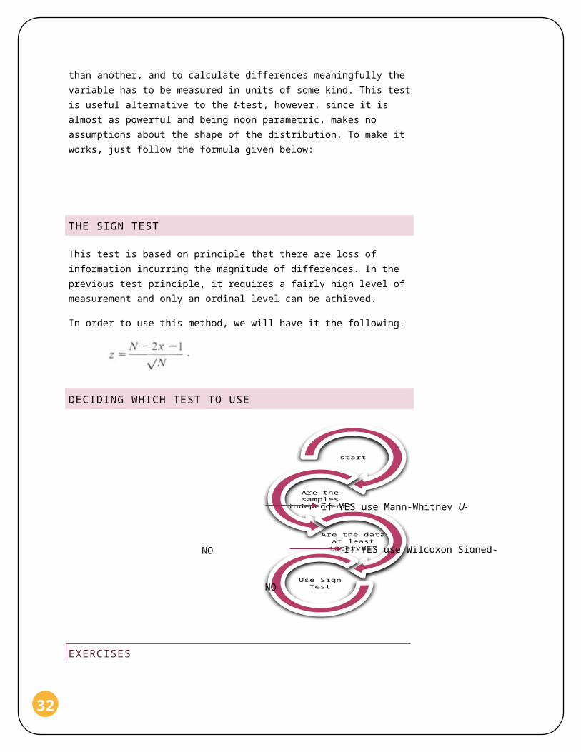
DECIDING WHICH TEST TO USE

EXERCISES

start

Are the samples

independent?

Are the data at least interval?

Use Sign Test

If YES use Mann-Whitney U-

If YES use Wilcoxon Signed-NO

NO

33

1. The following represent a teacher’s assessments of reading skill for two groups of children (data can be seen in book). Test, at the 2.5 per cent significance level, the hypothesis that the first group has a higher level of reading skill than the second.Answer:Since the data are probably best regarded as ordinal and the groups are independent, the Mann-Whitney U-test is appropriate. We rank all the data in the combined groups and find the rank sum for the smaller group.

GROUP 1 RANK GROUP 2 RANK

8 27 4 5.5

6 17 6 17

3 2 3 2

5 10.5 3 2

8 27 7 23

7 23 7 23

7 23 5 10.5

6 17 5 10.5

5 10.5 4 5.5

6 17 4 5.5

6 17 6 17

7 23 5 10.5

8 27 6 17

5 10.5

4 5.5

R1 = 241

34

(13×15)+13×142

−241

= 195 + 91 – 241 =45U2 = N1 N2 – U1 = (13 × 15) – 45 = 150U = Smaller of U1 and U2 =45The critical value of U for the 2.5 per cent level in a directional test with N1 =13 and N2 = 15. The calculated value of U is below the critical value, so we can claim a significant different at the 2.5 per cent level. Since group 1 has more of the higher ranks (this could be confirmed by calculating the mean rank for each group), the difference is in the predicted direction.

2. Two sets of ten sentences, differing in the degree of syntactic complexity, are raed individually, in randomised order, to a group of 30 informants, who are asked to repeat each sentence after a fixed time interval. The number of correctly remembered sentences ineach set, for each informant is as follows (can be found in book).Using a non-parametric test, test the hypothesis that thetwo sets of scores differ significantly at the 5 per centlevel.Answer:Since the data are the ratio type and the sets correlated, the Wilcoxon signed-ranks test is appropriate. We take the differences between pairs of scores; rank them, omitting any zero differences; assign to each rank the sign of difference it represents; and find the sums of positive and negative ranks.After processing the data, we got this:Sum of positive ranks = 253.5Sum of negative ranks = 71.5W = Smaller of the two= 71.5The critical value of W for the 5 per cent level and 25 pairs of non-tied scores in a non-directional test is 89.Since the calculated value of W lies below this, we can claim a significant difference between the two sets of scores at the 5 per cent level.

35

Since the number of pairs of scores is greater than 20, we can also use the z approximation:

Z=

71.5−(25×26)4

√25×26×5124

=−2.45

The critical value of z for the 5 per cent level in a non-directional test is 1.96. Since the calculated value of z (ignoring the sign) exceeds the critical value, we conclude that a significant difference can be claimed at the 5 per cent level.

3. An experiment is performed to test the effect of certain linguistic features on the politeness of two sentences inthe particular social context. Fifteen informants are asked to rate the two sentences on a scale from 1 (very impolite) to 5 (very polite), with the following results (can be seen in book).Test the hypothesis that sentence 2 is rated as more polite than sentence 1, at the 5 percent level.Answer:The data are ordinal and a repeated measures design is used. The sign test is therefore appropriate. We find thesign of the difference between each pair of scores, subtracting consistently.

Sentence 1 Sentence 2 Sign of

Sentence 1 - Sentence 2

1 3 -

2 2 0

1 4 -

2 3 -

3 1 +

2 4 -

1 1 0

36

2 3 -

3 5 -

1 3 -

2 3 -

1 4 -

2 1 +

2 4 -

1 3 -

There are 13 pairs of non-zero differences. 2 with the less frequent (positive) sign. Thus x =2. The critical value of x for the 5 per cent level and for 13 pairs in adirectional test is 3. Since the calculated value of x issmaller than the critical value. We may claim a significant difference at the 5 per cent level. Since therating for sentence 2 are higher than those for sentence 1 in 11 out of 15 cases, the differences are clearly in the predicted direction.

4. Two comparable groups of children, whose native language is not English, are taught to read English by two different methods, and their fluency is then assessed on a scale from 1 to 10. The scores are as follows in book.Do the two methods give significantly different results at the 5 per cent level?Answer:The data are ordinal and the groups independent. The Mann-Whitney U-test is therefore appropriate:U1 = 162.5U2 = 62.5U = Smaller of the two U values =62.5Critical value for U for the 5 per cent level and N1 = N2 = 15 in non-directional test is 64. Since the calculated value of U is smaller than the critical value, we now claim significance at the 5 per cent level. The ranks formethod B are higher overall.