Scheduling Strategies for Overloaded Real-Time Systems
51
ISSN 0249-6399 ISRN INRIA/RR--9455--FR+ENG RESEARCH REPORT N° 9455 February 2022 Project-Teams ROMA, TADaaM Scheduling Strategies for Overloaded Real-Time Systems Yiqin Gao, Guillaume Pallez, Yves Robert, Frédéric Vivien
-
Upload
khangminh22 -
Category
Documents
-
view
3 -
download
0
Transcript of Scheduling Strategies for Overloaded Real-Time Systems
ISS
N02
49-6
399
ISR
NIN
RIA
/RR
--94
55--
FR+E
NG
RESEARCHREPORTN° 9455February 2022
Project-Teams ROMA, TADaaM
Scheduling Strategies forOverloaded Real-TimeSystemsYiqin Gao, Guillaume Pallez, Yves Robert, Frédéric Vivien

RESEARCH CENTREGRENOBLE – RHÔNE-ALPES
Inovallée
655 avenue de l’Europe Montbonnot
38334 Saint Ismier Cedex
Scheduling Strategies for OverloadedReal-Time Systems
Yiqin Gao∗, Guillaume Pallez†, Yves Robert‡§, Frédéric Vivien‡
Project-Teams ROMA, TADaaM
Research Report n° 9455 — February 2022 — 48 pages
Abstract: This paper introduces and assesses novel strategies to schedule firm real-timejobs on an overloaded server. The jobs are released periodically and have the same rela-tive deadline. Job execution times obey an arbitrary probability distribution and can takeunbounded values (no WCET). We introduce three control parameters to decide when tostart or interrupt a job. We couple this dynamic scheduling with several admission policiesand investigate several optimization criteria, the most prominent being the Deadline MissRatio (DMR). Then we derive a Markov model and use its stationary distribution to deter-mine the best value of each control parameter. Finally we conduct an extensive simulationcampaign with 14 different probability distributions; the results nicely demonstrate howthe new control parameters help improve system performance compared with traditionalapproaches. In particular, we show that (i) the best admission policy is to admit all jobs;(ii) the key control parameter is to upper bound the start time of each job; (iii) the bestscheduling strategy decreases the DMR by up to 0.35 over traditional competitors.
Key-words: real-time system, firm jobs, overloaded system, admission policy, jobinterruption, Markov model, scheduling strategy.
Note: A short version of this work has appeared as a 4-page Work-In-Progress paper atRTSS’2021 [15].∗ Shanghai Jiao Tong University, China† Inria Bordeaux, France‡ LIP, École Normale Supérieure de Lyon, CNRS & Inria, France§ University of Tennessee Knoxville, USA
Stratégies d’ordonnancement pour un système entemps-réel surchargé
Résumé : Ce travail présente et évalue de nouvelles stratégies d’ordonnancementpour exécuter des tâches périodiques en temps réel sur une plate-forme sur-chargée. Les tâches arrivent périodiquement et ont le même délai relatifpour leur exécution. Les temps d’exécution des tâches obéissent à une dis-tribution de probabilité arbitraire et peuvent prendre des valeurs illimitées(pas de WCET). Certaines tâches peuvent être interrompues à leur admis-sion dans le système ou bien en cours d’exécution. Nous introduisons troisparamètres de contrôle pour décider quand démarrer ou interrompre unetâche. Nous associons cet ordonnancement dynamique à plusieurs politiquesd’admission et étudions plusieurs critères d’optimisation, le plus importantétant le Deadline Miss Ratio (DMR). Ensuite, nous dérivons un modèle deMarkov et utilisons sa distribution stationnaire pour déterminer la meilleurevaleur de chaque paramètre de contrôle. Enfin, nous conduisons de vastessimulations avec 14 distributions de probabilité différentes ; les résultats dé-montrent bien comment les nouveaux paramètres de contrôle contribuentà améliorer les performances du système par rapport aux approches tra-ditionnelles. En particulier, nous montrons que (i) la meilleure politiqued’admission est d’admettre toutes les tâches; (ii) le paramètre de contrôleclé est de limiter le temps de début de chaque tâche après son admission;(iii) la meilleure stratégie de planification diminue le DMR jusqu’à 0,35 parrapport aux concurrents traditionnels.
Mots-clés : système en temps réel, système surchargé, interruption, poli-tique d’admission, modèle de Markov model, stratégie d’ordonnancement

Scheduling Strategies for Overloaded Real-Time Systems 3
1 Introduction
Overloaded systems have become the norm in scientific computing. Withthe advent of parallel computing for many societal advances, traditionalcomputing systems are under a much higher load than was typically the casea few years ago. High-Performance Computing (HPC) systems run with autilization of almost 100% and a job waiting time of days [26]. In order tocope with this increase in submissions, several approaches are considered.In Cloud computing, the typical approach is to have dynamic pricing, withprices increasing as the resources become more scarce [32]. In HPC, highwaiting times are usually a deterrent with important negative consequences,such as limiting the number of very large jobs on HPC platforms [26].
In this work, we focus on real-time systems, but we borrow techniquesfrom HPC or Cloud computing. We consider a periodic task composed ofmany jobs that are released periodically and that must complete executionbefore some (relative) deadline D. To cope with overloading, several ap-proaches have been proposed [2]. For weakly-hard systems, some job dead-lines can be missed. There are two sub-categories then: either a job thatmissed its deadline must still be completed (soft jobs), or it can be ignored(firm jobs). For soft jobs, it is acceptable to miss some deadlines occasionally,but all jobs must be completed eventually. This specification is impossibleto meet for heavily loaded systems, e.g., with a short release period and longjob execution times. On the contrary, for firm systems, there is no valueto complete a job after its deadline. The objective is then to minimize theDeadline Miss Ratio (DMR), i.e., the fraction of jobs that fail to completeexecution before their deadline.
The main focus of this work is to introduce and assess several newscheduling techniques for firm real-time systems, which have many impor-tant applications, including multimedia, satellite-based tracking, financialforecast, and robotic assembly lines [21, 23]. When not all jobs can meettheir deadline, the scheduler can use a restrictive admission policy and de-cide to drop some jobs upon release. More importantly, the scheduler canalso interrupt the job that is currently executing on the server, at any timebefore its deadline, in order to launch another job instead. This is a naturalidea because a long-running job put the following jobs at risk. However,when interrupting a job to launch a new one, the time already spent by theserver to execute that job has been wasted, and there is no guarantee thatthe new job will complete faster than the interrupted one. Therefore, thedecision to start executing a job but to interrupt it before its deadline mustbe guided by sophisticated strategies. We investigate the impact of imposingconstraints on three key control parameters: (i) the maximum completiontime before interruption dmax (e.g., which can be smaller than the deadlineD to favor next jobs); (ii) the maximal execution time lmax allotted to thejob (e.g., which can depend upon the probability distribution of job execu-
RR n° 9455
4 Yiqin Gao, Guillaume Pallez, Yves Robert, Frédéric Vivien
tion times); and (ii) the maximum time elapsed between release time andstart-up time smax (e.g., which can be tuned according to system pressure).
Most real-time systems focus on jobs whose execution times obey a prob-ability distribution with bounded support [a, b], where a ≥ 0. The value b iscalled the Worst-Case Execution Time (WCET) and the typical assumptionis that b ≤ D. Enforcing a WCET is mandatory for hard systems wheredeadlines cannot be missed. It is also very important for soft systems whereall jobs must eventually complete. But for firm systems, one can relax theassumption and deal with standard distributions with infinite support (expo-nential, log-normal, half-normal, truncated normal, etc) chosen to encompassa wide range of characteristics.
Altogether, this work makes the following main contributions to the studyof firm real-time systems :
• we deal with job execution times which obey an arbitrary probabilitydistribution with unbounded support, hence, no WCET
• we consider several optimization objectives, some user-oriented, someplatform-oriented: DMR, system utilization, mean response time forsuccessful jobs, mean rejection time (see Section 3.2)
• we consider several job admission policies: all jobs, periodic, random,bounded-size queue (see Section 4.1)
• we introduce three new parameters to dynamically control schedulingstrategies that take decisions on the fly, and that decide to execute ajob, or not, based upon the current system state (see Section 4.2)
• we derive a Markov model and establish the existence of a uniquestationary distribution for all scenarios, which we use to analyticallydetermine the best value of the parameters and to express their per-formance (see Section 5)
• we conduct an extensive simulation campaign with 14 different proba-bility distribuions that lead to distinct system behaviors (see Sections 6and 7)
• we show that (i) the best admission policy is to admit all jobs; (ii) thekey control parameter is to upper bound the start time of each job;(iii) the best scheduling strategy decreases the DMR by up to 0.35over traditional competitors.
The rest of the paper is organized as follows. We survey related workin Section 2. We formally state the model and optimization criteria in Sec-tion 3. Section 4 is devoted to a description of the scheduling strategies. Weintroduce the Markov model and use its stationary distribution to computethe optimal values of the scheduling parameters in Section 5. We detail theexperimental framework in Section 6 and present all results in Section 7.Finally, Section 8 gives concluding remarks and hints for future work.
Inria

Scheduling Strategies for Overloaded Real-Time Systems 5
2 Related Work
We survey related work in this section. For the presentation, we distinguishreal-time applications (Section 2.1) from queuing networks (Section 2.2).This distinction is somewhat arbitrary, since similar ideas and techniquesare used in both frameworks.
2.1 Real-Time Applications
The specification of real-time systems relies on their cyclic nature, and isexpressed in terms of operations called jobs that have to be performed repet-itively. Real-time jobs are released periodically and must complete success-fully before a fixed time called the deadline. In the literature, real-timesystems are classified as hard and weakly hard [2]. For hard real-time jobs,no deadline should be missed: it is mandatory that each job completes be-fore its deadline. On the contrary, for weakly-hard jobs, some deadlines canbe missed. There are two sub-categories then: either a job that missed itsdeadline must still be completed (soft jobs), or it can be ignored (firm jobs).For soft jobs, it is acceptable to miss some deadlines occasionally, but alljobs must be completed eventually. On the contrary for firm jobs, there isno value to complete a job after its deadline.
When a real-time system is overloaded, it is unavoidable that some dead-lines are missed. For firm jobs, the widely used (m, k) approach is to guar-antee that at least m deadlines are satisfied out of every window of k con-secutive jobs (and to have a ratio m/k as high as possible) [18, 28, 31, 1, 7]1.For some applications, additional constraints, such as equally spacing thejobs matching their deadlines, may be enforced [33]. For instance, consider avideo application where jobs are frames to process; the (m, k) approach with,say, m = 10 and k = 20, ensures that at least half the frames are deliveredin time; but one might request that the good frames (those matching theirdeadlines) are more or less equally spaced in the window: receiving the firsthalf of every window of 20 consecutive frames would damage the quality ofthe video!
For soft jobs, the approach is different. All jobs have to be completedeventually. When the system is overloaded, an approach is either to increasethe deadline, or to decrease the release period, or both [3, 4]. Anotherapproach is to accumulate a backlog of jobs that are waiting for completionand to analyze the expected response time of the system [11]. In addition,some works study a mixed firm/soft setting where late jobs (that miss theirdeadlines) still have some value. For instance three decisions (abort currentjob, skip next job, queue next job) are available to the scheduler in [6, 27],
1In this work, we do not assume that jobs admit a finite worst-case execution time(WCET), which makes it impossible to guarantee any (m, k) constraint because somejobs can last for an arbitrary duration.
RR n° 9455
6 Yiqin Gao, Guillaume Pallez, Yves Robert, Frédéric Vivien
with the objective to minimize the deadline miss ratio (see Section 3 for adefinition). Finally, a variant of the problem is dealt with in [16]: job i needsthe output of job i− 1 to start, but can use that of job i− 2 is job i− 1 islate.
So far we have described systems where it was up to the scheduler toabort or skip some jobs. There are many variations: for instance, some jobsmay have two different types, skippable or not [22, 24], and only skippablejobs (blue jobs in [22]) are allowed to miss their deadline.
2.2 Queuing Networks
In this work, we deal with the list of waiting jobs via a queue: while themachine is occupied, all submitted jobs are waiting for their turn (or waitingto be killed) in a queue. This strongly differs from what is done in queueingtheory systems [19] where the typical constraint is to select in which orderjobs should be executed; so as to optimize an objective such as response time.Furthermore, job execution times obey the same probability distribution; toselect which jobs we execute next we use a simple First-Come-First-Servedstrategy amongst the jobs that have not been rejected.
The closer to our work is the job dropping model [8], where upon arrivalof a job, the system selects, at admission, whether the job should be dropped(i.e., should be rejected). The decision to drop a job often depends on afunction of queue parameters (number of jobs in the queue, average load ofthe queue): linear function (average queue size) [14] or other more compli-cated functions [13, 29]. Then, all jobs from the queue are executed (forexample following a FCFS strategy). Contrarily to the job dropping model,we propose to drop jobs dynamically.
In a series of publications [9, 10, 17, 25, 30], job pruning techniques havebeen investigated. The authors consider an oversubscribed system to whichjobs are submitted at random times. When a job is released, it is at firststored in a batch queue, and then can be allocated to the machine queueof a server by the mapping process. At each mapping event (completion orarrival of a job), the success probability of all jobs in the machine queueis recomputed, via a costly convolution over all possible durations of thejobs in the queue weighted by their respective probabilities. Jobs in thebatch queue are also considered when there remains a server with availablepositions after the previous computation. Jobs with low probability to meettheir deadline are dropped from the machine queue and deferred in the batchqueue. Deferring jobs means that their assignment to a server is postponed.In contrast, a job dropped from the machine queue is definitely removedfrom the system. Contrarily to our problem, there are several job types,several server types, and job arrival dates are random rather than periodic.This calls for a very costly solution where a whole convolution over a largetime window must be recomputed at each mapping event. Some jobs can be
Inria
Scheduling Strategies for Overloaded Real-Time Systems 7
dropped after some duration, a strategy also investigated in this work. Thestriking difference is that with a single job type, and with periodic releases,we are able to determine the optimal value of the key scheduling parametersonce and for all and to apply them on the fly, thereby providing a schedulewhose cost is constant and independent of the number of jobs.
3 Model and Optimization Criteria
This section details the model and states all optimization criteria studied inthis work.
3.1 Model
We consider a single periodic task whose jobs are periodically input to thesystem. The instance number i of the periodic task, called job i, i ≥ 1, isreleased at time ri = τ × (i− 1) and placed into the waiting queue; it mustcomplete not later than time di = ri +D, where τ is the period and D therelative deadline. If job i is not completed by its deadline di, it is consideredas failed, its execution is interrupted, and any time spent to execute part ofit has been wasted.
We assume that we have an arbitrary deadline D > τ . (If D ≤ τ ,the (trivial) solution is to never interrupt a job.) The problem becomeschallenging when the system gets overloaded: when we have, say, D = 5τ :some jobs might execute for a time longer than τ , thereby delaying thebeginning of the execution of the following jobs if they are not interruptedbefore reaching their deadline. We consider a general framework and assumethat job execution times obey some probability distributions with unboundedsupport [0,∞].
3.2 Optimization Criteria
We start with the most important criterion:
Deadline miss ratio (DMR) [11, 5]
This is the most frequently used metric in weakly-hard real-time systems,where one is looking for probabilistic guarantee that the deadline miss ratioof a job is below a threshold. Note that this metric is directly related to thejob execution rate metric, which corresponds to the expected number of jobsexecuted per time unit.
In addition to the deadline miss ratio, we study the following three rele-vant criteria:
RR n° 9455
8 Yiqin Gao, Guillaume Pallez, Yves Robert, Frédéric Vivien
Utilization [26]
This platform-oriented criterion corresponds to the proportion of time spentdoing computation that ends up in a success (i.e., the completion of a jobbefore its deadline). Note that the highest utilization does not guaranteethe lowest deadline miss ratio, because the scheduler could decide to executefewer longer jobs than more shorter ones.
Mean response time of successfully completed jobs [11, 26]
This corresponds to the delay between the release of the job and its comple-tion. When deadlines are enforced, this criterion is less important but doesprovide qualitative information about the various solutions.
Mean rejection time
This new criterion is important for an overloaded system. Intuitively, itcorresponds to the time it takes for the system to inform a user that its jobwill not be executed. Of course, this criterion must be coupled with another,otherwise the best strategy would be to reject all jobs at submission time.
4 Scheduling
Our scheduling strategies rely on both admission/rejection policies, and ontermination/interruption policies. An admission policy is the answer to thequestion: which jobs to admit into the system? Indeed, whenever a new jobis released, the scheduler must decide right away whether the job is admittedinto the system and granted the possibility to execute later. Alternatively, ajob can be immediately rejected (without the possibility of later execution).Among the advantages of job rejection, one can envision: (i) a decrease of theload on the system; (ii) a decrease of the number of jobs that must be queuedbefore execution; and (iii) a decrease of the time-to-failure for unsuccessfuljobs.
The scheduler must then decide in which order to execute admitted jobs,whether to launch the execution of an admitted job or to cancel it, andwhen to interrupt a running job. In this last case, the job is consideredfailed (without the possibility of later execution). This is interesting whenjobs are likely not to finish before their deadlines, in order to free the serverfor other jobs.
Because all jobs have the same relative deadline, we only consider policieswhich execute jobs in their order of arrival: these policies obey both the firstcome first served (FCFS) and the earliest deadline first (EDF) priority rules.We first cover possible admission policies (Section 4.1). Then, we describe aset of parameters controlling the launching and interrupting (killing) of jobs(Section 4.2). Finally, we define all the strategies under study (Section 4.3).
Inria
Scheduling Strategies for Overloaded Real-Time Systems 9
4.1 Admission Policies
We consider four types of admission policies:
1. The simplest admission policy is to admit all jobs submitted to thesystem. When needed, we tag variables describing the behavior underthis admission policy with the tag AA, which stands for All (jobs)Admitted.
2. A classical admission policy is to use a bounded queue of a fixed sizem. If, at the release time of job i there are alreadym jobs in the queue,job i is rejected. Strategies using a queue of size m will be tagged bythe prefix Queue(m) and variables with the tag queue .
3. Random admission policy: each job submitted to the system will beadmitted with probability α and rejected with probability 1 − α (re-gardless of the state of the system at the release time of the job). Wemark variables with the tag rand .
4. Periodic admission policy. The admission policy is defined by a pattern(i.e., a boolean array) A of length τA. The i-th job submitted to thesystem will be admitted (regardless of the state of the system) if andonly if A[i mod τA] is equal to True. We mark variables with the tagper .
4.2 Control Parameters
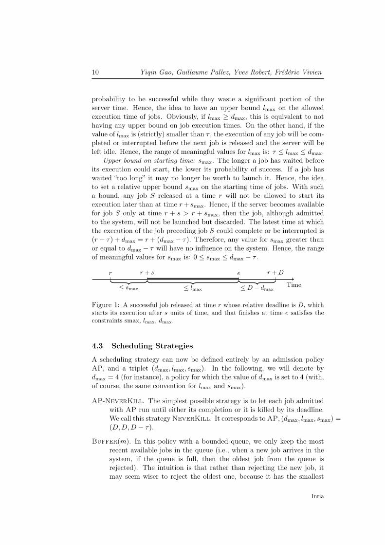
Launching and interrupting jobs are controlled through the following threeparameters (illustrated in Figure 1):
Upper bound on completion time: dmax. All jobs have a relative deadlineD. Hence, a job released at time r will have its execution stopped at timer+D if its execution has not successfully completed by that time. One canenvision that for some distributions of job execution times, when nearing theabsolute deadline r + D, the probability of the job completing successfullydrops so much that it may not be worth to continue executing it until thedeadline. To study this hypothesis, we introduce the upper bound dmax onthe completion time of a job. Any job, released at time r, will then haveits execution stopped at time r+ dmax if it has not completed by that time.By definition of deadlines, any value for dmax greater than or equal to Dwill have no influence on the system. Furthermore, if the value of dmax is(strictly) smaller than the period τ , one can prove by induction that theexecution of any job will be completed or interrupted before the next jobis released, and the server will be left idle. Hence, the range of meaningfulvalues for dmax is: τ ≤ dmax ≤ D.
Upper bound on execution time: lmax. One can envision long-tail distri-butions of job execution times for which long running jobs have very little
RR n° 9455
10 Yiqin Gao, Guillaume Pallez, Yves Robert, Frédéric Vivien
probability to be successful while they waste a significant portion of theserver time. Hence, the idea to have an upper bound lmax on the allowedexecution time of jobs. Obviously, if lmax ≥ dmax, this is equivalent to nothaving any upper bound on job execution times. On the other hand, if thevalue of lmax is (strictly) smaller than τ , the execution of any job will be com-pleted or interrupted before the next job is released and the server will beleft idle. Hence, the range of meaningful values for lmax is: τ ≤ lmax ≤ dmax.
Upper bound on starting time: smax. The longer a job has waited beforeits execution could start, the lower its probability of success. If a job haswaited “too long” it may no longer be worth to launch it. Hence, the ideato set a relative upper bound smax on the starting time of jobs. With sucha bound, any job S released at a time r will not be allowed to start itsexecution later than at time r+ smax. Hence, if the server becomes availablefor job S only at time r + s > r + smax, then the job, although admittedto the system, will not be launched but discarded. The latest time at whichthe execution of the job preceding job S could complete or be interrupted is(r − τ) + dmax = r + (dmax − τ). Therefore, any value for smax greater thanor equal to dmax − τ will have no influence on the system. Hence, the rangeof meaningful values for smax is: 0 ≤ smax ≤ dmax − τ .
Time
r r + s e r +D
≤ smax ≤ lmax ≤ D − dmax
Figure 1: A successful job released at time r whose relative deadline is D, whichstarts its execution after s units of time, and that finishes at time e satisfies theconstraints smax, lmax, dmax.
4.3 Scheduling Strategies
A scheduling strategy can now be defined entirely by an admission policyAP, and a triplet (dmax, lmax, smax). In the following, we will denote bydmax = 4 (for instance), a policy for which the value of dmax is set to 4 (with,of course, the same convention for lmax and smax).
AP-NeverKill. The simplest possible strategy is to let each job admittedwith AP run until either its completion or it is killed by its deadline.We call this strategy NeverKill. It corresponds to AP, (dmax, lmax, smax) =(D,D,D − τ).
Buffer(m). In this policy with a bounded queue, we only keep the mostrecent available jobs in the queue (i.e., when a new job arrives in thesystem, if the queue is full, then the oldest job from the queue isrejected). The intuition is that rather than rejecting the new job, itmay seem wiser to reject the oldest one, because it has the smallest
Inria

Scheduling Strategies for Overloaded Real-Time Systems 11
probability of success. This corresponds to the admission policy AA,along with the triplet (dmax, lmax, smax) = (D,D,mτ − 1): indeed,when smax = mτ − 1, any job waiting at least a time mτ between itsrelease time and the (potential) start of its execution is never launched.If a job has waited at least a time mτ , it means that there are at leastm other jobs waiting in the system.
AP-BestDmax, AP-BestLmax, and AP-BestSmax. A natural idea is topick the value for dmax (resp. lmax, smax) that minimizes the objectivefunction when the other two parameters are non limiting. Non-limitingparameters are defined as dmax = D, lmax = dmax, smax = dmax − τ .We discuss the complexity of these algorithms and their combination(optimizing for two or three parameters simultaneously) in Section 5.6.
In the following, when referring to a policy without mentioning the ad-mission policy AP, we assume that we are using AP = AA. The defaultobjective is to minimize the DMR.
5 Markov Model
If the probability distributionD of job execution times is discrete, one can usea Markov chain to describe the evolution of the system under the NeverKillpolicy. Then one can compute its stationary distribution and evaluate itsperformance for the different objective functions expressed in Section 3. Thisis for instance what is done in [11] for an underloaded system.
In this section, we show how this approach can be applied to the continu-ous case, by using discretization, and how it can be extended to model all theadmission policies listed in Section 4.1 and all the control parameters listedin Section 4.2. In Section 5.1, we start by describing the discretization (if Dis initially continuous rather than discrete) and by setting notations. Then,in Section 5.2, we construct the Markov chain when all tasks are admittedinto the system, before generalizing these Markov chains to other admissionpolicies in Section 5.3. In Section 5.4, we prove that all these Markov chainsadmit a unique stationary distribution. In Section 5.5 we show how to ex-press the four optimization criteria discussed in Section 3 in terms of theMarkov model. Finally, in Section 5.6 we establish the complexity of usingthe Markov chains to compute the optimal values for the parameters dmax,lmax, and smax.
5.1 Discretization and Notations
We define a quantum duration q, and we use it to discretize all durations. Weassume that the period τ and the relative deadline D both last an integralnumber of quanta. In other words, we have τ = b τq cq and D = bDq cq.
RR n° 9455

12 Yiqin Gao, Guillaume Pallez, Yves Robert, Frédéric Vivien
To ease the writing of the equations, and up to the complexity analysisexcluded (Section 5.6), we set that q lasts one arbitrary unit of time (q = 1with the right choice of time unit), and that all durations are expressed inthis arbitrary unit. Hence, the period now lasts τ quanta, and so on. Theonly assumption is that τ and D are integers.
We approximate the probability distribution D of job execution timesvia discretization. Let f be the probability density function of D. Let plbe the probability that a job execution time is equal to l (quanta) in thediscretized version of D. We conservatively compute pl by rounding up eachjob execution time to the nearest quantum multiple:
pl =
∫ lq
(l−1)qf(x)dx.
We study the evolution of the system due to the execution of a job Sreleased at a time r. Let s be the time job S has to wait after its ar-rival in the system until the server is available. Then the server will beavailable for job S at the date r + s. From Section 4.2, we have 0 ≤s ≤ dmax − τ . Also, the latest start time for a job is smax, and its ex-ecution can last at most a time lmax. Hence, we also have s ≤ lmax +dmax − τ . Altogether, this gives us 0 ≤ s ≤ σ with σ = min{smax +lmax, dmax}− τ . Job S is followed by a job T which is released at time r+ τ .We will compute the probability Ps,t that the server is available at time(r + τ) + t for job T if it was available at time r + s for job S.
5.2 When All Jobs Are Admitted
In this section, we study systems in which all jobs are admitted (AA policy).Still, the execution of some jobs may be aborted because of the lmax anddmax parameters, and the execution of some jobs may not be launched at allbecause of the smax parameter.
Let l denote the execution time of job S in the absence of any constraint(D, smax, lmax, and dmax). Without those constraints, the execution of jobS starts at time r+ s and completes at time r+ s+ l = (r+ τ)+ (s+ l− τ).Therefore, t = s + l − τ (resp. t = 0 if s + l − τ ≤ 0: job S finished beforethe release time of job T ). Then, Ps,t = pl (resp. Ps,0 =
∑l≤τ−s pl).
We now compute the value of Ps,t when taking smax, lmax, and dmax intoaccount. We first consider the case where the server is available too late forthe job to be launched. Then we focus on the subcase t = 0.
• Case s > smax.
In this case job S is not launched by definition of smax. Therefore theserver becomes available for job T at the time it became available forjob S. Therefore, for any s and t such that smax + 1 ≤ s ≤ σ and
Inria
Scheduling Strategies for Overloaded Real-Time Systems 13
0 ≤ t ≤ σ: { Ps,max{0,s−τ} = 1
Ps,t = 0 if t 6= max{0, s− τ}.
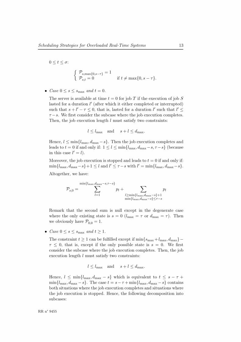
• Case 0 ≤ s ≤ smax and t = 0.
The server is available at time t = 0 for job T if the execution of job Slasted for a duration l′ (after which it either completed or interrupted)such that s+ l′ − τ ≤ 0, that is, lasted for a duration l′ such that l′ ≤τ−s. We first consider the subcase where the job execution completes.Then, the job execution length l must satisfy two constraints:
l ≤ lmax and s+ l ≤ dmax.
Hence, l ≤ min{lmax, dmax−s}. Then the job execution completes andleads to t = 0 if and only if: 1 ≤ l ≤ min{lmax, dmax−s, τ−s} (becausein this case l′ = l).
Moreover, the job execution is stopped and leads to t = 0 if and only if:min{lmax, dmax−s}+1 ≤ l and l′ ≤ τ−s with l′ = min{lmax, dmax−s}.Altogether, we have:
Ps,0 =
min{lmax,dmax−s,τ−s}∑l=1
pl +∑
l≥min{lmax,dmax−s}+1min{lmax,dmax−s}≤τ−s
pl
Remark that the second sum is null except in the degenerate casewhere the only existing state is s = 0 (lmax = τ or dmax = τ). Thenwe obviously have P0,0 = 1.
• Case 0 ≤ s ≤ smax and t ≥ 1.
The constraint t ≥ 1 can be fulfilled except if min{smax+ lmax, dmax}−τ ≤ 0, that is, except if the only possible state is s = 0. We firstconsider the subcase where the job execution completes. Then, the jobexecution length l must satisfy two constraints:
l ≤ lmax and s+ l ≤ dmax.
Hence, l ≤ min{lmax, dmax − s} which is equivalent to t ≤ s − τ +min{lmax, dmax− s}. The case t = s− τ +min{lmax, dmax− s} containsboth situations where the job execution completes and situations wherethe job execution is stopped. Hence, the following decomposition intosubcases:
RR n° 9455

14 Yiqin Gao, Guillaume Pallez, Yves Robert, Frédéric Vivien
– Case 1 ≤ t ≤ s − τ + min{lmax, dmax − s} − 1. We always havel ≥ 1 which gives us the additional constraint: t ≥ 1 + s − τ .In this subcase, the job completes after an execution which lastst− s+ τ :
Ps,t = pt−s+τ .
– Case 1 ≤ t and t = s− τ +min{lmax, dmax− s}. This correspondsto all remaining possible cases. Hence,
Ps,t = 1−min{lmax,dmax−s}−1∑
l=1
pl.
– Case t > s − τ + min{lmax, dmax − s}. None of these cases canhappen. Hence,
Ps,t = 0.
5.3 Other Admission Policies
Random admission policy. If the job S is not admitted, which hap-pens with probability 1-α, then the server is available for job T at timemax{0, s− τ}. If the job S is admitted, which happens with probability α,the probability that the server is available for job T at time t is the same aspreviously (under the condition that job S is admitted). Therefore, lettingPrands,t be the probability Ps,t for the random admission policy, we have:
Prands,t =
{αPs,t + (1− α) if t = max{0, s− τ},αPs,t otherwise.
Periodic admission policy. This case is quite close to the previousone. The main difference is that we need to record where we are within theperiod. Let Pper
(i−1)σ+s,t, with 1 ≤ i ≤ τA, 0 ≤ s, t ≤ σ, denote the probabilitythat, if the server was available at time s for job S and if job S was the n-thjob released in the system such that 1+(n mod τA) = i, then the server willbe available at time t for job T . Then we have:
• Case A[i] = True (job S is admitted).
Pper(i−1)σ+s,t = Ps,t.
• Case A[i] = False.
Pper(i−1)σ+s,t =
{1 if t = max{0, s− τ},0 otherwise.
Inria

Scheduling Strategies for Overloaded Real-Time Systems 15
Queues of size m. When all jobs were admitted, we were able to fullycharacterize the system for job S by solely relying on the time r+s at whichits processing would start. For queues, we need both this time and a vector ~Qof size δ (determined later) describing the state of the queue. For 0 ≤ l ≤ δ,~Q[l] is the number of jobs released prior to S which are still present in thesystem at the time r + l × τ , that is, the number of prior jobs which areeither in the queue or being processed. Hence, components of ~Q takes valuein {0, ...,m+1}. Note that, because the execution of S starts at time r+ s,the system does not contain any jobs released prior to S at least starting attime r + s. Therefore, ~Q[l] = 0 if l × τ ≥ s. By definition of σ, we haves ≤ σ. Hence, δ ≤ bστ c.
We need to compute the probability Pqueue
s, ~Q,t, ~Rthat the server is available
at time (r+ τ) + t for job T with a queue state ~R if it was available at timer + s for job S with queue state ~Q. We start by characterizing the queuestate if the server is available at time r + t for job T . We denote this queuestate by ~Q∗. We have two cases to consider:
• Case ~Q[0] = m+ 1. Then the queue is full and job S is not admitted.The only jobs released prior to T that may be present in the systemare jobs released prior to S. Their presence is recorded in ~Q. Hence:
~Q∗[l] =
{0 if lτ ≥ t,~Q[l + 1] otherwise.
The shift from l+ 1 to l is due to the fact that the reference point forjob T is one period (of length τ) later than for job S.
• Case ~Q[0] < m + 1. Then job S is admitted and is present in thesystem up to time t if t > 0. Hence:
~Q∗[l] =
{0 if lτ ≥ t,1 + ~Q[l + 1] otherwise.
If job S is admitted into the system, the probability that the server isavailable at time r + t for job T is Ps,t. Indeed, once a job is admitted thebehavior of the system is the same as when all jobs are admitted. If job S isnot admitted, then the server is available for job T at time r+s. Altogether,we obtain:
Pqueue
s, ~Q,t, ~R=
Ps,t if ~Q[0] < m+ 1 and ~R = ~Q∗,
1 if ~Q[0] = m+ 1, t = max{0, s− τ},and ~R = ~Q∗,
0 otherwise.
RR n° 9455

16 Yiqin Gao, Guillaume Pallez, Yves Robert, Frédéric Vivien
5.4 Asymptotic Behavior
In this section we prove that the Markov chains that we consider are bothirreducible and aperiodic. Since their number of states is always finite, thisis equivalent to say that these Markov chains are regular, hence, admit aunique stationary distribution [20].
Theorem 1. The Markov chains of Sections 5.2 and 5.3 are all both irre-ducible and aperiodic, and they all admit a unique stationary distribution.
Proof. We prove that all Markov chains are irreducible and aperiodic. Inthe following, we restrict to the case when all jobs are admitted (AA policy).The proof can then be easily extended to the other admission policies.
If lmax = τ or dmax = τ , the execution of any job will be completed orinterrupted before the next job is released. The system is then trivial, theMarkov chain has a single state, and the theorem is obviously true. Hence, inthe following we assume that we have lmax > τ and dmax > τ . In the proof,we assume that all possible execution times for a job do actually happen.That is, for any duration l ∈ {1...D}, pl > 0. We first show that all statesare reachable. By definition of σ, the range of (theoretically) possible statesis [0;σ]. Let us “forget” about dmax for a short while. The server is availablefor job S at time r + s. Because lmax > τ and pτ+1 > 0, with probabilitypτ+1 the execution of job S will last for a time τ + 1 and the server will beavailable for job T at time r + s+ τ + 1 = (r + τ) + s+ 1. Therefore, if thestate of the system is s for job S, it will be in the state t = s + 1 for jobT with probability pτ+1 > 0. Now, taking dmax into account, this is true aslong as s ≤ smax and s+ τ + 1 ≤ dmax.
Let us first consider the case s+τ+1 = dmax. If we reached it, this meansthat smax + lmax ≥ dmax, because smax ≥ s and lmax ≥ τ + 1. Therefore,the possible range of values is [0; dmax − τ ], and we have established thatall these states are reachable. Now consider the other case. Namely, wereached the case s = smax without, in the process, having jobs interruptedbecause of the value of dmax. Then, with probability pτ+j > 0, with j ∈[1;min{lmax; dmax − smax} − τ ], the execution of job S lasts until the timer + smax + τ + j = (r + τ) + smax + j. Hence, all states in the range[smax + 1;min{smax + lmax; dmax} − τ ] are reachable. Therefore, all possiblestates are reachable from the initial state, the state s = 0.
Now consider any state s > 0. With probability p1 > 0, the next state ist = max{0, s+1− τ}. If τ > 1, t < s, and from any state a strictly “smaller”state is reachable. Therefore, there is a path from any state to the state 0.This shows that the Markov chain is irreducible. Furthermore, there is a loopfrom state 0 to itself. Indeed, with probability
∑τk=1 pk > 0 a job execution
takes no longer than the period τ . Hence, if the state before the executionof the job was 0, this is also the case after its execution. Hence, the periodof state s = 0 is one. And because the chain is irreducible, all states have
Inria

Scheduling Strategies for Overloaded Real-Time Systems 17
period one too. Hence, the Markov chain is aperiodic when τ > 1.If τ = 1, there is a loop from state any state s to itself. Let l ≥ 1 be the
length of the execution of job S before it either completes or is killed. Thent = max{0, s + l − τ} = max{0, s + l − 1} = s + l − 1 ≥ s. Furthermore,if s ≤ smax, there is a loop from state s to itself because p1 > 0. Hence,the period of any state s ≤ smax is one. If s > smax, there is a path fromstate s to state s − 1, and then to state smax. Therefore, there is a pathfrom any state to the state smax. This shows that the Markov chain isirreducible. Therefore, all states have period one too. Hence the Markovchain is aperiodic when τ = 1. This concludes the proof.
A direct and important consequence of Theorem 1 is the following:
Corollary 1. For any admission policy defined in Section 4.1 and any choiceof the parameters dmax, lmax, and smax, the system converges to a uniqueasymptotic behavior.
5.5 Optimization Criteria
This section explains how to express the four optimization criteria discussedin Section 3 in terms of the stationary distrbution of Markov model. In thefollowing let π∞(s) denote the limit probability of occurrence of a state s,0 ≤ s ≤ σ (we also have the limit probability π∞(s, i) of state s at rank i inthe pattern for the admission pattern policy, and π∞(s, ~Q) for state s withqueue state ~Q when admission is defined by a queue). We give the formulafor all criteria with the AA policy, but only for DMR (deadline miss ratio)for the other admission policies (the other criteria can be derived similarly).
• Deadline miss ratio. The probability of success is computed as
PAAsucc =
σ∑s=0
π∞(s)
min{lmax,dmax−s}∑l=1
pl
and the deadline miss ratio is equal to DMRAA = 1− PAAsucc .
Under a random admission policy of parameter α, jobs are rejectedwith probability 1− α. Hence:
Prandsucc = α
σ∑s=0
π∞(s)
min{lmax,dmax−s}∑l=1
pl
When admissions are regulated through a pattern, only jobs releasedat ranks corresponding to admissions can meet their deadlines. Hence:
Ppersucc =
∑1≤i≤τAA[i]=True
σ∑s=0
π∞(s, i)
min{lmax,dmax−s}∑l=1
pl
RR n° 9455
18 Yiqin Gao, Guillaume Pallez, Yves Robert, Frédéric Vivien
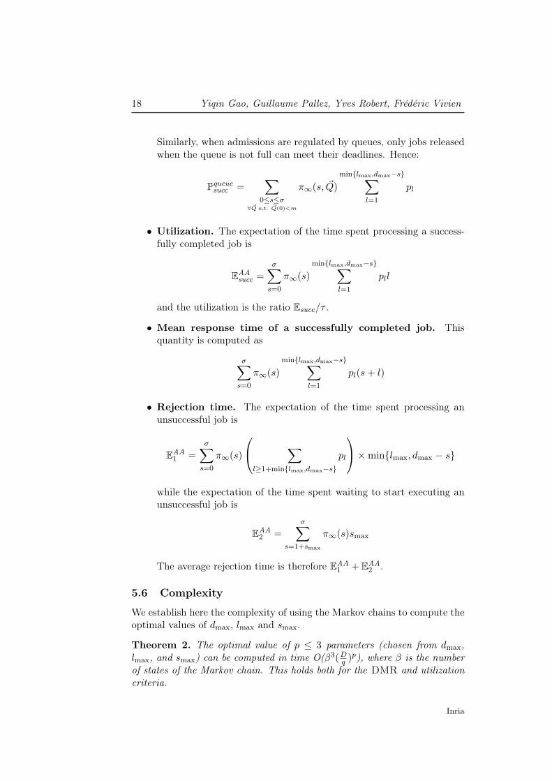
Similarly, when admissions are regulated by queues, only jobs releasedwhen the queue is not full can meet their deadlines. Hence:
Pqueuesucc =
∑0≤s≤σ
∀~Q s.t. ~Q(0)<m
π∞(s, ~Q)
min{lmax,dmax−s}∑l=1
pl
• Utilization. The expectation of the time spent processing a success-fully completed job is
EAAsucc =
σ∑s=0
π∞(s)
min{lmax,dmax−s}∑l=1
pll
and the utilization is the ratio Esucc/τ .
• Mean response time of a successfully completed job. Thisquantity is computed as
σ∑s=0
π∞(s)
min{lmax,dmax−s}∑l=1
pl(s+ l)
• Rejection time. The expectation of the time spent processing anunsuccessful job is
EAA1 =
σ∑s=0
π∞(s)
∑l≥1+min{lmax,dmax−s}
pl
×min{lmax, dmax − s}
while the expectation of the time spent waiting to start executing anunsuccessful job is
EAA2 =
σ∑s=1+smax
π∞(s)smax
The average rejection time is therefore EAA1 + EAA
2 .
5.6 Complexity
We establish here the complexity of using the Markov chains to compute theoptimal values of dmax, lmax and smax.
Theorem 2. The optimal value of p ≤ 3 parameters (chosen from dmax,lmax, and smax) can be computed in time O(β3(Dq )
p), where β is the numberof states of the Markov chain. This holds both for the DMR and utilizationcriteria.
Inria

Scheduling Strategies for Overloaded Real-Time Systems 19
Proof. For a given admission policy and a choice of values for the parametersdmax, lmax, and smax we build the corresponding Markov chain followingSections 5.2 and 5.3. We obtain a Markov chain with β states. Accordingto Theorem 1, this Markov chain is irreducible and aperiodic. We computeits stationary distribution in O(β3) steps. Using the stationary distributionand the objective function of choice, we can compute the performance of theadmission policy and the choice of values of dmax, lmax, and smax. Then, thebest value of dmax, lmax and/or smax is computed by trying all values; thereare at most D
q possible values for each of these three parameters.
We have β ≤ D−τq when all jobs are admitted or when the admission is
random, β ≤ τAD−τq when jobs are admitted following a pattern of size τA
and β ≤ D−τq (1 +m)δ = D−τ
q (1 +m)Dτ when jobs are admitted through a
queue of size m.For instance, with the AA policy, the complexity becomes O(Dq )
6 if weoptimize for the three parameters simultaneously. In Section 7 we show thatoptimizing only for smax, and using a binary search instead of an exhaustivesearch, leads to very good results while reducing the complexity down toO((Dq )
3 log(Dq )).
6 Evaluation Methodology
In this section, we first discuss the evaluation protocol in Section 6.1. Theanalysis and computation of the solution with the Markov model relies on adiscretization of time. The complicated problem to find a quantum size thatensures an accurate evaluation, while maintaining an acceptable complexity,is addressed in Section 6.2.
6.1 Evaluation Protocol
In this section, we detail the experimental framework. As seen in Section 3.1,a periodic task is characterized by:
• the distribution D of job execution times.
• the period τ , which has direct impact on the system load. We considerτ ∈ [0.1E(D); 2E(D)] by steps of 0.1; hence, 19 different values.
• the relative deadline D. We select D ∈ {2τ, 4τ, 6τ, 8τ, 10τ}. Intu-itively, the ratio D/τ is the number of consecutive jobs that can besimultanesouly present in the system.
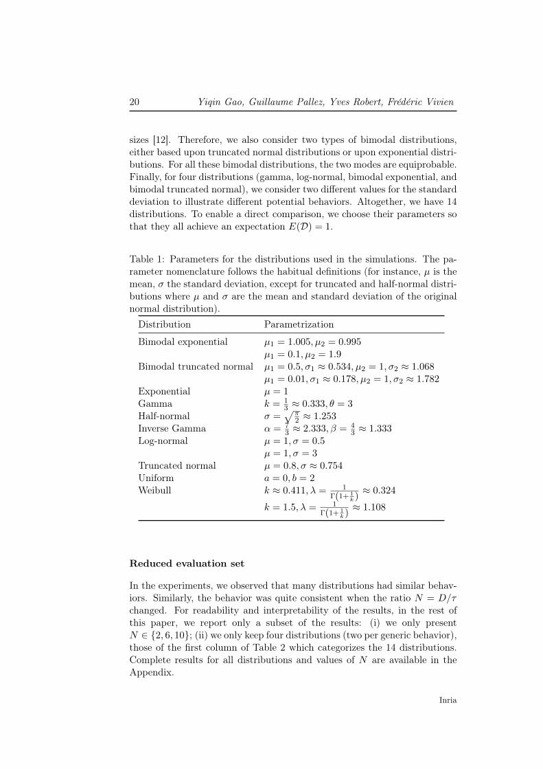
We use 8 standard probability distributions to generate job executiontimes (see the complete list and parameters in Table 1). In addition, mul-timodal distributions have been advocated to model jobs, file and object
RR n° 9455
20 Yiqin Gao, Guillaume Pallez, Yves Robert, Frédéric Vivien
sizes [12]. Therefore, we also consider two types of bimodal distributions,either based upon truncated normal distributions or upon exponential distri-butions. For all these bimodal distributions, the two modes are equiprobable.Finally, for four distributions (gamma, log-normal, bimodal exponential, andbimodal truncated normal), we consider two different values for the standarddeviation to illustrate different potential behaviors. Altogether, we have 14distributions. To enable a direct comparison, we choose their parameters sothat they all achieve an expectation E(D) = 1.
Table 1: Parameters for the distributions used in the simulations. The pa-rameter nomenclature follows the habitual definitions (for instance, µ is themean, σ the standard deviation, except for truncated and half-normal distri-butions where µ and σ are the mean and standard deviation of the originalnormal distribution).Distribution Parametrization
Bimodal exponential µ1 = 1.005, µ2 = 0.995µ1 = 0.1, µ2 = 1.9
Bimodal truncated normal µ1 = 0.5, σ1 ≈ 0.534, µ2 = 1, σ2 ≈ 1.068µ1 = 0.01, σ1 ≈ 0.178, µ2 = 1, σ2 ≈ 1.782
Exponential µ = 1Gamma k = 1
3 ≈ 0.333, θ = 3Half-normal σ =
√π2 ≈ 1.253
Inverse Gamma α = 73 ≈ 2.333, β = 4
3 ≈ 1.333Log-normal µ = 1, σ = 0.5
µ = 1, σ = 3Truncated normal µ = 0.8, σ ≈ 0.754Uniform a = 0, b = 2Weibull k ≈ 0.411, λ = 1
Γ(1+ 1k )≈ 0.324
k = 1.5, λ = 1Γ(1+ 1
k )≈ 1.108
Reduced evaluation set
In the experiments, we observed that many distributions had similar behav-iors. Similarly, the behavior was quite consistent when the ratio N = D/τchanged. For readability and interpretability of the results, in the rest ofthis paper, we report only a subset of the results: (i) we only presentN ∈ {2, 6, 10}; (ii) we only keep four distributions (two per generic behavior),those of the first column of Table 2 which categorizes the 14 distributions.Complete results for all distributions and values of N are available in theAppendix.
Inria
Scheduling Strategies for Overloaded Real-Time Systems 21
Table 2: Categorizing the behavior of the 14 distributions.Representativedistribution
Distributions with similarbehavior
LogNormalσ = 3(LN(3));
Bimodal Exponential (both);Weibull k < 1; Bimodal trun-cated normal (µ1 = µ2/100)
Exponential(Exp)LogNormalσ = 0.5(LN(0.5));
Uniform; Half-normal; Weibullk > 1; Bimodal truncated nor-mal (µ1 = µ2/2);
TruncatedNormal(TruncNorm)
Gamma; Inverse Gamma
6.2 Accuracy
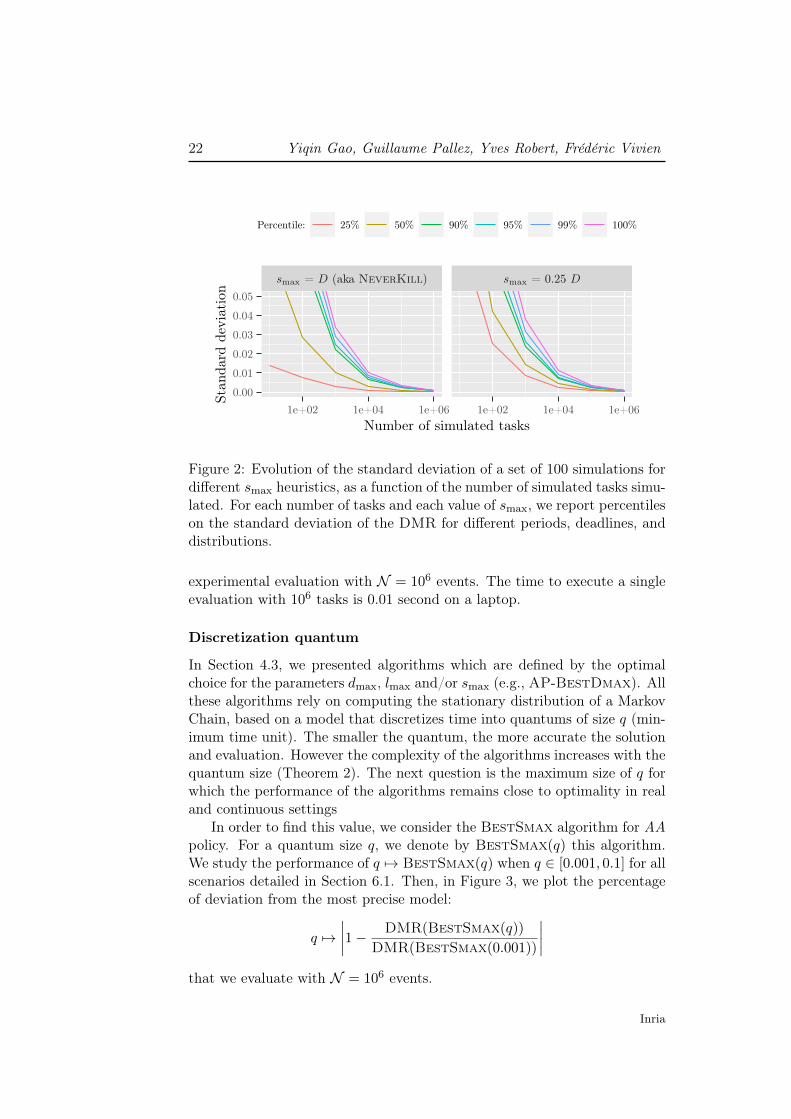
In order to evaluate the different scheduling algorithms, we have created anevent-based simulator. This simulator takes as input the application model(probability distribution, period, deadline) and a number of events N . Itstarts from an empty queue and simulates an execution until N jobs havebeen submitted into the system. The objectives are then evaluated over thecomplete execution.
Instantiation of the event-based simulator
The first question is how many events N should be chosen for the evalua-tion? In order to answer it, we perform the following experiments. Considerthe algorithm S-Max : s 7→ (AA, (dmax, lmax, smax) = (D,D, s)) (using thenotations from the Section 4.3, this means that we accept all jobs, dmax andlmax are not constraining, and smax is the input of the algorithm): by con-struction s belongs necessarily to the set [0, D]. We consider four variants ofit: S-Max(xD) for x ∈ {0.25, 0.5, 0.75, 1} to cover the whole scope of values.
When N varies in {102, 103, . . . , 106}:• We repeat all experiments proposed in Section 6.1 (14× 19× 5 = 1330
experiments), 100 times.
• We measure the standard deviation of all scenarios (1330 data points).
• We plot some quantiles of these standard deviations as a function ofN . These results are partially presented in Figure 2 (the other resultsare in Figure 13 of the Appendix).
From Figure 2, we see that the standard deviation with 106 jobs is lowerthan 0.001. This indicates that we can rely with high confidence on an
RR n° 9455
22 Yiqin Gao, Guillaume Pallez, Yves Robert, Frédéric Vivien
smax = D (aka NeverKill) smax = 0.25 D
1e+02 1e+04 1e+06 1e+02 1e+04 1e+060.00
0.01
0.02
0.03
0.04
0.05
Number of simulated tasks
Stan
dard
devi
atio
nPercentile: 25% 50% 90% 95% 99% 100%
Figure 2: Evolution of the standard deviation of a set of 100 simulations fordifferent smax heuristics, as a function of the number of simulated tasks simu-lated. For each number of tasks and each value of smax, we report percentileson the standard deviation of the DMR for different periods, deadlines, anddistributions.
experimental evaluation with N = 106 events. The time to execute a singleevaluation with 106 tasks is 0.01 second on a laptop.
Discretization quantum
In Section 4.3, we presented algorithms which are defined by the optimalchoice for the parameters dmax, lmax and/or smax (e.g., AP-BestDmax). Allthese algorithms rely on computing the stationary distribution of a MarkovChain, based on a model that discretizes time into quantums of size q (min-imum time unit). The smaller the quantum, the more accurate the solutionand evaluation. However the complexity of the algorithms increases with thequantum size (Theorem 2). The next question is the maximum size of q forwhich the performance of the algorithms remains close to optimality in realand continuous settings
In order to find this value, we consider the BestSmax algorithm for AApolicy. For a quantum size q, we denote by BestSmax(q) this algorithm.We study the performance of q 7→ BestSmax(q) when q ∈ [0.001, 0.1] for allscenarios detailed in Section 6.1. Then, in Figure 3, we plot the percentageof deviation from the most precise model:
q 7→∣∣∣∣1− DMR(BestSmax(q))
DMR(BestSmax(0.001))
∣∣∣∣that we evaluate with N = 106 events.
Inria

Scheduling Strategies for Overloaded Real-Time Systems 23
Period ∈ [0.1; 2]
0.03 0.05 0.100.000
0.002
0.004
0.006
0.008
Quantum duration
Abs
olut
eva
lue
ofde
viat
ion
Percentile: 50% 75% 90% 95% 99% 100%
Figure 3: Absolute value of deviation from the performance simulated with106 tasks predicted for heuristic S-Max whose parameter smax was definedby a Markov chain using a quantum q = 0.1. For each quantum size, manydifferent periods, deadlines, and distributions are evaluated whose percentiles(and worst-case) are presented.
From Figure 3, we see that the deviation is quite stable. The performanceof the model is accurate with q = 0.1. Indeed, for the case where q = 0.1,the deviation from the solution with q = 0.001 are always smaller than 0.01.Hence, in the following, we use q = 0.1 for the evaluations.
7 Evaluation Results
In this section, we evaluate the performance of the scheduling strategies. InSection 7.1, we focus on admission policy AA (all jobs are admitted): andstudy the impact of the three parameters dmax, lmax, and smax on the DMR.Then, in Section 7.2 we compare the performance achieved for AA with theother admission policies. Finally, in Section 7.3, we discuss the impact of thedifferent admission policies on objectives other than DMR (see Section 3.2).
7.1 When All Jobs Are Admitted
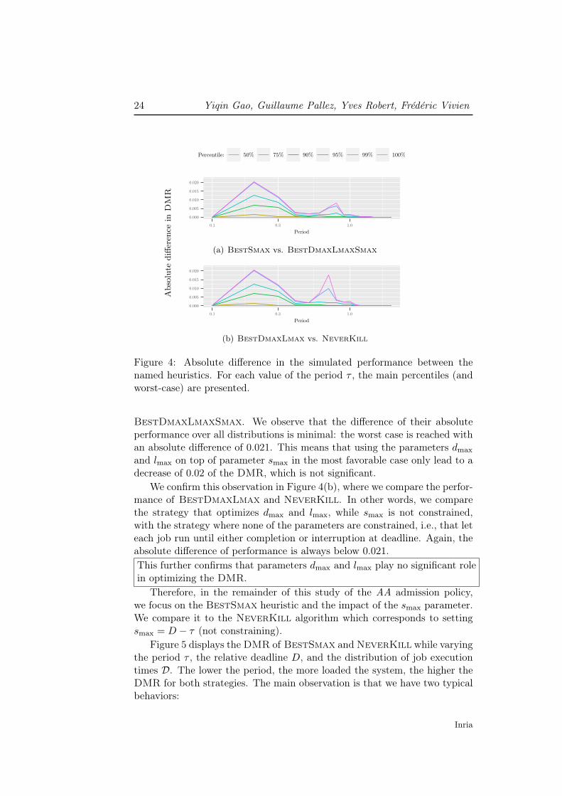
In Section 4.2 we have introduced three execution control parameters, namelydmax, lmax and smax. The first question to answer is: what is the relativeimpact of these parameters on the deadline miss ratio? To answerthis question, we compare on Figure 4 absolute performance in terms ofDMR of different heuristics.
The most complete heuristic is the BestDmaxLmaxSmax heuristicwhich chooses the combination minimizing the DMR for a given period τ , agiven distribution D, and a given relative deadline D, among all the possiblevalues for the three parameters. Hence, we use BestDmaxLmaxSmax as areference. On Figure 4(a) we compare the performance of BestSmax and
RR n° 9455
24 Yiqin Gao, Guillaume Pallez, Yves Robert, Frédéric Vivien
Absolutediffe
rencein
DM
R
0.000
0.005
0.010
0.015
0.020
0.1 0.3 1.0
Period
Percentile: 50% 75% 90% 95% 99% 100%
(a) BestSmax vs. BestDmaxLmaxSmax
0.000
0.005
0.010
0.015
0.020
0.1 0.3 1.0
Period
(b) BestDmaxLmax vs. NeverKill
Figure 4: Absolute difference in the simulated performance between thenamed heuristics. For each value of the period τ , the main percentiles (andworst-case) are presented.
BestDmaxLmaxSmax. We observe that the difference of their absoluteperformance over all distributions is minimal: the worst case is reached withan absolute difference of 0.021. This means that using the parameters dmax
and lmax on top of parameter smax in the most favorable case only lead to adecrease of 0.02 of the DMR, which is not significant.
We confirm this observation in Figure 4(b), where we compare the perfor-mance of BestDmaxLmax and NeverKill. In other words, we comparethe strategy that optimizes dmax and lmax, while smax is not constrained,with the strategy where none of the parameters are constrained, i.e., that leteach job run until either completion or interruption at deadline. Again, theabsolute difference of performance is always below 0.021.This further confirms that parameters dmax and lmax play no significant rolein optimizing the DMR.
Therefore, in the remainder of this study of the AA admission policy,we focus on the BestSmax heuristic and the impact of the smax parameter.We compare it to the NeverKill algorithm which corresponds to settingsmax = D − τ (not constraining).
Figure 5 displays the DMR of BestSmax and NeverKill while varyingthe period τ , the relative deadline D, and the distribution of job executiontimes D. The lower the period, the more loaded the system, the higher theDMR for both strategies. The main observation is that we have two typicalbehaviors:
Inria

Scheduling Strategies for Overloaded Real-Time Systems 25
Deadline/Period: 2 Deadline/Period: 6 Deadline/Period: 10
Tru
ncN
orm
LN
(0.5)Exp
LN
(3)
0.5 1.0 1.5 2.0 0.5 1.0 1.5 2.0 0.5 1.0 1.5 2.0
0.000.250.500.751.00
0.000.250.500.751.00
0.000.250.500.751.00
0.000.250.500.751.00
Period
Dea
dlin
em
iss
rati
o
NeverKill BestSmax
Figure 5: Absolute performance of job admission heuristics BestSmax andNeverKill (lower is better).
RR n° 9455

26 Yiqin Gao, Guillaume Pallez, Yves Robert, Frédéric Vivien
1. Distributions where the optimal solution is to not use smax as a con-straint (BestSmax = NeverKill), this is the case for the categoryof distribution represented by Exp and LN(3);
2. Distributions where the value of smax is important (TruncNorm,LN(0.5)). The peak performance are under heavy load (τ < 1) andlarge deadlines.
The performance of NeverKill does not appear to be impacted by the valueof the relative deadline (D) with respect to the period (τ). On the contrary,the improvement of BestSmax with respect to NeverKill increases withthe ratio D
τ and appears to reach a plateau when Dτ = 4 or 6, depending on
the distributionsWe can look specifically at the value of smax returned by the BestSmax
algorithm. In Figure 6, we represent these values, normalized to D − τ . In
Deadline/Period: 2 Deadline/Period: 6 Deadline/Period: 10
Tru
ncN
orm
LN
(0.5)Exp
LN
(3)
0.1 0.3 1.0 0.1 0.3 1.0 0.1 0.3 1.0
0.000.250.500.751.00
0.000.250.500.751.00
0.000.250.500.751.00
0.000.250.500.751.00
Period
Rel
ativ
eva
lue
ofs m
ax
Figure 6: Best value for the smax threshold for job admission heuristicBestSmax expressed as a fraction of the maximum meaningful value D−τ ,when the quantum length is 0.1 time unit.
practice, the performance of BestSmax can be similar for very differentvalues of smax. On the one hand, this makes BestSmax rather robust. Onthe other hand, this explains the fact that some curves are not smooth onFigure 6. The discretization also plays a role in these irregularities. Thisfigure confirms the two categories found in the previous result.
Inria
Scheduling Strategies for Overloaded Real-Time Systems 27
Altogether, we have shown that using BestSmax algorithm can have asignificant impact for some distributions. For other distributions, smax hasno impact (just like dmax and lmax), and NeverKill is a better solution: ithas same performance but does not need any pre-computation.Understanding what makes a distribution a good candidate for either one ofthe categories is a cahllenge that we leave to the future.
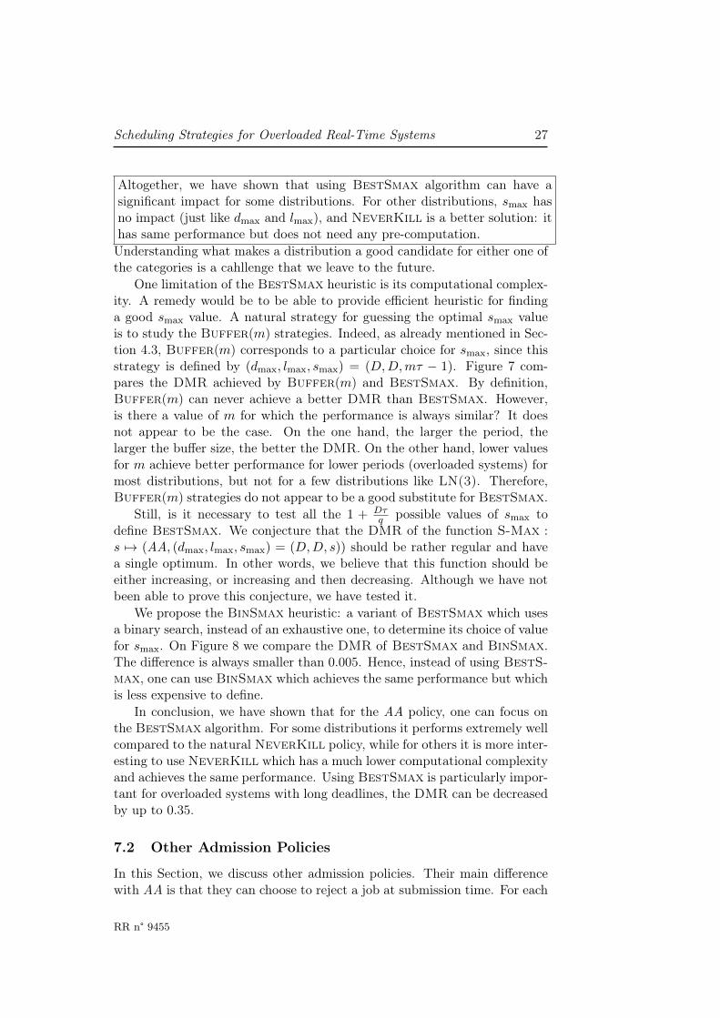
One limitation of the BestSmax heuristic is its computational complex-ity. A remedy would be to be able to provide efficient heuristic for findinga good smax value. A natural strategy for guessing the optimal smax valueis to study the Buffer(m) strategies. Indeed, as already mentioned in Sec-tion 4.3, Buffer(m) corresponds to a particular choice for smax, since thisstrategy is defined by (dmax, lmax, smax) = (D,D,mτ − 1). Figure 7 com-pares the DMR achieved by Buffer(m) and BestSmax. By definition,Buffer(m) can never achieve a better DMR than BestSmax. However,is there a value of m for which the performance is always similar? It doesnot appear to be the case. On the one hand, the larger the period, thelarger the buffer size, the better the DMR. On the other hand, lower valuesfor m achieve better performance for lower periods (overloaded systems) formost distributions, but not for a few distributions like LN(3). Therefore,Buffer(m) strategies do not appear to be a good substitute for BestSmax.
Still, is it necessary to test all the 1 + Dτq possible values of smax to
define BestSmax. We conjecture that the DMR of the function S-Max :s 7→ (AA, (dmax, lmax, smax) = (D,D, s)) should be rather regular and havea single optimum. In other words, we believe that this function should beeither increasing, or increasing and then decreasing. Although we have notbeen able to prove this conjecture, we have tested it.
We propose the BinSmax heuristic: a variant of BestSmax which usesa binary search, instead of an exhaustive one, to determine its choice of valuefor smax. On Figure 8 we compare the DMR of BestSmax and BinSmax.The difference is always smaller than 0.005. Hence, instead of using BestS-max, one can use BinSmax which achieves the same performance but whichis less expensive to define.
In conclusion, we have shown that for the AA policy, one can focus onthe BestSmax algorithm. For some distributions it performs extremely wellcompared to the natural NeverKill policy, while for others it is more inter-esting to use NeverKill which has a much lower computational complexityand achieves the same performance. Using BestSmax is particularly impor-tant for overloaded systems with long deadlines, the DMR can be decreasedby up to 0.35.
7.2 Other Admission Policies
In this Section, we discuss other admission policies. Their main differencewith AA is that they can choose to reject a job at submission time. For each
RR n° 9455

28 Yiqin Gao, Guillaume Pallez, Yves Robert, Frédéric Vivien
Deadline/Period: 2 Deadline/Period: 6 Deadline/Period: 10
Tru
ncN
orm
LN
(0.5)Exp
LN
(3)
0.1 0.3 1.0 0.1 0.3 1.0 0.1 0.3 1.0
0.000.250.500.751.00
0.000.250.500.751.00
0.000.250.500.751.00
0.000.250.500.751.00
Period
Dea
dlin
em
iss
rati
o
Buffer(1) Buffer(2) Buffer(4) Buffer(6) BestSmax
Figure 7: Deadline miss ratio of job admission heuristics BestSmax andBuffer(m) for different period τ and distributions while varying q.
Inria

Scheduling Strategies for Overloaded Real-Time Systems 29
Absolutediffe
-rencein
DM
R
0.000
0.005
0.010
0.015
0.020
0.1 0.3 1.0
Period
Percentile: 50% 75% 90% 95% 99% 100%
Figure 8: Absolute difference in the simulated performance between BestS-max vs. BinSmax. For each value of the period τ , the main percentiles(and worst-case) are presented.
of the three policies AP which do not admit all jobs (random, periodic andwith queues), we compare the performance of AP-BestDmaxLmaxSmax,with the policy from the previous section AA-BestSmax.
We start by studying queues with Figure 9. Note that an AA policycorresponds to a queue of unbounded size (although the queue is necessar-ily bounded by D/τ). Whatever the distribution and set of parameters,Queue(m) never achieves better performance than AA.
A striking observation however, is that under heavy load, the perfor-mance of Queue(1)-BestDmaxLmaxSmax is quite close to that of theAA policy, with guarantees that the number of jobs waiting is quite small.This is an interesting result as it allows to give faster negative answers tousers when we know that it is very likely that their jobs will not be accepted.
There is an exception for some distributions that correspond to the cate-gory of distributions where BestSmax = NeverKill (such as LN(3)). Inthis case, Queue(m) achieves worse performance even for very small periods.Overall, bounded queues are detrimental to the performance. This is partic-ularly true for distributions where the optimal strategy under AA is Nev-erKill. However for other distributions and under heavy load, the perfor-mance loss when using queues of size 1 is negligible.
For the random admission policy, Figure 10 presents the DMR of Best-DmaxLmaxSmax for different values of the admission ratio. Whatever thedistribution and set of parameters, the higher the admission ratio, the lowerthe DMR. The best choice is to have an admission ratio of 1, that is, toadmit all jobs. Again we observe significant difference for the category ofdistributions where NeverKill is the best strategy for the AA policy. Onecould wonder whether one could find an admission rate that depends on theload of the system that could be efficient for the other categories of distri-butions. A natural heuristic is one where the admission ratio is equal to theperiod, hence, ensuring a load of 1. This is plotted in black. This strategy
RR n° 9455

30 Yiqin Gao, Guillaume Pallez, Yves Robert, Frédéric Vivien
Deadline/Period: 2 Deadline/Period: 6 Deadline/Period: 10
Tru
ncN
orm
LN
(0.5)Exp
LN
(3)
0.1 0.3 1.0 0.1 0.3 1.0 0.1 0.3 1.0
0.000.250.500.751.00
0.000.250.500.751.00
0.000.250.500.751.00
0.000.250.500.751.00
Period
Dea
dlin
em
iss
rati
o
Queue(1) Queue(2) BestSmax
Figure 9: Deadline miss ratio of job admission policy Queue(m) applied onBestDmaxLmaxSmax for different period τ and distributions.
Inria

Scheduling Strategies for Overloaded Real-Time Systems 31
Deadline/Period: 2 Deadline/Period: 6 Deadline/Period: 10
Tru
ncN
orm
LN
(0.5)Exp
LN
(3)
0.1 0.3 1.0 0.1 0.3 1.0 0.1 0.3 1.0
0.000.250.500.751.00
0.000.250.500.751.00
0.000.250.500.751.00
0.000.250.500.751.00
Period
Dea
dlin
em
iss
rati
o
Admission ratio:min{1, τ} 0.1 0.2 0.3 0.4 0.5
0.6 0.7 0.8 0.9 1
Figure 10: Deadline miss ratio of random job admission policy applied onBestDmaxLmaxSmax for different period τ and distributions.
RR n° 9455
32 Yiqin Gao, Guillaume Pallez, Yves Robert, Frédéric Vivien
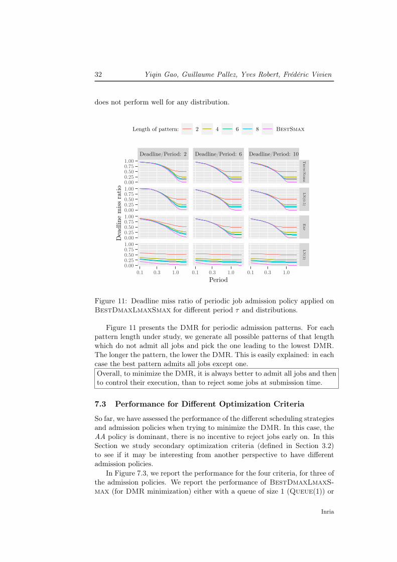
does not perform well for any distribution.
Deadline/Period: 2 Deadline/Period: 6 Deadline/Period: 10
Tru
ncN
orm
LN
(0.5)Exp
LN
(3)
0.1 0.3 1.0 0.1 0.3 1.0 0.1 0.3 1.0
0.000.250.500.751.00
0.000.250.500.751.00
0.000.250.500.751.00
0.000.250.500.751.00
Period
Dea
dlin
em
iss
rati
o
Length of pattern: 2 4 6 8 BestSmax
Figure 11: Deadline miss ratio of periodic job admission policy applied onBestDmaxLmaxSmax for different period τ and distributions.
Figure 11 presents the DMR for periodic admission patterns. For eachpattern length under study, we generate all possible patterns of that lengthwhich do not admit all jobs and pick the one leading to the lowest DMR.The longer the pattern, the lower the DMR. This is easily explained: in eachcase the best pattern admits all jobs except one.Overall, to minimize the DMR, it is always better to admit all jobs and thento control their execution, than to reject some jobs at submission time.
7.3 Performance for Different Optimization Criteria
So far, we have assessed the performance of the different scheduling strategiesand admission policies when trying to minimize the DMR. In this case, theAA policy is dominant, there is no incentive to reject jobs early on. In thisSection we study secondary optimization criteria (defined in Section 3.2)to see if it may be interesting from another perspective to have differentadmission policies.
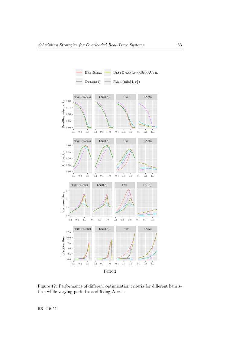
In Figure 7.3, we report the performance for the four criteria, for three ofthe admission policies. We report the performance of BestDmaxLmaxS-max (for DMR minimization) either with a queue of size 1 (Queue(1)) or
Inria
Scheduling Strategies for Overloaded Real-Time Systems 33
BestSmax BestDmaxLmaxSmaxUtil
Queue(1) Rand(min{1, τ})
TruncNorm LN(0.5) Exp LN(3)
0.1 0.3 1.0 0.1 0.3 1.0 0.1 0.3 1.0 0.1 0.3 1.0
0.00
0.25
0.50
0.75
1.00
Dea
dlin
em
iss
rati
o
TruncNorm LN(0.5) Exp LN(3)
0.1 0.3 1.0 0.1 0.3 1.0 0.1 0.3 1.0 0.1 0.3 1.0
0.00
0.25
0.50
0.75
1.00
Uti
lizat
ion
TruncNorm LN(0.5) Exp LN(3)
0.1 0.3 1.0 0.1 0.3 1.0 0.1 0.3 1.0 0.1 0.3 1.00
1
2
3
Res
pons
eti
me
TruncNorm LN(0.5) Exp LN(3)
0.1 0.3 1.0 0.1 0.3 1.0 0.1 0.3 1.0 0.1 0.3 1.0
0.0
2.5
5.0
7.5
10.0
12.5
Rej
ecti
onti
me
Period
Figure 12: Performance of different optimization criteria for different heuris-tics, while varying period τ and fixing N = 4.
RR n° 9455
34 Yiqin Gao, Guillaume Pallez, Yves Robert, Frédéric Vivien
with a random admission policy with an admission ratio equal to the period(Rand(min{1, τ}) (recall that τ ∈ [0.1, 2] hence the need for the minimum)).When all jobs are accepted, we report the performance of BestSmax (whichminimizes DMR). Finally, we also include the performance of a strategy thatuses the set of dmax, lmax, and smax parameters which maximizes the utiliza-tion (BestDmaxLmaxSmaxUtil).
As seen in the previous sections, except for Rand(min{1, τ}), the perfor-mance of the heuristics is quite close for DMR minimization. For utilization,however, the heuristics achieve significantly different performance, especiallyfor the exponential distribution. This hints at different possible trade-offsbetween DMR and utilization for those scenarios where utilization would bea criterion of interest.
For both the rejection time and the response time, BestSmax and Best-DmaxLmaxSmaxUtil achieve worse performance than Queue(1). Thiscan be easily explained. Queue(1) rejects many jobs at their admissiontime. This decreases the load in the system and lower the probability thatjobs are killed by their deadlines which, in turn, decreases the rejection time.This is especially true when the period is greater than 1. In such a case, thesystem is underloaded and rejected jobs are dropped exactly at their dead-lines. Also, when the system is less loaded, jobs are less impacted by theirpredecessors, which decreases their waiting time, and thus their responsetime. Rand(min{1, τ}) has an intermediate behavior due to a higher accep-tance rate.
7.4 Summary
Our thorough evaluation provides several important insights about schedul-ing strategies for overloaded real-time systems. The first one is that thedistribution of job execution times matters a lot: for some distributions,the naive strategy NeverKill (which admits all jobs and let them run un-til either they finish or meet their deadline) performs very well. For otherdistributions, the best strategy is to accept all jobs, and to decide earlytermination only based on the time spent in the queue (parameter smax).Determining whether a distribution fits either category remains an openproblem.
Finally, we investigated how optimizing DMR trades-off with other op-timization criteria. While BestSmax dominates in performance for DMRand utilization, it comes at the price of higher response time and rejectiontime. When quality of service is important, intermediate admission policies(such as Queue(1)) can be used under heavy load, and with a negligibleincrease of DMR.
Inria

Scheduling Strategies for Overloaded Real-Time Systems 35
8 Conclusion
This work has discussed several novel strategies to schedule firm real-timejobs on an overloaded server. We have introduced three control parametersto decide when to start or interrupt a job. Coupled with several admissionpolicies and aiming at different optimization criteria, our dynamic schedulingstrategies encompass a wide range of execution scenarios.
We have used discretization to derive a Markov model and used its sta-tionary distribution to determine the best value for each control parameter.An extensive simulation campaign with 14 different probability distributionshas shown that tuning the new control parameters, in particular smax, dra-matically improves system performance. We have reduced the complexity tofind the optimal value of smax by using a binary search. The ultimate goalwould be to identify a priori for which distributions smax is necessary, andfor which ones NeverKill should be preferred.
The main focus of this work has been on the DMR objective. Futurework will further study system utilization, which is an important criterionfor platform owners. Combining several objectives may be important too,e.g., minimizing DMR or maximizing utilization, while enforcing an upperbound on mean rejection time.
Finally, some applications may benefit from not treating all jobs equally;in a general setting, some particular jobs may have higher value for the userand, hence, should be executed successfully whenever possible. We believethat our approach can be extended to deal with such complicated scenarios.
References
[1] L. Ahrendts, S. Quinton, and R. Ernst. Finite ready queues as a meanfor overload reduction in weakly-hard real-time systems. In Proc. 25thInternational Conference on Real-Time Networks and Systems (RTNS),page 88–97. ACM, 2017.
[2] G. Bernat, A. Burns, and A. Liamosi. Weakly hard real-time systems.IEEE Trans. Computers, 50(4):308–321, 2001.
[3] G. Buttazzo, G. Lipari, and L. Abeni. Elastic task model for adaptiverate control. In Proc.19th IEEE Real-Time Systems Symposium, pages286–295, 1998.
[4] G. Buttazzo, M. Velasco, and P. Marti. Quality-of-control managementin overloaded real-time systems. IEEE Trans. Computers, 56(2):253–266, 2007.
RR n° 9455
36 Yiqin Gao, Guillaume Pallez, Yves Robert, Frédéric Vivien
[5] L.-C. Canon, A. K. W. Chang, Y. Robert, and F. Vivien. Schedulingindependent stochastic tasks under deadline and budget constraints.The Int. J. of High Perf. Computing Applications, 34(2):246–264, 2020.
[6] A. Cervin. Analysis of overrun strategies in periodic control tasks. IFACProceedings Volumes, 38(1):219–224, 2005.
[7] H. Choi, H. Kim, and Q. Zhu. Job-class-level fixed priority schedulingof weakly-hard real-time systems. In IEEE Real-Time and EmbeddedTechnology and Applications Symposium (RTAS), pages 241–253, 2019.
[8] A. Chydzinski. Queues with the dropping function and non-poissonarrivals. IEEE Access, 8:39819–39829, 2020.
[9] C. Denninnart, J. Gentry, A. Mokhtari, and M. A. Salehi. Efficient taskpruning mechanism to improve robustness of heterogeneous computingsystems. Journal of Parallel and Distributed Computing, 2020.
[10] C. Denninnart, J. Gentry, and M. A. Salehi. Improving robustness ofheterogeneous serverless computing systems via probabilistic task prun-ing. In 2019 IEEE IPDPS Workshops, pages 6–15. IEEE, 2019.
[11] J. L. Díaz, D. F. García, K. Kim, C.-G. Lee, L. L. Bello, J. M. López,S. L. Min, and O. Mirabella. Stochastic analysis of periodic real-timesystems. In 23rd IEEE RTSS, pages 289–300. IEEE, 2002.
[12] D. Feitelson. Workload modeling for computer systems performanceevaluation. Version 1.0.3, pages 1–607, 2014.
[13] C.-W. Feng, L.-F. Huang, C. Xu, and Y.-C. Chang. Congestion controlscheme performance analysis based on nonlinear red. IEEE SystemsJournal, 11(4):2247–2254, 2015.
[14] S. Floyd and V. Jacobson. Random early detection gateways for con-gestion avoidance. IEEE/ACM T. on Network., 1(4):397–413, 1993.
[15] Y. Gao, G. Pallez, Y. Robert, and F. Vivien. Evaluating Task DroppingStrategies for Overloaded Real-Time Systems (Work-In-Progress). In42nd Real Time Systems Symposium (RTSS). IEEE Computer SocietyPress, 2021.
[16] W. Geelen, D. Antunes, J. P. M. Voeten, R. R. H. Schiffelers, andW. P. M. H. Heemels. The impact of deadline misses on the controlperformance of high-end motion control systems. IEEE Trans. Indus-trial Electronics, 63(2):1218–1229, 2016.
[17] J. Gentry, C. Denninnart, and M. A. Salehi. Robust dynamic resourceallocation via probabilistic task pruning in heterogeneous computingsystems. In IPDPS, pages 375–384. IEEE, 2019.
Inria
Scheduling Strategies for Overloaded Real-Time Systems 37
[18] M. Hamdaoui and P. Ramanathan. A dynamic priority assignment tech-nique for streams with (m, k)-firm deadlines. IEEE Trans. Computers,44(12):1443–1451, 1995.
[19] M. Harchol-Balter. Open problems in queueing theory inspired by dat-acenter computing. Queueing Systems, 97(1):3–37, 2021.
[20] O. Häggström. Finite Markov Chains and Algorithmic Applications.Cambridge University Press, 2002.
[21] H. Kopetz. Real-Time Systems: Design Principles for Distributed Em-bedded Applications. Kluwer, USA, 2nd edition, 2011.
[22] G. Koren and D. Shasha. Skip-over: algorithms and complexity foroverloaded systems that allow skips. In RTSS, pages 110–117, 1995.
[23] C. Lin, T. Kaldewey, A. Povzner, and S. Brandt. Diverse soft real-timeprocessing in an integrated system. In RTSS, pages 369–378, 2006.
[24] A. Marchand and M. Chetto. Dynamic scheduling of periodic skippabletasks in an overloaded real-time system. In AICCSA, pages 456–464,2008.
[25] A. Mokhtari, C. Denninnart, and M. A. Salehi. Autonomous task drop-ping mechanism to achieve robustness in heterogeneous computing sys-tems. arXiv preprint arXiv:2005.11050, 2020.
[26] T. Patel, Z. Liu, R. Kettimuthu, P. Rich, W. Allcock, and D. Tiwari.Job characteristics on large-scale systems: long-term analysis, quantifi-cation, and implications. In SC’20, pages 1–17. IEEE, 2020.
[27] P. Pazzaglia, C. Mandrioli, M. Maggio, and A. Cervin. DMAC: deadline-miss-aware control. Dagstuhl Artifacts Ser., 5(1):03:1–03:3, 2019.
[28] P. Ramanathan. Graceful degradation in real-time control applicationsusing (m, k)-firm guarantee. In Proc. IEEE 27th Int. Symp. on FaultTolerant Computing, pages 132–141, 1997.
[29] V. Rosolen, O. Bonaventure, and G. Leduc. A RED discard strategyfor ATM networks and its performance evaluation with TCP/IP traffic.ACM SIGCOMM Computer Communication Review, 29(3):23–43, 1999.
[30] M. A. Salehi, J. Smith, A. A. Maciejewski, H. J. Siegel, E. K. Chong,J. Apodaca, L. D. Briceno, T. Renner, V. Shestak, J. Ladd, et al.Stochastic-based robust dynamic resource allocation for independenttasks in a heterogeneous computing system. Journal of Parallel andDistributed Computing, 97:96–111, 2016.
RR n° 9455
38 Yiqin Gao, Guillaume Pallez, Yves Robert, Frédéric Vivien
[31] R. West and C. Poellabauer. Analysis of a window-constrained schedulerfor real-time and best-effort packet streams. In Proc. 21st IEEE Real-Time Systems Symposium, pages 239–248, 2000.
[32] C. S. Yeo and R. Buyya. A taxonomy of market-based resource manage-ment systems for utility-driven cluster computing. Software: Practiceand Experience, 36(13):1381–1419, 2006.
[33] T. Yoshimoto and T. Ushio. Optimal arbitration of control tasks byjob skipping in cyber-physical systems. In 2011 IEEE/ACM 2nd Int.Conf.Cyber-Physical Systems, pages 55–64, 2011.
Inria

Scheduling Strategies for Overloaded Real-Time Systems 39
Appendix
This section includes all figures for the evaluation, with the 14 probabilitydistributions.
smax = D (aka NeverKill) smax = 0.75 D smax = 0.50 D smax = 0.25 D
1e+02 1e+04 1e+06 1e+02 1e+04 1e+06 1e+02 1e+04 1e+06 1e+02 1e+04 1e+060.00
0.01
0.02
0.03
0.04
0.05
Number of simulated tasks
Stan
dard
devi
atio
n
Percentile: 25% 50% 90% 95% 99% 100%
Figure 13: Evolution of the standard deviation of a set of 100 simulations fordifferent smax heuristics, as a function of the number of simulated tasks simu-lated. For each number of tasks and each value of smax, we report percentileson the standard deviation of the DMR for different periods, deadlines, anddistributions.
RR n° 9455

40 Yiqin Gao, Guillaume Pallez, Yves Robert, Frédéric Vivien
Deadline/Period: 2 Deadline/Period: 4 Deadline/Period: 6 Deadline/Period: 8 Deadline/Period: 10
Unifo
rm
Tru
ncN
orm
LN
(0.5)H
alfN
BiT
runcN
X2
BiE
xpS
imila
rExp
InvG
amma
LN
(3)B
iTru
ncN
X100
BiE
xpD
ifferen
tG
amma
Weibu
ll0.4W
eibull1.5
0.1 0.3 1.0 0.1 0.3 1.0 0.1 0.3 1.0 0.1 0.3 1.0 0.1 0.3 1.0
0.000.250.500.751.00
0.000.250.500.751.00
0.000.250.500.751.00
0.000.250.500.751.00
0.000.250.500.751.00
0.000.250.500.751.00
0.000.250.500.751.00
0.000.250.500.751.00
0.000.250.500.751.00
0.000.250.500.751.00
0.000.250.500.751.00
0.000.250.500.751.00
0.000.250.500.751.00
0.000.250.500.751.00
Period
Dea
dlin
em
iss
rati
o
Buffer(1) Buffer(2) Buffer(4) Buffer(6) BestSmax
Figure 14: Deadline miss ratio of job admission heuristics BestSmax andBuffer(m) for different period τ and distributions while varying q, theperformance are assessed through simulations of 106 jobs.
Inria
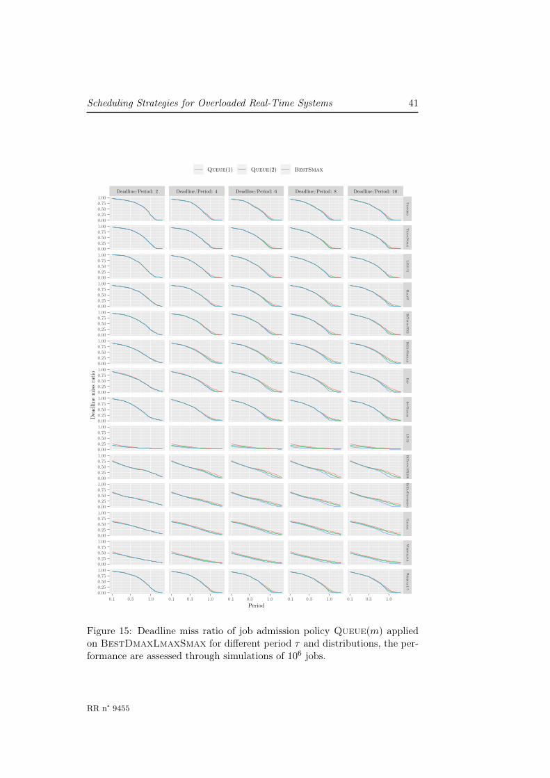
Scheduling Strategies for Overloaded Real-Time Systems 41
Deadline/Period: 2 Deadline/Period: 4 Deadline/Period: 6 Deadline/Period: 8 Deadline/Period: 10
Unifo
rm
Tru
ncN
orm
LN
(0.5)H
alfN
BiT
runcN
X2
BiE
xpS
imila
rExp
InvG
amma
LN
(3)B
iTru
ncN
X100
BiE
xpD
ifferen
tG
amma
Weibu
ll0.4W
eibull1.5
0.1 0.3 1.0 0.1 0.3 1.0 0.1 0.3 1.0 0.1 0.3 1.0 0.1 0.3 1.0
0.000.250.500.751.00
0.000.250.500.751.00
0.000.250.500.751.00
0.000.250.500.751.00
0.000.250.500.751.00
0.000.250.500.751.00
0.000.250.500.751.00
0.000.250.500.751.00
0.000.250.500.751.00
0.000.250.500.751.00
0.000.250.500.751.00
0.000.250.500.751.00
0.000.250.500.751.00
0.000.250.500.751.00
Period
Dea
dlin
em
iss
rati
o
Queue(1) Queue(2) BestSmax
Figure 15: Deadline miss ratio of job admission policy Queue(m) appliedon BestDmaxLmaxSmax for different period τ and distributions, the per-formance are assessed through simulations of 106 jobs.
RR n° 9455
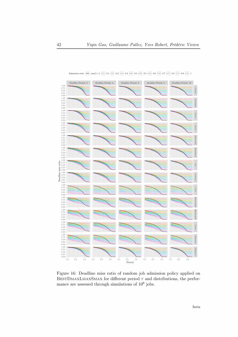
42 Yiqin Gao, Guillaume Pallez, Yves Robert, Frédéric Vivien
Deadline/Period: 2 Deadline/Period: 4 Deadline/Period: 6 Deadline/Period: 8 Deadline/Period: 10
Unifo
rm
Tru
ncN
orm
LN
(0.5)H
alfN
BiT
runcN
X2
BiE
xpS
imila
rExp
InvG
amma
LN
(3)B
iTru
ncN
X100
BiE
xpD
ifferen
tG
amma
Weibu
ll0.4W
eibull1.5
0.1 0.3 1.0 0.1 0.3 1.0 0.1 0.3 1.0 0.1 0.3 1.0 0.1 0.3 1.0
0.000.250.500.751.00
0.000.250.500.751.00
0.000.250.500.751.00
0.000.250.500.751.00
0.000.250.500.751.00
0.000.250.500.751.00
0.000.250.500.751.00
0.000.250.500.751.00
0.000.250.500.751.00
0.000.250.500.751.00
0.000.250.500.751.00
0.000.250.500.751.00
0.000.250.500.751.00
0.000.250.500.751.00
Period
Dea
dlin
em
iss
rati
o
Admission ratio: min{1, τ} 0.1 0.2 0.3 0.4 0.5 0.6 0.7 0.8 0.9 1
Figure 16: Deadline miss ratio of random job admission policy applied onBestDmaxLmaxSmax for different period τ and distributions, the perfor-mance are assessed through simulations of 106 jobs.
Inria

Scheduling Strategies for Overloaded Real-Time Systems 43
Deadline/Period: 2 Deadline/Period: 4 Deadline/Period: 6 Deadline/Period: 8 Deadline/Period: 10
Unifo
rm
Tru
ncN
orm
LN
(0.5)H
alfN
BiT
runcN
X2
BiE
xpS
imila
rExp
InvG
amma
LN
(3)B
iTru
ncN
X100
BiE
xpD
ifferen
tG
amma
Weibu
ll0.4W
eibull1.5
0.1 0.3 1.0 0.1 0.3 1.0 0.1 0.3 1.0 0.1 0.3 1.0 0.1 0.3 1.0
0.000.250.500.751.00
0.000.250.500.751.00
0.000.250.500.751.00
0.000.250.500.751.00
0.000.250.500.751.00
0.000.250.500.751.00
0.000.250.500.751.00
0.000.250.500.751.00
0.000.250.500.751.00
0.000.250.500.751.00
0.000.250.500.751.00
0.000.250.500.751.00
0.000.250.500.751.00
0.000.250.500.751.00
Period
Dea
dlin
em
iss
rati
o
Length of pattern: 2 3 4 5 6 7 8 BestSmax
Figure 17: Deadline miss ratio of periodic job admission policy applied onBestDmaxLmaxSmax for different period τ and distributions, the perfor-mance are assessed through simulations of 106 jobs.
RR n° 9455
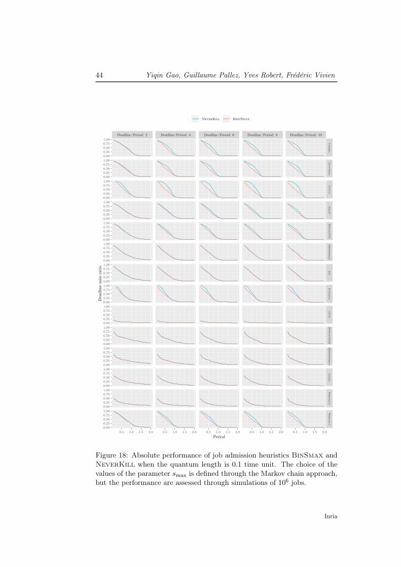
44 Yiqin Gao, Guillaume Pallez, Yves Robert, Frédéric Vivien
Deadline/Period: 2 Deadline/Period: 4 Deadline/Period: 6 Deadline/Period: 8 Deadline/Period: 10
Unifo
rm
Tru
ncN
orm
LN
(0.5)H
alfN
BiT
runcN
X2
BiE
xpS
imila
rExp
InvG
amma
LN
(3)B
iTru
ncN
X100
BiE
xpD
ifferen
tG
amma
Weibu
ll0.4W
eibull1.5
0.5 1.0 1.5 2.0 0.5 1.0 1.5 2.0 0.5 1.0 1.5 2.0 0.5 1.0 1.5 2.0 0.5 1.0 1.5 2.0
0.000.250.500.751.00
0.000.250.500.751.00
0.000.250.500.751.00
0.000.250.500.751.00
0.000.250.500.751.00
0.000.250.500.751.00
0.000.250.500.751.00
0.000.250.500.751.00
0.000.250.500.751.00
0.000.250.500.751.00
0.000.250.500.751.00
0.000.250.500.751.00
0.000.250.500.751.00
0.000.250.500.751.00
Period
Dea
dlin
em
iss
rati
o
NeverKill BestSmax
Figure 18: Absolute performance of job admission heuristics BinSmax andNeverKill when the quantum length is 0.1 time unit. The choice of thevalues of the parameter smax is defined through the Markov chain approach,but the performance are assessed through simulations of 106 jobs.
Inria

Scheduling Strategies for Overloaded Real-Time Systems 45
Deadline/Period: 2 Deadline/Period: 4 Deadline/Period: 6 Deadline/Period: 8 Deadline/Period: 10
Unifo
rm
Tru
ncN
orm
LN
(0.5)H
alfN
BiT
runcN
X2
BiE
xpS
imila
rExp
InvG
amma
LN
(3)B
iTru
ncN
X100
BiE
xpD
ifferen
tG
amma
Weibu
ll0.4W
eibull1.5
0.1 0.3 1.0 0.1 0.3 1.0 0.1 0.3 1.0 0.1 0.3 1.0 0.1 0.3 1.0
0
50
100
150
0
50
100
150
0
50
100
150
0
50
100
150
0
50
100
150
0
50
100
150
0
50
100
150
0
50
100
150
0
50
100
150
0
50
100
150
0
50
100
150
0
50
100
150
0
50
100
150
0
50
100
150
Period
Abs
olut
eva
lue
ofs m
ax
BestSmax
Figure 19: Best value for the smax threshold for job admission heuristicBestSmax, when the quantum length is 0.1 time unit.
RR n° 9455

46 Yiqin Gao, Guillaume Pallez, Yves Robert, Frédéric Vivien
Deadline/Period: 2 Deadline/Period: 4 Deadline/Period: 6 Deadline/Period: 8 Deadline/Period: 10
Unifo
rm
Tru
ncN
orm
LN
(0.5)H
alfN
BiT
runcN
X2
BiE
xpS
imila
rExp
InvG
amma
LN
(3)B
iTru
ncN
X100
BiE
xpD
ifferen
tG
amma
Weibu
ll0.4W
eibull1.5
0.1 0.3 1.0 0.1 0.3 1.0 0.1 0.3 1.0 0.1 0.3 1.0 0.1 0.3 1.0
0.00
0.25
0.50
0.75
1.00
0.00
0.25
0.50
0.75
1.00
0.00
0.25
0.50
0.75
1.00
0.00
0.25
0.50
0.75
1.00
0.00
0.25
0.50
0.75
1.00
0.00
0.25
0.50
0.75
1.00
0.00
0.25
0.50
0.75
1.00
0.00
0.25
0.50
0.75
1.00
0.00
0.25
0.50
0.75
1.00
0.00
0.25
0.50
0.75
1.00
0.00
0.25
0.50
0.75
1.00
0.00
0.25
0.50
0.75
1.00
0.00
0.25
0.50
0.75
1.00
0.00
0.25
0.50
0.75
1.00
Period
Rel
ativ
eva
lue
ofs m
ax
BestSmax
Figure 20: Best value for the smax threshold for job admission heuristicBestSmax expressed as a fraction of the maximum meaningful value D−τ ,when the quantum length is 0.1 time unit.
Inria
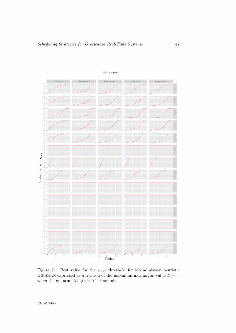
Scheduling Strategies for Overloaded Real-Time Systems 47
Deadline/Period: 2 Deadline/Period: 4 Deadline/Period: 6 Deadline/Period: 8 Deadline/Period: 10
Unifo
rm
Tru
ncN
orm
LN
(0.5)H
alfN
BiT
runcN
X2
BiE
xpS
imila
rExp
InvG
amma
LN
(3)B
iTru
ncN
X100
BiE
xpD
ifferen
tG
amma
Weibu
ll0.4W
eibull1.5
0.1 0.3 1.0 0.1 0.3 1.0 0.1 0.3 1.0 0.1 0.3 1.0 0.1 0.3 1.0
0.00
0.25
0.50
0.75
1.00
0.00
0.25
0.50
0.75
1.00
0.00
0.25
0.50
0.75
1.00
0.00
0.25
0.50
0.75
1.00
0.00
0.25
0.50
0.75
1.00
0.00
0.25
0.50
0.75
1.00
0.00
0.25
0.50
0.75
1.00
0.00
0.25
0.50
0.75
1.00
0.00
0.25
0.50
0.75
1.00
0.00
0.25
0.50
0.75
1.00
0.00
0.25
0.50
0.75
1.00
0.00
0.25
0.50
0.75
1.00
0.00
0.25
0.50
0.75
1.00
0.00
0.25
0.50
0.75
1.00
Period
Rel
ativ
eva
lue
ofs m
ax
BinSmax
Figure 21: Best value for the smax threshold for job admission heuristicBinSmax expressed as a fraction of the maximum meaningful value D − τ ,when the quantum length is 0.1 time unit.
RR n° 9455
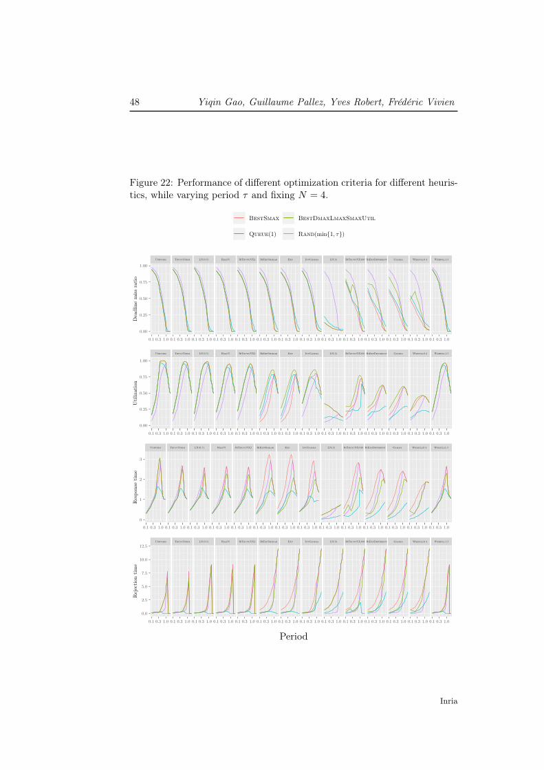
48 Yiqin Gao, Guillaume Pallez, Yves Robert, Frédéric Vivien
Figure 22: Performance of different optimization criteria for different heuris-tics, while varying period τ and fixing N = 4.
BestSmax BestDmaxLmaxSmaxUtil
Queue(1) Rand(min{1, τ})
Uniform TruncNorm LN(0.5) HalfN BiTruncNX2 BiExpSimilar Exp InvGamma LN(3) BiTruncNX100 BiExpDifferent Gamma Weibull0.4 Weibull1.5
0.1 0.3 1.0 0.1 0.3 1.0 0.1 0.3 1.0 0.1 0.3 1.0 0.1 0.3 1.0 0.1 0.3 1.0 0.1 0.3 1.0 0.1 0.3 1.0 0.1 0.3 1.0 0.1 0.3 1.0 0.1 0.3 1.0 0.1 0.3 1.0 0.1 0.3 1.0 0.1 0.3 1.0
0.00
0.25
0.50
0.75
1.00
Dea
dlin
em
iss
rati
o
Uniform TruncNorm LN(0.5) HalfN BiTruncNX2 BiExpSimilar Exp InvGamma LN(3) BiTruncNX100 BiExpDifferent Gamma Weibull0.4 Weibull1.5
0.1 0.3 1.0 0.1 0.3 1.0 0.1 0.3 1.0 0.1 0.3 1.0 0.1 0.3 1.0 0.1 0.3 1.0 0.1 0.3 1.0 0.1 0.3 1.0 0.1 0.3 1.0 0.1 0.3 1.0 0.1 0.3 1.0 0.1 0.3 1.0 0.1 0.3 1.0 0.1 0.3 1.0
0.00
0.25
0.50
0.75
1.00
Uti
lizat
ion
Uniform TruncNorm LN(0.5) HalfN BiTruncNX2 BiExpSimilar Exp InvGamma LN(3) BiTruncNX100 BiExpDifferent Gamma Weibull0.4 Weibull1.5
0.1 0.3 1.0 0.1 0.3 1.0 0.1 0.3 1.0 0.1 0.3 1.0 0.1 0.3 1.0 0.1 0.3 1.0 0.1 0.3 1.0 0.1 0.3 1.0 0.1 0.3 1.0 0.1 0.3 1.0 0.1 0.3 1.0 0.1 0.3 1.0 0.1 0.3 1.0 0.1 0.3 1.0
0
1
2
3
Res
pons
eti
me
Uniform TruncNorm LN(0.5) HalfN BiTruncNX2 BiExpSimilar Exp InvGamma LN(3) BiTruncNX100 BiExpDifferent Gamma Weibull0.4 Weibull1.5
0.1 0.3 1.0 0.1 0.3 1.0 0.1 0.3 1.0 0.1 0.3 1.0 0.1 0.3 1.0 0.1 0.3 1.0 0.1 0.3 1.0 0.1 0.3 1.0 0.1 0.3 1.0 0.1 0.3 1.0 0.1 0.3 1.0 0.1 0.3 1.0 0.1 0.3 1.0 0.1 0.3 1.0
0.0
2.5
5.0
7.5
10.0
12.5
Rej
ecti
onti
me
Period
Inria

RESEARCH CENTREGRENOBLE – RHÔNE-ALPES
Inovallée
655 avenue de l’Europe Montbonnot
38334 Saint Ismier Cedex
PublisherInriaDomaine de Voluceau - RocquencourtBP 105 - 78153 Le Chesnay Cedexinria.fr
ISSN 0249-6399