SCHEDULING STRATEGIES FOR MIXED DATA AND TASK PARALLELISM ON HETEROGENEOUS CLUSTERS

July 9, 2003 10:48 WSPC/119-PPL 00125

Parallel Processing Letters, Vol. 13, No. 2 (2003) 225–244c© World Scientific Publishing Company

SCHEDULING STRATEGIES FOR MIXED DATA AND TASK

PARALLELISM ON HETEROGENEOUS CLUSTERS

O. BEAUMONT

LaBRI, UMR CNRS 5800, Bordeaux, France

[email protected]

A. LEGRAND∗, L. MARCHAL† and Y. ROBERT‡

LIP, UMR CNRS-INRIA 5668, ENS Lyon, France∗[email protected]†[email protected]‡[email protected]

Received December 2002Revised April 2003

Accepted by J. Dongarra & B. Tourancheau

ABSTRACT

We consider the execution of a complex application on a heterogeneous “grid” computingplatform. The complex application consists of a suite of identical, independent problemsto be solved. In turn, each problem consists of a set of tasks. There are dependences(precedence constraints) between these tasks and these dependences are organized asa tree. A typical example is the repeated execution of the same algorithm on severaldistinct data samples. We use a non-oriented graph to model the grid platform, whereresources have different speeds of computation and communication. We show how todetermine the optimal steady-state scheduling strategy for each processor (the fraction oftime spent computing and the fraction of time spent communicating with each neighbor).This result holds for a quite general framework, allowing for cycles and multiple paths

in the platform graph.

Keywords: Heterogeneous processors; scheduling; mixed data and task parallelism;steady-state.

1. Introduction

In this paper, we consider the execution of a complex application, on a heteroge-

neous “grid” computing platform. The complex application consists of a suite of

identical, independent problems to be solved. In turn, each problem consists of a

set of tasks. There are dependences (precedence constraints) between these tasks. A

typical example is the repeated execution of the same algorithm on several distinct

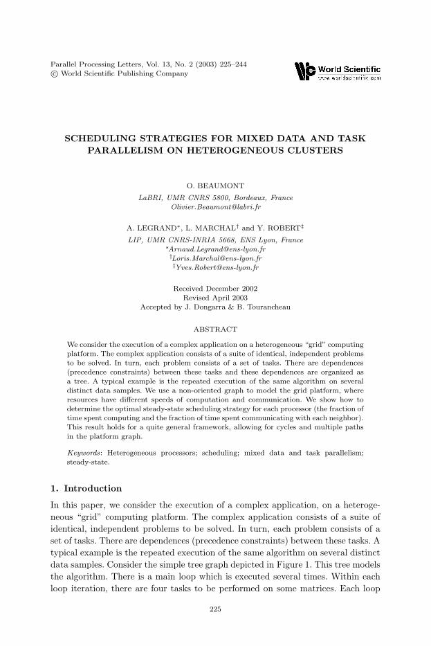
data samples. Consider the simple tree graph depicted in Figure 1. This tree models

the algorithm. There is a main loop which is executed several times. Within each

loop iteration, there are four tasks to be performed on some matrices. Each loop

225

July 9, 2003 10:48 WSPC/119-PPL 00125

226 O. Beaumont et al.

T4

T2 T3

T1

Figure 1: A simple tree example.

P2 P4

P3P1

Figure 2: A simple platform example

execute itself, and how many tasks to forward to each of its neighbors. Due to heterogeneity, theneighbors may receive different amounts of work (maybe none for some of them). Each neighborfaces in turn the same dilemma: determine how many tasks to execute, and how many to delegateto other processors. Note that the master may well need to send tasks along multiple paths toproperly feed a very fast but remote computing resource.

Because the problems are independent, their execution can be pipelined. At a given time-step,different processors may well compute different tasks belonging to different problem instances. Inthe example, a given processor Pi may well compute the tenth copy of task T1, correspondingto problem number 10, while another processor Pj computes the eight copy of task T3, whichcorresponds to problem number 8. However, because of the dependence constraints, note thatPj could not begin the execution of the tenth copy of task T3 before that Pi has terminated theexecution of the tenth copy of task T1 and sent the required data to Pj (if i 6= j).

Because the number of tasks to be executed on the computing platform is expected to be verylarge (otherwise why deploy the corresponding application on a distributed platform?), we focuson steady-state optimization problems rather than on standard makespan minimization problems.Minimizing the makespan, i.e. the total execution time, is a NP-hard problem in most practicalsituations [16, 30, 13], while it turns out that the optimal steady-state can be characterized veryefficiently, with low-degree polynomial complexity. For our target application, the optimal steadystate is defined as follows: for each processor, determine the fraction of time spent computing,and the fraction of time spent sending or receiving each type of tasks along each communicationlink, so that the (averaged) overall number of tasks processed at each time-step is maximum. Inaddition, we will prove that the optimal steady-state scheduling is very close to the absolute optimalscheduling: given a time bound K, it may be possible to execute more tasks than with the optimalsteady-state scheduling, but only a constant (independent of K) number of such extra tasks. To

2

Fig. 1. A simple tree example.

T4

T2 T3

T1

Figure 1: A simple tree example.

P2 P4

P3P1

Figure 2: A simple platform example

execute itself, and how many tasks to forward to each of its neighbors. Due to heterogeneity, theneighbors may receive different amounts of work (maybe none for some of them). Each neighborfaces in turn the same dilemma: determine how many tasks to execute, and how many to delegateto other processors. Note that the master may well need to send tasks along multiple paths toproperly feed a very fast but remote computing resource.

Because the problems are independent, their execution can be pipelined. At a given time-step,different processors may well compute different tasks belonging to different problem instances. Inthe example, a given processor Pi may well compute the tenth copy of task T1, correspondingto problem number 10, while another processor Pj computes the eight copy of task T3, whichcorresponds to problem number 8. However, because of the dependence constraints, note thatPj could not begin the execution of the tenth copy of task T3 before that Pi has terminated theexecution of the tenth copy of task T1 and sent the required data to Pj (if i 6= j).

Because the number of tasks to be executed on the computing platform is expected to be verylarge (otherwise why deploy the corresponding application on a distributed platform?), we focuson steady-state optimization problems rather than on standard makespan minimization problems.Minimizing the makespan, i.e. the total execution time, is a NP-hard problem in most practicalsituations [16, 30, 13], while it turns out that the optimal steady-state can be characterized veryefficiently, with low-degree polynomial complexity. For our target application, the optimal steadystate is defined as follows: for each processor, determine the fraction of time spent computing,and the fraction of time spent sending or receiving each type of tasks along each communicationlink, so that the (averaged) overall number of tasks processed at each time-step is maximum. Inaddition, we will prove that the optimal steady-state scheduling is very close to the absolute optimalscheduling: given a time bound K, it may be possible to execute more tasks than with the optimalsteady-state scheduling, but only a constant (independent of K) number of such extra tasks. To

2

Fig. 2. A simple platform example.

iteration is what we call a problem instance. Each problem instance operates on

different data, but all instances share the same task graph, i.e. the tree graph of

Figure 1. For each node in the task graph, there are as many task copies as there

are iterations in the main loop.

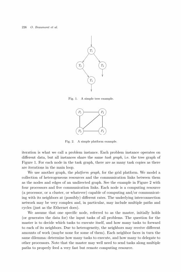
We use another graph, the platform graph, for the grid platform. We model a

collection of heterogeneous resources and the communication links between them

as the nodes and edges of an undirected graph. See the example in Figure 2 with

four processors and five communication links. Each node is a computing resource

(a processor, or a cluster, or whatever) capable of computing and/or communicat-

ing with its neighbors at (possibly) different rates. The underlying interconnection

network may be very complex and, in particular, may include multiple paths and

cycles (just as the Ethernet does).

We assume that one specific node, referred to as the master, initially holds

(or generates the data for) the input tasks of all problems. The question for the

master is to decide which tasks to execute itself, and how many tasks to forward

to each of its neighbors. Due to heterogeneity, the neighbors may receive different

amounts of work (maybe none for some of them). Each neighbor faces in turn the

same dilemma: determine how many tasks to execute, and how many to delegate to

other processors. Note that the master may well need to send tasks along multiple

paths to properly feed a very fast but remote computing resource.

July 9, 2003 10:48 WSPC/119-PPL 00125

Scheduling Strategies for Mixed Data and Task Parallelism 227

Because the problems are independent, their execution can be pipelined. At a

given time-step, different processors may well compute different tasks belonging to

different problem instances. In the example, a given processor Pi may well compute

the tenth copy of task T1, corresponding to problem number 10, while another

processor Pj computes the eight copy of task T3, which corresponds to problem

number 8. However, because of the dependence constraints, note that Pj could not

begin the execution of the tenth copy of task T3 before that Pi has terminated the

execution of the tenth copy of task T1 and sent the required data to Pj (if i 6= j).

Because the number of tasks to be executed on the computing platform is ex-

pected to be very large (otherwise why deploy the corresponding application on a

distributed platform?), we focus on steady-state optimization problems rather than

on standard makespan minimization problems. Minimizing the makespan, i.e. the

total execution time, is a NP-hard problem in most practical situations [16, 30, 13],

while it turns out that the optimal steady-state can be characterized very efficiently,

with low-degree polynomial complexity. For our target application, the optimal

steady state is defined as follows: for each processor, determine the fraction of time

spent computing, and the fraction of time spent sending or receiving each type

of tasks along each communication link, so that the (averaged) overall number of

tasks processed at each time-step is maximum. In addition, we will prove that the

optimal steady-state scheduling is very close to the absolute optimal scheduling:

given a time bound K, it may be possible to execute more tasks than with the

optimal steady-state scheduling, but only a constant (independent of K) number

of such extra tasks. To summarize, steady-state scheduling is both easy to compute

and implement, while asymptotically optimal, thereby providing a nice alternative

to circumvent the difficulty of traditional scheduling.

Our application framework is motivated by problems that are addressed by col-

laborative computing efforts such as SETI@home [27], factoring large numbers [14],

the Mersenne prime search [25], and those distributed computing problems orga-

nized by companies such as Entropia [15]. Several papers [29, 28, 18, 17, 39, 6, 4]

have recently revisited the master-slave paradigm for processor clusters or grids, but

all these papers only deal with independent tasks. To the best of our knowledge, the

algorithm presented in this paper is the first that allows precedence constraints in a

heterogeneous framework. In other words, this paper represents a first step towards

extending all the work on mixed task and data parallelism [35, 11, 26, 1, 36] towards

heterogeneous platforms. The steady-state scheduling strategies considered in this

paper could be directly useful to applicative frameworks such as DataCutter [9, 34].

The rest of the paper is organized as follows. In Section 2, we introduce our

base model of computation and communication, and we formally state the steady-

state scheduling to be solved. In Section 3, we provide the optimal solution to this

problem, using a linear programming approach. We prove the asymptotic optimality

of steady-state scheduling in Section 4. We work out two examples in Section 5.

We briefly survey related work in Section 6. Finally, we give some remarks and

conclusions in Section 7.

July 9, 2003 10:48 WSPC/119-PPL 00125


2. The Model

We start with a formal description of the application/architecture framework. Next

we state all the equations that hold during steady-state operation.

2.1. Application/architecture framework

The application

• Let P(1),P(2), . . . ,P(n) be the n problems to solve, where n is large

• Each problem P(m) corresponds to a copy G(m) = (V (m), E(m)) of the same tree

graph (V, E). The number |V | of nodes in V is the number of task types. In the

example of Figure 1, there are four task types, denoted as T1, T2, T3 and T4.

• Overall, there are n.|V | tasks to process, since there are n copies of each task

type.

The architecture

• The target heterogeneous platform is represented by a directed graph, the plat-

form graph.

• There are p nodes P1, P2, . . . , Pp that represent the processors. In the example of

Figure 2 there are four processors, hence p = 4. See below for processor speeds

and execution times.

• Each edge represents a physical interconnection. Each edge eij : Pi → Pj is

labeled by a value cij which represents the time to transfer a message of unit

length between Pi and Pj , in either direction: we assume that the link between

Pi and Pj is bidirectional and symmetric. A variant would be to assume two

unidirectional links, one in each direction, with possibly different label values.

If there is no communication link between Pi and Pj we let cij = +∞, so that

cij < +∞ means that Pi and Pj are neighbors in the communication graph.

With this convention, we can assume that the interconnection graph is (virtually)

complete.

• We assume a full overlap, single-port operation mode, where a processor node can

simultaneously receive data from one of its neighbor, perform some (independent)

computation, and send data to one of its neighbor. At any given time-step, there

are at most two communications involving a given processor, one in emission and

the other in reception. Other models can be dealt with, see [4, 2].

Execution times

• Processor Pi requires wi,k time units to process a task of type Tk.

• Note that this framework is quite general, because each processor has a different

speed for each task type, and these speeds are not related: they are inconsistent

with the terminology of [10]. Of course, we can always simplify the model. For

instance we can assume that wi,k = wi×δk, where wi is the inverse of the relative

July 9, 2003 10:48 WSPC/119-PPL 00125


speed of processor Pi, and δk the weight of task Tk. Finally, note that routers

can be modeled as nodes with no processing capabilities.

Communication times

• Each edge ek,l : Tk → Tl in the task graph is weighted by a communication cost

datak,l that depends on the tasks Tk and Tl. It corresponds to the amount of

data output by Tk and required as input to Tl.

• Recall that the time needed to transfer a unit amount of data from processor

Pi to processor Pj is ci,j . Thus, if a task T(m)k is processed on Pi and task

T(m)l is processed on Pj , the time to transfer the data from Pi to Pj is equal

to datak,l × ci,j ; this holds for any edge ek,l : Tk → Tl in the task graph and

for any processor pair Pi and Pj . Again, once a communication from Pi to Pj

is initiated, Pi (resp. Pj) cannot handle a new emission (resp. reception) during

the next datak,l × ci,j time units.

2.2. Steady-state equations

We begin with a few definitions:

• For each edge ek,l : Tk → Tl in the task graph and for each processor pair (Pi, Pj),

we denote by s(Pi → Pj , ek,l) the (average) fraction of time spent each time-unit

by Pi to send to Pj data involved by the edge ek,l. Of course s(Pi → Pj , ek,l) is

a nonnegative rational number. Think of an edge ek,l as requiring a new file to

be transferred from the output of each task T(m)k processed on Pi to the input

of each task T(m)l processed on Pj . Let the (fractional) number of such files sent

per time-unit be denoted as sent(Pi → Pj , ek,l). We have the relation:

s(Pi → Pj , ek,l) = sent(Pi → Pj , ek,l) × (datak,l × ci,j) (1)

which states that the fraction of time spent transferring such files is equal to the

number of files times the product of their size by the elemental transfer time of

the communication link.

• For each task type Tk ∈ V and for each processor Pi, we denote by α(Pi, Tk) the

(average) fraction of time spent each time-unit by Pi to process tasks of type Tk,

and by cons(Pi, Tk) the (fractional) number of tasks of type Tk processed per

time unit by processor Pi. We have the relation

α(Pi, Tk) = cons(Pi, Tk) × wi,k . (2)

We search for rational values of all the variables s(Pi → Pj , ek,l), sent(Pi →

Pj , ek,l), α(Pi, Tk) and cons(Pi, Tk). We formally state the first constraints to be

fulfilled.

Activities during one time-unit. All fractions of time spent by a processor to

do something (either computing or communicating) must belong to the interval

[0, 1], as they correspond to the average activity during one time unit:

July 9, 2003 10:48 WSPC/119-PPL 00125


∀Pi, ∀Tk ∈ V, 0 ≤ α(Pi, Tk) ≤ 1 (3)

∀Pi, Pj , ∀ek,l ∈ E, 0 ≤ s(Pi → Pj , ek,l) ≤ 1 . (4)

One-port model for outgoing communications. Because send operations to

the neighbors of Pi are assumed to be sequential, we have the equation:

∀Pi,∑

Pj∈n(Pi)

∑

ek,l∈E

s(Pi → Pj , ek,l) ≤ 1 (5)

where n(Pi) denotes the neighbors of Pi. Recall that we can assume a complete

graph owing to our convention with the ci,j .

One-port model for incoming communications. Because receive operations

from the neighbors of Pi are assumed to be sequential, we have the equation:

∀Pi,∑

Pj∈n(Pi)

∑

ek,l∈E

s(Pj → Pi, ek,l) ≤ 1 . (6)

Note that s(Pj → Pi, ek,l) is indeed equal to the fraction of time spent by Pi to

receive from Pj files of type ek,l.

Full overlap. Because of the full overlap hypothesis, there is no further constraint

on α(Pi, Tk) except that

∀Pi,∑

Tk∈V

α(Pi, Tk) ≤ 1 . (7)

For technical reasons it is simpler to have a single input task (a task without

any predecessor) and a single output task (a task without any successor) in the task

graph. To this purpose, we introduce two fictitious tasks, Tbegin which is connected

to the root of the tree and accounts for distributing the input files, and Tend which

is connected to every task with no successor in the graph. Because these tasks are

fictitious, we let wi,begin = wi,end = 0 for each processor Pi and no task of type

Tbegin is consumed by any processor (i.e. it requires no time at all).

Using Tend , we model two different situations: either the results (the output files

of the tree leaves) do not need to be gathered and should stay in place, or all the

output files have to be gathered to a particular processor Pdest (for visualization or

post processing, for example).

In the first situation (output files should stay in place) no file of type ek,end is

sent between any processor pair, for each edge ek,end : Tk → Tend . This is ensured

by the following equations:

July 9, 2003 10:48 WSPC/119-PPL 00125


∀Pi, cons(Pi, Tbegin) = 0

∀Pi, ∀Pj ∈ n(Pi), ∀ek,end : Tk → Tend ,

{

sent(Pi → Pj , ek,end ) = 0

sent(Pj → Pi, ek,end ) = 0 .

(8)

Note that we can let datak,end = +∞ for each edge ek,end : Tk → Tend , but we

need to add that s(Pi → Pj , ek,end ) = sent(Pi → Pj , ek,l) × (datak,l × ci,j) = 0 (in

other words, 0 × +∞ = 0 in this equation).

In the second situation, where results have to be collected on a single processor

Pdest then, as previously, we let wi,begin = 0 for each processor Pi, but we let

wdest ,end = 0 (on the processor that gathers the results) and wi,end = +∞ on

the other processors. Files of type ek,end can be sent between any processor pair

since they have to be transported to Pdest . In this situation, equations 8 have to be

replaced by the following equations:

∀Pi, cons(Pi, Tbegin) = 0

∀Pi 6= Pdest , cons(Pi, Tend) = +∞

cons(Pdest , Tend) = 0

(9)

2.3. Conservation laws

The last constraints deal with conservation laws : we state them formally, then we

work out an example to help understand these constraints.

Consider a given processor Pi, and a given edge ek,l in the task graph. During

each time unit, Pi receives from its neighbors a given number of files of type ek,l: Pi

receives exactly∑

Pj∈n(Pi)sent(Pj → Pi, ek,l) such files. Processor Pi itself executes

some tasks Tk, namely cons(Pi, Tk) tasks Tk, thereby generating as many new files

of type ek,l.

What does happen to these files? Some are sent to the neighbors of Pi, and

some are consumed by Pi to execute tasks of type Tl. We derive the equation:

∀Pi, ∀ek,l ∈ E : Tk → Tl,∑

Pj∈n(Pi)

sent(Pj → Pi, ek,l) + cons(Pi, Tk)

=∑

Pj∈n(Pi)

sent(Pi → Pj , ek,l) + cons(Pi, Tl) . (10)

It is important to understand that equation 10 really applies to the steady-state

operation. At the beginning of the operation of the platform, only input tasks are

available to be forwarded. Then some computations take place, and tasks of other

types are generated. At the end of this initialization phase, we enter the steady-

state: during each time-period in steady-state, each processor can simultaneously

July 9, 2003 10:48 WSPC/119-PPL 00125


perform some computations, and send/receive some other tasks. This is why equa-

tion 10 is sufficient, we do not have to detail which operation is performed at which

time-step.

In fact, equation 10 does not hold for the master processor Pmaster, because we

assume that it holds an infinite number of tasks of type Tbegin. It must be replaced

by the following equation:

∀ek,l ∈ E : Tk → Tl with k 6= begin ,

∑

Pj∈n(Pmaster)

sent(Pj → Pmaster, ek,l) + cons(Pmaster, Tk)

=∑

Pj∈n(Pmaster)

sent(Pmaster → Pj , ek,l) + cons(Pmaster, Tl) . (11)

Note that dealing with several masters would be straightforward, by writing equa-

tion 11 for each of them.

3. Computing the Optimal Steady-State

The equations listed in the previous section constitute a linear programming prob-

lem, whose objective function is the total throughput, i.e. the number of tasks Tend

consumed within one time-unit:p

∑

i=1

cons(Pi, Tend) . (12)

Here is a summary of the linear program:

Steady-State Scheduling Problem SSSP(G)Maximize

TP =∑p

i=1 cons(Pi, Tend ) ,

subjectto

∀i, ∀k, 0 ≤ α(Pi, Tk) ≤ 1

∀i, j,∀ek,l ∈ E, 0 ≤ s(Pi → Pj , ek,l) ≤ 1

∀i, j,∀ek,l ∈ E, s(Pi → Pj , ek,l) = sent(Pi → Pj , ek,l)(datak,l × ci,j)

∀i, ∀k, α(Pi, Tk) = cons(Pi, Tk) × wi,k

∀i,∑

Pj∈n(Pi)

∑

ek,l∈E s(Pi → Pj , ek,l) ≤ 1

∀i,∑

Pj∈n(Pi)

∑

ek,l∈E s(Pj → Pi, ek,l) ≤ 1

∀i,∑

Tk∈V α(Pi, Tk) ≤ 1

∀i, cons(Pi, Tbegin ) = 0

∀i, j,∀ek,end sent(Pi → Pj , ek,end ) = 0

∀i, ∀ek,l ∈ E,∑

Pj∈n(Pi)sent(Pj → Pi, ek,l) + cons(Pi, Tk)

=∑

Pj∈n(Pi)sent(Pi → Pj , ek,l) + cons(Pi, Tl)

∀ek,l ∈ Ewithk 6= begin,∑

Pj∈n(Pmaster)sent(Pj → Pmaster, ek,l) + cons(Pmaster , Tk)

=∑

Pj∈n(Pmaster)sent(Pmaster → Pj , ek,l) + cons(Pmaster, Tl)

July 9, 2003 10:48 WSPC/119-PPL 00125


We can state the main result of this paper:

Theorem 1. The solution to the previous linear programming problem provides

the optimal solution to SSSP(G)

Because we have a linear programming problem in rational numbers, we obtain

rational values for all variables in polynomial time (polynomial in the sum of the

sizes of the task graph and of the platform graph). When we have the optimal

solution, we take the least common multiple of the denominators, and thus we

derive an integer period for the steady-state operation.

4. Asymptotic Optimality

In this section we prove that steady-state scheduling is asymptotically optimal.

Given a task graph (extended with the initial and final tasks Tbegin and Tend), a

platform graph and a time bound K, define opt(G, K) as the optimal number of

tasks that can be computed using the whole platform, within K time-units. Let

TP (G) be the solution of the linear program SSSP(G) defined in Section 3. We

have the following result:

Lemma 1. opt(G, K) ≤ TP (G) × K

Proof. Consider an optimal scheduling. For each processor Pi, and each task type

Tk, let ti,k(K) be the total number of tasks of type Tk that have been executed

by Pi within the K time-units. Similarly, for each processor pair (Pi, Pj) in the

platform graph, and for each edge ek,l in the task graph, let ti,j,k,l(K) be the total

number of files of type ek,l tasks that have been forwarded by Pi to Pj within the

K time-units. The following equations hold true:

•∑

k ti,k(K).wi,k ≤ K (time for Pi to process its tasks)

•∑

Pj∈n(Pi)

∑

k,l ti,j,k,l(K).datak,l.ci,j ≤ K (time for Pi to forward outgoing tasks

in the one-port model)

•∑

Pj∈n(Pi)tj,i,k,l(K).datak,l.ci,j ≤ K (time for Pi to receive incoming tasks in the

one-port model)

•∑

Pj∈n(Pi)tj,i,k,l(K) + ti,k(K) =

∑

Pj∈n(Pi)ti,j,k,l(K) + ti,l(K) (conservation

equation holding for each edge type ek,l)

Let cons(Pi, Tk) =ti,k(K)

K, sent(Pi → Pj , ek,l) =

ti,j,k,l(K)K

. We also introduce

α(Pi, Tk) = cons(Pi, Tk).wi,k and s(Pi → Pj , ek,l) = sent(Pi → Pj , ek,l).datak,l.ci,j .

All the equations of the linear program SSSP(G) hold, hence∑p

i=1 cons(Pi, Tend) ≤

TP (G), the optimal value.

Going back to the original variables, we derive:

opt(G, K) =∑

i

ti,end (K) ≤ TP (G) × K .

July 9, 2003 10:48 WSPC/119-PPL 00125


Basically, Lemma 1 says that no scheduling can execute more tasks than the

steady state scheduling. There remains to bound the loss due to the initialization

and clean-up phases to come up with a well-defined scheduling algorithm based

upon steady-state operation. Consider the following algorithm (assume K is large

enough):

• Solve the linear program SSSP(G): compute the maximal throughput TP (G),

compute all the values α(Pi, Tk), cons(Pi, Tk), s(Pi → Pj , ek,l) and sent(Pi →

Pj , ek,l). Determine the time-period T . For each processor Pi, determine per i,k,l,

the total number of files of type ek,l that it receives per period. Note that all

these quantities are independent of K: they only depend upon the characteristics

wi,k , ci,j , and datak,l of the platform and task graphs.

• Initialization: the master sends per i,k,l files of type ek,l to each processor Pi. To

do so, the master generates (computes in place) as many tasks of each type as

needed, and sends the files sequentially to the other processors. This requires I

units of time, where I is a constant independent of K.

• Similarly, let J be the time needed by the following clean-up operation: each

processor returns to the master all the files that it holds at the end of the last

period, and the master completes the computation sequentially, generating the

last copies of Tend . Again, J is a constant independent of K.

• Let r = bK−I−JT

c.

• Steady-state scheduling: during r periods of time T , operate the platform in

steady-state, according to the solution of SSSP(G).

• Clean-up during the J last time-units: processors forward all their files to the

master, which is responsible for terminating the computation. No processor (even

the master) is active during the very last units (K − I − J may not be evenly

divisible by T ).

• The number of tasks processed by this algorithm within K time-units is equal to

steady(G, K) = (r + 1) × T × TP (G).

Clearly, the initialization and clean-up phases would be shortened for an actual

implementation, using parallel routing and distributed computations. But on the

theoretical side, we do not need to refine the previous bound, because it is sufficient

to prove the following result:

Theorem 2. The previous scheduling algorithm based upon steady-state operation

is asymptotically optimal:

limK→+∞

steady(G, K)

opt(G, K)= 1, .

Proof. Using Lemma 1, opt(G, K) ≤ TP (G).K. From the description of the algo-

rithm, we have steady(G, K) = ((r + 1)T ).TP (G) ≥ (K − I − J).TP (G), hence the

result because I , J , T and TP (G) are constants independent of K.

July 9, 2003 10:48 WSPC/119-PPL 00125


5. Working Out Some Example

5.1. A toy example

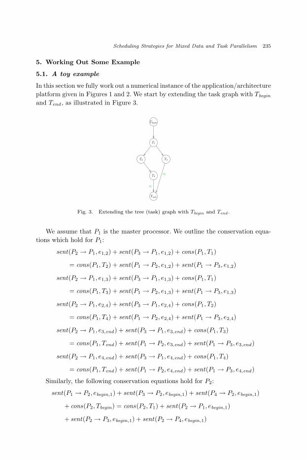
In this section we fully work out a numerical instance of the application/architecture

platform given in Figures 1 and 2. We start by extending the task graph with Tbegin

and Tend , as illustrated in Figure 3.

• Clean-up during the J last time-units: processors forward all their files to the master, which isresponsible for terminating the computation. No processor (even the master) is active duringthe very last units (K − I − J may not be evenly divisible by T ).

• The number of tasks processed by this algorithm within K time-units is equal to steady(G, K) =(r + 1) × T × TP (G).

Clearly, the initialization and clean-up phases would be shortened for an actual implementation,using parallel routing and distributed computations. But on the theoretical side, we do not needto refine the previous bound, because it is sufficient to prove the following result:

Theorem 2. The previous scheduling algorithm based upon steady-state operation is asymptoticallyoptimal:

limK→+∞

steady(G, K)

opt(G, K)= 1.

Proof. Using Lemma 1, opt(G, K) ≤ TP (G).K. From the description of the algorithm, we havesteady(G, K) = ((r + 1)T ).TP (G) ≥ (K − I − J).TP (G), hence the result because I, J , T andTP (G) are constants independent of K.

5 Working out some example

5.1 A toy example

In this section we fully work out a numerical instance of the application/architecture platform givenin Figures 1 and 2. We start by extending the task graph with Tbegin and Tend , as illustrated inFigure 3.

∞

∞T4

T2 T3

T1

Tend

Tbegin

Figure 3: Extending the tree (task) graph with Tbegin and Tend .

We assume that P1 is the master processor. We outline the conservation equations which holdfor P1:

sent(P2 → P1, e1,2) + sent(P3 → P1, e1,2)

+ cons(P1, T1) = cons(P1, T2)

+ sent(P1 → P2, e1,2) + sent(P1 → P3, e1,2)

9

Fig. 3. Extending the tree (task) graph with Tbegin and Tend .

We assume that P1 is the master processor. We outline the conservation equa-

tions which hold for P1:

sent(P2 → P1, e1,2) + sent(P3 → P1, e1,2) + cons(P1, T1)

= cons(P1, T2) + sent(P1 → P2, e1,2) + sent(P1 → P3, e1,2)





sent(P2 → P1, e3,end) + sent(P3 → P1, e3,end) + cons(P1, T3)

= cons(P1, Tend ) + sent(P1 → P2, e3,end) + sent(P1 → P3, e3,end)

sent(P2 → P1, e4,end) + sent(P3 → P1, e4,end) + cons(P1, T4)

= cons(P1, Tend ) + sent(P1 → P2, e4,end) + sent(P1 → P3, e4,end)

Similarly, the following conservation equations hold for P2:

sent(P1 → P2, ebegin,1) + sent(P3 → P2, ebegin,1) + sent(P4 → P2, ebegin,1)

+ cons(P2, Tbegin) = cons(P2, T1) + sent(P2 → P1, ebegin,1)

+ sent(P2 → P3, ebegin,1) + sent(P2 → P4, ebegin,1)

July 9, 2003 10:48 WSPC/119-PPL 00125


sent(P1 → P2, e1,2) + sent(P3 → P2, e1,2) + sent(P4 → P2, e1,2)

+ cons(P2, T1) = cons(P2, T2) + sent(P2 → P1, e1,2)

+ sent(P2 → P3, e1,2) + sent(P2 → P4, e1,2)


+ cons(P2, T1) = cons(P2, T3)

+ sent(P2 → P1, e1,3) + sent(P2 → P3, e1,3) + sent(P2 → P4, e1,3)


+ cons(P2, T2) = cons(P2, T4) + sent(P2 → P1, e2,4)

+ sent(P2 → P3, e2,4) + sent(P2 → P4, e2,4)

sent(P1 → P2, e3,end) + sent(P3 → P2, e3,end) + sent(P4 → P2, e3,end)

+ cons(P2, T3) = cons(P2, Tend) + sent(P2 → P1, e3,end )

+ sent(P2 → P3, e3,end) + sent(P2 → P4, e3,end)

sent(P1 → P2, e4,end) + sent(P3 → P2, e4,end) + sent(P4 → P2, e4,end)

+ cons(P2, T4) = cons(P2, Tend) + sent(P2 → P1, e4,end )

+ sent(P2 → P3, e4,end) + sent(P2 → P4, e4,end)

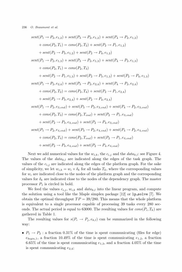
Next we add numerical values for the wi,k , the ci,j and the datak,l: see Figure 4.

The values of the datak,l are indicated along the edges of the task graph. The

values of the ci,j are indicated along the edges of the platform graph. For the sake

of simplicity, we let wi,k = wi × δk for all tasks Tk, where the corresponding values

for wi are indicated close to the nodes of the platform graph and the corresponding

values for δk are indicated close to the nodes of the dependency graph. The master

processor P1 is circled in bold.

We feed the values ci,j , wi,k and datak,l into the linear program, and compute

the solution using a tool like the Maple simplex package [12] or lp solve [7]. We

obtain the optimal throughput TP = 39/280. This means that the whole platform

is equivalent to a single processor capable of processing 39 tasks every 280 sec-

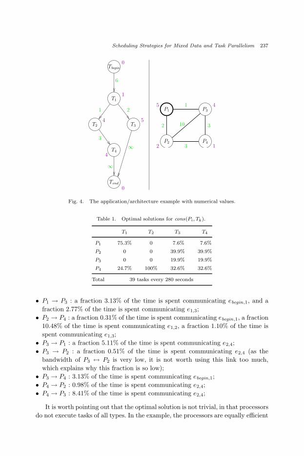
onds. The actual period is equal to 63000. The resulting values for cons(Pi, Tk) are

gathered in Table 1.

The resulting values for s(Pi → Pj , ek,l) can be summarized in the following

way:

• P1 → P2 : a fraction 0.31% of the time is spent communicating (files for edge)

ebegin,1, a fraction 10.49% of the time is spent communicating e1,2, a fraction

6.65% of the time is spent communicating e1,3, and a fraction 4.05% of the time

is spent communicating e2,4;

July 9, 2003 10:48 WSPC/119-PPL 00125


Tk, where the corresponding values for wi are indicated close to the nodes of the platform graphand the corresponding values for δk are indicated close to the nodes of the dependency graph. Themaster processor P1 is circled in bold.

3

21

∞

∞

6

5

0

0

4

4

1

T4

T2 T3

Tbegin

T1

Tend

2

1

3

310

45

2 1

P3P1

P2 P4

Figure 4: The application/architecture example with numerical values.

We feed the values ci,j , wi,k and datak,l into the linear program, and compute the solution usinga tool like the Maple simplex package [12] or lp_solve [7]. We obtain the optimal throughputTP = 39/280. This means that the whole platform is equivalent to a single processor capable ofprocessing 39 tasks every 280 seconds. The actual period is equal to 63000. The resulting valuesfor cons(Pi, Tk) are gathered in Table 1.

T1 T2 T3 T4

P1 75.3% 0 7.6% 7.6%P2 0 0 39.9% 39.9%P3 0 0 19.9% 19.9%P4 24.7% 100% 32.6% 32.6%

Total 39 tasks every 280 seconds

Table 1: Optimal solutions for cons(Pi, Tk)

The resulting values for s(Pi → Pj , ek,l) can be summarized in the following way:

• P1 → P2 : a fraction 0.31% of the time is spent communicating (files for edge) ebegin,1, afraction 10.49% of the time is spent communicating e1,2, a fraction 6.65% of the time is spentcommunicating e1,3, and a fraction 4.05% of the time is spent communicating e2,4;

• P1 → P3 : a fraction 3.13% of the time is spent communicating ebegin,1, and a fraction 2.77%of the time is spent communicating e1,3;

• P2 → P4 : a fraction 0.31% of the time is spent communicating ebegin,1, a fraction 10.48% ofthe time is spent communicating e1,2, a fraction 1.10% of the time is spent communicatinge1,3;

11

Fig. 4. The application/architecture example with numerical values.

Table 1. Optimal solutions for cons(Pi, Tk).

T1 T2 T3 T4

P1 75.3% 0 7.6% 7.6%

P2 0 0 39.9% 39.9%

P3 0 0 19.9% 19.9%

P4 24.7% 100% 32.6% 32.6%

Total 39 tasks every 280 seconds

• P1 → P3 : a fraction 3.13% of the time is spent communicating ebegin,1, and a

fraction 2.77% of the time is spent communicating e1,3;

• P2 → P4 : a fraction 0.31% of the time is spent communicating ebegin,1, a fraction

10.48% of the time is spent communicating e1,2, a fraction 1.10% of the time is

spent communicating e1,3;

• P3 → P1 : a fraction 5.11% of the time is spent communicating e2,4;

• P3 → P2 : a fraction 0.51% of the time is spent communicating e2,4 (as the

bandwidth of P3 ↔ P2 is very low, it is not worth using this link too much,

which explains why this fraction is so low);

• P3 → P4 : 3.13% of the time is spent communicating ebegin,1;

• P4 → P2 : 0.98% of the time is spent communicating e2,4;

• P4 → P3 : 8.41% of the time is spent communicating e2,4;

It is worth pointing out that the optimal solution is not trivial, in that processors

do not execute tasks of all types. In the example, the processors are equally efficient

July 9, 2003 10:48 WSPC/119-PPL 00125


on all task types: wi,k = wi × δk, hence only relative speeds count. We could have

expected each problem to be processed by a single processor, that would execute all

the tasks of the problem, in order to avoid extra communications; in this scenario,

the only communications would correspond to the input cost cbegin,1 = 6. However,

the intuition is misleading. In the optimal steady state solution, some processor

do not process some task types at all (see P2 and P3) , and some task types are

executed by one processor only (see T2). This example demonstrates that in the

optimal solution, the processing of each problem may well be distributed over the

whole platform.

An intuitive alternate strategy is the coarse-grain approach, where we require

each problem instance to be processed by a single processor: this processor would

execute all the tasks of the problem instance, thereby avoiding extra communi-

cations; in this scenario, the only communications correspond to the input cost

cbegin,1 = 2. We make several comments to this approach:

• First, there still remains to decide how many problems will be executed by each

processor. Our framework does provide the optimal answer: simply replace the

task graph by a single task, and compute its weight on a given processor as the

sum of the task durations on that processor.

• The number of equations will be be smaller with the coarse-grain approach,

but the time to solve the linear program is not a limiting factor: the answer

is instantaneous for the toy example. Larger examples require a few seconds of

off-the-shelf CPU time (see below).

• The coarse-grain approach may be simpler to implement, so it is a good strategy

to compute its throughput, and to compare it to the optimal solution. The idea

is to balance the gain brought by the optimal solution against the additional

complexity of the implementation. In the example, the throughput is equal to

311 tasks every 2520 seconds, 11.4 % less than the optimal steady state solution.

Furthermore, it may well be the case that some processors are more efficient for

certain task types (think of a number-cruncher processor, a visualization processor,

etc): then the coarse-grain approach will not be efficient (and even unfeasible if

some processors cannot handle some tasks at all). We handle these constraints by

writing the equations in a general setting, using the unknowns wi,k (the time for

Pi to process task type Tk).

To illustrate this point, consider the example again and let w3,2 = 1. Using a

coarse grain approach, the throughput would be equal to ≈ 0.13 task per second,

whereas the optimal throughput is equal to ≈ 0.170 task per second. which is an

improvement of more than 31%. This illustrates the full potential of the mixed data

and task parallelism approach.

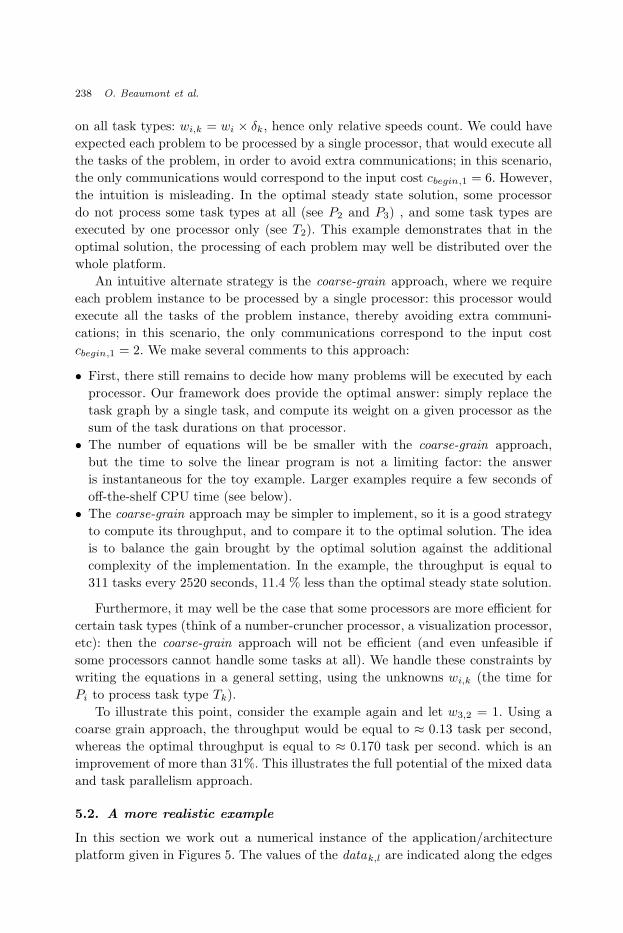
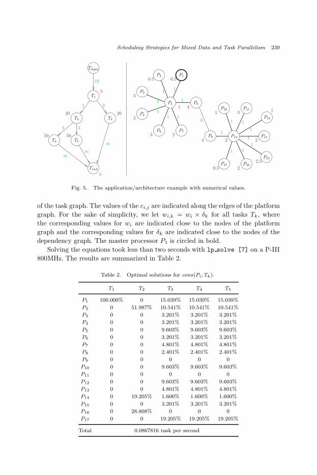
5.2. A more realistic example

In this section we work out a numerical instance of the application/architecture

platform given in Figures 5. The values of the datak,l are indicated along the edges

July 9, 2003 10:48 WSPC/119-PPL 00125


5.2 A more realistic example

In this section we work out a numerical instance of the application/architecture platform given inFigures 5. The values of the datak,l are indicated along the edges of the task graph. The valuesof the ci,j are indicated along the edges of the platform graph. For the sake of simplicity, we letwi,k = wi × δk for all tasks Tk, where the corresponding values for wi are indicated close to thenodes of the platform graph and the corresponding values for δk are indicated close to the nodes ofthe dependency graph. The master processor P1 is circled in bold.

1 2

31

10

∞∞

∞

0

5

20

50 50

20T3

Tend

Tbegin

T5T4

T1

T211

1

1

11

1

8 1 1

1

1

1

11

1

0.50.5

3

3

1

23

4

3

0.5

2

1

24

2.5

2

1

P1P2

P3

P4

P5

P7P6

P8

P11

P17

P13

P10

P14P9

P12

P15

P16

Figure 5: The application/architecture example with numerical values.

Solving the equations took less than two seconds with lp_solve [7] on a P-III 800MHz. Theresults are summarized in Table 2.

In the optimal solution, the two clusters (P1 to P8 and P9 to P17) are almost equally working,despite the slow inter-cluster communication link and the location of the input files on P1. Notethat the coarse-grain approach leads to a throughput equal to ≈ 0.0590517 task per second. Theimprovement of our method over a coarse-grain approach is then of more than 46%.

6 Related problems

There are two papers that are closely related to our work. First, the proof of the asymptotic opti-mality of steady-state scheduling (Section 4) is inspired by the paper of Bertsimas and Gamarnik [8],who have used a fluid relaxation technique to derive asymptotically optimal scheduling algorithms.They apply this technique to the job shop scheduling problem and to the packet routing problem.It would be very interesting to extend their results to a heterogeneous framework.

The second paper is by Taura and Chien [37], who consider the pipeline execution of taskgraphs onto heterogeneous platforms. This is exactly the problem that we target in this paper,except that they do not restrict to tree-shaped task graphs. Taura and Chien make the hypothesisthat all copies of a given task type must be executed on the same processor. This hypothesis wasintended as a simplification, but it renders the problem NP-complete, and the authors had to resort

13

Fig. 5. The application/architecture example with numerical values.

of the task graph. The values of the ci,j are indicated along the edges of the platform

graph. For the sake of simplicity, we let wi,k = wi × δk for all tasks Tk, where

the corresponding values for wi are indicated close to the nodes of the platform

graph and the corresponding values for δk are indicated close to the nodes of the

dependency graph. The master processor P1 is circled in bold.

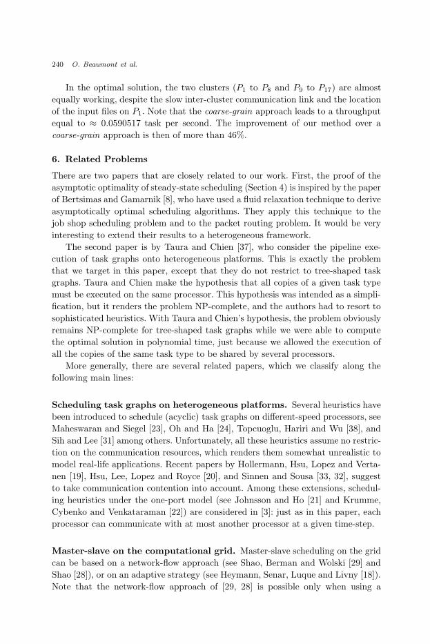
Solving the equations took less than two seconds with lp solve [7] on a P-III

800MHz. The results are summarized in Table 2.

Table 2. Optimal solutions for cons(Pi, Tk).

T1 T2 T3 T4 T5

P1 100.000% 0 15.039% 15.039% 15.039%

P2 0 51.987% 10.541% 10.541% 10.541%

P3 0 0 3.201% 3.201% 3.201%

P4 0 0 3.201% 3.201% 3.201%

P5 0 0 9.603% 9.603% 9.603%

P6 0 0 3.201% 3.201% 3.201%

P7 0 0 4.801% 4.801% 4.801%

P8 0 0 2.401% 2.401% 2.401%

P9 0 0 0 0 0

P10 0 0 9.603% 9.603% 9.603%

P11 0 0 0 0 0

P12 0 0 9.603% 9.603% 9.603%

P13 0 0 4.801% 4.801% 4.801%

P14 0 19.205% 1.600% 1.600% 1.600%

P15 0 0 3.201% 3.201% 3.201%

P16 0 28.808% 0 0 0

P17 0 0 19.205% 19.205% 19.205%

Total 0.0867816 task per second

July 9, 2003 10:48 WSPC/119-PPL 00125


In the optimal solution, the two clusters (P1 to P8 and P9 to P17) are almost

equally working, despite the slow inter-cluster communication link and the location

of the input files on P1. Note that the coarse-grain approach leads to a throughput

equal to ≈ 0.0590517 task per second. The improvement of our method over a

coarse-grain approach is then of more than 46%.

6. Related Problems

There are two papers that are closely related to our work. First, the proof of the

asymptotic optimality of steady-state scheduling (Section 4) is inspired by the paper

of Bertsimas and Gamarnik [8], who have used a fluid relaxation technique to derive

asymptotically optimal scheduling algorithms. They apply this technique to the

job shop scheduling problem and to the packet routing problem. It would be very

interesting to extend their results to a heterogeneous framework.

The second paper is by Taura and Chien [37], who consider the pipeline exe-

cution of task graphs onto heterogeneous platforms. This is exactly the problem

that we target in this paper, except that they do not restrict to tree-shaped task

graphs. Taura and Chien make the hypothesis that all copies of a given task type

must be executed on the same processor. This hypothesis was intended as a simpli-

fication, but it renders the problem NP-complete, and the authors had to resort to

sophisticated heuristics. With Taura and Chien’s hypothesis, the problem obviously

remains NP-complete for tree-shaped task graphs while we were able to compute

the optimal solution in polynomial time, just because we allowed the execution of

all the copies of the same task type to be shared by several processors.

More generally, there are several related papers, which we classify along the

following main lines:

Scheduling task graphs on heterogeneous platforms. Several heuristics have

been introduced to schedule (acyclic) task graphs on different-speed processors, see

Maheswaran and Siegel [23], Oh and Ha [24], Topcuoglu, Hariri and Wu [38], and

Sih and Lee [31] among others. Unfortunately, all these heuristics assume no restric-

tion on the communication resources, which renders them somewhat unrealistic to

model real-life applications. Recent papers by Hollermann, Hsu, Lopez and Verta-

nen [19], Hsu, Lee, Lopez and Royce [20], and Sinnen and Sousa [33, 32], suggest

to take communication contention into account. Among these extensions, schedul-

ing heuristics under the one-port model (see Johnsson and Ho [21] and Krumme,

Cybenko and Venkataraman [22]) are considered in [3]: just as in this paper, each

processor can communicate with at most another processor at a given time-step.

Master-slave on the computational grid. Master-slave scheduling on the grid

can be based on a network-flow approach (see Shao, Berman and Wolski [29] and

Shao [28]), or on an adaptive strategy (see Heymann, Senar, Luque and Livny [18]).

Note that the network-flow approach of [29, 28] is possible only when using a

July 9, 2003 10:48 WSPC/119-PPL 00125


full multiple-port model, where the number of simultaneous communications for a

given node is not bounded. Enabling frameworks to facilitate the implementation

of master-slave tasking are described in Goux, Kulkarni, Linderoth and Yoder [17],

and in Weissman [39].

Mixed task and data parallelism. There are a very large number of papers deal-

ing with mixed task and data parallelism. We quote the work of Subhlok, Stichnoth,

O’Hallaron and Gross [35], Chakrabarti, Demmel and Yelick [11], Ramaswamy, Sap-

atnekar and Banerjee [26], Bal and M. Haines [1], and Subhlok and Vondran [36],

but this list is by no means meant to be comprehensive. We point out, however,

that (to the best of our knowledge) none of the papers published in this area is

dealing with heterogeneous platforms.

7. Conclusion

In this paper, we have dealt with the implementation of mixed task and data

parallelism onto heterogeneous platforms. We have shown how to determine the

best steady-state scheduling strategy for a tree-shaped task graph and for a general

platform graph, using a linear programming approach.

This work can be extended in the following three directions:

• The first idea is to extend the approach to arbitrary task graphs, i.e. general

DAGs instead of trees. In fact, our approach can be extended to general DAGs,

but with a complexity which is proportional to the number of paths in the

DAG [5]. A large number of task graphs, such as trees, fork-join graphs, etc,

do have a polynomial number of paths. But for instance the Laplace task graph,

which is an oriented two-dimensional grid, has a number of paths exponential in

its node number. At the time of this writing, we do not whether the problem can

be solved in polynomial time for arbitrary task graphs.

• On the theoretical side, we could try to solve the problem of maximizing the

number of tasks that can be executed within K time-steps, where K is a given

time-bound. This scheduling problem is more complicated than the search for

the best steady-state. Taking the initialization phase into account renders the

problem quite challenging.

• On the practical side, we need to run actual experiments rather than simulations.

Indeed, it would be interesting to capture actual architecture and application

parameters, and to compare heuristics on a real-life problem suite, such as those

in [9, 34].

Acknowledgment

We would like to thank the reviewers for their constructive comments and

suggestions.

July 9, 2003 10:48 WSPC/119-PPL 00125


References

[1] H. Bal and M. Haines. Approaches for integrating task and data parallelism. IEEEConcurrency, 6(3):74–84, 1998.

[2] C. Banino, O. Beaumont, A. Legrand, and Y. Robert. Scheduling strategies formaster-slave tasking on heterogeneous processor grids. In PARA’02: InternationalConference on Applied Parallel Computing, LNCS 2367, pages 423–432. SpringerVerlag, 2002.

[3] O. Beaumont, V. Boudet, and Y. Robert. A realistic model and an efficient heuristicfor scheduling with heterogeneous processors. In HCW’2002, the 11th HeterogeneousComputing Workshop. IEEE Computer Society Press, 2002.

[4] O. Beaumont, L. Carter, J. Ferrante, A. Legrand, and Y. Robert. Bandwidth-centricallocation of independent tasks on heterogeneous platforms. In International Paralleland Distributed Processing Symposium IPDPS’2002. IEEE Computer Society Press,2002. Extended version available as LIP Research Report 2001-25.

[5] O. Beaumont, A. Legrand, L. Marchal, and Y. Robert. Optimal algorithms for thepipelined scheduling of task graphs on heterogeneous systems. Technical report, LIP,ENS Lyon, France, April 2003.

[6] O. Beaumont, A. Legrand, and Y. Robert. The master-slave paradigm with hetero-geneous processors. In D. S. Katz, T. Sterling, M. Baker, L. Bergman, M. Paprzycki,and R. Buyya, editors, Cluster’2001, pages 419–426. IEEE Computer Society Press,2001. Extended version available as LIP Research Report 2001-13.

[7] Michel Berkelaar. LP SOLVE: Linear Programming Code. URL:http://www.cs.sunysb.edu/ algorith/implement/lpsolve/implement.shtml.

[8] D. Bertsimas and D. Gamarnik. Asymptotically optimal algorithm for job shopscheduling and packet routing. Journal of Algorithms, 33(2):296–318, 1999.

[9] Michael D. Beynon, Tahsin Kurc, Alan Sussman, and Joel Saltz. Optimizing exe-cution of component-based applications using group instances. Future GenerationComputer Systems, 18(4):435–448, 2002.

[10] T. D. Braun, H. J. Siegel, and N. Beck. Optimal use of mixed task and data paral-lelism for pipelined computations. J. Parallel and Distributed Computing, 61:810–837,2001.

[11] S. Chakrabarti, J. Demmel, and K. Yelick. Models and scheduling algorithms formixed data and task parallel programs. J. Parallel and Distributed Computing,47:168–184, 1997.

[12] B. W. Char, K. O. Geddes, G. H. Gonnet, M. B. Monagan, and S. M. Watt. MapleReference Manual, 1988.

[13] P. Chretienne, E. G. Coffman Jr., J. K. Lenstra, and Z. Liu, editors. SchedulingTheory and its Applications. John Wiley and Sons, 1995.

[14] James Cowie, Bruce Dodson, R.-Marije Elkenbracht-Huizing, Arjen K. Lenstra,Peter L. Montgomery, and Joerg Zayer. A world wide number field sieve factoringrecord: on to 512 bits. In Kwangjo Kim and Tsutomu Matsumoto, editors, Advancesin Cryptology - Asiacrypt ’96, volume 1163 of LNCS, pages 382–394. Springer Verlag,1996.

[15] Entropia. URL: http://www.entropia.com.[16] M. R. Garey and D. S. Johnson. Computers and Intractability, a Guide to the Theory

of NP-Completeness. W. H. Freeman and Company, 1991.[17] J. P Goux, S. Kulkarni, J. Linderoth, and M. Yoder. An enabling framework for

master-worker applications on the computational grid. In Ninth IEEE InternationalSymposium on High Performance Distributed Computing (HPDC’00). IEEE Com-puter Society Press, 2000.

July 9, 2003 10:48 WSPC/119-PPL 00125


[18] E. Heymann, M. A. Senar, E. Luque, and M. Livny. Adaptive scheduling for master-worker applications on the computational grid. In R. Buyya and M. Baker, editors,Grid Computing - GRID 2000, pages 214–227. Springer-Verlag LNCS 1971, 2000.

[19] L. Hollermann, T. S. Hsu, D. R. Lopez, and K. Vertanen. Scheduling problems in apractical allocation model. J. Combinatorial Optimization, 1(2):129–149, 1997.

[20] T. S. Hsu, J. C. Lee, D. R. Lopez, and W. A. Royce. Task allocation on a networkof processors. IEEE Trans. Computers, 49(12):1339–1353, 2000.

[21] S. L. Johnsson and C.-T. Ho. Spanning graphs for optimum broadcasting and per-sonalized communication in hypercubes. IEEE Trans. Computers, 38(9):1249–1268,1989.

[22] D. W. Krumme, G. Cybenko, and K. N. Venkataraman. Gossiping in minimal time.SIAM J. Computing, 21:111–139, 1992.

[23] M. Maheswaran and H. J. Siegel. A dynamic matching and scheduling algorithm forheterogeneous computing systems. In Seventh Heterogeneous Computing Workshop.IEEE Computer Society Press, 1998.

[24] H. Oh and S. Ha. A static scheduling heuristic for heterogeneous processors. In Pro-ceedings of Europar’96, LNCS 1123. Springer Verlag, 1996.

[25] Prime. URL: http://www.mersenne.org.[26] S. Ramaswamy, S. Sapatnekar, and P. Banerjee. A framework for exploiting task and

data parallelism on distributed memory multicomputers. IEEE Trans. Parallel andDistributed Systems, 8(11):1098–1116, 1997.

[27] SETI. URL: http://setiathome.ssl.berkeley.edu.[28] G. Shao. Adaptive scheduling of master/worker applications on distributed computa-

tional resources. PhD thesis, Dept. of Computer Science, University Of California atSan Diego, 2001.

[29] G. Shao, F. Berman, and R. Wolski. Master/slave computing on the grid. In Hetero-geneous Computing Workshop HCW’00. IEEE Computer Society Press, 2000.

[30] B. A. Shirazi, A. R. Hurson, and K. M. Kavi. Scheduling and load balancing in paralleland distributed systems. IEEE Computer Science Press, 1995.

[31] G. C. Sih and E. A. Lee. A compile-time scheduling heuristic for interconnection-constrained heterogeneous processor architectures. IEEE Transactions on Paralleland Distributed Systems, 4(2):175–187, 1993.

[32] O. Sinnen and L. Sousa. Comparison of contention-aware list scheduling heuristics forcluster computing. In T. M. Pinkston, editor, Workshop for Scheduling and ResourceManagement for Cluster Computing (ICPP’01), pages 382–387. IEEE Computer So-ciety Press, 2001.

[33] O. Sinnen and L. Sousa. Exploiting unused time-slots in list scheduling consideringcommunication contention. In R. Sakellariou, J. Keane, J. Gurd, and L. Freeman, ed-itors, EuroPar’2001 Parallel Processing, pages 166–170. Springer-Verlag LNCS 2150,2001.

[34] M. Spencer, R. Ferreira, M. Beynon, T. Kurc, U. Catalyurek, A. Sussman, andJ. Saltz. Executing multiple pipelined data analysis operations in the grid. In 2002ACM/IEEE Supercomputing Conference. ACM Press, 2002.

[35] J. Subhlok, J. Stichnoth, D. O’Hallaron, and T. Gross. Exploiting task and dataparallelism on a multicomputer. In Fourth ACM SIGPLAN Symposium on Priciples& Practices of Parallel Programming. ACM Press, May 1993.

[36] J. Subhlok and G. Vondran. Optimal use of mixed task and data parallelism forpipelined computations. J. Parallel and Distributed Computing, 60:297–319, 2000.

[37] K. Taura and A. A. Chien. A heuristic algorithm for mapping communicating tasks

July 9, 2003 10:48 WSPC/119-PPL 00125


on heterogeneous resources. In Heterogeneous Computing Workshop, pages 102–115.IEEE Computer Society Press, 2000.

[38] H. Topcuoglu, S. Hariri, and M.-Y. Wu. Task scheduling algorithms for heterogeneousprocessors. In Eighth Heterogeneous Computing Workshop. IEEE Computer SocietyPress, 1999.

[39] J. B. Weissman. Scheduling multi-component applications in heterogeneous wide-areanetworks. In Heterogeneous Computing Workshop HCW’00. IEEE Computer SocietyPress, 2000.

SCHEDULING STRATEGIES FOR MIXED DATA AND TASK PARALLELISM ON HETEROGENEOUS CLUSTERS

Documents

Transcript of SCHEDULING STRATEGIES FOR MIXED DATA AND TASK PARALLELISM ON HETEROGENEOUS CLUSTERS