Scenario-based HVAC energy cost optimizer for ... - IBPSA

Scenario-based HVAC energy cost optimizer for heterogeneous heat-source systems of real-life hospital building

SungHo Park1, Ki Uhn Ahn2, Seungho Hwang3, Sunkyu Choi3,

Han Sol Shin2, Dong Hyuk Yi2, Cheol Soo Park2 1Korea Electric Power Corporation, Seoul, South Korea

2Department of Architecture and Architectural Engineering, College of Engineering, Seoul National University, Seoul, South Korea

3SK Telecom Co. Ltd., Seoul, South Korea

Abstract This paper presents the development of a HVAC

energy cost optimizer for a real-life hospital building. The building’s HVAC is configured with two Absorption Chiller-Heaters (ACHs, 150 & 120 US Refrigeration Ton [RT] respectively), four heat pumps (HPs, 20 USRT each), and one boiler (353 kW). The building's facility team suggests that their goal should be minimizing not ‘energy use’ but ‘energy cost’ and the building's operational scheme be made once a day in order to reduce operational effort. To solve this, the authors developed simulation models for ACHs (gas-fired), the HPs (electric) and the boiler (gas-fired). In addition to the simulation models, a sequencing control of the HPs was also developed. The HVAC energy cost optimizer estimates daily energy use and energy cost based on calculated daily energy demand of the building. The HVAC energy cost optimizer compares all possible operation scenarios and select an optimal one per day. It was found that the building’s energy cost can be saved by 23.5%. The reasons for the saving are threefold: (1) The HPs outperform the ACHs and the boiler in terms of thermal efficiency and cost-effectiveness. (2) The HVAC energy cost optimizer can select cost-effective energy sources considering the building’s energy demand, energy price (gas, electricity), and the equipment (ACHs, HPs, boiler) efficiency. (3) The sequencing control suggested by the authors enables the HPs to run at a higher COP than an existing control. It is highlighted in the paper that owing to the use of the simulation models, the simple and straightforward scenario-based control can save significant energy compared to the existing control of the building.

Introduction Building energy accounts for about 40% of the primary energy consumption (IEA, 2017). Many attempts have been made with regard to Energy Conservation Measures (ECMs) for building energy saving (Balaras et al., 2003; Rahman et al., 2010). Energy saving for existing buildings can be achieved either by introduction of energy-efficient systems or optimal operation (IBPSA 1987-2017). In South Korea, an increasing number of high-efficient mechanical components or energy management systems (e.g. Building Energy Management System [BEMS]) have been installed for energy retrofit of existing buildings. With the use of BEMS, building operators can monitor HVAC system through measured data, develop

optimal control strategies, compare, and provide operational support (Clarke, 2015). In recent years, as part of optimal control strategies, the Model Predictive Control (MPC) has been studied (IBPSA 1987-2017; Ahn et al., 2015; Afram et al., 2017; Asadi et al., 2014; Kim et al., 2016). The MPC can predict future states of the system and find optimal control variables that can minimize a cost function over the prediction horizon (Afram and Janabi-Sharifi, 2014; Ma et al., 2012; Huang, 2011; Xi, 2007).

However, it is disadvantageous that the MPC requires an accurate and laborious simulation model, and a rigorous optimization solver. In addition, the MPC requires sophisticated control hardware (sensor, actuators) for realizing the MPC, compared to conventional HVAC system control (Mařík et al., 2011). Thus, many buildings are still being manually controlled based on experiences of building operators (Fong et al., 2009). Rather than employing the MPC, this study presents simple scenario-based optimal control strategies at daily practice for a real-life hospital building. Even though the optimal control strategies suggested by the authors are simple and straightforward, the authors assumed that the simple scenario-based control strategies can still perform better than an existing control of the hospital building. The hospital building is located in Gun-san, South Korea. The building has eight floors above ground and one floor below ground. The total floor area of the building is 24,137m2 (Figure 1). The building has heterogeneous HVAC systems including two absorption chiller-heaters (ACHs, 150 and 120 US Refrigeration Ton [RT], respectively]), four heat pumps (HPs, 20 USRT each), one boiler for auxiliary heating (353kW), and one heat exchanger (HX) between two ACHs and four HPs. The configuration and specification of HVAC systems are as shown in Figure 2 and Table 1. Please note that the two ACHs and boiler use gas as a heat source, while four HPs use electricity as the heat source. As shown in Figure 2, the building’s HVAC system is installed in a complex manner. In other words, the ACHs can handle heating and cooling load of the building, while HPs can also handle heating and cooling load of the building as well as domestic hot water. In addition, the boiler produces domestic hot water. Three different mechanical systems (ACHs, HPs, boiler) can generate hot or chilled water using different heat sources (gas vs. electricity). In addition, several variables (appearing in blue color, Figure 2) were not measured due to absence of sensors.

________________________________________________________________________________________________

________________________________________________________________________________________________ Proceedings of the 16th IBPSA Conference Rome, Italy, Sept. 2-4, 2019

3022

https://doi.org/10.26868/25222708.2019.210979

Particularly, the building’s facility team suggested that their operational goal is not to minimize ‘energy use’ but to minimize ‘energy cost’. The other request received from the facility team was that they wanted to change their operational scheme only once a day in order to reduce operational effort.

Thus, the authors developed three different simulation models for the ACHs, the HPs, and the boiler, respectively. The HP simulation model was developed with an artificial neural network (ANN). The ACHs and boiler simulation models were developed with algebraic equations. Finally, a HVAC energy cost optimizer was developed to predict ‘energy use’ as well as ‘energy cost’ for all possible operational scenarios of the target building, and then to find an optimal scenario based on the calculated energy cost per each day.

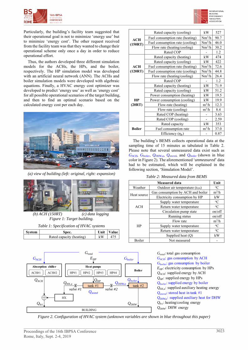
(a) view of building (left: original, right: expansion)

(b) ACH (150RT) (c) data logging

Figure 1: Target building.

Table 1: Specification of HVAC systems

System Spec. Unit Value Rated capacity (heating) kW 475

ACH (150RT)

Rated capacity (cooling) kW 527

Fuel consumption rate (heating) Nm3/h 90.7Fuel consumption rate (cooling) Nm3/h 46.0

Flow rate (heating/cooling) Nm3/h 30.2Rated COP - 1.2

ACH (120RT)

Rated capacity (heating) kW 474Rated capacity (cooling) kW 422

Fuel consumption rate (heating) Nm3/h 72.6Fuel consumption rate (cooling) Nm3/h 44.8

Flow rate (heating/cooling) Nm3/h 26.4Rated COP - 1.2

HP (20RT)

Rated capacity (heating) kW 71.9Rated capacity (cooling) kW 51.2

Power consumption (heating) kW 19.5Power consumption (cooling) kW 19.9

Flow-rate (heating) m3/h 12.3Flow-rate (cooling) m3/h 8.4

Rated COP (heating) - 3.63Rated COP (cooling) - 2.59

BoilerRated capacity kW 353

Fuel consumption rate m3/h 37.0Efficiency (𝜂 ) - 0.87

The building’s BEMS collects operational data at the sampling time of 15 minutes as tabulated in Table 2. Please note that several unmeasured data exist such as GACH, Gboiler, QDHW,a, Qstored, and Qboiler (shown in blue color in Figure 2). The aforementioned ‘unmeasured’ data had to be estimated, which will be explained in the following section, ‘Simulation Model’.

Table 2: Measured data from BEMS

Measured data UnitWeather Outdoor air temperature (tOA) oC

Heat sourceGas consumption by ACH and boiler m3/h

Electricity consumption by HP kW

ACH Supply water temperature oC Return water temperature oC

Circulation pump state on/off

HP

Running status on/offFlow rate m3/h

Supply water temperature oC Return water temperature oC

Supplied heat (Q) kW Boiler Not measured -

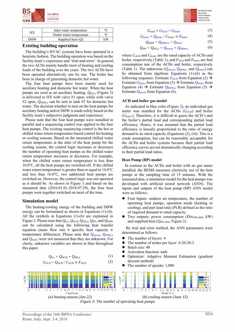
Figure 2. Configuration of HVAC system (unknown variables are shown in blue throughout this paper)

Heat pumps

HP#1 HP#2 HP#3 HP#4Boiler

Absorption chiller

ACH#1 ACH#2

BUILDING

EHP

Qh/c QDHW

QHP QboilerQDHW,a

QACH QHX,a

Qstored

Gtotal

HX

tank #1

GACH Gboiler

tank #2valve #1 valve #2

Gtotal: total gas consumptionGACH: gas consumption by ACHGboiler: gas consumption by boilerEHP: electricity consumption by HPsQACH: supplied energy by ACHQHP: supplied energy by HPsQboiler: supplied energy by boiler QHX,a: supplied auxiliary heating energyQstored: stored heat in tank #1QDHW,a: supplied auxiliary heat for DHWQh/c: heating/cooling energyQDHW: DHW energy

________________________________________________________________________________________________


3023

HX Inlet water temperature oC

Outlet water temperature oC DHW Supplied heat (Q) kW

Existing building operation The building’s HVAC systems have been operated in a heuristic fashion. The building operation was based on the facility team’s experience and ‘trial-and-error’. In general, the two ACHs mainly handle most of heating and cooling loads of the building over the years. The two ACHs have been operated alternatively one by one. The boiler has been in charge of generating domestic hot water. The four heat pumps have been mainly used for auxiliary heating and domestic hot water. When the heat pumps are used as an auxiliary heating, QHX,a (Figure 2) is delivered to HX with valve #1 open, while with valve #2 open, QDHW,a can be sent to tank #2 for domestic hot water. The decision whether to turn on the heat pumps for auxiliary heating and/or DHW is made solely based on the facility team’s subjective judgment and experience. Please note that the four heat pumps were installed in parallel and a sequencing control was applied to the four heat pumps. The existing sequencing control is the hot or chilled water return temperature-based control for heating or cooling seasons. Based on the measured chilled water return temperature at the inlet of the heat pump for the cooling season, the control logic increases or decreases the number of operating heat pumps as the chilled water return temperature increases or decreases. For example, when the chilled water return temperature is less than 10.0°C, all the heat pumps are switched off. If the chilled water return temperature is greater than or equal to 14.0°C and less than 16.0°C, two additional heat pumps are switched on. However, the control logic was not operated as it should be. As shown in Figure 3 and based on the measured data (2016.01.01-2018.07.29), the four heat pumps were together switched on most of the time.

Simulation model The heating/cooling energy of the building and DHW energy can be formulated as shown in Equations (1)-(6). All the symbols in Equations (1)-(6) are explained in Figure 2. Please note that Qh/c, QACH, QHX,a, QHP, and QDHW can be calculated using the following heat transfer equation (mass flow rate specific heat capacity temperature difference). Please note that Qstored, QDHW,a and Qboiler were not measured thus they are unknown. For clarity, unknown variables are shown in blue throughout this paper.

Qh/c = QACH + QHX,a (1)

GACH = QACH / CACH FACH (2)

Gtotal = GACH + Gboiler (3)

Gboiler = Qboiler / Cboiler Fboiler (4)

QDHW = QDHW,a + Qboiler (5)

QHP = QHX,a + Qstored + QDHW,a (6)

where CACH and Cboiler are the rated capacity of ACHs and boiler, respectively (Table 1), and FACH and Fboiler are fuel consumption rate of the ACHs and boiler, respectively (Table 1). The unknowns (Qstored, QDHW,a and Qboiler) can be obtained from algebraic Equations (1)-(6) as the following sequence: Estimate GACH from Equation (2) Estimate Gboiler from Equation (3) Estimate Qboiler from Equation (4) Estimate QDHW,a from Equation (5) Estimate Qstored from Equation (6).

ACH and boiler gas model

As indicated in blue color (Figure 2), no individual gas meter was installed for the ACHs (GACH) and boiler (Gboiler). Therefore, it is difficult to guess the ACH’s and the boiler’s partial load and corresponding partial load efficiency. Hence, it was assumed that the partial load efficiency is linearly proportional to the ratio of energy demand to its rated capacity (Equations (2), (4)). This is a crude assumption, but can be reasonably acceptable for the ACHs and boiler systems because their partial load efficiency curves are not dramatically changing according to their partial load ratios.

Heat Pump (HP) model

In contrast to the ACHs and boiler with no gas meter installed, the BEMS measures electricity use of the heat pumps at the sampling time of 15 minutes. With the measured data, a simulation model for the heat pumps was developed with artificial neural network (ANN). The inputs and outputs of the heat pump (HP) ANN model were as follows:

Four Inputs: outdoor air temperature, the number of operating heat pumps, operation mode (heating or cooling), and part load ratio (PLR) defined as the ratio of required demand to rated capacity.

Two outputs: power consumption (ElecHP,ANN, kW) and supplied heat (QHP,ANN, Figure 2).

By trial and error method, the ANN parameters were determined as follows:

The number of layers: 4 The number of nodes per layer: 4-20-20-2 Batch size: 48 Activation function: tanh Optimizer: Adaptive Moment Estimation (gradient

descent method) The number of epochs: 1,000

(a) heating season (Jan 22) (b) cooling season (June 15) Figure 3: The number of operating heat pumps

________________________________________________________________________________________________


3024

In total, 90,336 data points were collected during 2016.01.01-2018.07.29 at the sampling time of 15 minutes. The authors first excluded the data with the HPs off and then removed outliers from the data. As a result, 35,101 points were used for the training and testing of the HP ANN model. 75% (26,437 points) and 25% (8,664 points) out of 35,101 points were randomly sampled for training/validation and testing, respectively.

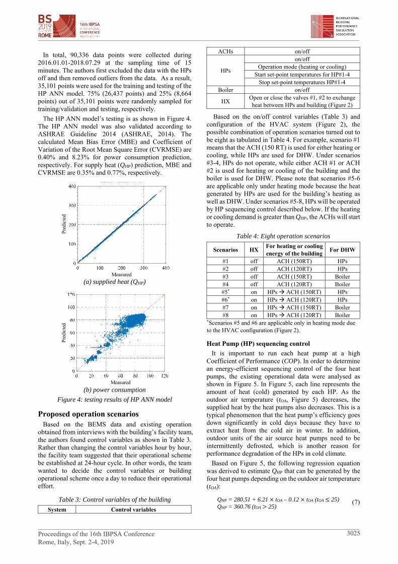
The HP ANN model’s testing is as shown in Figure 4. The HP ANN model was also validated according to ASHRAE Guideline 2014 (ASHRAE, 2014). The calculated Mean Bias Error (MBE) and Coefficient of Variation of the Root Mean Square Error (CVRMSE) are 0.40% and 8.23% for power consumption prediction, respectively. For supply heat (QHP) prediction, MBE and CVRMSE are 0.35% and 0.77%, respectively.

(a) supplied heat (QHP)

(b) power consumption

Figure 4: testing results of HP ANN model

Proposed operation scenarios Based on the BEMS data and existing operation obtained from interviews with the building’s facility team, the authors found control variables as shown in Table 3. Rather than changing the control variables hour by hour, the facility team suggested that their operational scheme be established at 24-hour cycle. In other words, the team wanted to decide the control variables or building operational scheme once a day to reduce their operational effort.

Table 3: Control variables of the building

System Control variables

ACHs on/off

HPs

on/off Operation mode (heating or cooling)

Start set-point temperatures for HP#1-4 Stop set-point temperatures HP#1-4

Boiler on/off

HX Open or close the valves #1, #2 to exchange heat between HPs and building (Figure 2)

Based on the on/off control variables (Table 3) and configuration of the HVAC system (Figure 2), the possible combination of operation scenarios turned out to be eight as tabulated in Table 4. For example, scenario #1 means that the ACH (150 RT) is used for either heating or cooling, while HPs are used for DHW. Under scenarios #3-4, HPs do not operate, while either ACH #1 or ACH #2 is used for heating or cooling of the building and the boiler is used for DHW. Please note that scenarios #5-6 are applicable only under heating mode because the heat generated by HPs are used for the building’s heating as well as DHW. Under scenarios #5-8, HPs will be operated by HP sequencing control described below. If the heating or cooling demand is greater than QHP, the ACHs will start to operate.

Table 4: Eight operation scenarios

Scenarios HXFor heating or cooling energy of the building

For DHW

#1 off ACH (150RT) HPs #2 off ACH (120RT) HPs #3 off ACH (150RT) Boiler #4 off ACH (120RT) Boiler #5* on HPs ACH (150RT) HPs #6* on HPs ACH (120RT) HPs #7 on HPs ACH (150RT) Boiler #8 on HPs ACH (120RT) Boiler

*Scenarios #5 and #6 are applicable only in heating mode due to the HVAC configuration (Figure 2).

Heat Pump (HP) sequencing control

It is important to run each heat pump at a high Coefficient of Performance (COP). In order to determine an energy-efficient sequencing control of the four heat pumps, the existing operational data were analysed as shown in Figure 5. In Figure 5, each line represents the amount of heat (cold) generated by each HP. As the outdoor air temperature (tOA, Figure 5) decreases, the supplied heat by the heat pumps also decreases. This is a typical phenomenon that the heat pump’s efficiency goes down significantly in cold days because they have to extract heat from the cold air in winter. In addition, outdoor units of the air source heat pumps need to be intermittently defrosted, which is another reason for performance degradation of the HPs in cold climate.

Based on Figure 5, the following regression equation was derived to estimate QHP that can be generated by the four heat pumps depending on the outdoor air temperature (tOA):

QHP = 280.51 + 6.21 tOA – 0.12 tOA (tOA 25) QHP = 360.76 (tOA 25)

(7)

Measured

Pre

dict

edP

redi

cted

Measured

________________________________________________________________________________________________


3025

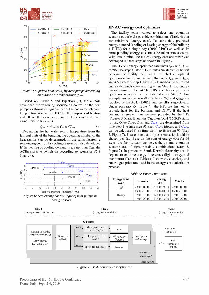
Figure 5: Supplied heat (cold) by heat pumps depending

on outdoor air temperature (tOA)

Based on Figure 5 and Equation (7), the authors developed the following sequencing control of the heat pumps as shown in Figure 6. Since the hot water set-point temperature was set to 60oC for the purposes of heating and DHW, the sequencing control logic can be derived using Equations (7)-(8).

QHP = 𝑚HP CP dTHP (8)

Depending the hot water return temperature from the fan-coil units of the building, the operating number of the heat pumps can be determined. In the same fashion, a sequencing control for cooling season was also developed. If the heating or cooling demand is greater than QHP, the ACHs starts to switch on according to scenarios #5-8 (Table 4).

Figure 6: sequencing control logic of heat pumps in heating season

HVAC energy cost optimizer The facility team wanted to select one operation scenario out of eight possible combinations (Table 4) that can minimize ‘energy cost’. To solve this, predicted energy demand (cooling or heating energy of the building + DHW) for a single day (00:00-24:00) as well as its corresponding energy cost must be taken into account. With this in mind, the HVAC energy cost optimizer was developed in three steps as shown in Figure 7.

The HVAC energy optimizer calculates Qh/c and QDHW for 96 time steps (1 step = 15 minutes, 96 steps = 24 hours) because the facility team wants to select an optimal operation scenario once a day. Obviously, Qh/c and QDHW are 96 1 vector (Step 1, Figure 7). Based on the estimated energy demands (Qh/c and QDHW) in Step 1, the energy consumption of the ACHs, HPs and boiler per each operation scenario can be calculated in Step 2. For example, under scenario #1 (Table 4), Qh/c and QDHW are supplied by the ACH (150RT) and the HPs, respectively. Under scenario #5 (Table 4), the HPs are first on to provide heat for the building and DHW. If the heat demand is greater than the heat provided by the HPs (Figures 5-6, and Equation (7)), then ACH (150RT) starts to run. Once QACH, QHP, and Qboiler are determined from time-step 1 to time-step 96, then GACH, ElecHP, and Gboiler can be calculated from time-step 1 to time-step 96 (Step 2, Figure 7). Please note that only one scenario should be chosen per day. Base on the sum of energy cost for 96 steps, the facility team can select the optimal operation scenario out of eight possible combinations (Step 3, Figure 7). In particular, South Korea's electricity cost is dependent on three energy time zones (light, heavy, and maximum) (Table 5). Tables 6-7 show the electricity and natural gas price rate used in the energy cost calculation process.

Table 5: Energy time zone

Energy time zone

Summer Spring /Fall

Winter

Light 23:00-09:00 23:00-09:00 23:00-09:00

Heavy 09:00-10:00 12:00-13:00 17:00-23:00

09:00-10:00 12:00-13:00 17:00-23:00

09:00-10:0012:00-17:0020:00-22:00

50 51 52 53 54 55 56 57 58 59 60

Hot water return temperature (oC)

0

1

2

3

4

# o

f H

Ps

HP#1 on

HP#2 on

HP#3 on

HP#4 on

𝑑𝑇 #

𝑑𝑇 #

𝑑𝑇 #

𝑑𝑇 #

# of

HP

s

Hot water return temperature (oC)

Figure 7: HVAC energy cost optimizer

Absorption chillermodel (Eq.2)

Heat pump ANNmodel

Boiler model (Eq.4)

∙Heating or cooling energy demand (Qh/c)

∙DHW energy demand (QDHW)

Total energy cost

(#1-#8)

𝐺

𝐸𝑙𝑒𝑐 ,𝑄 ,

𝐺

Scenarios(#1-#8)

Step 1(energy demand estimation)

Step 2(energy use calculation)

Step 3(energy cost calculation)

QACH

QHP

Qboiler

time-step 1

time-step 2

time-step 96

energy useat time step 1

Simulator

Cost table (Tables 6-7)

________________________________________________________________________________________________


3026

Maximum 13:00-12:0013:00-17:00

10:00-12:00 13:00-17:00

10:00-12:0013:00-20:0022:00-23:00

Table 6: Electricity price rate for hospital building (Korean Won [KRW]/kWh)

Base cost Energy time

zone Summer

Spring /Fall

Winter

8,320 Light 56.1 56.1 63.1 8,320 Heavy 109.0 78.6 109.2 8,320 Maximum 191.1 109.3 166.7

Table 7: Gas price rate (KRW/MJ)

Summer Spring/Fall Winter 16.4 15.8 10.2

Simulation results

Using the BEMS data (2016.01.01-2018.07.29, 711 days), the authors simulated the HVAC energy optimizer (Figure 7) and compared simulation results to the measured data. As shown in Figure 8 (a), gas consumption could be lowered by 65.4% during 2016.01.01-2018.07.29. This is because the HPs could generate the required heat at a higher thermal efficiency and better cost-effectiveness than the ACHs and boiler (Figure 8 (b)). However, the power consumption of the HPs has increased to a negligible extent (Figure 8 (c)). Hence, the

total operating energy cost can be saved by 23.5% compared to the existing operation (Figure 8 (d)). The reasons for energy savings can be categorized threefold as follows:

Reason #1: the HPs run at a higher thermal efficiency as well as better cost-effectiveness than the ACHs and boiler, as mentioned earlier.

Reason #2: the HVAC energy cost optimizer can select advantageous energy source by comparing two different energy costs (gas, electricity). Figure 9 shows the energy cost per (kWh· COPrated). In spring/fall, the use of gas for the ACHs and boiler is always disadvantageous to the electricity use for the HPs(Figure 9 (b)). However, in summer and winter seasons, there is a trade-off point between the electricity cost vs. gas cost (Figure 9 (a), (c)). For example, during the light and heavy time zones in summer and winter seasons, the use of HPs is much favoured compared to the ACHs and boiler. The HVAC energy cost optimizer can decide which systems to turns on among the ACHs, HPs and boiler for the reduction of energy cost. In particular, in winter season (heating mode), significant energy savings could be made by reducing gas consumption (ACH, boiler) and increasing the use of HPs. The

(a) Gas consumption by ACH and boiler

(b) Suplied energy by HP

(c) Power consumption by HP

(d) Total energy cost

Figure 8. HVAC energy cost optimizer simulation results (2016.06.01-2018.07.29)

Gas

(kW

h)Q

HP

(kW

h)E

lec

(kW

h)C

ost(

Won

)

________________________________________________________________________________________________


3027

HVAC energy cost optimizer could determine optimal operation scenarios for the energy cost saving per day considering the building’s energy demand.

(a) summer season

(b) spring/fall season

(c) winter season

Figure 9: Energy cost per COP (KRW/(kWh· COPrated))

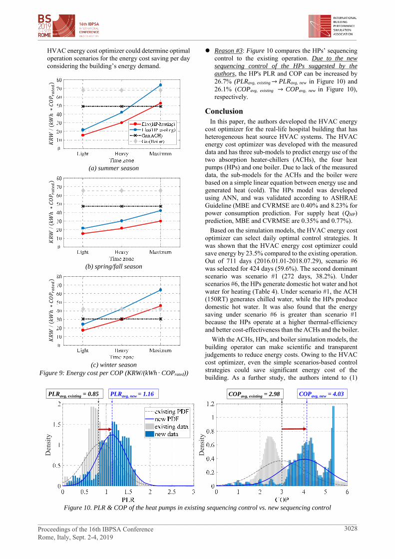
Reason #3: Figure 10 compares the HPs’ sequencing control to the existing operation. Due to the new sequencing control of the HPs suggested by the authors, the HP's PLR and COP can be increased by 26.7% (PLRavg, existing → PLRavg, new in Figure 10) and 26.1% (COPavg, existing → COPavg, new in Figure 10), respectively.

Conclusion In this paper, the authors developed the HVAC energy cost optimizer for the real-life hospital building that has heterogeneous heat source HVAC systems. The HVAC energy cost optimizer was developed with the measured data and has three sub-models to predict energy use of the two absorption heater-chillers (ACHs), the four heat pumps (HPs) and one boiler. Due to lack of the measured data, the sub-models for the ACHs and the boiler were based on a simple linear equation between energy use and generated heat (cold). The HPs model was developed using ANN, and was validated according to ASHRAE Guideline (MBE and CVRMSE are 0.40% and 8.23% for power consumption prediction. For supply heat (QHP) prediction, MBE and CVRMSE are 0.35% and 0.77%).

Based on the simulation models, the HVAC energy cost optimizer can select daily optimal control strategies. It was shown that the HVAC energy cost optimizer could save energy by 23.5% compared to the existing operation. Out of 711 days (2016.01.01-2018.07.29), scenario #6 was selected for 424 days (59.6%). The second dominant scenario was scenario #1 (272 days, 38.2%). Under scenarios #6, the HPs generate domestic hot water and hot water for heating (Table 4). Under scenario #1, the ACH (150RT) generates chilled water, while the HPs produce domestic hot water. It was also found that the energy saving under scenario #6 is greater than scenario #1 because the HPs operate at a higher thermal-efficiency and better cost-effectiveness than the ACHs and the boiler.

With the ACHs, HPs, and boiler simulation models, the building operator can make scientific and transparent judgements to reduce energy costs. Owing to the HVAC cost optimizer, even the simple scenarios-based control strategies could save significant energy cost of the building. As a further study, the authors intend to (1)

𝐾𝑅

𝑊/

𝑘𝑊ℎ

∗𝐶

𝑂𝑃

𝐾𝑅

𝑊/

𝑘𝑊ℎ

∗𝐶

𝑂𝑃

𝐾𝑅

𝑊/

𝑘𝑊ℎ

∗𝐶

𝑂𝑃

Figure 10. PLR & COP of the heat pumps in existing sequencing control vs. new sequencing control

Den

sity

PLRavg, existing = 0.85 PLRavg, new = 1.16

Den

sity

COPavg, existing = 2.98 COPavg, new = 4.03

________________________________________________________________________________________________


3028

develop an autonomous daily operation guideline for the building’s facility team and (2) compare the model predictive control to the developed scenarios-based control.

Acknowledgement This work was supported by the Korea Institute of Energy Technology Evaluation and Planning (KETEP) and the Ministry of Trade, Industry & Energy (MOTIE) of the Republic of Korea (No. 20182010106460).

References International Energy Agency (IEA) and United Nations

Development Programme (UNDP), Policy pathways: modernizing building energy codes.

Balaras, C. A., Dascalaki, E., Gaglia, A., & Droutsa, K. (2003). Energy conservation potential, HVAC installations and operational issues in Hellenic airports. Energy and buildings, 35(11), 1105-1120.

Rahman, M. M., Rasul, M. G., & Khan, M. M. K. (2010). Energy conservation measures in an institutional building in sub-tropical climate in Australia. Applied Energy, 87(10), 2994-3004.

Clarke, J. (2015). A vision for building performance simulation: a position paper prepared on behalf of the IBPSA Board. Journal of Building Performance Simulation, 8(2), 39-43.

IBPSA, Proceeding of IBPSA. 1987-2017, IBPSA.

Ahn, K. U., Kim, D. W., Kim, Y. J., Park, C. S., & Kim, I. H. (2015). Gaussian Process model for control of an existing building. Energy Procedia, 78, 2136-2141.

Afram, A., & Janabi-Sharifi, F. (2014). Theory and applications of HVAC control systems–A review of model predictive control (MPC). Building and Environment, 72, 343-355.

Afram, A., Janabi-Sharifi, F., Fung, A. S., & Raahemifar, K. (2017). Artificial neural network (ANN) based model predictive control (MPC) and optimization of HVAC systems: A state of the art review and case study of a residential HVAC system. Energy and Buildings, 141, 96-113.

Asadi, E., da Silva, M. G., Antunes, C. H., Dias, L., & Glicksman, L. (2014). Multi-objective optimization for building retrofit: A model using genetic algorithm and artificial neural network and an application. Energy and Buildings, 81, 444-456.

Kim, Y. M., Ahn, K. U., & Park, C. S. (2016). Issues of Application of Machine Learning Models for Virtual and Real-Life Buildings. Sustainability, 8(6), 543.

Ma, J., Qin, J., Salsbury, T., & Xu, P. (2012). Demand reduction in building energy systems based on economic model predictive control. Chemical Engineering Science, 67(1), 92-100.

Huang, G. (2011). Model predictive control of VAV zone thermal systems concerning bi-linearity and gain

nonlinearity. Control Engineering Practice, 19(7), 700-710.

Xi, X. C., Poo, A. N., & Chou, S. K. (2007). Support vector regression model predictive control on a HVAC plant. Control Engineering Practice, 15(8), 897-908.

Mařík, K., Rojíček, J., Stluka, P., & Vass, J. (2011, January). Advanced HVAC control: Theory vs. reality. In Preprints of the 18th IVAC World Congress, Milano, Italy (pp. 3108-3113).

Fong, K. F., Hanby, V. I., & Chow, T. T. (2009). System optimization for HVAC energy management using the robust evolutionary algorithm. Applied Thermal Engineering, 29(11-12), 2327-2334.

ASHRAE. (2014). ASHRAE Guideline 14-2014, for Measurement of Energy and Demand Saving. Atlanta: American Society of Heating, Refrigerating and Air-conditioning Engineers, Inc.

________________________________________________________________________________________________


3029

Scenario-based HVAC energy cost optimizer for ... - IBPSA

Documents

Transcript of Scenario-based HVAC energy cost optimizer for ... - IBPSA