Scalable Cross-Architecture Predictions of MemoryHierarchy Response for Scientific Applications

Gabriel Marinmgabi@cs.rice.edu

John Mellor-Crummeyjohnmc@cs.rice.edu

Department of Computer ScienceRice University

6100 Main St., MS 132Houston, TX 77005

ABSTRACTThe gap between processor and memory speeds has beengrowing with each new generation of microprocessors. Asa result, memory hierarchy response has become a criticalfactor limiting application performance. For this reason,we have been working to model the impact of memory ac-cess latency on program performance. We build upon ourprior work on constructing machine-independent characteri-zations of application behavior [9] by improving instruction-level modeling of the structure and scaling of data accesspatterns. This paper makes two contributions. First, it de-scribes static analysis techniques that help us build accuratereference-level characterizations of memory reuse patternsin the presence of complex interactions between loop un-rolling and multi-word memory blocks. Second, it describesa strategy for combining memory hierarchy response charac-terizations suitable for predicting behavior for fully associa-tive caches with a probabilistic technique that enables us topredict misses for set-associative caches. We validate our ap-proach by comparing our predictions (at loop, routine andprogram level) against measurements using hardware per-formance counters for several benchmarks on two platformswith different memory hierarchy characteristics over a largerange of problem sizes.

Keywordsreuse distance, static analysis, symbolic formulae, modeling,set-associative, cache miss predictions

1. INTRODUCTIONFor more than a decade, memory latency measured in

terms of processor cycles has increased with each new gen-eration of processors. For data-intensive programs, it iswidely accepted that memory hierarchy latency and band-width are the factors most limiting node performance onmicroprocessor-based systems. To alleviate this problem,modern architectures include one or more levels of cache be-tween the CPU and the main memory to boost availabledata bandwidth and help hide memory latency. However,caches are effective only if an application exhibits tempo-ral or spatial data reuse. Therefore, characterizing an ap-

plication’s memory access patterns is important for under-standing its performance and identifying opportunities foroptimization.

Predicting application behavior on a different architecturefor problem sizes not studied is difficult. Successful cross-architecture prediction requires an architecture-independentcharacterization of application behavior. Simple models thatextrapolate from hardware performance counter measure-ments (e.g. the number of cache or TLB misses) on a partic-ular machine cannot accurately predict application behav-ior on other architectures. Moreover, since an application’scache miss rate tends to grow in steps rather than smoothlywith the size of the working set, extrapolations of hardwarecounter measurements should be attempted over only a lim-ited range even on the same architecture.

In this paper, we expand upon our earlier work on cross-architecture prediction of application performance [9] witha focus on our techniques for predicting memory hierarchyresponse. We present a method for characterizing an ap-plication’s memory access patterns and a modeling strategythat enables predictions of cache miss counts at the instruc-tion level for different architectures and problem sizes.

New contributions of our work include static binary anal-ysis techniques for symbolically characterizing memory ref-erence access patterns, and a strategy for combining mem-ory hierarchy response models that assume full associativitywith a probabilistic technique that enables cache miss pre-dictions for set-associative caches. We present a set of ex-periments to validate our cache and TLB miss predictionsat loop, routine and program level. Our experiments com-pare measured and predicted memory hierarchy responsesof several applications on two different architectures over alarge range of problem sizes.

To model the memory hierarchy behavior of an applica-tion, we characterize the memory reuse distances1 seen byeach reference in the program. Memory reuse distance is ameasure of the number of unique memory blocks accessedbetween a pair of accesses to the same block. Characteriz-ing memory access behavior in this way for programs hastwo important advantages. First, data reuse distance is anapplication characteristic that is independent of target ar-chitecture. Second, reuse distance is a scalable measure ofdata reuse, which is the main determinant in cache per-

1Memory reuse distance is also known as LRU stack dis-tance.

formance. However, there is one exception to the claim oftotal architecture independence. To capture spatial reuse incache lines, we must collect reuse information with a mem-ory block size equal to the size of the cache line on the targetarchitecture. We will address this limitation again in Sec-tion 3. In addition, our reuse distance based models capturethe memory access pattern of an application, therefore it isonly sensible that they are not portable across high levelloop optimizations (HLO) such as tiling, loop interchange,unroll & jam, that change the application’s memory accesspattern.

The rest of this paper is organized as follows. Section 2presents static analysis that we use to guide both programinstrumentation and modeling. Section 3 describes our in-frastructure for collecting memory reuse distance (MRD)histograms from instrumented programs. Section 4 explainsour algorithm for synthesizing scalable models from the col-lected data. Section 5 shows how we predict the number ofcache misses for fully-associative or set-associative caches.Section 6 presents the results of using our methodology topredict cache and TLB miss counts at loop level for sev-eral NAS benchmarks on two different platforms. Section 7summarizes closely related work. Section 8 presents our con-clusions and our plans for future work.

2. STATIC ANALYSISWe use memory reuse distance as a metric to understand

and model memory locality in programs. To collect memoryreuse distance data, we instrument an application’s binaryand insert profiling code before each memory reference inthe program. Because we instrument object code instead ofsource code, our tools are language independent and natu-rally handle applications with modules written in differentlanguages. In addition, binary instrumentation enables usto study highly-optimized code whereas source code instru-mentation may inhibit aggressive compiler optimizations.

In this section, we describe our toolkit’s static analysiscapabilities. We use static analysis of binaries to guide everystep of our modeling and prediction process. Using staticanalysis, we

• reconstruct the control flow graph (CFG) for each rou-tine,2

• identify the natural loops in each CFG using intervalanalysis [12] and compute the loop nesting structure,

• derive symbolic formulae for each reference’s accesspattern, and

• identify references that must be profiled (e.g. we donot monitor accesses produced by register spill/unspillcode) and customize the profiling code for each mem-ory instruction.

The rest of this section describes a static analysis tech-nique for computing symbolic formulae that characterize theaccess pattern of each memory reference, and how we usethis analysis to improve modeling accuracy.

2CFG construction from a binary is performed by EEL [7]on top of which our toolkit’s binary analysis capabilities arebuilt.

2.1 Static Analysis of an Access PatternFor each memory reference, we statically derive several

symbolic formulae that describe the pattern of locations itaccesses during execution. We perform this analysis in-traprocedurally. We compute two types of formulae. Foreach reference in the program, we compute a formula forthe first location it accesses. For references inside loops, wealso compute formulae that describe how the accessed loca-tion changes from one iteration to the next.

We begin by constructing a first accessed location formulafor each reference in a routine. For each register used ina reference’s address computation, we recursively traversethe CFG backwards along use-def chains until either we en-counter a load immediate value, we cannot trace any fur-ther inside this routine (the traced register is the result ofa function call or we reach the top of the routine), or wedetermine that a formula for the register was already com-puted while analyzing a previous instruction. During thisbackward traversal of the CFG, we consider only forwardCFG edges. As we unwind each step of our traversal, wecompute a symbolic formula at each machine instructionalong the traversal by applying the instruction’s operator tothe formulae computed for its source registers. We cacheevery intermediate result so that we don’t have to traversethe same chain of instructions a second time when analyzinganother instruction.

During a use-def chain traversal, if we find that a registeris reloaded from the spill area, we trace backward alongCFG edges for a corresponding spill to the same locationand then resume our use-def chain traversal from the spill.We generalized our mechanism for handling reloaded spillvalues to work with arbitrary loads after we encountered abinary in which we found that the compiler had saved thevalue of a register in the data segment and later loaded it tocompute the address of a memory reference. If the value of aregister is defined by a load instruction, we trace backwardalong CFG edges for a store with a symbolic formula equalto the load’s symbolic formula3, and we continue tracingback from the register whose value was stored.

Formulae are restricted to sums of general terms includ-ing immediate values, loads from a constant address, loadsfrom the caller’s stack frame (an argument passed by refer-ence), and registers whose formulae cannot be written as asum of these terms (e.g. loads from an undetermined ad-dress, a product of two non-constant formulae, etc.). Eachterm of a formula can have integer numerator and denom-inator coefficients. With these restrictions, any non addi-tive (not an add or a sub) operation of two non-constantformulae will produce a register value. When at least oneoperand is a constant, several operations can be computedwithout simplification to a register value: multiply, divide,and left/right shift by a constant value can be performed byupdating the coefficients of each term in the non-constantoperand. If both operands are constants, all arithmetic andbitwise operators can be computed precisely.

For memory references inside loops, we compute addi-tional formulae that indicate how the accessed location dif-fers from one iteration to the next. We compute a stride for-mula for each loop level containing the reference. For eachlevel of a loop nest, we apply a recursive algorithm that tra-

3The symbolic formulae for the instructions upstream of theone currently analyzed have been already computed.

(a) matrix multiply source code (b) assembly for the innermost loop and the derived symbolic formulae

Figure 1: Static analysis example. The left subfigure presents the source code for a naive matrix multiplyimplementation, and on the right we have the SPARC assembly code for the innermost loop annotated withthe symbolic formulae computed for each memory reference.

verses backward along CFG edges, similar to the way we didwhen computing first accessed location formulae. However,when computing stride formulae, we consider only forwardCFG edges that are part of the analyzed loop and the loop’sback edge. This recursive search terminates when either weencounter a load immediate operation, we traced backwardsa complete iteration without finding a definition for this reg-ister (this register contains an invariant value with respectto this loop), or we reach a definition for a second time.In this last case, the found instruction is part of a chain ofinstructions that update an index variable. When the recur-sion returns, the stride formulae are computed by applyingthe mathematical operators corresponding to each interme-diate machine instruction to the non-invariant componentsof the source formulae.

The stride formulae are restricted to the same sums of gen-eral terms as the first accessed locations formulae. However,a stride formula has two additional flags that can be set bythe recursive algorithm. The first flag indicates if an accesshas an irregular stride; this flag is set if the reference’s strideis not constant for all iterations of that particular loop. Thesecond flag indicates if an access is indirect and it is set ifthe formula for the accessed location depends on the valueof another load which has a non-zero stride with respect tothis same loop.

For example, Figure 1(a) presents the source code for anaive implementation of the matrix multiply algorithm. Be-cause the program is written in C, the three matrices havebeen allocated as one-dimensional arrays and the rows ofeach matrix are contiguous in memory. The three matri-ces are dynamically allocated and their size is passed as anargument to the matrix multiply function to validate thecorrectness of the computed formulae in the presence of sym-bolic values.

Figure 1(b) presents the SPARC assembly code for theinnermost loop of the matrix multiply algorithm. The fivememory references have been annotated with symbolic for-mulae we derived through static analysis. Each referencehas a formula for the first accessed location, and three strideformulae, one for each level of the loop nest. Each refer-ence is also annotated with the corresponding source codearray access to make the code easier to understand. Thosefamiliar with the SPARC assembly language will recall thatregisters %i0, ..., %i5 are used for passing the first six in-

put arguments of a routine, and will notice that all symbolicformulae are correctly computed relative to the source codeon the left. The compiler has peeled one iteration of thek-loop, therefore the first location formulae correspond toi = 0, j = 0, k = 2. Although in the assembly code eachreference uses distinct address registers, the formulae forreferences to the same array show they are related. Thek-loop was unrolled by hand once4 and we compiled the bi-nary with unrolling disabled to keep the size of the assemblycode small for the purpose of this example, while at the sametime having the loop unrolled to show how this type of staticanalysis can uncover related references.

We say two references rs, rt located in the same loophave similar access patterns, if they have equal stride for-mulae relative to each loop containing them. In other wordsStride(rs, L

k) = Stride(rt, Lk) for every level k loop Lk con-

taining them, k ≥ 1. For our example in Figure 1(b), refer-ences A[i, k] and A[i, k +1], as well as references B[k, j] andB[k + 1, j] have equal strides at each loop level, and there-fore they have similar access patterns. This is no surprise forsomebody looking at the source code, but extracting suchinformation from binaries requires the detailed static anal-ysis we described.

2.2 Applications of Symbolic FormulaeA first use of the statically derived symbolic formulae is

at instrumentation time. Previously, we explained that wecollect memory reuse data at reference level. Such an ap-proach not only enables detailed predictions at instructionor loop level, but also enables more accurate models than ifwe collected aggregate reuse information for the entire pro-gram. However, as noted in [8, pages 46–53], modeling reusedistance data at instruction level is prone to errors due tothe alignment of data in memory when the reuse informa-tion is collected for larger than unit size memory blocks. Aswe describe in Section 3, to account for spatial reuse, wecollect reuse information of memory blocks, where the blocksize is equal to the line size of the target cache.

Consider now the matrix multiply example from Figure 1where the inner loop is unrolled once. Let’s assume that ar-ray A is always aligned to the start of a cache line. Because

4There must be additional code not included in the figurefor the k-loop to process the reminder element when N isodd.

A[i,k+1] hitA[i,k+1] miss

A[i,k] missA[i,k] hit

cache line boundary

N = 8 N = 9

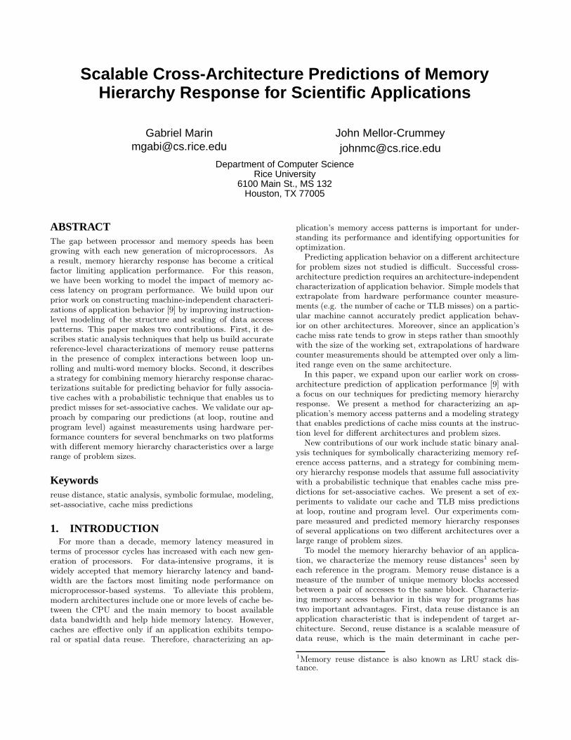
Figure 2: The distribution of cache misses for the two references to matrix A from the matrix multiplycode presented in Figure 1, for an even problem size (N=8) and an odd problem size (N=9), assuming anarchitecture with a cache line that holds four double elements.

the size of a cache line is a power of two, an even number ofarray elements will fit into a cache line. In our case, for aneven value of N , the reference corresponding to A[i, k + 1]will always see a small reuse distance due to spatial reuse,because A[i, k] will always perform the first access to a newcache line. However, for an odd value of N , A[i, k+1] will ac-cess a new cache line first for odd rows of A, while A[i, k] willaccess a new cache line first for even rows. Such inconsisten-cies between the reuse pattern at different problem sizes cancause large modeling errors for the affected references. How-ever, if we consider A[i, k] and A[i, k+1] together, the unionof their reuse distance data is consistent and predictable forevery problem size.

Figure 2 presents graphically this behavior for matrix sizes8 and 9, assuming an architecture where the cache line sizeis four times the size of an array element. In both cases,the total number of misses is approximately equal to onequarter of the number of memory accesses because only onemiss occurs per four-element cache line. However, the distri-bution of misses between the two references is different foreach problem size. This problem is even more pronouncedwhen the unrolling factor is greater and a larger number ofreferences are affected.

A similar problem occurs in codes working on arrays ofrecords when the cache line size is not a multiple of therecord size. In such a case, depending on the record index,different fields can occupy the first position of a cache line.As a result, different references encounter a long reuse dis-tance during the dynamic analysis depending on the recordindex. For this reason, at instrumentation time we find thesets of references that have similar access patterns and in-sert code that collects a single reuse distance histogram forevery such set.

After reuse distance histograms are collected, we performadditional static analysis to identify object code loops thathave their origin in the same source code loop, and we per-form additional aggregation between reference groups fromthese loops that have similar access patterns. We extendthe definition presented before to say that two references rs,rt located in different loops have similar access patterns, ifthey have equal stride formulae relative to each loop con-taining both of them, and their stride formulae relative todistinct, same level loops containing them have an integerratio. In other words: Stride(rs, L

kst) = Stride(rt, L

kst)

0 20 40 60 80 100 120

1

2

3

4

5

6

7

8

9−16

17−32

33−64

65−128

129−256

256+

6237

Number of sets

# of

ref

eren

ces

in s

et

both aggregation methodsaggregate same loop + remainder loopaggregate same loop onlyno aggregation

Figure 3: Distribution of the sizes of the instruc-tion groups derived for benchmark NAS BT 3.0when: (1) we perform no aggregation, (2) only ref-erences with similar patterns from the same loop aregrouped together, (3) we aggregate across adjacentobject code loops.

for every level k loop Lkst containing both references, and

Stride(rs, Lks )/Stride(rt, L

kt ) = m/n for every pair of dis-

tinct level k loops Lks and Lk

t containing references rs and rt

respectively, where m and n are integers and either m = 1or n = 1.

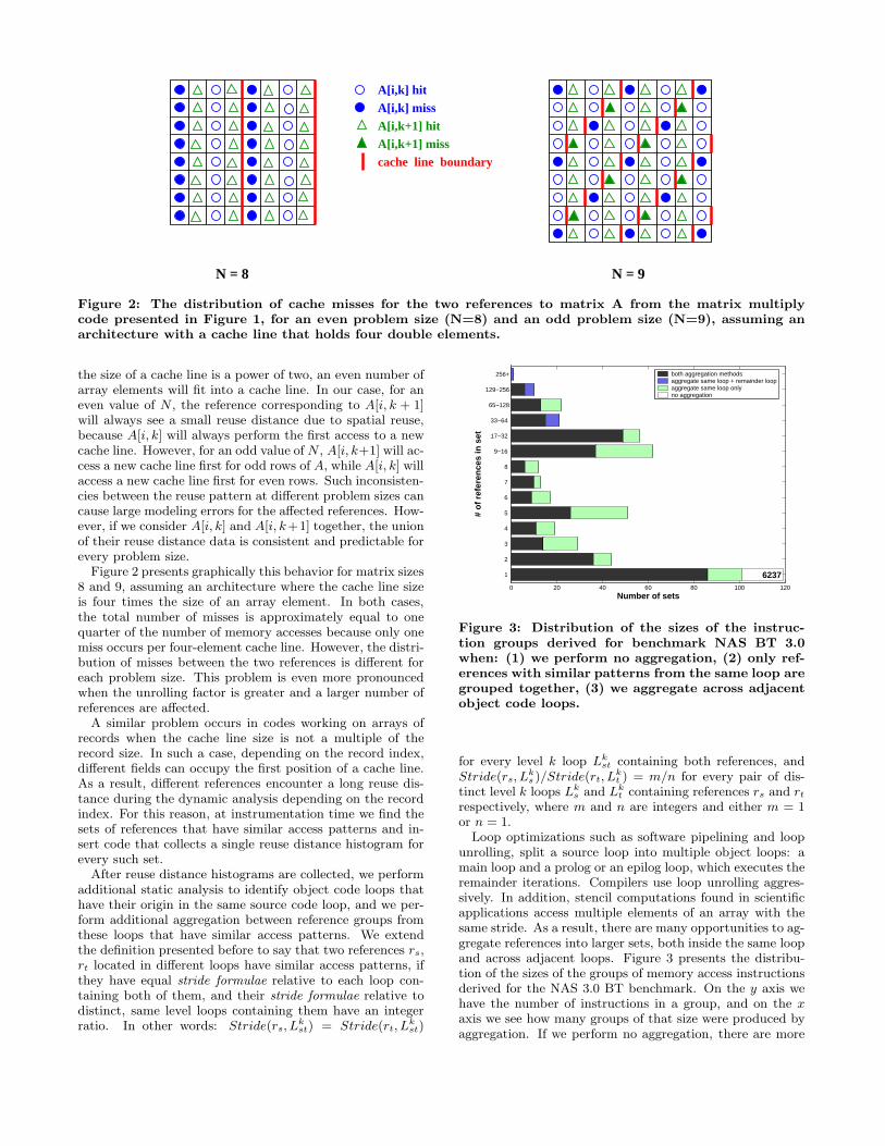
Loop optimizations such as software pipelining and loopunrolling, split a source loop into multiple object loops: amain loop and a prolog or an epilog loop, which executes theremainder iterations. Compilers use loop unrolling aggres-sively. In addition, stencil computations found in scientificapplications access multiple elements of an array with thesame stride. As a result, there are many opportunities to ag-gregate references into larger sets, both inside the same loopand across adjacent loops. Figure 3 presents the distribu-tion of the sizes of the groups of memory access instructionsderived for the NAS 3.0 BT benchmark. On the y axis wehave the number of instructions in a group, and on the xaxis we see how many groups of that size were produced byaggregation. If we perform no aggregation, there are more

Reuse Distance

L2 HitsL1 Hits

L1 size L2 size

Number ofReferences

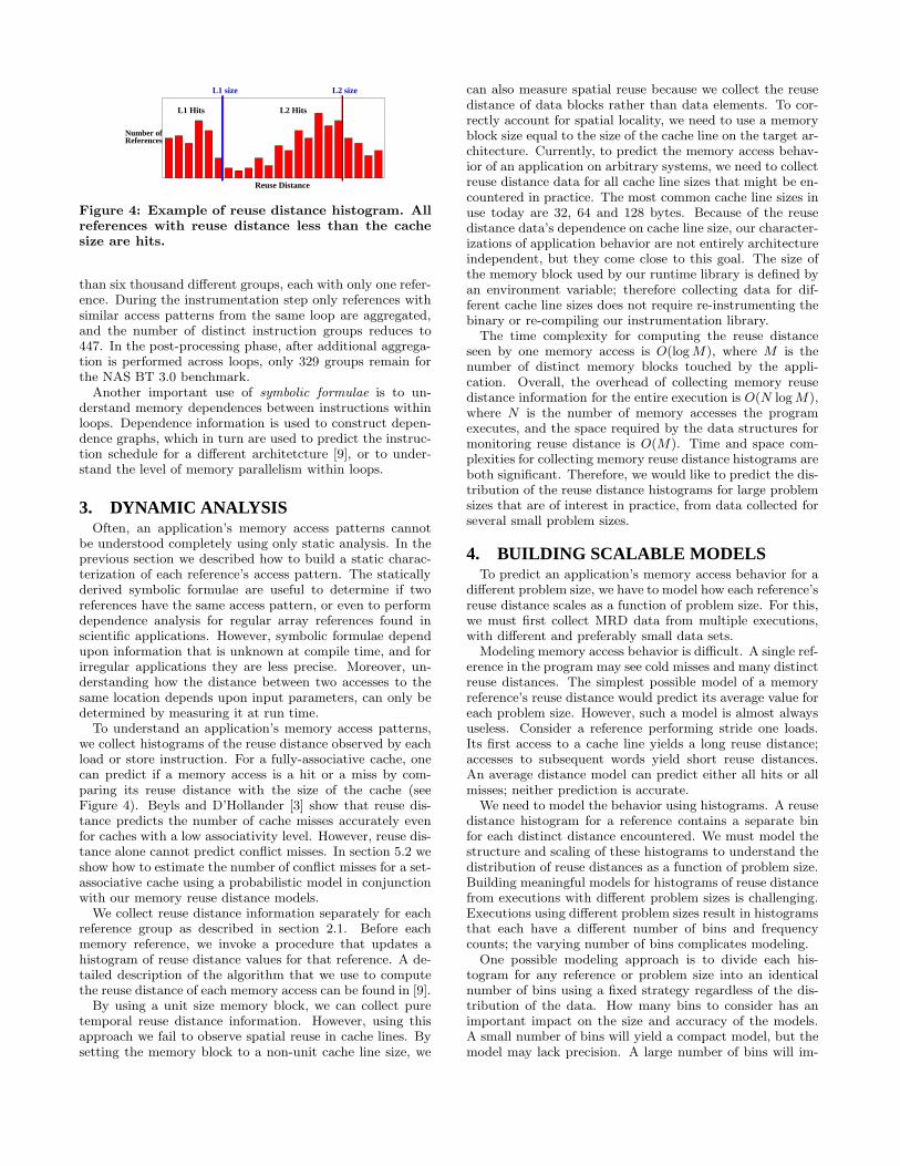
Figure 4: Example of reuse distance histogram. Allreferences with reuse distance less than the cachesize are hits.

than six thousand different groups, each with only one refer-ence. During the instrumentation step only references withsimilar access patterns from the same loop are aggregated,and the number of distinct instruction groups reduces to447. In the post-processing phase, after additional aggrega-tion is performed across loops, only 329 groups remain forthe NAS BT 3.0 benchmark.

Another important use of symbolic formulae is to un-derstand memory dependences between instructions withinloops. Dependence information is used to construct depen-dence graphs, which in turn are used to predict the instruc-tion schedule for a different architetcture [9], or to under-stand the level of memory parallelism within loops.

3. DYNAMIC ANALYSISOften, an application’s memory access patterns cannot

be understood completely using only static analysis. In theprevious section we described how to build a static charac-terization of each reference’s access pattern. The staticallyderived symbolic formulae are useful to determine if tworeferences have the same access pattern, or even to performdependence analysis for regular array references found inscientific applications. However, symbolic formulae dependupon information that is unknown at compile time, and forirregular applications they are less precise. Moreover, un-derstanding how the distance between two accesses to thesame location depends upon input parameters, can only bedetermined by measuring it at run time.

To understand an application’s memory access patterns,we collect histograms of the reuse distance observed by eachload or store instruction. For a fully-associative cache, onecan predict if a memory access is a hit or a miss by com-paring its reuse distance with the size of the cache (seeFigure 4). Beyls and D’Hollander [3] show that reuse dis-tance predicts the number of cache misses accurately evenfor caches with a low associativity level. However, reuse dis-tance alone cannot predict conflict misses. In section 5.2 weshow how to estimate the number of conflict misses for a set-associative cache using a probabilistic model in conjunctionwith our memory reuse distance models.

We collect reuse distance information separately for eachreference group as described in section 2.1. Before eachmemory reference, we invoke a procedure that updates ahistogram of reuse distance values for that reference. A de-tailed description of the algorithm that we use to computethe reuse distance of each memory access can be found in [9].

By using a unit size memory block, we can collect puretemporal reuse distance information. However, using thisapproach we fail to observe spatial reuse in cache lines. Bysetting the memory block to a non-unit cache line size, we

can also measure spatial reuse because we collect the reusedistance of data blocks rather than data elements. To cor-rectly account for spatial locality, we need to use a memoryblock size equal to the size of the cache line on the target ar-chitecture. Currently, to predict the memory access behav-ior of an application on arbitrary systems, we need to collectreuse distance data for all cache line sizes that might be en-countered in practice. The most common cache line sizes inuse today are 32, 64 and 128 bytes. Because of the reusedistance data’s dependence on cache line size, our character-izations of application behavior are not entirely architectureindependent, but they come close to this goal. The size ofthe memory block used by our runtime library is defined byan environment variable; therefore collecting data for dif-ferent cache line sizes does not require re-instrumenting thebinary or re-compiling our instrumentation library.

The time complexity for computing the reuse distanceseen by one memory access is O(log M), where M is thenumber of distinct memory blocks touched by the appli-cation. Overall, the overhead of collecting memory reusedistance information for the entire execution is O(N log M),where N is the number of memory accesses the programexecutes, and the space required by the data structures formonitoring reuse distance is O(M). Time and space com-plexities for collecting memory reuse distance histograms areboth significant. Therefore, we would like to predict the dis-tribution of the reuse distance histograms for large problemsizes that are of interest in practice, from data collected forseveral small problem sizes.

4. BUILDING SCALABLE MODELSTo predict an application’s memory access behavior for a

different problem size, we have to model how each reference’sreuse distance scales as a function of problem size. For this,we must first collect MRD data from multiple executions,with different and preferably small data sets.

Modeling memory access behavior is difficult. A single ref-erence in the program may see cold misses and many distinctreuse distances. The simplest possible model of a memoryreference’s reuse distance would predict its average value foreach problem size. However, such a model is almost alwaysuseless. Consider a reference performing stride one loads.Its first access to a cache line yields a long reuse distance;accesses to subsequent words yield short reuse distances.An average distance model can predict either all hits or allmisses; neither prediction is accurate.

We need to model the behavior using histograms. A reusedistance histogram for a reference contains a separate binfor each distinct distance encountered. We must model thestructure and scaling of these histograms to understand thedistribution of reuse distances as a function of problem size.Building meaningful models for histograms of reuse distancefrom executions with different problem sizes is challenging.Executions using different problem sizes result in histogramsthat each have a different number of bins and frequencycounts; the varying number of bins complicates modeling.

One possible modeling approach is to divide each his-togram for any reference or problem size into an identicalnumber of bins using a fixed strategy regardless of the dis-tribution of the data. How many bins to consider has animportant impact on the size and accuracy of the models.A small number of bins will yield a compact model, but themodel may lack precision. A large number of bins will im-

2025

3035

4045

50

0

0.2

0.4

0.6

0.8

10

1

2

3

4

5

6

7

x 104

Problem sizeNormalized frequency

Mem

ory

reus

e di

stan

ce

(a)

2025

3035

4045

50

0

0.2

0.4

0.6

0.8

10

1

2

3

4

5

6

7

x 104

Problem sizeNormalized frequency

Mem

ory

reus

e di

stan

ce

(b)

2025

3035

4045

50

0

0.2

0.4

0.6

0.8

10

1

2

3

4

5

6

7

x 104

Problem sizeNormalized frequency

Mem

ory

reus

e di

stan

ce

(c)

2025

3035

4045

50

0

0.2

0.4

0.6

0.8

10

1

2

3

4

5

6

7

x 104

Problem sizeNormalized frequency

Mem

ory

reus

e di

stan

ce

(d)

0 0.1 0.2 0.3 0.4 0.5 0.6 0.7 0.8 0.9 10

2

4

6

8

10

12

14

16x 10

4

Normalized frequency

Reu

se d

ista

nce

(e)

0 0.1 0.2 0.3 0.4 0.5 0.6 0.7 0.8 0.9 110

0

101

102

103

104

105

106

Normalized frequency

Reu

se d

ista

nce

(sem

ilog)

L1 size

L2 size

2048

24576

L1 hits

L2 hits

95.4%

98.4%

(f)

Figure 5: (a) MRD data collected for one reference in Sweep3D; (b) Model constant distance first, and lumpremaining data in one bin; (c) First split of the non-constant data; (d) Final model for the data in (a); (e)Model evaluation at problem size 70; (f) Model evaluation at problem size 70 on a logarithmic y axis, andpredictions for a 2048 blocks level 1 and 24576 blocks level 2 cache.

prove model accuracy, but will add unnecessary complexityand cost to modeling for many references that use only afew different reuse distances. To avoid this problem, we ex-amine a reference’s collected data and pick an appropriatenumber of bins and their boundaries to adequately representits histogram data across the range of problem sizes.

4.1 Modeling MRD HistogramsWe sort the bins in each reference’s MRD histogram by

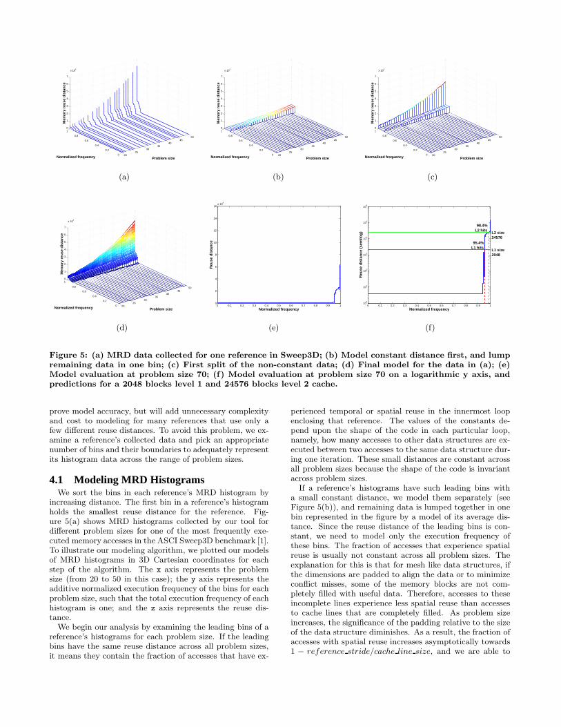
increasing distance. The first bin in a reference’s histogramholds the smallest reuse distance for the reference. Fig-ure 5(a) shows MRD histograms collected by our tool fordifferent problem sizes for one of the most frequently exe-cuted memory accesses in the ASCI Sweep3D benchmark [1].To illustrate our modeling algorithm, we plotted our modelsof MRD histograms in 3D Cartesian coordinates for eachstep of the algorithm. The x axis represents the problemsize (from 20 to 50 in this case); the y axis represents theadditive normalized execution frequency of the bins for eachproblem size, such that the total execution frequency of eachhistogram is one; and the z axis represents the reuse dis-tance.

We begin our analysis by examining the leading bins of areference’s histograms for each problem size. If the leadingbins have the same reuse distance across all problem sizes,it means they contain the fraction of accesses that have ex-

perienced temporal or spatial reuse in the innermost loopenclosing that reference. The values of the constants de-pend upon the shape of the code in each particular loop,namely, how many accesses to other data structures are ex-ecuted between two accesses to the same data structure dur-ing one iteration. These small distances are constant acrossall problem sizes because the shape of the code is invariantacross problem sizes.

If a reference’s histograms have such leading bins witha small constant distance, we model them separately (seeFigure 5(b)), and remaining data is lumped together in onebin represented in the figure by a model of its average dis-tance. Since the reuse distance of the leading bins is con-stant, we need to model only the execution frequency ofthese bins. The fraction of accesses that experience spatialreuse is usually not constant across all problem sizes. Theexplanation for this is that for mesh like data structures, ifthe dimensions are padded to align the data or to minimizeconflict misses, some of the memory blocks are not com-pletely filled with useful data. Therefore, accesses to theseincomplete lines experience less spatial reuse than accessesto cache lines that are completely filled. As problem sizeincreases, the significance of the padding relative to the sizeof the data structure diminishes. As a result, the fraction ofaccesses with spatial reuse increases asymptotically towards1 − reference stride/cache line size, and we are able to

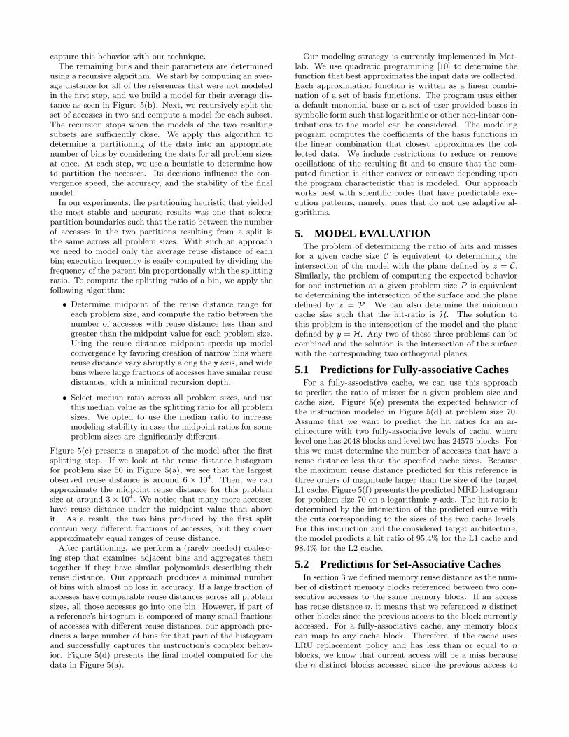
capture this behavior with our technique.The remaining bins and their parameters are determined

using a recursive algorithm. We start by computing an aver-age distance for all of the references that were not modeledin the first step, and we build a model for their average dis-tance as seen in Figure 5(b). Next, we recursively split theset of accesses in two and compute a model for each subset.The recursion stops when the models of the two resultingsubsets are sufficiently close. We apply this algorithm todetermine a partitioning of the data into an appropriatenumber of bins by considering the data for all problem sizesat once. At each step, we use a heuristic to determine howto partition the accesses. Its decisions influence the con-vergence speed, the accuracy, and the stability of the finalmodel.

In our experiments, the partitioning heuristic that yieldedthe most stable and accurate results was one that selectspartition boundaries such that the ratio between the numberof accesses in the two partitions resulting from a split isthe same across all problem sizes. With such an approachwe need to model only the average reuse distance of eachbin; execution frequency is easily computed by dividing thefrequency of the parent bin proportionally with the splittingratio. To compute the splitting ratio of a bin, we apply thefollowing algorithm:

• Determine midpoint of the reuse distance range foreach problem size, and compute the ratio between thenumber of accesses with reuse distance less than andgreater than the midpoint value for each problem size.Using the reuse distance midpoint speeds up modelconvergence by favoring creation of narrow bins wherereuse distance vary abruptly along the y axis, and widebins where large fractions of accesses have similar reusedistances, with a minimal recursion depth.

• Select median ratio across all problem sizes, and usethis median value as the splitting ratio for all problemsizes. We opted to use the median ratio to increasemodeling stability in case the midpoint ratios for someproblem sizes are significantly different.

Figure 5(c) presents a snapshot of the model after the firstsplitting step. If we look at the reuse distance histogramfor problem size 50 in Figure 5(a), we see that the largestobserved reuse distance is around 6 × 104. Then, we canapproximate the midpoint reuse distance for this problemsize at around 3 × 104. We notice that many more accesseshave reuse distance under the midpoint value than aboveit. As a result, the two bins produced by the first splitcontain very different fractions of accesses, but they coverapproximately equal ranges of reuse distance.

After partitioning, we perform a (rarely needed) coalesc-ing step that examines adjacent bins and aggregates themtogether if they have similar polynomials describing theirreuse distance. Our approach produces a minimal numberof bins with almost no loss in accuracy. If a large fraction ofaccesses have comparable reuse distances across all problemsizes, all those accesses go into one bin. However, if part ofa reference’s histogram is composed of many small fractionsof accesses with different reuse distances, our approach pro-duces a large number of bins for that part of the histogramand successfully captures the instruction’s complex behav-ior. Figure 5(d) presents the final model computed for thedata in Figure 5(a).

Our modeling strategy is currently implemented in Mat-lab. We use quadratic programming [10] to determine thefunction that best approximates the input data we collected.Each approximation function is written as a linear combi-nation of a set of basis functions. The program uses eithera default monomial base or a set of user-provided bases insymbolic form such that logarithmic or other non-linear con-tributions to the model can be considered. The modelingprogram computes the coefficients of the basis functions inthe linear combination that closest approximates the col-lected data. We include restrictions to reduce or removeoscillations of the resulting fit and to ensure that the com-puted function is either convex or concave depending uponthe program characteristic that is modeled. Our approachworks best with scientific codes that have predictable exe-cution patterns, namely, ones that do not use adaptive al-gorithms.

5. MODEL EVALUATIONThe problem of determining the ratio of hits and misses

for a given cache size C is equivalent to determining theintersection of the model with the plane defined by z = C.Similarly, the problem of computing the expected behaviorfor one instruction at a given problem size P is equivalentto determining the intersection of the surface and the planedefined by x = P . We can also determine the minimumcache size such that the hit-ratio is H. The solution tothis problem is the intersection of the model and the planedefined by y = H. Any two of these three problems can becombined and the solution is the intersection of the surfacewith the corresponding two orthogonal planes.

5.1 Predictions for Fully-associative CachesFor a fully-associative cache, we can use this approach

to predict the ratio of misses for a given problem size andcache size. Figure 5(e) presents the expected behavior ofthe instruction modeled in Figure 5(d) at problem size 70.Assume that we want to predict the hit ratios for an ar-chitecture with two fully-associative levels of cache, wherelevel one has 2048 blocks and level two has 24576 blocks. Forthis we must determine the number of accesses that have areuse distance less than the specified cache sizes. Becausethe maximum reuse distance predicted for this reference isthree orders of magnitude larger than the size of the targetL1 cache, Figure 5(f) presents the predicted MRD histogramfor problem size 70 on a logarithmic y-axis. The hit ratio isdetermined by the intersection of the predicted curve withthe cuts corresponding to the sizes of the two cache levels.For this instruction and the considered target architecture,the model predicts a hit ratio of 95.4% for the L1 cache and98.4% for the L2 cache.

5.2 Predictions for Set-Associative CachesIn section 3 we defined memory reuse distance as the num-

ber of distinct memory blocks referenced between two con-secutive accesses to the same memory block. If an accesshas reuse distance n, it means that we referenced n distinctother blocks since the previous access to the block currentlyaccessed. For a fully-associative cache, any memory blockcan map to any cache block. Therefore, if the cache usesLRU replacement policy and has less than or equal to nblocks, we know that current access will be a miss becausethe n distinct blocks accessed since the previous access to

this block have caused it to be evicted from the cache. Simi-larly, if the cache has more than n blocks, the current accessis a hit because the accessed block was not evicted yet.

For a set-associative cache with s sets and associativitylevel k, a memory block can map only to one of the k blocksof a single set, where the set is uniquely determined by theblock’s location in memory. As a result, an access with reusedistance n is a hit if less than k out of the n accessed blocksmap to this same set. The mapping of memory blocks tocache sets depends upon how data structures are laid out inmemory. However, we do not collect information about thelocation of accessed blocks. As Hill and Smith noted in [6],we can estimate set-associative LRU distance from fully-associative LRU distance using a statistical model. Thismodel is based on the simplifying assumption that accessedblocks are uniformly distributed in memory. In other words,the probability that two blocks map to the same set is 1/sand independent of where other blocks map.

With this assumption, we first compute the probabilitythat exactly i blocks out of n distinct blocks map to a givenset. We first notice that for i > n, the probability is zero be-cause we cannot have more than n blocks map to a single setwhen there are n blocks overall. The mapping probabilitycan be written as:

Pmapping(s, n, i) =

(

`

1s

´i `

s−1s

´n−i“

ni

”

if i ≤ n

0 if i > n

The probability formula for i ≤ n has three terms:

•`

1s

´ibecause i blocks must map onto a specific set (the

set of the currently accessed block)

•`

s−1s

´n−ibecause the other n−i blocks must map onto

the other s − 1 sets.

•

“

ni

”

because any combination of i blocks out of the

total number of n blocks can map onto our set.

The probability that an access with reuse distance n hitsin a set-associative cache with s sets and associativity k canbe written as:

Phit(s, k, n) =

min(k−1,n)X

i=0

„

1

s

«i „

s − 1

s

«n−i „

ni

«

and the probability of that access being a cache miss is 1minus the previous formula:

Pmiss(s, k, n) = 1 −

min(k−1,n)X

i=0

„

1

s

«i „

s − 1

s

«n−i „

ni

«

This model fits very well with our MRD model, because wedo not predict just an average distance for a reference, but ahistogram of how many times each distance is encountered.For each bin of a reference’s histogram we compute a missprobability as a function of the bin’s reuse distance. Theresulting probability represents the fraction of accesses inthat bin that should be expected as cache misses.

In the case of a fully-associative cache we have only one set(s = 1) and k represents the number of blocks in the cache.If n > k − 1, probability to hit in the cache is zero because`

s−1s

´n−i= 0 for any i ≤ k−1 < n. If n ≤ k−1, probability

to hit in the cache is one because the sum reduces to a single

term,“

ni

”

, where i = n ≤ k−1. Thus, the formula is valid

also in the special case of a fully-associative cache, althoughit is more efficient to use the direct method presented inSection 5.1 to compute the number of cache misses for fully-associative caches. However, we observe that while for afully-associative cache each bin counts as either all hits orall misses, in the case of a set-associative cache a bin canhave a dual behavior.

We can approximate the number of misses for a set-associativecache from the histogram of reuse distances predicted by ourMRD model, with the following formula:

Nummisses(Hist, s, k) =X

bini∈Hist

(Pmiss(s, k, Dbini)Fbini

)

where Dbiniand Fbini

are the average MRD of bini and theexecution frequency of bini respectively.

Although the assumption that accessed memory blocksare uniformly distributed in memory is not always true, themiss predictions for set-associative caches produced by thismodel (see section 6) are quite accurate.

6. RESULTSTo validate our approach, in this section we compute cache

and TLB miss predictions at the loop level for the ASCISweep3D benchmark and several of the NPB 2.3-serial andNPB 3.0 benchmarks, for mesh sizes ranging from 103 to2003. We compare our predictions against measurementsusing hardware performance counters on two different plat-form: an Itanium2 based machine and an Origin 2000 sys-tem based on the MIPS R12000 processor. The memoryhierarchy characteristics for the two testbed machines arepresented in table 1. On the Itanium, floating point loads

Level # blocks/associativity/block sizeItanium2 R12000

L1D 256/4-way/64 B 1024/2-way/32 BL2 2048/8-way/128 B 65536/2-way/128 BL3 12288/6-way/128 B –

L1 TLB5 32/fully/16 KB 64/fully/32 KB6

L2 TLB5 128/fully/16 KB –

Table 1: Memory hierarchy characteristics for thetestbed machines.

and stores bypass the small L1D cache and its associated L1TLB. Because the benchmarks used in this test suite are allfloating point intensive, the L1D cache and the L1 TLB ofthe Itanium2 machine have very little impact on their per-formance, and we do not present predictions for these twomemory levels.

Our memory reuse distance models for an application area function of cache line size, are parameterized by one ofthe application’s input parameters as described in Section 4,while size and associativity level of the target cache are usedduring evaluation (see Section 5) to predict the number of

5A TLB behaves exactly like an LRU cache with a numberof blocks equal to the number of entries in the TLB, and thesize of each block equal to the size of the memory mappedby each entry.6On the R12000, each TLB entry maps two consecutivepages, therefore the size of the memory mapped by an entryis 32 KB.

cache misses. Nowhere in this process we make use of infor-mation such as the CPU’s frequency or its number of func-tional units. Our cache miss predictions have nothing todo with the architecture of the CPU core. Therefore, whilewe consider only two platforms, we present predictions forsix different cache configurations (two cache levels and oneTLB level on each platform). From table 1 we see that thetestbed machines cover a diverse set of cache configurations,including capacity, block size and associativity.

To compute the predictions, we compiled the benchmarkson a Sun UltraSPARC-II system using the Sun WorkShop 6update 2 FORTRAN 77 5.3 compiler, and the optimizations:-xarch=v8plus -xO4 -depend -dalign -xtypemap=real:64. Mea-surements on the Itanium2 machine were performed on bi-naries compiled with the Intel Fortran Itanium Compiler8.0, and the optimization flags: -O2 -tpp2 -fno-alias. Onthe Origin 2000 system we compiled the binaries with theSGI Fortran compiler version 7.3.1.3m and the optimizationflags: -O3 -r10000 -64 -LNO:opt=0. We used the highestoptimization level but we disabled high-level loop optimiza-tions, because the sets of loop nest transformations imple-mented in the Sun, Intel and SGI compilers are different.Loop nest transformations change the execution order of theiterations of a loop nest, effectively altering an application’smemory access pattern.

We present results for three benchmarks on each of thetwo machines, including results at routine and loop level forone benchmark on each architecture. We present results forASCI Sweep3D and the BT benchmark from NPB 2.3-serialon both architectures. In addition, on the Itanium2 machinewe analyze in more detail the behavior of the hyper-plane2D implementation of LU from NPB 3.0 , and on the Origin2000 we look at the SP benchmark from NPB 3.0. The NASbenchmarks use statically allocated data structures, withthe maximum size of the working mesh specified at compiletime. The benchmarks can be compiled in several standardclasses named A, B and C, which have a maximum mesh sizeof 64, 102 and 162 respectively. We created an extra classL with a maximum mesh size of 200. We used static anddynamic analysis of the class A binaries to construct themodels. The measurements on the Itanium2 and R12000machines were performed on the binary of minimum classthat accommodates that particular size.

To compute the predictions, we collected MRD data forblock sizes 32, 128, 16 KB and 32 KB, for a set of problemsizes randomly selected between 20 and 50. We collecteddata on relatively small input problems to limit the cost ofexecuting the instrumented binaries. Next, we built mod-els of MRD parameterized by problem size for each of theapplications, as described in section 4. Finally, to predictthe cache and TLB miss counts, we evaluated the models ateach problem size of interest. For each memory hierarchylevel on each of the two machines, we predict a miss countfor a fully-associative cache of the same size as the actualcache on the machine using only the MRD models, and amiss count that takes associativity into account using theprobabilistic model described in section 5.2.

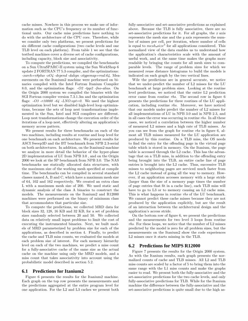
6.1 Predictions for Itanium2Figure 6 presents the results for the Itanium2 machine.

Each graph on the top row presents the measurements andthe predictions aggregated at the entire program level forone application. For the L2 and L3 caches we present both

fully-associative and set-associative predictions as explainedabove. Because the TLB is fully associative, there are noset-associative predictions for it. For all graphs, the x axisrepresents the mesh size and the y axis represents the num-ber of misses per cell, per iteration, where number of cellsis equal to mesh size3 for all applications considered. Thisnormalized view of the data enables us to understand howthe application’s characteristics scale with the amount ofuseful work, and at the same time makes the graphs morereadable by bringing the counts for all mesh sizes to com-parable levels. The range of problem sizes for which wemeasured reuse distance histograms to build the models isindicated on each graph by the two vertical lines.

Wile the predictions are in general accurate, we noticethat we under-predict the number of L2 misses for the LUbenchmark at large problem sizes. Looking at the routinelevel predictions, we noticed that the entire L2 predictionerror came from routine rhs. The second row in figure 6presents the predictions for three routines of the LU appli-cation, including routine rhs. Moreover, we have noticedthat our models under predict the number of L2 misses forall implementations of LU in NPB 3.0 and in NPB 2.3, andin all cases the error was occurring in routine rhs. In all thesecases, we noticed a correlation between the higher numberof measured L2 misses and a high rate of TLB misses. Asyou can see from the graph for routine rhs in figure 6, al-most all TLB misses measured for the LU application areproduced by this routine. On a TLB miss, the OS needsto find the entry for the offending page in the virtual pagetable which is stored in memory. On the Itanium, the pagetable is accessed through the L2 cache. This has the advan-tage that on a TLB miss, in addition to the offending entrybeing brought into the TLB, an entire cache line of pageentries is brought into the L2 cache. Thus, successive TLBmisses to neighboring pages are serviced much faster fromthe L2 cache instead of going all the way to memory. How-ever, if an application accesses memory with a large stride(larger than the size of a memory page times the numberof page entries that fit in a cache line), each TLB miss willhave to go to L3 or to memory causing an L2 cache miss.This is what happens in routine rhs of the LU benchmark.We cannot predict these cache misses because they are notproduced by the application explicitly, but are the resultof an interaction between the architectural design and theapplication’s access stride.

On the bottom row of figure 6, we present the predictionsand the measurements for two level 3 loops from routinerhs. For these loops, we notice that the number of L2 missespredicted by the model is zero for all problem sizes, but themeasurements on the Itanium2 show the code experiencesL2 misses once it starts missing in the TLB.

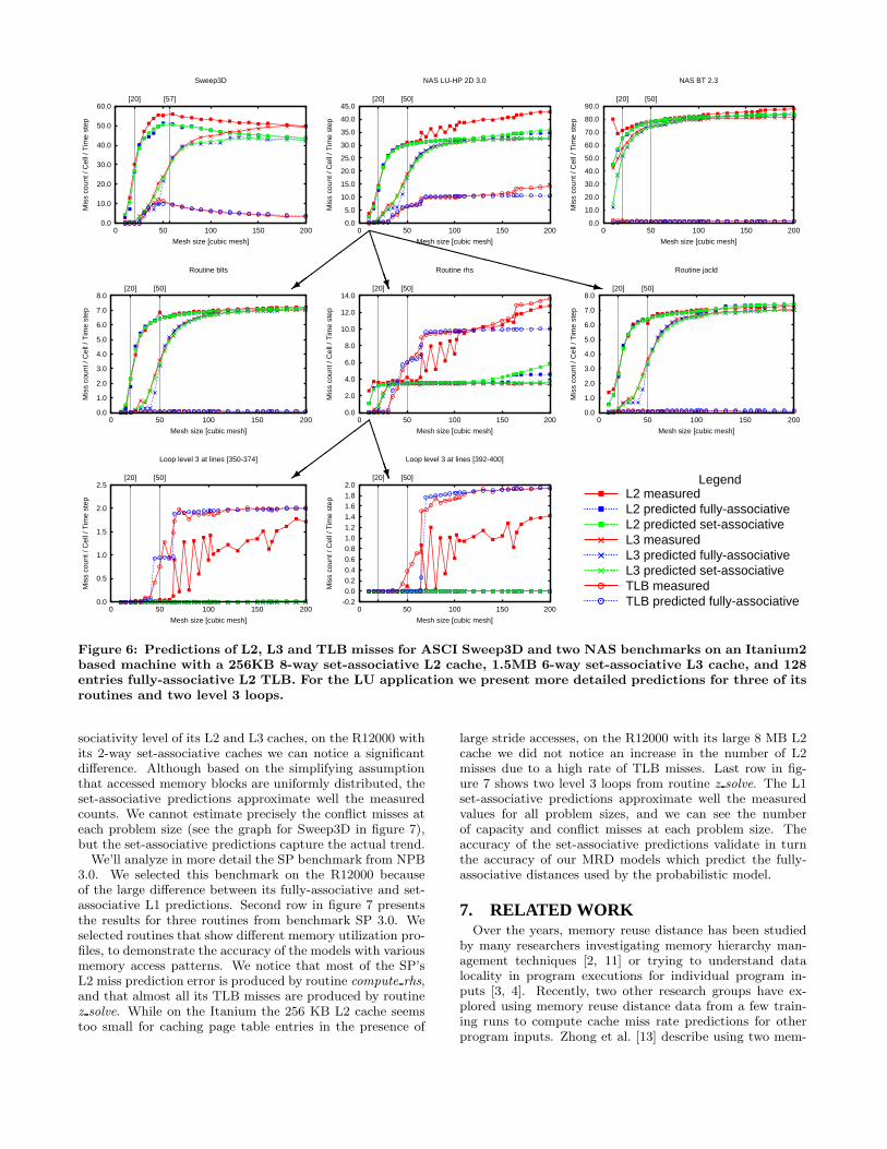
6.2 Predictions for MIPS R12000Figure 7 presents the results for the Origin 2000 system.

As with the Itanium results, each graph presents the nor-malized counts of cache and TLB misses. All L2 and TLBmiss counts are scaled by a factor of 5 to bring them into thesame range with the L1 miss counts and make the graphseasier to read. We present both the fully-associative and theset-associative predictions for the two cache levels, and onlyfully-associative predictions for TLB. While for the Itaniummachine the difference between the fully-associative and theset-associative predictions is quite small due to the high as-

0.0

10.0

20.0

30.0

40.0

50.0

60.0

0 50 100 150 200

[57][20]

Mis

s co

unt /

Cel

l / T

ime

step

Mesh size [cubic mesh]

Sweep3D

0.0

5.0

10.0

15.0

20.0

25.0

30.0

35.0

40.0

45.0

0 50 100 150 200

[50][20]

Mis

s co

unt /

Cel

l / T

ime

step

Mesh size [cubic mesh]

NAS LU-HP 2D 3.0

0.0

10.0

20.0

30.0

40.0

50.0

60.0

70.0

80.0

90.0

0 50 100 150 200

[50][20]

Mis

s co

unt /

Cel

l / T

ime

step

Mesh size [cubic mesh]

NAS BT 2.3

0.0

1.0

2.0

3.0

4.0

5.0

6.0

7.0

8.0

0 50 100 150 200

[50][20]

Mis

s co

unt /

Cel

l / T

ime

step

Mesh size [cubic mesh]

Routine blts

0.0

2.0

4.0

6.0

8.0

10.0

12.0

14.0

0 50 100 150 200

[50][20]

Mis

s co

unt /

Cel

l / T

ime

step

Mesh size [cubic mesh]

Routine rhs

0.0

1.0

2.0

3.0

4.0

5.0

6.0

7.0

8.0

0 50 100 150 200

[50][20]

Mis

s co

unt /

Cel

l / T

ime

step

Mesh size [cubic mesh]

Routine jacld

0.0

0.5

1.0

1.5

2.0

2.5

0 50 100 150 200

[50][20]

Mis

s co

unt /

Cel

l / T

ime

step

Mesh size [cubic mesh]

Loop level 3 at lines [350-374]

-0.2

0.0

0.2

0.4

0.6

0.8

1.0

1.2

1.4

1.6

1.8

2.0

0 50 100 150 200

[50][20]

Mis

s co

unt /

Cel

l / T

ime

step

Mesh size [cubic mesh]

Loop level 3 at lines [392-400]

LegendL2 measuredL2 predicted fully-associativeL2 predicted set-associativeL3 measuredL3 predicted fully-associativeL3 predicted set-associativeTLB measuredTLB predicted fully-associative

��

��

��=

BBBBBN

XXXXXXXXXXXXXXXXXz

��

��

��=

BBBBBN

Figure 6: Predictions of L2, L3 and TLB misses for ASCI Sweep3D and two NAS benchmarks on an Itanium2based machine with a 256KB 8-way set-associative L2 cache, 1.5MB 6-way set-associative L3 cache, and 128entries fully-associative L2 TLB. For the LU application we present more detailed predictions for three of itsroutines and two level 3 loops.

sociativity level of its L2 and L3 caches, on the R12000 withits 2-way set-associative caches we can notice a significantdifference. Although based on the simplifying assumptionthat accessed memory blocks are uniformly distributed, theset-associative predictions approximate well the measuredcounts. We cannot estimate precisely the conflict misses ateach problem size (see the graph for Sweep3D in figure 7),but the set-associative predictions capture the actual trend.

We’ll analyze in more detail the SP benchmark from NPB3.0. We selected this benchmark on the R12000 becauseof the large difference between its fully-associative and set-associative L1 predictions. Second row in figure 7 presentsthe results for three routines from benchmark SP 3.0. Weselected routines that show different memory utilization pro-files, to demonstrate the accuracy of the models with variousmemory access patterns. We notice that most of the SP’sL2 miss prediction error is produced by routine compute rhs,and that almost all its TLB misses are produced by routinez solve. While on the Itanium the 256 KB L2 cache seemstoo small for caching page table entries in the presence of

large stride accesses, on the R12000 with its large 8 MB L2cache we did not notice an increase in the number of L2misses due to a high rate of TLB misses. Last row in fig-ure 7 shows two level 3 loops from routine z solve. The L1set-associative predictions approximate well the measuredvalues for all problem sizes, and we can see the numberof capacity and conflict misses at each problem size. Theaccuracy of the set-associative predictions validate in turnthe accuracy of our MRD models which predict the fully-associative distances used by the probabilistic model.

7. RELATED WORKOver the years, memory reuse distance has been studied

by many researchers investigating memory hierarchy man-agement techniques [2, 11] or trying to understand datalocality in program executions for individual program in-puts [3, 4]. Recently, two other research groups have ex-plored using memory reuse distance data from a few train-ing runs to compute cache miss rate predictions for otherprogram inputs. Zhong et al. [13] describe using two mem-

0.0

50.0

100.0

150.0

200.0

250.0

0 50 100 150 200

[57][20]

Mis

s co

unt /

Cel

l / T

ime

step

Mesh size [cubic mesh]

Sweep3D

0.0

10.0

20.0

30.0

40.0

50.0

60.0

70.0

80.0

90.0

100.0

0 50 100 150 200

[50][20]

Mis

s co

unt /

Cel

l / T

ime

step

Mesh size [cubic mesh]

NAS SP 3.0

0.0

50.0

100.0

150.0

200.0

250.0

300.0

350.0

400.0

450.0

0 50 100 150 200

[50][20]

Mis

s co

unt /

Cel

l / T

ime

step

Mesh size [cubic mesh]

NAS BT 2.3

0.0

2.0

4.0

6.0

8.0

10.0

12.0

14.0

0 50 100 150 200

[50][20]

Mis

s co

unt /

Cel

l / T

ime

step

Mesh size [cubic mesh]

Routine y_solve

0.0

5.0

10.0

15.0

20.0

25.0

30.0

0 50 100 150 200

[50][20]

Mis

s co

unt /

Cel

l / T

ime

step

Mesh size [cubic mesh]

Routine z_solve

0.0

5.0

10.0

15.0

20.0

25.0

30.0

35.0

40.0

45.0

0 50 100 150 200

[50][20]

Mis

s co

unt /

Cel

l / T

ime

step

Mesh size [cubic mesh]

Routine compute_rhs

0.0

1.0

2.0

3.0

4.0

5.0

6.0

0 50 100 150 200

[50][20]

Mis

s co

unt /

Cel

l / T

ime

step

Mesh size [cubic mesh]

Loop level 3 at lines [95-109]

0.0

1.0

2.0

3.0

4.0

5.0

6.0

0 50 100 150 200

[50][20]

Mis

s co

unt /

Cel

l / T

ime

step

Mesh size [cubic mesh]

Loop level 3 at lines [117-122]

LegendL1 measuredL1 predicted fully-associativeL1 predicted set-associativeL2 measured (x5)L2 predicted fully-associative (x5)L2 predicted set-associative (x5)TLB measured (x5)TLB predicted fully-associative (x5)

��

��

��=

BBBBBN

XXXXXXXXXXXXXXXXXz

��

��

��=

BBBBBN

Figure 7: Predictions of L1, L2 and TLB misses for ASCI Sweep3D and two NAS benchmarks on a MIPSR12000 based machine with a 32KB 2-way set-associative L1 cache, 8MB 2-way set-associative L2 cache, and64 double entries fully-associative TLB. For the SP application we present more detailed predictions for threeof its routines and two level 3 loops.

ory reuse distance histograms that are an aggregation of allaccesses executed by a program as the basis for modeling.Fang et al. [5] use a similar modeling strategy but they col-lect data and build models on a per-instruction basis.

Our work differs from that of Zhong et al. and Fang etal. in six important ways. First, we characterize memoryaccess patterns at the level of references groups determinedthrough static analysis while the other two groups, respec-tively, build their models for the entire program or at thelevel of single instructions. Although we have never directlycompared our models against those produced by either of theother two approaches, we have experimented with differentlevels of aggregation using our implementation. In those ex-periments, we found that building models from histogramsconstructed at the program or routine level for non trivialprograms results in significant errors with our automatedmethod. Similarly, our first implementation of fine-grainmodeling (at the instruction-level) performed no aggregationand its accuracy was hurt by complex interactions betweenmulti-word memory blocks and loop unrolling [8, pages 46–

53]. Second, our modeling tool adaptively determines anappropriate partitioning of reuse distance histograms intobins while the other two groups use a fixed strategy basedeither on a constant number of bins (e.g. 1000) for everyhistogram, or on a logarithmic distribution of distances intobins. Third, we discover the appropriate modeling polyno-mials for each bin automatically and our models are linearcombinations of a set of basis functions with a dynamicallydetermined number of terms in each model. Zhong et al.and Fang et al. use combinations of only two terms whereone is selected from a small set of pre-determined functionsand the other is a free term. Fourth, we predict the ac-tual number of cache misses for different input sizes ratherthan just a miss rate. Fifth, we predict cache miss countsfor both fully-associative and set-associative caches. Finally,our models can be used to directly predict memory hierarchyresponses for problem sizes not measured; the other afore-mentioned techniques require partial execution of using theproblem size for which a prediction is desired to experimen-tally determine data sizes.

8. CONCLUSIONSThis paper describes a technique for constructing machine-

independent models that can be used to predict the mem-ory hierarchy response for an application on architecturesand problem sizes that have not been studied. By combin-ing models of application memory access patterns based ondata reuse distance with probabilistic models that capturethe essence of set-associativity in architectures, we are ableto accurately predict cache miss counts for a diverse set ofcache configurations over a large range of problem sizes. Invalidating the fidelity of our models, we found that archi-tectural quirks can cause differences between measured andpredicted performance. For instance, on Itanium2, cachingpage table entries in a relatively small L2 cache can producea significant number of additional L2 misses when the TLBmiss rate is high. Our memory reuse distance based modelscannot predict these additional L2 misses, as they are notcaused explicitly by memory references in the application.

Our reuse distance based models capture the memory ac-cess pattern of an application, therefore they are not portableacross HLO7 optimizations that change the application’smemory access pattern. We can predict the memory hierar-chy behavior of an application in the presence of HLO trans-formations by constructing models from measurements on abinary optimized with the same set of transformations. Cur-rently, neither our models nor any of the other application-centric models described in Section 7 can predict the num-ber of cache misses in the presence of hardware or softwareprefetching. However, prefetching algorithms implementedin hardware are usually not very complex and we plan to ex-plore predicting their effects through a combination of staticand dynamic analysis.

Our immediate plans for research in this area include an-alyzing the dependence graph of each loop to understandthe level of memory parallelism at loop level. Such informa-tion would enable us to predict the exposed latency for eachcache miss, which we can then use to refine our predictionsof execution time for scientific applications [9].

9. ACKNOWLEDGMENTSThis work was supported in part by the National Sci-

ence Foundation under Grant No. ACI 0103759 and theDepartment of Energy under Contract Nos. 03891-001-99-4G, 74837-001-03 49, and/or 86192-001-04 49 from the LosAlamos National Laboratory. We thank the Performanceand Architecture Laboratory at Los Alamos National Lab-oratory for hosting Gabriel as an intern during the summerof 2003. We thank Dick Hanson for his suggestions on mod-eling approaches with Matlab.

10. REFERENCES[1] The ASCI Sweep3D Benchmark Code. DOE

Accelerated Strategic Computing Initiative.http://www.llnl.gov/asci_benchmarks/asci/

limited/sweep3d/asci_sweep3d.html.

[2] B. Bennett and V. Kruskal. LRU stack processing.IBM Journal of Research and Development,19(4):353–357, July 1975.

7HLO = high level loop optimizations such as tiling, loopinterchange, unroll & jam, prefetching, etc.

[3] K. Beyls and E. D’Hollander. Reuse distance as ametric for cache behavior. In IASTED conference onParallel and Distributed Computing and Systems 2001(PDCS01), pages 617–662, 2001.

[4] C. Ding and Y. Zhong. Reuse distance analysis.Technical Report TR741, Dept. of Computer Science,University of Rochester, 2001.

[5] C. Fang, S. Carr, S. Onder, and Z. Wang.Reuse-distance-based Miss-rate Prediction on a PerInstruction Basis. In The Second ACM SIGPLANWorkshop on Memory System Performance,Washington, DC, USA, June 2004.

[6] M. D. Hill and A. J. Smith. Evaluating associativityin cpu caches. IEEE Trans. Comput.,38(12):1612–1630, 1989.

[7] J. Larus and E. Schnarr. EEL: Machine-IndependentExecutable Editing. In Proceedings of the ACMSIGPLAN Conference on Programming LanguageDesign and Implementation, pages 291–300, June1995.

[8] G. Marin. Semi-Automatic Synthesis of ParameterizedPerformance Models for Scientific Programs. Master’sthesis, Dept. of Computer Science, Rice University,Houston, TX, Apr. 2003.

[9] G. Marin and J. Mellor-Crummey. Cross-architectureperformance predictions for scientific applicationsusing parameterized models. In Proceedings of thejoint international conference on Measurement andmodeling of computer systems, pages 2–13. ACMPress, 2004.

[10] MathWorks. Optimization Toolbox: Functionquadprog. http://www.mathworks.com/access/helpdesk/help/toolbox/optim/quadprog.shtml.

[11] R. Mattson, J. Gecsei, D. Slutz, and I. Traiger.Evaluation techniques for storage hierarchies. IBMSystems Journal, 9(2):78–117, 1970.

[12] R. E. Tarjan. Testing flow graph reducibility. Journalof Computer and System Sciences, 9:355–365, 1974.

[13] Y. Zhong, S. G. Dropsho, and C. Ding. Miss RatePrediction across All Program Inputs. In Proceedingsof International Conference on Parallel Architecturesand Compilation Techniques, New Orleans, Louisiana,Sept. 2003.