Artificial Intelligence 147 (2003) 85–117

www.elsevier.com/locate/artint

SAT-based planning in complex domains:Concurrency, constraints and nondeterminism

Claudio Castellini, Enrico Giunchiglia ∗, Armando Tacchella

DIST — Università di Genova, Viale Causa 13, 16145 Genova, Italy

Received 22 June 2001

Abstract

Planning as satisfiability is a very efficient technique for classical planning, i.e., for planningdomains in which both the effects of actions and the initial state are completely specified. In thispaper we present C-SAT, a SAT-based procedure capable of dealing with planning domains havingincomplete information about the initial state, and whose underlying transition system is specifiedusing the highly expressive action language C. Thus, C-SAT allows for planning in domains involving(i) actions which can be executed concurrently; (ii) (ramification and qualification) constraintsaffecting the effects of actions; and (iii) nondeterminism in the initial state and in the effects ofactions. We first prove the correctness and the completeness of C-SAT, discuss some optimizations,and then we present C-PLAN, a system based on C-SAT. C-PLAN works on any C planning problem,but some optimizations have not been fully implemented yet. Nevertheless, the experimental analysisshows that SAT-based approaches to planning with incomplete information are viable, at least in thecase of problems with a high degree of parallelism. 2002 Elsevier Science B.V. All rights reserved.

Keywords:SAT-based planning; Planning under uncertainty; Concurrency; Satisfiability

1. Introduction

Propositional reasoning is a fundamental problem in many areas of Computer Science.Many researchers have put, and still put, years of effort in the design and implementation ofnew and more powerful SAT solvers. Moreover, the source code of many of these solversis freely available and can be used as the core engine of systems able to deal with more

* Corresponding author.E-mail address:giunchiglia@unige.it (E. Giunchiglia).

0004-3702/02/$ – see front matter 2002 Elsevier Science B.V. All rights reserved.

doi:10.1016/S0004-3702(02)00375-2

86 C. Castellini et al. / Artificial Intelligence 147 (2003) 85–117

complex tasks. For example, in [21] a state-of-the-art SAT solver is used as the basis for

the development of 8 efficient decision procedures for classical modal logics. In [8], a SATsolver is at the basis of a decider able to deal with Quantified Boolean Formulas (QBFs).In [28], a SAT solver is used as the search engine for a very efficient planning system ableto deal with STRIPS action descriptions and a completely specified initial state. In [4,11],SAT solvers are effectively applied to verify complex industrial designs.

In this paper we present C-SAT, a SAT-based procedure for checking the existence ofplans of length n in C [18] domains with incomplete information about the initial state.Notice that for any finite action description in any Boolean action language [33], there isan equivalent one—i.e., having the same transition diagram—specified in C . Thus, C-SAT

is fully general, and allows to consider domains involving, e.g.,

• actions which can be executed concurrently,• (ramification and/or qualification) constraints affecting the effects of actions [34],

and• nondeterminism in the initial state and/or in the effects of actions.

Because of nondeterminism, C-SAT employs a generate and test approach. The generateand test steps correspond to satisfiability and validity checks respectively, and both areperformed using a procedure built on top of a SAT solver. In the case of deterministicplanning domains, at most one plan is generated and then proved valid. Notice therelationship to situation-calculus type planning in first order logic (FOL) [23], and toplanning via Quantified Boolean Formulas (QBFs) [44]. In both FOL and QBF reasoning,it is possible to combine plan generation and verification in a single validity check. InFOL, the plan is retrieved by extracting variable bindings. In QBF reasoning, the plancorresponds to the assignment to the variables corresponding to actions.

We first prove the correctness and the completeness of C-SAT, discuss some optimiza-tions, and then we present C-PLAN, a planning system incorporating C-SAT as the coreengine. In order to have optimality of the returned plan, C-PLAN repeatedly calls C-SAT,checking for the existence of plans of increasing length. Our goal in developing C-SAT

and C-PLAN has been to see whether the good performances obtained by SAT-basedplanners in the classical case would extend to more complex problems involving, e.g.,concurrency and/or constraints and/or nondeterminism. The experimental analysis showsthat this is indeed the case, at least in the case of problems with a high degree of paral-lelism.

The paper is structured as follows. In Section 2 we briefly review the action language Cand show a simple example that will be used throughout the whole paper. In Section 3 westate the formal results laying the grounds to the proposed procedure, which is presentedand proved correct and complete in Section 4. Some optimizations are discussed inSection 5. Then, in Section 6 we show the structure of a system incorporating the proposedideas and present some experimental analysis. We end the paper with the conclusions inSection 7.

C. Castellini et al. / Artificial Intelligence 147 (2003) 85–117 87

2. Action language C

2.1. Syntax and semantics

We start with a set of atoms partitioned into the set of fluent symbolsand the set of actionsymbols. A formulais a propositional combination of atoms. An actionis an interpretationof the action symbols. Intuitively, to execute an action α means to execute concurrently the“elementary actions” represented by the action symbols satisfied by α.

An action descriptionis a set of

• static laws, of the form:

caused F if G, (1)

• and dynamic laws, of the form:

caused F if G after H, (2)

where F , G, H are formulas such that F and G do not contain action symbols. Both in (1)and in (2), F is called the headof the law.

Consider an action description D. A stateis an interpretation of the fluent symbols thatsatisfies G ⊃ F for every static law (1) in D. A transitionis a triple 〈σ,α,σ ′〉 where σ , σ ′are states and α is an action; intuitively σ is the initial state of the transition and σ ′ is itsresulting state. A formula F is causedin a transition 〈σ,α,σ ′〉 if it is

• the head of a static law (1) in D such that σ ′ satisfies G, or• the head of a dynamic law (2) in D such that σ ′ satisfies G and σ ∪ α satisfies H .

A transition 〈σ,α,σ ′〉 is causally explainedin D if its resulting state σ ′ is the onlyinterpretation of the fluent symbols that satisfies all formulas caused in this transition.

The transition diagramrepresented by an action description D is the directed graphwhich has the states of D as vertices, and which includes an edge from σ to σ ′ labeled α

for every transition 〈σ,α,σ ′〉 that is causally explained in D.

2.2. An example

In rules (2), we do not write “if G” when G is a tautology.Consider the following elaboration of the “safe from baby” example [17,40]. There are

a box and a baby crawling on the floor. The box is not dangerous for the baby if it containsdolls or if it is on the table. Otherwise, it is dangerous (e.g., because it contains hammers).We introduce the three fluent symbols Safe, OnTable, Dolls, and the static rules

caused Safeif OnTable∨ Dolls,

caused ¬Safeif ¬OnTable∧ ¬Dolls.(3)

88 C. Castellini et al. / Artificial Intelligence 147 (2003) 85–117

The box can be moved by the mother or the father of the baby. The action symbols are

MPutOnTable, FPutOnTable, MPutOnFloor, FPutOnFloor. The direct effects of actionsare defined by the following dynamic rules:

caused OnTableafter MPutOnTable∨ FPutOnTable,

caused ¬OnTableafter MPutOnFloor∨ FPutOnFloor.(4)

However, if the box does not contain dolls (e.g., if it is full of hammers), it can be movedon the table only by the mother and the father concurrently:

caused Falseafter ¬Dolls∧ ¬(MPutOnTable≡ FPutOnTable), (5)

where Falserepresents falsehood. Technically, if P is an arbitrarily chosen fluent symbol,the above rule is an abbreviation for the two rules obtained from (5) substituting first Pand then ¬P for False. All the fluents but Safeare inertial.1 This last fact is expressed bya pair of dynamic rules of the form

caused P if P after P,

caused ¬P if ¬P after ¬P,(6)

for each fluent P different from Safe[36].The transition diagram of the action description consisting of (3)–(6) is depicted in

Fig. 1. Both in the figure and in the rest of the paper, an action α (respectively a state σ ) isrepresented by the set of action symbols (respectively fluents) satisfied by α (respectivelyσ ).

Consider Fig. 1. As it can be observed, the transition system consists of two separatedsubsystems. In the first (upper in the figure), the baby is safe no matter the location ofthe box. This is the case when the box is full of dolls. In the other (lower in the figure),the baby is safe only when the box is on the table. The example shows only a few ofthe many expressive capabilities that C has. For example, the rules in (3) play the roleof ramification constraints [34]: Moving the box on the table has the indirect effect ofmaking the baby safe. (5) is a generalization of the traditional action preconditions from theSTRIPS literature: Here an action is a set of elementary actions, and Dolls is a preconditionfor the execution of {MPutOnTable} and {FPutOnTable}. The semantics of C takes intoaccount the fact that several elementary actions can be executed concurrently. Besidesthis, C allows also, e.g., for expressing qualification constraints, fluents that change bythemselves, actions with nondeterministic effects. See [18] for more details and examples.

2.3. Computing causally explained transitions

An action description is finite if its signature is finite and it consists of finitely manylaws. For any finite action description D, it is possible to compute a propositional formula

1 Intuitively, saying that a fluent is inertial corresponds to saying that by default it keeps its truth value after theexecution of an action. In our example, if we say that also Safeis inertial, the transition diagram associated to thedescription does not change. However, in general, not all fluents are inertial, and adding the inertiality default fordefined fluents (i.e., for fluents whose truth value is determined by the truth values of the others, like Safe) maylead to unwanted conclusions. See, for example, Lifschitz’ two switches example [32], and section “NoninertialFluents” in [18] for more details.

C. Castellini et al. / Artificial Intelligence 147 (2003) 85–117 89

Fig. 1. The transition diagram for (3)–(6).

trDi , called the transition relationof D, whose satisfying assignments correspond to thecausally explained transitions of D [18]. To make the computation of trDi easier to present,we restrict to finite action descriptions in which the head of the rules is a literal ([18]describes how to compute trDi in the general case). In this case, we say that the actiondescription is definite.

Consider a definite action description D. For any number i and any formula H in thesignature of D, Hi is the expression obtained from H by substituting each atom B with Bi .Intuitively, the subscript i represents time. If P is a fluent symbol, the atom Pi expressesthat P holds at time i . If A is an action symbol, the atom Ai expresses that A is amongthe elementary actions executed at time i . In the following, we abbreviate the static law (1)with 〈F,G〉, and the dynamic law (2) with 〈F,G,H 〉. trDi is the conjunction of

• for each fluent literal F , the formula

Fi+1 ≡∨

G:〈F,G〉∈DGi+1 ∨

∨G,H :〈F,G,H 〉∈D

Gi+1 ∧Hi,

• for each static causal law 〈F,G〉 in D, the formula

Gi ⊃ Fi.

For example, if D consists of (3)–(6), trDi is equivalent to the conjunction of theformulas:

Dollsi+1 ≡ Dollsi ,

Safei ≡ OnTablei ∨ Dollsi ,

Safei+1 ≡ OnTablei+1 ∨ Dollsi+1,

90 C. Castellini et al. / Artificial Intelligence 147 (2003) 85–117

OnTablei+1 ≡ MPutOnTablei ∨ FPutOnTablei∨ (7)

OnTablei ∧ ¬MPutOnFloori ∧ ¬FPutOnFloori ,

(MPutOnTablei ∨ FPutOnTablei )⊃ ¬(MPutOnFloori ∨ FPutOnFloori ),

¬Dollsi ⊃ (MPutOnTablei ≡ FPutOnTablei ).

In the rest of the paper, trDi is the formula defined as above if D is definite, and theformula defined analogously to ct1(D) in [18], otherwise. Furthermore, we will identifyany interpretation µ of D with the conjunction of the literals satisfied by µ. Thus, givenalso the previous notational convention, if µ is an assignment and i is a natural number, µi

has to be understood as ∧L:L is a literal,µ|=LLi.

Proposition 1 [18]. LetD be a finite action description. Let〈σ,α,σ ′〉 be a transition ofD.〈σ,α,σ ′〉 is causally explained inD iff σi ∧ αi ∧ σ ′

i+1 entails trDi .

3. Possible plans and valid plans

A historyfor an action description D is a path in the corresponding transition diagram,that is, a finite sequence

σ 0, α1, σ 1, . . . , αn, σn (8)

(n� 0) such that σ 0, σ 1, . . . , σ n are states, α1, . . . , αn are actions, and

〈σ i−1, αi , σ i〉 (1 � i � n)

are causally explained transitions of D. n is the lengthof the history (8).Let D be a finite action description. Consider D. As an easy consequence of

Proposition 1, we get the following proposition that will be used later.

Proposition 2. LetD be a finite action description. Ifσ 0, σ 1, . . . , σ n are states,α1, . . . , αn

are actions(n� 0), then(8) is a history iff∧n−1

i=0 (σii ∧ αi+1

i )∧ σn entails∧n−1

i=0 trDi .

Thus, an assignment satisfying∧n−1

i=0 trDi corresponds to a history and vice versa. Inthe above proposition, superscripts to states/actions denote the particular state/action, andsubscripts denote a time step. For example αi+1

i denotes the (i + 1)th action at the ith timestep.

A planning problemfor D is characterized by two formulas I and G in the fluentsignature, i.e., it is a triple 〈I,D,G〉. A state σ is initial (respectively goal) if σ satisfies I(respectively G). A planning problem 〈I,D,G〉 is deterministicif

• there is only one initial state, and• for any state σ and action α, there is at most one causally explained transition 〈σ,α,σ ′〉

in D.

A plan is a finite sequence α1; . . . ;αn (n� 0) of actions.

C. Castellini et al. / Artificial Intelligence 147 (2003) 85–117 91

3.1. Possible plans

Consider a planning problem π = 〈I,D,G〉. A plan α1; . . . ;αn is possiblefor π if thereexists a history (8) for D such that σ 0 is an initial state, and σn is a goal state. For example,the plan consisting of the empty sequence of actions is possible for the planning problem

〈¬OnTable, (3)–(6), Safe〉. (9)

In fact, there exists an initial state which is also a goal state.The following theorem is similar to Proposition 2 in [37], and is an easy consequence

of Proposition 2 in this paper.

Theorem 1. Letπ = 〈I,D,G〉 be a planning problem. A planα1; . . . ;αn is possible forπiff the formula

n−1∧i=0

αi+1i ∧ I0 ∧

n−1∧i=0

trDi ∧Gn

is satisfiable.

The execution of a possible plan is not ensured to lead to a goal state. Indeed, if D isdeterministic and there is only one initial state, then executing a possible plan leads to agoal state. This is the idea underlying planning as satisfiability in [26]. However, this isnot always the case in our setting, where actions can be nondeterministic and there can bemultiple initial states. For example, considering the planning problem (9), executing thepossible plan consisting of the empty sequence of actions is not ensured to lead to a goalstate: In fact, there is an initial state which is not a goal state.

3.2. Valid plans

As pointed out in [37], in order to be sure that a plan α1; . . . ;αn is good (they say“valid”), it is not enough to check that for any history (8) such that σ 0 is an initial state,σn is a goal state. According to this definition, the plan {MPutOnTable} would be validfor the planning problem (9). Indeed, {MPutOnTable} is not valid since this action is not“executable” in the initial states satisfying ¬Dolls. Intuitively, we have to check that theplan is also “always executable” in any initial state, i.e., executable for any initial state andany possible outcome of the actions in the plan. To make the notion of valid plan precise,we need the following definitions.

Consider a finite action description D and a plan �α = α1; . . . ;αn.An action α is executablein a state σ if for some state σ ′, 〈σ,α,σ ′〉 is a causally

explained transition of D. Let σ 0 be a state. The plan �α is always executable inσ 0 iffor any history

σ 0, α1, σ 1, . . . , αk, σ k (10)

with k < n, αk+1 is executable in σk . For example, if D consists of (3)–(6), theplan {MPutOnFloor}; {FPutOnFloor} is always executable in any state, while the plan{MPutOnFloor}; {FPutOnTable} is always executable only in the states satisfying Dolls.

92 C. Castellini et al. / Artificial Intelligence 147 (2003) 85–117

Assume that �α is a plan which is always executable in a state σ 0. A state σn is a possible

result of executing�α in σ 0 if there exists a history (8) for D. For example, in the case of(3)–(6), the state {} (i.e., the state which does not satisfy any fluent symbol) is a possibleresult of executing {MPutOnFloor}; {FPutOnFloor} in any state satisfying ¬Dolls.

Let π = 〈I,D,G〉 be a planning problem. A plan �α = α1; . . . ;αn is valid for π if forany initial state σ 0,

• �α is always executable in σ 0, and• any possible result of executing �α in σ 0 is a goal state.

Considering the planning problem (9), the plan {MPutOnTable} is not valid, while{MPutOnTable,FPutOnTable} is valid. Notice that valid plans correspond to “conformant”plans in [49]. In the following, we use the terms “conformant” and “valid” withoutdistinction.

Proposition 3. Let π = 〈I,D,G〉 be a planning problem. Let�α = α1; . . . ;αn be a planwhich is always executable in any initial state.�α is valid forπ iff

I0 ∧n−1∧i=0

αi+1i ∧

n−1∧i=0

trDi |=Gn. (11)

Proof. �α is always executable in any initial state by hypothesis. Thus, �α is valid iff (bydefinition) for any history (8) such that σ 0 is an initial state (i.e., σ 0 satisfies I ), σn is agoal state (i.e., σn satisfies G).

We consider the two directions separately.(⇒) �α is valid. Let µ be an interpretation that satisfies

I0 ∧n−1∧i=0

αi+1i ∧

n−1∧i=0

trDi .

By Proposition 2, there exists a corresponding history (8). Indeed, since �α is valid, σn

satisfies G, and thus σnn entails Gn.

(⇐) Assume �α is not valid and that (11) holds. Since �α is not valid there exists a history(8) in which

– σ 0 is an initial state, i.e., σ 0 satisfies I , and– σn is not a goal state, i.e., σn does not satisfy G.

By Proposition 2, to this history there corresponds an assignment µ satisfying

I0 ∧n−1∧i=0

αi+1i ∧

n−1∧i=0

trDi .

However, since (11) holds, µ satisfies Gn, which contradicts the fact that σn does notsatisfy G. ✷

C. Castellini et al. / Artificial Intelligence 147 (2003) 85–117 93

Thus, if a plan �α is always executable in any initial state, Proposition 3 establishes a

necessary and sufficient condition for determining whether �α is valid. Our next step is todefine, on the basis of trDi , the transition relation trtDi of a new automaton in which everyaction is always executable, thus enabling us to use Proposition 3: Intuitively, assumingthat an action α is not executable in a state σ , we add transitions leading from σ with labelα to “bad” states. A state σ is bad if goal states are not reachable from σ . In order to dothis, we first need to know when an action is executable in a state. Let PossDi be the formula

∃p1 . . .∃pntrDi[P 1i+1/p

1, . . . ,P ni+1/p

n]

(12)

where P 1, . . . ,P n are all the fluent symbols in D, and trDi [P 1i+1/p

1, . . . ,P ni+1/p

n] denotesthe formula obtained from trDi by substituting each fluent Pk

i+1 with a distinct propositionalvariable pk .

Proposition 4. Letα be an action and letσ be a state of a finite action descriptionD. α isexecutable inσ iff σi ∧ αi entails PossDi .

Proof. Let TransD be the set of causally explained transitions of D. By Proposition 1, trDiis logically equivalent to∨

σ,α,σ ′:〈σ,α,σ ′〉∈TransD

(σi ∧ αi ∧ σ ′i+1).

Thus, trDi [P 1i+1/p

1, . . . ,P ni+1/p

n] is∨σ,α,σ ′:〈σ,α,σ ′〉∈TransD

(σi ∧ αi ∧ σ ′

i+1

[P 1i+1/p

1, . . . ,P ni+1/p

n]),

and then the existential closure of the above formula is equivalent to∨σ,α:∃σ ′〈σ,α,σ ′〉∈TransD

(σi ∧ αi)

whence the thesis. ✷Notice that the propositional variables and the bounding quantifiers can always be

eliminated in (12), although the formula can become much longer in the process. However,if for each action we have its preconditions explicitly listed (as, e.g., in STRIPS), itis possible to compute the propositional formula equivalent to (12) by simple syntacticmanipulations, see [15]. For example, if trDi is the conjunction of the formulas (7), thenPossDi is equivalent to the conjunction of the following formulas:

Safei ≡ OnTablei ∨ Dollsi ,

(MPutOnTablei ∨ FPutOnTablei )⊃ ¬(MPutOnFloori ∨ FPutOnFloori ), (13)

¬Dollsi ⊃ (MPutOnTablei ≡ FPutOnTablei ).

From (13) follows that in the action description (3)–(6) the actions {MPutOnTable} and{FPutOnTable} are not executable in states satisfying ¬Dolls.

94 C. Castellini et al. / Artificial Intelligence 147 (2003) 85–117

We can now define the new transition relation trtD as the formula

i(trDi ∧ ¬Zi ∧ ¬Zi+1

)∨ (¬PossDi ∧Zi+1)∨ (Zi ∧Zi+1), (14)

where Z is a newly introduced fluent symbol. Given that trDi ⊃ PossDi holds, (14) islogically equivalent to

(¬Zi ∨Zi+1)∧ (trDi ∨Zi+1)∧ (¬PossDi ∨Zi ∨ ¬Zi+1

). (15)

Intuitively, if sf is the fluent signature of D, trtDi determines (in the sense of Proposition 1)the transition relation of an automaton

• whose set of states corresponds to the set of assignments of the signature sf ∪ {Z},and

• whose transitions are labeled with the actions ofD and are such that there is a transitionfrom a state σ to a state σ ′ with label α if and only if– σ and σ ′ satisfy ¬Z and 〈σD,α,σ ′

D〉 is a causally explained transition of D, or– σ satisfies ¬Z, σ ′ satisfies Z and α is not executable in σD , or– σ and σ ′ satisfy Z,where σD is the restriction of σ to sf (and similarly for σ ′

D).

The above intuition is made precise by the following proposition.

Proposition 5. LetD be a finite action description. Letσ,σ ′ be two states ofD, and letαbe an action. The following three facts hold:

(1) 〈σ,α,σ ′〉 is a causally explained interpretation ofD iff σi ∧¬Zi ∧αi ∧σ ′i+1 ∧¬Zi+1

entails(14).(2) α is not executable inσ iff σi ∧ ¬Zi ∧ αi ∧Zi+1 entails(14).(3) (14) entailsZi ⊃Zi+1.

Proof. The first two items follows by Propositions 1, 4. The last item is an easyconsequence of the fact that (14) is logically equivalent to (15). ✷

In the following theorem, StateD0 is the formula∧F,G:〈F,G〉∈D

G0 ⊃ F0,

representing the set of “possible initial states”. If D is (3)–(6), then StateD0 is equivalent to

Safe0 ≡ OnTable0 ∨ Dolls0.

Theorem 2. LetD be a finite action description. A planα1; . . . ;αn is valid for a planningproblem〈I,D,G〉 iff

I0 ∧ StateD0 ∧ ¬Z0 ∧n−1∧i=0

αi+1i ∧

n−1∧i=0

trtDi |=Gn ∧ ¬Zn. (16)

C. Castellini et al. / Artificial Intelligence 147 (2003) 85–117 95

Proof. We consider the two directions separately. Let �α = α1; . . . ;αn.

(⇒) �α is valid by hypothesis. Let µ be an interpretation that satisfies

I0 ∧ StateD0 ∧ ¬Z0 ∧n−1∧i=0

αi+1i ∧

n−1∧i=0

trtDi .

Since �α is valid, for any history (10) with k < n αk+1 is executable in σk . Thus(Proposition 4), µ satisfies PossDk , for each k < n. Since µ satisfies

∧n−1i=0 trtDi ∧ ¬Z0,

and trtDi is equivalent to (15), it follows that µ satisfies ¬Z1, . . . ,¬Zn and∧n−1

i=0 trDi . If µ

satisfies∧n−1

i=0 trDi , by Proposition 2, there exists a corresponding history (8). Thus, since�α is valid, σn satisfies G and µ satisfies Gn. The thesis follows from the fact that µ can bearbitrarily chosen.

(⇐) Assume �α is not valid and that (16) holds. Since �α is not valid then there existssome initial state σ 0 such that

(1) �α is not always executable in σ 0, or(2) a possible result of executing �α in σ 0 is not a goal state.

We consider only the first case: The proof in the second case can be done along the lines ofthe proof of Proposition 3 (notice that—once we have proved the first case—we can assumethat �α is always executable in σ0). If �α is not always executable in σ 0, then there exists ahistory (10) with k < n such that αk+1 is not executable in σk . Let µ be the assignment tothe variables in (16) defined by

µ(Fi)=

σ i(F ) if F is a fluent symbol of D and i � k,σk(F ) if F is a fluent symbol of D and k < i � n,αi+1(F ) if F is an action symbol of D and i � k,αk+1(F ) if F is an action symbol of D and k < i < n,False if Fi =Zi and i � k,True if Fi =Zi and k < i � n.

By construction, µ satisfies I0 ∧ StateD0 ∧ ¬Z0 ∧∧n−1i=0 αi+1

i ∧∧n−1i=0 trtDi . However, by

construction µ also satisfies Zn, which contradicts the hypotheses. ✷Considering the planning problem (9), Theorem 2 can be used, e.g., to establish that the

plans {MPutOnTable},{MPutOnTable,FPutOnTable} are respectively not valid and valid.To check it, consider the formula

I0 ∧ StateD0 ∧ ¬Z0 ∧n−1∧i=0

αi+1i ∧

n−1∧i=0

trtDi . (17)

In both cases n = 1. But,

• When α1 = {MPutOnTable}, (17) is equivalent to the conjunction of the formulas

¬OnTable0,

96 C. Castellini et al. / Artificial Intelligence 147 (2003) 85–117

Safe0 ≡ Dolls0,

¬Z0,

MPutOnTable∧ ¬FPutOnTable∧ ¬MPutOnFloor∧ ¬FPutOnFloor,

and the formulas

Safe1 ∨Z1,

Dolls0 ∨Z1,

Dolls1 ∨Z1,

OnTable1 ∨Z1,

¬Dolls0 ∨ ¬Z1.

This conjunction does not entail Safe1 ∧ ¬Z1. Indeed, {MPutOnTable} is a valid planfor (9) if Dolls initially holds.

• When α1 = {MPutOnTable,FPutOnTable}, (17) is equivalent to the conjunction of

¬OnTable0,

Safe0 ≡ Dolls0,

¬Z0,

MPutOnTable∧ FPutOnTable∧ ¬MPutOnFloor∧ ¬FPutOnFloor,

and the formulas

Safe1,

OnTable1,

Dolls1 ≡ Dolls0,

¬Z1.

This conjunction obviously entails Safe1 ∧ ¬Z1.

4. Computing valid plans in C

Consider a planning problem π = 〈I,D,G〉. Thanks to Theorem 2, we may divide theproblem of finding a valid plan for π into two parts:

1. generatea (possible) plan, and2. testwhether the generated plan is also valid.

The testing phase can be performed using any state-of-the-art complete SAT solver.According to Theorem 2, a plan α1; . . . ;αn is valid if and only if

I0 ∧ StateD0 ∧ ¬Z0 ∧n−1∧i=0

αi+1i ∧

n−1∧i=0

trtDi ∧ ¬(Gn ∧ ¬Zn) (18)

C. Castellini et al. / Artificial Intelligence 147 (2003) 85–117 97

is not satisfiable. For the generation phase, different strategies can be used:

1. generation of arbitrary plans of length n,2. generation of a subset of the possible plans of length n,3. generation of the whole set of (possible) plans of length n.

By checking the validity of each generated plan, we obtain a correct but possiblyincomplete procedure in the first two cases; and a correct and complete procedure in thelast case. Given a planning problem π and a natural number n, we say that a procedure is

• correct(for π,n) if any returned plan α1; . . . ;αn is valid for π , and• complete(for π,n) if it returns Falsewhen there is no valid plan α1; . . . ;αn for π .

By Theorem 1, possible plans of length n can be generated by finding assignmentssatisfying the formula

I0 ∧n−1∧i=0

trDi ∧Gn. (19)

This can be accomplished using incomplete SAT solvers like GSAT [47], or complete SATsolvers like SATO [51] or SIM [22]. For the generation of the whole set of possible plans,we may use a complete SAT solver, and

• at step 0, ask for an assignment satisfying (19), and• at step i + 1, ask for an assignment satisfying (19) and the negation of the plans

generated in the previous steps,

till no more satisfying assignments are found. This method for generating all possible planshas the advantage that the SAT decider is used as a blackbox. The obvious disadvantageis that the size of the input formula checked by the SAT solver may become exponentiallybigger than the original one. A better solution is to invoke the test insidethe SAT procedurewhenever a possible plan is found. In the case of the Davis–Logemann–Loveland (DLL)procedure [12], we get the procedure C-SAT represented in Fig. 2. In the figure,

• cnf(P ) is a set of clauses corresponding to P . The transformation from a formula intoa set of clauses can be performed using the conversions based on “renaming” (see,e.g., [42,50]).

• L is the literal complementary to L.• For any literal L and set of clauses ϕ, assign(L,ϕ) is the set of clauses obtained fromϕ by– deleting the clauses in which L occurs as a disjunct, and– eliminating L from the others.

98 C. Castellini et al. / Artificial Intelligence 147 (2003) 85–117

P := I0 ∧∧n−1 trD ∧Gn;

.

i=0 i

V := I0 ∧ StateD0 ∧ ¬Z0 ∧∧n−1i=0 trtDi ∧ ¬(Gn ∧ ¬Zn);

function C-SAT()return C-SAT_GENDLL(cnf(P ), {}).

function C-SAT_GENDLL(ϕ, µ)if ϕ = {} then return C-SAT_TEST(µ);if {} ∈ ϕ then return False;if { a unit clause {L} occurs in ϕ }

then return C-SAT_GENDLL(assign(L,ϕ),µ∪ {L});L := { a literal occurring in ϕ };return C-SAT_GENDLL(assign(L,ϕ),µ∪ {L}) or

C-SAT_GENDLL(assign(L,ϕ),µ∪ {L}).

/* base *//* backtrack *//* unit */

/* split */

function C-SAT_TEST(µ)α := { the set of literals in µ corresponding to action literals};foreach {plan α1; . . . ;αn s.t. each element in α is a conjunct in

∧n−1i=0 αi+1

i }

if not SAT(∧n−1

i=0 αi+1i

∧ V ) then exit with α1; . . . ;αn;return False.

Fig. 2. C-SAT, C-SAT_GENDLL and C-SAT_TEST.

Notice the “for each” iteration in the C-SAT_TEST procedure. Indeed, α may correspondto a partial assignment to the action signature. In order not to miss a possible plan we needto iterate over all the possible total assignments which extend α.

Main Theorem. Let π = 〈I,D,G〉 be a planning problem. Letn be a natural numberC-SAT is correct and complete forπ,n.

Proof. C-SAT is correct: This is a consequence of Theorem 2. C-SAT is complete: Allpossible plans are tested for validity. Indeed, if a plan is not possible, it is also not valid.Thus, if there is a valid plan, one will be returned. If there is no valid plan, Falsewill bereturned. ✷

5. Optimizations

Consider a planning problem π = 〈I,D,G〉 and a natural number n. The procedure C-SAT in Fig. 2 only checks the existence of valid plans of length n. Indeed, even assumingthat a plan is returned, we are not guaranteed about its optimality (we say that a planof length n is optimal if it is valid and there is no valid plan of length < n). This is adirect consequence of the expressive power of C , in which the nonexistence of a valid planof length n does not ensure the nonexistence of a valid plan of length m< n. Thus, if wewant to have a procedure returning optimal plans, we have to consider n= 0,1,2,3,4, . . .,

C. Castellini et al. / Artificial Intelligence 147 (2003) 85–117 99

and for each value of n, call C-SAT, exiting as soon as a valid plan is found. However, the

e

et

resulting procedure has three weaknesses, listed below:

1. For each n, there may be a huge number of possible plan to be generated and tested.As we will see in the first subsection, it is possible to avoid generating and testing allpossible plans for π , at the same time maintaining the correctness and completenessof C-SAT.

2. Considering C-SAT, we see that there is no interaction between the generation (doneby C-SAT_GENDLL) and the testing (done by C-SAT_TEST) phases. C-SAT_TEST, ifgiven a not valid plan, returns False, causing C-SAT_GENDLL to backtrack to thelatest choice point. However, it is well known that backtracking procedures mayexplore huge portions of the search space without finding a solution because of somewrong choices at the beginning of the search tree. The standard solution in SAT isto incorporate backjumping and learning schemas (see, e.g., [2,13,43]). In the secondsubsection, we show that it is possible to incorporate backjumping and learning alsoin C-SAT_GENDLL, thus overcoming the above mentioned problems.

3. There is no re-use of the computation done at different n-s. This is due to the fact thatwe have a separate run of C-SAT for each value of n. However, we can modify thetheory presented in Section 3 and C-SAT in order to return an optimal plan of lengthm � n if there is one, and False otherwise. This is the topic of the third and finalsubsection.

5.1. Eliminating possible plans

At a fixed length n, one drawback of C-SAT_GENDLL is that it generates all thepossible plans of length n, and there can be exponentially many. However, it is possible tosignificantly reduce the number of possible plans generated without loosing completeness.The basic idea is to consider only plans which are possible in a “deterministic version” ofthe original planning problem. In a deterministic version, all the sources of nondeterminism(in the initial state, in the outcome of the actions) are eliminated. The reason why this doesnot hinder completeness, is an easy consequence of the following proposition.

Proposition 6. Letπ = 〈I,D,G〉, π ′ = 〈I ′,D′,G′〉 be two planning problems in the samfluent and action signatures, and such that

1. every initial state ofD′ is also an initial state ofD (i.e.,I ′ ⊃ I is valid),2. for every actionα, the set of states ofD in whichα is executable is a subset of the s

of states ofD′ in whichα is executable(i.e., PossD ⊃ PossD′is valid),

3. every causally explained transition ofD′ is also a causally explained transition ofD(i.e., trD

′ ⊃ trD is valid),4. every goal state ofπ is also a goal state ofπ ′ (i.e.,G⊃G′ is valid).

If a plan is not possible forπ ′ then it is not valid forπ .

100 C. Castellini et al. / Artificial Intelligence 147 (2003) 85–117

Proof. Assume π and π ′ satisfy the hypotheses of the proposition. As a direct conse-

quence of the definition of valid plan, we have that any valid plan for π is also a valid planfor π ′. The thesis follows from the fact that, for any planning problem (and thus also forπ ′) a valid plan is also a possible plan. ✷

Consider a planning problem π = 〈I,D,G〉 with possibly many initial states and anondeterministic action description D.

According to the above proposition, in C-PLAN we can:

• generate possible plans by considering any planning problem π ′ satisfying theconditions in the Proposition 6, and

• test whether each of the generated possible plans is indeed valid.

The result is still a correct and complete planning procedure for π,n. Indeed, in choosingπ ′, we want to minimize the set of possible plans generated and then tested. Hence, wewant π ′ to be a “deterministic version of π”.

A planning problem π ′ = 〈I ′,D′,G′〉 is a deterministic version ofπ if the conditionsin Proposition 6 are satisfied, and

1. I ′ is satisfied by a single state,2. for each action α, the set of states in which α is executable in D is equal to the set of

states of D′ in which α is executable,3. for any action α and state σ , there is at most one state σ ′ such that 〈σ,α,σ ′〉 is a

causally explained transition of D′,4. G is equal to G′.

Of course (unless the planning problem is already deterministic) there are manydeterministic versions: Going back to our planning problem (9), we can either choose thatthe box is full of hammers, or of dolls, (i.e., we can assume that either Dolls or ¬Dollsinitially holds). In more complex scenarios there can be exponentially many deterministicversions, and the obvious question is whether there is one which is “best” according tosome criterion. If we consider the planning problem (9), we see that assuming that initiallyDolls holds, would lead to the generation and the test of the possible plan of length 0;while with the assumption ¬Dolls the first possible plan generated and tested has length1. Indeed, any valid plan for (9) has length greater or equal to 1. This is not by chance.In fact, let S be the set of deterministic versions of π . For each planning problem π ′ inS, let N(π ′) be the length of the shortest plan for π ′. Then, as an easy consequence ofProposition 6, the length of any valid plan for π is greater or equal to

maxπ ′∈S

N(π ′).

On the basis of this fact, we say that π ′ ∈ S is better thanπ ′′ ∈ S if

N(π ′)� N(π ′′). (20)

In other words, we prefer the deterministic versions which start to have solutions (eachcorresponding to a possible plan for the original planning problem) for the biggest possible

C. Castellini et al. / Artificial Intelligence 147 (2003) 85–117 101

value of n. In our planning problem (9), this would lead us to choose the deterministic

version in which ¬Dolls holds.

Determining the set of deterministic versions of π is not an easy task in general. Evenassuming that the computation of the elements in S is easy, determining for each pair π ′,π ′′of elements in S whether (20) holds, seems impractical. In the following, for simplicitywe assume to have nondeterminism only in the initial state. (Analogous considerationshold for actions with nondeterministic effects.) Under this assumption, we modify our C-SAT_GENDLL procedure in Fig. 2 in order to do the following:

• once an assignment µ satisfying cnf(P ) is found, we determine the assignment µ′ ⊆ µ

to the fluent variables at time 0,• if the possible plan corresponding to µ is not valid, and the planning problem is not

already deterministic, then we disallow future assignments extending µ′, by adding toI the clause consisting of the complement of the literals satisfied by µ′.

In this way, we progressively eliminate some initial states for which there is a deterministicversion having a possible plan of length n. At the end, i.e., when we get to a deterministicplanning problem π ′, π ′ is a deterministic version of π , and (20) holds for eachdeterministic version π ′′ of π .

In (9), the above procedure would do the following:

• At n = 0, an assignment satisfying Dolls0 and P will be generated. The correspondingpossible plan consisting of the empty sequence of actions will be tested for validity,and rejected. As a consequence, ¬Dolls will be added to I .

• At n = 1, there is only one possible plan for the new planning problem, and this planis also valid.

5.2. Incorporating backjumping and learning

Backjumping and learning are two familiar concepts in constraint satisfaction, andcan produce significant speed-ups (see, e.g., [2,13,43]). Furthermore, the incorporation ofanalogous techniques is reported to lead to analogous improvements in plan-graph basedplanning (see [25]).

We do not enter into the details about how to implement backjumping and learning inSAT, and assume that the reader is familiar with the topic (see [2,22,43]). Here we extendthe procedures described in [2,22], by adding the rejection of assignments correspondingto possible but not valid plans. Indeed, what we could do—assuming µ is an assignmentcorresponding to a possible but not valid plan �α = α1; . . . ;αn—is to return False andset

∨n−1i=0 ¬αi+1

i as the initial working reason. However, are there any better choices?According to the definition of valid plan, �α may be not valid for two reasons:

1. there is a history (10) with k < n, σ 0 an initial state, and αk+1 is not executable in σk ,or

2. �α is always executable in any initial state, but one of the possible outcomes ofexecuting �α in an initial state is not a goal state.

102 C. Castellini et al. / Artificial Intelligence 147 (2003) 85–117

In both cases, C-SAT_TEST determines an assignment µ′ satisfying∧n−1

αi+1 ∧ V , and

i=0 i

thus returns False. Also notice that in the first case, µ′ satisfies ¬Z0, . . . ,¬Zk,Zk+1, . . . ,

Zn with k < n. Then we can set∨k

i=0 ¬αi+1i as the initial working reason for rejecting

µ: Any assignment satisfying∧k

i=0 αi+1i does not correspond to a valid plan. Of course,

setting∨k

i=0 ¬αi+1i as working reason for rejecting µ is better than setting

∨n−1i=0 ¬αi+1

i :

Since k < n each disjunct in∨k

i=0 ¬αi+1i is also in

∨n−1i=0 ¬αi+1

i , and, if k < n − 1, thevice versa is not true.

5.3. Learning from previous attempts for smallern-s

A third source of inefficiency in our system is that the facts “learned” for smaller n-s arenot used for the current value of n. For example, we may discover over and over again thata certain action is not executable after a sequence of other actions. In order to overcome thisparticular problem, the obvious solution is to add the clauses learned at previous steps (andcorresponding to the “initial working reasons” described in previous subsection) also to thecurrent step. Of course, there can be exponentially many such clauses, and this approachdoes not seem feasible in practice. A much better solution is to avoid searching for validplans of increasing length. Instead, we may generate possible plans of length k � n bysatisfying

I0 ∧n−1∧i=0

trDi ∧(

n∨i=0

Gi

)(21)

and then test if for some k � n α1; . . . ;αk is valid by checking whether

I0 ∧ StateD0 ∧ ¬Z0 ∧n−1∧i=0

αi+1i ∧

n−1∧i=0

trtDi |=n∨

i=0

(Gi ∧ ¬Zi). (22)

In this way,

• we do not have a distinct run of C-SAT_GENDLL for each value of k � n, and thusclauses learned for k � n are naturally maintained and re-used, but

• we have lost optimality: If a plan is returned, it is not guaranteed to be the shortest one.

In order to regain optimality, we proceed as follows. Consider a planning problemπ = 〈I,D,G〉, and let trDi be defined as usual.

1. Instead of considering 〈I,D,G〉, we consider the planning problem 〈I,D′,G〉, whereD′ is characterized by trD

′i defined as((

trDi ∧ ¬NoOpi)∨

(( ∧P∈sf

Pi+1 ≡ Pi

)∧ NoOpi

))

∧(

NoOpi ⊃∧A∈sa

¬Ai

), (23)

C. Castellini et al. / Artificial Intelligence 147 (2003) 85–117 103

where sf and sa are, respectively, the fluent and action signatures of D, and NoOpis a

newly introduced action symbol. Intuitively, (23) defines (in the sense of Proposition 1)the transition relation of an automaton obtained from the transition system associatedto D by adding a transition

〈σ, {NoOp}, σ 〉for each state σ of D. Thus, on the basis of trD

′i , the formulas PossD

′i and trtD

′i are

defined as usual, while in the definition of the formulas P/V in Fig. 2 we have toreplace trD

′i , trtD

′i for trDi , trtDi respectively. Finally, in Fig. 2, assuming α1; . . . ;αn is

a plan of D′ such that

n−1∧i=0

αi+1i ∧ V

is not satisfiable, then we have to exit with the sequence of actions of D obtained fromα1; . . . ;αn by removing each αi such that αi(NoOp) = True. The result is a correctand complete procedure for π,k, with k � n.

2. To obtain optimality of the returned plan, we have to do some more work. In fact, wehave to guarantee that the sequence of possible plans generated and tested correspondsto plans of π of increasing length. In order to do this, we add the clauses

n−2∧i=0

(NoOpi ⊃ NoOpi+1) (24)

to the definition of P in Fig. 2. Then, we start the generation of the shortest possibleplans by forcing C-SAT_GENDLL to split first on the literal NoOpi not yet assigned andwith the smallest index i . In this way, we start looking for possible plans satisfyingNoOp0, and thus because of (24), also NoOp1, . . . ,NoOpn−1: These possible planscorrespond to plans of π having length 0. If π has no possible plan of length 0,backtrack to NoOp0 happens; ¬NoOp0 is set to true and NoOp1 is also set to truebecause of a splitting step. Again, because of (24), also NoOp2, . . . ,NoOpn−1 areset to true: These possible plans correspond to plans of π having length 1, and thecomputation proceeds along the same lines.

6. Implementation and experimental analysis

We have implemented C-PLAN, a system incorporating the ideas herein described. C-PLAN is still a prototype and is undergoing further developments. The current versionimplements the procedures in Fig. 2 with the optimizations described in Section 5.1 andin Section 5.2. It also assumes that, given a planning problem 〈I,D,G〉, each assignmentsatisfying I is a state of D.2 Fig. 3 shows the overall architecture of C-PLAN. In the figure,

2 This is not a restriction. Given any planning problem 〈I,D,G〉, we can instead consider the planningproblem 〈I ′,D,G〉 where I ′ is obtained from I by adding a conjunct G⊃ F for each static law (1) in D.

104 C. Castellini et al. / Artificial Intelligence 147 (2003) 85–117

Fig. 3. Architecture of C-PLAN.

blocks stand for modules of the system, and arrows show the data flow. The input/outputbehavior of each module is specified by the corresponding labels on the arrows. For themeaning of the labels see also Fig. 2.

Consider Fig. 3.CCALCcomputes the set of clauses corresponding to the transition relation trD0 of any

(not necessarily definite) action description D. The CCALCmodule has been kindly pro-vided by Norman McCain and is part of the CCALCsystem, see http://www.cs.utexas.edu/users/tag/cc.

CTCALCdetermines, on the basis of trD0 , the set of clauses corresponding to trtD0 . In ourcurrent version, CTCALCassumes that the set of preconditions of each action is explicit.More precisely, if the actions satisfying α are not executable in the states satisfying H , adynamic causal law

caused Falseafter H ∧ α

has to belong to D. With this assumption, the computation of PossDi and thus of trtDistarting from trDi can be done with simple syntactic manipulations, see [15]. Finally, bothCCALC and CTCALC implement clause form transformations based on renaming (see,e.g., [42]).

C-SAT and C-SAT_TEST implement the algorithms in Fig. 2 and the optimizationsin Sections 5.1, 5.2. Currently, C-SAT and C-SAT_TEST are implemented on top ofSIM [22]. SIM is an efficient library for SAT developed by our group, and features manysplitting heuristics and size/relevance learning [2].3 In all the following experiments, bothC-SAT_GENDLL and C-SAT_TEST use the unit-based heuristics described in [31] andrelevance learning of size 4 [2].

EXPANDis a module generating P/V formulas with a bigger value of n at each step.The lowest and highest values for n to try can be fixed by input parameters.

To evaluate the effectiveness of C-PLAN we consider an elaboration of the traditional“bomb in the toilet” problem from [38]. There is a finite set P of packages and a finite setT of toilets. One of the packages is armed because it contains a bomb. Dunking a package

3 In the previous version, used for the experimental analysis described in [15], these modules were based on*SAT [19], and *SAT was based on the SATO SAT solver [51].

C. Castellini et al. / Artificial Intelligence 147 (2003) 85–117 105

in a toilet disarms the package and is possible only if the package has not been previously

dunked. We first consider planning problems with |P | = 2,4,6,8,10,15,20, and |T | = 1.We compare our system with

• Bonet and Geffner’s GPT [6]: In GPT, planning as heuristic search is performed inthe space of belief states, where a belief state is a set of states or, more in general,a probability distribution over states. Both conformant and contingent planning arepossible: In the conformant case, the plan returned is guaranteed to be optimal. Onelimitation of GPT is that the complexity of some operations performed during thepreprocessing and the search scale with the dimension of the state space. As the authorssay, if the state space is sufficiently large, GPT does not even get off the ground. GPT

has been downloaded from Hector Geffner’s web page http://www.ldc.usb.ve/ hector/.• Cimatti and Roveri’s CMBP [9,10]: In CMBP, the planning domain is represented

as a finite state automaton, and Binary Decision Diagrams (BDDs) [7] are used torepresent and search the automaton. CMBP allows for planning domains specifiedin the AR language [20], and it can be very efficient. One limitation of CMBP isthat the size of the BDD representation of a formula (standing for a belief state orfor the transition relation of the automaton) critically depends on the way variablesare ordered in the BDD. Furthermore, in some cases, the size of the BDD maybecome exponential no matter what ordering is used. CMBP has been downloadedfrom http://www.cs.washington.edu/research/jair/contents/v13.html. CMBP has beenrun with the option -ptt as suggested by the authors during a personal communication.

• Rintanen’s QBFPLAN [44]: In QBFPLAN, the existence of a conformant plan of lengthn corresponds, via an encoding, to the satisfiability of a Quantified Boolean Formulawhose size polynomially increases with n. QBFPLAN uses parallel encoding, i.e., itallows to execute multiple, non-conflicting, elementary actions in a single time step.For optimal (parallel) planning, conformant plans of length 1,2 . . . are searched tillone is found, as for C-PLAN. In our experiments, we used the latest version of thesolver QSAT [45,46], i.e., QSAT v1.0 of February, 27th 2002. Both QBFPLAN and thelatest version of QSAT have been kindly provided by the author.

These are among the most recent conformant planners. The encoding of each problem isthe same for the four planners, modulo the different representation language. Both C-PLAN

and QBFPLAN use a parallel encoding, while CMBP and GPT are sequential planners: Theyexecute one action per time step.

The results for these four systems are shown in Table 1. In the table, we show:

• For GPT, the total time the system takes to solve the problem.• For CMBP, the number of steps (column “#s”) (i.e., the number of elementary actions)

and the total time needed to solve the problem (column “Total”).• For QBFPLAN,

– the number of steps (i.e., the number of parallel actions) (column “#s”),– the search time taken by the system at the last step (column “Last”),– the total search time (column “Tot-S”), i.e., the sum over all steps of the time taken

by QSAT, thus excluding the times necessary to build the QBF formula at each step.

106 C. Castellini et al. / Artificial Intelligence 147 (2003) 85–117

Table 1

Bomb in the toilet: Classic version

|P |–|T | GPT CMBP QBFPLAN C-PLAN

Total #s Total #s Last Tot-S #s #pp Last Tot-S Total

2−1 0.03 2 0.00 1 0.00 0.00 1 1 0.00 0.00 0.004−1 0.03 4 0.01 1 0.00 0.00 1 1 0.00 0.00 0.006−1 0.04 6 0.02 1 0.00 0.00 1 1 0.00 0.00 0.008−1 0.15 8 0.08 1 0.00 0.00 1 1 0.00 0.00 0.00

10−1 0.27 10 0.61 1 0.00 0.00 1 1 0.00 0.00 0.0015−1 17.05 15 42.47 1 0.01 0.01 1 1 0.00 0.00 0.0020−1 MEM – MEM 1 0.03 0.03 1 1 0.00 0.00 0.00

• For C-PLAN,– the number of steps (i.e., the number of parallel actions) (column “#s”),– the number of possible plans generated before finding a valid one (column “#pp”),– the search time taken by the system at the last step (column “Last”),– the total search time (column “Tot-S”), i.e., the sum over all steps of the time taken

by C-SAT_GENDLL and C-SAT_TEST,– the total time taken by the system to solve the problem, excluding the off-line time

taken by CCALC and CTCALC (column “Total”). This timing does not coincidewith “Tot-S” because it includes also the time required by EXPAND, and by otherinternal procedures.

Times are in seconds, and all the tests have been run on a Pentium III, 850 MHz, 512 MBRAM running Linux SUSE 7.0. For practical reasons, we stopped the execution of a systemif its running time exceeded 1200 s of CPU time or if it required more than the 512 MB ofavailable RAM. In the table, the first case is indicated with “TIME” and the second with“MEM”.

As it can be seen from Table 1, C-PLAN and QBFPLAN take full advantage of theirability to execute multiple elementary actions concurrently. Indeed, they solve the problemin only one step, by dunking all the packages. Furthermore, the time taken by these systemis not or barely measurable. CMBP and GPT have comparable performances, with CMBP

being better of a factor of 2-3. However, the most interesting data about these systems isthat when |P | = 20 they both run out of memory. As we have already said, both GPT andCMBP can require huge amounts of memory.

We also consider the elaboration of the “bomb in the toilet” in which dunking a packageclogs the toilet. There is the additional action of flushing the toilet, which is possibleonly if the toilet is clogged. The results are shown in Table 2 for |P | = 2,4,6,8,10 and|T | = 1,5,10. With one toilet, these problems are the “sequential version” of the previous.With multiple toilets they are similar to the “BMTC” problems in [10]. As we can seefrom Table 2, when there is only one toilet C-PLAN’s “Total” time slows down rapidlycompared to the other solvers. Indeed, |T | = 1 represents the purely sequential case inwhich the only valid plan consists in repeatedly dunking a package and flushing the toilettill all the packages have been dunked. By analysing these numbers and profiling the code,we discovered that:

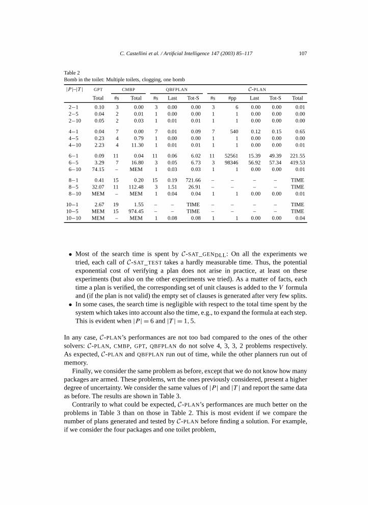
C. Castellini et al. / Artificial Intelligence 147 (2003) 85–117 107

Table 2

Bomb in the toilet: Multiple toilets, clogging, one bomb

|P |–|T | GPT CMBP QBFPLAN C-PLAN

Total #s Total #s Last Tot-S #s #pp Last Tot-S Total

2−1 0.10 3 0.00 3 0.00 0.00 3 6 0.00 0.00 0.012−5 0.04 2 0.01 1 0.00 0.00 1 1 0.00 0.00 0.002−10 0.05 2 0.03 1 0.01 0.01 1 1 0.00 0.00 0.00

4−1 0.04 7 0.00 7 0.01 0.09 7 540 0.12 0.15 0.654−5 0.23 4 0.79 1 0.00 0.00 1 1 0.00 0.00 0.004−10 2.23 4 11.30 1 0.01 0.01 1 1 0.00 0.00 0.01

6−1 0.09 11 0.04 11 0.06 6.02 11 52561 15.39 49.39 221.556−5 3.29 7 16.80 3 0.05 6.73 3 98346 56.92 57.34 419.536−10 74.15 – MEM 1 0.03 0.03 1 1 0.00 0.00 0.01

8−1 0.41 15 0.20 15 0.19 721.66 – – – – TIME8−5 32.07 11 112.48 3 1.51 26.91 – – – – TIME8−10 MEM – MEM 1 0.04 0.04 1 1 0.00 0.00 0.01

10−1 2.67 19 1.55 – – TIME – – – – TIME10−5 MEM 15 974.45 – – TIME – – – – TIME10−10 MEM – MEM 1 0.08 0.08 1 1 0.00 0.00 0.04

• Most of the search time is spent by C-SAT_GENDLL: On all the experiments wetried, each call of C-SAT_TEST takes a hardly measurable time. Thus, the potentialexponential cost of verifying a plan does not arise in practice, at least on theseexperiments (but also on the other experiments we tried). As a matter of facts, eachtime a plan is verified, the corresponding set of unit clauses is added to the V formulaand (if the plan is not valid) the empty set of clauses is generated after very few splits.

• In some cases, the search time is negligible with respect to the total time spent by thesystem which takes into account also the time, e.g., to expand the formula at each step.This is evident when |P | = 6 and |T | = 1,5.

In any case, C-PLAN’s performances are not too bad compared to the ones of the othersolvers: C-PLAN, CMBP, GPT, QBFPLAN do not solve 4, 3, 3, 2 problems respectively.As expected, C-PLAN and QBFPLAN run out of time, while the other planners run out ofmemory.

Finally, we consider the same problem as before, except that we do not know how manypackages are armed. These problems, wrt the ones previously considered, present a higherdegree of uncertainty. We consider the same values of |P | and |T | and report the same dataas before. The results are shown in Table 3.

Contrarily to what could be expected, C-PLAN’s performances are much better on theproblems in Table 3 than on those in Table 2. This is most evident if we compare thenumber of plans generated and tested by C-PLAN before finding a solution. For example,if we consider the four packages and one toilet problem,

108 C. Castellini et al. / Artificial Intelligence 147 (2003) 85–117

Table 3

Bomb in the toilet: Multiple toilets, clogging, possibly multiple bombs

|P |–|T | GPT CMBP QBFPLAN C-PLAN

Total #s Total #s Last Tot-S #s #pp Last Tot-S Total

2−1 0.03 3 0.00 3 0.00 0.00 3 3 0.00 0.00 0.002−5 0.04 2 0.00 1 0.00 0.00 1 1 0.00 0.00 0.002−10 0.24 2 0.02 1 0.01 0.01 1 1 0.00 0.00 0.02

4−1 0.17 7 0.01 7 0.06 0.18 7 15 0.01 0.02 0.024−5 0.06 4 0.54 1 0.01 0.01 1 1 0.01 0.00 0.014−10 0.38 4 7.13 1 0.02 0.02 1 1 0.02 0.00 0.02

6−1 0.08 11 0.03 11 0.90 47.94 11 117 0.25 1.39 2.016−5 0.33 7 10.71 3 0.71 124.14 3 48 0.62 0.66 1.366−10 7.14 – MEM 1 0.36 0.36 1 1 0.00 0.00 0.00

8−1 0.06 15 0.17 – – TIME 15 1195 12.23 147.25 184.298−5 2.02 11 90.57 – – TIME 3 2681 14.84 15.60 317.138−10 MEM – MEM 1 11.73 11.73 1 1 0.00 0.00 12.68

10−1 0.21 19 1.02 – – TIME – – – – TIME10−5 12.51 15 591.33 – – TIME – – – – TIME10−10 MEM – MEM 1 889.90 889.90 1 1 0.00 0.00 0.06

• with one bomb, as in Table 2, C-PLAN generates 540 possible plans and takes 0.65 s tosolve the problem (0.15 s of search time),

• with possibly multiple bombs, as in Table 3, C-PLAN generates 15 possible plans andtakes 0.02 s to solve the problem (0.02 s is also the search time).

To understand why, consider the case in which there is only one toilet and two packagesP1 and P2. For n = 0,

• If we know that there is one bomb, then there are no possible plans.• If we know nothing about the initial state, then there is the possible plan consisting

of the empty sequence of actions (corresponding to assuming that neither P1 nor P2

is armed). In this case, because of the determinization, C-PLAN adds a clause to theinitial state saying that at least one package is armed.

For n= 1, C-PLAN tries 2 possible plans in both scenarios. Assuming that the plan in whichP1 is dunked is generated first,

• If we know that there is one bomb, the plan is rejected, and—because of thedeterminization—a clause is added to the initial state allowing C-PLAN to concludethat the bomb is in P2. Then, for n = 2 and n = 3, any plan in which P2 is dunked ispossible.

• If we know nothing about the initial state, the plan is rejected, and—because of thedeterminization—a clause saying that the bomb is not in P1 or is in P2 is added to theinitial state. Then, C-PLAN generates the other plan in which only P2 is dunked. Also

C. Castellini et al. / Artificial Intelligence 147 (2003) 85–117 109

this plan is rejected and a clause saying that a bomb is in P1 or not in P2 is added to

the initial state. Thus, there is now only one initial state satisfying all the constraints,namely the one in which both P1 and P2 are armed. This allows C-PLAN to concludethat there are no possible plans for n = 2, and to immediately generate a valid plan atn = 3.

In any case, the optimizations described in Section 5.1 and Section 5.2 do help a lot. Indeed,if we consider the four packages and one toilet problem, and disable the optimizations,

• if we have one bomb, as in Table 2, C-PLAN generates 2145 possible plans and takes0.54 s to solve the problem (0.24 s in the last step),

• if we have possibly multiple bombs, as in Table 3, C-PLAN generates 3743 possibleplans and takes 0.93 s to solve the problem (0.72 s in the last step).

However, it turns out that for these domains, backjumping and learning do not help much:By disabling them, we get roughly the same times.

Also CMBP and GPT perform better on the problems in Table 3 than on the problemsin Table 2: Overall, C-PLAN, CMBP and GPT do not solve respectively 2, 3 and 2 of theproblems in Table 3. The situation is different for QBFPLAN: Now it is not able to solve4 problems. The motivation lies in the particular pruning heuristics used by QSAT. Inparticular, QSAT performs a partial elimination of the universal quantifiers, which is mosteffective when the formula contains few universal quantifiers, as in the case of the QBFsresulting from the problems in Table 2.4 Overall, we get roughly the same picture thatwe had before: C-PLAN and QBFPLAN take full advantage of their ability to concurrentlyexecute actions, and thus behave well on problems with multiple toilets. In some cases,both CMBP and GPT exhaust all the available memory.

On the basis of these comparative tests and given that C-PLAN is still at an early stageof development, we can conclude that C-PLAN (and QBFPLAN) is competitive with bothCMBP and GPT on problems with a high degree of parallelism. This is not surprising,since analogous results have been obtained in the classical setting. In particular, in [24],BLACKBOX [28], GRAPHPLAN [5], STAN [35] and HSPr [24], are comparatively testedon some logistics and rockets problems: The conclusion is that on these problems SATapproaches appear to do best.

The bomb in the toilet problems are a classic for testing planners with incompleteinformation. However, they do not lend themselves to be good benchmarks for SAT-

4 The encodings produced with QBFPLAN have the following form

∃a1 . . . an∀d1 . . . dm∃v1 . . . vf (

(¬d1 ∧ · · · ∧ ¬dm ⊃ s1)∧ (¬d1 ∧ · · · ∧ dm ⊃ s2)∧ · · · ∧ (d1 ∧ · · · ∧ dm ⊃ s2m)∧Φ)

where a1, . . . , an are the variables corresponding to actions; s1, . . . , s2m are conjunctions of literals, correspond-ing to all the possible initial states; d1, . . . , dm are “dummy” variables; v1, . . . , vf are the variables correspondingto fluents; see [44] for more details. In the experiments in Table 2 there are |P | possible initial states, and thuslog2 |P | dummy variables. In the experiments in Table 3 there are 2|P | possible initial states, and thus |P | dummyvariables.

110 C. Castellini et al. / Artificial Intelligence 147 (2003) 85–117

based planners. Indeed, the classical bomb in the toilet is evidently not a good benchmark

for SAT-based planners like C-PLAN (C-PLAN takes 0.00 s to solve all the problems weconsidered). Furthermore, there are few instances of these problems. In order to have moreinstances, we have to consider multiple toilets, possibly multiple bombs, the possibilitythat one toilet becomes clogged because of a dunking, etc. Of course, by adding parametersto the original problem, we get more and more instances. However, with these additionalparameters, it is no longer clear what is (are) the parameter(s) ruling the expected difficultyof the problem. Ideally, what we would like, is the ability to generate as many problemsas we want by having a direct control over the problems characteristics, such as size andexpected hardness (see, e.g., [1]). More precisely, what we would like is a test set meetingthe following five requirements:

1. Each problem should have a “small bound”: In other words, we have to be ableto determine a solution or the absence of a solution testing the system for small n(compared to the size of the problem). Indeed, given that the size of the P/V formulasis polynomial in n, but n can be exponential in the number of fluents of the input actiondescription, it does not make sense to apply our approach for big values of n.

2. Each problem should be “SAT challenging”: Finding a possible plan should be not aneasy task. This is necessary in order to stress the SAT-capabilities of the system.

3. Each problem has to have a “predictable difficulty” on average: We would like to havea parameter d whose value rules the expected difficulty of the problem. By increasingd , we should get more difficult problems.

4. For each value of d , it should be possible to “randomly generate” as many problemsas we want: This is necessary in order to get statistically meaningful results of theplanners’ performances.

5. (If possible) the problems should be “meaningful”: It would be nice if each instancecorresponded to a real-world problem.

In order to meet this last requirement, we started with a classical robot navigation problem.We are given an N × N grid, and M robots (with M < N ) can move in it. They startfrom one border of the grid and their goal is to reach the opposite side. In what follows,we assume that they start from the left border. Their duty is made not trivial because eachlocation in the grid may, or may be not, occupied by an object. In order to have a smallbound and have SAT-challenging problems, we assume that the locations of the objectsobey the “pigeonhole” principle: There is at least one object per column, and no morethan one per row. Pigeonhole formulas are well-known in the SAT-literature and they area standard benchmark for SAT-solvers. Furthermore, given that in each column there is atmost one object, if there exists a valid plan, then there is one whose length is � 2(N − 1).Finally, as in [1], in order to have a parameter ruling the difficulty of the problem, weassume that the location of d of the N objects is unknown: When d =N , we only know thatthe objects obey the pigeonhole principle, and therefore have a high-degree of uncertaintyin the location of the objects. When d = 1, we exactly know their location, and the problemboils down to a classical planning problem. Thus, d = 1 represents the basic case in whichit should be very easy to find the valid solutions: The location of all the objects is known,and we are facing a classical planning problem.

C. Castellini et al. / Artificial Intelligence 147 (2003) 85–117 111

Table 4

C-PLAN’s performances on robot navigation problems

N d M = 1 M = 2

Plan #s #pp Last Tot-S Total Plan #s #pp Last Tot-S Total

min Y 5 1 0.01 0.01 0.25 Y 5 1 0.01 0.01 0.6825% Y 5 1 0.01 0.01 0.31 Y 6 1 0.01 0.02 1.11

1 med Y 6 1 0.00 0.00 0.47 N 8 0 0.01 0.03 1.3275% N 8 0 0.00 0.00 0.65 N 8 0 0.02 0.08 1.41max Y 8 1 0.01 0.02 0.95 Y 8 1 0.02 0.07 2.10

min Y 5 1 0.01 0.01 0.27 Y 5 1 0.00 0.00 0.6925% Y 5 1 0.01 0.01 0.36 N 8 0 0.02 0.07 1.36

5 2 med Y 6 3 0.00 0.00 0.73 N 8 1 0.02 0.14 1.6275% Y 8 1 0.00 0.01 0.89 N 8 6 0.02 1.05 3.35max Y 7 51 0.53 0.65 10.17 – – – – – TIME

min Y 5 1 0.00 0.00 0.44 Y 5 2 0.01 0.01 1.0025% N 8 4 0.01 0.20 1.07 N 8 5 0.03 0.53 3.40

3 med N 8 6 0.45 0.69 1.82 N 8 13 0.03 2.84 7.1175% Y 7 19 2.27 2.49 5.01 N 8 102 0.03 29.62 49.51max N 8 142 27.15 34.94 45.12 – – – – – TIME

min Y 7 1 0.03 0.03 1.99 Y 7 1 0.04 0.04 6.0825% Y 7 1 0.02 0.02 2.12 Y 8 1 0.06 0.10 8.47

1 med Y 8 1 0.03 0.06 3.02 Y 8 1 0.06 0.10 8.7275% Y 8 1 0.04 0.06 3.15 Y 9 1 0.05 0.14 11.41max Y 10 1 0.04 0.14 5.48 Y 10 1 0.06 0.20 14.70

min Y 7 1 0.03 0.03 2.08 Y 7 1 0.03 0.03 6.2825% Y 7 1 0.02 0.02 3.09 Y 9 1 0.07 0.16 11.74

7 2 med Y 8 1 0.03 0.05 4.45 Y 8 3 0.05 0.08 14.2975% N 12 1 0.05 0.37 5.04 Y 9 10 5.28 5.38 28.29max Y 11 8 3.19 3.97 16.51 – – – – – TIME

min Y 7 1 0.03 0.03 3.75 N 12 0 0.10 0.52 9.2325% Y 8 1 0.03 0.06 6.03 Y 9 12 4.78 4.90 41.34

3 med Y 9 2 0.03 0.09 11.00 Y 9 109 339.89 340.00 439.0775% Y 9 12 12.42 15.56 26.60 – – – – – TIMEmax – – – – – TIME – – – – – TIME

min Y 9 1 0.08 0.08 11.46 Y 9 1 0.13 0.13 32.7225% Y 9 1 0.09 0.09 11.76 Y 9 1 0.13 0.13 33.89

1 med Y 10 1 0.10 0.18 14.66 Y 10 1 0.20 0.33 42.5775% Y 10 1 0.10 0.19 15.60 Y 10 1 0.15 0.28 43.61max Y 11 1 0.11 0.31 20.17 Y 11 1 0.16 0.44 54.18

min Y 9 1 0.08 0.08 11.73 Y 9 1 0.12 0.12 33.3825% Y 9 1 0.08 0.08 17.69 Y 9 2 0.12 0.12 57.19

9 2 med Y 10 1 0.11 0.19 22.90 Y 10 1 0.14 0.26 67.3775% Y 10 3 2.01 2.10 27.91 Y 11 12 26.12 26.37 130.15max – – – – – TIME – – – – – TIME

min N 16 0 0.18 1.21 19.69 N 16 0 0.36 2.44 40.6225% Y 9 1 0.09 0.09 24.00 Y 10 2 0.20 0.40 90.95

3 med Y 10 1 0.10 0.18 31.31 Y 10 7 0.22 0.36 200.5475% Y 11 10 34.00 37.74 84.65 – – – – – TIMEmax – – – – – TIME – – – – – TIME

112 C. Castellini et al. / Artificial Intelligence 147 (2003) 85–117

For each value of d , we generate 100 different instances by randomly placing N objects

in the grid according to the pigeonhole principle, and then by removing d of the N objects.We consider the case in which we have N = 5,7,9; d = 1,2,3; and M = 1,2 robots. Thefirst robot starts from the bottom-left corner and, when M = 2, the second starts from thetop-left corner. For each setting of the values for N and d we report the data for the samplesin which the “Total” time is

• the 1%-percentile, i.e., the minimum, (row “min”), or• the 25%-percentile (row “25%”), or• the 50%-percentile, i.e., the median, (row “med”), or• the 75%-percentile (row “75%”), or• the 100%-percentile, i.e., the maximum, (row “max”),

of the 100 timings we obtained. We remind that the Q%-percentileof a set S of valuesis the value V such that Q% of the values in S are smaller or equal to V . The set ofstatistics consisting of the {1%, 25%, 50%, 75%, 100%}-percentiles is known as the “five-number summary” and is most useful for comparing distributions [39]. For these samples,we show the same data as before, and also (column “Plan”) whether the problem has asolution (value “Y”) or not (value “N”). The results are shown in Table 4. Notice that weonly test C-PLAN, the main reason being that it is not clear to us how to naturally representthese problems in the languages of the other planners. As it can be seen from the Table 4,C-PLAN’s performances get worse and worse as M increases: When M = 1, C-PLAN is notable to solve problems having d = 3 and N = 7,9. When M = 2, C-PLAN is not able tosolve problems having d = 2,3 and N = 5,7,9. This confirms our expectations.

Considering the data in the Table, we see that the sometimes the search time spent bythe system is very small compared to its total running time (see, e.g., the data for N = 9).In these cases, most of the time is taken by other operations internal to the system, likethe expansion. About the expansion, it is worth remarking that in applications the actiondescription formalizing the scenario is rarely changed: Most of the times, it is the initialstate and/or the goal that change from time to time. This opens up the possibility to performthe expansion of both P and V in two steps:

• by computing off-line the formulas∧n−1

i=0 trDi and StateD0 ∧ ¬Z0∧n−1

i=0 trtDi , for thegiven action description D, and for each plausible n,

• by adding on-line the conjuncts corresponding to the specific initial and goal states(represented by the formulas I0, Gn for P , and I0, ¬(Gn ∧ ¬Zn) for V ).

Of course, in this way the on-line time necessary to compute the P and V formulas at eachstep becomes negligible.

7. Conclusions

We have presented a SAT-based procedure capable of dealing with planning domainshaving incomplete information about the initial state, and whose underlying transition sys-

C. Castellini et al. / Artificial Intelligence 147 (2003) 85–117 113

tem is specified in C . C allows for, e.g., concurrency, constraints, and nondeterminism.

We proved the correctness and completeness of the procedure, discussed some optimiza-tions, and then we presented C-PLAN, a system based on our procedure. The experimentalanalysis shows that SAT-based approaches to planning with incomplete information can becompetitive with CMBP [9,10], GPT [6], and QBFPLAN [44] at least in the case of prob-lems with a high degree of parallelism. We also propose a benchmark set for evaluatingSAT-based planners dealing with uncertainty.

In the last few years, there has been a growing interest in developing planners dealingwith uncertainty. If we restrict our attention to conformant planners, some of the mostpopular are CMBP [9,10], GPT [6], CGP [49], QBFPLAN [44] and WSPDF [16].

CMBP is based on the representation of the planning domain as a finite state automaton,and uses BDDs [7] to compactly represent and efficiently search the automaton. As wealready said, the algorithm is based on breadth first, backward search, and is able toreturn all conformant plans of minimal length. Furthermore, it is able to determine theabsence of a solution. Because of the breadth first search, CMBP can be very effective.However, it is well known that the size of BDDs critically depends on an either staticallyor dynamically fixed variable ordering, and that there are some problems which causean exponential blow up of the size of BDDs for any variable ordering. As we haveseen, on some problems, CMBP clogs all the available memory of our computer. Finally,CMBP’s input language is based on the action language AR [20], and thus misses someof the C expressive capabilities, like concurrency and qualification constraints. Morerecently, the authors proposed a new approach in which heuristic search is combinedwith the symbolic representation of the automaton, and proposed a new planner (calledHSCP) which outperforms CMBP by orders of magnitude with a much lower memoryconsumption [3]. However, HSCP is not guaranteed to return optimal plans.

In GPT the conformant planning problem is seen as a deterministic search problem inthe space of belief states. In GPT, search is based on the A∗ algorithm [41], and each beliefstate is stored separately. As a consequence GPT performances strictly rely on the goodnessof the function estimating the distance of a belief state, to the belief state representingthe goal. Indeed, GPT is able to conclude that a planning problem has no solution byexhaustively exploring the space of belief states. Finally, GPT input language is based onPDDL, extended to deal with probabilities and uncertainty, and thus it has some features(i.e., probabilities) that C misses, and it misses some of C expressive capabilities. It is worthremarking that the problem of effectively extending heuristic search based approaches inorder to deal with concurrency is still open. As we have seen, GPT can clog all the availablememory of the computer.

CGP (standing for “Conformant GraphPlan”) extends the classical plan-graph ap-proach [5] to deal with uncertainty in the initial state (in the corresponding paper, the au-thors say how to extend the approach to the case of actions with nondeterministic effects).The basic idea behind CGP is initialize a separate plan-graph for each possible determiniza-tion of the given planning problem. Thus, CGP performs poorly if run on problems withan high degree of uncertainty. According to the experimental results presented in [10,24],CGP is outperformed by CMBP and GPT. Finally, CGP’s input language is less expressivethan C .

114 C. Castellini et al. / Artificial Intelligence 147 (2003) 85–117

In QBFPLAN, planning in nondeterministic domains is reduced to reasoning about

Quantified Boolean Formulas (QBFs). QBFPLAN is not restricted to conformant planning,and can perform conditional planning under partial observability. Among the cited systems,QBFPLAN is the one that most closely resembles C-PLAN: For each planning problemand plan length n, a corresponding QBF formula is generated and then a QBF solver isinvoked. Also the search performed by the QBF solver reflects the search performed byC-PLAN: First a sequence of actions is generated, and then its validity is checked. Indeed,for any planning problem specified using any action language—as long as it is possible tocompute a propositional formula corresponding to the transition relation—it is relativelyeasy to specify QBFs whose solutions correspond to the existence of a solution at a givenlength. However, in C-PLAN we have a decoupling between the plan generation and theplan validation phases. Such decoupling allows to incorporate different procedures for thegeneration phase. For instance, if we have nondeterminism only in the initial state, thenwe can use a solver incorporating the optimization introduced in Section 5.1. Accordingto such optimization, one possible initial state ruled out at a certain time step, no longercomes to play in the subsequent time steps. This is not possible when the solving phase isjust a call to a solver used as a black box.

WSPDF is a simple (i.e., consisting of few lines of code) planner based on regressionand written in GOLOG. WSPDF’s good performances rely on domain dependent controlknowledge that is added to prune bad search paths. With the addition of control knowledge,WSPDF can be very effective. However, because of this additional information, WSPDF

plays in a different league than all the above mentioned planners, including C-PLAN.Our work can be seen as a follow up of [37]. In [37], the language of causal theories is

considered, and the notions of possible and valid plans are introduced. The action languageC is based on [36], and is less expressive than the language of causal theories used in [37].However, the focus in [37] is on stating some conditions under which a possible plan isalso valid. No procedure for computing valid plans in the general case (e.g., with multipleinitial states or actions with nondeterministic effects) is given.

In [15], it is showed that the general theory here presented can be specialized to dealwith “simple” nondeterministic domains. Intuitively, a domain is “simple”, if

• there are no static laws;• concurrency is not allowed; and• each elementary action A is characterized by m + 2 (m � 1) finite sets of fluentsP,E,N1, . . . ,Nm: P and E list respectively A’s preconditions and effects as inSTRIPS, while each Ni represents one of the possible outcomes of A.

For “simple” nondeterministic domains, “regular parallel” or “simple-split sequential”encodings in the style of [14,27,29] are possible. According to the experimental analysisdone in [15], the regular parallel encodings are those leading to the best performances, asin the classical case.

The encodings and optimizations presented in [15] are possible because of therestrictions on the syntax of the possible action descriptions. As we said in the introduction,the procedure C-SAT here described is fully general because it allows to consider any finiteC action description, and for any finite action description in any Boolean action language,

C. Castellini et al. / Artificial Intelligence 147 (2003) 85–117 115

there is an equivalent C action description. Given the generality of the procedure, and the

results of our experimental analysis, we believe that SAT-based approaches to planningwith incomplete information can be very effective at least on problems with a high degreeof parallelism. This belief is also confirmed by the results in [24] for the classical case, andby the very positive results that SAT-based approaches are having in formal verification.In this field, following the proposal of [4], a verification problem is converted into a SATproblem by unrolling the transition relation n-times (as proposed by Kautz and Selman inplanning [26]) and then by adding the initial state and the negation of the safety property tobe verified, as additional conjuncts. A SAT solver is then applied to the resulting formula tocheck whether it is satisfiable (in which case the property is violated) or not. This approachhas the same main weakness of C-PLAN, namely it is not applicable for big n-s. However,for relatively small n-s (corresponding in planning to problems with a high degree ofparallelism), this approach has showed to outperform all the others, see [4,11,48].

Finally, a very different SAT-based procedure for conformant planning has been veryrecently proposed in [30]. The idea behind such procedure is to start with a solutionwhich works in some deterministic version of the initial planning problem, and then tocontinue extending/modifying it till it works in all the possible deterministic versions.Some optimizations/heuristics are presented in order to improve performances.

Acknowledgements

We thank Vladimir Lifschitz, and Hudson Turner for comments and discussions on anearlier version of this paper. Thanks to Alessandro Cimatti and Hector Geffner for usefuldiscussions about model checking and heuristic search respectively. Jussi Rintanen kindlyprovided QBFPLAN and the latest version of QSAT. A special thank to Paolo Ferraris formany fruitful discussions on the topic of this paper. Paolo has also participated to the designof the architecture of C-PLAN, and he developed the first version of C-PLAN. NormanMcCain has made possible to integrate CCALCin C-PLAN. This work is supported by ASIand CNR.

References

[1] D. Achlioptas, C. Gomes, H. Kautz, B. Selman, Generating satisfiable problem instances, in: Proc. AAAI-2000, Austin, TX, 2000, pp. 256–261.

[2] R.J. Bayardo Jr., R.C. Schrag, Using CSP look-back techniques to solve real-world SAT instances, in: Proc.AAAI-97/IAAI-97, Providence, RI, AAAI Press, Menlo Park, CA, 1997, pp. 203–208.

[3] P. Bertoli, A. Cimatti, M. Roveri, Heuristic search + symbolic model checking = efficient conformantplanning, in: Proc. IJCAI-2001, Seattle, WA, 2001, pp. 467–472.

[4] A. Biere, A. Cimatti, E. Clarke, Y. Zhu, Symbolic model checking without BDDs, in: Proc. FifthInternational Conference on Tools and Algorithms for the Construction and Analysis of Systems (TACAS-99), Amsterdam, 1999, pp. 193–207.

[5] A. Blum, M. Furst, Fast planning through planning graph analysis, in: Proc. IJCAI-95, Montreal, Quebec,1995, pp. 1636–1642.

[6] B. Bonet, H. Geffner, Planning with incomplete information as heuristic search in belief space, in: Proc.AIPS-2000, Breckenridge, CO, 2000, pp. 52–61.

116 C. Castellini et al. / Artificial Intelligence 147 (2003) 85–117

[7] R.E. Bryant, Symbolic Boolean manipulation with ordered binary-decision diagrams, ACM Comput.

Surveys 24 (3) (1992) 293–318.

[8] M. Cadoli, A. Giovanardi, M. Schaerf, An algorithm to evaluate quantified boolean formulae, in: Proc.AAAI-98, Madison, WI, 1998, pp. 262–267.

[9] A. Cimatti, M. Roveri, Conformant planning via model checking, in: Proc. 5th European Conference onPlanning (ECP-99), Durham, UK, in: Lecture Notes in Computer Science, Vol. 1809, Springer, Berlin, 1999,pp. 21–34.

[10] A. Cimatti, M. Roveri, Conformant planning via symbolic model checking, J. Artificial Intelligence Res. 13(2000) 305–338.

[11] F. Copty, L. Fix, E. Giunchiglia, G. Kamhi, A. Tacchella, M. Vardi, Benefits of bounded model checkingat an industrial setting, in: Proc. 13th International Computer Aided Verification Conference (CAV 2001),Paris, in: Lecture Notes in Computer Science, Vol. 2102, Springer, Berlin, 2001, pp. 436–453.

[12] M. Davis, G. Logemann, D. Loveland, A machine program for theorem proving, Comm. ACM 5 (7) (1962)394–397.

[13] R. Dechter, Enhancement schemes for constraint processing: Backjumping, learning, and cutset decompo-sition, Artificial Intelligence 41 (3) (1990) 273–312.

[14] M. Ernst, T. Millstein, D. Weld, Automatic SAT-compilation of planning problems, in: Proc. IJCAI-97,Nagoya, Japan, 1997, pp. 1169–1177.

[15] P. Ferraris, E. Giunchiglia, Planning as satisfiability in nondeterministic domains, in: Proc. AAAI-2000,Austin, TX, 2000, pp. 748–753.

[16] A. Finzi, F. Pirri, R. Reiter, Open world planning in the situation calculus, in: Proc. AAAI-2000, Austin,TX, 2000, pp. 754–760.

[17] E. Giunchiglia, V. Lifschitz, Dependent fluents, in: Proc. IJCAI-95, Montreal, Quebec, 1995, pp. 1964–1969.[18] E. Giunchiglia, V. Lifschitz, An action language based on causal explanation: Preliminary report, in: Proc.

AAAI-98, Madison, WI, 1998, pp. 623–630.[19] E. Giunchiglia, A. Tacchella, *SAT: A system for the development of modal decision procedures, in: Proc.

17th International Conference on Automated Deduction (CADE-2000), Pittsburgh, PA, 2000, pp. 291–296.[20] E. Giunchiglia, G. Neelakantan Kartha, V. Lifschitz, Representing action: Indeterminacy and ramifications,

Artificial Intelligence 95 (1997) 409–443.[21] E. Giunchiglia, F. Giunchiglia, A. Tacchella, SAT-based decision procedures for classical modal logics,

J. Automat. Reason. 28 (2002) 143–171. Reprinted in: I. Gent, H. Van Maaren, T. Walsh (Eds.), SAT2000.Highlights of Satisfiability Research in the Year 2000, IOS Press, Amsterdam, 2000.

[22] E. Giunchiglia, M. Maratea, A. Tacchella, D. Zambonin, Evaluating search heuristics and optimizationtechniques in propositional satisfiability, in: Proc. International Joint Conference on Automated Reasoning(IJCAR-2001), Siena, Italy, in: Lecture Notes in Artificial Intelligence, Vol. 2083, Springer, Berlin, 2001,pp. 347–363.

[23] C. Green, Application of theorem proving to problem solving, in: Proc. IJCAI-69, Washington, DC, 1969,pp. 219–240.

[24] P. Haslum, H. Geffner, Admissible heuristics for optimal planning, in: Proc. AIPS-2000, Breckenridge, CO,2000, pp. 140–149.

[25] S. Kambhampati, Planning graph as (dynamic) CSP: Exploiting CBL, DDB and other CSP search techniquesin Graphplan, J. Artificial Intelligence Res. 12 (2000) 1–34.

[26] H. Kautz, B. Selman, Planning as satisfiability, in: Proc. ECAI-92, Vienna, Austria, 1992, pp. 359–363.[27] H. Kautz, B. Selman, Pushing the envelope: Planning, propositional logic and stochastic search, in: Proc.

AAAI-96, Portland, OR, 1996, pp. 1194–1201.[28] H. Kautz, B. Selman, BLACKBOX: A new approach to the application of theorem proving to problem

solving, in: Working Notes of the Workshop on Planning as Combinatorial Search, held in conjunction withAIPS-98, Pittsburgh, PA, 1998.

[29] H. Kautz, D. McAllester, B. Selman, Encoding plans in propositional logic, in: Proc. KR-96, Cambridge,MA, 1996, pp. 374–384.

[30] J.A. Kurien, P.P. Nayak, D.E. Smith, Fragment-based conformant planning, in: Proc. 6th Internat.Conference Artificial Intelligence Planning and Scheduling (AIPS-2002), 2002.

[31] C.M. Li, Anbulagan, Heuristics based on unit propagation for satisfiability problems, in: Proc. IJCAI-97,Nagoya, Japan, Morgan Kaufmann, San Francisco, CA, 1997, pp. 366–371.

C. Castellini et al. / Artificial Intelligence 147 (2003) 85–117 117

[32] V. Lifschitz, Frames in the space of situations, Artificial Intelligence 46 (1990) 365–376.

[33] V. Lifschitz, On the logic of causal explanation, Artificial Intelligence 96 (1997) 451–465.[34] F. Lin, R. Reiter, State constraints revisited, J. Logic Comput. 4 (1994) 655–678.[35] D. Long, M. Fox, The efficient implementation of the plan-graph, J. Artificial Intelligence Res. 10 (1999)

85–115.[36] N. McCain, H. Turner, Causal theories of action and change, in: Proc. AAAI-97, Providence, RI, 1997,

pp. 460–465.[37] N. McCain, H. Turner, Satisfiability planning with causal theories, in: Proc. Sixth International Conference

on Principles of Knowledge Representation and Reasoning (KR-98), Trento, Italy, 1998, pp. 212–223.[38] D. McDermott, A critique of pure reason, Computational Intelligence 3 (1987) 151–160.[39] D.S. Moore, G.P. McCabe, Introduction to the Practice of Statistics, Freeman, New York, 1993.[40] K. Myers, D. Smith, The persistence of derived information, in: Proc. AAAI-88, St. Paul, MN, 1988,

pp. 496–500.[41] N. Nilsson, Principles of Artificial Intelligence, Morgan Kaufmann, Los Altos, CA, 1980.[42] D.A. Plaisted, S. Greenbaum, A structure-preserving clause form translation, J. Symbolic Comput. 2 (1986)

293–304.[43] P. Prosser, Hybrid algorithms for the constraint satisfaction problem, Computational Intelligence 9 (3) (1993)

268–299.[44] J. Rintanen, Constructing conditional plans by a theorem prover, J. Artificial Intelligence Res. 10 (1999)

323–352.[45] J. Rintanen, Improvements to the evaluation of quantified boolean formulae, in: D. Thomas (Ed.), Proc.

IJCAI-99, Stockholm, Sweden, Vol. 2, Morgan Kaufmann, San Mateo, CA, 1999, pp. 1192–1197.[46] J. Rintanen, Partial implicit unfolding in the Davis-Putnam procedure for quantified Boolean formulae, in:

Proc. LPAR, in: Lecture Notes in Computer Science, Vol. 2250, Springer, Berlin, 2001, pp. 362–376.[47] B. Selman, H. Levesque, D. Mitchell, A new method for solving hard satisfiability problems, in: Proc.

AAAI-92, San Jose, CA, 1992, pp. 440–446.[48] O. Shtrichman, Tuning SAT checkers for bounded model-checking, in: Proc. 12th International Computer

Aided Verification Conference (CAV-2000), Chicago, IL, in: Lecture Notes in Computer Science, Vol. 1855,Springer, Berlin, 2000, pp. 480–494.

[49] D. Smith, D. Weld, Conformant Graphplan, in: Proc. AAAI-98, Madison, WI, 1998, pp. 889–896.[50] G. Tseitin, On the complexity of proofs in propositional logics, Seminars in Mathematics 8 (1970). Reprinted

in: J. Siekmann, G. Wrightson (Eds.), Automation of Reasoning: Classical Papers in Computational Logic1967–1970, Vol. 2, Springer, Berlin, 1983.

[51] H. Zhang, SATO: An efficient propositional prover, in: W. McCune (Ed.), Proc. CADE-14, Townsville,Australia, in: Lecture Notes in Artificial Intelligence, Vol. 1249, Springer, Berlin, 1997, pp. 272–275.