SAS Ch03 - Core Channel Thermal Hydraulics (final)
148
ANL/NE12/4 The SAS4A/SASSYS1 Safety Analysis Code System Nuclear Engineering Division
-
Upload
khangminh22 -
Category
Documents
-
view
1 -
download
0
Transcript of SAS Ch03 - Core Channel Thermal Hydraulics (final)

ANL/NE-‐12/4
The SAS4A/SASSYS-‐1 Safety Analysis Code System
Nuclear Engineering Division

About Argonne National Laboratory Argonne is a U.S. Department of Energy laboratory managed by UChicago Argonne, LLC under contract DE-‐AC02-‐06CH11357. The Laboratory’s main facility is outside Chicago, at 9700 South Cass Avenue, Argonne, Illinois 60439. For information about Argonne, see http://www.anl.gov.
Availability of This Report This report is available, at no cost, at http://www.osti.gov/bridge. It is also available on paper to the U.S. Department of Energy and its contractors, for a processing fee, from: U.S. Department of Energy Office of Scientific and Technical Information P.O. Box 62 Oak Ridge, TN 37831-‐0062 phone (865) 576-‐8401 fax (865) 576-‐5728 [email protected]
Disclaimer This report was prepared as an account of work sponsored by an agency of the United States Government. Neither the United States Government nor any agency thereof, nor UChicago Argonne, LLC, nor any of their employees or officers, makes any warranty, express or implied, or assumes any legal liability or responsibility for the accuracy, completeness, or usefulness of any information, apparatus, product, or process disclosed, or represents that its use would not infringe privately owned rights. Reference herein to any specific commercial product, process, or service by trade name, trademark, manufacturer, or otherwise, does not necessarily constitute or imply its endorsement, recommendation, or favoring by the United States Government or any agency thereof. The views and opinions of document authors expressed herein do not necessarily state or reflect those of the United States Government or any agency thereof, Argonne National Laboratory, or UChicago Argonne, LLC.

ANL/NE-‐12/4
The SAS4A/SASSYS-‐1 Safety Analysis Code System
Chapter 3: Steady-‐State and Transient Thermal Hydraulics in Core Assemblies
F. E. Dunn Nuclear Engineering Division Argonne National Laboratory January 31, 2012

The SAS4A/SASSYS-‐1 Safety Analysis Code System
3-‐ii ANL/NE-‐12/4

Steady-‐State and Transient Thermal Hydraulics in Core Assemblies
ANL/NE-‐12/4 3-‐iii
TABLE OF CONTENTS
Table of Contents ......................................................................................................................................... 3-‐iii List of Figures ............................................................................................................................................... 3-‐vii List of Tables ................................................................................................................................................. 3-‐vii Nomenclature ................................................................................................................................................ 3-‐ix Steady-‐State and Transient Thermal Hydraulics in Core Assemblies .................................... 3-‐1
3.1 Introduction .................................................................................................................................. 3-‐1 3.2 SAS Channel Approach ............................................................................................................. 3-‐5
3.2.1 Axial Mesh Structure .................................................................................................. 3-‐5 3.2.2 Radial Mesh Structure ................................................................................................ 3-‐9
3.2.2.1 Core and Blanket Region ........................................................................ 3-‐9 3.2.2.2 Gas Plenum Region .................................................................................... 3-‐9 3.2.2.3 Reflector Regions ....................................................................................... 3-‐9
3.3 Pre-‐boiling Transient Heat Transfer, Single Pin Model ........................................... 3-‐12 3.3.1 Core and Axial Blankets .......................................................................................... 3-‐13
3.3.1.1 Basic Equations ........................................................................................ 3-‐13 3.3.1.2 Finite Difference Equations ................................................................ 3-‐16
3.3.2 Reflector Zones .......................................................................................................... 3-‐28 3.3.2.1 Basic Equations ........................................................................................ 3-‐28 3.3.2.2 Finite Difference Equations ................................................................ 3-‐29 3.3.2.3 Solution of Finite Difference Equations ........................................ 3-‐31
3.3.3 Gas Plenum Region ................................................................................................... 3-‐33 3.3.3.1 Basic Equations ........................................................................................ 3-‐33 3.3.3.2 Finite Difference Equations ................................................................ 3-‐33 3.3.3.3 Solution of Finite Difference Equations ........................................ 3-‐35
3.3.4 Order of Solution ....................................................................................................... 3-‐38 3.3.5 Melting of Fuel or Cladding ................................................................................... 3-‐39 3.3.6 Coolant Inlet and Re-‐entry Temperature ....................................................... 3-‐40
3.4 Steady-‐State Thermal Hydraulics ..................................................................................... 3-‐43 3.4.1 Basic Equations .......................................................................................................... 3-‐43 3.4.2 Coolant Temperatures ............................................................................................ 3-‐44 3.4.3 Fuel and Cladding Temperatures in the Core and Axial Blankets ........ 3-‐44 3.4.4 Structure Temperatures in the Core Axial Blankets .................................. 3-‐46 3.4.5 Reflector, Structure, Cladding, and Gas Plenum Temperature
Outside the Core and Axial Blankets ................................................................. 3-‐47 3.5 Transient Heat Transfer after the Start of Boiling ..................................................... 3-‐47
3.5.1 Fuel and Cladding Temperatures in the Core and Axial Blanket .......... 3-‐47 3.5.2 Structure Temperatures ......................................................................................... 3-‐49
3.5.2.1 Semi-‐Implicit Calculations .................................................................. 3-‐50 3.5.2.2 Fully Implicit Calculations .................................................................. 3-‐52
3.5.3 Reflector Temperatures ......................................................................................... 3-‐53 3.5.3.1 Semi-‐Implicit Calculations .................................................................. 3-‐54

The SAS4A/SASSYS-‐1 Safety Analysis Code System
3-‐iv ANL/NE-‐12/4
3.5.3.2 Fully Implicit Calculations ................................................................... 3-‐55 3.5.4 Gas Plenum Region ................................................................................................... 3-‐56 3.5.5 Coolant Temperatures in Liquid Slugs ............................................................. 3-‐58
3.5.5.1 Eulerian Temperature Calculation .................................................. 3-‐58 3.5.5.2 Lagrangian Calculations for Interface Temperatures ............. 3-‐61 3.5.5.3 Lagrangian Calculation for Fixed Nodes ....................................... 3-‐63
3.6 Fuel-‐Cladding Bond Gap Conductance ............................................................................ 3-‐64 3.7 Fuel Pin Heat-‐transfer After Pin Disruption or Relocation of Fuel or
Cladding ....................................................................................................................................... 3-‐65 3.7.1 Fuel-‐pin Heat Transfer After Pin Disruption in PLUTO2 or
LEVITATE ...................................................................................................................... 3-‐65 3.8 Heat-‐transfer Time Step Control ....................................................................................... 3-‐68 3.9 Steady-‐State and Single-‐Phase Transient Hydraulics .............................................. 3-‐69
3.9.1 Introduction ................................................................................................................. 3-‐69 3.9.2 Basic Equations .......................................................................................................... 3-‐70 3.9.3 Flow Orifices ................................................................................................................ 3-‐76 3.9.4 Finite Difference Equations – Coolant Flow Rates ...................................... 3-‐77 3.9.5 Coolant Pressures ...................................................................................................... 3-‐78
3.10 Multiple-‐Pin Model .................................................................................................................. 3-‐79 3.10.1 Introduction ................................................................................................................. 3-‐79 3.10.2 Physical Model ............................................................................................................ 3-‐80 3.10.3 Numerical Methods .................................................................................................. 3-‐83 3.10.4 Detailed Mathematical Treatment ..................................................................... 3-‐84
3.10.4.1 Heat Transfer Calculations in the Core and Axial Blankets: Subroutine TSHTM3 ......................................................... 3-‐84
3.10.4.2 Heat Transfer Calculations in the Gas Plenum Region: Subroutine TSHTM2 .............................................................................. 3-‐86
3.10.4.3 Coolant Flow Rates: Subassembly TSCLM1 ................................ 3-‐87 3.10.4.4 Data Management for the Multiple Pin Option ........................... 3-‐96
3.10.5 Relationship Between Single Pin and Multiple Pin Models ..................... 3-‐98 3.11 Subassembly-‐to-‐subassembly Heat Transfer .............................................................. 3-‐98 3.12 Interaction with Other Models ........................................................................................... 3-‐99
3.12.1 Reactivity Feedback .............................................................................................. 3-‐100 3.12.2 Coupling Between Core Channels and PRIMAR-‐4 .................................... 3-‐100
3.13 Subroutine Descriptions and Flowcharts ................................................................... 3-‐102 3.14 Input and Output ................................................................................................................... 3-‐107
3.14.1 Input Description .................................................................................................... 3-‐107 3.14.1.1 Per Pin Basis ........................................................................................... 3-‐107 3.14.1.2 Structure/Duct Wall and Wrapper Wires ................................. 3-‐107 3.14.1.3 Empty Reflector Region ..................................................................... 3-‐111 3.14.1.4 Structure and Reflector Node Thickness ................................... 3-‐112 3.14.1.5 Coolant Re-‐entry Temperature ...................................................... 3-‐112
3.14.2 Output Description ................................................................................................ 3-‐112 3.15 Thermal Properties of Fuel and Cladding ................................................................... 3-‐116
3.15.1 Fuel Density .............................................................................................................. 3-‐116 3.15.2 Fuel Thermal Conductivity ................................................................................. 3-‐117

Steady-‐State and Transient Thermal Hydraulics in Core Assemblies
ANL/NE-‐12/4 3-‐v
References ................................................................................................................................................... 3-‐121 APPENDIX 3.1: Degree of Implicitness for Flow and Temperature Calculations ......... 3-‐123


Steady-‐State and Transient Thermal Hydraulics in Core Assemblies
ANL/NE-‐12/4 3-‐vii
LIST OF FIGURES
Figure 3.1-‐1: Interactions of Thermal-‐Hydraulic Routines with Other Modules ............. 3-‐3 Figure 3.1-‐2: Flowchart for the Pre-‐Voiding Core Channel Thermal Hydraulics
Driver (Subroutine TSCL0) ..................................................................................................... 3-‐4 Figure 3.2-‐1: SAS Channel Treatment .................................................................................................. 3-‐6 Figure 3.2-‐2: Axial Zones in a SASSYS-‐1/SAS4A Channel ............................................................ 3-‐7 Figure 3.2-‐3: Schematic of SASSYS-‐1/SAS4A Channel Discretization .................................... 3-‐8 Figure 3.2-‐4: Radial Temperature Nodes, Core and Axial Blanket Regions ..................... 3-‐10 Figure 3.2-‐5: Radial Temperature Nodes, Gas Plenum Region .............................................. 3-‐11 Figure 3.2-‐6: Radial Temperature Nodes, Reflector Region .................................................... 3-‐12 Figure 3.3-‐1: Coolant Re-‐entry Temperature Model ................................................................. 3-‐41 Figure 3.7-‐1: Radial Grid for the PLHTR Calculation ................................................................. 3-‐67 Figure 3.9-‐1: Subroutine TSCNV1, Pre-‐Boiling Coolant Flow Rates and Pressure
Distribution ................................................................................................................................ 3-‐71 Figure 3.9-‐2: Interactions Between Pre-‐Voiding Transient Hydraulics and Other
Modules ........................................................................................................................................ 3-‐73 Figure 3.9-‐3: Interactions Between Pre-‐Voiding Transient Hydraulics and Other
Modules ........................................................................................................................................ 3-‐75 Figure 3.10-‐1: SASSYS-‐1 Multiple Pin Representation and Thermocouple
Locations for the EBR-‐II XX09 Instrumented Subassembly .................................. 3-‐81 Figure 3.10-‐2: SASSYS-‐1 Multiple Pin Treatment of a Subassembly .................................. 3-‐82 Figure 3.10-‐3: Subassembly Coolant Flows ................................................................................... 3-‐88 Figure 3.13-‐1: Flowchart for Subroutine TSHTRN ................................................................... 3-‐105 Figure 3.13-‐2: Flowchart for Subroutine TSHTN3 ................................................................... 3-‐106 Figure 3.14-‐1: Sample Subassembly Thermal Hydraulics Output ..................................... 3-‐113 Figure A3.1-‐1: Finite Difference Solution as a Function of the Degree of
Implicitness .............................................................................................................................. 3-‐127 Figure A3.1-‐2: Degree of Implicitness as a Function of Normalized Time Step
Size ............................................................................................................................................... 3-‐128 Figure A3.1-‐3: Approximate Correlation for the Degree of Implicitness ....................... 3-‐130
LIST OF TABLES
Table 3.8-‐1: Criteria for Heat-‐Transfer Time Step Sizes .......................................................... 3-‐68 Table 3.14-‐1: Subassembly Thermal Hydraulics Input Variables ...................................... 3-‐108


Steady-‐State and Transient Thermal Hydraulics in Core Assemblies
ANL/NE-‐12/4 3-‐ix
NOMENCLATURE
Subscript Description c Coolant e Cladding f Fuel g Plenum gas kz Reflector zone p Gas plenum region si Structure inner node so Structure outer node 1 Beginning of the time step 2 End of the time step Symbol Description Units Ac Coolant flow area m2 Aep Cross sectional area of the clad in the gas plenum region m2 Ag Cross sectional area of the plenum gas m2 Afr, bfr Coefficients in the friction factor correlation: ! =
!!" !" !!" -‐-‐
c Specific heat J/kg-‐K cc Coolant specific heat J/kg-‐K ce Cladding specific heat J/kg-‐K cf Average fuel specific heat, averaged over a time step J/kg-‐K cm Modified specific heat in the melting range J/kg-‐K cmix Coolant specific heat in the mixing zone used for re-‐entry
temperature calculation J/kg-‐K
c1,c2,c3 Correlation constants used in coolant heat-‐transfer coefficients
-‐-‐
D Right-‐hand-‐side terms in the matrix equations for radial temperature profiles
J/m
D h Hydraulic diameter m dsti Structure inner node thickness m dsto Structure outer node thickness m Eec Heat flux from clad to coolant, integrated over a time step J/m2
Esc Heat flux form structure to coolant, integrated over a time J/m2

The SAS4A/SASSYS-‐1 Safety Analysis Code System
3-‐x ANL/NE-‐12/4
Symbol Description Units step
f Friction factor -‐-‐ fi Fraction of the structure thickness represented by the
inner node -‐-‐
fo Fraction of the structure thickness represented by the outer node
-‐-‐
g Acceleration of gravity m/s2 hb Bond gap conductance W/m2-‐K hc Coolant-‐film heat-‐transfer coefficient W/m2-‐K hcond Condensation heat-‐transfer coefficient for sodium vapor W/m2-‐K Heg Heat-‐transfer coefficient form the gas in the gas plenum to
the cladding W/m2-‐K
Herc Heat-‐transfer coefficient from the cladding or reflector outer node to the coolant
W/m2-‐K
hr Equivalent radiation heat-‐transfer coefficient W/m2-‐K Hrio Heat-‐transfer coefficient from the structure inner node to
the reflector outer node W/m2-‐K
Hsic Heat-‐transfer coefficient from the structure inner node to the coolant
W/m2-‐K
Hstio Heat-‐transfer coefficient from the structure inner node to the structure outer node
W/m2-‐K
i Radial node number -‐-‐ ic Core channel number -‐-‐ I1 Inertial integral in the momentum equation m-‐1
I2 Acceleration integral in the momentum equation m/kg I3 Friction integral in the momentum equation m/kg I4 Orifice term in the momentum equation m/kg I5 Density integral in the momentum equation kg/m2 j Fuel axial node number -‐-‐ jc Coolant axial node number -‐-‐ JC Axial node number -‐-‐ k Thermal conductivity W/m-‐K kep Cladding thermal conductivity in the gas plenum region W/m-‐K ki,j Weighted average thermal conductivity for heat flow from
node i to j W/m-‐K
Kor Orifice coefficient -‐-‐

Steady-‐State and Transient Thermal Hydraulics in Core Assemblies
ANL/NE-‐12/4 3-‐xi
Symbol Description Units L 1 for subassembly inlet, 2 for outlet -‐-‐ MZC Total number of coolant axial nodes -‐-‐ me Cladding mass kg mf Fuel mass kg Mmix Mass of sodium in the mixing volume kg NC Radial node number of the coolant node -‐-‐ NE Radial node number for the cladding mid-‐point -‐-‐ NE′ Radial node number for the cladding outer surface node -‐-‐ NE″ Radial node number for the cladding inner surface node -‐-‐ NN NT-‐1 -‐-‐ Nps Number of fuel pins represented by a channel -‐-‐ NR Radial node number for the fuel outer surface radius. (note
NR=NE″) -‐-‐
NSI Radial node number for the inner structure node -‐-‐ NSO Radial node number for the outer structure node -‐-‐ NT Radial node number for the fuel outer surface temperature
node -‐-‐
p Pressure Pa pb Pressure at the bottom of the subassembly Pa pb1,pb2 pb at beginning and end of a time step Pa pin Pressure in the coolant inlet plenum Pa Pj Heat production rate in axial node j W Pr Radial power shape, per unit mass -‐-‐ pt Pressure at the top of the subassembly Pa pt1,pt2 pt at the beginning and end of a time step Pa px Pressure in the coolant outlet plenum Pa ∂p∂z fr
Friction pressure drop Pa/m
∂p∂z k
Orifice pressure drop Pa/m
Qc Coolant heat source due to direct heating by neutrons and gamma rays
W/m3
Qct Total steady-‐state heat source per unit of coolant volume W/m3 Qec Heat flow from clad to coolant W/m3 qfe Fuel-‐to-‐cladding heat flux W/m2

The SAS4A/SASSYS-‐1 Safety Analysis Code System
3-‐xii ANL/NE-‐12/4
Symbol Description Units Qsc Heat flow from structure to coolant W/m3 Qsm(i) Sum of the heat sources for all radial nodes inside and
including node i W
Qst Structure heat source due to direct heating by neutrons and gamma rays
W/m2
Qv Heat source per unit volume W/m3 r Radius m rbrp Clad inner radius in the gas plenum region m Re Reynolds number -‐-‐ Rec Thermal resistance between clad and coolant m2-‐K/W Rehf Thermal resistance of the outer fourth of the cladding m2-‐K/W rerp Cladding outer radius in the gas plenum region m Rg Thermal resistance of the gas in the plenum m2-‐K/W ro(i) Steady-‐state radial mesh m Ser Perimeter of the cladding or reflector in contact with the
coolant m
Sst Structure perimeter, heat-‐transfer area per unit height m T Temperature K t Time s Tcin Coolant inlet temperature K Tcout Coolant outlet temperature K Teex Extrapolated clad temperature K Teq Equilibrium temperature in the mixing volume K Texp Temperature of the sodium expelled from the subassembly
into a mixing volume, averaged over a time step K
Tf Average fuel temperature at an axial node, mass-‐weighted average
K
Tg Plenum gas temperature K Tliq Liquidus temperature K Tout Bulk temperature in the coolant outlet plenum K tp1, tp2 Times at the beginning and end of a PRIMAR time step s Tri Reflector inner node temperature K Tro Reflector outer node temperature K Tsol Solidus temperature K To Temperature at the beginning of a time step K

Steady-‐State and Transient Thermal Hydraulics in Core Assemblies
ANL/NE-‐12/4 3-‐xiii
Symbol Description Units T1 Temperature at the beginning of a time step K T′1 Temperature of the coolant entering an axial node at the
end of a time step K
T2 Temperature at the end of a time step K T′2 Temperature of the coolant entering an axial node at the
end of a time step K
Umelt Heat of fusion J/kg v Velocity m/s w Coolant mass flow rate kg/s we Estimated mass flow rate kg/s wfe Thickness of the liquid-‐sodium film left on the cladding
after voiding occurs m
wfr Thickness of the liquid-‐sodium film left on the reflector after voiding occurs
m
wfst Thickness of the liquid-‐sodium film left on the structure after voiding occurs
m
w1,w2 w at beginning and end of a time step kg/s Δw Change in w during a time step kg/s x Distance m xI1(JC) Nodal contribution to I1 m-‐1 xI2(JC) Nodal contribution to I2 m/kg xI3(JC) Nodal contribution to I3 xI5(JC) Nodal contribution to I5 kg/m2 z Axial position m z Elevation m Δz Node height m zpb Elevation at the bottom of the gas plenum m zpt Elevation at the top of the gas plenum m zpℓℓ Reference elevation of the coolant inlet plenum m zpℓu Reference elevation of the coolant outlet plenum m α Heat capacity terms in the matrix equations for radial
temperature profiles J/m-‐K
αe Cladding thermal expansion coefficient K-‐1 αf Fuel thermal expansion coefficient K-‐1 β Thermal conductivity terms in the matrix equations for J/m-‐K

The SAS4A/SASSYS-‐1 Safety Analysis Code System
3-‐xiv ANL/NE-‐12/4
Symbol Description Units radial temperature profiles
γc Fraction of the total heat production that goes directly into the coolant
-‐-‐
γe Fraction of the total heat production that goes directly into the cladding
-‐-‐
γs Fraction of the total heat production that goes directly into the structure
-‐-‐
γ2 Ratio of the structure perimeter to the cladding perimeter -‐-‐ Δr Radial node size m Δri,j Effective radial distance for heat flow from node I to node j m Δt Time-‐step size s Δz Axial node height m ε Thermal emissivity -‐-‐ θ1,θ2 Degree of explicitness or implicitness in the solution -‐-‐ ρ Density kg/m3 ρc Coolant density kg/m3 ρcin Coolant density in the inlet plenum kg/m3 ρcout Coolant density in the outlet plenum kg/m3 (ρc)g Density times specific heat of the plenum gas J/m3-‐K (ρc)r Density times specific heat for the reflector J/m3-‐K ρe Cladding density kg/m3 σ Stefan-‐Bolzmann constant W/m2-‐K4 τ Time constant for flow rate changes s τc Condensation heat-‐transfer time constant s τro Time constant for temperature changes in the outer
reflector node s
τsti Time constant for temperature changes in the inner structure node
s
μ Coolant viscosity Pa-‐s µμ JC Average value of μ for node JC Pa-‐s ψ Source terms in the matrix equations for radial
temperature profiles -‐-‐

ANL/NE-‐12/4 3-‐1
STEADY-‐STATE AND TRANSIENT THERMAL HYDRAULICS IN CORE ASSEMBLIES
3.1 Introduction The core assembly thermal hydraulics treatment in SASSYS-‐1 and SAS4A includes
the calculation of fuel, cladding, coolant, and structure temperatures, as well as coolant flow rates and pressure distributions. This treatment includes melting of the fuel and cladding. Boiling of the coolant is also handled, as described in Chapter 12. The relocation of fuel and cladding after pin disruption is described in Chapters 13, 14, and 16; and relocation of molten fuel before pin disruption is described in Chapter 15.
Until recently, all of the core subassembly models in SAS4A and SASSYS-‐1 were single pin models: a single fuel pin and its associated coolant were used to represent a subassembly; and pin-‐to-‐pin variations within a subassembly were ignored. Recently a multiple pin option has been added to the code. A number of pins and their associated coolant can now be used to represent a subassembly, so variations within a subassembly can be accounted for. Currently the multiple pin option is only available for single-‐phase thermal hydraulics; it does not handle coolant boiling, in-‐pin fuel relocation, or pin disruption. Therefore, typical SASSYS-‐1 cases that do not get into coolant boiling can be handled with the multiple-‐pin model, but typical SAS4A core disruption cases can only be handled with single pin models.
Although SASSYS-‐1 and SAS4A are mainly transient codes both steady-‐state and transient temperatures and coolant pressures are calculated. The steady-‐state solutions are obtained from the transient equations after dropping all time derivatives. In general, the steady-‐state solutions in the single pin per subassembly model are not obtained by running a transient calculation at constant power and flow until the results approach a steady-‐state solution. Instead, the steady-‐state temperatures are obtained rapidly from a direct solution based on conservation of energy and the use of the same spatial finite differencing as used in the transient. On the other hand, a direct steady-‐state solution for the multiple pin option would be much more complicated, especially if subassembly-‐to-‐subassembly heat transfer is included. Therefore, a null transient with powers and flows held constant is used to obtain steady-‐state conditions for the multiple pin option.
The thermal hydraulics calculations are carried out in a number of separate modules, and each module is designed for a specific type of calculation. A steady-‐state thermal hydraulics module provides the initial conditions for the transient. The transient temperatures are calculated in a pre-‐voiding module (TSHTRN) until the onset of boiling. After the onset of boiling, the fuel-‐pin temperatures are calculated in a separate module (TSHTRV) that couples with the boiling module.
The core thermal-‐hydraulic routines interact with a number of other modules, as shown in Fig. 3.1-‐1. Before the onset of voiding, TSHTRN calculates the coolant temperatures used in the hydraulic calculations, whereas the hydraulics routines calculate the coolant flow rates used in TSHTRN. After the onset of voiding, coolant temperatures are calculated in TSBOIL, and this module supplies the heat flux at the cladding outer surface or the fuel outer surface to TSHTRV. TSBOIL uses the cladding

The SAS4A/SASSYS-‐1 Safety Analysis Code System
3-‐2 ANL/NE-‐12/4
temperatures from TSHTRV in its coolant temperature calculations. The point kinetics module supplies the power level used in the heat-‐transfer routines, and the heat-‐transfer routines supply the Doppler feedback reactivity as well as other temperature-‐dependent reactivity feedback. TSBOIL supplies the voiding reactivity. The inlet plenum temperature computed by PRIMAR-‐4 is used in calculating the inlet temperature for TSHTRN or TSBOIL, and TSHTRN or TSBOIL provides the subassembly outlet temperatures used by PRIMAR-‐4 to compute the outlet plenum temperature. If flow reversal occurs in a subassembly, then the outlet plenum temperature computed by PRIMAR-‐4 is used in calculating the coolant temperature at the top of the subassembly, and the temperature computed by TSHTRN or TSBOIL for the coolant leaving the bottom of the subassembly is used by PRIMAR-‐4 to calculate the inlet plenum temperature. PRIMAR-‐4 supplies the inlet and outlet plenum pressures that drive the coolant hydraulics calculations, and the core channel flows are provided to PRIMAR-‐4 by TSBOIL and the pre-‐voiding hydraulics. The initial coolant flow rate and pressure distribution are supplied to TSBOIL by the pre-‐voiding hydraulics routines.
The transient calculations in the codes used a multi-‐level time step approach, with separate time steps for each module. For the heat-‐transfer routines, all temperatures are known at the beginning of a heat-‐transfer step, and the routines calculate the new temperatures at the end of the step. The heat-‐transfer time step can be longer than the coolant time step or the PRIMAR time step, but the heat-‐transfer time step can be no longer than the main time step that is used for reactivity feedback and main printouts.
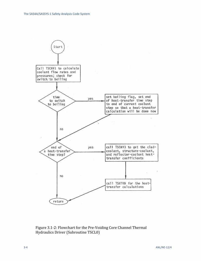
Figure 3.1-‐2 shows the flow through the pre-‐voiding core channel thermal hydraulics driver, TSCL0. This routine is entered once for each channel during each coolant time step. The coolant flow rates are calculated before the heat-‐transfer module (TSHTRN) is called. TSHTRN is only called if the current coolant time step completes a heat-‐transfer time step. The voiding model, TSHTRV, is described in Chapter 12.
In this chapter, Section 3.2 describes the mesh structure used for heat-‐transfer calculations. Then, Section 3.3 describes the pre-‐boiling transient heat-‐transfer calculations, followed by the steady-‐state thermal hydraulics calculations in Section 3.4. The pre-‐voiding transient heat transfer is discussed before the steady-‐state thermal hydraulics for two reasons. First, as previously mentioned, the codes are primarily transient codes, so the transient calculations are more important. Second, the finite difference approximations were made with the transient calculations in mind, and the steady-‐state solution was formulated to be consistent with the approximations used in the transient. Section 3.5 describes TSHTRV, the fuel-‐pin heat-‐transfer calculations in the boiling module. Section 3.6 describes the treatment of the bond-‐gap conductance between the fuel and the cladding. Section 3.7 describes modifications to the fuel pin heat transfer calculations for PLUTO2 and LEVITATE. The heat transfer time step control is described in Section 3.8. Section 3.9 describes steady-‐state and pre-‐voiding transient hydraulics. Section 3.10 describes the multiple pin option. Subassembly-‐to-‐subassembly heat transfers described in Section 3.11. Section 3.12 describes interaction with other modules. It is followed by sections including subroutine descriptions and flowcharts, thermal properties of fuel and cladding, and a description of the input to, and output from, the thermal hydraulic routines.

Steady-‐State and Transient Thermal Hydraulics in Core Assemblies
ANL/NE-‐12/4 3-‐3
Figure 3.1-‐1: Interactions of Thermal-‐Hydraulic Routines with Other Modules
The SAS4A/SASSYS-‐1 Safety Analysis Code System
3-‐4 ANL/NE-‐12/4
Figure 3.1-‐2: Flowchart for the Pre-‐Voiding Core Channel Thermal Hydraulics Driver (Subroutine TSCL0)

Steady-‐State and Transient Thermal Hydraulics in Core Assemblies
ANL/NE-‐12/4 3-‐5
3.2 SAS Channel Approach SASSYS-‐1 and SAS4A use of multi-‐channel treatment. Each channel represents a fuel
pin, its associated coolant, and a fraction of the subassembly duct wall, as indicated in Fig. 3.2-‐1. Usually, a channel is used to represent an average pin in a fuel subassembly or a group of similar subassemblies. A channel can also be used to represent a blanket assembly or a control-‐rod channel, and the hottest pin in a subassembly can be represented instead of the average pin. Different channels can be used to account for radial and azimuthal power variations within the core, as well as variations in coolant flow orificing and fuel burn-‐up. In the multiple pin option, more than one channel can be used to represent a subassembly
3.2.1 Axial Mesh Structure A channel usually represents the whole length of the subassembly, from coolant
inlet to coolant outlet. A number of axial zones are used, as indicated in Fig. 3.2-‐2. One zone represents the fuel-‐pin section, including the core, axial blankets, and gas plenum. Other zones represent reflector regions above and below the pin section. A maximum of 7 zones can be used in a channel. In general, radial dimensions and thermal properties are constant with a reflector zone. The pin section zone is treated separately in considerably more detail than the reflector zones. The gas plenum can be either above or below the core.
Figure 3.2-‐3 shows the axial mesh structure used for a channel. The coolant and structure nodes run the whole length of the channel. The coolant nodes are staggered with respect to the fuel, cladding, reflector, and structure nodes. Using coolant temperatures defined at the axial boundaries between cladding and structure nodes makes it easier to calculate accurate coolant temperatures. If non-‐uniform axial mesh sizes are used, a simple finite differencing of the coolant temperature equation gives accurate coolant temperatures with a staggered mesh, whereas if the coolant nodes were at the middle of the cladding nodes, then obtaining accurate coolant temperatures would require extra terms in the finite differencing of the coolant temperature equation.

The SAS4A/SASSYS-‐1 Safety Analysis Code System
3-‐6 ANL/NE-‐12/4
Figure 3.2-‐1: SAS Channel Treatment

Steady-‐State and Transient Thermal Hydraulics in Core Assemblies
ANL/NE-‐12/4 3-‐7
Figure 3.2-‐2: Axial Zones in a SASSYS-‐1/SAS4A Channel

The SAS4A/SASSYS-‐1 Safety Analysis Code System
3-‐8 ANL/NE-‐12/4
Figure 3.2-‐3: Schematic of SASSYS-‐1/SAS4A Channel Discretization

Steady-‐State and Transient Thermal Hydraulics in Core Assemblies
ANL/NE-‐12/4 3-‐9
3.2.2 Radial Mesh Structure
3.2.2.1 Core and Blanket Region Figure 3.2-‐4 shows the radial mesh structure used for temperature calculations in
the core and blanket regions. This figure represents one axial node. Between four and eleven radial nodes are used in the fuel, three in the cladding, one in the coolant, and two in the structure. In the fuel, the nodes can be set up on either an equal radial difference basis or an equal mass basis. In either case, the first and last nodes are half-‐size. For a given number of nodes, an equal radial difference mesh will usually give more accurate center-‐line temperatures, but equal mass nodes are sometimes used to get more nodes in the outer part of the fuel, where temperature gradients are steeper. Steady-‐state fuel restructuring can change the node sizes. Also, during the transient calculation, the radii will move with the fuel as it expands or contracts due to temperature changes. After the steady-‐state initialization, the mass of fuel associated with a radial node is constant, at least until fuel-‐pin disruption and coupling is made to PLUTO2, PINACLE, or LEVITATE in SAS4A.
The inner fuel node is at ! = 0 if there is no central void. Otherwise, it is at the fuel inner surface. The outer fuel node is at the fuel outer surface.
The “structure” represents each pin’s share of the duct wall. A wrapper wire can be lumped in with either the cladding or the structure.
3.2.2.2 Gas Plenum Region The radial mesh structure used in the gas plenum region is shown in Fig. 3.2-‐5. The
plenum gas is represented by a single axial and radial node. This gas is in contact with a number of axial cladding nodes. At each axial node, there is one radial node in the cladding, one in the coolant, and two in the structure.
3.2.2.3 Reflector Regions The radial mesh structure in an axial node in a reflector region is shown in Fig. 3.2-‐
6. Two nodes are used in the reflector, one in the coolant, and two in the structure.

The SAS4A/SASSYS-‐1 Safety Analysis Code System
3-‐10 ANL/NE-‐12/4
Figure 3.2-‐4: Radial Temperature Nodes, Core and Axial Blanket Regions

Steady-‐State and Transient Thermal Hydraulics in Core Assemblies
ANL/NE-‐12/4 3-‐11
Figure 3.2-‐5: Radial Temperature Nodes, Gas Plenum Region

The SAS4A/SASSYS-‐1 Safety Analysis Code System
3-‐12 ANL/NE-‐12/4
Figure 3.2-‐6: Radial Temperature Nodes, Reflector Region
3.3 Pre-‐boiling Transient Heat Transfer, Single Pin Model The transient fuel-‐pin temperature calculations in SASSYS-‐1 and SAS4A are similar
to the Crank-‐Nickolson scheme [3-‐1] used in SAS2A [3-‐2] and SAS3D [3-‐3], but there are a number of significant differences. One reason for these differences is to allow the use of larger heat-‐transfer time steps with less computing time per step. Another reason is to obtain greater accuracy and more precise energy balance.
In order to use very long heat-‐transfer time steps on one second or more in the pre-‐voiding phase of a very slow transient, the fuel, cladding, coolant, and structure temperatures at an axial node are computed simultaneously in non-‐voiding cases. Therefore, coolant temperatures are computed in the fuel-‐pin heat-‐transfer routine in the non-‐voiding situation.
The coupling between TSHTRN and the pre-‐voiding coolant dynamics routines is different from the coupling between TSHTRV and the voiding routines, although in both cases the coolant dynamics or voiding calculations are done before the fuel-‐pin heat-‐transfer calculations. In the non-‐voiding case, extrapolated coolant temperatures are used to obtain the temperature-‐dependent sodium properties used in the calculation of the coolant flow rates and heat-‐transfer coefficients. Then, TSHTRN uses these values to compute the coolant temperatures, and these new coolant temperatures are used in the next extrapolation. In the voiding routines, extrapolated cladding temperatures are used in the implicit calculation of the heat flux from cladding to coolant to obtain new

Steady-‐State and Transient Thermal Hydraulics in Core Assemblies
ANL/NE-‐12/4 3-‐13
coolant temperatures. The voiding routines then sum the integrated heat flux from cladding to coolant at each axial node, and this integrated heat flux at the cladding surface is used as a boundary condition in TSHTRV.
TSHTRN and TSHTRV are somewhat simpler than the corresponding TSHTR in SAS3A and SAS3D. In SAS3D, TSHTR contains extraneous material related to other modules, such as initiating cladding and fuel motion; this material is not included in the SASSYS-‐1 and SAS4A heat-‐transfer routines. Also, in SAS3D, the fuel mass for each radial node of each axial node is recomputed every time step from the temperature-‐dependent fuel density and the node radii. In SASSYS-‐1 and SAS4A the node mass is computed in the steady-‐state module and then stored for used in the transient. This node mass is held constant until fuel relocation starts.
Another difference between the SAS3D and SASSYS-‐1 heat-‐transfer routines is in the amount of vectorization of the algorithms and the coding. Some of the calculations in the SAS3D routines happen to vectorize, but a special effort was made to vectorize many more of the calculations in the SAS4A and SASSYS-‐1 heat-‐transfer routines. On a vector machine, such as CRAY-‐1, vectorized coding usually runs much faster than scalar coding. Even on the IBM 3033 or the CDC 6700 computers, which are normally considered to be scalar machines, vectorizable coding tends to run faster than unvectorizable coding. In general, vectorizing involves setting up arrays so that all elements in the array are processed in the same way and so that the results of a given calculation for one element in the array do not depend on the results for any other element in the array. Vectorization is partly just a coding matter, but it also involves choosing vectorizable algorithms or adapting algorithms for vectorization.
To some extent, the descriptions in Sections 3.3.1.2 to 3.3.1.3 below reflect the emphasis on vectorization. Intermediate quantities used in the solution are usually defined as elements in arrays, and, where possible, the array elements are defined so that all of the elements in an array can be treated in the same manner in the calculations. In order to emphasize the array nature of the solution, when a new array is introduced, all of the elements in the array are defined in the same section, even though many of the elements are often not used until later sections.
As indicated above in Section 3.2.2, three different radial mesh structures are used in the heat-‐transfer calculations: one for the core and blanket region, one for the gas plenum region, and one for the reflector regions. Different heat-‐transfer calculations are done for each of these three regions.
3.3.1 Core and Axial Blankets
3.3.1.1 Basic Equations The basic transient heat-‐transfer equation within the fuel and within the cladding is
QrTkr
rrtTc +⎟
⎠
⎞⎜⎝
⎛∂
∂
∂
∂=
∂
∂ 1ρ
(3.3-‐1)

The SAS4A/SASSYS-‐1 Safety Analysis Code System
3-‐14 ANL/NE-‐12/4
where ! = temperature
! = density
! = specific heat
! = radius
! = thermal conductivity
! = time
and ! = heat source per unit volume
Melting of fuel and cladding is treated using a melting range, bounded by solidus and liquidus temperatures, !sol and !liq, respectively, and a heat of fusion, !melt. Separate values of !sol, !liq, and !melt are used for the fuel and cladding. In the melting range, Eq. 3.3-‐1 is modified and becomes
QrTkr
rrtTcm +⎟
⎠
⎞⎜⎝
⎛∂
∂
∂
∂=
∂
∂ 1ρ
(3.3-‐2)
where
solliq
meltm TT
Uc
−=
(3.3-‐3)
In the actual solution of Eq. 3.3-‐2 for a time step, ! is used instead of !! in the calculation of the temperature change for the step. Then, if the temperatures are in the melting range, the computed temperature change is modified to account for the heat of fusion, as described in Section 3.3.5.
The heat flux, !!" , from the fuel outer surface to the cladding inner surface contains both a bond gap conductance term, ℎ! , and a radiation term:
!!" = ℎ! ! NT − ! NT" + !" ! NT ! − ! NT" ! (3.3-‐4)
where ! = thermal emissivity of the fuel
! = Stefan=Boltzman constant
!(NT) = fuel outer surface temperature

Steady-‐State and Transient Thermal Hydraulics in Core Assemblies
ANL/NE-‐12/4 3-‐15
and
!(NEʺ″) = cladding inner surface temperature
For the coolant, the basic heat-‐transfer equation is
( ) ( ) csceccc AQQQwcTrr
TAc ++=∂
∂+
∂
∂ρ
(3.3-‐5)
where !! = coolant flow area. The heat, !! , produced directly in the coolant is computed from the fraction, !! , of the total energy production that goes into neutron and gamma heating of the coolant:
!! =!!!(!)!!∆!(!)
(3.3-‐6)
where
( )jP = total heat production rate in axial node j
and
Δz(j) = axial node height
The heat flow from the cladding to the coolant, !!" is calculated as
!!" = ℎ! ! NE' − !(NC)2!"(NE')
!! (3.3-‐7)
and the heat flow from structure to coolant, !!" , is calculated as
!!" = ℎ! ! NSI − !(NC)!!"!! (3.3-‐8)
where !!" is the perimeter of the structure. The coolant heat-‐transfer coefficient, ℎ! , is calculated using
31
2
cAkcwDc
kDh
c
c
hhc +⎥⎦
⎤⎢⎣
⎡=
(3.3-‐9)
which is a form used in correlations for convective heat-‐transfer coefficients for low Prandtl number fluids, such as liquid metal [3-‐4]. The user supplied constants c1, c2, and c3 depend on the particular correlation used.
The structure is treated with a one-‐dimensional heat conduction equation:
The SAS4A/SASSYS-‐1 Safety Analysis Code System
3-‐16 ANL/NE-‐12/4
!"!"!" =
!!" !
!"!" + ! (3.3-‐10)
The treatment of the heat source, !, in the structure is discussed in Section 3.3.1.2.8.
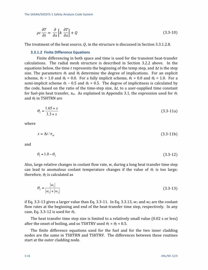
3.3.1.2 Finite Difference Equations Finite differencing in both space and time is used for the transient heat-‐transfer
calculations. The radial mesh structure is described in Section 3.2.2 above. In the equations below, the time t represents the beginning of the temp step, and Δt is the step size. The parameters θ1 and θ2 determine the degree of implications. For an explicit scheme, θ1 = 1.0 and θ2 = 0.0. For a fully implicit scheme, θ1 = 0.0 and θ2 = 1.0. For a semi-‐implicit scheme θ1 – 0.5 and θ2 = 0.5. The degree of implicitness is calculated by the code, based on the ratio of the time-‐step size, Δt, to a user-‐supplied time constant for fuel-‐pin heat transfer, τht. As explained in Appendix 3.1, the expression used for θ1 and θ2 in TSHTRN are
xx
+
+=
3.365.1
2θ
(3.3-‐11a)
where
httx τ/Δ= (3.3-‐11b)
and
!1 =1.0!!2 (3.3-‐12)
Also, large relative changes in coolant flow rate, w, during a long heat transfer time step can lead to anomalous coolant temperature changes if the value of θ1 is too large; therefore, θ2 is calculated as
21
12 ww
w+
=θ
(3.3-‐13)
if Eq. 3.3-‐13 gives a larger value than Eq. 3.3-‐11. In Eq. 3.3.13, w1 and w2 are the coolant flow rates at the beginning and end of the heat-‐transfer time step, respectively. In any case, Eq. 3.3-‐12 is used for θ1.
The heat transfer time step size is limited to a relatively small value (0.02 s or less) after the onset of boiling, and so TSHTRV used θ1 = θ2 = 0.5.
The finite difference equations used for the fuel and for the two inner cladding nodes are the same in TSHTRN and TSHTRV. The differences between these routines start at the outer cladding node.

Steady-‐State and Transient Thermal Hydraulics in Core Assemblies
ANL/NE-‐12/4 3-‐17
In general, the time derivative of a variable y is approximated as
( ) ( )t
tyttyty
Δ
−Δ+=
∂
∂
(3.3-‐14)
and the spatial derivative is approximated as
!y!t !"!1
y t, z+#z( )" y t, z( )#z
$
%&
'
() +!2
y t +#t, z+#z( )" y t +#t, z( )#z
$
%&
'
() (3.3-‐15)
In the following sections, it will be useful to refer to Fig. 3.2-‐4 for the radial node structure and the definitions of the radial node indexes.
3.3.1.2.1 Fuel Inner Surface, Node 1 There is an adiabatic boundary at the fuel inner surface; so the node 1, Eq. 3.3-‐1
becomes
!! 1 !! 1!! 1 − !! 1
∆!
=2!" 2 !" ! !!,!
!!!,!!! !! 2 − !! 1 + !! !! 2 − !! 1 + !(1)
(3.3-‐16)
where mf(i) = fuel mass at node i
( )ic = fuel heat capacity at radial node i at t = t1 + θ2Δy
T2(i) = temperature at t + Δt
T1(i) = temperature at time t
Δz(j) = axial mesh height
Δr(1)=2 r 2( )! r 1( )"# $% (3.3-‐17)
( ) ( ) ( ) NN21 ≤≤−+=Δ iiririr (3.3-‐18)
( ) ( ) ( )[ ]NTNR2NT rrr −=Δ (3.3-‐19)

The SAS4A/SASSYS-‐1 Safety Analysis Code System
3-‐18 ANL/NE-‐12/4
!" ! = ! !!! − !(!")
2 ! = !"",!",!"′ (3.3-‐20)
(note: NE" = NR)
( ) ( ) NEi12
1irr 1ii, ≤≤+Δ+Δ
=Δ +
ir
(3.3-‐21)
( )( ) ( ) ( ) ( )
( ) ( )NTi
iimiiP
imiPjPiQ NT
iifr
frsce ≤≤−−−
=
∑=
11
1
γγγ
(3.3-‐22)
( ) ( )4
EN ejPQ γ=ʹ′ʹ′
(3.3-‐23)
( ) ( )2
NE ejPQ γ=
(3.3-‐24)
( ) ( ) ( )EN4
EN ʹ′ʹ′==ʹ′ QjPQ eγ
(3.3-‐25)
where
( )jP = total power (watts) in axial node j
Pr(i) = radial power shape per unit mass
and
sce γγγ ,, = fraction of power in direct heating of clad, coolant, and structure, respectively.
The thermal conductivity, 2,1k used in Eq. 3.3-‐16 is a weighted average of the values for the two adjacent nodes. It is calculated as
ki,i+1 =k i( )k i+1( ) !r i( )+!r i+1( )"# $%k i( )!r i+1( )+ k i+1( )!r i( )
(3.3-‐26)
where

Steady-‐State and Transient Thermal Hydraulics in Core Assemblies
ANL/NE-‐12/4 3-‐19
k(i) = thermal conductivity for radial node i, evaluated using the fuel temperature extrapolated to t + θ2 Δt
Equation 3.3-‐26 is carried over from SAS3D. The fuel restructuring algorithm used in SAS3D uses up to three different fuel types (columnar, equiaxed, and unrestructured) for the fuel at each axial node. Sharp boundaries between fuel types are used. The radial mesh is adjusted, if necessary, so that fuel-‐type boundaries fall on radial node boundaries. One consequence of the sharp fuel-‐type boundaries in SAS3D is that the fuel thermal conductivity can change significantly from one node to the next at a fuel-‐type boundary. The average thermal conductivity of Eq. 3.3-‐26 will give accurate steady-‐state fuel temperatures even if the thermal conductivity has large jumps at node boundaries. The fuel restructuring provided by DEFORM-‐IV in SAS4A is somewhat smoother than that used in SAS3D, and the node-‐to-‐node changes in thermal conductivity in SAS4A are usually smaller than the corresponding changes at fuel-‐type boundaries in SAS3D, so the need for special weighting of the fuel thermal conductivities in SAS4A Lis less than in SAS3D, but Eq. 3.3-‐26 still provides more accurate fuel temperatures than simpler weighting schemes.
Note that even though most of the variables in Eqs. 3.3-‐16 to 3.3-‐26 vary with axial node j, the subscript j has only been included for some of these variables.
3.3.1.2.2 Inner Fuel Nodes, Nodes 2 to NN For fuel radial node I, Eq. 3.3-‐1 becomes
( ) ( ) ( ) ( )[ ]
( ) ( ) ( ) ( )[ ] ( ) ( )[ ]{ }
( ) ( ) ( ) ( )[ ] ( ) ( )[ ]{ } ( )iQiTiTiTiTr
kjzir
iTiTiTiTr
kjzir
tiTiTicim
ii
ii
ii
ii
ff
+−−+−−Δ
Δ−
−++−+Δ
Δ+=
Δ
−
−
−
+
=
112
1112
222111,1
,1
2221111,
1,
12
θθπ
θθπ
(3.3-‐27)
Note that the left-‐hand side of Eq. 3.3-‐27 represents the change in internal energy as node i, whereas the terms on the right-‐hand side represent heat conduction into node i from nodes i+1 and i-‐1, as well as the heat source in node i.
3.3.1.2.3 Fuel Outer Surface Node, Node NT The heat flux qfc, from the fuel outer surface to the cladding inner surface contains
both a bond gap conductance and a radiation term.
qfc = hb T NT( )!T N ""E( )#$ %& + !" T NT( )4 !T N ""E( )4#$
%& (3.3-‐28)
where hb = bond conductance

The SAS4A/SASSYS-‐1 Safety Analysis Code System
3-‐20 ANL/NE-‐12/4
ε = thermal emissivity of the fuel
and
σ = Stefan-‐Boltzmann constant.
The T4 terms are rewritten as
( ) ( ) ( ) ( )[ ]ENNTENNT 44 ʹ′ʹ′−=ʹ′ʹ′− TThTT r (3.3-‐29)
where
ℎ! =!! NT ! − !! NE" !
!!(NT)− !!(NE")= !! NT + !! NE" !! NT ! + !! NE" ! (3.3-‐30)
The approximation is then made that hr is a constant for a time step, and the equation for node NT becomes
!! NT !! NT !! NT − !!(NT)
!"
=2!" NT !" ! !NN,NT
!!NN,NT!! !! NN − !! NT
+ !! !! NN − !! NT 2!" NR !" ! ℎ!
+ !"ℎ! !! !! NE" − !!(NT) +!! !! NE"
− !!(NT) + ! NT
(3.3-‐31)
3.3.1.2.4 Cladding Inner Node, Node NEʺ″ For the cladding inner node, Eq. 3.3-‐1 becomes
Steady-‐State and Transient Thermal Hydraulics in Core Assemblies
ANL/NE-‐12/4 3-‐21
mece4
T2 N !!E( )"T1 N !!E( )#t
=2!#z j( )rNE kN !!E ,NE
#rN !!E ,NE
!1 T1 NE( )"T1 N !!E( )$%
&'+!2 T2 NE( )"T2 N !!E( )$
%&'{ }
" 2!r NR( )#z j( ) hb +!"hr( ) !1 T1 N !!E( )"T1 NT( )$% &'{
+!2 T2 N !!E( )"T2 NT( )$% &'} + Q N !!E( )
(3.3-‐32)
where ce = cladding heat capacity
me = cladding mass = 2!!! ! NE′ ! − ! NE ! !"(!) (3.3-‐33)
ρe = cladding density
and
( ) ( ) ( )[ ]NEENNE 41 rrrrNE −ʹ′+= (3.3-‐34)
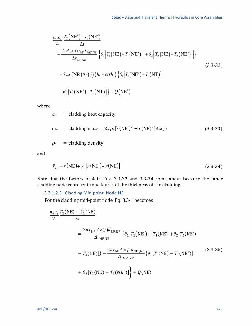
Note that the factors of 4 in Eqs. 3.3-‐32 and 3.3-‐34 come about because the inner cladding node represents one fourth of the thickness of the cladding.
3.3.1.2.5 Cladding Mid-‐point, Node NE For the cladding mid-‐point node, Eq. 3.3-‐1 becomes
!!!!2
!! NE − !!(NE)!"
=2!!NE'!"(!)!NE,NE'
!!NE,NE'!! !! NE' − !!(NE) +!! !! NE'
− !!(NE) −2!!NE!"(!)!NE",NE
!!NE",NE!! !! NE − !!(NE")
+ !! !! NE − !!(!"") + !(NE)
(3.3-‐35)

The SAS4A/SASSYS-‐1 Safety Analysis Code System
3-‐22 ANL/NE-‐12/4
where
rN !E = r NE( )+ 34 r N !E( )" r NE( )#$ %& 3.3-‐36)
3.3.1.2.6 Cladding Outer Node, Node NEʹ′ The out cladding node transfers heat to both the cladding mid-‐point node and the
coolant node, so the equation for the outer cladding node temperature is
!!!!4
!! NE' − !!(NE')!"
= −2!!NE'!" ! !NE,NE'
!NE,NE' !! !! NE' − !! NE
+ !! !! NE' − !! NE
+ 2!" NE' !" ! !!ℎ!!(!) !! NC − !! NE′
+ !!ℎ!!(!) !! NC − !! NE′ + !(N!')
(3.3-‐37)
Note that ( ).)NC( jcTT c= Also, hc1 and hc2 are the coolant heat-‐transfer coefficients at ! and ! + !" as calculated from Eq. 3.3-‐9,
3.3.1.2.7 Coolant, Node NC Coolant temperatures are calculated for the whole length of the subassembly,
whereas fuel temperatures are computed in the core and blankets only. Therefore, the axial coolant node mesh extends beyond the fuel mesh; and the coolant axial node index, jc, is related to the fuel axial node index, j, by
jc = j + jcblbt !1 (3.3-‐38)
where jcblbt is the coolant node at the bottom of the lower blanket. In the T1(i,j) and T2(i,j) arrays, the coolant node corresponds to
( ) ( )jcTjT c=,NC2 (3.3-‐39)
In the non-‐voiding case, the coolant flow is usually upward. In such a situation, the transient calculation for a time step starts at the subassembly inlet and works upward through the lower reflector zones, through the pin section, and finally through the
Steady-‐State and Transient Thermal Hydraulics in Core Assemblies
ANL/NE-‐12/4 3-‐23
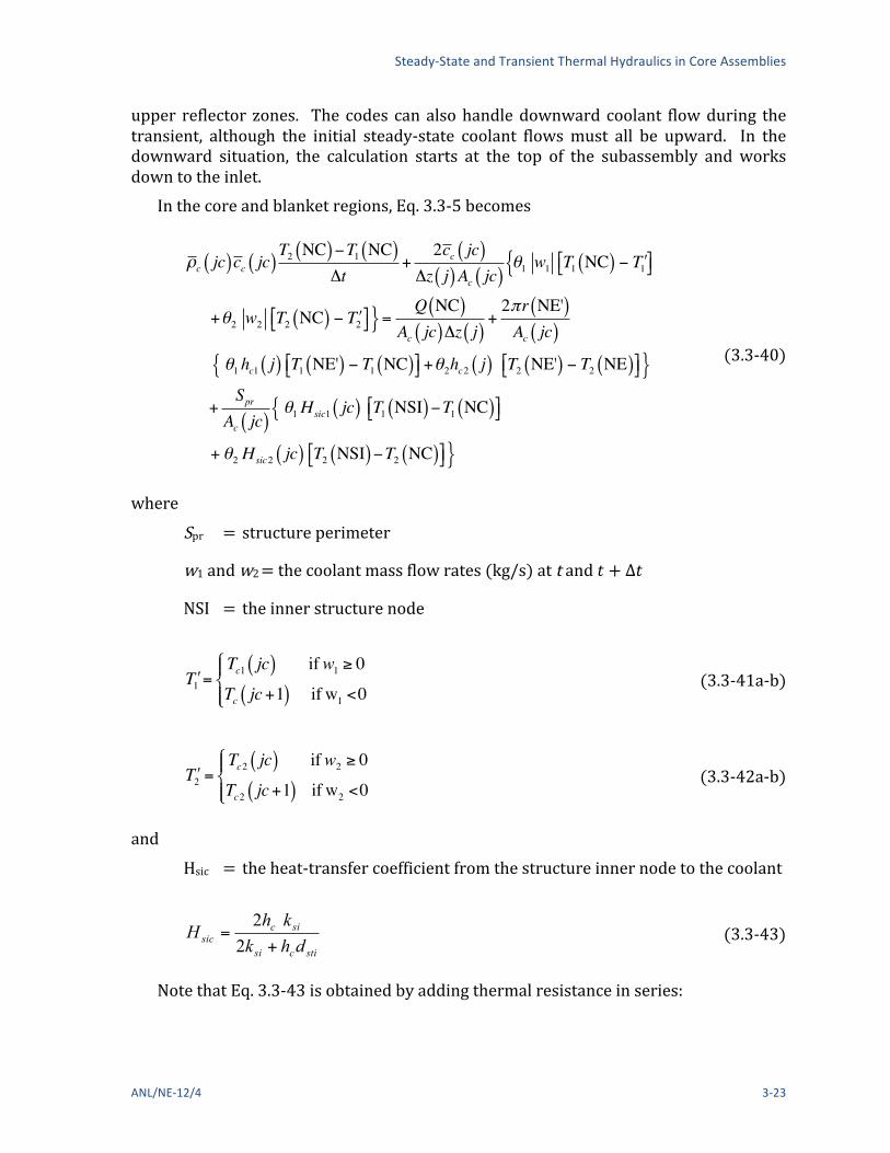
upper reflector zones. The codes can also handle downward coolant flow during the transient, although the initial steady-‐state coolant flows must all be upward. In the downward situation, the calculation starts at the top of the subassembly and works down to the inlet.
In the core and blanket regions, Eq. 3.3-‐5 becomes
!c jc( )cc jc( )T2 NC( )!T1 NC( )
"t+
2cc jc( )"z j( )Ac jc( )
!1 w1 T1 NC( ) ! #T1$% &'{
+!2 w2 T2 NC( ) ! #T2$% &'}=Q NC( )
Ac jc( )"z j( )+2!r NE'( )Ac jc( )
!1 hc1 j( ){ T1 NE'( ) ! T1 NC( )$% &' +!2hc2 j( ) T2 NE'( ) ! T2 NE( )$% &'}
+Spr
Ac jc( )!1Hsic1 jc( ){ T1 NSI( )!T1 NC( )$% &'
+ !2 Hsic2 jc( ) T2 NSI( )!T2 NC( )$% &'}
(3.3-‐40)
where Spr = structure perimeter
w1 and w2 = the coolant mass flow rates (kg/s) at t and ! + ∆!
NSI = the inner structure node
!T1 =Tc1 jc( ) ifw1 " 0
Tc jc+1( ) if w1 <0
#$%
&% (3.3-‐41a-‐b)
!T2 =Tc2 jc( ) ifw2 " 0
Tc2 jc+1( ) if w2 <0
#$%
&% (3.3-‐42a-‐b)
and Hsic = the heat-‐transfer coefficient from the structure inner node to the coolant
sticsi
sicsic dhk
khH
+=22
(3.3-‐43)
Note that Eq. 3.3-‐43 is obtained by adding thermal resistance in series:

The SAS4A/SASSYS-‐1 Safety Analysis Code System
3-‐24 ANL/NE-‐12/4
si
sti
csic kd
hH 211+=
(3.3-‐44)
3.3.1.2.8 Structure Inner Node, Node NSI In the core and blanket regions,
!c( )sti dstiT2 NSI( )!T1 NSI( )
"t=!1Hsic1 jc( ) T1 NC( ) ! T1 NSI( )#$ %&
+!2 Hsic2 jc( ) T2 NC( ) ! T2 NSI( )#$ %&
+Hstio jc( ) !1{ T1 NSO( ) ! T1 NSI( )#$ %&
+!2 T2 NSO( ) ! T2 NSI( )#$ %& } +Qstdsti
dsti + dsto
(3.3-‐45)
where NSO = outer structure node
dsti = thickness of inner structure node
dsto = thickness of outer structure node
sistososti
sosistio kdkd
kkH+
=2
(3.3-‐46)
ksi = thermal conductivity of the inner structure node
kso = thermal conductivity of the outer structure node
and !st = direct heating source in the structure.
The left-‐hand side of Eq. 3.3-‐45 represents the change in internal energy in the node. The terms on the right-‐hand side represent heat flow from the coolant and the outer structure node, as well as direct heating of the structure by neutrons and gamma rays. It is assumed that the direct heating source is divided between the inner and outer nodes in proportion to their thicknesses.
3.3.1.2.9 Structure Outer Node, Node NSO In the core and blankets,
Steady-‐State and Transient Thermal Hydraulics in Core Assemblies
ANL/NE-‐12/4 3-‐25
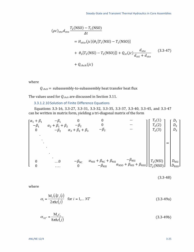
!" !"#!!"#!! NSO − !!(NSO)
!"
= !!"#$ !" !! !! NSI − !! NSO
+ !! !! NSI − !!(NSO) + !!" !"!!"#
!!"# + !!"#
+ !!!!!(!")
(3.3-‐47)
where !chch = subassembly-‐to-‐subassembly heat transfer heat flux
The values used for !chch are discussed in Section 3.11. 3.3.1.2.10 Solution of Finite Difference Equations Equations 3.3-‐16, 3.3-‐27, 3.3-‐31, 3.3-‐32, 3.3-‐35, 3.3-‐37, 3.3-‐40, 3.3-‐45, and 3.3-‐47
can be written in matrix form, yielding a tri-‐diagonal matrix of the form
!! + !!−!!0
. .
00
. .
−!!!! + !! + !!
−!!
. . . . .0. . . .
0−!!
!! + !! + !!
−!NC0
00−!!
!NSI + !NC + !NSI−!NSI
………
−!NSI!NSO + !NSI + !NSO
!!(1)!!(2)!!(3)
!!(NSI)!!(NSO)
=
!!!!!!
!NSI!NSO
(3.3-‐48)
where
( ) ( )( )
NTijzici f ,...1for
2Mf
1 =Δ
=π
α
(3.3-‐49a)
( )jzce
EN Δ=ʹ′ʹ′ π
α8Me
(3.3-‐49b)

The SAS4A/SASSYS-‐1 Safety Analysis Code System
3-‐26 ANL/NE-‐12/4
( ) ENe
NE jzc
ʹ′ʹ′=Δ
= απ
α 24Me
(3.3-‐49c)
ENEN ʹ′ʹ′ʹ′ =αα (3.3-‐49d)
( ) ( ) ( ) ( )( )
twjczjcccc
NC ΔΔ
+= 22cc
2jcAjccjc
θππ
ρα
(3.3-‐49e)
( )π
ρα
2Sdc prstisti=NSI
(3.3-‐49f)
( )π
ρα
2Sdc prstosto=NSO
(3.3-‐49g)
( )NNit
rkir
ii
iii ,....1for
12
1,
1, =ΔΔ
+=
+
+ θβ
(3.3-‐50a)
( ) [ ] thhNRr rbNT Δ+= εσθβ 2 (3.3-‐50b)
!!"" =!NE !NE",NE !!NE",NE
!!!" (3.3-‐50c)
!!" =!NE' !NE,NE' !!NE,NE'
!!!" (3.3-‐50d)
!NE' = !NE' ℎ!! ! !!!" (3.3-‐50e)
!NC =!!" 2 ! !sic2 !" !!!"
(3.3-‐50f)
!NSI =!!" 2 ! !stio !" !!!"
(3.3-‐50g)

Steady-‐State and Transient Thermal Hydraulics in Core Assemblies
ANL/NE-‐12/4 3-‐27
!NSO = 0 (3.3-‐50h)
( ) ( ) 1112
11
2
1111 21 ψβ
θθ
βθθ
α ++⎥⎦
⎤⎢⎣
⎡−= TTD
(3.3-‐51a)
Di =!1!2"i!1T1 i!1( )+T1 i( ) !1 !
"1"2
#i!1 +#i( )"
#$
%
&'
+!1!2"iT1 i+1( )+!1 for i = 2,...,NSI
(3.3-‐51b)
DNSO =!1!2"NSIT1 NSI( )+T1 NSO( ) !NSO !
"1"2
#NSI +#NSO( )"
#$
%
&' +!NSO
(3.3-‐51c)
!i =Q i( )!t2!!z j( )
for i =1,..., NE'
(3.3-‐52a)
( )( )
( )( )
[ ]2221112NCQ TwTw
jztjcc
jzt c
NC ʹ′+ʹ′Δ
Δ+
Δ
Δ= θθ
ππψ
(3.3-‐52b)
!!"# =! NSI !"2!"#(!)
(3.3-‐52c)
and
( )( )
TQ22
NSOQchchΔ+
Δ
Δ=
ππψ prNSO
Sjzt
(3.3-‐52d)
In these equations the α array is related to heat capacity, the β array is related to heat transfer between adjacent nodes, and the ψ array is related to the heat source.
The matrix equations 3.3-‐49 are solved by Gaussian elimination. First arrays Ai and Si are defined:
111 βα +=A (3.3-‐53a)

The SAS4A/SASSYS-‐1 Safety Analysis Code System
3-‐28 ANL/NE-‐12/4
Ai =!i +"i +"i=1 !"i!12
Ai!1for i = 2,..., NSO
(3.3-‐53b)
11 DS = (3.3-‐54a)
and
Si = Di +!i!1Si!1Ai!1
for i = 2,..., NSO
(3.3-‐54b)
Then,
T2 NSO( ) = SNSOANSO
(3.3-‐55a)
and
T2 i( ) = Si +!iAi
T2 i+1( ) for i =NSI, NC,..., 1
(3.3-‐55b)
3.3.2 Reflector Zones In reflector zones, a two-‐node slab geometry treatment is used at each axial node for
heat transfer to the “reflector”. The reflector represents any material in the subassembly outside the pin section.
Typically, this material includes shield orifice blocks near the subassembly inlet, and instrumentation in the upper part of the subassembly. Usually, this material does not come to the form of either pure slabs or pure cylinders, and so any simple geometrical treatment of it will be only an approximation. The best that one is likely to do with a simple heat-‐transfer calculation is to use a slab calculation with parameters chosen to match total heat capacity, total heat-‐transfer surface area, and the approximate effective thickness of the material.
3.3.2.1 Basic Equations The basic equations used for coolant and structure temperatures in reflector zones
are the same as Eqs. 3.3-‐5 and 3.3-‐10 used in the core and blanket regions, except that no heat generation is considered in the reflector zones. Therefore, the !c, term of Eq. 3.3-‐5 and the ! term of Eq. 3.3-‐10 are eliminated in the reflector zones. The reflector is treated with a one-‐dimensional heat conduction equation that is the same as the one used for the structure, except that the thermal properties ρ, c, and k used for the reflector can be different from those used for the structure.

Steady-‐State and Transient Thermal Hydraulics in Core Assemblies
ANL/NE-‐12/4 3-‐29
3.3.2.2 Finite Difference Equations Figure 3.2-‐6 shows the radial mesh structures used for an axial node in a reflector
region. 3.3.2.2.1 Reflector Inner Node Equation 3.3-‐10 becomes
( ) ( ) ( ) ( ) ( ) ( )[ ]{
( ) ( )[ ]}jcTjcT
jcTjcTjcHt
jcTjcTdc
riro
rirorioriri
rir
222
11112
−+
−=Δ−
θ
θρ
(3.3-‐56)
where (ρc)r = density times specific heat of the reflector
dri = thickness of inner node
Tri1, Tri2 = reflector inner node temperature at the beginning and end of the time step
Tro1, Tro2 = reflector outer node temperature at the beginning and end of the time step
dro = thickness of outer reflector node
and
Hrio =2kr
dri + dro (3.3-‐57)
Equation 3.3-‐57 is obtained by adding thermal resistances in series:
r
ro
r
ri
rio kd
kd
H 221
+=
(3.3-‐58)
Equation 3.3-‐56 is similar to Eq. 3.3-‐47 for the outer structure node, except there is no direct heating source in the reflectors.
3.3.2.2.2 Reflector Outer Node The equation for the reflector outer node temperature is similar to Eq. 3.3-‐45 for the
structure inner node:

The SAS4A/SASSYS-‐1 Safety Analysis Code System
3-‐30 ANL/NE-‐12/4
!c( )r droTro2 jc( )!Tro1 jc( )
"t=!1Herc1 jc( ) Tc1 jc( )!Tr01 jc( )#$ %&+!2Herc2 jc( ) Tc2 jc( )!Tr02 jc( )#$ %&
+Hrio jc( ) !1 Tri1 jc( )!Tro1 jc( )#$ %&+!2 Tri2 jc( )!Tro2 jc( )#$ %&{ }
(3.3-‐59)
where
2roc
r
rcerc dhk
khH+
=
(3.3-‐60)
Note that
( ) ( ) ( )[ ] 2/1++= jcTjcTjcT ccc (3.3-‐61)
3.3.2.2.3 Coolant Node In the reflector zones and in the gas plenum, Eq. 3.3-‐5 becomes
!c jc( )cc jc( )Tc2 jc( )!Tc1 jc( )
"t+
2cc jc( )"z jc( )Ac jc( )
!1 w1 Tc jc( )! #T1$% &'{
+!2 w2 Tc2 jc( )! #T2$% &'}
=Ser KZ( )Ac jc( )
!1Herc1 Ter1 jc( )!Tc1 jc( )$% &'{
+!2Herc2 Ter2 jc( )!Tc2 jc( )$% &'}+Spr
Ac jc( )!1Hsic1 Tri1 jc( )$%{
!Tc1 jc( )&'+!2 Hsci2 jc( ) Tsti2 jc( )!Tc2 jc( )$% &'}
(3.3-‐62)
where, in reflector zones, Ter1 = Trol
Ter2 = Tro2
Ser = Sr = reflector perimeter
Spr = structure perimeter
and !sti = structure inner node temperature
Steady-‐State and Transient Thermal Hydraulics in Core Assemblies
ANL/NE-‐12/4 3-‐31
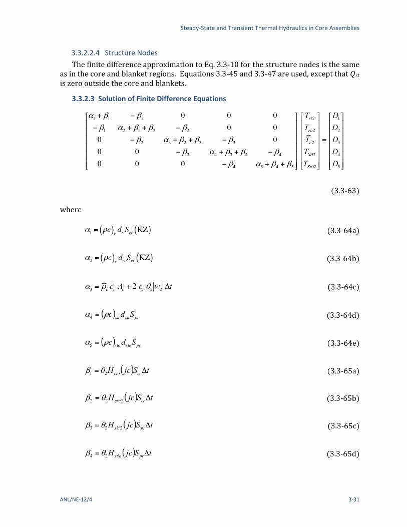
3.3.2.2.4 Structure Nodes The finite difference approximation to Eq. 3.3-‐10 for the structure nodes is the same
as in the core and blanket regions. Equations 3.3-‐45 and 3.3-‐47 are used, except that !st is zero outside the core and blankets.
3.3.2.3 Solution of Finite Difference Equations
⎥⎥⎥⎥⎥⎥
⎦
⎤
⎢⎢⎢⎢⎢⎢
⎣
⎡
=
⎥⎥⎥⎥⎥⎥
⎦
⎤
⎢⎢⎢⎢⎢⎢
⎣
⎡
⎥⎥⎥⎥⎥⎥
⎦
⎤
⎢⎢⎢⎢⎢⎢
⎣
⎡
++−
−++−
−++−
−++−
−+
5
4
3
2
1
02
2
2
2
2
5454
44343
33232
22121
111
00000
0000000
DDDDD
TTTTT
St
Sti
c
ro
ri
ββαβ
βββαβ
βββαβ
βββαβ
ββα
(3.3-‐63)
where
!1 = "c( )r driSer KZ( ) (3.3-‐64a)
!2 = "c( )r droSer KZ( ) (3.3-‐64b)
twcAc ccec Δ+= 223 2 θρα (3.3-‐64c)
( ) prstisti Sdcρα =4 (3.3-‐64d)
( ) prstosto Sdcρα =5 (3.3-‐64e)
( ) tSjcH errio Δ= 21 θβ (3.3-‐65a)
( ) tSjcH ererc Δ= 222 θβ (3.3-‐65b)
( ) tSjcH prsic Δ= 223 θβ (3.3-‐65c)
( ) tSjcH prstio Δ= 24 θβ (3.3-‐65d)

The SAS4A/SASSYS-‐1 Safety Analysis Code System
3-‐32 ANL/NE-‐12/4
θβ =5 (3.3-‐65e)
112
11
2
1111 rori TTD β
θθ
βθθ
α +⎥⎦
⎤⎢⎣
⎡−=
(3.3-‐66a)
Di =!1!2"i!1 ""T1 i!1( ) + ""T1 i( ) !1 !
"1"2
#i!1 +#1( )#
$%
&
'(
+!1!2"i ""T1 i+1( ) for i = 2, 4
(3.3-‐66b)
( ) ( ) ( ) ( )
[ ]222111
132
132
2
13112
2
13
2
432
TwTwztc
TTTD
c ʹ′+ʹ′ΔΔ
+
ʹ′ʹ′+⎥⎦
⎤⎢⎣
⎡+−ʹ′ʹ′+ʹ′ʹ′=
θθ
βθθ
ββθθ
αβθθ
(3.3-‐66c)
( ) ( ) ( ) tQSTTD chchpr Δ+⎥⎦
⎤⎢⎣
⎡+−ʹ′ʹ′+ʹ′ʹ′= 54
2
15114
2
15 54 ββ
θθ
αβθθ
(3.3-‐66d)
( ) ( )jcTT ri11 1 =ʹ′ʹ′ (3.3-‐67a)
( ) ( )jcTT ro11 2 =ʹ′ʹ′ (3.3-‐67b)
( ) ( )jcTT c11 3 =ʹ′ʹ′ (3.3-‐67c)
( ) ( )jcTT sti11 4 =ʹ′ʹ′ (3.3-‐67d)
and
( ) ( )jcTT sto11 5 =ʹ′ʹ′ (3.3-‐67e)
This tri-‐diagonal matrix is solved in the same manner as in Section 3.3.1.3 above.

Steady-‐State and Transient Thermal Hydraulics in Core Assemblies
ANL/NE-‐12/4 3-‐33
3.3.3 Gas Plenum Region In the gas plenum region, a single gas node is in contact with all axial cladding
nodes. A single radial node is used in the cladding, as indicated in Fig. 3.2-‐5.
3.3.3.1 Basic Equations The basic equations used in the cladding, coolant, and structure in the gas plenum
region are the same as those used in the core and blankets, except that there is no heat source term outside of the core and blankets. The gas is assumed to transfer heat only to the cladding, and the basic equation used for the gas temperature is
( ) ( ) ( ) dzTTHrdtdT
Aczzpt
pb
z
zgeegbrp
gggpbpt ∫ −=− πρ 2
(3.3-‐68)
where zpb = elevation at the bottom of the gas plenum
zpt = elevation at the top of the gas plenum
(ρc)g = density times specific heat for the plenum gas
Ag = cross sectional area of the gas plenum
Ag= π r2brp (3.3-‐69)
rbrp = cladding inner radius in the gas plenum region
Tg = gas temperature
Heg = heat-‐transfer coefficient from the plenum gas to the cladding node
Te = cladding temperature
3.3.3.2 Finite Difference Equations 3.3.3.2.1 Gas Plenum Equation 3.3-‐69 becomes
!c( )g AgTg2 !Tg1( )"t
= 2"rbrpHeg
#1 Te1 jp( )!Tg1#$ %&+#2 Te2 jp( )!Tg2#$ %&{ }jp' "z jp( )
"z jp( )jp'
(3.3-‐70)

The SAS4A/SASSYS-‐1 Safety Analysis Code System
3-‐34 ANL/NE-‐12/4
where jp = plenum node
Tg1 = plenum gas temperature at the beginning of the time step
Tg2 = plenum gas temperature at the end of the time step
gepbrperp
ep
ep
brperpg
eg Rkrrk
krr
RH
22
2
1+−
=−
+=
(3.3-‐71)
kep = cladding thermal conductivity in the gas plenum
and Rg = thermal resistance of the gas.
3.3.3.2.2 Cladding Node The equation for the cladding node is
( ) ( )
{ ( ) ( )[ ]
( ) ( )[ ]} { ( )[ ]( )[ ]}jpTT
jpTTHrjpTjcTH
jpTjcTHr
tjpTjpT
Ac
eg
egegbrpecerc
ecercerp
eeepee
222
1112222
1111
12
2
2
−+
−+−+
−=
Δ
−
θ
θπθ
θπ
ρ
(3.3-‐72)
where
ρe = cladding density
ce = cladding specific heat
!!" = ! !!"#! − !!"#! (3.3-‐73)
and rerp = cladding outer radius in the gas plenum region
3.3.3.2.3 Coolant Node The equation for the coolant node in the gas plenum region is the same as Eq. 3.3-‐62
for reflector zones, except that in the gas plenum

Steady-‐State and Transient Thermal Hydraulics in Core Assemblies
ANL/NE-‐12/4 3-‐35
( )2
brperpce
eeerc rrh
k
khH
−+
=
(3.3-‐74)
erpcr rS π2= (3.3-‐75)
and ke = cladding thermal conductivity.
3.3.3.2.4 Structure Nodes The finite difference approximations used for the structure in the gas plenum region
are the same as those used in the core and blankets. Equations 3.3-‐45 and 3.3-‐47 are used, except that !st is zero.
3.3.3.3 Solution of Finite Difference Equations A direct solution of the finite difference equations would be complicated, since Eq.
3.3-‐70 connects a number of axial nodes, each containing a number of radial nodes. Instead, an approximate solution method is used. This method uses the assumption that the total heat capacity of the gas is much less than the total heat capacity of the cladding in the gas plenum region, or
!c( )g Ag < < !e ce Aep (3.3-‐76)
which should always be the case. The solution method contains five steps: 1. Set Tg2 = Tg1. 2. Solve Eqs. 3.3-‐72, 3.3-‐62, 3.3-‐45, and 3.3-‐47 for all axial nodes in the gas
plenum to get new cladding, coolant, and structure temperatures. 3. Use Eq. 3.3-‐70 to obtain a new computed value for Tg2.
4. For each axial node, calculate the heat flow error, ΔE, due to the assumption in step 1:
( ) ( )12 gggg TTAcE −=Δ ρ (3.3-‐77)
5. Add this heat flow to the cladding, changing the cladding temperature:
!!! = !!! +!"
!!!!!!" (3.3-‐78)
In step 2, the equations for each axial node give a matrix equation of the form

The SAS4A/SASSYS-‐1 Safety Analysis Code System
3-‐36 ANL/NE-‐12/4
( )( )( )( ) ⎥
⎥⎥⎥
⎦
⎤
⎢⎢⎢⎢
⎣
⎡
=
⎥⎥⎥⎥
⎦
⎤
⎢⎢⎢⎢
⎣
⎡
ʹ′ʹ′
ʹ′ʹ′
ʹ′ʹ′
ʹ′ʹ′
⎥⎥⎥⎥
⎦
⎤
⎢⎢⎢⎢
⎣
⎡
++−
−++−
−++−
−+
4
3
2
1
2
2
2
2
4343
33232
22111
111
4321
000
000
DDDD
TTTT
ββαβ
βββαβ
βββαβ
ββα
(3.3-‐79)
where
!!!! 1 = !!!(!") (3.3-‐80a)
!!!! 2 = !!!(!") (3.3-‐80b)
!!!! 3 = !!"#!(!") (3.3-‐80c)
!!!! 4 = !!"!"(!") (3.3-‐80d)
egbrpepee HtrAc 21 2 θπρα Δ+= (3.3-‐81a)
!2 = "eceAe + 2cc #2 w2 !t (3.3-‐81b)
( ) prstisti Sdcρα =3 (3.3-‐81c)
( ) prstosto Sdcρα =4 (3.3-‐81d)
( ) tjcHr ercerp Δ= 221 2 θπβ (3.3-‐82a)
( ) tSjcH prsic Δ= 222 θβ (3.3-‐82b)
( ) tSjcH prstio Δ= 223 θβ (3.3-‐82c)
04 =β (3.3-‐82d)

Steady-‐State and Transient Thermal Hydraulics in Core Assemblies
ANL/NE-‐12/4 3-‐37
( ) ( ) ( )[ ]jpTTtHrTTD egegbrp 11112
11
2
1111 221 −Δ+ʹ′ʹ′+⎥
⎦
⎤⎢⎣
⎡−ʹ′ʹ′= πβ
θθ
βθθ
α
(3.3-‐83a)
D2 =!1!2"1 !!T1 1( )+ !!T1 2( ) !2 "
"1"2
#1 +#2( )#
$%
&
'(+!1!2"2 !!T1 3( )
+ 2 cc)t)z
!1 w1 !T1+!2 w2 !T2#$ &'
(3.3-‐83b)
D3 =!1!2"2 !!T1 2( )+ !!T1 3( ) !1 "
"1"2
#2 +#3( )#
$%
&
'(+!1!2"3 !!T1 4( )
(3.3-‐83c)
D4 =!1!2"3 !!T1 3( )+ !!T1 4( ) !4 "
"1"2
#3 +#4( )#
$%
&
'(+Spr Qchch )t
(3.3-‐83d)
( ) ( )jpTT e11 1 =ʹ′ʹ′ (3.3-‐84a)
( ) ( )jcTT c11 2 =ʹ′ʹ′ (3.3-‐84b)
( ) ( )jcTT sti11 3 =ʹ′ʹ′ (3.3-‐84c)
and
( ) ( )jcTT sto11 4 =ʹ′ʹ′ (3.3-‐84d)
This tri-‐diagonal matrix equation is solved in the same manner as in Section 3.3.1.3 above. For step 3, Eq. 3.3-‐70 is rewritten as
2
12 1 θd
sdTT gg ʹ′+
ʹ′ʹ′+=
(3.3-‐85)
where
( ) gg
egbrp
ActHr
dρ
π Δ=ʹ′2
(3.3-‐86)
and

The SAS4A/SASSYS-‐1 Safety Analysis Code System
3-‐38 ANL/NE-‐12/4
( )( ) ( ){ } ( )
( )∑
∑Δ
Δ+−
=ʹ′
jp
jpegc
jpz
jpzjpTTjpTs
22111 θθ
(3.3-‐87)
3.3.4 Order of Solution For a time step, the coolant flow rates are calculated before any temperatures are
calculated. Extrapolated coolant temperatures are used to obtain temperature-‐dependent coolant properties for the flow-‐rate calculations. Section 3.9 describes the pre-‐voiding coolant flow-‐rate calculations.
The order in which the temperature calculations are carried out depends on whether the coolant flow is up or down. In either case, the calculation goes in the direction of the flow. For upward flow, the calculation starts at the subassembly inlet. The coolant temperature at the first coolant node is set equal to the inlet temperatures, Tin:
( ) inc TT =12 (3.3-‐88)
The inlet temperature is supplied by the primary loop calculation, as discussed in Chapter 5. For each axial coolant node, jc, the coolant temperature, Tc2(jc), at the bottom of the node is used as input for the simultaneous calculation of temperatures at all radial nodes. The solutions in Sections 3.3.1, 3.3.2, and 3.3.3 provide ( )jcTc2 , the average coolant temperature for the axial node. The Tc2 (jc + 1) is obtained from
( ) ( ) ( )jcTjcTjcT ccc 222 21 −=+ (3.3-‐89)
This coolant temperature at the top of the node jc is the coolant inlet temperature used as input for the calculation at node jc + 1.
If the flow is downward, the process is the same, except that the calculation starts at the top of the subassembly and works down. The coolant reentry temperatures, upT , described in Section 3.3.6 is used as the starting point for the last coolant node MZC:
Tc2 MZC( ) = Tup! (3.3-‐90)
For each coolant node, jc, Tc2 (jc + 1) is used as input to the calculation of all radial nodes. The solutions in Sections 3.3.1, 3.3.2, and 3.3.3 again provide ( ).2 jcTc Then Tc2 (jc) is obtained from
( ) ( ) ( )12 222 +−= jcTjcTjcT ccc (3.3-‐91)

Steady-‐State and Transient Thermal Hydraulics in Core Assemblies
ANL/NE-‐12/4 3-‐39
3.3.5 Melting of Fuel or Cladding As discussed in Section 3.3.1.1, melting of both fuel and cladding is treated with a
melting range form a solidus temperature, !sol, to a liquidus temperature, !liq, rather than using a sharp melting temperature. Between the solidus and the liquidus, an effective specific heat, cm, based on the heat of fusion is used, as in Eq. 3.3-‐3. In the actual temperature calculations for a time step, the heat of fusion is neglected. Then, at the end of the step the temperatures are modified to account for the heat of fusion at any radial node that is going through the melting range. A number of different cases are considered, depending on the relationships between !1, the temperature at the beginning of the step, and !2, the temperature calculated for the end of the step, ignoring melting, !sol and !liq. In all cases, 2T ʹ′ʹ′ is the final adjusted temperature at the end of the step, and 2T ʹ′ would be the final adjusted temperature if it did not go beyond the melting range. Case 1: !! < !sol, !! > !sol
In this case, an adjusted temperature, 2T ʹ′ , is calculated as
( )m
solsol ccTTTT −+=ʹ′ 22
(3.3-‐92)
where c is the normal specific heat that was used in the calculation of T2. Then,
( )⎪⎩
⎪⎨
⎧
ʹ′
>ʹ′−ʹ′+=ʹ′
otherwise
if
2
222
T
TTccTTT
Tliq
mliqliq
(3.3-‐93a-‐b)
In essence, Eq. 3.3-‐92 divides the energy above the solidus by cm to get the temperature above the solidus; and Eq. 3.3-‐93 divides any energy above the liquidus by c to get the temperature above the liquidus. Case 2: !! > !liq, !! < !liq
In this case,
( )m
liqliq ccTTTT −+=ʹ′ 22
(3.3-‐94)
( )
⎪⎩
⎪⎨
⎧
ʹ′
>ʹ′−ʹ′+=ʹ′
otherwise
if
2
222
T
TTccTTT
Tsol
msolsol
(3.3-‐95a-‐b)
Case 3: !liq ≥ !! ≥ !sol

The SAS4A/SASSYS-‐1 Safety Analysis Code System
3-‐40 ANL/NE-‐12/4
In this case
( )mccTTTT 1212 −+=ʹ′
(3.3-‐96)
!T2 =
Tliq + !T2 "Tliq( ) cmc if !T2 > Tliq
Tsol + !T2 "Tsol( ) cmcif !T2 < Tsol
!T2 otherwise
#
$
%%%
&
%%%
(3.3-‐97a-‐b-‐c)
3.3.6 Coolant Inlet and Re-‐entry Temperature The coolant inlet temperature at the subassembly inlet and the re-‐entry
temperature at the subassembly outlet are determined mainly by the coolant plenum temperatures calculated in PRIMAR-‐4; but, in addition, mixing zones are modeled at the inlet and outlet of each channel. Therefore, the temperature of coolant entering a subassembly is based on the temperature in the part of the plenum in the immediate vicinity of the end of the subassembly, and the reentry temperature soon after an expulsion is based on both the bulk plenum temperature and the temperature of the coolant that was recently expelled.
The mixing mode uses a mass, !mix, of the coolant in the mixing volume, a specific heat, Cmix, of the coolant, and a time constant, !mix, for heat transfer or mixing between the mixing volume and the bulk plenum coolant. If all temperatures and flows are constant, then the mixing volume temperature, !mix, is assumed to approach an equilibrium value asymptotically with an exponential decay. Figure 3.3-‐1 shows the model for the outlet mixing volume.
If !mix1 is the mixing volume temperature at the beginning of a time step, the !mix2 is the value at the end, then
Tmix2 = Teq + Tmix1!Teq( ) e!"t!
(3.3-‐98)
For the outlet plenum,
1!=1!mix
+wMmix
(3.3-‐99)
where w is the average coolant flow rate at the subassembly outlet. The equilibrium temperature is

Steady-‐State and Transient Thermal Hydraulics in Core Assemblies
ANL/NE-‐12/4 3-‐41
Figure 3.3-‐1: Coolant Re-‐entry Temperature Model

The SAS4A/SASSYS-‐1 Safety Analysis Code System
3-‐42 ANL/NE-‐12/4
Teq =Tout if w ! 0
Tout!mix
+wTexpMmix
"
#$
%
&' ! if w > 0
(
)*
+*
(3.3-‐100a-‐b)
where expT is the average temperature of the sodium expelled from the top of the subassembly into the mixing volume during the time step. Tout is the bulk temperature in the outlet plenum. For the inlet plenum, the same equations are used except that w changes sign because positive flow results in flow from the inlet mixing volume into the subassembly inlet. For the inlet, Eqs. 3.3-‐100a and 3.3-‐100b become
Teq =Tin if w ! 0
Tin!mix
"wTexpMmix
#
$%
&
'( ! if w < 0
)
*+
,+
(3.3-‐101a-‐b)
where Tin is the bulk temperature in the inlet plenum.
The coolant inlet and reentry temperature calculations described above are used in both the pre-‐voiding module and the boiling module except when a vapor bubble has blown out of the top of the channel. In this case, the condensation of vapor in the outlet plenum raises the temperature in the mixing volume. A two-‐step process is used for each time step. In the first step, vapor condensation raises the mixing volume temperature. In the second step, heat transfer or mixing with the bulk plenum coolant is accounted for. For the first step, a condensation heat-‐transfer time constant, τc, is calculated as
! c =MmixCmixhcond !Zv per
(3.3-‐102)
where hcond is the vapor condensation heat-‐transfer coefficient, ΔZv is the length of the vapor bubble beyond the subassembly outlet, and per is the bubble perimeter or surface area per unit length. The value of per is taken from the coolant channel dimensions in the top node below the subassembly outlet. For step 1, the new mixing volume temperature, Tnew, is calculated as
Tnew = Tv + Tmix1 ! Tv( ) e!"t! c
(3.3-‐103)
where vT is the average vapor temperature in the part of the bubble above the subassembly outlet. In the second step, the final mixing volume temperature is calculated as

Steady-‐State and Transient Thermal Hydraulics in Core Assemblies
ANL/NE-‐12/4 3-‐43
Tmix2 = Tnew + Tout ! Tnew( ) 1!e!"t!mix
#
$%%
&
'((
(3.3-‐104)
3.4 Steady-‐State Thermal Hydraulics The steady-‐state thermal hydraulics calculations for a channel using the single pin
per subassembly option consist of direct solutions of the relevant steady-‐state equations, rather than running the transient calculations until they converge to a steady-‐state solution.
For the steady-‐sate calculations, the user specifies the coolant flow rate for each channel, the coolant inlet temperature and exit pressure, and the power in each node of each channel. The code then calculates the remaining coolant temperatures and pressures, as well as the temperatures in the fuel, cladding, structure, and reflectors. First, the coolant temperatures in a channel are calculated, starting at the inlet and working upward. The steady-‐state coolant temperature calculation requires only the coolant flow rate, the total power in each axial node, and the coolant heat capacity; so coolant temperatures can be calculated before the fuel and cladding temperatures are known. The second step is to calculate the coolant pressures, starting at the subassembly outlet and working down. Inlet orifice coefficients are adjusted so that all channels have the same total pressure drop. The pressure calculations are described in Section 3.9. The third step is to set the structure and reflector temperatures equal to the coolant temperatures everywhere except in the core and axial blankets. The gas plenum temperatures are also set equal to the coolant temperature in this region, and the cladding temperature in the gas plenum region is also set equal to the coolant temperature. Fourth, the fuel-‐pin temperatures are calculated for each axial node in the core and axial blankets, starting at the cladding outer surface and working inward. Last, the structure temperatures in the core and axial blankets are calculated.
3.4.1 Basic Equations The basic heat-‐transfer equations used in the steady-‐state calculations are the same
as those used for the transient solution, except that all of the time derivatives are dropped in the steady-‐state solution. These equations include Eq. 3.3-‐1 and Eqs. 3.4-‐4 to 3.3-‐10. Also, the spatial finite differencing used in the steady-‐state is the same as that used in the transient.
For the steady-‐state calculations, eq. 3.3-‐5 becomes
( ) cctc AQTwcdzd
=
(3.4-‐1)
where the total heat source per unit volume, Qct, at node jc is

The SAS4A/SASSYS-‐1 Safety Analysis Code System
3-‐44 ANL/NE-‐12/4
( ) ( ) ( ) ( ) ( )( )jczAjcPjcQjcQjcQjcQ
csceccct Δ
=++=
(3.4-‐2)
and ( )jcP is the total steady-‐state power (watts) in the node. For this equation, it is assumed that all heat generated in the fuel, cladding, and structure ends up in the coolant. Note that outside the core and axial blankets ( )jcP and ( )jcQct are zero.
For the steady-‐state fuel and cladding calculations, Eq. 3.3-‐1 is multiplied by 2!" and integrated from the fuel inner surface, rif, to give
( ) rdrQrdrdTkr
r
rif
ʹ′ʹ′ʹ′−= ∫ππ 22
(3.4-‐3)
where the adiabatic boundary condition at rif has been used.
3.4.2 Coolant Temperatures The finite difference form for Eq. 3.4-‐1 may be written as
wcc j( )Tc jc+1( )!Tc jc( )"# $%
&z jc( )=P jc( )&z jc( )
(3.4-‐4)
or
Tc jc+1( )= Tc jc( )+P jc( )wcc jc( )
(3.4-‐5)
where ( )jccc is the specific heat evaluated at the average temperature, ( )jcTc , given by
( ) ( ) ( )2
1++=
jcTjcTjcT ccc
(3.4-‐6)
Also, ( )1cT is equal to the inlet temperature:
( ) inc TT =1 (3.4-‐7)
Starting from jc = 1, Eq. 3.4-‐5 is used to match up the channel. An iteration is used to obtain consistency between ( )jccc and ( )jcTc .
3.4.3 Fuel and Cladding Temperatures in the Core and Axial Blankets At each axial node, the radial node powers, Q(i), are calculated using Eqs. 3.3-‐22 to

Steady-‐State and Transient Thermal Hydraulics in Core Assemblies
ANL/NE-‐12/4 3-‐45
3.3-‐25. Note that the Q in Eq. 3.4-‐3 is a power per unit volume, whereas Q(i) is an integral value for a node:
Q i( ) = 2!r Qdr dzri
ri+1
!z j( )
z j+1( )
!
(3.4-‐8)
The sums, Qsm(i), are calculated as
( ) ( )∑=
=i
iism iiQiQ
1 (3.4-‐9)
Equation 3.4-‐3 becomes
( ) ( ) ( )[ ] ( )ziQ
riTiTirk sm
iiii Δ
=Δ
−++
++
1,1,
112π
(3.4-‐10)
or
( ) ( ) ( )( ) zirk
iQriTiT
ii
smii
Δ+
Δ++=
+
+
121
1,
1,
π (3.4-‐11)
where 1, +Δ iir and 1, +iik are given by Eqs. 3.3-‐21 and 3.3-‐26.
The calculations for an axial node start with the coolant temperature that has already been calculated, as in the section above:
T NC, j( ) = T jc( ) (3.4-‐12)
Then the cladding surface temperature is given by
T NE'( ) = T NC( )+Qsm NE'( )
2!r NE'( )!zhc (3.4-‐13)
Cladding temperatures at nodes NE and NEʺ″ are calculated using Eq. 3.4-‐11. Since 1, +iik can be a function of Ti, a simple iteration between Eq. 3.4-‐11 and Eq. 3.3-‐26 is used.
The equation used for the fuel surface temperature is
2!r NR( ) hb T NT( )!T NE"( )"# $%+!" T NT( )4 !T NE"( )4"#
$%{ } =Qsm NT( )
&z (3.4-‐14)
or

The SAS4A/SASSYS-‐1 Safety Analysis Code System
3-‐46 ANL/NE-‐12/4
T NT( ) = d1 ! d2 T NT( )4 (3.4-‐15)
where
d1 = T NE"( )+Qsm NT( )
2!r NR( )!zhb+!"T NE"( )4
hb (3.4-‐16)
and
bhd εσ
=2
(3.4-‐17)
Equation 3.4-‐15 is solved by iteration. After the fuel surface temperature has been calculated, the inner fuel node
temperatures are calculated one at a time, starting at the outside and working inward, by iterating between Eqs. 3.4-‐11 and 3.3-‐26. In this procedure, T(i) is to be found after T(i+1) is known. First, T(i) is set equal to !(! + 1). Second, k(i) is to be found after T(i+1) is known. First, T(i) is set equal to !(! + 1). Second, k(i) is calculated as a function of the temperature, T(i). Third, 1, +iik is calculated using Eq. 3.3-‐26. Fourth, a new value for T(i) is calculated, using Eq. 3.4-‐11. Fifth, the new T(i) from the fourth step is compared with old value used in the second step. If the two values differ by less than a user-‐specified convergence criterion, then the iteration is finished, and the code goes on to the next node. Otherwise, the code goes back to the second step, using the new value of T(i), and repeats the process.
3.4.4 Structure Temperatures in the Core Axial Blankets The inner structure node temperature is calculated using
!zSpr Hsic T NSI( )"T NC( )#$ %&= ! sP j( ) (3.4-‐18)
or
T NSI( ) = T NC( )+! sP j( )!zSpr Hsic
(3.4-‐19)
The outer structure node is then calculated using
T NSO( ) = T NSI( )+! sP j( )dsto
!zSpr Hstio dsti + dsto( ) (3.4-‐20)

Steady-‐State and Transient Thermal Hydraulics in Core Assemblies
ANL/NE-‐12/4 3-‐47
3.4.5 Reflector, Structure, Cladding, and Gas Plenum Temperature Outside the Core and Axial Blankets
Outside the core and axial blankets no power sources are considered, so the reflector and structure temperatures at an axial node are the same as the coolant temperature for the steady-‐state. The coolant temperatures are the same at all axial nodes in the gas plenum region, and the cladding and gas temperatures in this region are equal to the coolant temperatures.
3.5 Transient Heat Transfer after the Start of Boiling After the start of boiling, the coolant temperatures are calculated in the coolant
routines, rather than being calculated simultaneously with fuel, cladding, and structure temperatures. Coupling between the boiling calculations and the non-‐coolant heat-‐transfer calculation takes place in two parts for each time step. First, the boiling routines us extrapolated cladding and structure temperatures to calculate the heat fluxes to the coolant for the boiling calculation. Then the heat fluxes actually used in the coolant routines are passed to the heat-‐transfer routines to be used as boundary conditions at the cladding, structure, and reflector surfaces. The net results of this procedure are that energy is conserved, and a fully implicit boiling calculation can be made without requiring a direct simultaneous solution of all of the fuel-‐pin temperatures in the boiling model. The coupling through extrapolated cladding and structure temperatures and heat fluxes at the cladding and structure surfaces imposes numerical stability limitations on the heat-‐transfer time-‐step sizes. Currently, fuel-‐pin temperatures are calculated at the end of the fuel-‐pin heat-‐transfer time step, whereas structure and reflector temperatures are calculated at every coolant time step. The coolant time step can be no longer than the heat-‐transfer step, and the coolant step is often much shorter. For typical fuel pins, the stability limit for the heat-‐transfer time step is of the order of .02 s. With a thin structure, the stability limit for structure temperature calculations could be less than .02 s, although for typical duct wall thicknesses (.12 in. or .003 m) the stability limit would be closer to one second. Should timing studies indicate that the structure and reflector temperature calculations account for a significant fraction of the total computing time, then the code will be modified so as to do these calculations less often than once every coolant time step.
3.5.1 Fuel and Cladding Temperatures in the Core and Axial Blanket The equations used for fuel and cladding temperatures after the switch to the
boiling module are the same as those used in the non-‐voiding module, except that in the boiling module the fuel-‐pin heat-‐transfer calculations stop at the cladding outer surface rather than carrying through to the structure outer node. The finite difference equations for radial nodes 1-‐NE are the same as Eqs. 3.3-‐16 to 3.3-‐36. For node NEʹ′ , the cladding outer node, the heat flux to the coolant at the cladding surface must be accounted for. Also, in a boiling region, a film of liquid sodium can be left on the cladding. Since the film is in intimate contact with the cladding, the heat capacity of the film is added to the heat capacity of the cladding outer node, rather than being accounted for in the boiling calculation. Thus, the finite difference equation for node NEʹ′ becomes
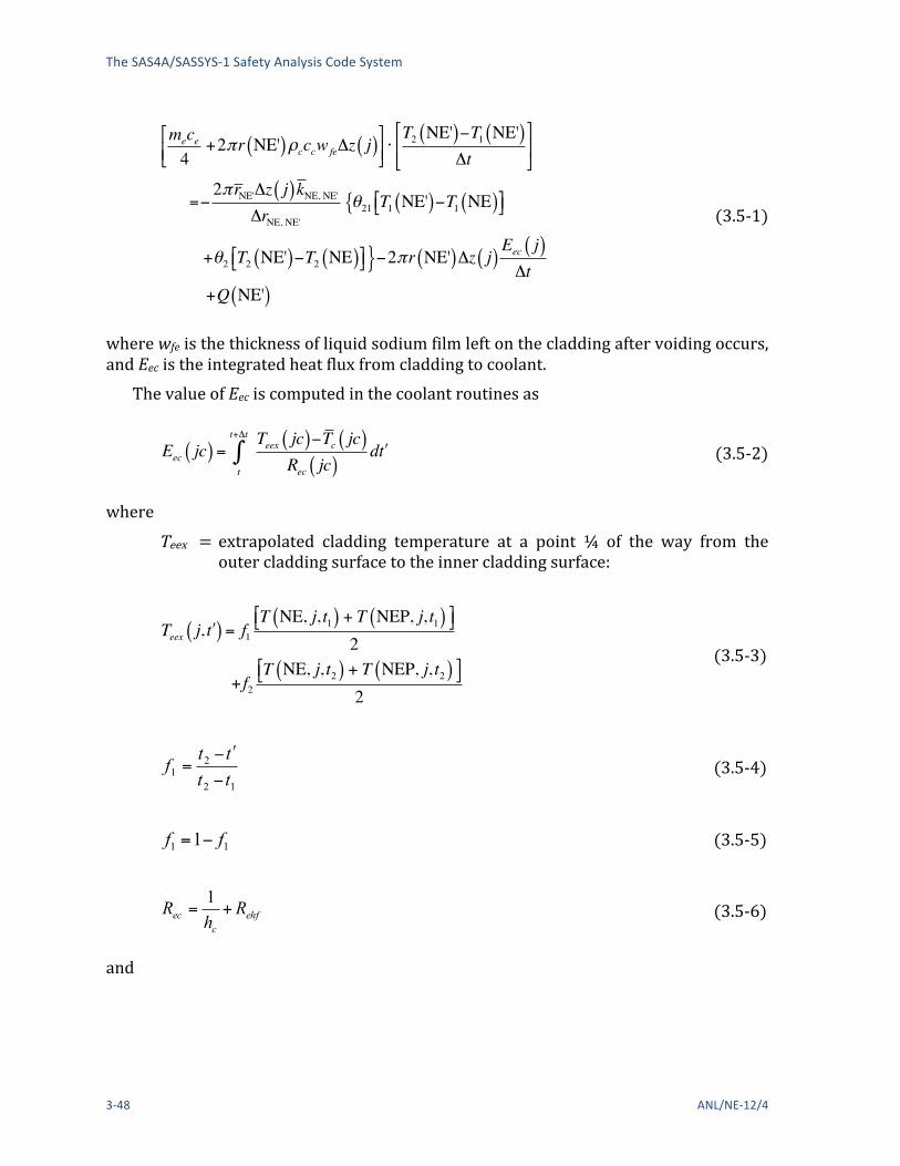
The SAS4A/SASSYS-‐1 Safety Analysis Code System
3-‐48 ANL/NE-‐12/4
mece4
+2!r NE'( )!cccwfe!z j( )"
#$%
&'(T2 NE'( ))T1 NE'( )
!t"
#$
%
&'
=)2! rNE'!z j( )kNE, NE'
!rNE, NE'
!21{ T1 NE'( ))T1 NE( )"# %&
+!2 T2 NE'( ))T2 NE( )"# %&})2!r NE'( )!z j( )Eec j( )!t
+Q NE'( )
(3.5-‐1)
where wfe is the thickness of liquid sodium film left on the cladding after voiding occurs, and Eec is the integrated heat flux from cladding to coolant.
The value of Eec is computed in the coolant routines as
Eec jc( ) =Teex jc( )!Tc jc( )
Rec jc( )d "t
t
t+#t
$ (3.5-‐2)
where Teex = extrapolated cladding temperature at a point ¼ of the way from the
outer cladding surface to the inner cladding surface:
Teex j, !t( ) = f1T NE, j, t1( ) + T NEP, j, t1( )"# $%
2
+ f2T NE, j, t2( ) + T NEP, j, t2( )"# $%
2
(3.5-‐3)
12
21 tt
ttf−
ʹ′−=
(3.5-‐4)
11 1 ff −= (3.5-‐5)
ehfc
ec Rh
R +=1
(3.5-‐6)
and

Steady-‐State and Transient Thermal Hydraulics in Core Assemblies
ANL/NE-‐12/4 3-‐49
Rehf =r NE'( )!r NE( )"# $%
ke
r NE'( ) 1 ! !e4 1!!c !! s( )
"
#&&
$
%''
r NE( )+3r NE'( )
(
)
**
+
**
,
-
**
.
**
(3.5-‐7)
If a node is partly voided, then Eec is averaged over the length of the node as well as integrated over time.
The fecc wcρ term is supplied by the boiling routines. It represents the heat capacity of any liquid film left on the cladding after voiding occurs. This term is zero unless voiding has occurred at this axial node. Since the film temperature tends to follow the cladding surface temperature more closely than it follows the vapor temperature, the film heat capacity is lumped with the cladding outer node, and film temperatures are not explicitly calculated in the boiling routines.
The finite difference equations are again put in a matrix form like Eq. 3.3-‐48, except that in the voiding case there are only NEʹ′ elements. The definitions of α, β, and D are the same as in Eqs. 3.3-‐49 to 3.3-‐51 for nodes 1-‐NE. For node NEʹ′, α is still given by Eq.
!NE' = 0 (3.5-‐8)
3.3-‐49d or 3.3-‐49b, except that the fecc wcρ term is added to it. Also,
and
DNE' =!1!2"NE T1 NE( )+T1 NE'( ) !NE' !
"1"2#NE
"
#$
%
&'+$NE' !r NE'( )Eec j( )
(3.5-‐9)
The equations are solved in the same manner as in the non-‐voiding case.
3.5.2 Structure Temperatures The basic equations used for the two structure radial nodes at an axial node are
( ) ( ) oststostistiosto
stosto fQTTHdtdTdc +−=ρ
(3.5-‐10)
and
( )[ ] ( ) ( )sc
sticiststistostio
stifstccstisti R
TTfQTTHdtdTwcdc −
++−=+ ρρ
(3.5-‐11)
where

The SAS4A/SASSYS-‐1 Safety Analysis Code System
3-‐50 ANL/NE-‐12/4
stosti
stii dd
df
+=
(3.5-‐12)
stosti
stoo dd
df+
=
(3.5-‐13)
and wfst = thickness of the liquid-‐sodium film left on the structure after voiding occurs. The heat capacity of the film in the boiling region, as represented by the pcccwfst
term, is supplied by the boiling routines to be added to the inner structure node. The structure temperature calculation is either a semi-‐implicit or a fully implicit
calculation, depending on the time-‐step in relation to an inner structure node heat-‐transfer time constant, stiτ , calculated as
( )sti
stististi k
dc2
2ρτ =
(3.5-‐14)
If Δt is less than τsti then the semi-‐implicit calculation is used. Otherwise the fully implicit calculation is used.
3.5.2.1 Semi-‐Implicit Calculations For the semi-‐implicit calculation, finite differencing of Eqs. 3.5-‐10 and 3.5-‐11 gives
( ) ( ) [ ] 0112212
2fQTTTTH
tTTdc ststostistosti
stiostostostosto +−+−=
Δ
−ρ
(3.5-‐15)
and
( )[ ] ( )
[ ]tEfQTTTTH
tTTwcdc
sciststistostisto
stio
stistifstccstisti
Δ−+−+−=
Δ
−+
1122
12
2
ρρ
(3.5-‐16)
where
( ) ( ) ( )( )
tdjcR
jcTjcTjcE
tt
t sc
cstexsc ʹ′
−= ∫
Δ+
(3.5-‐17)
The value of Esc is computed in the boiling routines. Tstex is the extrapolated structure inner node temperature, and
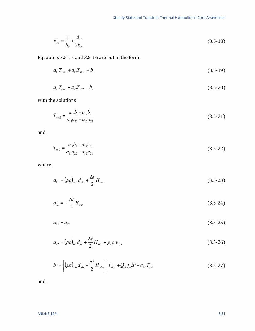
Steady-‐State and Transient Thermal Hydraulics in Core Assemblies
ANL/NE-‐12/4 3-‐51
sti
sti
csc k
dh
R2
1+=
(3.5-‐18)
Equations 3.5-‐15 and 3.5-‐16 are put in the form
1212211 bTaTa stisto =+ (3.5-‐19)
2222221 bTaTa stisto =+ (3.5-‐20)
with the solutions
21122211
2121222 aaaa
babaTsto −
−=
(3.5-‐21)
and
21122211
2212112 aaaa
babaTsti −
−=
(3.5-‐22)
where
( ) stiostosto Htdca211Δ
+= ρ
(3.5-‐23)
stioHta212Δ
−=
(3.5-‐24)
1221 aa = (3.5-‐25)
( ) fstccstiostisti wcHtdca ρρ +Δ
+=222
(3.5-‐26)
( ) 11211 2 stioststostiostosto TatfQTHtdcb −Δ+⎥⎦
⎤⎢⎣
⎡ Δ−= ρ
(3.5-‐27)
and

The SAS4A/SASSYS-‐1 Safety Analysis Code System
3-‐52 ANL/NE-‐12/4
( ) sciststostifstccstiostiosti QttfQTaTwcHtdcb Δ−Δ+−⎥⎦
⎤⎢⎣
⎡ +Δ
−= 11212 2ρρ
(3.5-‐28)
3.5.2.2 Fully Implicit Calculations Since the inner structure node may represent only a small fraction of the total
structure thickness, τsti can be small. If the time-‐step size is appreciably larger than τsti then the semi-‐implicit calculation can become numerically unstable. Therefore, a different algorithm is used for larger time-‐step sizes. This algorithm uses two steps. First, a fully implicit calculation is made, using a coolant temperature and thermal resistance to the coolant as structure surface boundary conditions, rather than using the integrated heat flux. In this first step, the heat flux from the coolant to the structure will, in general, not match the heat flux form structure to coolant used in the coolant calculations. Therefore, in the second step, the inner node and outer node structure temperatures are both adjusted by the same amount so that the integrated heat flux from structure to coolant is matched.
For the first step the finite difference equations used for the two structure node temperatures are
( ) ( ) ( ) oststostistiostosto
stosto fQTTHtTTdc +−=
Δ
−22
12ρ
(3.5-‐29)
and
!c( )sti dsti +!cccwfst!" #$
Tsti2 % Tsti1( )&t
= Hstio Tsto2 % Tsti2( )+Tc % Tsti2Rsc
+Qst fi (3.5-‐30)
where the values for Tc and Rsc are supplied by the coolant routines. The solutions for these two equations again have the same form as Eqs. 3.5-‐21 and 3.5-‐22 except that in this case the coefficients are defined as
( ) stiostosto Htdca Δ+= ρ11 (3.5-‐31)
stioHtaa Δ−== 2112 (3.5-‐32)
and
( )sc
stiofstccstisti RtHtwcdca Δ
+Δ++= ρρ22
(3.5-‐33)
The temperature difference, ΔTst, between the outer and inner nodes is then defined as

Steady-‐State and Transient Thermal Hydraulics in Core Assemblies
ANL/NE-‐12/4 3-‐53
22 stistost TTT −=Δ (3.5-‐34)
In the second step, ΔTst is preserved but the temperatures are adjusted so as to match the value of Esc supplied by the coolant routines:
!" !"#!!"# + !!!!!!"# !!"#! − !!"#! + !" !"#!!"# !!"#! − !!"#!
= !!" − !!" (3.5-‐35)
The solution to Eqs. 3.5-‐34 and 3.5-‐35 is
{ ( )
( )[ ] ( )}( ) ( )[ ]fstccstististosto
ststifstccstisti
stostostoscststo
wcdcdc
TTwcdc
TdcEtQT
ρρρ
ρρ
ρ
++
Δ+⋅++
+−Δ=
/
1
12
(3.5-‐36)
and
ststosti TTT Δ−= 22 (3.5-‐37)
Note that the second step can still cause numerical instabilities if the time-‐step size is too large or the total structure thickness is too small, but in the fully implicit scheme the stability limit is based on the total structure thickness, whereas in the semi-‐implicit scheme the stability is based mainly on the inner node thickness.
3.5.3 Reflector Temperatures In the boiling module the treatment of reflector temperatures is almost identical to
the structure temperature treatment. The main difference is that in the reflector, the outer node is in contact with the coolant, whereas in the structure, the inner code is in contact with the coolant. Also, in the reflector the density, specific heat, and thermal conductivity are the same for both nodes, whereas in the structure these properties can vary from inner node to outer node.
The basic equations are
( ) ( )riroriori
rir TTHdtdTdc −=ρ
(3.5-‐38)
and

The SAS4A/SASSYS-‐1 Safety Analysis Code System
3-‐54 ANL/NE-‐12/4
!c( )r dro +!cccwfr!" #$
dTrodt
= Hrio Tri % Tro( ) + Tc % Tro( )Herc
(3.5-‐39)
where wfr = thickness of the liquid-‐sodium film left on the reflector after voiding
occurs.
An outer reflector node heat-‐transfer time constant, τro, is calculated as
( )r
rorro k
dc2
2ρτ =
(3.5-‐40)
and a fully implicit calculation is used if the time-‐step size is greater than τro. Otherwise a semi-‐implicit calculation is used.
3.5.3.1 Semi-‐Implicit Calculations Finite differencing of Eqs. 3.5-‐38 and 3.5-‐39 gives
( ) ( ) ( )112212
2 rirorirorioriri
rir TTTTHtTTdc −+−=
Δ
−ρ
(3.5-‐41)
( )[ ]( ) ( )tETTTTH
tTTwcdc rc
roriroririoriri
frccror Δ−−+−=
Δ
−+ 1122
12
2ρρ
(3.5-‐42)
where
( ) tdHTTE erc
tt
tcrexrc ʹ′−= ∫
Δ+
(3.5-‐43)
These equations are put in the form
1212211 bTaTa rori =+ (3.5-‐44)
2222221 bTaTa rori =+ (3.5-‐45)
with the solution
21122211
2121222 aaaa
babaTri −
−=
(3.5-‐46)

Steady-‐State and Transient Thermal Hydraulics in Core Assemblies
ANL/NE-‐12/4 3-‐55
and
Tro2 =a11b2 !a21b1a11a22 !a12a21
(3.5-‐47)
The coefficients are
( ) riorir Htdca211Δ
+= ρ
(3.5-‐48)
rioHta212Δ
−=
(3.5-‐49)
1221 aa = (3.5-‐50)
( ) frccrioror wcHtdca ρρ +Δ
+=222
(3.5-‐51)
( ) 111 22 rorioririorir THtTHtdcb Δ+⎥⎦
⎤⎢⎣
⎡ Δ−= ρ
(3.5-‐52)
and
( ) rcririororiofrccror ETHtTHtwcdcb −Δ
+⎥⎦
⎤⎢⎣
⎡ Δ−+= 112 22
ρρ
(3.5-‐53)
3.5.3.2 Fully Implicit Calculations As in the structure temperature case, a two-‐step process is used. In the first step,
the finite difference equations used are
( ) ( ) ( )2212
rirorioriri
rir TTHtTTdc −=
Δ
−ρ
(3.5-‐54)
and
( )[ ]( ) ( ) ( ) ercrocroririororo
frccror HTTTTHtTTwcdc 222
12 −+−=Δ
−+ ρρ
(3.5-‐55)
The solutions again have the same form as Eqs. 3.5-‐46 and 3.5-‐47, with the coefficients

The SAS4A/SASSYS-‐1 Safety Analysis Code System
3-‐56 ANL/NE-‐12/4
given by
( ) riorir Htdca Δ+= ρ11 (3.5-‐56)
rioHta Δ−=12 (3.5-‐57)
1221 aa = (3.5-‐58)
( ) frccrioror wcHtdca ρρ +Δ+=22 (3.5-‐59)
( ) 11 ririr Tdcb ρ= (3.5-‐60)
and
!! = !" !!!" + !!!!!!" !!"# + !!!" !!"# (3.5-‐61)
The temperature difference between nodes, ΔTr, is defined as
22 rorir TTT −=Δ (3.5-‐62)
In the second step, ΔTr is preserved and Erc is matched. The energy conservation equation is
!" !!!" !!"! − !!"! + !" !!!" + !!!!!!" !!"! − !!"! = −!!" (3.5-‐63)
The solution to Eq. 3.5-‐62 and 3.5-‐63 is
!!"! =−!!" + !" !!!"!!"! + !" !!!" + !!!!!!" ∙ (!!"# + !!!)
!" ! !!" + !!" + !!!!!!" (3.5-‐64)
and
rriro TTT Δ−= 22 (3.5-‐65)
3.5.4 Gas Plenum Region The basic equations used for the cladding and gas temperatures in the gas plenum
region are Eq. 3.3-‐68 and the following equation:

Steady-‐State and Transient Thermal Hydraulics in Core Assemblies
ANL/NE-‐12/4 3-‐57
!eceAepdTe jp( )dt
= 2" rerpHerc Tc jc( )!Te jp( )"# $% + 2" rbrpHeg Tg !Te jp( )"# $% (3.5-‐66)
Since Eq. 3.3-‐68 links all of the cladding nodes in the gas plenum, a direct semi-‐implicit or implicit solution of Eqs. 3.3-‐68 and 3.5-‐66 would require a simultaneous solution for the gas temperature and all of the cladding node temperatures. Instead, the cladding temperatures are calculateed first, using the gas temperature at the beginning of the time step. Then the gas temperature is calculated using the newly computed cladding temperatures.
Finite differencing of Eq. 3.5-‐66 gives
!eceAepTe2 !Te1( )"t
=!2! rerpEec
"t+!rbrpHeg 2Tg1!Te2 !Te1( ) (3.5-‐67)
where Eec is calculated in the coolant routines in the same manner as indicated in Eq. 3.5-‐2, except that in the gas plenum only one radial node is used in the cladding, and Rehf becomes
e
brperpehf k
rrR
2−
=
(3.5-‐68)
The solution of Eq. 3.5-‐67 for Te2 gives
!!! =!!!!!!" − !!!"#!!"!" !!" − 2!!!"#!!! + 2!!!"#!!"!" !!!
!!!!!!" + !!!"#!!"!" (3.5-‐69)
In the second step, Eq. 3.3-‐70 is used with .2/121 ==θθ The solution for 2gT is
Tg2 =!c( )g Ag !!rbrp Heg "t#
$%&Tg1+!rbrp Heg "t s1 / s2
"c( )g Ag +!rbrp Heg "t (3.5-‐70)
where
( ) ( )[ ] ( )jpzjpTjpTsjp
ee Δ+=∑ 211
(3.5-‐71)
and
( )∑ Δ=jp
jpzs2
(3.5-‐72)
The SAS4A/SASSYS-‐1 Safety Analysis Code System
3-‐58 ANL/NE-‐12/4
3.5.5 Coolant Temperatures in Liquid Slugs Before the onset of coolant voiding, coolant temperatures are calculated at all node
boundaries, as indicated in Fig. 3.2-‐3. After the start of boiling, liquid coolant temperatures are calculated at all node boundaries outside vapor regions, as well as at moving nodes near the bubble interfaces. Two different types of calculations are made. Eulerian temperature calculations are made for fixed coolant nodes in the inlet and outlet liquid slugs. Lagrangian temperature calculations are made for the moving interface nodes and for any fixed nodes in liquid slugs between bubbles. There is also an option to use Lagrangian temperature calculations for all nodes, both fixed and moving.
The Eulerian calculation is probably more accurate for the fixed nodes. The main disadvantage of this method is that a sudden jump in inlet temperature can lead to a sawtooth temperature pattern, with the temperature high at one node, low at the next, and high again at the third node. The Lagrangian calculation does not exhibit this behavior. This sawtooth behavior is not unstable: the perturbation at any node is no larger than the jump in the inlet temperature, and the perturbations tend to die out in later time steps. Also, the coolant inlet and reentry temperature calculations described in Section 3.3.6 tend to eliminate sudden jumps in inlet and reentry temperatures.
3.5.5.1 Eulerian Temperature Calculation The basic equation used in this calculation is again E. 3.3-‐5. The heat fluxes Qec and
Qsc are calculated as
Qec =Te !Tc( )Rec
2!r NE'( )Ac
(3.5-‐73)
and
( )c
st
sc
csisc A
SRTTQ −
=
(3.5-‐74)
where Rec and Rsc are given by Eqs. 3.5-‐6 and 3.5-‐18, Te is the average of T(NE) and T(NEʹ′), and Tsi is the inner structure node temperature. In reflector zones, Te is replaced by the reflector outer node temperature; and in the gas plenum region, the one radial cladding node temperature is used. In the boiling module, the coolant temperatures are calculated before the cladding and structure temperatures are, so linear extrapolation in time is used to obtain values of Te and Tsi at the end of a time step.
A semi-‐implicit finite differencing of Eq. 3.3-‐5 gives

Steady-‐State and Transient Thermal Hydraulics in Core Assemblies
ANL/NE-‐12/4 3-‐59
p jc( )cc jc( )Ac jc( )Tc2 jc+1( )+Tc2 jc( )!Tc1 jc+1( )+Tc1 jc( )"# $%
2&t
+ cc jc( )w1Tc1 jc+1( )+Tc1 jc( )"# $%
2&z jc( )+ cc jc( )w2
Tc2 jc+1( )!Tc2 jc( )"# $%2&z jc( )
=Qc jc( )Ac jc( )+k5 jc( )Ac jc( )
42Te2 jc( )!Te2 jc( )!Tc2 jc+1( )
Rec2 jc( )
'()
*)
+2Te1 jc( )!Te1 jc( )!Tc1 jc+1( )
Rec1 jc( )+!2 jc( )
2Tsi2 jc( )!Tc2 jc( )!Tc2 jc+1( )Rsc2 jc( )
"
#++
+2Tsi1 jc( )!Tc1 jc( )!Tc1 jc+1( )
Rsc1 jc( )
$
%,,
-.)
/)
(3.5-‐75)
where
k5 jc( ) =
2!r NE', jc( )Ac jc( )
in thecoreand blankets
ser kz( )Ac jc( )
in a reflector region
2!rerpAc jc( )
in the gas plenum region
!
"
####
$
####
(3.5-‐76a-‐c)
and
( ) ( )( ) ( )jcAjck
jcSjcc
st
52 =γ
(3.5-‐77)
Solving for ( )12 +jcTc gives

The SAS4A/SASSYS-‐1 Safety Analysis Code System
3-‐60 ANL/NE-‐12/4
Tc2 jc+1( ) = Tc1 jc+1( ) !c jc( )! "tw1"z jc( )Ac jc( )
!k5 jc( )"thbr jc( )
2cc jc( )
#
$%%
&
'((
)*+
,+
+Tc2 jc( ) !! jc( )+ "tw2"z jc( )Ac jc( )
!k5 jc( )"t2cc jc( )
hb2 jc( )#
$%%
&
'((
+Tc1 jc( ) !c jc( )+ "tw1"z jc( )Ac jc( )
!k5 jc( )"t2cc jc( )
hb1 jc( )#
$%%
&
'((
+4"t
2cc jc( )k5 jc( ) !1 jc( )+
2"tQc jc( )cc jc( )
-.+
/+/ !c jc( ){
+"tw2
"z jc( )Ac jc( )+k5 jc( )"thb2 jc( )
2cc jc( )
-.+
/+
(3.5-‐78)
with
( )( )
( )( )jcRjc
jcRjch
scecb
1
2
11
1 γ+=
(3.5-‐79)
( )( )
( )( )jcRjc
jcRjch
scecb
2
2
22
1 γ+=
(3.5-‐80)
and
!1 jc( ) =1 2Te2 jc( )Rec2 jc( )
+Te1 jc( )Rec1 jc( )
+"2 jc( )Tsi2 jc( )Rsc2 jc( )
!
"##
$%&
'&
+Tsi1 jc( )Rsc1 jc( )
(
)**
+,-
(3.5-‐81)
If the inlet flow is positive, then the coolant temperature at node 1 is determined by the inlet temperature. Equation 3.5-‐78 is then used to march up the channel through the inlet liquid slug, with ( )12 +jcTc being computed after ( )jcTc2 . Similarly, if the flow in the upper liquid slug is downward, then the assembly outlet reentry temperature determines the coolant temperature at the last coolant node. Then an equation similar to Eq. 3.5-‐79 is used to march down through the upper liquid slug, with Tc2(jc) being computed after ( )12 +jcTc .
The Eulerian calculations always go from node to node in the direction of flow. An

Steady-‐State and Transient Thermal Hydraulics in Core Assemblies
ANL/NE-‐12/4 3-‐61
inlet slug expelling downward and an outlet liquid slug going upward are special cases, since in these cases the calculation starts at a liquid vapor interface rather than an end of the subassembly. The interface liquid temperatures are first calculated using the Lagrangian treatment described below. Then Eq. 3.5-‐78 or the equivalent equation for downward flow is used to calculate the temperatures at the fixed nodes within the liquid slug. For the first fixed node near the interface, some of the terms in Eq. 3.5-‐78 are modified. The moving interface node is treated as node jc. The interface temperature is used for ( )jcTc2 , and an interpolated value is used for ( )jcTc1 . The distance from the fixed node to the interface at the end of the step is used for ( )jczΔ . Interpolated interface cladding and structure temperatures are used in calculating φ1 for the interface node.
3.5.5.2 Lagrangian Calculations for Interface Temperatures For every liquid-‐vapor interface a vapor temperature is calculated at or very near
the interface. The liquid temperature right at the interface would be close to the vapor temperature, but there can be strong axial temperature gradients in the liquid near the interface. These strong axial gradients would only extend a short distance into the liquid. The heat flow through the interface into a small vapor bubble is accounted for, as described in Chapter 12; but since only one liquid temperature node is used near the interface, the axial temperature distribution neat the interface is not represented. A liquid temperature is calculated for each interface, but axial conduction is neglected in this calculation. Thus, the liquid interface temperature can be considered as either the interface temperature that would occur if there were no axial conduction or the temperature a short distance from the interface where axial conduction is negligible.
A Lagrangian formulation, moving with the liquid, is used for the interface temperature calculation. The basic equation used is
sceccc QQQ
DtDTc ++=ρ
(3.5-‐82)
where the Lagrangian total derivative is used. After finite differencing this equation gives

The SAS4A/SASSYS-‐1 Safety Analysis Code System
3-‐62 ANL/NE-‐12/4
!cicciT!i2 k,L( )!T!i1 k,L( )
"t
=Qc jc( )+k5 jc( )2
Tei1 k,L( )!T!i1 k,L( )Reci1 k,L( )
#$%
&%
+Tei2 k,L( )!T!i2 k,L( )
Rsci1 k,L( )
'(%
)%
*
+,,
+"2 jc( )Tsi1 k,L( )!T!i1 k,L( )
Rsci1 k,L( )+Tsi2 k,L( )!T!i2 k,L( )
Rsci2 k,L( )
*
+,,
#$%
&%
'(%
)%
(3.5-‐83)
or
T!i2 k,L( ) = T!i1 k,L( ) 1! d1 hbi1 k,L( )"# $%+ d1{ !1i[ k,L( )
+2 Qc jc( ) / k5 jc( ) $%}/ 1+ d1hbi2 k,L( )"# $% (3.5-‐84)
where
( )cici ctjck
dρ25
1Δ
=
(3.5-‐85)
( )( )
( )( )LkRjc
LkRLkh
sciecibi ,,
1,1
2
11
γ+=
(3.5-‐86)
( )( )
( )( )LkRjc
LkRLkh
sciecibi ,,
1,2
2
22
γ+=
(3.5-‐87)
k = bubble number
L = 1 for lower bubble interface, 2 for upper bubble interface
jc = coolant node containing the interface
!1i k,L( ) =Tei2 k,L( )Reci2 k,L( )
+Tei1 k,L( )Reci1 k,L( )
+"2 jc( )Tsi2 k,L( )Rsci2 k,L( )
+Tsi1 k,L( )Rsci1 k,L( )
!
"##
$
%&& (3.5-‐88)
Tei2, Tsi2 =cladding and structure interface temperatures at the end of the step, extrapolated in time and interpolated between fixed cladding nodes.

Steady-‐State and Transient Thermal Hydraulics in Core Assemblies
ANL/NE-‐12/4 3-‐63
Tei1, Tsi1 = same at the beginning of the time step.
Reci2, Rsci2 = values of Rec and Rsc at the interface at the end of the time step.
Reci1, Rsci1 = same at the beginning of the time step.
3.5.5.3 Lagrangian Calculation for Fixed Nodes The Lagrangian temperature calculations for fixed coolant nodes are similar to those
for interface nodes. The fluid particle that ends up at coolant node jc at the end of a time step is considered. During the time step, the particle travelled a distance
( )( ) ( )jjAjc
twwzccρ221 Δ+
=ʹ′Δ
(3.5-‐89)
where
⎪⎩
⎪⎨⎧
−
<+=
otherwise1
0if 21
jc
wwjcjj
(3.5-‐90)
At the beginning of the time step, the particle was at zʹ′ , given by
( ) zjczz c ʹ′Δ−=ʹ′ (3.5-‐91)
The coolant temperature, 1cT ʹ′ , at zʹ′ at the beginning of the step is obtained by linear interpolation between the nodes on either side of zʹ′ . Also, the cladding and structure temperatures, 1eT ʹ′ and 1sT ʹ′ , at zʹ′ at the beginning of the step are obtained by linear interpolation. The cladding and structure temperatures, 2eT ʹ′ and 2sT ʹ′ , at ( )jczc at the end of the time step are also obtained by linear interpolation between the cladding and structure nodes.
The result of finite differencing of Eq. 3.5-‐82 for the particle at node jc is
Tc2 jc( ) = !Tc1 1" !d1 hb1 jj( )#$ %&{ + !d1 !!1[ +2Qc jj( ) /k5 jj( )%&}/ 1+ !d1 hb2 jj( )#$ %& (3.5-‐92)
where
( )( ) ( )jjcjc
tjjkd
ccρΔ
=ʹ′ 51
(3.5-‐93)
and

The SAS4A/SASSYS-‐1 Safety Analysis Code System
3-‐64 ANL/NE-‐12/4
!!! =!!!!
!!"!(!!)+
!!!!
!!"!(!!)+ !! !!
!!!!
!!"!(!!)+
!!!!
!!"!(!!) (3.5-‐94)
Again, 1bh and 2bh are given by Eqs. 3.5-‐79 and 3.5-‐80.
3.6 Fuel-‐Cladding Bond Gap Conductance A number of gap-‐size-‐dependent bond gap correlations are available in SASSYS-‐1
and SAS4A. The bond gap conductance depends on two main factors: the gap size or the contact pressure between fuel and cladding after the gap has closed, and the correlation for bond gap conductance as a function of gap size or contact pressure. Since small differences in differential expansion between fuel and cladding can make the difference between an open gap and a closed gap, and since gap conductance correlations are strongly dependent on gap size, the models used for fuel and cladding thermal expansion and swelling might have a much larger impact on computed bond gap conductances than the choice of the particular correlation used for bond gap conductance as function of gap size.
There are a number of options for computing the gap size. One common option for oxide fuel is to use DEFORM-‐IV to compute the steady-‐state and transient dimensions. Chapter 8 describes DEFORM-‐IV and the bond gap conductance correlations that can be used with it. A second option would be to use DEFORM-‐IV for the steady-‐state but not for the transient. In this case, the gap size and gap conductance determined in the steady-‐state calculations would be constant during the transient. A third option is not to use DEFORM-‐IV at all. In this case the gap size is constant, based on the user-‐specified pin dimensions, and the bond gap conductance is constant. The fourth option is to use a simple thermal expansion model for the transient bond gap size. For a metal fuel, the DEFORM-‐5 model described in Chapter 9 can be used to obtain the bond gap conductance.
The simple thermal expansion model applies only to the transient calculation. It can be used either with or without the DEFORM-‐IV steady-‐state calculations, but it cannot be used with the transient DEFORM-‐IV. In this model, it is assumed that the gap size,
grΔ , is determined by simple thermal expansion of the fuel and cladding from their steady-‐state dimensions:
!rg = ro NE( )"ro NR( )
+ro NE( )+ro NE'( )#$ %&
2!e T NE( )"To NE( )#$ %&
"ro NR( )! f Tf "Tfo( )
(3.6-‐1)
where
or = steady-‐state radii,
Steady-‐State and Transient Thermal Hydraulics in Core Assemblies
ANL/NE-‐12/4 3-‐65
oT = steady-‐state temperature,
fT = average fuel temperature, mass-‐weighted average,
foT = average steady-‐state fuel temperature,
eα = cladding thermal expansion coefficient, and
fα = fuel thermal expansion coefficient
The bond gap conductance then has the form
g
bb r
hh
Δ=
(3.6-‐2)
or
b
ggg
gb
hCr
BAh
+Δ+
+=1
(3.6-‐3)
depending on the correlation chosen. In these correlations bh , gA , gB , and gC are user-‐supplied correlation coefficients. For either correlation, the bond gap conductance is also constrained to lie between user-‐supplied minimum and maximum values; so if a value outside this range is calculated using Eq. 3.6-‐2 or 3.6-‐3, the minimum or the maximum value is used instead.
3.7 Fuel Pin Heat-‐transfer After Pin Disruption or Relocation of Fuel or Cladding
The preceding sections describe fuel pin heat transfer with intact fuel pins and no relocation of fuel of cladding. After pin disruption or the relocation of fuel or cladding, the heat transfer calculations are modified. The modifications after the start of in-‐pin fuel relocation in the PINACLE module are described in Chapter 15. The modification after the start of cladding melting and relocation in the CLAP module are described in Chapter 13. The modifications after pin disruption are described in Section 3.7.1 below and in Chapters 14 and 16.
3.7.1 Fuel-‐pin Heat Transfer After Pin Disruption in PLUTO2 or LEVITATE When PLUTO2 or LEVITATE is active, the PLHTR subroutine calculates the heat
conduction in all solid fuel (including axial blankets) and also in the cladding which is in contact with the lower and upper coolant slugs. The heat conduction calculation of the cladding in the interaction region, which is between the lower and upper coolant slug,

The SAS4A/SASSYS-‐1 Safety Analysis Code System
3-‐66 ANL/NE-‐12/4
(see Fig. 14.1-‐4) is performed in the PLUTO2 or LEVITATE modules (see Section 14.5.2 and 16.5.7) using a shorter time step than the PLHTR calculation.
Along the interaction region, the heat flow rate from the cladding inner surface to the fuel outer surface is calculated in PLUTO2 or LEVITATE assuming a constant gap conductance of the value in existence at the time of initiation. The PLUTO2 or LEVITATE calculated heat flow rates are integrated over a PLHTR time step in order to provide PLHTR with the total heat added during a heat-‐transfer time step. Outside the interacting region the heat flow rate between the liquid sodium flow and the cladding outer surface is calculated in the PLCOOL subroutine of PLUTO2. The latter subroutine mainly determines the liquid sodium temperatures in the coolant slugs. It uses the same time step as the PLHTR subroutine.
The temperature calculations in the molten fuel cavity in the pins are performed by PLUTO2 or LEVITATE and are part of the in-‐pin fuel motion calculation in these modules. The heat flow rates from each molten cavity node to the surrounding sold fuel are also calculated in PLUTO2 or LEVITATE. Since the time steps of the latter modules are shorter than the PLHTR time steps, the PLUTO2 or LEVITATE heat flow rates have to be integrated over the whole heat-‐transfer time step, because the total heat transferred to the cavity wall during a heat-‐transfer time step is required by PLHTR.
The initial configuration of the molten pin cavity at the time of pin failure is determined in the PLUTO2 and LEVITATE initialization routines PLINPT and PLSET (see Section 14.2.2). PLINPT initializes the integer array IXJ(K) for each axial node K with the index of the innermost radial fuel node whose melt fraction has not yet exceeded the input value FNMELT. This array IZJ(K) thus determines the initial molten cavity configuration.
When PLUTO2 or LEDVITATE are active, additional fuel can melt into the cavity and thereby enlarge it. The integer array IZJ(K) is updated for each axial node K whenever another radial node exceeds the input value FNMELT. However, such a radial node is only gradually added to the molten cavity (see Eqs. 14.2-‐10 to 14.2-‐12). The heat conduction calculation in PLHTR includes this partial node.
Figure 3.7-‐1 shows the radial grid used in PLHTR. The heat conduction calculation covers the radial region from I = INDBOT to I = NTHELP. The latter can be the outermost radial fuel node (for axial nodes in the interaction region) or the outer cladding node (for axial nodes outside the interaction region). Temperatures and heat sources are defined at the midpoints of the grid in Fig. 3.7-‐1.
PLHTR is a modified version of the TSHTRV subroutine that calculates the fuel-‐pin heat transfer during coolant boiling and the reader is referred to Section 3.5 for a detailed presentation of the equations. One of the main differences is that the conduction calculation is done only in the solid fuel region and in the cladding outside the interaction region. This is achieved by having the calculational loops go from I = INDBOT to I = NTHELP (see Fig. 14.2-‐1) and by adding or subtracting the integrated heat flux to or from the solid fuel nodes at the boundaries in the form of heat sources or sinks, respectively. The integrated heat flux at the outer pin boundary is obtained from
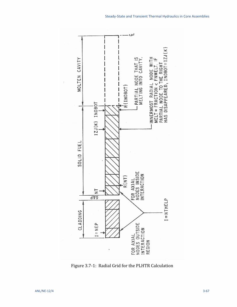
Steady-‐State and Transient Thermal Hydraulics in Core Assemblies
ANL/NE-‐12/4 3-‐67
Figure 3.7-‐1: Radial Grid for the PLHTR Calculation

The SAS4A/SASSYS-‐1 Safety Analysis Code System
3-‐68 ANL/NE-‐12/4
the array HFPICL, calculated in the PLUTO routine PLMISE or in the LEVITATE routine LESDEN. The integrated heat flux at the cavity boundary is obtained from the array HFCAWA; calculated in the PLUTO routine PC1PIN or the LVITATE routine LE1PIN. Moreover, the heat conduction terms at the fuel surface, which are necessary in the TSHTRV calculation, had to be set to zero. This meant setting the term BETA (NTHELP) in Eq. 3.3-‐48 to zero and ignoring all equations related to the cladding in Eq. 3.3-‐48.
3.8 Heat-‐transfer Time Step Control Each channel uses its own separate heat-‐transfer time step size, so that channels in
which temperatures are changing rapidly or in which boiling is occurring can use small heat-‐transfer time steps while other channels use larger steps.
After each heat-‐transfer time step, the size of the next step is determined, based on number of criteria. Most of these criteria are based on user-‐supplied values for maximum time step sizes and maximum temperature changes per step. The time step used in the smallest of the various criteria. If not other factor is more limiting, then the next heat-‐transfer step size is set equal to the initial main time-‐step size. This is usually in the range of .05-‐1.0 s. After the onset of boiling in a channel, a maximum boiling heat-‐transfer time step size, typically .01-‐.02 s, is used. In addition, a heat-‐transfer time step cannot go past the end of a main time step. Also, if the channel has not started boiling yet, then an attempt is made to end a heat-‐transfer time step right at, or very close to, the time when the first bubble is formed. For this purpose, the pre-‐boiling coolant routines make an estimate of the boiling time at the end of each coolant time step. The boiling time estimate is based on linear extrapolations in time for the coolant temperature and the saturation temperature at each axial node. The other criteria are based on the rate of change of the temperatures. The user supplies values of the maximum change per time step for the fuel and clad temperatures. Typical values are in the range of 30-‐50K. The rate of change of the fuel center-‐line temperature, the fuel surface temperature, and the clad mid-‐point temperature at each axial node are used to determine maximum time step sizes. After the minimum of the various time-‐step criteria has been found, the time step size is rounded to eight decimal places to minimize differences in results caused by different round-‐off errors on different computers. These criteria are summarized in Table 3.8-‐1.
Table 3.8-‐1: Criteria for Heat-‐Transfer Time Step Sizes 1. Initial time step size
2. Maximum boiling time step size, if boiling
3. End of a main time step
4. Initiation of boiling
5. Maximum fuel center-‐line temperature change
6. Maximum fuel surface temperature change
7. Maximum clad mid-‐point temperature change

Steady-‐State and Transient Thermal Hydraulics in Core Assemblies
ANL/NE-‐12/4 3-‐69
3.9 Steady-‐State and Single-‐Phase Transient Hydraulics
3.9.1 Introduction The core assembly hydraulics treatment in SAS4A and SASSYS-‐1 includes the
calculation of coolant flow rates and pressure distributions within each core channel. Coolant flow rates and pressures are calculated in a number of different places in the codes. They are used in the steady-‐state thermal hydraulics initialization; the pre-‐voiding thermal hydraulics module calculates coolant flows and pressures; and after the onset of voiding, they are calculated in the boiling module. This section describes only the steady-‐state and pre-‐voiding calculations. Chapter 12 describes the hydraulics calculations after the onset of voiding. Chapters 14 and 16 describe the hydraulics calculations after pin disruption.
The coolant flow provides the heat removal from the fuel pins, and so the main reason for calculating coolant flow rates before the onset of voiding is to provide information for the fuel-‐pin temperature calculations. Core channel flow rates are also needed for the PRIMAR-‐4 primary loop thermal hydraulics calculations. The pressure distribution within a channel is calculated mainly to obtain the pressure-‐dependent coolant saturation temperature used to determine the onset of boiling.
For the steady-‐state initialization the user specifies the initial coolant flow rate for each channel and the outlet plenum pressure. The code then calculates the pressure distribution in each channel, starting from the outlet and working down to the inlet. The channel with the largest steady-‐state pressure drop is used to determine the steady-‐state inlet plenum pressure; and the inlet orifice coefficients in all other channels are adjusted so that all channels have the same total steady-‐state pressure drop.
In the transient hydraulic calculations, both the coolant flow rates and the pressure distributions are calculated for each channel. Pressure boundary conditions are used for the transient coolant flow rate calculations. The driving pressures for these calculations are the inlet and outlet coolant plenum pressures supplied by the PRIMAR-‐4 module. Since all channels use the same inlet and outlet pressures, flow redistribution between channels is automatically accounted for as temperatures and flows change. Extrapolated coolant temperatures are used to evaluate coolant properties in the transient hydraulics calculations, since coolant flow rates for a time step are calculated before temperatures are calculated.
Figure 3.1-‐2 shows the logic flow in subroutine TSCL0, the driver for pre-‐voiding core channel thermal hydraulics. As indicated previously, a multi-‐level time step approach is used for the transient calculations in SAS4A and SASSYS-‐1. In general, the routines in a transient module start with all quantities knows at the beginning of a time step, and a pass through a module results in calculating the values of relevant parameters of the module for one channel at the end of the time step. Different time-‐step sizes can be used for different phenomena. In particular, the pre-‐voiding coolant hydraulics time step can be smaller than, but not larger than, the heat-‐transfer time step or the PRIMAR time step. One pass through TSCL0 calculates one coolant time step

The SAS4A/SASSYS-‐1 Safety Analysis Code System
3-‐70 ANL/NE-‐12/4
for one channel. If the coolant time step finishes a heat-‐transfer step, then the temperature calculations for the heat-‐transfer step are also carried out.
Figure 3.9-‐1 shows the logic flow in subroutine TSCNV1. This subroutine and the routines called by it carry out the pre-‐viding coolant flow and pressure calculations. Subroutine TSCNV1 also checks on whether to switch to the boiling model.
As indicated in Fig. 3.9-‐2, the pre-‐voiding transient hydraulics module interacts with PRIMAR and TSHTRN. PRIMAR supplies the inlet and outlet pressures that drive the coolant flows in the core channels. In return, TSCL0 supplies PRIMAR with the current channel flow rates, as well as hydraulic parameters to use in estimating future flow rates for the next PRIMAR time step. TSCL0 supplies the coolant flow rates to TSHTRN, and TSHTRN computes the coolant temperatures used by TSCL0.
3.9.2 Basic Equations Before the onset of voiding, the coolant is treated as incompressible, and the
basic equation used for liquid coolant flow in non-‐voided channels is
1!!!"!" +
!"!" +
1!!! !"!" = −
!"!" !"
−!"!" !
− !!! (3.9-‐1)
with w = w(t)-‐independent of z
w = coolant flow rate (kg/s) = !! ! !!
Ac = coolant flow area
p = pressure
ρc = density
v = coolant velocity (m/s)
z = axial position
t = time
droppressurefriction=⎟⎠
⎞⎜⎝
⎛∂∂
frzp
hcfr DAzp
2c
2
2wf
ρ=⎟
⎠
⎞⎜⎝
⎛∂∂
(3.9-‐2)

Steady-‐State and Transient Thermal Hydraulics in Core Assemblies
ANL/NE-‐12/4 3-‐71
Figure 3.9-‐1: Subroutine TSCNV1, Pre-‐Boiling Coolant Flow Rates and Pressure Distribution

The SAS4A/SASSYS-‐1 Safety Analysis Code System
3-‐72 ANL/NE-‐12/4
Figure 3.9-‐1: Subroutine TSCNV1, Pre-‐Boiling Coolant Flow Rates and Pressure Distribution (Cont’d)

Steady-‐State and Transient Thermal Hydraulics in Core Assemblies
ANL/NE-‐12/4 3-‐73
Figure 3.9-‐2: Interactions Between Pre-‐Voiding Transient Hydraulics and Other Modules

The SAS4A/SASSYS-‐1 Safety Analysis Code System
3-‐74 ANL/NE-‐12/4
f = friction factor, approximated either as
! = !!" Re !!" if Re ≥ !!"
!!"
Re if Re < !!" (3.9-‐3a)
or as
( ) Re/Re fLb
fr AAf fr += (3.9-‐3a)
where Afr bfr, and AfL are user-‐supplied correlation coefficients
Re = numberReynolds=
c
h
AwD
µ (3.9-‐4)
ReL = Reynolds number for the transition from turbulent to laminar flow
μ = viscosity
Dh = hydraulic diameter
Kzp⎟⎠
⎞⎜⎝
⎛∂∂
= orifice pressure drop
g = acceleration of gravity
ρ = density
The axial node structure shown in Fig. 3.2-‐3 is used for the coolant. Figure 3.9-‐3 shows which variables are defined at node boundaries and which are averages or integrals over the length of a node. With this mesh structure, integrating Eq. 3.9-‐1 over the length of the channel gives
!!!"!" + !! − !! + !
!!! + !!"! ! !!!!"!! + ! ! !! + ! !! = 0 (3.9-‐5)
where
!! = !"!!
=!!!! !
+!!!! !
+ !!! JCMZC!!
JC!!
(3.9-‐6)
and

Steady-‐State and Transient Thermal Hydraulics in Core Assemblies
ANL/NE-‐12/4 3-‐75
Figure 3.9-‐3: Interactions Between Pre-‐Voiding Transient Hydraulics and Other Modules

The SAS4A/SASSYS-‐1 Safety Analysis Code System
3-‐76 ANL/NE-‐12/4
XI1 JC( ) =!z JC( )Ac JC( )
(3.9-‐7)
!!!! !
and !!!! !
are effective inertial terms at the bottom and top of the subassembly.
I2 = XI 2 JC( )JC=1
MZC-1
!
(3.9-‐8)
XI 2 JC( ) = 1Ac JC( )2
1!c JC+1( )
!1
!c JC( )
"
#$$
%
&''
(3.9-‐9)
I3 =1
2!cAc2Dh
Dh
µAc
!
"#
$
%&'bfr
dz = XI3 JC( )JC=1
MXC(1
)
(3.9-‐10)
!!" JC =!"(JC)
!! JC + !! JC+ 1 !! JC !!! JC
!! JC! JC !! JC
!!"
(3.9-‐11)
I4 = Kor JC( )JC=1
MZC!1
"
(3.9-‐12)
I5 = !c dz! = XI 5 JC( )JC=1
MXC"1
#
(3.9-‐13)
XI 5 JC( ) = .5 !c JC( )+ !c JC+1( )!" #$%z JC( ) (3.9-‐14)
pb = pressure at bottom of channel, and pt – pressure at top of channel.
3.9.3 Flow Orifices As mentioned in the section on the SAS channel treatment in Section 3.2, the channel
is divided axially into a number of zones. One zone represents the fuel-‐pin region. Other zones represent regions above and below the fuel pins. At the bottom of each zone, a flow direction dependent orifice coefficient can be specified by the user. Another orifice coefficient can be used at the top of the upper zone. These orifices can represent orifice blocks, subassembly inlet and exit losses, and the pin support grid at the bottom of the pins. For each orifice, the user supplies one orifice coefficient for

Steady-‐State and Transient Thermal Hydraulics in Core Assemblies
ANL/NE-‐12/4 3-‐77
positive flow and another for negative flow. In addition, in the fuel-‐pin region, orifice coefficients representing equally spaced grid spacers can be specified. These orifice coefficients are used as the values of Kor(JC) in Eq. 3.9-‐12 for the appropriate axial nodes. The effect of each orifice is spread evenly over an axial node, rather than concentrated at a point.
3.9.4 Finite Difference Equations – Coolant Flow Rates If !! = ! ! ,!! = ! ! + !" ,!" = !! − !!, then we approximate Δw as
!" = !!!"!" !
+ !!!"!" !!!"
!" (3.9-‐15)
and
0.121 =+θθ (3.9-‐16)
in which θ2 is the degree of implicitness. For small time steps a semi-‐implicit calculation is used, with θ1 = θ2 = .5. For a fully implicit calculation for large time steps, θ1 = 0 and θ2 = 1.0. The value used for θ2 is
2
2
2 56284.312992.6266054.212992.6
xxxxx++
++=θ
(3.9-‐17)
where
x = Δt/τ (3.9-‐18)
and τ is the time constant for flow rate changes given by
! = !!/!! (3.9-‐19)
The definition of d1 is given by Eq. 3.9-‐25 below. This correlation for θ2 is discussed in Appendix 3.1. The additional approximations are made that
!! + !" ! ≃ !!! + 2!" !! (3.9-‐20)
( ) wwwwwwww Δ+−Δ+Δ+ 11111 2~ (3.9-‐21)
!! + !" !! + !" !!!!" ≃ !! !! !!!!" + 2+ !!" !! !!!!" !" (3.9-‐22)
These equations are combined to give

The SAS4A/SASSYS-‐1 Safety Analysis Code System
3-‐78 ANL/NE-‐12/4
!!!"!" + !! !!! − !!! + !! !!! − !!! + !! !!! + 2!!!!!"
+ !!"!! !! !! !!!!" + !! 2+ !!" !! !!!!"!"
+ !! !! !! + 2!! !! !" + !!! = 0
(3.9-‐23)
where pt1 and pt2 are the pressures at the top of the subassembly at the beginning and end of the time step. Similarly, pb1 and pb2 are the pressures at the bottom of the subassembly at the beginning and end of the time step, respectively.
Solving for the coolant flow rate change, Δw, gives
!w = !t !1 pb1 " pt1( )+!2 pb2 " pt2( )" I2w12 " AfrI3w1 w11+bfr#
$
"I4w1 w1 " g I5%&/ I1 +!t!2d1( )
(3.9-‐24)
where
!! = 2 !! !! + 2+ !!" !! !!!!" !!" !! + 2 !! !! (3.9-‐25)
The temperatures used to evaluate ρc and µ in Eqs. 3.9-‐9, 3.9-‐11, and 3.9-‐14 are extrapolated coolant temperatures, extrapolated to the end of the coolant step.
3.9.5 Coolant Pressures After the flow rate has been calculated, the coolant pressures in a channel at the end
of a time step are calculated. First, the pressure at node MZC, the last node at the top of the subassembly, is calculated as
p MXC( ) = pt2 +!ziA
"
#$%
&'t
(w(t
(3.9-‐26)
where
pt2 =!!! + !!"#$ ! !!"# − !! MZC (3.9-‐27)
zphi = outlet plenum elevation
!!"#$ = density at outlet
Steady-‐State and Transient Thermal Hydraulics in Core Assemblies
ANL/NE-‐12/4 3-‐79
px2 = coolant outlet plenum pressure at the end of the time step
Note that px2, the outlet plenum pressure supplied by the primary loop module, is defined at an elevation zplu, the elevation of the upper plenum, whereas ! MZC is calculated at ! MZC , so the gravity head term occurs in Eq. 3.9-‐27.
After ! MZC has been calculated, the other pressures are calculated, starting at node MZC-‐1 working down, using
p JC( ) = p JC+1( )+ XI1 JC( )!w!t
+w2 XI 2 JC( )+ Afr w w 1+bfr XI3 JC( )
+ w wKor JC( )+ gXI 5 JC( )
(3.9-‐28)
In Eqs. 3.9-‐25 and 3.9-‐28, the value used for ∂w/∂t is calculated at the end of the time step for the transient calculation as
!w!t
= pb2 " pt2[ "w22 I2 " Afrw2 w2
1+bfr I3"w2 w2 I4 " g I5#$ / I1 (3.9-‐29)
The pressure, pb2 at the bottom of the subassembly at the end of the time step is calculated as
pb2 = pin2 ! !cin g zc 1( )! zp!!"# $% (3.9-‐30)
pz = plenum location. Note that pin2, the inlet plenum pressure supplied by he primary loop module, is defined at an elevation pz , the elevation of the lower plenum.
The pressure distribution in the steady state is calculated the same as in the transient, except that ∂w/∂t is zero in the steady-‐state calculation.
3.10 Multiple-‐Pin Model
3.10.1 Introduction The new multiple pin treatment was added to the code to account for pin-‐to-‐pin
variations within a subassembly. This new multiple pin treatment can be used in at least two different ways. One approach is to use the new treatment to compute nominal or “best estimate” variations within a subassembly. Another approach is to compute hot channel behavior due to postulated deviations in coolant flow rate, coolant flow area, and pin power. When doing a whole-‐core analysis, one probably would not want the hot channel temperatures used in reactivity feedback calculation or in the core outlet temperatures that feed into the primary loop calculations. Therefore, one would probably use parallel treatments for the same subassembly: a nominal one-‐pin or multi-‐pin treatment used for reactivity feedback, plus a hot channel treatment decoupled from the reactivity feedback and from the primary loop calculation. The hot

The SAS4A/SASSYS-‐1 Safety Analysis Code System
3-‐80 ANL/NE-‐12/4
channel treatment would be de-‐coupled by setting reactivity feedback coefficients to zero and by setting the number of subassemblies represented by this treatment to zero.
The new multiple pin treatment allows a number of coupled channels to be used to model a single subassembly. Thus a channel can represent a part of a subassembly instead of the whole subassembly. Peaking factors can be mechanistically calculated by reducing coolant flow areas and flow rates or increasing pin power levels in some channels.
As previously mentioned, the multiple pin option is currently only available for steady-‐state and single phase transient calculations.
3.10.2 Physical Model In the new multiple pin option, the regions above and below the pin section of a
subassembly are still represented by a single channel; but a number of channels can be used to represent the pin section. Each channel in the pin section can represent one or more concentric rows of pins and their associated coolant. It is also possible for channels to represent slices of pins for a subassembly with a strong lateral power skew or for one with a hot subassembly on one side and a cool subassembly on the opposite side. Figure 3.10-‐1 illustrates one way that a number of channels can be used to model the pin section of a subassembly as concentric rings of pins and coolant subchannels. The thimble flow region in this figure is a feature of the EBR-‐II XX09 instrumented subassembly and is not found in ordinary subassemblies. This case concentrates on the coolant subchannels and splits the pins. It is also possible to shift the channel boundaries half a pin and use a pin-‐based representation with intact pins and split coolant subchannels. Currently up to 56 channels can be used to represent a subassembly.
The new option accounts for coolant-‐to-‐coolant heat transfer between adjacent channels, including the effects of both conduction and turbulent mixing. It also accounts for subassembly-‐to-‐subasembly heat transfer from the duct wall of a subassembly, through the interstitial sodium, to the duct wall of a neighboring subassembly. In addition, axial conduction in the coolant is accounted for.
Figure 3.10-‐2 illustrates the axial representation of the subassembly flow, with parallel flow paths through the pin section. Each channel used to represent the pin section of subassembly has its own separate time-‐dependent flow rate, and the flow rates in all channels in a subassembly are driven by common pressures at the inlet and outlet of the pin section. Thus, transient flow redistribution among channels is accounted for. The single flow rate in the regions above and below the pin section is the sum of the pin section flow rates, so the subassembly flow orifice sees the correct total flow rate. Even though the coolant-‐to-‐coolant heat transfer coefficient includes a term for turbulent mixing between coolant subchannels, one effect that the flow calculation does not account for is mass flow between channels in the pin section, although cross-‐flow at the ends of the pin section is allowed. Therefore, if recirculation loops occur within a subassembly at low flows, the model would calculate them; but the recirculation loops would go to the ends of the pin section.

Steady-‐State and Transient Thermal Hydraulics in Core Assemblies
ANL/NE-‐12/4 3-‐81
Figure 3.10-‐1: SASSYS-‐1 Multiple Pin Representation and Thermocouple Locations for the EBR-‐II XX09 Instrumented Subassembly

The SAS4A/SASSYS-‐1 Safety Analysis Code System
3-‐82 ANL/NE-‐12/4
Figure 3.10-‐2: SASSYS-‐1 Multiple Pin Treatment of a Subassembly
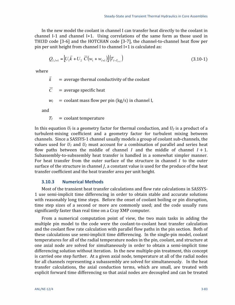
Steady-‐State and Transient Thermal Hydraulics in Core Assemblies
ANL/NE-‐12/4 3-‐83
In the new model the coolant in channel I can transfer heat directly to the coolant in channel I-‐1 and channel I+1. Using correlations of the same form as those used in THI3D code [3-‐6] and the HOTCHAN code [3-‐7], the channel-‐to-‐channel heat flow per pin per unit height from channel I to channel I+1 is calculated as:
( )[ ] ( )111211, +−++ ++=
ITIIII TwwCUkUQ (3.10-‐1)
where
k = average thermal conductivity of the coolant
C = average specific heat
wi = coolant mass flow per pin (kg/s) in channel I,
and TI = coolant temperature
In this equation UI is a geometry factor for thermal conduction, and U2 is a product of a turbulent-‐mixing coefficient and a geometry factor for turbulent mixing between channels. Since a SASSYS-‐1 channel usually models a group of coolant sub-‐channels, the values used for U1 and U2 must account for a combination of parallel and series heat flow paths between the middle of channel ! and the middle of channel ! + 1. Subassembly-‐to-‐subssembly heat transfer is handled in a somewhat simpler manner. For heat transfer from the outer surface of the structure in channel ! to the outer surface of the structure in channel !, a constant value is used for the produce of the heat transfer coefficient and the heat transfer area per unit height.
3.10.3 Numerical Methods Most of the transient heat transfer calculations and flow rate calculations in SASSYS-‐
1 use semi-‐implicit time differencing in order to obtain stable and accurate solutions with reasonably long time steps. Before the onset of coolant boiling or pin disruption, time step sizes of a second or more are commonly used; and the code usually runs significantly faster than real time on a Cray XMP computer.
From a numerical computation point of view, the two main tasks in adding the multiple pin model to the code were the coolant-‐to-‐coolant heat transfer calculation and the coolant flow rate calculation with parallel flow paths in the pin section. Both of these calculations use semi-‐implicit time differencing. In the single-‐pin model, coolant temperatures for all of the radial temperature nodes in the pin, coolant, and structure at one axial node are solved for simultaneously in order to obtain a semi-‐implicit time differencing solution without iteration. In the new multiple-‐pin treatment, this concept is carried one step further. At a given axial node, temperature at all of the radial nodes for all channels representing a subassembly are solved for simultaneously. In the heat transfer calculations, the axial conduction terms, which are small, are treated with explicit forward time differencing so that axial nodes are decoupled and can be treated

The SAS4A/SASSYS-‐1 Safety Analysis Code System
3-‐84 ANL/NE-‐12/4
separately except for the coolant convection terms. The axial coupling due to the coolant convection terms is handled by starting at one end of the subassembly and solving for axial nodes one at a time in the direction of the flow. If flow has reversed in some channels but not in others, the calculation progresses in the direction of the dominate flow; and explicit forward differencing is used for the coolant convection terms in the non-‐dominate flow direction channels. The subassembly-‐to-‐subassembly heat fluxes are calculated with explicit forward differencing in time, and this does impose a stability limit on the time step size. For typical subassembly duct wall thicknesses, the explicit subassembly-‐to-‐subassembly heat flux calculation limits the maximum time step size to a value in the range from .25 to .5 seconds. For the coolant flow rate calculations, the incompressible flow momentum equations are linearized about conditions at the beginning of the time step. Then, flow at the end of the step are calculated for all channels in a subassembly simultaneously.
A null transient is used to obtain steady-‐state temperatures at the start of the regular transient. First all coolant, pin, structure, and reflector temperatures in all subassemblies are set to the coolant inlet temperature. Then, the power levels and coolant flow rates are held constant while a number of transient heat transfer time steps are made. Since the pin thermal time constant and the coolant transit time through a subassembly are both less than a second, the null transient results converge rapidly if reasonably large time steps are used.
3.10.4 Detailed Mathematical Treatment The main computational parts of the new multiple pin model are the heat transfer
calculations in the pin section of a subassembly, the coolant flow rate calculations for a subassembly, the subassembly-‐to-‐subassembly heat transfer, and changes to the driver routines to call the appropriate new routines at the proper times. The pin section heat transfer calculations are done in two new subroutines: TSHTM3 calculates temperatures in the core and axial blankets, and TSHTM2 calculates temperatures in the gas plenum region. The existing TSHTN1 still calculates temperatures in the reflector zones above and below the pin section, but it was modified. TSHTN1 had to be modified slightly to pick up mixed mean outlet temperatures from the multiple channels representing the pin section. Also, axial conduction in the coolant was added to TSHTN1. The new TSCLM1 routine calculates transient coolant flow rates for a subassembly. The subassembly-‐to-‐subassembly heat fluxes are calculated in CHCHFL.
3.10.4.1 Heat Transfer Calculations in the Core and Axial Blankets: Subroutine TSHTM3
The multiple pin heat transfer calculations for the core and axial blankets in subroutine TSHTM3 are similar to the single pin calculations in the existing subroutine TSHTN3, as described in Section 3.3.1. One difference is that TSHTN3 does one time step for one channel each time it is called, whereas TSHTM3 solves for temperatures in all pins or channels representing a subassembly when it is called. Also, TSHTM3 adds extra terms for coolant-‐to-‐coolant heat transfer; and TSHTM3 includes axial conduction in the coolant.
Within a fuel pin, one-‐dimensional radial heat transfer is used. The basic heat

Steady-‐State and Transient Thermal Hydraulics in Core Assemblies
ANL/NE-‐12/4 3-‐85
transfer equation is Eq. 3.3-‐1. This part of the calculation in TSHTM3 is identical to the corresponding calculation in TSHTN3.
For the coolant in channel I, the heat transfer calculations are basically one-‐dimensional in the axial direction, with extra terms for coolant-‐to-‐coolant heat transfer from channel I-‐1 and I+1. The basic heat transfer equation is:
( ) cTc AQwcTzt
TcA =∂
∂+
∂
∂ρ
(3.10-‐2)
where Ac = coolant flow area
! = axial position
! = coolant mass flow rate
and Qr = total heat source per unit volume
The heat source contains a number of terms:
1.,1 +− ʹ′−ʹ′++++= IIIIaxsceccT QQQQQQQ (3.10-‐3)
where Qc = source due to direct heating of the coolant by neutrons and gamma rays,
Qec = heat flow from cladding to coolant,
Qsc = heat flow from structure to coolant,
Qax = axial conduction source, given by
zTk
zQax ∂
∂
∂
∂=
(3.10-‐4)
and
c
IIII A
QQ 1,
1,+
+ =ʹ′
(3.10-‐5)
where 1, +ʹ′ IIQ is given by equation 3.10-‐1. Note that Eq. 3.10-‐2 is the same as Eq. 3.3-‐5, except that additional source terms are included in the multiple pin model.

The SAS4A/SASSYS-‐1 Safety Analysis Code System
3-‐86 ANL/NE-‐12/4
Finite differencing in space and time is used to solve these heat transfer equations. Figure 3.2-‐3 shows the axial and radial mesh used for a single channel. In the multiple pin model the pin section mesh is repeated for each channel, but the axial reflector zones are only used in the first channel used to represent a subassembly. At each axial node in the core and axial blankets a number of radial nodes are used for the fuel, three radial nodes are used for the cladding, one node is used in the coolant, and two nodes are used in the structure. All channels, representing a subassembly must use the same axial mesh. Also, all subassemblies connected by subassembly-‐to-‐subassembly heat transfer must use the same axial mesh.
For a given time step, Eqs. 3.3-‐1 and 3.10-‐2 become linear finite difference equations. The temperatures are known at the beginning of the time step, and the temperature at the end of the step are the unknowns to be solved for. Semi-‐implicit time differencing is used for all terms except the axial conduction terms Qax, and the coolant-‐to-‐coolant terms IIQ ,1− and 1, +ʹ′ IIQ . The Qax axial conduction term is calculated explicitly based on temperatures at the beginning of the time step. The coolant-‐to-‐coolant terms are calculated fully implicitly, using the coolant flow rates and temperatures at the end of the step.
After finite differencing for one axial node, one obtains N simultaneous liner equations in N unknowns, where the unknowns are the temperatures at the end of the time step for all radial nodes in all channels representing the subassembly. These equations are solved by Gaussian elimination. The equations are basically tri-‐diagonal, with extra non-‐tri-‐diagonal terms for coolant-‐to-‐coolant heat transfer between channels. No full N by N matrix is ever set up by TSHTM3, and a general full matrix solution package is not used. Instead, only non-‐zero terms are computed and stored; and the Gaussian elimination solution was written specifically for this set of equations. The result is that the storage requirements vary linearly, rather than quadratically, with the maximum allowable value for N; and the computation time varies linearly, rather than quadratically, with the actual value of N.
3.10.4.2 Heat Transfer Calculations in the Gas Plenum Region: Subroutine TSHTM2 Subroutine TSHTM2 does the heat transfer calculations for one time step for all axial
nodes in the gas plenum region for all channels representing a subassembly when it is called. TSHTM2 is similar to TSHTM3, but TSHTM2 deals with fewer radial nodes. As shown in Figure 3.2-‐5, in the plenum region there are still two radial nodes in the structure and one in the coolant; but there is only one in the cladding; and there are no fuel nodes. Instead of fuel temperatures there is one gas temperature common to all of the axial nodes in a pin. As in TSHTM3, for a given axial node TSHTM2 solves simultaneously for temperatures at all radial modes in all channels representing a subassembly.
One special problem in TSHTM2 is the gas temperature, which is common to all axial nodes in the gas plenum region of a pin. Axial nodes are handled one at a time, rather than simultaneously, whereas a semi-‐implicit time differencing treatment would require solving for all axial nodes simultaneously. The new multiple-‐pin TSHTM2 routine handles this problem in a simpler manner than the old single-‐pin TSHTN2. The

Steady-‐State and Transient Thermal Hydraulics in Core Assemblies
ANL/NE-‐12/4 3-‐87
way that the gas temperature is handled is TSHTM2 is to calculate a separate gas temperature for each axial node. At the beginning of the time step, the gas temperatures at all axial nodes are set to one common value. Then separate values are calculated for each axial node at the end of the step. Finally, an average of the separate values is calculated for the one common value at the ed of the step.
3.10.4.3 Coolant Flow Rates: Subassembly TSCLM1 The coolant for rate calculation for a subassembly in the multiple-‐pin routine
TSCLM1 is much more complex than the corresponding calculation in the single pin routine TSCNV1. As shown in Figure 3.10-‐2, the multiple pin calculation involves multiple parallel flow paths in the pin section, in series with single flow paths in the reflector regions. Therefore, the multiple-‐pin routine TSCLM1 was written from scratch, rather than starting form the single pin TSCNV1 routine.
Figure 3.10-‐3 illustrates the main variables used in TSCLM1. Incompressible flow is used for these calculations, so conservation of mass gives
∑=k
kpkr NwwN1
(3.10-‐6)
where wr = coolant mass flow rate per pin in the reflector zones,
wpk = pin section coolant mass flow rate per pin in channel k,
Nk = number of pins in channel k,
and I = channel number of the first channel representing the subassembly.
The momentum equation for the pin section is
Lp
Acpk
dwpk
dt= pb ! pc !"ppk
(3.10-‐7)

The SAS4A/SASSYS-‐1 Safety Analysis Code System
3-‐88 ANL/NE-‐12/4
Figure 3.10-‐3: Subassembly Coolant Flows
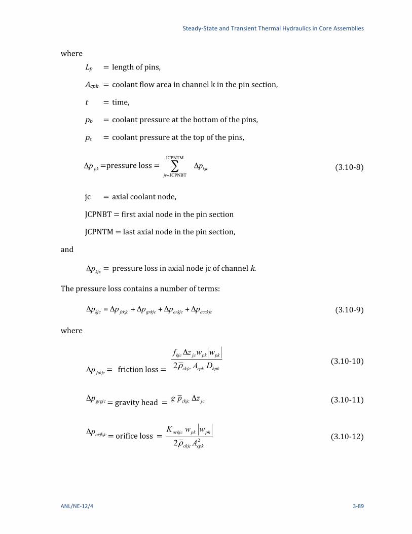
Steady-‐State and Transient Thermal Hydraulics in Core Assemblies
ANL/NE-‐12/4 3-‐89
where Lp = length of pins,
Acpk = coolant flow area in channel k in the pin section,
t = time,
pb = coolant pressure at the bottom of the pins,
pc = coolant pressure at the top of the pins,
pkpΔ =pressure loss = !pkjcjv=JCPNBT
JCPNTM
"
(3.10-‐8)
jc = axial coolant node,
JCPNBT = first axial node in the pin section
JCPNTM = last axial node in the pin section,
and
kjcpΔ = pressure loss in axial node jc of channel k.
The pressure loss contains a number of terms:
acckjcorkjcgrkjcfrkjckjc ppppp Δ+Δ+Δ+Δ=Δ (3.10-‐9)
where
frkjcpΔ = friction loss = hpkcpkckjc
pkpkjckjc
DAwwzf
ρ2Δ
(3.10-‐10)
grpjcpΔ = gravity head = jcckjc zpg Δ (3.10-‐11)
orfkjcpΔ = orifice loss = 22 cpkckjc
phpkorkjc
A
wwK
ρ (3.10-‐12)

The SAS4A/SASSYS-‐1 Safety Analysis Code System
3-‐90 ANL/NE-‐12/4
acckjcpΔ = acceleration term =
wpk2
Acpm2
1!ckjc+1
!1!ckjc
"
#$$
%
&''
(3.10-‐13)
jczΔ = axial node length,
kjcf = friction factor in channel k at node jc,
ckjcρ = coolant density at bottom of node jc in channel k,
ckjcρ = average coolant density in node jc in channel k,
hpkD = Hydraulic diameter,
and
orkjcK = orifice coefficient in node jc of channel k
The friction factor is calculated as in Eq. 3.9-‐3.
using
eR =Reynolds number = Dhpk wpk
µkjc Acpk (3.10-‐14)
and
kjcµ = viscosity of the coolant.
After semi-‐implicit finite differencing in time and linearization of the pressure drop terms, applying Eq. 3.10-‐7 to a time step from t to t + Δt gives
( ) ( ) ( ) wpkpkpkccbbpk
cpk
p Kwtpptpptptw
AL
Δ−Δ−Δ−−Δ+=Δ
Δ222 θθθ
(3.10-‐15)
where
pkwΔ = ( ) ( )twttw pkpk −Δ+ (3.10-‐16)
bpΔ = ( ) ( )tpttp bb −Δ+ (3.10-‐17)

Steady-‐State and Transient Thermal Hydraulics in Core Assemblies
ANL/NE-‐12/4 3-‐91
cpΔ = pc t +!t( )" pc t( ) (3.10-‐18)
2θ = degree of implicitness
1θ = 21 θ− (3.10-‐19)
Kwpk = Kwpkjcjc=JCPNBT
JCPNTM
!
(3.10-‐20)
acckjcwcrkjcfrkjcpk
kjcwpkjc KKK
wp
K ++=∂
Δ∂=
(3.10-‐21)
( ) ( )( )
( )( )⎪
⎪
⎩
⎪⎪
⎨
⎧
<Δ
≥Δ
+
=
etckjcpk
frkjc
etckjcpk
frkjcfr
frkjc
RRtwtp
RRtwtp
b
K
if
if2
(3.10-‐22a)
or
K frkjc = 2+ bfr( )Afr A RE( )bfr + AfL / RE!"
#$%zjc wpk t( )2pckjcDhpkAcpk
(3.10-‐22b)
( )( )twtp
Kpk
orfkjcwpkjc
Δ=2
(3.10-‐23)
and
( )( )twtp
kpk
acckjcacckjc
Δ=2
(3.10-‐24)
Equation 3.10-‐15 can then be written as
!pb "!pc = d0 pk + d0 pk + d1pk!wpk (3.10-‐25)
where

The SAS4A/SASSYS-‐1 Safety Analysis Code System
3-‐92 ANL/NE-‐12/4
( ) ( ) ( )2
0 θ
tptptpd pkbc
pk
Δ+−=
(3.10-‐26)
and
tKtAL
d wpkcpkppk Δ
Δ+=
2
21
/θ
θ
(3.10-‐27)
Applying a similar process to the upper and lower reflector regions gives:
pkk
b wDDp Δ+=Δ ∑ 10
(3.10-‐28)
and
!pc = D0u +D1uk" !wpk
(3.10-‐29)
where
( ) ( ) ( ) ( )2
210 θ
θθ tptpttptpD baa
Δ−−Δ++=
(3.10-‐30)
D1! =! Lkz / AcKZ
KA=1
KZPIN!1
" !!2#t Kw!
!2#t
(3.10-‐31)
( ) ( ) ( ) ( )2
210 θ
θθ tptpttptpD ucddu
Δ+−Δ++=
(3.10-‐32)
D1u =LKZ / AcKZ
KZ!KZPIN+1
KZM
" +!2#t Kwu
!2#t
(3.10-‐33)
LKZ = length of zone kz
AcKZ = coolant flow area in zone kz
KZPIN = axial zone number of the pin section

Steady-‐State and Transient Thermal Hydraulics in Core Assemblies
ANL/NE-‐12/4 3-‐93
KZM = last zone number
!p! = !prjcjc=1
JCPNBT"1
#
(3.10-‐34)
!pu = !prjcjc=JCPNTP
MZCM1
"
(3.10-‐35)
Δprjc = pressure loss in node jc of a reflector zone
JCPNBT = first axial node in pin section
JCPNTP = first axial node above the pin section
MZCM1 = last axial node
rw w
pK∂
Δ∂=
(3.10-‐36)
and
u
uwu w
pK∂
Δ∂=
(3.10-‐37)
Then, combining Eqs. (3.10-‐25) and (3.10-‐28) gives
cob pBBp Δ+=Δ 1 (3.10-‐38)
where
Bo =Do! !D1! S11!D1 f So
,
(3.10-‐39)
!! =−!!!!!1− !!!!!
(3.10-‐40)
∑=k pk
o dS ,1
1 (3.10-‐41)
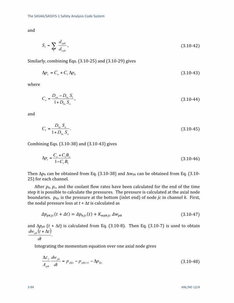
The SAS4A/SASSYS-‐1 Safety Analysis Code System
3-‐94 ANL/NE-‐12/4
and
∑=k pk
opk
dd
S ,1
1
(3.10-‐42)
Similarly, combining Eqs. (3.10-‐25) and (3.10-‐29) gives
boc pCCp Δ+=Δ 1 (3.10-‐43)
where
,1 1
11
ou
uouo SD
SDDC+
−=
(3.10-‐44)
and
.1 1
11
ou
ou
SDSD
C+
=
(3.10-‐45)
Combining Eqs. (3.10-‐38) and (3.10-‐43) gives
!pc =Co +C1Bo1"C1B1
(3.10-‐46)
Then Δpb can be obtained from Eq. (3.10-‐38) and Δwbk can be obtained from Eq. (3.10-‐25) for each channel.
After pb, pc, and the coolant flow rates have been calculated for the end of the time step it is possible to calculate the pressures. The pressure is calculated at the axial node boundaries. pkjc is the pressure at the bottom (inlet end) of node jc in channel k. First, the nodal pressure loss at t + Δt is calculated as
!!!"#$ ! + !" = !!!"# ! + !!"#$% !!!" (3.10-‐47)
and Δppk (t + Δt) is calculated from Eq. (3.10-‐8). Then Eq. (3.10-‐7) is used to obtain ( )
.dt
ttdwpk Δ+
Integrating the momentum equation over one axial node gives
kjcpkjcpkjcpk
cpk
j pppdtdw
Az
Δ−−=Δ
+1
(3.10-‐48)

Steady-‐State and Transient Thermal Hydraulics in Core Assemblies
ANL/NE-‐12/4 3-‐95
Starting by setting
cpkjJCPNTP Pp = (3.10-‐49)
the code marches down the channel, using Eq. (3.10-‐48) to obtain ppkjc after ppkjc+1 has been calculated. A similar procedure is used for calculating the pressures in the upper and lower reflector zones.
The equation used to compute the degree of implicitness as a function of time step size in TSCMV1 is
2
2
2 2 xcxaxbxa++
++=θ
(3.10-‐50)
where
x=Δt/τ (3.10-‐51)
τ = a time constant
a = 6.12992
b = 2.66054
and c = 3.56284
The basis for this expression is given in Appendix 3.1. For a single channel treatment, the time constant, τ would be
wuwwpk
KZM
KZ x
i
i
i
cKZ
KZ
KKKAL
AL
AL
+
⎟⎠
⎞⎜⎝
⎛+⎟
⎠
⎞⎜⎝
⎛+
=∑=
1
1τ
(3.10-‐52)
where
i
i
AL⎟⎠
⎞⎜⎝
⎛ = extra coolant inertia term at the subassembly inlet to account for inertia
of the coolant in the inlet plenum,
and
x
i
AL⎟⎠
⎞⎜⎝
⎛ = same for the subassembly outlet.

The SAS4A/SASSYS-‐1 Safety Analysis Code System
3-‐96 ANL/NE-‐12/4
Since a simultaneous solution of flows in all channels of an assembly plus the lower and upper reflector zones is required, the overall time constant is calculated as
∑
∑∑
++
⎟⎠
⎞⎜⎝
⎛+⎟
⎠
⎞⎜⎝
⎛++=
≠
k wpk
wuw
KZPINkZ x
i
i
i
cKZ
KZ
kcpk
p
k
KK
AL
AL
AL
AL
11
1
τ
(3.10-‐53)
3.10.4.4 Data Management for the Multiple Pin Option Implementation of the multiple pin option required modification of the data
management philosophy is SASSYS-‐1. Basically, the data management in SASSYS-‐1 was based on the idea of treating one channel at a time, and data for only one channel was accessible at any given time. With the multiple pin treatment, it is necessary to deal with a number of channels simultaneously; so the old data management scheme was not sufficient.
The data management scheme in SASSYS-‐1 goes back many years to the SAS3D code. It was designed for optimum performance and portability on an earlier generation of computers with limited memory, sometimes a two level memory structure, and an ANSI Standard FORTRAN 66 that severely limited the form of expressions that could be used for array subscripts. With current computers, these considerations no longer apply. Memory is plentiful, explicit two level memory structures are not used, and the current ANSI Standard FORTRAN 77 allows much more general subscript expressions. Therefore, it was possible to come up with modifications to the SASSYS-‐1 data management scheme that make it possible to access data for a number of channels simultaneously without impairing performance or portability.
The SAS3D data management scheme was developed in response to problems with the earlier SAS3A code. SAS3A handled channel-‐dependent data by adding a channel subscript to all channel-‐dependent variables. The channel subscript was dimensioned for 10 channels. All data, other than few temporary variables, was stored in COMMON blocks that were available to all subroutines. This scheme had the advantage that all data for all channels was always available. This scheme also had some disadvantages, both obvious and subtle. One disadvantage was that the code required 10 channels worth of memory any time it was run, even if only one channel was actually being used for a particular case. At the time the SAS3A code was in use, most computers did not have enough memory to fit 10 channels worth of data. Even if enough memory was available, using a large amount of memory often required the use of non-‐standard, system-‐dependent features that reduced code portability and it difficult to take the code that ran on one computer and get it to run on another computer. Another obvious disadvantage was that SAS3D could not run any case bigger than 10 channels, even if enough memory was available. A subtle disadvantage of the use of a channel subscript on arrays is that many computers use a data cache between the central processor and

Steady-‐State and Transient Thermal Hydraulics in Core Assemblies
ANL/NE-‐12/4 3-‐97
main memory. With a dimension of 10 for the channel subscript, about 90% of the data in the cache at any time may be for channels that are not currently being computed. Thus, the effectiveness of the cache is greatly reduced, and the code runs slower. One common way some of these problems are handled is through the use of the standard FORTRAN variable dimensioning capability that allows setting of maximum dimensions at run time, based on the size of the problem being run. The standard variable dimensioning approach is impractical or impossible with the SAS3A/SAS3D/SASSYS-‐1 codes because they use literally thousands of separate variable names for channel-‐dependent quantities.
The data management scheme developed for SAS3D and still used in SASSYS-‐1 and SAS4A uses a working memory and a storage area. All calculations are done with the data in the working memory. Data is stored in the storage area when it is currently not needed. The working memory contains both temporary variables and permanent variables. All permanent variables and most temporary variables are put in COMMON blocks. The permanent variables are saved in the storage area when they are not needed in the working memory, whereas temporary variables are not saved from the time step to time step. Data is moved from the working memory to the storage area and back in large blocks called data packs. Each data pack contains variables for only one channel or maybe for one module for one channel. The working memory is always a part of the central memory, whereas the storage area could in principle be either a dynamically allocated section of main memory or it could be on a disk. With a two level memory architecture, the working memory is in the smaller but faster level, whereas the storage area can be put in the larger but slower level. Data packs are moved between working memory and the storage area by a single subroutine, called DATMOV, which can be optimized for a particular computer. Code portability issues are then limited to the one routine DATMOV.
The modifications to the data management scheme in SASSYS-‐1 for the multiple pin option are based on the fact that currently the storage area is always in a dynamically allocated section of main memory. Explicit two level memory architectures are not currently used; and putting the storage area on a disk has proved to be impractical, because disk I/O is much too slow to keep up with the central processor speeds for SASSYS-‐1. Also, memory is now cheap, and plenty of memory is available on all machines where SASSYS-‐1 is likely to be run. Another aspect of the data management that is taken advantage of in the modifications is that the ordering of variables for a channel in the data storage area is the same as the ordering in the working area of blank common. When more than one channel is used to represent a subassembly, the data packs for the first channel are still moved into the working are by DATMOV, but the data for the rest of the channels stays in the storage area where it is accessed directly by adding the appropriate pointers to array subscripts. Thus, if T2(I,J) is a temperature at radial node I of axial node J, then a multiple-‐pin routine such as TSHTM3 refers to this variable as T2(I+IPT,J), where IPT is the channel-‐dependent pointer. For the first channel in the subassembly, IPT is set to 0, since DATMOV has put the data for the first channel into the COMMON block where the FORTRAN compiler expects it to be. For other channels, IPT is set to the offset between the working memory location and the storage area location for the channel. Since data packs are put into blank COMMON in

The SAS4A/SASSYS-‐1 Safety Analysis Code System
3-‐98 ANL/NE-‐12/4
the working memory in the same order that they are stored in the storage area, the value of the pointer for all floating point variables for a given channel is the same. Also, the pointer for all integers in a channel is the same. The pointer for a floating point variable will be different form the pointer for an integer if the word length of integers is different from the word length of floating point variables. The channel dependent pointers are computed once at the beginning for the run and stored in a labeled COMMON block where they can be used by all routines. The subassembly-‐to-‐subassembly heat flux routine CHCHFL accesses temperatures from many different channels. CHCHFL uses only pointers to access different channels. It does not use DATMOV at all.
3.10.5 Relationship Between Single Pin and Multiple Pin Models The single pin treatment and the multiple pin treatment coexist in the SASSYS-‐1 and
SAS4A codes; it is possible to use single pin treatments for some subassemblies and multiple pin treatments for other subassemblies in the same problem. There are now two separate sets of subroutines in the codes for computing single phase thermal hydraulics: the single pin routines and multiple pin routines. Since the multiple pin model can handle the case of a single pin per subassembly, the single pin single phase thermal hydraulics subroutines are now redundant; and at some point in the future they will probably be removed from the code.
As previously mentioned, currently the multiple pin model is only available for steady state and single phase transient calculations; no multiple pin treatment is available in the codes for coolant boiling, pin disruption, or relocation of fuel or cladding. In the future, the multiple pin treatment will probably be extended to coolant boiling and to relocation of fuel and cladding.
3.11 Subassembly-‐to-‐subassembly Heat Transfer SASSYS-‐1 contains a model for transferring heat from the duct wall of one
subassembly, through the interstitial sodium, to the duct wall of an adjacent subassembly. During normal, full power operation the subassembly-‐to-‐subassembly heat flow is usually small compared to the power generation rate, but at decay heat power levels the heat flow between a subassembly and its neighbors can be comparable to the power generation rate within the subassembly. This heat flow between adjacent subassemblies will affect subassembly-‐to-‐subassembly flow re-‐distribution at low flow rates; and at low powers and flow rates it will tend to cause all subassemblies to have similar temperature rises.
The subassembly duct wall is normally represented by the structure in a SAS channel; so this mode is implemented by transferring heat from the outer structure nodes of a SAS channel to the outer structure nodes of other SAS channels or to a constant temperature heat sink. Also, it is possible to transfer heat from the outer structure node of one channel to the coolant of another channel. This option was included in the code in order to treat the thimble flow region shown in Fig. 3.10-‐1. The equation for the structure to structure heat flux, QI,M(j), from channel I to channel M at axial node j is
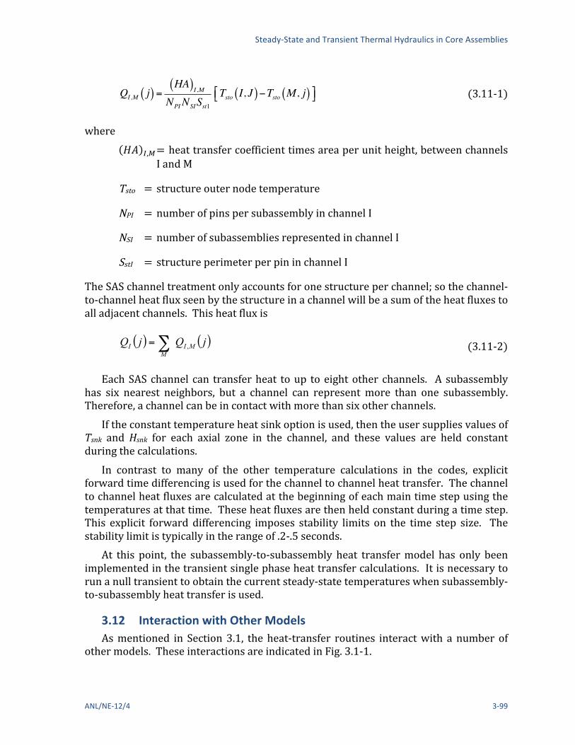
Steady-‐State and Transient Thermal Hydraulics in Core Assemblies
ANL/NE-‐12/4 3-‐99
QI ,M j( ) =HA( )I ,M
NPINSISst1Tsto I, J( )!Tsto M, j( )"# $%
(3.11-‐1)
where !" !,! = heat transfer coefficient times area per unit height, between channels
I and M
Tsto = structure outer node temperature
NPI = number of pins per subassembly in channel I
NSI = number of subassemblies represented in channel I
SstI = structure perimeter per pin in channel I
The SAS channel treatment only accounts for one structure per channel; so the channel-‐to-‐channel heat flux seen by the structure in a channel will be a sum of the heat fluxes to all adjacent channels. This heat flux is
( ) ( )∑=M
MII jQjQ ,
(3.11-‐2)
Each SAS channel can transfer heat to up to eight other channels. A subassembly has six nearest neighbors, but a channel can represent more than one subassembly. Therefore, a channel can be in contact with more than six other channels.
If the constant temperature heat sink option is used, then the user supplies values of Tsnk and Hsnk for each axial zone in the channel, and these values are held constant during the calculations.
In contrast to many of the other temperature calculations in the codes, explicit forward time differencing is used for the channel to channel heat transfer. The channel to channel heat fluxes are calculated at the beginning of each main time step using the temperatures at that time. These heat fluxes are then held constant during a time step. This explicit forward differencing imposes stability limits on the time step size. The stability limit is typically in the range of .2-‐.5 seconds.
At this point, the subassembly-‐to-‐subassembly heat transfer model has only been implemented in the transient single phase heat transfer calculations. It is necessary to run a null transient to obtain the current steady-‐state temperatures when subassembly-‐to-‐subassembly heat transfer is used.
3.12 Interaction with Other Models As mentioned in Section 3.1, the heat-‐transfer routines interact with a number of
other models. These interactions are indicated in Fig. 3.1-‐1.

The SAS4A/SASSYS-‐1 Safety Analysis Code System
3-‐100 ANL/NE-‐12/4
If PRIMAR-‐4 is being used, then the subassembly coolant outlet temperatures calculated in the heat-‐transfer routines are used by PRIMAR-‐4 to calculate the outlet plenum temperature. Also, if flow reversal occurs in a channel, then the temperature calculated in the heat-‐transfer routines for the coolant leaving the bottom of the subassembly is used by PRIMAR-‐4 in the calculation of the inlet plenum temperature. Section 3.3.6 describes how the inlet and outlet plenum temperatures are used in the calculations of the subassembly coolant inlet and reentry temperatures.
Before the onset of voiding, TSHTRN calculates the coolant temperatures used in the coolant channel hydraulics calculations, and the hydraulics routines calculate the coolant flow rates used by TSHTRN.
After the onset of voiding, coolant temperatures are calculate din TSBOIL. This module supplies the heat flux at the cladding outer surface, as defined in Eq. 3.5-‐2 and used in Eq. 3.5-‐9 to TSHTRV. TSBOIL uses the calculated cladding temperatures form TSHTRV to obtain extrapolated cladding temperatures, as in Eq. 3.5-‐3, for use in its coolant temperature calculations.
The point kinetics model supplies the power level used in the heat-‐transfer routines. In return, the heat-‐transfer routines supply the temperatures used to calculate reactivity feedback.
3.12.1 Reactivity Feedback The temperatures calculated in the core thermal hydraulics routines are used to
calculate various components of reactivity feedback. These reactivity components include Doppler feedback, axial expansion of the fuel and cladding, density changes in the sodium, core radial expansion and control rod drive expansion. These reactivity feedbacks are described in Chapter 4.
3.12.2 Coupling Between Core Channels and PRIMAR-‐4 As described in Chapter 5, the PRIMAR-‐4 calculations for a PRIMAR time step are
carried out before the core channel coolant calculations. PRIMAR-‐4 must make estimates of the core flows for a new time step, and it also makes corrections for the differences between its estimates for the previous step and values computed by the core channel coolant routines. The coolant routines supply information to PRIMAR-‐4 for use in these estimates and corrections. Also, PRIMAR-‐4 supplies inlet and outlet coolant plenum pressures and temperatures for the use in the core channel calculations.
The information supplied by PRIMAR-‐4 is
( )1pin tp = inlet plenum pressure at the beginning of the PRIMAR time step
( )1px tp = outlet plenum pressure at the beginning of the PRIMAR time step
dtdpin =time derivative of the inlet plenum pressure
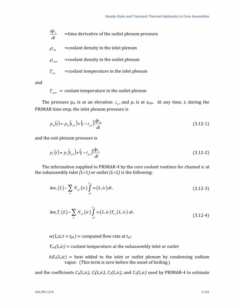
Steady-‐State and Transient Thermal Hydraulics in Core Assemblies
ANL/NE-‐12/4 3-‐101
dtdpx =time derivative of the outlet plenum pressure
cinρ =coolant density in the inlet plenum
coutρ =coolant density in the outlet plenum
cinT =coolant temperature in the inlet plenum
and
coutT = coolant temperature in the outlet plenum
The pressure pin is at an elevation zp!! and px is at zplu. At any time, t, during the PRIMAR time step, the inlet plenum pressure is
( ) ( ) ( )dtdptttptp in
ppinin 11 −+=
(3.12-‐1)
and the exit plenum pressure is
( ) ( ) ( )dtdptttptp x
ppxx 11 −+=
(3.12-‐2)
The information supplied to PRIMAR-‐4 by the core coolant routines for channel ic at the subassembly inlet (L=1) or outlet (L=2) is the following:
!mc L( )" Nps ic( )ic# w L, ic( )
p1
tp2
$ dt,
(3.12-‐3)
!mcTc L( )" Nps ic( )ic# w L, ic( )Tex L, ic( )
p1
tp2
$ dt,
(3.12-‐4)
w(L,ic,t = tp2) = computed flow rate at tp2
Tex(L,ic) = coolant temperature at the subassembly inlet or outlet
ΔEv(L,ic) = heat added to the inlet or outlet plenum by condensing sodium vapor. (This term is zero before the onset of boiling.)
and the coefficients Co(L,ic), Ci(L,ic), C2(L,ic), and C3(L,ic) used by PRIMAR-‐4 to estimate

The SAS4A/SASSYS-‐1 Safety Analysis Code System
3-‐102 ANL/NE-‐12/4
the core channel flow. PRIMAR-‐4 estimates the flow into or out or each subassembly using
dwe L, ic( )dt
=C0 L, ic( )+C1 L, ic( ) pin +C2 L, ic( ) px
+C3 L, ic( ) we L, ic( ) we L, ic( )
(3.12-‐5)
The core channel calculations use w as the flow rate per pin, whereas PRIMAR-‐4 estimates the total flow represented by a channel, so Nps(ic), the number of pins per subassembly times the number of subassemblies represented by the channel, comes into Eqs. 3.12-‐3, 3.12-‐4 and the calculations of the coefficients C0, C1, C2, and C3. In the pre-‐voiding module the coefficients are calculated as
( )( ) ( )( )[ ]1
50
1I
MZCzzzzIgNC upcoutpccinps −+−+
−= ρρ
(3.12-‐6)
11 I
NC ps=
(3.12-‐7)
12 CC −= (3.12-‐8)
and
( )ps
bfr
NIwwIwIAwI
Cfr
12
241
23223
++−=
+
(3.12-‐9)
In this case, the coefficients for L=2 are equal to those for L=1.
3.13 Subroutine Descriptions and Flowcharts The subroutines used in the core-‐channel thermal hydraulics calculations are
described below, grouped by the phase of the calculation where they are used. Steady-‐state Thermal Hydraulics:
SSTHRM-‐-‐ Driver for the steady-‐state calculations: SSCOOL-‐-‐ Calculations steady-‐state coolant, structure, reflector, and gas plenum
temperature for each axial node. Also calculates coolant pressure and saturation temperature at each axial node.
SSCLM1-‐-‐ Calculates steady-‐state coolant pressures and saturation temperatures for the multiple pin option.
SSHTR-‐-‐ Calculates steady-‐state fuel and cladding temperatures in the core and
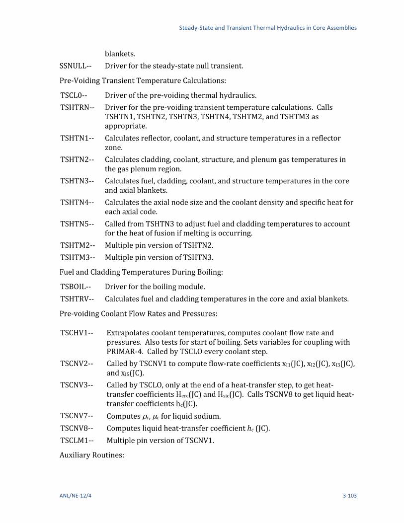
Steady-‐State and Transient Thermal Hydraulics in Core Assemblies
ANL/NE-‐12/4 3-‐103
blankets. SSNULL-‐-‐ Driver for the steady-‐state null transient.
Pre-‐Voiding Transient Temperature Calculations:
TSCL0-‐-‐ Driver of the pre-‐voiding thermal hydraulics. TSHTRN-‐-‐ Driver for the pre-‐voiding transient temperature calculations. Calls
TSHTN1, TSHTN2, TSHTN3, TSHTN4, TSHTM2, and TSHTM3 as appropriate.
TSHTN1-‐-‐ Calculates reflector, coolant, and structure temperatures in a reflector zone.
TSHTN2-‐-‐ Calculates cladding, coolant, structure, and plenum gas temperatures in the gas plenum region.
TSHTN3-‐-‐ Calculates fuel, cladding, coolant, and structure temperatures in the core and axial blankets.
TSHTN4-‐-‐ Calculates the axial node size and the coolant density and specific heat for each axial code.
TSHTN5-‐-‐ Called from TSHTN3 to adjust fuel and cladding temperatures to account for the heat of fusion if melting is occurring.
TSHTM2-‐-‐ Multiple pin version of TSHTN2. TSHTM3-‐-‐ Multiple pin version of TSHTN3.
Fuel and Cladding Temperatures During Boiling:
TSBOIL-‐-‐ Driver for the boiling module. TSHTRV-‐-‐ Calculates fuel and cladding temperatures in the core and axial blankets.
Pre-‐voiding Coolant Flow Rates and Pressures:
TSCHV1-‐-‐ Extrapolates coolant temperatures, computes coolant flow rate and pressures. Also tests for start of boiling. Sets variables for coupling with PRIMAR-‐4. Called by TSCLO every coolant step.
TSCNV2-‐-‐ Called by TSCNV1 to compute flow-‐rate coefficients xI1(JC), xI2(JC), xI3(JC), and xI5(JC).
TSCNV3-‐-‐ Called by TSCLO, only at the end of a heat-‐transfer step, to get heat-‐transfer coefficients Herc(JC) and Hsic(JC). Calls TSCNV8 to get liquid heat-‐transfer coefficients hc(JC).
TSCNV7-‐-‐ Computes ρc, µc for liquid sodium. TSCNV8-‐-‐ Computes liquid heat-‐transfer coefficient hc (JC). TSCLM1-‐-‐ Multiple pin version of TSCNV1.
Auxiliary Routines:

The SAS4A/SASSYS-‐1 Safety Analysis Code System
3-‐104 ANL/NE-‐12/4
CFUEL-‐-‐ Calculates the specific heat of the fuel as a function of temperature. For coding efficiency, one call to CFUEL gives the specific heats for all radial nodes at an axial node, rather than using as separate call to CFUEL for each radial node of each axial node.
CCLAD-‐-‐ Calculates the specific heat of the cladding as a function of temperature. One call to CCLAD returns the values for all axial nodes int eh core and axial blankets.
KFUEL-‐-‐ Calculates the thermal conductivity of the fuel as a function of temperature. One call to KFUEL provides the values for all radial nodes at an axial node.
KCLAD-‐-‐ Calculates cladding thermal conductivity as a function of temperature. One call to KCLAD returns the values for all axial nodes in the core and axial blankets.
INTRP-‐-‐ General interpolation routine that uses linear interpolation from a table to obtain y as a function of x. A single call to INTRP with an array of x’s will return an array of resulting y’s.
SHAPE-‐-‐ Multiplies the array of axial power shapes by the current time-‐dependent power to obtain the current power, in watts, at each axial node in a channel.
HBSMPL-‐-‐ Calculates the bond gap conductance at each axial node if the simple bond gap conductance model is used. Otherwise, DEFORM-‐II calculates the bond gap conductance; and HBSMPL is not called.
INVRT3-‐-‐ Solves a tri-‐diagonal matrix equation of arbitrary size.
Figure 3.1-‐2 is a flowchart for subroutine TSCLO, Fig. 3.13-‐1 is a flowchart for subroutine TSHTRN, and Fig. 3.13-‐2 is a flowchart for subroutine TSHTN3. The logic in the other pre-‐voiding single pin transient heat-‐transfer routines is very simple and straightforward. Subroutine TSHTRV is similar to TSHTN3, except that TSHTRV does not calculate coolant and structure temperatures. Also, in TSHTRV the axial nodes are completely de-‐coupled, so the order in which they are treated is immaterial. For simplicity, the axial node loop in TSHTRV always starts at the bottom and works up.

Steady-‐State and Transient Thermal Hydraulics in Core Assemblies
ANL/NE-‐12/4 3-‐105
Figure 3.13-‐1: Flowchart for Subroutine TSHTRN

The SAS4A/SASSYS-‐1 Safety Analysis Code System
3-‐106 ANL/NE-‐12/4
Figure 3.13-‐2: Flowchart for Subroutine TSHTN3

Steady-‐State and Transient Thermal Hydraulics in Core Assemblies
ANL/NE-‐12/4 3-‐107
3.14 Input and Output
3.14.1 Input Description The input variables used in the pre-‐voiding subassembly thermal hydraulics
calculations are listed in Table 3.14-‐1. Some additional comments on some of these input variables are listed below.
3.14.1.1 Per Pin Basis All of the core channel thermal hydraulic input to SASSYS-‐1 is on a per pin basis
rather than a per subassembly basis. Thus, the initial flow rate, WO, is kg/s per pin; and the perimeters SRFSTZ and SER are perimeters per pin. Also, ACCZ is a coolant flow area per pin, and the variables DZIAB and DZIAT are ratios of inertial lengths to flow areas per pin.
3.14.1.2 Structure/Duct Wall and Wrapper Wires Typically a SAS channel represents an average pin in a subassembly. In this case, the structure normally represents one pin’s share of the duct wall, and it may also include the wrapper wire. If there are N pins in the subassembly, then the thickness used for the structure is the actual duct wall thickness, and the perimeter used for the structure is the duct wall perimeter divided by N. The wrapper wire can be either lumped with the cladding or included in the structure. Since wrapper wires are in much better contact with the cladding than with the duct wall, the most accurate treatment of the wrapper wire is probably to lump it with the cladding by increasing the specific heat of the cladding by enough to account for the total heat capacity of the cladding plus the wrapper wire. The cladding dimensions would not be changed.
The problem with lumping the wrapper wires with the duct wall to produce a single “structure” is that typically the duct wall has a much larger ratio of volume to wetted surface area than a wrapper wire, so the wrapper wire temperature will respond much more rapidly than the duct wall temperature to a change in coolant temperature. The heat capacity of the duct wall is considerably greater than the heat capacity of all of the wrapper wires in a subassembly, but the total perimeter of the wrapper wires is greater than the perimeter of the duct wall. If the duct wall and wrapper wires are lumped together, then the thickness of the structure should be determined by the thickness of the duct wall, since the duct wall contains most of the heat capacity. Then the perimeter of the structure should be chosen to conserve the total volume or total heat capacity of the duct wall plus wrapper wires.
A SAS channel can be used to represent a central pin rather than an average pin in a subassembly. In this case, the duct wall would probably be ignored, and the “structure: would represent only the wrapper wire. The perimeter of the structure would equal the perimeter of a wrapper wire, and the thickness of the structure would equal one half of the wrapper wire radius in order to conserve volume.
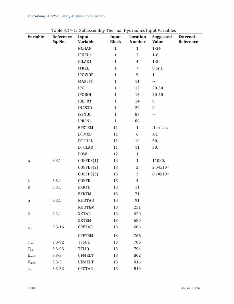
The SAS4A/SASSYS-‐1 Safety Analysis Code System
3-‐108 ANL/NE-‐12/4
Table 3.14-‐1: Subassembly Thermal Hydraulics Input Variables Variable Reference
Eq. No. Input Variable
Input Block
Location Number
Suggested Value
External Reference
NCHAN 1 1 1-‐34 IFUEL1 1 3 1-‐8 ICLAD1 1 4 1-‐3 ITKEL 1 7 0 or 1 IPOWOP 1 9 1 MAXSTP 1 11 -‐-‐ IPO 1 12 20-‐50 IPOBOI 1 13 20-‐50 IBLPRT 1 14 0 INAS3D 1 29 0 ISSNUL 1 87 -‐-‐ IPRSNL 1 88 EPSTEM 11 1 .1 or less DTMXB 11 6 .01 DTFUEL 11 10 50. DTCLAD 11 11 30. POW 12 1 ρ 3.3.1 COEFDS(1) 13 1 11080. COEFDS(2) 13 2 2.04x10-‐5 COEFDS(3) 13 3 8.70x10-‐9 k 3.3.1 COEFK 13 4 k 3.3.1 EXKTB 13 11 EXKTM 13 71 ρ 3.3.1 RHOTAB 13 91 RHOTEM 13 251 k 3.3.1 XKTAB 13 420 XKTEM 13 580 cf 3.3-‐16 CPFTAB 13 606
CPFTEM 13 766 Tsol 3.3-‐92 TFSOL 13 786 Tliq 3.3-‐93 TFLIQ 13 794 Umelt 3.3-‐3 UFMELT 13 802 Umelt 3.3-‐3 UEMELT 13 816 ce 3.3-‐32 CPCTAB 13 819
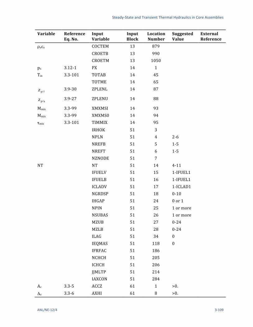
Steady-‐State and Transient Thermal Hydraulics in Core Assemblies
ANL/NE-‐12/4 3-‐109
Variable Reference Eq. No.
Input Variable
Input Block
Location Number
Suggested Value
External Reference
ρece COCTEM 13 879 CROETB 13 990 CROETM 13 1050 px 3.12-‐1 PX 14 1 Tin 3.3-‐101 TOTAB 14 45 TOTME 14 65
pz 3.9-‐30 ZPLENL 14 87
upz 3.9-‐27 ZPLENU 14 88
Mmix 3.3-‐99 XMXMSI 14 93 Mmix 3.3-‐99 XMXMS0 14 94 τmix 3.3-‐101 TIMMIX 14 95 IRHOK 51 3 NPLN 51 4 2-‐6 NREFB 51 5 1-‐5 NREFT 51 6 1-‐5 NZNODE 51 7 NT NT 51 14 4-‐11 IFUELV 51 15 1-‐IFUEL1 IFUELB 51 16 1-‐IFUEL1 ICLADV 51 17 1-‐ICLAD1 NGRDSP 51 18 0-‐10 IHGAP 51 24 0 or 1 NPIN 51 25 1 or more NSUBAS 51 26 1 or more MZUB 51 27 0-‐24 MZLB 51 28 0-‐24 ILAG 51 34 0 IEQMAS 51 118 0 IFRFAC 51 186 NCHCH 51 205 ICHCH 51 206 JJMLTP 51 214 IAXCON 51 284 Ac 3.3-‐5 ACCZ 61 1 >0. Δz 3.3-‐6 AXHI 61 8 >0.

The SAS4A/SASSYS-‐1 Safety Analysis Code System
3-‐110 ANL/NE-‐12/4
Variable Reference Eq. No.
Input Variable
Input Block
Location Number
Suggested Value
External Reference
Dh 3.3-‐9 DHZ 61 32 >0. dsti 3.3-‐45 DSTIZ 61 39 >0. dsto 3.3-‐47 DSTOZ 61 46 >0. PLENL 61 53 >0. RBR 61 54 >_ROUTFP RER 61 78 >RBR rbrp 3.3-‐68 RBRPL 61 102 >0. rcrp 3.3-‐73 RERPL 61 103 >RBRPL RINFP 61 104 ROUTFP 61 128 >RINFP ZONEL 61 152 >0. Spt 3.3-‐40 SRFSTZ 61 159 AREAPC 61 166 >0. dro 3.3-‐59 DRFO 61 169 >0. RBRO 61 180 >0. RERO 61 181 >0. Scr 3.3-‐62 SER 61 182 >0. dri 3.3-‐56 DRFI 61 189 >0. NPI 3.11-‐1 XXNPIN 61 274 >0. γs 3.3-‐22 GAMSS 62 2
γc 3.3-‐6 GAMTNC 62 4
γe 3.3-‐23 GAMTNE 62 5 PSHAPE 62 6 Pr 3.3-‐22 PSHAPR 62 30 AHBPAR 63 2 BHBPAR 63 3 CHIBPAR 63 4 HBMAX 63 5 HBMIN 63 6 HBPAR 63 7 ksi 3.3-‐43 XKSTIZ 63 11 kso 3.3-‐46 XKSTOZ 63 18 εσ 3.3-‐4 DEL 63 25 kr 3.3-‐57 XKRF 63 28 (ρc)sti 3.3-‐45 RHOCSI 63 37 >0.

Steady-‐State and Transient Thermal Hydraulics in Core Assemblies
ANL/NE-‐12/4 3-‐111
Variable Reference Eq. No.
Input Variable
Input Block
Location Number
Suggested Value
External Reference
(ρc)sto 3.3-‐47 RHOCSO 63 44 >0.
(ρc)r 3.3-‐56 RHOCR 63 51 >0.
(ρc)g 3.3-‐68 RHOCG 63 58 >0. Rg 3.3-‐71 RG 63 59 >0. αf 3.10-‐4 FUELEX 63 73
αe 3.10-‐5 CLADEX 63 74 Yf 3.10-‐8 YFUEL 63 75 Ye 3.10-‐9 YCLAD 63 76 FULREX 63 77 CLDREX 63 78 (HA)I,M 3.11-‐1 HACHCH 63 82 1/γht 3.3-‐116 TAVINV 63 104 .5-‐5 Afr 3.8-‐3 AFR 64 1 .1875 bfr 3.8-‐3 BFR 64 2 -‐.2 c1 3.3-‐9 C1 64 3 .025 2-‐5 c2 3.3-‐9 C2 64 4 .8 2-‐5 c3 3.3-‐9 C3 64 5 4.8 2-‐5 DWMAX 64 6 .2 ReL 3.9-‐3 RELAM 64 7 2100. AfL 3.9-‐3 AFLAM 64 8 64. WO 64 47 Kor 3.9-‐12 XKORV 64 48 XKORGD 64 64
b
i
Az⎟⎠
⎞⎜⎝
⎛ Δ 3.9-‐6 DZIAB 64 65 >0.
f
i
Az⎟⎠
⎞⎜⎝
⎛ Δ 3.9-‐6 DZIAT 64 66
Tout 3.3.-‐100 DTLMAX 64 69 15. U1 3.10-‐1 TUPL 64 74 U2 3.10-‐2 UACH1 64 189 UACH2 64 190
3.14.1.3 Empty Reflector Region Sometimes a reflector zone is used to represent an empty section of a subassembly.
The duct wall is usually represented by the structure; and since there is nothing but

The SAS4A/SASSYS-‐1 Safety Analysis Code System
3-‐112 ANL/NE-‐12/4
sodium inside the duct wall, there is nothing for the reflector to represent. The code requires a “reflector” in every axial zone except the pin section, so some input for the reflector must be included. The reflector perimeter, SER, cannot be zero; but it can be set to a very small value, such as 10-‐9, so that it would have no impact on coolant temperatures. Also, the total reflector thickness, DRFI plus DRFO, must be a reasonable value, 0.003 m or more, to prevent numerical instabilities in the reflector temperature calculations in the boiling module. The pre-‐voiding reflector temperature calculations are numerically stable for any reflector greater than zero.
3.14.1.4 Structure and Reflector Node Thickness Two radial nodes are used in the reflectors and in the structure. The only
restrictions on node thicknesses are that the total reflector thickness and the total structure thickness must be reasonable; 0.003 m or more, to prevent numerical instabilities in the temperature calculations in the boiling module. Usually, the node in contact with the coolant, the inner structure node or the outer reflector node, represents approximately 10% of the total thickness; and the other node represents the rest. Then the small node in contact the coolant will react rapidly to rapid changes in the coolant temperatures, whereas the larger node will dominate the longer-‐term response to the slow changes.
3.14.1.5 Coolant Re-‐entry Temperature If PRIMAR-‐1 is being used, then the re-‐entry temperature calculation describe in
Section 3.3.6 uses the input variable TUPL for the bulk temperature of the coolant in the outlet plenum. If PRIMAR-‐4 is being used, then the outlet plenum temperature is computed by PRIMAR-‐4; and TUPL is not used.
3.14.2 Output Description Figure 3.14-‐1 shows a typical thermal hydraulic output for one step of the transient.
The output is largely self-‐explanatory. Note that on the first page of this output the axial location, coolant temperature, saturation temperature, and pressure are the values at node boundaries; whereas the cladding, structure, plenum, and reflector temperatures are the values at node mid-‐points. Also, on the second page the radial fuel temperatures are the values at node mid-‐points except for the inner and outer fuel temperature, as indicated in Fig. 3.2-‐4; whereas the radii are the values of radial node boundaries.
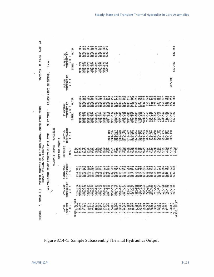
Steady-‐State and Transient Thermal Hydraulics in Core Assemblies
ANL/NE-‐12/4 3-‐113
Figure 3.14-‐1: Sample Subassembly Thermal Hydraulics Output

The SAS4A/SASSYS-‐1 Safety Analysis Code System
3-‐114 ANL/NE-‐12/4
Figure 3.14-‐1: Sample Subassembly Thermal Hydraulics Output (Cont’d.)

Steady-‐State and Transient Thermal Hydraulics in Core Assemblies
ANL/NE-‐12/4 3-‐115
Figure 3.14-‐1: Sample Subassembly Thermal Hydraulics Output (Cont’d.)

The SAS4A/SASSYS-‐1 Safety Analysis Code System
3-‐116 ANL/NE-‐12/4
3.15 Thermal Properties of Fuel and Cladding All material property data for fuel and cladding are cast as functions or subroutines
to allow for modularization and the ease of making changes. This also allows for the incorporation of different materials data in a straightforward manner. In a number of the correlations used, the units are inconsistent with the SI unit system adopted by SASSYS-‐1 and SAS4A. The routines that use these correlations carry out the appropriate units conversions internally.
The thermal properties for fuel and cladding are described in this section. Sodium properties are described in Chapter 12.
3.15.1 Fuel Density The fuel density can be obtained either form a user-‐supplied table of density vs
temperature or from a correlation with
( ) ( )221 2732731 −+−+=
TCTCo
fρ
ρ
(3.15-‐1)
where
ρo = The theoretical density at 273 K, kg/m3
C1,C2 = Input coefficients
T = Temperature, K
This applies between 273 K and the solidus temperature. The liquid fuel density is given by
( )2731 3 −+=
TCoρρ
(3.15-‐2)
where C3 = Input coefficient
This applies to temperatures above the liquidus. For the range between the solidus and liquidus temperatures, a linear interpolation is performed.
These equations are found in the function RHOF. Suggested values of coefficients are from the Nuclear Systems Materials Handbook [3-‐8].
ρc = COEFDS(1) = 11.05x10³ kg/m3 (mixed oxide)
C1 = COEFDS(2) = 2.04x10-‐5 K-‐1
C2 = COEFDS(3) = 8.70x10-‐9 K-‐2

Steady-‐State and Transient Thermal Hydraulics in Core Assemblies
ANL/NE-‐12/4 3-‐117
C3 = COEFDS(2) = 9.30x10-‐5 K-‐1
3.15.2 Fuel Thermal Conductivity Four different options exist for the fuel thermal conductivity. These are controlled
through the input parameter IRHOK. IRHOK = 0
The thermal conductivity as function of temperature is input in table form through the variable arrays XKTAB and XKTEM. IRHOK =1
For this option, the conductivity equations are given by:
( )( )
CTC
fTxTk
D
°≤≤°
−+=
2000800for
4465.4888.1011.1
2
1
(3.15-‐3)
( ) ( )( )
CT
TkTk
°≤
+=
800for
196.0044.12844.16880012
(3.15-‐4)
( ) ( ) CTkTk °>= 2000for200013 (3.15-‐5)
where k1,k2,k3 = Fuel thermal conductivity, W/m-‐k
T = Temperature, ºC
fD = Fuel fraction of theroretical density
IRHOK = 2 This form of the conductivity is given by
k1 T( ) = C1 ! fD( ) fD !1"# $%1
C2 +C3T( )+C4T
3"
#&&
$
%''
for 0.75 ( fD ( 0.95
(3.15-‐6)

The SAS4A/SASSYS-‐1 Safety Analysis Code System
3-‐118 ANL/NE-‐12/4
( ) ( )
95.0for
113 37
652
>
⎥⎦
⎤⎢⎣
⎡+
+−=
D
D
f
TCTCC
fTk
(3.15-‐7)
where C1,C2,C3,C4,C5,C6,C7 = Input variables
k1,k2 = Fuel conductivity W/m-‐k
T = Temperature, K
If T is greater than the melting temperature, it is set to the melting temperature. Suggested values:
C1= COEFK(1) = 2.1
C2= COEFK(2) = 2.88x10-‐3
C3= COEFK(3) = 2.52x10-‐5
C4= COEFK(4) = 2.83x10-‐10
C5= COEFK(5) = 5.75x10-‐2
C6= COEFK(6) = 5.03x10-‐4
C7= COEFK(7) = 2.91x10-‐11
IRHOK = 3 This conductivity form is [3-‐9]
k1 T( ) = 4.005x10³
T ! 273( )+ 402.4+ 0.6416x10!10T 3
(3.15-‐8)
where T = Temperature, K
k = Conductivity in W/m-‐k
This is the correlation for UO2 and is converted to mixed oxide by subtracting 0.2.
!! ! = !! ! − 0.2 (3.15-‐9)

Steady-‐State and Transient Thermal Hydraulics in Core Assemblies
ANL/NE-‐12/4 3-‐119
The porosity correction term was derived for use in the COMETHE-‐IIIJ [2-‐10] code and is given by
432 1581.402.3029.11 εεεε +−−−=pf (3.15-‐10)
where fp = Porosity multiplier
ε = 1 -‐ ρf = Fractional porosity
ρf = fractional fuel density = actual density/theoretical density
The conductivity is therefore given by
( ) ( ).2 TkfTk p= (3.15-‐11)
Two different routines contain the above correlations, FK and KFUEL. The function FK returns a single value of the conductivity for a single invocation and is used in the steady-‐state calculation. The subroutine KFUEL returns the conductivity values for each radial node in the current axial segment. It is used in the transient calculational procedure.


Steady-‐State and Transient Thermal Hydraulics in Core Assemblies
ANL/NE-‐12/4 3-‐121
REFERENCES
NOTICE Several references in this document refer to unpublished information. For a list of available open-‐literature citations, please contact the authors.


ANL/NE-‐12/4 3-‐123
APPENDIX 3.1: DEGREE OF IMPLICITNESS FOR FLOW AND TEMPERATURE CALCULATIONS
A typical calculation in SASSYS-‐1 involves finding the value of a temperature or a flow rate at the end of a time step given the values of relevant parameters at the beginning of the step, as well as the values of driving functions at the beginning and end of the step. Linearized finite difference approximations to the relevant differential equations are usually used, and the accuracy of the finite differencing in time will depend both on the size of the time step and on the degree of implicitness in the solution. By picking appropriate values for the degree of implicitness, it is possible to improve the accuracy of the solution.
The differential equations used for temperatures and flow rates are of the form
( )tyfdtdy ,=
(A3. 1-‐12)
Where y is the flow rate or temperature being calculated, and f is a function of y and time. The finite difference approximation used for Eq. A3.1-‐1 is
( ) ( )22211112 ,, tyftyf
tyy
θθ +=Δ
−
(A3. 1-‐13)
where t1 = time at the beginning of the time step
t2 = time at the end of the time step
y1 = y at t1
y2 = y at t2
12 ttt −=Δ (A3. 1-‐14)
0.121 =+θθ (A3. 1-‐15)
The parameters θ1 and θ2 determines the degree of implicitness of the solution: for a fully explicit solution θ1 = 1.0 and θ2 = 0.0, whereas for a fully implicit solution θ1 = 0.0 and θ2 = 1.0.
After linearizing, equation A3.1-‐1 can be put in the form
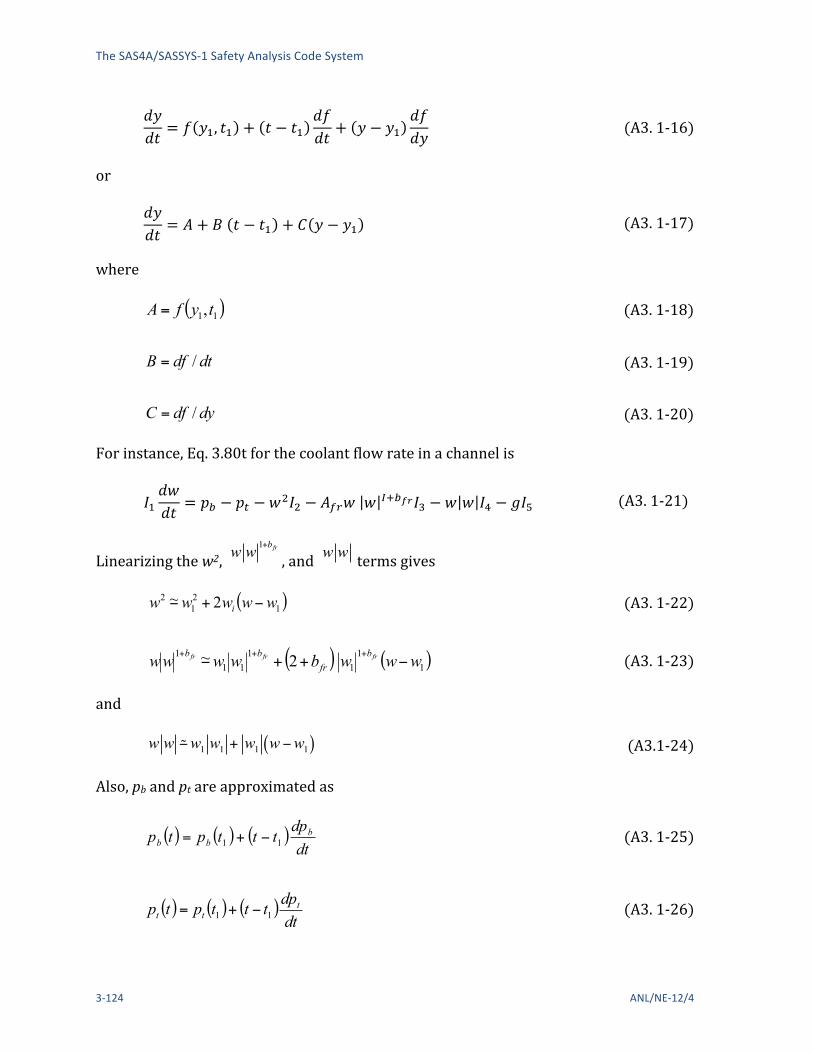
The SAS4A/SASSYS-‐1 Safety Analysis Code System
3-‐124 ANL/NE-‐12/4
!"!" = ! !!, !! + ! − !!
!"!" + ! − !!
!"!" (A3. 1-‐16)
or
!"!" = ! + ! ! − !! + ! ! − !! (A3. 1-‐17)
where
( )11,tyfA= (A3. 1-‐18)
dtdfB /= (A3. 1-‐19)
dydfC /= (A3. 1-‐20)
For instance, Eq. 3.80t for the coolant flow rate in a channel is
!!!"!" = !! − !! − !!!! − !!"! ! !!!!"!! − ! ! !! − !!! (A3. 1-‐21)
Linearizing the w2, w w 1+bfr
, and w w terms gives
( )121
2 2~ wwwww i −+− (A3. 1-‐22)
( ) ( )111
111
1 2~ wwwbwwww frfrfr bfr
bb−++−
+++
(A3. 1-‐23)
and
w w !!w1 w1 + w1 w!w1( ) (A3.1-‐24)
Also, pb and pt are approximated as
( ) ( ) ( )dtdp
tttptp bbb 11 −+=
(A3. 1-‐25)
( ) ( ) ( )dtdptttptp t
tt 11 −+=
(A3. 1-‐26)

Steady-‐State and Transient Thermal Hydraulics in Core Assemblies
ANL/NE-‐12/4 3-‐125
where
( ) ( )12
12
tttptp
dtdp bbb
−
−=
(A3. 1-‐27)
and
( ) ( )12
12
tttptp
dtdp ttt
−
−=
(A3. 1-‐28)
Then Eq. A3.1-‐10 has the form of Eq. A3.1-‐6 if
A = pb t1( )! pt t1( )!w12I2 ! Afr w1 w11+bfr I3{
!w1 w1 I4 ! gI5}/ I1 (A3. 1-‐29)
1Idtdp
dtdp
Btb −
=
(A3. 1-‐30)
and
C = !2w1 I2 ! 2+ bfr( )Afr w1
1+bfr ! w1 I4"#
$%
I1 (A3. 1-‐31)
The exact solution for Eq. A3.1-‐6 is
( ) ( )( ) ( )1/21
11 ttBeBAyy tt −+−−=− −− τττ τ (A3. 1-‐32)
where
C1
−=τ
(A3. 1-‐33)
The finite difference approximation used for Eq. A3.1-‐6 is
( )122212 yyCtBA
tyy
−+Δ+=Δ
−θθ
(A3. 1-‐34)
where

The SAS4A/SASSYS-‐1 Safety Analysis Code System
3-‐126 ANL/NE-‐12/4
12 ttt −=Δ (A3. 1-‐35)
The solution of Eq. A3.1-‐23 for y2 is
τθθ/1 2
22
12 ttBtyy
Δ+
Δ+ΑΔ=−
(A3. 1-‐36)
Figure A3.1-‐1 shows y2 -‐ y1, as given by Eq. A3.1-‐25, as a function of θ2 for the case where A = 1, B = .5, Δt = 2, and τ = 1. Also shown is the exact solution from Eq. A3.1-‐21. Note that a value θ2 can be found such that the finite difference solution of Eq. A3.1-‐25 exactly matches the differential equation solution, given by Eq. A3.1-‐21, for this case. Also note that neither a fully explicit solution, θ2 = 0, nor a fully implicit solution, θ2 = 1.0, is very accurate for particular case. An explicit solution would be numerically unstable for Δt greater than τ; and values considerably smaller than the time constant τ.
For any values of the parameters in Eq. A3.1-‐21 and Eq. A3.1-‐25, a value of θ2 can be chosen such that the finite difference solution matches the solution of the differential equation by setting t = t2 in Eq. A3.1-‐21 and combining this equation with Eq. A3.1-‐25 to give
A! !B! 2( ) 1! e!"t/!( )+B! "t = #"t +"2B"t2
1+"2"t / ! (A3. 1-‐37)
solving for θ2 gives
( )
( )τ
τ
τ
τθ/
/
2
1
1
t
t
et
et
Δ−
Δ−
−Δ
−−Δ
=
(A3. 1-‐38)
Note that A and B cancelled out of Eq. A3.1-‐27, and θ2 is a function only of Δt/t.
Figure A3.1-‐2 shows θ2, given by Eq. A3.1-‐27, as a function of Δt/τ. This figure also shows some approximations to this function, as discussed below. For small values of Δt/τ, θ2 approaches 0.5, where as for large values of Δt/τ , θ2 approaches 1.0.

Steady-‐State and Transient Thermal Hydraulics in Core Assemblies
ANL/NE-‐12/4 3-‐127
Figure A3.1-‐1: Finite Difference Solution as a Function of the Degree of Implicitness

The SAS4A/SASSYS-‐1 Safety Analysis Code System
3-‐128 ANL/NE-‐12/4
Figure A3.1-‐2: Degree of Implicitness as a Function of Normalized Time Step Size
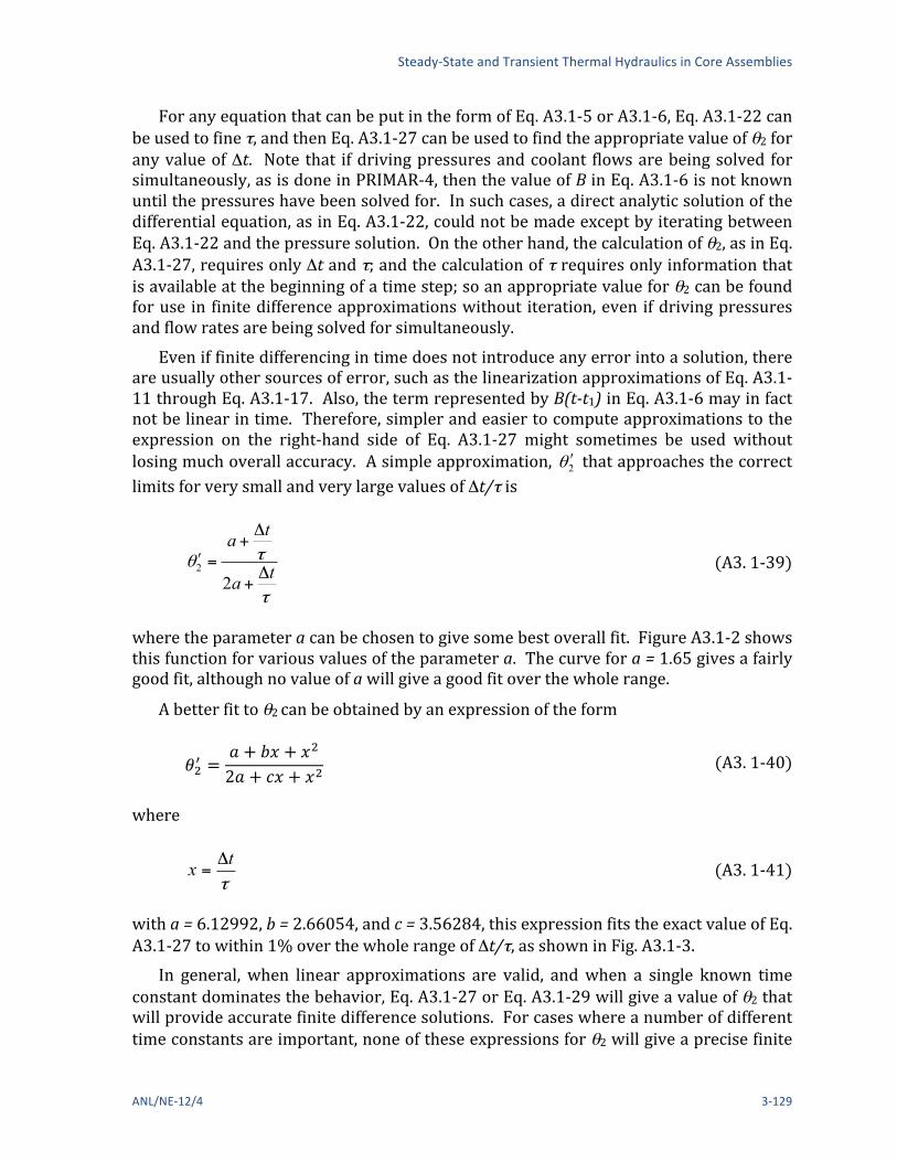
Steady-‐State and Transient Thermal Hydraulics in Core Assemblies
ANL/NE-‐12/4 3-‐129
For any equation that can be put in the form of Eq. A3.1-‐5 or A3.1-‐6, Eq. A3.1-‐22 can be used to fine τ, and then Eq. A3.1-‐27 can be used to find the appropriate value of θ2 for any value of Δt. Note that if driving pressures and coolant flows are being solved for simultaneously, as is done in PRIMAR-‐4, then the value of B in Eq. A3.1-‐6 is not known until the pressures have been solved for. In such cases, a direct analytic solution of the differential equation, as in Eq. A3.1-‐22, could not be made except by iterating between Eq. A3.1-‐22 and the pressure solution. On the other hand, the calculation of θ2, as in Eq. A3.1-‐27, requires only Δt and τ; and the calculation of τ requires only information that is available at the beginning of a time step; so an appropriate value for θ2 can be found for use in finite difference approximations without iteration, even if driving pressures and flow rates are being solved for simultaneously.
Even if finite differencing in time does not introduce any error into a solution, there are usually other sources of error, such as the linearization approximations of Eq. A3.1-‐11 through Eq. A3.1-‐17. Also, the term represented by B(t-‐t1) in Eq. A3.1-‐6 may in fact not be linear in time. Therefore, simpler and easier to compute approximations to the expression on the right-‐hand side of Eq. A3.1-‐27 might sometimes be used without losing much overall accuracy. A simple approximation, 2θ ʹ′ that approaches the correct limits for very small and very large values of Δt/τ is
τ
τθ ta
ta
Δ+
Δ+
=ʹ′2
2
(A3. 1-‐39)
where the parameter a can be chosen to give some best overall fit. Figure A3.1-‐2 shows this function for various values of the parameter a. The curve for a = 1.65 gives a fairly good fit, although no value of a will give a good fit over the whole range.
A better fit to θ2 can be obtained by an expression of the form
!!! =! + !" + !!
2! + !" + !! (A3. 1-‐40)
where
τtx Δ
=
(A3. 1-‐41)
with a = 6.12992, b = 2.66054, and c = 3.56284, this expression fits the exact value of Eq. A3.1-‐27 to within 1% over the whole range of Δt/τ, as shown in Fig. A3.1-‐3.
In general, when linear approximations are valid, and when a single known time constant dominates the behavior, Eq. A3.1-‐27 or Eq. A3.1-‐29 will give a value of θ2 that will provide accurate finite difference solutions. For cases where a number of different time constants are important, none of these expressions for θ2 will give a precise finite

The SAS4A/SASSYS-‐1 Safety Analysis Code System
3-‐130 ANL/NE-‐12/4
difference solution for all time-‐step sizes. Even in this case, though, θ2 should approach 0.5 for small time steps, and it should approach 1.0 for large time steps. Therefore, an expression of the form given by Eq. A3.1-‐28 may be appropriate in such cases.
Figure A3.1-‐3: Approximate Correlation for the Degree of Implicitness


The SAS4A/SASSYS-‐1 Safety Analysis Code System
3-‐132 ANL/NE-‐12/4