SAPIENZA

University of Rome

Department of Biology and Biotechnology “Charles Darwin”

Reverse Engineering of Natural Systems by Graph Theory

Daniele Capocefalo

XXXI cycle

PhD PROGRAMME IN LIFE SCIENCES

Supervisor

Marco Tripodi

Tutor Coordinator

Tommaso Mazza Marco Tripodi

Director of PhD program:

Prof. Marco Tripodi

Department of Cellular Biotechnology and Hematology,

“Sapienza” University, Rome

Scientific Supervisors:

Prof. Marco Tripodi

Department of Cellular Biotechnology and Hematology,

“Sapienza” University, Rome

Scientific Tutor:

Dr. Tommaso Mazza

Bioinformatics Unit,

IRCCS Casa Sollievo della Sofferenza, San Giovanni Rotondo

To Eva and Amelia. Always Forward.

To Mauro, Tommaso, and the BFX lab. For their unwavering patience.

Table of Contents

TABLE OF CONTENTS ........................................................................................................................... 8

SUMMARY ................................................................................................................................................ 1

INTRODUCTION ...................................................................................................................................... 3

SYSTEMS BIOLOGY ............................................................................................................................... 3 NETWORK BIOLOGY ........................................................................................................................... 10 NETWORK INFERENCE METHODS ........................................................................................................ 13

RESULTS ................................................................................................................................................. 17

AIM OF THE WORK ................................................................................................................................. 17 NETWORK ANALYSIS REVEALS RNA-RNA CROSSTALK AND HIGHLIGHTS THE ROLE OF MICRORNA-

SOCIETIES IN HUMAN COLORECTAL CANCER ........................................................................................... 19 1. Background ................................................................................................................................... 19 2. Inferring Gene-Regulatory networks from enriched biological processes .................................... 25 3. Functional modules in literature-based and experimental miRNA networks ................................ 28 4. The leading topological position of miRNA-145 is fundamental for the upholding of cohesiveness

and functional cooperation among modules ..................................................................................... 38 5. Measuring the effect of the induced expression of miR-145 in CRC cell lines .............................. 41 6. MAPK signaling pathway is modulated by miR-145 ectopic expression in CRC cell lines........... 42 7. Conclusions ................................................................................................................................... 45

PYNTACLE: A TOOL FOR THE ASSESSMENT OF CRITICAL PROPERTIES OF NETWORKS ........................... 49 1. Background ................................................................................................................................... 49 2. Pyntacle functionalities ................................................................................................................. 53 3. Pyntacle benchmarks and performance comparisons ................................................................... 62 4. The future of Pyntacle ................................................................................................................... 65

THE NESTEDNESS OF FOOD-WEBS ........................................................................................................ 69 1. Background ................................................................................................................................... 69 2. Food Webs network analysis ......................................................................................................... 73 3. Key player and nestedness analyses reveal common features in food webs .................................. 76 4. Conclusions ................................................................................................................................... 84

CHARACTERIZATION OF SEX-SPECIFIC MECHANISMS OF AGING IN CORRELATION NETWORKS OF ADULT

DROSOPHILA MELANOGASTER ............................................................................................................... 87

1. Background ................................................................................................................................... 87 2. Co-Expression analysis of sex-specific transcriptomes reveals different co-expression module hubs

........................................................................................................................................................... 91 3. Network analysis of consensus overlap reveals common key-players in male and female co-

expression modules in Drosophila .................................................................................................... 97 4. Conclusions ................................................................................................................................. 103

DISCUSSION ......................................................................................................................................... 107

MATERIALS AND METHODS .......................................................................................................... 113

NETWORK ANALYSIS REVEALS RNA-RNA CROSSTALK AND HIGHLIGHTS THE ROLE OF SOCIETIES OF

MICRORNAS IN HUMAN COLORECTAL CANCER .................................................................................... 113 1. Data sources ................................................................................................................................ 113 2. Statistical analyses ...................................................................................................................... 113 3. Gene selection strategy and in silico functional and pathway analyses ...................................... 114 4. MiRNA selection strategy ............................................................................................................ 115 5. Networks construction ................................................................................................................. 116 6. Topological network analysis ...................................................................................................... 117 7. Strongly connected components .................................................................................................. 118 8. MiRNAome and MAPK signaling pathway profiling after miR-145 transfection in CRC cell lines

......................................................................................................................................................... 118 PYNTACLE ........................................................................................................................................ 121 1. Technical specifications .............................................................................................................. 122 2. Availability, installation, and testing ........................................................................................... 124 3. Shortest Path search strategies ................................................................................................... 125 4. Canonical and non-canonical centrality indices ......................................................................... 127 5. Group-centrality and key-player metrics .................................................................................... 135 6. Key player search optimizations ................................................................................................. 140 7. Ancillary operations .................................................................................................................... 143 8. Supported network file formats ................................................................................................... 145 9. Benchmarks data ......................................................................................................................... 148 10. Benchmarks specifications ........................................................................................................ 150

THE NESTEDNESS OF FOOD-WEBS ...................................................................................................... 153 1. Food webs ................................................................................................................................... 153 2. Network analysis ......................................................................................................................... 154 3. Multi-node centrality ................................................................................................................... 155

4. Nestedness ................................................................................................................................... 155 CHARACTERIZATION OF SEX-SPECIFIC MECHANISMS OF AGING IN CORRELATION NETWORKS OF ADULT

DROSOPHILA MELANOGASTER ............................................................................................................... 157 1. RNA-Seq data availability and processing .................................................................................. 157 2. Sex-specific co-expression network analysis and module eigengenes detection ......................... 157 3. Paired consensus analysis of module eigengenes of male and female flies................................. 160 4. Network analysis of overlapping genes among consensus and sex-specific modules ................. 161

REFERENCES ....................................................................................................................................... 163

ACKNOWLEDGEMENTS ................................................................................................................... 185

APPENDIX - EXCERPT OF PYNTACLE SITE MATERIAL ........................................................ 187

QUICK STARTUP GUIDE ......................................................................................................................... 187 1. Setting Pyntacle for the first use .................................................................................................. 187 2. Dataset description...................................................................................................................... 188 3. Command line Startup Guide ...................................................................................................... 190 4. Pyntacle library startup guide ..................................................................................................... 201

MINIMUM GRAPH REQUIREMENTS ........................................................................................................ 211

PUBLICATIONS ................................................................................................................................... 215

1

Summary

With the advent of high-throughput technology, Biological research widened its horizons

in terms of biomarkers and mechanisms of action of several diseases and phenotypes. On

the other hand, complex diseases, like diabetes, several neurodegenerative pathologies

and cancer, are still orphan of a cause and then of a cure. One of the possible reasons is

that these are not strictly monogenic diseases since they result from a global interplay

between molecular players and master regulators. In this context, where “the whole is

something over and above its parts and not just the sum of them all” (Aristotle 384-322

B.C.), is clear that the Cartesian reductionism cannot completely help understand how a

disease arises and develops.

Systems Biology comes on the stage here and puts emphasis on whole behavior as being

basically indivisible. It sustains the Smuts’s holistic theory according to which whole

systems such as cells, tissues, organisms, and populations were proposed to have unique

emergent properties and that it was impossible to reassemble the behavior of the whole

from the properties of the individual components. Hence, new technologies were

necessary to define and understand the behavior of systems.

New mathematical models and computational approaches emerged in the past decades.

Thereby taking inspiration from the theory of graphs. Aspects of nature that could be

explained by the interaction of individual agents were modeled as networks and their

properties studied topologically. Speculations on the global structure of biological

systems were based on two important assertions: systems have a hierarchical structure,

2

and the structure is held together by numerous linkages to construct very complex

networks.

In this work, we retrace this path by first reconstructing and studying a complex

molecular system made by gene and microRNA expression profiles in patients affected

by colorectal cancer. We show how the study of topological properties of the system

helped identifying a tiny subnetwork of master-regulator and effectors that, individually,

were associated to poor survival rates when extremely expressed. Group-effects were not

captured, until the development of Pyntacle, a cross-platform and open source Python

suite of high-performance computing algorithms for the discovery of key-players in

networks. Pyntacle is introduced and presented in this work and then used proficiently in

two other case studies. The former regards ecological food webs and reports on the

assessment of their nestedness property, which is an indicator of their global robustness

and redundancy. The latter is an exploration of the relationships between sex and ageing

process in Drosophila melanogaster, which developed into two computational steps:

definition of co-expressing modules of genes and identification of sex independent key-

players molecules in male and female flies.

3

Introduction

Systems Biology

The 19th century focused on two important concepts that originate already in the 17th

century. The former is based on the Cartesian notion of complexity according to which a

system can be reduced to pieces that can be more easily managed individually and, then,

reassembled to deduce the whole behavior. The theory of Reductionism was strongly

influenced by the Newton’s success in mathematically describing planetary movements

and characterizing gravity, and resisted till the present days, where, for example, plant

biology grounds on the simple assumption that higher levels in a biological hierarchy can

easily be understood from the behavior of the lower levels.

Reaction against this reductionist attitude began among a few biologists (Von

Bertalanffy, 1950; Smuts and Holst, 1926) in the early part of the 20th century. They

spoke a new language of life in which complexity, organization, orchestration, holism,

interconnectedness, and evolution became more dominant terms. Their objections to

reductionism were twofold. First, it was apparent from simple investigations on the brain

and animal development that the structure of an entire system actually constrained the

behavior of the component parts. Reductionist mechanistic investigations would miss the

vital element of orchestration. Second, many scientists were still bound to the much older

Aristotelian view of the natural phenomena, according to which “the whole is something

over and above its parts and not just the sum of them all” (Aristotle 384-322 B.C.). This

theory dominated science up to the 17th century. It was then abandoned with the

development of experimental physics and later biology, before coming up again with Jan

4

Smuts (1870–1950), naturalist, philosopher and twice Prime Minister of South Africa.

He coined the commonly used term holism. Whole systems such as cells, tissues,

organisms, and populations were proposed to have unique emergent properties

(Trewavas, 2006) and it was impossible to reassemble the behavior of the whole from the

properties of the individual components. New technologies were hence required to define

and understand the biological systems.

The technological response did not take long to arrive. The new microarray chips and

high-throughput sequencing platforms were used to massively profile the Human

Genome in the early 2000s (Venter et al., 2001), and hundreds of thousands of other

genomes in the coming years by means of increasingly more efficient Next-Generation

Sequencing (NGS) platforms. These new laboratory techniques allowed to dissect and

study the individual “components” of cells, tissues, and organisms with high resolution

and specificity, thereby opening new scientific horizons on all the omics layers (Levy and

Myers, 2016).

The term ‘omics’ refers to any technique that enables the massive analysis of entire

catalogues of molecular reservoirs, such as, for example, the whole genome sequencing

(genomics), the overall expression levels of the mRNA species (transcriptomics), or the

quantification of the abundance of mature protein products within a cell (proteomics).

Probably the most famous example of use of NGS techniques on multi-omics layers is

The Cancer Genome Atlas (TCGA) (Tomczak et al., 2015). This project, started in 2006

as a joint initiative by the National Cancer Institute (NCI) and the National Human

Genome Research Institute (NHGRI) and was the first global attempt to characterize and

unravel the genomic and molecular landscapes of a few cancers. It later expanded on

5

many other cancer types and included several other institutions that, together,

collaborated to produce genomic data for more than 11,000 patients across 33 tumor

types. For each tumor type, information on single nucleotide variations (SNV), copy

number variations (CNV), gene and microRNA expression profiles, and methylation

profiles were made available together with clinical, treatment and follow-up information

for most subjects.

While the TCGA is a clear example of Reductionism, the consequent Pan-Cancer Atlas,

which issued from the TCGA, is a notable example of holism. The Pan-Cancer Atlas

provides, in fact, a uniquely comprehensive, in-depth, and interconnected understanding

of how, where, and why tumors arise in humans (Hoadley et al., 2018). This is a

contingent example of how reductionism and holism can be reconciled, although being

often posed in opposition to each other. There is a need to understand how organisms are

put together (reductionism) just as in turn there is a need to understand why they are put

together in the way that they are (systems; holism). Systems Biology is an attempt to

explain this embedded complexity.

Although Systems Biology did not stem from Molecular Biology, but originated from the

convergence of thermodynamics and chemical kinetics (Westerhoff and Palsson, 2004),

it is widely recognized that the omics revolution widely contributed to its spreading and

popularity. Being Systems Biology an interdisciplinary field that has its roots in the

theorization of a mathematical model behind observational data to infer the properties of

the system, its knowledge base can be applied to a plethora of disciplines, from Ecology

(Purdy et al., 2010) to drug design (Cho et al., 2006). Its widespread use and the variety

of its forms make difficult, even for researchers in the field, to give a unanimous

6

definition of Systems Biology. However, besides all point of views, being them

methodological (Breitling, 2010), technical (Kitano, 2002; Potters, 2010) or

philosophical (Boogerd et al., 2007), all agree on the fundamental concept that Systems

Biology is not a mere collection of biological entities and their measurements, but of the

relationships among them, that, if known, can be used to build a computational model of

the system of interest. Such structure is generally named network.

A network, often referred to as graph, is a mathematical system made by nodes, the

entities that populates the system, and edges, the interactions that occur between nodes.

The level of abstraction used with real world systems makes networks the model of choice

in a variety of fields other than Biology, from Information Theory to Social Sciences. For

example, a network might be made by all the web pages of the World Wide Web

(WWW), the nodes being pages and the edges being hyperlinks among them. A kind of

network like this is used by the Google search engine to traverse all web pages of the

WWW and to rank and identify the ones that are important in terms of the number of

hyperlinks that points to them (Page et al., 1998). Recently, studies on the dynamics of

social networks became popular because they attempted to explain complex social events

and to capture the spreading of information across communities of people united by

common beliefs. These communities, known as tribes or echo chambers (Del Vicario et

al., 2016) spread news about their topics of interest much faster than people who do not

belong to them can do, and often reinforce their convictions, turning people with

moderate beliefs into one with more extreme views on the subject, a phenomenon often

called polarization (Del Vicario et al., 2017).

7

Nowadays, networks are used ubiquitously in Systems Biology. They mainly differ for

assortment and completeness of information. In fact, most biological networks focus on

and depict only a portion of a natural phenomenon. This is the main reason why several

kinds of biological networks exist: protein–protein interaction (PPI) networks, gene

regulatory networks (DNA–protein interaction networks), signaling networks, gene co-

expression networks (transcript–transcript association networks), metabolic networks,

neuronal networks, food webs, between-species interaction networks and within-species

interaction networks. The p53 transcription factor of Homo sapiens is an example of PPI

network (Figure 1A) that particularly focuses only on the proteins that physically interact

with the human p53 transcription factor. All these kinds of networks may also be

composed by heterogeneous nodes, namely by nodes representing different kinds of

molecules (e.g., enzymes, genes, miRNAs). Signaling networks, also known as pathways,

are notoriously heterogeneous networks, since they represent not only the different types

of interactions among protein products, but the whole cellular signaling cascades and

their actors, which enable them to function. The p53 pathway (available from the KEGG

database (Kanehisa and Goto, 2000), Figure 1B) adds to its PPI interaction network

available from the STRING web service (Szklarczyk et al., 2015) information on the

nature of the interactions among protein products, feedbacks loops of activation and

inhibition, types of molecules represented by nodes (i.e., genes, enzymes, substrates) and

on the processes that are activated downstream.

Irrespective of the inner semantics of networks, Systems Biology developed a big area of

research aimed at characterizing the architectural structure of networks, irrespective of

whether they were molecular or social. Several evidences support indeed the existence of

a global hierarchy and, then, that the network organization is not the fruit of chance, but

8

of the emergent need to protect important properties of networks, like the robustness,

which hold when the topology of their nodes and edges is preserved. A system is robust

when it resists to any kind of interference in the structures of nodes and edges, thus still

retaining most of its key functions (Csete and Doyle, 2002). The bacterial chemotaxis

process is a notable example. E. coli has been proven to exhibit strong variations in

enzymes concentration and time to adapt in response to chemotaxis stimuli (Alon et al.,

1999), still responding precisely to exogenous stimuli. This area of research is named

Network Biology.

9

10

Figure 1: A) the interaction network of the TP53 human transcription factor and its closest neighbors as

reported by the latest version of the STRING database (accessed Sept. 2018). B) the pathway of TP53 as

reported by KEGG is itself a direct network in which coding genes, protein product and transcription factors

are linked not only on the base of interactions, but by activation, inhibition, phosphorylation and other

stimuli. A pathway is indeed a network, and each link may correspond to a class of edges that compose it.

Network Biology

Understanding the topology of networks is the main purpose of Network Biology.

Mathematically speaking, networks are actually graphs, which collect points and lines

connecting some (possibly all) nodes. The points of a graph are most commonly known

as graph vertices, but they may also be called “nodes” or “points”. Similarly, the lines are

most commonly known as edges, even if they may also be called “arcs” or “lines”. The

vertices belonging to an edge are called the ends or end vertices of the edge. The edges

may either connect one vertex to another or a vertex to itself. In the second case, they

form self-loops. It is then possible that a vertex is not connected with any other vertex. In

this case it is called isolated node.

Different kinds of graphs exist. When the orientation of the edges matters, the graph is

called directed. In the opposite case, it is called undirected. One important class of graphs

consists of those that do not have self-loops or parallel edges. Such graphs are called

simple. In a simple graph, no two edges share the same ends, then the specification of

two ends is sufficient to identify an edge. A simple graph G can be defined as the

ensemble of (V, E), where V is a set of vertices and E is a set of edges. Hence, E = {(i, j)

11

| i, j ∈ V} and (i, j) is equals to (j, i) in undirected graphs. If two vertices are adjacent to

each other, namely they are linked by one edge, they are called neighbors. When instead

multiple edges join the same pair of nodes, the graph is said multigraph. In such case,

each connection indicates a different type of information. This is an important feature

since there are networks such as PPI networks in which two proteins might be

evolutionary related, co-occur in the literature or co-express in some experiments,

resulting by this way in three different connections, each one with a different meaning

and representing a different layer of information. If a graph contains multiple edges and

self-loops it is called pseudograph.

Molecular pathways are notable examples of directed graphs (Figure 1B) since their

edges describe the subjects and the objects of the interactions. Undirected graphs were

extensively used to represent many other natural systems, from ecological, to population

dynamics and molecular systems. In particular, PPI networks are actually undirected

graphs (or multigraphs), since edges often represent a kind of relationship of which both

the connected nodes are equally subjects and objects. Irrespective of the direction of

edges, a graph can be weighted or unweighted, depending on the availability of numerical

attributes of edges (Figure 2).

A graph may be comprised of several connected components and isolates. In this case,

the graph is a supergraph made by two or more subgraphs. The bigger subgraph is the

largest connected component.

As the only relevant factor that shapes a Graph is represented by the links among nodes,

the aesthetics of the graph does not matter as long as the links are not rewired. For

example, it does not matter whether the edges drawn are straight or curved. Edges

12

(sometimes referred to as links) can connect nodes in any way possible or curved, or

whether one node is to the left or right of another.

Figure 2: Different types of graphs. (Left) undirected graphs, where no orientation of edges is specified;

(center) directed graphs, where edges have directions; (right) weighted graphs, where links are

accompanied by numerical values indicating a sort of strength factor.

13

Network inference methods

Several methods exist to build biological networks. These are mainly divided into two

classes according to whether they take information from literature or public databases

(literature-based methods) or straight from experimental data (experimental-based

methods).

The former class makes use of highly curated sources of molecular interactions, like for

example STRING and BioGRID. STRING is a database of known and predicted protein-

protein interactions that contains 9.643.763 proteins from 2.031 organisms (Szklarczyk

et al., 2015). The interactions include direct (physical) and indirect (functional)

associations; they stem from computational prediction, from knowledge transfer between

organisms, and from interactions aggregated from other (primary) databases. Interactions

are derived from five main sources: genomic context predictions; high-throughput lab

experiments, (conserved) co-expression, automated text-mining and previous knowledge

in databases. Similarly, the Biological General Repository for Interaction Datasets

(BioGRID) is a public database that archives genetic and protein interaction data from

model organisms and humans (Chatr-aryamontri et al., 2017). It currently holds over

1,400,000 interactions curated from both high-throughput datasets and individual focused

studies, as derived from over 57,000 publications in the primary literature. Current

curation drives are focused on particular areas of biology to enable insights into

conserved networks and pathways that are relevant to human health. A known tool using

these and other similar databases is, for example, GeneMANIA (Mostafavi et al., 2008).

It finds other genes that are related to a set of input genes, using a very large set of

functional association data. Association data include protein and genetic interactions,

14

pathways, co-expression, co-localization and protein domain similarity. The resulting

network will be a multigraph made by as many nodes as the input genes plus the number

of found interacting genes, and as many edges as the total number of literature hits. We

still miss, however, detailed database that store interaction among non-coding genes, or

non-coding-coding relationships, such as the relationships among small non-coding

RNAs, such as miRNA and their target genes. In this regulatory network, links are drawn

if a miRNA has a direct effect on a gene ectopic expression. Although these networks

proved useful in the characterization of the regulatory network of several diseases (Jiang

et al., 2012; Yang et al., 2017; Ye et al., 2018), and some tools were developed to use

network analysis techniques to provide insights on the role of non-coding-RNAs and

their coding counterparts (da Silveira et al., 2018), there is plenty of room for

improvement.

The latter class is made by slightly more complex methods that infer interactions from

experimental data. Gene expression data are used to deduce gene co-expression. Co-

expressing genes are linked by edges in a network which, in turn, are eventually weighted

by the statistics used to assess the co-expression. Researchers trained in statistics often

measure gene co-expression by the correlation coefficient. Computer scientists, trained

in information theory, tend to use a mutual information (MI) based measure. Thus far,

the majority of published articles use the correlation coefficient as co-expression measure

(Zhang and Horvath, 2005; Zhou et al., 2002), but hundreds of articles have used the

mutual information (MI) measure with notable results, showing that the contribution of

15

these two means to assess gene-to-gene relationships are equivalent (Daub et al., 2004;

Priness et al., 2007; Song et al., 2012). Several articles have used simulations and real

data to compare the two co-expression measures when clustering gene expression data.

Allen et al. have found that correlation based network inference method WGCNA

(Langfelder and Horvath, 2008) and mutual information based method ARACNE

(Margolin et al., 2006) both perform well in constructing global network structure (Allen

et al., 2012). Steuer et al. show that mutual information and the Pearson correlation have

an almost one-to-one correspondence when measuring gene pairwise relationships within

their investigated data set, justifying the application of Pearson correlation as a measure

of similarity for gene-expression measurements (Steuer et al., 2002). In simulations, no

evidence could be found that mutual information performs better than correlation for

constructing co-expression networks (Lindlöf and Lubovac, 2005). However, MI

continues to be used in recent publications. Some authors have argued that MI is more

robust than Pearson correlation in terms of distinguishing various clustering solutions

(Priness et al., 2007). On the other hand, although MI is well defined for discrete or

categorical variables, it is non-trivial to estimate the mutual information between

quantitative variables, and corresponding permutation tests can be computationally

intensive. In contrast, the correlation coefficient and other model-based association

measures are ideally suited for relating quantitative variables. At last, it must be noted

that the majority of network inference methods was built using microarray as main source

of expression and questions. Co-expression analysis based on RNA-Seq data is still in its

primes and thus many of these techniques are forwarded from one experimental setting

16

to another. This may lead to incorrect results, as the two techniques are overlapping, but

have different source of noise that, if not addressed carefully, may undermine the

connections in a co-expression of MI network. Appropriate evaluations of the factors

that may affect functional connectivity and topology in co-expression network is thus a

main concern within the network biology community. For this purpose, a detailed

evaluation of all the methods used in co-expression analysis was performed and revealed

that the simpler the measure of distance, the highest is the reliability of co-expression

network (Ballouz et al., 2015). On this regard, the size and the depth of the samples are

more important than the normalizing procedures each method apply for noise reduction.

17

Results

Aim of the Work

The use of network models in Systems Biology is not just a nuance within the broad

landscape of bioinformatics approaches, but it is the backbone, which they rely on, to

uncover system-wide relationships among molecules. Network-based methods exploit

solid mathematical tools to identify molecules that play critical roles in

pathophysiological cellular processes, to unravel the complexity of natural systems, their

structure, i,e. their topology, and to reveal the presence and the interplay of subgroups of

nodes (communities). This work aims at presenting and using a broad set of graph-based

algorithms and tools in several contexts, proving the usefulness of biological network

analysis as a framework on which to rephrase biological questions.

First, we reviewed and used the standard methods used in the Network Biology

community to describe the architecture of the colorectal cancer molecular network

formed by coding and non-coding genes. We studied and assessed the role of some small

non-coding RNAs, the microRNAs, on the protein-protein interaction network made by

the deregulated genes in colorectal cancer and found the communities of miRNAs that,

together, contributed to the carcinogenesis. Moreover, by studying the indirect and long-

range relationships among molecules, we assessed the role of miR-145 as a master

regulator of the population of all miRNAs. This showed that the miRNAs network is

hierarchically organized.

Second, we applied the same topological indices to a set of ecological networks plus some

new metrics that accounted not only for the centrality of individual molecules but also

18

for that of groups of nodes. Group centrality metrics were developed in other scientific

contexts and were extensively used in Ecology to search and find the species that,

together, are responsible for an ecosystem development and maintenance. These group

centrality metrics are almost unknown in the Network Ecology community. In fact, the

existing software tools in this area of research still lack the ability to determine the team-

play effects in networks.

For this reason, using Python dynamic programming, we developed Pyntacle, a swiss

knife tool for network analysis that exploits many of the current standard analysis

methods to find key-players. Key-players are groups of nodes that appear to be

determinant for the fragmentation or the reachability of the network boundaries. We

compared Pyntacle to the only other existing software tool that performs group centrality

analysis and found that it outperforms the competitor R package by several orders of

magnitude, with a gap in performance that increases with the network sizes.

We thus tested Pyntacle with real ecological networks. In particular, we have

characterized the topological structures of 27 food-webs, belonging to terrestrial

ecosystems, and identified a nested structure within them. Then, we resorted to Molecular

Biology and used Pyntacle to identify critical groups of molecules that, together, may

contribute to the sex-specific aging phenotype in Drosophila melanogaster.

19

Network analysis reveals RNA-RNA crosstalk and highlights the role of microRNA-societies in human colorectal cancer

1. Background

Network analysis has particularly impacted on Biology in the understanding of the

mechanisms that underlie the onset and progression of cancer whenever it dealt with high-

throughput data. Cancer is a multifaceted disease that causes a dramatic reshaping of the

cellular molecular processes. This phenomenon is specific for each cancer type and

individuals, although molecular hallmarks can be largely found in the literature (Fouad

and Aanei, 2017; Hanahan and Weinberg, 2000). The reason why many cancer subtypes

exhibit a low survival, coupled with the difficulty of treating two tumors of the very same

nature can be ascribed, at least in part, in its irregular cellular heterogeneity, which makes

diverse subpopulations of tumor cells in every individual with distinct characters

(molecular signatures). The obvious consequence is that it is quite complicated to trace-

back the time and the causative event (the point of origin or the cellular Big Bang

(Sottoriva et al., 2015)) which the tumor originated from. What makes things worse is

that cellular heterogeneity impacts significantly also in the efficacy of the response to

therapies (Fisher et al., 2014), since cells may be less susceptible to some drugs than

others (Dagogo-Jack and Shaw, 2017). These points have encouraged the development

of a new area of research: precision medicine (Drew, 2016; Hodson, 2016). The

underlying concept of precision medicine is that health care is individually tailored on

the basis of a person's genes, lifestyle and environment. Although this concept was not

new, advances in genetics, the growing availability of health data and progress in the

20

omics, is now presenting an opportunity to make precise personalized patient care a

clinical reality.

Network Biology is a keystone of personalized medicine techniques, since it bridges all

the omics and their data and helps to determine the so-called “master regulators” (Kin

Chan, 2013). Master regulators are pivotal molecules, which are not necessarily tightly

connected with other molecules, but which plays critical roles in sustaining cancer and

its deadly mechanisms. Since they are supposed to be the closest molecules to the point

of origin of a tumor, several attempts were made to discover them in different cancers.

Colorectal cancer (CRC), also known as bowel cancer and colon cancer, is the

development of cancer from the colon or rectum (parts of the large intestine). CRC that

are confined within the wall of the colon may be curable with surgery, while cancer that

has spread widely are usually not curable, with management being directed towards

improving quality of life and symptoms. According to the 2014 World Cancer Report,

the five-year survival rate in the United States is around 65%. The individual likelihood

of survival depends on how advanced the cancer is, whether or not all the cancer can be

removed with surgery and the person's overall health. Globally, colorectal cancer is the

third most common type of cancer, making up about 10% of all cases. In 2012, there were

1.4 million new cases and 694,000 deaths from the disease. It is more common in

developed countries, where more than 65% of cases are found (Stewart and Wild, 2014).

It is less common in women than men.

In the context of CRC, we studied the transcriptomic regulation of messenger RNA

mediated by micro-RNAs (miRNAs), a class of a small non-coding RNA molecules that

are involved in the post-transcriptional regulation of RNA transcripts, by base-pairing to

21

partially complementary sites on the target messenger RNAs (mRNAs), usually in the 3-

untranslated region (3 UTR). Each miRNA has the potential to target many genes, with

many miRNAs able to synergistically regulate the same mRNA transcript (Huntzinger

and Izaurralde, 2011; Kim and Nam, 2006). The alterations in the population of non-

coding transcripts may play important roles in cancer pathogenesis. Numerous miRNA

encoding genes are frequently located at fragile genomic sites or within regions

frequently deleted or amplified in neoplastic diseases (Calin et al., 2004). The

accumulation of alteration in the miRNA population, with processes such as deletion,

mutation or methylation of miRNA-encoding genes may cause deregulated expression of

critical miRNAs, which can then act as oncomiRs or tumor suppressors (Calore et al.,

2013).

In colorectal cancer, the main hallmark of carcinogenesis is the accumulation of genetic

alterations in oncogenes and tumor suppressor genes, which control crucial cellular

processes such as proliferation, differentiation and apoptosis in the colorectal epithelium

(Markowitz and Bertagnolli, 2009). The first group of genetic alterations includes

inducers of chromosomal instability, which is driven by amplifications/deletions of whole

or subsections of chromosomes that can underlie both the progressive inactivation of

tumor suppressor genes, such as adenomatous polyposis coli (APC), deleted in colorectal

cancer SMAD4 and TP53, and the activation of oncogenes such as KRAS (Cunningham

et al., 2010; Tarafa et al., 2000). The second group of genetic alterations induces

microsatellite instability (MSI), which is associated with mutations in genes containing

simple repeats, such as those encoding the epidermal growth factor receptor (EGFR), the

apoptotic factor BCL2-associated X protein (BAX) and the transforming growth factor β

receptor II (TGFBR2). MSI results in the inactivation of genes belonging to the DNA

22

mismatch repair family (Jensen et al., 2009; Wright et al., 2005). These two genetic

alterations rarely occur together in the same colorectal cancer specimen (Gervaz et al.,

2002)and have a different impact on survival, with MSI showing an improved prognosis

compared to chromosomal instability (Boland and Goel, 2010a; Saridaki et al., 2014).

The third group of genetic alterations includes epigenetic alterations, which together

make the so said CpG island methylator phenotype (CIMP). CIMP is characterized by

epigenetic instability and by high methylation levels of the promoters of some tumor

suppressor genes, such as the Cyclin-Dependent Kinase Inhibitor 2A (CDKN2/p16),

insulin-like growth factor 2 (IGF2) and MLH1 (Pritchard and Grady, 2011).

All these events impact several key-signalling pathways that are commonly deregulated

in carcinogenesis, including WNT-β-catenin, EGFR, mitogen-activated protein

kinase(MAPK), TGF- β and phosphatidylinositol 3-kinase (PI3K). Alterations in the

WNT-β-catenin pathway are responsible for many epithelial tumors, being involved in

approximately 30–70% of human sporadic colorectal cancers (CRCs). Mutations in the

APC gene, affecting the carboxy-terminal region, are implicated in β-Catenin and axin

binding, leading to the deregulated nuclear translocation of the β-catenin transcription

factor from the cytoplasm (Polakis, 2000). This induces the genesis of a tumor phenotype

by enhancing the transcription of several oncogenes and target genes, such as MYC and

CCND1 (Kobayashi et al., 2000). Sporadic CRCs, negative for APC or CTNNB1 gene

mutations, are characterized by activation of the WNT signaling pathway via APC

inhibition by miR-135, which, in turn, is upregulated in CRC, or by direct modulation of

β-catenin by miR-200a, which alternatively interacts with the 3’ UTR of CTNNB1 or

drives the down-regulation of the ZEB1/2 gene (Huang et al., 2010). EGFR is an

important player in colorectal carcinogenesis, being a modulator of critical cellular

23

processes such as proliferation, adhesion and migration. The EGFR intracellular signal

transduction pathways include components of the MAPK, PI3K, signal transducer and

activator of transcription, protein kinase C and phospholipase D pathways. In particular,

the MAPK pathway modulates numerous key kinases, which, in turn, control cell growth,

differentiation, proliferation, apoptosis and migration through a series of intermediate

proteins, including RAF, MEK and RAS (Dhillon et al., 2007). The latter is a critical gene

since it can unleash its signalling cascade either by PI3K, thereby inhibiting apoptosis, or

by RAF, thereby stimulating cellular proliferation. The anomalous activation of the

receptor tyrosine kinases or the gain-of-function mutations occurring in the RAS or RAF

genes are reported to cause the deregulation of the RAS-RAF-MEK-ERK-MAPK axis,

which, in turn, is a frequent therapeutic target (Phipps et al., 2013; Roberts and Der, 2007;

Santarpia et al., 2012). Interestingly, the down-regulation of miR143 was shown to

contribute to ERK/MAPK activation, as well as to KRAS and ERK5 repression (Akao et

al., 2007).

The onset and progression of colorectal cancer are linked to a combination of causal

perturbations occurring at any omics layer (Muzny et al., 2012) and relevant studies have

brought out the anomalous interactions between gene transcripts and miRNA molecules

as crucial causes of carcinogenesis (Caldas and Brenton, 2005; Hecker et al., 2013;

Mezlini et al., 2013; Piepoli et al., 2012). Bearing these findings, we sought to define the

mRNA–miRNA cross-talks in search of mutual and combined effects on the colorectal

carcinogenesis process by means of computational and analytical methods from Systems

Biology, in particular using network analysis techniques, to inspect both transcriptome

layers and their interactions, and to look for socially central (groups of) molecules. We

24

addressed this issue by a multifaceted analysis strategy, encompassing a series of

functional enrichment, topological and clustering analyses, which were conducted on

genome-wide mRNA and miRNA expression profiles of matched pairs of tumor and

adjacent non-tumorous mucosa samples obtained from CRC patients. In-silico analyses

highlighted the prominent topological position of miRNA-145 and its mechanistic role in

maintaining cohesiveness and functional cooperation among groups of key miRNAs and

genes. Given the critical tumor suppressive role of miR145, its action, combined with

several other miRs, was deemed responsible for a coordinated program of patterned gene

regulation, whose master regulator was miR-145. The discovery of its partners and of the

unexplored effects of their interactions in colorectal carcinogenesis was, therefore, a

further objective of this work. This was achieved by first identifying in- silico the co-

expressing partners of miR-145, and then, by perturbing them in vitro in four CRC cell

lines. We verified that the ectopic expression of miR-145 impacts the whole miRNA

network and that, downstream, this perturbs the MAPK signalling cascade.

25

2. Inferring Gene-Regulatory networks from enriched biological processes

Differential expression analysis of CRC stage IV tumor tissues at versus their matched

adjacent non-tumorous tissues defined a total of 4.441 genes significantly deregulated

between matched tumor and (2.549 up-regulated and 1.892 down-regulated in the CRC

specimens), of which 1.645 and 878, respectively, maintained the same expression

direction in at least five experiments deposited in the EBI Gene Expression ATLAS

(Kapushesky et al., 2012). To confirm these findings, we verified that the CRC pathway

(hsa05210 KEGG pathway, in Figure 3) was significantly impacted. Twenty-eight out of

45 genes of this pathway were deregulated in a statistically significant way (p =1.32e-10).

These genes are known to functionally participate in four macro biological processes

(BPs): proliferation, (anti)-apoptosis, growth and cell cycle control.

This list of genes was used to perform the gene enrichment functional analysis. 2091

genes, 83% of the whole gene pool was found to be significantly associated to these BPs

with respect to the 9089 genes, that accounted for 52.1% of the background set of genes,

known to carry out these processes (p < 0.0001). By confronting the log-Odds ratios, the

classes of BPs were classified as cancer-favourable (adjusted p =0.016) and cancer-

protection. This classification was done on their positive or negative association to

colorectal carcinogenesis and in general to cancer-related processes (adjusted p < 0.001).

Specifically, cancer-favourable processes included 48 genes hampering apoptosis, 23

genes promoting cell cycle progression, 92 genes increasing proliferation and 9 genes

promoting cell growth. Cancer-protection genes encompassed 106 apoptosis-favourable

genes, 53 genes promoting cell cycle control, 95 genes hindering proliferation and 24

26

Figure 3: The landscape of the genes involved in CRC onset. Up-regulated genes (in red) and down-

regulated genes (in blue) of the CRC pathway (KEGG id: hsa05210). TFC7 and LEF1 symbols are

encompassed in TCF/LEF, while PI3K includes PIK3R2, PIK3CG PIK3C.

genes decreasing cell growth. The remaining genes fell in the cancer-related set of BPs,

158 of which were apoptosis-associated, 105 involved in cell cycle regulation, 199 were

proliferation modulators and 42 were related to cell growth. 391 genes were selected on

the bases of these findings and were submitted to the GeneMania (Mostafavi et al., 2008)

Cytoscape plugin, to reconstruct the interaction map among these genes. Genes were

connected among them if at least one verified experimental interaction was stored in the

27

GeneMania database. As GeneMania also stores information from other sources, the

resulting link in the interaction network were enriched by means of relationships of co-

expression (52.65% of the total number of relationships), co-localization (14.85%),

physical interactions (13.52%), shared pathways (9.06%), shared predicted interactions

(8.44%), shared genetic interactions (1.23%) and shared protein domains (0.26%). The

network is hence a multigraph since it allows more than one edge connecting two nodes.

As the information in this multigraph was redundant, and in order to process the network

for further analysis, the network was reduced to a simple graph, as described in the

Materials and Methods chapter, section 1.5.

The resulting network is made of one connected component with relative complexity.

The global properties of this component, when measured, yielded clustering coefficient

= 0.257, diameter = 4 and network density = 0.095. Network density ranges from 0 to 1,

and measures how densely a network is populated with edges (so the ratio between the

total number of edges in a network and the number of nodes in the network). A network

with no edges and solely isolated nodes has a density equal to 0. This network was

divided using the clusterONE algorithm (Nepusz et al., 2012), with default parameters.

The tool performs modular decomposition searching for communities (i.e., groups of

nodes) in the network, identifying 11 distinct communities in the overall interaction

network (Figure 4). This procedure identified 11 modules, classified and divided into two

cancer-protection and nine cancer-favourable modules, according to the BPs of the genes

that populate them, and as to whether their genes are up-regulated or down-regulated.

Among the most central genes, also known as intramodular hubs TP53 (module 6), MYC

(module 10), CDK4 (module 2), CTNNB1 (module 4), CHEK1 and CDK2 (module 1)

were found to be the top six genes, in terms of centrality measures, for at least three out

28

of the four centrality metrics (degree, closeness, betweenness, clustering coefficient),

hence confirming their central role in the network. Intramodular hubs link to several

proteins that are highly self-connected and that are, therefore, more likely to perform any

biological task in cooperation (Liang and Li, 2007). Such hubs are almost never

pleiotropic, meaning they do not take part in other functions other than the ones reported

for each one.

3. Functional modules in literature-based and experimental miRNA networks

To uncover the miRNAs regulatory network for the genes responsible for the CRC

development for the transcriptional regulation of genes responsible for the CRC, the 391

genes were screened against the Human Molecular Disease Database (Li et al., 2014) and

only those known to be associated to CRC were selected. The miRNAs that directly target

these genes were retrieved through to the miRSystem online resource (Lu et al., 2012).

The miRNA-target list is reported in Table 1. Selected miRNAs are given in input to the

Ingenuity Pathway Analysis Software (IPA) to recreate a literature-based network for 19

of these miRNAs, altogether with the genes controlled by them (Figure 5A). Links were

drawn if the physical interaction between miRNAs and genes were found to be

experimentally validated or there was concrete evidence of the participation of the same

cancer-related biological functions.

29

Figure 4: Modules identified by network clustering using the ClusterONE algorithm. Nodes are genes that

are connected by undirect relationships (edges). An edge between a pair of genes when at least one

experimental evidence of interaction is present between the genes.

30

Gene Module Expression level in

CRC Targeting miRNAs

BCL2

down miR-17, miR-20a, miR-18a

CCNA2 module 1 up miR-145

CCND1 module 10 up miR-17, miR-195, miR-20a, miR-19a,

miR-99a

CDC25A

up miR-21

CDK6

up miR-185, miR-195, miR-21, miR-29a

CXCL12 module 5 down miR-23a-3p

E2F1 module 1 up miR-17, miR-20a, miR-21, miR-93,

miR-18a

E2F3 module 1 up miR-195

FAS module 7 down miR-21

FOXO1

down miR-183, miR-27a

HEXIM1

down miR-17

HSPA8 module 3 up miR-106a, miR-17, miR-20a, miR-26b,

miR-93

IL6R module 9 down miR-21

IL8 module 3 up miR-17, miR-20a

LRP5 module 8 up miR-23a-3p, miR-23b, miR-27a, miR-

375

KLF4 module 5 down miR-10b

31

KRAS module 4 down miR-143, miR-18a

MYC module

10

up miR-145, miR99a, miR-18a

NOTCH1 module 4 up miR-23b

PDCD4 module 7 down miR-21

PPIF module 3 up miR-21

RM1

up miR-106a

RUNX1 module 2 up miR-106a, miR-17, miR-20a, miR-27a,

miR-18a

SMC1A module 2 up let-7e

SPARC module 9 up miR-29a

VEGFA module 9 up miR-106a, miR-17, miR-20a, miR-19a,

miR-18a

Table 1: MiRNAs targeting de-regulated genes n CRC tumor samples when compared to matched-normal

tissues. Cells with text in bold identify the five genes with the best scores in terms of observed identification

probability (O) and expected probability (E) ratios.

32

An experimental network was derived from the 41 above-mentioned miRNAs. A miRNA

was selected to populate this network only if it was differentially expressed between

tumor and adjacent non-tumorous tissues and significantly correlated with at least a

miRNA within the network. The sign of correlation was not kept into account, as we

focused only on miRNA-gene relationships rather than their regulation pattern. Thirty-

nine out of 41 miRNAs resulted to be linked by 148 edges (Figure 5B). The experimental

network almost included the literature-based network. MiRNAs with no links with other

miRNAs were discarded. Moreover, the experimental network contained miRNAs not

present in the literature-based network, such as miR-335.

The two networks were compared in search of similarity and differences. Edges were

compared using the assumption that if two miRNAs are connected to the same target

gene, they are connected the same way. This analysis showed that the two networks

presented distinct topological features. This may imply that the literature network is

incomplete and misses unknown functional relationships between miRNAs involved in

CRC development.

Topological analysis based on several key centrality metrics such as degree, closeness,

betweenness clustering coefficient and radiality of the experimental network indicated

two significant clusters: a triangle made of miR-708, miR-18b and miR-17 and a clique

made of miR-144, miR-1246, miR-1275 and miR-99a. Both modules were made of nodes

not present in the literature-based network, except for miR-17. MiR-17 and miR-1246 or

miR-99a were used as seeding nodes by Cluster ONE for the detection of the modules.

Among these, miR-708, miR-18a, miR-18b and miR-17, together with miR-92b, miR-

10b and let-7e were the most important miRNAs of the network, from a positional

33

perspective (Table 2). These miRNAs control four of six intramodular hubs, namely

TP53, MYC, CDK4 and CDK2 which, in this context, can be considered as intermodular

hubs, as they connect the two modules (as depicted in Figure 6). This intermodular hubs

are for the most part pleiotropic and are directly linked to different biological modules,

interacting with different partners at different moments and/or within different cellular

compartments. These miRNAs also control the top five genes in terms of O/E scores (see

Material and Methods, section 1.4 for a detailed explanation of the O/E scoring criterion):

CCNA2 (module 1), MYC (module 10), LRP5 (module 8), E2F1 (module 1), HSPA8

(module 3), from the initial list of 391 genes.

34

Figure 5: Literature-based and experimental networks of miRNA interactions. (A) Literature-based

network: two miRNAs are connected if there is any evidence of physical or (cancer-related) functional

interactions. (B) Experimental network: it connects any two miRNAs if they are differentially expressed

between matched pairs of tumor and adjacent, non-tumoral mucosa samples and their expression values

correlates significantly. Colors represent miRNA clusters. Labels are colored according to the topological

importance of the miRNA in the network by means of classical centrality metrics: degree, clustering

coefficient, closeness, betweenness. Edges in red emphasize if the miRNA makes a closed triangle or a

clique.

35

Figure 6: The heterogeneous network of MiRNAs–mRNAs intermodular hubs. The triangle made of miR-

708, miR-18b, miR-17 and the clique made of miR-144, miR-1246, miR-1275, miR-99 interacts with four

intermodular hub coding genes: TP53, CDK4 and MYC, while the triangle formed by miR-708, miR-18b,

miR-17 controls CDK2.

36

ID Degree Betweenness Closeness Radiality Clustering Coefficient rank

hsa-mir-17 7 0.12114046 0.48611111 0.82380952 0.52380952 4

hsa-mir-18a 9 0.13434641 0.51470588 0.84285714 0.30555556 4

hsa-mir-92b 10 0.16535814 0.51470588 0.84285714 0.24444444 4

hsa-mir-708 14 0.32231693 0.55555556 0.86666667 0.14285714 4

hsa-mir-106a 8 0.0688362 0.49295775 0.82857143 0.32142857 3

hsa-mir-18b 10 0.10160731 0.47945205 0.81904762 0.31111111 3

hsa-mir-10b 8 0.17204106 0.44444444 0.75 0.28571429 2

hsa-mir-31 2 0 0.38043478 0.72857143 1 1

hsa-mir-149 2 0 0.31818182 0.64285714 1 1

hsa-mir-19a 3 2.40E-01 0.37634409 0.72380952 0.66666667 1

hsa-mir-567 2 0 0.36082474 0.7047619 1 1

hsa-mir-144 3 0 0.33333333 0.66666667 1 1

hsa-mir-21 4 0.00640056 0.41666667 0.76666667 0.5 1

hsa-mir-1280 3 0.15368357 0.45283019 0.75833333 0.33333333 1

hsa-mir-27a 5 0.00584634 0.40697674 0.75714286 0.4 1

hsa-mir-20a 5 0.01515806 0.43209877 0.78095238 0.4 1

hsa-mir-182 8 0.09012205 0.42682927 0.77619048 0.28571429 1

hsa-mir-1246 5 0.05109044 0.41666667 0.76666667 0.4 1

hsa-mir-1275 7 0.03921769 0.38888889 0.73809524 0.28571429 1

hsa-mir-99a 8 0.0829972 0.41176471 0.76190476 0.17857143 1

hsa-mir-23b 2 0.00487995 0.39772727 0.74761905 0 0

hsa-mir-26b 2 0.0096732 0.36842105 0.71428571 0 0

hsa-mir-375 2 0.05714286 0.33653846 0.67142857 0 0

hsa-mir-422a 2 0.01171669 0.30434783 0.61904762 0 0

hsa-mir-497 3 0.00642857 0.32407407 0.65238095 0 0

hsa-let-7e 3 0.01291116 0.41176471 0.76190476 0.33333333 0

hsa-mir-345 3 0.0507403 0.39325843 0.74285714 0 0

37

hsa-mir-23a 5 0.01582166 0.40697674 0.75714286 0.3 0

hsa-mir-143 3 0.07103641 0.32407407 0.65238095 0 0

hsa-mir-150 5 0.049175 0.43209877 0.78095238 0 0

hsa-mir-195 5 0.06793451 0.42682927 0.77619048 0.2 0

hsa-mir-93 4 0.03502268 0.43209877 0.78095238 0 0

hsa-mir-145 4 0.12216687 0.4375 0.78571429 0 0

hsa-mir-133b 1 0 0.36082474 0.7047619 0 0

hsa-mir-215 1 0 0.3271028 0.65714286 0 0

hsa-mir-183 1 0 0.30172414 0.61428571 0 0

hsa-mir-29a 1 0 0.33802817 0.60833333 0 0

hsa-mir-224 1 0 0.25362319 0.50952381 0 0

hsa-mir-185 1 0 0.24647887 0.49047619 0 0

Table 2: Topological centralities for the miRNAs targeting CRC genes in the co-expression and interaction

network. Yellow labeled miRNAs identify the closed triangles and the clique identified in the network.

38

4. The leading topological position of miRNA-145 is fundamental for the upholding

of cohesiveness and functional cooperation among modules

Upstream analysis of intra/intermodular hub genes revealed a noticeable mechanistic and

topological position of miR-145 (z-score = 2.35), miR-9 (z-score 2.11) and miR-137 (z-

score = 2.07). Among these, only mir-145 was found to be differentially expressed in

CRC samples.

The hypothesis that miR-145 could be identified as a master regulator of the CRC

network was sustained both statistically, by the experimental network and functionally

by the literature-based network. MiR-145 was strongly correlated with the miRNAs in

Figure 5B. To verify the importance of miR-145 in the upstream regulation of these

miRNAs, the expression profiling was compared in the TCGA database by downloading

CRC profile expressions. This analysis not only confirmed that the expression of miR-

145 correlates with that of miR-17, miR-23b and miR-99a (one of the seeding nodes) but

also that these were likely to be causally dependent on miR-145 (P < 0.0001). Besides,

let-7e and miR-92b positively correlate with miR-145 (Figures 7A and 7C) and high

expression values of let-7e and miR-92b resulted in moderate risk factors, if coupled with

high expression values of miR-145 (Figures 7B and 7D). Similarly, low profiles of let-7e

and miR-92b conferred a worse prognosis, if coupled with low expression values of miR-

145. High values of miR-10b and miR-143, instead, were risk factors if concomitant with

low values of miR-145 (data not shown).

39

More generally, miR-145 resulted to be directly connected with several components of

important clusters of miRNAs, which in turn targeted relevant intra/inter-modular hub

genes, as reported in Supplementary Table S3. Topologically, miR-145 was linked

through miR-93 to the triangle made of miR-708, miR-18b and miR-17 and to the clique

made of miR-144, miR-1246, miR-1275 and miR-99a, thereby controlling, even

indirectly, four intramodular hubs, specifically TP53, MYC, CDK4 and CDK2.

We will not discuss the importance here of miR-145 deregulation in colorectal

carcinogenesis, well aware that molecular competition represents a universal and frequent

form of gene regulation that operates also in RNA regulatory networks. Instead, we will

focus here on the short-range interactions of miR-145 with the aim to highlight its apical

regulative role on key genes and biological functions related to CRC development.

40

Figure 7: miR-145 associations with important deregulated miRNAs in CRC using TCGA expression level

profiles A) correlation between miR-145 expression values and let-7e B) Kaplan-Meier curve of low

(below median) and high (above median) expression values of let-7e compared with miR-145 C)

correlation between miR-92b and miR-145 D) Kaplan-Meier curve of miR-92b when expression is low

(below median) and high (above median) compared to miR-145 expression profiles.

41

5. Measuring the effect of the induced expression of miR-145 in CRC cell lines

To test the importance of the deregulation of miR-145 and its specific effect on its

miRNA partners, we assessed whole miRNA expression in vitro in four human colorectal

cancer cell lines after miRNA-145 induction (Material and Methods section 1.7). Only

miRNAs showing statistically significant differential expression (P < 0.05, log2FC ≥ 1.5,

log2FC ≤ −1.5) after miR-145 ectopic expression were considered. Several miRNAs were

differentially expressed in the four tested cell lines: 82 miRNAs in the CaCo2 cell line

(32 up-regulated and 50 down-regulated), 120 miRNAs in HT-29 cells (58 up-regulated

and 62 down-regulated), 90 miRNAs in HCT116 cells (49 up-regulated and 41 down-

regulated) and 95 miRNAs in the SW480 cell line (58 up-regulated and 37 down-

regulated). Among these, three direct partners of miR-145 were modulated in three of

four cell lines. In particular, miR-99a was highly down-regulated in CaCo2 cells (p =

0.036, log2 FC = −4.36), miR-23b was mildly down-regulated in the HT29 cell line (p =

0.004, log2 FC = −1.81), and miR-143 was up-regulated in SW480 cells (p = 0.046, log2

FC =1.52). Furthermore, among the deregulated miRNAs, we found at least one miRNA,

for each cell line, that was indirectly connected to the miR-145: miR-23a (p =0.004, log2

FC = −5.14) in CaCo2 cells; miR-23a (p =0.008, log2 FC = −1.84) and miR-27a (p

=0.039, log2 FC = −2.5) in HT29 cell, with both included in miR23a∼miR27a∼miR24-

2 cluster, and being down-regulated; miR-18a* (p = 0.002, log2 FC = 2.32), included in

the miR17∼miR92a cluster, and miR-24-1* (P < 0.001, log2 FC = 2.4), included in

miR23b∼miR27b∼miR3074 cluster, were up-regulated in SW480 cells. MiR-1246 was

also up-regulated in HCT-116 cells (p = 0.041, log2 FC = 3.47) and mildly in HT29 cells

(p = 0.038, log2 FC = 1.32).

42

The enrichment of the direct and indirect targets of miR-145 that resulted from our in-

silico analysis, other than providing enrichment with several expected cell-cycle related

processes, did significantly enrich two important pathways: the PI3K pathway through

FGF3, FRAP1 and RPTOR (p = 0.000049), the WNT signaling pathway through FZD5,

FZD8 and PPP3CA (p = 0.00039), and the MAPK signaling pathway through CRK, FAS,

MAP3K5, MAP3K8, MAPK14, RAPGEF2, RPS6KA5, TGFBR2, CHUK, DUSP5,

MAP4K3, PDGFA, RRAS2, DUSP8, FGF4, HSPA8, FGFR3, FRAP1 and PPP3CA

genes (p = 0.0289).

6. MAPK signaling pathway is modulated by miR-145 ectopic expression in CRC cell

lines

The main impact of miR-145 over-expression induced the expression of several genes

participating in the MAPK signalling pathway. Their expression profiles were compared

with those measured in cells without miR-145 overexpression, as well as in matched

tumorous and adjacent non-tumorous colon tissues obtained from CRC patients (Figure

8A).

Looking in depth at the genes responsible for the CRC development, CDKN2C greatly

increased its expression both in CaCo2 and in HT-29 cells (log2 FC = 3.43 and 4.46,

respectively), while this differential expression was not observed in the genome-wide

profiling study. On the other hand, MAP2K4 slightly increased its expression in both

HCT116 and HT-29 cells (log2 FC =1.69 and 1.37, respectively), whereas it was

significantly down-regulated in the tumor tissues (log2 FC = -2.87). A similar trend was

43

observed in HT29 cells for the following genes: CDKN1A, CDKN2B, KRAS, PRDX6 and

SMAD4. KRAS and SMAD4 that were up-regulated after transfection (log2 FC =1.53 and

2.74, respectively), but were down-regulated in our CRC specimens (log2 FC = −2.63 and

−3.1, respectively). Finally, ELK1 and CDK2, which exhibited elevate closeness and

degree centrality scores, were both up-regulated in our CRC specimens (log2 FC = 4.56

and 4.34, respectively). In contrast, ELK1 was down-regulated in HCT116 cells (log2 FC

= −4.64) and up-regulated in HT-29 cells (log2 FC = 1.93), while CDK2 was

imperceptibly down-regulated in SW480 cells (log2 FC = −1.17) and up-regulated in HT-

29 cells (log2 FC = 2.27), after miR-145 transfection (Figure 7B). Interestingly, HT29

cells showed up-regulation of most of the MAPK pathway genes, except for CDKN1C,

LAMTOR3 and RLPO.

These genes are not direct targets of miR-145, but of miR23a, miR-23b, miR-26b, miR-

99a and miR-18a, which in turn, were deregulated in the four cell lines, as an effect of

the ectopic expression of 7. miR-145. In fact, we found alterations of both miR-23a and

miR-23b in HT-29 cells. Being highly similar in their mature sequences, they are

expected to control the same transcripts, which are known to mostly belong to the KRAS

and TGFβ signalling pathways, and which, in our study, are those of the K-RAS, cMYC

and E2F1 genes, as reported in Figure 8B.

44

Figure 8: A) Heatmap of the expression levels of the genes composing the MAPK signaling pathway in

four CRC cell lines after miR-145 ectopic expression. For comparative purposes, gene expression values

of matched pairs of tumor and adjacent non-tumorous mucosa samples are also reported. B) The

downstream effects of miR-145 ectopic expression: Pathway map representing the downstream effects of

the miR-145 ectopic expression in the HT-29 cell line.

45

7. Conclusions

The integrative analysis of mRNA–miRNA and miRNA–miRNA interactions identified

two cancer-protection and nine cancer-favourable modules of genes and provided

interesting evidence on mRNA–miRNA crosstalk in CRC. Several genes emerged that

demonstrated a relevant dual role, both being intramodular and intermodular hubs in the

interaction network built from experimental interaction evidences. A strongly connected

sub-network was made up, in fact, by TP53, MYC, CDK4, CTNNB1, CHEK1 and CDK2,

which were the most central genes (some of the intramodular hubs). CDK4, CDK2 and

especially TP53 and MYC also acted as intermodular hubs because they connected two

cohesive clusters, the one made of miR-99a, miR-144 and miR-1275, for which miR-

1246 worked as seeding node, and the triangle made up of miR-18b, miR-708 and miR-

17, the latter being the seeding node.

The expression level of miR-145 was highly correlated with the above-mentioned clique

and triangle and, directly or indirectly, with miR-93, miR-143, miR-18a, miR-23a and

miR-23b, miR-31, miR-345, miR26b, miR-185 and miR-20a, thus acting as potent

modulator of four intramodular hubs, namely TP53, MYC, CDK4 and CDK2I, and as the

genuine actuator of a number of important biological functions and pathways

(Mogilyansky and Rigoutsos, 2013; Olive et al., 2010; Sylvestre et al., 2007).

First, miR-145 demonstrated to exert a certain control on the cell cycle process through

a series of partners: BCL2, FAS, PPIF, MYC and E2F1. The control of mir-145 over

MYC is of particular importance, as it promotes the transcription of the polycistronic

cluster miR-17∼92 (also known as oncomiR-1) one of the most potent oncogenic

46

clusters, participating to cell proliferation and apoptosis control (Woods et al., 2007).

The regulation of miR-145 to E2F1 is also crucial because it binds to the promoter region

of the miR-17∼92. In particular, miR-145 evidenced a significantly negative causal

influence on two of the six members of this cluster, miR-17 and miR-18a. The

concomitant lower expression values of miR-145 and miR-18a are prognostic evidence

of poor survival as emerged from analysis of TCGA data. In a network perspective, we

notice that E2F1 exhibits the highest clustering coefficient score, confirming its high

connectedness in the whole network and of their tight relationships with its interacting

neighbourhood. Most of the components of this cluster are directly linked to miR-145

(Figure 3B). The control on cell cycle-related processes by miR-145 is strengthened by

its indirect modulation of the expression of miR-21 (Figure 3B) and by the direct control

of CDC25A and CDK6 genes (the CDK6 gene, in particular, was the 10th gene in

descending order for closeness centrality).

Second, miR-145 ectopic expression in CRC cell lines triggered the downstream

deregulation of critical genes, a significantly high number of which are closely related to

the MAPK signaling pathway. MYC is activated by various mitogenic signals, such as

WNT, SHH and EGF, via the MAPK/ERK signaling pathway, and was found to be

aberrantly expressed in our dataset. Equally, ELK1, which is known to induce the c-fos

proto-oncogene upon phosphorylation by MAPKs (Hipskind et al., 1991), was

deregulated in our cell lines, being under the control of miR-143, which in turn correlates

with miR-145. CDK2 regulates G1/S transition and S phase progression in association

with cyclin E and A. Its activation is dependent on its localization in the nucleus, which

can happen upon the formation of CDK2/MAP Kinase complexes (Blanchard et al.,

2000). MiR-145 has a double indirect influence on this gene, via the MAPK signaling

47

pathway and because of its negative correlation with miR-18a, of which CDK2 is a

theoretical target. MAPKs are also known to modulate the outcome of SMAD activation

by TGF-β. Cross-signalling mechanisms between the SMAD and MAPK pathways take

place and affect cell fate in the context of carcinogenesis (Javelaud and Mauviel, 2005).

MiR-145 exerts a double control even on SMAD4 (module 3), modulating the MAPKs

and directly targeting SMAD4.

Third, miR-145 was tightly connected with miR-143, in line with the literature. They

share numerous target genes involved in various cancer-related events, with both

influencing phenotypic patterns, as evidenced by experiments entailing the concomitant

ectopic expression of the miR-143∼miR-145 polycistronic cluster in the HT-29, HCT116

and SW480 cell lines, and showing significant decrease in proliferation, migration,

anchorage-independent growth and chemoresistance; these miRNAs can work

independently or synergistically, with an effect on the colon cancer transcriptome and

proteome being characterized by distinct and shared functional effects (Akao et al., 2006;

Bauer and Hummon, 2012; Pagliuca et al., 2013). The miR-143∼miR-145 polycistronic

cluster targets the RAS-responsive element-binding protein (RREB1) and KRAS (Chen

et al., 2009b), which, in turn, induce down-regulation of the cluster, thereby sustaining a

feed-forward mechanism (Kent et al., 2010) that could explain the concurrent down-

regulation of KRAS and miR-143∼miR-145 cluster in our CRC cohort. From this study,

it emerges that it is likely that miR-143 is an effector of miR-145, rather than being equal

cooperators. By the analysis of TCGA data it comes out that the expression of miR-143

is linearly dependent on the expression of miR-145 and that the prognosis of the patients

with low levels of miR-145 and high levels of miR-143 is dismal.

48

In conclusion, the simultaneous evaluation of the transcriptome and miRNAome of

matched pairs of tumor and adjacent non-tumorous mucosa samples of CRC patients

helped to identify several modules of genes and miRNAs. A multifaceted enrichment

analysis through network construction revealed that these modules can cooperate, rather

compete, as micro-societies, in the fulfilment of pathophysiological mechanisms

underlying the onset and development of CRC. Although several, if not all, members of

these clusters could potentially be considered good prognostic and therapeutic targets,

many of them, alone, proved to be globally ineffective in the treatment of the disease. For

this reason, the hunt for biomarkers shifts attention towards the master-regulators, i.e. the

molecules that, when pharmaceutically targeted, can plausibly result in a maximal

derangement and destabilization of the core tumor machinery. We focused on miR-145,

which, following in silico and in vitro analysis, demonstrated a high potential in this

direction and could be reliably targeted for diagnostic and prognostic purposes, and,

indirectly, to provide new therapeutic targets for coding genes using known and novel

gene-to-miRNA relationships.

49

Pyntacle: a tool for the assessment of critical properties of networks

1. Background

The plasticity of the relationships among cellular functions was well explained using

network models for several model organisms such as for example, the Saccharomyces

cerevisiae. The study of the geometrical organization (topology) of its PPI network

allowed the identification of a group of key proteins that are more tightly connected than

the rest of the proteins in the interactome network (Figure 9), a typical feature that

characterizes the so called scale-free networks (Barabási and Albert, 1999). This result

supported several other studies to establish a direct relationship between the connectivity

of proteins and their importance in a network. Another important feature of PPI networks,

which arose after this first result, was that the removal of single genes in a PPI network

does not alter dramatically the phenotype of an organism, as the removal of hub proteins

does. Hence, PPI networks were reported to be scale-free, although statistical analysis

has refuted many of these claims and seriously questioned others (Clauset et al., 2009),

and that their architectural configuration was an immediate proxy for the functional

activity of the organism that network was abstracted from. The echoes of these

achievements were sensed by Medicine as well. Graph models were used to attempt to

figure out disease mechanisms of onset and development. The key point of view was that

a disease phenotype is rarely the consequence of the malfunctioning of an individual

effector molecule, rather it summarizes various pathophysiological processes that result

from several components of the network.

50

Figure 9: The largest component of the S. cerevisiae PPI network taken from (Jeong et al., 2001). Protein

(nodes) are colored according to their phenotypic effect when deleted: red = lethal, green = non-lethal,

orange = slow growth, yellow=unknown.

Network medicine (Barabasi et al., 2011) exploits graph theory to thoroughly understand

the architecture of the human diseasome (Goh et al., 2007; Wysocki and Ritter, 2011), a

51

graph in which nodes are cellular components linked if they contribute to the disease

phenotype.

Figure 10: The Disease Gene Network (DGN) of Homo sapiens taken from (Goh et al., 2007). Each node

is a gene, and they are connected if they are implicated in the same disorder. The width of the node is

proportional to the number of disorders the gene is found to be implicated in. Colored nodes mark genes

that are implicated into a single disease family, dark grey genes mark genes that are associated with multiple

diseases class and light grey genes are unclassified.

52

This theoretical approach is particularly beneficial when dealing with polygenic disorders

or complex traits, where the abnormality in a single effector gene product fails to explain

the pathogenesis of a disease. These models, like the one depicted in Figure 10, enabled

to study the interplay among biomarkers of distinct phenotypes and to find and

acknowledge the common molecules among several diseases. Graph theory provides a

number of tools to identify the most central nodes within a network. Here the concept of

centrality is synonymous of importance. A topologically important node may be that with

many relationships with other nodes or the one that lies in many pathways or again that

is closer to most other nodes (Pavlopoulos et al., 2011). In this context, importance

matters and is secondary to the topological structure of a network. A basic assumption is

in fact that biological systems are nonrandom in nature, but that are tightly organized in

structures that underlie hierarchical structures (Ravasz et al., 2002). Besides, the study of

local and global properties of individual nodes and networks partially explained the

mechanics of complex systems, leaving the team play effect of nodes on the whole

systems largely unexplored. In fact, although much explicative, global and local

centrality metrics such those described in Materials and Methods, Section 2.4) do not

capture the combined effects of groups of nodes, their systemic interplay and the role

they exert on a network. The majority of cellular functions are in fact fulfilled by groups

of genes, each playing a peculiar role in the cell functioning. Programmed Cell Death,

for example, is a multifaceted, intracellular process that requires the cooperative effects

of many genes to occur, as there is no upstream gene that can initiate the apoptotic cascade

alone (Xu et al., 2009). Moreover, these genes often do not directly interact with each

other, rather they target overlapping sets of genes and transcription factors to exert their

53

functions. For this reason, new topological metrics able to measure the centrality of

groups of nodes are needed. Pyntacle attempts to answer this need.

Figure 11: The Pyntacle Official Logo.

2. Pyntacle functionalities

Pyntacle is both an open-source command line tool and a Python 3 package. Its dual

nature allows its use as both a command line and as a standalone tool for network

analysis. Pyntacle faces the problem of identifying key-player nodes that, together,

optimally diffuse something through a network or that maximally disrupt or fragment a

network when removed. These problems can be solved optimally, by the greedy

heuristics presented in (Borgatti, 2006), or exactly by a brute-force combinatorial

optimization strategy. The latter yields all tied groups of nodes that exhibit the best

solutions for both problems. It is implemented to fits snugly into the memory of a PC and

to mitigate the combinatorial explosion phenomenon of huge networks when using HPC

54

clusters equipped with many computing cores. Table 3 pinpoints the main Pyntacle

functions.

The possibility to choose between an exact, but slow optimization method rather than a

suboptimal, but fast method ensures flexibility to researchers: the greedily optimized

search of groups of key-players is recommended when dealing with big networks (over

1,000 nodes). On the other hand, brute-force search reports all the best solutions, at the

cost of increasing running times. It is thus recommended with small networks. More

details regarding the key-player metrics implemented in Pyntacle can be found in

Material and Methods, section 2.5. Although real-world problems are typically sparse

and can be solved by algorithms that work best with graphs that have few edges, many

of the algorithms in Pyntacle are optimized to work with increasingly complex networks.

Along with key-players concepts, we have implemented indices to quantify the

sparseness of graphs (Mazza et al., 2010; Randic, 1997), including the compactness and

completeness indices, which Pyntacle takes as reference metrics to assess the global

complexity of graphs. Additionally, Pyntacle implements the radiality topological index.

Radiality is a node centrality measure that is commonly used to assess node centrality in

combination with closeness and eigenvector centrality. In a PPI network, radiality can be

interpreted as the probability of a protein to be functionally relevant for several other

proteins, but with the possibility to be irrelevant for a few other proteins. Thus, a protein

55

Command Modules Brief Description

keyplayer kp-finder Find the set of length X for each KP metric

kp-info Find KP metrics for a specific set of nodes

metrics global Compute Global Metrics for the whole graph

local Compute local metrics for each node, or a subset of nodes

set union Merge two graphs

intersection Intersect Two graphs

difference Find the exclusive edge set in two graphs

convert

Convert one network file into another one

communities fastgreedy Divide your sugraph into modules (A Clauset, MEJ Newman and C Moore: Finding

community structure in very large networks)

leading-

eigenvector

Divide your sugraph into modules (Newman: Finding community structure in networks

using the eigenvectors of matrices)

community-

walktrap

Divide your sugraph into modules using random walks (Pascal Pons, Matthieu Latapy:

Computing communities in large networks using random walks)

infomap Divide your sugraph into modules (M. Rosvall and C. T. Bergstrom: Maps of information

flow reveal community structure in complex networks)

generate

Generate Random networks based on several topologies and criteria (for simulation

purposes)

Table 3: Pyntacle command line main commands and subcommands, when available.

56

with high radiality, compared to the average radiality of the network, will be easily central

to the regulation of other proteins but with some proteins not influenced by its activity.

Thus, a network with a very high average radiality is more likely to be organized in

functional modules, whereas a network with very low average radiality will behave more

likely as an open cluster of proteins connecting different regulatory modules. All these

interpretations are often accompanied with the contemporary evaluation of eccentricity

and closeness. Since radiality suffers for networks with one giant component and many

small components, we implemented the radiality-reach metrics, which simply applies to

each component, independently. A detailed description of all the implemented metrics in

Pyntacle is given in the Materials and Methods chapter, section 2.4.

Analysis of signaling pathways and their cross-talks is a cornerstone of Systems Biology.

A number of developmental processes rely on cross-talk, and their aberrant regulation

was associated to inflammatory response defects as well as to cancer and

neurodegeneration (Espinoza and Miele, 2013; Mazzoccoli et al., 2014; Yu and Kang,

2013). Studying the cross-talks among interacting pathways is challenging, also because

it depends on the organism, tissue, environment, and the experimental settings. Looking

at pathways as individual networks, Pyntacle eases the exploration of their cross-talks by

means of logical set operations: union, intersection, and difference. Isolated pathways

can thus be compared or merged and then studied topologically using the set of operations

available in Pyntacle.

Biological organization of real systems has been proven to be modular, also at a

molecular level (Hartwell et al., 1999). Molecular systems often exert their activity by

organizing the genome into regulatory modules, which are sets of co-regulated genes that

57

share a common function (Segal et al., 2003). These modules undergo aberrant reshaping

when molecular functions are altered, such as in cancer (Thiagalingam, 2006; Wu and

Stein, 2012). Hence, the identification of modules in networks is a compelling task in

Network Biology. The literature is wide on this regard, and the quest for optimally

defining communities is still open, with many algorithms proposed in as many contexts

(Habib and Paul, 2010). A carefully selected subset of them where wrapped and added to

Pyntacle, which include: the well-known community fastgreedy algorithm (Clauset et al.,

2004), especially designed for large networks (over 1,000 nodes); the eigenvector

method (Newman, 2006), which defines a measure of modularity between groups of

nodes and tries to maximize it by iterative node swapping; two methods based on random

walks, namely the community infomap (Rosvall and Bergstrom, 2007) and the

community walktrap algorithm (Pons and Latapy, 2006). (For details please jump to the

Materials and Methods chapter, section 2.7). These algorithms can partially be tuned by

passing specific command line parameters. In addition, modules can be filtered according

to specific criteria (e.g., minimum or maximum number of nodes, number of components,

etc.).

Networks can be represented in a variety of data formats. This is a crucial issue, as these

data formats vary greatly in size, structure, and metadata attached to nodes and edges.

When designing Pyntacle, we committed to the task of relieving the user from the burden

of creating Pyntacle-compliant input files. Pyntacle can load and write adjacency

matrices, edge lists and DOT files as textual files or Python pickles as binary files in order

to be compatible with the major network analysis and visualization tools, like Gephi

(Bastian et al., 2009) and UCINET (Borgatti et al., 2002). Moreover, it is fully compatible

with Cytoscape (Shannon et al., 2003) through the SIF and DOT languages. Additional

58

information, namely properties and attributes of graphs, nodes or edges can be imported

both via command line and through the Pyntacle library. These file formats are

thoroughly addressed in the Material and Methods, chapter, section 2.8. Furthermore,

thanks to the Pyntacle convertion tool, it is possible to quickly convert one file format

into another.

Figure 12: Pyntacle example report of the results obtained using the greedy optimization method on the

Caenorhabditis elegans connectome.

When studying real-world networks, it is common practice to compare any finding

obtained with them with those obtained with simulated, theoretical, networks. The

59

Connectome of Caenorhabditis elegans (White et al., 1986), which is the first complete

map of all the connections among the neurons of the small nematode, for example, has

been long since thought to have a scale-free topology, whereas several studies proved

that the assortment of its links and the node degree distribution approximate its topology

to a small-world network (Amaral et al., 2000; Towlson et al., 2013). This incongruence

has, of course, an important impact on any topological interpretation one might conclude

on this network. For this reason, we equipped Pyntacle with a series of in-silico network

generators. They can create Erdos-Renyi models (Erdős and Rényi, 1959), Watts-

Strogatz small-world networks (Watts and Strogatz, 1998), Barabasi-Albert scale-free

graphs (Barabási and Albert, 1999) and hierarchical tree networks (Bradley, 2001).

Pyntacle reports the results of its analyses in textual, Excel or binary files. One example

report is shown in Figure 12. In particular, the binary file is actually a pickle binary file

that can be easily imported in other Python programs and that significantly compresses

the size of the embedded network. Visualization is also a key-feature of Pyntacle. It

produces ready-to-publish graph images using the cairo package

(https://cairographics.org/), a cross-platform graphic library with portings for several

interpreters, from C to Python. Plots are produced, by default, for small networks (less

than 1000 nodes), although the user can choose not to plot the graph at all. Images can be

saved in several file formats, like svg, pdf and png. Nodes in graphs can be arranged by

means of known layout algorithms as, for example, the Fruchterman-Reingold layout

(Fruchterman and Reingold, 1991), the force-directed layout, which is best suited for

graphs that exhibit scale free topologies, the Reingold-Tilford layout (Reingold and

Tilford, 1981), which is best suited for trees and networks with hierarchies, such as

transcriptional cascades. Plots features are customized according to the type of analysis.

60

For key-player analysis, for example (Figure 13A), key-player nodes are greater in radius

than the other nodes and are colored differently, according to the key-player metric. When

measuring the global properties of a network, the user can choose to remove a subset of

nodes and then compare how global properties change with and without the removed

nodes. In this case, we provide two plots, one before and one after the node removal,

marking the nodes that have been removed with different colors and sizes (Figure 13B

and Figure 13C) When detecting communities, we plot all the communities found in a

network in separate files using custom color-codes option, as shown in Figure 13D and

Figure 13E.

Many of the Pyntacle functionalities are prone for High-Performance Computing (HPC)

devices, thereby allowing the user to speed up the code execution. Pyntacle is in fact able

to use both CPU multi-threading and GPU acceleration by resorting to Numba, a Python

library that translates a subset of Python and NumPy instructions into machine code using

Just-In-Time (JIT) compilation. The core of Pyntacle is built around the igraph package

(Csárdi and Nepusz, 2006), an open source portable Python library capable of handling

huge graphs with millions of vertices and edges. We choose to resort to igraph not only

for its capability of storing networks of considerable sizes but also because its graph

object can encase several layers of information and allows fast computation of a wide

variety of network types. While, currently, Pyntacle supports only unweighted,

undirected graphs with binary relationships, the use of the igraph library allows further

extensions to other network types, such as directed, weighted, signed and bipartite

networks. Finally, igraph is widely used in the network biology community: several tools

were designed around it (Cowley et al., 2012; Revell; Türei et al., 2016) and its use was

61

62

Figure 13: Examples of Pyntacle plots for the C. elegans connectome. A) optimal key-player set for dF (in

pink), and its direct neighbours; B) Plot produced before and C) after the removal of the nodes marked in

blue; D) communites identified with the fastgreedy algorithm; E) the induced subgraph of D) for the dark

green community.

proficient in several independent studies (Xie et al., 2018). Hence, its universality allows

Pyntacle to be used in different contexts and to be exploited maximally.

On our official website: http://pyntacle.css-mendel.it, we provide full documentation,

installation guides, tutorials, case studies, benchmarks and other information about

Pyntacle. Some of these are reported in the Appendix of this work of thesis.

3. Pyntacle benchmarks and performance comparisons

Pyntacle is not the only tool that can search set of key-player nodes. To date, two other

network analysis tools exist that are able to perform this task using a greedy optimization

strategy. The first one is a standalone application that runs on Windows and was designed

by Borgatti in 2006 (http://www.analytictech.com/keyplayer/keyplayer.htm). This

software package is part of the UCINET software ecosystem (Borgatti et al., 2002) and

is accessed through a graphical user interface. Unfortunately, it crashes and stops working

when importing networks of moderate size (N>500), regardless of the machine’s memory

and hardware architecture. These two hurdles made difficult to perform benchmarks of

this tool. The other available tool is the keyplayer R package (An and Liu, 2016a), a

collection of different R scripts that compute the key-player search over adjacency

matrices imported in R as dataframes. The performances of the two packages were

measured on single-core greedy optimization runs on a series of both real and in-silico

63

test networks of different sizes, setting the kp-set size to 2. We distinguished between

small, medium and large size networks and measured the elapsed time in seconds (Figure

14). Extensive description of the test datasets and the benchmarks setup can be found in

Materials and Methods, section 2.9 and 2.10. Each measurement was done in triplicate.

A notable difference in computing times was found between Pyntacle and the R library,

as Pyntacle was generally faster for all metrics and with small and medium-sized

networks (Figure 14). Besides, only Pyntacle was able to find optimal key-player sets for

large-sized graphs in a reasonable amount of time (<1 week). The dF metrics is the most

computationally complex since it requires to recompute the shortest path distance matrix

for all nodes at each algorithm iteration. Despite this, Pyntacle is still faster than the

keyplayer R package.

The brute-force search was run in parallel on 1, 4, 8, 16, and 32 CPU cores on small and

mid-size networks. Speedups measurements revealed that the peak in performance was

generally achieved with 8 CPU cores when calculating the dF index (Figure 15). Since

the other indices were generally simpler than dF, we did not verify any improvement in

performance resorting to parallel computing. This finding is expected, as the parallel

brute-force execution is designed for large graphs.

64

Figure 14: Computation times for the greedy optimization search performed with Pyntacle (green bars)

and the keyplayer R package (orange bars). Times are measured in seconds and averaged over three

replicates. For small networks (A-C), medium networks (D-F) and large networks (D-F). Each column

represents a different comparable key player metric. For large networks, the R keyplayer package failed to

make a single run after 1 week of execution, hence it’s not shown.

65

Figure 15: Speedup times for dF using Pyntacle key player search by means of the brute-force search

algorithm. Times were computed for 4,8 16 and 32 CPU cores over the times at a single core.

4. The future of Pyntacle

Pyntacle is still in its primes and is actively implemented and extended. To present (Oct

2018), 12 versions of Pyntacle were released on our GitHub page

(https://github.com/mazzalab/pyntacle). These releases added several new

functionalities, corrected bugs, increased portability, usability and interoperability across

operative systems and greatly enhanced the speed and the reliability of algorithms, as

66

well as providing insightful documentation on methods, classes and case examples. The

ultimate goal is to make Pyntacle a swiss-knife for network analysis, encasing both

known algorithms in molecular network biology, metrics and techniques for

disentangling the complexity of biological systems. The focus remains on the

understanding of the orchestrated role of key groups of nodes. Indeed, other measures of

group centrality exist, other than the fragmentation and reachability, like for example the

group centrality metrics (Everett and Borgatti, 2005), that we plan to implement in the

next releases. These metrics were conceived in the context of social sciences and consist

in the adaptation of classical topological metrics designed for individual nodes, like the

degree, betweenness and closeness, to groups of nodes. Their main implications are in

the assessment of network redundancy: in a social network, if the ties issuing from a node

are redundant, then they can be removed without affecting the centrality of the group of

nodes which it belongs to. Similarly, with PPI network, a protein with high degree may

be thought to be very important. However, its removal may have no effect on the overall

network connectivity because there might exist other nodes whose links might equally

bridge the neighborhood of the removed node.

While Social Sciences contribute significantly in the development of Network Biology,

Ecology was second to none. Ecological networks were used to represent trophic

interactions among species in the same ecosystem (food webs), relationships between

individuals of the same species (animal social networks) or the population flow between

habitable patches (landscape ecology) (Pereira and Jordán, 2017). These systems are very

different. The study of complex ecological systems is challenging, as the spectrum of

problems is wide. Thus, ecologists need effective tools to get insights onto their systems

of interest. These same tools could then be used with the molecular networks, even though

67

most of them are still unknown to the molecular biology community. This is an issue

largely underrated, as these tools could bring novelty to the field and propose new

strategies for determining key-molecules in a molecular network. For example, a known

rule of thumb is that a protein exerts its function at-most within its two steps

neighborhood, in a molecular network. After two steps, its effects are irrelevant. At

present, no topological measures are used to quantify the indirect effects of molecules in

a network, measures that are instead being theorized for decades in Ecology (Wootton,

1994), to assess how the dramatic changes in a population may affect the rest of the

ecological niche. These indirect interactions can be weighted and measured, to a certain

extent, with various topological measures. Among these, we put particular attention to

the Ti and Wi indices (Jordán et al., 2014), which are used to measure the importance of

keystone species (species that are important for the essential maintenance of a system)

in a food web. With Pyntacle, we aim to implement these new features soon and test them

on known biological networks, with the aim at analyzing the whole human interactome.

Currently, Pyntacle deals only with graphs. We plan to enable Pyntacle to also work with

weighted and signed networks and to make it more accessible to the scientific community.

Finally, while Pyntacle is already able to import and export networks in a variety of data

formats, it will be compatible with all tools that speak the Systems Biology Markup

Language (SBML)(Hucka et al., 2003) and the KEGGML

(https://www.kegg.jp/kegg/xml/docs/) format. Parsers for these file formats will be

designed and implemented in the next Pyntacle releases.

68

69

The nestedness of food-webs

1. Background

Our planet is currently facing the sixth mass extinction from the origin of life. Extinction

rates of species rose dramatically, from one to three species per hour in the last decades

(Lawton and May, 1996); anthropogenic contribution was essential to this acceleration

(De Vos et al., 2015), and apparently no solution exists a to slow down this process in

the short term. We know that biodiversity is important, but we do not yet clearly

understand its functional aspects and the possible ways to maintain it (Terborgh, 1999).

To understand the functional diversity, we would need to know more about the roles that

species play in ecological communities (Jones et al., 1994; Timon McPhearson, 2003).

For these reasons, food webs, complex ecological networks depicting the relationship

among species and their hierarchies, became a proxy to understand the dynamics of

ecosystems and to develop strategies for ecosystem management and upkeep. The ability

of an ecosystem to function depends on its state and the processes that support it (Mumby

et al., 2014). Because ecosystem state and processes are dynamic and influenced by many

forms of stress (Hastings, 2010), a vast literature exists on the subject of food webs

resilience (Gunderson). Resilience in ecology is the ability of ecosystems to shift the

communities that composes them even in the absence of acute disturbance events

(Scheffer and Carpenter, 2003), while maintaining their balance. Resilience is a proxy to

study the evolutionary trajectories of endangered ecosystems such as coral reefs (Mumby

et al., 2013) where it was used to prove that, in the Caribbean reefs, the ecosystem could

resist by replacing corals with seaweed.

70

While resilience is a proxy for vulnerability studies and ecosystem maintenance, other

indicators exist that can be used to assess ecosystem properties and their reaction to

external changes, such as vulnerability (Füssel and Klein, 2006; Turner et al., 2003) and

robustness (Carlson and Doyle, 2002). These features are widely studied not only in

ecology, but in social network analysis as well. The first one attempts to measure the

expected harm experienced by a system due to its exposure to a disturbance, and it is

widely used in risk-hazard research when assessing the anthropogenic effect or major

climate change disruption on endangered ecosyst2. ems.

The second one, robustness, was borrowed from engineering and control theory (Carlson

and Doyle, 2002). Robustness is defined as the capacity of a system to maintain a desired

state despite fluctuations in the behavior of its component parts or its environment.

Robustness does not imply that the system must remain unchanged, but also describes

the ability of the system to adapt and innovate in anticipation or in response to a

disturbance. Hence, a robust system requires functional redundancy and feedback

controls to compensate for changes in environment. A good analogy is an aircraft in

flight. A robust flight does not deviate in altitude yet might adapt to changing

environmental conditions by altering the angle of its wings while also having redundant

systems so that a single engine failure does not prevent function. A large fluctuation in

function is undesirable as it may be fatal for the passengers, and this is the main difference

between robustness and vulnerability. Vulnerability can be kept low in a system that

experiences large fluctuations in state (or, in our example, altitude) providing that it

recovers quickly, but a robust system cannot tolerate a large fluctuation in state.

Therefore, robustness is a key property that must be assessed when studying food webs

in economical contexts, such as fisheries management, as the depletion of a series of

71

species within the ecosystem may have profound impact on the ecosystems populations

and on the maintenance of the ecosystem itself. In food web ecology, robustness is used

to quantify the change in network properties that result from a loss of individual or groups

of species.

Understanding and predicting the robustness and vulnerability of complex ecological

networks is a topic of increasing relevance. There is a general agreement among the

network ecology community that nodes in certain critical network positions may have an

area of effect that is greater than their neighborhood, thus having a much higher impact

on network functioning. The loss of these key nodes may easily generate cascading

effects in the network. This is particularly crucial in ecosystem management when

assessing the importance of keystone species, species that has a disproportionately huge

effect on the food web compared to their topological position and the direct neighbors in

terms of consumptions (Mills and Doak, 1993). These species play a key role in

maintaining the structure of an ecological community (Jordán, 2009). The removal of key

species in a food web can compromise the whole system, breaking the balance between

species consumption and creating irreversible damages (Cohn, 1998). The cascade of

interactions among species are hard to predict since secondary effects depend on the

architecture of the network. Thus, the issue is to relate the role of these groups of nodes

to the overall architecture of the network, a question that remains open and has been

widely addressed in the past few years (Gunderson; Jones et al., 1994; Jordán et al., 2005).

Focusing research on these key nodes can be one way to tame and handle complexity

(Jordán, 2009) and assess the relative importance of species in ecological communities

(Mills and Doak, 1993; Paine, 1969; Power et al., 1996). Various network centrality

measures at node levels were previously tested on food webs to quantify and identify

72

important network positions (Estrada, 2007; Jordán and Scheuring, 2004) and structural

analyses (Allesina and Bodini, 2004; Jordán, 2009) are increasingly supported by

dynamical studies (Jordán et al., 2008; Livi et al., 2011).

These latter suggest that key positions may not be identified only by local indices (like

node degree). Other measures that considers the indirect neighborhood of nodes are

needed to assess the importance of species in a food web. A number of experimental and

modelling works (Brose et al., 2005; Menge, 1995) support the importance of indirect

effects in biological systems. This justifies the search of other non-local mesoscale

metrics that could explain the indirect effects better than the standard metrics and assess

the overall role of groups of unconnected nodes within the network. Apart from

expanding the neighborhood of focal nodes (increasing the distance for network effects),

it has also been suggested that the number of local nodes may also be expanded from 1

to n. Group metric centralities such as key players and others (Borgatti, 2006; Borgatti et

al., 2002), were applied in other fields of science, such as landscape ecology, to identify

the importance of unconnected habitat patches spanning wide areas for bird migrations

(Pereira and Jordán, 2017; Pereira et al., 2017). This approach suggests that the positional

importance of network nodes may not be characterized independently, one by one, but

rather simultaneously. The importance of mesoscale analyses to address ecosystem

vulnerability was proven both empirically, with the discovery of keystone species

complexes (Daily et al., 1993) and theoretically, by means of network modelling

techniques in ecosystem management studies focusing on the consumption of fisheries

(May et al., 1979). Recent attempts have been made to model and determine the identity

of keystone species complexes in real ecosystems by network analysis (Ortiz et al., 2013,

2015, 2017). Although the predominant view on network robustness is focused on local

73

and single-node analyses (by modelling for example the degree distribution of food webs

(Dunne et al., 2002)), little or no efforts were made to quantify group centrality effects

that underlie the functioning of an ecosystem. Besides, key player sets of large size may

perfectly or partly include the members of smaller ones, i.e., they may be nested to some

extent. This property of key-player sets, called nestedness, has been already used to study

the relationship between important species and network conservation (Benedek et al.,

2007).

In this chapter we move from centrality metrics to the use of non-local, multi-node

approach based on key players by means of Pyntacle. We have quantified the

macroscopic (network-level) topological properties of 27 real food webs derived from

marine ecology studies, calculated local centrality for each species and ranked species by

importance accordingly, computed key-player centrality metrics using Pyntacle on

increasing size and quantified the nestedness of these group of nodes, focusing on the

correlation between nestedness and other topological network properties. We reasoned

on the nestedness concept, and of its consequences on the efficiency and success of

conservation efforts. We argue that large nestedness makes the network more predictable

and manageable (Benedek et al., 2007), so our results may have implications to the

efficiency of conservation efforts of terrestrial ecosystems.

2. Food Webs network analysis

The studied macroscopic network parameters are presented in Table 5. The smallest and

the largest network, in terms of the number of nodes, were the cat (N = 48) and the

carpinteria food web (N = 128), respectively. Depending on the various actual numbers

74

of links (E), density ranged from Δ = 0.06 (aka a, cow17, martins, narr, troy) to Δ = 0.16

(demp su). Average degree ranged from <k>= 4 (aka b, cow17, narr) to <k>= 18.72

(carpinteria). Diameter ranged from D= 4 (black, cow17, german, healy, stony) to D= 7

(cow1), and the average shortest path length ranged from <SpL>= 2.19 (carpinteria) to

<Sp>= 2.9 (cow1). The average clustering coefficient ranged from CC= 0.02 (cat, kyeb,

sutton sp, sutton su) to CC = 0.25 (carpinteria) and the weighted clustering coefficient

ranged from CCw= 0 (broad, sutton sp, sutton su) to CCw= 0.25 (carpinteria).

Finally, to enrich the topological information, we measured the overall fragmentation

status of each food web using the distance-based fragmentation (dF, see Materials and

methods, section 2.5) (Table 5). The initial mean fragmentation value was 0,54, ranging

from dF = 0.48 (carpinteria, demp su) to dF = 0.6 (troy). These findings show that food

webs exhibit a high fragmentation (54%) and that, despite the short distances, the

potential to stretch them is quite high.

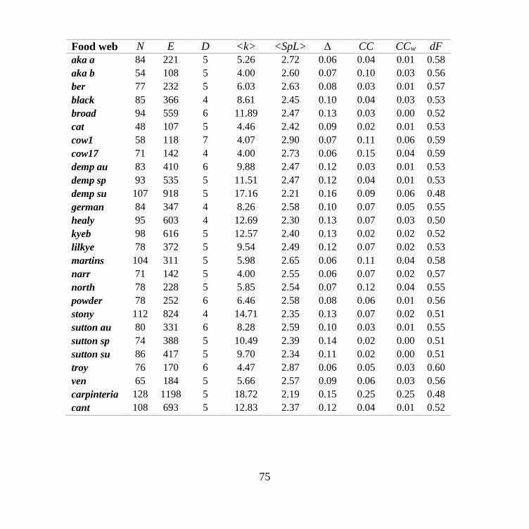
75

Food web N E D <k> <SpL> Δ CC CCw dF

aka a 84 221 5 5.26 2.72 0.06 0.04 0.01 0.58

aka b 54 108 5 4.00 2.60 0.07 0.10 0.03 0.56

ber 77 232 5 6.03 2.63 0.08 0.03 0.01 0.57

black 85 366 4 8.61 2.45 0.10 0.04 0.03 0.53

broad 94 559 6 11.89 2.47 0.13 0.03 0.00 0.52

cat 48 107 5 4.46 2.42 0.09 0.02 0.01 0.53

cow1 58 118 7 4.07 2.90 0.07 0.11 0.06 0.59

cow17 71 142 4 4.00 2.73 0.06 0.15 0.04 0.59

demp au 83 410 6 9.88 2.47 0.12 0.03 0.01 0.53

demp sp 93 535 5 11.51 2.47 0.12 0.04 0.01 0.53

demp su 107 918 5 17.16 2.21 0.16 0.09 0.06 0.48

german 84 347 4 8.26 2.58 0.10 0.07 0.05 0.55

healy 95 603 4 12.69 2.30 0.13 0.07 0.03 0.50

kyeb 98 616 5 12.57 2.40 0.13 0.02 0.02 0.52

lilkye 78 372 5 9.54 2.49 0.12 0.07 0.02 0.53

martins 104 311 5 5.98 2.65 0.06 0.11 0.04 0.58

narr 71 142 5 4.00 2.55 0.06 0.07 0.02 0.57

north 78 228 5 5.85 2.54 0.07 0.12 0.04 0.55

powder 78 252 6 6.46 2.58 0.08 0.06 0.01 0.56

stony 112 824 4 14.71 2.35 0.13 0.07 0.02 0.51

sutton au 80 331 6 8.28 2.59 0.10 0.03 0.01 0.55

sutton sp 74 388 5 10.49 2.39 0.14 0.02 0.00 0.51

sutton su 86 417 5 9.70 2.34 0.11 0.02 0.00 0.51

troy 76 170 6 4.47 2.87 0.06 0.05 0.03 0.60

ven 65 184 5 5.66 2.57 0.09 0.06 0.03 0.56

carpinteria 128 1198 5 18.72 2.19 0.15 0.25 0.25 0.48

cant 108 693 5 12.83 2.37 0.12 0.04 0.01 0.52

76

Table 4: Overall properties of the 27 food webs: N = number of nodes; E=number of links, D=diameter,

<k>= average degree, <Sp>=average shortest path, Δ=density, CC=average clustering coefficient,

CCw=weighted clustering coefficient, dF=distance-based fragmentation status.

3. Key player and nestedness analyses reveal common features in food webs

To understand whether key species were peculiar to specific food webs, and to reveal the

underlying organization of food webs, we computed key-player sets of increasing sizes

(1 to 4) for each key-player metric, both for fragmentation and reachability. Moreover,

since the m-reach reachability metric requires the specification of a maximum distance

length, we set m = 1 to 3. Results are shown in Figure 16A for all measures but

reachability and Figure 16B for m-reach. The increase in size of the kp-set has dramatic

consequences on most of the fragmentation metrics, showing a linear relationship

between the increasing set size and the increase in fragmentation.

Moreover, two nodes resulted to be required to reach the majority of nodes in any of such

networks with a maximum m-reach distance of 2 since a single node alone was not able

to reach the whole network. This confirms that the study of groups of nodes are critical

and more relevant than the study of single nodes in terms of reachability in heterogeneous

food webs. Moreover, keystone species exert their functions in groups, reinforcing the

idea that more than one keystone species is present in each ecosystem.

We then computed the nestedness between kp-set for each metric (Materials and

Methods, section 2.3) and reported results in Table 5. We wondered whether food web

topology has any significant effect on the nestedness of keystone species complexes in

these 27 food webs. For this reason, we computed the Spearman correlation coefficient

77

(P) between 9 topological metrics that are strongly related to the topology and 6 measures

of nestedness for each food web. Among the 6 topological indices, only 6 were significant

(Figure 17), and in each of these, M2 was the nestedness index (F, dF, dR, M1 and M3

did not show any significant correlation). M2 correlated positively with dF and <SpL>,

and negatively with Δ and <k> (N, E, d, CC and CCw did not show any significant

correlation). The four significant correlations are between M2 and dF (ρ = 0.681; p =

0.0009), M2 and Δ (ρ = -0.678; p = 0.001), M2 and <k> (ρ = -0.637; p = 0.00035) and

M2 and <SpL> (ρ = 0.605; p = 0.00084). All of them are strongly significant. Only a few

topological features can be used as a proxy for assessing the nestedness of central node

sets, but most of these show quite strong correlations. Our results suggest that in networks

where shortest paths are shorter, and density is higher, nestedness is lower, so systems-

based conservation can be less predictive and efficient. One example is the Sutton tussock

grassland in springtime (Figure 18A). Here, the single most central organism in the

network is Unidentifiable detritus (#0, black in Figure 18A). The most central pair is the

diatom Cocconeis sp. and the larvae of the riffle beetle Hydora nitida (#10 and #61, blue).

The group of the three most central network positions are the red alga Audouinella sp.,

the diatom Navicula avenacea and the caddisfly Pycnocentrodes spp. (#9, #30 and #70,

red). The four most central organisms are the alga Epithemia zebra, the diatom Eunotia

spp., the fishfly Archicauliodes diversus and Chironomid type 'Diamesid Blond' (#18,

#19, #49 and #52, orange). Hence, the increasing core of key organisms is perfectly

unnested (M2 = 0, up to 4 groups). Accordingly, dF is low (0,51), Δ is high (0,14), <k>

is high F (10,49) and <SpL> is small (2,39).

78

Figure 16: Fragmentation and reachability tendencies of food webs. A) Evolution of fragmentation

metrics using F and dF and of dR reachability. B) m-reach tendencies for each m-reach distance value for

node set of size 1 to 4 for a series of food webs. The majority of food webs (98%) are reached by 2 nodes

in at most 2 hops.

Apart from the single-node core (n = 1), the larger cores (n > 1) are always composed of

both plants (e.g. diatoms) and animals (e.g. caddisfly). On the contrary, in less connected

and less compact networks, nestedness is higher, so a multi-species approaches fairly

reinforce the results of single-species analyses. One example is the Dempsters tussock

grassland in autumn (Figure 18B). Here, the single most central organism in the network

is Unidentifiable detritus (#0, black). The most central pair is Unidentifiable detritus and

Terrestrial invertebrates (#2, blue). The group of the three most central network positions

are Unidentifiable detritus, and the caddisflies Olinga feredayi and Tiphobiosis sp. (#68

79

in orange and #76 in red). The four most central organisms are Tiphobiosis sp. as well as

the alga Epithemia zebra (#18, yellow), another alga Spirogyra sp. (#37, yellow) and a

mayfly Nesameletus ornatus (#66 yellow). Here, the composition of the core is a little bit

more nested (M2 = 47,22) and, accordingly, dF is somewhat higher (0,53), Δ is lower

(0,12), <k> is a little lower (9,88) and <SpL> is longer (2,47). The Supplementary

material shows the nestedness patterns for each food web. The nestedness patterns for

each kp-set iteration (data not shown) does not allow to compare the nestedness patterns

for specific species in different food webs, limiting the search for keystone species. It

must be noted, however, that node #0 is almost always Unidentifiable detritus (or some

similarly large aggregated group, e.g. Terrestrial invertebrate remains), underpinning the

importance of inorganic material for the development of ecosystems. In many networks,

this is part of the key player complexes. Biologically speaking, this is an artefact: the

detritus is clearly a well-connected component of food webs.

80

Food web F dR dF M1 M2 M3

aka a 100 100 80.56 100 77.78 0

aka b 100 100 94.44 91.67 77.78 0

ber 94.44 100 100 86.11 38.89 5.56

black 100 94.44 77.78 100 41.67 5.56

broad 100 100 94.44 61.11 5.56 0

cat 100 100 100 100 8.33 16.67

cow1 100 36.11 86.11 30.56 72.22 16.67

cow17 100 86.11 100 77.78 33.33 0

demp au 100 91.67 100 100 50 0

demp sp 100 100 55.56 100 72.22 0

demp su 50 100 27.78 100 47.22 0

german 100 69.44 72.22 63.89 8.33 0

healy 100 100 100 94.44 5.56 16.67

kyeb 100 100 100 94.44 27.78 0

lilkye 91.67 100 100 94.44 16.67 0

martins 100 47.22 83.33 66.67 22.22 0

narr 91.67 100 94.44 100 41.67 8.33

north 100 91.67 66.67 91.67 72.22 5.56

powder 100 100 94.44 100 77.78 0

stony 100 100 100 100 5.56 8.33

sutton au 100 61.11 91.67 77.78 38.89 0

sutton sp 100 100 86.11 100 16.67 8.33

sutton su 100 100 100 94.44 25 0

troy 100 100 100 100 0 8.33

ven 100 58.33 94.44 66.67 16.67 0

carpinteria 100 100 91.67 94.44 77.78 11.11

cant 94.44 100 100 100 41.67 0

Table 5: Nestedess computed for the kp-sets of sizes from 1 to 4 nodes for each of the key-player metrics.

Kp-sets were found using the Pyntacle greedy optimization algorithm.

81

Figure 17: Correlations between nestedness values of m-reach metrics vs. topological features of the

network. A-D: correlations between m-reach nestedness with a maximum distance length of 2 (M2) and

distance-based fragmentation (A), density (B), average degree (C) and average shortest path length (D). E:

correlation between nestedness computed for m-reach at a maximum distance of 3 (M3) and average

degree.

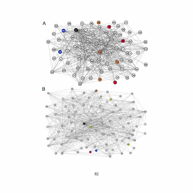
82

83

Figure 18: Network views of two food webs and the kp-sets found using the m-reach metrics. A) Sutton

tussock grassland in spring (sutton sp) food web and the identified keystone species using m-reach group

centrality metrics. In black the set of size 1, in blue the set with size 2, in red the set with size 3, in orange

the set with size 4. B) Dempster tussock grassland in autumn (demp au) food web. In black the set made

with size 1; the set with size 2 includes both the black and the blue sets; the set with size 3 includes the

black set, the orange set and the red set. Finally, the set with size 4 includes the orange and the yellow sets.

It is worth noticing that Unidentifiable detritus, even if it is frequently the key-group with

size 1, is frequently missing in larger key-player sets (e.g. for n = 4 in the demp au food

web). So, even if it single-handedly dominates the network structure, its position is not

significant anymore if we think in terms of a larger network core. Apart from the large

aggregated groups typically being in the center of the network, the four organisms that

can be in key position also in single-species cores (n = 1) are the diatom Fragilaria

vaucheriae (#19 in the broad food web), the shore crab Hemigrapsus oregonensis (#45

in the carpinteria food web), the mayfly Deleatidium spp. (#34 in the north food web)

and the diatom Rhoicosphenia curvata (#16 in the powder food web). Hemigrapsus

appears in all of the four studied kp-sets in the carpinteria food web (n = 1, 2, 3, 4). Some

communities are described by several versions of the food web (e.g. seasonal versions

like demp au, demp sp, demp su). In some cases, these versions differ a lot in nestedness

(demp and sutton), while in others there is only a small difference between the versions

(aka, cow).

84

4. Conclusions

The dynamical behavior of complex ecological systems can be dominated by a few

critically important components. Finding these could dramatically increase our

understanding, the predictability of models and the efficiency of management efforts. We

studied a comparable set of empirical food webs and identified the structurally most

important n nodes in them. Whether or not these small sets were nested was correlated to

some topological properties of these networks.

Network features influencing nestedness can be regarded as topological constraints on

the predictability and efficiency of management and systems-based conservation. It

remains unclear to us how can M2 and M3 be negatively and positively correlated with

<k>, respectively. There is a need for a better understanding of the biology of the key-

groups and the ecology of nested vs non-nested communities. If certain groups (e.g.

zooplankton, diatoms) appear frequently in the core of food webs, these can be thought

to be real keystone species. This is especially important if the core is nested: this means

that the community is really dominated by a single species. We still know nothing about

the kinds of communities (or the set of abiotic factors) that can be associated with nested

patterns. Biologically speaking, this is the most promising future research line.

Our results are based on a set of 27 empirical food webs in the size range between 48 and

128 trophic groups. This is the typical size scale for food webs in the literature. All the

webs were described by the same methodological standards, so they are comparable to

each other. In order to see if these results are generalizable, research is needed in at least

two directions. First, one wants to see if topological properties scale with network size.

85

For this, much larger networks should be studied – and the topological properties studied

here can be more and more relevant and interesting for larger graphs. The limitation here

is that empirical networks are not larger. Much larger networks (N>500) could be

constructed by dramatically increasing the resolution of trophic groups (e.g. by adding

bacteria and replacing trophic groups by biological species) but these networks would not

be biologically comparable to the present ones (even if being mathematically more

interesting). Second, toy networks of the same size ranges can be generated by various

algorithms (i.e. by using the pyntacle generate command) and empirical topologies

could be compared to the theoretical distributions. This kind of randomization analysis is

fairly straightforward in community ecology; however, it is not easy to see which

generative algorithms give the most realistic results as the nature of the current models

available in the ecological community yield particular issues that must be addressed (W.

Fox, 2006; Williams and Martinez, 2000). These studies could reveal if the reported

relationships are universal properties of networks in general or they are specific to only

food webs for some biological (ecological) reasons. If the results are food web-specific,

we need to understand the biological reasons. If the results will be shown to be of general

nature, conclusions can be drawn also in other fields of research. For example, terrorist

networks have been shown to have large average shortest paths and low density (Krebs,

2002), properties suggesting that their efficient “management” is possible – in the context

of homeland security. This work is of mostly conceptual and methodological nature. We

suggest that the search for the cores of ecosystem networks opens several research lines

that could massively contribute to systems-based conservation biology and management,

with applications ranging from marine fisheries to pollination systems.

86

87

Characterization of sex-specific mechanisms of aging in correlation networks of adult Drosophila Melanogaster

1. Background

Aging is a natural process that occurs, continuously, through the entire individual’s life.

This process develops a progressive loss of physiological integrity, leading to impairment

of vital functions, increased vulnerability and, finally, to death. This deterioration is the

primary risk factor for major human pathologies, including diabetes, cardiovascular

disorders, neurodegenerative diseases, and cancer. The identification of the markers of

aging is one of the major challenges of biomedical research of the 21st century. One of

the major hallmarks of aging was the discovery that the progress in aging is controlled,

to some extent, by genetic pathways and biochemical processes that are evolutionarily

conserved across complex multicellular organisms. The expansion of this field parallels

that of cancer biology: the continuously increasing availability of molecular data in

cancer research from the early 2000s onwards allowed to better understand the molecular

mechanisms underlying cancer initiation and maintenance. This was possible by merging

and studying together several kinds of data, from metabolomics to epigenetics (Fouad

and Aanei, 2017; Hanahan and Weinberg, 2011). The current scientific consensus

supports nine main hallmarks of physiological aging, which can be manipulated

experimentally to accelerate aging or ameliorate the health span: genomic instability,

telomere attrition, epigenetic alterations, loss of proteostasis, deregulated nutrient

sensing, mitochondrial dysfunction, cellular senescence, stem cell exhaustion, and altered

88

intercellular communication (López-Otín et al., 2013). A major challenge is to dissect the

interconnectedness between the candidate hallmarks and their relative contributions to

aging, with the final goal of identifying pharmaceutical targets to improve human health

during aging, with minimal side effects. Transcriptional changes are the core of these

hallmarks since the reshaping of the transcriptome constantly models these processes.

Changes in the expression levels and interactions of multiple gene networks occur in an

aging multicellular organism. A major challenge is to understand which pathways and

processes are altered and thus contribute to the manifestation of the hallmarks of aging.

The overall balance of these events articulates at the organismal level into the integrative

hallmarks to achieve the “aging phenotype” (Aunan et al., 2016).

A growing body of evidence (Frenk and Houseley, 2018; Kenyon, 2010; Seim et al.,

2016) suggests that changes in the levels of expression of different genes reflect in

changes in pathways which contribute to the manifestation of different hallmarks. These

changes occur relatively early in life (Aunan et al., 2016; Bryois et al., 2017). In the past

years, many studies have focused on describing the aging-related transcriptomic changes

(da Costa et al., 2016; Doroszuk et al., 2012; Swindell, 2009). For technical and economic

reasons, most studies on human (and vertebrate models) aging transcriptomics have

focused on one or few cell types from single or few tissues (Boisvert et al., 2018;

Haustead et al., 2016; Wood et al., 2013). Such conditions fail to underpin how each

pathway contributes to the “aging phenotype” at the organism level. In order to overcome

this difficulty, several studies in whole invertebrates have proven insightful. These

89

studies have mainly been conducted on Drosophila melanogaster in different times of

development by means of the microarray technology (Girardot et al., 2006; McCarroll et

al., 2004) (Zhan et al., 2007). Analysis of parts of the body of this organism as well as of

the whole organism determined a large number of sex-specific transcripts downregulated

during aging and a set of age-specific changes, correlating to a limited number of

biological processes differentially expressed in the head or thorax of the fly (Carlson et

al., 2015). Refinement of spatial-temporal expression of these results by Zhan et al. (Zhan

et al., 2007), showed that gradual changes in different aging tissues have little overlap.

However, these pioneering studies were performed using microarray platforms and did

not explore sex-specificity that could have a reshaping effect on the aging phenotype.

Currently, high-throughput RNA sequencing (RNA-Seq) allows for a higher sensitivity

even for lowly expressed transcripts and a wide range of techniques that can be used to

model the expression data according to the research aims. Among the landscape of

possibilities, correlation networks have grown in popularity in the last few years as they

enable the integration of large transcriptional datasets (Li et al., 2015; Liseron-Monfils

and Ware, 2015). Co-expression network analysis allows the simultaneous identification,

clustering, and exploration of thousands of genes with similar expression patterns across

multiple conditions (co-expressed genes). Their use allowed for a better understanding of

the functional dynamics of gene interplay, to the characterization of biological processes,

and to the study of the expression dynamics of complex disease mechanisms

(Emamjomeh et al., 2017). By means of gene correlation networks, it was possible to

define modules of tightly knit of co-expressed genes and to identify peculiar gene

90

signatures related to clinical traits of the human prefrontal cortex of old human brains

when compared to young ones (Hu et al., 2018). It was also possible to reveal aging-

related gene/pathway and cross-tissue relationships that had been observed for a long

time by physiologists without being validated at the molecular level (Huang et al., 2011).

The human brain co-expression network, in particular, was the object of intense studies,

as it was also possible to spot that schizophrenia and normal human aged brains show

similar patterns of co-expression in the frontal cortex (Kim et al., 2018). These works,

however, lack the characterization of the co-expression network communities that are

embedded within aging tissues.

In the present study, we tried to extend the current knowledge of aging mechanisms in

Drosophila and the techniques that are based on co-expression networks using the theory

of graphs. Centrality indices and algorithms for the measurement of team-play effect of

conserved genes in both sexes were used to assess their importance within the co-

expression modules. We made use of publicly available RNA-Seq data (Graveley et al.,

2011), to build co-expression networks for male and female flies using the Weighted

Gene Clustering Network analysis (WGCNA) (Langfelder and Horvath, 2008) method.

These networks were then compared. A list of genes that are important in the architecture

of sex-specific modules was finally obtained. We studied the functional enrichment of

sex-specific genes in female and male flies using the Gene Ontology. We then assessed

the common genes between the paired overlap consensus and each sex-specific module.

To assess their importance in the corresponding networks, we applied local and global

91

centrality indices on each sex-specific correlation network. This revealed several groups

of genes that can be considered potential markers of the sex-specific aging process. This

work is part of a broader analysis of sex and aging in fly and serves as a backbone to

select candidate genes to be screened using other data wrangling techniques and in vitro

assays.

2. Co-Expression analysis of sex-specific transcriptomes reveals different co-

expression module hubs

In a first step, we sought to reconstruct stage-specific correlation modules of co-

expression for male and female flies. Using the data from (Graveley et al., 2011), we run

the Weighted Gene Co-expression Network Analysis (WGCNA) method on RNA-Seq

data obtained on samples of of adult flies. The procedure for detecting these modules is

described in Materials and Methods, section 5.2. This analysis allowed to retrieve 27

modules for male and 28 for female. The size and number of these showed a remarkable

variance, both within the same sex and between genders. The majority of genes in males

was clustered in 6 big modules, each containing more than 500 genes (blue cluster

N=535, brown N=688, brown2 N=1264, floral white N=536, and pale turquoise N=

2280) (Figure 19, left panel). The network of co-expression in females was centered

around two hub co-expression modules: black (N=2461) and turquoise (N=2280) (Figure

19, right panel). In both cases, half of the coding genes did not cluster together (56.6%

for male and 50.6% for female). We then sought to analyze the interplay among these

92

modules. We summarized the overall expression values within modules using the module

eigengenes (Materials and Methods, section 5.2). We assessed the relationships between

the eigengenes by computing the correlation among summarized expression levels and

by using hierarchical clustering to identify the groups of synchronized module

eigengenes. This allowed calculating also the distance between modules. In males (Figure

20), we observed that the majority of hub module eigengenes exhibited positive

correlations with other small hubs, except for the brown2 and pale turquoise hubs that

grouped together. In female (Figure 21), the black hub was separate from the other

module eigengenes, while the turquoise module eigengenes aggregated with a series of

smaller module eigengenes: salmon4 (N=34), darkorange2 (N=44) and red (N=215). This

suggests that the turquoise hub may function as an aggregator of smaller functions,

possibly leading to a hierarchical organization between turquoise and its neighbors.

To conclude the exploration of sex-specific modules, we performed gene set enrichment

analysis (GSEA) on each module. The enriched functions were aggregated into macro

functional categories by REVIGO (Supek et al., 2011). Treemaps for each module,

depicting the most important biological processes (BPs) represented in each module,

were created. Figure 22 shows the most notable example, which is the bisque4 module

(N=54) that has been characterized later in this chapters by means of network analysis:

this module is represented by a plethora of BPs, which are summarized into two macro

functional categories important for aging: the oxidative stress-related processes and the

93

metabolic functions. This reinforces the idea that the aging process is altogether sustained

and fed by modules of co-expressing genes.

94

Figure 19: Bubble plots representing the modules and their sizes of co-expressing genes in the population

of female (right) and male (left).

95

Figure 20: Clustering dendrogram (upper plot) that summarizes the eigengenes correlations (lower plot)

in male co-expression networks.

96

Figure 21: Clustering dendrogram (upper plot) that summarizes the eigengenes correlations (lower plot)

in female co-expression networks.

97

Figure 22: GO enrichment as summarized by REVIGO in a treemap showing the most important BPs for

the bisque4 co-expression module in the male flies. Aggregated processes have the same colors, and the

aggregated GO processes are shown in bold in each group of tiles.

3. Network analysis of consensus overlap reveals common key-players in male and

female co-expression modules in Drosophila

Gene co-expression networks constructed from Drosophila RNA-Seq data allowed to

capture the relationships between genes. The built of the sex-specific functional modules

bridged the gap between individual genes and emergent global properties of the interplay

98

among genes in the two genders. This variability may underlie a different contribution of

genes in the establishment of different biological processes in aging. Some biological

functions could be performed by the same genes, while others can be more associated to

one sex than another. For this reason, we identified common mechanisms of co-

expression by building a common co-expression network between both sexes in order to

find consensus modules across the two genders (Langfelder and Horvath, 2007;

Langfelder et al., 2013). A total of 18 co-expression consensus modules were found.

These modules include genes that premusibly participate to common functional

mechanisms among the two sexes. We measured the preservation index between the

consensus network and the sex-specific networks, discovering that the sex-specific co-

expression networks and the consensus network were moderately well-preserved

(preservation=0.6), with a greater contribution on the consensus network of the male

dataset than the female one (data not shown).

We then reasoned on the common features. First, we identified the common genes

between each sex-specific module and selected only significant overlaps between each

consensus/sex-specific module pair with a hypergeometric test (Figure 23, both

matrices). Significant gene overlaps were then traced back to the original sex-specific

modules and their orchestrated effects of each overlap were explored by measuring the

distance-based fragmentation (dF) key-player measure before and after node removal.

We found that, on overall, the removal of the overlaps had a double effect on the initial

network fragmentation status. Removing some nodes resulted in an increase in

99

fragmentation, while removing other nodes resulted in a decreased fragmentation,

suggesting that these last nodes might play peripheral roles in the network. We focused

our attention on the bisque4 male module, identified before. This small module,

composed by 37 nodes and 358 edges, has a significant overlap with the magenta

consensus module (n=16, -logo-value=11), whose removal increased the overall module

fragmentation by 10% (dF=0.1), as shown in Figure 24, top panel. We then evaluated

the overlap with the turquoise female module (-logp=18) and found that its removal did

not modify considerably the fragmentation status of the network, with a <0.2% increase

(dF<0.001) (Figure 24, bottom panel). On overall, these findings suggest that consensus

modules are able to spot key players selectively, pinpointing that sex-specific genes have

different functional roles in aging according to the gender of flies.

100

101

Figure 23: Number of overlapping genes between sex-specific (rows) and consensus co-expression

modules (columns), for male (upper plot) and female (lower plot) flies. Numbers represent counts and the

colors highlight the significance of the overlap between the two gender datasets.

102

Figure 24: Distance-based fragmentation measured for the male bisque4 co-expression module (top) and

the female turquoise co-expression module (bottom) before and after overlaps removal. Dotted red line

shows the the initial fragmentation value. Point colors represent the consensus module from which the

overlap has been derived.

103

4. Conclusions

The aging phenotype is not the consequence of a single gene malfunctioning, but of the

constant, concerted, transcriptome-wide modification of gene abundances over the

lifespan on an adult individual (Harris et al., 2017). The relationship between sex and

aging has been object of intense researches over the past few years (Berghella et al., 2014;

Harris et al., 2017; Kamei et al., 2018). Multicellular model organisms provide an ideal

benchmark on which to study the dynamics of aging, and the small fly Drosophila

melanogaster is a key organism to characterize aging processes due to its short lifespan

and its low maintenance cost (Girardot et al., 2006); the search for molecular determinant

of aging is already begun. In this study, we provided an analytic blueprint for the

exploration of the relationships between sex and gender in the fly. We used publicly

available adult fly RNA-Seq data and showed that modules of correlation networks

strongly differ from adult and female flies in size and composition. A vast portion (over

50%) of the Drosophila correlation networks is scattered, and not connected enough to

trace their origin to a single co-expression module. These preliminary data suggest that a

consistent part of the transcriptome of female and male flies does not depend on tight

mechanisms of co-expression for determining their regulation. Moreover, males exhibit

a more homogeneous distribution of genes within modules, with a series of medium-sized

hubs that are supported by small hubs, each devoted to its functional, cellular tasks. We

hypothesize that the failure (or removal) of one of these hubs may not bring major

perturbation to the overall co-expression network architecture, because of the distributed

104

load of biological processes that is compensated by other co-expression modules. Female

co-expression modules, on the other hand, lack this homogeneity and are completely

summarized by their two giant hubs. While this modular configuration makes the removal

of one of them critical for the overall co-expression network, this should occur unlikely

by simply removing sets of genes. Moreover, since the majority of biological processes

are exerted by genes clustered in these modules, the female flies are more subjected than

males to bear the consequences of the aging process. Then, to assess if part of each sex-

specific network organization was shared across different modules, we built a consensus

correlation network and used it to derive the consensus modules This analysis showed

that the two genders contribute differently to all the correlation network modules. While

a weak preservation value was found among the consensus module and its sex-specific

counterpart, the consensus between the two transcriptomes was marginal, with genes of

a sex-specific module spread over many other consensus modules in the opposite gender

counterpart. The different gene distribution can have dramatic effects on the overall

architecture of the two co-expression transcriptomes. This dissimilarity was found also

at the module level. In fact, common genes among two different co-expression modules

may have different topological importance, thus not contributing equally to their

corresponding networks of origin. This concept pointed us to characterize the common

genes in the consensus modules and their counterpart, to assess their topological

importance. Group centrality metrics such as the key-players were ideal candidates to

explore this contribution to the consensus network since they could measure the team-

play effect that these genes exhibit in their network niche altogether. We focused on the

105

overlap between bisque4, a small module of the male fly found relevant in the oxidative

stress and the metabolic processes and the turquoise female co-expression hub, a giant

subcomponent of the female co-expression network. We found that the contribution to

the overall fragmentation of the network is higher when removing the overlapped genes

than its female counterpart, a clear index of how the organization of the communities

within each co-expression network differs greatly, with a higher degree of conservation

in the turquoise female network. All in all, these data point to different mechanisms of

aging between genders in fly.

106

107

Discussion

With the increased availability of biological data, Biology is questioning its roots. High-

throughput techniques, coupled with novel massive scale assays and computer science

advancements are producing data faster than what researchers take to analyze them and

yielding results. Data regard each layer of the omics world, from genomics to

epigenomics. They make increasingly more sense if considered together, namely if

shifting from the classical reductionist approach, that focus on the individual molecules,

to the holistic view, which considers, instead, the whole system of molecules taken

together. Besides its roots dates much earlier than these couple of decades, Systems

Biology is the ideal framework to make this transition possible (Westerhoff and Palsson,

2004). The field takes from the reductionist approach to overlap a holistic approach, thus

studying how a system is made and the relationships among its components.

The knowledge of how a system is shaped is crucial. Its particular form has direct

consequences on the observed phenomena of interest. It has been proven, in fact, that the

geometrical organization of a system, also known as topology, tightly characterizes the

dynamical behaviors of the system itself. This is particularly important in the context of

molecular biology, where changes between the patterns of interaction between genes or

their protein products can have dramatic consequences on the system itself (Cho et al.,

2016). Moreover, by predicting the functioning of a system, a systems biologist can

108

foresee which perturbations might lead to a new or altered phenotype (Cho et al., 2016).

Networks, which are simple mathematical abstractions that model the interactions among

components of a system, are at the core of Systems Biology. By means of Graph Theory,

we are able to spot network features using a wide range of mathematical metrics, which

study the centrality, namely the importance, of single entities with respect to the system’s

functional behavior.

This work aimed at exploring the potential of Network Biology in different biological

areas of research. We first used widely known centrality indices to study the regulome of

miRNAs, short non-coding sequences that modulate gene expression in colorectal cancer.

By first identifying differentially expressed genes between CRC specimens and their

matched normal tissues, we reconstructed the interactome of deregulated proteins in this

disease. We then performed an integrative analysis of mRNA–miRNA and miRNA–

miRNA interactions and identified two cancer-protection and nine cancer-favorable

modules of genes, providing interesting evidence on mRNA–miRNA crosstalks in CRC.

The analysis of the miRNA regulome also allowed to derive a series of miRNAs, chosen

through a core-set of local topological centrality indices, that controlled important key

genes in the process of CRC development. These resulted to be controlled, in turn, by the

deregulated expression of miR-145, which we defined a master regulator of the small

non-coding transcriptome and, hence, of some critical biological functions involved in

the carcinogenesis.

109

The aforementioned node indices, e.g. degree and betweenness, are well-known in

molecular network analysis and are widely used for tackling the most basic problems in

network analysis. However, the landscape of centrality indices is large, as networks are

used as a reasoning framework in several scientific disciplines, from Social Sciences to

Ecology. These indices are not necessarily local or global in nature but can account for

other levels of detail. For example, one could reason on the team-play effects of a group

of nodes in a network, and their overall contributions to the topology and the information

flow within it, rather than sticking to classical centrality indices. These classes of metrics,

mostly unexplored by the molecular network community, can be crucial to pinpoint the

role of groups of nodes in a network. For example, it is common knowledge that, even if

a gene exhibit an extraordinary pleiotropic character, pathways and processes are rarely

deregulated (activated or silenced) by a single gene perturbation (El-Brolosy and Stainier,

2017; Xu et al., 2009). The perturbation of a group of genes can instead have major effects

on the same network, thereby deranging the cell’s normal state.

Group centrality metrics enable to screen and evaluate for these types of dynamics. In

line with these arguments, we introduced Pyntacle, a Python 3 library and a command

line cross-platform tool for the exploration and search of groups of nodes, also known as

key-players, that can potentially affect the fragmentation on the network, when removed,

or that can be used as proxies to quickly reach the boundaries of a network. Pyntacle was

equipped with the most disparate tools and algorithms for local and global topological

studies, in order to make a swiss knife tool for network analysis.

110

We made huge efforts to make Pyntacle available through different channels. A website

was provided (http://pyntacle.css-mendel.it) with extensive documentation and case

studies. To boost Pyntacle performances, we equipped it with a series of algorithms that

execute algorithms efficiently both on individual CPU processors, as well as in parallel

on multicore processors and on CUDA cores of HPC graphics card, NVIDIA-enabled.

To test the ability of Pyntacle to spot key-nodes, we compared Pyntacle performance

versus those of a R library, keyplayer, which similarly performs group centrality analysis.

Pyntacle outperforms this library by several orders of magnitude and is able to spot key-

players even with large graphs, as well as with the interactome of small multicellular

eukaryotic organisms, such as the one of the small nematode C. elegans. Pyntacle is

actively maintained and reviewed and future plans include the extension of its

functionalities with novel topological indices, which are used in Ecology and Social

Sciences, and the improvement of its performance, allowing it to search and find key-

players through the greatest biological network known to date: the human interactome

(~20000 coding proteins).

We tested the usefulness of Pyntacle in two studies, presented in this work. The first one,

to date in press, is a methodological study in the area of Network Ecology. In this work,

we explored the role of key-players in a series of food webs, binary graphs that depict

trophic relationships among species in an ecosystem. Key-players of different sizes were

computed for each of the group centrality metrics available in Pyntacle, and a measure of

nestedness, a probability that a smaller set of size k is included in a bigger one j, was

111

measured. Through nestedness linked to a reachability measure (i.e., m-reach of distance

2), we found a positive correlation between the average degree of <k> of food webs and

reachability, a feature more relevant in tightly connected networks than in sparse graphs.

Network features correlated with nestedness can be regarded as topological constraints

on the predictability and efficiency of management and systems-based conservation,

hence providing a series of insights useful to decide which species to take into

consideration, a task that is of increasing importance considering the current warnings on

the climate changes and ecosystems deterioration.

The second study is instead a classic example of network analysis to infer structural

properties of molecular networks. This work, currently ongoing, is part of a more general

effort to identify the role of sex in the aging process in a model organism, the fly

Drosophila melanogaster. In this work, we reconstructed the co-expression network

architecture of adult female and male fly specimens using publicly available RNA-Seq

data measured along the developmental stages of the male and female flies. These

networks were built by means of the Weighted Gene Clustering Network Analysis, a

computation tool that allows building a series of gene-to-gene relationships by means of

fine-tuned measures of signed weighted correlations, other than raw correlation

coefficients. It also allows the detection of modules of co-expression, communities of

tightly linked nodes that exhibit strong inter-correlations. This first step of analysis

concluded that half of the coding and non-coding transcriptome of the fly is located

outside the identified communities, pointing to them as candidates for being object of

112

regulation by other means other than co-expression. The genes belonging to the

communities, on the other hand, were differently distributed through the two stages,

showing that the underlying architecture of the two genders is variable to some extent.

This is expected, as during adulthood, female and male flies perform reproduction, hence

their overall transcriptome abundance may exhibit different properties that require a

reshaping of these connections. Sex-specific gene set enrichment analysis allowed us to

identify a series of sex-specific co-expression modules that could be linked to the aging

processes to assess similarities between co-expression modules. We reconstructed the

consensus co-expression networks of the two genders and compared them with the two

co-expression networks of the two stages. This analysis showed that common co-

expression modules are weakly correlated to the sex-specific ones, reinforcing our idea

according to which the transcriptomes vary based on the genders. We then computed the

overlaps between each sex-specific modules of co-expression and their consensus

counterparts and found that these genes had a different effect on the fragmentation of the

sex-specific modules of origin. These findings would have not been possible without

Pyntacle, that was also used to perform a series of ancillary operations (not reported here)

to study the topology of these co-expression modules.

We showed the power of network models in biological studies. This opens new

horizons for the analysis of complex molecular networks using non-trivial mathematics.

This will help making new discoveries, thereby allowing to unravel the complexity of

life, one index at a time.

113

Materials and Methods

Network analysis reveals RNA-RNA crosstalk and highlights the role of societies of microRNAs in human colorectal cancer

1. Data sources

The datasets analyzed in this study consists of the transcriptome and miRNAome (Piepoli

et al., 2012) of a set of 14 matched pairs of tumor and adjacent non-tumorous mucosa

samples obtained from colorectal cancer (CRC) patients and evaluated with the GeneChip

Human Exon 1.0 ST array and GeneChip miRNA 2.0 array (Affymetrix, Santa Clara,

CA, USA). Raw data are available in the ArrayExpress platform with ID: E-MTAB-829

and E-MTAB-752.

2. Statistical analyses

Expression data analyses were performed using GNU R ver. 3.0.2 (http://www.r-

project.org) and the Partek Genomics Suite ver. 6.6 (Partek, St. Louis, MO, USA). Low-

level analysis and normalization were performed using GCRMA (Wu et al., 2005) and

Partek. We evaluated the probeset intensity values and kept only those significantly

detected in at least six samples. To reduce noise, we also removed the probesets that do

not map to an Entrez gene. Batch effects were removed by the Partek's batch effect

removal algorithm. The resulting genes and miRs were tested for differential expression,

114

using the paired t-statistics. Under the assumption of equal variance between groups,

allowing a number of false positives equals to 2% of the genome and setting the minimum

log2 fold change (log2 FC) expression barriers to ±1.5, we achieved a statistical power

of 0.8. Correlations between miRNA expression values were estimated using the

Spearman's rank correlation coefficient (rs) using Rcmdr (Fox, 2005). The relationships

between miR-145 and its direct and indirect partners were ascertained by regression

analysis. Time-to-event analysis was performed by the Mantel-Haenszel test and the 50%

percentiles of miRNAs were used to dichotomize patients into low and high expression

groups. Kaplan–Meier curves were drawn for CRC patients taken from The Cancer

Genome Atlas (TCGA) dataset (https://tcga-data.nci.nih.gov/tcga/tcgaHome2.jsp). A p-

value <0.05 was considered statistically significant. Equality of proportion was assessed

by the Chi-squared test.

3. Gene selection strategy and in silico functional and pathway analyses

To make results more reliable, only differentially expressed genes deregulated in at least

five CRC-related experiments retrieved from Gene Expression Atlas (Kapushesky et al.,

2012) were selected. These underwent functional enrichment analysis against the Gene

Ontology FAT subset and the set of genes with probe sets included in the used Affymetrix

chips. Results obtained with DAVID (Huang et al., 2009) web services were cross-

checked with Babelomics (Medina et al., 2010) and considered for inclusion if

Bonferroni-corrected significance levels did not exceed 5%. General functional classes

were refined by a mixture test between the elim and weight algorithms (Alexa et al.,

2006). These determined the best enrichment in a bottom-up order, by progressively

115

removing genes from functional classes, which were enriched by more specific

categories. This analytical procedure facilitated the identification of specific cancer-

favorable and cancer-protection processes, with statistical confidence. Pathways were

detected by ToppGene (Chen et al., 2009a), where the hypergeometric distribution with

False Discovery Rate (FDR) correction was used as the standard method for determining

statistical significance. The P-value cut-off was set to 0.05, while the gene limits ranged

from 1 to 1500

4. MiRNA selection strategy

We obtained a list of miRs that were reliably associated with CRC by intersecting the set

of miRs reported by miRSystem (Lu et al., 2012) to target the genes selected in the

previous analytical steps with that of miRs associated to CRC, according to the Human

microRNA disease Database (HMDD) (Li et al., 2014). MiRSystem is a database that

integrates seven well-known target gene prediction programs: DIANA, miRanda,

miRBridge, PicTar, PITA, rna22 and TargetScan. The observed identification probability

(O) for a given gene is the proportion of the queried miRNAs predicted to target that

gene, whereas the expected probability (E) is the proportion of all miRNAs in the

miRSystem database predicted to target that gene, i.e. the number of target gene-miRNA

pairs deposited in the miRSystem database. This expected probability represents the

chance of one gene being randomly selected by miRNAs. We only considered

experimentally validated targets, with an O/E ratio greater than 1.5.

116

5. Networks construction

We obtained multigraphs connecting genes by querying a number of heterogeneous data

sources: (i) Interpro and PFAM, (ii) Gene Expression Omnibus, (iii) BIOGRID and IREF,

(iv) PathwayCommons, IMID, NCI-NATURE, REACTOME, KEGG, BIOCARTA and

(v) BIOGRID, BIND, HPRD, INTACT, MINT, MPPI, OPHID, through GeneMANIA

(Mostafavi et al., 2008). We linked any two genes by an undirected edge, whenever an

evidence of interaction was found, which we weighted with a value provided by

GeneMANIA that indicates the predictive power of the selected dataset for that edge.

Several pairs of genes could be connected by more than one edge. In such a case, we

agglomerated the weights of multiple edges by the injective function:

𝑊𝐴𝐵 = ∑ 𝑊𝐴𝐵𝑖

𝑛

𝑖=1

where n is the number of edges connecting any two nodes A and B, and i refers to the ith

edge. WABi stands for the weight of the ith edge. The multiplicative factor 𝑒𝑛

𝑛 is meant to

give increasing importance to multiple links in respect to isolated links (Mazzoccoli et

al., 2013). We then built weighted graphs with weights over the edges (carrying the

reliability of the corresponding interactions).

MiRNAs were given in input to Ingenuity Pathway Analysis (IPA), which wired a

network based on the Ingenuity Pathways Knowledge Base. This knowledge base has

been abstracted into a large network, called the Global Molecular Network, composed of

thousands of molecules that interact with each other. Two molecules (miRNAs and genes

117

here) are connected if there is a path in the network between them. Interactions can be

physical and functional. We considered only physical interactions and cancer-related

functions, to build a literature-based network. Dashed edges stand for indirect

relationships between molecules, i.e. they summarize paths longer than one step.

The same set of miRNAs was filtered to contain only those that were differentially

expressed between our CRC and control tissues as well as those that exhibited any

significant correlation of expression with at least another miRNA (P-value < 0.05, rs >

0.4 or rs < −0.4). The resulting miRNAs were linked with non-oriented edges, since

correlation is a symmetric measure, and weighted using the Spearman's rank correlation

coefficient (rs), to make an experimental network (Piepoli et al., 2012)

6. Topological network analysis

Genes and miRNAs were assigned a topological importance. All the considered metrics

were based on the enumeration of links (or shortest paths). Considering a path from s ∈

V to t ∈ V, with V the set of nodes, as an alternating sequence of nodes and edges

beginning with s and ending with t, such that each edge connects its preceding with its

succeeding node, we calculated the length of a path by summing the inverse weights of

its edges. The idea is that highly correlated miRNAs or functionally closest genes

minimize their distance. We calculated degree, betweenness, closeness, radiality, and

clustering coefficient centrality indices, as described below, and ranked miRNAs and

genes accordingly. The privileged topological position of miRs was inferred by a

combination of the IPA's tools: BioProfiler and Upstream Regulatory Analysis. These

118

allowed inferring both which molecule might be considered causally relevant. Activation

z-scores were conservatively kept to a minimum of ±2. Networks were drawn by

Cytoscape 3.0 (Shannon et al., 2003).

7. Strongly connected components

Functional affinities of genes and miRNAs were sought among highly cohesive groups

of genes and miRNAs. To this end, we used the ClusterONE algorithm (Nepusz et al.,

2012). It handles weighted graphs and generates overlapping clusters. It starts from a

single node and greedily adds or removes new nodes if they alter the cohesiveness of the

group. Subgroups of less than five nodes or having a density less than a given threshold

(set at 3) were discarded. Finally, redundant cohesive subgroups were merged to form

larger subgroups to make the results easier to interpret.

8. MiRNAome and MAPK signaling pathway profiling after miR-145 transfection in CRC cell lines

To identify any functional synergistic pairs of miRNAs, the global miRNA expression

profile was obtained in the transfected CRC cell lines, as previously reported (Piepoli et

al., 2012) (ArrayExpress ID: E-MTAB-2704). Briefly, CaCo2, SW480, HCT116, and

HT-29 cell lines were transiently transfected using HiPerfect Transfection Reagent

(QIAGEN), with synthetic miR-145 mimic (MSY0000437, QIAGEN), following the

manufacturer's instructions, as previously described (Panza et al., 2014). The total RNA

119

was purified using the RNeasy kit (QIAGEN) and labeled using the 3DNA Array

Detection FlashTagTM RNA Labeling Kit (www.genisphere.com). Samples were

hybridized on Gene-Chip miRNA Array (www.affymetrix.com), washed and scanned

with an Affymetrix Scanner. MiRNA expression data were then processed and analyzed

using the Robust Multi-array Average algorithm and deposited in the EMBL-EBI

ArrayExpress.

To assess the effect exerted by miR-145 on the MAPK signaling pathway, gene

expression levels of the transfected cell lines were quantified by using RT2 MAP Kinase

Signaling Pathway PCR Arrays (SABiosciences). Briefly, mRNA and cDNA were

prepared using reagents and equipment from QIAGEN (QIAGEN Hamburg, Germany)

and assayed with the RT2 MAP Kinase Signaling Pathway PCR Arrays (SABiosciences)

with SABiosciences RT2 qPCR Master Mix according to the manufacturer's instructions.

Plates were read on 7900 TaqMan (Applied BioSystem, Life Technologies Corporation)

with 1 cycle of 10 min at 95°C followed by 45 cycles of 15 s at 95°C and 1 min at 60°C.

SYBR Green fluorescence was monitored at the annealing step of each cycle and

analyzed with SDS v.2.4 software (Applied BioSystem, Life Technologies Corporation).

The analysis of the gene expression was completed using the SA Biosciences PCR Array

Data Analysis Web Portal, as recommended by the manufacturer, and verified using the

ΔΔCt method.

120

121

Pyntacle

Pyntacle is a multifaceted library designed for Python 3.5 version onwards. The package

has been tested for all the subsequent Python 3 versions including the latest Python

release (3.7). Pyntacle is designed to be both a Python library and a command line tool.

The command line interface is more straightforward. It is designed to run automatically

the majority of Pyntacle functionalities and is addressed to the user with limited

programming knowledge. On the other hand, the Python 3 code library is highly

customizable and allows to fine-tune a variety of operations. It targets the experienced

Python users that perform bioinformatic tasks on a daily basis and would like to add

Pyntacle to their custom scripts or to their automated pipelines. For users with basic

programming skills that would still like to use Pyntacle in conjunction with their scripts

and code, we provided a utility, called octopus, that wraps many of the Pyntacle

functionalities to finally make them easily approachable.

Other than providing a series of classical centrality metrics to topologically analyze a

network, Pyntacle implements a few algorithms for the discovery of important groups of

nodes, or key players. Moreover, Pyntacle is optimized to perform a series of ancillary

operations, such as set operations between graphs, community finding, and file format

conversion. We provide the hereafter a detailed overview of the most prominent

functionalities, along with some supplementary materials (guides and network

specifications) described in Appendix. The same material, along with a complete

documentation, is available on our website (http://pyntacle.css-mendel.it) as a series of

Jupyter Notebooks.

122

1. Technical specifications

All classes and methods in Pyntacle are arranged in a directory-tree like fashion (Figure

25). This organization helps to compartmentalize each functionality, to quickly debug

and control the soundness of the code and to ensure that new functionalities can be added

without the risk of breaking the whole package.

We built Pyntacle around the igraph package (Csárdi and Nepusz, 2006), a widely known

cross-platform library for network analysis. The igraph.Graph object, is the very heart

of Pyntacle, as it allows to store and manage huge graphs. Wùith igraph, we were able to

store networks as big as the PPI network of Homo sapiens, stored in APID (Prieto and

De Las Rivas, 2006), encompassing ~15000 nodes and ~175000 edges. Moreover, igraph

allows enriching nodes, edges, and the whole graph with attributes, which are

implemented as unordered collections of keys:values. Pyntacle reserves a set of

private attributes, which are listed and described in Appendix 2 – Minimum Graph

Requirements. While the igraph.Graph object allows to represent any type of network,

the currecnt version of Pyntacle works with simple graphs only. Moreover, to avoid

ambiguities, nodes are required to have a unique name (stored by default in the name

attribute). For the same reason, multigraphs, namely networks with more than one edge

connecting two nodes, are not supported, as edges are identified by the nodes they

connect.

123

Figure 25: The directory tree of the command line interface and the Pyntacle library: green shapes enlist

all the possible Pyntacle command line sub-commands. Violet boxes represent the most important Pyntacle

modules upon which the command line is built.

124

2. Availability, installation, and testing

Pyntacle is cross-platform and can be installed on a wide range of operating systems

(Table 6). The main distribution channel is the Anaconda package manager, which is an

open-source repository and environment management system that runs on Windows,

macOS, and Linux. Users can install Pyntacle through Miniconda, a mini version of

Anaconda, which includes the most essential binaries for Python from the version 2.3

onwards. Miniconda allows to install automatically Pyntacle and to take care of its

software dependencies. The source code is versioned and made available on the Pyntacle

official GitHub page: https://github.com/mazzalab/pyntacle. Finally, to make the

installation and usage of Pyntacle easier, we built a Docker image on Ubuntu 16.04 and

have made it available on the Docker Hub website:

https://hub.docker.com/r/mazzalab/pyntacle. The Docker machine contains all the

necessary requirements to run Pyntacle in a virtualized system and is best suited for

servers equipped with high-performance computing hardware. A second Docker machine

was built for benchmarking Pyntacle and the keyplayer R package by (An and Liu,

2016a). Apart from Pyntacle itself, this Docker machine contains the binary files of the

keyplayer R package, several sample networks and a Python program that automatizes

the execution of the benchmarks. Finally, a series of unit tests to ensure that Pyntacle has

been correctly installed are provided and executed through the pyntacle test

command by the Pyntacle command line. Appendix 1 contains a Quick Startup Guide,

available taken verbatim from Pyntacle website, that allows the user to familiarize with

the core abilities of Pyntacle.

125

Conda Docker Binaries

Windows ✔ ✔

Mac ✔ ✔ ✔

Debian/Ubuntu ✔ ✔ ✔

Centos ✔ ✔ ✔

Other Linux Distributions ✔ ✔

Table 6: Availability of Pyntacle for each supported operative system and all the distribution channels.

3. Shortest Path search strategies

The shortest path is the minimum least distance that occurs between a pair of vertices

{i,j} in a network with the assumption that they are connected, meaning that at least one

path exists that connects the two pairs. If the nodes are disconnected, the distance is

infinite by definition. In simple graphs, this distance is measured in terms of hop, which

is the minimum number of edges between the node pairs. This distance is computed

differently according to the network type: in undirected weighted networks, for example,

the shortest path is the one with the minimum sum of the weights over the edges that

make the path between two nodes. Computing the shortest path is a computationally

intensive task since its execution time increases with the size of the network. Solving the

problem of finding the shortest path between two nodes in the least amount of time has

been widely explored. For simple graphs, all shorting paths connecting a given node to

126

all other nodes of a network can be computed by the Dijkstra’s algorithm (Dijkstra, 1959)

with a temporal complexity of 𝑂(|𝑉|2), where V is the number of nodes of a graph.

Finding all the shortest paths between any pair of nodes is as challenging as propedeutical

for the key-player algorithms implemented in Pyntacle. To this extent, we provided two

parallel versions of the Floyd-Warshall algorithm (Floyd, 1962), one running on

multicore computers and the other on CUDA-enabled graphic processors. This was made

possible resorting to Numba, a Python library that translates Python functions into

machine code optimized for high-performance computing (HPC) hardware and relieves

the heavy computational requirements (𝑂(|𝑉|3)). However, CPU and GPU accelerations

are not required with small graphs, since the computing overheads are largely greater that

the overall computing times on single CPU cores. For this reason, we implemented a

decision-tree-based algorithm that drives the choice of the best computing mode (i.e.,

single CPU, multi-CPU in parallel or GPU) based on the topological features (i.e.,

number of nodes and density) of the network to be analyzed (Figure 26). As anticipated,

one of the criteria used to choose the best computing mode is the graph density (Δ), which

is defined as:

𝚫 =2𝐸

𝑁(𝑁 − 1)

where E is the total number of edges over the total number of nodes N.

127

Figure 26: A decision tree driving the chosen of the best computing mode for the computation of the

shortest paths. N=number of nodes in the graph; =graph density; igraph BF: the igraph shortest path

implementation through brute-force.

4. Canonical and non-canonical centrality indices

Pyntacle is equipped with a series of classical local and global centrality metrics. The

complete list of these metrics is available in Table 6, where it is also specified whether

the measure was borrowed from igraph or designed and implemented in Pyntacle. We

distinguish between three groups of metrics.

Local metrics for individual nodes;

128

Global metrics for the whole graph;

Key-Player metrics for groups of nodes.

All these metrics are implemented through Python static methods, which thus can be

quickly used in Python shell environments and in interactive notebooks, as for example

the popular Jupyter Notebook (Kluyver et al., 2016; Pérez and Granger, 2007).

Among these metrics, the most known is the degree, k. It is defined as:

𝑘𝑖 = ∑ 𝑎𝑖𝑗𝑗

where a is a link between the node i and j. For binary networks, a=1, as multigraphs are

not currently supported. The degree distribution of all nodes is fundamental to define the

overall topology of a graph as well as to calculate the average degree (< 𝑘 >) of a

network:

< 𝑘 > = ∑ 𝑘𝑖1≤𝑖≤𝑛

𝑛

where n is the total number of vertices of a network.

Another core metrics universally considered to be a good evaluator of node centrality is

the betweenness (g). It is defined, for a vertex v, as:

𝑔(𝑣) = ∑𝜎𝑠𝑡(𝑣)

𝜎𝑠𝑡𝑠≠𝑣≠𝑡

129

where 𝜎𝑠𝑡 is the total number of shortest paths from node s to node t and where 𝜎𝑠𝑡(𝑣) is

the number of the paths that pass through the vertex v. It is then clear that the betweenness

is important whenever searching for vertices that are essential in the information flow

through a graph. Node betweenness (b) is based on the shortest path calculation,

introduced in the previous section. The same holds for the closeness (c) centrality, which

is another local metrics based on the reciprocal of the sum of the length of the shortest

paths between the node of interest and all the other nodes, over the total number of nodes

in the graph:

𝑐(𝑣) =𝑉

∑ 𝑑(𝑦, 𝑥)𝑦

where d(y,x) is the distance between vertices x and y. The distance between disconnected

nodes, in this case, is defined as the reciprocal of infinity, hence 0. The closeness

measures how easily other vertices can be reached from a node.

Another good evaluator of centrality is the diameter (D), which is the longest shortest

path in a network:

𝐷 = 𝑚𝑎𝑥(𝑑(𝑥, 𝑦))

Finally, it is important in real-world networks to measure the degree to which nodes in a

group tend to cluster together. For this reason, we included in Pyntacle the well-known

clustering coefficient (CC), an index that can be computed both locally and globally. The

global version is meant to quantify the overall clustering in the network, whereas the local

gives an indication of the embeddedness of individual nodes. The local clustering

coefficient for a vertex vi is then calculated as the proportion of links between the vertices

130

within the neighborhood of vi divided by the number of links that could possibly exist

between them:

𝐶𝐶𝑖 = 𝑛𝑢𝑚𝑏𝑒𝑟 𝑜𝑓 𝑐𝑙𝑜𝑠𝑒𝑑 𝑡𝑟𝑖𝑎𝑛𝑔𝑙𝑒𝑠 𝑐𝑜𝑛𝑒𝑐𝑡𝑒𝑑 𝑡𝑜 𝑣𝑖

𝑛𝑢𝑚𝑏𝑒𝑟 𝑜𝑓 𝑡𝑟𝑖𝑝𝑙𝑒𝑠 𝑐𝑒𝑛𝑡𝑒𝑟𝑒𝑑 𝑎𝑟𝑜𝑢𝑛𝑑 𝑣𝑖

where a triple centered around vi is a set of two edges connected to i. Hence, two measures

of CC can be derived, both included in Pyntacle. The first one, the average clustering

coefficient (CC) is defined as the average of all clustering coefficients of a network:

𝐶𝐶 = 1

𝑁 ∑ 𝐶𝐶𝑖

𝑛

𝑖=1

where N is the total number of nodes in the graph. High values of clustering coefficients

of a network denote the tendency of the network to be highly clustered and connected, a

property that is typical of small-world networks (Watts and Strogatz, 1998).

The second global clustering coefficient index is the weighted clustering coefficient

(CCw) (Scott et al., 1996), which is the average of each node’s clustering coefficient

weighted by their degree values:

𝐶𝐶𝑤 = 1

𝑁∑

𝐶𝐶𝑖

𝑘

𝑛𝑖=1 .

Furthermore, the PageRank algorithm (Page et al., 1998) was added to the Pyntacle’s

collection of algorithms. It was already used in biology to derive hierarchies among nodes

(Li and Zhao, 2016). Similarly, the radiality (R) metrics, also known as integration

centrality, was implemented to measure the closeness of a node in respect to the other

nodes of a network. It is defined as:

131

𝑅 =∑ 𝐷 − 𝑑𝑖𝑗 + 1𝑖≠𝑗

𝐷(𝑛 − 1)

where n is the total number of nodes in a graph, d is the distance between a vertex i and

all other nodes j and D is the diameter. High values of radiality denote that a node is

generally closer to the other nodes. Lower values, on the contrary, mean that a node is

peripheral.

The second global clustering coefficient index is the weighted clustering coefficient

(CCw) (Scott et al., 1996), which is the average of each node’s clustering coefficient

weighted by their degree values:

𝐶𝐶𝑤 = 1

𝑁∑

𝐶𝐶𝑖

𝑘

𝑛𝑖=1 .

132

Metric Property of Implemented in

Degree node igraph

Shortest Path node igraph and Pyntacle

Betweenness node igraph

Closeness node igraph

Clustering Coefficient node igraph

Eccentricity node igraph

Pagerank node igraph

Eigenvector Centrality node igraph

Radiality node Pyntacle

Radiality Reach node Pyntacle

Diameter graph igraph

Radius graph igraph

Number of Components graph Pyntacle

Density graph igraph

Pi graph Pyntacle

Average Clustering Coefficient graph igraph

Weighted Clustering Coefficient graph igraph

Average Degree graph Pyntacle

Average Radiality graph Pyntacle

Average Radiality Reach graph Pyntacle

Average Closeness graph Pyntacle

Average Eccentricity graph Pyntacle

Completeness - naive graph Pyntacle

Completeness graph Pyntacle

Compactness graph Pyntacle

F group of nodes Pyntacle

dF group of nodes Pyntacle

m-reach group of nodes Pyntacle

dR group of nodes Pyntacle

133

Table 7: The topological indices implemented in Pyntacle, along with the nature of the metrics and their

source (if ported from igraph or written from scratches in Pyntacle.

Furthermore, the PageRank algorithm (Page et al., 1998) was added to the Pyntacle’s

collection of algorithms. It was already used in biology to derive hierarchies among nodes

(Li and Zhao, 2016). Similarly, the radiality (R) metrics, also known as integration

centrality, was implemented to measure the closeness of a node in respect to the other

nodes of a network. It is defined as:

𝑅 =∑ 𝐷 − 𝑑𝑖𝑗 + 1𝑖≠𝑗

𝐷(𝑛 − 1)

where n is the total number of nodes in a graph, d is the distance between a vertex i and

all other nodes j and D is the diameter. High values of radiality denote that a node is

generally closer to the other nodes. Lower values, on the contrary, mean that a node is

peripheral. The formulation of the radiality lacks precision when a network has more than

one component, as the distance between disconnected nodes is infinite by definition.

Considering that many biological networks, such as pathways or correlation networks,

are often composed of several components, we reformulated the radiality equation. The

modified version is called radiality-reach (RR) and, for any vertex i belonging to the

component k, it can be formulated as:

𝑅𝑅𝑖 = 𝑅𝑖𝜖𝑘 𝑠𝑘

𝑁

where sk is the size of the component k for the node i and where N is the overall size of

the network. This ensures that the radiality is proportional to the size of the component

134

in a network and that nodes with high radiality and that belong to a bigger component

counts more than nodes in other components. The radiality-reach has the same numerical

boundaries than the radiality. It equals 0 when the node is an isolate, while it holds the

same value of radiality if the network is composed by a single component only.

Finally, we addressed in Pyntacle the issue of providing the biological community clear

metrics to measure the sparseness of a graph. The definition of the level of denseness (or

sparseness) of a network was relegated to abstract concepts or rule-of-thumbs. Generally

speaking, a dense graph is meant to have a number of edges (E) that is closest to the

maximum number of possible edges. Conversely, a sparse graph has a number of edges

that is close to the number of nodes (N). While these assumptions hold true for when the

number of edges is higher or lower than the total possible number of nodes, this definition

become weaker when E/N approximates to the 0.5 threshold, as this raises uncertainty in

whether to classify the network as dense or sparse. Moreover, graphs with different sizes

may have the same density, still exhibiting different numbers of zeros and non-zero

elements in their adjacency matrices. For this reason, in the past few decades researchers

struggled to propose clear and distinct definitions of network sparsity. Ràndic and De

Alba proposed the compactness index (𝜌) (Randic, 1997) as:

𝜌 = (𝑁2

2𝐸− 1) ∗ (1 −

1

𝑁)

where E and N are the total number of nodes and edges, respectively. This formula is

asymptotical, as networks with ρ > 1 are classified as dense, while graphs with ρ < 1 are

classified as sparse. Every graph exhibits either a greater or a smaller ρ number than the

critical value since this last is not analytically obtainable by the formula. Inspire by this

135

index, other metrics were proposed such as the completeness index () (Mazza et al.,

2010), which is defined as:

= 𝐸

𝑍=

∑ ∑ 𝑎𝑖𝑗𝑗∈𝑉,𝑗≠𝑖𝑖∈𝑉

∑ ∑ 1 − 𝑎𝑖𝑗𝑗∈𝑉,𝑗≠𝑖𝑖∈𝑉

Although the two indices look really close in most cases, their difference increases when

the size and the density of the graphs increase. This is a direct consequence of the

unbalanced formula of the compactness index which underestimates (and hence

misclassifies) large and extremely dense graphs. Both these metrics, as well as other less

notorious definition of sparseness are implemented in Pyntacle.

5. Group-centrality and key-player metrics

The negative key-player problem (KPP-NEG) aims at defining metrics that better

represent the role of a group of nodes in terms of cohesiveness. Some local metrics exist

that can be calculated to assess the overall network cohesion, as e.g., the node degree or

betweenness centrality. However, there are cases where these may fail. Let us consider,

for example, the toy network in Figure 27 and reported in the original Borgatti’s paper.

Degree and betweenness would agree to consider node 1 the best option to fragment the

network. However, this choice has no effect on disconnecting the network, since a link

between nodes 7 and 8 remains that keeps the total number of components to 1. In

contrast, removing node 8 does create two components, although itself does not exhibit

the highest centrality values.

136

Figure 27: The toy network used by Borgatti to explain the KPP-NEG problem. Node 1 (in blue) is the

node with the highest degree (k=9). However, its removal has no effects on the network cohesiveness

compared to the removal of node 8 (in red), that creates, instead, two separate components even if its degree

is lower than that of node 1 (k=6).

To solve this problem, two metrics were proposed: F and dF. These two metrics are both

global metrics that represent the overall fragmentation status of the network. The first one

stands for fragmentation. It counts the number of sub components and is defined as:

𝐹 =∑ 𝑠𝑘(𝑠𝑘−1)𝑘

𝑛(𝑛−1)

where n is the number of nodes, and sk is the size (number of nodes) of the kth component.

F ranges from 0 to 1. If a network has only one component, F = 0. If a network consists

of only isolates, F = 1.

137

The other fundamental fragmentation metric is distance fragmentation, dF and is defined

as:

𝑑𝐹 = 1 −

2 ∑1

𝑑𝑖𝑗𝑖>𝑗

𝑛(𝑛 − 1)

where dij is the distance between the ith node and the jth node and is 1 when the nodes are

adjacent and 0 (the inverse of the distance) when the nodes are unconnected, as they

belong to different network subcomponents. As for F, dF ranges from 0 to 1, with 0

representing a clique (every node is connected to each other) and 1 representing a network

of isolates.

Biological networks are less susceptible to fragmentation than other kinds of networks.

This might be due to their high redundancy that, in turn, works protecting from different

types of perturbation (e.g., genetic mutations, environment). Perturbations are tackled by

robust traits, like modularity, bow-tie architectures, degeneracy, and other topological

features. Robustness is a topological property and is linked to the network density only

marginally. Removal of only the edge connecting two groups of nodes in a dense network

might, in fact, be critical and cause the fragmentation of the network.

The second concern relates to the shortest path calculation for the dF metrics. The

calculation of the shortest paths for all nodes in a graph is a computationally intensive

task, whose time of execution scales with the size and the sparsity of a network. The

formulation of the dF includes the calculation of the shortest paths between any pair of

nodes in a network. This might be computationally demanding and time-consuming when

computing dF on a large network (>103 nodes), especially when searching for key-player.

138

Moreover, network density appears to heavily impact on running times, as shown in our

benchmarks. Multicore/GPU computing techniques were exploited to alleviate the

overall computational load and increase algorithmic performance.

The second problem is known as the positive key-player positive (KPP-POS). It concerns

the accessibility and the information spreading from a group of nodes of a network

through their direct and indirect partners. This problem can be formulated as follows:

“Given a graph G, with n nodes and l links, what is the subset of n of size k that can reach

as many remaining nodes as possible via direct links or shortest paths?”

This problem introduces the concept of reachability. When dealing with reachability, one

immediately thinks to the closeness metrics. Thus, the more central a node, the closer it

is to all other nodes. However, even if node 4 of the graph in Figure 28 has the highest

closeness measure, it is not the most central node in terms of reachability, since it reaches

6 nodes with 2 links or less, while node 3 can reach 8 nodes with 2 links or less.

The conclusion is that canonical metrics may provide sub-optimal solutions, that however

might be improved by topological metrics designed for groups of nodes. We hence

implemented two reachability metrics to cope with this issue: m-reach and dR.

m-reach (Ck) is a reachability measure that counts how many unique nodes can be reached

from a node set in m steps, where m is the maximum distance (shortest path) between the

set and the remaining nodes. The formulation is:

𝐶𝑘 = ∑ ⋃ 𝑟𝑖𝑗𝑚𝑖 𝜖 𝐾𝑗𝜖 𝑉−𝐾

where m is the minimum distance between any node i belonging to the set K and any node

139

Figure 28: Toy network to explain the concept of reachability. Node 4 (in blue) has the highest closeness

value (C=0.5). However, if we aim at finding the node that reaches the most of other nodes in two steps or

less, node 3 (in red) is the best choice although having a closeness value of C=0.48.

j outside the set, while mr is a reachability matrix, where mrij = 1 if i can reach j via a path

of length m or less, and mrij = 0 otherwise. The m-reach ranges from 0 to n-k, where n is

the total number of nodes while k is the size of the set. The disadvantage of this measure

is that it assumes that all paths of length m or less are equally important and that all paths

longer than m are wholly irrelevant.

dR stands for distance-weighted Reach and, as dF, is a more sensitive measure of the

distances (shortest path) between the node set and the remaining nodes in the graph. It is

defined as:

𝑑𝑅 =

∑1

𝑑𝐾𝑗𝑗

𝑛

where n is the total number of nodes in the graph and dKj is the minimum distance

(shortest path) between any member i of the node set and the remaining nodes in the

140

graph. In the toy graph shown in Figure 29, the distances between the nodes {1,7}, which

make the set of interest, are set to 1 by convention. Thus, dK,1 = 1 and dK,7 = 1. The

distance from the set to node 5 is 1, since 1 is the length of the shortest path from either

1 or 7 to 5. Similarly, dK,3 = 1, dK,4 = 2, dK,2 = 2, dK,6 = 2. Hence, dR ranges from 0 and 1.

It is 0 when the set is completely disconnected from the other nodes. It is 1 when the set

is adjacent to all other nodes of the network.

Figure 29: Toy network to explain the dR metrics. Node 5 (pink) is reach by node 1 in two hops, and by

node 7 in 1 hops the latter is taken as the minimum distance between the set {1,7} and node 5.

6. Key player search optimizations

Pyntacle allows to search for the best key-player set (kp-set) that maximizes the

fragmentation or the reachability of a given set of size k. Two methods currently exist to

141

do that. The first one is a greedy optimization search algorithm. It does not aim at finding

the best kp-set, as this would require:

𝑁!

(𝑁 − 𝑘)! ∗ 𝑘!

iterations, where N is the size of the graph and k is the size of the group. While these

operations can easily be performed on small networks (<= 1000 nodes), the increase of

both the size of the network and of k may have dramatic consequences in terms of

computating time. The optimization works by first selecting a group of nodes of size k,

and then by swapping every member in the node set with each other nodes in the graph

until there is no set with a better centrality value. The following pseudocode summarizes

the operation performed during any iteration:

1. select k nodes at random to populate the set S

2. define an initial value for the kp metric of choice for S

3. for each node u in S and each node v not in S:

a. compute DELTAkp = difference in the kp-metric if u and v

were swapped

4. select the set with the highest DELTAkp

a. if DELTAkp > max(all DELTAkp recorded), terminate, else:

b. swap nodes with the greatest improvement in fit and store

the DELTAkp value and the node set

5. Go to step 3

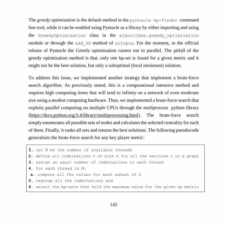
142

The greedy optimization is the default method in the pyntacle kp-finder command

line tool, while it can be enabled using Pyntacle as a library by either importing and using

the GreedyOptimization class in the algorithms.greedy_optimization

module or through the add_GO method of octopus. For the moment, in the official

release of Pyntacle the Greedy optimization cannot run in parallel. The pitfall of the

greedy optimization method is that, only one kp-set is found for a given metric and it

might not be the best solution, but only a suboptimal (local minimum) solution.

To address this issue, we implemented another strategy that implement a brute-force

search algorithm. As previously stated, this is a computational intensive method and

requires high computing times that will tend to infinity on a network of even moderate

size using a modest computing hardware. Thus, we implemented a brute-force search that

exploits parallel computing on multiple CPUs through the multiprocess python library

(https://docs.python.org/3.4/library/multiprocessing.html). The brute-force search

simply enumerates all possible sets of nodes and calculates the selected centrality for each

of them. Finally, it ranks all sets and returns the best solutions. The following pseudocode

generalizes the brute-force search for any key player metric:

1. let N be the number of available threads

2. define all combinations c of size k for all the vertices v in a graph

3. assign an equal number of combinations to each thread

4. for each thread in N:

a. compute all the values for each subset of k

5. regroup all the combinations and

6. select the kp-sets that hold the maximum value for the given kp metric

143

Bruteforce search can be enabled in the pyntacle kp-finder command line tool by

passing the –implementation brute-force argument, while the number of threads

can be passed through the --threads argument. If not specified, Pyntacle uses all the

threads available on the machine in which it is running minus one. In the Pyntacle library,

brute-force can be invoked using the BruteForce class in the

algorithms.brute_force module or through the add_BF method of octopus.

7. Ancillary operations

A plethora of ancillary functionalities was added to Pyntacle. We divided these graph

operations in two classes:

Logical set operations and

Community finding algorithms

The first class of operations is used to perform the union, intersection and difference

among two graphs as described in (Harary, 1994; Skiena, 1990). For intersection, we

consider the intersection G3 between two graphs G1, formed by v1 and e1 vertices and

edges, and G2, with v2 and e2 edges, the common set of nodes and edges between the two,

such as:

𝐺3[𝑣3, 𝑒3] = 𝐺1[𝑣1, 𝑒1] ∩ 𝐺2[𝑣2, 𝑒2]

The union of two graphs on the other hand, is the union of edges and vertices of G1 and

G2:

144

𝐺3[𝑣3, 𝑒3] = 𝐺1[𝑣1, 𝑒1] ∪ 𝐺2[𝑣2, 𝑒2] = [𝑣1 ∪ 𝑣2 , 𝑒1 ∪ 𝑒2]

Finally, the difference graph G3 is the intersection among the set of edges minus the

connecting edges in common between the two graphs G1 and G2, such as:

𝐺3[𝑣3, 𝑒3] = 𝐺1[𝑣1, 𝑒1] \ 𝐺2[𝑣2, 𝑒2] = [𝑣1 ∪ 𝑣2, 𝑒1\𝑒2]

Community finding algorithms on the other hand are means to divide a graph into several

induced subgraphs of tightly associated nodes with respect to the rest of the graph.

Community finding is an open field and different algorithms are used depending on the

scientific context. In general, there is no correct solution when defining communities,

because the definition of a community is itself questionable. Each partitioning algorithm

relies on its definition of modularity, a measure to distinguish how tight is the group of

nodes identified as a community, and on specific thresholds that are used to distinguish

one community from another one. For this reason, we implemented some of the most

famous algorithms in community finding for scale free, small-world and random graphs.

Specifically, we focused on the fastgreedy algorithm (Clauset et al., 2004), the infomap

algorithm (Rosvall and Bergstrom, 2007), the leading eigenvector algorithm (Newman,

2006) and the walktrap algorithm (Pons and Latapy, 2006). The explanation of each

algorithm is beyond the scope of this work, but to generalize, we will focus on the

fastgreedy algorithm by Clauset, that works best on large and sparse networks with an

underlying hub-and-spoke configuration, such as many biological networks. This

algorithm assigns at first a modularity score on each node of the network based on the

interconnectedness with its neighbors. Through a series of iteration, adjacent nodes with

similar modularity scores are merged until the difference between each group of nodes is

such that they cannot be merged anymore. The threshold for defining the merge cut point

145

is found through a clustering based on Euclidean distances, that dynamically defines the

modularity threshold according to the distance between branches. Dense networks or

small networks may not show distant cut points; hence the algorithm could also fail at

defining distinct communities. Therefore, it is suited for large graphs.

8. Supported network file formats

Pyntacle is compliant to a variety of network file formats. The first and most common is

the network representation through adjacency matrix. An adjacency matrix is a squared

nxn table.

Both row i and column j indices refer to nodes in a network. Non-zero values filling cells

(aij) indicate the presence of connecting edges between the relative nodes, so that

𝑎𝑖𝑗 = {≠ 0 if there is an edge from 𝑗 to 𝑖

0 otherwise

The values stored in each cell of the matrix represent connection among nodes. Several

types of matrices exist that can represent different network types, from unweighted and

undirected to weighted and directed. In Pyntacle, we only support simple graphs. Their

adjacency matrices will hold ones between two distinct nodes if these are connected by

an edge, and zeroes otherwise.

𝑎𝑖𝑗 = {1 if there is an edge between 𝑗 and 𝑖 ≠ 𝑗

0 otherwise

146

Self-loops are not allowed. Adjacency matrices usually have a header, but this is optional.

In the first scenario (header is present), we assume that the header is in both the first row

and the first column of the file and identical, like in the example in Figure 30A.

Figure 30: Toy examples of network text file formats supported by Pyntacle. A) Adjacency matrix B) Edge

list C) Simple Interaction File (SIF).

In the case the matrix does not have a header, the vertices are enumerated from the first

to the last row. Adjacency matrices can have any file extension. By default, the .adjm

extension is used. Cells in an adjacency matrix file are supposed to be delimited by

tabulation (\t, or tab) unless otherwise specified. If not explicitly specified, the separator

character will be inferred, before resorting to the default choice.

147

Edge Lists files are another common way to store a graph. An edge-list is a list, or array,

containing pairs of nodes. Thus, each element of the array represents a link directionally

connecting the first (a) to the second (b) node of the pair. If a network is meant to be

undirected, each pair a→b must be accompanied by a pair b→a, such as the example

reported in Figure 30B. We support undirect, unweighted edge lists, separated by a

uniform separator character. As for adjacency matrices, Pyntacle uses the .egl file

extension by convention, but files can have any extension as long as they store text.

Pyntacle was equipped with a parser for the Simple Interaction File (SIF) format. It is the

most used format by standard application for biological networks analysis and

visualization, like Cytoscape (Shannon et al., 2003). Its syntax is agile and simple. It

allows Cytoscape to represent properties of both networks and edges. Usually, the file is

made by 3 or more columns (see Figure 30C). The first and third column represent the

source and target nodes with the type of their interaction specified in the 2nd column. The

order of the columns is just conventional, and it is generally not relevant, as the user can

choose what is the meaning of these columns in the process of importing a network in

Cytoscape.

The last textual file format supported is the DOT file format. DOT is a widely known file

format with an easy syntax that is well suited to graph plotting. It is widely used by

graphical visualization tools such as Graphviz (Ellson et al., 2004). The power of DOT

relies just on its syntax, that allows to interpret and store much graphical information (like

edge thickness or node colors with gradients), thus representing networks used in several

kinds of contexts. More information on the DOT file format can be found on the official

Graphviz documentation. Many tools already support the importing and exporting of

DOT files, such as the popular NetworkX library. igraph, on the other hand, supports only

148

the exporting of DOT files. We implemented a parser that addresses the specific problem

of importing undirected networks.

Finally, networks can be given to Pyntacle as pickled binary files containing igraph

objects, if these graphs are compliant with the minimum requirements described in

Appendix 2.

9. Benchmarks data

We performed benchmarks on a dataset comprising 12 test networks, that are listed in

Table 8. The dataset contains a variety of small (N<100), medium (N100 and N<1000)

and large (N1000) sized graphs, stored in binary adjacency matrices. These networks

come from two sources. Six of them are real networks. The three food webs (carpinteria,

north, cat) were downloaded from the NCEAS ecological repository

(www.nceas.ucsb.edu/interactionweb) and have the minimum, maximum and median

number of nodes among all the food webs available in NCEAS. These case studies allow

studying the interplay among species using the key-player algorithms, as described in the

chapter 4 of Results. The Caenorhabditis elegans connectome (CAEEL_connectome),

downloaded from wormbase database

(http://www.wormatlas.org/neuronalwiring.html#Connectivitydata), represents a well-

studied case of a small world network (Towlson et al., 2013). The PPI interactome of the

small nematode is a well-known example of scale-free topology (Li et al., 2004). The

advice-seeking ties among global consulting companies (AdvSeek network) is the

smallest network (N=32, E=55, =0.11089) taken from (Borgatti, 2006) (Figure 8 in the

corresponding paper). The biggest is the interactome of C. elegans (N=3303, E=5561,

149

=0.00102) downloaded from APID on February 2018. All the networks were converted

into undirected networks while weights were neglected. Only the largest component of

each network was considered.

The remaining six models are binary networks that follow random topologies. They were

created according to the Erdős–Rényi model (Erdős and Rényi, 1959) by means of one

of the Pyntacle’s generators. The size of the networks ranges from n=100 to n=1000,

while the wiring probability ranges from P = 0.3 to P = 0.7 at steps of 2, where P is the

probability that a link is placed among a pair of nodes.

Network Type N E

Carpinteria NCEAS Food Web 128 1198 0.14739

North NCEAS Food Web 78 228 0.07592

Cat NCEAS Food Web 48 107 0.09486

AdvSeek Borgatti Case Study 32 55 0.11089

CAEEL_connectome Neuronal wiring of the nematode C. elegans 279 1960 0.05054

Random 100-0.3 Artifical network 100 1492 0.30141

Random - 100-0.5 Artificial network 100 2489 0.50283

Random - 100-0.7 Artificial network 100 3426 0.76582

Random 1000-0.3 Artificial network 1000 149998 0.3003

Random 1000-0.5 Artificial network 1000 249983 0.50047

Random 1000-0.7 Artificial network 1000 349370 0.69944

APID_CAEEL Level 2 interactome of C. elegans downloaded from APID 3303 5561 0.00102

Table 8: Description of the test networks used for benchmarking Pyntacle. N=total number of nodes;

E=total number of edges, =graph density. Blue, orange and green colors mark big, medium and small

sized graphs, respectively.

150

10. Benchmarks specifications

Benchmarks were performed on a custom Docker Image running Ubuntu 16.04, that can

be downloaded at https://hub.docker.com/r/mazzalab/pyntacle_benchmarks/. This

Docker machine was deployed into a local server equipped with 4 AMD Opteron®

processor 6172 @2100MHz frequency, with 12 CPU cores each, 256 GB of RAM and

connected by InfiniBand through Mellanox/Intel host bus adapters and network switches.

CUDA acceleration was not available.

Pyntacle version 0.2.4 and the keyplayer R Package (An and Liu, 2016b) version 1.0.3

were installed in the Docker machine. Binaries for the two packages were retrieved from

Conda and CRAN, respectively. The key-player search was performed by means of the

greedy optimization algorithm, which was run for all the small and medium-size networks

described in the previous section. For Pyntacle, we run the keyplayer kp-finder

command, setting a seed of 100. For the R keyplayer package, we wrapped its greedy

optimization method in a custom R script, and timing was measured using the default

timing libraries provided by R version 3.4.

A kp-set size of 2 was sought with both software. The timing of the greedy optimization

was calculated only for comparable key-player metrics. The R package lacks for the F

fragmentation measure, while the dR formulation slightly differs from the one described

by Borgatti (section 5 of this chapter).

The remaining key player metrics, dF fragmentation and m-reach reachability, were

comparable in their formulations. For m-reach, its maximum distance was set to 1 for

both tools. The maximum allowed execution time for each algorithmic iteration was set

151

to 1 week. For Pyntacle, the brute-force search for was performed for small size networks.

Speedup plots for each key-player metric were obtained by dividing the execution times

measured on single cores over their timings using 4,8,16 and 32 CPU cores. For all

benchmarks, times were measured in triplicate, and the results were summarized by

computing the mean of the times 𝜇𝑇 and their standard deviations σ𝑇.

152

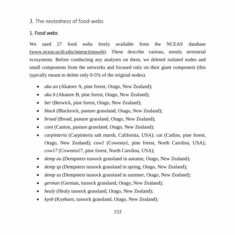
153

The nestedness of food-webs

1. Food webs

We used 27 food webs freely available from the NCEAS database

(www.nceas.ucsb.edu/interactionweb). These describe various, mostly terrestrial

ecosystems. Before conducting any analyses on them, we deleted isolated nodes and

small components from the networks and focused only on their giant component (this

typically meant to delete only 0-5% of the original nodes).

aka an (Akatore A, pine forest, Otago, New Zealand);

aka b (Akatore B, pine forest, Otago, New Zealand);

ber (Berwick, pine forest, Otago, New Zealand);

black (Blackrock, pasture grassland, Otago, New Zealand);

broad (Broad, pasture grassland, Otago, New Zealand);

cant (Canton, pasture grassland, Otago, New Zealand);

carpinteria (Carpinteria salt marsh, California, USA); cat (Catlins, pine forest,

Otago, New Zealand); cow1 (Coweeta1, pine forest, North Carolina, USA);

cow17 (Coweeta17, pine forest, North Carolina, USA);

demp au (Dempsters tussock grassland in autumn, Otago, New Zealand);

demp sp (Dempsters tussock grassland in spring, Otago, New Zealand);

demp su (Dempsters tussock grassland in summer, Otago, New Zealand);

german (German, tussock grassland, Otago, New Zealand);

healy (Healy tussock grassland, Otago, New Zealand);

kyeb (Kyeburn, tussock grassland, Otago, New Zealand);

154

lilkye (LilKyeburn, tussock grassland, Otago, New Zealand);

martins (Martins, pine forest, Maine, USA);

narr (Narrowdale, pine forest, Otago, New Zealand);

north (NorthCol, broadleaf forest, Otago, New Zealand);

powder (Powder, broadleaf forest, Otago, New Zealand);

stony (Stony, tussock grassland, Otago, New Zealand);

sutton au (Sutton tussock grassland in autumn, Otago, New Zealand);

sutton sp (Sutton tussock grassland in spring, Otago, New Zealand);

sutton su (Sutton tussock grassland in summer, Otago, New Zealand);

troy (Troy, pine forest, Maine, USA);

ven (Venlaw, pine forest, Otago, New Zealand).

Geographic distribution is thus quite narrow, but this does not seem to have any known

effect on the results.

2. Network analysis

We calculated nine global (macroscopic) topological properties for each network using

Pyntacle. The number of nodes (N) and the number of interactions (E) are trivial

properties of every network. We used this information to compute the density Δ of each

food web (see the “Shortest Path search strategies” section above). For each species in

each food web, we also computed the degree k, and used it to compute the average degree

<k> for all nodes in the network. Finally, we computed the clustering coefficient CCi and

155

used it to derive for each network its average clustering coefficient CC and its weighted

global clustering coefficient CCw. This latter puts larger emphasis on clusters around

more connected nodes. The whole networks were characterized by the average shortest

path lengths (<Sp>) and their maximum values, the diameters, D. Finally, the distance

weighted fragmentation (dF) was computed for each network before performing the final

key-player analysis.

3. Multi-node centrality

Multi-node centrality analyses have already been performed on different types of

ecological networks including food webs (González et al., 2016) and habitat networks

(Rubio et al., 2015). The most central multi-node sets of n = 1 to n = 4 nodes were

identified for the 27 food webs that solved the KPP-POS and KPP-NEG problems. For

the latter problem, F and dF where calculated. For the former problem, the m-reach

centrality (M) with m = 1, 2 and 3 steps (M1, M2, and M3, respectively) and dR where

computed. Each of these metrics were computed for groups of 1 to 4 nodes.

4. Nestedness

The nestedness of presence-absence ecological data (Podani and Schmera, 2011) has a

rich literature with well-developed methods (An and Liu, 2016a; Kelt, 1997; Podani et

al., 2013). The nestedness approach has also been extended to ecological interactions in

simple graphs (Fortuna et al., 2010). Here we study the nestedness of ecological

156

interaction networks in a very different way (Benedek et al., 2007; Ortiz et al., 2013),

quantifying the set–subset relationships of central nodes in a network. We calculated the

nestedness of central node sets (i.e. the overlap among the sets of size n = 1 to 4) using

the Nrow metric (Boland and Goel, 2010b). Nrow is the average percentage of nodes of

the smaller sets that are contained in the larger sets, taking all possible pairs of sets. For

example, for the food web demp au, the key player sets for M2 (m-reach using a

maximum distance of 2) n = 1 to 4 nodes were {0} for n = 1, {0 ,2} for n = 2, {0,68,76}

for n = 3 and {76,18,37,66} for n = 4. For n =1 and n = 2, there is perfect overlap. For n

=1 and n = 3, there is partial overlap, since the smaller set (n =1) is a subset of the larger

one (n = 3). For n= 2 and n = 4, there is no overlap, since the two sets have no common

elements. Averaging all the 6 overlaps, we have Nrow = 47.22, which is the nestedness

value for M2 in the demp au food web (see the species identities for this food web in

Discussion). The same was done for the remaining centrality measures (F, dF, M2, M3,

and dR).

157

Characterization of sex-specific mechanisms of aging in correlation networks of adult Drosophila Melanogaster

1. RNA-Seq data availability and processing

We downloaded the publicly available data used by Graveley (Graveley et al., 2011) from

the small read archive (SRA) available at NCBI (accession number ID:SRA009364). This

dataset comprises 234 raw fastq files corresponding to Drosophila development and

aging timepoints. Each timepoint encompassed 4 to 6 biological replicates per sampling.

We assessed read quality using the FastQC (Andrews, 2010) software version 0.11.5 and

used Trimmomatic (Bolger et al., 2014) version 0.36 to perform read trimming and

filtering. Specifically, reads were trimmed using a sliding window of 4 base calls and a

minimum window average PHRED quality of 30. Reads with less than 15 nucleotides

after trimming were removed. Reads were mapped by means of Tophat2 (Trapnell et al.,

2009) against the Drosophila genome version 6.10 downloaded from NCBI, following

developer’s recommendations. Raw counts for each gene were estimated by first piling-

up aligned reads on the Drosophila GFF annotation version 6.13 provided by FlyBase

(Gramates et al., 2017), encompassing 16,271 genes, by means of the HTSeq pipeline

(Anders et al., 2014) using the intersection-nonempty criterion for counting features.

2. Sex-specific co-expression network analysis and module eigengenes detection

To search for modules of sex-specific gene correlation in female and male flies, we made

use of the Weighted Gene Clustering Network Analysis (WGCNA) R package

(Langfelder and Horvath, 2008) version 1.64.1. WGCNA includes a series of utilities to

perform module detection of groups of tightly connected genes and to summarize these

158

modules into module eigengenes. Module eigengenes are used to study the relationships

between groups of nodes using standard correlation techniques. To build co-expression

networks, raw counts of adult male and female flies were converted to reads per kilobase

per million (RPKM) with edgeR (Robinson et al., 2010) and then log2 transformed adding

a pseudo-count of 1 to correct genes with no counts, following the guidelines described

in the WGCNA documentation. Counts with no expression over each stage were removed

by means of the goodSampleGenes function by WGCNA, thereby filtering 4277 and

759 genes for female and male, respectively. Sample outliers were removed by

performing an explorative hierarchical clustering on each development stage, and by

removing samples from male 5-days replicate #1 and #4, replicate #4 and #5 for female

at 5 days and the replicate #3 for female 30 days.

Signed correlation networks were derived by computing a signed correlation adjacency

matrix A. Each cell aij stores correlations measures that lie between 0 (unconnected) and

1 (fully connected) that are computed using the signed correlation formula:

𝑎𝑖𝑗𝑠𝑖𝑔𝑛𝑒𝑑

= [𝑐𝑜𝑟(𝑥𝑖, 𝑥𝑗)

2]

where cor is the Pearson correlation coefficient r between any pair of summarized gene

expression (by average) xij. is a soft power threshold that is determined by means of the

pickSoftPowerThreshold WGCNA function. This soft power filters weak and

negative correlations and allows to approximate the corresponding correlation network

to a scale-free topology. The threshold for each dataset was set to =20 for both female

and male and was chosen by looking at the connectance (average degree, <k>) plotted

159

over each soft power value, from 2 to 20, for each dataset. The correlations were then

used to derive an unsigned Topological Overlap Measure (TOM) (Yip and Horvath,

2007), an index of connectedness among gene pairs that kept into account the

connectance of each pair and the contribution of the common neighbors of each gene pair

using the following formula:

𝑇𝑂𝑀𝑖𝑗 = |𝑎𝑖𝑗 + ∑ 𝑎𝑖𝑢𝑎𝑢𝑗𝑢≠𝑖,𝑗 |

min(𝑘𝑖, 𝑘𝑗) + 1 − |𝑎𝑖𝑗|

where k is the degree and u is any common neighbor of the aij pair.

Each value of the TOM matrix was then subtracted to 1 for creating a dissimilarity TOM

(dissTOM) matrix, on which a hierarchical clustering was applied to detect modules that

were labeled using RGB colors. These modules were then merged if their distance in the

clustering dendrogram was lower than a threshold (2 for male and 1.7 for female),

allowing to detect 27 final co-expression modules for male and 25 for female. Finally,

module eigengenes were derived by computing the principal components of each

correlation module detected, and another network of module eigengenes was computed

by means of the correlations among module eigengenes. This module eigengene network

was then used to assess the similarity and commonality among module eigengenes.

The genes contained in both the unmerged and merged modules for sex-specific analyses

were functionally enriched in silico, using the Drosophila Gene Ontology (GO)

vocabulary downloaded from R on March 2017. The redundancy in the list of

significantly enriched GO terms and their summarization in upper-tree GO processes was

performed by iteratively querying all the modules to ReviGO (Supek et al., 2011), a Web

160

server that summarizes lists of GO terms by finding a representative subset of the terms

using a simple clustering algorithm that relies on semantic similarity measures.

3. Paired consensus analysis of module eigengenes of male and female flies

We performed consensus module eigengene analysis, described in (Langfelder and

Horvath, 2007), in order to assess commonalities in the architecture of the corresponding

adult co-expression networks. We followed the standard procedure described in the

WGCNA website documentation. In brief, log2 RPKMs for each gene were filtered using

the goodSampleGenes for multi-leveled expression data available in WGCNA filtering

a total of xxx genes. Then signed correlations and the corresponding TOM matrices for

each sex were computed using the same rationale described in the previous paragraph.

The soft power threshold was raised to 20 for both data sets after evaluating topological

measures for approximating both networks to a scale-free topology. To correct for the

statistical variance of the two datasets, we scaled the male TOM such that the 95th

percentile equals the 95th percentile of the female TOM. A quantile-quantile (Q-Q)

distribution was estimated to assess the impact of the scaling on the two TOMs before

computing the consensus TOM and the relative dissTOM. The latter was used to create a

dendrogram based on hierarchical clustering by means of Euclidean distance. Adjacent

modules were merged using a dynamic-tree cut algorithm and allowing the algorithm to

choose the appropriate threshold.

The correlation network of consensus module eigengenes was then compared to each sex-

specific module eigengene network. Correlation among the sex-specific and the

161

consensus module eigengenes was computed along with the preservation, the absolute

correlation among the two classes of module eigengenes over the total number of

consensus eigengenes.

Finally, overlaps among each consensus modules and each sex-specific module were

assessed by creating a matrix of overlaps containing the common genes between any

consensus modules and the sex-specific ones. A hypergeometric test was performed on

each overlap to assess the significance and to filter out overlaps due by chance (-log(p) >

3).

4. Network analysis of overlapping genes among consensus and sex-specific modules

We used the overlaps resulting comparing the consensus and the stage-specific modules

and analyzed their effect on the corresponding stage-specific networks by means of

Pyntacle. We filtered out non-significant overlaps, the overlaps whose dimension was

inferior to 10 (n=10) and considered only sex-specific modules of at least 50 nodes

(N=50). Modules of co-expression were mined from the global correlation networks of

each stage and correlations were filtered by dividing each correlation distribution into

quartiles and taking only the upper quartile, to retain only the strongest co-expression

measures in the module. These induced weighted subgraphs were later turned to

undirected graphs.

We first measured the global topology indices for each consensus modules and assessed

the local centrality measures of module overlap measuring the degree, clustering

162

coefficient, closeness, and the betweenness centrality metrics for each gene in each

overlap. Moreover, we performed group-centrality analysis using the distance-based

fragmentation (dF) measure in Pyntacle by means of the pyntacle keyplayer kp-info

command line tool to weight the effect of the removal of overlapped genes in their

corresponding sex-specific modules (see “Group-centrality and key-player metrics”

section).

163

References

Akao, Y., Nakagawa, Y., and Naoe, T. (2006). MicroRNAs 143 and 145 are possible

common onco-microRNAs in human cancers. Oncol. Rep. 16, 845–850.

Akao, Y., Nakagawa, Y., and Naoe, T. (2007). MicroRNA-143 and -145 in Colon Cancer.

DNA Cell Biol. 26, 311–320.

Alexa, A., Rahnenführer, J., and Lengauer, T. (2006). Improved scoring of functional

groups from gene expression data by decorrelating GO graph structure. Bioinformatics

22, 1600–1607.

Allen, J.D., Xie, Y., Chen, M., Girard, L., and Xiao, G. (2012). Comparing statistical

methods for constructing large scale gene networks. PLoS One 7, e29348.

Allesina, S., and Bodini, A. (2004). Who dominates whom in the ecosystem? Energy flow

bottlenecks and cascading extinctions. J. Theor. Biol. 230, 351–358.

Alon, U., Surette, M.G., Barkai, N., and Leibler, S. (1999). Robustness in bacterial

chemotaxis. Nature 397, 168–171.

Amaral, L.A.N., Scala, A., Barthelemy, M., and Stanley, H.E. (2000). Classes of small-

world networks. Proc. Natl. Acad. Sci. USA 97, 11149–11152.

An, W., and Liu, Y.-H. (2016a). keyplayer: An R Package for Locating Key Players in

Social Networks. R J. 8, 257–268.

An, W., and Liu, Y.-H. (2016b). keyplayer: An R Package for Locating Key Players in

Social Networks. R J. 8, 257–268.

Anders, S., Pyl, P.T., and Huber, W. (2014). HTSeq A Python framework to work with

high-throughput sequencing data. Bioinformatics 31, 166–169.

Andrews, S. (2010). FastQC - A quality control tool for high throughput sequence data.

http://www.bioinformatics.babraham.ac.uk/projects/fastqc/.

Http://Www.Bioinformatics.Babraham.Ac.Uk/Projects/Fastqc/.

164

Aunan, J.R., Watson, M.M., Hagland, H.R., and Søreide, K. (2016). Molecular and

biological hallmarks of ageing. Br. J. Surg. 103, e29–e46.

Ballouz, S., Verleyen, W., and Gillis, J. (2015). Guidance for RNA-seq co-expression

network construction and analysis: Safety in numbers. Bioinformatics 31, 2123–2130.

Barabasi, A.-L., Gulbahce, N., and Loscalzo, J. (2011). Network medicine: a network-

based approach to human disease. Nat. Rev. Genet. 12, 56–68.

Barabási, A.L., and Albert, R. (1999). Emergence of scaling in random networks. Science

(80-. ). 286, 509–512.

Bastian, M., Heymann, S., and Jacomy, M. (2009). Gephi: An Open Source Software for

Exploring and Manipulating Networks. Third Int. AAAI Conf. Weblogs Soc. Media 361–

362.

Bauer, K.M., and Hummon, A.B. (2012). Effects of the miR-143/-145 microRNA cluster

on the colon cancer proteome and transcriptome. J. Proteome Res. 11, 4744–4754.

Benedek, Z., Jordán, F., and Báldi, A. (2007). Topological keystone species complexes

in ecological interaction networks. Community Ecol. 8, 1–7.

Berghella, A., Contasta, I., Marulli, G., D’Innocenzo, C., Garofalo, F., Gizzi, F.,

Bartolomucci, M., Laglia, G., Valeri, M., Gizzi, M., et al. (2014). Ageing gender-specific

&quot;Biomarkers of Homeostasis&quot;, to protect ourselves against the diseases of the

old age. Immun. Ageing 11, 3.

Von Bertalanffy, L. (1950). The theory of open systems in physics and biology. Science

(80-. ). 111, 23–29.

Blanchard, D.A., Mouhamad, S., Auffredou, M.-T., Pesty, A., Bertoglio, J., Leca, G., and

Vazquez, A. (2000). Cdk2 associates with MAP Kinase in vivo and its nuclear

translocation is dependent on MAP Kinase activation in IL-2-dependent Kit 225 T

lymphocytes. Oncogene 19, 4184–4189.

Boisvert, M.M., Erikson, G.A., Shokhirev, M.N., and Allen, N.J. (2018). The Aging

165

Astrocyte Transcriptome from Multiple Regions of the Mouse Brain. Cell Rep. 22, 269–

285.

Boland, R.C., and Goel, A. (2010a). Microsatellite instability in colorectal cancer.

Gastroenterology 138, 2073–2087.

Boland, R.C., and Goel, A. (2010b). A consistent metric for nestedness analysis in

ecological systems: Reconciling concept and measurement. Gastroenterology 138, 2073–

2087.

Bolger, A.M., Lohse, M., and Usadel, B. (2014). Trimmomatic: A flexible trimmer for

Illumina sequence data. Bioinformatics 30, 2114–2120.

Boogerd, F., Bruggeman, F.J., Hofmeyr, J.-H.S., and Westerhoff, H. V (2007). Systems

biology: philosophical foundations (Elsevier).

Borgatti, S.P. (2006). Identifying sets of key players in a social network. Comput. Math.

Organ. Theory 12, 21–34.

Borgatti, S.P., Everett, M., and Freeman, L.C. (2002). UCINET 6.0 for windows:

Software for social network analysis, user´s guide. Anal. Technol. Inc. 47.

Bradley, R. (2001). Understanding computer science for advanced level : the study guide

(Cheltenham: Nelson Thornes).

Breitling, R. (2010). What is systems biology? Front. Physiol. 1 MAY.

Brose, U., Cushing, L., Berlow, E.L., Jonsson, T., Banasek-Richter, C., Bersier, L.-F.,

Blanchard, J.L., Brey, T., Carpenter, S.R., Blandenier, M.-F.C., et al. (2005). Body Sizes

of Consumers and Their Resources. Ecology 86, 2545–2545.

Bryois, J., Buil, A., Ferreira, P.G., Panousis, N.I., Brown, A.A., Viñuela, A., Planchon,

A., Bielser, D., Small, K., Spector, T., et al. (2017). Time-dependent genetic effects on

gene expression implicate aging processes. Genome Res. 27, 545–552.

Caldas, C., and Brenton, J.D. (2005). Sizing up miRNAs as cancer genes. Nat. Med. 11,

712–714.

166

Calin, G.A., Sevignani, C., Dumitru, C.D., Hyslop, T., Noch, E., Yendamuri, S., Shimizu,

M., Rattan, S., Bullrich, F., Negrini, M., et al. (2004). Human microRNA genes are

frequently located at fragile sites and genomic regions involved in cancers. Proc. Natl.

Acad. Sci. 101, 2999–3004.

Calore, F., Lovat, F., and Garofalo, M. (2013). Non-Coding RNAs and Cancer. Int. J.

Mol. Sci. 14, 17085–17110.

Carlson, J.M., and Doyle, J. (2002). Complexity and robustness. Proc. Natl. Acad. Sci.

99, 2538–2545.

Carlson, K.A., Gardner, K., Pashaj, A., Carlson, D.J., Yu, F., Eudy, J.D., Zhang, C., and

Harshman, L.G. (2015). Genome-wide gene expression in relation to age in large

laboratory cohorts of drosophila melanogaster. Genet. Res. Int. 2015, 1–19.

Chatr-aryamontri, A., Oughtred, R., Boucher, L., Rust, J., Chang, C., Kolas, N.K.,

O’Donnell, L., Oster, S., Theesfeld, C., Sellam, A., et al. (2017). The BioGRID

interaction database: 2017 update. Nucleic Acids Res. 45, D369–D379.

Chen, J., Bardes, E.E., Aronow, B.J., and Jegga, A.G. (2009a). ToppGene Suite for gene

list enrichment analysis and candidate gene prioritization. Nucleic Acids Res. 37, W305–

W311.

Chen, X., Guo, X., Zhang, H., Xiang, Y., Chen, J., Yin, Y., Cai, X., Wang, K., Wang, G.,

Ba, Y., et al. (2009b). Role of miR-143 targeting KRAS in colorectal tumorigenesis.

Oncogene 28, 1385–1392.

Cho, C.R., Labow, M., Reinhardt, M., van Oostrum, J., and Peitsch, M.C. (2006). The

application of systems biology to drug discovery. Curr. Opin. Chem. Biol. 10, 294–302.

Cho, H., Berger, B., and Peng, J. (2016). Compact Integration of Multi-Network

Topology for Functional Analysis of Genes. Cell Syst. 3, 540–548.e5.

Clauset, A., Newman, M.E.J., and Moore, C. (2004). Finding community structure in

very large networks. Phys. Rev. E - Stat. Nonlinear, Soft Matter Phys. 70, 066111.

167

Clauset, A., Shalizi, C.R., and Newman, M.E.J. (2009). Power-Law Distributions in

Empirical Data. SIAM Rev. 51, 661–703.

Cohn, J.P. (1998). Understanding Sea Otters. Bioscience 48, 151–155.

da Costa, J.P., Vitorino, R., Silva, G.M., Vogel, C., Duarte, A.C., and Rocha-Santos, T.

(2016). A synopsis on aging—Theories, mechanisms and future prospects. Ageing Res.

Rev. 29, 90–112.

Cowley, M.J., Pinese, M., Kassahn, K.S., Waddell, N., Pearson, J. V., Grimmond, S.M.,

Biankin, A. V., Hautaniemi, S., and Wu, J. (2012). PINA v2.0: Mining interactome

modules. Nucleic Acids Res. 40.

Csárdi, G., and Nepusz, T. (2006). The igraph software package for complex network

research. InterJournal Complex Syst. 1695, 1–9.

Csete, M.E., and Doyle, J.C. (2002). Reverse engineering of biological complexity.

Science (80-. ). 295, 1664–1669.

Cunningham, D., Atkin, W., Lenz, H.-J., Lynch, H.T., Minsky, B., Nordlinger, B., and

Starling, N. (2010). Colorectal cancer. Lancet 375, 1030–1047.

Dagogo-Jack, I., and Shaw, A.T. (2017). Tumour heterogeneity and resistance to cancer

therapies. Nat. Rev. Clin. Oncol. 15, 81–94.

Daily, G.C., Ehrlich, P.R., and Haddad, N.M. (1993). Double keystone bird in a keystone

species complex. Proc. Natl. Acad. Sci. U. S. A. 90, 592–594.

Daub, C.O., Steuer, R., Selbig, J., and Kloska, S. (2004). Estimating mutual information

using B-spline functions--an improved similarity measure for analysing gene expression

data. BMC Bioinformatics 5, 118.

Dhillon, A.S., Hagan, S., Rath, O., and Kolch, W. (2007). MAP kinase signalling

pathways in cancer. Oncogene 26, 3279–3290.

Dijkstra, E.W. (1959). A note on two problems in connexion with graphs. Numer. Math.

1, 269–271.

168

Doroszuk, A., Jonker, M.J., Pul, N., Breit, T.M., and Zwaan, B.J. (2012). Transcriptome

analysis of a long-lived natural Drosophila variant: a prominent role of stress- and

reproduction-genes in lifespan extension. BMC Genomics 13, 167.

Drew, L. (2016). Pharmacogenetics: The right drug for you. Nature 537, S60–S62.

Dunne, J.A., Williams, R.J., and Martinez, N.D. (2002). Network structure and

biodiversity loss in food webs: robustness increases with connectance. Ecol. Lett. 5, 558–

567.

El-Brolosy, M.A., and Stainier, D.Y.R. (2017). Genetic compensation: A phenomenon in

search of mechanisms. PLoS Genet. 13, 1–17.

Ellson, J., Gansner, E.R., Koutsofios, E., North, S.C., and Woodhull, G. (2004). Graphviz

and Dynagraph — Static and Dynamic Graph Drawing Tools. 127–148.

Emamjomeh, A., Saboori Robat, E., Zahiri, J., Solouki, M., and Khosravi, P. (2017).

Gene co-expression network reconstruction: a review on computational methods for

inferring functional information from plant-based expression data. Plant Biotechnol. Rep.

11, 71–86.

Erdős, P., and Rényi, A. (1959). On Random Graphs I. Publ. Math. 6, 290–297.

Espinoza, I., and Miele, L. (2013). Deadly crosstalk: Notch signaling at the intersection

of EMT and cancer stem cells. Cancer Lett. 341, 41–45.

Estrada, E. (2007). Topological structural classes of complex networks. Phys. Rev. E -

Stat. Nonlinear, Soft Matter Phys. 75, 1–12.

Everett, M.G., and Borgatti, S.P. (2005). Extending Centrality. In Models and Methods

in Social Network Analysis, P.J. Carrington, J. Scott, and S. Wasserman, eds.

(Cambridge: Cambridge University Press), pp. 57–76.

Fisher, R., Pusztai, L., and Swanton, C. (2014). Cancer heterogeneity: Implications for

targeted therapeutics. Nature 509, 479–485.

Floyd, R.W. (1962). Algorithm 97: Shortest path. Commun. ACM 5, 345.

169

Fortuna, M.A., Stouffer, D.B., Olesen, J.M., Jordano, P., Mouillot, D., Krasnov, B.R.,

Poulin, R., and Bascompte, J. (2010). Nestedness versus modularity in ecological

networks: two sides of the same coin? J. Anim. Ecol. 79, 811–817.

Fouad, Y.A., and Aanei, C. (2017). Revisiting the hallmarks of cancer. Am. J. Cancer

Res. 7, 1016–1036.

Fox, J. (2005). The R Commander: A Basic-Statistics Graphical User Interface to R. J.

Stat. Softw. 14, 1–42.

Frenk, S., and Houseley, J. (2018). Gene expression hallmarks of cellular ageing.

Biogerontology.

Fruchterman, T.M.J., and Reingold, E.M. (1991). Graph drawing by force‐directed

placement. Softw. Pract. Exp. 21, 1129–1164.

Füssel, H.-M., and Klein, R.J.T. (2006). Climate Change Vulnerability Assessments: An

Evolution of Conceptual Thinking. Clim. Change 75, 301–329.

Gervaz, P., Cerottini, J.-P., Bouzourene, H., Hahnloser, D., Doan, C.L., Benhattar, J.,

Chaubert, P., Secic, M., Gillet, M., and Carethers, J.M. (2002). Comparison of

microsatellite instability and chromosomal instability in predicting survival of patients

with T3N0 colorectal cancer. Surgery 131, 190–197.

Girardot, F., Lasbleiz, C., Monnier, V., and Tricoire, H. (2006). Specific age related

signatures in Drosophila body parts transcriptome. BMC Genomics 7, 69.

Goh, K.-I., Cusick, M.E., Valle, D., Childs, B., Vidal, M., and Barabási, A.-L. (2007).

The human disease network. Proc. Natl. Acad. Sci. U. S. A. 104, 8685–8690.

González, J., Ortiz, M., Rodríguez-Zaragoza, F., and Ulanowicz, R.E. (2016).

Assessment of long-term changes of ecosystem indexes in Tongoy Bay (SE Pacific

coast): Based on trophic network analysis. Ecol. Indic. 69, 390–399.

Gramates, L.S., Marygold, S.J., Santos, G. dos, Urbano, J.-M., Antonazzo, G., Matthews,

B.B., Rey, A.J., Tabone, C.J., Crosby, M.A., Emmert, D.B., et al. (2017). FlyBase at 25:

170

looking to the future. Nucleic Acids Res. 45, D663–D671.

Graveley, B.R., Brooks, A.N., Carlson, J.W., Duff, M.O., Landolin, J.M., Yang, L.,

Artieri, C.G., van Baren, M.J., Boley, N., Booth, B.W., et al. (2011). The developmental

transcriptome of Drosophila melanogaster. Nature 471, 473–479.

Gunderson, L.H. Ecological Resilience--In Theory and Application. Annu. Rev. Ecol.

Syst. 31, 425–439.

Habib, M., and Paul, C. (2010). A survey of the algorithmic aspects of modular

decomposition. Comput. Sci. Rev. 4, 41–59.

Hanahan, D., and Weinberg, R.A. (2000). The Hallmarks of Cancer. Cell 100, 57–70.

Hanahan, D., and Weinberg, R.A. (2011). Hallmarks of Cancer: The Next Generation.

Cell 144, 646–674.

Harary, F. (1994). Graph theory (Addison-Wesley Publishing Company).

Harris, S.E., Riggio, V., Evenden, L., Gilchrist, T., McCafferty, S., Murphy, L., Wrobel,

N., Taylor, A.M., Corley, J., Pattie, A., et al. (2017). Age-related gene expression changes

and transcriptome wide association study of physical and cognitive aging traits in the

Lothian Birth Cohort 1936. Aging (Albany. NY). 9, 2489–2503.

Hartwell, L.H., Hopfield, J.J., Leibler, S., and Murray, A.W. (1999). From molecular to

modular cell biology. Nature 402, C47–C52.

Hastings, A. (2010). Timescales, dynamics, and ecological understanding. Ecology 91,

3471–3480.

Haustead, D.J., Stevenson, A., Saxena, V., Marriage, F., Firth, M., Silla, R., Martin, L.,

Adcroft, K.F., Rea, S., Day, P.J., et al. (2016). Transcriptome analysis of human ageing

in male skin shows mid-life period of variability and central role of NF-κB. Sci. Rep. 6,

26846.

Hecker, N., Stephan, C., Mollenkopf, H.-J., Jung, K., Preissner, R., and Meyer, H.-A.

(2013). A New Algorithm for Integrated Analysis of miRNA-mRNA Interactions Based

171

on Individual Classification Reveals Insights into Bladder Cancer. PLoS One 8, e64543.

Hipskind, R.A., Roa, V.N., Muller, C.G.F., Raddy, E.S.P., and Nordheim, A. (1991). Ets-

related protein Elk-1 is homologous to the c-fos regulatory factor p62TCF. Nature 354,

531–534.

Hoadley, K.A., Yau, C., Hinoue, T., Wolf, D.M., Lazar, A.J., Drill, E., Shen, R., Taylor,

A.M., Cherniack, A.D., Thorsson, V., et al. (2018). Cell-of-Origin Patterns Dominate the

Molecular Classification of 10,000 Tumors from 33 Types of Cancer. Cell 173, 291–

304.e6.

Hodson, R. (2016). Precision medicine. Nature 537, S49.

Hu, Y., Pan, J., Xin, Y., Mi, X., Wang, J., Gao, Q., and Luo, H. (2018). Gene Expression

Analysis Reveals Novel Gene Signatures Between Young and Old Adults in Human

Prefrontal Cortex. Front. Aging Neurosci. 10, 259.

Huang, D.W., Sherman, B.T., and Lempicki, R.A. (2009). Systematic and integrative

analysis of large gene lists using DAVID bioinformatics resources. Nat. Protoc. 4, 44–

57.

Huang, K., Zhang, J.X., Han, L., You, Y.P., Jiang, T., Pu, P.Y., and Kang, C.S. (2010).

MicroRNA roles in beta-catenin pathway. Mol. Cancer 9, 252.

Huang, T., Zhang, J., Xie, L., Dong, X., Zhang, L., Cai, Y.-D., and Li, Y.-X. (2011).

Crosstissue Coexpression Network of Aging. Omi. A J. Integr. Biol. 15, 665–671.

Hucka, M., Finney, A., Sauro, H.M., Bolouri, H., Doyle, J.C., Kitano, H., and the rest of

the SBML Forum:, A.P., Arkin, A.P., Bornstein, B.J., Bray, D., et al. (2003). The systems

biology markup language (SBML): a medium for representation and exchange of

biochemical network models. Bioinformatics 19, 524–531.

Huntzinger, E., and Izaurralde, E. (2011). Gene silencing by microRNAs: Contributions

of translational repression and mRNA decay. Nat. Rev. Genet. 12, 99–110.

Javelaud, D., and Mauviel, A. (2005). Crosstalk mechanisms between the mitogen-

172

activated protein kinase pathways and Smad signaling downstream of TGF-β:

Implications for carcinogenesis. Oncogene 24, 5742–5750.

Jensen, S.A., Vainer, B., Kruhøffer, M., and Sørensen, J.B. (2009). Microsatellite

instability in colorectal cancer and association with thymidylate synthase and

dihydropyrimidine dehydrogenase expression. BMC Cancer 9, 25.

Jeong, H., Mason, S.P., Barabási, A.L., and Oltvai, Z.N. (2001). Lethality and centrality

in protein networks. Nature 411, 41–42.

Jiang, W., Chen, X., Liao, M., Li, W., Lian, B., Wang, L., Meng, F., Liu, X., Chen, X.,

Jin, Y., et al. (2012). Identification of links between small molecules and miRNAs in

human cancers based on transcriptional responses. Sci. Rep. 2, 1–8.

Jones, C.G., Lawton, J.H., and Shachak, M. (1994). Organisms as Ecosystem Engineers.

Oikos 69, 373.

Jordán, F. (2009). Keystone species and food webs. Philos. Trans. R. Soc. Lond. B. Biol.

Sci. 364, 1733–1741.

Jordán, F., and Scheuring, I. (2004). Network ecology: Topological constraints on

ecosystem dynamics. Phys. Life Rev. 1, 139–172.

Jordán, F., Liu, W.-C., and van Veen, J.F. (2005). Quantifying the importance of species

and their interactions in a host-parasitoid community. Community Ecol. 4, 79–88.

Jordán, F., Okey, T.A., Bauer, B., and Libralato, S. (2008). Identifying important species:

Linking structure and function in ecological networks. Ecol. Modell. 216, 75–80.

Jordán, F., Liu, W., Davis, A.J., Memmott, J., Oikos, S., Mar, F., Jordan, F., Davis, W.,

and Topological, A.J. (2014). Topological Keystone Species : Measures of Positional

Importance in Food Webs in of positional Topological keystone species : measures

importance food webs. 112, 535–546.

Kamei, J., Ito, H., Aizawa, N., Hotta, H., Kojima, T., Fujita, Y., Ito, M., Homma, Y., and

Igawa, Y. (2018). Age-related changes in function and gene expression of the male and

173

female mouse bladder. Sci. Rep. 8, 2089.

Kanehisa, M., and Goto, S. (2000). KEGG: Kyoto Encyclopedia of Genes and Genomes.

Kapushesky, M., Adamusiak, T., Burdett, T., Culhane, A., Farne, A., Filippov, A.,

Holloway, E., Klebanov, A., Kryvych, N., Kurbatova, N., et al. (2012). Gene Expression

Atlas update - Value-added database of microarray and sequencing-based functional

genomics experiments. Nucleic Acids Res. 40, D1077–D1081.

Kelt, D.A. (1997). Review: Nestedness Temperature Calculator. Bull. Ecol. Soc. Am. 78,

63–65.

Kent, O.A., Chivukula, R.R., Mullendore, M., Wentzel, E.A., Feldmann, G., Lee, K.H.,

Liu, S., Leach, S.D., Maitra, A., and Mendell, J.T. (2010). Repression of the miR-143/145

cluster by oncogenic Ras initiates a tumor-promoting feed-forward pathway. Genes Dev.

24, 2754–2759.

Kenyon, C.J. (2010). The genetics of ageing. Nature 464, 504–512.

Kim, V.N., and Nam, J.W. (2006). Genomics of microRNA. Trends Genet. 22, 165–173.

Kim, S., Jo, Y., Webster, M.J., and Lee, D. (2018). Shared co-expression networks in

frontal cortex of the normal aged brain and schizophrenia. Schizophr. Res.

Kin Chan, S.S. (2013). What is a Master Regulator? J. Stem Cell Res. Ther. 03.

Kitano, H. (2002). Systems biology: A brief overview. Science (80-. ). 295, 1662–1664.

Kluyver, T., Ragan-kelley, B., Pérez, F., Granger, B., Bussonnier, M., Frederic, J.,

Kelley, K., Hamrick, J., Grout, J., Corlay, S., et al. (2016). Jupyter Notebooks—a

publishing format for reproducible computational workflows. Position. Power Acad.

Publ. Play. Agents Agendas 87–90.

Kobayashi, M., Honma, T., Matsuda, Y., Suzuki, Y., Narisawa, R., Ajioka, Y., and

Asakura, H. (2000). Nuclear translocation of beta-catenin in colorectal cancer. Br. J.

Cancer 82, 1689–1693.

174

Krebs, V. (2002). Mapping Networks of Terrorist Cells. Connections 24, 43–52.

Langfelder, P., and Horvath, S. (2007). Eigengene networks for studying the relationships

between co-expression modules. BMC Syst. Biol. 1, 54.

Langfelder, P., and Horvath, S. (2008). WGCNA : an R package for weighted correlation

network analysis.

Langfelder, P., Mischel, P.S., and Horvath, S. (2013). When Is Hub Gene Selection Better

than Standard Meta-Analysis? PLoS One 8.

Lawton, J.H., and May, R.M. (1996). Extinction Rates. J. Evol. Biol. 9, 124–126.

Levy, S.E., and Myers, R.M. (2016). Advancements in Next-Generation Sequencing.

Annu. Rev. Genomics Hum. Genet. 17, 95–115.

Li, J., and Zhao, P.X. (2016). Mining Functional Modules in Heterogeneous Biological

Networks Using Multiplex PageRank Approach. Front. Plant Sci. 7, 1–11.

Li, S., Armstrong, C.M., Bertin, N., Ge, H., Milstein, S., Boxem, M., Vidalain, P.O., Han,

J.D.J., Chesneau, A., Hao, T., et al. (2004). A Map of the Interactome Network of the

Metazoan C. elegans. Science (80-. ). 303, 540–543.

Li, Y., Qiu, C., Tu, J., Geng, B., Yang, J., Jiang, T., and Cui, Q. (2014). HMDD v2.0: a

database for experimentally supported human microRNA and disease associations.

Nucleic Acids Res. 42, D1070–D1074.

Li, Y., Pearl, S.A., and Jackson, S.A. (2015). Gene Networks in Plant Biology:

Approaches in Reconstruction and Analysis. Trends Plant Sci. 20, 664–675.

Liang, H., and Li, W.-H. (2007). MicroRNA regulation of human protein protein

interaction network. Rna 13, 1402–1408.

Lindlöf, A., and Lubovac, Z. (2005). Simulations of simple artificial genetic networks

reveal features in the use of Relevance Networks. In Silico Biol. 5, 239–249.

Liseron-Monfils, C., and Ware, D. (2015). Revealing gene regulation and associations

175

through biological networks. Curr. Plant Biol. 3–4, 30–39.

Livi, C.M., Jordán, F., Lecca, P., and Okey, T.A. (2011). Identifying key species in

ecosystems with stochastic sensitivity analysis. Ecol. Modell. 222, 2542–2551.

López-Otín, C., Blasco, M.A., Partridge, L., Serrano, M., and Kroemer, G. (2013). The

hallmarks of aging. Cell 153.

Lu, T.P., Lee, C.Y., Tsai, M.H., Chiu, Y.C., Hsiao, C.K., Lai, L.C., and Chuang, E.Y.

(2012). MiRSystem: An integrated system for characterizing enriched functions and

pathways of microRNA targets. PLoS One 7, e42390.

Margolin, A.A., Nemenman, I., Basso, K., Wiggins, C., Stolovitzky, G., Favera, R., and

Califano, A. (2006). ARACNE: An Algorithm for the Reconstruction of Gene Regulatory

Networks in a Mammalian Cellular Context. BMC Bioinformatics 7, S7.

Markowitz, S.D., and Bertagnolli, M.M. (2009). Molecular Basis of Colorectal Cancer.

N. Engl. J. Med. 361, 2449–2460.

May, R.M., Beddington, J.R., Clark, C.W., Holt, S.J., and Laws, R.M. (1979).

Management of Multispecies Fisheries. Science (80-. ). 205, 267–277.

Mazza, T., Romanel, A., and Jordán, F. (2010). Estimating the divisibility of complex

biological networks by sparseness indices. Brief. Bioinform. 11, 364–374.

Mazzoccoli, G., Tomanin, R., Mazza, T., D’Avanzo, F., Salvalaio, M., Rigon, L., Zanetti,

A., Pazienza, V., Francavilla, M., Giuliani, F., et al. (2013). Circadian transcriptome

analysis in human fibroblasts from Hunter syndrome and impact of iduronate-2-sulfatase

treatment. BMC Med. Genomics 6, 37.

Mazzoccoli, G., Colangelo, T., Panza, A., Rubino, R., Tiberio, C., Palumbo, O., Carella,

M., Trombetta, D., Gentile, A., Tavano, F., et al. (2014). Analysis of clock gene-miRNA

correlation networks reveals candidate drivers in colorectal cancer. Oncotarget 7.

McCarroll, S.A., Murphy, C.T., Zou, S., Pletcher, S.D., Chin, C.S., Jan, Y.N., Kenyon,

C., Bargmann, C.I., and Li, H. (2004). Comparing genomic expression patterns across

176

species identifies shared transcriptional profile in aging. Nat. Genet. 36, 197–204.

Medina, I., Carbonell, J., Pulido, L., Madeira, S.C., Goetz, S., Conesa, A., Tárraga, J.,

Pascual-Montano, A., Nogales-Cadenas, R., Santoyo, J., et al. (2010). Babelomics: An

integrative platform for the analysis of transcriptomics, proteomics and genomic data

with advanced functional profiling. Nucleic Acids Res. 38, W210–W213.

Menge, B.A. (1995). Indirect effects in marine rocky intertidal interaction webs: Patterns

and importance. Ecol. Monogr. 65, 21–74.

Mezlini, A.M., Wang, B., Deshwar, A., Morris, Q., and Goldenberg, A. (2013).

Identifying Cancer Specific Functionally Relevant miRNAs from Gene Expression and

miRNA-to-Gene Networks Using Regularized Regression. PLoS One 8, e73168.

Mills, L.S., and Doak, D.F. (1993). The Keystone-Species Concept in Ecology and

Conservation. Bioscience 43, 219–224.

Mogilyansky, E., and Rigoutsos, I. (2013). The miR-17/92 cluster: a comprehensive

update on its genomics, genetics, functions and increasingly important and numerous

roles in health and disease. Cell Death Differ. 20, 1603–1614.

Mostafavi, S., Ray, D., Warde-Farley, D., Grouios, C., and Morris, Q. (2008).

GeneMANIA: a real-time multiple association network integration algorithm for

predicting gene function. Genome Biol. 9 Suppl 1, S4.

Mumby, P.J., Steneck, R.S., and Hastings, A. (2013). Evidence for and against the

existence of alternate attractors on coral reefs. Oikos 122, 481–491.

Mumby, P.J., Chollett, I., Bozec, Y.-M., and Wolff, N.H. (2014). Ecological resilience,

robustness and vulnerability: how do these concepts benefit ecosystem management?

Curr. Opin. Environ. Sustain. 7, 22–27.

Muzny, D., Bainbridge, M., Chang, K., Dinh, H., Drummond, J., Fowler, G., Kovar, C.,

Lewis, L., Morgan, M., Newsham, I., et al. (2012). Comprehensive molecular

characterization of human colon and rectal cancer. Nature 487, 330–337.

177

Nepusz, T., Yu, H., and Paccanaro, A. (2012). Detecting overlapping protein complexes

in protein-protein interaction networks. Nat. Methods 9, 471–472.

Newman, M.E.J. (2006). Finding community structure in networks using the eigenvectors

of matrices. Phys. Rev. E - Stat. Nonlinear, Soft Matter Phys. 74, 036104.

Olive, V., Jiang, I., and He, L. (2010). mir-17-92, a cluster of miRNAs in the midst of the

cancer network. Int. J. Biochem. Cell Biol. 42, 1348–1354.

Ortiz, M., Levins, R., Campos, L., Berrios, F., Campos, F., Jordán, F., Hermosillo, B.,

Gonzalez, J., and Rodriguez, F. (2013). Identifying keystone trophic groups in benthic

ecosystems: Implications for fisheries management. Ecol. Indic. 25, 133–140.

Ortiz, M., Rodriguez-Zaragoza, F., Hermosillo-Nuñez, B., and Jordán, F. (2015). Control

strategy scenarios for the alien lionfish Pterois volitans in Chinchorro bank (Mexican

Caribbean): Based on semi-quantitative loop analysis. PLoS One 10, e0130261.

Ortiz, M., Hermosillo-Nuñez, B., González, J., Rodríguez-Zaragoza, F., Gómez, I., and

Jordán, F. (2017). Quantifying keystone species complexes: Ecosystem-based

conservation management in the King George Island (Antarctic Peninsula). Ecol. Indic.

81, 453–460.

Page, L., Page, L., Brin, S., Motwani, R., and Winograd, T. (1998). The PageRank

Citation Ranking: Bringing Order to the Web.

Pagliuca, A., Valvo, C., Fabrizi, E., Di Martino, S., Biffoni, M., Runci, D., Forte, S., De

Maria, R., and Ricci-Vitiani, L. (2013). Analysis of the combined action of miR-143 and

miR-145 on oncogenic pathways in colorectal cancer cells reveals a coordinate program

of gene repression. Oncogene 32, 4806–4813.

Paine, R.T. (1969). A Note on Trophic Complexity and Community Stability. Am. Nat.

103, 91–93.

Pavlopoulos, G.A., Secrier, M., Moschopoulos, C.N., Soldatos, T.G., Kossida, S., Aerts,

J., Schneider, R., and Bagos, P.G. (2011). Using graph theory to analyze biological

networks. BioData Min. 4.

178

Pereira, J., and Jordán, F. (2017). Multi-node selection of patches for protecting habitat

connectivity: Fragmentation versus reachability. Ecol. Indic. 81, 192–200.

Pereira, J., Saura, S., and Jordán, F. (2017). Single-node vs. multi-node centrality in

landscape graph analysis: key habitat patches and their protection for 20 bird species in

NE Spain. Methods Ecol. Evol. 8, 1458–1467.

Pérez, F., and Granger, B.E. (2007). IPython: A System for Interactive Scientific

Computing Python: An Open and General- Purpose Environment. Comput. Sci. Eng. 9,

21–29.

Phipps, A.I., Buchanan, D.D., Makar, K.W., Win, A.K., Baron, J.A., Lindor, N.M.,

Potter, J.D., and Newcomb, P.A. (2013). KRAS-mutation status in relation to colorectal

cancer survival: the joint impact of correlated tumour markers. Br. J. Cancer 108, 1757–

1764.

Piepoli, A., Tavano, F., Copetti, M., Mazza, T., Palumbo, O., Panza, A., di Mola, F.F.,

Pazienza, V., Mazzoccoli, G., Biscaglia, G., et al. (2012). Mirna Expression Profiles

Identify Drivers in Colorectal and Pancreatic Cancers. PLoS One 7, e33663.

Podani, J., and Schmera, D. (2011). A new conceptual and methodological framework

for exploring and explaining pattern in presence - absence data. Oikos 120, 1625–1638.

Podani, J., Ricotta, C., and Schmera, D. (2013). A general framework for analyzing beta

diversity, nestedness and related community-level phenomena based on abundance data.

Ecol. Complex. 15, 52–61.

Polakis, P. (2000). Wnt signaling and cancer. Genes Dev. 14, 1837–1851.

Pons, P., and Latapy, M. (2006). Computing Communities in Large Networks Using

Random Walks. J. Graph Algorithms Appl. 10, 191–218.

Potters, G. (2010). Systems Biology of the Cell.

Power, M.E., Tilman, D., Estes, J.A., Menge, B.A., Bond, W.J., Mills, L.S., Daily, G.,

Castilla, J.C., Lubchenco, J., and Paine, R.T. (1996). Challenges in the Quest for

179

Keystones. Bioscience 46, 609–620.

Prieto, C., and De Las Rivas, J. (2006). APID: Agile Protein Interaction DataAnalyzer.

Nucleic Acids Res. 34, W298-302.

Priness, I., Maimon, O., and Ben-Gal, I. (2007). Evaluation of gene-expression clustering

via mutual information distance measure. BMC Bioinformatics 8, 111.

Pritchard, C.C., and Grady, W.M. (2011). Colorectal cancer molecular biology moves

into clinical practice. Gut 60, 116–129.

Purdy, K.J., Hurd, P.J., Moya-Laraño, J., Trimmer, M., Oakley, B.B., and Woodward, G.

(2010). Systems Biology for Ecology. pp. 87–149.

Randic, M. (1997). Dense Graphs and Sparse Matrices. J. Chem. Inf. Model. 37, 1078–

1081.

Ravasz, E., Somera, A.L., Mongru, D.A., and Oltvai, Z.N. (2002). Hierarchical

Organization of Modularity in Metabolic Networks. 297, 1551–1555.

Reingold, E.M., and Tilford, J.S. (1981). Tidier Drawings of Trees. IEEE Trans. Softw.

Eng. SE-7, 223–228.

Revell, L.J. APPLICATION phytools: an R package for phylogenetic comparative

biology (and other things).

Roberts, P.J., and Der, C.J. (2007). Targeting the Raf-MEK-ERK mitogen-activated

protein kinase cascade for the treatment of cancer. Oncogene 26, 3291–3310.

Robinson, M.D., McCarthy, D.J., and Smyth, G.K. (2010). edgeR: a Bioconductor

package for differential expression analysis of digital gene expression data.

Bioinformatics 26, 139–140.

Rosvall, M., and Bergstrom, C.T. (2007). Maps of random walks on complex networks

reveal community structure. 105.

Rubio, L., Bodin, Ö., Brotons, L., and Saura, S. (2015). Connectivity conservation

180

priorities for individual patches evaluated in the present landscape: How durable and

effective are they in the long term? Ecography (Cop.). 38, 782–791.

Santarpia, L., Lippman, S.M., and El-Naggar, A.K. (2012). Targeting the MAPK–RAS–

RAF signaling pathway in cancer therapy. Expert Opin. Ther. Targets 16, 103–119.

Saridaki, Z., Souglakos, J., and Georgoulias, V. (2014). Prognostic and predictive

significance of MSI in stages II/III colon cancer. World J. Gastroenterol. 20, 6809–6814.

Scheffer, M., and Carpenter, S.R. (2003). Catastrophic regime shifts in ecosystems:

linking theory to observation. Trends Ecol. Evol. 18, 648–656.

Scott, J., Wasserman, S., Faust, K., and Galaskiewicz, J. (1996). Social Network

Analysis: Methods and Applications. Br. J. Sociol. 47, 375.

Segal, E., Shapira, M., Regev, A., Pe’er, D., Botstein, D., Koller, D., and Friedman, N.

(2003). Module networks: Identifying regulatory modules and their condition-specific

regulators from gene expression data. Nat. Genet. 34, 166–176.

Seim, I., Ma, S., and Gladyshev, V.N. (2016). Gene expression signatures of human cell

and tissue longevity. Npj Aging Mech. Dis. 2, 16014.

Shannon, P., Markiel, A., Ozier, O., Baliga, N.S., Wang, J.T., Ramage, D., Amin, N.,

Schwikowski, B., and Ideker, T. (2003). Cytoscape: A software Environment for

integrated models of biomolecular interaction networks. Genome Res. 13, 2498–2504.

da Silveira, W., Renaud, L., Simpson, J., Glen, W., Hazard, E., Chung, D., Hardiman, G.,

da Silveira, W.A., Renaud, L., Simpson, J., et al. (2018). miRmapper: A Tool for

Interpretation of miRNA–mRNA Interaction Networks. Genes (Basel). 9, 458.

Skiena, S. (1990). Implementing discrete mathematics combinatorics and graph theory

with Mathematica (Cambridge University Press).

Smuts, J.C., and Holst, S. (1926). Holism and evolution : the original source of the

holistic approach to life (Sierra Sunrise Books).

Song, L., Langfelder, P., and Horvath, S. (2012). Comparison of co-expression measures:

181

mutual information, correlation, and model based indices. BMC Bioinformatics 13, 328.

Sottoriva, A., Kang, H., Ma, Z., Graham, T.A., Salomon, M.P., Zhao, J., Marjoram, P.,

Siegmund, K., Press, M.F., Shibata, D., et al. (2015). A Big Bang model of human

colorectal tumor growth. Nat Genet 47, 209–216.

Steuer, R., Kurths, J., Daub, C.O., Weise, J., and Selbig, J. (2002). The mutual

information: detecting and evaluating dependencies between variables. Bioinformatics

18 Suppl 2, S231-40.

Stewart, B.W., and Wild, C.P. (2014). World Cancer Report 2014.

Supek, F., Bošnjak, M., Škunca, N., and Šmuc, T. (2011). REVIGO Summarizes and

Visualizes Long Lists of Gene Ontology Terms. PLoS One 6, e21800.

Swindell, W.R. (2009). Accelerated failure time models provide a useful statistical

framework for aging research. Exp. Gerontol. 44, 190–200.

Sylvestre, Y., De Guire, V., Querido, E., Mukhopadhyay, U.K., Bourdeau, V., Major, F.,

Ferbeyre, G., and Chartrand, P. (2007). An E2F/miR-20a autoregulatory feedback loop.

J. Biol. Chem. 282, 2135–2143.

Szklarczyk, D., Franceschini, A., Wyder, S., Forslund, K., Heller, D., Huerta-Cepas, J.,

Simonovic, M., Roth, A., Santos, A., Tsafou, K.P., et al. (2015). STRING v10: Protein-

protein interaction networks, integrated over the tree of life. Nucleic Acids Res. 43,

D447–D452.

Tarafa, G., Villanueva, A., Farré, L., Rodríguez, J., Musulén, E., Reyes, G., Seminago,

R., Olmedo, E., Paules, A.B., Peinado, M.A., et al. (2000). DCC and SMAD4 alterations

in human colorectal and pancreatic tumor dissemination. Oncogene 19, 546–555.

Terborgh, J. (1999). Requiem for Nature. Isl. Press 31, 55–57.

Thiagalingam, S. (2006). A cascade of modules of a network defines cancer progression.

Cancer Res. 66, 7379–7385.

Timon McPhearson, P. (2003). The Importance of Species: Perspectives on

182

Expendability and Triage.

Tomczak, K., Czerwińska, P., and Wiznerowicz, M. (2015). The Cancer Genome Atlas

(TCGA): An immeasurable source of knowledge. Wspolczesna Onkol. 1A, A68–A77.

Towlson, E.K., Vertes, P.E., Ahnert, S.E., Schafer, W.R., and Bullmore, E.T. (2013). The

Rich Club of the C. elegans Neuronal Connectome. J. Neurosci. 33, 6380–6387.

Trapnell, C., Pachter, L., and Salzberg, S.L. (2009). TopHat: discovering splice junctions

with RNA-Seq. Bioinformatics 25, 1105–1111.

Trewavas, A. (2006). A Brief History of Systems Biology: “Every object that biology

studies is a system of systems.” Francois Jacob (1974). Plant Cell Online 18, 2420–2430.

Türei, D., Korcsmáros, T., and Saez-Rodriguez, J. (2016). OmniPath: Guidelines and

gateway for literature-curated signaling pathway resources. Nat. Methods 13, 966–967.

Turner, B.L., Kasperson, R.E., Matson, P.A., McCarthy, J.J., Corell, R.W., Christensen,

L., Eckley, N., Kasperson, J.X., Luers, A., Martello, M.L., et al. (2003). A framework for

sustainability science: A renovated IPAT identity. PNAS 99, 7860–7865.

Venter, J.C., Adams, M.D., Myers, E.W., Li, P.W., Mural, R.J., Sutton, G.G., Smith,

H.O., Yandell, M., Evans, C. a, Holt, R. a, et al. (2001). The sequence of the human

genome. Science 291, 1304–1351.

Del Vicario, M., Bessi, A., Zollo, F., Petroni, F., Scala, A., Caldarelli, G., Stanley, H.E.,

and Quattrociocchi, W. (2016). The spreading of misinformation online. Proc. Natl.

Acad. Sci. 201517441.

Del Vicario, M., Scala, A., Caldarelli, G., Stanley, H.E., and Quattrociocchi, W. (2017).

Modeling confirmation bias and polarization. Sci. Rep. 7, 40391.

De Vos, J.M., Joppa, L.N., Gittleman, J.L., Stephens, P.R., and Pimm, S.L. (2015).

Estimating the normal background rate of species extinction. Conserv. Biol. 29, 452–462.

W. Fox, J. (2006). Current food web models cannot explain the overall topological

structure of observed food webs. Oikos 115, 97–109.

183

Watts, D.J., and Strogatz, S.H. (1998). Collective dynamics of “small-world” networks.

Nature 393, 440–442.

Westerhoff, H. V, and Palsson, B.O. (2004). The evolution of molecular biology into

systems biology. Nat. Biotechnol. 22, 1249–1252.

White, J.G., Southgate, E., Thomson, J.N., and Brenner, S. (1986). The structure of the

nervous system of the nematode Caenorhabditis elegans. Philos. Trans. R. Soc. Lond. B.

Biol. Sci. 314, 1–340.

Williams, R.J., and Martinez, N.D. (2000). Simple rules yield complex food webs. Nature

404, 180–183.

Wood, S.H., Craig, T., Li, Y., Merry, B., and De Magalhães, J.P. (2013). Whole

transcriptome sequencing of the aging rat brain reveals dynamic RNA changes in the dark

matter of the genome. Age (Omaha). 35, 763–776.

Woods, K., Thomson, J.M., and Hammond, S.M. (2007). Direct Regulation of an

Oncogenic Micro-RNA Cluster by E2F Transcription Factors. J. Biol. Chem. 282, 2130–

2134.

Wootton, J.T. (1994). The Nature and Consequences of Indirect Effects in Ecological

Communities. Annu. Rev. Ecol. Syst. 25, 443–466.

Wright, C.M., Dent, O.F., Newland, R.C., Barker, M., Chapuis, P.H., Bokey, E.L.,

Young, J.P., Leggett, B.A., Jass, J.R., and Macdonald, G.A. (2005). Low level

microsatellite instability may be associated with reduced cancer specific survival in

sporadic stage C colorectal carcinoma. Gut 54, 103–108.

Wu, G., and Stein, L. (2012). A network module-based method for identifying cancer

prognostic signatures. Genome Biol. 13, R112.

Wu, J., Irizarry, R., Macdonald, J., and Gentry, J. (2005). Background adjustment using

sequence information. R Packag. Version 2.

Wysocki, K., and Ritter, L. (2011). Diseasome An Approach to Understanding Gene–

184

Disease Interactions. Annu. Rev. Nurs. Res. 29, 55–72.

Xie, M., Chen, H., Huang, L., O’Neil, R.C., Shokhirev, M.N., and Ecker, J.R. (2018).

Author Correction: A B-ARR-mediated cytokinin transcriptional network directs

hormone cross-regulation and shoot development (Nature Communications I2018) DOI:

10.1038/s41467-018-03921-6). Nat. Commun. 9, 1604.

Xu, D., Woodfield, S.E., Lee, T. V, Fan, Y., Antonio, C., and Bergmann, A. (2009).

Genetic control of programmed cell death (apoptosis) in Drosophila. Fly (Austin). 3, 78–

90.

Yang, Q., Pan, W., and Qian, L. (2017). Identification of the miRNA–mRNA regulatory

network in multiple sclerosis. Neurol. Res. 39, 142–151.

Ye, Y., Li, S.-L., and Wang, S.-Y. (2018). Construction and analysis of mRNA, miRNA,

lncRNA, and TF regulatory networks reveal the key genes associated with prostate

cancer. PLoS One 13, e0198055.

Yip, A.M., and Horvath, S. (2007). Gene network interconnectedness and the generalized

topological overlap measure. BMC Bioinformatics 14, 1–14.

Yu, K.R., and Kang, K.S. (2013). Aging-related genes in mesenchymal stem cells: A

mini-review. Gerontology 59, 557–563.

Zhan, M., Yamaza, H., Sun, Y., Sinclair, J., Li, H., and Zou, S. (2007). Temporal and

spatial transcriptional profiles of aging in Drosophila melanogaster. Genome Res. 17,

1236–1243.

Zhang, B., and Horvath, S. (2005). A General Framework for Weighted Gene Co-

Expression Network Analysis. Stat. Appl. Genet. Mol. Biol. 4, Article17.

Zhou, X., Kao, M.-C.J., and Wong, W.H. (2002). Transitive functional annotation by

shortest-path analysis of gene expression data. Proc. Natl. Acad. Sci. 99, 12783–12788.

185

Acknowledgements

We are grateful to Christoph Gohlke, from the Laboratory for Fluorescence Dynamics,

University of California, for providing Windows unofficial binaries of the iGraph Python

extension package;

We thank Prof. Ferenc Jordán of the Danube Research Institute for its thoughtful

comments and critics that allowed to ameliorate Pyntacle;

Finally, thanks to IRCSS Ospedale Casa Sollievo della Sofferenza for supporting this

work.

186

187

Appendix - Excerpt of Pyntacle site material

Quick startup guide

In this brief tutorial, we will show you how to use Pyntacle to find key player nodes (the

kp-set) through a network using the key-player metrics of fragmentation and reachability.

Fragmentation is the effect of removing nodes on the communication and structure of a

network. Reachability is the property of nodes to reach their direct or indirect neighbors

in a network. Although we will provide here a brief explanation of these concepts, we

recommend reading the Material and Methods section for detailed description of the key

player metrics.

This guide will help using Pyntacle both from your command shell and as a Python

library. All data used in this tutorial are available for download at http://pyntacle.css-

mendel.it/resources/tutorials/startup_guide/startup_guide_data.zip.

1. Setting Pyntacle for the first use

After installing Pyntacle as described in Installation Instructions available at

https://github.com/mazzalab/pyntacle, you can find the binary files by typing in your

shell:

which pyntacle

For example, this is the location of the Pyntacle’s binaries on a Linux Mint 18 system

where Pyntacle was installed through the Conda distribution on the user’s home

directory:

188

/home/d.capocefalo/miniconda3/bin/pyntacle

Alternatively, you may run Pyntacle through our Docker Image or build a custom

Pyntacle Docker Image by editing the Dockerfile provided on our website at

http://pyntacle.css-mendel.it/resources/docker/pyntacle.dockerfile.

It is suggested to create a new Python virtual environment using the virtualenv tool

or a Conda environment and install Pyntacle there. This will avoid any conflict among

libraries.

If using Pyntacle as a Python library, typing:

import pyntacle

on a Python 3 shell will end with no error if Pyntacle was successfully installed.

2. Dataset description

The toy dataset is the network of advice-seeking ties among global consulting companies

(also called in this tutorial the AdvSeek network). This network was already used in the

original paper by Stephen P. Borgatti, in which Key Player metrics are introduced,

Identifying sets of key players in a social network.

The network can is the following:

189

Figure 31: The AdvSeek Network used by Borgatti.

this network is available at the following link:

http://pyntacle.css-mendel.it/resources/tutorials/startup_guide/Figure_8.adjm as an

adjacency matrix (see Materials and Methods, section 2.8). Nodes in the network are

labeled with the initials of the consultants. Since some of the consultants share the same

initials, we appended progressive numbers to their initials (e.g. BS, BS2, BS3, etc.) to be

190

compliant with the Pyntacle Minimum Requirements (see the Minimum Requirements

section in Appendix 2). Edges represents relationships among consultants.

3. Command line Startup Guide

TESTING THE PYNTACLE COMMAND LINE

To check that Pyntacle is properly installed and working, a set of unit tests can be run by

typing in the command shell:

pyntacle test

Pyntacle will perform several operations that will end with a similar message no errors

will be encountered.

Ran 23 tests in 1.002s

OK

<pyntacle.pyntacle.App object at 0x7f7c22f8be10>

Once verified the correct installation of Pyntacle, we replicated some of the results of

Borgatti’s original article (Borgatti, 2006) in two steps.

KP-INFO - COMPUTE KEY-PLAYER METRICS FOR A GIVEN SET OF NODES

As a first step, the Pyntacle kp-info module will be used to measure the dF metric

(fragmentation) for a specific node set of the AdvSeek network. Borgatti measured the

191

dF value of the pair {HB, WD} and obtained a value of 0.817. We recall here that dF

ranges from 0 to 1, when 0 means maximum connectedness (i.e., the network is a clique)

and 1 means maximum disconnection (all nodes are isolates). This result can be replicated

by typing:

pyntacle keyplayer kp-info -i Figure_8.adjm -t dF --nodes HB,WD

This command returns the following output on your shell:

Reading input file...

Adjacency Matrix from Figure_8.txt imported

Nodes given as input: ['HB', 'WD']

Computing dF for nodes HB,WD

Elapsed Time: 0.00 sec

Keyplayer metric(s) DF:

Starting value for dF is 0.64755. Removing nodes ['HB', 'WD'] gives a

dF value of 0.81506

Producing report in txt format.

Generating plots in pdf format.

pyntacle Keyplayer completed successfully. Ending

192

The resulting fragmentation can be better assessed comparing the dF of the original

network (before removal) with that calculated after the removal of the set. For this reason,

the kp-info module returns also the dF value of the original network.

Results of the kp-info module can be saved in several file formats (default is the tab-

separated value file format), along with a graphical network representation, when the

network is small enough to be clearly represented in a picture (generally in the order of

hundreds of nodes). These plots will be stored in a sub-directory, “pyntacle-plots”, of the

current working directory.

Note: you can redirect both the report and the plots to a custom directory, using the --

directory/-d argument.

The representation of the AdvSeek network follows where the removed nodes were

represented in purple.

193

Figure 32: the AdvSeek Network reported by Pyntacle keyplayer kp-info command. Nodes in purple

shows the input set used to compute their dF index. Thicker edges around the kp-set highlight the {HB,

WD} neighborhood.

194

KP-FINDER - GREEDY OPTIMIZATION SEARCH

In case one wants to find the set of nodes of a particular size that maximally fragments

the network or reaches the highest number of other nodes, a greedy optimization

algorithm was implemented. It may not obtain the best unordered set of nodes of size k

for the selected metrics, since this task would require:

𝑁!

(𝑁 − 𝑘)! ∗ 𝑘!

operations, where N is the size of the graph. Starting from a random set of nodes and then

swapping nodes with others outside the set until the key-player metrics cannot be

improved, one dramatically reduces the number of operations at the cost of suboptimal

solutions. This algorithm is particularly useful when dealing with large networks, in the

order of thousands or tenth of thousands of nodes, like a whole mammal PPI network.

The key-player metric chosen in this tutorial is the m-reach, which is a measure of

reachability. It aims at counting the number of nodes reached by a key-player set of size

k in m steps or less. In Borgatti’s paper, the m-reach metrics is calculated on the AdvSeek

network, with the number of steps set to 1, as shown in Table 9.

kp-set size Nodes reached % of network

reached

kp-set

2 17 53 {BM, BS3}

3 23 72 {BM, BS3, NP}

195

Table 9: The best key player (kp) set of different sizes for the m-reach metric using a maximum distance

(m) of 1, along with the number of nodes reached and the percentage of the network covered. Note: The

node BS is here called BS3 as there are 3 synonymous nodes in the original graph)

To reproduce this result, type:

pyntacle keyplayer kp-finder -i Figure_8.adjm -k 2 -m 1 -t mreach --

seed 100

The kp-finder enables the use of the greedy optimization search algorithm by

default. This behavior can be changed using the -I/--implementation argument

and setting the brute-force option (as you will read in the next paragraph). The --

seed argument ensures results reproducibility, as the random initial set selection and

node swapping will always be the same.

Pyntacle will output:

Reading input file...

Adjacency Matrix from Figure_8.txt imported

Using Greedy Optimization Algorithm for searching optimal KP-Set

Finding best set of kp-nodes of size 2 using an MREACH measure of 1 (kp

pos measure)

An optimal kp-set of size 2 is (BS3, BM) with score 15

Elapsed Time: 0.02 sec

Search for the best kp set completed!

196

### RUN SUMMARY ###

kp set size: 2

With the given distance of 1, 15 nodes are reached by the kp-set (BS3,

BM).

The total percentage of nodes, which includes the kp-set, is 53.12%

### END OF SUMMARY ###

Producing report in txt format.

Generating plots in pdf format.

2018-08-06 10:54:41,569 - WARNING - A directory named "pyntacle-plots"

already exists, I may overwrite something in > there

pyntacle Keyplayer completed successfully. Ending

Note: We report the number of only the nodes reached by the kp-set (m-reach) and the

percentage of reached nodes, which includes the kp-set (as from Borgatti’s paper).

Results are stored in a text file in the current working directory, together with a visual

plot that will highlight the nodes being part of the resulting kp-set. Thickness of edges

will decrease as the distance from the kp-set (m) will increase.

Similarly, the optimal set of size 3 can be sought typing:

pyntacle keyplayer kp-finder -i Figure_8.adjm -k 3 -m 1 -t mreach --seed

1

This will produce the following output:

197

Reading input file...

Adjacency Matrix from Figure_8.txt imported

Using Greedy Optimization Algorithm for searching optimal KP-Set

Finding best set of kp-nodes of size 3 using an MREACH measure of 1 (kp

pos measure)

An optimal kpp-set of size 3 is (KR, BM, NP) with score 20

Elapsed Time: 0.05 sec

Search for the best kp set completed!

### RUN SUMMARY ###

kp set size: 3

With the given distance of 1, 20 nodes are reached by the kp-set (KR,

BM, NP).

The total percentage of nodes, which includes the kp-set, is 71.88%

### END OF SUMMARY ###

Producing report in txt format.

Generating plots in pdf format.

2018-08-06 11:00:19,952 - WARNING - A directory named "pyntacle-plots"

already exists, I may overwrite something in there

198

pyntacle Keyplayer completed successfully. Ending

The resulting kp-set ({KR, BM, NP}) is not the same reported by Borgatti ({BM, BS3,

NP}), despite their scores being identical. This means that this network holds more kp-

sets of size 3 with equal fragmentation scores.

A way of getting all these sets would be to run the greedy optimization search algorithm

several times, setting different seeds. But this will not guarantee to capture all existing

kp-sets. Another, exact, way would be to switch to the Brute-force search algorithm, as

we will discuss in the next section.

KP-FINDER - BRUTE-FORCE SEARCH

Contrary to the greedy optimization search algorithm, the brute-force search algorithm

seeks and finds the best solutions at the price of high demand of computing resources and

running times. However, it was implemented to calculate the desired metrics for all

combinations of size k of nodes in parallel on multiple CPUs, if available. The brute-

force algorithm can be enabled by setting the -I/--implementation parameter with

brute-force. By default, Pyntacle will use all available computing cores minus one (e.g.

7 cores out of 8 in an octacore processor). However, this can be tuned by the -T/--

threads parameter.

Let's consider again the AdvSeek network and the case discussed in the previous

section. The greedy optimization search did not replicate Borgatti's findings on the

199

AdvSeek network. Searching again the best kp-sets of size 3 with the brute-force search

algorithm:

pyntacle keyplayer kp-finder -i figure_8.adjm -k 3 -m 1 -t mreach -I

brute-force

Note: The brute-force algorithm does not need to specify a seed, because it will always

converge to the best solutions.

The command will result in:

Reading input file...

Adjacency Matrix from

/home/local/MENDEL/d.capocefalo/Desktop/benchmarks/test_networks/Real_

Borgatti_figure_8.adjm imported

Using Brute Force for searching optimal KP-Set

Finding best set of kp-nodes of size 3 using an MREACH measure of 1 (kp

pos measure)

The best kp-sets for metric mreach of size 3 are [('KR', 'BM', 'NP'),

('BS3', 'BM', 'NP')] with score 20

Elapsed Time: 0.97 sec

Search for the best kp set completed!

### RUN SUMMARY ###

kp set size: 3

With the given distance of 1, 20 nodes are reached by the kp-sets ((KR,

BM, NP), (BS3, BM, NP)).

The total percentage of nodes, which includes the kp-set, is 71.88%

200

### END OF SUMMARY ###

Producing report in txt format.

Generating plots in pdf format.

The two best solutions were finally found. This concludes the quick start guide of

Pyntacle via command line. The same problems will be tackled using Pyntacle as a

Python library.

201

4. Pyntacle library startup guide

The library is designed for intermediate-to-expert Python users with a basic knowledge

of object-oriented programming and some experience with the igraph package (not

necessarily for python, as igraph is available also for the C and R languages). If you are

not familiar with igraph, we recommend reading its python tutorial, available at

http://igraph.org/python/doc/tutorial/tutorial.html.

Pyntacle is built around igraph and perform its calculations on instances of

igraph.Graph objects. Pyntacle provides several utilities for importing/exporting

from/to igraph.Graph objects to/from several textual network file formats. We refer

in this context to the file formats description depicted in Materials and Methods, section

2.8 for more details on regard. Moreover, we recommend reading the Appendix 2 on

minimum network requirements to see whether your network can be parsed and used by

Pyntacle. Finally, a complete description of each class and method is available from our

API Documentation page.

IMPORT A NETWORK USING PYNTACLE

Networks can be imported from file via the PyntacleImporter class of the io_stream

module. This class contains a series of handy methods that parse and store an input graph

into an igraph.Graph object and initialize all the Pyntacle reserved attributes (described

in Appendix 2).

202

Considering again the AdvSeek network, which is available as an adjacency matrix from

file “figure_8.adjm”, it is imported with the following command:

>>> from pyntacle.io_stream.importer import PyntacleImporter

>>> adv = PyntacleImporter.AdjacencyMatrix("figure_8.adjm")

Adjacency matrix from figure_8.adjm imported

It is an igraph.Graph object, that can exploits all the built-in igraph functions:

>>> type(adv)

igraph.Graph

The adv object can be also inspected thoroughly to see its composition using igraph

summarization functions to see the Advseek nodes, edges and attributes:

>>> adv.summary()

"IGRAPH UN-- 32 55 -- ['figure_8']\n+ attr: __implementation (g),

__sif_interaction_name (g), name (g), __parent (v), name (v),

__sif_interaction (e), adjacent_nodes (e)"

OCTOPUS: A CONVENIENT PYNTACLE WRAPPER

The classes and methods used to perform all the operations described in the command

line guide are not encompassed into a single module, but they are rather divided in

appropriate sub-methods, that can be recalled. A handy wrapper of all these methods is

203

the Octopus class. It is contained in the tools module. The list of all the Octopus

methods can be inspected:

>>> from pyntacle.tools.octopus import Octopus

>>> dir(Octopus)

['__class__','__delattr__','__dict__','__dir__','__doc__','__eq__','__

format__','__ge__','__getattribute__','__gt__','__hash__','__init__','

__init_subclass__','__le__','__lt__','__module__','__ne__','__new__','

__reduce__','__reduce_ex__','__repr__','__setattr__','__sizeof__','__s

tr__','__subclasshook__','__weakref__','add_BF_F','add_BF_dF','add_BF_

dR','add_BF_mreach','add_F','add_GO_F','add_GO_dF','add_GO_dR','add_GO

_mreach','add_average_closeness','add_average_clustering_coefficient',

'add_average_degree','add_average_eccentricity','add_average_radiality

','add_average_radiality_reach','add_average_shortest_path_length','ad

d_betweenness','add_closeness','add_clustering_coefficient','add_compa

ctness','add_compactness_correct','add_completeness','add_completeness

_naive','add_components','add_dF','add_degree','add_density','add_diam

eter','add_eccentricity','add_eigenvector_centrality','add_kp_F','add_

kp_dF','add_kp_dR','add_kp_mreach','add_median_shortest_path_length','

add_pagerank','add_pi','add_radiality','add_radiality_reach','add_radi

us','add_shortest_path','add_shortest_path_igraph','add_weighted_clust

ering_coefficient']

When calling an Octopus function on an igraph object, Octopus will execute the

corresponding Pyntacle function and will assign a new attribute to the graph with the

result of the function as a value. For example, let's suppose one wants to compute the

average degree of the AdvSeek network. Typing:

>>> Octopus.add_average_degree(adv)

204

will trigger the computation of the average degree, will create an average_degree

attribute for the graph and will set the result (3.4375) to it. We can check it by recalling

all the attributes of the adv object:

>>> adv.attributes()

['name', '__sif_interaction_name', '__implementation',

'average_degree']

And then inspecting the value stored in the average_degree attribute:

>>> adv["average_degree"]

3.4375

OCTOPUS - COMPUTE KEY-PLAYER METRICS FOR A GIVEN SET OF NODES

Let's say we want to reproduce Borgatti's results for network fragmentation on the

AdvSeek network we already discussed in the previous command line tutorial. We can

do this using Octopus like in the following example:

>>> Octopus.add_kp_dF(adv, nodes=["HB", "WD"])

Computing dF for nodes (HB, WD)

Elapsed Time: 0.00 sec

Where nodes is a list of names of the nodes belonging to the kp-set.

Octopus will add a new attribute, dF_kpinfo, to the graph adv. This attribute is a

dictionary, where each item is a key:value pair made by a (sorted) tuple of nodes (the kp-

205

set) and the corresponding dF value. This is valid for each of the key player metrics we

implemented.

>>> adv.attributes()

['name', '__sif_interaction_name', '__implementation',

'average_degree', 'dF_kpinfo']

and

>>> adv["dF_kpinfo"]

{('HB', 'WD'): 0.81716}

dF is a relative metric, in the sense that the effect of removing a set can be appreciated if

compared with the fragmentation level of the original network. The initial dF value of a

network we can be computed by using the add_dF method:

>>> Octopus.add_dF(adv)

The initial dF is stored in the corresponding dF attribute:

>>> adv["dF"]

0.64939

Now, we can conclude that removing HB and WD will result in an increase in

fragmentation of (roughly) 17%.

206

OCTOPUS - GREEDY OPTIMIZATION SEARCH

The previous greedy optimization, which was performed by the command line kp-finder

command, can be replicated with the add_GO_mreach method.

>>> Octopus.add_GO_mreach(adv,kp_size=2, m=1, seed=100)

An optimal kp-set of size 2 is (BS3, BM) with score 15

Elapsed Time: 0.02 sec

Like in the previous section, Octopus adds an attribute to the graph that stores a

dictionary of node names (kp-set) and centrality measures. In this example, the attribute

will be called mreach_1_greedy, since the centrality metrics is the m-reach with m=1

argument and obtained with a run of the greedy optimization search algorithm

>>> adv.attributes()

['name', '__sif_interaction_name', '__implementation',

'average_degree', 'dF_kpinfo', 'dF', 'mreach_1_greedy']

The name is as much informative as possible. It shows that the m-reach metric with an

m distance of 1 was searched with the greedy optimization criteria. This ensures that all

the greedy optimization key player search for m-reach of distance 1 will be stored here.

As before, we can see the corresponding dictionary keys and their values associated to

them:

>>> adv["mreach_1_greedy"]

{('BM', 'BS3'): 15}

207

OCTOPUS - BRUTEFORCE SEARCH

Finally, the brute-force search performed before using Pyntacle Command line can be

replicated with Octopus using the maximum number of available computing cores

minus one.

>>> Octopus.add_BF_mreach(adv, kp_size=3, m=1)

The best kpp-sets for metric mreach of size 3 are [('KR', 'BM', 'NP'),

('BS3', 'BM', 'NP')] with score 20

Elapsed Time: 1.07 sec

Again, we can see that a new attribute storing the BruteForce search is stored into the

adv object. This attribute is stored in the mreach_1_bruteforce attribute. This

attribute will contain a tuple of 3 storing the node names as key and the corresponding

m-reach result as value. This attribute does not overlap with the other key player searches

we performed, to ensure a different layer of information for each search.

>>> adv["mreach_1_bruteforce"]

{(('BM', 'KR', 'NP'), ('BM', 'BS3', 'NP')): 20}

EXPORT THE IGRAPH.GRAPH OBJECT

Any igraph.Graph can then be saved to a text or binary file. Additionally, graphs stored

in binary files retain all their attributes. The export utilities are implemented in the

PyntacleExporter class of the io_stream module. Let's export the adv network into

a binary format:

208

>>> from pyntacle.io_stream.exporter import PyntacleExporter

>>> PyntacleExporter.Binary(adv, "advseek.graph")

Graph successfully exported to Binary at path:

/home/d.capocefalo/Quick_Startup_Guide/advseek.graph

this will return a file named ‘advseek.graph’ in our current directory (we print the

absolute path by default).

KEY PLAYER SEARCH WITHOUT OCTOPUS - BRUTE - FORCE SEARCH (CASE EXAMPLE)

The same operations performed with Octopus can also be performed by resorting to the

Pyntacle APIs (algorithms and tools modules). These methods rely on an array of

enumerators by which specifying:

the key-player metrics to be calculated;

the computing modes for some of the Pyntacle’s methods (i.e., serial, parallel CPU,

parallel GPU).

These enumerators are implemented in the tools module and can be imported as:

#this enumerator stores all the reachability metrics

>>> from tools.enums import KpposEnum

#this one handles all the implementations

>>>from tools.enums import CmodeEnum

KpposEnum currently includes two reachability metrics: m-reach and dR:

>>> dir(KpposEnum)

209

['__class__', '__doc__', '__members__', '__module__', 'dR', 'mreach']

CmodeEnum contains four values: auto, igraph, cpu and gpu; auto is the default

choice and commands Pyntacle to choose the best computing mode, according to the

specific features of the graph is working on. The igraph value is chosen if one relies

on the single-core implementations of igraph of some algorithms underlying the Pyntacle

methods, while cpu is used when one relies only on Pyntacle functions, the

computationally heavy ones being just-in-time compiled by Numba and run in parallel

on multicore processors. Finally, gpu is used to defer computationally heavy functions

to be executed on GPU-enabled NVIDIA graphics cards, if available. The value of this

enumerator can be passed to the implementation parameter of any key-player methods.

>>> dir(CmodeEnum)

['__class__', '__doc__', '__members__', '__module__', 'auto', 'cpu',

'gpu', 'igraph']

For example, the brute-force search executed before with Octopus can be replicated

using the BruteForceSearch method this way:

>>> from pyntacle.algorithms.bruteforce_search import BruteforceSearch as bfs

>>> bfs.reachability(graph=adv, implementation=CmodeEnum.igraph,

kp_type=KpposEnum.mreach,m=1,kp_size=3)

The best kp-sets for metric mreach of size 3 are [('KR', 'BM', 'NP'),

('BS3', 'BM', 'NP')] with score 20

([('KR', 'BM', 'NP'), ('BS3', 'BM', 'NP')], 20)

210

211

Minimum Graph requirements

Currently, Pyntacle works with unweighted and undirected graphs, which meet the

following criteria:

A graph must contain at least two nodes and one edge;

A unique identifier must be set for each node as a node name attribute. This

attribute is added by default by the Pyntacle import methods;

Two nodes must be linked by one edge only, as multigraphs are not supported;

Any instance g of the igraph.Graph object must have a name attribute that must

be set with a list of strings (e.g., g[“name”] = [”Graph1”]). When importing

a graph from file, the name attribute will be filled with the name of the file.

The name attribute will be used by some Pyntacle utilities, like the set operations

between networks, to keep track of the original graphs which this graph is

resulting from

Pyntacle exchanges information with a graph through attributes. Some attributes are

reserved but their values can be edited manually. Others (the ones in bold) can only be

read. Table 10 lists all the reserved attributes and specifies the graph’s elements (e.g., the

graph itself, nodes or edges) which they can be applied to, the data types that they can

hold and a general description of the attributes.

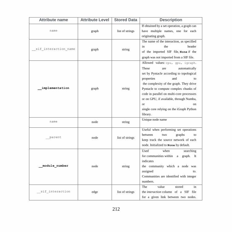
212

Attribute name Attribute Level Stored Data Description

name graph list of strings

If obtained by a set operation, a graph can

have multiple names, one for each

originating graph.

__sif_interaction_name graph string

The name of the interaction, as specified

in the header

of the imported SIF file, None if the

graph was not imported from a SIF file.

__implementation graph string

Allowed values: cpu, gpu, igraph.

These are automatically

set by Pyntacle according to topological

properties and to

the complexity of the graph. They drive

Pyntacle to compute complex chunks of

code in parallel on multi-core processors

or on GPU, if available, through Numba,

or on

single core relying on the iGraph Python

library.

name node string Unique node name

__parent node list of strings

Useful when performing set operations

between two graphs to

keep track the source network of each

node. Initialized to None by default.

__module_number node string

Used when searching

for communities within a graph. It

indicates

the community which a node was

assigned to.

Communities are identified with integer

numbers.

__sif_interaction edge list of strings

The value stored in

the interaction column of a SIF file

for a given link between two nodes.

213

None if the graph was not imported from

a SIF file.

adjacent_nodes edge tuple of strings A tuple containing the attribute name of

two adjacent nodes by this edge.

weights edge float or int

Weight assigned to an edge by algorithms

that work

with or make weighted graphs, such as

the pagerank algorithm.

Table 10: Pyntacle reserved attribute for the igraph.Graph object, at each level. Attribute Names

in bold are read-only and cannot be overwritten.

214

215

Publications

Mazzoccoli, G., Colangelo, T., Panza, A., Rubino, R., Tiberio, C., Palumbo, O., Carella,

M., Trombetta, D., Gentile, A., Tavano, F., et al. (2016). Analysis of clock gene-miRNA

correlation networks reveals candidate drivers in colorectal cancer. Oncotarget 7.

Mazza, T., Mazzoccoli, G., Fusilli, C., Capocefalo, D., Panza, A., Biagini, T., Castellana,

S., Gentile, A., De Cata, A., Palumbo, O., et al. (2016). Multifaceted enrichment analysis

of RNA-RNA crosstalk reveals cooperating micro-societies in human colorectal cancer.

Nucleic Acids Res. 44.

Castellana, S., Fusilli, C., Mazzoccoli, G., Biagini, T., Capocefalo, D., Carella, M.,

Vescovi, A.L., and Mazza, T. (2017). High-confidence assessment of functional impact

of human mitochondrial non-synonymous genome variations by APOGEE. PLoS

Comput. Biol. 13.

Mazza, T., Copetti, M., Capocefalo, D., Fusilli, C., Biagini, T., Carella, M., De Bonis,

A., Mastrodonato, N., Piepoli, A., Pazienza, V., et al. (2017). MicroRNA co-expression

networks exhibit increased complexity in pancreatic ductal compared to Vater’s papilla

adenocarcinoma. Oncotarget 8.

Mazzoccoli, G., Castellana, S., Carella, M., Palumbo, O., Tiberio, C., Fusilli, C.,

Capocefalo, D., Biagini, T., Mazza, T., and Lo Muzio, L. (2017). A primary tumor gene

expression signature identifies a crucial role played by tumor stroma myofibroblasts in

lymph node involvement in oral squamous cell carcinoma. Oncotarget 8.

216

Pezzilli, S., Ludovico, O., Biagini, T., Mercuri, L., Alberico, F., Lauricella, E., Dallali,

H., Capocefalo, D., Carella, M., Miccinilli, E., et al. (2017). Insights from molecular

characterization of adult patients of families with multigenerational diabetes. Diabetes

67.

Castellana, S., Mazza, T., Capocefalo, D., Genov, N., Biagini, T., Fusilli, C.,

Scholkmann, F., Relógio, A., Hogenesch, J.B., and Mazzoccoli, G. (2018). Systematic

Analysis of Mouse Genome Reveals Distinct Evolutionary and Functional Properties

Among Circadian and Ultradian Genes. Front. Physiol. 9, 1178.

Capocefalo, D., Pereira, J., Mazza, T., Jordán, F. (2018) Food web topology and nested

keystone species complexes. Complexity, 1979214, 8.

Capocefalo D., Truglio M., Biagini T., Castellana S., Mazzoccoli G., Carella M., Vescovi

A.L., Jordán F., Mazza T., Computing group-centrality topological parameters of

networks with Pytnacle Bioinformatics, submitted.

Caris-Maldonado. J.C., Capocefalo D. (as co-author), Lopez-Quilodran N., Molina-

Fernandez C., Arias-Carrasco R., Sepúlveda-Hermosilla G., Slater A., Martinez P., van

Zundert B., Vargas R., Mazza T., Maracaja-Coutinho V., Tevy, M.F. The dynamic aging

transcriptome of Drosophila Melanogaster, manuscript in preparation.

217