V.Chandrasekhar, Associate Professor, CSE Year, Semester, Br
Upload
khangminh22Category
view
10download
0
SAP PRESS is a joint initiative of SAP and Rheinwerk Publishing. The know-how offered by SAP specialists combined with the expertise of Rheinwerk Publishing offers the reader expert books in the field. SAP PRESS features first-hand information and expert advice, and provides useful skills for professional decision-making.
SAP PRESS offers a variety of books on technical and business-related topics for the SAP user. For further information, please visit our website: http://www.sap-press.com.
Silvia, Frye, Berg SAP HANA: An Introduction (4th Edition) 2017, 549 pages, hardcover and e-book www.sap-press.com/4160
Jonathan Haun SAP HANA Security Guide 2017, 541 pages, hardcover and e-book www.sap-press.com/4227
Anil Bavaraju Data Modeling for SAP HANA 2.0 2019, approx. 475 pp., hardcover and e-book www.sap-press.com/4722
Alborghetti, Kohlbrenner, Pattanayak, Schrank, Sboarina SAP HANA XSA: Native Development for SAP HANA 2018, 607 pages, hardcover and e-book www.sap-press.com/4500

Rudi de Louw
SAP HANA® 2.0 Certification Guide: Application Associate Exam

Dear Reader,
It has been my privilege to work with Rudi for two years now on two different editions of this book. He’s everything an editor looks for in an author: knowledgeable, dedi- cated, and communicative (I always know exactly what he’s working on)! SAP HANA is a difficult topic to write a certification guide for, as it’s an ever-moving target, and ensuring the most up-to-date coverage requires mastery of many areas. Rudi has always been happy to do the hard work of getting the best information, and we’ve been glad to have him.
Sadly, this will be Rudi’s final edition as author of this book, as his career moves on to new (and hopefully bigger and better!) things. Rudi, we wish you nothing but luck in all your future endeavors! (And if you happen to find yourself working on a different SAP topic where we don’t yet have a book? Well, I think I can safely say we’d be delighted to bring you back into the fold.)
What did you think about SAP HANA 2.0 Certification Guide: Application Associate Exam? Your comments and suggestions are the most useful tools to help us make our books the best they can be. Please feel free to contact me and share any praise or criti-cism you may have.
Thank you for purchasing a book from SAP PRESS!
Meagan White Editor, SAP PRESS
[email protected] www.sap-press.com Rheinwerk Publishing • Boston, MA

Notes on Usage
This e-book is protected by copyright. By purchasing this e-book, you have agreed to accept and adhere to the copyrights. You are entitled to use this e-book for personal purposes. You may print and copy it, too, but also only for personal use. Sharing an electronic or printed copy with others, however, is not permitted, neither as a whole nor in parts. Of course, making them available on the Internet or in a company network is illegal as well.
For detailed and legally binding usage conditions, please refer to the section Legal Notes.
This e-book copy contains a digital watermark, a signature that indicates which person may use this copy:

Imprint
This e-book is a publication many contributed to, specifically:
Editor Meagan WhiteAcquisitions Editor Hareem ShafiCopyeditor Julie McNameeCover Design Graham GearyPhoto Credit iStockphoto.com/680541274/© panimoniProduction E-Book Kelly O’CallaghanTypesetting E-Book SatzPro, Krefeld (Germany)
We hope that you liked this e-book. Please share your feedback with us and read the Service Pages to find out how to contact us.
ISBN 978-1-4932-1829-5 (print) ISBN 978-1-4932-1830-1 (e-book) ISBN 978-1-4932-1831-8 (print and e-book)
© 2019 by Rheinwerk Publishing, Inc., Boston (MA) 3rd edition 2019
The Library of Congress has cataloged the printed edition as follows:Names: De Louw, Rudi, author.Title: SAP HANA 2.0 certification guide : application associate exam / Rudi de Louw.Other titles: SAP HANA certification guideDescription: 3rd edition. | Bonn ; Boston : Rheinwerk Publishing, 2019. | Revised edition of: SAP HANA certification guide / Rudi de Louw. 2016. | Includes index.Identifiers: LCCN 2019017642 (print) | LCCN 2019018195 (ebook) | ISBN 9781493218301 | ISBN 9781493218295 (alk. paper)Subjects: LCSH: Relational databases--Examinations--Study guides. | Business enterprises--Computer networks--Examinations--Study guides. | Computer programmers--Certification. | SAP HANA (Electronic resource)--Examinations--Study guides.Classification: LCC QA76.9.D32 (ebook) | LCC QA76.9.D32 D45 2019 (print) | DDC 005.75/6076--dc23LC record available at https://lccn.loc.gov/2019017642

7
Contents
Acknowledgments .............................................................................................................................. 15
Preface .................................................................................................................................................... 17
1 SAP HANA Certification Track—Overview 25
Who This Book Is For .......................................................................................................... 26
SAP HANA Certifications .................................................................................................. 27
Associate-Level Certification ......................................................................................... 28
Specialist-Level Certification ......................................................................................... 30
SAP HANA Application Associate Certification Exam ......................................... 30
Exam Objective .................................................................................................................. 32
Exam Structure .................................................................................................................. 34
Exam Process ...................................................................................................................... 36
Summary ................................................................................................................................. 37
2 SAP HANA Training 39
SAP Education Training Courses ................................................................................... 40
Training Courses for SAP HANA Certifications ........................................................ 41
Additional SAP HANA Training Courses .................................................................... 42
Other Sources of Information ........................................................................................ 43
SAP Help ............................................................................................................................... 43
SAP HANA Home Page and SAP Community ........................................................... 46
SAP HANA Academy ......................................................................................................... 46
openSAP ............................................................................................................................... 48
Hands-On with SAP HANA ............................................................................................... 49
Where to Get an SAP HANA System ........................................................................... 50
Project Examples ............................................................................................................... 61
Where to Get Data ............................................................................................................ 63

Contents8
Exam Questions ................................................................................................................... 64
Types of Questions ........................................................................................................... 64
Elimination Technique .................................................................................................... 67
Bookmark Questions ........................................................................................................ 67
General Examination Strategies ................................................................................... 68
Summary ................................................................................................................................. 69
3 Technology, Architecture, and Deployment Scenarios 71
Objectives of This Portion of the Test ........................................................................ 72
Key Concepts Refresher .................................................................................................... 73
In-Memory Technology ................................................................................................... 73
Architecture and Approach ............................................................................................ 79
Deployment Scenarios .................................................................................................... 93
SAP HANA in the Cloud ................................................................................................... 104
SAP Analytics Cloud and Business Intelligence ....................................................... 108
Important Terminology .................................................................................................... 114
Practice Questions .............................................................................................................. 116
Practice Question Answers and Explanations ........................................................ 122
Takeaway ................................................................................................................................ 126
Summary ................................................................................................................................. 127
4 Modeling Tools, Management, and Administration 129
Objectives of This Portion of the Test ........................................................................ 131
Key Concepts Refresher .................................................................................................... 132
New Modeling Process .................................................................................................... 132
New Architecture for Modeling and Development ............................................... 138

Contents 9
Creating a Project .............................................................................................................. 145
Creating SAP HANA Design-Time Objects ................................................................ 155
Building and Managing Information Models .......................................................... 162
Refactoring .......................................................................................................................... 170
Important Terminology .................................................................................................... 174
Practice Questions ............................................................................................................... 175
Practice Question Answers and Explanations ........................................................ 178
Takeaway ................................................................................................................................ 180
Summary ................................................................................................................................. 180
5 Information Modeling Concepts 181
Objectives of This Portion of the Test ........................................................................ 182
Key Concepts Refresher .................................................................................................... 183
Tables .................................................................................................................................... 183
Views ..................................................................................................................................... 183
Cardinality ........................................................................................................................... 186
Joins ..................................................................................................................................... 186
Core Data Services Views ............................................................................................... 197
Cube ..................................................................................................................................... 200
Calculation Views ............................................................................................................. 204
Other Modeling Artifacts ............................................................................................... 208
Semantics ............................................................................................................................ 213
Hierarchies .......................................................................................................................... 213
Important Terminology .................................................................................................... 216
Practice Questions ............................................................................................................... 217
Practice Question Answers and Explanations ........................................................ 225
Takeaway ................................................................................................................................ 229
Summary ................................................................................................................................. 229
Contents10
6 Calculation Views 231
Objectives of This Portion of the Test ........................................................................ 232
Key Concepts Refresher .................................................................................................... 233
Data Sources for Calculation Views ............................................................................ 234
Calculation Views: Dimension, Cube, and Cube with Star Join ........................ 235
Working with Nodes ........................................................................................................ 248
Semantics Node ................................................................................................................. 263
Important Terminology .................................................................................................... 269
Practice Questions .............................................................................................................. 271
Practice Question Answers and Explanations ........................................................ 275
Takeaway ................................................................................................................................ 278
Summary ................................................................................................................................. 278
7 Modeling Functions 279
Objectives of This Portion of the Test ........................................................................ 280
Key Concepts Refresher .................................................................................................... 281
Calculated Columns ......................................................................................................... 281
Restricted Columns .......................................................................................................... 286
Filters ..................................................................................................................................... 291
Variables .............................................................................................................................. 293
Input Parameters .............................................................................................................. 297
Session Variables ............................................................................................................... 302
Currency ............................................................................................................................... 303
Hierarchies .......................................................................................................................... 308
Hierarchy Functions ......................................................................................................... 316
Important Terminology .................................................................................................... 326
Practice Questions .............................................................................................................. 328
Practice Question Answers and Explanations ........................................................ 333
Takeaway ................................................................................................................................ 336
Summary ................................................................................................................................. 336
Contents 11
8 SQL and SQLScript 337
Objectives of This Portion of the Test ........................................................................ 339
Key Concepts Refresher .................................................................................................... 340
SQL ..................................................................................................................................... 340
SQLScript .............................................................................................................................. 347
Views, Functions, and Procedures ............................................................................... 362
Catching Up with SAP HANA 2.0 .................................................................................. 365
Important Terminology .................................................................................................... 365
Practice Questions ............................................................................................................... 366
Practice Question Answers and Explanations ........................................................ 371
Takeaway ................................................................................................................................ 374
Summary ................................................................................................................................. 374
9 Data Provisioning 375
Objectives of This Portion of the Test ........................................................................ 376
Key Concepts Refresher .................................................................................................... 377
Concepts .............................................................................................................................. 378
SAP Data Services .............................................................................................................. 383
SAP Landscape Transformation Replication Server ............................................... 385
SAP Replication Server ..................................................................................................... 387
SAP HANA Smart Data Access ....................................................................................... 388
SAP HANA Smart Data Integration and SAP HANA Smart Data Quality ........ 392
SAP HANA Streaming Analytics .................................................................................... 395
SQL Anywhere and Remote Data Sync ....................................................................... 397
Flat Files ................................................................................................................................ 399
Web Services (OData and REST) ................................................................................... 400
SAP Vora ............................................................................................................................... 401
SAP HANA Data Management Suite ........................................................................... 402
Important Terminology .................................................................................................... 403
Practice Questions ............................................................................................................... 405

Contents12
Practice Question Answers and Explanations ........................................................ 408
Takeaway ................................................................................................................................ 410
Summary ................................................................................................................................. 410
10 Text Processing and Predictive Modeling 411
Objectives of This Portion of the Test ........................................................................ 413
Key Concepts Refresher .................................................................................................... 414
Text Processing .................................................................................................................. 414
Predictive Modeling ......................................................................................................... 432
Important Terminology .................................................................................................... 452
Practice Questions .............................................................................................................. 453
Practice Question Answers and Explanations ........................................................ 456
Takeaway ................................................................................................................................ 457
Summary ................................................................................................................................. 458
11 Spatial, Graph, and Series Data Modeling 459
Objectives of This Portion of the Test ........................................................................ 461
Key Concepts Refresher .................................................................................................... 461
Spatial Modeling ............................................................................................................... 462
Graph Modeling ................................................................................................................. 480
Series Data Modeling ....................................................................................................... 498
Important Terminology .................................................................................................... 508
Practice Questions .............................................................................................................. 509
Practice Question Answers and Explanations ........................................................ 513
Takeaway ................................................................................................................................ 517
Summary ................................................................................................................................. 517
Contents 13
12 Optimization of Information Models 519
Objectives of This Portion of the Test ........................................................................ 520
Key Concepts Refresher .................................................................................................... 521
Architecture and Performance ..................................................................................... 521
Redesigned and Optimized Applications .................................................................. 522
Effects of Good Performance ........................................................................................ 523
Information Modeling Techniques ............................................................................. 524
Optimization Tools ........................................................................................................... 525
Best Practices for Optimization .................................................................................... 536
Important Terminology .................................................................................................... 542
Practice Questions ............................................................................................................... 543
Practice Question Answers and Explanations ........................................................ 546
Takeaway ................................................................................................................................ 548
Summary ................................................................................................................................. 548
13 Security 549
Objectives of This Portion of the Test ........................................................................ 550
Key Concepts Refresher .................................................................................................... 551
Usage and Concepts ......................................................................................................... 551
SAP HANA XSA and SAP HANA Deployment Infrastructure ............................... 554
Users ..................................................................................................................................... 559
Roles ..................................................................................................................................... 565
Privileges .............................................................................................................................. 569
Assigning Roles to Users ................................................................................................. 577
Data Security ...................................................................................................................... 578
Important Terminology .................................................................................................... 581
Practice Questions ............................................................................................................... 582
Practice Question Answers and Explanations ........................................................ 585
Takeaway ................................................................................................................................ 587
Summary ................................................................................................................................. 587

Contents14
14 Virtual Data Models 589
Objectives of This Portion of the Test ........................................................................ 591
Key Concepts Refresher .................................................................................................... 591
Reporting in the Transactional Systems ................................................................... 592
SAP HANA Live .................................................................................................................... 595
SAP S/4HANA Embedded Analytics ............................................................................ 608
Important Terminology .................................................................................................... 612
Practice Questions .............................................................................................................. 613
Practice Question Answers and Explanations ........................................................ 617
Takeaway ................................................................................................................................ 619
Summary ................................................................................................................................. 620
The Author ............................................................................................................................................. 621
Index ........................................................................................................................................................ 623
Service Pages ..................................................................................................................................... I Legal Notes ......................................................................................................................................... II

15
Acknowledgments
“Write the vision, and make it plain upon tables, that he may run that readeth it.”
– Habakkuk 2:2 (King James Bible)
SAP PRESS had the vision for a book on the SAP HANA certification exam, and it
was my privilege to write it and make it plain. It’s my wish that every reader of this
book runs with the knowledge and understanding gained from it.
All the writing has now even produced what I jokingly refer to as a “trilogy.” This is
the third and final edition from my side.
In my more than eight-year journey with SAP HANA, I’ve met hundreds of people,
all passionate about SAP HANA. Thank you to all of you!
Thank you to the entire team at SAP PRESS for making this book happen, and espe-
cially to the SAP PRESS editor, Meagan White, and the other editors for your input.
Thank you to all my SAP Co-Innovation Lab colleagues for your support and the
discussions we had around SAP HANA. And an extra thank you to Skhu, Phillip,
and Tshepo for all your input and encouragement.
I’m very thankful to all of you: my family, my friends, my colleagues, and everyone
I’ve worked with to build great things with SAP HANA.
To my readers: I trust that your journey will be even more amazing!

17
Preface
The SAP PRESS Certification Series is designed to provide anyone who is preparing
to take an SAP certified exam with all the review, insight, and practice they need to
pass the exam. The series is written in practical, easy-to-follow language that pro-
vides targeted content focused on what you need to know to successfully take
your exam.
This book is specifically written for those interested in using the SAP HANA 2.0
version and preparing to take the SAP Certified Application Associate – SAP HANA
(C_HANAIMP_15) exam. This book will also be helpful to those of you taking some
of the older exams, such as the SPS 14 exam (C_HANAIMP_14). The SAP Certified
Application Associate – SAP HANA exam tests the taker in the areas of data model-
ing. It focuses on core SAP HANA skills, as opposed to skills that are specific to a
particular implementation type (e.g., SAP Business Warehouse on SAP HANA or
SAP Business Suite on SAP HANA). The SAP Certified Application Associate – SAP
HANA test can be taken by anyone who signs up.
Using this book, you’ll walk away with a thorough understanding of the exam’s
structure and what to expect when taking it. You’ll receive a refresher on the key
concepts covered on the exam, and you’ll be able to test your skills via sample
practice questions and answers. The book is closely aligned with the course sylla-
bus and the exam structure, so all the information provided is relevant and appli-
cable to what you need to know to prepare. We explain the SAP products and
features using practical examples and straightforward language, so you can pre-
pare for the exam and improve your skills in your day-to-day work as an SAP
HANA data modeler. Each book in the series has been structured and designed to
highlight what you really need to know.
Preface18
Structure of This Book
Each chapter begins with a clear list of the learning objectives, as shown here:
Techniques You’ll Master
� Prepare for the exam
� Understand the general exam structure
� Access practice questions for preparation
From there, you’ll dive into the chapter and get right into the test objective cover-
age.
Throughout the book, we’ve also provided several elements that will help you
access useful information:
� Tips call out useful information about related ideas and provide practical sug-
gestions for how to use a particular function. For example:
Tip
This book contains screenshots and diagrams to guide your understanding of the many
information-modeling concepts.
� Notes provide other resources to explore or special tools or services from SAP
that will help you with the topic under discussion. For example:
Note
This certification guide covers all topics you need to successfully pass the exam. It pro-
vides sample questions similar to those found on the actual exam.
� SPS 04 notes will show you what is new in SAP HANA SPS 04. This will help you
when studying exams after C_HANAIMP_15. For example:
SPS 04
When studying for the C_HANAIMP_15 exam, you can ignore these notes when doing
your final preparation. But they will be helpful to keep you up to date and can be used to
prepare for later exams when they get published.
Each chapter that covers an exam topic is organized in a similar fashion so you can
become familiar with the structure and easily find the information you need.
Here’s an example of a typical chapter structure:
Preface 19
� Introductory bullets
The beginning of each chapter discusses the techniques you must master to be
considered proficient in the topic for the certification examination.
� Topic introduction
This section provides you with a general idea of the topic at hand to frame
future sections. It also includes objectives for the exam topic covered.
� Real-world scenario
This section shows a real-world scenario where these skills would be beneficial
to you or your company.
� Objectives
This section provides you with the necessary information to successfully pass
this portion of the test.
� Key concept refresher
This section outlines the major concepts of the chapter. It identifies the tasks
you’ll need to understand or perform properly to answer the questions on the
certification examination.
� Important terminology
Just prior to the practice examination questions, we provide a section to review
important terminology. This may be followed by definitions of various terms
from the chapter.
� Practice questions
The chapter then provides a series of practice questions related to the topic of
the chapter. The questions are structured in a similar way to the actual ques-
tions on the certification examination.
� Practice question answers and explanations
Following the practice exercise are the solutions to the practice exercise ques-
tions. As part of the answer, we discuss why an answer is considered correct or
incorrect.
� Takeaway
This section provides a takeaway or reviews the areas you should now under-
stand. This refresher section identifies the key concepts in the chapter and pro-
vides some tips related to the chapter.
� Summary
Finally, we conclude with a summary of the chapter.
Now that you have an idea of how the book is structured, the following list will
dive into the individual topics of the exam covered in each chapter:
Preface20
� Chapter 1, SAP HANA Certification Track—Overview, provides a look at the dif-
ferent certifications for SAP HANA: associate, professional, and specialist. It
then looks at the general exam objectives, structure, and scoring.
� Chapter 2, SAP HANA Training, discusses the available training and training
material for test takers, so you know where to look for answers beyond the
book. We identify the SAP Education training courses available for classroom,
virtual, and e-learning, in addition to SAP Learning Hub offerings. We then look
into additional resources, including the official SAP documentation and the
SAP HANA Academy video tutorials. We also talk about the SAP HANA, express
edition, which you can use to get practical experience.
� Chapter 3, Technology, Architecture, and Deployment Scenarios, walks through
the evolution of SAP HANA’s in-memory technology, including how it
addresses the problems of the past, such as slow disks. From there, you’re given
an overview of the persistence layer, before looking at the different deployment
options, including cloud deployments, and delving into the new SAP HANA
extended application services, advanced model (SAP HANA XSA) features.
� Chapter 4, Modeling Tools, Management, and Administration, introduces you
to what’s new in SAP HANA 2.0, the new architecture and modeling process, and
the SAP HANA modeling tools, including SAP Web IDE for SAP HANA. In addi-
tion, you’ll learn how to create new information models, tables, and data.
� Chapter 5, Information-Modeling Concepts, discusses general modeling con-
cepts such as cubes, fact tables, and the difference between attributes and mea-
sures, in addition to covering general modeling best practices.
� Chapter 6, Calculation Views, looks in depth at the three primary information
views in SAP HANA and how to build information models using calculation
views.
� Chapter 7, Modeling Functions, takes what you’ve learned one step further by
showing you how to enhance your calculation views with calculated columns,
filter expressions, and more.
� Chapter 8, SQL and SQLScript, reviews how to enhance SAP HANA models using
SQL and SQLScript to create tables, read and filter data, create calculated col-
umns, implement procedures, use user-defined functions, and more.
� Chapter 9, Data Provisioning, introduces the concepts, tools, and methods for
data provisioning in SAP HANA. Coverage runs from SAP Data Services to SAP
HANA streaming analytics.
Preface 21
� Chapter 10, Text Processing and Predictive Modeling, looks at advanced topics,
such as creating a text search index, implementing fuzzy search, performing
text analysis, and creating predictive analysis models.
� Chapter 11, Spatial, Graph, and Series Data Modeling, looks at more of the
advanced topics, such as using the key components of spatial processing, work-
ing with relationships between data objects using graphs, and understanding
series data.
� Chapter 12, Optimization of Information Models, reviews how to monitor,
investigate, and optimize data models in SAP HANA. We’ll look at how optimi-
zation affects architecture, performance, and information-modeling tech-
niques. We’ll then dive into the different tools used for optimization including
the SQL Analyzer, SAP HANA cockpit, debug query mode, and performance
analysis mode.
� Chapter 13, Security, discusses how users, roles, and privileges work together.
We’ll look at the different types of users, template roles, and privileges that are
available in the SAP HANA system.
� Chapter 14, Virtual Data Models, looks at how to adapt predelivered content to
your own business solutions using SAP HANA Live. You’ll learn about SAP
HANA Live’s different views, and its two primary tools: SAP HANA Live Browser
and SAP HANA Live extension assistant. We also look at SAP S/4HANA embed-
ded analytics, which uses similar concepts.
What’s New in the Third Edition
Readers of the first two books will be interested to find out what is new in this edi-
tion. We’re working with SAP HANA 2.0, using the same user interface as is used by
SAP Cloud Platform. While the modeling concepts are still the same as SAP HANA
1.0, the way you work with SAP HANA 2.0 has changed significantly.
SAP HANA now ensures that the development you do for on-premise systems will
also work in the cloud. This was accomplished by moving SAP HANA into the con-
tainer and microservices world using SAP HANA XSA. This change has had a huge
ripple effect on architecture, modeling tools, managing models, and security, to
give a few examples. A bigger distinction now exists between design-time and run-
time objects, which leads to updated processes for creating information models
(design-time), building these information models to create runtime objects, and,
finally, storing, managing, and securing these models.
Preface22
We now use SAP Web IDE for SAP HANA instead of SAP HANA Studio. All the
screens shown in the book, with their descriptions, were updated to reflect this
change. Chapter 4 now discusses this new modeling environment, instead of the
old SAP HANA Studio and SAP HANA Web-Based Development Workbench. The
bigger distinction between the design-time and runtime objects brought in new
tools as well, such as the Git repository, the building process (for creating runtime
objects), and new rules for managing your models.
In the sections on graphical calculation views, the following additional node types
are discussed: non-equi joins, minus, intersects, hierarchy functions, and ano-
nymization. Hierarchy functionality has expanded as well.
The largest changes are in the areas of advanced modeling. The SAP training
courses now include a three-day training course on the topics of text processing,
predictive modeling, spatial processing, graph modeling, and series data. The
exam now has more emphasis on these topics, with the marks for this area moving
up from 10% to 25%.
Tip
Even though the exam is based on SAP HANA 2.0 SPS 03, this book also addresses SAP
HANA 2.0 SPS 04.
Practice Questions
We want to give you some background on the test questions before you encounter
the first few in the chapters. Just like the exam, each question has a basic structure:
� Actual question
Read the question carefully, and be sure to consider all the words used in the
question because they can impact the answer.
� Question hint
This isn’t a formal term, but we call it a hint because it tells you how many
answers are correct. If only one is correct, normally it tells you to choose the cor-
rect answer. If more than one is correct, like the actual certification examina-
tion, it indicates the correct number of answers.
� Answers
The answers to select from depend on the question type. The following ques-
tion types are possible:

Preface 23
– Multiple response: More than one correct answer is possible.
– Multiple choice: Only a single answer is correct.
– True/false: Only a single answer is correct. These types of questions aren’t
used in the exam, but they are used in the book to test your understanding.
Summary
With this certification guide, you’ll learn how to approach the content and key
concepts highlighted for each exam topic. In addition, you’ll have the opportunity
to practice with sample test questions in each chapter. After answering the prac-
tice questions, you’ll be able to review the explanation of the answer, which dis-
sects the question by explaining why the answers are correct or incorrect. The
practice questions give you insight into the types of questions you can expect,
what the questions look like, and how the answers relate to the question. Under-
standing the composition of the questions and seeing how the questions and
answers work together is just as important as understanding the content. This
book gives you the tools and understanding you need to be successful. Armed with
these skills, you’ll be well on your way to becoming an SAP Certified Application
Associate in SAP HANA.

Chapter 1
SAP HANA Certification Track—Overview
Techniques You’ll Master
� Understand the different levels of SAP HANA certifications
� Find the correct SAP HANA certification exam for you
� Learn the scoring structure of the certification exams
� Discover how to book your SAP HANA certification exam
Chapter 1 SAP HANA Certification Track—Overview26
Welcome to the exciting world of SAP HANA! SAP as a company is moving at full
speed to update all of its solutions to use SAP HANA. Some solutions have even
changed completely to better leverage the capabilities of SAP HANA. In many
senses, the future of SAP is tied to the SAP HANA platform.
SAP HANA itself is developing at a fast pace to provide all the features required for
innovation. Many of the new areas that we see SAP working in, such as cloud and
mobile, are enabled because of SAP HANA’s many features. The best-known SAP
HANA feature is its fast response times. Both cloud and mobile can suffer from
latency issues, and they certainly improve with faster response times.
With the large role that SAP HANA now plays, the demand for experienced profes-
sionals with SAP HANA knowledge has grown. By purchasing this book, you’ve
taken the first step toward meeting these demands and advancing your career via
knowledge of SAP HANA.
Note
Five different certifications are available for SAP HANA, and each focuses on a different
topic. The focus of this book is on the SAP Certified Application Associate – SAP HANA cer-
tification, which is the most in-demand SAP HANA certification.
In this chapter, we’ll discuss the target demographic of this book before diving into
a discussion of the various SAP HANA certification exams available. We’ll then
look at the specific exam this book is based on before examining the structure of
that exam.
Who This Book Is For
This book covers SAP HANA from a modeling and application perspective for the
C_HANAIMP_15 exam. As such, this book is meant for quite a large group of people
from various backgrounds and interests. In a broad sense, this book talks about
how to work with data and information—and more people work with information
now than ever before.
This book doesn’t go into the more technical topics (e.g., installations, upgrades,
monitoring, updates, backups, and transports) addressed by some of the other SAP
HANA certifications.
SAP HANA Certifications Chapter 1 27
Let’s discuss who can benefit from this book:
� Information modelers are a core audience group for this book because the main
topic is information modeling. This includes people who come from an enter-
prise data warehouse (EDW) background.
� Developers need to create and use information models—whether for SAP appli-
cations using ABAP, cloud applications using Java or Node, web services, mobile
apps, or new SAP HANA applications using SAPUI5.
� Database administrators (DBAs) must understand how to use the new in-
memory and columnar database technologies of SAP HANA.
� Architects want to understand SAP HANA concepts, get an overview of what SAP
HANA entails, and plan new landscapes and solutions using SAP HANA.
� Data integration and data provisioning specialists need to know how to process
data in an optimal manner using SAP HANA.
� Report-writing professionals constantly create, find, and consume information
models. Often, the need for these information models arises from the reporting
needs of business users. An understanding of how to create these information
models in SAP HANA will be of great benefit.
� Data scientists, or anyone working with big data and data mining, are always
looking for faster, smarter, and more efficient ways to get results that can help
businesses innovate. SAP HANA has proven that it can certainly contribute to
these areas.
� Technical performance tuning experts have to understand the intricacies of the
new in-memory and columnar database paradigm to fully utilize and leverage
the performance that SAP HANA can provide.
If you fit into one or more of these categories, excellent! You’re in the right place.
Regardless, if you’ve bought this book in preparation for the exam, our primary
goal is to help you succeed; all exam takers are welcome.
SAP HANA Certifications
There are currently five certification examinations available for SAP HANA, as
listed in Table 1.1. Note that the certifications have different prefixes. The C prefix
indicates full, core exams for SAP HANA data modeling; and the E prefix indicates
certification exams for specialists.
Chapter 1 SAP HANA Certification Track—Overview28
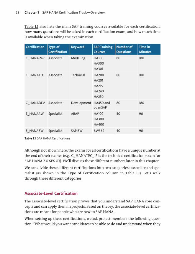
Table 1.1 also lists the main SAP training courses available for each certification,
how many questions will be asked in each certification exam, and how much time
is available when taking the examination.
Although not shown here, the exams for all certifications have a unique number at
the end of their names (e.g., C_HANATEC_15 is the technical certification exam for
SAP HANA 2.0 SPS 03). We’ll discuss these different numbers later in this chapter.
We can divide these different certifications into two categories: associate and spe-
cialist (as shown in the Type of Certification column in Table 1.1). Let’s walk
through these different categories.
Associate-Level Certification
The associate-level certification proves that you understand SAP HANA core con-
cepts and can apply them in projects. Based on theory, the associate-level certifica-
tions are meant for people who are new to SAP HANA.
When setting up these certifications, we ask project members the following ques-
tion: “What would you want candidates to be able to do and understand when they
Certification Type of
Certification
Keyword SAP Training
Courses
Number of
Questions
Time in
Minutes
C_HANAIMP Associate Modeling HA100
HA300
HA301
80 180
C_HANATEC Associate Technical HA200
HA201
HA215
HA240
HA250
80 180
C_HANADEV Associate Development HA450 and
openSAP
80 180
E_HANAAW Specialist ABAP HA100
HA300
HA400
40 90
E_HANABW Specialist SAP BW BW362 40 90
Table 1.1 SAP HANA Certifications

SAP HANA Certifications Chapter 1 29
join your project immediately after passing the certification exam?” Understand-
ing the different concepts in SAP HANA and when to use them is important.
Three of the SAP HANA certifications fall under the associate level: C_HANAIMP
(modeling), C_HANATEC (technical), and C_HANADEV (development).
C_HANAIMP Modeling Certification
As previously discussed, the C prefix indicates the full, core exams for SAP HANA
data modeling. IMP refers to the implementation of SAP HANA applications. This
examination consists of 80 questions, and you’re given three hours to complete
the exam.
The certification doesn’t have any prerequisites. The SAP training courses that
help you prepare for this certification exam are HA100, HA300, and HA301. This
book and this certification exam are intended for information modelers, DBAs,
architects, SAP HANA application developers, ABAP and Java developers, people
who perform data integration and reporting, those who are interested in technical
performance tuning, SAP Business Warehouse (SAP BW) information modelers,
data scientists, and anyone who wants to understand basic SAP HANA modeling
concepts.
This certification exam tests your knowledge in SAP HANA subjects such as archi-
tecture, deployment, information modeling, security, optimization, administra-
tion, SAP HANA Live, and some advanced modeling topics, such as predictive, text,
graph, geospatial, and series data modeling.
C_HANATEC Technical Certification
The C_HANATEC certification exam is meant for technical people such as system
administrators, DBAs, SAP Basis people, technical support personnel, and hard-
ware vendors. This certification doesn’t have any prerequisites. The training
courses for this exam are HA200, HA201, HA215, HA240, and HA250.
This certification exam tests your knowledge of SAP HANA installations, updates,
upgrades, migrations, system monitoring, administration, configuration, perfor-
mance tuning, high availability, troubleshooting, backups, and security.

Chapter 1 SAP HANA Certification Track—Overview30
C_HANADEV Development Certification
The C_HANADEV certification exam is meant for SAP HANA architects and devel-
opers of both backend and frontend systems. This certification doesn’t have any
prerequisites. The main training course for this exam is HA450. The openSAP
courses by Thomas Jung and Rich Heilman will definitely help you when preparing
for this exam.
This certification exam tests your knowledge of SAP HANA development topics,
such as SAP HANA modeling; SAP HANA extended application services, advanced
model (SAP HANA XSA); SAPUI5; server-side JavaScript; SQLScript; OData services;
and deployment.
Specialist-Level Certification
The specialist exams prove that you can apply SAP HANA concepts in your current
specialist area. These are for people who are already certified in other areas outside
of SAP HANA, and want to gain additional knowledge of SAP HANA and how to
apply it to their specialties. Such people have backgrounds in SAP BW or ABAP, for
example.
Each specialist exam includes 40 questions, and you have an hour and a half to
complete the exam. They all have prerequisites (i.e., you have to be certified in a
specialist area before you’re allowed to take these SAP HANA certification exams).
There are two specialist exams:
� E_HANAAW ABAP Certification
This specialist exam for ABAP developers requires that you’re certified with
ABAP. The main additional training course for this exam is HA400, in which
you learn how ABAP development is different in SAP HANA systems than in
older SAP NetWeaver systems.
� E_HANABW SAP BW on SAP HANA Certification
This exam for people specializing in SAP BW requires that you’re certified with
SAP BW. The main training course for this exam is BW362.
SAP HANA Application Associate Certification Exam
Now, let’s focus on the objective and structure of the C_HANAIMP certification
that this book targets and look at the latest C_HANAIMP certification exam.
SAP HANA Application Associate Certification Exam Chapter 1 31
SAP is evolving fast and is constantly being updated. Originally, a new major Sup-
port Package Stack (SPS) update of SAP HANA was released twice a year, requiring
SAP Education to update all training materials and certification exams every six
months. Fortunately, SAP changed this to one release per year, so all SAP certifica-
tions remain valid for the past two versions. In other words, your SAP HANA certi-
fication, depending on when you received it, will be valid for one and a half to two
years. This is regrettably a slightly shorter time frame than for most other SAP cer-
tifications, some of which can remain valid for many years. In a sense, this is the
cost of working in such a fast-moving environment.
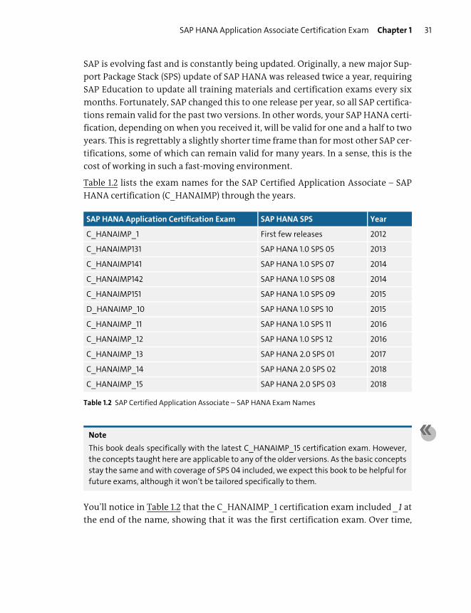
Table 1.2 lists the exam names for the SAP Certified Application Associate – SAP
HANA certification (C_HANAIMP) through the years.
Note
This book deals specifically with the latest C_HANAIMP_15 certification exam. However,
the concepts taught here are applicable to any of the older versions. As the basic concepts
stay the same and with coverage of SPS 04 included, we expect this book to be helpful for
future exams, although it won’t be tailored specifically to them.
You’ll notice in Table 1.2 that the C_HANAIMP_1 certification exam included _1 at
the end of the name, showing that it was the first certification exam. Over time,
SAP HANA Application Certification Exam SAP HANA SPS Year
C_HANAIMP_1 First few releases 2012
C_HANAIMP131 SAP HANA 1.0 SPS 05 2013
C_HANAIMP141 SAP HANA 1.0 SPS 07 2014
C_HANAIMP142 SAP HANA 1.0 SPS 08 2014
C_HANAIMP151 SAP HANA 1.0 SPS 09 2015
D_HANAIMP_10 SAP HANA 1.0 SPS 10 2015
C_HANAIMP_11 SAP HANA 1.0 SPS 11 2016
C_HANAIMP_12 SAP HANA 1.0 SPS 12 2016
C_HANAIMP_13 SAP HANA 2.0 SPS 01 2017
C_HANAIMP_14 SAP HANA 2.0 SPS 02 2018
C_HANAIMP_15 SAP HANA 2.0 SPS 03 2018
Table 1.2 SAP Certified Application Associate – SAP HANA Exam Names
Chapter 1 SAP HANA Certification Track—Overview32
SAP started including the year in the certification exam name—for example,
C_HANAIMP151. The first two numbers of 151 refer to the year, 2015, and the last
number, 1, refers to the first half of the year. In this case, this combination corre-
sponds to SPS 09.
In 2015, the naming convention was updated to refer directly to the SAP HANA
SPS number. That is, the SPS 12 exam was called C_HANAIMP_12 instead of
C_HANAIMP162. The _12 suffix indicates SPS 12.
With the new SAP HANA 2.0 releases, the numbering continues on from 12. As this
exam is the third one for SAP HANA 2.0, the exam was called C_HANAIMP_15.
SAP Education delivered delta exams for SAP HANA, which will make it easier to
extend the life of your SAP HANA certification. The D prefix in Table 1.2 indicates a
delta certification exam. You needed to have passed the C_HANAIMP151 certifica-
tion exam before you could take the D_HANAIMP_10 delta exam.
Tip
The SPS version for the on-premise version of SAP HANA, which we’re referring to in this
book, differs from that of the cloud version. We’re using SAP HANA 2.0 SPS 03. The corre-
sponding version on SAP Cloud Platform is SAP HANA 2.0 SPS 04.
Now that we’ve introduced the SAP Certified Application Associate – SAP HANA
certification, the next section will look at the exam as a whole: its objective, struc-
ture, and general process.
Exam Objective
In Figure 1.1, the official name of the certification examination is shown in all
uppercase letters as C_HANAIMP_15. On the left, you can see that the Level is Asso-
ciate.
On the right side, you can see that the exam has 80 questions. The Cut Score in this
example page is 64%, which means that you need to get 64% in this certification
examination to pass. The Duration of the exam is 180 mins. The exam is available
in English and Korean.
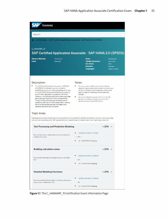
SAP HANA Application Associate Certification Exam Chapter 1 33
Figure 1.1 The C_HANAIMP_15 Certification Exam Information Page

Chapter 1 SAP HANA Certification Track—Overview34
Note that there used to be a PDF link for sample questions. This has now been
replaced by a sample exam that uses the actual exam system you’ll use when writ-
ing the exam. Just click on View more next to Sample Questions to open the sample
exam. In this case, there are 10 sample questions you can look at to get an idea of
what the actual examination questions look like. We normally recommend that
you keep the sample questions in reserve for later; don’t dive in right away. You
can use the sample questions to judge whether or not you’re ready for the certifi-
cation examination.
Tip
As a general rule, if you say “Huh?” when you look at the sample questions, then you’re
not yet ready for the exam.
The examination itself is focused on certain tasks.
Exam Structure
When you scroll down through the web page shown in Figure 1.1, you’ll see how the
exam is structured and scored. Each of the topic areas are mentioned there, as well
as the percentage that each area contributes toward your final score in the certifi-
cation exam.
The first area is Text Processing and Predictive Modeling. When you expand this
area, you can see that the HA300 training course is available for studying the con-
tent required to answer questions on this topic. More than 12% (actually about 15%)
of the questions fall into the Text Processing and Predictive Modeling topic, which
means that there are roughly 12 questions in the certification exam on this topic.
The second area is Building calculation views. When you expand this area, you can
see that the HA300 training course is available. More than 12% of the questions fall
into the Building calculation views, which means that there are roughly 12 ques-
tions in the certification exam on this topic.
The fourth area, Technology, architecture and deployment scenarios of SAP HANA,
is roughly 10% (between 8% and 12%) of the exam, meaning that it covers about
eight questions. The HA100 training course is available for more information on
this topic. Other portions of the exam follow this same percentage determination
and provide short descriptions.
SAP HANA Application Associate Certification Exam Chapter 1 35
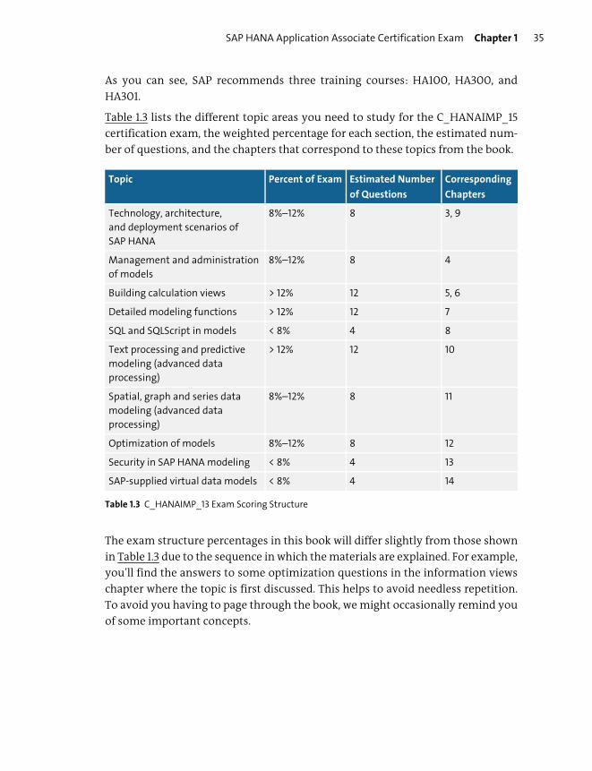
As you can see, SAP recommends three training courses: HA100, HA300, and
HA301.
Table 1.3 lists the different topic areas you need to study for the C_HANAIMP_15
certification exam, the weighted percentage for each section, the estimated num-
ber of questions, and the chapters that correspond to these topics from the book.
The exam structure percentages in this book will differ slightly from those shown
in Table 1.3 due to the sequence in which the materials are explained. For example,
you’ll find the answers to some optimization questions in the information views
chapter where the topic is first discussed. This helps to avoid needless repetition.
To avoid you having to page through the book, we might occasionally remind you
of some important concepts.
Topic Percent of Exam Estimated Number
of Questions
Corresponding
Chapters
Technology, architecture,
and deployment scenarios of
SAP HANA
8%–12% 8 3, 9
Management and administration
of models
8%–12% 8 4
Building calculation views > 12% 12 5, 6
Detailed modeling functions > 12% 12 7
SQL and SQLScript in models < 8% 4 8
Text processing and predictive
modeling (advanced data
processing)
> 12% 12 10
Spatial, graph and series data
modeling (advanced data
processing)
8%–12% 8 11
Optimization of models 8%–12% 8 12
Security in SAP HANA modeling < 8% 4 13
SAP-supplied virtual data models < 8% 4 14
Table 1.3 C_HANAIMP_13 Exam Scoring Structure

Chapter 1 SAP HANA Certification Track—Overview36
Exam Process
You can book the certification exam you want to take at http://s-prs.co/v487606.
You can see a list of available certification exams at http://s-prs.co/v487607.
On the SAP Training website (https://training.sap.com/), choose the country you
live in or the country that you want to take the exam in. You can also choose to
write the exam in the cloud, using the Certification Hub subscription. The price of
the certification exam and available dates will appear in the right column on the
web page. Currently, the SAP HANA certification exams are also still administered
in SAP examination centers even though the exam is an online exam.
Note
New certification exams, such as C_HANAIMP_15, are administered in the cloud. Cloud
certifications use remote proctoring, in which an exam proctor watches you (the test
taker) remotely via your computer’s webcam. You have to show the proctor the entire
room before the exam begins by moving your webcam or your computer around. These
test proctors have been trained to identify possible cheating.
When you arrive for the exam, you’ll need a form of identification. During your
certification exam, you won’t have access to online materials, books, your mobile
phone, or the Internet.
As you mark answer options, the answers are immediately stored on a server to
ensure that you don’t lose any work. When you finish all your certification exam
questions and submit the entire exam, you receive the results immediately. If you
don’t pass the certification exam, you can take it up to two more times. (This
retake option hopefully won’t be important to any of the readers of this book!)
Normally, you’ll receive the printed certificate about a week later at your examina-
tion center, or you can receive it by mail. You can also see your certificate in the
Acclaim portal. You can find more information on how to register yourself at their
website at https://www.youracclaim.com/. The Acclaim platform is used by several
large companies to manage people’s certifications. Your certification status will be
shown here, and it allows potential customers or employers to verify your certifi-
cations. The Acclaim portal also allows you to share your SAP Global Certification
digital badges on major social networks like Facebook and LinkedIn. You can share
and promote all your certifications from SAP and other companies to give the eco-
system a comprehensive overview of all your skills.

Summary Chapter 1 37
Summary
You should now understand the various SAP HANA certification examinations
and be able to identify which exam is right for you. You know about the scoring
structure of C_HANAIMP_15, so you can focus your study time and energy accord-
ingly.
As you work through this book, we’ll guide you through the questions and content
that can be expected.
Best wishes on your exam!


Chapter 2
SAP HANA Training
Techniques You’ll Master
� Identify SAP Education training courses for SAP HANA
� Find related SAP courses
� Discover other sources of information and courses on the
Internet
� Set up your own SAP HANA system to get practical experience
� Develop strategies for taking your SAP certification exam

Chapter 2 SAP HANA Training40
In this chapter, we’ll provide an overview of options for available resources and
training courses to prepare for your certification exam. We’ll look into SAP Educa-
tion, which makes SAP HANA training courses available for each certification and
provides related courses that can enhance your skills and understanding. We’ll
also discuss various sources on the Internet that provide SAP HANA documenta-
tion, video tutorials, ways to get hands-on experience, and free online courses.
Finally, we’ll review some techniques for taking the certification exam.
SAP Education Training Courses
You can attend SAP official training courses in a couple of different ways. These
training course options provide flexibility for learning and access to relevant
materials, so you can customize your studies to your lifestyle.
These different types of training courses include the following:
� Classroom training
The first and most obvious option is classroom training, in which you attend
SAP HANA courses in a classroom with a trainer for a few days. Classroom train-
ing courses provide a printed manual and a system through which you can
practice and perform exercises. At the end of the course, you’ll walk away with a
better understanding of what is described in that training material.
Classroom training is a popular option that allows individuals to focus on learn-
ing in an environment in which they can ask questions, perform exercises, dis-
cuss information with other students, and get away from their offices and
emails.
� Virtual classrooms
You can also attend SAP courses via virtual classrooms. The virtual approach is
similar to training in real-life classrooms, but you don’t sit in a physical class-
room with a trainer. Instead, your trainer teaches you via the Internet in a vir-
tual classroom. You still have the ability to ask questions, chat online with other
students, and perform exercises.
� E-learning
You can participate in the same training courses via e-learning as well. In this
case, you’re provided with a training manual and an audio recording of course
presentations. However, you don’t have an instructor to ask questions of, and
there is no interaction with others who are learning the same topic. Given that
this type of training normally happens after hours, it requires some discipline.

SAP Education Training Courses Chapter 2 41
� SAP Learning Hub
The last training course option is to use the SAP Learning Hub, a service you
subscribe to yearly. Your subscription grants you access to the entire SAP port-
folio of e-learning courses across every topic in the cloud, training materials,
some vouchers for taking certification exams, learning rooms, hands-on train-
ing systems, and forums for asking questions. You can find further details about
the SAP Learning Hub at their website at https://training.sap.com/learninghub.
Tip
After you’ve joined the SAP Learning Hub, we recommend that you join the SAP HANA
Modeling Learning room. This is by far the largest and most active room, and it’s very
helpful while preparing for this exam. The SAP people managing this room have regular
webinars on exam topics, provide sample questions, and quickly answer everyone’s ques-
tions.
You can also look at the Learning Journey for SAP HANA modeling at http://s-
prs.co/v487600. This shows the preceding points to you in a semi-graphical chart.
In the next two sections, we’ll discuss SAP HANA training courses specific to the
certification exams and additional courses related to SAP HANA that may prove
useful in your learning.
Training Courses for SAP HANA Certifications
Table 2.1 lists the SAP HANA training courses for the latest C_HANAIMP certifica-
tion exams, the length of each course, and each course’s prerequisites, if any.
Certification SAP Training Course Length Prerequisites
C_HANAIMP_14 HA100, collection 14 2 days N/A
HA300, collection 14 5 days HA100
HA301, collection 14 3 days HA300
C_HANAIMP_15 HA100, collection 15 2 days N/A
HA300, collection 15 5 days HA100
HA301, collection 15 3 days HA300
Table 2.1 SAP Training Courses for C_HANAIMP Certification Exams
Chapter 2 SAP HANA Training42
The HA100 training course is the two-day introductory course that everyone must
take, regardless of which direction you want to go with SAP HANA. HA100 pro-
vides a quick introduction to SAP HANA architecture, the different concepts of in-
memory computing, and basic SAP HANA modeling concepts, data provisioning
(how to get data into SAP HANA), and how to use SAP HANA information models
in reports.
The HA300 training course goes into more detail on the modeling concepts and
the security aspects of SAP HANA.
As of SAP HANA SPS 02 (collection 14), the HA301 training course was added. The
SAP HANA advanced modeling topics, previously found in the HA300 course,
were moved to this new three-day training course, expanded with more content,
and these topics now contribute 25% to the C_HAMAIMP_15 certification exam.
You’ll need to take the HA100, HA300, and HA301 courses to prepare for the certi-
fication exam.
Tip
All the answers to the associate-level SAP HANA certification exams are guaranteed to be
somewhere in the official SAP training material.
Additional SAP HANA Training Courses
The following SAP training courses related to SAP HANA modeling can comple-
ment your skills and knowledge of SAP HANA:
� HOHAM1
This two-day course teaches modelers that used SAP HANA 1.0 how to migrate
their old (legacy) information models from SAP HANA extended application
services, classic model (SAP HANA XS) to SAP HANA extended application ser-
vices, advanced model (SAP HANA XSA). It’s a Virtual Live Classroom (VLC)
training course, where the trainer teaches the course via an online platform.
The course is practical, hands-on migration training—hence, the HO (for
“hands-on”) in the name.
� HA450
This three-day course merges SAP HANA modeling with the native application
development that you can perform with SAP HANA’s application server. It
teaches how you can take an SAP HANA information model, expose it as an
OData or REST web service, and consume it in the JavaScript framework called
Other Sources of Information Chapter 2 43
SAPUI5. You can also write the C_HANADEV certification exam after attending
this training course.
� UX402
This course complements the HA450 training course. It focuses on developing
user interfaces (UIs) with SAPUI5.
� HA215
If you want to learn about SAP HANA performance tuning, the two-day HA215
course complements the HA100 and HA300 courses.
� BW362
If you come from an SAP Business Warehouse (SAP BW) background, BW362 is a
related course that might help you. This course shows how you can build infor-
mation models with SAP BW on SAP HANA.
� HA400
If you come from an ABAP background, you should think about attending the
HA400 training course. It takes the knowledge that you gained in HA100,
HA300, and HA301 and shows you how to apply that knowledge in your ABAP
development environment. You’ll learn that the ways in which you access the
SAP HANA information models and interface with the SAP HANA database are
completely different from the ways to perform similar tasks in all the other
databases you’ve used through the years.
SAP Education offers a wide variety of courses to enhance your skills and further
your career. However, it’s important to know what resources are available outside
the classroom as well. In the next section, we’ll look at additional resources for
continued learning.
Other Sources of Information
You’ll find that there is no shortage of information about SAP HANA. In fact, so
much information is available that it’s almost impossible to get through it all. To
help focus your search, let’s look at some of the most popular sources.
SAP Help
SAP Help (http://help.sap.com) is a valuable resource for your SAP and SAP HANA
education. A lot of great documentation is provided on this website. At http://

Chapter 2 SAP HANA Training44
s-prs.co/v487608, you’ll find all available documentation provided in PDF format
(see Figure 2.1) in the Documentation Download area.
Figure 2.1 SAP HANA Documentation on SAP Help
Useful PDF files include the following:
� SAP HANA Modeling Guide for SAP HANA XS Advanced Model
We highly recommend this modeling guide, which provides the foundation for
working with and building SAP HANA information models. There are two other
modeling guides as well, namely for SAP HANA Studio and the Web Workbench.
We recommend that you focus on the SAP HANA XSA version.
Other Sources of Information Chapter 2 45
� SAP HANA Interactive Education (SHINE) for SAP HANA XS Advanced
This guide is found when you click on the View All button in the Development
area of the screen. SHINE is a demo package that you can install into your own
SAP HANA system or your company’s SAP HANA sandbox system. It provides a
lot of data and models, with examples of how to create good information mod-
els. The example screens in this book make use of the SHINE package. We’ll look
at SHINE later in this chapter.
� SAP HANA Security Guide
This guide tells you everything you need to know about security in more detail.
We’ll discuss what you need to know about security for the exam in Chapter 13.
� SAP HANA Troubleshooting and Performance Analysis Guide
Learn how to properly troubleshoot your SAP HANA database and enhance
overall performance with this guide.
� What’s New in the SAP HANA Platform 2.0
This document lists the new features in the Support Package Stacks (SPSs) of
SAP HANA 2.0 since SPS 00.
� SAP HANA reference guides
There is an entire section of reference guides that provide more specific and
focused discussions of particular SAP HANA topics:
– SAP HANA SQLScript Reference
– SAP HANA XS JavaScript Reference
– SAP HANA XS JavaScript API Reference
– SAP HANA XS DB Utilities JavaScript API Reference
– SAP HANA Business Function Library (BFL)
– SAP HANA Predictive Analysis Library (PAL) Reference
� SAP HANA Developer Quick Start Guide
This specific developer’s guide is presented as a set of tutorials.
� SAP HANA Developer Guide for SAP HANA XS Advanced Model
We recommend reviewing this guide, especially because development and
information modeling are closely linked in SAP HANA. This guide teaches you
how to build applications in SAP HANA, write procedures, and more. This
includes information on building UIs using SAPUI5.
For some of these documents, it might be helpful to have an actual system to play
with because some guides provide step-by-step instructions for certain actions.
We discuss how to get your own SAP HANA system in a later section.
Chapter 2 SAP HANA Training46
SAP HANA Home Page and SAP Community
The main website for SAP HANA is found at www.sap.com/products/hana.html,
which offers the latest news about SAP HANA and its different use cases. Along
with the SAP HANA home page, the SAP Community provides a central location
for members of different SAP communities and solution users. At http://s-prs.co/
v487609, you can ask questions about your own SAP HANA system, and SAP
employees will answer them. In addition, take a look at http://s-prs.co/v487610
where many other community support options are described.
SAP HANA Academy
From http://s-prs.co/v487611 or using a Google search, you can find a link to the
SAP HANA Academy. The SAP HANA Academy area of YouTube provides hundreds
of free video tutorials on all topic areas of SAP HANA, which you can access directly
via www.youtube.com/user/saphanaacademy/playlists. Figure 2.2 shows the play-
lists screen for the SAP HANA Academy.
These videos are created by SAP employees who perform actual tasks on an SAP
HANA system. If you’ve never made a backup of an SAP HANA system, for exam-
ple, you can search for a video on how to do just that, with step-by-step instruc-
tions performed on an actual system.
Because there are so many video clips available, we recommend that you select the
Playlists option from the YouTube menu bar, as shown in Figure 2.2. Alternatively,
you can go to the URL provided.
With each new SAP HANA release, new videos are added to the SAP HANA Acad-
emy YouTube channel, as shown in the SAP HANA SPS - What’s New row in Figure
2.2.
You’ll also see other playlists here that are worth investigating, for example, Appli-
cation Development and Delivery (Application Developer) and Predictive Analysis
(Data Scientist), as shown in Figure 2.3. Many of the advanced modeling topics dis-
cussed in the HA301 training course, such as graph and spatial modeling, are
examined in individual playlists.

Other Sources of Information Chapter 2 47
Figure 2.2 SAP HANA Academy at YouTube
Figure 2.3 Playlists for Application Development and Predictive Analysis
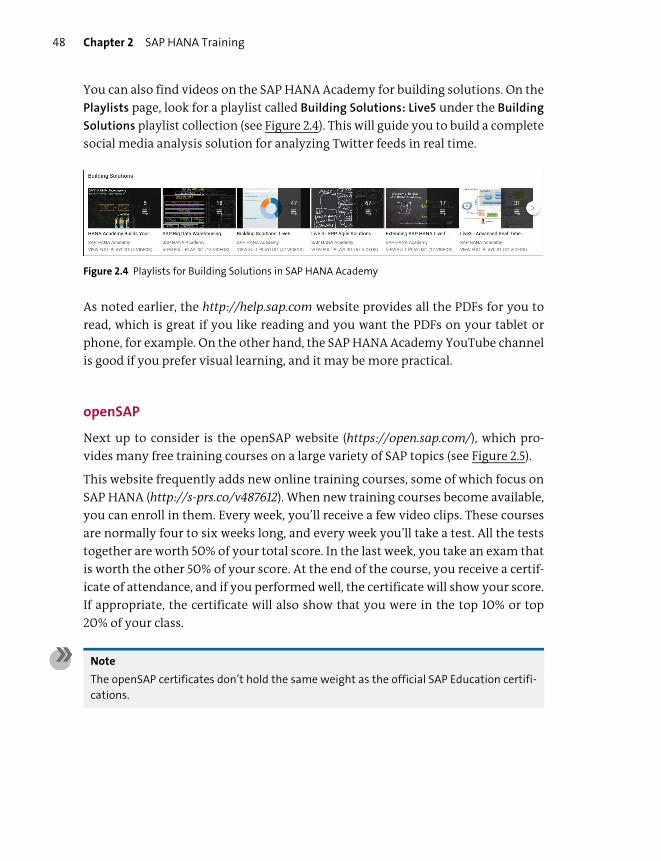
Chapter 2 SAP HANA Training48
You can also find videos on the SAP HANA Academy for building solutions. On the
Playlists page, look for a playlist called Building Solutions: Live5 under the Building
Solutions playlist collection (see Figure 2.4). This will guide you to build a complete
social media analysis solution for analyzing Twitter feeds in real time.
Figure 2.4 Playlists for Building Solutions in SAP HANA Academy
As noted earlier, the http://help.sap.com website provides all the PDFs for you to
read, which is great if you like reading and you want the PDFs on your tablet or
phone, for example. On the other hand, the SAP HANA Academy YouTube channel
is good if you prefer visual learning, and it may be more practical.
openSAP
Next up to consider is the openSAP website (https://open.sap.com/), which pro-
vides many free training courses on a large variety of SAP topics (see Figure 2.5).
This website frequently adds new online training courses, some of which focus on
SAP HANA (http://s-prs.co/v487612). When new training courses become available,
you can enroll in them. Every week, you’ll receive a few video clips. These courses
are normally four to six weeks long, and every week you’ll take a test. All the tests
together are worth 50% of your total score. In the last week, you take an exam that
is worth the other 50% of your score. At the end of the course, you receive a certif-
icate of attendance, and if you performed well, the certificate will show your score.
If appropriate, the certificate will also show that you were in the top 10% or top
20% of your class.
Note
The openSAP certificates don’t hold the same weight as the official SAP Education certifi-
cations.
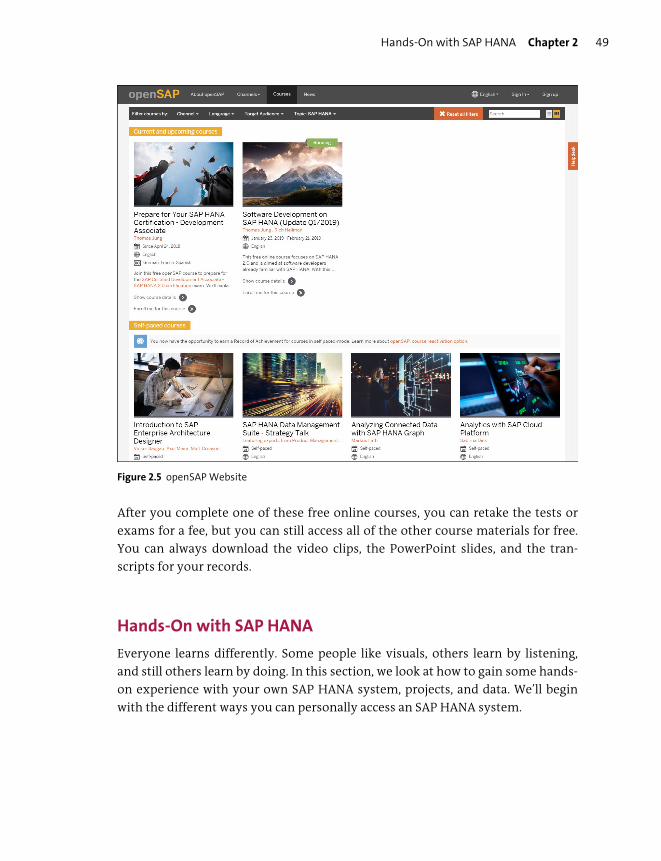
Hands-On with SAP HANA Chapter 2 49
Figure 2.5 openSAP Website
After you complete one of these free online courses, you can retake the tests or
exams for a fee, but you can still access all of the other course materials for free.
You can always download the video clips, the PowerPoint slides, and the tran-
scripts for your records.
Hands-On with SAP HANA
Everyone learns differently. Some people like visuals, others learn by listening,
and still others learn by doing. In this section, we look at how to gain some hands-
on experience with your own SAP HANA system, projects, and data. We’ll begin
with the different ways you can personally access an SAP HANA system.
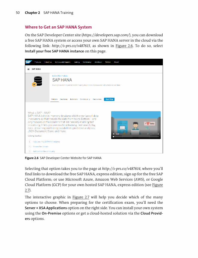
Chapter 2 SAP HANA Training50
Where to Get an SAP HANA System
On the SAP Developer Center site (https://developers.sap.com/), you can download
a free SAP HANA system or access your own SAP HANA server in the cloud via the
following link: http://s-prs.co/v487613, as shown in Figure 2.6. To do so, select
Install your free SAP HANA instance on this page.
Figure 2.6 SAP Developer Center Website for SAP HANA
Selecting that option takes you to the page at http://s-prs.co/v487614, where you’ll
find links to download the free SAP HANA, express edition; sign up for the free SAP
Cloud Platform; or use Microsoft Azure, Amazon Web Services (AWS), or Google
Cloud Platform (GCP) for your own hosted SAP HANA, express edition (see Figure
2.7).
The interactive graphic in Figure 2.7 will help you decide which of the many
options to choose. When preparing for the certification exam, you’ll need the
Server + XSA Applications option on the right side. You can install your own system
using the On-Premise options or get a cloud-hosted solution via the Cloud Provid-
ers options.
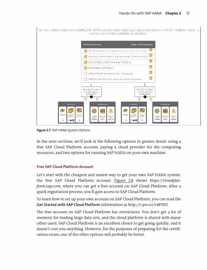
Hands-On with SAP HANA Chapter 2 51
Figure 2.7 SAP HANA System Options
In the next sections, we’ll look at the following options in greater detail: using a
free SAP Cloud Platform account, paying a cloud provider for the computing
resources, and two options for running SAP HANA on your own machine.
Free SAP Cloud Platform Account
Let’s start with the cheapest and easiest way to get your own SAP HANA system:
the free SAP Cloud Platform account. Figure 2.8 shows https://cloudplat-
form.sap.com, where you can get a free account on SAP Cloud Platform. After a
quick registration process, you’ll gain access to SAP Cloud Platform.
To learn how to set up your own account on SAP Cloud Platform, you can read the
Get Started with SAP Cloud Platform information at http://s-prs.co/v487615.
The free account on SAP Cloud Platform has restrictions. You don’t get a lot of
memory for loading large data sets, and the cloud platform is shared with many
other users. SAP Cloud Platform is an excellent choice to get going quickly, and it
doesn’t cost you anything. However, for the purposes of preparing for the certifi-
cation exam, one of the other options will probably be better.
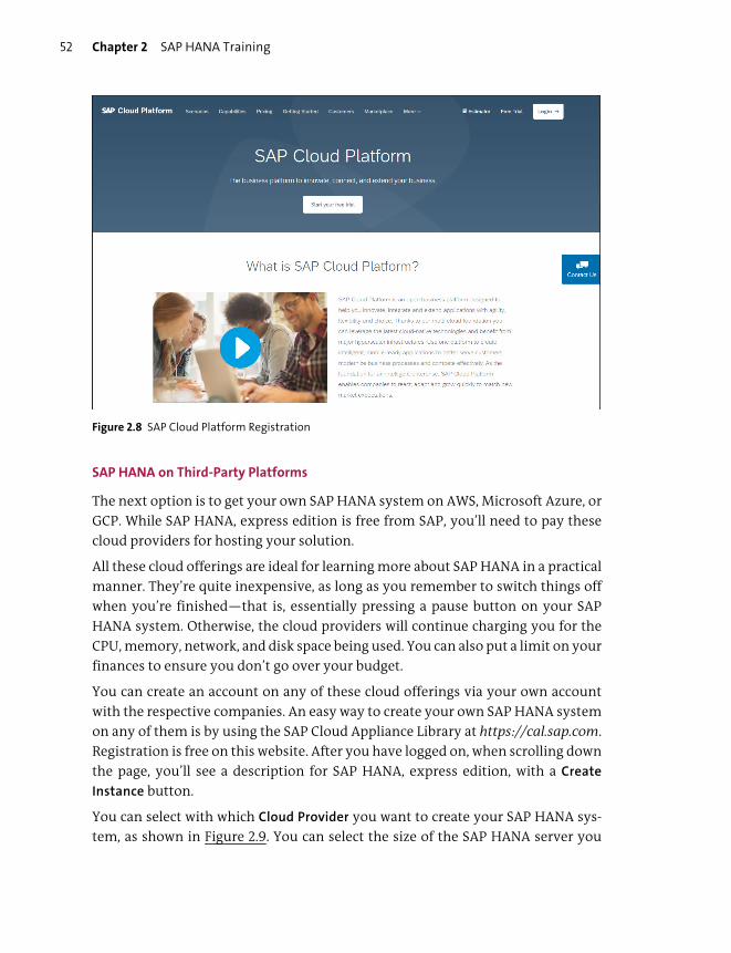
Chapter 2 SAP HANA Training52
Figure 2.8 SAP Cloud Platform Registration
SAP HANA on Third-Party Platforms
The next option is to get your own SAP HANA system on AWS, Microsoft Azure, or
GCP. While SAP HANA, express edition is free from SAP, you’ll need to pay these
cloud providers for hosting your solution.
All these cloud offerings are ideal for learning more about SAP HANA in a practical
manner. They’re quite inexpensive, as long as you remember to switch things off
when you’re finished—that is, essentially pressing a pause button on your SAP
HANA system. Otherwise, the cloud providers will continue charging you for the
CPU, memory, network, and disk space being used. You can also put a limit on your
finances to ensure you don’t go over your budget.
You can create an account on any of these cloud offerings via your own account
with the respective companies. An easy way to create your own SAP HANA system
on any of them is by using the SAP Cloud Appliance Library at https://cal.sap.com.
Registration is free on this website. After you have logged on, when scrolling down
the page, you’ll see a description for SAP HANA, express edition, with a Create
Instance button.
You can select with which Cloud Provider you want to create your SAP HANA sys-
tem, as shown in Figure 2.9. You can select the size of the SAP HANA server you
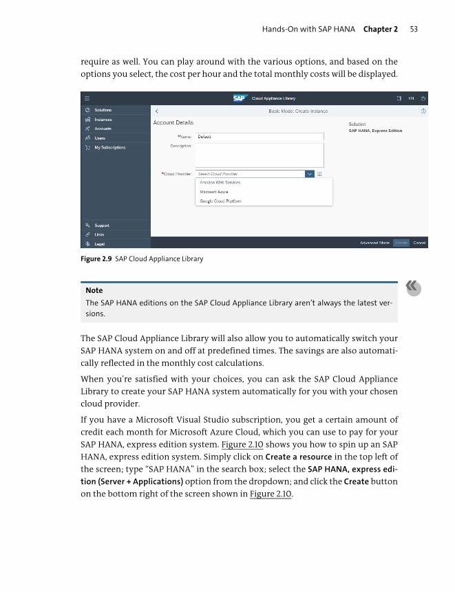
Hands-On with SAP HANA Chapter 2 53
require as well. You can play around with the various options, and based on the
options you select, the cost per hour and the total monthly costs will be displayed.
Figure 2.9 SAP Cloud Appliance Library
Note
The SAP HANA editions on the SAP Cloud Appliance Library aren’t always the latest ver-
sions.
The SAP Cloud Appliance Library will also allow you to automatically switch your
SAP HANA system on and off at predefined times. The savings are also automati-
cally reflected in the monthly cost calculations.
When you’re satisfied with your choices, you can ask the SAP Cloud Appliance
Library to create your SAP HANA system automatically for you with your chosen
cloud provider.
If you have a Microsoft Visual Studio subscription, you get a certain amount of
credit each month for Microsoft Azure Cloud, which you can use to pay for your
SAP HANA, express edition system. Figure 2.10 shows you how to spin up an SAP
HANA, express edition system. Simply click on Create a resource in the top left of
the screen; type “SAP HANA” in the search box; select the SAP HANA, express edi-
tion (Server + Applications) option from the dropdown; and click the Create button
on the bottom right of the screen shown in Figure 2.10.
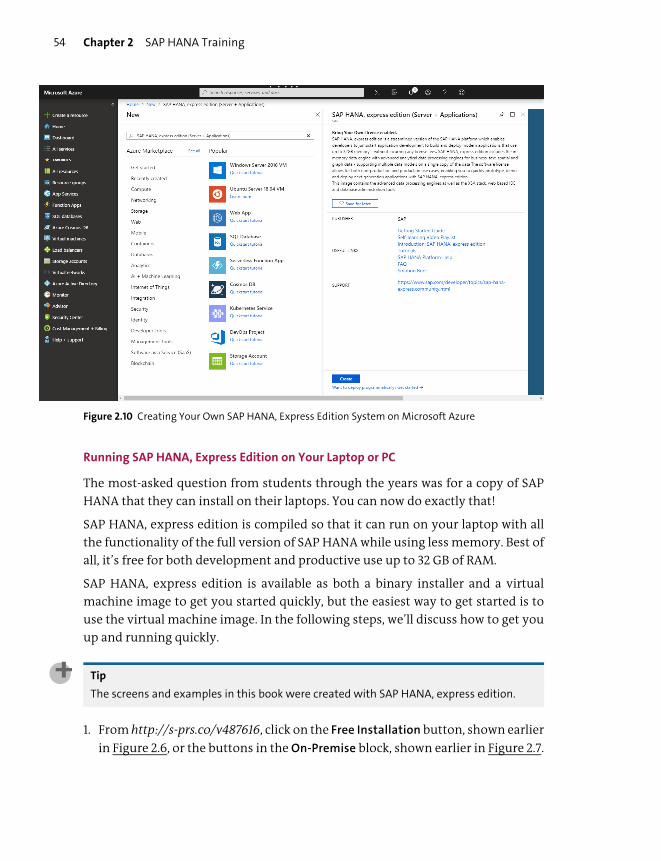
Chapter 2 SAP HANA Training54
Figure 2.10 Creating Your Own SAP HANA, Express Edition System on Microsoft Azure
Running SAP HANA, Express Edition on Your Laptop or PC
The most-asked question from students through the years was for a copy of SAP
HANA that they can install on their laptops. You can now do exactly that!
SAP HANA, express edition is compiled so that it can run on your laptop with all
the functionality of the full version of SAP HANA while using less memory. Best of
all, it’s free for both development and productive use up to 32 GB of RAM.
SAP HANA, express edition is available as both a binary installer and a virtual
machine image to get you started quickly, but the easiest way to get started is to
use the virtual machine image. In the following steps, we’ll discuss how to get you
up and running quickly.
Tip
The screens and examples in this book were created with SAP HANA, express edition.
1. From http://s-prs.co/v487616, click on the Free Installation button, shown earlier
in Figure 2.6, or the buttons in the On-Premise block, shown earlier in Figure 2.7.
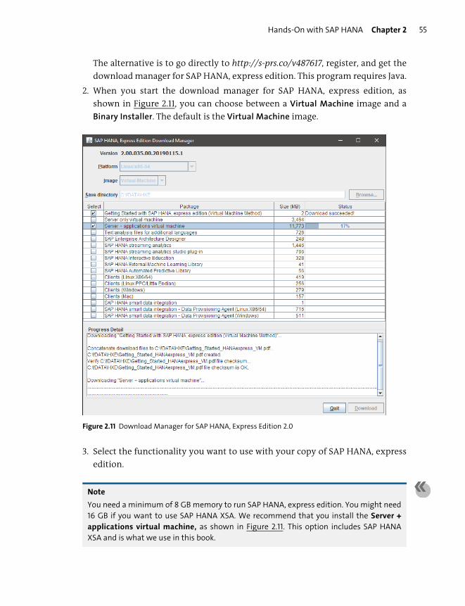
Hands-On with SAP HANA Chapter 2 55
The alternative is to go directly to http://s-prs.co/v487617, register, and get the
download manager for SAP HANA, express edition. This program requires Java.
2. When you start the download manager for SAP HANA, express edition, as
shown in Figure 2.11, you can choose between a Virtual Machine image and a
Binary Installer. The default is the Virtual Machine image.
Figure 2.11 Download Manager for SAP HANA, Express Edition 2.0
3. Select the functionality you want to use with your copy of SAP HANA, express
edition.
Note
You need a minimum of 8 GB memory to run SAP HANA, express edition. You might need
16 GB if you want to use SAP HANA XSA. We recommend that you install the Server +applications virtual machine, as shown in Figure 2.11. This option includes SAP HANA
XSA and is what we use in this book.

Chapter 2 SAP HANA Training56
Options you might select include the following:
– The first selection on the list is the Getting Started with SAP HANA express
edition (Virtual Machine Method) PDF file. This document will help you install
your copy of SAP HANA, express edition. You can also follow the instructions
at http://s-prs.co/v487618.
– The Virtual Machine option already includes the SUSE Linux Enterprise
Server (SLES) operating system. If you use the Binary Installer option, you’ll
need to download a certified operating system. See the next section for links.
4. Ensure you have the VMware Workstation Player (for Windows and Linux) or
VMware Fusion (for Mac).
Tip
The VMware Workstation 15 Player is free for personal use and can be downloaded at
their website at www.vmware.com/go/downloadplayer/.
After you’ve installed SAP HANA, express edition, you need to set up the environ-
ment so that you can start using it for information modeling. You can get guid-
ance by following the tutorials for SAP HANA, express edition at http://s-prs.co/
v487619 or by following the steps described in the PDF you downloaded previously
per Figure 2.11. However, the following steps will help you quickly set up your SAP
system so that you can get to the screens we’ll show in this book:
1. Make sure your hosts file contains a reference to hxehost as described in the
Getting Started guide.
2. Check if the XS engine is up and running by opening http://hxehost:8090 in
your browser.
Tip
We recommend that you use the Google Chrome browser.
3. Check that SAP HANA XSA and services are running by opening https://hxe-
host:39030. This will show you a list of apps that are running and their web
addresses. You can open any of these apps by clicking on their web addresses.
Check that the xsa-cockpit and webide apps are running as shown in Figure 2.12.
If you see the web app running, it means you’ve also installed the SHINE demo
application. Many of the demo screens we show in this book use the SHINE
demo application.
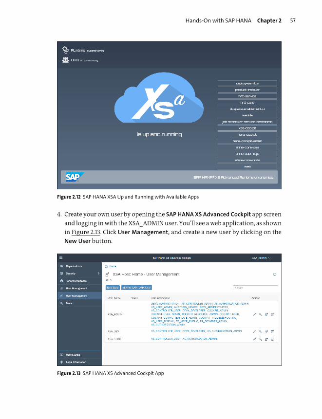
Hands-On with SAP HANA Chapter 2 57
Figure 2.12 SAP HANA XSA Up and Running with Available Apps
4. Create your own user by opening the SAP HANA XS Advanced Cockpit app screen
and logging in with the XSA_ADMIN user. You’ll see a web application, as shown
in Figure 2.13. Click User Management, and create a new user by clicking on the
New User button.
Figure 2.13 SAP HANA XS Advanced Cockpit App

Chapter 2 SAP HANA Training58
5. Add your new user to the development space.
6. Open the Organizations screen, and select HANAExpress. You’ll see two spaces
named development and SAP, as shown in Figure 2.14.
Figure 2.14 SAP HANA XSA Administration App: Organization and Space Management
7. Select the development space. Select the Members option on the menu. You
should see that the XSA_ADMIN and XSA_DEV users are already in this space.
8. Click on the Add Members button, and enter your user name.
9. Select the Space Developer checkbox next to your user name, and click the OK
button. Your user is now added to the development space.
10. Open the webide app. We’ll spend a lot of time in SAP Web IDE for SAP HANA.
In Chapter 4, we’ll describe it in more detail.
11. Log in with your new user name. SAP Web IDE for SAP HANA won’t have any
content for your new user. To get up and running quickly, you can clone or
import the source code of the SHINE SAP HANA XSA demo application. A few
tips are as follows:
– The easiest way to get the source code for SHINE is to clone it from GitHub.
Open the menu, and select File • Git • Clone Repository. When asked for a Git
Repository, enter the public GitHub address where SAP HANA SHINE resides,
that is, “https://github.com/SAP/hana-shine-xsa”. SAP Web IDE for SAP
HANA will download all the source code, information models, and design-
time objects for you.

Hands-On with SAP HANA Chapter 2 59
– If you’ve already installed SHINE during the SAP HANA install, open the
Web app, and click on the icon in the top-right corner. This will download a
ZIP file to your local machine with the SHINE source code. In the webide app,
open the menu, and select File • Import • File or Project. Then select the ZIP
file from SHINE on your local machine.
12. Next, set the space where you want to work in the Project Settings for your
project. As shown in Figure 2.15, select the second-level node (which is your
project), and right-click on the name. In the popup context menu, select Project •
Project Settings.
Figure 2.15 SAP Web IDE for SAP HANA: Configuring Project Settings for a Project
13. On the next screen, select Space, and then choose the development space from
the dropdown list. This is the same space you added your user to earlier. Click
Save and then Close.
14. The last step is to build your SHINE application. At the moment, you only have
the source code, but you want it to create a schema, users, tables with data,
information models, and much more for you. This is accomplished by building
your project. As shown in Figure 2.16, select the second-level node (your proj-
ect), and right-click on the name. In the popup context menu, select Build •
Build.
15. After the core-db module has been built, you can open it. Open the src folder,
then the models folder, and open the PRODUCTS.hdbcalculationview model.
You should see something that looks like Figure 2.17.

Chapter 2 SAP HANA Training60
Figure 2.16 SAP Web IDE on SAP HANA: Building the SHINE Demo Application
Figure 2.17 SAP Web IDE on SAP HANA: Showing an SAP HANA Graphical Information Model
Congratulations! You now have a fully working SAP HANA system.

Hands-On with SAP HANA Chapter 2 61
Building an SAP HANA System
You can also install SAP HANA on a server. You’ll need some certified hardware, an
operating system, and the SAP HANA software. Note that you’ll need a registered
S-user name and password before you can download the SAP HANA software. If
you’re an existing SAP customer or SAP partner, you can ask your system admin-
istrator for a logon user.
The requirements for the hardware and how to install the SAP HANA software can
be found at http://s-prs.co/v487620.
Note
It’s recommended that you use a machine with a minimum of 24 GB or 32 GB of memory.
If you have less memory, you should use SAP HANA, express edition.
The certified operating systems for SAP HANA are SLES for SAP Applications and
Red Hat Enterprise Linux for SAP HANA. You can find the SLES for SAP Applica-
tions at www.suse.com/products/sles-for-sap/, or you can get a copy of Red Hat
Enterprise Linux for SAP HANA from https://developers.redhat.com/products/sap/
overview/.
You’ll also need to download a copy of the SAP HANA software from http://s-
prs.co/v487621. In the alphabetical list of products, select H, choose SAP HANA Plat-
form Edition, and then follow the instructions in installation guides on http://s-
prs.co/v487620.
Project Examples
After you have your own SAP HANA system, the next step is to start using it. In this
section, we’ll discuss how to start working on SAP HANA projects and how you can
use the SHINE demo package or create your own project.
Using the SHINE Demo Package
One option to get some practice in SAP HANA is to explore the content available in
the SHINE demo package. We’ll use the SHINE demo throughout this book. It’s
fully documented and is used by SAP as an example for how to develop SAP HANA
applications. You can see what the SHINE demo application looks like in Figure
2.18.

Chapter 2 SAP HANA Training62
Figure 2.18 SHINE (SAP HANA Interactive Education) for SAP HANA XS Advanced Model Screen
The SHINE documentation can be found at http://s-prs.co/v487620 in the Develop-
ment area by clicking the View All button.
Creating Your Own Project
You can also think up your own projects. You can start very simply by just learning
to work with individual topics discussed in the book, such as fuzzy text search, cur-
rency conversion, input parameters, hierarchies, and spatial joins. You can also
add some security on top of this, for example, to limit the data for a single user to
just one year.
The next step is to think about creating a report that can analyze the performance
of a particular data set. This is a good exercise because you’ll have to take end-user
requirements and learn how to translate them into the required SAP HANA infor-
mation models. Then, you’ll design and create these models. Finally, you can
expand these information models into an application.
You can also look at incorporating something such as SAP Lumira to easily create
attractive storyboards. You can download a free copy of SAP Lumira from https://
saplumira.com/.
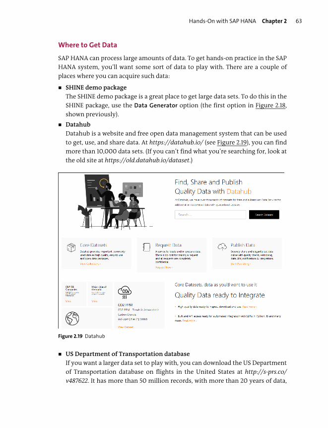
Hands-On with SAP HANA Chapter 2 63
Where to Get Data
SAP HANA can process large amounts of data. To get hands-on practice in the SAP
HANA system, you’ll want some sort of data to play with. There are a couple of
places where you can acquire such data:
� SHINE demo package
The SHINE demo package is a great place to get large data sets. To do this in the
SHINE package, use the Data Generator option (the first option in Figure 2.18,
shown previously).
� Datahub
Datahub is a website and free open data management system that can be used
to get, use, and share data. At https://datahub.io/ (see Figure 2.19), you can find
more than 10,000 data sets. (If you can’t find what you’re searching for, look at
the old site at https://old.datahub.io/dataset.)
Figure 2.19 Datahub
� US Department of Transportation database
If you want a larger data set to play with, you can download the US Department
of Transportation database on flights in the United States at http://s-prs.co/
v487622. It has more than 50 million records, with more than 20 years of data,

Chapter 2 SAP HANA Training64
including departure airport, destination airport, airline, flight number, airborne
time, flight delays and cancellations, and so on. You can use this data to experi-
ment with the predictive capabilities of SAP HANA described in Chapter 10, for
example, to predict whether your US flight will be delayed and by how much.
Exam Questions
Now, we’ll change gears a bit and look at the SAP certification exams and how to
approach them. Let’s look at the examination question types and some tips and
hints about how to complete the certification exam.
Types of Questions
An international team sets up the SAP HANA certification exams. All the questions
are written in English, and all the communication is in English. Because the exam
teams are international, a lot of attention is focused on making sure that every-
body will understand what is meant by each question, avoiding possible double
meanings or ambiguities. Some of the exams get translated into other languages,
so simple and straightforward questions work best.
Figure 2.20 shows three types of questions that you’ll find in the certification
exam.
Figure 2.20 Three Types of Certification Exam Questions
Which of the following are components of SAP HANA Data Warehousing Foundation?Note: There are 3 correct answers to this question.
Which of the following approaches can be used to implement union pruning?Note: There are 2 correct answers to this question.
In your calculation view, you CANNOTenable a hierarchy for time dependency.What could be the reason for this?
The hierarchy is a parent-child type.
The hierarchy is a level type.
You did NOT reference a DIMENSION of the type TIME.
You did NOT include a historycolumn table.
Define a constant value for each datasource in the Union Node.
Define the cardinality between the datasources.
Define a restricted column and include it in both data sources of a union.
Define union pruning conditions in apruning configuration table.
Native DataStore Object
SAP Data Hub
CompositeProvider
Data LifeCycle Manager
Data Distribution Optimizer
Exam Questions Chapter 2 65
The first question is multiple choice. The radio buttons indicate that you can only
choose one of the four available answer options. There will be three or four differ-
ent options, with only one correct answer. (Most of the time there will be four
answer options. The newer exams have a few questions that only have three
answer options for this type of question. The older exams always had four
options.)
The other two questions are called multiple-response questions, of which there are
two types:
� With the first type of multiple-response question, there are four possible
answers, and there will always be two correct answers and two incorrect
answers. In the exam, this will be indicated by the words, “Note: There are two
correct answers to this question.”
� The other type of multiple-response question has five possible answers, of which
three will always be correct, and two will be incorrect; you must select three cor-
rect answers. Above the answers, you’ll see the words, “Note: There are three
correct answers to this question.”
Both types of multiple-response questions use checkboxes, and you must select
however many answers are correct.
All three types of questions have exactly the same weight. You either get a ques-
tion right or you get it wrong. It’s a binary system: 0 or 1.
For a multiple-response question with two correct and two incorrect answers, you
must select two answers. If you select three answers or one answer, you don’t
receive any points. If you select two answers and they are the correct two answers,
then you earn a point.
Tip
Select as many answers as are required! If you’re certain that an option is correct, select
it. If you’re doubtful about an answer, at least select the correct number of answers. If
you don’t select anything, you won’t earn any points. Even if you plan to come back to the
question later, we still recommend that you select the exact number of answer options
required.
Multiple-choice questions normally make up the majority of the questions for the
associate-level core exams. More than half of the questions will have only one cor-
rect answer.
Chapter 2 SAP HANA Training66
Note
In the certification exam, there are no fill-in-the-blank questions. There are also no true
or false questions in the certification exam, but we’ll use true or false questions in this
book for training purposes.
The questions and the answers themselves appear randomly. In other words, two
people could be taking the same exam, sitting next to each other, and the order in
which the questions appear for each person would be different. In addition, for
similar questions, the order of A, B, C, and D (the answer options) is different for
different people. Because answer options are randomized, you’ll never find any
questions that list “All of the above” or “None of the above” as a possible answer.
The questions in the SAP certification exams tend to be very short and to the
point. All extra words and descriptions have been cut away, ensuring that you’ll
have enough time to complete the exams. We’ve never heard anyone complain
about the time limits in the SAP HANA certification exams.
Because the questions are to the point, every word counts. Every word is there for
a reason and has a purpose, so don’t ignore any word—especially words such as
always, only, and must. Always indicates on every occasion, only means that no
other options are allowed, and must indicates something that is mandatory. In the
answer options, you could see some optional actions that would be valid actions in
normal circumstances, but if they aren’t mandatory, they are incorrect answers for
questions asking what you must do. Therefore, for questions using the word must,
pay attention to optional steps versus mandatory steps.
The certification exams use a minimum of negative words, which are only used for
troubleshooting questions. All negative words in a question are written in capital
letters—for example, “You did something and it is NOT working. What is the rea-
son?” You can see an example of this in the first question in Figure 2.20 shown ear-
lier in this section.
Tip
Don’t just learn the facts as if everything will always work properly. Systems break in real
life, and you need to know why they didn’t work and how to fix or troubleshoot the prob-
lem. There will be questions in the exam to test this knowledge.
Now that we’ve looked at the general structure of SAP certification exam ques-
tions, let’s look at the strategy of elimination in the exam.

Exam Questions Chapter 2 67
Elimination Technique
Experience has shown that the elimination technique can be useful for answering
exam questions. In this technique, you start by finding the wrong answers instead
of finding the right answers.
When creating exams, it’s fairly easy to set up questions, but it’s hard to think up
wrong answers that still sound credible. Because it’s so difficult to write credible
wrong answers, it’s normally easier to eliminate the wrong answers first. As Sher-
lock Holmes would say, whatever remains, however improbable, must be the
truth.
To show how efficient this technique can be, look at the multiple-response ques-
tion with five different options (refer to Figure 2.20, right). There are three correct
and two incorrect answers, so it saves you time to find the two incorrect ones,
rather than trying to find the three correct answers.
Tip
Make sure you know which keywords apply to which area. The wrong answers could
come from an unrelated area, but the words sound like they might belong to the area in
which the question is asked. Don’t confuse the words from different topic areas.
Bookmark Questions
In the certification exam, you can always bookmark questions and return to them
later. Figure 2.21 shows the sample exam you can write for C_HANAIMP_15. You
can see the Assessment Navigator block in the bottom-right corner of the screen.
You’ll notice that the top-left corner of question 1 is marked. By clicking on the
bookmarked question in the Assessment Navigator, it will take you directly to that
question.
If you’re not confident about a question, mark it. We still recommend that you
complete the right number of answer options: If two answers are required, fill in
two options. If three are required, select three options. Then, mark the question so
that you can review it later.
Tip
Watch out when you do the review; your initial choice tends to be the correct one.
Remember, don’t overanalyze the question.
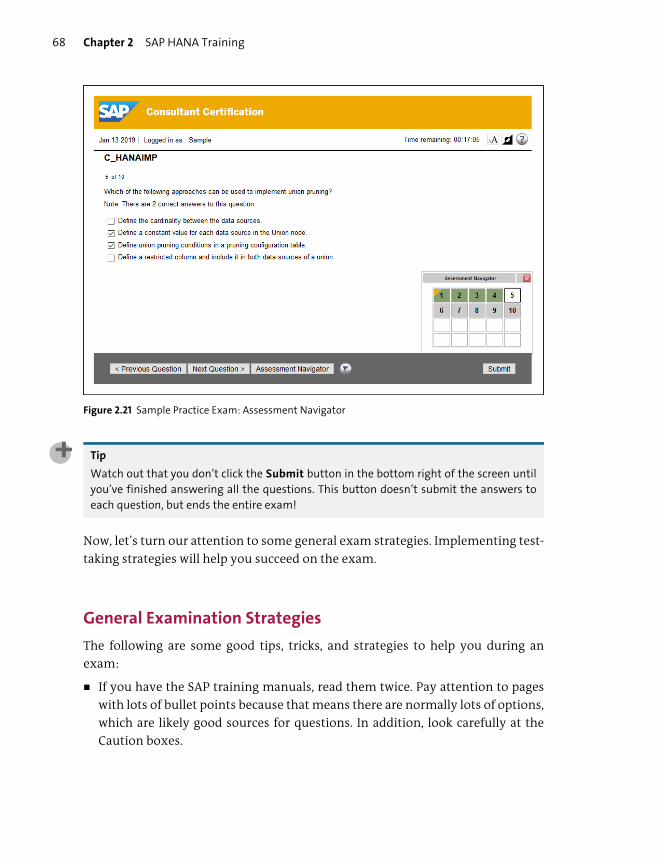
Chapter 2 SAP HANA Training68
Figure 2.21 Sample Practice Exam: Assessment Navigator
Tip
Watch out that you don’t click the Submit button in the bottom right of the screen until
you’ve finished answering all the questions. This button doesn’t submit the answers to
each question, but ends the entire exam!
Now, let’s turn our attention to some general exam strategies. Implementing test-
taking strategies will help you succeed on the exam.
General Examination Strategies
The following are some good tips, tricks, and strategies to help you during an
exam:
� If you have the SAP training manuals, read them twice. Pay attention to pages
with lots of bullet points because that means there are normally lots of options,
which are likely good sources for questions. In addition, look carefully at the
Caution boxes.
Summary Chapter 2 69
� For this associate-level certification exam, when using this book, read the entire
chapters and answer all the questions. If you don’t get the answers right or don’t
understand the question, reread that section. This is the equivalent of reading
the SAP training materials twice.
� Make sure that you’ve answered all the questions and that you’ve selected the
correct number of answer options. If the question says that three answers are
correct, then make sure that you’ve marked three—not four or two.
� Occasionally, you’ll find answer options that are opposites—for example, X is
true, and X is NOT true. In that case, make sure you select one of the pair.
� In our experience with SAP HANA certification exams, the answers from one
question don’t provide answers to another question. SAP Education is careful to
make sure that this doesn’t happen in its exams.
� Watch out for certain trigger words. Alarm bells should go off when you see
only, must, and always.
� Look out for impossible combinations. For example, if a question is about mea-
sures, then the answer can’t be something to do with dimension calculation
views because you can’t find measures for such views.
� Some words can be different in different countries. For example, some people
talk about a right-click menu, but in other places in the world, this same feature
is known as a context menu. This is the menu that pops up in a specific context,
and you access this menu by right-clicking.
� Make sure you get a good night’s rest before the exam.
Summary
You should now know which SAP Education training courses you can attend for
your certification examination, which related SAP courses will complement your
knowledge and skills, and where to get hands-on experience. In addition, we intro-
duced many free sources of information on the Internet, training videos on You-
Tube, and online courses at openSAP.
You can now form a winning strategy for taking your SAP certification exam. In
the next chapter, we’ll begin looking at exam questions and concepts, focusing
first on the technology, architecture, and deployment scenarios of SAP HANA.


Chapter 3
Technology, Architecture, and Deployment Scenarios
Techniques You’ll Master
� Understand in-memory technologies and how SAP HANA
uses them
� Get to know the internal architecture of SAP HANA
� Describe the SAP HANA persistence layer
� Learn the different ways that SAP HANA can be deployed
� Know when to use different deployment methods, including
the various cloud options
Chapter 3 Technology, Architecture, and Deployment Scenarios72
In this chapter, you’ll become familiar with the various deployment scenarios for
SAP HANA and evaluate appropriate system configurations, including cloud
deployments. We’ll introduce the in-memory paradigm and the thinking behind
how SAP HANA uses in-memory technologies, and you’ll get a glimpse of how to
develop information models with SAP HANA. By the end, you’ll better understand
how SAP HANA functions in all types of solutions and use cases you might require.
Real-World Scenario
You start a new project. The business users describe what they want and
expect you to suggest an appropriate architecture for how to deploy SAP
HANA. You have to decide between building something new in SAP HANA or
migrating the current system to use SAP HANA. You also have to decide if you
should use SAP HANA in the cloud and, if so, which type of service you’ll need.
When you understand the internal architecture of SAP HANA, it can lead to
unexpected benefits for your company. You can use the fact that SAP HANA
uses compression in memory combined with an understanding of how SAP
HANA uses disks and backups to provide a customer with an excellent busi-
ness case for moving its business solution to SAP HANA. This can lead to dra-
matically lower operational costs and reduced risk because the compression
lets SAP HANA use less memory, which leads to smaller backups and imme-
diately reduces the storage space required by the business (operational
costs). These backups take less time, don’t require any downtime, and can be
made at any time of the day, leading to reduced risk.
Objectives of This Portion of the Test
The objective of this portion of the SAP HANA certification test is to evaluate your
basic understanding of the various SAP HANA deployment scenarios and the cor-
responding system configurations. The certification exam expects SAP HANA
modelers to have a good understanding of the following topics:
� How SAP HANA uses in-memory technology, including elements such as col-
umns, tables, compression, delta buffer, and partitioning
� SAP HANA architecture concepts
� The persistence layer in SAP HANA
� The various ways that SAP HANA can be deployed
Key Concepts Refresher Chapter 3 73
� How SAP HANA can be deployed in the cloud
� The direction SAP is taking by allowing your modeling and development work
to run on both standalone and cloud deployments of SAP HANA
� An overview of using SAP HANA with analytics and business intelligence (BI)
Note
This portion contributes about 10% of the total certification exam score.
Key Concepts Refresher
We’ll start with something that most people know very well: Moore’s Law. Even if
you’ve never heard of it, you’ve seen its effects on the technology around you, for
example, with your mobile phone. Put simply, this means that the overall process-
ing power for computers doubles about every two years. Therefore, you can buy a
computer for roughly the same price as about two years ago, and it will be about
twice as fast and powerful as the older one. This held true for mobile phones as
well. (Lately Moore’s Law hasn’t kept up, and devices such as high-end mobile
phones have risen in price.)
Moore’s Law is useful for understanding system performance and response times.
If you have a report that is running slow, let’s say an hour long, you can fix this by
buying faster hardware. You can easily decrease the processing time of your slow
report from 1 hour to 30 minutes to 15 minutes by just waiting a while and then
buying faster computers. However, a few years ago that simple recipe stopped
working. Our easy upgrade path was no longer available, and we had to approach
the performance issues in new and innovative ways. Data volumes also keep grow-
ing, adding to the problem. SAP realized these problems early and worked on the
solution we now know as SAP HANA.
In this chapter, we’ll discuss SAP HANA’s in-memory technology and how it
addresses the aforementioned issues. We’ll then look at SAP HANA’s architecture
and approaches. Finally, we’ll walk through the various deployment options avail-
able, including cloud options and using SAP HANA for analytics.
In-Memory Technology
SAP HANA uses in-memory technology. But, just what is in-memory technology?
In-memory technology is an approach to querying data residing in RAM, as

Chapter 3 Technology, Architecture, and Deployment Scenarios74
opposed to physical disks. The results of doing so lead to shortened response
times, which enable enhanced analytics for BI/analytic applications.
In this section, we’ll walk through the process that leads us to use in-memory tech-
nology, which will illustrate the importance of this new technology.
Multicore CPU
After years of CPUs getting faster, we seemed to hit a wall when CPU speeds
reached about 3 GHz. It became difficult to make a single CPU faster while keeping
it cool enough. Therefore, chip manufacturers moved from a single CPU per chip
to multiple CPU cores per chip.
Instead of increasingly fast machines, machines now stay at roughly the same
speed but have more cores. If a specific report takes an hour and only runs on a sin-
gle core, that report won’t run any faster thanks to more CPU cores. We can run
multiple reports simultaneously, but each of them will run for an hour. To speed
up reports, we need to rewrite software to take full advantage of new multicore
CPU technology—that is, through parallel processing—which is a problem that
has been faced by most software companies.
SAP addressed this problem by making sure that all operations in SAP HANA are
making full use of all available CPU cores.
Slow Disk
When talking about poor system performance, you can place a lot of blame on
slow hard disks. Table 3.1 shows how slow a disk is when compared to memory.
Operation Latency
(in Nanoseconds)
Relative to Memory
Read from level 1 (L1) cache 0.5 ns 200 times faster
Read from level 2 (L2) cache 7 ns 14 times faster
Read from level 3 (L3) cache 15 ns 6.7 times faster
Read from memory 100 ns –
Send 1 KB over 1 Gbps network 10,000 ns 100 times slower
Read from solid state disk (SSD) 150,000 ns 1,500 time slower
Table 3.1 Latency of Hardware Components and Performance of Components Shown Relative to RAM

Key Concepts Refresher Chapter 3 75
To give you an idea of how slow a disk really is, think about this: if reading data
from RAM takes one minute, it will take more than two months to read the same
data from disk! In reality, there is less of a difference when we start reading and
streaming data sequentially from disks, but this example prompts the idea that
there must be better ways of writing systems.
The classic problem is that alternatives such as RAM have been prohibitively
expensive, and there hasn’t been enough RAM available in a machine to replace
disks.
Therefore, the way we’ve designed and built software systems for the past 30 or
more years has been heavily influenced by the fact that disks are slow. This affects
the way everyone from technical architects to developers to auditors thinks about
system and application design. Consider these three examples of the wide effect of
slow disks:
� SAP NetWeaver
SAP NetWeaver architecture uses one database server and multiple application
servers (Figure 3.1).
Figure 3.1 SAP NetWeaver Architecture: One Database Server, Many Application Servers
Read from disk 10,000,000 ns 100,000 times slower
Send network packet from the US
West Coast to Europe and back
150,000,000 ns 1,500,000 times slower
Operation Latency
(in Nanoseconds)
Relative to Memory
Table 3.1 Latency of Hardware Components and Performance of Components Shown Relative to RAM (Cont.)
Database Server
ApplicationServer
ApplicationServer
ApplicationServer
Calculations Business Rules
DB Independent
Chapter 3 Technology, Architecture, and Deployment Scenarios76
Because the database stores data on disks that are slow, the database becomes
the bottleneck in the system. In any system, you always try to minimize the
impact of the bottlenecks and the load on the system. Therefore, we move the
data into multiple application servers to work with it there, using the database
server as little as possible. In SAP systems, we used it so little that we were data-
base independent. SAP systems even used their own database-independent
ABAP Data Dictionaries.
In the application servers, we run all the code, perform all the calculations, and
execute the business rules. We use memory buffers to store a working set of
data. In many SAP systems, 99.5% of all database reads come from these mem-
ory buffers, thus minimizing the effects of the slow disk. The SAP system archi-
tecture was heavily influenced by the fact that the disk is slow.
� Financial systems data storage
Inside financial systems, we store data such as year-to-date data, month-to-date
data, balances, and aggregates. For reporting, we have cubes, dimensions, and
more aggregates. These values are all updated and stored in financial systems to
improve performance.
Take the case of the year-to-date figure. We don’t really need to store this infor-
mation because we can calculate it from the data. The problem is that to calcu-
late the year-to-date figure, we need to read millions of records from the data-
base, which the database reads from the slow disk. Therefore, we could calculate
the current year-to-date figure, but doing so would be too slow. Because disk
storage is cheap and plentiful, we just add this value into the database in
another table. With every new transaction, we simply add the new value to the
current year-to-date value and update the database. Now reports can run a lot
faster on disk.
If the disk was fast, we would not need to store these values. Can you imagine a
financial system without these values? Ask accountants to imagine a financial
system without balances! Why store balances when you can calculate them?
When you see the reaction on their faces, you’ll understand how even their
thinking has been influenced by the effects of slow disks.
We’ll return to this example in the next section.
� Data warehouses
One of the many reasons we have data warehouses is that we need fast and flex-
ible reporting. We build large cubes with precalculated, stored aggregates that
we can use for reporting and to slice and dice the data. Building these cubes
takes time and processing power. Reading the masses of data from disk for the

Key Concepts Refresher Chapter 3 77
reports can be slow. If we keep these cubes inside our financial system, for
example, then a single user running a large report from these cubes can pull the
system’s performance down. That one reporting user affects thousands of other
users.
Therefore, SAP created separate data warehouses to reduce the impact of
reporting on operational and transactional systems. Those reporting users can
now run their heavy, slow reports away from the operational and transactional
systems. The database world now is split into two parts: the online transac-
tional processing (OLTP) databases for the financial, transactional, and opera-
tions systems, and the online analytical processing (OLAP) data warehouses
(see Figure 3.2).
Figure 3.2 OLTP vs. OLAP: Keeping Operational Reporting Separate from Operational Systems for Performance Reasons
If disks were fast, and we could create aggregates fast enough, we would be able
to perform most of our operational reporting directly in the operational sys-
tem, where the users expect and need it. We would not have separate OLTP and
OLAP systems. Again, slow disks influenced architectural design principles.
These three examples prove that slow disks influenced system design, architec-
ture, and thinking for many years. If we could eliminate the slow disk bottleneck
from our systems, we could then change our minds about how to design and
implement systems. Hence, SAP HANA represents a paradigm shift.
SAP ERP,SAP CRM,
SAP SRM, …
DataWarehouse
Database(OLAP)
Database(OLTP)
Pre-calculated stored values
Chapter 3 Technology, Architecture, and Deployment Scenarios78
Loading Data into Memory
In the first of the three examples in the previous section, you saw that we’ve used
memory where possible to speed things up with memory caching. Nevertheless,
until a few years ago, memory was still very expensive. Then, memory prices
started coming down fast, and we asked, “Can we load all data into memory
instead of just storing it on disk?”
Customer databases for business systems can easily be 10 TB (10,000 GB) in size.
The largest available hardware when SAP HANA was developed had only 512 GB to
1 TB of memory, presenting a problem. SAP obviously needed to compress data to
fit it into the available memory. We’re not talking here about ZIP or RAR compres-
sion, which needs to be decompressed again before it’s usable, but dictionary com-
pression. Dictionary compression involves mapping distinct values to consecutive
numbers. Using this type of compression enables the data to be used in its com-
pressed format.
Column-Oriented Database
For years, it was common to store data in rows. Row-based databases work well
with spinning disks to read single records faster. However, when we start storing
data in memory, there are fewer valid reasons to use row-based storage. At that
point, we can decide to use row-based or column-based storage.
Why would we use columns instead of rows? When we start looking at compress-
ing data, then row-oriented data doesn’t work particularly well because we mix dif-
ferent types of data—such as cities with salaries and employee numbers—in every
record. The average compression we get is about two times (i.e., data is stored in
about 50% of the original space).
When we store the same data in columns, we now group similar data together. By
using dictionary compression, we can achieve excellent compression, and thus
column-based storage starts making more sense for in-memory databases.
Another way in which we can save space is via indices. If we look inside an SAP sys-
tem, we find that about half the data volume is taken up by indices, which are actu-
ally sorted columns. When we store the data in columns in memory, do we really
need indices? We can save that space. With such column-oriented database advan-
tages, we end up with 5 to 20 times compression.
Let’s get back to our original problem of 10 TB databases, but machines with only
1 TB of memory. By using column-based storage, compression, and no indices, we

Key Concepts Refresher Chapter 3 79
can fit a 10 TB database into the 1 TB of available memory. Even though we focused
on the preferred column-oriented concept here, note that SAP HANA can handle
both row- and column-based tables.
Removing Bottlenecks
When we manage to load the database entirely into memory, exciting things start
happening. We break free from the slow disk bottleneck that had a stranglehold on
system performance for many years and can start exploring new architectures.
As always, even if our systems become thousands of times faster, at some stage,
we’ll reach new constraints. These constraints will determine what the new archi-
tecture will look like. The way we provide new business solutions will depend on
the characteristics of this new architecture.
Architecture and Approach
The new in-memory computing paradigm has changed the way we approach solu-
tions. Different architectures and deployment options are now possible with SAP
HANA.
Changing from a Database to a Platform
The biggest change in approach is how and where we work with the data. Disks
were always slow, causing the database to become a bottleneck. Thus, we moved
the processing of data onto application servers to minimize the pressure on this
disk bottleneck.
Now, data storage has moved from disk to memory, which is much faster. There-
fore, we needed to reexamine our assumptions about the database being the bot-
tleneck. In this new in-memory architecture, it makes no sense to move data from
the memory of the database server to the memory of the application servers via a
relatively slow network. In that case, the network will become the bottleneck, and
we’ll duplicate functionality.
New bottlenecks require new architectures. Our new bottleneck arises because we
have many CPU cores that need to be fed as quickly as possible from memory.
Therefore, we must put the CPUs close to the memory (i.e., the data). In doing so,
we realized that SAP HANA can be offered as an appliance. As shown in Figure 3.3,
it doesn’t make sense to copy data from the memory of the database server to the

Chapter 3 Technology, Architecture, and Deployment Scenarios80
memory of the application server as we’ve always done (left arrow). We instead
now move the code to execute within the SAP HANA server (right arrow).
Figure 3.3 Moving Data In-Memory
Our solution approach also needed to change. Instead of moving data away from
the database to the application servers—as we’ve done for many years—we now
want to keep it in the database. Many database administrators (DBAs) have done
this for years via stored procedures. Instead of stored procedures, in SAP HANA, we
use graphical information models, as we’ll discuss in Chapter 4 through Chapter 7.
You can also use stored procedures and table functions if necessary. We’ll look at
this in Chapter 8.
Note
Instead of moving data to the code, we now move the code to the data. We can easily
implement this process by way of SAP HANA graphical modeling techniques.
When you start running code inside the database, it’s only a matter of time before
it changes from a database into a platform. When people tell you that SAP HANA is
“just another database,” ask them which other database incorporates many pro-
gramming languages, a web server, an application server, an HTML5 framework, a
development environment, replication and cleaning of data, integration with
most other databases, predictive analytics, machine learning, and multitenancy—
the reactions can be interesting.
Application Server
Database Server
Calculations
Calculations
Move data to theapplication (code)
The OldApproach
Move code to thedatabase (data)
The NewApproach
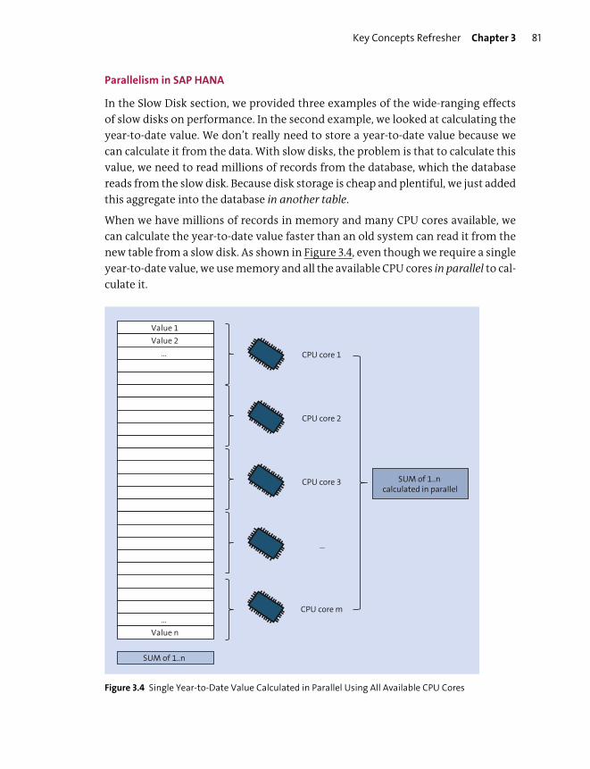
Key Concepts Refresher Chapter 3 81
Parallelism in SAP HANA
In the Slow Disk section, we provided three examples of the wide-ranging effects
of slow disks on performance. In the second example, we looked at calculating the
year-to-date value. We don’t really need to store a year-to-date value because we
can calculate it from the data. With slow disks, the problem is that to calculate this
value, we need to read millions of records from the database, which the database
reads from the slow disk. Because disk storage is cheap and plentiful, we just added
this aggregate into the database in another table.
When we have millions of records in memory and many CPU cores available, we
can calculate the year-to-date value faster than an old system can read it from the
new table from a slow disk. As shown in Figure 3.4, even though we require a single
year-to-date value, we use memory and all the available CPU cores in parallel to cal-
culate it.
Figure 3.4 Single Year-to-Date Value Calculated in Parallel Using All Available CPU Cores
Value 1
CPU core 1
Value 2…
…Value n
CPU core 2
CPU core 3
…
CPU core m
SUM of 1..n
SUM of 1..ncalculated in parallel
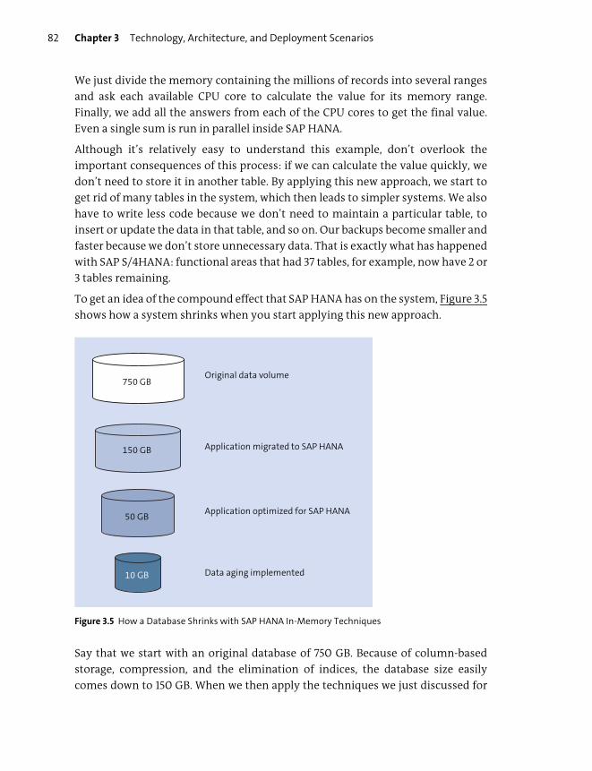
Chapter 3 Technology, Architecture, and Deployment Scenarios82
We just divide the memory containing the millions of records into several ranges
and ask each available CPU core to calculate the value for its memory range.
Finally, we add all the answers from each of the CPU cores to get the final value.
Even a single sum is run in parallel inside SAP HANA.
Although it’s relatively easy to understand this example, don’t overlook the
important consequences of this process: if we can calculate the value quickly, we
don’t need to store it in another table. By applying this new approach, we start to
get rid of many tables in the system, which then leads to simpler systems. We also
have to write less code because we don’t need to maintain a particular table, to
insert or update the data in that table, and so on. Our backups become smaller and
faster because we don’t store unnecessary data. That is exactly what has happened
with SAP S/4HANA: functional areas that had 37 tables, for example, now have 2 or
3 tables remaining.
To get an idea of the compound effect that SAP HANA has on the system, Figure 3.5
shows how a system shrinks when you start applying this new approach.
Figure 3.5 How a Database Shrinks with SAP HANA In-Memory Techniques
Say that we start with an original database of 750 GB. Because of column-based
storage, compression, and the elimination of indices, the database size easily
comes down to 150 GB. When we then apply the techniques we just discussed for
750 GB
150 GB
50 GB
10 GB
Original data volume
Application migrated to SAP HANA
Application optimized for SAP HANA
Data aging implemented
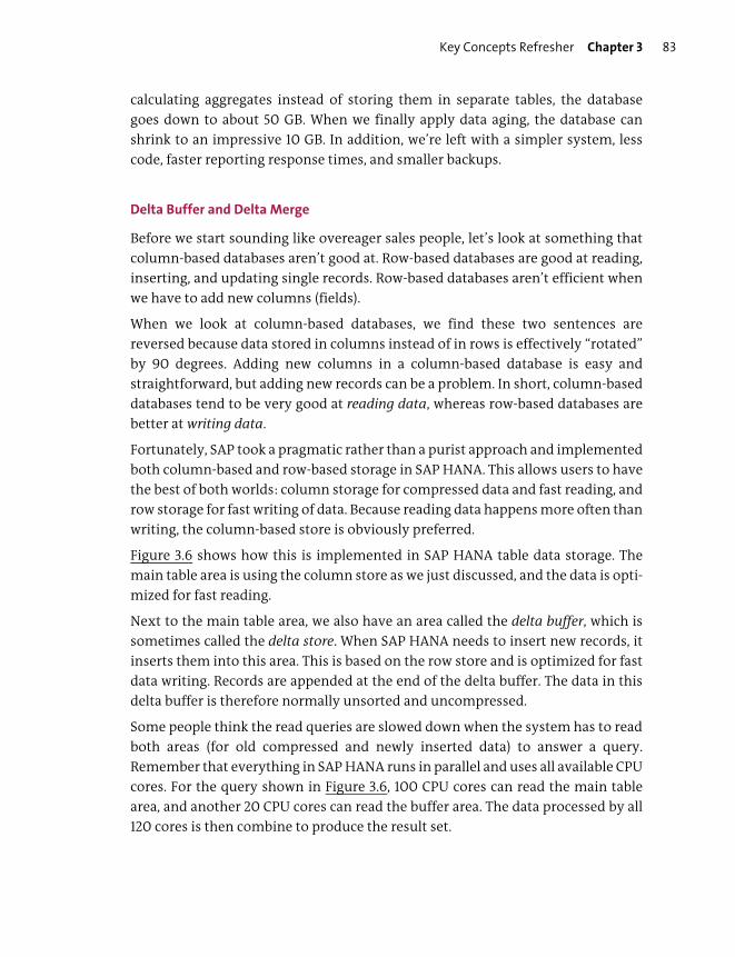
Key Concepts Refresher Chapter 3 83
calculating aggregates instead of storing them in separate tables, the database
goes down to about 50 GB. When we finally apply data aging, the database can
shrink to an impressive 10 GB. In addition, we’re left with a simpler system, less
code, faster reporting response times, and smaller backups.
Delta Buffer and Delta Merge
Before we start sounding like overeager sales people, let’s look at something that
column-based databases aren’t good at. Row-based databases are good at reading,
inserting, and updating single records. Row-based databases aren’t efficient when
we have to add new columns (fields).
When we look at column-based databases, we find these two sentences are
reversed because data stored in columns instead of in rows is effectively “rotated”
by 90 degrees. Adding new columns in a column-based database is easy and
straightforward, but adding new records can be a problem. In short, column-based
databases tend to be very good at reading data, whereas row-based databases are
better at writing data.
Fortunately, SAP took a pragmatic rather than a purist approach and implemented
both column-based and row-based storage in SAP HANA. This allows users to have
the best of both worlds: column storage for compressed data and fast reading, and
row storage for fast writing of data. Because reading data happens more often than
writing, the column-based store is obviously preferred.
Figure 3.6 shows how this is implemented in SAP HANA table data storage. The
main table area is using the column store as we just discussed, and the data is opti-
mized for fast reading.
Next to the main table area, we also have an area called the delta buffer, which is
sometimes called the delta store. When SAP HANA needs to insert new records, it
inserts them into this area. This is based on the row store and is optimized for fast
data writing. Records are appended at the end of the delta buffer. The data in this
delta buffer is therefore normally unsorted and uncompressed.
Some people think the read queries are slowed down when the system has to read
both areas (for old compressed and newly inserted data) to answer a query.
Remember that everything in SAP HANA runs in parallel and uses all available CPU
cores. For the query shown in Figure 3.6, 100 CPU cores can read the main table
area, and another 20 CPU cores can read the buffer area. The data processed by all
120 cores is then combine to produce the result set.
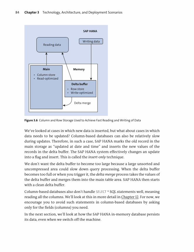
Chapter 3 Technology, Architecture, and Deployment Scenarios84
Figure 3.6 Column and Row Storage Used to Achieve Fast Reading and Writing of Data
We’ve looked at cases in which new data is inserted, but what about cases in which
data needs to be updated? Column-based databases can also be relatively slow
during updates. Therefore, in such a case, SAP HANA marks the old record in the
main storage as “updated at date and time” and inserts the new values of the
records in the delta buffer. The SAP HANA system effectively changes an update
into a flag and insert. This is called the insert-only technique.
We don’t want the delta buffer to become too large because a large unsorted and
uncompressed area could slow down query processing. When the delta buffer
becomes too full or when you trigger it, the delta merge process takes the values of
the delta buffer and merges them into the main table area. SAP HANA then starts
with a clean delta buffer.
Column-based databases also don’t handle SELECT * SQL statements well, meaning
reading all the columns. We’ll look at this in more detail in Chapter 12. For now, we
encourage you to avoid such statements in column-based databases by asking
only for the fields (columns) you need.
In the next section, we’ll look at how the SAP HANA in-memory database persists
its data, even when we switch off the machine.
SAP HANA
Reading dataWriting data
Main
Delta buffer
Memory
• Column store• Read-optimized
• Row store• Write-optimized
Delta merge

Key Concepts Refresher Chapter 3 85
Persistence Layer
The most frequently asked question about SAP HANA and its in-memory concept
is as follows: “Because memory is volatile and loses its contents when you switch
off its power source, what happens to SAP HANA’s data when you lose power or
switch off the machine?”
The short answer is that SAP HANA still uses disks. However, whereas other data-
bases are disk-based and optionally load data into memory, SAP HANA is in-mem-
ory and merely uses disks to back up the data for when the power is switched off.
The focus is totally different.
The disk storage and the data storage happens in the persistence layer, and storing
data on disk is called persistence.
If hardware fails, having the data also stored in the persistence layer allows for full
recovery. Newer nonvolatile memory, which doesn’t lose its contents when the
power gets switched off, influences the architecture of SAP HANA’s persistence
layer going forward.
SPS 04
As of SAP HANA 2.0 SPS 04, you can use Intel Optane DC persistent (nonvolatile) memory
instead of DRAM in 50% to 80% of your SAP HANA server’s memory slots. SAP HANA is the
first database to use this new type of memory in nonvolatile App Direct Mode. Depend-
ing on the size of the database, it cuts the startup time down to 8% of the usual startup
time on the same hardware.
This type of memory is a bit slower than normal DRAM, but due to the way that SAP
HANA uses data, observed real-life results show performance very close to that of DRAM.
An added benefit is that these memory modules are larger than the DRAM configura-
tions, so you can, for example, put more memory into a four-socket server than you nor-
mally would.
SAP HANA SPS 04 also has a fast restart option that you can use when patching and
restarting SAP HANA. This won’t work when upgrading or rebooting a server. However,
persistent memory (PMEM) does work for such scenarios.
Let’s look at the various ways SAP HANA uses disks and the persistence layer in the
following sections.
SAP HANA as a Distributed Database
Just like many newer databases, SAP HANA can be deployed as a distributed data-
base. One of the advantages that SAP HANA has due to its in-memory architecture
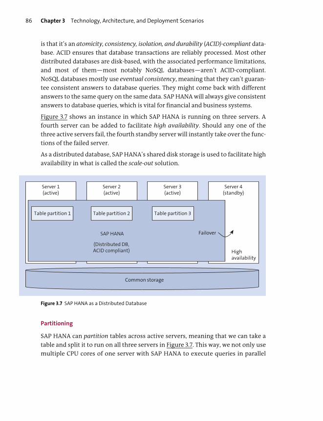
Chapter 3 Technology, Architecture, and Deployment Scenarios86
is that it’s an atomicity, consistency, isolation, and durability (ACID)-compliant data-
base. ACID ensures that database transactions are reliably processed. Most other
distributed databases are disk-based, with the associated performance limitations,
and most of them—most notably NoSQL databases—aren’t ACID-compliant.
NoSQL databases mostly use eventual consistency, meaning that they can’t guaran-
tee consistent answers to database queries. They might come back with different
answers to the same query on the same data. SAP HANA will always give consistent
answers to database queries, which is vital for financial and business systems.
Figure 3.7 shows an instance in which SAP HANA is running on three servers. A
fourth server can be added to facilitate high availability. Should any one of the
three active servers fail, the fourth standby server will instantly take over the func-
tions of the failed server.
As a distributed database, SAP HANA’s shared disk storage is used to facilitate high
availability in what is called the scale-out solution.
Figure 3.7 SAP HANA as a Distributed Database
Partitioning
SAP HANA can partition tables across active servers, meaning that we can take a
table and split it to run on all three servers in Figure 3.7. This way, we not only use
multiple CPU cores of one server with SAP HANA to execute queries in parallel
Server 1(active)
Server 4(standby)
Server 2(active)
Server 3(active)
SAP HANA
(Distributed DB,ACID compliant)
Common storage
Table partition 1 Table partition 2 Table partition 3
Failover
Highavailability
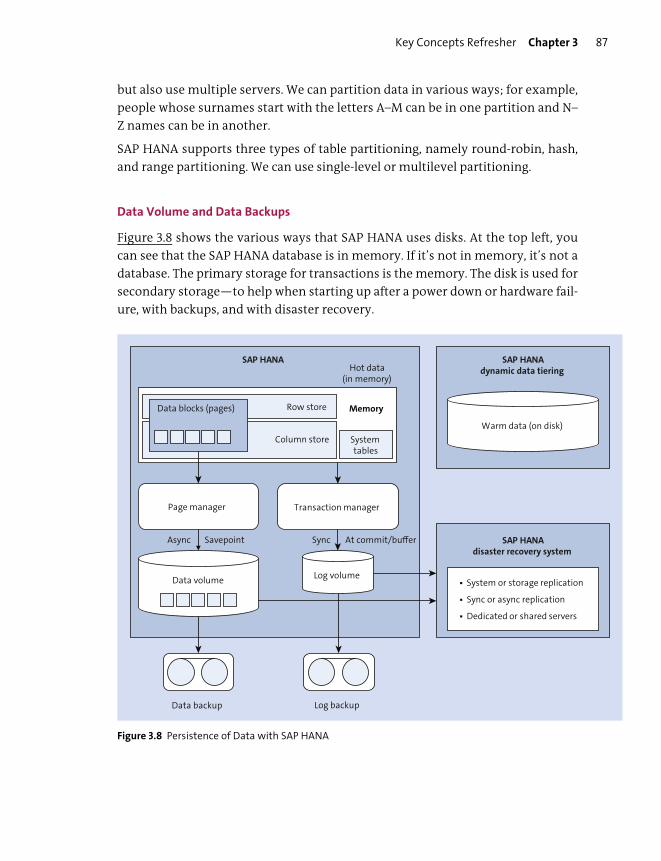
Key Concepts Refresher Chapter 3 87
but also use multiple servers. We can partition data in various ways; for example,
people whose surnames start with the letters A–M can be in one partition and N–
Z names can be in another.
SAP HANA supports three types of table partitioning, namely round-robin, hash,
and range partitioning. We can use single-level or multilevel partitioning.
Data Volume and Data Backups
Figure 3.8 shows the various ways that SAP HANA uses disks. At the top left, you
can see that the SAP HANA database is in memory. If it’s not in memory, it’s not a
database. The primary storage for transactions is the memory. The disk is used for
secondary storage—to help when starting up after a power down or hardware fail-
ure, with backups, and with disaster recovery.
Figure 3.8 Persistence of Data with SAP HANA
System tables
SAP HANA
Page manager Transaction manager
Log volume
Data blocks (pages)
Data volume
Data backup Log backup
Row store
Column store
Memory
SAP HANAdynamic data tiering
Warm data (on disk)
Hot data(in memory)
SAP HANAdisaster recovery system
� System or storage replication
� Sync or async replication
� Dedicated or shared servers
Async SyncSavepoint At commit/buffer
Chapter 3 Technology, Architecture, and Deployment Scenarios88
Data is stored as blocks (also sometimes called pages) in memory. Every 10 min-
utes, a process called a savepoint runs that synchronizes these memory blocks to
disks in the data volume. Only the blocks that contain data that have changed in
the past 10 minutes are written to the data volume. This process is controlled by
the page manager. The savepoint process runs asynchronously in the background.
Data backups are made from the disks in the data volume. When you request a
backup, SAP HANA first runs a savepoint and ensures that the data in the data vol-
ume is consistent, and then starts the backup process.
Note
The backup reads the data from the disks (secondary storage) in the data volume. This
doesn’t affect the database operations because the SAP HANA database continues work-
ing from memory (primary storage). Therefore, you don’t have to wait for an after-hours
time window to start a backup.
SAP HANA can unload (drop) data blocks from memory when it needs more mem-
ory for certain operations. This unloading of data from memory isn’t a problem
because SAP HANA knows that all the data is also safely stored in the data volume.
It will unload the least-used portions of the data. It doesn’t unload the entire least-
used table, but only the columns or even portions of a column that weren’t used
recently. In a scale-out solution, it can even unload parts of a table partition. The
most it might have to do is trigger a savepoint before unloading the least-used
data. The persistence layer is therefore a very useful feature of SAP HANA.
Log Volume and Log Backups
In the middle section of Figure 3.8, shown previously, you can see the transaction
manager writing to the log volume. The page manager and transaction manager
are subprocesses of the SAP HANA index server process, which is the main SAP
HANA process. If this process stops, then SAP HANA stops.
When you edit data in SAP HANA, the transaction manager manages these
changes. All changes are stored in a log buffer in memory. When you COMMIT the
transaction, the transaction manager doesn’t commit the transaction to memory
until it’s also committed to the disks in the log volume, so this is a synchronous
operation. Because the system has to wait for a reply from a disk in this case, fast
SSDs are used in the log volume. This synchronous writing operation is also trig-
gered if the log buffer becomes full.
Key Concepts Refresher Chapter 3 89
The log files in the log volume are backed up regularly using scheduled log back-
ups.
Note
SAP HANA doesn’t lose transactions, even if a power failure occurs, because it doesn’t
commit a transaction to the in-memory database unless it’s also written to the disks in
the log volume.
Startup
The data in the data volume isn’t a “database.” Instead, think of it as an organized
and controlled memory dump. If it was a database on disk, it would have to convert
the disk-based database format to an in-memory format each time it started up.
Now, it can just reload the “memory dump” from disk back into memory as
quickly as possible.
When you start up an SAP HANA system, it performs what is called a lazy load. It
first loads the system tables into memory and then the row store. Finally, it loads
any column tables that you’ve specified. Because the data volumes are only
updated by the savepoint every 10 minutes, some transactions might not be in the
data volume; SAP HANA loads those transactions from the log volume. Any trans-
action that was committed stays committed, and any transaction that wasn’t com-
mitted is rolled back. This ensures a consistent database.
SAP HANA then reports that it’s ready for work. This ensures that SAP HANA sys-
tems can start up quickly. Any other data that is required for queries gets loaded in
the background. Again, SAP HANA doesn’t have to load an entire table into mem-
ory; it can load only certain columns or part of a column into memory. In a scale-
out system, it will load only the required partitions.
Disks are therefore useful for getting the data back into memory after system
maintenance or potential hardware failures.
Disaster Recovery
At the bottom right of Figure 3.8, shown earlier, you can see that the data volume
and logs also are used to facilitate disaster recovery. In disaster recovery, you make
a copy of the SAP HANA system in another data center. If your data center is
flooded or damaged in an earthquake, your business can continue working from
the disaster recovery copy.

Chapter 3 Technology, Architecture, and Deployment Scenarios90
The initial large copy of the system can be performed by replicating the data vol-
ume. After the initial copy is made, only the changes are replicated as they are writ-
ten to the log volume. This is known as log replication.
This replication can be performed by the SAP HANA system itself or by the storage
vendor of the disks in the data and log volumes. The replication can happen either
synchronously or asynchronously. You can also choose whether to use dedicated
hardware for the disaster recovery copy or shared hardware by using the disaster
recovery machines for development and quality assurance purposes.
Note
Disaster recovery is covered in more detail in the HA200 course, and in the SAP HANA
administration guide at http://s-prs.co/v487620.
Active/Active (Read-Enabled) Mode
SAP HANA 2.0 has a powerful new feature called active/active (read-enabled) mode
that allows you to actively use the disaster recovery hardware to help carry the
load on a production system and enhance performance.
This feature only works when you’ve dedicated hardware for the disaster recovery
system. After the disaster recovery system (also known as the secondary system)
is synchronized with the primary SAP HANA system, only the updates need to be
sent across via log replication, as shown in Figure 3.9. The changes are then
replayed asynchronously on the secondary system.
Figure 3.9 SAP HANA Active/Active (Read-Enabled) Mode
Because both systems are in sync and contain the same data, we can now use the
secondary system for reporting and other read-only requirements. Updates must
SAP HANA(secondary)
Disaster recoverysystem
SAP HANA(primary)
Log replication
Application
Read and write Read-only
Log replayedasynchronously

Key Concepts Refresher Chapter 3 91
happen on the primary system because the direction of the log replication is only
from the primary to the secondary system. Any actions that insert, edit, update, or
delete data therefore need to use the primary system. All other actions can use
either the primary or the secondary system. The load is thus spread across both
systems. This feature means you can buy smaller machines because you can use
the dedicated disaster recovery hardware to help with your productive load, lead-
ing to cost savings.
Previously, we mentioned how reporting users could affect the performance of
operational systems of old disk-based systems. The solution was to separate OLTP
and OLAP into different applications. With SAP HANA, we run both together. Using
the active/active (read-enabled) mode, we can still separate read-intense opera-
tions, such as reporting or data analysis, using the secondary system. But this is
now still running on the same application based on SAP HANA instead of a sepa-
rate data warehouse.
SPS 04
With SAP HANA SPS 04, you can now create multiple secondary sites using multi-target
replication. This can be used, for example, to have multiple secondary sites for regions to
decrease latency for end users.
Data Aging
The final piece of the persistence layer is found at the top right of Figure 3.8, shown
earlier. This is where disks are used for data aging.
Data aging is normally described by the speed at which the data can be accessed.
Data in memory can be accessed very quickly, so this is referred to as “hot” data.
Data on disk is a bit slower, so this is called “warm” data. Data in other storage, such
as an SAP IQ database or a Hadoop data lake, is called “cold” data. The temperature
of the data refers to how fast data can be accessed, with hot having the fastest
access. As the speed of data access decreases, the price of the storage also normally
decreases.
The idea behind data aging is that we want the latest data, that is, the data used
most often, in the hot storage area. As the data becomes older, we don’t need it as
often, and it can be moved to the warm storage area. After a while, we’ll probably
never use the data again, but we might need to keep it due to regulatory require-
ments. In that case, we can move it to the cold storage area. You can specify data
aging rules inside SAP HANA to take, for example, all data older than five years and

Chapter 3 Technology, Architecture, and Deployment Scenarios92
write it to the next storage area. All queries to the data still work perfectly but are
just slower because they are read from disk instead of memory.
The warm storage area is managed as a unified part of the SAP HANA database.
This is in contrast to the cold storage area, which is managed separately, although
the data is still accessible at any time. With SAP HANA, there are three options for
warm data, as follows:
� Native storage extension (NSE)
This is the primary warm storage option for SAP HANA. It’s an intelligent built-
in extension that supports all SAP HANA data types and models. NSE allows for
a simple system landscape and is scalable with good performance.
� Extension node
This option allows for better performance than NSE.
� Dynamic tiering
This option allows for a larger data volume than NSE.
You shouldn’t mix multiple warm store options in one landscape for complexity
reasons.
In SAP HANA 2.0, we can use the extension node warm store using multistore
tables that are partitioned across both the in-memory data store and the extended
storage on disk, as shown in Figure 3.10. The partitions with the most recent data
can be in memory, and the remaining partitions can be in the extended storage.
SPS 04
SAP HANA extension node benefits from new partitioning and scale-out features in SAP
HANA SPS 04. Some of the new features are partition grouping and a range-hash parti-
tion scheme.
Figure 3.10 Data Aging Using Multistore Tables
You’ll need extended storage installed before you can use multistore tables.
Extended storage
SAP HANA
Table partition 1 Table partition 2
Memory storage
Multistore table

Key Concepts Refresher Chapter 3 93
Tip
Multistore tables are only available in SAP HANA 2.0.
Deployment Scenarios
People sometimes get confused about SAP HANA when it’s only defined with a sin-
gle concept, such as SAP HANA is a database. After a while, they hear seemingly
conflicting information that doesn’t fit into that simple description. In this sec-
tion, we’ll look at the various ways that SAP HANA can be used and deployed: as a
database, as an accelerator, as a platform, as a data warehouse, or in the cloud.
When looking at SAP HANA’s in-memory technology, and especially the fact that
we should ideally move code away from the application servers into SAP HANA, it
became clear that SAP systems needed to be rewritten completely.
Because SAP HANA doesn’t need to store values such as year-to-date, aggregates,
or balances, we should ideally remove them from the database. By doing so, we can
get rid of a significant percentage of the tables in, for example, a financial system.
However, that implies that we should also trim the code that calculated those
aggregates and inserted them into the tables we removed. In this way, we can also
remove a significant percentage of our application code.
Next, the slow parts of the remaining code that manipulate data should be moved
into graphical calculation views in SAP HANA, removing even more code from our
application. If we follow this logic, we obviously have to completely rewrite our
systems. This wasn’t easy for SAP, which has millions of lines of code in every sys-
tem and an established client base. This approach can be very disruptive. Disrup-
tive innovation is great when you’re disrupting other companies’ markets, but not
so much when you disrupt your own markets. Ask an existing SAP customer if he
wants this new technology, and he probably will say, “Yes, but not if it means a
reimplementation that will require lots of time, money, people, and effort.” Com-
pletely rewriting the system would lead to customers replacing their systems with
the new solution; that also means that customers with the older systems would
not benefit at all from this innovation.
If you look at the new SAP S/4HANA systems, you’ll see that they follow the more
disruptive approach we just described. SAP has also stated that its business appli-
cations will be migrated to run on SAP HANA. In most cases, they will just run on
SAP HANA, as these systems will be optimized to make full use of SAP HANA’s
capabilities.

Chapter 3 Technology, Architecture, and Deployment Scenarios94
However, there are other ways in which we can implement this disruptive new
technology in a nondisruptive way—and this is how SAP approached the process
when implementing SAP HANA a few years ago. The following sections walk
through the deployment scenarios for implementation.
SAP HANA as a Side-by-Side Accelerator Solution
The first SAP HANA deployment scenario is a side-by-side accelerator solution, as
illustrated in Figure 3.11.
Figure 3.11 SAP HANA Deployed as a Nondisruptive Side-by-Side Accelerator Solution
In this deployment scenario, the source systems stay as they are. No changes are
required. We add SAP HANA on the side to accelerate only those transactions or
reports that have performance issues in the source systems, and then we duplicate
the relevant data from the source system to SAP HANA. This duplication is nor-
mally performed by the SAP Landscape Transformation Replication Server. (We’ll
discuss this topic in Chapter 9.) The copied data in SAP HANA is then used for
analysis or reporting.
SAP HANA
Analytics andReporting
Innovation without disruption
Non-SAP
Database
SAP ERP
Database
SAP CRM
Database
SLTReplication
Server
Key Concepts Refresher Chapter 3 95
The advantages of this deployment option include the following:
� Because we just copy data, we don’t change the source system at all. Therefore,
everyone can use this innovation without the disruption (even those who have
very old SAP systems).
� We can use this option for all types of systems, not just the latest SAP systems.
In fact, a large percentage of the systems that use SAP HANA are non-SAP sys-
tems.
� We don’t have to copy the data for an entire system. If a report already runs in
three seconds, that’s good enough; it doesn’t have to run in three milliseconds.
If a report runs for two hours, but runs only once a year and is scheduled to run
overnight, that’s fine too. We only take the data into SAP HANA that we need to
accelerate.
� We can replicate data from a source system in real time. The reports running on
SAP HANA are always fully up to date.
Even though we make a copy of data, remember that SAP HANA compresses this
data and doesn’t copy all the data. Therefore, the SAP HANA system is much
smaller than the source systems in this deployment scenario.
However, the SAP HANA system in the scenario we described starts as a blank sys-
tem. You’ll have to load the data into SAP HANA, build your own information
models, link them to your reports and programs, and look after the security. Much
of what we’ll discuss in this book is relevant for this type of work.
Using SAP HANA in the side-by-side deployment involves some work because it
starts as a blank system. SAP quickly realized that special use cases occurred at
many of their customers where some common processes were slow; one of these
processes is profitability analysis. Profitability is something that any company
needs to focus on, but profitably analysis reports are slow running due to the large
amounts of data they have to process. By loading profitability data into SAP HANA,
the response times of these reports go from hours to mere seconds (see Figure
3.12).
For these accelerator cases, SAP provides prebuilt models in SAP HANA. SAP also
slightly modified the ABAP code for Profitability Analysis (CO-PA) to read the data
from SAP HANA instead of the original database. SAP Landscape Transformation
Replication Server replicates just the required profitability data from the SAP ERP
system to the SAP HANA system.

Chapter 3 Technology, Architecture, and Deployment Scenarios96
Figure 3.12 SAP HANA Used as an Accelerator for a Current SAP Solution
The installation and configuration process is performed at a customer site over a
few days, instead of weeks and months. The only thing that changes for the end
users is that they have to get used to the increased processing speed, and no one
has a problem with that!
The SAP HANA Live topic that we’ll discuss in Chapter 14 can also be used in a side-
by-side configuration.
SAP HANA as a Database
When SAP released the side-by-side solution, many people thought that it would
replace their data warehouses. However, this worry was alleviated when SAP
announced that SAP HANA would be used as the database under SAP Business
Warehouse (SAP BW). Figure 3.13 illustrates a typical (older) SAP landscape.
SAP HANA can be used to replace the databases under the older SAP BW, SAP Cus-
tomer Relationship Management (SAP CRM), and SAP ERP (which are part of SAP
Business Suite) systems. There are well-established database migration proce-
dures to replace a current database with SAP HANA. In each case, SAP HANA
replaces the database only. The SAP systems still use the SAP application servers as
they did previously, and end users still access the SAP systems as they always did,
via the SAP application servers. All reports, security, and transports are performed
as before. Only the system administrators and DBAs have to learn SAP HANA and
log in to the SAP HANA systems.
SAP ERP
Database
SAP HANACO-PAABAP
SLTReplication
Server

Key Concepts Refresher Chapter 3 97
Figure 3.13 Typical Current SAP Landscape Example
When you use SAP HANA as a method to just accelerate reporting and analytics,
you get a similar situation. The users log in to the reporting and analytics tools,
and they basically use SAP HANA as a database.
Figure 3.14 looks very similar to Figure 3.13, except that the various databases were
replaced by SAP HANA.
By only replacing the database, SAP again managed to provide most of the benefit
of this new in-memory technology to businesses but without the cost, time, and
effort of disruptive system replacements. The applications’ code wasn’t forked to
produce different code for SAP BW on SAP HANA versus SAP BW on older data-
bases.
Over time, after customers and partners became familiar with SAP HANA, SAP
moved these solutions completely over to SAP HANA. We now have SAP S/4HANA
and SAP BW/4HANA that replace the SAP ERP and SAP BW systems, respectively,
that just used SAP HANA as yet another database.
Enterprise datawarehouse(SAP BW)
Corporatereporting and
analytics
Database
Non-SAP
Database
SAP ERP
Database
SAP CRM
Database

Chapter 3 Technology, Architecture, and Deployment Scenarios98
Figure 3.14 SAP HANA as Database Can Change the Current Landscape
Let’s look at the example of SAP BW in a bit more detail. Because SAP HANA can
address both OLAP and OLTP in a single system, a data warehousing solution such
as SAP BW has changed a lot. SAP started with the “classic” SAP BW that was run-
ning on other databases. When SAP HANA was released, SAP BW was ported to also
run on SAP HANA, and it used SAP HANA as just another database. The application
stayed roughly the same.
Remember that the “classic” SAP BW has its own information modeling objects—
for example, InfoCubes and DataStore Objects (DSOs). These objects in SAP BW are
built in the application server layer. Even if SAP BW is powered by SAP HANA, and
these SAP BW objects are optimized for SAP HANA, they are still completely differ-
ent from the normal SAP HANA information models, such as calculation views.
As SAP HANA became more popular, and people started realizing the advantages
of using SAP HANA, new features started appearing in SAP BW. With SAP BW 7.4,
Enterprise datawarehouse(SAP BW)
Corporatereporting and
analytics
SAP HANA
Non-SAP
Database
SAP ERP
SAP HANA
SAP CRM
SAP HANA

Key Concepts Refresher Chapter 3 99
we had SAP BW powered by SAP HANA. We could use the classical SAP BW model-
ing objects alongside some new SAP HANA-specific ones such as Advanced Data-
Store Objects (Advanced DSOs). It could also run both the old 3.x and the new 7.x
data flows. SAP HANA enhanced the performance of SAP BW significantly.
SAP then rewrote its SAP Business Suite systems to make full use of SAP HANA.
In the process, the systems became a lot simpler and smaller. This is the SAP
S/4HANA system.
Looking at SAP BW, SAP decided to do the same for SAP BW by creating a new ver-
sion of SAP BW, called SAP BW/4HANA, that relies solely on SAP HANA. It doesn’t
run on any other database, like the “classic” SAP BW did.
In the process, SAP also simplified and reduced the size of SAP BW but with even
more capabilities. Table 3.2 shows how the number of modeling objects was
reduced from 10 to just 4. For example, the InfoCubes and DSOs we mentioned ear-
lier were both replaced with Advanced DSOs. In SAP BW/4HANA, these old objects
aren’t available. Old functionality such as 3.x data flows are also no longer avail-
able.
SAP HANA as a Platform
The next way we can deploy SAP HANA is by using it as a full development plat-
form. SAP HANA is more than just an in-memory database. We’ll quickly discuss
how SAP HANA 1.0 evolved into a development platform.
Classic SAP BW SAP BW/4HANA
� MultiProvider
� InfoSet
� CompositeProvider
� Virtual Provider
� CompositeProvider
� Virtual Provider
� Transient Provider
� Open ODS view
� InfoCube
� DSO
� Hybrid Provider
� Persistent Staging Area (PSA) Table
� Advanced DSO
� InfoObject � InfoObject
Table 3.2 Reduced Number of Modeling Object Types in SAP BW/4HANA

Chapter 3 Technology, Architecture, and Deployment Scenarios100
Which other database has several different programming languages included and
has version control, code repositories, and a full application server built in? SAP
HANA 1.0 already had all of these. This makes SAP HANA 1.0 not just a database,
but a platform. You can program in SQL, SQLScript (an SAP HANA-only enhance-
ment that we’ll look at in Chapter 8), R, and JavaScript.
However, the main feature we use inside SAP HANA 1.0 when deploying it as a plat-
form is the application server, called the SAP HANA extended application services
(SAP HANA XS) engine, which is used via web services (see Figure 3.15). A new ver-
sion of the SAP HANA XS engine appeared in the last support packs of SAP HANA
1.0, called SAP HANA extended application services, advanced model (SAP HANA
XSA). The older version we’re discussing here was renamed to SAP HANA extended
application services, classic model (SAP HANA XS). The SAP HANA XS engine is a
full web and application server built into SAP HANA 1.0 that is capable of serving
and consuming web pages and web services.
Figure 3.15 SAP HANA 1.0 as a Development Platform
When we deploy SAP HANA 1.0 as a platform, we only need an HTML5 browser and
SAP HANA XS. In this case, we still develop data models as we discussed previously
with the side-by-side accelerator deployment, but we also develop a full applica-
tion in SAP HANA using JavaScript and an HTML framework called SAPUI5. All this
functionality is built in to SAP HANA 1.0 and SAP HANA XS.
HTML5 browser
Mobile(tablet or
phone)
Model-View-Controller (MVC)
SAP HANA
SAP HANA viewsSAP HANA views• SAP HANA views
• SQL, SQLScript
Model
Extended ApplicationServices (XS engine)
• OData
• REST
• Server-side JavaScript
ControllerView displayed
View createdusing SAPUI5
• HTML5• CSS3• Client-side JavaScript

Key Concepts Refresher Chapter 3 101
The web application development paradigm that many frameworks use is called
model-view-controller (MVC). Model in this case refers to the information models
that we’ll build in SAP HANA and is the focus of this book. We expose these infor-
mation models in the controller as OData or REST web services. This functionality
is available in SAP HANA and is easy to use. You can enhance these web services
using server-side JavaScript, meaning that SAP HANA runs JavaScript as a program-
ming language inside the server.
The last piece is the view, which is created using the SAPUI5 framework. The
screens are the same as the SAP Fiori screens in the new SAP S/4HANA systems,
which are HTML5 screens. What is popularly referred to as HTML5 actually consists
of HTML5, Cascading Style Sheets (CSS3), and client-side JavaScript. In this case, the
JavaScript runs in the end user’s browser.
By using JavaScript for both the view and the controller, SAP HANA XS developers
only have to learn one programming language to create powerful web applications
and solutions that leverage the power and performance of SAP HANA.
We can even create native mobile applications for Apple iOS, Android, and other
mobile platforms. Some free applications, such as Cordova, take the SAP HANA
web applications and compile them into native mobile applications, which can
then be distributed via mobile application stores. As a result, you can use SAP
HANA’s power directly from your mobile phone. You can also use the SAPUI5
application with the React framework and React Native to create native mobile
applications.
In the next chapter, we’ll see how these concepts expanded with SAP HANA XSA
and SAP HANA 2.0.
SAP HANA as an SQL Data Warehouse
A relatively new use case of SAP HANA is as an enterprise data warehouse (EDW).
SAP has offered the SAP BW system for customer’s data warehousing needs for
many years. SAP BW has evolved to use SAP HANA and has been optimized for SAP
HANA with SAP BW/4HANA. It’s still the recommended route for customers who
want strong built-in features for data governance and integrity, processes, con-
trols, and integration to other SAP systems for an enterprise-wide solution. How-
ever, more and more companies want to build their own data warehouse using
only SAP HANA.
Whereas SAP BW is a data warehousing application using SAP HANA, the new SAP
SQL Data Warehousing approach is a developer-oriented and SQL-driven approach

Chapter 3 Technology, Architecture, and Deployment Scenarios102
to data warehousing using SAP HANA XS. In both cases, you can provision data
using the SAP tools (discussed in Chapter 9) and using the SAP BusinessObjects
tools or SAP Analytics Cloud (discussed later in this chapter).
SAP HANA has provided strong support for the OLAP warehousing functionality
for many years now. You’ll see this in the next few chapters. SAP has now added an
optional component called the SAP HANA data warehousing foundation for opti-
mized data distribution, lifecycle management, monitoring, and scheduling. This
additional functionality helps companies build native data warehouses using just
SAP HANA.
Note
SAP HANA data warehousing foundation starts with a blank system and offers a do-it-
yourself approach to build your own data warehouse using loosely coupled tools that
may have separate repositories.
Figure 3.16 shows the high-level architecture of the SAP SQL Data Warehousing
with SAP HANA data warehousing foundation version 2.0. At the bottom are the
various data sources of the data provisioned to SAP HANA, which we’ll cover in
Chapter 9.
The middle of the figure shows SAP SQL Data Warehousing, and we’ll focus on
most of the modeling and development functionality shown here in this book.
The left side of the figure shows the various tools we’ll use in this book for building
what is required in the data warehouse. The right side of the figure shows the vari-
ous data lake options that we can exchange data with.
Finally, the reporting and analysis layer appears at the top, as discussed later in
this chapter.
Tip
The versions of SAP HANA data warehousing foundation are independent from the ver-
sions of SAP HANA. It’s important to note that SAP HANA data warehousing foundation
1.0 used SAP HANA XS, whereas the current SAP HANA data warehousing foundation 2.0
uses SAP HANA XSA.
Although Figure 3.16 shows SAP HANA data warehousing foundation 2.0, we’ll also
quickly discuss SAP HANA data warehousing foundation 1.0.
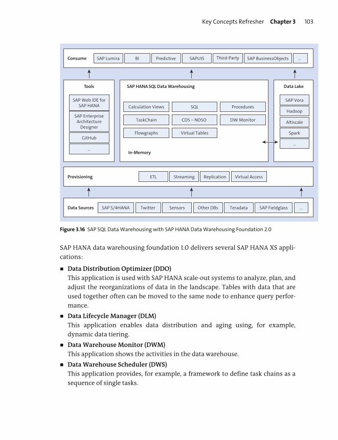
Key Concepts Refresher Chapter 3 103
Figure 3.16 SAP SQL Data Warehousing with SAP HANA Data Warehousing Foundation 2.0
SAP HANA data warehousing foundation 1.0 delivers several SAP HANA XS appli-
cations:
� Data Distribution Optimizer (DDO)
This application is used with SAP HANA scale-out systems to analyze, plan, and
adjust the reorganizations of data in the landscape. Tables with data that are
used together often can be moved to the same node to enhance query perfor-
mance.
� Data Lifecycle Manager (DLM)
This application enables data distribution and aging using, for example,
dynamic data tiering.
� Data Warehouse Monitor (DWM)
This application shows the activities in the data warehouse.
� Data Warehouse Scheduler (DWS)
This application provides, for example, a framework to define task chains as a
sequence of single tasks.
Data Sources SAP S/4HANA Twitter Sensors Other DBs Teradata SAP Fieldglass …
Provisioning ETL Streaming Replication Virtual Access
Consume SAP Lumira BI Predictive SAPUI5 Third-Party SAP BusinessObjects …
Tools
SAP Web IDE forSAP HANA Calculation Views
SAP Vora
Data Lake
GitHub
…
Hadoop
Altiscale
Spark
…
SAP EnterpriseArchitecture
Designer
SAP HANA SQL Data Warehousing
In-Memory
SQL Procedures
TaskChain CDS – NDSO DW Monitor
Flowgraphs Virtual Tables
Chapter 3 Technology, Architecture, and Deployment Scenarios104
The last two options were shown as planned functionality in SAP HANA 1.0, but
they are available in SAP HANA 2.0.
You might ask when you would use SAP SQL Data Warehousing. If you want to
build your own data warehousing as part of an application you’re building, you
prefer a web user experience such as a 100% open SQL approach, you want the
freedom to create custom data models and processes, or you want to use tech-
niques such as DevOps and continuous integration, testing, and deployment, this
is definitely something you should look at.
SAP HANA in the Cloud
SAP HANA has many features that make it ideal for use in a cloud platform envi-
ronment. SAP, like many other enterprises, has moved aggressively into the cloud
with many of its solutions. Many features that are required for smooth cloud oper-
ations were built into SAP HANA over the past few years.
SAP HANA works great as a cloud enabler because it accelerates applications, pro-
viding users with fast response times, which we all expect from such environ-
ments.
Multitenant Database Containers
The multitenant database containers (MDC) deployment option became available
as of SAP HANA 1.0 SPS 09 and helps us move from the world where everything is
deployed in the company’s data center, called on premise, to the cloud. We can now
have multiple isolated databases inside a single SAP HANA system, as shown in
Figure 3.17. Each of these isolated databases is referred to as a tenant.
Think of tenants occupying an apartment building in which each tenant has a
front door key and owns furniture inside his or her apartment. Other tenants can’t
get into another tenant’s apartment without permission. However, the mainte-
nance of the entire apartment building is performed by a single team. If the build-
ing needs repairs to the water pipes, all tenants will be without water for a while.
In the same way, tenants in MDC have their own unique business systems, data,
and business users. In Figure 3.17, you can see that each of the three tenants has its
own unique applications installed and connected to its own tenant database
inside SAP HANA.
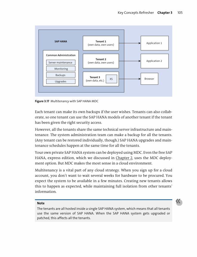
Key Concepts Refresher Chapter 3 105
Figure 3.17 Multitenancy with SAP HANA MDC
Each tenant can make its own backups if the user wishes. Tenants can also collab-
orate, so one tenant can use the SAP HANA models of another tenant if the tenant
has been given the right security access.
However, all the tenants share the same technical server infrastructure and main-
tenance. The system administration team can make a backup for all the tenants.
(Any tenant can be restored individually, though.) SAP HANA upgrades and main-
tenance schedules happen at the same time for all the tenants.
Your own private SAP HANA system can be deployed using MDC. Even the free SAP
HANA, express edition, which we discussed in Chapter 2, uses the MDC deploy-
ment option. But MDC makes the most sense in a cloud environment.
Multitenancy is a vital part of any cloud strategy. When you sign up for a cloud
account, you don’t want to wait several weeks for hardware to be procured. You
expect the system to be available in a few minutes. Creating new tenants allows
this to happen as expected, while maintaining full isolation from other tenants’
information.
Note
The tenants are all hosted inside a single SAP HANA system, which means that all tenants
use the same version of SAP HANA. When the SAP HANA system gets upgraded or
patched, this affects all the tenants.
Application 1SAP HANA Tenant 1(own data, own users)
Tenant 2(own data, own users) Application 2
BrowserTenant 3(own data, etc.) XS
Common Administration
Upgrades
Backups
Monitoring
Server maintenance

Chapter 3 Technology, Architecture, and Deployment Scenarios106
Cloud Deployments
We’ve now discussed various ways to deploy SAP HANA. Most of the time, we
think of these deployments as running on premise on a local server, but all of
these scenarios can also be deployed in the cloud. In cloud deployments, virtual-
izations manage applications such as SAP HANA. VMware vSphere virtual
machine deployments of SAP HANA are fully supported, both for development
and production instances.
With cloud deployments, you’ll be introduced to various new terms:
� Infrastructure as a service (IaaS)
An infrastructure includes things such as network, memory, CPU, and storage.
IaaS provides infrastructure in the cloud to support your deployments.
� Platform as a service (PaaS)
PaaS uses solutions such as SAP Cloud Platform. In this scenario, you use not
only the same infrastructure as IaaS but also a platform, such as a Java applica-
tion service or the SAP HANA platform services.
� Software as a service (SaaS)
This cloud offering provides certain software, such as SAP SuccessFactors or SAP
C/4HANA.
� Managed cloud as a service (McaaS)
In McaaS, SAP manages the entire environment for you, including backups,
disaster recovery, high availability, patches, and upgrades. An example of this is
the SAP HANA Enterprise Cloud.
Public, Private, and Hybrid Cloud
Your cloud scenario could be public, private, or hybrid. Let’s look at what each of
those terms means and when each scenario applies.
The easiest and cheapest way for you to get an instance of SAP HANA for use with
this book is via Amazon Web Services (AWS), Google Cloud Platform (GCP), or
Microsoft Azure. We’ve looked at this in Chapter 2. By using your own account, you
can have an SAP HANA system up and running in minutes. This is available to
everyone—the public—so therefore this is a public cloud. In this example, the
cloud provider provides IaaS.
The reason this is called a public cloud is that the infrastructure is shared by mem-
bers of the public. You don’t get your own dedicated machine at Amazon, Micro-
soft, Google, or any other public cloud provider.
Key Concepts Refresher Chapter 3 107
If you host SAP HANA in your own data center or in a hosted environment specif-
ically for you only, then it’s a private or hybrid cloud. A private cloud offers the
same features that you would find in a public cloud, but it’s dictated by different
forms of access. With a private cloud, the servers in the cloud provider’s data cen-
ter are dedicated for your company only. No other companies’ programs or data
are allowed on these servers.
A hybrid cloud involves either combining a public and private cloud offering, or
running a private and public cloud together. With a hybrid cloud, you connect
your private cloud’s server back to your own data center via a secure network con-
nection. In that case, the servers in the cloud act as if they are part of your data cen-
ter, even though they are actually in the cloud provider’s data center. An example
of a hybrid cloud is using a Microsoft Azure cloud and another private cloud
together.
SAP HANA Enterprise Cloud
SAP HANA Enterprise Cloud offers SAP applications as cloud offerings. You can
choose to run SAP HANA, SAP BW/4HANA, SAP S/4HANA, SAP CRM, SAP Business
Suite, and many others as a full service offering in the cloud. All the systems that
you would normally run on premise are available in SAP HANA Enterprise Cloud.
SAP provides and manages the hardware, infrastructure, SAP HANA, and other SAP
systems for the customer. The customer only has to provide the license keys for
these systems. This is referred to as bring your own license.
SAP HANA Enterprise Cloud is seen as an MCaaS solution on a private cloud, but it
can also be deployed in a hybrid cloud offering.
SAP Cloud Platform
SAP Cloud Platform is a PaaS that allows you to build, extend, and run applications
in the cloud. Services include SAPUI5, HTML5, SAP HANA platform services, Java
applications, and more.
SAP Cloud Platform was previously known as SAP HANA Cloud Platform. Behind
the scenes, more than just a name change happened. SAP Cloud Platform not only
uses SAP HANA but also many open-source technologies such as OpenStack and
Cloud Foundry. SAP is a Founding Platinum Level Member of the Cloud Foundry
Foundation, which means that you can use Cloud Foundry buildpacks and Docker
Chapter 3 Technology, Architecture, and Deployment Scenarios108
containers, with microservices written in any language of your choice, in SAP
Cloud Platform.
SAP Cloud Platform also offers a wide range of services to get your cloud applica-
tions up and running quickly. These can be, for example, security, HTML frame-
work, database, Internet of Things (IoT), machine learning, predictive, provision-
ing, analytics, mobile, development, build, and deployment services. You can even
sell your SAP Cloud Platform applications in the SAP App Center.
SAP Cloud Platform forms the core of the new SAP Leonardo offering, where SAP
focuses on digital innovation and transformation. SAP Cloud Platform will also
run on the cloud offerings of Amazon, Google, and Microsoft. This new option is
termed multi-cloud.
To better understand SAP Cloud Platform, Cloud Foundry, and the new develop-
ment process, we’ll return to SAP HANA in the next chapter and look deeper into
SAP HANA XSA.
SAP Analytics Cloud and Business Intelligence
One topic that has been heavily influenced by SAP HANA is that of analytics. Run-
ning fast and interactive analytics in the cloud was unforeseen just a few years ago.
Everyone was using on-premise reporting tools, and these reports often took
hours to generate. SAP HANA changed that very quickly by generating the same or
better reports in mere seconds.
Today the focus is on SAP Analytics Cloud, but SAP has a lot of other noncloud BI
tools as well, which you’ll see in the next sections. You can connect all these tools
to SAP HANA; however, all BI tools must be used correctly with SAP HANA to
ensure optimal benefit.
SAP Analytics Cloud
In the space of two or three years, the emphasis moved from running analytics and
reports on your own computer to using SAP Analytics Cloud. One of the main
advantages is that SAP Analytics Cloud gets updated every few weeks, whereas the
on-premise tools often had update cycles of years.
Another advantage is that SAP Analytics Cloud displays everything in your
browser. It doesn’t matter whether you’re using a tablet, a Windows laptop, or an
Apple Mac, you no longer need to install drivers, special programs, and the like.
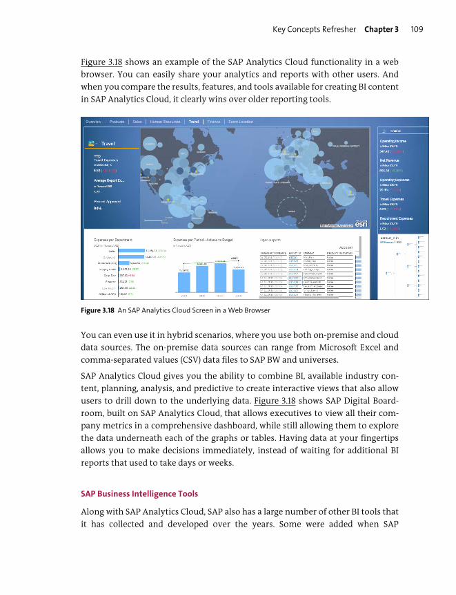
Key Concepts Refresher Chapter 3 109
Figure 3.18 shows an example of the SAP Analytics Cloud functionality in a web
browser. You can easily share your analytics and reports with other users. And
when you compare the results, features, and tools available for creating BI content
in SAP Analytics Cloud, it clearly wins over older reporting tools.
Figure 3.18 An SAP Analytics Cloud Screen in a Web Browser
You can even use it in hybrid scenarios, where you use both on-premise and cloud
data sources. The on-premise data sources can range from Microsoft Excel and
comma-separated values (CSV) data files to SAP BW and universes.
SAP Analytics Cloud gives you the ability to combine BI, available industry con-
tent, planning, analysis, and predictive to create interactive views that also allow
users to drill down to the underlying data. Figure 3.18 shows SAP Digital Board-
room, built on SAP Analytics Cloud, that allows executives to view all their com-
pany metrics in a comprehensive dashboard, while still allowing them to explore
the data underneath each of the graphs or tables. Having data at your fingertips
allows you to make decisions immediately, instead of waiting for additional BI
reports that used to take days or weeks.
SAP Business Intelligence Tools
Along with SAP Analytics Cloud, SAP also has a large number of other BI tools that
it has collected and developed over the years. Some were added when SAP

Chapter 3 Technology, Architecture, and Deployment Scenarios110
acquired Business Objects. Others were BI tools developed for use with SAP BW.
Others are new tools developed to make use of SAP HANA or to add new BI fea-
tures, such as visualization and predictive analysis.
SAP also has the powerful SAP BusinessObjects BI platform, where reports, with
their user administration, security, storage, and scheduling, can be centrally man-
aged.
SAP realized that the list of BI tools was too long and decided to converge these
into just five:
� SAP Analysis for Microsoft Office
This tool runs as a Microsoft Office plug-in. It appears in Excel as an additional
ribbon bar menu and provides powerful reporting from trusted OLAP data
sources, such as SAP HANA.
� SAP Lumira, discovery edition
This comparatively new tool for self-service and visualization of analytics was
designed with SAP HANA in mind, so it leverages SAP HANA features to deliver
fast results. SAP Lumira, discovery edition integrates with SAP Analytics Cloud.
It’s also easy to consume SAP Lumira content on mobile devices via the SAP
BusinessObjects Mobile app. SAP Lumira is well suited for ad hoc types of ana-
lytics; you can view and visualize any type of data in the way you like with min-
imal effort.
� SAP Lumira, designer edition
This tool is used to create dashboards, OLAP web applications, and guided ana-
lytics. It features native (direct) connections to SAP BW and SAP HANA, and it
falls into the professionally authored category, in which analytic content is cen-
trally governed. Because it’s more of a developer’s tool, some knowledge of Java-
Script is required to get the most out of the tool. SAP Lumira, designer edition,
has a “what you see is what you get” (WYSIWYG) design environment.
� SAP BusinessObjects Web Intelligence
Popularly called WebI, this is one of the most popular SAP BI tools because it’s
easy to work with, yet powerful and fast enough to get the job done. It was one
of the first self-service style BI tools from SAP. End users can consume SAP intel-
ligence reports using the mobile app or via a browser.
� SAP Crystal Reports
This tool is used to create reports that often have the exact specifications and
look of the existing paper forms in a “pixel-perfect” format. SAP Crystal Reports

Key Concepts Refresher Chapter 3 111
focuses on professionally authored reports, which can be viewed on desktops,
browsers, and offline. This tool has been around since the 1990s and was proba-
bly one of the first reporting tools that most modelers and developers used.
Let’s now see how you can use these tools with SAP HANA.
Using Business Intelligence Tools with SAP HANA
One of the most important lessons to learn from the way that SAP Analytics Cloud
works is how it utilizes interactive drilldown analytics. When we use BI tools this
way, people become more productive because SAP HANA is actually being used in
the optimal way.
Let’s use Excel as an example. It’s obviously not an SAP tool but has been the most
widely used and best-known BI tool available for more than 30 years.
Excel is probably the ultimate self-service BI tool. However, despite all its flexibil-
ity, it’s also easy to use it “incorrectly.” If you import 700,000 records into Excel
and then build a pivot table on that data, you’re not using Excel in the best possible
way. If you use it that way, you use Excel as a database—and it’s not meant to be a
database. You’re also straining the network while transferring that much data. You
get users complaining about how slow their reports are, only to discover that they
run them in Excel on old laptops with very little memory on a slow network.
A better way to use Excel is to connect it to SAP HANA information views, as shown
in Figure 3.19 1. You can then build the pivot table directly on the SAP HANA view
2. In this case, SAP HANA performs all the calculations, and Excel just displays the
results. The 700,000 records stay in SAP HANA, and the minimum amount of data
for displaying the results is transferred via the network. SAP HANA usually also
uses less memory and thus is faster.
The best way to test if you’re using BI tools correctly is to ask whether it will work
on a mobile device, such as a tablet. If you load 700,000 records into Excel, it won’t
work on your tablet. The tablet simply doesn’t have enough memory, and your
mobile data costs will be high. With the “correct” way, on the other hand, you
could probably get this setup working on the mobile app version of Excel if you
had the correct driver installed.
An added benefit of letting SAP HANA do the heavy lifting is that your reports and
analytics become interactive; for example, drilldowns are easy to implement.

Chapter 3 Technology, Architecture, and Deployment Scenarios112
Figure 3.19 Using SAP HANA Information Models with Hierarchies in an Excel Pivot Table
Connecting Business Intelligence Tools to SAP HANA
SAP HANA provides drivers known as SAP HANA clients that are commonly used
to connect SAP HANA to other types of databases and BI tools or vice versa.
The query language sent over these connections is normally SQL, which we’ll dis-
cuss in Chapter 8. It can also sometimes be multidimensional expressions (MDX).
MDX is a query language for OLAP databases, similar to how SQL is a query lan-
guage for relational OLTP databases. The MDX standard was adopted by a wide
range of OLAP vendors, including SAP.
Let’s look at some of the common database connections you might encounter:
� Open Database Connectivity (ODBC)
ODBC acts as a translation layer between an application and a database via an
ODBC driver. You write your database queries using a standard application
Key Concepts Refresher Chapter 3 113
programming interface (API) for accessing database information. The ODBC
driver translates these into database-specific queries, making your database
queries database and operating system independent. By changing the ODBC
driver to that of another database and changing your connection information,
your application will work with another database.
� Java Database Connectivity (JDBC)
JDBC is similar to ODBC, but it’s specifically aimed at the Java programming lan-
guage.
� Object Linking and Embedding Database for Online Analytical
Processing (ODBO)
ODBO provides an API for exchanging metadata and data between an applica-
tion and an OLAP server (e.g., a data warehouse using cubes). You can use ODBO
to connect Excel to SAP HANA.
� Business Intelligence Consumer Services (BICS)
BICS is an SAP-proprietary database connection. This direct client connection
performs better and faster than MDX. Hierarchies are supported, negating the
need for MDX in SAP environments. Because this is an SAP-only connection
type, you can only use it between two SAP systems, for example, from an SAP-
provided BI tool to SAP HANA.
The fastest way to connect to a database is via dedicated database libraries. ODBC
and JDBC insert another layer in the middle that can impact your database query
performance. Some reporting tools offer a choice of connectors, for example,
allowing you to use either a JDBC or an ODBC connector.
Excel uses the ODBO driver to connect to SAP HANA. It’s the only BI tool that uses
this driver. The ODBO driver implies that it uses MDX, which means it can read
cubes, and Excel is able to consume SAP HANA calculation cube views. You can
actually see this in Figure 3.19 in the dialog box on the left.
SAP HANA Providing the Semantic Layer
If you used older reporting or BI tools, you’ll know that you had to add a semantic
layer between the data sources and your reports. Pure data, for example, doesn’t
have hierarchies defined, but you need hierarchies when users want to drill down
deeper into the data. SAP BusinessObjects Universe Designer was used for creating
“universes,” and this evolved into the Information Design Tool while the “uni-
verses” evolved into semantic layers. These tools combined multiple data sources
into harmonized models that could be used for reporting.

Chapter 3 Technology, Architecture, and Deployment Scenarios114
You’ll see in the following chapters how SAP HANA provides these features while
you’re creating your information models. SAP also uses this in its various prod-
ucts, such as SAP S/4HANA and SAP C/4HANA. The raw data is combined and fil-
tered, additional fields are calculated, aggregates are created, currencies are
converted, and semantics are added in the models. When you expose the models,
they are ready for consumption by any reporting tool—even a 30-year-old tool
such as Excel!
You’ve now seen how SAP HANA architecture works, from the hardware with
memory and CPU cores, all the way up to the cloud platforms and analytics.
Important Terminology
The following important terminology was covered in this chapter:
� In-memory technology
In-memory technology is an approach to querying data residing in RAM, as
opposed to physical disks. The results of doing so lead to shortened response
times. This enables enhanced analytics for BI/analytic applications.
� SAP HANA architecture
No longer constrained by disks, other solutions were added, including column-
based storage, compression, no indices, delta merges, scale-out, partitioning,
and parallelism.
With the paradigm shift to in-memory technologies, various programming lan-
guages and application development processes were added to SAP HANA.
SAP HANA still uses disks but purely as secondary storage (backup) because
memory is volatile. With the data and log volumes, SAP HANA ensures that no
data ever gets lost. The data and log volumes are also used for backups, when
starting up the SAP HANA system, and for disaster recovery.
� Persistence layer
The disk storage and data storage happens in the persistence layer, and storing
data on disk is called persistence.
� SAP HANA as a side-by-side accelerator
Source systems stay as they are, and SAP HANA is added on the side to acceler-
ate any transactions or reports that have performance issues in the source sys-
tems. The relevant data is duplicated from the source system to SAP HANA.
This duplication is normally performed by the SAP Landscape Transformation
Replication Server. The copied data in SAP HANA is then used for analysis or
Important Terminology Chapter 3 115
reporting. SAP provides prebuilt models in SAP HANA to accelerate processes
such as profitability data. SAP Landscape Transformation Replication Server
replicates just the required profitability data from the SAP ERP system to the
SAP HANA system.
� SAP HANA as a database
SAP HANA is used to replace the databases under SAP BW, SAP CRM, and SAP
ERP (all part of the SAP Business Suite). There are well-established database
migration procedures to replace the current database with SAP HANA. In each
case, SAP HANA replaces the database only.
� SAP HANA as a platform
SAP HANA is a development platform. By combining the SAP HANA informa-
tion models with development in the SAP HANA XS application server, we can
build powerful custom web applications.
� Public cloud
A public cloud is available to anyone, offering any type of cloud service. The
infrastructure is shared by members of the public. You don’t get your own ded-
icated machine at Amazon or any other public cloud provider.
� Private cloud
A private cloud offers the same features that you would find in a public cloud,
but it’s dictated by different forms of access. With a private cloud, the servers in
the cloud provider’s data center are dedicated for your company only. No other
companies’ programs or data are allowed on these servers.
� Hybrid cloud
A hybrid cloud involves either combining a public and private cloud offering or
running a private and public cloud together. With a hybrid cloud, you connect
your private cloud’s server back to your own data center via a secure network
connection. In that case, the servers in the cloud act as if they are part of your
data center, even though they are actually in the cloud provider’s data center.
� SAP HANA Enterprise Cloud
SAP HANA Enterprise Cloud offers all the SAP applications as cloud offerings.
You can choose to run SAP HANA, SAP BW, SAP ERP, SAP CRM, SAP Business
Suite, and many others as a full-service offering in the cloud. All the systems
that you would normally run on premise are available in SAP HANA Enterprise
Cloud.
� SAP Cloud Platform
This PaaS allows you to build, extend, and run applications in the cloud. This
includes SAPUI5, HTML5, SAP HANA XS, Java applications, and more.
Chapter 3 Technology, Architecture, and Deployment Scenarios116
� SAP HANA extended application services, classic model (SAP HANA XS)
SAP HANA XS embeds an application server into SAP HANA and allows develop-
ers and modelers to use SAP HANA as a platform. It uses the MVC paradigm for
creating web services.
� SAP HANA extended application services, advanced model (SAP HANA XSA)
SAP HANA XSA is the new expanded version of SAP HANA XS that is used exten-
sively in SAP HANA 2.0.
Practice Questions
These practice questions will help you evaluate your understanding of the topics
covered in this chapter. The questions shown are similar in nature to those found
on the certification examination. Although none of these questions will be found
on the exam itself, they allow you to review your knowledge of the subject. Select
the correct answers, and then check the completeness of your answers in the
“Practice Question Answers and Explanations” section. Remember, on the exam,
you must select all correct answers and only correct answers to receive credit for
the question.
1. Which technologies does SAP HANA use to load more data into memory?
(There are 3 correct answers.)
� A. Eliminate indices.
� B. Use ZIP compression.
� C. Use dictionary compression.
� D. Store data in column tables.
� E. Use multicore CPU parallelism.
2. True or False: With SAP HANA, you can run OLAP and OLTP together in one
system with good performance.
� A. True
� B. False
Practice Questions Chapter 3 117
3. True or False: SAP HANA contains both row and column tables.
� A. True
� B. False
4. How do you move code to SAP HANA? (There are 2 correct answers.)
� A. Delete the application server.
� B. Use stored procedures in SAP HANA.
� C. Use graphical data models in SAP HANA.
� D. Use row tables in SAP HANA.
5. In which SAP HANA solution do you eliminate stored data, such as year-to-
date figures?
� A. SAP BW on SAP HANA
� B. SAP CRM on SAP HANA
� C. SAP S/4HANA
� D. SAP HANA Enterprise Cloud
6. Which deployment scenario can you use to accelerate reporting from an old
SAP R/3 system?
� A. SAP HANA as a database
� B. SAP HANA as a platform
� C. SAP HANA as a side-by-side accelerator
� D. SAP HANA multitenant database containers (MDC)
7. Which deployment scenarios feature security staying in the application
server and end users not logging in to the SAP HANA system? (There are 2 cor-
rect answers.)
� A. SAP HANA as a platform with an SAP HANA XS application
� B. SAP HANA as a database
� C. SAP HANA as a side-by-side accelerator
� D. SAP HANA as a reporting server
Chapter 3 Technology, Architecture, and Deployment Scenarios118
8. For which deployment scenario does SAP deliver prebuilt data models?
� A. SAP HANA as a platform
� B. SAP HANA as a side-by-side accelerator
� C. SAP HANA as an SQL Data Warehouse
� D. SAP HANA on the cloud
9. True or False: SAP HANA is just a database.
� A. True
� B. False
10. What is normally used to build SAP HANA XS applications inside SAP HANA?
(There are 2 correct answers.)
� A. Java
� B. JavaScript
� C. SAPUI5
� D. ABAP
11. Which type of cloud solution is SAP HANA Enterprise Cloud an example of?
� A. Platform as a service (PaaS)
� B. Infrastructure as a service (IaaS)
� C. Software as a service (SaaS)
� D. Managed cloud as a service (MCaaS)
12. Which type of cloud solution is Amazon Web Services (AWS) an example of?
� A. Hybrid cloud
� B. Public cloud
� C. Private cloud
� D. Community cloud

Practice Questions Chapter 3 119
13. True or False: VMware vSphere virtual machines are fully supported for pro-
ductive SAP HANA instances.
� A. True
� B. False
14. You use parallelism to calculate a year-to-date value quickly, which eliminates
a table from the database. What are some of the implications of this action?
(There are 3 correct answers.)
� A. Smaller database backups
� B. Less code
� C. Better user interfaces
� D. Faster response times
� E. Faster inserts into the database
15. What enables the delta buffer technique to speed up both reads and inserts in
SAP HANA?
� A. Using column-based tables only
� B. Using row-based tables only
� C. Using both row-based and column-based tables
� D. Using only the insert-only technique
16. What technique is used to convert record updates into insert statements in
the delta buffer?
� A. Unsorted inserts
� B. Insert-only
� C. Sorted inserts
� D. Parallelism
17. What phrase describes the main table area in the delta merge scenario?
� A. Read-optimized
� B. Write-optimized
� C. Unsorted inserts
� D. Row store

Chapter 3 Technology, Architecture, and Deployment Scenarios120
18. What does the C in ACID-compliant stand for?
� A. Complexity
� B. Consistency
� C. Complete
� D. Constant
19. Which of the following are results of deploying SAP HANA as a distributed
(scale-out) solution? (There are 2 correct answers.)
� A. Disaster recovery
� B. High availability
� C. Failover
� D. Backups
20. Which words are associated with the log volume? (There are 2 correct
answers.)
� A. Synchronous
� B. Transaction manager
� C. Page manager
� D. Savepoint
21. Of which SAP HANA process are the transaction manager and page manager a
part?
� A. Application server
� B. Statistics server
� C. Index server
� D. Name server
22. What type of load does SAP HANA perform when starting up?
� A. Lazy load
� B. Complete load
� C. Fast load
� D. Log load
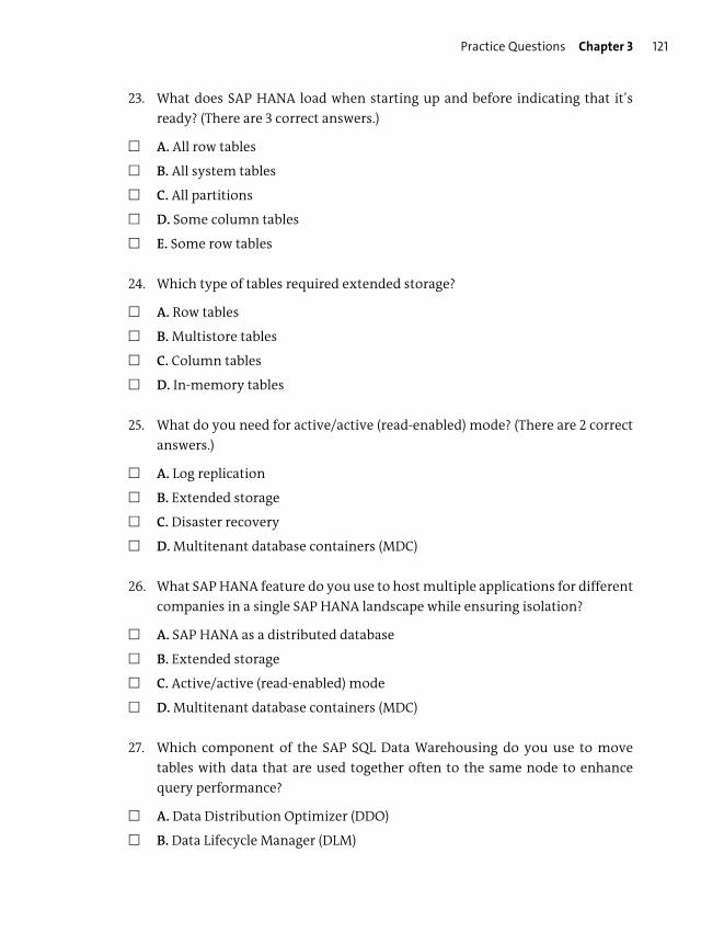
Practice Questions Chapter 3 121
23. What does SAP HANA load when starting up and before indicating that it’s
ready? (There are 3 correct answers.)
� A. All row tables
� B. All system tables
� C. All partitions
� D. Some column tables
� E. Some row tables
24. Which type of tables required extended storage?
� A. Row tables
� B. Multistore tables
� C. Column tables
� D. In-memory tables
25. What do you need for active/active (read-enabled) mode? (There are 2 correct
answers.)
� A. Log replication
� B. Extended storage
� C. Disaster recovery
� D. Multitenant database containers (MDC)
26. What SAP HANA feature do you use to host multiple applications for different
companies in a single SAP HANA landscape while ensuring isolation?
� A. SAP HANA as a distributed database
� B. Extended storage
� C. Active/active (read-enabled) mode
� D. Multitenant database containers (MDC)
27. Which component of the SAP SQL Data Warehousing do you use to move
tables with data that are used together often to the same node to enhance
query performance?
� A. Data Distribution Optimizer (DDO)
� B. Data Lifecycle Manager (DLM)

Chapter 3 Technology, Architecture, and Deployment Scenarios122
� C. Data Warehouse Monitor (DWM)
� D. Data Warehouse Scheduler (DWS)
28. Which BI tool queries SAP HANA using MDX?
� A. SAP Analysis for Microsoft Office
� B. SAP Lumira, discovery edition
� C. SAP BusinessObjects Web Intelligence
� D. Microsoft Excel
29. You want to publish your BI content directly to SAP Analytics Cloud. Which
tool do you use?
� A. SAP Lumira, discovery edition
� B. SAP Crystal Reports
� C. SAP Analysis for Microsoft Office
30. Which of the following ways of publishing SAP HANA information model con-
tent could require some JavaScript knowledge?
� A. Creating BI content with SAP Lumira, designer edition
� B. Creating a CompositeProvider in SAP BW
� C. Creating a report in SAP Crystal Reports
Practice Question Answers and Explanations
1. Correct answers: A, C, D
SAP HANA uses column tables, dictionary compression, and eliminating indi-
ces to load more data into memory.
However, it doesn’t use ZIP compression because ZIP-compressed files would
have to be uncompressed before the data could be used.
Multicore CPU parallelism helps with the performance but doesn’t directly
address the data volume issue. It contributes indirectly because, by using it, we
can eliminate things such as year-to-date tables as in SAP S/4HANA.

Practice Question Answers and Explanations Chapter 3 123
2. Correct answer: A
Yes, with SAP HANA, we can run OLAP and OLTP together in one system with
good performance. Normally, this isn’t possible in the traditional database sys-
tem.
Note
There are no True-False questions in the actual certification exam, but we use them here
to help you check if you understood this chapter.
3. Correct answer: A
Yes, SAP HANA contains both row and column tables.
4. Correct answers: B, C
Use stored procedures and graphical data models to execute the code in SAP
HANA.
Deleting the application server won’t help with running the code in SAP HANA,
unless we develop all that same functionality in the SAP HANA XS server.
Using row tables in SAP HANA has nothing to do with executing code.
5. Correct answer: C
In SAP S/4HANA, many aggregate tables are removed, and the solution is sim-
plified.
6. Correct answer: C
SAP HANA as a side-by-side accelerator doesn’t change the source systems.
7. Correct answers: B, D
With SAP HANA as a side-by-side accelerator and platform, users have to log in
to SAP HANA.
With SAP HANA as a database and reporting server, users log in via the applica-
tion server or reporting tools.
8. Correct answer: B
SAP delivers prebuilt data models for the special cases of the side-by-side accel-
erators, for example, for profitability analysis.
9. Correct answer: B
False. SAP HANA isn’t just a database. SAP HANA can also be used as a platform.
Databases don’t normally have application servers, version control, code repos-
itories, and various programming languages built in.
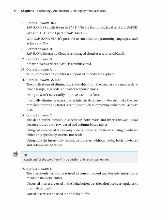
Chapter 3 Technology, Architecture, and Deployment Scenarios124
10. Correct answers: B, C
SAP HANA XS applications in SAP HANA are built using JavaScript and SAPUI5.
Java and ABAP aren’t part of SAP HANA XS.
With SAP HANA XSA, it’s possible to run other programming languages, such
as Java and C++.
11. Correct answer: D
SAP HANA Enterprise Cloud is a managed cloud as a service (MCaaS).
12. Correct answer: B
Amazon Web Services (AWS) is a public cloud.
13. Correct answer: A
True. Productive SAP HANA is supported on VMware vSphere.
14. Correct answers: A, B, D
The implications of eliminating such tables from the database are smaller data-
base backups, less code, and faster response times.
Doing so won’t necessarily improve user interfaces.
It actually eliminates extra inserts into the database but doesn’t make the cur-
rent data inserts any faster. Techniques such as removing indices will achieve
that.
15. Correct answer: C
The delta buffer technique speeds up both reads and inserts in SAP HANA
because it uses both row-based and column-based tables.
Using column-based tables only speeds up reads, not inserts. Using row-based
tables only speeds up inserts, not reads.
Using only the insert-only technique is useless without having both row-based
and column-based tables.
Tip
Watch out for the word “only” in a question or in an answer option.
16. Correct answer: B
The insert-only technique is used to convert record updates into insert state-
ments in the delta buffer.
Unsorted inserts are used in the delta buffer, but they don’t convert updates to
insert statements.
Sorted inserts aren’t used in the delta buffer.

Practice Question Answers and Explanations Chapter 3 125
Parallelism isn’t relevant in this case.
17. Correct answer: A
The main table area in the delta merge scenario is read-optimized.
The delta store is write-optimized, uses unsorted inserts, is uncompressed, and
is based on the row store.
18. Correct answer: B
ACID stands for atomicity, consistency, isolation, and durability.
19. Correct answers: B, C
Deploying SAP HANA as a distributed (scale-out) solution results in high avail-
ability and failover capability.
Disaster recovery and backups work whether the SAP HANA system is distrib-
uted or on a single server.
20. Correct answers: A, B
Synchronous and transaction manager are associated with the log volume.
Page manager and savepoint are associated with the data volume.
21. Correct answer: C
The transaction manager and page manager are part of the index server.
The statistics server and name server services are also part of SAP HANA, but
they aren’t discussed in this book.
22. Correct answer: A
SAP HANA performs a lazy load when starting up.
23. Correct answers: A, B, D
During the lazy load, SAP HANA loads all row tables, all system tables, and some
column tables.
SAP HANA doesn’t have to load all partitions of a table.
24. Correct answer: B
Multistore tables require extended storage. The other tables will work whether
we use extended storage or not.
25. Correct answers: A, C
You need log replication and disaster recovery for active/active (read-enabled)
mode.
Extended storage separates data between a memory (hot) store and a disk
(warm) store.
Multitenant database containers (MDC) separate tenants.
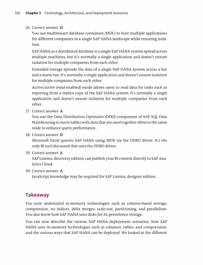
Chapter 3 Technology, Architecture, and Deployment Scenarios126
26. Correct answer: D
You use multitenant database containers (MDC) to host multiple applications
for different companies in a single SAP HANA landscape while ensuring isola-
tion.
SAP HANA as a distributed database is a single SAP HANA system spread across
multiple machines, but it’s normally a single application and doesn’t ensure
isolation for multiple companies from each other.
Extended storage spreads the data of a single SAP HANA system across a hot
and a warm tier. It’s normally a single application and doesn’t ensure isolation
for multiple companies from each other.
Active/active (read-enabled) mode allows users to read data for tasks such as
reporting from a replica copy of the SAP HANA system. It’s normally a single
application and doesn’t ensure isolation for multiple companies from each
other.
27. Correct answer: A
You use the Data Distribution Optimizer (DDO) component of SAP SQL Data
Warehousing to move tables with data that are used together often to the same
node to enhance query performance.
28. Correct answer: D
Microsoft Excel queries SAP HANA using MDX via the ODBO driver. It’s the
only BI tool discussed that uses the ODBO driver.
29. Correct answer: A
SAP Lumira, discovery edition, can publish your BI content directly to SAP Ana-
lytics Cloud.
30. Correct answer: A
JavaScript knowledge may be required for SAP Lumira, designer edition.
Takeaway
You now understand in-memory technologies such as column-based storage,
compression, no indices, delta merges, scale-out, partitioning, and parallelism.
You also know how SAP HANA uses disks for its persistence storage.
You can now describe the various SAP HANA deployment scenarios; how SAP
HANA uses in-memory technologies such as columns, tables, and compression;
and the various ways that SAP HANA can be deployed. We looked at the different
Summary Chapter 3 127
advantages of each deployment method to help you decide which one fits your
requirements best. Finally, we looked at how SAP HANA can also be deployed in
the cloud and for multiple tenants.
Summary
You’ve learned the various ways you can deploy SAP HANA. With this knowledge,
you can make recommendations to business users for an appropriate system
architecture and landscape.
In the next chapter, we’ll discuss changes that SAP HANA XSA brought to the SAP
HANA architecture and modeling processes. We’ll also look at the tools with which
we create information models and how to manage and administrate these models.


Chapter 4
Modeling Tools, Manage-ment, and Administration
Techniques You’ll Master
� Understand the new modeling and development process in
SAP HANA 2.0
� Learn how the new SAP HANA XSA architecture complements
SAP Cloud Platform
� Explain the difference between design-time and runtime objects
� Identify the different working areas in SAP Web IDE for
SAP HANA
� Get to know the SAP HANA modeling tools
� Learn how to complete the different steps in a project’s model-
ing and development process
� Learn how to work with tables and data
� Know how to create new information models
� Understand how to solve build errors by learning about the
SAP HANA XSA build processes
� Understand the deployment process and learn how it fits into
SAP’s transport processes
� Describe the administration and management steps required in
a project
� Perform refactoring techniques on information models
Chapter 4 Modeling Tools, Management, and Administration130
Tip
If you haven’t worked with SAP HANA 2.0 before, this will possibly be the most important
chapter for you.
You now understand where SAP HANA came from and how it works from an archi-
tectural point of view. SAP HANA has been growing fast, but the world hasn’t stood
still. There has been progress in many different areas, such as cloud platforms,
containers, development best practices, new programming paradigms, microser-
vices, NoSQL databases, machine learning, blockchain, Internet of Things (IoT),
DevOps, continuous integration, and, perhaps most of all, customer expectations.
SAP HANA 2.0 is, in some sense, a response to this progress. In this chapter, we’ll
look at what is new in SAP HANA 2.0 from many different angles. First, we’ll look at
the new modeling and development process. This information is necessary to put
many of the new changes into context. These changes include the new architec-
ture, the new web-based user interface (UI), and the new tools. We’ll also cover how
to start a modeling project, how to create and run information models, and how to
get them into the production system within the new system. You’ll understand
why the system behaves the way it does; when you get errors, you’ll know why and
how to solve them.
We’ll start with some process and architecture diagrams before moving on to the
actual system itself. We’ll describe the steps you need to get going with SAP HANA
modeling on your own system and your own projects.
Real-World Scenario
You’re working on a project that requires you to create information models.
To do so, you use SAP Web IDE for SAP HANA to create and edit these views
graphically. You can use this tool from anywhere, even when using cloud sys-
tems.
Sometimes you reach for the other tools in your toolkit: SAP HANA database
explorer, SAP HANA cockpit, SAP HANA XSA cockpit, and SAP Enterprise
Architecture Designer (SAP EA Designer).
When working on a project with SAP HANA, you’ll use modeling tools all the
time. You have to be familiar with the SAP HANA modeling tools, know when
to use which one, and be able to find your way around the various screens.

Objectives of This Portion of the Test Chapter 4 131
SAP HANA has grown over the past few years, and the modeling tools now
help you accomplish a wide variety of tasks. The features have also grown to
provide rich functionality. It therefore takes some time to learn how to find
your way around the various menus, options, and screens.
All the information models you created for your project are in your develop-
ment system. You feel confident about the work you’ve created, so now it’s
time to take it to the production system. You need to transport your infor-
mation models through the SAP HANA landscape. Before end users can use
your information models in the production system, your models need to be
deployed to the production system.
As the project progresses, new customer requirements arise. Your informa-
tion models need to adapt to changing business conditions. You ensure they
do so by using the refactoring tools built in to the SAP HANA modeling tools.
Objectives of This Portion of the Test
The objective of this portion of the SAP HANA certification is to test your under-
standing of how to create, manage, build, deploy, and refactor your information
models with the various SAP HANA modeling and development tools. Your insight
will be tested by describing various scenarios that result in error messages, and
you have to know why the errors were triggered.
The certification exam expects you to have a good understanding of the following
topics:
� The modeling and development process in SAP HANA 2.0
� The SAP HANA extended application services, advanced model (SAP HANA XSA)
and SAP HANA Deployment Infrastructure (HDI) architecture
� Differences between design-time and runtime objects
� SAP Web IDE for SAP HANA and the SAP HANA modeling tools
� The different steps in the complete modeling and development process of a
project, from creating a project, to working with tables and information models
� Solving build errors by understanding the SAP HANA XSA build processes
� The deployment process and how this fits in with SAP’s transport processes
� The administration and management steps required in a project
� The various refactoring tools and techniques available
Chapter 4 Modeling Tools, Management, and Administration132
Note
This portion contributes up to 10% of the total certification exam score.
Key Concepts Refresher
In the previous chapter, we briefly introduced you to SAP HANA extended applica-
tion services, classic model (SAP HANA XS). We’ll now begin by describing SAP
HANA XS in a bit more detail, and then move on to SAP HANA extended applica-
tion services, advanced model (SAP HANA XSA) with HDI.
Note
In the What’s New Guide for SAP HANA 2.0 SPS 03, in the section for SAP HANA XS and
the SAP HANA repository, it says,
“SAP HANA Extended Application Services classic model (XS classic) and SAP HANA Reposi-
tory are deprecated as of SAP HANA 2.0 SPS 02.”
You can also see SAP Note 2465027 for more details.
New Modeling Process
In SAP HANA 1.0, we had two main working areas, as shown in Figure 4.1. We had
the Content area, where we created our information models. These models were
stored in a repository inside SAP HANA. In addition to our models, we could also
store other files there, such as HTML and JavaScript code. The files in the SAP
HANA repository are known as design-time files because we edit them to design
our models and code.
When we activated these models, a copy got stored in the _SYS_BIC schema in the
Catalog area, and the _SYS_REPO user became the owner of these files. These copies
are available to users, which they then use to run analysis, reports, and applica-
tions on the system. These copies were known as the runtime files because the
users used them to run their queries. These files were stored together with the
database tables and the data. Tables were grouped together in schemas.
By storing and working with the design-time and runtime files in two different
areas, there is a separation between design-time and runtime files. We used trans-
ports to copy the design-time files to a production environment, where we could
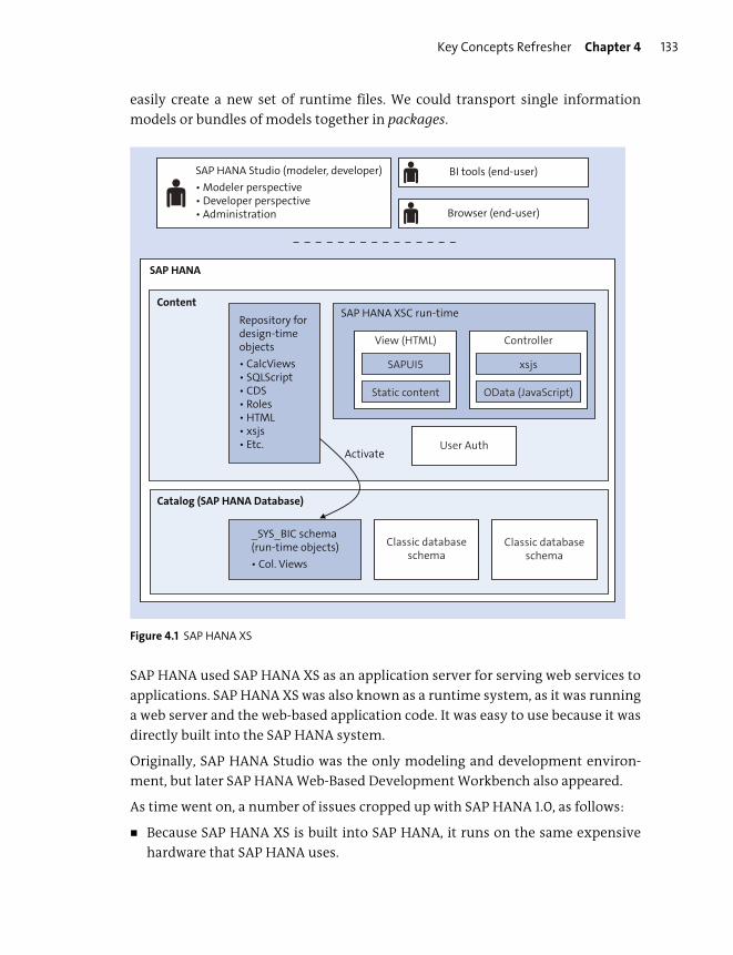
Key Concepts Refresher Chapter 4 133
easily create a new set of runtime files. We could transport single information
models or bundles of models together in packages.
Figure 4.1 SAP HANA XS
SAP HANA used SAP HANA XS as an application server for serving web services to
applications. SAP HANA XS was also known as a runtime system, as it was running
a web server and the web-based application code. It was easy to use because it was
directly built into the SAP HANA system.
Originally, SAP HANA Studio was the only modeling and development environ-
ment, but later SAP HANA Web-Based Development Workbench also appeared.
As time went on, a number of issues cropped up with SAP HANA 1.0, as follows:
� Because SAP HANA XS is built into SAP HANA, it runs on the same expensive
hardware that SAP HANA uses.
SAP HANA Studio (modeler, developer)• Modeler perspective• Developer perspective• Administration Browser (end-user)
BI tools (end-user)
SAP HANA
ContentSAP HANA XSC run-time
View (HTML)
Static content
SAPUI5
User Auth
Controller
xsjs
OData (JavaScript)
Catalog (SAP HANA Database)
Classic databaseschema
Repository for design-time objects• CalcViews• SQLScript• CDS• Roles• HTML• xsjs• Etc.
Classic databaseschema
Activate
_SYS_BIC schema(run-time objects)• Col. Views

Chapter 4 Modeling Tools, Management, and Administration134
� There was only one copy of the SAP HANA XS application server for an SAP
HANA system, leading to scalability limitations.
� The tight coupling of SAP HANA XS in SAP HANA servers led to some problem-
atic networking designs.
� XS JavaScript and the associated development process were quite different from
the latest advances in the JavaScript development community. When compa-
nies need skilled people, it helps if the development processes they use fit in
with what the rest of the industry does. New people can get up to speed quicker,
and support improves in case of problems.
� The built-in repository lacked certain vital features like version control, forking,
and merging branches.
� Table definitions weren’t transportable. Core data services (CDS) was intro-
duced in the later versions of SAP HANA 1.0 to address this.
SAP also needed to address some industry requirements:
� SAP started using SAP HANA in more of its cloud business systems. Due to fea-
ture differences between the cloud and the on-premise offerings, better feature
parity was needed between these offerings.
Tip
Many of the changes in SAP HANA 2.0 and SAP HANA XSA can be summarized by three
words: cloud, containers, and microservices.
� The development and modeling processes in the cloud environments were differ-
ent from that of the on-premise solutions. Web-based UIs are vital for cloud sys-
tems. Best practices such as the twelve-factor app, found at https://12factor.net/,
for cloud-native development emerged and got adopted. People wanted a consis-
tent way to work with both cloud and on-premise development and modeling.
� The speed of updates in cloud offerings is much faster than that of their on-
premise cousins, requiring new ways of providing application services. System
administrators and developers now use new automated build and testing pro-
cesses, DevOps, continuous integration, continuous delivery, blue-green
deployment, and so on.
� Cloud environments were enabled by the arrival of virtual machines. Over time,
people started adding more and more virtual machines to servers, and certain
limits showed up. This led to the concept of containers, which are much smaller,
can start very quickly, and can scale easily when used with cloud platforms. The
combination of containers and web services led to the emergence of microser-

Key Concepts Refresher Chapter 4 135
vices architectures. There was a need for a way to make use of these new con-
cepts.
� A microservices architecture needs a runtime to manage the various containers
and the microservices running in each container. SAP decided to use Cloud
Foundry for this. Cloud Foundry is an open-source, multi-cloud application
platform as a service (PaaS) offering. The new SAP Cloud Platform uses Cloud
Foundry.
� Cloud hyperscalers, such as Amazon, Microsoft, and Google, are used by many
SAP customers. The Cloud Foundry PaaS, containers, and microservices devel-
oped with SAP run on the offerings from these companies. SAP customers can
this leverage their other development and solutions they already have running
on these cloud infrastructures.
These gaps in coverage led to the development of SAP HANA XSA, which brought a
new modeling and development process with it, as shown in Figure 4.2. In the fig-
ure, the process moves from the left to the right. One of the first things to notice is
that there is now a total separation of the design-time environment (left side)
from the runtime environment (right side). Where these were previously together
in an SAP HANA system, they are now completely separate.
Note
You might have noticed already that we keep mentioning modeling and development in
the same breath. You’ll use development objects in your information models, and your
information models will be used by developers in their web applications. SAP HANA mod-
eling has become an integral part of the development process.
The process starts in the top-left corner of Figure 4.2. You use SAP Web IDE for SAP
HANA to start a project, create and edit information models, and then build them.
Tip
If you worked a lot with SAP HANA 1.0, you might be tempted to continue using SAP
HANA Studio. You can’t use SAP HANA Studio to develop SAP HANA XSA applications
because it doesn’t work with the new SAP HANA HDI infrastructure. You need to use SAP
Web IDE for SAP HANA.
Your models get stored in a Git repository instead of an SAP HANA repository. Git
is the most-used repository by developers worldwide. This allows for version
control, forking, and merging. Git integration is built into the SAP HANA XSA mod-
eling and development tools.
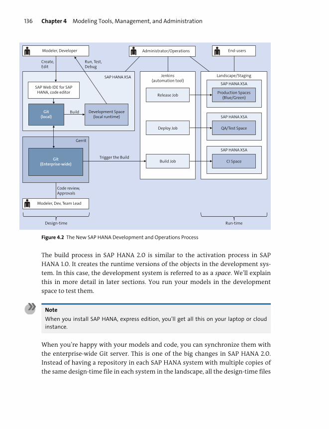
Chapter 4 Modeling Tools, Management, and Administration136
Figure 4.2 The New SAP HANA Development and Operations Process
The build process in SAP HANA 2.0 is similar to the activation process in SAP
HANA 1.0. It creates the runtime versions of the objects in the development sys-
tem. In this case, the development system is referred to as a space. We’ll explain
this in more detail in later sections. You run your models in the development
space to test them.
Note
When you install SAP HANA, express edition, you’ll get all this on your laptop or cloud
instance.
When you’re happy with your models and code, you can synchronize them with
the enterprise-wide Git server. This is one of the big changes in SAP HANA 2.0.
Instead of having a repository in each SAP HANA system with multiple copies of
the same design-time file in each system in the landscape, all the design-time files
Administrator/OperationsModeler, Developer
Modeler, Dev, Team Lead
SAP HANA XSA Jenkins(automation tool)
Landscape/Staging
SAP HANA XSA
SAP HANA XSA
SAP HANA XSA
Production Spaces(Blue/Green)
QA/Test Space
CI Space
Release Job
Deploy Job
Build Job
Development Space(local runtime)
SAP Web IDE for SAPHANA, code editor
Gerrit
Git(local)
Code review,Approvals
Create,Edit
Run, Test,Debug
Build
Trigger the Build
Design-time Run-time
Git(Enterprise-wide)
End-users
Key Concepts Refresher Chapter 4 137
are now in one master repository. Git allows for many different version and
branches. You have a stable production branch, but you can also have different
development branches where people are trying out different new ideas. When the
idea gets accepted, the code is merged into the integration and testing branches.
You can fork a branch, which creates a copy, and test out something new in a sand-
box. Git allows large teams of developers to seamlessly work together on large or
complex software projects.
You can also use Gerrit, which is Git with some additional features added, such as
enabling code reviews and approvals. The team lead can sit with modelers and
developers to review their work and approve the changes.
Tip
In this book, we’ll focus on the process up to this point. In this section, we give a descrip-
tion of the rest of the process to give you an understanding of how your work gets into
the production system where end users can start using it and the business can start get-
ting value out of it.
In many cases, the update in the enterprise-wide Git or the approval in Gerrit, trig-
gers an automated build of the project, and a build job updates the changes into
the continuous integration (CI) space (system) where you can see how your mod-
els and code work together with everybody else’s.
The build job is set up, configured, and managed by the administrators as part of
the operations area. Many times, they need to understand what your code is trying
to do and what it will change. On the other hand, you need to know how, when, and
where your code gets used. This collaboration has led to DevOps; development
and operations working together.
The administrators (operations) can use something such as Jenkins, which is an
open-source automation server that is used to automate tasks related to the build-
ing, testing, and deploying of software.
Quality assurance (QA) testers can trigger a deploy job. Testing users can then test
everyone’s updates in an environment that is very similar to the production envi-
ronment. This is also sometimes called the staging server.
After all testing has been approved, a release job is triggered that updates the pro-
duction system. To ensure continuous uptime on the production servers, a blue-
green deployment strategy can be implemented. You can read more about this at
http://s-prs.co/v487624 and http://s-prs.co/v487625.
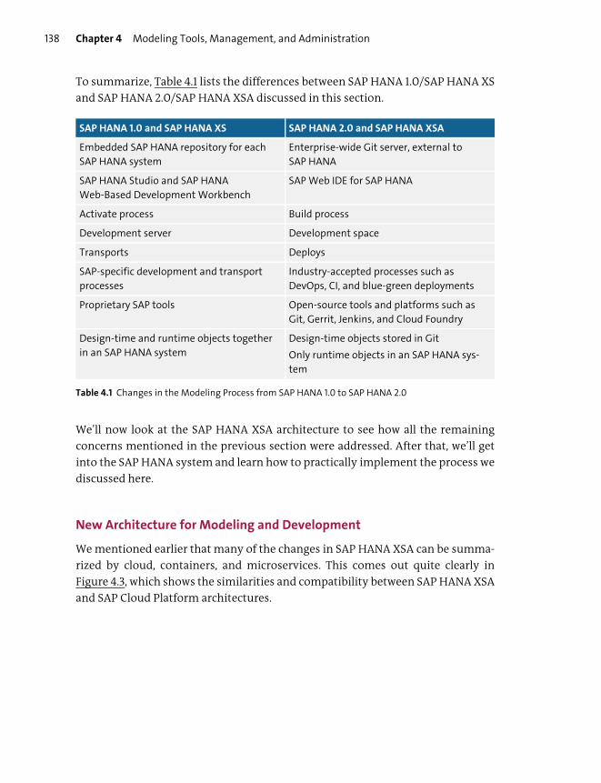
Chapter 4 Modeling Tools, Management, and Administration138
To summarize, Table 4.1 lists the differences between SAP HANA 1.0/SAP HANA XS
and SAP HANA 2.0/SAP HANA XSA discussed in this section.
We’ll now look at the SAP HANA XSA architecture to see how all the remaining
concerns mentioned in the previous section were addressed. After that, we’ll get
into the SAP HANA system and learn how to practically implement the process we
discussed here.
New Architecture for Modeling and Development
We mentioned earlier that many of the changes in SAP HANA XSA can be summa-
rized by cloud, containers, and microservices. This comes out quite clearly in
Figure 4.3, which shows the similarities and compatibility between SAP HANA XSA
and SAP Cloud Platform architectures.
SAP HANA 1.0 and SAP HANA XS SAP HANA 2.0 and SAP HANA XSA
Embedded SAP HANA repository for each
SAP HANA system
Enterprise-wide Git server, external to
SAP HANA
SAP HANA Studio and SAP HANA
Web-Based Development Workbench
SAP Web IDE for SAP HANA
Activate process Build process
Development server Development space
Transports Deploys
SAP-specific development and transport
processes
Industry-accepted processes such as
DevOps, CI, and blue-green deployments
Proprietary SAP tools Open-source tools and platforms such as
Git, Gerrit, Jenkins, and Cloud Foundry
Design-time and runtime objects together
in an SAP HANA system
Design-time objects stored in Git
Only runtime objects in an SAP HANA sys-
tem
Table 4.1 Changes in the Modeling Process from SAP HANA 1.0 to SAP HANA 2.0

Key Concepts Refresher Chapter 4 139
Figure 4.3 Similarities and Compatibility between SAP HANA XSA and SAP Cloud Platform Architectures
Both architectures have three layers. The bottom layer is different between SAP
HANA XSA and SAP Cloud Platform. SAP HANA XSA is running on servers, which
can be on premise or on the cloud. SAP Cloud Platform is running on OpenStack,
an open-source infrastructure as a service (IaaS) platform, in the SAP data centers
or on the cloud platforms of Amazon, Google, and Microsoft.
The next layer of both, the platforms, are getting a lot closer. Both SAP HANA XSA
and SAP Cloud Platform are based on Cloud Foundry. Both add additional services
to enhance the standard Cloud Foundry offering, such as routing, security, sched-
uling, integration, UI framework (SAPUI5), database services (e.g., the SAP HANA
database), and so on. These are shown as the Backing Services in the diagram.
The top layer is really where it starts making sense for modelers and developers.
The application and HDI containers are identical on both SAP HANA XSA and SAP
Cloud Platform.
Containers and virtual machines are both used to isolate applications and their
dependencies into a single “unit” that can run anywhere. Both remove the need
for physical hardware. This enables efficient use of servers in terms of energy
SAP HANA XSA
Servers
HDI Containers
Backing Services
UAA, Job scheduler, Connectivity, UX, Data Quality, APIs, Integration, Mobile, Machine Learning, IoT, …
SAP HANA database platform
SAP HANA XSA runtime
Application Containers
SAP Cloud Platform with Cloud Foundry
Additional Platform Services
IaaS
OpenStack, Private Cloud, Multi-Cloud (Amazon WS, MS Azure, Google CP)
SAP Cloud Platform
Cloud Foundry
HDI Containers
Application Containers
Backing Services
UAA, Job scheduler, Connectivity, UX, Data Quality, APIs, Integration, Mobile, Machine Learning, IoT, …Redis, PostgreSQL, RabbitMQ, MongoDB
Containers and services
Platform layer
Infrastructure layer
Chapter 4 Modeling Tools, Management, and Administration140
costs. However, where virtual machines require an operating system for each vir-
tual machine, containers use new features in modern operating systems that
allow them to create thousands of small isolated units to run on a single server and
operating system.
Containers fully isolate the application, the users, the memory and CPU usage, and
the network. Their popularity in recent years stems from the fact that they scale
fast and easily. Say you have a small web service running in a container. When
there aren’t many requests for this service, only one container is sufficient. As the
load increases, the platform layer—also known as the container runtime—auto-
matically creates more copies of the container to meet the increased demand.
When the load decreases, the number of copies is also reduced, which is a huge
benefit for companies that can’t predict how much hardware is required for a ser-
vice or application.
The container isolation helps teams work at full speed on their own code. One
team can work, for example, on the financial calculations service, while another
team focuses on the UI. Both teams can deploy updates to the production system
independently from each other.
Tip
The independence of containers, referred to as loose coupling, is important for continu-
ous integration (CI) and continuous deployment (CD).
Another advantage is that you can now use the programming language that best
suits your needs for that particular service. You could use JavaScript for the UI and
Golang for the financial calculations service. This approach is sometimes called
“bring your own language” (BYOL).
Even though you can use multiple programming languages, the container run-
time makes this appear seamless to end users via the routing service. The UI ser-
vice could use a URL such as https://server/ui, whereas the financial calculations
service could use https://server/fincalcs. The routing service directs (routes) the
user requests to the correct services in the different containers. If you use a stan-
dard UI framework, such as SAPUI5, all your applications will have a consistent
look and feel, despite the fact that the underlying services are using different pro-
gramming languages.
Each container also contains the environment required to run the services contained
in it. A Java service might require Tomcat, whereas PHP (Hypertext Preprocessor)
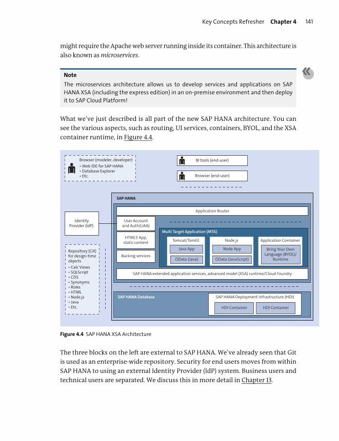
Key Concepts Refresher Chapter 4 141
might require the Apache web server running inside its container. This architecture is
also known as microservices.
Note
The microservices architecture allows us to develop services and applications on SAP
HANA XSA (including the express edition) in an on-premise environment and then deploy
it to SAP Cloud Platform!
What we’ve just described is all part of the new SAP HANA architecture. You can
see the various aspects, such as routing, UI services, containers, BYOL, and the XSA
container runtime, in Figure 4.4.
Figure 4.4 SAP HANA XSA Architecture
The three blocks on the left are external to SAP HANA. We’ve already seen that Git
is used as an enterprise-wide repository. Security for end users moves from within
SAP HANA to using an external Identity Provider (IdP) system. Business users and
technical users are separated. We discuss this in more detail in Chapter 13.
Browser (modeler, developer)• Web IDE for SAP HANA• Database Explorer• Etc. Browser (end-user)
BI tools (end-user)
SAP HANA
Multi Target Application (MTA)
Application Container
Bring Your OwnLanguage (BYOL)/
Runtime
HTML5 App,static content Tomcat/TomEE
OData (Java)
Java App
User Accountand Auth(UAA)
Node.js
Node App
OData (JavaScript)
SAP HANA extended application services, advanced model (XSA) runtime/Cloud Foundry
Application Router
SAP HANA Database
IdentityProvider (IdP)
SAP HANA Deployment Infrastructure (HDI)
HDI ContainerHDI Container
Backing servicesRepository (Git)for design-timeobjects• Calc Views• SQLScript• CDS• Synonyms• Roles• HTML• Node.js• Java• Etc.

Chapter 4 Modeling Tools, Management, and Administration142
The SAP HANA system has two major areas: (1) the SAP HANA database at the bot-
tom of the diagram, and (2) SAP HANA XSA. You can run SAP HANA XSA inside the
SAP HANA system on the same server as the SAP HANA database (e.g., SAP HANA
XS), but you can also separate it to run on one or more other cheaper servers. This
addresses the first two requests in the list, as these cheaper servers can scale
cheaply and easily, and the network configurations can be hardened. This is indi-
cated by the dashed line between the two areas.
In SAP HANA XSA, you can combine services in different programming languages
into a one application by creating a multi-target application (MTA) project. You
can write one service in Java, another in JavaScript, and yet another in a language
of your choice. During deployment, SAP HANA XSA will automatically create dif-
ferent application containers for each of these services. This multi-language con-
figuration is specified by the mta.yaml file in your project. You can use either the
SAP HANA XSA runtime or SAP Cloud Platform to “host” these application con-
tainers.
Tip
SAP HANA XSA and SAP Cloud Platform use the industry-accepted Node.js when working
with JavaScript.
In the SAP HANA database area, you’ll notice something interesting. Each schema
in an SAP HANA XSA database is now a container.
In our project, you add an SAP HANA database (HDB) module. In this module
(folder), you add all your design-time objects, such as tables, calculation views, and
SQL procedures. The HDB module definition is also added to the mta.yaml file. The
HDB module is for your design-time objects.
When you build your HDB module, it creates an SAP HANA database container.
This replaces the classical database schemas in the older version of SAP HANA.
These containers that contain just SAP HANA database runtime objects are called
HDI containers. They contain only runtime objects, as all design-time objects are
stored in Git, even the design-time database objects. The HDI container function-
ality is part of the SAP HANA runtime and is part of SAP Cloud Platform runtime
should you choose to deploy your HDI containers on the cloud.
One of the first problems you might encounter is due to the fact that containers
provide full isolation. This radically impacts all SAP HANA security and can be frus-
trating when you’re used to the old way of working.
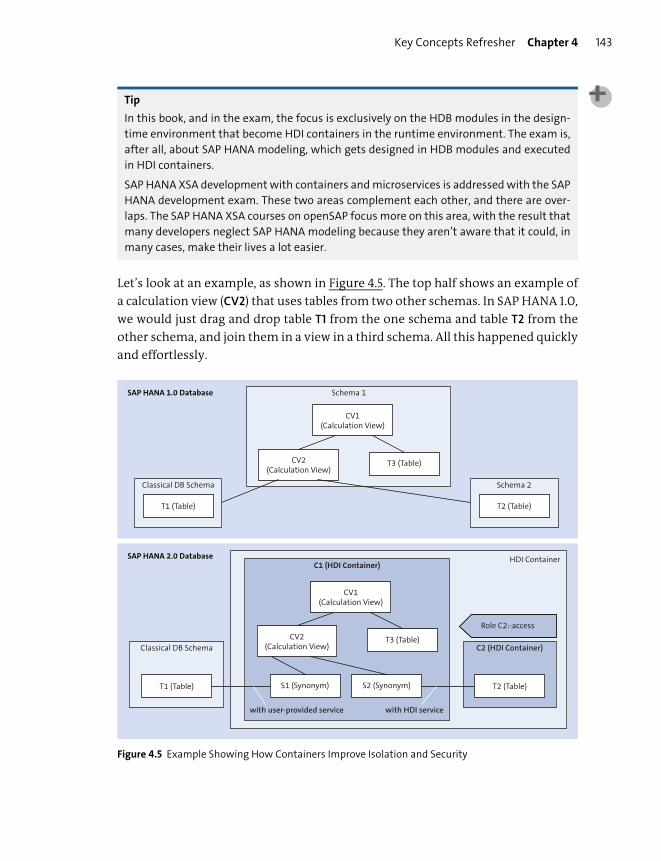
Key Concepts Refresher Chapter 4 143
Tip
In this book, and in the exam, the focus is exclusively on the HDB modules in the design-
time environment that become HDI containers in the runtime environment. The exam is,
after all, about SAP HANA modeling, which gets designed in HDB modules and executed
in HDI containers.
SAP HANA XSA development with containers and microservices is addressed with the SAP
HANA development exam. These two areas complement each other, and there are over-
laps. The SAP HANA XSA courses on openSAP focus more on this area, with the result that
many developers neglect SAP HANA modeling because they aren’t aware that it could, in
many cases, make their lives a lot easier.
Let’s look at an example, as shown in Figure 4.5. The top half shows an example of
a calculation view (CV2) that uses tables from two other schemas. In SAP HANA 1.0,
we would just drag and drop table T1 from the one schema and table T2 from the
other schema, and join them in a view in a third schema. All this happened quickly
and effortlessly.
Figure 4.5 Example Showing How Containers Improve Isolation and Security
SAP HANA 1.0 Database
Classical DB Schema
T1 (Table)
Schema 2
T2 (Table)
Schema 1
T3 (Table)
CV1(Calculation View)
CV2(Calculation View)
SAP HANA 2.0 Database HDI ContainerC1 (HDI Container)
Classical DB Schema C2 (HDI Container)
T1 (Table) T2 (Table)S2 (Synonym)S1 (Synonym)
T3 (Table)
with user-provided service with HDI service
CV1(Calculation View)
CV2(Calculation View)
Role C2::access

Chapter 4 Modeling Tools, Management, and Administration144
If we try this in HDI, we get authorization errors. Because the three schemas are all
fully isolated in three different containers, you’ll have to look at the security when
designing a scenario like this to also enforce loose coupling between different con-
tainers in microservices architectures.
The bottom half shows that to get this working, you have to create a synonym for
each external table you want to use. Each HDI container also has a default access
authorization role that gets created when you first create the container. You need
to assign this role to the owner of your container (schema). Lastly, if you’re con-
necting to a classical database schema, you also need to provide a service. If you
connect to another HDI container, the SAP HANA or SAP Cloud Platform runtimes
already have such a service for you. We discuss all this in more detail in Chapter 13.
To summarize, Table 4.2 lists the differences between SAP HANA 1.0/SAP HANA XS
and SAP HANA 2.0/SAP HANA XSA discussed in this section.
SAP HANA 1.0 and SAP HANA XS SAP HANA 2.0 and SAP HANA XSA
SAP HANA XS is embedded in SAP HANA. SAP HANA can be run on separate cheaper
servers.
The database is integrated with the
application.
The data layer is decoupled.
End users of native SAP HANA applications
are managed inside SAP HANA.
End users are managed from an external IdP
system.
Business users and technical users are
together.
Business users and technical users are
separated.
SAP HANA XS is different from SAP Cloud
Platform.
SAP HANA XSA and SAP Cloud Platform
share the same PaaS layer using Cloud
Foundry. Both use a microservices architec-
ture with containers. You can deploy the
same models and code to either platform.
All code and information models are in one
SAP HANA system.
Each application’s services are in its own
container, and SAP HANA information mod-
els are in HDI containers.
All database objects are together in one
SAP HANA database.
Each project and HDB module’s database
objects are isolated in its own HDI container.
Explicit references are used to tables in
other schemas.
Synonyms, authorizations (role assigned),
and possibly a user-provided service are
needed.
XS JavaScript is used. Node.js is used.
Table 4.2 Changes in the Architecture from SAP HANA 1.0 to SAP HANA 2.0
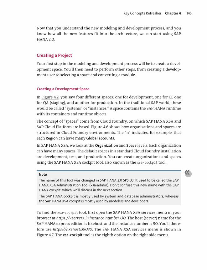
Key Concepts Refresher Chapter 4 145
Now that you understand the new modeling and development process, and you
know how all the new features fit into the architecture, we can start using SAP
HANA 2.0.
Creating a Project
Your first step in the modeling and development process will be to create a devel-
opment space. You’ll then need to perform other steps, from creating a develop-
ment user to selecting a space and converting a module.
Creating a Development Space
In Figure 4.2, you saw four different spaces: one for development, one for CI, one
for QA (staging), and another for production. In the traditional SAP world, these
would be called “systems” or “instances.” A space contains the SAP HANA runtime
with its containers and runtime objects.
The concept of “spaces” come from Cloud Foundry, on which SAP HANA XSA and
SAP Cloud Platform are based. Figure 4.6 shows how organizations and spaces are
structured in Cloud Foundry environments. The “n” indicates, for example, that
each Region can have many Global accounts.
In SAP HANA XSA, we look at the Organization and Space levels. Each organization
can have many spaces. The default spaces in a standard Cloud Foundry installation
are development, test, and production. You can create organizations and spaces
using the SAP HANA XSA cockpit tool, also known as the xsa-cockpit tool.
Note
The name of this tool was changed in SAP HANA 2.0 SPS 03. It used to be called the SAP
HANA XSA Administration Tool (xsa-admin). Don’t confuse this new name with the SAP
HANA cockpit, which we’ll discuss in the next section.
The SAP HANA cockpit is mostly used by system and database administrators, whereas
the SAP HANA XSA cockpit is mostly used by modelers and developers.
To find the xsa-cockpit tool, first open the SAP HANA XSA services menu in your
browser at https://<server>:3<instance-number>30. The host (server) name for the
SAP HANA express edition is hxehost, and the instance number is 90. You’ll there-
fore use https://hxehost:39030. The SAP HANA XSA services menu is shown in
Figure 4.7. The xsa-cockpit tool is the eighth option on the right-side menu.

Chapter 4 Modeling Tools, Management, and Administration146
Figure 4.6 Cloud Foundry Organizations and Spaces
Figure 4.7 SAP HANA XSA Services Menu
Cloud Foundry Environment
User account Home
Region
Global Account
Subaccount
Space
Organization
Cloud Foundry applications
Cloud Foundry services
SAP Cloud Platform

Key Concepts Refresher Chapter 4 147
Tip
You can also find SAP Web IDE for SAP HANA (webide) and the SAP HANA Interactive Edu-
cation (SHINE) demo (web) on the SAP HANA XSA services menu.
After you’ve opened the xsa-cockpit tool, you’ll see the screen as shown in Figure
4.8. You can click on the New Organization button to create a new organization.
This example shows the HANAExpress organization for SAP HANA, express edi-
tion.
Figure 4.8 SAP HANA XS Advanced Cockpit to Add a New Organization
Note
The UI of the SAP HANA XSA cockpit was changed from the SAP Fiori launchpad look-and-
feel to that of the new SAP Cloud Platform.
Figure 4.9 shows the details of the HANAExpress organization screen. The right side
shows the Spaces. You can add a new development space for your SAP HANA mod-
eling by clicking on the New Space button.
Tip
It’s recommended that you create a development space, instead of using the default SAP
space. In SAP HANA, express edition, the development space is already created for you.
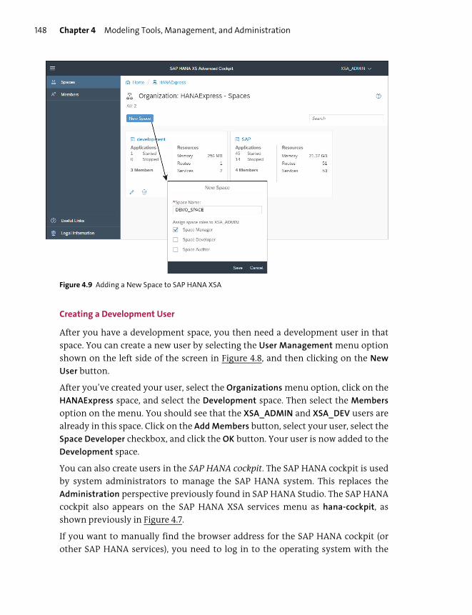
Chapter 4 Modeling Tools, Management, and Administration148
Figure 4.9 Adding a New Space to SAP HANA XSA
Creating a Development User
After you have a development space, you then need a development user in that
space. You can create a new user by selecting the User Management menu option
shown on the left side of the screen in Figure 4.8, and then clicking on the New
User button.
After you’ve created your user, select the Organizations menu option, click on the
HANAExpress space, and select the Development space. Then select the Members
option on the menu. You should see that the XSA_ADMIN and XSA_DEV users are
already in this space. Click on the Add Members button, select your user, select the
Space Developer checkbox, and click the OK button. Your user is now added to the
Development space.
You can also create users in the SAP HANA cockpit. The SAP HANA cockpit is used
by system administrators to manage the SAP HANA system. This replaces the
Administration perspective previously found in SAP HANA Studio. The SAP HANA
cockpit also appears on the SAP HANA XSA services menu as hana-cockpit, as
shown previously in Figure 4.7.
If you want to manually find the browser address for the SAP HANA cockpit (or
other SAP HANA services), you need to log in to the operating system with the
Key Concepts Refresher Chapter 4 149
<System ID>adm user. The system ID for SAP HANA, express edition is hxe, and
you need to log in with the hxeadm user. On the command line, type “xs apps”.
You’ll see a list of SAP HANA XSA services, as shown in Figure 4.10.
Figure 4.10 Running “xs apps” on the Command Line to Find Application URLs
To find the SAP HANA cockpit, look for a service called cockpit-web-app. In this
case, the browser address (top line) is https://hxehost:51046. This will probably be
different on your system.
If the service shows as STOPPED in the second column, you can start it by going to
the xsa-cockpit tool, and selecting the Applications menu option, as shown in
Figure 4.11. You’ll then see the list of services. Here you can start any services that
were stopped.
You can create users and assign roles to the users using the SAP HANA cockpit.
We’ll discuss this in Chapter 13.
Figure 4.12 shows what the SAP HANA cockpit looks like. Most of the functionality
in the SAP HANA cockpit is for system administrators, so it won’t be discussed
here.
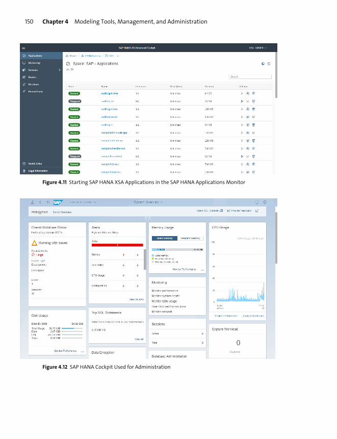
Chapter 4 Modeling Tools, Management, and Administration150
Figure 4.11 Starting SAP HANA XSA Applications in the SAP HANA Applications Monitor
Figure 4.12 SAP HANA Cockpit Used for Administration

Key Concepts Refresher Chapter 4 151
Project Creation Options
You can now open the SAP Web IDE for SAP HANA (webide) tool, which is the main
tool we’ll use for modeling and development.
Even though the names are similar, SAP Web IDE for SAP HANA isn’t the same as
the SAP Web IDE that is used for developing SAP Fiori apps.
When you open SAP Web IDE for SAP HANA, you’ll have an empty Workspace
where you’ll create SAP HANA projects. Each project will be for an SAP HANA appli-
cation, for which you create development and modeling objects.
SPS 04
From SAP HANA SPS 04, you can have multiple workspaces in SAP Web IDE for SAP HANA.
Tip
The following three words sound similar but refer to completely different topics, so it’s
important not to confuse them:
� Space
Space refers to a development or production system.
� Workspace
Workspace refers to your working area in SAP Web IDE for SAP HANA, where you create
projects with development and modeling objects.
� Namespace
Namespace is used for naming development and modeling objects, and it helps deter-
mine the name of the runtime objects in the containers.
There are three ways to create a new SAP HANA project. The following are shown
in Figure 4.13:
1. The first is to right-click on Workspace, and select New from the menu. This cre-
ates a blank project. You then create an SAP HANA MTA Project.
2. The second is to Import an existing project. You need to have previously
exported a project. We’ll look at this a bit more.
3. Lastly, you can Clone a project from the Git repository.
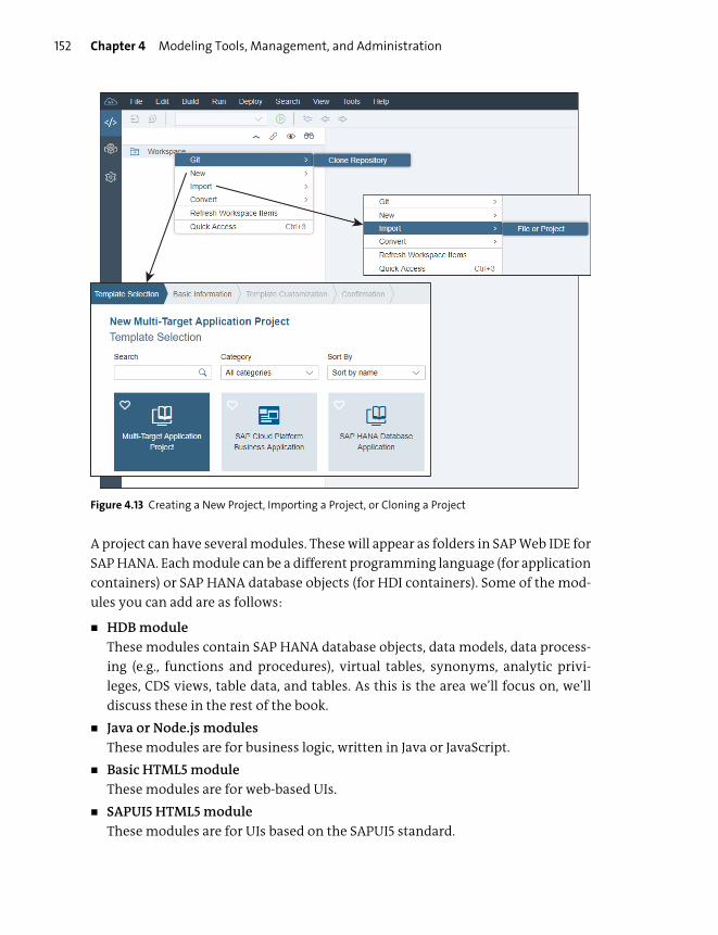
Chapter 4 Modeling Tools, Management, and Administration152
Figure 4.13 Creating a New Project, Importing a Project, or Cloning a Project
A project can have several modules. These will appear as folders in SAP Web IDE for
SAP HANA. Each module can be a different programming language (for application
containers) or SAP HANA database objects (for HDI containers). Some of the mod-
ules you can add are as follows:
� HDB module
These modules contain SAP HANA database objects, data models, data process-
ing (e.g., functions and procedures), virtual tables, synonyms, analytic privi-
leges, CDS views, table data, and tables. As this is the area we’ll focus on, we’ll
discuss these in the rest of the book.
� Java or Node.js modules
These modules are for business logic, written in Java or JavaScript.
� Basic HTML5 module
These modules are for web-based UIs.
� SAPUI5 HTML5 module
These modules are for UIs based on the SAPUI5 standard.
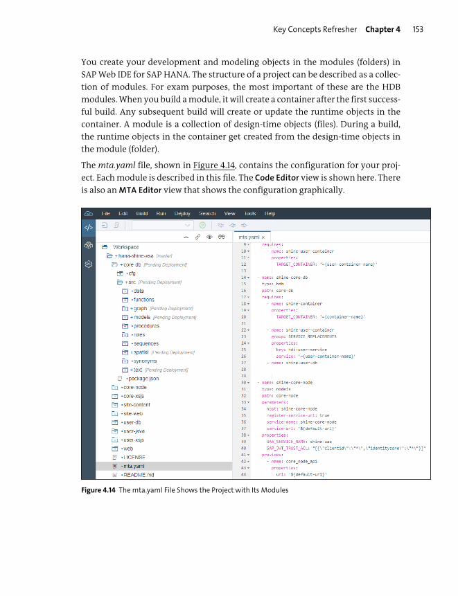
Key Concepts Refresher Chapter 4 153
You create your development and modeling objects in the modules (folders) in
SAP Web IDE for SAP HANA. The structure of a project can be described as a collec-
tion of modules. For exam purposes, the most important of these are the HDB
modules. When you build a module, it will create a container after the first success-
ful build. Any subsequent build will create or update the runtime objects in the
container. A module is a collection of design-time objects (files). During a build,
the runtime objects in the container get created from the design-time objects in
the module (folder).
The mta.yaml file, shown in Figure 4.14, contains the configuration for your proj-
ect. Each module is described in this file. The Code Editor view is shown here. There
is also an MTA Editor view that shows the configuration graphically.
Figure 4.14 The mta.yaml File Shows the Project with Its Modules
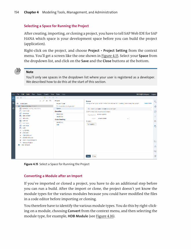
Chapter 4 Modeling Tools, Management, and Administration154
Selecting a Space for Running the Project
After creating, importing, or cloning a project, you have to tell SAP Web IDE for SAP
HANA which space is your development space before you can build the project
(application).
Right-click on the project, and choose Project • Project Setting from the context
menu. You’ll get a screen like the one shown in Figure 4.15. Select your Space from
the dropdown list, and click on the Save and the Close buttons at the bottom.
Note
You’ll only see spaces in the dropdown list where your user is registered as a developer.
We described how to do this at the start of this section.
Figure 4.15 Select a Space for Running the Project
Converting a Module after an Import
If you’ve imported or cloned a project, you have to do an additional step before
you can run a build. After the import or clone, the project doesn’t yet know the
module types for the various modules because you could have modified the files
in a code editor before importing or cloning.
You therefore have to identify the various module types. You do this by right-click-
ing on a module, choosing Convert from the context menu, and then selecting the
module type, for example, HDB Module (see Figure 4.16).
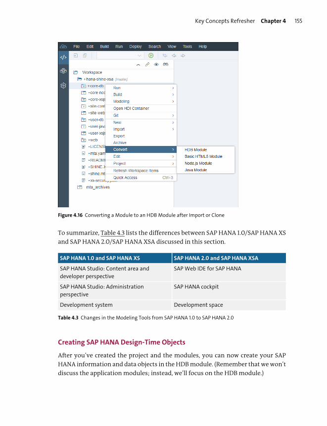
Key Concepts Refresher Chapter 4 155
Figure 4.16 Converting a Module to an HDB Module after Import or Clone
To summarize, Table 4.3 lists the differences between SAP HANA 1.0/SAP HANA XS
and SAP HANA 2.0/SAP HANA XSA discussed in this section.
Creating SAP HANA Design-Time Objects
After you’ve created the project and the modules, you can now create your SAP
HANA information and data objects in the HDB module. (Remember that we won’t
discuss the application modules; instead, we’ll focus on the HDB module.)
SAP HANA 1.0 and SAP HANA XS SAP HANA 2.0 and SAP HANA XSA
SAP HANA Studio: Content area and
developer perspective
SAP Web IDE for SAP HANA
SAP HANA Studio: Administration
perspective
SAP HANA cockpit
Development system Development space
Table 4.3 Changes in the Modeling Tools from SAP HANA 1.0 to SAP HANA 2.0

Chapter 4 Modeling Tools, Management, and Administration156
In SAP Web IDE for SAP HANA, the modules appear as folders. The SAP HANA infor-
mation and data objects appear as files in these folders.
SAP Enterprise Architecture Designer
First, we’ll quickly introduce SAP Enterprise Architecture Designer (SAP EA
Designer). As the name indicates, it’s a tool that you use for designing enterprise
architecture diagrams and models during the planning and design phase of an SAP
HANA project. You can visually create data models and views in this tool. This is
one of the ways to create SAP HANA design-time objects.
You can also use it to reverse-engineer existing SAP HANA information views. In
Figure 4.17, we used the Reverse HDI Files option to create an enterprise architec-
ture diagram of an existing SHINE calculation view. You can use this feature to
help you in migration projects from other databases to SAP HANA or SAP Cloud
Platform. As it can create the required CDS artifacts used by the application pro-
gramming model for SAP Cloud Platform, this functionality can save you a lot of
time. (We’ll discuss CDS in the Creating a Table Using Core Data Services section.)
You can use SAP EA Designer to get a complete overview of new or existing proj-
ects. It allows you to use the collaborative web-based environment to design a
project’s models, data flows, processes, requirements, and so on.
Figure 4.17 SAP Enterprise Architecture Designer

Key Concepts Refresher Chapter 4 157
SAP EA Designer is updated more often than SAP HANA, and new features appear
quite quickly. With SAP HANA SPS 03, we got a new type of table called system-ver-
sioned tables. (We’ll take a quick look at this in Chapter 8.) While there was still lim-
ited documentation about the CDS format for this new table type, we could
already create such tables using the SAP EA Designer tool, and it would create the
required and compliant CDS files for us.
SAP EA Designer provides General Data Protection Regulation (GDPR) support in
data models and can generate the SAP HANA data security features of anonymiza-
tion.
SAP Web IDE for the SAP HANA User Interface
Before we create new SAP HANA design-time objects (files) in SAP Web IDE for SAP
HANA, let’s take a good look around to understand the tool better.
Figure 4.18 shows an annotated overview of a typical screen in SAP Web IDE for SAP
HANA, which is composed of the following:
� A standard menu bar appears across the top of the screen.
� Starting at the left, we see a vertical toolbar with three icons. The first accesses
the Development tool 1, which is the equivalent of the Developer Perspective in
SAP HANA Studio. We use this to create and edit design-time objects.
The second accesses the SAP HANA database explorer 2, which is the equiva-
lent of the Catalog area in SAP HANA Studio. We use this to work with the run-
time objects. We’ll look at the SAP HANA database explorer tool more in the
next section.
� The next area to the right is the Workspace area, which has a folder-like tree
structure. The top folder is the Workspace. Below this we have the project 7 (in
this example, hana-shine-xsa), which is equivalent to an application. The project
folder contains several modules 8, and the modules subfolders contain objects
9 (i.e., files).
� The middle area is the Scenario area k in which we can create and update our
SAP HANA information models. When you open an information model, the
name of the model appears in a tab at the top of this area 4 (in this example, it’s
the PRODUCTS.hdbcalculationview tab). On the left of this area is the palette
toolbar 3, which shows what nodes you can use to create the SAP HANA infor-
mation model.
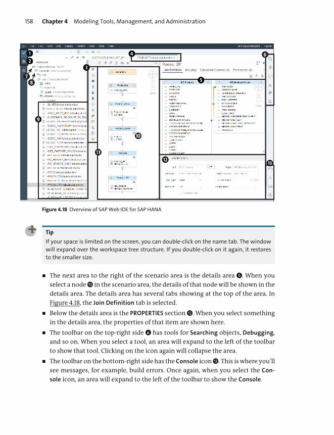
Chapter 4 Modeling Tools, Management, and Administration158
Figure 4.18 Overview of SAP Web IDE for SAP HANA
Tip
If your space is limited on the screen, you can double-click on the name tab. The window
will expand over the workspace tree structure. If you double-click on it again, it restores
to the smaller size.
� The next area to the right of the scenario area is the details area 5. When you
select a node j in the scenario area, the details of that node will be shown in the
details area. The details area has several tabs showing at the top of the area. In
Figure 4.18, the Join Definition tab is selected.
� Below the details area is the PROPERTIES section l. When you select something
in the details area, the properties of that item are shown here.
� The toolbar on the top-right side 6 has tools for Searching objects, Debugging,
and so on. When you select a tool, an area will expand to the left of the toolbar
to show that tool. Clicking on the icon again will collapse the area.
� The toolbar on the bottom-right side has the Console icon m. This is where you’ll
see messages, for example, build errors. Once again, when you select the Con-
sole icon, an area will expand to the left of the toolbar to show the Console.
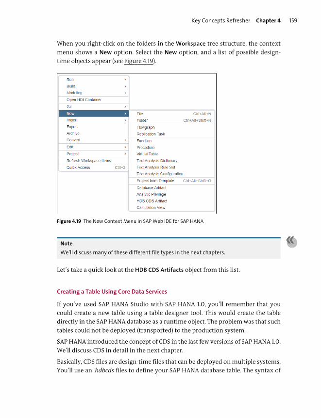
Key Concepts Refresher Chapter 4 159
When you right-click on the folders in the Workspace tree structure, the context
menu shows a New option. Select the New option, and a list of possible design-
time objects appear (see Figure 4.19).
Figure 4.19 The New Context Menu in SAP Web IDE for SAP HANA
Note
We’ll discuss many of these different file types in the next chapters.
Let’s take a quick look at the HDB CDS Artifacts object from this list.
Creating a Table Using Core Data Services
If you’ve used SAP HANA Studio with SAP HANA 1.0, you’ll remember that you
could create a new table using a table designer tool. This would create the table
directly in the SAP HANA database as a runtime object. The problem was that such
tables could not be deployed (transported) to the production system.
SAP HANA introduced the concept of CDS in the last few versions of SAP HANA 1.0.
We’ll discuss CDS in detail in the next chapter.
Basically, CDS files are design-time files that can be deployed on multiple systems.
You’ll use an .hdbcds files to define your SAP HANA database table. The syntax of
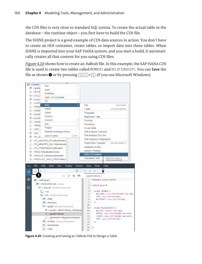
Chapter 4 Modeling Tools, Management, and Administration160
the CDS files is very close to standard SQL syntax. To create the actual table in the
database—the runtime object—you first have to build the CDS file.
The SHINE project is a good example of CDS data sources in action. You don’t have
to create an HDI container, create tables, or import data into these tables. When
SHINE is imported into your SAP HANA system, and you start a build, it automati-
cally creates all that content for you using CDS files.
Figure 4.20 shows how to create an .hdbcds file. In this example, the SAP HANA CDS
file is used to create two tables called MEMBERS and RELATIONSHIPS. You can Save the
file as shown 1 or by pressing (Ctrl)+(S) (if you use Microsoft Windows).
Figure 4.20 Creating and Saving an .hdbcds File to Design a Table

Key Concepts Refresher Chapter 4 161
Documentation
As you near the end of a modeling project, documentation becomes important.
You need to hand your modeling work over to someone else. There are always
good reasons for the many decisions you make, such as why the various nodes of
a calculation view are in a specific order. Documentation tools and features in SAP
HANA, such as notes, allow you to communicate that information to anyone who
may work on your project in the future.
In the context menu of a calculation view (see Figure 4.21), you’ll find a very useful
documentation feature. The Generate Document option documents graphical cal-
culation views in SAP HANA. Figure 4.21 shows an example of the HTML output
generated. You can select an entire module (folder), and it will generate the HTML
documents for all of your calculation views in one go.
Figure 4.21 Generating Documentation of SAP HANA XSA Calculation Views
To summarize, Table 4.4 lists the differences between SAP HANA 1.0/SAP HANA XS
and SAP HANA 2.0/SAP HANA XSA discussed in this section.
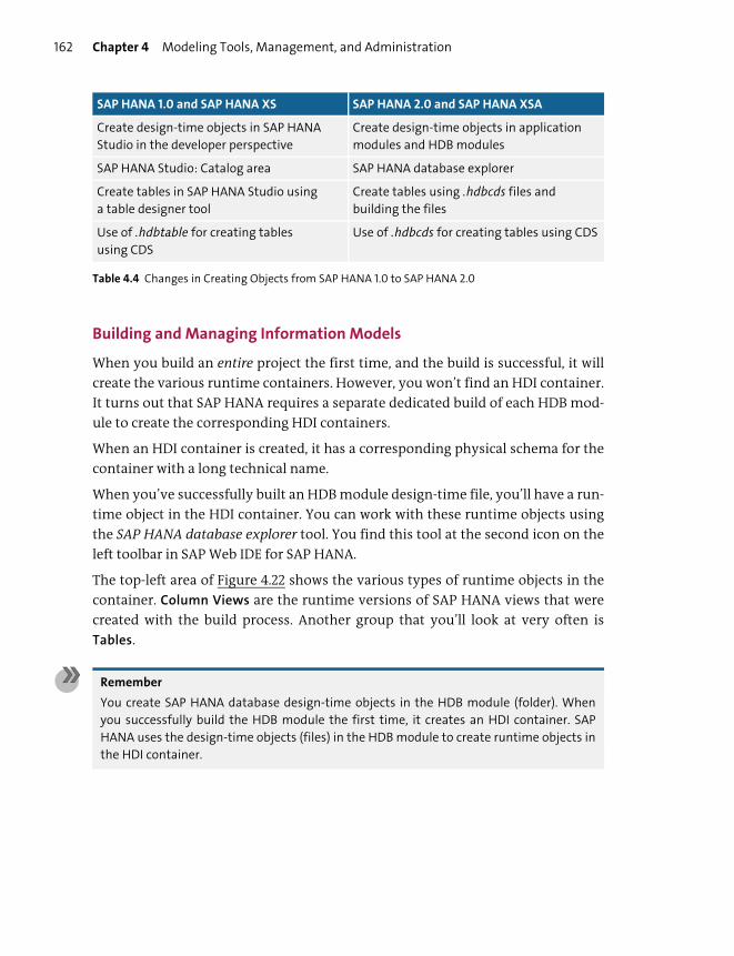
Chapter 4 Modeling Tools, Management, and Administration162
Building and Managing Information Models
When you build an entire project the first time, and the build is successful, it will
create the various runtime containers. However, you won’t find an HDI container.
It turns out that SAP HANA requires a separate dedicated build of each HDB mod-
ule to create the corresponding HDI containers.
When an HDI container is created, it has a corresponding physical schema for the
container with a long technical name.
When you’ve successfully built an HDB module design-time file, you’ll have a run-
time object in the HDI container. You can work with these runtime objects using
the SAP HANA database explorer tool. You find this tool at the second icon on the
left toolbar in SAP Web IDE for SAP HANA.
The top-left area of Figure 4.22 shows the various types of runtime objects in the
container. Column Views are the runtime versions of SAP HANA views that were
created with the build process. Another group that you’ll look at very often is
Tables.
Remember
You create SAP HANA database design-time objects in the HDB module (folder). When
you successfully build the HDB module the first time, it creates an HDI container. SAP
HANA uses the design-time objects (files) in the HDB module to create runtime objects in
the HDI container.
SAP HANA 1.0 and SAP HANA XS SAP HANA 2.0 and SAP HANA XSA
Create design-time objects in SAP HANA
Studio in the developer perspective
Create design-time objects in application
modules and HDB modules
SAP HANA Studio: Catalog area SAP HANA database explorer
Create tables in SAP HANA Studio using
a table designer tool
Create tables using .hdbcds files and
building the files
Use of .hdbtable for creating tables
using CDS
Use of .hdbcds for creating tables using CDS
Table 4.4 Changes in Creating Objects from SAP HANA 1.0 to SAP HANA 2.0
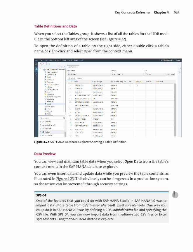
Key Concepts Refresher Chapter 4 163
Table Definitions and Data
When you select the Tables group, it shows a list of all the tables for the HDB mod-
ule in the bottom left area of the screen (see Figure 4.22).
To open the definition of a table on the right side, either double-click a table’s
name or right-click and select Open from the context menu.
Figure 4.22 SAP HANA Database Explorer Showing a Table Definition
Data Preview
You can view and maintain table data when you select Open Data from the table’s
context menu in the SAP HANA database explorer.
You can even insert data and update data while you preview the table contents, as
illustrated in Figure 4.23. This obviously can be dangerous in a production system,
so the action can be prevented through security settings.
SPS 04
One of the features that you could do with SAP HANA Studio in SAP HANA 1.0 was to
import data into a table from CSV files or Microsoft Excel spreadsheets. One way you
could do it in SAP HANA 2.0 was by defining a CDS .hdbtabledata file and specifying the
CSV file. With SPS 04, you can now import data from medium-sized CSV files or Excel
spreadsheets using the SAP HANA database explorer.
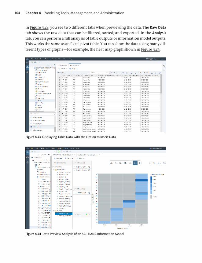
Chapter 4 Modeling Tools, Management, and Administration164
In Figure 4.23, you see two different tabs when previewing the data. The Raw Data
tab shows the raw data that can be filtered, sorted, and exported. In the Analysis
tab, you can perform a full analysis of table outputs or information model outputs.
This works the same as an Excel pivot table. You can show the data using many dif-
ferent types of graphs—for example, the heat map graph shown in Figure 4.24.
Figure 4.23 Displaying Table Data with the Option to Insert Data
Figure 4.24 Data Preview Analysis of an SAP HANA Information Model

Key Concepts Refresher Chapter 4 165
SQL Console
In the Raw Data tab, you also have the Edit SQL Statement in SQL Console option,
which opens a SQL statement for viewing the table or viewing data in the SQL Con-
sole tool.
You can now modify the SQL statement and see the results below it, as shown in
Figure 4.25.
Figure 4.25 Data Preview of an SAP HANA Information Model
Note
Never use the SQL Console to create database objects. You can use it to observe changes
in reading data and for opening the Analyze SQL tool. We discuss this very useful tool in
Chapter 12.
You have to create SAP HANA database objects using CDS.
If you create an SAP HANA database object using the SQL Console, only the run-
time version of the object will exist in the current HDI container. No design-time
object will exist.

Chapter 4 Modeling Tools, Management, and Administration166
When you build and deploy your HDB module/HDI container to another space,
the build and deployment will be successful. The object you created using the SQL
Console will, however, be missing from that space because only the design-time
objects get built and deployed.
If you wanted to create objects using the SQL Console, you would have to manually
do it the same way in every space (system). Another problem with doing this is
that someone needs similar security access to create it in the production environ-
ment, which is a huge security risk.
Naming Runtime Objects
When you build a design-time object, the build process creates the runtime ver-
sion of that object. The question we ask now is, “What is the name of that runtime
object in the container?” This is important to know, as this is the name that analyt-
ics or reporting users need to use.
The intuitive assumption is that the file name of the design-time object will be the
name of the runtime object. For most objects, that assumption will work, but it
won’t work for all objects. If you look at Figure 4.20 again, you’ll see that you create
two tables with one .hdbcds design-time definition file. We can’t give both tables
the same name. Therefore, runtime objects are named as <namespace>::<object-name>.
We mentioned namespaces before when we said there was a difference between a
space, a workspace, and a namespace. A namespace is used when naming develop-
ment and modeling objects, and it helps determine the name of the runtime
objects in the containers.
By default, the namespace is blank. If you have a design-time object called
View1.hdbcalculationview, the default name for the runtime object will be ::View1.
Note
The runtime object name is the same as the file name of the design-time object, without
the file extension, for example, .hdbcalculationview.
Because the runtime object names must be unique, you shouldn’t have View1.hdbcalcu-lationview and View1.hdbfunction in the same folder as both will generate runtime
objects with the name ::View1.
In a small project, there is probably not much to be gained by specifying a name-
space. In larger projects, or when developing libraries and application program-
ming interfaces (APIs), you get to the situation where some objects can have the
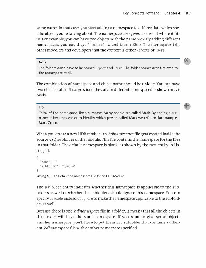
Key Concepts Refresher Chapter 4 167
same name. In that case, you start adding a namespace to differentiate which spe-
cific object you’re talking about. The namespace also gives a sense of where it fits
in. For example, you can have two objects with the name Show. By adding different
namespaces, you could get Report::Show and Users::Show. The namespace tells
other modelers and developers that the context is either Reports or Users.
Note
The folders don’t have to be named Report and Users. The folder names aren’t related to
the namespace at all.
The combination of namespace and object name should be unique. You can have
two objects called Show, provided they are in different namespaces as shown previ-
ously.
Tip
Think of the namespace like a surname. Many people are called Mark. By adding a sur-
name, it becomes easier to identify which person called Mark we refer to, for example,
Mark Green.
When you create a new HDB module, an .hdinamespace file gets created inside the
source (src) subfolder of the module. This file contains the namespace for the files
in that folder. The default namespace is blank, as shown by the name entity in Lis-
ting 4.1.
{"name": """subfolder": "ignore"
}
Listing 4.1 The Default.hdinamespace File for an HDB Module
The subfolder entity indicates whether this namespace is applicable to the sub-
folders as well or whether the subfolders should ignore this namespace. You can
specify cascade instead of ignore to make the namespace applicable to the subfold-
ers as well.
Because there is one .hdinamespace file in a folder, it means that all the objects in
that folder will have the same namespace. If you want to give some objects
another namespace, you’ll have to put them in a subfolder that contains a differ-
ent .hdinamespace file with another namespace specified.
Chapter 4 Modeling Tools, Management, and Administration168
You can also specify the namespace in a design-time file, but then it must corre-
spond to the namespace specified in the .hdinamespace file. Conflicts will cause
build errors. Remember the namespace is specified by the .hdinamespace file in
the same folder or by an .hdinamespace file in the parent folder with cascading
enabled.
Tip
If no .hdinamespace file is found, or if the .hdinamespace file is empty, the namespace is
assumed to be blank.
We’ve mentioned that by default the file name of the design-time object deter-
mines the name of the runtime object. The exception to this is where we have
design-time files in which many objects are specified in a single file. We already
saw an example in Figure 4.20, where we created two tables—MEMBERS and RELA-
TIONSHIPS—with the graphf.hdbcds design-time definition file. If our namespace is
specified as tables.graph, the runtime objects will be called tables.graph::MEMBERS
and tables.graph::RELATIONSHIPS. In this case, the file name graphf is ignored.
Synonyms are another example. You can create many synonyms in a single .hdb-
synonym file.
Tip
When you need to access an external data source, you must first define a local synonym
in an .hdbsynonym file. You might also need to create or update the .hdbgrants (“permis-
sions”) file to ensure that the external data source can actually be accessed.
Build Errors
You know by this time that you need to build the design-time file to create the run-
time files. End users use the runtime files (refer to the top-right side of Figure 4.2).
When you’re developing or modeling SAP HANA information views, you only
have the design-time files. Until you do the build, no one can run these views.
Tip
When you want to view the results of a calculation view, you need to first build the view.
If you make some changes, save the view, and then ask for a preview of the data without
building it first, you’ll get the results from the previous build—without your latest
changes.

Key Concepts Refresher Chapter 4 169
In a book, it’s easy to show you the build menu and assume that all will go well. But
in real life, you’ll occasionally get build errors. You need to know why you get the
errors because that will help you figure out how to solve them. We’ll examine
some examples of build errors in the following.
Figure 4.26 shows a build error in the console window at the bottom. The high-
lighted error message reads no measure or attribute present. In this case, we
haven’t yet mapped the input fields to the output fields, and the view had no out-
put fields in the top layer. We’ll look more at how to create this type of view in
Chapter 6.
Figure 4.26 A Build Error
Sometimes the build messages aren’t that clear. Then you’ll have to understand
which other objects your view may depend on.
Let’s look at an example where you use a table from another schema in your view.
When you build only your view—not the entire HDB module—you might get a
build error. When you’re using a table from another schema, you already know
that you need a synonym and an authorization assigned. You might also need a
user-defined cross-schema service if the table is from a classic database schema. If,
Chapter 4 Modeling Tools, Management, and Administration170
for example, the synonym isn’t yet built, you’ll get a build error. You could also get
build errors because you don’t have the authorization, the service hasn’t been
deployed yet, or even that the other schema and tables haven’t yet been created in
the space (system) where you’re doing the build.
Build errors can really get tricky when you start renaming or deleting objects.
Sometimes you can introduce build errors when you refactor your code or models.
Refactoring
Refactoring is the process of restructuring your information models without
changing their external behavior (i.e., their result sets). You do this to improve,
simplify, and clarify the design of your models, for example, when you move
information models inside the system from one module to another or when you
rename an information model.
Renaming or moving an information model isn’t always a trivial task. If the infor-
mation model is used in many other models, you’ll have to update those models
as well. You can easily find yourself having to update tens of information models
when simply trying to rename a single information model that these models all
use.
Concepts such as refactoring are used in larger projects to ensure your modeling
work stays fresh and useful. The idea is similar to gardening: you need to mow the
lawn, pull weeds, and prune the roses to maintain a beautiful garden. This idea of
upkeep can also be applied to the administration of your data models.
We’ll start by looking at some of the refactoring features in SAP HANA. After that,
we’ll look at some examples of what to watch out for so that you don’t break your
models.
Where-Used
In the refactoring process, you may have to figure out where a specific information
model is used. Figure 4.27 shows the context menu of an information model in the
SAP HANA database explorer. By selecting the Where-Used Browser menu option,
SAP HANA finds all the places where that information model is used. This is very
useful to see the impact a planned refactoring will have.

Key Concepts Refresher Chapter 4 171
Figure 4.27 Where-Used Browser Option for Finding Where an SAP HANA Information Model Is Used
Replacing Data Sources and Nodes in an SAP HANA View
Figure 4.28 shows two context menus of nodes in a graphical calculation view. In
this case, you can replace the data sources used in the node or even replace or
delete the entire node.
Figure 4.28 Replacing Data Sources and Nodes in an SAP HANA View
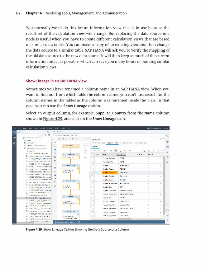
Chapter 4 Modeling Tools, Management, and Administration172
You normally won’t do this for an information view that is in use because the
result set of the calculation view will change. But replacing the data source in a
node is useful when you have to create different calculation views that are based
on similar data tables. You can make a copy of an existing view and then change
the data source to a similar table. SAP HANA will ask you to verify the mapping of
the old data source to the new data source. It will then keep as much of the current
information intact as possible, which can save you many hours of building similar
calculation views.
Show Lineage in an SAP HANA view
Sometimes you have renamed a column name in an SAP HANA view. When you
want to find out from which table the column came, you can’t just search for the
column names in the tables as the column was renamed inside the view. In that
case, you can use the Show Lineage option.
Select an output column, for example, Supplier_Country from the Name column
shown in Figure 4.29, and click on the Show Lineage icon.
Figure 4.29 Show Lineage Option Showing the Data Source of a Column
Key Concepts Refresher Chapter 4 173
Go down the layers of nodes, and you can see that the Supplier_Country column
was introduced by the Addresses table in the second (from the bottom) join node.
This works, even if the column got renamed along the way.
Avoiding and Fixing Errors as a Result of Refactoring
We end our journey into the new world of SAP HANA 2.0 by looking at some exam-
ples where the build process gives errors when you might not expect them. By
looking at why this happens, you’ll also understand the build process better.
For our first example, we look at a case with two information models called A and
B. We start by creating Model A, and then we create Model B based on Model A. We
know that we have to build Model A first because Model B depends on it.
When we’ve successfully built both models, we rename a field inside Model A. This
field is used in Model B. When we build the models we expect Model A to build suc-
cessfully as the field was just renamed, and this won’t break the model. We expect
the build of Model B to give an error that it can’t find the field it expects from
Model A.
In this case, our expectation is wrong. The build of Model A will give an error. SAP
HANA does an end-to-end check when you do the build, even if you just ask it to
only build Model A. It sees that Model B depends on Model A and that one of the
fields that Model B requires from Model A isn’t there anymore. Because Model A is
now breaking the “contract” it has with Model B, the build of Model A will give an
error.
Remember
SAP HANA does an end-to-end check when doing a build, even if you just ask it to build a
single model.
Instead of renaming a field in Model A, what happens if we rename Model A to
Model E? In this case, the build of Model E (the new name) will be successful, but
the build of Model B, or the build of the entire HDB module (Model B and Model E),
will fail.
Even though the build process does end-to-end dependency checks, you broke the
link between Model A and Model B by renaming Model A to Model E. Model E is
now independent. Model B is based on Model A, which now doesn’t exist, so the
build gives an error.

Chapter 4 Modeling Tools, Management, and Administration174
Tip
Use the Where-Used option to find which models will “break” before you rename an SAP
HANA information model.
Deleting objects can cause weird effects. Coming back to our example of Model A
and Model B, where Model B is based on Model A, let’s assume we’ve successfully
built both models. The runtime objects for both models exist in the HDI container.
What happens when we delete Model A? When we make a change to Model B, and
rebuild it, we expect the build to fail. But the build succeeds. This is because SAP
HANA does an incremental build. It looks at what needs to be rebuilt. It sees Model
A’s runtime object in the HDI container and sees that it doesn’t need a rebuild, so
it just rebuilds Model B.
If we now do a build of the entire HDB module, it finally realizes that Model A is
deleted and then gives a build error.
Hint
After deleting files from the HDB module, do a build of the entire module.
If you ever want to delete an entire folder or subfolder, don’t just delete the mod-
ule (folder). First delete the files in the folder, and do a build of the module (folder).
Then you can delete the folder.
If you first delete the files, the build process realizes that the design-time files have
been deleted, and it then deletes the runtime objects from the HDI container. If
you delete the entire module (folder), you can’t trigger a build any more, and the
runtime objects won’t get deleted from the HDI container.
Important Terminology
In this chapter, we covered the following important terminology:
� Design-time objects
These objects are definitions (metadata) for what SAP HANA should create
when running information models. They are seen as the “inactive” versions,
and end users can’t run them.
� Runtime version
When you build an information model, SAP HANA checks the model and cre-
ates an “active copy” of the information model in the container (schema). This
active copy is called a runtime version.
Practice Questions Chapter 4 175
� Container
An isolated miniature virtual machine that contains runtime objects.
� Build
The process of creating a runtime object from the design-time files.
� Deploy
The process of distributing your development and modeling work to other sys-
tems, for example, production.
� Git
A powerful open-source repository of design-time objects that allows for ver-
sion control, forking, and merging of branches.
� SAP Web IDE for SAP HANA
The web-based environment used for creating SAP HANA design-time objects.
� SAP HANA database explorer
The web-based tool used to work with SAP HANA runtime objects.
� HDB module
A collection of SAP HANA database design-time objects
� HDI container
The container and schema created when you build an HDB module.
� Refactoring
The process of restructuring your information models without changing their
external behavior to improve, simplify, and clarify the design of your models.
Practice Questions
These practice questions will help you evaluate your understanding of the topics
covered in this chapter. The questions shown are similar in nature to those found
on the certification examination. Although none of these questions will be found
on the exam itself, they will allow you to review your knowledge of the subject.
Select the correct answers, and then check the completeness of your answers in
the “Practice Question Answers and Explanations” section. Remember that on the
exam, you must select all correct answers, and only correct answers, to receive
credit for the question.

Chapter 4 Modeling Tools, Management, and Administration176
1. What development tool is available for creating SAP HANA XSA and HDI infor-
mation models?
� A. SAP HANA Studio
� B. SAP HANA Web-Based Development Workbench
� C. SAP HANA database explorer
� D. SAP Web IDE for SAP HANA
2. True or False: CDS only works with runtime objects.
� A. True
� B. False
3. Refactoring is used with which of the following actions?
� A. Improving your modeling design
� B. Translating
� C. Deployment
� D. Documenting
4. For what tasks would you use the Where-Used option in SAP HANA?
� A. To find all places where an information model has been deployed
� B. To find all places where a developer updated information models
� C. To find all places where an information model is used
5. You have Model B that is based on Model A. You have NOT built any of the
models yet. You delete Model A. What happens during the build? (There are 2
correct answers.)
� A. You get a build error when you build Model B.
� B. The build of Model B is successful.
� C. You get an error when you build the entire HDB module.
� D. The build of the entire HDB module is successful.

Practice Questions Chapter 4 177
6. You have Model B that is based on Model A. You have successfully built both
models. You delete Model B. What happens during the build? (There are 3 cor-
rect answers.)
� A. You get a build error when you build Model A.
� B. The build of Model A is successful.
� C. You get an error when you build the entire HDB module.
� D. The build of the entire HDB module is successful.
� E. Model B gets deleted from the HDI container.
7. What should you use to create tables in an HDI container? (There are 2 correct
answers.)
� A. SQL console
� B. Core data services (CDS)
� C. SAP HANA database explorer
� D. SAP Enterprise Architecture Designer
8. What do you need to read a table from another HDI container in your infor-
mation model? (There are 3 correct answers.)
� A. A user-defined service
� B. Authorization
� C. Synonym
� D. An HDI service
� E. Authentication
9. What do you need to do after creating a new project with an HDB module?
� A. Create an .hdinamespace file
� B. Convert the new module to an HDB module.
� C. Select a space for running the project.
10. True or False: You can use the Show Lineage tool to find out which model
another model is based on.
� A. True
� B. False

Chapter 4 Modeling Tools, Management, and Administration178
Practice Question Answers and Explanations
1. Correct answer: D
You can use SAP Web IDE for SAP HANA to create SAP HANA XSA and HDI infor-
mation models.
SAP HANA Studio and SAP HANA Web-Based Development Workbench were
used with SAP HANA 1.0 and SAP HANA XS. SAP HANA XS has been deprecated
from SAP HANA 2.0 SPS 02. These older tools don’t have functionality to work
with HDI containers.
The SAP HANA database explorer can show HDI container objects but doesn’t
create them.
2. Correct answer: B
False—CDS objects are design-time objects. They create runtime objects when
they are activated. The word “only” makes this statement false.
Tip
Remember that simple true or false questions don’t occur in the certification exam. The
other questions with at three or four answers are more representative of the questions
you’ll find in the certification exam.
3. Correct answer: A
Refactoring is used to improve your modeling design. You can use it, for exam-
ple, to rename SAP HANA models.
Translating is used to translate your models to other languages (e.g., Chinese).
Deployment is taking your modeling work from the development system to
the production system.
Documenting is writing documents and explaining your modeling work.
4. Correct answer: C
You use the Where-Used option in SAP HANA to find all the places an informa-
tion model is used.
5. Correct answers: A, C
You have Model B that is based on Model A. You have NOT built any of the mod-
els yet. You delete Model A: You get a build errors when you build Model B and
the entire HDB module because Model B depends on Model A. You get an error
on Model B because you haven’t yet built either one of the models.

Practice Question Answers and Explanations Chapter 4 179
6. Correct answers: B, D
You have Model B that is based on Model A. You have successfully built both
models. You delete Model B: The build of both Model A and the entire HDB
module is successful.
Model B’s runtime object also gets deleted from the HDI container. You only
deleted the design-time object from the HDB module. The build deletes the
runtime object.
7. Correct answers: B, D
You should use CDS and SAP Enterprise Architecture Designer to create tables
in an HDI container.
You should never use SQL Console to create tables as they can’t be deployed
(transported).
You can’t use SAP HANA database explorer to create tables.
8. Correct answers: B, C, D
You need authorization, a synonym, and an HDI service to read a table from
another HDI container in your information model.
You need a user-defined service when reading a table from a classic database
schema, not from another HDI container.
Authentication is your login credentials, such as a user name and password. Do
not confuse this with authorization, which signifies what you’re allowed to do.
9. Correct answer: C
You need to select a space for running the project after creating a new project
with an HDB module.
An .hdinamespace file is created automatically when you create an HDB mod-
ule.
You only have to convert the new module to an HDB module after an import.
10. Correct answer: B
False. You do NOT use the Show Lineage tool to find out which model another
model is based on. You can use it to find out where a specific column in an
information view originates from.

Chapter 4 Modeling Tools, Management, and Administration180
Takeaway
You should now understand the SAP HANA 2.0 development and modeling pro-
cess and architecture in more detail. After reading this chapter, you should be able
to create a project, create and build new SAP HANA information models, refactor
your modeling work, and solve build error situations.
In addition, you now should have a working knowledge of what happens behind
the scenes when you create and build a model.
Summary
In this chapter, we discussed the SAP HANA modeling tools: SAP Web IDE for SAP
HANA, SAP HANA database explorer, SAP HANA cockpit, SAP EA Designer, and the
SAP HANA XSA cockpit. You know how they work and when to use them.
You can now use this knowledge for the modeling chapters ahead. The next chap-
ter will teach you the fundamentals of modeling.
Chapter 5
Information Modeling Concepts
Techniques You’ll Master
� Understand general data modeling concepts such as views,
cubes, fact tables, and hierarchies
� Know when to use the different types of joins in SAP HANA
� Examine the differences between attributes and measures
� Learn about the different types of information views that
SAP HANA uses
� Get to know projections, aggregations, and unions used in
SAP HANA information views
� Describe core data services (CDS) in SAP HANA
� Get a glimpse of best practices and general guidelines for data
modeling in SAP HANA

Chapter 5 Information Modeling Concepts182
Before moving onto the more advanced modeling concepts, it’s important to
understand the basics. In this chapter, we’ll discuss the general concepts of infor-
mation modeling in SAP HANA. We’ll start off by reviewing views, join types,
cubes, fact tables, hierarchies, the differences between attributes and measures,
the different types of information views that SAP HANA offers, and CDS views.
From there, we’ll take a deeper dive into SAP HANA’s information views, as well as
concepts such as calculated columns, how to perform currency conversions, input
parameters, and so on.
Real-World Scenario
You start a new project. Many of the project team members have some
knowledge of traditional data modeling concepts and describe what they
need in those terms. You need to know how to take those terms and ideas,
translate them into SAP HANA modeling concepts, and implement them in
SAP HANA in an optimal way.
Some of the new concepts in SAP HANA are quite different from what you’re
used to, for example, not storing the values of a cube, but instead calculating
it when required. If you understand these modeling concepts, you can
quickly understand and create real-time applications and reports in SAP
HANA.
Objectives of This Portion of the Test
The objective of this portion of the SAP HANA certification is to test your under-
standing of basic SAP HANA modeling artifacts.
For the certification exam, SAP HANA modelers must have a good understanding
of the following topics:
� The different types of joins available in SAP HANA and when to use each one
� How the SAP HANA information views correspond to traditional modeling arti-
facts
� The different types of SAP HANA views and when to use them
� The purpose of CDS in SAP HANA
Key Concepts Refresher Chapter 5 183
Note
This portion contributes up to 5% of the total certification exam score.
Key Concepts Refresher
This section looks at some of the core data modeling concepts used when working
with SAP HANA and that will be covered on the exam. Let’s start from where the
data is stored in SAP HANA by looking at tables.
Tables
Tables allow you to store information in rows and columns. Inside SAP HANA,
there are different ways of storing data: in row-oriented tables or column-oriented
tables. In a normal disk-based database, we use row-oriented storage because it
works faster with transactions in which we’re reading and updating single records.
However, because SAP HANA works in memory, we prefer the column-oriented
method of storing data in the tables, which allows for the use of compression in
memory, removes the storage overhead of indexes, saves a lot of space, and opti-
mizes performance by loading compressed data into computer processors.
Next, we can begin combining the tables in SAP HANA information models.
Views
The first step in building information models is building views. A view is a database
entity that isn’t persistent and is defined as the projection of other entities, such as
tables.
For a view, we take two or more tables, link these different tables together on
matching columns, and select certain output fields. Figure 5.1 illustrates this pro-
cess.

Chapter 5 Information Modeling Concepts184
Figure 5.1 Database View
There are four steps when creating database views:
1. Select the tables.
Select two or more tables that have related information, for example, two tables
listing the groceries you bought. One table contains the shop where you bought
each item, the date, the total amount, and how you paid for your groceries. The
other table contains the various grocery items you bought.
2. Link the tables.
Next, link the selected tables on matching columns. In our example, perhaps
our two tables both have shopping spree numbers, which should ideally be a
unique number for every shopping trip you took. We call this a key field. You can
link the tables together with joins or unions.
3. Select the output fields.
You want to show a certain number of columns that are of interest, for example,
to use in grocery analytics. Normally, you don’t want all the available columns
as part of the output.
Selected field 1 Join
Left Table Right Table
Foreign key
Primary key
Selected field 2
Selected field 3
View
Selected field 1
Selected field 2
Selected field 3
Result of the view looks like a table
Key Concepts Refresher Chapter 5 185
4. Save the view.
Finally, save your view, and it’s created in the database. These views are some-
times called SQL views. You can even add some filters on your data in the view,
for example, to show only the shopping trips in 2019 or all the shopping trips in
which you bought apples.
When you call this view, the database gathers the data. The database view pulls the
tables out, links them together, chooses the selected output fields, reads the data
in the combined fields, and returns the result set. After this, the view “disappears”
until you call it again. Then, the database deletes all the output from the view. It
doesn’t store this data from the view inside the database storage.
Tip
It’s important to realize that database views don’t store the result data. Each time you
call a view, it performs the full process again.
You might have also heard about materialized views, in which people store the out-
put created by a view in another table. However, in our definition of views, we
stated that a view is a database entity that isn’t persistent; that is the way we use the
term view in SAP HANA.
The data stays in the database tables. When we call the view, the database gathers
the subset of data from the tables, showing us only the data that we asked for. If we
ask a database view for that same data a few minutes later, the database will
regather and recalculate the data.
This concept is quite important going forward because you make extensive use of
views in SAP HANA. For example, SAP HANA creates a cube-like view, sends the
results back to you, and “disappears” again. SAP HANA performs this process fast,
avoiding consuming a lot of extra memory by not storing static results. What
really makes this concept important is the way it enables you to perform real-time
reporting.
In the few minutes between running the same view twice, our data in the table
might have changed. If we use the same output from the view every time, we won’t
get the benefit of seeing the effect of the updated data. Extensive caching of result
sets doesn’t help when we want real-time reporting.
Note
Real-time reporting requires recalculating results because the data can keep changing.
Views are designed to handle this requirement elegantly.
Chapter 5 Information Modeling Concepts186
We’ve discussed the basic type of database views here, but SAP HANA takes the
concept of views to an entirely new level! Before we get there, we’ll look at a few
more concepts that we’ll need for our information-modeling journey.
Cardinality
When joining tables together, we need to define how much data we expect to get
from the various joined tables. This part of the relationship is called the cardinal-
ity.
You’ll typically work with four basic cardinalities. The cardinality is expressed in
terms of how many records on the left side join to how many records on the right
side. The cardinalities are as follows:
� One-to-one
Each record on the left side matches with one record on the right side. For
example, say you have a lookup table of country codes and country names. In
the left table, you have a country code called ZA. In the right table (the lookup
table), this matches with exactly one record, showing that the country name of
South Africa is associated with ZA.
� One-to-many
In this case, each record on the left side matches with many records on the
right side. For example, say you have a list of publishers in the left table. For
one publisher—such as SAP PRESS—you find many published books.
� Many-to-one
This is the inverse of one-to-many in that many records on the left side match
one record on the right side. For example, this case may apply when many peo-
ple in a small village are all buying items at the local corner shop.
� Many-to-many
In this case, many records on the left side match many records on the right side,
such as when many people read many web pages.
Joins
Before we look at the different types of joins, let’s quickly discuss the idea of “left”
and “right” tables. Sometimes, it doesn’t make much difference which table is on
the left of the join and which table is on the right because some join types are sym-
metrical. However, with a few join types, it does make a difference.

Key Concepts Refresher Chapter 5 187
We recommend putting the most important table, seen as the main table, on the
left of the join. An easy way to remember which table should be the table on the
right side of the join is to determine which table can be used for a lookup or for a
dropdown list in an application (see Figure 5.2).
Figure 5.2 Table Used for Dropdown List on Right-Hand Side of a Join
This doesn’t always mean that this table has to be physically positioned on the left
of the screen in our graphical modeling tools. When creating a join in SAP HANA,
the table we start the join from (by dragging and dropping) becomes the left table
of the join.
Databases are highly optimized to work with joins; they are much better at it than
you can hope to be in your application server or reporting tool. SAP HANA takes
this to the next level with its new in-memory and parallelization techniques.
In SAP HANA, there are a number of different types of joins. Some of these are the
same as in traditional databases, but others are unique to SAP HANA. Let’s start by
looking at the basic join types.
Left Table—Invoices
Right Table—Customers
Field 1 Field n Customers
Invoice 1 Customer 1
Invoice 2 Customer 1
Invoice 3 Customer 2
Customers Field 1 … Field n
Customer 1
Customer 2
Customers
Customer 1
Customer 2
Customers lookup

Chapter 5 Information Modeling Concepts188
Basic Join Types
The basic join types that you’ll find in most databases are inner joins, left outer
joins, right outer joins, and full outer joins. You can specify the join types in data-
bases using SQL statements. We’ll discuss SQL in more detail in Chapter 8.
The easiest way to visualize these join types is to use circles, as shown in Figure 5.3.
This is a simplified illustration of what these join types do. (The assumption is that
the tables illustrated here contain unique rows; that is, we join the tables via pri-
mary and foreign keys, as illustrated earlier in Figure 5.1. If the tables contain dupli-
cate records, this visualization doesn’t hold.)
Figure 5.3 Basic Join Types and Their Result Sets
The left circle represents the table on the left side of the join. In Figure 5.3, the left
table contains the two values A and B. The right circle represents the table on the
right side of the join and contains the values B and C.
Right Table
B
C
Left Table
A
B
Right Table
B
C
Left Table
A
B
Right Table
B
C
Left Table
A
B
Inner Join
B B
Right Table
B
C
Left Table
A
B
Full Outer Join
A NULL
B B
NULL C
Left Outer Join
A NULL
B B
Right Outer Join
B B
NULL C

Key Concepts Refresher Chapter 5 189
Inner Join
The inner join is the most widely used join type in most databases. When in doubt
and working with a non-SAP HANA database, try an inner join first.
The inner join returns the results from the area where the two circles overlap. In
effect, this means that a value is shown only if it’s found to be present in both the
left and the right tables. In our case, in Figure 5.3, you can see that the value B is
found in both tables. Because we’re only working with the “overlap” area, it doesn’t
matter for this join type which table is on the left or on the right side of the join.
Left Outer Join
When using an inner join, you may find that you’re not getting all the data back
that you require. To retrieve the data that was left out, you use a left outer join.
You’ll only use this join type when this need arises.
With a left outer join, everything in the table on the left side is shown (first table).
If there are matching values in the right table, these are shown. If there are any
“missing” values in the right-hand table, these are shown with a NULL value. For this
join type, it’s important to know which tables are on the left and the right side of
the join.
Right Outer Join
The inverse of the left outer join is the right outer join. This shows everything from
the right table (second table). If there are matching values in the left table, these
are shown. If there are any missing values in the left-hand table, these are shown
with a NULL value.
Full Outer Join
As of SAP HANA 1.0 SPS 11, we have the full outer join. Many other databases also
have this join type, so it’s still regarded as one of the four basic join types. This join
type combines the result sets of both the left outer join and right outer join into a
single result set.
Self-Joins
There isn’t really a join type called a self-join; the term refers to special cases in
which a table is joined to itself. The same table is both the left table and the right
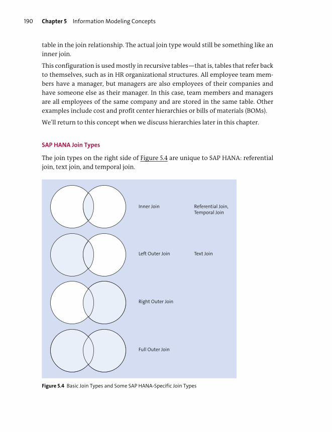
Chapter 5 Information Modeling Concepts190
table in the join relationship. The actual join type would still be something like an
inner join.
This configuration is used mostly in recursive tables—that is, tables that refer back
to themselves, such as in HR organizational structures. All employee team mem-
bers have a manager, but managers are also employees of their companies and
have someone else as their manager. In this case, team members and managers
are all employees of the same company and are stored in the same table. Other
examples include cost and profit center hierarchies or bills of materials (BOMs).
We’ll return to this concept when we discuss hierarchies later in this chapter.
SAP HANA Join Types
The join types on the right side of Figure 5.4 are unique to SAP HANA: referential
join, text join, and temporal join.
Figure 5.4 Basic Join Types and Some SAP HANA-Specific Join Types
Inner Join
Left Outer Join
Right Outer Join
Referential Join,Temporal Join
Text Join
Full Outer Join
Key Concepts Refresher Chapter 5 191
Referential Join
The referential join type normally returns exactly the same results as an inner
join. So, what’s the difference? There are many areas in which SAP HANA tries to
optimize the performance of queries and result sets. In this case, even though a
referential join gives the same results as an inner join, it provides a performance
optimization under certain circumstances.
The referential join uses referential integrity between the tables in the join. Refer-
ential integrity is used in a business system to ensure that data in the left and right
tables match. For example, we can’t have an invoice that isn’t linked to a customer,
and the customer must be inserted into the database before we’re allowed to cre-
ate an invoice for that customer. Note that you don’t need a value on both sides of
the join: you may have a customer without an invoice, but you may not have an
invoice without a customer.
If we can prove that the data in our tables has referential integrity, which most
data in financial business systems has, then we can use a referential join. In this
case, if we’re not reading any data from the right table, then SAP HANA can quite
happily ignore the entire right table and the join itself, and it doesn’t have to do
any checking, which speeds up the whole process.
To understand referential joins in a bit more detail, let’s look at an example. Let’s
say you have a table on the left of the join containing invoices. The table on the
right contains the products you sold. These tables are joined with a referential join.
Several reports query these tables.
If the report asks for data from both tables, the referential join behaves like an
inner join. If fields from the right table are requested, an inner join is executed.
The interesting aspects of a referential join kick in when a report only requests
fields from the left table containing the invoice data. When no data from the right
table is requested, the join isn’t executed. This is how SAP HANA optimizes the per-
formance of the queries. This case is very common in cubes, which are used in
most analytics, reporting, and business intelligence scenarios. (We’ll explain cubes
in the next sections.)
The only exception to this is the rare instance where the cardinality is 1:n. In this
case, the referential join has to execute the query, even if no fields from the right
table are requested. In that case, it executes an inner join as usual.
Inner joins are slower than referential joins as they will always execute the join,
even if no fields from the right table are requested. Left outer joins perform simi-
larly to referential joins, but they give different results.
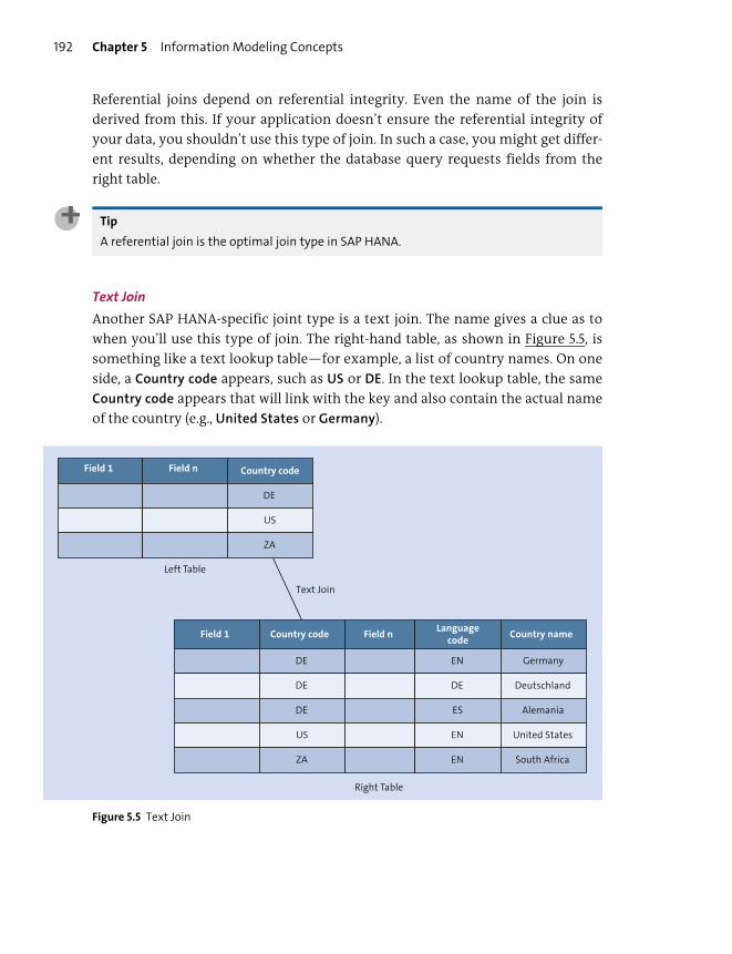
Chapter 5 Information Modeling Concepts192
Referential joins depend on referential integrity. Even the name of the join is
derived from this. If your application doesn’t ensure the referential integrity of
your data, you shouldn’t use this type of join. In such a case, you might get differ-
ent results, depending on whether the database query requests fields from the
right table.
Tip
A referential join is the optimal join type in SAP HANA.
Text Join
Another SAP HANA-specific joint type is a text join. The name gives a clue as to
when you’ll use this type of join. The right-hand table, as shown in Figure 5.5, is
something like a text lookup table—for example, a list of country names. On one
side, a Country code appears, such as US or DE. In the text lookup table, the same
Country code appears that will link with the key and also contain the actual name
of the country (e.g., United States or Germany).
Figure 5.5 Text Join
Text Join
Left Table
Right Table
Field 1 Field n Country code
DE
US
ZA
Field 1 Country code Country nameField nLanguage
code
DE EN Germany
Deutschland
Alemania
United States
South Africa
DE DE
DE ES
US EN
ZA EN

Key Concepts Refresher Chapter 5 193
Note
SAP sells software in many countries, and SAP business systems are available in multiple
languages.
In Figure 5.5, the names of the countries are translated into different languages.
The fourth column in the text lookup table, called the Language code, indicates
into which language the country name has been translated. For example, for the
country called DE and a language code of EN, the name of the country is in English
and thus is Germany. If the language code was DE (for German), the name of the
country would be Deutschland, and if the language code was ES (for Español, indi-
cating Spanish), then the name of the country would be Alemania. Therefore, one
country can have totally different names depending on what language you speak.
In such a case, SAP HANA does something clever: By looking at the browser, the
application server, or the machine that you’re working on, it determines the lan-
guage in which you’ve logged in. If you’re logged in using English, it knows to use
the name Germany. If you’re logged in using German, it provides the German
country name Deutschland for you.
The text join behaves like a left outer join but always has a cardinality of one-to-
one (1:1). In other words, it only returns a single country name based on the lan-
guage you’re logged in with. Even if you’re logged in via mobile phone, your
mobile phone has a certain language setting.
Temporal Join
The temporal join is used when we have FROM and TO date and time fields, or inte-
gers. For example, say you’re storing the fuel price for gasoline in a specific table.
From the beginning of this month to the end of this month, gasoline sells for a cer-
tain price. Next month, the price differs, and, maybe two weeks later, it’s adjusted
again. Later, you’ll have a list of all the gasoline prices for different time periods.
As a car owner, you now want to perform calculations for how much you’ve paid
for your gasoline each time you filled up your tank. However, you just have the
number of gallons and the dates of when you filled up.
You can say, “OK, on this date, I filled up the tank.” You then have to look up which
date range your filling-up date falls within and find the price for that specific date.
You can then calculate what you paid to fill your tank for each of your dates. Figure
5.6 illustrates this example.

Chapter 5 Information Modeling Concepts194
This date range lookup can be a little more complicated in a database. Sometimes,
programmers read the data into an application server and then loop through the
different records. In this case, a temporal join makes it easy because SAP HANA will
perform the date lookups in the FROM and the TO fields automatically for you, com-
pare it to the date you’ve supplied, and get you the right fuel price at that specific
date. It will perform all the calculations automatically for you—a great time and
effort saver.
Figure 5.6 Temporal Join for Gasoline Prices
A temporal join uses an inner join to do the work. A temporal join requires valid
FROM and TO dates (in the gasoline price table) and a valid date-time column (in your
car logbook table).
Spatial Join
Spatial joins became available in SAP HANA 1.0 SPS 09. SAP HANA provides spatial
data types, which we can use, for example, with maps. These all have the prefix ST_.
A location on a map, with longitude and latitude, is an ST_POINT data type. (We’ll
discuss spatial data and analytics further in Chapter 11.)
Temporal JoinLeft Table
Right Table—Pricelist
Field 1 Field n Date
27 February
14 April
13 May
Field 1 From To Gas Price
1 January 28 February 12.22
1 March 1 April 11.45
2 April 25 April 11.50
26 April 10 May 12.77
11 May 25 May 11.33

Key Concepts Refresher Chapter 5 195
We can use special spatial joins between tables in SAP HANA (see Figure 5.7). Say
you have a map location stored in a ST_POINT data type in one table. In the other
table, you have a list of suburbs described in a ST_POLYGON data type. You can now
join these two tables with a spatial join and define the spatial join to use the ST_
CONTAINS method. For each of the locations (ST_POINT), this will calculate in which
suburb (ST_POLYGON) they are located (ST_CONTAINS).
Figure 5.7 Spatial Join
About a dozen methods like ST_CONTAINS are available for spatial joins. For exam-
ple, you can test if a road crosses a river, if one area overlaps another (e.g., mobile
phone tower reception areas), or how close certain objects are to each other.
Dynamic Joins
A dynamic join isn’t really a join type; it’s a join property. It’s also a performance
enhancement available for SAP HANA. After you’ve defined a join, you can mark it
as a dynamic join.
Note
For a dynamic join to work, you have to join the left and right tables on multiple columns.
Spatial Join usingmethod ST_CONTAINS
Left Table
Right Table
Field 1 Field n ST_POINT
(x1, y1)
(x2, y2)
(x2, y3)
Field 1 ST_POLYGON Field n

Chapter 5 Information Modeling Concepts196
Let’s assume you define a static (normal) join on columns A, B, and C between two
tables, as shown in Figure 5.8. In this case, the join criteria on all three columns will
be evaluated every time the view is called in a query.
Figure 5.8 Dynamic Join on Multiple Columns
If you now mark the join as dynamic, the join criteria will only be evaluated on the
columns involved in the query to the view. If you only ask for column A in your
query of the view, then only column A’s join criteria will be evaluated. The join cri-
teria on columns B and C won’t be evaluated, and your system performance
improves.
Tip
If your query doesn’t request any of the join columns in the dynamic join, it will produce a
runtime error.
Lateral Join
We’ve discussed the join types that are used most often. You might also need to use
some specialized join types occasionally. One of these is a lateral join. The lateral
Dynamic Join
Left Table
Right Table
Field 1 A Field nB C
Field 1 A Field nB C

Key Concepts Refresher Chapter 5 197
join helps you do row-by-row processing of data using the database engine, instead
of having to copy the data to the application server and processing it using loops.
Joins like these improve the performance of complex queries by ten or a hundred
times.
SPS 04
In SAP HANA SPS 04, we get a lateral join. Say you want to join a left table to a subquery.
Normally you would write the following:
SELECT A, B FROM TABLE_LEFT INNER JOIN (SELECT C, D FROM RIGHT_TABLE WHERE E < 100) ON …
However, you have cases where you want to let the subquery depend on values in the left
table. Instead of having E < 100 in the preceding statement, you want to use E < TABLE_LEFT.VALUE. You basically want a FOR EACH loop through the left table, computing which
rows should be joined from the right table. You can use a lateral join for this. The lateral
join works together with the INNER and LEFT OUTER joins.
We change the earlier line to the following:
SELECT A, B FROM TABLE_LEFT INNER JOIN LATERAL (SELECT C, D FROM RIGHT_TABLE WHERE E < TABLE_LEFT.VALUE) ON …
We’ve now discussed most of the join types. In the next section, we discuss a con-
cept that has become very important with SAP HANA modeling: CDS views.
Core Data Services Views
CDS is a modeling concept that has become important with SAP HANA 2.0 using
SAP HANA extended application services, advanced model (SAP HANA XSA), as
well as the new application programming model of SAP Cloud Platform. To under-
stand why we need CDS, it’s important to remember the wider context of how SAP
HANA systems are deployed.
While learning SAP HANA, you work with a single system, but productive environ-
ments normally include development, quality assurance, and production systems.
You perform development in the development environment, in which you have
special modeling and development privileges. Your models and code then enter
the quality assurance system for testing. When everyone is satisfied with the
results, the models and code move to the production system. You don’t have any
modeling and development privileges in the quality assurance and production
systems; you therefore need another way to create views and other database
objects in the production system, ideally without giving people special privileges.
Chapter 5 Information Modeling Concepts198
An SAP HANA system can be deployed as the database for an SAP business system.
In such a case, ABAP developers in the SAP business system don’t have any model-
ing and development privileges, even in the SAP HANA database development sys-
tem. We need a way to allow ABAP developers to create views and other database
objects in the database system without these special privileges.
With that in mind, let’s look at why CDS is a good idea with the following example:
You need to create a new schema in your SAP HANA database. It’s easy to use a
short SQL statement to do this, but remember the wider context. Someone will
need the same create privileges in the production system! We want to avoid this
because giving anyone too much authorization in a production system can
weaken security and encourage hackers.
CDS allows for a better way to create such a schema: specify the schema creation
statement once by creating a CDS (text) file with the schema_name="DEMO"; instruc-
tion. CDS files have a .hdbcds file extension. When we deploy this CDS file to the
production system, the SAP HANA system automatically creates the schema for
us. In the background, SAP HANA automatically converts the CDS file into the
equivalent schema creation SQL statement and executes this statement.
The system administrators don’t get privileges to create any schemas in the pro-
duction system. They have rights to import CDS files, but they have no control
over the contents of the CDS files, for example, the name of the schema; that’s
decided by the business. CDS thus gives us a nice way to separate what the busi-
ness needs from what database administration can do.
There’s much more to CDS. You can specify table structures (metadata) and associ-
ations (relationships) between tables with CDS. When deploying this CDS file to
production, it creates the new tables with their relationships. Even more impres-
sive, if you want to modify the table structures later, you just update the CDS file.
When you redeploy the CDS file, SAP HANA doesn’t delete the existing tables and
re-create them; it automatically generates and executes the correct SQL state-
ments to modify only the minimal changes to the existing table structures, for
example, adding only a new column. CDS doesn’t replace SQL statements because
it ultimately translates back into SQL statements. CDS adds the awareness to use a
table creation SQL statement the first time it’s run, but a table modification SQL
statement the second time it’s run. The biggest advantage of this smart behavior is
that the data already stored in a table is kept. If we ran a table creation statement
the second time, it would delete the contents of the table. Not something we want
in a productive system!

Key Concepts Refresher Chapter 5 199
Note
We don’t define the schema name when we create CDS artifacts such as tables. The
schema name is added automatically and is the name of the SAP HANA Deployment
Infrastructure (HDI) container into which the artifacts are deployed.
We can also define new semantic types for when we create tables. Instead of using
a DATE data type for a field, we can define a DELIVERY_DATE. On a lower level, it still
uses a DATE type, but it gives us some business context (e.g., deliveries) when defin-
ing the field. If we later change the semantic type, for example, we add more deci-
mal figures to a PAYMENT type, all tables automatically get updated to reflect the new
behavior.
We can also create views using CDS. These CDS views can be used as data sources
in our SAP HANA information views. Note that these CDS views don’t replace the
more powerful calculation views we can create in SAP HANA. (We discuss these in
Chapter 6 and Chapter 7.) Calculation views are very good for analysis and report-
ing. Developers who create OData services and SAP Fiori screens sometimes prefer
to stick to CDS views, using a text environment rather than the graphical tools.
ABAP developers can also use CDS inside ABAP. When a CDS view is sent to the SAP
HANA system, it creates the necessary SAP HANA database objects without the
ABAP developer having to log in to the SAP HANA database. Because ABAP is data-
base independent, the same CDS file sent to another database will create the data-
base objects relevant to that database. Because of this database independence, the
versions of CDS for ABAP and CDS for SAP HANA have slight differences.
In SAP HANA 1.0, we used the SAP HANA tools to create tables. In SAP HANA 2.0
with HDI, we use CDS to create tables. The tables in a database are often referred to
as the persistence layer.
Tip
If you want to learn CDS better, or are interested in learning more of SAP HANA XSA
development, we recommend that you look at the series of 64 videos that Thomas Jung
created on his private YouTube channel at http://s-prs.co/487601.
The example screens in this book make use of the SAP HANA Interactive Education
(SHINE) demo package described in Chapter 2. SHINE is a good example of CDS in
action. You don’t have to create a schema, create tables, or import data into these
tables. When SHINE is imported and deployed into your SAP HANA system, it
automatically creates all that content for you by using CDS statements. This shows
Chapter 5 Information Modeling Concepts200
how using CDS in your SAP HANA projects keeps everything together—from the
creation of the persistence layer, to views, to security. When you deploy a project
to other systems, these artifacts are automatically created for you during the build
process.
Tip
The SAP Cloud Application Programming Model relies on CDS and is important for model-
ers and developers going forward.
The application programming model is a framework comprised of CDS, service Software
Development Kits (SDKs) for working with services in Java and Node.js, cloud-native plat-
form, and tools in SAP Web IDE working together with local tools on the same projects.
You can read more about the application programming model at http://s-prs.co/v487602.
On the page that appears, click on the Next> link to get a list of tutorials on this topic.
SPS 04
SAP Cloud Application Programming Model is supported with SAP HANA 2.0 SPS 04.
Now, let’s take our knowledge of these concepts to the next “dimension.”
Cube
One of the most important modeling concepts we’ll cover is the cube. We’ll expand
on this concept when we discuss the information views available in SAP HANA. In
this section, we’ll use a very simplistic approach to describing cubes to give you an
understanding of the important concepts.
When you look at a cube the first time, it looks like multiple tables that are joined
together, which might be true at a database level. What makes a cube a cube, how-
ever, are the rules for joining these tables together.
The tables you join together contain two types of data: transactional data and mas-
ter data. As shown in Figure 5.9, the main table in the middle is called a fact table,
which is where our transactional data is stored. The transactional data stored in
the fact table is referred to as either key figures or measures. In SAP HANA, we just
use the term measures.
The side tables are called dimension tables, and this is where our master data is
stored, which is referred to as characteristics, attributes, or sometimes even facets.

Key Concepts Refresher Chapter 5 201
In SAP HANA, we just use the term attributes. In the following sections, we’ll walk
through an example and then provide you with some definitions of key terms.
Figure 5.9 Cube Features
Example
Our cube example will be simplified to communicate the most basic principles. In
our example, we’ll work with the sentence “Laura buys 10 apples.” You’ll agree that
this sentence describes a financial transaction: Laura went to the shop to buy
some apples, she paid for them, and the shop owner made some profit.
Where will we store this transaction’s data in the cube? There are a couple of rules
that we have to follow. The simplest rule is that you store the data on which you
can perform calculations in the fact table, and you store all other data on which
you can’t perform calculations in the dimension tables.
In our transaction of “Laura buys 10 apples,” we first look at Laura. Can we perform
a calculation on Laura? No, we can’t. Therefore, we should put her name into one
of the dimension tables. We put her name in the top dimension table in Figure
Dimension TableFact Table
Dimension Table
Dimension Table
ContainsAttributes
ContainsAttributes
ContainsAttributes
ContainsMeasures

Chapter 5 Information Modeling Concepts202
5.10. Laura isn’t the only customer of that shop; her name is stored with those of
many other people in this dimension table. We’ll call this table the customer
dimension table.
Figure 5.10 Financial Transaction Data Stored in a Cube
Next, let’s look at the apples. Can we perform calculations on apples? No, we can’t,
so again this data goes into a dimension table. The shop doesn’t sell only apples; it
also sells a lot of other products. The second dimension table is therefore called the
product dimension table.
In an enterprise data warehouse (EDW), we would normally limit the number of
dimension tables that we link to the fact table for performance reasons. Typically,
in an SAP Business Warehouse (SAP BW) system, we limit the number of dimen-
sion tables to a maximum of 16 or 18.
Finally, let’s look at the number of apples, 10. Can we perform a calculation on
that? Yes we can, because it’s a number. We therefore store that number in the fact
table.
To complete the picture, if Laura buys more apples, then she is a top customer; let’s
say she’s customer number 2. Apples are something the store keeps in stock, so
apples are product number 7.
If we store a link (join) to customer 2 and another link (join) to product 7 and the
number 10 (number of apples), we would say that it constitutes a complete trans-
action. We can abbreviate the transaction “Laura buys 10 apples” to 2, 10, and 7 in
Product 7—Apples
Customer 2—Laura,Product 7—Apples,
Quantity—10
Customer 2—Laura
Customer table
Product table
Financial transaction:Laura buys 10 apples
Key Concepts Refresher Chapter 5 203
our specific cube (2 indicates Laura, 10 indicates the number of apples, and 7 the
apples).
Laura and apples are part of our master data. The transaction itself is stored in the
fact table. We’ve now put a real-life transaction into the cube.
Tip
You can have master data without associated transactions. As the shopkeeper, you have
apples (master data) for sale, but no one has bought them yet (no transaction). Similarly
you can have customers such as Laura (master data) but no invoice yet.
The reverse doesn’t apply, however. You can’t have an invoice without a customer or
products.
Hopefully, this gives you a better idea of what a cube is and how to use it. Let’s
complete this short tour of cubes by clarifying a few terms ahead.
Key Terms
As previously shown in Figure 5.9, attributes are stored in dimension tables, and
measures are stored in fact tables. Let’s define attributes and measures:
� Attributes
Attributes describe the parts of a transaction, such as the customer Laura or the
product apples. This is also referred to as master data. We can’t perform calcula-
tions on attributes.
� Measures
Measures are something we can measure and perform calculations on. Measur-
able (transactional) information goes into the fact table.
Other key terms to be aware of are as follows:
� Fact tables in the data foundation
Figure 5.10 showed only a single fact table, but sometimes we have more com-
plex cubes that include multiple fact tables. In SAP HANA, we call a group of fact
tables (or the single fact table) the data foundation, although some people refer
to the entire group of tables as the fact table.
Tip
When we join the data foundation (fact tables) to the dimension tables, we always put
the data foundation on the left side of the join.

Chapter 5 Information Modeling Concepts204
� Star joins
The join between the data foundation and the dimension tables is normally a
referential join in SAP HANA. We refer to this as a star join, which indicates that
this isn’t just a normal referential join between low-level tables but also a join
between a data foundation and dimension tables. This is seen as a join at a
higher level.
Remember
You use star joins to join dimension tables to a fact table.
With all the building blocks in place, let’s start examining the graphical SAP HANA
information views.
Calculation Views
Let’s start our introduction to SAP HANA information views by looking back at
what we learned when we discussed cubes. When we graphically build complex
views in SAP, we call these calculation views. These are different from SQL views
and CDS views. Calculations views can be far more powerful and complex than
these other views.
We’ll now take what we’ve learned, and see how SAP HANA implements this with
different types of calculation views. We can then combine these calculation views
to build complex information models.
Types of Calculation Views
SAP HANA has three types of calculation views:
� Dimension views
The first thing we need to build cubes is the master data. Master data is stored in
dimension tables. Sometimes, dimension tables are created for the cubes. In
SAP HANA, we don’t create dimension tables as separate tables; instead, we
build them as views by using the master data tables.
We join all the low-level database tables that contain the specific master data
we’re interested in into a view. For example, we might join two tables in a view
to build a new Products dimension in SAP HANA, and maybe another three
tables to build a new Customers dimension.
Key Concepts Refresher Chapter 5 205
We use calculation views of type dimension, also called dimension calculation
views. In this book, we’ll refer to these type of views simply as dimension views.
Just as the same master data is used in many cubes, we’ll reuse dimension views
in many of the other SAP HANA information views. We can even build our own
library of dimension views.
� Star join views
In the same way, instead of storing data in cubes, we can create another type of
view in SAP HANA that produces the same results as a traditional cube. These
views produce the same results as an old-fashioned, traditional cube called cal-
culation views of type cube with star join.
Terminology
In this book, we’ll simply refer to these types of views as star join views, not as cube views,
which would lead to confusion. This is because the third type of SAP HANA view is a calcu-
lation view of type cube.
The results created by the star join views in SAP HANA are the same as that of a
cube in an EDW, except that in a data warehouse, the data is stored in a cube.
With SAP HANA, the data isn’t stored in a cube but is calculated when required.
To build a star join view, follow these steps:
– Create the dimension views you need as separate calculation views of type
dimension.
– In the calculation view of type cube with star join (star join view), join the
transaction tables together to form the data foundation.
– Join the data foundation (or single fact table) to the dimension calculation
views using star joins.
� Cube views
This view type provides even more powerful capabilities. For example, you can
combine multiple star join views (“cubes”) to produce a combined result set. In
SAP BW, we call this combined result set a MultiProvider. In SAP HANA, we call
these calculation views of type cube. Use cases for this type of view include the
following:
– In your holding company, you want to combine the financial data from mul-
tiple subsidiary companies.
– You want to compare your actual expenses for 2019 with your planned bud-
get for 2019.

Chapter 5 Information Modeling Concepts206
– You have archived data in an archive database that you want to combine with
current data in SAP HANA’s memory to compare sales periods over a number
of years.
Using and Building the Information Model
Now that you know how to build individual views, let’s examine how to use the
different types of SAP HANA calculation views together in information modeling.
Figure 5.11 provides an overview of everything you’ve learned in this chapter and
how each topic fits together.
Figure 5.11 Different SAP HANA Calculation Views Working Together
On the top left-hand side, you can see our source systems: an SAP source system
and a non-SAP source system. SAP HANA doesn’t care from which system the data
comes. In many projects, we have more non-SAP systems that we get data from
Data provisioning tool, e.g. SDI
SAP source system
Database
Non-SAP source system
Database
Report or query
HTML5 browser
Star-join view
(“Cube”)
Star-join view
(“Cube”)
Application server
SAP HANA
Calculation view of type cube
Union
Star-join view (“Cube”)Tables
Table 1 Table 8
Table 2 Table 9
Table 3 Table 10
Table 4 Table 11
Table 5 Table 12
Table 6
Table 7 Data Foundation
Apples
Quantity – 10
Laura
Customerdimension view
Productsdimension view
Star Join(Logical Join)

Key Concepts Refresher Chapter 5 207
than SAP systems. We extract the data from these systems using various data pro-
visioning tools, which we’ll look at in Chapter 9.
The data is stored in row tables in these source systems. When we use data provi-
sioning methods and tools, the data is put into column tables in the SAP HANA
database, as illustrated in the bottom-left corner of Figure 5.11.
Now, let’s start building our information models on top of these tables. If we want
to build something like a cube for our analytics or reporting, we use SAP HANA cal-
culation views. First, we need the equivalent of a dimension table, such as our
product or customer dimension table. To do this, we’ll build a dimension view (a
calculation view of type dimension). This is indicated in Figure 5.11 by Laura and
Apples, which represent the customer and product dimension views. We create
these dimension views the same way we create any other view: take two tables,
join them together, select certain output fields, and save it.
After the dimension views are created, we build a data foundation for the cube. The
data foundation is for all the transactional data. The data foundation stores mea-
sures, such as the number 10 for the 10 apples that Laura bought. We build a data
foundation in a similar fashion to building a dimension view via either multiple
tables or a single table. If using multiple tables, we join them together, select the
output fields, and build our data foundation.
To complete the cube, we have to link our data foundation (fact tables) to the
dimensions with a star join. Finally, to complete our star join view, we also select
the output fields for our cube. The created star join view will produce the same
result as a cube, but, in this case, no data is stored, and it performs much better.
In the next step, we can create a calculation view of type cube, in which we com-
bine two star join views (cubes). We can combine the star join views using a join or
a union. We recommend a union in this case because it leads to better perfor-
mance than a join.
Finally, we can build reports, analytics, or applications on our calculation view, as
shown in the top right of Figure 5.11.
Let’s now think about the process from the other side and look at what happens
when we call our report or application that is built on the calculation view on the
right side of our diagram. This is the top-down view of Figure 5.11.
The calculation view doesn’t store the data; instead, it has to gather and calculate
all the data required by the report. SAP HANA looks at the calculation view’s
description and recognizes that it has to build two star join views and union them
together by first determining how to build the star join views.
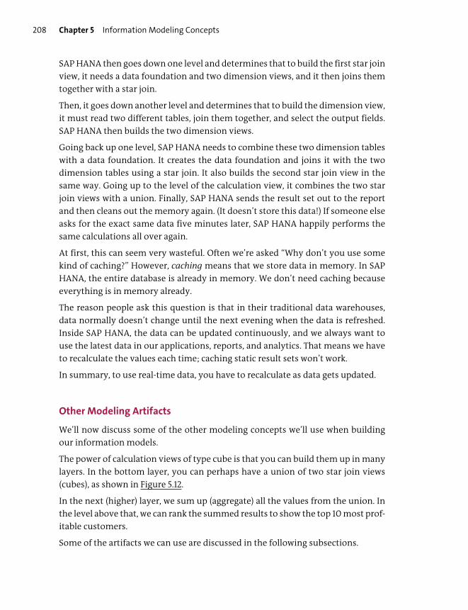
Chapter 5 Information Modeling Concepts208
SAP HANA then goes down one level and determines that to build the first star join
view, it needs a data foundation and two dimension views, and it then joins them
together with a star join.
Then, it goes down another level and determines that to build the dimension view,
it must read two different tables, join them together, and select the output fields.
SAP HANA then builds the two dimension views.
Going back up one level, SAP HANA needs to combine these two dimension tables
with a data foundation. It creates the data foundation and joins it with the two
dimension tables using a star join. It also builds the second star join view in the
same way. Going up to the level of the calculation view, it combines the two star
join views with a union. Finally, SAP HANA sends the result set out to the report
and then cleans out the memory again. (It doesn’t store this data!) If someone else
asks for the exact same data five minutes later, SAP HANA happily performs the
same calculations all over again.
At first, this can seem very wasteful. Often we’re asked “Why don’t you use some
kind of caching?” However, caching means that we store data in memory. In SAP
HANA, the entire database is already in memory. We don’t need caching because
everything is in memory already.
The reason people ask this question is that in their traditional data warehouses,
data normally doesn’t change until the next evening when the data is refreshed.
Inside SAP HANA, the data can be updated continuously, and we always want to
use the latest data in our applications, reports, and analytics. That means we have
to recalculate the values each time; caching static result sets won’t work.
In summary, to use real-time data, you have to recalculate as data gets updated.
Other Modeling Artifacts
We’ll now discuss some of the other modeling concepts we’ll use when building
our information models.
The power of calculation views of type cube is that you can build them up in many
layers. In the bottom layer, you can perhaps have a union of two star join views
(cubes), as shown in Figure 5.12.
In the next (higher) layer, we sum up (aggregate) all the values from the union. In
the level above that, we can rank the summed results to show the top 10 most prof-
itable customers.
Some of the artifacts we can use are discussed in the following subsections.
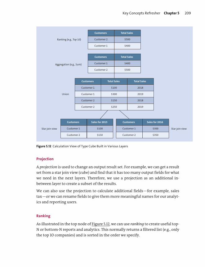
Key Concepts Refresher Chapter 5 209
Figure 5.12 Calculation View of Type Cube Built in Various Layers
Projection
A projection is used to change an output result set. For example, we can get a result
set from a star join view (cube) and find that it has too many output fields for what
we need in the next layers. Therefore, we use a projection as an additional in-
between layer to create a subset of the results.
We can also use the projection to calculate additional fields—for example, sales
tax—or we can rename fields to give them more meaningful names for our analyt-
ics and reporting users.
Ranking
As illustrated in the top node of Figure 5.12, we can use ranking to create useful top-
N or bottom-N reports and analytics. This normally returns a filtered list (e.g., only
the top 10 companies) and is sorted in the order we specify.
Union
Aggregation (e.g., Sum)
Ranking (e.g., Top 10)
Star join view Star join view
Customers
Customer 2
Customer 1
Total Sales
$500
$400
Customers
Customer 1
Customer 2
Total Sales
$400
$500
Customers
Customer 1
Customer 2
Sales for 2015
$100
$150
Customers
Customer 1
Customer 2
Sales for 2016
$300
$350
Customers
Customer 1
Customer 1
Total Sales
$100
$300
Customer 2
Customer 2
$150
$250
Total Sales
2018
2019
2018
2019
Chapter 5 Information Modeling Concepts210
Aggregation
The word aggregation means a collection of things. In SQL, we use aggregations to
calculate values such as the sum of a list of values. Aggregations in databases pro-
vide the following functions:
� Sum
Adds up all the values in the list.
� Count
Counts how many values (records) there are in the list.
� Minimum
Finds the smallest value in the list.
� Maximum
Finds the largest value in the list.
� Average
Calculates the arithmetical mean of all the values in the list.
� Standard deviation
Calculates the standard deviation of all the values in the list.
� Variance
Calculates the variance of all the values in the list.
Normally, we would only calculate aggregations of measures. (Remember that
measures are values we can perform calculations on, which usually means our
transactional data.) For example, we could calculate the total number of apples a
shop sold in 2019. However, in SAP HANA, we can also create aggregations of attri-
butes, essentially creating a list of unique values.
Union
A union combines two result sets. Figure 5.12, shown previously, illustrates this by
combining the results of two star join views.
In SAP HANA graphical calculation views, we’re not restricted to combining two
result sets; we can combine multiple result sets. SAP HANA merges these multiple
result sets into a single result set.
Let’s say we have four result sets—A, B, C, and D—that we union together.
Although we union multiple result sets, that doesn’t mean the performance will be
bad. If SAP HANA detects that you’re not asking for data from A and D, it won’t
even generate the result sets for A and D; it will only work with B and C.
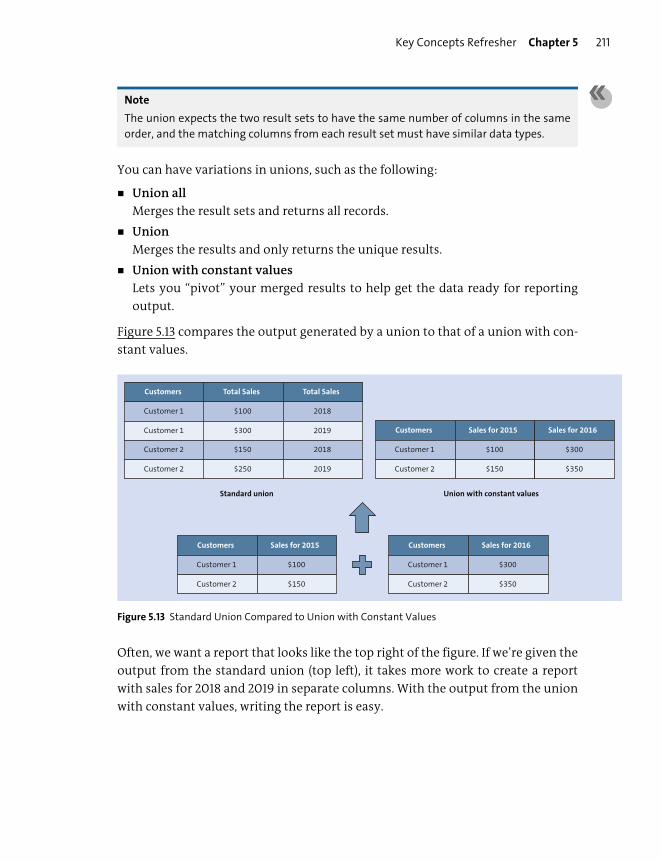
Key Concepts Refresher Chapter 5 211
Note
The union expects the two result sets to have the same number of columns in the same
order, and the matching columns from each result set must have similar data types.
You can have variations in unions, such as the following:
� Union all
Merges the result sets and returns all records.
� Union
Merges the results and only returns the unique results.
� Union with constant values
Lets you “pivot” your merged results to help get the data ready for reporting
output.
Figure 5.13 compares the output generated by a union to that of a union with con-
stant values.
Figure 5.13 Standard Union Compared to Union with Constant Values
Often, we want a report that looks like the top right of the figure. If we’re given the
output from the standard union (top left), it takes more work to create a report
with sales for 2018 and 2019 in separate columns. With the output from the union
with constant values, writing the report is easy.
Standard union Union with constant values
Customers
Customer 1
Customer 1
Total Sales
$100
$300
Customer 2
Customer 2
$150
$250
Total Sales
2018
2019
2018
2019
Customers
Customer 1
Customer 2
Sales for 2015
$100
$150
Customers
Customer 1
Customer 2
Sales for 2016
$300
$350
Customers
Customer 1
Customer 2
Sales for 2015
$100
$150
Sales for 2016
$300
$350

Chapter 5 Information Modeling Concepts212
Earlier in Figure 5.11, we showed that you should use a union rather than a join for
performance reasons. But what happens if the two star join views that you want to
union together don’t have the same output fields? In that case, the union will
return an error. How do we solve this problem?
Figure 5.14 illustrates an example. On top, we have the ideal case in which both star
join views have matching columns. In the middle, we have a case in which only col-
umn B matches. Normally, we would use a join, as shown.
We solve this problem by creating a projection for each of the two star join views.
We add the missing columns (field C in the left table, and field A in the right table)
and assign a NULL value to those new additional columns. We can then perform a
union on the two projections because they now have matching columns.
Figure 5.14 Standard Union, Join, and Join Converted to Union
In SAP HANA, we can perform two more operations on the result sets of the left
and right tables. Instead of just combining the two result sets in a union, we can
Union
Join convertedto union
Right Table
B
C
Left Table
A
B
Right Table
A
B
Left Table
A
CC
B
Right Table
A = NULL
B
Left Table
A
CC = NULL
B
Inner Join
B (left side) B (right side)
Inner Join
A (left side)
A (right side)
B (left side)
C (left side)
B (right side)
Union
A (left side)
B (left side)
B (right side)
C (right side)
C (right side)
Key Concepts Refresher Chapter 5 213
find out which records occur in both the result sets or, alternatively, which records
occur only in one of the two result sets.
Imagine you have a marketing campaign where you want to sell gaming head-
phones to customers. In this case, you might want to target only those customers
who bought both a computer and a large wide-screen monitor. You’ll have one
result set with customers who bought computers, and another result set with cus-
tomers who bought large wide-screen monitors. Instead of using a union, you’ll
now use an intersect operation for use in your marketing campaign.
However, if your marketing campaign is to sell large wide-screen monitors to cus-
tomers who bought computers but did not buy any screens, you would use a
minus operation.
We’ll look at these again in the next chapter.
Semantics
An important step that some modelers skip is to add more meaning to the output
of their information models. Semantics, as a general term, is the study of meaning.
For example, we can use semantics in SAP HANA to rename fields in a system so
their purpose becomes clearer. Some database fields have really horrible names.
Using semantics, you can change the name of these fields to be more meaningful
for your end users. This is especially useful when users create reports. If you have
a reporting background, you’ll know that a reporting universe can fulfill a similar
function.
We can also show that certain fields are related to each other, for example, a cus-
tomer number and a customer name field. Another example that is used often is
that of building a hierarchy. By using a hierarchy, you can see how fields are
related to each other with regards to drilling down for reports.
Hierarchies
Hierarchies are used in reporting to enable intelligent drilldown. Figure 5.15 illus-
trates two examples: users can start with a list of sales for all the different coun-
tries; they can then drill down to the sales of the provinces (or states) of a specific
country and finally down to the sales of a city.
End users can see the sales figures for just the country, region (state or province),
or city (town). Even though countries and cities are two different fields, they’re
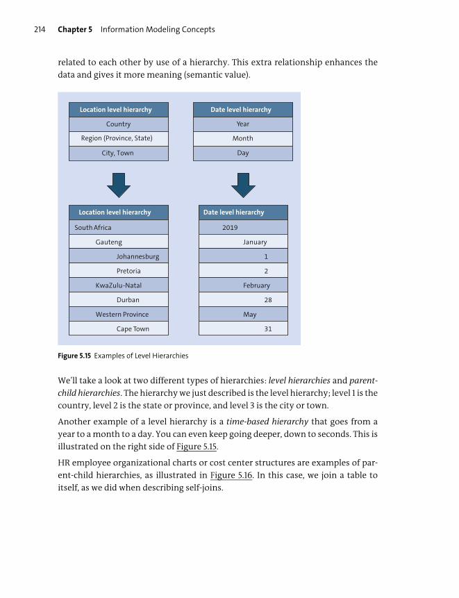
Chapter 5 Information Modeling Concepts214
related to each other by use of a hierarchy. This extra relationship enhances the
data and gives it more meaning (semantic value).
Figure 5.15 Examples of Level Hierarchies
We’ll take a look at two different types of hierarchies: level hierarchies and parent-
child hierarchies. The hierarchy we just described is the level hierarchy; level 1 is the
country, level 2 is the state or province, and level 3 is the city or town.
Another example of a level hierarchy is a time-based hierarchy that goes from a
year to a month to a day. You can even keep going deeper, down to seconds. This is
illustrated on the right side of Figure 5.15.
HR employee organizational charts or cost center structures are examples of par-
ent-child hierarchies, as illustrated in Figure 5.16. In this case, we join a table to
itself, as we did when describing self-joins.
Location level hierarchy Date level hierarchy
South Africa
Gauteng
Johannesburg
Pretoria
KwaZulu-Natal
Durban
Western Province
Cape Town
2019
January
1
2
February
28
May
31
Location level hierarchy
Country
Region (Province, State)
City, Town
Date level hierarchy
Year
Month
Day
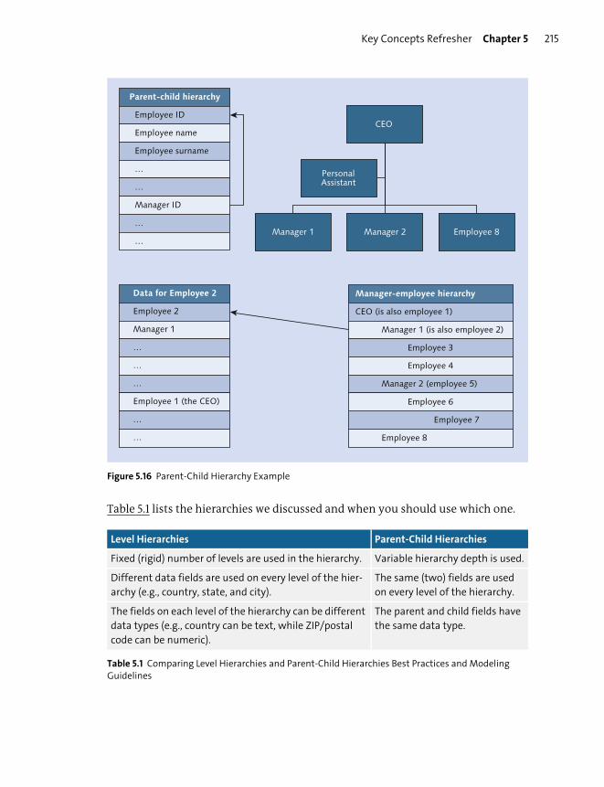
Key Concepts Refresher Chapter 5 215
Figure 5.16 Parent-Child Hierarchy Example
Table 5.1 lists the hierarchies we discussed and when you should use which one.
Level Hierarchies Parent-Child Hierarchies
Fixed (rigid) number of levels are used in the hierarchy. Variable hierarchy depth is used.
Different data fields are used on every level of the hier-
archy (e.g., country, state, and city).
The same (two) fields are used
on every level of the hierarchy.
The fields on each level of the hierarchy can be different
data types (e.g., country can be text, while ZIP/postal
code can be numeric).
The parent and child fields have
the same data type.
Table 5.1 Comparing Level Hierarchies and Parent-Child Hierarchies Best Practices and Modeling Guidelines
CEO (is also employee 1)
Manager 1 (is also employee 2)
Employee 3
Employee 4
Manager 2 (employee 5)
Employee 6
Employee 7
Employee 8
CEO
Manager 1 Manager 2 Employee 8
PersonalAssistant
Parent-child hierarchy
Manager-employee hierarchy
Employee ID
Employee name
Employee surname
…
…
Manager ID
…
…
Data for Employee 2
Employee 2
Manager 1
…
…
…
Employee 1 (the CEO)
…
…

Chapter 5 Information Modeling Concepts216
Let’s end our tour of modeling concepts with a summary of best practices for mod-
eling views in SAP HANA. Many of the basic modeling guidelines that we find in
traditional data modeling and reporting environments are still applicable in SAP
HANA. We can summarize the basic principles as follows:
� Limit (filter) the data as early as possible.
It’s wasteful to send millions of data records across a slow network to a report-
ing tool when the report only uses a few of these data records. It makes a lot
more sense to send only the data records that the report requires, so we want to
filter the data before it hits the network.
In the same way, we don’t want to send data to a star join view when we can fil-
ter it in the earlier dimension view—hence, the rule to filter as early as possible.
� Perform calculations as late as possible.
Assume you have column A and column B in a table. The table contains billions
of records. We can add the values of column A and column B in a formula for
every data record, which means the server performs billions of calculations and
finally adds up the sum total of all these calculated fields.
It would be much faster to calculate the sum total for column A and the sum
total for column B and then calculate the formula. In that case, we perform the
calculation once instead of billions of times. We delay the calculation as long as
possible for performance reasons.
Important Terminology
In this chapter, we focused on various modeling concepts and how they’re used in
SAP HANA. We introduced the following important terms:
� Views
We started by looking at views and realized that we can leverage the fact that
SAP HANA already has all the data in memory, that the servers have lots of CPU
cores available, and that SAP HANA runs everything in parallel. We therefore
don’t need to store the information in cubes and dimension tables but can use
views to generate the information when we need it. This also gives us the advan-
tage of real-time results.
� Joins
We have both normal database join types, such as inner and left outer joins, and
SAP HANA-specific types, such as referential, text, temporal, and spatial joins. In
the process, we also looked at the special case of self-joins and at dynamic joins
as an optimization technique.

Practice Questions Chapter 5 217
� Core data services (CDS)
CDS provides a way to separate business semantics and intent from database
operations.
� Cubes
A cube consists of a data foundation made up of fact tables that contain the
transactional data and that are linked to dimension tables that contain master
data. The data foundation is linked to the dimension tables with star joins.
� Attributes and measures
Attributes describe elements involved in a transaction. Transactional data that
we can perform calculations on is called a measure and is stored in the fact
tables.
� Calculation views
In SAP HANA, we take the concept of views to higher levels. We can create
dimension tables and cubes as dimension views and star join views. Dimension
views are calculation views of type dimension. Star join views are calculation
views of type cube with a star join. The final type of information view is the cal-
culation view of type cube, which we can use to perform even more powerful
processes.
� Modeling artifacts
Inside our views, we can use unions, projections, aggregations, and ranking.
Unions are quite flexible and can be used for a direct merge of result sets, or we
can use a union with constant values to create report-ready result sets.
Practice Questions
These practice questions will help you evaluate your understanding of the topics
covered in this chapter. The questions shown are similar in nature to those found
on the certification examination. Although none of these questions will be found
on the exam itself, they will allow you to review your knowledge of the subject.
Select the correct answers, and then check the completeness of your answers in
the “Practice Question Answers and Explanations” section. Remember, on the
exam, you must select all correct answers and only correct answers to receive
credit for the question.
In this section, we have a few questions with graphics attached. In the certification
exam, you might also see a few questions that include graphics.
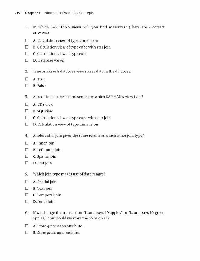
Chapter 5 Information Modeling Concepts218
1. In which SAP HANA views will you find measures? (There are 2 correct
answers.)
� A. Calculation view of type dimension
� B. Calculation view of type cube with star join
� C. Calculation view of type cube
� D. Database views
2. True or False: A database view stores data in the database.
� A. True
� B. False
3. A traditional cube is represented by which SAP HANA view type?
� A. CDS view
� B. SQL view
� C. Calculation view of type cube with star join
� D. Calculation view of type dimension
4. A referential join gives the same results as which other join type?
� A. Inner join
� B. Left outer join
� C. Spatial join
� D. Star join
5. Which join type makes use of date ranges?
� A. Spatial join
� B. Text join
� C. Temporal join
� D. Inner join
6. If we change the transaction “Laura buys 10 apples” to “Laura buys 10 green
apples,” how would we store the color green?
� A. Store green as an attribute.
� B. Store green as a measure.
Practice Questions Chapter 5 219
� C. Store green as a spatial data type.
� D. Store green as a CDS view.
7. True or False: A view always shows all the available columns of the underlying
tables.
� A. True
� B. False
8. You have a view with two tables joined by a left outer join. If you redesign the
view and accidently swap the two tables around, what should you do to the
join?
� A. Keep the left outer join.
� B. Change the join to a text join.
� C. Change the join to a right outer join.
� D. Change the join to a referential join.
9. What do you call the data displayed in the data foundation of an SAP HANA
information view?
� A. Facets
� B. Measures
� C. Characteristics
� D. Key figures
10. You’re writing a mobile application for the World Series. You have details
about all the baseball players and the baseball scores for all the previous
games. How do you use the data of the player information and the scores?
� A. Both the player information and the scores are used as master data.
� B. Both the player information and the scores are used as transactional data.
� C. The player information is used as master data, and the scores are used as
transactional data.
� D. The player information is used as transactional data, and the scores are
used as master data.

Chapter 5 Information Modeling Concepts220
11. Look at Figure 5.17. You’re selling books that have been translated into various
languages. What join type should you use?
� A. Left outer join
� B. Text join
� C. Temporal join
� D. Referential join
Figure 5.17 What Type of Join Should You Use?
12. Which of the following are reasons you should use core data services (CDS) to
create a schema? (There are 2 correct answers.)
� A. The database administrator might type the name wrong.
� B. The database administrator should not get those privileges in the produc-
tion system.
� C. The focus is on the business requirements.
� D. The focus is on the database administration requirements.
Left Table
Right Table
SPRAS Title
EN
CN
AR
FR
RU
What join should you use here?
Field 1 Field n Book ID
Field 1 Field nBook ID

Practice Questions Chapter 5 221
13. Look at Figure 5.18. A company sends out a lot of quotes. Some customers
accept the quotes, and they’re invoiced. The company asks you to find a list of
the customers that did NOT accept the quotes. How do you find the customers
that received quotes but did NOT receive invoices?
� A. Use a right outer join.
Filter to show only the NULL values on the right table.
� B. Use a left outer join.
Filter to show only customers on the right table.
� C. Use a left outer join.
Filter to show only the NULL values on the right table.
� D. Use a right outer join.
Filter to show only customers on the left table.
Figure 5.18 Find the Customers That Received Quotes but Not Invoices
What join should you use here?
Left Table—Quotes
Right Table—Invoices
Quote ID … Customer ID
Invoice ID … …Customer ID
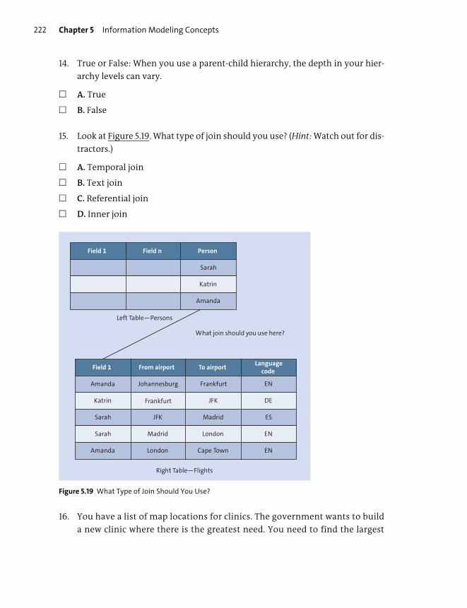
Chapter 5 Information Modeling Concepts222
14. True or False: When you use a parent-child hierarchy, the depth in your hier-
archy levels can vary.
� A. True
� B. False
15. Look at Figure 5.19. What type of join should you use? (Hint: Watch out for dis-
tractors.)
� A. Temporal join
� B. Text join
� C. Referential join
� D. Inner join
Figure 5.19 What Type of Join Should You Use?
16. You have a list of map locations for clinics. The government wants to build
a new clinic where there is the greatest need. You need to find the largest
From airport
Johannesburg
Frankfurt
JFK
Madrid
London
What join should you use here?
Right Table—Flights
Left Table—Persons
Languagecode
EN
DE
ES
EN
EN
Field 1
Amanda
Katrin
Sarah
Sarah
Amanda
To airport
Frankfurt
JFK
Madrid
Field 1
London
Cape Town
Field n Person
Sarah
Katrin
Amanda
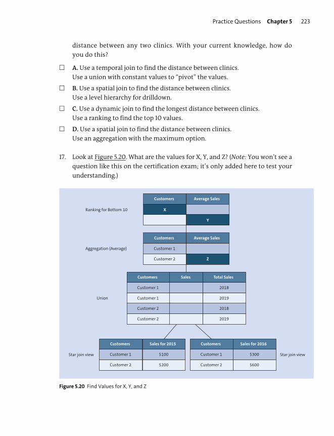
Practice Questions Chapter 5 223
distance between any two clinics. With your current knowledge, how do
you do this?
� A. Use a temporal join to find the distance between clinics.
Use a union with constant values to “pivot” the values.
� B. Use a spatial join to find the distance between clinics.
Use a level hierarchy for drilldown.
� C. Use a dynamic join to find the longest distance between clinics.
Use a ranking to find the top 10 values.
� D. Use a spatial join to find the distance between clinics.
Use an aggregation with the maximum option.
17. Look at Figure 5.20. What are the values for X, Y, and Z? (Note: You won’t see a
question like this on the certification exam; it’s only added here to test your
understanding.)
Figure 5.20 Find Values for X, Y, and Z
Union
Aggregation (Average)
Ranking for Bottom 10
Star join view Star join view
Customers Average Sales
Customers
Customer 1
Customer 2
Sales for 2015
$100
$200
Customers
Customer 1
Customer 2
Sales for 2016
$300
$600
Customers
Customer 1
Customer 1
Sales
Customer 2
Customer 2
Total Sales
2018
2019
2018
2019
X
Y
Customers Average Sales
Z
Customer 1
Customer 2
Chapter 5 Information Modeling Concepts224
� A. X = Customer 2, Y = 400, Z = 800
� B. X = Customer 1, Y = 400, Z = 400
� C. X = Customer 1, Y = 800, Z = 800
� D. X = Customer 2, Y = 200, Z = 400
18. You have to build a parent-child hierarchy. What type of join do you expect to
use?
� A. Relational join
� B. Temporal join
� C. Dynamic join
� D. Self-join
19. You have two result sets: one of customers who booked the venue for an
event, and another of customers who want flowers for the event. What do you
use to find the customers who booked both the venue and flowers?
� A. Union
� B. Minus
� C. Intersect
� D. Inner join
20. Look at Figure 5.21. What join type should you use to see all the suppliers?
� A. Left outer join
� B. Right outer join
� C. Inner join
� D. Referential join
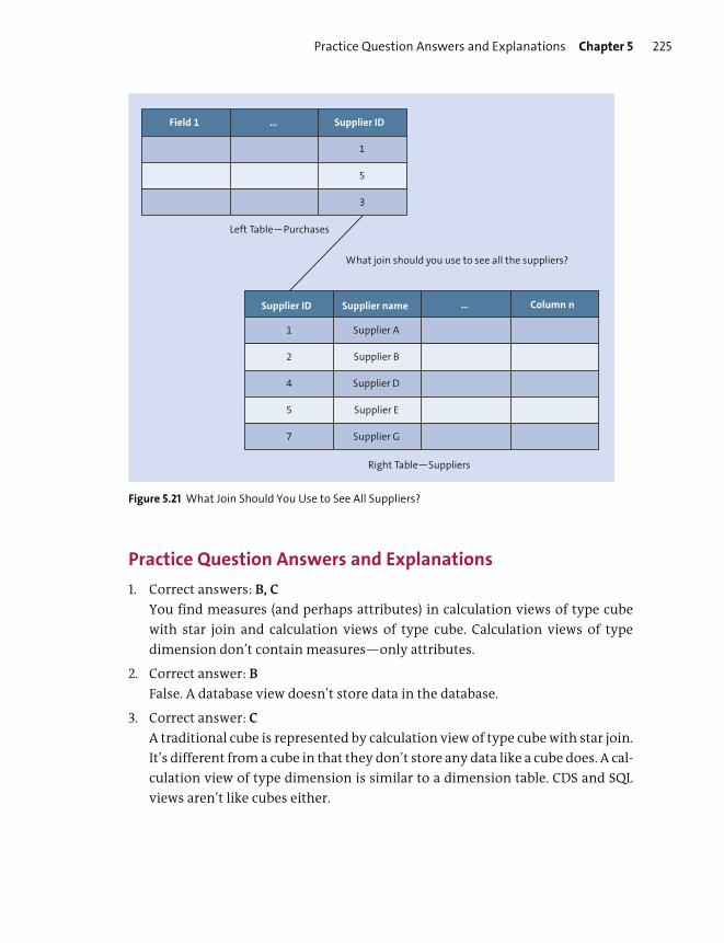
Practice Question Answers and Explanations Chapter 5 225
Figure 5.21 What Join Should You Use to See All Suppliers?
Practice Question Answers and Explanations
1. Correct answers: B, C
You find measures (and perhaps attributes) in calculation views of type cube
with star join and calculation views of type cube. Calculation views of type
dimension don’t contain measures—only attributes.
2. Correct answer: B
False. A database view doesn’t store data in the database.
3. Correct answer: C
A traditional cube is represented by calculation view of type cube with star join.
It’s different from a cube in that they don’t store any data like a cube does. A cal-
culation view of type dimension is similar to a dimension table. CDS and SQL
views aren’t like cubes either.
What join should you use to see all the suppliers?
Supplier ID
1
2
4
5
7
Right Table—Suppliers
Left Table—Purchases
Field 1 … Supplier ID
1
5
3
Supplier name
Supplier A
Supplier B
Supplier D
Supplier E
Supplier G
… Column n

Chapter 5 Information Modeling Concepts226
4. Correct answer: A
A referential join gives the same results as an inner join but speeds up the cal-
culations in some cases by assuming referential integrity of the data. It’s the
optimal join type in SAP HANA.
5. Correct answer: C
A temporal join requires FROM and TO fields in the table on the right side of the
join and a date-time column in the table on the left side of the join.
6. Correct answer: A
We’ll store the color green as an attribute. We can’t “measure” or perform cal-
culations on the color green. Green isn’t a spatial data type. CDS views aren’t rel-
evant in this context.
7. Correct answer: B
False. A view doesn’t always show all the available columns of the underlying
tables. You have to select the output fields of a view. The word always in the
statement is what makes it false.
8. Correct answer: C
A right outer join is the inverse of the left outer join. Therefore, if you reverse
the order of the tables, you can “reverse” the join type. It’s important to note
that this doesn’t work for a text join. A text join is only equivalent to a left outer
join. For a text join, you have to always be careful about the order of the tables.
9. Correct answer: B
The data displayed in the data foundation of an SAP HANA information view is
called measures. In SAP HANA, we talk about attributes and measures. The other
names might be used in other data modeling environments, but not in SAP
HANA.
10. Correct answer: C
The player information is used as master data, and the scores are used as trans-
actional data. You can’t perform calculations on the players. Therefore, this
data is used in the dimensions and is seen as master data. You definitely per-
form calculations on the scores, so these are used in the fact tables, which
means they are transactional data.
11. Correct answer: B
Figure 5.17 shows the SPRAS column and a list of languages. The need for a
translation is also hinted at in the question, meaning this should be a text join.
There isn’t enough information to select any of the other answer options.

Practice Question Answers and Explanations Chapter 5 227
12. Correct answers: B, C
You should use CDS to create a schema because the database administrator
should not get those privileges in the production system, and the focus should
be on the business requirements.
13. Correct answer: C
Look carefully at Figure 5.18. The question asks you to find all the customers
who received quotes but did not receive invoices.
The answer only gives us left outer or right outer as options. Because the ques-
tion states they want all customers from the quotes (left) table, you might try a
left outer join first.
Now look at Figure 5.3 to see the difference between the left and right outer
joins. Look especially at where the NULL values are shown. With a left outer join,
the NULL values are found in the right table. With a right outer join, the NULL val-
ues are found in the left table.
We want to find the customers who did not get invoices. With a left outer join,
the NULL values are found on the right side: that group is the one we’re looking
for. Therefore, filter for the NULL values on the right table.
Note
Any time a negative phrase or word is used in the certification exam, it’s shown in capital
letters to bring attention to the fact that it’s a negative word.
14. Correct answer: A
True. Yes, the depth of your hierarchy levels can vary when you use a parent-
child hierarchy.
15. Correct answer: C
You should use a referential join.
There are two distractors to try and throw you off track:
A temporal join uses FROM and TO fields but only for date-time fields. This exam-
ple is for airports.
The second distractor was to try to get you to select the text join. The language
code has nothing to do with translations but has to do with the airline’s pri-
mary language.
Choose a referential join because you can see the same people traveling in both
tables, so it seems that these two tables have referential integrity.

Chapter 5 Information Modeling Concepts228
If the tables didn’t have referential integrity, you would have chosen an inner
join.
16. Correct answer: D
Only a spatial join can give the distance between different points on a map.
After you have the distances, there are two ways you can find the largest dis-
tance between any two clinics:
Use a ranking to find the top 10 values.
Use an aggregation with the maximum option.
17. Correct answer: B
See the full solution in Figure 5.22.
X = Customer 1, Y = 400, Z = 400.
Note that we’re using average in the aggregation node, not sum.
In the ranking node, we’re asking for the bottom 10, not the top 10.
Figure 5.22 Full Solution: X = Customer 1, Y = 400, Z = 400
Union
Aggregation (Average)
Ranking for Bottom 10
Star join view Star join view
Customers
Customer 1
Customer 2
Total Sales
200
400
Customers
Customer 1
Customer 2
Total Sales
200
400
Customers
Customer 1
Customer 2
Sales for 2015
$100
$200
Customers
Customer 1
Customer 2
Sales for 2016
$300
$600
Customers
Customer 1
Customer 1
Total Sales
100
300
Customer 2
Customer 2
200
600
Year
2018
2019
2018
2019
Summary Chapter 5 229
18. Correct answer: D
You expect to use a self-join when you build a parent-child hierarchy. Refer to
Figure 5.16 for an illustration.
19. Correct answer: C
You use an intersect operation to find the customers that booked both the
venue and flowers.
20. Correct answer: B
To see everything on the right table, use a right outer join.
Note that these tables don’t have referential integrity. If we had asked the ques-
tion a little differently, this could have been important.
Takeaway
You should now have a general understanding of information modeling concepts:
views, joins, cubes, star joins, data foundations, dimension tables, and so on. In
this chapter, you learned about the differences between attributes and measures
and the value of CDS in the development cycle. You’ve seen the various types of
views that SAP HANA uses, how to use them together, and what options you have
available for your information modeling. Finally, we examined a few best practices
and guidelines for modeling in SAP HANA in general.
Summary
You’ve learned about many modeling concepts and how they are applied and
implemented in SAP HANA.
You’re now ready to go into the practical details of learning how to use the various
SAP HANA calculation views and how to enhance these views with the various
modeling artifacts that we have available to us in each of these different views.

Chapter 6
Calculation Views
Techniques You’ll Master
� Learn to create SAP HANA calculation views
� Identify which type of SAP HANA calculation view to use
� Explore the various types of calculation views
� Know how to select the correct joins and nodes
� Get to know the value of semantics in information modeling
Chapter 6 Calculation Views232
In the past two chapters, we discussed the modeling concepts and tools required
for building SAP HANA information views. In this chapter and the next, we’ll build
on that foundation. We’ll focus on how to graphically create information views in
the SAP HANA system and how to enhance these views with additional functional-
ity.
In this chapter, you’ll learn to create the different types of calculation views, select
the correct nodes for what you want to achieve, and use the Semantics node to add
additional value for business users.
Real-World Scenario
You start a new project in which a business wants to expand the range of ser-
vices it offers its customers. You’re responsible for building the information
models in SAP HANA.
You have to build about 50 new SAP HANA information views. As you plan
your information views, you notice several master data tables that you’ll use.
By creating a few well-designed dimension views, you cater not only to the
needs of this project but also to future requirements. You see this as a
“library” of reusable dimension views.
While you’re busy designing these dimension views, you also gather some
analytics and reporting requirements. Most of the analytics requirements
are addressed by building star join views and calculation views of type cube.
You address some of the reporting requirements by delivering semantically
enhanced information models that are easier for your colleagues and end
users to work with.
The company wants to create a mobile app. Working together with some of
the developers, you quickly create a few calculation views to provide them
with information that would have taken them hours to create via code. The
performance of the calculation views you created are also very good, which
delights the mobile app users.
Objectives of This Portion of the Test
The purpose of this portion of the SAP HANA certification exam is to test your
knowledge of modeling SAP HANA information views.
Key Concepts Refresher Chapter 6 233
The certification exam expects you to have a good understanding of the following
topics:
� Creating SAP HANA information views
� Calculation views of type dimension
� Calculation views of type cube with star join
� Calculation views of type cube
� Selecting the correct joins and nodes to produce accurate results
� Choosing the correct type of SAP HANA information view
� Understanding the value that semantics adds to the information-modeling
process
Note
This portion contributes more than 10% of the total certification exam score.
Key Concepts Refresher
In Chapter 4, we examined SAP HANA modeling tools, and, in Chapter 5, we looked
at modeling concepts. Now, it’s time to put them together, implementing the
modeling concepts with the tools to create SAP HANA calculation views.
There are three types of SAP HANA calculation views, which we briefly covered in
Chapter 5. First are dimension views, for the master data in the system. All data in
these views are treated as attributes, even numeric fields. Second, star join views
let you build cube-like information models. Third, calculation views of type cube
let you build enhanced multidimensional data structures and information mod-
els.
Tip
We refer to calculation views of type dimension as dimension views and to calculation
views of type cube with star join as star join views. The last category is called calculation
views of type cube.
The last category can cause some confusion because some people and older web pages
still refer to the last category simply as calculation views. In this book, we use the latest
official name—calculation views of type cube—because that’s what they’re referred to in
the SAP HANA certification exam. We use the name calculation views to refer to all three
types of calculation views.
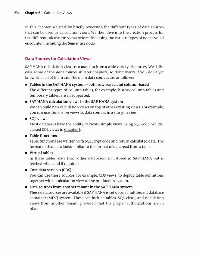
Chapter 6 Calculation Views234
In this chapter, we start by briefly reviewing the different types of data sources
that can be used by calculation views. We then dive into the creation process for
the different calculation views before discussing the various types of nodes you’ll
encounter, including the Semantics node.
Data Sources for Calculation Views
SAP HANA calculation views can use data from a wide variety of sources. We’ll dis-
cuss some of the data sources in later chapters, so don’t worry if you don’t yet
know what all of them are. The main data sources are as follows:
� Tables in the SAP HANA system—both row-based and column-based
The different types of column tables, for example, history column tables and
temporary tables, are all supported.
� SAP HANA calculation views in the SAP HANA system
We can build new calculation views on top of other existing views. For example,
you can use dimension views as data sources in a star join view.
� SQL views
Most databases have the ability to create simple views using SQL code. We dis-
cussed SQL views in Chapter 5.
� Table functions
Table functions are written with SQLScript code and return calculated data. The
format of that data looks similar to the format of data read from a table.
� Virtual tables
In these tables, data from other databases isn’t stored in SAP HANA but is
fetched when and if required.
� Core data services (CDS)
You can use these sources, for example, CDS views, to deploy table definitions
together with a calculation view to the production system.
� Data sources from another tenant in the SAP HANA system
These data sources are available if SAP HANA is set up as a multitenant database
container (MDC) system. These can include tables, SQL views, and calculation
views from another tenant, provided that the proper authorizations are in
place.

Key Concepts Refresher Chapter 6 235
Calculation Views: Dimension, Cube, and Cube with Star Join
We create calculation views using graphical modeling. The aim is to do as much
modeling work as possible with graphical calculation views. As SAP HANA has
matured, there has been less emphasis on writing code when creating information
models.
In this section, we’ll walk through the steps for creating these calculation views.
We’ll use the SAP HANA Interactive Education (SHINE) demo application and,
where possible, give you the name of the modeling objects we used. You can use
this to follow along practically in your own SAP HANA system.
Creating Calculation Views
You create calculation views in your Workspace in SAP Web IDE for SAP HANA.
Select and right-click on the SAP HANA database module and folder in which you
want to create the calculation view. You’ll see a context menu like the one shown
in Figure 6.1.
Figure 6.1 Context Menu for Creating SAP HANA Calculation Views
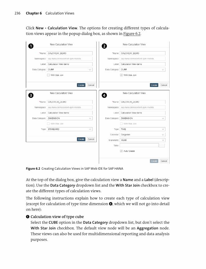
Chapter 6 Calculation Views236
Click New • Calculation View. The options for creating different types of calcula-
tion views appear in the popup dialog box, as shown in Figure 6.2.
Figure 6.2 Creating Calculation Views in SAP Web IDE for SAP HANA
At the top of the dialog box, give the calculation view a Name and a Label (descrip-
tion). Use the Data Category dropdown list and the With Star Join checkbox to cre-
ate the different types of calculation views.
The following instructions explain how to create each type of calculation view
(except for calculation of type time dimension 4, which we will not go into detail
on here):
1 Calculation view of type cube
Select the CUBE option in the Data Category dropdown list, but don’t select the
With Star Join checkbox. The default view node will be an Aggregation node.
These views can also be used for multidimensional reporting and data analysis
purposes.

Key Concepts Refresher Chapter 6 237
2 Calculation view of type cube with star join
Select the CUBE option in the Data Category dropdown list, and select the With
Star Join checkbox. The default view node will be a Star Join node. These views
can be used for multidimensional reporting and data analysis purposes.
3 Calculation view of type dimension
Select the DIMENSION option in the Data Category dropdown list. The default
view node will be a Projection node. These views don’t support multidimen-
sional reporting and data analysis. You can use dimension calculation views as
data sources for other calculation views.
Click the Create button to create the calculation view.
If you select the DEFAULT option in the Data Category dropdown list, you’ll create
a type of calculation view that can only be used internally in SAP HANA or con-
sumed by SQL. An external client tool—for example, a reporting tool—won’t be
able to use this calculation view because the DEFAULT calculation view doesn’t cre-
ate the hierarchy views used by the reporting tools when you build the calculation
view. If you’re not using hierarchies, or the calculation view will only be used by
reporting tools that can’t use hierarchies, you can use the DEFAULT calculation
view type.
SPS 04
To be clearer on what the limitation is of the DEFAULT calculation view type, it’s now
named SQL Access Only in SAP HANA 2.0 SPS 04.
Creating Time Dimension Calculation Views
You can also create a special type of dimension view, called a time dimension view.
When creating a dimension calculation view, you can specify the Type as Time, as
shown in the bottom-right corner of Figure 6.2, shown previously. Additional
fields then become available, where you can specify the Calendar (Gregorian or Fis-
cal) and the Granularity (e.g., yearly).
In Figure 6.3, we see an example of a time dimension view.
Note
This example is found in the SHINE demo application; the calculation view is called
TIME_DIM. (The example here was modified to a time dimension view.)

Chapter 6 Calculation Views238
Figure 6.3 Creating Time-Based Calculation Views in SAP Web IDE for SAP HANA
The time-based calculation view adds a time dimension to information views.
Remember that dimensions contain attributes that describe a transaction. If we
add a time and date when the transaction happens, we’ve added another attribute
(time). These time attributes are stored in a time dimension. We can use this to
enhance the information model with drilldown capabilities on a time hierarchy.
We’ll discuss hierarchies in more detail in Chapter 7.
Working with a Calculation View
A calculation view includes different working areas. A calculation view of type
dimension is shown in Figure 6.4 in SAP Web IDE for SAP HANA.
Tip
In SHINE, look for PO_ITEM. The join type should actually be a text join.
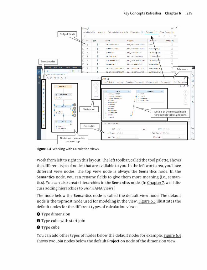
Key Concepts Refresher Chapter 6 239
Figure 6.4 Working with Calculation Views
Work from left to right in this layout. The left toolbar, called the tool palette, shows
the different type of nodes that are available to you. In the left work area, you’ll see
different view nodes. The top view node is always the Semantics node. In the
Semantics node, you can rename fields to give them more meaning (i.e., seman-
tics). You can also create hierarchies in the Semantics node. (In Chapter 7, we’ll dis-
cuss adding hierarchies to SAP HANA views.)
The node below the Semantics node is called the default view node. The default
node is the topmost node used for modeling in the view. Figure 6.5 illustrates the
default nodes for the different types of calculation views:
1 Type dimension
2 Type cube with start join
3 Type cube
You can add other types of nodes below the default node; for example, Figure 6.4
shows two Join nodes below the default Projection node of the dimension view.
Nodes with semanticsnode on top
Properties
Details of the selected node,for example tables and joins
Navigation
Select nodes
Output fields
Tab menu
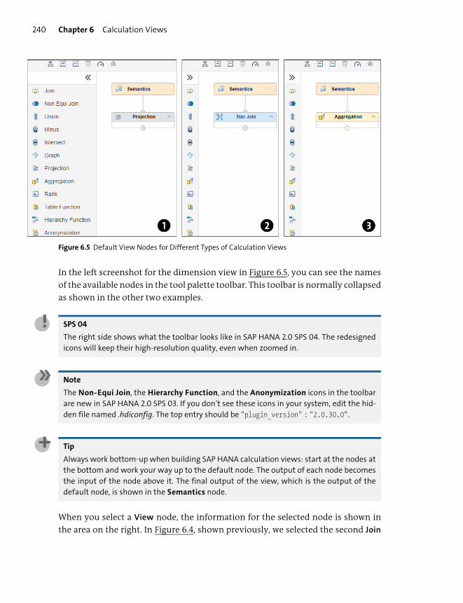
Chapter 6 Calculation Views240
Figure 6.5 Default View Nodes for Different Types of Calculation Views
In the left screenshot for the dimension view in Figure 6.5, you can see the names
of the available nodes in the tool palette toolbar. This toolbar is normally collapsed
as shown in the other two examples.
SPS 04
The right side shows what the toolbar looks like in SAP HANA 2.0 SPS 04. The redesigned
icons will keep their high-resolution quality, even when zoomed in.
Note
The Non-Equi Join, the Hierarchy Function, and the Anonymization icons in the toolbar
are new in SAP HANA 2.0 SPS 03. If you don’t see these icons in your system, edit the hid-
den file named .hdiconfig. The top entry should be "plugin_version" : "2.0.30.0".
Tip
Always work bottom-up when building SAP HANA calculation views: start at the nodes at
the bottom and work your way up to the default node. The output of each node becomes
the input of the node above it. The final output of the view, which is the output of the
default node, is shown in the Semantics node.
When you select a View node, the information for the selected node is shown in
the area on the right. In Figure 6.4, shown previously, we selected the second Join
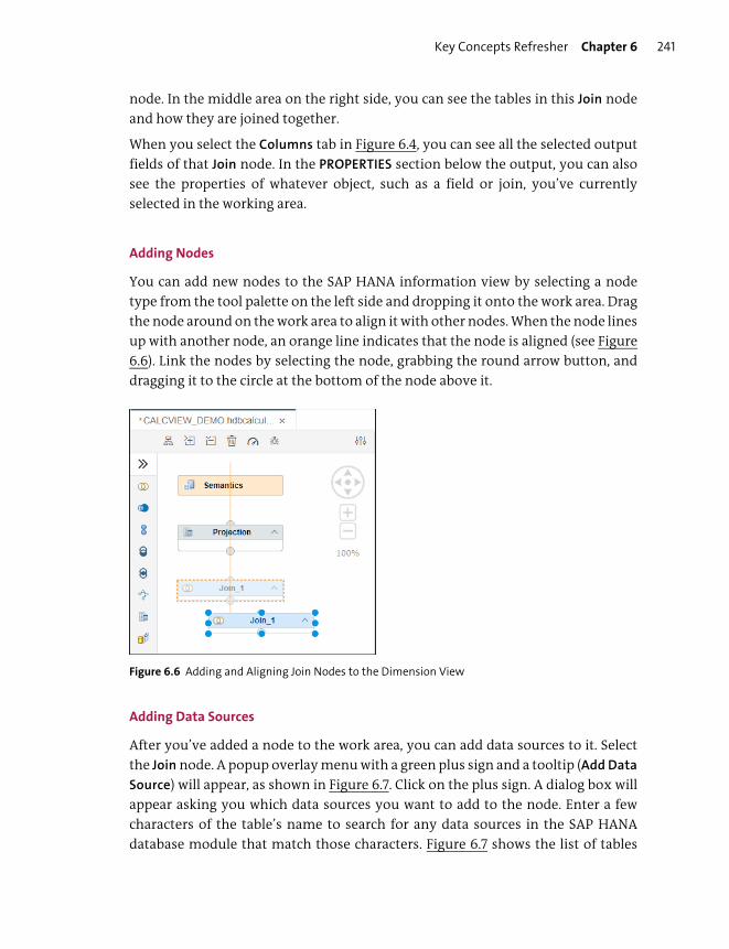
Key Concepts Refresher Chapter 6 241
node. In the middle area on the right side, you can see the tables in this Join node
and how they are joined together.
When you select the Columns tab in Figure 6.4, you can see all the selected output
fields of that Join node. In the PROPERTIES section below the output, you can also
see the properties of whatever object, such as a field or join, you’ve currently
selected in the working area.
Adding Nodes
You can add new nodes to the SAP HANA information view by selecting a node
type from the tool palette on the left side and dropping it onto the work area. Drag
the node around on the work area to align it with other nodes. When the node lines
up with another node, an orange line indicates that the node is aligned (see Figure
6.6). Link the nodes by selecting the node, grabbing the round arrow button, and
dragging it to the circle at the bottom of the node above it.
Figure 6.6 Adding and Aligning Join Nodes to the Dimension View
Adding Data Sources
After you’ve added a node to the work area, you can add data sources to it. Select
the Join node. A popup overlay menu with a green plus sign and a tooltip (Add Data
Source) will appear, as shown in Figure 6.7. Click on the plus sign. A dialog box will
appear asking you which data sources you want to add to the node. Enter a few
characters of the table’s name to search for any data sources in the SAP HANA
database module that match those characters. Figure 6.7 shows the list of tables

Chapter 6 Calculation Views242
matching the search for employee data sources. Then, select the data sources, and
click on Finish to add them to the node.
If you click on the Create Synonym button, you can specify the details of the syn-
onyms required. This is part of security (Chapter 13). If you just click on Finish after
selecting the data source, the synonyms are created without asking you for details.
Figure 6.7 Adding Data Sources to a View Node
Creating Joins
After you’ve added the data sources to the data foundation, you’ll want to join the
data sources together. Create a join by taking the field from one table and drop-
ping it onto a related field of another table. Figure 6.8 shows what this looks like in
SAP Web IDE for SAP HANA.

Key Concepts Refresher Chapter 6 243
Go to the PROPERTIES area to select the Join Type from the dropdown 1, and set the
Cardinality 2. Make sure you have the join (the line between the tables) selected as
shown; otherwise, the properties won’t show the correct information.
Figure 6.8 Creating a Join and Setting Properties in SAP Web IDE for SAP HANA
Tip
When you create a join, get into the habit of always dropping the field from the main
table onto the related field of the smaller lookup table.
For some join types, it makes no difference in which direction you do the drag and drop.
With a text join, however, it matters.
The join types that are available in calculation views are as follows:
� Referential join
� Inner join
� Left outer join
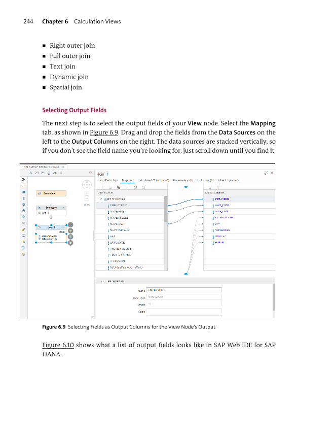
Chapter 6 Calculation Views244
� Right outer join
� Full outer join
� Text join
� Dynamic join
� Spatial join
Selecting Output Fields
The next step is to select the output fields of your View node. Select the Mapping
tab, as shown in Figure 6.9. Drag and drop the fields from the Data Sources on the
left to the Output Columns on the right. The data sources are stacked vertically, so
if you don’t see the field name you’re looking for, just scroll down until you find it.
Figure 6.9 Selecting Fields as Output Columns for the View Node’s Output
Figure 6.10 shows what a list of output fields looks like in SAP Web IDE for SAP
HANA.
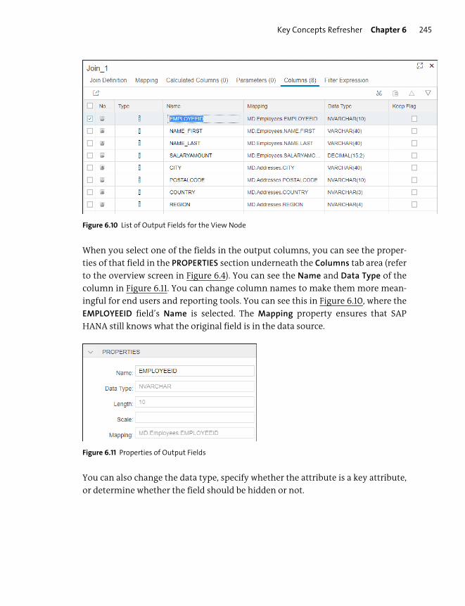
Key Concepts Refresher Chapter 6 245
Figure 6.10 List of Output Fields for the View Node
When you select one of the fields in the output columns, you can see the proper-
ties of that field in the PROPERTIES section underneath the Columns tab area (refer
to the overview screen in Figure 6.4). You can see the Name and Data Type of the
column in Figure 6.11. You can change column names to make them more mean-
ingful for end users and reporting tools. You can see this in Figure 6.10, where the
EMPLOYEEID field’s Name is selected. The Mapping property ensures that SAP
HANA still knows what the original field is in the data source.
Figure 6.11 Properties of Output Fields
You can also change the data type, specify whether the attribute is a key attribute,
or determine whether the field should be hidden or not.

Chapter 6 Calculation Views246
Often, you’ll want to select all the fields coming from a lower node as the output
fields of the node. In this case, right-click the name of the data source, and select
Add To Output, as shown in Figure 6.12.
Figure 6.12 Selecting All Fields from the View Node as Output Fields
An alternative way of selecting output fields is to drag the name of the data source
to the Output Columns. All the fields in the data source will be added to the Output
Columns on the right.
The Keep Flag
When we take another look at Figure 6.10, we see that the right-side column is
named Keep Flag. This flag is available for each output column in any of the View
nodes, but it’s particularly important when we aggregate data. In older SAP HANA
systems, this was called the Calculate Before Aggregation flag.
We use this flag when the level of granularity has an impact on the outcome of a
measure, that is, when the order in which you do things matter. Let’s look at an
example by considering the sales data in Table 6.1.

Key Concepts Refresher Chapter 6 247
If we first add the columns, we get $55 for the cost per item column and 110 for the
number of items column. When we then multiply these values, we get an aggre-
gate value of $6,050, which isn’t correct.
We should first do the multiplication because a cost per item value is only relevant
for that specific item. When we multiply the values first, we get a cost of $500 for
both rows. When we now create the aggregate (sum), we get the correct value of
$1,000.
This is applicable to formulas where the sequence in which you do them makes a
difference, for example, with multiplication and division. In this case, you should
do the calculations before creating the aggregate.
Practically, it means that you’ll put the following formula in a View node below the
Aggregation node. A Projection node is a good choice for this.
Cost per Item × Number of Items
Finalizing the Calculation View
In Chapter 5, we discussed how to build SAP HANA information views in layers,
with each node building on the previous ones. After you’ve finished building the
calculation view, there are three final steps to follow:
1. Click the Save button above the Workspace area (see Figure 6.13 1). You can also
select the Save option from the File menu 1, or press (Ctrl)+(S) on your key-
board.
2. You then need to Build the calculation view. (We discussed the entire build pro-
cess in Chapter 4.) You can select Build Selected Files from the File menu, the
Build menu, or from the context (right-click) menu 2.
3. Preview your data by selecting the Data Preview option from the menu. (We dis-
cussed the preview functionality in Chapter 4.)
Month Cost per Item Number of Items
January $50 10
January $5 100
Table 6.1 Cost per Item Data Needing the Keep Flag

Chapter 6 Calculation Views248
Figure 6.13 Save and Build the Calculation View
Congratulations! You now know how to create calculation views in SAP HANA.
Working with Nodes
In Chapter 5, we looked at the modeling concepts of joins, star joins, projection,
ranking, aggregation, and union. All of these options are available in calculation
views as View nodes. You can add these View nodes from the tool palette toolbar
on the left of the main work area, as shown earlier in Figure 6.12. These are the basic
building blocks to use in the different layers of your calculation views.
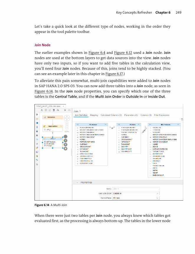
Key Concepts Refresher Chapter 6 249
Let’s take a quick look at the different type of nodes, working in the order they
appear in the tool palette toolbar.
Join Node
The earlier examples shown in Figure 6.4 and Figure 6.12 used a Join node. Join
nodes are used at the bottom layers to get data sources into the view. Join nodes
have only two inputs, so if you want to add five tables in the calculation view,
you’ll need four Join nodes. Because of this, joins tend to be highly stacked. (You
can see an example later in this chapter in Figure 6.17.)
To alleviate this pain somewhat, multi-join capabilities were added to Join nodes
in SAP HANA 2.0 SPS 03. You can now add three tables into a Join node, as seen in
Figure 6.14. In the Join node properties, you can specify which one of the three
tables is the Central Table, and if the Multi Join Order is Outside In or Inside Out.
Figure 6.14 A Multi-Join
When there were just two tables per Join node, you always knew which tables got
evaluated first, as the processing is always bottom-up. The tables in the lower node

Chapter 6 Calculation Views250
get evaluated first. When using the new multi-join functionality, you have to spec-
ify the priority sequence. When you specify Outside In, the join furthest from the
central table is executed first, whereas with Inside Out, the closest join is executed
first.
There are cases where the result set is the same regardless of the order in which
joins get executed, for example, when all the joins used are inner joins. However,
if you mix inner joins and left outer joins, the result set can vary depending on the
join execution sequence.
Non-Equi Join Node
Another new feature that was introduced with SAP HANA 2.0 SPS 03 is the Non-
Equi Join node. In this case, the join condition isn’t represented by an equal opera-
tor, but by comparison operators such as greater than, less than, less and equal to,
and so on.
So when would you use a non-equi join? In Figure 6.15, we’re looking at orders.
Figure 6.15 A Non-Equi Join Node
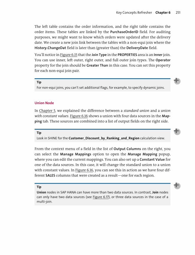
Key Concepts Refresher Chapter 6 251
The left table contains the order information, and the right table contains the
order items. These tables are linked by the PurchaseOrderID field. For auditing
purposes, we might want to know which orders were updated after the delivery
date. We create a new join link between the tables with a non-equi join where the
History.ChangeDat field is later than (greater than) the DeliveryDate field.
You’ll notice in Figure 6.15 that the Join Type in the PROPERTIES area is an Inner join.
You can use inner, left outer, right outer, and full outer join types. The Operator
property for the join should be Greater Than in this case. You can set this property
for each non-equi join pair.
Tip
For non-equi joins, you can’t set additional flags, for example, to specify dynamic joins.
Union Node
In Chapter 5, we explained the difference between a standard union and a union
with constant values. Figure 6.16 shows a union with four data sources in the Map-
ping tab. These sources are combined into a list of output fields on the right side.
Tip
Look in SHINE for the Customer_Discount_by_Ranking_and_Region calculation view.
From the context menu of a field in the list of Output Columns on the right, you
can select the Manage Mappings option to open the Manage Mapping popup,
where you can edit the current mappings. You can also set up a Constant Value for
one of the data sources. In this case, it will change the standard union to a union
with constant values. In Figure 6.16, you can see this in action as we have four dif-
ferent SALES columns that were created as a result—one for each region.
Tip
Union nodes in SAP HANA can have more than two data sources. In contrast, Join nodes
can only have two data sources (see Figure 6.17), or three data sources in the case of a
multi-join.
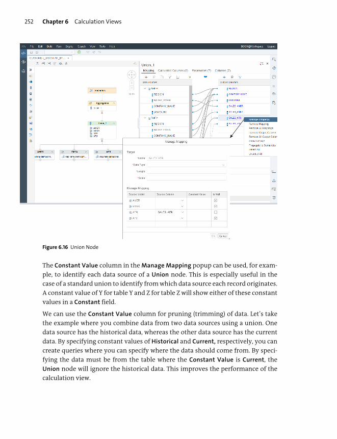
Chapter 6 Calculation Views252
Figure 6.16 Union Node
The Constant Value column in the Manage Mapping popup can be used, for exam-
ple, to identify each data source of a Union node. This is especially useful in the
case of a standard union to identify from which data source each record originates.
A constant value of Y for table Y and Z for table Z will show either of these constant
values in a Constant field.
We can use the Constant Value column for pruning (trimming) of data. Let’s take
the example where you combine data from two data sources using a union. One
data source has the historical data, whereas the other data source has the current
data. By specifying constant values of Historical and Current, respectively, you can
create queries where you can specify where the data should come from. By speci-
fying the data must be from the table where the Constant Value is Current, the
Union node will ignore the historical data. This improves the performance of the
calculation view.

Key Concepts Refresher Chapter 6 253
Figure 6.17 Two Inputs Allowed for a Join Node, and Multiple Inputs Allowed for a Union Node
SAP HANA includes even more performance enhancements for the Union node.
You can make unions run faster by using a pruning configuration table. In this
table, you can specify pruning conditions (e.g., filters) to be applied to some col-
umns. For example, a pruning condition can specify that the year must be 2019 or
later. This filters the data and complies with our first modeling guideline: limit (fil-
ter) the data as early as possible. You can specify the Pruning Config Table in the
Advanced section of the Semantics node.
When you select the data source of a Union node in the Mapping tab, you can see
the Properties of that data source in the area below, as shown in Figure 6.18. You’ll
notice that we also have an Empty Union Behavior selection.

Chapter 6 Calculation Views254
Figure 6.18 Empty Union Behavior
By default, we don’t expect any data returned from a data source if the query
doesn’t need data from it. Sometimes, however, it might be useful to know that a
certain data source didn’t return any data. To activate this, you have to set a Con-
stant Value for each data source to uniquely identify it. You then choose Row with
Constants for the Empty Union Behavior. When no data is expected from a data
source, it will still return one record where all fields have null values except the
unique Constant Value that identifies the data source. We can use this to identify
data sources that didn’t return any data to our query.

Key Concepts Refresher Chapter 6 255
SPS 04
While we’re looking at the Mapping tab of the Union node, we can quickly note a new
feature of SAP HANA 2.0 SPS 04. In Figure 6.18, you see the PROPERTIES of the second
data source. When you click on the Union node itself, the PROPERTIES section will show
the options you can set for the entire node. In SPS 04, you have a new option called Parti-tion Local Execution, as shown in Figure 6.19. This enables you to control the level of par-
allelization based on processed table content, for example, by perform currency
conversion or aggregation in parallel for every country or time period in a query.
Figure 6.19 Enabling Parallelization in a Node in SAP HANA 2.0 SPS 04
You start the parallelization process by selecting the column that controls the level of
parallelization at the lowermost Union node. The level of the parallelization is based on
data, as a parallel thread is started for each distinct value of the specified column. If you
don’t select a column, the parallelization uses table partitioning.
In a later (higher) Union node that is fed by only one source, you switch it off again.
You have to switch the parallelization on and off in the same view; it won’t work across
views. You can only have one parallelization block per view.
Intersect and Minus Nodes
In SAP HANA, we have two more operations we can perform on the result sets of
the left and right tables. Instead of just combining the two result sets in a union,
we can use an Intersect node to find out which records occur in both result sets.
Alternatively, we use a Minus node to find out which records occur only in one of
the two result sets, eliminating records that occur in both nodes or only in the
other node.
If you remember the marketing campaign in the previous chapter where you
wanted to sell gaming headphones to customers. In this case, you might want to
target only those customers who bought both a computer and a large wide-screen
monitor. You’ll have one result set with customers who bought computers, and
another result set with customers who bought large wide-screen monitors.
Chapter 6 Calculation Views256
Instead of using a union, you’ll now use an Intersect node for use in your market-
ing campaign. Figure 6.20 shows this example, where the Category from Projec-
tion_1 is computers, and the Category from Projection_2 is large wide-screen
monitors. Note that both these projections get their data from the same Join node.
Each projection then uses a unique filter to get the required information.
Figure 6.20 An Intersect Node
However, if your marketing campaign is to sell such monitors to customers who
bought computers but have not yet bought screens, you would use a Minus node.
Another example could be where you want to find all orders that haven’t been
invoiced yet.
Graph Node
The Graph node is an interesting addition to the tool palette. It delivers functional-
ity that you would not normally expect in information modeling. (We’ll discuss
graph modeling in Chapter 11.) Graph modeling is used when you want to analyze
relationships between entities, for example, analyzing who are currently “friends”
on Facebook, and using that to calculate what the chances are of two unrelated
people becoming Facebook friends in the future.

Key Concepts Refresher Chapter 6 257
For this, you’ll need a table with people on Facebook, and another table with the
existing “friends” relationships between these people. You then need to create a
graph workspace linking these two tables.
The Graph node must always be the bottom (leaf) node in a calculation view, as
shown in Figure 6.21. It uses the graph workspace as its data source. In addition,
you have to ensure that the referential integrity remains on your data when using
graph modeling.
In the SAP HANA graph reference guide on SAP Help, they use the example of rela-
tionships between various gods and deities in Greek mythology.
Figure 6.21 Graph Node
Projection Node
Projection nodes can be used to remove some fields from a calculation view. If you
don’t send all the input fields to the output area, the fields that aren’t in the output
area won’t appear to client tools.
You can also use Projection nodes to rename fields, filter data, and add new calcu-
lated columns to a calculation view. (We’ll discuss filter expressions and calculated
columns in Chapter 7.)
Chapter 6 Calculation Views258
Aggregation Node
The Aggregation node in calculation views can calculate single summary values
from a large list of values; for example, you can create a sum (single summary
value) of all the values in a table column. These summary values are useful for
high-level reporting, dashboards, and analytics. (The functionality is similar to the
GROUP BY statement in SQL.) The Aggregation node in calculation views also sup-
ports all the usual functions: sum, count, minimum, maximum, average, standard
deviation, and variance. For performance reasons, be cautious when using the last
three functions (average, standard deviation, and variance) on very large stacked
calculation views.
You normally calculate aggregates of measures, but in SAP HANA, you also can cre-
ate aggregates of attributes, which basically creates a list of unique values.
Tip
Watch out when creating average, standard deviation, and variance aggregates in
stacked scenarios as this could affect the performance of your calculation views.
Rank Node
We can use Rank nodes to create top N or bottom N lists of values to sort results. In
the Definition tab of a Rank node, you can access extra properties to specify the
Rank node behavior.
Figure 6.22 shows the Rank node area. The Sort Direction field allows you to specify
whether you want a top N or bottom N list. The Order By field allows you to specify
what you want to sort the list by, such as the Product_Price. In this case, the top 10
most expensive items will be shown.
The Threshold field specifies how many entries you want in the list. If you specify a
Fixed value of “10”, you’ll produce a top 10 or bottom 10 list. You can also choose to
set this value from an Input Parameter, which means that the calculation view will
ask for a value each time a query is run on this view. (We’ll discuss input parame-
ters in Chapter 7.)
You can also partition the data by a specific column. In the example in Figure 6.22,
we selected the Country column. In this case, we’ll get the top 10 most expensive
items for each country.

Key Concepts Refresher Chapter 6 259
Figure 6.22 Rank Node
By default, these partition columns are always used. When you select the Dynamic
Partition Elements checkbox, SAP HANA will ignore any of the specified partition
columns that aren’t included in the query. In other words, if your query doesn’t
include the Country column (in Figure 6.22) in the query, SAP HANA will ignore the
Country partition column.
Finally, and most importantly, you can specify that a new output column must be
generated. You can then use the column created by Generate Rank Column in
analysis or reporting tools to sort the results.
SPS 04
The Rank node is the one node that had the biggest update with SAP HANA 2.0 SPS 04.
Just do a quick compare of Figure 6.22 (SPS 03) with Figure 6.23 (SPS 04).
� The Generate Rank Column and the Logical Partition area are still the same.
� The Order By column was expanded to a Sort Column area to allow for multiple sort
columns.
� The Sort Direction is renamed to Result Set Direction.
� The Threshold value is now Target Value.
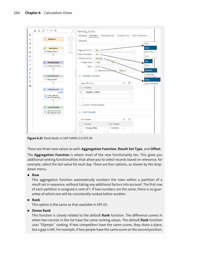
Chapter 6 Calculation Views260
Figure 6.23 Rank Node in SAP HANA 2.0 SPS 04
There are three new values as well: Aggregation Function, Result Set Type, and Offset.
The Aggregation Function is where most of the new functionality lies. This gives you
additional ranking functionalities that allow you to select records based on relevance, for
example, select the last value for each day. There are four options, as shown by the drop-
down menu:
� RowThis aggregation function automatically numbers the rows within a partition of a
result set in sequence, without taking any additional factors into account. The first row
of each partition is assigned a rank of 1. If two numbers are the same, there is no guar-
antee of which one will be consistently ranked before another.
� RankThis option is the same as that available in SPS 03.
� Dense RankThis function is closely related to the default Rank function. The difference comes in
when two records in the list have the same ranking values. The default Rank function
uses “Olympic” ranking. If two competitors have the same scores, they share a place,
but a gap is left. For example, if two people have the same score on the second position,

Key Concepts Refresher Chapter 6 261
they both have a rank of 2. There is then a gap (there is no rank of 3), and the next posi-
tion has a rank of 4. With the Dense Rank function, the next position won’t have a rank
of 4, but of 3. There are therefore no gaps in the ranking.
� SumThe Sum function will keep showing records until the sum of the records is below the
target value. You specify a range by setting the Target Value and Offset values. The
range will start where the Rank Column value is larger than the Offset value, and will
continue while the Rank Column value is less or equal to the Offset value + the TargetValue. This can be used to report data on quantiles, such as quartiles. The Sum function
will only use the first Sort Column.
The Result Set Type is based on either the rank number (Absolute) or on the percentage(a value between 0 and 1).
If you want to ignore the first five values in a ranking, you simply specify an Offset of “5”.
In this case, we use a Result Set Type based on the rank number (Absolute).
Table Function Node
A Table Function node is code written in SQL or SQLScript which returns a result set
that looks and behaves as if it came from a table with data. We’ll discuss table func-
tions in more detail in Chapter 8.
Hierarchy Function Node
The Hierarchy Function node is a new feature in SAP HANA 2.0 SPS 03. Hierarchy
functions enable you to build information models with hierarchical data stored in
tables. Such tables typically have data records arranged in a tree or directed graph.
We’ll discuss hierarchies and hierarchy functions in the next chapter.
Anonymization Node
The Anonymization node is also a new feature in SAP HANA 2.0 SPS 03.
A lot of business data contains personal or sensitive information, and many large
corporates seem to show very little respect for your data. They seem reluctant to
get rid of this data as they want to use it for statistical analysis. The anonymization
methods in SAP HANA 2.0 SPS 03 still allow you to gain statistically valid insights
from your data but also protect the privacy of individuals. It works by modifying
individual records without changing the aggregated statistics. For example, you

Chapter 6 Calculation Views262
can “scramble” salary data so that no one can find out a particular individual’s sal-
ary, but the aggregates such as sum, average, and so on still stay the same.
A method such as k-anonymity is an intuitive and widely used method for modi-
fying data for privacy protection. It hides the individual record in a group of simi-
lar records, thus significantly reducing the possibility that the individual can be
identified.
The topic of data privacy is often treated as a security topic and will therefore be
discussed in Chapter 13.
Star Join Node
The Star Join node, which is the default View node in star join views, is used only to
join a data foundation with fact tables to dimension views.
Tip
The join types available in the Star Join node are the same as the normal joins in a Joinnode, for example, referential joins. It’s what they’re joining that differs.
Figure 6.24 shows a Star Join node.
Note
Look in SHINE for the Test calculation view.
The middle block in the Join Definition tab is the data foundation, which comes
from a Join node with two fact tables. The other blocks are calculation views of type
dimension.
Note
Only calculation views of type dimension are supported as the dimension data sources in
the Star Join node of a calculation view.
The Star Join node is the default node of calculation views of type cube with star
join. Use Join nodes, shown as Join_1 in Figure 6.24, to join all the transactional
tables together. The uppermost Join node contains all the measures. The output
from this last Join node becomes the data foundation for the Star Join node. Figure
6.24 only has one Join node called Join_1 for the data foundation.
Then add the required dimension views, which have to be calculation views of type
dimension, into the Star Join node and join them to the data foundation.
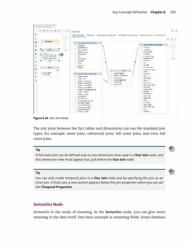
Key Concepts Refresher Chapter 6 263
Figure 6.24 Star Join Node
The star joins between the fact tables and dimensions can use the standard join
types, for example, inner joins, referential joins, left outer joins, and even full
outer joins.
Tip
A full outer join can be defined only on one dimension view used in a Star Join node, and
this dimension view must appear last, just before the Star Join node.
Tip
You can only create temporal joins in a Star Join node and by specifying the join as an
inner join. In that case, a new section appears below the join properties where you can set
the Temporal Properties.
Semantics Node
Semantics is the study of meaning. In the Semantics node, you can give more
meaning to the data itself. One basic example is renaming fields. Some database
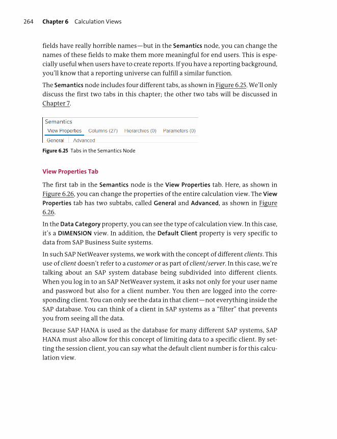
Chapter 6 Calculation Views264
fields have really horrible names—but in the Semantics node, you can change the
names of these fields to make them more meaningful for end users. This is espe-
cially useful when users have to create reports. If you have a reporting background,
you’ll know that a reporting universe can fulfill a similar function.
The Semantics node includes four different tabs, as shown in Figure 6.25. We’ll only
discuss the first two tabs in this chapter; the other two tabs will be discussed in
Chapter 7.
Figure 6.25 Tabs in the Semantics Node
View Properties Tab
The first tab in the Semantics node is the View Properties tab. Here, as shown in
Figure 6.26, you can change the properties of the entire calculation view. The View
Properties tab has two subtabs, called General and Advanced, as shown in Figure
6.26.
In the Data Category property, you can see the type of calculation view. In this case,
it’s a DIMENSION view. In addition, the Default Client property is very specific to
data from SAP Business Suite systems.
In such SAP NetWeaver systems, we work with the concept of different clients. This
use of client doesn’t refer to a customer or as part of client/server. In this case, we’re
talking about an SAP system database being subdivided into different clients.
When you log in to an SAP NetWeaver system, it asks not only for your user name
and password but also for a client number. You then are logged into the corre-
sponding client. You can only see the data in that client—not everything inside the
SAP database. You can think of a client in SAP systems as a “filter” that prevents
you from seeing all the data.
Because SAP HANA is used as the database for many different SAP systems, SAP
HANA must also allow for this concept of limiting data to a specific client. By set-
ting the session client, you can say what the default client number is for this calcu-
lation view.
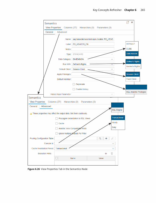
Key Concepts Refresher Chapter 6 265
Figure 6.26 View Properties Tab in the Semantics Node

Chapter 6 Calculation Views266
The Session Client option will filter the data to display only data from the specific
SAP client you’re using for your session, for example, from a reporting tool.
Instead of using one of these two options, you can also explicitly specify the SAP
client number that you want to display data for, for example, “800”, by selecting
the Fixed Client option.
Tip
Settings in the Semantics node of a calculation view takes precedence over client set-
tings made elsewhere, for example, the default client property for an SAP Web IDE user.
For the Apply Privileges setting, you can choose between no privileges or SQL Ana-
lytic Privileges. (We’ll discuss these options in more detail in Chapter 13 when dis-
cussing security.) We recommend always using SQL Analytic Privileges for
production systems.
Setting the Deprecate checkbox doesn’t mean that the calculation view won’t work
any longer; it will merely warn people that this calculation view has now been suc-
ceeded by a newer version somewhere in the system and that they should use the
newer version because this one will disappear someday in the future. When you
add this calculation view in another data model, you’ll see a warning not to use
this calculation view. The calculation view will still work as usual, however.
In the Advanced subtab, you can set the Execute In to SQL Engine. You’ll only set
this preference when developing SAP HANA Live calculation views. More informa-
tion on SAP HANA Live calculation views can be found in Chapter 14. Normally you
shouldn’t set any of the Advanced properties.
Columns Tab
The next tab in the Semantics node is the Columns tab (see Figure 6.27). In this tab,
the Type column shows whether the field is a measure or an attribute. This is very
helpful to analytics and reporting tools to ensure that the data is shown and
manipulated in the appropriate formats; for example, numeric fields (measures)
can be aggregated.
Renaming fields is easy. In the Columns tab, click the Name of the field, and type
the new name. The same rule applies for the Label. The label is used, for example,
when creating SAP HANA extended application services, advanced model (SAP
HANA XSA) and HTML5 applications, or in some reporting tools.
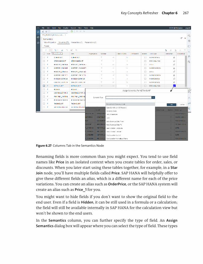
Key Concepts Refresher Chapter 6 267
Figure 6.27 Columns Tab in the Semantics Node
Renaming fields is more common than you might expect. You tend to use field
names like Price in an isolated context when you create tables for order, sales, or
discounts. When you later start using these tables together, for example, in a Star
Join node, you’ll have multiple fields called Price. SAP HANA will helpfully offer to
give these different fields an alias, which is a different name for each of the price
variations. You can create an alias such as OrderPrice, or the SAP HANA system will
create an alias such as Price_1 for you.
You might want to hide fields if you don’t want to show the original field to the
end user. Even if a field is Hidden, it can be still used in a formula or a calculation;
the field will still be available internally in SAP HANA for the calculation view but
won’t be shown to the end users.
In the Semantics column, you can further specify the type of field. An Assign
Semantics dialog box will appear where you can select the type of field. These types
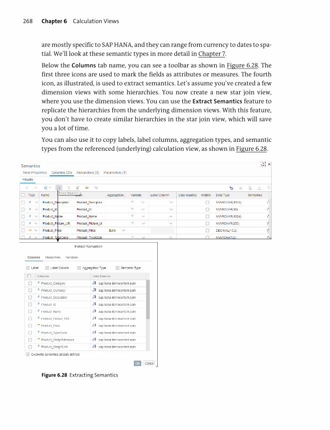
Chapter 6 Calculation Views268
are mostly specific to SAP HANA, and they can range from currency to dates to spa-
tial. We’ll look at these semantic types in more detail in Chapter 7.
Below the Columns tab name, you can see a toolbar as shown in Figure 6.28. The
first three icons are used to mark the fields as attributes or measures. The fourth
icon, as illustrated, is used to extract semantics. Let’s assume you’ve created a few
dimension views with some hierarchies. You now create a new star join view,
where you use the dimension views. You can use the Extract Semantics feature to
replicate the hierarchies from the underlying dimension views. With this feature,
you don’t have to create similar hierarchies in the star join view, which will save
you a lot of time.
You can also use it to copy labels, label columns, aggregation types, and semantic
types from the referenced (underlying) calculation view, as shown in Figure 6.28.
Figure 6.28 Extracting Semantics

Important Terminology Chapter 6 269
Lastly, let’s take a quick look at the Show Lineage option accessed via the fifth icon
on the toolbar (Figure 6.29).
To use this option, select an output column, and click on the Show Lineage icon.
The left side shows in each node where the column occurred. Go down the layers
of nodes, and you can see that the Supplier_Country column was introduced by the
Addresses table in the second Join node. This works even if the column got
renamed along the way.
Figure 6.29 Using the Show Lineage Option to Find the Node an Output Column Originated From
Important Terminology
In this chapter, the following terminology was used:
� Data sources
SAP HANA information views can use data from a wide variety of sources. The
main data sources are as follows:
– Row-based and column-based tables

Chapter 6 Calculation Views270
– SAP HANA information views in the SAP HANA system
– Decision tables
– SQL views
– Table functions
– Virtual tables with data from other databases
– CDS
– Data sources from another tenant in the SAP HANA system, if SAP HANA is
set up as an MDC system
� Aggregation node
Used to calculate single summary values from a large list of values; supports
sum, count, minimum, maximum, average, standard deviation, and variance.
� Graph node
Used for modeling relationships between entities and querying calculations,
such as the shortest path between two entities.
� Join node
Used to get data sources into information views.
� Projection node
Used to remove some fields from a calculation view, rename fields, filter data,
and add new calculated columns to a calculation view.
� Rank node
Used to create top N or bottom N lists of values to sort results.
� Star join node
Used to join a data foundation with fact tables to dimension views. The join
types available in the star join node are the same as the normal joins in a join
node. It’s what they’re joining that differs.
� Union node
Used to combine multiple data sources. You can make unions run even faster
by using a pruning configuration table.
� Intersect node
Used to find the records that occur in all the data sources.
� Minus node
Used to find the records that are found only in one of the data sources.
� Semantics node
Used to give meaning to the data in information views.

Practice Questions Chapter 6 271
� Calculation view of type dimension
Information views used for master data.
� Calculation view of type cube with star join
Views used for multidimensional reporting and data analysis purposes.
� Calculation view of type cube
Views used for more powerful multidimensional reporting and data analysis
purposes.
Practice Questions
These practice questions will help you evaluate your understanding of the topics
covered in this chapter. The questions shown are similar in nature to those found
on the certification examination. Although none of these questions will be found
on the exam itself, they will allow you to review your knowledge of the subject.
Select the correct answers, and then check the completeness of your answers in
the “Practice Question Answers and Explanations” section. Remember, on the
exam, you must select all correct answers and only correct answers to receive
credit for the question.
1. For what type of data are SAP HANA calculation views of type dimension
used?
� A. Transactional data
� B. Master data
� C. Materialized cube data
� D. Calculated data
2. Which of the following node types can you use to build a dimension view?
(There are 3 correct answers.)
� A. Star Join node
� B. Aggregation node
� C. Data Foundation node
� D. Semantics node
� E. Union node
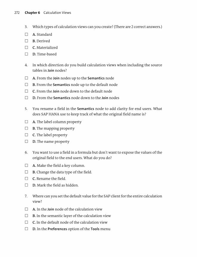
Chapter 6 Calculation Views272
3. Which types of calculation views can you create? (There are 2 correct answers.)
� A. Standard
� B. Derived
� C. Materialized
� D. Time-based
4. In which direction do you build calculation views when including the source
tables in Join nodes?
� A. From the Join nodes up to the Semantics node
� B. From the Semantics node up to the default node
� C. From the Join node down to the default node
� D. From the Semantics node down to the Join nodes
5. You rename a field in the Semantics node to add clarity for end users. What
does SAP HANA use to keep track of what the original field name is?
� A. The label column property
� B. The mapping property
� C. The label property
� D. The name property
6. You want to use a field in a formula but don’t want to expose the values of the
original field to the end users. What do you do?
� A. Make the field a key column.
� B. Change the data type of the field.
� C. Rename the field.
� D. Mark the field as hidden.
7. Where can you set the default value for the SAP client for the entire calculation
view?
� A. In the Join node of the calculation view
� B. In the semantic layer of the calculation view
� C. In the default node of the calculation view
� D. In the Preferences option of the Tools menu
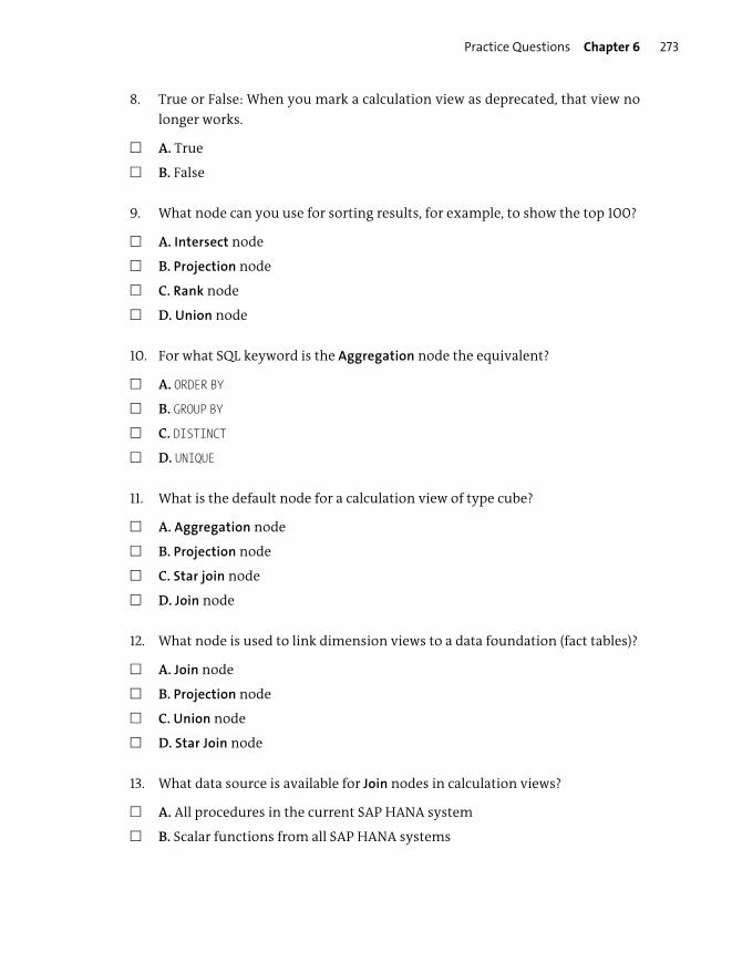
Practice Questions Chapter 6 273
8. True or False: When you mark a calculation view as deprecated, that view no
longer works.
� A. True
� B. False
9. What node can you use for sorting results, for example, to show the top 100?
� A. Intersect node
� B. Projection node
� C. Rank node
� D. Union node
10. For what SQL keyword is the Aggregation node the equivalent?
� A. ORDER BY
� B. GROUP BY
� C. DISTINCT
� D. UNIQUE
11. What is the default node for a calculation view of type cube?
� A. Aggregation node
� B. Projection node
� C. Star join node
� D. Join node
12. What node is used to link dimension views to a data foundation (fact tables)?
� A. Join node
� B. Projection node
� C. Union node
� D. Star Join node
13. What data source is available for Join nodes in calculation views?
� A. All procedures in the current SAP HANA system
� B. Scalar functions from all SAP HANA systems

Chapter 6 Calculation Views274
� C. Calculation views from other tenants in an MDC system
� D. Web services from the Internet
14. Which join types are available in a Join node of a calculation view? (There are
2 correct answers.)
� A. Referential joins
� B. Spatial joins
� C. Cross joins
� D. Temporal joins
15. From where does the extract semantics feature get the definition of hierar-
chies?
� A. From the current calculation view
� B. From the table data sources
� C. From the underlying dimension views
� D. From the SQL view data sources
16. You want to see in a Union node which data sources return no results for a
query. How do you achieve this?
� A. Set the is Null property in the Manage Mapping dialog.
� B. Create a union pruning configuration table.
� C. Create a standard union.
� D. Set the Empty Union Behavior property.
17. You want to ignore columns defined in the Rank node that aren’t included in
the query. What setting do you set?
� A. Default Client
� B. Keep Flag
� C. Dynamic Partition Elements
� D. Hidden
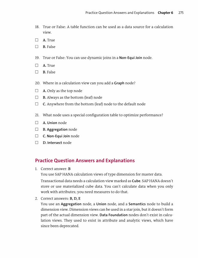
Practice Question Answers and Explanations Chapter 6 275
18. True or False: A table function can be used as a data source for a calculation
view.
� A. True
� B. False
19. True or False: You can use dynamic joins in a Non-Equi Join node.
� A. True
� B. False
20. Where in a calculation view can you add a Graph node?
� A. Only as the top node
� B. Always as the bottom (leaf) node
� C. Anywhere from the bottom (leaf) node to the default node
21. What node uses a special configuration table to optimize performance?
� A. Union node
� B. Aggregation node
� C. Non-Equi Join node
� D. Intersect node
Practice Question Answers and Explanations
1. Correct answer: B
You use SAP HANA calculation views of type dimension for master data.
Transactional data needs a calculation view marked as Cube. SAP HANA doesn’t
store or use materialized cube data. You can’t calculate data when you only
work with attributes; you need measures to do that.
2. Correct answers: B, D, E
You use an Aggregation node, a Union node, and a Semantics node to build a
dimension view. Dimension views can be used in a star join, but it doesn’t form
part of the actual dimension view. Data Foundation nodes don’t exist in calcu-
lation views. They used to exist in attribute and analytic views, which have
since been deprecated.
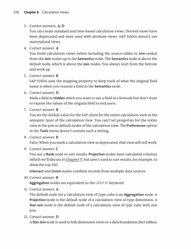
Chapter 6 Calculation Views276
3. Correct answers: A, D
You can create standard and time-based calculation views. Derived views have
been deprecated and were used with attribute views. SAP HANA doesn’t use
materialized views.
4. Correct answer: A
You build calculation views (when including the source tables in Join nodes)
from the Join nodes up to the Semantics node. The Semantics node is above the
default node, which is above the Join nodes. You always start from the bottom
and work up.
5. Correct answer: B
SAP HANA uses the mapping property to keep track of what the original field
name is when you rename a field in the Semantics node.
6. Correct answer: D
Mark a field as Hidden when you want to use a field in a formula but don’t want
to expose the values of the original field to end users.
7. Correct answer: B
You set the default value for the SAP client for the entire calculation view in the
semantic layer of the calculation view. You can’t set properties for the entire
view in the join or default nodes of the calculation view. The Preferences option
in the Tools menu doesn’t contain such a setting.
8. Correct answer: B
False. When you mark a calculation view as deprecated, that view will still work.
9. Correct answer: C
You use a Rank node to sort results. Projection nodes have calculated columns
(which we’ll discuss in Chapter 7), but aren’t used to sort results, for example, to
show the top 100.
Intersect and Union nodes combine records from multiple data sources.
10. Correct answer: B
Aggregation nodes are equivalent to the GROUP BY keyword.
11. Correct answer: A
The default node for a calculation view of type cube is an Aggregation node. A
Projection node is the default node of a calculation view of type dimension. A
Star Join node is the default node of a calculation view of type cube with star
join.
12. Correct answer: D
A Star Join node is used to link dimension views to a data foundation (fact tables).

Practice Question Answers and Explanations Chapter 6 277
13. Correct answer: C
Calculation views from other tenants in an MDC system are available as data
sources for Join nodes in calculation views.
Scalar functions don’t return table result sets, and procedures don’t have to
generate any result sets. (For more information, see Chapter 8.)
14. Correct answers: A, B
Referential joins and spatial joins are available in a Join node of a calculation
view. Temporal joins are only available in Aggregation nodes and Star Join
nodes.
15. Correct answer: C
The Extract Semantics option can get the definition of hierarchies from the
underlying dimension views.
Table data sources and SQL view data sources don’t have hierarchies.
16. Correct answer: D
You set the Empty Union Behavior property if want to see in a Union node which
data sources return no results for a query.
You create a union pruning configuration table for performance reasons.
For the Empty Union Behavior to work, you need to set constant values. A stan-
dard union doesn’t use constant values.
17. Correct answer: C
You set the Dynamic Partition Elements checkbox if you want to ignore col-
umns defined in Rank node that aren’t included in the query.
The Default Client setting is used in the Semantics node for the entire calcula-
tion view.
The Keep Flag and the Hidden flag are set for each field in the Output Columns
tab on all nodes.
18. Correct answer: A
True. A table function can be used as a data source for a calculation view.
19. Correct answer: B
False. You can’t use dynamic joins in a Non-Equi Join node.
Tip
Some questions in the exam will only have three answer options, like the following ques-
tion.

Chapter 6 Calculation Views278
20. Correct answer: B
A Graph node must always be the bottom (leaf) node.
21. Correct answer: A
Union nodes can use a special configuration table to optimize performance for
union pruning.
Takeaway
You should now know how to create SAP HANA information views and when to
create each type of calculation view based on your business requirements. You’ve
learned how to add data sources, create joins, add nodes, and select output fields.
In Table 6.2, we define the different information views and provide a list of their
individual features.
Summary
You learned how to create calculation views and add data sources, joins, nodes,
and output columns. You added meaning to the output columns in the Semantics
node and set the properties for the view.
In the next chapter, we’ll discuss how to further enhance our information views
with additional functionality, such as filter expressions, calculated columns, cur-
rency conversions, and hierarchies.
Calculation Views of
Type Dimension
Calculation View of
Type Cube with Star Join
Calculation View of
Type Cube
Purpose: Create a dimension
for our analytic modeling
needs
Purpose: Create a cube for
our analytic requirements
Purpose: Create more
advanced information
models
� Treats all data as attri-
butes
� Uses mostly joins
Combines fact tables with
dimensions
Focuses on extra functional-
ity, such as aggregations,
joins, projections, ranking,
and unions
Table 6.2 Information View Features

Chapter 7
Modeling Functions
Techniques You’ll Master
� Learn how to define calculated and restricted columns
� Examine filter operations and filter expressions
� Identify when to create variables and input parameters
� Understand currency and currency conversions
� Know how to create hierarchies for use in reporting tools
� Use Hierarchy Function nodes to create hierarchies for use inside
the calculation views

Chapter 7 Modeling Functions280
In previous chapters, you learned how to build SAP HANA calculation views. In this
chapter, you’ll see how to enhance calculation views with additional functionality,
including adding output fields, filtering data, converting currencies, asking for
inputs at the time they are run, and implementing hierarchies.
Real-World Scenario
You’re working on an SAP HANA modeling project and are asked to help with
publishing the company’s financial results for the year.
You copy some of the calculation views that you’ve created before and start
adding additional features to them. First, you filter the data to the last finan-
cial year and to the required company code. You then implement currency
conversions on all the financial transactions, so that the results can be pub-
lished in a single currency.
The board members aren’t sure if they want the results in US dollars or in
euros, so they ask you to give them a choice when they run their queries on
the SAP HANA calculation views. They also ask you to create a dashboard
where they can drill down into the results to see any missing data or issues.
Finally, you create an overview report showing the past few years of financial
results side by side.
Objectives of This Portion of the Test
The purpose of this portion of the SAP HANA certification exam is to test your
knowledge of SAP HANA modeling and calculation views, as well as your under-
standing of how to enhance and refine these views with additional functionality.
The certification exam expects you to have a good understanding of the following
topics:
� Calculated columns
� Restricted columns
� Filter operations
� Variables
� Input parameters

Key Concepts Refresher Chapter 7 281
� Currency and currency conversions
� Hierarchies
� Hierarchy functions
Note
This portion contributes up to 15% of the total certification exam score. This is one of the
largest portions of the certification exam.
Key Concepts Refresher
In the previous chapter, we saw how to create output columns for our calculation
view. In this chapter, we’ll learn about creating additional output fields. We’ll see
how to add calculated columns, restricted columns, counters, and currency con-
version columns to the list of output fields in our calculation views. In our discus-
sions on these topics, see if you can identity which feature solves each problem
described in the real-world scenario described previously.
Let’s start with the first of our nine topics on how to enhance our SAP HANA calcu-
lation views with modeling functions: calculated columns.
Calculated Columns
Up to this point, we’ve created calculation views using available data sources.
However, quite often, we’ll want SAP HANA to do some calculations for us on that
data (e.g., calculate the sales tax on a transaction).
In the past, this was usually done using reporting tools. However, SAP HANA has
all the data available and can do the calculations without having to send all the
data to the reporting tool. SAP HANA does the calculations faster than reporting
tools and sends only the results to reporting tools, saving calculation time, band-
width, and network time.
When we create calculated columns in SAP HANA, it adds additional output col-
umns to the output of our views. The calculated results are displayed in these cal-
culated columns. Figure 7.1 illustrates how calculated columns work.

Chapter 7 Modeling Functions282
Figure 7.1 Calculated Columns Added as Additional Output
On the left side of Figure 7.1 is our source data from a table. We added two calcu-
lated columns on the right. The first calculated column calculates discounts, and
the second one calculates the sales tax.
Note
The calculated columns are part of the output of the calculation view. The results aren’t
stored anywhere, but they are calculated and displayed each time the view is called.
We’ll start by discussing the calculated columns in SAP HANA that behave like
those we just described. After that, we’ll also look at counters, which create calcu-
lated columns for the number of items in specified groupings of data.
Creating Calculated Columns
In SAP Web IDE for SAP HANA, we create calculated columns in the work area of a
node. In the Calculated Columns tab, we select the + option, as shown in Figure 7.2.
When you click on the name of the calculated column, you’ll get the work area. In
the work area, you can enter the various settings for the calculated column. For
example, you have to specify the Name, Label, and Data Type of the new column
you want to create.
You can also specify what Semantic Type you want to assign to your new calculated
columns, for example, making it a Date or a Currency column.
Item Quantity Price Total
Device 2 $200 $400
Plug 500 $5 $2500
Cable 200 $10 $2000
Connector 7 $20 $140
Adapter 3 $50 $150
Discount Sales Tax (VAT)
$380 $57
$2250 $338
$1800 $270
$133 $20
$143 $21
Calculated columns
5% discount, but10% if more than
100 items
15% Sales Tax(VAT)
Table
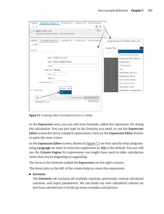
Key Concepts Refresher Chapter 7 283
Figure 7.2 Creating a New Calculated Column in a Node
In the Expression area, you can add your formula, called the expression, for doing
the calculation. You can just type in the formula you need, or use the Expression
Editor screen for more complex expressions. Click on the Expression Editor button
to open the next screen.
In the Expression Editor screen, shown in Figure 7.3, we first specify what program-
ming Language we want to write the expression in. SQL is the default. You can still
use the Column Engine for expressions you might have used in older calculation
views that you’re migrating or upgrading.
The focus is the formula (called the Expression) on the right column.
The three tabs on the left of the screen help us create the expression:
� Elements
The Elements tab contains all available columns, previously created calculated
columns, and input parameters. We can build our new calculated column on
previous calculations to build up more complex calculations.

Chapter 7 Modeling Functions284
� Functions
The Functions tab contains various useful functions, such as converting data
types, working with strings, doing the basic mathematical calculations, and
working with dates. We also have some extra functions, for example, the if()
function for if-then-else calculations, but these are only available when the Lan-
guage is set to Column Engine. You can also get some online help when clicking
the i (information) icon.
� Operators
The Operators tab contains operators, for example, for adding, multiplying,
comparing, or combining columns.
Figure 7.3 Using the Expression Editor to Create the Formula for Calculated Columns
All the examples here use measures. However, we can also create calculated col-
umns for attributes as well. The Functions also allow us to work with strings and
dates, so we can create expressions using attributes.
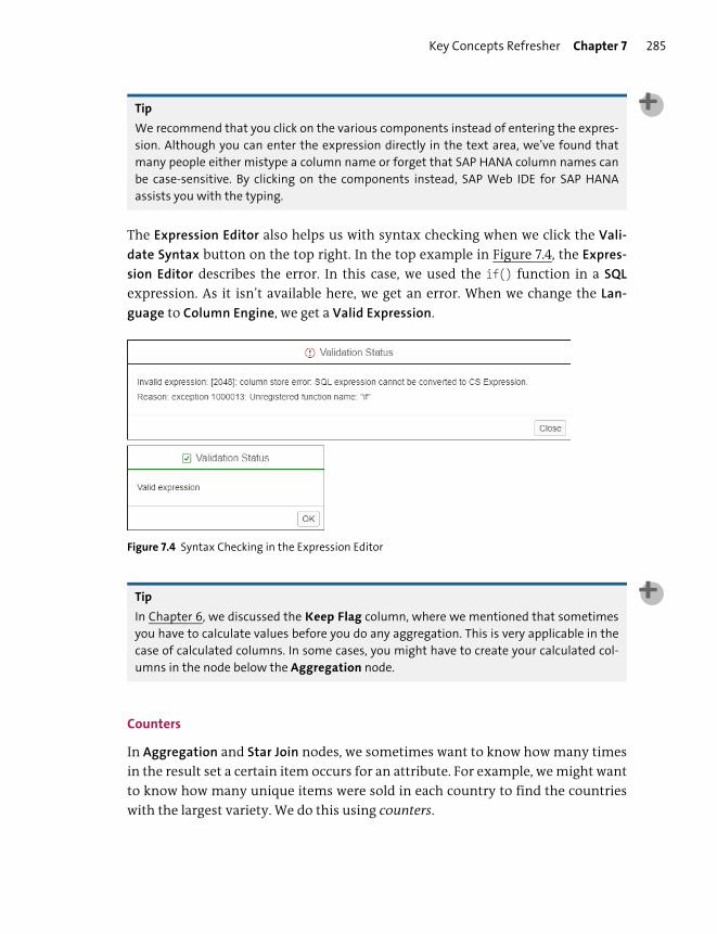
Key Concepts Refresher Chapter 7 285
Tip
We recommend that you click on the various components instead of entering the expres-
sion. Although you can enter the expression directly in the text area, we’ve found that
many people either mistype a column name or forget that SAP HANA column names can
be case-sensitive. By clicking on the components instead, SAP Web IDE for SAP HANA
assists you with the typing.
The Expression Editor also helps us with syntax checking when we click the Vali-
date Syntax button on the top right. In the top example in Figure 7.4, the Expres-
sion Editor describes the error. In this case, we used the if() function in a SQL
expression. As it isn’t available here, we get an error. When we change the Lan-
guage to Column Engine, we get a Valid Expression.
Figure 7.4 Syntax Checking in the Expression Editor
Tip
In Chapter 6, we discussed the Keep Flag column, where we mentioned that sometimes
you have to calculate values before you do any aggregation. This is very applicable in the
case of calculated columns. In some cases, you might have to create your calculated col-
umns in the node below the Aggregation node.
Counters
In Aggregation and Star Join nodes, we sometimes want to know how many times
in the result set a certain item occurs for an attribute. For example, we might want
to know how many unique items were sold in each country to find the countries
with the largest variety. We do this using counters.

Chapter 7 Modeling Functions286
The option to create a new counter is found in the calculated column’s create (+)
menu in Aggregation and Star Join nodes (see Figure 7.5). In the Calculated Column
tab, click the + icon, and select the Counter option to create a new counter. In our
example, we’ll put the counter on items sold.
We can also use multiple columns in the Counter section to expand our example
to add item categories, for example, to show which country has the largest variety
of items for electronics, the largest variety of items for industrial pumps, and so
on.
Figure 7.5 Creating a New Counter
Restricted Columns
The easiest way to explain restricted columns is to think of a reporting requirement
that you frequently encounter. For example, let’s say we have a website where we

Key Concepts Refresher Chapter 7 287
work with the data of who visited the website and what device they used. We use a
view like the one shown in Figure 7.6. Our data from the source table is in the two
columns on the left. We can see how many users connected with each type of
device, organized per row.
We would like our report to be like the bottom right of the screen in Figure 7.6,
where we have a column for each device with the total number of users for each
device. You might know this as a pivot table. We already saw in Chapter 5 that we
could use a union with constant values to achieve a similar result.
We can also achieve this by creating a restricted column for each device. This adds
a new additional output column to our view. When we create a restricted column
for the mobile phones, we restrict our column to only show mobile phone data.
Everything else in that column is NULL. When we now aggregate the restricted col-
umn, we get the total number of users visiting the website on mobile phones. We
create a restricted field for each device to create our report.
Figure 7.6 Creating Four Restricted Columns and Aggregating the Result Sets
Device Number of users
Mobile phone 20
Tablet 10
Desktop 10
Mobile phone 10
Mobile phone 40
Laptop 20
Tablet 20
Laptop 30
Mobile phone 50
Mobile phone 40
Laptop 20
Desktop 20
Mobile phone Tablet Laptop Desktop
160 30 70 30
Mobile phone Tablet Laptop Desktop
20
10
10
10
40
20
20
30
50
40
20
20
Aggregated results
Restricted columnsTable

Chapter 7 Modeling Functions288
Tip
Even though a union with constant values can achieve a similar output result, you don’t
always have tables with similar field structures available to do a union. Using restricted
columns to achieve this output result will always work and is easy to set up.
Because we need aggregation for this to work properly, restricted columns are only
available in the Aggregation and Star Join nodes.
Note
We create restricted columns on attributes. For example, it doesn’t make sense to create
a Reporting column with a heading of “25” (measure). However, a Mobile phone column
(an attribute) provides more useful information.
Creating a restricted column is similar to creating a calculated column. In the
Restricted Columns tab, as shown in Figure 7.7, we click the + icon.
Tip
In SAP HANA Interactive Education (SHINE), look for the PURCHASE_COMMON_CUR-RENCY calculation view.
In the right side of the work area, we create our restricted column. We specify the
name of the restricted column and what data we want to display in the column. In
this case, we chose the GROSSAMOUNT column.
In the Restrictions area, we can add one or more restrictions, such as the year has
to be 2019, the device has to be a mobile phone, or only show the Flat screens sold
(Figure 7.7).
If we add multiple restrictions, SAP HANA automatically creates the relevant AND
and OR operators. For example, if we have two restrictions for the year 2019 and
2020, the Expression Editor will use year = 2019 OR year = 2020.

Key Concepts Refresher Chapter 7 289
Figure 7.7 Creating a Restricted Column for the Net Amount of Invoices
When we enter a value, such as “2019” for the year, we can ask the Expression Editor
screen to give us a list of existing values currently stored in the system. In Figure
7.8, we asked for a list of item categories. In the list, we see, for example, Flat screens
and Graphic cards. This popup list is called the value help list. You’ll find these value
help lists in all the modeling screens.
In the restricted column creation dialog, in the Restrictions area, we can choose to
use an Expression rather than specify individual Column values. We can then use
the Expression Editor to generate the relevant portion of the SQL WHERE statement
directly.
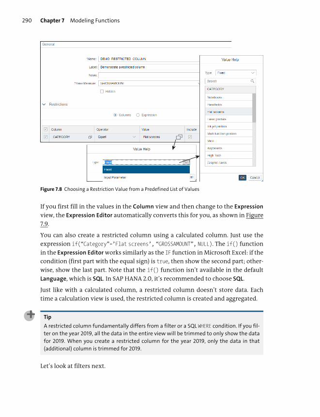
Chapter 7 Modeling Functions290
Figure 7.8 Choosing a Restriction Value from a Predefined List of Values
If you first fill in the values in the Column view and then change to the Expression
view, the Expression Editor automatically converts this for you, as shown in Figure
7.9.
You can also create a restricted column using a calculated column. Just use the
expression if(“Category”=’Flat screens’, “GROSSAMOUNT”, NULL). The if() function
in the Expression Editor works similarly as the IF function in Microsoft Excel: if the
condition (first part with the equal sign) is true, then show the second part; other-
wise, show the last part. Note that the if() function isn’t available in the default
Language, which is SQL. In SAP HANA 2.0, it’s recommended to choose SQL.
Just like with a calculated column, a restricted column doesn’t store data. Each
time a calculation view is used, the restricted column is created and aggregated.
Tip
A restricted column fundamentally differs from a filter or a SQL WHERE condition. If you fil-
ter on the year 2019, all the data in the entire view will be trimmed to only show the data
for 2019. When you create a restricted column for the year 2019, only the data in that
(additional) column is trimmed for 2019.
Let’s look at filters next.

Key Concepts Refresher Chapter 7 291
Figure 7.9 Using the Expression Editor to Create Restrictions on Restricted Columns
Filters
Sometimes we don’t want to show all the data from a specific table. For example,
we might only want to show data for the year 2019. In this case, we can apply a fil-
ter. Filters restrict the data for the entire data source. They are therefore similar to
the WHERE condition in an SQL statement. When we apply filters, SAP HANA can
work a lot faster because it doesn’t have to work with and sift through all the data.
Something to keep in mind is that you can leverage partitions when designing fil-
ter expressions. When a field has been partitioned, SAP HANA has already sepa-
rated the data by values. If you create a filter on a partitioned column, you can
expect good performance on your filter expressions.
There are three different ways we can use filtering. We can use filter expressions in
the calculation views, and this is what we’ll use most of the time. The other two fil-
tering methods are specific to SAP systems written on SAP NetWeaver and are
there for compatibility reasons. We’ll start with using filter expressions in our cal-
culation views.

Chapter 7 Modeling Functions292
Filter Expressions
To create a filter expression, select the Filter Expression tab in the work area of your
node. This puts you into the Expression Editor, as shown in Figure 7.10, where you
can create an expression.
Figure 7.10 Creating a Filter Expression in a Projection or Join Node
This works similar to the Expression Editor for calculated and restricted columns.
In this case, however, the filter expression will be similar to the WHERE condition of
an SQL statement. A filter icon will appear next to the name of the Filter Expres-
sion tab after you’ve created a filter expression.
In the left work area of your calculation view, where you see the view nodes, you’ll
also see a filter icon in the node, as shown in Figure 7.11.
Figure 7.11 A Filter Expression Icon in the View Node
Key Concepts Refresher Chapter 7 293
Filtering for SAP Clients
Filtering of data can be implemented more widely than the examples we’ve just
seen. In Chapter 6, we saw how to set an option for filtering to an SAP client in the
Semantics node. Later, we’ll see another example of limiting data to the session cli-
ent for data from SAP financial systems. Chapter 8 and Chapter 13 also provide fur-
ther details on filtering for an SAP client using SQL/SQLScript and security,
respectively.
Domain Fixed Values
SAP ERP and SAP S/4HANA use the ABAP programming language, which has some
powerful Data Dictionary features. In ABAP, we can define reusable data elements
(e.g., data types) and use them in our table definitions.
Sometimes we want these data elements to only allow a range of values. We define
a domain with the range of values and use this domain with the data element. In
all the tables where that specific data element is used, the users can now only enter
values that are in the specified range.
Instead of a range, we can also specify fixed values for the domain, which are
known as the domain fixed values. These are values that won’t change, and the
users can only choose from the available list when they enter data into the fields.
Let’s look at some examples: Say the users need to enter a gender. The domain val-
ues are fixed to male and female. This is very similar to the value help shown ear-
lier in Figure 7.8. Another example could be the possible statuses of a sales order,
which could be Quoted, Sold, Delivered, Invoiced, and Paid.
The lists of fixed values are stored in tables DD07L and DD07T in the SAP ERP system.
Because these tables are so valuable for business systems, we often replicate (or
import) these tables to SAP HANA. We can then use these values in SAP HANA for
the Value Help screens, similar to that shown earlier in Figure 7.8.
These domain fixed values can now also be used to filter business data; for exam-
ple, we can filter the sales data to the domain fixed value of paid to see only the
sales that are already paid.
Variables
In the previous section, we looked at filtering. These filters were all static, in the
sense that we couldn’t change them after we specified them. Each time you query
the view, the same filters are used.

Chapter 7 Modeling Functions294
Frequently, however, we’ll want the system to ask us at runtime what we would
like to filter on. Instead of always filtering the view on the year 2019, we can specify
which year’s data we want to see. If we query the view from a reporting tool, we
even expect the reporting tool to pop up a dialog box and ask us what we would
like to filter on. In other words, you only specify the filter when the query is run on
the calculation view.
This dynamic type of filtering is done with variables. We define variables in the
Semantics node of a calculation view. In Chapter 6, we discussed the first two tabs
available in the Semantics node. Now we’ll look at one of the remaining two tabs:
Parameters.
In Figure 7.12, we see the Semantics node. In the Parameters tab, we select the + icon
to reveal the dropdown menu, and select the Variable option.
Figure 7.12 Creating a Variable in the Semantics Node
In the General work area (Figure 7.13), we start by specifying the Name of the vari-
able.
In the Selection Type field, we can choose what type of variable we want to create.
There are three types of variables:
� Single Value
The variable only asks for one (single) value; for example, the year is 2019.
� Interval
The variable asks for from and to values, for example, the years from 2015 to
2018.
� Range
The variable asks for a single value but combines it with another operator; for
example, the year is greater and equal to 2015.
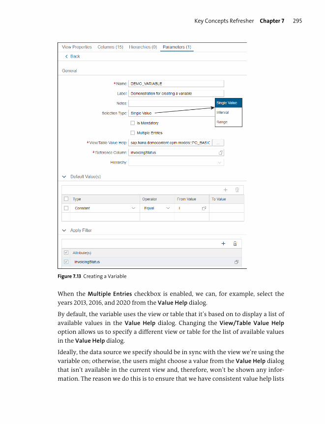
Key Concepts Refresher Chapter 7 295
Figure 7.13 Creating a Variable
When the Multiple Entries checkbox is enabled, we can, for example, select the
years 2013, 2016, and 2020 from the Value Help dialog.
By default, the variable uses the view or table that it’s based on to display a list of
available values in the Value Help dialog. Changing the View/Table Value Help
option allows us to specify a different view or table for the list of available values
in the Value Help dialog.
Ideally, the data source we specify should be in sync with the view we’re using the
variable on; otherwise, the users might choose a value from the Value Help dialog
that isn’t available in the current view and, therefore, won’t be shown any infor-
mation. The reason we do this is to ensure that we have consistent value help lists
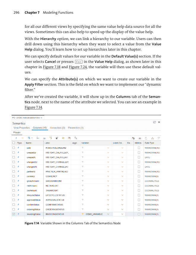
Chapter 7 Modeling Functions296
for all our different views by specifying the same value help data source for all the
views. Sometimes this can also help to speed up the display of the value help.
With the Hierarchy option, we can link a hierarchy to our variable. Users can then
drill down using this hierarchy when they want to select a value from the Value
Help dialog. You’ll learn how to set up hierarchies later in this chapter.
We can specify default values for our variable in the Default Value(s) section. If the
user selects Cancel or presses (Esc) in the Value Help dialog, as shown later in this
chapter in Figure 7.18 and Figure 7.24, the variable will then use these default val-
ues.
We can specify the Attribute(s) on which we want to create our variable in the
Apply Filter section. This is the field on which we want to implement our “dynamic
filter.”
After we’ve created the variable, it will show up in the Columns tab of the Seman-
tics node, next to the name of the attribute we selected. You can see an example in
Figure 7.14.
Figure 7.14 Variable Shown in the Columns Tab of the Semantics Node

Key Concepts Refresher Chapter 7 297
When we preview our calculation view, a Variable/Input Parameters screen will
appear in SAP Web IDE for SAP HANA, as shown in Figure 7.15. We have to supply
these values before SAP will run our view and return the results. If we supplied
default values, these values will be prepopulated in the fields, and we just continue
running the query on our calculation view.
When we select the icon on the right side of the FROM field (see Figure 7.15), a Value
Help dialog will appear with a list of available values that we can choose from.
Figure 7.15 Variable Dialog
Input Parameters
Input parameters are very similar to variables except where variables are specifi-
cally created for dynamic filtering, input parameters are more generic. For exam-
ple, we can use them in formulas or expressions.
Let’s look at an example: An outstanding payments report asks you for how many
months outstanding you want to see the results. This time period can then be used
in a calculated column’s expression to calculate the results we asked for. The
report can be used by the debt-collecting department for payments outstanding
longer than two months, while the legal department will use the same report to
ask for payments outstanding longer than six months.
We’ll start by learning how to create input parameters, and then take a quick look
at how to map them to different information-modeling objects.
Creating Input Parameters
Input parameters are created in the Semantics node (see Figure 7.16). We can also
create input parameters in all the node types. The input parameter work area and
the various dropdown menu options are shown in Figure 7.16.
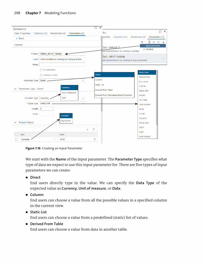
Chapter 7 Modeling Functions298
Figure 7.16 Creating an Input Parameter
We start with the Name of the input parameter. The Parameter Type specifies what
type of data we expect to use this input parameter for. There are five types of input
parameters we can create:
� Direct
End users directly type in the value. We can specify the Data Type of the
expected value as Currency, Unit of measure, or Date.
� Column
End users can choose a value from all the possible values in a specified column
in the current view.
� Static List
End users can choose a value from a predefined (static) list of values.
� Derived From Table
End users can choose a value from data in another table.
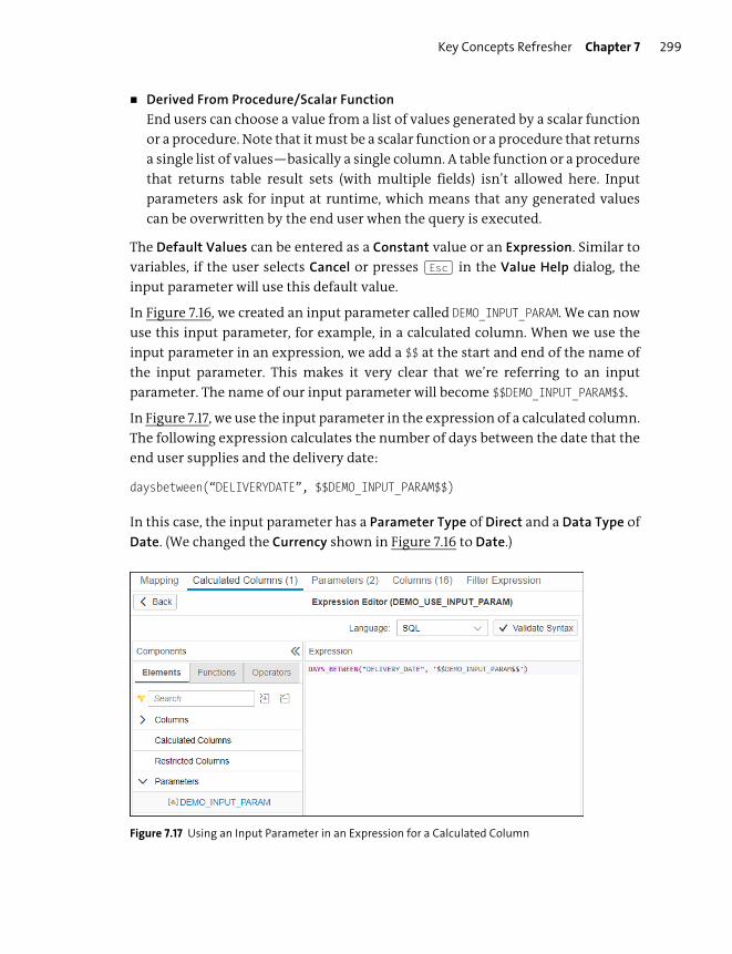
Key Concepts Refresher Chapter 7 299
� Derived From Procedure/Scalar Function
End users can choose a value from a list of values generated by a scalar function
or a procedure. Note that it must be a scalar function or a procedure that returns
a single list of values—basically a single column. A table function or a procedure
that returns table result sets (with multiple fields) isn’t allowed here. Input
parameters ask for input at runtime, which means that any generated values
can be overwritten by the end user when the query is executed.
The Default Values can be entered as a Constant value or an Expression. Similar to
variables, if the user selects Cancel or presses (Esc) in the Value Help dialog, the
input parameter will use this default value.
In Figure 7.16, we created an input parameter called DEMO_INPUT_PARAM. We can now
use this input parameter, for example, in a calculated column. When we use the
input parameter in an expression, we add a $$ at the start and end of the name of
the input parameter. This makes it very clear that we’re referring to an input
parameter. The name of our input parameter will become $$DEMO_INPUT_PARAM$$.
In Figure 7.17, we use the input parameter in the expression of a calculated column.
The following expression calculates the number of days between the date that the
end user supplies and the delivery date:
daysbetween(“DELIVERYDATE”, $$DEMO_INPUT_PARAM$$)
In this case, the input parameter has a Parameter Type of Direct and a Data Type of
Date. (We changed the Currency shown in Figure 7.16 to Date.)
Figure 7.17 Using an Input Parameter in an Expression for a Calculated Column

Chapter 7 Modeling Functions300
Tip
We have $$CLIENT$$ and $$LANGUAGE$$ built into SAP HANA. These don’t ask for values at
runtime, but instead give the SAP client number filter currently in use and the current
logon language of the end user.
You can see $$CLIENT$$ used later in this chapter in Figure 7.23.
When we preview the calculation view in SAP Web IDE for SAP HANA, and the
input parameter has a Data Type of Date, a calendar is displayed where you can
choose the date you want (see Figure 7.18).
Figure 7.18 Date Input Parameter
Mapping Input Parameters
Using input parameters is a very powerful modeling concept. We can link input
parameters to many different information-modeling objects. In Figure 7.19, we
select the Parameters tab, and then click on the Manage input parameter mappings
icon.
We can change the Type of mapping to the following:
� Data Sources
We can map the input parameters in this calculation view, for example, to the
input parameters in an underlying calculation view, such as a dimension view.

Key Concepts Refresher Chapter 7 301
� Procedures/Scalar function for input parameters
We can map the input parameters in this calculation view to the input parame-
ters of a scalar function or procedure. Similarly to when we discussed the type
of input parameter when creating one, it must be a scalar function or a proce-
dure that returns a single list of values—basically a single “column.”
� Views for value help for variables/input parameters
We can map the input parameters in this calculation view to the input parame-
ters of an external view for value help.
� Views for value help for attributes
When you’re filtering the attributes in the underlying data sources that use
other calculation views as value help, you can map the input parameters in
these value help views to the input parameters of this calculation view.
Figure 7.19 Mapping Input Parameters
In Figure 7.19, we use a scalar function as the source. But the Source Input Parame-
ters list on the bottom left is empty because we have the Type of mapping specified
as Data Sources and not as Procedures/Scalar function for input parameters. If you
change to the correct mapping Type, the Source Input Parameters will automati-
cally show up.

Chapter 7 Modeling Functions302
Note
Unfortunately, the phrase input parameters has two meanings in SAP HANA. The first
meaning is for the input parameters we discussed earlier in this chapter, which ask for
“input” from a user at runtime. The second meaning is that SQLScript procedures and
functions can have input parameters and output parameters. These functions need
“input” and give “output.” The preceding mapping gives a way to link these different
types of input parameters.
Session Variables
Input parameters have a lot of uses as we’ve just seen. There are a few cases where
predefined input parameters can be very helpful. In some applications, you might
want to know extra information such as the name of the user that is logged in, the
name of the application that is calling the calculation view, and even the name of
the SAP HANA extended application services, advanced model (SAP HANA XSA)
user when a technical user is used to talk to the SAP HANA information models.
In many modern applications, such as the microservices running in SAP HANA
XSA containers, developers are using command-line parameters. These are values
that are passed to an application at execution time. These developers have been
asking for the same feature for SAP HANA applications. Users currently have to set
the value of an input parameter each time they call a calculation view that asks
them for a value. What we need is something that is set once and stays active for
the duration of each user’s session.
SPS 04
SAP HANA 2.0 SPS 04 has two more options in the dropdown menu when you add a new
parameter. The updated menu is shown in Figure 7.20.
Figure 7.20 Creating a Session Variable in SAP HANA 2.0 SPS 04
Key Concepts Refresher Chapter 7 303
You can create a Fuzzy Search Parameter for helping users when searching text fields.
We’ll look at this option in Chapter 10.
The other option is to create a Session Variable. As the name suggests, this is like an
input parameter but with a value that is set for your current session. Think of working
session on the system as the time from when you log in until you log out.
You can use some predefined session variables, such as the name of the user that is
logged in. You can also create your own session variables, which allows you to control the
processing flow based on the value in your session variable.
For example, when working with financial data in a cube, you have both budget data and
actual expenses. (We discussed this in Chapter 5 when looking at how to build an infor-
mation model.) You can now set a session variable to only work with the budget data or
only work with the actual expenses. In a Union node, you can use the session variable in
the Mapping tab for constant pruning, or you can use a filter on the session variable in
another type of node.
Working with either hot or warm data in your session is another example. (We discussed
hot and warm data in Chapter 3 in the Data Aging section.)
Currency
SAP is well known for its business systems. An important part of financial and
business information models is their ability to work with currencies.
In Figure 7.21, we can see the Columns tab of a calculation view. We have a few out-
put fields that are currency fields, for example, four Sales amounts for different
regions.
When we look at the Properties of these fields, they are treated as numeric fields
(measures). We can improve on that by changing the Semantic Type property to
Amount with Currency Code.
When we change the Semantic Type of a field to currency, an Assign Semantics
screen appears as shown in Figure 7.22.
SPS 04
SAP HANA 2.0 SPS 04 also has a Hyperlink semantic type. Tools, such as web browsers,
that know how to consume hyperlinks can use this information for added functionality.
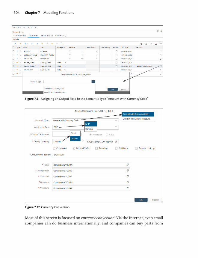
Chapter 7 Modeling Functions304
Figure 7.21 Assigning an Output Field to the Semantic Type “Amount with Currency Code”
Figure 7.22 Currency Conversion
Most of this screen is focused on currency conversion. Via the Internet, even small
companies can do business internationally, and companies can buy parts from
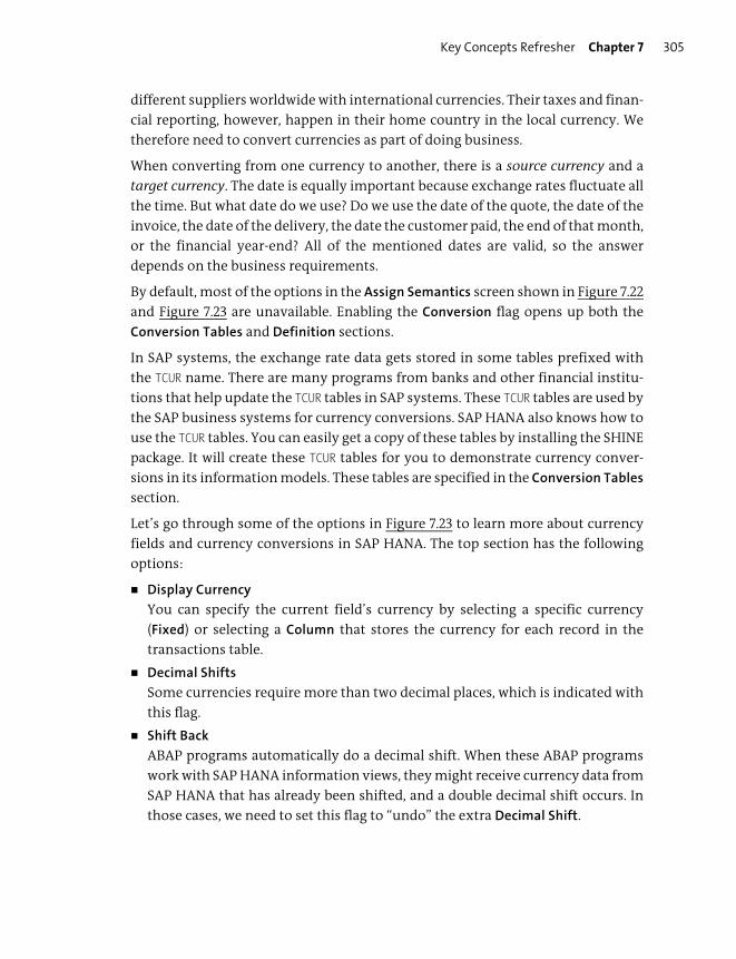
Key Concepts Refresher Chapter 7 305
different suppliers worldwide with international currencies. Their taxes and finan-
cial reporting, however, happen in their home country in the local currency. We
therefore need to convert currencies as part of doing business.
When converting from one currency to another, there is a source currency and a
target currency. The date is equally important because exchange rates fluctuate all
the time. But what date do we use? Do we use the date of the quote, the date of the
invoice, the date of the delivery, the date the customer paid, the end of that month,
or the financial year-end? All of the mentioned dates are valid, so the answer
depends on the business requirements.
By default, most of the options in the Assign Semantics screen shown in Figure 7.22
and Figure 7.23 are unavailable. Enabling the Conversion flag opens up both the
Conversion Tables and Definition sections.
In SAP systems, the exchange rate data gets stored in some tables prefixed with
the TCUR name. There are many programs from banks and other financial institu-
tions that help update the TCUR tables in SAP systems. These TCUR tables are used by
the SAP business systems for currency conversions. SAP HANA also knows how to
use the TCUR tables. You can easily get a copy of these tables by installing the SHINE
package. It will create these TCUR tables for you to demonstrate currency conver-
sions in its information models. These tables are specified in the Conversion Tables
section.
Let’s go through some of the options in Figure 7.23 to learn more about currency
fields and currency conversions in SAP HANA. The top section has the following
options:
� Display Currency
You can specify the current field’s currency by selecting a specific currency
(Fixed) or selecting a Column that stores the currency for each record in the
transactions table.
� Decimal Shifts
Some currencies require more than two decimal places, which is indicated with
this flag.
� Shift Back
ABAP programs automatically do a decimal shift. When these ABAP programs
work with SAP HANA information views, they might receive currency data from
SAP HANA that has already been shifted, and a double decimal shift occurs. In
those cases, we need to set this flag to “undo” the extra Decimal Shift.
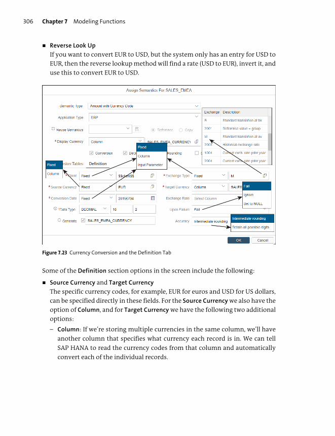
Chapter 7 Modeling Functions306
� Reverse Look Up
If you want to convert EUR to USD, but the system only has an entry for USD to
EUR, then the reverse lookup method will find a rate (USD to EUR), invert it, and
use this to convert EUR to USD.
Figure 7.23 Currency Conversion and the Definition Tab
Some of the Definition section options in the screen include the following:
� Source Currency and Target Currency
The specific currency codes, for example, EUR for euros and USD for US dollars,
can be specified directly in these fields. For the Source Currency we also have the
option of Column, and for Target Currency we have the following two additional
options:
– Column: If we’re storing multiple currencies in the same column, we’ll have
another column that specifies what currency each record is in. We can tell
SAP HANA to read the currency codes from that column and automatically
convert each of the individual records.
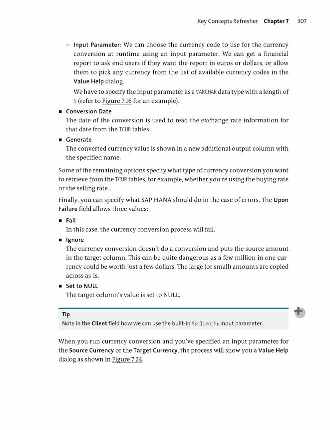
Key Concepts Refresher Chapter 7 307
– Input Parameter: We can choose the currency code to use for the currency
conversion at runtime using an input parameter. We can get a financial
report to ask end users if they want the report in euros or dollars, or allow
them to pick any currency from the list of available currency codes in the
Value Help dialog.
We have to specify the input parameter as a VARCHAR data type with a length of
5 (refer to Figure 7.16 for an example).
� Conversion Date
The date of the conversion is used to read the exchange rate information for
that date from the TCUR tables.
� Generate
The converted currency value is shown in a new additional output column with
the specified name.
Some of the remaining options specify what type of currency conversion you want
to retrieve from the TCUR tables, for example, whether you’re using the buying rate
or the selling rate.
Finally, you can specify what SAP HANA should do in the case of errors. The Upon
Failure field allows three values:
� Fail
In this case, the currency conversion process will fail.
� Ignore
The currency conversion doesn’t do a conversion and puts the source amount
in the target column. This can be quite dangerous as a few million in one cur-
rency could be worth just a few dollars. The large (or small) amounts are copied
across as-is.
� Set to NULL
The target column’s value is set to NULL.
Tip
Note in the Client field how we can use the built-in $$client$$ input parameter.
When you run currency conversion and you’ve specified an input parameter for
the Source Currency or the Target Currency, the process will show you a Value Help
dialog as shown in Figure 7.24.
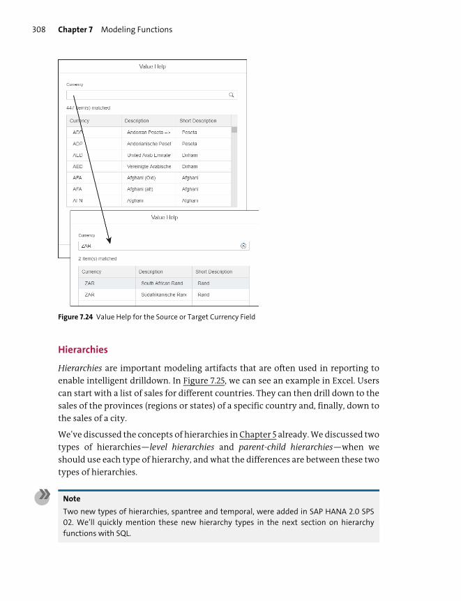
Chapter 7 Modeling Functions308
Figure 7.24 Value Help for the Source or Target Currency Field
Hierarchies
Hierarchies are important modeling artifacts that are often used in reporting to
enable intelligent drilldown. In Figure 7.25, we can see an example in Excel. Users
can start with a list of sales for different countries. They can then drill down to the
sales of the provinces (regions or states) of a specific country and, finally, down to
the sales of a city.
We’ve discussed the concepts of hierarchies in Chapter 5 already. We discussed two
types of hierarchies—level hierarchies and parent-child hierarchies—when we
should use each type of hierarchy, and what the differences are between these two
types of hierarchies.
Note
Two new types of hierarchies, spantree and temporal, were added in SAP HANA 2.0 SPS
02. We’ll quickly mention these new hierarchy types in the next section on hierarchy
functions with SQL.
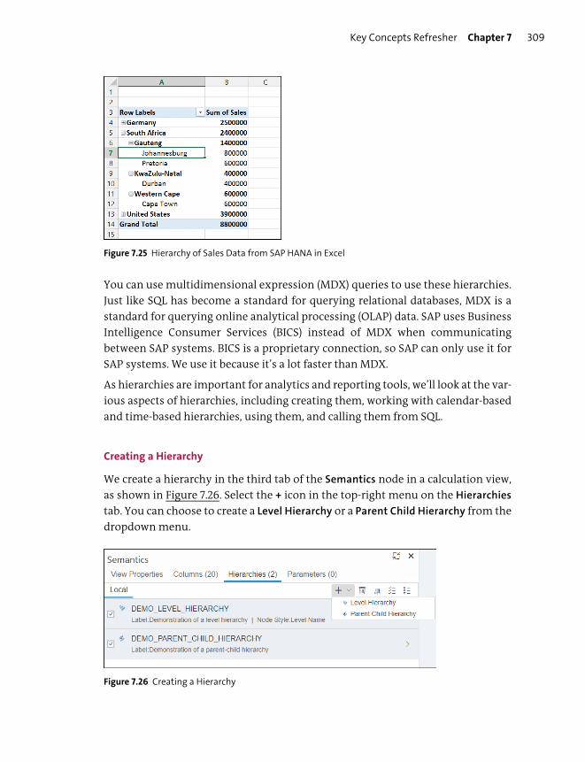
Key Concepts Refresher Chapter 7 309
Figure 7.25 Hierarchy of Sales Data from SAP HANA in Excel
You can use multidimensional expression (MDX) queries to use these hierarchies.
Just like SQL has become a standard for querying relational databases, MDX is a
standard for querying online analytical processing (OLAP) data. SAP uses Business
Intelligence Consumer Services (BICS) instead of MDX when communicating
between SAP systems. BICS is a proprietary connection, so SAP can only use it for
SAP systems. We use it because it’s a lot faster than MDX.
As hierarchies are important for analytics and reporting tools, we’ll look at the var-
ious aspects of hierarchies, including creating them, working with calendar-based
and time-based hierarchies, using them, and calling them from SQL.
Creating a Hierarchy
We create a hierarchy in the third tab of the Semantics node in a calculation view,
as shown in Figure 7.26. Select the + icon in the top-right menu on the Hierarchies
tab. You can choose to create a Level Hierarchy or a Parent Child Hierarchy from the
dropdown menu.
Figure 7.26 Creating a Hierarchy

Chapter 7 Modeling Functions310
You can specify the hierarchy options by clicking on the name of the hierarchy,
and completing the fields in the work area in SAP Web IDE for SAP HANA. You start
by specifying the Name of the hierarchy.
In Figure 7.27, we create a level hierarchy in SAP HANA where we add the different
levels. On each level, you select a specific field name in the dropdown list. Each
level uses a different column in a level hierarchy. You can also specify the sorting
order and on which column it has to sort.
Figure 7.27 Level Hierarchy
Figure 7.27 shows an example of a level hierarchy using geographic attributes.
Level 1 is the region (e.g., Africa or Asia), level 2 is the country, and level 3 is the city.
In Figure 7.28, you can see an example of a parent-child hierarchy of an HR organi-
zational structure with managers and employees. In this case, the manager has the
parent role, and the employee has the child role.
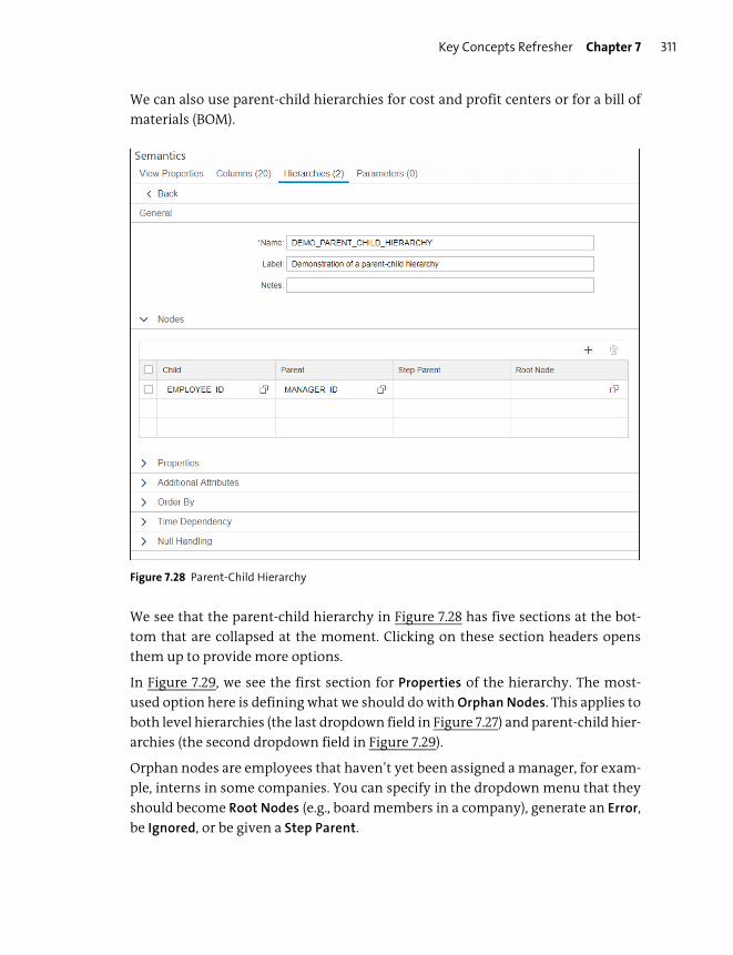
Key Concepts Refresher Chapter 7 311
We can also use parent-child hierarchies for cost and profit centers or for a bill of
materials (BOM).
Figure 7.28 Parent-Child Hierarchy
We see that the parent-child hierarchy in Figure 7.28 has five sections at the bot-
tom that are collapsed at the moment. Clicking on these section headers opens
them up to provide more options.
In Figure 7.29, we see the first section for Properties of the hierarchy. The most-
used option here is defining what we should do with Orphan Nodes. This applies to
both level hierarchies (the last dropdown field in Figure 7.27) and parent-child hier-
archies (the second dropdown field in Figure 7.29).
Orphan nodes are employees that haven’t yet been assigned a manager, for exam-
ple, interns in some companies. You can specify in the dropdown menu that they
should become Root Nodes (e.g., board members in a company), generate an Error,
be Ignored, or be given a Step Parent.
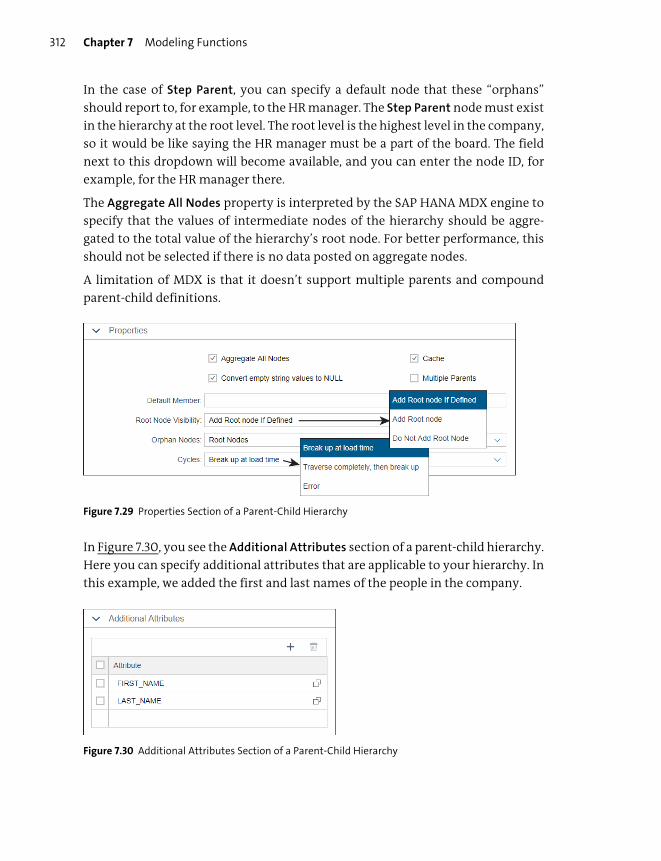
Chapter 7 Modeling Functions312
In the case of Step Parent, you can specify a default node that these “orphans”
should report to, for example, to the HR manager. The Step Parent node must exist
in the hierarchy at the root level. The root level is the highest level in the company,
so it would be like saying the HR manager must be a part of the board. The field
next to this dropdown will become available, and you can enter the node ID, for
example, for the HR manager there.
The Aggregate All Nodes property is interpreted by the SAP HANA MDX engine to
specify that the values of intermediate nodes of the hierarchy should be aggre-
gated to the total value of the hierarchy’s root node. For better performance, this
should not be selected if there is no data posted on aggregate nodes.
A limitation of MDX is that it doesn’t support multiple parents and compound
parent-child definitions.
Figure 7.29 Properties Section of a Parent-Child Hierarchy
In Figure 7.30, you see the Additional Attributes section of a parent-child hierarchy.
Here you can specify additional attributes that are applicable to your hierarchy. In
this example, we added the first and last names of the people in the company.
Figure 7.30 Additional Attributes Section of a Parent-Child Hierarchy
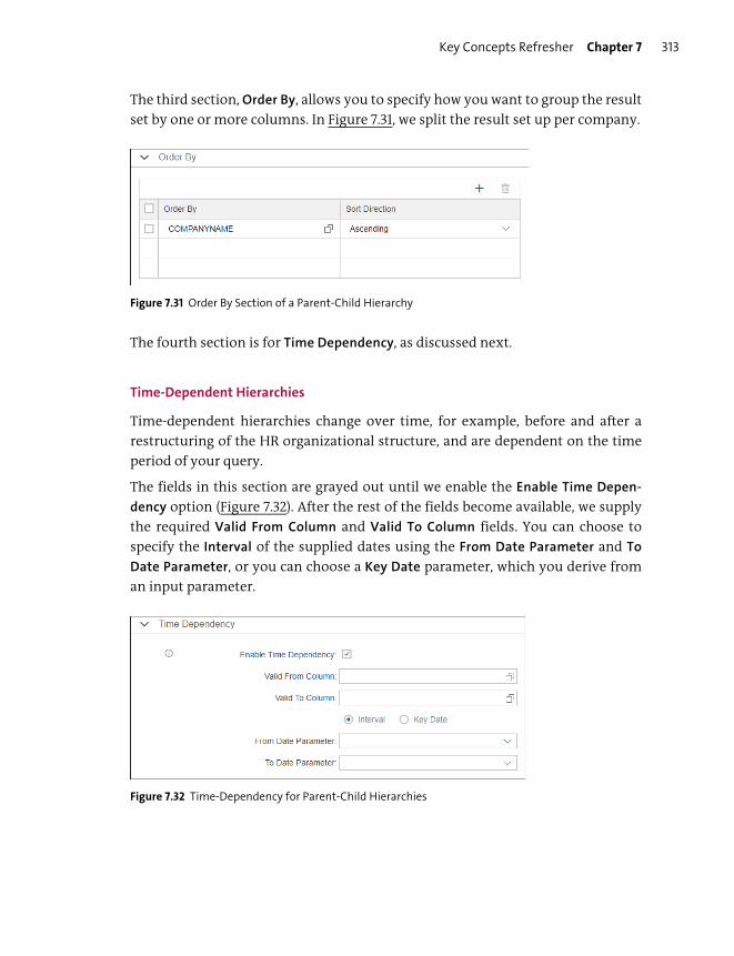
Key Concepts Refresher Chapter 7 313
The third section, Order By, allows you to specify how you want to group the result
set by one or more columns. In Figure 7.31, we split the result set up per company.
Figure 7.31 Order By Section of a Parent-Child Hierarchy
The fourth section is for Time Dependency, as discussed next.
Time-Dependent Hierarchies
Time-dependent hierarchies change over time, for example, before and after a
restructuring of the HR organizational structure, and are dependent on the time
period of your query.
The fields in this section are grayed out until we enable the Enable Time Depen-
dency option (Figure 7.32). After the rest of the fields become available, we supply
the required Valid From Column and Valid To Column fields. You can choose to
specify the Interval of the supplied dates using the From Date Parameter and To
Date Parameter, or you can choose a Key Date parameter, which you derive from
an input parameter.
Figure 7.32 Time-Dependency for Parent-Child Hierarchies
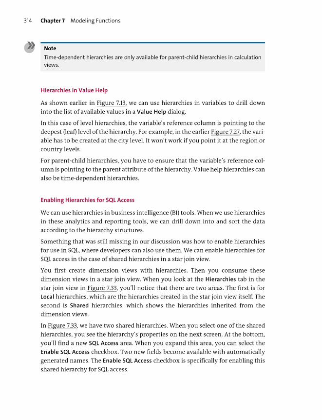
Chapter 7 Modeling Functions314
Note
Time-dependent hierarchies are only available for parent-child hierarchies in calculation
views.
Hierarchies in Value Help
As shown earlier in Figure 7.13, we can use hierarchies in variables to drill down
into the list of available values in a Value Help dialog.
In this case of level hierarchies, the variable’s reference column is pointing to the
deepest (leaf) level of the hierarchy. For example, in the earlier Figure 7.27, the vari-
able has to be created at the city level. It won’t work if you point it at the region or
country levels.
For parent-child hierarchies, you have to ensure that the variable’s reference col-
umn is pointing to the parent attribute of the hierarchy. Value help hierarchies can
also be time-dependent hierarchies.
Enabling Hierarchies for SQL Access
We can use hierarchies in business intelligence (BI) tools. When we use hierarchies
in these analytics and reporting tools, we can drill down into and sort the data
according to the hierarchy structures.
Something that was still missing in our discussion was how to enable hierarchies
for use in SQL, where developers can also use them. We can enable hierarchies for
SQL access in the case of shared hierarchies in a star join view.
You first create dimension views with hierarchies. Then you consume these
dimension views in a star join view. When you look at the Hierarchies tab in the
star join view in Figure 7.33, you’ll notice that there are two areas. The first is for
Local hierarchies, which are the hierarchies created in the star join view itself. The
second is Shared hierarchies, which shows the hierarchies inherited from the
dimension views.
In Figure 7.33, we have two shared hierarchies. When you select one of the shared
hierarchies, you see the hierarchy’s properties on the next screen. At the bottom,
you’ll find a new SQL Access area. When you expand this area, you can select the
Enable SQL Access checkbox. Two new fields become available with automatically
generated names. The Enable SQL Access checkbox is specifically for enabling this
shared hierarchy for SQL access.
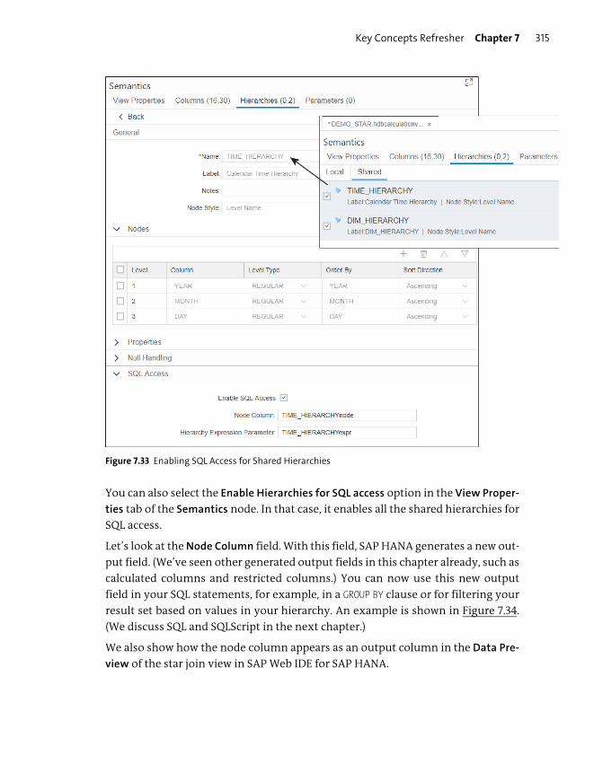
Key Concepts Refresher Chapter 7 315
Figure 7.33 Enabling SQL Access for Shared Hierarchies
You can also select the Enable Hierarchies for SQL access option in the View Proper-
ties tab of the Semantics node. In that case, it enables all the shared hierarchies for
SQL access.
Let’s look at the Node Column field. With this field, SAP HANA generates a new out-
put field. (We’ve seen other generated output fields in this chapter already, such as
calculated columns and restricted columns.) You can now use this new output
field in your SQL statements, for example, in a GROUP BY clause or for filtering your
result set based on values in your hierarchy. An example is shown in Figure 7.34.
(We discuss SQL and SQLScript in the next chapter.)
We also show how the node column appears as an output column in the Data Pre-
view of the star join view in SAP Web IDE for SAP HANA.
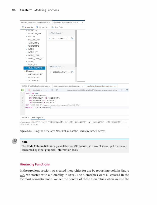
Chapter 7 Modeling Functions316
Figure 7.34 Using the Generated Node Column of the Hierarchy for SQL Access
Note
The Node Column field is only available for SQL queries, so it won’t show up if the view is
consumed by other graphical information tools.
Hierarchy Functions
In the previous section, we created hierarchies for use by reporting tools. In Figure
7.25, we started with a hierarchy in Excel. The hierarchies were all created in the
topmost semantic node. We get the benefit of these hierarchies when we use the
Key Concepts Refresher Chapter 7 317
entire calculation view in BI tools with features such as drilldown and aggrega-
tions. In star join cubes, it can help us with dimensional navigation on fact tables,
including a time dimension. And we can use these hierarchies with Value Help
popups when choosing a value for a variable.
But what if we want to work with hierarchal data inside our calculation view? What
if we need to use the hierarchical metadata in analytical operations? For example,
some companies have a policy that people in a managerial position should have at
least seven people reporting to them. If they have less than seven people in their
team, they should also have some team tasks in addition to their management
responsibilities. How do we identify such individuals? We want a query that says,
“Show all managers where the number of direct team members is fewer than
seven.” In technical terms, we would ask, “Show all individuals with fewer than
seven hierarchy siblings at a hierarchy distance of one.”
This isn’t possible with the level and parent-child hierarchies we’ve created in the
semantic node over the past few years because these are used for navigation or
aggregation.
Note
The hierarchies we create in the Semantic node are mostly for use by analytics and
reporting tools outside of SAP HANA. The hierarchies we create in the Hierarchy Functionnodes are for use inside the calculation view.
As we saw in Chapter 6, SAP HANA has some new types of graphical calculation
view nodes that were added since SAP HANA 2.0 SPS 03. The one we’ll use here is
the Hierarchy Function node.
These nodes automatically generate hierarchy metadata from the data that is sup-
plied by the data sources. This generated metadata can be used inside the other
nodes in the graphical calculation view or in the output of the calculation view.
We can use the Hierarchy Function nodes in two ways in the graphical calculation
views:
� Generating the basic hierarchy metadata
We add a data source to the Hierarchy Function node. This node will then auto-
matically add additional output fields with values that help describe the basic
hierarchy, for example, how many people are reporting to a specific manager.
� Navigating the hierarchy
We feed the results (output) from the previous (generating) Hierarchy Function
Node into another Hierarchy Function Node. In this case, we select the navigate
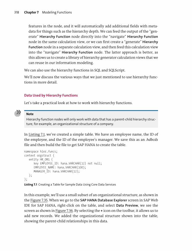
Chapter 7 Modeling Functions318
features in the node, and it will automatically add additional fields with meta-
data for things such as the hierarchy depth. We can feed the output of the “gen-
erate” Hierarchy Function node directly into the “navigate” Hierarchy Function
node in the same calculation view, or we can first create a “generate” Hierarchy
Function node in a separate calculation view, and then feed this calculation view
into the “navigate” Hierarchy Function node. The latter approach is better, as
this allows us to create a library of hierarchy generator calculation views that we
can reuse in our information modeling.
We can also use the hierarchy functions in SQL and SQLScript.
We’ll now discuss the various ways that we just mentioned to use hierarchy func-
tions in more detail.
Data Used by Hierarchy Functions
Let’s take a practical look at how to work with hierarchy functions.
Note
Hierarchy function nodes will only work with data that has a parent-child hierarchy struc-
ture, for example, an organizational structure of a company.
In Listing 7.1, we’ve created a simple table. We have an employee name, the ID of
the employee, and the ID of the employee’s manager. We save this as an .hdbcds
file and then build the file to get SAP HANA to create the table.
namespace hier.funcs;context orgstruct {
entity HR_ORG {key EMPLOYEE_ID: hana.VARCHAR(12) not null;EMPLOYEE_NAME: hana.VARCHAR(100);MANAGER_ID: hana.VARCHAR(12);
};};
Listing 7.1 Creating a Table for Sample Data Using Core Data Services
In this example, we’ll use a small subset of an organizational structure, as shown in
the Figure 7.35. When we go to the SAP HANA Database Explorer screen in SAP Web
IDE for SAP HANA, right-click on the table, and select Data Preview, we see the
screen as shown in Figure 7.36. By selecting the + icon on the toolbar, it allows us to
add new records. We added the organizational structure shown into the table,
showing the parent-child relationships in this data.
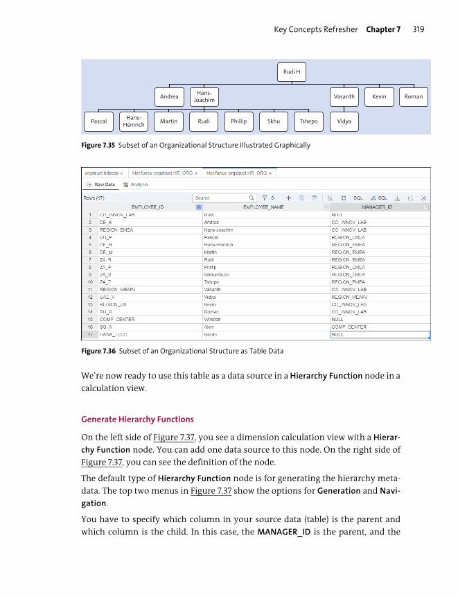
Key Concepts Refresher Chapter 7 319
Figure 7.35 Subset of an Organizational Structure Illustrated Graphically
Figure 7.36 Subset of an Organizational Structure as Table Data
We’re now ready to use this table as a data source in a Hierarchy Function node in a
calculation view.
Generate Hierarchy Functions
On the left side of Figure 7.37, you see a dimension calculation view with a Hierar-
chy Function node. You can add one data source to this node. On the right side of
Figure 7.37, you can see the definition of the node.
The default type of Hierarchy Function node is for generating the hierarchy meta-
data. The top two menus in Figure 7.37 show the options for Generation and Navi-
gation.
You have to specify which column in your source data (table) is the parent and
which column is the child. In this case, the MANAGER_ID is the parent, and the
Rudi H
Andrea Hans-Joachim
Pascal Hans-Heinrich Martin Rudi Phillip Skhu Tshepo
Vasanth
Vidya
Kevin Roman

Chapter 7 Modeling Functions320
EMPLOYEE_ID is the child. In the Start field, you can specify which department you
want to analyze. All other records that aren’t part of that department will be
ignored. In this case, the records numbered 15–17 in Figure 7.36 won’t be included
in the result set.
You can additionally specify the Depth of the hierarchy you want. If you leave this
blank, it will go down to the lowest levels. You can also specify how orphan nodes
should be handled (Orphan Handling). Finally, you can specify if you want the
result set sorted; for example, you can sort the hierarchy by the names of the peo-
ple by selecting the EMPLOYEE_NAME field in the Order By area.
Figure 7.37 Creating a Dimension Calculation View with a Generation Hierarchy Function Node
In Figure 7.38, all three columns of the table are mapped to the output of the Hier-
archy Function node. Notice that the mapping automatically renamed the Man-
ager_ID field to PARENT_ID and the Employee_ID field to NODE_ID.
If you look at the number of output columns, however, you’ll notice that there are
nine columns. The generation Hierarchy Function node automatically created an
additional six columns.
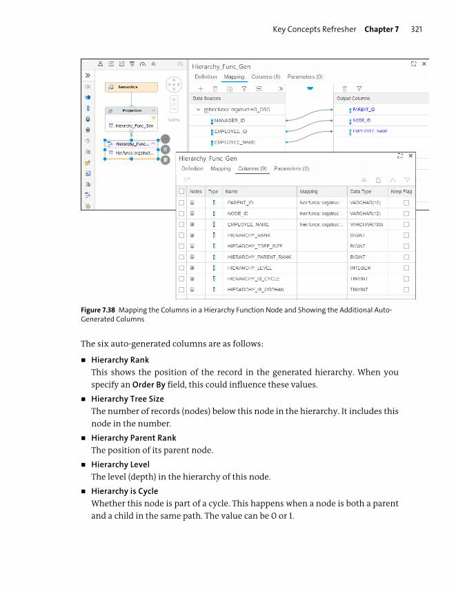
Key Concepts Refresher Chapter 7 321
Figure 7.38 Mapping the Columns in a Hierarchy Function Node and Showing the Additional Auto-Generated Columns
The six auto-generated columns are as follows:
� Hierarchy Rank
This shows the position of the record in the generated hierarchy. When you
specify an Order By field, this could influence these values.
� Hierarchy Tree Size
The number of records (nodes) below this node in the hierarchy. It includes this
node in the number.
� Hierarchy Parent Rank
The position of its parent node.
� Hierarchy Level
The level (depth) in the hierarchy of this node.
� Hierarchy is Cycle
Whether this node is part of a cycle. This happens when a node is both a parent
and a child in the same path. The value can be 0 or 1.

Chapter 7 Modeling Functions322
� Hierarchy is Orphan
Whether this node is an orphan. The value can be 0 or 1.
In Figure 7.39, you can see the output from the generation Hierarchy Function
node. For each record or node in the hierarchy, you can see the various values in
the auto-generated fields just described.
Figure 7.39 Previewing the Data of a Hierarchy Function Node
You can now use this dimensional calculation view with the generation Hierarchy
Function node in other calculation views.
Navigate Hierarchy Functions
Figure 7.40 shows a new dimensional calculation view. It’s very similar to the one
shown in Figure 7.37, except that the Hierarchy Function node doesn’t have a table
as a data source; instead it uses the previous calculation view with the generation
Hierarchy Function node. In this case, you specify the Hierarchy Function node as a
navigation type.
In Figure 7.37, you can see how to specify the navigation as moving down the hier-
archy (Hierarchy Descendants), moving up the hierarchy (Hierarchy Ancestors), or
staying at the same level (Hierarchy Siblings).
When looking at the Columns tab, you’ll see that a single auto-generated field
called Hierarchy Distance was created. This gives the distance between this node
and another node, expressed by the difference in levels. You can specify the other
node by filling in the Start Rank field.

Key Concepts Refresher Chapter 7 323
Figure 7.40 Creating a Dimension Calculation View with a Navigational Hierarchy Function Node
Figure 7.41 illustrates one way of achieving this. Here we moved the data source to
a project node below the navigation Hierarchy Function node, and then we inserted
another project node with a filter between them. The filter is a simple expression
that allows you to filter the result set to a single record. In this case, we specified a
unique NODE_ID.
In the navigation Hierarchy Function node, you can select any of the fields from the
filtered Projection node. In this example, it’s HIERARCHY_RANK.
When you now look at the Mapping and Columns tabs, you’ll notice an additional
auto-generated column called START_RANK, as shown in Figure 7.42.
We started this discussion by giving an example of identifying all managers where
the number of direct team members is fewer than seven. In technical terms, we
would ask, “Show all individuals with fewer than seven hierarchy siblings at a hier-
archy distance of one.”
You’re now ready to build such queries in your graphical calculation views.
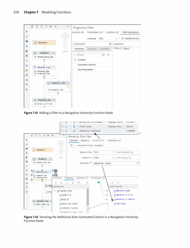
Chapter 7 Modeling Functions324
Figure 7.41 Adding a Filter to a Navigation Hierarchy Function Node
Figure 7.42 Showing the Additional Auto-Generated Column in a Navigation Hierarchy Function Node
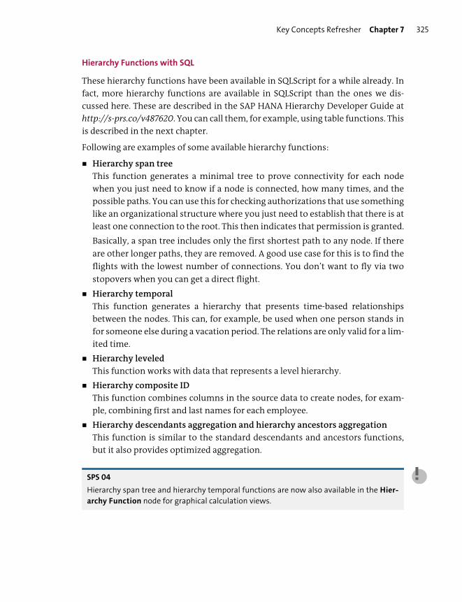
Key Concepts Refresher Chapter 7 325
Hierarchy Functions with SQL
These hierarchy functions have been available in SQLScript for a while already. In
fact, more hierarchy functions are available in SQLScript than the ones we dis-
cussed here. These are described in the SAP HANA Hierarchy Developer Guide at
http://s-prs.co/v487620. You can call them, for example, using table functions. This
is described in the next chapter.
Following are examples of some available hierarchy functions:
� Hierarchy span tree
This function generates a minimal tree to prove connectivity for each node
when you just need to know if a node is connected, how many times, and the
possible paths. You can use this for checking authorizations that use something
like an organizational structure where you just need to establish that there is at
least one connection to the root. This then indicates that permission is granted.
Basically, a span tree includes only the first shortest path to any node. If there
are other longer paths, they are removed. A good use case for this is to find the
flights with the lowest number of connections. You don’t want to fly via two
stopovers when you can get a direct flight.
� Hierarchy temporal
This function generates a hierarchy that presents time-based relationships
between the nodes. This can, for example, be used when one person stands in
for someone else during a vacation period. The relations are only valid for a lim-
ited time.
� Hierarchy leveled
This function works with data that represents a level hierarchy.
� Hierarchy composite ID
This function combines columns in the source data to create nodes, for exam-
ple, combining first and last names for each employee.
� Hierarchy descendants aggregation and hierarchy ancestors aggregation
This function is similar to the standard descendants and ancestors functions,
but it also provides optimized aggregation.
SPS 04
Hierarchy span tree and hierarchy temporal functions are now also available in the Hier-archy Function node for graphical calculation views.

Chapter 7 Modeling Functions326
Important Terminology
In this chapter, we touched on different ways to enhance our SAP HANA calcula-
tion views and enrich our information models. The following list describes the
important terms covered in this chapter:
� Calculated columns
Adds additional output columns to our calculation views and allows us to calcu-
late new values.
� Counters
Shows how many times something has occurred within a result set.
� Restricted columns
Restricts the data shown in a particular column or field and outputs the
restricted values in an additional output field.
� Filter expressions
Used if we don’t want to show all the data from a specific table or to only show
specific data. This can use both static and dynamic filtering.
� Domain fixed values
Values from the ABAP Data Dictionary, and the users can only choose from the
available list when they enter data into the fields.
� Variables
The three types of variables:
– Single value: The variable only asks for one (single) value; for example, the
year is 2019.
– Interval: The variable asks for from and to values, for example, the years from
2016 to 2019.
– Range: The variable asks a single value but combines it with another opera-
tor; for example, the year is greater and equal to 2018.
� Input parameters
The five types of input parameters we can create:
– Direct: Directly enter the value. We can specify the Data Type of the expected
value. There are three data types we can use for Direct: Currency, Unit of mea-
sure, and Date.
– Column: Choose a value from all the possible values in a specified column in
the current view.
– Derived From Table: Choose a value from data in another table.

Important Terminology Chapter 7 327
– Static List: Choose a value from a predefined (static) list of values.
– Derived From Procedures/Scalar Function: Choose a value from a list of values
generated by a scalar function or procedure.
� Currency conversion
Used when converting from source currency to target currency. A date for the
conversion also has to be supplied.
� Hierarchies
Used in reporting to enable intelligent drilldown.
� Time-dependent hierarchies
Hierarchies that change over time, for example, before and after a restructuring
of the HR organizational structure, and are dependent on the time period of
your query.
� Hierarchy function nodes
Nodes where hierarchies are generated from a data source. These hierarchies
can be used for analytical purposes inside the calculation view.
Table 7.1 shows in which view node some of the features are available. For example,
filter expressions aren’t available in Graph and Hierarchy Function nodes.
Node Type Calculated
Columns
Counters Restricted
Columns
Input
Parameters
Filter
Expressions
Join Yes – – Yes Yes
Star Join Yes Yes Yes Yes Yes
Projection Yes – – Yes Yes
Aggregation Yes Yes Yes Yes Yes
Rank – – – Yes Yes
Union Yes – – Yes Yes
Graph – – – Yes –
Intersect,
Minus
Yes – – Yes Yes
Hierarchy
Function
– – – Yes –
Table 7.1 Features per Node
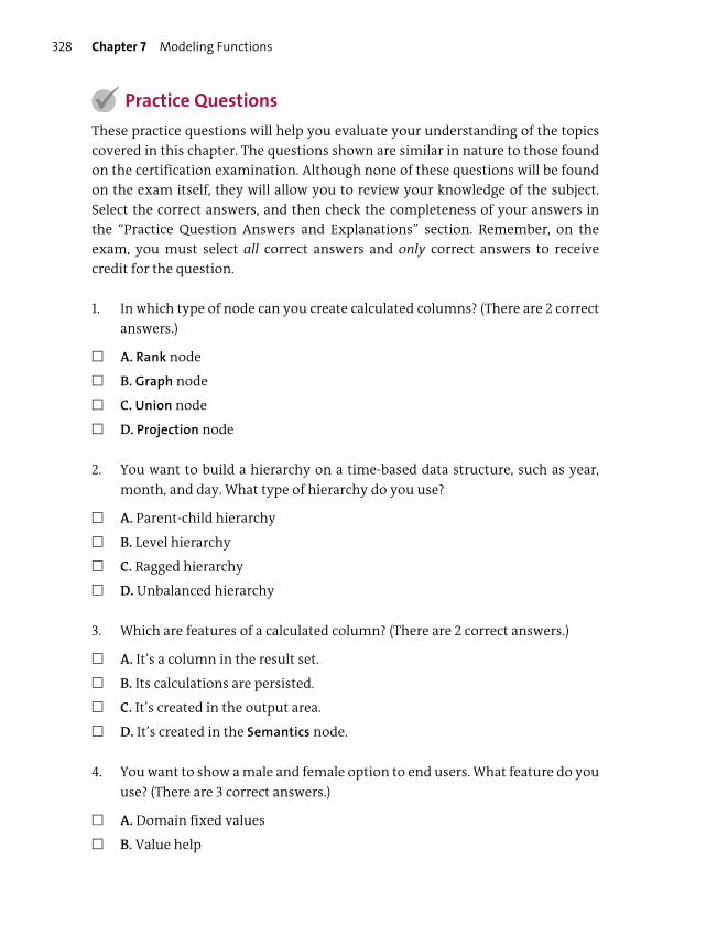
Chapter 7 Modeling Functions328
Practice Questions
These practice questions will help you evaluate your understanding of the topics
covered in this chapter. The questions shown are similar in nature to those found
on the certification examination. Although none of these questions will be found
on the exam itself, they will allow you to review your knowledge of the subject.
Select the correct answers, and then check the completeness of your answers in
the “Practice Question Answers and Explanations” section. Remember, on the
exam, you must select all correct answers and only correct answers to receive
credit for the question.
1. In which type of node can you create calculated columns? (There are 2 correct
answers.)
� A. Rank node
� B. Graph node
� C. Union node
� D. Projection node
2. You want to build a hierarchy on a time-based data structure, such as year,
month, and day. What type of hierarchy do you use?
� A. Parent-child hierarchy
� B. Level hierarchy
� C. Ragged hierarchy
� D. Unbalanced hierarchy
3. Which are features of a calculated column? (There are 2 correct answers.)
� A. It’s a column in the result set.
� B. Its calculations are persisted.
� C. It’s created in the output area.
� D. It’s created in the Semantics node.
4. You want to show a male and female option to end users. What feature do you
use? (There are 3 correct answers.)
� A. Domain fixed values
� B. Value help
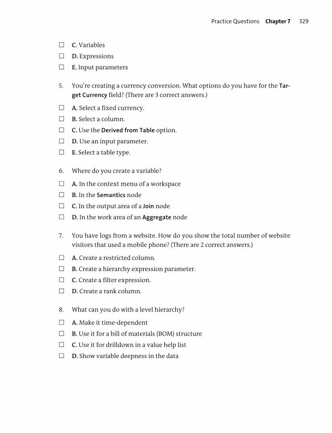
Practice Questions Chapter 7 329
� C. Variables
� D. Expressions
� E. Input parameters
5. You’re creating a currency conversion. What options do you have for the Tar-
get Currency field? (There are 3 correct answers.)
� A. Select a fixed currency.
� B. Select a column.
� C. Use the Derived from Table option.
� D. Use an input parameter.
� E. Select a table type.
6. Where do you create a variable?
� A. In the context menu of a workspace
� B. In the Semantics node
� C. In the output area of a Join node
� D. In the work area of an Aggregate node
7. You have logs from a website. How do you show the total number of website
visitors that used a mobile phone? (There are 2 correct answers.)
� A. Create a restricted column.
� B. Create a hierarchy expression parameter.
� C. Create a filter expression.
� D. Create a rank column.
8. What can you do with a level hierarchy?
� A. Make it time-dependent
� B. Use it for a bill of materials (BOM) structure
� C. Use it for drilldown in a value help list
� D. Show variable deepness in the data

Chapter 7 Modeling Functions330
9. What can a variable be used for?
� A. Currency conversion
� B. Calculated column expression
� C. Call a procedure in SQLScript
� D. Filtering
10. You’re working with a currency measure. What is decimal shift used for?
� A. To increase the accuracy of the currency conversion
� B. To undo the decimal adjustment for ABAP
� C. For currencies with more than two decimal places
� D. To avoid rounding errors during the conversion
11. What variable type do you use if you want to allow the user to choose the years
from 2016 to 2019?
� A. Single value
� B. Interval
� C. Range
� D. Multiple entries
12. What do you create to find the number of unique items sold per shop?
� A. A calculation view with a restricted column in an Aggregation node
� B. A calculation view with a counter in a Projection node
� C. A calculation view with a counter in an Aggregation node
� D. An analytic view with a calculated column in a Star Join node
13. What can you use to limit the number of records produced by a calculation
view? (There are 3 correct answers.)
� A. SAP client restrictions
� B. Domain fixed values
� C. Filter expressions
� D. Restricted columns
� E. Generated columns

Practice Questions Chapter 7 331
14. You created a calculated column in a star join view for a table containing the
number of units ordered, the price per unit, and the number of units in stock.
You get the wrong results. What could be the problem?
� A. You mistyped the calculated column expression.
� B. You chose the SQL expression syntax.
� C. You did not enable the Keep Flag.
� D. You did not enable the currency conversion.
15. Where can you create a filter expression?
� A. In an Aggregation node
� B. In a Data Foundation node
� C. In a Projection node
� D. In the Semantics node
16. Which tables do you need for currency conversion?
� A. DD07*
� B. TCUR*
� C. BICS*
� D. SHINE*
17. What do you use to build a financial report for the company’s board members
that allows them to choose if they want the report to be in euros or dollars?
� A. An input parameter from an Aggregation node
� B. A variable from the Semantics node
� C. A variable from a Projection node
� D. An input parameter from the Semantics node
18. What type of input parameters do you use to choose the data from a field in
the current table?
� A. Direct
� B. Derived from table
� C. Value help
� D. Column
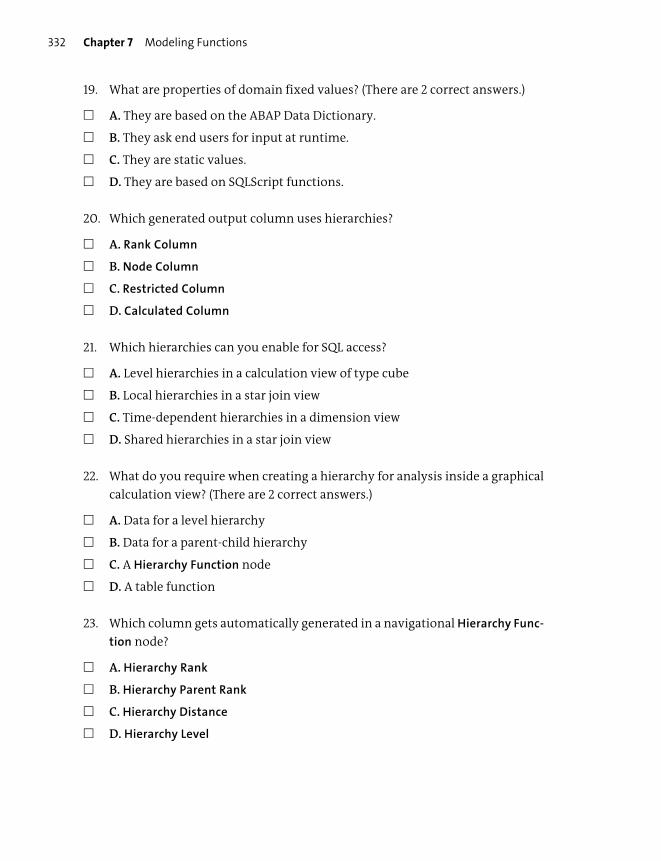
Chapter 7 Modeling Functions332
19. What are properties of domain fixed values? (There are 2 correct answers.)
� A. They are based on the ABAP Data Dictionary.
� B. They ask end users for input at runtime.
� C. They are static values.
� D. They are based on SQLScript functions.
20. Which generated output column uses hierarchies?
� A. Rank Column
� B. Node Column
� C. Restricted Column
� D. Calculated Column
21. Which hierarchies can you enable for SQL access?
� A. Level hierarchies in a calculation view of type cube
� B. Local hierarchies in a star join view
� C. Time-dependent hierarchies in a dimension view
� D. Shared hierarchies in a star join view
22. What do you require when creating a hierarchy for analysis inside a graphical
calculation view? (There are 2 correct answers.)
� A. Data for a level hierarchy
� B. Data for a parent-child hierarchy
� C. A Hierarchy Function node
� D. A table function
23. Which column gets automatically generated in a navigational Hierarchy Func-
tion node?
� A. Hierarchy Rank
� B. Hierarchy Parent Rank
� C. Hierarchy Distance
� D. Hierarchy Level

Practice Question Answers and Explanations Chapter 7 333
Practice Question Answers and Explanations
1. Correct answers: C, D
You can create calculated columns in a Union node and a Projection node.
If you got this wrong, it might be that you remember it from SAP HANA 1.0. Cal-
culated columns are now available in more view nodes than before.
2. Correct answer: B
You use a level hierarchy to build a hierarchy on a time-based data structure.
Time-based means you have year on level 1, months on level 2, and days on
level 3.
Only a parent-child hierarchy can be a time-dependent hierarchy. (The words
are confusing, so watch out. Here we mentioned the data structure.) It just illus-
trates that you could achieve fairly similar functionality with both types of
hierarchies, although the approaches are quite different.
Ragged and unbalanced hierarchies aren’t mentioned in SAP HANA.
3. Correct answers: A, C
Features of a calculated column: it’s a column in the result set and is created in
the output area.
Its calculations aren’t persisted! It’s NOT created in the Semantics nodes.
4. Correct answers: B, C, E
You can show a male and female option to users with either variables or input
parameters, and by opening the value help.
Domain fixed values can be used for filtering. Male and female got mentioned
in the “Domain Fixed Values” section, but the context there was completely dif-
ferent.
5. Correct answers: A, B, D
The options you have for the target currency field in a currency conversion are
as follows:
Select a fixed currency.
Select a column.
Use an input parameter.
6. Correct answer: B
You create a variable in the Semantics node.

Chapter 7 Modeling Functions334
7. Correct answers: A, C
You show the total number of website visitors that used a mobile phone by cre-
ating either a restricted column or a filter expression.
A hierarchy expression parameter is created when you enable a hierarchy for
SQL access.
A rank column will rank them by numbers but doesn’t show the total number.
(You could perhaps rank all the data, rank the data, and then search for the total
number in the rankings. So, technically, it’s possible but requires that you still
manually search the correct output.)
8. Correct answer: C
A level hierarchy can be used for drilldown in a value help list. Only parent-child
hierarchies have time-dependency, variable deepness in the data, and can be
used for a BOM structure.
9. Correct answer: D
A variable can be used for filtering.
You’ll use input parameters for currency conversion and in calculated column
expression.
You can’t call a procedure via a SQLScript variable in SQLScript (which we’ll look
at in the next chapter). You use the CALL syntax and use output parameters.
10. Correct answer: C
Decimal shift is used for currencies with more than two decimal places. Deci-
mal shift back is used to undo the decimal adjustment for ABAP.
11. Correct answer: B
You use an interval variable type if you want to allow the user to choose dates
from 2016 to 2019.
Range would allow for years > 2016. Don’t confuse the range type with the inter-
val type.
12. Correct answer: C
You create a calculation view with a counter in an Aggregation node to find the
number of unique items sold per shop. You need a counter for this, so two
answers are eliminated. A calculation view with a counter in a Projection node
isn’t valid because a counter can’t be created in a Projection node.
13. Correct answers: A, B, C
You can use SAP client restrictions, domain fixed values, and filter expressions
to limit the number of records produced by a calculation view.
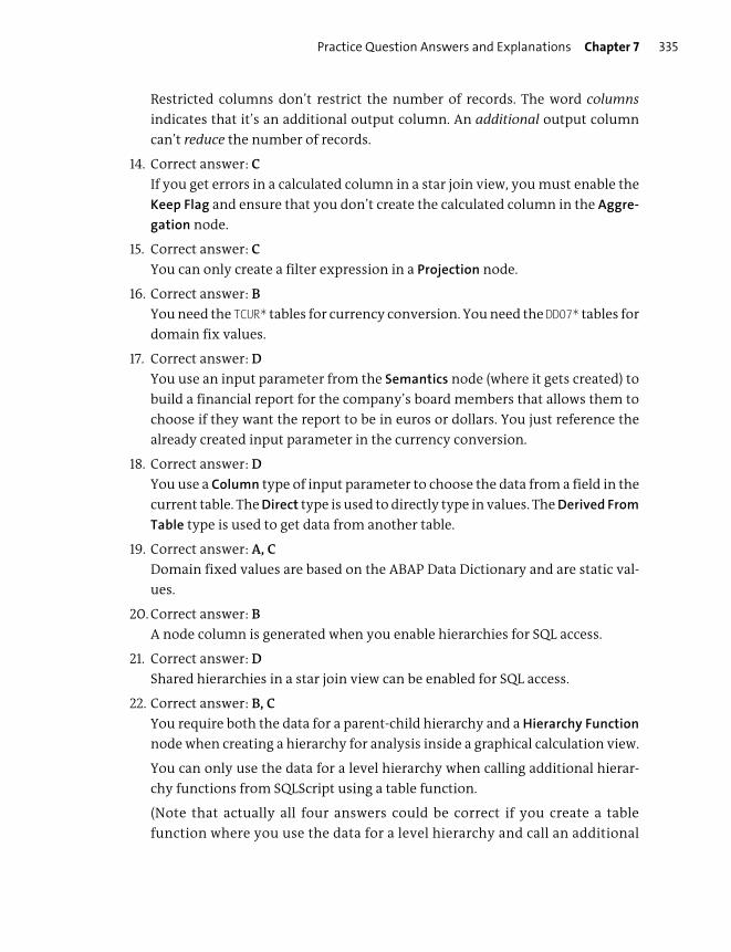
Practice Question Answers and Explanations Chapter 7 335
Restricted columns don’t restrict the number of records. The word columns
indicates that it’s an additional output column. An additional output column
can’t reduce the number of records.
14. Correct answer: C
If you get errors in a calculated column in a star join view, you must enable the
Keep Flag and ensure that you don’t create the calculated column in the Aggre-
gation node.
15. Correct answer: C
You can only create a filter expression in a Projection node.
16. Correct answer: B
You need the TCUR* tables for currency conversion. You need the DD07* tables for
domain fix values.
17. Correct answer: D
You use an input parameter from the Semantics node (where it gets created) to
build a financial report for the company’s board members that allows them to
choose if they want the report to be in euros or dollars. You just reference the
already created input parameter in the currency conversion.
18. Correct answer: D
You use a Column type of input parameter to choose the data from a field in the
current table. The Direct type is used to directly type in values. The Derived From
Table type is used to get data from another table.
19. Correct answer: A, C
Domain fixed values are based on the ABAP Data Dictionary and are static val-
ues.
20. Correct answer: B
A node column is generated when you enable hierarchies for SQL access.
21. Correct answer: D
Shared hierarchies in a star join view can be enabled for SQL access.
22. Correct answer: B, C
You require both the data for a parent-child hierarchy and a Hierarchy Function
node when creating a hierarchy for analysis inside a graphical calculation view.
You can only use the data for a level hierarchy when calling additional hierar-
chy functions from SQLScript using a table function.
(Note that actually all four answers could be correct if you create a table
function where you use the data for a level hierarchy and call an additional

Chapter 7 Modeling Functions336
hierarchy function from SQLScript, and then use this table function inside a
graphical calculation view. You’ll understand this better after having read
the next chapter.)
23. Correct answer: C
The Hierarchy Distance column gets automatically created in a navigational
Hierarchy Function node.
The other three columns get automatically created in a generation Hierarchy
Function node.
Takeaway
You should now know how to enhance SAP HANA calculation views with the nine
different modeling features we’ve discussed in this chapter. You know how to cre-
ate calculated and restricted columns to add additional output fields to your calcu-
lation views. You’ve looked at filtering and filter expressions, and you’ve learned
how to limit the data early in your modeling process.
You can now identify when to create variables and input parameters to allow busi-
ness users to specify what outputs they want to see in the result sets of your calcu-
lation views at runtime.
Working with currency, you now understand how to add currency conversions to
your financial reports.
Finally, you now know how to create hierarchies to provide powerful drilldown
capabilities for your end users and for analyzing hierarchical data in your organi-
zation.
Summary
We learned how to work with calculated columns, restricted columns, and filters in
our calculation views. We added variables and input parameters to add a new level
of dynamic interaction to our modeling by allowing the end users to specify what
they are looking for in each query of the SAP HANA calculation views. We also saw
how to enrich our calculation views with currency conversions and hierarchies.
In the next chapter, we’ll discuss how to use SQL and SQLScript to provide the
advanced features that you might not be able to do with the graphical calculation
views we discussed in previous chapters.
Chapter 8
SQL and SQLScript
Techniques You’ll Master
� Get a basic understanding of SQL and how to use it with your
SAP HANA information models
� Learn SQLScript in SAP HANA and find out how it extends and
complements SQL
� Understand how the SAP HANA modeling environment with
SQL and SQLScript has changed over the past few years
� Create and use table and scalar functions with your graphical
SAP HANA information views
� Develop procedures in SAP HANA using SQL and SQLScript
Chapter 8 SQL and SQLScript338
We’ve made a few references about SQL and SQLScript up to this point. Even in
Chapter 7, we enabled hierarchies for SQL access, and you saw how to use the gen-
erated node column in a GROUP BY clause. In this chapter, we look at how to use SQL
and SQLScript to enhance your graphical modeling capabilities.
You’ve already seen how you can use SQLScript in your calculation views, for
example, in the expression editors of the calculated and restricted columns, in
filter expressions, and in creating default values for input parameters (in the Cre-
ating Input Parameters section of Chapter 7). We’ll also see some use of it in Chap-
ter 13 when we look at security.
In many large SAP HANA projects, you’ll reach a point at which you need to do
something more than what is offered by the graphical information views. Infor-
mation modeling using SQL and SQLScript offer more powerful options. You lose
the productivity and simplicity of working graphically with information views,
but you gain flexibility and control.
As SAP HANA has matured, the graphical modeling tools have grown such that the
requirements for SQL and SQLScript have been reduced. In the past, after you
started working with SQL and SQLScript, you had to continue in that environment
(or choose to create any subsequent layers in your information models there as
well). Since SAP HANA 1.0 SPS 11, you can work graphically with your SAP HANA
information views, address the occasional constraint with SQL and SQLScript, and
bring this development back into the graphical SAP HANA modeling environ-
ment. You can then continue building the remaining layers of your information
models using the graphical information views. The focus has therefore shifted
toward the graphical modeling environment for SAP HANA modelers.
Note
There is definitely less focus now on SQL and SQLScript in the average modeling workflow
than there was in the past. However, a good grasp of development processes and basic
programming knowledge will always be to your benefit.
In this chapter, we’ll get you up to speed quickly on the SAP HANA information
views and how to integrate your SQL/SQLScript development back into the graph-
ical modeling environment.
Objectives of This Portion of the Test Chapter 8 339
Real-World Scenario
You’ve been working on a large SAP HANA project for a few months when a
group of business users asks if you can help to make security access more
powerful and sync it to automatically use their hierarchal organizational
structures. You base the analytic privileges on a procedure that easily
exploits these structures.
The company is quickly moving into the area of mobile business services and
plans to deliver some new, real-time business dashboards to executives and
managers. SAP HANA is an obvious choice, and your modeling and develop-
ment skills are required to build the link to the mobile screens. Using your
SQLScript knowledge, you quickly figure out ways to create powerful dash-
boards that respond fast on the mobile screens.
You’ve noticed lately how the expression editors in the graphical modeling
environment are now using SQL syntax. By leveraging your SQL knowledge,
you improve many of the features end users are using daily in their analytics.
Objectives of This Portion of the Test
The purpose of this portion of the SAP HANA certification exam is to test your
knowledge of modeling using SQL and SQLScript.
The certification exam expects you to have a good understanding of the following
topics:
� Standard SQL and how it relates to SAP HANA
� SQLScript in SAP HANA
� How to create and use user-defined functions (UDFs), especially table functions
� Procedures in SAP HANA using SQL and SQLScript
Note
This portion contributes about 5% of the total certification exam score.

Chapter 8 SQL and SQLScript340
Key Concepts Refresher
Structured Query Language (SQL) is a widely used database programming language
standardized by the American National Standards Institute (ANSI) and the Interna-
tional Organization for Standardization (ISO). The standard is often referred to as
ANSI SQL.
Despite the existence of these standards, most SQL vendors extend ANSI SQL to
provide enhanced capabilities for their individual database products. Microsoft
uses an extended version called Transact-SQL (T-SQL), and Oracle uses PL/SQL.
SAP HANA provides SQLScript, which is an extension of ANSI SQL, to provide extra
capabilities for the unique in-memory components that SAP delivers. We’ve
already seen many of these features, for example, column tables, parameterized
information views, delta buffers, multiple result sets in parallel, and built-in cur-
rency conversions. The ANSI SQL standard doesn’t provide these features. How-
ever, SAP HANA supports ANSI SQL statements.
In this chapter, we provide only a short introduction to SQL and SQLScript, and we
do assume you have some knowledge of SQL. You can find the full SAP HANA SQL
and SQLScript reference guides at http://s-prs.co/v487620.
SQL
SQL uses a set-oriented approach for working with data.
Tip
Rather than working with individual records, you should focus on working with the entire
result set that consists of many data records.
You specify what should happen to all the data records in the result set at once.
This allows databases to be efficient when processing data because they can paral-
lelize the processing of these records. Databases are faster at processing data than
application servers because SQL is a set-oriented declarative language, whereas
application servers typically use procedural or object-oriented languages that pro-
cess records one at a time.
SQL Language
SQL is used to define, manipulate, and control database objects. These actions are
specified by various subsets of the language:

Key Concepts Refresher Chapter 8 341
� Data Definition Language (DDL)
This is used, for example, to CREATE, ALTER (modify), RENAME, or DROP (delete) table
definitions.
� Data Manipulation Language (DML)
This is used to manipulate data, for example, insert new data into a table or
update the data in a table. Examples in SQL include INSERT, UPDATE, and DELETE.
� Data Query Language (DQL)
This is used to SELECT (access) data. It doesn’t modify any data.
� Data Control Language (DCL)
This is used for data security, for example, to GRANT privileges to a database user.
� Transaction Control Language (TCL)
This is used to control database transactions, for example, to COMMIT or ROLLBACK
database transactions.
SQL is also subdivided into several language elements, as listed in Table 8.1.
Element Short Description
Identifiers Names of database objects, for example, a table called BOOKS.
Data types Specifies the characteristics of the data stored in the database, for exam-
ple, a string stored as a NVARCHAR data type.
Operators Used to assign, compare, or calculate values, for example, =, >=, + (add), *
(multiply), AND, and UNION ALL.
Expressions Clauses that produce result sets consisting of either scalar values or tables
consisting of columns and rows of data. Examples include aggregations,
such as SUM, or IF…THEN…ELSE logic using CASE.
Predicates Specifies conditions that can be evaluated to TRUE, FALSE, or UNKNOWN. These
can be used to filter statement and query results or to change program
flow. They are typically used in the WHERE conditions of the SELECT state-
ment, for example, A >= 100.
Queries Retrieves data from the database based on specific criteria. Queries use
the SELECT statement, for example, SELECT * from BOOKS.
Statements Commands to create persistent effects on schemas or data and control
transactions, program flow, connections, and sessions.
Functions Provides methods to evaluate expressions. They can be used anywhere an
expression is allowed. Various functions are built into SQL, for example,
LENGTH(BOOKNAME).
Table 8.1 Elements of SQL
Chapter 8 SQL and SQLScript342
There are a few important points to remember about SQL when working with SAP
HANA:
� Identifiers can be delimited or undelimited, meaning the names of database
objects are or are not enclosed in double quotes. If you don’t enclose identifiers
with quotes, they are treated as uppercase. Therefore, BOOKS, Books, and books all
reference the same table name.
Delimited identifiers are treated as case-sensitive and can include characters in
the name that would be forbidden by undelimited identifiers. SAP HANA uses
Unicode, so the range of characters in a name can be wide. In this case, table
"BOOKS" and table "books" are treated as two separate tables.
� NULL is a special indicator used by SQL to show that there is no value.
� The LIKE predicate can be used for SQL searches. SELECT author FROM books WHERE
title LIKE ‘%HANA%’; will search for all books with the word HANA in the title.
We’ll look at this in more detail in Chapter 10.
� Statements in SQL include the semicolon (;) statement terminator. This is a
standard part of SQL grammar. Insignificant whitespace is generally ignored in
SQL statements, and queries and can be used to make such statements and que-
ries more readable.
We’ll now look at some SQL statements that correspond to SAP HANA modeling
constructs you’re already familiar with.
Creating Tables
The short version of the SQL syntax to create a table is as follows:
CREATE [<table_type>] TABLE <table_name>;<table_type> ::= COLUMN | ROW | GLOBAL TEMPORARY |GLOBAL TEMPORARY COLUMN | LOCAL TEMPORARY | LOCAL TEMPORARY COLUMN |VIRTUAL
This means that you have to type “CREATE TABLE BOOKS;” to create an empty
table called BOOKS. In this example, <tablename> is BOOKS. You can choose what to
type in place of the <tablename> placeholder.
Anything in square brackets, such as [<table_type>], is optional. If you want your
table to be a column table, type “CREATE COLUMN TABLE BOOKS;”, for example. If you
don’t specify the type of table, the system will create a row table because that’s
what ANSI SQL expects.

Key Concepts Refresher Chapter 8 343
Note
The CREATE COLUMN TABLE is already the first bit of SQLScript that you meet. Standard ANSI
SQL just caters for CREATE TABLE. The extra COLUMN keyword is specific to SAP HANA, and
this “extension” is therefore part of SQLScript.
In addition, note that the syntax of SQLScript fits in exactly with that standard SQL syn-
tax. The same syntax is used to create a standard row table (CREATE TABLE) and an SAP
HANA column table (CREATE COLUMN TABLE).
With SAP HANA SPS 03, we got a new table type called SAP HANA versioned tables.
Also known as system-versioned tables, they have actually been part of ANSI SQL
since 2011. Instead of a single table, you use two tables. Both these tables must be
in the same SAP HANA Deployment Infrastructure (HDI) folder. The first table is a
normal column table. The second is a history table that is linked to the first table
with a WITH SYSTEM VERSIONING HISTORY TABLE clause. This table has the same fields as
the first table, with additional VALIDFROM and VALIDTO time stamp fields. The first
table contains your data, just like any other table. But when you update a record,
instead of forgetting the previous values, the system-versioned table automati-
cally copies the values in the updated record to the second table and updates the
VALIDFROM and VALIDTO fields, before updating the record in the first table.
When you query the first table, it behaves like a normal column table. However,
you can execute special SELECT statements with a “time-travel clause” on these
types of tables to get the data as it was at a certain time. We can therefore read a
table as it was at any point in time. This can be useful for tables that refer to finan-
cial transactions and can completely change the way that systems perform period
closings. Rather than you having to code all the logic to handle historical data, it’s
built in to the database engine. You also don’t have to put logic for reading histor-
ical data into every database query.
Tip
SAP HANA versioned tables replace the old HISTORY COLUMN tables. You should not use HIS-TORY COLUMN tables.
SAP Enterprise Architecture Designer (SAP EA Designer) (discussed in Chapter 4)
has a feature in which it creates SAP HANA versioned tables for you with just a few
clicks. You create a normal column table and then activate the Versioning option in
the properties.
Chapter 8 SQL and SQLScript344
SPS 04
SAP HANA SPS 04 adds a variation of SAP HANA versioned tables called application time
period tables. These are basically the same as SAP HANA versioned tables, but they use
valid time periods specified by the business rather than the system time of when a record
was updated. You can create these by creating a .hdbapplicationtime file. Just remember
to ensure that you also add the correct plugin in the (hidden) .hdiconfig file.
Reading Data
The query, the most common operation in SQL, uses the SELECT statement—for
example:
SELECT [TOP <unsigned_integer>] [ ALL | DISTINCT ]<select_list> <from_clause> [(<subquery>)] [<where_clause>][<group_by_clause>] [<having_clause>] [<order_by_clause>][<limit_clause>] [<for_update_clause>] [<time_travel_clause>];
One of the shortest statements that can be used to read data from table BOOKS is
SELECT * FROM BOOKS;. This returns all the fields and data from table BOOKS, in effect
putting the entire table in the result set.
Tip
We recommend never using SELECT * statements as it can severely impact the query per-
formance of column tables. Because SAP HANA primarily uses column tables, this type of
SELECT statement should be avoided!
A better way is to specify the <select_list>, for example, SELECT author, title,
price FROM BOOKS;. In this case, you only read the author, title, and price columns for
all the books.
Note the [<time_travel_clause>] for use with SAP HANA versioned tables.
SPS 04
What is tremendously helpful for developers in SAP HANA 2.0 SPS 04 is the FOR JSONclause. This returns the result set in JavaScript Object Notation (JSON) format.
Key Concepts Refresher Chapter 8 345
Filtering Data
In SAP HANA, we sometimes use a filter, by using the WHERE clause as part of a
SELECT statement, for example:
SELECT author, title, price FROM BOOKS WHERE title LIKE ‘%HANA%’;
Creating Projections
Inside a Projection node in SAP HANA views, you can rename fields easily via the AS
keyword in SQL, for example:
SELECT author, title AS bookname, price FROM BOOKS;
The title field is now renamed to bookname in the result set.
Creating Calculated Columns
Creating calculated columns looks almost the same as renaming fields, but there is
an added formula, as shown here:
SELECT author, title, price * discount AS discount_price FROM BOOKS;
In this case, we added a new calculated column called discount_price.
Created Nested Reads and Aggregates
In SAP HANA views, we often have many layers; in SQL, we use nested SELECT state-
ments. These nested queries are also known as subqueries. For example:
SELECT author, title, price FROM BOOKSWHERE price > (SELECT AVG(price) FROM BOOKS);
The SELECT AVG(price) FROM BOOKS statement (subquery) returns the average price of
all the books in table BOOKS. The entire query above returns the books that are more
expensive than the average price.
You can create aggregates, such as with an aggregation node in a calculation view,
using standard aggregation functions in SQL. We discussed aggregation in Chapter 5.
Chapter 8 SQL and SQLScript346
Creating Joins
SAP HANA views normally have many joins. Here is an example of how to create
an inner join between two tables:
SELECT BOOKS.author, BOOKS.title, BOOKS.price,BOOK_SALES.total_sold FROM BOOKSINNER JOIN BOOK_SALESON BOOKS.book_number = BOOK_SALES.booknumber;
The field on which both tables are joined is the book_number field.
Creating Unions
Union nodes in calculation views can be performed by using the UNION operator, for
example:
SELECT author, title, price FROM BOOKSUNION
SELECT author, title, price FROM BOOKS_OUT_OF_PRINT;
You can also use the UNION ALL operator instead of UNION. The UNION operator returns
only distinct values, whereas UNION ALL will return all records, including duplicate
records.
Conditional Statements
You can handle if-then logic in SQL via the CASE statement, for example:
SELECT author, title, price,CASE WHEN title LIKE '%HANA'%' THEN 'Yes' ELSE 'No' ENDAS interested_in_book FROM BOOKS
Here, we’ve added a calculated column called interested_in_book to our query. If
the book’s title contains the word HANA, we indicate that we’re interested in it.
With that short introduction, you’ve seen how to do many of the things we’ve
done before using graphical modeling in calculation views, but now using SQL.

Key Concepts Refresher Chapter 8 347
SQLScript
SQLScript exposes many of the memory features of SAP HANA to SQL developers.
Column tables, parameterized information views, delta buffers, multiple result
sets in parallel, built-in currency conversions at the database level, fuzzy text
searching, spatial data types, and Predictive Analysis Libraries (PAL) make SAP
HANA unique. The only way to make this functionality available via SQL queries,
even from other applications, is to provide it via SQL extensions.
We’ve come across many of these features in earlier chapters. We’ll look in more
detail at the fuzzy text search and PAL in Chapter 10, as well as learn more about
the Application Function Library (AFL) that includes predictive and business func-
tions that can be used with SQLScript. In Chapter 11, we’ll learn more about spatial
functions, graph processing, and series data in SAP HANA
In Chapter 5, we saw the spatial join type used between a ST_POINT data type (e.g., a
location) and an ST_POLYGON (e.g., a suburb). The spatial functions can be called from
SQLScript to access and manipulate spatial data.
SAP HANA also has to cater to SAP-specific requirements, for example, limiting
data to a specific “client” (e.g., 100) in the SAP business systems. In SAP HANA, you
can use a SESSION_CONTEXT(CLIENT) function in the WHERE clause of a query to limit
data in a session to a specific client.
In this section, we’ll look at the various features of SQLScript.
Separate Statements Using Variables
One of the unique approaches of SQLScript is the use of variables to break a large,
complex SQL statement into smaller, simpler statements. This makes the code
much easier to read and to understand, and it also helps with SAP HANA’s perfor-
mance because many of these smaller statements can be run in parallel.
Let’s look at an example:
books_per_publisher = SELECT publisher, COUNT (*) ASnum_books FROM BOOKS GROUP BY publisher;
publisher_with_most_books = SELECT * FROM:books_per_publisher WHERE num_books >=(SELECT MAX (num_books) FROM :books_per_publisher);

Chapter 8 SQL and SQLScript348
We would normally write this as a single SQL statement using a temporary table or
by repeating a subquery multiple times. In our example, we’ve broken this into
two smaller SQL statements by using table variables.
The first statement calculates the number of books each publisher has and stores
the entire result set into the table variable called books_per_publisher. This variable
containing the entire result set is used twice in the second statement.
Tip
Notice that the table variable is prepended in SQLScript with a colon (:) to indicate that
this is used as an input variable. All output variables use only the name, and all input vari-
ables have a colon prepended.
The second statement uses :books_per_publisher as input and uses a nested SELECT
statement.
The SQLScript compiler and optimizer will determine how to best execute these
statements, whether by using a common subquery expression with database hints
or by combining them into a single complex query. The code becomes simpler to
write, easier to understand, and more maintainable.
SPS 04
In SAP HANA 2.0 SPS 04, these variables can even be treated like tables. You can modify
data in SQLScript table variables with statements such as INSERT, UPDATE, and DELETE. You
must just remember to prepend a colon to the variable name, for example, INSERT INTO:variable . . ..
By breaking the SQL statement into smaller statements, we also mirror the way
we’ve learned to build graphical information views in SAP HANA. Look at the two
calculation views in Figure 8.1; if you had to write all this in SQL, it would be quite
difficult to create optimal code.
Just like we start building graphical information views from the bottom up, we do
the same with our SQLScript code. We won’t write all the SQLScript code here, but
just some pseudocode to illustrate the point. We start with a Union node on the
right side of the model in Figure 8.1:
union_output = SELECT * FROM AMER UNION SELECT * FROM EMEA;

Key Concepts Refresher Chapter 8 349
The first nodes in the left-side model are Join nodes. You can use the output from
a previous Join node as the source for one side of the join:
join_output = SELECT * FROM :previous_join_outputINNER JOIN SELECT * FROM get_employees_by_name_filter('Jones');
Each time, the output from the lower node becomes the input for the next higher
node. As you can see, this layered approach to information modeling is easy to
write in SQLScript.
Figure 8.1 SAP HANA Calculation Views in Layers
Chapter 8 SQL and SQLScript350
Imperative Logic
Most of the SQL and SQLScript code we’ve worked with to this point has used
declarative logic. In other words, we’ve used the set-oriented paradigm that con-
tributes to SQL’s performance. We’ve asked the database to hand us back all the
results immediately when the query has completed. Occasionally, you might pre-
fer to receive the answers to a query one record at a time. This is most often the
case when running SQL queries from application servers. In these cases, you’ll use
imperative logic, meaning you’ll “loop” through the results one at a time. You can
also use conditionals, such as in if-then logic. As such, the imperative login con-
trols the flow of data to the application server.
Imperative logic is (mostly) not available in ANSI SQL; therefore, SAP HANA pro-
vides it as part of SQLScript.
Tip
Remember that imperative logic doesn’t perform as well as declarative logic. SAP HANA
can’t optimize the imperative logic to the same performance levels as that of declarative
logic. If you require the best performance, try to avoid imperative logic.
There are different ways to implement imperative logic in SQLScript:
� WHILE loop
The WHILE loop will execute some SQLScript statements as long as the condition
of the loop evaluates to TRUE:
WHILE <condition> DOsome SQLScript statements…
END WHILE
� FOR loop
The FOR loop will iterate a number of times, beginning with a loop counter start-
ing value and incrementing the counter by one each time, until the counter is
greater than the end value:
FOR <loop-var> IN [REVERSE] <start_value> .. <end_value> DOsome SQLScript statements…
END FOR
SPS 04
In addition to declarative and imperative logic, we also get recursive SQLScript in SAP
HANA 2.0 SPS 04. This is where a function or procedure can call itself. We can illustrate
this by using the standard example of recursively calculating factorials, as shown in Lis-
ting 8.1.
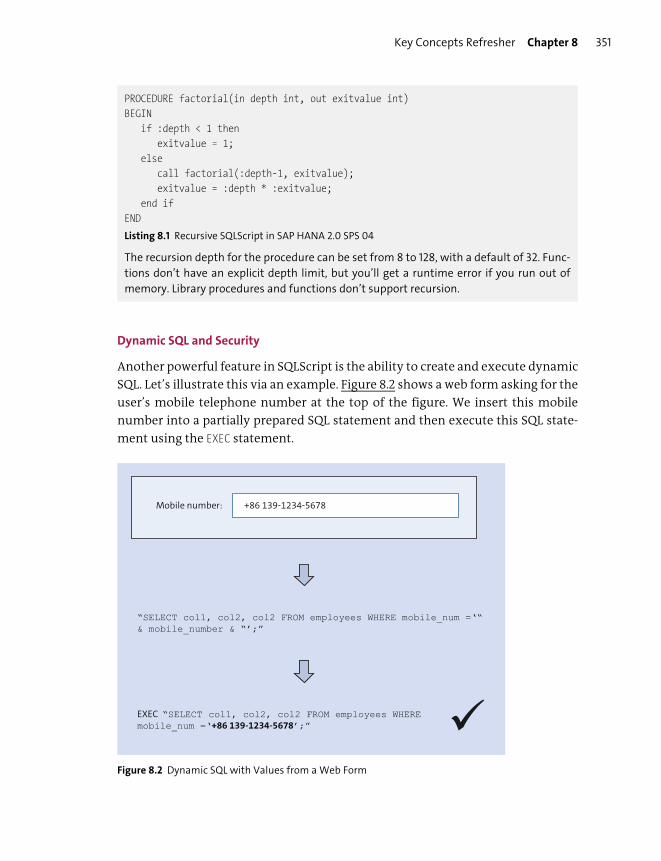
Key Concepts Refresher Chapter 8 351
PROCEDURE factorial(in depth int, out exitvalue int)BEGIN
if :depth < 1 thenexitvalue = 1;
elsecall factorial(:depth-1, exitvalue);exitvalue = :depth * :exitvalue;
end ifEND
Listing 8.1 Recursive SQLScript in SAP HANA 2.0 SPS 04
The recursion depth for the procedure can be set from 8 to 128, with a default of 32. Func-
tions don’t have an explicit depth limit, but you’ll get a runtime error if you run out of
memory. Library procedures and functions don’t support recursion.
Dynamic SQL and Security
Another powerful feature in SQLScript is the ability to create and execute dynamic
SQL. Let’s illustrate this via an example. Figure 8.2 shows a web form asking for the
user’s mobile telephone number at the top of the figure. We insert this mobile
number into a partially prepared SQL statement and then execute this SQL state-
ment using the EXEC statement.
Figure 8.2 Dynamic SQL with Values from a Web Form
Mobile number: +86 139-1234-5678
“SELECT col1, col2, col2 FROM employees WHERE mobile_num =‘“ & mobile_number & “’;”
EXEC “SELECT col1, col2, col2 FROM employees WHEREmobile_num =‘+86 139-1234-5678’;” �

Chapter 8 SQL and SQLScript352
Each user gets a unique SQL statement created especially for him or her. The per-
formance isn’t as good as static SQL statements, but this is more powerful and flex-
ible.
There is one problem: if you’re not careful, hackers can use this setup to break into
your system. This has been one of the top security vulnerabilities in web applica-
tions for many years now.
Let’s look at the web form again. This time, in Figure 8.3, hackers enter more infor-
mation than just the mobile telephone number. They add a closing quote and a
semicolon. When this is inserted into our prepared SQL statement, it closes the
current statement. (Remember that SQL statements are terminated by a semico-
lon.)
Figure 8.3 Dynamic SQL with SQL Injection from a Web Form
Anything after this is executed as another SQL statement—so the hackers can
enter something like DROP DATABASE that might delete the entire database. Or they
can try various SQL statements to read or modify data values in the database.
SAP HANA includes some new features related to this problem, such as the new
IS_SQL_INJECTION_SAFE function, which helps prevent such attacks.
If you remember to prevent security vulnerabilities such as SQL injection,
dynamic SQL can enable you to write some powerful applications. You can change
Mobile number: +86 139-1234-5678’;DROP DATABASE;‘
“SELECT col1, col2, col2 FROM employees WHERE mobile_num =‘“& mobile_number & “’;”
EXEC “SELECT col1, col2, col2 FROM employees WHEREmobile_num =‘+86 139-1234-5678’;DROP DATABASE;’’” �
Key Concepts Refresher Chapter 8 353
data sources at any time, link them to applications, and build adaptive user inter-
faces.
Again, keep in mind that this power also comes at the price of some performance.
Because SAP HANA has to evaluate SQL statements at runtime, the performance of
dynamic SQL statements can’t be as good as that of static SQL statements.
The other downside of using dynamic SQL statements is that the result set can’t be
passed to a SQLScript variable because the EXEC statement doesn’t return an entire
result set. (You can return a single record into a scalar variable.)
User-Defined (Table and Scalar) Functions
User-defined functions (UDFs) are custom, read-only functions in SAP HANA. You
write your own functions that can be called in a similar fashion as SQL functions.
There are two types of UDFs: scalar functions and table functions. The main differ-
ence is whether you want a function to return values as simple data types (e.g., an
integer) or in complete “table-like” result sets. A scalar function can return one or
more values, but these values have to be single data types. A table function returns
a set of data.
Tip
Both types of UDFs are read-only. You may not execute any DDL or DML statements
inside these functions.
We create functions as shown in Listing 8.2.
CREATE FUNCTION <func_name> [(<parameter_clause>)]RETURNS <return_type>[LANGUAGE SQLSCRIPT][SQL SECURITY <DEFINER | INVOKER>][DEFAULT SCHEMA <default_schema_name>] AS
{ BEGIN<function_body>
END }
Listing 8.2 Creating User-Defined Functions
Here are a few important points to note about UDFs:
� RETURNS
Depending on the type of data we return, RETURNS will be a scalar or a table func-
tion.
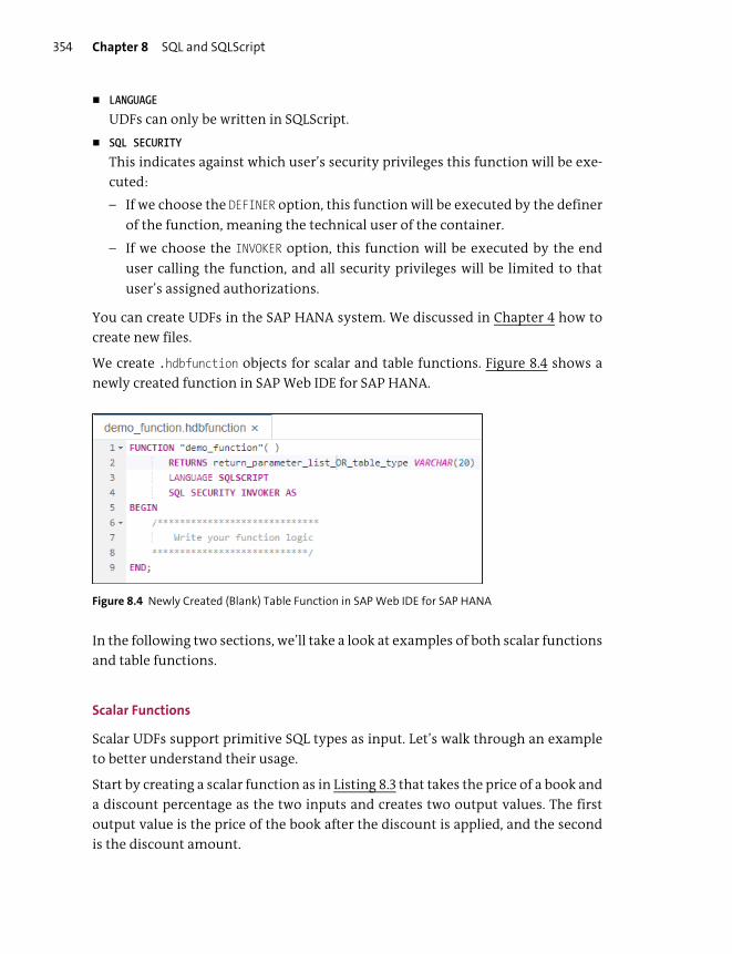
Chapter 8 SQL and SQLScript354
� LANGUAGE
UDFs can only be written in SQLScript.
� SQL SECURITY
This indicates against which user’s security privileges this function will be exe-
cuted:
– If we choose the DEFINER option, this function will be executed by the definer
of the function, meaning the technical user of the container.
– If we choose the INVOKER option, this function will be executed by the end
user calling the function, and all security privileges will be limited to that
user’s assigned authorizations.
You can create UDFs in the SAP HANA system. We discussed in Chapter 4 how to
create new files.
We create .hdbfunction objects for scalar and table functions. Figure 8.4 shows a
newly created function in SAP Web IDE for SAP HANA.
Figure 8.4 Newly Created (Blank) Table Function in SAP Web IDE for SAP HANA
In the following two sections, we’ll take a look at examples of both scalar functions
and table functions.
Scalar Functions
Scalar UDFs support primitive SQL types as input. Let’s walk through an example
to better understand their usage.
Start by creating a scalar function as in Listing 8.3 that takes the price of a book and
a discount percentage as the two inputs and creates two output values. The first
output value is the price of the book after the discount is applied, and the second
is the discount amount.
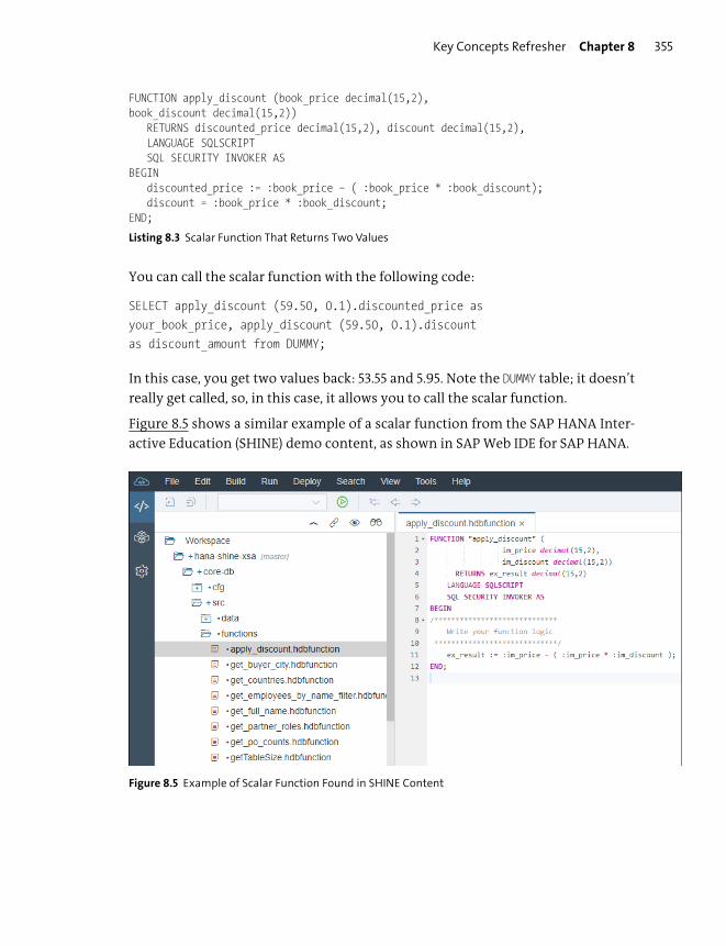
Key Concepts Refresher Chapter 8 355
FUNCTION apply_discount (book_price decimal(15,2),book_discount decimal(15,2))
RETURNS discounted_price decimal(15,2), discount decimal(15,2),LANGUAGE SQLSCRIPTSQL SECURITY INVOKER AS
BEGINdiscounted_price := :book_price – ( :book_price * :book_discount);discount = :book_price * :book_discount;
END;
Listing 8.3 Scalar Function That Returns Two Values
You can call the scalar function with the following code:
SELECT apply_discount (59.50, 0.1).discounted_price asyour_book_price, apply_discount (59.50, 0.1).discountas discount_amount from DUMMY;
In this case, you get two values back: 53.55 and 5.95. Note the DUMMY table; it doesn’t
really get called, so, in this case, it allows you to call the scalar function.
Figure 8.5 shows a similar example of a scalar function from the SAP HANA Inter-
active Education (SHINE) demo content, as shown in SAP Web IDE for SAP HANA.
Figure 8.5 Example of Scalar Function Found in SHINE Content
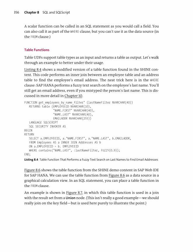
Chapter 8 SQL and SQLScript356
A scalar function can be called in an SQL statement as you would call a field. You
can also call it as part of the WHERE clause, but you can’t use it as the data source (in
the FROM clause.)
Table Functions
Table UDFs support table types as an input and returns a table as output. Let’s walk
through an example to better under their usage.
Listing 8.4 shows a modified version of a table function found in the SHINE con-
tent. This code performs an inner join between an employee table and an address
table to find the employee’s email address. The neat trick here is in the WHERE
clause: SAP HANA performs a fuzzy text search on the employee’s last name. You’ll
still get an email address, even if you mistyped the person’s last name. This is dis-
cussed in more detail in Chapter 10.
FUNCTION get_employees_by_name_filter" (lastNameFilter NVARCHAR(40))RETURNS table (EMPLOYEEID NVARCHAR(10),
"NAME.FIRST" NVARCHAR(40),"NAME.LAST" NVARCHAR(40),EMAILADDR NVARCHAR(255))
LANGUAGE SQLSCRIPTSQL SECURITY INVOKER AS
BEGINRETURN
SELECT a.EMPLOYEEID, a."NAME.FIRST", a."NAME.LAST", b.EMAILADDR,FROM Employees AS a INNER JOIN Addresses AS bON a.EMPLOYEEID = b. EMPLOYEEIDWHERE contains("NAME.LAST", :lastNameFilter, FUZZY(0.9));
END;
Listing 8.4 Table Function That Performs a Fuzzy Text Search on Last Names to Find Email Addresses
Figure 8.6 shows the table function from the SHINE demo content in SAP Web IDE
for SAP HANA. We can use the table function from Figure 8.6 as a data source in a
graphical calculation view. In an SQL statement, you can place a table function in
the FROM clause.
An example is shown in Figure 8.7, in which this table function is used in a join
with the result set from a Union node. (This isn’t really a good example—we should
really join on the key field—but is used here purely to illustrate the point.)
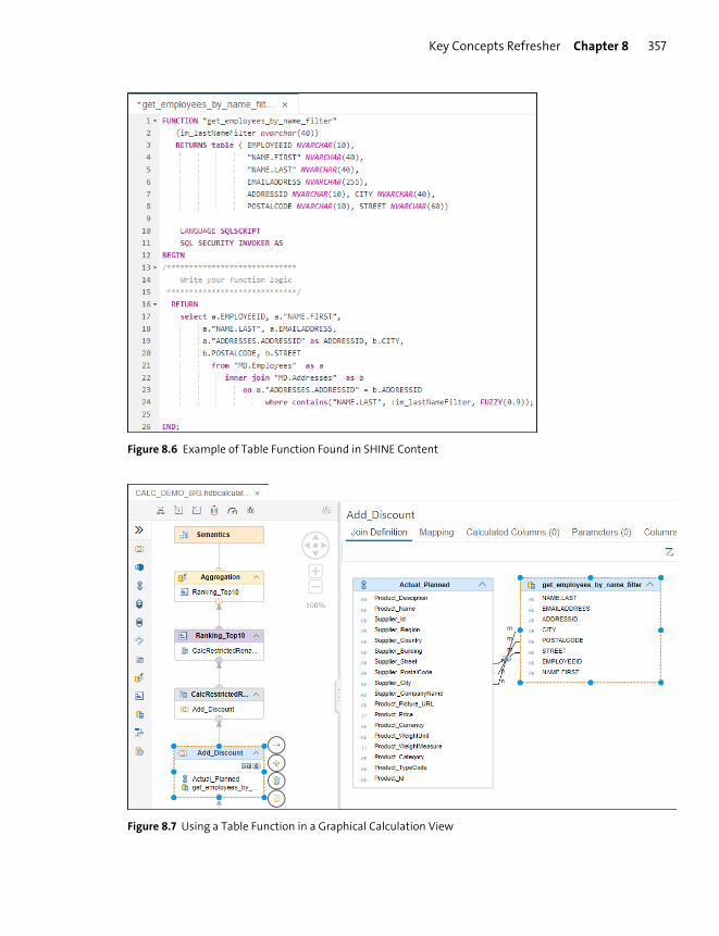
Key Concepts Refresher Chapter 8 357
Figure 8.6 Example of Table Function Found in SHINE Content
Figure 8.7 Using a Table Function in a Graphical Calculation View

Chapter 8 SQL and SQLScript358
Procedures
A procedure is a subroutine consisting of SQL statements. Procedures can be called
or invoked by applications that access the database. Procedures are sometimes
also known as stored procedures.
Procedures are more powerful than UDFs. Whereas UDFs are read-only and can’t
change any data in the system, procedures can insert, change, and delete data. You
can execute any DDL or DML statements inside a procedure. Whereas a table func-
tion can only return one result set, procedures can return many result sets as out-
put. These multiple result sets can be scalar and tabular.
Listing 8.5 illustrates how to create procedures.
CREATE PROCEDURE <proc_name> [(<parameter_clause>)][LANGUAGE <SQLSCRIPT | R>][SQL SECURITY <DEFINER | INVOKER>][DEFAULT SCHEMA <default_schema_name>][READS SQL DATA [WITH RESULTS VIEW <view_name>]] AS
{ BEGIN [SEQUENTIAL EXECUTION]<procedure_body>
END }
Listing 8.5 Creating Procedures
The following syntax items are used in Listing 8.5:
� LANGUAGE
Procedures can be written in SQLScript or in R. R is a popular open-source pro-
gramming language and data analysis software environment for statistical
computing.
� SQL SECURITY
Indicates against which user’s security privileges this function will be executed:
– If we choose the DEFINER option, this function will be executed by the definer
of the function, meaning the technical user of the container. This is the
default for procedures.
– If we choose the INVOKER option, this function will be executed by the end
user calling the function, and all security privileges will be limited to that
user’s assigned authorizations.
� READS SQL DATA
Marks the procedure as being read-only. The procedure then can’t change the
data or database object, and it can’t contain DDL or DML statements. If you try

Key Concepts Refresher Chapter 8 359
to activate a read-only procedure that contains DDL or DML statements, you’ll
get activation errors.
� WITH RESULTS VIEW
Specifies that a view (that we have to supply) can be used as the output of a read-
only procedure. When a result view is defined for a procedure, it can be called by
an SQL statement in the same way as a table or view.
� SEQUENTIAL EXECUTION
Forces sequential execution of the procedure logic; no parallelism is allowed.
� PARALLEL EXECUTION
Allows parallel execution of the procedure logic.
Some important points to note with regards to procedures:
� A procedure doesn’t require any input and output parameters. If we have input
and output parameters, they must be explicitly typed. The input and output
parameters of a procedure can have any of the primitive SQL types or a table
type. In SQLScript, we can also define table types. Table types are similar to data-
base tables but don’t have an instance. They are like a template for future use.
They are used to define parameters for a procedure that needs to use tabular
results.
� If we require table outputs from a procedure, we have to use table types.
� Any read-only procedure may only call other read-only procedures. The advan-
tage of using a read-only procedure is that certain optimizations are available
for read-only procedures, such as not having to check for database locks; this is
one of the performance enhancements in SAP HANA.
� Note that WITH RESULTS VIEW is a subclause of the READS SQL clause, so the same
restrictions apply to it as those for read-only procedures.
Let’s switch gears. Similar to UDFs, we can create procedures. In this case, we create
an .hdbprocedure object. Figure 8.8 shows a procedure in SAP Web IDE for SAP
HANA. Procedures are called with the CALL statement. You can call the procedure
shown in Figure 8.8 with the following statement:
CALL "get_product_sales_price" ('HT-1000', ?);
The results of this CALL statement, as executed in the SQL Console in SAP Web IDE
for SAP HANA, are shown in Figure 8.9.
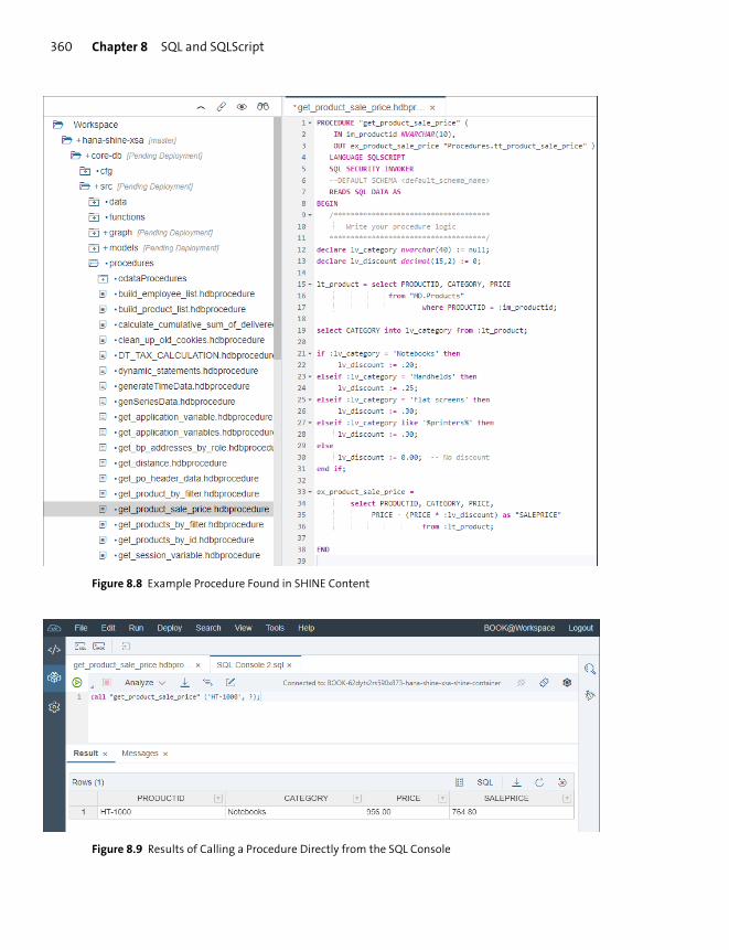
Chapter 8 SQL and SQLScript360
Figure 8.8 Example Procedure Found in SHINE Content
Figure 8.9 Results of Calling a Procedure Directly from the SQL Console
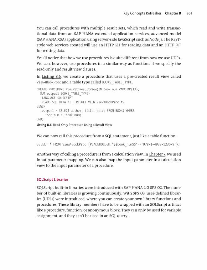
Key Concepts Refresher Chapter 8 361
You can call procedures with multiple result sets, which read and write transac-
tional data from an SAP HANA extended application services, advanced model
(SAP HANA XSA) application using server-side JavaScript such as Node.js. The REST-
style web services created will use an HTTP GET for reading data and an HTTP PUT
for writing data.
You’ll notice that how we use procedures is quite different from how we use UDFs.
We can, however, use procedures in a similar way as functions if we specify the
read-only and result view clauses.
In Listing 8.6, we create a procedure that uses a pre-created result view called
View4BookProc and a table type called BOOKS_TABLE_TYPE.
CREATE PROCEDURE ProcWithResultView(IN book_num VARCHAR(13),OUT output1 BOOKS_TABLE_TYPE)LANGUAGE SQLSCRIPTREADS SQL DATA WITH RESULT VIEW View4BookProc AS
BEGINoutput1 = SELECT author, title, price FROM BOOKS WHERE
isbn_num = :book_num;END;
Listing 8.6 Read-Only Procedure Using a Result View
We can now call this procedure from a SQL statement, just like a table function:
SELECT * FROM View4BookProc (PLACEHOLDER."$$book_num$$"=>'978-1-4932-1230-9');
Another way of calling a procedure is from a calculation view. In Chapter 7, we used
input parameter mapping. We can also map the input parameter in a calculation
view to the input parameter of a procedure.
SQLScript Libraries
SQLScript built-in libraries were introduced with SAP HANA 2.0 SPS 02. The num-
ber of built-in libraries is growing continuously. With SPS 03, user-defined librar-
ies (UDLs) were introduced, where you can create your own library functions and
procedures. These library members have to be wrapped with an SQLScript artifact
like a procedure, function, or anonymous block. They can only be used for variable
assignment, and they can’t be used in an SQL query.

Chapter 8 SQL and SQLScript362
SPS 04
The preceding restrictions have been removed with SPS 04. You now don’t need to wrap
library members in an SQLScript artifact, and you can use library functions directly in an
SQL query.
SPS 04 also adds a library for logging, as well as an end user unit test framework.
Multilevel Aggregation
Sometimes, you may need to return multiple result sets with a single SQL state-
ment. In normal SQL, this might not always be possible, but we can use multilevel
aggregation with grouping sets to achieve this in SQLScript.
Let’s start by looking at an example (Listing 8.7) in SQLScript of how we would cre-
ate two result sets.
-- Create result set 1books_pub_title_year = SELECT publisher, name, year, SUM(price)FROM BOOKS WHERE publisher = pubisher_idGROUP BY publisher, name, year;-- Create result set 2books_year = SELECT year, SUM(price) FROM BOOKSGROUP BY year;
Listing 8.7 Creating Two Result Sets in SQLScript
You can create both of these result sets from a single SQL statement using GROUPINGSETS, as shown in Listing 8.8.
SELECT publisher, name, year, SUM(price)FROM BOOKS WHERE publisher = pubisher_idGROUP BY GROUPING SETS ((publisher, name, year), (year))
Listing 8.8 Creating Multiple Result Sets from a Single SQL Statement with Grouping Sets
You now have a good understanding of SQLScript and the powerful capabilities it
brings to your modeling toolbox. Let’s now look at when you should use this func-
tionality and how to ensure that you use the latest variations of these features.
Views, Functions, and Procedures
Taking a step back, let’s look at how to best address our modeling requirements. In
SAP HANA we have three main approaches: views, UDFs, and procedures. Let’s first
discuss each of these options, and then we’ll discuss when you should use each
one.
Key Concepts Refresher Chapter 8 363
Information Views
We’ve discussed SAP HANA information views in detail in preceding chapters.
You’ve built these views using the graphical environment, and you’ve now also
learned how to also create these view using SQLScript.
Some of the characteristics of views include the following:
� Views are treated like tables. You can use SELECT, WHERE, GROUP BY, and ORDER BY
statements on views.
� Views are static. They always return the same columns, and you look at a set of
data in the same way.
� Views always return one result set.
� Views are mostly used for reading data.
User-Defined Functions
After learning about UDFs, you should be familiar with their characteristics, such
as the following:
� Functions always return results. A table function returns a set, and a scalar func-
tion returns one or more values.
� Functions require input parameters.
� The code in UDFs is read-only. Functions can’t change, update, or delete data or
database objects. You can’t insert data with functions, so you can’t use transac-
tions or COMMIT and ROLLBACK in functions.
� Functions can’t call EXEC statements; otherwise, you could build a dynamic
statement to change data and execute it.
� You can call the results of functions in SELECT statements and in WHERE and HAV-
ING clauses.
� Functions can be used in a join.
� Table functions can’t call procedures because procedures can change data. You
have to stick to the read-only paradigm of functions.
� Functions use SQLScript code. This can include imperative logic in which you
loop through results or apply an if-then logic flow to the results.
Procedures
Procedures are the most powerful of the three approaches. Some of the character-
istics of procedures include the following:

Chapter 8 SQL and SQLScript364
� Procedures can use transactions with COMMIT and ROLLBACK. They can modify
tables and data, unless they are marked as read-only. Read-only procedures may
only call other read-only procedures.
� Procedures can call UDFs, but UDFs can’t call procedures.
� Procedures don’t have to return any values but may return multiple result sets.
Procedures also don’t need to specify any input parameters.
� Procedures provide full control because all code functionality is allowed in pro-
cedures.
� Procedures can use try-catch blocks for errors.
� Procedures can also use dynamic SQL—but be aware of security vulnerabilities
such as SQL injection when using dynamic SQL.
SPS 04
Up to SAP HANA 2.0 SPS 04, dynamic SQL was always considered as read-write. With SPS
04, you can now specify dynamic SQL in a procedure to be read-only by using the READSSQL DATA clause. This especially helps performance by parallelizing multiple read-only
dynamic SQL statements.
If you use dynamic SQL in a read-only procedure, SAP HANA automatically assumes that
the dynamic SQL in such a procedure is also read-only. Why else would you include it into
a read-only procedure?
When to Use What Approach
After all that detail, the recommendation of when to use each of the three
approaches is quite easy to make:
� In order of functionality, procedures come in first, followed by UDFs, and then
views.
� In order of performance, we have the reverse: views give the best performance,
then UDFs (because they are permanently read-only), and then procedures.
Tip
Use the minimal approach to get the results you require. If you can do it with views, then
use views. If you can’t do it with views, then try using UDFs. If that still doesn’t meet the
requirements, create a procedure. This way, you do the least work and get the best per-
formance.

Important Terminology Chapter 8 365
Catching Up with SAP HANA 2.0
Figure 8.7 illustrated how to use a table function in a graphical calculation view.
This option changes how we approach modeling in SAP HANA projects and shows
how strong the graphical modeling environment has become.
We can work graphically with our SAP HANA views, create UDFs or procedures for
the occasional constraint, and bring these back into the graphical SAP HANA mod-
eling environment. We can then continue building the remainder of our SAP
HANA information models using the graphical information views.
We should, however, stick to the latest modeling best practices:
� The main guideline to keep in mind is that you should create design-time
objects that can be deployed to multiple systems, such as development, testing,
and production. Don’t create runtime objects as these can’t easily be copied to
other systems.
� Many modelers and developers used the SQL Console to create procedures. This
creates runtime objects that can’t be transported to the production system. The
recommended way is to create design-time objects—for example, .hdbproce-
dure objects—instead of using the CREATE PROCEDURE statement.
� Don’t create database objects (e.g., tables) using SQL statements such as CREATE
TABLE. Rather use core data services (CDS) objects such as .hdbcds. Even the
.hdbtable is deprecated. You can use .hdbtabledata for loading data into the
tables created by the CDS objects from data files (e.g., comma-separated values
[CSV] files).
Important Terminology
The following important terminology was used in this chapter:
� SQL
Structured Query Language (SQL) is a database programming language used to
enhance your modeling process when you have requirements that graphical
views can’t fulfill.
� SQLScript
SQLScript exposes many of the memory features of SAP HANA to SQL develop-
ers. This includes working with column tables, parameterized information
views, delta buffers, multiple result sets in parallel, built-in currency conver-
sions at the database level, fuzzy text searching, spatial data types, and PAL. The
Chapter 8 SQL and SQLScript366
only way to make this functionality available via SQL queries, even from other
applications, is to provide it via SQL extensions, that is, SQLScript.
� User-defined functions (UDF)
UDFs are custom, read-only functions in SAP HANA.
� Procedures (stored procedures)
A procedure is a subroutine consisting of SQL statements. Procedures can be
called or invoked by applications that access the database.
� Imperative logic
Occasionally, you might prefer to receive the answers to a query one record at a
time. This is most often the case when running SQL queries from application
servers. In these cases, you’ll use imperative logic, meaning you’ll “loop”
through the results one at a time
� Dynamic SQL
Dynamic SQL is when you build up SQL strings on the fly using code and then
execute them.
Practice Questions
These practice questions will help you evaluate your understanding of the topics
covered in this chapter. The questions shown are similar in nature to those found
on the certification examination. Although none of these questions will be found
on the exam itself, they will allow you to review your knowledge of the subject.
Select the correct answers, and then check the completeness of your answers in
the “Practice Question Answers and Explanations” section. Remember, on the
exam, you must select all correct answers and only correct answers to receive
credit for the question.
1. What paradigm describes the SQL language?
� A. Set-oriented
� B. Object-oriented
� C. Procedural
� D. Application-focused

Practice Questions Chapter 8 367
2. To what subset of SQL does the SELECT statement belong?
� A. DML
� B. DDL
� C. DCL
� D. DQL
3. True or False: Delimited identifiers are treated as case-sensitive.
� A. True
� B. False
4. What is used in SQL to indicate that there is no value?
� A. Zero
� B. Empty quotes
� C. NULL
� D. Spaces
5. What character is used to terminate SQL statements?
� A. ? (question mark)
� B. : (colon)
� C. ; (semicolon)
� D. . (period)
6. What SELECT statement isn’t recommended for use with column tables?
� A. SELECT *
� B. SELECT with a time-travel clause
� C. SELECT ALL
� D. SELECT in a subquery
7. True or False: A union returns all values in a result set, even duplicate records.
� A. True
� B. False

Chapter 8 SQL and SQLScript368
8. What character is prepended to a SQLScript variable when it’s used as an input
variable?
� A. ! (exclamation mark)
� B. : (colon)
� C. _ (underscore)
� D. & (ampersand)
9. What should you keep in mind when using imperative logic in SQLScript?
� A. It delivers the best possible performance.
� B. You can only use if-then logic.
� C. You can loop through records.
� D. It matches SQL’s set-oriented paradigm.
10. What should you keep in mind when using dynamic SQL? (There are 2 correct
answers.)
� A. It’s always bad for security.
� B. It could be used for SQL injection.
� C. You can dynamically change your data sources.
� D. It delivers the best possible performance.
11. You created a user-defined function with a return type of BIGINT. What type of
function have you created?
� A. SQL function
� B. Scalar function
� C. Table function
� D. Window function
12. In which programming languages can you create procedures in SAP HANA?
(There are 2 correct answers.)
� A. SQLScript
� B. L
� C. JavaScript
� D. R

Practice Questions Chapter 8 369
13. You created a user-defined function with the INVOKER security option. Which
user’s authorizations are checked when the function is executed?
� A. The owner of the function
� B. The container’s technical user
� C. The SYSTEM user
� D. The user calling the function
14. What is the preferred way to create a procedure?
� A. Use the CREATE PROCEDURE statement in the SQL console.
� B. Create a .procedure file.
� C. Create a .hdbprocedure file.
� D. Use the Import menu in SAP Web IDE for SAP HANA.
15. With which statement can you call a table function? (There are 2 correct
answers.)
� A. CALL
� B. INSERT INTO
� C. SELECT
� D. EXEC
16. What statement is allowed in a user-defined function?
� A. COMMIT
� B. EXEC
� C. INSERT
� D. JOIN
17. You want to call a procedure in a SELECT statement (e.g., a table function).
Which clauses do you have to specify? (There are 2 correct answers.)
� A. LANGUAGE SQLSCRIPT
� B. WITH RESULTS VIEW
� C. SEQUENTIAL EXECUTION
� D. READS SQL DATA
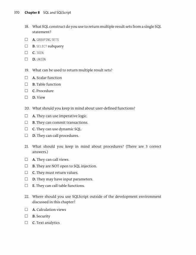
Chapter 8 SQL and SQLScript370
18. What SQL construct do you use to return multiple result sets from a single SQL
statement?
� A. GROUPING SETS
� B. SELECT subquery
� C. JOIN
� D. UNION
19. What can be used to return multiple result sets?
� A. Scalar function
� B. Table function
� C. Procedure
� D. View
20. What should you keep in mind about user-defined functions?
� A. They can use imperative logic.
� B. They can commit transactions.
� C. They can use dynamic SQL.
� D. They can call procedures.
21. What should you keep in mind about procedures? (There are 3 correct
answers.)
� A. They can call views.
� B. They are NOT open to SQL injection.
� C. They must return values.
� D. They may have input parameters.
� E. They can call table functions.
22. Where should you use SQLScript outside of the development environment
discussed in this chapter?
� A. Calculation views
� B. Security
� C. Text analytics
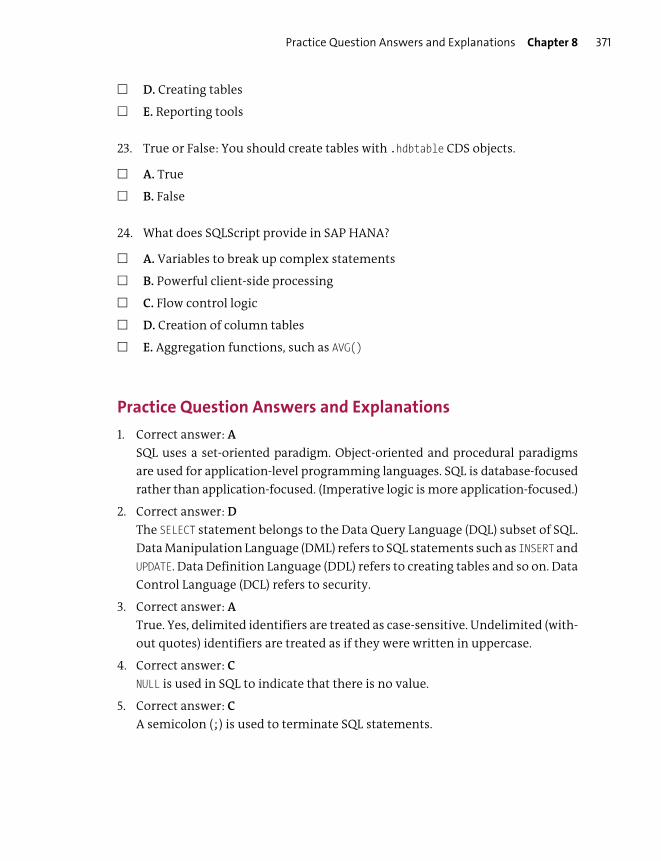
Practice Question Answers and Explanations Chapter 8 371
� D. Creating tables
� E. Reporting tools
23. True or False: You should create tables with .hdbtable CDS objects.
� A. True
� B. False
24. What does SQLScript provide in SAP HANA?
� A. Variables to break up complex statements
� B. Powerful client-side processing
� C. Flow control logic
� D. Creation of column tables
� E. Aggregation functions, such as AVG()
Practice Question Answers and Explanations
1. Correct answer: A
SQL uses a set-oriented paradigm. Object-oriented and procedural paradigms
are used for application-level programming languages. SQL is database-focused
rather than application-focused. (Imperative logic is more application-focused.)
2. Correct answer: D
The SELECT statement belongs to the Data Query Language (DQL) subset of SQL.
Data Manipulation Language (DML) refers to SQL statements such as INSERT and
UPDATE. Data Definition Language (DDL) refers to creating tables and so on. Data
Control Language (DCL) refers to security.
3. Correct answer: A
True. Yes, delimited identifiers are treated as case-sensitive. Undelimited (with-
out quotes) identifiers are treated as if they were written in uppercase.
4. Correct answer: C
NULL is used in SQL to indicate that there is no value.
5. Correct answer: C
A semicolon (;) is used to terminate SQL statements.
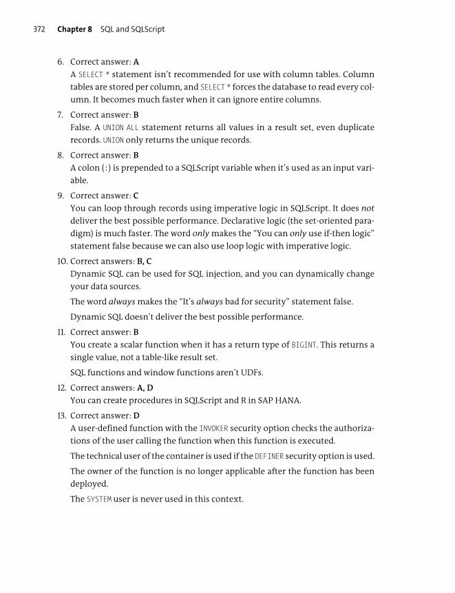
Chapter 8 SQL and SQLScript372
6. Correct answer: A
A SELECT * statement isn’t recommended for use with column tables. Column
tables are stored per column, and SELECT * forces the database to read every col-
umn. It becomes much faster when it can ignore entire columns.
7. Correct answer: B
False. A UNION ALL statement returns all values in a result set, even duplicate
records. UNION only returns the unique records.
8. Correct answer: B
A colon (:) is prepended to a SQLScript variable when it’s used as an input vari-
able.
9. Correct answer: C
You can loop through records using imperative logic in SQLScript. It does not
deliver the best possible performance. Declarative logic (the set-oriented para-
digm) is much faster. The word only makes the “You can only use if-then logic”
statement false because we can also use loop logic with imperative logic.
10. Correct answers: B, C
Dynamic SQL can be used for SQL injection, and you can dynamically change
your data sources.
The word always makes the “It’s always bad for security” statement false.
Dynamic SQL doesn’t deliver the best possible performance.
11. Correct answer: B
You create a scalar function when it has a return type of BIGINT. This returns a
single value, not a table-like result set.
SQL functions and window functions aren’t UDFs.
12. Correct answers: A, D
You can create procedures in SQLScript and R in SAP HANA.
13. Correct answer: D
A user-defined function with the INVOKER security option checks the authoriza-
tions of the user calling the function when this function is executed.
The technical user of the container is used if the DEFINER security option is used.
The owner of the function is no longer applicable after the function has been
deployed.
The SYSTEM user is never used in this context.

Practice Question Answers and Explanations Chapter 8 373
14. Correct answer: C
The preferred way to create a procedure is to create an .hdbprocedure file.
Methods A and B are deprecated! (This shows how much things have changed
over the past few years.)
15. Correct answers: C, D
You can call a table function with SELECT and EXEC statements. EXEC can be used
to build a dynamic SQL statement that contains a SELECT statement, for exam-
ple.
You CAN’T use a function to INSERT INTO because it’s read-only.
CALL is how procedures are called.
16. Correct answer: D
JOIN is allowed in a UDF.
COMMIT, EXEC, and INSERT aren’t read-only statements. A UDF won’t even build
when you have these in the function.
17. Correct answers: B, D
You need the WITH RESULTS VIEW and READS SQL DATA clauses to call a procedure in
a SELECT statement.
18. Correct answer: A
GROUPING SETS can return multiple result sets from a single SQL statement.
All the other statements use multiple sources but return a single result set.
19. Correct answer: C
Procedures can return multiple result sets.
Table functions and views can only return single result sets.
Scalar functions return (multiple) single values, not sets.
20. Correct answer: A
UDFs can use imperative logic.
They can’t commit transactions or use dynamic SQL (because they are read-
only), and they can’t call procedures. (However, procedures can call UDFs.)
21. Correct answers: A, D, E
Procedures can call views and table functions, and they may have input param-
eters.
They may, but not must, return values.
Because they can use dynamic SQL, they could be open to SQL injection.
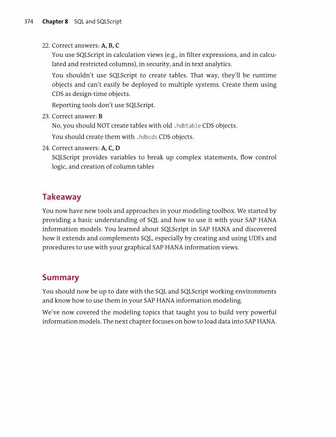
Chapter 8 SQL and SQLScript374
22. Correct answers: A, B, C
You use SQLScript in calculation views (e.g., in filter expressions, and in calcu-
lated and restricted columns), in security, and in text analytics.
You shouldn’t use SQLScript to create tables. That way, they’ll be runtime
objects and can’t easily be deployed to multiple systems. Create them using
CDS as design-time objects.
Reporting tools don’t use SQLScript.
23. Correct answer: B
No, you should NOT create tables with old .hdbtable CDS objects.
You should create them with .hdbcds CDS objects.
24. Correct answers: A, C, D
SQLScript provides variables to break up complex statements, flow control
logic, and creation of column tables
Takeaway
You now have new tools and approaches in your modeling toolbox. We started by
providing a basic understanding of SQL and how to use it with your SAP HANA
information models. You learned about SQLScript in SAP HANA and discovered
how it extends and complements SQL, especially by creating and using UDFs and
procedures to use with your graphical SAP HANA information views.
Summary
You should now be up to date with the SQL and SQLScript working environments
and know how to use them in your SAP HANA information modeling.
We’ve now covered the modeling topics that taught you to build very powerful
information models. The next chapter focuses on how to load data into SAP HANA.
Chapter 9
Data Provisioning
Techniques You’ll Master
� Learn what data provisioning is
� Understand the basic data provisioning concepts
� Get to know some of the various SAP data provisioning tools
available for SAP HANA
� Know when to use the different SAP data provisioning tools in
the context of SAP HANA
� Identify the benefits of each data provisioning method
� Gain a working knowledge of some features in a few of the SAP
provisioning tools
Chapter 9 Data Provisioning376
In this chapter, we’ll cover how to provide data to SAP HANA information models
and the basic principles and tools used for data provisioning in SAP HANA. For our
information models to work properly, we need to ensure that we get the right data
into SAP HANA at the right time.
There are people who specialize in each of the data provisioning tools discussed,
and there are special training courses for every one of these tools. Our aim, there-
fore, isn’t to dive deep into detail about the various concepts and tools, but to give
you a high-level working knowledge of what each tool does to help you under-
stand the concepts involved when provisioning data into SAP HANA, to enable
you to have a meaningful conversation on the topic, and to help you choose the
right tool for your business requirements.
Real-World Scenario
You start a new project that involves SAP HANA, and you’re asked to provide
data for the SAP HANA system.
You start by asking important questions about the expected data provision-
ing: Where is the data stored currently? Is the data clean? Will the data be
updated in the source systems, or is this a once-off data provisioning pro-
cess? Does the business need the data in real time, or is a delay of some hours
acceptable? Does the data need to be stored in the SAP HANA system? Does
the business already have a data provisioning tool that you can reuse? Will
the data provisioning process be limited to SAP HANA only?
After evaluating all these factors, you recommend the right data provision-
ing tool to the business, one that is applicable to its budget, circumstances,
and requirements.
Objectives of This Portion of the Test
The objective of this portion of the SAP HANA certification is to test your high-
level understanding of the various SAP data provisioning tools available for get-
ting data into an SAP HANA system.
Key Concepts Refresher Chapter 9 377
The certification exam expects you to have a good understanding of the following
topics:
� General data provisioning concepts
� Different SAP data provisioning tools
� Similarities and differences between the various provisioning tools
� When to use a particular SAP provisioning tool
� Features of some of the SAP data provisioning tools
Note
This portion contributes about 4% of the total certification exam score.
Key Concepts Refresher
In Chapter 5, we started by looking at the basic information modeling concepts.
We presented an overview diagram of the different types of information models in
SAP HANA and how they all work together to help solve business requirements.
This overview diagram is shown again in Figure 9.1.
So far, we’ve focused our attention on the bottom half of the diagram: on informa-
tion modeling inside SAP HANA. In this chapter, our attention shifts to the upper-
left corner of the diagram. You need to know how to supply your SAP HANA infor-
mation models with the data they require.
SAP HANA doesn’t really differentiate whether the data comes from SAP or from
non-SAP source systems. Data is data, regardless of where it comes from. Combined
with the fact that SAP HANA is a full platform—and not just a dumb database—this
makes it an excellent choice for all companies. SAP HANA is meant not only for tra-
ditional SAP customers but also for a wide range of other companies, from small
startups to large corporations. In fact, SAP works with thousands of startups and
smaller partners, helping them use SAP HANA to deliver innovative solutions that
are “nontraditional” in the SAP sense.
In this chapter, we’ll look at some of the various data provisioning concepts and
tools.
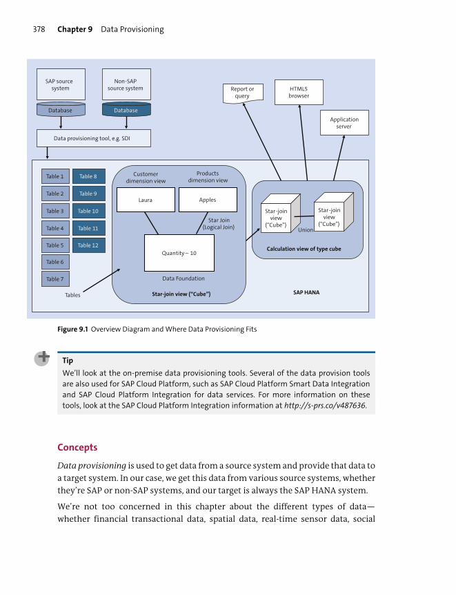
Chapter 9 Data Provisioning378
Figure 9.1 Overview Diagram and Where Data Provisioning Fits
Tip
We’ll look at the on-premise data provisioning tools. Several of the data provision tools
are also used for SAP Cloud Platform, such as SAP Cloud Platform Smart Data Integration
and SAP Cloud Platform Integration for data services. For more information on these
tools, look at the SAP Cloud Platform Integration information at http://s-prs.co/v487636.
Concepts
Data provisioning is used to get data from a source system and provide that data to
a target system. In our case, we get this data from various source systems, whether
they’re SAP or non-SAP systems, and our target is always the SAP HANA system.
We’re not too concerned in this chapter about the different types of data—
whether financial transactional data, spatial data, real-time sensor data, social
Data provisioning tool, e.g. SDI
SAP source system
Database
Non-SAP source system
Database
Report or query
HTML5 browser
Star-join view
(“Cube”)
Star-join view
(“Cube”)
Application server
SAP HANA
Calculation view of type cube
Union
Star-join view (“Cube”)Tables
Table 1 Table 8
Table 2 Table 9
Table 3 Table 10
Table 4 Table 11
Table 5 Table 12
Table 6
Table 7 Data Foundation
Apples
Quantity – 10
Laura
Customerdimension view
Productsdimension view
Star Join(Logical Join)
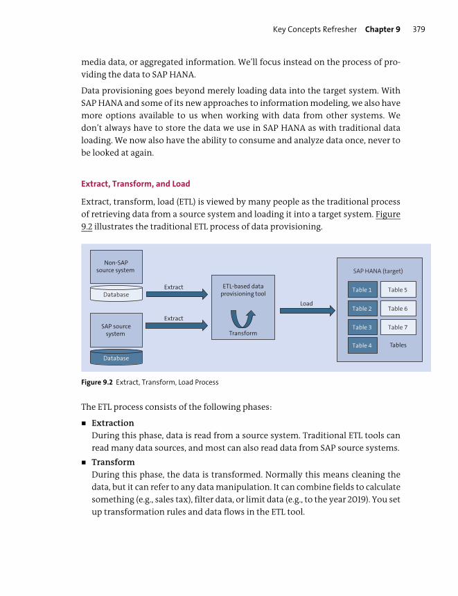
Key Concepts Refresher Chapter 9 379
media data, or aggregated information. We’ll focus instead on the process of pro-
viding the data to SAP HANA.
Data provisioning goes beyond merely loading data into the target system. With
SAP HANA and some of its new approaches to information modeling, we also have
more options available to us when working with data from other systems. We
don’t always have to store the data we use in SAP HANA as with traditional data
loading. We now also have the ability to consume and analyze data once, never to
be looked at again.
Extract, Transform, and Load
Extract, transform, load (ETL) is viewed by many people as the traditional process
of retrieving data from a source system and loading it into a target system. Figure
9.2 illustrates the traditional ETL process of data provisioning.
Figure 9.2 Extract, Transform, Load Process
The ETL process consists of the following phases:
� Extraction
During this phase, data is read from a source system. Traditional ETL tools can
read many data sources, and most can also read data from SAP source systems.
� Transform
During this phase, the data is transformed. Normally this means cleaning the
data, but it can refer to any data manipulation. It can combine fields to calculate
something (e.g., sales tax), filter data, or limit data (e.g., to the year 2019). You set
up transformation rules and data flows in the ETL tool.
Load
ETL-based dataprovisioning tool
Transform
Non-SAPsource system
Database
SAP sourcesystem
Database
Extract
Extract
SAP HANA (target)
Tables
Table 1 Table 5
Table 2 Table 6
Table 3 Table 7
Table 4
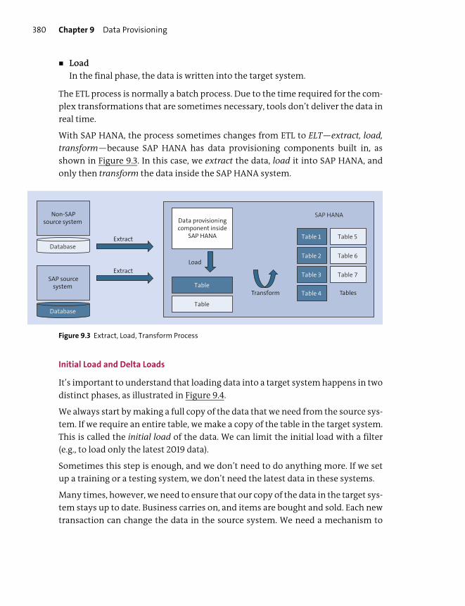
Chapter 9 Data Provisioning380
� Load
In the final phase, the data is written into the target system.
The ETL process is normally a batch process. Due to the time required for the com-
plex transformations that are sometimes necessary, tools don’t deliver the data in
real time.
With SAP HANA, the process sometimes changes from ETL to ELT—extract, load,
transform—because SAP HANA has data provisioning components built in, as
shown in Figure 9.3. In this case, we extract the data, load it into SAP HANA, and
only then transform the data inside the SAP HANA system.
Figure 9.3 Extract, Load, Transform Process
Initial Load and Delta Loads
It’s important to understand that loading data into a target system happens in two
distinct phases, as illustrated in Figure 9.4.
We always start by making a full copy of the data that we need from the source sys-
tem. If we require an entire table, we make a copy of the table in the target system.
This is called the initial load of the data. We can limit the initial load with a filter
(e.g., to load only the latest 2019 data).
Sometimes this step is enough, and we don’t need to do anything more. If we set
up a training or a testing system, we don’t need the latest data in these systems.
Many times, however, we need to ensure that our copy of the data in the target sys-
tem stays up to date. Business carries on, and items are bought and sold. Each new
transaction can change the data in the source system. We need a mechanism to
Data provisioningcomponent inside
SAP HANA
Table
Table
Load
Transform
Non-SAPsource system
Database
SAP sourcesystem
Database
Extract
Extract
SAP HANA
Tables
Table 1 Table 5
Table 2 Table 6
Table 3 Table 7
Table 4

Key Concepts Refresher Chapter 9 381
update the data in the target system. We could just delete the data in the target sys-
tem and perform the initial load again. For small sets of data, this approach can
work, but it quickly becomes inefficient and wasteful for large data sets.
Figure 9.4 Initial Load of Tables and Subsequent Delta Updates
A more efficient method is to look at the data that has changed and apply the data
changes to our copy of the data in the target system. These data changes are
referred to as the delta, and applying these changes to the target system is called a
delta load. The various data provisioning tools can differ substantially in the way
they implement the delta load mechanism. One method of achieving this is repli-
cation.
Replication
Replication emphasizes the time aspect of the data loading process. ETL focuses on
ensuring that the data is clean and in the correct format in the target system. Rep-
lication does less of that, but it gets the data into the target system as quickly as
possible. As such, the replication process appears quite simple, as shown in Figure
9.5.
SAP HANAtarget system
SAP HANAtarget system
Table
Dataprovisioning
tool
Source system
Table
Table
Source system
Table
Delta data loads
Initial data loads
Dataprovisioning
tool
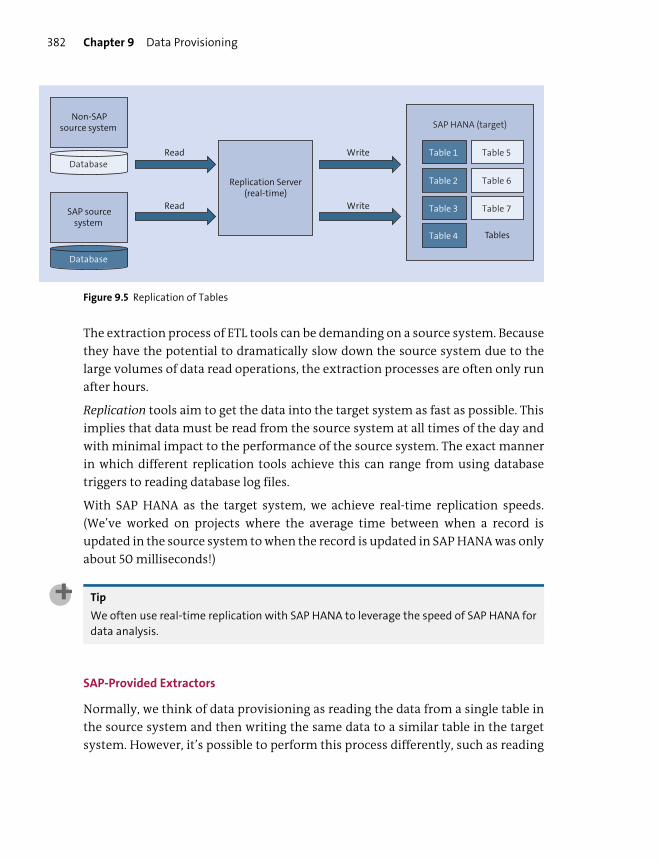
Chapter 9 Data Provisioning382
Figure 9.5 Replication of Tables
The extraction process of ETL tools can be demanding on a source system. Because
they have the potential to dramatically slow down the source system due to the
large volumes of data read operations, the extraction processes are often only run
after hours.
Replication tools aim to get the data into the target system as fast as possible. This
implies that data must be read from the source system at all times of the day and
with minimal impact to the performance of the source system. The exact manner
in which different replication tools achieve this can range from using database
triggers to reading database log files.
With SAP HANA as the target system, we achieve real-time replication speeds.
(We’ve worked on projects where the average time between when a record is
updated in the source system to when the record is updated in SAP HANA was only
about 50 milliseconds!)
Tip
We often use real-time replication with SAP HANA to leverage the speed of SAP HANA for
data analysis.
SAP-Provided Extractors
Normally, we think of data provisioning as reading the data from a single table in
the source system and then writing the same data to a similar table in the target
system. However, it’s possible to perform this process differently, such as reading
Replication Server(real-time)
Read
Read Write
Write
Non-SAPsource system
Database
SAP sourcesystem
Database
SAP HANA (target)
Tables
Table 1 Table 5
Table 2 Table 6
Table 3 Table 7
Table 4
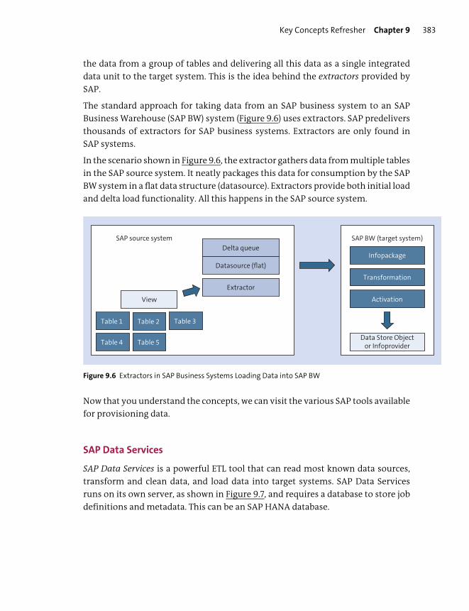
Key Concepts Refresher Chapter 9 383
the data from a group of tables and delivering all this data as a single integrated
data unit to the target system. This is the idea behind the extractors provided by
SAP.
The standard approach for taking data from an SAP business system to an SAP
Business Warehouse (SAP BW) system (Figure 9.6) uses extractors. SAP predelivers
thousands of extractors for SAP business systems. Extractors are only found in
SAP systems.
In the scenario shown in Figure 9.6, the extractor gathers data from multiple tables
in the SAP source system. It neatly packages this data for consumption by the SAP
BW system in a flat data structure (datasource). Extractors provide both initial load
and delta load functionality. All this happens in the SAP source system.
Figure 9.6 Extractors in SAP Business Systems Loading Data into SAP BW
Now that you understand the concepts, we can visit the various SAP tools available
for provisioning data.
SAP Data Services
SAP Data Services is a powerful ETL tool that can read most known data sources,
transform and clean data, and load data into target systems. SAP Data Services
runs on its own server, as shown in Figure 9.7, and requires a database to store job
definitions and metadata. This can be an SAP HANA database.
SAP BW (target system)
Table 4
View
Table 1 Table 2 Table 3
Table 5
SAP source system
Extractor
Datasource (flat)
Transformation
Activation
Data Store Objector Infoprovider
InfopackageDelta queue

Chapter 9 Data Provisioning384
Figure 9.7 SAP Data Services
The extraction capabilities of SAP Data Services are well known in the industry. It
can read many data sources—even obscure ones, such as old COBOL copybooks.
However, SAP Data Services can also read all the latest social media feeds available
on the Internet, and it can communicate with most databases and large business
applications. You can also use it with stores of unstructured data, such as Hadoop.
SAP Data Services can get data from SAP business systems in various ways. We can
use it to directly read a system’s databases. We could also use some of the built-in
extractors we discussed previously.
Another way SAP Data Services can get data from SAP business systems is by using
an ABAP data flow. ABAP is the programming language that SAP uses to write the
SAP Business Suite systems. SAP Data Services can write some ABAP code that you
can load into the SAP source system. This code becomes part of an ABAP data flow
and is a faster and more reliable way to extract the data from an SAP source sys-
tem.
SAP Data Services can also provide complex transformations. SAP Data Services is
actually several products combined. When people refer to SAP Data Services, they
normally refer to the data provisioning product called Data Integrator. Another
product called SAP Data Quality Management is also combined under the SAP Data
Services product name.
All SAP Data Services products ensure that you have clean and reliable informa-
tion to work with. You may have heard the old saying, “garbage in, garbage out.” If
you have rubbish data going into your reporting system, you get rubbish data in
your reports. SAP HANA’s great performance doesn’t make this go away. It just
changes that old saying to, “garbage in, garbage out fast!”
SAP Data Quality Management
ABAP Data Flows
Load
Transform
Non-SAPsource system
Database
SAP sourcesystem
Database
Extract
Extract
SAP HANA (target)
Tables
Table 1 Table 5
Table 2 Table 6
Table 3 Table 7
Table 4
Job Server
Designer
SAP Data Services(Data Integrator)
Key Concepts Refresher Chapter 9 385
You can use SAP Data Services for data provisioning in the following scenarios:
� A strong ETL tool is required.
� Certain data sources need to be read (e.g., legacy systems).
� Transformation of data is required, for example, when data isn’t clean.
� Real-time data provisioning isn’t a business requirement.
� A customer already has an instance of SAP Data Services running and requires
you to use the current infrastructure and skills available.
� The business requires a tool that delivers data to multiple destinations, of which
SAP HANA is one.
SAP Landscape Transformation Replication Server
SAP Landscape Transformation Replication Server is a data provisioning tool that
uses replication to load data into SAP HANA. Remember that the focus of a replica-
tion server is to load data into the target system as fast as possible.
SAP Landscape Transformation Replication Server started as a tool that SAP devel-
oped and used internally to help companies migrating data between SAP systems,
for example, when companies wanted to consolidate systems after a merger or
acquisition. SAP Landscape Transformation Replication Server is written in ABAP
and runs on the SAP NetWeaver platform, just like SAP ERP and other SAP business
systems. The tool was successfully used for years for data migrations, but it
became more popular and well known with the arrival of SAP HANA.
SAP Landscape Transformation Replication Server works with both SAP and non-
SAP source systems. It uses the same database libraries as the SAP Business Suite
and therefore supports all the same databases as the SAP business systems, includ-
ing SAP HANA, SAP Adaptive Server Enterprise (SAP ASE), SAP MaxDB, Microsoft
SQL Server, IBM DB2, Oracle, and Informix. We recommend that SAP Landscape
Transformation Replication Server be installed on its own server, as shown in
Figure 9.8, even though you can install it inside a source system based on SAP Net-
Weaver.
SAP Landscape Transformation Replication Server uses a trigger-based method for
real-time replication. All databases have a trigger whereby they can spur an action
to occur when data changes in a table. For example, if data is updated or deleted, or
if new data is inserted in a specific table, you can set up a database trigger to also
write these changes to a special replication log table. SAP Landscape Transforma-
tion Replication Server replication is also known as trigger-based replication. The
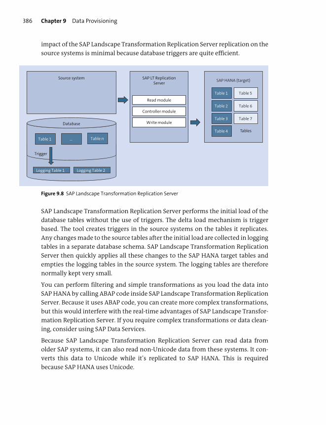
Chapter 9 Data Provisioning386
impact of the SAP Landscape Transformation Replication Server replication on the
source systems is minimal because database triggers are quite efficient.
Figure 9.8 SAP Landscape Transformation Replication Server
SAP Landscape Transformation Replication Server performs the initial load of the
database tables without the use of triggers. The delta load mechanism is trigger
based. The tool creates triggers in the source systems on the tables it replicates.
Any changes made to the source tables after the initial load are collected in logging
tables in a separate database schema. SAP Landscape Transformation Replication
Server then quickly applies all these changes to the SAP HANA target tables and
empties the logging tables in the source system. The logging tables are therefore
normally kept very small.
You can perform filtering and simple transformations as you load the data into
SAP HANA by calling ABAP code inside SAP Landscape Transformation Replication
Server. Because it uses ABAP code, you can create more complex transformations,
but this would interfere with the real-time advantages of SAP Landscape Transfor-
mation Replication Server. If you require complex transformations or data clean-
ing, consider using SAP Data Services.
Because SAP Landscape Transformation Replication Server can read data from
older SAP systems, it can also read non-Unicode data from these systems. It con-
verts this data to Unicode while it’s replicated to SAP HANA. This is required
because SAP HANA uses Unicode.
Source system
Database
Table 1 … Table n
Logging Table 1 Logging Table 2
Trigger
Read module
Controller module
Write module
SAP HANA (target)
Tables
Table 1 Table 5
Table 2 Table 6
Table 3 Table 7
Table 4
SAP LT ReplicationServer
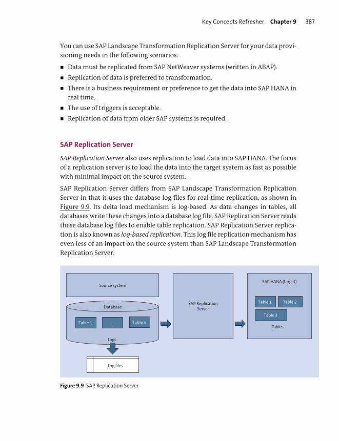
Key Concepts Refresher Chapter 9 387
You can use SAP Landscape Transformation Replication Server for your data provi-
sioning needs in the following scenarios:
� Data must be replicated from SAP NetWeaver systems (written in ABAP).
� Replication of data is preferred to transformation.
� There is a business requirement or preference to get the data into SAP HANA in
real time.
� The use of triggers is acceptable.
� Replication of data from older SAP systems is required.
SAP Replication Server
SAP Replication Server also uses replication to load data into SAP HANA. The focus
of a replication server is to load the data into the target system as fast as possible
with minimal impact on the source system.
SAP Replication Server differs from SAP Landscape Transformation Replication
Server in that it uses the database log files for real-time replication, as shown in
Figure 9.9. Its delta load mechanism is log-based. As data changes in tables, all
databases write these changes into a database log file. SAP Replication Server reads
these database log files to enable table replication. SAP Replication Server replica-
tion is also known as log-based replication. This log file replication mechanism has
even less of an impact on the source system than SAP Landscape Transformation
Replication Server.
Figure 9.9 SAP Replication Server
SAP ReplicationServer
Source systemSAP HANA (target)
Table 1 Table 2
Table 3
Database
Table 1 … Table n
Log files
Logs
Tables
Chapter 9 Data Provisioning388
SAP Replication Server works with both SAP and non-SAP source systems and sup-
ports many databases. Replication servers don’t focus on the filtering or transfor-
mation of data before loading the data into SAP HANA.
The database log files contain all the changes in a database. SAP Replication Server
can use this information to replicate entire databases. For example, SAP ASE data-
bases use SAP Replication Server to replicate the database log files for disaster
recovery purposes.
Tip
The features of SAP Replication Server, such as log-based replication, have been incorpo-
rated into SAP HANA smart data integration. SAP HANA smart data integration is built in
to SAP HANA and is therefore preferred for our purposes.
You can use SAP Replication Server for your data provisioning needs in the follow-
ing scenarios:
� Replication of data is preferred to transformation.
� There is a business requirement or preference to get the data into SAP HANA in
real-time.
� The use of triggers isn’t acceptable.
� No pool or cluster tables need to be replicated.
� The business requires minimal impact on the source system.
� Database replication is needed for disaster recovery purposes.
� The business requires a tool that delivers data to multiple destinations, of which
SAP HANA is one.
SAP HANA Smart Data Access
SAP HANA smart data access provides SAP HANA with direct access to data in a
remote database. In this case, we don’t store the data in the SAP HANA database;
we can access it at any time. We merely consume the remote data when required.
SAP HANA smart data access allows you to create virtual tables, that is, empty
tables that point to tables or views inside another database somewhere (see Figure
9.10). Some databases have a similar feature called proxy tables (also sometimes
called data federation).

Key Concepts Refresher Chapter 9 389
Figure 9.10 SAP HANA Smart Data Access and Virtual Tables
SAP HANA smart data access has various database adapters it uses to connect
these virtual tables to a large number of databases. These adapters include the fol-
lowing:
� SAP HANA, SAP ASE, SAP IQ, SAP Event Stream Processor, and SAP MaxDB
� Hadoop (Hive), Spark, and SAP Vora
� IBM DB2 and IBM Netezza
� Microsoft SQL Server
� Oracle
� Teradata
SAP HANA smart data access can also use an Open Database Connectivity (ODBC)
framework to connect to other databases via ODBC.
When you ask for data from a virtual table, SAP HANA connects to the remote
database across the network, logs in, and requests the relevant data from the
remote table or view. You can combine the data from the remote database table
with data stored in SAP HANA. You can use a virtual table in SAP HANA informa-
tion models, just like native SAP HANA tables. SAP HANA smart data access will
automatically convert the data types from those used in the remote database to
SAP HANA data types.
Report
SAP HANA
SAP HANATable
View
VirtualTable
Remote Database
Table ViewRead and write
via network
SDA

Chapter 9 Data Provisioning390
Virtual Tables vs. Native Tables
You can’t expect the same performance from SAP HANA smart data access virtual tables
as from SAP HANA native tables. SAP HANA tables are loaded in the memory of SAP
HANA. The data from the virtual table is fetched from a relatively slow disk-based data-
base across the network.
Keep in mind that SAP HANA smart data access reads data from remote tables
directly, as it’s stored. SAP HANA smart data access can’t do any data cleansing
because it reads data from remote tables. SAP HANA also doesn’t have any sched-
uling tool, so SAP HANA smart data access can’t be used for ETL processes or repli-
cation. It just reads the data from the remote tables as the need arises; for example,
a reporting query requires data to be stored in a remote table.
SAP HANA provides the following optimizations for SAP HANA smart data access
virtual tables:
� SAP HANA caches data that it reads from remote databases. If the data is found
in the cache, the data is read from the cache, and no request is sent to the
remote database.
� SAP HANA can use join relocation. If you join two virtual tables from different
remote databases, it can copy the smaller remote table to a temporary table in
the remote system with the larger table. It then requests the second remote sys-
tem to join the larger table to the temporary table.
� SAP HANA can push down queries to remote databases if it will execute faster in
the remote database, rather than copy lots of data via the network. For example,
a remote database can calculate an aggregate faster on half a million records
than it will take to copy these records across the network for SAP HANA to
aggregate. SAP HANA smart data access collects statistics for all its virtual
sources to help with such optimizations.
� SAP HANA also has optimization features for aggregating data. It uses func-
tional compensation to compensate for certain (missing) features in other data-
bases.
We often hear about people wanting to put all their data into a single physical data
warehouse to analyze it there. Some variations are called data lakes. This scenario
is referred to as big data (see Figure 9.11, left).
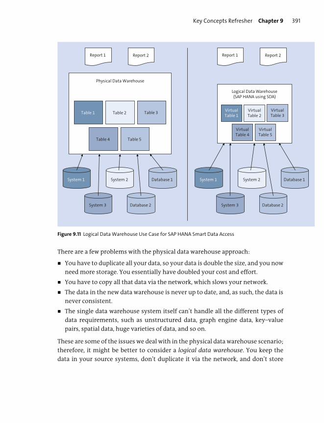
Key Concepts Refresher Chapter 9 391
Figure 9.11 Logical Data Warehouse Use Case for SAP HANA Smart Data Access
There are a few problems with the physical data warehouse approach:
� You have to duplicate all your data, so your data is double the size, and you now
need more storage. You essentially have doubled your cost and effort.
� You have to copy all that data via the network, which slows your network.
� The data in the new data warehouse is never up to date, and, as such, the data is
never consistent.
� The single data warehouse system itself can’t handle all the different types of
data requirements, such as unstructured data, graph engine data, key–value
pairs, spatial data, huge varieties of data, and so on.
These are some of the issues we deal with in the physical data warehouse scenario;
therefore, it might be better to consider a logical data warehouse. You keep the
data in your source systems, don’t duplicate it via the network, and don’t store
System 3 Database 2 System 3 Database 2
Report 1 Report 2 Report 1 Report 2
System 2System 1 Database 1 System 2System 1 Database 1
Physical Data Warehouse
Table 4
Table 1 Table 2 Table 3
Table 5
Logical Data Warehouse(SAP HANA using SDA)
VirtualTable 4
VirtualTable 1
VirtualTable 2
VirtualTable 3
VirtualTable 5
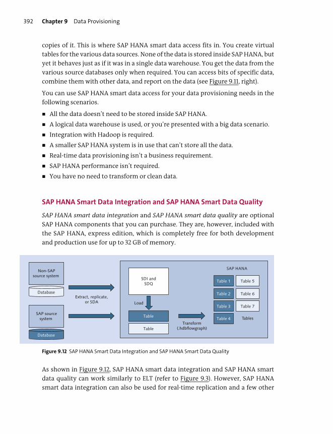
Chapter 9 Data Provisioning392
copies of it. This is where SAP HANA smart data access fits in. You create virtual
tables for the various data sources. None of the data is stored inside SAP HANA, but
yet it behaves just as if it was in a single data warehouse. You get the data from the
various source databases only when required. You can access bits of specific data,
combine them with other data, and report on the data (see Figure 9.11, right).
You can use SAP HANA smart data access for your data provisioning needs in the
following scenarios.
� All the data doesn’t need to be stored inside SAP HANA.
� A logical data warehouse is used, or you’re presented with a big data scenario.
� Integration with Hadoop is required.
� A smaller SAP HANA system is in use that can’t store all the data.
� Real-time data provisioning isn’t a business requirement.
� SAP HANA performance isn’t required.
� You have no need to transform or clean data.
SAP HANA Smart Data Integration and SAP HANA Smart Data Quality
SAP HANA smart data integration and SAP HANA smart data quality are optional
SAP HANA components that you can purchase. They are, however, included with
the SAP HANA, express edition, which is completely free for both development
and production use for up to 32 GB of memory.
Figure 9.12 SAP HANA Smart Data Integration and SAP HANA Smart Data Quality
As shown in Figure 9.12, SAP HANA smart data integration and SAP HANA smart
data quality can work similarly to ELT (refer to Figure 9.3). However, SAP HANA
smart data integration can also be used for real-time replication and a few other
SDI andSDQ
Non-SAPsource system
Database
SAP sourcesystem
Database
Table
Table
Extract, replicate,or SDA
Transform(.hdbflowgraph)
Load
SAP HANA
Tables
Table 1 Table 5
Table 2 Table 6
Table 3 Table 7
Table 4

Key Concepts Refresher Chapter 9 393
scenarios. Over time, SAP has incorporated many of the data provisioning features
from other tools into SAP HANA smart data integration.
The other fact that counts in favor of SAP HANA smart data integration is that
many of SAP’s business systems have migrated to run on SAP HANA. SAP HANA
smart data integration has evolved so much over the past few years, that you can
apply the simple rule, “When in doubt, use SAP HANA smart data integration.” It’s
even the preferred integration tool on SAP Cloud Platform.
Using various adapters, including SAP HANA smart data access adapters, we can
replicate or consume data in SAP HANA. Then, using SAP HANA smart data quality
capabilities, we can transform and clean that data.
Note
You can find more information about SAP HANA smart data integration at http://s-
prs.co/v487637.
SAP HANA Smart Data Integration
SAP HANA smart data integration can use various adapters to replicate, load, or
consume data in SAP HANA. Via SAP HANA smart data access adapters, SAP HANA
smart data integration can consume data from a large list of databases using vir-
tual tables. SAP HANA smart data integration has some real-time adapters, for
example, reading the database log files of source systems such as Oracle, Microsoft
SQL Server, and IBM DB2 databases. These same adapters can be used to read data
from SAP systems such as SAP ERP. SAP HANA smart data integration also has a
real-time adapter for Twitter, as well as batch adapters for reading web services via
OData and for reading data from Hadoop Hive. There is even an adapter for Micro-
soft Excel.
The difference between the log-based adapters for SAP HANA smart data integra-
tion and SAP Replication Server is that SAP HANA smart data integration has SAP
HANA as the target system for your data provisioning, whereas a standalone SAP
Replication Server system can have many target systems.
Tip
SAP HANA smart data integration has become the preferred SAP data provisioning tool
for SAP. This is due to its wide range of adapters that provide both batch and real-time
replication capabilities, and the fact that many SAP systems are now running on SAP
HANA.
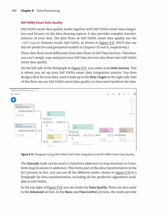
Chapter 9 Data Provisioning394
SAP HANA Smart Data Quality
SAP HANA smart data quality works together with SAP HANA smart data integra-
tion and focuses on the data cleaning aspects. It also provides complex transfor-
mations of your data. The data flows in SAP HANA smart data quality use the
.hdbflowgraph features inside SAP HANA, as shown in Figure 9.13. (We’ll also use
this for predictive and geospatial models in Chapters 10 and 11, respectively.)
These data flows work differently from data flows in SAP Data Services. Therefore,
you can’t simply copy and paste your SAP Data Services data flows into SAP HANA
smart data quality.
On the left side of the flowgraph in Figure 9.13, you create your Data Sources. This
is where you set up your SAP HANA smart data integration sources. You then
design a flow for your data, until it ends up in the Data Target on the right side. Part
of this flow can use SAP HANA smart data quality to clean and transform the data.
Figure 9.13 Flowgraph Using SAP HANA Smart Data Integration and SAP HANA Smart Data Quality
The Geocode node can be used to transform addresses to map locations or trans-
form map locations to addresses. This forms part of the data transformation in the
ELT process. In fact, you can use all the different nodes, shown in Figure 9.14 in a
flowgraph for data transformation, including all the predictive algorithms avail-
able in SAP HANA.
In the top right of Figure 9.14, you see nodes for Data Quality. There are also some
in the Advanced section. In the Basic and Flow Control sections, the nodes provide
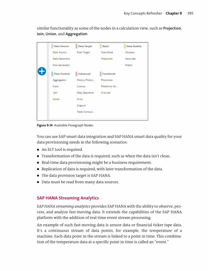
Key Concepts Refresher Chapter 9 395
similar functionality as some of the nodes in a calculation view, such as Projection,
Join, Union, and Aggregation.
Figure 9.14 Available Flowgraph Nodes
You can use SAP smart data integration and SAP HANA smart data quality for your
data provisioning needs in the following scenarios:
� An ELT tool is required.
� Transformation of the data is required, such as when the data isn’t clean.
� Real-time data provisioning might be a business requirement.
� Replication of data is required, with later transformation of the data.
� The data provision target is SAP HANA.
� Data must be read from many data sources.
SAP HANA Streaming Analytics
SAP HANA streaming analytics provides SAP HANA with the ability to observe, pro-
cess, and analyze fast-moving data. It extends the capabilities of the SAP HANA
platform with the addition of real-time event stream processing.
An example of such fast-moving data is sensor data or financial ticker tape data.
It’s a continuous stream of data points, for example, the temperature of a
machine. Each data point in the stream is linked to a point in time. This combina-
tion of the temperature data at a specific point in time is called an “event.”
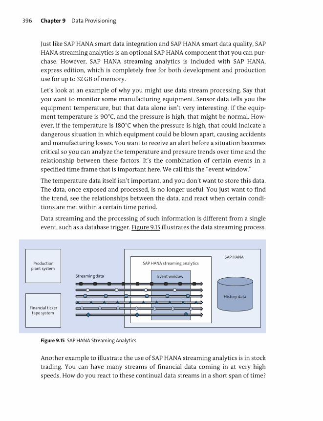
Chapter 9 Data Provisioning396
Just like SAP HANA smart data integration and SAP HANA smart data quality, SAP
HANA streaming analytics is an optional SAP HANA component that you can pur-
chase. However, SAP HANA streaming analytics is included with SAP HANA,
express edition, which is completely free for both development and production
use for up to 32 GB of memory.
Let’s look at an example of why you might use data stream processing. Say that
you want to monitor some manufacturing equipment. Sensor data tells you the
equipment temperature, but that data alone isn’t very interesting. If the equip-
ment temperature is 90°C, and the pressure is high, that might be normal. How-
ever, if the temperature is 180°C when the pressure is high, that could indicate a
dangerous situation in which equipment could be blown apart, causing accidents
and manufacturing losses. You want to receive an alert before a situation becomes
critical so you can analyze the temperature and pressure trends over time and the
relationship between these factors. It’s the combination of certain events in a
specified time frame that is important here. We call this the “event window.”
The temperature data itself isn’t important, and you don’t want to store this data.
The data, once exposed and processed, is no longer useful. You just want to find
the trend, see the relationships between the data, and react when certain condi-
tions are met within a certain time period.
Data streaming and the processing of such information is different from a single
event, such as a database trigger. Figure 9.15 illustrates the data streaming process.
Figure 9.15 SAP HANA Streaming Analytics
Another example to illustrate the use of SAP HANA streaming analytics is in stock
trading. You can have many streams of financial data coming in at very high
speeds. How do you react to these continual data streams in a short span of time?
Productionplant system
Financial tickertape system
History data
SAP HANA
Streaming data
SAP HANA streaming analytics
Event window

Key Concepts Refresher Chapter 9 397
What do you react to? A single stock going down may not be a problem, but if
many stock prices start going down quickly within a certain time window—say,
five minutes—that could indicate a stock market crash. The single price values are
of little importance. The important information is found in combining many
trends and finding the trend in a certain time window.
The Internet of Things (IoT) isn’t in the future—it’s already here. Millions of devices
are now connected and delivering information. We even have lightbulbs with
built-in Wi-Fi that can be controlled from an app on your smartphone. How do you
take advantage of all the data that’s available? How do you collect it and analyze it?
With SAP HANA streaming analytics, not only can you analyze data streams but
you also can store this data and perform deeper, wider analytics of it at a later
stage. In this way, SAP HANA streaming analytics and SAP HANA complement
each other. SAP HANA streaming analytics is also a vital part of the SAP Leonardo
technology stack, where SAP looks at innovative solutions touching areas such as
the IoT, machine learning, and blockchain.
You can use SAP HANA streaming analytics for your data provisioning needs in
the following scenarios:
� Real-time streaming data for events in a certain time window must be analyzed
and reacted to properly.
� Fast-moving data is observed, processed, and analyzed, but not stored.
� Data is processed as-is; there is no data cleaning, but you have to find a signal in
spite of the noisy data.
� Only data where something interesting is happening needs to be stored. The
rest of the data gets discarded, resulting in huge storage savings.
SQL Anywhere and Remote Data Sync
Up to this point, we’ve made the assumption that we always have good, stable, and
constant connectivity between the data sources and SAP HANA. Unfortunately,
that isn’t always the case.
Let’s consider some scenarios where we can’t assume that we have such connectiv-
ity:
� Remote workplaces, such as ships, trains, oil rigs, and mines, that lose connec-
tivity for periods of time (also known as satellite servers)
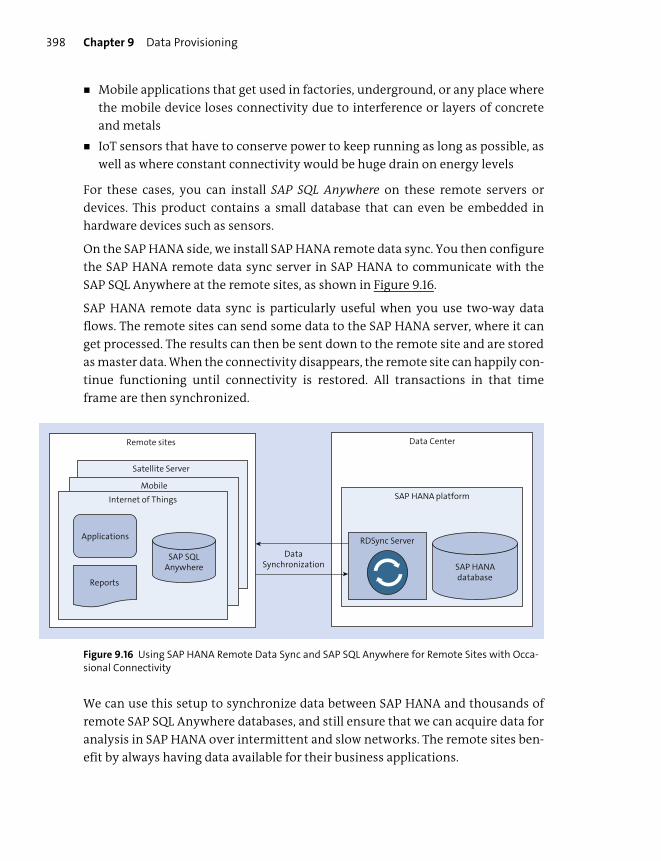
Chapter 9 Data Provisioning398
� Mobile applications that get used in factories, underground, or any place where
the mobile device loses connectivity due to interference or layers of concrete
and metals
� IoT sensors that have to conserve power to keep running as long as possible, as
well as where constant connectivity would be huge drain on energy levels
For these cases, you can install SAP SQL Anywhere on these remote servers or
devices. This product contains a small database that can even be embedded in
hardware devices such as sensors.
On the SAP HANA side, we install SAP HANA remote data sync. You then configure
the SAP HANA remote data sync server in SAP HANA to communicate with the
SAP SQL Anywhere at the remote sites, as shown in Figure 9.16.
SAP HANA remote data sync is particularly useful when you use two-way data
flows. The remote sites can send some data to the SAP HANA server, where it can
get processed. The results can then be sent down to the remote site and are stored
as master data. When the connectivity disappears, the remote site can happily con-
tinue functioning until connectivity is restored. All transactions in that time
frame are then synchronized.
Figure 9.16 Using SAP HANA Remote Data Sync and SAP SQL Anywhere for Remote Sites with Occa-sional Connectivity
We can use this setup to synchronize data between SAP HANA and thousands of
remote SAP SQL Anywhere databases, and still ensure that we can acquire data for
analysis in SAP HANA over intermittent and slow networks. The remote sites ben-
efit by always having data available for their business applications.
Data CenterRemote sites
Satellite Server
MobileInternet of Things SAP HANA platform
RDSync Server
SAP HANAdatabase
SAP SQLAnywhere
Applications
Reports
DataSynchronization

Key Concepts Refresher Chapter 9 399
Flat Files
Flat files (also called comma-separated values [CSV] files) are the simplest way to
provision data to SAP HANA. Especially in proof-of-concept (POC) or sandbox test-
ing projects, you can waste time connecting SAP HANA to the various source sys-
tems. You don’t need the latest data; you just want to find out if an idea you have
for information modeling will work.
As such, it makes sense to ask the business to provide you with the data in flat files,
and then you can load the data into SAP HANA for the POC or sandbox develop-
ment (see Figure 9.17).
Figure 9.17 Loading Data into SAP HANA from Text Files Using Core Data Services (CDS)
In SAP Web IDE for SAP HANA, you create an .hdbtabledata file. You can see an
example in Figure 9.18 from the SAP HANA Interactive Education (SHINE) demo. In
line 7, it specifies that the file is a CSV file, and line 8 specifies the name of the text
file.
The entire SHINE demo application is built this way, and it loads the demo data
using this method.
SPS 04
One of the features that you could do with SAP HANA Studio in SAP HANA 1.0 was to
import data into a table from CSV files or Excel spreadsheets. With SPS 04, you can now
import data from medium-sized CSV files or Excel spreadsheets using the SAP HANA
database explorer.
CSV data file
SAP HANA
Tables
Table 1 Table 5
Table 2 Table 6
Table 3 Table 7
Table 4
Import data files
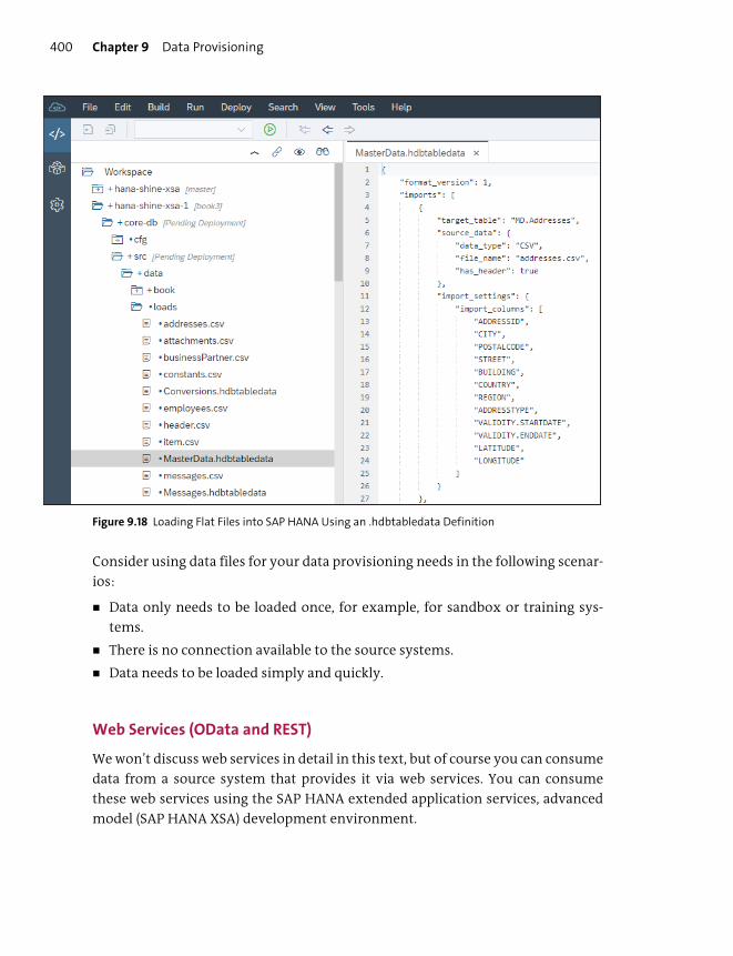
Chapter 9 Data Provisioning400
Figure 9.18 Loading Flat Files into SAP HANA Using an .hdbtabledata Definition
Consider using data files for your data provisioning needs in the following scenar-
ios:
� Data only needs to be loaded once, for example, for sandbox or training sys-
tems.
� There is no connection available to the source systems.
� Data needs to be loaded simply and quickly.
Web Services (OData and REST)
We won’t discuss web services in detail in this text, but of course you can consume
data from a source system that provides it via web services. You can consume
these web services using the SAP HANA extended application services, advanced
model (SAP HANA XSA) development environment.
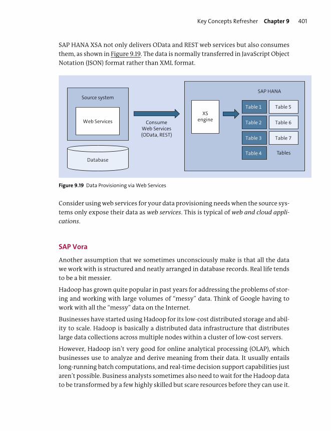
Key Concepts Refresher Chapter 9 401
SAP HANA XSA not only delivers OData and REST web services but also consumes
them, as shown in Figure 9.19. The data is normally transferred in JavaScript Object
Notation (JSON) format rather than XML format.
Figure 9.19 Data Provisioning via Web Services
Consider using web services for your data provisioning needs when the source sys-
tems only expose their data as web services. This is typical of web and cloud appli-
cations.
SAP Vora
Another assumption that we sometimes unconsciously make is that all the data
we work with is structured and neatly arranged in database records. Real life tends
to be a bit messier.
Hadoop has grown quite popular in past years for addressing the problems of stor-
ing and working with large volumes of “messy” data. Think of Google having to
work with all the “messy” data on the Internet.
Businesses have started using Hadoop for its low-cost distributed storage and abil-
ity to scale. Hadoop is basically a distributed data infrastructure that distributes
large data collections across multiple nodes within a cluster of low-cost servers.
However, Hadoop isn’t very good for online analytical processing (OLAP), which
businesses use to analyze and derive meaning from their data. It usually entails
long-running batch computations, and real-time decision support capabilities just
aren’t possible. Business analysts sometimes also need to wait for the Hadoop data
to be transformed by a few highly skilled but scare resources before they can use it.
XSengine
Database
SAP HANA
Tables
Table 1 Table 5
Table 2 Table 6
Table 3 Table 7
Table 4
Source system
Web Services ConsumeWeb Services(OData, REST)
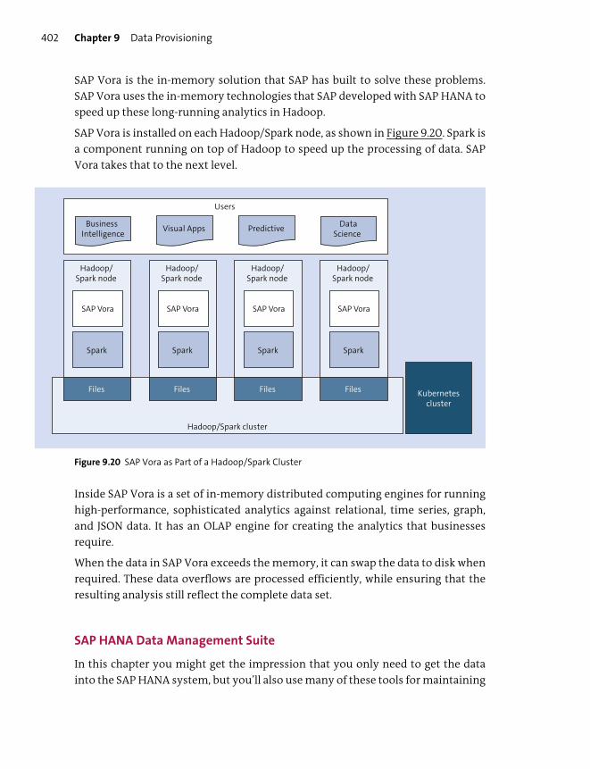
Chapter 9 Data Provisioning402
SAP Vora is the in-memory solution that SAP has built to solve these problems.
SAP Vora uses the in-memory technologies that SAP developed with SAP HANA to
speed up these long-running analytics in Hadoop.
SAP Vora is installed on each Hadoop/Spark node, as shown in Figure 9.20. Spark is
a component running on top of Hadoop to speed up the processing of data. SAP
Vora takes that to the next level.
Figure 9.20 SAP Vora as Part of a Hadoop/Spark Cluster
Inside SAP Vora is a set of in-memory distributed computing engines for running
high-performance, sophisticated analytics against relational, time series, graph,
and JSON data. It has an OLAP engine for creating the analytics that businesses
require.
When the data in SAP Vora exceeds the memory, it can swap the data to disk when
required. These data overflows are processed efficiently, while ensuring that the
resulting analysis still reflect the complete data set.
SAP HANA Data Management Suite
In this chapter you might get the impression that you only need to get the data
into the SAP HANA system, but you’ll also use many of these tools for maintaining
Hadoop/Spark cluster
Hadoop/ Spark node
SAP Vora
Files Kubernetescluster
Spark
Hadoop/ Spark node
Files
Spark
Hadoop/ Spark node
Files
Spark
Hadoop/ Spark node
Files
Spark
Users
Data ScienceVisual AppsBusiness
Intelligence Predictive
SAP Vora SAP Vora SAP Vora

Important Terminology Chapter 9 403
the data. This maintenance might be to keep data up to date, especially for master
data in the case of master data management. Or it might be due to regulations
such as General Data Protection Regulation (GDPR) that force you to check,
update, and delete user data.
Data is often called the “oil” of this century. Even engines need some fresh oil
every now and then. SAP released SAP HANA Data Management Suite in 2018 to
help with this kind of data maintenance and to help with managing data from
multiple sources, such as legacy databases, cloud systems, desktop programs, sen-
sors, and data lakes. You can then enrich that data with spatial, text, graph, predic-
tive, and series processing, which we discuss in the next two chapters.
Many of the tools in SAP HANA Data Management Suite are available individually.
In the suite they are used together to manage the data for the entire enterprise.
Tools included are as follows:
� SAP HANA for in-memory processing of the data, ETL, modeling, development,
data anonymization, security, and much more.
� SAP Enterprise Architecture Designer (SAP EA Designer) for defining an enter-
prise-wide metadata model to manage the data models and data rules, and cre-
ate a harmonized view of the data. (We discussed SAP EA Designer in Chapter 4.)
� SAP Cloud Platform Big Data Services to manage the big data services in the
cloud. This includes SAP Vora that we discussed in this chapter.
� SAP Data Hub for providing a central system for data governance, orchestra-
tion, pipelining, integration, and federation of data in the company.
Important Terminology
In this chapter, we covered the following important terms:
� Data provisioning
Get data from a source system and provide that data to a target system.
� Extract, transform, load (ETL)
The ETL process consists of the following phases:
– Extraction: Data is read from a source system. Traditional ETL tools can read
many data sources, and most can also read data from SAP source systems.
– Transform: Data is transformed. Normally this means cleaning the data, but
it can refer to any data manipulation.
– Load: Data is written into the target system.
Chapter 9 Data Provisioning404
� Initial load
The process of making a full copy of data from the source system. If we require
an entire table, we make a copy of the table in the target system.
� Delta load
Look at the data that has changed, and apply the data changes to the copy of the
data in the target system. These data changes are referred to as the delta, and
applying these changes to the target system is called a delta load.
� SAP extractors
Read data from a group of tables and deliver the data as a single integrated data
unit to the target system.
� SAP Data Services
Solution used to integrate, improve the quality of, profile, process, and deliver
data.
� SAP Landscape Transformation Replication Server
Uses replication to load data into SAP HANA. Remember that the focus of a rep-
lication server is to load data into the target system as fast as possible.
� SAP Replication Server
Uses replication to load data into SAP HANA. SAP Replication Server differs
from SAP Landscape Transformation Replication Server in that it uses the data-
base log files for real-time replication. SAP Replication Server reads these data-
base log files to enable table replication. SAP Replication Server replication is
also known as log-based replication.
� SAP HANA smart data access
Provides SAP HANA with direct access to data in a remote database.
� SAP HANA smart data integration
Uses various adapters to replicate, load, or consume data in SAP HANA.
� SAP HANA smart data quality
Used to cleanse and enrich data persisted in the SAP HANA database.
� SAP HANA streaming analytics
Allows you to observe, process, and analyze fast-moving data. You can create
continuous projects in Computation Continuous Language (CCL) to model
streaming information. You can then issue continuous queries to analyze the
data.
� SAP HANA remote data sync
Allows you to synchronize data between SAP HANA and thousands of remote
SAP SQL Anywhere databases, while still ensuring that you can acquire data for
analysis in SAP HANA over intermittent and slow networks.

Practice Questions Chapter 9 405
� SAP Vora
Uses the in-memory technologies that SAP developed with SAP HANA to speed
up long-running analytics in Hadoop and Spark clusters.
Practice Questions
These practice questions will help you evaluate your understanding of the topic.
The questions shown are similar in nature to those found on the certification
examination. Although none of these questions will be found on the exam itself,
they will allow you to review your knowledge of the subject. Select the correct
answers, and then check the completeness of your answers in the “Practice Ques-
tion Answers and Explanations” section. Remember, on the exam, you must select
all correct answers and only correct answers to receive credit for the question.
1. Which of the following SAP data provisioning tools can provide real-time data
provisioning? (There are 3 correct answers.)
� A. SAP HANA smart data integration
� B. SAP Data Services
� C. SAP Replication Server
� D. SAP HANA smart data quality
� E. SAP Landscape Transformation Replication Server
2. What is the correct sequence for loading data with SAP Data Services?
� A. Extract • Load • Transform
� B. Load • Transform • Extract
� C. Load • Extract • Transform
� D. Extract • Transform • Load
3. Which of the following data provisioning tools can provide a delta load of a
table from the source system?
� A. SAP HANA streaming analytics
� B. SAP HANA smart data access
� C. SAP Landscape Transformation Replication Server
� D. Flat files

Chapter 9 Data Provisioning406
4. Which of the following data operations can you perform with SAP HANA
smart data access? (There are 2 correct answers.)
� A. Data federation
� B. Logical data warehouse
� C. Physical data warehouse
� D. Real-time replication
5. You want to retrieve data from a web application. Which of the following
could you use? (There are 3 correct answers.)
� A. JSON
� B. REST
� C. JDBC
� D. BICS
� E. OData
6. Which data provisioning tools can use SAP HANA adapters? (There are 2 cor-
rect answers.)
� A. SAP HANA smart data access
� B. SAP HANA streaming analytics
� C. SAP HANA smart data integration
� D. SAP Replication Server
7. Which of the following data provisioning tools can you use to read data
directly from Twitter? (There are 3 correct answers.)
� A. SAP Replication Server
� B. SAP HANA XS engine
� C. SAP Data Services
� D. SAP HANA smart data integration
� E. SAP HANA smart data access
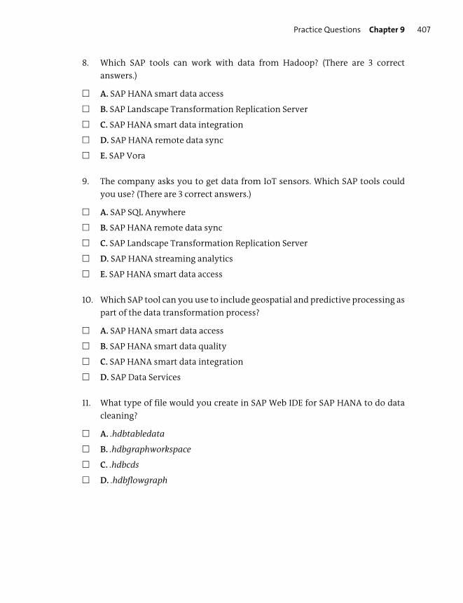
Practice Questions Chapter 9 407
8. Which SAP tools can work with data from Hadoop? (There are 3 correct
answers.)
� A. SAP HANA smart data access
� B. SAP Landscape Transformation Replication Server
� C. SAP HANA smart data integration
� D. SAP HANA remote data sync
� E. SAP Vora
9. The company asks you to get data from IoT sensors. Which SAP tools could
you use? (There are 3 correct answers.)
� A. SAP SQL Anywhere
� B. SAP HANA remote data sync
� C. SAP Landscape Transformation Replication Server
� D. SAP HANA streaming analytics
� E. SAP HANA smart data access
10. Which SAP tool can you use to include geospatial and predictive processing as
part of the data transformation process?
� A. SAP HANA smart data access
� B. SAP HANA smart data quality
� C. SAP HANA smart data integration
� D. SAP Data Services
11. What type of file would you create in SAP Web IDE for SAP HANA to do data
cleaning?
� A. .hdbtabledata
� B. .hdbgraphworkspace
� C. .hdbcds
� D. .hdbflowgraph
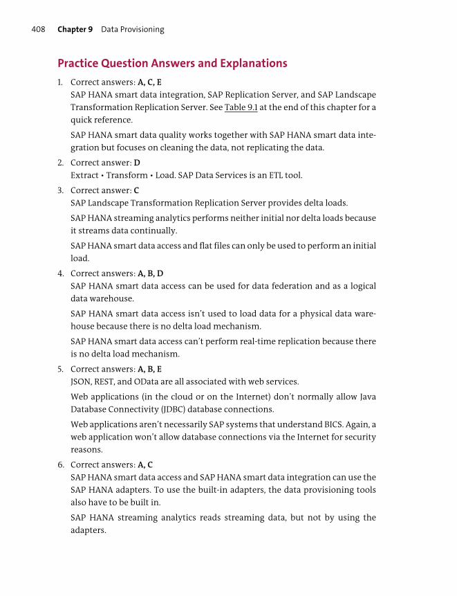
Chapter 9 Data Provisioning408
Practice Question Answers and Explanations
1. Correct answers: A, C, E
SAP HANA smart data integration, SAP Replication Server, and SAP Landscape
Transformation Replication Server. See Table 9.1 at the end of this chapter for a
quick reference.
SAP HANA smart data quality works together with SAP HANA smart data inte-
gration but focuses on cleaning the data, not replicating the data.
2. Correct answer: D
Extract • Transform • Load. SAP Data Services is an ETL tool.
3. Correct answer: C
SAP Landscape Transformation Replication Server provides delta loads.
SAP HANA streaming analytics performs neither initial nor delta loads because
it streams data continually.
SAP HANA smart data access and flat files can only be used to perform an initial
load.
4. Correct answers: A, B, D
SAP HANA smart data access can be used for data federation and as a logical
data warehouse.
SAP HANA smart data access isn’t used to load data for a physical data ware-
house because there is no delta load mechanism.
SAP HANA smart data access can’t perform real-time replication because there
is no delta load mechanism.
5. Correct answers: A, B, E
JSON, REST, and OData are all associated with web services.
Web applications (in the cloud or on the Internet) don’t normally allow Java
Database Connectivity (JDBC) database connections.
Web applications aren’t necessarily SAP systems that understand BICS. Again, a
web application won’t allow database connections via the Internet for security
reasons.
6. Correct answers: A, C
SAP HANA smart data access and SAP HANA smart data integration can use the
SAP HANA adapters. To use the built-in adapters, the data provisioning tools
also have to be built in.
SAP HANA streaming analytics reads streaming data, but not by using the
adapters.
Practice Question Answers and Explanations Chapter 9 409
SAP Replication Server reads database log files.
7. Correct answers: B, C, D
Twitter does have web services. This isn’t specified in the book, so in the actual
exam, this option would not appear because it makes too many assumptions.
For the purposes of this book, we assumed that everyone knows what Twitter is
and that it has web services.
SAP Data Services can read social media feeds, as discussed in the Extracting
Data section.
SAP HANA smart data integration has a Twitter adapter. See the SAP HANA
Smart Data Integration section for more information.
8. Correct answers: A, C, E
SAP HANA smart data access, SAP HANA smart data integration, and SAP Vora
can work with data from Hadoop.
SAP Landscape Transformation Replication Server can only use SAP ABAP sys-
tems as the data source.
SAP HANA remote data sync connects to remote SAP SQL Anywhere databases.
9. Correct answers: A, B, D
You can use SAP SQL Anywhere to store the IoT sensor data, and you then use
SAP HANA remote data sync to get it to SAP HANA.
SAP HANA streaming analytics is often used to stream sensor data to SAP HANA.
SAP Landscape Transformation Replication Server uses SAP systems as data
sources.
SAP HANA smart data access doesn’t connect to sensors (unless some fancy
new device embeds a database!).
10. Correct answer: B
You can you use SAP HANA smart data quality to include geospatial and predic-
tive processing as part of the data transformation process.
SAP HANA smart data access doesn’t have transformation capabilities.
SAP HANA smart data integration is used to get the data to SAP HANA smart
data quality.
SAP Data Services doesn’t have predictive processing as part of the data trans-
formation process.
11. Correct answer: D
You create an .hdbflowgraph file in SAP Web IDE for SAP HANA to do data clean-
ing.
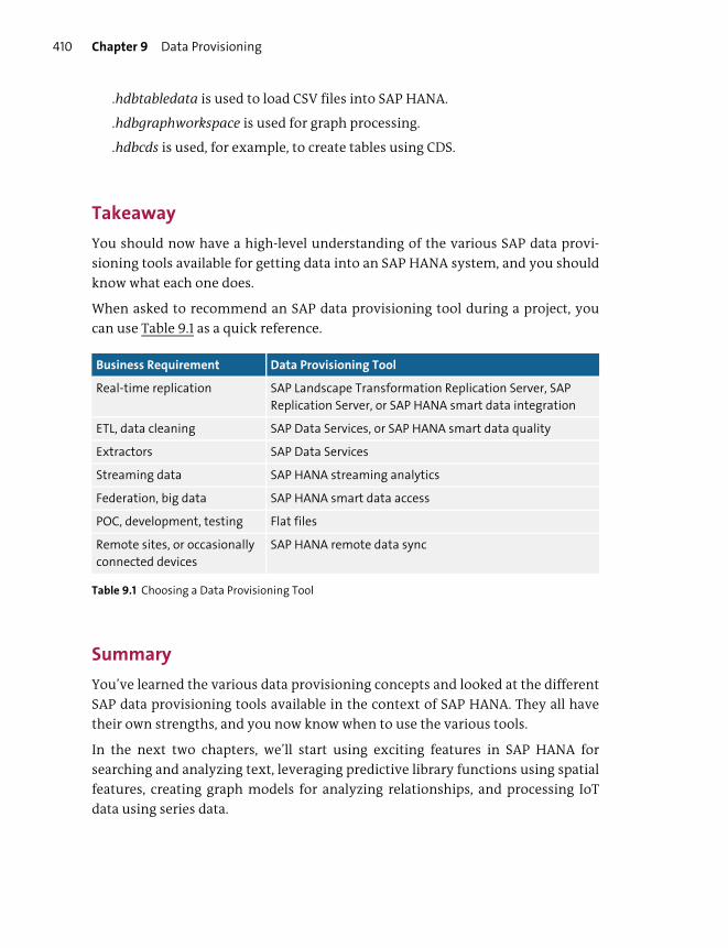
Chapter 9 Data Provisioning410
.hdbtabledata is used to load CSV files into SAP HANA.
.hdbgraphworkspace is used for graph processing.
.hdbcds is used, for example, to create tables using CDS.
Takeaway
You should now have a high-level understanding of the various SAP data provi-
sioning tools available for getting data into an SAP HANA system, and you should
know what each one does.
When asked to recommend an SAP data provisioning tool during a project, you
can use Table 9.1 as a quick reference.
Summary
You’ve learned the various data provisioning concepts and looked at the different
SAP data provisioning tools available in the context of SAP HANA. They all have
their own strengths, and you now know when to use the various tools.
In the next two chapters, we’ll start using exciting features in SAP HANA for
searching and analyzing text, leveraging predictive library functions using spatial
features, creating graph models for analyzing relationships, and processing IoT
data using series data.
Business Requirement Data Provisioning Tool
Real-time replication SAP Landscape Transformation Replication Server, SAP
Replication Server, or SAP HANA smart data integration
ETL, data cleaning SAP Data Services, or SAP HANA smart data quality
Extractors SAP Data Services
Streaming data SAP HANA streaming analytics
Federation, big data SAP HANA smart data access
POC, development, testing Flat files
Remote sites, or occasionally
connected devices
SAP HANA remote data sync
Table 9.1 Choosing a Data Provisioning Tool

Chapter 10
Text Processing and Predictive Modeling
Techniques You’ll Master
� Know how to create a text search index
� Discover fuzzy text search, text analysis, and text mining
� Get to know the types of prediction algorithms
� Learn how to create a predictive analysis model
Chapter 10 Text Processing and Predictive Modeling412
Now that you understand the basics of SAP HANA information modeling, it’s time
to take your knowledge to the next level. In this chapter, we’ll cover two different
topics: text processing and predictive modeling. In the next chapter we’ll discuss
spatial, graph, and series data modeling. These five topics are independent from
each other but can be combined in projects; for an example, see the Real-World
Scenario box.
In this chapter and the next, we’ll do a deep dive into some advanced modeling
with SAP HANA. Each topic that we’ll discuss is a specialist area on its own, on
which people build their careers. We obviously won’t go that deep into these top-
ics, but you’ll have a good base for more detailed learning on any of these topics at
the end of these two chapters.
These two chapters probably include the most changes from the previous edition.
In the second edition, these topics were in one chapter, as they were only 10% of
the certification exam. SAP Education has expanded its material on advanced
modeling with SAP HANA to a separate three-day training course named HA301,
and it’s now 25% of the certification exam.
Most of these advanced topic areas are components of SAP HANA that are only
available in SAP HANA, enterprise edition. The enterprise edition contains every-
thing from the standard edition and components such as text processing, predic-
tive modeling, and spatial, graph, and streaming analytics.
SAP HANA, express edition, has all of these components and is a free edition for
both development and production with usage up to 32 GB. You can easily expand
up to 128 GB by purchasing more memory usage. To move beyond 128 GB, you’ll
need to upgrade to a full-use license edition.
We’ll begin our discussion with text modeling—specifically, how to search and
find text even if misspelled, how to analyze text to find sentiment, and how to
mine text in documents. Then, we’ll look at how to build predictive analysis mod-
els for business users using a powerful built-in library and graphical web-based
tools.
Real-World Scenario
You’re working on an SAP HANA project at a pharmaceutical company.
The company has created a mobile web application with SAP HANA for its
sales representatives. However, users are struggling to find products on
their mobile phones because the keyboard is small, and the names of the
Objectives of This Portion of the Test Chapter 10 413
pharmaceutical products are quite difficult to type correctly. Therefore,
you implement a fuzzy text search that allows users to enter roughly what
they want, and the SAP HANA system finds the correct products. The com-
pany later tells you that this also helped users avoid adding duplicate
entries into the system.
You improve this mobile application by suggesting products to the sales
reps. You create a predictive analysis model in SAP HANA to help with sales
forecasting by looking at the seasonal patterns to determine when people
use certain products more (e.g. , in the winter).
You also notice that there were many comments about the company’s prod-
ucts on Facebook and Twitter. You process these comments in SAP HANA
and can quickly tell the marketing department which products people are
talking about, as well as alert the company if people are making negative
comments about any product. You provide special alerts to the sales reps to
inform the customers about these products.
And, of course, you win the “Best Employee” award for the year!
Objectives of This Portion of the Test
The purpose of this portion of the SAP HANA certification exam is to test your
knowledge of advanced modeling with SAP HANA.
The certification exam expects you to have a good understanding of the following
topics:
� How to create a text search index
� Fuzzy text search and text search queries
� Text analysis and the text analytics configurations
� Text mining
� The types of prediction algorithms
� How to create a predictive analysis model
Note
This portion contributes up to 15% of the total certification exam score.
Chapter 10 Text Processing and Predictive Modeling414
Key Concepts Refresher
In recent years, the field of text and language processing has expanded dramati-
cally. Topics such as talking computers that were previously only found in science
fiction stories now fill the media. The daily technology news articles talk glowingly
of chatbots, artificial intelligence (AI), natural language processing (NLP), text-to-
speech, and speech-to-text. Many people have voice-based “assistants” in their
homes and on their phones where they regularly talk to Alexa, Siri, and the Google
Assistant. Automatic language translation is improving due to new deep learning
systems and powerful custom-made processors.
You often have to help set the right expectations when working in a project. With
all the media attention, it’s easy to get caught up in believing you can do every-
thing with such language technologies. While some of it works well for shorter
sentences, this won’t replace translators or editors. Even if it’s 99% correct, this
paragraph would have at least one major mistake in it, let alone the subtler
nuances of language, such as intonation, double meanings, irregular verbs, puns,
oxymorons, irony, satire, and sarcasm. For example, “I named my dog five miles
so I can tell people that I walk five miles every day.” Or, “Help stamp out, eliminate,
and abolish redundancy!”
In the next section, we’ll focus on some of the text processing features built into
SAP HANA. SAP also has chatbots, robotic process automation (RPA), and machine
learning, but we won’t discuss these here.
Text Processing
As you know, in Google, you type in a few words, and the Google search engine
returns a list of web pages that best meet your search query, ranked to your prefer-
ences. It used to indicate when you typed a word incorrectly and suggested
another spelling with the question, Did you mean…?. Now, however, the Google
search engine has become so confident that it no longer suggests the correction
with a qualifying question, but instead says Showing results for…. If you’re con-
vinced your original entry is correct, it will allow you to Search instead for [what-
ever you entered]. Even more revolutionary is the search engine’s ability to predict
what you want as you type.
In the following, we’ll first provide you with a brief overview of text processing.
We’ll then look at working with the text features in SAP HANA—namely, text
searches, text analysis, and text mining. However, before we can discuss each of

Key Concepts Refresher Chapter 10 415
these topics in more detail, we first need to create a full-text index. As you’ll see in
Figure 10.1, the full-text index is the backbone of all these processes.
Text Processing Overview
Google search is a good example of what you can do with SAP HANA in your infor-
mation models. We can perform fuzzy text searches, such as the “Did you mean”
example, and we can perform text mining to find the best document out of a large
collection for a user. We can also use text analysis to find out if people wrote some
text with a positive or negative sentiment.
Figure 10.1 provides an overview of the various text processing processes in SAP
HANA. We can use SAP HANA text processing on any table column that has some
text data included. In this case, we want to process the data in the Description field.
This column could have data in a NVARCHAR field, or documents such as PDFs stored
in a BLOB or TEXT field. We have to prepare the data in this field before we can run
text processing queries on it. There are three main scenarios for querying the text.
We’ll discuss each of these in more detail in upcoming subsections:
� Text search
This feature is used when we want to find out which records contain some
search terms. To get this working, we first need to create a full-text index for the
Description field. The full-text index is created in a hidden column in the table
and can only be accessed indirectly via the SAP HANA text processing features.
When SAP HANA creates the full-text index, it first processes the files contained
in the Description field if we store documents in it. It can extract the text from
these documents, can detect the language the text is written in, and break up
the text in words or terms—a process called tokenization. Lastly, SAP HANA can
convert these tokens into their root words using a process called stemming.
� Text analysis
This feature extends the functionality of the full-text index. When creating the
full-text index, we need to specify a text analysis configuration file and activate
text analysis, which is used when we want to find out the sentiment of the text
or to extract more semantic details from the text. With text analysis, SAP HANA
can find parts-of-speech, group nouns, and extract entities and facts. (Noun
groups are words that are often used together, for example, global economy or
fish and chips.) All these results are stored in a new table with a $TA_ prefix.
� Text mining
This feature extends the functionality of the full-text index and text analysis
results. Where text searching and text analysis work within a document, text
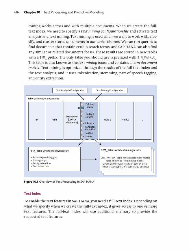
Chapter 10 Text Processing and Predictive Modeling416
mining works across and with multiple documents. When we create the full-
text index, we need to specify a text mining configuration file and activate text
analysis and text mining. Text mining is used when we want to work with, clas-
sify, and cluster stored documents in our table columns. We can run queries to
find documents that contain certain search terms, and SAP HANA can also find
any similar or related documents for us. These results are stored in new tables
with a $TM_ prefix. The only table you should use is prefixed with $TM_MATRIX_.
This table is also known as the text mining index and contains a term document
matrix. Text mining is optimized through the results of the full-text index and
the text analysis, and it uses tokenization, stemming, part-of-speech tagging,
and entity extraction.
Figure 10.1 Overview of Text Processing in SAP HANA
Text Index
To enable the text features in SAP HANA, you need a full-text index. Depending on
what we specify when we create the full-text index, it gives access to one or more
text features. The full-text index will use additional memory to provide the
requested text features.
ID Title Field 1 Field 2 …
Table with text or documents
Full text index
Text Analysis Configuration Text Mining Configuration
$TA_ table with text analysis results $TM_ tables with text mining results
Description(text or
document)
$TM_MATRIX_ table for text document matrix(also known as “text mining index”)
Optimized through results of text analysis (tokens, stems, part-of-speech tags, entities)
• Part-of-speech tagging• Noun groups• Entity extraction• Fact extraction
• File proc.
• Languagedetection
• Tokens
• Stems
(hiddencolumn)

Key Concepts Refresher Chapter 10 417
Listing 10.1 provides an example of a SQL statement to create a full-text index
named DEMO_TEXT_INDEX on a column called SOME_TEXT in a column table. This full-
text index enables the SOME_TEXT column for text search and analysis.
CREATE FULLTEXT INDEX DEMO_TEXT_INDEX ON"DEMO_TEXT" ("SOME_TEXT")LANGUAGE DETECTION ('EN')SEARCH ONLY ONFUZZY SEARCH INDEX ONTEXT ANALYSIS ON
CONFIGURATION 'EXTRACTION_CORE_VOICEOFCUSTOMER'TEXT MINING OFF;
Listing 10.1 SQL Statement to Create a Full-Text Index
Let’s examine the different text elements of the SQL statement in Listing 10.1:
� CREATE FULLTEXT INDEX
The first line creates a full-text index from the SOME_TEXT column in the DEMO_
TEXT table.
� LANGUAGE DETECTION
SAP HANA will attempt to detect the language of your text. You can specify on
what languages it should focus with this clause. In this case, we indicated that
our text is all in English.
� SEARCH ONLY ON
This clause saves some memory by not copying the source text into the full-text
index.
� FUZZY SEARCH INDEX ON
This enables or disables the fault-tolerant search feature. This feature is also
called fuzzy text search. You can speed up the fuzzy search on string types by
creating an additional data structure called a fuzzy search index. However, you
should be aware that this additional index increases the memory requirements
of the table. In addition, don’t confuse the fuzzy search index with the full-text
index; it’s just an additional data structure to the full-text index.
� TEXT ANALYSIS ON
This enables or disables the text analysis feature.
� CONFIGURATION
This is the name of the configuration. The text analysis feature needs a configu-
ration file. Some standard configurations ship with SAP HANA, and you can also
create your own.
� TEXT MINING OFF
This enables or disables the text-mining feature.

Chapter 10 Text Processing and Predictive Modeling418
Tip
The full-text index isn’t just used for text searches on a column but can also enable lan-
guage detection, search, text analysis, and text mining on that column.
You open the definition of the column table by double-clicking the table’s name in
the Data Explorer perspective of SAP Web IDE for SAP HANA. In the Indexes tab,
you’ll see the full-text index named DEMO_TEXT_INDEX that you just created.
When you select this index, you’ll see the details of the full-text index as shown in
Figure 10.2.
Figure 10.2 Full-Text Index Details
You can see from the checkboxes that we enabled Fuzzy Search Index and Text Ana-
lysis and disabled Text Mining in this index.
When Fuzzy Search Index is enabled for text-type columns, the full-text index
increases the memory size of the columns by an additional 10% approximately.

Key Concepts Refresher Chapter 10 419
When text analysis is enabled, the increase in the memory size due to the full-text
index depends on many factors, but it can be as large as that of the column itself.
Tip
Remember that a full-text index is created for a specific column, not for the entire table.
Figure 10.2 shows the Column Name as SOME_TEXT. You’ll have to create a full-text
index for every column that you want to search or analyze.
SAP HANA will automatically create full-text indexes for columns with data types
TEXT, BINTEXT, and SHORTTEXT. These are called implicit full-text indexes. In this case,
the content of the table column is stored in the form of the full-text index to save
memory consumption. The original column content is recreated from the full-text
index when you use a SQL SELECT statement. Because the focus for TEXT-type fields
is on search, SQL operations such as JOIN, CONCAT, LIKE, HAVING, WHERE, ORDER BY, and
GROUP BY, and aggregates such as COUNT and SUM aren’t supported.
For other column types, you must manually create the full-text index, as we
described in Listing 10.1. You can only manually create a full-text index for col-
umns with the VARCHAR, NVARCHAR, ALPHANUM, CLOB, NCLOB, and BLOB data types. When
you manually create a full-text index, it’s called an explicit full-text index. The con-
tent of the table column is stored in its original format.
When you manually create an index, SAP HANA attaches a hidden column to the
column you indexed. This hidden column contains extracted textual data from
the source column; the original source column remains unchanged. Search que-
ries are performed on the hidden column, but the data returned is from the source
column. The full-text index doesn’t store the results of your search or analysis, but
it does enables the search/analysis.
Note
You can put the SQL statement in a procedure (using an .hdbprocedure file). This way, you
can deploy it later on the production system. The recommended way to create full-text
indexes is using core data services (CDS). You can find the CDS syntax in the SAP HANA
Search Developer Guide at http://s-prs.co/v487620, in the Creating Full-Text Indexes
Using CDS Annotations section.
You can create the same full-text index as you did with SQL code in Listing 10.1
using CDS syntax in an .hdbfulltextindex file. When you compare this with Listing
10.2, you’ll see that they are identical, except that the CDS file doesn’t have the CRE-
ATE statement.
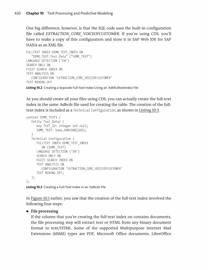
Chapter 10 Text Processing and Predictive Modeling420
One big difference, however, is that the SQL code uses the built-in configuration
file called EXTRACTION_CORE_VOICEOFCUSTOMER. If you’re using CDS, you’ll
have to make a copy of this configuration and store it in SAP Web IDE for SAP
HANA as an XML file.
FULLTEXT INDEX DEMO_TEXT_INDEX ON"DEMO_TEXT.Text_Data" ("SOME_TEXT")
LANGUAGE DETECTION ('EN')SEARCH ONLY ONFUZZY SEARCH INDEX ONTEXT ANALYSIS ON
CONFIGURATION 'EXTRACTION_CORE_VOICEOFCUSTOMER'TEXT MINING OFF
Listing 10.2 Creating a Separate Full-text Index Using an .hdbfulltextindex File
As you should create all your files using CDS, you can actually create the full-text
index in the same .hdbcds file used for creating the table. The creation of the full-
text index is included as a Technical Configuration, as shown in Listing 10.3.
context DEMO_TEXT3 {Entity Text_Data2 {
key TEXT_ID: Integer not null;SOME_TEXT: hana.VARCHAR(100);
}Technical Configuration {
FULLTEXT INDEX DEMO_TEXT_INDEXON (SOME_TEXT)
LANGUAGE DETECTION ('EN')SEARCH ONLY ONFUZZY SEARCH INDEX ONTEXT ANALYSIS ON
CONFIGURATION 'EXTRACTION_CORE_VOICEOFCUSTOMER'TEXT MINING OFF;
};};
Listing 10.3 Creating a Full-Text Index in an .hdbcds File
In Figure 10.1 earlier, you saw that the creation of the full-text index involved the
following four steps:
� File processing
If the column that you’re creating the full-text index on contains documents,
the file processing step will extract text or HTML from any binary document
format to text/HTML. Some of the supported Multipurpose Internet Mail
Extensions (MIME) types are PDF, Microsoft Office documents, LibreOffice
Key Concepts Refresher Chapter 10 421
documents, plain text, HTML, and XML. These documents are typically stored in
a BLOB-type field in the database table.
� Language detection
SAP HANA has the ability to identify the language the text is written in. It then
uses this to apply the appropriate tokenization and stemming in the next steps.
You can specify the language as in the example code of Listing 10.3. You can also
specify a column name that specifies the language for that record. There are 32
languages supported in SAP HANA 2.0 SPS 03. Every new SPS release of SAP
HANA keeps enhancing the list of languages and the available features. Not all
features are available in all languages. Some features are only available for
English, other are available for a few languages, and some are available for all
the available languages.
� Tokenization
This is where the system breaks documents, paragraphs, and sentences into
individual words; for example, “I need some coffee” is decomposed to the
words “I”, “need”, “some”, and “coffee”.
� Stemming
Here the system normalizes tokens to its linguistic base form, for example, the
words “ran”, running”, and “runs” are all converted to the stem word “run”.
The results of these steps are stored in the full-text index and used when you
query the column for text search results.
Text Search
Text searching works on all string columns, even without a full-text index. How-
ever, text search will always use the full-text index if it exists for the preprocessed
text that has gone through file filtering and tokenization. Full-text indexes are
especially beneficial for multiple words and long text, such as documents.
After you’ve created a full-text index, you can do various types of text searches.
The first type of search is the exact text search, which is comparable to a WHERE
clause in SQL, but can be more powerful. This is the default type of text search that
will be used if you don’t specify the text search type explicitly. When you do a lin-
guistic text search, the search will find matches using stemming and return all
words with the same stem as the searched word.
When you’ve created a full-text index with the fuzzy search option enabled, you
can do fault-tolerant searches on your text data. (These are also called fuzzy
searches.) This means you can misspell words, and SAP HANA will still find the text
Chapter 10 Text Processing and Predictive Modeling422
for you. The real-world scenario at the beginning of the chapter illustrates this
point in a somewhat exaggerated manner. SAP HANA will find alternative (US and
UK) spellings for words such as color/colour, artifact/artefact, utilize/utilise, and
check/cheque. Incorrectly entered words, such as typing coat, will still return the
correct word, which was probably cost.
Note
SAP HANA includes an embedded search via the built-in sys.esh_search() procedure.
With this procedure, you can use an existing ABAP SQL connection instead of an SAP
HANA extended application services, classic model (SAP HANA XS) OData service for fuzzy
text searches in SAP HANA from SAP business applications.
For more information on this new application programming interface (API), see the SAP
HANA Search Developer Guide at http://s-prs.co/v487620.
In Chapter 8, we discussed the LIKE operator in SQL. You can search for a random
pharmaceutical product name (e.g., Guaiphenesin) via the following SQL state-
ment:
SELECT productname, price from Products where productname LIKE
‘%UAIPH%’;
This will find the name if you type the first few characters correctly. If you search
for “%AUIPH%” (which is misspelled) instead, you won’t find anything. There is a
better way that will return the text you’re searching for, in spite of being mis-
spelled.
In SAP HANA, you can use the CONTAINS predicate to use the fuzzy text search fea-
ture. In this case, you use the following SQL statement:
SELECT SCORE(), productname, price from Products whereCONTAINS(productname, ‘AUIPH’, FUZZY(0.8)) ORDER BY SCORE() DESC;
The CONTAINS predicate only works on column tables. It doesn’t work across multi-
ple tables or views and doesn’t work with calculated columns.
The SCORE() function helps sort the results from the most relevant to the least rel-
evant.
Tip
Remember that your users won’t type SQL statements; you’ll create these statements in
a user-defined function (UDF) and call them from your graphical calculation view or your
SAP HANA extended application services, advanced model (SAP HANA XSA) application.
Key Concepts Refresher Chapter 10 423
The CONTAINS predicate has three parameters: the column name you want to search
on, the search string itself (even if misspelled), and how “fuzzy” you want the
search results to be in this case. The fuzziness factor can range from zero (every-
thing matches) to one (requires an exact match). This factor is called the fuzzy
threshold value.
Note
There are two terms used for the fuzziness factor. When you specify the amount of fuzzi-
ness in the query, it’s called the fuzzy score. When you get the results, the fuzziness factor
is called the fuzzy threshold.
Using the FUZZY() function as the third parameter of the CONTAINS predicate shows
that you want to do a fuzzy text search. If you want to do an exact text search,
instead use the EXACT keyword or leave out the third parameter. You can use the
LINGUISTIC keyword as the third parameter to do a linguistic text search.
Tip
The linguistic text search uses the language detection and stemming results from the
full-text index. It’s quite a lot of work for the system to create the stemming results, so
SAP HANA allows you to switch it off when you create the full-text index by specifying
FAST PREPROCESS OFF.
If you want to search on all columns with a full-text search index, you can specify
the CONTAINS predicate as follows:
CONTAINS (*, ‘AUIPH’, FUZZY(0.8))
In this case, the asterisk (*) in the first parameter to the CONTAINS predicate ensures
that the search includes all columns. When you search on multiple columns at
once, it’s called a freestyle search. Instead of a freestyle search, you can specify
which columns (multiple) you want to include or exclude in the list.
You can use some special characters in the search string (the second parameter) as
well:
� Double quotes (")
Everything between the double quotes is searched for exactly as it appears.
� Asterisk (*)
Replaces zero or more characters in the search string; for example, cat* matches
cats, catalogues, and so on.
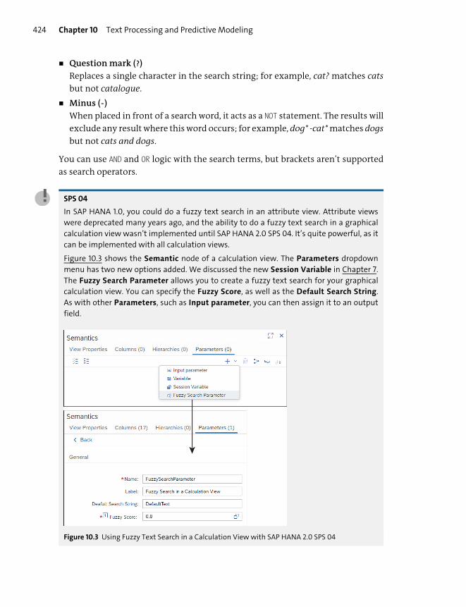
Chapter 10 Text Processing and Predictive Modeling424
� Question mark (?)
Replaces a single character in the search string; for example, cat? matches cats
but not catalogue.
� Minus (-)
When placed in front of a search word, it acts as a NOT statement. The results will
exclude any result where this word occurs; for example, dog* -cat* matches dogs
but not cats and dogs.
You can use AND and OR logic with the search terms, but brackets aren’t supported
as search operators.
SPS 04
In SAP HANA 1.0, you could do a fuzzy text search in an attribute view. Attribute views
were deprecated many years ago, and the ability to do a fuzzy text search in a graphical
calculation view wasn’t implemented until SAP HANA 2.0 SPS 04. It’s quite powerful, as it
can be implemented with all calculation views.
Figure 10.3 shows the Semantic node of a calculation view. The Parameters dropdown
menu has two new options added. We discussed the new Session Variable in Chapter 7.
The Fuzzy Search Parameter allows you to create a fuzzy text search for your graphical
calculation view. You can specify the Fuzzy Score, as well as the Default Search String.
As with other Parameters, such as Input parameter, you can then assign it to an output
field.
Figure 10.3 Using Fuzzy Text Search in a Calculation View with SAP HANA 2.0 SPS 04

Key Concepts Refresher Chapter 10 425
You can combine text search queries with additional functions to enhance your
text search queries and results. With the SCORE() function, you’ve just seen an
example of an additional function that helps with sorting the results of the text
search by relevance. Some other functions that you can use are as follows:
� NEAR()
This function allows you to do a proximity search for words that are near to each
other. Let’s say you have a sentence like “I passed the SAP HANA certification
exam.” The query WHERE CONTAINS(*, ‘NEAR(exam, hana), 2, false’) will find the
places where the word exam is within 2 tokens distance of the word HANA. The
false parameter indicates that you don’t care about the sequence of the words.
� HIGHLIGHTED()
You can use this function to highlight the search term in the results in bold.
Your query can be something like SELECT HIGHLIGHTED(TITLE), DESCRIPTION FROM
TABLE1 WHERE CONTAINS(“TITLE”), ‘HANA’);. The search term “HANA” will be
shown in bold; for example, I passed the SAP HANA certification exam.
� SNIPPETS()
This function is similar to the HIGHLIGHTED() function, except that it will return a
short snippet instead of the entire sentence or paragraph. For example, a query
like SELECT SNIPPET(TITLE), DESCRIPTION FROM TABLE1 WHERE CONTAINS(“TITLE”),
‘HANA’); will return . . . passed the SAP HANA certification . . . with an ellipsis on
both sides of the snippet.
� WEIGHT()
With this function, you can give a higher relevance (more weight) to search
terms that are in the Title column than those in the Description column—using
the table in Figure 10.1 as an example. You can create a query like WHERE CON-
TAINS((“TITLE”, “DECRIPTION”), ‘exam’, WEIGHT(1, 0.5)). The weight is a value
between 0 and 1. In this case, the query will give a relevance of 1 for finding the
word exam in the Title and 0.5 for finding it in the Description.
Text Analysis
After you’ve created a full-text index with the TEXT ANALYSIS option enabled, you
can also analyze text with the SAP HANA text analysis feature, both via entity
analysis and sentiment analysis.
You create text analysis via the full-text index. The abbreviated statement is as fol-
lows:

Chapter 10 Text Processing and Predictive Modeling426
CREATE FULLTEXT INDEX INDEX_NAME ON TABLE_NAME ("COLUMN_NAME")TEXT ANALYSIS ON
CONFIGURATION 'CONFIG_NAME';
You need the TEXT ANALYSIS ON clause, and a CONFIGURATION NAME is optional. There
are a few built-in configurations, but you can also create your own industry-spe-
cific configuration files. Each of the configurations has its own unique extraction
rules and dictionaries of entity values and types.
In the earlier example shown in Listing 10.1, we created the full-text index (called
DEMO_TEXT_INDEX) on table DEMO_TEXT. When you look at the table in the SAP HANA
database explorer perspective, you’ll notice that SAP HANA has created an addi-
tional table: $TA_DEMO_TEXT_INDEX (see Figure 10.4, bottom left). This is the same
name of the full-text index we created, prepended with $TA_ to denote text analy-
sis. You get the text analysis request results back in table $TA.
Tip
Table $TA isn’t the full-text index; it’s a table that contains the results of the text analysis.
Figure 10.4 Source Table (DEMO_TEXT) and $TA_ Text Analysis Results Table
The original table included the values in Table 10.1 in the SOME_TEXT column.
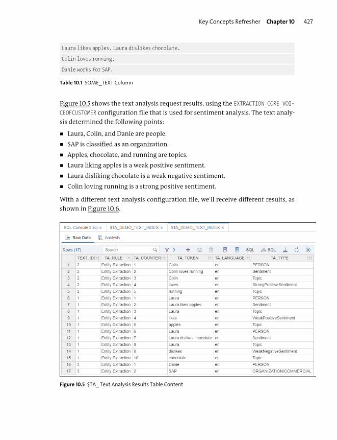
Key Concepts Refresher Chapter 10 427
Figure 10.5 shows the text analysis request results, using the EXTRACTION_CORE_VOI-
CEOFCUSTOMER configuration file that is used for sentiment analysis. The text analy-
sis determined the following points:
� Laura, Colin, and Danie are people.
� SAP is classified as an organization.
� Apples, chocolate, and running are topics.
� Laura liking apples is a weak positive sentiment.
� Laura disliking chocolate is a weak negative sentiment.
� Colin loving running is a strong positive sentiment.
With a different text analysis configuration file, we’ll receive different results, as
shown in Figure 10.6.
Figure 10.5 $TA_ Text Analysis Results Table Content
Laura likes apples. Laura dislikes chocolate.
Colin loves running.
Danie works for SAP.
Table 10.1 SOME_TEXT Column
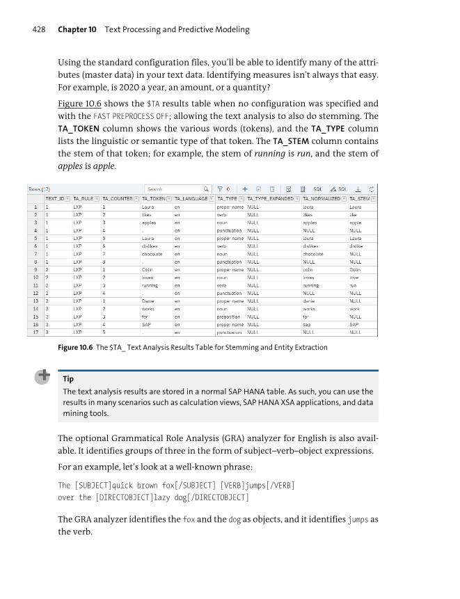
Chapter 10 Text Processing and Predictive Modeling428
Using the standard configuration files, you’ll be able to identify many of the attri-
butes (master data) in your text data. Identifying measures isn’t always that easy.
For example, is 2020 a year, an amount, or a quantity?
Figure 10.6 shows the $TA results table when no configuration was specified and
with the FAST PREPROCESS OFF; allowing the text analysis to also do stemming. The
TA_TOKEN column shows the various words (tokens), and the TA_TYPE column
lists the linguistic or semantic type of that token. The TA_STEM column contains
the stem of that token; for example, the stem of running is run, and the stem of
apples is apple.
Figure 10.6 The $TA_ Text Analysis Results Table for Stemming and Entity Extraction
Tip
The text analysis results are stored in a normal SAP HANA table. As such, you can use the
results in many scenarios such as calculation views, SAP HANA XSA applications, and data
mining tools.
The optional Grammatical Role Analysis (GRA) analyzer for English is also avail-
able. It identifies groups of three in the form of subject–verb–object expressions.
For an example, let’s look at a well-known phrase:
The [SUBJECT]quick brown fox[/SUBJECT] [VERB]jumps[/VERB]over the [DIRECTOBJECT]lazy dog[/DIRECTOBJECT]
The GRA analyzer identifies the fox and the dog as objects, and it identifies jumps as
the verb.
Key Concepts Refresher Chapter 10 429
Tip
Text analysis results are stored in a flat structure with the table $TA. As such, it’s hard to
represent the complex relationships between the extracted entities. This is one area
where graph processing can certainly help. By combining text processing with graph
analysis, you can start using graph queries from Chapter 11 to examine the text analysis
with various algorithms. For example, you can discover closely connected relationships
between entities that you won’t see when just looking at table $TA.
SAP HANA has seven built-in text analysis configurations. You’ve already seen the
EXTRACTION_CORE_VOICEOFCUSTOMER configuration when we used it for sentiment
analysis. There are three configurations for linguistic analysis.
� LINGANALYSIS_BASIC
This configuration is used for tokenization only.
� LINGANALYSIS_FULL
This configuration is used for tokenization and stemming. If you don’t specify a
configuration file, this configuration is used. An example of the results was
shown earlier in Figure 10.6.
� LINGANALYSIS_STEMS
This configuration is used for tokenization, stemming, and parts of speech.
Parts-of-speech tags word categories, for example, showing that quick is an
adjective.
The four configurations for extraction analysis extend the LINGANALYSIS_FULL con-
figuration:
� EXTRACTION_CORE
This configuration is used for extracting standard entities, such as persons and
phone numbers.
� EXTRACTION_CORE_ENTERPRISE
This configuration is used for extracting business relations. Examples are mem-
bership information, management changes, product releases, mergers and
acquisitions, and organizational information.
� EXTRACTION_CORE_PUBLIC_SECTOR
This configuration is used for extracting government entities. Examples are
action and travel events, military units, spatial references, and details of per-
sons, such as aliases, appearances, attributes, and relationships.
� EXTRACTION_CORE_VOICEOFCUSTOMER
This configuration is used for extracting sentiment analysis. We saw an exam-
ple of this when we produced the results in Figure 10.5.
Chapter 10 Text Processing and Predictive Modeling430
All text analysis configurations consist of three elements.
� Dictionary
The dictionary is a repository of entity categories and their possible values, for
example, top soccer (football) countries such as Spain, Germany, Netherlands,
Italy, and Brazil. It’s created with an .hdbtextdict file.
� Rule set
The rule set contains the rules that define how an entity can be identified; for
example, a national identity number can start with the birth date of the person
and should be 14 numbers in total. It’s created with an .hdbruleset file.
� Text analysis configurations file
The configuration file defines aspects of the text analysis process, for example,
which dictionaries and rule sets to use, whether to use linguistic or entity
extraction, and which phases of these extractions (like tokenization) should be
used. It’s created with an .hdbtextconfig file.
When you build your own custom text analysis configuration, you’ll build the files
in the sequence above. It might be easier, however, to copy the existing files in SAP
HANA and then modify them. All three of these files are XML files that can be
edited with standard editors, including the code editor in SAP Web IDE for SAP
HANA.
Note
For more information about text analysis configurations, refer to the SAP HANA Text
Analysis Developer Guide at http://s-prs.co/v487620.
Text Mining
Fuzzy searches and text analysis work with a word, sentence, or paragraph—but
with text mining, you can work with entire documents. These documents can be
web pages, Microsoft Word documents, or PDF files that are loaded into SAP
HANA.
Text mining uses the full-text indexing and text analysis processes, as shown ear-
lier in Figure 10.1. Text mining uses these to produce a matrix of documents and
terms. When using text mining in SAP HANA, you can perform the following tasks:
� Categorize documents.
� Find top-ranked documents related to a particular term.
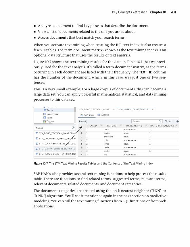
Key Concepts Refresher Chapter 10 431
� Analyze a document to find key phrases that describe the document.
� View a list of documents related to the one you asked about.
� Access documents that best match your search terms.
When you activate text mining when creating the full-text index, it also creates a
few $TM tables. The term-document matrix (known as the text mining index) is an
optional data structure that uses the results of text analysis.
Figure 10.7 shows the text mining results for the data in Table 10.1 that we previ-
ously used for the text analysis. It’s called a term-document matrix, as the terms
occurring in each document are listed with their frequency. The TEXT_ID column
has the number of the document, which, in this case, was just one or two sen-
tences.
This is a very small example. For a large corpus of documents, this can become a
large data set. You can apply powerful mathematical, statistical, and data mining
processes to this data set.
Figure 10.7 The $TM Text Mining Results Tables and the Contents of the Text Mining Index
SAP HANA also provides several text mining functions to help process the results
table. There are functions to find related terms, suggested terms, relevant terms,
relevant documents, related documents, and document categories.
The document categories are created using the on k-nearest neighbor (“kNN” or
“k-NN”) algorithm. You’ll see it mentioned again in the next section on predictive
modeling. You can call the text mining functions from SQL functions or from web
applications.
Chapter 10 Text Processing and Predictive Modeling432
Tip
Remember that users won’t work at the lower level that we’ve described in this chapter:
They will want to use text features from a browser-based application interface. This is
why SAP has focused on supplying various JavaScript APIs for SAP HANA modelers and
developers.
Note
You can get more information in the “Full-Text Search with SAP HANA Platform” open-
SAP course at http://s-prs.co/v487632.
At http://s-prs.co/v487620, you can find three developer guides for text processing: the
SAP HANA Search Developer Guide, the SAP HANA Text Analysis Developer Guide, and
the SAP HANA Text Mining Developer Guide. You will have to click on the View All button
in the Development section to find some of these guides. Or download all the files from
the Documentation Download section.
You can also view the SAP HANA Academy on YouTube. The playlist for text processing is
at http://s-prs.co/v487633.
Now that you know how to work with text data in SAP HANA and can use fault-tol-
erant text searches, text analysis, and text mining in SAP HANA modeling work,
let’s move on to predictive modeling.
Predictive Modeling
In this section, we’ll look at the SAP HANA Predictive Analysis Library (PAL) and
how to use it to create a predictive analysis model. We’ll look at predicting future
probabilities and trends and how you can use this functionality in business. In the
real-world scenario at the beginning of the chapter, we described a use case in
which you might create a predictive model in SAP HANA to help sales reps with
their sales forecasting by looking at seasonal patterns; for example, people use
more pharmaceuticals for allergies in the spring.
There are many use cases for PAL, which is built in to SAP HANA. Here are just a
couple examples:
� For financial institutions such as banks, you can detect fraud by looking at
abnormal transactions.
� For fleet management and car rental companies, you can predict which parts
will break soon in a vehicle and replace them before they actually break.
Key Concepts Refresher Chapter 10 433
We’ll see some more use cases when we discuss the types of algorithms and what
you can use them for. Before discussing PAL in more detail, let’s take a quick look
at the wider picture. PAL is just one of several tools available for addressing
machine learning and predictive analysis requirements in your projects.
� Predictive Analysis Library (PAL)
PAL provides more than 90 classic and trending algorithms for native in-data-
base processing of data that you can use in your information modeling.
� Automated Predictive Library (APL)
The embedded SAP Predictive Analytics automated analytics engine processes
your data automatically with multiple scenarios and determines which predic-
tive algorithm is the best for your scenario using structural risk minimization.
APL makes it quick and easy for nonexpert data scientists to consume applica-
tions built on SAP HANA.
� SAP domain-specific libraries
There are several SAP solutions that have libraries for native in-database pro-
cessing of application data, for example, the Unified Demand Forecast library
for customer activities and the Optimization Function Library (OFL) for supply
chain solutions.
� Application Function Library (AFL) Software Development Kit (SDK)
This SDK allows SAP partners and customers to create their own functions in
libraries similar to PAL, OFL, and Unified Demand Forecast. The code is written
in C++, and the custom-created libraries can be used internally in the company
or can be sold to SAP customers.
� TensorFlow integration
TensorFlow is an open-source deep learning library from Google that is used for
many scenarios, for example, image classification where the system “recog-
nizes” objects in photographs. You can call TensorFlow models from SAP HANA
External Machine Learning AFL.
� R integration
You’ve seen in Chapter 8 that you can write procedures using SQLScript. You
can also write procedures in R, AFL, and GraphScript. R is a programming lan-
guage used by many statisticians and data miners. You can do everything in
PAL and more using R. The advantage is that you can reuse lots of code from
other projects. PAL is much faster for business data, however, because it runs in
database, whereas the R code and the data are sent to an R server to run exter-
nally.
Chapter 10 Text Processing and Predictive Modeling434
SPS 04
Integration to Python was added with SAP HANA 2.0 SPS 04 via a Python API for SAP
HANA machine learning. Many data scientists are using Python for fast prototyping of
their machine learning models. You can now leverage the SAP HANA machine learning
libraries to process the data in SAP HANA from calls in Python.
The R integration has also been expanded with an R API for SAP HANA machine learning
to leverage SAP HANA directly from your R code.
Predictive modeling uses statistical algorithms on a set of input data to “guess” the
probability of a specific outcome. We can use this for data mining where you use
these algorithms to find patterns in the data.
A variation of this that is discussed a lot in the media is machine learning. In this
case, we use statistical algorithms to let the computer look at, analyze, and “learn”
from the data by automatically building a predictive model. We can then run new
data through the generated model to let the system predict and provide the prob-
ability of any outcomes we’re interested in.
We’ll now discuss PAL in more detail.
Predictive Analysis Library
Predictive analytics refers to statistics applied to prediction, machine learning, or
data mining processes. Those statistics need a lot of complex algorithms. You can
program these algorithms in a programming language such as Java or use algo-
rithms already created in a language such as R. The problem is that you then have
to transfer the data to external servers instead of processing it in SAP HANA. Some
languages, such as Python, are quite slow in general. You should preferably write
such complex algorithms in a compiled language, such as C++, for fast execution.
If you want to keep the data in the database, SQL or SQLScript isn’t an option as
these are set-oriented data languages.
PAL is a library of such algorithms, written in C++, and running inside SAP HANA.
You don’t have to transfer any data between SAP HANA and another application
server.
The algorithms in PAL were carefully selected based on the most commonly used
algorithms in the market, algorithms generally available in other database prod-
ucts, and algorithms required by SAP applications. Over the years, the library has
grown to fulfill almost all requirements from SAP HANA projects. Recently added
algorithms tend to be the popular trending algorithms from areas such as
machine learning.
Key Concepts Refresher Chapter 10 435
In SAP HANA, the predictive analysis functions are grouped together in the PAL.
PAL defines functions that you can call from SQLScript and use to perform various
predictive analysis algorithms.
You can use these PAL functions to prepare your data for further analysis, for
example, building a predictive model. You can then use this trained model on new
data to make predictions for this data. For example, when traveling, you want to
know if your flight will be delayed. You can train a predictive model by feeding it
all the historical flight data. After the model is prepared, you can give it your flight
details. The model will then predict whether your flight will be delayed or not.
You’ll learn how to build this in SAP HANA in the “Machine Learning Models” sec-
tion later in this chapter.
In PAL, predictive analysis algorithms are grouped in 10 categories; we’ll take a
quick look at some of the categories and discuss a few popular algorithms to give
you an idea of what is possible. The categories, minus the miscellaneous one that
serves as a catch-all for anything left over, are as follows:
� Association
For an example of an association use case, think of Amazon’s suggestions: Cus-
tomers who bought this item also bought. The Apriori algorithm can be used to
analyze shopping baskets. It can then identify products that are commonly pur-
chased together and group them together in the shop, such as flashlights and
batteries. You could even offer a discount on the flashlights because you know
that people will need to buy batteries for them, and you can make enough profit
on the batteries. (Notice, however, that the inverse isn’t necessarily true; a dis-
count on the batteries won’t encourage people to buy flashlights.)
� Clustering
With clustering, you divide data into groups (clusters) of items that have similar
properties. For example, you can group servers with similar usage characteris-
tics, such as email servers that all have a lot of network traffic on port 25 during
the day. You might use the popular k-means algorithm for this purpose.
Another example is computer vision, in which you cluster pictures of human
faces using the affinity propagation algorithm. Clustering is sometimes also
called segmentation. The focus of clustering is the algorithm figuring out by
itself what is the best way to group existing data together.
� Regression
Regression plots the best possible line or curve through the historical data. You
can then use that line or curve to predict future values. This could be used by the
previously mentioned car rental company. The company has had 5,000 of these
Chapter 10 Text Processing and Predictive Modeling436
vehicles before, and so it has good information available to predict when certain
parts in a similar vehicle will break.
� Classification
The process of classification takes historical data and trains predictive models
using, for example, decision trees. You can then send new data to the predictive
model you’ve trained, and the model will attempt to predict which class the new
data belongs to. This process is often referred to as supervised learning. The
focus here is on getting accurate predictions for unknown data.
� Preprocessing and data preparation
This category of algorithms is used to prepare data before further processing.
These algorithms may improve the accuracy of the predictive models by reduc-
ing the noise.
� Time series
For an example of a time series, think of the real-life scenario at the beginning
of the chapter, in which we built a predictive model to forecast sales by looking
at seasonal patterns. You might also see, for example, a monthly pattern in
shops of higher sales after paydays.
� Social network analysis
Algorithms in this category are used to predict the likelihood of a future link
between two people who have no link yet. This is used by companies such as
Facebook and LinkedIn.
� Statistics and outlier detection
This category includes some statistical algorithms to find out how closely vari-
ables are related to or are independent from each other. One example is the
Grubbs’ test algorithm, which is used to detect outliers. This could be used in the
fraud detection use case we mentioned earlier, in which certain transactions are
different from the others. (Often, we first use a clustering algorithm to group
transactions together and then detect outliers for each group/cluster after.)
� Recommender systems
These algorithms, as the name suggests, make recommendations by analyzing
product associations, the purchase history of the buyer, and external factors,
such as the general economy. Music playlists are good examples.
Figure 10.8 shows the PAL algorithms, per category, that are available in SAP HANA
2.0 SPS 03.
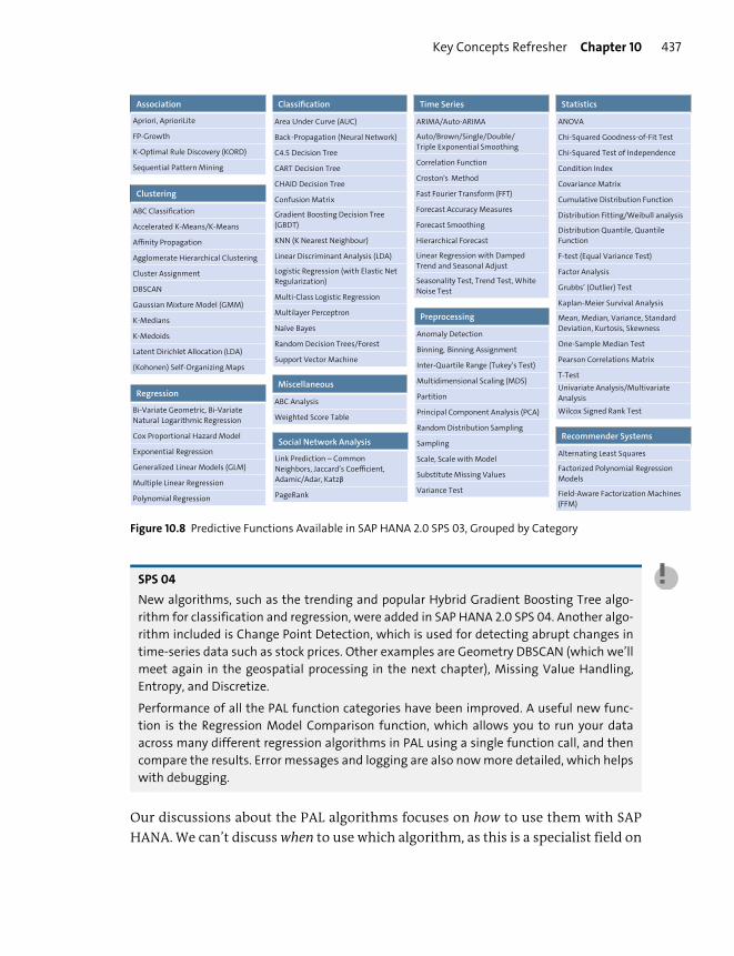
Key Concepts Refresher Chapter 10 437
Figure 10.8 Predictive Functions Available in SAP HANA 2.0 SPS 03, Grouped by Category
SPS 04
New algorithms, such as the trending and popular Hybrid Gradient Boosting Tree algo-
rithm for classification and regression, were added in SAP HANA 2.0 SPS 04. Another algo-
rithm included is Change Point Detection, which is used for detecting abrupt changes in
time-series data such as stock prices. Other examples are Geometry DBSCAN (which we’ll
meet again in the geospatial processing in the next chapter), Missing Value Handling,
Entropy, and Discretize.
Performance of all the PAL function categories have been improved. A useful new func-
tion is the Regression Model Comparison function, which allows you to run your data
across many different regression algorithms in PAL using a single function call, and then
compare the results. Error messages and logging are also now more detailed, which helps
with debugging.
Our discussions about the PAL algorithms focuses on how to use them with SAP
HANA. We can’t discuss when to use which algorithm, as this is a specialist field on
Statistics
ANOVA
Chi-Squared Goodness-of-Fit Test
Chi-Squared Test of Independence
Condition Index
Covariance Matrix
Cumulative Distribution Function
Distribution Fitting/Weibull analysis
Distribution Quantile, Quantile Function
F-test (Equal Variance Test)
Factor Analysis
Grubbs’ (Outlier) Test
Kaplan-Meier Survival Analysis
Mean, Median, Variance, Standard Deviation, Kurtosis, Skewness
One-Sample Median Test
Pearson Correlations Matrix
T-TestUnivariate Analysis/Multivariate Analysis
Wilcox Signed Rank Test
Clustering
ABC Classification
Accelerated K-Means/K-Means
Affinity Propagation
Agglomerate Hierarchical Clustering
Cluster Assignment
DBSCAN
Gaussian Mixture Model (GMM)
K-Medians
K-Medoids
Latent Dirichlet Allocation (LDA)
(Kohonen) Self-Organizing Maps
Classification
Area Under Curve (AUC)
Back-Propagation (Neural Network)
C4.5 Decision Tree
CART Decision Tree
CHAID Decision Tree
Confusion Matrix
Gradient Boosting Decision Tree (GBDT)
KNN (K Nearest Neighbour)
Linear Discriminant Analysis (LDA)
Logistic Regression (with Elastic Net Regularization)
Multi-Class Logistic Regression
Multilayer Perceptron
Naïve Bayes
Random Decision Trees/Forest
Support Vector Machine
Regression
Bi-Variate Geometric, Bi-Variate Natural Logarithmic Regression
Cox Proportional Hazard Model
Exponential Regression
Generalized Linear Models (GLM)
Multiple Linear Regression
Polynomial Regression
Association
Apriori, AprioriLite
FP-Growth
K-Optimal Rule Discovery (KORD)
Sequential Pattern Mining
Preprocessing
Anomaly Detection
Binning, Binning Assignment
Inter-Quartile Range (Tukey’s Test)
Multidimensional Scaling (MDS)
Partition
Principal Component Analysis (PCA)
Random Distribution Sampling
Sampling
Scale, Scale with Model
Substitute Missing Values
Variance Test
Time Series
ARIMA/Auto-ARIMA
Auto/Brown/Single/Double/ Triple Exponential Smoothing
Correlation Function
Croston's Method
Fast Fourier Transform (FFT)
Forecast Accuracy Measures
Forecast Smoothing
Hierarchical Forecast
Linear Regression with Damped Trend and Seasonal Adjust
Seasonality Test, Trend Test, White Noise Test
Social Network Analysis
Link Prediction – Common Neighbors, Jaccard’s Coefficient,
Adamic/Adar, Katzβ
PageRank
Recommender Systems
Alternating Least Squares
Factorized Polynomial Regression Models
Field-Aware Factorization Machines (FFM)
Miscellaneous
ABC Analysis
Weighted Score Table
Chapter 10 Text Processing and Predictive Modeling438
its own. To properly use PAL in SAP HANA, you’ll either need to know what and
when to use it yourself or work with someone who does.
Note
If you want to learn about the different PAL algorithms in more detail, there are two great
sources. The first is the SAP HANA Academy on YouTube, which has a dedicated video for
each algorithm and a few overview video tutorials. You can find the PAL playlist at http://
s-prs.co/v487634.
The other source is the SAP HANA Predictive Analysis Library (PAL) Reference Guide from
the Reference section at http://s-prs.co/v487620. You can start with the table of contents
to look at the categories and see which algorithms are available in the category you need.
You can then look at the information for each of the algorithms, for example:
� The description of the algorithm, its perquisites, and capabilities
� The inputs and outputs that are required, as well as the data types for each column
� Sample code for using the algorithm, and what results can be expected
If you already know the specific algorithm that you want to use or are working
with someone who does, you can use the search feature to find that specific func-
tion.
Installing and Configuring Predictive Analysis Library
PAL is an optional installation with SAP HANA. As it’s part of the SAP HANA, enter-
prise edition, you might have to ask the SAP HANA system administrator to install
it for your project. If you’re using the SAP HANA, express edition, as we are in this
book, it’s already preinstalled for you when you use the Server + Applications ver-
sion. You’ll have used this version if you followed along when we discussed the
basic SAP HANA modeling in SAP Web IDE for SAP HANA.
PAL is part of the AFL that ships with all SAP HANA systems. AFL is an optional
component; if you want to use the predictive analysis algorithms in PAL, you have
to install AFL. AFL also includes a Business Function Library (BFL). You can check
that PAL is installed by querying the system views SYS.AFL_AREAS and SYS.AFL_
FUNCTIONS.
PAL uses a special engine in SAP HANA called the scriptserver. Because partners
and customers can write their own function libraries using the AFL SDK, and
because some algorithms can run for a longer time, SAP HANA has to protect its
kernel against any instability. PAL and any other function libraries written with
the AFL SDK run inside the scriptserver. By default, the scriptserver isn’t running.
Key Concepts Refresher Chapter 10 439
You’ll need to add the scriptserver in your tenant database. In the SAP HANA,
express edition, this is named HXE. The scriptserver doesn’t run in the SYSTEMDB.
You can run the following command while you’re connected to the SYSTEMDB data-
base (replace HXE with the name of your tenant database):
ALTER DATABASE HXE ADD 'scriptserver';
After the installation, you have to ensure that the scriptserver is started in the
tenant database and make sure the correct roles and authorizations are assigned
to your SAP HANA user. (Roles and how to assign them are discussed in Chapter
13.)
You can check that the scriptserver is running, by running the following query in
the tenant database:
SELECT * FROM SYS.M_SERVICES;
You also have to assign the necessary roles and privileges. Your development user
will need the AFL__SYS_AFL_AFLPAL_EXECUTE role to execute the PAL procedures.
Both the SAP HANA Deployment Infrastructure (HDI) service technical user and
the HDI container owners need to have been granted SELECT privileges on the PAL
procedures. The HDI service technical user can be granted privileges through its
specific default role called XSA_DEV_USER_ROLE. You’ll need to assign this role to your
development user as well.
The HDI container owners can be granted privileges through the default role called
_SYS_DI_OO_DEFAULTS.
The easiest way to set this up properly is to use the code snippet provided by the
SAP HANA Academy. You can view the video called “PAL 146 Getting Started with
HANA 20 SPS02” in the YouTube playlist we mentioned in the previous subsec-
tion. Or you can just run the code snippet on GitHub that Phillip describes in the
video (the code snippet for setting this up is available at http://s-prs.co/v487635).
You’ll have to do this for your SAP HANA, express edition, or you won’t be able to
create the flowgraphs we’ll discuss next.
After PAL is installed and configured, you can create predictive models graphically
in SAP Web IDE for SAP HANA. There are three ways to call the PAL algorithms.
� The easiest way to is to create a flowgraph. Even people who don’t know SAP
HANA modeling that well, such as a data scientist in your team, can use the
flowgraphs.

Chapter 10 Text Processing and Predictive Modeling440
� You can also create an SAP HANA AFLLANG procedure. We won’t go into much
detail on this.
� You can call the catalog SQLScript procedures provided.
We’ll start using PAL by creating flowgraphs.
Creating a Predictive Model Using Flowgraphs
We mentioned flowgraphs in Chapter 9 already, when discussing SAP HANA smart
data integration and SAP HANA smart data quality. We’ll configure the predictive
analytics flowgraphs to generate the procedures we need to execute the predictive
model. We can, however, also run the model directly inside the flowgraph editor. A
flowgraph is a file with an .hdbflowgraph extension. It allows you to design and run
data transformation procedures and tasks without typing a single line of code.
You create an .hdbflowgraph file from the New context menu in your project. The
flowgraph editor opens, as shown in Figure 10.9. Before creating your flowgraph,
you’ll need to set the runtime behavior type of your flowgraph. You can do this in
the Properties dialog box. You can open this dialog box by clicking on the top-right
icon that looks like a small gear. In the Settings tab, you can select the Runtime
Behavior Type in the dropdown menu. There are four options:
� Batch Task
This behavior type processes data as a batch or when loaded with an initial load.
It can’t be run in real time. A stored procedure and a task are created after build-
ing the flowgraph. You can schedule this to run at regular intervals.
� Realtime Task
This behavior type allows you to process data in real time. A stored procedure
and two tasks are created when you build the flowgraph. The first task is a batch
or initial load of the input data. The second task is run in real time for any
updates that occur to that input data.
� Transactional Task
This also allows you to process data in real time. A single task is created after
building the flowgraph. This task is run in real time when any updates occur to
the input data. It doesn’t include an initial load as it assumes that all data col-
lected comes from a transactional system.
� Procedure
We’ll only discuss this type of runtime behavior in this chapter. It allows you to
process data using stored procedures. It can’t be run in real time. When you
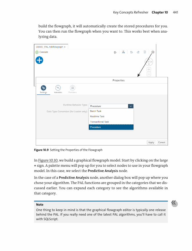
Key Concepts Refresher Chapter 10 441
build the flowgraph, it will automatically create the stored procedures for you.
You can then run the flowgraph when you want to. This works best when ana-
lyzing data.
Figure 10.9 Setting the Properties of the Flowgraph
In Figure 10.10, we build a graphical flowgraph model. Start by clicking on the large
+ sign. A palette menu will pop up for you to select nodes to use in your flowgraph
model. In this case, we select the Predictive Analysis node.
In the case of a Predictive Analysis node, another dialog box will pop up where you
chose your algorithm. The PAL functions are grouped in the categories that we dis-
cussed earlier. You can expand each category to see the algorithms available in
that category.
Note
One thing to keep in mind is that the graphical flowgraph editor is typically one release
behind the PAL. If you really need one of the latest PAL algorithms, you’ll have to call it
with SQLScript.
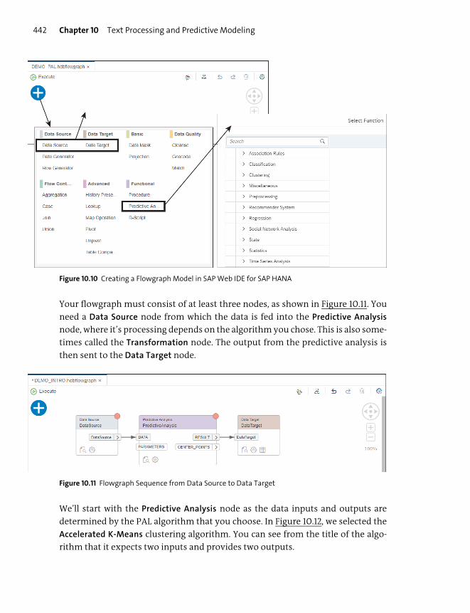
Chapter 10 Text Processing and Predictive Modeling442
Figure 10.10 Creating a Flowgraph Model in SAP Web IDE for SAP HANA
Your flowgraph must consist of at least three nodes, as shown in Figure 10.11. You
need a Data Source node from which the data is fed into the Predictive Analysis
node, where it’s processing depends on the algorithm you chose. This is also some-
times called the Transformation node. The output from the predictive analysis is
then sent to the Data Target node.
Figure 10.11 Flowgraph Sequence from Data Source to Data Target
We’ll start with the Predictive Analysis node as the data inputs and outputs are
determined by the PAL algorithm that you choose. In Figure 10.12, we selected the
Accelerated K-Means clustering algorithm. You can see from the title of the algo-
rithm that it expects two inputs and provides two outputs.
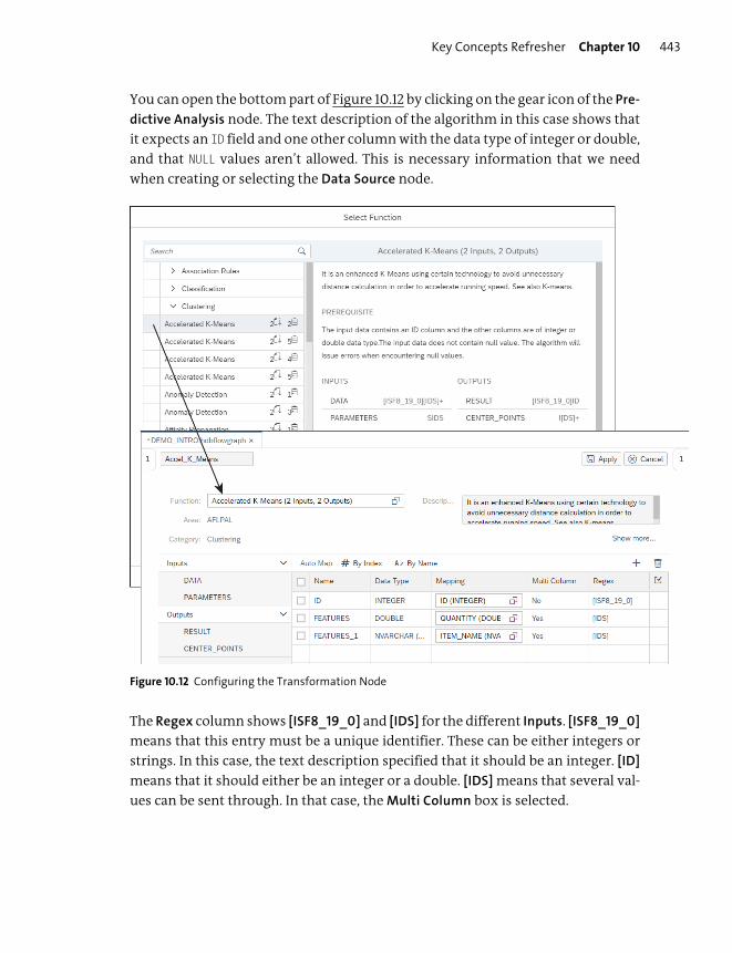
Key Concepts Refresher Chapter 10 443
You can open the bottom part of Figure 10.12 by clicking on the gear icon of the Pre-
dictive Analysis node. The text description of the algorithm in this case shows that
it expects an ID field and one other column with the data type of integer or double,
and that NULL values aren’t allowed. This is necessary information that we need
when creating or selecting the Data Source node.
Figure 10.12 Configuring the Transformation Node
The Regex column shows [ISF8_19_0] and [IDS] for the different Inputs. [ISF8_19_0]
means that this entry must be a unique identifier. These can be either integers or
strings. In this case, the text description specified that it should be an integer. [ID]
means that it should either be an integer or a double. [IDS] means that several val-
ues can be sent through. In that case, the Multi Column box is selected.
Chapter 10 Text Processing and Predictive Modeling444
The mapping of input fields from the data source is normally done automatically.
The columns are handled in the same order in which they are defined in the data
source.
You now know from the Predictive Analysis node that the data source must supply
at least two columns, of which the first must be an ID field. These field data types
can either be integer or double.
Figure 10.13 shows the configuration of the Data Source node. In Figure 10.11,
shown earlier, the top-right corner of the Data Source node has a red dot. This indi-
cates that the node isn’t yet configured. To configure it, you click on the gear icon
at the bottom of the node.
The main selection here is the type of data source that you want to use. The HANA
Object button allows you to select SAP HANA tables, views, synonyms, CDS enti-
ties, table functions, and so on. If you don’t use procedure-type flowgraphs, you
can also select calculation views. In this case, we’re using a procedure-type flow-
graph, so we can’t use a calculation view as a data source.
Sometimes you might want to have a more dynamic setup. You can choose to use
a Table Type as a data source, as shown in Figure 10.13. You’ll have to specify the col-
umns and the data type of each column. The input table will be passed into the
procedure call as an input parameter.
Tip
Choosing a Table Type as a data source is only available for procedure-type flowgraphs.
We provide the expected input fields with the required data types to the Predictive
Analysis node. In this example it could be something like product sales data, where
we want to cluster according to quantities. We pass through the item IDs, the
quantities, and the item names.
The configuration of the Data Target node is very similar to that of the Data Source
node. The data target defines where you want to put the calculated results. This
could be an existing SAP HANA table; in which case, you select HANA Object. If
you’re creating a procedure-type flowgraph, you can select Table Type.
If you want to create a new table for the results, you can select Template Table, as
shown in Figure 10.14. If the Predictive Analysis node creates several result sets, you
don’t have to retrieve all of them. If result sets aren’t mapped to a Data Target
node, they won’t be stored.

Key Concepts Refresher Chapter 10 445
Figure 10.13 Configuring the Data Source Node
Figure 10.14 Configuring the Data Target Node
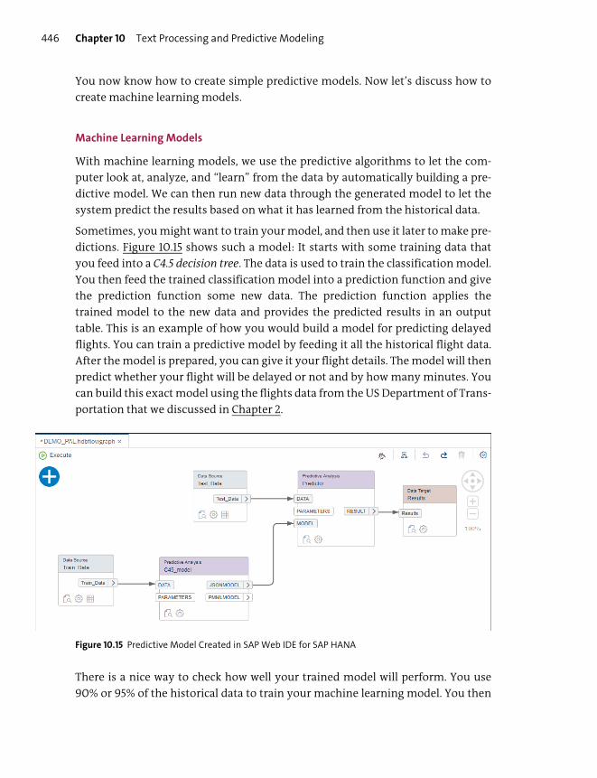
Chapter 10 Text Processing and Predictive Modeling446
You now know how to create simple predictive models. Now let’s discuss how to
create machine learning models.
Machine Learning Models
With machine learning models, we use the predictive algorithms to let the com-
puter look at, analyze, and “learn” from the data by automatically building a pre-
dictive model. We can then run new data through the generated model to let the
system predict the results based on what it has learned from the historical data.
Sometimes, you might want to train your model, and then use it later to make pre-
dictions. Figure 10.15 shows such a model: It starts with some training data that
you feed into a C4.5 decision tree. The data is used to train the classification model.
You then feed the trained classification model into a prediction function and give
the prediction function some new data. The prediction function applies the
trained model to the new data and provides the predicted results in an output
table. This is an example of how you would build a model for predicting delayed
flights. You can train a predictive model by feeding it all the historical flight data.
After the model is prepared, you can give it your flight details. The model will then
predict whether your flight will be delayed or not and by how many minutes. You
can build this exact model using the flights data from the US Department of Trans-
portation that we discussed in Chapter 2.
Figure 10.15 Predictive Model Created in SAP Web IDE for SAP HANA
There is a nice way to check how well your trained model will perform. You use
90% or 95% of the historical data to train your machine learning model. You then

Key Concepts Refresher Chapter 10 447
feed the remaining 10% or 5% of the data into your model to get the predicted val-
ues. Because this is actually historical data, you have the result of what really hap-
pened. You can now compare the historical result with the predictive values to
evaluate the accuracy of your predictive model.
The main difference between this model and the simpler one in the previous sec-
tion is that these models have several steps. The first step trains the model, then
you can validate and test it. Finally, you use the trained model for predictions.
You can even add another step before the model training step, by first using parti-
tioning-type algorithms to divide the data into several subsets. You can use 90% of
your data to train the model, and the remaining 10% to validate it with. Or you can
use preprocessing (data preparation) algorithms on the raw data to first shape it
into a usable format.
SPS 04
To improve the performance of machine learning models in SAP HANA 2.0 SPS 04, you
can now keep your trained PAL predictive models in memory. You parse the model once,
keep the model state in memory, and can then execute repeatedly on the stored model
that is kept in memory for repeated scoring.
When you build a flowgraph model, you start on the left side and work toward the
right side, as shown in Figure 10.15. First, add a data input node, and select a table
with data. Put this on the left side of the work area. Next, select a PAL function
from the popup palette menu, and add it to the work area. Then, connect the Data
Source node to the PAL function node. You carry on in this fashion until your data
model is complete.
When you want to run your predictive model, you can click the Execute button in
the top left of the flowgraph editor. The biggest advantage of flowgraphs is that
they are very easy and flexible. Data science can be quite complex, and you don’t
always know which algorithms will produce the best results. Using graphical flow-
graphs, you can test the performance of several algorithms to find the best solu-
tion.
SQLScript Procedures Created by the Flowgraph
When you’re satisfied with your predictive model, you can build it in SAP Web IDE
for SAP HANA. With a procedure-type flowgraph, it will create a set of two proce-
dures automatically during the build process.
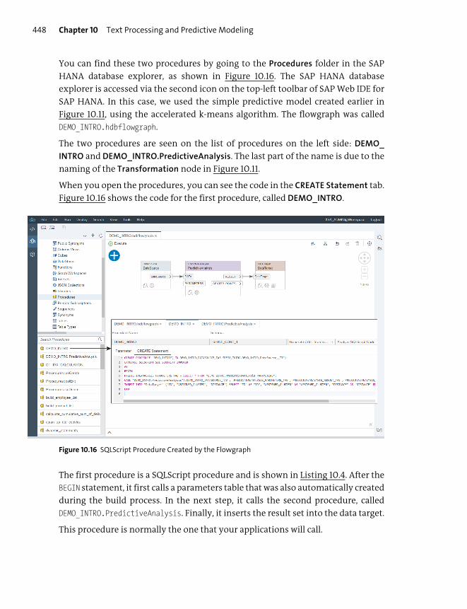
Chapter 10 Text Processing and Predictive Modeling448
You can find these two procedures by going to the Procedures folder in the SAP
HANA database explorer, as shown in Figure 10.16. The SAP HANA database
explorer is accessed via the second icon on the top-left toolbar of SAP Web IDE for
SAP HANA. In this case, we used the simple predictive model created earlier in
Figure 10.11, using the accelerated k-means algorithm. The flowgraph was called
DEMO_INTRO.hdbflowgraph.
The two procedures are seen on the list of procedures on the left side: DEMO_
INTRO and DEMO_INTRO.PredictiveAnalysis. The last part of the name is due to the
naming of the Transformation node in Figure 10.11.
When you open the procedures, you can see the code in the CREATE Statement tab.
Figure 10.16 shows the code for the first procedure, called DEMO_INTRO.
Figure 10.16 SQLScript Procedure Created by the Flowgraph
The first procedure is a SQLScript procedure and is shown in Listing 10.4. After the
BEGIN statement, it first calls a parameters table that was also automatically created
during the build process. In the next step, it calls the second procedure, called
DEMO_INTRO.PredictiveAnalysis. Finally, it inserts the result set into the data target.
This procedure is normally the one that your applications will call.

Key Concepts Refresher Chapter 10 449
CREATE PROCEDURE "DEMO_INTRO"(IN DEMO_INTRO_DATASOURCE_TAB"DEMO_INTRO.DEMO_INTRO_DataSource__TT")
LANGUAGE SQLSCRIPTSQL SECURITY INVOKER AS
BEGINPREDICTIVEANALYSIS_PARAMETERS_TAB =
SELECT * FROM "DEMO_INTRO.PredictiveAnalysis_PARAMETERS";CALL "DEMO_INTRO.PredictiveAnalysis"(:DEMO_INTRO_DATASOURCE_TAB,
:PREDICTIVEANALYSIS_PARAMETERS_TAB,PREDICTIVEANALYSIS_RESULT_TAB,PREDICTIVEANALYSIS_CENTER_POINTS_TAB );
INSERT INTO "DataTarget" ("ID", "ASSIGNED_CLUSTER", "DISTANCE")SELECT "ID" AS "ID",
"ASSIGNED_CLUSTER" AS "ASSIGNED_CLUSTER","DISTANCE" AS "DISTANCE"FROM :PREDICTIVEANALYSIS_RESULT_TAB;
END
Listing 10.4 SQLScript Procedure
Listing 10.5 shows some of the code of the second procedure. The interesting thing
here is that this isn’t written in SQLScript, but in AFLLANG. The AREA parameter
shows as AFLPAL, showing that it’s calling a PAL function. The FUNCTION is shown as
ACCELERATEDKMEANS. In the PARAMETERS section, you can see the input fields that we
specified in Figure 10.13. The PARAMETERS section is basically in JavaScript Object
Notation (JSON) format.
CREATE PROCEDURE "SHINE_CORE_1"."DEMO_INTRO.PredictiveAnalysis"(IN p1 "SHINE_CORE_1"."DEMO_INTRO.PredictiveAnalysis_DATA__TT",IN p2 "SHINE_CORE_1"."DEMO_INTRO.PredictiveAnalysis_PARAMETERS__TT",OUT p3 "SHINE_CORE_1"."DEMO_INTRO.PredictiveAnalysis_RESULT__TT",OUT p4"SHINE_CORE_1"."DEMO_INTRO.PredictiveAnalysis_CENTER_POINTS__TT")
LANGUAGE AFLLANGSQL SECURITY INVOKERREADS SQL DATA AS
BEGINAFLLANGVERSION='2';SCHEMA='_SYS_AFL';AREA='AFLPAL';FUNCTION='ACCELERATEDKMEANS';PARAMETERS=';
"TABLE",in,TrexTable,,,,;"ID",,,INT,,INTEGER,;"QUANTITY",,,DOUBLE,,DOUBLE,;"ITEM_NAME",,,STRING,,NVARCHAR,50;…
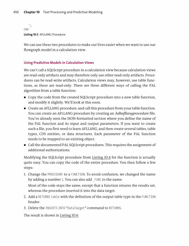
Chapter 10 Text Processing and Predictive Modeling450
';END
Listing 10.5 AFLLANG Procedure
We can use these two procedures to make our lives easier when we want to use our
flowgraph model in a calculation view.
Using Predictive Models in Calculation Views
We can’t call a SQLScript procedure in a calculation view because calculation views
are read-only artifacts and may therefore only use other read-only artifacts. Proce-
dures can be read-write artifacts. Calculation views may, however, use table func-
tions, as these are read-only. There are three different ways of calling the PAL
algorithm from a table function:
� Copy the code from the created SQLScript procedure into a new table function,
and modify it slightly. We’ll look at this soon.
� Create an AFLLANG procedure, and call this procedure from your table function.
You can create an AFLLANG procedure by creating an .hdbafllangprocedure file.
You’ve already seen the JSON-formatted section where you define the name of
the PAL function and its input and output parameters. If you want to create
such a file, you first need to learn AFLLANG, and then create several tables, table
types, CDS entities, or data structures. Each parameter of the PAL function
needs to be mapped to an existing object.
� Call the documented PAL SQLScript procedures. This requires the assignment of
additional authorizations.
Modifying the SQLScript procedure from Listing 10.4 for the function is actually
quite easy. You can copy the code of the entire procedure. You then follow a few
steps:
1. Change the PROCEDURE to a FUNCTION. To avoid confusion, we changed the name
by adding a number 1. You can also add _FUNC to the name.
Most of the code stays the same, except that a function returns the results set,
whereas the procedure inserted it into the data target.
2. Add a RETURNS table with the definition of the output table type in the FUNCTION
header.
3. Delete the INSERTS INTO “DataTarget” command to RETURNS.
The result is shown in Listing 10.6.
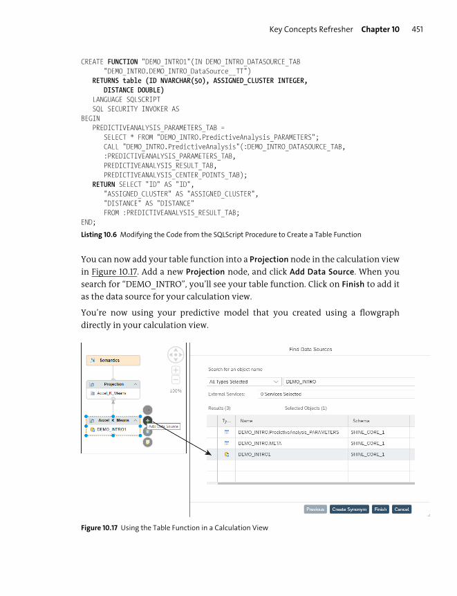
Key Concepts Refresher Chapter 10 451
CREATE FUNCTION "DEMO_INTRO1"(IN DEMO_INTRO_DATASOURCE_TAB"DEMO_INTRO.DEMO_INTRO_DataSource__TT")
RETURNS table (ID NVARCHAR(50), ASSIGNED_CLUSTER INTEGER,DISTANCE DOUBLE)
LANGUAGE SQLSCRIPTSQL SECURITY INVOKER AS
BEGINPREDICTIVEANALYSIS_PARAMETERS_TAB =
SELECT * FROM "DEMO_INTRO.PredictiveAnalysis_PARAMETERS";CALL "DEMO_INTRO.PredictiveAnalysis"(:DEMO_INTRO_DATASOURCE_TAB,:PREDICTIVEANALYSIS_PARAMETERS_TAB,PREDICTIVEANALYSIS_RESULT_TAB,PREDICTIVEANALYSIS_CENTER_POINTS_TAB);
RETURN SELECT "ID" AS "ID","ASSIGNED_CLUSTER" AS "ASSIGNED_CLUSTER","DISTANCE" AS "DISTANCE"FROM :PREDICTIVEANALYSIS_RESULT_TAB;
END;
Listing 10.6 Modifying the Code from the SQLScript Procedure to Create a Table Function
You can now add your table function into a Projection node in the calculation view
in Figure 10.17. Add a new Projection node, and click Add Data Source. When you
search for “DEMO_INTRO”, you’ll see your table function. Click on Finish to add it
as the data source for your calculation view.
You’re now using your predictive model that you created using a flowgraph
directly in your calculation view.
Figure 10.17 Using the Table Function in a Calculation View
Chapter 10 Text Processing and Predictive Modeling452
Creating a Predictive Model Using SQLScript
You can also create a predictive model purely by using SQLScript instead of graph-
ical modeling tools. This is the way that predictive models were originally created
in SAP HANA before the graphical tools existed.
Since SAP HANA 2.0 SPS 02, SAP provides SQLScript procedures that you can use to
directly use the PAL algorithms. These procedures are found in the _SYS_AFL
schema. This makes the SQLScript code a lot easier and shorter. Before SPS 02, you
had to write your own wrapper code, which could be quite time-consuming. This is
now easy enough that you could even use these procedures interactively in the
SQL Console.
You’ve now mastered predictive modeling and machine learning using the PAL in
SAP HANA.
Important Terminology
In this chapter, we looked at the following important terms:
� Full-text index
Depending on what you specify when you create the full-text index, it gives
access to one or more text features. The full-text index will use additional mem-
ory to provide the requested text features.
� Fuzzy text search
This search type enables or disables the fault-tolerant search feature.
� Text analysis
Text analysis provides a vast number of possible entity types and analysis rules
for many industries in many languages.
� Text mining
When using text mining in SAP HANA, you can perform the following tasks:
– Categorize documents.
– Find top-ranked terms related to a particular term.
– Analyze a document to find key phrases that describe the document.
– See a list of documents related to the one you asked about.
– Access documents that best match your search terms.
� Predictive Analysis Library (PAL)
Defines functions that you can use to perform various predictive analysis algo-
rithms.

Practice Questions Chapter 10 453
Practice Questions
These practice questions will help you evaluate your understanding of the topics
covered in this chapter. The questions shown are similar in nature to those found
on the certification examination. Although none of these questions will be found
on the exam itself, they will allow you to review your knowledge of the subject.
Select the correct answers, and then check the completeness of your answers in
the “Practice Question Answers and Explanations” section. Remember, on the
exam, you must select all correct answers and only correct answers to receive
credit for the question.
1. Which text feature do you use to find sentiment in textual data?
� A. Full-text index
� B. Fuzzy text search
� C. Text analysis
� D. Text mining
2. You create a full-text index. For what text feature clause do you need to spec-
ify a configuration?
� A. SEARCH ONLY
� B. FUZZY SEARCH INDEX
� C. TEXT MINING
� D. TEXT ANALYSIS
3. What is the recommended way to create full-text indexes?
� A. User-defined functions
� B. Procedures
� C. Core data services
� D. SQL statements in the SQL Console
4. For which data types does SAP HANA automatically create full-text indexes?
(There are 3 correct answers.)
� A. NVARCHAR
� B. SHORTTEXT
Chapter 10 Text Processing and Predictive Modeling454
� C. BINTEXT
� D. CLOB
� E. TEXT
5. What predicate do you use for fuzzy text search in the WHERE clause of a SQL
statement?
� A. LIKE
� B. ANY
� C. IN
� D. CONTAINS
6. What do you use in a SQL query to sort fuzzy text search results by relevance?
� A. RANK()
� B. SCORE()
� C. SORT BY
� D. TOP
7. True or False: The full-text index is stored in table $TA.
� A. True
� B. False
8. Which two elements are part of a text analysis configuration? (There are 2 cor-
rect answers.)
� A. Entity extraction
� B. Dictionary
� C. Noun groups
� D. Rule set
9. What PAL algorithm category can you use for supervised learning?
� A. Classification
� B. Clustering
� C. Association
� D. Social network analysis
Practice Questions Chapter 10 455
10. What PAL algorithm would you use to analyze shopping baskets?
� A. K-means
� B. Decision tree
� C. Apriori
� D. Link prediction
11. What must be installed for PAL to work?
� A. SAP HANA BFL
� B. SAP HANA AFL
� C. SAP HANA APL
12. True or False: The scriptserver must be added to the SYSTEMDB database for
PAL to work properly.
� A. True
� B. False
13. Which files can you use to call PAL functions? (There are 3 correct answers.)
� A. .hdbcds
� B. .hdbprocedure
� C. .hdbworkspace
� D. .afllangprocedure
� E. .hdbflowgraph
14. Which runtime behavior type for a flowgraph can process data in real time?
� A. Transactional task
� B. Procedure
� C. Batch task
15. Which data sources can you use in the Data Source node of a procedure-type
flowgraph? (There are 2 correct answers.)
� A. A calculation view
� B. A table type

Chapter 10 Text Processing and Predictive Modeling456
� C. A CDS view
� D. A template table
Practice Question Answers and Explanations
1. Correct answer: C
You use text analysis with the EXTRACTION_CORE_VOICEOFCUSTOMER configuration
to find sentiment in textual data.
2. Correct answer: D
You need to specify a configuration with the TEXT ANALYSIS clause when you cre-
ate a full-text index.
3. Correct answer: C
The recommended way going forward to create full-text indexes is using CDS.
We never recommend using SQL statements in the SQL Console because you’ll
have to retype everything again in the production system. Procedures are
acceptable and usable, but CDS is the recommended way.
4. Correct answers: B, C, E
SAP HANA automatically creates full-text indexes for TEXT, BINTEXT, and SHORT-
TEXT. For NVARCHAR and CLOB, you have to create full-text indexes manually.
5. Correct answer: D
You use the CONTAINS predicate for fuzzy text search in the WHERE clause of a SQL
statement. The LIKE predicate only uses exact matching, not fuzzy text search.
6. Correct answer: B
You use the SCORE() function in a SQL query to sort fuzzy text search results by
relevance. RANK, SORT BY, and TOP can’t be used to sort SAP HANA fuzzy text
search results.
7. Correct answer: B
False. The full-text index is NOT stored in table $TA.
8. Correct answers: B, D
A text analysis configuration consists of a text analysis configuration file, a dic-
tionary, and a rule set.
Entity extraction and noun groups are some of the results of a text analysis.
9. Correct answer: A
You can use the algorithms in the PAL classification category for supervised
learning.

Takeaway Chapter 10 457
Clustering is sometimes also called unsupervised learning.
10. Correct answer: C
Use the Apriori PAL algorithm to analyze shopping baskets.
11. Correct answer: B
You must install AFL for PAL to work.
BFL is also part of AFL, but a completely separate library from PAL.
APL is the automated predictive library and is a separate product.
12. Correct answer: B
False. The scriptserver must actually be added to the tenant database for PAL to
work properly. It can’t be added to the SYSTEMDB database.
13. Correct answers: B, D, E
PAL functions can be called from flowgraphs (.hdbflowgraph), AFLLANG proce-
dures (.afllangprocedure), and SQLScript procedures (.hdbprocedure).
.hdbcds and .hdbworkspace files can’t call code.
14. Correct answer: A
A runtime behavior of the transactional task type for a flowgraph can process
data in real time.
Procedure and batch task types of runtime behavior for a flowgraph can’t pro-
cess data in real time.
15. Correct answers: B, C
You can use table types and CDS views as data sources in the Data Source node
of a procedure-type flowgraph.
You can’t use a calculation view as a data source in the Data Source node of a
procedure-type flowgraph.
A template table can only be used in a Target Data node; not in a Data Source
node.
Note
Some questions in the certification exam will only have three answer options.
Takeaway
You now know how to create a text search index for use with the fuzzy text search,
text analysis, and text mining features in SAP HANA. You can use these features to
Chapter 10 Text Processing and Predictive Modeling458
provide fault-tolerant searches, sentiment analysis, and document references for
the users of your information models.
We also discussed the categories and some of the algorithms in PAL and learned
how to create advanced predictive analysis models for machine learning.
Summary
We discussed a few aspects of text analysis: how to search and find text even if the
user misspells it, how to analyze text to find sentiment, and how to mine text in
documents. We explained how to build a predictive analysis model for business
users using the flowgraph editor, and we saw how to get the system to automati-
cally create procedure code to be used in calculation views.
In the next chapter, we’ll look at information modeling with spatial, graph, and
series data.
Chapter 11
Spatial, Graph, and Series Data Modeling
Techniques You’ll Master
� Understand the key components of spatial processing, such as
spatial reference systems (SRSs), data types, joins, predicates,
functions, expressions, and clustering
� Learn how to use the key spatial components in both graphical
and SQLScript modeling
� Work with relationships between data objects using graphs
� Get an overview of SAP HANA series data
� Understand the advantages of using SAP HANA for series data
� Get to know some of the SAP HANA series data functionalities

Chapter 11 Spatial, Graph, and Series Data Modeling460
After understanding the basics of SAP HANA information modeling, we started by
taking your knowledge to the next level in the previous chapter with text process-
ing and predictive modeling. In this chapter, we’ll cover three more topics: spatial,
graph, and series data modeling. All five topics can be used independently from
each other, but they can also be combined in projects. We’ll look at an example of
how to combine spatial and graph modeling in this chapter.
We’ll begin our discussion with spatial processing and how to combine business
data with maps and geospatial capabilities to extract more value. We already met
the Graph node in calculation views. Here we’ll take another quick look at the
topic. After that, series data is the fifth and last topic that will complement your
knowledge of advanced SAP HANA modeling techniques. In this chapter, we’ll just
provide an overview on the topic. You can combine series data with aggregation,
analysis, and predictive modeling to create valuable insights into real-world oper-
ations.
Real-World Scenario
You’re working on an SAP HANA project at a pharmaceutical company. The
company has created a mobile web application with SAP HANA for its sales
representatives.
To provide the sales reps with a list of new potential customers and to save
them time by not contacting people working in nonrelated fields, you ana-
lyze the relationships between people in your SAP Customer Relationship
Management (SAP CRM) system.
You add some what-if map-based analytics to the mobile app so that sales
reps can change the areas where they are working and see the impact on their
projected sales figures.
The company also has a fleet of vehicles for deliveries of their products. All
the vehicles are fitted with tracking devices, as well as a variety of sensors to
monitor the vehicles. The company wants a dashboard that shows where the
vehicles are (time series data), what they are doing (e.g., loading goods or
driving), and when they will be at their destinations. This dashboard shows a
combination of real-time data, inferred status information, and arrival time
predictions.

Key Concepts Refresher Chapter 11 461
You also notice that by analyzing the historical data, you can add planned
dates for servicing the vehicles based on their mileage, the way the drivers
handled their vehicles, and warnings from sensors in the vehicles You can
then calculate projected running costs of the fleet and even show if the com-
pany needs fewer or more vehicles in its fleet.
Objectives of This Portion of the Test
The purpose of this portion of the SAP HANA certification exam is to test your
knowledge of advanced modeling with SAP HANA.
The certification exam expects you to have a good understanding of the following
topics:
� The key components of spatial processing, such as SRSs, data types, joins, pred-
icates, functions, expressions, and clustering
� The use of spatial components in both graphical and SQLScript modeling
� The key concepts of graph processing
� Basic series data modeling techniques
� How to create a series table
Note
This portion contributes up to 12% of the total certification exam score.
Key Concepts Refresher
In this chapter, we’ll look at spatial and geospatial processing, graph modeling, and
series data. From the real-world scenario above, you can get some idea of what is
possible with the knowledge you’ll gain from this chapter. The real value starts
appearing when you learn to combine several of these modeling capabilities.
One example that you’ll most likely have used is GPS routing. The destination is a
geospatial point. The roads linking your current location to your destination form
a graph. Each road has certain characteristics, for example, the speed limit and
whether it’s a tarred or tolled road. In this case, you combine spatial with graph
modeling.

Chapter 11 Spatial, Graph, and Series Data Modeling462
Another example is when you order items from an online store. Business informa-
tion from your order, such as the items and whether you paid for same-day deliv-
ery, is linked to the geospatial data of your address. The vehicle is most likely
monitored for real-time feedback, the data is stored using series data, and this his-
torical data is processed with predictive algorithms to determine the next mainte-
nance service. The online store can use machine learning with weather and traffic
patterns to determine when best to deliver your order, and it can use text process-
ing from social media to determine if people are satisfied with their purchases.
The first topic we’ll discuss in this chapter is spatial processing in SAP HANA.
Spatial Modeling
SAP HANA has very strong native spatial data processing capabilities, and they just
keep getting better with each new version.
Companies want to be able to use all the data they have in useful ways. They might
have a variety of tools, their data is often captured in different formats, and they
use different services. Compatibility and integration is therefore a must-have
requirement when working with geospatial data. You might get data from satel-
lites or weather services. How do you combine this data with the data in your own
databases, even when some departments in the company are using different
open-source and commercial tools?
SAP HANA is certified Open Geospatial Consortium (OGC) compliant. The OGC is a
consensus standards organization that creates open standards for geospatial con-
tent and services. As an industry standard, it’s important that SAP HANA conforms
to these standards. One of these standards is ISO/IEC 13249-3 SQL/MM Spatial (the
“MM” is for multimedia). These specify SQL functions that you can use to manipu-
late spatial data in SQL code. We’ll look at these functions in this section.
The Environmental Systems Research Institute (ESRI) is the largest international
software supplier of geographic information system (GIS) software, and it has
about 43% of the worldwide GIS software market share. ESRI has an entire suite of
GIS software, called ArcGIS. ESRI developed the ESRI shapefile vector format, which
has become a de facto standard to transport spatial data. SAP HANA is ESRI GIS
Enterprise Geodatabase certified. SAP HANA also works with several map provid-
ers, such as HERE and OpenStreetMap. HERE was formerly known as Navteq, and
then Nokia Here maps. OpenStreetMap is a collaborative project, like Wikipedia,
that creates a free and editable map of the world.

Key Concepts Refresher Chapter 11 463
We’ll discuss some of the SAP HANA spatial features and capabilities in this sec-
tion. We’ll start by looking at how to store two- and three-dimensional spatial data
in SAP HANA, and how to use the data in calculation views using spatial joins,
expressions, functions, and predicates. We’ll demonstrate that you can enrich the
master data of your customer data by geotagging and geocoding to provide longi-
tude and latitude information to customer addresses. You can then visualize and
analyze your enterprise data using standard SAP analytics clients, such as SAP
Analytics Cloud. We’ll also take a quick look at spatial clustering and the SAP HANA
spatial services.
Tip
Geospatial processing is a subset of spatial processing related to geography. Spatial pro-
cessing can include CAD models, augmented reality (AR), virtual reality (VR), or even mod-
els of the human body, and it uses a three-dimensional coordinate system that differs
from the geospatial coordinates of longitude, latitude, and height above sea level. In this
chapter, we’ll focus on the geospatial subset.
As with any new topic, half the work is learning the vocabulary. We start by clear-
ing up some misconceptions that you might still have from your school days.
Spatial Reference Systems
Most schools have a big map of the world somewhere on a wall. Most often this
map is the Mercator map of the world, as illustrated on the left side of Figure 11.1.
There are many advantages to using this map. It’s nice rectangular format fits
nicely on a classroom wall. The biggest advantage is that you can plan routes from
one place to another using straight lines. Just think about that for a moment. The
earth is a three-dimensional sphere. To travel long distances, you’ll actually travel
over the horizon, that is, in a three-dimensional curve. This map simplifies it to a
flat straight line using a Cartesian coordinate system, which makes calculation
easy and fast.
The disadvantage is that to accomplish these amazing feats, it has to distort reality.
On the Mercator map shown in Figure 11.1, it seems that Greenland and Africa are
about the same size, yet Africa is 14 times larger than Greenland. You can see the
actual distortion by using the map tool on http://s-prs.co/v487626 or looking at the
map graphic at http://s-prs.co/v487627.
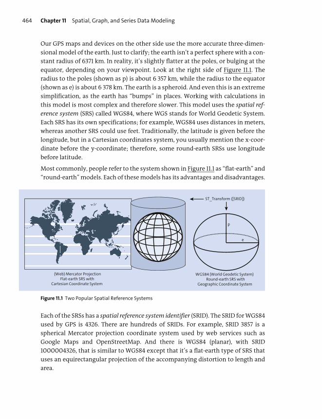
Chapter 11 Spatial, Graph, and Series Data Modeling464
Our GPS maps and devices on the other side use the more accurate three-dimen-
sional model of the earth. Just to clarify; the earth isn’t a perfect sphere with a con-
stant radius of 6371 km. In reality, it’s slightly flatter at the poles, or bulging at the
equator, depending on your viewpoint. Look at the right side of Figure 11.1. The
radius to the poles (shown as p) is about 6 357 km, while the radius to the equator
(shown as e) is about 6 378 km. The earth is a spheroid. And even this is an extreme
simplification, as the earth has “bumps” in places. Working with calculations in
this model is most complex and therefore slower. This model uses the spatial ref-
erence system (SRS) called WGS84, where WGS stands for World Geodetic System.
Each SRS has its own specifications; for example, WGS84 uses distances in meters,
whereas another SRS could use feet. Traditionally, the latitude is given before the
longitude, but in a Cartesian coordinates system, you usually mention the x-coor-
dinate before the y-coordinate; therefore, some round-earth SRSs use longitude
before latitude.
Most commonly, people refer to the system shown in Figure 11.1 as “flat-earth” and
“round-earth” models. Each of these models has its advantages and disadvantages.
Figure 11.1 Two Popular Spatial Reference Systems
Each of the SRSs has a spatial reference system identifier (SRID). The SRID for WGS84
used by GPS is 4326. There are hundreds of SRIDs. For example, SRID 3857 is a
spherical Mercator projection coordinate system used by web services such as
Google Maps and OpenStreetMap. And there is WGS84 (planar), with SRID
1000004326, that is similar to WGS84 except that it’s a flat-earth type of SRS that
uses an equirectangular projection of the accompanying distortion to length and
area.
(Web) Mercator ProjectionFlat-earth SRS with
Cartesian Coordinate System
p
e
WGS84 (World Geodetic System)
Geographic Coordinate SystemRound-earth SRS with
ST_Transform ([SRID])

Key Concepts Refresher Chapter 11 465
Tip
As a best practice, always specify the SRID when working with spatial data. Your assump-
tions don’t always work, and it’s easy to make mistakes when the SRID isn’t specified.
If your data is stored in the 4326 format, but you want to use it with data available
in these systems, you’ll need to transform your data to the 3857 format (or trans-
form the other data to 4326). You can do this using the ST_Transform function. We’ll
discuss spatial functions later in this section.
Sometimes you also need to transform your data to a different SRS if the spatial
functions you want to use don’t work in the SRS of your data. For example, some
of the spatial functions in SAP HANA don’t support round-earth SRSs. You’ll have
to transform your data to a planar SRS before calling those functions.
SPS 04
The spatial functions in SAP HANA that don’t support round-earth SRSs are decreasing
with every new release of SAP HANA.
SAP HANA also has a default SRS of 0, which is a two-dimensional (planar) system
that is strictly Cartesian without any relationship to the earth’s shape. This SRS can
be used, for instance, to reference a space of limited dimensions, such as an office
building, a factory, or a cornfield.
SPS 04
The in-memory representation of geometries in planar SRSs has been optimized and now
uses up to 50% less memory. This memory footprint reduction is important to lower the
total cost of ownership (TCO) for SAP HANA.
You need to specify the SRID when creating tables with spatial data in SAP HANA.
Creating Tables with Spatial Data
When you work with graphics programs on your computer, it often shows you the
position of your mouse or pen cursor with coordinates (x, y). Spatial data is often
also stored this way. Or your GPS shows you a point of interest (POI) such as a
restaurant as latitude and longitude, depending on what SRS it uses. This is similar
to (x, y).
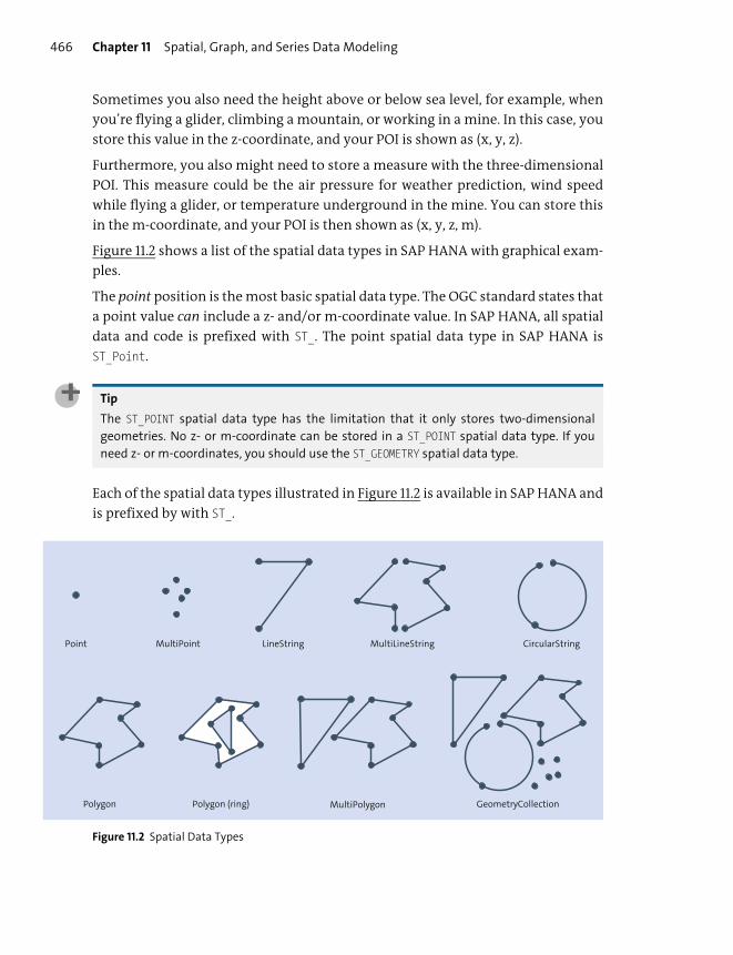
Chapter 11 Spatial, Graph, and Series Data Modeling466
Sometimes you also need the height above or below sea level, for example, when
you’re flying a glider, climbing a mountain, or working in a mine. In this case, you
store this value in the z-coordinate, and your POI is shown as (x, y, z).
Furthermore, you also might need to store a measure with the three-dimensional
POI. This measure could be the air pressure for weather prediction, wind speed
while flying a glider, or temperature underground in the mine. You can store this
in the m-coordinate, and your POI is then shown as (x, y, z, m).
Figure 11.2 shows a list of the spatial data types in SAP HANA with graphical exam-
ples.
The point position is the most basic spatial data type. The OGC standard states that
a point value can include a z- and/or m-coordinate value. In SAP HANA, all spatial
data and code is prefixed with ST_. The point spatial data type in SAP HANA is
ST_Point.
Tip
The ST_POINT spatial data type has the limitation that it only stores two-dimensional
geometries. No z- or m-coordinate can be stored in a ST_POINT spatial data type. If you
need z- or m-coordinates, you should use the ST_GEOMETRY spatial data type.
Each of the spatial data types illustrated in Figure 11.2 is available in SAP HANA and
is prefixed by with ST_.
Figure 11.2 Spatial Data Types
MultiLineString CircularStringLineStringMultiPointPoint
GeometryCollectionMultiPolygonPolygon Polygon (ring)

Key Concepts Refresher Chapter 11 467
Figure 11.3 shows the hierarchy of the spatial data types. The top data type is ST_
Geometry, and it’s a superset of all the other spatial data types.
The following list describes the spatial data types:
� ST_Geometry
This is the supertype for all the other spatial data types; you can store objects
such as linestrings, polygons, and circles in this data type. Then you can use the
TREAT expression to specify which data type you want to work with. For exam-
ple, TREAT( geometry1 AS ST_Polygon ).ST_Area() will take a geometry, treat it like
a polygon, and ask the size of the polygon’s area.
� ST_Point
A point is a single location in space with x- and y-coordinates at a minimum.
Points are often used to represent addresses, as in the shop example in Figure
11.4 in the next section.
� ST_LineString
A linestring is a line, which can be used to represent rivers, railroads, and roads.
In the shop example, it could represent a delivery route.
� ST_CircularString
A circularstring is a connected sequence of circular arc segments, much like a
linestring with circular arcs between points.
� ST_Polygon
A polygon defines an area. In the shop example, this is used to represent the
suburbs in the second table (see Figure 11.4 in the next section; most suburbs
don’t have regular square shapes).
� ST_MultiPoint
A multipoint is a collection of points. For example, it could represent all the dif-
ferent locations (addresses) where a company has shops.
� ST_MultiLineString
A multilinestring is a collection of linestrings. In the shop example, this collec-
tion could include all the deliveries that a shop has to make on a certain day for
which the driver goes to different customers or suppliers.
� ST_MultiPolygon
A multipolygon is a collection of polygons; for example, the suburbs could be
combined to indicate the area of the city or town.
� ST_GeometryCollection
A geometry collection is a collection of any of the spatial data types mentioned
in this list.

Chapter 11 Spatial, Graph, and Series Data Modeling468
Figure 11.3 Hierarchy of the Spatial Data Types
Now that you know the spatial data types, it’s easy to created tables using core data
services (CDS). In Listing 11.1 you can see the CDS code used for creating two exam-
ple tables. The first table stores the location of the shops or branches of a company.
In this case, ST_Point is OK because we only need the longitude and latitude of the
shops. The second table stores the shapes of all the suburbs in the city.
namespace spatial.spatialdb;
context spatialtables{
entity GEO_SHOP {key SHOP_ID: Integer not null;SHOP_NAME: hana.VARCHAR(100);SHOP_LOCATION: hana.ST_POINT;
};
entity GEO_SUBURB {key SUBURB_ID: Integer not null;SUBURB_NAME: hana.VARCHAR(100);SUBURB_SHAPE: hana.ST_GEOMETRY;
};};
Listing 11.1 CDS Syntax for Creating Two Tables with Spatial Data
We can now use these tables in our calculation views.
SPS 04
As from SAP HANA 2.0 SP 04, we can now also store spatial data in warm and cold storage
using native storage extension (NSE). We discussed data aging in Chapter 3. This helps to
lower the TCO for SAP HANA for customers with lots of spatial data.
ST_Geometry
ST_Point ST_LineString ST_CircularString ST_Polygon ST_GeometryCollection
ST_MultiPoint ST_MultiLineString TS_MultiPolygon
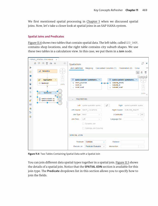
Key Concepts Refresher Chapter 11 469
We first mentioned spatial processing in Chapter 5 when we discussed spatial
joins. Now, let’s take a closer look at spatial joins in an SAP HANA system.
Spatial Joins and Predicates
Figure 11.4 shows two tables that contain spatial data. The left table, called GEO_SHOP,
contains shop locations, and the right table contains city suburb shapes. We use
these two tables in a calculation view. In this case, we put them in a Join node.
Figure 11.4 Two Tables Containing Spatial Data with a Spatial Join
You can join different data spatial types together in a spatial join. Figure 11.5 shows
the details of a spatial join. Notice that the SPATIAL JOIN section is available for this
join type. The Predicate dropdown list in this section allows you to specify how to
join the fields.
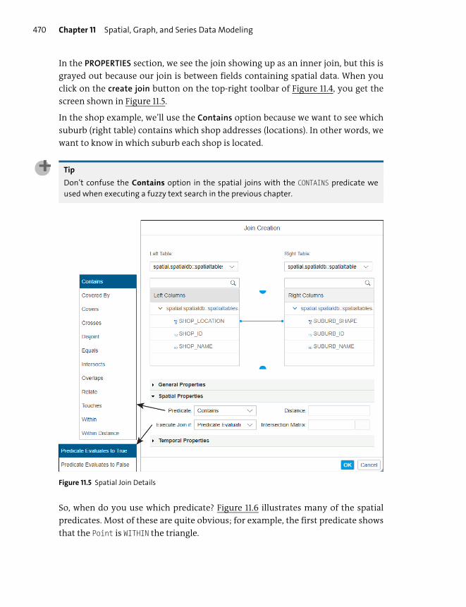
Chapter 11 Spatial, Graph, and Series Data Modeling470
In the PROPERTIES section, we see the join showing up as an inner join, but this is
grayed out because our join is between fields containing spatial data. When you
click on the create join button on the top-right toolbar of Figure 11.4, you get the
screen shown in Figure 11.5.
In the shop example, we’ll use the Contains option because we want to see which
suburb (right table) contains which shop addresses (locations). In other words, we
want to know in which suburb each shop is located.
Tip
Don’t confuse the Contains option in the spatial joins with the CONTAINS predicate we
used when executing a fuzzy text search in the previous chapter.
Figure 11.5 Spatial Join Details
So, when do you use which predicate? Figure 11.6 illustrates many of the spatial
predicates. Most of these are quite obvious; for example, the first predicate shows
that the Point is WITHIN the triangle.

Key Concepts Refresher Chapter 11 471
Figure 11.6 Spatial Predicates
There are a few things to watch out for though:
� We think of shapes as, for example, a triangle or an ellipse with a surface area.
There is the area of the shape and the exterior, which is everything outside the
shape. But there are actually three “areas” to watch out for. There is the inside
area, the exterior outside, and the boundary. Think of the boundary as the skin
around your body, separating your insides from the outside. A shape can have
more than one boundary; for example, a doughnut or ring shape has a round
boundary on the outside, as well as a round boundary on the inside for the hole.
Look at Figure 11.9 in the middle left to see an example of such a shape.
� The ST_Touches predicate is where another shape overlaps with one or more
points of the boundary but doesn’t overlap with any points inside. Hence,
returning to the analogy of thinking of the boundary as your skin, this is what
happens when someone touches you.
.ST_Within ( )
.ST_Disjoint ( )
.ST_Equals ( )
.ST_Crosses ( )
.ST_Touches ( )
.ST_Contains ( )
.ST_Intersects ( )
.ST_Overlaps ( )
.ST_Intersects ( )
.ST_Covers ( )
.ST_Contains ( ) = false
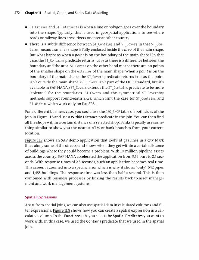
Chapter 11 Spatial, Graph, and Series Data Modeling472
� ST_Crosses and ST_Intersects is when a line or polygon goes over the boundary
into the shape. Typically, this is used in geospatial applications to see where
roads or railway lines cross rivers or enter another country.
� There is a subtle difference between ST_Contains and ST_Covers in that ST_Con-
tains means a smaller shape is fully enclosed inside the area of the main shape.
But what happens when a point is on the boundary of the main shape? In that
case, the ST_Contains predicate returns false as there is a difference between the
boundary and the area. ST_Covers on the other hand means there are no points
of the smaller shape on the exterior of the main shape. When a point is on the
boundary of the main shape, the ST_Covers predicate returns true as the point
isn’t outside the main shape. (ST_Covers isn’t part of the OGC standard, but it’s
available in SAP HANA.) ST_Covers extends the ST_Contains predicate to be more
“tolerant" for the boundaries. ST_Covers and the symmetrical ST_CoveredBy
methods support round-earth SRSs, which isn’t the case for ST_Contains and
ST_Within, which work only on flat SRSs.
For a different business case, you could use the GEO_SHOP table on both sides of the
join in Figure 11.5 and use a Within Distance predicate in the join. You can then find
all the shops within a certain distance of a selected shop. Banks typically use some-
thing similar to show you the nearest ATM or bank branches from your current
location.
Figure 11.7 shows an SAP demo application that looks at gas lines in a city (dark
lines along some of the streets) and shows when they get within a certain distance
of buildings where they could become a problem. With 10 million pipeline assets
across the country, SAP HANA accelerated the application from 3.5 hours to 2.5 sec-
onds. With response times of 2.5 seconds, such an application becomes real time.
This screen is zoomed into a specific area, which is why it shows “only” 642 pipes
and 1,455 buildings. The response time was less than half a second. This is then
combined with business processes by linking the results back to asset manage-
ment and work management systems.
Spatial Expressions
Apart from spatial joins, we can also use spatial data in calculated columns and fil-
ter expressions. Figure 11.8 shows how you can create a spatial expression in a cal-
culated column. In the Functions tab, you select the Spatial Predicates you want to
work with. In this case, we used the Contains predicate that we used in the spatial
join.
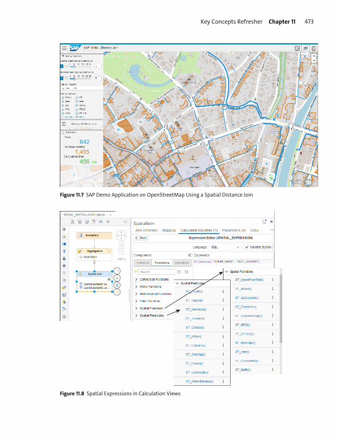
Key Concepts Refresher Chapter 11 473
Figure 11.7 SAP Demo Application on OpenStreetMap Using a Spatial Distance Join
Figure 11.8 Spatial Expressions in Calculation Views
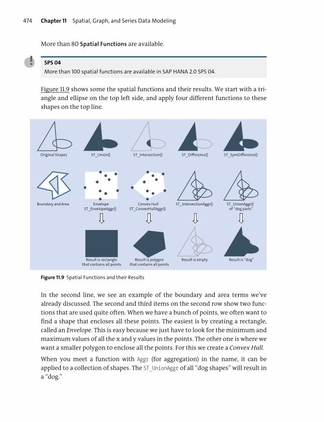
Chapter 11 Spatial, Graph, and Series Data Modeling474
More than 80 Spatial Functions are available.
SPS 04
More than 100 spatial functions are available in SAP HANA 2.0 SPS 04.
Figure 11.9 shows some the spatial functions and their results. We start with a tri-
angle and ellipse on the top left side, and apply four different functions to these
shapes on the top line.
Figure 11.9 Spatial Functions and their Results
In the second line, we see an example of the boundary and area terms we’ve
already discussed. The second and third items on the second row show two func-
tions that are used quite often. When we have a bunch of points, we often want to
find a shape that encloses all these points. The easiest is by creating a rectangle,
called an Envelope. This is easy because we just have to look for the minimum and
maximum values of all the x and y values in the points. The other one is where we
want a smaller polygon to enclose all the points. For this we create a Convex Hull.
When you meet a function with Aggr (for aggregation) in the name, it can be
applied to a collection of shapes. The ST_UnionAggr of all “dog shapes” will result in
a “dog.”
EnvelopeST_EnvelopeAggr()
Convex HullST_ConvexHullAggr()
Boundary and Area
ST_Union() ST_Intersection() ST_Difference() ST_SymDifference()Original Shapes
ST_IntersectionAggr() ST_UnionAggr()of “dog parts”
Result is “dog”Result is emptyResult is polygonthat contains all points
Result is rectanglethat contains all points

Key Concepts Refresher Chapter 11 475
Geocoding in an SAP HANA Flowgraph
Geocoding is the process of converting address information into geographic loca-
tions, such as latitude and longitude. Because business data is associated with
address information without location information, geocoding is important to
enable geographic analysis of such address data. In many businesses, huge value is
unlocked by using this additional type of analysis.
Reverse geocoding does exactly the reverse, as the name implies. It takes geospa-
tial data such as latitude and longitude, tells you what company is located there,
and returns the address data.
This functionality needs a geocoding index. This is very similar to the full-text
index we already discussed in the previous chapter, except that we work with
address and geospatial data instead of text data.
SAP HANA smart data quality, that we discussed in Chapter 9, provides native
geocoding and reverse geocoding capabilities in SAP Web IDE for SAP HANA. This
can be accessed with a Geocode node in a graphical flowgraph model. In Figure
11.10, we combined the Geocode node in an SAP HANA smart data quality workflow
that also includes data cleansing.
Figure 11.10 Flowgraph Model with a Geocode Node
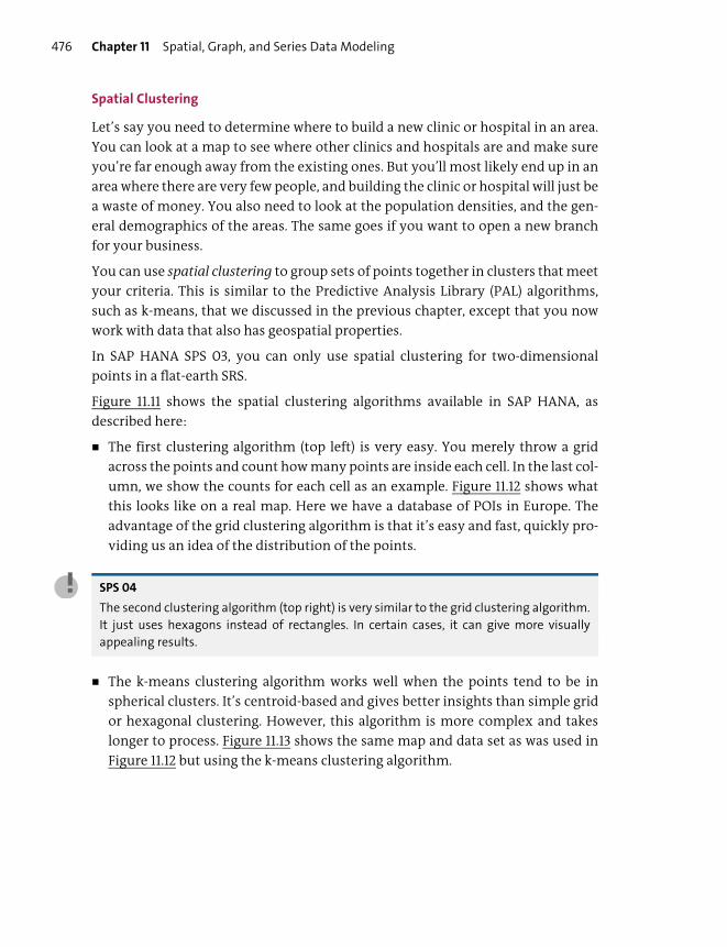
Chapter 11 Spatial, Graph, and Series Data Modeling476
Spatial Clustering
Let’s say you need to determine where to build a new clinic or hospital in an area.
You can look at a map to see where other clinics and hospitals are and make sure
you’re far enough away from the existing ones. But you’ll most likely end up in an
area where there are very few people, and building the clinic or hospital will just be
a waste of money. You also need to look at the population densities, and the gen-
eral demographics of the areas. The same goes if you want to open a new branch
for your business.
You can use spatial clustering to group sets of points together in clusters that meet
your criteria. This is similar to the Predictive Analysis Library (PAL) algorithms,
such as k-means, that we discussed in the previous chapter, except that you now
work with data that also has geospatial properties.
In SAP HANA SPS 03, you can only use spatial clustering for two-dimensional
points in a flat-earth SRS.
Figure 11.11 shows the spatial clustering algorithms available in SAP HANA, as
described here:
� The first clustering algorithm (top left) is very easy. You merely throw a grid
across the points and count how many points are inside each cell. In the last col-
umn, we show the counts for each cell as an example. Figure 11.12 shows what
this looks like on a real map. Here we have a database of POIs in Europe. The
advantage of the grid clustering algorithm is that it’s easy and fast, quickly pro-
viding us an idea of the distribution of the points.
SPS 04
The second clustering algorithm (top right) is very similar to the grid clustering algorithm.
It just uses hexagons instead of rectangles. In certain cases, it can give more visually
appealing results.
� The k-means clustering algorithm works well when the points tend to be in
spherical clusters. It’s centroid-based and gives better insights than simple grid
or hexagonal clustering. However, this algorithm is more complex and takes
longer to process. Figure 11.13 shows the same map and data set as was used in
Figure 11.12 but using the k-means clustering algorithm.

Key Concepts Refresher Chapter 11 477
� The DBSCAN clustering algorithm works best with nonspherical clusters. It’s
density-based, meaning it requires a certain number of data points in the neigh-
borhood of a point. You can set the radius of the neighborhood.
Figure 11.11 Spatial Clustering Algorithms
Figure 11.12 shows the grid clustering algorithm used on a map of Europe with a
database of POIs, such as restaurants, museums, hospitals, schools, ATMs, and
public transport. You can choose which type of POI you want, zoom into the area
you plan to visit, and choose the spatial clustering algorithm to analyze the data
for that area and POI category.
Figure 11.13 shows the same map but using the k-means clustering algorithm.
Hexagonal Grid (from SPS 04)
DBSCAN
Rectangular Grid
5
2
3
0
2
4
1
0
K-means
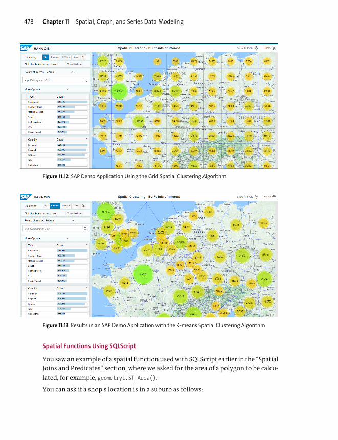
Chapter 11 Spatial, Graph, and Series Data Modeling478
Figure 11.12 SAP Demo Application Using the Grid Spatial Clustering Algorithm
Figure 11.13 Results in an SAP Demo Application with the K-means Spatial Clustering Algorithm
Spatial Functions Using SQLScript
You saw an example of a spatial function used with SQLScript earlier in the “Spatial
Joins and Predicates” section, where we asked for the area of a polygon to be calcu-
lated, for example, geometry1.ST_Area().
You can ask if a shop’s location is in a suburb as follows:
Key Concepts Refresher Chapter 11 479
SUBURB_SHAPE.ST_CONTAINS(SHOP_LOCATION1)
You can also see how far two shops are from each other as follows:
SHOP_LOCATION1.ST_WITHINDISTANCE(SHOP_LOCATION2)
You can use a spatial join with the ST_Within predicate. When ST_Within returns 1,
it means shape b is inside shape a, as follows:
SELECT b.id as b_within, a.name, a.shape, b.point FROM A, B WHERE b.point.ST_Within( a.shape ) = 1;
If you want to find all the shapes that aren’t within shape a, you just use a spatial
join where ST_Within returns 0, as follows:
SELECT b.id as b_not_within, a.name, a.shape, b.point FROM A, B WHERE b.point.ST_Within( a.shape ) = 0;
You can see that the spatial functions are used like methods in object orientation,
using a dot-notation.
Note
You can find all the spatial functions and their descriptions in the SAP HANA Spatial Ref-
erence guide at http://s-prs.co/v487620.
A software development kit (SDK) is also available that you can use to create your
own custom geospatial algorithms.
Importing and Exporting Spatial Data
In SAP HANA, you can import and export spatial data in the Well-Known Text
(WKT) and the Well-Known Binary (WKB) formats. These formats are part of the
OGC standards. You can also import and export the extended versions of these for-
mats, which are used by PostGIS: Extended Well-Known Text (EWKT) and
Extended Well-Known Binary (EWKB).
In addition, SAP HANA can import all ESRI shapefiles, except the MultiPatch shape
type. SAP HANA can export spatial data in the GeoJSON and Scalable Vector
Graphic (SVG) file formats. The SVG file format is maintained by World Wide Web
Consortium (W3C) and is supported by all modern browsers.

Chapter 11 Spatial, Graph, and Series Data Modeling480
Sometimes you get public spatial data in comma-separated values (CSV) files. As
we discussed before, you can import these using CDS .hdbtabledata files or using
SAP Web IDE for SAP HANA in SAP HANA 2.0 SPS 04.
SAP HANA Spatial Services
In 2018, SAP released a set of spatial services on the cloud. These services include
weather information, earth observation, and satellite imagery, for example, from
the European Space Agency (ESA). You can subscribe to these SAP HANA spatial
services and call them using application programming interfaces (APIs). You can
find more information at http://s-prs.co/v487603.
You can use this set of services, for example, in agricultural scenarios to look at sat-
ellite imagery of biomass. This gives you an excellent overview of how fast crops
are growing or where there are problem areas caused by insects or plant diseases.
Crop insurers can use this information to assess their risk, farmers can use it to cal-
culate crop forecasts, and governments can use it to plan food security.
SPS 04
SAP HANA spatial services is now available inside GeoTools. GeoTools is a free open-
source GIS toolkit that is used by many open-source and commercial software projects.
GeoServer is one of the prominent server-side geoprocessing and data access software
tools that uses GeoTools. These tools can now all access and serve geodata stored in SAP
HANA.
Note
To learn more about spatial processing in SAP HANA, look at the examples in the SAP
HANA Interactive Education (SHINE) demo content. Here, you can find many examples of
spatial processes; for example, screens in which you can select shops on a map on the left
of the screen and see their sales details in the area on the right.
You can find more information about spatial data in the SAP HANA Spatial Reference
Guide. There is also an openSAP course called “Spatial Analysis with SAP HANA Platform”
at http://s-prs.co/v487628 from mid-2017. There is also an SAP HANA Academy playlist for
spatial analysis on YouTube at http://s-prs.co/v487604.
Graph Modeling
Next, we’ll discuss graph processing. In this case, we’re not talking about reporting
graphs, which can be thought of as charts. Instead, think about social media
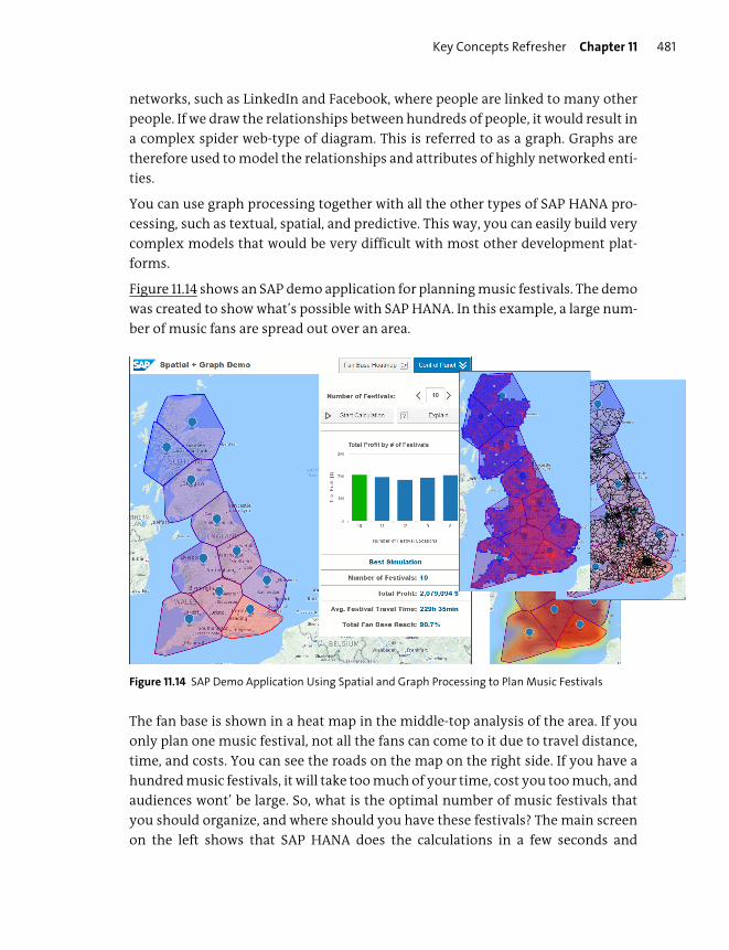
Key Concepts Refresher Chapter 11 481
networks, such as LinkedIn and Facebook, where people are linked to many other
people. If we draw the relationships between hundreds of people, it would result in
a complex spider web-type of diagram. This is referred to as a graph. Graphs are
therefore used to model the relationships and attributes of highly networked enti-
ties.
You can use graph processing together with all the other types of SAP HANA pro-
cessing, such as textual, spatial, and predictive. This way, you can easily build very
complex models that would be very difficult with most other development plat-
forms.
Figure 11.14 shows an SAP demo application for planning music festivals. The demo
was created to show what’s possible with SAP HANA. In this example, a large num-
ber of music fans are spread out over an area.
Figure 11.14 SAP Demo Application Using Spatial and Graph Processing to Plan Music Festivals
The fan base is shown in a heat map in the middle-top analysis of the area. If you
only plan one music festival, not all the fans can come to it due to travel distance,
time, and costs. You can see the roads on the map on the right side. If you have a
hundred music festivals, it will take too much of your time, cost you too much, and
audiences wont’ be large. So, what is the optimal number of music festivals that
you should organize, and where should you have these festivals? The main screen
on the left shows that SAP HANA does the calculations in a few seconds and
Chapter 11 Spatial, Graph, and Series Data Modeling482
suggests 10 festivals at the places shown. It also generates a heat map (middle-bot-
tom map) of the traffic patterns that your music festivals will create.
In this demo, we have spatial data with the locations of where the music fans stay
and where we’ll have the festivals. We also have graph data in the form of the
roads, linking various spatial locations together. We also have to combine this
with business data, such as how far are fans prepared to travel, how much should
the tickets be, what does a music festival cost the organizers, and how much time
is involved with organizing and running such events.
To understand the process of how to create graph models, we’ll start with a small
example of a group of people. From a sketch, we’ll see how to create this in SAP
HANA. After we’ve created the graph, we can view and analyze it using various
graph algorithms. With this background, it will be easy to implement it into a cal-
culation view. We’ll close off the topic by looking at two graph query languages
available in SAP HANA and how graphs are different from hierarchies.
Creating Graphs in SAP HANA
Graph processing allows you to discover patterns in real time on large volumes of
data, which is something that isn’t possible for humans. We can query the graph to
find answers to questions such as the following:
� What are the chances of two specific people going on a date?
� Who is the best person to connect with on LinkedIn to get contact with a buyer?
� In this region, what are the best products to sell to people according to their
likes and dislikes on Facebook?
You could develop such queries using standard SQL, but it would be very complex,
and the performance would probably be really bad. A lot of specialized graph data-
bases have appeared over the past five years. The disadvantage of such specialized
databases is that it becomes difficult to combine it with other data and business
information to solve wider problems and create more powerful solutions.
SAP HANA has, in addition to all its other features, a special graph-processing
engine to handle graph queries elegantly and fast. In SAP HANA 2.0, you can query
the graph data using graphical calculation views, the Cypher Query Language
(Cypher), or GraphScript.
LinkedIn makes suggestions of who you can connect with next based on the peo-
ple you’re currently connected with and who they are connected with. They need
some form of graph processing to do this. It’s quite complex because people work

Key Concepts Refresher Chapter 11 483
for companies, some people are looking for new jobs, other people want to show
their thought leadership, some want to advertise their products and services, and
yet others want to recruit someone for a position at another company. People
have different roles and needs, and this shapes the different types of relationships.
For us to understand graph processing, we’ll use a much smaller example. Figure
11.15 shows an example of a few colleagues and their various relationships. The col-
leagues are obviously also working for SAP. There is an organizational structure in
the company with reporting lines. Most of the colleagues are married. Even in this
small group, we already see at least three different types of relationships, and we
have two types of entities: a company and people.
With this small group, we can draw the relationships in a diagram. However, when
we look at hundreds of millions of relationships—such as those on LinkedIn—
drawing such a diagram obviously becomes impractical.
Figure 11.15 Graph Diagram Showing Relationships
Let’s assume we wanted to analyze this graph. We first need to put the data into the
SAP HANA system. For this, you’ll need a table with the people and the company.
These are the nodes in the graph, as illustrated in Figure 11.15. These nodes are
called vertices and are stored in a normal SAP HANA column table. Each vertex can
have multiple attributes, for example, whether this node is a person or a company,
whether the person is male or female, the age of the person, and so on. These attri-
butes are simply additional fields in the column table.
Tshepo
Lerato
Sikhumbuzo Phillip
Hans-Joachim
SAPMichelle
Kele
Person
Company
Works for
Reports to
Married to

Chapter 11 Spatial, Graph, and Series Data Modeling484
In another table, we store the relationships, such as the existing “friends” relation-
ships between these people. These relationships are called edges and are also
stored in column tables. You can have different types of relationships between
people. In Figure 11.15, we have “married to,” which is a bidirectional relationship,
and “works for,” which only has a single direction. The direction of the “works for”
relationship is “outgoing” for the employee of the company and “incoming” for
the company.
The nodes are the people and the company, and the lines are the relationships. The
lines can have flow direction, meaning we can run traces, such as the reporting
lines in a company. From this, we can deduce the organizational structure. In this
case, it would be similar to a hierarchy. But these lines can also flow in “circles,” or
in both directions, which would not be allowed in hierarchies.
The direction of a relationship is determined by the “source” and “target” attri-
butes. For example, the “works for” relationship has the employee’s name in the
“source” field, and the company’s name in the “target” field. While this sounds
very specific, just remember that many tables in a normal business system fit this
pattern. In commercial systems, when you ship a product to someone, you have
pickup and delivery addresses. When you fly, you have departure and arrival air-
ports. Any table with “from” and “to” fields is usable. Even normal SAP HANA
views with financial data according to time periods—with start and end dates—
can be used. Even if a table doesn’t exactly have this format, you can create a view
that does and use the view for the graph processing.
Tip
It’s important to realize that you can use normal tables and information views for graph
processing in SAP HANA with your current business data. You don’t need a separate spe-
cialized database or tables for graph processing when using SAP HANA.
You can use the attributes in vertices and edges when querying the graph. Remem-
ber that these attributes are the additional fields in the database tables or views.
The important piece that you need to enable the graph processing in SAP HANA is
a graph workspace. A graph workspace is a simple file that links the vertex table to
the edge table.
Note
The graph workspace simply contains the definition of the graph model and how the ver-
tices and edge tables relate to each other.

Key Concepts Refresher Chapter 11 485
Building the Graph Tables and Workspace
Now that you have an idea of how SAP HANA enables graph processing, let’s create
the graph for Figure 11.15 and then use SAP HANA to analyze it. This simple exam-
ple will make it easy for you to understand the entire process.
We already know that we need two tables: a vertex table for the nodes and an edge
table for the relationships.
In Figure 11.15 we have two types of nodes: people and the company. All the nodes
have a name. Our vertex table therefore just needs two fields: the NAME and the
TYPE. This table is defined in the CDS table definition in Listing 11.2 and is called
MEMBERS. In our case, the names are unique, so we can use the NAME field as the key
field. Otherwise, we would have had to add a key field with unique values for each
record.
The RELATIONSHIPS table needs SOURCE and TARGET fields. Both fields simply use the
NAME (key field) of the person or company from the MEMBERS vertex table. We also
need to specify the TYPE of relationship, for example, “works for.” And we add a KEY
field.
namespace graph.graphteam;
context team{
entity MEMBERS {key NAME: hana.VARCHAR(100) not null;TYPE: hana.VARCHAR(100);
};
entity RELATIONSHIPS {key KEY: Integer not null;SOURCE: hana.VARCHAR(100) not null;TARGET: hana.VARCHAR(100) not null;RELATIONSHIP: hana.VARCHAR(100);
};
};
Listing 11.2 CDS Code to Create Tables for Vertices (Members) and Edges (Relationships)
After you’ve created your .hdbcds file, build it to create the two tables.
The next file we need is an .hdbworkspace file to create the graph workspace. This
is a database artifact file. Listing 11.3 shows how to define the workspace file.
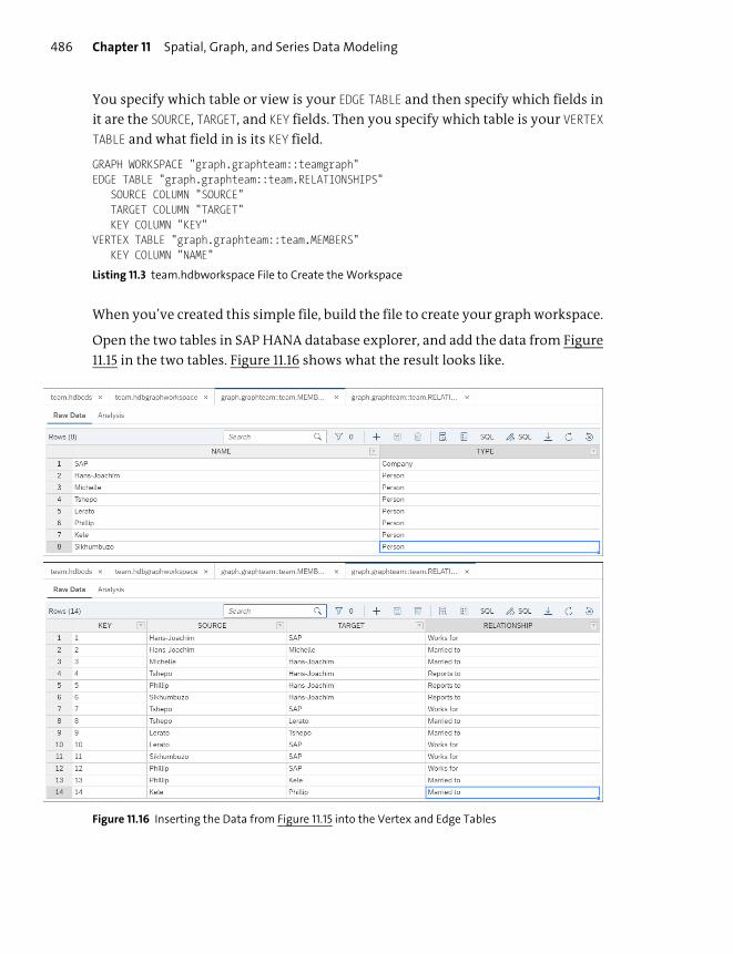
Chapter 11 Spatial, Graph, and Series Data Modeling486
You specify which table or view is your EDGE TABLE and then specify which fields in
it are the SOURCE, TARGET, and KEY fields. Then you specify which table is your VERTEX
TABLE and what field in is its KEY field.
GRAPH WORKSPACE "graph.graphteam::teamgraph"EDGE TABLE "graph.graphteam::team.RELATIONSHIPS"
SOURCE COLUMN "SOURCE"TARGET COLUMN "TARGET"KEY COLUMN "KEY"
VERTEX TABLE "graph.graphteam::team.MEMBERS"KEY COLUMN "NAME"
Listing 11.3 team.hdbworkspace File to Create the Workspace
When you’ve created this simple file, build the file to create your graph workspace.
Open the two tables in SAP HANA database explorer, and add the data from Figure
11.15 in the two tables. Figure 11.16 shows what the result looks like.
Figure 11.16 Inserting the Data from Figure 11.15 into the Vertex and Edge Tables

Key Concepts Refresher Chapter 11 487
You’ve now built your first graph in SAP HANA. Next, we’ll view and analyze your
graph.
Viewing and Analyzing Graphs
You used the SAP HANA database explorer to insert data into the vertex and edge
tables. On the top left area, look for the Graph Workspaces, as shown in Figure 11.17.
This shows the list of graph workspaces in your SAP HANA Deployment Infrastruc-
ture (HDI) container. Right-click on your workspace, and select the View Graph
option.
Figure 11.17 Using the SAP HANA Database Explorer to View Graphs
Your graph will now show in the area on the right in SAP Web IDE for SAP HANA.
You can rearrange the nodes to appear where you want them. When you compare
the graph shown in Figure 11.18, you’ll see that this is exactly what we had in Figure
11.15!
To get the names on the edges (relationships), use the Options icon in the top-right
corner, and set the Edge label.
Tip
The SAP HANA Graph Reference Guide and some blogs refer to an SAP HANA Graph
Viewer that you install via SAP HANA Studio. You don’t need that because this graph
viewer is built in to the SAP HANA database explorer in SAP Web IDE for SAP HANA.
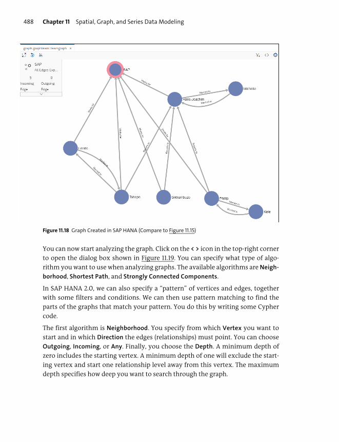
Chapter 11 Spatial, Graph, and Series Data Modeling488
Figure 11.18 Graph Created in SAP HANA (Compare to Figure 11.15)
You can now start analyzing the graph. Click on the < > icon in the top-right corner
to open the dialog box shown in Figure 11.19. You can specify what type of algo-
rithm you want to use when analyzing graphs. The available algorithms are Neigh-
borhood, Shortest Path, and Strongly Connected Components.
In SAP HANA 2.0, we can also specify a “pattern” of vertices and edges, together
with some filters and conditions. We can then use pattern matching to find the
parts of the graphs that match your pattern. You do this by writing some Cypher
code.
The first algorithm is Neighborhood. You specify from which Vertex you want to
start and in which Direction the edges (relationships) must point. You can choose
Outgoing, Incoming, or Any. Finally, you choose the Depth. A minimum depth of
zero includes the starting vertex. A minimum depth of one will exclude the start-
ing vertex and start one relationship level away from this vertex. The maximum
depth specifies how deep you want to search through the graph.
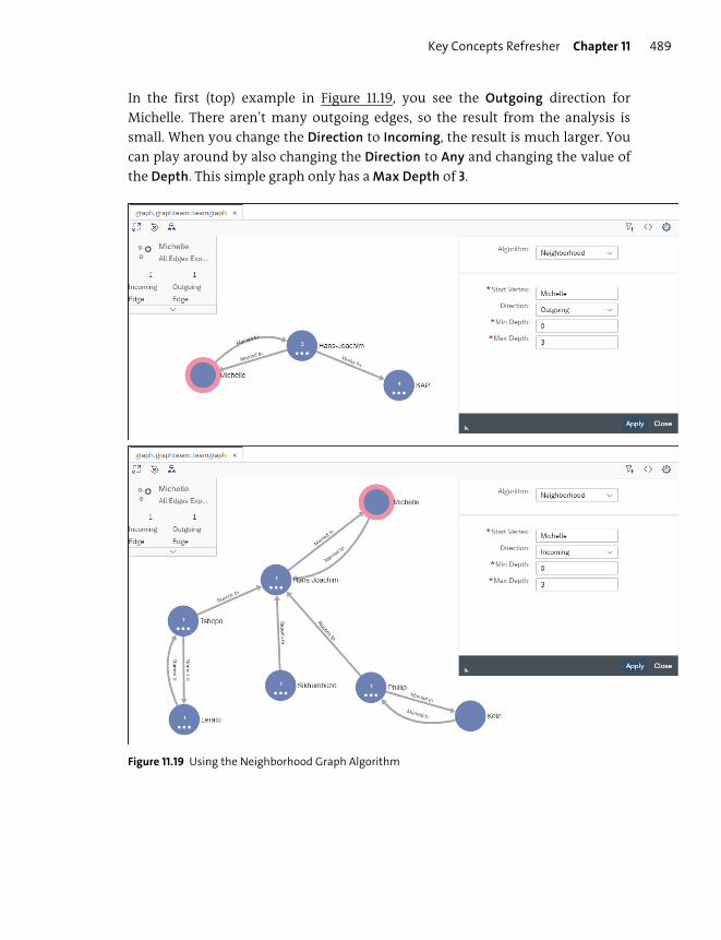
Key Concepts Refresher Chapter 11 489
In the first (top) example in Figure 11.19, you see the Outgoing direction for
Michelle. There aren’t many outgoing edges, so the result from the analysis is
small. When you change the Direction to Incoming, the result is much larger. You
can play around by also changing the Direction to Any and changing the value of
the Depth. This simple graph only has a Max Depth of 3.
Figure 11.19 Using the Neighborhood Graph Algorithm
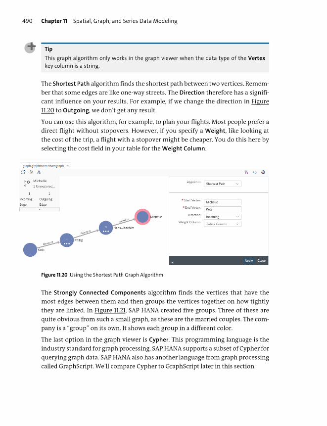
Chapter 11 Spatial, Graph, and Series Data Modeling490
Tip
This graph algorithm only works in the graph viewer when the data type of the Vertexkey column is a string.
The Shortest Path algorithm finds the shortest path between two vertices. Remem-
ber that some edges are like one-way streets. The Direction therefore has a signifi-
cant influence on your results. For example, if we change the direction in Figure
11.20 to Outgoing, we don’t get any result.
You can use this algorithm, for example, to plan your flights. Most people prefer a
direct flight without stopovers. However, if you specify a Weight, like looking at
the cost of the trip, a flight with a stopover might be cheaper. You do this here by
selecting the cost field in your table for the Weight Column.
Figure 11.20 Using the Shortest Path Graph Algorithm
The Strongly Connected Components algorithm finds the vertices that have the
most edges between them and then groups the vertices together on how tightly
they are linked. In Figure 11.21, SAP HANA created five groups. Three of these are
quite obvious from such a small graph, as these are the married couples. The com-
pany is a “group” on its own. It shows each group in a different color.
The last option in the graph viewer is Cypher. This programming language is the
industry standard for graph processing. SAP HANA supports a subset of Cypher for
querying graph data. SAP HANA also has another language from graph processing
called GraphScript. We’ll compare Cypher to GraphScript later in this section.

Key Concepts Refresher Chapter 11 491
Figure 11.21 Using the Strongly Connected Components Graph Algorithm
We won’t teach Cypher in this book, but we’ll show you an example so you can get
a feel for it. Listing 11.4 shows the Cypher code for showing the incoming edges to
the SAP vertex. In this case, we could have achieved the same by using the Neigh-
borhood graph algorithm, specifying “SAP” as the Start Vertex, and choosing
Incoming as the Direction. But, of course, you’ll use Cypher for cases where the
other algorithms don’t provide what you’re looking for.
MATCH (a)-[e]->(b)WHERE b.NAME = 'SAP'RETURN a.NAME AS name, e.RELATIONSHIP as relation
Listing 11.4 Cypher Code to Get All Relationships Going to “SAP”
Figure 11.22 shows the result of our Cypher code.
Now that you’ve seen and played with the graph viewer, working with the Graph
node in calculation views will be easy.
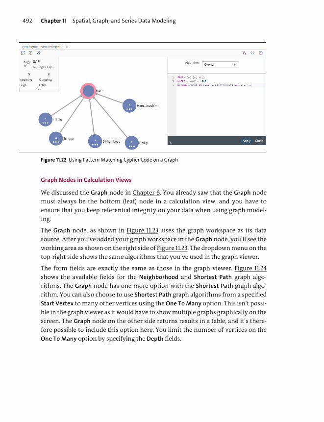
Chapter 11 Spatial, Graph, and Series Data Modeling492
Figure 11.22 Using Pattern Matching Cypher Code on a Graph
Graph Nodes in Calculation Views
We discussed the Graph node in Chapter 6. You already saw that the Graph node
must always be the bottom (leaf) node in a calculation view, and you have to
ensure that you keep referential integrity on your data when using graph model-
ing.
The Graph node, as shown in Figure 11.23, uses the graph workspace as its data
source. After you’ve added your graph workspace in the Graph node, you’ll see the
working area as shown on the right side of Figure 11.23. The dropdown menu on the
top-right side shows the same algorithms that you’ve used in the graph viewer.
The form fields are exactly the same as those in the graph viewer. Figure 11.24
shows the available fields for the Neighborhood and Shortest Path graph algo-
rithms. The Graph node has one more option with the Shortest Path graph algo-
rithm. You can also choose to use Shortest Path graph algorithms from a specified
Start Vertex to many other vertices using the One To Many option. This isn’t possi-
ble in the graph viewer as it would have to show multiple graphs graphically on the
screen. The Graph node on the other side returns results in a table, and it’s there-
fore possible to include this option here. You limit the number of vertices on the
One To Many option by specifying the Depth fields.
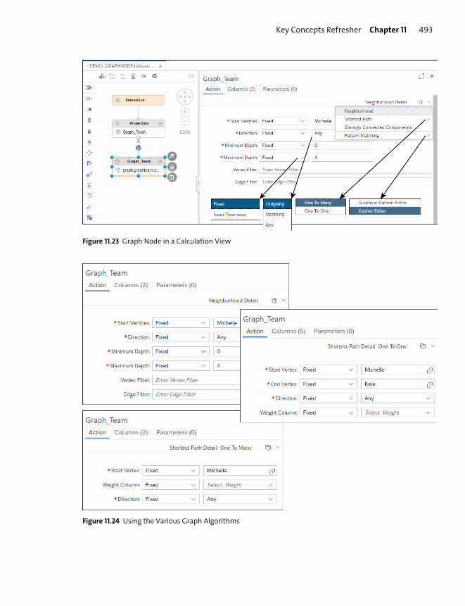
Key Concepts Refresher Chapter 11 493
Figure 11.23 Graph Node in a Calculation View
Figure 11.24 Using the Various Graph Algorithms

Chapter 11 Spatial, Graph, and Series Data Modeling494
The Strongly Connected Components graph algorithm doesn’t have any properties
or form fields.
After you’ve specified some properties for your Graph node, you need to Save and
Build your calculation view. You can then do a Data Preview of the results.
Figure 11.25 shows the Properties area for the Strongly Connected Components
graph algorithm, as well as the result after a build. You’ll notice that the results are
the same as what we got in the graph viewer earlier in Figure 11.21.
Figure 11.25 Strongly Connected Components Graph Algorithm and Results
Tip
It makes sense to use the graph viewer when exploring the possibilities. After you know
what you’re looking for, you can create the Graph node. The Graph node isn’t as conve-
nient for exploring possibilities because you have to do a Save, Build, and Data Previewfor each round. After you know what you need, it’s much better at using the results
together with other business data in a calculation view.
Lastly, we can use the same Cypher code from Listing 11.4 in the Cypher editor of
the Graph node, as shown in Figure 11.26. The results, in table format instead of
graphical, are the same as those shown earlier in Figure 11.22.
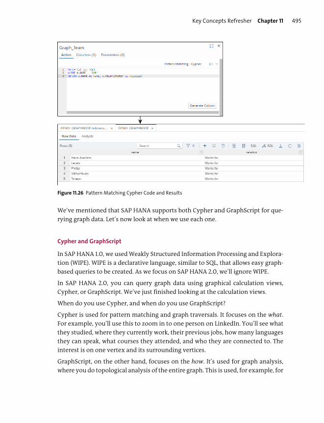
Key Concepts Refresher Chapter 11 495
Figure 11.26 Pattern Matching Cypher Code and Results
We’ve mentioned that SAP HANA supports both Cypher and GraphScript for que-
rying graph data. Let’s now look at when we use each one.
Cypher and GraphScript
In SAP HANA 1.0, we used Weakly Structured Information Processing and Explora-
tion (WIPE). WIPE is a declarative language, similar to SQL, that allows easy graph-
based queries to be created. As we focus on SAP HANA 2.0, we’ll ignore WIPE.
In SAP HANA 2.0, you can query graph data using graphical calculation views,
Cypher, or GraphScript. We’ve just finished looking at the calculation views.
When do you use Cypher, and when do you use GraphScript?
Cypher is used for pattern matching and graph traversals. It focuses on the what.
For example, you’ll use this to zoom in to one person on LinkedIn. You’ll see what
they studied, where they currently work, their previous jobs, how many languages
they can speak, what courses they attended, and who they are connected to. The
interest is on one vertex and its surrounding vertices.
GraphScript, on the other hand, focuses on the how. It’s used for graph analysis,
where you do topological analysis of the entire graph. This is used, for example, for
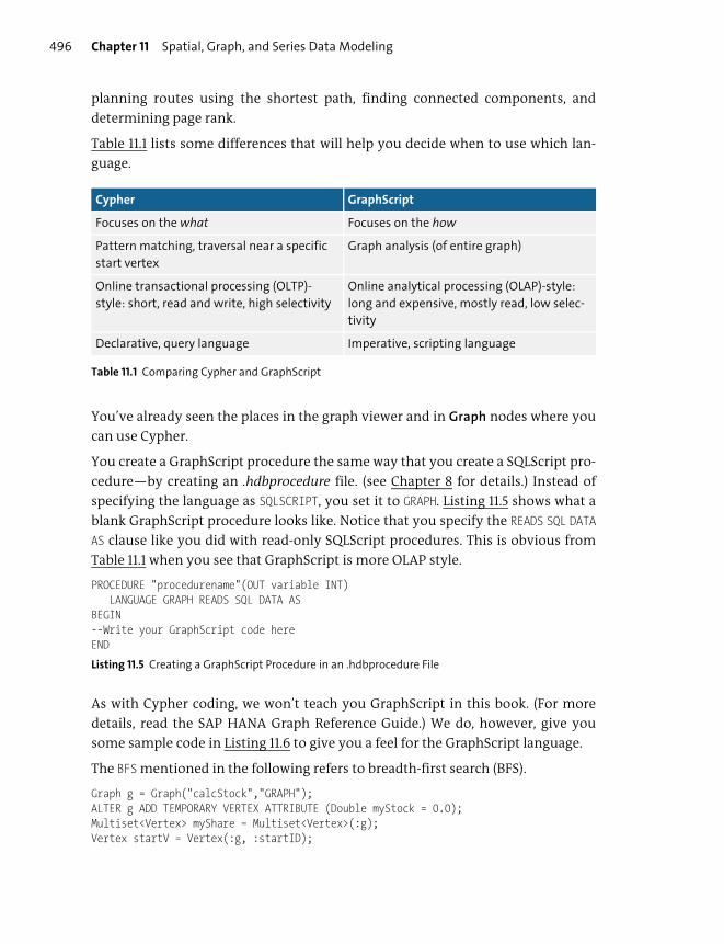
Chapter 11 Spatial, Graph, and Series Data Modeling496
planning routes using the shortest path, finding connected components, and
determining page rank.
Table 11.1 lists some differences that will help you decide when to use which lan-
guage.
You’ve already seen the places in the graph viewer and in Graph nodes where you
can use Cypher.
You create a GraphScript procedure the same way that you create a SQLScript pro-
cedure—by creating an .hdbprocedure file. (see Chapter 8 for details.) Instead of
specifying the language as SQLSCRIPT, you set it to GRAPH. Listing 11.5 shows what a
blank GraphScript procedure looks like. Notice that you specify the READS SQL DATA
AS clause like you did with read-only SQLScript procedures. This is obvious from
Table 11.1 when you see that GraphScript is more OLAP style.
PROCEDURE "procedurename"(OUT variable INT)LANGUAGE GRAPH READS SQL DATA AS
BEGIN--Write your GraphScript code hereEND
Listing 11.5 Creating a GraphScript Procedure in an .hdbprocedure File
As with Cypher coding, we won’t teach you GraphScript in this book. (For more
details, read the SAP HANA Graph Reference Guide.) We do, however, give you
some sample code in Listing 11.6 to give you a feel for the GraphScript language.
The BFS mentioned in the following refers to breadth-first search (BFS).
Graph g = Graph("calcStock","GRAPH");ALTER g ADD TEMPORARY VERTEX ATTRIBUTE (Double myStock = 0.0);Multiset<Vertex> myShare = Multiset<Vertex>(:g);Vertex startV = Vertex(:g, :startID);
Cypher GraphScript
Focuses on the what Focuses on the how
Pattern matching, traversal near a specific
start vertex
Graph analysis (of entire graph)
Online transactional processing (OLTP)-
style: short, read and write, high selectivity
Online analytical processing (OLAP)-style:
long and expensive, mostly read, low selec-
tivity
Declarative, query language Imperative, scripting language
Table 11.1 Comparing Cypher and GraphScript

Key Concepts Refresher Chapter 11 497
TRAVERSE BFS :g FROM :startVON VISIT EDGE (Edge e, Bigint levels) {Vertex s = SOURCE(:e);Vertex v = TARGET(:e);if (:levels == 0L) { v.myStock = :e.myStock; }else { v.myStock = :v.myStock + :s.myStock; }if (:v.myStock >= 25.0) {
myShare = :myShare UNION {:v};}
};
Listing 11.6 Sample GraphScript Code
SPS 04
In SAP HANA 2.0 SPS 04, the SAP HANA graph engine can now be used directly in SQL sub-
queries using the OPENCYPHER_TABLE function. The information is returned in JSON format.
GraphScript has been expanded in SPS 04 and includes new algorithms. You can now also
use virtual tables with GraphScript, which extends the reach of GraphScript to many
other databases and federated data sources. (See the SAP HANA Smart Data Access sec-
tion in Chapter 9.) You can now also use GraphScript for processing ad hoc graphs on
data structures without having to first create a graph workspace.
Graphs versus Hierarchies
In Chapter 7, we spent a lot of time explaining the hierarchy functionality in SAP
HANA calculation views. In many cases, graphs and hierarchies can look very sim-
ilar. In Table 11.2 is a short summary to help you choose between hierarchies and
graphs.
Hierarchy Graph
Uses standard SQL, ad hoc hierarchies, and
SQL views
Uses domain-specific languages such as
GraphScript and Cypher
Data often in a single table, including a
single edge type (e.g., “parent”)
Needs two tables for vertices and edges
with a clear distinction between them
Uses a graph workspace to link them
together
Few predefined traversal algorithms in SQL Powerful pattern matching queries
Optimized for tree topology—strictly
top-down
Generic graph topology—can have “cyclical”
occurrences
Table 11.2 Differences between Hierarchies and Graphs
Chapter 11 Spatial, Graph, and Series Data Modeling498
Note
You can learn more about SAP HANA graph processing in the SAP HANA Graph Reference
Guide. There is an openSAP course from mid-2018 on graph processing called “Analyzing
Connected Data with SAP HANA Graph” at http://s-prs.co/v487629. And, of course, there
are videos on the topic on YouTube in the SAP HANA Academy channel.
Series Data Modeling
When searching for information on series data, you’ll notice that it’s normally
referred to as “time series” data. SAP HANA uses “series data” because it can also
include any data in a series form, including events and transactions. Time series
data is often associated with the Internet of Things (IoT), where sensors capture
and send out monitoring or event data. However, series data can also include data
such as database log files.
In the database world, interest in the topic of time series databases has seen the
most growth of all types of databases over the past two years. At http://s-prs.co/
v487630, you can scroll down the page to see the Trend of the last 24 months. Time
series databases have clearly seen the fastest growth in interest. Many new data-
bases were released into the market that focus exclusively on time series data.
Many of them basically store the data using a label (or “tag”) with key–value pairs.
This is typical for many NoSQL databases.
We’ll just provide an overview on the topic. You can combine series data with
aggregation, analysis, and predictive modeling to create valuable insights into
real-world operations.
Series Data in Everyday Life
Let’s say you want to keep track of your weight. Every morning after waking up,
you joyfully jump on the bathroom scale and record your weight. After a while, the
data will look something like that shown in Table 11.3.
You’ve created a time series. The series data is a sequence of regular measurements
taken over a period of time.
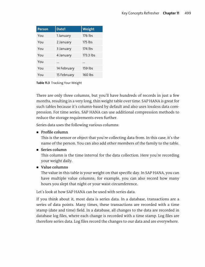
Key Concepts Refresher Chapter 11 499
There are only three columns, but you’ll have hundreds of records in just a few
months, resulting in a very long, thin weight table over time. SAP HANA is great for
such tables because it’s column-based by default and also uses lossless data com-
pression. For time series, SAP HANA can use additional compression methods to
reduce the storage requirements even further.
Series data uses the following various columns:
� Profile column
This is the sensor or object that you’re collecting data from. In this case, it’s the
name of the person. You can also add other members of the family to the table.
� Series column
This column is the time interval for the data collection. Here you’re recording
your weight daily.
� Value columns
The value in this table is your weight on that specific day. In SAP HANA, you can
have multiple value columns; for example, you can also record how many
hours you slept that night or your waist circumference.
Let’s look at how SAP HANA can be used with series data.
If you think about it, most data is series data. In a database, transactions are a
series of data points. Many times, these transactions are recorded with a time
stamp (date and time) field. In a database, all changes to the data are recorded in
database log files, where each change is recorded with a time stamp. Log files are
therefore series data. Log files record the changes to our data and are everywhere.
Person Date1 Weight
You 1 January 176 lbs
You 2 January 175 lbs
You 3 January 174 lbs
You 4 January 173.3 lbs
You … …
You 14 February 159 lbs
You 15 February 160 lbs
Table 11.3 Tracking Your Weight

Chapter 11 Spatial, Graph, and Series Data Modeling500
Tip
Because we’re working with time stamps, it’s recommended to store them using a single
standard, for example, UTC or UTC with a constant offset. Changes to daylight savings or
differences in time zones between countries can introduce complexities when combining
series data with regular business data.
As series data looks similar to normal data, you could use normal tables for series
data. But sometimes the workload for series data isn’t exactly the same as a nor-
mal transactional workload. The volumes of data are normally also much larger.
Hence, we need some special-purpose optimized features for managing series
data. SAP HANA provides such features.
Examples of Series Data
Before diving into the details, let’s look at some use cases for series data and why
companies are so interested in this data. In the previous Real-World Scenario box,
you already saw one such use case.
With the rise of sensors and IoT, the amount of generated data is increasing dra-
matically. For example, many cities around the world have installed smart meters
at each home. In cities like Johannesburg, South Africa, you could have 1 million
smart meters for electricity or water. These smart meters generate a reading every
15 minutes. Each meter therefore creates 2,920 readings per year. For 1 million
meters, there are 2.9 billion readings per year! With such volumes of data, efficient
storage is vital.
The reason that cities are interested in such data is that they can analyze it to see
usage patterns and make predictions for planning infrastructure and providing
services for the population. With readings every 15 minutes, they can deduce what
devices were used in each 15-minute interval. Assume a stove uses 500 W in 15
minutes, a hot water heater uses 250 W in 15 minutes, a TV uses 25 W, and an LED
lightbulb uses 2 W. If they get a reading of 29 W in the past 15 minutes, they can
deduce that this home probably had a TV and two lights on. If they get a reading of
512 W, the people were probably cooking and had a few lights on. The city then
aggregates this data to see when people wake up, shower, and have breakfast. They
use this to predict traffic patterns and electricity demand, see the effects of rain
and cold weather, and so on.
Another use case is seen in vehicles. All modern cars have a slot for an On-Board
Diagnostics (OBD2) device. You can buy a fairly cheap device and plug it into your

Key Concepts Refresher Chapter 11 501
car to see the data from your car, for example, speed and fuel consumption, as well
as diagnostic and warning messages. As an exercise, you can build a tool in SAP
HANA to analyze your driving, and use this information to decrease your fuel con-
sumption.
With the move to cloud and microservices architectures, the field of DevOps is
growing daily. DevOps is a software development methodology that combines
software development (Dev) with operations (Ops). DevOps aims to automate
many of the processes in the software development cycle, reducing the time to
market for new services. To ensure service uptime and optimal performance, you
need to constantly monitor these microservices. Analyzing log files has become so
important that new time series databases, such as Prometheus, have sprung up to
address this need.
Other use cases are daily currency conversion rates, share prices, and rainfall per
month.
As you can see, series data allows you to collect large volumes of data, analyze the
way this data behaves over time, and use the information for patterns, trends, and
forecasts. The fields of engineering, technology, electronics, development, opera-
tions, statistics, signal processing, and machine learning are coming together
when we work with series data.
Note
It’s important to realize that data in the real world isn’t always perfect or complete. You’ll
always get some missing readings or some abnormal readings due to network errors,
faulty sensors, buffer overflows, bad code, or myriad other reasons.
Internet of Things, Edge Processing, and Equidistant Series Data
We started looking at IoT, smart meters, and OBD2 devices in the previous section.
To better understand IoT, we can also look at a common IoT scenario—exercise
and smart watches. As you move, run, or exercise, the watch saves your GPS loca-
tion, the elevation, and your heart rate every second.
So how does the watch know what your heart rate is at any moment of time? The
electronics of the watch actually detect the individual heartbeats and measure the
time between the heartbeats. The top graph in Figure 11.27 illustrates resting heart-
beats. The time between heartbeats, shown as t1, is relatively long—just over 1 sec-
ond. The bottom graph in Figure 11.27 illustrates heartbeats during exercise, and
the time (t2) is much shorter.

Chapter 11 Spatial, Graph, and Series Data Modeling502
Figure 11.27 Heart Rates Measured by a Smart Watch
The watch now counts the number of heartbeats in a time period to calculate your
heart rate. If it measures 20 heartbeats in 15 seconds, it calculates that this would
result in 80 heartbeats per minute, and thus your heart rate is 80 bpm (beats per
minute).
The important thing to realize is that almost all IoT devices do some calculations
on the data. This is called IoT edge processing.
The watch processes your heartbeat data, averages it over the past few seconds,
calculates your heart rate, and displays this average to you every second. The
watch doesn’t store the “raw” data, which is, in this case, the time at which each
heartbeat occurs. Rather, the watch stores the calculated value of your heart rate
each second.
The series data that the watch provides every second is called equidistant. Equidis-
tant is when the time increments between successive records in the series data are
a constant—in this case, 1 second. When you look at the heartbeat data that the
watch actually measured (refer to Figure 11.27), you’ll see that t1 and t2 aren’t the
same. Using edge processing, the watch changed the nonequidistant heartbeat
series data into equidistant heart rate series data.
The heartbeat data is showing the actual events, that is, the exact time when each
heartbeat occurred. The heart rate data, on the other side, shows aggregate sum-
maries at regular intervals of 1 second. From this, you see that recording actual
event data provides nonequidistant series data. Aggregated data normally pro-
vides equidistant series data. For example, actual financial transactions (events)
are nonequidistant, whereas daily or monthly balances (aggregates) are equidis-
tant.
t1
t2Heart rate at 150 bpm
Heart rate at 50 bpm (beats per minute)
Key Concepts Refresher Chapter 11 503
It’s not just edge processing that performs aggregation of series data. You can also
aggregate series data in SAP HANA, as discussed later in this appendix.
SAP HANA can also convert nonequidistant series data into equidistant data.
Using series data functions, you can specify which rounding rules you want to
apply. For example, you can round 8:30 down to 8:00 or up to 9:00.
You might be concerned that you’re losing some data when IoT devices are using
aggregations. Most of the time, this isn’t a concern because you normally don’t
want that much data. When exercising, you don’t want to see each heartbeat. The
aggregated heart rate information is exactly what you need at that point. If, how-
ever, you’re a medical practitioner, you might be interested in the actual heart-
beats, for example, to detect irregular heartbeats or atrial fibrillation.
In manufacturing plants, “historian” databases are used to store the IoT series
data. These databases can then be used later to do predictive maintenance using
predictive algorithms like those we discussed in Chapter 10.
Note
IoT and series data are very often combined with streaming data, predictive modeling,
and machine learning. Everything you learned in Chapter 10 and this chapter is used
together in powerful ways to create business insights. SAP HANA provides everything you
need for addressing these requirements.
SAP HANA for Series Data
Due to the increased popularity of time series databases, quite a few of these new
databases have appeared in the market. As the market is maturing, users of these
time series databases run into some limitations; for example, some of them only
allow a single value field (like Table 11.3). This is due to the key–value pair structure
they received from their NoSQL heritage. You have to create another new table to
add a new value column. In SAP HANA, you can have multiple value columns—for
example, you can also record how many hours you slept that night or your waist
circumference—all in the same table.
One of the biggest limitations of dedicated time series databases is that they can
only store time series data. SAP HANA databases can contain both series data and
regular business data. From a modeling perspective, there is no difference be-
tween these different types of database tables. You can integrate series data with
any other type of data to produce powerful applications and analytics by using
Chapter 11 Spatial, Graph, and Series Data Modeling504
calculation views or standard SQL statements to query any table, including series
data tables.
Many of the dedicated time series databases use their own limited query lan-
guages with SQL-like syntax that just introduces mental friction. Existing SQL-
based tools don’t work with these databases. SAP HANA series data can be accessed
using standard SQL, in which simple queries stay simple, complex queries are
powerful, and joins are easy. Data modelers and business users can get started
immediately using familiar business intelligence (BI) tools, using legacy systems
to query this data, and inheriting a vast ecosystem of functionality (e.g., streaming
data; extract, transform, load (ETL); enterprise resource planning (ERP); BI; visual-
ization; etc.).
Although there is no difference in using a series table in SAP HANA from a model-
ing perspective, technically, there is obviously a difference between series data
tables and regular column tables. You’ve seen that series data can have large vol-
umes and that the tables tend to be long and thin. SAP HANA can use additional
compression methods to reduce the storage requirements even further.
In Table 11.3 previously, you saw a series data table. While you can store this data in
a normal column table in SAP HANA, which will already provide quite good com-
pression, you can do even better. Instead of actually storing the series (Date1) col-
umn, you can calculate these dates. The table is an equidistant series data table,
meaning that the time period between dates of successive records is a constant.
SAP HANA only has to store the start date and the equidistant time period—
instead of the entire column! To calculate the date for the fourth record, SAP
HANA takes the start date (1 January) and adds three days to give you 4 January.
The formula for calculating is therefore as follows:
Calculated time stamp = Starting time stamp + (Record number – 1) × Equidistant
time period
SAP HANA does this compression automatically in the background when you use
an equidistant series table, so you won’t see the compression or the calculations.
You can use calculation views and normal SQL statements, as if the data is actually
stored in the table instead of being calculated.
You can find out how to calculate how much space you save when using an equi-
distant series table instead of a column table by watching the SAP HANA Academy
videos about series data on YouTube (http://s-prs.co/v487605). In the specific case
given in these videos, they only used about 12% of the space. The source code is at
http://s-prs.co/v487631.
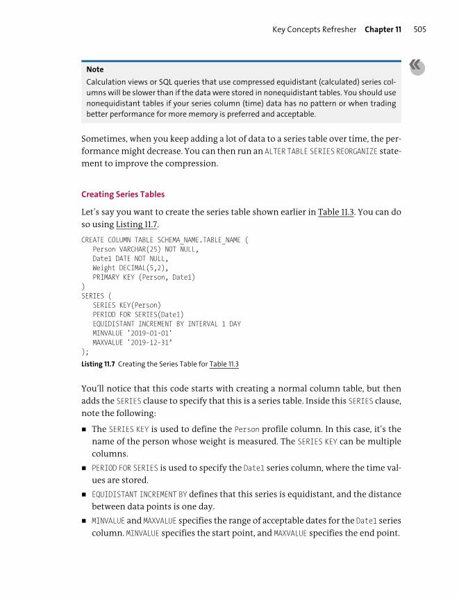
Key Concepts Refresher Chapter 11 505
Note
Calculation views or SQL queries that use compressed equidistant (calculated) series col-
umns will be slower than if the data were stored in nonequidistant tables. You should use
nonequidistant tables if your series column (time) data has no pattern or when trading
better performance for more memory is preferred and acceptable.
Sometimes, when you keep adding a lot of data to a series table over time, the per-
formance might decrease. You can then run an ALTER TABLE SERIES REORGANIZE state-
ment to improve the compression.
Creating Series Tables
Let’s say you want to create the series table shown earlier in Table 11.3. You can do
so using Listing 11.7.
CREATE COLUMN TABLE SCHEMA_NAME.TABLE_NAME (Person VARCHAR(25) NOT NULL,Date1 DATE NOT NULL,Weight DECIMAL(5,2),PRIMARY KEY (Person, Date1)
)SERIES (
SERIES KEY(Person)PERIOD FOR SERIES(Date1)EQUIDISTANT INCREMENT BY INTERVAL 1 DAYMINVALUE '2019-01-01'MAXVALUE '2019-12-31’
);
Listing 11.7 Creating the Series Table for Table 11.3
You’ll notice that this code starts with creating a normal column table, but then
adds the SERIES clause to specify that this is a series table. Inside this SERIES clause,
note the following:
� The SERIES KEY is used to define the Person profile column. In this case, it’s the
name of the person whose weight is measured. The SERIES KEY can be multiple
columns.
� PERIOD FOR SERIES is used to specify the Date1 series column, where the time val-
ues are stored.
� EQUIDISTANT INCREMENT BY defines that this series is equidistant, and the distance
between data points is one day.
� MINVALUE and MAXVALUE specifies the range of acceptable dates for the Date1 series
column. MINVALUE specifies the start point, and MAXVALUE specifies the end point.

Chapter 11 Spatial, Graph, and Series Data Modeling506
SAP HANA will also create a trigger for the table, which will return errors if you try
to insert dates that aren’t in the specified range or if the date doesn’t align with the
daily interval (in this case).
You can use the SERIES_GENERATE function to prepopulate the entire series column
(Date1). The rows are then ready for just adding values (Weight) at a later point.
You can alter a series table using the ALTER TABLE statement. However, the SERIES
clause of an existing series table can’t be altered.
Horizontal and Vertical Aggregation
A challenge you’ll often face when working with series tables is how to JOIN two
series tables with different time intervals. To solve this, you must use horizontal
aggregation.
Horizontal aggregation is when you take granular data and aggregate it to a less
granular level. For example, you can aggregate hourly data to a daily level. Or you
can disaggregate the data to a more granular level, for example, breaking up
hourly data to 15-minute intervals.
Note
Horizontal aggregation doesn’t change the data in the series table. It’s merely a “view”
that displays the data at a higher or lower level of granularity and allows you to JOINseries tables with different time intervals.
You can use normal aggregation functions, such as SUM and AVG, for aggregating the
value columns. When taking the Date1 series column, for example, to a less granu-
lar level, you use the SERIES_ROUND function. In Listing 11.8, horizontal aggregation
is applied to the data from Table 11.3. In this case, you use the ROUND_DOWN option,
meaning that 14 February gets rounded down to the month of February, rather
than rounded up to the month of March. In this case, this is quite obvious, but,
sometimes, you’ll want 8:59 to be rounded up to 9:00, rather than rounded down
to 8:00.
SELECTPerson,SERIES_ROUND(Date1, 'INTERVAL 1 MONTH', ROUND_DOWN) AS Monthly,AVG(Weight) AS MonthlyWeight
FROM SCHEMA_NAME.TABLE_NAMEGROUP BY Person, SERIES_ROUND(Date1, 'INTERVAL 1 MONTH', ROUND_DOWN);
Listing 11.8 Horizontal Aggregation
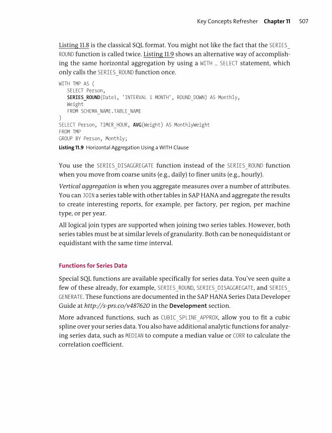
Key Concepts Refresher Chapter 11 507
Listing 11.8 is the classical SQL format. You might not like the fact that the SERIES_
ROUND function is called twice. Listing 11.9 shows an alternative way of accomplish-
ing the same horizontal aggregation by using a WITH … SELECT statement, which
only calls the SERIES_ROUND function once.
WITH TMP AS (SELECT Person,SERIES_ROUND(Date1, 'INTERVAL 1 MONTH', ROUND_DOWN) AS Monthly,WeightFROM SCHEMA_NAME.TABLE_NAME
)SELECT Person, TIMER_HOUR, AVG(Weight) AS MonthlyWeightFROM TMPGROUP BY Person, Monthly;
Listing 11.9 Horizontal Aggregation Using a WITH Clause
You use the SERIES_DISAGGREGATE function instead of the SERIES_ROUND function
when you move from coarse units (e.g., daily) to finer units (e.g., hourly).
Vertical aggregation is when you aggregate measures over a number of attributes.
You can JOIN a series table with other tables in SAP HANA and aggregate the results
to create interesting reports, for example, per factory, per region, per machine
type, or per year.
All logical join types are supported when joining two series tables. However, both
series tables must be at similar levels of granularity. Both can be nonequidistant or
equidistant with the same time interval.
Functions for Series Data
Special SQL functions are available specifically for series data. You’ve seen quite a
few of these already, for example, SERIES_ROUND, SERIES_DISAGGREGATE, and SERIES_
GENERATE. These functions are documented in the SAP HANA Series Data Developer
Guide at http://s-prs.co/v487620 in the Development section.
More advanced functions, such as CUBIC_SPLINE_APPROX, allow you to fit a cubic
spline over your series data. You also have additional analytic functions for analyz-
ing series data, such as MEDIAN to compute a median value or CORR to calculate the
correlation coefficient.

Chapter 11 Spatial, Graph, and Series Data Modeling508
Important Terminology
In this chapter, we looked at the following important terms:
� Spatial processing
Processing that uses data to describe, manipulate, and calculate the position,
shape, and orientation of objects in a defined space.
� Spatial reference systems (SRSs)
Specifications for various flat-earth and round-earth models.
� Spatial joins and predicates
The way that spatial shapes and points can be related to each other.
� Spatial functions
Special OGC-compliant functions to process spatial data in the system.
� Geocoding
The process of converting address information into geographic locations, such
as latitude and longitude.
� Graph processing
Used to process relationship and attributes of highly networked entities.
� Vertices
Nodes in a graph that are related to each other.
� Edge
Relationships between vertices in a graph.
� Graph workspace
File linking the vertex data used in a graph to the edge data.
� Time series data
A sequence of regular measurements taken over a period of time.
� Equidistant
Refers to when the time increments between successive records in the series
data are constant, for example, one hour.
� Horizontal aggregation
Taking granular data and aggregating it to a less granular level. For example,
you can aggregate hourly data to a daily level or disaggregate the data to a more
granular level, such as breaking up hourly data to 15-minute intervals.

Practice Questions Chapter 11 509
Practice Questions
These practice questions will help you evaluate your understanding of the topics
covered in this chapter. The questions shown are similar in nature to those found
on the certification examination. Although none of these questions will be found
on the exam itself, they will allow you to review your knowledge of the subject.
Select the correct answers, and then check the completeness of your answers in
the “Practice Question Answers and Explanations” section. Remember, on the
exam, you must select all correct answers and only correct answers to receive
credit for the question.
1. What spatial data type would you use to store multiple shop locations?
� A. ST_Point
� B. ST_MultiPoint
� C. ST_Polygon
� D. ST_MultiLineString
2. Which spatial data formats can you import into SAP HANA? (There are 2 cor-
rect answers.)
� A. Scalable Vector Graphic (SVG)
� B. Well-Known Text (WKT)
� C. ESRI shapefiles
� D. GeoJSON
3. Which modeling features can you use in flowgraphs? (There are 2 correct
answers.)
� A. Text
� B. Predictive
� C. Spatial
� D. Graph

Chapter 11 Spatial, Graph, and Series Data Modeling510
4. SAP HANA spatial functions are compliant to the standards set by which com-
pany?
� A. OGC
� B. ESRI
� C. W3C
� D. HERE
5. What characteristics does the WGS84 (planar) spatial reference system (SRS)
have? (There are 2 correct answers.)
� A. It’s a flat-earth type SRS,
� B. It uses a geographic coordinate system.
� C. It’s a round-earth type SRS.
� D. It uses a Cartesian coordinate system.
6. What is the default spatial reference system identity (SRID) for SAP HANA?
� A. 0 (2D planar)
� B. 4326 (WGS84)
� C. 3857 (Web Mercator)
7. What is the m-coordinate in a spatial point used for?
� A. The height above or below sea level
� B. Measures, such as wind speed
� C. The latitude
� D. The longitude
8. A spatial point is on the boundary of a shape. Which predicate do you use to
accept it as enclosed by the shape?
� A. ST_Contains
� B. ST_Within
� C. ST_Covers
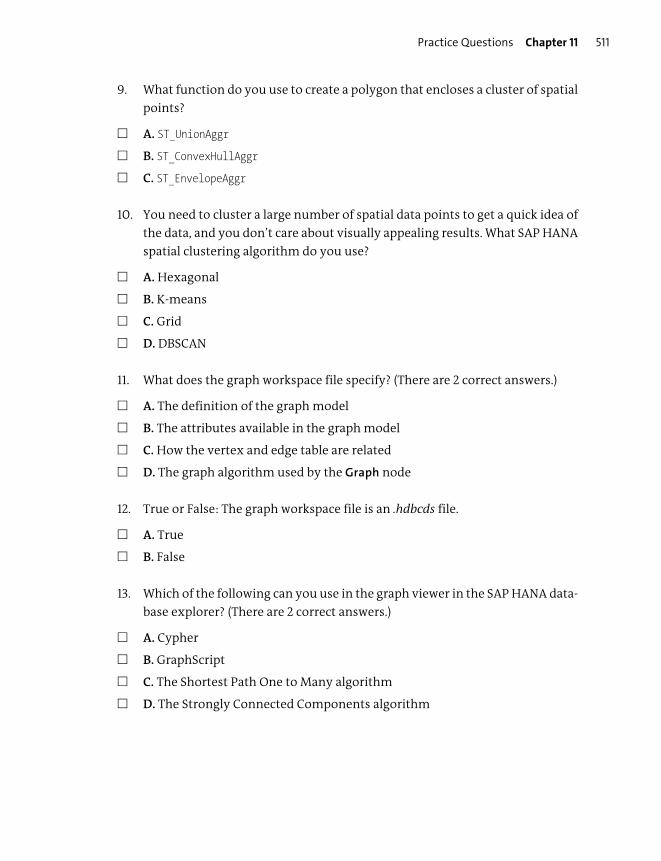
Practice Questions Chapter 11 511
9. What function do you use to create a polygon that encloses a cluster of spatial
points?
� A. ST_UnionAggr
� B. ST_ConvexHullAggr
� C. ST_EnvelopeAggr
10. You need to cluster a large number of spatial data points to get a quick idea of
the data, and you don’t care about visually appealing results. What SAP HANA
spatial clustering algorithm do you use?
� A. Hexagonal
� B. K-means
� C. Grid
� D. DBSCAN
11. What does the graph workspace file specify? (There are 2 correct answers.)
� A. The definition of the graph model
� B. The attributes available in the graph model
� C. How the vertex and edge table are related
� D. The graph algorithm used by the Graph node
12. True or False: The graph workspace file is an .hdbcds file.
� A. True
� B. False
13. Which of the following can you use in the graph viewer in the SAP HANA data-
base explorer? (There are 2 correct answers.)
� A. Cypher
� B. GraphScript
� C. The Shortest Path One to Many algorithm
� D. The Strongly Connected Components algorithm
Chapter 11 Spatial, Graph, and Series Data Modeling512
14. Which graph algorithm do you use to find the cheapest route to a specified
destination?
� A. Strongly Connected Components
� B. Shortest Path One to Many
� C. Neighborhood
� D. Shortest Path One to One
15. Which property do you specify for the graph algorithm to find the cheapest
route to a specified destination?
� A. Direction
� B. Weight
� C. Minimum Depth
� D. Maximum Depth
16. True or False: The Graph node must be the bottom node in a cube calculation
view.
� A. True
� B. False
17. You need to use a Graph node with a shortest path algorithm in a calculation
view, and require the end users to only specify the start vertex at runtime.
What is the easiest way to achieve this?
� A. Use a GraphScript procedure.
� B. Write an SAP HANA XSA application.
� C. Use input parameters.
� D. Use a REST API call.
18. Bonus Question: Which language do you use when you need to use a tree-like
topology with a declarative query language?
� A. Cypher
� B. SQLScript
� C. GraphScript

Practice Question Answers and Explanations Chapter 11 513
19. What are the vertices in a graph model?
� A. The nodes themselves
� B. The relationships between the nodes
� C. The attributes of the nodes
20. What will you use to convert daily series data to an hourly level?
Note: There are 2 correct answers to this question.
� A. Vertical aggregation
� B. Horizontal aggregation
� C. SERIES_DISAGGREGATE
� D. SERIES_ROUND
21. What do you use to create an equidistant series table?
� A. CREATE TABLE
� B. CREATE SERIES TABLE
� C. CREATE COLUMN TABLE
� D. CREATE HISTORY COLUMN TABLE
22. You create an equidistant series table. In the SERIES clause, what do use to
identify the profile column?
� A. SERIES KEY
� B. PERIOD FOR SERIES
� C. EQUIDISTANT INCREMENT BY
� D. PRIMARY KEY
Practice Question Answers and Explanations
1. Correct answer: B
Use a ST_MultiPoint data type to store multiple shop locations. ST_Point can
only store a single shop location, and ST_Polygon and ST_MultiLineString can’t
be used for shop locations.

Chapter 11 Spatial, Graph, and Series Data Modeling514
2. Correct answers: B, C
You can import Well-Known Text (WKT) and ESRI shapefiles into SAP HANA.
You can only export Scalable Vector Graphic (SVG) and GeoJSON file formats.
3. Correct answers: B, C
Predictive and spatial modeling can be done in flowgraphs.
4. Correct answer: A
The SAP HANA spatial functions are compliant to the standards set by OGC.
ESRI is the largest spatial software vendor and sets the de facto standard for
shape files.
The W3C looks after the standard for SVG (and other web standards)
HERE provides maps.
5. Correct answers: A, D
The WGS84 (planar) spatial reference system (SRS) is a flat-earth type SRS and
uses a Cartesian coordinate system.
If you got this wrong, it’s because it was a trick question. The WGS84 (planar)
SRS is NOT the same as the WGS84 SRS. Check the information below Figure 11.1.
6. Correct answer: A
The default spatial reference system identity (SRID) for SAP HANA is 0 (2D pla-
nar).
Many times, you should rather use 4326 (WGS84).
7. Correct answer: B
The m-coordinate is a spatial point used for measures such as wind speed. (M is
for measure.)
8. Correct answer: C
You use ST_Covers to accept that a spatial point is on the boundary of a shape as
enclosed by the shape.
ST_Contains and ST_Within don’t show a point on the boundary of a shape as
being enclosed by the shape.
9. Correct answer: B
You use the ST_ConvexHullAggr function to create a polygon that encloses a clus-
ter of spatial points.
The ST_EnvelopeAggr function returns a rectangle, which technically is also a
polygon. This is therefore a bad question, as someone could argue about the
answer, and would thus not occur in the real exam.

Practice Question Answers and Explanations Chapter 11 515
10. Correct answer: C
You use the SAP HANA grid spatial clustering algorithm to cluster a large num-
ber of spatial data points to get a quick idea of the data or when you don’t care
about visually appealing results.
The hexagonal spatial clustering algorithm (in SPS 04) might create more visu-
ally appealing results.
The k-means and DBSCAN spatial clustering algorithms aren’t as quick as the
grid spatial clustering algorithm.
11. Correct answers: A, C
The graph workspace file specifies the definition of the graph model and how
the vertex and edge table are related.
The attributes available in the graph model are just the additional fields avail-
able in the tables or views.
12. Correct answer: B
False: The graph workspace file is NOT an .hdbcds file but an .hdbworkspace file.
13. Correct answers: A, D
You use Cypher and the Strongly Connected Components algorithm in the
graph viewer in the SAP HANA database explorer.
GraphScript uses an .hdbprocedure file.
The Shortest Path One to Many algorithm is available in the Graph node but
NOT in the graph viewer.
14. Correct answer: D
You use the Shortest Path One to One graph algorithm to find the cheapest
route to a specified destination.
The Shortest Path One to Many graph algorithm would also be correct if the
question did not say “specified destination,” as you could generate all routes
and pick the cheapest one for your destination.
15. Correct answer: B
You specify the Weight Column property for the graph algorithm to find the
cheapest route to a specified destination.
16. Correct answer: A
True: The graph node must be the bottom node in a cube calculation view and,
actually, for all calculation views.

Chapter 11 Spatial, Graph, and Series Data Modeling516
17. Correct answer: C
When you need to use a Graph node with a Shortest Path algorithm in a calcu-
lation view and require the end users to only specify the start vertex at runtime,
you simply use input parameters (refer to Figure 11.23).
Writing an SAP HANA XSA application could work, but not in all cases; for
example, it won’t work when you want the users to specify the start vertex
while they are using SAP Analytics Cloud.
18. Correct answer: B
You use SQLScript when you need to use a tree-like topology with a declarative
query language. The tree-like topology refers to hierarchies.
Cypher is a declarative query language, but it’s used for generic graph topology.
This question is too detailed and hard, which is why it was marked as a bonus
question. If you could answer it correctly, you know the topic very well!
19. Correct answer: A
The vertices in a graph model are the nodes.
The relationships between the nodes are called edges.
20. Correct answer: B, C
You use horizontal aggregation and SERIES_DISAGGREGATE to convert daily series
data to an hourly level. In this case, you go to hourly, which means there are
more values. You need to disaggregate to achieve this.
SERIES_ROUND is used with aggregation. Aggregation (e.g., SUM) takes many values
and reduces them to one value.
21. Correct answer: C
You use CREATE COLUMN TABLE with a SERIES clause to create a series table.
There is no CREATE SERIES TABLE statement.
CREATE TABLE creates a row table.
A history column table is for audit log type tables, where you keep a full history
of all changes made to the table.
22. Correct answer: A
You identify the profile column, which is the name of the “sensor” in IoT, with
SERIES KEY.
The PERIOD FOR SERIES (used on the series column) is used for the time period.
Note
Some questions in the certification exam will only have three answer options.

Summary Chapter 11 517
Takeaway
You now understand the key components of spatial processing, which spatial data
types are available, and how to perform spatial joins in SAP HANA information
views.
You also know how to work with nodes (vertices) and relationships (edges) in a
graph, as well as how to combine them using a graph workspace. You’ve used the
graph viewer in the SAP HANA database explorer and used Graph nodes in graphi-
cal calculation views. And you know the differences between Cypher and Graph-
Script, and hierarchies and graphs.
Finally, you learned how to create a series table, understood what an equidistant
series is, and gained a basic understanding of series data modeling techniques.
Summary
We discussed how to use spatial processing, how to combine business data with
maps, and how to easily do complex queries on networked entities.
In the same way, we can combine graph data with business data to create powerful
queries that can’t be solved using traditional hierarchies and reporting methods.
We discussed important aspects of SAP HANA series data, including the advan-
tages of using SAP HANA. Throughout this overview of SAP HANA series data,
you’ve learned more about the SAP HANA series data functionality, as well as the
basic concepts of series data in SAP HANA, such as series tables, equidistant series
data, and horizontal aggregation.
In the next chapter, we’ll look at how to improve SAP HANA information models
to achieve optimal performance.

Chapter 12
Optimization of Information Models
Techniques You’ll Master
� Understand the performance enhancements in SAP HANA
� Get to know techniques for optimizing performance
� Learn how to use the SAP HANA optimization tools
� Implement good modeling practices for optimal performance
� Create optimal SQL and SQLScript

Chapter 12 Optimization of Information Models520
During our exploration of SAP HANA, we’ve frequently come across the topic of
performance. SAP HANA is well known for the improvements it brings to business
process runtimes and its real-time computing abilities.
In this chapter, we’ll discuss some of these performance enhancements that are
built in to SAP HANA and review the techniques you’ve learned previously. We’ll
then look into new ways of pinpointing performance issues and discuss how to
use the optimization tools built in to SAP HANA. Finally, we’ll examine some
guidelines and best practices when modeling and writing SQL and SQLScript code.
Real-World Scenario
The CEO of your company reads a 2009 study by Akamai stating that 40% of
online shoppers will abandon a website that takes longer than three seconds
to load.
Therefore, you’re tasked with helping to achieve a response time of less than
three seconds for most reports and analytics that sales representatives use.
Many such users work on tablets, especially when they are visiting custom-
ers. You decide to use a mobile-first approach, creating interactive analytics
and reports to reduce network requirements.
Some of the reports currently take more than two minutes to run on SAP
HANA. Using your knowledge of optimization, you manage to bring these
times down to just a few seconds.
Objectives of This Portion of the Test
The purpose of this portion of the SAP HANA certification exam is to test your
knowledge of the SAP HANA modeling tools.
The certification exam expects you to have a good understanding of the following
topics:
� Performance enhancements in SAP HANA
� Techniques for optimizing performance
� Using the performance analysis mode, debug mode, and other optimization
tools
� Good modeling practices for optimal performance
� Creating optimal SQL and SQLScript
Key Concepts Refresher Chapter 12 521
Note
This portion contributes about 10% of the total certification exam score.
Key Concepts Refresher
In the preceding chapters, we’ve discussed many performance enhancements that
are built-in to the design of SAP HANA; in this chapter, we’ll walk through various
optimization topics in SAP HANA.
Architecture and Performance
The largest and most fundamental change that comes with SAP HANA technology
is the move from disks to memory. The in-memory technology that SAP HANA is
built on has been one of the biggest contributors of performance improvements.
The decision to break with the legacy of disk-based systems and use in-memory
systems as the central focus point (and everything that comes with this) has led to
significant changes in performance.
The next step was to combine memory and multicore CPUs. If we store everything
in memory and have plenty of processing power, we don’t have to store calculated
results. We just recalculate them when we need them, which opens the door to
real-time computing. Real-time computing requires that results be recalculated
each time they’re needed because the data might have changed since the last
query.
This combination of memory and CPU processing power led to new innovations.
Now, you can combine online transactional processing (OLTP) and online analyti-
cal processing (OLAP) together in the same system: the OLAP components don’t
need the storage of precalculated cubes and can be recalculated without impacting
the performance of the OLTP system.
Another innovation prompted by combining memory and CPU is data compres-
sion. This both reduces memory requirements and helps to better utilize CPUs by
loading more data in the level 1 CPU cache. Loading more data into CPUs once
again improves performance.
To improve compression, SAP HANA prefers columnar storage. Along with many
advantages, columnar storage also has a few disadvantages: inserting new records
and updating existing records aren’t handled as efficiently in column tables as in

Chapter 12 Optimization of Information Models522
row tables. To solve this, SAP HANA implemented the insert-only principle with
delta buffers. We use row storage for delta buffers to improve insert speeds and
then use delta merges to bring the data back to columnar storage, which leads to
better read performance.
Tip
The performance improvements in SAP HANA don’t mean that we can be negligent in
modeling and development. For example, you shouldn’t use SELECT * statements or
choose any unnecessary fields in queries because doing so decreases the efficiency of the
column storage.
Using multicore processors, everything in SAP HANA was designed from the
ground up to run in parallel. Even a single aggregation value is calculated using
parallelism. This led to SAP HANA growing from a single hardware appliance to a
distributed scale-out system that can work across multiple server nodes and
finally to multitenant database containers (MDCs). Tables can now also be parti-
tioned across multiple servers. With more servers, the scale and performance of
SAP HANA systems has vastly advanced.
Redesigned and Optimized Applications
While combining memory and processors, we also saw that moving data from
memory to application servers isn’t the optimal way to work with an in-memory
database. It makes more sense to push down some of the application logic to the
SAP HANA system for fast access to the data in memory and plenty of computing
resources for calculations.
SAP started by making SAP HANA available as a side-by-side accelerator solution
to improve issues with long-running processes in current systems. Over time, SAP
business applications were migrated to SAP HANA and reengineered to make use
of the advantages it offers.
With SAP S/4HANA, we now have a system that uses views instead of materialized
aggregates in lookup tables, significantly reducing the size of the system, simplify-
ing the code, and enriching the user experience.

Key Concepts Refresher Chapter 12 523
Effects of Good Performance
We sometimes hear the following: “Why do we have to optimize our SAP HANA
models that much? Surely five minutes for an analysis, a report, or some screen is
good enough.” Yes, sometimes a response time of five minutes is good enough.
But this means people focus only on the task at hand. They don’t look at what is
possible and what they’re currently not doing.
What other things, which were previously impossible, can we do now if this cur-
rent process runs in less than a second? What other data can we combine with the
current process that unlocks more business value? How can we change our busi-
ness because of this?
Example
Most people see SAP HANA as just some technology. Some people see SAP HANA as an
enabler. Few people view SAP HANA as a “change agent.” The history of SAP over the past
few years is proof of how SAP HANA can change a business.
When SAP HANA was released, there was a lot of focus on how it could be used to
accelerate reports and analytics. At some stage, people realized that they could not
only process the same amount of data faster, but they could now process more
data. SAP started using SAP HANA for big data scenarios.
One of the major sources of big data is sensors or what is called the Internet of
Things (IoT). Many of these “things” (sensors) are sending a constant stream of
data out, which results in large data sets that keep growing. (We look at streaming
data in Chapter 9.) SAP evolved this focus on the IoT into its new SAP Leonardo
portfolio.
When you work with big data, you start with historical analysis. But if the perfor-
mance is great, you can start looking at using this historical analysis to predict
events. (We discussed the predictive capabilities of SAP HANA in Chapter 10.) SAP
now has the SAP Predictive Maintenance and Service system that uses historical
IoT data from machines to predict the optimal time to service, maintain, and
upgrade these machines, as well as exactly which parts need to be replaced at what
point in time. This results in huge savings.
The next step from predictive is machine learning. Some people now call some
things machine learning that are still really predictive. Machine learning can build
on predictive, but it also has elements such as neural networks. SAP HANA has a
Chapter 12 Optimization of Information Models524
machine learning component, which is even available for SAP HANA, express edi-
tion. Machine learning with SAP HANA is also part of the new SAP Leonardo port-
folio.
Look at the user’s experience. If a system takes five minutes to respond, you can’t
really use it on a mobile device. We started the chapter with a study that showed
people expected answers in less than three seconds on mobile. More than half the
requests on the Internet are now coming from mobile devices. A response time of
five minutes isn’t good enough in this case.
Lastly, when system responses are fast, you can start moving these systems to the
cloud. People can now access these systems from any device and from anywhere.
SAP now has a huge focus on cloud systems. Many of these would never have
worked if the responses to users were slow. SAP Cloud Platform is now a central
component in the SAP Leonardo portfolio and the new “Intelligent Enterprise.”
Without good performance and a focus on optimizing their modeling and devel-
opment, products such as SAP Leonardo and SAP Cloud Platform might never
have been conceived. Performance can open doors to new business models.
Let’s see what we’ve learned already to help us with optimizing our information
models.
Information Modeling Techniques
In previous chapters, we discussed some techniques that can help optimize infor-
mation models, such as the following:
� Limit data as quickly as possible by doing the following:
– Define filters on the source data.
– Apply variables in your SAP HANA views to push down filters at runtime.
– Select only the fields that you require in your query results. Don’t use SELECT *.
– Let SAP HANA perform the calculations and send only the calculated results
to a business application, instead of sending lots of data to the application
and performing the calculations there.
– Don’t output your data as granular (at record level) in a calculation view
when your analysis displays it as aggregates.
� Speed up filters by partitioning the tables that you filter on.
� Perform calculations as late as possible. For example, perform aggregation
before calculation where possible.
Key Concepts Refresher Chapter 12 525
� Use referential joins when your data has referential integrity. When working
with referential integrity, the SAP HANA system doesn’t have to evaluate the
join for all queries.
� Similarly, use dynamic joins to optimize the join performance for certain que-
ries.
� Join tables on key fields or indexed columns.
� Use a union instead of a join for combining large sets of data.
� Make unions even more efficient by using union pruning. We discussed this in
Chapter 6 already, when discussing unions.
� Where possible, use a single fact table in a data foundation of a star join view.
� Build up your information views in layers. This helps SAP HANA to process the
requests in parallel, which drastically improves performance.
If you use these techniques, you’ll avoid many optimization hazards. These tech-
niques should be part of your everyday workflow.
The best optimization is not having to optimize. By avoiding the pitfalls in this
chapter, you’ll most likely not need to optimize your modeling later. In spite of
your best efforts, however, sometimes you need to optimize an information
model.
Optimization Tools
When optimizing an SAP HANA information model, a number of tools are at your
disposal. You need to know when to pick which optimization tool and how to use
it.
Note
If you’ve worked with SAP HANA 1.0 before, you’ll notice some of the tools that you once
knew have changed. We won’t discuss SAP HANA database engines, the Explain Plan tool,
the Visualize Plan tool, or the Administration Perspective. These were available in SAP
HANA 1.0 and SAP HANA Studio. Instead, we’ll focus on the new tools found in SAP Web
IDE for SAP HANA.

Chapter 12 Optimization of Information Models526
Performance Analysis Mode
Performance analysis mode is available from the top toolbar when you build SAP
HANA calculation views. You can switch this mode on or off when designing infor-
mation views. The tool will analyze your view and suggest possible improvements.
When you select a node—for example, the Join node—in your view, and then open
the Performance Analysis tab (top right), you might see some improvement recom-
mendations from the SAP HANA system. You’ll notice that a new tab, Performance
Analysis, has been added to the right side of the editor in which you design the
information view.
Figure 12.1 shows the Product calculation view from the SAP HANA Interactive Edu-
cation (SHINE) content. We select the first (bottom) node in the view, and see the
Performance Analysis of this Join node.
Figure 12.1 Performance Analysis Mode Optimization Suggestions
Key Concepts Refresher Chapter 12 527
The first section includes the Join Type and Cardinality of the join. The next section
includes the Partition Type and Number of Rows of each of the tables in the join. If
we have many rows in a table, SAP HANA might suggest that we partition the table
to improve performance. In this case, the BusinessPartner table is already parti-
tioned using a Hash partition.
There are two possible improvement suggestions in Figure 12.1:
� Proposed cardinality
In this case, we didn’t specify any cardinality on the join. SAP HANA analyzed
the tables and the Join node and suggested that a n..1 cardinality should be set.
Setting the cardinality will allow SAP HANA to execute the view faster because
it won’t have to calculate what the cardinality is first. The suggestion of n..1 car-
dinality makes sense because we’ll order multiple products (left table) from
each supplier (right table). A message stating Selected cardinality does not
match the proposed cardinality is shown below the Cardinality field.
� Join type
SAP HANA looked at the data to see if referential integrity was ensured. Because
Referential Integrity is Maintained in this case, we can use a referential join
instead of the inner join type in this Join node.
In the SAP Web IDE for SAP HANA preferences for the Modeler section, you can set
the option to always open calculation views in performance analysis mode. You
can also set a threshold for the number of records in a table where performance
analysis mode will display a warning symbol next to this table. This will remind
you to pay special attention to very large tables. You can use partitioning on such
tables to improve performance, and you can apply filters that process only the
required data.
In addition to the cardinality, join type, and number of records in a table, perfor-
mance analysis mode will also provide you with warnings when the following is
true:
� Joins are based on calculated columns.
� Restricted columns are based on calculated columns.
Performance analysis mode works on the runtime artifact. So, even if you did not
build your calculation view yet, this mode will still give you valuable information.

Chapter 12 Optimization of Information Models528
Debug Mode
Right next to the Performance Analysis button on the toolbar is the Debug This
View button, as shown in Figure 12.2.
Figure 12.2 Activating the Debug Query Mode in a Calculation View
In Figure 12.3, we selected the Join node in the view, and opened the Debug Query
tab of this node that appeared on the top-right side of the editor.
You can see the SQL generated by the calculation view up to this point, as well as
the result set. This is very useful to debug your views, for example, if a field is miss-
ing or giving different results than what you expected. You can now trace it node
by node to see where you went wrong.
In Figure 12.4, we selected the next Join node. Comparing the SQL and the result set
with that of Figure 12.3, you can see that the new table that was joined in this node
added the PRODUCT_DESCRIPTION field.
Figure 12.3 Analyzing the SQL for a Join Node, along with the Result Set from That Node

Key Concepts Refresher Chapter 12 529
Figure 12.4 Analyzing the SQL for the Next Node Join
The debug query mode works in the runtime view of the calculation view but uses
the active version of the calculation view. If you’ve made changes to your calcula-
tion view, you must Save and Build before you run debug query mode, or you
won’t get the correct results.
SQL Analyzer
The previous two tools are used while you’re designing your graphical calculation
views. The SQL Analyzer tool is used to measure the performance of a calculation
view when you run it.
Measuring performance of a running view clearly states that we’ll work with run-
time objects. For this, we have to open the SAP HANA database explorer in SAP
Web IDE for SAP HANA.
Select the SAP HANA Deployment Infrastructure (HDI) container and the Column
Views folder. A list of views that were successfully built is shown on the bottom-
left area. In Figure 12.5, we again selected the same Product view from the SHINE
content that we looked at earlier.
Right-click on Column Views, and select Generate SELECT Statement from the con-
text menu.
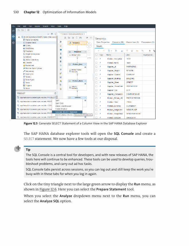
Chapter 12 Optimization of Information Models530
Figure 12.5 Generate SELECT Statement of a Column View in the SAP HANA Database Explorer
The SAP HANA database explorer tools will open the SQL Console and create a
SELECT statement. We now have a few tools at our disposal.
Tip
The SQL Console is a central tool for developers, and with new releases of SAP HANA, the
tools here will continue to be enhanced. These tools can be used to develop queries, trou-
bleshoot problems, and carry out ad hoc tasks.
SQL Console tabs persist across sessions, so you can log out and still keep the work you’re
busy with in these tabs for when you log in again.
Click on the tiny triangle next to the large green arrow to display the Run menu, as
shown in Figure 12.6. Here you can select the Prepare Statement tool.
When you select the Analyze dropdown menu next to the Run menu, you can
select the Analyze SQL option.
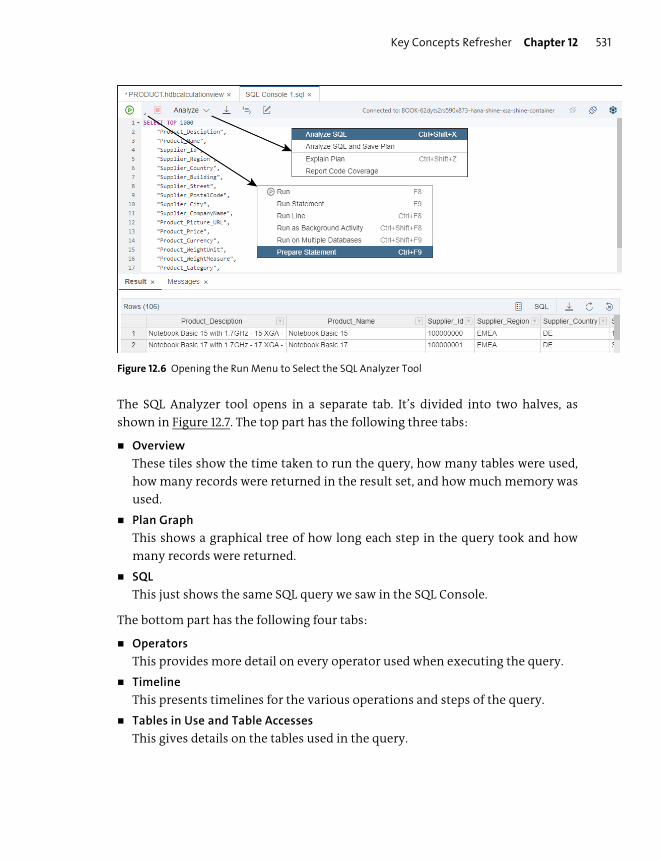
Key Concepts Refresher Chapter 12 531
Figure 12.6 Opening the Run Menu to Select the SQL Analyzer Tool
The SQL Analyzer tool opens in a separate tab. It’s divided into two halves, as
shown in Figure 12.7. The top part has the following three tabs:
� Overview
These tiles show the time taken to run the query, how many tables were used,
how many records were returned in the result set, and how much memory was
used.
� Plan Graph
This shows a graphical tree of how long each step in the query took and how
many records were returned.
� SQL
This just shows the same SQL query we saw in the SQL Console.
The bottom part has the following four tabs:
� Operators
This provides more detail on every operator used when executing the query.
� Timeline
This presents timelines for the various operations and steps of the query.
� Tables in Use and Table Accesses
This gives details on the tables used in the query.
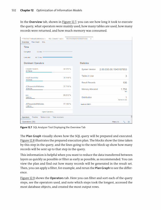
Chapter 12 Optimization of Information Models532
In the Overview tab, shown in Figure 12.7, you can see how long it took to execute
the query, what operators were mainly used, how many tables are used, how many
records were returned, and how much memory was consumed.
Figure 12.7 SQL Analyzer Tool Displaying the Overview Tab
The Plan Graph visually shows how the SQL query will be prepared and executed.
Figure 12.8 illustrates the prepared execution plan. The blocks show the time taken
by this step in the query, and the lines going to the next block up show how many
records will be sent up to that step in the query.
This information is helpful when you want to reduce the data transferred between
layers as quickly as possible or filter as early as possible, as recommended. You can
view the plan and find out how many records will be generated in the result set.
Then, you can apply a filter, for example, and rerun the Plan Graph to see the differ-
ence.
Figure 12.9 shows the Operators tab. Here you can filter and sort each of the query
steps, see the operators used, and note which steps took the longest, accessed the
most database objects, and created the most output rows.
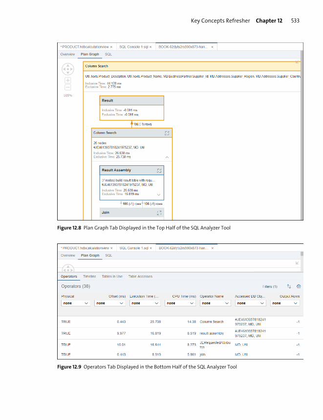
Key Concepts Refresher Chapter 12 533
Figure 12.8 Plan Graph Tab Displayed in the Top Half of the SQL Analyzer Tool
Figure 12.9 Operators Tab Displayed in the Bottom Half of the SQL Analyzer Tool
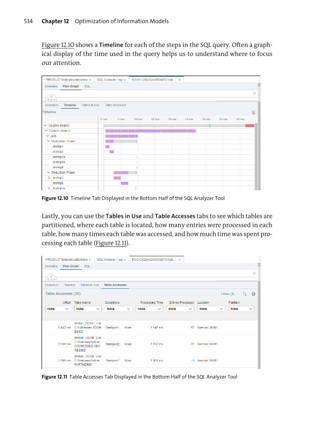
Chapter 12 Optimization of Information Models534
Figure 12.10 shows a Timeline for each of the steps in the SQL query. Often a graph-
ical display of the time used in the query helps us to understand where to focus
our attention.
Figure 12.10 Timeline Tab Displayed in the Bottom Half of the SQL Analyzer Tool
Lastly, you can use the Tables in Use and Table Accesses tabs to see which tables are
partitioned, where each table is located, how many entries were processed in each
table, how many times each table was accessed, and how much time was spent pro-
cessing each table (Figure 12.11).
Figure 12.11 Table Accesses Tab Displayed in the Bottom Half of the SQL Analyzer Tool
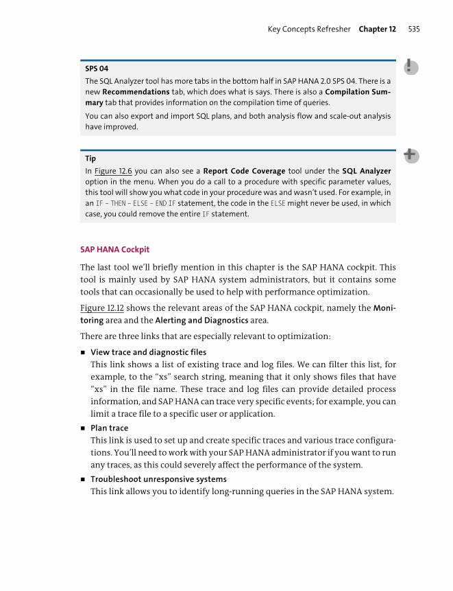
Key Concepts Refresher Chapter 12 535
SPS 04
The SQL Analyzer tool has more tabs in the bottom half in SAP HANA 2.0 SPS 04. There is a
new Recommendations tab, which does what is says. There is also a Compilation Sum-mary tab that provides information on the compilation time of queries.
You can also export and import SQL plans, and both analysis flow and scale-out analysis
have improved.
Tip
In Figure 12.6 you can also see a Report Code Coverage tool under the SQL Analyzeroption in the menu. When you do a call to a procedure with specific parameter values,
this tool will show you what code in your procedure was and wasn’t used. For example, in
an IF – THEN – ELSE – END IF statement, the code in the ELSE might never be used, in which
case, you could remove the entire IF statement.
SAP HANA Cockpit
The last tool we’ll briefly mention in this chapter is the SAP HANA cockpit. This
tool is mainly used by SAP HANA system administrators, but it contains some
tools that can occasionally be used to help with performance optimization.
Figure 12.12 shows the relevant areas of the SAP HANA cockpit, namely the Moni-
toring area and the Alerting and Diagnostics area.
There are three links that are especially relevant to optimization:
� View trace and diagnostic files
This link shows a list of existing trace and log files. We can filter this list, for
example, to the “xs” search string, meaning that it only shows files that have
“xs” in the file name. These trace and log files can provide detailed process
information, and SAP HANA can trace very specific events; for example, you can
limit a trace file to a specific user or application.
� Plan trace
This link is used to set up and create specific traces and various trace configura-
tions. You’ll need to work with your SAP HANA administrator if you want to run
any traces, as this could severely affect the performance of the system.
� Troubleshoot unresponsive systems
This link allows you to identify long-running queries in the SAP HANA system.
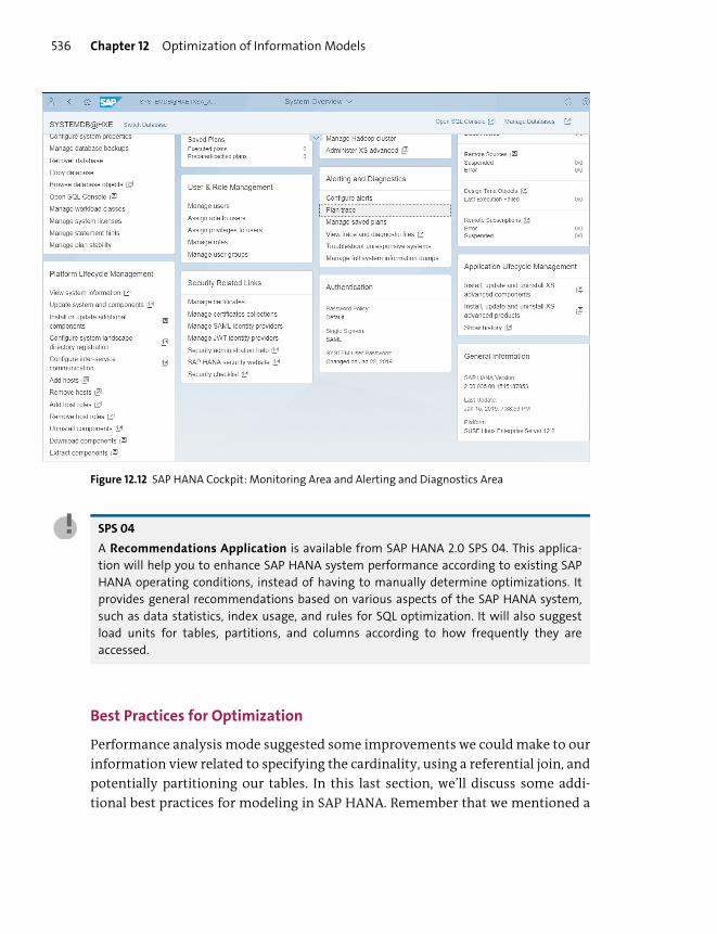
Chapter 12 Optimization of Information Models536
Figure 12.12 SAP HANA Cockpit: Monitoring Area and Alerting and Diagnostics Area
SPS 04
A Recommendations Application is available from SAP HANA 2.0 SPS 04. This applica-
tion will help you to enhance SAP HANA system performance according to existing SAP
HANA operating conditions, instead of having to manually determine optimizations. It
provides general recommendations based on various aspects of the SAP HANA system,
such as data statistics, index usage, and rules for SQL optimization. It will also suggest
load units for tables, partitions, and columns according to how frequently they are
accessed.
Best Practices for Optimization
Performance analysis mode suggested some improvements we could make to our
information view related to specifying the cardinality, using a referential join, and
potentially partitioning our tables. In this last section, we’ll discuss some addi-
tional best practices for modeling in SAP HANA. Remember that we mentioned a

Key Concepts Refresher Chapter 12 537
few best practices earlier in the chapter when we summarized concepts you’ve
learned previously in the book.
We can divide these best practices into two areas: those related to the graphical
view design and those related to SQL and SQLScript.
Best Practices for Calculation Views
The following are some additional best practices to optimize calculation views:
� Reduce data transfer between calculation views.
� Reduce the intermediate results between nodes inside a calculation view.
� Try to create calculations (e.g., in calculated columns) as late as possible in the
model.
� Implement filters at a table level. Don’t build filters on top of a calculated col-
umn, as this will do a lot of calculation before you filter the data. By filtering
first, you can eliminate a lot of calculations.
� The SAP HANA query optimizer tries to push filters down to the lower layers.
Sometimes you have a node that gets inputs from multiple nodes, for example,
the Intersect node in Chapter 6. The data flow splits before this node and has
parallel nodes. If you have a filter in the nodes above, the optimizer has to push
the filter down through these parallel nodes. Normally, it won’t do it as the
semantic correctness might be affected. If you know that the semantic meaning
won’t be affected, you can set the Ignore Multiple Outputs for Filter flag to force
the filter pushdown.
� Don’t send all information to the analytics and reporting tools; instead, make
your reports more interactive, using actions such as “click to drill down,” and
make multiple smaller requests from SAP HANA. The SAP HANA system will use
less memory, be more efficient, and respond faster. With less data moving
across the network, the user experience improves. In addition, by sending less
information to the analytics and reporting tools, you make these tools more
mobile-friendly.
� Select only the fields you require; columnar databases don’t like working with
all the columns.
� Specify the cardinality in a join. This can improve the runtimes for large models
as the optimizer can prune an entire data source from a join if certain prerequi-
sites are met, like only reading data from the left-side table in a referential join.
Just make sure that you also update the cardinality setting if you update the
model at a later stage.
Chapter 12 Optimization of Information Models538
� For joins:
– Use left outer joins rather than right outer joins. Try to use n:1 or 1:1 cardinal-
ity with the left outer joins.
– Try to reduce the number of join fields.
– Avoid joins on calculated columns.
– Avoid joins where the data types of the join fields are different, as this will
need type conversions.
� Investigate whether partitioning your tables is a valid option.
� Let SAP HANA do the hard work such as aggregations and calculations.
� Identify recurring patterns, and put them into a reuse “library.” For example,
you might always join the order header and the order details tables. Put this
into a separate calculation view, and reuse it as a data source for multiple other
calculation views. This also helps with breaking monolithic calculation views
into smaller parts. Added advantages are that the smaller parts are easier to
understand, and the reduced duplication leads to less maintenance.
� Avoid mixing core data services (CDS) views with calculation views. Even
though you can use CDS views as data sources in calculation views, the perfor-
mance isn’t as good as when you use the tables directly in the calculation view
and create the view functionality yourself.
� Enable caching for calculation views where applicable. If the query results are
extremely fast to generate, it might not make sense to enable caching. Caching
can be activated and controlled by the system administrator at the database
level. You can control caching at the level of an individual calculation view in
the Advanced tab of the Semantic node. You can set the Cache Invalidation
Period so that it expires after a transaction changes data in one of the data
sources, after an hour or after a day. This choice depends on the data require-
ments of the individual calculation view.
� Use Star Join nodes for OLAP queries. You can get similar results with Join
nodes, but it won’t perform as well.
� Try to use dedicated tables or views for value help lookups. It will be faster, and
users will get consistent values across all calculation views that use this Value
Help dialog. You can filter the list of values for users through analytic privileges.
This will show them only the values they are allowed to see and use. We’ll dis-
cuss analytic privileges in the next chapter.

Key Concepts Refresher Chapter 12 539
Tip
Remember that SAP HANA uses authorizations as a filter. If a user is only allowed to see
one cost center, that is essentially a “filter,” and SAP HANA will use it to speed up the
query. In this case, security isn’t an overhead as in many other systems but an optimiza-
tion technique.
Partitioning
We’ve seen partitioning mentioned a few times as a solution to some performance
issues. Partitioning was already introduced in Chapter 3, but let’s discuss it a bit
more.
Although partitioning is normally managed by the system administrator or data-
base administrator, it’s still good to understand how to use it. Many times, model-
ers are called on to help with partitioning as they understand the tables and their
use.
Partitioning is when we subdivide a column store table into multiple separate
“blocks.” For example, we can split the table into blocks where partition 1 has all
the records where people’s names start with the letter A, partition 2 for B, and so
on. These partitions can then be spread across multiple servers. We can also keep
the partitions on a single server. This can still improve performance as it’s now
easy for the database to select only the records for people with names that start
with the letter M, for example.
Tip
Partitioning can only be used with column tables—not with row tables.
Partitioning is different from table distribution where several (whole) tables are
distributed across multiple servers. In that case, the tables stay as a whole. Table A
gets loaded on server 1, table B on server 2, and so on. In that case, tables aren’t split
up, but distributed, whereas with partitioning, a single table gets split up.
Following are some of the reasons for partitioning tables:
� The load is balanced across multiple servers. Query performance improves as
multiple servers are all working together in parallel to help process the data of a
single table.
Chapter 12 Optimization of Information Models540
� If a query, for example, only asks for people’s names that start with the letter in
the example above, the request is only executed on the server where the parti-
tion resides.
� If a table is partitioned over multiple servers, the delta merge management is
more efficient.
SAP HANA will split tables with more than 2 billion records to improve perfor-
mance.
Partitioning is transparent to the SQL used for the queries. SAP HANA will auto-
matically handle the partitioning logic in the background. You don’t need to spec-
ify partitions in your SQL queries.
Partitions are defined when a table is created, or they can be created later with an
ALTER TABLE statement. You can specify this using either SQL or CDS. You have full
control over partitions; for example, you can split them, merge them, move them
to other servers, and so on.
SAP HANA supports three types of table partitioning:
� Round robin
This is the easiest type of table partitioning. A new record is automatically
assigned to the next partition in a circular fashion. You don’t have to under-
stand the data or specify which columns to use for the partitioning.
� Hash
For hash partitioning, you specify the columns to use for the partitioning. SAP
HANA computes hash values and distributes the data evenly. You don’t really
need to understand the actual content in the table.
� Range
Range partitioning requires that you know the data in the table really well. You
have to specify not only the columns to use for the partitioning but also in what
ranges to split the data, for example, by years 2010–2015, 2016–2018, and 2019–
2020.
We can even create multilevel partitions. This is when you partition the partitions.
For example, you can use hash partitioning to enable load balancing across multi-
ple servers and then use range partitioning at the next level to split the data per
year, perhaps for performance reasons.
Key Concepts Refresher Chapter 12 541
SQL and SQLScript Guidelines
We mentioned several best practices for optimizing SQL and SQLScript in Chapter
8, including the following:
� Don’t use SELECT * statements.
� Try to avoid imperative logic with a loop or branch logic. SQL uses a set-oriented
approach for best performance. When you use imperative statements, you dic-
tate the logic flow, making it very hard for the SQL optimizer to produce a better
plan and parallelize the logic for improved performance.
� Avoid using cursors. Cursors are a powerful feature in most databases that allow
you to apply some action on one record at a time in a result set. The resultant
reduction in performance is similar to the imperative logic in the previous
point.
� Break large, complex SQL statements into smaller independent steps using SQL-
Script variables. This can improve the parallelization of the execution of the
query. The calculated result set can be referred to multiple times, eliminating
repetitions of the same SQL statements. It will also reduce the complexity,
decreasing your development time.
� Use procedures or grouping sets to return multiple results sets.
� Try to write code that is free from side effects. When code changes the state of
the database, for example, by creating or altering tables, inserting or updating
data, or deleting records, you slow things down. Read-only code, such as table
functions, doesn’t alter the state of the database.
� Use SQL syntax instead of the older calculation engine functions. SAP HANA has
to convert these to SQL—this process is called unfolding—and the SQL opti-
mizer might not be able to fully optimize this converted code.
Even though we might not use calculation engine functions in our SQLScript code
any longer, there are other places these can still appear. Figure 12.13 shows the
Expression Editor screen for a calculated column in a graphical calculation view. In
this case, we needed the IF() function, which isn’t available in an SQL expression.
It’s recommended that you use SQL in the Expression Editor screen whenever pos-
sible.
Tip
For more SAP HANA optimization and performance information, you can attend the
HA215 training course. You can find more information about this course at http://s-
prs.co/v487623.
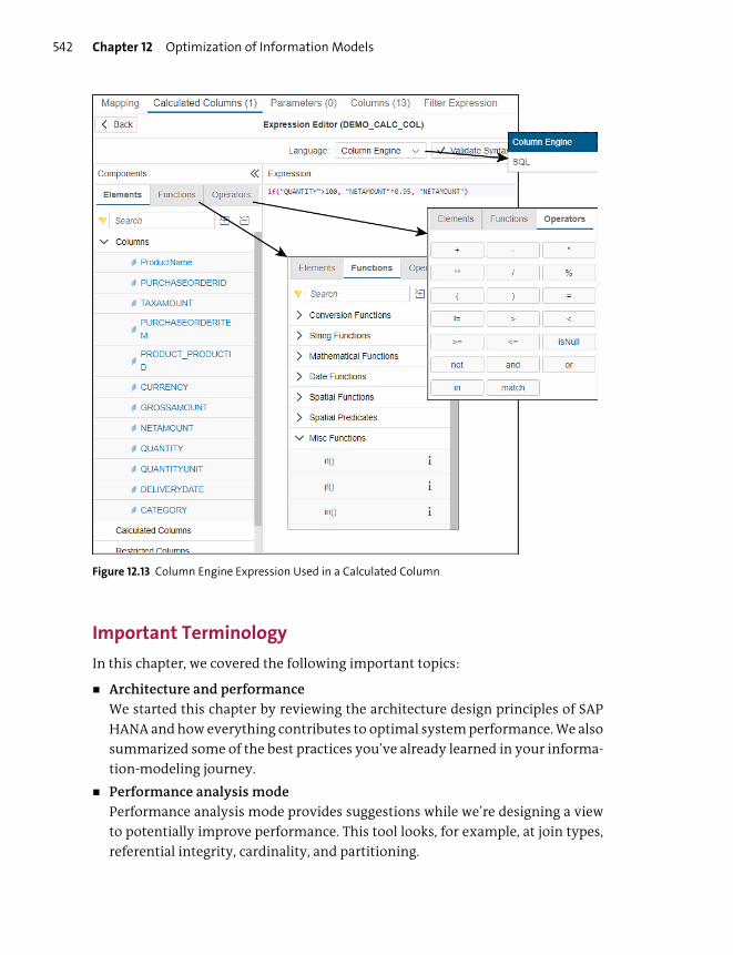
Chapter 12 Optimization of Information Models542
Figure 12.13 Column Engine Expression Used in a Calculated Column
Important Terminology
In this chapter, we covered the following important topics:
� Architecture and performance
We started this chapter by reviewing the architecture design principles of SAP
HANA and how everything contributes to optimal system performance. We also
summarized some of the best practices you’ve already learned in your informa-
tion-modeling journey.
� Performance analysis mode
Performance analysis mode provides suggestions while we’re designing a view
to potentially improve performance. This tool looks, for example, at join types,
referential integrity, cardinality, and partitioning.

Practice Questions Chapter 12 543
� Debug query mode
Debug query mode shows the SQL generated in a calculation view up to the
selected node. This can be used to see where fields get added and how that
affects the result set.
� SQL Analyzer
The SQL Analyzer tool shows graphical flows for the SQL plans. We can see the
number of records returned per operator in the plan, the number of records,
and the time each step of the query took in the executed plan. We can also com-
bine the graphical flow with a timeline and an operator list.
� SAP HANA cockpit
The SAP HANA cockpit provides access to the SQL cache of all SQL statements
previously run in the SAP HANA system. We can also create and read trace files
for identifying exactly what happens in the SAP HANA system when a query is
executed.
� Best practices
Finally, we looked at some best practices for ensuring that SAP HANA informa-
tion models perform optimally.
Practice Questions
These practice questions will help you evaluate your understanding of the topics
covered in this chapter. The questions shown are similar in nature to those found
on the certification examination. Although none of these questions will be found
on the exam itself, they will allow you to review your knowledge of the subject.
Select the correct answers, and then check the completeness of your answers in
the “Practice Question Answers and Explanations” section. Remember, on the
exam, you must select all correct answers and only correct answers to receive
credit for the question.
1. What combination enabled real-time computing?
� A. In-memory technology with solid-state disks
� B. In-memory technology and multicore CPUs
� C. Multicore CPUs and solid-state disks
� D. Multicore CPUs with large level 1 caches
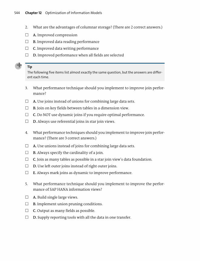
Chapter 12 Optimization of Information Models544
2. What are the advantages of columnar storage? (There are 2 correct answers.)
� A. Improved compression
� B. Improved data reading performance
� C. Improved data writing performance
� D. Improved performance when all fields are selected
Tip
The following five items list almost exactly the same question, but the answers are differ-
ent each time.
3. What performance technique should you implement to improve join perfor-
mance?
� A. Use joins instead of unions for combining large data sets.
� B. Join on key fields between tables in a dimension view.
� C. Do NOT use dynamic joins if you require optimal performance.
� D. Always use referential joins in star join views.
4. What performance techniques should you implement to improve join perfor-
mance? (There are 3 correct answers.)
� A. Use unions instead of joins for combining large data sets.
� B. Always specify the cardinality of a join.
� C. Join as many tables as possible in a star join view’s data foundation.
� D. Use left outer joins instead of right outer joins.
� E. Always mark joins as dynamic to improve performance.
5. What performance technique should you implement to improve the perfor-
mance of SAP HANA information views?
� A. Build single large views.
� B. Implement union pruning conditions.
� C. Output as many fields as possible.
� D. Supply reporting tools with all the data in one transfer.

Practice Questions Chapter 12 545
6. What performance technique should you implement to improve the perfor-
mance of SAP HANA information views that include SQLScript?
� A. Use imperative logic.
� B. Use SELECT *.
� C. Break large statements into smaller steps.
� D. Use dynamic SQL.
7. What performance techniques should you implement to improve the perfor-
mance of SAP HANA information views? (There are 3 correct answers.)
� A. Perform calculations before aggregation in your analytic views.
� B. Minimize the transfer of data between the execution engines.
� C. Investigate partitioning of large tables.
� D. Apply filters as late as possible.
� E. Push down aggregations to SAP HANA.
8. What information can you find in the plan graph? (There are 2 correct
answers.)
� A. Execution engines used
� B. Number of records returned in each step
� C. Time taken for each step
� D. Plan trace
9. What information can you find in the SAP HANA cockpit? (There are 2 correct
answers.)
� A. SQL generated in each step
� B. Trace and log files
� C. List of operators
� D. Plan trace

Chapter 12 Optimization of Information Models546
10. What information can you find in performance analysis mode when you view
the analysis for a Join node? (There are 2 correct answers.)
� A. Suggested filter for the tables in the Join node
� B. Total number of records returned by the node
� C. Time taken by the join
� D. Tables used by the join in the node
Practice Question Answers and Explanations
1. Correct answer: B
The combination of in-memory technology and multicore CPUs enabled real-
time computing.
Solid-state disks are still disks and relatively slow compared to memory.
Multicore CPUs with large level 1 caches help, but also need in-memory tech-
nology because level 1 caches are quite small, for example, 256 KB.
2. Correct answers: A, B
The advantages of columnar storage include improved compression and data-
reading performance. (Because data is compressed, you can read more data at
the same I/O speed.)
Improved data-writing performance is for row storage.
Neither column nor row has improved performance when all fields are selected
via SELECT *.
3. Correct answer: B
Joining on key fields between tables in a dimension view will improve join per-
formance.
The answer “Use joins instead of unions for combining large data sets” has joins
and unions swapped around: you should use unions rather than joins.
Dynamic joins are created to improve performance.
The word always makes the “Always use referential joins” answer wrong.
4. Correct answers: A, B, D
The following are the correct performance techniques to improve join perfor-
mance: use unions instead of joins for combining large data sets, always specify
the cardinality of a join, and use left outer joins instead of right outer joins.
You should try to use only one table in a star join view’s data foundation.
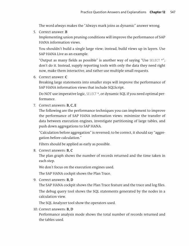
Practice Question Answers and Explanations Chapter 12 547
The word always makes the “Always mark joins as dynamic” answer wrong.
5. Correct answer: B
Implementing union pruning conditions will improve the performance of SAP
HANA information views.
You shouldn’t build a single large view; instead, build views up in layers. Use
SAP HANA Live as an example.
“Output as many fields as possible” is another way of saying “Use SELECT *”;
don’t do it. Instead, supply reporting tools with only the data they need right
now, make them interactive, and rather use multiple small requests.
6. Correct answer: C
Breaking large statements into smaller steps will improve the performance of
SAP HANA information views that include SQLScript.
Do NOT use imperative logic, SELECT *, or dynamic SQL if you need optimal per-
formance.
7. Correct answers: B, C, E
The following are the performance techniques you can implement to improve
the performance of SAP HANA information views: minimize the transfer of
data between execution engines, investigate partitioning of large tables, and
push down aggregations to SAP HANA.
“Calculation before aggregation” is reversed; to be correct, it should say “aggre-
gation before calculation.”
Filters should be applied as early as possible.
8. Correct answers: B, C
The plan graph shows the number of records returned and the time taken in
each step.
We don’t focus on the execution engines used.
The SAP HANA cockpit shows the Plan Trace.
9. Correct answers: B, D
The SAP HANA cockpit shows the Plan Trace feature and the trace and log files.
The debug query tool shows the SQL statements generated by the nodes in a
calculation view.
The SQL Analyzer tool show the operators used.
10. Correct answers: B, D
Performance analysis mode shows the total number of records returned and
the tables used.
Chapter 12 Optimization of Information Models548
Takeaway
You now have a checklist of modeling practices to ensure optimal performance for
SAP HANA information models, including guidelines for creating optimal SQL and
SQLScript.
You can use the SAP HANA cockpit to identify long-running and expensive state-
ments and to perform traces of specific queries and user activities. Performance
analysis mode helps improve your SAP HANA information models by providing
optimization suggestions.
Summary
You’ve seen that SAP HANA has been built from the ground up with many perfor-
mance enhancements to enable high-performing processes. However, you still
have to do your part if you expect the best results.
You’ve now created SAP HANA information models with graphical views and with
SQL and SQLScript. You’ve also learned how to optimize your information models.
In the next chapter, we’ll look at how to apply security to your finished SAP HANA
information models.
Chapter 13
Security
Techniques You’ll Master
� Know when to use the different SAP HANA security features
� Understand how users, roles, and privileges work together
� Know how to create new users and roles
� Learn the various types of privileges
� Explain analytic privileges
� Assign roles to users
� Be familiar with the SAP HANA Deployment Infrastructure (HDI)
and SAP HANA extended application services, advanced model
(SAP HANA XSA) security concepts

Chapter 13 Security550
In this chapter, we’ll discuss how to implement security on the information mod-
els you’ve built. Security is frequently a specialist area, with people dedicated to
looking after system security and user administration.
We won’t go into all the details of SAP HANA security in this chapter, but we’ll give
you a good overview to help you with most of the scenarios you’ll encounter in
your day-to-day information-modeling work and those that are covered on the
exam.
Real-World Scenario
You get an error message in SAP HANA indicating that you don’t have suffi-
cient privileges to do a certain task. In cases like these, you’ll need to know
how to resolve this kind of error message. For this situation, the answer is
simply granting a right to a special user. In some cases, you may need to build
special roles and privileges.
In other cases, you may be asked by the project manager to assist with setting
up the security on the information models. Because you built these informa-
tion models in SAP HANA, you’ll have a good idea of which users should have
certain privileges.
You might also have to comply with certain regulations to ensure data secu-
rity and privacy by using data masking and data anonymization techniques.
Objectives of This Portion of the Test
The purpose of this portion of the SAP HANA certification exam is to test your
knowledge of SAP HANA security.
The certification exam expects you to have a good understanding of the following
topics:
� When to use SAP HANA security, and when to use application security
� How users, roles, and privileges work together
� Understanding system users and how to create new users
� Working with analytic privileges
� Assigning the various types of privileges to a role
� Building a new role, and assigning it to a user

Key Concepts Refresher Chapter 13 551
� Understanding HDI and SAP HANA XSA security concepts
� Using masking and anonymization for data security and privacy
Note
This portion contributes about 5% of the total certification exam score.
Key Concepts Refresher
Security determines what people are allowed to do and see in business applica-
tions. Although we want to stop any unauthorized people from getting access to
company information, we also want to allow business users to do their work with-
out hindrance. There are various ways to achieve this balance in SAP HANA.
In this section, we’ll discuss the basic use cases for security in SAP HANA and
important security concepts. We’ll then look at how to create users, how these
users can access the system, and what roles and privileges these users should get
to achieve their goals. We’ll also discuss data security in general and data masking
in particular.
Usage and Concepts
Let’s begin by looking at when to use security measures in SAP HANA before tack-
ling important concepts.
Use Cases
The use cases for implementing security in SAP HANA depend on the deployment
scenario. Let’s look at the different deployment scenarios and their security man-
agement:
� SAP HANA as a database
In a deployment scenario in which SAP HANA is used as the database for busi-
ness applications such as SAP ERP, SAP Customer Relationship Management
(SAP CRM), and SAP Business Warehouse (SAP BW), you don’t need to create SAP
HANA users and roles for the business users. These users log in to the various
SAP systems via the SAP application servers, and all end-user security is man-
aged by these applications. This is shown on the left side of Figure 13.1. You’ll still
need to create a few SAP HANA users and roles for the system administrator
users, but you don’t need to create anything for the business users.

Chapter 13 Security552
Figure 13.1 Security for SAP HANA as Database vs. Platform
� SAP HANA as a platform
In deployment scenarios in which SAP HANA is used as a platform, end users
need to log in and work directly in the SAP HANA system. In such cases, you
might need to create users and assign roles for these users. In this chapter, we’ll
focus primarily on these scenarios.
� SAP HANA Live
For SAP HANA Live, which we’ll discuss in Chapter 14, you also need end users to
log in and work in the SAP HANA system. However, sometimes they also work
in SAP HANA Live models via SAP applications. In this case, you need to manage
the users in the SAP applications and use the Authorization Assistant tool to
automatically create the correct SAP HANA Live users and roles inside the SAP
HANA system. This chapter won’t focus on this use case.
We’ve mentioned users and their roles in this section. In the next section, we’ll
look at how these concepts work together in SAP HANA.
SAP HANA
SAP HANA
Database
Non-SAP
SAP ERP
SAP CRMEnterprise data
warehouse(SAP BW)
SAP HANA SAP HANA
Browser and mobile
SAP HANAXSA
SAP HANA as a Database SAP HANA as a Platform
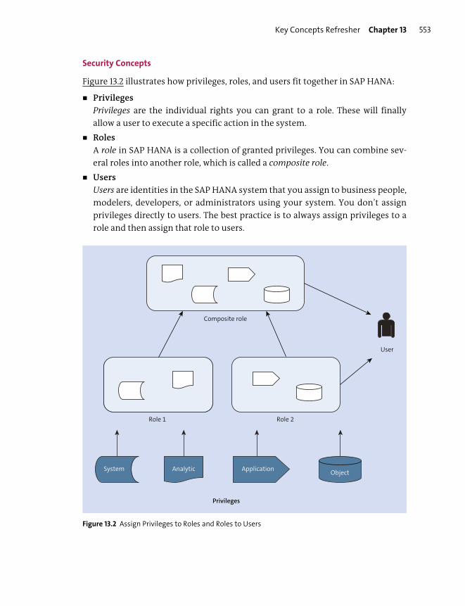
Key Concepts Refresher Chapter 13 553
Security Concepts
Figure 13.2 illustrates how privileges, roles, and users fit together in SAP HANA:
� Privileges
Privileges are the individual rights you can grant to a role. These will finally
allow a user to execute a specific action in the system.
� Roles
A role in SAP HANA is a collection of granted privileges. You can combine sev-
eral roles into another role, which is called a composite role.
� Users
Users are identities in the SAP HANA system that you assign to business people,
modelers, developers, or administrators using your system. You don’t assign
privileges directly to users. The best practice is to always assign privileges to a
role and then assign that role to users.
Figure 13.2 Assign Privileges to Roles and Roles to Users
Composite role
Role 1 Role 2
Privileges
System Analytic Application Object
User
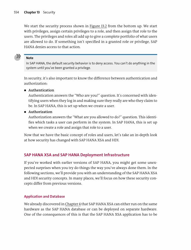
Chapter 13 Security554
We start the security process shown in Figure 13.2 from the bottom up. We start
with privileges, assign certain privileges to a role, and then assign that role to the
users. The privileges and roles all add up to give a complete portfolio of what users
are allowed to do. If something isn’t specified in a granted role or privilege, SAP
HANA denies access to that action.
Note
In SAP HANA, the default security behavior is to deny access. You can’t do anything in the
system until you’ve been granted a privilege.
In security, it’s also important to know the difference between authentication and
authorization:
� Authentication
Authentication answers the “Who are you?” question. It’s concerned with iden-
tifying users when they log in and making sure they really are who they claim to
be. In SAP HANA, this is set up when we create a user.
� Authorization
Authorization answers the “What are you allowed to do?” question. This identi-
fies which tasks a user can perform in the system. In SAP HANA, this is set up
when we create a role and assign that role to a user.
Now that we have the basic concept of roles and users, let’s take an in-depth look
at how security has changed with SAP HANA XSA and HDI.
SAP HANA XSA and SAP HANA Deployment Infrastructure
If you’ve worked with earlier versions of SAP HANA, you might get some unex-
pected surprises when you try do things the way you’ve always done them. In the
following sections, we’ll provide you with an understanding of the SAP HANA XSA
and HDI security concepts. In many places, we’ll focus on how these security con-
cepts differ from previous versions.
Application and Database
We already discovered in Chapter 4 that SAP HANA XSA can either run on the same
hardware as the SAP HANA database or can be deployed on separate hardware.
One of the consequences of this is that the SAP HANA XSA application has to be
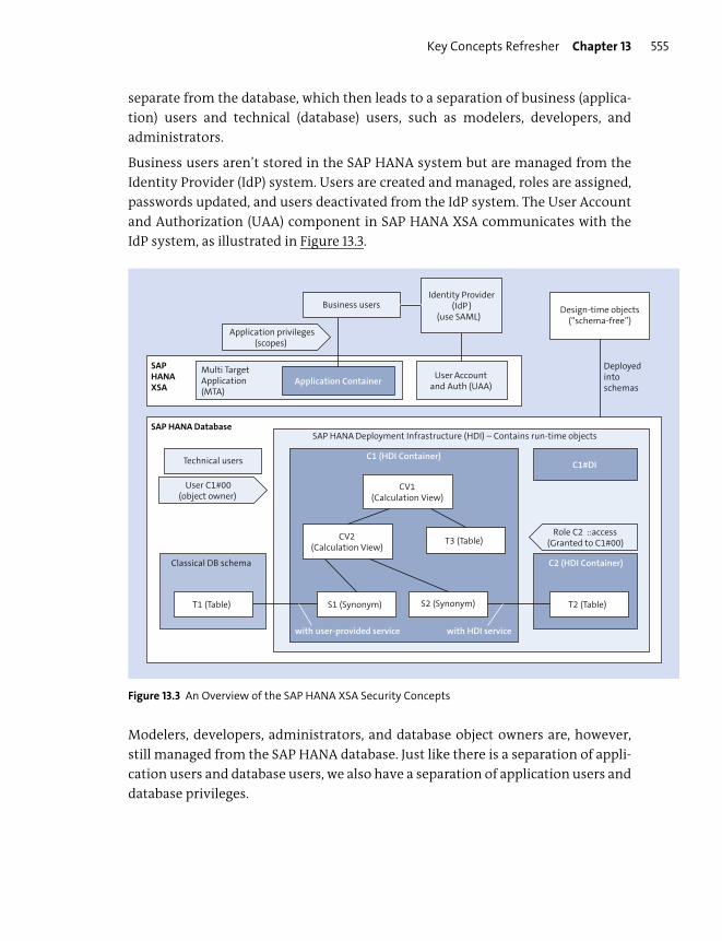
Key Concepts Refresher Chapter 13 555
separate from the database, which then leads to a separation of business (applica-
tion) users and technical (database) users, such as modelers, developers, and
administrators.
Business users aren’t stored in the SAP HANA system but are managed from the
Identity Provider (IdP) system. Users are created and managed, roles are assigned,
passwords updated, and users deactivated from the IdP system. The User Account
and Authorization (UAA) component in SAP HANA XSA communicates with the
IdP system, as illustrated in Figure 13.3.
Figure 13.3 An Overview of the SAP HANA XSA Security Concepts
Modelers, developers, administrators, and database object owners are, however,
still managed from the SAP HANA database. Just like there is a separation of appli-
cation users and database users, we also have a separation of application users and
database privileges.
SAP HANA DatabaseSAP HANA Deployment Infrastructure (HDI) – Contains run-time objects
C1 (HDI Container)
Classical DB schema C2 (HDI Container)
T1 (Table) T2 (Table)S2 (Synonym)S1 (Synonym)
C1#DI
T3 (Table)
with user-provided service with HDI service
SAPHANAXSA
Multi TargetApplication(MTA)
Application ContainerUser Account
and Auth (UAA)
Identity Provider (IdP )
(use SAML)Business users
Application privileges (scopes)
CV1(Calculation View)
CV2(Calculation View)
Technical users
Role C2 ::access(Granted to C1#00)
User C1#00(object owner)
Design-time objects(“schema-free”)
Deployedintoschemas

Chapter 13 Security556
Design-Time and Runtime Objects
The next big change is that design-time objects are now separate from runtime
objects. We used to store the design-time objects in the SAP HANA system where
we finally used it. If you used the same object in a development system, a test sys-
tem, and a production system, you would store three separate copies of the same
object. These local copies of the objects were then “activated” to become runtime
objects in the same SAP HANA system. These activated (runtime) objects belonged
to the _SYS_REPO user.
We now store a single copy of the design-time object in a Git repository and
“deploy” it to multiple systems. Modelers and developers create such design-time
objects, such as calculation views and procedures (refer to the top-right area of
Figure 13.3).
System administrators and database administrators (DBAs), on the other side,
manage the deployment process and the runtime objects in the containers of the
SAP HANA database.
The biggest difference for modelers and developers is that we now work in a
“schema-free” way. Because the same design-time object can be deployed to mul-
tiple systems, such as testing and production, we can’t explicitly reference data-
base schemas. Schema names can be different for different HDI containers. The
actual schema names are assigned as part of the deployment process.
By default, SAP HANA Studio always created roles as runtime objects in the local
SAP HANA system. These runtime roles can’t be transported from development to
testing and production systems.
In SAP Web IDE for SAP HANA and the SAP HANA cockpit, we now create design-
time roles that can be deployed to multiple target systems.
Containers Isolate Schemas
In SAP HANA 1.0, in general, we had several schemas in the Catalog area. Each
schema was basically just a collection of SAP HANA runtime objects. There was no
isolation of schemas, so it was easy to create a calculation view that joined tables
from two different schemas. We merely used explicit references to the tables.
If we now try to do the same in an HDI container, we get a You are not authorized
message. In the bottom half of Figure 13.3, you see an illustration of how we should
do this in HDI containers.
Key Concepts Refresher Chapter 13 557
HDI containers contain similar runtime objects as in the classical schemas in the
Catalog area. These could be tables, indexes, calculation views, table functions, and
procedures. Each HDI container is equivalent to a database schema, but with some
important differences and extras.
The word “containers” implies that they are isolated from each other and from the
“outside world.” This is the main difference to keep in mind as we discuss HDI con-
tainers. The “extras” we mentioned are as follows:
� Each HDI container has its own technical user, that is, the owner of all the run-
time objects in the container (schema). For a container named C1, this user will
be called C1#00. This is different from before, where the _SYS_REPO user was the
owner of all runtime objects in the entire SAP HANA system.
� Each HDI container has another associated container that is used for application
programming interfaces (APIs) and storage. For a container named C1, this asso-
ciated container is called C1#DI.
� Each HDI container has a generic default role that is automatically created when
you create the container. For a container named C1, this role is called C1::access.
This role (shown much later in this chapter in Figure 13.10), contains a role for
running services that allows external users data access to this HDI container
(schema), as well as object privileges to read, insert, update, and delete data.
Let’s return to our example of creating a calculation view that joins tables from
two different schemas.
Referring to Figure 13.3, we do our modeling in an HDI container called C1. We cre-
ate our calculation view, called CV2, that joins table T1 from a classical schema with
table T2 in another HDI container C2. Because container C2 is isolated, we need per-
mission to read the table. We need to assign the C2::access role to the C1#00 user
and create a synonym S2 to point to table T2. Synonym S2 uses the built-in HDI ser-
vice to read table T2.
When we read table T1 in the classical schema, we also have to create synonym S1
to read the table. But because this table is in a classical schema, we can’t use the
HDI service, and we have to use a user-defined service. We also need the C2::access
role assigned to the C1#00 user.
If we access a table in the same HDI container, such as table T3, this works as usual.
No extra steps are required because this table is located in the same container.
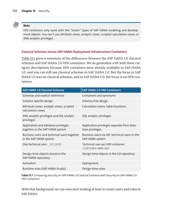
Chapter 13 Security558
Note
HDI containers only work with the “newer” types of SAP HANA modeling and develop-
ment objects. You can’t use attribute views, analytic views, scripted calculation views, or
XML analytic privileges.
Classical Schemas versus SAP HANA Deployment Infrastructure Containers
Table 13.1 gives a summary of the differences between the SAP HANA 1.0 classical
schemas and SAP HANA 2.0 HDI containers. We do generalize a bit with these cat-
egory descriptions because HDI containers were already available in SAP HANA
1.0, and you can still use classical schemas in SAP HANA 2.0. But the focus in SAP
HANA 1.0 was on classical schemas, and in SAP HANA 2.0, the focus is on HDI con-
tainers.
With that background, we can now start looking at how to create users and roles in
SAP HANA.
SAP HANA 1.0 Classical Schemas SAP HANA 2.0 HDI Containers
Schemas and explicit references Containers and synonyms
Schema-specific design Schema-free design
Attribute views, analytic views, scripted
calculation views
Calculation views, table functions
XML analytic privileges and SQL analytic
privileges
SQL analytic privileges
Application and database privileges
together in the SAP HANA system
Application privileges separate from data-
base privileges
Business users and technical users together
in the SAP HANA system
Business users via IdP, technical users in the
SAP HANA system
One technical user: _SYS_REPO Technical user per HDI container:
<CONTAINER-NAME>#00
Design-time objects stored in the
SAP HANA repository
Design-time objects in the Git repository
Activation Deployment
Runtime roles (SAP HANA Studio) Design-time roles
Table 13.1 Comparing Security on SAP HANA 1.0 Classical Schemas with Security on SAP HANA 2.0 HDI Containers
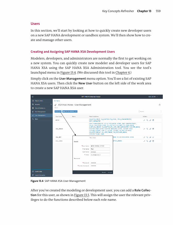
Key Concepts Refresher Chapter 13 559
Users
In this section, we’ll start by looking at how to quickly create new developer users
on a new SAP HANA development or sandbox system. We’ll then show how to cre-
ate and manage other users.
Creating and Assigning SAP HANA XSA Development Users
Modelers, developers, and administrators are normally the first to get working on
a new system. You can quickly create new modeler and developer users for SAP
HANA XSA using the SAP HANA XSA Administration tool. You see the tool’s
launchpad menu in Figure 13.4. (We discussed this tool in Chapter 4.)
Simply click on the User Management menu option. You’ll see a list of existing SAP
HANA XSA users. Then click the New User button on the left side of the work area
to create a new SAP HANA XSA user.
Figure 13.4 SAP HANA XSA User Management
After you’ve created the modeling or development user, you can add a Role Collec-
tion for this user, as shown in Figure 13.5. This will assign the user the relevant priv-
ileges to do the functions described below each role name.
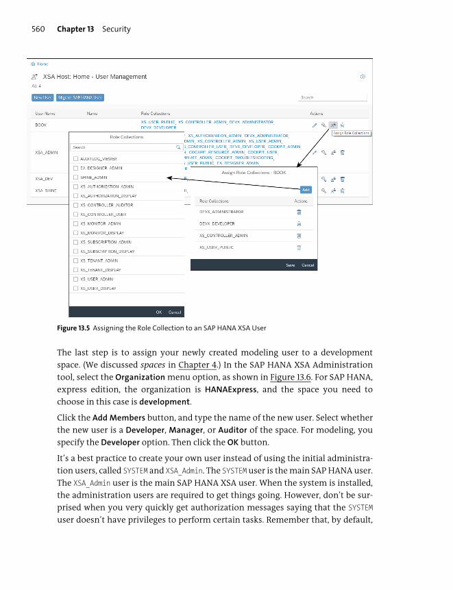
Chapter 13 Security560
Figure 13.5 Assigning the Role Collection to an SAP HANA XSA User
The last step is to assign your newly created modeling user to a development
space. (We discussed spaces in Chapter 4.) In the SAP HANA XSA Administration
tool, select the Organization menu option, as shown in Figure 13.6. For SAP HANA,
express edition, the organization is HANAExpress, and the space you need to
choose in this case is development.
Click the Add Members button, and type the name of the new user. Select whether
the new user is a Developer, Manager, or Auditor of the space. For modeling, you
specify the Developer option. Then click the OK button.
It’s a best practice to create your own user instead of using the initial administra-
tion users, called SYSTEM and XSA_Admin. The SYSTEM user is the main SAP HANA user.
The XSA_Admin user is the main SAP HANA XSA user. When the system is installed,
the administration users are required to get things going. However, don’t be sur-
prised when you very quickly get authorization messages saying that the SYSTEM
user doesn’t have privileges to perform certain tasks. Remember that, by default,
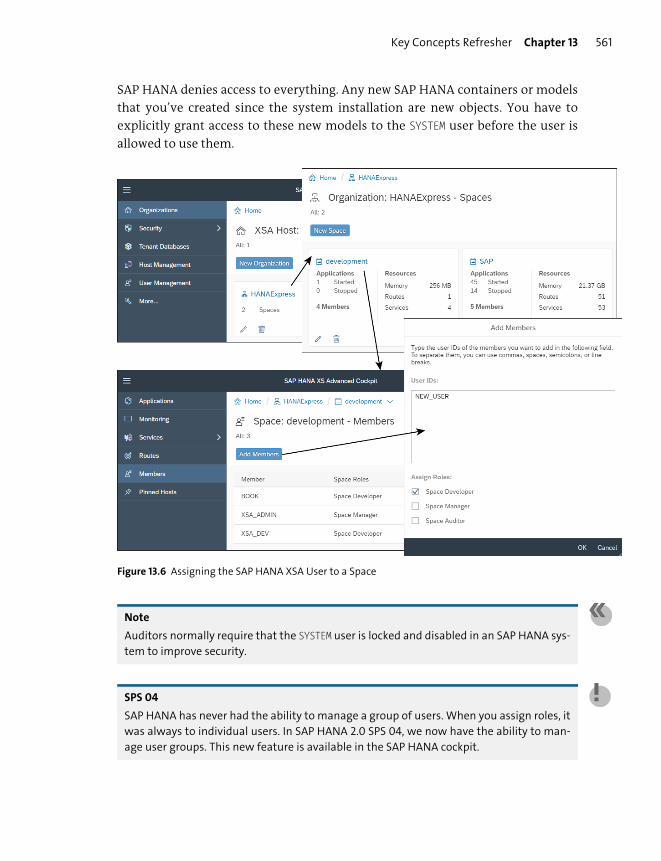
Key Concepts Refresher Chapter 13 561
SAP HANA denies access to everything. Any new SAP HANA containers or models
that you’ve created since the system installation are new objects. You have to
explicitly grant access to these new models to the SYSTEM user before the user is
allowed to use them.
Figure 13.6 Assigning the SAP HANA XSA User to a Space
Note
Auditors normally require that the SYSTEM user is locked and disabled in an SAP HANA sys-
tem to improve security.
SPS 04
SAP HANA has never had the ability to manage a group of users. When you assign roles, it
was always to individual users. In SAP HANA 2.0 SPS 04, we now have the ability to man-
age user groups. This new feature is available in the SAP HANA cockpit.
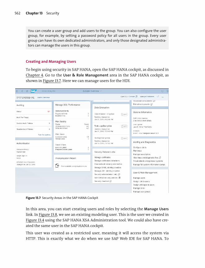
Chapter 13 Security562
You can create a user group and add users to the group. You can also configure the user
group, for example, by setting a password policy for all users in the group. Every user
group can have its own dedicated administrators, and only those designated administra-
tors can manage the users in this group.
Creating and Managing Users
To begin using security in SAP HANA, open the SAP HANA cockpit, as discussed in
Chapter 4. Go to the User & Role Management area in the SAP HANA cockpit, as
shown in Figure 13.7. Here we can manage users for the HDI.
Figure 13.7 Security Areas in the SAP HANA Cockpit
In this area, you can start creating users and roles by selecting the Manage Users
link. In Figure 13.8, we see an existing modeling user. This is the user we created in
Figure 13.4 using the SAP HANA XSA Administration tool. We could also have cre-
ated the same user in the SAP HANA cockpit.
This user was created as a restricted user, meaning it will access the system via
HTTP. This is exactly what we do when we use SAP Web IDE for SAP HANA. To
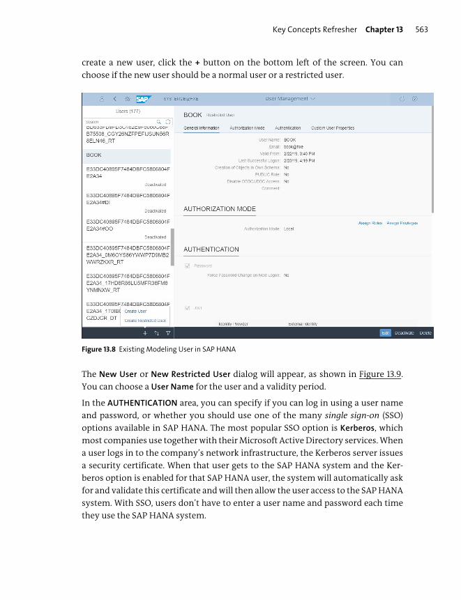
Key Concepts Refresher Chapter 13 563
create a new user, click the + button on the bottom left of the screen. You can
choose if the new user should be a normal user or a restricted user.
Figure 13.8 Existing Modeling User in SAP HANA
The New User or New Restricted User dialog will appear, as shown in Figure 13.9.
You can choose a User Name for the user and a validity period.
In the AUTHENTICATION area, you can specify if you can log in using a user name
and password, or whether you should use one of the many single sign-on (SSO)
options available in SAP HANA. The most popular SSO option is Kerberos, which
most companies use together with their Microsoft Active Directory services. When
a user logs in to the company’s network infrastructure, the Kerberos server issues
a security certificate. When that user gets to the SAP HANA system and the Ker-
beros option is enabled for that SAP HANA user, the system will automatically ask
for and validate this certificate and will then allow the user access to the SAP HANA
system. With SSO, users don’t have to enter a user name and password each time
they use the SAP HANA system.
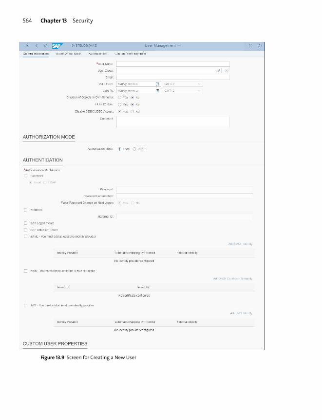
Chapter 13 Security564
Figure 13.9 Screen for Creating a New User

Key Concepts Refresher Chapter 13 565
Tip
Users in an SAP HANA system aren’t transportable. You can’t create users in a develop-
ment system and transport them to the production system with all their roles and privi-
leges. This is by design, as you don’t want development and modeling users in the
production system, and you don’t want end users in the development system.
Roles
In the previous section, we looked at creating users and assigning them roles. In
this section, we’ll take a deeper dive into SAP HANA’s roles and discuss the various
template roles available and the steps for creating a role in the system.
Template Roles
SAP provides a few template roles that you can use as examples for building your
own, or you can use them as a starting point and extend them. We don’t recom-
mend modifying any of the template roles directly; instead, copy them and mod-
ify the copy.
The following two template roles are important:
� MONITORING
This is a role that provides read-only access to the SAP HANA system. You pro-
vide this, for example, to a system administrator or monitoring tool that needs
to check your system. Users that have this role assigned can’t modify anything
in the system.
� MODELING
This role is given to modelers so they can create information models in the SAP
HANA system. We don’t recommend giving this role to any user in the produc-
tion system. Users with this role assigned can create and modify objects in the
system and can read all data, even sensitive or confidential data.
These types of roles are also known as global roles. They are schema-independent.
Creating Roles in SAP HANA Cockpit
You can see all the roles in SAP HANA by clicking the Manage Roles link in the SAP
HANA cockpit, as shown earlier in Figure 13.7. A list of all the roles in SAP HANA, as
shown in Figure 13.10, will show in the left column. When you select a role, the
details appear on the right side.
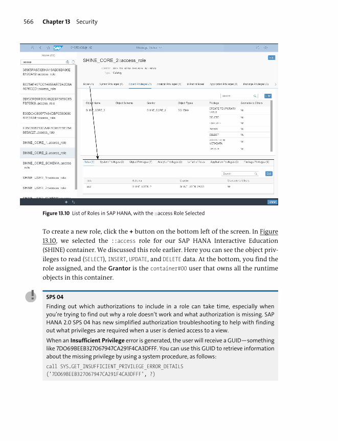
Chapter 13 Security566
Figure 13.10 List of Roles in SAP HANA, with the ::access Role Selected
To create a new role, click the + button on the bottom left of the screen. In Figure
13.10, we selected the ::access role for our SAP HANA Interactive Education
(SHINE) container. We discussed this role earlier. Here you can see the object priv-
ileges to read (SELECT), INSERT, UPDATE, and DELETE data. At the bottom, you find the
role assigned, and the Grantor is the container#00 user that owns all the runtime
objects in this container.
SPS 04
Finding out which authorizations to include in a role can take time, especially when
you’re trying to find out why a role doesn’t work and what authorization is missing. SAP
HANA 2.0 SPS 04 has new simplified authorization troubleshooting to help with finding
out what privileges are required when a user is denied access to a view.
When an Insufficient Privilege error is generated, the user will receive a GUID—something
like 7DO69BEEB327067947CA291F4CA3DFFF. You can use this GUID to retrieve information
about the missing privilege by using a system procedure, as follows:
call SYS.GET_INSUFFICIENT_PRIVILEGE_ERROR_DETAILS('7DO69BEEB327067947CA291F4CA3DFFF', ?)
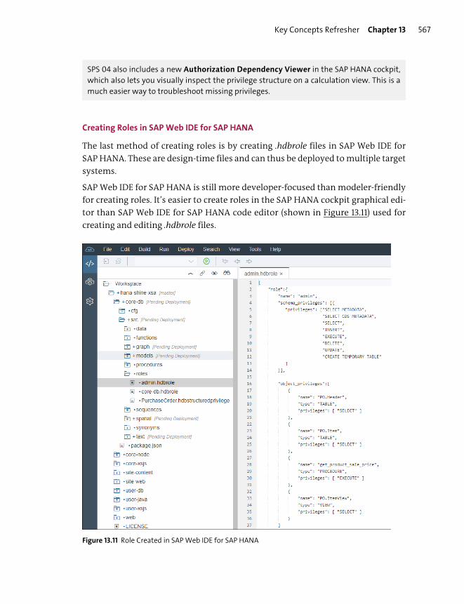
Key Concepts Refresher Chapter 13 567
SPS 04 also includes a new Authorization Dependency Viewer in the SAP HANA cockpit,
which also lets you visually inspect the privilege structure on a calculation view. This is a
much easier way to troubleshoot missing privileges.
Creating Roles in SAP Web IDE for SAP HANA
The last method of creating roles is by creating .hdbrole files in SAP Web IDE for
SAP HANA. These are design-time files and can thus be deployed to multiple target
systems.
SAP Web IDE for SAP HANA is still more developer-focused than modeler-friendly
for creating roles. It’s easier to create roles in the SAP HANA cockpit graphical edi-
tor than SAP Web IDE for SAP HANA code editor (shown in Figure 13.11) used for
creating and editing .hdbrole files.
Figure 13.11 Role Created in SAP Web IDE for SAP HANA
Chapter 13 Security568
The example in Figure 13.11 is the admin.hdbrole role in the SHINE demo.
Tip
The .hdbrole files are design-time objects that can be transported to the production sys-
tem. This improves security because you don’t need someone with rights to create roles
in the production system.
Earlier, we mentioned that you should always create design-time files in a schema-
free manner. You can see that that the illustrated role doesn’t contain any schema
names. But what should you do if you really need to create a schema-specific
authorization where you have to specify the schema name?
In this case, you can create a single .hdbroleconfig file that contains the name of the
schema, as shown in Listing 13.1.
{"DemoRole":{
"SchemaReference1":{"schema":"DemoSchema1"
}}
}
Listing 13.1 A Sample .hdbcroleconfig File
You can now refer to this .hdbroleconfig file in many .hdbrole files, as shown in Lis-
ting 13.2.
"schema_roles":[{
"schema_reference":" SchemaReference1","names": ["Role1", "Role2"]
}]
Listing 13.2 .hdbrole File Referencing the .hdbroleconfig File
Instead of having to modify the schema name in many .hdbrole files, you only
have to update the single .hdbroleconfig file.
Tip
You should never create roles in the SQL Console using SQL statements. These roles are
immediately created as runtime objects and can’t be transported (deployed) to other sys-
tems.
Key Concepts Refresher Chapter 13 569
Tip
If you want to give users with this role the right to assign the role to others users, you
need to include WITH GRANT OPTION privileges in the role. In this case, the name of the role
must end with a hash (#), for example, role#.
Privileges
In this section, we’ll discuss the different types of privileges available in SAP
HANA. We’ve already seen schema privileges in Figure 13.11. In Figure 13.10, shown
earlier, we can see the following tabs for five other types of privileges:
� System Privileges
� Object Privileges
� Analytic Privileges
� Application Privileges
� Package Privileges
When you build or extend a role, you can assign these different types of privileges.
Each of these privileges has its own tab in the Manage Roles editing screen. You can
add new privileges in each tab by clicking on the Edit button.
A dialog box will present a list of relevant privileges to choose from. All of these
dialog boxes have a text field in which you can enter some search text. The list of
available privileges will be limited according to the search text you type.
Tip
You can only add privileges. There is no concept in SAP HANA of taking away privileges
because the default behavior is to deny access.
System Privileges
System privileges can be associated with system administration. These privileges
grant users the rights to work with the SAP HANA system. Most of the system priv-
ileges are applicable to DBAs and system administrators. Figure 13.12 shows an
example of system privileges.
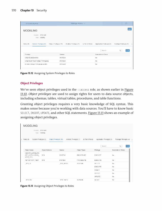
Chapter 13 Security570
Figure 13.12 Assigning System Privileges to Roles
Object Privileges
We’ve seen object privileges used in the ::access role, as shown earlier in Figure
13.10. Object privileges are used to assign rights for users to data source objects,
including schemas, tables, virtual tables, procedures, and table functions.
Granting object privileges requires a very basic knowledge of SQL syntax. This
makes sense because you’re working with data sources. You’ll have to know basic
SELECT, INSERT, UPDATE, and other SQL statements. Figure 13.13 shows an example of
assigning object privileges.
Figure 13.13 Assigning Object Privileges to Roles
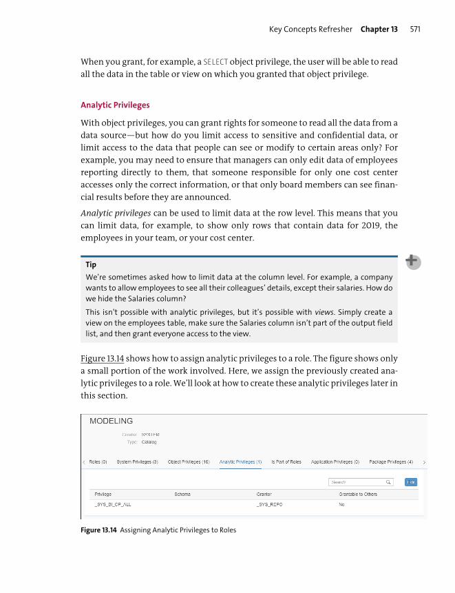
Key Concepts Refresher Chapter 13 571
When you grant, for example, a SELECT object privilege, the user will be able to read
all the data in the table or view on which you granted that object privilege.
Analytic Privileges
With object privileges, you can grant rights for someone to read all the data from a
data source—but how do you limit access to sensitive and confidential data, or
limit access to the data that people can see or modify to certain areas only? For
example, you may need to ensure that managers can only edit data of employees
reporting directly to them, that someone responsible for only one cost center
accesses only the correct information, or that only board members can see finan-
cial results before they are announced.
Analytic privileges can be used to limit data at the row level. This means that you
can limit data, for example, to show only rows that contain data for 2019, the
employees in your team, or your cost center.
Tip
We’re sometimes asked how to limit data at the column level. For example, a company
wants to allow employees to see all their colleagues’ details, except their salaries. How do
we hide the Salaries column?
This isn’t possible with analytic privileges, but it’s possible with views. Simply create a
view on the employees table, make sure the Salaries column isn’t part of the output field
list, and then grant everyone access to the view.
Figure 13.14 shows how to assign analytic privileges to a role. The figure shows only
a small portion of the work involved. Here, we assign the previously created ana-
lytic privileges to a role. We’ll look at how to create these analytic privileges later in
this section.
Figure 13.14 Assigning Analytic Privileges to Roles

Chapter 13 Security572
Tip
In Figure 13.14, the role was assigned an analytic privilege called _SYS_BI_CP_ALL. Be care-
ful when assigning this analytic privilege; it grants access to the entire data set of the
information views involved. It effectively bypasses the analytic privilege restrictions
defined on a view. This analytic privilege shouldn’t be granted to end users in a produc-
tion system.
Note that this privilege is part of the MODELING role, as shown here. The MODELING role
shouldn’t be granted to any end users in a production system as this will allow them to
see all the data in the production system!
Think about how analytic privileges behave when they are used with layered infor-
mation views. Assume you need access to information about your cost center. Let’s
view this from the reporting side. You run a report that it calls view A. View A then
calls another view, called B. (View A is built on top of view B.) You can only see your
cost center information if you have an analytic privilege that allows you to see the
information being assigned to both views.
If you have the analytic privilege assigned to only one of the two views, you won’t
be able to see your cost center information.
Tip
It will help you to think of analytic privileges across multiple stacked views as an inner
join. Only the analytic privileges specified in both views are applied.
Another aspect of analytic privileges to think about is what result you want to
achieve when using multiple restrictions. Let’s assume you have two restrictions:
the first is year = 2018, and the second is cost center = 123.
� If you need year = 2018 AND cost center = 123, you must specify both restrictions
in a single analytic privilege. In this case, you’ve limited what the user sees even
more than when you use only one of the restrictions. The AND clause restricts the
results more.
� If you need year = 2018 OR cost center = 123, you must create two separate ana-
lytic privileges and assign both to the same view. In this case, you’ve increased
the amount of data in the result compared to just using one of the restrictions.
The OR clause lets the user see more.
Tip
Analytic privileges are the most-used privileges for information-modeling work.

Key Concepts Refresher Chapter 13 573
You can create analytic privileges in the same context menu where you created all
your SAP HANA information views. In the context menu, select New • Analytic
Privilege. This creates an .hdbanalyticprivilege file. In the next step, choose the
information views that you want to restrict access to.
After you’ve selected the information views, you can create the row-level access
restrictions. On the left side of the screen in Figure 13.15, you can add more infor-
mation views. On the right side of the screen, create your restrictions.
Figure 13.15 Assigning Analytic Privilege Restrictions
There are three ways to specify the restrictions:
� Attributes
With this option, you first select the attributes that you want to create the
restrictions on. In this example, we chose the COMPANYNAME field. You then
have to specify the restrictions. In this example, we restrict the supplier to be
SAP only.
In Figure 13.15, we show Attributes restrictions, which is the default. You can also
restrict the validity period of the analytic privilege, as shown in Figure 13.16.
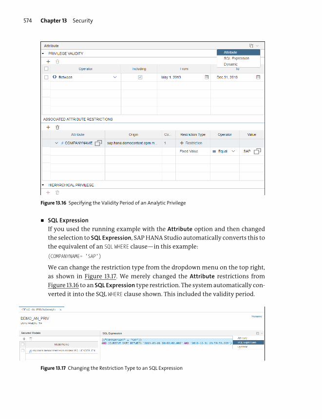
Chapter 13 Security574
Figure 13.16 Specifying the Validity Period of an Analytic Privilege
� SQL Expression
If you used the running example with the Attribute option and then changed
the selection to SQL Expression, SAP HANA Studio automatically converts this to
the equivalent of an SQL WHERE clause—in this example:
(COMPANYNAME= 'SAP')
We can change the restriction type from the dropdown menu on the top right,
as shown in Figure 13.17. We merely changed the Attribute restrictions from
Figure 13.16 to an SQL Expression type restriction. The system automatically con-
verted it into the SQL WHERE clause shown. This included the validity period.
Figure 13.17 Changing the Restriction Type to an SQL Expression

Key Concepts Refresher Chapter 13 575
� Dynamic
The last option is the most powerful. We can also use a procedure to create the
WHERE clause dynamically. This must be a read-only procedure that only has one
output parameter. The output it generates must be the same as the WHERE clause
shown earlier, for example, (COMPANYNAME= ‘SAP’).
In Figure 13.18, we select a procedure. You can also use a synonym that points to
a procedure in another HDI container or schema.
Figure 13.18 Selecting a Procedure for Generating Dynamic Analytic Privileges
As a modeler, you’ll sometimes get error messages. One of the most common
error messages when working with analytic privileges occurs when you build the
analytic privilege. You’ll get a Cannot use structured privilege for view not regis-
tered for STRUCTURED PRIVILEGE CHECK error message. The Build will fail as shown
in Figure 13.19.
In your analytic privilege, you specified the views that this analytic privilege
applies to. One of these views isn’t configured to use SQL analytic privileges.
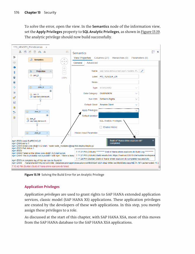
Chapter 13 Security576
To solve the error, open the view. In the Semantics node of the information view,
set the Apply Privileges property to SQL Analytic Privileges, as shown in Figure 13.19.
The analytic privilege should now build successfully.
Figure 13.19 Solving the Build Error for an Analytic Privilege
Application Privileges
Application privileges are used to grant rights to SAP HANA extended application
services, classic model (SAP HANA XS) applications. These application privileges
are created by the developers of these web applications. In this step, you merely
assign these privileges to a role.
As discussed at the start of this chapter, with SAP HANA XSA, most of this moves
from the SAP HANA database to the SAP HANA XSA applications.
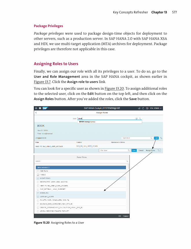
Key Concepts Refresher Chapter 13 577
Package Privileges
Package privileges were used to package design-time objects for deployment to
other servers, such as a production server. In SAP HANA 2.0 with SAP HANA XSA
and HDI, we use multi-target application (MTA) archives for deployment. Package
privileges are therefore not applicable in this case.
Assigning Roles to Users
Finally, we can assign our role with all its privileges to a user. To do so, go to the
User and Role Management area in the SAP HANA cockpit, as shown earlier in
Figure 13.7. Click the Assign role to users link.
You can look for a specific user as shown in Figure 13.20. To assign additional roles
to the selected user, click on the Edit button on the top left, and then click on the
Assign Roles button. After you’ve added the roles, click the Save button.
Figure 13.20 Assigning Roles to a User

Chapter 13 Security578
Data Security
The topic of data security has always been important with SAP HANA because it’s
used as a database and a development platform. How and by whom the data is con-
sumed are inherent and expected features.
One of the basic principles of system security is segregation of duties. This means
that you’re not allowed to have only one person responsible for the administra-
tion of the security. Different people have different responsibilities, and the
responsibilities are divided in such a way that one single person can’t create and
assign rights to themselves or others that give them special privileges that can be
used for corruption or fraud.
As a modeler, you might be creating analytic privileges. Security administrators
then add these as part of a role, and the system administrators can assign this role
to people in the organization. The security auditors will check the system regularly
to ensure that the segregation of duties principle isn’t violated.
The system administrators set up the integration to the Lightweight Directory
Access Protocol (LDAP) server, such as Microsoft Active Directory, to enable SSO in
the SAP HANA system. They might also configure the Security Assertion Markup
Language (SAML) servers for enabling SSO in web browsers. This is required for
SAP HANA XSA to work securely in organizations.
Roles are only set up in a development server; they are assigned to users in the
production server. This segregates privileges across the landscape. Similarly,
developers and modelers can only write code and create information models in
the development server, but these are run by end users with the correct roles in
the production server.
SAP HANA has had data security features such as encryption of data files (data vol-
umes, log volumes, and backups) and audit logs for many years now. These are
configured by the system administrators and checked by the security auditors.
You can also encrypt individual table columns with SAP HANA client-controlled
keys.
Data masking is used when you want to reduce the exposure of sensitive informa-
tion. An example of data masking that you already know is when typing your pass-
word. Your password isn’t shown as text, but “masked” by displaying dots or
blanks.
Another typical use case is when working with credit card numbers. You have to
hide this information from DBAs and users with broad access. Even users that
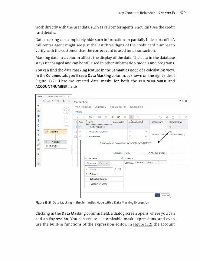
Key Concepts Refresher Chapter 13 579
work directly with the user data, such as call center agents, shouldn’t see the credit
card details.
Data masking can completely hide such information, or partially hide parts of it. A
call center agent might see just the last three digits of the credit card number to
verify with the customer that the correct card is used for a transaction.
Masking data in a column affects the display of the data. The data in the database
stays unchanged and can be still used in other information models and programs.
You can find the data masking feature in the Semantics node of a calculation view.
In the Columns tab, you’ll see a Data Masking column, as shown on the right side of
Figure 13.21. Here we created data masks for both the PHONENUMBER and
ACCOUNTNUMBER fields
Figure 13.21 Data Masking in the Semantics Node with a Data Masking Expression
Clicking in the Data Masking column field, a dialog screen opens where you can
add an Expression. You can create customizable mask expressions, and even
use the built-in functions of the expression editor. In Figure 13.21 the account
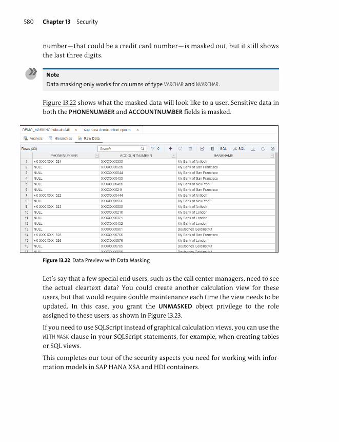
Chapter 13 Security580
number—that could be a credit card number—is masked out, but it still shows
the last three digits.
Note
Data masking only works for columns of type VARCHAR and NVARCHAR.
Figure 13.22 shows what the masked data will look like to a user. Sensitive data in
both the PHONENUMBER and ACCOUNTNUMBER fields is masked.
Figure 13.22 Data Preview with Data Masking
Let’s say that a few special end users, such as the call center managers, need to see
the actual cleartext data? You could create another calculation view for these
users, but that would require double maintenance each time the view needs to be
updated. In this case, you grant the UNMASKED object privilege to the role
assigned to these users, as shown in Figure 13.23.
If you need to use SQLScript instead of graphical calculation views, you can use the
WITH MASK clause in your SQLScript statements, for example, when creating tables
or SQL views.
This completes our tour of the security aspects you need for working with infor-
mation models in SAP HANA XSA and HDI containers.
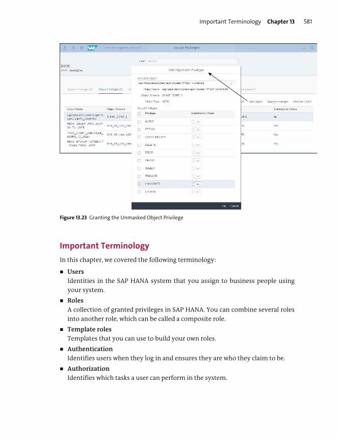
Important Terminology Chapter 13 581
Figure 13.23 Granting the Unmasked Object Privilege
Important Terminology
In this chapter, we covered the following terminology:
� Users
Identities in the SAP HANA system that you assign to business people using
your system.
� Roles
A collection of granted privileges in SAP HANA. You can combine several roles
into another role, which can be called a composite role.
� Template roles
Templates that you can use to build your own roles.
� Authentication
Identifies users when they log in and ensures they are who they claim to be.
� Authorization
Identifies which tasks a user can perform in the system.
Chapter 13 Security582
� Privileges
The individual rights you can grant to a role or a user. In SAP HANA, there are
different types of privileges:
– System privileges: These privileges grant users the rights to work with the SAP
HANA system. Most of the system privileges are applicable to database and
system administrators.
– Object privileges: These privileges are used to assign rights for users to data
source objects, including schemas, tables, virtual tables, procedures, and
table functions. Requires very basic knowledge of SQL syntax.
– Analytic privileges: These privileges control access to SAP HANA data models.
There are two types of analytic privileges: classic XML-based analytic privi-
leges and the new SQL-based analytic privileges. There is a migration tool to
convert the old XML-based analytic privileges to the new SQL-based analytic
privileges.
� Restrictions in analytic privileges
Row-level access restrictions that can be implemented using analytic privileges.
Practice Questions
These practice questions will help you evaluate your understanding of the topic.
The questions shown are similar in nature to those found on the certification
examination. Although none of these questions will be found on the exam itself,
they will allow you to review your knowledge of the subject. Select the correct
answers, and then check the completeness of your answers in the “Practice Ques-
tion Answers and Explanation” section. Remember, on the exam, you must select
all correct answers and only correct answers to receive credit for the question.
1. Which are the recommended assignments in SAP HANA? (There are 2 correct
answers.)
� A. Privileges to users
� B. Roles to users
� C. Roles to roles
� D. Roles to privileges

Practice Questions Chapter 13 583
2. In which SAP HANA deployment scenarios will end users be created as users
in the SAP HANA system? (There are 2 correct answers.)
� A. SAP BW powered by SAP HANA
� B. SAP S/4HANA
� C. SAP HANA as a platform
� D. SAP HANA Live
3. True or False: The default behavior of SAP HANA is to allow access.
� A. True
� B. False
4. Your newly created analytic privilege does NOT want to build. What must you
do?
� A. Grant rights to the _SYS_REPO user.
� B. Assign the ::access role to the HDI container user.
� C. Change the Apply Privileges property of the view.
� D. Change the analytic privilege to use an SQL Expression.
5. What do you have to assign to users to allow single sign-on (SSO)?
� A. SQL analytic privileges
� B. Kerberos authentication
� C. TRUST ADMIN system privilege
� D. Application privileges
6. True or False: Object privileges on a table with SELECT rights will allow you to
access all the data.
� A. True
� B. False
Chapter 13 Security584
7. What can you use to limit users to see only 2018 data? (There are 2 correct
answers.)
� A. An object privilege
� B. A SQL analytic privilege
� C. A view with a filter
� D. A view with a restricted column
8. You have two calculation views for viewing manufactured products. The WORLD
calculation view shows worldwide information. The INDIA calculation view is
built on top of the WORLD calculation view and shows information for Indian
products. What privilege must you assign to see your department’s specific
data in a report built on the INDIA calculation view?
� A. An analytic privilege on the WORLD calculation view
� B. An analytic privilege on the INDIA calculation view
� C. An analytic privilege on both calculation views
� D. An object privilege on the WORLD calculation view
9. You want to read a table from an SAP HANA classical schema. What do you
need to do to get it working? (There are 3 correct answers.)
� A. Use an explicit reference to the schema.
� B. Make use of a user-provided service.
� C. Make use of the built-in HDI service.
� D. Create a synonym.
� E. Assign the provided ::access role to your container’s technical user.
10. True or false: SAP HANA XSA application users are managed from an external
Identity Provider (IdP) system.
� A. True
� B. False

Practice Question Answers and Explanations Chapter 13 585
11. Where do you assign a user as a developer in a development space?
� A. SAP HANA XSA Administration tool
� B. SAP HANA cockpit
� C. SAP Web IDE for SAP HANA
12. What do you use to ensure that each account holder of a bank account can
only see his or her own identity document details in a calculation view?
� A. Audit logs
� B. Analytic privileges
� C. Data masking
Practice Question Answers and Explanations
1. Correct answers: B, C
We can assign roles to other roles and roles to users in SAP HANA.
We could assign privileges to users in SAP HANA 1.0, but this wasn’t recom-
mended. In SAP HANA 2.0, this option was removed.
We can’t assign roles to privileges. We can only assign privileges to roles.
2. Correct answers: C, D
End users might be created as users in the SAP HANA system in the SAP HANA
as a platform deployment scenario. In the case of SAP HANA XSA, where the
application and database are separated, we also don’t need to create end users
in the SAP HANA database.
With SAP HANA Live, users are created in the SAP application server, and they
are automatically created by the Authorization Assistant in SAP HANA.
With SAP BW on SAP HANA and SAP S/4HANA, users are created in the SAP
application servers, not in SAP HANA.
3. Correct answer: B
False. The default behavior of SAP HANA is to deny access.
Note
True or False questions are included to help your understanding, but the actual certifica-
tion exam doesn’t have such questions.
Chapter 13 Security586
4. Correct answer: C
If your newly created analytic privilege does NOT want to build, you must
change the Apply Privileges property of the view.
Granting rights to the _SYS_REPO user isn’t applicable to HDI containers because
each container has its own technical user.
Assigning the ::access role to the HDI container user is used for accessing data
from another container and is unrelated to this issue.
Changing the analytic privilege to use an SQL expression won’t solve the prob-
lem because all the types of restrictions in an analytic privilege are equivalent.
An SQL expression isn’t a super power!
5. Correct answer: B
You have to assign Kerberos authentication to users to allow SSO.
6. Correct answer: A
True. Yes, an object privilege on a table with SELECT rights will allow you to
access all the data.
7. Correct answers: B, C
You can use a view with a filter or a SQL analytic privilege to limit users to see
only 2018 data. A view with a restricted column will show all the data in all the
fields, except in the restricted column.
8. Correct answer: C
You need an analytic privilege on both calculation views to see the depart-
ment’s specific data in a report built on the INDIA calculation view.
If you only have access to one of the two views, SAP HANA will deny access to
the other view, and your reporting data will not show.
9. Correct answers: B, D, E
If you want to read a table from an SAP HANA classical schema, you need to
make use of a user-provided service, create a synonym, and assign the provided
::access role to your container’s technical user.
We work in a schema-free way with HDI containers, so you don’t use an explicit
reference to the schema.
The built-in HDI service is used when accessing a table from another HDI con-
tainer, not from a classical schema.
10. Correct answer: A
True. SAP HANA XSA application users are managed from an external IdP sys-
tem.
Summary Chapter 13 587
11. Correct answer: A
You can assign a user as a developer in a development space using the SAP
HANA XSA Administration tool via the Organization and Space Management
tile.
The SAP HANA cockpit is where you can create users and roles, as well as assign
roles to users.
You use SAP Web IDE for SAP HANA to create .hdbrole and .hdbanalyticprivilege
files.
12. Correct answer: B
You use analytic privileges to ensure that each account holder of a bank
account can only see his or her own identity document details in a calculation
view.
Data masking hides data from anyone who isn’t allowed to see all the data
Audit logs don’t control what data people can or can’t see. They just log what
data people have seen.
Takeaway
You should now have a good overview of security in SAP HANA, especially as it
relates to information modeling. You should understand when to use SAP HANA
security and how users, roles, and privileges work together.
You know how to create new users and roles and how to assign the various types
of privileges, and you can explain analytic privileges and how to create them.
In your journey, you also learned best practices and picked up practical tips to
work with in your SAP HANA projects.
Summary
We started by looking at when to use SAP HANA security and when to use an appli-
cation’s security. We then went into the details of creating users and roles and
assigning privileges. Along the way, we discussed analytic privileges, which are
particularly applicable to our modeling knowledge. We also looked at data security
and privacy, using data masking and data anonymization.

Chapter 13 Security588
In our last chapter, we’ll explore how SAP HANA calculation views are used in SAP
ERP systems running on SAP HANA, and how this has evolved on the journey to
SAP S/4HANA.
Chapter 14
Virtual Data Models
Techniques You’ll Master
� Understand the concepts behind SAP HANA Live
� Get to know the two architecture options for SAP HANA Live
� Learn about SAP HANA Live’s virtual data model (VDM) and
understand what you’re allowed to use and modify within it
� Choose the correct SAP HANA Live views for your reports
� Know how to use the SAP HANA Live Browser tool
� Know how to use the SAP HANA Live extension assistant
� Design your own SAP HANA Live views
� Extend and adapt standard SAP HANA Live views for your
reporting requirements
� Find out how the SAP HANA Live VDMs have evolved into the
SAP S/4HANA embedded analytics
Chapter 14 Virtual Data Models590
Thus far, we’ve primarily discussed using SAP HANA as a modeling and develop-
ment platform. In this chapter, we’ll turn our attention to the architecture deploy-
ment scenario, in which SAP HANA—via SAP HANA Live—is used as the database
for SAP business systems such as SAP ERP, SAP Customer Relationship Manage-
ment (SAP CRM), and SAP Supply Chain Management (SAP SCM). We’ll also look at
how SAP HANA Live has evolved over the past few years into SAP S/4HANA
embedded analytics.
Real-World Scenario
Imagine that you’re asked to help design and develop some new reports for
a company—but these aren’t the usual management reports. The company
wants to streamline its product deliveries.
The company has been struggling to continuously plan the shipping of its
products during the day. The company receives a shipping schedule from the
data warehouse system every morning, but traffic jams and new customer
orders quickly render this planned schedule useless. This causes backlogs at
the loading zones and costs the company more in shipping because it can’t
combine various customer orders in a single shipment.
Someone has tried using a Microsoft Excel spreadsheet, but the data isn’t
kept up to date, and it can’t consolidate the data from all the data sources.
After hearing about SAP HANA’s ability to analyze data in real time, the com-
pany asks you to create some real-time delivery planning reports.
You know that there are prebuilt SAP HANA Live information models avail-
able for the SAP ERP system, and you can use a few of these SAP HANA Live
information models to meet this business need quickly.
A few months later, the company migrated its SAP ERP system to SAP
S/4HANA. You know what is different in the new SAP S/4HANA embedded
analytics from the older SAP HANA Live, so you can guide the company to get
the solution up and running quickly using the new virtual data model (VDM).

Key Concepts Refresher Chapter 14 591
Objectives of This Portion of the Test
The objective of this portion of the SAP HANA certification is to test your knowl-
edge of SAP HANA Live and SAP S/4HANA embedded analytics concepts. The certi-
fication exam expects you to have a good understanding of the following topics:
� SAP HANA Live concepts and architecture
� A high-level overview of SAP HANA Live implementation
� The architecture of SAP HANA Live with the VDM
� How to find and consume the right SAP HANA Live information models using
the SAP HANA Live Browser
� How to extend and modify the available SAP HANA Live models to address busi-
ness requirements
� A high-level view of SAP S/4HANA embedded analytics, and how this differs
from SAP HANA Live
Note
This portion contributes up to 5% of the total certification exam score. The exam ques-
tions for this portion include the topic of core data services (CDS), which we discussed in
Chapter 5.
Key Concepts Refresher
Simply put, SAP HANA Live uses predelivered content in the form of calculation
views for real-time operational reporting. SAP S/4HANA uses predelivered content
in the form of ABAP CDS views. In this chapter, we’ll look first at the real-world sce-
nario again. Then we’ll walk through the history of business information systems
to understand the problem posed in this scenario better and determine how using
SAP HANA Live and SAP S/4HANA embedded analytics addresses this problem.
Then, we’ll look at what necessitated SAP HANA Live, similar to Chapter 3, in which
we discussed the impact SAP HANA’s fast in-memory architecture had on systems
that traditionally used slower disk memory.
From there, we’ll dive into the architecture of SAP HANA Live, its VDM, its many
views, and steps for installation and administration. After we’ve covered these
foundational topics, we’ll shift our attention to the primary tools used within SAP
HANA Live: SAP HANA Live Browser and SAP HANA Live extension assistant. Then
we’ll discuss the steps for modifying SAP HANA Live information models.
Chapter 14 Virtual Data Models592
Finally, we’ll look at how the concepts of SAP HANA Live have evolved to SAP
S/4HANA embedded analytics using ABAP CDS views.
Reporting in the Transactional Systems
Many years ago, SAP only had a single product, called SAP R/3. This offering blos-
somed into the SAP ERP system that is still used today. SAP ERP did everything for
companies, from finances to manufacturing, procurement, and sales to delivery,
payroll, and store management. The SAP ERP system was a transactional system,
what we now call an online transactional processing (OLTP) system (also called an
operational system). All reports were run from within this system, although they
tended to be simple “listing” reports.
Over time, the need arose for more complex reports. In response, more advanced
analytics and dashboard tools were provided. Through these tools, people learned
how to use cubes to analyze data. When developers tried to build these new analyt-
ics into the transactional system, they discovered that these new reporting fea-
tures had a huge impact on the performance of the SAP ERP system. A single
reporting user running a large cube could consume more data from the database
than hundreds of transactional users. It was unacceptable that a single user could
slow the entire system down, causing hundreds of other users to suffer the conse-
quences of slow responses.
To address such performance issues, all reporting data from the transactional sys-
tem was copied to a newly invented reporting system. The era of data warehouses
had arrived. All reporting data is updated from the transactional system to the
data warehouse during the night. This way, the performance of the transactional
system remained acceptable during the workday. The new data warehouses were
called online analytical processing (OLAP) systems, and OLTP and OLAP went their
separate ways (see Figure 14.1).
This departure helped the performance of both systems but eventually led to
countless other headaches. Because data was only copied once every 24 hours,
reports were always outdated because yesterday’s data was used for the reports.
We couldn’t see what was happening in the OLTP system in real time. People then
started using Microsoft Excel spreadsheets to address some of the issues, which in
turn led to more problems and risks (e.g., reports that didn’t agree, wrong formu-
las, and an inability to consolidate information).

Key Concepts Refresher Chapter 14 593
Figure 14.1 Separate OLTP and OLAP Systems
Note
Our real-world scenario at the start of the chapter provides a good example of how yes-
terday’s data and planning can’t address today’s traffic jams.
SAP HANA can solve such problems because it can work with both OLAP and OLTP
data in a single system, without causing slow performance when reporting users
analyze large data sets.
By introducing SAP HANA Live, which moves the operational reporting function-
ality from the data warehouse back into the operational system, SAP solved many
of the problems we just mentioned.
If you’re wondering if SAP HANA makes data warehouses such as SAP Business
Warehouse (SAP BW) irrelevant, the short answer is no because data warehouses
are multipurpose. In the real-world scenario we used for this chapter, we only
looked at the operational reporting aspects of data warehouses, which aren’t par-
ticularly strong points for such systems. If you had a single operational system
with a single warehouse for reporting, you could do everything with SAP HANA—
but reality tends to be more complex.
Most companies use their data warehouses to consolidate data from many sys-
tems, as shown in Figure 14.2. They use data warehouse features such as the follow-
ing:
� Data governance
� Preconfigured content in the form of cube definitions and reports
� Data lifecycle management, including data aging and a complete history of
business transactions
Data updated every night
Database(OLTP)
SAP ERP,SAP CRM,SAP SRM,
SAP GRC, …
Database(OLAP)
Datawarehouse
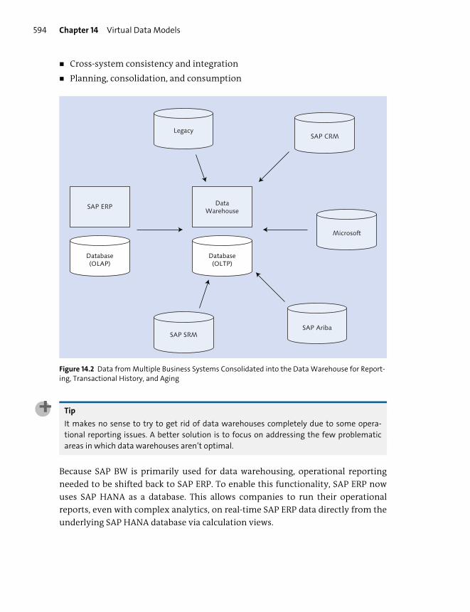
Chapter 14 Virtual Data Models594
� Cross-system consistency and integration
� Planning, consolidation, and consumption
Figure 14.2 Data from Multiple Business Systems Consolidated into the Data Warehouse for Report-ing, Transactional History, and Aging
Tip
It makes no sense to try to get rid of data warehouses completely due to some opera-
tional reporting issues. A better solution is to focus on addressing the few problematic
areas in which data warehouses aren’t optimal.
Because SAP BW is primarily used for data warehousing, operational reporting
needed to be shifted back to SAP ERP. To enable this functionality, SAP ERP now
uses SAP HANA as a database. This allows companies to run their operational
reports, even with complex analytics, on real-time SAP ERP data directly from the
underlying SAP HANA database via calculation views.
Database(OLAP)
Database(OLTP)
SAP ERP DataWarehouse
SAP SRM
Microsoft
SAP CRMLegacy
SAP Ariba

Key Concepts Refresher Chapter 14 595
Note
The SAP HANA Live calculation views were built using the SAP HANA Studio based on
tables in a classical database schema. They aren’t .hdbcalculationview files, and don’t use
data sources in SAP HANA Deployment Infrastructure (HDI) containers. Up to now, we’ve
focused on the SAP HANA extended application services, advanced model (SAP HANA
XSA) concepts, whereas SAP HANA Live was built using the older SAP HANA 1.0 approach.
SAP HANA Live
SAP HANA Live is the tool used to install, select, maintain, and modify the SAP
HANA calculation views used for operational reporting in the SAP ERP system. SAP
HANA Live isn’t limited to SAP ERP but also is available for many other SAP busi-
ness systems, such as SAP CRM, SAP SCM, SAP Governance, Risk, and Compliance
(SAP GRC), and SAP Product Lifecycle Management (SAP PLM).
Some of the benefits of SAP HANA Live include the following:
� Real-time reporting and analytics are run on up-to-date information.
� SAP HANA doesn’t need to store precalculated aggregates in cubes.
� OLTP and OLAP run in the same system, which can help reduce the total cost of
ownership (TCO).
� Access is provided for any reporting tool or application.
� Customers and partners can extend SAP HANA Live to suit their needs.
Now that you have a better understanding of how SAP HANA Live came to be, the
following subsections will dive further into SAP HANA Live’s architecture, VDMs,
views, administration procedures, and modifications.
SAP HANA Live Architecture
SAP HANA Live needs an SAP HANA database. Connecting to an SAP HANA data-
base can be achieved in two ways (in this case, we just concentrate on the SAP ERP
system, but this also applies to all the other SAP business systems such as SAP
CRM, SAP SCM, SAP GRC, and SAP PLM; see Figure 14.3):
� SAP HANA as a database
The first option is to migrate an SAP ERP system’s database to SAP HANA. No
additional systems are required. This is also known as the integrated scenario.

Chapter 14 Virtual Data Models596
� SAP HANA as a side-by-side accelerator
The second option is to keep your current SAP ERP database, for example,
Microsoft SQL Server, and install an SAP HANA system as a side-by-side acceler-
ator (as discussed in Chapter 3). Then, you replicate the required database tables
to the SAP HANA system using SAP Landscape Transformation Replication
Server. You can find more information about SAP Landscape Transformation
Replication Server in Chapter 9. SAP Landscape Transformation Replication
Server enables real-time replication so that SAP HANA always has the latest data
available. For this scenario, you need to install the SAP Landscape Transforma-
tion Replication Server and SAP HANA systems.
Figure 14.3 Architecture Options for SAP HANA Live
After you’ve connected to an SAP HANA database, you can build reports, analytics,
and dashboards directly on the SAP HANA Live content. Other applications can
also call this content directly.
Note
In both architectural scenarios, SAP HANA Live is installed in the SAP HANA database.
SAP ERP
Other Database
SAP HANAwith SAP HANA
Live loaded
SAP ERP
SAP HANA
with SAP HANALive loaded
Option 1: SAP HANA as a database
SLT
Option 2: SAP HANA as a sidecar
Reports & Analytics
Replication

Key Concepts Refresher Chapter 14 597
SAP HANA Live Virtual Data Model
SAP HANA Live content consists primarily of calculation views that are designed,
created, and delivered by SAP. These calculation views are built for operational
reporting instead of analytical reporting purposes and, therefore, use mostly join
nodes. The information models are relational rather than dimensional (cube-like).
A system administrator loads the SAP HANA Live content into the SAP HANA data-
base. These calculation views are layered in a structure called the SAP HANA Live
virtual data model (VDM), as mentioned earlier. SAP HANA Live is structured inter-
nally as shown in Figure 14.4.
Figure 14.4 SAP HANA Live VDM
The VDM consists of the following types of views:
� Private views
These are built directly on the database tables and on other private views. These
denormalize the database source data for use in the reuse views.
Database Tables
SAP HANA Live – Virtual Data Model (VDM)
Reports, Analytics,and Applications
Private Views
Reuse Views
Query Views
Value Help
Views
Standard SAP HANA Live content
Customer Query Views
Customer Extensions

Chapter 14 Virtual Data Models598
� Reuse views
These structure the data in a way that business processes can use. These views
can be reused by other views.
� Query views
These can be consumed directly by analytical tools and applications. They
aren’t reused by other views. These views are used when designing reports.
� Customer query views
These are created either by copying SAP-provided query views or by creating
your own query views. You can add your own filters, variables, or input param-
eters to these views. You can also expose additional data fields or hide fields
that aren’t required.
� Value help views
These are used as lookups (i.e., dropdown lists or filter lists) for selection lists in
analytical tools and business applications. They make it easier for users to filter
data by providing a list of possible values to choose from. Value help views
aren’t used in other VDM views; they are consumed directly by analytical tools
and business applications.
Tip
You should never call private and reuse views directly.
You can build your reports, analytics, or business applications directly on query
views. These can be either SAP-provided query views or custom query views. When
you run your report, these query views are called. They in turn call the relevant
reuse views, which call the relevant private views, which in turn read the relevant
database tables. The value help views are called whenever dropdown lists are used
to display possible values that a user can choose from.
Note
Modifying any SAP-provided VDM views isn’t recommended because all SAP-provided
VDM views are overwritten when a newer version of the SAP HANA Live content is
installed. There is no mechanism like the one in ABAP, in which the system asks if you
want to keep any customer changes.
Therefore, you should always make a copy of a VDM query view to modify, rather than
modifying the original.
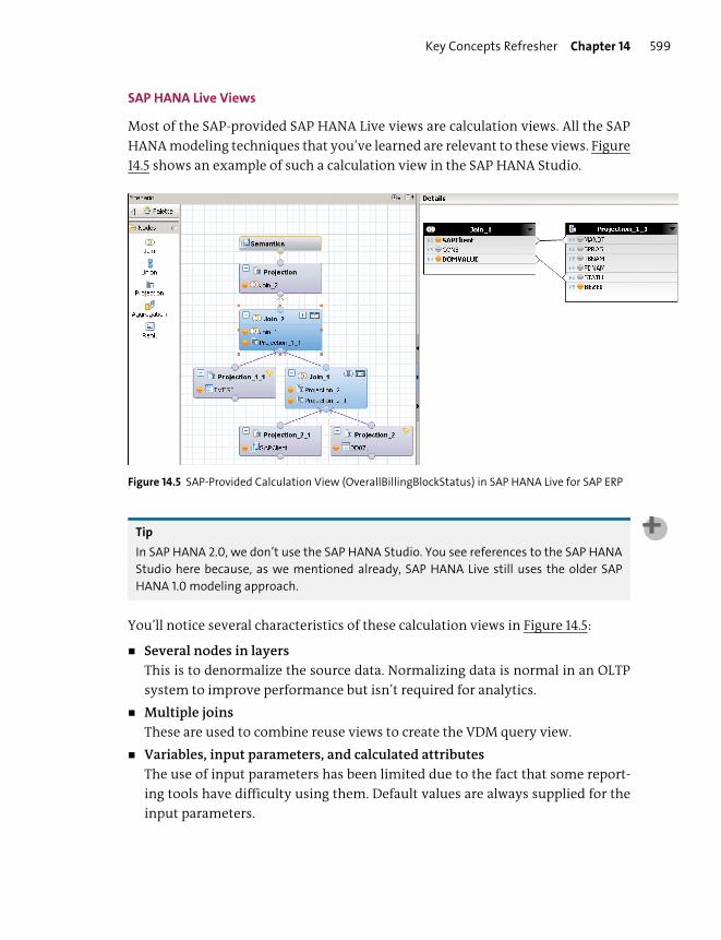
Key Concepts Refresher Chapter 14 599
SAP HANA Live Views
Most of the SAP-provided SAP HANA Live views are calculation views. All the SAP
HANA modeling techniques that you’ve learned are relevant to these views. Figure
14.5 shows an example of such a calculation view in the SAP HANA Studio.
Figure 14.5 SAP-Provided Calculation View (OverallBillingBlockStatus) in SAP HANA Live for SAP ERP
Tip
In SAP HANA 2.0, we don’t use the SAP HANA Studio. You see references to the SAP HANA
Studio here because, as we mentioned already, SAP HANA Live still uses the older SAP
HANA 1.0 modeling approach.
You’ll notice several characteristics of these calculation views in Figure 14.5:
� Several nodes in layers
This is to denormalize the source data. Normalizing data is normal in an OLTP
system to improve performance but isn’t required for analytics.
� Multiple joins
These are used to combine reuse views to create the VDM query view.
� Variables, input parameters, and calculated attributes
The use of input parameters has been limited due to the fact that some report-
ing tools have difficulty using them. Default values are always supplied for the
input parameters.

Chapter 14 Virtual Data Models600
SAP HANA Live Administration
SAP HANA Live is installed in the SAP HANA database. A system administrator will
normally install the SAP HANA Live content package.
After SAP HANA Live is installed on an SAP HANA system, you’ll see the content in
the Content folder, under sap/hba, as shown in Figure 14.6. You can explore the cal-
culation views in the SAP HANA Studio. We don’t recommend that you change the
views here. As mentioned earlier, all the SAP-provided VDM views are overwritten
when a newer version of the SAP HANA Live content is installed. There is no mech-
anism in place within SAP HANA Live to ask if you want to keep any customer
changes, so you could lose all your hard work during an SAP HANA Live update.
Figure 14.6 SAP HANA Live Content Package in the SAP HANA Studio
Note
SAP HANA Live has its own release cycles and timelines. SAP HANA Live content updates
don’t have to correspond to the SAP HANA system update cycles and timelines.
In the sap/hba package, you’ll also find various web-based tools for working with
SAP HANA Live content:
� SAP HANA Live Browser
This tool is used to find the right query views for your reporting needs.
� SAP HANA Live extension assistant
This tool helps you copy and modify views based on your business require-
ments.
Let’s look at the full breadth of SAP HANA Live Brower’s functionality.
SAP HANA Live Browser
The SAP HANA Live Browser tool is a web-based (HTML5) application that enables
you to find the correct views for your reporting or analytics requirements. Some-
times, you might need to ask an SAP functional person that knows the source

Key Concepts Refresher Chapter 14 601
system well to help you find the required views. For example, to find sales infor-
mation in an SAP ERP system, you might need the advice of an SAP ERP Sales and
Distribution (SAP ERP SD) consultant.
You can find the SAP HANA Live Browser tool (Figure 14.7) by accessing http://<SAP
HANA server hostname>:8000/sap/hana/hba/explorer. (This assumes that the
instance number is 00.)
In this section, we’ll walk through the different areas found in the SAP HANA Live
Browser, starting with the top menu’s ALL VIEWS section (see Figure 14.7).
Figure 14.7 SAP HANA Live Browser
Here you can search for views by typing a part of the name of the view in the Filter
field. For each view, you can see the following information:
� View name
� Description of the view
� View category (private, reuse, or query view)
� View type (mostly calculation views)

Chapter 14 Virtual Data Models602
� To which area of the application the view is applicable
� In which SAP HANA package the view is located
Figure 14.8 shows a partial list of views that we can use for procurement reports.
Figure 14.8 Filter String Entry to Find Views
You can access many features in SAP HANA Live Browser from the provided tool-
bar (see Figure 14.9).
Figure 14.9 SAP HANA Live Browser Toolbar
The following functions are available from the toolbar:
� Open Definition
The Open Definition tab (Figure 14.10) shows the metadata of the SAP HANA Live
view. These fields are available for your reports and analytics. If you need other
fields, you’ll have to use the SAP HANA Live extension assistant.
� Open Content
The Open Content tab (Figure 14.11) shows a preview of the data an SAP HANA
Live view will produce.
� Open Cross Reference
The Open Cross Reference tab (Figure 14.12) shows an interactive and graphical
depiction of all the related tables and views used by this specific SAP HANA Live
view. You can also see an outline version instead of the graphical version.
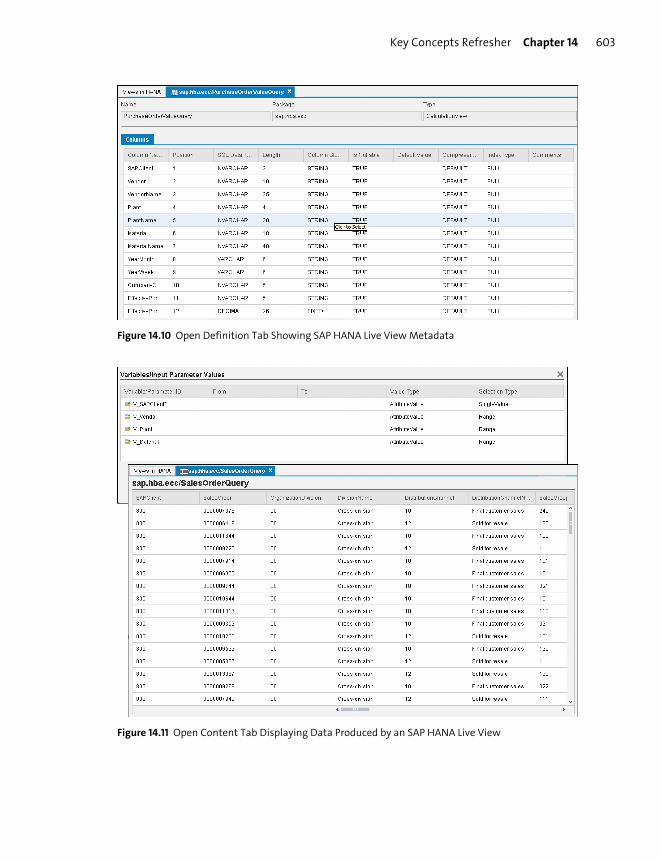
Key Concepts Refresher Chapter 14 603
Figure 14.10 Open Definition Tab Showing SAP HANA Live View Metadata
Figure 14.11 Open Content Tab Displaying Data Produced by an SAP HANA Live View
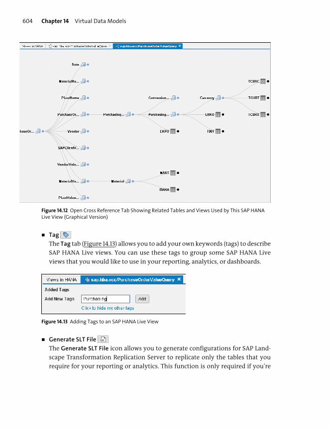
Chapter 14 Virtual Data Models604
Figure 14.12 Open Cross Reference Tab Showing Related Tables and Views Used by This SAP HANA Live View (Graphical Version)
� Tag
The Tag tab (Figure 14.13) allows you to add your own keywords (tags) to describe
SAP HANA Live views. You can use these tags to group some SAP HANA Live
views that you would like to use in your reporting, analytics, or dashboards.
Figure 14.13 Adding Tags to an SAP HANA Live View
� Generate SLT File
The Generate SLT File icon allows you to generate configurations for SAP Land-
scape Transformation Replication Server to replicate only the tables that you
require for your reporting or analytics. This function is only required if you’re
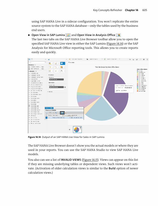
Key Concepts Refresher Chapter 14 605
using SAP HANA Live in a sidecar configuration. You won’t replicate the entire
source system to the SAP HANA database—only the tables used by the business
end users.
� Open View in SAP Lumira and Open View in Analysis Office
The last two tabs on the SAP HANA Live Browser toolbar allow you to open the
specified SAP HANA Live view in either the SAP Lumira (Figure 14.14) or the SAP
Analysis for Microsoft Office reporting tools. This allows you to create reports
easily and quickly.
Figure 14.14 Output of an SAP HANA Live View for Sales in SAP Lumira
The SAP HANA Live Browser doesn’t show you the actual models or where they are
used in your reports. You can use the SAP HANA Studio to view SAP HANA Live
models.
You also can see a list of INVALID VIEWS (Figure 14.15). Views can appear on this list
if they are missing underlying tables or dependent views. Such views won’t acti-
vate. (Activation of older calculation views is similar to the Build option of newer
calculation views.)

Chapter 14 Virtual Data Models606
Figure 14.15 List of Invalid SAP HANA Live Views
Until now, we’ve discussed the developer edition of the SAP HANA Live Browser.
There is also a business user version of SAP HANA Live Browser available at http://
<SAP HANA server host>:8000/sap/hana/hba/explorer/buser.html. This version
only allows you to find a model, preview the content, and open the view in SAP
Lumira or SAP Analysis for Microsoft Office. It’s meant for nontechnical users,
such as functional consultants or specialists.
Advanced features, such as generating SAP Landscape Transformation Replication
Server files, viewing broken models, tagging a model, or opening graphical cross
references, aren’t available in the business user edition of the SAP HANA Live
Browser.
SAP HANA Live Extension Assistant: Modify Views
Earlier in the chapter, Figure 14.5 showed an example of an SAP HANA Live view,
which is similar to any other view in SAP HANA. There are two ways to modify SAP
HANA Live views:
� SAP HANA Studio
We can use the SAP HANA Studio to modify, preview, test, debug, and trace SAP
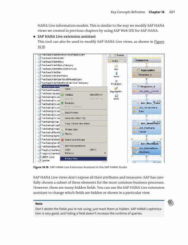
Key Concepts Refresher Chapter 14 607
HANA Live information models. This is similar to the way we modify SAP HANA
views we created in previous chapters by using SAP Web IDE for SAP HANA.
� SAP HANA Live extension assistant
This tool can also be used to modify SAP HANA Live views, as shown in Figure
14.16.
Figure 14.16 SAP HANA Live Extension Assistant in the SAP HANA Studio
SAP HANA Live views don’t expose all their attributes and measures; SAP has care-
fully chosen a subset of these elements for the most common business processes.
However, there are many hidden fields. You can use the SAP HANA Live extension
assistant to change which fields are hidden or shown in a particular view.
Note
Don’t delete the fields you’re not using; just mark them as hidden. SAP HANA’s optimiza-
tion is very good, and hiding a field doesn’t increase the runtime of queries.
Chapter 14 Virtual Data Models608
Note
You can only extend reuse and query views, and you can extend a particular view multi-
ple times.
The SAP HANA Live extension assistant can’t extend the following:
� A query view that contains a Union node.
� A query view that contains an Aggregation node as one of the middle nodes. An
Aggregation node as the top node is normal and allowed.
� Your own custom views. It only recognizes SAP-delivered views.
Tip
You shouldn’t extend SAP-delivered views. Make a copy, and extend that instead.
You should now have a good understanding of what SAP HANA Live offers to cus-
tomers and when to use it. Now we turn our attention to a newer VDM, namely
SAP S/4HANA embedded analytics.
SAP S/4HANA Embedded Analytics
We’ve already mentioned that SAP HANA Live has evolved into SAP S/4HANA
embedded analytics. As the advantages of SAP HANA became more apparent,
SAP created a completely new version of SAP ERP that uses only SAP HANA:
SAP S/4HANA. With this new architecture and the lessons learned, we see that SAP
HANA Live evolved into SAP S/4HANA embedded analytics.
Tip
SAP S/4HANA only runs on SAP HANA, so there is no side-by-side option for SAP S/4HANA
embedded analytics as we have with SAP HANA Live.
Logically, as more customers migrate over to SAP S/4HANA, the SAP S/4HANA
embedded analytics is taking over from SAP HANA Live.
Similar Features
Many things in SAP HANA Live work very well and were kept in SAP S/4HANA
embedded analytics. The appearance and mechanisms might have been updated,
but the essence and intent of the following features stayed the same:
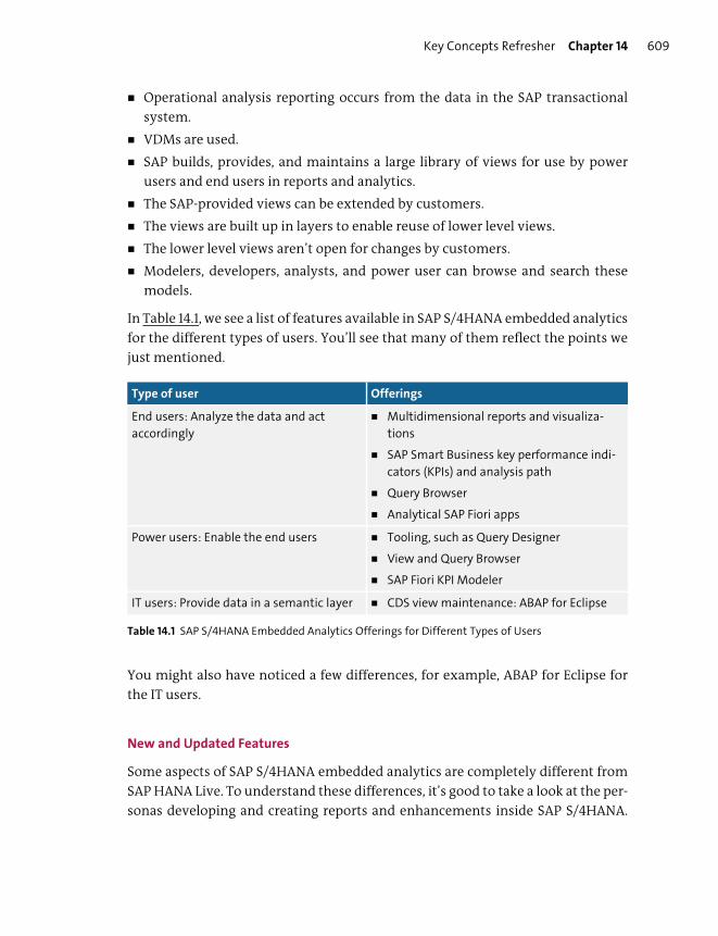
Key Concepts Refresher Chapter 14 609
� Operational analysis reporting occurs from the data in the SAP transactional
system.
� VDMs are used.
� SAP builds, provides, and maintains a large library of views for use by power
users and end users in reports and analytics.
� The SAP-provided views can be extended by customers.
� The views are built up in layers to enable reuse of lower level views.
� The lower level views aren’t open for changes by customers.
� Modelers, developers, analysts, and power user can browse and search these
models.
In Table 14.1, we see a list of features available in SAP S/4HANA embedded analytics
for the different types of users. You’ll see that many of them reflect the points we
just mentioned.
You might also have noticed a few differences, for example, ABAP for Eclipse for
the IT users.
New and Updated Features
Some aspects of SAP S/4HANA embedded analytics are completely different from
SAP HANA Live. To understand these differences, it’s good to take a look at the per-
sonas developing and creating reports and enhancements inside SAP S/4HANA.
Type of user Offerings
End users: Analyze the data and act
accordingly
� Multidimensional reports and visualiza-
tions
� SAP Smart Business key performance indi-
cators (KPIs) and analysis path
� Query Browser
� Analytical SAP Fiori apps
Power users: Enable the end users � Tooling, such as Query Designer
� View and Query Browser
� SAP Fiori KPI Modeler
IT users: Provide data in a semantic layer � CDS view maintenance: ABAP for Eclipse
Table 14.1 SAP S/4HANA Embedded Analytics Offerings for Different Types of Users
Chapter 14 Virtual Data Models610
While modelers and analysts focused more on SAP BW, the people creating opera-
tional reporting and extending the functionality of the SAP ERP system have
mostly been the ABAP developers. There is more focus on the ABAP developer
with SAP S/4HANA embedded analytics.
Another point to keep in mind is where these users do their work. Both ABAP
developers and SAP BW modelers work in SAP applications. They work at the appli-
cation layer, and not in the lower database layer. Herein lies a “problem” with SAP
HANA Live as this is completely developed in the database layer. These users need
SAP HANA login details and work outside of their normal working environments
with SAP HANA Live.
The next point to look at is the fact that SAP HANA calculation views are read-only
views. Many transactional systems require actions to be taken at certain times and
when certain conditions occur. Reading and writing would work far better here.
With this in mind, SAP decided to build SAP S/4HANA embedded analytics with
ABAP CDS views.
Note
ABAP CDS and SAP HANA CDS are somewhat similar, but they aren’t the same. SAP HANA
CDS views are specific to SAP HANA. ABAP CDS can be use with other databases as well
and therefore isn’t as feature-rich as SAP HANA CDS.
Tip
The concept of CDS, which we already discussed in Chapter 5, is also part of the “SAP-sup-
plied virtual data models” exam topic area.
We can now look at some of the features in SAP S/4HANA embedded analytics that
differ from those of SAP HANA Live:
� The views are created with ABAP CDS.
� The views are built and stored in the ABAP Data Dictionary.
� All authorizations are done with standard security roles in the application. (SAP
HANA Live uses SAP HANA analytic privileges for security.)
� The ABAP CDS views are created in a text editor (not a graphical modeler) in the
ABAP for Eclipse environment. This is similar to the SAP HANA Studio, which is
also based on Eclipse.
� The focus is on developers rather than on modelers.
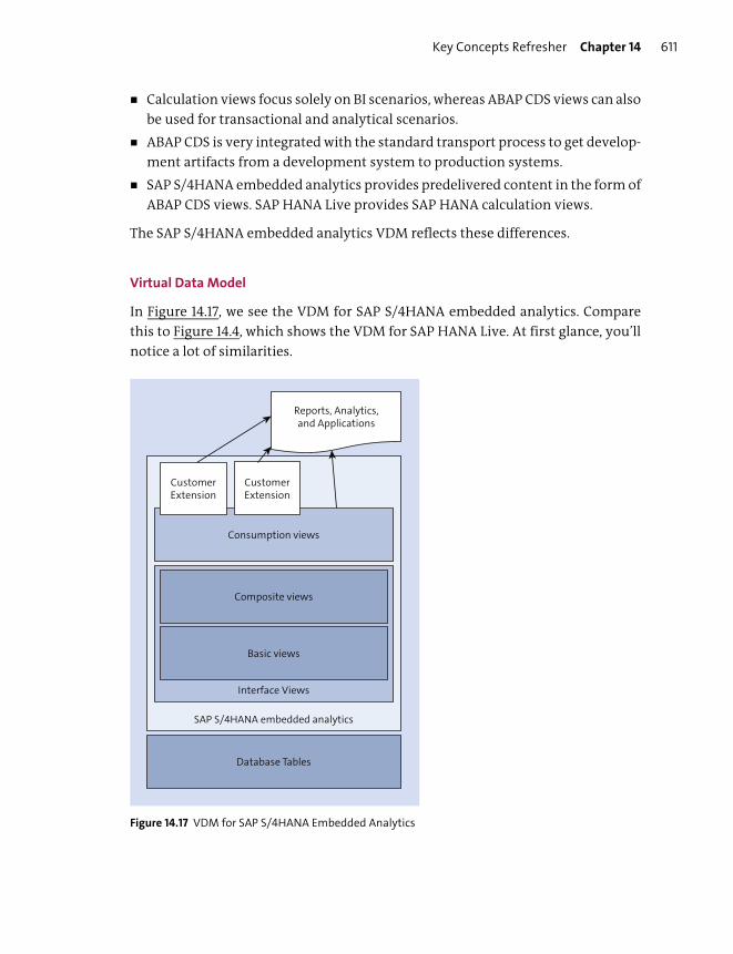
Key Concepts Refresher Chapter 14 611
� Calculation views focus solely on BI scenarios, whereas ABAP CDS views can also
be used for transactional and analytical scenarios.
� ABAP CDS is very integrated with the standard transport process to get develop-
ment artifacts from a development system to production systems.
� SAP S/4HANA embedded analytics provides predelivered content in the form of
ABAP CDS views. SAP HANA Live provides SAP HANA calculation views.
The SAP S/4HANA embedded analytics VDM reflects these differences.
Virtual Data Model
In Figure 14.17, we see the VDM for SAP S/4HANA embedded analytics. Compare
this to Figure 14.4, which shows the VDM for SAP HANA Live. At first glance, you’ll
notice a lot of similarities.
Figure 14.17 VDM for SAP S/4HANA Embedded Analytics
Database Tables
SAP S/4HANA embedded analytics
Reports, Analytics,and Applications
Basic views
Composite views
Consumption views
Interface Views
CustomerExtension
CustomerExtension

Chapter 14 Virtual Data Models612
The main difference seems to be the naming of the views in the different layers.
Instead of private and reuse views, we now have basic and composite views. Just as
you aren’t allowed to modify private and reuse views in SAP HANA Live, the same
restrictions apply to the basic and composite views in SAP S/4HANA embedded
analytics.
Where we had query views and customers extensions in SAP HANA Live, we have
consumption views and customer extensions in SAP S/4HANA embedded analyt-
ics.
Note
The certification exam focuses on the modeling aspects of SAP HANA. As such, the inter-
est in this chapter was more on the calculation views as used in SAP HANA Live. We spent
less time on ABAP CDS views because it’s outside the scope of SAP HANA modeling.
Important Terminology
In this chapter, we covered the following important terminology:
� Operational reporting
Operational reporting is reporting that is done on transactional data (e.g., sales
and deliveries) to enable people to do their work today (e.g., delivering a sold
item). SAP BW reports are normally the next day only, and they don’t help with,
for example, today’s deliveries. SAP HANA Live is meant only for operational
reporting requirements in SAP operational systems such as SAP ERP.
� SAP HANA Live
SAP HANA Live consists of SAP-created calculation views (for the most part) and
several tools for working with these SAP HANA views.
� SAP HANA Live views
The SAP HANA Live views are organized in an architectural structure called the
VDM. The different SAP HANA Live views are as follows:
– Private views: These are built directly on the database tables and on other pri-
vate views. These denormalize the database source data for use in the reuse
views.
– Reuse views: These structure the data in a way that business processes can
use. These views can be reused by other views.

Practice Questions Chapter 14 613
– Query views: These can be consumed directly by analytical tools and applica-
tions. They aren’t reused by other views. These views are used when design-
ing reports.
– Customer query views: These are created either by copying SAP-provided
query views or by creating your own query views. You can add your own fil-
ters, variables, or input parameters to these views. You can also expose addi-
tional data fields or hide fields that aren’t required.
– Value help views: These are used as lookups (i.e., dropdown lists or filter lists)
for selection lists in analytical tools and business applications. They make it
easier for users to filter data by providing a list of possible values to choose
from. Value help views aren’t used in other VDM views; they are consumed
directly by analytical tools and business applications.
� SAP HANA Live Browser
The SAP HANA Live Browser tool is a web-based (HTML5) application that
enables you to find the correct views for your reporting or analytics require-
ments.
� SAP HANA Live extension assistant
The SAP HANA Live extension assistant tool is used to modify SAP HANA Live
views.
� SAP S/4HANA embedded analytics
SAP S/4HANA embedded analytics consists of SAP-created ABAP CDS views and
several tools for working with these views.
Practice Questions
These practice questions will help you evaluate your understanding of the topics
covered in this chapter. The questions shown are similar in nature to those found
on the certification examination. Although none of these questions will be found
on the exam itself, they will allow you to review your knowledge of the subject.
Select the correct answers, and then check the completeness of your answers in
the “Practice Question Answers and Explanations” section. Remember, on the
exam, you must select all correct answers and only correct answers to receive
credit for the question.
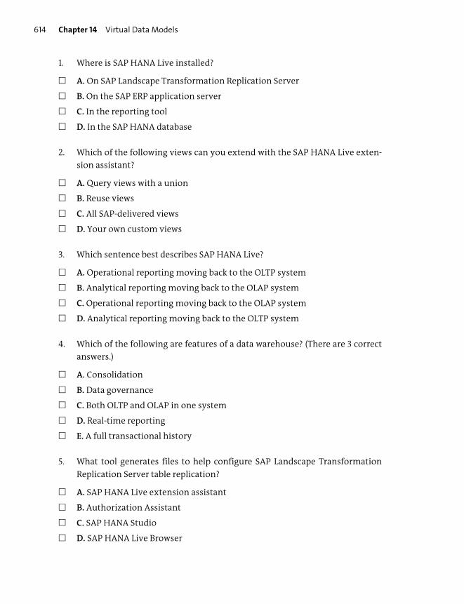
Chapter 14 Virtual Data Models614
1. Where is SAP HANA Live installed?
� A. On SAP Landscape Transformation Replication Server
� B. On the SAP ERP application server
� C. In the reporting tool
� D. In the SAP HANA database
2. Which of the following views can you extend with the SAP HANA Live exten-
sion assistant?
� A. Query views with a union
� B. Reuse views
� C. All SAP-delivered views
� D. Your own custom views
3. Which sentence best describes SAP HANA Live?
� A. Operational reporting moving back to the OLTP system
� B. Analytical reporting moving back to the OLAP system
� C. Operational reporting moving back to the OLAP system
� D. Analytical reporting moving back to the OLTP system
4. Which of the following are features of a data warehouse? (There are 3 correct
answers.)
� A. Consolidation
� B. Data governance
� C. Both OLTP and OLAP in one system
� D. Real-time reporting
� E. A full transactional history
5. What tool generates files to help configure SAP Landscape Transformation
Replication Server table replication?
� A. SAP HANA Live extension assistant
� B. Authorization Assistant
� C. SAP HANA Studio
� D. SAP HANA Live Browser

Practice Questions Chapter 14 615
6. True or False: You can create custom query views by directly modifying SAP-
delivered query views.
� A. True
� B. False
7. True or False: When you upgrade SAP HANA Live content, you can choose to
keep your modifications.
� A. True
� B. False
8. Which of following are features associated with SAP HANA Live? (There are 2
correct answers.)
� A. A new data warehouse
� B. Hundreds of predeveloped views
� C. Web-based tools
� D. Precalculated aggregates stored in cubes
9. Which of the following terms are associated with an operational system?
(There are 2 correct answers.)
� A. OLTP
� B. OLAP
� C. Transactional
� D. Data warehouse
10. True or False: SAP HANA Live replaces SAP BW.
� A. True
� B. False
11. True or False: You can view metadata of SAP HANA Live views with the busi-
ness user version of the SAP HANA Live Browser.
� A. True
� B. False
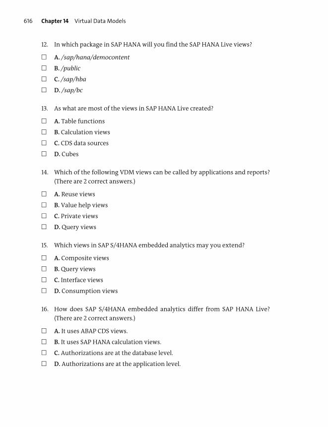
Chapter 14 Virtual Data Models616
12. In which package in SAP HANA will you find the SAP HANA Live views?
� A. /sap/hana/democontent
� B. /public
� C. /sap/hba
� D. /sap/bc
13. As what are most of the views in SAP HANA Live created?
� A. Table functions
� B. Calculation views
� C. CDS data sources
� D. Cubes
14. Which of the following VDM views can be called by applications and reports?
(There are 2 correct answers.)
� A. Reuse views
� B. Value help views
� C. Private views
� D. Query views
15. Which views in SAP S/4HANA embedded analytics may you extend?
� A. Composite views
� B. Query views
� C. Interface views
� D. Consumption views
16. How does SAP S/4HANA embedded analytics differ from SAP HANA Live?
(There are 2 correct answers.)
� A. It uses ABAP CDS views.
� B. It uses SAP HANA calculation views.
� C. Authorizations are at the database level.
� D. Authorizations are at the application level.
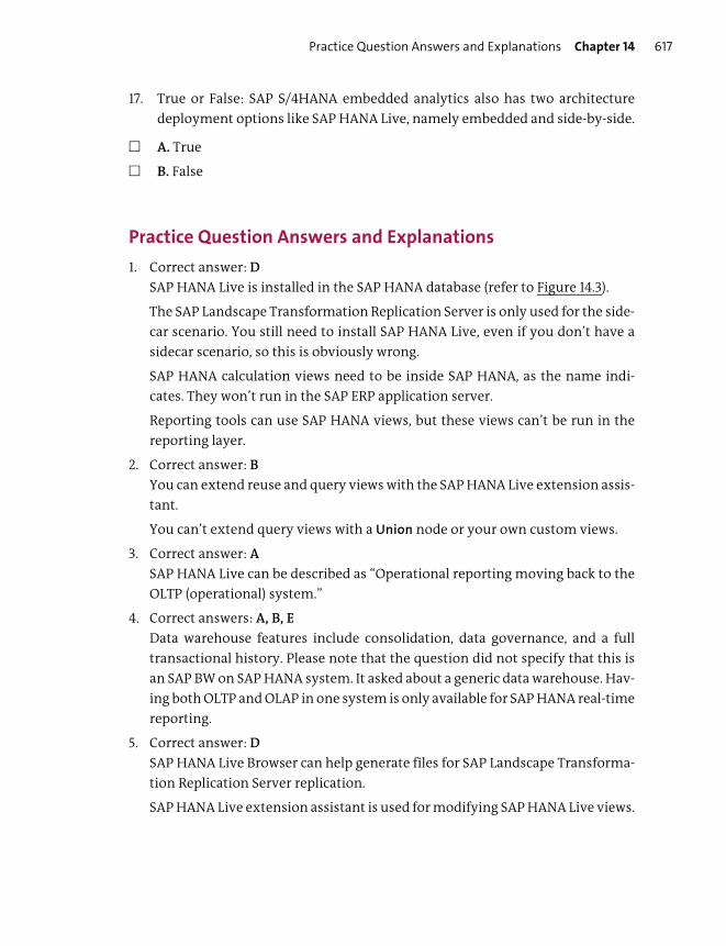
Practice Question Answers and Explanations Chapter 14 617
17. True or False: SAP S/4HANA embedded analytics also has two architecture
deployment options like SAP HANA Live, namely embedded and side-by-side.
� A. True
� B. False
Practice Question Answers and Explanations
1. Correct answer: D
SAP HANA Live is installed in the SAP HANA database (refer to Figure 14.3).
The SAP Landscape Transformation Replication Server is only used for the side-
car scenario. You still need to install SAP HANA Live, even if you don’t have a
sidecar scenario, so this is obviously wrong.
SAP HANA calculation views need to be inside SAP HANA, as the name indi-
cates. They won’t run in the SAP ERP application server.
Reporting tools can use SAP HANA views, but these views can’t be run in the
reporting layer.
2. Correct answer: B
You can extend reuse and query views with the SAP HANA Live extension assis-
tant.
You can’t extend query views with a Union node or your own custom views.
3. Correct answer: A
SAP HANA Live can be described as “Operational reporting moving back to the
OLTP (operational) system.”
4. Correct answers: A, B, E
Data warehouse features include consolidation, data governance, and a full
transactional history. Please note that the question did not specify that this is
an SAP BW on SAP HANA system. It asked about a generic data warehouse. Hav-
ing both OLTP and OLAP in one system is only available for SAP HANA real-time
reporting.
5. Correct answer: D
SAP HANA Live Browser can help generate files for SAP Landscape Transforma-
tion Replication Server replication.
SAP HANA Live extension assistant is used for modifying SAP HANA Live views.
Chapter 14 Virtual Data Models618
The Authorization Assistant helps with creating users and roles for SAP HANA
Live.
The SAP HANA Studio doesn’t have this functionality.
6. Correct answer: A
This is actually a “bad” question. It’s clear from this chapter that you should not
create custom query views by directly modifying SAP-delivered query views.
However, the question asked if you can do it. Technically, it’s possible—but
you’ll lose all your hard work during the next update of the SAP HANA Live con-
tent.
7. Correct answer: B
When you upgrade the SAP HANA Live content, there is no option for you to
keep your modifications. All changes to SAP-delivered content will be lost. This
is different from the process in ABAP systems, which does ask if you want to
save your modifications.
This question was very similar to the previous question. In the certification
exam, you won’t find one question providing the answer to another. The SAP
team ensures that this doesn’t happen.
8. Correct answers: B, C
SAP HANA Live consists of hundreds of predeveloped views, as well as some
web-based tools.
SAP HANA Live isn’t a new data warehouse, as we clearly specified that it
doesn’t replace SAP BW.
With SAP HANA, we don’t store precalculated aggregates in cubes. This is only
done in old non-SAP HANA data warehouses.
9. Correct answers: A, C
An operational system is the transactional (OLTP) system.
10. Correct answer: B
SAP HANA Live does NOT replace SAP BW. Only the operational reporting por-
tion moves back from the data warehouse to the transactional system.
11. Correct answer: B
You can’t view the metadata of SAP HANA Live views within the business user
version of SAP HANA Live Browser. Metadata, like table definitions, is only used
by modelers and developers. This version is meant for nontechnical users.
Takeaway Chapter 14 619
12. Correct answer: C
The SAP HANA Live views are in the /sap/hba subpackage. Refer to Figure 14.6
to see the SAP HANA Live content in the SAP HANA Studio.
13. Correct answer: B
Most of the views in SAP HANA Live are calculation views.
14. Correct answers: B, D
Query views and value help views can be called by applications and reports
(refer to Figure 14.4).
Reuse views and private views may not be called directly.
15. Correct answer: D
You may extend consumption views in SAP S/4HANA embedded analytics.
Query views are in SAP HANA Live.
Interface views and composite views may not be extended.
16. Correct answers: A, D
SAP S/4HANA embedded analytics differs from SAP HANA Live in that it uses
ABAP CDS views, and authorizations are at the application level.
SAP HANA Live uses SAP HANA calculation views, and the authorizations are at
the database level.
17. Correct answer: B
False: SAP S/4HANA embedded analytics does not have two architecture
deployment options like SAP HANA Live. It does not have a side-by-side option
because it can only be deployed on SAP HANA.
Takeaway
You should now know what SAP HANA Live is, the concepts behind it, and the
architecture options.
You can use your understanding of the VDM to choose which views can be used,
modified, or extended, and you can use the SAP HANA Live Browser tool to help
design your reports.
You also got an overview of how SAP HANA Live has evolved into SAP S/4HANA
embedded analytics and how this differs from SAP HANA Live.
Chapter 14 Virtual Data Models620
Summary
In this chapter, you used your knowledge of SAP HANA modeling in a scenario in
which SAP HANA is used as a database for SAP business systems such as SAP ERP.
The difference here is that SAP has developed hundreds of information models
already, and you can tap into this vast resource to build powerful analytical
reports quickly.
This chapter completes your learning experience with SAP HANA modeling. We
wish you the best of luck with your SAP HANA certification exam!
621
The Author
Rudi de Louw is head of the SAP Co-Innovation Lab at SAP
in South Africa where he supports SAP partners in building
or improving their business ideas and systems with SAP
platforms such as SAP HANA, SAP Cloud Platform, and SAP
Leonardo. In this role, he also helps partners extend the
integration of their current business products with avail-
able and emerging SAP technologies.
Rudi has been working with SAP HANA since 2010, and he
has been involved from the outset in preparing the SAP
HANA certification exams. He has provided software and technology solutions to
businesses for more than 25 years and has a passion for sharing knowledge, men-
toring, understanding new technologies, and finding innovative ways to leverage
these skills to help individuals in their development.

623
Index
A
ABAP ......................................................................... 384
ABAP Data Dictionary ....................................... 610
Accelerated K-Means ......................................... 442
Accelerator deployment ...................................... 96
profitability analysis ........................................ 95
Acclaim platform .................................................... 36
ACID-compliant database ................................... 86
Active/active (read-enabled) mode ................ 90
Advanced DSO ......................................................... 99
Affinity propagation .......................................... 435
AFLLANG ................................................................. 449
procedure ........................................................... 450
Aggregation ........................................ 210, 217, 522
function .............................................................. 260
Aggregation node .......... 258, 270, 271, 273, 276
restricted column ........................................... 288
Algorithms ............................................................. 435
Alias ........................................................................... 267
Amazon Web Services (AWS) ......... 50, 106, 118
American National Standards
Institute (ANSI) ................................................ 340
Analytic privileges ........................... 571, 582, 586
assign to role .................................................... 571
Anonymization node ........................................ 261
Application Function Library (AFL) ............ 347,
433, 438
Application privileges ....................................... 576
Application time period tables ...................... 344
Apply privileges property ................................ 583
Apriori algorithm ................................................ 435
ArcGIS ....................................................................... 462
Architecture .......................... 71, 79, 114, 521, 542
Associated container ......................................... 557
Association algorithms ..................................... 435
Asynchronous replication .................................. 90
Attribute .................................... 181, 200, 203, 217
calculated column .......................................... 284
restricted column ........................................... 288
restrictions ........................................................ 573
Authentication ..................................................... 554
Authorization .............................................. 539, 554
Assistant ............................................................. 552
Automated Predictive Library (APL) ........... 433
B
Backups ............................................................... 87, 88
Best practices ........................................................ 215
Big data ........................................................... 390, 523
limitations ......................................................... 391
BIGINT ...................................................................... 372
Blue-green deployment .................................... 134
Bookmark questions ............................................. 67
Bottleneck ................................................................. 79
Branch logic ........................................................... 541
Bring your own language (BYOL) .................. 140
Bring-your-own-license .................................... 107
Build error .............................................................. 169
Build process ...................................... 129, 131, 175
Business Function Library (BFL) .................... 438
Business Intelligence Consumer
Services (BICS) ......................................... 113, 309
Business intelligence tools .............................. 314
BW362 ......................................................................... 43
C
C_HANADEV ............................................................ 30
C_HANAIMP ............................................................. 29
C_HANAIMP_15 .............................................. 17, 26
scoring ................................................................... 35
C_HANATEC ............................................................. 29
C4.5 decision tree ................................................ 446
Caching .................................................................... 208
Calculated column ....... 182, 279, 281, 326, 328,
345, 346
analytic view .................................................... 331
counter ................................................................ 285
create ................................................................... 282
input parameter .............................................. 299
Index624
Calculation view .............. 98, 204, 207, 235, 557
Calculation view of type cube .... 205, 217, 218,
225, 233, 271, 273
aggregation node ........................................... 276
create ................................................................... 236
with star join ................................. 217, 218, 225
Calculation view of type cube with
star join ..................................................... 233, 271
create ................................................................... 237
star join node .......................................... 262, 276
Calculation view of type dimension .......... 205,
217, 225, 233, 238, 271
create ................................................................... 237
projection node ............................................... 276
Calculation views ........... 93, 168, 207, 231, 301,
330, 450, 505
adding data sources ...................................... 241
adding nodes .................................................... 241
create ................................................................... 235
creating joins ................................................... 242
data source ....................................................... 234
default node ..................................................... 240
graph nodes ...................................................... 492
node order ......................................................... 240
output area ....................................................... 303
save ...................................................................... 247
selecting output fields .................................. 244
variable .............................................................. 297
Calculations .................................................. 216, 524
CALL statement .................................................... 359
Cardinality ....................... 186, 243, 527, 537, 544
many-to-many ................................................ 186
many-to-one .................................................... 186
one-to-many .................................................... 186
one-to-one ......................................................... 186
type ...................................................................... 186
CDS views ................................... 197, 217, 220, 610
ABAP .................................................................... 199
benefits ............................................................... 198
data sources ..................................................... 199
Certification
prefix ...................................................................... 27
track ........................................................................ 25
Characteristic ........................................................ 200
Circularstring ........................................................ 467
Classification algorithms ................................. 436
Classroom training ................................................ 40
Clients ...................................................................... 264
Client-side JavaScript ........................................ 101
Cloud Foundry ..................................................... 145
Clustering algorithm ................................ 435, 436
Column table ................................................. 89, 340
Columnar storage ...................................... 521, 544
Column-based
database ............................................................... 83
input parameter .................................... 298, 326
storage ................................................................... 83
table ........................................................................ 79
Column-oriented tables ................................... 183
Columns ................................................................. 183
CompositeProvider ............................................... 99
Compression ............................................................ 72
Conditional statement ..................................... 346
Container ................................... 134, 139, 175, 556
isolation ............................................................. 140
Contains predicate ............................................. 422
Continuous delivery .......................................... 134
Continuous integration ................ 130, 134, 137
Convex Hull .......................................................... 474
Core data services (CDS) ...... 134, 159, 181, 197,
227, 234, 270, 468
full-text index .................................................. 419
Counters .............................................. 285, 286, 326
CPU .............................................................................. 79
in parallel ............................................................. 81
speed ....................................................................... 74
CSS ............................................................................. 101
CSV file .................................................................... 399
Cubes ........................ 181, 200, 201, 217, 218, 225
Currency ................................................................. 303
conversion ........ 182, 279, 304, 305, 327, 329,
347, 365
decimal shift ..................................................... 305
decimal shift back .......................................... 305
definition options .......................................... 306
display ................................................................ 305
reverse look up ................................................ 306
source and target ........................................... 305
Customer query view ............................... 598, 613
Cypher .................................................. 490, 494, 495
D
Data
aging ............................................................... 83, 91

Index 625
Data (Cont.)
backup .................................................................... 87
category .................................................... 236, 237
compression ........................................... 521, 544
federation .......................................................... 388
filter ...................................................................... 345
foundation .................. 203, 207, 217, 226, 525
lake ....................................................................... 390
masking .............................................................. 578
mining ................................................................. 434
noise ..................................................................... 436
persistence ............................................................ 87
preview ............................................................... 164
read ............................................................ 344, 544
records ................................................................ 340
security ............................................................... 578
sets ........................................................................... 63
source ........................................................ 234, 269
storage ................................................................... 76
temperatures ....................................................... 91
type ....................................................................... 341
volume ................................................. 87–90, 125
Data Control Language (DCL) ............... 341, 371
Data Definition Language (DDL) .................. 341,
353, 371
Data Distribution Optimizer .......................... 103
Data Lifecycle Manager ..................................... 103
Data Manipulation Language
(DML) ......................................................... 341, 371
Data modeling
artifact ...................................................... 208, 217
limit and filter .................................................. 216
Data preparation algorithms .......................... 436
Data provisioning ..................................... 375, 403
concepts ............................................................. 378
tools ..................................................................... 377
Data Query Language (DQL) ........ 341, 367, 371
Data Warehouse Monitor ................................ 103
Data Warehouse Scheduler ............................. 103
Data warehouses .................................................... 76
features ............................................................... 593
Database
administrator ...................................................... 27
column-oriented ................................................ 78
deployment .......................................................... 96
migration .................................................... 96, 115
to platform ........................................................... 79
view ...................................................................... 184
Datahub ...................................................................... 63
DBSCAN clustering ............................................. 477
Debug mode ................................................. 520, 528
Debug query mode .................................... 543, 547
Decimal shift ......................................................... 330
Decision
table ..................................................................... 270
tree ........................................................................ 436
Declarative logic .................................................. 350
Dedicated disaster recovery hardware .......... 90
Default view node ............................................... 239
Definer ..................................................................... 354
Delimited identifiers ................................ 342, 371
Delta .......................................................................... 404
buffer ............................... 83, 119, 347, 365, 522
load ................................................... 381, 387, 404
merge ..................................................... 83, 84, 522
store ........................................................................ 83
Deployment ................................ 71, 129, 131, 175
accelerator ........................................................... 96
cloud .................................................................... 106
database ................................................................ 96
development platform .......................... 99, 100
scenarios .............................................. 71, 93, 118
side-by-side solution ........................................ 94
virtual machine ............................................... 106
Deprecate ....................................................... 266, 273
Derived from procedures/scalar
function input parameter .................. 299, 327
Derived from table input
parameter ................................................. 298, 326
Design-time files ................................................. 568
Design-time objects .............. 129, 131, 174, 556
Development platform deployment ............. 99
programming languages ............................ 100
SAP HANA XS ................................................... 100
Development process ............................... 129, 131
Development user .............................................. 148
DevOps ....................................... 104, 134, 137, 501
Dictionary compression ...................................... 78
Dimension
calculation view .............................................. 205
table ............................... 200, 202, 207, 208, 217
view ... 205, 207, 217, 233, 262, 271, 273, 544
Direct input parameter ............................ 298, 326
Disaster recovery .................................................... 89
Distributed database ............................................ 85
Documentation ................................................... 161

Index626
Domain fixed values ...................... 293, 326, 328
Dynamic join .................. 195, 196, 216, 244, 525
Dynamic restrictions ......................................... 575
Dynamic SQL ............................................... 351, 364
E
E_HANAAW ABAP certification ....................... 30
E_HANABW SAP BW on SAP HANA
certification ......................................................... 30
Edge processing ................................................... 502
E-learning .................................................................. 40
Elimination technique ......................................... 67
Enterprise data warehouse (EDW) ................ 101
Entity analysis ...................................................... 425
Envelope ................................................................. 474
Equidistant ................................................... 502, 508
ESRI ........................................................................... 462
Exact text search ................................................. 421
Exam
objectives .............................................................. 32
process ................................................................... 36
questions .............................................................. 64
structure ................................................................ 34
EXEC statement ................................................... 351
Explicit full-text index ...................................... 419
Expression ............................................................. 341
Expression Editor ............................. 285, 292, 541
calculated column ......................................... 283
elements ............................................................. 283
functions area .................................................. 284
operators area ................................................. 284
restricted column ........................................... 288
Extended Well-Known Binary (WKB) .......... 479
Extended Well-Known Text (WKT) .............. 479
Extract semantics ............................................... 268
Extract, transform, load (ETL) ............... 379, 403
Extraction ............................................................... 379
F
Facet ......................................................................... 200
Fact table ................. 181, 200, 202, 203, 207, 217
Fault-tolerant text search ................................ 421
Fields
hide ...................................................................... 272
original ............................................................... 272
Fields (Cont.)
output ................................................................. 244
rename ............................................................... 272
Filter ......................... 264, 291, 524, 532, 537, 584
expression ............................. 279, 292, 326, 331
operations ......................................................... 279
variable .............................................................. 294
Flat file ..................................................................... 399
use case .............................................................. 400
Flowgraph .............................................................. 448
editor ................................................................... 447
For loop ................................................................... 350
Formula ................................................................... 247
Free system .............................................................. 50
Freestyle search ................................................... 423
Full outer join .................................... 188, 189, 244
Full-text index ...... 415, 416, 418, 426, 452, 453
column ................................................................ 419
create ................................................................... 417
hidden column ................................................ 419
Function ................................................................. 341
Fuzzy text search ......... 347, 356, 365, 411, 415,
417, 421, 452
alternative names .......................................... 422
fuzzy threshold value ................................... 423
G
Geocoding ........................................... 394, 475, 508
GeoJSON ................................................................. 479
Geometry collection .......................................... 467
Geospatial processing ....................................... 463
GeoTools ................................................................. 480
Gerrit ........................................................................ 137
Git ........................................................... 135, 136, 175
GitHub ........................................................................ 58
Google ...................................................................... 414
Google Cloud Platform (GCP) .......... 50, 52, 106
Grammatical Role Analysis (GRA)
analyzer .............................................................. 428
Graph
algorithm .......................................................... 490
modeling ................................................... 459, 480
node ......................................... 256, 270, 275, 492
view and analyze ............................................ 487
vs hierarchies ................................................... 497
workspace ......................................................... 485
Index 627
Graph processing ...................................... 482, 508
build ..................................................................... 485
edge ...................................................................... 484
pattern matching ........................................... 488
vertices ................................................................ 483
Graphical data model ........................................ 123
Graphical flowgraph model ............................ 441
Graphical information model ........................... 80
GraphScript ......................................... 482, 495, 496
Grid clustering ...................................................... 477
Grouping set .......................................................... 541
Grubbs’ test algorithm ...................................... 436
H
HA100 ......................................................................... 42
HA215 ......................................................................... 43
HA300 ......................................................................... 42
HA301 ......................................................................... 42
HA400 .................................................................. 30, 43
HA450 ......................................................................... 42
Hard disk .................................................................... 74
Hardware ................................................................... 61
Hash partitioning ................................................ 540
HDB module ............................. 142, 152, 162, 175
HDI ............................................... 139, 142, 144, 549
HDI container .......................... 175, 487, 557, 558
security ............................................................... 557
hdinamespace file ............................................... 167
Hidden fields ......................................................... 245
Hierarchy .......................... 181, 213, 214, 279, 308
composite ID .................................................... 325
create ................................................................... 309
leveled ................................................................. 325
orphan nodes ................................................... 311
parent-child ...................................................... 312
semantics node ................................................ 309
shared .................................................................. 314
span tree ............................................................. 325
SQL access .......................................................... 314
temporal ............................................................. 325
value help .......................................................... 314
Hierarchy function ................................... 261, 316
columns .............................................................. 321
data ...................................................................... 318
generate ............................................................. 319
navigate ............................................................. 322
Hierarchy function (Cont.)
node ............................................................ 279, 317
SQL ........................................................................ 325
High availability ........................................... 86, 120
shared disk storage ........................................... 86
HOHAM1 ................................................................... 42
Horizontal aggregation ........................... 506, 508
HTML5 ............................................................ 100, 101
Hybrid cloud ................................................ 107, 115
I
Identifier ........................................................ 341, 342
Identity provider (IdP) ...................................... 141
system ................................................................. 555
if() ............................................................................... 284
Imperative logic ................................ 350, 368, 541
Implicit full-text index ..................................... 419
Index server .................................................... 88, 120
InfoCube .................................................................... 98
InfoObject .................................................................. 99
Information model
building .............................................................. 162
concepts ............................................................. 181
refactoring ..................................... 129, 170, 175
techniques ......................................................... 524
use and build .................................................... 206
Information modeler ........................................... 27
Information views ..................................... 233, 573
characteristics ................................................. 363
data source ....................................................... 273
layered ................................................................ 572
parameterized ................................................. 340
performance ..................................................... 544
Infrastructure as a service (IaaS) .......... 106, 139
Initial load ........................................... 380, 386, 404
In-memory ......................................................... 78, 82
data movement .................................................. 80
technology ................................. 71, 73, 114, 543
Inner join ....... 188, 189, 191, 216, 218, 226, 243
Input parameter .................... 182, 279, 297, 300,
302, 326
create ................................................................... 298
date ...................................................................... 300
expression ......................................................... 299
mapping ............................................................. 300
type .............................................................. 298, 326
Index628
Insert-only ................................................................ 84
principle ............................................................. 522
International Organization for
Standardization (ISO) ................................... 340
Internet of Things (IoT) ......... 130, 397, 498, 523
Intersect .................................................................. 213
Intersect node ............................................. 256, 270
Interval ........................................................... 294, 326
Invoker .................................................................... 354
security ............................................................... 372
J
Java Database Connectivity (JDBC) .............. 113
JavaScript ....................................................... 100, 134
server-side ......................................................... 101
Jenkins ..................................................................... 137
Join .................. 182, 184, 186, 190, 216, 231, 242,
363, 527
basic ..................................................................... 188
dynamic join .................................................... 195
node ......................................... 241, 249, 262, 270
performance ..................................................... 544
referential join ................................................. 191
relocation .......................................................... 390
self-join ............................................................... 189
spatial join ........................................................ 194
star join .............................................................. 204
temporal join ................................................... 193
text join .............................................................. 192
type ...................................................................... 187
K
Keep flag ................................................................. 246
Kerberos ............................................... 563, 583, 586
Key field .................................................................. 184
Key figure ............................................................... 200
K-means .................................................................. 435
k-means clustering ............................................. 476
L
Language ....................................................... 354, 358
detection ................................................... 417, 421
Lateral join ............................................................. 197
Lazy load .......................................................... 89, 125
Left outer join ................ 188, 189, 193, 216, 226,
243, 544
Level hierarchy .... 214, 215, 308, 310, 328, 329
geographic ........................................................ 310
Linestring ............................................................... 467
Linguistic text search ........................................ 421
Load .......................................................................... 380
Log
backup ............................................................ 88, 89
buffer ...................................................................... 88
volume ......................................................... 88, 125
Log replication ........................................................ 90
Logical data warehouse .................................... 391
Loop ....................................................... 368, 372, 541
M
Machine learning ....................................... 434, 523
Machine learning model .................................. 446
Managed cloud as a service (McaaS) ........... 106
Many-to-many cardinality .............................. 186
Many-to-one cardinality .................................. 186
Mapping property ........................... 245, 272, 276
Master data ................................ 204, 217, 226, 271
Materialized view ................................................ 185
Measures ................ 181, 200, 203, 217, 219, 226
calculated column ......................................... 284
restricted column ........................................... 288
Memory block ......................................................... 88
Mercator ................................................................. 463
Microservices ..................................... 130, 135, 141
Microsoft Azure ..................................... 50, 52, 106
Microsoft Excel .................................................... 122
Minus node .................................................. 256, 270
Minus operation .................................................. 213
Modeling
best practices ................................................... 365
process ....................................................... 129, 131
role .............................................................. 565, 572
tools ..................................................................... 129
Model-view-controller (MVC) ........................ 101
Monitoring role ................................................... 565
Moore’s Law ............................................................. 73
mta.yaml ................................................................ 153
Multi cloud ............................................................ 108
Multicore CPUs ........................................... 521, 543
Multidimensional expression (MDX) ......... 309

Index 629
Multilevel aggregation ...................................... 362
Multilinestring ..................................................... 467
Multiple-choice question .................................... 65
Multiple-response questions ............................ 65
Multipoint .............................................................. 467
Multipolygon ........................................................ 467
Multistore table ............................................ 92, 121
Multi-target application (MTA) ..................... 142
Multi-target replication ....................................... 91
Multitenancy ........................................................ 105
Multitenant database container (MDC) .... 104,
234, 270
N
Namespace ................................................... 151, 166
Nodes .............................................................. 231, 248
Non-equi join ........................................................ 250
NoSQL databases .................................................... 86
NULL ...................................................... 342, 367, 371
O
Object Linking and Embedding Database
for Online Analytical Processing ............. 113
Object privileges ........................................ 570, 582
OData ....................................................... 42, 101, 400
service .................................................................. 422
OLAP ............................................... 77, 116, 521, 592
OLTP ................................................ 77, 116, 521, 592
One-to-many cardinality ................................. 186
One-to-one cardinality ...................................... 186
Open Database Connectivity (ODBC) .......... 112
Open Geospatial Consortium
(OGC) ......................................................... 462, 479
Open ODS view ........................................................ 99
openSAP ..................................................................... 48
certification ......................................................... 48
Operating system ................................................... 61
Operational reporting ............................. 612, 614
Operator ........................................................ 288, 341
Optimization ......................................................... 519
best practices .................................................... 536
tools ..................................................................... 525
Optimize calculation views ............................. 537
Outlier ...................................................................... 436
Outlier detection algorithms ......................... 436
Output field .................................................. 184, 244
P
Package privileges ............................................... 577
Page manager ................................................ 88, 125
Parallel execution ............................................... 359
Parallelism ...................................................... 81, 522
Parameter ............................................................... 359
Parent-child hierarchy .................. 214, 215, 224,
308, 310
Partitioned table ..................................................... 86
Partitioning .................................................... 86, 539
Performance .......................................................... 521
enhancements ................................................. 519
Performance analysis mode ....... 520, 526, 542,
546, 547
Persistence layer .......................... 71, 85, 114, 199
PL/SQL ..................................................................... 340
Plan graph .............................................................. 532
Plan trace ................................................................ 547
Platform as a service (PaaS) .................... 106, 135
Point ......................................................................... 467
Point of interest (POI) ........................................ 465
Polygon ................................................................... 467
PostGIS .................................................................... 479
Predicates ...................................................... 341, 469
list ......................................................................... 469
tips ........................................................................ 470
Predictive ................................................................ 432
Predictive Analysis Library (PAL) ....... 432–435,
447, 452, 454
algorithms ......................................................... 436
Predictive modeling ........................ 411, 432, 440
data source ....................................................... 442
data target ........................................................ 442
predictive analysis node .............................. 442
tasks ..................................................................... 440
Preprocessing algorithms ................................ 436
Primary storage ...................................................... 87
Private cloud ................................................ 107, 115
Private view .................................................. 597, 612
Privileges ............................................. 549, 553, 582
analytic privilege ............................................ 571
application privilege ..................................... 576
object privilege ................................................ 570

Index630
Privileges (Cont.)
system privilege .............................................. 569
type ...................................................................... 569
Procedure ................................... 358, 362, 366, 368
characteristics ................................................. 363
create ................................................................... 358
parameter .......................................................... 359
read-only ............................................................ 361
Project
create your own ................................................. 62
example ................................................................. 61
Projection ............................................ 209, 217, 345
Projection node ................................ 257, 270, 328
Proof-of-concept (POC) ..................................... 399
Proximity search ................................................. 425
Proxy table ............................................................. 388
Pruning configuration table ........................... 253
Public cloud ........................................ 106, 115, 124
Q
Query ....................................................................... 341
Query unfolding .................................................. 541
Query view .......................................... 598, 599, 613
R
R integration ......................................................... 433
R language ..................................................... 100, 372
RAM ............................................................................. 75
Range ............................................................... 294, 326
partitioning ...................................................... 540
Rank node ........................................... 258, 270, 273
dynamic partition element ........................ 274
sorting ................................................................. 258
Ranking .......................................................... 209, 217
Reads SQL data ..................................................... 358
Real-time
computing ................................................ 521, 543
data ...................................................................... 208
reporting ............................................................ 185
Recommender systems .................................... 436
Recursive table ..................................................... 190
Red Hat Enterprise Linux ................................... 61
Refactoring ................................ 129, 170, 175, 176
errors ................................................................... 173
Referential integrity ................................. 191, 226
Referential join ............. 190–192, 216, 218, 226,
227, 243, 277, 525
star join .............................................................. 204
Regression algorithms ...................................... 435
Relationship direction ...................................... 484
Replication ...................................................... 95, 381
Report writers .......................................................... 27
Reporting system ................................................ 592
REST .......................................................... 42, 101, 401
Restricted column .................. 279, 286, 287, 326
operator ............................................................. 288
using calculated columns ........................... 290
Restrictions ........................................................... 573
Returns .................................................................... 353
Reuse view .......................................... 598, 599, 612
Reverse geocoding .............................................. 475
Right outer join .............. 188, 189, 219, 226, 244
Roles ......................... 549, 553, 557, 565, 581, 585
assign to user ................................................... 577
composite role ........................................ 553, 581
create ................................................................... 565
template role .................................................... 565
Round robin partitioning ................................ 540
Row-based
database ............................................................... 83
storage ................................................................... 83
table ........................................................................ 79
Row-oriented tables ........................................... 183
Rows ......................................................................... 183
storage ................................................................ 522
Runtime objects ............................... 129, 131, 556
naming ............................................................... 166
Runtime version ................................................. 174
S
Sales forecasting .................................................. 432
Sandbox .................................................................. 399
SAP Analysis for Microsoft Office ....... 110, 605
SAP Analytics Cloud ........................ 108, 122, 126
SAP Basis .................................................................... 29
SAP Business Suite ...................................... 99, 385
SAP Business Warehouse (SAP BW) ..... 96, 202,
383, 551
SAP BusinessObjects Web Intelligence ...... 110
SAP BW on SAP HANA .................. 43, 97, 99, 585
SAP BW/4HANA ...................................................... 99

Index 631
SAP C/4HANA ....................................................... 106
SAP Cloud Appliance Library ...................... 52, 53
SAP Cloud Application Programming
Model .................................................................. 200
SAP Cloud Platform ................... 50, 51, 106, 107,
129, 524
SAP Community ..................................................... 46
SAP CRM .................................................................. 551
SAP Crystal Reports .................................. 110, 122
SAP Data Quality Management ..................... 384
SAP Data Services ............................. 383, 384, 405
SAP Developer Center .......................................... 50
SAP Digital Boardroom ..................................... 109
SAP Education .......................................................... 39
SAP Enterprise Architecture Designer ........ 156
SAP ERP .......................................................... 551, 594
SAP extractor .............................................. 382, 404
SAP Fiori .................................................................. 101
SAP HANA
as a database ..................................... 96, 98, 595
as a development platform ........................... 99
as a platform .................................................... 115
as a side-by-side accelerator
solution ................................................... 94, 596
as a virtual machine ...................................... 106
as an accelerator ............................................... 96
BI tools ................................................................ 111
client .................................................................... 112
cloud .......................................................... 104, 106
create calculation view ................................ 236
data provisioning ........................................... 377
flowgraph .......................................................... 475
for series data ................................................... 503
information models ...................................... 157
project ................................................................. 151
reference guides ................................................. 45
Security Guide ..................................................... 45
SQLScript Reference .......................................... 45
training courses .......................................... 39, 41
Troubleshooting and Performance
Analysis Guide ............................................... 45
SAP HANA 1.0 as a development
platform ............................................................. 100
SAP HANA Academy ............................................. 46
SAP HANA Business Function Library (BFL)
Reference .............................................................. 45
SAP HANA certifications ..................................... 28
all exams ............................................................... 31
associate level ..................................................... 28
specialist level ..................................................... 30
SAP HANA cockpit ....... 145, 148, 149, 535, 543,
547, 556, 567
security ............................................................... 562
SAP HANA Data Management Suite ............ 403
SAP HANA database explorer .... 162, 163, 175,
318, 486, 530
SAP HANA deployment infrastructure ...... 139
SAP HANA Developer Guide .............................. 45
SAP HANA Developer Quick Start Guide ...... 45
SAP HANA Enterprise Cloud ........ 106, 107, 115
private cloud .................................................... 107
SAP HANA Interactive Education
(SHINE) .............. 45, 56, 61, 199, 262, 356, 480
application ........................................................... 59
data sets ................................................................ 63
SAP HANA Live .............. 547, 583, 585, 591, 593,
597, 610, 614
administration ................................................ 600
architecture ............................................. 595, 596
benefits ............................................................... 595
definition ........................................................... 591
reporting in transactional systems ......... 592
security ............................................................... 552
tags ....................................................................... 604
views ....................................... 589, 599, 606, 612
SAP HANA Live Browser ................ 589, 600, 613
all views .............................................................. 601
invalid views ..................................................... 605
toolbar ................................................................ 602
SAP HANA Live extension assistant ........... 589,
600, 606, 613, 614
restrictions ........................................................ 608
SAP HANA Modeling Guide ............................... 44
SAP HANA Predictive Analysis Library (PAL)
Reference .............................................................. 45
SAP HANA remote data sync .......................... 398
SAP HANA smart data access ......................... 388
adapter ............................................................... 389
virtual tables .................................................... 390
SAP HANA smart data integration ...... 392, 393
SAP HANA smart data quality ..... 392, 394, 475
SAP HANA spatial services .............................. 480

Index632
SAP HANA SPS 04 .... 85, 91, 151, 163, 197, 200,
237, 240, 255, 259, 302, 303, 325, 344, 348,
350, 362, 364, 399, 424, 434, 437, 447, 465,
468, 474, 476, 480, 497, 535, 536, 561, 566
SAP HANA streaming analytics ............ 395, 396
SAP HANA Studio ................................................ 556
SAP HANA views .................................................. 171
SAP HANA XS .................. 100, 101, 138, 144, 162
application privileges ................................... 576
DB Utilities JavaScript API Reference ........ 45
JavaScript API Reference ................................ 45
JavaScript Reference ........................................ 45
SAP HANA XSA ......... 55, 56, 100, 138, 143, 144,
162, 361, 422, 549
administration tool ....................................... 562
architecture ............................................. 129, 131
Cockpit ................................................................... 57
development users ......................................... 559
runtime ............................................................... 142
security concepts ............................................ 554
SAP HANA, express edition .............. 50, 56, 136
local system ......................................................... 54
SAP Help .................................................................... 43
SAP Landscape Transformation
Replication Server ................................. 385, 596
trigger-based replication ............................ 385
SAP Learning Hub .................................................. 41
SAP Leonardo ............................................... 397, 523
SAP Lumira ..................................................... 62, 605
SAP Lumira, designer edition ............... 110, 122
SAP Lumira, discovery edition ............. 110, 122
SAP NetWeaver ....................................................... 75
SAP Predictive Maintenance and
Service ................................................................. 523
SAP Replication Server ............................. 387, 388
SAP resources .......................................................... 43
SAP S/4HANA ...................... 82, 93, 101, 123, 585
SAP S/4HANA embedded analytics .... 608, 613
new features ..................................................... 609
SAP HANA Live ................................................ 608
SAP SQL Anywhere ............................................. 398
SAP SQL Data Warehousing ................... 102, 104
SAP SuccessFactors ............................................. 106
SAP Vora ........................................................ 401, 402
SAP Web IDE for SAP HANA ........... 58, 129, 131,
151, 175, 300, 448, 475, 487, 527, 556
output fields ..................................................... 244
SAP Web IDE for SAP HANA (Cont.)
roles ..................................................................... 567
UI .......................................................................... 158
SAPUI5 .............................................. 27, 43, 100, 101
Savepoint ................................................. 88, 89, 125
Scalable Vector Graphic (SVG) ....................... 479
Scalar function .................................. 337, 353, 354
Scale-out architecture .......................................... 86
Schema ........................................................... 556, 558
SCORE() function ................................................. 422
Scriptserver ........................................................... 438
Search ...................................................................... 417
Seasonal pattern .................................................. 432
Secondary storage ................................................. 87
Security ................................................ 351, 539, 549
concepts .................................................... 551, 553
HDI ....................................................................... 554
SAP HANA as a database ............................ 551
SAP HANA as a platform .................... 552, 583
single sign-on ................................................... 563
user and role management ........................ 562
Segmentation ....................................................... 435
Segregation of duties ........................................ 578
SELECT * ................................................ 344, 367, 372
Self-join .......................................................... 189, 216
Semantics ............................................................... 213
Semantics node ................................ 263, 270–272
columns tab ...................................................... 266
hide fields .......................................................... 267
input parameter ............................................. 297
renaming fields ............................................... 266
session client .................................................... 266
top node ............................................................. 239
variable .............................................................. 294
view properties tab ........................................ 264
Sentiment analysis .................................... 425, 453
Sequential execution ........................................ 359
Series data ..................................................... 498, 499
examples ............................................................ 500
modeling ................................................... 459, 498
Series tables ........................................................... 505
Servers ........................................................................ 86
Session variable .......................................... 302, 303
Set-oriented .................................................. 340, 366
Shortest path algorithm .......................... 490, 492
Show lineage ................................................ 172, 269

Index 633
Side-by-side deployment .................................... 94
advantages ........................................................... 95
blank system ........................................................ 95
Single sign-on ....................................................... 583
Single value .................................................. 294, 326
Slow disk .................................................................... 77
Smart meter ........................................................... 500
Social network analysis algorithms ............. 436
Software ..................................................................... 61
Software as a service (SaaS) ............................. 106
Space ............................................................... 151, 560
development ..................................................... 145
Spatial
clustering ........................................................... 476
data type ......................................... 347, 365, 466
data type, supertype ...................................... 467
expressions ........................................................ 472
functions ............................................................ 478
import data ....................................................... 479
join ........................ 194, 216, 244, 274, 277, 469
join type .............................................................. 347
modeling .................................................. 459, 462
point ..................................................................... 466
processing ....................................... 459, 463, 508
Spatial reference system (SRS) ....................... 464
Spatial reference system identifier
(SRID) ................................................................... 464
Spatial TREAT expression ................................ 467
SQL ....................................... 100, 337, 340, 365, 519
analytic privileges ................................ 266, 584
conditional statement .................................. 346
creating calculated column ....................... 345
creating projections ...................................... 345
creating tables ................................................. 342
creating union ................................................. 346
Data Definition Language .......................... 341
Data Manipulation Language .................. 341
dynamic ........................................... 351, 368, 372
Expression Editor ............................................ 283
filter data ........................................................... 345
guidelines ........................................................... 541
language ............................................................ 340
query .................................................................... 532
reading data ..................................................... 344
security ..................................................... 354, 358
SQL (Cont.)
set-oriented ....................................................... 340
view ................................................... 185, 234, 270
SQL Analyzer ............................ 529, 531, 543, 547
SQL Console ..................... 165, 359, 530, 531, 568
SQL Editor ............................................................... 574
SQL Engine ............................................................. 266
SQL/MM .................................................................. 462
SQLScript ...... 100, 302, 337, 340, 347, 362, 372,
447, 448, 519, 541, 545, 580
compiler ............................................................. 348
declarative logic .............................................. 350
dynamic SQL ..................................................... 351
for loop ............................................................... 350
libraries ............................................................... 361
multilevel aggregation ................................ 362
optimizer ............................................................ 348
predictive model ............................................. 452
procedure ........................................................... 358
security ...................................................... 351, 352
separate statement ........................................ 347
variable ............................................................... 347
while loop .......................................................... 350
Standard deviation ............................................. 210
Standard union .................................................... 251
Star join ................................................................... 204
referential join ................................................. 204
view ............................................................. 207, 217
views .................................................................... 205
Star join node ..................................... 270, 273, 276
data foundation .............................................. 262
restricted column ........................................... 288
Statement ............................................................... 341
Static list input parameter ...................... 298, 327
Statistics algorithms .......................................... 436
Stemming ...................................................... 415, 421
Stored procedure ................................. 80, 123, 358
Strongly connected components
algorithm .................................................. 490, 494
Sum ........................................................................... 210
Supervised learning .................................. 436, 454
SUSE Linux Enterprise Server (SLES) ....... 56, 61
Synchronous ......................................................... 125
replication ............................................................ 90
System privileges ................................................ 569
System-versioned tables .................................. 343

Index634
T
Table ................................................................ 183, 198
create ................................................................... 342
data source .............................................. 234, 269
definitions ......................................................... 163
function ........................................... 337, 353, 356
function node .................................................. 261
join ....................................................................... 525
left and right .................................................... 186
link ........................................................................ 184
partitioned ................................................. 86, 534
recursive ............................................................. 190
select .................................................................... 184
split ...................................................................... 540
type ...................................................................... 444
Technical performance tuning experts ........ 27
Technical user ....................................................... 557
Template roles ...................................................... 565
modeling role ................................................... 565
monitoring role ............................................... 565
Temporal join ................ 190, 193, 194, 216, 218,
226, 277
Tenants ........................................................... 104, 274
TensorFlow ............................................................ 433
Term document matrix ................................... 416
Text analysis ............................. 411, 415, 425, 452
configuration file ........................................... 415
elements ............................................................. 430
result storage ................................................... 429
results .................................................................. 427
SAP HANA ......................................................... 429
Text index .............................................................. 416
Text join .................. 190, 192, 216, 220, 226, 244
left outer join ................................................... 193
Text mining ..................... 411, 415, 417, 430, 452
capabilities ............................................... 430, 452
configuration file ........................................... 416
index .................................................................... 416
Text processing ........................................... 411, 414
Text search ............................................................. 415
Time dimension .................................................. 238
calculation view .............................................. 237
Time series ............................................................. 436
data ...................................................................... 508
database ............................................................ 498
Time-based calculation view ................. 238, 272
Time-based hierarchy ....................................... 214
Time-dependent hierarchy ............................. 313
value help .......................................................... 314
Tokenization ................................................ 415, 421
Trace and diagnostic files ................................ 535
Training courses ....................................... 28, 41, 42
BW362 ............................................................. 30, 43
HA100 ...................................................... 29, 35, 42
HA200 ................................................................... 29
HA201 ..................................................................... 29
HA215 ............................................................... 29, 43
HA240 .................................................................... 29
HA250 .................................................................... 29
HA300 ...................................................... 29, 35, 42
HA301 .............................................................. 29, 42
HA400 ............................................................ 30, 43
HA450 ............................................................. 30, 42
HOHAM1 ............................................................... 42
UX402 .................................................................... 43
Transaction Control Language (TCL) ........... 341
Transaction manager ........................ 88, 120, 125
Transactional data .............................................. 217
Transact-SQL (T-SQL) ......................................... 340
Transform .............................................................. 379
Trigger ..................................................................... 385
Twelve-factor app ............................................... 134
U
UDF ............................................... 353, 358, 366, 368
characteristics ................................................. 363
Undelimited identifier ..................................... 342
Unicode .......................................................... 342, 386
Union .............. 184, 207, 210, 211, 217, 525, 544
all .......................................................................... 211
creating .............................................................. 346
empty behavior ............................................... 254
pruning ............................................................... 544
with constant values ........................... 211, 251
Union node ................................ 251, 270, 271, 328
constant value ................................................. 252
mapping ............................................................. 252
pruning configuration table ...................... 253
User Account and Authorization (UAA) .... 555
Users ...................................................... 549, 553, 559
SYSTEM user ..................................................... 560
Index 635
V
Value help ..................................................... 289, 301
hierarchy ............................................................ 314
view ............................................................ 598, 613
Variable ................... 279, 293, 326, 329, 330, 348
create ......................................................... 294, 295
modeling ............................................................ 294
type ............................................................. 294, 326
Variance .................................................................. 210
Versioned table .................................................... 343
Vertical aggregation ........................................... 507
Views ........................ 181–183, 216, 218, 362, 571
disappear ........................................................... 185
save ...................................................................... 185
Virtual classrooms ................................................. 40
Virtual data model (VDM) .............. 21, 589, 591,
597, 611
Virtual machines ................................................. 119
Virtual table ........................................ 234, 270, 389
vs native table .................................................. 390
VMware Player ........................................................ 56
VMware vSphere .............................. 106, 119, 124
W
Web services ....................................... 100, 400, 401
Well-Known Binary (WKB) ............................... 479
Well-Known Text (WKT) ................................... 479
WGS84 ...................................................................... 464
What’s New documentation .............................. 45
Where-used ......................................... 170, 174, 176
While loop .............................................................. 350
With results view ................................................. 359
Workspace ..................................................... 151, 157
World Geodetic System .................................... 464
X
xsa-cockpit tool .................................................... 147


i
Service Pages
The following sections contain notes on how you can contact us.
Praise and Criticism
We hope that you enjoyed reading this book. If it met your expectations, please do recom-mend it. If you think there is room for improvement, please get in touch with the editor of the book: [email protected]. We welcome every suggestion for improvement but, of course, also any praise!
You can also share your reading experience via Twitter, Facebook, or email.
Supplements
If there are supplements available (sample code, exercise materials, lists, and so on), they will be provided in your online library and on the web catalog page for this book. You can directly navigate to this page using the following link: http://www.sap-press.com/4876. Should we learn about typos that alter the meaning or content errors, we will provide a list with corrections there, too.
Technical Issues
If you experience technical issues with your e-book or e-book account at SAP PRESS, please feel free to contact our reader service: [email protected].
About Us and Our Program
The website http://www.sap-press.com provides detailed and first-hand infor-mation on our current publishing program. Here, you can also easily order all of our books and e-books. Information on Rheinwerk Publishing Inc. and additional contact options can also be found at http://www.sap-press.com.

ii
Legal Notes
This section contains the detailed and legally binding usage conditions for this e-book.
Copyright Note
This publication is protected by copyright in its entirety. All usage and exploitation rights are reserved by the author and Rheinwerk Publishing; in particular the right of reproduc-tion and the right of distribution, be it in printed or electronic form.
© 2019 by Rheinwerk Publishing, Inc., Boston (MA)
Your Rights as a User
You are entitled to use this e-book for personal purposes only. In particular, you may print the e-book for personal use or copy it as long as you store this copy on a device that is solely and personally used by yourself. You are not entitled to any other usage or exploitation.
In particular, it is not permitted to forward electronic or printed copies to third parties. Furthermore, it is not permitted to distribute the e-book on the Internet, in intranets, or in any other way or make it available to third parties. Any public exhibition, other publica-tion, or any reproduction of the e-book beyond personal use are expressly prohibited. The aforementioned does not only apply to the e-book in its entirety but also to parts thereof (e.g., charts, pictures, tables, sections of text).
Copyright notes, brands, and other legal reservations as well as the digital watermark may not be removed from the e-book.
Digital Watermark
This e-book copy contains a digital watermark, a signature that indicates which person may use this copy. If you, dear reader, are not this person, you are violating the copyright. So please refrain from using this e-book and inform us about this violation. A brief email to [email protected] is sufficient. Thank you!
iii
Trademarks
The common names, trade names, descriptions of goods, and so on used in this publication may be trademarks without special identification and subject to legal regulations as such.
All of the screenshots and graphics reproduced in this book are subject to copyright © SAP SE, Dietmar-Hopp-Allee 16, 69190 Walldorf, Germany. SAP, the SAP logo, ABAP, Ariba, ASAP, Concur, Concur ExpenseIt, Concur TripIt, Duet, SAP Adaptive Server Enterprise, SAP Advantage Database Server, SAP Afaria, SAP ArchiveLink, SAP Ariba, SAP Business ByDesign, SAP Business Explorer, SAP BusinessObjects, SAP BusinessObjects Explorer, SAP BusinessObjects Lumira, SAP BusinessObjects Roambi, SAP BusinessObjects Web Intelligence, SAP Business One, SAP Business Workflow, SAP Crystal Reports, SAP Early-Watch, SAP Exchange Media (SAP XM), SAP Fieldglass, SAP Fiori, SAP Global Trade Services (SAP GTS), SAP GoingLive, SAP HANA, SAP HANA Vora, SAP Hybris, SAP Jam, SAP Max-Attention, SAP MaxDB, SAP NetWeaver, SAP PartnerEdge, SAPPHIRE NOW, SAP Power-Builder, SAP PowerDesigner, SAP R/2, SAP R/3, SAP Replication Server, SAP S/4HANA, SAP SQL Anywhere, SAP Strategic Enterprise Management (SAP SEM), SAP SuccessFactors, The Best-Run Businesses Run SAP, TwoGo are registered or unregistered trademarks of SAP SE, Walldorf, Germany.
Limitation of Liability
Regardless of the care that has been taken in creating texts, figures, and programs, neither the publisher nor the author, editor, or translator assume any legal responsibility or any liability for possible errors and their consequences.
Copyright © 2022 FDOKUMEN