40567A: Microsoft Excel associate 2019 - Washington ...
508
Course Orientation 40567A Microsoft Excel associate 2019 Student version
-
Upload
khangminh22 -
Category
Documents
-
view
0 -
download
0
Transcript of 40567A: Microsoft Excel associate 2019 - Washington ...

Course Orientation 40567A Microsoft Excel associate 2019 Student version

Microsoft Excel associate 2019
2
Microsoft license terms This courseware is the copyrighted work of Microsoft and/or its suppliers, and is licensed, not sold, to you. Microsoft grants you a license to use this courseware, but only in accordance with the “Guidelines” below. Except as expressly provided for herein, you may not copy, adapt, modify, prepare derivative works of, distribute, publicly display, sell or use this courseware, in whole or in part, for any commercial purpose without the express prior written consent of Microsoft Corporation.
This courseware is provided to you “as-is.” Microsoft makes no warranties as to this courseware, express or implied. MICROSOFT CORPORATION HEREBY DISCLAIMS ALL WARRANTIES AND CONDITIONS WITH REGARD TO THE SOFTWARE, INCLUDING ALL WARRANTIES AND CONDITIONS OF MERCHANTABILITY, WHETHER EXPRESS, IMPLIED OR STATUTORY, FITNESS FOR A PARTICULAR PURPOSE, TITLE AND NON-INFRINGEMENT. Microsoft may change or alter the information in this courseware, including URL and other Internet Web site references, without notice to you.
Examples depicted herein are provided for illustration purposes only and are fictitious. No real association or connection is intended or should be inferred.
This courseware does not provide you with any legal rights to any intellectual property in or to any Microsoft products.
The Microsoft Terms of Use are incorporated herein by reference.
Guidelines This courseware is only for use by instructors and only to teach a class for current Microsoft Imagine Academy program members. As a student, the following terms apply to your use of this courseware:
• you will not grant any rights to copy, adapt, modify, prepare derivative works of, distribute, publicly display or sell this courseware;
• you may not distribute this courseware; and • you will maintain and not alter, obscure or remove any copyright or other protective
notices, identifications or branding in or on the courseware.
© 2020 Microsoft. All rights reserved.

Microsoft Excel associate 2019
3
Contributors Sponsored and published by Microsoft, this course was developed by the following group of Microsoft Office Specialists (MOS), Microsoft Innovative Educators (MIE), Microsoft Innovative Educator Experts (MIEE), Microsoft Certified Trainers (MCT), Microsoft Certified Systems Engineers (MCSE) Microsoft Certified Systems Administrators (MCSA), Modern Desktop Administrators (MDA), Microsoft Most Valuable Professionals (MVP), computer science educators, and artists.
Dave Burkhart Teacher, New Lexington Schools, Ohio
Sharon Fry
MCT, MOS Master, MTA
Conan Kezema MCT, MCSE, MCSA
Cory Larson Illustrator and animator
Denise McLaughlin MCT, MOS Master
Tim McMichael Faculty, Estrella Mountain Community College, Computer Information Systems and Microsoft Office
Pat Phillips Computer science education consultant
Heather Severino MCT Regional Lead, Microsoft MVP: Office Apps and Services, MOS Master, MOS Expert: Excel, MCSA – BI Reporting
Marisa Vitiello Art Director

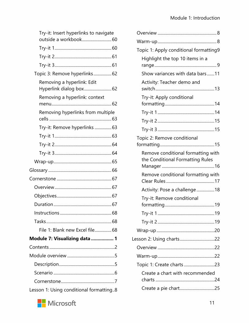
Contents Module 1: Introduction ....................... 1
Contents .............................................................. 2 Module overview ............................................. 4
Description ..................................................... 4 Scenario .......................................................... 5 Cornerstone ................................................... 5
Lesson 1: Getting to know Excel ................ 6 Overview ......................................................... 6 Warm-up ........................................................ 6 Topic 1: Create and open workbooks . 7
Create a new workbook ....................... 7 Open an existing workbook ............... 8 Create a new workbook by using an existing workbook .................................. 9 Activity: Guess and tell ......................... 9 Try-it: Create and open workbooks 9 Try-it 1 ...................................................... 10 Try-it 2 ...................................................... 10
Topic 2: Explore the Excel interface .. 11
Explore the ribbon and manage views ......................................................... 13 Activity: Guess and tell ...................... 14 Try-it: Explore the Excel interface .. 15 Try-it ......................................................... 15 Resources ................................................ 15
Wrap-up ....................................................... 16 Lesson 2: Introducing the Excel fundamentals .................................................. 17
Overview ...................................................... 17
Warm-up ...................................................... 17 Topic 1: Enter and edit data ................. 18
Enter data ................................................ 18 Complete a data entry ....................... 18 Edit cell contents .................................. 19 Cancel a cell entry ................................ 19 Clear cell contents ............................... 19 Activity: Pose a challenge ................. 20 Try-it: Enter and edit data................. 20 Try-it 1 ...................................................... 20 Try-it 2 ...................................................... 21
Topic 2: Save workbooks ....................... 21 Save a new workbook ........................ 22 Save an existing workbook .............. 22 Save an existing workbook as another name or to a new location .................................................... 22 Save a workbook in a different format ....................................................... 23 Save a workbook as a PDF ............... 23 Convert a workbook to a newer version ...................................................... 24 Activity: Discuss and learn ................ 24 Try-it: Save workbooks ...................... 25 Try-it: 1 ..................................................... 25 Try-it: 2 ..................................................... 26 Try-it: 3 ..................................................... 26
Wrap-up ....................................................... 27 Lesson 3: Navigating and filling cells .... 28
Overview ...................................................... 28 Warm-up ...................................................... 28

Module 1: Introduction
2
Topic 1: Navigate to named cells, ranges, or workbook elements ........... 29
Navigate to a named cell, range, or table .......................................................... 30 Display workbook elements ............ 30 Activity: Tell a story ............................. 31 Try-it: Navigate to named cells, ranges, or workbook elements ...... 32 Try-it 1 ...................................................... 32 Try-it 2 ...................................................... 33 Try-it 3 ...................................................... 33
Topic 2: Search for data ......................... 34 Find data in a workbook ................... 34 Replace data in a workbook............ 35 Activity: Show and tell ....................... 36 Try-it: Search for data ........................ 36 Try-it 1 ...................................................... 37 Try-it 2 ...................................................... 37
Topic 3: Use the AutoFill feature ........ 38 AutoFill using a pointer device ...... 38 AutoFill using the Fill command .... 39 AutoFill a series of numbers with a pointing device ..................................... 39 Activity: Guess and tell ...................... 40 Try-it: AutoFill ........................................ 40 Try-it: 1 ..................................................... 40 Resources ................................................ 40 Instructions ............................................ 40 Try-it: 2 ..................................................... 41 Try-it: 3 ..................................................... 41
Wrap-up ....................................................... 42 Glossary ............................................................ 44
Cornerstone ..................................................... 45 Overview ...................................................... 45 Objectives .................................................... 45
Duration ................................................... 45 Instructions ............................................. 45 Tasks .......................................................... 46
Thumbnail image ...................................... 48 Module 2: Managing worksheets and workbooks ............................................ 1
Contents .............................................................. 2 Module overview ............................................. 4
Description .................................................... 4 Scenario .......................................................... 5 Cornerstone .................................................. 5
Lesson 1: Structuring a worksheet ........... 6 Overview ........................................................ 6 Warm-up ........................................................ 6 Topic 1: Set up columns, rows, and cells ................................................................... 7
Insert a row into a worksheet ........... 7 Delete a row ............................................. 7
Insert a column ....................................... 8 Delete a column ..................................... 8 Delete multiple columns or rows .... 9 Adjust a row height or column width ........................................................... 9 Insert a cell .............................................. 10 Delete a cell ............................................ 10 Activity: Student teach back ............ 10 Try-it: Columns, rows, and cells ...... 11
Topic 2: Set up worksheets ................... 12

Module 1: Introduction
3
Insert an extra worksheet ................. 12 Delete a worksheet ............................. 13 Rename a worksheet .......................... 13 Move a worksheet within the same workbook ................................................ 14 Copy a worksheet within the same workbook ................................................ 14 Move a worksheet to a different workbook ................................................ 15 Copy a worksheet to a different workbook ................................................ 16 Activity: Discuss and learn ............... 16 Try-it: Worksheets ............................... 17 Try-it 1 ...................................................... 17 Try-it 2 ...................................................... 17
Wrap-up ....................................................... 18 Lesson 2: Editing a worksheet ................. 20
Overview ...................................................... 20 Warm-up ..................................................... 20 Topic 1: Cut, copy, paste, and move data ................................................................ 21
Cut data ................................................... 21 Copy data ............................................... 22 Further ways to copy data ............... 23 Paste copied or cut data ................... 23 Move data .............................................. 24 Activity: Group/team .......................... 24 Try-it: Cut, copy, paste, and move 25 Try-it 1 ...................................................... 25 Try-it 2 ...................................................... 26
Topic 2: Use Paste Special .................... 27 Paste Special .......................................... 27
Activity: Pose a question ................... 28 Try-it: Paste Special ............................. 29 Try-it: 1 ..................................................... 29 Try-it: 2 ..................................................... 30 Try-it: 3 ..................................................... 30
Wrap-up ....................................................... 31 Lesson 3: Customizing views and toolbars ............................................................. 32
Overview ...................................................... 32 Warm-up ...................................................... 32 Topic 1: Freeze panes and workbook views .............................................................. 33
Change the screen zoom .................. 33 Change screen display ....................... 34 Freeze worksheet titles ...................... 34 Unfreeze worksheet titles ................. 35 Move between workbook windows ................................................... 35 View all the workbooks you want to interact with ........................................... 35 View two workbooks side by side . 36 Split your screen into panes ............ 36 Clear worksheet panes ....................... 37 Navigation keyboard shortcuts ...... 37 Activity: Research ................................. 38 Try-it: Freeze panes and workbook views .......................................................... 39
Topic 2: Use the Quick Access Toolbar .......................................................... 39
Use the ribbon to customize the Quick Access Toolbar ......................... 40 Customize using the Quick Access Toolbar ..................................................... 40

Module 1: Introduction
4
Activity: Show and tell ....................... 42 Try-it: Quick Access Toolbar ........... 42 Try-it: 1 ..................................................... 42 Try-it: 2 ..................................................... 43 Try-it: 3 ..................................................... 44
Wrap-up ....................................................... 45 Glossary ............................................................ 46 Cornerstone .................................................... 47
Overview ...................................................... 47 Objectives .................................................... 47
Duration .................................................. 47 Instructions ................................................. 48
File 1: Cornerstone_beehive_data_starter .xlsx ............................................................ 48 File 2: Cornerstone_honeybee_colonies_ starter.csv ................................................ 49
Module 3: Formatting cells ................. 1Contents .............................................................. 2 Module overview ............................................. 4
Description ..................................................... 4 Scenario .......................................................... 5 Cornerstone ................................................... 6
Lesson 1: Formatting cells ............................ 7 Overview ......................................................... 7 Warm-up ........................................................ 7 Topic 1: Format font and cells ............... 8
Font group commands on the Home tab ................................................... 8 The Format Cells dialog box ........... 10 Mini Toolbar .......................................... 12
Activity: Show and tell ........................ 12 Try-it: Format font and cells ............ 14 Try-it 1 ...................................................... 14 Try-it 2 ...................................................... 15 Try-it 3 ...................................................... 16
Topic 2: Apply number formats .......... 17 Number command group on the Home tab ................................................ 17 Important facts about number formats ..................................................... 17 Activity: Think-Pair-Share ................. 18 Try-it: Apply number formats ......... 19 Try-it 1 ...................................................... 19 Try-it 2 ...................................................... 20 Try-it 3 ...................................................... 21
Topic 3: Reuse formats ........................... 22 Format Painter ....................................... 22 Activity: Discuss and learn ................ 24 Try-it: Reuse formats .......................... 24 Try-it .......................................................... 25
Wrap-up ....................................................... 25
Lesson 2: Aligning cells ............................... 27 Overview ...................................................... 27 Warm-up ...................................................... 27 Topic 1: Modify cell alignment, orientation, and indentation ................ 28
Alignment group commands on the Home tab ................................................ 28 Alignment commands in the Format Cells dialog box .................................... 29 Activity: Teacher demonstration, Switch ....................................................... 30

Module 1: Introduction
5
Try-it: Modify cell alignment, orientation, and indentation ........... 31Try-it 1 ...................................................... 31 Try-it 2 ...................................................... 30 Try-it 3 ...................................................... 32
Topic 2: Merge cells and wrap text ... 33 Merge & Center ................................... 34 Center Across Selection .................... 34 Wrap Text ............................................... 35 Activity: Pose a challenge ................. 35 Try-it: Merge cells and wrap text .. 36 Try-it ......................................................... 36
Wrap-up ....................................................... 37 Lesson 3: Using cell styles ......................... 39
Overview ...................................................... 39 Warm up ...................................................... 39 Topic 1: Apply cell styles ....................... 40
Finding the Cell Styles ....................... 40 Using and modifying cell styles ..... 41 Activity: Each one, teach one .......... 42 Activity instructions ............................ 42 Try-it: Apply cell styles ....................... 43 Try-it ......................................................... 43
Topic 2: Clear formatting ...................... 45 Activity: Show and tell ....................... 46 Try-it: Clear formatting ...................... 47 Try-it ......................................................... 47
Wrap-up ....................................................... 48 Glossary ............................................................ 49 Cornerstone .................................................... 50
Overview ...................................................... 50
Objectives .................................................... 51 Duration ....................................................... 52 Instructions .................................................. 52 Tasks .............................................................. 52
File: Cornerstone_volunteers_list_starter .xlsx ............................................................ 52
Module 4: Managing tables and range data ........................................................ 1Contents .............................................................. 2 Module overview ............................................. 4
Description .................................................... 4 Scenario .......................................................... 5 Cornerstone .................................................. 6
Lesson 1: Understanding tables and ranges .................................................................. 7
Overview ........................................................ 7 Warm-up ........................................................ 7 Topic 1: Format data as a table and change the table style .............................. 8
Create a table without a style applied ....................................................... 9 Create a table with a style applied at the same time ........................................ 10 Activity: Tell a story ............................. 13 Try-it: Format data as a table and change the table style ........................ 14 Try-it .......................................................... 14 Try-it 2 ...................................................... 15
Topic 2: Convert a table to a range ... 15 Activity: Pose a challenge ................. 16 Activity instructions ............................. 16 Try-it: Convert a table to a range .. 16

Module 1: Introduction
6
Wrap-up ....................................................... 17 Lesson 2: Configuring table format options .............................................................. 19
Overview ...................................................... 19 Warm-up ..................................................... 19 Topic 1: Configure table style options ......................................................... 20
Activity: Discuss and learn ............... 21 Activity instructions ............................ 22 Try-it: Configure table style options ..................................................... 22
Topic 2: Insert and manage rows, columns, and the total number of rows ............................................................... 23
Use the Resize command ................. 23 Enter data ............................................... 24 Paste data ............................................... 24 Insert data............................................... 25 To insert a column .............................. 26 Delete rows or columns in a table 27 Total Row ................................................ 27 Activity: Discuss and learn ............... 28 Try-it: Insert and manage rows, columns, and total number of rows ........................................................... 29
Wrap-up ....................................................... 30 Lesson 3: Naming tables and ranges .... 31
Overview ...................................................... 31 Warm-up ..................................................... 31 Topic 1: Name a table ............................ 32
Activity: Pose a challenge ................. 33 Activity instructions ............................ 34
Try-it: Name a table ............................ 34 Topic 2: Define a named range ........... 35
Edit and delete named ranges ....... 37 Activity: Discuss and learn ................ 38
Try-it: Define a named range ............... 39 Try-it 1 ...................................................... 39
Wrap-up ....................................................... 40 Lesson 4: Sorting and filtering ................. 42
Overview ...................................................... 42 Warm-up ...................................................... 42 Topic 1: Sort and filter records ............ 43
Sort a cell range column in ascending or descending order ..... 44 Change the Sort Options Orientation for a data set ................. 44 Sort a table column in ascending or descending order ................................. 44 Filter a cell range column ................. 45 Filter a table column ........................... 47 Clear a filter from a column ............. 47 Clear all filters in a worksheet ......... 48 Remove all filters in a worksheet ... 49
Activity: Show and tell ........................ 49 Try-it: Sort and filter records ........... 50
Topic 2: Perform a custom sort ........... 50 Sort text ................................................... 51 Sort numbers ......................................... 52 Sort dates and times ........................... 53 Sort by more than one column ...... 55 Sort by cell color, font color, or icon ............................................................ 56 Activity: Pose a challenge ................. 57

Module 1: Introduction
7
Activity instructions ............................ 57 Try-it: Perform a custom sort .......... 58
Wrap-up ....................................................... 58 Cornerstone .................................................... 60
Overview ...................................................... 60 Objectives .................................................... 60 Duration ....................................................... 61 Instructions ................................................. 61 Tasks .............................................................. 61
File 1: Cornerstone_Munsons_apparel_ starter.xlsx ............................................... 62 File 2: Cornerstone_Munsons_bee_product_inventory_ starter.xlsx ...................... 63
Glossary ............................................................ 64 Module 5: Using formulas and functions ............................................... 1
Contents .............................................................. 2 Module overview ............................................. 4
Description ..................................................... 4 Scenario .......................................................... 5 Cornerstone ................................................... 5
Lesson 1: Performing basic calculations . 6 Overview ......................................................... 6 Warm-up ........................................................ 6 Topic 1: Understand basic formulas .... 7
Order of operations ............................... 9 Use parentheses to modify the order of operations ............................. 10 Activity: Show and tell ....................... 10 Use cell references in formulas ...... 11
Try-it: Understand basic formulas . 12 Try-it 1 ...................................................... 12 Try-it 2 ...................................................... 13 Try-it 3 ...................................................... 13
Topic 2: Display formulas ...................... 14 Activity: Show and tell ........................ 15 Try-it: Display formulas ...................... 16
Wrap-up ....................................................... 16 Lesson 2: Using references in formulas 18
Overview ...................................................... 18 Warm-up ...................................................... 18 Topic 1: Understand relative and absolute references ................................. 19
Use relative cell references in a formula ..................................................... 19 Use absolute cell references in a formula ..................................................... 20 Use mixed cell references in a formula ..................................................... 21 Activity: Tell a story ............................. 22 Try-it: Understand relative and absolute references ............................. 22
Topic 2: Use named ranges and worksheet references in formulas ...... 23
Use worksheet references in a formula ..................................................... 26 Activity: Quiz Me! ................................. 26 Try-it: Use named ranges and worksheet references in formulas . 27 Try-it 1 ...................................................... 27 Try-it 2 ...................................................... 28
Wrap-up ....................................................... 28 Lesson 3: Introducing functions .............. 30

Module 1: Introduction
8
Overview ...................................................... 30 Warm-up ..................................................... 30 Topic 1: Use functions in calculations ................................................. 31
Use the Function Library to insert functions ................................................. 32 Use the SUM function ....................... 34 Use the AVERAGE function .............. 35 Activity: Show me how ...................... 35 Try-it: Use functions in calculations ............................................ 36 Try-it 1 ...................................................... 36 Try-it 2 ...................................................... 37
Topic 2: Use MAX and MIN functions in formulas .................................................. 37
Overview of the MAX function ....... 37 Overview of the MIN function ........ 38 Activity: Show me how ...................... 38 Try-it: Use MAX and MIN functions in formulas ............................................. 39 Try-it 1 ...................................................... 39 Try-it 2 ...................................................... 39
Wrap-up ....................................................... 40 Lesson 4: Using count functions ............. 41
Overview ...................................................... 41 Warm-up ..................................................... 41 Topic 1: Use COUNT and COUNTA functions to analyze data ...................... 42
The COUNT Function ......................... 42 The COUNTA Function ...................... 42 Activity: Discuss and learn ............... 43
Try-it: Use COUNT and COUNTA functions to analyze data ................. 44 Try-it 1 ...................................................... 44 Try-it 2 ...................................................... 44
Topic 2: Use the COUNTBLANK function ........................................................ 45
The COUNTBLANK function ............ 45 Activity: Pose a challenge ................. 46 Try-it: Use the COUNTBLANK function .................................................... 46
Wrap-up ....................................................... 47 Lesson 5: Using logical functions ............ 49
Overview ...................................................... 49 Warm-up ...................................................... 49 Topic 1: Understand IF statements .... 50
Use logical operators ......................... 50 Activity: Discuss and learn ................ 51 Try-it: Understand IF statements ... 51
Topic 2: Use the IF function .................. 52 IF function syntax ................................. 52 Considerations when using the IF function .................................................... 53 Activity: Show and tell ........................ 53 Try-it: Use the IF function ................. 54 Try-it 1 ...................................................... 54 Try-it 2 ...................................................... 55
Wrap-up ....................................................... 55 Glossary ............................................................. 57 Cornerstone ..................................................... 58
Overview ...................................................... 58 Objectives .................................................... 58 Duration ....................................................... 59

Module 1: Introduction
9
Instructions ................................................. 59 Tasks .............................................................. 59
File 1: Cornerstone_attendance_ticketsales_starter.xlsx ............................................. 59
Module 6: Getting and transforming data ........................................................ 1
Contents .............................................................. 2 Module overview ............................................. 5
Description ..................................................... 5 Scenario .......................................................... 6 Cornerstone ................................................... 6
Lesson 1: Importing data .............................. 7 Overview ......................................................... 7 Warm-up ........................................................ 7 Scenario .......................................................... 8 Topic 1: Get data from other sources . 8
Get & transform data ............................ 8 Activity: Pose a challenge .................... 9 Try-it: Get data from other sources . 9
Topic 2: Import data from .txt files ... 10 Using Notepad to review a .txt file .............................................................. 10 Getting data from .txt files ............... 10 Activity: Show and tell ....................... 11 Try-it: Import data from .txt files ... 11
Topic 3: Import data from .csv files .. 12 Using Notepad to review a .csv file .............................................................. 12 Getting data from .csv files .............. 12 Activity: Show and tell ....................... 12 Try-it: Import data from .csv files .. 13
Wrap-up ....................................................... 14 Lesson 2: Manipulating text ...................... 15
Overview ...................................................... 15 Warm-up ...................................................... 15 Topic 1: Convert text to columns ....... 16
Splitting text into columns ............... 16 Activity: Discuss and learn ................ 17 Try-it: Convert text to columns ...... 18
Topic 2: Extract text by using the LEFT, RIGHT, MID, and LEN functions .......... 19
LEFT function ......................................... 19 RIGHT function ...................................... 20 LEN function ........................................... 21 MID function .......................................... 21 Character counting .............................. 22 Activity: Show and tell ........................ 23 Try-it: Extract text by using the LEFT, RIGHT, MID, and LEN functions ..... 24 Try-it 1 ...................................................... 24 Try-it 2 ...................................................... 25 Try-it 3 ...................................................... 25
Try-it 4 ...................................................... 26 Wrap-up questions .................................. 26
Lesson 3: Converting text .......................... 28 Overview ...................................................... 28 Warm-up questions ................................. 28 Topic 1: Convert text by using the PROPER function ....................................... 29
Converting Text: PROPER ................. 29 Copying a formula to multiple cells ............................................................ 29 Using Paste Special ............................. 30

Module 1: Introduction
10
Activity: Tell a story ............................. 31 Try-it: Convert text by using the PROPER function ................................. 31 Try-it 1 ...................................................... 32 Try-it 2 ...................................................... 32 Try-it 3 ...................................................... 32
Topic 2: Convert text by using the UPPER and LOWER functions .............. 33
Converting Text: UPPER .................... 33 Converting Text: LOWER .................. 34 Activity: Show and tell ....................... 34 Try-it: Convert text by using the UPPER and LOWER functions ......... 35 Try-it 1 ...................................................... 35 Try-it 2 ...................................................... 35 Try-it 3 ...................................................... 36
Wrap-up ....................................................... 36 Lesson 4: Combining text .......................... 38
Overview ...................................................... 38 Warm-up ..................................................... 38 Topic 1: Combine text by using the CONCAT function ..................................... 39
Combining text: CONCAT ................ 39 Adding space or a word between data when using the CONCAT function ................................................... 40 Combining text using absolute cell references ............................................... 40 Activity: Discuss and learn ............... 41 Try-it: Combine text by using the CONCAT function ................................ 42 Try-it 2 ...................................................... 43 Try-it 3 ...................................................... 43
Topic 2: Combine text by using the TEXTJOIN function ................................... 44
Combining text: TEXTJOIN ............... 44 Combining text: CONCAT and TEXTJOIN ................................................. 44 Activity: Pose a challenge ................. 45 Try-it: Combine text by using the TEXTJOIN function ............................... 46 Try-it 1 ...................................................... 46 Try-it 2 ...................................................... 47
Wrap-up ....................................................... 47 Lesson 5: Inserting hyperlinks .................. 49
Overview ...................................................... 49 Warm-up ...................................................... 49 Topic 1: Insert hyperlinks to navigate inside a workbook .................................... 50
Creating a hyperlink to place within the document ........................................ 51 Creating a hyperlink to a cell range ......................................................... 52 Activity: Tell a story ............................. 53 Try-it: Insert hyperlinks to navigate inside a workbook ............................... 55 Try-it 1 ...................................................... 55 Try-it 2 ...................................................... 55 Try-it 3 ...................................................... 56
Topic 2: Insert hyperlinks to navigate outside a workbook ................................. 57
Creating a hyperlink to another file ............................................................... 57 Creating a hyperlink to a website . 58 Activity: Discuss and learn ................ 59
Module 1: Introduction
11
Try-it: Insert hyperlinks to navigate outside a workbook ............................ 60 Try-it 1 ...................................................... 60 Try-it 2 ...................................................... 61 Try-it 3 ...................................................... 61
Topic 3: Remove hyperlinks ................. 62 Removing a hyperlink: Edit Hyperlink dialog box .......................... 62 Removing a hyperlink: context menu ......................................................... 62 Removing hyperlinks from multiple cells ........................................................... 63 Try-it: Remove hyperlinks ................ 63 Try-it 1 ...................................................... 63 Try-it 2 ...................................................... 64 Try-it 3 ...................................................... 64
Wrap-up ....................................................... 65 Glossary ............................................................ 66 Cornerstone .................................................... 67
Overview ...................................................... 67 Objectives .................................................... 67 Duration ....................................................... 67 Instructions ................................................. 68 Tasks .............................................................. 68
File 1: Blank new Excel file ................ 68 Module 7: Visualizing data ................. 1
Contents .............................................................. 2 Module overview ............................................. 5
Description ..................................................... 5 Scenario .......................................................... 6 Cornerstone ................................................... 7
Lesson 1: Using conditional formatting .. 8
Overview ........................................................ 8 Warm-up ........................................................ 8 Topic 1: Apply conditional formatting 9
Highlight the top 10 items in a range ........................................................... 9 Show variances with data bars ....... 11 Activity: Teacher demo and switch ........................................................ 13 Try-it: Apply conditional formatting ............................................... 14 Try-it 1 ...................................................... 14 Try-it 2 ...................................................... 15 Try-it 3 ...................................................... 15
Topic 2: Remove conditional formatting .................................................... 15
Remove conditional formatting with the Conditional Formatting Rules Manager .................................................. 16 Remove conditional formatting with Clear Rules .............................................. 17 Activity: Pose a challenge ................. 18 Try-it: Remove conditional formatting ............................................... 19 Try-it 1 ...................................................... 19 Try-it 2 ...................................................... 19
Wrap-up ....................................................... 20 Lesson 2: Using charts ................................. 22
Overview ...................................................... 22 Warm-up ...................................................... 22 Topic 1: Create charts ............................. 23
Create a chart with recommended charts ........................................................ 24 Create a pie chart ................................. 25

Module 1: Introduction
12
Activity: Show and learn ................... 27 Try-it: Create charts ............................ 27 Try-it 1 ...................................................... 27 Try-it 2 ...................................................... 28
Topic 2: Add alternative text ............... 28 Add Alt Text using the context menu ......................................................... 29 Mark a visual object as decorative 30 Activity: Discussion ............................. 31 Try-it: Add Alt Text .............................. 31 Try-it 1 ...................................................... 32 Try-it 2 ...................................................... 32
Topic 3: Move charts ............................... 32 Move a chart on the worksheet ..... 33 Move a chart to a different worksheet ............................................... 33 Activity: Discuss and learn ............... 34 Try-it: Move charts .............................. 34 Try-it 1 ...................................................... 34 Try-it 2 ...................................................... 35 Try-it 3 ...................................................... 35
Wrap-up ....................................................... 36 Lesson 3: Editing charts .............................. 37
Overview ...................................................... 37 Warm-up ..................................................... 37 Topic 1: Add a data series .................... 38
Add a data series to your chart ..... 38 Use select data to add and remove source data ............................................ 40 Activity: Demonstration .................... 41 Try-it: Add data series........................ 42
Try-it 1 ...................................................... 42 Try-it 2 ...................................................... 42
Topic 2: Switch between rows and columns ........................................................ 43
Activity: Demonstration ..................... 43 Try-it: Switch between rows and columns.................................................... 44
Wrap-up ....................................................... 45 Lesson 4: Understanding chart elements ........................................................... 46
Overview ...................................................... 46 Warm-up ...................................................... 46 Topic 1: Add chart elements ................ 47
Activity: Show and Tell ....................... 48 Try-it: Add chart elements ................ 48 Try-it 1 ...................................................... 48 Try-it 2 ...................................................... 49 Try-it 3 ...................................................... 49
Topic 2: Modify chart elements .......... 50 Edit the text of a title in a chart ...... 50 Format a chart element with the Format task pane ................................. 51 Format a chart element with the Chart Tools tab ..................................... 51 Activity: Discuss and Learn ............... 52 Try-it: Modify chart elements .......... 52 Try-it 1 ...................................................... 52 Try-it 2 ...................................................... 53 Try-it 3 ...................................................... 53
Wrap-up ....................................................... 54 Lesson 5: Understanding chart styles and layouts ............................................................... 56

Module 1: Introduction
13
Overview ...................................................... 56 Warm-up ..................................................... 56 Topic 1: Apply layouts ............................ 57
Activity: Demo ....................................... 58 Try-it: Apply layouts ........................... 59
Topic 2: Apply styles and colors ......... 59 Apply a Quick Style from the ribbon ....................................................... 60 Apply a quick style with Chart Styles ........................................................ 60 Apply a color scheme from the ribbon ....................................................... 61 Apply a color scheme with Chart Styles ........................................................ 61 Activity: Discuss and learn ............... 62 Try-it: Apply styles and colors ........ 63 Try-it 1 ...................................................... 63 Try-it 2 ...................................................... 63
Wrap-up ....................................................... 64 Lesson 6: Understanding sparklines ...... 65
Overview ...................................................... 65 Warm-up ..................................................... 65 Topic 1: Insert sparklines ....................... 66
Activity: Tell a story ............................. 68 Try-it: Insert sparklines ...................... 68 Try-it 1 ...................................................... 68 Try-it 2 ...................................................... 69
Topic 2: Modify sparklines .................... 69 Show sparkline markers and highlights ................................................ 69 Apply a style to sparklines ............... 70 Activity: Continue the story ............. 71
Try-it: Modify sparklines .................... 71 Try-it 1 ...................................................... 71 Try-it 2 ...................................................... 72 Try-it 3 ...................................................... 72
Wrap-up ....................................................... 73
Lesson 7: Understanding the Quick Analysis feature .............................................. 74
Overview ...................................................... 74 Warm-up ...................................................... 74 Topic 1: Use Quick Analysis to format data ................................................................ 75
Add conditional formatting using Quick Analysis ....................................... 76 Add a chart or sparklines using Quick Analysis ....................................... 76 Add totals for data using Quick Analysis .................................................... 77 Activity: Demo and experiment ...... 78 Try-it: Quick Analysis .......................... 78 Try-it 1 ...................................................... 78 Try-it 2 ...................................................... 79
Topic 2: Disable the Quick Analysis feature ........................................................... 79
Activity: Discuss .................................... 80 Try-it: Disable the Quick Analysis feature ...................................................... 81
Wrap-up ....................................................... 81 Glossary ............................................................. 82 Cornerstone ..................................................... 83
Overview ...................................................... 83 Objectives .................................................... 83 Duration ....................................................... 84

Module 1: Introduction
14
Instructions ................................................. 84 Tasks .............................................................. 84
File 1: Cornerstone_solar_array_data_ starter.xlslx .............................................. 84
Module 8: Preparing to print and checking for issues .............................. 1Contents .............................................................. 2 Module overview ............................................. 4
Description ..................................................... 4 Scenario .......................................................... 5 Cornerstone ................................................... 6
Lesson 1: Preparing to print ........................ 7 Overview ......................................................... 7 Warm-up ........................................................ 7 Topic 1: Understand the print settings ............................................................ 8
Access print settings ............................. 8 Settings ....................................................... 9 Set the print area ................................. 12 Print ........................................................... 13 Activity: Discuss and learn ............... 14 Try-it: Understanding the print settings .................................................... 14 Try-It 1 ...................................................... 14 Try-It 2 ...................................................... 15 Try-It 3 ...................................................... 15
Topic 2: Understand page setup ........ 16 Page Setup dialog box ...................... 18 Set margins ............................................ 18 Sheet settings ....................................... 19 Activity: Question time ...................... 20
Try-it: Understand page setup........ 21 Try-It 1 ...................................................... 21 Try-It 2 ...................................................... 21
Wrap-up ....................................................... 22 Lesson 2: Using headers and footers .... 24
Overview ...................................................... 24 Warm-up ...................................................... 24 Topic 1: Add headers and footers ..... 25
Add headers or footers by using the Insert tab ................................................. 25 Add headers or footers by using the Page Setup dialog box ....................... 26 Activity: Discuss and learn ................ 28 Try-it: Add headers or footers ........ 29 Try-It 1 ...................................................... 29 Try-It 2 ...................................................... 29
Topic 2: Edit headers and footers ...... 30 Edit a header or footer using Page Layout view ............................................. 30 Edit a header or footer using the Page Setup dialog box ....................... 31 Remove all headers and footers .... 32 Activity: Switch ...................................... 32 Try-it: Edit headers and footers ...... 33 Try-It 1 ...................................................... 33 Try-It 2 ...................................................... 33
Wrap-up ....................................................... 34 Lesson 3: Checking for issues ................... 36
Overview ...................................................... 36 Warm-up ...................................................... 36 Topic 1: Modify the basic workbook properties .................................................... 37

Module 1: Introduction
15
Workbook properties ......................... 38 Activity: Pose a question................... 40 Try-it: Modify basic workbook properties ............................................... 40 Try-It 1 ...................................................... 40 Try-It 2 ...................................................... 41
Topic 2: Inspect workbooks for issues ............................................................. 41
Inspect a workbook ............................ 42 Check accessibility............................... 45 Compatibility issues ............................ 47 Activity: What’s the correct category? ................................................ 49 Try-it: Inspect workbooks for issues ........................................................ 49 Try-It 1 ...................................................... 49
Try-It 2 ...................................................... 50 Wrap-up ....................................................... 51
Glossary ............................................................. 53 Cornerstone ..................................................... 54
Overview ...................................................... 54 Objectives .................................................... 54 Duration ....................................................... 55 Instructions .................................................. 55 Tasks .............................................................. 55
File 1: Cornerstone_membership_starter .xlsx ............................................................ 55 File 2: Cornerstone2_finances_starter .xlsx ............................................................ 56

Student Guide 40567A Microsoft Excel associate 2019 Module 1: Introduction

Module 1: Introduction
2
Contents
Contents .............................................................. 2
Module overview ............................................. 4
Description ..................................................... 4
Scenario .......................................................... 5
Cornerstone ................................................... 5
Lesson 1: Getting to know Excel ................ 6
Overview ......................................................... 6
Warm-up ........................................................ 6
Topic 1: Create and open workbooks . 7
Create a new workbook ....................... 7
Open an existing workbook ............... 8
Create a new workbook by using an existing workbook .................................. 9
Activity: Guess and tell ......................... 9
Try-it: Create and open workbooks 9
Try-it 1 ...................................................... 10
Try-it 2 ...................................................... 10
Topic 2: Explore the Excel interface .. 11
Explore the ribbon and manage views ......................................................... 13
Activity: Guess and tell ...................... 14
Try-it: Explore the Excel interface .. 15
Try-it ......................................................... 15
Resources ................................................ 15
Wrap-up ....................................................... 16
Lesson 2: Introducing the Excel fundamentals .................................................. 17
Overview ...................................................... 17
Warm-up ...................................................... 17
Topic 1: Enter and edit data ................. 18
Enter data ................................................ 18
Complete a data entry ....................... 18
Edit cell contents .................................. 19
Cancel a cell entry ................................ 19
Clear cell contents ............................... 19
Activity: Pose a challenge ................. 20
Try-it: Enter and edit data................. 20
Try-it 1 ...................................................... 20
Try-it 2 ...................................................... 21
Topic 2: Save workbooks ....................... 21
Save a new workbook ........................ 22
Save an existing workbook .............. 22
Save an existing workbook as another name or to a new location ..................................................................... 22
Save a workbook in a different format ....................................................... 23
Save a workbook as a PDF ............... 23
Convert a workbook to a newer version ...................................................... 24
Activity: Discuss and learn ................ 24
Try-it: Save workbooks ...................... 25
Try-it: 1 ..................................................... 25
Try-it: 2 ..................................................... 26
Try-it: 3 ..................................................... 26
Wrap-up ....................................................... 27
Lesson 3: Navigating and filling cells .... 28

Module 1: Introduction
3
Overview ...................................................... 28
Warm-up ..................................................... 28
Topic 1: Navigate to named cells, ranges, or workbook elements ........... 29
Navigate to a named cell, range, or table .......................................................... 30
Display workbook elements ............ 30
Activity: Tell a story ............................. 31
Try-it: Navigate to named cells, ranges, or workbook elements ...... 32
Try-it 1 ...................................................... 32
Try-it 2 ...................................................... 33
Try-it 3 ...................................................... 33
Topic 2: Search for data ......................... 34
Find data in a workbook ................... 34
Replace data in a workbook............ 35
Activity: Show and tell ....................... 36
Try-it: Search for data ........................ 36
Try-it 1 ...................................................... 37
Try-it 2 ...................................................... 37
Topic 3: Use the AutoFill feature ........ 38
AutoFill using a pointer device ....... 38
AutoFill using the Fill command .... 39
AutoFill a series of numbers with a pointing device ..................................... 39
Activity: Guess and tell ....................... 40
Try-it: AutoFill ........................................ 40
Try-it: 1 ..................................................... 40
Resources ................................................ 40
Instructions ............................................. 40
Try-it: 2 ..................................................... 41
Try-it: 3 ..................................................... 41
Wrap-up ....................................................... 42
Glossary ............................................................. 44
Cornerstone ..................................................... 45
Overview ...................................................... 45
Objectives .................................................... 45
Duration ................................................... 45
Instructions ............................................. 45
Tasks .......................................................... 46
Thumbnail image ...................................... 48

Module 1: Introduction
4
Module overview Description Welcome to the first module of the Excel Associate course, in which you’ll will get the chance to get know Excel 2019. Excel 2019 is a robust software program included in the Microsoft Office suite. It is used to create spreadsheets, where data is arranged in rows and columns; imagine Excel as a big table of data. Excel is extremely versatile and powerful, and it can be used for answering questions about data through analysis and visualization. It almost does your work for you!
This module will set you up for your future use of Excel, whether that’s at home, in class, or at work. At the end of each module, you’ll complete a Cornerstone project that will help embed the skills that you’ve learned and during each lesson. You’ll also participate in activities and try-its to practice and learn new skills. As you go through the lessons, you’ll find helpful links to websites that will provide further learning and maybe even a little homework! You will also find handy notes and tips. Good luck and enjoy the course!
Lesson Learning objective Exam objective(s)
Getting to know Excel
Create and open workbooks; become familiar with the Excel interface.
Not mapped
Introducing the Excel fundamentals
Enter and edit data; save workbooks in alternate formats
• 1.5.2
Navigating and filling cells
Navigate to named cells, named ranges and other workbook objects; search for data and use Autofill to fill cell contents.
• 1.2.2 • 1.2.1 • 2.1.2
Helping a fellow intern with Microsoft Excel
Open/create/save workbooks; enter/edit data including AutoFill cell contents; search for data; and navigate to named cells, named cell ranges, and other workbook objects.
• .5.2 • 1.2.1 • 1.2.2 • 2.1.2
Table 1: Objectives by lesson

Module 1: Introduction
5
Scenario You’ve been working as an intern within the finance team of a farming operation. The finance team is currently working on converting as much paperwork as they can to digital. You’ve been working with a sales analysist for the past year. Several inexperienced interns will be starting soon, and they have no prior Excel experience. You’ve been tasked with teaching the interns Excel basics that will allow them to assist you with inputting the sales and personnel data. You’ve used Excel only a few times and you know that you don’t have enough knowledge to teach the interns everything they’ll need to know to be able to do their jobs. To get prepared, you’re going back to the basics to make sure you have the skills you’ll need to train the interns.
Cornerstone One of the interns has been working on two workbooks containing data that summarize the annual produce for various fruit and vegetables. The data needs to be ready for a meeting with your boss within the next hour. You’ll need to examine the files before the meeting to ensure the data is correct and that nothing is missing from data.
You’ll need to use AutoFill to enter data, locate named cells, find and replace data, and save the workbooks in alternate formats.
If your aim is to become an Excel expert, then completing the lessons and Cornerstone in this module and future modules will help you reach your goal sooner than you think. If you don’t want to be an Excel expert, just great at Excel, then these lessons and Cornerstone will help.

Module 1: Introduction
6
Lesson 1: Getting to know Excel Overview This lesson is intended to introduce you to Microsoft Excel 2019. You’ll learn how to open, create, and save workbooks, including saving to alternate formats. You’ll also learn how to enter and edit data within a worksheet. Finally, you’ll learn how to navigate to named ranges, tables, and cells, and how to use AutoFill.
Warm-up This is the first lesson in Excel, but you might have some past experience with spreadsheets. Be ready to share your experience with the class. Where have you observed spreadsheets being used? Have you ever used Excel?
Use these questions to find out what you already know about this lesson’s topics:
1. When you are in the Excel application, what shortcut key can you use to open an existing workbook?
Select the correct option.
a. Ctrl+Alt+O
b. Ctrl+O
c. Shift+O
d. Ctrl+Shift+O
2. Which area of the Excel application has the following three commands: Save, Undo, and Redo?
Select the correct option.
a. Status Toolbar
b. Mini Toolbar
c. Quick Access Toolbar
d. Formula Bar

Module 1: Introduction
7
3. How can you access the Backstage view?
Select the correct option.
a. Windows key
b. Select File
c. Select Home
d. Ctrl+B
4. To create a new workbook:
Select all that apply.
a. Go to File > New
b. Select Ctrl+N on your keyboard
c. Select Ctrl+O on your keyboard
d. Go to File > Open
Topic 1: Create and open workbooks One of the quickest ways to do anything in Excel, or any other Office application, is
to use keyboard shortcuts. For example, to create a new workbook you can use Ctrl+N and to open an existing workbook you can use Ctrl+O.
There are hundreds of keyboard shortcuts available and they really do help save time. Do not underestimate the value of the shortcut! Many keyboard shortcuts are common across Office apps and are used throughout the Microsoft Office Suite. Basic keyboard shortcuts remove the need for the new user to navigate through numerous commands on the ribbon. Learn keyboard shortcuts, and you’ll take the guesswork out trying to find out how to do things like Print, whether it’s a Word document, an Excel document, or just about any other document you encounter today.
Here are some of the ways to create and open workbooks:
Create a new workbook 1. Either select Ctrl+N or select New on the Quick Access Toolbar if it has been
added, or File > New.
2. Select the type of workbook to create. It can either be a new blank workbook, themost common way to start, or any pre-built template, which are great and can save alot of time with content and design.

Module 1: Introduction
8
Open an existing workbook 1. Start by selecting Ctrl+O, or via File > Open.
2. Depending upon where the workbook is stored, you might be able to either:
o Simply double-click (or select the space bar and Enter) on the file if it is listed inthe Open screen.Or
o Select the workbook listed under Workbooks (the file will open immediately).Or
o Select Folder (or other online location) to locate the folder in which the file isstored, select the folder to open it, and then select the file to open.
Figure 1. File Open screen – Workbooks and Folders
Or
o Select This PC, then select the folder on the recent list, or select the Navigate upone level arrow to move up a level within the file structure and continue tolocate the file.Or
o Select Browse to go to the Open dialog box (Ctrl+F12 will go here also). Locatethe file to open and double-click to open it, or select it once and then selectOpen.
o Extra tip: Consider using Windows E to open the File Explorer to quickly locatethe file you would like to open. When you find the file you want, double-click onit or select the spacebar and enter. If it’s an Excel file, it will open in Excel,otherwise it will open in the application it belongs to.
Video
To view a video on creating workbooks, go to: Create a new workbook

Module 1: Introduction
9
Create a new workbook by using an existing workbook Using Ctrl+O or File > Open, after the workbook has been located, you can right-click or access the context menu and then select Open a Copy.
Activity: Guess and tell The teacher will open Excel and create a new workbook and open an existing workbook. Be prepared to answer questions about opening files and other commands in Backstage view.
Resources required You will need the following resources for this activity:
• Excel 2019• L1_T1_act_calendar.xlsx
Activity instructions The following are the steps that you must perform during this activity:
1. Open Excel and create a new workbook.
2. Follow along with the teacher.
3. Answer/ask questions.
Did you know?
There are 1,048,576 rows and 16,384 columns in a standard Excel workbook? That’s a whopping 17,179,869,184 cells!
Try-it: Create and open workbooks This is a leveled try-it to create a new workbook in Excel 2019 in preparation for
Topic 2, and to open a copy of an existing workbook.

Module 1: Introduction
10
Try-it 1 In this try-it, you’ll create a new workbook by using the Backstage view and/or a shortcut key.
Resources You’ll need the following resources for this activity:
• None required
Instructions The following are the general tasks that you must perform during this try-it:
1. Close any open files without saving them.
2. Create a new workbook by using a shortcut key.
3. Create another workbook by using any design template.
4. Close all open files, leaving one open to help with the next topic.
Try-it 2 In this try-it, you’ll create a new workbook using a shortcut key and you’ll use an existing workbook to open a copy of it.
Resources You’ll need the following resources for this activity:
• Any existing workbook
Instructions The following are the general tasks that you must perform during this try-it:
1. Close any open files without saving them.
2. Create a new workbook by using a shortcut key.
3. Use the Open window to open a copy of any existing workbook listed.
4. Close all open files, leaving one open to help with the next topic.

Module 1: Introduction
11
Topic 2: Explore the Excel interface Before you dive into learning how to set up a workbook, let’s get you comfortable
with the application interface and terminology.
When you open Excel for the first time, you’re prompted with a menu to create a new file or open an existing file.
Figure 2. Excel interface
At the top of the application, there’s a bar known as the ribbon, which holds several tabs; these are usually File, Insert, Page Layout, Formula, Data, Review, View, and Help. Your ribbon might have different tabs. Each tab contains commands assembled together in logical groups.
The first ribbon tab is File. When the File tab is selected, it does not display a ribbon. Instead, it displays a panel on the left side of the application and includes commands such as: Information, New, Open, Save, Print, Share, Export, Options, and more. This panel area is referred to as the Backstage view.
• Think of the Backstage view as opening the curtain to access what’s going onbehind the workbook.
• When you have a workbook open and select the File menu, the workbook Info tabwill be displayed by default.

Module 1: Introduction
12
• At any time, select the back arrow in Backstage view to return to the workbooksheet, or select the Esc key on your keyboard.
When a workbook, even a blank workbook, is opened in Excel, other elements in the application interface will be activated, with the workbook area taking up most of the application area.
Directly above the ribbon, in the upper-right corner of the application (in the Title bar) are the commands Minimize, Restore, and Close to manage the size of the screen.
Next to that, you’ll find Ribbon Display Options. From here, there are three options that you can select to hide or collapse the ribbon as necessary. For example, if you have a large set of data and need more space to view it, you can temporarily collapse the ribbon and then bring it back into view when needed.
• Auto-hide Ribbon – Hide the ribbon. Select the top of the application to show it. Assoon as this option is selected, the entire ribbon is collapsed. To display the ribbonfor a quick view or to access the commands simply select More, the ellipsis (…) atthe top right of the window, or select the ALT key. To fully restore and show theribbon and commands again, select the third option.
• Show Tabs – Show ribbon tabs only. Select a tab to show the commands. This willcollapse the commands chunk below the tab name, but all the commands are stillaccessible from the tab name.
• Show Tabs and Commands – Show ribbon tabs and commands all at the sametime. This is the default view, where the entire ribbon is expanded, displaying all thetabs and their associated commands.
Figure 3. Ribbon display options
Note: If you double-click on any tab label twice, the ribbon will automatically hide. Double-click again to show the full tabs and commands.

Module 1: Introduction
13
In the upper-left corner above the ribbon is the Quick Access Toolbar. The Quick Access Toolbar can be displayed above or below the ribbon and can be customized to your needs. You’ll learn more about this later in the course. By default, the Quick Access Toolbar will display the AutoSave, Save, Undo, Redo and a drop-down menu.
Search (also known as Tell Me) is in the center of the Title bar. You can search for commands, get insights from an internet search, or get Excel help from here. Search/Tell Me is also available in other Office 2019 and Office 365 applications and is in the same position for each application.
The Name box and the Formula Bar are directly underneath the ribbon. You’ll learn more about these during the course.
At the bottom of the worksheet, you’ll find the Sheet tabs contained within the current workbook. The default sheet names are Sheet1, Sheet2, and so forth. Next to that there is the New sheet button (a little +) to add extra sheets as necessary.
Over to the right of the screen there is a Vertical scrollbar and there is a Horizontal scrollbar along the bottom to help you scroll through the worksheet. Finally, underneath the horizontal scroll bar, you’ll find Display Settings, with three screen views: Normal, Page Layout, and Page Break Preview. You’ll also find the Zoom slider bar, which lets you increase or decrease the size of the worksheet that is displayed on the screen.
Explore the ribbon and manage views If you’re new to Excel 2019, take a few minutes to read each tab description below, then go check each tab ribbon in the application. As you observe the groups and tools in a ribbon, go back and review the ribbon tab name. There is a correlation here; the name of the tab is a hint to the tools it holds. Insert contains many tools to insert something into a worksheet, like an image, table, chart, to name a few.
• File (Backstage View) – Access and manage application and workbook settings.• Home – The popular tools and commands used most, like the Clipboard tools, font
formatting, cell alignment, and number formatting.• Insert – Add objects and elements into your worksheet, such as Pictures, Icons,
Charts and SmartArt.• Draw – Make notes with a digital pen, convert ink to a shape, and convert ink to
math. (If your device is not touch screen enabled, you might need to add this tab tothe ribbon.)
• Page Layout – Modify the workbook themes, page setup, and sheet options.• Formulas – Create functions, define names, audit formulas, and set calculation
options.

Module 1: Introduction
14
• Data – Get data from other sources, create queries, sort, filter, and use other datatools.
• Review – Perform proofing, track changes, protection, and accessibility functions forthe worksheet.
• View – Manage and modify workbook views, zoom in and out, arrange workbookwindows, and create macros.
• Help – Access Excel help, contact Microsoft support, give feedback about Excel, andaccess learning.
Did you know?
You can change your pointer device into a rainbow or galaxy pen and draw on screen. You’ll find it on the Draw tab. (You might need to add the Draw tab to the ribbon first).
Activity: Guess and tell A guess and tell activity requires you to pay close attention to the demonstration so that you can respond to the teacher’s question or prompt.
Resources required You will need the following resources for this activity:
• Any open workbook or new blank workbook
Activity instructions The following are the steps that you must perform during this activity:
1. Observe as the teacher demonstrates the different Excel interface elements.
2. Follow along with the steps and note where the teacher has navigated, so that youhave a solid understanding of each interface element. Pay close attention to eachcommand the teacher mentions and note the group and tab on which it resides.
3. The teacher might ask you to guess the purpose of a command. You might be ableto identify commands not specifically called out in this activity.

Module 1: Introduction
15
4. Feel free to share your knowledge with your classmates or ask questions while theteacher is demonstrating to get further clarification. For example:
a. What is the purpose of the Quick Access Toolbar?
b. What actions can I perform in the Backstage view?
c. Which tab should I go to if I want to insert a formula in my spreadsheet?
Try-it: Explore the Excel interface Open a blank workbook and use it to find key components of the Excel interface.
Try-it Explore the Excel interface on your device to locate the key elements. When you find the elements, consider their individual purpose.
Resources You’ll need the following resources for this activity:
• L1_T2_try_interface_starter.docx.
Instructions 1. Open a blank workbook in Excel.
2. Open L1_T2_try_interface_starter.docx and refer to the first column.
3. Identify the commands that you need to locate in the interface.
4. Fill in the table.
5. If you need help, ask your teacher to pair you with a partner.

Module 1: Introduction
16
Wrap-up Turn to a nearby student partner. Ask each other to describe something they learned in class today that they’ll be able to use the next time they use Excel. Be prepared to share with the class.
Then, use these questions to be sure you’ve learned these concepts from the lesson.
1. Where will you find the formula bar?
Select the correct option.
a. File > Open
b. File > Options
c. Directly below the ribbon
d. On the Quick Access Toolbar
2. If you double-click a ribbon tab twice, what happens to the ribbon?
Select the correct option.
a. It disappears.
b. It will show tabs only.
c. It will auto hide.
d. It will move to the bottom of the screen.
3. If you have the ribbon on the Auto-hide setting, there will be an _______________ next to the Ribbon Display Options.
Fill in the blank space.
4. When you access File > Open, you can switch between workbooks and _______________.
Fill in the blank space.
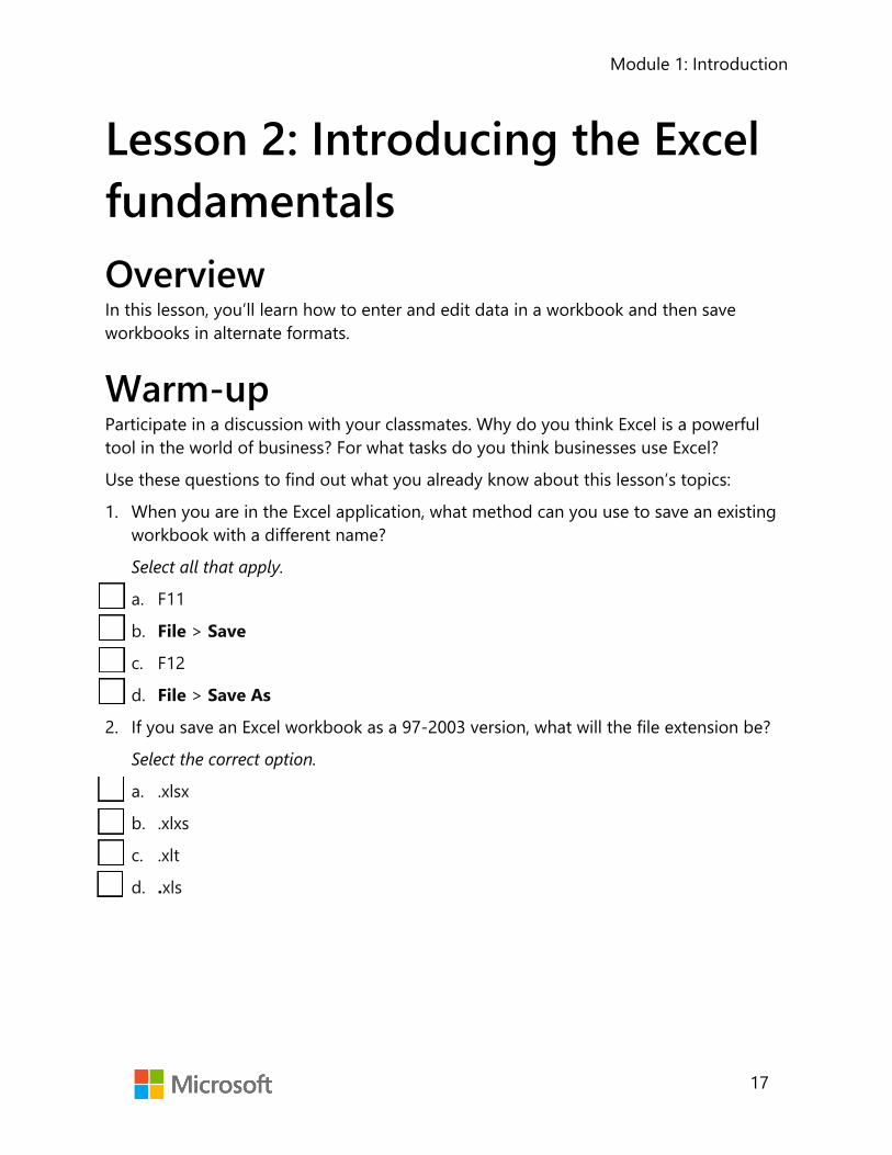
Module 1: Introduction
17
Lesson 2: Introducing the Excel fundamentals Overview In this lesson, you’ll learn how to enter and edit data in a workbook and then save workbooks in alternate formats.
Warm-up Participate in a discussion with your classmates. Why do you think Excel is a powerful tool in the world of business? For what tasks do you think businesses use Excel?
Use these questions to find out what you already know about this lesson’s topics:
1. When you are in the Excel application, what method can you use to save an existing workbook with a different name?
Select all that apply.
a. F11
b. File > Save
c. F12
d. File > Save As
2. If you save an Excel workbook as a 97-2003 version, what will the file extension be?
Select the correct option.
a. .xlsx
b. .xlxs
c. .xlt
d. .xls

Module 1: Introduction
18
3. By default, when you select Enter to complete a cell entry, where will the active cell be?
Select the correct option.
a. In the row below
b. In the row above
c. In the next cell to the left
d. In the next cell to the right
4. When you enter data into a cell, where else on-screen will what you have entered display?
Select the correct option.
a. The cell below
b. The cell above
c. The ribbon
d. The formula bar
Topic 1: Enter and edit data To enter data into an open worksheet, you can simply select a cell, enter text or
numbers, and select enter on the keyboard to complete the entry. You’ll probably want to alter the width of the columns and height of the rows at some point. That functionality will be covered in the next module.
Enter data 1. Open the existing workbook or create a new one.
2. Select the cell in which you’d like to enter data and begin entering text or numbers.
Complete a data entry 1. Select Enter, which will move you to the row below.
2. Use the Tab key to move to the adjacent cell to the right of the current cell.
3. Use the Shift Tab keys to move to the adjacent cell to the left of the current cell.
4. Use any directional arrow key to move one cell in any direction.

Module 1: Introduction
19
5. Select the Enter button (tick) next to the formula bar to stay in the same cell (or select Ctrl+Enter).
6. Select any other cell. (This is not best practice, but it is a commonly used method.)
Edit cell contents • Select the cell that you wish to edit, make your alterations directly within the cell or
via the formula bar, and use any method to complete the edit. Or
• Double-click into the cell to edit in an exact position within the cell or formula bar, and use any method to complete the edit.
Or
• Select F2, make your alterations, and use any method to complete the entry.
Cancel a cell entry 1. Select Esc on your keyboard before completing the entry, or
2. Select the Cancel button (X) next to the formula bar before completing the entry.
Clear cell contents • Access the context menu or right-click on a cell to clear, and select Clear Contents. Or
• Select Delete on your keyboard. Note: If you select Delete from the context menu, Excel will want to shift data into the deleted cell(s)!
You can use the Undo or Redo commands or (Ctrl+Z or Ctrl+Y) to undo or redo any actions.
Did you know?
You can undo/redo up to 100 actions, even after a file has been saved. Although undoing 100 actions could lose a lot of work, and maybe just making an edit would be better!

Module 1: Introduction
20
Additional information
For more information on the Undo or Redo command, go to: Undo, redo, or repeat an action
Activity: Pose a challenge The teacher will open Excel, create a new workbook, and enter some data. You’ll be asked to suggest ways to complete the data entry.
Resources required You’ll need the following resources for this activity:
• New blank workbook
Activity instructions Follow the teacher’s demonstration. Be prepared to ask and answer questions.
1. Open a new blank workbook.
2. Follow the teacher’s instructions.
3. Participate in the activity as directed.
4. Offer suggestions on how to complete the task when asked by the teacher.
Try-it: Enter and edit data Now that you can access the tools and options of Excel, it’s time to put all of that
knowledge to work. In this try-it, you’ll enter and edit data in an existing workbook. Entering that data gets into an Excel workbook is an essential skill. You want the interns at Munson’s Pickles and Preserves Farm to be Excel “power users” and to understand that there are many ways to accomplish this task.
Try-it 1 Entering data into a workbook.
Resources You’ll need the following resources for this activity:
• Open L2_T1_try1_visitors_starter.xlsx in this lesson’s Learning Activity Resources.

Module 1: Introduction
21
Instructions The following are the general tasks that you must perform during this try-it:
1. Open L2_T1_try1_visitor_starters.xlsx.
2. Enter 161 into cell B3.
3. Enter 248 into the cell below (C3).
4. Note the new values in cells H3 and H4. (The teacher will decide how you should note the values because that depends on the resources available.)
5. Save the workbook as the same name plus your initials. For example, L2_T1_try1_visitor_starters_DM.xlsx.
Try-it 2 Edit data and clear the contents of cells.
Resources You’ll need the following resources for this activity:
• Open L2_T1_try2_visitors_starter.xlsx in this lesson’s Learning Activity Resources.
Instructions 1. Open L2_T1_try2_visitors_starter.xlsx.
2. Use a keyboard shortcut to edit the contents of cell A6 to contain Group/Family instead of Group.
3. Clear the contents of cell B20.
4. Save the workbook as the same name plus your initials. For example, L2_T1_try2_visitor_starters_DM.xlsx.
Topic 2: Save workbooks If you make changes to a new workbook or an existing workbook, and you want to
keep the changes, you’ll need to save the workbook. Before saving, consider whether you would like the workbook saved in an online location, which is useful for collaboration purposes, or whether you would like it saved locally.
Saving a file follows a similar process as opening a file. Depending upon where you wish to store the workbook or what format you want to use, the process will differ slightly.

Module 1: Introduction
22
Save a new workbook 1. Go to File and select Save.
2. Check the location/folder to store the workbook in.
3. Enter an appropriate name, and select Save.
Or
1. Select Ctrl+S.
2. Give the workbook an appropriate name.
3. Check the location to store it in, and select Save. (If you select More Save Options, you will go to Backstage, Save As and can continue from there).
Save an existing workbook • From File, select Save, or Ctrl+S. Or
• Select the Save command on the Quick Access Toolbar.
Save an existing workbook as another name or to a new location 1. From File, select Save As, or select F12.
2. Check the location/folder to save the workbook in.
3. If you are changing the name, enter the new name and select Save.
Did you know?
A workbook can have up to 218 characters in the filename. But note that the file path (the names of folders in which it is stored) is part of the name and is included in the 218 characters.

Module 1: Introduction
23
Save a workbook in a different format 1. Start by going to File and select Save As, or F12.
2. Check the location/folder to save the workbook in.
3. Enter a suitable name for the workbook, and select the drop-down in the Save as type box.
4. Select the type of file you would like to save the workbook as, for example, PDF, Template, or Excel 97-2003 workbook.
5. When you use Save As to save a file, depending upon what you wish to do, you can either:
o Enter a name in the filename box, and select Save (this will be in the last location you were using). Or
o Select This PC, then select the folder on the recent list or select the Navigate up one level arrow to move up a level within the file structure, locate the folder to store in, then give the workbook a new name if necessary, and select Save.
Or
o Select Browse to go to the Save As dialog box (F12 will go there directly). Locate the folder to save in, double-click to open it or to select the folder, and then select Enter, give the workbook a new name if necessary, and select Save. Or
o Select the OneDrive/SharePoint/Online location and continue to locate the folder to store in, give the workbook a new name if necessary, and select Save.
Save a workbook as a PDF 1. From File, select Export, and then Create PDF/XPS.
2. Check the location to store it in and edit the filename if necessary.
3. Select Publish to have the active worksheets exported to PDF.
Or
• Select Options to alter the page range and what to publish, for example, to ignore any print areas or remove document properties, select OK, and then select Publish.
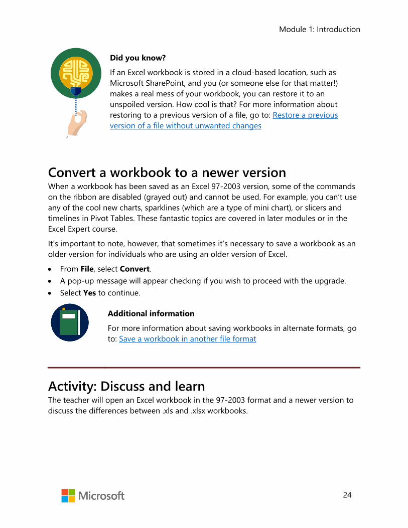
Module 1: Introduction
24
Did you know?
If an Excel workbook is stored in a cloud-based location, such as Microsoft SharePoint, and you (or someone else for that matter!) makes a real mess of your workbook, you can restore it to an unspoiled version. How cool is that? For more information about restoring to a previous version of a file, go to: Restore a previous version of a file without unwanted changes
Convert a workbook to a newer version When a workbook has been saved as an Excel 97-2003 version, some of the commands on the ribbon are disabled (grayed out) and cannot be used. For example, you can’t use any of the cool new charts, sparklines (which are a type of mini chart), or slicers and timelines in Pivot Tables. These fantastic topics are covered in later modules or in the Excel Expert course.
It’s important to note, however, that sometimes it’s necessary to save a workbook as an older version for individuals who are using an older version of Excel.
• From File, select Convert. • A pop-up message will appear checking if you wish to proceed with the upgrade. • Select Yes to continue.
Additional information
For more information about saving workbooks in alternate formats, go to: Save a workbook in another file format
Activity: Discuss and learn The teacher will open an Excel workbook in the 97-2003 format and a newer version to discuss the differences between .xls and .xlsx workbooks.

Module 1: Introduction
25
Resources required You’ll need the following resources for this activity:
• Open L2_T2_act_membership_summary.xlsx in this lesson’s Learning Activity Resources.
• Open L2_T2_act_membership_summary.xls in this lesson’s Learning Activity Resources.
Activity instructions Follow the teacher’s demonstration. Be prepared to ask and answer questions.
1. Open L2_T2_act_membership_summary.xls and L2_T2_act_membership_summary.xlsx.
2. Compare both versions and observe any differences.
3. Answer/ask questions.
4. Close both workbooks.
Try-it: Save workbooks In this try-it, you’ll save a workbook in various formats. Try-It 1 will cover saving a
workbook with a different name. At Munson’s Pickles and Preserves Farm, the preferred naming style is to use underscores instead of spaces or dashes within the filename. Try-It 2 will cover converting older files into a newer version, and Try-It 3 will cover exporting a file to PDF, which is Munson’s preferred file type for sending workbooks as an email.
Try-it: 1 Save an existing workbook with a different name.
Resources You’ll need the following resources for this activity:
• Open L2_T2_try1_Jan_June_starter.xlsx in this lesson’s Learning Activity Resources.
Instructions The following are the general tasks that you need to perform during this try-it:
1. Open L2_T2_try1_Jan_June_starter.xlsx.
2. Save as Jan_June_Summary_plus your initials.xlsx in the lesson’s Learning Activity Resources folder.

Module 1: Introduction
26
Try-it: 2 Convert an older version workbook into a new version file.
Resources You’ll need the following resources for this activity:
• Open L2_T2_try2_sales_starter.xls in this lesson’s Learning Activity Resources.
Instructions The following are the general tasks that you need to perform during this try-it:
1. Open L2_T2_try2_sales_starter.xls.
2. Convert to a newer version of Excel.
3. Then save the file using the same name plus your initials.
Try-it: 3 Export an existing workbook to PDF so that it cannot be easily edited. When worksheets are emailed outside of Munson’s, it is preferred that they are sent as a PDF.
Resources You’ll need the following resources for this activity:
• Open L2_T2_try3_Jan-June_starter.xlsx in this lesson’s Learning Activity Resources.
Instructions The following are the general tasks that you need to perform during this try-it:
1. Open L2_T2_try3_Jan-June_starter.xlsx in this lesson’s Learning Activity Resources.
2. Export to PDF with the name Jan_June_Summary plus your initials.
3. Ensure that any print areas are ignored and that all document properties are not included before publishing to PDF.
Additional information
For more information about saving workbooks in alternate formats, go to: Save a workbook as a template

Module 1: Introduction
27
Wrap-up Now that you have learned how to enter data and save workbooks in alternate formats, ask your neighbor if they can think of any way that they might be able to use Excel at home or at school. Use these questions to check your understanding of what you learned in this lesson:
1. Select the _______________ next to the formula bar to complete a data entry into a celland remain in the same cell.
Fill in the blank space.
2. Which format can a workbook be saved in?
Select all that apply.
a. .xlsx
b. .xlxs
c. .xls
d. .xlsm
3. Which statement is true?
Select all that apply.
a. There is no difference between using Convert or using Save As to upgrade aworkbook to the latest version of Excel.
b. Converting a file replaces the old-version file with a new-version file, leaving onecopy.
c. When a file is converted, you’ll be able to use the full functionality of Excel.
d. A file saved in an older version of Excel cannot be opened in Excel 2019.
4. The _______________ key moves one cell position to the right of the currently selectedcell.
Fill in the blank space.

Module 1: Introduction
28
Lesson 3: Navigating and filling cells Overview In this lesson, you’ll learn how to navigate to named cells, ranges, and other workbook objects, and how to search for data and use AutoFill to fill cell contents automatically. Sometimes, you inherit a workbook containing special formatting, formulas, named ranges, cells, or tables, all of which might not be obvious. Being able to familiarize yourself with everything that a workbook contains will help save time in future and help you understand the data better.
Warm-up Continue the discussion that you had with your classmates during the last lesson: What career do you think you might choose in your future? How do you imagine Excel might be used in your work?
Now use these questions to find out what you already know about this lesson’s topics:
1. The box directly under the ribbon, on the left side of the screen, is known as the _______________ box.
Fill in the blank space.
2. What is the keyboard shortcut key to go to elements of a workbook?
Select all that apply.
a. Ctrl+E
b. Ctrl+F
c. Ctrl+G
d. F5

Module 1: Introduction
29
3. If cell A1 contained the number 1 and you used AutoFill to fill the cells automatically down to A20, what number would be in cell A20?
Select the correct option.
a. 20
b. 10
c. 2
d. 1
4. If cell A1 contained January and you used AutoFill to fill the cells automatically across to L1, the contents of L1 would be _______________.
Fill in the blank space.
5. The Find command is located on the Find & _______________ button on the Home tab.
Fill in the blank space.
6. What is the keyboard shortcut key to search for data in a workbook?
Select the correct option.
a. Ctrl+E
b. Ctrl+F
c. Ctrl+G
d. F5
Topic 1: Navigate to named cells, ranges, or workbook elements
Did you know that a workbook can contain hidden information? Not everything on display is obvious.
Every cell in Excel has a unique reference, that is, A1, B1, C1, and others. However, you can apply a name of your own choice to cells, ranges of data, and tables. All this will be covered in more detail later in the course. In this lesson, you’ll learn how to quickly go to named cells, ranges, or tables by using the Name Box and the Go To command. The Go To command can also highlight workbook elements, such as formulas and conditional formatting. Again, this will be covered in more detail later in the course.

Module 1: Introduction
30
Navigate to a named cell, range, or table Enter any cell reference into the Name Box and select Enter, and you’ll navigate there. However, if a workbook contains a named item, you can use the Name Box to jump there also.
1. Select the drop-down button on the Name Box. (The Name Box is directly beneath the ribbon, on the left side of the screen.)
2. Select the name of the item you wish to jump to from the list.
Or
1. From the Find & Select command on the Home tab, select Go To (Ctrl+G or F5) to open the Go To dialog box.
2. Select the item you wish to jump to and select OK.
Display workbook elements • Select Find & Select on the Home tab, and then select Go To Special.
Or
1. Select Ctrl+G or F5 and select Special.
2. Select the item to display, and select OK.
Figure 4. Go To Special dialog box

Module 1: Introduction
31
Additional information
To review the article on navigating to named ranges, go to: Find named ranges
To review the article on finding cells that meet specific conditions, go to: Find and select cells that meet specific conditions
Did you know?
You can use the Name Box to jump to any cell within a workbook. Enter your initials, your age, and your shoe size into the box and select Enter, that is, DML168 and that’s where you’ll jump! What about the initials of your favorite pop music group and the year you first discovered their music? Or your favorite film and the year it was produced?
Activity: Tell a story The teacher will open L3_T1_act_summary.xlsx and ask how to find named cells or cells that have special formatting applied, such as conditional formatting, or any cells that contain formulas. Don’t worry about what conditional formatting is, because that will be covered in more detail later in the course. If you take the expert course, you’ll learn more there.
Additional information
If you decide that you can’t wait to find out more about conditional formatting, check out this link: Use conditional formatting to highlight information
If you would like to discover more about named ranges, go to: Create a named range from selected cells in a worksheet
Formulas are coming soon in this course, but if you want to check out formulas in advance, go to: Overview of formulas in Excel
Module 1: Introduction
32
Resources required You’ll need the following resources for this activity:
• Open L3_T1_act_summary.xlsx in this lesson’s Learning Activity Resources.
Activity instructions The following are the steps that you need to perform during this activity:
1. Open L3_T1_act_summary.xlsx and follow along with the teacher.
2. Offer suggestions on how to find any conditional formatting contained within the worksheet.
Try-it: Navigate to named cells, ranges, or workbook elements
You have inherited a workbook containing named ranges and want to familiarize yourself with the workbook components. Try-It 1 will cover navigating to a named cell. Try-It 2 will navigate to a table, and Try-It 3 will highlight cells on screen that contain formulas.
Try-it 1 Locate a named cell.
Resources You’ll need the following resources for this activity:
• Open L3_T1_try1_summary_starter.xlsx in this lesson’s Learning Activity Resources.
Instructions The following are the general tasks that you must perform during this try-it:
1. Open L3_T1_try1_summary_starter.xlsx.
2. Locate the cell named Total_New_Members.
3. Compare the value with your elbow partner(s). It can be tricky to find the selected cell, so make sure that everyone is finding the selected cell.

Module 1: Introduction
33
Try-it 2 Locate a named table.
Resources You’ll need the following resources for this activity:
• Open L3_T1_try2_summary_starter.xlsx in this lesson’s Learning Activity Resources.
Instructions The following are the general tasks that you need to perform during this try-it:
1. Open L3_T1_try2_summary_starter.xlsx.
2. Locate the table named Jan_June.
3. Do you recognize what just occurred? If not, ask your elbow partner(s) to check if they know.
Try-it 3 Highlight cells containing a formula.
Resources You’ll need the following resources for this activity:
• Open L3_T1_try3_summary_starter.xlsx in this lesson’s Learning Activity Resources.
Instructions The following are the general tasks that you must perform during this try-it:
1. Open L3_T1_try3_summary_starter.xlsx.
2. Go to the Membership Summary sheet.
3. Use a shortcut key or command to highlight any cells containing a formula.
4. Make a list of any column or row containing formulas.
5. Check with your elbow partner(s) to check if you have noted the correct columns and rows.
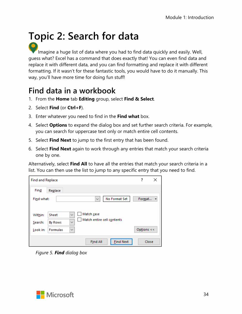
Module 1: Introduction
34
Topic 2: Search for data Imagine a huge list of data where you had to find data quickly and easily. Well,
guess what? Excel has a command that does exactly that! You can even find data and replace it with different data, and you can find formatting and replace it with different formatting. If it wasn’t for these fantastic tools, you would have to do it manually. This way, you’ll have more time for doing fun stuff!
Find data in a workbook 1. From the Home tab Editing group, select Find & Select.
2. Select Find (or Ctrl+F).
3. Enter whatever you need to find in the Find what box.
4. Select Options to expand the dialog box and set further search criteria. For example, you can search for uppercase text only or match entire cell contents.
5. Select Find Next to jump to the first entry that has been found.
6. Select Find Next again to work through any entries that match your search criteria one by one.
Alternatively, select Find All to have all the entries that match your search criteria in a list. You can then use the list to jump to any specific entry that you need to find.
Figure 5. Find dialog box

Module 1: Introduction
35
If you have expanded the dialog box to set more options:
1. Select the drop-down arrow next to Within to search the current sheet or the entire workbook.
2. Select the drop-down arrow next to Search to search by row or column.
3. From the drop-down next to Look in, you can look in formulas, values, notes, or comments.
4. Check Match case to find items that match the case you have entered in the Find what box.
5. Check Match entire cell contents to ignore cells that have partial match (for example, if you searched for apple, it would ignore apples.
6. Select Format to search for specific types of formatting. This will open the Format Cells dialog box. Set the formatting to search for in the dialog box and select OK.
Replace data in a workbook 1. From the Home tab Editing group, select Find & Select.
2. Select Replace (or Ctrl+H).
3. Or select Find and switch to the Replace tab.
4. Enter whatever you need to find in the Find what box.
5. Enter whatever you need to replace it with in the Replace with box.
6. Select Options to expand the dialog box and add further criteria as described previously.
7. Select Replace and repeat as necessary to replace all entries that match your criteria one by one, or select Replace All to replace all entries in one action.
If you have used the Find or Replace to for formatting, select the drop-down arrow against Format to clear the set formatting if necessary.
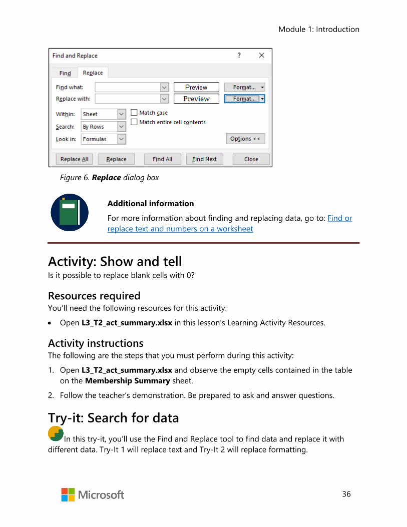
Module 1: Introduction
36
Figure 6. Replace dialog box
Additional information
For more information about finding and replacing data, go to: Find or replace text and numbers on a worksheet
Activity: Show and tell Is it possible to replace blank cells with 0?
Resources required You’ll need the following resources for this activity:
• Open L3_T2_act_summary.xlsx in this lesson’s Learning Activity Resources.
Activity instructions The following are the steps that you must perform during this activity:
1. Open L3_T2_act_summary.xlsx and observe the empty cells contained in the table on the Membership Summary sheet.
2. Follow the teacher’s demonstration. Be prepared to ask and answer questions.
Try-it: Search for data In this try-it, you’ll use the Find and Replace tool to find data and replace it with
different data. Try-It 1 will replace text and Try-It 2 will replace formatting.

Module 1: Introduction
37
Try-it 1 Find text within a workbook and replace with different text.
Resources You’ll need the following resources for this activity:
• Open L3_T2_try1_summary_starter.xlsx in this lesson’s Learning Activity Resources.
Instructions The following are the general tasks that you must perform during this try-it:
1. Open L3_T2_try1_summary_starter.xlsx.
2. Replace every entry of the word Junior with Child in the entire workbook.
3. Save the workbook as the same name plus your initials.
Try-it 2 Find specific formatting within a workbook and replace with different formatting.
Resources You’ll need the following resources for this activity:
• Open L3_T2_try2_summary_starter.xlsx in this lesson’s Learning Activity Resources.
Instructions The following are the general tasks that you need to perform during this try-it:
1. Open L3_T2_try2_summary_starter.xlsx.
2. Replace every cell with Arial font to Cambria, size 11 in the entire workbook.
3. Save the workbook as the same name plus your initials.

Module 1: Introduction
38
Topic 3: Use the AutoFill feature AutoFill allows you to copy entries from the active cell to adjacent cells sequentially
or by repeating the entry. For example, you might wish to enter the months of the year in your worksheet. You can enter any month and then use AutoFill to complete the rest.
AutoFill using a pointer device 1. Select the cell(s) to be sequentially copied.
2. Position the pointer at the bottom right corner of the cell(s). The pointer will change to a small black cross.
3. Select and drag over the cells required.
4. Release the pointer to complete the action.
5. An AutoFill Options button is displayed in the corner of the filled data.
6. Select a tag to change the fill to another option; for example, you might wish to copy the data rather than fill a data series.
Figure 7. AutoFill Options
Did you know?
Years ago, there were no fill options when you filled data in Excel. You had to select more than one cell to make a sequence, or you had to use the Ctrl key while filling. Why not experiment with dates or numbers?
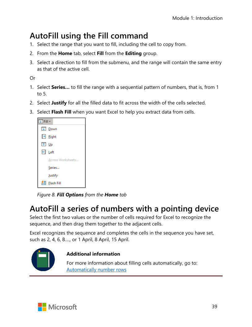
Module 1: Introduction
39
AutoFill using the Fill command 1. Select the range that you want to fill, including the cell to copy from.
2. From the Home tab, select Fill from the Editing group.
3. Select a direction to fill from the submenu, and the range will contain the same entry as that of the active cell.
Or
1. Select Series… to fill the range with a sequential pattern of numbers, that is, from 1 to 5.
2. Select Justify for all the filled data to fit across the width of the cells selected.
3. Select Flash Fill when you want Excel to help you extract data from cells.
Figure 8. Fill Options from the Home tab
AutoFill a series of numbers with a pointing device Select the first two values or the number of cells required for Excel to recognize the sequence, and then drag them together to the adjacent cells.
Excel recognizes the sequence and completes the cells in the sequence you have set, such as 2, 4, 6, 8…., or 1 April, 8 April, 15 April.
Additional information
For more information about filling cells automatically, go to: Automatically number rows

Module 1: Introduction
40
Activity: Guess and tell Teacher will demonstrate using AutoFill and then ask you to guess what will be filled automatically, using various data examples.
Resources required You’ll need the following resources for this activity:
• New blank workbook for experimenting with different AutoFill options.
Activity instructions The following are the steps that you must perform during this activity:
1. Open a new blank workbook or create a new sheet in any open workbook.
2. Suggest answers to the teacher’s questions.
Try-it: AutoFill This try-it will give you a chance to practice using AutoFill to automatically fill cells
so that you are equipped with different techiques that you can show to the other interns and use to enter sequential data into worksheets in the future.
Try-it: 1 Use AutoFill to enter months.
Resources You’ll need the following resources for this activity:
• Open a new workbook.
Instructions The following are the general tasks that you must perform during this try-it:
1. Open a new blank workbook.
2. Enter Jan in cell A1 and Mon in B2.
3. Fill both cells down to row 20.
4. If the contents of A20 is not Aug and the contents of B20 is not Sat, try it again.
5. Save the file as Fill_Months_Days plus your initials in the Learning Resource folder.

Module 1: Introduction
41
Try-it: 2 Use AutoFill to enter sequential numbers.
Resources You’ll need the following resources for this activity:
• Open a new blank workbook.
Instructions The following are the general tasks that you need to perform during this try-it:
1. Open a new blank workbook.
2. Enter 5 into A1 and 10 into A2.
3. Fill the cells down to A20 so that they automatically are incremented by 5.
4. Enter 7 into B1 and 14 into B2.
5. Fill the cells down to B20 so that they automatically are incremented by 7.
6. The contents of A20 should be 100 and the contents of B20 should be 140. If not, try again.
7. Save the file as Fill_Numbers plus your initials in the Learning Resource folder.
Try-it: 3 Use AutoFill to enter sequential dates.
Resources You’ll need the following resources for this activity:
• Open a blank workbook.
Instructions The following are the general tasks that you must perform during this try-it:
1. Open a new blank workbook.
2. Enter the current date in cell A1.
3. Enter the date in 7 days’ time in B1.
4. Fill the dates across to J1 so that they automatically are incremented by 7 days.
5. Enter the current date into cell A2.
6. Enter the date in thirty days’ time in B2.

Module 1: Introduction
42
7. Fill across to J2 so that each cell increments by one month.
8. Save the file as Fill_Dates plus your initials in the Learning Resource folder.
Additional information You can create your own custom list that you can use with AutoFill. For further information, go to: Create or delete a custom list for sorting and filling data
Flash Fill is an option within AutoFill options that has not been covered in this module. For further information on Flash Fill, go to Using Flash Fill in Excel
Wrap-up Turn to a neighbor and share the favorite thing that you learned about AutoFill or anything else covered in the module. Be prepared to share with the class. Then use these questions to check what you learned in this lesson:
1. When a cell or range has a defined name, what is that known as?
Select all that apply.
a. Range
b. Named range
c. Named cell
d. Defined cell
2. Which of the following shortcuts can you use to highlight cells containing formulas?
Select all that apply.
a. F5
b. F6
c. F4
d. Ctrl+G
3. If you used AutoFill to fill Quarter 1 into cell A1 down to A5, what would the contents of A5 contain?
Select the correct option.
a. Quarter 5
b. Quarter 3
c. Quarter 4
d. Quarter 1

Module 1: Introduction
43
4. If you used AutoFill to fill Jan from cell A1 across to L1, which of the following AutoFill options will be available to select?
Select all that apply.
a. Copy cells
b. Fill formatting only
c. Fill without formatting
d. Fill months
5. You can use the Replace feature to find specific formatting and replace with different formatting. True or false?
a. True
b. False
6. Which is the correct shortcut to access the Replace feature?
Select the correct option.
a. Ctrl+G
b. Ctrl+H
c. Ctrl+R
d. Ctrl+I
Note: If you have any concerns about any topics covered in this module, ask your teacher for assistance.

Module 1: Introduction
44
Glossary Backstage Accessed via File tab. Here you can save, save as, print, open, check
file info, export to PDF, and other tasks.
Template A master file that can be used to create new files.
AutoFill A tool that allows you to automatically fill cell contents based on the starting content.
Named Range A cell or range with a defined name applied. This topic will be covered in detail in a later module.
Go To A tool that helps you navigate to specific cells, ranges, elements, or cells with special attributes such as formulas and conditional formatting.
Conditional Formatting
Special formatting applied to cells to display various criteria. This topic will be covered in detail in a later module.

Module 1: Introduction
45
Cornerstone Overview In this Cornerstone, you’ll edit two workbooks, which will include finding data, filling cells automatically with AutoFill, navigating to workbook elements and saving in alternate formats. Using these tools will not only save you time in the future but also help prepare you for the next module in this course.
Objectives Cornerstone objectives MOS Exam objective(s)
Use AutoFill to automatically fill data into cells
• 2.1.2: Fill cells by using Auto Fill
Save workbooks in alternate formats • 1.5.2: Save workbooks in alternative file formats
Search for data • 1.2.1 Search for data within a workbook
Navigate to named cells, ranges, or workbook elements
• 1.2.2 Navigate to named cells, ranges, or workbook elements
Table 2: Cornerstone objectives
Duration 50 minutes
Instructions 1. Complete the tasks for each file.
2. When saving your file, add your name to the end of the filename, for example: Cornerstone_Mod1_Dwayne_Espino. Follow your teacher’s directions for where to save your files.
3. Refer to the thumbnail image provided to observe how your project should generally appear.

Module 1: Introduction
46
4. When you’re done with the Cornerstone, assess your completion and enter the points you think you earned within the task lists below. You can request help from your teacher if required.
Tasks You will work with two files in this Cornerstone. The following are the tasks you must perform within each file.
File 1: Cornerstone_Starter.xlsx
Task: AutoFill (2 points) 1. Enter Qtr1 in cell B1 on the Produce sheet. (1 point)
2. Use AutoFill to fill all four quarters of the year to cell E1. (1 point) (Exam objective 2.1.2)
Points scored: _______ /2
Task: Edit cell contents (1 point) • Edit the contents of cell E7 to the value of 6694 (1 point)
Points scored: _______ /1
Task: Locate named cell (2 points) 1. Locate the named cell Total. (1 point) (Exam objective 1.2.2)
2. Enter the contents of the named cell into cell A2 of the Summary sheet. (1 point)
Points scored: _______ /2
Task: Find and Replace (2 points) • Find every cell with an Arial font and replace with the Cambria font in the entire
workbook. (2 points) (Exam objective 1.2.1)
Points scored: _______ /2
Task: Save as PDF (2 points) • Export the entire workbook as a PDF with the name Cornerstone_Mod1_Plus your
name in this lesson’s Learning Activity Resources folder. (2 points) (Exam objective 1.2.1)
Points scored: _______ /2
FILE 1 TOTAL POINTS: _______ /9

Module 1: Introduction
47
File 2: Cornerstone2_starter.xls
Task: Find and replace (2 points) • Replace every entry of corn with sweetcorn in the entire workbook. (2 points) (Exam
objective 1.2.1)
Points scored: _______ /2
Task: Navigate (4 points) 1. Navigate to the range named W_S_Total.(1 point) (Exam objective 1.2.2)
2. Enter the number it contains into cell J1 on the All Year sheet. (1 point)
3. Navigate to the range named S_A_Total.(1 point) (Exam objective 1.2.2)
4. Enter the number it contains into cell J2 on the All Year sheet. (1 point)
Points scored: _______ /4
Task: Edit cell contents (1 point) • Edit the text in cell E80 on the Winter-Spring sheet to Winter-Spring Total. (1
point)
Points scored: _______ /1
Task: Convert file (2 point) • Convert the file to the newest version of Excel and then save the file as
Cornerstone2_Mod1_plus your name. (2 points) (Exam objective 1.2.1)
Points scored: _______ /2
FILE 2 TOTAL POINTS: _______ /9

Module 1: Introduction
48
Thumbnail image Your finished project should appear similar to this image.
Solution 1:
The Summary sheet contains 159,863 centered in cell A2.
The Produce sheet contains the text Qtr1 in cell B1, Qtr2 in cell C2, Qtr3 in cell D2, and Qtr4 in cell E2.
Solution 2:
(This workbook contains a lot of data that will not reproduce well as a screen shot.)

Student Guide 40567A Microsoft Excel associate 2019 Module 2: Managing worksheets and workbooks

Module 2: Managing worksheets and workbooks
2
Contents
Contents .............................................................. 2
Module overview ............................................. 4
Description ..................................................... 4
Scenario .......................................................... 5
Cornerstone ................................................... 5
Lesson 1: Structuring a worksheet ............ 6
Overview ......................................................... 6
Warm-up ........................................................ 6
Topic 1: Set up columns, rows, and cells ................................................................... 7
Insert a row into a worksheet ............ 7
Delete a row ............................................. 7
Insert a column ........................................ 8
Delete a column ...................................... 8
Delete multiple columns or rows ..... 9
Adjust a row height or column width ............................................................ 9
Insert a cell ............................................. 10
Delete a cell ........................................... 10
Activity: Student teach back ............ 10
Try-it: Columns, rows, and cells ..... 11
Topic 2: Set up worksheets .................. 12
Insert an extra worksheet ................. 12
Delete a worksheet ............................. 13
Rename a worksheet .......................... 13
Move a worksheet within the same workbook ................................................ 14
Copy a worksheet within the same workbook ................................................ 14
Move a worksheet to a different workbook ................................................ 15
Copy a worksheet to a different workbook ................................................ 16
Activity: Discuss and learn ................ 16
Try-it: Worksheets ................................ 17
Try-it 1 ...................................................... 17
Try-it 2 ...................................................... 17
Wrap-up ....................................................... 18
Lesson 2: Editing a worksheet .................. 20
Overview ...................................................... 20
Warm-up ...................................................... 20
Topic 1: Cut, copy, paste, and move data ................................................................ 21
Cut data ................................................... 21
Copy data ................................................ 22
Further ways to copy data ................ 23
Paste copied or cut data ................... 23
Move data ............................................... 24
Activity: Group/team .......................... 24
Try-it: Cut, copy, paste, and move 25
Try-it 1 ...................................................... 25
Try-it 2 ...................................................... 26
Topic 2: Use Paste Special ..................... 27
Paste Special .......................................... 27
Activity: Pose a question ................... 28
Try-it: Paste Special ............................. 29
Try-it: 1 ..................................................... 29

Module 2: Managing worksheets and workbooks
3
Try-it: 2 ..................................................... 30
Try-it: 3 ..................................................... 30
Wrap-up ....................................................... 31
Lesson 3: Customizing views and toolbars ............................................................. 32
Overview ...................................................... 32
Warm-up ..................................................... 32
Topic 1: Freeze panes and workbook views .............................................................. 33
Change the screen zoom ................. 33
Change screen display....................... 34
Freeze worksheet titles ...................... 34
Unfreeze worksheet titles ................. 35
Move between workbook windows .................................................................... 35
View all the workbooks you want to interact with ........................................... 35
View two workbooks side by side ............................................................ 36
Split your screen into panes............ 36
Clear worksheet panes ...................... 37
Navigation keyboard shortcuts ..... 37
Activity: Research ................................. 38
Try-it: Freeze panes and workbook views ......................................................... 39
Topic 2: Use the Quick Access Toolbar ......................................................................... 39
Use the ribbon to customize the Quick Access Toolbar ......................... 40
Customize using the Quick Access Toolbar ..................................................... 40
Activity: Show and tell ........................ 42
Try-it: Quick Access Toolbar ............ 42
Try-it: 1 ..................................................... 42
Try-it: 2 ..................................................... 43
Try-it: 3 ..................................................... 44
Wrap-up ....................................................... 45
Glossary ............................................................. 46
Cornerstone ..................................................... 47
Overview ...................................................... 47
Objectives .................................................... 47
Duration ................................................... 47
Instructions .................................................. 48
File 1: Cornerstone_beehive_data _starter.xlsx ............................................. 48
File 2: Cornerstone_honeybee_colonies _starter.csv .............................................. 49

Module 2: Managing worksheets and workbooks
4
Module overview Description Now that you’ve been introduced to Microsoft Excel in Module 1, this module will expand your knowledge in many areas of the app, which will help you as you progress though the course. In this module you’ll learn how to manage worksheets, columns, and rows. No matter what type of data you’re working in Excel, you need to know how to manage worksheet columns, rows, and cells so that data is more easily understood. You’ll also learn how to cut, copy, paste, and move data, including how to use Paste Special. Finally, you’ll learn how to customize your screen appearance and how to customize the Quick Access Toolbar.
Each lesson will include activities and try-its that will help you understand why, when, where, and how you might use these skills. At the end of the module you’ll complete a cornerstone. Most of the objectives listed in the following table will be included in the cornerstone, with the addition of a few objectives covered in Module 1. It’s always good to be reminded of what you already know. That way you’re less likely to forget these fantastic skills in future!
Lesson Learning objective Exam objective(s)
Structure a worksheet
• Adjust columns and rows in a worksheet • Insert, delete, rename, move, or copy
worksheets
• 2.1.3 • 2.1.4 • 1.3.2
Edit a worksheet
• Cut, copy, paste, and move data • Paste data by using special paste options
• 2.1.1
Customize views and toolbars
• Freeze worksheet panes, and change worksheet and window views
• Customize the Quick Access Toolbar
• 1.4.2 • 1.4.3 • 1.4.4 • 1.4.1
Cornerstone Inherited beekeeping workbook
• Insert columns and rows • Insert and delete cells • Adjust columns and rows • Cut, copy, paste and move data • Customize views • Save in alternate formats
• 2.1.3 • 2.1.4 • 1.3.2 • 2.1.1 • 1.4.3 • 1.5.2
Table 1: Objectives by lesson
Module 2: Managing worksheets and workbooks
5
Scenario Munson’s Pickles and Preserves Farm has several honeybee apiaries that they lend to area farms for crop pollination. They have been tracking the movement of the hives in workbooks.
You’ve inherited beekeeping workbooks from a colleague that track the locations, dates, and other associated information about the hives. They are a mess! The workbook, its worksheets, their columns, rows, and cells are inconsistent in size and format. It’s your job to tidy these up for easier viewing and structure consistency. In a brief perusal of the document you’ve noted that:
• Columns and rows need to be resized. • Information needs to be copied and moved from one area to another while keeping
the associated formatting. • Panes need to be frozen for easier viewing across many rows and columns. • Data needs to be repositioned.
Cornerstone You’ve inherited two workbooks tracking beehive data and they are in much need of restructuring; columns and rows are inconsistent, and headings are missing. You need to fix them! The heading row on each worksheet needs to be frozen at the top for easier viewing. This cornerstone will help build these key skills when you’re working in Excel.

Module 2: Managing worksheets and workbooks
6
Lesson 1: Structuring a worksheet Overview This lesson is about the various ways in which you can adjust worksheets, columns, rows, and cells. The topics in this lesson include inserting, deleting, and resizing columns and rows. It also includes inserting, deleting, copying, moving, and renaming worksheets. This lesson will also cover cutting, moving, copying, and pasting data, and customizing the Quick Access Toolbar and your application display.
The skills covered in this lesson are key to your future productivity in Excel. You might even be surprised by how many ways there are to use copy and paste!
Warm-up Ask your neighbor if they have any questions about the topics covered in Module 1. Help them if you can, then use these questions to find out what you already know about this lesson’s topics:
1. Which of these methods can you use to insert a new row in a worksheet?
Select all that apply.
a. Right-click or access the context menu for a row number, select Insert
b. Right-click or access the context menu for a column header, select Insert
c. Right-click or access the context menu for a cell, select Insert Entire Row
d. Home, Cells group, Insert > Insert Sheet Rows
2. Which of these methods can you use to set the width of a column in a worksheet?
Select the correct option.
a. Double-click between a column divider to make it autofit
b. Select the divider between 2 rows and drag up or down
c. Right-click or access the context menu for a column header and select Row Height
d. Select Format in the Cells group, and then select Row Height

Module 2: Managing worksheets and workbooks
7
3. When you select all the columns in your worksheet and double-click on a column divider, that is known as __________________________.
Fill in the blank space.
4. To delete a column in a worksheet, you can select the column header and use which of the following shortcut keys?
Select the correct option.
a. Ctrl+Plus sign (+)
b. Ctrl+Slash (/)
c. Ctrl+Hyphen (-)
d. Ctrl+Asterisk (*)
Topic 1: Set up columns, rows, and cells As the content of a worksheet develops and your knowledge of Excel expands, at
some time you’ll probably need to insert or delete columns, rows, and cells. You might also need to adjust the column width or row height. This will help with the readability of your data. As usual there are many ways to adjust a workbook. Here are some of the ways you can complete the following actions.
Insert a row into a worksheet To insert a row into a worksheet, you can either:
• Right-click or access the context menu on top of the row header and choose Insert. • Select the row header, and then select the Ctrl+ Plus sign (+) keys. • Select the row header. Then on the ribbon, on the Home tab, select the Insert Cells
button drop-down list, and then select Insert Sheet Rows
Note: The number of rows you select will determine the number of rows that will be inserted.
Delete a row To delete a row, you can either:
• Right-click the top of the row header or access its context menu, and then select Delete.
• Select the row header, and then select the Ctrl + Hyphen (-) keys.

Module 2: Managing worksheets and workbooks
8
• Select the row header. Then on the ribbon, on the Home tab, select the Delete Cells button, and then select Delete Sheet Rows.
• Right-click or access the context menu on a cell and choose Delete from the menu, then select Entire Row.
Note: the number of rows you select will determine the number of rows that will be deleted.
Insert a column To insert a column, you can either:
• Right-click on top of the column header or access its context menu, and then from the menu, select Insert.
• Select the column header, and then select Ctrl + Plus sign (+). • Select the column header. Then on the ribbon, on the Home tab, select the Insert
Cells button, and then select Insert Column Rows.
Note: the number of columns you select will determine the number of columns that will be inserted.
Delete a column To delete a column, you can either:
• Right-click on top of the column header or access its context menu, and then select Delete.
• Select the column header, and then select the Ctrl + Hyphen (-). • Select the column header. Then on the ribbon, on the Home tab, select the Delete
Cells button, and then select Delete Sheet Columns. • Right-click on a cell or access its context menu, select Delete, and then select Entire
Column.
Note: the number of columns you select will determine the number of columns that will be deleted.
Module 2: Managing worksheets and workbooks
9
Delete multiple columns or rows To delete multiple columns or rows, you can choose from either of the following two tasks:
1. Select the first column or row you would like to delete.
2. Hold the Ctrl key, and then the select any column or row you would like to delete. (This allows you to select nonconsecutive columns or rows.)
3. Use any of the previous deletion methods to delete them.
Or
1. Select the first column or row you want to delete.
2. Hold the Shift key, and the select the last column or row you would like to delete. (This allows you to delete a block of columns or rows.)
3. Use any of the previous deletion methods to delete them.
Note: you cannot delete columns and rows simultaneously. You can only delete multiple columns, or multiple rows at one time.
Adjust a row height or column width To adjust a row height or column width, you can either:
• Select the rows or columns to be adjusted. Then move your pointing device between any of the selected rows or columns. When you’re pointing device changes shape, select the divider and drag to the size you would like. As you drag your pointing device, the points (pixels) increase or decrease.
• Select the rows or columns to be adjusted. Then move your mouse between any of the selected rows or columns. When your mouse changes shape, double-click. The rows or columns will be the exact size they need to be to fit the data. This is known as AutoFit.
• Right-click or access the context menu on the selected rows or columns, and then select Row Height or Column Height. Set the exact size you would like and select OK.
• Select the rows or columns you would like to adjust, and then on the ribbon, on the Home tab, from the Format button, select the options you would like to use.
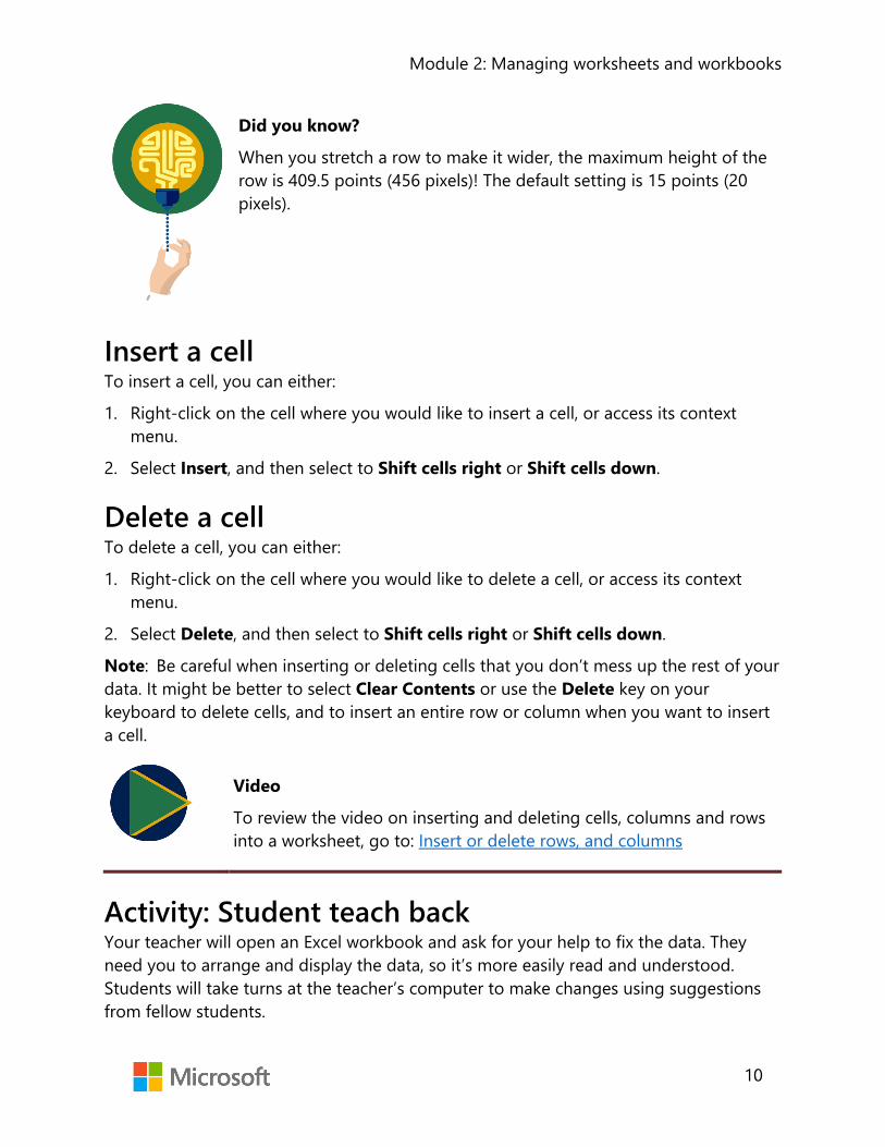
Module 2: Managing worksheets and workbooks
10
Did you know?
When you stretch a row to make it wider, the maximum height of the row is 409.5 points (456 pixels)! The default setting is 15 points (20 pixels).
Insert a cell To insert a cell, you can either:
1. Right-click on the cell where you would like to insert a cell, or access its context menu.
2. Select Insert, and then select to Shift cells right or Shift cells down.
Delete a cell To delete a cell, you can either:
1. Right-click on the cell where you would like to delete a cell, or access its context menu.
2. Select Delete, and then select to Shift cells right or Shift cells down.
Note: Be careful when inserting or deleting cells that you don’t mess up the rest of your data. It might be better to select Clear Contents or use the Delete key on your keyboard to delete cells, and to insert an entire row or column when you want to insert a cell.
Video
To review the video on inserting and deleting cells, columns and rows into a worksheet, go to: Insert or delete rows, and columns
Activity: Student teach back Your teacher will open an Excel workbook and ask for your help to fix the data. They need you to arrange and display the data, so it’s more easily read and understood. Students will take turns at the teacher’s computer to make changes using suggestions from fellow students.
Module 2: Managing worksheets and workbooks
11
Resources required You will need the following resource for this activity:
• Open L1_T1_act_volunteer_sheet.xlsx in this lesson’s Learning Activity Resources.
Activity instructions You need to perform the following task during this activity:
• Volunteer to take control at the teacher’s computer and/or offer suggestions to fellow students on how to improve the readability of the data shown.
Try-it: Columns, rows, and cells You’ll have 20 seconds to try to fix a problem with a workbook. When the time is
up, you’ll move to the next computer and continue from where your neighbor left it. When the full time is up, you’ll return to your own computer to review what has happened to your workbook.
Resources You will need the following resource for this activity:
• Open L1_T1_try_volunteers_starter.xlsx in this lesson’s Learning Activity Resources.
Activity instructions Participate in the activity by following these instructions:
1. Open L1_T1_try_volunteers_starter.xlsx.
2. Examine the worksheet: are the column and row widths okay? Is data out of line? Is there anything missing?
3. Within 20 seconds, make any alteration you feel is appropriate and improves the readability in the way the data is displayed.
4. When instructed, move to your neighbor’s computer, and make further alterations to their worksheet.
5. Continue moving along to other computers as instructed, and make any further alterations that you think might be needed to improve the readability of the data.
6. When the time is up, return to your own computer to review what has changed with your workbook. Are the column and row widths okay? Is data out of line? Is there anything missing?
7. Save the workbook with the original file name and your initials.

Module 2: Managing worksheets and workbooks
12
Topic 2: Set up worksheets Every new workbook has one worksheet by default, named Sheet1. As your
workbook develops you might need to add additional worksheets. If so, having worksheets named Sheet1, Sheet2, Sheet3, and so forth is not very helpful for future reference. For example, how can you know what data is on a worksheet named Sheet1?
There’s also every probability that you’ll need to move worksheets around or copy them. Imagine your confusion when Sheet1 is moved and is now located at the end of the workbook instead of in the first location.
For these reasons, you’ll want to keep your workbook organized. You’ll want to rename worksheets to something meaningful, so at a glance you’ll know what data is in them. If your workbook contains unnecessary worksheets, such as blank worksheets or duplicated worksheets, it’s a good idea to delete them. The following information will help you take control of worksheets in your workbooks.
Did you know?
You can start Excel with an accessible template to better support your users’ accessibility needs. For further information, refer to: Start with an accessible Excel template
Insert an extra worksheet To insert an extra worksheet, use one of the following three methods:
• Select the New Sheet button (the plus (+) next to the worksheet tabs at the bottom of the screen). This will insert a new worksheet to the right of the active worksheet.
• Right-click or access the context menu on any existing worksheet tab, and then select Insert. Select the type of worksheet to insert from the selections available, and then select Insert. This will insert a worksheet to the left side the active worksheet.
• On the ribbon, on the Home tab, select the Insert Cells button drop-down menu, and then select Insert Sheet.

Module 2: Managing worksheets and workbooks
13
Delete a worksheet To delete a worksheet, use one of the following two methods:
• Right-click the top of the worksheet tab or access its context menu, and then select Delete.
• On the ribbon, on the Home tab, select Delete Cells, and then select Delete Sheet.
Note: You can select more than one worksheet at a time by holding either the Shift key or Ctrl key. The Shift key will allow you to select a range of worksheets, while the Ctrl key will allow you to select nonconsecutive worksheets.
Another Note: Take extra care when deleting worksheets—you cannot undo this action! If you accidentally delete a worksheet, while you could close the workbook without saving it, you could lose lots of work in the process.
Rename a worksheet When you rename a worksheet, you need to consider some naming conventions. For more information on renaming worksheets, check out the Additional Information section. To rename a worksheet, use one of the following three methods:
• Double-click the current worksheet name, and when the existing name is selected, enter a new name. Then select anywhere off the tab to save the changes.
• Right-click the worksheet name or access its context menu, and then select Rename. Enter a new name, and then select anywhere off the tab to save the changes.
• On the ribbon, on the Home tab, select Format, and then select Rename Sheet. Enter a new name, and then select anywhere off the tab to save the changes.
Did you know?
You cannot use these characters * / \ ? : [ ] within a worksheet name because these characters are used for coding and unpredictable things might happen behind the scenes. (Don’t panic, you don’t need to know about coding in this module!) For the Excel veteran, in Excel 2019, you can add spaces in the worksheet name!

Module 2: Managing worksheets and workbooks
14
Move a worksheet within the same workbook To move a worksheet within the same workbook, you can use one of the following methods:
1. Right-click or access the context menu on top of the worksheet tab, and then select Move or Copy. In the Move or Copy dialog box, select which worksheet you would like to move the worksheet before or select move to end, and then select OK.
Or
2. Select Format from the Home tab and then select Move or Copy Sheet. In the Move or Copy dialog box, select which worksheet you would like to move the worksheet before or select move to end, and then select OK.
Figure 1: Move or Copy dialog box
3. Select on the worksheet tab to move, hold the mouse, drag the worksheet to the new position, and release the mouse.
Copy a worksheet within the same workbook To move a worksheet within the same workbook, you can use one of the following methods:
1. Select Format from the Home tab, and then select Move or Copy Sheet.
Or
2. Right-click the top of the worksheet tab name or access its context menu, and then select Move or Copy. In the Move or Copy dialog box, select the Create a copy check box. In the Before sheet list, select which worksheet you would like the new worksheet inserted before, or select move to end, and then select OK.
Or
3. Select the worksheet tab to copy, hold the mouse and Ctrl key, drag the worksheet to the new position, and release the mouse.

Module 2: Managing worksheets and workbooks
15
Move a worksheet to a different workbook If you need to move a worksheet to another workbook, you don’t need to use copy and paste. Excel has a command that will move the worksheet for you. For this to work though, you must have both workbooks open.
To move a worksheet to a different workbook:
1. For the worksheet you want to move, right-click the worksheet tab name or access its context menu. (Alternatively, you can select Format on the ribbon, on the Home tab.)
2. Select Move or Copy.
3. In the Move or Copy dialog box, select the To book drop-down icon, and then select the workbook to move the worksheet to. (If you are creating a new workbook with the worksheet, select new book).
Figure 2: Move or Copy dialog box, drop-down arrow
4. In the Before copy pane, select which worksheet you want to move the worksheet before or select move to end. Then select OK.
Figure 3: Move or Copy dialog box, Before sheet list

Module 2: Managing worksheets and workbooks
16
Copy a worksheet to a different workbook Imagine you’ve created a worksheet in a workbook that contains data that can be used in other workbooks. Rather than having to insert a new worksheet into the other workbook and then copying and pasting the original worksheet into the workbook, you can use the Copy worksheet command. However, just like moving a worksheet between workbooks, you must have both workbooks open for this to work.
To copy a worksheet to a different workbook:
1. Right-click on the name of the worksheet tab that you want to copy, or access its context menu. (Alternatively, you can select Format on the ribbon, on the Home tab.)
2. Select Move or Copy.
3. Select the Create a copy check box.
4. Select the To book drop-down arrow, and choose which workbook to copy it to. (If you are creating a new workbook with the worksheet, select new book).
5. In the Before copy pane, select which worksheet you want to insert the worksheet before, or select move to end. Then select OK.
Additional information
To review the article on renaming worksheets, go to: Rename a worksheet
To review the video on moving or copying a worksheet, go to: Move or copy worksheets or worksheet data
Activity: Discuss and learn Your teacher will open a discussion regarding naming conventions (giving worksheets a suitable name) when renaming worksheets.
Resources required You will need the following resource for this activity:
• Open L1_T2_act_produce.xlsx in this lesson’s Learning Activity Resources.

Module 2: Managing worksheets and workbooks
17
Activity instructions You will need to perform the following steps during this activity:
1. Open L1_T2_act_produce.xlsx.
2. Examine the data on the three worksheets, and consider suitable names for the worksheets. Is there anything obvious about the seasons or the months on each worksheet?
3. Engage in the discussion, by asking and answering questions.
Try-it: Worksheets In this leveled try-it activity, you’ll rename worksheets to better reflect what each
worksheet contains, you’ll copy a worksheet into a new workbook, and rename the worksheet.
Try-it 1 In this try-it, you’ll rename worksheets.
Resources You will need the following resource for this activity:
• Open L1_T2_try1_volunteer_hours_starter.xlsx in this lesson’s Learning Activity Resources.
Activity instructions Participate in the activity by following these instructions:
1. Open L1_T2_try1_volunteer_hours_starter.xlsx.
2. Examine the contents of each worksheet, and rename them to make it clear whether it’s for a 28, 30, or 31-day month. For example, you could use the name 30-day month.
3. Save the workbook with the original file name plus your initials.
Try-it 2 In this try-it, you’ll copy a worksheet to a new workbook.

Module 2: Managing worksheets and workbooks
18
Resources You will need the following resource for this activity:
• Open L1_T2_try2_volunteer_hours_starter.xlsx in this lesson’s Learning ActivityResources.
Activity instructions Participate in the activity by following these instructions:
1. Open L1_T2_try2_volunteer_hours_starter.xlsx, and copy Sheet 1 to a newworkbook.
2. Rename the worksheet 30-day month.
3. Save the new workbook as Apr_Jun_Sept_Nov_plus your initials to this lesson’sLearning Activity Resources folder.
Wrap-up Use these questions to check what you learned in this lesson:
1. Which is the correct shortcut to copy a worksheet to another worksheet in the sameworkbook?
Select the correct option.
a. Select the sheet to copy, then use Ctrl, drag and drop
b. Select the sheet to copy, then use drag and drop
c. Select the sheet to copy, then use Shift, drag and drop
d. Select the sheet to copy, then use Alt, drag and drop
2. Which of the following processes can you use to rename a worksheet?
Select all that apply.
a. Right-click in any blank cell and select Rename Sheet.
b. Right-click on the sheet tab and select Rename.
c. Select Format in the Cells group and select Edit Sheet Name.
d. Select Format in the Cells group and select Rename Sheet.

Module 2: Managing worksheets and workbooks
19
3. Which of these methods can you use to set the width of a row in a worksheet?
Select all that apply.
a. Select Format in the Cells group and select AutoFit Row Height.
b. Right-click on a row header and select Column Height.
c. Double-click between a column divider to make it AutoFit.
d. Right-click on a row header and select Row Height.
4. To insert a row into a worksheet, you can select the row header and use which of the following shortcuts?
Select the correct option.
a. Ctrl+Plus sign (+)
b. Ctrl+Hyphen (-)
c. Ctrl+Asterisk (*)
d. Ctrl+Slash (/)

Module 2: Managing worksheets and workbooks
20
Lesson 2: Editing a worksheet Overview In this lesson you’ll learn how to cut, copy, paste, and move data in an Excel workbook, including using the Paste Special feature. Paste Special is so unique that it gets a topic all its own. You’ll learn a bit about it in Topic 1, and then explore it in more detail in Topic 2.
Warm-up In the previous lesson, you learned how to move or copy worksheets. In this lesson you’ll learn how to move or copy data, including using Paste Special options. Use these questions to find out what you already know about this lesson’s topics:
1. Ctrl+C is the keyboard shortcut to ____________________ data?
Fill in the blank space.
2. What is the keyboard shortcut to cut data from a cell?
Select the correct option.
a. Ctrl+C
b. Ctrl+D
c. Ctrl+X
d. Ctrl+Z
3. To paste copied data from horizontal to vertical, which option would you use from Paste Special?
Select the correct option.
a. Values
b. Formulas
c. Transpose
d. Formatting only

Module 2: Managing worksheets and workbooks
21
4. The keyboard shortcut to access the Paste Special dialog box is:
Select the correct options.
a. Ctrl+Alt+A
b. Ctrl+V
c. Ctrl+Alt+V
d. Ctrl+Shift+P
Topic 1: Cut, copy, paste, and move data
Why would you repeatedly add data into a worksheet that you have created before when you could simply copy and paste it or move it instead? This topic will cover the many ways in which you can use cut, copy, paste, and move data in Excel. You might already know many techniques; however, you might even be surprised how many ways there are!
Cut data If you want to move data from one position to another, you can cut the data and paste it into the new position instead of having to re-enter data in the new position. You can also simply move the data using your pointer device (described later in this topic).
To cut data:
1. Select the cell(s) to cut, then either select Ctrl+X, or right-click or access the contextmenu, and then select Cut.
2. On the ribbon, on the Home tab, in the Clipboard group, select the Cut button.
Note: Nothing will happen, except for a dotted line rotating around the selected cell or cells. However, the cut data has been added to the Clipboard. You need to paste the cut data somewhere else if you want to re-use it.

Module 2: Managing worksheets and workbooks
22
Did you know?
If you right-click on selected cells or access their context menu and select Delete, Excel will assume you want to cut the cells and will offer you the option to move data from the neighboring cells up, left, down, or right, depending on where you started the action.
If you right-click on selected cells or access their context menu and choose Clear Contents, the data contained will be deleted (in the same way as using the delete key on a keyboard) and the data in other cells will not be moved.
Copy data Copying data in Excel is similar to copying data in Microsoft Word. To copy data, you can use one of the following two methods:
• Select the cells(s) to copy, then either select Ctrl+C, or right-click the cells or accesstheir context menu, and select Copy.
• Select the cells(s) to copy, then on the ribbon, on the Home tab, in the Clipboardgroup, select the Copy button.
Any data you copy in Excel will be added to the Clipboard, which you can access via the Clipboard launcher icon in the corner of the Clipboard group. If you don’t paste the copied data before performing a different action though, it will disappear from the clipboard and you’ll need to copy it again.
Did you know?
If you open the Clipboard, up to 24 copied items can be listed and pasted at any time while working in Excel. It even will list anything you copy from other applications, such as from Word or Microsoft PowerPoint.

Module 2: Managing worksheets and workbooks
23
Further ways to copy data There are even more ways you can copy data:
• Select Ctrl + D to duplicate the cell(s) above selected cell(s), for example, if cell B1contained the text Honeybees, and if you selected cell B2 and then selected Ctrl+D,cell B2 would then also contain the text Honeybees.
• Select Ctrl + R to repeat the cell(s) to the left of selected cell(s). For example, if cellD3 contained the number 3000, and if you selected cell E3 and then selected Ctrl+R,cell E3 would then also contain the number 3000.
• Select cells to copy, then select Ctrl, and drag.o Use Format Painter to copy formatting or special attributes (but not content)
from selected cells to other cells. The format of a cell refers to attributes such asfont style, size, color, and borders. (We will be covering Format Painter in moredetail later in the lesson.)
• Use AutoFill, and select Copy from the AutoFill options tag.
Paste copied or cut data There are several methods you can use to paste your copied or cut data. After selecting the cell where you want to paste the data:
• Select Ctrl+V.• Right-click or access the context menu, select Paste, then select the paste option you
need.• Select the Paste button in the Clipboard group.• Select the Paste button drop-down, and select a different paste option.• Select Enter on keyboard.• Select Ctrl+Alt+V to open the Paste Special dialog box and use any of its options.• Select the item to paste from the Office Clipboard, if it’s open.• If you’ve copied a whole row, right-click or access the context menu and select
Insert Copied Row. (You use the same process for columns by selecting InsertCopied Column.)
• Right-click or access the context menu, select Insert Copied Cells, then choose toshift cells one of the directions suggested.

Module 2: Managing worksheets and workbooks
24
Move data To move data, select the cells you want to move, and then use one of the following two methods:
• Select Ctrl+X, select the cells you want to move the data to, and then use anymethod to paste the data.
• Move to the border of the selected cells, then select and drag it to the new positionin which you want it. Don’t use the bottom, right corner of the selected cells though,as this will fill the data to the new position rather than move it.
Video
To review the video on Copy and Paste, go to: Move or copy cells and cell contents
Additional information
For further information on how to cut, copy, move, or paste data, go to: Excel help center, and use the search box to search. You can use this site to research anything you want to know about Excel or any other Microsoft application.
Activity: Group/team Students will collaborate to research and learn about various ways in which you can cut, copy, paste, and move data.
Resources required You will need the following resources for this activity:
• Open a workbook or use paper to record your team’s answers.• After completing your research, open
L2_T1_act_cut_copy_paste_move_reference.docx in this lesson’s Learning ActivityResources to compare results.

Module 2: Managing worksheets and workbooks
25
Activity instructions You will need to perform the following steps during this group/team activity:
1. Work with a partner or two as instructed by your teacher. Discuss and decide upon aprocess to research and record the information you learn about each editing strategy(Cut, Copy, Paste, and Move).
2. Open any workbook or use any design template to create a new workbook to use forresearch purposes.
3. Create four categories either on paper, in a Word document, or in an Excel workbookto record what you learn about Cut, Copy, Paste, and Move.
4. Use the Ask me or other resources to identify methods to accomplish each task. Addthe details about what you learned, under the appropriate category.
5. If you’re having difficulty finding methods of using Cut, Copy, Paste, and Move, askthe teacher for help.
6. When finished, compare your results with other teams.
Try-it: Cut, copy, paste, and move As you have learned, there are many ways to cut, copy, paste, and move data. In the
following try-it you’ll have a chance to practice some of these methods.
Try-it 1 In this try-it, you’ll copy information from a Word document into Excel.
Resources You will need the following resources for this activity:
• Open L2_T1_try1_ingredients_starter.docx in this lesson’s Learning ActivityResources.
• Open L2_T1_try1_event_volunteers_starter.xlsx in this lesson’s Learning ActivityResources.

Module 2: Managing worksheets and workbooks
26
Activity instructions Participate in the activity by following these instructions:
The following are the general tasks that you need to perform during this try-it:
1. Open L2_T1_try1_event_volunteers_starter.xlsx andL2_T1_try1_ingredients_starter.doc.
2. Copy the illustration of a garlic bulb from L2_T1_try1_ingredients_starter.docx intothe Master List worksheet in L2_T1_try1_event_volunteers_starter.xlsx.
3. Move the illustration anywhere in the heading area so that no text is obscured.
4. When you’ve completed the tasks, save and close the workbook with the original filename plus your initials.
5. Close the Word document.
Try-it 2 In this try-it, you’ll copy and paste data from one worksheet to another.
Resources You will need the following resource for this activity:
• Open L2_T1_try2_event_volunteers_starter.xlsx in this lesson’s Learning ActivityResources.
Activity instructions Participate in the activity by following these instructions:
1. Open L2_T1_try2_event_volunteers_starter.xlsx.
2. Copy column C from the Master list worksheet and insert it between column B andC on the Event Volunteers worksheet.
3. Use any method to move the data that has moved out of line so that it’s in thecorrect place.
4. Copy row 2 from the Master list worksheet and insert it between rows 1 and 2 onthe Event Volunteers worksheet.
5. Once you’ve completed the tasks, close and save the workbook with the original filename plus your initials.

Module 2: Managing worksheets and workbooks
27
Topic 2: Use Paste Special The Paste Special feature allows you to paste copied items in various ways,
including format only, value only, or as a link. In technical terms you could say that Paste Special allows you to paste the attributes of a cell rather than the contents of a cell. Most office applications offer Paste Special options. However, Excel’s options are probably some of the most impressive!
Paste Special To access the Paste Special options:
1. Copy the data you want to paste, and then paste the data to the new location usingone of the methods you’ve learned.
2. Once you’ve pasted the data, a (Ctrl) button will display. Selecting the button opensa list of options, as indicated in the following screenshot.
Figure 4: Paste Special options
From here you can choose from many different paste options. For example, you can choose to paste formatting only, paste a link to the copied data, or keep the source column widths.
Alternatively, you can access the Paste Special dialog box by copying the data you want to paste, and then selecting from one of the following methods:
• On the ribbon, in the Clipboard group, select the Paste command drop-down arrowand choose one of the options.
• Right-click the data or access its context menu, then drag it on top of itself to pasteas values.

Module 2: Managing worksheets and workbooks
28
• Right-click the data or access its context menu and select Paste Special.• Select Ctrl+Alt+V to open the Paste Special dialog box, as in the following figure.
Figure 5: Paste Special dialog box
The Paste Special dialog box provides the most paste options of all the methods. For example, you can choose to paste calculations when you paste on top of existing numerical data.
Additional information
For more information on using Paste Special, go to: Paste options
Activity: Pose a question During this activity, your teacher will pose questions about Paste Special.
Resources required You will need the following resource for this activity:
• Open L2_T2_act_common_bees.xlsx in this lesson’s Learning Activity Resources.

Module 2: Managing worksheets and workbooks
29
Activity instructions 1. Open L2_T2_act_common_bees.xlsx and follow along as the teacher demonstrates
Paste Special.
2. Ask any questions you might have, and answer any questions you know the answerto.
3. Close the workbook without saving it.
Try-it: Paste Special In this series of leveled try-it activities, you’ll use the headings from an existing
workbook to make a list in a new workbook. You’ll also paste data as values, and paste data using the Paste Special dialog box.
Try-it: 1 In this try-it, you’ll cut and paste data from horizontal to vertical.
Resources You will need the following resource for this activity:
• Open L2_T2_try1_volunteer_shift_form_starter.xlsx in this lesson’s LearningActivity Resources.
Activity instructions Participate in the activity by following these instructions:
1. Open L2_T2_try1_volunteer_shift_form_starter.xlsx and create a new workbook.
2. Copy the range A5 to G5 from L2_T2_try1_volunteer_shift_form_starter.xlsx intothe new workbook, so the data is pasted from horizontal to a vertical list beginningat cell A1.
3. Set the column width for column A to 20, and the row heights for rows 1-9 to 33.
4. Save the new workbook as Time_Slot_plus your initials in the lesson’s LearningActivity Resources folder for use later.

Module 2: Managing worksheets and workbooks
30
Try-it: 2 In this try-it, you’ll paste data as values.
Resources You will need the following resource for this activity:
• Open L2_T2_try2_volunteer_shift_form_starter.xlsx in this lesson’s LearningActivity Resources.
Activity instructions Participate in the activity by following these instructions:
1. Open L2_T2_try2_volunteer_shift_form_starter.xlsx and create a new workbook.
2. Copy the range name Station_Time_Slots into a new workbook so the data ispasted as values in cell A1.
3. Set the column widths for all the columns containing data to 18, and save theworkbook as Shift_form_plus your initials in the lesson’s Learning Activity Resourcesfolder.
Try-it: 3 In this try-it, you’ll paste data using the Paste Special dialog box.
Resources You will need the following resource for this activity:
• Open L2_T2_try3_volunteer_shift_form_starter.xlsx in this lesson’s LearningActivity Resources folder.
Activity instructions Participate in the activity by following these instructions:
1. Open L2_T2_try3_volunteer_shift_form_starter.xlsx.
2. Copy the range name Station_Time_Slots and use a keyboard shortcut to paste itinto a new workbook starting in cell A1.
3. Use another keyboard shortcut to access the Paste Special dialog box and setcolumn widths.
4. Save the new workbook as Volunteer_form_plus your initials in the lesson’sLearning Activity Resources folder.

Module 2: Managing worksheets and workbooks
31
Wrap-up Play a rock, paper, scissors hand game with a nearby student. When one person loses a round, they must describe one of the Paste Special options. The winner of that round must think of a situation when that option would be useful. Continue playing until the three Paste Special options have been discussed.
Alternatively, take turns to describe what you know about Paste Special, or what option is usually available in the paste options.
Then use the following questions to check what you learned in this lesson:
1. When you’ve copied data, which of the following is a correct method to paste itsomewhere else?
Select all that apply.
a. Select where you want to paste the data, and then select enter on your keyboard.
b. Right-click or access the context menu for where you want to paste the data, andselect Paste.
c. Select where to paste, and then select Ctrl+V.
d. Right-click or access the context menu for where you want to paste the data, andthen select Paste here.
2. The option that allows you to copy data that is vertical and paste it horizontal isknown as ______________________.
Fill in the blank space.
3. Which statement is true?
Select all that apply.
a. When you’ve right-clicked or accessed the context menu on a cell where youwant to paste data, Paste Special is not available on the context menu.
b. When you’ve right-clicked or accessed the context menu on a cell where youwant to paste data, you can select Paste Special on the context menu.
c. When you’ve copied data, you can access Paste Special using Ctrl+Alt+V.
d. The Paste Special button can be found on the Paste drop-down arrow on theHome tab.
4. When you cut data from a cell, Excel adds it to the __________________________.
Fill in the blank space.

Module 2: Managing worksheets and workbooks
32
Lesson 3: Customizing views and toolbars Overview In this lesson you’ll learn about different ways to arrange the Excel screen display, and to customize the Quick Access Toolbar to suit your needs. You’ll also learn several ways to quickly navigate around a workbook. All of these skills will make you a more efficient Excel user and prepare you for more advanced assignments in the lessons to come.
Warm-up In Lesson 2 you learned about several ways to cut, copy, paste, and move data. Ask your neighbor to recall any keyboard shortcuts they can remember, then use these questions to find out what you already know about this lesson’s topics:
1. The Quick Access Toolbar has which commands by default?
Select all that apply.
a. AutoSave
b. Save As
c. Undo
d. Redo
2. You can customize the Quick Access Toolbar via which method?
Select all that apply.
a. Right-click or access the context menu of a button on the ribbon and add it.
b. Right-click or access the context menu on the ribbon and select CustomizeQuick Access Toolbar.
c. On the File tab, select Options, and then select the Quick Access Toolbar.
d. Right-click or access the context menu on top of a button on the Quick AccessToolbar and remove it.
3. You can find Freeze panes on the ____________________________ tab.
Fill in the blank space.

Module 2: Managing worksheets and workbooks
33
4. Which of the following commands does not belong to the Windows group on the View tab?
Select the correct option.
a. Hide
b. Split
c. Zoom
d. Arrange All
Topic 1: Freeze panes and workbook views
When you’re faced with a worksheet containing a vast amount of data, you might find it helpful to customize how your worksheet displays on your screen. In this topic you’ll learn how to do that using Freeze Panes, Split Screen, Arrange All, and the Zoom. Most of the commands that help with this are on the View tab, or next to the zoom bar in the bottom, right corner of the Excel interface.
Change the screen zoom You can change the magnification of your screen using one of two methods:
• In the bottom, right corner of your screen, either select and drag the slide bar, or select the zoom out (-) or zoom in (+) icons to increase or decrease magnification in blocks of 10 percent.
Figure 6: Zoom slider bar
Or
1. On the View tab on the ribbon, select an option from the Zoom group.
Figure 7: Commands in the Zoom group
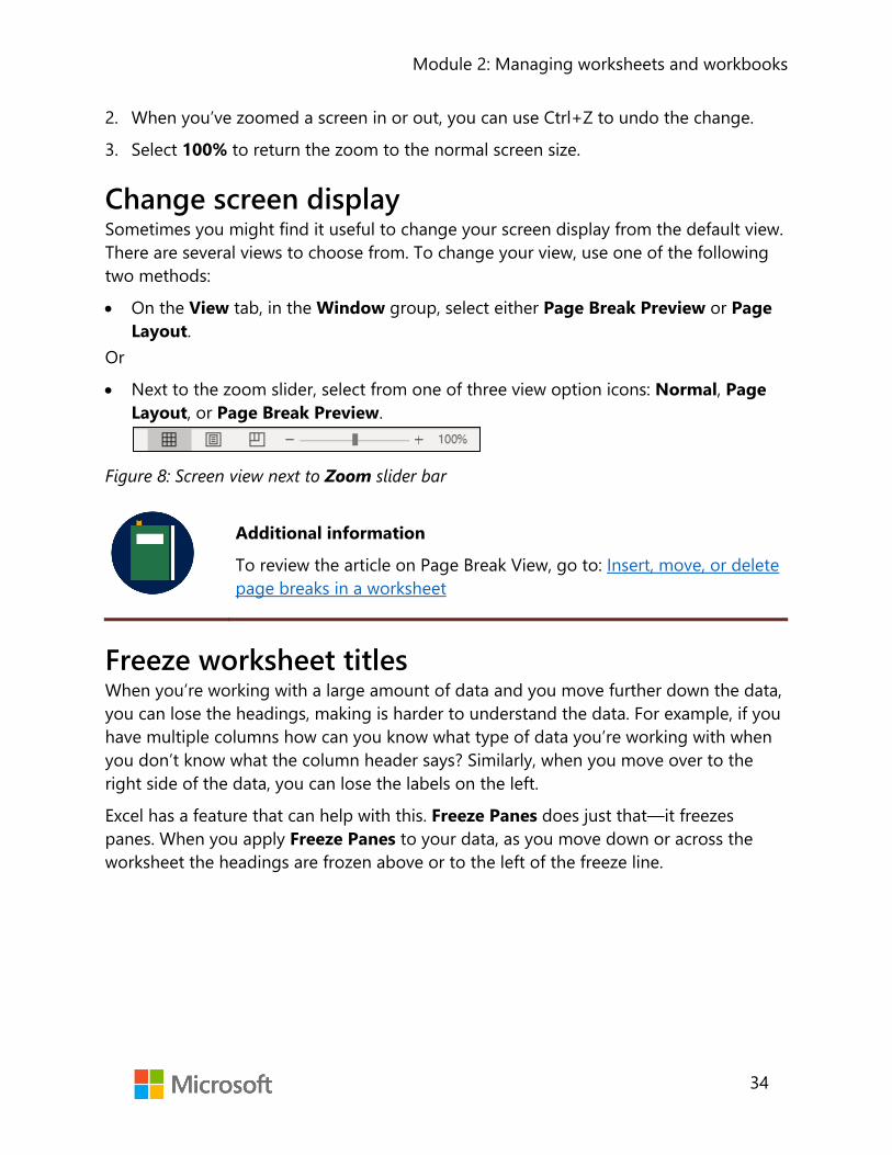
Module 2: Managing worksheets and workbooks
34
2. When you’ve zoomed a screen in or out, you can use Ctrl+Z to undo the change.
3. Select 100% to return the zoom to the normal screen size.
Change screen display Sometimes you might find it useful to change your screen display from the default view. There are several views to choose from. To change your view, use one of the following two methods:
• On the View tab, in the Window group, select either Page Break Preview or Page Layout.
Or
• Next to the zoom slider, select from one of three view option icons: Normal, Page Layout, or Page Break Preview.
Figure 8: Screen view next to Zoom slider bar
Additional information
To review the article on Page Break View, go to: Insert, move, or delete page breaks in a worksheet
Freeze worksheet titles When you’re working with a large amount of data and you move further down the data, you can lose the headings, making is harder to understand the data. For example, if you have multiple columns how can you know what type of data you’re working with when you don’t know what the column header says? Similarly, when you move over to the right side of the data, you can lose the labels on the left.
Excel has a feature that can help with this. Freeze Panes does just that—it freezes panes. When you apply Freeze Panes to your data, as you move down or across the worksheet the headings are frozen above or to the left of the freeze line.

Module 2: Managing worksheets and workbooks
35
To insert a freeze line:
1. Select the cell where you want the freeze to be applied. For example, if you want row 1 to be frozen in place when you scroll down, and columns A and B to be frozen in place when you move across to the right, your cursor should be in cell C2.
2. On the View tab, in the Window group, select Freeze Panes.
3. Select from Freeze Panes to freeze around the current position of your cursor, Freeze Top Row, or Freeze First Column.
Unfreeze worksheet titles When you are ready to unfreeze your worksheet, you follow almost the same steps:
1. On the View tab, in the Window group, select Freeze Panes.
2. Choose Unfreeze Panes.
Video
To review the video on freezing panes, go to: Freeze panes to lock rows and columns
Move between workbook windows If you have more than one workbook open at a time and you’re switching back and forth from workbook to workbook, you might find it useful to use the Switch Windows command.
To move between workbooks, you can use either of the following methods:
• On the View tab, in the Window group, select Switch Windows, and then select the workbook name you want to switch to or select Ctrl F6.
Or
• Select the workbook name on the taskbar, and then select Alt+Tab.
View all the workbooks you want to interact with To simultaneously view all the workbooks you want to interact with:
1. On the View tab, in the Window group, select Arrange All.
2. In the Arrange Windows dialog box, select either Tiled, Horizontal, Vertical, or Cascade, and then select OK.

Module 2: Managing worksheets and workbooks
36
Note: Just as you can view multiple workbooks simultaneously, you can also view multiple worksheets from the same workbook simultaneously. To do this:
1. In the Window group, select New Window in every worksheet that you want to view.
2. Then, from any of the worksheets you’ve just selected, select Arrange All.
View two workbooks side by side To view two workbooks side by side:
1. Open the two workbooks you want to view.
2. On the View tab, in the Window group, select View Side by Side.
3. If you don’t want the screens to be synchronized when you scroll, de-select Synchronous Scrolling.
Figure 9: Synchronous Scrolling command
Split your screen into panes When you’re working in a really large worksheet, using the split command can be quite helpful, especially if you need to interact with the top, bottom, left, or right side of the screen at the same time. You can split your screen into four panes, so the bottom of the worksheet can be displayed on screen at the same time as the top, and the left side of the worksheet can be displayed at the same time as the right side.
To split your screen into panes:
1. Select the cell where the split is to be located.
2. On the View tab, in the Window group, select Split.
3. Select any pane to activate it, or select the F6 key to activate each pane in sequence.
Additional information
To review the article on Split panes, go to: Split panes to lock rows or columns in separate worksheet areas

Module 2: Managing worksheets and workbooks
37
Clear worksheet panes To clear the worksheet panes, use one of the following methods:
• Double-click on the split lines individually. (If you have four split screens, you can switch to half screens first this way.)
• Select and drag the split lines away to the edge of the worksheet. • On the View tab, in the Window group, select Split.
Navigation keyboard shortcuts As you’ve learned, there are various ways to navigate around a workbook. In Module 1, you used named ranges that already existed in a workbook to navigate, and you also learned about the Go To command. However, Excel also offers simple navigational keyboard shortcuts that you can use, as listed in the following table.
To move: Select: One cell to the right (right arrow key) One cell to the left (left arrow key) One cell up (up arrow key)
One cell down (down arrow key)
To the right edge of the current area* Ctrl+(right arrow key)
To the left-hand edge of the current area* Ctrl+ (left arrow key)
To the top edge of the current area* Ctrl+ (up arrow key)
To the bottom edge of the current area* Ctrl+ (down arrow key)
To the first cell in the row Home
To the end of the row End
To the beginning of the worksheet* Ctrl+Home
To the lowest data entry point on right hand side* Ctrl+End
One screen up Page Up
One screen down Page Down
One screen to the right Alt+Page Down One screen to the left Alt+Page Up One cell to the right within a selection Tab

Module 2: Managing worksheets and workbooks
38
To move: Select: One cell to the left within a selection Shift+Tab
One cell up within a selection Shift+Enter
One cell down within a selection Enter
Table 2: Navigation keyboard shortcuts
* Adding the Shift key to any of the keyboard shortcuts marked with an asterisk will select all the data in that direction, or at least to the first cell or the last cell in that worksheet.
As you work through the lessons and modules in this course try to practice these navigational shortcuts to help you remember them in the future. They will save you time and make working on your data much easier!
Additional information
To review the article on Excel shortcut keys, go to: Keyboard Shortcuts in Excel
Activity: Research When you need help with Excel, it’s important to know how to find it. In this activity you’ll be using the help tools to research changing screen and window views, including arranging windows and splitting worksheet panes.
The teacher will open two workbooks and ask you to gather as much information as possible in 10 minutes about changing the screen view and navigating around workbooks. Consider how to complete the following tasks in your research:
1. Change the screen display to make the data easier to work with, including freezing panes.
2. Display more than one workbook on screen at the same time.
3. Display more than one worksheet from the same workbook on screen at the same time.
4. Split the screen into two or four panes.

Module 2: Managing worksheets and workbooks
39
Resources required You will need the following resources for this activity:
• Open L3_T1_act_this_year.xlsx in this lesson’s Learning Activity Resources. • Open L3_T1_act_last_year.xlsx in this lesson’s Learning Activity Resources.
Activity instructions You will need to perform the following steps during this activity:
1. Open both L3_T1_act_this_year.xlsx and L3_T1_act_last_year.xlsx.
2. Use any method available to you to research changing the screen and window views.
Try-it: Freeze panes and workbook views In this try-it you’ll help your partner by teaching them at least two different
methods to either change the screen or window view, or freeze worksheet titles.
Resources You will need the following resources for this activity:
• Open L3_T1_try_this_year_starter.xlsx in this lesson’s Learning Activity Resources. • Open L3_T1_try_last_year_starter.xlsx in this lesson’s Learning Activity Resources.
Activity instructions Prepare two or three things you can teach your partner about how to change the screen and window view, and/or how to freeze worksheet titles.
Topic 2: Use the Quick Access Toolbar As the name implies, the Quick Access Toolbar is a place for you to quickly access
the tools you use most often. Think of this as the expressway for getting your work done.
In this topic you’ll learn how to customize the toolbar so that you can add your favorite or most used tools and commands. This skill will help make your work with Excel much easier. If you have a computer at home, you might decide to customize its toolbar as well!
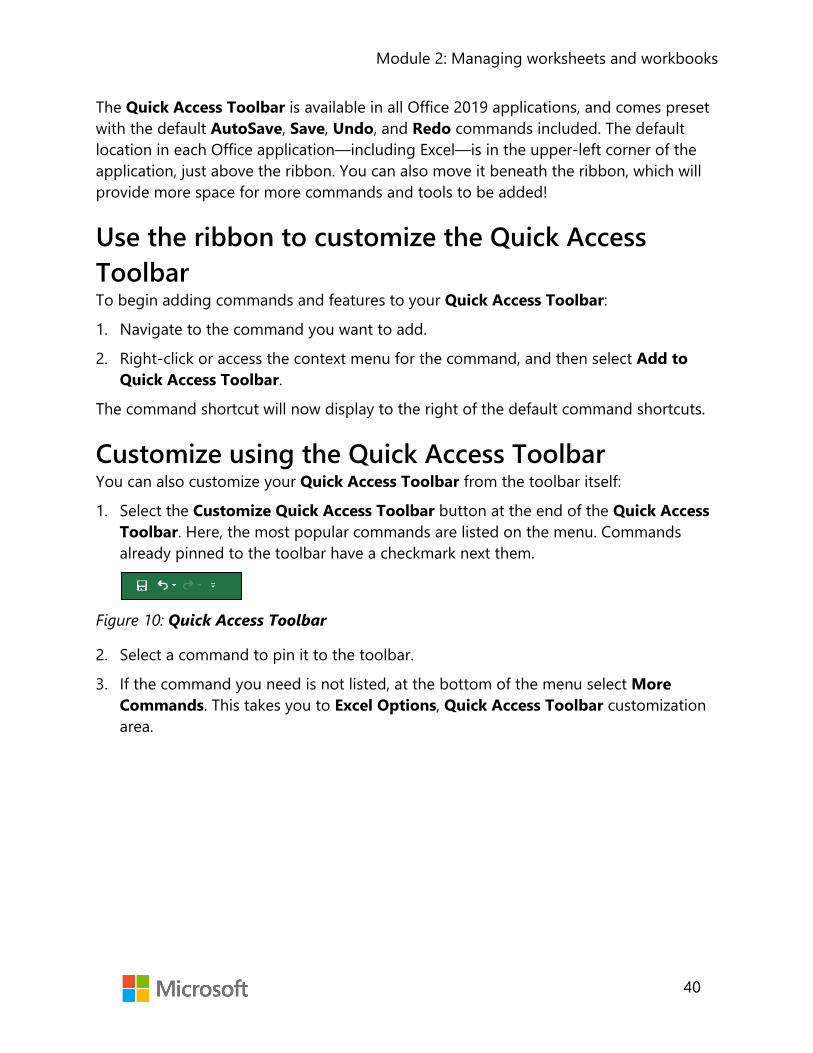
Module 2: Managing worksheets and workbooks
40
The Quick Access Toolbar is available in all Office 2019 applications, and comes preset with the default AutoSave, Save, Undo, and Redo commands included. The default location in each Office application—including Excel—is in the upper-left corner of the application, just above the ribbon. You can also move it beneath the ribbon, which will provide more space for more commands and tools to be added!
Use the ribbon to customize the Quick Access Toolbar To begin adding commands and features to your Quick Access Toolbar:
1. Navigate to the command you want to add.
2. Right-click or access the context menu for the command, and then select Add to Quick Access Toolbar.
The command shortcut will now display to the right of the default command shortcuts.
Customize using the Quick Access Toolbar You can also customize your Quick Access Toolbar from the toolbar itself:
1. Select the Customize Quick Access Toolbar button at the end of the Quick Access Toolbar. Here, the most popular commands are listed on the menu. Commands already pinned to the toolbar have a checkmark next them.
Figure 10: Quick Access Toolbar
2. Select a command to pin it to the toolbar.
3. If the command you need is not listed, at the bottom of the menu select More Commands. This takes you to Excel Options, Quick Access Toolbar customization area.

Module 2: Managing worksheets and workbooks
41
4. The column on the left displays a list of commands to choose from. However, if the command need does not display:
a. Select the drop-down menu in the Choose commands from field, and then select from one of the options.
Figure 11: Excel Options - Quick Access Toolbar
b. Select a command, and then select the Add >> button. The command will now display in the Customize Quick Access Toolbar column.
c. To re-arrange the order of the commands on the toolbar from left to right, select a command in the Customize Quick Access Toolbar column, then select the Move up or Move down arrows to position the command. The command at the top will be in the farthest left position of the Quick Access Toolbar continuing one position to the right for each command listed.
5. After you’ve completed your modifications, select OK.
Just as commands on a ribbon are organized in groups, the commands listed in the Quick Access Toolbar can be organized into groups by adding separators. To do that, access the Customize Quick Access Toolbar dialog box (as described above), select <Separator> from the list of commands and then Add >>.

Module 2: Managing worksheets and workbooks
42
Video
To review the video on customizing the Quick Access Toolbar, go to: Video: Customize the Quick Access Toolbar
Additional information
For more information about customizing the Quick Access Toolbar, go to: Customize the Quick Access Toolbar
Activity: Show and tell Your teacher will now demonstrate adding buttons to Quick Access Toolbar directly from the ribbon, and from a command’s drop-down arrow. They also will demonstrate how to reposition the Quick Access Toolbar above or below the ribbon.
Resources required You will need the following resource for this activity:
• Open L3_T2_act_common_bees.xlsx in this lesson’s Learning Activity Resources.
Activity instructions You will need to perform the following steps during this activity:
• Open L3_T2_act_common_bees.xlsx and follow the teacher’s instructions.
Try-it: Quick Access Toolbar In this series of leveled try-it activities, you’ll add commands to the Quick Access
Toolbar using the Customize Quick Access Toolbar button. You’ll then add commands from More Commands, and move commands to different postions on the Quick Access Toolbar. You’ll learn more advanced Quick Access Toolbar options, such as adding separators to group commands.
Try-it: 1 In this try-it, you’ll customize the Quick Access Toolbar using the Quick Access Toolbar button.

Module 2: Managing worksheets and workbooks
43
Resources You will need the following resource for this activity:
• Open L3_T2_try1_common_bees_starter.xlsx or use any other open workbook in this lesson’s Learning Activity Resources.
Activity instructions Participate in the activity by following these instructions:
1. Add the New command to the Quick Access Toolbar using customize Quick Access Toolbar button.
2. Go to More Commands, and add any other command from the Commands not in the Ribbon list.
Try-it: 2 In this try-it, you’ll customize the Quick Access Toolbar using right-click or accessing the context menu, and via Excel options.
Resources You will need the following resource for this activity:
• Open L3_T2_try2_common_bees_starter.xlsx or use any other open workbook in this lesson’s Learning Activity Resources.
Activity instructions Participate in the activity by following these instructions:
1. Add the Sort button to the Quick Access Toolbar by accessing the Sort context menu (with a right-click).
2. Use the Quick Access Toolbar context menu (right-click) to open Excel options and customize the Quick Access Toolbar.
3. In the Excel options window, from the Choose commands from drop-down menu, select Commands not in the Ribbon, and add at least three extra commands to the Quick Access Toolbar.
4. Move any of the newly added commands up or down the list as necessary to make it easier to find the command later.

Module 2: Managing worksheets and workbooks
44
Try-it: 3 In this try-it, you’ll customize the Quick Access Toolbar via Backstage, including adding separators.
Resources You will need the following resource for this activity:
• Open L3_T2_try3_common_bees_starter.xlsx or use any other open workbook this lesson’s Learning Activity Resources.
Activity instructions Participate in the activity by following these instructions:
1. Customize the Quick Access Toolbar via Backstage, adding commands from Commands not in the Ribbon.
2. Add two separators and reorder commands into groups.
3. Right-click or access the context menu to add Spelling, and then Check Accessibility to the Quick Access Toolbar.
4. Via Backstage, add at least three further commands of your choice from Commands not in the Ribbon.
5. Access More Commands again, and add a separator to the Quick Access Toolbar.
6. Add further separators if necessary, and reposition the commands into logical groups.
Did you know?
The abbreviation for the Quick Access Toolbar, QAT, is pronounced “cat” in many countries/regions.

Module 2: Managing worksheets and workbooks
45
Wrap-up In this lesson you learned how to customize the Quick Access Toolbar. Work with your neighbor to find out how to reset your Quick Access Toolbar back to the default settings. When you find out how, reset your Quick Access Toolbar. Help anyone else in the class that has not been able to find out how to do it.
Then use these questions to check what you learned in this lesson:
1. Which of the following statements are true?
Select the correct option.
a. The Quick Access Toolbar can be moved to beneath the ribbon.
b. The Quick Access Toolbar cannot be reset to default settings.
c. The Quick Access Toolbar cannot be moved beneath the ribbon.
d. The Quick Access Toolbar cannot be hidden from view.
2. Instead of removing all the commands you added to the Quick Access Toolbar, you can use the _________________ tool to set it back to only the default commands.
Fill in the blank space.
3. In the bottom, left corner of the Excel interface, which of the following screen views are not available?
Select the correct option.
a. Print preview
b. Page break preview
c. Page layout
d. Normal
4. To display more than one workbook on the screen at the same time, you would use the __________________________ command.
Fill in the blank space.
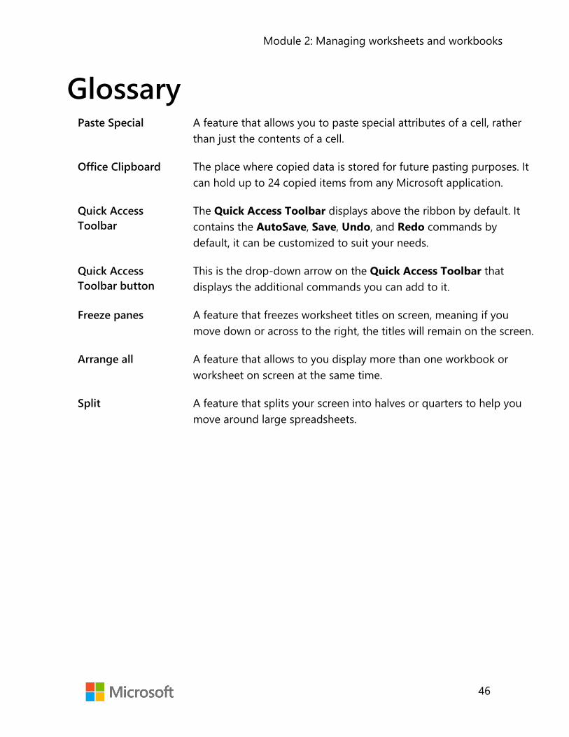
Module 2: Managing worksheets and workbooks
46
Glossary Paste Special A feature that allows you to paste special attributes of a cell, rather
than just the contents of a cell.
Office Clipboard The place where copied data is stored for future pasting purposes. It can hold up to 24 copied items from any Microsoft application.
Quick Access Toolbar
The Quick Access Toolbar displays above the ribbon by default. It contains the AutoSave, Save, Undo, and Redo commands by default, it can be customized to suit your needs.
Quick Access Toolbar button
This is the drop-down arrow on the Quick Access Toolbar that displays the additional commands you can add to it.
Freeze panes A feature that freezes worksheet titles on screen, meaning if you move down or across to the right, the titles will remain on the screen.
Arrange all A feature that allows to you display more than one workbook or worksheet on screen at the same time.
Split A feature that splits your screen into halves or quarters to help you move around large spreadsheets.

Module 2: Managing worksheets and workbooks
47
Cornerstone Overview In this cornerstone, you’ll edit two documents that Fernando, the beekeeper at Munson’s, uses. The documents track the health of beehives across the United States and the population statistics in honeybee colonies. The data has been edited by interns with less Excel experience than you. You need to make the data more presentable and easier to understand when it’s sent as a PDF. One of the documents is a .xlsx file and the other a .csv file. The data contains inconsistent columns and rows, headings are missing, and the data is a little messy.
Objectives The following table outlines the Cornerstone objectives and their corresponding MOS exam objectives.
Insert columns and rows • 2.1.3: Insert and delete multiple columns and rows
Insert and delete cells • 2.1.4: Insert and delete cells
Adjust columns and rows • 1.3.2: Adjust row height and column width
Cut, copy, paste, and move data • 2.1.1: Paste data by using special paste options
Customize views • 1.4.3: Freeze worksheet rows and columns
• 1.4.4: Change window views
Save in alternate formats • 1.5.2: Save in alternate formats
Table 3: Cornerstone objectives
Duration 50 minutes
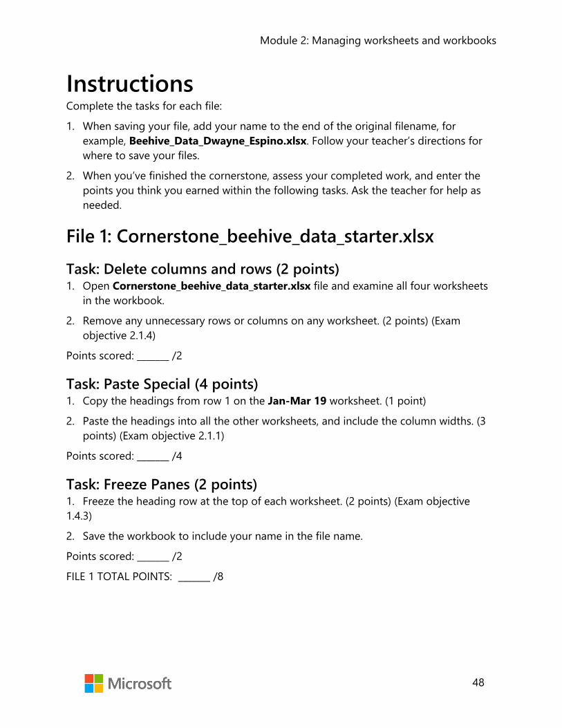
Module 2: Managing worksheets and workbooks
48
Instructions Complete the tasks for each file:
1. When saving your file, add your name to the end of the original filename, forexample, Beehive_Data_Dwayne_Espino.xlsx. Follow your teacher’s directions forwhere to save your files.
2. When you’ve finished the cornerstone, assess your completed work, and enter thepoints you think you earned within the following tasks. Ask the teacher for help asneeded.
File 1: Cornerstone_beehive_data_starter.xlsx Task: Delete columns and rows (2 points) 1. Open Cornerstone_beehive_data_starter.xlsx file and examine all four worksheets
in the workbook.
2. Remove any unnecessary rows or columns on any worksheet. (2 points) (Examobjective 2.1.4)
Points scored: _______ /2
Task: Paste Special (4 points) 1. Copy the headings from row 1 on the Jan-Mar 19 worksheet. (1 point)
2. Paste the headings into all the other worksheets, and include the column widths. (3points) (Exam objective 2.1.1)
Points scored: _______ /4
Task: Freeze Panes (2 points) 1. Freeze the heading row at the top of each worksheet. (2 points) (Exam objective 1.4.3)
2. Save the workbook to include your name in the file name.
Points scored: _______ /2
FILE 1 TOTAL POINTS: _______ /8

Module 2: Managing worksheets and workbooks
49
File 2: Cornerstone_honeybee_colonies_starter.csv Task: Save the file as .xlsx (1 point) • Open Cornerstone_honeybee_colonies_starter.csv, and save the file as a .xlsx file
named Colonies_plus your name. (1 point) (Exam objective 1.5.2) Points scored: _______ /1
Task: Insert rows (2 points) 1. Insert two rows at the beginning of the worksheet. (1 point) (Exam objective 2.1.3)
2. Enter the text, April to June Statistics in cell A1. (1 point)
Points scored: _______ /2
Task: Zoom (1 point) • Enlarge or zoom the workbook to 120% to make the data appear larger on the
screen. (Exam objective 1.5.2)
Points scored: _______ /1
Task: Rename a worksheet (1 point) • Rename the worksheet to Colonies_Apr_to_June.
Points scored: _______ /1
Task: Column widths (2 points) • Set column A to a width of 20 (145 pixels) and set columns from B to H to AutoFit.
(1 point) (Exam objective: 1.3.2)
Points scored: _______ /2
Task: Move data (2 points) • Move the data in column K to three rows beneath the table, into column A (there
should be three empty rows between the table and the additional information). (1 point) (Exam objective 2.1.3)
Points scored: _______ /2

Module 2: Managing worksheets and workbooks
50
Task: Delete cells (1 point) 1. Find the text Virginia and observe that the data is out of line.
2. Fix the data so that the numbers are in the correct position. (1 point) (Exam objective 2.1.4)
3. Save the workbook.
Points scored: _______ /1
FILE 2 TOTAL POINTS: _______ /10

Student Guide 40567A Microsoft Excel associate 2019 Module 3: Formatting cells

Formatting cells
2
Contents
Contents .............................................................. 2
Module overview ............................................. 4
Description ..................................................... 4
Scenario .......................................................... 5
Cornerstone ................................................... 6
Lesson 1: Formatting cells ............................ 7
Overview ......................................................... 7
Warm-up ........................................................ 7
Topic 1: Format font and cells ............... 8
Font group commands on the Home tab ................................................... 8
The Format Cells dialog box ........... 10
Mini Toolbar .......................................... 12
Activity: Show and tell ....................... 12
Try-it: Format font and cells ............ 14
Try-it 1 ...................................................... 14
Try-it 2 ...................................................... 15
Try-it 3 ...................................................... 16
Topic 2: Apply number formats .......... 17
Number command group on the Home tab ................................................ 17
Important facts about number formats: .................................................... 17
Activity: Think-Pair-Share ................. 18
Try-it: Apply number formats ......... 19
Try-it 1 ...................................................... 19
Try-it 2 ...................................................... 20
Try-it 3 ...................................................... 21
Topic 3: Reuse formats ........................... 22
Format Painter ....................................... 22
Activity: Discuss and learn ................ 24
Try-it: Reuse formats .......................... 24
Try-it .......................................................... 25
Wrap-up ....................................................... 25
Lesson 2: Aligning cells ............................... 27
Overview ...................................................... 27
Warm-up ...................................................... 27
Topic 1: Modify cell alignment, orientation, and indentation ................ 28
Alignment group commands on the Home tab ................................................ 28
Alignment commands in the Format Cells dialog box .................................... 29
Activity: Teacher demonstration, Switch ....................................................... 30
Try-it: Modify cell alignment, orientation, and indentation ........... 31
Try-it 1 ...................................................... 31
Try-it 2 ...................................................... 31
Try-it 3 ...................................................... 32
Topic 2: Merge cells and wrap text ... 33
Merge & Center.................................... 34
Center Across Selection ..................... 34
Wrap Text ................................................ 35
Activity: Pose a challenge ................. 35
Try-it: Merge cells and wrap text ... 36
Try-it .......................................................... 36

Formatting cells
3
Wrap-up ....................................................... 37
Lesson 3: Using cell styles ......................... 39
Overview ...................................................... 39
Warm up ...................................................... 39
Topic 1: Apply cell styles ....................... 40
Finding the Cell Styles ....................... 40
Using and modifying cell styles ..... 41
Activity: Each one, teach one .......... 42
Activity instructions ............................ 42
Try-it: Apply cell styles ....................... 43
Try-it ......................................................... 43
Topic 2: Clear formatting ...................... 45
Activity: Show and tell ....................... 46
Try-it: Clear formatting ...................... 47
Try-it .......................................................... 47
Wrap-up ....................................................... 48
Glossary ............................................................. 49
Cornerstone ..................................................... 50
Overview ...................................................... 50
Objectives .................................................... 51
Duration ....................................................... 52
Instructions .................................................. 52
Tasks .............................................................. 52
File: Cornerstone_volunteers_list _starter.xlsx ............................................. 52

Formatting cells
4
Module overview Description You’ll encounter many circumstances in which you’re required or wish to apply different appearance properties to data in a spreadsheet, which is also known as formatting. Formatting worksheet data can enable readers to present and understand information more quickly and clearly. This module includes learning activities and projects that will help you learn how to format the appearance of data within a Microsoft Excel worksheet. In earlier modules, you learned how to work with the structure of worksheets. In this module, you’ll work on the appearance, or formatting, of cells in a variety of ways.
Excel provides many tools that you can use to control the appearance of the data within the cells of a worksheet and the formatting of the cells themselves. You can manage the overall style of all formatting elements. This ability also extends to coordinating with documents created in other Office applications, such as Microsoft Word and PowerPoint, so that the style across all Office documents can be consistent.
You’ll delve into the different aspects of formatting that enable you to transform your Excel worksheet from a plain, bland spreadsheet to the professional-looking product that you’ve likely observed in your school textbooks and office workplaces.
At the end of this module, you’ll have the opportunity to use the skills you’ve learned in the Cornerstone project to transform an ordinary worksheet of text and numbers into a polished, professional worksheet document.
Lesson Learning objective Exam objective(s)
Formatting cells
Apply font, cell, and number formatting to worksheet cells
Use Format Painter
• 2.2.6 • 2.2.5 • 2.2.3
Aligning cells Modify cell content alignment, orientation, and indentation
Merge cells and wrap text in a cell
• 2.2.2 • 2.2.6 • 2.2.1 • 2.2.4
Using cell styles
Apply styles to cells
Clear formatting from cells
• 2.2.7 • 2.2.8

Formatting cells
5
Lesson Learning objective Exam objective(s)
Cornerstone: Taking the workbook style challenge
Format text and numbers
Format cell backgrounds and borders
Set alignment, orientation, and indentation of cell contents
Merge cells and wrap text
Apply cell styles
Remove formatting
• All of the above
Table 1: Objectives by lesson
Scenario Munson’s Pickles and Preserves Farm is a popular destination for school trips, family agricultural tourism, and youth summer camps.
A member of the events management team has shown you several fantastic Microsoft Word documents for the upcoming events. These Word documents were designed following the Munson’s Pickles and Preserves Farm Style Guide, a document that provides the branding guidelines for all documents created for the farm.
The internship students, including you, have been asked to help ensure that the events management team’s existing Excel workbooks follow the Munson’s Pickles and Preserves Farm Style Guide. Munson’s Workbook Style Challenge for the interns is on!
In the worksheets provided for this module, you must apply formatting to the cells and cell contents, align content in a cell, merge cells, wrap text in a cell, and apply cell styles. Don’t worry if you don’t know what all that means. We’ll cover each step as we go along.

Formatting cells
6
Cornerstone After you’ve completed the lessons and try-its, and navigated through several scenarios, the Cornerstone project will combine everything and test your ability to apply what you’ve learned.
Munson’s maintains a Volunteers List worksheet to store information related to the people who volunteer at Munson’s farm. After you finish formatting the Events List worksheet to follow the Munson’s Pickles and Preserves Farm style guide, the event coordinator asks you to apply the same formatting styles to the Volunteers List worksheet to maintain consistency. You’ll need to apply formatting to the Volunteers List worksheet to make it similar to the Events List worksheet that you’ll work on during the lessons. To do so, you’ll:
• Change the font, color, size, and style of text. • Change fill color and borders of cells. • Apply number and date formats. • Configure vertical and horizontal alignment of cell contents. • Enable text to wrap to multiple lines within the same cell. • Merge multiple cells together into one larger cell. • Apply built-in cell styles. • Remove formatting.

Formatting cells
7
Lesson 1: Formatting cells Overview You now know how to create a spreadsheet and enter data. Although it’s critical for a spreadsheet to be accurate and functional, it’s also important for users to find it attractive and easy to follow. At the end of this lesson, you’ll be able to apply font and cell formatting to a worksheet to enhance the style and presentation of data. You’ll also be able to accelerate the formatting process by using Format Painter.
Warm-up Use these questions to find out what you already know about this lesson’s topics:
1. Which of the following options can you use to format the contents of a cell?
Select all that apply.
a. Font Size
b. Sort
c. Italic
d. Underline
2. To display a cell’s value with a money symbol and two decimal places, you wouldapply a ____________________ number format.
3. Two of the main format options for a cell’s appearance are:
Select the correct option.
a. Fill Color and Table
b. Border and Fill Color
c. Page Layout and Border
d. Print Layout and Fill Color
4. The ____________________ tool allows you to copy formatting from one selection andpaste it onto another selection.

Formatting cells
8
Topic 1: Format font and cells Cells in an Excel worksheet have many attributes that you can change to set the
appearance of both the contents of the cell and the cell itself. This is called formatting, and you can use it to make worksheets more attractive. Perhaps even more importantly, formatting can be used to help people who interact with the worksheet understand the information more easily and quickly identify important points within the data. For example, you can use colors and font styles for emphasis and indicate if numbers refer to item quantities or amounts of money.
As is often the case in software applications, there are multiple ways to manage font and cell formatting in Excel. One method for formatting cells is using the ribbon, specifically the Home tab. On this tab, you’ll find the command groups Font, Alignment, Number, and Styles that contain the most commonly used commands for cell formatting. Later in this topic, you’ll explore using the Format Cells dialog box and the Mini Toolbar.
Font group commands on the Home tab The Font group on the Home tab of the ribbon contains several commands for font and cell formatting. Refer to Figure 1: Font command group.
Figure 1: Font command group
The easiest way to get familiar with these commands is to try them! Remember that you can use the Undo command if you don’t like the formatting that you’ve applied.
If you use a mouse, you can display a ScreenTip by pointing to a command without clicking the mouse. (This is also known as hovering the mouse pointer.) ScreenTips provide at least the name of the command, possibly a feature description, and sometimes, in parentheses, a keyboard shortcut for that command. For your reference, the following table lists all the available commands in the Font group.
Command Name: For selection, will: How to Use: Font Apply a font from a list Select from drop-down list Font Size Set the size of the text in points
(a measurement unit for font) Select from drop-down list, or enter a value

Formatting cells
9
Command Name: For selection, will: How to Use: Increase Font Size Quickly increase font size Select the button Decrease Font Size Quickly decrease font size Select the button Bold Make text bold Select the button, or
Ctrl+B Italic Make text italic Select the button, or
Ctrl+I Underline + Double Underline
Make text single or double underline
Select the button or drop-down arrow to change underline option, or Ctrl+U for current option
Borders Several options for borders Select from drop-down list with many choices to apply border segments, styles, colors, more borders
Fill Color Set the background color of the cell. Default is No Fill
Select the button or drop-down arrow to change selected color
Font Color Set the color of the text contents of the cell
Select the button or drop-down arrow to change selected color
Dialog Box Launcher
Not all commands can be shown in a command group. To access all options for a group, this button will open the Dialog Box for all the commands.
Select the button (lower right corner of the group)
Table 2: Commands in the Font command group in the ribbon
Did you know?
The fonts you choose can have affect how users react to and interpret the data you’re presenting. If a font is difficult to read, that might cause someone to feel anxious or annoyed. A fun or cartoonish font might give an impression that the information is not to be taken seriously. Too many fonts in one page can cause confusion. It also depends on whether a person is reading a worksheet on a computer monitor, on printed paper, or on a projected screen. Choose fonts carefully and thoughtfully!
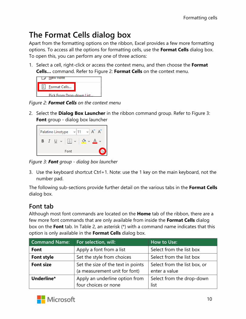
Formatting cells
10
The Format Cells dialog box Apart from the formatting options on the ribbon, Excel provides a few more formatting options. To access all the options for formatting cells, use the Format Cells dialog box. To open this, you can perform any one of three actions:
1. Select a cell, right-click or access the context menu, and then choose the Format Cells… command. Refer to Figure 2: Format Cells on the context menu.
Figure 2: Format Cells on the context menu
2. Select the Dialog Box Launcher in the ribbon command group. Refer to Figure 3: Font group - dialog box launcher
Figure 3: Font group - dialog box launcher
3. Use the keyboard shortcut Ctrl+1. Note: use the 1 key on the main keyboard, not the number pad.
The following sub-sections provide further detail on the various tabs in the Format Cells dialog box.
Font tab Although most font commands are located on the Home tab of the ribbon, there are a few more font commands that are only available from inside the Format Cells dialog box on the Font tab. In Table 2, an asterisk (*) with a command name indicates that this option is only available in the Format Cells dialog box.
Command Name: For selection, will: How to Use: Font Apply a font from a list Select from the list box Font style Set the style from choices Select from the list box Font size Set the size of the text in points
(a measurement unit for font) Select from the list box, or enter a value
Underline* Apply an underline option from four choices or none
Select from the drop-down list

Formatting cells
11
Command Name: For selection, will: How to Use: Color Set the color of the contents of
the cell Select from the drop-down menu
Normal font* Resets the text formatting to the default options
Select the check box
Effects* Apply effects of strikethrough and/or Superscript (smaller and raised) or Subscript (smaller and lowered)
Select the check box(es)
Preview* Displays the effect of the selections on the text
None needed
Table 3: Font commands in the Format Cells dialog box
Border tab The gray lines around all cells are called gridlines. By default, gridlines are only visual aids to designate where cells are, and the lines do not print. To add lines with a choice of styles and colors around cells, use border formatting.
On the Border tab, for Line, first select the desired Style and Color, and then select the Outline, Inside, or specific border segment buttons of the selected cells. The white box represents the overall selected cell or cells and will preview the choices made. Applying borders can be confusing because cells share borders with their neighbor cells. For example, the bottom border of one cell is the top border of the cell in the next row. It might take some practice to gain an understanding of how to apply the border formats that you want to use. To observe the true result of your border formatting, deselect the cells that you formatted by selecting a cell away from that area.
Fill tab Fill refers to the background coloring or pattern of a cell. Choices include simple solid colors, effects of gradients, and two-color patterns. The Sample rectangle on the Fill tab will display a preview of the selected fill.

Formatting cells
12
Mini Toolbar You can also use the Mini Toolbar to quickly access the most frequently used formatting commands and contextual commands that will change depending on what you’re doing at the time. On your selected cell(s), right-click to show the context menu and the Mini Toolbar. Refer to the Figure 4: Excel Mini Toolbar example.
Figure 4: Excel Mini Toolbar example
Additional information
For more information on formatting text in cells, go to: Format text in cells
For more information about changing the fill color of cells, go to: Add or change the background color of cells
For more information on cell borders, go to: Apply or remove cell borders on a worksheet
Activity: Show and tell Your overall task for the lessons in this module is to improve the appearance of the Munson’s List of Events data on the EventsList worksheet. Before you can begin the task, you need to know what formatting options are available. In this activity, your teacher will open an Excel workbook to demonstrate, and together you’ll explore the different cell formatting options and practice the methods that this topic describes.
You’ll also review the Munson’s Pickles and Preserves Farm style guide document to learn the guidelines for branding of documents for Munson’s Pickles and Preserves Farm. Note that the Excel files provided as Learning Activity Resources for this module have an Office document theme for Munson’s applied to them, to simplify following Munson’s style guide. Refer to the following callout to learn about Themes:

Formatting cells
13
Did you know?
Document themes in Microsoft Office provide a way to control and quickly change the overall appearance of the fonts, colors, and effects on objects in your document, even across the different applications of Excel, Word, and PowerPoint! When you apply Theme Fonts and Theme Colors to your document, and then change the theme, all the theme elements will change to provide a completely different appearance. There are many themes built into Office applications. Additionally, you can customize and create your own themes!
To see an example of how themes can affect your Excel workbook, in the L1_T1_act_events_list_starter.xlsx file, go to the Themes worksheet and follow the instructions there.
For more information on using document themes in Excel, go to: Change the appearance of your worksheet
Resources required You’ll need the following resources for this activity:
• L1_T1_act_events_list_starter.xlsx in this lesson’s Learning Activity Resources folder.
• Munson_style_guide_document.docx from the Media folder inside Learning Activity Resources.
Activity instructions Participate in the activity by following these instructions:
1. Open the L1_T1_act_events_list_starter.xlsx workbook and go to the EventsList worksheet.
2. Open the Munson_style_guide_document.docx and review the contents.
3. Go to the FontsCells worksheet in the Excel workbook.
4. Observe the teacher’s demonstrations and your own Excel window, and follow any instructions given.
5. Be sure to save any changes to the file before moving on to the Try-it.

Formatting cells
14
Try-it: Format font and cells You’ll use the methods and commands discussed in this topic and demonstrated
by your teacher to apply formatting to cells on Munson’s List of Events worksheet. All three try-its will accomplish the same formatting to the EventsList worksheet, but each asks you to use a different method—the ribbon, or the dialog box, or the dialog box and the Mini Toolbar. You only need to do one of the try-its, but it’s good experience to do two or even all three.
Try-it 1 Scenario You’ll begin to improve the appearance of Munson’s List of Events on the EventsList worksheet as a participant in Munson’s Workbook Style Challenge for the interns.
Resources You’ll need the following resources for this activity:
• Open L1_T1_try1_events_list_starter.xlsx in this lesson’s Learning Activity Resources. Alternatively, you can continue working in the workbook that you used during the learning activity.
Instructions Working in Munson’s List of Events on the EventsList worksheet in the workbook, you must perform the following tasks to apply any unfinished formatting to cells. Some of the tasks might have been completed during the Activity with the teacher.
Use the Font command group on the Home tab of the ribbon to apply the following formatting:
1. For cells A1:E1 on the worksheet:
a. Set Font to Theme Fonts > Verdana (Headings).
b. Set Font Size to 28.
c. Set Font Color to Theme Colors: Blue, Accent 2.
d. Set Fill Color to Theme Colors: Gold, Accent 5, Lighter 80%.
2. For all the cells under Event Name (cells B4:B18) on the worksheet:
o Set font style to Bold
Formatting cells
15
3. For all the list data (cells A3:H18) on the worksheet:
o Set All Borders to Theme Colors > Blue, Accent 2 with the thinnest solid style. 4. Save the file.
Try-it 2 Resources You’ll need the following resources for this activity:
• Open L1_T1_try2_events_list_starter.xlsx in this lesson’s Learning Activity Resources. Alternatively, you can continue working in the workbook you used during the learning activity.
Instructions Working in the EventsList worksheet in the workbook, you must perform the following tasks to apply any unfinished formatting to cells. Some of the tasks might have been completed during the Activity with the teacher.
Use the Format Cells dialog box and the Mini Toolbar to apply the following formatting:
1. For cells A1:E1 on the worksheet:
a. Set Font to Theme Fonts > Verdana (Headings).
b. Set Font Size to 28.
c. Set Font Color to Theme Colors: Blue, Accent 2.
d. Set Fill Color to Theme Colors: Gold, Accent 5, Lighter 80%.
2. For all the cells under Event Name (cells B4:B18) on the worksheet:
o Set font style to Bold. 3. For all the list data (cells A3:H18) on the worksheet:
o Set Outline and Inside Borders to Theme Colors: Blue, Accent 2 with the thinnest solid style.
4. Save the file.

Formatting cells
16
Try-it 3 Resources You’ll need the following resources for this activity:
• Open L1_T1_try3_events_list_starter.xlsx in this lesson’s Learning Activity Resources. Alternatively, you can continue working in the workbook that you used during the learning activity.
Instructions Working in the EventsList worksheet in the workbook, you must perform the following tasks to apply any unfinished formatting to cells. You might have completed some of the tasks during the activity with the teacher.
Use the Format Cells dialog box and the Mini Toolbar to apply the following formatting on the worksheet:
1. For cells A1:E1 and A3:H3 on the worksheet (Hint: press and hold the Ctrl key to make multiple nonadjacent selections.):
a. Set Font to Theme Fonts > Verdana (Headings).
b. Set Font Color to Theme Colors: Blue, Accent 2.
c. Set Fill Color to Theme Colors: Gold, Accent 5, Lighter 80%.
2. For only cells A1:E1 on the worksheet.
o Set Font Size to 28. 3. For all the cells under Event Name (cells B4:B18 on the worksheet):
o Set font style to Bold. 4. For all the list data (cells A3:H18) on the worksheet:
o Set Outline and Inside Borders to Theme Colors: Blue, Accent 2 with the thinnest solid style.
5. For only cells A3:H3 on the worksheet:
a. Set Font to Theme Fonts > Cambria (Body).
b. Set Font Color to Theme Colors: Black, Text 1.
6. Set Background Color to No Color. Save the file.

Formatting cells
17
Topic 2: Apply number formats When cells contain text, for the most part the text displayed in the cell is what
appears in the formula bar. However, when a cell contains a number value of some kind, you can make the cell display that value in many ways to indicate meaning without changing the actual value in that cell.
For example, if you enter 12345 in a cell, does that number represent a quantity of an item, an amount of money, a date (yes, dates are numbers!), a number of minutes, or hours? Or is it a postal code or a product number, which aren’t truly numeric values but are actually text values?
The general test for determining if digits are a numeric value or text is this: would or could calculations ever be performed on this value? If the answer is yes, and that includes dates and times, then it’s a number. If the answer is no, then it’s text.
Number command group on the Home tab The Number group on the Home tab of the ribbon contains several ways to select number formatting. Refer to Figure 5: Number command group. The options in this group include:
• A drop-down list with choices for commonly used formats and access to the Format Cells dialog box via the More Number Formats… command.
• Shortcut buttons to apply the Accounting Number Format (the dollar sign), Percent Style (the percent sign), and Comma Style (the large comma).
• Buttons to increase or decrease the number of decimal places displayed.
Figure 5: Number command group
Important facts about number formats • Number formats are applied to cells, and that format then applies to whatever may
be entered into that cell at any time. • The number format usually will not affect any true text values that are entered in the
cell. Actual numeric values will be affected.

Formatting cells
18
• Number formatting does not change the value itself. For example, if you enter 1.25 in a cell that is set to only display one decimal place, it will display as 1.3, but when used in a calculation, it will still be 1.25.
Additional information
For more information on number formats in Excel, go to: Quick Start: Format numbers in a worksheet and Format numbers
For more information on formatting dates, go to: Format a date the way you want
Activity: Think-Pair-Share You’ll examine a worksheet containing cells without number formatting. You’ll think of responses to the questions provided, and then share the ideas with a partner. There will be a follow-up discussion, with the teacher providing demonstration as needed.
Resources required You’ll need the following resources for this activity:
• Open L1_T2_act_events_list_starter.xlsx in this lesson’s Learning Activity Resources folder.
Did you know?
For Excel, the calendar begins with January 1, 1900, or Day 1. (In Excel for Mac, that year is 1904.) Every day counts as one more since that date. This is how Excel can perform calculations for dates; for example, someone’s age. Additionally, every portion of a day is a fraction or decimal, or a portion of 1, starting at midnight. So, if you have 1/31/1900 6:00 AM in a cell, Excel “thinks” of it as 31.25. What number do you think today is? Or your birthdate and time?
For more information about Excel date systems, go to: Date systems in Excel
For more information about changing the Excel date system, go to: Change the date system, format, or two-digit year interpretation

Formatting cells
19
Activity instructions As you examine Munson’s List of Events on the EventsList worksheet, think about the following questions, and then share your response ideas with your partner.
1. What are some different types of numbers?
2. When is number formatting critical in a worksheet?
3. How might consistent number formatting help someone understand the data?
4. How can you apply number formatting to a cell, multiple cells, or an entire worksheet?
Participate in the follow-up discussion. Pay attention to any demonstrations or instructions by the teacher.
Try-it: Apply number formats Now that you have some understanding of what number formats can do for your
worksheet and how to apply them, you need to try it. If you’re unsure and want to practice first, go to Try-it 1, and then go to Try-it 2. If you’re feeling more confident, go directly to Try-it 2 or Try-it 3.
Try-it 1 Resources You’ll need the following resources for this Try-it:
• Open L1_T2_try1_events_list_starter.xlsx in this lesson’s Learning Activity Resources. Alternatively, you can continue working in the workbook that you used during the learning activity.
Instructions The following are the general tasks that you must perform during this Try-it:
1. Switch to the NumbersTry1 worksheet.
2. For each column of data, select all the data under the column name, then apply the format indicated at the top of each column.
For example, select cells A4:A21 and apply the General number format as indicated in cell A3. For cells B4:B21, apply the number format of Number. For cells C4:C21, apply the Currency number format. Continue through all the columns of data or until you’re comfortable enough to move on to Try-it 2.

Formatting cells
20
3. Note and compare the different results in each column. The notes in row 24 describe the expected results.
4. Save the file and continue on to Try-it 2.
Try-it 2 Resources You’ll need the following resources for this Try-it:
• Open L1_T2_try2_events_list_starter.xlsx in this lesson’s Learning Activity Resources. Alternatively, you can continue working in the workbook that you used during the learning activity.
Instructions The following are the general tasks that you must perform during this Try-it:
1. In the EventsList worksheet, use the Number group on the Home tab of the ribbon to apply number formatting to the List of Events data.
2. For all the cells under Start Date (cells D4:D18) in the worksheet:
o Apply the Short Date format. 3. For all the cells under # of Days (cells E4:E18) in the worksheet:
o Apply the Number format. 4. For all the cells under Budget (cells H4:H18) in the worksheet:
a. Apply the Accounting format.
b. Decrease the decimal places to display whole numbers (no decimal places).
5. As a test of your formatting, enter the data for the following event in the next event row (Num 13) and observe how the formatted cells accept the entries that you make:
Event Name: New Year’s Eve Year: 2020 Start Date: 12/31/2020 # of Days: 1 Open To: Public Description: TBD Budget: 135000
6. Save the file.

Formatting cells
21
Try-it 3 Resources You’ll need the following resources for this Try-it:
• Open L1_T2_try3_events_list_starter.xlsx in this lesson’s Learning Activity Resources. Alternatively, you can continue working in the workbook that you used during the learning activity.
Instructions The following are the general tasks that you must perform during this Try-it:
1. Working in the EventsList worksheet, use the Format Cells dialog box, then the Number tab to apply number formatting as follows:
a. For all the cells under Start Date (cells D4:D18) in the worksheet:
i. As an experiment, select the appropriate option so that the first date displays as 28-Mar-2019.
ii. Undo the last formatting action to restore the cells to their original default format.
iii. Apply the Short Date format. Observe that there is no apparent change, as the date cells were already in that format, and the text and blank cells do not display differently with a date format.
b. For all the cells under # of Days (cells E4:E18) on the worksheet:
Apply the number format of Number.
c. For all the cells under Budget (cells H4:H18) on the worksheet:
i. Apply the Accounting format.
ii. Decrease the decimal places to display whole numbers (no decimal places).

Formatting cells
22
2. As a test of your formatting, enter the data for the following event in the next event row (Num 13), and observe how the formatted cells accept the entries you make:
Event Name: New Year’s Eve Year: 2020 Start Date: 12/31/2020 # of Days: 1 Open To: Public Description: TBD Budget: 135000
3. If there’s time, switch to the NumbersTry3 worksheet, and follow the instructions there to experiment with more advanced number formatting.
4. Save the file.
Topic 3: Reuse formats Format Painter
Excel provides several options for formatting cells and cell contents, and it can be overwhelming to make decisions. After you’ve decided on the formatting choices for a portion of your worksheet, it could be frustrating and time consuming to figure out what those choices were when you want to apply the same formatting to other cells.
Let’s say you’ve spent a great deal of time and effort formatting cells on your worksheet to make it the best document that you possibly can. Your title uses the headings font size of 18 pt, and it is just the right blue; your column headers are bold, centered, and colored; your numeric data cells are formatted for Number and Accounting; some of your text data cells are aligned left, some are centered; plus all the other formatting you’ve done. Then one of your coworkers adds more data to your worksheet—more columns, and more numeric and text data—and all that data is unformatted. You want a clean, consistent look for the entire worksheet. How can you possibly remember all the formatting that you selected to now apply it to the newly added data?
Fortunately, you don’t need to do anything to keep track because Excel already does that for you. It also provides a handy tool for you to copy formatting from one selection and apply it to one or more other selections. This tool is the Format Painter.

Formatting cells
23
Format Painter is located on the Home tab in the Clipboard command group. The ScreenTip gives you some basic instructions on how to use it. Refer to the Figure 6: Format Painter option with ScreenTip displayed.
Figure 6: Format Painter option with ScreenTip displayed
While Format Painter is active and ready to use, the mouse pointer will have a paint brush symbol attached to the thick white plus (+) sign, and the selection from which you copied formatting will be surrounded by an animated moving border. If you select the Format Painter once, it’ll turn off automatically after you apply it once. If you double-click the Format Painter, it will stay active until you do one of the following:
• Select the Format Painter command again, or • Press the Esc key on the keyboard.
Additional information
For more information on using Format Painter in Excel, go to: Copy cell formatting

Formatting cells
24
Video
To review the video on using Format Painter, go to: Video: Copy cell formatting
Activity: Discuss and learn Working in the workbook, you’ll go to the IdeasPages worksheet. Observe the teacher’s demonstration and follow any instructions given. Be sure to save any changes to the file before moving on to the Try-it.
Your teacher will demonstrate and lead a discussion on how and why to use Format Painter.
Resources required You’ll need the following resources for this Try-it:
• Open L1_T3_act_events_list_starter.xlsx in this lesson’s Learning Activity Resources.
Activity instructions You might follow along in the workbook as the teacher uses Format Painter to transform some unformatted data into a ready-to-print presentation piece. Participate in the discussion. Some questions to consider while discussing the use of Format Painter:
• How does using Format Painter compare to using the Copy and Paste commands? • Why do you think it’s important to keep formatting consistent in a worksheet? • How might formatting become inconsistent? • How can using Format Painter help improve your productivity?
Try-it: Reuse formats You can use Format Painter to copy and paste formatting from one selection of a
cell or cells to another selection, and from one selection to multiple other selections. Observing Munson’s List of Events on the EventsList worksheet, you decide you’d like the data in the Open To column to be formatted like the data in the Event Name column. You’ll also apply some formatting to one of the column labels and then quickly apply that formatting to other column labels.

Formatting cells
25
Try-it Resources You’ll need the following resources for this Try-it:
• Open L1_T3_try_events_list_starter.xlsx in this lesson’s Learning Activity Resources. Alternatively, you can continue working in the workbook used during the learning activity.
Instructions 1. Go to the EventsList worksheet, if it’s not already active.
2. Use Format Painter to copy the formatting from one of the Event Name data cells to all the list cells under the column label Open To (cells F4:F18).
3. Apply a font color and fill color of your choice to cell A3 and make it Italic. Then use Format Painter to copy the formatting from cell A3 and apply it to alternating column labels (cells C3, E3, G3).
Wrap-up Consider things such as traffic signs and imagine them as only words that all have the same appearance. Trying to use and comprehend data that has no formatting can be difficult. You’ve now begun to transform the plain data on the EventsList worksheet for the Munson’s Pickles and Preserves Farm List of Events to be easier to read and follow, instantly identifying numeric values as dates or money, and emphasizing text with attributes such as bold and italic. Your fellow events team members have noticed and are commenting on the improved appearance. They also appreciate that it’s becoming easier for them to interpret the information on the worksheet.
Use these questions to check what you learned in this lesson:
1. Which command do you use to change the color of a cell background?
Select the correct option.
a. Background color
b. Fill color
c. Border color
d. Font color

Formatting cells
26
2. In the Munson’s List of Events on the EventsList worksheet, which number format does the data in the Year column need?
Select the correct option.
a. Short Date
b. Accounting
c. Long Date
d. General (no specific format)
3. To make text and numbers inside a cell larger, you must use the ____________________ formatting option.
4. How can you most efficiently copy all Font, Cell, Alignment, and Number formatting from one cell to multiple other cells?
Select the correct option.
a. Select the one cell with the formatting that you want to copy, select the Copy command, select the other cells, and then select the Paste command.
b. Select the one cell with the formatting that you want to copy, double-click the Format Painter command, select the other cells, then select the Format Painter command to turn it off.
c. Select the one cell with the formatting that you want to copy, use the Format Cells command, then select the other cells.
d. Select the one cell with the formatting that you want to copy, select and hold Ctrl while you select the other cells, then select the Format Painter command.
Additional information
For more information on formatting cells containing numbers, go to the following links:
• Available number formats in Excel • Format numbers as percentages • Create a custom number format • Convert numbers stored as text to numbers • How to correct a ##### error For more information on copying and pasting formats, go to: Paste options

Formatting cells
27
Lesson 2: Aligning cells Overview Imagine that you have a spreadsheet with many columns of numbers but none of the numbers line up with other numbers, making it difficult to read and compare the values to each other. Or you’d like to have the titles at the top of the worksheet centered over the data. You also have names for columns that need to go on more than one line or be rotated to read vertically. At the end of this lesson, you’ll understand the different types of alignment for content within cells. You’ll also know how to apply alignment formatting to cells, and how to use the Wrap Text format and Merge & Center features. Cell alignment is helpful for keeping your data consistent and getting the best fit in the available space on your worksheet.
Warm-up Use these questions to find out what you already know about this lesson’s topics:
1. The types of alignment for contents of a cell include:
Select all that apply.
a. Horizontal
b. Vertical
c. Italic
d. Rotation
2. To display text in a cell turned on its side or on an angle, you change the____________________.
Select the correct option to fill in the blank space.
a. Position
b. Orientation
c. Wrapping
d. Margins
3. You can align cell contents centered over multiple columns with _____________.

Formatting cells
28
4. Which formatting feature for alignment will put the contents of a cell on multiple lines within the same cell?
Select the correct option.
a. Long Date
b. Indent
c. Increase Font Size
d. Wrap Text
Topic 1: Modify cell alignment, orientation, and indentation Alignment group commands on the Home tab
The Alignment group on the Home tab of the ribbon contains several commands for aligning cell contents. Refer to Figure 7: Alignment command group. Alignment is the term for the positioning of content within the cell. This can be horizontal and vertical, and also rotated, indented, wrapped, and merged and centered.
Figure 7: Alignment command group
Command Name: For selection, will: How to Use:
Top Align, Middle Align, Bottom Align
Three options for vertical positioning of cell contents
Select one of the options
Align Left, Center, Align Right
Three options for horizontal positioning of cell contents
Select one of the options
Orientation Rotation options for cell contents
Select from the drop-down list of several options

Formatting cells
29
Command Name: For selection, will: How to Use:
Decrease Indent, Increase Indent
Move content closer to or farther away from cell border
Select one of the options
Wrap Text Forces text to multiple lines within the cell when needed
Select to toggle on or off
Merge & Center Three options for combining cells into a new larger cell and one option to unmerge cells
Select for merge and center, or select other options from drop-down
Dialog box launcher
Open the Format Cells dialog box to the Alignment tab
Select the button (lower right corner of the group)
Table 4: Commands in the Alignment command group in the ribbon
Alignment commands in the Format Cells dialog box Although most alignment commands are located on the Home tab of the ribbon, there are a few more alignment commands only available from inside the Format Cells dialog box on the Font tab. In the following table, command names and format options with an asterisk (*) include options only available in the Format Cells dialog box.
Command Name: For selection, will: How to Use: Text alignment: Horizontal
Includes more options than Left, Center, and Right on the ribbon*
Select from the list box
Text alignment: Vertical
Includes more options than Top, Middle, and Bottom on the ribbon*
Select from the list box
Text alignment: Indent
Sets a number of indent positions for use with Horizontal options of Left (Indent) and Right (Indent)*
Use the spin buttons or enter a number
Text control: Wrap text
Forces text to multiple lines within the cell when needed
Select the check box to enable
Text control: Shrink to fit*
Forces cell contents to a smaller size that enables fitting the cell size—be careful, it can make the text extremely small!
Select the check box to enable

Formatting cells
30
Command Name: For selection, will: How to Use: Text control: Merge cells
Combines selected cells into one larger cell
Select the check box to enable
Right-to-left: Text direction*
For use with languages that write from right-to-left
Select from the drop-down
Orientation Rotates the cell contents by a number of degrees*
Use the spin buttons or enter a number
Table 5: Alignment commands in Format Cells dialog box
Additional information
For a more information and a video on aligning or rotating text, go to: Align or rotate text in a cell
Video
To review the video on aligning text in a cell, go to: Video: Align text in a cell
Activity: Teacher demonstration, Switch Your teacher will demonstrate modifying cell alignment, orientation, and indentation, and then start the Switch activity.
You’ll open the same workbook. Your teacher will ask you to perform a series of cell-alignment tasks for a specific amount of time. When the teacher calls out “Switch!” move to your neighbor’s seat quickly to perform the next set of tasks, continuing from what your neighbor has done. Repeat this until the teacher calls out “Switch back home.”
When you work in a collaborative environment like a workplace, you’ll often be asked to work on Excel files that you did not create. You’ll need to get familiar with picking up where someone else left off on creating or editing worksheets and workbooks.
Resources required You’ll need the following resources for this activity:
• L2_T1_act_events_list_starter.xlsx in this lesson’s Learning Activity Resources folder and go to the AlignmentAct worksheet.

Formatting cells
31
Activity instructions You might follow along in the workbook as the teacher demonstrates. Be ready to move to your neighbor’s seat to follow instructions on that computer.
Try-it: Modify cell alignment, orientation, and indentation
Now that you have some understanding of what you can use alignment settings to accomplish in your worksheet and how to apply them, you must implement these settings. If you’re unsure and want to practice first, use Try-it 1.
Try-it 1 Before you attempt to modify alignment, orientation, and indent settings for any cells on the EventsList worksheet, you want to try out the different types of alignment, orientation, and indent settings on another practice worksheet that has been provided.
Resources You’ll need the following resources for this Try-it:
• Open L2_T1_try1_events_list_starter.xlsx in this lesson’s Learning Activity Resources. Alternatively, you can continue working in the workbook that you used during the learning activity.
Instructions Switch to the AlignmentTry1 worksheet. From the ribbon Home tab, Alignment command group, use the options to apply the alignment, orientation, and indent settings indicated by the text in each cell. Note the different results in each cell. When you’re ready to work on the EventsList worksheet, move on to Try-it 2.
Try-it 2 Resources You’ll need the following resources for this Try-it:
• Open L2_T1_try2_events_list_starter.xlsx in this lesson’s Learning Activity Resources. Alternatively, you can continue working in the workbook that you used during the learning activity or do Try-it 1.

Formatting cells
32
Instructions The following are the general tasks that you must perform during this Try-it:
1. Use the Alignment group on the Home tab of the ribbon to apply alignment, orientation, and indent settings to the EventsList worksheet.
2. Clear the test entries for the New Year’s Eve event from the last row of data (cells B16:H16).
3. For cells A1:E1 in the worksheet:
o Set vertical alignment to Middle Align. 4. For all the data cells in the list (cells A4:H18):
o Set vertical alignment to Top Align. 5. For all the cells under Num (cells A4:A18) in the worksheet:
o Apply Center horizontal alignment. 6. For all the cells under Year (cells C4:C18) in the worksheet:
a. Apply different Orientation options and note the results.
b. Remove any Orientation settings on these cells.
c. Apply Center horizontal alignment.
7. For all the cells under Start Date and # of Days (cells D4:E18) in the worksheet:
o Apply Center horizontal alignment. 8. For all the cells under # of Days (cells E4:E18) in the worksheet:
o Remove Center horizontal alignment. 9. For all the cells under Open To (cells F4:F18) in the worksheet:
o Apply Indent of one position. 10. Save the file.
Try-it 3 Resources You’ll need the following resources for this Try-it:
• Open L2_T1_try3_events_list_starter.xlsx in this lesson’s Learning Activity Resources. Alternatively, you can continue working in the workbook that you used during the learning activity or do Try-it 1.

Formatting cells
33
Instructions Use the Alignment tab of the Format Cells dialog box to apply the following alignment, orientation, and indent settings to the EventsList worksheet:
1. Clear the test data for the New Year’s Eve event from the last row of data (cells B16:H16).
2. For cells A1:E1 on the worksheet:
o Set vertical alignment to Middle Align. 3. For all the data cells in the list (cells A4:H18):
o Set vertical alignment to Top Align. 4. For all the cells under Num (cells A4:A18) in the worksheet:
o Apply Center horizontal alignment. 5. For all the cells under Year (cells C4:C18) in the worksheet:
a. Apply different Orientation options and note the results.
b. Remove any Orientation settings on these cells.
6. For all the cells under Year, Start Date, and # of Days (cells C4:E18) in the worksheet:
o Apply Center horizontal alignment. 7. For all the cells under # of Days (cells E4:E18) in the worksheet:
o Remove Center horizontal alignment. 8. For all the cells under Open To (cells F4:F18) in the worksheet:
o Apply Indent of one position. Finished! You’re more than halfway to completing a finished List of Events. Topic 2 will give you the last set of commands to finish the cell alignment tasks for the EventsList worksheet.
Topic 2: Merge cells and wrap text Excel is all about calculations and lists. Its strength is in helping you take raw data
and transform it into usable information. However, Excel isn’t limited to just number calculations and data management. Being a part of Microsoft Office ensures that the Excel environment complements Word’s word processing functionality and PowerPoint’s presentation capability. This is where a few seemingly awkward aspects of a numbers and data application can still produce the presentable results you want for reports, lists, and other documents.
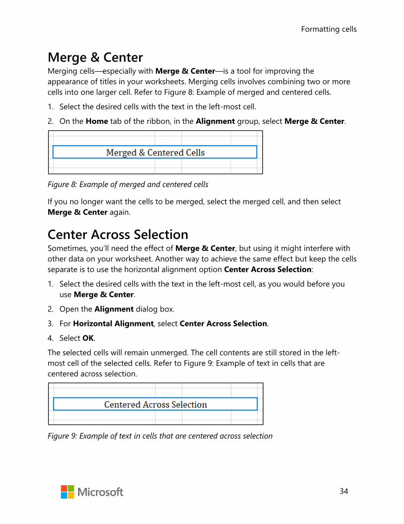
Formatting cells
34
Merge & Center Merging cells—especially with Merge & Center—is a tool for improving the appearance of titles in your worksheets. Merging cells involves combining two or more cells into one larger cell. Refer to Figure 8: Example of merged and centered cells.
1. Select the desired cells with the text in the left-most cell.
2. On the Home tab of the ribbon, in the Alignment group, select Merge & Center.
Figure 8: Example of merged and centered cells
If you no longer want the cells to be merged, select the merged cell, and then select Merge & Center again.
Center Across Selection Sometimes, you’ll need the effect of Merge & Center, but using it might interfere with other data on your worksheet. Another way to achieve the same effect but keep the cells separate is to use the horizontal alignment option Center Across Selection:
1. Select the desired cells with the text in the left-most cell, as you would before you use Merge & Center.
2. Open the Alignment dialog box.
3. For Horizontal Alignment, select Center Across Selection.
4. Select OK.
The selected cells will remain unmerged. The cell contents are still stored in the left-most cell of the selected cells. Refer to Figure 9: Example of text in cells that are centered across selection.
Figure 9: Example of text in cells that are centered across selection

Formatting cells
35
Wrap Text Wrap Text is ideal for cells that contain text that is too long for the width of the cell. This might be column headers, or cells that contain notes or description text. Wrap Text will make text inside a cell flow onto multiple lines as needed within the width of that column. You can also start a new line inside a cell by using the Alt+Enter keyboard shortcut (Windows) or CONTROL+OPTION+RETURN (macOS), which then also applies Wrap Text to that cell. This is also known as inserting a line break. Refer to Figure 10: Example of a cell containing text with Wrap Text turned on.
Figure 10: Example of a cell containing text with Wrap Text turned on
Additional information
For more information on merging and unmerging cells, go to: Merge and unmerge cells
For more information on enabling text to wrap to multiple lines within a cell, go to: Wrap text in a cell. For more information on inserting a line break inside a cell on multiple operating systems, go to: Start a new line of text inside a cell in Excel
Video
To review the video on about merging and unmerging cells, go to: Video: Merge and unmerge cells.
Activity: Pose a challenge Your teacher will point out that the title text “List of Events” is not centered in the space it occupies. Also, many cells have a lot of text that isn’t visible because there isn’t room to show all that text. How might you fix these issues?
Resources required You’ll need the following resources for this activity:
• Open L2_T2_act_events_list_starter.xlsx in this lesson’s Learning Activity Resources.

Formatting cells
36
Activity instructions Participate in the activity by following these instructions:
1. Open the same file that the teacher has open, so that you can follow along.
2. Brainstorm with other students on ways to solve the format problems on the worksheet that students and/or your teacher point out.
3. If you have a proposed solution, you can volunteer to demonstrate from the teacher’s computer so that everyone can follow along and learn from what you do.
Try-it: Merge cells and wrap text The title on the EventsList worksheet needs to be centered in the space it
occupies, and several cells on the worksheet have more text in them than can be displayed with the current cell sizing. Your goal is to use the method that you think will be the most efficient to accomplish the tasks listed—commands in the ribbon or the Format Cells dialog box. You don’t want to change any of the column widths, but you’ll need to make sure that all the text in the cells is visible.
Try-it Resources You’ll need the following resources for this Try-it:
• Open L2_T2_try_events_list_starter.xlsx in this lesson’s Learning Activity Resources.
Instructions The following are the general tasks that you must perform during this Try-it:
1. Merge the cells and center the title in the space of cells A1:E1.
2. Apply Wrap Text to data columns in which there are cells containing text that’s not visible, including the cells for the empty rows of the list. Don’t change column widths, but make sure that row heights are adjusted as necessary.
3. Remove the Merge & Center setting for the title cells in the space of A1:E1.
4. Center the text in A1 across the space of cells A1:E1.
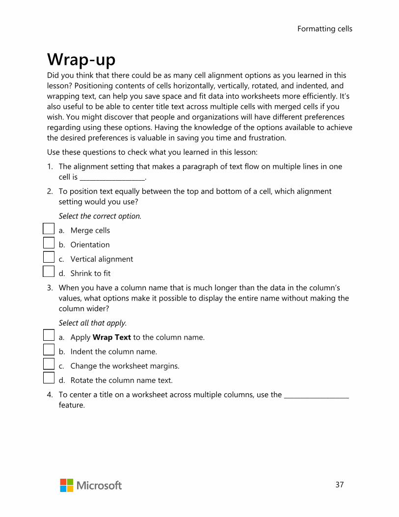
Formatting cells
37
Wrap-up Did you think that there could be as many cell alignment options as you learned in this lesson? Positioning contents of cells horizontally, vertically, rotated, and indented, and wrapping text, can help you save space and fit data into worksheets more efficiently. It’s also useful to be able to center title text across multiple cells with merged cells if you wish. You might discover that people and organizations will have different preferences regarding using these options. Having the knowledge of the options available to achieve the desired preferences is valuable in saving you time and frustration.
Use these questions to check what you learned in this lesson:
1. The alignment setting that makes a paragraph of text flow on multiple lines in onecell is ____________________.
2. To position text equally between the top and bottom of a cell, which alignmentsetting would you use?
Select the correct option.
a. Merge cells
b. Orientation
c. Vertical alignment
d. Shrink to fit
3. When you have a column name that is much longer than the data in the column’svalues, what options make it possible to display the entire name without making thecolumn wider?
Select all that apply.
a. Apply Wrap Text to the column name.
b. Indent the column name.
c. Change the worksheet margins.
d. Rotate the column name text.
4. To center a title on a worksheet across multiple columns, use the ____________________feature.

Formatting cells
38
Did you know?
In Excel, you can increase flexibility and formatting options, especially for large amounts of text, by adding a text box onto your worksheet. You can size and position the text box without being constrained by the structure of your worksheet’s rows and columns.
You can format the text box with no outline and fill the cells with white so that it blends in with the worksheet as if the text were in cells. Then, inside the text box, you can select portions of text and apply many of the font and alignment options from the Home tab of the ribbon.
Or, you can be more creative with the text box, which is only one of many shapes that you can add in Excel. When you select the shape or text inside the shape, a new contextual tab become available on the ribbon called Shape Format. The ribbon tab contains a large collection of formatting options that you can use for the shape and the text!
For more information, go to:
• Add, copy, or delete a text box • Add shapes • Add or remove borders for text boxes, pictures, and shapes • Add a fill or effect to a shape or text box
Formatting cells
39
Lesson 3: Using cell styles Overview At the end of this lesson, you’ll know how to take advantage of the power of cell styles in Excel to control and speed up formatting of cells on an Excel worksheet. You’ll also be able to clear all formatting from cells, including styles.
Warm up Use these questions to find out what you already know about this lesson’s topics:
1. Where on the ribbon will you find cell styles?
Select the correct option.
a. Home tab, Font group
b. Page Layout tab, Themes group
c. Home tab, Styles group
d. Insert tab, Illustrations group
2. Where would you use Headings cell styles?
Select all that apply.
a. Cells at the top of a column of data
b. Cells that label rows of data
c. Cells that contain totals
d. Cells that contain comments
3. Cell styles can help you to:
Select all that apply.
a. Keep consistency in formatting.
b. Make your worksheets easier to read.
c. Apply formatting more quickly.
d. Perform calculations.

Formatting cells
40
Topic 1: Apply cell styles By now, you’ve seen that consistency in formatting is helpful to people who use
Excel worksheets. As you gain more experience with using Excel, you’ll find that it’s also simpler for you when you’re creating the worksheets.
You’ve also learned that there are many formatting options and settings for cells and their contents. Formatting one cell or selection of cells could require you to make several choices and perform several steps to get the appearance you want. What if you want to apply that same formatting to multiple other selections in the same workbook later—or in other workbooks? It could become quite time consuming. Fortunately, Excel has a feature called Cell Styles to help you with this.
Finding the Cell Styles Note that the appearance of the command for Cell Styles on the ribbon can vary because of the ribbon’s flexible, adaptive nature. If your Excel window has a lot of room, Cell Styles will be displayed in a gallery with several styles already visible. Refer to Figure 11: Styles command group on the Home tab with Cell Styles gallery.
Figure 11: Styles command group on the Home tab with Cell Styles gallery
The three buttons on the right edge of a gallery are used for scrolling the gallery or to open more of the gallery. Refer to Figure 12: Gallery buttons.
Figure 12: Gallery buttons
If your Excel window is compact because of sizing or screen resolution, then Cell Styles might only be available as a button. Refer to Figure 13: Styles command group on the Home tab with Cell Styles button.

Formatting cells
41
Figure 13: Styles command group on the Home tab with Cell Styles button
Using and modifying cell styles To apply a cell style: 1. Select a cell or multiple cells.
2. Select the desired cell style from the Cell Styles gallery or button.
To modify a cell style 1. Right-click or access the context menu on the cell style, and then select Modify… to
open the Style dialog box.
2. In the Style dialog box, select the Format… button to open the Format Cells dialog box.
3. In the Format Cells dialog box, make selections as desired, and then select OK.
4. In the Style dialog box, select the check boxes for the formats that you want to include.
5. Select OK.
Additional information
For more information on cell styles, go to: Change the format of a cell
For more information on applying, creating, or removing cell styles, go to: Apply, create, or remove a cell style
For more information on copying cell styles from another workbook, go to: Copy cell styles from another workbook
Video
To review the video on applying styles, go to: Apply styles

Formatting cells
42
Did you know?
Many actions in Microsoft Office applications can be repeated quickly by using a keyboard shortcut—the F4 key or Ctrl+Y (Windows) or Command+Y (macOS).
For more information on repeating actions, go to: Undo, redo, or repeat an action
Activity: Each one, teach one Students will use Excel Help to learn how to apply a style to a cell and explore the cell styles in Excel. Then, students will pair up to take turns answering a list of questions.
Resources required You’ll need the following resources for this activity:
• Open L3_T1_act_events_list_starter.xlsx in this lesson’s Learning Activity Resources. • The Office Help & Training Center website. • The Excel Help system. Depending on the version of Excel that you’re using and your
operating system, this could be accessible from the Help tab on the ribbon, the File tab on the ribbon, or the Search box in the Excel window title bar. You can also use the Tell me what you want to do… box or the F1 key on the keyboard. Refer to the following callout for additional information.
Additional information
For more information on accessing the Excel Help system, go to: Where is the product Help in Office?
Activity instructions You’ve discovered that using a feature called cell styles in Excel can save you a considerable amount of time when formatting a worksheet, and you want to learn more about it.

Formatting cells
43
Participate in the activity by following these instructions:
• Go to the EventsList worksheet. If you need to, use the Help resources to learn how to apply Excel cell styles. Then, with a partner, take turns answering these questions: o Which cells in this activity worksheet might you apply the good and bad styles
to? o Which cells are best to apply headings and titles styles to? o What happens to cells that have a style applied if you modify the style? o What other kinds of styles might be useful for the activity worksheet?
After completing this activity, you’ll know how to apply cell styles and you might have some ideas on how to use cell styles on your worksheet. Some cell styles are more useful than others, and not every style works universally. Excel provides several ready-made styles that work well in their intended category. When the built-in styles don’t fit your needs, you can modify them to suit your purpose.
Try-it: Apply cell styles
This Try-it illustrates how appropriate application of Cell Styles can quickly transform bland, amateur spreadsheets into professional documents. You realize that the column headers on the Munson’s List of Events on the EventsList worksheet could be easily and consistently formatted if you use a cell style. Because this is the last step in your worksheet transformation, you need to review the Munson’s Pickles and Preserves Farm style guide document to be sure that your formatted worksheet complies with the guide’s standards.
Try-it Resources You’ll need the following resources for this Try-it:
• Open L3_T1_try_events_list_starter.xlsx in this lesson’s Learning Activity Resources folder.
Open Munson_style_guide_document.docx from the Media folder in this module’s Learning Activity Resources.
Formatting cells
44
Instructions The following are the general tasks that you must perform during this Try-it:
1. Review the Munson’s Pickles and Preserves Farm style guide document and your EventsList worksheet to confirm that the worksheet is formatted to meet the guide’s specifications.
2. Apply the different Headings cell styles to the column headers of the list (cells A3:H3). Note how each cell style changes the appearance of the headers. Select any other cell outside the data to reveal the true appearance. Apply the Heading 3 style to the column headers.
3. Note that the cells that had been filled with green are still filled with green, although the font, font color, and bordering of the cells has changed. Also note that the font used is the theme body font Cambria, but it should be the theme headings font Verdana to comply with Munson’s style guide.
4. In the Cell Styles gallery, right-click or access the context menu for the Heading 3 style you applied and select Modify….
a. Note that the options selected for Style includes are only Font and Border, and the options for Number, Alignment, Fill, and Protection are not selected. This means that applying this style will only affect the font and border formatting of the selected cells. That’s why the green fill color remained.
b. Change the Format for the Font to Verdana (Headings) 9 pt. for the style.
5. Select all the column header cells and change the Fill Color to No Fill.
6. Now that you’ve corrected those problems, select all the column headers, make the text centered in the cells, and wrap the text on two lines. Although only one of the column headers needs the text wrapped, you want to keep the formatting consistent for all the column headers.
During or after the Try-it, your teacher will display the final solution for the EventsList worksheet with the expected finished appearance for the Munson’s List of Events. Now it’s time to check your results. Does your data on the Munson’s List of Events match the solution? If it doesn’t match, apply any formatting options to make it match. If it does match, congratulations!
You have only one more topic before you’re ready for the Cornerstone.
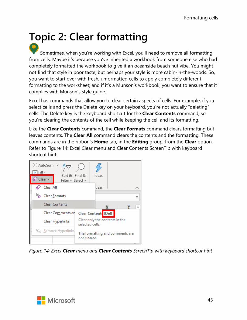
Formatting cells
45
Topic 2: Clear formatting Sometimes, when you’re working with Excel, you’ll need to remove all formatting
from cells. Maybe it’s because you’ve inherited a workbook from someone else who had completely formatted the workbook to give it an oceanside beach hut vibe. You might not find that style in poor taste, but perhaps your style is more cabin-in-the-woods. So, you want to start over with fresh, unformatted cells to apply completely different formatting to the worksheet; and if it’s a Munson’s workbook, you want to ensure that it complies with Munson’s style guide.
Excel has commands that allow you to clear certain aspects of cells. For example, if you select cells and press the Delete key on your keyboard, you’re not actually “deleting” cells. The Delete key is the keyboard shortcut for the Clear Contents command, so you’re clearing the contents of the cell while keeping the cell and its formatting.
Like the Clear Contents command, the Clear Formats command clears formatting but leaves contents. The Clear All command clears the contents and the formatting. These commands are in the ribbon’s Home tab, in the Editing group, from the Clear option. Refer to Figure 14: Excel Clear menu and Clear Contents ScreenTip with keyboard shortcut hint.
Figure 14: Excel Clear menu and Clear Contents ScreenTip with keyboard shortcut hint

Formatting cells
46
Additional information
For more information on clearing formats from cells, go to: Clear cells of contents or formats
Did you know?
Formatting cells adds to the file size of an Excel workbook, just as worksheets, data, and formulas do. As a best practice, you should avoid formatting the complete worksheet and instead just format the areas that you’re using. Unnecessarily large files take up more storage space and can become slow to respond.
How much of a difference could it make? Consider this point: Most worksheets that you build will only take up a relatively small portion of an Excel worksheet. For example, if your worksheet list or report uses cells A1:N1000 (14,000 cells) and prints out on 60 pages, that’s only using a tiny fraction—not even 1% of the cells on the entire worksheet (over 17 billion!). So, if you have 100% of a worksheet formatted when you only need less than 1% formatted, that’s a lot of unnecessary extra formatting data in your workbook file.
For more information on finding and clearing unnecessary formatting on a worksheet, go to: Locate and reset the last cell on a worksheet
Activity: Show and tell This is a student-driven demonstration on removing all cell formatting. One student works from the teacher computer that is projected in the classroom. Other students help the student through the steps. If some students cannot figure this out, they can reference the “Clear cells of contents or formats” article for assistance. That article was listed in the Additional information callout in this topic. The teacher might also provide hints.
Resources required You’ll need the following resources for this activity:
• Open L3_T2_act_ideas_pages_starter.xlsx in this lesson’s Learning Activity Resources.
• The Excel Help feature.

Formatting cells
47
Activity instructions You or another student will use the teacher computer. The students will direct the presenting student on the steps to clear formatting from all the cells on the worksheet. Some key indicators of success:
• There is no more color on the worksheet. • All cells use the same font, with no bold or italics. • The gridlines are all the same. • Text data is aligned left and numbers are aligned right (in the Alignment tab of the
Format Cells dialog box, Horizontal will be set to General). • No cell contents are rotated, and all are aligned to the bottom of the cells.
What other clues indicate that there’s no formatting on the worksheet? Do you have any other observations?
Try-it: Clear formatting
Try-it Now that you’ve successfully completed the transformation of the Munson’s List
of Events on the EventsList worksheet, you’re ready to start working on the next workbook for the Munson’s Workbook Style Challenge for the interns. However, when you open the workbook, it seems that someone already formatted the worksheet, and that the format doesn’t follow the guidelines in the Munson’s Pickles and Preserves Farm style guide document. You must use the Clear Formats command to remove all formatting from the worksheet.
Resources You’ll need the following resources for this Try-it:
• Open L3_T2_try_volunteers_list_starter.xlsx in this lesson’s Learning Activity Resources.
Instructions The following are the general tasks that you must perform during this Try-it:
1. Open L3_T2_try_volunteers_list_starter.xlsx.
2. Remove all formatting from the entire VolunteersList worksheet.
3. Refer to the indicators of success in the learning activity to verify that you’ve completed the task.

Formatting cells
48
Wrap-up In this lesson, you’ve learned how to use Cell Styles to quickly and consistently apply multiple formatting attributes to a worksheet. To accelerate that process, you learned that you can use the Repeat command for some actions. Throughout this module, you learned many different ways to apply formatting, and some of them require a few steps. Consider how using Cell Styles and Repeat can improve your productivity and help you get your work done more quickly.
You also learned in this lesson that there’s an easy way to remove all formatting with the Clear Formats command. This makes preparing cells and worksheets for new formatting easier and prevents conflicting and inconsistent formatting from trying to fix existing formatting.
1. Which of the following styles are built-in cell styles in Excel?
Select all that apply.
a. Calculation
b. Chart
c. Warning Text
d. Comma
2. If you have a cell at the bottom of a column that adds up all the numbers in thecolumn, you might apply the ____________________ cell style.
3. What kinds of formatting can be included in cell styles?
Select all that apply.
a. Font Size
b. Margins
c. Fill Color
d. Text Alignment
4. When you need a selection of cells to have only the original default formatting, youshould use the ____________________ command.

Formatting cells
49
Glossary Alignment Positioning content or objects horizontally or vertically, lining up with
cell borders, in Excel.
Attributes Qualities, characteristics, or properties.
Column data Cells containing data below the column header.
Column headers Cells at the top of a column of data that contain the names of the columns. Also called column labels.
Default Starting setting or option, before any choice is applied by the user.
Dialog box A window in which to enter information or make selections.
Format, Formatting
(n.) The appearance properties of items or objects, including fonts, font size, colors, borders, and numbers. (v.) Change or set these properties and apply the changes.
Row labels Cells at the beginning of a row of data that contain the name of the row or the category of the row’s data. Also called row headers.
ScreenTip Small windows that display descriptive text when you rest the pointer on a command or control.

Formatting cells
50
Cornerstone Overview After you’ve completed the lessons and try-its and navigated through several scenarios, the Cornerstone project will combine everything and test your ability to apply what you’ve learned.
Munson’s maintains a List of Volunteers in an Excel file to store information on the people who volunteer at Munson’s farm. After you finish formatting the EventsList worksheet to follow the Munson’s Pickles and Preserves Farm style guide, the event coordinator asks you to similarly transform the VolunteersList worksheet to maintain consistency. You’ll need to apply formatting to the VolunteersList worksheet to make it similar to the EventsList worksheet that transformed during the lessons. To do so, you’ll:
• Change the font, color, size, and style of text. • Change fill color and borders of cells. • Apply number and date formats. • Reuse formatting from cells to apply to other cells. • Configure vertical and horizontal alignment of cell contents. • Enable text to wrap to multiple lines within the same cell. • Merge multiple cells together into one larger cell. • Apply built-in cell styles. • Remove formatting.
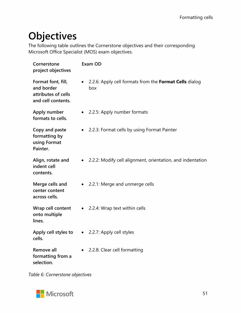
Formatting cells
51
Objectives The following table outlines the Cornerstone objectives and their corresponding Microsoft Office Specialist (MOS) exam objectives.
Cornerstone project objectives
Exam OD
Format font, fill, and border attributes of cells and cell contents.
• 2.2.6: Apply cell formats from the Format Cells dialog box
Apply number formats to cells.
• 2.2.5: Apply number formats
Copy and paste formatting by using Format Painter.
• 2.2.3: Format cells by using Format Painter
Align, rotate and indent cell contents.
• 2.2.2: Modify cell alignment, orientation, and indentation
Merge cells and center content across cells.
• 2.2.1: Merge and unmerge cells
Wrap cell content onto multiple lines.
• 2.2.4: Wrap text within cells
Apply cell styles to cells.
• 2.2.7: Apply cell styles
Remove all formatting from a selection.
• 2.2.8: Clear cell formatting
Table 6: Cornerstone objectives

Formatting cells
52
Duration 50 minutes
Instructions 1. Complete the tasks below for each file.
2. When you first save your file, add your name to the end of the filename, for example: Cornerstone_volunteers_list_Dwayne_Espino. Follow your teacher’s directions for where to save your files. Be sure to save your file regularly throughout the Cornerstone tasks and after you finish.
3. When you’ve finished the Cornerstone, assess your completion and enter the points that you think you earned within the task lists below. You can ask for your teacher’s help, if required.
Tasks You’ll work with one file in this Cornerstone. The following are the tasks that you must complete within this file.
File: Cornerstone_volunteers_list_starter.xlsx Task: Format the title of the list (14 points) 1. Open Cornerstone_volunteers_list_starter.xlsx. (1 point)
2. Format the title of the worksheet, List of Volunteers, so that it’s centered horizontally in the five-cell space allowed for it to the left of the Munson’s Pickles and Preserves Farm logo. (4 points) (Exam objective 2.2.1)
3. Position the title so that it’s centered vertically within the row it occupies. (3 points) (Exam objective 2.2.2)
4. Format the title with the following attributes: (Exam objective 2.2.6)
a. Theme Font: Verdana (Headings) (1 point)
b. 28 pt. (1 point)
c. Theme Font Color: Blue, Accent 2 (2 points)
d. Theme Fill Color: Gold, Accent 5, Lighter 80% (2 points)
Points scored: _______ /14

Formatting cells
53
Task: Apply the common attributes to the list cells (5 points) 1. Change the borders to the thinnest solid-line style with the color of Blue, Accent 2
for the outline and inside borders. (3 points) (Exam objective 2.2.6)
2. Make the cell contents start at the top of the cells. (2 points) (Exam objective 2.2.2)
Points scored: _______ /5
Task: Format the list column headers (9 points) 1. Format the column headers as Heading 3 style. (2 points) (Exam objective 2.2.7)
2. Without changing the column widths, make sure all the text in the column headers is readable. (4 points) (Exam objective 2.2.4)
3. Center the headers horizontally within each cell. (1 point) (Exam objective 2.2.2)
4. Make sure that the cell contents line up at the bottom of the cells. (2 points) (Exam objective 2.2.2)
Points scored: _______ /9
Task: Format the data cells in the Num column (1 point) • Center the numbers horizontally within each cell. (1 point) (Exam objective 2.2.2) Points scored: _______ /1
Task: Format the data cells in the First Name column (3 points) • Format all the first-name cells with the following attributes: (Exam objective 2.2.6)
a. Make them bold and italic. (1 point)
b. Change the font color to Theme Color: Dark Green, Accent 1. (1 point)
c. Set the fill color to Theme Color: Gold, Accent 5, Lighter 80%. (1 point)
Points scored: _______ /3
Task: Format the data cells in the Last Name column (3 points) • Make the formatting of all the last-name cells match the formatting of the first name
cells. (3 points) (Exam objective 2.2.3)
Points scored: _______ /3

Formatting cells
54
Task: Make a copy of your work (6 points) To capture the work that you’ve completed before continuing to make changes, you’ll make a copy of part of your work in another location on the worksheet and give it a heading.
1. In cell A30, enter the text: Showing My Work. (1 point)
2. Format cells A30:H30 with Heading 1. (2 points) (Exam objective 2.2.7)
3. Copy all the cells in the list only (cells A3:H23) and then paste starting at A32. (3 points)
4. Leave this area of the worksheet as it is for the remainder of the Cornerstone.
Points scored: _______ /6
Task: Reformat the data cells in the First Name and Last Name columns (6 points) 1. Go back to the original data area of the worksheet, clear the formatting from the first
name and last name data cells but not the headers. (2 points) (Exam objective 2.2.6)
2. For the first name and last name data cells:
a. Make the formatting the same as the data cells under the Roles header. (3 points) (Exam objective 2.2.3)
b. Make the cells bold. (1 point)
Points scored: _______ /6
Task: Format the data cells in the Start Date column (4 points) • Format the start-date data cells with the following attributes:
a. Center the data horizontally within each cell. (1 point) (Exam objective 2.2.2)
b. Format so that the start date for Maura Mejia is 11/29/2013 or 29-11-2013. (3 points) (Exam objective 2.2.5)
Points scored: _______ /4
Task: Format the Days Worked data cells (5 points) • Format the Days-Worked data cells with the following attributes:
a. Align the data to the right within each cell. (1 point) (Exam objective 2.2.2)
b. Format as a number with one decimal place. (4 points) (Exam objective 2.2.5)
Points scored: _______ /5
Formatting cells
55
Task: Format the phone number data cells (5 points) • Format the phone number data cells with the following attributes:
a. Center the data horizontally within each cell. (1 point) (Exam objective 2.2.2)
b. Format as a phone number. (4 points) (Exam objective 2.2.5)
Points scored: _______ /5
Task: Format the data cells in the Roles column (4 points) • Without changing the column widths, make sure all the text in the Roles column
data cells is readable. (4 points) (Exam objective 2.2.4) Points scored: _______ /4
Task: Test the formatting (5 points) • As a test of your formatting skills, enter the data for the following volunteer in the
next list row (Num 12), and verify that it has the correct formatting. Refer to the solution file displayed by the teacher to compare your results. (5 points):
First Name: <your own first name> Last Name: <your own last name> Start Date: 12/31/2020 Days Worked: 0 Home Phone: 1234567 Mobile Phone: 1234567 Roles: Parking, food server/seller, ticket sales
Points scored: _______ /5
TOTAL POINTS: _______ /70
Student Guide 40567A Microsoft Excel associate 2019 Module 4: Managing tables and range data

Managing tables and range data
2
Contents
Contents .............................................................. 2
Module overview ............................................. 4
Description ..................................................... 4
Scenario .......................................................... 5
Cornerstone ................................................... 6
Lesson 1: Understanding tables and ranges ................................................................... 7
Overview ......................................................... 7
Warm-up ........................................................ 7
Topic 1: Format data as a table and change the table style ............................... 8
Create a table without a style applied ........................................................ 9
Create a table with a style applied at the same time ....................................... 10
Activity: Tell a story ............................. 13
Try-it: Format data as a table and change the table style ....................... 14
Try-it ......................................................... 14
Try-it 2 ...................................................... 15
Topic 2: Convert a table to a range .. 15
Activity: Pose a challenge ................. 16
Activity instructions ............................ 16
Try-it: Convert a table to a range .. 16
Wrap-up ....................................................... 17
Lesson 2: Configuring table format options .............................................................. 19
Overview ...................................................... 19
Warm-up ..................................................... 19
Topic 1: Configure table style options .......................................................... 20
Activity: Discuss and learn ................ 21
Activity instructions ............................. 22
Try-it: Configure table style options ..................................................... 22
Topic 2: Insert and manage rows, columns, and the total number of rows ................................................................ 23
Use the Resize command ................. 23
Enter data ................................................ 24
Paste data ............................................... 24
Insert data ............................................... 25
To insert a column ............................... 26
Delete rows or columns in a table 27
Total Row ................................................ 27
Activity: Discuss and learn ................ 28
Try-it: Insert and manage rows, columns, and total number of rows ........................................................... 29
Wrap-up ....................................................... 30
Lesson 3: Naming tables and ranges .... 31
Overview ...................................................... 31
Warm-up ...................................................... 31
Topic 1: Name a table ............................. 32
Activity: Pose a challenge ................. 33
Activity instructions ............................. 34
Try-it: Name a table ............................ 34
Topic 2: Define a named range ........... 35

Managing tables and range data
3
Edit and delete named ranges ....... 37
Activity: Discuss and learn ............... 38
Try-it: Define a named range .............. 39
Try-it 1 ...................................................... 39
Wrap-up ....................................................... 40
Lesson 4: Sorting and filtering ................. 42
Overview ...................................................... 42
Warm-up ..................................................... 42
Topic 1: Sort and filter records ........... 43
Sort a cell range column in ascending or descending order ..... 44
Change the Sort Options Orientation for a data set ................. 44
Sort a table column in ascending or descending order ................................ 44
Filter a cell range column ................. 45
Filter a table column .......................... 47
Clear a filter from a column ............ 47
Clear all filters in a worksheet ........ 48
Remove all filters in a worksheet .. 49
Activity: Show and tell ....................... 49
Try-it: Sort and filter records ........... 50
Topic 2: Perform a custom sort .......... 50
Sort text ................................................... 51
Sort numbers ......................................... 52
Sort dates and times ........................... 53
Sort by more than one column ...... 55
Sort by cell color, font color, or icon ............................................................ 56
Activity: Pose a challenge ................. 57
Activity instructions ............................. 57
Try-it: Perform a custom sort .......... 58
Wrap-up ....................................................... 58
Cornerstone ..................................................... 60
Overview ...................................................... 60
Objectives .................................................... 60
Duration ....................................................... 61
Instructions .................................................. 61
Tasks .............................................................. 61
File 1: Cornerstone_Munsons_apparel_ starter.xlsx ............................................... 62
File 2: Cornerstone_Munsons_bee_product_inventory_ starter.xlsx ....................... 63
Glossary ............................................................. 64
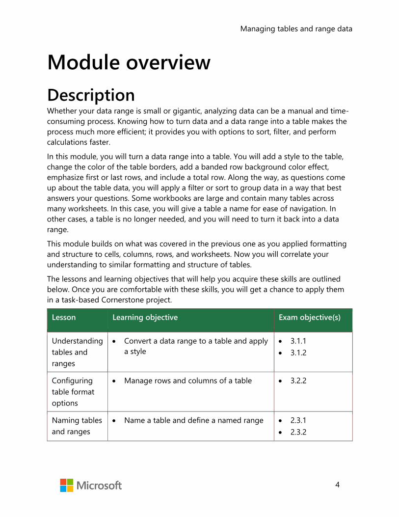
Managing tables and range data
4
Module overview Description Whether your data range is small or gigantic, analyzing data can be a manual and time-consuming process. Knowing how to turn data and a data range into a table makes the process much more efficient; it provides you with options to sort, filter, and perform calculations faster.
In this module, you will turn a data range into a table. You will add a style to the table, change the color of the table borders, add a banded row background color effect, emphasize first or last rows, and include a total row. Along the way, as questions come up about the table data, you will apply a filter or sort to group data in a way that best answers your questions. Some workbooks are large and contain many tables across many worksheets. In this case, you will give a table a name for ease of navigation. In other cases, a table is no longer needed, and you will need to turn it back into a data range.
This module builds on what was covered in the previous one as you applied formatting and structure to cells, columns, rows, and worksheets. Now you will correlate your understanding to similar formatting and structure of tables.
The lessons and learning objectives that will help you acquire these skills are outlined below. Once you are comfortable with these skills, you will get a chance to apply them in a task-based Cornerstone project.
Lesson Learning objective Exam objective(s)
Understanding tables and ranges
• Convert a data range to a table and apply a style
• 3.1.1 • 3.1.2
Configuring table format options
• Manage rows and columns of a table • 3.2.2
Naming tables and ranges
• Name a table and define a named range • 2.3.1 • 2.3.2

Managing tables and range data
5
Lesson Learning objective Exam objective(s)
Sorting and filtering
• Sort and filter data range and table records
• 3.2.2 • 3.3.1 • 3.3.2
Cornerstone: Organizing farm merchandise data
• Format data as a table, work with table style options, create a named table, and filter and sort data
• 3.1.1 • 3.1.2 • 3.1.3 • 3.2.1 • 3.2.2 • 3.2.3 • 3.3.1 • 3.3.2
Table 1: Objectives by lesson
Scenario Munson’s Pickles and Preserves Farm distributes their harvested crops to many local and regional outlets, including grocery stores, restaurants, farmers markets, and their own onsite farm stand.
Distribution data is captured in workbooks, but workbooks are not set up for filtering and sorting the harvest yield, distribution routes, wholesale pricing, retail pricing, and more.
You have been asked to sort out the disorderly data. Your first task is to create the tables that capture information such as harvest yield, distribution locations, wholesale prices, etc. The tables allow you to quickly filter, sort, and find specific information. Because time is precious, and production on the farm doesn’t stand still, you need to get this done quickly.

Managing tables and range data
6
Cornerstone At the end of this module, the cornerstone will help you recall how to manage tables and data.
It’s a task-based project to help you practice the following skills:
• Convert a range of data to a table • Convert a table to a range • Modify table settings and options • Modify a table or range • Apply sorting to data • Apply filtering to data

Managing tables and range data
7
Lesson 1: Understanding tables and ranges Overview After this lesson, you’ll be proficient in creating and formatting a table created in Excel. You’ll be able to format a range as a table, change a table style, and convert a table to a range.
Warm-up In the previous lesson, you learned how to apply worksheet styles to cells and remove formatting from worksheet cells.
In this lesson, you will learn how similar formatting can be applied to a range of cells by formatting these as a table. With the help of the Format as Table and Table commands, you will learn two different processes to accomplish this. The Format as Table command creates a table and applies a style at the same time. However, the Table command creates a table only. A style can be applied later if the user chooses.
You will also learn how to convert a table back to a range.
Get ready for discussions and step-by-step demonstrations, along with opportunities to put to practice what you learn along the way. But first, check how well you know the prerequisite concepts needed to follow this lesson.
Use these questions to find out what you already know about this lesson’s topics:
1. What keyboard shortcut can you use to insert a table?
Select the correct option.
a. Ctrl+T
b. Ctrl+Shift+=
c. Ctrl+Shift+L
d. Ctrl+Shift+-
Managing tables and range data
8
2. A _____________________ provides the capability to select the arrow in the column header to narrow the data.
3. What option is a unique combination of borders and shading to change the appearance of the table?
Select the correct option.
a. Themes
b. Effects
c. Styles
d. Colors
4. A table can be converted to which of the following?
Select the correct option.
a. Chart
b. PivotTable
c. Data range
d. SmartArt
Topic 1: Format data as a table and change the table style
Imagine you have been given an Excel workbook full of popular video game data that has been collected over the past few years. You want to use the data to find answers to some questions you have about your favorite games. Trying to answer these questions by organizing the data can be a time-consuming and manual process. Converting the data into a table gives it structure to help you quickly manage and analyze it.
There are several ways to insert a table.
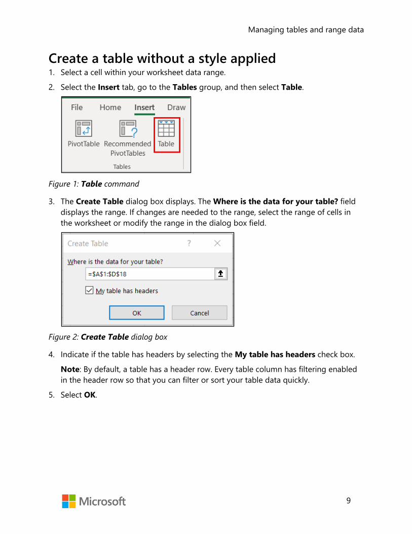
Managing tables and range data
9
Create a table without a style applied 1. Select a cell within your worksheet data range.
2. Select the Insert tab, go to the Tables group, and then select Table.
Figure 1: Table command
3. The Create Table dialog box displays. The Where is the data for your table? field displays the range. If changes are needed to the range, select the range of cells in the worksheet or modify the range in the dialog box field.
Figure 2: Create Table dialog box
4. Indicate if the table has headers by selecting the My table has headers check box.
Note: By default, a table has a header row. Every table column has filtering enabled in the header row so that you can filter or sort your table data quickly.
5. Select OK.

Managing tables and range data
10
Did you know?
You can insert a table by using the keyboard shortcut Ctrl+T.
Create a table with a style applied at the same time 1. Select the cell or the data range.
2. On the Home tab, go to the Styles group, and then select Format as Table.
Figure 3: Format as Table command
3. The Styles gallery appears with three categories of styles to choose from: light, medium, and dark.

Managing tables and range data
11
Figure 4: Format as Table Style Gallery
4. Place the cursor over a style and observe the live preview of this table style applied to the data range.
5. Select a style that is appropriate for the worksheet and overall workbook style. Some companies have specific branding to go with a logo.
6. In the Format as Table dialog box, set the cell range.

Managing tables and range data
12
7. Indicate whether the table has headers by selecting the My Table has headers check box.
8. Select OK.
Video
To review the video on creating a formatting table, go to: Create a table
When a cell in a table is selected, by design, the Table Tools Design contextual ribbon displays. The application indicates a table has been selected, and it presents all the Table commands in one ribbon. This makes it convenient for you to customize table styles, table options, and other formatting quickly.
For now, let’s focus on the Table Styles group.
Figure 5: Table Styles group
If the table created doesn’t already have a style applied or you need to change the current style that has been applied, you can select a new style from the Table Styles group; for example, you know your boss dislikes purple and you want to select another color. To change the style:
• Select Row 1 of n button to view the gallery styles row-by-row or select the More button to display the entire gallery at once. Note that the value of n might vary based on the number of rows in your table.
• Select a style to update the table.
Figure 6: Table Styles gallery
Note when you select a cell outside of the table area, the Design ribbon disappears.

Managing tables and range data
13
Did you know?
Data tables are part of a suite of What-If Analysis commands. Go to: Calculate multiple results by using a data table for more information.
Activity: Tell a story Get ready for a story shared by your teacher about the challenges of organizing data. This activity includes a group discussion and teacher-led demonstration of converting a data range into a table and applying a style. In this activity, your teacher will tell a story to highlight how turning a data range into a table can help with data analysis. You’ll participate in a group discussion on how the process of creating a table with the Table command differs from the Format as Table command.
Resources required You will need the following resources for this activity:
• Open L1_T1_act_crop_distribution_starter.xlsx in this lesson’s Learning Activity Resources.
Activity instructions Participate in the activity by following these instructions:
1. Observe the workbook the teacher has opened.
2. Ask clarifying questions.
3. Answer questions asked by the teacher.
4. Participate in the group discussion.

Managing tables and range data
14
Try-it: Format data as a table and change the table style
Crop harvesting at Munson’s is a fast-paced process. Munson’s does an excellent job of capturing information about when the crop was picked, by what team, and where the crop goes from there through distribution. You need quick ways to get answers to questions such as what fruit was shipped to our community-supported agriculture shareholders last month? For this and other sorting and filtering capabilities, you need to convert the data range into a table and then apply a style.
In this leveled try-it, you will discover how converting a data range into a table helps you organize data quicker and allows for different formats to be applied.
Try-it Resources You will need the following resources for this try-it:
• Open the L1_T1_try1_crop_distribution_starter.xlsx file in this lesson’s Learning Activity Resources.
• Select the CSA worksheet.
Instructions The following are the general tasks that you need to perform during this try-it:
1. Navigate to the CSA worksheet.
2. Convert the data range into a table.
3. Select any cell in the data range.
4. Format the data range as a table.
5. Select a style from the Style gallery categories (Light, Medium, or Dark).
6. Don’t forget to save your work!
If you are confident your solution file is complete for this exercise and have time to attempt the next try-it, leave the solution file open. It should be the same as the Try-it 2 starter file.

Managing tables and range data
15
Try-it 2 Resources You will need the following resources for this try-it:
• Open the L1_T1_try2_crop_distribution_starter.xlsx file in this lesson’s Learning Activity Resources.
Instructions The following are the general tasks that you need to perform during this try-it:
1. Navigate to the Processing worksheet.
2. Convert the data range, cells A1 to F21, into a table.
3. Select any cell in the data range.
4. Insert a table.
5. Apply a style from the Styles gallery categories (Light, Medium, or Dark).
6. Don’t forget to save your work!
Topic 2: Convert a table to a range Sometimes a table is no longer needed to represent groups of data in a meaningful
way. While working on a group project, you might have inherited an Excel table that your team member has created. You like the style formatting that was applied to the table but just need a range that can still be sorted and filtered. You can convert a table back to a range of data while retaining the table style without the table functionality.
To convert a table to a range of data:
1. Select any cell in the table, go to the Table Tools Design ribbon, and then select Tools group.
2. Select Convert to Range. Alternatively, right-click or access the context menu, and then from the context menu, select Table > Convert to Range.
Figure 7: Convert to Range command

Managing tables and range data
16
Note table features are no longer available. The row headers no longer include the sort and filter arrows.
Activity: Pose a challenge The teacher poses a challenge to you: find a way to take the table created in the last topic activity and convert it back to a range. You’ll participate in a group discussion to examine the options for converting a table back to a range. You’ll then follow the teacher in a teacher-led demonstration.
Resources required You will need the following resources for this activity:
• Open the L1_T2_act_crop_distribution_starter.xlsx file.
Activity instructions 1. Go to the Crop_Sourcing worksheet.
2. Work with a fellow student to figure out how to convert the Crop Sourcing table back to a data range.
3. Here are some clues to get help with this challenge:
o Observe the available table ribbon commands. o Enter keywords, such as convert range, in the Tell me what you want to do field. o Use the F1 key to get help or go to the File tab and select Help (question mark
icon). o Ask the teacher or other students questions for additional help.
Try-it: Convert a table to a range While working on your group project, you discover that you no longer need the
table format for the data, but you want to keep the style of the table. You need to convert the table back to a range.
In this stand-alone try-it, you will apply your learning and see for yourself how you can convert a table back to a range.
Resources You will need the following resources for this try-it:
• Open the L1_T2_try_crop_distribution_starter.xlsx file in this lesson’s Learning Activity Resources.

Managing tables and range data
17
Instructions The following are the general tasks that you need to perform during this try-it:
1. Go to the Processing worksheet.
2. Convert the table to a range.
3. Don’t forget to save your work!
Wrap-up In the previous lesson, you learned how to apply styles to worksheet cells and remove formatting from worksheet cells. This lesson relates how similar formatting can be applied to a range of cells by formatting these as a table. With the help of the Format as Table and Table commands, you learned about two different processes to accomplish this. The Format as Table command creates a table and applies a style at the same time. The Table command creates a table only, and a style can be applied later.
You also learned that when a table is no longer needed, it can be converted back to a range with the help of the Convert to Range command within the Table Tools Design ribbon.
All the tools you learned in this lesson can help you quickly create a table and go back to a range as needed.
Use these questions to check what you learned in this lesson:
1. Which command creates a table and simultaneously applies a table style?
Select the correct option.
a. Insert Table
b. Data Table
c. Format as Table
d. From Table/Range
2. Which ribbon tab contextually appears when a cell in a table is selected?
Select the correct option.
a. Format
b. Analyze
c. Design
d. View

Managing tables and range data
18
3. Which of the following options are table style categories?
Select all that apply.
a. Light
b. Standard
c. Dark
d. Custom
4. A _____________________ row is automatically included by default when a table is inserted.

Managing tables and range data
19
Lesson 2: Configuring table format options Overview In this lesson, you will configure table options, including inserting a header row, table rows, table columns, and a table total row, adding a banded row effect, and removing rows and columns.
Warm-up In the previous lesson, you learned how to create a table from a range and how to convert a table back to a range. This was a great start to working with ranges and tables.
In this lesson, you will learn how to configure table format options and insert and manage rows, columns, and a total row.
Get ready for discussions and step-by-step demonstrations, along with opportunities to put to practice what you learn along the way. But first, check how well you know the prerequisite concepts needed to follow this lesson.
Use these questions to find out what you already know about this lesson’s topics:
1. What are the steps you need to take to turn the Filter button on or off?
Select all that apply.
a. Go to the Design tab, Table Styles Options group, and then select/clear theFilter button.
b. Go to the Home tab, Editing group, Sort & Filter, and then select Filter.
c. Go to the Data tab, Sort & Filter group, and then select Filter.
d. With a table cell selected, right-click or access the context menu, select Filter,and then select either Clear Filter from, or Reapply.

Managing tables and range data
20
2. Which table row calculates numeric data by using functions?
Select the correct option.
a. Header row
b. Total row
c. Banded row
d. Footer row
3. _____________________ are even rows that are formatted differently than odd rows.
4. The command _____________________ provides a way to select additional rows and columns to include in an existing table.
Topic 1: Configure table style options In the previous lesson, you learned how to quickly create a table with a predefined
table style.
Sometimes a predefined style isn’t enough. Imagine you have a table that tracks all the school fundraisers, including the name of the fundraiser, which school club ran it, fundraiser date, and how much money each one made. You need to emphasize the money column. With the Style Options group of commands, you can adjust options for table elements. Selecting the Last Column box in the Table Styles Options group of the Table Tools Design ribbon makes the money column (last column) bold. Other table elements such as Header and Total Rows, First Column, Banded Rows and Columns, as well as Auto Filtering can be enabled or disabled as well.
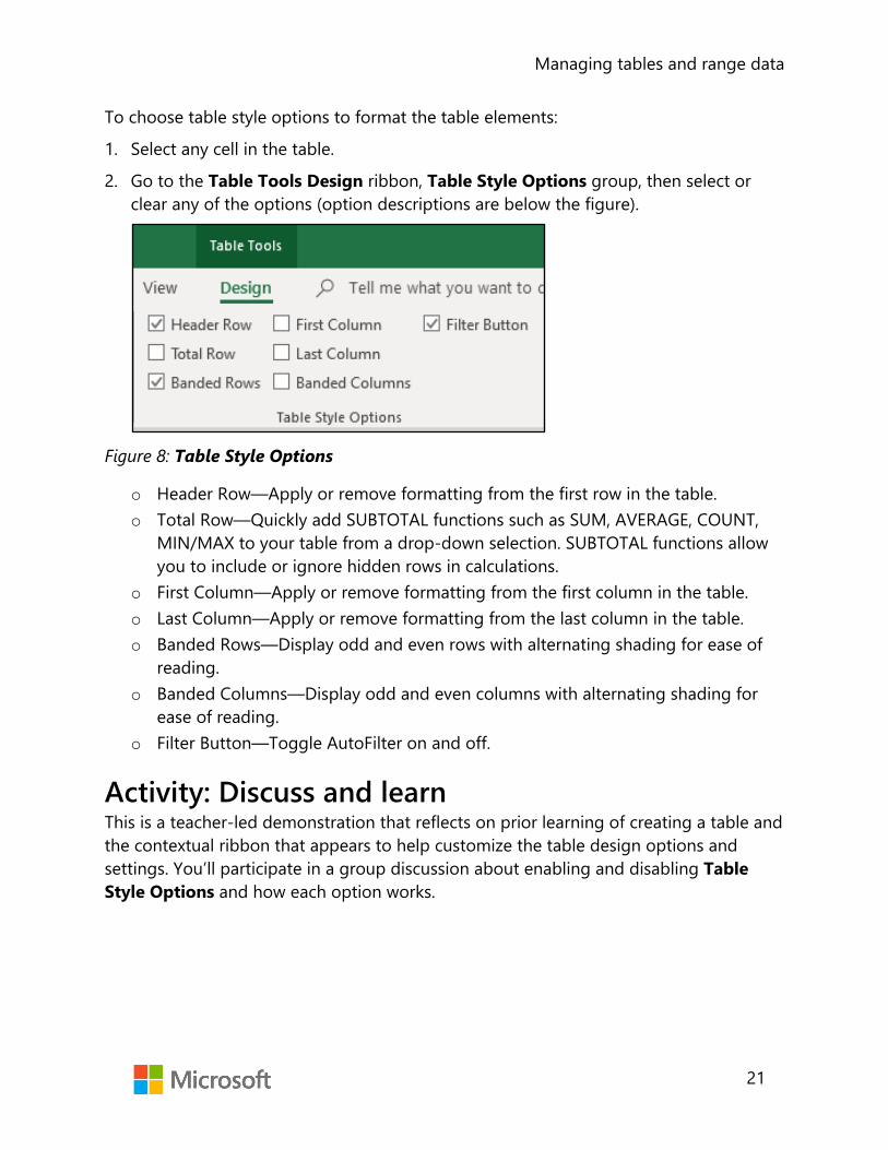
Managing tables and range data
21
To choose table style options to format the table elements:
1. Select any cell in the table.
2. Go to the Table Tools Design ribbon, Table Style Options group, then select or clear any of the options (option descriptions are below the figure).
Figure 8: Table Style Options
o Header Row—Apply or remove formatting from the first row in the table. o Total Row—Quickly add SUBTOTAL functions such as SUM, AVERAGE, COUNT,
MIN/MAX to your table from a drop-down selection. SUBTOTAL functions allow you to include or ignore hidden rows in calculations.
o First Column—Apply or remove formatting from the first column in the table. o Last Column—Apply or remove formatting from the last column in the table. o Banded Rows—Display odd and even rows with alternating shading for ease of
reading. o Banded Columns—Display odd and even columns with alternating shading for
ease of reading. o Filter Button—Toggle AutoFilter on and off.
Activity: Discuss and learn This is a teacher-led demonstration that reflects on prior learning of creating a table and the contextual ribbon that appears to help customize the table design options and settings. You’ll participate in a group discussion about enabling and disabling Table Style Options and how each option works.

Managing tables and range data
22
Resources required You will need the following resources for this activity:
• Open L2_T1_act_crop_distribution_starter.xlsx
Activity instructions Participate in the activity by following these instructions:
1. You and your teacher will open the same L2_T1_act_crop_distribution_starter.xlsx starter file and examine the table formatting in the Crop_Sourcing worksheet.
2. Your teacher will also demonstrate how to make Table Style Option changes and lead a group discussion.
Try-it: Configure table style options In this stand-alone try-it, you will apply your learning and see for yourself how you
can apply style options to an existing table.
Resources You will need the following resources for this try-it:
• Open L2_T1_try_crop_distribution_starter.xlsx in this lesson’s Learning Activity Resources.
Instructions The following are the general tasks that you need to perform during this try-it:
1. Go to the Processing worksheet.
2. Select any cell within the table.
3. Enable the table header row.
4. Observe the filters in the header row.
5. Emphasize the first column of the table.
6. Observe the formatting change for the first column.
7. Emphasize the last column of the table.
8. Observe the formatting change for the last column.
9. Save your work.

Managing tables and range data
23
Topic 2: Insert and manage rows, columns, and the total number of rows
After you create an Excel table, you can add or remove rows and columns by using different methods, which include:
• Using the Resize command • Entering text or numbers in a cell just below the last row or to the right of the last
column • Pasting data into a cell • Inserting rows or columns between existing rows or columns
Use the Resize command 1. Select any cell within a table in an Excel worksheet.
2. Go to the Table Tools Design ribbon, the Properties group, and then select Resize Table.
Figure 9: Resize Table command
3. Select the range you want to include, starting with the upper left-most cell.

Managing tables and range data
24
4. In the following example, the original table includes the range, A1:G4.
Figure 10: Original table
o After resizing to add additional columns and rows, the table includes the range, A1:H4.
Figure 11: Updated table
Enter data • To add a row to a table, start entering data in a cell below the last table row. The
table expands to include the new row. • To add a column to the right of the table, start entering text or numbers in a cell to
the right of the last column.
Paste data • To add a row, paste the data in the left-most cell below the last table row. • To add a column, paste the data to the right of the table’s right-most column. • If the data pasted has as many or fewer columns than the table, the table expands to
include all the cells in the range pasted. • If the data pasted has more columns than the table, the extra columns are not
included as part of the table. You will need to use the Resize command to expand the table to include the data.

Managing tables and range data
25
Insert data To insert a row:
1. Pick any cell that is not part of the header row and right-click or access the context menu.
2. Select Insert, and then select Table Rows Above.
Figure 12: Context menu—Insert Table Row command

Managing tables and range data
26
Note: If the selection is in the last row, Table Rows Above or Table Rows Below can be selected.
To insert a column 1. Pick any cell in the table and right-click or access the context menu.
2. Select Insert, and then select Table Columns to the Left.
Figure 13: Insert a column

Managing tables and range data
27
Delete rows or columns in a table Table rows and columns can be deleted from the Home ribbon or the right-click context menu.
From the Home ribbon 1. Select the table rows or table columns.
2. Go to the Home ribbon, Cells group, and select the arrow next to the Delete command. Then, select Delete Table Rows or Delete Table Columns.
Right-click context menu 1. Select the table rows or table columns.
2. Right-click or access the context menu, and then select Table Columns or Table Rows.
Total Row A Total Row can be displayed at the end of the table. By default, it uses the SUBTOTAL function to display a total of the numeric data in a column. Instead of manually inserting a formula or function to calculate ticket sales for a school play or sports game, by checking the Total Row box in the Style Options group, Excel quickly calculates the total for you. In the last topic, you applied style options to a table such as a header row, banded rows and columns, and a filter button. Another command called Total Row is also a command that is part of the Table Style Options.
Video
To review the video on how to total numeric data in a table, go to: Add a total row to a table
To enable a total row at the end of a table:
1. Select a cell within the table.
2. Go to the Design Table Tools ribbon, the Table Style Options group, and select the Total Row box.
3. The Total Row is inserted at the bottom of the table.
4. The default Total Row setting uses the SUBTOTAL function for SUM. This is a Structured Reference formula and is exclusive to Excel tables. You can also apply a different function to the total value by selecting the More Functions option or by writing your own.
Managing tables and range data
28
Additional information
To expand your learning, discover how to use structured references in tables by going to: Using structured references with Excel tables
Did you know?
There is a keyboard shortcut for the Total Row command.
Use the Ctrl+Shift+T keyboard shortcut to add a total row at the bottom of a table.
Activity: Discuss and learn This is a teacher-led group discussion and demonstration building on learning from a previous topic about how to insert and delete columns and rows in a data range. Students will be able to compare what they previously learned about working with data ranges with the process of inserting and deleting columns, rows, and a total row in a table.
Resources required You will need the following resources for this activity:
• Open L2_T2_act_crop_distribution_starter.xlsx in this lesson’s Learning Activity Resources.
Activity instructions Participate in the activity by following these instructions.
Your teacher will project a workbook that contains a data range and a table and will ask for your help with adding and removing columns and rows.
1. Examine the workbook data range and table.
2. When asked by the teacher, suggest how to add columns, rows, and a total row.
3. When asked by the teacher, suggest how to remove columns and rows.

Managing tables and range data
29
Try-it: Insert and manage rows, columns, and total number of rows
A Munson’s colleague has updated the Processing worksheet to include row totals for each crop item. You need to insert a column for notes and include a total row to display the average total.
Resources You will need the following resources for this try-it:
• Open L2_T2_try_crop_distribution_starter.xlsx in this lesson’s Learning Activity Resources.
Instructions The following are the general tasks that you need to perform during this try-it:
1. Go to the Processing worksheet.
2. Select cell E2.
3. Insert a table column to the left.
4. Observe the table. The new column has been inserted.
5. In cell E1, replace the text, Column1, with Notes.
6. Add a total row to the table.
7. Observe the table. A total row has been added in Column H.
8. Change the table total to display an average total.
9. Now you have a total row with the average displayed for all numeric values in the Total column displayed.
10. Don’t forget to save your work!

Managing tables and range data
30
Wrap-up In the previous lesson, you learned how to create a table from a range and how to convert a table back to a range. This was a great start to working with ranges and tables.
In this lesson, you learned how to configure table format options and insert and manage rows, columns, and a total row.
All the tools you learned in this lesson can help you quickly apply formatting to a variety of table layouts.
Use these questions to check what you learned in this lesson:
1. What keyboard shortcut can you use to turn on or turn off a Total Row at the end of the table?
Select the correct option.
a. Ctrl+F
b. Ctrl+Shift+T
c. Ctrl+Shift+F
d. Ctrl+T
2. On which tab can you find the Insert Sheet Columns and Insert Sheet Rows commands?
Select the correct option.
a. Page Layout
b. Insert
c. Home
d. View
3. The _____________________ check box displays special formatting for the first column of the table.
4. _____________________ are even columns formatted differently than odd columns.

Managing tables and range data
31
Lesson 3: Naming tables and ranges Overview In this lesson, you will give ranges and tables unique names, making it easier for navigation and referencing within a workbook.
Warm-up In the previous lesson, you learned how to configure table format options.
In this lesson, you will learn how to change the default name assigned to a table to something more meaningful to the data included. You will also learn how to name a range of cells.
Use these questions to find out what you already know about this lesson’s topics:
1. A range can be named in the Name Box.
Select the correct option.
a. True
b. False
2. Which of the following options cannot be part of a range name?
Select the correct option.
a. Space
b. Number
c. Period
d. Underscore

Managing tables and range data
32
3. What is the default name for a new table?
Select the correct option.
a. Table_1
b. Table 1
c. Table.1
d. Table1
4. A table name can have up to _____________________ characters.
Topic 1: Name a table You may recall from earlier lessons that each time you create a new workbook,
Excel assigns a default name to the workbook according to this naming convention: Book1, Book2, Book3, and so on.
When a new worksheet is added to a workbook, Excel assigns a default name to the worksheet according to this naming convention: Sheet1, Sheet2, Sheet3, and so on.
A newly added table is no different. Each time you create a table, Excel assigns a default name to the table according to this naming convention: Table1, Table2, Table3, and so on.
Let’s say you have a workbook that tracks how much money you make with a part-time job. Sheet1 or Table1 doesn’t help you understand which month’s pay it is. Naming it January or January_Pay can make a big difference!
As the previous example illustrated, to make it easier for reference purposes, you can change a table name to something more meaningful as it applies to the table data.
Before you rename a table, here are the rules you must follow:
• Use valid characters. Always begin a name with a letter; an underscore character (_); or a backslash (\). Use letters, numbers, periods, and underscore characters for the rest of the name. Exceptions: You can’t use “C”, “c”, “R”, or “r” for the name, because they’re already designated as a shortcut for selecting the column or row for the active cell when you enter them in the Name or Go To box.
• Don’t use cell references. Names can’t be the same as a cell reference, such as Z$100 or R1C1.
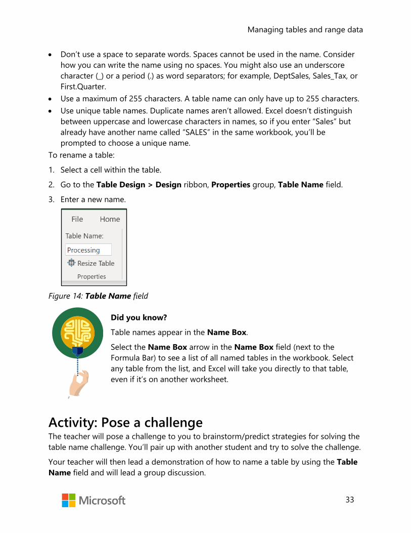
Managing tables and range data
33
• Don’t use a space to separate words. Spaces cannot be used in the name. Consider how you can write the name using no spaces. You might also use an underscore character (_) or a period (.) as word separators; for example, DeptSales, Sales_Tax, or First.Quarter.
• Use a maximum of 255 characters. A table name can only have up to 255 characters. • Use unique table names. Duplicate names aren’t allowed. Excel doesn’t distinguish
between uppercase and lowercase characters in names, so if you enter “Sales” but already have another name called “SALES” in the same workbook, you’ll be prompted to choose a unique name.
To rename a table:
1. Select a cell within the table.
2. Go to the Table Design > Design ribbon, Properties group, Table Name field.
3. Enter a new name.
Figure 14: Table Name field
Did you know?
Table names appear in the Name Box.
Select the Name Box arrow in the Name Box field (next to the Formula Bar) to see a list of all named tables in the workbook. Select any table from the list, and Excel will take you directly to that table, even if it’s on another worksheet.
Activity: Pose a challenge The teacher will pose a challenge to you to brainstorm/predict strategies for solving the table name challenge. You’ll pair up with another student and try to solve the challenge.
Your teacher will then lead a demonstration of how to name a table by using the Table Name field and will lead a group discussion.

Managing tables and range data
34
Resources required You will need the following resources for this activity:
• Open L3_T1_act_crop_distribution_starter.xlsx in this lesson’s Learning Activity Resources.
Activity instructions The teacher will lead a discussion about naming tables. Participate in the activity by following these instructions:
1. Listen to the instructions given by the teacher.
3. Apply critical thinking to find possible solutions to the challenge.
4. Share your solutions with the class.
Try-it: Name a table The Crop_Distribution workbook will be shared with many colleagues at
Munson’s once it's finalized. You realize the table you have been working with has the default name, Table3. You need to rename the table to something that more closely represents the data it contains. This will surely help everyone find and work with the table much quicker!
Resources You will need the following resources for this try-it:
• Open L3_T1_try_crop_distribution_starter.xlsx in this lesson’s Learning Activity Resources.
Instructions The following are the general tasks that you need to perform during this try-it:
1. Go to the Processing worksheet table.
2. Select a cell within the table.
3. Replace the current name, Table2, with ProcessedOrders.
4. Observe the named tables including the updated table name you just changed, ProcessedOrders.
5. Don’t forget to save your work!

Managing tables and range data
35
Topic 2: Define a named range In the previous topic, you named a table. You can also name a range of cells.
Naming a range can be useful for quickly navigating to the range from the Name Box or Go To command. It can also help simplify the process of referencing cells in a formula.
• There are a several ways to name a range of cells. Before you try naming a range, here are the naming rules you must follow: o Use valid characters. Always begin a name with a letter; an underscore character
(_); or a backslash (\). Use letters, numbers, periods, and underscore characters for the rest of the name. Exceptions: You can’t use “C”, “c”, “R”, or “r” for the name, because they’re already designated as a shortcut for selecting the column or row for the active cell when you enter them in the Name or Go To box.
o Don’t use cell references. Names can’t be the same as a cell reference, such as Z$100 or R1C1.
o Don’t use a space to separate words. Spaces cannot be used in the name. Consider how you can write the name using no spaces. You might also use an underscore character (_) or a period (.) as word separators; for example, DeptSales, Sales_Tax or First. Quarter.
o Use a maximum of 255 characters. A range name can only have up to 255 characters.
o Use unique range names. Duplicate names aren’t allowed. Excel doesn’t distinguish between uppercase and lowercase characters in names, so if you enter “Sales” but already have another name called “SALES” in the same workbook, you’ll be prompted to choose a unique name.
• There are several different commands you can use to name a range. Let’s start with the Name Box. Name a range with the Name Box:
a. Select the range you want to name.
b. Select the Name Box.
c. Type or input a name and press Enter.

Managing tables and range data
36
Figure 15: Name Box field
• Next, let’s work with the Create from Selection command. Name a range with the Create from Selection command:
a. Select the range you want to name, including the row or column labels.
b. Select the Formulas ribbon, Defined Names, and then select Create from Selection.
c. In the Create Names from Selection dialog box, select the check boxes depending on the location of your row/column header.
d. If you have only a header row at the top of the table, just select Top row.
e. If you have a top row and left column header, select Top row and Left column options, and so on.
f. Select OK.
g. Names are automatically selected and applied based on the column or row labels.
• The Define Name command is another way to give a range a name. Name a range with Define Name:
a. Select the range you want to name.
b. Go to the Formulas tab, Defined Names group, and select Define Name. Alternatively, right-click or access the context menu, and select Define Name.
c. In the New Name dialog box, Name field, enter a name.
d. The Scope field is set to Workbook by default. This means the named range is accessible from a worksheet of the workbook. If it only needs to be accessible from a specific worksheet, select the arrow, and from the drop-down list select the name of the worksheet.
e. Add an optional comment about this range in the Comment field.

Managing tables and range data
37
f. The Refer to field displays the worksheet and range specified. If the range needs to be updated, select this field.
g. Enter text or numbers in the field or select new cells to update.
h. If the New Name dialog box is in the way of the range, select the arrow within this field to collapse the dialog box.
i. Select the arrow again to expand the dialog box.
j. Select OK.
• The Name Manager command is one other method to create a named range. Define a range name with the Name Manager:
a. Select the range you want to name.
b. Go to the Formulas tab, Defined Names group, and select Name Manager.
c. In the New Name dialog box, in the Name field, type or input a name.
d. The Scope field is set to Workbook by default. This means the named range is accessible from a worksheet of the workbook. If it only needs to be accessible from a specific worksheet, select the arrow, and from the drop-down list select the name of the worksheet.
e. Add an optional comment about this range in the Comment field.
f. The Refer to field displays the worksheet and range specified. If the range needs to be updated, select this field. Enter the cell references in the field or select new cells to update. If the New Name dialog box is in the way of the range, select the arrow within this field to collapse the dialog box. Then select the arrow again to expand the dialog box.
g. Select OK.
Edit and delete named ranges • Named ranges cannot be managed through the Name Box area. If a named range
needs to be updated or deleted, use the Name Manager command. To edit a named range:
a. Go to the Formulas tab, select the Defined Names group, and select Name Manager.
b. In the Name Manager dialog box, select the named range from the list.
c. Select the Edit button.

Managing tables and range data
38
d. Make the necessary changes to the Name, Scope, Comment, and Refers To fields.
e. Select OK.
f. Select Close.
• Here’s how to delete a named range: a. Go to the Formulas tab, select the Defined Names group, and select Name
Manager.
b. In the Name Manager dialog box, select the named range from the list.
c. Select the Delete button.
d. A question displays asking if you are sure you want to delete the named range. Select OK.
e. Select OK again.
f. Select Close.
Additional information
For more information on inserting a named range in a formula, go to: Insert a named range into a formula in Excel
Video
• Use the Video quick part if you are inserting videos. • Use the following boilerplate text to introduce a link/video: To review the video on defining and using names in formulas, go to: Define and use names in formulas
Activity: Discuss and learn This is a teacher-led demonstration and group discussion to help you build on the previous learning about naming a table and how naming cell ranges has a similar process and naming convention.

Managing tables and range data
39
Resources required You will need the following resources for this activity:
• Open L3_T2_act_crop_distribution_starter.xlsx in this lesson’s Learning Activity Resources.
Activity instructions Your teacher will demonstrate how to name a table with the Table Name field and name a range of cells with the Name Box field, Create from Selection command, Define Name command, and Name Manager command. You will also observe how to edit and delete named ranges with the Name Manager command.
Participate in the activity by following these instructions:
1. Open the Crop_Distribution workbook.
2. Get familiar with the workbook contents, worksheets, and named areas: tables, cells, and cell ranges.
3. Observe the demonstration and discussion of renaming a table led by the teacher.
4. Participate in the group discussion.
Try-it: Define a named range You have a table that has been converted to a range. You want to make it easier
for everyone working with this data range in the future by naming the range. You need to apply a descriptive name to the range.
Try-it 1 In this stand-alone try-it, you will apply a name to a range of cells.
Resources You will need the following resources for this try-it:
• Open L3_T2_try_crop_distribution_starter.xlsx in this lesson’s Learning Activity Resources.
Managing tables and range data
40
Instructions The following are the general tasks that you need to perform during this try-it:
1. Go to the Processing worksheet.
2. Select the cell range A2:G21.
3. Name the range: ProcessedOrders.
4. Go to another worksheet within the Crop_Distribution workbook.
5. Observe the named ranges and named tables.
6. Select ProcessedOrders from the list.
7. Observe the area it takes you to and that is selected.
8. Don’t forget to save your work!
Wrap-up In the previous lesson, you learned how to configure table format options and insert and manage rows, columns, and a total row.
In this lesson, you learned how to update the name of a table to something more meaningful for the data it represents. You also learned how to give a range of cells a meaningful name. Giving tables and ranges of cells names can help workbook readers quickly navigate to the associated data. Named ranges can also be used in formulas.
Use these questions to check what you learned in this lesson:
1. Which of the following fields create a named range?
Select all that apply.
a. Name Box
b. Create from Selection
c. Define Name
d. Name Manager
2. You can name a range with a right-click or using the context menu.
Select the correct option.
a. True
b. False

Managing tables and range data
41
3. The _____________________ command is where a named range can be created, edited, and deleted.
4. You can access a table from which of the following areas?
Select all that apply.
a. Find
b. Name Box
c. Go To
d. Selection Pane

Managing tables and range data
42
Lesson 4: Sorting and filtering Overview In this lesson you will sort and filter records in a data range and table.
Warm-up In the previous lesson, you learned how to update a table name and name a range of cells. In this lesson, you will learn how to sort and filter data in cell ranges and tables.
Use these questions to find out what you already know about this lesson’s topics:
1. Which command displays data in an alphabetized or numerical order?
Select the correct option.
a. Filter
b. Sort
c. Replace
d. Arrange All
2. Which command provides a way to sort with multiple levels?
Select the correct option.
a. Custom Sort
b. Sort A to Z
c. Sort Z to A
d. Sort Smallest to Largest
e. Sort Largest to Smallest
3. A filter based on cell color can be applied to a column.
Select the correct option.
a. True
b. False
4. A _____________________ is created to sort by any other characteristic that doesn’t sort well alphabetically.

Managing tables and range data
43
Topic 1: Sort and filter records You’re a farmer, and you sell honey at the local farmers market. Well, you didn’t sell
the honey in the past, but your enterprising daughter did before she went off to college. Now that you are doing it, you’ve been trying to organize everything. After entering all the sales receipts into an Excel spreadsheet, you see that there is no organization to the sales. You’d like to sort the receipts in a variety of ways. First, you’d like to sort these by honey categories—wildflower, orange blossom, and clover—to understand which varieties are the favorites among the local community. Next, you’d like to filter transactions with multiple sales in chronological order to determine changes to the upcoming sales promotions that you have to approve.
What do you do? Sort and filter.
Depending on the data arrangement orientation, you can sort columns or rows to display text such as names or companies in alphabetical order or numbers from largest to smallest.
There may be times that sorting isn’t enough; there’s just too much data in the worksheet to figure out the answers to the questions you have about the data. For this or similar situations, filtering can help. You can choose which data to temporarily hide for a column or multiple columns.
Sorting options depend on the contents of the column or row selected. If it contains a text string, the sorting options will be A to Z (ascending order) or Z to A (descending order). If it contains a numeric string, the sorting options will be smallest to largest number or largest to smallest number.
While cell range and table columns and rows have the same sort and filter capabilities (also called AutoFilter) and the process is similar, it’s worth going over the steps for each.

Managing tables and range data
44
Sort a cell range column in ascending or descending order 1. Select a cell in the column you want to sort.
2. Right-click or access from the context menu, select Sort, and then:
a. To sort an alpha text string, select Sort A to Z or Sort Z to A. You may also go to the Home ribbon, Editing group, select Sort & Filter, and select Sort A to Z or Sort Z to A.
b. To sort a numeric string, select Sort Smallest to Largest or Sort Largest to Smallest. You may also go to the Home ribbon, Editing group, select Sort & Filter and Sort Smallest to Largest or Sort Largest to Smallest.
Note: When a column is sorted, the related information in the other columns moves as well.
Change the Sort Options Orientation for a data set Most data sets are arranged in a column layout with labels defining the information in each column. For this reason, the default setting for sorting orientation is to sort top to bottom. If the data set you are working with is a row labeled layout, you will need to change the Sort Options Orientation.
1. Go to the Home ribbon, Editing group.
2. Select Sort & Filter, and then select Custom Sort.
3. In the Sort Options dialog box Orientation section, select the Sort left to right option.
4. Select OK.
Sort a table column in ascending or descending order 1. Locate the Filter command next to the column label you want to sort. If the Filter
command is not present, go to the Table Tools Design ribbon, Table Style Options group, and check the Filter Button box.
2. Select the Filter command. From the context menu, if sorting text, select Sort A to Z or Sort Z to A. If sorting numbers, select Sort Smallest to Largest or Sort Largest to Smallest.

Managing tables and range data
45
Did you know?
• If fill colors have been applied to cells, sort by color can also be selected.
When a table column is sorted, the related information in the other columns moves as well. If fill colors have been applied to cells, the sort by color option can be selected.
Additional information
For more information about sorting and filtering data by color, go to: Guidelines and examples for sorting and filtering data by color
Filter a cell range column 1. Select a cell within the range.
2. Locate the column you want to sort. If the Filter option is not available in the column header row, go to the Table Tools Design ribbon, the Table Style Options group, and then select the Filter box.
3. Select the column Filter command.
4. Select Text Filters or Number Filters, and then select a comparison like Between.

Managing tables and range data
46
Figure 16: Table Number Filters context menu
5. Enter the filter criteria and select OK.
Video
To review the video on sorting and filtering records, go to: Sorting and filtering data

Managing tables and range data
47
Filter a table column When you put your data in a table, filter controls are automatically added to the table headers.
1. Select the column Filter option from the column you want to filter. If someone working in the table has previously turned the filter off, go to the Table Tools Design ribbon, the Table Style Options group, and select the Filter box.
2. Clear (Select All) and select the boxes you want to show.
3. Select OK.
4. The column Filter command icon changes, indicating that not all data is displayed in this column. Select this icon to change or clear the filter.
Video
To review the video on filtering data go to: Filter data in a range or table
Clear a filter from a column Select the Filter button next to the column header, and then select Clear Filter from the context menu<column name>.

Managing tables and range data
48
Figure 17: Clear Filter command
Clear all filters in a worksheet Navigate to the Data tab and then select Clear.
Figure 18: Clear command
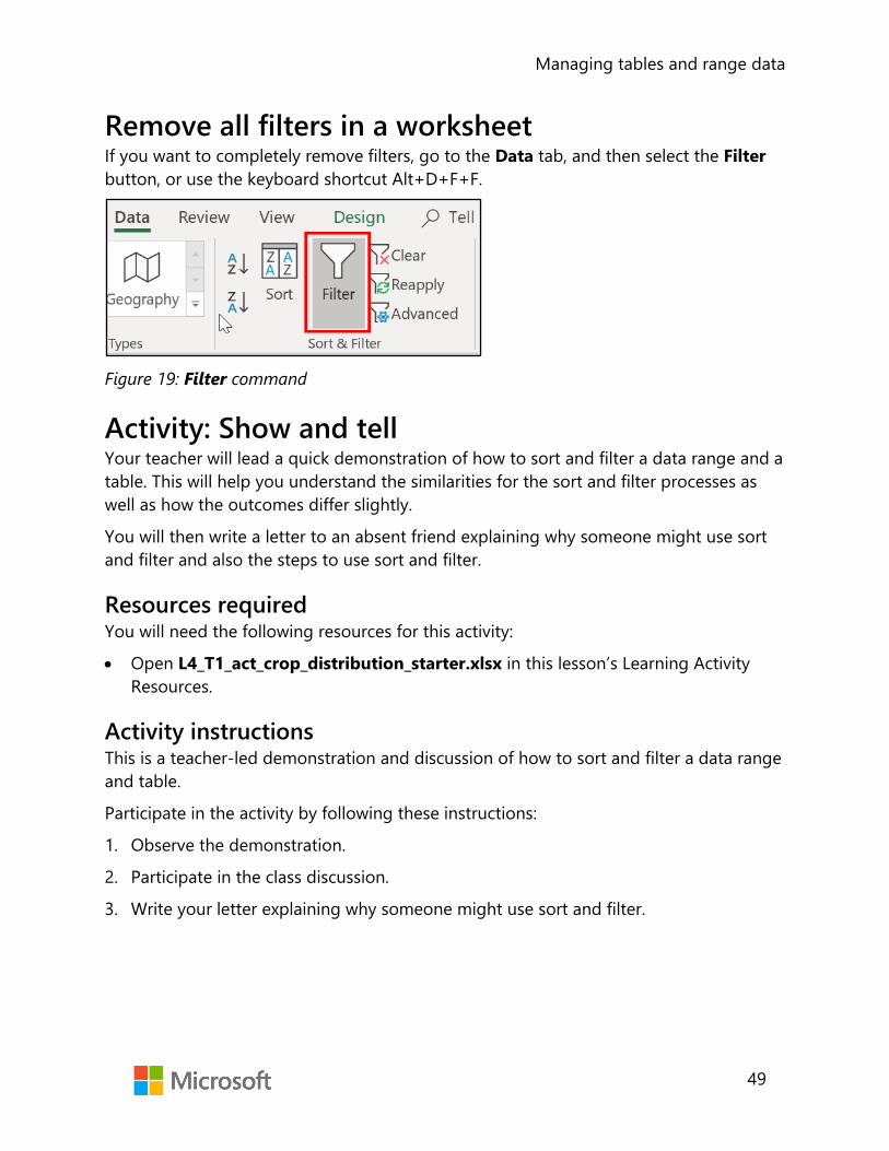
Managing tables and range data
49
Remove all filters in a worksheet If you want to completely remove filters, go to the Data tab, and then select the Filter button, or use the keyboard shortcut Alt+D+F+F.
Figure 19: Filter command
Activity: Show and tell Your teacher will lead a quick demonstration of how to sort and filter a data range and a table. This will help you understand the similarities for the sort and filter processes as well as how the outcomes differ slightly.
You will then write a letter to an absent friend explaining why someone might use sort and filter and also the steps to use sort and filter.
Resources required You will need the following resources for this activity:
• Open L4_T1_act_crop_distribution_starter.xlsx in this lesson’s Learning Activity Resources.
Activity instructions This is a teacher-led demonstration and discussion of how to sort and filter a data range and table.
Participate in the activity by following these instructions:
1. Observe the demonstration.
2. Participate in the class discussion.
3. Write your letter explaining why someone might use sort and filter.

Managing tables and range data
50
Try-it: Sort and filter records Your boss at Munson’s has asked about orders placed by Liberty’s Delightful Sinful
Bakery & Café. You need to filter the Processing_Range worksheet to only display orders from this buyer.
In this stand-alone try-it, you will work with a partner to sort and filter data in a table.
Resources You will need the following resources for this try-it:
• Open L4_T1_try_crop_distribution_starter.xlsx in this lesson’s Learning Activity Resources.
Instructions The following are the general tasks that you need to perform during this try-it:
1. Go to the Processing worksheet.
2. Sort the Crop column in A to Z order.
3. Filter the Buyer column to display Liberty’s Delightful Sinful Bakery & Café only.
4. Don’t forget to save your work so that it is filtered when your boss opens it!
Topic 2: Perform a custom sort
Video
To review the video on sorting a table, go to: Sort data in a range or table
Sorting data is an integral part of data analysis. Imagine you are tracking a list of birthday party invite responses. You can arrange a list of names in alphabetical order, compile a list of guests each invitee is bringing, and sort these numbers from the highest to the lowest. You can even order rows by colors or icons assigned to special guests. Sorting data helps you quickly visualize and understand your data better, organize and find the data that you want, and make more effective decisions.

Managing tables and range data
51
Text can be sorted alphabetically in ascending or descending order (A to Z or Z to A); numbers can also be sorted in ascending or descending order (smallest to largest or largest to smallest); and dates and times can be sorted in ascending or descending order (oldest to newest and newest to oldest) in one or more columns.
Sort text 1. Select a cell in the column you want to sort.
2. On the Data tab, in the Sort & Filter group, do one of the following:
o To quick sort in ascending order, select (Sort A to Z). To quick sort in descending order, select (Sort Z to A).
Figure 20: Sort commands
• If a table filter has been enabled, you can also select the Filter command for a column and then select a quick sort in ascending Sort A to Z; descending Sort Z to A; or select sort by Color Custom Sort.

Managing tables and range data
52
Figure 21: Filter context menu Sort commands
Did you know?
If there is a mix of data stored as text and numbers in a column, you can access the Format Cells dialog box with the keyboard shortcut, Ctrl+1. Then you can select the Number tab, General Category, and select Number or Text.
Sort numbers 1. Select a cell in the column you want to sort.
2. On the Data tab, in the Sort & Filter group, do one of the following:
o To sort from low to high, select Sort Smallest to Largest. o To sort from high to low, select Sort Largest to Smallest.

Managing tables and range data
53
Figure 22: Sort commands
If a table filter has been enabled, you can also select the Filter command for a column and then select a quick sort. To sort from low to high, select (Sort Smallest to Largest); from high to low (Sort Largest to Smallest); or Sort by Color (Custom Sort).
Figure 23: Filter context menu Number Sort commands
Sort dates and times 1. Select a cell in the column you want to sort.
2. On the Data tab, in the Sort & Filter group, do one of the following:
o To sort from an earlier to a later date or time, select Sort Oldest to Newest. o To sort from a later to an earlier date or time, select Sort Newest to Oldest.

Managing tables and range data
54
Figure 24: Sort commands
If a table filter has been enabled, you can also select the Filter command for a column and then select a quick sort. To sort from an earlier to a later date or time, select (Sort Smallest to Largest); from a later to an earlier date or time, select (Sort Largest to Smallest); or Sort by Color (Custom Sort).
Figure 25: Filter context menu Sort commands

Managing tables and range data
55
Did you know?
• Extra leading spaces from imported data can affect sorting. The TRIM function can remove all leading spaces.
To review an article on how to use the TRIM function, go to: TRIM Function
Sort by more than one column You may want to sort by more than one column or row when you have data that you want to group by the same value in one column or row, and then sort another column or row within that group of equal values. For example, if you have a School club column and a Student column, you can first sort by School club (to group all the students in the same school club together) and then sort by name (to put the names in alphabetical order within each school club). You can sort by up to 64 columns. For best results, the range of cells that you sort should have column headings.
1. Select any cell in the table.
2. On the Data tab, in the Sort & Filter group, click Sort.
3. In the Sort dialog box, under Column, in the Sort by box, select the first column that you want to sort.
4. Under Sort On, select the type of sort. Do one of the following:
o To sort by text, number, or date and time, select Values. o To sort by format, select Cell Color, Font Color, or Cell Icon.
5. Under Order, select how you want to sort. Do one of the following:
o For text values, select A to Z or Z to A. o For number values, select Smallest to Largest or Largest to Smallest. o For date or time values, select Oldest to Newest or Newest to Oldest.
6. To sort based on a custom list, select Custom List.
7. To add another column to sort by, click Add Level, and then repeat steps 3–5. To copy a column to sort by, select the entry, and then click Copy Level.
8. To delete a column to sort by, select the entry, and then click Delete Level.
Note: You must keep at least one entry in the list.

Managing tables and range data
56
9. To change the order in which the columns are sorted, select an entry, and then click the Up or Down arrow next to the Options button to change the order.
Entries higher in the list are sorted before entries lower in the list.
Figure 26: Custom Sort—Multiple levels
Sort by cell color, font color, or icon If you have manually or conditionally formatted a range of cells or a table column by cell color or font color, you can also sort by these colors. You can also sort by an icon set that you created with conditional formatting.
1. Select a cell in the column you want to sort.
2. On the Data tab, in the Sort & Filter group, click Sort.
3. In the Sort dialog box, under Column, in the Sort by box, select the column that you want to sort.
4. Under Sort On, select Cell Color, Font Color, or Cell Icon.
5. Under Order, click the arrow next to the button and then, depending on the type of format, select a cell color, font color, or cell icon.

Managing tables and range data
57
6. Next, select how you want to sort. Do one of the following:
a. To move the cell color, font color, or icon to the top or to the left, select On Top for a column sort, and On Left for a row sort.
b. To move the cell color, font color, or icon to the bottom or to the right, select On Bottom for a column sort, and On Right for a row sort.
Note: There is no default cell color, font color, or icon sort order. You must define the order that you want for each sort operation.
7. To specify the next cell color, font color, or icon to sort by, click Add Level, and then repeat steps three through five.
8. Make sure that you select the same column in the Then by box and that you make the same selection under Order.
9. Keep repeating for each additional cell color, font color, or icon that you want included in the sort.
Activity: Pose a challenge The teacher poses a challenge to your class: brainstorm/predict strategies for solving the challenge of sorting multiple columns. You will read an Office support article to help solve it and work in groups to solve the challenge. You will race against other student groups. The winning group of students will demonstrate to the class how to complete the task. If other groups find different ways to complete the same task, those student groups will also demonstrate their process.
Your teacher will then quickly review how to sort multiple columns using the Custom Sort command.
Resources required You will need the following resources for this activity:
• Open the Office support article link and read the instructions to help solve the challenge. Also open the L4_T2_act_crop_distribution_starter.xlsx starter file and follow the Activity instructions. o Sort data using a custom list.
Activity instructions Participate in the activity by following these instructions:
1. Go to the Crop_Sourcing_Range worksheet.
2. Join the group assigned by your teacher.

Managing tables and range data
58
3. Read the Sort data using a custom list support article and discuss with your team members.
4. Observe the table in the Crop_Sourcing_Table worksheet.
5. Sort the multiple columns in this order: Date Picked, and then Crop.
6. Observe the teacher-led demonstration.
Try-it: Perform a custom sort In this stand-alone try-it, you will sort multiple columns of a table. You need to
know which crops are being purchased the most by each buyer (in alphabetical order). You need to apply a multiple column sort to determine this.
Resources You will need the following resources for this try-it:
• Open L4_T2_try_crop_distribution_starter.xlsx in this lesson’s Learning Activity Resources.
Instructions The following are the general tasks that you need to perform during this try-it:
1. Go to the Processing worksheet.
2. Sort the Units column from largest to smallest.
3. Sort the Buyer column in A to Z order.
4. What answer did you find? Which buyer has purchased the most units of a produce item?
5. Don’t forget to save your work!
Wrap-up In the previous lesson, you learned how to update the name of a table to something more meaningful for the data it represents. You also learned how to give a range of cells a meaningful name.
In this lesson, you learned how to arrange the contents of a data set and table with the help of the sort and filter commands. When the arrangement involves several columns of data, you learned how sorting multiple columns can quickly update the column contents order to accomplish this.

Managing tables and range data
59
Use these questions to check what you learned in this lesson:
1. Which ribbon command clears the filter and the sort state for the current range of data?
Select all that apply.
a. Home ribbon, Editing group, Clear Formats
b. Data ribbon, Sort & Filter, Clear
c. Home ribbon, Editing group, Sort & Filter, Clear
d. Data ribbon, Sort & Filter, Reapply
2. Which of the following options are choices in the Sort Options dialog box?
Select all that apply.
a. Case sensitive
b. Delete level
c. Orientation
d. Copy level
3. The filter choice _____________________ displays only empty cells.
4. Each _____________________ determines the order a custom sort displays the data.

Managing tables and range data
60
Cornerstone Overview In this Cornerstone, you will analyze the farm market apparel and bee products workbooks by creating tables; applying settings, sorting, and filtering a table; and converting a table to a range.
Objectives The following table outlines the Cornerstone objectives and their corresponding Microsoft Office Specialist (MOS) exam objectives.
Convert a worksheet data range to a table
• 3.1.1: Create Excel tables from cell ranges
Apply a pre-formatted style to a table
• 3.1.2 Apply table styles
Apply sorting to a table column
• 3.3.2: Sort data by multiple columns
Apply filtering to table columns
• 3.3.1: Filter records
Modify a table by inserting a new column
• 3.2.1: Add or remove table rows and columns
Apply emphasis to a table column
• 3.2.1: Add or remove table rows and columns
Setup a filter for a table
• 3.2.2: Configure table style options
Modify a table to include a total row
• 3.2.3: Insert and configure total rows

Managing tables and range data
61
Configure a table total row
• 3.2.3: Insert and configure total rows
Modify a table's style options by removing a banded row effect
• 3.2.2: Configure table style options
Convert a table to a range
• 3.1.3: Convert tables to cell ranges
Apply a name to a range
• 2.3.1: Define a named range
Table 2: Cornerstone objectives
Duration 25 minutes
Instructions 1. Complete the tasks below for each file.
2. When saving your file, add your name to the end of the filename; for example, Munsons_ApparelDwayne_Espino. Follow your teacher’s directions for where to save your files.
3. When you’re done with the Cornerstone, assess your completion and enter the points you think you earned within the task lists below. You can use the help of your teacher if you need it.
Tasks You will work with two files in this Cornerstone. The following are the tasks you need to do within each file.
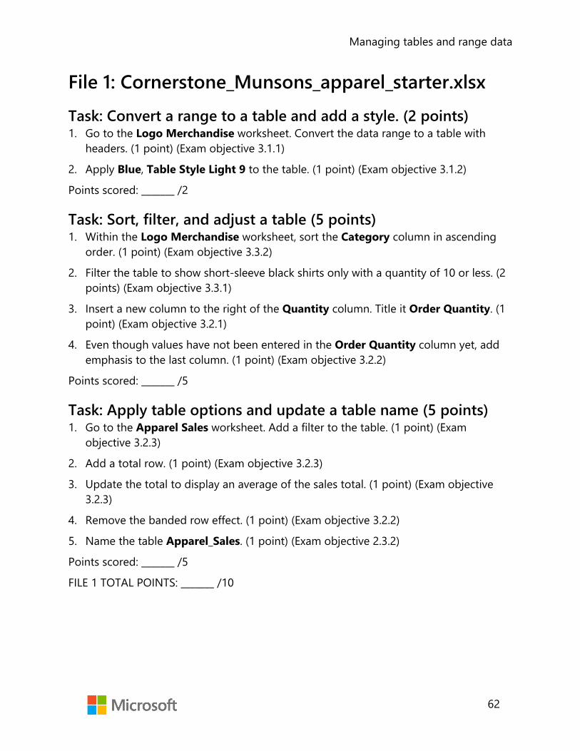
Managing tables and range data
62
File 1: Cornerstone_Munsons_apparel_starter.xlsx Task: Convert a range to a table and add a style. (2 points) 1. Go to the Logo Merchandise worksheet. Convert the data range to a table with
headers. (1 point) (Exam objective 3.1.1)
2. Apply Blue, Table Style Light 9 to the table. (1 point) (Exam objective 3.1.2)
Points scored: _______ /2
Task: Sort, filter, and adjust a table (5 points) 1. Within the Logo Merchandise worksheet, sort the Category column in ascending
order. (1 point) (Exam objective 3.3.2)
2. Filter the table to show short-sleeve black shirts only with a quantity of 10 or less. (2 points) (Exam objective 3.3.1)
3. Insert a new column to the right of the Quantity column. Title it Order Quantity. (1 point) (Exam objective 3.2.1)
4. Even though values have not been entered in the Order Quantity column yet, add emphasis to the last column. (1 point) (Exam objective 3.2.2)
Points scored: _______ /5
Task: Apply table options and update a table name (5 points) 1. Go to the Apparel Sales worksheet. Add a filter to the table. (1 point) (Exam
objective 3.2.3)
2. Add a total row. (1 point) (Exam objective 3.2.3)
3. Update the total to display an average of the sales total. (1 point) (Exam objective 3.2.3)
4. Remove the banded row effect. (1 point) (Exam objective 3.2.2)
5. Name the table Apparel_Sales. (1 point) (Exam objective 2.3.2)
Points scored: _______ /5
FILE 1 TOTAL POINTS: _______ /10

Managing tables and range data
63
File 2: Cornerstone_Munsons_bee_product_inventory_ starter.xlsx Task: Convert a table to a range and give the range a name(2points) 1. Go to the Cosmetics Inventory worksheet. Convert the table to a range. (1 point)
(Exam objective 3.1.3)
2. Select the cell range A2:E15 and name the range Bee_cosmetics. (1 point) (Exam objective 2.3.1)
Points scored: _______ /2
FILE 2 TOTAL POINTS: _______ /2
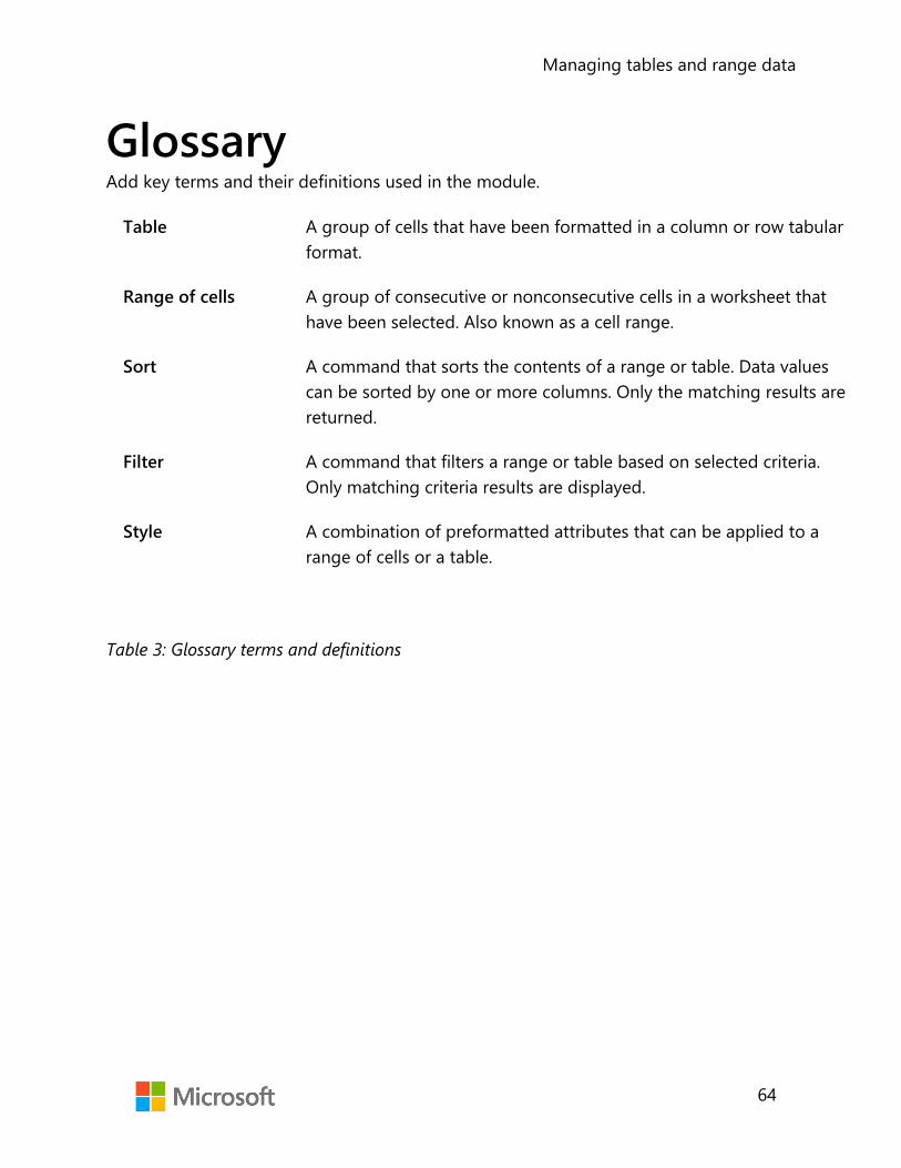
Managing tables and range data
64
Glossary Add key terms and their definitions used in the module.
Table A group of cells that have been formatted in a column or row tabular format.
Range of cells A group of consecutive or nonconsecutive cells in a worksheet that have been selected. Also known as a cell range.
Sort A command that sorts the contents of a range or table. Data values can be sorted by one or more columns. Only the matching results are returned.
Filter A command that filters a range or table based on selected criteria. Only matching criteria results are displayed.
Style A combination of preformatted attributes that can be applied to a range of cells or a table.
Table 3: Glossary terms and definitions

Student Guide 40567A Microsoft Excel associate 2019 Module 5: Using formulas and functions

Using formulas and functions
2
Contents
Contents .............................................................. 2
Module overview ............................................. 4
Description ..................................................... 4
Scenario .......................................................... 5
Cornerstone ................................................... 5
Lesson 1: Performing basic calculations . 6
Overview ......................................................... 6
Warm-up ........................................................ 6
Topic 1: Understand basic formulas .... 7
Order of operations ............................... 9
Use parentheses to modify the order of operations ............................. 10
Activity: Show and tell ....................... 10
Use cell references in formulas ...... 11
Try-it: Understand basic formulas 12
Try-it 1 ...................................................... 12
Try-it 2 ...................................................... 13
Try-it 3 ...................................................... 13
Topic 2: Display formulas ...................... 14
Activity: Show and tell ....................... 15
Try-it: Display formulas ..................... 16
Wrap-up ....................................................... 16
Lesson 2: Using references in formulas 18
Overview ...................................................... 18
Warm-up ..................................................... 18
Topic 1: Understand relative and absolute references ................................. 19
Use relative cell references in a formula ..................................................... 19
Use absolute cell references in a formula ..................................................... 20
Use mixed cell references in a formula ..................................................... 21
Activity: Tell a story ............................. 22
Try-it: Understand relative and absolute references ............................. 22
Topic 2: Use named ranges and worksheet references in formulas ...... 23
Use worksheet references in a formula ..................................................... 26
Activity: Quiz Me! ................................. 26
Try-it: Use named ranges and worksheet references in formulas . 27
Try-it 1 ...................................................... 27
Try-it 2 ...................................................... 28
Wrap-up ....................................................... 28
Lesson 3: Introducing functions .............. 30
Overview ...................................................... 30
Warm-up ...................................................... 30
Topic 1: Use functions in calculations ......................................................................... 31
Use the Function Library to insert functions .................................................. 32
Use the SUM function ........................ 34
Use the AVERAGE function .............. 35
Activity: Show me how ....................... 35

Using formulas and functions
3
Try-it: Use functions in calculations ............................................ 36
Try-it 1 ...................................................... 36
Try-it 2 ...................................................... 37
Topic 2: Use MAX and MIN functions in formulas .................................................. 37
Overview of the MAX function ....... 37
Overview of the MIN function ........ 38
Activity: Show me how ...................... 38
Try-it: Use MAX and MIN functions in formulas ............................................. 39
Try-it 1 ...................................................... 39
Try-it 2 ...................................................... 39
Wrap-up ....................................................... 40
Lesson 4: Using count functions ............. 41
Overview ...................................................... 41
Warm-up ..................................................... 41
Topic 1: Use COUNT and COUNTA functions to analyze data ...................... 42
The COUNT Function ......................... 42
The COUNTA Function ...................... 42
Activity: Discuss and learn ............... 43
Try-it: Use COUNT and COUNTA functions to analyze data ................. 44
Try-it 1 ...................................................... 44
Try-it 2 ...................................................... 44
Topic 2: Use the COUNTBLANK function ........................................................ 45
The COUNTBLANK function ............ 45
Activity: Pose a challenge ................. 46
Try-it: Use the COUNTBLANK function .................................................... 46
Wrap-up ....................................................... 47
Lesson 5: Using logical functions ............ 49
Overview ...................................................... 49
Warm-up ...................................................... 49
Topic 1: Understand IF statements .... 50
Use logical operators ......................... 50
Activity: Discuss and learn ................ 51
Try-it: Understand IF statements ... 51
Topic 2: Use the IF function .................. 52
IF function syntax ................................. 52
Considerations when using the IF function .................................................... 53
Activity: Show and tell ........................ 53
Try-it: Use the IF function ................. 54
Try-it 1 ...................................................... 54
Try-it 2 ...................................................... 55
Wrap-up ....................................................... 55
Glossary ............................................................. 57
Cornerstone ..................................................... 58
Overview ...................................................... 58
Objectives .................................................... 58
Duration ....................................................... 59
Instructions .................................................. 59
Tasks .............................................................. 59
File 1: Cornerstone_attendance_ticketsales_starter.xlsx ............................................. 59

Using formulas and functions
4
Module overview Description One of the primary strengths of Microsoft Excel is its ability to perform both basic and complex calculations. This is likely the main reason why you choose to use Excel when working with numerical data. Similar to a calculator, you can use an Excel worksheet to add, subtract, multiply, and divide numbers by using simple formulas or by integrating them into complex functions.
In this module, you will learn how to use Excel to perform calculations on data using formulas and functions. The module begins with a discussion on basic concepts of formulas and calculations and ends with an introduction to more complex concepts related to using functions. You will also learn how relative and absolute references and named ranges can help you in devising a formula or function within your worksheet.
The following table provides an outline of the specific lessons and learning objectives that are covered in this module.
Lesson Learning objective Exam objective(s)
Performing basic calculations
Create formulas to perform basic calculations, understand calculation operators and order of precedence, and display formulas
• 1.4.6
Using references in formulas
Use relative, absolute, and mixed references; define named ranges and worksheet references in formulas
• 4.1.1 • 4.1.2
Introducing functions Use basic functions in formulas such as SUM, AVERAGE, MAX, and MIN
• 4.2.1
Using count functions Use count functions in formulas such as COUNT, COUNTA, and COUNTBLANK
• 4.2.2
Using logical functions Use logical functions in formulas such as the IF function
• 4.2.3

Using formulas and functions
5
Lesson Learning objective Exam objective(s)
Cornerstone: Calculating and summarizing event attendance and ticket sales
Use Excel to complete a report that summarizes the attendance and ticket sales data to help the management team assess the success of an event
• 1.4.6 • 4.1.1 • 4.1.2 • 4.2.1 • 4.2.2 • 4.2.3
Table 1: Exam objectives by lesson
Scenario Munson’s Pickles and Preserves Farm’s weeklong Fall Festival event has ended. To prepare for a post-event review meeting, you have been asked to summarize the number of visitors and determine the sales revenue for the farm event. You have a workbook containing a worksheet with data logged during the event.
Cornerstone Munson’s Pickles and Preserves Farm hosts many public events throughout the year. Typically, admission tickets are sold with different pricing for junior, youth, adult, senior, family, and group attendees. After each event, the management team holds a meeting to review how successful the event was and what can be improved for future events. To help prepare for the post-event review meeting, you need to complete a report that summarizes the attendance and ticket sales data to help the management team assess the success of the event. You have a workbook that includes a worksheet with the data logged during the Munson’s event.

Using formulas and functions
6
Lesson 1: Performing basic calculations Overview In Excel, knowing how to create a basic formula to perform a calculation is the foundation for many more complex tasks. Simply knowing how to add, subtract, multiply, or divide numbers in Excel allows you to perform many of the calculations routinely used in worksheets.
In this lesson, you will learn how to create basic formulas to perform calculations in an Excel worksheet. You will also observe how the mathematical order of operations is used to calculate a specific result. Finally, you will learn how formulas are displayed in an Excel worksheet.
Warm-up Use these questions to find out what you already know about this lesson’s topics:
1. A formula is used in an Excel workbook to _______________________.
Fill in the blank space.
2. What is the answer to the following calculation: (4+6)*2-10/2 ?
Select the correct option.
a. 5
b. 3
c. 15
d. -30
Using formulas and functions
7
3. Which of the following operators is used to start a formula in Excel?
Select the correct option.
a. *
b. /
c. =
d. $
4. Which of following operators is used to multiply in Excel?
Select the correct option.
a. *
b. /
c. ^
d. X
5. PEMDAS is the acronym for _______________________.
Fill in the blank space
Topic 1: Understand basic formulas To perform calculations in Excel, you enter a formula into the worksheet. A formula is a mathematical equation that performs calculations on values in a worksheet. Formulas often perform calculations related to addition, subtraction, multiplication, and division but can also contain more advanced features such as Excel Functions.
A formula contains one or more of the following:
• Cell reference—The coordinate of a specific cell. For example, A1 refers to the cell located in the A column and the first row.
• Range of cell references—A specification used to indicate a set of adjacent cells. For example, cells A1 to A5 can be referred to as A1:A5 when specifying the range.
• Operator—A symbol used in mathematical operations to specify the calculations to be performed.
• Constant—A number or text value that is entered directly into a formula. • Function—A pre-built command in Excel that performs mathematical operations
such as automatically adding up a range of cells or looking up values to be used in calculations.

Using formulas and functions
8
Did you know?
You begin a formula with an equal (=) sign at the start of the calculation. This is used so that Excel can distinguish the formula from regular data in the worksheet.
When you enter a formula in an Excel worksheet, the result of the calculation is displayed in the cell. You can view the underlying formula by selecting the cell and then referring to the formula bar.
As shown in Figure 1, the active cell is A1, which has the value of 22. The formula bar displays the formula that was entered to result in this calculation.
Figure 1: Viewing a formula

Using formulas and functions
9
Excel uses arithmetic operators when performing calculations in formulas. Refer to Table 2, which describes the more common arithmetic operators used for formulas in Excel.
Arithmetic operator
Name Calculation Example
+ Plus sign Addition 10+5
- Minus sign Subtraction 10-5
* Asterisk Multiplication 10*5
/ Forward slash Division 10/5
% Percent sign Percent 50%
^ Caret Exponentiation 10^2
Table 2: Arithmetic operators
Order of operations You will often use more than one operator in a formula. To ensure that your formula results in the correct calculation, you need to understand how the calculation takes place.
Excel follows standard mathematical rules called the order of operations when calculating a formula. Table 3 describes the order of operations.
Arithmetic operator Description
- Negative number
% Percent
^ Exponentiation
* and / Multiplication and division in order left to right
+ and - Addition and subtraction in order left to right
Table 3: Order of operations

Using formulas and functions
10
Excel performs operations in the order shown from top to bottom in Table 3. For example, consider the formula 3+6 * 2.
Following the order of operations, multiplication takes place first: 6 * 2. The result of 12 is then added to 3 with the final calculation of 15.
Use parentheses to modify the order of operations You can override the standard order of operations by using parentheses in a formula. Excel always performs calculations inside parentheses first before continuing with the rest of the order of operations.
For example, if the above formula is changed to contain parentheses, the result is much different: (3+6) * 2.
With the parentheses taking precedence, the first calculation results in 9. Then the standard order resumes to multiply by 2. The final result is now 18.
Did you know?
You can remember the order of operations by using the acronym: PEMDAS (parentheses, exponents, multiplication, division, addition, subtraction).
Activity: Show and tell In this activity, your teacher will demonstrate how to create calculations with formulas. Your teacher will also show you how the order of operations will affect the result of a calculation.
Resources required You will need the following resources for this activity:
None.
Activity instructions Pay close attention as your teacher demonstrates the following tasks:
1. Entering a simple formula into a cell.
2. Using arithmetic operators in formulas.

Using formulas and functions
11
3. Changing the order of operations in formulas.
4. Using cell references in formulas.
Use cell references in formulas Although you can use constant numbers in formulas, more often you will want to use cell references instead. A cell reference identifies the coordinate of a specific cell. For example, A1 refers to column A and row 1. The power behind using a cell reference is that you can change the data in a cell and immediately observe the results of any formula that references the cell.
For example, in Figure 2, the number 10 is entered in cell A1 and the number 8 is entered in cell B1. The formula in cell C1 is configured to add the two numbers together. Notice that C1 does not contain the constant values (10 and 8) but rather the cell references of A1 and B1. If you decide to change the values in cells A1 and B1, the formula in C1 automatically calculates to the new result.
Figure 2: Using cell references for calculating a formula
Did you know?
You can either type the formula or you can use the mouse and select the cells to be included in the formula. After you type the = sign, simply use the mouse and select the cells you want to include in the calculation before and after the operator.
Additional information
For more information on types of operators and order of operations, go to: Calculation operators and precedence

Using formulas and functions
12
Try-it: Understand basic formulas In this leveled try-it activity, you will open a blank document and create a simple
formula. You will then open an existing document and devise a more complex formula with multiple operators and sets of parentheses.
Try-it 1 In this try-it, you will open a blank document and create a simple formula.
Resources You will need the following resources for this try-it:
• Open a blank worksheet in Excel.
Instructions The following are the general tasks that you need to perform during this try-it:
1. In the blank worksheet, enter numbers as shown in the following table:
A B C
1 10 8
2 15 6
3 25 10
4 22 2
2. In cell C1, create a formula that adds cells A1 and B1. Use constant numbers for this formula.
3. In cell C2, create a formula that subtracts cells A2 and B2. Use cell references for this formula.
4. In cell C3, create a formula that multiplies cells A3 and B3. Use cell references for this formula.
5. In cell C4, create a formula that divides cells A4 and B4. Use cell references for this formula.
6. In cell A1, change the number to 20.
7. In cell A2, change the number to 10.
8. In cell A3, change the number to 10.

Using formulas and functions
13
9. In cell A4, change the number to 40.
10. Which results automatically changed? Why?
11. Save and close the file.
Try-it 2 In this try-it, you will open an existing document and devise a more complex formula with two operators and parentheses.
Resources You will need the following resources for this try-it:
• Open L1_T1_try2_formula_two_operators_starter.xlsx in this lesson’s Learning Activity Resources.
Instructions The following are the general tasks that you need to perform during this try-it:
1. In cell D2, create a formula that adds cells A2 and B2 and then subtracts cell C2.
2. In cell D3, create a formula that adds cells A3 and B3 and then multiplies cell C3.
3. In cell D4, create a formula that subtracts cells A4 and B4 and then divides cell C4.
4. Use parentheses to modify the formula in cell D3 so that the result is 750.
5. Use parentheses to modify the formula in cell D4 so that the result is 25.5.
6. Save and close the file.
Try-it 3 In this try-it, you will open an existing document and devise a more complex formula with four operators and parentheses.
Resources You will need the following resources for this try-it:
• Open L1_T1_try3_formula_parentheses_starter.xlsx in this lesson’s Learning Activity Resources.
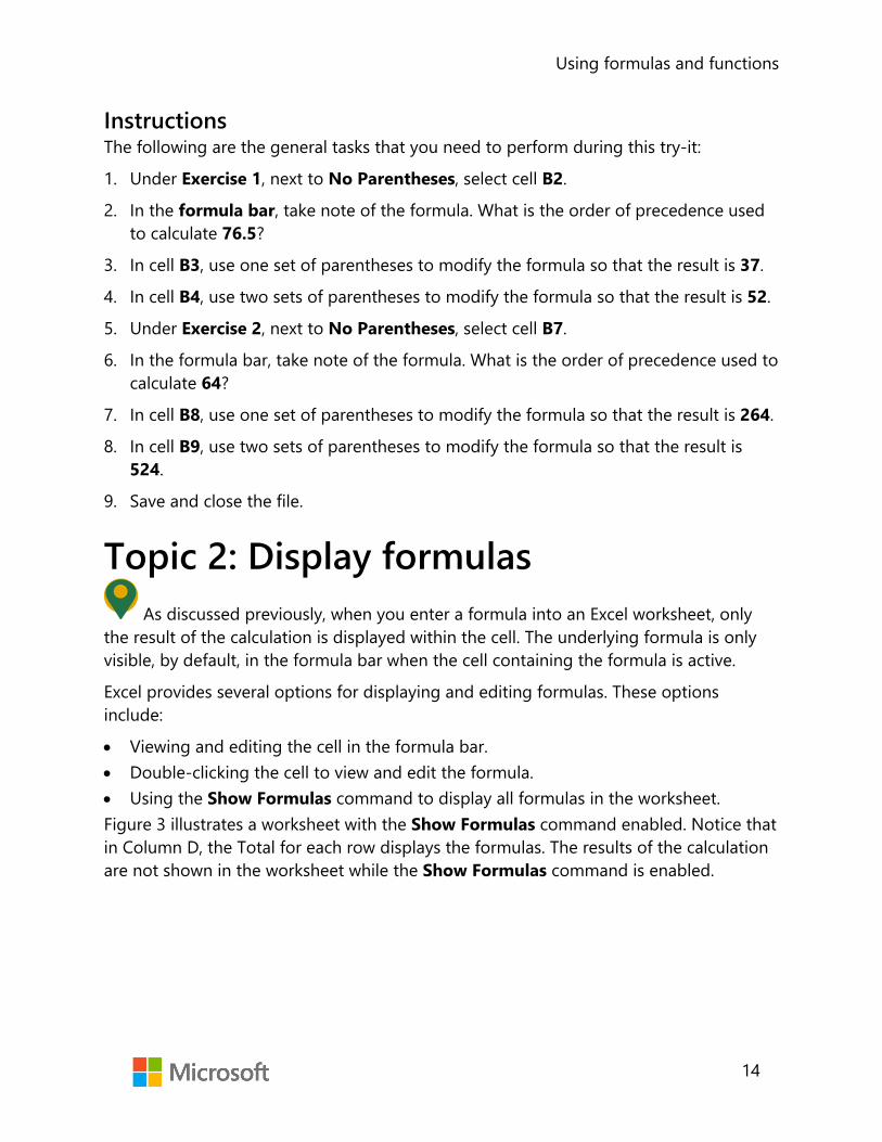
Using formulas and functions
14
Instructions The following are the general tasks that you need to perform during this try-it:
1. Under Exercise 1, next to No Parentheses, select cell B2.
2. In the formula bar, take note of the formula. What is the order of precedence used to calculate 76.5?
3. In cell B3, use one set of parentheses to modify the formula so that the result is 37.
4. In cell B4, use two sets of parentheses to modify the formula so that the result is 52.
5. Under Exercise 2, next to No Parentheses, select cell B7.
6. In the formula bar, take note of the formula. What is the order of precedence used to calculate 64?
7. In cell B8, use one set of parentheses to modify the formula so that the result is 264.
8. In cell B9, use two sets of parentheses to modify the formula so that the result is 524.
9. Save and close the file.
Topic 2: Display formulas As discussed previously, when you enter a formula into an Excel worksheet, only
the result of the calculation is displayed within the cell. The underlying formula is only visible, by default, in the formula bar when the cell containing the formula is active.
Excel provides several options for displaying and editing formulas. These options include:
• Viewing and editing the cell in the formula bar. • Double-clicking the cell to view and edit the formula. • Using the Show Formulas command to display all formulas in the worksheet. Figure 3 illustrates a worksheet with the Show Formulas command enabled. Notice that in Column D, the Total for each row displays the formulas. The results of the calculation are not shown in the worksheet while the Show Formulas command is enabled.

Using formulas and functions
15
Figure 3: Show Formulas option enabled
To enable the Show Formulas command, select the Formulas tab, and then in the Formula Auditing group, select Show Formulas.
Did you know?
When you double-click a cell to edit the formula, if you do not press Enter, you can cancel all edits by pressing the Esc key on the keyboard. If you do press Enter, you can use the Undo command to revert to the previous entry in the cell.
Activity: Show and tell In this activity, your teacher will demonstrate various ways to display and edit formulas.
Resources required You will need the following resources for this activity:
None.
Activity instructions Pay close attention as your teacher demonstrates the following tasks:
1. Using the formula bar.
2. Displaying and editing a formula within a cell.
3. Using the Show Formulas command.

Using formulas and functions
16
Try-it: Display formulas In this try-it activity, you will open an existing document and use several methods
to display formulas in an Excel worksheet.
Resources You will need the following resources for this try-it:
• Open L1_T2_try_display_formulas_starter.xlsx in this lesson’s Learning Activity Resources.
Instructions The following are the general tasks that you need to perform during this try-it:
1. Select cell D2 and notice the formula displayed in the formula bar.
2. Select cell D3 and press F2 on the keyboard. Notice the formula displayed in the cell.
3. Press Esc to cancel the cell display mode.
4. From the ribbon, enable the Show Formulas command.
5. Save and close the file.
Wrap-up Use these questions to check what you learned in this lesson:
1. The formula =6*2/3 produces the same result as =6*(2/3).
Select the correct option.
a. True
b. False
2. Which of the following symbols can you use to override the order of operations?
Select the correct option.
a. “ “
b. @
c. ( )
d. *

Using formulas and functions
17
3. The +, -, *, and / are all examples of _______________________.
Fill in the blank space.
4. To display formulas in the worksheet, you can select the _______________________ command in the ribbon.
Fill in the blank space.
5. Which following operator is used to divide in Excel?
Select the correct option.
a. *
b. /
c. ^
d. @
Using formulas and functions
18
Lesson 2: Using references in formulas Overview As you learned in Lesson 1, a cell reference identifies the coordinates of a cell based upon the column letter and row number. To provide more flexibility in your worksheet, you typically use cell references instead of hard coding constant values when creating a formula in Excel.
In this lesson, you will learn the types of cell references that can be used when devising a formula in an Excel worksheet. You will also learn how named ranges and references are used in formulas to refer to cell references within or across worksheets.
Warm-up Use these questions to find out what you already know about this lesson’s topics:
1. If you do not want a cell reference to change when you copy or move it, you need to make a(n) _______________________ cell reference in a formula.
Fill in the blank space.
2. Which of the following is the best example of a mixed cell reference?
Select the correct option.
a. A2
b. $A$2
c. A2:B5
d. A$2

Using formulas and functions
19
3. Which of the following symbols specifies an absolute reference?
Select the correct option.
a. %
b. &
c. $
d. @
4. Which of the following is a valid named range?
Select the correct option.
a. A7
b. Sales_Data
c. Sales Data
d. Sales\Data
Topic 1: Understand relative and absolute references
The benefit of using a cell reference is that when you copy the formula to a new location, the cell reference automatically updates. However, there may be times that you need the formula to always refer to a specific cell, regardless of where the formula is copied to in the worksheet. To ensure that your formulas calculate as intended, it is important to understand the concepts of relative, absolute, and mixed cell references.
Use relative cell references in a formula As you copy a formula from one location to another in a worksheet, you will notice that, by default, the formula reference changes based upon where you copy the formula to. What actually is copied is related to the “pattern” of the formula as opposed to the specific references in the formula. This is called a relative cell reference.
For example, as shown in Figure 4, the first table has cell E1 selected. The formula within the cell is =B1+C1+D1. When this formula is copied to cells E2 and E3, notice that the cell reference changes based upon where the formula is copied to. Cell E2 shows a formula of =B2+C2+D2, and cell E3 shows a formula of =B3+C3+D3.

Using formulas and functions
20
Figure 4: Relative cell references
Did you know?
You can use the standard Copy and Paste feature to copy formulas to another location in the worksheet; if the cells are adjacent to the original cell, you can use the Auto Fill handle to copy the formula.
Use absolute cell references in a formula You may have circumstances where you do not want a cell reference to change when it is moved or copied. An absolute cell reference refers to a formula that contains a specific cell or range of cells that do not change regardless of where the formula is copied or moved to.
To specify an absolute cell reference in a formula, use the dollar sign ($) before the column and the row of the cell you want to reference.
For example, as shown in Figure 5, the first table has cell F2 selected. The formula within the cell is =$B$6*E2. This formula multiplies the Bonus in cell B6 with the Total in cell E2 to calculate the Bonus amount in cell F2.
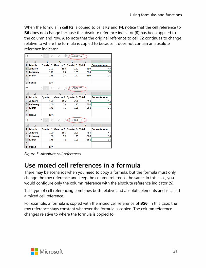
Using formulas and functions
21
When the formula in cell F2 is copied to cells F3 and F4, notice that the cell reference to B6 does not change because the absolute reference indicator ($) has been applied to the column and row. Also note that the original reference to cell E2 continues to change relative to where the formula is copied to because it does not contain an absolute reference indicator.
Figure 5: Absolute cell references
Use mixed cell references in a formula There may be scenarios when you need to copy a formula, but the formula must only change the row reference and keep the column reference the same. In this case, you would configure only the column reference with the absolute reference indicator ($).
This type of cell referencing combines both relative and absolute elements and is called a mixed cell reference.
For example, a formula is copied with the mixed cell reference of B$6. In this case, the row reference stays constant wherever the formula is copied. The column reference changes relative to where the formula is copied to.

Using formulas and functions
22
Did you know?
As you create a formula using cell references, you can toggle between relative, absolute, and mixed references by pressing F4 on the keyboard. This will cycle through the various reference types and add or remove the dollar sign ($) in the formula.
Additional information
For more information on using relative, absolute, and mixed references, go to: Switch between relative, absolute, and mixed references
Activity: Tell a story In this activity, your teacher will describe and demonstrate a scenario to help you understand how relative and absolute references are used in formulas.
Resources required You will need the following resources for this activity:
None.
Activity instructions Your teacher will open a document that contains Munson’s Pickles and Preserves Farm sales data for shareholder memberships. Munson’s plans to donate a percentage of sales to a local food bank. Pay close attention as your teacher demonstrates the following tasks:
1. How relative cell references work in a formula.
2. How absolute cell references work in a formula.
Try-it: Understand relative and absolute references For this exercise, you will open an existing Excel workbook and configure formulas
to use relative and absolute cell references.

Using formulas and functions
23
Resources You will need the following resources for this try-it:
• Open L2_T1_try_donation_amount_starter.xlsx in this lesson’s Learning ActivityResources.
Instructions The following are the general tasks that you need to perform during this try-it:
1. In the Donation Amount column, in cell F3, create a formula that calculates 10% ofthe total sales in January. Be sure to use relative cell references for the formula.
2. Copy the formula from cell F3 to cells F4 to F8.
3. Take note of the calculations. Are the calculations correct, and do they refer to thecorrect cell references?
4. Edit the formula in cell F3 to use absolute cell references where needed.
5. Copy the formula from cell F3 to cells F4 to F8.
6. Take note of the calculations. Are the calculations now correct, and do they refer tothe correct cell references?
Topic 2: Use named ranges and worksheet references in formulas
Module 4: Managing tables and ranges introduced you to the concept of defining a named range. As you might recall, a named range can either be a single cell or a group of cells with a designated name.
Using a named range in a worksheet provides several benefits. For larger worksheets, a named range can be used as a type of bookmark, which enables you to quickly navigate to the location that has been named. For formulas, a named range enables you to assign meaningful names to cells or groups of cells, which can be used in place of the column and row references. The named range can also be assigned a scope to be used within a specific worksheet or even be referred to from multiple worksheets within the entire workbook.
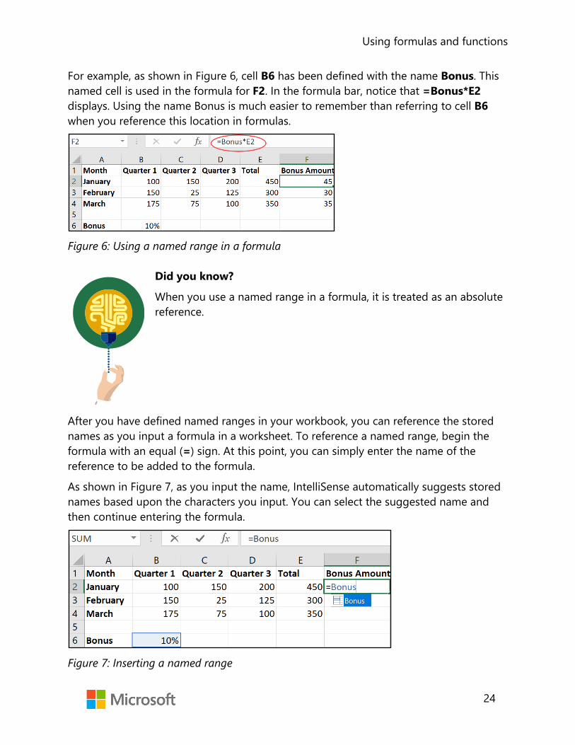
Using formulas and functions
24
For example, as shown in Figure 6, cell B6 has been defined with the name Bonus. This named cell is used in the formula for F2. In the formula bar, notice that =Bonus*E2 displays. Using the name Bonus is much easier to remember than referring to cell B6 when you reference this location in formulas.
Figure 6: Using a named range in a formula
Did you know?
When you use a named range in a formula, it is treated as an absolute reference.
After you have defined named ranges in your workbook, you can reference the stored names as you input a formula in a worksheet. To reference a named range, begin the formula with an equal (=) sign. At this point, you can simply enter the name of the reference to be added to the formula.
As shown in Figure 7, as you input the name, IntelliSense automatically suggests stored names based upon the characters you input. You can select the suggested name and then continue entering the formula.
Figure 7: Inserting a named range

Using formulas and functions
25
Another method used to add a named range to a formula is to select the Use in Formula option found in the Defined Names group of the ribbon. As shown in Figure 8, this option displays all the named ranges defined in the workbook. This is quite handy if you do not remember the name of a specific range that needs to be referenced in a formula.
Figure 8: Use in Formula button showing named ranges
Did you know?
The Paste Names option in the Use in Formula command is used to create a list of names and cell references stored in the workbook. This information can be used as a guide to show reviewers each of the defined named ranges and their associated cell ranges.
Additional information
For additional information on defining and using names in formulas, go to: Define and use names in formulas

Using formulas and functions
26
Use worksheet references in a formula A worksheet reference refers to a cell, range of cells, or named range located in another worksheet. You might use worksheet references whenever you need to create formulas that reference data throughout multiple worksheets. For example, one worksheet may display a summary of data based upon information located in other worksheets within the workbook.
The format of a formula that references a cell in another worksheet is as follows:
• SheetName!CellAddress• SheetName! refers to the name of the sheet that contains the data.• CellAddress refers to the column and row reference that contains the data.
Did you know?
You can also reference data in another workbook by including the name of the workbook in square brackets ([ ]); for example, [WorkbookName]SheetName!CellAddress.
Activity: Quiz Me! In this activity, you will participate in a teacher-led discussion and demonstration on how to define and use named ranges in formulas.
Resources required You will need the following resources for this activity:
None
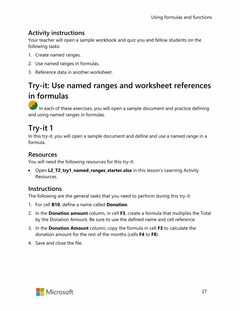
Using formulas and functions
27
Activity instructions Your teacher will open a sample workbook and quiz you and fellow students on the following tasks:
1. Create named ranges.
2. Use named ranges in formulas.
3. Reference data in another worksheet.
Try-it: Use named ranges and worksheet references in formulas
In each of these exercises, you will open a sample document and practice defining and using named ranges in formulas.
Try-it 1 In this try-it, you will open a sample document and define and use a named range in a formula.
Resources You will need the following resources for this try-it:
• Open L2_T2_try1_named_ranges_starter.xlsx in this lesson’s Learning ActivityResources.
Instructions The following are the general tasks that you need to perform during this try-it:
1. For cell B10, define a name called Donation.
2. In the Donation amount column, in cell F3, create a formula that multiples the Totalby the Donation Amount. Be sure to use the defined name and cell reference.
3. In the Donation Amount column, copy the formula in cell F3 to calculate thedonation amount for the rest of the months (cells F4 to F8).
4. Save and close the file.
Using formulas and functions
28
Try-it 2 In this try-it, you will open a sample document and create a formula with worksheet references.
Resources You will need the following resources for this try-it:
• Open L2_T2_try2_worksheet_references_starter.xlsx in this lesson’s Learning Activity Resources.
Instructions The following are the general tasks that you need to perform during this try-it:
1. Select the Quarter2 sheet.
2. In cell F3, configure a formula that will multiply the Donation named range by the January Total on the Quarter2 sheet.
3. On the Quarter2 sheet, in the Donation Amount column, copy the formula in cell F3 to calculate the Donation Amount for the rest of the months (cells F4 to F8).
4. On the Summary sheet, in cell B3, configure a formula that adds the Donation Amount for January from the Quarter1 and Quarter2 sheets.
5. On the Summary sheet, in the Donation Amount column, copy the formula in cell B3 to calculate the Donation Amount for the rest of the months (cells B4 to B8).
6. On the Quarter1 sheet, change the Donation percentage rate and observe the changes to the amounts in the workbook.
Wrap-up Use these questions to check what you learned in this lesson:
1. Which keyboard shortcut can you use to toggle relative, absolute, and mixed references?
Select the correct option.
a. F1
b. F4
c. F6
d. F8

Using formulas and functions
29
2. Review the following formula: =$C$2*A7. This formula uses which of the following reference types?
Select the correct option.
a. Absolute
b. Relative
c. Mixed
d. Worksheet
3. Review the following formula: =Sales!C10+A7. This formula uses which of the following reference types?
Select the correct option.
a. Absolute
b. Relative
c. Named
d. Worksheet
4. Describe two methods you can use to create a named range.
_______________________
_______________________
5. Describe the benefits of using a named range.
_______________________
Fill in the blank space.

Using formulas and functions
30
Lesson 3: Introducing functions Overview Excel’s built-in functions provide a relatively simple and efficient way to perform complex tasks within your worksheet. A function is a predefined formula used for specific purposes and calculations. There are over 470 functions in Excel, covering numerous categories, including mathematical calculations, lookup operations, logical evaluations, and calculating dates and times.
In this lesson, you will learn the concept of functions and how they are used in an Excel worksheet. You will also review several of the more common functions such as SUM, AVERAGE, MAX, and MIN to identify how these functions can help you with your formula and worksheet calculations.
Warm-up Your teacher will introduce the topics to be covered in this lesson. Be prepared to discuss and answer the following questions during the classroom discussion:
1. Which function is used to add specified values?
Select the correct option.
a. AVERAGE
b. SUM
c. COUNT
d. MAX
2. Like a standard formula, a function begins with an equal sign (=). True or false?
Select the correct option.
a. True
b. False

Using formulas and functions
31
3. You want to add a range of cells and then divide by the number of cell entries. Which function can help you with this task?
Select the correct option.
a. AVERAGE
b. COUNT
c. IF
d. MAX
4. The _______________________ command helps you search and select a function to be used in a worksheet.
Fill in the blank space.
Topic 1: Use functions in calculations To effectively use a function in your worksheet, you need to understand how it is
structured and which components are required or optional. A function is structured with the following elements:
• Function name: All functions begin with the standard equal (=) sign followed by the name of the function and an opening and closing parentheses.
• Arguments: Most functions use arguments within the brackets, which often refer to cell references or ranges to include in the calculation. For functions that do contain multiple arguments, at least one argument is required; additional arguments are optional, with each separated by a comma.
To insert a function into a worksheet, start by entering the equal (=) sign followed by the name of the function. As you enter the function name, Excel uses IntelliSense to provide a list of all the functions related to the letters you type. When the intended function is displayed, use the Tab key to have Excel automatically finish the function name and start the opening parentheses for you. Figure 9 shows an example of the structure for the SUM function. Take note of the function name, required argument, and optional arguments.
Figure 9: SUM function structure

Using formulas and functions
32
Did you know?
Not all functions contain arguments. For example, to insert a formula that returns today’s date, you can simply use the =TODAY() function. Notice that this function still follows the correct structure but does not contain or require any arguments within the brackets.
Use the Function Library to insert functions The Formulas tab in Excel contains the Function Library, where you will find all the functions listed by category, such as Financial, Logical, Date &Time, Math & Trig, and so on.
Figure 10 shows the Function Library and its categories.
Figure 10: Function Library
You can use the Function Library to browse for a specific function to insert into your worksheet. After you select a function to be used, the function wizard launches to assist in adding additional arguments and finalizing the build of your formula.
If you need assistance in finding a function to perform a specific task, use the Insert Function command found in the Function Library or to the left of the formula bar.
As shown in Figure 11, Insert Function helps you search for a function by name, description, or category. You then select the function name to launch the function wizard, which is used to help build your formula.

Using formulas and functions
33
Figure 11: Insert Function dialog box
Did you know?
Another method to open the Insert Function dialog box is to use the Shift F3 shortcut key combination on the keyboard.
If you select a function that requires additional arguments, the function wizard displays the Function Arguments dialog box. As shown in Figure 12, the Function Arguments dialog box provides helpful guidance to build the formula, including sections to add additional arguments as needed. The dialog box also displays expected results and descriptions on how the function is structured.

Using formulas and functions
34
Figure 12: Function arguments for the SUM function
Use the SUM function One of the more common types of calculations used in a worksheet is adding numbers together to result in a sum total. You can easily use the plus (+) sign to add a range of numbers. However, for large ranges of numbers, the formula could become quite unmanageable.
As shown in Figure 13, the formula in cell F2 manually adds the cells from A2 to E2. Using this type of formula is prone to input error because each cell must be manually entered into the calculation.
The formula in cell F3 contains the SUM function, which totals the range of cells from A3 to E3, as indicated by A3:E3.
Figure 13: Comparing manual addition to the SUM function
Did you know?
You can use the Alt = keyboard shortcut to enter the SUM function into a cell. This will start the formula and will then require you to specify the cells to be calculated.

Using formulas and functions
35
Use the AVERAGE function Some worksheet calculations may require you to add a range of cells and then divide by the number of cell entries. The result displays the average of the values entered in the cells. Similar to the SUM function, you can manually input the calculation. However, using the AVERAGE function is easier because it performs the calculation automatically.
To calculate the average for a range of cells, start with the equal (=) sign followed by the word AVERAGE and then an opening parentheses. You can then input or select the range of cells to average.
Figure 14 shows the AVERAGE function as it is manually typed into a cell. As with all functions, you can also use the Insert Function command or the Function Library to insert the formula as needed.
Figure 14: AVERAGE Function
Additional information
For more information on functions, go to: Formulas and functions
Activity: Show me how This is a teacher-led demonstration showing how to integrate the SUM and AVERAGE functions into formulas within an Excel worksheet.
Resources required You will need the following resources for this activity:
None

Using formulas and functions
36
Activity instructions Pay close attention as your teacher demonstrates the following tasks. You will have a chance to test out your new knowledge on your own after the teacher-led demonstration:
1. Manually enter formulas to calculate the sum and average of specified cells.
2. Use the SUM function to simplify adding values for specified cells.
3. Use the AVERAGE function to simplify calculating averages.
Try-it: Use functions in calculations In each of these exercises, you will open a sample document and then practice
using the SUM and AVERAGE functions.
Try-it 1 In this try-it, you will open a sample document and practice using SUM function.
Resources You will need the following resources for this try-it:
• Open L3_T1_try1_sum_function_starter.xlsx in this lesson’s Learning Activity Resources.
Instructions The following are the general tasks that you need to perform during this try-it:
1. In cell F2, input the column header Total.
2. In cell A9, input the column header Total.
3. In cell F3, use the Function Library to enter a function that sums B3 to E3.
4. Copy the formula from cell F3 to cell F4 through to cell F8.
5. In cell B9, use the Insert Function wizard to enter a function that sums B3 to B8.
6. Copy the formula from cell B9 to cell C9 through to cell F9.
7. Select cells B9 to F9 and format a Top and Double Bottom Border for the range of cells.
8. Save and close the file.

Using formulas and functions
37
Try-it 2 In this try-it, you will open a sample document and practice using AVERAGE function.
Resources You will need the following resources for this try-it:
• Open L3_T1_try2_average_function_starter.xlsx in this lesson’s Learning Activity Resources.
Instructions The following are the general tasks that you need to perform during this try-it:
1. In cell G3, use the Insert Function wizard to enter a function that averages cells B3 to E3.
2. Copy the formula from cell G3 to cell G4 through to cell G9.
3. Save and close the file.
Topic 2: Use MAX and MIN functions in formulas
As mentioned previously, all functions in the Function Library are grouped into several categories. Located in the Statistical category are two functions that are useful when analyzing financial data: the MAX function and the MIN function.
Overview of the MAX function The MAX function returns the largest value in a specified range of cells in the worksheet. This function is useful if, for example, you need to determine the highest expense or revenue amount in a financial worksheet.
As shown in Figure 15, the MAX function consists of the name followed by an opening parentheses. The first argument is required and can be either a number, named range, or cell reference. All subsequent arguments are optional. The final part of the function is the closed parentheses.
Figure 15: MAX function
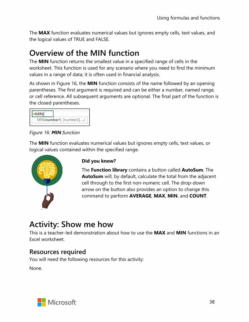
Using formulas and functions
38
The MAX function evaluates numerical values but ignores empty cells, text values, and the logical values of TRUE and FALSE.
Overview of the MIN function The MIN function returns the smallest value in a specified range of cells in the worksheet. This function is used for any scenario where you need to find the minimum values in a range of data; it is often used in financial analysis.
As shown in Figure 16, the MIN function consists of the name followed by an opening parentheses. The first argument is required and can be either a number, named range, or cell reference. All subsequent arguments are optional. The final part of the function is the closed parentheses.
Figure 16: MIN function
The MIN function evaluates numerical values but ignores empty cells, text values, or logical values contained within the specified range.
Did you know?
The Function library contains a button called AutoSum. The AutoSum will, by default, calculate the total from the adjacent cell through to the first non-numeric cell. The drop-down arrow on the button also provides an option to change this command to perform AVERAGE, MAX, MIN, and COUNT.
Activity: Show me how This is a teacher-led demonstration about how to use the MAX and MIN functions in an Excel worksheet.
Resources required You will need the following resources for this activity:
None.
Using formulas and functions
39
Activity instructions Participate in the activity by assisting your teacher in performing the following tasks:
1. Insert the MAX function to find the largest value.
2. Insert the MIN function to find the smallest value.
Try-it: Use MAX and MIN functions in formulas In each of these exercises, you will open a sample document and practice using the
MAX and MIN functions.
Try-it 1 In this try-it, you will open a sample document and practice using MAX function.
Resources You will need the following resources for this try-it:
• Open L3_T2_try1_max_monthly_usage_starter.xlsx in this lesson’s Learning Activity Resources.
Instructions The following are the general tasks that you need to perform during this try-it:
1. In cell A16, input the row header Max Usage.
2. In cell B16, use the Function Library to enter a function that finds the maximum value for energy usage in 2012.
3. Copy the formula from cell B16 to cell C16 through to cell I16.
4. Select cells A16 to I16 and format a Top and Double Bottom Border for the range of cells. Format the range to be bold.
5. Save and close the file.
Try-it 2 In this try-it, you will open a sample document and practice using MIN function.
Resources You will need the following resources for this try-it:
• Open L3_T2_try2_min_monthly_usage_starter.xlsx in this lesson’s Learning Activity Resources.

Using formulas and functions
40
Instructions The following are the general tasks that you need to perform during this try-it:
1. In cell A17, input the row header Min Usage.
2. In cell B17, use the Function Library to enter a function that finds the minimumvalue for energy usage in 2012.
3. Copy the formula from cell B17 to cell C17 through to cell I17.
4. Select cells A16 to I16 and format a Top and Double Bottom Border for the rangeof cells. Format the range to be bold.
5. Save and close the file.
Wrap-up Use these questions to check what you learned in this lesson:
1. Which of the following are not evaluated in the MAX or MIN functions?
Select all that apply.
a. Cells with number values
b. Ranges with number values
c. Empty cells
d. Text values in the specified range
2. You need to determine the largest value in a range of numbers. Which functionshould you use?
Select the correct option.
a. MIN
b. SUM
c. COUNT
d. MAX
3. A(n) _______________________ is a predefined formula used for specific purposes andcalculations.
Fill in the blank space.

Using formulas and functions
41
Lesson 4: Using count functions Overview As you analyze statistical data in a worksheet, there may be times when you need to determine how many cells contain numeric or text values. Or you may simply want to know how many cells are empty within a large worksheet.
Excel provides the COUNT, COUNTA, and COUNTBLANK functions, which can each assist with these types of analysis. In this lesson, you learn the use and structure of the Count functions in Excel.
Warm-up Use these questions to find out what you already know about this lesson’s topics:
1. The COUNTBLANK function counts the number of _______________________ cells in a range.
Fill in the blank space.
2. The COUNT functions are in which of the Function Library categories?
Select the correct option.
a. Financial
b. Date & Time
c. Math & Trig
d. Statistical
3. The COUNT function counts the following value types:
Select all that apply.
a. Numeric constants
b. Numeric cell ranges
c. Text values
d. Empty cells
e. Numeric cell references
4. The _______________________ function counts all the nonblank entries in a range.
Fill in the blank space.

Using formulas and functions
42
Topic 1: Use COUNT and COUNTA functions to analyze data
The COUNT and COUNTA functions are found in the Statistical category of the Formula Library. Both functions are used to analyze specified data ranges to determine how many cells contain values.
The COUNT Function The COUNT function is used to indicate how many cells contain a numeric value. Numeric values can include constants, cell references, and ranges. The types of numbers that are counted include negative numbers, percentages, dates, time, and fractions.
Empty cells, text values, and the logical values TRUE and FALSE are ignored and are not counted.
Figure 17 shows the structure of the COUNT function. Similar to all other functions, it begins with an equal (=) sign followed by the name and opening parentheses. The value1 argument is required and typically refers to a range of cells. All other arguments are optional.
Figure 17: COUNT function
Video
To review the video on how to use the COUNT function, go to: COUNT function
The COUNTA Function The COUNTA function counts the number of cells that are not empty in a specified range. Values that are counted include numbers, text, logical values, error values, and empty text strings.
The COUNTA function does not count cells that are completely empty.

Using formulas and functions
43
Figure 18 shows the structure of the COUNTA function. The function begins with an equal (=) sign followed by the name and opening parentheses. The value1 argument is required and typically refers to a range of cells. All other arguments are optional.
Figure 18: COUNTA function
Additional information
For more information on using the COUNTA function, go to: COUNTA function
Activity: Discuss and learn This is a teacher-led discussion and demonstration about how to use the COUNT and COUNTA functions in an Excel worksheet.
Resources required You will need the following resources for this activity:
None.
Activity instructions Pay close attention as your teacher demonstrates the following tasks. You will have a chance to test out your new knowledge on your own after the teacher-led demonstration:
1. Use the COUNT function to determine how many Produce Box types have had sales to shareholders.
2. Use the COUNTA function to determine how many Produce Box types have been allocated to shareholders.

Using formulas and functions
44
Try-it: Use COUNT and COUNTA functions to analyze data
In each of these exercises, you will open a sample document and practice using the COUNT and COUNTA functions.
Try-it 1 In this try-it, you will open a sample document and practice using COUNT function.
Resources You will need the following resources for this try-it:
• Open L4_T1_try1_count_producebox_starter.xlsx in this lesson’s Learning Activity Resources.
Instructions The following are the general tasks that you need to perform during this try-it:
1. On the Sales tab, in cell E10, use the Function Library to enter a function that counts how many Produce Box types have been sold to shareholders.
2. In cell B5, enter 150. Does the count change?
3. In cell E7, enter the text Yes. Does the count change?
4. Save and close the file.
Try-it 2 In this try-it, you will open a sample document and practice using COUNTA function.
Resources You will need the following resources for this try-it:
• Open L4_T1_try2_counta_producebox_starter.xlsx in this lesson’s Learning Activity Resources.

Using formulas and functions
45
Instructions The following are the general tasks that you need to perform during this try-it:
1. On the Allocation tab, in cell G9, use the Function Library to enter a function that counts how many Produce Box types have been allocated to shareholders.
2. In cells D5 and H4 enter Yes. Does the count change?
3. In cells B5 and G6 enter 100. Does the count change?
4. How does the COUNTA function differ from the COUNT function used in the previous exercise?
5. Save and close the file.
Topic 2: Use the COUNTBLANK function
The COUNT and COUNTA functions are quite beneficial in counting the number of cells that have a supported value entered. However, both these functions do not count the number of cells that, when evaluated, return a blank value. There may be circumstances, especially in financial analysis worksheets, where you might need to determine how many cells return a blank value when evaluated.
The COUNTBLANK function The COUNTBLANK function counts the number of empty or blank cells in a specified range. Any cells that include numbers, text, logical values, and error values are not counted.
Consider the following when you use the COUNTBLANK function:
• Cells that contain zero (0) are not considered blank and will not be counted because zero is a number.
• If a cell contains a formula that returns an empty text string (“ “), Excel will consider the cell blank and will count that cell.
Figure 19 shows the structure of the COUNTBLANK function. The function begins with an equal (=) sign followed by the name and opening parentheses. The range argument is required and refers to a range of cells to be evaluated.

Using formulas and functions
46
Figure 19: COUNTBLANK function
Additional information
For more information on the COUNTBLANK function, go to: COUNTBLANK function
Activity: Pose a challenge This is a teacher-led discussion and demonstration about how to use the COUNTBLANK function in an Excel worksheet.
Resources required You will need the following resources for this activity:
None.
Activity instructions Pay close attention as your teacher demonstrates the following tasks. You will have a chance to test out your new knowledge on your own after the teacher-led demonstration:
• On the Membership Summary tab, determine how many entries are missing in the New Membership section of the table.
Try-it: Use the COUNTBLANK function In this try-it activity, you will use the COUNTBLANK function to determine empty
cells in a worksheet.
Resources You will need the following resources for this try-it:
• Open L4_T2_try_summary_starter.xlsx in this lesson’s Learning Activity Resources.
Using formulas and functions
47
Instructions The following are the general tasks that you need to perform during this try-it:
1. On the Membership Summary tab, in cell F35, use the Function Library to enter a function that will determine how many entries are missing in the New Membership section of the table.
2. In cell F37, use the Function Library to enter a function that will determine how many entries are missing in the Renewed Membership section of the table.
3. Review the results and ensure that the results match the number of missing entries in the table.
4. Save and close the file.
Wrap-up Use these questions to check what you learned in this lesson:
1. The COUNT function will not count negative numbers when evaluating a range of values. True or false?
Select the correct option.
a. True
b. False
2. A cell that contains zero (0) is evaluated as a blank cell. True or false?
Select the correct option.
a. True
b. False
3. The COUNTBLANK function counts the following value types:
Select all that apply.
a. Numeric constants
b. Numeric cell ranges
c. Empty text strings
d. Empty cells
e. Errors

Using formulas and functions
48
4. The _______________________ function counts all the numeric values in a specified range.
Fill in the blank space.

Using formulas and functions
49
Lesson 5: Using logical functions Overview One of the more powerful aspects of Excel is its ability to perform a logical comparison between values in a worksheet and produce a result. In many cases, the result is further evaluated, and specific actions are performed to provide additional insight into the analysis. Excel includes a variety of logical functions, including Boolean functions, conditional functions, and constant value functions.
In this lesson, you are introduced to the IF function, which is one of the most popular conditional logical functions in Excel.
Warm-up Use these questions to find out what you already know about this lesson’s topics:
1. You are constructing an IF statement that evaluates whether cell C9 is greater than 150. Which logical operator would you use?
Select the correct option.
a. =
b. <
c. >
d. <>
2. How many arguments does a typical IF statement use to evaluate conditions?
Select the correct option.
a. 1
b. 3
c. 2
d. 4
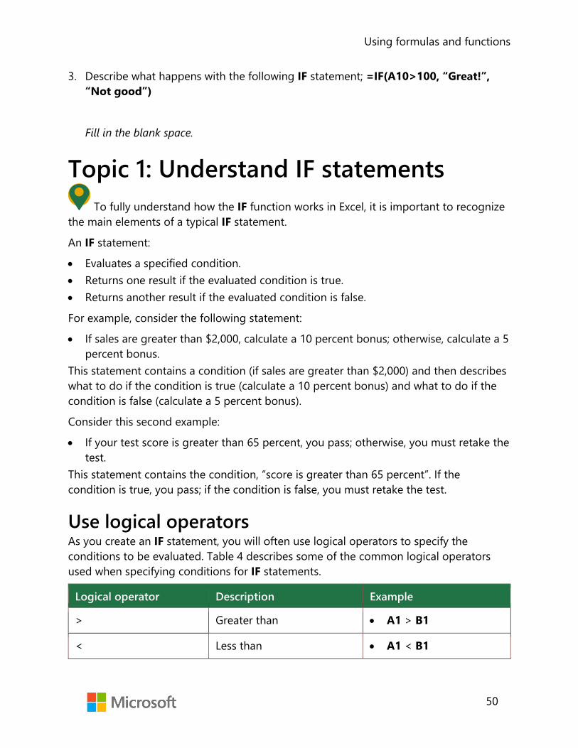
Using formulas and functions
50
3. Describe what happens with the following IF statement; =IF(A10>100, “Great!”,“Not good”)
Fill in the blank space.
Topic 1: Understand IF statements To fully understand how the IF function works in Excel, it is important to recognize
the main elements of a typical IF statement.
An IF statement:
• Evaluates a specified condition.• Returns one result if the evaluated condition is true.• Returns another result if the evaluated condition is false.
For example, consider the following statement:
• If sales are greater than $2,000, calculate a 10 percent bonus; otherwise, calculate a 5percent bonus.
This statement contains a condition (if sales are greater than $2,000) and then describes what to do if the condition is true (calculate a 10 percent bonus) and what to do if the condition is false (calculate a 5 percent bonus).
Consider this second example:
• If your test score is greater than 65 percent, you pass; otherwise, you must retake thetest.
This statement contains the condition, “score is greater than 65 percent”. If the condition is true, you pass; if the condition is false, you must retake the test.
Use logical operators As you create an IF statement, you will often use logical operators to specify the conditions to be evaluated. Table 4 describes some of the common logical operators used when specifying conditions for IF statements.
Logical operator Description Example
> Greater than • A1 > B1
< Less than • A1 < B1

Using formulas and functions
51
Logical operator Description Example
= Equal to • A1 = B1
<> Not equal to • A1 <> B1
>= Greater than or equal to • A1 >= B1
<= Less than or equal to • A1 <= B1
Table 4: Logical operators used for conditions
Activity: Discuss and learn In this activity, the teacher will display several IF statements for you to analyze.
Resources required You will need the following resources for this activity:
None.
Activity instructions Follow along as the teacher presents several IF statements. As you analyze each statement, discuss:
• What is the condition being evaluated? • What happens if the result is true? • What happens if the result is false?
Try-it: Understand IF statements This try-it activity has you identify examples of using IF statements in Excel.
Resources You will need the following resources for this try-it:
None.

Using formulas and functions
52
Instructions The following are the general tasks that you need to perform during this try-it:
1. Pair up with a fellow student and discuss: What are three situations where an IF statement would be useful in an Excel worksheet?
2. Share your ideas with the class.
Topic 2: Use the IF function IF statements are integrated into an Excel worksheet by using the IF function. The
IF function follows the same principle as an IF statement where a condition is evaluated and then returns a specific result based upon a TRUE or FALSE evaluation.
IF functions are quite useful in an Excel worksheet such as in the following situations:
• You need to test if a condition is true or false when evaluated against data in a worksheet.
• You need to output specific text based upon the evaluation of a condition. • You need to perform additional calculations on data based upon the evaluation of a
condition.
IF function syntax As shown in Figure 20, the IF function begins with an equal (=) sign followed by the name and opening parentheses. The function contains three arguments described as follows:
• logical_test (required)—A value or expression that specifies the condition you want to test.
• value_if_true (optional)—The value you want returned if the result of the logical_test is TRUE. This can contain numbers, text, and additional formulas or functions to be evaluated.
• value_if_false (optional)—The value you want returned if the result of the logical_test is FALSE. This can contain numbers, text, and additional formulas or functions to be evaluated.
Figure 20: IF function

Using formulas and functions
53
Considerations when using the IF function As shown in the syntax, the IF function only requires the logical_test argument in the formula. Both the value_if_true and the value_if_false arguments are optional. It is important to understand the impact to your formula if you omit the TRUE or FALSE arguments.
When constructing an IF function, consider the following:
• If you omit the value_if_true argument, the IF function will return 0 when the condition is met. For example, consider the following statement: =IF(A1>100, “No”) If A1 is greater than 100, then 0 will automatically display since the second argument is omitted. If A1 is not greater than 100, the text “No” will display.
• If you omit the value_if_false argument, when the condition is false, the IF function will return the logical value of FALSE. If you place a comma after the value_if_true argument, the evaluation will return a 0. For example, consider the following statement: =IF(A1>100, “Yes”) The value_if_false argument is omitted. This results in the logical value of FALSE being displayed. If you place a comma after the word “Yes”, the evaluation will return a 0.
Did you know?
If you do not want the IF statement to display any value when the condition is evaluated, enter double quotes (““) in the argument that you want to have blank. For example: =IF(A1>100, “Yes”, ““) results in an empty string when the formula is evaluated as FALSE.
Video
To review the video and additional information on how to use the IF function, go to: IF function
Activity: Show and tell In this activity, your teacher will demonstrate and explain how to use the IF function in an Excel worksheet.

Using formulas and functions
54
Resources required You will need the following resources for this activity:
None.
Activity instructions Pay close attention as your teacher demonstrates and explains the following tasks:
1. Determine the structure of an IF statement.
2. Construct an IF function to perform an evaluation of data.
Try-it: Use the IF function In this try-it activity, you will open a sample document and create and troubleshoot
IF functions.
Try-it 1 In this try-it, you will open a sample document and create an IF function.
Resources You will need the following resources for this try-it:
• Open L5_T2_try1_matching_if_statement_starter.xlsx in this lesson’s Learning Activity Resources.
Instructions The following are the general tasks that you need to perform during this try-it:
1. In the Company Match column, in cell G3, create a formula that evaluates the following:
o If the donation amount is over $150, display the word “Match.” o If the donation amount is not over $150, display the word “No Match.”
2. Copy the formula created in cell G3 to cells G4 through to G8.
3. Bonus step: Apply a conditional formatting rule to the Company Match column that highlights all entries that say Match with a Light Red Fill with Dark Red Text.
4. In cell H2, enter the column heading Match Amount.

Using formulas and functions
55
5. In the Match Amount column, in cell H3, create a formula that evaluates the following:
o If the Company Match entry says Match, then multiply the donation amount by 2 to get the match amount.
o If the Company Match entry says No Match, then display 0 in the Match amount column.
6. Copy the formula created in cell H3 to cells H4 through to H8.
7. Save and close the file.
Try-it 2 In this try-it, you will open a sample document and edit an IF function.
Resources You will need the following resources for this try-it:
• Open L5_T2_try2_edit_if_statement_starter.xlsx in this lesson’s Learning Activity Resources.
Instructions The following are the general tasks that you need to perform during this try-it:
1. In the Company Match column, in cell G3, edit the If statement as follows:
o If the donation amount is equal to or over $150, then multiply the donation amount by 2 to get the company match amount.
o If the donation amount is not over $150, then display a blank cell. 2. Copy the formula created in cell G3 to cells G4 through to G8.
3. Save and close the file.
Wrap-up Use these questions to check what you learned in this lesson:
1. An IF function can contain additional calculations as arguments. True or false?
Select the correct option.
a. True
b. False

Using formulas and functions
56
2. Describe what happens with the following IF statement; =IF(C20>=25,C20*5,)
3. Consider the following formula: =IF(C20>=25,C20*5,). What happens to a false result if you remove the last comma in the If statement?Select the correct answer.
a. 0 is displayed.
b. FALSE is displayed.
c. Error is displayed.
d. C20*5 is displayed.

Using formulas and functions
57
Glossary Formula A mathematical equation that performs calculations on values in a
worksheet.
Value A representation in Excel that can be a number, cell address, date, text, or range of cells.
Constant A number or text value that is entered directly into a cell.
Operator An indicator used to specify the type of calculation to take place, such as add (+); subtract (-); multiply (*); or divide (/).
Function A pre-built command in Excel that performs mathematical operations such as automatically adding up a range of cells or looking up values to be used in calculations.
Order of operations
A standard mathematical process used to determine which operator to calculate first when evaluating a formula.
Cell reference Identifies a cell’s location within a worksheet.
Relative cell reference
A cell or range reference in a formula that changes based upon the relation to the cell containing the formula.
Absolute cell reference
A cell reference in a formula that refers to a specific cell or range regardless of where the formula is located in the worksheet.
Mixed cell reference
A cell or range in a formula that uses both a relative and absolute reference.
Named range A single cell or group of cells in an Excel worksheet with a designated name.
Function A predefined formula that is used for a specific purpose and performs special calculations in an Excel worksheet.
Table 5: Glossary terms and definitions
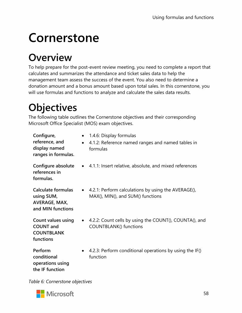
Using formulas and functions
58
Cornerstone Overview To help prepare for the post-event review meeting, you need to complete a report that calculates and summarizes the attendance and ticket sales data to help the management team assess the success of the event. You also need to determine a donation amount and a bonus amount based upon total sales. In this cornerstone, you will use formulas and functions to analyze and calculate the sales data results.
Objectives The following table outlines the Cornerstone objectives and their corresponding Microsoft Office Specialist (MOS) exam objectives.
Configure, reference, and display named ranges in formulas.
• 1.4.6: Display formulas • 4.1.2: Reference named ranges and named tables in
formulas
Configure absolute references in formulas.
• 4.1.1: Insert relative, absolute, and mixed references
Calculate formulas using SUM, AVERAGE, MAX, and MIN functions
• 4.2.1: Perform calculations by using the AVERAGE(), MAX(), MIN(), and SUM() functions
Count values using COUNT and COUNTBLANK functions
• 4.2.2: Count cells by using the COUNT(), COUNTA(), and COUNTBLANK() functions
Perform conditional operations using the IF function
• 4.2.3: Perform conditional operations by using the IF() function
Table 6: Cornerstone objectives

Using formulas and functions
59
Duration 50 minutes
Instructions 1. Complete the tasks below for each file.
2. When saving your file, add your name to the end of the filename; for example,“Cornerstone_attendance_ticketsales_Dwayne_Espino.” Follow your teacher’sdirections for where to save your files.
3. When you’re done with the Cornerstone, assess your completion and enter thepoints you think you earned within the task lists below. You can use the help of yourteacher if you need it.
Tasks You will work with one file in this Cornerstone. The following are the tasks you need to do within the file.
File 1: Cornerstone_attendance_ticketsales_starter.xlsx Task: Configure, reference, and display named ranges in formulas (10 points) 1. Open Cornerstone_attendance_ticketsales_starter.xlslx. On the BlueberryFestival
worksheet, configure a named range called Attendance that includes values B5 toB10. (2 points) (Exam objective 4.1.2)
2. Configure a named range called Cost_per_Ticket that includes values C5 to C10. (2points) (Exam objective 4.1.2)
3. In cell D5, calculate the total sales for each membership category. Be sure to create aformula that references the named ranges. (2 points) (Exam objective 4.1.2)
4. Copy the formula from cell D5 to cells D6 through D10. (2 points)
5. Turn on the Show Formulas command. Call your teacher to verify this step and thenturn off the Show Formulas command. (2 points) (Exam objective 1.4.6)
Points scored: /10
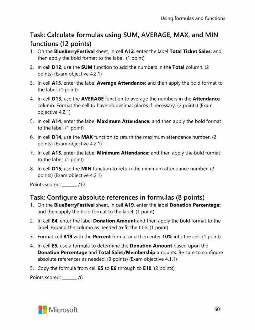
Using formulas and functions
60
Task: Calculate formulas using SUM, AVERAGE, MAX, and MIN functions (12 points) 1. On the BlueBerryFestival sheet, in cell A12, enter the label Total Ticket Sales: and
then apply the bold format to the label. (1 point)
2. In cell D12, use the SUM function to add the numbers in the Total column. (2 points) (Exam objective 4.2.1)
3. In cell A13, enter the label Average Attendance: and then apply the bold format to the label. (1 point)
4. In cell D13, use the AVERAGE function to average the numbers in the Attendance column. Format the cell to have no decimal places if necessary. (2 points) (Exam objective 4.2.1)
5. In cell A14, enter the label Maximum Attendance: and then apply the bold format to the label. (1 point)
6. In cell D14, use the MAX function to return the maximum attendance number. (2 points) (Exam objective 4.2.1)
7. In cell A15, enter the label Minimum Attendance: and then apply the bold format to the label. (1 point)
8. In cell D15, use the MIN function to return the minimum attendance number. (2 points) (Exam objective 4.2.1)
Points scored: _______ /12
Task: Configure absolute references in formulas (8 points) 1. On the BlueBerryFestival sheet, in cell A19, enter the label Donation Percentage:
and then apply the bold format to the label. (1 point)
2. In cell E4, enter the label Donation Amount and then apply the bold format to the label. Expand the column as needed to fit the title. (1 point)
3. Format cell B19 with the Percent format and then enter 10% into the cell. (1 point)
4. In cell E5, use a formula to determine the Donation Amount based upon the Donation Percentage and Total Sales/Membership amounts. Be sure to configure absolute references as needed. (3 points) (Exam objective 4.1.1)
5. Copy the formula from cell E5 to E6 through to E10. (2 points)
Points scored: _______ /8

Using formulas and functions
61
Task: Perform conditional operations using the IF function (6 points) 1. On the BlueBerryFestival sheet, in cell F4, enter the label Bonus and then apply the
bold format to the label. (1 point)
2. In cell F5, use a formula to evaluate the following: (3 points) (Exam objective 4.2.3)
If the Donation Amount is greater than 100, calculate a 10 percent bonus on the Donation amount; otherwise, leave a blank cell.
3. Copy the formula from cell F5 to F6 through to F10. (2 points)
Points scored: _______ /6
Task: Count values using COUNT and COUNTBLANK functions (9 points) 1. On the BlueBerryFestival sheet, in cell A16, enter the label Number of Bonus
Entries: and then apply the bold format to the label. (1 point)
2. On the BlueBerryFestival sheet, in cell A17, enter the label Number of No Bonus Entries: and then apply the bold format to the label. (1 point)
3. In cell C16, use a formula to count the number of cells under the Bonus heading that contains a value. (2 points) (Exam objective 4.2.2)
4. In cell C17, use a formula to count the number of empty cells under the Bonus heading. (2 points) (Exam objective 4.2.2)
5. Format all numbers that represent dollar amount to the Currency format. (3 points)
Points scored: _______ /9
FILE 1 TOTAL POINTS: _______ /45

Student Guide 40567A Microsoft Excel associate 2019 Module 6: Getting and transforming data

Getting and transforming data
2
Contents
Contents .............................................................. 2
Module overview ............................................. 5
Description ..................................................... 5
Scenario .......................................................... 6
Cornerstone ................................................... 6
Lesson 1: Importing data .............................. 7
Overview ......................................................... 7
Warm-up ........................................................ 7
Scenario .......................................................... 8
Topic 1: Get data from other sources . 8
Get & transform data ............................ 8
Activity: Pose a challenge .................... 9
Try-it: Get data from other sources . 9
Topic 2: Import data from .txt files ... 10
Using Notepad to review a .txt file .............................................................. 10
Getting data from .txt files ............... 10
Activity: Show and tell ....................... 11
Try-it: Import data from .txt files ... 11
Topic 3: Import data from .csv files .. 12
Using Notepad to review a .csv file .............................................................. 12
Getting data from .csv files .............. 12
Activity: Show and tell ....................... 12
Try-it: Import data from .csv files .. 13
Wrap-up ....................................................... 14
Lesson 2: Manipulating text ..................... 15
Overview ...................................................... 15
Warm-up ...................................................... 15
Topic 1: Convert text to columns ....... 16
Splitting text into columns ............... 16
Activity: Discuss and Learn ............... 17
Try-It: Convert text to columns ...... 18
Topic 2: Extract text by using the LEFT, RIGHT, MID, and LEN functions .......... 19
LEFT function ......................................... 19
RIGHT function ...................................... 20
LEN function ........................................... 21
MID function .......................................... 21
Character counting .............................. 22
Activity: Show and tell ........................ 23
Try-it: Extract text by using the LEFT, RIGHT, MID, and LEN functions ..... 24
Try-it 1 ...................................................... 24
Try-it 2 ...................................................... 25
Try-it 3 ...................................................... 25
Try-it 4 ...................................................... 26
Wrap-up questions .................................. 26
Lesson 3: Converting text .......................... 28
Overview ...................................................... 28
Warm-up questions ................................. 28
Topic 1: Convert text by using the PROPER function ....................................... 29
Converting Text: PROPER ................. 29
Copying a formula to multiple cells ............................................................ 29
Using Paste Special ............................. 30
Getting and transforming data
3
Activity: Tell a story ............................. 31
Try-it: Convert text by using the PROPER function ................................. 31
Try-it 1 ...................................................... 32
Try-it 2 ...................................................... 32
Try-it 3 ...................................................... 32
Topic 2: Convert text by using the UPPER and LOWER functions .............. 33
Converting Text: UPPER .................... 33
Converting Text: LOWER .................. 34
Activity: Show and tell ....................... 34
Try-it: Convert text by using the UPPER and LOWER functions ......... 35
Try-it 1 ...................................................... 35
Try-it 2 ...................................................... 35
Try-it 3 ...................................................... 36
Wrap-up ....................................................... 36
Lesson 4: Combining text .......................... 38
Overview ...................................................... 38
Warm-up ..................................................... 38
Topic 1: Combine text by using the CONCAT function ..................................... 39
Combining text: CONCAT ................ 39
Adding space or a word between data when using the CONCAT function ................................................... 40
Combining text using absolute cell references ............................................... 40
Activity: Discuss and learn ............... 41
Try-it: Combine text by using the CONCAT function ................................ 42
Try-it 2 ...................................................... 43
Try-it 3 ...................................................... 43
Topic 2: Combine text by using the TEXTJOIN function ................................... 44
Combining text: TEXTJOIN ............... 44
Combining text: CONCAT and TEXTJOIN ................................................. 44
Activity: Pose a challenge ................. 45
Try-it: Combine text by using the TEXTJOIN function ............................... 46
Try-it 1 ...................................................... 46
Try-it 2 ...................................................... 47
Wrap-up ....................................................... 47
Lesson 5: Inserting hyperlinks .................. 49
Overview ...................................................... 49
Warm-up ...................................................... 49
Topic 1: Insert hyperlinks to navigate inside a workbook .................................... 50
Creating a hyperlink to place within the document ........................................ 51
Creating a hyperlink to a cell range ......................................................... 52
Activity: Tell a story ............................. 53
Try-it: Insert hyperlinks to navigate inside a workbook ............................... 55
Try-it 1 ...................................................... 55
Try-it 2 ...................................................... 55
Try-it 3 ...................................................... 56
Topic 2: Insert hyperlinks to navigate outside a workbook ................................. 57
Creating a hyperlink to another file ............................................................... 57
Creating a hyperlink to a website . 58
Activity: Discuss and learn ................ 59

Getting and transforming data
4
Try-it: Insert hyperlinks to navigate outside a workbook ............................ 60
Try-it 1 ...................................................... 60
Try-it 2 ...................................................... 61
Try-it 3 ...................................................... 61
Topic 3: Remove hyperlinks ................. 62
Removing a hyperlink: Edit Hyperlink dialog box .......................... 62
Removing a hyperlink: context menu ......................................................... 62
Removing hyperlinks from multiple cells ........................................................... 63
Try-it: Remove hyperlinks ................ 63
Try-it 1 ...................................................... 63
Try-it 2 ...................................................... 64
Try-it 3 ...................................................... 64
Wrap-up ....................................................... 65
Glossary ............................................................. 66
Cornerstone ..................................................... 67
Overview ...................................................... 67
Objectives .................................................... 67
Duration ....................................................... 67
Instructions .................................................. 68
Tasks .............................................................. 68
File 1: Blank new Excel file ................ 68

Getting and transforming data
5
Module overview Description At times you might want to work with large quantities of data within a spreadsheet. This can become difficult and cause errors when entering data manually into the spreadsheet. Microsoft Excel 2019 allows you to use other sources to import the needed data, thus reducing the potential for errors.
The following table outlines the lessons in this module and their corresponding learning objectives.
Lesson Learning objective Exam objective(s)
Importing data
Import data from text files (.txt and .csv) • 1.1.1 • 1.1.2
Manipulating text
Use Text-to-Columns and the LEFT, RIGHT, MID, and LEN functions
• 4.3.1
Converting text
Use the PROPER, UPPER, and LOWER functions
• 4.3.2
Combining text
Use the CONCAT and TEXTJOIN functions • 4.3.2
Inserting hyperlinks
Insert hyperlinks for navigation within and outside the workbook, and remove hyperlinks
• 1.2.3
Importing data into a workbook
Import data from text files; manipulate, convert, and combine text using Text-to-Columns and Text functions; insert hyperlinks for navigation
• 1.1.1 • 1.1.2 • 1.2.3 • 4.3.1 • 4.3.2
Table 1: Objectives by lesson
Getting and transforming data
6
Scenario The best months to sow, plant, and harvest crops are at a set time each year. As a Research & Development intern, you have been asked to check common problems with crop growth.
You have separate .csv and .txt files containing useful crop information. You need to import the data from these files into an Excel workbook. You also need to fix issues with the data formatting—some data has some text in upper case and lower case and unnecessary spaces. Other related data needs to be accessible from the workbook by inserting a hyperlink.
Cornerstone At times, you may use crop growth data from other sources to help plan the crop growth for Munson’s. This data might come in a .txt or .csv format, such as from government websites, which you are required to import into your workbook without retyping it. After importing the data, you may find capitalization errors in the data or you might want to separate or combine data from what you have been provided. You perform these tasks by using the built-in functions in Excel.

Getting and transforming data
7
Lesson 1: Importing data Overview In this lesson, you’ll explore what is meant by data, and how you can bring large data sets into an Excel file. You’ll learn how to use the Get & Transform option to bring in data from .txt and .csv files.
Warm-up Use these questions to find out what you already know about this lesson’s topics:
1. Which of the following options best describes a .txt file?
Select the correct option.
a. A special spreadsheet file containing dates
b. A file used to store numbers
c. A file used to hold data without formatting
d. A file used to hold music files
2. What is a delimiter?
Select the correct option.
a. A way to combine data
b. A way to organize data
c. Something used to limit the use of data
d. A process to collect data
3. What is unique about a .csv file?
Select the correct option.
a. It contains only numeric data
b. The file uses a space to separate data
c. It uses a comma as a delimiter
d. It is a file type restricted to the use of a word processing program
4. List three ways you can separate data within a data file.
____________________________________________________________________________________

Getting and transforming data
8
Scenario Munson’s Pickles and Preserves currently has a customer list containing customer names, addresses, and phone numbers in a document file. They need all the information within that file placed into an Excel workbook. You have been given the task to place the customer information into the Excel workbook. How would you attempt this task?
Come up with your own ideas on how to complete this task. Be prepared to discuss your ideas with a partner and then with the rest of the class.
Topic 1: Get data from other sources Data is a group of letters, symbols, and numbers that a computer can perform
operations upon to create useful information. The data can be manipulated in different ways to create useful information. Data can be obtained from many different sources. Each time you enter your name and other information into a website to purchase an item or add your name to a mailing list, you are entering data that the computer will later use to perform a task for users of the data. You can store data in different types of files. Excel will allow you to use those files to enter the data into your Excel worksheet.
Get & transform data Excel allows you to get data from sources other than other Excel files, and enter the data yourself. To import data from other sources:
1. Select the Data tab.
2. On the Get & Transform Data tab, select to get data from the source of your choice.
Additional information
For more information on importing data from external data sources, go to: Import data from external data sources (Power Query)

Getting and transforming data
9
Activity: Pose a challenge Excel’s Data tab allows you to get data from several different sources. In this activity, you’ll explore the functions within the Data tab.
Resources You will not need any resources for this activity.
Activity instructions Participate in the activity by following these instructions:
1. Open a blank Excel worksheet.
2. You have been given a word processor file with the names, addresses, and phonenumbers of customers, and are asked to enter this data into an Excel spreadsheet.
3. You’re very limited on time. How do you get the data from the word processor fileinto the Excel spreadsheet correctly and quickly?
Try-it: Get data from other sources In this standalone try-it, you will explore the options that are available within the
Data tab.
Resources You will not need any resources for this activity.
Instructions The following steps are the general tasks that you need to perform during this try-it:
1. Open a blank Excel worksheet.
2. On the Home ribbon, select the Data tab.
3. Study the Get & Transform Data group.
4. Be prepared to discuss the following questions with the class:
o What different data formats can you use with Excel?o What do you think is meant by .csv?o What resources do you think exist on the web that might be used for data?

Getting and transforming data
10
Topic 2: Import data from .txt files Sometimes, you’ll have to work with data within a word-processor file. You can
convert these files into a .txt file. A .txt file is a file format that contains no formatting; it has only text, numbers, and symbols. You can identify a .txt file by its extension .txt.
Using Notepad to review a .txt file To use Notepad to review a .txt file:
1. Locate a .txt file.
2. Right-click or access the context menu for the file, select Open With, and then select Notepad.
Getting data from .txt files To retrieve the data from .txt files:
1. Open a blank Excel workbook.
2. On the Home ribbon, select the Data tab.
3. In the Get & Transform Data group, select From Text/CSV.
4. In the Import Data dialog box, find the .txt file, and then select Import.
5. A second dialog box will open displaying the data you will be bringing into Excel. This dialog box allows you to preview the data prior to bringing it into Excel.
6. In the Delimiter drop-down menu, select the type of delimiter that will work for this file, and then select Load. A delimiter determines how the data is separated into columns. In this file, the delimiter is a tab.
7. The data from the .txt file will be loaded into the Excel file.
Additional information
For more information on importing or exporting text (.txt or .csv) files, go to: Import or export text (.txt or .csv) files

Getting and transforming data
11
Activity: Show and tell Opening .txt files using Notepad will enable you to preview what the file contains prior to using the Get & Transform Data tool within Excel.
Resources required You will need the following resource for this activity:
• Open the L1_T2_act_customer_list.txt file in this lesson’s Learning Activity Resources folder.
Activity instructions Participate in the activity by following these instructions:
1. Using the L1_T2_act_customer_list.txt file, right-click or access the context menu for the file, select Open With, and then select Notepad.
2. Study the data within the file and answer the following questions:
o What data is included in the file? o What categories are used to organize the data? o How is the data separated? What is used between the categories?
Try-it: Import data from .txt files In this standalone try-it, you will import data from a .txt file into a blank Excel
worksheet.
Resources You will need the following resource for this try-it:
• Locate the L1_T2_try_customer_list_starter.txt file in this lesson’s Learning Activity Resources folder.
Instructions During this try-it, you will perform the following tasks:
1. In a blank Excel workbook, get the data from the L1_T2_try_customer_list_starter.txt and import it into the blank workbook using Tab as the delimiter.
2. Save your work.

Getting and transforming data
12
Topic 3: Import data from .csv files Sometimes, you will find data within a .csv file. .csv stands for Comma Separated
Values. The process for importing .csv data into Excel is very similar to the process for importing .txt data. However, a .csv file is set up in a slightly different way.
Using Notepad to review a .csv file To use Notepad to review a .csv file:
1. Locate a .csv file.
2. Right-click the file or open it from the context menu, select Open With, and then select Notepad.
Getting data from .csv files To get data from a .csv file:
1. Using a blank Excel workbook, on the Home ribbon, select the Data tab.
2. In the Get & Transform Data group, select From Text/CSV.
3. In the Import Data dialog box, find the .csv file, and then select Import.
A second dialog box will open displaying the data you will be bringing into Excel. This dialog box allows you to preview the data prior to bringing it into Excel.
4. In the Delimiter drop-down menu, select Comma. A .csv file separates the data into columns using a comma. Then, select the Load button.
The data from the .csv file will be loaded into the Excel file.
Additional information
For more information on importing or exporting text (.txt or .csv) files, go to: Import or export text (.txt or .csv) files
Activity: Show and tell You can open a .csv file using the Notepad app the same way you can open a .txt file. Opening .csv files using Notepad will allow you to preview what the file contains prior to using the Get & Transform Data group within Excel.

Getting and transforming data
13
Resources required You will need the following resource for this activity:
• Locate L1_T3_act_customer_purchases.csv file in this lesson’s Learning Activity Resources folder.
Activity instructions Participate in the activity by following these instructions:
1. Using the L1_T3_act_customer_purchases.csv file, right-click the file or open the context menu, select Open With, and then select Notepad.
2. Study the data within the file and answer the following questions:
a. What data does this file contain?
b. What categories are used to organize the data?
c. Can you locate the commas that separate the categories?
Try-it: Import data from .csv files In this standalone try-it, you will import data from a .txt file into a blank Excel
worksheet.
Resources You will need the following resource for this try-it:
• Locate the L1_T3_try_customer_purchases_starter.csv file in this lesson’s Learning Activity Resources folder.
Instructions You will perform the following general tasks during this try-it:
1. In a blank Excel workbook, import the data from the L1_T3_try_customer_purchases_starter.csv file and use Comma as the delimiter.
2. Save your work.
Getting and transforming data
14
Wrap-up Use these questions to check what you learned in this lesson:
1. What does a delimiter do?
Select the correct option.
a. It provides a way to give color and style to a workbook.
b. It tells Excel how to organize data into columns.
c. It tells Excel where to place a title for a workbook.
d. It gives information about the data being imported.
2. What delimiter does a CSV file use?
Select the correct option.
a. Tab
b. Spacebar
c. Hash tag
d. Comma
3. What is data?
Select all that apply.
a. It’s a group of letters, numbers, and symbols that a computer can perform an operation on.
b. It’s the same thing as information.
c. It’s information that is used to track daily sales.
d. It’s a graphical representation.
4. ________________________ is the option users use in Excel to bring in data from sources such as TXT and CSV files.
5. Give a detailed example of when you might need to bring outside data into Excel to create a worksheet.
________________________

Getting and transforming data
15
Lesson 2: Manipulating text Overview When using data files, sometimes the data isn’t divided up into useful components. At times, two or more pieces of data will be included within the same category, when the user will want it to be in separate categories. Excel allows you to manipulate the data so that you can separate one category of data into two or more columns.
Warm-up Use these questions to find out what you already know about this lesson’s topics:
1. Which of the following options would be the best way to separate data?
Select the correct option.
a. One category: Name + address + zip code + phone number
b. Two categories: Name + address & zip code + phone number
c. Three categories: Name & address & zip code + phone number
d. Four categories: Name & address & zip code & phone number
2. Which of the following options would be the best way to categorize someone’sname?
Select the correct option.
a. Just one category with first and last name.
b. Just one category with the last name first and first name last.
c. Two categories with the first and last name in one category and the phonenumber in the second category.
d. Two categories with the first name in one category and the last name in a secondcategory.

Getting and transforming data
16
3. Which of the following answers explains how to use the MID function?
Select the correct option.
a. MID allows users to find the midpoint of a line.
b. The MID function allows the user to specify a starting point and how many characters to extract from that point.
c. The MID function takes the data to the left and the right of a category starting from the middle of the data.
d. MID finds the middle column of a group of columns within a workbook.
4. To separate the area code from a phone number, use the ________________________ function.
5. Explain how separating the area code from a phone number might be useful.
________________________
Topic 1: Convert text to columns Munson’s Pickle and Preserves now has their Customer List and Customer
Purchases data in an Excel file. They would like to increase their marketing efforts assigning two marketing associates to make calls to follow up with their customers. As many of their customers are within the state of Kansas, it makes sense to assign one marketing associate to the state of Kansas, and the second to all the other states. To complete this task, Munson’s needs to separate all the phone numbers within their Customer List into area codes and phone numbers.
Splitting text into columns You can separate data from one column into multiple columns. To separate the data, you use a delimiter. A delimiter is a method for separating text.
To split text into columns:
1. On the Home ribbon, select the Data tab, and locate the Data Tools group.
2. Select the column containing the data you want to separate.
3. Select the Text to Columns option.
4. In the Convert Text to Columns Wizard - Step 1 of 3, make sure the Delimited radio button has been selected.

Getting and transforming data
17
Figure 1: Convert Text to Columns Wizard - Step 1 of 3 dialog box
5. Select the Next button.
6. In the Convert Text to Columns Wizard - Step 2 of 3, select the type of delimiter to use to separate the data. The Other choice allows you to enter a dash as a delimiter.
Figure 2: Convert Text to Columns Wizard - Step 2 of 3 dialog box
7. Select Finish.
Your .csv file will now be entered into your Excel file.
Activity: Discuss and learn Munson’s has sent an email asking for data in one column of a workbook to be split into two columns. What type of data do you think could be in the column that needs to be split into two columns?

Getting and transforming data
18
Resources required You will need the following resource for this activity:
• Locate L2_T1_act_customer_names_starter.xlsx file in this lesson’s Learning Activity Resources folder.
Activity instructions Participate in the activity by completing these steps:
1. On the Data tab locate the Data Tools group.
2. Select column A (the column with the customer names in it).
3. Select the Text to Columns option.
4. In the Convert Text to Columns Wizard - Step 1 of 3, make sure the Delimited radio button has been selected.
5. Select Next.
6. In the Convert Text to Columns Wizard - Step 2 of 3, select the Space option.
7. Select Finish.
Your result should place the customer’s first name in the A column and the customer’s last name in the B column.
Try-it: Convert text to columns One way to divide up the phone numbers into area codes and phone numbers is
to use Text to Columns. Text to Columns uses a delimiter to determine how to separate the text into separate columns. A delimiter could be any character that is used between the separate parts.
Resources required You will need the following resource for this try-it:
• Open the L2_T1_try_customer_list_starter.xlsx file found in this lesson’s Learning Activity Resources folder.

Getting and transforming data
19
Instructions You will need to perform the following general tasks during this try-it:
1. Select column H (the column with the phone numbers in it).
2. Use the Text to Columns option to separate the phone number into columns using the dash as the delimiter.
3. Save your work.
Topic 2: Extract text by using the LEFT, RIGHT, MID, and LEN functions
Using the Text to Columns feature doesn’t really fix Munson’s problem. When using the Text to Columns function, the area code is separated out, but the seven-digit phone number is separated into two parts because of the second dash. Munson’s would like the area code by itself and the rest of the phone number left intact. There are several ways of accomplishing this task. All the solutions deal with the idea of extracting parts of a string.
A string is a collection of characters upon which no mathematical calculations are to be performed. For example, a phone number or zip code is a collection of specialized characters called numbers; however, these numbers are not going to be used in a mathematical way—they are a string.
Strings can contain groupings of specialized characters called text. The information you are reading now is text. The letters are grouped together to form words, the words are grouped together to form sentences, and so forth.
LEFT function The LEFT function allows you to select a specific number of characters starting from the left side of the data.
To use the LEFT function in a formula:
1. Select the cell where you want your resulting data to be placed.
2. In the formula bar, enter =LE

Getting and transforming data
20
3. The wizard will offer suggestions to complete your function. Make sure LEFT is highlighted, and then select the Tab button.
Figure 3: Wizard suggesting function names
The wizard leads you through completing your function by displaying the required data to complete the function. For example, =LEFT(text, [num_chars]). This function takes the left number of characters you specify from the text you enter.
RIGHT function The RIGHT function allows you to select a specific number of characters starting from the right side of the data.
To use the RIGHT function in a formula:
1. Select the cell where you want your resulting data to be placed.
2. In the formula bar, enter =RI.
3. The wizard will offer suggestions to complete your function. Make sure RIGHT is highlighted, and then select the Tab key.
Figure 4: Wizard making function suggestions
4. The wizard will lead you through completing your function. It will display the data necessary to complete the function. For example, =RIGHT(text, [num_chars]). This is very similar to the LEFT function. This function takes the right number of characters you specify from the text you enter.

Getting and transforming data
21
LEN function The LEN function counts the number of characters within a text string.
To use the LEN function in a formula:
1. Select the cell where you want your resulting data to be placed.
Variations of the LEFT and RIGHT functions make it possible to select various selections of text from data. For example, if you want to remove the area code from a phone number, you could do that combining the RIGHT function with the LEN function. The LEN function determines the length of the data and then manipulates the data according to your specifications.
2. In the formula bar, enter =RI.
3. The wizard will offer suggestions to complete your function. Make sure RIGHT is highlighted, and then select the Tab button.
Figure 5: Wizard making function suggestions
4. You want to remove the area code from each phone number. Enter the cell reference where the phone number is held. For example, if the phone number is stored in column B2 use B2 for the text reference in both the RIGHT and LEN functions. You will also need to subtract four characters from the length of the data. Your function should read like this: =RIGHT(B2,(LEN(B2)-4)).
5. You can combine the LEFT function with the LEN function in a similar manner.
MID function The MID function allows you to remove text from data starting at any point you designate within a text string. You can also designate the number of characters to extract from the data.
To use the MID function in a formula:
1. Select the cell where you want your resulting data to be placed.
An additional way to extract data from a column is to use the MID function. The MID function allows you to start from the left of the data and move in a specified number of characters and then extract so many characters.
2. In the formula bar, enter =MID.
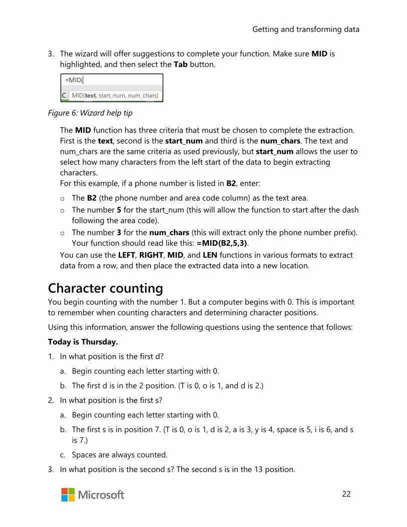
Getting and transforming data
22
3. The wizard will offer suggestions to complete your function. Make sure MID is highlighted, and then select the Tab button.
Figure 6: Wizard help tip
The MID function has three criteria that must be chosen to complete the extraction. First is the text, second is the start_num and third is the num_chars. The text and num_chars are the same criteria as used previously, but start_num allows the user to select how many characters from the left start of the data to begin extracting characters. For this example, if a phone number is listed in B2, enter:
o The B2 (the phone number and area code column) as the text area. o The number 5 for the start_num (this will allow the function to start after the dash
following the area code). o The number 3 for the num_chars (this will extract only the phone number prefix).
Your function should read like this: =MID(B2,5,3). You can use the LEFT, RIGHT, MID, and LEN functions in various formats to extract data from a row, and then place the extracted data into a new location.
Character counting You begin counting with the number 1. But a computer begins with 0. This is important to remember when counting characters and determining character positions.
Using this information, answer the following questions using the sentence that follows:
Today is Thursday.
1. In what position is the first d?
a. Begin counting each letter starting with 0.
b. The first d is in the 2 position. (T is 0, o is 1, and d is 2.)
2. In what position is the first s?
a. Begin counting each letter starting with 0.
b. The first s is in position 7. (T is 0, o is 1, d is 2, a is 3, y is 4, space is 5, i is 6, and s is 7.)
c. Spaces are always counted.
3. In what position is the second s? The second s is in the 13 position.

Getting and transforming data
23
Additional information
For more information on the LEFT function, go to: LEFT, LEFTB functions
Additional information
For more information on the RIGHT function, go to: RIGHT, RIGHTB functions
Additional information
For more information on the LEN function, go to: LEN, LENB functions
Additional information
For more information on the MID function, go to: MID, MIDB functions
Activity: Show and tell There might be times when you’ll need to separate data in a cell. This can happen when text in a column of data includes combined values. Selecting one of the functions will allow you to extract a portion of the data into a new cell.
Resources required You will need the following resource for this activity:
• Locate L2_T2_act_zip_codes_starter.xlsx file in this lesson’s Learning Activity Resources folder.
Activity instructions Participate in the activity by following these instructions:
1. In D1, enter LEFT. In E1, enter RIGHT. In F1, enter LEN. In G1, enter MID.
2. In D2, use the LEFT function to extract the five-digit zip code. Enter the function =LEFT(C2,5).
3. Use the Fill Handle to copy the formula for the remaining zip codes.

Getting and transforming data
24
4. In E2, use the RIGHT function to extract the last four digits of the nine-digit zip code. Enter the function =RIGHT(C2,4).
5. Use the Fill Handle to copy the formula for the remaining zip codes.
6. In F2, use the LEFT and LEN functions to extract five-digit zip code and the dash following the five digits. Enter the function =LEFT(C2,LEN(C2)-4).
7. Use the Fill Handle to copy the formula for the remaining zip codes.
8. In G2, use the MID function to extract the two digits on each side of the dash. Your result should be similar to XX-XX where the X’s are numbers. Enter the function =MID(C2,4,5).
9. Use the Fill Handle to copy the formula for the remaining zip codes.
Try-it: Extract text by using the LEFT, RIGHT, MID, and LEN functions
In this leveled try-it activity, you will use the LEFT, RIGHT, MID, and LEN functions to extract data from an Excel worksheet.
Try-it 1 In this try-it, you’ll use the LEFT function to extract the area codes from phone numbers.
Resources You will need the following resource for this try-it:
• Open your Customer_List.xlsx file created in Lesson 1 or use the L2_T2_try1_customer_list_area_code_left_starter.xlsx in this lesson’s Learning Activity Resources folder.
Instructions You will complete the following general tasks during this try-it:
1. In cell I1, enter Area Code.
2. In cell J1, enter Phone Number.
3. Use the LEFT function to extract the Area Code into I2.
4. Use the Fill Handle to copy the formula for the rest of the phone numbers.
5. Save your work.

Getting and transforming data
25
Try-it 2 In this try-it, you’ll use the RIGHT function to extract data to the right of a specified character.
Resources You will need the following resource for this try-it:
• Open L2_T2_try2_customer_list_area_code_right_starter.xlsx in this lesson’s Learning Activity Resources folder.
Instructions You will complete the following general tasks during this try-it:
1. In cell J2, use the RIGHT function to extract the phone number without the area code.
2. Use the Fill Handle to copy the formula for the rest of the phone numbers.
3. Save your work.
Try-it 3 In this try-it, you’ll use the LEN function along with other functions to extract a specified number of characters from data.
Resources You will need the following resource for this try-it:
• Open your Customer_List_Area_Code_RIGHT.xlsx file created in the Lesson 2 Try-it 2, or use the L2_T2_try3_customer_list_area_code_len_starter.xlsx in this lesson’s Learning Activity Resources folder.
Instructions You will complete the following general tasks during this try-it:
1. Select cell K1, and then enter Four Digit.
2. Select cell K2.
3. Combine the RIGHT and LEN functions to extract the phone number prefixes.
4. Use the Fill Handle to copy the formula for the rest of the phone numbers.
5. Save your work.

Getting and transforming data
26
Try-it 4 In this try-it, you’ll use the MID function to extract a specified number of characters from data.
Resources You will need the following resource for this try-it:
• Open L2_T2_try4_customer_list_area_code_mid_starter.xlsx in this lesson’sLearning Activity Resources folder.
Instructions You will complete the following general tasks during this try-it:
1. Place the cursor in cell L1, and then enter Middle.
2. Select cell L2.
3. Use the MID function to extract the phone prefix.
4. Use the Fill Handle to copy the formula for the rest of the phone numbers.
5. Save your work.
Wrap-up 1. The data in H2 is I like strawberries. What would the result be for the function
=LEFT(H2,4)?
Select the correct option.
a. I lik
b. I like
c. I li
d. I like s
2. The data in J2 is the zip code 43892-3424. What would the result be for the function=MID(J2,7,4)?
Select all that apply
a. -342
b. -34
c. 3424
d. 424

Getting and transforming data
27
3. There are ________________________ characters in this zip code 45392-2342?
4. If the data in I2 is 345-555-3425, which of the following would result in the data 555being extracted?
Select all that apply
a. =LEFT(I2,3)
b. =RIGHT(I2,8)
c. =MID(I2,5,3)
d. =LEFT(I2,LEN(I2)-5)
5. Indicate the correct order for entering the LEFT function in the formula bar.
Indicate the correct sequence by adding numbers 1 to 4 next to the following items.
a. Number of characters ________________________
b. LEFT ________________________
c. = ________________________
d. Cell reference ________________________

Getting and transforming data
28
Lesson 3: Converting text Overview When importing data into Excel from outside sources, the data might not always be formatted correctly. Sometimes data will have all the text capitalized., which might not be the most useful way to understand it. Excel provides functions to change that data.
Warm-up 1. Which of the following functions would correct the capitalization errors in MAIN
STREET?
Select the correct option.
a. PROPER
b. UPPER
c. LOWER
d. TITLE
2. Which of the following is an example of the function LOWER?
Select all that apply
a. SUNSHINE
b. Rain
c. snow
d. wIND
3. How would you convert text within a spreadsheet from all lowercase to every firstletter of every word capitalized?
Select all that apply
a. Reenter the information.
b. Use a function.
c. You can’t change it.
d. Use a text color tool.

Getting and transforming data
29
4. What would the formula be to convert the text in A2:A10 to all lower-case?
________________________
5. How would you replace the formulas in B2:B10 with the values from A2:A10?
________________________
Topic 1: Convert text by using the PROPER function
Munson’s just received a new customer list. When they opened the list, they found that the customers names, street addresses, and the state abbreviations are all lowercase. This is not the proper format for mailing out mail to their customers, and the file needs to be fixed. The customer list is rather large and reentering the names isn’t a feasible option.
Converting Text: PROPER The PROPER function capitalizes the first letter of each word within the selected cell.
To convert text using PROPER:
1. Select the cell where you want your resulting data to be placed.
2. Enter =PROPER( .
3. Enter the cell reference for the data you want to convert the first letter of each wordto a capital letter.
4. End the formula with an ending parenthesis ). Your formula should be similar to=PROPER(A3).
5. Select Enter.
Copying a formula to multiple cells Use one of the following techniques to copy a formula to multiple cells:
• Right-click a cell or open the context menu, and select Copy. Then select the rangeof cells you want to copy the formula to, right-click or access the context menu, andthen select Paste.
• Select the cell housing the formula, and from the Home tab, select Copy.

Getting and transforming data
30
• Select the area you want to copy the formula to, and then from the Home tab, selectPaste.
• Use the Fill Handle found in cell of the formula, and drag the Fill Handle down toH27.
Using Paste Special When using the PROPER function, the newly created data refers to the data found in the original location. Because the data in the original location isn’t that useful, it would be helpful to delete this data. However, if it’s deleted, the newly created data will contain an error message. To solve this problem, Excel provides a Paste Value option previously discussed in Module 2, Lesson 2: “Edit a worksheet.”
To use Paste Special:
1. After you have applied the PROPER function to the data and copied to the correctcells, keep the range of newly created cells selected.
2. Select Copy, and then select the Paste Special button.
Figure 7: Paste Special button
3. Within the Paste dialog box, select Paste Values, and then select Values. This willreplace the formula that was created with the value from the referenced cell.
Figure 8: Paste Values
4. Adjust the column as needed to fit the data.

Getting and transforming data
31
Additional information
For more information on the PROPER function, go to: PROPER function
Additional information
For more information on Paste Special, go to: Paste options
Activity: Tell a story You have just been given a .txt file and have been asked to import the data into an Excel workbook. When you finish importing the data into the workbook, you notice that all the text was entered with the CapsLock key on so all the letters are capitalized. Fortunately, Excel has functions to convert the case of text.
Resources required You will need the following resource for this activity:
• Locate L3_T1_act_customer_names_starter.xlsx file in this lesson’s LearningActivity Resources folder.
Activity instructions Participate in the activity by following these instructions:
1. In B2, enter =PROPER(A2), and then select Enter.
The data in A2 (tina bright) will be converted to Tina Bright.
2. Copy the formula from B2 to B3:B27.
3. Select the range B2:B27.
4. On the Home tab, in the Clipboard group, select Copy.
5. Select the Paste Special option.
6. In the dialog box, locate the Paste Values section.
7. Select the Paste Values, Values option. This will remove the formula reference andreplace it with the converted text.
Try-it: Convert text by using the PROPER function In this leveled try-it activity, you will use the PROPER function to convert text.

Getting and transforming data
32
Try-it 1 Resources You will need the following resource for this try-it:
• Open L3_T1_try1_customer_list_starter.xlsx in this lesson’s Learning ActivityResources folder.
Instructions You will perform the following general tasks during this try-it:
1. In H1, enter Names.
2. Use the PROPER function to convert the names within column H.
3. Save your work.
Try-it 2 Resources You will need the following resource for this try-it:
• Open L3_T1_try2_customer_list_starter.xlsx in this lesson’s Learning ActivityResources folder.
Instructions You will perform the following general tasks during this try-it:
1. Converting a single cell wasn’t that helpful when all the names needed converted, socopy the formula from H2 to the range H3:H27.
2. Save your work.
Try-it 3 Resources You will need the following resource for this try-it:
• Open the L3_T1_try3_customer_list_starter.xlsx file in this lesson’s LearningActivity Resources folder.

Getting and transforming data
33
Instructions Review the formula that was previously entered in cells H2:H27 and note, these cells all refer to the data found in column A. Because the data in column A isn’t that useful, it would be nice to delete this column. However, if you delete column A, the cells in column H will contain an error message.
You will perform the following general tasks during this try-it:
1. In H1, enter Names.
2. In H2, convert the text from A2 using the PROPER function.
3. Copy this formula to H2:H27.
4. Use Paste Special to remove the PROPER function and replace it with the convertedtext.
5. Reuse these steps to convert the address from column B to column I, and the citiesfrom column C to column J respectively using PROPER case. Don’t forget to use thePaste Values option.
6. Save your work.
Topic 2: Convert text by using the UPPER and LOWER functions
In the previous topic, PROPER case converted text so that the first letter of every word was capitalized. This isn’t always something you need though. At times, text needs to be converted to all uppercase or all lowercase. Both functions are similar in their use. This topic will focus on converting text to uppercase.
Converting Text: UPPER The UPPER function is similar in use to the PROPER function. However, the UPPER function converts text to all uppercase.
To convert text to all uppercase:
1. Select the cell where you want your converted text to be placed.
2. Enter =UPPER(.
3. Enter the cell reference for the data you want to convert, ending with a closingparenthesis ). Your resulting function should be similar to =UPPER(A2).

Getting and transforming data
34
Converting Text: LOWER The LOWER function is similar in use to the PROPER and UPPER functions. However, the LOWER function converts text to all lowercase.
To convert text to all lowercase:
1. Select the cell where you want your converted text to be placed.
2. Enter =LOWER(.
3. Enter the cell reference for the data you want to convert, ending with a closingparenthesis ). Your resulting function should be similar to =LOWER(A2).
Additional information
For more information on the UPPER function, go to: UPPER function
Additional information
For more information on the LOWER function, go to: LOWER function.
Activity: Show and tell You import another .txt file into Excel and this one has a mix of uppercase and lowercase data. In some cases, you have to change data from lowercase to uppercase and in other cases, you have to change data from uppercase to lowercase. You will use the Excel functions to convert the case of text.
Resources required You will need the following resource for this activity:
• Locate L3_T2_act_customer_names_starter.xlsx file in this lesson’s LearningActivity Resources folder.
Activity instructions Participate in the activity by following these instructions:
1. In C2, enter =UPPER(A2), and then select Enter.
All the letters in A2 will now be uppercase in C2.
2. In E2, enter =LOWER(A2), and then select Enter.
All the letters in A2 will now be lowercase in E2.

Getting and transforming data
35
Try-it: Convert text by using the UPPER and LOWER functions
In this leveled try-it activity, you will use the UPPER function to convert text.
Try-it 1 Resources You will need the following resource for this try-it:
• Open L3_T2_try1_customer_list_starter.xlsx in this lesson’s Learning ActivityResources folder.
Instructions You will complete the following general tasks during this try-it:
1. Place the cursor in cell K1, and then enter State.
2. Use the UPPER function in cell K2 to convert the two-digit state code to alluppercase letters.
3. Save your work.
Try-it 2 Resources You will need the following resource for this try-it:
• Open L3_T2_try2_customer_list_starter.xlsx in this lesson’s Learning ActivityResources folder.
Instructions You will complete the following general tasks during this try-it:
1. Place the cursor in cell K3.
2. Use the UPPER function in cell K3 to convert the two-digit state code to alluppercase letters.
3. Use the Fill Handle to copy this formula from K3:K27.
4. Save your work.

Getting and transforming data
36
Try-it 3 Resources You will need the following resource for this try-it:
• Open the L3_T2_try3_customer_list_starter.xlsx in this lesson’s Learning ActivityResources folder.
Instructions You will complete the following general tasks during this try-it:
1. In K1, enter State.
2. Use the UPPER function in cell K2 to convert the two-digit state code to alluppercase letters.
3. Use the Fill Handle to copy this formula from K2:K27.
4. Apply Paste Special, Values to the cell range to remove the function and replace itwith the correct text.
5. Save your work.
Wrap-up 1. Which of the following options would be an example of the result after using the
UPPER function?
Select the correct option.
a. guy rabin
b. GUY RABIN
c. gUY rABIN
d. Guy Rabin
2. Which function functions would be best to apply to a cell containing a title of a bookwhere the first letter of every word should be capitalized?
Select all that apply.
a. UPPER
b. LOWER
c. TITLE
d. PROPER

Getting and transforming data
37
3. By using ________________________ the reference cells can be deleted because theformulas have converted to values.

Getting and transforming data
38
Lesson 4: Combining text Overview Sometimes you might find that data from one area would be better served when combined with another area. For example, a data resource might have an individual’s first name in one column and the last name in another column. It might be best to combine the two data fields together. In the Customer Purchases file, the customer names were split into two separate columns. Excel provides a function that allows you to combine these two pieces of information into one.
Warm-up 1. Which of the following situations would make most sense for combining them into
one category?
Select the correct option.
a. Birth date and year
b. Last name and car model
c. Favorite color and shoe size
d. Year in college and weight
2. How would you combine text from different columns within a workbook?
Select the correct option.
a. Reenter the information into a new column.
b. Use the CONCAT option
c. Use the COMBINE option
d. Use a plus sign (+) between the two cell references (for example, A2+B2)

Getting and transforming data
39
3. A list of items exists within the cells in column A. The items need to be placed in cellB2 with commas between each item as a list. Which of the following is the correctprocedure to complete this task?
Select the correct option.
a. Use =TEXTJOIN(", ",true,A1:A13).
b. Reenter the items in B2 by using commas between each item.
c. Use =COMMAS(A1:A13).
d. Use =CONCAT(A1:A13, ", ",B2).
4. Which of the following functions allow you to combine items using a comma (,), asemicolon (;), or a space( )?
Select the correct option
a. CONCAT
b. COMBIN
c. ADD
d. TEXTJOIN
Topic 1: Combine text by using the CONCAT function Combining text: CONCAT The CONCAT function enables you to take data from two different cells and combine them into one cell.
To combine text from two different cells into one cell:
1. Select the cell where you want your converted text to be placed.
2. Enter =CONCAT(.
3. Next, enter the two cells housing the data you want to combine, separated by acomma. For example, =CONCAT(A2,B2) would combine the data in cell A2 with thedata in B2.
4. Adjust the cell to fit the text.

Getting and transforming data
40
Did you know?
CONCAT is a more powerful replacement for CONCATENATE, which will still work for existing workbooks and has backwards compatibility.
Adding space or a word between data when using the CONCAT function When using the CONCAT function, space is not automatically added between the combined data.
To add space or a word between data:
• Use the double quotation marks followed by a space and ending with a double quotation mark. For example, =CONCAT(A2," ",B2) would combine the data from cell A2 followed by a space, and then the data from B2.
In a similar manner, you can add a word between data combined using the CONCAT function. For example, =CONCAT(A2," and ",B2) would combine the data from cell A2 followed by a space, the word and, and then the data from B2.
Combining text using absolute cell references There might be times when you will need to combine the data located in one cell with multiple other cells. You can do this by using absolute cell references.
When you use a cell reference, you have been entering the cell as a column and row reference such as A2. This is called a relative cell reference. A relative cell reference changes when it’s copied to another location. If you use a formula or function using a relative cell reference and copy it to succeeding rows, the row value of the reference will change. The same is true for the column reference.
An absolute reference puts a dollar sign ($) before the column, row, or both depending on which reference you want to remain the same.

Getting and transforming data
41
As an example, if you want to CONCAT the data in cell A2 with A1 in cell B2:
1. Enter =CONCAT(A2," ",A1) in B2. The result would be the data from A2 followed by a space, and then the data from A1.
2. Copy this function to B3. This would result in the function =CONCAT(A3," ",A2) because both A2 and A1 in the original function are relative references.
3. Revise B2 to =CONCAT(A2," ",$A$1). This will ensure that the reference will always be to A1, no matter where the function was copied.
Additional information
For more information on the CONCAT function, go to: CONCAT function
Additional information
For more information on relative, absolute, and mixed references, go to: Switch between relative, absolute, and mixed references
Activity: Discuss and learn Why might you need to combine text? How might text from different cells need to be combined?
Munson’s Marketing Department is planning a new marketing campaign and wants to focus it around the premium line of preserves. A worksheet already exists with a listing of the preserves. Instead of recreating the list, you have been asked to combine the data within the worksheet to create the names of each preserve to be used in the marketing campaign.
Resources required You will need the following resource for this activity:
• Locate L4_T1_act_product_list_starter.xlsx file in this lesson’s Learning Activity Resources folder.
Activity instructions Participate in the activity by following these instructions:
1. In cell E4, enter =CONCAT(A2, This will access the text Munson’s Own Premium.
2. Enter " ", to place a space after the text, and after the next section of text.
3. Enter A4, to access the text Strawberry.

Getting and transforming data
42
4. Enter " ", to place a space after the text, and after the next section of text.
5. Enter A3) to access the text Preserves.
The final function should read =CONCAT(A2," ",A4," ",A3). The resulting text should be Munson’s Own Premium Strawberry Preserves.
Copying this function from E4 to E5:E8 will result in a jumbled result of words.
You want the text Munson’s Own Premium and Preserves to always be used and for the name of the preserve to change as the function is copied. To achieve this, you need to make these pieces of text to be absolute references:
1. Edit the function adding the absolute references to the respective cells.
2. Your resulting function should be =CONCAT($A$2," ",A4," ",$A$3).
3. Use this function to copy to the cell range A5:A8.
Try-it: Combine text by using the CONCAT function In this leveled try-it activity, you will use the CONCAT function to combine text.
Try-it 1
Resources You will need the following resource for this try-it:
• Open L4_T1_try1_customer_purchases_starter.xlsx in this lesson’s Learning Activity Resources folder.
Instructions 1. Place the cursor in cell G1, and enter the word Names.
2. In G2, use the CONCAT function to combine the first and last name of the customer.
3. Copy the formula from G2:G27.
4. Adjust the column to fit the text.
5. Save your work.

Getting and transforming data
43
Try-it 2 Resources You will need the following resource for this try-it:
• Open L4_T1_try2_customer_purchases_starter.xlsx file in this lesson’s Learning Activity Resources folder.
Instructions You will need to perform the following general tasks during this try-it:
1. In cell H2, create a CONCAT formula to combine the price of the item purchased with the name of the item purchased. Be sure there is a space between the price of the item purchased and the item purchased name.
2. Copy this formula to H3:H27.
3. Adjust column H to fit the data.
4. Save your work.
Try-it 3 Resources You will need the following resource for this try-it:
• Open L4_T1_try3_customer_purchases_starter.xlsx file in this lesson’s Learning Activity Resources folder.
Instructions 1. In cell A29, enter 2019. This is the year when all the purchases on this workbook
were made.
2. In cell I2, enter a function using CONCAT to combine the data in column B with the data in A29.
3. Copy the formula from I2:I27.
4. Adjust column I to fit the data.
5. Save your work.

Getting and transforming data
44
Topic 2: Combine text by using the TEXTJOIN function Combining text: TEXTJOIN TEXTJOIN is a function you can use for simple combinations of data with a delimiter.
To combine text using TEXTJOIN:
1. Select the cell where you want your converted text to be placed.
2. Enter =TEXTJOIN(.
3. TEXTJOIN requires several pieces of information to perform the function. The first piece of information is the delimiter. Place the delimiter between the data that is being combined. The delimiter being used must be entered into the function using double quotations marks on either side of the delimiter. The delimiter could be a space between the double quotation marks, which would create a space between the data.
4. The next piece of information to put into the equation is whether you want empty cells ignored. This piece of information is set to either true (yes, you want empty cells ignored) or false (you don’t want empty spaced ignored).
5. The final piece of information you need to put in the equation is the cell locations of the text to be combined.
For example: If you wanted to combine the text in cell A2 with B2 and to place a dash between the pieces of text ignoring any empty cells, your resulting function would be =TEXTJOIN("-",true,A2,B2).
Combining text: CONCAT and TEXTJOIN You can also combine the CONCAT and TEXTJOIN functions to create more complex combinations of text.
Additional information
For more information on the TEXTJOIN function, go to: TEXTJOIN function

Getting and transforming data
45
Activity: Pose a challenge What if you had repetitive text (such as a list of items) to combine with text in another cell? What could you do to accomplish this task?
You could use CONCAT to combine the text while you could use TEXTJOIN to combine the repetitive text.
Munson’s needs to create item numbers for their preserves to use in their upcoming catalog. The item number is created by using the location of the item, aisle location, and identifier number. This data is separated by a dash. You have been asked to create these item numbers.
Resources required You will need the following resource for this activity:
• Open the L4_T2_act_product_list_starter.xlsx file in this lesson’s Learning Activity Resources folder.
Activity instructions Participate in the activity by following these instructions:
1. In H4, enter =TEXTJOIN(. The data for the item number is located in cells A4, B4, and C4. Munson’s wants this data separated by a dash.
2. In your TEXTJOIN function, enter "-" as the delimiter followed by a comma.
3. Enter true to ignore any empty cells followed by a comma.
4. Enter A4,B4,C4 to combine the data from those cells followed by a closing a parenthesis ).
5. Your resulting function should be =TEXTJOIN("-",true,A4,B4,C4).
6. Copy this formula to H4:H8.
7. In A10, Munson’s would like the sentence Munson’s Own Premium preserves include strawberry, cherry, apple, mixed berry, and plum. to display.
8. In A10, enter =CONCAT(A2," ",D3 followed by a comma. This will combine Munson’s Own Premium and Preserves with a space between the text.
9. Next, we need to add in the word include. Enter " include " followed by a comma, making sure you place a space before and after the word include. This will place a space between the words being combined.
10. Next, to create the list of preserves, you will need to use the TEXTJOIN function. Enter TEXTJOIN(.

Getting and transforming data
46
11. Enter ", " making sure to place a space after the comma followed by another comma. This will be used as a delimiter between the words in the list.
12. Enter true followed by a comma, to ignore empty cells.
13. Enter D4:D8 to place the types of preserves in the list.
14. End the function with double parenthesis )).
15. Your final function should be =CONCAT(A2, " ",D3," include ",TEXTJOIN(", ",TRUE,D4:D8))
16. Select Enter.
17. The text in cell A10 should now be Munson’s Own Premium Preserves include strawberry, cherry, apple, mixed berry, plum.
Try-it: Combine text by using the TEXTJOIN function
In this leveled try-it activity, you will use the TEXTJOIN function to combine text.
Try-it 1 Resources required You will need the following resource for this activity:
• Open L4_T2_try1_customer_list_starter.xlsx in this lesson’s Learning Activity Resources folder.
Activity instructions Participate in the activity by following these instructions:
1. In I1, enter Full Address.
2. Use the TEXTJOIN function in I2 to connect the Name, Address, Address2, City, State, and Zip Code to form a full address for each customer separated by commas.
3. Copy this formula down to I27 using the Fill Handle.
4. Adjust the column to fit the text.
5. Save your work.
Getting and transforming data
47
Try-it 2 Resources You will need the following resource for this try-it:
• Open the L4_T2_try2_current_items_starter.xlsx file in this lesson’s Learning Activity Resources folder.
Instructions The range of cells A3:C13 contains the listing of item currently on hand at Munson’s Pickles and Preserves. You need to combine this information with the partially completed sentence in A17 for both the Pickles and Preserves categories.
You will complete the following general tasks during this try-it:
1. In cell A19, combine the CONCAT and TEXTJOIN functions to create the following statement Pickle items we currently have on hand include: Sweet Pickles, Dill Pickles, Kosher Pickles.
2. Use the previous steps to create a similar statement for the Preserves category.
3. Save your work.
Wrap-up 1. Cell A2 contains the first name, and B2 contains the last name. Which of the
following is the correct formula to combine both the first and last name?
Select the correct option.
a. =CONCAT(A2," ",B2)
b. =TEXTJOIN(A2:B2,false," ")
c. =COMBIN(A2," ",B2)
d. =A2 + " " + B2

Getting and transforming data
48
2. Cell A1 contains the area code for a phone number. Cell B1 contains the seven-digit phone number with a dash separating the third and fourth numbers. What would be the result of the formula =TEXTJOIN(A1:B1,true," ")?
Select the correct option.
a. 555-345-0162
b. 555 345 0162
c. 555-345 0162
d. 555 345-0162
3. Which of the following can you use as a delimiter within a TEXTJOIN function?
Select the correct option.
a. A space
b. A comma (,)
c. A dash (-)
d. All the above.
4. A school secretary has an Excel file containing parents’ and guardians’ names and the names of the students who live with them. This information needs to be combined so that a list can be created connecting the students with the parents or guardians they live with in the same household. Remembering that there might be more than one guardian in the household and might be more than one student living in the same household, which function would be best to use in this situation?
Select the correct option.
a. CONCAT, using a delimiter of a space.
b. TEXTJOIN, using true and a comma with a space as a delimiter.
c. TEXTCOMB, using a comma delimiter.
d. TEXTJOIN, using false and a comma as a delimiter.
5. To combine text from one cell with another cell, use the ________________________function.

Getting and transforming data
49
Lesson 5: Inserting hyperlinks Overview Munson’s Pickles and Preserves now has a customer list and a list of current items for sale to the public. The marketing department has decided to target customers who commonly purchase specific products. Production of each product happens at different times of the year, so it would be helpful to the marketing department to know which customers to target when a fresh batch of sweet pickles have been produced. This would provide the name and address of those customers to target their efforts during that time of year.
Warm-up 1. You can use a hyperlink to connect which of the following?
Select all that apply.
a. A cell
b. A range of cells
c. A named range of cells
d. A website
2. Customer email addresses have been added to a file. The email addressesautomatically become active links. How can you remove these active links withoutremoving the email address?
Select the correct option.
a. Clear the cells.
b. Right-click or access the context menu and select remove hyperlink.
c. When entering the email address, enter a space after the email address.
d. Use the Link option on the Insert menu.

Getting and transforming data
50
3. When creating a hyperlink within a cell, what is the best method for creating the hyperlink?
Select the correct option.
a. Select descriptive text for the link, and in the Insert tab, in the Links group, select Link to create it.
b. Copy and paste the link into the cell.
c. Use the LINK feature and allow Excel to create the text.
d. Always connect the cell with a website.
4. Which is the proper way to insert a hyperlink within a cell?
Select the correct option.
a. =HYPERLINK(www.website.com,true,open)
b. Select text within a cell, then on the Insert tab, in the Links group, select Link.
c. Copy and paste a hyperlink into the cell.
d. Enter the link directly into the cell.
5. Using a hyperlink within a workbook makes ________________________ to a place within the workbook or outside the workbook easier.
Topic 1: Insert hyperlinks to navigate inside a workbook
Munson’s marketing department is well versed in marketing techniques. However, the marketing staff is not familiar with using Excel. The information they need to properly market to customers is located within an Excel workbook. Navigation needs to be provided within the workbook to help the marketing department obtain the information they need.
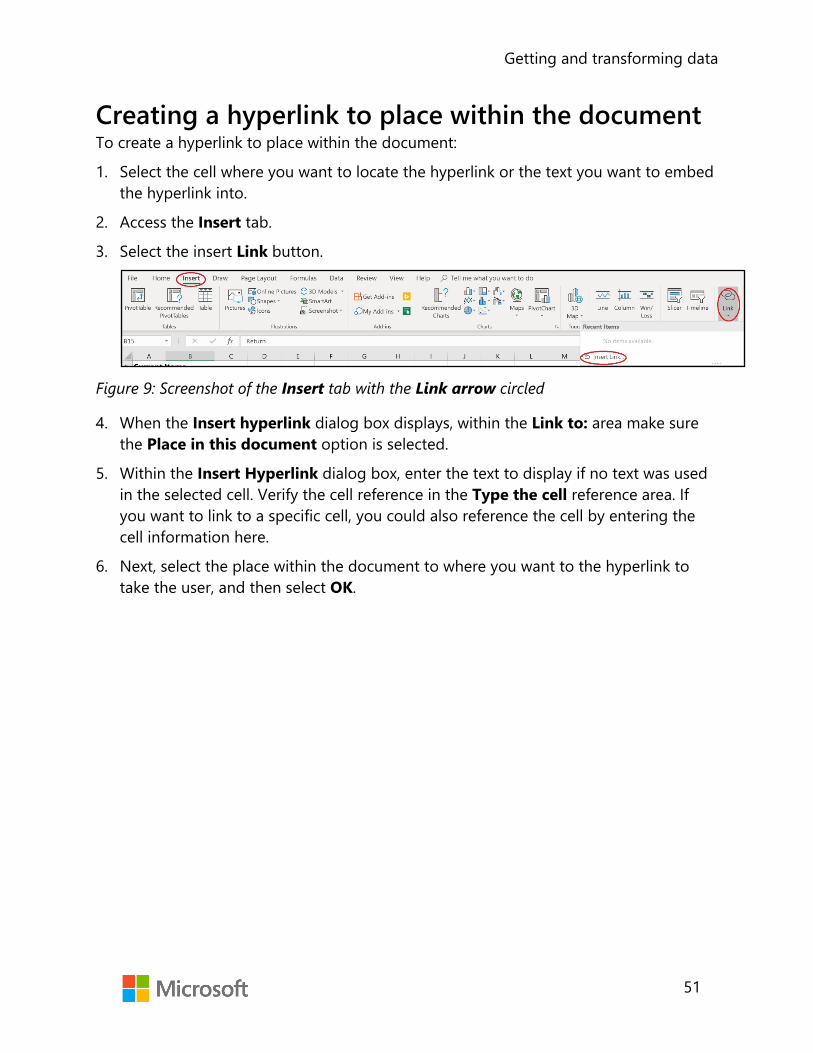
Getting and transforming data
51
Creating a hyperlink to place within the document To create a hyperlink to place within the document:
1. Select the cell where you want to locate the hyperlink or the text you want to embed the hyperlink into.
2. Access the Insert tab.
3. Select the insert Link button.
Figure 9: Screenshot of the Insert tab with the Link arrow circled
4. When the Insert hyperlink dialog box displays, within the Link to: area make sure the Place in this document option is selected.
5. Within the Insert Hyperlink dialog box, enter the text to display if no text was used in the selected cell. Verify the cell reference in the Type the cell reference area. If you want to link to a specific cell, you could also reference the cell by entering the cell information here.
6. Next, select the place within the document to where you want to the hyperlink to take the user, and then select OK.

Getting and transforming data
52
Figure 10: Insert Hyperlink dialog box
Creating a hyperlink to a cell range The marketing department would like to select on a customer’s recently purchased item and then be taken to the current related items and pricing.
1. Select the cell where the hyperlink should be located.
2. From the Insert tab, select Insert Link.
3. In the Insert Link dialog box, a list of defined names will display. In this example the defined name areas are Pickle_Cust, Pickles, Pres_Cust, and Preserves. Make sure in the Link to: area that Place in this document is selected.

Getting and transforming data
53
4. Select the defined named area you want to link, and then select OK. In this example, you are using Pickles.
Figure 11: Insert Hyperlink dialog box
Additional information
For more information on working with hyperlinks in Excel, go to: Work with hyperlinks in Excel
Activity: Tell a story Munson’s has hired you to create Excel files for them. However, the rest of the staff isn’t as proficient working with Excel as you are. Munson’s has asked you to create hyperlinks within a workbook to guide users of the file to different areas.
Resources required You will need the following resource for this activity:
• Locate L5_T1_act_data_starter.xlsx file in this lesson’s Learning Activity Resources folder.

Getting and transforming data
54
Activity instructions Participate in the activity by following these instructions:
1. Verify that you are on the Home Page tab of the workbook ribbon.
2. B7 contains the text Customer List. This text needs to be linked to the Customer List tab. Select B7, and then select the Insert ribbon.
3. In the Links group, select the Link option.
4. In the Insert Hyperlink dialog box, verify that the Text to display is Customer List.
5. In the Link to: group, select Place in this Document.
6. In the Or select a place in this document: area, under Cell Reference, select Customer List. This will link the words Customer List to the Customer List workbook tab.
7. Select the OK button.
8. Press Enter.
9. Select the hyperlink to test it. Verify it takes you to the Customer List tab.
10. While on the Customer List tab, review text in cell A29. When selected, you will need to make this text return the user to Home Page.
11. Select A29, and then on the ribbon, select the Insert tab.
12. In the Links group, select the Link option.
13. In the Insert Hyperlink dialog box, verify that the Text to display is Return to Home Page.
14. In the Link to: group, select Place in this Document.
15. In the Or select a place in this document: area, under Cell Reference, select Home Page. This will link the Customer List tab back to the Home Page workbook tab.
16. Select the OK button.
17. Press Enter.
18. Select the hyperlink to test it.
19. Use the same process to link the text in cells B9, B11, and B13 to their respective workbook tabs, and link the Return to Home Page text in each cell back to the Home Page tab.

Getting and transforming data
55
Try-it: Insert hyperlinks to navigate inside a workbook
You will create links within a workbook to make navigation from one area to another easier.
Try-it 1 Resources You will need the following resource for this try-it:
• Open L5_T1_try1_customer_list_starter.xlsx in this lesson’s Learning Activity Resources folder.
Instructions You will need to perform the following general tasks during this try-it:
1. Open the Items worksheet.
2. Verify that cell B15 has the word Return in it. This needs to be a hyperlink back to the Customer tab so that the marketing department can move back and forth between the two worksheets without using the tabs.
3. Create this hyperlink.
4. Save your work.
Try-it 2 Resources You will need the following resource for this try-it:
• Open L5_T1_try2_customer_list_starter.xlsx in this lesson’s Learning Activity Resources folder.
Instructions You will need to perform the following general tasks during this try-it:
1. Access the Items worksheet.
2. Select cells B4:C6.

Getting and transforming data
56
3. Review the Name box to verify that cells B4:C6 are named Pickles.
Figure 12: Named region of Pickles
4. Access the Customers tab.
5. The marketing department would like to select on a customer’s recently purchased item and then be taken to the current related items and pricing. Yeen Zhuang is the first person in the list to have purchased pickles. Create this hyperlink.
6. Use the Return link to return to the Customers tab.
7. Use steps 4 through 6 to create a link for Tina Bright. The name of the range for preserves in the Items tab is Preserves.
8. Save your work.
Try-it 3 Resources You will need the following resource for this try-it:
• Open L5_T1_try3_customer_list_starter.xlsx in this lesson’s Learning Activity Resources folder.
Instructions You will need to perform the following general tasks during this try-it:
1. Access the Items tab.
2. Select A3 (the word Pickle).
3. On the Insert tab, select the Insert Link button.
4. Create a hyperlink from the word Pickle to the Pickle_Cust Defined Name area.

Getting and transforming data
57
5. Select the link to test it. It should take you to the Customer List tab and highlight Pickle purchases.
6. Complete a similar procedure to link the word Preserve in the Items worksheet to the cells in the named region Pres_Cust.
7. Save your work.
Topic 2: Insert hyperlinks to navigate outside a workbook
Munson’s would like to provide its customers with definitions of pickle types, and include some pickle recipes. The marketing department has also asked for email addresses for each customer to be added so that they can use these emails to send marketing materials.
Creating a hyperlink to another file To create a hyperlink to another file:
1. Select the cell where you want to the link to be located.
2. From the Insert tab, select the Insert Link button.
3. In the Insert Hyperlink dialog box, make sure the Existing File or Web Page is highlighted in the Link to: area. In the Look in: area, make sure Current Folder is highlighted, and then browse to the document you want to link. You can use the tools to the Browse for File option to help locate the file.

Getting and transforming data
58
Figure 13: Insert Hyperlink dialog box
4. In the Text to display area, enter a description of the file to which you are linking, and then select OK.
5. Select the link to test it.
Creating a hyperlink to a website Creating a hyperlink to a website is like linking to a file. To create a hyperlink to a website:
1. Select the cell where you want to locate the link to a website.
2. Access the Insert ribbon, and then select the Insert Link button.
3. In the Insert Hyperlink dialog box, make sure Existing File or Web page is highlighted. In the Address area, enter http://munsonspicklesandpreservesfarm.com.
4. In the Text to display area, enter a description of the website to which you are linking, and then select OK.
5. Select the link to test it.
Getting and transforming data
59
Additional information
For more information on working with hyperlinks in Excel, go to: Work with hyperlinks in Excel
Activity: Discuss and learn How do you think hyperlinks to external sources might be used within a workbook? What external sources do you think would be linked within a workbook?
Munson’s would like for you to add their recent Quarterly Report to the Home Page tab of the Data file. They have asked that a link to the Microsoft Support website also be added for those who need more information about using Excel. They also have a third request, which is to add your email address so that users can email you with questions about the file.
Resources required You will need the following resources for this activity:
• Locate L5_T2_act_data_starter.xlsx file in this lesson’s Learning Activity Resources folder.
• Locate the L5_T2_act_quarterly_report.docx file in this lesson’s Learning Activity Resources folder.
Activity instructions Participate in the activity by following these instructions:
1. Verify that you are on the Home Page tab of the workbook.
2. Select cell A15 (Quarterly Report), and then access the Insert tab.
3. In the Links area, select Link.
4. In the Insert Hyperlink dialog box, in the Link to: area, select Existing File or Web Page.
5. Use the Browse for File option to locate the Quartery_report.docx file.
6. Select the Quarterly_report.docx file, and then select OK.
7. Press Enter and select the hyperlink to test it.
8. Select cell A17 (Microsoft Support), and then access the Insert ribbon.
9. In the Links area, select the Link option.

Getting and transforming data
60
10. In the Insert Hyperlink dialog box, in the Link to: area, select Existing File or Web Page.
11. In the Address: area, enter http://support.microsoft.com, and then select OK.
12. Press Enter and select the hyperlink to test it.
13. Select cell A19, and then access the Insert ribbon.
14. In the Links area, select the Link option.
15. In the Insert Hyperlink dialog box, in the Link to: area, select E-mail address.
16. Verify that the Text to display: area has Email technical support at Munson’s.
17. In the E-mail address: area, enter [email protected], and then select OK.
Note: You cannot test this email link because it’s a fictious email address.
Try-it: Insert hyperlinks to navigate outside a workbook
You can also create hyperlinks to places outside of a workbook. Places outside a workbook could include a website or an email. The marketing department would like to include links to the company’s information about pickle types, recipes, and the company’s website to the customer list.
Try-it 1 Resources You will need the following resources for this try-it:
• Open L5_T2_try1_customer_list_starter.xlsx in this lesson’s Learning Activity Resources folder.
• Locate L5_T2_try1_pickle_types.docx in this lesson’s Learning Activity Resources. • Locate L5_T2_try1_pickle_recipes.docx in this lesson’s Learning Activity Resources.
Instructions You will need to complete the following general tasks during this try-it:
1. In cell A30, enter the text Suggested Resources.
2. In cell A31, enter the text Pickle Types.
3. In cell A32, enter the text Pickle Recipes.
4. In cell A33, enter the text Munson’s Website.

Getting and transforming data
61
5. Select cell A31 (Pickle Types), and create a link to L5_T2_try1_pickle_types.docx.
6. Select the link to test it. It should take you to a document describing the types of pickles sold by Munson’s.
7. Use a similar procedure to link A32 (Pickle Recipes) to the L5_T2_try1_pickle Recipes.docx document, which is located in the Learning Activity Resources folder for this lesson.
8. Save your work.
Try-it 2 Resources You will need the following resource for this try-it:
• Open L5_T2_try2_customer_list_starter.xlsx in this lesson’s Learning Activity Resources folder.
Instructions You will need to complete the following general tasks during this try-it:
1. Select A33, the text Munson’s Website.
2. Create a hyperlink to the Munson’s website using the URL http://munsonspicklesandpreservesfarm.com and then select OK. Select the link to test it. The link will take you to a Microsoft webpage.
3. Save your work.
Try-it 3 Resources You will need the following resource for this try-it:
• Open L5_T2_try3_customer_list_starter.xlsx in this lesson’s Learning Activity Resources folder.
Instructions You will need to complete the following general tasks during this try-it:
1. In cell I1, enter Email Address.
2. In cell I2, create an email address for Tina Bright by using her first name and @contoso.com ([email protected]).

Getting and transforming data
62
3. Continue this procedure for all of the customers within the Customer List file.
4. As you continue entering email addresses, Excel will find the pattern you are creating using the email addresses and will autofill the remaining emails for you. To accept the Autofill suggestions, select the Tab button.
5. Save your work.
Topic 3: Remove hyperlinks For various reasons, you might need to remove hyperlinks. As you enter an email
address or website address into a cell, it automatically becomes a hyperlink. This can make it difficult to access the cell to edit it, or select it because the hyperlink is activated. Therefore, you might need to remove a hyperlink from an Excel workbook.
Removing a hyperlink: Edit Hyperlink dialog box To remove a hyperlink from an Excel workbook:
1. In the Insert ribbon, select the Link symbol.
Figure 14: Link symbol
2. Select the Remove Link button. The hyperlink will be removed.
Removing a hyperlink: context menu To remove a hyperlink using the context menu:
1. Right-click or open the context menu for the hyperlink.
2. In the context menu, select Remove Hyperlink.
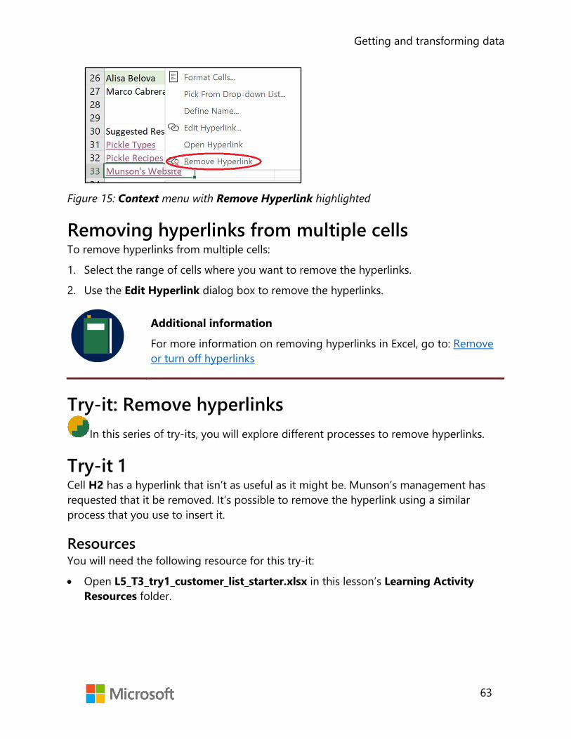
Getting and transforming data
63
Figure 15: Context menu with Remove Hyperlink highlighted
Removing hyperlinks from multiple cells To remove hyperlinks from multiple cells:
1. Select the range of cells where you want to remove the hyperlinks.
2. Use the Edit Hyperlink dialog box to remove the hyperlinks.
Additional information
For more information on removing hyperlinks in Excel, go to: Remove or turn off hyperlinks
Try-it: Remove hyperlinks In this series of try-its, you will explore different processes to remove hyperlinks.
Try-it 1 Cell H2 has a hyperlink that isn’t as useful as it might be. Munson’s management has requested that it be removed. It’s possible to remove the hyperlink using a similar process that you use to insert it.
Resources You will need the following resource for this try-it:
• Open L5_T3_try1_customer_list_starter.xlsx in this lesson’s Learning Activity Resources folder.

Getting and transforming data
64
Instructions You will need to perform the following general tasks during this try-it:
1. Select G2 and use the arrow keys to move to H2.
2. Use the Edit Hyperlink dialog box to remove the hyperlink.
3. Use this same process to remove the link in H3.
4. Save your work.
Try-it 2 Munson’s has found its website URL is too long for many customers, so the company is in the process of changing it. While this is in process, management has asked for the hyperlink to the website within the Customer List file to be removed. Use the arrow keys (or an alternate method) to move the cursor to A33.
Resources You will need the following resource for this try-it:
• Open L5_T3_try2_customer_list_starter.xlsx in this lesson’s Learning Activity Resources folder.
Instructions You will need to perform the following general tasks during this try-it:
1. Use the context menu to remove the hyperlink.
2. Save your work.
Try-it 3 Sometimes you’ll want to remove hyperlinks from multiple cells. Feedback from Munson’s customers has been negative when receiving emails. Management has requested that you remove the email hyperlinks, but would like to keep the emails for possible future use.
Resources You will need the following resource for this try-it:
• Open L5_T3_try3_customer_list_starter.xlsx in this lesson’s Learning Activity Resources folder.
Getting and transforming data
65
Instructions You will need to perform the following general tasks during this try-it:
1. Use the Edit Hyperlink dialog box to remove all the email hyperlinks.
2. Save your work.
Wrap-up 1. When creating a link to a document within a workbook, which area of the Insert
Hyperlink dialog box would you use?
Select the correct option.
a. Create a new file
b. Email address
c. Place in this document
d. Existing file or webpage
2. You can edit or remove a hyperlink using which action?
Select the correct option.
a. Selecting the hyperlinked cell and selecting delete.
b. Selecting the hyperlinked cell and selecting Tab.
c. Selecting the hyperlinked cell and using the Link command found on the Inserttab.
d. Selecting the hyperlinked cell and using the Edit ribbon.
3. Which of the following statements about hyperlinks is false?
Select the correct option.
a. When removing multiple hyperlinks, they must be removed one at a time.
b. You can remove a hyperlink by right-clicking on it or accessing the context menu,and then selecting Remove hyperlink.
c. You can link hyperlinks to several areas including an internal cell, an externaldocument, an email address, or a website.
d. A hyperlink to a named group of cells can be created.
4. ________________________ provide navigation throughout a workbook or to externalresources.

Getting and transforming data
66
Glossary CONCAT An Excel function that allows for data from multiple cells to be
combined.
.csv A file containing data that is separated by commas.
Delimiter A character used to separate individual pieces of data.
Hyperlink A feature that takes the user to another location either within the document, external file, or website.
LOWER An Excel function that converts every letter to lowercase.
PROPER An Excel function that allows the first letter of every word to be capitalized.
String A collection of characters upon which no mathematical calculations are to be performed (for example, letters, zip codes, or telephone numbers).
Text A collection of letters that have meaning.
TEXTJOIN An Excel function that combines data from multiple cells into a list separated by a delimiter.
.txt A file that contains data that is commonly separated by tabs.
UPPER An Excel function that converts every letter to uppercase.
Table 2: Glossary terms and definitions

Getting and transforming data
67
Cornerstone Overview In this cornerstone, you will need to combine data from different sources, fix issues that arise in the data, and insert links to other helpful material.
Objectives The following table outlines the cornerstone objectives and their corresponding MOS exam objectives.
Import text • 1.1.1: Import data from .txt files. • 1.1.2: Import data from .csv files.
Manipulate text • 4.3.1: Format text by using RIGHT(), LEFT(), and MID() functions
Convert text • 4.3.2: Format text by using UPPER(), LOWER(), and LEN() functions
Combine text • 4.3.2: Format text by using UPPER(), LOWER(), and LEN() functions
Hyperlinks • 1.2.3: Insert and remove hyperlinks.
Table 3: Cornerstone objectives
Duration 40 minutes

Getting and transforming data
68
Instructions Complete the following tasks for each file.
1. When saving your file, add your name to the end of the filename, for example:“Crops_Dwayne_Espino.” Follow your teacher’s directions for where to save your files.
2. When you’re done with the cornerstone, assess your completed product and enterthe points you think you earned within the task lists at the end of the tasks. You canask your teacher for help if required.
Tasks You will work with three files in this Cornerstone. The following steps are the tasks you need to complete within each file.
File 1: Blank new Excel file Task: Import text (4 points) 1. Open a blank Excel document. Import the Cornerstone_crop_planting_starter.txt
file. (2 point) (Exam objective 1.1.1)
2. In the second worksheet, Sheet 1, import theCornerstone_crop_problems_starter.csv file. (2 points) (Exam objective 1.1.2)
Points scored: _______ /4
Task: Manipulate text (4 points) • Switch back to the tab containing the Crop Planting information. Extract data from
cells E3:E13 so that only the field number is placed in cells G3:G13. (4 points) (Examobjective 4.3.1)
Points scored: _______ /4

Getting and transforming data
69
Task: Convert Text (12 points) 1. Within the worksheet containing the Crop Planting information, convert the crop
names in column A so that the first letters of the words are capitalized in column H. (3 points) (Exam objective 4.3.2)
2. Continuing to work in the worksheet containing the Crop Planting information, convert the type of crop in column B to all lowercase in column I. (3 points) (Exam objective 4.3.2)
3. Switch to the worksheet containing the Crop Growing Problems. Convert the data in cells A3:A13 to only the first letters capitalized in cells E3:E13. (3 points) (Exam objective 4.3.2)
4. Continue to work in the worksheet containing the Crop Growing Problems. Convert the data in cells B3:B13 to uppercase in cells F3:F13. (3 points) (Exam objective 4.3.2)
Points scored: _______ /12
Task: Combine text (4 points) • Switch to the Crop Planting worksheet. In cells J3:J13 combine the crop name with
the crop type using a space, a dash and final space between the crop name and crop type. (i.e., Cabbage - red) (4 points) (Exam objective 4.3.2)
Points scored: _______ /4
Task: Hyperlinks (8 points) 1. Continue working in the Crop Planting worksheet. In cell A15, enter Munson’s
website, and hyperlink the text to the Munson’s website (http://munsonspicklesandpreservesfarm.com) (4 points) (Exam objective 1.2.3)
2. Switch to the worksheet containing the Crop Problems information. In cell A15, enter Resources. Link this text to the document in the Resources folder for this cornerstone named Helpful Resources to Battle Crop Concerns. (4 points) (Exam objective 1.2.3)
Points scored: _______ /8
TOTAL POINTS: _______ /32

Student guide 40567A Microsoft Excel associate 2019 Module 7: Visualizing Data
Visualizing data
2
Contents
Contents .............................................................. 2
Module overview ............................................. 5
Description ..................................................... 5
Scenario .......................................................... 6
Cornerstone ................................................... 7
Lesson 1: Using conditional formatting .. 8
Overview ......................................................... 8
Warm-up ........................................................ 8
Topic 1: Apply conditional formatting 9
Highlight the top 10 items in a range............................................................ 9
Show variances with data bars ....... 11
Activity: Teacher demo and switch ....................................................... 13
Try-it: Apply conditional formatting .............................................. 14
Try-it 1 ...................................................... 14
Try-it 2 ...................................................... 15
Try-it 3 ...................................................... 15
Topic 2: Remove conditional formatting ................................................... 15
Remove conditional formatting with the Conditional Formatting Rules Manager .................................................. 16
Remove conditional formatting with Clear Rules .............................................. 17
Activity: Pose a challenge ................. 18
Try-it: Remove conditional formatting .............................................. 19
Try-it 1 ...................................................... 19
Try-it 2 ...................................................... 19
Wrap-up ....................................................... 20
Lesson 2: Using charts ................................. 22
Overview ...................................................... 22
Warm-up ...................................................... 22
Topic 1: Create charts ............................. 23
Create a chart with recommended charts ........................................................ 24
Create a pie chart ................................. 25
Activity: Show and learn .................... 27
Try-it: Create charts ............................. 27
Try-it 1 ...................................................... 27
Try-it 2 ...................................................... 28
Topic 2: Add alternative text ................ 28
Add Alt Text using the context menu ......................................................... 29
Mark a visual object as decorative 30
Activity: Discussion .............................. 31
Try-it: Add Alt Text .............................. 31
Try-it 1 ...................................................... 32
Try-it 2 ...................................................... 32
Topic 3: Move charts ............................... 32
Move a chart on the worksheet ..... 33
Move a chart to a different worksheet ................................................ 33
Activity: Discuss and learn ................ 34
Try-it: Move charts .............................. 34

Visualizing data
3
Try-it 1 ...................................................... 34
Try-it 2 ...................................................... 35
Try-it 3 ...................................................... 35
Wrap-up ....................................................... 36
Lesson 3: Editing charts .............................. 37
Overview ...................................................... 37
Warm-up ..................................................... 37
Topic 1: Add a data series .................... 38
Add a data series to your chart ..... 38
Use select data to add and remove source data ............................................ 40
Activity: Demonstration .................... 41
Try-it: Add data series........................ 42
Try-it 1 ...................................................... 42
Try-it 2 ...................................................... 42
Topic 2: Switch between rows and columns ........................................................ 43
Activity: Demonstration .................... 43
Try-it: Switch between rows and columns ................................................... 44
Wrap-up ....................................................... 45
Lesson 4: Understanding chart elements ........................................................... 46
Overview ...................................................... 46
Warm-up ..................................................... 46
Topic 1: Add chart elements ................ 47
Activity: Show and Tell ...................... 48
Try-it: Add chart elements ............... 48
Try-it 1 ...................................................... 48
Try-it 2 ...................................................... 49
Try-it 3 ...................................................... 49
Topic 2: Modify chart elements .......... 50
Edit the text of a title in a chart ...... 50
Format a chart element with the Format task pane ................................. 51
Format a chart element with the Chart Tools tab ..................................... 51
Activity: Discuss and Learn ............... 52
Try-it: Modify chart elements .......... 52
Try-it 1 ...................................................... 52
Try-it 2 ...................................................... 53
Try-it 3 ...................................................... 53
Wrap-up ....................................................... 54
Lesson 5: Understanding chart styles and layouts ............................................................... 56
Overview ...................................................... 56
Warm-up ...................................................... 56
Topic 1: Apply layouts ............................ 57
Activity: Demo ....................................... 58
Try-it: Apply layouts ............................ 59
Topic 2: Apply styles and colors ......... 59
Apply a Quick Style from the ribbon ....................................................... 60
Apply a quick style with Chart Styles ......................................................... 60
Apply a color scheme from the ribbon ....................................................... 61
Apply a color scheme with Chart Styles ......................................................... 61
Activity: Discuss and learn ................ 62
Try-it: Apply styles and colors ......... 63
Try-it 1 ...................................................... 63
Try-it 2 ...................................................... 63
Wrap-up ....................................................... 64

Visualizing data
4
Lesson 6: Understanding sparklines ...... 65
Overview ...................................................... 65
Warm-up ..................................................... 65
Topic 1: Insert sparklines ....................... 66
Activity: Tell a story ............................. 68
Try-it: Insert sparklines ...................... 68
Try-it 1 ...................................................... 68
Try-it 2 ...................................................... 69
Topic 2: Modify sparklines .................... 69
Show sparkline markers and highlights ................................................ 69
Apply a style to sparklines ............... 70
Activity: Continue the story ............. 71
Try-it: Modify sparklines ................... 71
Try-it 1 ...................................................... 71
Try-it 2 ...................................................... 72
Try-it 3 ...................................................... 72
Wrap-up ....................................................... 73
Lesson 7: Understanding the Quick Analysis feature ............................................. 74
Overview ...................................................... 74
Warm-up ..................................................... 74
Topic 1: Use Quick Analysis to format data ................................................................ 75
Add conditional formatting using Quick Analysis ....................................... 76
Add a chart or sparklines using Quick Analysis ....................................... 76
Add totals for data using Quick Analysis .................................................... 77
Activity: Demo and experiment ...... 78
Try-it: Quick Analysis .......................... 78
Try-it 1 ...................................................... 78
Try-it 2 ...................................................... 79
Topic 2: Disable the Quick Analysis feature ........................................................... 79
Activity: Discuss .................................... 80
Try-it: Disable the Quick Analysis feature ...................................................... 81
Wrap-up ....................................................... 81
Glossary ............................................................. 82
Cornerstone ..................................................... 83
Overview ...................................................... 83
Objectives .................................................... 83
Duration ....................................................... 84
Instructions .................................................. 84
Tasks .............................................................. 84
File 1: Cornerstone_solar_array_data_ starter.xlslx .............................................. 84

Visualizing data
5
Module overview Description Providing visualizations of your data make it easier for people to understand and analyze the data. Microsoft Excel provides a wide array of tools for creating these visual data representations. Formatting styles can emphasize important data points or values. Charts and sparklines provide visual depictions of trends, and Alt Text provide a critical way for users with visual impairments to get information displayed visually.
In this module, you’ll learn to leverage all these tools to make your workbooks useful, and impactful. This module builds on your understanding of data and formulas to help you get the most from your data, whether you want to better understand the data yourself or are preparing to print your workbook.
The following table outlines the lessons in this module and their corresponding learning and exam objectives.
Lesson Learning objective Exam objective(s)
Using conditional formatting
Apply and remove conditional formatting
• 2.4.2 • 2.4.3
Using charts Create and move charts • 5.1.1 • 5.1.2 • 5.3.3
Editing charts Add a data series to a chart and switch between the X and Y axis
• 5.2.1 • 5.2.2
Understanding chart elements
Add and remove chart elements from an existing chart
• 5.2.3
Understanding chart styles and layouts
Apply layouts, styles, and colors to an existing chart
• 5.3.1 • 5.3.2
Understanding sparklines
Insert and modify sparklines • 2.4.1

Visualizing data
6
Lesson Learning objective Exam objective(s)
Understanding the Quick Analysis feature
Use the Quick Analysis feature to quickly transform data
N/A
Cornerstone: Observing farm energy data
Assist a colleague by adding visualizations to data related to solar energy production, consumption, and costs
• 2.4.1 • 2.4.2 • 2.4.3 • 5.1.1 • 5.1.2 • 5.2.1 • 5.2.2 • 5.2.3 • 5.3.1 • 5.3.2 • 5.3.3 • 5.3.3
Table 1: Objectives by lesson
Scenario Munson’s Pickles and Preserves is in an extremely favorable climate for solar energy production. Last year Munson’s invested in a solar array to provide electricity for all operations. The solar array has been a huge part of the farm’s digital transformation, and is an exciting project for everyone to witness. Everyone at the farm is proud of the initiative to move to a renewable source of electricity, and they’ve all been anxious to know what the data says about the endeavor. In fact, it seems like the entire community wants to know how well the solar project is going!
A colleague has been collecting as much data as possible related to the solar array and overall electricity consumption on the farm. He is enthusiastic to share with everyone that the solar array has made a big difference, but he is having a hard time understanding the data, let alone explaining it—it really just looks like a bunch of numbers! Knowing that you’re getting pretty good at Excel, he wants your help to create visualizations for all this data about solar energy production, consumption, and costs. You’ll need to add some conditional formatting, charts, and sparklines to help make the data clear.

Visualizing data
7
Cornerstone This module concludes with a cornerstone in which you’ll make data about Munson’s solar array easier to view and understand. In this cornerstone, you’ll:
• Apply conditional formatting to draw attention to important data. • Create charts to visually represent the data, and customize those charts, as
necessary. • Improve the readability and visual impact of charts by applying styles, layouts, and
color schemes. • Add and customize sparklines to demonstrate general trends and emphasize
important data points.

Visualizing data
8
Lesson 1: Using conditional formatting Overview In this lesson, you’ll use conditional formatting to emphasize and highlight important pieces of data. You’ll learn how to apply conditional formatting, and you’ll also learn how to remove it. The activities in this lesson will give you the opportunity to practice applying and removing a variety of conditional formatting options.
Warm-up Use these questions to find out what you already know about this lesson’s topics:
1. Conditional formatting uses a condition to determine a cell’s _________.
Select the correct option.
a. Value
b. Appearance
c. Size
d. Location
2. Which of the following values can be indicated using conditional formatting?
Select all that apply.
a. High or low values
b. Average values
c. Projected values based on the data
d. Duplicate values

Visualizing data
9
3. Which of the following options are types of conditional formatting?
Select all that apply.
a. Color scales
b. Tables
c. Pie charts
d. Data bars
e. Highlight cells rules
f. SmartArt
4. You can indicate positive, negative, or neutral values with icons by using______________________.
Topic 1: Apply conditional formatting An Excel workbook can include a lot of data, and sometimes all that data can
overwhelm the user and make it difficult to understand. For example, imagine you’re planning a hike next week and have a table of the temperature forecast every hour for all seven days—that’s a lot of numbers! You only care about avoiding the times when the temperature is going to be too hot or too cool, but to find those you’d have to search through every hour of each day. Fortunately, Excel provides several features to help you quickly analyze your data.
Conditional formatting allows you to emphasize differences in your data by changing the cells’ appearance based on criteria. If you use it to draw attention to the really hot and really cool temperatures, you can easily find the perfect time to schedule your hike.
Highlight the top 10 items in a range To draw attention to the highest values in your data, select the range of cells you want to format. The following screenshot depicts a set of data selected for conditional formatting.

Visualizing data
10
Figure 1: A range of cells selected for conditional formatting
Next, select the Home tab, and then in the Styles group, select Conditional Formatting to access the conditional formatting options. The following screenshot is of Conditional Formatting options.
Figure 2: Conditional Formatting options
To draw attention to the highest (Top) or lowest (Bottom) numbers in your selected range, select Top/Bottom Rules, and then select Top 10 Items to open the Top 10 Items dialog box, as in the following screenshot.

Visualizing data
11
Figure 3: Top 10 Items dialog box
The number lets you select how many cells to format, which is set to 10 by default. The with options allow you to choose different ways to emphasize the cells. The depicted options will find the top 10 values and format their cells with Light Red Fill and Dark Red Text. Select OK to apply the conditional formatting. The following screenshot depicts conditional formatted used to highlight the top 10 numbers.
Figure 4: Conditional formatting highlights the top 10 numbers
Show variances with data bars The conditional formatting options also include a pre-defined setting for using data bars to demonstrate variances between data within a range. This is useful for providing a visual representation of how the values compare to each other.

Visualizing data
12
To add data bars, select the range of cells you want to format. Select Home, and then in the Styles group, select Conditional Formatting to access the conditional formatting options. From those options, select Data Bars to bring up the options for data bars. The options include a variety of colors with both gradient and solid fills. The following screenshot depicts the Data Bars options.
Figure 5: The Data Bars options
Select the color you want to apply the data bars to your data. The following screenshot depicts data bars with a solid blue fill.

Visualizing data
13
Figure 6: Data Bars with solid blue fill
Additional information
For more information about applying conditional formatting, go to: Use conditional formatting to highlight information
Video
To review the video on conditional formatting, go to: Use conditional formatting
Activity: Teacher demo and switch In this activity, your teacher will demonstrate how to apply conditional formatting. Next, you’ll move from computer to computer trying different conditional formatting settings as directed by the teacher, before returning to your original computer to review how your data is displayed.
Resources required You will need the following resource for this activity:
• Open L1_T1_act_daily_cell_production.xlsx in this lesson’s Learning Activity Resources.

Visualizing data
14
Activity instructions Participate in the activity by following these instructions:
1. Observe the teacher demonstrating how to apply conditional formatting to a range of cells.
2. Ask clarifying questions.
3. On your own computer, apply the conditional formatting rule as directed by the teacher.
4. Switch to a new computer as instructed by the teacher. Observe the formatting applied by the previous student. As directed by the teacher, add an additional conditional formatting rule to the data range.
5. Continue to switch and apply new conditional formatting as directed by the teacher.
6. Return to your original computer. Note the conditional formatting rules currently in place.
Try-it: Apply conditional formatting In this leveled try-it activity, you’ll apply several different conditional formatting
rules to a workbook to make the data easier to understand and analyze.
Note: Kilowatt hours (kWh) is a measure of energy often used to measure electrical energy used or produced. 1 kWh is equivalent to 1,000 watts of power for one hour.
Try-it 1 In this try-it, you’ll add data bars to one column of values.
Resources You will need the following resource for this try-it:
• Open L1_T1_try1_energy_needs_met_starter.xlsx in this lesson’s Learning Activity Resources.
Instructions During this try-it you’ll perform the following task:
• Apply solid orange data bars to the range B4:B9.

Visualizing data
15
Try-it 2 In this try-it, you’ll apply conditional formatting to emphasize the lowest values in the data.
Resources You will need the following resource for this try-it:
• Open L1_T1_try2_energy_needs_met_starter.xlsx.
Instructions During this try-it you’ll perform the following task:
• Select range B4:H9 and apply conditional formatting that displays the bottom five items with light red fill, and without changing the text color.
Try-it 3 In this try-it, you’ll add icons to emphasize the variance between cell values.
Resources You will need the following resource for this try-it:
• Open L1_T1_try3_energy_needs_met_starter.xlsx.
Instructions During this try-it you’ll perform the following task:
• Apply three traffic lights (unrimmed) to the range I4:I9.
Topic 2: Remove conditional formatting
Excel gives you many options for conditional formatting on a range of cells, and because you can apply multiple rules to the same set of data, there are thousands of combinations available. That means you might find yourself experimenting to find the best way to make your data clear and easy to analyze. This means you’ll need to be able to remove formatting to try different approaches.
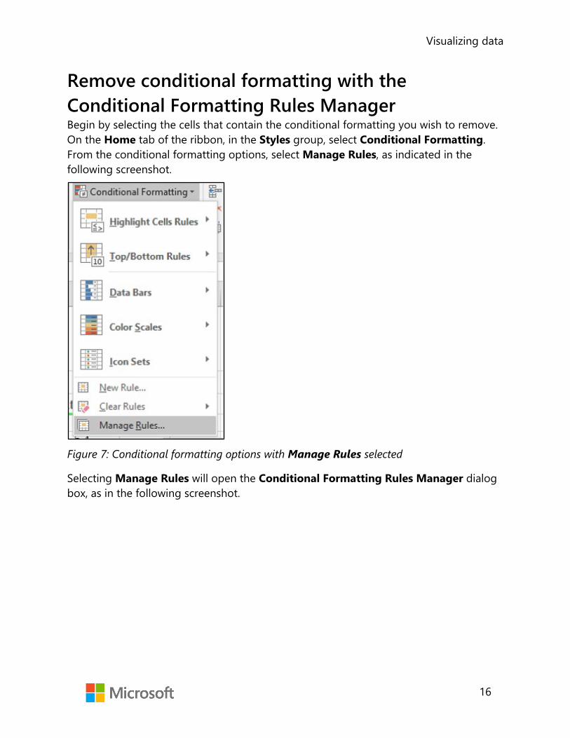
Visualizing data
16
Remove conditional formatting with the Conditional Formatting Rules Manager Begin by selecting the cells that contain the conditional formatting you wish to remove. On the Home tab of the ribbon, in the Styles group, select Conditional Formatting. From the conditional formatting options, select Manage Rules, as indicated in the following screenshot.
Figure 7: Conditional formatting options with Manage Rules selected
Selecting Manage Rules will open the Conditional Formatting Rules Manager dialog box, as in the following screenshot.

Visualizing data
17
Figure 8: The Conditional Formatting Rules Manager dialog box
This dialog box will list all the conditional formatting rules currently applied to any cells within your range. Select the rule you want to remove, and then select Delete Rule. Repeat this process for any additional rules you want to remove.
Did you know?
The Conditional Formatting Rules Managers also allows you to adjust the order in which multiple rules are applied. Simply select a rule you wish to move, and then use the up and down arrows to move it to where you want.
Remove conditional formatting with Clear Rules If you want to clear all conditional formatting rules for a selection of cells, you can use the Clear Rules feature. Select Home, and then in the Styles group, select Conditional Formatting. On the conditional formatting options that display, select Clear Rules, as in the following screenshot.

Visualizing data
18
Figure 9: The conditional formatting options with Clear Rules selected
To clear the conditional rules for all cells, select Clear Rules from Entire Sheet. If you want to remove conditional formatting from only the selected cells, select Clear Rules from Selected Cells.
Additional information
For more information on removing conditional formatting, refer to the Clear conditional formatting sub-section in: Use conditional formatting to highlight information
Activity: Pose a challenge The teacher will direct you to complete a challenge to learn how efficient you are at removing conditional formatting.

Visualizing data
19
Resources required You will need the following resource for this activity:
• Any worksheet with conditional formatting applied.
Activity instructions Participate in the activity by following these instructions:
1. As directed by the teacher, remove conditional formatting from your worksheet.
2. Be prepared to share how you removed the conditional formatting.
Try-it: Remove conditional formatting In this leveled try-it activity, you’ll practice removing conditional formatting that
has been applied to different parts of a worksheet.
Try-it 1 In this try-it, you’ll remove conditional formatting from a range of cells.
Resources You will need the following resource for this try-it:
• Open L1_T2_try1_energy_needs_met_starter.xlsx in this lesson’s Learning Activity Resources.
Instructions During this try-it, you’ll perform the following task:
• Remove conditional formatting from cells B4:H9.
Try-it 2 In this try-it, you’ll remove conditional formatting from a single cell, and from an entire worksheet.
Resources You will need the following resource for this try-it:
• Open L1_T2_try2_ energy_needs_met_starter.xlsx in this lesson’s Learning Activity Resources.

Visualizing data
20
Instructions The following steps are the general tasks that you need to perform during this try-it:
1. Remove conditional formatting from only cell I6.
2. Remove conditional formatting from the entire worksheet.
Wrap-up Use these questions to check what you learned in this lesson:
1. Which of the following conditional formatting rules is the best option for emphasizing the variance between values in a data range?
Select the correct option.
a. Top 10%
b. Bottom 10 items
c. Duplicate Values
d. Color Scales
2. Which features can you use to remove conditional formatting?
Select all that apply.
a. New Rule
b. Manage Rules
c. Clear Rules
d. Data Bars
e. Color Scales
3. 3 Signs is an option for the ____________________ conditional formatting rule.
Select all that apply.
a. Color Scales
b. Icon Sets
c. Highlight Between
d. Data Bars

Visualizing data
21
4. Conditional formatting with the ______________________ option will shade every selected cell based on how its value compares to the average.
5. What happens if multiple conditional formatting rules are applied to the same cell?
Select the correct option.
a. None of the rules are evaluated, and the cell is left unformatted.
b. Only the first rule is applied, and the cell is formatted accordingly.
c. All rules are applied in order, formatting the cell with every rule.
d. Only the last rule is applied, and the cell is formatted accordingly.

Visualizing data
22
Lesson 2: Using charts Overview In this lesson, you’ll explore one of the most useful tools for visualizing your spreadsheet data: charts. The activities in this lesson show you how to create charts, add Alt Text to make your worksheets more accessible, and position your charts exactly where you want them.
Video
What are the different ways in which you can visualize data to present data effectively? Review the video Data visualization. What are the two things that stood out for you?
Warm-up Use these questions to find out what you already know about this lesson’s topics:
1. If you want Microsoft Excel to suggest a chart for your data, use the______________________ feature.
2. Which of the following best describes the role of Alt Text?
Select the correct option.
a. Allows data to be translated into different languages.
b. Assists users with a screen reader who are accessing the workbook.
c. Provides additional information for a chart’s legend.
d. Enables users to input text quickly.

Visualizing data
23
3. Which of the following actions can be done with the Move Chart dialog box?
Select all that apply.
a. Make a duplicate copy of a chart.
b. Move a chart to a new worksheet.
c. Move a chart to an existing worksheet.
d. Move a chart to a Microsoft PowerPoint presentation.
4. How does Excel determine what data to use when creating a chart?
Select the correct option.
a. It uses all data on the current worksheet.
b. It uses all data in the current workbook.
c. It uses the selected cell and all adjacent cells.
d. It uses only the selected cells.
Topic 1: Create charts The right chart can represent your data in a way that helps you or your audience
understand the bigger picture that the data has to offer. Often, it’s great to view all the numbers, but many times we just want to know what it all means. What am I spending my money on? Is my energy usage getting better or worse over time? How big of an impact is that exam going to have on my grade? A good chart can make these kinds of evaluations more obvious.
Did you know?
You can create charts in Excel with chart elements that better support your users' accessibility needs. For further information, refer to Create more accessible charts in Excel.

Visualizing data
24
Create a chart with recommended charts With so many ways to present your data in a chart, it can be difficult to know which to choose. Luckily, Excel offers Recommended Charts to give you a great starting point. Select the data for which you want to create a chart. On the ribbon, select Insert, and then in the Charts group, select Recommended Charts. This opens the Insert Chart dialog box, as depicted in the following screenshot.
Figure 10: The Insert Chart dialog box

Visualizing data
25
The Insert Chart dialog box offers you a variety of choices based on how your data is arranged. Select the chart type you want, and then select OK. The following screenshot depicts an example of a line chart added with recommended charts.
Figure 11: Example of a line chart added with recommended charts
Additional information
For more information about the recommended charts feature, go to: Create a chart with recommended charts
Create a pie chart One of the most common and useful charts is the pie chart. Pie charts work well when you have one row or one column of data. To create a pie chart, select the data you want to include in your pie chart. On the ribbon, select Insert. In the Charts group, select Insert Pie or Doughnut Chart, and then select the chart you want. The following screenshot depicts the choices after selecting Insert Pie or Doughnut Chart.

Visualizing data
26
Figure 12: Choices after selecting Insert Pie or Doughnut Chart
A pie chart such as the following example 2-D Pie chart will be placed in the worksheet.
Figure 13: An example pie chart
Additional information
For more information on creating a pie chart, go to: Add a pie chart
For more information on the different chart types in Excel, go to: Available chart types in Office
For more information on selecting the correct data for a different chart types, go to: Select data for a chart

Visualizing data
27
Video
To review the video on creating a chart and adding a trend line, go to: Create a chart from start to finish
Activity: Show and learn In this activity, the teacher will show you how to create two different charts. You’ll then have the chance to try creating the same charts yourself.
Resources required You will need the following resource for this activity:
• Open L2_T1_act_daily_cell_production.xlsx in this lesson’s Learning Activity Resources.
Activity instructions Participate in the activity by following these instructions:
1. Observe as the teacher demonstrates how to create a pie chart on the PieChart worksheet.
2. Ask the teacher any clarifying questions you might have.
3. Create a pie chart from the same data as in the demonstration.
4. Observe as the teacher switches to the Column worksheet and adds a column chart.
5. Ask the teacher any clarifying questions you might have.
6. Create a column chart on the Column worksheet using the same data ranges as the teacher.
Try-it: Create charts A colleague at Munson’s Pickles and Preserves Farm would like some assistance
analyzing the farm’s electricity consumption. This is a series of leveled try-it activities that will ask you to create charts to represent different types of data.
Try-it 1 In this try-it you’ll select two ranges of data and create a line chart.

Visualizing data
28
Resources You will need the following resource for this try-it:
• Open L2_T1_try1_monthly_usage_starter.xlsx in this lesson’s Learning Activity Resources.
Instructions The following steps are the general tasks that you need to perform during this try-it:
1. On the Monthly worksheet, select the monthly energy usages data for all months and years.
2. Create a Clustered Column Chart using the selected data.
Try-it 2 In this try-it you’ll select two ranges of data and create a line chart.
Resources You will need the following resource for this try-it:
• Open L2_T1_try2_monthly_usage_starter.xlsx in this lesson’s Learning Activity Resources.
Instructions The following steps are the general tasks that you need to perform during this try-it:
1. On the Summary worksheet, select the average energy usage for each month, listed in kWh.
2. Create a 3D Pie Chart using the selected data.
Topic 2: Add alternative text Alternative text, or Alt Text, is critical for ensuring that all users can access your
content. Many users with visual impairments use a screen reader such as Microsoft Narrator, which reads information aloud from the screen and enables users to interact with a computer without using a mouse. In such a situation, it’s easy to miss critical information, or experience frustration when content includes visual items such as images and infographics.
Where does Alt Text fit in? When a screen reader encounters graphical content, the user will hear the Alt Text read aloud. If there’s no Alt Text, they will only know that there’s a piece of visual information, but not be able to discern anything about what it shows!

Visualizing data
29
In all kinds of documents, adding Alt Text for images and infographics is helpful; in Excel, it’s especially critical to include Alt Text for charts and other visualizations that are intended to help us understand data.
Add Alt Text using the context menu To add Alt Text, right-click or access the context menu for the object, and then select Edit Alt Text. If you’re adding Alt Text to a chart or SmartArt graphic, be sure to select the border of the graphic rather than an individual piece of the graphic. The following screenshot depicts a chart’s context menu with Edit Alt Text selected.
Figure 14: Context menu with Edit Alt Text selected
In the Alt Text pane, enter your alternative text describing the item. In general, your description should be one or two sentences describing the object for someone who can’t see it. The following screenshot depicts the Alt Text pane with an example of an Alt Text description.

Visualizing data
30
Figure 15: The Alt Text pane with an example of an Alt Text description
Did you know?
You can also access the Alt Text pane from the ribbon. Select the chart, and then on the Chart Tools ribbon, select Format. In the Accessibility group, select Alt Text.
Mark a visual object as decorative A worksheet might include visual elements that are simply added to increase visual interest but do not contain any information. Examples of this might include a stylistic border or decorative item. You can mark these objects so that people using screen readers will hear that they are decorative and will know they aren’t missing any information.
To mark an element as decorative, right-click or access the context menu of the object, and then select Edit Alt Text. In the Alt Text pane, select the Mark as Decorative check box, as demonstrated in the following screenshot.
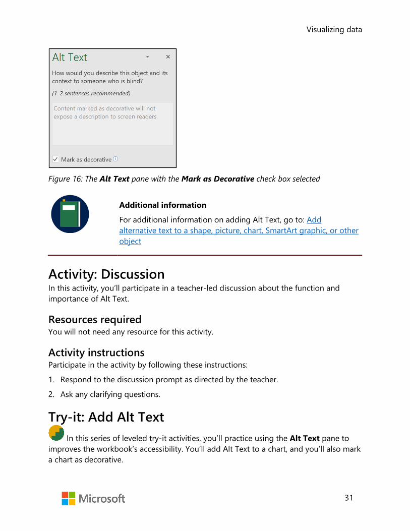
Visualizing data
31
Figure 16: The Alt Text pane with the Mark as Decorative check box selected
Additional information
For additional information on adding Alt Text, go to: Add alternative text to a shape, picture, chart, SmartArt graphic, or other object
Activity: Discussion In this activity, you’ll participate in a teacher-led discussion about the function and importance of Alt Text.
Resources required You will not need any resource for this activity.
Activity instructions Participate in the activity by following these instructions:
1. Respond to the discussion prompt as directed by the teacher.
2. Ask any clarifying questions.
Try-it: Add Alt Text In this series of leveled try-it activities, you’ll practice using the Alt Text pane to
improves the workbook’s accessibility. You’ll add Alt Text to a chart, and you’ll also mark a chart as decorative.

Visualizing data
32
Try-it 1 In this try-it, you’ll mark a chart in an Excel workbook as decorative, for people using a screen reader.
Resources You will need the following resource for this try-it:
• Open L2_T2_try1_monthly_usage_starter.xlsx in this lesson’s Learning Activity Resources.
Instructions The following steps are the general tasks that you need to perform during this try-it:
1. Select the Summary worksheet.
2. Mark the 3D pie chart as decorative.
Try-it 2 In this try-it, you’ll add appropriate Alt Text to a chart in an Excel workbook so people using screen readers understand what information the chart conveys.
Resources You will need the following resource for this try-it:
• Open L2_T2_try2_monthly_usage_starter.xlsx in this lesson’s Learning Activity Resources.
Instructions The following steps are the general tasks that you need to perform during this try-it:
1. Select the Monthly worksheet.
2. Add Alt Text describing the general content of the chart. Try to limit yourself to one or two sentences.
Topic 3: Move charts Excel allows you to move a chart to any location on a worksheet, which enables
you to place it where it will have the most impact, and where it won’t cover any other information. You can also move a chart to a different worksheet within the same workbook, or to a new worksheet.
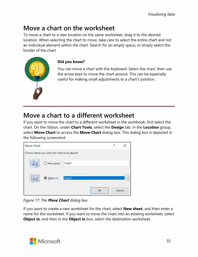
Visualizing data
33
Move a chart on the worksheet To move a chart to a new location on the same worksheet, drag it to the desired location. When selecting the chart to move, take care to select the entire chart and not an individual element within the chart. Search for an empty space, or simply select the border of the chart.
Did you know?
You can move a chart with the keyboard. Select the chart, then use the arrow keys to move the chart around. This can be especially useful for making small adjustments to a chart’s position.
Move a chart to a different worksheet If you want to move the chart to a different worksheet in the workbook, first select the chart. On the ribbon, under Chart Tools, select the Design tab. In the Location group, select Move Chart to access the Move Chart dialog box. This dialog box is depicted in the following screenshot.
Figure 17: The Move Chart dialog box
If you want to create a new worksheet for the chart, select New sheet, and then enter a name for the worksheet. If you want to move the chart into an existing worksheet, select Object in, and then in the Object in box, select the destination worksheet.

Visualizing data
34
Additional information
For more information on moving a chart, go to: Move or resize a chart
Activity: Discuss and learn In this activity, you’ll participate in a teacher-led discussion on different ways to move a chart.
Resources required You will need the following resource for this activity:
• Open L2_T3_act_daily_cell_production.xlsx in this lesson’s Learning Activity Resources.
Activity instructions Participate in the activity by following these instructions:
1. Participate in the discussion about different ways to move a chart.
2. Use one of the methods discussed to move the chart on the Monthly worksheet to a location below the data.
3. Use another of the methods to move the chart on the Summary worksheet to a location next to the data.
Try-it: Move charts This leveled try-it activity gives you practice moving charts with a variety of
methods.
Try-it 1 In this try-it, you’ll use Cut and Paste to move a chart.
Resources You will need the following resource for this try-it:
• Open L2_T3_try1_monthly_usage_starter.xlsx in this lesson’s Learning Activity Resources.

Visualizing data
35
Instructions The following steps are the general tasks that you need to perform during this try-it:
1. Create a new worksheet with the name SummaryChart.
2. Use Cut to remove the 3D pie chart from the Summary worksheet, and then use Paste to place it on the SummaryChart worksheet.
Try-it 2 In this try-it, you’ll move a chart to an existing worksheet, and then position it so it doesn’t cover any data.
Resources You will need the following resource for this try-it:
• Open L2_T3_try2_monthly_usage_starter.xlsx in this lesson’s Learning Activity Resources.
Instructions The following steps are the general tasks that you need to perform during this try-it:
1. Use the Move Chart dialog box to move the line chart on the Monthly worksheet to the Summary worksheet.
2. Position the chart next to the data table on the Summary chart in a location that doesn’t cover any data, such as cell C2.
Try-it 3 This try-it will direct you to move a chart to a new worksheet using the Move Chart dialog box.
Resources You will need the following resource for this try-it:
• Open L2_T3_try3_monthly_usage_starter.xlsx in this lesson’s Learning Activity Resources.
Instructions The following steps are the general tasks that you need to perform during this try-it:
• Use the Move Chart dialog box to move the line chart on the Summary worksheet to a new worksheet with the name DetailChart.

Visualizing data
36
Wrap-up Use these questions to check what you learned in this lesson:
1. What is the effect of marking a graphic element as “decorative”?
Select the correct option.
a. The object is locked and cannot be altered.
b. Data is disconnected from the chart so that it does not update.
c. The object becomes part of the workbook’s template.
d. Screen readers will notify users that it doesn’t contain information.
2. Which data arrangement is ideal for a pie chart?
Select the correct option.
a. Multiple rows and columns of data
b. A single row or column of data
c. A single cell of conditionally formatted data
d. Any number of rows and columns; however, data must be in a table
3. What is the preferred length of Alt Text?
Select the correct option.
a. A few words
b. One or two sentences
c. One or two paragraphs
4. To remove a chart from the current worksheet and place it on a newly created worksheet, use the ______________________ dialog box.
5. Visual elements that do not contain any information should be marked as ______________________.
Additional information
For more information on writing effective Alt Text, go to: Everything you need to know to write effective alt text

Visualizing data
37
Lesson 3: Editing charts Overview This lesson will focus on how to edit a chart after you’ve created it. You’ll learn how to add a data series to an existing chart, and you’ll find out how to switch between rows and columns in your charts.
Warm-up Use these questions to find out what you already know about this lesson’s topics:
1. Which of the following terms refers to a row or column of data in a worksheet that is plotted in a chart?
Select the correct option.
a. A data series
b. Axis
c. Data label
d. Data table
2. You added data to the worksheet after the chart was created. Why might you need to add more data to a chart?
Select all that apply.
a. You didn’t select all the data when you created the chart.
b. You want to switch the rows and columns in the chart.
c. You want to move the chart to another worksheet.
d. You want to add the chart to a PowerPoint presentation or Microsoft Word document.
e. You added data to the worksheet after the chart was created.

Visualizing data
38
3. Which of the following explanations are reasons to switch the rows and columns ona chart?
Select all that apply.
a. To change to a different chart type.
b. To move the chart to a different worksheet.
c. To check if you prefer to orient the chart differently.
d. To correct a column chart only rendering one column.
e. To correct a pie chart that is only displaying a category name.
4. The ______________________button allows you exclude some data from a chart.
Topic 1: Add a data series A workbook in Excel is often a living document. That is, you can continue to use the
same workbook over a long period of time, adding more and more data. For example, if you use a spreadsheet to keep track of your personal budget for the month, you’ll want to keep using it when the month ends. Instead of creating a new workbook, you can just add a column of data for the new month. However, any charts you made to visualize your past months’ budgets are now missing the new month! Or perhaps you just made a mistake when you created the chart, leaving out a row or column of data you intended to include. For these reasons and more, you need to be able to change which pieces of data are included in a chart.
Add a data series to your chart A data series is a row or column of values in a worksheet. When you select the rows and columns of numbers to include in a chart, you’re selecting the data series you want to visualize.
Next, you select a chart style. The data currently used as a source for the chart is indicated on the worksheet with sizing handles at the corners. The following screenshot depicts the source data for a selected pie chart.

Visualizing data
39
Figure 18: The source data for a pie chart
In this example, the chart includes only data for Monday through Friday; Saturday and Sunday are not reflected. Select and drag the sizing handles to include all the data you want included in the chart. Alternatively, right-click or access the context menu on the chart and choose Select Data from the context menu. Then, edit the Chart data range box to the correct range. The following screenshot depicts the same chart with the new data included.
Figure 19: Source data for a pie chart that includes the two additional columns of data

Visualizing data
40
Use select data to add and remove source data If you wish to exclude some data from your chart, or if your chart is on a separate worksheet from your data, you can use the Select Data Source dialog box. To access the dialog box, right-click or access the context menu on the chart, and then select Data Source. The Select Data Source dialog box is depicted in the following screenshot.
Figure 20: Select Data Source dialog box with data for Tuesday and Thursday excluded
Leave the dialog box open, and select the worksheet. Then select and drag to select the data to include in the chart. Alternatively, you can edit the Chart data range box to include the correct cell range. Use the check boxes to select each data series you want to include, and unselect each data series you want to exclude. In the previous example, data for Tuesday and Thursday are excluded from the chart. After selecting the data you want included and excluded, select OK.

Visualizing data
41
Did you know?
You can also access the Select Data Source dialog box through a chart’s context menu. Right-click or access the context menu on the chart, and then choose Select Data.
Additional information
For more information on adding a data series to a chart, go to: Add a data series to your chart
Activity: Demonstration In this activity, the teacher will demonstrate different ways to add or remove a data series in an existing chart.
Resources required You will need the following resource for this activity:
• Open L3_T1_act_daily_cell_production.xlsx in this lesson’s Learning Activity Resources.
Activity instructions Participate in the activity by following these instructions:
1. Observe the teacher as they demonstrate how to add a data series to a chart by adjusting the borders indicated in the worksheet.
2. Ask clarifying questions.
3. On your computer, add a data series to a chart as directed by the teacher.
4. Observe the teacher as they demonstrate the Select Data Source dialog box.
5. Ask clarifying questions.
6. On your computer, use the Select Data Source dialog box as directed by the teacher.

Visualizing data
42
Try-it: Add data series In this leveled try-it activity, you’ll add a data series to an existing chart using two
different methods.
Try-it 1 In this try-it, you’ll add data to a chart by expanding the border to include all necessary data.
Resources You will need the following resource for this try-it:
• Open L3_T1_try1_energy_needs_met_starter.xlsx in this lesson’s Learning Activity Resources.
Instructions The following steps are the general tasks that you need to perform during this try-it:
1. Select the Monthly worksheet.
2. Inspect the source data for the line chart and note the two sets of data that are not included. Drag the bordering line to include all data in the worksheet, or right-click or access the context menu on the chart and choose Select Data from the context menu. Then, edit the Chart data range box to the correct cell range.
Try-it 2 This try-it activity will have you exclude some data from a chart.
Resources You will need the following resource for this try-it:
• Open L3_T1_try2_energy_needs_met_starter.xlsx in this lesson’s Learning Activity Resources.
Instructions The following steps are the general tasks that you need to perform during this try-it:
1. Select the Monthly worksheet.
2. Modify the data source for the line chart so that the Air Conditioning data series is not displayed in the chart.
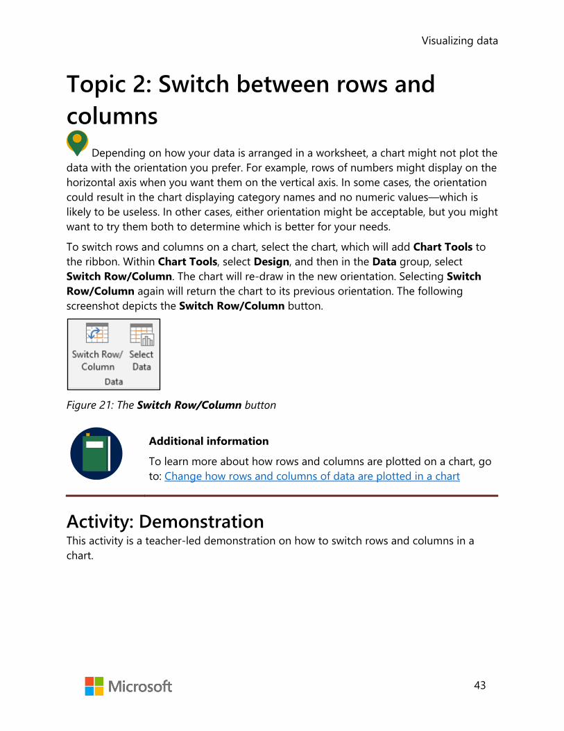
Visualizing data
43
Topic 2: Switch between rows and columns
Depending on how your data is arranged in a worksheet, a chart might not plot the data with the orientation you prefer. For example, rows of numbers might display on the horizontal axis when you want them on the vertical axis. In some cases, the orientation could result in the chart displaying category names and no numeric values—which is likely to be useless. In other cases, either orientation might be acceptable, but you might want to try them both to determine which is better for your needs.
To switch rows and columns on a chart, select the chart, which will add Chart Tools to the ribbon. Within Chart Tools, select Design, and then in the Data group, select Switch Row/Column. The chart will re-draw in the new orientation. Selecting Switch Row/Column again will return the chart to its previous orientation. The following screenshot depicts the Switch Row/Column button.
Figure 21: The Switch Row/Column button
Additional information
To learn more about how rows and columns are plotted on a chart, go to: Change how rows and columns of data are plotted in a chart
Activity: Demonstration This activity is a teacher-led demonstration on how to switch rows and columns in a chart.

Visualizing data
44
Resources required You will need the following resource for this activity:
• Open L3_T2_act_daily_cell_production.xlsx in this lesson’s Learning Activity Resources.
Activity instructions Participate in the activity by following these instructions:
1. Observe as the teacher demonstrates switching rows and columns on a pie chart.
2. Ask clarifying questions.
3. On your computer, select the pie chart and switch the rows and columns. Note the difference in how the data is plotted.
4. Switch the orientation back and forth a couple of times to observe how the feature works.
Try-it: Switch between rows and columns In this standalone Try-it, you’ll correct a chart that is oriented incorrectly.
Resources You will need the following resource for this try-it:
• Continue with the Energy Needs Met workbook from the Try-it activity in Topic 1. Alternatively, open L3_T2_try_energy_needs_met_starter.xlsx in this lesson’s Learning Activity Resources.
Instructions The following steps are the general tasks that you need to perform during this try-it:
1. Select the Averages worksheet. Observe that the pie chart is not useful because it’s displaying a category name rather than data values.
2. Switch rows and columns for the chart so that it displays values for all six categories.

Visualizing data
45
Wrap-up Use these questions to check what you learned in this lesson:
1. The Select Data Source dialog box allows you to do which of the following?
Select all that apply.
a. Delete data from a selection
b. Select an entirely new range of data
c. Select what color is used for each data series on the chart
d. Change to a new type of chart
e. Exclude some data from the chart
2. What does the Switch Row/Column button do?
Select the correct option.
a. Paste row data into a column
b. Rearrange data in a range of cells
c. Change the orientation of axes in a chart
d. Toggle Axis Titles off and on
3. A ______________________is a row or column of numbers in a worksheet that are plottedin a chart.

Visualizing data
46
Lesson 4: Understanding chart elements Overview In this lesson, you’ll work with the individual components that make up an Excel chart. You’ll learn to change these chart elements to make your visualizations clearer, such as making the title of the chart more descriptive. You’ll also learn to add and remove elements, including a legend and data labels.
Warm-up Use these questions to find out what you already know about this lesson’s topics:
1. A Microsoft Excel chart is made up of multiple ______________________ which can beadded, removed, and modified to customize the chart.
2. Which of the following terms describes a grid at the bottom of a chart that displaysthe values represented in the chart?
Select the correct option.
a. Axes
b. Data label
c. Data table
d. Legend
3. A Microsoft Excel chart can contain the following titles:
Select all that apply.
a. Axis title(s)
b. Chart title(s)
c. Column and row title(s)
d. Data title(s)
e. Legend title(s)
4. A ______________________indicates the general pattern of a data series.

Visualizing data
47
Topic 1: Add chart elements While the primary function of a chart is to display the data itself, Excel offers a
variety of elements that you can add to a chart to make it more interesting and easier to understand. Titles, labels, legends, and more, can all be added, removed, and modified to make your chart more effective.
To add new elements, begin by selecting the chart. Then, next to the chart select the Chart Elements button, as highlighted in the following screenshot.
Figure 22: The Chart Elements button
After selecting the Chart Elements button, you’re presented with the list of chart elements you can add, as in the following screenshot.
Figure 23: A list of available Chart Elements options

Visualizing data
48
Select the check boxes for all elements you want to add to the chart.
Additional information
For more information on adding chart elements, go to: Add a legend to a chart
Activity: Show and Tell In this activity, students in the group will add a variety of elements to a chart on the teacher’s computer.
Resources required You will need the following resource for this activity:
• Open L4_T1_act_daily_cell_production.xlsx in this lesson’s Learning Activity Resources.
Activity instructions Participate in the activity by following these instructions:
• As directed by the teacher, participate when it’s your turn to add a single element to the chart on the teacher’s computer.
Try-it: Add chart elements In this leveled try-it activity, you’ll add a variety of chart elements to different
charts.
Try-it 1 This try-it activity asks you to add a single element to a chart.
Resources You will need the following resource for this try-it:
• Open L4_T1_try1_maintenance_costs_starter.xlsx in this lesson’s Learning Activity Resources.
Instructions You’ll need to perform the following task during this try-it:
• Add data labels to the 3D pie chart.

Visualizing data
49
Try-it 2 This try-it activity has you to add a single element to a chart.
Resources You will need the following resource for this try-it:
• Open L4_T1_try2_monthly_usage_starter.xlsx in this lesson’s Learning Activity Resources.
Instructions The following steps are the general tasks that you need to perform during this try-it:
1. Add a data table to the chart. Include legend keys in the data table.
2. Remove the legend now that the information is now provided by the data table.
Try-it 3 This try-it activity asks you to add a single element to a chart.
Resources You will need the following resource for this try-it:
• Open L4_T1_try3_daily_cell_production_starter.xlsx in this lesson’s Learning Activity Resources.
Instructions The following steps are the general tasks that you need to perform during this try-it:
1. Add a data table (with legend keys) to the line chart.
2. Remove the legend from the chart.
3. Add a linear trend line based on the Friday data series.

Visualizing data
50
Topic 2: Modify chart elements After you’ve added the necessary elements to your chart, you might notice Excel is
not display them in the manner you want. For example, the chart title might just display “Chart Title”. Likewise, visual elements such as grid lines might need to be adjusted. Excel manages each element of a chart individually, allowing you to modify those individual components as you wish. Learning how to modify the individual elements of your charts will enable you to create charts that say and demonstrate exactly what you want.
You modify different types of elements in different ways. You can change the text of a chart or axis title to say whatever you want, for instance, but you can’t change the value of a data label.
Edit the text of a title in a chart To change the contents of a chart or axis title, begin by selecting the title you wish to modify, and then select the title again to switch the title to editing mode. Now you can select the text you want to change, and enter the new text. You can place a line break in a title by pressing ENTER while in editing mode. The following screenshot has a chart title in editing mode with the existing text selected.
Figure 24: A chart title in editing mode with the existing text selected
Titles for the chart and each axis can be edited independently by repeating this process.

Visualizing data
51
Video
To review the video on editing chart titles, go to: Add or remove titles in a chart
Format a chart element with the Format task pane Not every chart element has editable text—or any text at all! But every element can be formatted. One way to format an element is to use the Format task pane. To access it right-click or access the context menu on a chart element, and then select Format <chart element>. Notice that the context menu will indicate which type of element you’re modifying. For example, if you right-click or access the context menu on a chart title, the context menu will list Format Chart Title as an option. This changes to Format Data Labels if you right-click or access the context menu on a data label.
After the Format task pane opens, you can select any element in the chart and the task pane will automatically update to reflect the new element. The following screenshot depicts the Format task pane when an axis title is selected.
Figure 25: The Format task pane when an axis title is selected
Selecting the small icons at the top of the Format task pane presents corresponding options for formatting the element. After you finish your formatting, you can close the Format task pane, or leave it open if you’re going to format other elements.
Format a chart element with the Chart Tools tab In addition to the Format task pane, you can also modify a chart element using the ribbon. Select the element you want to modify, which will add the Chart Tools tab if it was not already available. Within the Chart Tools tab, select Format. The ribbon now presents a variety of tools for modifying the selected chart element. For example, the Shape Styles group includes the Shape Fill, Shape Outline, and Shape Effects buttons within the Shape Styles group, as depicted in the following screenshot.

Visualizing data
52
Figure 26: The Shape Fill, Shape Outline, and Shape Effects buttons within the Shape Styles group
Use the tools the Shapes Styles group to modify the fill, outline, or effects individually, or choose one of the predefined shape styles.
Additional information
For more information on formatting chart elements, go to: Format elements of a chart
Activity: Discuss and Learn Engage in the discussion with the teacher about selecting chart elements.
Resources required You will need the following resource for this activity:
• Open L4_T2_act_daily_cell_production.xlsx in this lesson’s Learning Activity Resources.
Activity instructions Participate in the teacher-led discussion and make the corresponding adjustments to the chart elements on your computer.
Try-it: Modify chart elements In this series of leveled try-it activities, you’ll modify a variety of chart elements.
Try-it 1 In this try-it activity, you’ll edit the text of a chart title.

Visualizing data
53
Resources You will need the following resource for this try-it:
• Open L4_T2_try1_energy_needs_met_starter.xlsx in this lesson’s Learning Activity Resources.
Instructions The following steps are the general tasks that you need to perform during this try-it:
1. On the Monthly worksheet, change the text of the line chart title to Percentage of Electrical Needs Met by Solar Array.
2. On the Averages worksheet, change the text of the 3D pie chart title to Average Percentage of Needs Met.
Try-it 2 This activity will prompt you to remove chart elements and edit title text.
Resources You will need the following resource for this try-it:
• Open L4_T2_try2_energy_needs_met_starter.xlsx in this lesson’s Learning Activity Resources.
Instructions The following steps are the general tasks that you need to perform during this try-it:
1. On the Monthly worksheet, remove the data labels from the line chart.
2. Change the text of the vertical axis title to Percentage Met.
3. Change the horizontal axis title text to Month.
4. Remove the trendline.
Try-it 3 In this try-it activity, you’ll change data labels.
Resources You will need the following resource for this try-it:
• Open L4_T2_try3_energy_needs_met_starter.xlsx in this lesson’s Learning Activity Resources.

Visualizing data
54
Instructions The following steps are the general tasks that you need to perform during this try-it:
1. Select the Averages worksheet.
2. Change the data labels on the 3D pie chart to display only the percentage on the outside end.
Wrap-up Use these questions to check what you learned in this lesson:
1. Which chart element displays a grid of the chart’s underlying data?
Select the correct option.
a. Legend
b. Data table
c. Data labels
d. Trendline
2. Which chart element displays details about a data series and/or individual data points?
Select the correct option.
a. Trendline
b. Axes
c. Chart Title
d. Data labels
e. Data titles
3. Which of the following options allow you to modify chart elements?
Select all that apply.
a. The Format task pane
b. The Data tab on the ribbon
c. The Page Layout tab on the ribbon
d. The Chart Tools tab
e. The Chart Elements task pane

Visualizing data
55
4. ______________________ make a chart easier to read by providing regularly spaced reference lines for comparison.

Visualizing data
56
Lesson 5: Understanding chart styles and layouts Overview In this lesson, you’ll focus on making your charts impactful and attractive by changing their layout and appearance. You’ll learn how to use layouts and styles that are predefined in Excel, and you’ll also discover how to change the color scheme of chart.
Warm-up Use these questions to find out what you already know about this lesson’s topics:
1. A ______________________is an arrangement of chart elements within a chart.
2. Which of the following are not changed when you select a style?
Select the correct option.
a. The font(s) used in text elements
b. The position of elements
c. Shadows and glows
3. Which of the following statements is true about predefined chart layouts?
Select the correct option.
a. They can only be applied to a chart once.
b. They must be created by the user.
c. They can only be applied to column charts.
d. They arrange the position of chart elements.
4. Excel offers predefined ______________________ for charts rather than forcing you to pick individual colors.

Visualizing data
57
Topic 1: Apply layouts A chart can consist of many individual chart elements, each of which you can
modify and customize extensively. While this gives you a great deal of flexibility, it can also lead to endless tinkering as you try different combinations in search of just the right arrangement. To help with this, Excel offers a variety of predefined layouts that you can use to quickly view different ways of organizing chart elements. After you select the quick layout that you like, you can still adjust individual elements to get exactly the layout you want.
Did you know?
In Excel, chart layout refers to which chart elements are included, and the position of those elements. Fonts and colors are not part of the chart layout and are applied separately.
You access the Quick Layout tool from the ribbon. First, select the chart you want to edit. This will make Chart Tools available on the ribbon. Select the Design tab, and then in the Chart Layouts group, select Quick Layout. This will make the predefined Quick Layout options available, which are in the following screenshot.

Visualizing data
58
Figure 27: The Quick Layout options for a chart
As you navigate over the choices, Excel updates your chart to display a preview of the layout. It also displays a window with the layout number, and a list of elements included in the layout. From here you can select the layout you want.
Additional information
For more information on changing the layout of a chart, go to: Change the layout or style of a chart
Activity: Demo In this activity, the teacher will demonstrate the Quick Layout tool.
Resources required You will need the following resource for this activity:
• Open L5_T1_act_daily_cell_production.xlsx in this lesson’s Learning Activity Resources.
Activity instructions Follow along as the teacher demonstrates a variety of layouts.

Visualizing data
59
Try-it: Apply layouts This standalone try-it activity allows you to practice applying a predefined layout
to a chart.
Resources You will need the following resource for this try-it:
• Open L5_T1_try_energy_needs_met_starter.xlsx in this lesson’s Learning Activity Resources.
Instructions The following steps are the general tasks that you need to perform during this try-it:
1. On the Monthly worksheet, apply Layout 5 to the line chart.
2. On the Averages worksheet, apply Layout 1 to the 3D pie chart.
Topic 2: Apply styles and colors After you’ve chosen a chart layout, including the chart elements you’ll include and
their positions within the chart, you’ll want to add the finishing touches. To make sure your chart is eye-catching, you can apply a style and colors.
A chart’s style determines the fonts used for text elements, and how the color scheme is applied to all elements.
Did you know?
A chart makes use of many different colors—they are a big part of what makes a chart so useful! Rather than requiring you to choose each of the individual colors to use in your chart, Excel allows you to pick a color scheme. A color scheme is a collection of colors specifically chosen to look great and offer enough contrast to make your charts easy to see.

Visualizing data
60
Apply a Quick Style from the ribbon You can access predefined chart styles from the ribbon. Begin by selecting the chart you want to adjust so that Chart Tools is added to the ribbon. From there, select the Design tab, and then in the Chart Styles group, select a predefined Chart Quick Style. Select More to display all available styles, as called out in the following screenshot.
Figure 28: The gallery of Chart Quick Style options with the More icon highlighted
As you navigate over the choices, Excel updates your chart and displays a preview of the style along with a tooltip containing the style number. Select the style you want.
Apply a quick style with Chart Styles You can also apply a predetermined style using Chart Styles. First, select the chart. Then select Chart Styles next to the chart, as called out in the following screenshot.
Figure 29: The Chart Styles button, highlighted in red
A window will display with a gallery of Quick Style choices. As you navigate over the choices, Excel updates your chart to show a preview of the style and displays a tooltip with the style number. Select the style you want.

Visualizing data
61
Apply a color scheme from the ribbon To select a color scheme from the ribbon, begin by selecting the chart you want to adjust so that Chart Tools is added to the ribbon. Then select the Design tab, and then in the Chart Styles group, select Change Colors. The following screenshot depicts the gallery of color schemes.
Figure 30: The gallery of color schemes
As you navigate over the choices, Excel updates your chart to display a preview of the scheme and displays a tooltip identifying the scheme palette number. Select the scheme you want.
Apply a color scheme with Chart Styles You can also apply a color scheme using Chart Styles. First, select the chart. Next, select the Chart Styles icon next to the chart, and select the Color option, as in the following screenshot.

Visualizing data
62
Figure 31: Chart Styles with the Color option selected
A window will display with a gallery of color scheme choices. As you navigate over the choices, Excel updates your chart to display a preview of the color scheme, in addition to a tooltip identifying the name of the color scheme. Select the scheme you want.
Activity: Discuss and learn Engage in the discussion with the teacher about applying colors and styles to a chart.
Resources required You will need the following resource for this activity:
• Open L5_T2_act_daily_cell_production.xlsx in this lesson’s Learning Activity Resources.
Activity instructions Participate in the teacher-led discussion, and then apply the styles and color schemes to the chart on your computer.
Visualizing data
63
Try-it: Apply styles and colors In this leveled try-it activity, you’ll apply predefined styles and color schemes to
charts.
Try-it 1 In this activity, you’ll practice applying a Quick Style and a color scheme to a chart.
Resources You will need the following resource for this try-it:
• Open L5_T2_try1_energy_needs_met_starter.xlsx in this lesson’s Learning Activity Resources.
Instructions The following steps are the general tasks that you need to perform during this try-it:
1. On the Averages worksheet, choose a predefined style and apply it to the 3D pie chart.
2. Choose and apply a predefined color scheme to the 3D pie chart.
Try-it 2 In this activity, you’ll practice applying a Quick Style and a color scheme to a chart.
Resources You will need the following resource for this try-it:
• Open L5_T2_try2_energy_needs_met_starter.xlsx in this lesson’s Learning Activity Resources.
Instructions The following steps are the general tasks that you need to perform during this try-it:
1. On the Monthly worksheet, apply Style 11 to the line chart.
2. Apply Monochromatic Palette 2 to the line chart.

Visualizing data
64
Wrap-up Use these questions to check what you learned in this lesson:
1. How can you find the name of a predefined chart layout?
Select the correct option.
a. By opening the Format task pane
b. By viewing the workbook properties
c. By opening Chart Elements
d. By hovering over a selection in the gallery
2. A ______________________rearranges chart elements but does not alter their appearance.
3. Where can you access Chart Styles?
Select all that apply.
a. As a button to the right of a selected chart.
b. On the context menu after selecting a chart.
c. In the Data tab of the ribbon
d. In the Chart Tools Format tab in the ribbon
e. In the Chart Tools Design tab in the ribbon

Visualizing data
65
Lesson 6: Understanding sparklines Overview In this lesson, you’ll learn how to insert sparklines to give a visual representation of a trend in your data. You’ll also explore the different chart types available as sparklines, and you’ll learn how to modify the format of a sparkline.
Warm-up Use these questions to find out what you already know about this lesson’s topics:
1. What are the different chart types for sparklines?
Select all that apply.
a. Bar
b. Column
c. Line
d. Pie
e. Win/Loss
2. Sparklines are often used to emphasize a(n) ______________________in a data series.
3. Which of the following options can you use to emphasize data points on a sparkline?
Select the correct option.
a. Data labels
b. Markers
c. Callouts
d. Gridlines
4. Use a predefined ______________________ to quickly modify settings related to the appearance of sparklines.

Visualizing data
66
Topic 1: Insert sparklines Charts provide a valuable tool for displaying data in a large, easy-to-read format,
which can present a great deal of information. However, a chart does take up a large space on a worksheet, and there are times when you’ll just want a simple, clear indication of one aspect of your data. Excel allows you to add a sparkline, which is a small visualization of data—so small, in fact, that it fits in a single cell! Sparklines are most useful when they are used to demonstrate a trend in your data, and work best when placed near the data they represent.
Imagine tracking your grades each week for each of your classes. Each course could fill a row, with a column for each week. Sparklines would be a great way to display how your grade is trending over the weeks in each course. With just a glance, you could find which grades are improving and which classes need more attention.
To insert a sparkline, select an empty cell near the data you want to represent. On the ribbon, select the Insert tab, and then in the Sparklines group, select the type of sparkline you want: Line, Column, or Win/Loss, as in the following screenshot.
Figure 32: The Sparklines group
The Create Sparklines dialog box prompts you for the information to create the sparkline. In the Data Range box, enter the range of cells with data for the sparkline. The Location Range specifies the cell or cells in which the sparklines will be placed, and will already be populated with the cell you selected. After the Data Range box is selected, you can either enter the cell range or you can select the desired cell range in the worksheet. The following screenshot depicts the Create Sparklines dialog box next to a selected range of data.
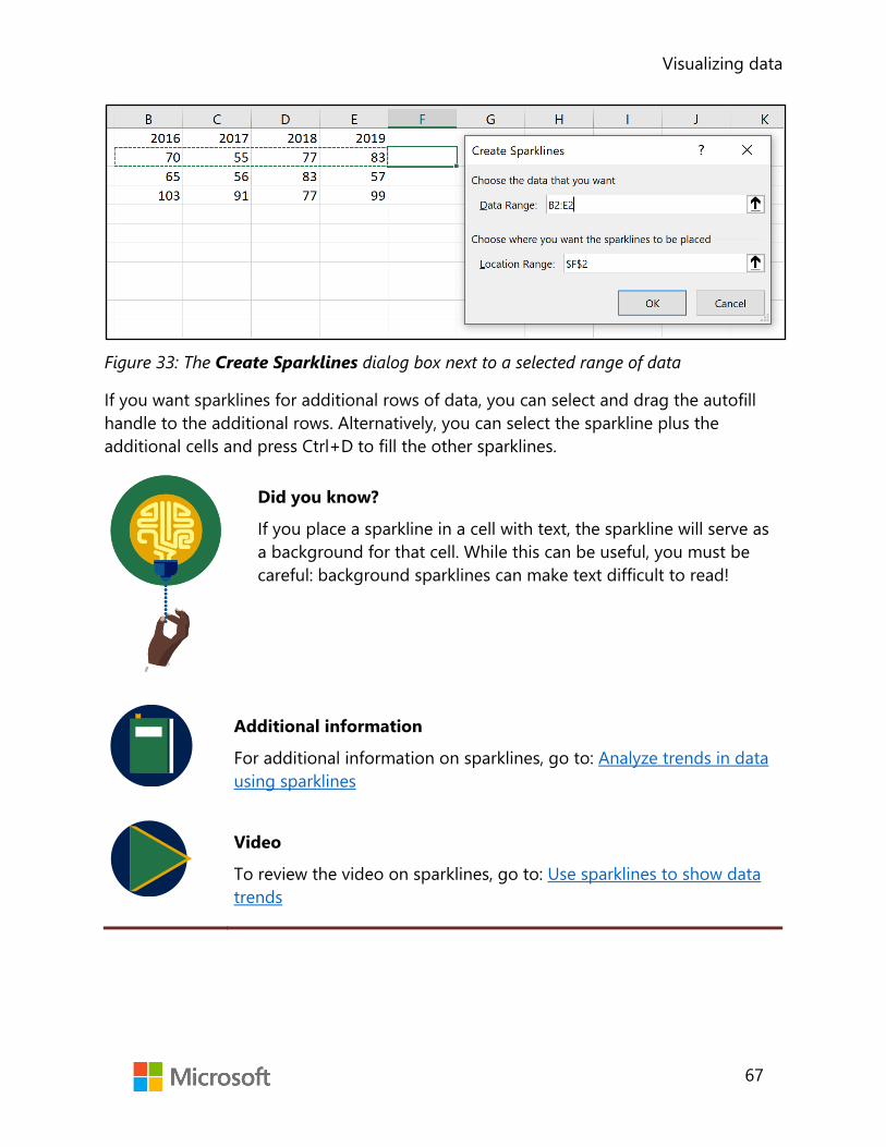
Visualizing data
67
Figure 33: The Create Sparklines dialog box next to a selected range of data
If you want sparklines for additional rows of data, you can select and drag the autofill handle to the additional rows. Alternatively, you can select the sparkline plus the additional cells and press Ctrl+D to fill the other sparklines.
Did you know?
If you place a sparkline in a cell with text, the sparkline will serve as a background for that cell. While this can be useful, you must be careful: background sparklines can make text difficult to read!
Additional information
For additional information on sparklines, go to: Analyze trends in data using sparklines
Video
To review the video on sparklines, go to: Use sparklines to show data trends
Visualizing data
68
Activity: Tell a story In this activity, the teacher will lead you through inserting sparklines to emphasize data trends.
Resources required You will need the following resource for this activity:
• Open L6_T1_act_daily_cell_production.xlsx in this lesson’s Learning Activity Resources.
Activity instructions Add sparklines to the worksheets as directed by the teacher.
Try-it: Insert sparklines In this leveled try-it activity, you’ll add two different types of sparklines to a
workbook.
Try-it 1 This activity will have you practice inserting Line sparklines to emphasize data trends.
Resources You will need the following resource for this try-it:
• Open L6_T1_try1_weekly_cell_production_starter.xlsx in this lesson’s Learning Activity Resources.
Instructions The following are the general tasks that you need to perform during this try-it:
1. On the AngleAdjustments worksheet, create a Line sparkline in cell H4. Include the data in cells B4:G4.
2. Fill the sparkline down to the rest of the rows of data on the worksheet.
3. In cell H3, enter the text Performance.

Visualizing data
69
Try-it 2 This activity will have you practice inserting Win/Loss sparklines to emphasize data trends.
Resources You will need the following resource for this try-it:
• Open L6_T1_try2_weekly_cell_production_starter.xlsx in this lesson’s Learning Activity Resources.
Instructions The following steps are the general tasks that you need to perform during this try-it:
1. On the SurplusEnergy worksheet, create a Win/Loss sparkline in cell H4. Include the data in cells B4:G4.
2. Fill the sparkline in the rest of the rows of data on the worksheet.
3. In cell H3, enter the text Surplus/Deficit.
Topic 2: Modify sparklines Due to their small size and their focus on single sets of data, you can’t customize
sparklines to the same degree as charts. However, Excel does offer a robust set of options for customizing sparklines. As with charts, familiarizing yourself with these options will help you create effective sparklines.
Show sparkline markers and highlights Sparklines don’t have enough space to label data with values, but you do have some options for emphasizing particularly significant individual values, such as the highest and lowest values.
Select the sparklines you want to modify to add the Sparkline tab to the ribbon, and then select the Design tab. A series of check boxes in the Show group allow you to select which individual data points to emphasize. In Line sparklines, selecting Markers will add a marker to all datapoints; this option is not available for Column and Win/Loss sparklines. High Point and Low Point add markers or highlights to the highest and lowest values, respectively. First Point and Last Point emphasize the first and last data points in the series, respectively, and Negative Points will highlight and values below zero. The following screenshot depicts the Show group with High Point and Low Point selected.

Visualizing data
70
Figure 34: The Show group with High Point and Low Point selected
Apply a style to sparklines Excel includes predefined sparklines styles to help you find just the right appearance for your sparklines. You can also modify their colors. Select the sparklines you want to modify to add the Sparkline tab to the ribbon, and then select the Design tab. The Style group includes a gallery of Quick Styles. Navigating to a quick style will update the sparklines on your worksheet and display a preview of the settings.
The Style group (displayed in the following screenshot) also includes a Sparkline Color option to change the primary color of your sparklines, and a Marker Color option to customize how markers and highlights are presented.
Figure 35: The Style group within the Design tab in Sparkline Tools
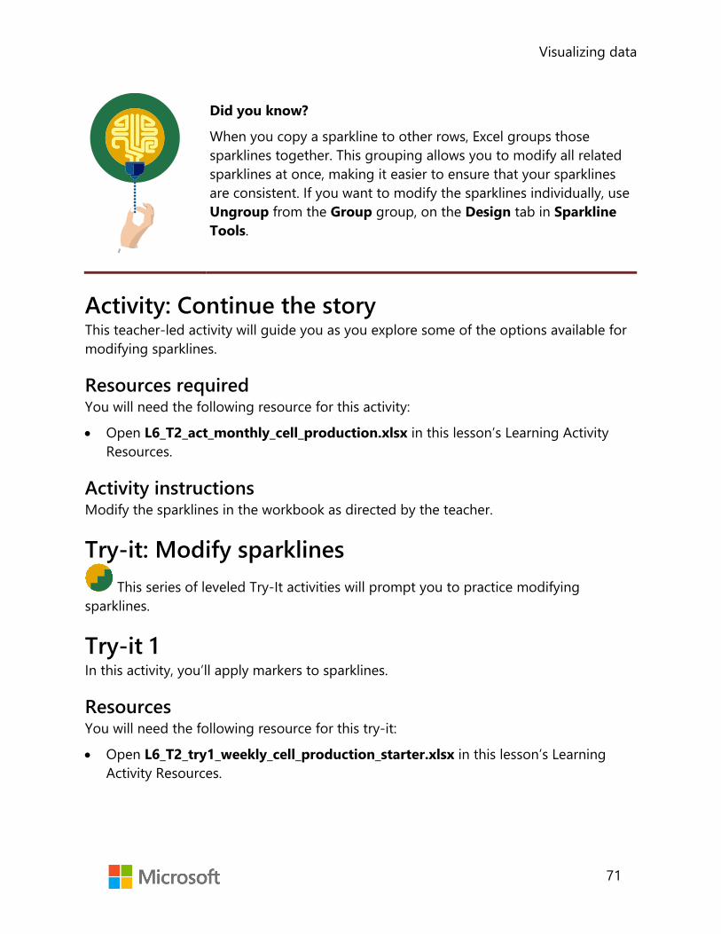
Visualizing data
71
Did you know?
When you copy a sparkline to other rows, Excel groups those sparklines together. This grouping allows you to modify all related sparklines at once, making it easier to ensure that your sparklines are consistent. If you want to modify the sparklines individually, use Ungroup from the Group group, on the Design tab in Sparkline Tools.
Activity: Continue the story This teacher-led activity will guide you as you explore some of the options available for modifying sparklines.
Resources required You will need the following resource for this activity:
• Open L6_T2_act_monthly_cell_production.xlsx in this lesson’s Learning Activity Resources.
Activity instructions Modify the sparklines in the workbook as directed by the teacher.
Try-it: Modify sparklines This series of leveled Try-It activities will prompt you to practice modifying
sparklines.
Try-it 1 In this activity, you’ll apply markers to sparklines.
Resources You will need the following resource for this try-it:
• Open L6_T2_try1_weekly_cell_production_starter.xlsx in this lesson’s Learning Activity Resources.

Visualizing data
72
Instructions The following steps are the general tasks that you need to perform during this try-it:
• On the AngleAdjustments worksheet, add High Point markers to the Line sparklines.
Try-it 2 This activity will give you the opportunity to practice customizing sparkline markers.
Resources You will need the following resource for this try-it:
• Open L6_T2_try2_weekly_cell_production_starter.xlsx in this lesson’s Learning Activity Resources.
Instructions The following steps are the general tasks that you need to perform during this try-it:
1. On the AngleAdjustments worksheet, add Low Point markers to the Line sparklines.
2. On the same sparklines, change High Point markers to green, and set the Low Point markers to red.
Try-it 3 In this try-it activity, you’ll practice modifying individual sparklines.
Resources You will need the following resource for this try-it:
• Open L6_T2_try3_weekly_cell_production_starter.xlsx in this lesson’s Learning Activity Resources.
Instructions The following steps are the general tasks that you need to perform during this try-it:
1. On the AngleAdjustments worksheet, remove the High Point and Low Point markers to the Line sparklines.
2. Ungroup the first three Line sparklines so that you can modify them individually.
3. Apply orange High Point markers to each of the first three sparklines.
4. Apply black markers to all datapoints in the remaining four sparklines.

Visualizing data
73
Wrap-up Use these questions to check what you learned in this lesson:
1. By default, related sparklines are managed together in a ______________________.
2. Which of the following options is used to emphasize the largest value in a data series?
Select the correct option.
a. First Point
b. High Point
c. Last Point
d. Low Point
3. To modify an individual sparkline, you must first __________________ it.
Select all that apply.
a. Clear
b. Detach
c. Select
d. Ungroup
4. The ______________________ chart type emphasizes the difference between positive and negative values in the data series.

Visualizing data
74
Lesson 7: Understanding the Quick Analysis feature Overview This lesson will explore a useful tool for quickly and easily transforming, visualizing, and analyzing data. The Quick Analysis feature lets you add visualizations such as charts, sparklines, and conditional formatting. It also automates the process of adding useful formulas to total or average your data.
Warm-up Use these questions to find out what you already know about this lesson’s topics:
1. How can you access the Quick Analysis tool?
Select the correct option.
a. Navigate to the Data tab on the ribbon.
b. Right-click or access the context menu on a chart or sparkline.
c. Select a range of cells.
d. Select Conditional Formatting from the Home tab on the ribbon.
2. Which of the following can you add using Quick Analysis?
Select all that apply.
a. A color scale
b. A chart
c. A trendline
d. A predefined color scheme

Visualizing data
75
3. Where are Totals calculations placed when added using the Quick Analysis feature?
Select all that apply.
a. On a new worksheet
b. Beginning at cell A1
c. On the last row visible on the screen
d. Adjacent to the data range
4. Which of the following options best describes the role of the Quick Analysis feature?
Select the correct option.
a. Quickly generate new values based on existing data.
b. Forecast or project a future value.
c. Analyze data and generate a text-based report.
d. Quickly generate totals and visualizations.
Topic 1: Use Quick Analysis to format data There are many options for visualizing and analyzing data in a spreadsheet, and Excel gives you a large variety of tools to present your data in exactly the right way. The Quick Analysis feature gives you a speedy way to do some of the most common analysis and visualization tasks in Excel. You might use Quick Analysis to answer a quick question in a workbook, then delete those additions from the workbook. With data that you are sharing with other people, Quick Analysis can give you a jump start when adding visualizations to make the data easier for others to understand.
To use the Quick Analysis feature, select a range of cells you want to analyze; this will make the Quick Analysis icon available at the bottom, right corner of your selected range, as called out in the following.

Visualizing data
76
Figure 36: A selection of cells with the Quick Analysis icon highlighted in red
Add conditional formatting using Quick Analysis To add conditional formatting, select a range of data, select the Quick Analysis icon, and then select the Formatting tab. By navigating to an option in the gallery, the worksheet updates to display a preview of using the formatting option you chose. The following screenshot depicts the Formatting options in Quick Analysis.
Figure 37: Formatting tab options in Quick Analysis
Select a choice to add that conditional formatting to the data range.
Add a chart or sparklines using Quick Analysis To add a chart or sparklines, select a range of data, select the Quick Analysis icon, and then select either the Charts or Sparklines tab. As you navigate to options, the worksheet updates to display a preview of the choice. Note that the options offered in the gallery are based on the Recommended Charts feature and could vary from the example in the following screenshot.

Visualizing data
77
Figure 38: Charts tab options in Quick Analysis
Select your desired chart or sparklines to insert it into the worksheet.
Add totals for data using Quick Analysis The Totals tab options in Quick Analysis makes calculations based on your numbers and adds the results in the cells next to or below your data.
To add totals for data, select a range of data, select Quick Analysis, and then select the Totals option. By navigating to a calculations option in the gallery (as displayed in the following screenshot), the worksheet updates to display a preview of the choice.
Figure 39: Totals tab options in Quick Analysis
Select a calculation to add the corresponding formulas to your worksheet.
Did you know?
Everything added with Quick Analysis is just like any other part of your workbook. For example, a chart created with Quick Analysis is just like a chart created from the ribbon—you can modify it just like any other chart. This is true for everything Quick Analysis offers.

Visualizing data
78
Video
To review the video on Quick Analysis, go to: Analyze your data instantly
Activity: Demo and experiment In this activity, the teacher will demonstrate the Quick Analysis feature. After the demonstration, you’ll practice using Quick Analysis.
Resources required You will need the following resource for this activity:
• Open L7_T1_act_monthly_cell_production.xlsx in this lesson’s Learning Activity Resources.
Activity instructions Participate in the activity by following these instructions:
1. Participate in the demonstration led by the teacher.
2. Try out a variety of Quick Analysis tools. Be sure to try different selections to observe how the options change.
Try-it: Quick Analysis In these leveled Try-It activities, you’ll practice using different Quick Analysis tools.
Try-it 1 In this try-it, you’ll use Quick Analysis to add averages to a range of data.
Resources You will need the following resource for this try-it:
• Open L7_T1_try1_weekly_cell_production_starter.xlsx in this lesson’s Learning Activity Resources.

Visualizing data
79
Instructions The following steps are the general tasks that you need to perform during this try-it:
1. On the AngleAdjustments worksheet, use Quick Analysis to add averages to row 11 for columns B through G.
2. On the SurplusEnergy worksheet, use Quick Analysis to add averages to the right of each row of data.
Try-it 2 In this try-it activity, you’ll practice adding visualizations using Quick Analysis.
Resources You will need the following resource for this try-it:
• Open L7_T1_try2_weekly_cell_production_starter.xlsx in this lesson’s Learning Activity Resources.
Instructions The following steps are the general tasks that you need to perform during this try-it:
1. On the AngleAdjustments worksheet, use Quick Analysis to highlight all cells with values greater than 3.0. Use a yellow fill with dark yellow text.
2. On the SurplusEnergy worksheet, use Quick Analysis to add a color scale to the data.
Topic 2: Disable the Quick Analysis feature
Part of the flexibility available to Excel users is the ability to customize which tools you use and how you implement them. While Quick Analysis makes it convenient to access some commonly used features, you might want to disable it.
The setting to disable Quick Analysis is in the Excel Options window. Select File on the ribbon, and then select Options. The Show Quick Analysis options on selection check box allows you to enable or disable the feature. The following screenshot depicts the Options window with the Show Quick Analysis options on selection check box selected.

Visualizing data
80
Figure 40: The Options window with the Show Quick Analysis options on selection check box selected
To disable the feature, ensure that the check box is cleared.
Activity: Discuss In this activity, the teacher will lead a discussion about Quick Analysis.
Resources required You will not need any resources for this try-it.
Activity instructions Participate in the group discussion.

Visualizing data
81
Try-it: Disable the Quick Analysis feature In this activity, the teacher will present the group with a challenge. Do your best to
complete the challenge as directed.
Resources You will not need any resources for this try-it.
Instructions Complete the group challenge as directed by the teacher.
Wrap-up Use these questions to check what you learned in this lesson:
1. Which of the following statements is true of Quick Analysis charts?
Select the correct option.
a. Chart type choices vary depending on the selection.
b. Only a few of the most popular charts types are available.
c. Generated charts cannot be customized.
d. The list of chart types can be customized in the Options window.
2. Which of the following cannot be added using Quick Analysis?
Select the correct option.
a. Charts
b. Cell styles
c. Sparklines
d. Conditional formatting
e. Averages
3. You can disable the Quick Analysis feature from the ______________________ window.

Visualizing data
82
Glossary Alt Text A description of a graphic element used by screen readers to
describe the information included in a visual object.
Chart A visual representation of one or more data series.
Chart element An individual element of a chart, such as a title or legend.
Conditional Formatting
A feature that applies cell formatting based on the value of that cell.
Data series A row or column of related values in a worksheet.
Rules Manager A tool that allows you to add, remove, edit, and prioritize conditional formatting rules.
Quick Analysis A feature that provides previews of analysis and visualization tools.
Quick Style A predefined collection of settings used to configure a visual element, such as a chart or sparkline.
Quick Layout A predefined arrangement of chart elements.
Sparkline A miniature chart that occupies a single cell and provides a visual representation of data.
Table 2: Glossary terms and definitions

Visualizing data
83
Cornerstone Overview In this cornerstone, you’ll improve on and add to visualizations in a workbook with data related to the solar array installed last year at Munson’s Pickles and Preserves Farm. You’ll remove and add conditional formatting, add charts and sparklines, and make changes to a chart already in the workbook. You’ll also use layouts, styles, and colors to alter the appearance of these visualizations.
Objectives The following table outlines the Cornerstone objectives and their corresponding MOS exam objectives.
Apply and remove conditional formatting
• 2.4.2: Apply built-in conditional formatting • 2.4.3: Remove conditional formatting
Create and move charts
• 5.1.1: Create charts • 5.1.2: Create chart sheets • 5.3.3: Add alternative text to charts for accessibility
Add a data series to a chart
• 5.2.1: Add data series to charts • 5.2.2: Switch between rows and columns in source data
Add and remove chart elements from a chart
• 5.2.3: Add and modify chart elements
Apply layouts, styles, and colors to charts
• 5.3.1: Apply chart layouts • 5.3.2: Apply chart styles • 5.3.3: Add alternative text to charts for accessibility
Insert and modify sparklines
• 2.4.1: Insert Sparklines
Table 3: Cornerstone objectives

Visualizing data
84
Duration 50 minutes
Instructions Complete the following tasks for each file:
1. When saving your file, add your name to the end of the filename, for example: “Cornerstone_Solar_Array_Data_Dwayne_Espino.” Follow your teacher’s directions for where to save your files.
2. When you’re done with the Cornerstone, assess your completed product, and enter the points you think you earned within the task lists below. You can take the help of your teacher if required.
Tasks You’ll work with one file in this Cornerstone. The following steps are the tasks you need to complete within the file.
File 1: Cornerstone_solar_array_data_starter.xlslx Task: Apply and remove conditional formatting (4 points) 1. Open Cornerstone_solar_array_data_starter.xlslx and select the MonthlyUsage
worksheet. Remove all the conditional formatting. (2 points) (Exam objective 2.4.3)
2. Apply a conditional formatting rule that adds a Red - Yellow - Green color scale, so that the months with the highest usage are shaded red. (2 points) (Exam objective 2.4.2)
Points scored: _______ /4
Task: Insert sparklines (5 points) 1. On the MonthlyUsage worksheet, add a Line sparkline to the January row next to
the value for 2019. (2 points) (Exam objective 2.4.1)
2. Fill that sparkline through the December row. (1 point) (Exam objective 2.4.1)
3. Modify all sparklines to indicate the high point for each row. (2 points) (Exam objective 2.4.1)
Points scored: _______ /5

Visualizing data
85
Task: Add a data series to a chart (3 points) 1. On the MonthlySurplus worksheet, switch the row and column on the pie chart. (1
point) (Exam objective 5.2.2)
2. Add the data for October, November, and December to the pie chart. (2 point) (Exam objective 5.2.1)
Points scored: _______ /3
Task: Modify a chart (4 points) 1. Move the pie chart to a new chart worksheet named SurplusEnergy. (2 points)
(Exam objective 5.1.2)
2. Change the color scheme for the chart to Colorful Palette 3. (2 point)
Points scored: _______ /4
Task: Create and modify a chart (4 points) 1. On the MonthlyUsage worksheet, create a clustered column chart with all the
numeric data on the worksheet. Position it below the data. (2 points) (Exam objective 5.1.1)
2. Apply Layout 2. (1 point) (Exam objective 5.3.1)
3. Edit the chart title to Monthly Usage. (1 points) (Exam objective 5.2.3)
Points scored: _______ /4
Task: Add and remove chart elements from a chart (7 points) 1. On the MonthlyUsage worksheet, remove the data labels from the clustered column
chart. (2 points) (Exam objective 5.2.3)
2. Add primary major horizontal gridlines. (3 points) (Exam objective 5.2.3)
3. On the SurplusEnergy worksheet, add data labels with data callouts. Remove the legend. (2 points) (Exam objective 5.2.3)
Points scored: _______ /7

Visualizing data
86
Task: Add Alt Text (2 points) 1. On the MonthlyUsage worksheet, add Alt Text to the clustered column chart. (1
points) (Exam objective 5.3.3)
2. On the SurplusEnergy worksheet, add Alt Text to the pie chart. (1 points) (Exam objective 5.3.3)
Points scored: _______ /2
FILE 1 TOTAL POINTS: _______ /29

Student guide 40567A Microsoft Excel associate 2019 Module 8: Preparing to print and checking for issues
Preparing to print and checking for issues
2
Contents
Contents .............................................................. 2
Module overview ............................................. 4
Description ..................................................... 4
Scenario .......................................................... 5
Cornerstone ................................................... 6
Lesson 1: Preparing to print ........................ 7
Overview ......................................................... 7
Warm-up ........................................................ 7
Topic 1: Understand the print settings ............................................................................ 8
Access print settings ............................. 8
Settings ....................................................... 9
Set the print area ................................. 12
Print ........................................................... 13
Activity: Discuss and learn ............... 14
Try-it: Understanding the print settings .................................................... 14
Try-It 1 ...................................................... 14
Try-It 2 ...................................................... 15
Try-It 3 ...................................................... 15
Topic 2: Understand page setup ........ 16
Page Setup dialog box ...................... 18
Set margins ............................................ 18
Sheet settings ....................................... 19
Activity: Question time ...................... 20
Try-it: Understand page setup ....... 21
Try-It 1 ...................................................... 21
Try-It 2 ...................................................... 21
Wrap-up ....................................................... 22
Lesson 2: Using headers and footers .... 24
Overview ...................................................... 24
Warm-up ...................................................... 24
Topic 1: Add headers and footers ..... 25
Add headers or footers by using the Insert tab ................................................. 25
Add headers or footers by using the Page Setup dialog box ....................... 26
Activity: Discuss and learn ................ 28
Try-it: Add headers or footers ........ 29
Try-It 1 ...................................................... 29
Try-It 2 ...................................................... 29
Topic 2: Edit headers and footers ...... 30
Edit a header or footer using Page Layout view ............................................. 30
Edit a header or footer using the Page Setup dialog box ....................... 31
Remove all headers and footers .... 32
Activity: Switch ...................................... 32
Try-it: Edit headers and footers ...... 33
Try-It 1 ...................................................... 33
Try-It 2 ...................................................... 33
Wrap-up ....................................................... 34
Lesson 3: Checking for issues ................... 36
Overview ...................................................... 36
Warm-up ...................................................... 36
Topic 1: Modify the basic workbook properties .................................................... 37

Preparing to print and checking for issues
3
Workbook properties ......................... 38
Activity: Pose a question................... 40
Try-it: Modify basic workbook properties ............................................... 40
Try-It 1 ...................................................... 40
Try-It 2 ...................................................... 41
Topic 2: Inspect workbooks for issues ............................................................. 41
Inspect a workbook ............................ 42
Check accessibility............................... 45
Compatibility issues ............................ 47
Activity: What’s the correct category? ................................................ 49
Try-it: Inspect workbooks for issues ........................................................ 49
Try-It 1 ...................................................... 50
Try-It 2 ...................................................... 50
Wrap-up ....................................................... 51
Glossary ............................................................. 53
Cornerstone ..................................................... 54
Overview ...................................................... 54
Objectives .................................................... 54
Duration ....................................................... 55
Instructions .................................................. 55
Tasks .............................................................. 55
File 1: Cornerstone_membership_starter .xlsx ............................................................ 55
File 2: Cornerstone2_finances_starter.xlsx ..................................................................... 56
Preparing to print and checking for issues
4
Module overview Description Welcome to the last module in this course. Now that you have gained a vast collection of skills, it’s time to finalize your workbooks in preparation for printing and presenting to third parties. Finalizing workbooks can be time consuming. However, it is always worth taking the time to add the final changes to your workbooks. It’s also important to ensure that your workbooks are as accessible as possible for everyone that needs to access the data. In this module, you will set the page and print settings of a workbook, add headers and footers, and check for any accessibility issues and personal information contained within your workbooks.
On completion of this module, there will be a Capstone that will give you the chance to flaunt your Microsoft Excel skills to your fellow classmates and the teacher. You might even impress yourself with your amazing skills!
Lesson Learning objective Exam objective(s)
Preparing to print Configure a workbook’s print settings and page setup.
• 1.5.1 • 1.5.3 • 1.3.1
Using headers and footers
Add and edit headers and footers in a worksheet.
• 1.3.3
Checking for issues Modify basic workbook properties and inspect a workbook for issues.
• 1.4.5 • 1.5.4
Cornerstone: Preparing a financial workbook for printing
Finalizing workbooks to present to third parties
• All of these
Table 1: Objectives by lesson

Preparing to print and checking for issues
5
Scenario The farm would like to start using drones to track crop health. Eventually, the data from the drones will help make the farm much more productive. But the initial development cost is high. To help with the costs, farm management executives will meet with a potential investor next week. Because you’ve gained so much Excel experience during your internship so far, they’d like your help in finalizing a couple of important workbooks to print and present to the investor.

Preparing to print and checking for issues
6
Cornerstone The farm is trying to find money to fund drone technology to track crop health. The owners have a meeting with a potential investor tomorrow.
You need to prep the workbooks for printing, which includes adding headers and footers, changing the print settings, and inspecting the workbooks for any accessibility and compatibility issues. In addition to that, you need to edit the worksheets to ensure that there is no missing data.

Preparing to print and checking for issues
7
Lesson 1: Preparing to print Overview In this lesson, you will learn how to configure a workbook for printing using the options within page setup and changing the print settings. Sometimes, how you imagine the workbook on paper is nothing like it in reality. A workbook that prints on several sheets of paper can often be set to print on fewer sheets or on one sheet of paper.
Warm-up Take a minute or two to reflect with your classmates on the most valuable skills that you have learned so far in the previous modules. Has there been any topic that has helped you in any of your other classes? Then use these questions to find out what you already know about this lesson’s topics:
1. Which of the following keyboard shortcuts opens the Print menu?
Select the correct option.
a. Ctrl+V
b. Ctrl+P
c. Windows+P
d. Windows+E
2. Which of the following can you use to access the Page Setup dialog box?
Select all that apply.
a. Ctrl+P
b. Any dialog launcher on the Page Layout tab
c. Any dialog launcher on the Home tab
d. Windows+P

Preparing to print and checking for issues
8
3. On which tab in the Page Setup dialog box can you change the page orientation?
Select the correct option.
a. Sheet
b. Header/Footers
c. Margins
d. Page
4. There are ________________________ tabs on the Page Setup dialog box.
Topic 1: Understand the print settings At Munson’s Pickles and Preserves Farm, the goal is to print on as little paper as
possible and wherever possible not to print at all. However, sometimes there is no other option than to print a workbook. By default, Excel will print all data entered into a worksheet, and that can often waste a lot of paper. Before sending anything to the printer, it’s always a good idea to observe how it will print. When you select Print, you are in the Print Preview mode, which means you get a preview of how it will print. From here, you will be able to set many print options.
Access print settings To alter any print settings, you will need to access the Print dialog box (refer to Figure 1):
• From File, select Print, or • Select Ctrl+P on your keyboard. There are many print settings available to customize and print your workbook according to your preferences.

Preparing to print and checking for issues
9
Figure 1: Print dialog box
Settings Under Settings, you can set the following options prior to printing: which worksheets and pages to print, collation, orientation, paper size, margins, and scaling.
Go to Settings to set which worksheets within the workbook you would like to print (refer to Figure 2).
Active sheets Select to print all sheets that are currently selected.
Entire workbook Select to print every worksheet within the workbook.
Print Selection Select to print the area you have currently selected on the worksheet.
Print selected table This option will be available if you have selected a formatted table in your worksheet.
Ignore print area Select if you have set a print area previously and you don’t want to clear it.
Table 2: What to print options

Preparing to print and checking for issues
10
Figure 2: Print settings
Pages Enter the page number you would like to print in the Pages box and the to box if you want to print a selection of pages in the worksheet; for example, pages 1 to 3 (refer to Figure 3).
Collation Select Collated to switch between collated and uncollated. If you were to print 10 copies of a three-page worksheet, collated would print pages 1 to 10 three times, uncollated would print three copies of page 1, three copies of page 2, etc. (refer to Figure 3).
Orientation Select Portrait Orientation to switch between portrait or landscape orientation (refer to Figure 3).
Page size Select Letter to select the paper size such as A4, A3, or Letter (refer to Figure 3).
Margins Select Normal to select a different margin setting (refer to Figure 3, covered in more detail in Topic 2).

Preparing to print and checking for issues
11
Scaling Select No Scaling to set one of the following options: • No Scaling will print all data on the necessary
amount of paper. • Fit Sheet on One Page will reduce the font size to
fit all the data onto one sheet of paper (although you might not be able to read it!).
• Fit All Columns on One Page will reduce all the columns to fit onto one page. Additional rows will print onto more pages.
• Fit all Rows on One page will reduce all the rows to fit onto one page. Additional columns will print onto more pages.
Table 3: Print Setting options
Figure 3: Default print settings
Additional information
To review the article on scaling a worksheet, go to: Scale a worksheet

Preparing to print and checking for issues
12
If the options on the Print screen are not enough to set up the page exactly to your preferences or needs, select Page Setup at the bottom of the list. This will open the Page Setup dialog box (refer to Figure 4). Here, you will find four tabs with much more detail to work with: Page, Margins, Headers/Footers, and Sheet.
Figure 4: Page Setup dialog box
Did you know?
If you entered data in every cell in column A through the last row in the worksheet, and if you tried to print the workbook without changing the settings, you would print over twenty-two thousand pages. Please don’t try it out!!
Set the print area Sometimes there are areas on the worksheet that have reference data that you don’t intend to print. If that is the case, you might find it useful to set a print area. The print area that you set will remain until you change or clear it.

Preparing to print and checking for issues
13
To set a specific print area:
• Select the data you wish to print. • Select Print Area on the Page Layout group. • Select Set Print Area. To add further print areas:
• Select the data you wish to print. • Select Print Area on the Page Layout group. • Select Add to Print Area. To clear a print area:
• Select Print Area on the Page Layout group. • Select Clear Print Area.
Additional information
To review the article on setting the print area on a worksheet, go to: Set or clear a print area on a worksheet
Print When you are ready to print, select the Print button. Before printing, you can set the number of copies to print in the Copies box and select the specific printer or PDF in the Printer box (refer to Figure 5).
Figure 5: Print button

Preparing to print and checking for issues
14
Activity: Discuss and learn In this activity, you will participate in a teacher-led discussion about why it is important to consider the page and print settings before you print a workbook.
Resources required You will need the following resources for this activity:
• Open L1_T1_act_annual_produce.xlsx in this lesson’s Learning Activity Resources.
Activity instructions Participate in the activity by following these instructions:
1. Open L1_T1_act_annual_produce.xlsx.
2. Select File, and then select Print.
3. Offer suggestions about how to make the data print more effectively.
4. Work with a partner to edit the print settings. Review the results of your changes asyou work.
Try-it: Understanding the print settings In this leveled try-it, you will set the print area on a worksheet and print to PDF.
Try-it 1 You have recently been tracking honey sales and you need to print a selection of the worksheet for a colleague.
Resources You will need the following resources for this try-it: • Open L1_T1_try1_annual_produce_starter.xlsx in this lesson’s Learning Activity
Resources.
Instructions The following are the general tasks to perform during this try-it:
1. Open L1_T1_try1_annual_produce_starter.xlsx.
2. Set the print area to print only the Honey products.
3. Print the area to PDF using the name Honey_Plus your initials.pdf.

Preparing to print and checking for issues
15
Try-it 2 You have been tracking Nuts and Homemade items for Summer and Autumn and need to only print two portions of the worksheet to hand off to a colleague.
Resources You will need the following resources for this try-it: • Open L1_T1_try2_annual_produce_starter.xlsx in this lesson’s Learning Activity
Resources.
Instructions The following are the general tasks to perform during this try-it:
1. Open L1_T1_try2_annual_produce_starter.xlsx.
2. Set the print area for all the Nuts.
3. Add the Homemade Crafts to the current print area.
4. Set the worksheet to print all columns in landscape orientation.
5. Print both areas to PDF using the name Nuts_&_Crafts_Plus your initials.pdf.
Try-it 3 You need to fit the entire worksheet onto one sheet to prepare it as a PDF for emailing it to your colleague.
Resources You will need the following resources for this try-it: • Open L1_T1_try3_annual_produce_starter.xlsx in this lesson’s Learning Activity
Resources.
Instructions The following are the general tasks to perform during this try-it:
1. Open L1_T1_try3_annual_produce_starter.xlsx.
2. Clear any print areas that have been set.
3. Set the worksheet to print all columns landscape on one sheet.
4. Print the entire worksheet to PDF using the name Annual_Produce_Plus yourinitials.pdf.

Preparing to print and checking for issues
16
Topic 2: Understand page setup If the thought of all the options in the Page Setup dialog box is overwhelming,
you might prefer to work with the three groups of buttons on the Page Layout tab on the ribbon: Page Setup, Scale to Fit, and Sheet Options (refer to Figure 6).
Each of these groups has a dialog launcher in the corner that you can use to access the Page Setup dialog box.
Figure 6: Page Layout tab
Margins Select Margins to choose one of the following options: • Normal is the default setting.• Select Wide to add more space between the edge of
the paper and your data.• Select Narrow to leave less space between the edge
of the paper and your data.• Select Custom to open the Page Setup dialog box,
which will allow you to set the margins exactly as youwant them.
Orientation Portrait is the default setting and useful for narrow data. Landscape is useful for wider data.
Size Select Size to change to a different paper size.
Print Area Select Print Area to set the print area, clear, or add more print areas.
Breaks Select Breaks to display where the pages break on the current worksheet.
Background Select Background to insert a picture to print in the background on the worksheet.

Preparing to print and checking for issues
17
Print Titles Select Print Titles to set which rows to repeat at the top of every printed page or columns to repeat on the left side of every printed page.
Table 4: Page Setup options
Width Enter the number of pages to shrink the width of your data in the Width box, for example 1 page wide.
Height Enter the number of pages to shrink the height of your data in the Height box, for example 1 page tall.
Scale Enter the percentage to shrink or increase the size of your data in the Scale box. Leave the width and height set on Automatic to use this feature.
Table 5: Scale to Fit options
Gridlines Select the View box to display the gridlines on screen Select the Print box to print gridlines around your data, meaning you don’t need to manually add borders.
Headings • Select the View box to display the column and rowheaders on screen.
• Select the Print box to print the columns and rowheaders around your data.
Table 6: Sheet Options
Additional information
To review the article on editing the page setup of a worksheet, go to: Page Setup

Preparing to print and checking for issues
18
Page Setup dialog box As already mentioned, in this lesson, you can access the print and page setup options via File > Print or via the Page Layout tab on the ribbon. However, you might occasionally need to access the Page Setup dialog box for further options. To do that, either:
• Go to File, then Print (Ctrl+P) and select the Page Setup link at the bottom of thesettings panel, or
• Select any dialog launcher on the Page Layout tab.• Select the tab in which would like to work.
Set margins To alter the margins in a worksheet (refer to Figure 7):
• Select the Margins tab in the Page Setup dialog box.• Set the Top, Header, Left, Right, Bottom, and Footer with your preferences.• Select to center on the page Horizontally or Vertically as per your requirements.• Select OK to return to the Print screen.
Figure 7: Margins tab in Page Setup dialog box
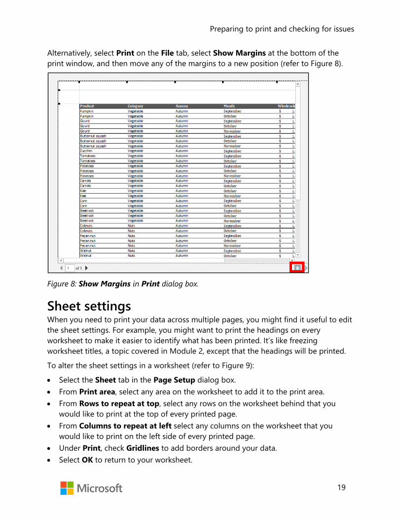
Preparing to print and checking for issues
19
Alternatively, select Print on the File tab, select Show Margins at the bottom of the print window, and then move any of the margins to a new position (refer to Figure 8).
Figure 8: Show Margins in Print dialog box.
Sheet settings When you need to print your data across multiple pages, you might find it useful to edit the sheet settings. For example, you might want to print the headings on every worksheet to make it easier to identify what has been printed. It’s like freezing worksheet titles, a topic covered in Module 2, except that the headings will be printed.
To alter the sheet settings in a worksheet (refer to Figure 9):
• Select the Sheet tab in the Page Setup dialog box.• From Print area, select any area on the worksheet to add it to the print area.• From Rows to repeat at top, select any rows on the worksheet behind that you
would like to print at the top of every printed page.• From Columns to repeat at left select any columns on the worksheet that you
would like to print on the left side of every printed page.• Under Print, check Gridlines to add borders around your data.• Select OK to return to your worksheet.

Preparing to print and checking for issues
20
Figure 9: Sheet tab in Page Setup dialog box
Additional information
For more information on configuring print settings, go to: Print a worksheet or workbook
Activity: Question time In this activity, you will consider the questions asked by your teacher about the many ways in which you can access the Page Setup dialog box and what options are available in the dialog box that are not available elsewhere.
Resources required You will need the following resources for this activity:
• Open L1_T2_act_summary.xlsx in this lesson’s Learning Activity Resources.

Preparing to print and checking for issues
21
Activity instructions Participate in the activity by following these instructions:
1. Open L1_T2_act_summary.xlsx.
2. Use any method suggested to access the Page Setup dialog box.
3. Work with a partner to compare the Page Layout, Print, and Page Setup options.
4. Experiment with any of the Page Setup options and observe the results using PrintPreview.
5. Close the workbook without saving it.
Try-it: Understand page setup In this try-it, you will set the paper size, orientation, and margins.
Try-it 1 You are preparing a worksheet to print to PDF on A4 paper.
Resources You will need the following resources for this try-it:
• Open L1_T2_try1_summary_starter.xlsx in this lesson’s Learning Activity Resources.
Instructions The following are the general tasks to perform during this try-it:
1. Open L1_T2_try1_summary_starter.xlsx.
2. Set the worksheet to print to PDF on A4 in the portrait orientation.
3. Save the workbook with its original name and append your initials on the end.
Try-it 2 You are preparing data to print as large as possible to make it easier for your colleagues to follow.
Resources You will need the following resources for this try-it: • Open L1_T2_try2_summary_starter.xlsx in this lesson’s Learning Activity Resources.

Preparing to print and checking for issues
22
Instructions The following are the general tasks to perform during this try-it:
1. Open L1_T2_try2_summary_starter.xlsx and set the workbook to print to PDF.
2. Use the Page Setup dialog box to set the following:
a. Set the Summary worksheet to print on A4 in the landscape orientation.
b. Set the left margin to 1.0 and the right margin to 1.0.
c. Set the worksheet to print in the center horizontally and vertically.
d. Scale the worksheet to increase the Print Scale to 140%.
Wrap-up Use these questions to check what you learned in this lesson:
1. Select ________________________ to set rows to repeat at the top.
2. Which method can you use to force data to print on one sheet width?
Select all that apply.
a. From Scale to Fit group, set width to one page.
b. From Scale to Fit group set height to one page.
c. Select File, then select Print. Select Scaling, and then select Fit all Columns on One page.
d. Select File, and then select Print. Select Scaling, and then select Fit Sheet on One page.
3. From the left side of the box to right side of the box, indicate the order in which the tabs are in the Page Setup dialog box.
Indicate the correct sequence by adding numbers 1-4 next to the following items.
a. Sheet
b. Header/Footer
c. Page
d. Margins
Preparing to print and checking for issues
23
4. On which group will you find these commands?
a. Scale to Fit
b. Sheet Options
c. Page Setup
Categorize the following items by adding the appropriate group name next to each item.
a. Gridlines ________________________
b. Width ________________________
c. Size ________________________

Preparing to print and checking for issues
24
Lesson 2: Using headers and footers Overview In this lesson, you will learn how to add and edit headers and footers that will repeat on each printed page, in preparation for printing. Similar to Word, you can add page numbers, the date, time, text, and graphics. When you add headers and footers to a worksheet, they are hidden from view unless you are in the Page Layout view, while in Word they are faded out when you are working in the main document.
You can access the Header and Footer via the Insert tab on the ribbon or via Page Setup.
Warm-up Challenge your neighbor to find any command, within 10 seconds, to help with the print or page settings. For example, where do you go to have the headings repeated on every page, or which command can you select to change the page to landscape? Then, use these questions to find out what you already know about this lesson’s topics:
1. Which of the following statements is true?
Select all that apply.
a. You normally enter a workbook header into the first row of a worksheet.
b. Normal view hides a workbook header from display.
c. You can observe a workbook header by selecting File, and then Print.
d. A workbook header appears on screen when you are working in Page Break Preview.
Preparing to print and checking for issues
25
2. Which of the following methods can you use to access the footer in a worksheet?
Select all that apply.
a. Select Header & Footer on the Insert tab.
b. Select File > Print > Page Setup.
c. Select the dialog launcher in the Scale to Fit group on the Page Layout tab.
d. Select the dialog launcher in the Sheet Options group on the Page Layout tab.
3. There are three sections in the header: ________________________, center, and ________________________.
4. The Header & Footer command can be found in the ________________________ group on the Insert tab.
Topic 1: Add headers and footers There are two main methods of entering data into the header or footer in a
workbook. You can select Header/Footer from the Text group on the Insert tab or you can access the header and footer via the Page Setup dialog box. As you know, there are many ways to access the Page Setup dialog box.
When you are preparing a workbook to print, you should allow space for the header or footer if you are going to add content.
Add headers or footers by using the Insert tab 1. Select Header & Footer in the Text group. This will take you into Page Layout view.
2. The hidden header and footer areas will appear, and the Header & Footer Tools Design tab will open on the ribbon (refer to Figure 10).
Figure 10: Header & Footer Tools Design contextual tab

Preparing to print and checking for issues
26
3. Select either the Left, Center, or Right section under Header and begin entering text or numbers, or select any of the commands on the Header & Footer Tools Design tab in the Header & Footer Elements group such as Page Number, Current Date, or File Path.
4. Select Go to Footer in the Navigation group to view the footer area.
5. When you have finished editing the header or footer, select any cell outside the of the header or footer and select the Normal view command next to the Zoom tool’s slider at the bottom of the screen.
Did you know?
The electronic spreadsheet was invented in the mid 1960s. Who’d have thought it was so old!
Add headers or footers by using the Page Setup dialog box 1. Select File > Print or select Ctrl+P on the keyboard, and then select the link to Page
Setup, or use any dialog box on the Page Layout tab.
2. Select the Header/Footer tab in the Page Setup dialog box (refer to Figure 11).

Preparing to print and checking for issues
27
Figure 11: Page Setup dialog box, Header/Footer tab
3. Select the drop-down arrow under Header to select a pre-populated field, or
4. Select the drop-down arrow under Footer to select a pre-populated field, or
5. Select Custom Header or Custom Footer to specify where to place the fields or text in the header or footer.
When you select Custom Header or Custom Footer, the options are the same, except that one will be at the top of each page and the other at the bottom of each page as shown in the following figure:

Preparing to print and checking for issues
28
Figure 12: Custom Header dialog box
6. Select the Left section, the Center section, or the Right section, and then select the command you want from the small bar across the top of the sections.
7. Select Insert Page Number to have automatic page numbers applied to each page.
8. Select any other field such as Number of Pages, Date, Time, File Path, or File Name. Remember to include a space between fields or they will appear to connect when printed.
9. Select OK to close the dialog box and OK again to close the Page Setup dialog box.
Additional information
To review the article on adding headers and footers into a workbook, go to: Headers and footers in a worksheet
Activity: Discuss and learn Your teacher will open L2_T1_act_summary.xlsx and ask anyone with a printed copy if there is additional information that would help them understand the data.
Resources required You will need the following resources for this activity:
• Open L2_T1_act_summary.xlsx in this lesson’s Learning Activity Resources.

Preparing to print and checking for issues
29
Activity instructions Participate in the activity by following these instructions:
1. Open L2_T1_act_summary.xlsx.
2. Select File, and then select Print.
3. Follow along in the discussion and offer suggestions.
Try-it: Add headers or footers A workbook created by your colleague needs information added to the header and
footer prior to printing.
Try-it 1 You need to add the date and time into the footer of a workbook and a heading into the header.
Resources You will need the following resources for this try-it: • Open L2_T1_try1_summary_starter.xlsx in this lesson’s Learning Activity Resources.
Instructions The following are the general tasks to perform during this try-it:
1. Use the Insert tab to add Sales this Year in the center of the header on theSummary worksheet.
2. Apply size 12 and bold formatting to the text.
3. Then add the date and time to automatically update in the right section of thefooter.
4. Save the workbook with its original name and append your initials on the end.
Try-it 2 You need to add information into the header and footer, including inserting the Munson’s logo into the header in preparation for an important meeting.
Resources You will need the following resources for this try-it: • Open L2_T1_try2_summary_starter.xlsx in this lesson’s Learning Activity Resources.

Preparing to print and checking for issues
30
Instructions The following are the general tasks to perform during this try-it:
1. Use the Page Setup dialog box to add the following into the All Year worksheet:
a. Add page numbers to the left section of the footer.
b. Add the File Path to the right section of the footer.
c. Enter Munson’s Pickles and Preserves Farm into the center header.
2. Insert the Munson’s logo into the right section of the header on the Summaryworksheet.
3. Save the workbook with its original name and append your initials on the end.
Topic 2: Edit headers and footers Now that you know how to add headers and footers, you will need to know how to
edit them. Imagine you inherited a workbook that already contained data in the header or footer that was incorrect, in the wrong place, or had the wrong type of font color applied, and you did not know how to edit them.
Edit a header or footer using Page Layout view 1. Either select Header & Footer on the Insert tab, or, select the Page Layout View
button on the status bar beside the Zoom tool.
2. Select the header or footer text you want to change.
3. Set the formatting options that you want to apply from the Font group on theHome tab or use one of the options available on the mini toolbar that appearswhen you select the text (refer to Figure 13).
Figure 13: Header & Footer mini formatting toolbar

Preparing to print and checking for issues
31
By default, data entered into the header or footer sections will be scaled according to how you have scaled the worksheet to print. You can change the options as follows (refer to Figure 14):
1. Clear the Scale with Document box in the Options group on the Header & Footertab.
2. Select the Different First Page box if you would like to have a different header orfooter on the first page of the worksheet that you print.
3. Select Different Odd & Even Pages if you would like every printed odd page to bedifferent to every printed even page.
Figure 14: Options group on the Header & Footer tab
Note that you can use your cut, copy, and paste skills to move data from one section to another in the header or footer (you covered these skills in detail in Module 2).
When you finish making your edits, select any cell outside of the header or footer area, and then select the Normal button on the status bar or select Normal on the View tab.
Edit a header or footer using the Page Setup dialog box 1. Use any method to access the Page Setup dialog box, select Custom Header or
Custom Footer.
2. Select any text or field that you want to edit, and then select Format text to openthe Format Cells dialog box (refer to figure 15).
3. Select any formatting you would like to apply, and then select OK.

Preparing to print and checking for issues
32
Figure 15: Custom Footer dialog box
Remove all headers and footers 1. To quickly clear all the data contained within a header, access the Page Setup dialog
box.
2. Select the drop-down arrow under Header, and then select (none) from the list ofchoices.
3. Select the drop-down arrow under Footer, and then select (none) from the list ofchoices.
4. Select OK to close the dialog box.
5. Select OK again to close the Page Setup dialog box.
Additional information
To information on formatting text in a header or footer, go to: Format text in headers or footers
Activity: Switch This activity will be a switch activity where you will make a change on your own device and then move to the next device to make a change. (Note: An accessibility alternative is included in the Teaching Guide.)
Preparing to print and checking for issues
33
Resources required You will need the following resources for this activity:
• Open L2_T2_act_summary.xlsx in this lesson’s Learning Activity Resources.
Activity instructions Participate in the activity by following these instructions:
1. Open L2_T2_act_summary.xlsx.
2. Make any alteration to the header or footer or page setup that you think isappropriate.
3. When the teacher calls, “switch,” move to the computer to the right of your owncomputer and make another edit.
4. Return to your own computer when instructed and examine the worksheet in PrintPreview.
Try-it: Edit headers and footers Edit the headers and footers in a worksheet to improve the printed display.
Try-it 1 In this try-it, you will delete and switch information from a workbook’s header into the footer.
Resources You will need the following resources for this try-it:
• Open L2_T2_try1_summary_starter.xlsx in this lesson’s Learning Activity Resources.
Instructions The following are the general tasks to perform during this try-it:
1. Delete the image in the center section of the header and the unnecessary row.
2. Apply a bold size 14 font to the text in the center of the header.
3. Switch the date and time from the header to the left section of the footer.
4. Switch the page numbers from the header into the right section of the footer.
Try-it 2 Edit the information in a workbook’s header and footer.

Preparing to print and checking for issues
34
Resources You will need the following resources for this try-it:
• Open L2_T2_try2_summary_starter.xlsx in this lesson’s Learning Activity Resources.
Instructions The following are the general tasks to perform during this try-it:
1. Use the Page Setup dialog box to switch the Munson’s logo from the center section to the right section of the header.
2. Switch the content of the center section of the footer into the right section and edit it so that the page number displays “Page 1 of 4” instead of “Page 1.”
3. Apply regular size 10 formatting to all the data in the footer.
Wrap-up K-W-L: Create a three-column list. In the K column, write what you know about the day’s topic. In the W column, write what you wonder about the topic. In the L column, write what you need to learn to be proficient in the topic. Then, use these questions to observe what you learned in this lesson:
1. When you insert a page number into a workbook, how is the code for the field displayed?
Select the correct option.
a. & [Pages]
b. &[Pages]
c. & [Page]
d. &[Page]
2. Which tab in the Page Setup dialog box can you use to change the page orientation?
Select the correct option.
a. Sheet
b. Headers & Footers
c. Margins
d. Page

Preparing to print and checking for issues
35
3. Which workbook view can you use to display the headers or footers while you are editing a worksheet?
Select the correct option.
a. Normal
b. Page Break Preview
c. Page Layout
d. Custom Views
4. The Page Setup dialog box has four tabs. From left to right, what is the order of the tabs?
Indicate the correct sequence by adding numbers 1-4 next to the following items.
a. Header/Footer
b. Page
c. Sheet
d. Margins

Preparing to print and checking for issues
36
Lesson 3: Checking for issues Overview In this lesson, you will learn about the importance of checking your workbooks for issues, such as removing personal information and workbook properties, ensuring your workbooks are as inclusive as possible for people with disabilities, and confirming compatibility with earlier versions of Excel.
Warm-up Ask your neighbor what they found most useful from the previous two lessons in this module. Then use these questions to find out what you already know about this lesson’s topics:
1. Where would you go to review the properties of any workbook?
Select the correct option.
a. File > Account
b. File > Options
c. File > Save As
d. File > Info
2. Which of the following items can you find within workbook properties?
Select all that apply.
a. Size
b. Tags
c. Last Modified
d. Version History
3. To inspect a workbook, select File > Info and then select ________________________.
Preparing to print and checking for issues
37
4. Which of the following methods can you use to check for any compatibility issues?
Select all that apply.
a. File > Info > Check for Issues > Check Compatibility.
b. File > Info > Manage Workbook.
c. Select Check Compatibility from the Review tab.
d. Select Smart Lookup from the Review tab.
Topic 1: Modify the basic workbook properties
Every time you create a new workbook, edit a workbook, or print a workbook, Backstage logs a behind-the-scenes record of that action. There are many properties stored on your behalf as you’re working on your documents, such as the file size, the author, and the date last modified. Have you ever encountered the term “metadata?” The properties stored in your workbook are metadata.
You can add further information to the properties that help describe or identify your documents. This could be helpful when you need to search through hundreds of documents for files. Workbook properties can also help manage and organize your files.

Preparing to print and checking for issues
38
Workbook properties At any time, you can add additional data to a workbook’s properties (refer to Figure 16). For example, you might want to add tags (also known as keywords), comments, categories, or author names.
1. To access workbook properties, select File and then Info. The right side of the Info window will list Properties.
Figure 16: File > Info window
2. Select any property field and enter the data you would like to store. You will not be able to add to or edit all properties listed, such as the workbook size and the creation date. (Refer to Figure 17.)
3. Select Enter or select anywhere outside of the property field to finish the entry.
Figure 17: Comments field
4. At the bottom of the panel, you can switch between Show Fewer Properties and Show All Properties.

Preparing to print and checking for issues
39
5. Select Properties at the top of the panel and select Advanced Properties to open the Properties dialog box (refer to Figure 18). There are five tabs to work with: General, Summary, Statistics, Contents, and Custom.
Figure 18: Properties dialog box
Alternatively: 1. Select Windows+E to open File Explorer.
2. Locate any file in which you would like to edit the properties, right-click or access the context menu, and then select Properties. The Properties dialog box will open.
3. Make your alterations and select OK to close the dialog box.
Additional information
To review the article on modifying workbook properties, go to: View or change the properties for an Office file

Preparing to print and checking for issues
40
Activity: Pose a question Your teacher will ask a question about why anyone might need to edit or remove the information in the workbook properties.
Resources required You will need the following resources for this activity:
• Open L3_T1_act_membership_revenue.xlsx in this lesson’s Learning Activity Resources.
Activity instructions Participate in the activity by following these instructions:
1. Select File, and then select Info.
2. Examine workbook properties and ask or answer questions when prompted.
Try-it: Modify basic workbook properties At Munson’s Pickles and Preserves Farm, you should add information to a
document’s properties to make it easier to search for files. Many interns come and go at the farm and they often switch departments. It is helpful to know what information documents have without having to open and examine them.
Try-it 1 Add your name as the workbook author and information into the comments field.
Resources You will need the following resources for this try-it:
• Open L3_T1_try1_membership_revenue_starter.xlsx in this lesson’s Learning Activity Resources.
Instructions The following are the general tasks to perform during this try-it:
1. Add your name as author.
2. In the Comments field, enter New and renewed memberships last year.
3. In the Company field, add Munson’s.
4. Save the workbook with its original name and append your initials on the end.

Preparing to print and checking for issues
41
Try-it 2 Add the information into the tags and subject fields and remove the current author name.
Resources You will need the following resources for this try-it:
• Open L3_T1_try2_membership_revenue_starter.xlsx in this lesson’s Learning Activity Resources.
Instructions The following are the general tasks to perform during this try-it:
1. Remove the current author name and add your own.
2. Add the Membership Revenue for Title.
3. Add New Members, Renewed Members for the Tags.
4. In the Status field, add Finance team to check totals.
5. Edit the comment so that is has the four-digit number for last year: 2020 instead of last year.
6. Save the workbook with its original name and append your initials on the end.
Topic 2: Inspect workbooks for issues When you inspect a workbook for issues, there are three main things to ask
yourself:
• Is the data accessible to people with disabilities? o People who are blind or have low vision can understand your data more easily
if you consider accessibility when you create your workbooks. For example, always add alternative text to all images such as charts and pictures and consider contrast when applying color to text or backgrounds.
• Is it compatible for people using earlier versions of Office? o There are some fantastic features in Excel 2019, but will any feature you use
make a significant difference to anyone that might be using an earlier version of Excel?

Preparing to print and checking for issues
42
• Is there any personal information or hidden data that you should remove before sharing the workbook with others?
o When you share workbooks internally or externally, it’s a good idea to review the document for hidden data or personal information. In a digital world, identity theft is a serious matter. Always be aware of the information that people can find out about you, your friends and family, your colleagues, and your company.
Luckily, Excel can help you inspect your workbooks for accessibility, compatibility, and hidden data.
Inspect a workbook There are many hidden items in the background of a workbook. When you inspect a workbook, you can remove any issues. However, prior to inspecting the workbook it might be worth saving a copy because sometimes actions cannot be undone when removing properties.
To observe what is going on behind the scenes of a workbook:
1. Select File, and then select Info.
2. Select Check for Issues on the Info window, and then select Inspect Document from the drop-down list (refer to Figure 19).
Figure 19: Check for Issues button in File > Info
3. Scroll through the list of content and select or clear any item listed. (Refer to Figure 20.)

Preparing to print and checking for issues
43
Figure 20: Document Inspector dialog box
4. Select Inspect to inspect the document for possible issues as shown in the following figure.

Preparing to print and checking for issues
44
Figure 21: Document Inspector results
5. Select Remove All if you would like to remove any issues that were found by the inspector.
6. Select Reinspect if you wish to reinspect the workbook.
7. Select Close when you finish with the inspector.
The Document Inspector can check for the following potential issues:
• Comments • Document properties and personal information • Data models • Content add-ins • Task Pane add-ins • PivotTables, PivotCharts, cube formulas, slicers, and timelines • Embedded documents • Macros, forms, and active X controls

Preparing to print and checking for issues
45
• Links to other files • Real time data functions • Excel surveys • Defined scenarios • Active filters • Custom worksheet properties • Hidden names • Ink • Long external references • Custom XML data • Headers and footers • Hidden rows, columns, and worksheets • Invisible content
Additional information
For more information on removing hidden data and personal information, go to: Remove hidden data and personal information by inspecting documents, presentations, or workbooks
Did you know?
There are some important regulations in place for data protection inside and outside of the European Union, known as General Data Protection Regulations (GDPR). You don’t need to worry about that now, but this is something that could affect you in your future career when working with European companies or clients. In the meantime, remember, if you don’t want anyone to have access to any personal information, remove it before you send out documents.
Check accessibility It’s always a good idea to check any file you are working on for accessibility issues. It’s a great habit to develop as you never know who will need to access the data in the future. The data might be fine for you, but is it okay for everyone that has access to it? To assist in your understanding of these concepts, we have created a short video that emphasizes the importance of inclusivity and accessibility.

Preparing to print and checking for issues
46
Video
To review the video on inclusivity and accessibility, go to: Creating for everyone
To check for accessibility issues:
1. Select File, and then select Info.
2. Select Check for Issues on the Info window, and then Check Accessibility from the drop-down list.
3. Alternatively, select Check Accessibility from the Review tab. An Accessibility Checker pane will open on the screen and it will list any issues found during the accessibility check (refer to Figure 22).
Figure 22: Accessibility Checker pane

Preparing to print and checking for issues
47
4. Check the Keep accessibility checker running while I work check box if you would like to know about any new issues while you work.
If there are any issues, there will be an Investigate warning in the status bar. If there are no issues, there will be a Good to go message.
Here are some typical issues to avoid:
• Using default worksheet names • Hard to read text contrast • Merging cells • Missing alt text
Additional information
To review the article on workbook accessibility, go to: Make your Excel documents accessible to people with disabilities
Compatibility issues You might recall from Module 1, that there is sometimes a need to save a file in an earlier version of Excel. As you know, this can result in a significant loss of functionality.
However, compatibility issues not only affect files saved as an Excel 97-2003, they can also affect files opened in Excel 2007, Excel 2010, or other versions.
Imagine you have created a wonderful workbook that has various images, such as SmartArt, Charts and Sparklines, but when you open it in an earlier version of Excel some of the features have been removed or are not editable. How disappointing would that be? If anyone else needs to access the workbook, and they are using an earlier version of Excel, this is something you need to consider. As usual, Excel can help!
To check for compatibility issues:
1. Select File, and then select Info.
2. Select Check for Issues on the Info window, and then Check Compatibility from the drop-down list. The Compatibility Checker will summarize any issues (refer to Figure 23).

Preparing to print and checking for issues
48
Figure 23: Compatibility Checker dialog box
3. Select Find to navigate directly to the worksheet that has the issue.
4. Select the arrow against Select versions to show to choose which versions of Excel you want to check for compatibility.
5. Select Copy to New Sheet if you would like a summary of all issues listed on a separate worksheet.
6. Select OK to close the dialog box.
Additional information
To review the article on workbook compatibility, go to: Worksheet compatibility issues
Here are some typical issues that Excel can find:
• Fonts that earlier versions do not recognize • Graphics such as SmartArt, Charts, and Sparklines • Data formatted as a table

Preparing to print and checking for issues
49
Did you know?
Files saved as Excel 97-2003 only had 65,536 rows and 256 columns. How did we ever cope with such as small spreadsheet?
Activity: What’s the correct category? In this activity, you will mark whether the items listed are workbook properties that you can remove, whether they have compatibility or accessibility issues, or whether they are workbook properties than you cannot edit or remove.
Resources required You will need the following resources for this activity:
• Open L3_T2_act_categories.docx in this lesson’s Learning Activity Resources. You can also open L3_T2_act_soil_testing.xlsx for reference, if necessary.
Activity instructions Participate in the activity by following these instructions:
1. In the second column of L3_T2_act_categories.docx work with a partner to enter the following:
o R if the item in the first column is a property that you can remove o A if the item in the first column is a potential accessibility or compatibility
issue o P if the item in the first column is a property that you cannot remove
2. Compare your answers with another pair.
3. Then, open L3_T2_act_categories_solution.docx, and check your answers.
Try-it: Inspect workbooks for issues At Munson’s, all employees, interns, and volunteers should check every document
for accessibility issues and personal information.

Preparing to print and checking for issues
50
Try-it 1 Note how many accessibility issues there are in the entire workbook.
Resources You will need the following resources for this try-it:
• Open L3_T2_try1_soil_testing_starter.xlsx in this lesson’s Learning Activity Resources.
Instructions The following are the general tasks to perform during this try-it:
1. Inspect the workbook for accessibility issues.
2. Enter the number of issues in cell B18, B19, and B20 on the Comparisons worksheet.
3. Save the workbook with its original name and append your initials on the end.
Try-it 2 Check workbook for accessibility and compatibility issues. Make changes to clear any issues and remove any personal information.
Resources You will need the following resources for this try-it:
• Open L3_T2_try2_soil_testing_starter.xlsx in this lesson’s Learning Activity Resources.
Instructions The following are the general tasks to perform during this try-it:
1. Inspect the workbook for accessibility issues.
2. Make any alterations as appropriate. With color contrast issues, apply any formatting that the accessibility checker accepts or use the automatic font color.
3. Remove all personal information from the document properties. Leave the headers and footers as they are.
4. Copy any compatibility issues to a new worksheet.
5. Save the workbook with its original name and append your initials on the end.

Preparing to print and checking for issues
51
Wrap-up Create a concept map: draw a circle in the middle of a piece of paper and write the word that represents the main concept you learned about in this lesson. Add lines and more circles to add supporting concepts and even more lines and circles to add other sub-concepts, if necessary. Compare your map with your neighbor.
Accessibility Alternative:
Teach a friend: select one thing you learned today and reteach it to a classmate.
If time permits, use these questions to check what you learned in this lesson:
1. Which of the following may contain metadata that can help describe or identify a file, including the author?
Select all that apply.
a. Name Manager
b. Workbook Properties
c. Header
d. Page Setup
2. Which of the following information can the Document Inspector check for?
Select all that apply.
a. Personal information
b. Hidden columns and rows
c. Comments
d. Headers and Footers
3. On which tab on the ribbon can you find the Check Accessibility command?
Select the correct option.
a. Insert
b. Page Layout
c. View
d. Review

Preparing to print and checking for issues
52
4. Which of the following issues can the compatibility checker detect?
Select all that apply
a. Merged cells
b. Table formats
c. Data beyond 256 columns
d. Default worksheet names

Preparing to print and checking for issues
53
Glossary Header An area on a worksheet reserved for adding data to appear at the
top of every printed page, such as a document title.
Footer An area on a worksheet reserved for adding data to appear at the bottom of every printed page, such as the page number, date, time, or file path (where a workbook is stored).
Document properties
Metadata included in the background of a workbook, such as the author’s name, date created, and date last modified.
Accessibility Making your workbooks as inclusive as possible for people with disabilities and readable by a screen reader.
Compatibility Ensuring your workbooks can be opened in earlier versions without losing content or functionality.
Field A computer code that adds data to a workbook, for example, a document property or the date field in a header or footer.
Table 7: Glossary terms and definitions
Additional information
For more information on General Data Protection Regulations (GDPR), go to: Data protection, courtesy the EU.

Preparing to print and checking for issues
54
Cornerstone Overview The farm is trying to find money to fund drone technology to track crop health. Tomorrow, the owners have a meeting with a potential investor.
You need to prep the workbooks for printing including adding headers and footers, modifying the print settings, and inspecting the workbook for any accessibility and compatibility issues. In addition, you need to edit the worksheets to ensure there is no missing data.
Objectives The following table outlines the Cornerstone objectives and their corresponding Microsoft Office Specialist (MOS) exam objectives.
Configure a workbook’s print settings and page setup
• 1.5.1: Set a print area • 1.5.3: Configure print settings • 1.3.1: Modify page setup
Add and edit headers and footers
• 1.3.3: Customize headers and footers
Modify workbook properties and inspect workbooks
• 1.4.5: Modify basic workbook properties • 1.5.4: Inspect workbooks for issues
Auto fill data • 2.1.2 Fill cells by using AutoFill
Perform calculations
• 4.2.1 Perform calculations by using the AVERAGE(), MAX(), MIN(), and SUM() functions
Edit chart elements • 5.2.3 Add and modify chart elements
Table 8: Cornerstone objectives

Preparing to print and checking for issues
55
Duration 50 minutes
Instructions 1. Complete the following tasks for each file.
2. When saving your file, add your name to the end of the filename, for example: Cornerstone_Dwayne_Espino. Follow your teacher’s directions for the location to save your files.
3. When you’re done with the Cornerstone, assess your completion and enter the points you think you earned within the following task lists. You can ask your teacher if you need help.
Tasks You will work with two files in this Cornerstone. The following are the tasks to perform within each file.
File 1: Cornerstone_membership_starter.xlsx Task: Set print area (1 point) • Set the worksheet to print all cells containing data except the data in column K and
L. (1 points) (Exam objective 1.5.1) Points scored: ________ /1
Task: Check for issues (5 points) 1. Remove all personal information and document properties. (2 points) (Exam
objective 1.4.5)
2. Check for accessibility issues and fix as necessary. (For any color contrast issues, set the font color to automatic.) (2 points) (Exam objective 1.5.4)
3. Set the workbook to automatically check for compatibility when the workbook is saved. (1 point) (Exam objective 1.5.4)
Points scored: ________ /5

Preparing to print and checking for issues
56
Task: Print and page settings (2 points) 1. Set the worksheet to print landscape on one sheet of paper. (1 point) (Exam
objective 1.3.1)
2. Set the worksheet to print in the center of the page horizontally and vertically withgridlines. (1 point) (Exam objective 1.5.3)
Points scored: ________ /2
Task: Headers and footers (2 points) 1. Enter Munson’s Membership This Year with a size 12 bold font in the center
section of the header. (2 points) (Exam objective 1.3.3)
2. Save the workbook to include your name in the title.
Points scored: ________ /2
FILE 1 TOTAL POINTS: ________ /10
File 2: Cornerstone2_finances_starter.xlsx Task: Workbook properties (2 point) • Add the text Sales and donations in the workbook properties comment field. (2
point) (Exam objective 1.4.5)Points scored: ________ /2
Task: Print and page settings (2 points) 1. In the Sales by Category worksheet, hide gridlines from display. (1 point) (Exam
objective 1.3.1)
2. Ensure that the Donations worksheet prints on one page with portrait orientation. (1point) (Exam objective 1.3.1)
Points scored: ________ /2
Task: AutoFill (2 points) • In the Donations worksheet, use AutoFill to enter a series of numbers against each
name in column A and column E starting at 1 in cell A2. (2 points) (Exam objective2.1.2)
Points scored: ________ /2

Preparing to print and checking for issues
57
Task: AutoSum (2 points) • In the Donations worksheet, create a formula in cell H82 that will add all the
donations received in column D and H. (2 points) (Exam objective 4.2.1) Points scored: ________ /2
Task: Edit chart elements (2 points) 1. In the Sales by Category worksheet, edit the chart title to Sales by Category. (1
point) (Exam objective 5.2.3)
2. Position the legend beneath the chart. (1 point) (Exam objective 5.2.3)
Points scored: ________ /2
Task: Remove personal information (2 points) 1. Remove all personal information and document properties. (2 points) (Exam
objective 1.4.5)
2. Save the workbook to include your name in the title.
Points scored: ________ /2
FILE 2 TOTAL POINTS: ________ /12