Sampling based on timing: Time encoding machines on shift-invariantsubspaces

David Gontiera, Martin Vetterlib

aDepartment of Mathematics, École Normale Supérieure (ENS)45 rue d’Ulm, 75005 Paris, France

bSchool of Computer and Communications Sciences, École Polytechnique Fédérale de Lausanne (EPFL)CH-1015 Lausanne, Switzerland

Abstract

Sampling information using timing is an approach that has received renewed attention in samplingtheory. The question is how to map amplitude information into the timing domain. One suchencoder, called time encoding machine, was introduced by Lazar and Tóth in [23] for the specialcase of band-limited functions. In this paper, we extend their result to a general framework includingshift-invariant subspaces. We prove that time encoding machines may be considered as non-uniformsampling devices, where time locations are unknown a priori. Using this fact, we show that perfectrepresentation and reconstruction of a signal with a time encoding machine is possible wheneverthis device satisfies some density property. We prove that this method is robust under timingquantization, and therefore can lead to the design of simple and energy efficient sampling devices.

Keywords:Time encoding machine, Integrate-and-fire, Shift-invariant subspaces, Quantization, Reproducingkernels, Non-uniform sampling, Signal representation

1. Introduction

Given a function f(t) from a functional space E, sampling can be done in two different ways.In one approach, samples are taken at pre-defined sampling times tnn∈Z, leading to a sequencefnn∈Z = f(tn)n∈Z. In this case, the question is when a set tn allows an exact representationof f(t), or more fundamentally, a stable representation of f(t). Examples of such sampling resultsare the Whittaker-Shannon sampling theorem [26], where E is the set of band-limited functionsBL([−Ω,Ω]) and tn = n(π/Ω), sampling in shift-invariant subspaces [29], or sampling of signalswith finite rate of innovation (FRI) [30].

Another, dual method, is sampling based on timing. Instead of recording the value of f(t) ata preset time instant, one records the time at which the function takes on a preset value. Insteadof the function itself, one may also consider the output of an operator O[·] applied to the function.For example, one may record the instants where f(t) or O[f ](t) crosses a certain threshold.

Email addresses: david.gontier@ens.fr (David Gontier), martin.vetterli@epfl.ch (Martin Vetterli)

Preprint submitted to Applied and Computational Harmonic Analysis January 8, 2013

arX

iv:1

108.

3149

v2 [

cs.I

T]

7 J

an 2

013

Examples of such sampling methods include Logan’s theorem for the representation of octaveband functions from zero crossing [24], various schemes generally known as delta-modulation [27], aswell as a method called time encoding machine by Lazar and Tóth [23] that mimics the integrate-and-fire model of neurons.

Why study such sampling with time schemes ? On the one hand, the duality with respect to themore traditional sampling at preset time makes it intriguing from a mathematical point of view. Onthe other hand, sampling by timing appears in nature, neurons being an example, and can lead to theimplementation of very simple and low-cost sampling devices. A bucket that automatically emptiesitself once filled can be used as a time encoding machine to perform pluviometry. Finally, samplingby timing is potentially a more energy efficient way to acquire signals, since the basic elements(clocks, comparators, integrators,...) are lower power devices than high resolution analog-to-digitalconverters.

The purpose of the present paper is to analyze one class of sampling by timing schemes, namelytime encoding machines of which the integrate-and-fire scheme of Lazar and Tóth [23] is an example.The goal is to extend the validity of exact sampling by timing to broader classes of signals andoperators, and to quantify robustness to timing quantization for these classes. By using the toolsof frame theory and non-uniform sampling developed by Aldroubi, Feichtinger and Gröchenig [1, 3,15, 17, 18, 19], it is possible to show that exact time encoding machines can be derived for a broadclass of shift-invariant subspaces, and that these machines are robust to bounded timing noise.

The outline of the paper is as follows. Section 2 defines general time encoding machines (TEM)with two exemplary cases, crossing and integrate-and-fire TEMs. Section 3 reviews some propertiesof shift-invariant subspaces (SISS). In particular, the notion of reproducing kernel Hilbert spacesis reviewed. The main theorems linking density and invertibility of TEMs on SISS are presentedin Section 4, as well as the fast reconstruction of the signal. Section 5 handles the special case offinite dimensional problems, to provide implementable algorithms. The question of stability underquantization noise is studied both theoretically and numerically in Section 6. Finally, possibleresearch directions are indicated in Section 7.

2. Time Encoding Machine

We first extend the definition of Time Encoding Machine (or TEM) introduced by Lazar andTóth [21, 22, 23]:

Definition 1. A Time Encoding Machine is an operator T which maps a space E of real valuedfunctions to strictly increasing sequences of reals:

T : E → RZ

f(t) 7→ T f = tn with

. . . < tn < tn+1 < . . .

limn→±∞

tn = ±∞.

The set tn denotes the sampling times. We also say that T sampled f at time t if t ∈ T f .We call a Time Decoding Machine (or TDM) an operator D which maps an increasing sequence ofreals into the space E. If D T = IdE, T is said to be invertible, and D is an inverse of T .

The expression to sample may be confusing, for no measure of amplitude is recorded. In practice,TEM are meant to encode a signal in real time, so that the fact that T samples f at some time

2

t depends only on the set (t′, f(t′)) , t′ ≤ t. We will only consider those types of TEMs in thispaper. An important property of TEM is T-density :

Definition 2. A sequence tnn∈Z is T -dense if

∀n ∈ Z, tn+1 − tn ≤ T.

A TEM is T -dense if, for every input signals in E, the output is T -dense.

We now present two common cases of TEMs, namely crossing TEM and integrate-and-fire TEM.

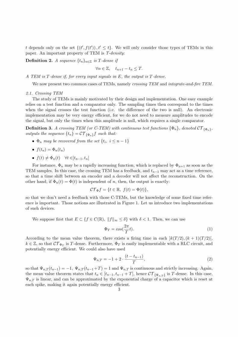
2.1. Crossing TEMThe study of TEMs is mainly motivated by their design and implementation. One easy example

relies on a test function and a comparator only. The sampling times then correspond to the timeswhen the signal crosses the test function (i.e. the difference of the two is null). An electronicimplementation may be very energy efficient, for we do not need to measure amplitudes to encodethe signal, but only the times when this amplitude is null, which requires a single comparator.

Definition 3. A crossing TEM (or C-TEM) with continuous test functions Φn, denoted CT Φn,outputs the sequence tn = CT Φnf such that:

• Φn may be recovered from the set ti, i ≤ n− 1

• f(tn) = Φn(tn)

• f(t) 6= Φn(t) ∀t ∈]tn−1, tn[

For instance, Φn may be a rapidly increasing function, which is replaced by Φn+1 as soon as theTEM samples. In this case, the crossing TEM has a feedback, and tn−1 may act as a time reference,so that a time shift between an encoder and a decoder will not affect the reconstruction. On theother hand, if Φn(t) = Φ(t) is independent of n, then, the output is exactly:

CT Φf = t ∈ R, f(t) = Φ(t),

so that we don’t need a feedback with those C-TEMs, but the knowledge of some fixed time refer-ence is important. Those notions are illustrated in Figure 1. Let us introduce two implementationsof such devices.

We suppose first that E ⊂ f ∈ C(R), ‖f‖∞ ≤ δ with δ < 1. Then, we can use

ΦT = cos(2π

Tt). (1)

According to the mean value theorem, there exists a firing time in each ]k(T/2), (k + 1)(T/2)[,k ∈ Z, so that CT ΦT

is T -dense. Furthermore, ΦT is easily implementable with a RLC circuit, andpotentially energy efficient. We could also have used

Ψn,T = −1 + 2 · (t− tn−1)

T, (2)

so that Ψn,T (tn−1) = −1, Ψn,T (tn−1 +T ) = 1 and Ψn,T is continuous and strictly increasing. Again,the mean value theorem states that tn ∈ [tn−1, tn−1 + T ], hence CT Ψn,T is T -dense. In this case,Ψn,T is linear, and can be approximated by the exponential charge of a capacitor which is reset ateach spike, making it again potentially energy efficient.

3

f(t)

Ψ(t)

Comparatorf(t) = Ψ(t) ? tn

0 2 4 6 8 10 12

1

0.8

0.6

0.4

0.2

0

0.2

0.4

0.6

0.8

1

f(t)

Ψ(t)tn

tn

(a) C-TEM without feedback

f(t)

Ψn(t)

Comparatorf(t) = Ψn(t) ? tn

0 2 4 6 8 10 12

1

0.8

0.6

0.4

0.2

0

0.2

0.4

0.6

0.8

1

f(t)

Ψn(t)

tn−1

tn

(b) C-TEM with feedback

Figure 1: Diagrams representing two types of Crossing Time Encoding Machine. The device (a)uses a cosine as a test function, and there is no feedback. The device (b) uses a uses linear testfunctions which are reset at each spike, it has a feedback.

2.2. Integrate-and-Fire TEMThe study of neurons leads to a different class of TEMs. It is shown that a neuron may be

well-represented by an integrate-and-fire TEM [12][16]:

Definition 4. An Integrate-and-Fire TEM (or IF-TEM) with test functions Φn, denoted IT Φn,outputs the sequence tn = IT Φn f such that:

• Φn may be recovered from the set ti, i ≤ n− 1

•∫ tntn−1

f(u)du = Φn(tn)

•∫ ttn−1

f(u)du 6= Φn(t) ∀t ∈]tn−1, tn[

Therefore, an IF-TEM is nothing but a C-TEM on the integrated signal: F (t) =∫ t−∞ f(u)du.

In addition to providing a suitable model for neurons, it may be interesting to study those TEMs

4

for integrated signals since they have nice properties, such as being continuous and differentiable.We will show in Section 4.3 that integrate-and-fire TEMs are adjoint to crossing TEMs.

3. Non-Uniform Sampling and Shift-Invariant Subspaces

Throughout this study, we will work within the context of shift-invariant subspaces. The purposeof this section is to review the tools related to this framework. The notion of reproducing kernelHilbert space will also be recalled, as sampling theory requires the samples to be well-defined. Allthose notions but Lemma 3.2 may be found in [1, 3, 4, 10, 11, 13, 14, 25].

3.1. Shift-Invariant SubspacesDefinition 5. A Shift-Invariant SubSpace (or SISS) generated by the real function λ(t) and of orderp is defined by

V p(λ) :=

f(t) =

∑k∈Z

ckλ(t− k), (ck)k∈Z ∈ lp(R)

.

We use the term shift-invariant, but only shifts over Z are considered in this definition. A specialcase is the space of band-limited functions B :=

f ∈ L2(R), Supp(f) ⊂ [−π, π]

= V 2(sincπ),

where sincπ(t) = sin(πt)/(πt), and f = Ff is the classic Fourier transform:

f(ω) =

∫ ∞−∞

f(t)e−iωtdt.

B is invariant under every shift. This result comes directly from the Shannon sampling theorem[26]. We will work mainly in the Hilbert space L2(R) (p = 2). We recall (see [11] or [25]) that

∀f, g ∈ V 2(λ), 〈f | g〉 =1

2π

∫ 2π

0c(ω)d(ω)Gλ(ω)2dω (3)

where c(ω) =∑ck exp(−ikω), d(ω) =

∑dk exp(−ikω), and the coefficients ck, dk are respectively

the one of f and g: f =∑

k∈Z ckλ(· − k) and g =∑

k∈Z dkλ(· − k). We have defined

Gλ(ω) :=

(∑k∈Z| λ(ω + 2kπ) |2

)1/2

.

We deduce from this that

Lemma 3.1. The norms ‖ · ‖L2 and ‖f‖l2 :=∑

k∈Z |ck|2 are equivalent if and only if

∃0 < A ≤ B <∞ such that 0 < A ≤ Gλ(ω) ≤ B <∞.

Those properties are also equivalent to the fact that λ(· − k)k∈Z is a frame of V 2(λ) (see [25,chap. 5]).

5

3.2. Reproducing Kernel Hilbert spaceIn order to calculate the crossings of a function from V 2(λ) with a test function, we would like

f(t) to be well-defined for each t ∈ R.

Definition 6. A Hilbert space H is called a reproducing kernel Hilbert space (or RKHS) if the linearoperators

Kx0 : H → Rf 7→ f(x0)

are continuous, for all x0 ∈ H.

In the case of V 2(λ), this condition is easily obtained whenever λ satisfies some weak conditions.For instance, Aldroubi, Feichtinger and Gröchenig proved that it is enough to have λ in the so-calledamalgam Wiener space W 1(C), i.e.(∑

k

ess supx∈[0,1]

|λ(x+ k)|

)<∞.

These authors have studied these spaces extensively in theory [13, 14] and in the non-uniformsampling framework [1, 3, 4]. We will not review this theory, and use the different condition that λsatisfies 0 < A ≤ Gλ ≤ B <∞ and is in the Sobolev space H1(R):

H1(R) :=f ∈ L2, ‖f‖H1 <∞

with ‖f‖2H1 = ‖f‖2L2 + ‖f ′‖2L2 =

1

2π

∫R

(1 + ω2)|f(ω)|2dω.

Lemma 3.2. If λ ∈ H1(R) satisfies 0 < A ≤ Gλ ≤ B < ∞, then V 2(λ) is a RKHS, and we haveV 2(λ) → L∞ ∩ C.

Proof. Let f =∑

k∈Z ckλ(· − k) be an element of V 2(λ). Let x0 ∈ [0, 1] (the extension to x0 ∈ R issimilar), then we have:

f(x0)2 =

(∑k∈Z

ckλ(x0 − k)

)2

≤

(∑k∈Z|ck|2

)·

(∑k∈Z|λ(x0 − k)|2

)(Cauchy-Schwarz)

The first term is ‖f‖2l2 , which is equivalent to ‖f‖2L2 according to Lemma (3.1). The secondone is bounded, as the following calculation shows. We recall that H1(R) → C(R) (injection ofSobolev), so that λ is continuous, and we can define yk = argmin[−k,−k+1] |λ|. Then, with the

6

Cauchy-Schwarz inequality, and the AM-GM inequality:

∑k∈Z|λ(x0 − k)|2 =

∑k∈Z

(λ(yk)

2 + 2

∫ x0−k

yk

λ(t)λ′(t)dt

)

≤∑k∈Z

λ(yk)2 + 2

∑k∈Z

(∫ x0−k

yk

λ(t)2dt

)1/2

·(∫ x0−k

yk

λ′(t)2dt

)1/2

≤∑k∈Z

(∫ −k+1

−kλ(yk)

2dt

)+∑k∈Z

(∫ x0−k

yk

λ(t)2dt

)+∑k∈Z

(∫ x0−k

yk

λ′(t)2dt

)

≤∑k∈Z

(∫ −k+1

−kλ(t)2dt

)+∑k∈Z

(∫ −k+1

−kλ(t)2dt

)+∑k∈Z

(∫ −k+1

−kλ′(t)2dt

)= 2‖λ‖2L2 + ‖λ′‖2L2 ≤ 2‖λ‖2H1 .

We have therefore proved that f(x0) ≤ c‖λ‖H1‖f‖L2 , hence V 2(λ) is a RKHS.To prove that f is continuous, we write again :

|f(x)− f(y)|2 ≤

(∑k∈Z|ck|2

)·

(∑k∈Z|λ(x− k)− λ(y − k)|2

)

≤ ‖f‖2l2 ·∑k∈Z

(∫ y−k

x−kλ′(t)dt

)2

≤ ‖f‖2l2 · |x− y| ·∑k∈Z

∫ y−k

x−kλ′(t)2dt

which converges to 0 whenever y → x, so that f is continuous.

Note that because f is continuous and bounded, if we normalize f ∈ V 2(λ) so that ‖f‖∞ = 1,it is possible to construct a T -dense C-TEM for any T > 0 (take for instance CT a cosωt with a > 1and ω = π/T ).

In this case, point-wise evaluations are continuous functionals in this space. Therefore, the Riesztheorem states that for all x ∈ R, there exists a function Kx ∈ V 2(λ) such that:

∀f ∈ V 2(λ), f(x) = 〈f | Kx〉.

K(y, x) = Kx(y) is called the reproducing kernel of the space. An expression of Kx is given by

Kx(t) =∑k∈Z

λ(x− k)λ(t− k) =∑k∈Z

λ(x− k)λ(t− k), (4)

where λ(· − k)k is the bi-orthogonal frame of the frame λ(· − k)k:

λ(t) := F−1

(λ(ω)

G2λ(ω)

)so that ˆ

λ(ω) =λ(ω)

G2λ(ω)

.

7

This fact can be easily proved using (3), so that we have the relations:

〈λ(· − k) | λ(· − l)〉 = δkl.

This bi-othogonal frame is useful to write explicitly the projector PV 2 on V 2(λ) (which is closedwhenever 0 < A ≤ Gλ ≤ B <∞):

∀f ∈ L2, (PV 2f)(t) = 〈f | Kt〉 =∑k∈Z〈f | λ(· − k)〉 λ(t− k), (5)

so that the kth coefficient of (PV 2f) in the λ(· − k) frame is 〈f | λ(· − k)〉.

4. Time Encoding Machine on Shift-Invariant Subspaces

After this review of non-uniform sampling on SISS, we are ready to analyze TEM in detail andgive a sufficient conditions for these machines to be invertible.

4.1. General analysisTime encoding machines provide an elegant way to encode amplitude information into the timing

domain. Indeed, from the output tnn∈Z of a known Crossing-TEM, we can reconstruct the testfunctions Φn, hence recover f(tn) = Φn(tn). Therefore, we can consider TEMs as a special methodof non-uniform sampling, where the locations of the samples depend on the input function. In orderto construct an approximation of the signal, we introduce the operator Vtn (denoted V ) definedas follows. Let

sn =tn−1 + tn

2

so that 1[sn,sn+1[ is the Voronoï region of tn. Then V f is defined by:

V f(t) =

∞∑n=∞

f(tn) · 1[sn,sn+1[(t). (6)

V f is a piecewise constant function: V f(t) = f(tn) for t ∈ [sn, sn+1[. The key fact is that, fora Crossing-TEM CT , we can compute V f from the output tn = CT f . Hence, if we can invertV , we can recover the signal f(t). This is the case whenever ‖Id − V ‖ < 1 on a well-definedspace. ‖f − V f‖L2 is an integral of the difference between a function f(t) and its approximationby a piece-wise linear function V f(t). According to the Riemann sums, we have the intuition that,provided that tn are dense enough, this difference should be small. The following calculations havebeen used by Gröchenig in [17], then by Lazar and Tóth in [23], or Chen, Han and Jia in [6, 8]. Wereview them for completeness. We have:

‖f − V f‖2L2 =

∫ ∞−∞|f(t)− V f(t)|2dt =

∑n∈Z

∫ sn+1

sn

|f(t)− f(tn)|2dt

=∑n∈Z

∫ tn

sn

|f(t)− f(tn)|2dt+∑n∈Z

∫ sn+1

tn

|f(t)− f(tn)|2dt. (7)

We then use Wirtinger’s inequality:8

Lemma 4.1 (Wirtinger’s inequality). Let f, f ′ ∈ L2(a, b) with f(a) = 0 or f(b) = 0, then:∫ b

af(u)2du ≤ 4

π2(a− b)2

∫ b

af ′(u)2du.

Proof. We calculate, for f ∈ L2(0, π/2) with f(0) = 0,∫ b

a(f ′(u)2 − f(u)2)du =

∫ π/2

0[f ′(u)− f(u) cot(u)]2du−

∫ π/2

0(f2(u) cot(u))′du︸ ︷︷ ︸

0

≥ 0,

and we obtain the general inequality with a change of variables.

We suppose now that f ′ ∈ L2, so that using Wirtinger’s inequality in (7) leads to

‖f − V f‖2L2 ≤∑n∈Z

4

π2(tn − sn)2

∫ tn

sn

|f ′(t)|2dt+4

π2(sn+1 − tn)2

∫ sn+1

tn

|f ′(t)|2dt. (8)

We can see that this error depends on the differences (tn − sn), or (tn+1 − tn). If we suppose that(tn+1 − tn) < T , so that (tn − sn) < T/2 and (sn+1 − tn) < T/2, equation (8) becomes:

‖f − V f‖2L2 ≤T 2

π2

∑n∈Z

∫ tn

sn

|f ′(t)|2dt+

∫ sn+1

tn

|f ′(t)|2dt ≤ T 2

π2‖f ′‖2L2 . (9)

Finally, if f ∈ V 2(λ), and λ′ ∈ L2, we can use a final inequality:

Lemma 4.2 (Chen, Han, Jia [8]). Let λ ∈ H1(R), then,

∀f ∈ V 2(λ), ‖f ′‖L2 ≤

(sup

ω∈[0,2π[

Gλ′(ω)

Gλ(ω)

)‖f‖L2 .

Proof. Let f(t) =∑

k ckλ(t− k), so that f ′(t) =∑

k ckλ′(t− k). We use the formula of the scalar

product in V 2(λ) described in (3): we can write c(ω) =∑

k ck · exp(−ikω), so that:

‖f‖2L2 =1

2π

∫ 2π

0|c(ω)|2 ·Gλ(ω)2dω.

In a similar way, we have:

‖f ′‖2L2 =1

2π

∫ 2π

0|c(ω)|2·Gλ′(ω)2dω ≤ 1

2π

∫ 2π

0|c(ω)|2·Gλ(ω)2·

(Gλ′(ω)

Gλ(ω)

)2

dω ≤

(sup

ω∈[0,2π[

Gλ′(ω)

Gλ(ω)

)2

‖f‖2L2 .

Plugging this into (9) leads to:

‖f − V f‖2L2 ≤T 2

π2‖f ′‖2 ≤ T 2

π2·

(sup

ω∈[0,2π[

Gλ′(ω)

Gλ(ω)

)2

· ‖f‖2L2 . (10)

We are now able to state our main theorem.9

4.2. Sufficient conditions for invertibility of TEMsWe define

E =λ ∈ H1(R), 0 < A ≤ Gλ(ω) ≤ B <∞ and Gλ′(ω) <∞

as a shorthand to have λ satisfy the condition of Lemma 3.2 so that V 2(λ) is a RKHS, with theextra condition:

supω

Gλ′(ω)

Gλ(ω)<∞.

In the following, we will denote P := PV 2 the projection on V 2(λ) as defined in (5).

Theorem 1. Let λ ∈ E andτ = π · inf

ω

Gλ(ω)

Gλ′(ω)> 0,

then, for all T < τ , every Crossing-TEM CT which is T -dense is invertible. Moreover, if tn =CT f , an iterative reconstruction is given by the sequence:

f1 = PV f0

fk+1 = f1 + (Id− PV )fk, (11)

where P is the orthogonal projector on V 2(λ) and V = Vtn is defined in (6). We have:

‖f − fk‖L2 ≤(Tτ

)k‖f‖L2 −−−→

k→00.

Proof. With the above notations, using (10), we have:

‖f − PV f‖L2 = ‖P (f − PV f)‖L2 = ‖f − V f‖L2 ≤T

τ‖f‖L2 , ∀f ∈ V 2(λ).

The operator (PV ) : V 2(λ) → V 2(λ) verifies ‖Id − PV ‖ ≤ T/τ < 1 whenever T < τ , hence isinvertible. We then show that f − fk = (Id− PV )kf by induction. We have indeed:

f−fk+1 = f−f1−(Id−PV )fk = (Id−PV )f−(Id−PV )fk = (Id−PV )(f−fk) = (Id−PV )k+1f,

so that ‖f − fk‖L2 ≤ (T/τ)‖f‖L2 . Finally, because f1, hence all the fk can be calculated from theoutput tn of the Crossing-TEM, this TEM is invertible.

In the case λ = sincπ for instance, we have λ = 1[−π,π[, so that Gλ = 1. Then, we haveλ′(ω) = ω1[−π,π[, hence (inf Gλ/Gλ′) = π. Our theorem states in this case that if T < 1, then aT -dense TEM on band-limited functions is invertible. We find the Nyquist bound, which is (almost)the optimal bound we could hope for, according to the Beurling-Landau theorem. The reader mayfind a complete study of the band-limited case in [5, 20] or in the very good book [31]. In thegeneral case, this bound is not optimal. Chen, Han and Jia discussed this bound in [6]. Chen, Itohand Shiki studied the case of wavelet subspaces in [9]. Aldroubi and Feichtinger have calculatedan optimal bound for cardinal spline spaces in [2], which is better than the one given with thistheorem. Gröchenig has also studied the case where λ ∈ H2(R) in [17], and derived another boundusing a different Wirtinger inequality. He also noticed that one can speed up the convergence

10

using piecewise linear functions instead of piecewise constant functions for the operator V (we geta convergence in O(βn) instead of O(αn), with β < α).

The operator (PV ) consists in calculating a piecewise constant function approximating f ∈V 2(λ) on tn, and projecting the result back on V 2(λ). This theorem states that the operator(PV ) is invertible whenever tn is dense enough. It links therefore density and invertibility ofTEMs, and provides an iterative method to reconstruct the signal with an exponential speed ofconvergence. We could also have calculated the inverse directly: let f ∈ V 2(λ) be represented bythe infinite column vector c = (. . . , ck, ck+1, . . .)

T of its coefficients: f(t) =∑

k ckλ(t− k), then

Lemma 4.3. Let M and A be infinite matrices over Z × Z with coefficients Mjk = λ(tj − k) andAki =

∫ si+1

siλ(u− k)du. If f(t) =

∑k ckλ(t− k) and g(t) = PV f =

∑k dkλ(t− k), then d = AMc.

Proof. We first have:f1(t) := (V f)(t) =

∑j∈Z

f(tj) · 1Vj (t)

and according to (5),

g(t) = (PV f)(t) = (Pf1)(t) =∑k∈Z

∑j∈Z

f(tj) · 〈1Vj | λ(· − k)〉λ(t− k).

We check that 〈1Vj | λ(· − k)〉 =∫ sj+1

sjλ(u− k)du = Akj and that f(tj) =

∑k ckλ(tj − k) = (Mc)j .

Altogether,dk =

∑j

f(tj) · 〈1Vj | λ(· − k)〉 =∑j

Akj(Mc)j

which can also be written d = AMc.

The question of whether we can recover a signal f from its samples f(tn) = 〈f | Kn〉 has aclassic answer in frame theory: we can do so whenever there exists 0 < A ≤ B < ∞ such that forall f ∈ V 2(λ), A‖f‖2L2 ≤

∑f(tn)2 ≤ B‖f‖L2 , i.e. Ktn is a frame. In particular, if there exists

0 < δ ≤ T such that δ ≤ tn+1− tn ≤ T , then this is the case (see [3]), and we can recover the signalin a stable way with:

f(t) =∑k∈Z

f(tn)Ktn(t)

where Ktn is the bi-orthogonal frame of Ktn. In our case, we are not using the fact that tn+1−tn ≥ δ, but the weaker form : limn→±∞ tn = ±∞. This may lead to an unstable reconstruction,but we can always deduce a stable one by erasing some extra data, according to this result. Insteadof deleting data, we have chosen the more elegant way of weighting the samples (see [17]). Indeed,we can show that:

A‖f‖2L2 ≤∑n∈Z

wnf(tn)2 = ‖V f‖2L2 ≤ B‖f‖2L2 with wn = sn+1 − sn.

11

4.3. Integrate-and-Fire TEM as the adjoint of crossing TEMWe show in this section that IF-TEMs may be seen as the quasi-adjoint case of C-TEMs.

Indeed, with an IF-TEM IT , we may now recover Φn(tn) =∫ tn+1

tnf(u)du from tnn∈Z = IT f .

We introduce the operator Z = Ztn defined by

(Zf)(t) :=∑n∈Z

∫ tn+1

tn

f(u)du ·Ksn+1(t).

We do not comment on the spaces on which Z acts, for we are mainly interested into the operator(PZ) which will have a meaning. Note for instance that P : L2 → V 2(λ) can be defined on a largerspace than L2, namely V 2(λ)′, the dual space of V 2(λ). Let also introduce the operator

(V ′f)(t) :=∑n∈Z

f(sn+1) · 1[tn,tn+1[(t).

Lemma 4.4. If tn is T-dense, with limn→±∞ tn = ±∞, then

• V ′ is well-defined and linear continuous as an operator from H1 to L2.

• If λ ∈ E, (PV ′) is an operator from V 2(λ) to V 2(λ), and we have:

∀f, g ∈ V 2(λ), 〈f | (PV ′)g〉 = 〈(PZ)f | g〉

Proof. Let f ∈ H1(R), then

‖V ′f‖2L2 =∑n∈Z

(tn+1 − tn)f(sn+1)2.

As in the proof of Lemma 3.2, we introduce yn+1 = min[tn,tn+1] |f |, so that

‖V ′f‖2L2 =∑n∈Z

(tn+1 − tn) ·

(f(yn+1)2 +

∫ sn+1

yn+1

2f(u)f ′(u)du

)

≤∑n∈Z

(tn+1 − tn)f(yn+1)2 + T∑n∈Z

(∫ tn+1

tn

f(u)2du+

∫ tn+1

tn

f ′(u)2du

)≤ (T + 1)‖f‖2L2 + T‖f ′‖2L2 ≤ (T + 1)‖f‖2H1 .

which proves the first point. We notice then that if λ ∈ E, then V 2(λ) ∈ H1, so that (PV ′) is acontinuous operator from V 2(λ) to itself. Finally, for f, g ∈ V 2(λ),

〈f | (PV ′)g〉 = 〈Pf | (PV ′)g〉 = 〈f | V ′g〉 =

∫f(u)

∑n

1[tn,tn+1[(u) 〈g | Ksn+1〉du

=∑n∈Z

∫ tn+1

tn

f(u)

∫ ∞−∞

g(t)Ksn+1(t)dt

=

∫ ∞−∞

g(t)(∑

n

∫ tn+1

tn

f(u)du ·Ksn+1(t))dt = 〈Zf | g〉 = 〈(PZ)f | g〉

12

The operator V ′ is very close to the operator V introduced previously: only the role of tn and snhas been permuted. But because the only important property of V used to prove the invertibilityof (PV ) is that sn+1− sn < T whenever tn+1− tn < T , and because of the tautology tn+1− tn < Twhenever tn+1 − tn < T , we can conclude as in Theorem 1:

Theorem 2. Let λ ∈ E andτ = π · inf

ω

Gλ(ω)

Gλ′(ω),

then, for all T < τ , every IF-TEM which is T -dense is invertible. Moreover, the reconstruction issimilar to the one of Theorem 1, using the operator Z instead of V .

Proof. Similar to Theorem 1. Notice that, restricted on V 2(λ), (Id− PZ)∗ = (Id− PV ′), so that‖Id− PZ‖V 2 = ‖Id− PV ′‖V 2 < 1, and the same reconstruction method works.

This duality has been noticed by Lazar and Tóth in [23] in the case of V 2(sincπ), and we haveextended it for all SISS using only properties from RKHS.

In the rest of the paper, we will only consider Crossing-TEM, due to this duality.

4.4. Fast algorithm for reconstructionWe now present an algorithm which does not need the knowledge of λ to work. Indeed, according

to Lemma 4.3, we have to calculate Aki =∫ sj+1

sjλ(u)du. But λ may have a large support, so

that those elements are computationally expensive to calculate. An alternative has been given byGröchenig in [18]. We recall that M is the matrix with elements Mik = λ(ti− k). We suppose thatthe output tn is T -dense, and we denote τ = π · inf(Gλ/Gλ′) as in Theorem 1.

Lemma 4.5 (Gröchenig [18]). Let D be the diagonal matrix with elements dii = wi = si+1− si, letM∗ be the adjoint of M , then U := (M∗DM) is an operator from V 2(λ) to itself, and for all µ ∈ R,

‖Id− µU‖V 2 ≤ max

1− µ(1− γ)2, µ(1 + γ)2 − 1

with γ =T

τ.

In particular, if T < τ , with the optimal choice µ = (1 + γ2)−1, we find

‖Id− µU‖V 2 ≤ β :=2γ

1 + γ2< 1.

Note that the speed of convergence is slower (we have a convergence in O(βn) instead of O(αn),and β > γ), but each iterative step is faster to calculate: the matrix A is no longer required; weonly need to compute the diagonal matrix D and M , which is inexpensive.

As we did before, we conclude that U is invertible, and it gives a reconstruction of the signalwith an iterative method. We have actually proved that M is left-invertible as soon as T < τ , anda left inverse of M may be M ‡ = U−1M∗D = (µM∗DM)−1µM∗D. Of course, we could have usedthe pseudo-inverse M † = (M∗M)−1M∗, but the inverse of (M∗M) is more difficult to calculate,and less stable with respect to numerical error. We also notice that we introduced the matrix D tocompensate an accumulation of tn.

13

5. Periodic case

As we have seen, TEMs allow to encode a large class of signals in real time, without loss ofinformation. However, the decoding cannot be executed in real time. We also have consideredinfinite length signals in our model, which is not practical from an algorithmic point of view. In thissection, we focus on the finite dimensional case. For instance, the signal may be in a shift-invariantsubspace and K-periodic, so that it can be described with a finite number of coefficients. The signalcould also be with finite support, but this case can be handled as a periodic case, which is why wewill focus on periodic signals. Studying the finite dimensional case will also allow us to estimatethe effects of noise.

5.1. Shift-invariant subspace and TEMs on L2K

We will work in the Hilbert space

L2K(R) := f,∀x ∈ R, f(x+K) = f(x),

∫ K

0f2(x)dx <∞

together with the scalar product

〈f | g〉 =1

K

∫ K

0f(x)g(x)dx.

The Fourier series theorem states that f ∈ L2K(R) may be written as

f(t) =∑n∈Z

fn · exp

(2iπn

Kt

), with fn =

¯f−n = 〈f(t) | exp

(2iπn

Kt

)〉.

We introduce, for λ ∈ L2K(R), the periodic shift-invariant subspace:

V 2K(λ) := f(t) =

K∑k=1

ckλ(t− k), ck ∈ R.

The space is now of finite dimension, hence it is always closed in L2K(R). The two norms ‖f‖l2 :=(∑K

k=1 |ck|2)1/2

, where f =∑K

k=1 ckλ(· − k), and ‖f‖L2K

are equivalent whenever the map

RK → V 2K(λ)

(ck) 7→∑K

k=1 ckλ(t− k)

is injective.Because we would like to recover the signal working only on [−K/2,K/2], we suppose that

TEMs samples only within this interval. The output is therefore tnn=1..J = T f , where −K/2 ≤t1 < t2 < · · · < tJ < K/2. We introduce tJ+1 := t1 + K, and we modify slightly the definition ofT -density, to handle periodicity:

Definition 7. An increasing sequence t1, t2, · · · , tJ is T -dense if

tn+1 − tn ≤ T, ∀n = 1..J.

With this definition, all the previous results hold: a TEM on V 2K(λ) is invertible if it is T -dense

on [−K/2,K/2], and we can recover the signal using iterative algorithms. We are now interestedin a more convenient way to recover our signal. If λ satisfies some additional properties, then thisreconstruction may be done in a more efficient way.

14

5.2. λ with finite supportThis method was introduced by Gröchenig and Schwab in [19]. We suppose that the restriction

of λ over [−K/2,K/2] has support of size S, and that S << K. Without loss of generality, wecan suppose Supp(λ) ⊂ [−S/2, S/2]. We can think of polynomial splines for instance, since theyhave a small support. Let J be the number of samples taken by our C-TEM inside [−K/2,K/2],and let M be the matrix of size J × K with elements Mjk = λ(tj − k). Let f be the columnvector of size J with elements f(tj), and c = (c1, · · · cn)T the vector representing our input signal:f(t) =

∑Kk=1 ckλ(t− k). Then:

f = Mc

and we can recover c if and only if M is left invertible. According to Lemma 4.5, this is the case iftn is dense enough, and a left inverse may be calculated by:

M ‡ = (µMTDM)−1µMTD.

The positive definite matrix U := MTDM of size K ×K has elements:

Ukl =

J∑j=1

wjλ(tj − k)λ(tj − l). (12)

Lemma 5.1. A necessary condition to have λ(tj−k)λ(tj− l) 6= 0 is to have |tj−k| mod K ≤ S/2and |tj − l| mod K ≤ S/2. In particular, if |k − l| mod K > S, then Ukl = 0.

Proof. This follows from the fact that the support of λ is included in ([−S/2, S/2] +KZ), and fromthe triangular inequality |k − l| ≤ |k − tj |+ |tj − l|.

Therefore, most of the coefficients of the matrix U are zero: U is zero except on a large diagonalof size S, plus on its corners. Notice that if we work with finite support signals and not withperiodic ones, then this property holds, without the modulo K. In this case, U has just a large nonnull diagonal. In both cases, the matrix U is invertible with a fast algorithm in O(S2), using theCholeski decomposition for sparse matrices.

6. Robustness to noise

With physical devices, time locations of the samples can only be recorded with finite precision,so that the effective recorded time t′n is different from the real time tn. This may result fromquantization error for instance. The purpose of this section is to show that time encoding machinesare robust under this type of error. Note that we do not suppose the signal to be noisy, but onlythe locations of the samples.

6.1. Some generalities about bounded errorsWe will study the error in the case of periodic signals. We suppose therefore that λ isK-periodic.

We recall the study so far in this finite case:

Lemma 6.1. There exists τ such that, for all T < τ , for all t = (t1, · · · , tJ) which is T -dense, thematrix M(t) with elements M(t)jk = λ(tj − k) of size J ×K is left invertible.

15

We will denote in the following

N(t) = (M(t)TM(t))−1M(t)T

to be the pseudo-inverse of M(t). In this case, the reconstruction is given by:

c = N(t)Φ(t)

where Φ(t) = (Φ1(t1), · · ·ΦJ(tJ)) = (f(t1), · · · , f(tJ)) for a Crossing-TEM. Because of the noise, wewould have access to t′ = (t′1, · · · t′J), and thus to some M(t′) and some Φ′(t′). The reconstructionfrom the noisy data is:

c’ = N(t′)Φ′(t′).

Several problems may occur. The fact that the functions Φn may depend on the past is notwell suited for our study, for we do not have a model to describe the effect of the noise on thosefunctions. Therefore, we will study the case Φn = Φ, or Φ′(t′) = Φ(t′). Then, if we want M(t′) tobe left invertible, we should ensure that t′ is T ′-dense with T ′ < τ . In particular, we cannot use anunbounded model for the noise in the timing domain. We introduce the infinite norm of t − t′ tobe:

‖t− t′‖∞ := supn=1..J

(|tn − t′n|),

and for ε > 0, we denote the closed ball of center t and radius ε by

B(t, ε) :=t′ = (t′1, · · · , t′J), ‖t− t′‖∞ ≤ ε

.

Lemma 6.2. Let T < T ′ < τ . If t = (t1, · · · tJ) is T -dense, with T < τ , then, for all t′ ∈ B(t, ε0)where ε0 = (T ′ − T )/2, t′ is T ′-dense. In particular, M(t′) is invertible for all t′ ∈ B(t, ε0).

Proof. We use the triangular inequality:

t′n+1 − tn ≤ |t′n+1 − tn+1|+ |tn+1 − tn|+ |tn − t′n| ≤ ε0 + T + ε0 ≤ T ′.

If J is too big, then the size of the matrices may explode. However, we may always suppose thisnumber to be bounded by a constant:

Lemma 6.3. Let t = (t1, · · · tJ) be T -dense. Then there exists J ′ < 2dK/T e and a sequence(i1, · · · iJ ′) such that t = (ti1 , · · · ti′J ) is still T -dense. In particular, M (t) is a submatrix of M(t) ofsize J ′ ×K which is left invertible.

Proof. With the notation tJ+1 = t1 +K, we construct in by induction:

i1 = 1in+1 = maxj ∈ [1 · · · J + 1], |tj − ti1 | ≤ T

.

This sequence is constant from a certain rank J ′+1, and we have tiJ′+1= tJ+1 = ti1 +K. Moreover,

with this definition, we always have tin+2 − tin ≥ T . Finally, we write:

K = tiJ′+1− ti1 = (tiJ′+1

− ti(2bJ′/2c+1)) + (ti(2bJ′/2c+1)

− ti(2bJ′/2c−1)) + · · ·+ (ti3 − ti1) > bJ ′/2c · T.

Therefore, (K/T ) > bJ ′/2c, dK/T e > J ′/2 and J ′ < 2dK/T e.16

Because M (t) is left invertible, of size J ′ × K, we can use it to reconstruct the signal: c’ =N (t)Φ(t). Thus, we can always suppose the number of lines of M to be less than 2dK/2e withoutloss of generality. Note that because M is full column rank, there exists K lines such that theK × K resulting sub-matrix is invertible. We could have concluded that this sub-matrix is stillinvertible whenever t is taken in a small neighborhood, for the set of invertible matrices is an openset. However, we do not have any expression of this neighborhood. This is why we have chosento take more lines, to guarantee T -density, and therefore left-invertibility on a large neighborhood,according to Lemma 6.2.

6.2. Robustness under bounded noise in the timing domainIn sampling theory for band-limited signals, the error introduced by quantization in the am-

plitude domain leads to an error MSE(X ′, X) = O(ε2), where X ′ is the reconstruction from thenoisy data, X is the original data, and MSE stands for the Mean Square Error: MSE(X ′, X) =‖X ′−X‖2l2 . Thao and Vetterli have shown in [28] that we also have MSE(X ′, X) = O(r−2) wherer denotes the oversampling rate. This theorem has been extended by Chen, Han and Jia in [7, 8]for non-uniform sampling in shift-invariant subspaces. Using the mean value theorem, these articlesuse the fact that having oversampling is equivalent to having infinite precision of the amplitude ofsome f(tn), where the locations tn are not known precisely (but are more and more precise withthe oversampling factor). Here, we are working in the framework of TEMs in a finite dimensionalspace. In this case, we also have MSE(X ′, X) = O(ε2). The calculations are similar to the ones in[28].

Theorem 3. Let λ be of class C1 and K-periodic. Let CT Φ be a C-TEM on V 2K(λ) without feedback

which is T -dense, with T < τ = π inf(Gλ/Gλ′). Let T ′ such that T < T ′ < τ and ε0 = (T ′ − T )/2.Then, there exists a constant α which depends only on λ,Φ,K and T ′ such that, for all outputt = (t1, · · · tJ) of CT Φ, for all t′ = (t′1, · · · t′J) ∈ B(t, ε0), we have:

‖N(t′)Φ(t′)−N(t)Φ(t)‖l2 ≤ α‖t′ − t‖∞.

Proof. According to Lemma 6.3, we can always suppose J = J0 = 2dK/T e. We introduce ε =‖t′ − t‖∞ < ε0. Let Sδ := t = (t1, · · · tJ0), t is increasing, t is δ-dense. According to Lemma 6.2,

ST +B(0, ε0) ⊂ ST ′

and ST ′ is compact (it is closed and bounded in RJ0). Lemma 6.2 ensures that N(t) is well-definedin ST +B(0, ε0), and its expression is:

N(t) = (M(t)TM(t))−1M(t)T .

In particular, the coefficients of N(t) are continuous with respect to the coefficients ofM(t). There-fore, if λ is of class C1, so are the coefficients ofN(t). Actually, if we denote byNkj(t) the coefficientsof N(t), and F ikj(t) = ∂

∂tiNkj(t) the coefficients of F i(t) = ∂

∂tiN(t), then all those functions are

continuous on the compact ST ′ . Thus, we can find a constant α1 such that:

∀t ∈ ST ′ , |Nkj(t)| ≤ α1 and |F ikj(t)| ≤ α1.

17

For a matrix A = (Aij) of size K × J0, and for b ∈ RJ0 , using the Cauchy-Schwartz inequality, wehave:

‖Ab‖2l2 =

K∑i=1

( J0∑j=1

Aijbj

)2≤

K∑i=1

( J0∑j=1

A2ij

)·( J0∑j=1

b2j

)≤ K · J2

0 · (maxA2ij) · (max b2j ). (13)

We also have the Taylor inequality:

|Φ(t′i)− Φ(ti)| ≤ |t′i − ti| · supt∈(ti,t′i)

Φ′(t) ≤ ε‖Φ′‖∞ (14)

and

|Nik(t′)−Nij(t)| ≤

J0∑j=1

|t′j − tj | · supt∈(tj ,t′j)

|F jik(t)| ≤ α1J0ε. (15)

We now write

‖N(t′)Φ(t′)−N(t)Φ(t)‖l2 ≤ ‖N(t′)(Φ(t′)− Φ(t)

)‖l2 + ‖

(N(t′)−N(t)

)Φ(t)‖l2 .

Using inequalities (13) and (14), the first term is bounded above by:

‖N(t′)(Φ(t′)− Φ(t)

)‖2l2 ≤ KJ

20 ·maxNij(t)2 ·max (Φ(t′i)− Φ(ti))

2 ≤ (KJ20α

21‖Φ′‖2∞)ε2.

The second term is bounded in the same way with (13) and (15):

‖(N(t′)−N(t)

)Φ(t)‖2l2 ≤ KJ

20 ·max(Nij(t

′)−Nij(t))2 ·max Φ(ti)2 ≤ (KJ4

0α21‖Φ‖2∞)ε2.

Altogether, we proved that

‖N(t′)Φ(t′)−N(t)Φ(t)‖l2 ≤ α · ε with α :=√KJ0α1

√‖Φ′‖2∞ + J2

0‖Φ‖2∞.

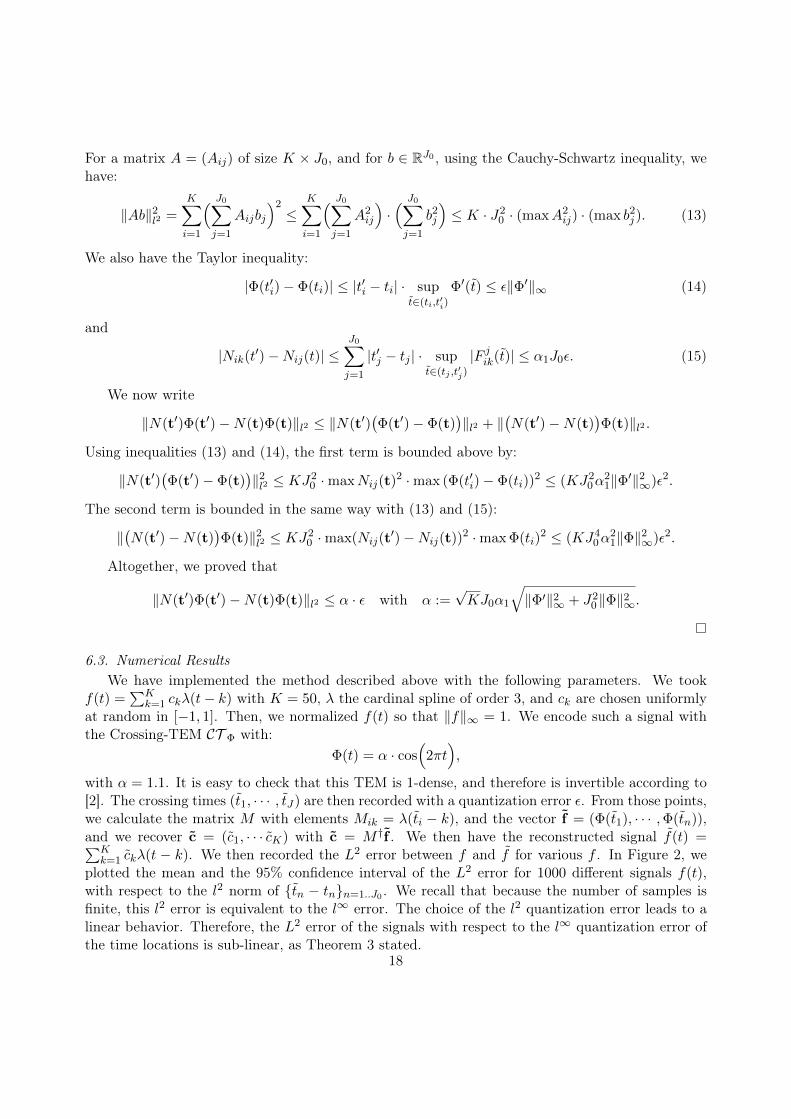
6.3. Numerical ResultsWe have implemented the method described above with the following parameters. We took

f(t) =∑K

k=1 ckλ(t− k) with K = 50, λ the cardinal spline of order 3, and ck are chosen uniformlyat random in [−1, 1]. Then, we normalized f(t) so that ‖f‖∞ = 1. We encode such a signal withthe Crossing-TEM CT Φ with:

Φ(t) = α · cos(

2πt),

with α = 1.1. It is easy to check that this TEM is 1-dense, and therefore is invertible according to[2]. The crossing times (t1, · · · , tJ) are then recorded with a quantization error ε. From those points,we calculate the matrix M with elements Mik = λ(ti − k), and the vector f = (Φ(t1), · · · ,Φ(tn)),and we recover c = (c1, · · · cK) with c = M †f . We then have the reconstructed signal f(t) =∑K

k=1 ckλ(t − k). We then recorded the L2 error between f and f for various f . In Figure 2, weplotted the mean and the 95% confidence interval of the L2 error for 1000 different signals f(t),with respect to the l2 norm of tn − tnn=1..J0 . We recall that because the number of samples isfinite, this l2 error is equivalent to the l∞ error. The choice of the l2 quantization error leads to alinear behavior. Therefore, the L2 error of the signals with respect to the l∞ quantization error ofthe time locations is sub-linear, as Theorem 3 stated.

18

mean error

95% confidence interval

‖tn − tn‖l2

‖f − f‖L2

Figure 2: The L2 error of the signal versus the l2 quantization error of the time locations.

7. Future Work

The tools we used to prove the invertibility of dense C-TEMs are the following facts: V 2(λ) is aRKHS, there exists an orthogonal projection onto this space, we can use Wirtinger’s inequality onthis space, and finally, there is an inequality of the form:

∀f ∈ V 2(λ), ‖f ′‖L2 ≤ C‖f‖L2

saying that the map:D : V 2(λ) ⊂ H1 → L2

f 7→ f ′

is continuous. Therefore, similar results may be derived on a space F where those requirements aresatisfied. We have the general

Theorem 4. If F is a closed subspace of H1 such that the norms ‖.‖H1 and ‖.‖L2 are equivalenton F , i.e. there exists a constant C such that:

∀f ∈ F, ‖f ′‖L2 ≤ C · ‖f‖L2 ,

then, every C-TEM (and IF-TEM) which is T -dense, with T < τ := π/C, is invertible.19

Proof. Because F ⊂ H1 ⊂ L2 is closed, we already have the existence of an orthogonal projectoron F . We can use the Wirtinger’s inequality for F ∈ L2. Finally, F is a RKHS because H1 is aRKHS for its norm (with kernel Kt(u) = e−|t−u|/2), and because the H1 norm and L2 norm areequivalent on F . Finally, the exact same proof of Theorem 1 and Theorem 2 can be derived, whichgives the result.

Therefore, our result about TEMs on SISS can probably be extended in this direction. However,while it is easy to show that V 2(λ) satisfies the conditions of Theorem 4, it may be more difficultto extend it to some other cases. Moreover, the case of SISS allowed us to deduce the algorithmsfor this case.

Another direction to look at for future work is the behavior of the error. While we showed thatthe error is sub-linear in the l∞ quantization error, we noticed that this error appears to be actuallylinear in the l2 quantization error. We could not prove this fact, nor could we give an explicit boundof the decay of the error.

A final direction, and probably the most difficult one is the following remark. If λ has finitesupport [0, S], then all the elements of the matrix M are zero, except on a large diagonal, andthe matrix M is left-invertible. Suppose that the TEM has sampled J times during the interval[k1, k2], then the value of the function on this interval depends on K = k2 − k1 + S coefficients.In particular, if the TEM has density T < 1, and if the interval is large enough, we can ensurethat J ≥ K, so that there are more equations than coefficients involved. But we cannot concludethat the sub-matrix involving those equations and coefficients is still left-invertible. Aldroubi andGröchenig showed that it is the case for cardinal splines SISS, because of the very special structureof those functions [2]. This would allow us to reconstruct the signal independently of the past, andtherefore provides us better algorithms for reconstruction, or bounds for the error.

References

[1] A. Aldroubi and H.G. Feichtinger. Exact iterative reconstruction algorithm for multivariate irregularly sampledfunctions in spline-like spaces: the Lp-theory. Proc. Amer. Math. Soc., 126(9):2677–2686, 1998.

[2] A. Aldroubi and K. Gröchenig. Beurling-Landau-type theorems for non-uniform sampling in shift invariantspline spaces, 1999.

[3] A. Aldroubi and K. Gröchenig. Nonuniform sampling and reconstruction in shift-invariant spaces. SIAM Review,43, 2001.

[4] A. Aldroubi and K. Gröchenig. Non-uniform weighted average sampling and exact reconstruction in shift-invariant and wavelet spaces. Applied Computer Harmonic Analysis, 13:151–161, 2002.

[5] F.J. Beutler. Error-free recovery of signals from irregularly spaced samples. SIAM Review, 8(3):328–335, July1966.

[6] W. Chen, B. Han, and R.Q. Jia. Maximal gap of a sampling set for the iterative reconstruction algorithm inshift invariant spaces. IEEE Signal Processing Letters, 11(8):655–658, 2004.

[7] W. Chen, B. Han, and R.Q. Jia. Estimate of aliasing error for non-smooth signal prefiltered by quasi-projectioninto shift invariant spaces. IEEE Transactions on Signal Processing, 53(5):1927–1933, 2005.

[8] W. Chen, B. Han, and R.Q. Jia. On simple oversampled A/D conversion in shift invariant spaces. IEEETransactions on Information Theory, 51(2):648–657, 2005.

[9] W. Chen, S. Itoh, and J. Shiki. Irregular sampling theorems for wavelet subspaces. IEEE Transaction onInformation Theory, 44(3):1131–1142, 1998.

[10] W. Chen, S. Itoh, and J. Shiki. On sampling in shift invariant spaces. IEEE Transactions on InformationTheory, 48(10):2802–2810, 2002.

[11] I. Daubechies. Ten Lectures on Wavelets. CBMS-NSF Reg. Conf. Series in Applied Math. SIAM, 1992.

20

[12] P. Dayan and L.F. Abbott. Theoretical Neuroscience: Computational and Mathematical Modeling of NeuralSystems. The MIT Press, 2001.

[13] H.G. Feichtinger. Generalized amalgams, with applications to Fourier transform. Canad. J. Math., 42(3):395–409, 1990.

[14] H.G. Feichtinger. Wiener amalgams over Euclidean spaces and some of their applications. In Function spaces(Edwardsville, IL, 1990), volume 136 of Lecture Notes in Pure and Appl. Math., pages 123–137. Dekker, NewYork, 1992.

[15] H.G. Feichtinger, K. Gröchenig, and T. Strohmer. Efficient numerical methods in non-uniform sampling theory,1995.

[16] W. Gerstner and W. Kistler. Spiking Neuron Models: Single Neurons, Populations, Plasticity. CambridgeUniversity Press, 2002.

[17] K. Gröchenig. Reconstruction algorithms in irregular sampling. Mathematics of Computation, 59:181–181, 1992.[18] K. Gröchenig. A discrete theory of irregular sampling. Linear Algebra and Its Applications, 193:129–150, 1993.[19] K. Gröchenig and H. Schwab. Fast local reconstruction methods for nonuniform sampling in shift invariant

spaces. SIAM Journal on Matrix Analysis and Applications, 2002:24–899, 2003.[20] H.J. Landau. Necessary density conditions for sampling and interpolation of certain entire functions. Acta

Mathematica, 117:37–52, 1967.[21] A.A. Lazar. Time encoding with an integrate-and-fire neuron with a refractory period. Neurocomputing, 58-

60:53–58, June 2004.[22] A.A. Lazar. Time encoding machines with multiplicative coupling, feedforward and feedback. IEEE Transactions

on Circuits and Systems-II: Express Briefs, 53(8):672–676, August 2006.[23] A.A. Lazar and L.T. Tóth. Perfect recovery and sensitivity analysis of time encoded bandlimited signals. IEEE

Transactions on Circuits and Systems-I: Regular Papers, 51(10):2060–2073, October 2004.[24] B.D. Logan. Information in the zero crossings of bandpass signals. The Bell System Technical Journal, 56:487–

510, 1977.[25] S. Mallat. A Wavelet Tour of Signal Processing, Third Edition: The Sparse Way. Academic Press, 3rd edition,

2008.[26] C.E. Shannon. Communication in the Presence of Noise. Proceedings of the IRE, 37(1):10–21, January 1949.[27] R. Steele. Delta Modulation Systems. Wiley New York„ 1975.[28] N.T. Thao and M. Vetterli. Reduction of the MSE in R-times oversampled A/D conversion O(1/R) to O(1/R2).

IEEE Transactions on Signal Processing, 42:200–203, 1994.[29] M. Unser. Sampling-50 years after Shannon. Proceedings of the IEEE, pages 569–587, 2000.[30] M. Vetterli, P. Marziliano, and T. Blu. Sampling signals with finite rate of innovation. IEEE Transactions on

Signal Processing, 50:1417–1428, 2002.[31] B. Young. An Introduction to Nonharmonic Fourier Series. Academic Press, New York :, 1980.

21