sample-Solution Manual Basic Business Statistics Concepts ...
113
INSTRUCTOR’S SOLUTIONS MANUAL GAIL ILLICH PAUL ILLICH McLennan Community College Southeast Community College B ASIC B USINESS S TATISTICS : C ONCEPTS AND A PPLICATIONS FOURTEENTH EDITION Mark L. Berenson Montclair State University David M. Levine Baruch College, City University of New York Kathryn A. Szabat La Salle University David F. Stephan Two Bridges Instructional Technology
-
Upload
khangminh22 -
Category
Documents
-
view
0 -
download
0
Transcript of sample-Solution Manual Basic Business Statistics Concepts ...
INSTRUCTOR’S SOLUTIONS MANUAL
GAIL ILLICH PAUL ILLICH McLennan Community College Southeast Community College
BASIC BUSINESS STATISTICS: CONCEPTS AND APPLICATIONS
FOURTEENTH EDITION
Mark L. Berenson Montclair State University
David M. Levine Baruch College, City University of New York
Kathryn A. Szabat La Salle University
David F. Stephan Two Bridges Instructional Technology

The author and publisher of this book have used their best efforts in preparing this book. These efforts include the development, research, and testing of the theories and programs to determine their effectiveness. The author and publisher make no warranty of any kind, expressed or implied, with regard to these programs or the documentation contained in this book. The author and publisher shall not be liable in any event for incidental or consequential damages in connection with, or arising out of, the furnishing, performance, or use of these programs. Reproduced by Pearson from electronic files supplied by the author. Copyright © 2019, 2015, 2010 by Pearson Education, Inc. 221 River Street, Hoboken, NJ 07030. All rights reserved. No part of this publication may be reproduced, stored in a retrieval system, or transmitted, in any form or by any means, electronic, mechanical, photocopying, recording, or otherwise, without the prior written permission of the publisher. Printed in the United States of America.
ISBN-13: 978-0-13-468501-4 ISBN-10: 0-13-468501-6

Copyright ©2019 Pearson Education, Inc.
Table of Contents
Teaching Tips...................................................................................................................................1 Chapter 1 Defining and Collecting Data ............................................................................................... 39 Chapter 2 Organizing and Visualizing Variables ................................................................................. 47 Chapter 3 Numerical Descriptive Measures ....................................................................................... 151 Chapter 4 Basic Probability ................................................................................................................ 195 Chapter 5 Discrete Probability Distributions ...................................................................................... 205 Chapter 6 The Normal Distribution and Other Continuous Distributions .......................................... 235 Chapter 7 Sampling Distributions....................................................................................................... 267 Chapter 8 Confidence Interval Estimation .......................................................................................... 293 Chapter 9 Fundamentals of Hypothesis Testing: One-Sample Tests .................................................. 331 Chapter 10 Two-Sample Tests ............................................................................................................. 373 Chapter 11 Analysis of Variance .......................................................................................................... 433 Chapter 12 Chi-Square and Nonparametric Tests ................................................................................ 459 Chapter 13 Simple Linear Regression .................................................................................................. 487 Chapter 14 Introduction to Multiple Regression .................................................................................. 535 Chapter 15 Multiple Regression Model Building ................................................................................. 585 Chapter 16 Time-Series Forecasting ..................................................................................................... 645 Chapter 17 Business Analytics ............................................................................................................. 715 Chapter 18 A Roadmap for Analyzing Data ......................................................................................... 743 Chapter 19 Statistical Applications in Quality Management (Online) ................................................. 807 Chapter 20 Decision Making (Online) .................................................................................................. 837
Online Sections ......................................................................................................................................... 877 Instructional Tips and Solutions for Digital Cases ................................................................................... 907 The Brynne Packaging Case ..................................................................................................................... 943

Copyright ©2019 Pearson Education, Inc.
The CardioGood Fitness Case .................................................................................................................. 945 The Choice Is Yours/More Descriptive Choices Follow-up Case .......................................................... 1057 The Clear Mountain State Student Surveys Case .................................................................................... 1153 The Craybill Instrumentation Company Case ........................................................................................ 1325 The Managing Ashland MultiComm Services Case ................................................................................ 1327 The Mountain States Potato Company Case ........................................................................................... 1375 The Sure Value Convenience Stores Case .............................................................................................. 1383

Copyright ©2019 Pearson Education, Inc. 1
Teaching Tips
Our Starting Point
Of late, business statistics has been expanding and combining with other disciplines to form new fields of
study such as business analytics. Because of these changes, business statistics has become an increasingly
important part of business education. One must consistently reflect on which business statistics topics
should get taught and how those topics should be taught.
As authors, we seek ways to continuously improve the teaching of business statistics have always
guided our efforts. We are members of the Decision Sciences Institute (DSI) and American Statistical
Association (ASA) and attend their annual conferences. We are members of the DSI Data, Analytics and
Statistics Instruction (DASI) Special Interest Group and are frequent presenters at DASI sessions held at
annual and regional DSI meetings. We use the ASA’s Guidelines for Assessment and Instruction
(GAISE) reports and combine them with our experiences teaching business statistics to a diverse student
body at several large universities.
What to teach and how to teach it are particularly significant questions to ask during a time of
change. As an author team, we bring a unique collection of experiences that we believe helps us find the
proper perspective in balancing the old and the new. Mark Berenson and David Levine were the first
educators to create a business statistics textbook that discussed using statistical software and that used
computer output as illustrations. They introduced many additional teaching and curricular innovations in
their careers, and with David Stephan developed the first comprehensive introductory business statistics
textbook that featured Microsoft Excel.
Kathryn Szabat has provided statistical advice to various business and non-business communities.
Her extensive background in statistics and operations research and her experiences interacting with
professionals in practice guided her to develop and chair a new, interdisciplinary Business Systems and
Analytics department, in response to the technology- and data-driven changes occurring in business
today. David Stephan, an information system specialist, devised new courses and teaching methods for
computer information systems, creating and teaching in one of the first personal computer classrooms in a
large school of business. He became involved in early digital media efforts to improve education and
lectured about the importance of data in a digital media, which led him to join Berenson’s and Levine’s
efforts to improve statistics education and simplify interactions with statistical programs. Our work also
benefits from teaching and research interests and the diversity of interests and generous contributions of
our past co-author, Timothy Krehbiel.

2 Teaching Tips
Copyright ©2019 Pearson Education, Inc.
Five Guiding Principles
When writing for introductory business statistics students, five principles guide us.
1. Help students see the relevance of statistics to their own careers by providing examples drawn from the functional areas in which they may be specializing. Students need a frame of reference
when learning statistics, especially when statistics is not their major. That frame of reference for
business students should be the functional areas of business, such as accounting, finance, information
systems, management, and marketing. Each statistics topic needs to be presented in an applied context
related to at least one of these functional areas. The focus in teaching each topic should be on its
application in business, the interpretation of results, the evaluation of the assumptions, and the
discussion of what should be done if the assumptions are violated.
2. Emphasize interpretation of statistical results over mathematical computation. Introductory
business statistics courses should recognize the growing need to interpret statistical results that
computerized processes create. This makes the interpretation of results more important than knowing
how to execute the tedious hand calculations required to produce them.
3. Give students ample practice in understanding how to apply statistics to business. Both
classroom examples and homework exercises should involve actual or realistic data as much as
possible. Students should work with data sets, both small and large, and be encouraged to look
beyond the statistical analysis of data to the interpretation of results in a managerial context.
4. Familiarize students with how to use statistical software to assist business decision-making.
Introductory business statistics courses should recognize that programs with statistical functions are
commonly found on a business decision maker’s desktop computer. Integrating statistical software
into all aspects of an introductory statistics course enables the course to focus on interpretation of
results instead of computations (see second point).
5. Provide clear instructions to students for using statistical applications. Books should explain
clearly how to use programs such as Microsoft Excel, JMP, and Minitab with the study of statistics,
without having those instructions dominate the book or distract from the learning of statistical
concepts.

Teaching Tips 3
Copyright ©2019 Pearson Education, Inc.
First Things First Chapter
In a time of change, you can never know exactly what knowledge and background students bring into an
introductory business statistics classroom. Add that to the need to curb the fear factor about learning
statistics that so many students begin with, and there’s a lot to cover even before you teach your first
statistical concept.
We created “First Things First” to meet this challenge. This unit sets the context for explaining
what statistics is (not what students may think!) while ensuring that all students share an understanding of
the forces that make learning business statistics critically important today. Especially designed for
instructors teaching with course management tools, including those teaching hybrid or online courses,
“First Things First” has been developed to be posted online or otherwise distributed before the first class
meets.
We would argue that the most important class is the first class. First impressions are critically
important. You have the opportunity to set the tone to create a new impression that the course will be
important to the business education of your students. Make the following points:
This course is not a math course.
State that you will be learning analytical skills for making business decisions.
Explain that the focus will be on how statistics can be used in the functional areas of business.
This book uses a systematic approach for meeting a business objective or solving a business problem.
This approach goes across all the topics in the book and most importantly can be used as a framework in
real world situations when students graduate. The approach has the acronym DCOVA, which stands for
Define, Collect, Organize, Visualize, and Analyze.
Define the business objective or problem to be solved and then define the variables to be studied.
Collect the data from appropriate sources
Organize the data
Visualize the data by developing charts
Analyze the data by using statistical methods to reach conclusions.
You can begin by emphasizing the importance of defining your objective or problem. Then, discuss the
importance of operational definitions of variables to be considered and define variable, data, and
statistics.
Just as computers are used not just in the computer course, students need to know that statistics is
used not just in the statistics course. This leads you to a discussion of business analytics in which data is
used to make decisions. Make the point that analytics should be part of the competitive strategy of every

4 Teaching Tips
Copyright ©2019 Pearson Education, Inc.
organization especially when “big data”, meaning data collected in huge volumes at very fast rates, needs
to be analyzed.
1. Inform the students that there is an Excel Guide, a JMP Guide, and a Minitab Guide at the end of
each chapter.
2. Strongly encourage or require students to read the guide for the software they will be using as
preparation for using that software with this book.

Teaching Tips 5
Copyright ©2019 Pearson Education, Inc.
Chapter 1 You need to continue the discussion of the Define task by establishing the types of variables. Mention the
importance of having an operational definition for each variable. Be sure to discuss the different types
carefully because the ability to distinguish between categorical and numerical data will be crucial later in
the course. Go over examples of each type of variable and have students provide examples of each type.
Then, if you wish, you can cover the different measurement scales.
Then move on to the C of the DCOVA approach, collecting data. Mention the different sources of
data and make sure to cover the fact that data often needs to be cleaned of errors. Then, you could spend
some time discussing sampling, even if it is just using the table of random numbers to select a random
sample. You may want to take a bit more time and discuss the types of survey sampling methods and
issues involved with survey sampling results. The Think About This essay discusses the important issue of
the use of Web-based surveys.
There is also a section on Data Cleaning that discusses the issues that occur in data collection.
This is followed by a section on data formatting that includes the important concepts of stacking and
unstacking variables and recoding variables. The last section discusses the types of errors that occur in
surveys.
The chapter also introduces three continuing cases related to the Managing Ashland MultiComm
Services, CardioGood Fitness, and Clear Mountain State Student Surveys that appear at the end of many
chapters. The Digital Cases are introduced in this chapter also. In these cases, students visit Web sites
related to companies and issues raised in the Using Statistics scenarios that start each chapter. The goal of
the Digital Cases is for students to develop skills needed to identify misuses of statistical information. As
would be the situation with many real-world cases, in Digital Cases, students often need to sift through
claims and assorted information in order to discover the data most relevant to a case task. They will then
have to examine whether the conclusions and claims are supported by the data. (Instructional tips for
using the Managing Ashland MultiComm Services, and Digital Cases and solutions to the Managing
Ashland MultiComm Service, CardioGood Fitness, Clear Mountain State Student Surveys, and Digital
Cases are included in this Instructor’s Solutions Manual.).
Make sure that students read the Excel Guide and/or JMP Guide or Minitab Guide at the end of
each chapter. The Workbook Excel instructions provide step-by-step instructions and live worksheets that
automatically update when data changes. The PHStat Excel instructions provide instructions for using the
PHStat add-in with Excel. The Analysis ToolPak instructions provide instructions for using the Analysis
ToolPak, the Excel statistical add-in that is included with Microsoft Excel.

6 Teaching Tips
Copyright ©2019 Pearson Education, Inc.
Chapter 2 This chapter moves on to the organizing and visualizing steps of the DCOVA framework. If you are
going to collect sample data to use in Chapters 2 and 3, you can illustrate sampling by conducting a
survey of students in your class. Ask each student to collect his or her own personal data concerning the
time it takes to get ready to go to class in the morning or the time it takes to get to school or home from
school. First, ask the students to write down a definition of how they plan to measure this time. Then,
collect the various answers and read them to the class. Then, a single definition could be provided (such
as the time to get ready is the time measured from when you get out of bed to when you leave your home,
recorded to the nearest minute). In the next class, select a random sample of students and use the data
collected (depending on the sample size) in class when Chapters 2 and 3 are discussed. Then, move on to
the Organize step that involves setting up your data in an Excel, JMP, or Minitab. Show the summary
worksheet and develop tables to help you prepare charts and analyze your data. Begin your discussion for
categorical data with the example on p. 43 concerning the percentage of the time millennials use different
devices for watching television and then if you wish, explain that you can sometimes organize the data
into a two-way table that has one variable in the row and another in the column.
Continue with organizing data (but now for numerical data) by referring to the cost of a restaurant
meal on p. 46. Show the simple ordered array and how a frequency distribution, percentage distribution,
or cumulative distribution can summarize the raw data in a way that is more useful.
Now you are ready to tackle the Visualize step. A good way of starting this part of the chapter is to
display the following quote.
"A picture is worth a thousand words."
Students will almost certainly be familiar with Microsoft® Word and may have already used Excel to
construct charts that they have pasted into Word documents. Now you will be using Excel or JMP or
Minitab to construct many different types of charts. Return to the data previously discussed on what
devices millennials use to watch television and illustrate how a bar chart and pie chart can be constructed.
Mention their advantages and disadvantages. A good example is to show the data on incomplete ATM
transactions on p. 75 and how the Pareto chart enables you to focus on the vital few categories. If time
permits, you can discuss the side-by-side bar chart for a contingency table.
To examine charts for numerical variables you can either use the restaurant data previously
mentioned or data that you have collected from your class. You may want to begin with a simple stem-
and-leaf display that both organizes the data and shows a bar type chart. Then move on to the histogram
and the various polygons, pointing out the advantages and disadvantages of each.

Teaching Tips 7
Copyright ©2019 Pearson Education, Inc.
If time permits, you can discuss the scatter plot and the time-series plot for two numerical
variables. Otherwise, you can wait until you get to regression analysis. Also, you may want to discuss
how multidimensional tables allow you to see several variables simultaneously.
If the opportunity is available, we believe that it is worth the time to cover Section 2.9 on Pitfalls in
Organizing and Visualizing Data. This is a topic that students very much enjoy because it allows for a
great deal of classroom interaction. After discussing the fundamental principles of good graphs, try to
illustrate the improper display shown in Figure 2.31. Ask students what is “bad” about this figure. Follow
up with a homework assignment involving Problems 2.69 – 2.73 (USA Today is a great source).
You will find that the chapter review problems provide large data sets with numerous variables. Report
writing exercises provide the opportunity for students to integrate written and/or oral presentation with the
statistics they have learned.
The Managing Ashland MultiComm Services case enables students to examine the use of
statistics in an actual business environment. The Digital Case refers to the EndRun Financial Services and
claims that have been made. The CardioGood Fitness case focuses on developing a customer profile for a
market research team. The Choice Is Yours Follow-up expands on the chapter discussion of the mutual
funds data. The Clear Mountain State Student Survey provides data collected from a sample of
undergraduate students and a separate sample of graduate students.
The Excel, JMP, and Minitab Guides for this and the remaining chapters are organized according
to the sections of the chapter. They are quite extensive because they cover both organizing and visualizing
many different graphs. The Excel Guide includes instructions for Workbook, PHStat, and the Analysis
ToolPak. Pick and choosing among these choices enables you to choose the approaches that you prefer.

8 Teaching Tips
Copyright ©2019 Pearson Education, Inc.
Chapter 3 This chapter on descriptive numerical statistical measures represents the initial presentation of statistical
symbols in the text. Students who need to review arithmetic and algebraic concepts can read Appendix A
for a quick review or use appropriate texts online streaming videos or pay for study aids from third-parties
such www.videoaidedinstruction.com (for which one of the authors serves as a video instructor). Once
again, as with the tables and charts constructed for numerical data, it is useful to provide an interesting set
of data for classroom discussion. If a sample of students was selected earlier in the semester and data
concerning student time to get ready or commuting time were collected (see Chapters 1 and 2), use these
data in developing the numerous descriptive summary measures in this chapter. (If they have not been
developed, use other data for classroom illustration.)
Discussion of the chapter begins with the property of central tendency. We have found that
almost all students are familiar with the arithmetic mean (which they know as the average) and most
students are familiar with the median. A good way to begin is to compute the mean for your classroom
example. Emphasize the effect of extreme values on the arithmetic mean and point out that the mean is
like the center of a seesaw -- a balance point. Note that you will return to this concept later when you
discuss the variance and the standard deviation. You might want to introduce summation notation at this
point and express the arithmetic mean in formula notation as in Equation (3.1). (Alternatively, you could
wait until you cover the variance and standard deviation.) A classroom example in which summation
notation is reviewed is usually worthwhile. Remind the students again that Appendix A includes a review
of arithmetic and algebra and summation notation and refer them to other sources, if necessary
The next statistic to compute is the median. Be sure to remind the students that the median as a
measure of position must have all the values ranked in order from lowest to highest. Be sure to have the
students compare the arithmetic mean to the median and explain that this tells us something about another
property of data (skewness). Following the median, the mode can be briefly discussed. Once again, have
the students compare this result to those of the arithmetic mean and median for your data set. If time
permits, you can also discuss the geometric mean which is heavily used in finance.
The completion of the discussion of central tendency leads to the second characteristic of data,
variability. Mention that all measures of variation have several things in common: (1) they can never be
negative, (2) they will be equal to 0 when all items are the same, (3) they will be small when there isn't
much variation, and (4) they will be large when there is a great deal of variation.
The first measure of variability to consider is the simplest one, the range. Be sure to point out that
the range only provides information about the extremes, not about the distribution between the extremes.
Point out that the range lacks one important ingredient, the ability to take into account each data value.
Bring up the idea of computing the differences around the mean, but then return to the fact that as the

Teaching Tips 9
Copyright ©2019 Pearson Education, Inc.
balance point of the seesaw, these differences add up to zero. At that point, ask the students what they can
do mathematically to remove the negative sign for some of the values. Most likely, they will answer by
telling you to square them (although someone may realize that the absolute value could be taken). Next,
you may want to define the squared differences as a sum of squares. Now you need to have the students
realize that the number of values being considered affects the magnitude of the sum of squared
differences. Therefore, it makes sense to divide by the number of values and compute a measure called
the variance. If a population is involved, you divide by N, the population size, but if you are using a
sample, you divide by n - 1, to make the sample result a better estimate of the population variance. You
can finish the development of variation by noting that because the variance is in squared units, you need
to take the square root to compute the standard deviation.
Another measure of variation that can be discussed is the coefficient of variation. Be sure to
illustrate the usefulness of this as a measure of relative variation by using an example in which two data
sets have vastly different standard deviations, but also vastly different means. A good example is one that
involves the volatility of stock prices. Point out that the variation of the price should be considered in the
context of the magnitude of the arithmetic mean. By changing values in the data provided, students can
observe how the mean, median, and standard deviation are affected.
The final measure of variation is the Z score. Point out that this provides a measure of variation in
standard deviation units. You can also say that you will return to Z scores in Chapter 6 when the normal
distribution will be discussed.
You are now ready to move on to the third characteristic of data, shape. Be sure to clearly define
and illustrate both symmetric and skewed distributions by comparing the mean and median. You may also
want to briefly mention the property of kurtosis which is the relative concentration of values in the center
of the distribution as compared to the tails. This statistic is provided by Excel through an Excel function
or the Analysis Toolpak and by JMP or Minitab. Once these three characteristics have been discussed,
you are ready to show how they can be computed using Excel, JMP, or Minitab.
Now that these measures are understood, you can further explore data by computing the quartiles,
the interquartile range, the five number summary, and constructing a boxplot. You begin by determining
the quartiles. Reference here can be made to the standardized exams that most students have taken, and
the quantile scores that they have received (97th percentile, 48th percentile, 12th percentile, …, etc.).
Explain that the 1st and 3rd quartiles are merely two special quantiles -- the 25th and 75th, that unlike the
median (the 2nd quartile), are not at the center of the distribution. Once the quartiles have been
computed, the interquartile range can be determined. Mention that the interquartile range computes the
variation in the center of the distribution as compared to the difference in the extremes computed by the
range.

10 Teaching Tips
Copyright ©2019 Pearson Education, Inc.
You can then discuss the five-number summary of minimum value, first quartile, median, third
quartile, and maximum value. Then, you construct the boxplot. Present this plot from the perspective of
serving as a tool for determining the location, variability, and symmetry of a distribution by visual
inspection, and as a graphical tool for comparing the distribution of several groups. It is useful to display
Figure 3.9 on page 142 that indicates the shape of the boxplot for four different distributions. Then, use
PHStat or JMP or Minitab to construct a boxplot. Note that you can construct the boxplot for a single
group or for multiple groups.
If you desire, you can discuss descriptive measures for a population and introduce the empirical rule and
the Chebyshev rule.
If time permits, and you have covered scatter plots in Chapter 2, you can briefly discuss the
covariance and the coefficient of correlation as a measure of the strength of the association between two
numerical variables. Point out that the coefficient of correlation has the advantage as compared to the
covariance of being on a scale that goes from -1 to +1. Figure 3.12 on p. 150 is useful in depicting scatter
plots for different coefficients of correlation.
Once again, you will find that the chapter review problems provide large data sets with numerous
variables.
The Managing Ashland MultiComm Services case enables students to examine the use of
descriptive statistics in an actual business environment. The Digital Case continues the evaluation of the
EndRun Financial Services discussed in the Digital Case in Chapter 2. The CardioGood Fitness case
focuses on developing a customer profile for a market research team. More Descriptive Choices Follow-
up expands on the discussion of the mutual funds data. The Clear Mountain State Student Survey
provides data collected from a sample of undergraduate students and a separate sample of graduate
students.
The Excel Guide for the chapter includes instructions on using different Excel functions to
compute various statistics. Alternatively, you can use PHStat or the Analysis ToolPak to compute a list of
statistics. PHStat can be used to construct a boxplot. Or you can use JMP or Minitab.

Teaching Tips 11
Copyright ©2019 Pearson Education, Inc.
Chapter 4 The chapter on probability represents a bridge between the descriptive statistics already covered and the
topics of statistical inference, regression, time series, and quality improvement to be covered in
subsequent chapters. In many traditional statistics courses, often a great deal of time is spent on
probability topics that are of little direct applicability in basic statistics. The approach in this text is to
cover only those topics that are of direct applicability in the remainder of the text.
You need to begin with a relatively concise discussion of some probability rules. Essentially,
students really just need to know that (1) no probability can be negative, (2) no probability can be more
than 1, and (3) the sum of the probabilities of a set of mutually exclusive events adds to 1.0. Students
often understand the subject best if it is taught intuitively with a minimum of formulas, with an example
that relates to a business application shown as a two-way contingency table (see the Using Statistics
example). If desired, you can use Workbook Excel or PHStat to compute probabilities from the
contingency table.
Once these basic elements of probability have been discussed, if there is time and you desire,
conditional probability and Bayes’ theorem can be covered. The Think About This concerning email
SPAM is a wonderful way of helping students realize the application of probability to everyday life. In
addition, you may wish to spend a bit of time going over counting rules, especially if the binomial
distribution will be covered in Chapter 5.
Be aware that in a one-semester course where time is particularly limited, these topics may be of
marginal importance. The Digital Case in this chapter extends the evaluation of the EndRun Financial
Services to consider claims made about various probabilities. The CardioGood Fitness, More Descriptive
Choices Follow-up, and Clear Mountain State Student Survey each involve developing contingency tables
to be able to compute and interpret conditional and marginal probabilities.
12 Teaching Tips
Copyright ©2019 Pearson Education, Inc.
Chapter 5 Now that the basic principles of probability have been discussed, the probability distribution is developed
and the expected value and variance (and standard deviation) are computed and interpreted. Given that a
probability distribution has been defined, you can now discuss some specific distributions. Although
every introductory course undoubtedly covers the normal distribution to be discussed in Chapter 6, the
decision about whether to cover the binomial or Poisson distributions is matter of personal choice and
depends on whether the course is part of a two-course sequence.
If the binomial distribution is covered, an interesting way of developing the binomial formula is
to follow the Using Statistics example that involves an accounting information system. Note, in this
example, the value for p is 0.10. (It is best not to use an example with p = 0.50 because this represents a
special case). The discussion proceeds by asking how you could get three tagged order forms in a sample
of 4. Usually a response will be elicited that provides three items of interest out of four selections in a
particular order such as Tagged Tagged Not Tagged Tagged. Ask the class, what would be the probability
of getting Tagged on the first selection? When someone responds 0.1, ask them how they found that
answer and what would be the probability of getting Tagged on the second selection. When they answer
0.1 again, you will be able to make the point that in saying 0.1 again, they are assuming that the
probability of Tagged stays constant from trial to trial. When you get to the third selection and the
students respond 0.9, point out that this is a second assumption of the binomial distribution -- that only
two outcomes are possible -- in this case Tagged and Not Tagged, and the sum of the probabilities of
Tagged and Not Tagged must add to 1.0. Now you can compute the probability of three out of four in this
order by multiplying (0.1)(0.1)(0.9)(0.1) to get 0.0036. Ask the class if this is the answer to the original
question. Point out that this is just one way of getting three Tagged out of four selections in a specific
order, and, that there are four ways to get three Tagged out of four selections This leads to the
development of the binomial formula Equation (5.4). You might want to do another example at this point
that calls for adding several probabilities such as three or more Tagged, less than three Tagged, etc.
Complete the discussion of the binomial distribution with the computation of the mean and standard
deviation of the distribution. Be sure to point out that for samples greater than five, computations can
become unwieldy and the student should use PHStat, an Excel function, the binomial tables (see the
online Binomial.pdf tables), JMP, or Minitab.
Once the binomial distribution has been covered, if time permits, other discrete probability
distributions can be presented. If you cover the Poisson distribution, point out the distinction between the
binomial and Poisson distributions. Note that the Poisson is based on an area of opportunity in which you
are counting occurrences within an area such as time or space. Contrast this with the binomial distribution
in which each value is classified as of interest or not of interest. Point out the equations for the mean and

Teaching Tips 13
Copyright ©2019 Pearson Education, Inc.
standard deviation of the Poisson distribution and indicate that the mean is equal to the variance. Because
the computation of probabilities from these discrete probability distributions can become tedious for other
than small sample sizes, it is important to discuss PHStat, an Excel function the Poisson tables (see the
online Poisson.pdf tables) or JMP or Minitab.
The covariance of a probability distribution is included as an online section. The hypergeometric
distribution is also included as an online section.
The Managing Ashland MultiComm Services case for this chapter relates to the binomial
distribution. The Digital Case involves the expected value and standard deviation of a probability
distribution and applications of the covariance in finance.

14 Teaching Tips
Copyright ©2019 Pearson Education, Inc.
Chapter 6 Now that probability and probability distributions have been discussed in Chapters 4 and 5, you are ready
to introduce the normal distribution. We recommend that you begin by mentioning some reasons that the
normal distribution is so important and discuss several of its properties. We would also recommend that
you do not show Equation (6.1) in class as it will just intimidate some students. You might begin by
focusing on the fact that any normal distribution is defined by its mean and standard deviation and display
Figure 6.3 on p. 226. Then, you can introduce an example and you can explain that if you subtracted the
mean from a particular value, and divided by the standard deviation, the difference between the value and
the mean would be expressed as a standardized normal or Z score that was discussed in Chapter 3. Next,
use Table E.2, the cumulative normal distribution, to find probabilities under the normal curve. In the
text, the cumulative normal distribution is used because this table is consistent with results provided by
Excel, JMP, and Minitab. Make sure that all the students can find the appropriate area under the normal
curve in their cumulative normal distribution tables. If anyone cannot, show them how to find the correct
value. Be sure to remind the class that because the total area under the curve adds to 1.0, the word area is
synonymous with the word probability. Once this has been accomplished, a good approach is to work
through a series of examples with the class, having a different student explain how to find each answer.
The example that will undoubtedly cause the most difficulty will be finding the values corresponding to
known probabilities. Slowly go over the fact that in this type of example the probability is known, and the
Z value needs to be determined, which is the opposite of what the student has done in previous examples.
Also point out that in cases in which the unknown X value is below the mean, the negative sign must be
assigned to the Z value. Once the normal distribution has been covered, you can use PHStat, or various
Excel functions or JMP or Minitab to compute normal probabilities. You can also use the Visual
Explorations in Statistics Normal distribution procedure. This will be useful if you intend to use examples
that explore the effect on the probabilities obtained by changing the X value, the population mean, , or
the standard deviation, . The Think About This essay provides a historical perspective of the application
of the normal distribution.
If you have sufficient time in the course, the normal probability plot can be discussed. Be sure to
note that all the data values need to be ranked in order from lowest to highest and that each value needs to
be converted to a normal score. Again, you can either use PHStat to generate a normal probability plot,
use Excel functions with Excel charts, or use JMP or Minitab.
If time permits, you may want to cover the uniform distribution and refer to the table of random
numbers as an example of this distribution. The exponential distribution is included as an online section
also.

Teaching Tips 15
Copyright ©2019 Pearson Education, Inc.
The Managing Ashland MultiComm Services case for this chapter relates to the normal
distribution. The Digital Case involves the normal distribution and the normal probability plot. The
CardioGood Fitness, More Descriptive Choices Follow-up, and Clear Mountain State Student Survey
each involve developing normal probability plots.

16 Teaching Tips
Copyright ©2019 Pearson Education, Inc.
Chapter 7 The coverage of the normal distribution in Chapter 6 flows into a discussion of sampling distributions.
Point out the fact that the concept of the sampling distribution of a statistic is important for statistical
inference. Make sure that students realize that problems in this section will find probabilities concerning
the mean, not concerning individual values. It is helpful to display Figure 7.4 on p. 260 to show how the
Central Limit Theorem applies to different shaped populations. A useful classroom or homework exercise
involves using PHStat, Excel, or JMP or Minitab to form sampling distributions. This reinforces the
concept of the Central Limit Theorem.
The Managing Ashland MultiComm Services case for this chapter relates to the sampling
distribution of the mean. The Digital Case also involves the sampling distribution of the mean.
You might want to have students experiment with using the Visual Explorations add-in workbook
to explore sampling distributions. You can also use either Excel functions, the PHStat add-in, the
Analysis ToolPak, or JMP or Minitab to develop sampling distribution simulations.

Teaching Tips 17
Copyright ©2019 Pearson Education, Inc.
Chapter 8 You should begin this chapter by reviewing the concept of the sampling distribution covered in Chapter 7.
It is important that the students realize that (1) an interval estimate provides a range of values for the
estimate of the population parameter, (2) you can never be sure that the interval developed does include
the population parameter, and (3) the proportion of intervals that include the population parameter within
the interval is equal to the confidence level.
Note that the Using Statistics example for this chapter, which refers to the Ricknel Home Centers
is actually a case study that relates to every part of the chapter. This scenario is a good candidate for use
as the classroom example demonstrating an application of statistics in accounting. It also enables you to
use the DCOVA approach of Define, Collect, Organize, Visualize, and Analyze in the context of
statistical inference.
When introducing the t distribution for the confidence interval estimate of the population mean,
be sure to point out the differences between the t and normal distributions, the assumption of normality,
and the robustness of the procedure. It is useful to display Table E.3 in class to illustrate how to find the
critical t value. When developing the confidence interval for the proportion, remind the students that the
normal distribution may be used here as an approximation to the binomial distribution as long as the
assumption of normality is valid [when n and ( )1n are at least 5].
Having covered confidence intervals, you can move on to sample size determination by turning
the initial question of estimation around, and focusing on the sample size needed for a desired confidence
level and width of the interval. In discussing sample size determination for the mean, be sure to focus on
the need for an estimate of the standard deviation. When discussing sample size determination for the
proportion, be sure to focus on the need for an estimate of the population proportion and the fact that a
value of 0.5 2can be used in the absence of any other estimate. If time permits, you may wish to
discuss the effect of the finite population (this is an Online Topic that can be downloaded from the text
web site) on the width of the confidence interval and the sample size needed. Point out that the correction
factor should always be used when dealing with a finite population but will have only a small effect when
the sample size is a small proportion of the population size.
Due to the existence of a large number of accounting majors in many business schools, we have
included an online section on applications of estimation in auditing. Two applications are included, the
estimation of the total, and difference estimation. In estimating the total, point out that estimating the total
is similar to estimating the mean, except that you are multiplying both the mean and the width of the
confidence interval by the population size. When discussing difference estimation, be sure that the
students realize that all differences of zero must be accounted for in computing the mean difference and
the standard deviation of the difference when using Equations (8.8) and (8.9).

18 Teaching Tips
Copyright ©2019 Pearson Education, Inc.
Because the formulas for the confidence interval estimates and sample sizes discussed in this
chapter are straightforward, using PHStat or Workbook Excel can remove much of the tedious nature of
these computations or you can use JMP or Minitab.
Also included is an online section on bootstrapping which is an alternative approach to
developing confidence intervals and an online section on the application of confidence intervals in
auditing.
The Managing Ashland MultiComm Services case for this chapter involves developing various
confidence intervals and interpreting the results in a marketing context. The Digital Case also relates to
confidence interval estimation. This chapter marks the first appearance of the Sure Value Convenience
Store case which places the student in the role of someone working in the corporate office of a nationwide
convenience store franchise. This case will appear in the next three chapters, Chapters 9–11, and also in
Chapter 15. The CardioGood Fitness, More Descriptive Choices Follow-up, and Clear Mountain State
Student Survey each involve developing confidence interval estimates.
You can use either Excel functions, the PHStat add-in, or JMP or Minitab to construct confidence
intervals for means and proportions and either Excel functions or the PHStat add-in to determine the
sample size for means and proportions.

Teaching Tips 19
Copyright ©2019 Pearson Education, Inc.
Chapter 9 A good way to begin the chapter is to focus on the reasons that hypothesis testing is used. We believe that
it is important for students to understand the logic of hypothesis testing before they delve into the details
of computing test statistics and making decisions. If you begin with the Using Statistics example
concerning the filling of cereal boxes, slowly develop the rationale for the null and alternative hypotheses.
Ask the students what conclusion they would reach if a sample revealed a mean of 200 grams (They will
all say that something is the matter) and if a sample revealed a mean of 367.99 grams (Almost all will say
that the difference between the sample result and what the mean is supposed to be is so small that it must
be due to chance). Be sure to make the point out that hypothesis testing enables you to take away the
decision from a person's subjective judgment and enables you to make a decision while at the same time
quantifying the risks of different types of incorrect decisions. Be sure to go over the meaning of the Type
I and Type II errors, and their associated probabilities and along with the concept of statistical power
(more extensive coverage of the power of a test is included in Section 9.6 which is an Online Topic.
Set up an example of a sampling distribution, such as Figure 9.1 on p. 314, and show the regions
of rejection and nonrejection. Explain that the sampling distribution and the test statistic involved will
change depending on the characteristic being tested. Focus on the situation where is unknown if you
have numerical data. Emphasize that is virtually never known. It is also useful at this point to introduce
the concept of the p-value approach as an alternative to the classical hypothesis testing approach. Define
the p-value and use the phrase given in the text “If the p-value is low, Ho must go” as the rule for rejecting
the null hypothesis. Indicate that the p-value approach is a natural approach when using Excel or JMP or
Minitab, because the p-value can be determined by using PHStat, Excel functions, the Analysis Toolpak,
or JMP or Minitab.
Once the initial example of hypothesis testing has been developed, you need to focus on the
differences between the tests used in various situations. The Chapter 9 summary table is useful for this
because it presents a roadmap for determining which test is used in which circumstance. Be sure to point
out that one-tail tests are used when the alternative hypothesis involved is directional (e.g., 368,
0.20 ). Examine the effect on the results of changing the hypothesized mean or proportion.
The Managing Ashland MultiComm Services case, Digital Case, and the Sure Value Convenience
Store case each involves the use of the one-sample test of hypothesis for the mean.
You can use either Excel functions, the PHStat add-in, or JMP or Minitab to carry out the
hypothesis tests for means and proportions.

20 Teaching Tips
Copyright ©2019 Pearson Education, Inc.
Chapter 10 This chapter discusses tests of hypothesis for the differences between two groups. The chapter begins
with t tests for the difference between the means, then covers the Z test for the difference between two
proportions and concludes with the F test for the ratio of two variances.
The first test of hypothesis covered is usually the test for the difference between the means of two
groups for independent samples. Point out that the test statistic involves pooling of the sample variances
from the two groups and assumes that the population variances are the same for the two groups. Students
should be familiar with the t distribution, assuming that the confidence interval estimate for the mean has
been previously covered. Point out that a stem-and-leaf display, a boxplot, or a normal probability plot
can be used to evaluate the validity of the assumptions of the t test for a given set of data. This allows you
to once again use the DCOVA approach of Define, Collect, Organize, Visualize, and Analyze to meet a
business objective.
Once the t test has been discussed, you can use the Excel worksheets provided with the
Workbook Excel approach, PHStat, the Analysis Toolpak, or JMP or Minitab to determine the test
statistic and p-value. Mention that if the variances are not equal, a separate variance t test can be
conducted. The Think About This essay is a wonderful example of how the two-sample t test was used to
solve a business problem that a student had after she graduated and had taken the introductory statistics
course.
At this point, having covered the test for the difference between the means of two independent
groups, if you have time in your course, you can discuss a test that examines differences in the means of
two paired or matched groups. The key difference is that the focus in this test is on differences between
the values in the two groups because the data have been collected from matched pairs or repeated
measurements on the same individuals or items. Once the paired t test has been discussed, the Workbook
Excel approach, PHStat, the Analysis Toolpak, or JMP or Minitab can be used to determine the test
statistic and p-value.
You can continue the coverage of differences between two groups by testing for the difference
between two proportions. Be sure to review the difference between numerical and categorical data
emphasizing the categorical variable used here classifies each observation as of interest or not of interest.
Make sure that the students realize that the test for the difference between two proportions follows the
normal distribution. A good classroom example involves asking the students if they enjoy shopping for
clothing and then classifying the yes and no responses by gender. Because there will often be a difference
between males and females, you can then ask the class how we might go about determining whether the
results are statistically significant.

Teaching Tips 21
Copyright ©2019 Pearson Education, Inc.
The F-test for the variances can be covered next. Be sure to carefully explain that this distribution, unlike
the normal and t distributions, is not symmetric and cannot have a negative value because the statistic is
the ratio of two variances. Remind the students that the larger variance is in the numerator. Be sure to
mention that a boxplot of the two groups and normal probability plots can be used to determine the
validity of the assumptions of the F test. This is particularly important here because this test is sensitive to
non-normality in the two populations. The Workbook Excel approach, PHStat, the Analysis Toolpak, or
JMP or Minitab can be used to determine the test statistic and p-value.
The online section on effect size is particularly appropriate when you have big data with very
large sample sizes.
Be aware that the Managing Ashland MultiComm Services case, because it contains both
independent sample and matched sample aspects, involves all the sections of the chapter except the test
for the difference between two proportions. The Digital Case is based on two independent samples. Thus,
only the sections on the t test for independent samples and the F test for the difference between two
variances are involved. The Sure Value Convenience Store case now involves a decision between two
prices for coffee. The CardioGood Fitness, More Descriptive Choices Follow-up, and Clear Mountain
State Student Survey each involve the determination of differences between two groups on both
numerical and categorical variables.
You can use either Excel functions, the PHStat add-in, the Analysis ToolPak, or JMP or Minitab
to carry out the hypothesis tests for the differences between means and variances and for the paired t test.
You can also use Excel functions, the PHStat add-in, or JMP or Minitab to carry out the hypothesis test
for the differences between two proportions.

22 Teaching Tips
Copyright ©2019 Pearson Education, Inc.
Chapter 11 If the one-way ANOVA F test for the difference between c means is to be covered in your course, a good
way to start is to go back to the sum of squares concept that was originally covered when the variance and
standard deviation were introduced in Section 3.2. Explain that in the one-way Analysis of Variance, the
sum of squared differences around the overall mean can be divided into two other sums of squares that
add up to the total sum of squares. One of these measures differences among the means of the groups and
thus is called sum of squares among groups (SSA), while the other measures the differences within the
groups and is called the sum of squares within the groups (SSW). Be sure to remind the students that,
because the variance is a sum of squares divided by degrees of freedom, a variance among the groups and
a variance within the groups can be computed by dividing each sum of squares by the corresponding
degrees of freedom. Make the point that the terminology used in the Analysis of Variance for variance is
Mean Square, so the variances computed are called MSA, MSW, and MST. This will lead to the
development of the F statistic as the ratio of two variances. A useful approach at this point when all
formulas are defined, is to set up the ANOVA summary table. Try to minimize the focus on the
computations by reminding students that the Analysis of Variance computations can be done using
Workbook Excel, PHStat, the Analysis Toolpak, or JMP or Minitab. It is also useful to show how to
obtain the critical F value by either referring to Table E.5 or the Excel or JMP or Minitab results. Be sure
to mention the assumptions of the Analysis of Variance and that the boxplot and normal probability plot
can be used to evaluate the validity of these assumptions for a given set of data. Levene’s test can be used
to test for the equality of variances. Workbook Excel, PHStat, or JMP or Minitab can be used to compute
the results for this test.
Once the Analysis of Variance has been covered, if time permits (which it may not in a one-
semester course), you will want to determine which means are different. Although many approaches are
available, this text uses the Tukey-Kramer procedure that involves the Studentized range statistic shown
in Table E.7. Be sure that students compare each paired difference between the means to the critical
range. Note that you can use Workbook Excel, PHStat, or JMP or Minitab to compute Tukey-Kramer
multiple comparisons.
The factorial design model provides coverage of the two-way analysis of variance with equal
number of observations for each combination of factor A and factor B. The approach taken in the text is
primarily conceptual because, due to the complexity of the computations, the Analysis ToolPak, PHStat,
or JMP or Minitab should be used to perform the computations. You should develop the concept of
partitioning the total sum of squares (SST) into factor A variation (SSA), factor B variation (SSB),
interaction (SSAB) and random variation (SSE). Then move on to the development of the ANOVA table
displayed in Table 11.7 on p. 418. Perhaps the most difficult concept to teach in the factorial design

Teaching Tips 23
Copyright ©2019 Pearson Education, Inc.
model is that of interaction. We believe that the display of an interaction graph such as the one shown in
Figure 11.13 on p. 421 is helpful. In addition, showing an example such as Example 11.2 on p. 422 is
particularly important, so that students observe the lack of parallel lines when significant interaction is
present. Be sure to emphasize that the interaction effect is always tested prior to the main effects of A and
B, because the interpretation of effects A and B will be affected by whether the interaction is significant.
The online Section 11.3 discusses the randomized block design and online Section 11.4 briefly
discusses the difference between the F tests involved when there are fixed and random effects.
The Managing Ashland MultiComm Services case for this chapter involves the one-way ANOVA
and the two-factor factorial design. The Digital Case uses the One Way ANOVA. The Sure Value
Convenience Store case now involves a decision among four prices for coffee. The CardioGood Fitness,
More Descriptive Choices Follow-up, and Clear Mountain State Student Survey each involves using the
one-way ANOVA to determine whether differences in numerical variables exist among three or more
groups
In this chapter, using Workbook Excel is more complicated than in other chapters, so you may
want to focus on using the Analysis ToolPak, PHStat, or JMP or Minitab.

24 Teaching Tips
Copyright ©2019 Pearson Education, Inc.
Chapter 12 This chapter covers chi-square tests and nonparametric tests. The Using Statistics example concerning
hotels relates to the first three sections of the chapter.
If you covered the Z test for the difference between two proportions in Chapter 10, you can return
to the example you used there and point out that the chi-square test can be used as an alternative. A good
classroom example involves asking the students if they enjoy shopping for clothing and then classifying
the yes and no responses by gender. Because there will often be a difference between males and females,
you can then ask the class how they might go about determining whether the results are statistically
significant. The expected frequencies are computed by finding the mean proportion of items of interest
(enjoying shopping) and items not of interest (not enjoying shopping) and multiplying by the sample sizes
of males and females respectively. This leads to the computation of the test statistic. Once again as with
the case of the normal, t, and F distribution, be sure to set up a picture of the chi-square distribution with
its regions of rejection and non-rejection and critical values. In addition, go over the assumptions of the
chi square test including the requirement for an expected frequency of at least five in each cell of the 2 ×
2 contingency table.
Now you are ready to extend the chi-square test to more than two groups. Be sure to discuss the
fact that with more than two groups, the number of degrees of freedom will change and the requirements
for minimum cell expected frequencies will be somewhat less restrictive. If you have time, you can
develop the Marascuilo procedure to determine which groups differ.
The discussion of the chi-square test concludes with the test of independence in the r by c table.
Be sure to go over the interpretation of the null and alternative hypotheses and how they differ from the
situation in which there are only two rows.
If you will be covering the Wilcoxon rank sum test, begin by noting that if the normality
assumption was seriously violated, this test would be a good alternative to the t test for the difference
between the means of two independent samples. Be sure to discuss the need to rank all the data values
without regard to group. Review the fact that the statistic T1 refers to the sum of the ranks for the group
with the smaller sample size. If small samples are involved, be sure to point out that the null hypothesis is
rejected if the test statistic T1 is less than or equal to the lower critical value or greater than or equal to the
upper critical value. In addition, explain when the normal approximation can be used. Point out that
Workbook Excel, PHStat, JMP, or Minitab can be used for the Wilcoxon rank sum test.
If the Kruskal-Wallis rank test is to be covered, you can explain that if the assumption of
normality has been seriously violated, the Kruskal-Wallis rank test may be a better test procedure than the
one-way ANOVA. Once again, be sure to discuss the need to rank all the data values without regard to
group. Go over how to find the critical values of the chi-square statistic using Table E.4. As was the case

Teaching Tips 25
Copyright ©2019 Pearson Education, Inc.
with the Wilcoxon rank sum test, Workbook Excel, PHStat, JMP, or Minitab can be used for the Kruskal-
Wallis rank test.
If you wish, you can briefly discuss the McNemar test which is an Online section. Explain that
just like you used the paired-t test when you had related samples of numerical data, you use the McNemar
test instead of the chi-square test when you have related samples of categorical data. Make sure to state
that for two samples of related categorical data, the McNemar test is more powerful than the chi-square
test.
You can then move on, if you wish, to the one sample test for the variance which is an Online
Topic. Remind the students that if they are doing a two-tail test, they also need to find the lower critical
value in the lower tail of the chi-square distribution.
The Wilcoxon signed ranks test and the Friedman rank test are online topics. The Wilcoxon
signed ranks test is a nonparametric alternative to the paired t test. The Friedman rank test is a
nonparametric alternative to the randomized block design.
The Managing Ashland MultiComm Services case extends the survey discussed in Chapter 8 to
analyze data from contingency tables. The Digital Case also involves analyzing various contingency
tables. The Sure Value Convenience Store case and the CardioGood Fitness case now involve using the
Kruskal-Wallis test instead of the one-way ANOVA, The More Descriptive Choices Follow-up and Clear
Mountain State Student Survey cases involve both contingency tables and nonparametric tests.
You can use Workbook Excel, PHStat, JMP, or Minitab for testing differences between the
proportions, tests of independence, and also for the Wilcoxon rank sum test and the Kruskal-Wallis test.

26 Teaching Tips
Copyright ©2019 Pearson Education, Inc.
Chapter 13 Regression analysis is probably the most widely used and misused statistical method in business and
economics. In an era of easily available statistical and spreadsheet applications, we believe that the best
approach is one that focuses on the interpretation of regression results obtained from such applications,
the assumptions of regression, how those assumptions can be evaluated, and what can be done if they are
violated. Although we also feel that might be useful for students to work out at least one small example
with the aid of a hand calculator, we believe that there should be minimal focus on hand calculations.
A good way to begin the discussion of regression analysis is to focus on developing a model that
can provide a better prediction of a variable of interest. The Using Statistics example, which forecasts
sales for a clothing store, is useful for this purpose. You can extend the DCOVA approach discussed
earlier by defining the business objective, discussing data collection, and data organization before moving
on to the visualization and analysis in this chapter. Be sure to clearly define the dependent variable and
the independent variable at this point.
Once the two types of variables have been defined, the example should be introduced. Explain the
goal of the analysis and how regression can be useful. Follow this with a scatter plot of the two variables.
Before developing the Least Squares method, review the straight-line formula and note that different
notation is used in statistics for the intercept and the slope than in mathematics. At this point, you need to
develop the concept of how the straight line that best fits the data can be found. One approach involves
plotting several lines on a scatter plot and asking the students how they can determine which line fits the
data better than any other. This usually leads to a criterion that minimizes the differences between the
actual Y value and the value that would be predicted by the regression line. Remind the class that when
you computed the mean in Chapter 3, you found out that the sum of the differences around the mean was
equal to zero. Tell the class that the regression line in two dimensions is similar to the mean in one
dimension, and that the differences between the actual Y value and the value that would be predicted by
the regression line will sum to zero. Students at this point, having covered the variance, will usually tell
you just to square the differences. At this juncture, you might want to substitute the regression equation
for the predicted value and tell the students that because you are minimizing a quantity, derivatives are
used. We discourage you from doing the actual proof, but mentioning derivatives may help some students
realize that the calculus they may have learned in mathematics courses is actually used to develop the
theory behind the statistical method. The least-squares concepts discussed can be reinforced by using the
Visual Explorations in Statistics Simple Linear Regression procedure on p. 493. This procedure produces
a scatter plot with an unfitted line of regression and a floating control panel of controls with which to
adjust the line. The spinner buttons can be used to change the values of the slope and Y intercept to

Teaching Tips 27
Copyright ©2019 Pearson Education, Inc.
change the line of regression. As these values are changed, the difference from the minimum SSE
changes.
The solution obtained from the Least Squares method enables you to find the slope and Y
intercept. In this text, because the emphasis is on the interpretation of software results, focus is now on
finding the regression coefficients on the output shown in Figure 13.4 on p. 489. Once this has been done,
carefully review the meaning of these regression coefficients in the problem involved. The coefficients
can now be used to predict the Y value for a given X value. Be sure to discuss the problems that occur if
you try to extrapolate beyond the range of the X variable. Now you can show how to use either the
Workbook Excel, the Analysis ToolPak, PHStat, JMP, or Minitab to obtain the regression output.
Tell the students that now you need to determine the usefulness of the regression model by
subdividing the total variation in Y into two component parts, explained variation or regression sum of
squares (SSR) and unexplained variation or error sum of squares (SSE). Once the sum of squares has been
determined and the coefficient of determination r2 computed, be sure to focus on the interpretation.
Having computed the error sum of squares (SSE), the standard error of the estimate can be computed.
Make the analogy that the standard error of the estimate has the same relationship to the regression line
that the standard deviation had to the arithmetic mean.
The completion of this initial model development phase enables you to begin focusing on the
validity of the model fitted. First, go over the assumptions and emphasize the fact that unless the
assumptions are evaluated, a correct regression analysis has not been carried out. Reiterate the point that
this is one of the things that people are most likely to do incorrectly when they carry out a regression
analysis.
Once the assumptions have been discussed, you are ready to begin evaluating whether they are
true for the model that has been fit. This leads into a discussion of residual analysis. Emphasize that
Excel, JMP, or Minitab can be used to determine the residuals and that in determining whether there is a
pattern in the residuals, you look for gross patterns that are obvious on the plot, not minor patterns that are
not obvious. Be sure to note that the residual plot can also be used to evaluate the assumption of equal
variance along with whether there is a pattern in the residuals over time if the data have been collected in
sequential order. Point out that finding no pattern (i.e., a random pattern) means that the model fit is an
appropriate one. However, it does not mean that other alternative models involving additional variables
should not be considered. Mention also, that a normal probability plot of the residuals can be helpful in
determining the validity of the normality assumption. If time permits, the discussion of the Anscombe
data in Section 13.9 serves as a strong reinforcement of the importance of residual analysis.

28 Teaching Tips
Copyright ©2019 Pearson Education, Inc.
If time is available, you may wish to discuss the Durbin-Watson statistic for autocorrelation. Be
sure to discuss how to find the critical values from the table of the D statistic and the fact that sometimes
the results will be inconclusive.
Once the model fit has been found to be appropriate, inferences in regression can be made. First
cover the t or F test for the slope by referring to the Excel, JMP, or Minitab results. Here, the p-value
approach is usually beneficial. Then, if time permits, you can discuss the confidence interval estimate for
the mean and the prediction interval for the individual value.
The Managing Ashland MultiComm Services case, the Digital Case, and the Brynne Packaging
case each involves a simple linear regression analysis of a set of data.

Teaching Tips 29
Copyright ©2019 Pearson Education, Inc.
Chapter 14 If time is available in the course, you can now move on to multiple regression. You should point out that
Microsoft Excel, JMP, or Minitab needs to be used to perform the computations in multiple regression.
Once you have the results, you need to focus on the interpretation of the regression coefficients and how
the interpretation differs between simple linear regression and multiple regression. Mention the aspects of
multiple regression that are similar in interpretation to those in simple regression -- prediction, residual
analysis, coefficient of determination, and standard error of the estimate. If possible, the coefficient of
partial determination is important to cover in order to be able to evaluate the contribution of each X
variable to the model. Remind the students that to compute the coefficient of partial determination, they
will need the total sum of squares, the regression sum of squares of the model that includes both variables,
and the regression sum of squares for each independent variable given that the other independent variable
is already included in the model.
If sufficient time is available, you can move on to the dummy variable model. With dummy
variables, be sure to mention that the categories must be coded as 0 and 1. In addition, indicate the
importance of determining whether there is an interaction between the dummy variable and the other
independent variables. Further discussion can include interaction terms in regression models.
Logistic regression is a topic that has become more important with the growth of business
analytics because often there is the need to predict a categorical dependent variable. Explain that unlike
Least Squares regression, you are predicting the odds ratio and the probability of an event of interest not a
numerical value. You may need to briefly mention natural logarithms and refer students to Appendix A.
Make the point that Excel, JMP, or Minitab will perform the complex computations involved in logistic
regression and all the student will need to do is interpret the results provided.
Both the Managing Ashland MultiComm Services case and the Digital Case involve developing a
multiple regression model that includes dummy variables.
To perform multiple regression, you can use Workbook Excel, the Analysis ToolPak, PHStat,
JMP, or Minitab. To perform logistic regression, you can use Workbook Excel, PHStat, JMP, or Minitab.
The online section on Influence Analysis discusses several methods for determining the
importance of individual data points.

30 Teaching Tips
Copyright ©2019 Pearson Education, Inc.
Chapter 15 The amount of coverage that can be given to multiple regression in a one-semester course is often limited
or not even possible. However, in a two-semester course, additional topics can be covered. Collinearity
should be mentioned when multiple regression is covered, because it represents one of the problems that
can occur with multiple regression models. In terms of the coverage of the quadratic regression model,
note that it can be considered as a multiple regression model in which the second independent variable is
the square of the first independent variable.
If you are teaching a two-semester course or a course that focuses more on regression, you may
be able to cover various topics and also include an introduction to transformations and the capstone topic
in regression, model building. This text focuses on the more modern and inclusive approach called best
subsets regression that enables the examination of all possible regression models. Excel with PHStat,
JMP, or Minitab includes model building using this approach and provides various statistics for each
model including the Cp statistic. If you are using the example presented in Section 15.4, be sure to show
the results of all the models. Carefully discuss the steps involved in model building presented on page 607
and the Figure 15.18 roadmap for model building on page 614.
The Mountain States Potato Company case and the Craybill Instrumentation case provide rich
data sets for model building. The Sure Value Convenience Stores case provides an opportunity to fit a
quadratic regression model. The Digital Case here expands the Digital Case presented in Chapter 14 to
consider additional variables.
To perform quadratic regression, you can define the quadratic terms using Excel or Minitab and
then use Workbook Excel, the Analysis ToolPak, PHStat, JMP, or Minitab. To build multiple regression
models, you need to use PHStat, JMP, or Minitab.

Teaching Tips 31
Copyright ©2019 Pearson Education, Inc.
Chapter 16 A good way to begin the discussion of time-series models is to indicate how these models are different
from the regression models considered in the previous chapters. In particular, you should focus on the fact
that three types of models will be considered, (1) classical models that use least-squares regression in
which the independent variable is the time period, (2) moving average and exponential smoothing
methods in which no trend is assumed to be present, and (3) autoregressive models in which the
independent variable(s) represent values of the dependent variable that have been lagged by one or more
time periods.
You may wish to begin by discussing moving average and exponential trend methods. Emphasize
the fact that these models are appropriate for smoothing a series when the nature of the trend is unclear or
no trend is thought to exist. Point out the fact that the moving average method is not used to forecast into
the future and the exponential smoothing method is used to forecast only one period into the future. Be
sure to indicate that there is a certain amount of subjectivity involved in any forecast in exponential
smoothing because the choice of a weight is somewhat arbitrary. Be sure that students are aware that
Excel functions and the Analysis ToolPak, JMP, or Minitab can be used to compute moving averages and
exponential smoothing results.
You can then move on to the Least Squares trend models and consider three models -- the linear
trend model, the curvilinear or quadratic trend model, and the exponential trend model. Several points
should be made before beginning the discussion. First, to make the interpretation simpler, the first year of
the time series is coded with an X value of zero. Second, remind students that the computations can be
done using Workbook Excel, PHStat, or with the Analysis ToolPak, JMP, or Minitab. Third, be sure to
indicate that we use the Principle of Parsimony in choosing a model. This principle states that if a simpler
model is as good as a more complex one, the simpler model should be chosen. If the exponential trend
model is to be covered, remind the students that because the model is linear in the logarithms,
antilogarithms of the regression coefficients must be taken in order to express the model in the original
units of measurement and to express the predicted Log Y values in the original units for calculating the
magnitude of the residuals for model comparison statistics. Point out also that if 1 is subtracted from the
antilogarithm of the slope, the rate of growth predicted by the model will be obtained. Reiterate that the
exponential model is most appropriate in situations in which the time series is changing at an increasing
rate so that the percentage difference from period to period is constant.
An additional approach to forecasting involves autoregressive modeling. Go over the fact that in
an autoregressive model, the independent variable is a lagged dependent variable from a previous time
period. A first-order autoregressive model has its independent variable as the dependent variable from the
previous time period, while a second-order model has an additional independent variable from a time

32 Teaching Tips
Copyright ©2019 Pearson Education, Inc.
period that is two periods prior to the one being considered. You might also mention the fact that these
autoregressive models are simpler versions of the widely used autoregressive integrated moving average
(ARIMA) models.
Now that numerous models have been considered for forecasting purposes, you can turn to the
critical issue of choosing the most appropriate model. Emphasize the fact that there are two
considerations, the pattern of the residuals and the amount of error in the forecast. Point out the
importance of choosing a model that does not have a pattern in the residuals. Also mention that the mean
absolute deviation approach is widely used, but that there are other alternative measures that could be
considered.
Discussion in the next section focuses on quarterly or monthly data. The approach used in the text
involves regression in which dummy variables are used to represent the months or quarters. Use Excel,
JMP, or Minitab to obtain the results of this complex dummy variable model and slowly go over the
interpretation of the intercept, the regression coefficient that refers to time, and the coefficients of the
dummy variables. Be sure to note that for monthly data, each dummy variable relates to the multiplier for
that month relative to December (for quarterly data each quarter is relative to the fourth quarter).
Index numbers is an Online Topic that can be downloaded from the text web site.
Begin with the simple price index and then point out that indexes for a group of commodities are common
in business. Mention the Consumer Price Index as an example of an aggregate price index. Point out the
difference between an unweighted aggregate price index and weighted price indexes that consider the
consumption quantities of each commodity.
The Managing Ashland MultiComm Services case and the Digital Case involve forecasting future
sales for monthly data. The Digital Case involves a comparison of models for two different sets of data.
To compute moving averages, you use Excel, the Analysis ToolPak, JMP, or Minitab. To compute
exponentially smoothed values, you use Excel, the Analysis ToolPak, JMP, or Minitab. To compute
linear, quadratic, exponential trend, autoregressive, and monthly/quarterly models, you use Excel
functions followed by Workbook Excel, the Analysis ToolPak, PHStat, JMP, or Minitab.

Teaching Tips 33
Copyright ©2019 Pearson Education, Inc.
Chapter 17 This chapter on Business Analytics has undergone major revision for this edition. If you are teaching a
one-semester course, you might integrate some of the descriptive analytics material in Section 17.1 into
the discussion of tables and charts. However, a full discussion of the material in this chapter would be
easier to accomplish in a two-semester course or a separate course on business analytics.
You may wish to begin the chapter with a discussion of how analytics have become so important.
This can be followed by mentioning the types of analytics followed by the difference between supervised
learning and unsupervised learning. Then you can provide examples of the various graphs used in Section
17.2 such as dashboards, and bubble charts. Most of these graphs will require the use of software such as
JMP.
Section 17.3 discusses regression trees. Regression trees are used when the dependent variable is
numerical. With regression trees, the dependent variable is broken down according to values of the
independent variables. With regression trees, you may want to use the same example that you may have
used in Chapter 14 or 15 and then compare the results. With regression trees, you may want to use the
same example that you may have used in Chapter 14 or 15 and then compare the results.
Section 17.4 discusses classification trees. Classification trees are used when the dependent
variable is categorical. With classification trees, the dependent variable is broken down according to
values of the independent variables. A good approach might be to use the same example that you may
have used in logistic regression and then compare the results.
Sections 17.5 on cluster analysis and 17.6 on multiple correspondence analysis and
multidimensional scaling differ from all the other topics in the book in that they are focused on
classifying objects into groups and/or interpreting how the objects differ. In cluster analysis, make sure to
point out that different clustering criteria can lead to different results. In multidimensional scaling point
out that it may be difficult to interpret the dimensions separating the objects even in two dimensions.

34 Teaching Tips
Copyright ©2019 Pearson Education, Inc.
Chapter 18 This chapter represents the culmination of the book. All too often students who complete an introductory
business statistics course or courses are faced with a situation in subsequent business courses or new
business situations of trying to figure out what statistical methods are appropriate. Whereas, when they
were learning methods in a specific chapter, they could assume that their solution lay with the methods
covered in the chapter, now things are more open ended.
This chapter provides a roadmap for helping students deal with this situation. The chapter breaks
the task down according to whether you are dealing with numerical variables or categorical variables.
Then, a series of questions are asked and answers provided for each one of these circumstances.
A good strategy may be to make students aware of Chapter 18 as you proceed through the
semester especially when you reach different hypothesis testing procedures. After you complete a chapter
(for example, Chapter 10), you can refer to the questions in Chapter 18 so that students will have a better
chance of seeing the big picture.

Teaching Tips 35
Copyright ©2019 Pearson Education, Inc.
Online Chapter 19 This chapter, which is only online and not in the text, can be downloaded from the text web site. In order
to fully understand the role of statistics in quality management, the themes of quality management and
Six Sigma need to be mentioned. Although students may wonder why this is either being discussed in a
statistics class (or why they are reading non-statistical material), they usually enjoy learning about this
subject because it provides a rationale for how the statistics course relates to management.
You may want to begin the discussion of control charts by demonstrating the Red Bead
experiment. Tell the students that two broad categories of control charts will be considered attribute charts
in Sections 19.2 and 19.4 and variables charts in Section 19.5.
Once this introduction has been completed, an overview of the theory of control charts can be
undertaken. Begin by referring to the normal distribution and mention Shewhart's concern about
committing errors in determining special causes. Tell the students that setting the limits at three standard
deviation units away from the mean is done to ensure that there is only a small chance that a stable
process will have special cause signals that appear and cannot be explained. Continue the discussion by
noting that the integer value 3 made computations simpler in an era prior to the availability of calculators
and computers, and that experience has shown that this serves the purpose of keeping false alarms to a
minimum.
Once these topics have been discussed, you are ready to begin covering specific control charts.
The choice of where to start is an individual one. The simplest approach is to begin with the p chart and
refer to the Red Bead experiment and then use other examples such as those shown in Section 19.2. Be
sure that students are aware that Excel, PHStat, JMP, or Minitab can be used to construct the p chart. If
time permits, you may wish to also cover the c chart. If you choose to do so, be sure to focus on the fact
that the variable involved represents the number of nonconformities per unit (an area of opportunity).
The discussion of variables charts should begin with a review of the distinction between attribute
and variables charts. Briefly discuss the decisions that need to be made when sample sizes are to be
determined and subgroups are to be formed. Be sure to emphasize the fact that variables charts are usually
done in pairs, one for the variability and the other for the mean. Emphasize the notion that if the
variability chart is out of control, you will be unable to meaningfully interpret the chart for the mean.
Again, note that Excel, PHStat, JMP, or Minitab can be used to construct both R and X charts.
If time permits, you may wish to discuss the topic of process capability. This topic reinforces any
previous coverage of the normal distribution. Be sure to go over the distinction between control limits
and specification limits and the differences between the various capability statistics.
The themes of quality management and the inclusion of a discussion of the work of Deming and
Shewhart allow you to distinguish between common causes of variation and special causes of variation.

36 Teaching Tips
Copyright ©2019 Pearson Education, Inc.
Perhaps the best way to reinforce this is by conducting the Red Bead experiment (see Section 19.3). This
experiment enables the student to see the distinction between the two types of variation. The amount of
time spent on Sections 19.7 and 19.8 is a matter of instructor discretion. Some may wish to just list the
fourteen points and have students read the section, while others will want to cover the points in detail.
Regardless of which approach is taken, in order to emphasize the importance of statistics, the Shewhart-
Deming PDSA cycle needs to be mentioned because the study stage typically involves the use of
statistical methods. In addition, points 6 (institute training on the job) and 13 (encourage education and
self-improvement for everyone) underscore the importance of everyone within an organization being
familiar with the basic statistical methods required to manage a process. Students find the experiment of
counting Fs (see Figure 19.9) particularly intriguing because they can't believe that they have messed up
such a seemingly easy set of directions.
The importance of statistics can be reinforced by briefly covering the Six Sigma®, an approach
that is being used by many large corporations. Go over the DMAIC model and compare it to Deming’s 14
points.
The Harnswell Company Sewing Machine Company case contains several phases and uses R and
X charts. The Managing Ashland MultiComm Services case also has several phases and uses the p chart
and R and X charts.

Teaching Tips 37
Copyright ©2019 Pearson Education, Inc.
Online Chapter 20 This chapter, which is only online and not in the text, can be downloaded from the text web site. It
expands on the development of the expected value and standard deviation of a probability distribution and
Bayes’ theorem to develop additional concepts in decision making. In this chapter, all topics refer to the
Using Statistics example of the mutual fund and the marketing of organic salad dressings first discussed
in Example 20.1. Begin the chapter with the payoff table and the notion of alternative courses of action
(some prefer using decision trees). Reiterate that payoffs are often available or can be determined from
the profit or cost structure of a problem as shown in problems 20.3 – 20.5. When teaching opportunity
loss, be sure to emphasize that you are finding the optimal action and the opportunity loss for each event
(row of our payoff table).
The coverage of criteria for decision making covers several criteria including maximax, maximin,
expected monetary value, expected opportunity loss, and the return-to-risk ratio. Be sure to remind
students that, the expected monetary value and the return to risk ratio may lead to different optimal
actions. Note that PHStat includes a Decision Making submenu selection that provides choices to
compute for the various criteria for a given payoff table and event probabilities (or you can use Workbook
Excel). Other selections enables you to demonstrate changes in either the probabilities or the returns and
their effect on the results. If time permits, Bayes’ theorem can be used to revise probabilities based on
sample information and the utility concept can be introduced.


Copyright ©2019 Pearson Education, Inc. 39
CHAPTER 1
1.1 (a) The type of beverage sold yields categorical or “qualitative” responses. (b) The type of beverage sold yields distinct categories in which no ordering is implied. 1.2 Three sizes of U.S. businesses are classified into distinct categories—small, medium, and large—
in which order is implied. 1.3 (a) The time it takes to download a video from the Internet is a continuous numerical or
“quantitative” variable because time can have any value from 0 to any reasonable unit of time.
(b) The download time is a ratio scaled variable because the true zero point in the measurement is zero units of time.
1.4 (a) The number of cellphones is a numerical variable that is discrete because the outcome is
a count. It is ratio scaled because it has a true zero point. (b) Monthly data usage is a numerical variable that is continuous because any value within a
range of values can occur. It is ratio scaled because it has a true zero point. (c) Number of text messages exchanged per month is a numerical variable that is discrete
because the outcome is a count. It is ratio scaled because it has a true zero point. (d) Voice usage per month is a numerical variable that is continuous because any value
within a range of values can occur. It is ratio scaled because it has a true zero point. (e) Whether a cellphone is used for email is a categorical variable because the answer can be
only yes or no. This also makes it a nominal-scaled variable. 1.5 (a) numerical, continuous, ratio scale (b) numerical, discrete, ratio scale (c) categorical, nominal scale (d) categorical, nominal scale 1.6 (a) Categorical, nominal scale. (b) Numerical, continuous, ratio scale. (c) Categorical, nominal scale. (d) Numerical, discrete, ratio scale. (e) Categorical, nominal scale. 1.7 (a) numerical, continuous, ratio scale * (b) categorical, nominal scale (c) categorical, nominal scale (d) numerical, discrete, ratio scale *Some researchers consider money as a discrete numerical variable because it can be “counted.” 1.8 (a) numerical, continuous, ratio scale * (b) numerical, discrete, ratio scale (c) numerical, continuous, ratio scale * (d) categorical, nominal *Some researchers consider money as a discrete numerical variable because it can be “counted.”

40 Chapter 1: Defining and Collecting Data
Copyright ©2019 Pearson Education, Inc.
1.9 (a) Income may be considered discrete if we “count” our money. It may be considered continuous if we “measure” our money; we are only limited by the way a country's monetary system treats its currency.
(b) The first format is preferred because the responses represent data measured on a higher scale.
1.10 The underlying variable, ability of the students, may be continuous, but the measuring device, the
test, does not have enough precision to distinguish between the two students. 1.11 (a) The population is “all working women from the metropolitan area.” A systematic or
random sample could be taken of women from the metropolitan area. The director might wish to collect both numerical and categorical data.
(b) Three categorical questions might be occupation, marital status, type of clothing. Numerical questions might be age, average monthly hours shopping for clothing, income.
1.12 The answer depends on the chosen data set. 1.13 The answer depends on the specific story. 1.14 The answer depends on the specific story. 1.15 The transportation engineers and planners should use primary data collected through an
observational study of the driving characteristics of drivers over the course of a month. 1.16 The information presented there is based mainly on a mixture of data distributed by an
organization and data collected by ongoing business activities. 1.17 (a) 001 (b) 040 (c) 902 1.18 Sample without replacement: Read from left to right in 3-digit sequences and continue unfinished
sequences from end of row to beginning of next row.
Row 05: 338 505 855 551 438 855 077 186 579 488 767 833 170 Rows 05–06: 897 Row 06: 340 033 648 847 204 334 639 193 639 411 095 924 Rows 06–07: 707 Row 07: 054 329 776 100 871 007 255 980 646 886 823 920 461 Row 08: 893 829 380 900 796 959 453 410 181 277 660 908 887 Rows 08–09: 237 Row 09: 818 721 426 714 050 785 223 801 670 353 362 449 Rows 09–10: 406 Note: All sequences above 902 and duplicates are discarded. 1.19 (a) Row 29: 12 47 83 76 22 99 65 93 10 65 83 61 36 98 89 58 86 92 71 Note: All sequences above 93 and all repeating sequences are discarded.

Solutions to End-of-Section and Chapter Review Problems 41
Copyright ©2019 Pearson Education, Inc.
1.19 (b) Row 29: 12 47 83 76 22 99 65 93 10 65 83 61 36 98 89 58 86 cont. Note: All sequences above 93 are discarded. Elements 65 and 83 are repeated. 1.20 A simple random sample would be less practical for personal interviews because of travel costs
(unless interviewees are paid to attend a central interviewing location). 1.21 This is a probability sample because the selection is based on chance. It is not a simple random
sample because A is more likely to be selected than B or C. 1.22 Here all members of the population are equally likely to be selected and the sample selection
mechanism is based on chance. But not every sample of size 2 has the same chance of being selected. For example the sample “B and C” is impossible.
1.23 (a) Since a complete roster of full-time students exists, a simple random sample of 200
students could be taken. If student satisfaction with the quality of campus life randomly fluctuates across the student body, a systematic 1-in-20 sample could also be taken from the population frame. If student satisfaction with the quality of life may differ by gender and by experience/class level, a stratified sample using eight strata, female freshmen through female seniors and male freshmen through male seniors, could be selected. If student satisfaction with the quality of life is thought to fluctuate as much within clusters as between them, a cluster sample could be taken.
(b) A simple random sample is one of the simplest to select. The population frame is the registrar’s file of 4,000 student names.
(c) A systematic sample is easier to select by hand from the registrar’s records than a simple random sample, since an initial person at random is selected and then every 20th person thereafter would be sampled. The systematic sample would have the additional benefit that the alphabetic distribution of sampled students’ names would be more comparable to the alphabetic distribution of student names in the campus population.
(d) If rosters by gender and class designations are readily available, a stratified sample should be taken. Since student satisfaction with the quality of life may indeed differ by gender and class level, the use of a stratified sampling design will not only ensure all strata are represented in the sample, it will also generate a more representative sample and produce estimates of the population parameter that have greater precision.
(e) If all 4,000 full-time students reside in one of 10 on-campus residence halls which fully integrate students by gender and by class, a cluster sample should be taken. A cluster could be defined as an entire residence hall, and the students of a single randomly selected residence hall could be sampled. Since each dormitory has 400 students, a systematic sample of 200 students can then be selected from the chosen cluster of 400 students. Alternately, a cluster could be defined as a floor of one of the 10 dormitories. Suppose there are four floors in each dormitory with 100 students on each floor. Two floors could be randomly sampled to produce the required 200 student sample. Selection of an entire dormitory may make distribution and collection of the survey easier to accomplish. In contrast, if there is some variable other than gender or class that differs across dormitories, sampling by floor may produce a more representative sample.
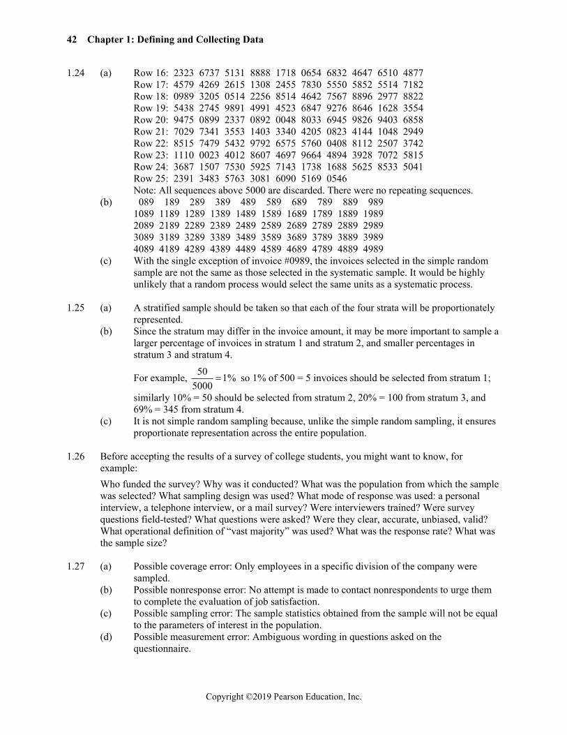
42 Chapter 1: Defining and Collecting Data
Copyright ©2019 Pearson Education, Inc.
1.24 (a) Row 16: 2323 6737 5131 8888 1718 0654 6832 4647 6510 4877 Row 17: 4579 4269 2615 1308 2455 7830 5550 5852 5514 7182 Row 18: 0989 3205 0514 2256 8514 4642 7567 8896 2977 8822 Row 19: 5438 2745 9891 4991 4523 6847 9276 8646 1628 3554 Row 20: 9475 0899 2337 0892 0048 8033 6945 9826 9403 6858 Row 21: 7029 7341 3553 1403 3340 4205 0823 4144 1048 2949 Row 22: 8515 7479 5432 9792 6575 5760 0408 8112 2507 3742 Row 23: 1110 0023 4012 8607 4697 9664 4894 3928 7072 5815 Row 24: 3687 1507 7530 5925 7143 1738 1688 5625 8533 5041 Row 25: 2391 3483 5763 3081 6090 5169 0546 Note: All sequences above 5000 are discarded. There were no repeating sequences. (b) 089 189 289 389 489 589 689 789 889 989 1089 1189 1289 1389 1489 1589 1689 1789 1889 1989 2089 2189 2289 2389 2489 2589 2689 2789 2889 2989 3089 3189 3289 3389 3489 3589 3689 3789 3889 3989 4089 4189 4289 4389 4489 4589 4689 4789 4889 4989 (c) With the single exception of invoice #0989, the invoices selected in the simple random
sample are not the same as those selected in the systematic sample. It would be highly unlikely that a random process would select the same units as a systematic process.
1.25 (a) A stratified sample should be taken so that each of the four strata will be proportionately
represented. (b) Since the stratum may differ in the invoice amount, it may be more important to sample a
larger percentage of invoices in stratum 1 and stratum 2, and smaller percentages in stratum 3 and stratum 4.
For example, 50 1%5000
so 1% of 500 = 5 invoices should be selected from stratum 1;
similarly 10% = 50 should be selected from stratum 2, 20% = 100 from stratum 3, and 69% = 345 from stratum 4.
(c) It is not simple random sampling because, unlike the simple random sampling, it ensures proportionate representation across the entire population.
1.26 Before accepting the results of a survey of college students, you might want to know, for
example:
Who funded the survey? Why was it conducted? What was the population from which the sample was selected? What sampling design was used? What mode of response was used: a personal interview, a telephone interview, or a mail survey? Were interviewers trained? Were survey questions field-tested? What questions were asked? Were they clear, accurate, unbiased, valid? What operational definition of “vast majority” was used? What was the response rate? What was the sample size?
1.27 (a) Possible coverage error: Only employees in a specific division of the company were
sampled. (b) Possible nonresponse error: No attempt is made to contact nonrespondents to urge them
to complete the evaluation of job satisfaction. (c) Possible sampling error: The sample statistics obtained from the sample will not be equal
to the parameters of interest in the population. (d) Possible measurement error: Ambiguous wording in questions asked on the
questionnaire.

Solutions to End-of-Section and Chapter Review Problems 43
Copyright ©2019 Pearson Education, Inc.
1.28 The results are based on an online survey. If the frame is supposed to be smart phone and tablet users, how is the population defined? This is a self-selecting sample of people who responded online, so there is an undefined nonresponse error. Sampling error cannot be determined since this is not a random sample.
1.29 Before accepting the results of the survey, you might want to know, for example:
Who funded the study? Why was it conducted? What was the population from which the sample was selected? What was the frame being used? What sampling design was used?
What mode of response was used: a personal interview, a telephone interview, or a mail survey? Were interviewers trained? Were survey questions field-tested? What other questions were asked? Were they clear, accurate, unbiased, and valid? What was the response rate? What was the margin of error? What was the sample size?
1.30 Before accepting the results of the survey, you might want to know, for example: Who funded the
study? Why was it conducted? What was the population from which the sample was selected? What sampling design was used? What mode of response was used: a personal interview, a telephone interview, or a mail survey? Were interviewers trained? Were survey questions field-tested? What other questions were asked? Were the questions clear, accurate, unbiased, and valid? What was the response rate? What was the margin of error? What was the sample size? What frame was used?
1.31 A population contains all the items of interest whereas a sample contains only a portion of the
items in the population. 1.32 A statistic is a summary measure describing a sample whereas a parameter is a summary measure
describing an entire population. 1.33 Categorical random variables yield categorical responses such as yes or no answers. Numerical
random variables yield numerical responses such as your height in inches. 1.34 Discrete random variables produce numerical responses that arise from a counting process.
Continuous random variables produce numerical responses that arise from a measuring process. 1.35 Both nominal scaled and ordinal scaled variables are categorical variables but no ranking is
implied in nominal scaled variable such as male or female while ranking is implied in ordinal scaled variable such as a student’s grade of A, B, C, D and F.
1.36 Both interval scaled and ratio scaled variables are numerical variables in which the difference
between measurements is meaningful but an interval scaled variable does not involve a true zero such as standardized exam scores while a ratio scaled variable involves a true zero such as height.
1.37 Items or individuals in a probability sampling are selected based on known probabilities while
items or individuals in a nonprobability samplings are selected without knowing their probabilities of selection.
1.38 Microsoft Excel or Minitab could be used to perform various statistical computations that were
possible only with a slide-rule or hand-held calculator in the old days.

44 Chapter 1: Defining and Collecting Data
Copyright ©2019 Pearson Education, Inc.
1.39 (a) The population of interest was 18–54 year olds who currently own a smartphone and/or tablet, and who use and do not use these devices to shop.
(b) The sample was the 1,003 18–54 year olds who currently own a smartphone and/or tablet, who use and do not use these devices to shop, and who participated in Adobe System study.
(c) A parameter of interest is the proportion of all tablet users in the population who use their device to purchase products and services.
(d) A statistic used to estimate the parameter of interest in (c) is the proportion of tablet users in the sample who use their device to purchase products and services.
1.40 The answers to this question depend on which article and its corresponding data set is being selected. 1.41 (a) The population of interest was supply chain executives in a wide range of industries
representing a mix of company sizes from across three global regions: Asia, Europe, and the Americas.
(b) The sample was the 503 supply chain executives in a wide range of industries representing a mix of company sizes from across three global regions: Asia, Europe, and the Americas surveyed by PwC.
(c) A parameter of interest is the proportion of supply chain executives in the population who acknowledge that the supply chain is seen as a strategic asset in their company.
(d) A statistic used to estimate the parameter of interest in (c) is the proportion of supply chain executives in the sample who acknowledge that the supply chain is seen as a strategic asset in their company.
1.42 The answers to this question depend on which data set is being selected. 1.43 (a) Categorical variable: Which of the following best describes this firm’s primary business? (b) Numerical variable: On average, what percent of total monthly revenues are e-commerce
revenues? 1.44 (a) The population of interest was the collection of all the 10,000 benefitted employees at the
University of Utah when the study was conducted. (b) The sample consisted of the 3,095 benefitted employees participated in the study. (c) gender: categorical; age: numerical; education level: numerical; marital status:
categorical; household income: numerical; employment category: categorical 1.45 (a) (i) categorical (ii) categorical (iii) numerical, discrete (iv) categorical (b) The answers will vary. (c) The answers will vary. 1.46 Microsoft Excel: This product features a spreadsheet-based interface that allows users to organize, calculate, and
organize data. Excel also contains many statistical functions to assist in the description of a dataset. Excel can be used to develop worksheets and workbooks to calculate a variety of statistics including introductory and advanced statistics. Excel also includes interactive tools to create graphs, charts, and pivot tables. Excel can be used to summarize data to better understand a population of interest, compare across groups, predict outcomes, and to develop forecasting models. These capabilities represent those that are generally relevant to the current course.
Excel also includes many other statistical capabilities that can be further explored on the Microsoft Office Excel official website.

Solutions to End-of-Section and Chapter Review Problems 45
Copyright ©2019 Pearson Education, Inc.
1.46 Minitab 18: cont. Minitab 18 has a comprehensive set of statistical methods including introductory and advanced
statistical procedures. Minitab 18 features include basic descriptive statistical procedures, graph and chart creation, diagnostic tests, analysis of variance, regression, time series and forecasting analyses, nonparametric analyses, cross-tabulation, chi-square and related tests, and other statistical procedures. Minitab 18 utilizes a user friendly interface that allows one to quickly identify the appropriate procedure. The interface also allows one to easily export results including charts and graphs to facilitate the creation of presentations and reports. These Minitab 18 features would allow one to summarize data to better understand a population of interest, compare across groups, predict outcomes, and to develop forecasting models. These capabilities represent those that are generally relevant to the current course. Minitab 18 also includes many other statistical capabilities that can be further explored on the Minitab official website.
JMP: JMP has a comprehensive set of statistical methods including introductory and advanced
statistical procedures. JMP features include basic descriptive statistical procedures, graph and chart creation, diagnostic tests, analysis of variance, regression, time series and forecasting analyses, nonparametric analyses, cross-tabulation, chi-square and related tests, and other statistical procedures. JMP utilizes a user friendly interface that allows one to quickly identify the appropriate procedure. JMP also contains predictive analytic tools such as classification trees to classify data into groups. These JMP features would allow one to summarize data to better understand a population of interest, compare across groups, predict outcomes, and to develop forecasting models. These capabilities represent those that are generally relevant to the current course. JMP also includes many other statistical capabilities that can be further explored on the JMP official website.
1.47 (a) The population of interest include banking executives representing institutions of various
sizes and U.S. geographic locations. (b) The collected sample includes 163 banking executives from institutions of various sizes
and U.S. geographic locations. (c) A parameter of interest is the percentage of the population of banking executives that
identify customer experience initiatives as an area where increased spending is expected. (d) A statistic used to the estimate the parameter in (c) is the percentage of the 163 banking
executives included in the sample who identify customer experience initiatives as an area where increased spending is expected. In this case, the statistic is 55%.
1.48 The answers are based on an article titled “U.S. Satisfaction Still Running at Improved Level”
and written by Lydia Saad (August 15, 2018). The article is located on the following site: https://news.gallup.com/poll/240911/satisfaction-running-improved-level.aspx?g_source=link_NEWSV9&g_medium=NEWSFEED&g_campaign=item_&g_content=U.S.%2520Satisfaction%2520Still%2520Running%2520at%2520Improved%2520Level
The population of interest includes all individuals aged 18 and older who live within the 50 U.S. states and the District of Columbia.
The collected sample includes a random sample of 1,024 individuals aged 18 and older who live within the 50 U.S. states and the District of Columbia.
A parameter of interest is the percentage of the population of individuals aged 18 and older and live within the 50 U.S. states and the District of Columbia who are satisfied with the direction of the U.S.
A statistic used to the estimate the parameter in (c) is the percentage of the 1,024 individuals included in the sample. In this case, the statistic is 36%.

46 Chapter 1: Defining and Collecting Data
Copyright ©2019 Pearson Education, Inc.
1.49 The answers were based on information obtained from the following site: https://www.pwc.com/gx/en/ceo-survey/2017/pwc-ceo-20th-survey-report-2017.pdf
(a) The population of interest included CEOs representing a mix of industries from 79 countries. (b) The sample included 1,379 CEOs. The percentage of CEOs by continent were as follows:
North America (11%), Western Europe (21%), Central and Eastern Europe (11%), Latin America (12%), Middle East and Africa (9%), and Asia Pacific (36%).
(c) A parameter of interest would be the percentage of CEOs among the population of interest that believe social media could have a negative impact on the level of stakeholder trust in their industry over the next few years.
(d) The statistic used to estimate the parameter in (c) is the percentage of CEOs among the 1,379 CEOs included in the sample who believe social media could have a negative impact on the level of stakeholder trust in their industry over the next few years. In this case, the statistic is 87%.
1.50 (a) One variable collected with the American Community Survey is marital status with the
following possible responses: now married, widowed, divorced, separated, and never married.
(b) The variable in (a) represents a categorical variable. (c) Because the variable in (a) is a categorical, this question is not applicable. If one had
chosen age in years from the American Community Survey as the variable, the answer to (c) would be discrete.
1.51 Answers will vary depending on the specific sample survey used. The below answers were based
on the sample survey located at: http://www.zarca.com/Online-Surveys-Non-Profit/association-salary-survey.html
(a) An example of a categorical variable included in the survey would be whether one had obtained an undergraduate degree with yes or no as possible answers.
(b) An example of a numerical variable included in the survey would be the respondent’s annual base salary for the past year.
1.52 (a) The population of interest consisted of 10,000 benefited employees of the University of Utah. (b) The sample consisted of 3,095 employees of the University of Utah. (c) Gender, marital status, and employment category represent categorical variables. Age in years,
education level in years completed, and household income represent numerical variables. 1.53 (a) Key social media platforms used represents a categorical variable. The frequency of
social media usage represents a discrete numerical variable. Demographics of key social media platform users represent categorical variables.
(b) 1. Which of the following is your preferred social media platform: YouTube, Facebook, or Twitter?
2. What time of the day do you spend the most amount of time using social media: morning, afternoon, or evening?
3. Please indicate your ethnicity? 4. Which of the following do you most often use to access social media: mobile device,
laptop computer, desktop computer, other device? 5. Please indicate whether you are a home owner: Yes or No? (c) 1. For the past week, how many hours did you spend using social media? 2. Please indicate your current age in years. 3. What was your annual income this past year? 4. Currently, how many friends have you accepted on Facebook? 5. Currently, how many twitter followers do you have?

Copyright ©2019 Pearson Education, Inc. 47
CHAPTER 2
2.1 (a)
Category Frequency Percentage A 13 26% B 28 56% C 9 18%
(b) Category “B” is the majority. 2.2 (a) Table frequencies for all student responses
Student Major Categories Gender A C M Totals
Male 14 9 2 25 Female 6 6 3 15 Totals 20 15 5 40
(b) Table percentages based on overall student responses
Student Major Categories Gender A C M Totals
Male 35.0% 22.5% 5.0% 62.5% Female 15.0% 15.0% 7.5% 37.5% Totals 50.0% 37.5% 12.5% 100.0%
Table based on row percentages
Student Major Categories Gender A C M Totals
Male 56.0% 36.0% 8.0% 100.0% Female 40.0% 40.0% 20.0% 100.0% Totals 50.0% 37.5% 12.5% 100.0%
Table based on column percentages
Student Major Categories Gender A C M Totals
Male 70.0% 60.0% 40.0% 62.5% Female 30.0% 40.0% 60.0% 37.5% Totals 100.0% 100.0% 100.0% 100.0%
2.3 (a) You can conclude that in 2011 Android, iOS, and OtherOS dominated the market in
2011. In 2012, 2013, 2014, and 2015 Android and iOS dominated the market. Android has increased its market share from 49.2% in 2011 to 80.7% in 2015. iOS has seen a slight decrease in market share from 18.8% in 2011 to 17.7% in 2015. OtherOS market share has declined from 19.8% in 2011 to 0.2% in 2015. Blackberry has also seen a significant decrease from 10.3% in 2011 to 0.3% in 2015. Microsoft reached its highest market share in 2013 with 3.3% and its lowest in 2015 with 1.1%.
(b) iOS increased its market share from 14.8% in 2014 to 17.7% in 2015. Android’s market share has remained steady from 2014 to 2015 while Microsoft, Blackberry, and OtherOS have all lost market share.

48 Chapter 2: Organizing and Visualizing Variables
Copyright ©2019 Pearson Education, Inc.
2.4 (a)
Category Total Percentages Bank Account or Service 202 9.330% Consumer Loan 132 6.097% Credit Card 175 8.083% Credit Reporting 581 26.836% Debt Collection 486 22.448% Mortgage 442 20.416% Student Loan 75 3.464% Other 72 3.326% Grand Total 2165
(b) There are more complaints for credit reporting, debt collection, and mortgage than the other categories. These categories account for about 70% of all the complaints.
(c)
Company Total Percentage Bank of America 42 3.64% Capital One 93 8.07% Citibank 59 5.12% Ditech Financial 31 2.69% Equifax 217 18.82% Experian 177 15.35% JPMorgan 128 11.10% Nationstar Mortgage 39 3.38% Navient 38 3.30% Ocwen 41 3.56% Synchrony 43 3.73% Trans-Union 168 14.57% Wells Fargo 77 6.68% Grand Total 1153
(d) Equifax, Trans-Union, and Experion, all of which are credit score companies, have the most complaints.
2.5 Executives anticipate Artificial Intelligence/Machine Learning technology to have the greatest
disruptive impact on their firm in the next decade followed by Digital Technologies such as mobile, social media and IoT. They anticipate Financial Tech Solutions and Cloud computing will have some disruptive impact while Blockchain and other technologies to have little impact.
2.6 The largest sources of summer power-generating capacity in the United States are natural gas
followed by coal. Nuclear, hydro, wind and other generate about the same, and solar generates very little.

Solutions to End-of-Section and Chapter Review Problems 49
Copyright ©2019 Pearson Education, Inc.
2.7 (a)
Technologies Frequency Percentage Wearable technology 9 10.00% Blockchain technology 9 10.00% Artificial Intelligence 17 18.89% Iot: retail insurance 23 25.56% Iot: commerical insurance 5 5.56% Social media 27 30.00% Grand Total 90
(b) Professionals expect to be using Social media and Iot: retail insurance technologies the most over the next year followed by Artificial Intelligence. Professionals do not expect to be using Wearable, Blockchain, and Iot: commercial insurance technologies much over the next year.
2.8 (a) Table of row percentages:
GENDER OVERLOADED Male Female Total Yes 44.08% 55.92% 100.00% No 53.54% 46.46% 100.00% Total 51.64% 48.36% 100.00%
Table of column percentages:
GENDER OVERLOADED Male Female Total Yes 17.07% 23.13% 20.00% No 82.93% 76.87% 80.00% Total 100.00% 100.00% 100.00%
Table of total percentages:
GENDER OVERLOADED Male Female Total Yes 8.82% 11.18% 20.00% No 42.83% 37.17% 80.00% Total 51.64% 48.36% 100.00%
(b) Approximately the same percentages of males and females as a percentage of the total number of people surveyed feel overloaded with too much information. As percentages of those who do and do not feel overloaded, the genders differ mildly. However, four times as many people do not feel overloaded at work than those that do.

50 Chapter 2: Organizing and Visualizing Variables
Copyright ©2019 Pearson Education, Inc.
2.9 (a)
Column Percentage OUTCOME CATEGORY Successful Not Successful Total
Film & Video 36.02% 36.81% 36.51% Games 15.44% 18.24% 17.19% Music 40.20% 24.38% 30.34% Technology 8.34% 20.56% 15.96% Total 100.00% 100.00% 100.00%
Row Percentages OUTCOME CATEGORY Successful Not Successful Total
Film & Video 37.15% 62.85% 100.00% Games 33.84% 66.16% 100.00% Music 49.91% 50.09% 100.00% Technology 19.69% 80.31% 100.00% Total 37.67% 62.33% 100.00%
Total Percentages
OUTCOME CATEGORY Successful Not Successful Total
Film & Video 13.57% 22.95% 36.51% Games 5.82% 11.37% 17.19% Music 15.14% 15.20% 30.34% Technology 3.14% 12.82% 15.96% Total 37.67% 62.33% 100.00%
(b) The row percentages are most informative because they provide a percentage of successful projects within each category which allows one to compare across categories.
(c) Music kick starter projects were the most successful with approximately 50% of the projects succeeding compared to less than 20% of the Technology projects. The Film & Video and Games categories had success rates in between the Music and Technology categories, with success rates of 37% and 34% respectively.
2.10 Social recommendations had very little impact on correct recall. Those who arrived at the link
from a recommendation had a correct recall of 73.07% as compared to those who arrived at the link from browsing who had a correct recall of 67.96%.
2.11 Ordered array: 63 64 68 71 75 88 94

Solutions to End-of-Section and Chapter Review Problems 51
Copyright ©2019 Pearson Education, Inc.
2.12 Ordered array: 73 78 78 78 85 88 91 2.13 (a) (166 + 100)/591 * 100 = 45.01% (b) (124 + 77)/591 * 100 = 34.01% (c) (59 + 65)/591 * 100 = 20.98% (d) 45% of the incidents took fewer than 2 days and 66% of the incidents were detected in
less than 8 days. 79% of the incidents were detected in less than 31 days.
2.14 216,000 61,000 33,333.336 so choose 40,000 as interval width
(a) $60,000 – under $100,000; $100,000 – under $140,000; $140,000 – under $180,000; $180,000 – under $220,000; $220,000 – under $260,000; $260,000 – under $300,000
(b) $40,000
(c) 60,000 100000 800002 similarly, the remaining class midpoints are $120,000;
$160,000; $200,000; $240,000; $280,000 2.15 (a) 222.67 262.50 262.67 276.40 278.00 290.83 292.87 298.00 318.67 324.33 332.93 345.09 346.70 380.67 398.55 418.14 422.45 423.50 429.00 441.00 492.71 505.77 539.68 571.50 585.20 696.33 718.50 726.40 789.20 878.20 (b)
NBA Cost Cost $ Frequency Percentage
200 but less than 300 8 27% 300 but less than 400 7 23% 400 but less than 500 6 20% 500 but less than 600 4 13% 600 but less than 700 1 3% 700 but less than 800 3 10% 800 but less than 900 1 3% Total 30 100%
(c) 70% of the costs to attend a NBA basketball game are between $200 and $500 with 27% of the costs between $200 and $300. Three teams or 10% of the NBA teams have costs between $700 and $800.

52 Chapter 2: Organizing and Visualizing Variables
Copyright ©2019 Pearson Education, Inc.
2.16 (a)
Electricity Costs Electricity Costs Frequency Percentage
$80 but less than $100 4 8% $100 but less than $120 7 14% $120 but less than $140 9 18% $140 but less than $160 13 26% $160 but less than $180 9 18% $180 but less than $200 5 10% $200 but less than $220 3 6%
(b)
Electricity Costs Frequency Percentage Cumulative %
$ 99 4 8.00% 8.00% $119 7 14.00% 22.00% $139 9 18.00% 40.00% $159 13 26.00% 66.00% $179 9 18.00% 84.00% $199 5 10.00% 94.00% $219 3 6.00% 100.00%
(c) The majority of utility charges are clustered between $120 and $180. 2.17 (a)
Commuting Time (minutes) Frequency Percentage 200 but less than 230 12 40% 230 but less than 260 9 30% 260 but less than 290 4 13% 290 but less than 320 3 10% 320 but less than 350 1 3% 350 but less than 380 1 3%
30 100%
(b)
Commuting Time (minutes) Frequency Percentage Cumulative % 200 but less than 230 12 40% 40% 230 but less than 260 9 30% 70% 260 but less than 290 4 13% 83% 290 but less than 320 3 10% 93% 320 but less than 350 1 3% 97% 350 but less than 380 1 3% 100%
30 100%

Solutions to End-of-Section and Chapter Review Problems 53
Copyright ©2019 Pearson Education, Inc.
2.17 (c) The majority of commuters living in or near cities spend from 200 up to 230 minutes cont. commuting each week. 70% of commuters spend from 200 up to 260 minutes
commuting each week. 2.18 (a), (b)
Credit Score Frequency Percent (%) Cumulative Percent (%)
560 – under 580 4 0.16 0.16 580 – under 600 24 0.93 1.09 600 – under 620 68 2.65 3.74 620 – under 640 290 11.28 15.02 640 – under 660 548 21.32 36.34 660 – under 680 560 21.79 58.13 680 – under 700 507 19.73 77.86 700 – under 720 378 14.71 92.57 720 – under 740 168 6.54 99.11 740 – under 760 22 0.86 99.96 760 – under 780 1 0.04 100.00
(c) The average credit scores are concentrated between 620 and 720. 2.19 (a), (b)
Bin Frequency Percentage Cumulative % -0.00350 but less than -0.00201 13 13.00% 13.00% -0.00200 but less than -0.00051 26 26.00% 39.00% -0.00050 but less than 0.00099 32 32.00% 71.00% 0.00100 but less than 0.00249 20 20.00% 91.00% 0.00250 but less than 0.00399 8 8.00% 99.00% 0.004 but less than 0.00549 1 1.00% 100.00%
(c) Yes, the steel mill is doing a good job at meeting the requirement as there is only one steel part out of a sample of 100 that is as much as 0.005 inches longer than the specified requirement.
2.20 (a), (b)
Time in Seconds Frequency Percent (%)
5 – under 10 8 16% 10 – under 15 8 30% 15 – under 20 8 36% 20 – under 25 8 12% 25 – under 30 8 6%

54 Chapter 2: Organizing and Visualizing Variables
Copyright ©2019 Pearson Education, Inc.
2.20 (b) cont.
Time in Seconds Percentage Less Than
5 0 10 16 15 46 20 82 25 94 30 100
(c) The target is being met since 82% of the calls are being answered in less than 20 seconds 2.21 (a)
Call Duration (seconds) Frequency Percentage 60 up to 119 7 14% 120 up to 179 12 24% 180 up to 239 11 22% 240 up to 299 11 22% 300 up to 359 4 8% 360 up to 419 3 6% 420 and longer 2 4%
50 100%
(b) Call Duration (seconds) Frequency Percentage Cumulative %
60 up to 119 7 14% 14% 120 up to 179 12 24% 38% 180 up to 239 11 22% 60% 240 up to 299 11 22% 82% 300 up to 359 4 8% 90% 360 up to 419 3 6% 96% 420 and longer 2 4% 100%
50 100%
(c) The call center’s target of call duration less than 240 seconds is only met for 60% of the calls in this data set.
2.22 (a), (b) Manufacturer A:
Bin Cell Frequency Percentage Cumulative Pctage. 6,500 but less than 7,500 3 7.50% 7.50% 7,500 but less than 8,500 5 12.50% 20.00% 8,500 but less than 9,500 20 50.00% 70.00% 9,500 but less than 10,500 9 22.50% 92.50% 10,500 but less than 11,500 3 7.50% 100.00%

Solutions to End-of-Section and Chapter Review Problems 55
Copyright ©2019 Pearson Education, Inc.
2.22 (a) Manufacturer B: cont.
Bin Cell Frequency Percentage Cumulative Pctage. 7,500 but less than 8,500 2 5.00% 5.00% 9,500 but less than 9,500 8 20.00% 25.00% 9,500 but less than 10,500 16 40.00% 65.00% 10,500 but less than 11,500 9 22.50% 87.50% 11,500 but less than 12,500 5 12.50% 100.00%
(c) Manufacturer B produces bulbs with longer lives than Manufacturer A. The cumulative percentage for Manufacturer B shows 65% of its bulbs lasted less than 10,500 hours, contrasted with 70% of Manufacturer A’s bulbs, which lasted less than 9,500 hours. None of Manufacturer A’s bulbs lasted more than 11,499 hours, but 12.5% of Manufacturer B’s bulbs lasted between 11,500 and 12,499 hours. At the same time, 7.5% of Manufacturer A’s bulbs lasted less than 7,500 hours, whereas all of Manufacturer B’s bulbs lasted at least 7,500 hours
2.23 (a)
Amount of Soft Drink Frequency Percentage 1.850 – 1.899 1 2% 1.900 – 1.949 5 10% 1.950 – 1.999 18 36% 2.000 – 2.049 19 38% 2.050 – 2.099 6 12% 2.100 – 2.149 1 2%
Amount of Soft Drink Frequency Less Than Percentage Less Than
1.899 1 2% 1.949 6 12% 1.999 24 48% 2.049 43 86% 2.099 49 98% 2.149 50 100%
(b) The amount of soft drink filled in the two liter bottles is most concentrated in two
intervals on either side of the two-liter mark, from 1.950 to 1.999 and from 2.000 to 2.049 liters. Almost three-fourths of the 50 bottles sampled contained between 1.950 liters and 2.049 liters.

56 Chapter 2: Organizing and Visualizing Variables
Copyright ©2019 Pearson Education, Inc.
2.24 (a)

Solutions to End-of-Section and Chapter Review Problems 57
Copyright ©2019 Pearson Education, Inc.
2.24 (b) The Pareto chart is best for portraying these data because it not only sorts the frequencies cont. in descending order but also provides the cumulative line on the same chart. (c) You can conclude that searching and buying online was the highest category and the
other three were equally likely. 2.25 (a)

58 Chapter 2: Organizing and Visualizing Variables
Copyright ©2019 Pearson Education, Inc.
2.25 (a) cont.
(b) The Pareto diagram is better than the pie chart or the bar chart because it not only sorts the frequencies in descending order, it also provides the cumulative polygon on the same scale.
(c) From the Pareto diagram it is obvious that more than 50% of their day is spent sleeping and taking part in leisure and sports.
2.26 (a)
(b) 32% + 19% + 33% = 84%

Solutions to End-of-Section and Chapter Review Problems 59
Copyright ©2019 Pearson Education, Inc.
2.26 (c) cont.
(d) The Pareto diagram is better than the pie chart because it not only sorts the frequencies in descending order, it also provides the cumulative polygon on the same scale.
2.27 (a)
(b) The “vital few” reasons for the categories of complaints are “Credit Reporting”, “Debt Collection”, and “Mortgage” which account for 70% of the complaints. The remaining are the “trivial many” which make up 30% of the complaints.
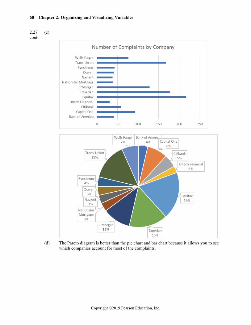
60 Chapter 2: Organizing and Visualizing Variables
Copyright ©2019 Pearson Education, Inc.
2.27 (c) cont.
(d) The Pareto diagram is better than the pie chart and bar chart because it allows you to see which companies account for most of the complaints.

Solutions to End-of-Section and Chapter Review Problems 61
Copyright ©2019 Pearson Education, Inc.
2.28 (a)
0 0.05 0.1 0.15 0.2 0.25
Cooking
Cooling
Electronics
Heating
Lighting
Other
Refrigeration
Water heating
Wet cleaning
Type
of U
se P
erce
ntag
e
Bar Chart
Cooking 2% Cooling
15%
Electronics 9%
Heating 15%
Lighting 13%
Other 23%
Refrigeration 10%
Water heating 10%
Wet cleaning 3%
Pie Chart

62 Chapter 2: Organizing and Visualizing Variables
Copyright ©2019 Pearson Education, Inc.
2.28 (a) cont.
0%10%20%30%40%50%60%70%80%90%100%
0%10%20%30%40%50%60%70%80%90%
100%
Othe
r
Cool
ing
Heat
ing
Light
ing
Refri
gera
tion
Wat
er h
eatin
g
Elec
tron
ics
Wet
clea
ning
Cook
ing
Type of Use Percentage
Pareto Chart
(b) The Pareto diagram is better than the pie chart and bar chart because it not only sorts the frequencies in descending order; it also provides the cumulative polygon on the same scale.
(c) Other, cooling, heating and lighting accounted for 66% of the residential electricity consumption in the United States.
2.29 (a)

Solutions to End-of-Section and Chapter Review Problems 63
Copyright ©2019 Pearson Education, Inc.
2.29 (a) cont.
(b) Insurance professionals expect Social Media, AI, and IOT retail insurance to be most used in the insurance industry in the coming year.
2.30 (a)
(b) Females are more likely to be overloaded with information.

64 Chapter 2: Organizing and Visualizing Variables
Copyright ©2019 Pearson Education, Inc.
2.31 (a)
(b) Of the successful kickstarter projects, music projects make up the largest part. 2.32 (a)
407
193
150
91
0 100 200 300 400 500
Recommendation
Browsing
Side-by-side Bar Chart
NoYes

Solutions to End-of-Section and Chapter Review Problems 65
Copyright ©2019 Pearson Education, Inc.
2.32 (b) Social recommendations had very little impact on correct recall. cont. 2.33
Stem-and-leaf of Finance Scores 5 34 6 9 7 4 9 38
2.34 Ordered array: 50 74 74 76 81 89 92 2.35 (a) Ordered array: 9.1 9.4 9.7 10.0 10.2 10.2 10.3 10.8 11.1 11.2 11.5 11.5 11.6 11.6 11.7 11.7 11.7 12.2 12.2 12.3 12.4 12.8 12.9 13.0 13.2 (b) The stem-and-leaf display conveys more information than the ordered array. We can
more readily determine the arrangement of the data from the stem-and-leaf display than we can from the ordered array. We can also obtain a sense of the distribution of the data from the stem-and-leaf display.
(c) The most likely gasoline purchase is between 11 and 11.7 gallons. (d) Yes, the third row is the most frequently occurring stem in the display and it is located in
the center of the distribution. 2.36 (a)
Stem Unit 100 2 2 6 6 8 8 9 3 0 2 2 3 5 5 8 4 0 2 2 2 3 4 9 5 1 4 7 9 6 7 0 2 3 9 8 8
(b) The results are concentrated between $220 and $490. 2.37 (a) Download Speed 4.5 7.1 10.3 10.8 11.2 16.7 20.8 22.7 24.0
Upload Speed 3.0 3.8 6.0 6.2 6.4 9.1 11.1 13.2 14.3

66 Chapter 2: Organizing and Visualizing Variables
Copyright ©2019 Pearson Education, Inc.
2.37 (b) Download Speeds: Stem unit :1 cont.
Upload Speeds: Stem unit 1
(b) The stem-and-leaf display conveys more information than the ordered array. We can more readily determine the arrangement of the data from the stem-and-leaf display then we can from the ordered array. We can also obtain a sense of the distribution of the data from the stem-and-leaf display.
(c) Download speeds are concentrated around 10 mbs and Upload speeds are concentrated around 6 mbs.

Solutions to End-of-Section and Chapter Review Problems 67
Copyright ©2019 Pearson Education, Inc.
2.38 (a)
Histogram
0
2
4
6
8
10
12
14
90 110 130 150 170 190 210
Midpoints
Freq
uenc
y
Percentage Polygon
0%
5%
10%
15%
20%
25%
30%
70 90 110 130 150 170 190 210 230
(b)
Cumulative Percentage Polygon
0%10%20%30%40%50%60%70%80%90%
100%
79 99 119 139 159 179 199 219 239
(c) The majority of utility charges are clustered between $120 and $180. 2.39 The cost of attending a baseball game is concentrated around $65 with twelve teams at that cost.
Four teams have costs of $85 and one team is has the highest cost of $115.

68 Chapter 2: Organizing and Visualizing Variables
Copyright ©2019 Pearson Education, Inc.
2.40 Property taxes on a $176K home seem concentrated between $700 and $2,200 and also between $3,200 and $3,700.
2.41 (a)
(b)

Solutions to End-of-Section and Chapter Review Problems 69
Copyright ©2019 Pearson Education, Inc.
2.41 (b) cont.
Cumulative Percentage Polygon of Weekly Commuting Time
(c) The majority of Americans living in cities spend an average of 280 minutes or less
commuting each week. Approximately 38% spend between 210 and 230 minutes commuting each week with a small percentage commuting spending between 370 to 380 minutes commuting each week.
2.42 (a)

70 Chapter 2: Organizing and Visualizing Variables
Copyright ©2019 Pearson Education, Inc.
2.42 (b) cont.
(c) The average credit scores are concentrated between 622 and 730.
2.43 (a)
(b) Yes, the steel mill is doing a good job at meeting the requirement as there is only one
steel part out of a sample of 100 that is as much as 0.005 inches longer than the specified requirement.

Solutions to End-of-Section and Chapter Review Problems 71
Copyright ©2019 Pearson Education, Inc.
2.44 (a)

72 Chapter 2: Organizing and Visualizing Variables
Copyright ©2019 Pearson Education, Inc.
2.44 (b) cont.
(c) The target is being met since 82% of the calls are being answered in less than 20 seconds. 2.45 (a)

Solutions to End-of-Section and Chapter Review Problems 73
Copyright ©2019 Pearson Education, Inc.
2.45 (a) cont.
(b)
(c) The call center’s target of call duration less than 240 seconds is only met for 60% of the calls in this data set.

74 Chapter 2: Organizing and Visualizing Variables
Copyright ©2019 Pearson Education, Inc.
2.46 (a)

Solutions to End-of-Section and Chapter Review Problems 75
Copyright ©2019 Pearson Education, Inc.
2.46 (b) cont.
(c) Manufacturer B produces bulbs with longer lives than Manufacturer A

76 Chapter 2: Organizing and Visualizing Variables
Copyright ©2019 Pearson Education, Inc.
2.47 (a)
(b)
Amount of Soft Drink Frequency Less Than Percentage Less Than 1.899 1 2% 1.949 6 12 1.999 24 48 2.049 43 86 2.099 49 98 2.149 50 100
(c) The amount of soft drink filled in the two liter bottles is most concentrated in two
intervals on either side of the two-liter mark, from 1.950 to 1.999 and from 2.000 to 2.049 liters. Almost three-fourths of the 50 bottles sampled contained between 1.950 liters and 2.049 liters.

Solutions to End-of-Section and Chapter Review Problems 77
Copyright ©2019 Pearson Education, Inc.
2.48 (a)
0123456789
10
0 2 4 6 8 10
Y
X
Scatter Plot
(b) There is no relationship between X and Y. 2.49 (a)
(b) Annual sales appear to be increasing until 2011 then remain flat from 2011 to 2013 followed by a decline after 2013.
2.50 (a)
0100200300400500
0 50 100 150 200
US G
ross
First Weekend
Scatter Plot
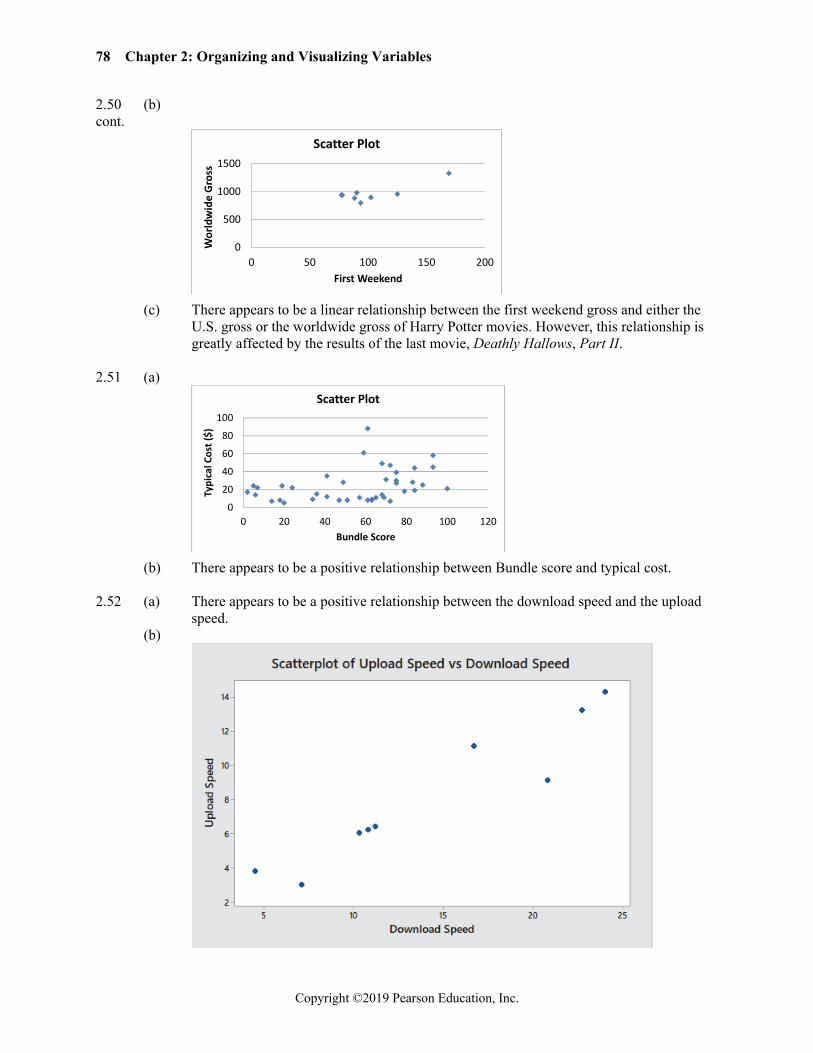
78 Chapter 2: Organizing and Visualizing Variables
Copyright ©2019 Pearson Education, Inc.
2.50 (b) cont.
0
500
1000
1500
0 50 100 150 200
Wor
ldw
ide
Gros
s
First Weekend
Scatter Plot
(c) There appears to be a linear relationship between the first weekend gross and either the U.S. gross or the worldwide gross of Harry Potter movies. However, this relationship is greatly affected by the results of the last movie, Deathly Hallows, Part II.
2.51 (a)
020406080
100
0 20 40 60 80 100 120
Typi
cal C
ost (
$)
Bundle Score
Scatter Plot
(b) There appears to be a positive relationship between Bundle score and typical cost. 2.52 (a) There appears to be a positive relationship between the download speed and the upload
speed. (b)

Solutions to End-of-Section and Chapter Review Problems 79
Copyright ©2019 Pearson Education, Inc.
2.52 (c) Yes, this is borne out by the data cont. 2.53 (a)
(b) There does not appear to be a relationship between GDP and social media usage. (c)
(d) There is a positive relationship between GDP and internet usage.

80 Chapter 2: Organizing and Visualizing Variables
Copyright ©2019 Pearson Education, Inc.
2.54 (a) Excel output:
(b) There is a great deal of variation in the returns from decade to decade. Most of the returns are between 5% and 15%. The 1950s, 1980s, and 1990s had exceptionally high returns, and only the 1930s and 2000s had negative returns.
2.55 (a)
(b) There is an upward trend in home sales price until 2006. Prices decline or remain flat from 2006 – 2011. From 2011 – 2016 there is an upward trend in median price of new home sales. There is a huge drop in median prices in September 2015. This should be investigated further and may be just an error in the data file.

Solutions to End-of-Section and Chapter Review Problems 81
Copyright ©2019 Pearson Education, Inc.
2.56 (a)
(b) There was a decline in movie attendance from 2001 to 2016. During that time, movie attendance increased from 2001 to 2002 but then by 2016 decreased to a level below 2001.
2.57 (a)

82 Chapter 2: Organizing and Visualizing Variables
Copyright ©2019 Pearson Education, Inc.
2.57 (a) cont.
(b) There does not appear to be a pattern present in the number of Ads ran between the opening kickoff and the final whistle over the years from 2006 to 2015.
(c) The total elapse run time (in minutes) of commercials increased from 2007 to 2013 followed by a declined in 2014 and 2015.
2.58 (a) Pivot Table in terms of %
Count of Type Star Rating Type One Two Three Four Five Grand
Total Growth 5.43% 17.12% 27.35% 11.27% 2.71% 63.88% Large 3.76% 7.72% 13.57% 5.43% 1.67% 32.15% Mid-Cap 1.25% 5.43% 7.52% 3.13% 0.63% 17.96% Small 0.42% 3.97% 6.26% 2.71% 0.42% 13.78% Value 2.92% 10.65% 13.99% 7.31% 1.25% 36.12% Large 2.09% 6.68% 9.19% 3.97% 1.25% 23.18% Mid-Cap 0.63% 2.09% 2.71% 1.04% 0.00% 6.47% Small 0.21% 1.88% 2.09% 2.30% 0.00% 6.48% Grand Total 8.35% 27.77% 41.34% 18.58% 3.97% 100.00%
(b) The growth and value funds have similar patterns in terms of star rating and type. Both growth and value funds have more funds with a rating of three. Very few funds have ratings of five.
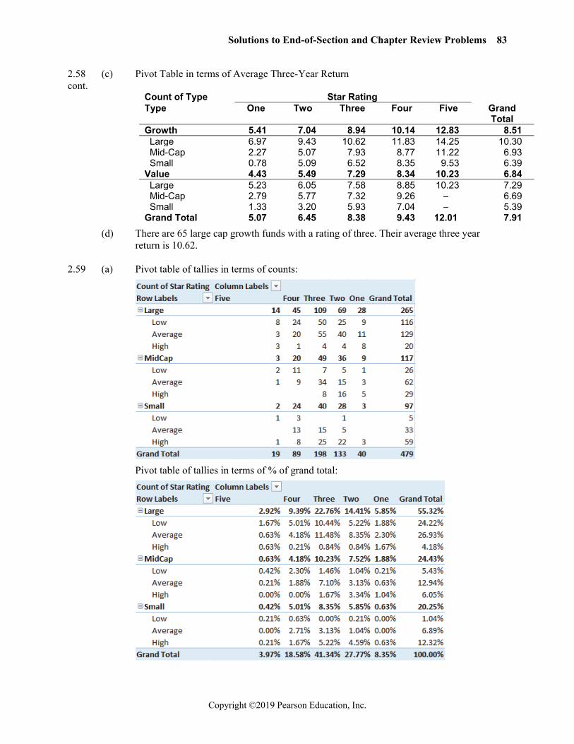
Solutions to End-of-Section and Chapter Review Problems 83
Copyright ©2019 Pearson Education, Inc.
2.58 (c) Pivot Table in terms of Average Three-Year Return cont.
Count of Type Star Rating Type One Two Three Four Five Grand
Total Growth 5.41 7.04 8.94 10.14 12.83 8.51 Large 6.97 9.43 10.62 11.83 14.25 10.30 Mid-Cap 2.27 5.07 7.93 8.77 11.22 6.93 Small 0.78 5.09 6.52 8.35 9.53 6.39 Value 4.43 5.49 7.29 8.34 10.23 6.84 Large 5.23 6.05 7.58 8.85 10.23 7.29 Mid-Cap 2.79 5.77 7.32 9.26 – 6.69 Small 1.33 3.20 5.93 7.04 – 5.39 Grand Total 5.07 6.45 8.38 9.43 12.01 7.91
(d) There are 65 large cap growth funds with a rating of three. Their average three year return is 10.62.
2.59 (a) Pivot table of tallies in terms of counts:
Pivot table of tallies in terms of % of grand total:

84 Chapter 2: Organizing and Visualizing Variables
Copyright ©2019 Pearson Education, Inc.
2.59 (b) For the large-cap funds, the three-star rating category had the highest percentage of cont. funds, followed by two-star, four-star, one-star, and five-star. Very few large-cap funds
had ratings of five. This pattern was also seen with the mid-cap funds as a group. The same pattern was observed with the small-cap funds. However, the pattern was more subtle in that the differences in percentage were less in many cases.
Within the large-cap fund category, the highest percentage of funds were in the average-risk category followed by the low-risk and high-risk categories. Within the mid-cap category, the highest percentage of funds were in the average-risk category followed by the high and low risk categories. Within the small-cap category, the highest percentage of funds were in the high-risk category followed by the average and low risk categories.
(c)
(d) There are four high-risk large-cap funds with a three-star rating. Their average three-year return is 11.36.
2.60
Count of Type Star Rating Type One Two Three Four Five Grand
Total Growth 5.43% 17.12% 27.35% 11.27% 2.71% 63.88% Large 1.25% 2.09% 4.80% 3.55% 1.46% 13.15% Mid-Cap 1.67% 7.72% 15.87% 6.05% 0.42% 31.73% Small 2.51% 7.31% 6.68% 1.67% 0.84% 19.00% Value 2.92% 10.65% 13.99% 7.31% 1.25% 36.12% Large 0.84% 4.38% 7.10% 4.38% 0.84% 17.54% Mid-Cap 1.25% 4.80% 5.85% 2.71% 0.42% 15.03% Small 0.84% 1.46% 1.04% 0.21% 0.00% 3.55% Grand Total 8.35% 27.77% 41.34% 18.58% 3.96% 100.00%
(b) Patterns of star rating conditioned on risk: For the growth funds as a group, most are rated as three-star, followed by two-star, four-
star, one-star, and five-star. The pattern of star rating is different among the various risk growth funds.
For the value funds as a group, most are rated as three-star, followed by two-star, four-star, one-star and five-star. Among the high-risk value funds, more are two-star than three-star.
Most of the growth funds are rated as average-risk, followed by high-risk and then low-risk. The pattern is not the same among all the rating categories.

Solutions to End-of-Section and Chapter Review Problems 85
Copyright ©2019 Pearson Education, Inc.
2.60 (b) Most of the value funds are rated as low-risk, followed by average-risk and then cont. high-risk. The pattern is the same among the three-star, four-star, and five-star value
funds. Among the one-star and two-star funds, there are more average risk funds than low risk funds.
(c)
Count of Type Star Rating Type One Two Three Four Five Grand
Total Growth 5.41 7.04 8.94 10.14 12.83 8.51 Large 7.53 8.60 9.89 10.29 12.64 9.87 Mid-Cap 6.17 7.99 9.28 10.43 11.96 9.06 Small 3.83 5.59 7.45 8.76 13.59 6.64 Value 4.43 5.49 7.29 8.34 10.23 6.84 Large 5.29 7.00 7.66 8.57 10.74 7.76 Mid-Cap 5.01 4.98 6.97 7.96 9.23 6.41 Small 2.71 2.63 6.53 8.39 – 4.13 Grand Total 5.07 6.45 8.38 9.43 12.01 7.91
The three-year returns for growth funds is higher than for value funds. The return is higher for funds with higher ratings than lower ratings. This pattern holds for the growth funds for each risk level. For the low risk and average risk value funds, the return is lowest for the funds with a two-star rating.
(d) There are 32 growth funds with high risk with a rating of three. These funds have an average three-year return of 7.45.
2.61 (a) Pivot table of tallies in terms of counts:

86 Chapter 2: Organizing and Visualizing Variables
Copyright ©2019 Pearson Education, Inc.
2.61 (a) Pivot table of tallies in terms of % of grand total: cont.
(b) For growth funds, most are rated as three-star followed by two-star, four-star, one-star
and five-star. Among the growth funds, large-cap and mid-cap had the same pattern of star-rating as observed for growth funds in general. Small-cap growth funds had the same pattern with the exception of having the same the number of funds rated as one-star and five-star. The pattern of star-rating is different among the various risk levels within the large-cap, mid-cap and small-cap growth funds.
For value funds, most are rated as three-star followed by two-star, four-star, one-star, and five-star. Among the value funds, the pattern is the same for large-cap and mid-cap funds. Small-cap value funds have a different pattern. The pattern of star-rating is different among the various risk levels within the large-cap, mid-cap and small-cap funds.
(c) The tables in 2.58 through 2.60 are easier to interpret because they contain fewer fields. The table in 2.61 tallies star rating across three fields: market type, market cap, and risk level. Problems 2.58 through 2.60 tally star rating across two fields.
(d) Problem 2.60 reveals that most value funds are rated as low-risk followed by average-risk and high-risk. Problem 2.61 reveals that this is only the case among large-cap value funds. Most mid-cap value funds are rated as average-risk followed by low-risk and high-risk. Most small-cap value funds are rated as average-risk followed by high-risk and low-risk. Problem 2.61 also reveals that among small-cap funds rated as average-risk, most are rated as four-star, followed by three-star and two-star. Because Problem 2.61 includes four fields compared to three fields included in problems 2.58 through 2.60, additional patterns can be observed.

Solutions to End-of-Section and Chapter Review Problems 87
Copyright ©2019 Pearson Education, Inc.
2.62 The fund with the highest five-year return of 15.72 is a large cap growth fund that has a four-star rating and low risk.
2.63 (a)
(b)
(c) The results from (a) reveal that the average of SD increases as the risk level increases while average of assets decreases as risk level increases. The results from (b) reveal that the average of SD is higher for growth funds compared to value funds. The patterns suggest that value funds are likely to be associated with less risk because the average of SD was lower among value funds and low risk funds.
2.64 Funds 479, 471, 347, 443, and 477 have the lowest five-year return.

88 Chapter 2: Organizing and Visualizing Variables
Copyright ©2019 Pearson Education, Inc.
2.65 (a)
(b)
(c) For the 1-year versus 10-year return chart, the 10-year returns are much higher than the 1-year returns with similar 5-year returns near 7 percent for all three market cap categories. For the 1-year versus 5-year chart, the returns are all higher for the 5-year returns compared to the 1-year returns. The 5-year returns are higher than the 10-year returns. The large-cap 5-year return is higher than the mid-cap and small 5-year returns.
(d) Because the average 5-year returns were all higher than the 10-year returns for all market cap categories, one can conclude that the returns were lower in years 6 through 10. Without annual data, one cannot conclude that this was due to consistent lower returns across the years or the result of one or two years with lower returns.

Solutions to End-of-Section and Chapter Review Problems 89
Copyright ©2019 Pearson Education, Inc.
2.66 The five funds with the lowest five-year return have (1) midcap growth, average risk, one-star rating, (2) midcap growth, high risk, two-star rating, (3) large value, average risk, two-star rating, (4) midcap growth, high risk, one-star rating, and (5) small value, average risk, two-star rating.
2.67 (a)
(b) The sparklines reveal that a general trend upward in home prices during the months of
February, May, November, and December and they have remained steady in September after a jump from a low in 2001.
(c) In the Time-series plot one can see an upward trend in home sales price until 2006. Prices decline or remain flat from 2006 – 2011. From 2011 – 2016 there is an upward trend in median price of new home sales. With the exception of one year, the September home prices are fairly stable. This could be an error in the data.
2.68 There has been a decline in the price of natural gas over time. However, there is no pattern within
the years. For some years, the price is higher in the beginning of the year. For other years, the price is higher in the latter part of the year. Sometimes, there is little variation within the year.
2.69 Student project answers will vary 2.70 Student project answers will vary

90 Chapter 2: Organizing and Visualizing Variables
Copyright ©2019 Pearson Education, Inc.
2.71 (a) There is a title. (b) None of the axes are labeled. (c)

Solutions to End-of-Section and Chapter Review Problems 91
Copyright ©2019 Pearson Education, Inc.
2.72 (a) There is a title. (b) The simplest possible visualization is not used. (c)

92 Chapter 2: Organizing and Visualizing Variables
Copyright ©2019 Pearson Education, Inc.
2.73 (a) None. (b) The use of chartjunk. (c)
2.74 Answers will vary depending on selection of source.

Solutions to End-of-Section and Chapter Review Problems 93
Copyright ©2019 Pearson Education, Inc.
2.75 (a)
7%7%
17%
25%
40%
4%
Exploed Pie Chart
Online Payment Check Credit card Debit card Cash Other
0%
5%
10%
15%
20%
25%
30%
35%
40%
OnlinePayment
Check Credit card Debit card Cash Other
Cone Chart

94 Chapter 2: Organizing and Visualizing Variables
Copyright ©2019 Pearson Education, Inc.
2.75 (a) cont.
0%
5%
10%
15%
20%
25%
30%
35%
40%
OnlinePayment
Check Credit card Debit card Cash Other
Pyramid Chart
(b) The bar chart and the pie chart should be preferred over the exploded pie chart, doughnut chart, the cone chart and the pyramid chart since the former set is simpler and easier to interpret.
2.76 (a)
10%
73%
17%
Exploed Pie Chart
Low risk Average risk High risk

Solutions to End-of-Section and Chapter Review Problems 95
Copyright ©2019 Pearson Education, Inc.
2.76 (a) cont.
0%
10%
20%
30%
40%
50%
60%
70%
80%
Low risk Average risk High risk
Cone Chart
0%
10%
20%
30%
40%
50%
60%
70%
80%
Low risk Average risk High risk
Pyramid Chart
(b) The bar chart and the pie chart should be preferred over the exploded pie chart, doughnut chart, the cone chart and the pyramid chart since the former set is simpler and easier to interpret.
2.77 A histogram uses bars to represent each class while a polygon uses a single point. The histogram
should be used for only one group, while several polygons can be plotted on a single graph. 2.78 A summary table allows one to determine the frequency or percentage of occurrences in each
category.

96 Chapter 2: Organizing and Visualizing Variables
Copyright ©2019 Pearson Education, Inc.
2.79 A bar chart is useful for comparing categories. A pie chart is useful when examining the portion of the whole that is in each category. A Pareto diagram is useful in focusing on the categories that make up most of the frequencies or percentages.
2.80 The bar chart for categorical data is plotted with the categories on the vertical axis and the
frequencies or percentages on the horizontal axis. In addition, there is a separation between categories. The histogram is plotted with the class grouping on the horizontal axis and the frequencies or percentages on the vertical axis. This allows one to more easily determine the distribution of the data. In addition, there are no gaps between classes in the histogram.
2.81 A time-series plot is a type of scatter diagram with time on the x-axis. 2.82 Because the categories are arranged according to frequency or importance, it allows the user to
focus attention on the categories that have the greatest frequency or importance. 2.83 Percentage breakdowns according to the total percentage, the row percentage, and/or the column
percentage allow the interpretation of data in a two-way contingency table from several different perspectives.
2.84 A contingency table contains information on two categorical variables whereas a
multidimensional table can display information on more than two categorical variables. 2.85 The multidimensional PivotTable can reveal additional patterns that cannot be seen in the
contingency table. One can also change the statistic displayed and compute descriptive statistics which can add insight into the data.
2.86 In a PivotTable in Excel, double-clicking a cell drills down and causes Excel to display the
underlying data in a new worksheet to enable you to then observe the data for patterns. In Excel, a slicer is a panel of clickable buttons that appears superimposed over a worksheet to enable you to work with many variables at once in a way that avoids creating an overly complex multidimensional contingency table that would be hard to comprehend and interpret.
2.87 Sparklines are compact time-series visualizations of numerical variables. Sparklines can also be
used to plot time-series data using smaller time units than a time-series plot to reveal patterns that the time-series plot may not.
2.88 (a)

Solutions to End-of-Section and Chapter Review Problems 97
Copyright ©2019 Pearson Education, Inc.
2.88 (a) cont.
(b)

98 Chapter 2: Organizing and Visualizing Variables
Copyright ©2019 Pearson Education, Inc.
2.88 (c) The publisher gets the largest portion (66.06%) of the revenue. 24.93% is editorial cont. production manufacturing costs. The publisher’s marketing accounts for the next largest
share of the revenue, at 11.6%. Author and bookstore personnel each account for around 11 to 12% of the revenue, whereas the publisher and bookstore profit and income account for more than 26% of the revenue. Yes, the bookstore gets almost twice the revenue of the authors.
2.89 (a) Number of Movies

Solutions to End-of-Section and Chapter Review Problems 99
Copyright ©2019 Pearson Education, Inc.
2.89 (a) cont.

100 Chapter 2: Organizing and Visualizing Variables
Copyright ©2019 Pearson Education, Inc.
2.89 (a) cont.

Solutions to End-of-Section and Chapter Review Problems 101
Copyright ©2019 Pearson Education, Inc.
2.89 (a) Gross cont.

102 Chapter 2: Organizing and Visualizing Variables
Copyright ©2019 Pearson Education, Inc.
2.89 (a) Gross cont.

Solutions to End-of-Section and Chapter Review Problems 103
Copyright ©2019 Pearson Education, Inc.
2.89 (a) Tickets Sold cont.

104 Chapter 2: Organizing and Visualizing Variables
Copyright ©2019 Pearson Education, Inc.
2.89 (a) Tickets Sold cont.

Solutions to End-of-Section and Chapter Review Problems 105
Copyright ©2019 Pearson Education, Inc.
2.89 (a) Tickets Sold cont.

106 Chapter 2: Organizing and Visualizing Variables
Copyright ©2019 Pearson Education, Inc.
2.89 (a) Tickets Sold cont.

Solutions to End-of-Section and Chapter Review Problems 107
Copyright ©2019 Pearson Education, Inc.
2.89 (b) Based on the Pareto chart for the number of movies, “Original screenplay”, “Based on cont. real life events” and “Based on fiction/short story” are the “vital few” and capture about
88% of the market share. According to the Pareto chart for gross (in $millions), “Original screenplay”, “Based on fiction book/short story” and “Based on comic/graphic novel” are the “vital few” and capture about 74% of the market share. According to the Pareto chart for number of tickets sold (in millions), “Original screenplay”, “Based on fiction book/short story” and “Based on comic/graphic novel” are the “vital few” and capture about 75% of the market share.
2.90 (a)

108 Chapter 2: Organizing and Visualizing Variables
Copyright ©2019 Pearson Education, Inc.
2.90 (a) cont.
(b) The pie chart or the Pareto chart would be best. The pie chart would allow you to see each category as part of the whole, while the Pareto chart would enable you to see that Small marketing/content marketing team is the dominant category.
(c)

Solutions to End-of-Section and Chapter Review Problems 109
Copyright ©2019 Pearson Education, Inc.
2.90 (c) cont.
(d) The pie chart or the Pareto chart would be best. The pie chart would allow you to see
each category as part of the whole while the Pareto chart would enable you to see that very committed to content marketing is the dominant category.
(e) Most organizations have a small marketing/content marketing team and are very committed to content marketing.