S803/77/11 Statistics Paper 1 - SQA

AH

*S8037711*©

NationalQualicationsSPECIMEN ONLY

Total marks — 30

Attempt ALL questions.

You may use a calculator.

To earn full marks you must show your working in your answers.

State the units for your answer where appropriate.

Write your answers clearly in the answer booklet provided. In the answer booklet you must clearly identify the question number you are attempting.

Use blue or black ink.

Before leaving the examination room you must give your answer booklet to the Invigilator; if you do not, you may lose all the marks for this paper.

You may refer to the Statistics Advanced Higher Statistical Formulae and Tables.

S803/77/11 StatisticsPaper 1

Date — Not applicable

Duration — 1 hour

Total marks — 30

Attempt ALL questions

1. An extract from a draft report by a researcher is given below.

It is known to contain some flaws and questionable methodology.

Read it and then answer the questions that follow.

1

5

10

15

20

25

30

35

The Academy Awards, or Oscars, are some of the most, if not the most, important and prestigious film awards to be presented. A recently brought up topic when discussing the Oscars was Leonardo Di Caprio’s lack of one, or more correctly former lack of. But did Di Caprio deserve to win an Oscar when he did? Should he have won earlier? I decided to tackle these questions in two parts. First, I will try to approximate the distribution of previous nominations before the first win with a Poisson distribution. Then I will find the probability of Di Caprio receiving his number of previous nominations before receiving an award. Hopefully, I will find an answer to the burning question that has been plaguing the internet for the past few years.

One interesting factor in trying to determine who will win the year’s Leading Actor award is how many previous nominations each actor has had. The inverse of this is how many nominations it takes before an actor wins their first award. Simple logic dictates that an actor who gets nominated a lot must be a good actor, therefore should win an award after a certain number of nominations. Therefore, after a first win, one should be able to determine the number previous nominations an actor has had. I will try and see if the number of previous nominations before a first win can be approximated with a Poisson distribution.

I sourced data from the official Oscars database, recording the name of every winner of the Leading Actor award. Unfortunately, due to the Oscars having a starting time, some of this data will skew the distribution, as winners in the first few years will not have had an opportunity to acquire previous nominations, due to there not being an award to be nominated for. So, I removed the first four years of wins, counting them only as nominations. I went with the first four years, as the fifth year marked the first time an actor who won an Oscar had a previous nomination. After eliminating these years as wins, I removed any repeats of names due to winning multiple awards over the years, as this question only looks at the first award won. I chose not to do any form of sampling, simply recording data from the whole population. The reason for this was that it did not take much time or effort to gather the whole population (besides the aforementioned four years). If I had done sampling, I most likely would have performed a systematic random sample, ordering the winners by the year they won. I would have then picked every nth year, depending on how large a sample I wanted, and selected the actor who won that year. Finally, to complete my data set, I established how many previous nominations each actor had before their first Oscar win. These numbers ranged anywhere from 0 (indicating a first nomination win), to 6 previous nominations in the case of Paul Newman. I then summarised how many actors had each number of nominations, producing the following data:

Number of nominations before first win 0 1 2 3 4 5 6

Number of actors with this many nominations 38 23 3 8 2 0 1

MARKS 1. (continued)

4035302520151050

0 1 2 3 4 65

Distribution of nominations

series 1

40

45

We can now perform a chi-squared goodness-of-fit test to see if this distribution can be approximated by a Poisson distribution with mean λ.

H0: The number of nominations before a first Oscar can be approximated using a Poisson distribution of mean λ.

H1: The number of nominations before a first Oscar cannot be approximated using a Poisson distribution of mean λ.

α = 0·05, one tailed test

X = Approximation of number of nominations before first Oscar

X ~ Po(λ)

(a) Read through lines 18 to 26.

State the name given to this type of data collection.

(b) Read through lines 29 to 32.

Given the type of data collection, explain why systematic sampling would be unnecessary in this context.

(c) The graph in the report is default output from a software package. Describe how this output should be edited for improvement before publication.

(d) In line 34, Paul Newman is identified as having the largest number of previous nominations.

Show that his number of nominations is an outlier for this data set, and state why this should be expected.

(e) The report claims that a Poisson distribution would possibly fit the data which only came from looking at the graph.

Using the data provided, show that an estimate for the parameter λ is 0·89, to two decimal places.

[Turn over

1

1

2

3

1


A partially filled table of expected frequencies for the fitted Po(0·89) distribution is given below.

Number of nominations before first win 0 1 2 3 4 5 6

Observed frequencies 38 23 3 8 2 0 1

Expected frequencies under Po(0·89) 12·2 3·6 0·8 0·1 0·0

(f) Calculate the missing expected frequencies for the first two categories and state which categories you would subsequently combine, and why.

(g) Explain, with justification, what the underlying assumptions of the Poisson distribution are in this context and whether they are realistic.

The chi-squared goodness-of-fit test concluded that H0 was not rejected.

Leonardo Di Caprio was nominated 3 times before his first Oscar win.

(h) The researcher calculated the probability of Leonardo being nominated 3 or more times before winning to be 0·0612.

Show how this probability was obtained.

3

4

2

MARKS 2. Resting metabolic rate is the amount of energy that is used to keep the body

functioning in a resting state (that is, without allowing for physical activity). It is believed to account for somewhere between 60% and 70% of a healthy adult’s normal energy expenditure. A simple model proposes that a human being’s resting metabolic rate, R, is related to their weight, W, by the following equation, where k and β are unknown constants

βR kW=

Taking (natural) logarithms of both sides of this equation gives

log log β logR k W= +

The resting metabolic rate (kcals/day) and weight (kg) of 258 adult males were obtained in standardised conditions. Men were not accepted into this study if they were judged to be overweight or obese. The data were analysed using a statistical computing package, which generated the following scatter plot of log R against log W.

7∙9

7∙8

7∙7

7∙6

7∙5

7∙4

7∙3

7∙2

7∙1

7∙0

logR

4∙0 4∙1 4∙2 4∙3 4∙4 4∙5

logW

Scatter plot of log (resting metabolic rate) against log (weight)

(a) Referring to the scatter plot, describe the relationship between log R and log W.

A linear regression was fitted to the data, giving the following output.

logR = 4·660 + 0·6468 logW

(b) Give a possible reason why the regression was carried out on the log-transformed data instead of the raw data.

[Turn over

2

1


The following scatter plot of the residuals against the fitted values was obtained.

0∙4

0∙3

0∙2

0∙1

0∙0

–0∙1

–0∙2

–0∙3

–0∙4

resi

dual

7∙2 7∙3 7∙4 7∙5 7∙6

fitted value

Scatter plot of residuals against fitted values

(c) Referring to this residual plot, discuss the validity of two assumptions required when fitting a linear model.

A two-tailed test of the null hypothesis that β = 0 gave the following output.

b SE(b) t-value p-valuelogW 0·6468 0·0730 8·87 <0·0005

(d) State the further assumption that would be required for this test.

Write down your conclusion from the test.

The fitted model was used to obtain a 95% confidence interval and a 95% prediction interval for a weight of 60 kg and these are given below.

Regression equation

logR = 4·660 + 0·6468 logW

VariablelogW

Setting4·09

(log60 = 4·09)

Fit SE(Fit) 95% CI 95% PI7·30573 0·0131526 (7·27983, 7·33163) (7·09476, 7·51670)

(e) Explain what can be concluded from these two intervals.

In your answer, make it clear how the two intervals give different information.

(f) State a concern you might have about interpreting a confidence interval or prediction interval, obtained from this model, for a person whose weight is 100 kg.

[END OF SPECIMEN QUESTION PAPER]

2

3

4

1

AH

©

NationalQualicationsSPECIMEN ONLY

S803/77/11 StatisticsPaper 1

Marking Instructions

The information in this publication may be reproduced to support SQA qualifications only on a non-commercial basis. If it is reproduced, SQA should be clearly acknowledged as the source. If it is to be used for any other purpose, written permission must be obtained from [email protected].

Where the publication includes materials from sources other than SQA (ie secondary copyright), this material should only be reproduced for the purposes of examination or assessment. If it needs to be reproduced for any other purpose it is the user’s responsibility to obtain the necessary copyright clearance.

These marking instructions have been provided to show how SQA would mark this specimen question paper.

This is a transcription error and so the mark is not awarded.

This is no longer a solution of a quadratic equation, so the mark is not awarded.

General marking principles for Advanced Higher Statistics Always apply these general principles. Use them in conjunction with the detailed marking instructions, which identify the key features required in candidates’ responses. The marking instructions for each question are generally in two sections: • generic scheme — this indicates why each mark is awarded • illustrative scheme — this covers methods which are commonly seen throughout the marking In general, you should use the illustrative scheme. Only use the generic scheme where a candidate has used a method not covered in the illustrative scheme. (a) Always use positive marking. This means candidates accumulate marks for the demonstration of

relevant skills, knowledge and understanding; marks are not deducted for errors or omissions. (b) If you are uncertain how to assess a specific candidate response because it is not covered by the

general marking principles or the detailed marking instructions, you must seek guidance from your team leader.

(c) One mark is available for each . There are no half marks. (d) If a candidate’s response contains an error, all working subsequent to this error must still be

marked. Only award marks if the level of difficulty in their working is similar to the level of difficulty in the illustrative scheme.

(e) Only award full marks where the solution contains appropriate working. A correct answer with

no working receives no mark, unless specifically mentioned in the marking instructions. (f) Candidates may use any mathematically correct method to answer questions, except in cases

where a particular method is specified or excluded. (g) If an error is trivial, casual or insignificant, for example 6 × 6 = 12, candidates lose the

opportunity to gain a mark, except for instances such as the second example in point (h) below. (h) If a candidate makes a transcription error (question paper to script or within script), they lose

the opportunity to gain the next process mark, for example

2 5 7 9 4

4 3 0

1

x x xx x

x

+ + = +− + =

=

The following example is an exception to the above

( )( )

2 5 7 9 4

4 3 0

3 1 0

1 or 3

x x xx x

x xx

+ + = +− + =

− − ==

This error is not treated as a transcription error, as the candidate deals with the intended quadratic equation. The candidate has been given the benefit of the doubt and all marks awarded.

(i) Horizontal/vertical marking If a question results in two pairs of solutions, apply the following technique, but only if indicated in the detailed marking instructions for the question. Example:

5 6 5 x = 2 x = −4 6 y = 5 y = −7

Horizontal: 5 x = 2 and x = −4 Vertical: 5 x = 2 and y = 5 6 y = 5 and y = −7 6 x = −4 and y = −7 You must choose whichever method benefits the candidate, not a combination of both. (j) In final answers, candidates should simplify numerical values as far as possible unless specifically

mentioned in the detailed marking instruction. For example

1512

must be simplified to 54

or 1

14

431


150·3

must be simplified to 50 4

53


64 must be simplified to 8* *The square root of perfect squares up to and including 100 must be known. (k) Do not penalise candidates for any of the following, unless specifically mentioned in the detailed

marking instructions:

• working subsequent to a correct answer • correct working in the wrong part of a question • legitimate variations in numerical answers/algebraic expressions, for example angles in

degrees rounded to nearest degree • omission of units • bad form (bad form only becomes bad form if subsequent working is correct), for example

( )( )( )

3 2

3 2

4 3 2

2 3 2 2 1 written as

2 3 2 2 1

2 5 8 7 2

gains full credit

x x x x

x x x x

x x x x=

+ + + +

+ + + × +

+ + + +

• repeated error within a question, but not between questions or papers

(l) In any ‘Show that…’ question, where candidates have to arrive at a required result, the last

mark is not awarded as a follow-through from a previous error, unless specified in the detailed marking instructions.

(m) You must check all working carefully, even where a fundamental misunderstanding is apparent

early in a candidate’s response. You may still be able to award marks later in the question so you must refer continually to the marking instructions. The appearance of the correct answer does not necessarily indicate that you can award all the available marks to a candidate.

(n) You should mark legible scored-out working that has not been replaced. However, if the scored-

out working has been replaced, you must only mark the replacement working.

(o) If candidates make multiple attempts using the same strategy and do not identify their final answer, mark all attempts and award the lowest mark. If candidates try different valid strategies, apply the above rule to attempts within each strategy and then award the highest mark. For example: Strategy 1 attempt 1 is worth 3 marks.

Strategy 2 attempt 1 is worth 1 mark.

Strategy 1 attempt 2 is worth 4 marks.

Strategy 2 attempt 2 is worth 5 marks.

From the attempts using strategy 1, the resultant mark would be 3.

From the attempts using strategy 2, the resultant mark would be 1.

In this case, award 3 marks.

Marking instructions for each question

Question Generic scheme Illustrative scheme Max mark

1. (a) •1 state collection method

•1 census

1

(b) •2 comment

•2 for example, no need to sample

when you have whole population

1

(c) •3 state improvement •4 state improvement

•3 needs axes labelled •4 remove ‘series 1’ label

2

(d) •5 calculate IQR •6 calculate upper fence and

compare •7 state reason

•5 IQR = 1 •6 upper fence 2·5 6= < •7 the distribution is skewed

3

(e) •8 estimate

λ

•8

( )( )

0 38 1 23 2 3 3 8 4 2 5 0 6 1

38 23 3 8 2 0 1

67750·89(2dp)

× + × + × + × + × + × + ×

+ + + + + +

=

=

=

1


(f) •9 calculate frequencies

•10 state categories to combine •11 state reason for combining

•9 missing expected frequencies are 30·8 and 27·4

•10 combine categories 2 to 6

inclusive… •11 to ensure that at least 80% of the

expected frequencies should be at least 5 and none less than 1

3

(g) •12 state assumption •13 comment •14 state assumption •15 comment

•12 independence of nominations •13 this is plausible as the

nomination of one actor is independent of the nomination of another actor

•14 the mean number of nominations

for one actor is assumed to be the same for all actors

•15 this may not be true as not all

actors are equally good

4

(h) •16 show strategy •17 continue strategy

•16 0·89 0·891 0·89e e− −− − K

•17 ( )2 0·890·89

0·06122

e−

− =K

2


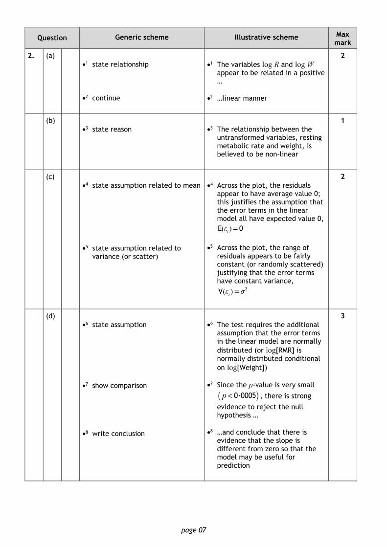
2. (a) •1 state relationship •2 continue

•1 The variables log R and log W

appear to be related in a positive …

•2 …linear manner

2

(b) •3 state reason

•3 The relationship between the

untransformed variables, resting metabolic rate and weight, is believed to be non-linear

1

(c) •4 state assumption related to mean

•5 state assumption related to

variance (or scatter)

•4 Across the plot, the residuals

appear to have average value 0; this justifies the assumption that the error terms in the linear model all have expected value 0,

( )iε =E 0 •5 Across the plot, the range of

residuals appears to be fairly constant (or randomly scattered) justifying that the error terms have constant variance,

( )iε σ= 2V

2

(d) •6 state assumption •7 show comparison

•8 write conclusion

•6 The test requires the additional

assumption that the error terms in the linear model are normally distributed (or log[RMR] is normally distributed conditional on log[Weight])

•7 Since the p-value is very small

( )0·0005p < , there is strong

evidence to reject the null hypothesis …

•8 …and conclude that there is

evidence that the slope is different from zero so that the model may be useful for prediction

3


(e) •9 give an interpretation of

confidence interval •10 write conclusion •11 give an interpretation of

prediction interval •12 write conclusion

•9 conclude from the confidence

interval that, with 95% confidence, the mean log[RMR] …

•10 …in the population of healthy

adult males who weigh 60 kg is between 7·28 and 7·33

•11 conclude from the prediction

interval that the log[RMR] of an individual healthy adult male…

•12 …who weighs 60 kg is very likely

to be between 7·09 and 7·52

4

(f) •13 state reason

•13 a weight of 100 kg corresponds to

log[Weight] = 4·61. This is clearly outside the range of sample values (and might fall into the range of overweight or obese values that were deliberately omitted from the study) so the fitted model might not be valid at this weight.

1

[END OF SPECIMEN MARKING INSTRUCTIONS]

S803/77/11 Statistics Paper 1 - SQA

Documents

Transcript of S803/77/11 Statistics Paper 1 - SQA