Rules and strategies for program transformation - Unpaywall
42
Rules and Strategies for Program Transformation* Alberto Pettorossi I and Maurizio Proietti 2 1 Electronics Department, University of Rome II, Via della Ricerca Scientifica, 1-00133 Roma, Italy, emaih adp~iasi.rm.cnr.it 2 IASI CNR, Viale Manzoni 30, 1-00185 Roma, Italy, email: [email protected] Abstract We present an overview of the program transformation methodology, focusing our attention on the so-called 'rules + strategies' approach in the case of functional and logic programs. The paper is intended to offer an introduction to the subject; it is not a complete account of the work in the area. 1 Introduction The program transformation approach to the development of programs has first been advocated by [Burstall-Darlington 77], although the basic ideas were already presented in previous papers by the same authors [Darlington 72, Burstall-Darlington 75]. In that approach the task of writing a correct and efficient program is realized in two phases: the first phase consists in writing an initial, maybe inefficient, program whose correctness can easily be shown, and the second phase, possibly divided into various subphases, consists in transforming the initial program so to get a new program which is more efficient. This methodology may avoid the difficulty of designing the invariant assertions of loops which are often quite intricate, especially for very efficient algorithms. The experience gained by the scientific comnmnity during the past two decades shows that the methodology of program transformation is very valuable and attractive, in par- ticular for the task of programming 'in the small', that is, when writing single modules of large software systems. Program transformation has also the advantage of being adaptable to various pro- gramming paradigms. In this paper we will focus our attention to the functional and logic cases. The basic idea of the program transformation approach is depicted in Fig. 1. From the initial program P0, which is the given specification, we want to obtain a final program Pn with the same semantic value, that is, Sem(Po) = Sem(P~) for some given semantic * This work has been partially supported by the 'Progetto Finalizzato Sistemi Informatici e Calcolo Parallelo' of the CNR, Italy, under grant n. 89.00026.69, MURST 40%, and Esprit Compulog II.
-
Upload
khangminh22 -
Category
Documents
-
view
3 -
download
0
Transcript of Rules and strategies for program transformation - Unpaywall
Rules and Strategies for Program Transformation*
Alberto Pe t toross i I and Mauriz io Proie t t i 2
1 Electronics Department, University of Rome II, Via della Ricerca Scientifica, 1-00133 Roma, Italy, emaih adp~iasi.rm.cnr.it
2 IASI CNR, Viale Manzoni 30, 1-00185 Roma, Italy, email: [email protected]
Abstrac t
We present an overview of the program transformation methodology, focusing our at tention on the so-called 'rules + strategies' approach in the case of functional and logic programs. The paper is intended to offer an introduction to the subject; it is not a complete account of the work in the area.
1 I n t r o d u c t i o n
The program transformation approach to the development of programs has first been advocated by [Burstall-Darlington 77], although the basic ideas were already presented in previous papers by the same authors [Darlington 72, Burstal l-Darlington 75].
In that approach the task of writing a correct and efficient program is realized in two phases: the first phase consists in writing an initial, maybe inefficient, program whose correctness can easily be shown, and the second phase, possibly divided into various subphases, consists in transforming the initial program so to get a new program which is more efficient.
This methodology may avoid the difficulty of designing the invariant assertions of loops which are often quite intricate, especially for very efficient algorithms.
The experience gained by the scientific comnmnity during the past two decades shows tha t the methodology of program transformation is very valuable and attractive, in par- t icular for the task of programming 'in the small ' , that is, when writing single modules of large software systems.
Program transformation has also the advantage of being adaptable to various pro- gramming paradigms. In this paper we will focus our at tention to the functional and logic cases.
The basic idea of the program transformation approach is depicted in Fig. 1. From the initial program P0, which is the given specification, we want to obtain a final program Pn with the same semantic value, that is, Sem(Po) = Sem(P~) for some given semantic
* This work has been partially supported by the 'Progetto Finalizzato Sistemi Informatici e Calcolo Parallelo' of the CNR, Italy, under grant n. 89.00026.69, MURST 40%, and Esprit Compulog II.
264 Alberto Pettorossi and Maurizio Proietti
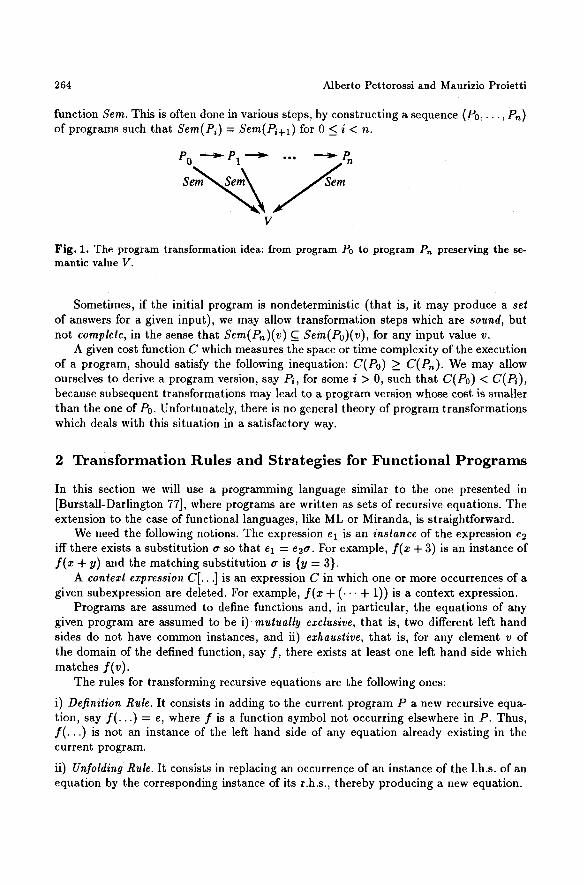
function Sem. This is often done in various steps, by constructing a sequence (P0, . . . , Pn) of programs such that Sem(Pi) = Sem(Pi+l) for 0 _< i < n.
P0 ~ P1 ~ "'" ~ Pn
V
Fig. 1. The program transformation idea: from program P0 to program Pn preserving the se- mantic value V.
Sometimes, if the initial program is nondeterministic ( that is, it may produce a set of answers for a given input), we may allow transformation steps which are sound, but not complete, in the sense that Sem(Pn)(v) C Sem(Po)(V), for any input value v.
A given cost function C which measures the space or t ime complexity of the execution of a program, should satisfy the following inequation: C(Po) > C(P,). We may allow ourselves to derive a program version, say Pi, for some i > 0, such that C(Po) < C(P~), because subsequent transformations may lead to a program version whose cost is smMler than the one of P0. Unfortunately, there is no general theory of program transformations which deals with this situation in a satisfactory way.
2 Transformation Rules and Strategies for Functional Programs
In this section we will use a programming language similar to the one presented in [Burstall-Darlington 77], where programs are written as sets of recursive equations. The extension to the case of functional languages, like ML or Miranda, is straightforward.
We need the following notions. The expression el is an instance of the expression e2 iff there exists a substitution ~ so that el = e2tr. For example, f (x + 3) is an instance of f (x + y) and the matching substitution cr is {y = 3}.
A context expression C[.. .] is an expression C in which one or more occurrences of a given subexpression are deleted. For example, f (x A- ( ." + 1)) is a context expression.
Programs are assumed to define functions and, in particular, the equations of any given program are assumed to be i) mutually exclusive, that is, two different left hand sides do not have common instances, and ii) exhaustive, that is, for any element v of the domain of the defined function, say f , there exists at least one left hand side which matches f(v).
The rules for transforming recursive equations are the following ones:
i) Definition Rule. It consists in adding to the current program P a new recursive equa- tion, say f ( . . . ) = e, where f is a function symbol not occurring elsewhere in P. Thus, f ( . . . ) is not an instance of the left hand side of any equation already existing in the current program.
ii) Unfolding Rule. It consists in replacing an occurrence of an instance of the 1.h.s. of an equation by the corresponding instance of its r.h.s., thereby producing a new equation.
Rules and Strategies for Program Transformation 265
For example, if we unfold the subexpression f(n + 1) in f(n + 2) = (n + 2) x f ( n + 1) using the equation f(n + 1) = (n + 1) • f(n), we get the new equation:
f (n + 2) = (n + 2) • ((n + 1) • f(n)).
iii) Folding Rule. It is the inverse of the unfolding rule. It consists in replacing an oc- currence of an instance of the r.h.s, of an equation by the corresponding instance of its l.h.s., thereby producing a new equation.
New programs are obtained from old ones by deriving new equations using the defini- tion, unfolding, and folding rules, and then considering mutually exclusive and exhaustive equations.
It can be shown that using the above three tranformation rules, partial correctness is preserved, that is, if the transformed program terminates then it computes the value computed by the original program [Kott 78].
However, during program transformation we are usually required to preserve total correctness, that is, i) the given program terminates iff the derived program terminates, and ii) in the case of termination, both programs compute the same result. Thus, after applying the definition, unfolding, and folding rules, we should also check that the derived program terminates for all input values for which the given program terminates.
We now list some more transformation rules which are often found in the literature (see, for instance, [Burstall-Darlington 77]):
iv) Instantiatiou Rule. It consists in the introduction of an instance of an already existing equation.
For example, by instantiating n to m + 1 in the equation: f(n + 1) --= (n + 1) x f(n), we get, after simplification, f (m + 2) = (m + 2) x f (m + 1).
v) Where-abstraction Rule. We replace a recursive equation f ( . . . ) = C[e] by the new equation: f ( . . . ) = C[z] w h e r e z = e, provided that z is a variable which does not occur in f ( . . . ) ---- C[e].
The use of the where-clause has the advantage that in the call-by-value mode of execution, the evaluation of the subexpression e is performed only once.
vi) Laws. We derive a new equation by using equalities which hold in the algebra of the basic operators. For instance, the equation f (n+ 1) = f(n) • ( n + 1) can be derived from f(n -4- 1) = (n + 1) x f(n), because • is commutative.
When performing program transformations we may end up with a final program which is equal to the initial one (recall that the folding rule is the inverse of the unfolding rule). Thus, during the transformation process, we need strategies which may allow us to derive programs with improved performance.
This can be done by introducing new functions, often called in the literature eureka functions. In the early days of the transformation methodology, those functions were generated by clever insights (hence their name) and not by strategies.
Unfortunately, there is no general theory of strategies which ensure that the derived programs are more efficient than the initial ones. However, partial results are available for some classes of programs.
Here are some transformation strategies which have been proposed in the literature. We will see them in action in various examples below.
266 Alberto Pettorossi and Maurizio Proietti
i) Composition Strategy. If the subexpression f(g(x)) occurs in an expression e,
- we introduce the function h(x) =d~] f(g(x)), - we find recursive equations for h(x), and - we replace f(g(x)) by h(x) in e, and possibly elsewhere in the given program.
A similar strategy, called Internal Specialization, is presented in [Scherlis 81]. By using the composition strategy one may avoid the construction of intermediate
da ta structures which are produced by g and used as input for f . This s trategy often allows the derivation of programs with bet ter performance than those obtained by lazy evaluation [Wadler 85] if the intermediate da ta structure is infinite and the 'next i tem' of the output of f can be produced by knowing only a finite port ion of the output of g.
it) Tupling Strategy. If the functions f1(x, x t l , . . . , xin) . . . . , fr(x, x r l , . . . , xrm) occur in an expression e,
- we introduce the function:
h ( X , X l l , - . . , X r m ) - - - d e f ( f l ( X , X l l , . . . , X l n ) , . . . , f r ( X , X r l , . . . , X r r n ) ) ,
- we find recursive equations for h(x, Xll . . . . ,x~m), and - we replace fi(x . . . . ) by 7ri(h(x, x11,...,Xrm)) for i : 1 , . . . , r , where ~ri denotes the
i-th projection function.
The use of the tupling strategy is very useful if the functions f l , . . . , f~ all have access to the same data structure x which is used by no other function. In this case the store used for x can be released as soon as the value of h has been computed. Often, by doing so, one may improve the time x space performance [Pettorossi 84].
The tupling strategy is also very effective when several functions require the compu- tat ion of the same subexpression, in which case we tuple together those functions.
By avoiding either multiple accesses to da ta structures or common subcomputat ions one often gets linear recursive programs (that is, equations whose r.h.s, has one recursive call only) from non-linear ones.
iii) Generalization Strategy. It is of various kinds as we now indicate.
1. Generalization from expressions to variables [Boyer-Moore 75, Aubin 79]. Given a recursive equation of the form f ( x l , . . . , xn) = e, such tha t a subexpression s occurs in e, we introduce the generalized recursive equation:
g(x, x l , . . . , x , ) = e[x/s] where x is a fresh new variable and e[xls] denotes the expression e with x subst i tuted f o r 8.
We then find recursive equations for g(x, x l , . . . , xn) , and we replace in the given program the occurrences of f ( e l , . �9 �9 en) by g(s, e l , . . . , e,~) for some given expressions e l i �9 . . ~e n .
2. Generalization from functions to functions by implicit definition [Darlington 81, Pet- torossi 84]. Let us consider a recursive equation of the form: f ( xx , . . . , xn) = C[expr]. Let {xi ] 1 < i < k} is the set of free variables in expr.
- We introduce the function g with arity k, such that there exist some expressions e l , . . . , ek (possibly with the variables xi 's) such that for all values of the variables xi's we have: C[g(el,... ,ek)] = C[expr],
Rules and Strategies for Program Transformation 267
- we find recursive equations for g(xl . . . . , xk), and - we replace the equation f (xl . . . . , xn) = C[expr] by the following one:
f ( ~ l , . . . , ~ , ) = c [ g ( e l . . . . ,e~)]. 3. Lambda Abstraction [Pettorossi-Skowron 87].
I t consists in replacing a given expression el by el[x/e2] w h e r e x = e2, or equiva- lently, (Ax.el[x/e2]) e2, where x is a fresh new variable and e2 is a subexpression of e 1 �9
Lambda Abstract ion is a form of generalization which can be applied when i) an expression and one of its subexpressions both visit the same da ta s t ructure and ii) tha t subexpression determines a mismatch which makes it impossible to perform a folding step.
We now give some examples of application of the strategies we have introduced. E x a m p l e 1 ( T h e C o m p o s i t i o n S t r a t e g y : Lis t P r o c e s s i n g ) The following program computes the sum of the even elements of a list, say l, of natural numbers.
1.1 eveusum(l) = sum(even(I)) 1.2 even([ ]) = [] 1.3 even(a :l) : i f odd(a) t h e n even(l) else a: even(l) 1.4 sum(l]) = 0 1.5 sum(a:l) .-= a A- sum(l).
Now, by using the composition strategy we can avoid the construction of the inter- mediate list of the even elements of l, which is the value of even(l) and it is passed as input to sum(_). We compose the functions sum(_) and even(_) and we define the new function:
h(I) =d~I sum(even(l)) . Thus, 1.6 h([ ]) = sum(even([ ])) = {unfolding} = 0 1.7 h(a :l) = sum(even(a:l)) : {unfolding} :
= sum(if odd(a) t h e n even(l) else a: even(l)) = {strictness of sum} : = i f odd(a) t h e n sum(even(l)) else sum(a :even(l)) = {unfolding} = = i f odd(a) t h e n sum(even(l)) else a + sum(even(I)) = {folding} = = i f odd(a) t h e n h(1) else a + h(1).
We finally express evensum in terms of the composite function h. In our case from Equation 1.1 we simply have: evensum(I) = h(l). []
During the derivation of Equation 1.7, the various transformation steps for h(_) have been suggested by the so called need for folding [Darlington 81], that is, the requirement of making recursive cMls to the composite function h(_), rather than to the component functions sum(_) and even(_).
In particular, the use of the strictness of sum was due to the syntactic requirement of producing the occurrences of sum(even(l)) which can then be folded using h(l). By performing those folding steps, the efficiency improvements due to the unfoldings from sum(even(a: l)) to i f odd(a) t h e n sum(even(l)) else a + sum(even(l)), can be i tera ted at each level of recursion, and thus, they become computat ionally significant. Indeed, in what follows we will see that by performing folding steps we may transform an exponential t ime algori thm into a linear time one.
268 Alberto Pettorossi and Maurizio Proietti
The idea of need for folding plays a major role in the program transformation method- ology. It can be regarded as a meta-strategy because, as we will see in the examples below, it is the need for folding that often suggests the suitable strategies to apply.
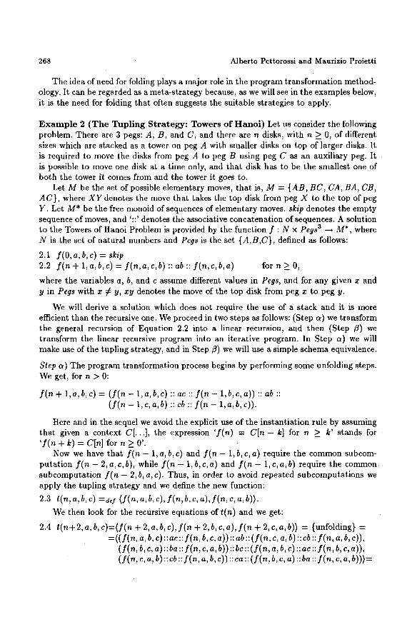
E x a m p l e 2 ( T h e T u p l i n g S t r a t e g y : Towers o f H a n o i ) Let us consider the following problem. There are 3 pegs: A, B, and C, and there are n disks, with n > 0, of different sizes which are stacked as a tower on peg A with smaller disks on top of larger disks. It is required to move the disks from peg A to peg B using peg C as an auxiliary peg. It is possible to move one disk at a time only, and that disk has to be the smallest one of both the tower ft comes from and the tower it goes to.
Let M be the set of possible elementary moves, tha t is, M = {AB, BC, CA, BA, CB, AC}, where X Y denotes the move that takes the top disk from peg X to the top of peg Y. Let M* be the free monoid of sequences of elementary moves, skip denotes the empty sequence of moves, and ':: ' denotes the associative concatenation of sequences. A solution to the Towers of Hanoi Problem is provided by the function f : N x Pegs 3 ~ M*, where N is the set of natural numbers and Pegs is the set {A,B,C}, defined as follows:
2.1 f(O,a,b,c) = skip 2.2 f ( n + l , a , b , c ) - - f ( n , a , c , b ) : : a b : : f ( n , c , b , a ) for n >_ 0,
where the variables a, b, and c assume different values in Pegs, and for any given x and y in Pegs with x ~ y, xy denotes the move of the top disk from peg x to peg y.
We will derive a solution which does not require the use of a stack and it is more efficient than the recursive one. We proceed in two steps as follows: (Step a) we transform the general recursion of Equation 2.2 into a linear recursion, and then (Step j3) we transform the linear recursive program into an i terative program. In Step or) we will make use of the tupling strategy, and in Step ~) we will use a simple schema equivalence.
Step v~) The program transformation process begins by performing some unfolding steps. We get, for n > 0:
f ( n + 1,a,b,c) =- ( f ( n - 1,a,b,c) :: ac :: f (n - 1,b,c,a)) :: ab :: ( f ( n - 1, c,a,b) :: cb :: f ( n - 1,a,b,c)).
Here and in the sequel we avoid the explicit use of the instantiat ion rule by assuming that given a context C[.. .] , the expression ' f (n) = C [ n - k] for n >__ k' stands for ' f (n -4- k) = C[n] for n _> 0'.
Now we have that f (n - 1, a, b, c) and f (n - 1, b, c, a) require the common subcom- putat ion f ( n - 2, a, c, b), while f ( n - 1, b, c, a) and f ( n - 1, e, a, b) require the common subcomputat ion f ( n - 2, b, a, c). Thus, in order to avoid repeated subcomputat ions we apply the tupling strategy and we define the new function:
2.3 t(n,a,b,c)=clef ( f (n ,a ,b ,c ) , f (n ,b ,c ,a ) , f (n ,c ,a ,b ) ) .
We then look for the recursive equations of t(n) and we get:
2.4 t ( n + 2 , a, b, e)=(f(n + 2, a, b, c), f (n + 2, b, c, a), f ( n + 2, c, a, b)) = {unfolding} = =((f(n,a,b,c)::ac:: f(n,b,e,a))::ab::(f(n,c,a,b)::cb:: f (n ,a ,b ,c)) ,
( f (n, b, c, a):: ba :: f (n , c, a, b)):: bc :: ( f (n , a, b, c):: ac :: f (n , b, c, a)), ( f (n, c, a, b):: cb:: f (n , a, b, c)):: ca:: ( f (n , b, c, a): : ba :: f (n , c, a, b)))--
Rules and Strategies for Program Transformation 269
={folding and where-abstraction} = =((u::ae::v)::ab::(w::cb::u),
(v::ba::w)::bc::(u::ac::v), (w::cb::u)::ca::(v::ba::w)) w h e r e ( u , v , w ) = t ( n , a , b , c ) for n > 0 .
Since t (n+2 , a, b, c) is defined in terms of t (n , a, b, c), in order to ensure the terminat ion of the evaluation of t(n + 2, a, b, c) for n > 0, we need to provide the equations for t(0, a, b, c) and t(1, a, b, c). By unfolding we get:
2.5 t(0, a, b, c) = (skip, skip, skip) 2.6 t (1,a,b,c) = Cab, be, ca).
Thus, we have obtained a linear recursive program for the function t. We then express the function y ( n , a, b, c) in terms of t ( n - 2, a, b, c) by unfolding and where-abstract ion steps. We get:
2.7 y (n ,a ,b , e )= ( ( y (n -2 , a ,b ,e)::ac::y(n-2,b,c ,a)) :: ab :: ( y ( n - 2 , c, a, b):: cb :: f ( n - 2, a, b, c))) =
=((u::ac::v)::ab::(w::cb::u)) w h e r e (u ,v ,w) = t(n-2, a,b,c) for n > 2 .
In order to preserve termination, since f (n , a, b, e) is defined in terms o f t ( n - 2 , a, b, c), we have to provide the values of f(O, a, b, e) and f(1, a, b, c). From Equations 2.1 and 2.2 we get:
2.8 f(0, a, b, c) = skip 2.9 f (1 , a, b, c) = ab.
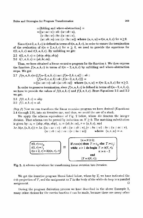
Step fl) Now we can transform the linear recursive program we have derived (Equations 2.4 through 2.9), into an iteratlve one, and thus, we avoid the use of a stack.
We apply the schema equivalence of Fig. 2 below, where div denotes the integer division. That schema can be proved by induction on N _> 0. The matching subst i tut ion is given by: z0 = (skip, skip, skip), Zl = Cab, bc, ca), r = Ca, b, c), and Ax.h(x, Ca, b,c)) = Ax.C(u :: ac :: v) : : ab :: (w :: cb :: u),(v :: ba :: w) : : bc :: (u :: ac :: v),
(w :: eb :: u) :: ca :: (v :: ba :: w)~ where (u, v, ~ /= x.
Ii (0, r) =z 0 1 (1, r) = z 1 (n + 2, r) = h(t(n, r), r
{n=N_>O} 1 if even(n) then T :=z 0 else T :=Zl; while n > 1 do begin T := h(T, r);
n : = n - 2 end
IT = t(N, r)}
Fig. 2. A schema equivalence for transforming linear recursion into iteration.
We get the iterative program Hanoi listed below, where by 71/ we have indicated the i-th projection of T, and the assignment to T in the body of the while-do loop is a parallel assignment. []
During the program derivation process we have described in the above Example 2, many other choices for the eureka function t can be made, because there are many other
270 Alberto Pettorossi and Maurizio Proietti
{n = N > 0} Program Hanoi i f n = 0 t h e n F := skip else if n = 1 t h e n F := ab else b e g i n n := n - 2; i f even(n) t h e n T := (skip, skip, skip) else T := (ab, bc, ca);
whi le n > 1 do b e g i n T := (T1 :: ac :: T2 :: ab :: T3 :: cb :: T1, T2 :: ba :: T3 :: bc :: T1 :: ac :: 7"2, T3 :: cb :: T1 :: ca :: T2 :: ba :: T3);
n : ~ - n - - 2
end; F := T1 : : a c : : T 2 : : a b : : T 3 : : c b : : T 1
end {F = f (N,a ,b ,c)}
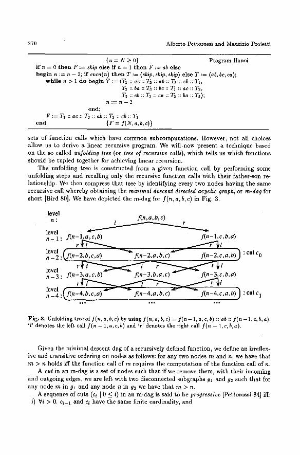
sets of funct ion calls which have common subcomputa t ions . However, not all choices allow us to derive a linear recursive program. We will n o w present a technique based on the so called unfolding tree (or tree of recursive calls), which tells us which funct ions should be tupled together for achieving linear recursion.
The unfolding tree is const ructed from a given funct ion call by performing some unfolding steps and recalling only the recursive funct ion calls wi th their fa ther-son re- lat ionship. We then compress that tree by identifying every two nodes having the same recursive call whereby obtaining the minimal descent directed acyclic graph, or m-dag for short [Bird 80]. We have depicted the m-dag for f ( n , a, b, c) in Fig. 3.
level f ( n ,a ,b , c )
n: l
level ~ n - 1 : f ( n - l , a , c , b ) f ( n - l , c , b , a )
r ~ ~ . . , ~ ~ l
leveln_2: ( f ( n - 2 , b , c , a ) ~ " ~ f ( n - 2 , a , b , c ) ~ f(n-2,c,a,b)) : cUtco
level r ~ ~ ~ l n - 3 : f ( n - 3 , a , c , b ) f ( n - 3 , b , a , c ) f ( n - 3 , c , b , a )
r l ,d~'-~ ~'n~ l r ,~w'-- ~ . .~ r l
n-4:level ( f ( n - 4 , b , c , a ) f ( n - 4 , a , b , c ) f ( n - 4 , c , a , b ) J : c u t c 1
F ig . 3. Unfolding tree of f (n , a, b, c) by using f (n , a, b, c) = f (n - 1, a, c, b) :: ab :: f (n - 1, c, b, a). 'l' denotes the left call f (n - 1,a,c,b) and ' r ' denotes the right call f ( n - 1,c,b,a).
Given the min imal descent dag of a recursively defined funct ion, we define an irreflex- i re and t ransi t ive ordering on nodes as follows: for any two nodes m and n, we have tha t m > n holds iff the function call of m requires the computa t ion of the funct ion call of n.
A cut in an m-dag is a set of nodes such tha t if we remove them, wi th their incoming and outgoing edges, we are left wi th two disconnected subgraphs gl and g2 such tha t fo r any node m in gl and any node n in g2 we have tha t m > n.
A sequence of cuts (ci I 0 < i) in an m-dag is said to be progressive [Pettorossi 84] iff: i) Vi > 0. ci-x and ci have the same finite cardinality, and
Rules and Strategies for Program Transformation 271
ii) Vi > O. ci_ 1 # ci, and iii) Vi > 0. Vn E ci. 3m E ci-1. if n # m then m > n, and iv) V i > 0 . V m E c i _ l . 3 n E c i . i f n # m t h e n m > n .
From i) and ii) it follows that for all i > 0, neither ci-1 is contained in ci nor c/ is contained in ci-1. In intuitive terms, while moving along a progressive sequence of cuts from Ci_l to ci we trade ' large' nodes for 'small ' nodes. Thus, given the m-dag of Fig. 3 where m > n is depicted by positioning the node m above the node n, we have, among others, the following cuts:
co = { f ( n - 2 ,a ,b , c ) , f (n - 2, b , c , a ) , f ( n - 2,c,a,b)}, cl = { f ( n - 4, a ,b , c ) , f (n - 4, b , c ,a ) , f (n - 4 ,c ,a ,b )} , . . . ,
and S = (co, c l , . . . ) is a progressive sequence of cuts. It can be shown that if a progressive sequence of cuts (ci I 0 < i) exists for the m-dag
of the function call f such that : i) the initial function call of f can be computed from the function calls of the cut co,
and ii) there exists a function, say h, not depending on i and such tha t for each i >_ 0, the
function calls of ci-1 can be computed from those of ci using h, then the tupling strategy which tuples together the function calls in a cut, generates a linear recursive program for the computation of f .
This result allowed us to perform Step ~) of the derivation of Example 2. Indeed, Equation 2.3 has been determined by tupling the function calls of a cut in the above mentioned sequence 5:.
With respect to Step t3) of that derivation, that is, the transformation from a linear recursive program to an iterative one, we want to mention that there is a general result [Paterson-Hewitt 70] which ensures that every linear reeursion can be t ranslated into an i teration using a constant number of memory cells ( that is, avoiding the use of a stack). However, that result cannot be used in the context of the program transformation methodology, because it degrades the time performances from O(n) to O(n2). Thus, we used, instead, the schema equivalence of Fig 2.
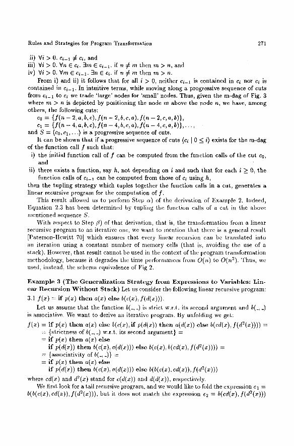
E x a m p l e 3 ( T h e G e n e r a l i z a t i o n S t r a t e g y f r o m E x p r e s s i o n s to V a r i a b l e s : Lin- e a r R e c u r s i o n W i t h o u t S t a c k ) Let us consider the following linear reeursive program:
3.1 f ( x ) -- i f p(x) t h e n a(x) else b(c(x), f (d(x)) ) . Let us assume that the function b(_, _) is strict w.r.t, its second argument and b(_, _)
is associative. We want to derive an iterative program. By unfolding we get:
f ( z ) = i f p(x) t h e n a(x) else b(c(x), if p(d(x)) t h e n a(d(x)) e l se b(cd(x), f (d2(x)) ) ) = = {strictness of b(_,_) w.r.t, its second argument} = = i f p(x) t h e n a(x) else
i f p(d(x)) t h e n b(c(x), a(d(x))) else b(c(x), b(cd(x), f (d2(x))) ) = = {assoeiativity of b(_,_)} = = i f p(x) t h e n a(x) e l se
i f p(d(x)) t h e n b(c(x), a(d(x))) else b(b(c(x), cd(x)), f (d2(x)))
where cd(x) and d2(/) s tand for c(d(x)) and d(d(x)), respectively. We first look for a tail recursive program, and we would like to fold the expression el =
b(b(c(x), cd(x)), f (d2(x))) , but it does not match the expression e2 = b(cd(x), f (d2(x) ) )
272 Alberto Pettorossi and Maurizio Proietti
which is the value of f(d(x)) for p(d(x)) = false. The mismatch between the first argu- ments of the outermost b's in el and e2 makes it impossible to perform a folding step.
Thus, the need for folding suggests the following definition, which introduces the variable y:
3.2 F(y ,x )=des b(y, f (x)) ,
whose r.h.s, is an expression which generalizes both el and e2. We get: f ( y , x) =def b(y, f (x)) = {using Equation 3.1} =
= b(y, i f p(x) t h e n a(x) else b(c(x), f(d(x)))) = {strictness of b(_,_)} = = if p(x) t h e n b(y, a(x)) else b(y, b(c(x), f(d(x)))) = {associativity of b(_, _)} = = if p(x) t h e n b(y, a(x)) else b(b(y, e(x)), f(d(x))) = {folding} = = if p(x) t h e n b(y, a(x)) else F(b(y, c(x)), d(x)).
Thus, by folding Equation 3.1 we get the following program for f (x) :
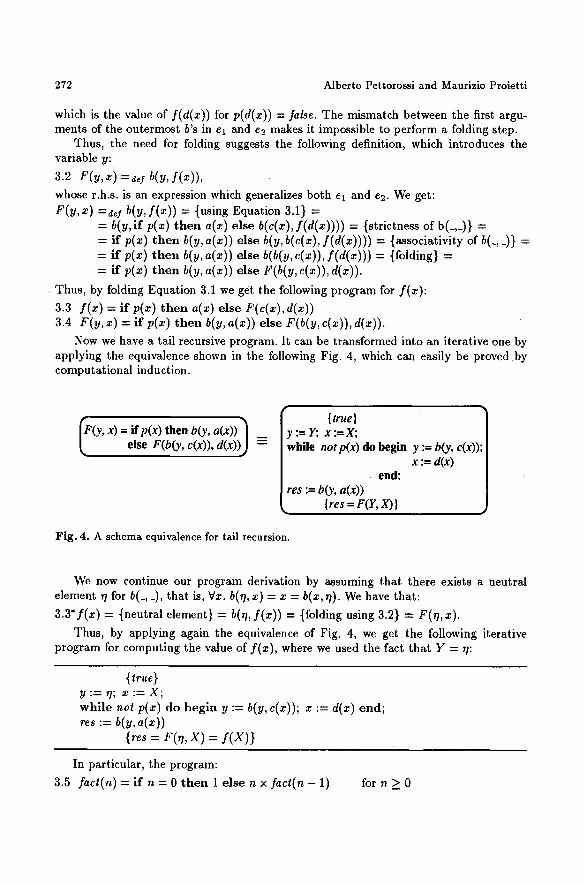
3.3 f (x) = if p(x) t h e n a(x) else F(c(x),d(x)) 3.4 F(y, x) = if p(x) t h e n b(y, a(x)) else F(b(y, c(x)), d(x)).
Now we have a tail recursive program. It can be transformed into an iterative one by applying the equivalence shown in the following Fig. 4, which can easily be proved by computational induction.
Ffy, x) = if p(x) then b(y, a(x)) else F(b(y, c(x)), d(x))) ~
{ true} := Y; x := X;
while notp(x) do begin y := b(y, c(x)); x := d(x)
end; res := b(y, a(x))
{ res = F(Y, X) }
Fig. 4. A schema equivalence for tail recursion.
We now continue our program derivation by assuming that there exists a neutral element ~/for b(_, _), that is, Vx. b(~l, x) = x = b(x, ~). We have that:
3.3* f (x ) = {neutral element} = b(T1, f (x)) = {folding using 3.2} = F(0, x).
Thus, by applying again the equivalence of Fig. 4, we get the following iterative program for computing the value of f (x) , where we used the fact that Y = ~/:
{true} y:=~/ ; x : = X ; whi le not p(x) do beg in y := b(y, c(x)); x := d(x) end; rcs := b(y, a(x))
{res = F(r h X) = f (X)}
In particular, the program:
3.5 fact(n) = if n = 0 t h e n 1 else n x f a c t ( n - 1) for n > 0
Rules and Strategies for Program Transformation 273
is an instance of Equation 3.1 for b(y, z) = y x x, a(z) = y = 1, and c(x) = z. Thus, Equations 3.3* and 3.4 produce the following tail recursive program for fact(n):
3.6 fact(n) = G(1,n) for n > 0 3.7 G(v,n) = if n = 0 t h e n V else G(y x n , n - 1).
The corresponding iterative program obtained by using the equivalence of Fig. 4, is:
{N >_ 0} Program Factorial.1 y : = l ; n : = N ; w h i l e n # O d o b e g i n y : = y x n ; n : = n - l e n d ; res := y x 1
{ms = G(1, N) = fact(N)}
where the precondition {true} of Fig. 4 has been strengthened by {N > 0}. In this last program we can replace n r 0 by n > 0 (because N >_ 0) and y x 1 by y. We can also get rid of the variable res, and use instead the variable y. Thus, the assignment res := y x 1 can be avoided. We get:
{N > 0} Program Factorial.2 y : = 1; n : = N ; w h i l e n > 0 d o b e g i n y : = y x n ; n : = n - l e n d ;
{y = fact(N)}
o The program for the function f consisting of Equations 3.3* and 3.4 can also be
derived from Equation 3.1 by applying the so called accumulation strategy [Bird 84], whereby given an associative operation (b(_,_), in our case), we can store the partial results of its application at each reeursive call, in a new argument (y, in our case). The derivation we have presented in the above Example 3, indicates that such a new argument which plays the role of an accumulator, comes from a generalization step.
Now we give some more examples where it will be shown that:
i) the generalization strategy from (sub)expressions to variables may allow us to get a tail recursive program, even though the initial program is not linear recursive (Example 4),
ii) the generalization from functions to functions by implicit definition may allow us to exponentially reduce the time complexity (Example 5), and
iii) the Lambda Abstraction strategy allows us to define and manipulate pointers in a disciplined way and visit data structures only once (Example 6). (For a transforma- tional approach to the derivation of programs which use pointers, the reader may also refer to [MSller 93]).
E x a m p l e 4 ( T h e Ge ne ra l i z a t i on S t r a t e g y f r o m Expres s ions t o Var iab les : T ree P r o c e s s i n g ) Let us consider the following program which computes the height of a binary tree [Chatelin 76].
4.1 h(tip(m)) = 0 4.2 h(tree(S,T)) = 1 + max(h(S),h(T)).
We perform some unfolding steps starting from Equation 4.2 and we have:
274 Alberto Pettorossi and Maurizio Proietti
4.3 h(tree(S, T)) = 1 + maz(h(S), h(T)) = = max(1 + h(S), 1 + h(T)) = {assuming S = tree(Sl, 6'2)} = = max(2 + max(h(S1), h(S2)), 1 + h(T)) = = {distributivity of + over max} = = max(max(2 + h(S1), 2 + h(S2)), 1 + h(T)) = = {associativity of maz} = = max(2 + h(S1), max(2 + h(S2), 1 + h(T))).
In order to get a tail recursive program by folding, we match this last expression against the previous versions of the r.h.s, of Equation 4.3. We have that the expression max(2 + h(S1), max(2 + h(S2), 1 + h(T)))is an instance of max(1 + h(S) , 1 + h(T)) if we generalize the constant 1 (occurring in 1 + h(S)) and the second argument 1 + h(T) to the variables n and u, respectively. ThuS, we define the following generalized function g:
4.4 g(n, S, It) =def max(n + h(S), u).
We have that:
4.5 h(T) = {properties of max} = max(O + h(T),O) = {folding using 4.4} = g(O,T,O). The recursive equations for the function g are as follows:
4.6 g(n, tip(m),u) = {by 4.4 and 4.1} = maz(n+O,u) = max(n,u) 4.7 g(n, tree(S,T),u) = max(n + h(tree(S,T)),u) = {unfolding} =
= maz(n + 1 + max(h(S), h(T)), u) = = {distributivity of + over max} = = maz(max(n + 1 + h(S),n + 1 + h(T)),u) = = {associativity of max} = = max(n + 1 + h(S), max(n + 1 + h(T); u)) = = {folding using 4.4} = = g(n + 1, S, max(n + 1 + h(T), u)).
By a final folding step using 4.4 we get:
4.8 g(n, tree(S, T), u) = g(n + 1, S, g( , + 1, T, u)).
Thus, one of the two genuine recursive calls in the r.h.s, of Equation 4.2 has been transformed into a tail recursive one.
The final program is made out of the equations 4.5, 4.6, and 4.8. []
Example 5 ( T h e G e n e r a l i z a t i o n S t r a t e g y f r o m F u n c t i o n s to F u n c t i o n s : L i n e a r R e c u r r e n c e R e l a t i o n s in L o g a r i t h m i c T i m e ) We first consider the simple case of the Fibonacci function.
5.1 f (0) = 1 Program Fibonacci.0 5.2 / ( 1 ) = 1 5.3 f (n + 2) = f(n-4- 1) + f(n) for n > 0.
We first generalize the two occurrences of the constant 1 in the r.h.s. 's of Equations 5.1 and 5.2 to the distinct variables a0 and al . We get the following equations, where n > 0 :
5.4 G(ao,al,0) = a0 5.5 G(ao,al, 1) = al
Rules and Strategies for Program Transformation 275
5.6 G ( a o , a l , n + 2) = G(ao, a l , n + 1) + G(ao, a l ,n) 5.7 f ( n ) = G(1, 1, n).
We then generalize the constant 2 occurring in Equation 5.6 to a variable, say k, and we define the following function for n >_ 0 and k >_ 0:
5.8 F(ao, al, n, k) =a~f G(ao, al, n + k).
We have: 5.9 F(ao, al, n, O) = G(ao, ax, n) 5.10 F(ao ,a l , n ,1 ) = G(ao,a l ,n + 1) 5.11 F(ao, el, n, k + 2) = G(a0, e l , n + k + 2) -- {unfolding} =
= G(ao, al, n -1- k -t- 1) + G(ao, al , n + k) = {folding} = = F(ao, al, n, k + 1) + F(ao, al, n, k).
We may then perform some unfolding steps s tar t ing from F(ao, al , n, k + 2). We get:
F(ao, al, n, k + 2) = F(ao, al, n, k + 1) + F(ao, al, n, k) = = 2 F(ao, al, n, k) + F(ao, al, n, k - i) = = 3F(ao, a l , n , k - 1) + 2 F ( a 0 , a l , n , k - 2)
and eventually we get:
F(ao, al, n, k --1- 2) = Cl F(ao, al, n, 1) -~- c2 F(ao, al, n, O) = -- Cl G(ao, al, n + l ) + c2 G(ao, at, n).
We can now perform a generalization step from functions to functions by implicit definition and we assume that the constants cl and c2 are the values of two functions, say s(k) and r(k). Thus, we assume that:
5.12 F ( a 0 , a l , n , k ) = r(k) C(ao,al ,n) + s(k) G(ao,a l ,n + 1)
and we look for the explicit definition of the functions r(k) and s(k).
From Equations 5.9 and 5.12 we get: G(ao, al, n) = r(O) G(ao, a,, n) + s(O) C(ao, a,, n + 1), and since this equality should hold for all values of a0 and al, we get: r(0) = 1 and s(0) = 0.
Analogously, from Equations 5.10 and 5.12 we get: r(1) = 0 and s(1) = 1. From the r.h.s. 's of Equations 5.11 and 5.12 (for k + 2 instead of k) we get:
F(ao, al, n, k + 1) + F(ao, Ctl, n, k) ~- r(]r At- 2)a(ao, Ctl, n) -4- s(k -[- 2)a(ao, al, n -4- 1).
By Equation 5.12 for k and k + 1 we have:
,.(k + 1)C(ao, a~, n) + s(k + 1)c(,~o, a~, n + 1.) +, ' (k)a(ao, ,~, n) + s(k)C(~o, a~, ,~ + 1) = = r(k A- 2)G(a0, a l , n) q- s(k q- 2)G(a0, al , n -4- 1)
which gives us the two equations: r ( k + 2 ) = r (k+ 1 ) + r ( k ) and s ( k + 2 ) = s ( k + 1 ) + s ( k ) .
Therefore, having r(0) = 1, ,'(1) = 0, and r(k + 2) = r(k + 1) + r(k) we derive by Equations 5.4, 5.5, and 5.6 that :
r ( k ) = G ( 1 , 0 , k) and s ( k ) = G ( O , l , k ) .
Thus, from Equation 5.12 we get for n > 0 and k >_ 0:
5.13 G(a0, a l , n A- k) = G(1,0, k) G(a0, el, n) -4- G(O, 1, k) G(ao, a l , n + 1).
From Equation 5.13 for n = k and n = k + 1 we get Equations 5.14 and 5.15 of the following program for computing the Fibonacci function, where n > 0 and k > 0:
276 Alberto Pettorossi and Maurizio Proietti
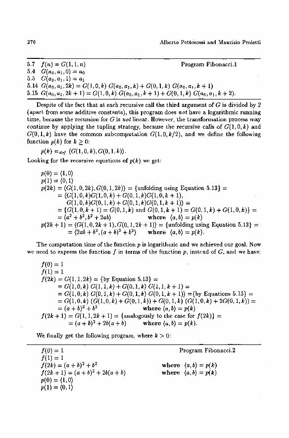
5.7 f (n )=G(1 ,1 ,n ) Program Fibonacci.1 5.4 G(ao,al,O) = ao 5.5 G(ao ,a l ,1 ) :a l 5.14 G(ao, al ,2k)=G(1,0, k) G(ao,al, k ) + G ( O , l , k ) e ( a o , a l , k + l ) 5.15 G(ao, a l ,2k+l )=G(1 ,O,k )G(ao ,a~ ,k+ 1) +G(O,l ,k) G(ao,al ,k+2).
Despite of the fact that at each recursive call the third argument of G is divided by 2 (apart from some additive constants), this program does noL have a logarithmic running time, because the recursion for G is not linear. However, the transformation process may continue by applying the tupling strategy, because the recursive calls of G(1,0, k) and G(0, 1, k) have the common subcomputation G(1,O,k/2), and we define the following function p(k) for k _> 0:
p(k) = a ~ y (a(1, 0, k),G(O, 1, k)). Looking for the recursive equations of p(k) we get:
p(0) = (1,0) p(1) = (0, 1) p(2k) = (G(1,0, 2k), G(0, 1,2k)) = {unfolding using Equation 5.13} =
= (G(1, 0, k)e(1,0, k) + G(0, 1, k)G(1, 0, k + 1), a(1, 0, k)G(O, 1, k) + G(O, 1, k)e(o, 1, k + 1)) =
= {e(1 ,0 , k + 1) = G(0, 1, k) and G(0, 1, k + 1) = G(0, 1, k) + G(1,0, k)} = : (a 2 Jr b 2, b 2 + 2ab) w h e r e (a, b) = p(k)
p(2k + 1) = (G(1,0,2k + 1),G(0, 1,2k + 1)) = {unfolding using Equation 5.13} = = (2ab + b 2, (a + b) 2 + b 2) w h e r e (a, b) = p(k).
The computation time of the function p is logarithmic and we achieved our goal. Now we need to express the function f in terms of the function p, instead of G, and we have:
f ( 0 ) = 1 f ( 1 ) = 1 f(2k) = G ( 1 ,
= G ( 1 , = G ( 1 , = G ( 1 ,
1,2k) = {by Equation 5.13} = 0, c(1,1, k) + c(0,1, k) G(1, 1, k + 1) = 0, k) G(0, 1, k) + G(0, 1, k) G(0, 1, k + 1)) ={by Equations 5.13} = 0, k) (G(1, 0, k) + G(0, 1, k)) + G(0, 1, k) (G(1, 0, k) + 2G(0, 1, k)) =
= (a + b) 2 + b 2 w h e r e (a, b) = p(k) f(2k + 1) = e(1 , 1,2k + 1) = {analogously to the case for f(2k)} =
= (a + b) 2 + 2b(a + b) w h e r e (a, b) = p(k).
We finally get the following program, where k > 0:
f(0)= 1 f ( 1 ) : 1 J(2k)=(a+b)2+b2 f(2k+l)=(a+b)2+2b(a+b) p(0)= (1,0) p(1)=(0,1)
Program Fibonacci.2
where (a,b) = p(k) where (a, b) = p(k)
Rules and Strategies for Program Transformation
p ( 2 k ) = (a ~ + b ~ , 2 a b + b ~) p(2~ + 1) = (~.b + b ~, (~ + b) 2 + b~)
where (a,b) : p(k) where (a,b) = p(k).
277
The derivation of this program for the logarithmic evaluation of the Fibonacci function shows the strength of the combined use of the generalization strategy together with the tupling strategy. In what follows we will see more examples of this synergism between the two strategies.
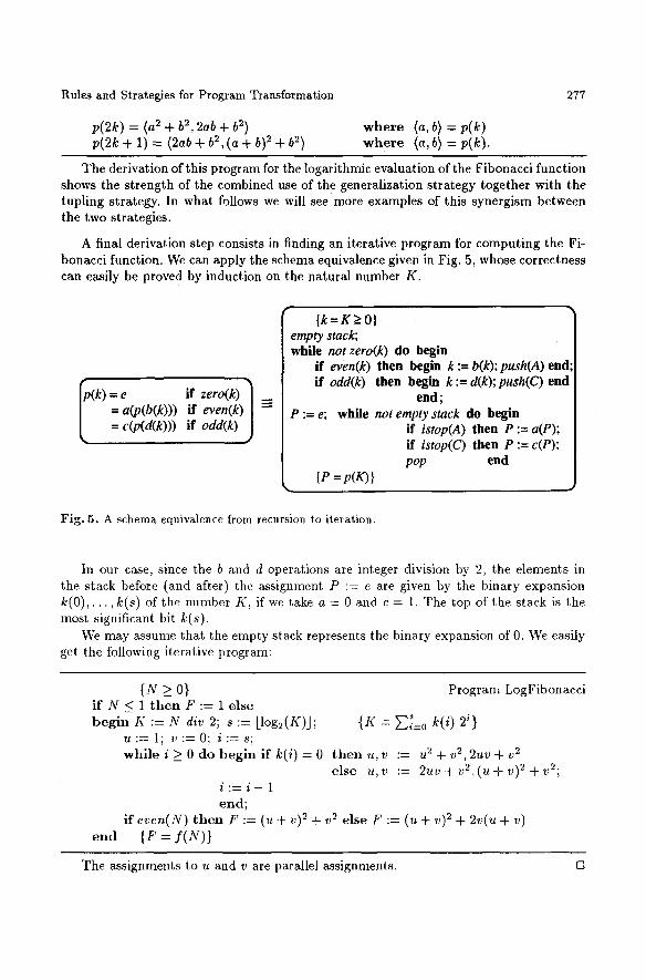
A final derivation step consists in finding an iterative program for computing the Fi- bonacci function. We can apply the schema equivalence given in Fig. 5, whose correctness can easily be proved by induction on the natural number K.
p(k)= e if zero(k) = a(p(b(k))) if even(k)] = c(p(d(k))) if odd(k) J
I k = K > 0 } empty stack; while not zero(k) do begin
if even(k) then begin k := b(k); push(A) end if odd(k) then begin k := d(k); push(C) end
end; P := e; while not empty stack do begin
if istop(A) then P := a(P); if istop(C) then P := c(P); pop end
{P = p(K)}
Fig. 5. A schema equivalence from recursion to iteration.
In our case, since the b and d operations are integer division by 2, the elements in the stack before (and after) the assignment P := e are given by the binary expansion k (O) , . . . , k ( s ) of the number K, if we take a = 0 and c = 1. The top of the stack is the most significant bit k(s).
We may assume that the empty stack represents the binary expansion of 0. We easily get the following iterative program:
{N >__ o} i f N < l t h e n F : = l e l s e b e g i n I f := N div 2; s := [log2(K)J;
e n d
Program LogFibonacei
{K = E;=0 k(i) 2 ~} u : - - 1; v : = 0 ; i : = s ; w h i l e i > 0 d o b e g i n i f k ( i ) = 0 t h e n u , v := u 2 + v 2,2uv + v ~
else u ,v := 2 u v + v 2 , ( u + v ) 2 + v 2 ; i : = i - 1 end;
i f even(N) t h e n F := (u + v) 2 + v 2 e lse F := (u + v) 2 + 2v(u + v) {F = / ( N ) }
The assignments to u and v are parallel assignments. []
278 Alberto Pettorossi and Maurizio Proietti
We can extend the derivation shown in Example 5 to any homogeneous linear recur- rence relation with constant coefficients of order r in any semiring structure, with the two operations denoted by + and x. Hence, we can derive a logarithmic time algorithm for computing any function h defined as follows:
h(0) = h 0 , . . . , h ( r - 1) = hr_l h(n) = (box h ( n - r)) + . . . + (br-1 x h ( n - 1)) for n > r.
The interested reader may refer to [Pettorossi-Burstall 82].
Example 6 (The Lambda Abstraction Strategy: Palindrome in One Visit Avoiding the Append F u n c t i o n ) Let us consider the following program for testing whether or not a given list 1 is palindrome.
6.1 palindrome(l) = eqlist(1, rev( I) ) 6.2 eqZist([ ], []) = t , ~ e
6.3 eqlist(a:11, b:12) = (a = b) and eqlist(ll, 12) 6.4 rev([]) = [1 6 .5 ,~v(a:Z) = , ~ ( l ) : : [a] 6.6 �9 :: U = i f �9 = [ ] t h e n y else hd(~ ) : ( tZ (~ ) : : y)
where : and :: are the infix operators for cons and append, respectively. This program visits the given list twice, a first time for its reversal (using rev) and a second time for testing equality (using eqlist). We look for a program which visits the given list only once. We also want to avoid the use of the append function which is expensive, because using Equation 6.6 the number of cons operations needed for reversing a list of length n is O(n2).
Equations 6.4 and 6.5 can be transformed into a tai l recursive form as indicated in Example 3. Indeed, they are an instance of Equation 3.1 for p(x) = null(x) , a(x) = ~/= [], b(z, y) = y :: x, c(z) = [hd(x)], and d(x) = tl(x). By writing h(z, y) instead of F ( y , z ) , from Equations 3.3* and 3.4 we get:
6.7 ,~v(t) = h(Z,[]) 6 .8 h ( [ ] , ~ ) = 6.9 h(a : l , z ) = h(l,[a] :: z) = h( l ,a:x) ,
where h( l , x ) =d~f vev(1) :: x. Thus, we obtain a program without the append function by replacing the equations 6.4, 6.5, and 6.6 by the equations 6.7, 6.8, and 6.9. Then, in order to derive a program which goes through the input list only once, we continue our program transformation by applying the composition strategy. We get:
6.10 palindrome([ ]) = eqlist([ ], rev([ ])) = {unfolding} = true 6.11 palindrome(a: I) = eqlist( a : I, rev( a : l)) = {unfolding} =
= (a = hd(rev(a: I))) and eqlist(l, t l(rev(a: l))).
When trying to fold the r.h.s, of Equation 6.11 using Equation 6.1 we have a mismatch between the expression eqlist(l, rev(l)) in Equation 6.1 and eqlist(l, t l (rev(a: I))) in Equa- tion 6.11. We can apply the Lambda Abstraction strategy which consists in abstract ing away the mismatching argument. In our case we rewrite Equation 6.11 as follows:
6.12 palindrome( a : l) = eqlist( a : I, rev( a : l)) = {by Lambda Abstract ion} = = ()~z. eqlist(a:l, x ) )rev(a: l ) = {Equation 6.7} = = ($z. eqlist(a :1, x))h(a :1, []).
Rules and Strategies for Program Transformation 279
Now, both Ax. eqlist(a: I, x) and h(a:l, []) visit the same data structure a: l . We can use the tupling strategy and we define:
6.13 Q(I) =d,Y ()tx. eqlist(l, x), h(l, [])), whose recursive equations are as follows:
Q([ ]) = ()tx. eqlist([ ], x), h([ ], [ ])) = {unfolding} = (Ax. null(x), []) Q(a : l) = ( )tx. eqlist( a : l, x), h( a : I, [ ])) = {unfolding} =
= (Ax. (a = hd(x)) and eqlist(l, tl(x)), h(l, [a])).
We cannot fold this last equation using Equation 6.13 because of the mismatch be- tween h(I, []) and h(I, [a]). Thus, we generalize in the definition of the function Q(I) the list [ ] to a variable, say y, and we define the tupled function:
6.14 R(l, y) =dq (Ax. eqlist(I, x), h(l, y)), whose recursive equations are as follows:
6.15 R([ 1, y) = (Ax. eqlist([ ], x), h([ ], y)) = (Ax. null(x), y) 6.16 R(a :1, y) = (Ax. a = hd(x) and eqlist(I, tl(x)), h(I, a: y)) -- {folding} =
= (Ax. a = hd(x) and u(tl(x)), v) w h e r e (u, v) = R(l, a: y).
We finally express Equation 6.12 in terms of the components of the function R, thereby getting Equation 6.12" below. We have:
6.11 palindrome([ ]) : true 6.12" palindrome(a:l) = u(v) 6.15 R([ ] ,y ) = (Ax. nul l (x) ,y) 6.16 R(a: l , y ) = (•x.a = hd(z) and u(tl(x)), v)
Program Palindrome. 1 w h e r e (u,v) = R(a:l , [])
w h e r e (u, v) = R(l, a: y).
This final algorithm visits the input list only once because the recursive definition of R(a: l , y ) is in terms of R(l ,y) only.
Notice that if instead of Lambda Abstraction, we apply generalization from expres- sions to variables, we should introduce the function S(x,1, y) =a~y (eqlist(l, x), h(I, y)), instead of R(l, y). However, by doing so we would not be able to express palindrome in terms of S(x, I, y).
We can further improve the linear recursive program Palindrome.1 we have derived, by transforming it into an iterative one as follows. We have:
6.17 palindrome(a: l) = eqlist(a:l, rev(a:l)) = {commutativity of eqlist} = = eqlist(rev(a: l), a: l) = {folding using Equation 6.14} = = 7rl(R(rev(a: I), y)) (a: I) for some y,
where, as usual, ~ l ( ( x , v ) ) = ~.
From Equation 6.16 we also have that 7rl(R(a :l,_)) does not depend on the value of 7r2(R(I, _)). Thus, when computing palindrome(a: l) according to the above Program Palindrome.l, we do not need the second projection of R(rev(a: l), _).
Moreover, in the recursive definition of R we have that the second argument of R is only used for modifying itself. This means that there exists a function T such that Vl, y. T(l) = "a'l(R(l, y)). Indeed, we have: T(l) = Ax. eqlist(l, x).
Thus, from Equations 6.17, 6.15, and 6.16 we get:
6.17" palindrome(a: l) = T(rev(a: l))(a: l)
and the following program:
280 Alberto Pettorossi and Maurizio Proietti
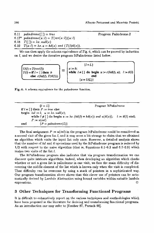
6.11 palindrome([ ]) = true 6.17" palindrome(a: I) = T(rev(a: l ) ) (a :l) 6.18 T ( [ ] ) = Ax. null(x) 6.19 T(a:l) = Ax.a = hd(x) and (T(I)ll(x));
Program Palindrome.2
We can then apply the schema equivalence of Fig. 6, which can be proved by induction on l, and we derive the iterative program ItPalindrome listed below.
UT((I = T(rev(l)) 1 /) = i f I = [ ] t h e n b
else c(hd(l), T(tl(1)))
Iu It = L } Ol := b; w h i l e l r [ ] d o b e g i n u := c(hd(l), u); l := tl(
end [u = U(L)}
Fig. 6. A schema equivalence for the palindrome function.
{I = L} Program ItPalindrome if I = [ ] then P := true else begin inl := 1; u := )tx. null(x);
while l # [] do begin u := ~x. (hd(l) = hd(x)) and u(tl(x)); 1 := tl(l) end; P := u(inl)
end {P = palindrome(L)}
The final assignment P := u(inl) in the program ItPalindrome could be considered as a second visit of the given list l, and it may seem a bit strange to claim that we obtained an algorithm which visits the input list only once. However, a detailed analysis shows that the number of hd and tl operations used by the ItPalindrome program is reduced by 1/3 with respect to the naive algorithm (that is, Equations 6.1-6.3 and 6.7-6.9) which makes two visits of the list I.
The ItPalindrome program also indicates that via program transformation we can discover quite intricate algorithms. Indeed, when developing an algorithm which checks whether or not a given list is palindrome in one visit, we face the main difficulty of dis- covering the middle element of the list which is known only when the visit is completed. That difficulty can be overcome by using a stack of pointers in a sophisticated way. Our program transformation above shows that this clever use of pointers can be auto- matically derived by Lambda Abstraction using bound variables within suitable lambda expressions. O
3 O t h e r T e c h n i q u e s f o r T r a n s f o r m i n g F u n c t i o n a l P r o g r a m s
It is difficult to exhaustively report on the various techniques and methodologies which have been proposed in the literature for deriving and transforming functional programs. As an introduction one may refer to [Feather 87, Partsch 90].
Rules and Strategies for Program Transformation 281
Here we want to consider: i) the Partial Evaluation (or Mixed Computation) technique [Ershov 82], ii) the Staging Transformation technique [Jcrring-Scherlis 86], and iii) the Finite Differencing technique [Paige-Koenig 82], and compare them with the strategies we have presented above.
For other methods, such as: combinatory techniques [Turner 79], supercombinator methods [Hughes 82], local recursions [Bird 84a], promotion strategies [Bird 84b], lambda liftings [Johnsson 85], and lambda hoistings [Takeichi 87], we suggest to look at the original papers.
Partial Evaluation (related to Program Division [Jones 87] and Variable Splitting [Bj#rner et al. 88]) is defined via a function PEval : Programs x Data ---, Programs, which given a program p and its input data d, produces a new program, called the residual program. It is assumed that the data d can be split into two components dl and d2, that is, d =(dl, d2) such that the following equation holds:
vial , a~) = ( PE~at(Vdl)) a2. PEval(pdl) is the residual program and it is obtained by ' importing' the information relative to the data component dl into the program p.
Partial Evaluation is used for improving program performance when the value of dl is known at compile time. It is also used for automatically producing compilers from interpreters.
Partial Evaluation can be viewed as the inverse of Lambda Abstraction in the sense that the latter one is defined by the function Lambda: Programs ---+ (Programs • Data), which 'exports ' information from a given program and satisfies the following equation:
for any given program p and data d, p d-= pl(dl , d) where Lambda(p) =- (Pl, dl).
Similarly to Partial Evaluation, the Staging Transformation [J0rring-Scherlis 86] is a technique whereby the computation of a given function, say f ( x , y), is performed 'in stages', that is, f ( x , y) is computed as the value of the expression f2(fl(X), y), where f l and f2 are suitable auxiliary functions such that:
f(x,y) = f2(f1(x), Y). The idea behind the Staging Transformation is the assumption that the argument x is known 'before' y (for instance, x is known at compile time and y is known at run time) and that, having computed the value of f l (x) , we can then very efficiently evaluate re.
Staging Transformation can be viewed as a particular generalization from functions to functions by implicit definition. Indeed, one may apply twice that generalization strategy for obtaining from the equation f ( z , y) = expr the functions f l and f2 such that f ( x , y) = f2( f l ( z ) , y) holds.
Finile Differencing [Paige-Koenig 82] is a program transformation technique based on the compiling technique called reduction of the operator strength. In the following example we will present this technique and at the same time we will show that the efficiency improvements due to finite differencing can be obtained by suitable generalization and folding steps. The transformation process goes as follows.
i) We first look for a tail recursive program. By doing so, the computations to be per- formed from one recursive call to the next, are only the ones related to the evaluation
282 Alberto Pettorossi and Maurizio Proietti
of a substitution, say 0, which computes the new recursive arguments from the old ones.
ii) We then generalize suitable subexpressions, so that the substitution 0 can be effi- ciently evaluated.
E x a m p l e 7 (F in i te Di f fe renc ing via Generalization: Accumulat ion in M o n o i d s ) Let us suppose that we are given the following program:
7.1 f ( 0 ) - - e(0) 7.2 f (n + 1) = g(e(n + 1), f(n)) for n _> 0,
where: i) g(x, y) is an associative operation with neutral element r/ (thus, g defines a monoid), and ii) for any n > 0, e(n) can be efficiently evaluated from the value of e (n+ 1) by computing 6(e(n + 1), n) for some given function ~f, while the direct evaluation of e(n) from the value of n is computationally expensive.
We may say that f is the accumulation of g over 'e(n),...,e(1),e(O)' because for n > 0 we have that f(n) = g(e(n),...g(e(1),e(0))...).
In these hypotheses Finite Differencing produces the following tail recursive program:
7.1 f(0) = e(0) 7.3 f (n + 1) = H(y,e(n + 1),n) for n >_ 0 7.4 g(acc, z, O) = g(g(acc, z), e(0)) 7.5 g ( a e c , z , n + l ) = g ( g ( a c c , z ) , $ ( z , n + l ) , n ) for n ~ 0.
Nowwe will show that this efficient program can be derived by applying the gener- alization strategy. We begin our transformation process by unfolding Equation 7.2. For n > 0 we have:
f (n + 1) = g(e(n + 1), f(n)) = {unfolding} = g(e(n + 1), g(e(n), f (n - 1))).
To derive a tail recursive program, the expression g(e(n + 1), g(e(n), f ( n - 1))) should be an instance of the r.h.s, of Equation 7.2 via the substitution {n = n - 1} which relates the recursive calls of the function f .
Thus, we first use the associativity property of g for allowing the matching of the subexpression f (n - 1), and we get:
7.6 f ( n + 1) = g(g(e(n+ 1) ,e (n) ) , f (n- 1)).
Then, in order to fold the r.h.s, of Equation 7.6 using Equation 7.2, we need to generalize the subexpression g(e(n + 1), e(n)), which does not match e(n + 1), to a variable, say y, and we define the function:
7.7 G(y,n) =dey g(y,f(n)) for n > 0.
Thus, we get the following program:
7.1 / ( 0 ) = e(O) 7.8 f(n + 1) = {folding 7.2 using 7.7} = G(e(n + 1), n) for n >_ 0 7.o G(~, 0) = g(~, e(0)) 7.10 e ( y , n + 1) = {by 7.7} = g ( y , f ( n + 1)) =
= {unfolding} = g(y, g(e(n + 1), f(n))) = = {associativity of g} = g(g(y, e(n + 1)), f(n)) =
Rules and Strategies for Program Transformation
= {folding using 7.7} = = a(g(y, e(n + 1)), n) for n > O.
283
This program is tail recursive, but unfortunately, it is not efficient because by Equation 7.10 the folding substitution {y = g(y,e(n + 1)), n + 1 = n}, which computes the new arguments of G from the old ones, requires the expensive evaluation of e(n -4- 1). We can avoid this drawback by unfolding Equation 7.10 and performing a generalization step as follows:
G(y, n + 1) = G(g(y, e(n + 1)), n) = {unfolding using 7.10} = = V(g(g(y, e(n + 1)), e(n)), n - 1).
This last expression is an instance of the previous expression G(g(y,e(n + 1)),n) according to the substitution {y = g(y,e(n + 1)), e(n + 1) = e(n), n = n - 1}, which can be efficiently computed if the values of y, e(n + 1), and n are available. Those values will indeed he available if we promote e(n q- 1) to be an argument of a new function, say H, defined by generalization from functions to functions starting from the r.h.s, of Equation 7.10. Thus, H should satisfy the following:
7.11 H ( y , e ( n + l ) , n ) =d~l e ( g ( y , e ( n + l ) ) , n ) f o r n > 0 .
For the function H we have:
7.12 H(y,e(1),O) = {by 7.11} = G(g(y,e(1)),O) = {by 7.7 & 7.1} = g(g(y,e(1)),e(O)) 7.13 H ( y , e ( n + 2 ) , n + l ) - - {by 7.11} = G ( g ( y , e ( n + 2 ) ) , n + l ) = {by 7.10} =
= G(g(g(y, e(n + 2)), e(n + 1)),n) = {folding using 7.11} = = H(g(y, e(n + 2)), e(n + 1), n) = = {by e(n + 1) = 5(e(n + 2),n + 1)} = = H ( g ( y , e ( n + 2 ) ) , 5 ( e ( n + 2 ) , n T 1 ) , n ) for n_>0.
The definition of the function H is obtained by replacing in Equations 7.12 and 7.13 the second argument by a variable, say z. As a result, we get the following final program:
7.1 f(0) = e(0) 7.14 f (n + 1) = G(e(n + 1), n) = {neutrality of q} = G(g(q, e(n + 1)), n) =
= H(O, e(n + 1), n) for n ~ 0 7.12" H(y, z, O) = g(g(y, z), e(0)) 7.13" H ( y , z , n + 1) = H(g(y , z ) ,5 (z ,n+ 1),n) for n > 0.
This program is equal to the one made out of Equations 7.1, 7.3, 7.4, and 7.5 which is produced by the Finite Differencing technique. Notice that our derivation avoids the insights which are often required by the Finite Differencing technique, like, for instance, the understanding that the first argument of H is an accumulator variable which stores the value of g(... g(g(o, e(n + 1)), e(n)) , . . . , e(k)) for some k, with 0 < k < n + 1, during the computation of f (n + 1).
Now, if we want to efficiently compute the following function ss (see [Partseh 90], page 295) for computing the sum of squares:
ss(O) = 0
ss(n + 1) = (n + 1) 2 + ss(n) for n _> O,
284 Alberto Pettorossi and Maurizio Proietti
we may use Equations 7.1, 7.14, 7.12", and 7.13", where we have that : i) g(z, y) = x + y, ii) e(0) = ,7 = 0, iii) e(n) = n 2, and iv) ~(z, y) = z - 2y - 1. Thus, we get the following program which avoids repeated squaring operations:
ss(O) = 0
ss(n + 1) = H(O, (n + 1) 2, n) for n > 0 H(y,z,O) = y+ z H(y , z ,n+ 1) = H(y+ z , z - 2(n + 1 ) - 1,n) for n > 0. D
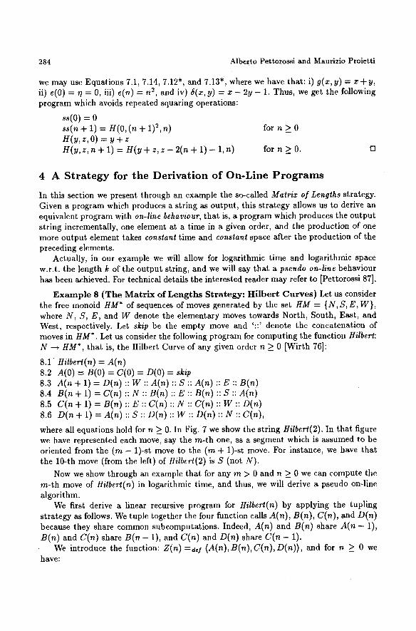
4 A Strategy for the Derivation of On-Line Programs
In this section we present through an example the so-called Matrix of Lengths strategy. Given a program which produces a string as output , this s trategy allows us to derive an equivalent program with on-line behaviour, that is, a program which produces the output string incrementally, one element at a t ime in a given order, and the production of one more output element takes constant t ime and constant space after the production of the preceding elements.
Actually, in our example we will allow for logarithmic time and logarithmic space w.r.t, the length k of the output string, and we will say that a pseudo on-line behaviour has been achieved. For technical details the interested reader may refer to [Pettorossi 87].
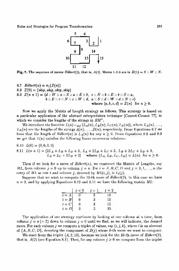
E x a m p l e 8 ( T h e M a t r i x of Lengths Strategy: Hilbert C u r v e s ) Let us consider the free monoid HM* of sequences of moves generated by the set HM = {N, S, E, W}, where N, S, E, and W denote the elementary moves towards North, South, East, and West, respectively. Let skip be the empty move and ':: ' denote the concatenation of moves in HM*. Let us consider the following program for computing the function Hilbert: N ---* HM*, that is, the Hilbert Curve of any given order n > 0 [Wirth 76]:
8 . 1 Hilbert(n) = A(n) 8.2 A(0) = S(0) = C(0) = D(0) = skip 8.3 A(n + 1) = O(n) :: W :: A(n) :: S :: Ain ) :: E :: B(n) 8.4 B(n + 1) = Cin ) :: N :: B(n) :: E :: Bin ) :: S :: A(n) 8.5 C(n + 1) = B(n) :: E :: C(n) :: N :: C(n) :: W :: D(n) 8.6 D(n+ 1) = A(n):: S :: D(n):: W : : D(n):: N :: C(n),
where all equations hold for n > 0. In Fig. 7 we show the string Hilbert(2). In that figure we have represented each move, say the m-th one, as a segment which is assumed to be oriented from the (m - 1)-st move to the (m + 1)-st move. For instance, we have that the 10-th move (from the left) of Hilbert(2) is S (not N).
Now we show through an example that for any m > 0 and n > 0 we can compute the m-th move of Hilbert(n) in logarithmic time, and thus, we will derive a pseudo on-line algorithm.
We first derive a linear recursive program for Hilbert(n) by applying the tupling strategy as follows. We tuple together the four function calls A(n), Bin), C(n), and D(n) because they share common subcomputations. Indeed, A(n) and B(n) share A(n - 1), S(n) and C(n) share B(n - 1), and C(n) and D(n) share C(n - 1).
We introduce the function: Z(n)=gel (A(n),BIn),V(n), D(n)), and for n > 0 we have:
Rules and Strategies for Program Transformation
5 4
9 ] 8 14
11 12
285
Fig. 7. The sequence of moves Hilbert(2), that is, A(2). Moves 1-2-3 are in D(1) = S :: W :: N.
8.7 nilb~n(n) = . , ( z ( . ) ) 8.s z(0) = (skip, skip, skip, skip) 8.9 Z ( n + l ) - - (d :: W :: a :: S :: a :: E :: b, c : : N : : b : : E : : b : : S : : a ,
b : : E : : c : : N : : c : : W : : d , a : : S : : d : : W : : d : : N : : c ) where (a, b, c, d) = Z(n) for n > 0.
Now we apply the Matrix of Length strategy as follows. This strategy is based on a particular application of the abstract interpretation technique [Cousot-Cousot 77], in which we consider the lengths of the strings in HM*.
We introduce the function L(n)=d~f (nA(n), Ls(n), Lc(n), LD(n)), where nA(n) . . . . , LD (n) are the lengths of the strings A(n),. . . , D(n), respectively. From Equations 8.7 we have that the length of Hilbert(n) is LA(n) for any n >_ 0. From Equations 8.8 and 8.9 we get that L(n) satisfies the following linear recurrence relations:
8.10 L(O)=(O,O,O,O)
8.11 L ( n + I ) = ( 2 L A + L B + L D + 3 , L A + 2 L B + L c + 3 , L B + 2 L c + L D + 3 , LA + Lc + 2LD + 3) where (LA, LB, Lc, LD) = L(n) for n > 0.
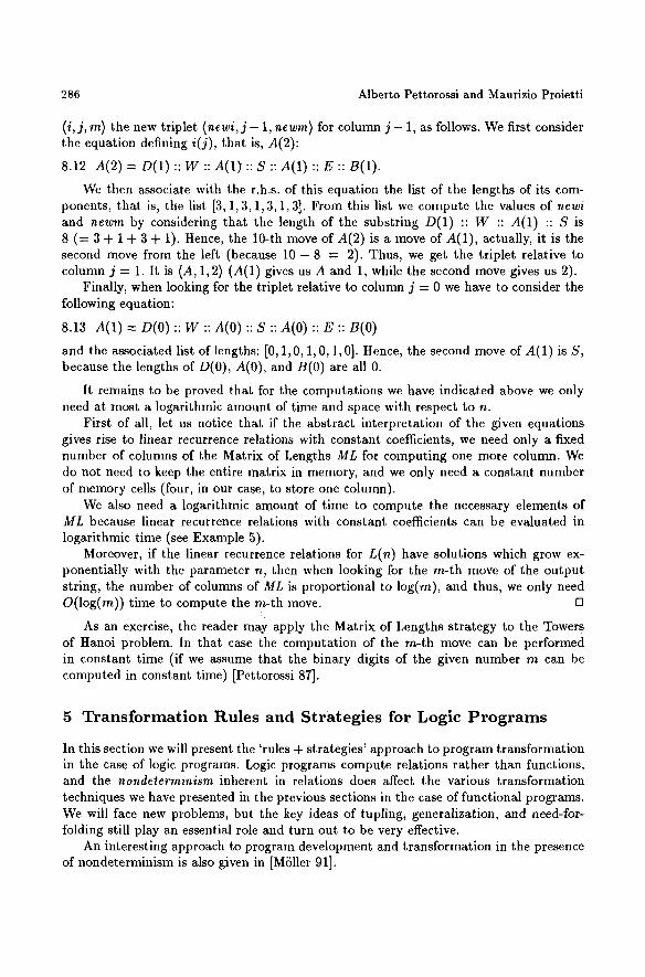
Then if we look for a move of Hilbert(n), we construct the Matrix of Lengths, say ML, from column j = 0 up to column j = n. For i = A , B , C , D and j = 0, 1 , . . . , n the entry of ML at row i and column j , denoted by ML(i,j), is Li(j).
Suppose that we want to compute the 10-th move of Hilbert(2). In this case we have n = 2, and by applying Equations 8.10 and 8.11 we have the following matrix ML:
C[ j = 0 j = l j = 2
i = A 0 3 15 i = 0 3 15 i = 0 3 15 i = 0 3 15
The application of our strategy continues by looking at one column at a time, from column j = n (= 2) down to column j = 0 until we find, as we will indicate, the desired move. For each column j we compute a triplet of values, say (i, j , k), where i is an element of {A, B, C, D}, denoting the component of Z(j) whose k-th move we want to compute.
We start from the triplet (A, 2, 10), because we look for the 10-th move of Hilbert(2), that is, A(2) (see Equation 8.1). Then, for any column j > 0 we compute from the triplet
286 Alberto Pettorossi and Maurizio Proietti
( i , j , m) the new triplet (newi, j - 1, newm) for column j - 1, as follows. We first consider the equation defining i(j), that is, A(2):
8.12 A ( 2 ) = D ( 1 ) : : W : : A ( 1 ) : : S : : A ( 1 ) : : E : : B ( 1 ) .
We then associate with the r.h.s, of this equation the list of the lengths of its com- ponents, that is, the list [3, 1, 3, 1,3,1, 3]. From this list we compute the values of newi and newm by considering that the length of the substring D(1) :: W :: A(1) :: S is 8 (= 3 + 1 + 3 + 1). Hence, the 10-th move of A(2) is a move of A(1), actually, it is the second move from the left (because 10 - 8 = 2). Thus, we get the triplet relative to column j = 1. It is (A, 1,2) (A(1) gives us A and 1, while the second move gives us 2).
Finally, when looking for the triplet relative to column j = 0 we have to consider the following equation:
8.13 A(1) = D(0) : : W :: A(0) :: S :: A(0) :: E :: B(0)
and the associated list of lengths: [0, 1,0, 1, 0, 1,0]. Hence, the second move of A(1) is S, because the lengths of n(0) , A(0), and B(0) are all 0.
It remains to be proved that for the computations we have indicated above we only need at most a logarithmic amount of time and space with respect to n.
First of all, let us notice that if the abstract interpretation of the given equations gives rise to linear recurrence relations with constant coefficients, we need only a fixed number of columns of the Matrix of Lengths ML for computing one more column. We do not need to keep the entire matrix in memory, and we only need a constant number of memory cells (four, in our case, to store one column).
We also need a logarithmic amount of time to compute the necessary elements of ML because linear recurrence relations with constant coefficients can be evaluated in logarithmic time (see Example 5).
Moreover, if the linear recurrence relations for L(n) have solutions which grow ex- ponentially with the parameter n, then when looking for the m-th move of the output string, the number of columns of ML is proportional to log(m), and thus, we only need O(log(m)) time to compute the m-th move. D
As an exercise, the reader may apply the Matrix of Lengths strategy to the Towers of Hanoi problem. In that case the computation of the m-th move can be performed in constant time (if we assume that the binary digits of the given number m can be computed in constant time) [Pettorossi 87].
5 Transformation Rules and Strategies for Logic Programs
In this section we will present the 'rules + strategies' approach to program transformation in the case of logic programs. Logic programs compute relations rather than functions, and the nondeterminism inherent in relations does affect the various transformation techniques we have presented in the previous sections in the case of functional programs. We will face new problems, but the key ideas of tupling, generalization, and need-for- folding still play an essential role and turn out to be very effective.
An interesting approach to program development and transformation in the presence of nondeterminism is also given in [MSller 91].
Rules and Strategies for Program Transformation 287
5.1 S y n t a x a n d S e m a n t i c s o f Logic P r o g r a m s
We assume tha t we are given a first order language L made out of a finite set of function symbols with arities (including at least one constant, that is, a 0-ary function symbol), a finite set of predicate symbols, and a countably infinite set of variable symbols. Function and predicate symbols are denoted by lower case letters, while variables are denoted by upper case letters.
Given a predicate symbol p of arity n and terms h , . - . ,t,~ built out of function and variable symbols, we say that p(tx . . . . , tn) is an atom. A goal is a (possibly empty) conjunction of atoms.
A (definite) clause, say C, is a s tatement of the following form:
YXI, . . . ,Xk.(Ax A . . . AAm --+ H), which is also written as: H ~ A 1 , . . . ,Am,
where: i) X 1 , . . . ,Xk are the variables occurring in A1 A . . . A Am ~ H, it) A 1 , . . . ,Am with m > 0, is a goal, called the body of the clause and denoted by bd(C), and iii) H is an atom, called the head of the clause and denoted by hd(C).
A (definite) logic program is a conjunction of clauses. Given a term t we denote by vats(t) the set of variables occurring in t. The same
notat ion will also be used for the variables occurring in atoms, goals, and clauses. A te rm (or an atom) is said to be ground if no variable occurs in it. Given a clause C of the form H *-- A 1 , . . . , A,~, B 1 , . . . , Bn, the linking variables of A 1 , . . . , Am in C are those occurring in A 1 , . . . , A m and also in H, B 1 , . . . , B n .
The Herbrand universe Hs associated with L, is the set of terms which are built out of the function symbols of L. The least Herbrand model M(P) of a program P is the following set of ground atoms:
M(P) = {p(tl,...,t,~) I P is a predicate symbol in L, { t l , . . . , t , } C_ HL, and P ~ p(tl . . . . ,t~)}.
For any given predicate symbol p occurring in L, M(p, P) is the subset of M(P) consisting of atoms with predicate p. Two programs P1 and P2 are said to be equivalent w.r.t, the predicate p if[" i ( p , P1) = M(p, P2).
We will assmne that the reader has some familiarity with the operat ional semantics of logic programs which is based on resolution [Lloyd 87].
5.2 T r a n s f o r m a t i o n R u l e s for Logic P r o g r a m s
We now introduce the transformation rules which will be used for obtaining new logic programs from old ones.
i) Definition Rule. It consists in introducing a new predicate defined in terms of already existing ones.
it) Unfolding Rule. It consists in performing a resolution step. There are the following two main differences with respect to the functional case.
1. The resolution step produces a unifying substitution (not a matching subst i tut ion, as it happens in a rewriting step for functional programs). Thus, when we unfold a clause C w.r.t, an a tom A in bd(C) using a clause D in the current program, we
288 Alberto Pettorossi and Maurizio Proietti
replace A by the bd(D) and we then apply to the resulting clause the substitution which unifies A and hd(D).
2. In the functional case we have assumed that the equations defining a program are mutually exclusive. Thus, by unfolding a given equation we may get at most one new equation. In contrast, in the logical case there may be several clauses whose heads are unifiable with an atom A in the body of a clause C. As a result, by unfolding C w.r.t. A using the clauses of the current program, we will obtain several clauses, say C1 . . . . , Ca. By an application of the unfolding rule we replace C by all clauses C1 , . . . , C , .
iii) Folding Rule. As in the functional case, the folding rule is the inverse of the unfolding rule.
There are some pitfalls to be avoided when applying the folding rule. For instance, we cannot fold clause C: p(X) ~- q(t(X)) using D: r ~-- q(Y), even though the body of C is an instance of the body of D. Indeed, by replacing q(t(X)) by the head r of D we get the clause p(X) ~-- r, from which by unfolding we get p(X) *-- q(Y) which is different from clause C.
Notice that if instead of clause D we consider the clause E: r(Y) *-- q(Y), where the variable Y is an argument of the head predicate, then it is possible to fold clause C using E. In general, it is the case that by considering extra variables as arguments of the head predicate we can perform folding steps which otherwise are impossible.
iv) Goal Replacement Rule. Let P be a program, C a clause in P, and G1 a goal occurring in the body of C. Suppose that for some goal G2 the following formula is true in the least Herbrand model M(P) of P:
VX1, . . . , Xk. (3Y1, �9 �9 �9 Y,~. G1 ~ 3Z1 , . . . , Z , . G2)
where: X1, . . . ,Xk are the linking variables of G1 in C, {Y1,...,Ym} = vats(G1) -
{ x l , . . . , xk}, { z ~ , . . . , z , } = vats(G2) - {X~ , . . . , Xk}, and {Z~, . . . , Z , } n var~(C) = 0. Then, in the body of C we can replace G1 by G~.
v) Clause Deletion Rule. Let P be a program and C a clause in P. We get a new program Q by deleting C from P if C is true in M(Q).
We may apply clause deletion in the following cases: i) bd(C) contains an atom which is not unifiable with the head of any other clause in P, and ii) C is subsumed by a different clause D in P, that is, there exists a substitution 8 such that hd(D)~ = hd(C) and bd(D)O is a sub-conjunction of atoms in bd(C).
The application of the transformation rules preserves soundness, in the sense that if we derive program P~ from program P1, then for each predicate p in P1 we have that: M(p, P2) C_ M(p, P1). By forcing some restrictions on the use of those transforma- tion rules [Tamaki-Sato 84], we also preserve completeness, that is, we get: M(p, P~) D_ M(p, P1).
The reader may easily verify that the use of the rules in the examples of program transformation we will present in this section, preserves both soundness and completeness.
Variants of the above transformation rules can be shown to be correct w.r.t, other logic languages and program semantics (see, for instance, [Bossi-Cocco 90, Gardner- Shepherdson 91, Kawamura-Kanamori 88, Proietti-Pettorossi 91, Sato 90, Seki 91]).
Rules and Strategies for Program Transformation 289
5.3 Transformation Strategies for Logic Programs
Here we list some of the strategies we use for transforming logic programs.
i) Predicate Tupling Strategy [Pettorossi-Proietti 87, Debray 88]. This strategy, also called tupling, for short, consists in selecting some atoms, say A1 , . . . , An, with n > 1, occurring in the body of a clause C. We introduce a new predicate ncwp defined by a clause T of the form:
newp(X1, . . . ,X~) ~ A1, . . . ,An
where X x , . . . , Xk are the linking variables of A1 , . . . , An in C. We then look for the re- cursive definition of the predicate newp by performing some unfolding, goal replacement, and clause deletion steps followed by some folding steps using clause T.
We finally fold the atoms A1, . . . , A,~ in the body of clause C using clause T.
The tupling strategy is often applied when A1 , . . . , A , share some variables. The pro- gram improvements which can be achieved by using this strategy in the case of logic programs are similar to those which can be achieved by using the composition and/or the tupling strategies in the case of functional programs. In particular, we need to evalu- ate only once the subgoals which are common to the computations evoked by the tupled atoms A1 , . . . , A , . We can also avoid multiple visits of data structures and the construc- tion of intermediate bindings.
As in the functional case, the folding steps needed for deriving the recursive definition of the predicate newp can often be performed only if we introduce some new predicates by means of definition clauses.
In addition, by using the tupling strategy we can sometimes obtain a new program version which simulates the execution of the initial program according to a computation rule different from the 'left-to-right' one used by Prolog. An automated technique which applies this transformation strategy for reducing the nondeterminism of Prolog programs is the Compiling Control technique [Bruynooghe et al. 89].
In the sequel we will consider the following three strategies which can be used for introducing those new predicates: the loop absorption, the generalization, and the implicit definition strategy.
In order to describe those strategies we will represent the process of performing un- folding and goal replacement steps starting from a clause, say D, as a tree of clauses, called unfolding tree. The root of the unfolding tree is clause D, and for each clause derived by applying either unfolding or goal replacement to a clause E of the unfolding tree we construct a new son of E. In an unfolding tree we also have the usual relations of descendant clause and ancestor clause.
it) Loop Absorption Strategy [Proietti-Pettorossi 90]. Suppose that a clause C in an un- folding tree has the form: H ~ A1, . . . , Am, B1 , . . . , Bn, and the body of a descendant D of C contains an instance of A1 , . . . , Am. Suppose also that the clauses in the path from C to D have been generated by applying no transformation rule to B1 , . . . , Bn.
The loop absorption strategy is applied by introducing a new predicate defined by the following clause A:
newp(Xa, . . . ,Xk) ~- A1, . . . ,An
290 Alberto Pettorossi and Maurizio Proietti
where {Xl . . . . , Xk} is the minimum subset of vars(A~, . . . , Am) which is necessary to fold both C and D using a clause whose body is A1 , . . . ,An . We then look for the recursive definition of the predicate newp.
A similar strategy is also used in the above mentioned Compiling Control technique.
iii) Generalization Strategy. Given a clause C of the form: H ~ A1, . . . , Am, Bx , . . . , Bn , we define a new predicate genp by a clause G of the form:
genp(X1, . . . , Xk) ~-- GenA1, . . . , GenAm
where (GenA1, . . . , GenAm)O = A 1 , . . . , A m , for a given substitution O, and X 1 , . . . , X k are the variables which are necessary to fold C using G. We then fold C using G and we get:
H ~-- genp(X1, . . . ,Xk)O, B1, . . . ,Bn.
We finally look for the recursive definition of the predicate genp. A suitable form of the clause G introduced by generalization can often be obtained by
matching clause C against one of its descendants, say D, in the unfolding tree which is considered during program transformation. In particular, we will consider the case where:
1. D is the clause K ~ E x , . . . , E r n , F 1 , . . . , F r , and D has been obtained from C by applying no transformation rule to B1 , . . . , B,~,
2. the goal GenA1, . . . , GenA,~ is the most concrete generalization of both A1 , . . . , Am and E l , . . . , Era, and
3. {X1, . . . ,Xk} is the minimum subset of vars(GenA1, . . . , GenAm) which is necessary to fold both C and D using a clause whose body is GenA1, . . . , GenAm.
In our logical language we do not have abstraction operators, and thus, we cannot consider techniques similar to the Lambda Abstraction strategy which has been presented in the case of functional programs (see Section 2). However, we will show in Example 10 below that the effects of abstractions may sometimes be simulated in logic programming by exploiting the power of the unification mechanism.
A strategy which is analogous to the generalization from functions to functions by implicit definition presented in Section 3, can be obtained as a particular case of the following one.
iv) Implicit Definition Strategy. Let P be a program and C one of its clauses of the form: H ~-- A 1 , . . . , Am, G1, where G1 is a goal made out of one or more atoms. Suppose that we want to replace Ga by a goal of the form: 'G2, impl(V1, . . . , Vh)', where impl is a new predicate symbol of arity h, and the V/'s are variables. In order to do so, according to the Goal Replacement Rule we have to look for a set Expl of clauses such that in the least Herbrand model M ( P A Expl) the following formula holds:
VX1, . . . , Xk. (3Y1, . . . , Ym.G1 ~ 3Z1 , . . . , Zn.(G2, impl(V1, . . . , Vh))) (1)
where: i) X1 , . . . ,Xk are the linking variables of G1, ii) {Y1,... ,Ym} = vars(G1) - {X1, . . . ,Xk} , iii) {Zl . . . . ,Zn} = vars(G2, impl(V1, . . . ,Vh)) - { X 1 , . . . , X k } , and iv) { z l , . . , z , } n vars(C) = O.
The set Expl provides an explicit definition of the predicate impl which is implicitly defined by Equation 1. A practical method to find the set Expl consists of the following four steps:
Rules and Strategies for Program Transformation 291
Step 1. We consider two different definitions of a new predicate, say newp, by introducing two clauses with body G1 and (G2, impl(V~,..., Vh)), respectively, that is:
D1. newp(X1,.. . ,Xk) ~-- G1 D2. newp(X1 .. . . , Xk) *--- G2, impl(V1, . . ., Vh)
Step 2. We look for the recursive definition of newp by using the program PAD1 thereby producing a program Q1 equivalent to P A D1.
Step 3. We then unfold every occurrence of newp in Q1 by using clause D~ and get a program Q2.
Step 4. We finally obtain the set Ezpl by requiring that by unfolding the occurrences of impl(V1,..., Vh) in P A D2 using the clauses in Expl we derive program Q2.
Notice that the validity of Equation 1 in M(P A Expl) follows from the fact that both programs (P A O1 A Expl) and (P A D2 A Expl) can be transformed into (Q~ A Expl), and therefore, the two definitions of newp are equivalent. Indeed, by Step 2 we have that (P A D1 A Expl) can be transformed into (Q1 A Expl). On the other hand, by Step 4 we have that (PAD2AExpl) can he transformed into (Q2AExpl) by performing an unfolding step, and by Step 3 program Q1 can be obtained from Q2 by performing a folding step.
The above implicit definition strategy generalizes the one presented in [Kanamori- Maeji 86] and it is related to the technique described in [Kott 82] for proving properties of functional programs based on unfold/fold transformations.
In the following example of logic program transformation we will show that the strate- gies described in this section can be used for reducing the amount of nondeterminism in a given program. In particular, we will make use of the tupling, loop absorption, and implicit definition strategies.
We will end this section by demonstrating in Example l0 the use of the generalization strategy.
E x a m p l e 9 ( P r i m e N u m b e r s ) Let us consider the problem of computing the list P of the first N prime numbers for any given natural number N > 0. To this purpose we define a relation primes(N, P) by means of the following program, called Primes:
9.1 primes(N, P) ~-- initial(L), nol_div_by_smaller( L, P), length( P, N) 9.2 initial([2])*--- 0.3 initial([H, lilT]) ~ initial([KIT]), plus(l(, 1, H) 9.4 not_di~_bu_smalle~([ ], [ ] ) ~ - 9.5 not_div_by_smaller([HlT], P) ~ not_div_by_smaller(T, Q), div_tests( H, Q, P) 9.6 div_tests( H, Q, [H}Q]) ,-- not_div_any( H, Q) 9.7 div_tests(H, Q, Q) +- div_some(H, Q) 9.s length(l],0) ~ - 9.9 length([HIT], N) *-- length(T, N1), plus(i l , 1, N)
where we assume that: i) plus(X, Y, Z) holds iff X + Y = Z, ii) not_div_any(H, L) holds iff H is not divisible by any number of the list L, and iii) div_some(H, L) holds iff H is divisible by a number in L.
Notice that: i) initial(L) holds iff L is the list [M, M - 1 , . . . , 2] of consecutive natural nmnbers for some number M, ii) not_div_by_smaller(L, P) holds iff P is the sublist of L
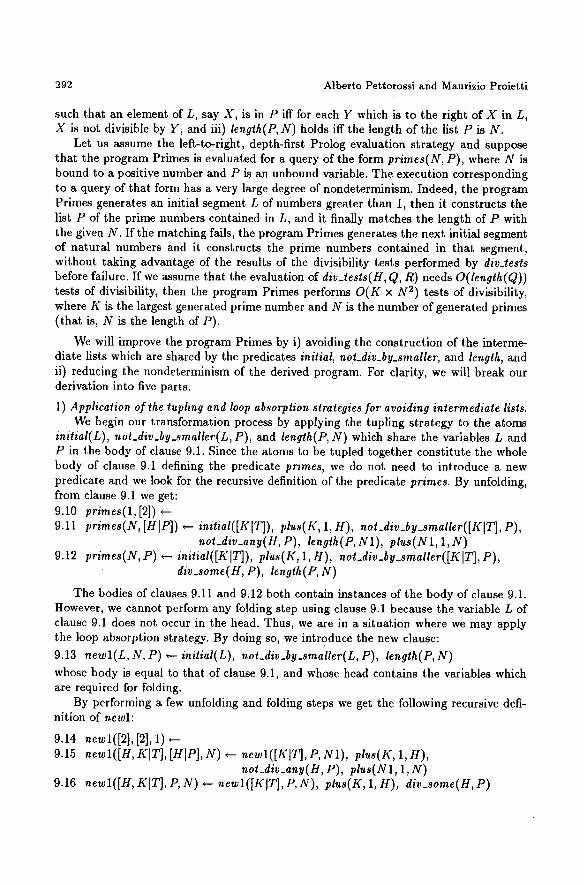
292 Alberto Pettorossi and Maurizio Proietti
such that an element of L, say X, is in P iff for each Y which is to the right of X in L, X is not divisible by Y, and iii) length(P, N) holds iff the length of the list P is N.
Let us assume the left-to-right, depth-first Prolog evaluation strategy and suppose that the program Primes is evaluated for a query of the form primes(N, P), where N is bound to a positive number and P is an unbound variable. The execution corresponding to a query of that form has a very large degree of nondeterminism. Indeed, the program Primes generates an initial segment L of numbers greater than 1, then it constructs the list P of the prime numbers contained in L, and it finally matches the length of P with the given N. If the matching fails, the program Primes generates the next initial segment of natural numbers and it constructs the prime numbers contained in that segment, without taking advantage of the results of the divisibility tests performed by divotests before failure. If we assume that the evaluation of div_tests(H, Q, R) needs O(length(Q)) tests of divisibility, then the program Primes performs O(K x N 2) tests of divisibility, where K is the largest generated prime number and N is the number of generated primes (that is, N is the length of P).
We will improve the program Primes by i) avoiding the construction of the interme- diate lists which are shared by the predicates initial, not_div_by_smaller, and length, and ii) reducing the nondeterminism of the derived program. For clarity, we will break our derivation into five parts.
1) Application of the tupling and loop absorption strategies for avoiding intermediate lists. We begin our transformation process by applying the tupling strategy to the atoms
initial(L), not_ally_by_smaller(L, P), and length(P, N) which share the variables L and P in the body of clause 9.1. Since the atoms to be tupled together constitute the whole body of clause 9.1 defining the predicate primes, we do not need to introduce a new predicate and we look for the recursive definition of the predicate primes. By unfolding, from clause 9.1 we get: 9.10 primes(l,[2]) +-- 9.11 primes(N, [HIP]) ~ initial([KIT~) , plus(K, 1, H), not_div_by_smaller([KIT~, P),
not_div_any( H, P), length(P, N1), plus(N1, 1, N) 9.12 primes(N, P) ~ initial([glT]), plus(K, 1, H), not_div_by_smaller([gl~ , P),
div_some( H, P), length(P, N) The bodies of clauses 9.11 and 9.12 both contain instances of the body of clause 9.1.
However, we cannot perform any folding step using clause 9.1 because the variable L of clause 9.1 does not occur in the head. Thus, we are in a situation where we may apply the loop absorption strategy. By doing so, we introduce the new clause:
9.13 newl( L, N, P) ~ initial(L), not_div_by_smaller( L, P), length(P, N) whose body is equal to that of clause 9.1, and whose head contains the variables which are required for folding.
By performing a few unfolding and folding steps we get the following recursive defi- nition of newl:
9.14 new1([2],[2], 1) 9.15 newl([H, KIT], [HIP], N) ~ newl([KlT], P, N1), plus(K, 1, H),
not_div_any( H, P), plus(N1, 1, N) 9.16 newl([H, KIT~, P, N) ~ newl([Kl~ , P, U), plus(K, 1, H), div_some(H, P)
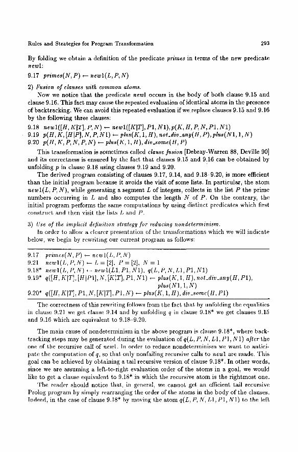
Rules and Strategies for Program Transformation 293
By folding we obtain a definition of the predicate primes in terms of the new predicate newl: 9.17 primes(N, P) ~-- newl(L, P, N)
2) Fusion of clauses with common atoms. Now we notice that the predicate newl occurs in the body of both clause 9.15 and
clause 9.16. This fact may cause the repeated evaluation of identical atoms in the presence of backtracking. We can avoid this repeated evaluation if we replace clauses 9.15 and 9.16 by the following three clauses:
9.18 newl([g, KIT], P, N) *--- newl([glT], P1, g l ) ,p (g , H, P, N, P1, g l ) 9.19 p(H, K, [HIP], N, P, g l ) ~- plus(K, 1, H), not_div_any(H, P), plus(N1, 1, N) 9.20 p(H, K, P, N, P, N) ~ plus(If, 1, H), div_some(H, F)
This transformation is sometimes called clause fusion [Debray-Warren 88, Deville 90] and its correctness is ensured by the fact that clauses 9.15 and 9.16 can be obtained by unfolding p in clause 9.18 using clauses 9.19 and 9.20.
The derived program consisting of clauses 9.17, 9.14, and 9.18-9.20, is more efficient than the initial program because it avoids the visit of some lists. In part icular , the a tom newl(L, P, N), while generating a segment L of integers, collects in the list P the prime numbers occurring in L and also computes the length N of P . On the contrary, the initial program performs the same computations by using distinct predicates which first construct and then visit the lists L and P.
3) Use of the implicit definition strategy for reducing nondeterminism. In order to allow a clearer presentation of the transformations which we will indicate
below, we begin by rewriting our current program as follows:
9.17 9.21 9.18" 9.19"
9.20*
primes(N, P) ~-- newl(L, P, N) newl(L,P,N) ~-- L = [2], P = [2], N = 1 newl(L, P, N) ~- newl(L1, P1, N1), q(L, P, N, L1, F1, N1) q([H, KIT], [HIP1], N, [KIT], P1, N1) ~ plus(K, 1, H), not_div_any(H, P1),
plus(N1, 1, N) q([H, KIT], Pl, N, [KIT], Pl, N) ~- plus(l(, 1, H ), div_some( H, P l )
The correctness of this rewriting follows from the fact that by unfolding the equalities in clause 9.21 we get clause 9.14 and by unfolding q in clause 9.18" we get clauses 9.15 and 9.16 which are equivalent to 9.18-9.20.
The main cause of nondeterminism in the above program is clause 9.18", where back- tracking steps may be generated during the evaluation of q(L, P, N, L1, P1, N1) after the one of the recursive call of new1. In order to reduce nondeterminism we want to antici- pate the computat ion of q, so that only nonfailing recursive calls to new1 are made. This goal can be achieved by obtaining a tail recursive version of clause 9.18". In other words, since we are assuming a left-to-right evaluation order of the atoms in a goal, we would like to get a clause equivalent to 9.18" in which the recursive atom is the r ightmost one.
The reader should notice that, in general, we cannot get an efficient tail recursive Prolog program by simply rearranging the order of the atoms in the body of the clauses. Indeed, in the case of clause 9.18" by moving the atom q(L, P, N, L1, P1, N1) to the left
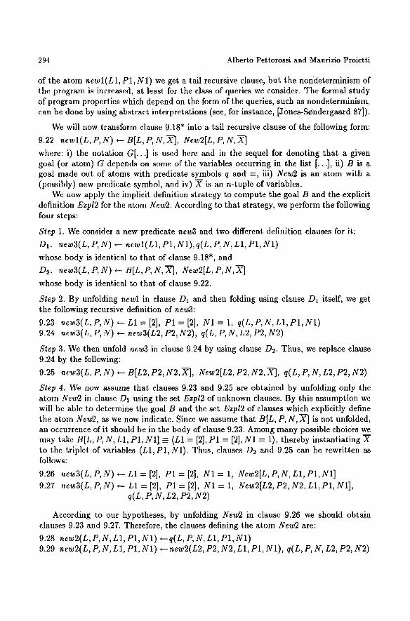
294 Alberto Pettorossi and Maurizio Proietti
of the atom newl(L1, P1, N1) we get a tail recursive clause, but the nondeterminism of the program is increased, at least for the class of queries we consider. The formal study of program properties which depend on the form of the queries, such as nondeterminism, can be done by using abstract interpretations (see, for instance, [Jones-Scndergaard 87]).
We will now transform clause 9.18" into a tail recursive clause of the following form:
9.22 newl(L,P,g) ~-- B[L,P,N,X---], New2[L,P,N,X--~ where: i) the notation G[...] is used here and in the sequel for denoting that a given goal (or atom) G depends on some of the variables occurring in the list [...], ii) B is a goal made out of atoms with predicate symbols q and =, iii) New2 is an atom with a (possibly) new predicate symbol, and iv) ~" is an n-tuple of variables.
We now apply the implicit definition strategy to compute the goal B and the explicit definition Ezpl2 for the atom New2. According to that strategy, we perform the following four steps:
Step 1. We consider a new predicate new3 and two different definition clauses for it:
D~. new3(L,P,N) ~ newl(Ll,Pl,gl),q(L,P,g, Ll, P l ,Y l ) whose body is identical to that of clause 9.18", and
02. new3(L,P,N) ~-- B[L,P,N,X--7, New2[L,P,N,X-- 7 whose body is identical to that of clause 9.22.
Step 2. By unfolding newl in clause D1 and then folding using clause D1 itself, we get the following recursive definition of new3: 9.23 new3(L,P,g) ~-- L1 = [2], P1 = [2], g l = 1, q(L,P,N, L1,P1,N1) 9.24 new3(L, P, N) ~ new3(L2, P2, N2), q(L, P, N, L2, P2, g 2 )
Step 3. We then unfold new3 in clause 9.24 by using clause D2. Thus, we replace clause 9.24 by the following:
9.25 new3(L, P, N) ~-- B[L2, P2, g 2 , X----I, New2[L2, P2, N2, X---], q(L, P, N, L2, P2, g 2 )
Step 4. We now assume that clauses 9.23 and 9.25 are obtained by unfolding only the atom New2 in clause D2 using the set Expl2 of unknown clauses. By this assumption we will be able to determine the goal B and the set Expl2 of clauses which explicitly define the atom New2, as we now indicate. Since we assume that B[L, P, N,X--] is not unfolded, an occurrence of it should be in the body of clause 9.23. Among many possible choices we may take B[L, P, N, L1, P1, N1] _= (L1 = [2], P1 = [2], N1 = 1), thereby instantiating Z to the triplet of variables (L1, P1, N1). Thus, clauses D2 and 9.25 can be rewritten as follows:
9.26 new3(L, P, N) ~-- L1 = [2], P1 = [2], N1 = 1, New2[L, P, N, L1, P1, N1] 9.27 new3(L, P, N) ~-- L1 = [2], P1 = [2], N1 = 1, New2[L2, P2, g2, L1, P1, N1],
q(L, P, N, L2, P2, N2)
According to our hypotheses, by unfolding New2 in clause 9.26 we should obtain clauses 9.23 and 9.27. Therefore, the clauses defining the atom New2 are:
9.28 new2(n,P,N, Ll, P l ,g l )~q(L ,P ,N , LI,PI,N1) 9.29 new2(L,P,N, L1, PI,N1) ~new2(n2,P2, g2,Ll, P1,N1), q(L,P,N, L2, P2, N2)
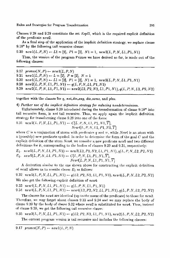
Rules and Strategies for Program Transformation 295
Clauses 9.28 and 9.29 constitute the set Expl2, which is the required explicit definition of the predicate new2.
As a final step of the application of the implicit definition strategy, we replace clause 9.18" by the following tail recursive clause:
9.30 newl( L,P, N) +-- L1 --- [2], P l --- [2], N1 -- 1, new2( L,P,N, L1,P1,N1) Thus, the version of the program Primes we have derived so far, is made out of the
following clauses:
9.17 primes(N, P) ~-- newl(L, P, N) 9.21 newl(L, P, N) +-- L = [21, P = [2], N = 1 9.30 newl(L, P, N) +-- nl = [2], P1 = [2], g l -- 1, new2(L, P, N, nl, P1, g l ) 9.28 new2(L,P,N, LI, P1,N1) +- q(L,P,N, LI,PI,N1) 9.29 new2(L, P, N, L1, P1, N1) +-- new2(n2, P2, N2, L1, P1, Yl) , q(L, P, N, L2, P2, g 2 )
together with the clauses for q, not_div.any, div_some, and plus.
4) Further use of the implicit definition strategy for reducing nondeterminism. Unfortunately, clause 9.29 introduced during the transformation of clause 9.18" into
tail recursive form, is not tail recursive. Thus, we apply again the implicit definition strategy for transforming clause 9.29 into one of the form:
9.31 new2(L,P,N, L1, P1,N1) ~-- C[L,P,N, L1, P1,N1,7], New4[L, P, N, L1, P1, N1, Y--~
where C is a conjunction of atoms with predicates q and =, while New4 is an atom with a (possibly) new predicate symbol. In order to determine the form of the goal C and the explicit definition of the atom New4, we consider a new predicate new5 and two different definitions for it, corresponding to the bodies of clauses 9.29 and 9.31, respectively:
El. new5(L, P, N, L1, Pl, N1) ~- new2(L2, P2, N2, L1, P1, N1), q(L, P, N, L2, P2, N2) E2. new5(L,P,N, L1, P1, N1) ~- C[L,P,N, LI, P1,N1,Y--],
New4[L, P, N, L1, P1, N1, A derivation similar to the one shown above for constructing the explicit definition
of new2 allows us to rewrite clause E2 as follows:
9.32 new5(L, P, N, L1, P1, N1) +-- q(L2, P2, N2, L1, P1, N1), new4(L, P, N, L2, P2, N2)
We also get the following explicit definition of new4: 9.33 new4(n,P,N, Ll, P l ,g l ) +- q(L,P,N, L1,P1,N1) 9.34 new4(L, P, N, L1, P1, g l ) +-- new4(n2, P2, N2, L1, P1, N1), q(L, P, N, L2, P2, g 2 )
The clauses for new4 are identical (up to the name of the predicate) to those for new2. Therefore, we may forget about clauses 9.33 and 9.34 and we may replace the body of clause 9.29 by the body of clause 9.32 where new2 is substituted for new4. Thus, instead of clause 9.29, we get the following tail recursive clause:
9.35 new2(L, P, N, L1, P1, N1) +--- q(L2, P2, N2, L1, P1, N1), new2(L, P, N, L2, P2, N2)
The current program version is tail recursive and includes the following clauses:
9.17 primes(N,P) ~- newl(L,P,N)
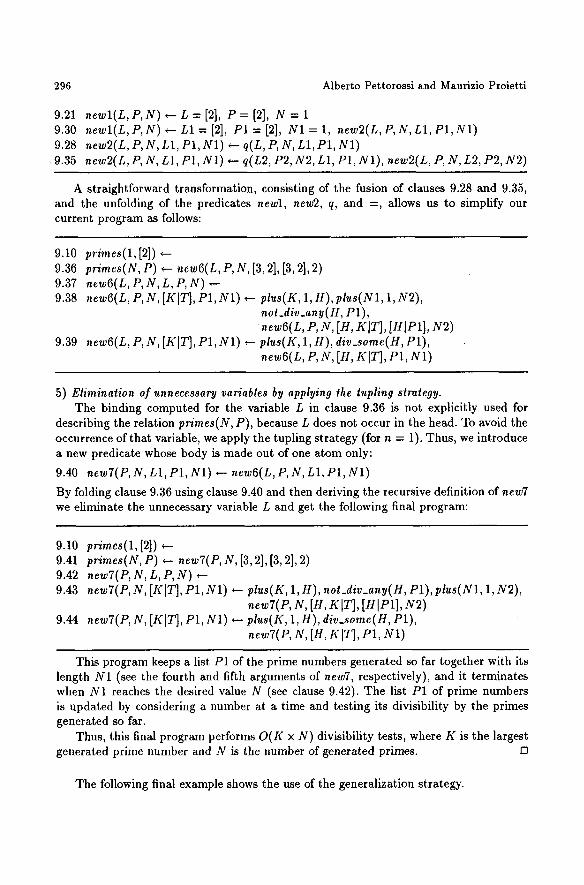
296 Alberto Pettorossi and Maurizio Proietti
9.21 newl(L,P,N)~--L=[2], P = [ 2 ] , N = I 9.30 newl( L, P, N) *-- L1-- [2], P1 - - [21, N I = 1, new2(L,P,N, L1,P1,N1) 9.28 new2(L, P, N, L1, P1, Yl ) ~ q(L, P, N, nl, P1, g l ) 9.35 new2(L, P, N, L1, P1, g l ) ~ q(L2, P2, g2, L1, P1, g l ) , new2(L, P, N, L2, P2, N2)
A straightforward transformation, consisting of the fusion of clauses 9.28 and 9.35, and the unfolding of the predicates new1, new2, q, and =, allows us to simplify our current program as follows:
9.10 primes(l, [21) 9.36 primes(N, P) ~- uew6( L, P, N, [3, 2], [3, 21, 2) 9.37 new6(L, P, N, L, P, N) *-- 9.38 new6(n, P, N, [//IT], P1, N1) ~ plus(K, 1, H), plus(gl, 1, Y2),
not_div_any(H, P1), new6( L, P, N, [H, KIT], [HIP1], N2)
9.39 new6(L, P, N, [KIT], P1, N1) *- plus(K, 1, H), ally_some(H, P1), new6(i, P, N, [H, KIT], Pl, N1)
5) Elimination of unnecessary variables by applying the tupling strategy. The binding computed for the variable L in clause 9.36 is not explicitly used for
describing the relation primes(N, P), because L does not occur in the head. To avoid the occurrence of that variable, we apply the tupling strategy (for n = 1). Thus, we introduce a new predicate whose body is made out of one atom only:
9.40 new7(P,N, L1,P1, N1) *-- new6(L,P,N, L1, P1,N1) By folding clause 9.36 using clause 9.40 and then deriving the recursive definition of new7 we eliminate the unnecessary variable L and get the following final program:
9.10 primes(1,[2]) ~- 9.41 primes(N, P) ~-- new7(P, N, [3, 2], [3, 2], 2) 9.42 new7(P, N, L, P, N) 9.43 new7(P, N, [/fiT], P1, N1) ~- plus(K, 1, g), not_div_any(H, P1), plus(N1, 1, N2),
new7( P, N, [H, KIT], [HIP1 ], N2) 9.44 new7( P, N, [I/17~, P1, N1) *-- plus(K, 1, H), ally_some(H, Pl) ,
new7( P, N, [H, KIT~, P1, N1)
This program keeps a list P1 of the prime numbers generated so far together with its length N1 (see the fourth and fifth arguments of newT, respectively), and it terminates when N1 reaches the desired value N (see clause 9.42). The list P1 of prime numbers is updated by considering a number at a time and testing its divisibility by the primes generated so far.
Thus, this final program performs O(K x N) divisibility tests, where K is the largest generated prime number and N is the number of generated primes. D
The following final example shows the use of the generalization strategy.
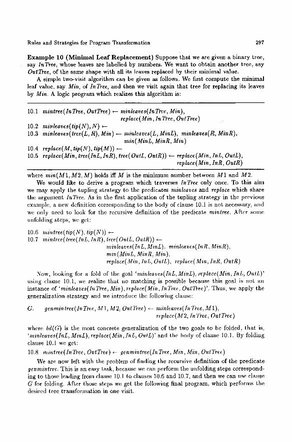
Rules and Strategies for Program Transformation 297
E x a m p l e 10 ( M i n i m a l L e a f R e p l a c e m e n t ) Suppose that we are given a binary tree, say InTree, whose leaves are labelled by numbers. We want to obtain another tree, say OutTree, of the same shape with all its leaves replaced by their minimal value.
A simple two-visit algorithm can be given as follows. We first compute the minimal leaf value, say Min, of InTree, and then we visit again that tree for replacing its leaves by Min. A logic program which realizes this algori thm is:
10.1 mintree( InTree, OutTree) ~ minleaves(InTree, Min), replace( Min, In Tree, OutTree)
10.2 minleaves(tip(N), N) 10.3 minleaves( tree( L, R), Min ) *-- minleaves( L, MinL), minleaves( R, MinR ),
min( MinL, MinR, Min ) 10.4 replace(M, tip(N), lip(M)) *-- 10.5 replace( Min, tree( InL, lnR), tree( OutL, OutR) ) ~ replace( Min, InL, OutL),
replace( Min, lnR, OutR )
where rain(M1, M2, M) holds iff M is the minimum number between M1 and M2. We would like to derive a program which traverses InTree only once. To this aim
we may apply the tupling strategy to the predicates minleaves and replace which share the argument lnTree. As in the first application of the tupling s t rategy in the previous example, a new definition corresponding to the body of clause 10.1 is not necessary, and we only need to look for the recursive definition of the predicate mintree. After some unfolding steps, we get:
10.6 minlree(tip(N), tip(N)) ~-- 10.7 minlree( tree(lnL, InR), tree( OutL, OutR)) ,---
minleaves( InL, MinL), minleaves( InR, MinR ), min( MinL, MinR, Min ), replace( Min, InL, OutL), replace( Min, InR, OutR)
Now, looking for a fold of the goal 'minleaves(InL, MinL), r~eplace(Min, InL, OutL)' using clause 10.1, we realize that no matching is possible because this goal is not an instance of 'minleaves(InTree, Min), replace(Min,InTree, OutTree)'. Thus, we apply the generalization strategy and we introduce the following clause:
G. genmintree(InTree, M1, M2, OutTree) ~-- minleaves(In Tree, M1), replace(M2, In Tree, Out Tree )
where bd(G) is the most concrete generalization of the two goals to be folded, tha t is, 'minleaves(InL, MinL), replace(min, InL, OutL)' and the body of clause 10.1. By folding clause 10.1 we get:
10.8 mintree( In Tree, OutTree) ~-- genmintree( In Tree, min, min, OutTree) We are now left with the problem of finding the recursive definition of the predicate
genmintree. This is an easy task, because we can perform the unfolding steps correspond- ing to those leading from clause 10.1 to clauses 10.6 and 10.7, and then we can use clause G for folding. After those steps we get the following final program, which performs the desired tree transformation in one visit.
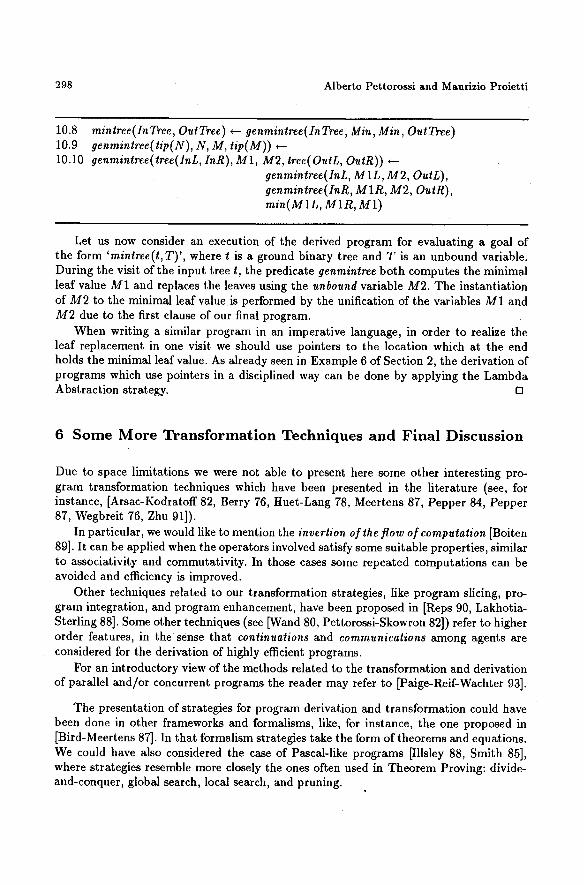
298 Alberto Pettorossi and Maurizio Proietti
10.8 minlree( In Tree, OutTree ) ~-- genmintree( In Tree, Min, Min, OutTree ) 10.9 genmintree(tip(g),N,M, lip(M)) ~-- 10.10 genminlree( tree( InL, InR ), M1, M2, lree( OutL, OuLR ) ) *--
genminlree(InL, M1L, M2, OulL), genminlree( InR, M1R, M2, OutR), min(M1L, M1R, M1)
Let us now consider an execution of the derived program for evaluating a goal of the form 'mintree(t,T)', where t is a ground binary tree and T is an unbound variable. During the visit of the input tree t, the predicate genmintree both computes the minimal leaf value M1 and replaces the leaves using the unbound variable M2. The instantiation of M2 to the minimal leaf value is performed by the unification of the variables M1 and M2 due to the first clause of our final program.
When writing a similar program in an imperative language, in order to realize the leaf replacement in one visit we should use pointers to the location which at the end holds the minimal leaf value. As already seen in Example 6 of Section 2, the derivation of programs which use pointers in a disciplined way can be done by applying the Lambda Abstraction strategy. I:3
6 S o m e M o r e T r a n s f o r m a t i o n T e c h n i q u e s a n d F i n a l D i s c u s s i o n
Due to space limitations we were not able to present here some other interesting pro- gram transformation techniques which have been presented in the literature (see, for instance, [Arsac-Kodratoff 82, Berry 76, I-Iuet-Lang 78, Meertens 87, Pepper 84, Pepper 87, Wegbreit 76, Zhu 91]).
In particular, we would like to mention the invcrtion of the flow of computation [Boiten 89]. It can be applied when the operators involved satisfy some suitable properties, similar to associativity and commutativity. In those cases some repeated computations can be avoided and efficiency is improved.
Other techniques related to our transformation strategies, like program slicing, pro- gram integration, and program enhancement, have been proposed in [Reps 90, Lakhotia- Sterling 88]. Some other techniques (see [Wand 80, Pettorossi-Skowron 82]) refer to higher order features, in the sense that continuations and communications among agents are considered for the derivation of highly efficient programs.
For an introductory view of the methods related to the transformation and derivation of parallel and/or concurrent programs the reader may refer to [Paige-Reif-Wachter 93].
The presentation of strategies for program derivation and transformation could have been done in other frameworks and formalisms, like, for instance, the one proposed in [Bird-Meertens 87]. In that formalism strategies take the form of theorems and equations. We could have also considered the case of Pascal-like programs [Illsley 88, Smith 85], where strategies resemble more closely the ones often used in Theorem Proving: divide- and-conquer, global search, local search, and pruning.
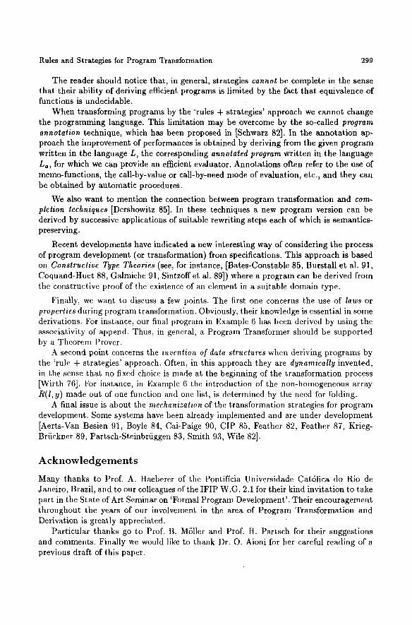
Rules and Strategies for Program Transformation 299
The reader should notice that, in general, strategies cannot be complete in the sense that their ability of deriving efficient programs is limited by the fact that equivalence of functions is undecidable.
When transforming programs by the 'rules + strategies' approach we cannot change the programming language. This limitation may be overcome by the so-called program annotation technique, which has been proposed in [Schwarz 82]. In the annotation ap- proach the improvement of performances is obtained by deriving from the given program written in the language L, the corresponding annotated program written in the language La, for which we can provide an efficient evaluator. Annotations often refer to the use of memo-functions, the call-by-value or call-by-need mode of evaluation, etc., and they can be obtained by automatic procedures.
We also want to mention the connection between program transformation and com- pletion techniques [Dershowitz 85]. In these techniques a new program version can be derived by successive applications of suitable rewriting steps each of which is semantics- preserving.
Recent developments have indicated a new interesting way of considering the process of program development (or transformation) from specifications. This approach is based on Constructive Type Theories (see, for instance, [Bates-Constable 85, Burstall et al. 91, Coquand-Huet 88, Galmiche 91, Sintzoff et al. 89]) where a program can be derived from the constructive proof of the existence of an element in a suitable domain type.
Finally, we want to discuss a few points. The first one concerns the use of laws or properties during program transformation. Obviously, their knowledge is essential in some derivations. For instance, our final program in Example 6 has been derived by using the associativity of append. Thus, in general, a Program Transformer should be supported by a Theorem Prover.
A second point concerns the invention of data st~tctures when deriving programs by the 'rule + strategies' approach. Often, in this approach they are dynamically invented, in the sense that no fixed choice is made at the beginning of the transformation process [Wirth 76]. For instance, in Example 6 the introduction of the non-homogeneous array R(l, y) made out of one function and one list, is determined by the need for folding.
A final issue is about the mechanization of the transformation strategies for program development. Some systems have been already implemented and are under development [Aerts-Van Besien 91, Boyle 84, Cai-Paige 90, CIP 85, Feather 82, Feather 87, Krieg- Brfickner 89, Partsch-Steinbrfiggen 83, Smith 93, Wile 82].
A c k n o w l e d g e m e n t s
Many thanks to Prof. A. Haeberer of the Pontiffcia Universidade Cat61ica do Rio de Janeiro, Brazil, and to our colleagues of the IFIP W.G. 2.1 for their kind invitation to take part in the State of Art Seminar on 'Formal Program Development'. Their encouragement throughout the years of our involvement in the area of Program Transformation and Derivation is greatly appreciated.
Particular thanks go to Prof. B. MSller and Prof. H. Partsch for their suggestions and comments. Finally we would like to thank Dr. O. Aioni for her careful reading of a previous draft of this paper.
300 Alberto Pettorossi and Maurizio Proietti
R e f e r e n c e s
[Aerts-Van Besieu 91] Aerts, K., Van Besien, D.: Autolap: A System for Transforming Logic Programs. Department of Electronics, Report University of Rome II, Rome, Italy (1991)
[Arsac-Kodratoff 82] Arsac, J., Kodratoff, Y.: Some Techniques for Recursion Removal From Recursive Functions. ACM Toplas 4 (2) (1982) 295-322
[Aubin 79] Aubin, R.: Mechanizing Structural Induction: Part I and II. Theoretical Computer Science 9 (3) (1979) 329-362
[Bates-Constable 85] Bates, J.L., Constable, R.L.: Proofs as Programs. ACM Toplas 7 (1) (1985) 113-136
[Berry 76] Berry, G.: Bottom-Up Computation of Recursive Programs. RAIRO Informatique Thfiorique 10 (3) (1976) 47-82
[Bird 80] Bird, R.S.: Tabulation Techniques for Recursive Programs. ACM Computing Surveys 12 (4) (1980) 403-418
[Bird 84a] Bird, R.S.: Using Circular Programs to Eliminate Multiple Traversal of Data. Acta Informatica 21 (1984) 239-250.
[Bird 84b] Bird, R.S.: The Promotion and Accumulation Strategies in Transformational Pro- gramming. ACM Toplas 6 (4) (1984) 487-504
[Bird-Meertens 87] Bird, R.S., Meertens, L.G.L.T.: Two Exercises Found in a Book on Algo- rithmics. TC2 WG 2.1 Working Conference on Program Specification and Transformation, Bad TSlz (Germany) North Holland (1987) 451-457
[Bjorner et al. 88] Bjcrner, D., Ershov, A.P., Jones, N.D. (eds.): Partial Evaluation and Mixed Computation. IFIP TC2 Workshop on Partial and Mixed Computation, Gammel Avernaes (Denmark) North, Holland (1988)
[Boiten 89] Boiten, E.A.: Improving Recursive Functions by Inverting the Order of Evaluation. Tech. Report no. 89-10 University of Nijmegen, The Netherlands (1989)
[Bossi-Cocco 90] Bossi, A., Cocco, N.: Basic Transformation Operations for Logic Programs which Preserve Computed Answer Substitutions. Tech. Rep. University of Padova (Italy) (1990) (to appear in the Special Issue of the Journal of Logic Programming on Partial Deduction)
[Boyle 84] Boyle, J.M.: Lisp to Fortran - Program Transformation Applied. In: Pepper, P. (ed.): Proc. Workshop on Program Transformation and Programming Environments. Nato ASI Series F, Computer and Systems Sciences 8, Springer Verlag (1984) 291-298
[Boyer-Moore 75] Boyer, R.S., Moore, J.S.: Proving Theorems About LISP Functions. JACM 22 (1) (1975) 129-144
[Bruynooghe et al. 89] Bruynooghe, M., De Schreye, D., Krekels, B.: Compiling Control. Jour- nal of Logic Programming 6 (1 & 2) (1989) 135-162
[Burstall et al. 91] Burstall, R.M. et al.: The Lego Project. Computer Science Department, Ed- inburgh University, Edinburgh (Scotland) (1991)
[Burstall-Darlington 75] Burstall, R.M., Darlington, J.: Some Transformations for Developing Recursive Programs. Proceedings of the International Conference on Reliable Software, Los Angeles USA (1975) 465-472
[Burstall-Darlington 77] Burstall, R.M., Darlington, J.: A Transformation System for Develop- ing Recursive Programs. JACM, 24 (1) (1977) 44-67
Rules and Strategies for Program Transformation 301
[Cai-Paige 90] Cai, J., Palge, R.: The RAPTS Transformation System. Computer Science De- partment, New York University, New York USA (1990)
[Chatelin 76] Chatelin, P.: Program Manipulation: to Duplicate is not to Complicate. Report CNRS Laboratoire d'Informatique. Oniversit6 de Grenoble (France) (1976)
[CIP 85] CIP Language Group: The Munich Project CIP. Lecture Notes in Computer Science 183, Springer Verlag (1985)
[Coquand-Huet 88] Coquand, T., Huet, G.: The Calculus of Constructions. Information and Computation 76 (1988) 95-120
[Cousot-Cousot 77] Cousot, P., Cousot, R.: Abstract Interpretation: A Unified Lattice Model for Static Analysis of Programs by Construction of Approximation of Fixpoints. 4th POPL (1977) 238-252
[Darlington 72] Darlington, J.: A Semantic Approach to Automatic Program Improvement. Ph.D. Thesis, Department of Machine Intelligence, Edinburgh University, Edinburgh, U.K. (1972)
[Darlington 81] Darlington, J.: An Experimental Program Transformation System. Artificial Intelligence 16 (1981) 1-46
[Debray 88] Debray, S.K.: Unfold/Fold Transformations and Loop Optimization of Logic Pro- grams. Proceedings Sigplan 88, Conference on Programming Language Design and Imple- mentation, Atlanta, Georgia USA, Sigplan Notices 23 (7) (1988) 297-307
[Debray-Warren 88] Debray, S.K., Warren, D.S.: Automatic Mode Inference for Logic Programs. Journal of Logic Programming 5 (1988) 207-229
[Dershowitz 85] Dershowitz, N.: Synthesis by Completion. Proc. 9th International Joint Con- ference on Artificial Intelligence 1 (1985) 208-214
[Deville 90] Deville, Y.: Logic Programming: Systematic Program Development. Addison- Wesley (1990)
[Ershov 82] Ershov, A.P.: Mixed Computation: Potential Applications and Problems for Study. Theoretical Computer Science 18 (1982) 41-67
[Feather 82] Feather, M.S.: A System for Assisting Program Transformation. ACM Toplas 4 (1) (1982) 1-20
[Feather 87] Feather, M.S.: A Survey and Classification of Some Program Transformation Tech- niques. Proc. TC2 IFIP Working Conference on Program Specification and Transforma- tion, Bad T61z (Germany) North Holland (1987) 165-195
[Galmiche 91] Galmiche, D.: Proofs and Program Development in AF2. Notes of the IFIP W.G. 2.1 Meeting, Louvain-la-Neuve (Belgium) (1991)
[Gardner-Shepherdson 91] Gardner P.A., Shepherdson J.C.: Unfold/Fold Transformations of Logic Programs. In: Lassez J.-L., Plotkin G. (eds.): Computational Logic, Essays in Honor of Alan Robinson. MIT Press (1991) 565-583
[Hogger 81] Hogger C.J.: Derivation of Logic Programs. JACM 28 (2) (1981) 372-392 [Huet-Lang 78] Huet, G., Lang, B.: Proving and Applying Program Transformation Expressed
with Second-Order Patterns. Acta Informatica 11 (1978) 31-55
[Hughes 82] Hughes, R.J.M.: Super-combinators a New Implementation Method for Applicative Languages. Proc. 1982 ACM Symposium on Lisp and Functional Programming, Pittsburgh PA, USA (1982) 1-10
[Illsley 88] Illsley, M.: Transforming Imperative Programs. Ph.D. Thesis, Computer Science De- partment, Edinburgh University, Edinburgh (Scotland) (1988)
302 Alberto Pettorossi and Maurizio Proietti
[Johnsson 85] Johnsson, T.: Lambda Lifting: Transforming Programs to Recursive Equations. Functional Programming Languages and Computer Architecture, Nancy (France) Lecture Notes in Computer Science 201, Springer Verlag (1985) 190-203
[Jones 87] Jones, N.D.: Automatic Program Specialization: A Re-Examination From Basic Prin- ciples. In: Bjcrner, D. Ershov, A.P. (eds.): Proc. IFIP TC2 Working Conference on Partial and Mixed Computation. Ebberup (Denmark) (1987) 225-282
[Jones-SOndergaard 87] Jones, N., S0ndergaard, H.: A Semantics-Based Framework for the Ab- stract Interpretation of Prolog. In: Abramsky, S. and Hankin, C. (eds.): Abstract Inter- pretation of Declarative Languages. Ellis Horwood (1987) 123-142
[Jcrring-Scherlis 86] Jorring, U., Scherlis, W.L.: Compilers and Staging Transformations. Thir- teenth Annual ACM Symposium on Principles of Programming Languages, St. Peters- burgh Beach, Florida, USA (1986) 86-96
[Kanamori-Maeji 86] Kanamori, T., Maeji, M.: Derivation of Logic Programs from Implicit Def- inition. Technical Report TR-178, ICOT, Tokyo (Japan) (1986)
[Kawamura-Kanamori 88] Kawamura, T., Kanamori, T.: Preservation of Stronger Equivalence in Unfold/Fold Logic Program Transformation. Proc. Int. Conf. on Fifth Generation Com- puter Systems, Tokyo (Japan) (1988) 413-422
[Kott 78] Kott, L: About Transformation System: A Theoretical Study. 3~me Colloque Inter- national sur la Programmation, Dunod, Paris (France) (1978) 232-247
[Kott 82] Kott, L: The McCarthy's Induction Principle: 'Oldy' but 'Goody'. Calcolo 19 (1) (1982) 59-69
[Krieg-Briickner 89] Krieg-Brfickner, B. (ed.): COMPASS, a COMPrehensive Algebraic ap- proach to System Specification and development. ESPRIT Basic Research Working Group 3264, Objectives, State of the Art, References. University of Bremen, Germany, Bericht no. 6/89 (1989)
[Lakhotia-Sterling 88] Lakhotia, A., Sterling, L.: Composing Recursive Logic Programs with Clausal Join. New Generation Computing 6 (2 & 3) (1988) 211-226
[Lloyd 87] Lloyd, J.W.: Foundations of Logic Programming. Springer Verlag, 2nd edition (1987)
[Meertens 87] Meertens, L.G.L.T. (ed.): Program Specification and Transformation. Proc. IFIP TC2 W.G. 2.1 Working Conference on Program Specification and Transformation, Bad TSlz (Germany) North Holland (1987)
[MSller 91] MSller, B.: Relations as a Program Development Language. Proc. IFIP TC2 Working Conference on Constructing Programs from Specifications, Pacific Grove, California USA, North Holland (1991)
[MSller 93] MSller, B.: Derivation of Graph and Pointer Algorithms. In this book (1993)
[Paige-Koenig 82] Paige, R., Koenig, S.: Finite Differencing of Computable Expressions. ACM Toplas 4 (3) (1982) 402-454
[Paige-Reif-Wachter 93] Paige, R., Reif, J., and Wachter, R. (eds): Parallel Algorithm Deriva- tion and Program Transformation. Proc. Workshop at Courant Institute of Mathematical Sciences, New York USA, Kluwer Academic Publishers (1993)
[Partsch 90] Partsch, H.A.: Specification and Transformation of Programs. Springer Verlag, New York (1990)
[Partsch-Steinbriiggen 83] Partsch, H.A., Steinbrfiggen, R.: Program Transformation Systems. ACM Computing Surveys 15 (1983) 199-236
Rules and Strategies for Program Transformation 303
[Paterson-Hewitt 70] Paterson, M.S., Hewitt, C.E.: Comparative Schematology. Conference on Concurrent Systems and Parallel Computation Project MAC, Woods Hole, Mass. USA (1970) 119-127
[Pepper 84] Pepper, P. (ed.): Program Transformation and Programming Environments. Work- shop Report, Nato ASI Series F 8, Springer Verlag (1984)
[Pepper 87] Pepper, P. (ed.): A Simple Calculus for Program Transformation (Inclusive of In- duction). Science of Computer Programming 9 (1987) 22t-262
[Pettorossi 84] Pettorossi, A.: Methodologies for Transformations and Memoing in Applicative Languages. Ph.D. Thesis, Edinburgh University, Edinburgh, Scotland (1984)
[Pettorossi 87] Pettorossi, A.: Derivation of Efficient Programs for Computing Sequences of Actions. Theoretical Computer Science 53 (1987) 151-167
[Pettorossi-Burstall 82] Pettorossi, A., Burstall, R.M.: Deriving Very Efficient Algorithms for Evaluating Linear Recurrence Relations Using the Program Transformation Technique. Acta Informatica 18 Springer Verlag (1982) 181-206
[Pettorossi-Proietti 87] Pettorossi, A., Proietti, M.: Importing and Exporting Infomation in Pro- gram Development. Proc. IFIP TC2 Workshop on Partial Evaluation and Mixed Compu- tation, Gammel Avernaes (Denmark) North Holland (1987) 405-425
[Pettorossi-Skowron 82] Pettorossi, A., Skowron, A.: Communicating Agents for Applicative Concurrent Programming. Proc. Intern. Syrup. on Programming, Turin, Italy, Lecture Notes in Computer Science 137, Springer Verlag (1982) 305-322
[Pettorossi-Skowron 87] Pettorossi, A., Skowron, A.: Higher Order Generalization in Program Derivation. Proe. Tapsoft '87, Pisa, Italy, Lecture Notes in Computer Science 250, Springer Verlag (1987) 182-196
[Proietti-Pettorossi 90] Proietti, M., Pettorossi, A.: Synthesis of Eureka Predicates for Devel- oping Logic Programs. Proc. ESOP '90, Copenhagen, Lecture Notes in Computer Science 432, Springer Verlag (1990) 306-325
[Proietti-Pettorossi 91] Proietti, M., Pettorossi, A.: Semantics Preserving Transformation Rules for Prolog. Proc. ACM Symposium on Partial Evaluation and Semantics Based Program Manipulation, PEPM '91, New Haven USA, Sigplan Notices 26 9 (1991) 274-284
[Reps 90] Reps, T.: Algebraic Properties of Program Integration. Proc. ESOP '90, Lecture Notes in Computer Science 432, Springer Verlag (1990) 326-340
[Sato 90] Sato, T.: An Equivalence Preserving First Order Unfold/Fold Transformation System. Proc. 2nd International Conference on Algebraic and Logic Programming, ALP '90, Nancy (France) Lecture Notes in Computer Science 463, Springer Verlag (1990) 175-188
[Scherlis 81] Seherlis, W.L.: Program Improvement by Internal Specialization. Proc. 8th ACM Symposium on Principles of Programming Languages, Williamsburgh, Va. (1981) 41-49
[Schwarz 82] Sehwarz, J.: Using Annotations to Make Recursive Equations Behave. IEEE Trans- actions on Software Engineering SE 8 (1) (1982) 21-33
[Seki 91] Seki, H.: Unfold/Fold Transformation of Stratified Programs. Theoretical Computer Science 86 (1991) 107-139
[Sintzoff et al. 89] Sintzoff, M., Weber, M., de Groote, Ph., Cazin, J.: Definition 1.1 of the Generic Development Language Deva. Technical Report, Unit~ d'Informatique, Universitd Catholique de Louvain, Louvain-La-Neuve, Belgium (1989)
[Smith 85] Smith, D.R.: The Design of Divide and Conquer Algorithms. Science of Computer Programming 5 (1985) 37-58
304 Alberto Pettorossi and Maurizio Proietti
[Smith 93] Smith, D.R.: Automatic Derivation of Algorithms. In this book (1993)
[Takeichi 87] Takeichi, M.: Partial Parametrization Eliminates Multiple Traversals of Data Structures. Acta Informatica 24 (1987) 57-77
[Tamaki-Sato 84] Tamaki, H., Sato, T.: Unfold/Fold Transformation of Logic Programs. Proc. 2nd InternationM Conference on Logic Programming, Uppsala (Sweden) (1984) 127-138
[Turner 79] Turner, D.A: A New Implementation Technique for Applicative Languages. Software Practice and Experience 9 (1979) 31-49
[Wadler 85] Wadler, P.L.: Listlessness is Better than Laziness. Ph.D. Thesis, Computer Science Department, CMU-CS-85-171, Carnegie Mellon University, Pittsburgh USA (1985)
[Wand 80] Wand, M.: Continuation-based Program Transformation Strategies. JACM 27 (1) (1980) 164-180
[Wegbreit 76] Wegbreit, B.: Goal-directed Program Transformation. IEEE Transactions on Soft- ware Engineering SE 2 (1976) 69-79
/Wile 82] Wile, D.: POPART: Producer of Parser and Related Tools. Technical Report RR-82- 21, ISI, 4676 Admiralty Way, Marina del Rey, California USA (1982)
[Wirth 76] Wirth, N.: Algorithms + Data Structures = Programs. Prentice Hall, Inc. (1976)
[Zhu 91] Zhu, H.: How Powerful are Folding / Unfolding Transformations? Techn. Report CSTR- 91-2, Brunel University, Uxbridge, Middlesex, U.K. (1991)