Revisiting Mid-Level Patternsfor Cross-Domain Few-Shot Recognition

Yixiong Zou1,3, Shanghang Zhang2, Jianpeng Yu3, Yonghong Tian1∗, José M. F. Moura3Peking University1, University of California, Berkeley2, Carnegie Mellon University3

{zoilsen,yhtian}@pku.edu.cn,shz@eecs.berkeley.edu,{jianpeny,moura}@andrew.cmu.edu

ABSTRACTExisting few-shot learning (FSL) methods usually assume baseclasses and novel classes are from the same domain (in-domainsetting). However in practice, it may be infeasible to collect suffi-cient training samples for some special domains to construct baseclasses. To solve this problem, cross-domain FSL (CDFSL) is pro-posed very recently to transfer knowledge from general-domainbase classes to special-domain novel classes. Existing CDFSL worksmostly focus on transferring between near domains, while rarelyconsider transferring between distant domains, which is even morechallenging. In this paper, we study a challenging subset of CDFSLwhere the novel classes are in distant domains from base classes,by revisiting the mid-level features, which are more transferableyet under-explored in main stream FSL work. To boost the discrim-inability of mid-level features, we propose a residual-predictiontask to encourage mid-level features to learn discriminative infor-mation of each sample. Notably, such mechanism also benefits thein-domain FSL and CDFSL in near domains. Therefore, we providetwo types of features for both cross- and in-domain FSL respec-tively, under the same training framework. Experiments under bothsettings on six public datasets, including two challenging medi-cal datasets, validate the rationale of the proposed method anddemonstrate state-of-the-art performance. Code will be released1.

CCS CONCEPTS• Computing methodologies → Computer vision; Image rep-resentations; Transfer learning.

KEYWORDSCross-domain few-shot learning;Mid-level features; Few-shot learn-ingACM Reference Format:Yixiong Zou1,3, Shanghang Zhang2, Jianpeng Yu3, Yonghong Tian1∗, José M.F. Moura3. 2021. Revisiting Mid-Level Patterns for Cross-Domain Few-ShotRecognition. In Proceedings of the 29th ACM International Conference on

1https://pkuml.org/resources/code.html

∗ indicates corresponding author.

Permission to make digital or hard copies of all or part of this work for personal orclassroom use is granted without fee provided that copies are not made or distributedfor profit or commercial advantage and that copies bear this notice and the full citationon the first page. Copyrights for components of this work owned by others than ACMmust be honored. Abstracting with credit is permitted. To copy otherwise, or republish,to post on servers or to redistribute to lists, requires prior specific permission and/or afee. Request permissions from permissions@acm.org.MM ’21, October 20–24, 2021, Virtual Event, China© 2021 Association for Computing Machinery.ACM ISBN 978-1-4503-8651-7/21/10. . . $15.00https://doi.org/10.1145/3474085.3475243

Multimedia (MM ’21), October 20–24, 2021, Virtual Event, China. ACM, NewYork, NY, USA, 10 pages. https://doi.org/10.1145/3474085.3475243

1 INTRODUCTIONFew-shot learning (FSL) [41] has been proposed recently to recog-nize objects in novel classes given only few training samples, withknowledge transferred from base classes (classes with sufficienttraining samples). Existing FSL works [31, 41] usually assume thein-domain setting, where base classes and novel classes are fromthe same domain. However, such setting may not stand in practice,because for domains where data is hard to obtain, it may be infeasi-ble to collect sufficient training samples from them to construct thebase classes either, as shown in Fig. 1. To solve this problem, veryrecently, cross-domain FSL (CDFSL) [5, 40] has been proposed tohandle a more realistic setting where data from the general domain(which is easier to collect [5], e.g., ImageNet [8]) are sampled asbase classes, while data from other domains are defined as novelclasses. Compared with the general domain, the novel-class do-mains may contain semantic shift (general-domain to birds [5]),style-shift (natural images to pencil-paintings [49]), or both [14](general-domain to medical microscopic images, as shown in Fig. 1).The novel-class domains may vary from being close to being distantagainst the base-class domain [14], because no assumptions couldbe made about what novel classes would appear and no one couldenumerate all possible classes in base classes.

However, existing CDFSLworks [5, 40] mostly focus on the trans-ferring between domains that are close to each other, while rarelyconsider that for distant domains. For instance, some specializeddomains such as medical domains usually lack labeled training sam-ples and are very different from the general domain. It is beneficialwhile challenging to transfer knowledge from general-domain tofacilitate recognition of novel classes in these specialized domains.Therefore in this paper, we aim to solve a more challenging subset ofthe CDFSL problem where base classes and novel classes are fromdistant domains, termed as distant-domain FSL for abbreviation.Moreover, to facilitate the definition of distant domains, we alsouse the Proxy-A-Distance (PAD) [4, 10] to quantitatively measuredomain distances (as shown in Tab. 1 and section 4.2).

To address distant-domain FSL, the model should learn transfer-able patterns from general-domain base classes and transfer themto distant-domain novel classes. Much work [46] on transfer learn-ing suggests features from shallower (mid-level) layers are moretransferable than those from deeper layers. Intuitively, as shownin Fig. 1 (top), high-level patterns from the general domain, suchas wings and limbs, can hardly be transferred to distant-domainnovel classes, while mid-level patterns, such as circle and dot, areeasier to be transferred. Quantitatively, as shown in Fig. 1 (bottom),mid-level features from the third and second blocks of ResNet [16]

arX

iv:2

008.

0312

8v4

[cs

.CV

] 1

Nov

202

1

Figure 1: Top: Samples in the general domain are easy toobtain, while they may be hard to obtain in special do-mains (e.g. medical data) which could be distant from thegeneral domain. To transfer knowledge from easy-to-obtainbase classes in the general domain to novel classes in thedistant domain (a challenging subset of cross-domain few-shot recognition), we revisit mid-level patterns that aremore transferable than high-level patterns. Bottom: Quanti-tative evaluation of features fromdifferent blocks of ResNetwhen transferring base-class trained model to distant cross-domain datasets, where mid-level features (3rd and 2ndblocks) could show better performance compared with thehigh-level features (4th block, i.e., the last layer).

could show better performance than the high-level features fromthe forth block (i.e., the last block) when transferring base-classtrained model to distant-domain datasets2. The utilization of mid-level features has been widely explored in the research on transferlearning [25], yet it is far from being well explored in FSL. Therefore,in this paper, we revisit mid-level features to learn transferable anddiscriminative mid-level features for distant-domain FSL.

Although mid-level features are more transferable than high-level features, they may not be discriminative enough. To boosttheir discriminability, during the base-class training, we design aresidual-prediction task to encourage mid-level features to learn thediscriminative information of each sample. The insight is that weassume each class has its unique character that could not be easilydescribed by high-level patterns from other classes, while mid-levelpatterns can be more effective to describe it. Such unique charac-ter provides information to learn more discriminative mid-levelfeatures. Intuitively, for example in Fig. 1, to describe the uniquecharacter of zebra, zebra stripes, with knowledge from dogs, it ishard to use high-level patterns (e.g., high-level semantic part [37])2To avoid ambiguity, we denote the feature/pattern of the last layer of the backbonenetwork as high-level feature/pattern, and denote the feature/pattern of the layersother than the first and the last layer as the mid-level feature/pattern

from dogs, while it is much easier to use mid-level patterns such asstripe to describe it, which indicates such unique character providessuitable information to facilitate the learning of more discrimina-tive mid-level features. Moreover, as an example, such stripe-likepattern could help the medical analysis [32], i.e., distant-domainrecognition. Specifically, we first extract features for base-class sam-ples with the backbone network being trained by classifying suchsample into 𝑁 base classes. Then, for each training sample, we usehigh-level patterns from other 𝑁 − 1 base classes to reconstructthe extracted feature, and obtain the residual feature by removingthe reconstructed feature from the extracted feature. Such residualfeature contains the discriminative information of this sample thatis suitable for the mid-level features to learn. Finally, we chooseall layers in the backbone network other than the first layer andthe last layer to be the mid-layer set, layer-wisely learn weights forall the corresponding mid-level features, and force the weightedcombined mid-level features to predict the discriminative residualfeatures, which encourages mid-level features to be discriminative.

Note that although we aim at boosting the distant-domain FSL,our method is also effective for in-domain FSL and CDFSL innear domains. The base-class training process designed above isa pseudo-novel-class training strategy, which views the currenttraining sample as a pseudo-novel-class sample, providing simu-lated in-domain novel-class data, and views the other classes aspseudo-base classes. As adequate information is provided whenclassifying such sample into base classes, its feature can be viewedas the ground truth for the pseudo-novel training process, and weare trying to predict such pseudo-novel features by reconstructingthem via high-level patterns from pseudo-base classes. The lowerbound of the reconstruction loss validates our assumption thateach class has its unique character (Tab. 10). On the other hand, bypredicting the discriminative pseudo-novel residual features, weare also encouraging the model to have the capability to predictreal residual features for the real novel-class samples. Combiningthe predicted high-level feature and residual feature would outputthe whole predicted feature for the in-domain and near-domainnovel class sample, thus boosting the in-domain FSL and CDFSL innear domains. Therefore, we provide two types of features for bothdistant-domain and in-domain novel-class recognition respectively,under the same training framework, according to the quantitativemeasure of domain distances by the Proxy-A-Distance (PAD) [10].For distant-domain novel classes, we use the weighted concate-nation of mid-level features in the candidate mid-layer set as thefinal feature. For in-domain or near-domain novel classes, we useall base-class prototypes to perform the high-level feature recon-struction, and combine it with the predicted residual term to bethe final feature. Finally, the nearest neighbor classification will beperformed for the novel-class recognition for all settings.

In all, our contributions can be summarized as follows:• To solve CDFSL in distant domains, we revisit mid-levelfeatures to explore their transferability and discriminability,which is seldom studied in the main stream FSL work.

• To enhance the discriminability of mid-level features, wepropose a residual-prediction task to explore the uniquecharacter of each class.

• Our method is effective for not only the distant-domainFSL but also the in-domain FSL and near-domain CDFSL

with different types of descriptive features. Experimentsunder both settings on six public datasets, including twochallenging medical datasets, demonstrate state-of-the-artperformance. Code will be released.

2 RELATEDWORKFew-shot learning methods can be roughly grouped into em-bedding based method [11, 41, 44, 55–57], meta-learning basedmethod [2, 9, 28, 54], and hallucination based method [15, 43]. Thepseudo-novel-class strategy is also adopted in [12]. Very recently,some works [5, 6, 39, 40, 49] studied the problem of cross-domainFSL, which train the model on general-domain classes and evaluateit on novel classes from other domains. [40] proposed to insertaffine transformations sampled from the Gaussian distribution tointermediate layers to help the generalization. [49] proposed toutilize the domain adversarial adaptation mechanism to handle thestyle shift problem. We also study the problem of cross-domain FSL,and focus on a more challenging subset, i.e., distant-domain FSL.Transferability of deep networks has been researched in the fieldof transfer learning [46], which shows an decreasing trend of trans-ferability when going deeper into the deep network. Such phe-nomenon has also been applied in applications such as [25, 48, 50].Some works [21, 23, 24] in FSL utilize features of multiple appendedlayers to handle the hierarchy of classes. The only work makes useof mid-level features, to the best of our knowledge, is [18], whichdirectly applied mid-level features to the classification.In all, theusage of mid-level features is far from being well explored in FSLyet, which we revisit in this paper to boost both the distant-domainand the in/near-domain FSL.

3 METHODOLOGYTo learn transferable and discriminative mid-level features, wepropose a residual-prediction task to explore the unique character ofeach class, which will benefit both the distant- and in/near-domainFSL. The framework is shown in Fig. 2.

3.1 PreliminariesFew-shot learning (FSL) aims at recognizing novel classes given onlyfew training samples. Following the setting of current works [34],we are provided with both base classes C𝑏𝑎𝑠𝑒 with sufficient train-ing samples, and novel classes C𝑛𝑜𝑣𝑒𝑙 where only few training sam-ples are available. Note that C𝑏𝑎𝑠𝑒 and C𝑛𝑜𝑣𝑒𝑙 are non-overlapping.The difference between in-domain FSL and cross-domain FSL liesin whether C𝑏𝑎𝑠𝑒 and C𝑛𝑜𝑣𝑒𝑙 are from the same domain [5]. Few-shot learning is conducted on the training set (a.k.a. support set) ofC𝑛𝑜𝑣𝑒𝑙 , and the evaluation is carried on the corresponding testingset (a.k.a. query set). For a fair comparison, current works alwaysconduct a 𝐾-way 𝑛-shot evaluation, which means 𝐾 novel classes{𝐶𝑈𝑖}𝐾𝑖=1 will be sampled from C𝑛𝑜𝑣𝑒𝑙 with 𝑛 novel-class training

samples {𝑥𝑈𝑖 𝑗}𝑛𝑗=1 in each class. For each sampled dataset (i.e., 𝐾 · 𝑛

training samples+ testing samples, a.k.a. episode), the nearest neigh-bor classification will be performed, which is represented as

𝑦𝑞 = argmax𝑦𝑖

𝑃 (𝑦𝑖 |𝑥𝑈𝑞 ) = argmax𝑖

𝑒𝑠 (𝐹 (𝑥𝑈𝑞 ),𝑝𝑈

𝑖)∑𝐾

𝑘=1 𝑒𝑠 (𝐹 (𝑥𝑈𝑞 ),𝑝𝑈

𝑘)

(1)

Figure 2: Framework. Top: Given a training sample (e.g., ze-bra) from base classes, besides classifying it into 𝑁 baseclasses, we also conduct high-level feature reconstructionbased on the other 𝑁 − 1 base classes’ prototypes (e.g., dogs,birds, human). Then the residual term will be calculated asthe difference between the extracted feature and the recon-structed feature (e.g., zebra without stripes, maybe a whitehorse). Mid-level features from multiple mid-layers willbe dynamically weighted to predict the residual term (e.g.,stripes). Such training will benefit both the distant-domainand in/near-domain FSL. Bottom: When testing on novelclasses, we provide two types of features for both distant-domain and in/near-domain novel classes respectively.

where 𝐹 () is the feature extractor, 𝑥𝑈𝑞 is the testing sample (a.k.a.query sample), 𝑦𝑖 refers to class 𝐶𝑈

𝑖, 𝑦𝑞 is the estimated label for

𝑥𝑈𝑞 , 𝑠 (, ) is the similarity function (e.g., cosine similarity), and 𝑝𝑈𝑖

isthe estimated prototype for class 𝐶𝑈

𝑖, which is typically calculated

as 𝑝𝑈𝑖

= 1𝑛

∑𝑛𝑗=1 𝐹 (𝑥𝑈𝑖 𝑗 ) [36]. Based on 𝑦𝑞 , the performance will be

evaluated on the sampled dataset. Repeat this sampling-evaluationprocedure for hundreds of times, the performance of the evaluatedmodel will be obtained.

Before the non-parametric training and testing on novel classes,the model also needs to be (pre-)trained on the base classes [34] tolearn prior knowledges. In this work, we utilize the cosine classi-fier [5, 21] to be our baseline model, which is regarded as a simplebut effective baseline. Given 𝑁 base classes {𝐶𝑖 }𝑁𝑖=1, it trains themodel by the cross-entropy loss given the input 𝑥 and its label 𝑦 as

𝐿𝑐𝑙𝑠 = −𝑙𝑜𝑔 (𝑃 (𝑦 |𝑥)) = −𝑙𝑜𝑔 ( 𝑒𝜏𝑊 𝑐

𝑦 𝑓𝑐 (𝑥 )∑𝑁

𝑖=1 𝑒𝜏𝑊 𝑐

𝑖𝑓 𝑐 (𝑥 ) ) (2)

where 𝑓 (𝑥) ∈ 𝑅𝑑×1 is the extracted feature using the backbone 𝑓 (),𝑊 ∈ 𝑅𝑁×𝑑 is the parameter for the fully connected (FC) layer, the

superscript 𝑐 denotes the vector is 𝐿2 normalized (𝑊 𝑐𝑖=𝑊𝑖/| |𝑊𝑖 | |2,

𝑓 𝑐 (𝑥) = 𝑓 (𝑥)/| |𝑓 (𝑥) | |2), and 𝜏 is a pre-defined hyper-parameter.We follow [31] to abandon the biases term of the FC layer. As theforward pass of the FC layer is equivalent to the calculation of thecosine similarity of𝑊 𝑐

𝑖and 𝑓 𝑐 (𝑥), this baseline is named the cosine

classifier. After the training on C𝑏𝑎𝑠𝑒 , the backbone will be applieddirectly as the feature extractor for novel classes (i.e., set 𝐹 = 𝑓 inEq. 1), and the nearest neighbor classification will be performed.3.2 Residual-prediction taskAlthough mid-level patterns could be more transferable than high-level ones [46], they may not be discriminative enough. Therefore,to boost the discriminability of mid-level features, we propose aresidual-prediction task for the base-class training which encour-ages mid-level features to learn the discriminative information ineach sample. Intuitively, for example, to describe zebra with knowl-edge from dogs, it is easy to transfer high-level patterns such asfeet, tail to zebra. But for zebra’s unique character, zebra stripes,it is hard to transfer high-level patterns (e.g., semantic parts [37])from dogs, but it is much easier to transfer mid-level patterns suchas stripe itself to describe it. Also, as an example, such stripe-likepattern could help the medical analysis [32], i.e., distant-domainrecognition. Inspired by this, we assume every class has its uniquecharacter that could not be easily described by high-level patternsfrom other classes, for which mid-level patterns can be more effec-tive, providing discriminative information suitable for mid-levelfeatures to learn. To improve mid-level features with such informa-tion, the residual prediction task can be divided into the followingsteps as shown in Fig. 2 (top): we first extract the feature for eachbase-class sample (e.g., zebra) with the backbone network beingtrained by the classification loss in Eq.2. Then, for each sample, wedesign to use high-level patterns from other classes (e.g., dogs, birds,human) to reconstruct the extracted feature (high-level reconstruc-tion), and we remove the reconstructed feature (e.g., zebra withoutstripe, maybe a white horse) from the extracted feature, outputtinga discriminative residual feature (e.g., stripes), which contains thediscriminative information for this sample that is suitable for mid-level features to learn. Finally, we constrain mid-level features topredict such discriminative residual feature, which pushes mid-levelfeatures to be discriminative. Our method is jointly trained with𝐿𝑐𝑙𝑠 and the residual-prediction task. Details are in the following.3.2.1 High-level Reconstruction. Firstly, given a training sam-ple 𝑥 , we use high-level patterns from other base classes to represent(reconstruct) its extracted feature 𝑓 (𝑥). Current works [12, 31] sug-gest that the parameters of the base-class FC parameters𝑊 couldbe viewed as the prototypes of base classes, and each row of𝑊 (aprototype) contains the overall information of the correspondingclass, which refers to the high-level patterns because it exists inthe same feature space as that of the backbone’s final layer. There-fore, prototypes are used to reconstruct 𝑓 (𝑥). The prototypes ofthe other 𝑁 − 1 base classes for 𝑥 is denoted as the prototype set{𝑊𝑖 }𝑖≠𝑦 where 𝑦 is the label of 𝑥 and𝑊𝑖 ∈ 𝑅𝑑 is the same as thecorresponding row in the FC parameters𝑊 .

The reconstruction is based on the feature and prototypes av-eragely split along the channel axis. For easy understanding, webegin with the situation where no splitting is applied. Specifically,we use the extracted feature 𝑓 (𝑥) to apply the nearest neighbor

Figure 3: Illustration of high-level reconstruction.

search over {𝑊𝑖 }𝑖≠𝑦 , and query top𝑚 prototypes with the highestcosine similarities to form the neighboring prototype set {𝑊𝑖 }𝑚𝑖=1.Then, the reconstructed feature is calculated as the mean of allqueried prototypes as 𝑅(𝑥,𝑊 ) = 1

𝑚

∑𝑚𝑖=1𝑊𝑖 .

To provide a better reconstruction of the extracted feature, wesplit the extracted feature 𝑓 (𝑥) averagely into 𝑆 splits along thechannel axis, denoted as {𝑓𝑘 (𝑥)}𝑆𝑘=1 where 𝑓𝑘 (𝑥) ∈ 𝑅𝑑/𝑆×1, i.e.,concatenate all split features in {𝑓𝑘 (𝑥)}𝑆𝑘=1 could obtain the origi-nal feature 𝑓 (𝑥). We also split each prototype into 𝑆 splits along thechannel axis, where each split of prototypes is denoted as {𝑊 𝑘

𝑖}𝑖≠𝑦 ,

where𝑊 𝑘𝑖

∈ 𝑅1×𝑑/𝑆 . Then, the above nearest neighbor searchingare conducted split-wisely between each 𝑓𝑘 (𝑥) and {𝑊 𝑘

𝑖}𝑖≠𝑦 , out-

putting a split of reconstructed feature 𝑅𝑘 (𝑥,𝑊 ) ∈ 𝑅𝑑/𝑆×1, andfinally the reconstructed feature 𝑅(𝑥,𝑊 ) ∈ 𝑅𝑑×1 is the concatena-tion of all splits of reconstructed features, as shown in Fig. 3. As thequeried neighboring prototypes can be different across each splitgroup 𝑘 , the splitting operation can provide a closer reconstruc-tion of 𝑓 (𝑥) compared with directly applying the whole feature(Tab. 10).

Then, we constrain the reconstructed feature to be close to 𝑓 (𝑥)in the cosine similarity space with the loss

𝐿𝑟𝑒𝑐𝑜𝑛 = | |𝑓 𝑐 (𝑥) − 𝑅𝑐 (𝑥,𝑊 ) | |22 (3)

where 𝑅𝑐 (𝑥,𝑊 ) is the 𝐿2 normalized 𝑅(𝑥,𝑊 ). Note that by apply-ing this loss, we are also trying to decompose 𝑓 (𝑥) into the splitprototypes, which can implicitly integrate the composition infor-mation of base classes into the feature, thus helping the in-domainFSL.3.2.2 Residual Calculation. In experiments (Tab. 10), we findthat for the best case that 𝑓 (𝑥) could be improved for in-domain FSL,𝐿𝑟𝑒𝑐𝑜𝑛 remains about 0.11 to 0.25. Keeping enlarging the weight of𝐿𝑟𝑒𝑐𝑜𝑛 will largely decrease the performance, indicating the bestcase that the high-level reconstruction can reach, which verifies ourassumption that every class has its character that could not be easilyrepresented by high-level patterns from other classes. By removingthe high-level patterns from 𝑓 (𝑥), we will get a discriminativeresidual feature which contains the discriminative informationsuitable for mid-level features to learn.

As both 𝑓 𝑐 (𝑥) and 𝑅𝑐 (𝑥,𝑊 ) are 𝐿2 nor-malized, these vectors can be viewed tobe distributed on a unit circle (left fig-ure). Intuitively, the residual term andthe high-level reconstructed term shouldnot be representative of each other,which implies they should be orthogo-nal. Therefore, we prolong the 𝐿2 normal-ized feature 𝑓 𝑐 (𝑥) to 𝑓 𝑐𝑝 (𝑥) by 𝑓 𝑐𝑝 (𝑥) =

𝑓 𝑐 (𝑥)/𝑐𝑜𝑠 ⟨𝑓 𝑐 (𝑥), 𝑅𝑐 (𝑥,𝑊 )⟩, where the cosine value could be ob-tained as 1 − 𝐿𝑟𝑒𝑐𝑜𝑛/2. Moreover, this prolonging could also sta-bilize the training. Thus, the residual is calculated as 𝑟 (𝑥,𝑊 ) =

𝑓 𝑐𝑝 (𝑥) − 𝑅𝑐 (𝑥,𝑊 ) ∈ 𝑅𝑑×1.

3.2.3 Residual Prediction. Then, to boost the discriminabilityof the mid-level features, we utilize the mid-level feature to predictthe residual term. The predicted residual term is the weighted com-bination of multiple transformed mid-level features from a fixedmid-layer set {𝑚𝑙 (𝑥)}𝐿𝑙=1 where 𝐿 is the number of total candidatemid-layers and𝑚𝑙 (𝑥) ∈ 𝑅𝑑𝑙×1 is the mid-level feature for layer 𝑙 .For better understanding, we begin with the scenario where onlyone mid-layer 𝑚𝑙 (𝑥) is used for the residual prediction, and theweighted combination of multiple layers will be included after-wards.

As a vector can be decomposed into its direction (𝐿2 normalizedvector) and length (𝐿2 norm), we can re-write the residual term as

𝑟 (𝑥,𝑊 ) = 𝑟 (𝑥,𝑊 )| |𝑟 (𝑥,𝑊 ) | |2

· | |𝑟 (𝑥,𝑊 ) | |2 = 𝑟𝑐 (𝑥,𝑊 ) · | |𝑟 (𝑥,𝑊 ) | |2 (4)

In practice, we find it is beneficial to predict the direction (𝑟𝑐 (𝑥,𝑊 ))and the length | |𝑟 (𝑥,𝑊 ) | |2 of the residual term separately. For bet-ter understanding, we first introduce the prediction of the residualterm’s direction, which is similar to the prediction of its length.Therefore, firstly our aim is to transform a mid-level feature𝑚𝑙 (𝑥)to predict 𝑟𝑐 (𝑥,𝑊 ). As it is the mid-level feature instead of anotherhigh-level feature that is what we want, we should avoid learninganother high-level feature by utilizing any deep and complex trans-formation network during the prediction. Therefore, we simplytransform the mid-level feature by multiplying a matrix and addinga bias on it, which is calculated as

𝑟𝑐𝑙(𝑥,𝑊 ) =

𝑊 𝑟𝑙𝑚𝑙 (𝑥) + 𝑏𝑟𝑙

| |𝑊 𝑟𝑙𝑚𝑙 (𝑥) + 𝑏𝑟𝑙 | |2

(5)

where𝑊 𝑟𝑙∈ 𝑅𝑑×𝑑𝑙 and 𝑏𝑟 ∈ 𝑅𝑑×1 are the weights and the biases for

the transformation, and𝑑𝑙 is the dimension of layer 𝑙 . The predictionis also 𝐿2 normalized to represent a direction, which simplifies theprediction.

Similarly, the prediction of the residual term’s length | |𝑟 (𝑥,𝑊 ) | |2(a scalar) is also performed by a simple transformation as

𝑟𝑠𝑙(𝑥,𝑊 ) =𝑊 𝑠

𝑙𝑚𝑙 (𝑥) + 𝑏𝑠𝑙 (6)

where𝑊 𝑠𝑙∈ 𝑅𝑑𝑙 and 𝑏𝑠

𝑙∈ 𝑅 are the corresponding parameters.

Given the predicted direction and length from𝑚𝑙 (𝑥), the pre-dicted residual term can be represented as 𝑟𝑙 (𝑥,𝑊 ) = 𝑟𝑐

𝑙(𝑥,𝑊 ) ·

𝑟𝑠𝑙(𝑥,𝑊 ) ∈ 𝑅𝑑×1, and we design a loss as | |𝑟𝑐

𝑙(𝑥,𝑊 ) − 𝑟𝑐 (𝑥,𝑊 ) | |22 +

𝛼 (𝑟𝑠𝑙(𝑥,𝑊 ) − ||𝑟 (𝑥,𝑊 ) | |2)2 to separately push the direction and

length to be close to the residual term.For the prediction frommultiplemid-layers, we learn twoweights

for each layer’s predicted direction and predicted length respec-tively, which are denoted as 𝑎𝑙 (𝑥) and 𝑎𝑠𝑙 (𝑥) and calculated as

𝑎𝑙 (𝑥) =𝑡𝑙 (𝑚𝑙 (𝑥))∑𝐿𝑘=1 𝑡𝑘 (𝑚𝑙 (𝑥))

; 𝑎𝑠𝑙(𝑥) =

𝑡𝑠𝑙(𝑚𝑙 (𝑥))∑𝐿

𝑘=1 𝑡𝑠𝑘(𝑚𝑙 (𝑥))

(7)

where 𝑡𝑙 () and 𝑡𝑠𝑙 (𝑥) are implemented as two independent single-layer perceptrons appended to the corresponding mid-level feature𝑚𝑙 (𝑥) and each will output a scalar value. With these layer-wise

Figure 4: Illustration of residual prediction. Each circle de-notes a scalar, each arrow in a sector denotes a 𝐿2 normal-ized vector, and blue circles denote the layer weights. Sincea vector can be decomposed into its direction (𝐿2 normal-ized vector) and length (𝐿2 norm), we separately predict theresidual term’s direction 𝑟𝑐 (𝑥,𝑊 ) (brown arrow) and length| |𝑟 (𝑥,𝑊 ) | |2 (brown circle). The predicted direction 𝑟𝑐 (𝑥,𝑊 )and length 𝑟𝑠 (𝑥,𝑊 ) are the weighted combination of theeach direction 𝑟𝑙 (𝑥,𝑊 ) and 𝑟𝑠

𝑙(𝑥,𝑊 ) which are transformed

from each mid-layer 𝑚𝑙 (𝑥), and are weighted by the layerspecific weights 𝑎𝑙 (𝑥) and 𝑎𝑠𝑙 (𝑥) (blue circles).

weights, we can simply use a fixed candidatemid-layer set to includeall layers other than the first and the last layer.

Then, the weighted combination of the predicted direction andlength from multiple mid-layers can be represented as

𝑟𝑐 (𝑥,𝑊 ) =∑𝐿𝑙=1 𝑎𝑙 (𝑥) · 𝑟

𝑐𝑙(𝑥,𝑊 )

| |∑𝐿𝑙=1 𝑎𝑙 (𝑥) · 𝑟

𝑐𝑙(𝑥,𝑊 ) | |2

𝑟𝑠 (𝑥,𝑊 ) =𝐿∑︁𝑙=1

𝑎𝑙 (𝑥) · 𝑟𝑠𝑙 (𝑥,𝑊 )

(8)

Finally, the prediction loss which separately pushes the directionand length to be close is calculated as

𝐿𝑚𝑖𝑑 = | | ˆ𝑟𝑐 (𝑥,𝑊 ) − 𝑟𝑐 (𝑥,𝑊 ) | |22 + 𝛼 (𝑟𝑠 (𝑥,𝑊 ) − | |𝑟 (𝑥,𝑊 ) | |2)2 (9)

where 𝑟𝑐 (𝑥,𝑊 ) and | |𝑟 (𝑥,𝑊 ) | |2 is the direction and length of theresidual term respectively, and 𝛼 is a pre-defined hyper-parameter.The first part of 𝐿𝑚𝑖𝑑 is the direction prediction loss, and the secondpart is the length prediction loss. This process is shown in Fig. 4.

The final loss for base-class training is

𝐿 = 𝐿𝑐𝑙𝑠 + _1𝐿𝑟𝑒𝑐𝑜𝑛 + _2𝐿𝑚𝑖𝑑 (10)where _1 and _2 are predefined hyper-parameters.

3.3 Novel-class RecognitionAlthough we aim to boost mid-level features for distant-domainclasses, this framework is also effective for in-domain FSL andCDFSL in near domains. We provide two novel-class features underthe same training framework, for both the distant- and in/near-domain settings respectively as shown in Fig. 2 (bottom), accordingto the quantitative domain distance measure by PAD [10].3.3.1 Distant-domain. As all mid-level features within the candi-date mid-feature set are improved but they are of different featuredimensions, we use the weighted concatenation of all mid-levelfeatures as the final feature as

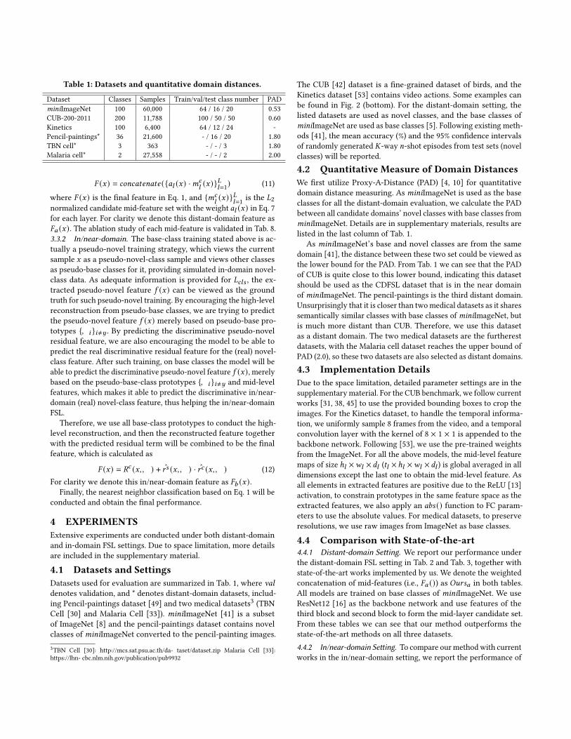
Table 1: Datasets and quantitative domain distances.

Dataset Classes Samples Train/val/test class number PADminiImageNet 100 60,000 64 / 16 / 20 0.53CUB-200-2011 200 11,788 100 / 50 / 50 0.60Kinetics 100 6,400 64 / 12 / 24 -Pencil-paintings* 36 21,600 - / 16 / 20 1.80TBN cell* 3 363 - / - / 3 1.80Malaria cell* 2 27,558 - / - / 2 2.00

𝐹 (𝑥) = 𝑐𝑜𝑛𝑐𝑎𝑡𝑒𝑛𝑎𝑡𝑒 ({𝑎𝑙 (𝑥) ·𝑚𝑐𝑙 (𝑥)}𝐿𝑙=1) (11)

where 𝐹 (𝑥) is the final feature in Eq. 1, and {𝑚𝑐𝑙(𝑥)}𝐿

𝑙=1 is the 𝐿2normalized candidate mid-feature set with the weight 𝑎𝑙 (𝑥) in Eq. 7for each layer. For clarity we denote this distant-domain feature as𝐹𝑎 (𝑥). The ablation study of each mid-feature is validated in Tab. 8.3.3.2 In/near-domain. The base-class training stated above is ac-tually a pseudo-novel training strategy, which views the currentsample 𝑥 as a pseudo-novel-class sample and views other classesas pseudo-base classes for it, providing simulated in-domain novel-class data. As adequate information is provided for 𝐿𝑐𝑙𝑠 , the ex-tracted pseudo-novel feature 𝑓 (𝑥) can be viewed as the groundtruth for such pseudo-novel training. By encouraging the high-levelreconstruction from pseudo-base classes, we are trying to predictthe pseudo-novel feature 𝑓 (𝑥) merely based on pseudo-base pro-totypes {𝑊𝑖 }𝑖≠𝑦 . By predicting the discriminative pseudo-novelresidual feature, we are also encouraging the model to be able topredict the real discriminative residual feature for the (real) novel-class feature. After such training, on base classes the model will beable to predict the discriminative pseudo-novel feature 𝑓 (𝑥), merelybased on the pseudo-base-class prototypes {𝑊𝑖 }𝑖≠𝑦 and mid-levelfeatures, which makes it able to predict the discriminative in/near-domain (real) novel-class feature, thus helping the in/near-domainFSL.

Therefore, we use all base-class prototypes to conduct the high-level reconstruction, and then the reconstructed feature togetherwith the predicted residual term will be combined to be the finalfeature, which is calculated as

𝐹 (𝑥) = 𝑅𝑐 (𝑥,𝑊 ) + 𝑟𝑠 (𝑥,𝑊 ) · 𝑟𝑐 (𝑥,𝑊 ) (12)For clarity we denote this in/near-domain feature as 𝐹𝑏 (𝑥).

Finally, the nearest neighbor classification based on Eq. 1 will beconducted and obtain the final performance.

4 EXPERIMENTSExtensive experiments are conducted under both distant-domainand in-domain FSL settings. Due to space limitation, more detailsare included in the supplementary material.

4.1 Datasets and SettingsDatasets used for evaluation are summarized in Tab. 1, where valdenotes validation, and * denotes distant-domain datasets, includ-ing Pencil-paintings dataset [49] and two medical datasets3 (TBNCell [30] and Malaria Cell [33]). miniImageNet [41] is a subsetof ImageNet [8] and the pencil-paintings dataset contains novelclasses of miniImageNet converted to the pencil-painting images.3TBN Cell [30]: http://mcs.sat.psu.ac.th/da- taset/dataset.zip Malaria Cell [33]:https://lhn- cbc.nlm.nih.gov/publication/pub9932

The CUB [42] dataset is a fine-grained dataset of birds, and theKinetics dataset [53] contains video actions. Some examples canbe found in Fig. 2 (bottom). For the distant-domain setting, thelisted datasets are used as novel classes, and the base classes ofminiImageNet are used as base classes [5]. Following existing meth-ods [41], the mean accuracy (%) and the 95% confidence intervalsof randomly generated 𝐾-way 𝑛-shot episodes from test sets (novelclasses) will be reported.4.2 Quantitative Measure of Domain DistancesWe first utilize Proxy-A-Distance (PAD) [4, 10] for quantitativedomain distance measuring. As miniImageNet is used as the baseclasses for all the distant-domain evaluation, we calculate the PADbetween all candidate domains’ novel classes with base classes fromminiImageNet. Details are in supplementary materials, results arelisted in the last column of Tab. 1.

As miniImageNet’s base and novel classes are from the samedomain [41], the distance between these two set could be viewed asthe lower bound for the PAD. From Tab. 1 we can see that the PADof CUB is quite close to this lower bound, indicating this datasetshould be used as the CDFSL dataset that is in the near domainof miniImageNet. The pencil-paintings is the third distant domain.Unsurprisingly that it is closer than twomedical datasets as it sharessemantically similar classes with base classes of miniImageNet, butis much more distant than CUB. Therefore, we use this datasetas a distant domain. The two medical datasets are the furtherestdatasets, with the Malaria cell dataset reaches the upper bound ofPAD (2.0), so these two datasets are also selected as distant domains.4.3 Implementation DetailsDue to the space limitation, detailed parameter settings are in thesupplementarymaterial. For the CUB benchmark, we follow currentworks [31, 38, 45] to use the provided bounding boxes to crop theimages. For the Kinetics dataset, to handle the temporal informa-tion, we uniformly sample 8 frames from the video, and a temporalconvolution layer with the kernel of 8 × 1 × 1 is appended to thebackbone network. Following [53], we use the pre-trained weightsfrom the ImageNet. For all the above models, the mid-level featuremaps of size ℎ𝑙 ×𝑤𝑙 × 𝑑𝑙 (𝑡𝑙 ×ℎ𝑙 ×𝑤𝑙 × 𝑑𝑙 ) is global averaged in alldimensions except the last one to obtain the mid-level feature. Asall elements in extracted features are positive due to the ReLU [13]activation, to constrain prototypes in the same feature space as theextracted features, we also apply an 𝑎𝑏𝑠 () function to FC param-eters to use the absolute values. For medical datasets, to preserveresolutions, we use raw images from ImageNet as base classes.

4.4 Comparison with State-of-the-art4.4.1 Distant-domain Setting. We report our performance underthe distant-domain FSL setting in Tab. 2 and Tab. 3, together withstate-of-the-art works implemented by us. We denote the weightedconcatenation of mid-features (i.e., 𝐹𝑎 ()) as 𝑂𝑢𝑟𝑠𝑎 in both tables.All models are trained on base classes of miniImageNet. We useResNet12 [16] as the backbone network and use features of thethird block and second block to form the mid-layer candidate set.From these tables we can see that our method outperforms thestate-of-the-art methods on all three datasets.4.4.2 In/near-domain Setting. To compare ourmethodwith currentworks in the in/near-domain setting, we report the performance of

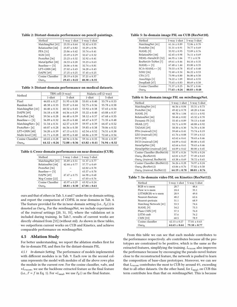
Table 2: Distant-domain performance on pencil-paintings.Method 5-way 1-shot 5-way 5-shotMatchingNet [41] 23.35 ± 0.64 32.42 ± 0.55RelationNet [44] 23.87 ± 0.82 33.29 ± 0.96PPA [31] 23.86 ± 0.42 33.74 ± 0.41SGM [43] 23.49 ± 0.29 32.67 ± 0.32ProtoNet [36] 23.23 ± 0.32 32.92 ± 0.41MetaOptNet [20] 24.53 ± 0.20 33.23 ± 0.63Baseline++ [5] 24.06 ± 0.46 32.74 ± 0.81LFT+GNN [40] 27.02 ± 0.43 34.28 ± 0.43DAPN [49] 27.25 ± 0.25 37.45 ± 0.25Cosine Classifier 28.19 ± 0.24 37.21 ± 0.37Ours𝑎 29.45 ± 0.22 40.38 ± 0.35

Table 3: Distant-domain performance on medical datasets.

Method TBN cell (3-way) Malaria cell (2-way)1-shot 5-shot 1-shot 5-shot

Pixel 44.03 ± 0.27 51.95 ± 0.38 53.01 ± 0.40 53.79 ± 0.53Random Init 48.38 ± 0.33 55.87 ± 0.44 52.75 ± 0.36 55.78 ± 0.58MatchingNet [41] 44.40 ± 0.31 60.52 ± 0.43 53.92 ± 0.38 57.65 ± 0.54DAPN [49] 54.18 ± 0.38 64.56 ± 0.29 55.22 ± 0.40 63.88 ± 0.37ProtoNet [36] 59.56 ± 0.28 66.48 ± 0.39 58.12 ± 0.37 67.68 ± 0.55Baseline++ [5] 56.89 ± 0.32 66.25 ± 0.40 60.47 ± 0.37 71.35 ± 0.48MatchingNet+ [6] 51.54 ± 0.31 62.57 ± 0.39 59.97 ± 0.39 64.47 ± 0.52ProtoNet+ [6] 60.07 ± 0.28 66.56 ± 0.38 59.85 ± 0.38 70.06 ± 0.52LFT+GNN [40] 54.20 ± 0.39 67.13 ± 0.31 62.54 ± 0.52 74.51 ± 0.38Multi-level [18] 61.71 ± 0.28 68.95 ± 0.40 60.86 ± 0.39 72.60 ± 0.54Cosine Classifier 60.65 ± 0.28 68.96 ± 0.36 59.16 ± 0.35 70.41 ± 0.39Ours𝑎 64.12 ± 0.26 72.88 ± 0.36 63.82 ± 0.41 76.94 ± 0.32

Table 4: Cross-domain performance on near domains (CUB).Method 5-way 1-shot 5-way 5-shotMatchingNet [41] 35.89 ± 0.51 51.37 ± 0.77RelationNet [44] 42.44 ± 0.77 57.77 ± 0.69ProtoNet [36] − 62.02 ± 0.70Baseline++ [5] − 65.57 ± 0.70DAPN [49] 47.47 ± 0.75 66.98 ± 0.68Neg-Cosine [22] − 67.03 ± 0.76Cosine Classifier 45.97 ± 0.29 65.92 ± 0.24Ours𝑏 48.81 ± 0.30 67.04 ± 0.61

ours and that of others in Tab. 5, 6 and 7 under the in-domain setting,and report the comparison of CDFSL in near domains in Tab. 4.The feature provided for the in/near-domain setting (i.e., 𝐹𝑏 ()) isdenoted as 𝑂𝑢𝑟𝑠𝑏 . For the miniImageNet, we include experimentsof the trainval settings [20, 31, 35], where the validation set isincluded during training. In Tab.7, results of current works aredirectly obtained from [53] (without std). As shown in these tables,we outperform current works on CUB and Kinetics, and achievecomparable performance on miniImageNet.

4.5 Ablation StudyFor better understanding, we report the ablation studies first forthe in-domain FSL and then for the distant-domain FSL.4.5.1 In-domain Setting. The performance of models implementedwith different modules is in Tab. 9. Each row in the second col-umn represents the model with modules of all the above rows plusthe module in the current row. For the cosine classifier, +𝑎𝑏𝑠 , and+𝐿𝑟𝑒𝑐𝑜𝑛 , we use the backbone extracted feature as the final feature(i.e., 𝐹 = 𝑓 in Eq. 1). For +𝐿𝑚𝑖𝑑 , we use 𝐹𝑏 () as the final feature.

Table 5: In-domain image FSL on CUB (ResNet10).Method 5-way 1-shot 5-way 5-shotMatchingNet [41] 61.16 ± 0.89 72.86 ± 0.70ProtoNet [36] 51.31 ± 0.91 70.77 ± 0.69MAML [9] 55.92 ± 0.95 72.09 ± 0.76RelationNet [44] 62.45 ± 0.98 76.11 ± 0.69DEML+MetaSGD [52] 66.95 ± 1.06 77.1 ± 0.78ResNet18+TriNet [7] 69.61 ± 0.46 84.10 ± 0.35MAML++ [3] 67.48 ± 1.44 83.80 ± 0.35SCA+MAML++ [3] 70.33 ± 0.78 85.47 ± 0.40S2M2 [26] 72.40 ± 0.34 86.22 ± 0.53CFA [17] 73.90 ± 0.80 86.80 ± 0.50AssoAlign [1] 74.22 ± 1.09 88.65 ± 0.55DeepEmb [47] 75.65 ± 0.83 88.69 ± 0.50Cosine Classifier 71.37 ± 0.25 86.57 ± 0.46Ours𝑏 77.65 ± 0.26 88.83 ± 0.48

Table 6: In-domain image FSL onminiImageNet.Method 5-way 1-shot 5-way 5-shotMatchingNet [41] 46.56 ± 0.84 55.31 ± 0.73ProtoNet [36] 49.42 ± 0.78 68.20 ± 0.66MAML [9] 48.70 ± 1.84 63.11 ± 0.92RelationNet [44] 50.44 ± 0.82 65.32 ± 0.70Dynamic FS [12] 55.45 ± 0.89 70.13 ± 0.68SNAIL [27] 55.71 ± 0.99 68.88 ± 0.92TADAM [29] 58.50 ± 0.30 76.70 ± 0.30PPA (trainval) [31] 59.60 ± 0.41 73.74 ± 0.19LEO (trainval) [35] 61.76 ± 0.08 77.59 ± 0.12DCO [20] 62.62 ± 0.61 78.63 ± 0.46DCO (trainval) [20] 64.09 ± 0.62 80.00 ± 0.45MetaOptNet [20] 62.64 ± 0.61 78.63 ± 0.46MetaOptNet (trainval) [20] 64.09 ± 0.62 80.00 ± 0.45Cosine Classifier (ResNet10) 55.97 ± 0.26 74.95 ± 0.24Ours𝑏 (ResNet10) 62.01 ± 0.27 77.49 ± 0.63Ours𝑏 (trainval, ResNet10) 63.38 ± 0.69 78.72 ± 0.65Cosine Classifier (ResNet12) 56.26 ± 0.28 74.97 ± 0.24Ours𝑏 (ResNet12) 63.06 ± 0.76 77.82 ± 0.58Ours𝑏 (trainval, ResNet12) 64.19 ± 0.78 80.01 ± 0.76

Table 7: In-domain video FSL on Kinetics (ResNet12).Method 5-way 1-shot 5-way 5-shotRGB w/o mem 28.7 48.6Flow w/o mem 24.4 33.1LSTM(RGB) w/o mem 28.9 49.0Nearest-finetune 48.2 62.6Nearest-pretrain 51.1 68.9Matching Network [41] 53.3 74.6MAML [9] 54.2 75.3Plain CMN [19] 57.3 76.0LSTM-cmb 57.6 76.2CMN [53] 60.5 78.9Cosine classifier 62.13 ± 0.27 77.81 ± 0.63Ours𝑏 64.63 ± 0.64 79.10 ± 0.77

From this table we can see that each module contributes tothe performance respectively. 𝑎𝑏𝑠 contributes because all the pro-totypes are constrained to be positive, which is the same as theextracted features, simplifying the training. 𝐿𝑟𝑒𝑐𝑜𝑛 also improvesthe performance because by encouraging the pseudo-novel featureclose to the reconstructed feature, the network is pushed to learnthe composition of base-class prototypes. Moreover, we can seethat 𝐿𝑟𝑒𝑐𝑜𝑛 contributes the most to CUB by around 4%, exceedingthat to all other datasets. On the other hand, for 𝐿𝑚𝑖𝑑 , on CUB thisterm contribute less than that on miniImageNet. This is because

Table 8: Ablation study by distant-domain 1-shot testing.

Case Method Forth Block(Final-layer)

Third Block(Mid-layer)

Second Block(Mid-layer)

Concatenation ofmid-features (Ours𝑎)

PencilResNet12

5-way 1-shot

Cosine 28.19 ± 0.24 28.35 ± 0.23 27.21 ± 0.21 27.95 ± 0.23+abs 28.22 ± 0.21 28.84 ± 0.21 27.95 ± 0.22 28.89 ± 0.22

+ 𝐿𝑟𝑒𝑐𝑜𝑛 28.29 ± 0.22 28.12 ± 0.24 27.61 ± 0.24 28.12 ± 0.23+ 𝐿𝑚𝑖𝑑 28.09 ± 0.21 29.21 ± 0.25 28.13 ± 0.22 29.45 ± 0.22

TBN CellResNet12

3-way 1-shot

Cosine 60.25 ± 0.28 60.27 ± 0.29 60.74 ± 0.27 60.55 ± 0.28+abs 62.22 ± 0.32 62.82 ± 0.29 62.05 ± 0.31 61.78 ± 0.28

+ 𝐿𝑟𝑒𝑐𝑜𝑛 58.66 ± 0.31 61.09 ± 0.30 60.57 ± 0.29 60.95 ± 0.27+ 𝐿𝑚𝑖𝑑 59.61 ± 0.29 62.76 ± 0.27 63.98 ± 0.27 64.12 ± 0.26

Malaria CellResNet12

2-way 1-shot

Cosine 59.16 ± 0.35 61.04 ± 0.37 59.66 ± 0.38 59.90 ± 0.37+abs 59.50 ± 0.32 60.40 ± 0.36 58.86 ± 0.39 59.68 ± 0.38

+ 𝐿𝑟𝑒𝑐𝑜𝑛 58.83 ± 0.34 61.40 ± 0.39 59.97 ± 0.39 60.79 ± 0.38+ 𝐿𝑚𝑖𝑑 61.63 ± 0.36 63.29 ± 0.35 63.14 ± 0.41 63.82 ± 0.41

Table 9: Ablation study under the in-domain set-ting.

Study Case Method 5-way 1-shot (%) 5-way 5-shot (%)

CUBResNet10

cosine classifier 71.37 ± 0.25 86.57 ± 0.46+ abs 72.84 ± 0.26 86.99 ± 0.23

+ 𝐿𝑟𝑒𝑐𝑜𝑛 76.47 ± 0.27 87.22 ± 0.24+ 𝐿𝑚𝑖𝑑 77.65 ± 0.26 88.23 ± 0.48

miniImageNetResNet10

cosine classifier 55.97 ± 0.26 74.95 ± 0.24+ abs 57.83 ± 0.26 75.25 ± 0.71

+ 𝐿𝑟𝑒𝑐𝑜𝑛 59.15 ± 0.25 75.73 ± 0.83+ 𝐿𝑚𝑖𝑑 62.01 ± 0.27 77.49 ± 0.63

KineticsResNet12

cosine classifier 62.13 ± 0.27 77.81 ± 0.63+ abs 62.67 ± 0.26 78.27 ± 0.61

+ 𝐿𝑟𝑒𝑐𝑜𝑛 63.59 ± 0.25 78.91 ± 0.60+ 𝐿𝑚𝑖𝑑 64.63 ± 0.64 79.10 ± 0.77

CUB is a fine-grained dataset for birds. As nearly all birds con-tain similar high-level patterns (e.g., wings, beak), the high-levelfeature reconstruction on CUB will be much easier than that onminiImageNet. InminiImageNet, various classes exist, such as dogs,cars, ships, which means these classes may not contains as manyover-lapped high-level patterns as that on CUB, making the high-level feature reconstruction harder. Therefore, 𝐿𝑟𝑒𝑐𝑜𝑛 promotesmore on CUB. Moreover, it can also explain why 𝐿𝑚𝑖𝑑 promotesmore on miniImageNet than CUB: As there are larger residualterms on miniImageNet that could not be well reconstructed byprototypes, the mid-level prediction helps more.

4.5.2 Distant-domain Setting. The ablation study is in Tab. 8, withthe feature of the forth (i.e., final), the third, the second block andthe concatenation of the third and second block (i.e., 𝐹𝑎 ()). Wecan see that almost all forth blocks’ features are outperformed bythat of the third blocks, which is consistent with the study [46]that mid-level features can be more transferable than final-layer’sfeature, and verifies the choice of distant domain datasets. For thischallenging setting, methods that helps the in-domain FSL cannotshow significant improvements now, because by fitting the baseclasses (especially +𝐿𝑟𝑒𝑐𝑜𝑛), the model is likely to learn more aboutthe domain-specific information which may harm the transferabil-ity. Meanwhile, by applying 𝐿𝑚𝑖𝑑 , we can see a clear improvementof mid-level features over baselines and the forth layer features,which verifies the our motivation: boosting the discriminability ofmid-level features by the residual-prediction task.

4.5.3 Comparison of high-level reconstruction. We trained ourmodelwith 𝐿𝑟𝑒𝑐𝑜𝑛 on miniImageNet with different splits in Tab. 10, withthe optimal performance and the 𝐿𝑟𝑒𝑐𝑜𝑛 value. We can see by split-ting the extracted feature and prototypes, the reconstructed fea-ture gets closer to the extracted feature (𝐿𝑟𝑒𝑐𝑜𝑛 decreases as splitsincrease), leading to the best feature implicitly encoded with base-class prototypes (setting splits to 4, obtaining the accuracy at 59.15).Also, we can see that for the best improved feature, 𝐿𝑟𝑒𝑐𝑜𝑛 remainslarger than 0.1, which coarsely corresponds to an angle of 20◦ inthe degree measure, verifying the existence of residual terms.

4.6 VisualizationTo verify the contribution of mid-level patterns, we visualize theactivated regions on novel classes of miniImageNet in Fig. 5. Asthe high-level and mid-level representations are already implicitly

Table 10: Hyper-parameters of high-level feature recon-struction. Experiments are conducted onminiImageNet.

Method Segments 5-way 1-shot (%) 𝐿𝑟𝑒𝑐𝑜𝑛

without 𝐿𝑟𝑒𝑐𝑜𝑛 - 57.83 ± 0.26 -

Average over queried

1 58.25 ± 0.28 0.194 59.15 ± 0.25 0.1616 58.94 ± 0.26 0.1464 58.21 ± 0.26 0.11

Figure 5: Visualization of the final-layer feature maps whentrained with (w/) and without (w/o) 𝐿𝑚𝑖𝑑 , and the trans-formed mid-layer feature maps (t. mid). w/ mid cover moreactivated regions than w/o mid, where the difference cancoarsely correspond to that of t. mid.

encoded in the extracted feature, we visualize the final-layer fea-ture maps of models trained with (w/) and without (w/o) the 𝐿𝑚𝑖𝑑 ,together with the transformed mid-layer feature maps (t. mid), bymeans of summing up and resizing all the feature maps [51]. We cansee the model trained without 𝐿𝑚𝑖𝑑 covers less activated regionsthan that trained with 𝐿𝑚𝑖𝑑 , indicating regions that are unable tobe described by the baseline method are now better described byour model. The difference in the covered activated regions coarselycorresponds to the activated regions of the transformed mid-layerfeature maps, which verifies the contribution of mid-level patterns.

5 CONCLUSIONTo learn transferable and discriminative mid-level features for thedistant-domain FSL, we proposed a residual-prediction task con-sisting of the high-level feature reconstruction and the mid-levelresidual prediction, which consistently achieves state-of-the-art per-formance and better. Extensive experiments on both the distant- andin-domain settings including image recognition and video recogni-tion show the rationale and the insights of the proposed method.

6 ACKNOWLEDGMENTSThis work is partially supported by Key-Area Research and Develop-ment Program of Guangdong Province under contact No.2019B0101-53002, and grants from the National Natural Science Foundation ofChina under contract No. 61825101 and No. 62088102.

REFERENCES[1] Arman Afrasiyabi, Jean-François Lalonde, and Christian Gagné. 2020. Associative

alignment for few-shot image classification. In European Conference on ComputerVision. Springer, 18–35.

[2] Marcin Andrychowicz, Misha Denil, Sergio Gomez, Matthew W Hoffman, DavidPfau, Tom Schaul, Brendan Shillingford, and Nando De Freitas. 2016. Learningto learn by gradient descent by gradient descent. In NeurIPS. 3981–3989.

[3] Antreas Antoniou et al. 2019. Learning to learn by Self-Critique. arXiv preprintarXiv:1905.10295 (2019).

[4] Shai Ben-David, John Blitzer, Koby Crammer, and Fernando Pereira. 2007. Anal-ysis of representations for domain adaptation. In Advances in neural informationprocessing systems. 137–144.

[5] Wei-Yu Chen, Yen-Cheng Liu, Zsolt Kira, Yu-Chiang Frank Wang, and Jia-BinHuang. 2019. A Closer Look at Few-shot Classification. CoRR abs/1904.04232(2019). arXiv:1904.04232 http://arxiv.org/abs/1904.04232

[6] Yinbo Chen, Xiaolong Wang, Zhuang Liu, Huijuan Xu, and Trevor Darrell. 2020.A New Meta-Baseline for Few-Shot Learning. arXiv preprint arXiv:2003.04390(2020).

[7] Zitian Chen, Yanwei Fu, Yinda Zhang, Yu-Gang Jiang, Xiangyang Xue, and LeonidSigal. 2018. Semantic feature augmentation in few-shot learning. arXiv preprintarXiv:1804.05298 86 (2018), 89.

[8] Jia Deng,Wei Dong, Richard Socher, Li-Jia Li, Kai Li, and Li Fei-Fei. 2009. Imagenet:A -scale hierarchical image database. In CVPR. Ieee, 248–255.

[9] Chelsea Finn, Pieter Abbeel, and Sergey Levine. 2017. Model-agnostic meta-learning for fast adaptation of deep networks. arXiv preprint arXiv:1703.03400(2017).

[10] Yaroslav Ganin, Evgeniya Ustinova, Hana Ajakan, Pascal Germain, HugoLarochelle, François Laviolette, Mario Marchand, and Victor Lempitsky. [n.d.].Domain-adversarial training of neural networks. The Journal of Machine LearningResearch 17 ([n. d.]).

[11] Victor Garcia and Joan Bruna. 2017. Few-shot learning with graph neural net-works. arXiv preprint arXiv:1711.04043 (2017).

[12] Spyros Gidaris and Nikos Komodakis. 2018. Dynamic Few-Shot Visual Learningwithout Forgetting. In CVPR. 4367–4375.

[13] Xavier Glorot, Antoine Bordes, and Yoshua Bengio. 2011. Deep sparse rectifierneural networks. In AISTATS. 315–323.

[14] Yunhui Guo, Noel C Codella, Leonid Karlinsky, James V Codella, John R Smith,Kate Saenko, Tajana Rosing, and Rogerio Feris. 2019. A Broader Study of Cross-Domain Few-Shot Learning. (2019).

[15] Bharath Hariharan and Ross Girshick. 2017. Low-shot visual recognition byshrinking and hallucinating features. In ICCV. 3018–3027.

[16] Kaiming He, Xiangyu Zhang, Shaoqing Ren, and Jian Sun. 2016. Deep residuallearning for image recognition. In CVPR. 770–778.

[17] Ping Hu, Ximeng Sun, Kate Saenko, and Stan Sclaroff. 2019. Weakly-supervisedCompositional Feature Aggregation for Few-shot Recognition. arXiv preprintarXiv:1906.04833 (2019).

[18] Shaoli Huang and Dacheng Tao. 2019. All you need is a good representation:A multi-level and classifier-centric representation for few-shot learning. arXivpreprint arXiv:1911.12476 (2019).

[19] Łukasz Kaiser, Ofir Nachum, Aurko Roy, and Samy Bengio. 2017. Learning toremember rare events. arXiv preprint arXiv:1703.03129 (2017).

[20] Kwonjoon Lee, Subhransu Maji, Avinash Ravichandran, and Stefano Soatto. 2019.Meta-learning with differentiable convex optimization. In CVPR. 10657–10665.

[21] Aoxue Li, Tiange Luo, Zhiwu Lu, Tao Xiang, and Liwei Wang. 2019. Large-Scale Few-Shot Learning: Knowledge Transfer With Class Hierarchy. In CVPR.7212–7220.

[22] Bin Liu, Yue Cao, Yutong Lin, Qi Li, Zheng Zhang, Mingsheng Long, and Han Hu.2020. Negative margin matters: Understanding margin in few-shot classification.In European Conference on Computer Vision. Springer, 438–455.

[23] Lu Liu, Tianyi Zhou, Guodong Long, Jing Jiang, Lina Yao, and Chengqi Zhang.2019. Prototype propagation networks (PPN) for weakly-supervised few-shotlearning on category graph. arXiv preprint arXiv:1905.04042 (2019).

[24] Lu Liu, Tianyi Zhou, Guodong Long, Jing Jiang, and Chengqi Zhang. 2019. Learn-ing to propagate for graph meta-learning. In Advances in Neural InformationProcessing Systems. 1037–1048.

[25] Mingsheng Long, Yue Cao, Jianmin Wang, and Michael I Jordan. 2015. Learn-ing transferable features with deep adaptation networks. arXiv preprintarXiv:1502.02791 (2015).

[26] Puneet Mangla, Mayank Singh, Abhishek Sinha, Nupur Kumari, Vineeth N Bal-asubramanian, and Balaji Krishnamurthy. 2019. Charting the Right Manifold:Manifold Mixup for Few-shot Learning. arXiv preprint arXiv:1907.12087 (2019).

[27] Nikhil Mishra, Mostafa Rohaninejad, Xi Chen, and Pieter Abbeel. 2017. A simpleneural attentive meta-learner. arXiv preprint arXiv:1707.03141 (2017).

[28] Tsendsuren Munkhdalai and Hong Yu. 2017. Meta networks. In ICML. JMLR. org,2554–2563.

[29] Boris Oreshkin, Pau Rodríguez López, Alexandre Lacoste, et al. 2018. Tadam: Taskdependent adaptive metric for improved few-shot learning. In NeurIPS. 721–731.

[30] Tatdow Pansombut, Siripen Wikaisuksakul, Kittiya Khongkraphan, and AniruthPhon-on. 2019. Convolutional Neural Networks for Recognition of LymphoblastCell Images. Computational Intelligence and Neuroscience 2019 (2019).

[31] Siyuan Qiao, Chenxi Liu, Wei Shen, and Alan L Yuille. 2017. Few-shot imagerecognition by predicting parameters from activations. CoRR, abs/1706.03466 1(2017).

[32] Maithra Raghu, Chiyuan Zhang, Jon Kleinberg, and Samy Bengio. 2019. Trans-fusion: Understanding transfer learning for medical imaging. arXiv preprintarXiv:1902.07208 (2019).

[33] Sivaramakrishnan Rajaraman, Sameer K Antani, Mahdieh Poostchi, KamolratSilamut, Md A Hossain, Richard J Maude, Stefan Jaeger, and George R Thoma.2018. Pre-trained convolutional neural networks as feature extractors towardimproved malaria parasite detection in thin blood smear images. PeerJ 6 (2018),e4568.

[34] Sachin Ravi and Hugo Larochelle. 2016. Optimization as a model for few-shotlearning. (2016).

[35] Andrei A Rusu, Dushyant Rao, Jakub Sygnowski, Oriol Vinyals, Razvan Pascanu,Simon Osindero, and Raia Hadsell. 2019. Meta-learning with latent embeddingoptimization. ICLR (2019).

[36] Jake Snell, Kevin Swersky, Richard Zemel, et al. 2017. Prototypical networks forfew-shot learning. In NeurIPS. 4077–4087.

[37] Pavel Tokmakov, Yu-Xiong Wang, and Martial Hebert. 2019. Learning composi-tional representations for few-shot recognition. In ICCV. 6372–6381.

[38] Eleni Triantafillou, Richard Zemel, and Raquel Urtasun. 2017. Few-shot learningthrough an information retrieval lens. In NeurIPS. 2255–2265.

[39] Eleni Triantafillou, Tyler Zhu, Vincent Dumoulin, Pascal Lamblin, Utku Evci,Kelvin Xu, Ross Goroshin, Carles Gelada, Kevin Swersky, Pierre-Antoine Man-zagol, et al. 2019. Meta-dataset: A dataset of datasets for learning to learn fromfew examples. arXiv preprint arXiv:1903.03096 (2019).

[40] Hung-Yu Tseng, Hsin-Ying Lee, Jia-Bin Huang, and Ming-Hsuan Yang. 2020.Cross-Domain Few-Shot Classification via Learned Feature-Wise Transformation.arXiv preprint arXiv:2001.08735 (2020).

[41] Oriol Vinyals, Charles Blundell, Tim Lillicrap, Daan Wierstra, et al. 2016. Match-ing networks for one shot learning. In NeurIPS.

[42] CatherineWah, Steve Branson, Peter Welinder, Pietro Perona, and Serge Belongie.2011. The caltech-ucsd birds-200-2011 dataset. (2011).

[43] Yu-Xiong Wang, Ross Girshick, Martial Hebert, and Bharath Hariharan. 2018.Low-shot learning from imaginary data. In CVPR. 7278–7286.

[44] Flood Sung Yongxin Yang, Li Zhang, Tao Xiang, Philip HS Torr, and Timothy MHospedales. 2018. Learning to compare: Relation network for few-shot learning.(2018).

[45] Han-Jia Ye, Hexiang Hu, De-Chuan Zhan, and Fei Sha. 2018. Learning embeddingadaptation for few-shot learning. arXiv preprint arXiv:1812.03664 (2018).

[46] Jason Yosinski, Jeff Clune, Yoshua Bengio, and Hod Lipson. 2014. How transfer-able are features in deep neural networks?. In Advances in neural informationprocessing systems. 3320–3328.

[47] Chi Zhang, Yujun Cai, Guosheng Lin, and Chunhua Shen. 2020. DeepEMD:Few-Shot Image Classification with Differentiable Earth Mover’s Distance andStructured Classifiers. In Proceedings of the IEEE/CVF Conference on ComputerVision and Pattern Recognition. 12203–12213.

[48] Guopeng Zhang and Jinhua Xu. 2018. Person re-identification by mid-level at-tribute and part-based identity learning. In Asian Conference on Machine Learning.PMLR, 220–231.

[49] An Zhao, Mingyu Ding, Zhiwu Lu, Tao Xiang, Yulei Niu, Jiechao Guan, Ji-RongWen, and Ping Luo. 2020. Domain-Adaptive Few-Shot Learning. arXiv preprintarXiv:2003.08626 (2020).

[50] Yang Zhong, Josephine Sullivan, and Haibo Li. 2016. Leveraging mid-level deeprepresentations for predicting face attributes in thewild. In 2016 IEEE InternationalConference on Image Processing (ICIP). IEEE, 3239–3243.

[51] Bolei Zhou, Aditya Khosla, Agata Lapedriza, Aude Oliva, and Antonio Torralba.2016. Learning deep features for discriminative localization. In CVPR. 2921–2929.

[52] Fengwei Zhou, Bin Wu, and Zhenguo Li. 2018. Deep Meta-Learning: Learning toLearn in the Concept Space. arXiv preprint arXiv:1802.03596 (2018).

[53] Linchao Zhu and Yi Yang. 2018. Compound memory networks for few-shot videoclassification. In ECCV. 751–766.

[54] Yixiong Zou, Yemin Shi, Daochen Shi, Yaowei Wang, Yongsheng Liang, andYonghong Tian. 2020. Adaptation-Oriented Feature Projection for One-shotAction Recognition. IEEE Transactions on Multimedia (2020).

[55] Yixiong Zou, Yemin Shi, Yaowei Wang, Yu Shu, Qingsheng Yuan, and YonghongTian. 2018. Hierarchical temporal memory enhanced one-shot distance learningfor action recognition. In 2018 IEEE International Conference on Multimedia andExpo (ICME). IEEE, 1–6.

[56] Yixiong Zou, Shanghang Zhang, Guangyao Chen, Yonghong Tian, Kurt Keutzer,and José MF Moura. 2020. Annotation-Efficient Untrimmed Video Action Recog-nition. arXiv preprint arXiv:2011.14478 (2020).

[57] Yixiong Zou, Shanghang Zhang, Ke Chen, Yonghong Tian, Yaowei Wang, andJosé MF Moura. 2020. Compositional Few-Shot Recognition with PrimitiveDiscovery and Enhancing. In Proceedings of the 28th ACM MM. 156–164.